Embed Size (px)
Citation preview
HoloRec3D : A free Matlab toolbox for digital
holography
Mozhdeh Seifi, Corinne Fournier, Loıc Denis
To cite this version:
Mozhdeh Seifi, Corinne Fournier, Loıc Denis. HoloRec3D : A free Matlab toolbox for digitalholography. 2012. <ujm-00749137>
HAL Id: ujm-00749137
https://hal-ujm.archives-ouvertes.fr/ujm-00749137
Submitted on 6 Nov 2012
HAL is a multi-disciplinary open accessarchive for the deposit and dissemination of sci-entific research documents, whether they are pub-lished or not. The documents may come fromteaching and research institutions in France orabroad, or from public or private research centers.
L’archive ouverte pluridisciplinaire HAL, estdestinee au depot et a la diffusion de documentsscientifiques de niveau recherche, publies ou non,emanant des etablissements d’enseignement et derecherche francais ou etrangers, des laboratoirespublics ou prives.
HoloRec3D : A free Matlab® toolboxfor digital holography
Mozhdeh Seifi,Corinne Fournier,Loic Denis
Universite de Lyon, F-42023, Saint-Etienne, France,CNRS, UMR5516, Laboratoire Hubert Curien,Universite de Saint-Etienne
Telecom Saint Etienne, F-42000, Saint- Etienne, France.
October 2012
Abstract
In-line digital holography is an imaging technique which is being
increasingly used for studying 3D flows. It has been previously shown
that very accurate reconstructions of objects could be achieved with
the use of an inverse problems framework. The goal of HoloRec3D is
to reconstruct the volume of interest using this approach. A simple
Graphical User Interface accompanies the scripts to facilitate the use
of this toolbox. A recently published multi-scale method is included
providing the advanced users with a fast and accurate reconstruction.
1 Introduction
Digital Holography (DH) is a 3-D imaging technique which has been widelydeveloped during the past few decades thanks to the enormous advancesin digital imaging and computer technology. This technique achieves 3-Dreconstruction of objects from a 2D hologram-image and reaches accuraciesin the range of - or smaller than - the wavelength. As 3-D information codedin a digital hologram can be recorded in one shot, this technique can beused with high speed cameras to perform time-resolved 3-D reconstructionsof high speed phenomena. This metrological tool is used in experimentalmechanics, biology, or fluid dynamics.
Over the past decade, several algorithms for the analysis of hologramshave been proposed. They are mostly based on a common approach to holo-gram processing: digital reconstruction based on the simulation of hologram
1
diffraction [1, 2]. These so-called classical approaches suffer from artifactsintrinsic to holography: twin-image contamination of the reconstructed im-ages, image distortions for objects located close to the hologram borders.The analysis of the reconstructed planes is therefore limited by these de-fects [3]. In contrast to this approach, the inverse problems perspectivedoes not transform the hologram but performs object detection and locationby matching a model of the hologram [4, 5]. Information is thus extractedfrom the hologram in an optimal way [6, 7], leading to two essential results:an improvement of the axial accuracy [4] and the capability to extend thereconstructed field beyond the physical limit of the sensor size (out-of-fieldreconstruction [5]).
In this document, we introduce a Matlab® toolbox dedicated to InverseProblems approach for digital hologram reconstruction. Accurate 3D recon-struction of in line digital holograms of spherical objects, typically droplets,bubbles [8] or beads is the direct target of HoloRec3D although the optionof classical back propagation method is available for general objects. Thetheoretical background of the inverse problems approach can be found fromthe references.
HoloRec3D can be found here for download. The structure of this doc-ument is as following. In Sec. 2 the system requirements and configurationare described. In Sec. 3 the use of graphical user interface is detailed. Weconclude this document by describing the use of sample scripts for a moreadvanced use of HoloRec3D in Sec. 4 which includes the use of multi-scalemethod [9].
Please kindly note that any use of HoloRec3D should be cited using thisdocument as the reference:
M. Seifi, C. Fournier and L. Denis, ”HoloRec3D : A free Matlab® toolboxfor digital holography”,HAL-UJM, Oct 2012.
2 Setting the environmental parameters
The system requirements for using HoloRec3D is the Matlab® environmentequipped with the Image Processing and the Optimization toolbox. Thecode can be downloaded from here. All the folders should be unzipped inthe folder ”/HoloRec3D”. This folder should be added to the Matlab®’spath. This can be done by opening the Matlab® environment, browsing tothe folder ”/HoloRec3D” and typing the following in the command line:
2
>> HoloRec3DPath(pwd);This command adds the HoloRec3D’s folder to the path. Another way is
to add the folders manually to the path by opening the Matlab® environmentand selecting ”Set path...” from File in the toolbar. In the next window, thebutton ”Add with subfolders” will add the selected folder (”/HoloRec3D”)and its sub-folders to the path. This will change the path of the Matlab®
permanently which is not recommended.The mex functions are compiled for Matlab® R2009a and R2010b. If the
version of Matlab® is different, this e-mail address can be used to receivethe suitable ”.mex” functions for a specific system configuration.
3 Getting Started : Graphical User Interface
The Graphical User Interface (GUI) provides a simple tool to use HoloRec3Dwithout the need for a deep knowledge of the implementation. To start withthe GUI, type the following in the command line:
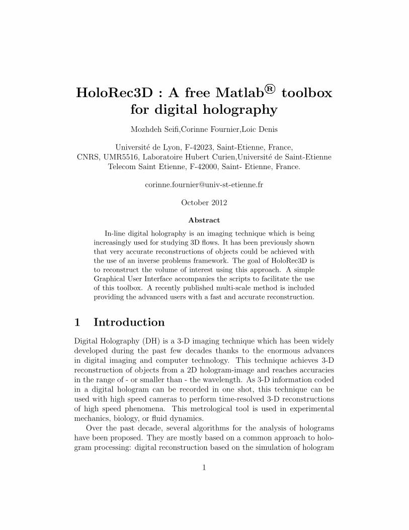
>> GUI;The window showed in Fig. 1 will be opened. This Window consists in
three main parts: (i) Pre-process, (ii) Basics: Simulate and observe, (iii)Advanced: Process the hologram.
3.1 ”Pre-process”
This part of the GUI is used to convert raw image files containing the cap-tured holograms to the Matlab® data files (i.e., ”.mat” files) and removethe background of the holograms. The background is calculated as the meanof the raw images. To use this option, the button ”Browse” can be usedin this section of GUI to browse to the folder containing the raw images,and to select one raw image. The processed data will be saved in the folder”/HoloRec3D/DATA” under the name ”hologram video manual.mat”. Us-ing the button ”Show the holograms” will show the video of the processedhologram in a separate figure.
3.2 ”Basics: Simulate and/or visualize”
The second part of the GUI facilitates the simulation and the visualizationof the (existing) holograms. It is possible to either simulate one hologram or
3
(a)
(b)
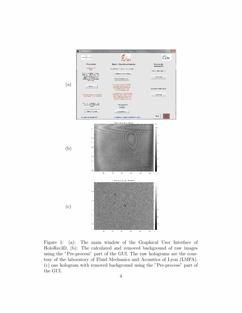
(c)
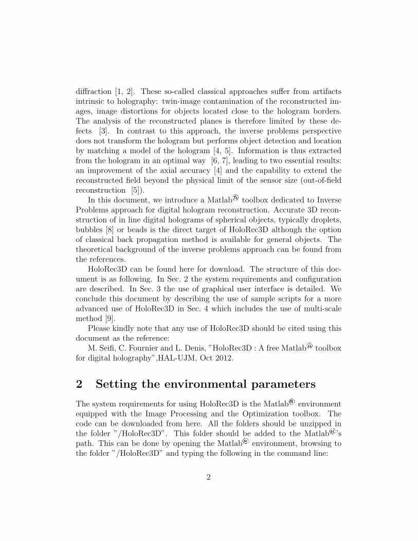
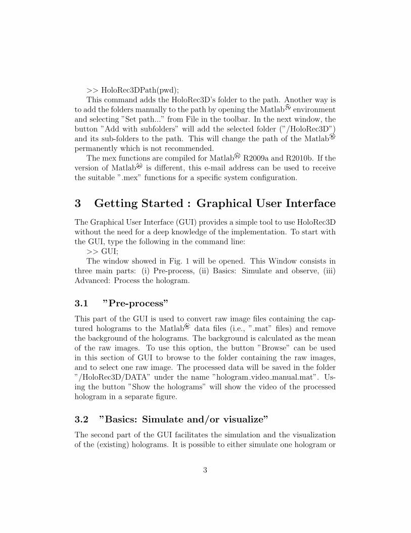
Figure 1: (a): The main window of the Graphical User Interface ofHoloRec3D, (b): The calculated and removed background of raw imagesusing the ”Pre-process” part of the GUI. The raw holograms are the cour-tesy of the laboratory of Fluid Mechanics and Acoustics of Lyon (LMFA).(c) one hologram with removed background using the ”Pre-process” part ofthe GUI.
4
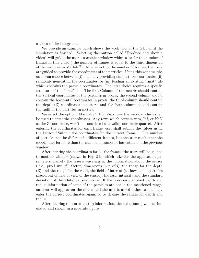
a video of the holograms.We provide an example which shows the work flow of the GUI until the
simulation is finished. Selecting the button called ”Produce and show avideo” will guide the users to another window which asks for the number offrames in this video ( the number of frames is equal to the third dimensionof the matrices in Matlab®). After selecting the number of frames, the usersare guided to provide the coordinates of the particles. Using this window, theusers can choose between (i) manually providing the particles coordinates,(ii)randomly generating the coordinates, or (iii) loading an existing ”.mat” filewhich contains the particle coordinates. The later choice requires a specificstructure of the ”.mat” file. The first Column of the matrix should containthe vertical coordinates of the particles in pixels, the second column shouldcontain the horizontal coordinates in pixels, the third column should containthe depth (Z) coordinates in meters, and the forth column should containthe radii of the particles in meters.
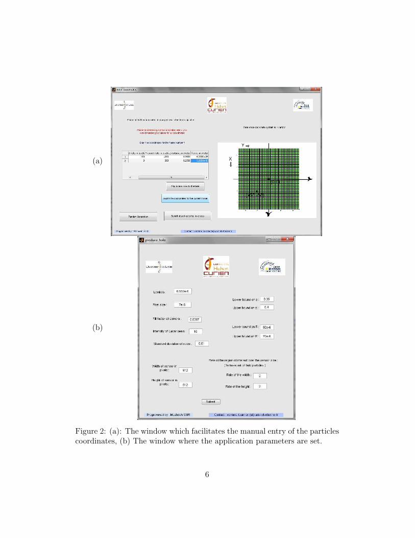
We select the option ”Manually”. Fig. 2-a shows the window which shallbe used to enter the coordinates. Any rows which contain zero, Inf, or NaNas the Z coordinate, won’t be considered as a valid coordinate quartet. Afterentering the coordinates for each frame, user shall submit the values usingthe button ”Submit the coordinates for the current frame”. The numberof particles can be different in different frames, but the user can’t enter thecoordinates for more than the number of frames he has entered in the previouswindow.
After entering the coordinates for all the frames, the users will be guidedto another window (shown in Fig. 2-b) which asks for the application pa-rameters, namely the laser’s wavelength, the information about the sensor( i.e., pixel size, fill factor, dimensions in pixels), the range for the depth(Z) and the range for the radii, the field of interest (to have some particlesplaced out of field of view of the sensor), the laser intensity and the standarddeviation of the white Gaussian noise. If the previously entered depth andradius information of some of the particles are not in the mentioned range,an error will appear on the screen and the user is asked either to manuallyenter the correct coordinates again, or to change the ranges for depth andradius.
After entering the correct setup information, the hologram(s) will be sim-ulated and shown in a separate figure.
5
(a)
(b)
Figure 2: (a): The window which facilitates the manual entry of the particlescoordinates, (b) The window where the application parameters are set.
6
3.3 ”Process the hologram(s)”
The last section of the GUI is used to reconstruct the volume of interestfrom the holograms. Two main approaches are implemented in this part:(i) inverse problems approach method , (ii) classical light back-propagationmethod. The inverse problems approach is implemented to process the holo-grams of spherical objects, whereas the light back propagation method canprocess the holograms of any types of objects. It should be noted that bothimplementation assume an inline setup for the hologram recording.
3.3.1 Inverse Problems Approach
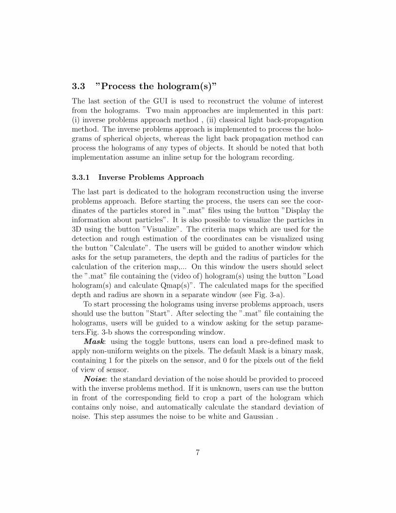
The last part is dedicated to the hologram reconstruction using the inverseproblems approach. Before starting the process, the users can see the coor-dinates of the particles stored in ”.mat” files using the button ”Display theinformation about particles”. It is also possible to visualize the particles in3D using the button ”Visualize”. The criteria maps which are used for thedetection and rough estimation of the coordinates can be visualized usingthe button ”Calculate”. The users will be guided to another window whichasks for the setup parameters, the depth and the radius of particles for thecalculation of the criterion map,... On this window the users should selectthe ”.mat” file containing the (video of) hologram(s) using the button ”Loadhologram(s) and calculate Qmap(s)”. The calculated maps for the specifieddepth and radius are shown in a separate window (see Fig. 3-a).
To start processing the holograms using inverse problems approach, usersshould use the button ”Start”. After selecting the ”.mat” file containing theholograms, users will be guided to a window asking for the setup parame-ters.Fig. 3-b shows the corresponding window.
Mask: using the toggle buttons, users can load a pre-defined mask toapply non-uniform weights on the pixels. The default Mask is a binary mask,containing 1 for the pixels on the sensor, and 0 for the pixels out of the fieldof view of sensor.
Noise: the standard deviation of the noise should be provided to proceedwith the inverse problems method. If it is unknown, users can use the buttonin front of the corresponding field to crop a part of the hologram whichcontains only noise, and automatically calculate the standard deviation ofnoise. This step assumes the noise to be white and Gaussian .
7
(a)
(b)
(1) (2)
Figure 3: (a-1): The GUI for using the options of inverse problems approach,(a-2): Correlation map for z=0.48 m, R=42 µm. The holograms are thecourtesy of the laboratory of Fluid Mechanics and Acoustics of Lyon (LMFA),(b-1): The GUI window which is used to define the application parametersfor the hologram reconstruction using inverse problems approach.
8
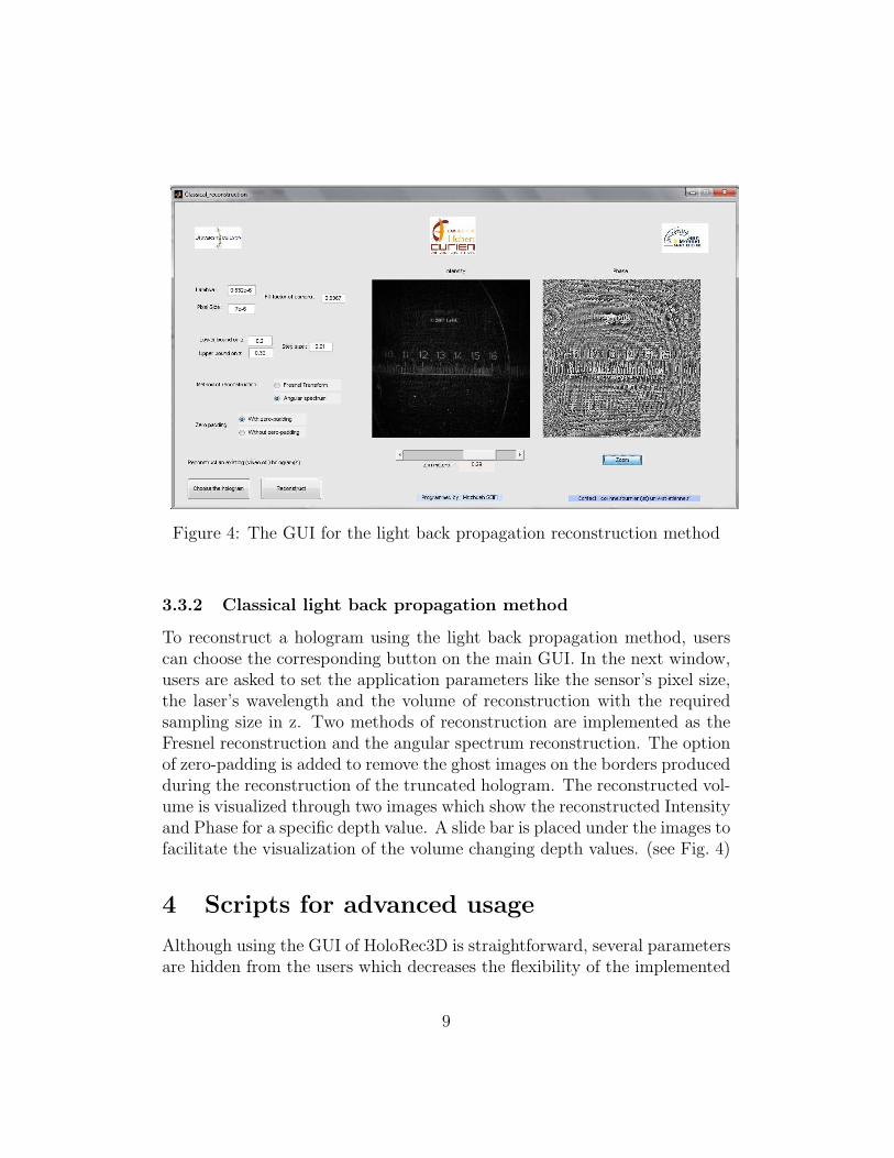
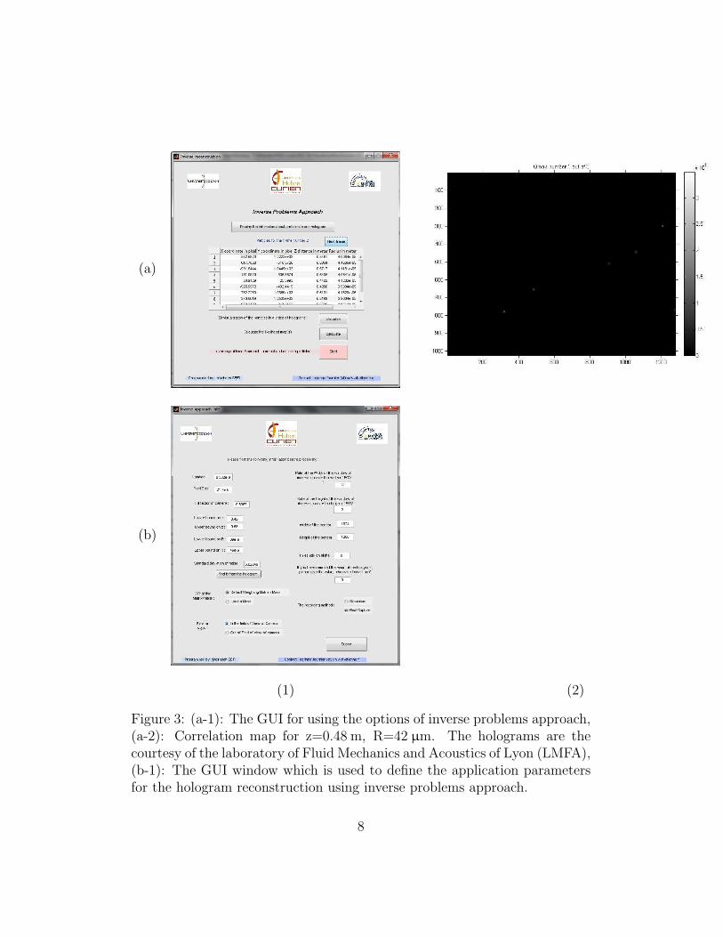
Figure 4: The GUI for the light back propagation reconstruction method
3.3.2 Classical light back propagation method
To reconstruct a hologram using the light back propagation method, userscan choose the corresponding button on the main GUI. In the next window,users are asked to set the application parameters like the sensor’s pixel size,the laser’s wavelength and the volume of reconstruction with the requiredsampling size in z. Two methods of reconstruction are implemented as theFresnel reconstruction and the angular spectrum reconstruction. The optionof zero-padding is added to remove the ghost images on the borders producedduring the reconstruction of the truncated hologram. The reconstructed vol-ume is visualized through two images which show the reconstructed Intensityand Phase for a specific depth value. A slide bar is placed under the images tofacilitate the visualization of the volume changing depth values. (see Fig. 4)
4 Scripts for advanced usage
Although using the GUI of HoloRec3D is straightforward, several parametersare hidden from the users which decreases the flexibility of the implemented
9
methods. A more advanced use of the toolbox is to directly work with thefunctions and scripts. In this section, we introduce the contents of the foldersand address two sample scripts which can be used to access the toolbox ona deeper level.
4.1 Folders and Files
HoloRec3D contains four main folders: (i) IPA, (ii) GUI, (iii) FAST, (iv)Data. ”IPA” includes the ”.m” source files, ”.mex” binary files and the helpfor the ”.mex” files. ”GUI” contains the ”.m” source files and the .fig fileswhich together build the GUI of HoloRec3D. ”FAST” includes additional”.m” files implementing a fast and accurate multi-scale framework. Finally”Data” contains the sample simulated/real holograms, coordinates of parti-cles, and a ”temp” folder used for internal parameter handling.
In addition to these folders, some simulated/real holograms are put online which are accessible through this link. Users should unzip these foldersbefore starting to use them.
4.2 Sample scripts
To start using HoloRec3D through the functions, users can find two samplescripts. The first one which introduces the use of inverse problems approachis placed in ”./HoloRec3D/IPA” under the name ”MAIN IPA.m” . The filecontains the list of the function’s parameters which are required to be setbeforehand for (i) a simulation case, (ii) the case of the real holograms ofLMFA, (iii) an unknown application which can be used by the users to applytheir own application.
A second script introduces the multi-scale method. It is place in”./HoloRec3D/FAST” under the name ”MAIN FAST.m” . Similar to theother script, this script is written to guide the users to use the multi-scalemethod.
References
[1] T. Kreis, Handbook of Holographic Interferometry: Optical and Digital
Methods (Wiley-VCH, 2005), 1st ed.
[2] U. Schnars, W. Juptner, Digital Holography (Springer, 2005).
10
[3] J. Gire, L. Denis, C. Fournier, E. Thiebaut, F. Soulez, and C. Ducot-tet, “Digital holography of particles: benefits of the inverse problemsapproach,” Measurement Science and Technology 19, 074005 (2008).
[4] F. Soulez, L. Denis, C. Fournier, E. Thiebaut, and C. Goepfert, “Inverse-problem approach for particle digital holography: accurate locationbased on local optimization,” JOSA A 24, 1164–1171 (2007).
[5] F. Soulez, L. Denis, E. Thiebaut, C. Fournier, and C. Goepfert, “Inverseproblem approach in particle digital holography: out-of-field particledetection made possible,” Journal of the Optical Society of America. A,Optics, Image Science, and Vision 24, 3708–3716 (2007).
[6] C. Fournier, L. Denis, E. Thiebaut, T. Fournel, and M. Seifi, “Inverseproblem approaches for digital hologram reconstruction,” in “Proceed-ings of SPIE,” , vol. 8043 (2011), vol. 8043, p. 80430S.
[7] C. Fournier, L. Denis, and T. Fournel, “On the single point resolution ofon-axis digital holography,” Journal of the Optical Society of America.A, Optics, Image Science, and Vision 27, 1856–1862 (2010).
[8] D. Chareyron, J. L. Marie, C. Fournier, J. Gire, N. Grosjean, L. Denis,M. Lance, and L. Mees, “Testing an in-line digital holography inversemethod for the lagrangian tracking of evaporating droplets in homoge-neous nearly isotropic turbulence,” New Journal of Physics 14, (2012)043039 (26pp).
[9] M. Seifi, C. Fournier, L. Denis, N. Grosjean, J. L. Marie, “Three-dimensional reconstruction of particle holograms: a fast and accuratemultiscale approach,” JOSA A 29, 1808–1817 (2012).
11