Embed Size (px)
Citation preview
Under Revision
LECTURE NOTE
COURSE CODE- BCE 303
GEOTECHNICAL ENGINEERING-I
Under Revision
SYLLABUS
Module –I
Introduction: Origin of soils, formation of soils, clay mineralogy and soil structure, basic
terminology and their relations, index properties of soils.
Soil classification: Particle size distribution, use of particle size distribution curve, Particle
size classification, textural classification, HRB classification, Unified classification system,
Indian standard soil classification system, Field identification of soils.
Soil moisture: Types of soil water, capillary tension, capillary siphoning.
Stress conditions in soil: Total stress, pore pressure and effective stress.
Module – II
Permeability: Darcy’s law, permeability, factors affecting permeability, determination of
permeability (laboratory and field methods), permeability of stratified soil deposits.
Estimation of yield from wells.
Seepage analysis: Seepage pressure, quick condition, laplace equation for two –dimensional
flow, flow net, properties and methods of construction of flow net, application of flow net,
seepage through anisotropic soil and non-homogenous soil, seepage through earth dam.
Module – III
Soil compaction: Compaction mechanism, factors affecting compaction, effect of compaction
on soil properties, density moisture content relationship in compaction test, standard and
modified proctor compaction tests, field compaction methods, relative compaction,
compaction control.
Soil consolidation: Introduction, spring analogy, one dimensional consolidation, Terzaghi’s
theory of one dimensional consolidation, consolidation test, determination of coefficient of
consolidation.
Module –IV
Shear strength of soils: Mohr’s stress circle, theory of failure for soils, determination of shear
strength (direct shear test, tri-axial compression test, unconfined compression test, van shear
test), shear characteristics of cohesionless soils and cohesive soils.
Stabilization of soil: Introduction, mechanical stabilization, cement stabilization, lime
stabilization, bituminous stabilization, chemical stabilization, thermal stabilization, electrical
stabilization, stabilization by grouting, use of geo-synthetic materials, reinforced earth.
Reference Books:
1. Geotechnical Engineering, C. Venkatramaiah, New Age International publishers.
2. Geotechnical Engineering, T.N. Ramamurthy & T.G. Sitharam, S. Chand & Co.
3. Soil Mechanics, T.W. Lambe & Whiteman, Wiley Eastern Ltd, Nw
Under Revision
LECTURE 1
Introduction:
The term "soil" can have different meanings, depending upon the field in which it is considered.
To a geologist, it is the material in the relative thin zone of the Earth's surface within which roots occur, and which
are formed as the products of past surface processes. The rest of the crust is grouped under the term "rock".
To a pedologist, it is the substance existing on the surface, which supports plant life.
To an engineer, it is a material that can be:
built on: foundations of buildings, bridges
built in: basements, culverts, tunnels
built with: embankments, roads, dams
supported: retaining walls
Soil Mechanics is a discipline of Civil Engineering involving the study of soil, its behaviour and application as an
engineering material.
Soil Mechanics is the application of laws of mechanics and hydraulics to engineering problems dealing with
sediments and other unconsolidated accumulations of solid particles, which are produced by the mechanical and
chemical disintegration of rocks, regardless of whether or not they contain an admixture of organic constituents.
Soil consists of a multiphase aggregation of solid particles, water, and air. This fundamental composition gives rise
to unique engineering properties, and the description of its mechanical behavior requires some of the most classic
principles of engineering mechanics.
Engineers are concerned with soil's mechanical properties: permeability, stiffness, and strength. These depend
primarily on the nature of the soil grains, the current stress, the water content and unit weight.
Formation of Soils:
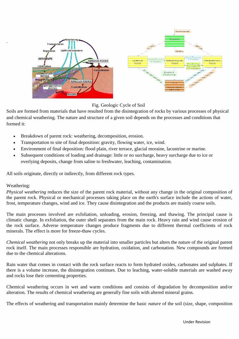
Soil is formed from rock due to erosion and weathering action. Igneous rock is the basic rock formed from the
crystallization of molten magma. This rock is formed either inside the earth or on the surface. These rocks
undergo metamorphism under high temperature and pressure to form Metamorphic rocks. Both Igneous and
metamorphic rocks are converted in to sedimentary rocks due to transportation to different locations
by the agencies such as wind, water etc. Finally, near the surface millions of years of erosion and weathering
converts rocks in to soil.
Under Revision
.
Fig. Geologic Cycle of Soil
Soils are formed from materials that have resulted from the disintegration of rocks by various processes of physical
and chemical weathering. The nature and structure of a given soil depends on the processes and conditions that
formed it:
Breakdown of parent rock: weathering, decomposition, erosion.
Transportation to site of final deposition: gravity, flowing water, ice, wind.
Environment of final deposition: flood plain, river terrace, glacial moraine, lacustrine or marine.
Subsequent conditions of loading and drainage: little or no surcharge, heavy surcharge due to ice or
overlying deposits, change from saline to freshwater, leaching, contamination.
All soils originate, directly or indirectly, from different rock types.
Weathering:
Physical weathering reduces the size of the parent rock material, without any change in the original composition of
the parent rock. Physical or mechanical processes taking place on the earth's surface include the actions of water,
frost, temperature changes, wind and ice. They cause disintegration and the products are mainly coarse soils.
The main processes involved are exfoliation, unloading, erosion, freezing, and thawing. The principal cause is
climatic change. In exfoliation, the outer shell separates from the main rock. Heavy rain and wind cause erosion of
the rock surface. Adverse temperature changes produce fragments due to different thermal coefficients of rock
minerals. The effect is more for freeze-thaw cycles.
Chemical weathering not only breaks up the material into smaller particles but alters the nature of the original parent
rock itself. The main processes responsible are hydration, oxidation, and carbonation. New compounds are formed
due to the chemical alterations.
Rain water that comes in contact with the rock surface reacts to form hydrated oxides, carbonates and sulphates. If
there is a volume increase, the disintegration continues. Due to leaching, water-soluble materials are washed away
and rocks lose their cementing properties.
Chemical weathering occurs in wet and warm conditions and consists of degradation by decomposition and/or
alteration. The results of chemical weathering are generally fine soils with altered mineral grains.
The effects of weathering and transportation mainly determine the basic nature of the soil (size, shape, composition
Under Revision
and distribution of the particles).
The environment into which deposition takes place, and the subsequent geological events that take place there,
determine the state of the soil (density, moisture content) and the structure or fabric of the soil (bedding,
stratification, occurrence of joints or fissures)
Transportation agencies can be combinations of gravity, flowing water or air, and moving ice. In water or air, the
grains become sub-rounded or rounded, and the grain sizes get sorted so as to form poorly-graded deposits. In
moving ice, grinding and crushing occur, size distribution becomes wider forming well-graded deposits.
In running water, soil can be transported in the form of suspended particles, or by rolling and sliding along the
bottom. Coarser particles settle when a decrease in velocity occurs, whereas finer particles are deposited further
downstream. In still water, horizontal layers of successive sediments are formed, which may change with time, even
seasonally or daily.
Wind can erode, transport and deposit fine-grained soils. Wind-blown soil is generally uniformly-graded.
A glacier moves slowly but scours the bedrock surface over which it passes.
Gravity transports materials along slopes without causing much alteration.
Under Revision
LECTURE 2
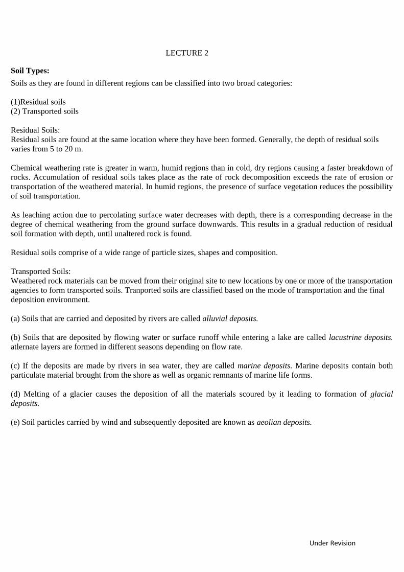
Soil Types:
Soils as they are found in different regions can be classified into two broad categories:
(1)Residual soils
(2) Transported soils
Residual Soils:
Residual soils are found at the same location where they have been formed. Generally, the depth of residual soils
varies from 5 to 20 m.
Chemical weathering rate is greater in warm, humid regions than in cold, dry regions causing a faster breakdown of
rocks. Accumulation of residual soils takes place as the rate of rock decomposition exceeds the rate of erosion or
transportation of the weathered material. In humid regions, the presence of surface vegetation reduces the possibility
of soil transportation.
As leaching action due to percolating surface water decreases with depth, there is a corresponding decrease in the
degree of chemical weathering from the ground surface downwards. This results in a gradual reduction of residual
soil formation with depth, until unaltered rock is found.
Residual soils comprise of a wide range of particle sizes, shapes and composition.
Transported Soils:
Weathered rock materials can be moved from their original site to new locations by one or more of the transportation
agencies to form transported soils. Tranported soils are classified based on the mode of transportation and the final
deposition environment.
(a) Soils that are carried and deposited by rivers are called alluvial deposits.
(b) Soils that are deposited by flowing water or surface runoff while entering a lake are called lacustrine deposits.
atlernate layers are formed in different seasons depending on flow rate.
(c) If the deposits are made by rivers in sea water, they are called marine deposits. Marine deposits contain both
particulate material brought from the shore as well as organic remnants of marine life forms.
(d) Melting of a glacier causes the deposition of all the materials scoured by it leading to formation of glacial
deposits.
(e) Soil particles carried by wind and subsequently deposited are known as aeolian deposits.
Under Revision
Phase Relations of Soils:
Soil is not a coherent solid material like steel and concrete, but is a particulate material. Soils, as they exist in nature,
consist of solid particles (mineral grains, rock fragments) with water and air in the voids between the particles. The
water and air contents are readily changed by changes in ambient conditions and location.
As the relative proportions of the three phases vary in any soil deposit, it is useful to consider a soil model which
will represent these phases distinctly and properly quantify the amount of each phase. A schematic diagram of the
three-phase system is shown in terms of weight and volume symbols respectively for soil solids, water, and air. The
weight of air can be neglected.
The soil model is given dimensional values for the solid, water and air components.
Total volume, V = Vs + Vw + Vv
Three-phase System:
Soils can be partially saturated (with both air and water present), or be fully saturated (no air content) or be perfectly
dry (no water content).
In a saturated soil or a dry soil, the three-phase system thus reduces to two phases only, as shown.
Under Revision
LECTURE 3
The various relations can be grouped into:
Volume relations
Weight relations
Inter-relations
Volume Relations:
As the amounts of both water and air are variable, the volume of solids is taken as the reference quantity. Thus,
several relational volumetric quantities may be defined. The following are the basic volume relations:
1. Void ratio (e) is the ratio of the volume of voids (Vv) to the volume of soil solids (Vs), and is expressed as a
decimal.
2. Porosity (n) is the ratio of the volume of voids to the total volume of soil (V ), and is expressed as a percentage.
Void ratio and porosity are inter-related to each other as follows:
and
3. The volume of water (Vw) in a soil can vary between zero (i.e. a dry soil) and the volume of voids. This can be
expressed as the degree of saturation (S) in percentage.
For a dry soil, S = 0%, and for a fully saturated soil, S = 100%.
4. Air content (ac) is the ratio of the volume of air (Va) to the volume of voids.
5. Percentage air voids (na) is the ratio of the volume of air to the total volume.
Under Revision
Density is a measure of the quantity of mass in a unit volume of material. Unit weight is a measure of the weight of a
unit volume of material. Both can be used interchangeably. The units of density are ton/m³, kg/m³ or g/cm³. The
following are the basic weight relations:
1. The ratio of the mass of water present to the mass of solid particles is called the water content (w), or sometimes
the moisture content.
Its value is 0% for dry soil and its magnitude can exceed 100%.
2. The mass of solid particles is usually expressed in terms of their particle unit weight or specific gravity (Gs)
of the soil grain solids.
where = Unit weight of water
For most inorganic soils, the value of Gs lies between 2.60 and 2.80. The presence of organic material reduces the
value of Gs.
3. Dry unit weight is a measure of the amount of solid particles per unit volume.
4. Bulk unit weight is a measure of the amount of solid particles plus water per unit volume.
5. Saturated unit weight is equal to the bulk density when the total voids is filled up with water.
6. Buoyant unit weight or submerged unit weight is the effective mass per unit volume when the soil is
submerged below standing water or below the ground water table.
Weight Relations:
Under Revision
LECTURE 4
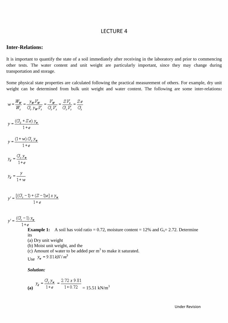
Example 1: A soil has void ratio = 0.72, moisture content = 12% and Gs= 2.72. Determine
its
(a) Dry unit weight
(b) Moist unit weight, and the
(c) Amount of water to be added per m3 to make it saturated.
Use
Solution:
(a) = 15.51 kN/m3
Inter-Relations:
It is important to quantify the state of a soil immediately after receiving in the laboratory and prior to commencing
other tests. The water content and unit weight are particularly important, since they may change during
transportation and storage.
Some physical state properties are calculated following the practical measurement of others. For example, dry unit
weight can be determined from bulk unit weight and water content. The following are some inter-relations:
Under Revision
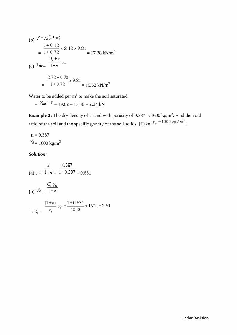
(b)
= = 17.38 kN/m3
(c) =
= = 19.62 kN/m3
Water to be added per m3 to make the soil saturated
= = 19.62 – 17.38 = 2.24 kN
Example 2: The dry density of a sand with porosity of 0.387 is 1600 kg/m3. Find the void
ratio of the soil and the specific gravity of the soil solids. [Take ]
n = 0.387
= 1600 kg/m3
Solution:
(a) e = = = 0.631
(b) =
Gs =
Under Revision
LECTURE 5
Soil Classification:
It is necessary to adopt a formal system of soil description and classification in order to describe the various
materials found in ground investigation. Such a system must be meaningful and concise in an engineering context,
so that engineers will be able to understand and interpret.
It is important to distinguish between description and classification:
Description of soil is a statement that describes the physical nature and state of the soil. It can be a description of a
sample, or a soil in situ. It is arrived at by using visual examination, simple tests, observation of site conditions,
geological history, etc.
Classification of soil is the separation of soil into classes or groups each having similar characteristics and
potentially similar behaviour. A classification for engineering purposes should be based mainly on mechanical
properties: permeability, stiffness, strength. The class to which a soil belongs can be used in its description.
The aim of a classification system is to establish a set of conditions which will allow useful comparisons to be made
between different soils. The system must be simple. The relevant criteria for classifying soils are the size
distribution of particles and the plasticity of the soil.
For measuring the distribution of particle sizes in a soil sample, it is necessary to conduct different particle-size tests.
Wet sieving is carried out for separating fine grains from coarse grains by washing the soil specimen on a 75 micron
sieve mesh.
Dry sieve analysis is carried out on particles coarser than 75 micron. Samples (with fines removed) are dried and
shaken through a set of sieves of descending size. The weight retained in each sieve is measured. The cumulative
percentage quantities finer than the sieve sizes (passing each given sieve size) are then determined.
The resulting data is presented as a distribution curve with grain size along x-axis (log scale) and percentage passing
along y-axis (arithmetic scale).
Sedimentation analysis is used only for the soil fraction finer than 75 microns. Soil particles are allowed to settle
from a suspension. The decreasing density of the suspension is measured at various time intervals. The procedure is
based on the principle that in a suspension, the terminal velocity of a spherical particle is governed by the diameter
of the particle and the properties of the suspension.
In this method, the soil is placed as a suspension in a jar filled with distilled water to which a deflocculating agent is
added. The soil particles are then allowed to settle down. The concentration of particles remaining in the suspension
at a particular level can be determined by using a hydrometer. Specific gravity readings of the solution at that same
level at different time intervals provide information about the size of particles that have settled down and the mass of
Under Revision
soil remaining in solution.
The results are then plotted between % finer (passing) and log size.
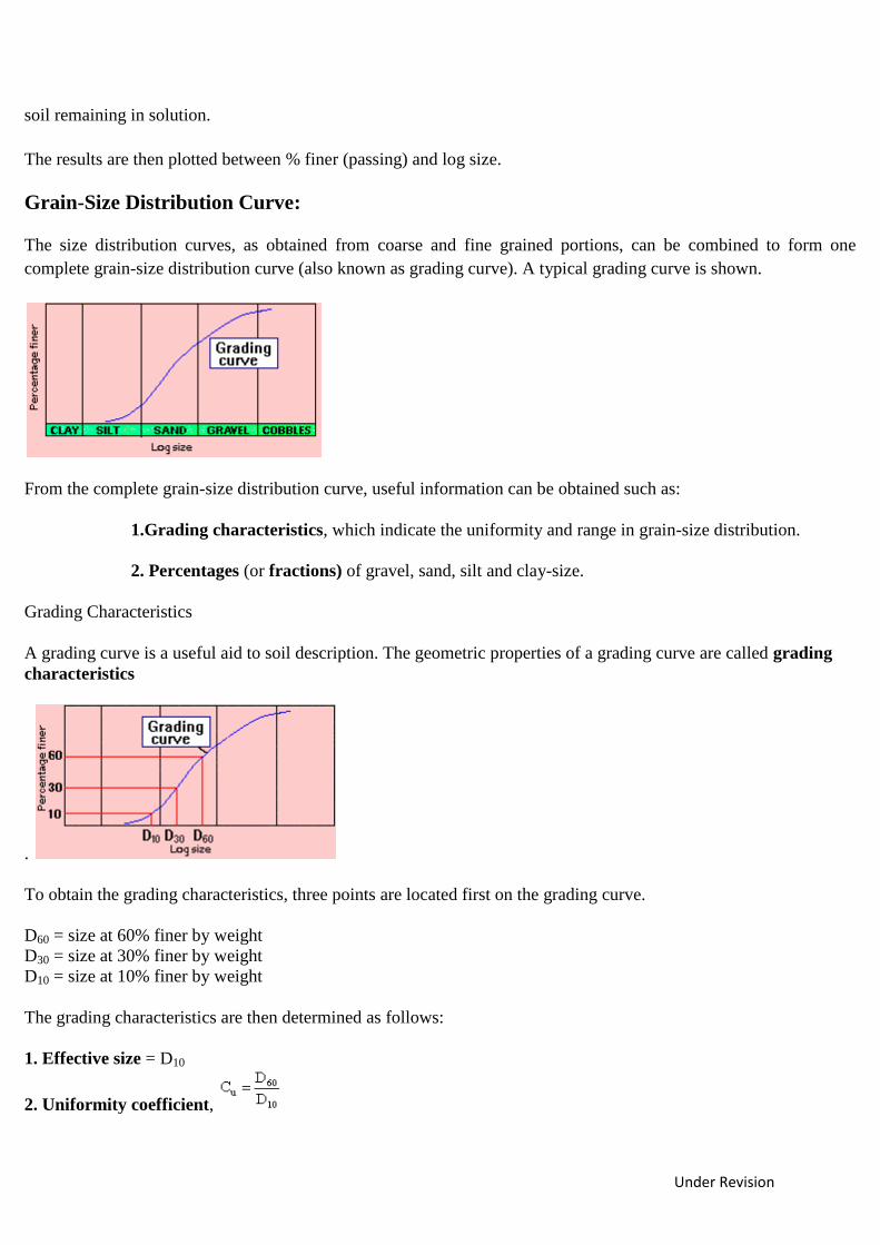
Grain-Size Distribution Curve:
The size distribution curves, as obtained from coarse and fine grained portions, can be combined to form one
complete grain-size distribution curve (also known as grading curve). A typical grading curve is shown.
From the complete grain-size distribution curve, useful information can be obtained such as:
1.Grading characteristics, which indicate the uniformity and range in grain-size distribution.
2. Percentages (or fractions) of gravel, sand, silt and clay-size.
Grading Characteristics
A grading curve is a useful aid to soil description. The geometric properties of a grading curve are called grading
characteristics
.
To obtain the grading characteristics, three points are located first on the grading curve.
D60 = size at 60% finer by weight
D30 = size at 30% finer by weight
D10 = size at 10% finer by weight
The grading characteristics are then determined as follows:
1. Effective size = D10
2. Uniformity coefficient,

Under Revision
3. Curvature coefficient,
Both Cu and Cc will be 1 for a single-sized soil.
Cu > 5 indicates a well-graded soil, i.e. a soil which has a distribution of particles over a wide size range.
Cc between 1 and 3 also indicates a well-graded soil.
Cu < 3 indicates a uniform soil, i.e. a soil which has a very narrow particle size range.
Under Revision
LECTURE 6
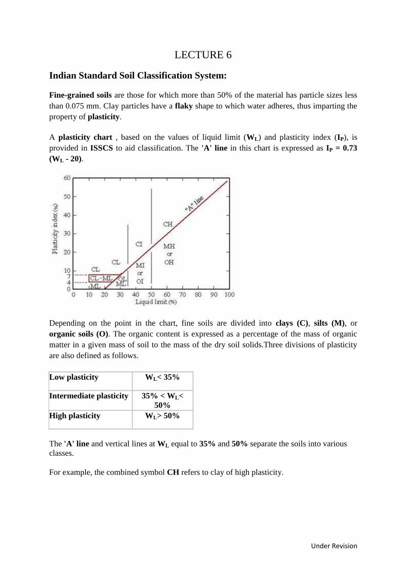
Indian Standard Soil Classification System:
Fine-grained soils are those for which more than 50% of the material has particle sizes less
than 0.075 mm. Clay particles have a flaky shape to which water adheres, thus imparting the
property of plasticity.
A plasticity chart , based on the values of liquid limit (WL) and plasticity index (IP), is
provided in ISSCS to aid classification. The 'A' line in this chart is expressed as IP = 0.73
(WL - 20).
Depending on the point in the chart, fine soils are divided into clays (C), silts (M), or
organic soils (O). The organic content is expressed as a percentage of the mass of organic
matter in a given mass of soil to the mass of the dry soil solids.Three divisions of plasticity
are also defined as follows.
Low plasticity WL< 35%
Intermediate plasticity 35% < WL<
50%
High plasticity WL> 50%
The 'A' line and vertical lines at WL equal to 35% and 50% separate the soils into various
classes.
For example, the combined symbol CH refers to clay of high plasticity.
Under Revision
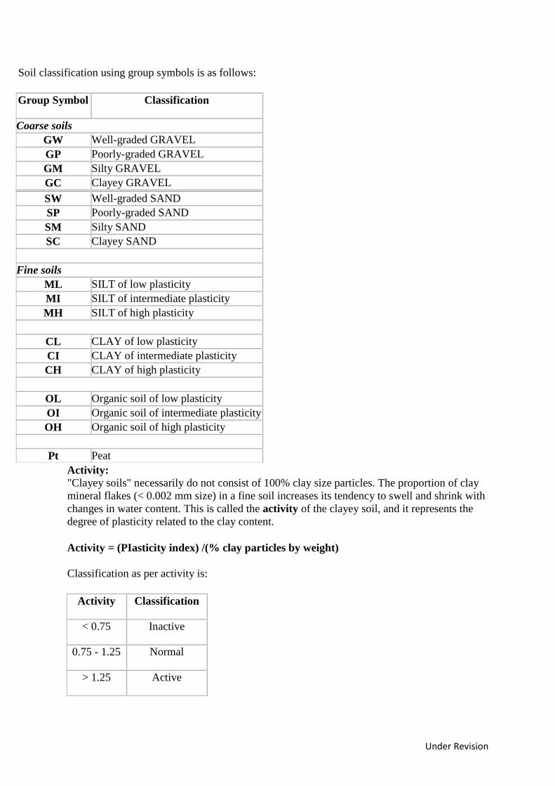
Soil classification using group symbols is as follows:
Group Symbol Classification
Coarse soils
GW Well-graded GRAVEL
GP Poorly-graded GRAVEL
GM Silty GRAVEL
GC Clayey GRAVEL
SW Well-graded SAND
SP Poorly-graded SAND
SM Silty SAND
SC Clayey SAND
Fine soils
ML SILT of low plasticity
MI SILT of intermediate plasticity
MH SILT of high plasticity
CL CLAY of low plasticity
CI CLAY of intermediate plasticity
CH CLAY of high plasticity
OL Organic soil of low plasticity
OI Organic soil of intermediate plasticity
OH Organic soil of high plasticity
Pt Peat
Activity: "Clayey soils" necessarily do not consist of 100% clay size particles. The proportion of clay
mineral flakes (< 0.002 mm size) in a fine soil increases its tendency to swell and shrink with
changes in water content. This is called the activity of the clayey soil, and it represents the
degree of plasticity related to the clay content.
Activity = (PIasticity index) /(% clay particles by weight)
Classification as per activity is:
Activity Classification
< 0.75 Inactive
0.75 - 1.25 Normal
> 1.25 Active
Under Revision
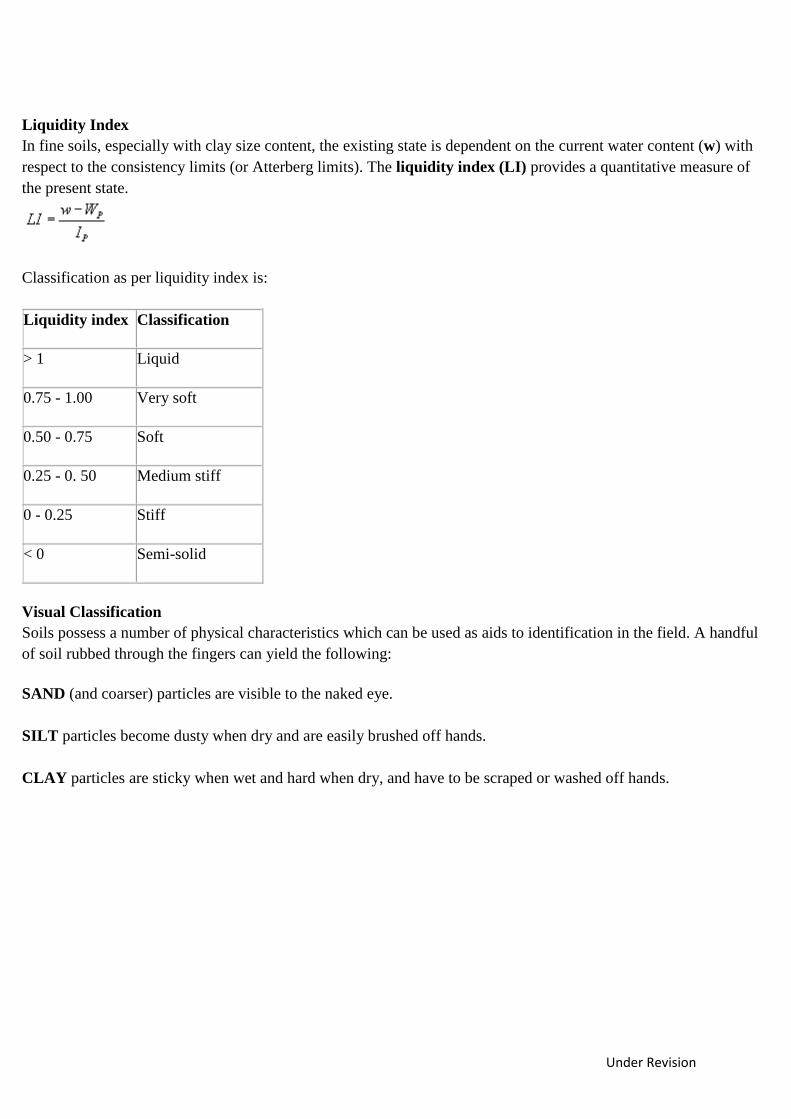
Liquidity Index
In fine soils, especially with clay size content, the existing state is dependent on the current water content (w) with
respect to the consistency limits (or Atterberg limits). The liquidity index (LI) provides a quantitative measure of
the present state.
Classification as per liquidity index is:
Liquidity index Classification
> 1 Liquid
0.75 - 1.00 Very soft
0.50 - 0.75 Soft
0.25 - 0. 50 Medium stiff
0 - 0.25 Stiff
< 0 Semi-solid
Visual Classification
Soils possess a number of physical characteristics which can be used as aids to identification in the field. A handful
of soil rubbed through the fingers can yield the following:
SAND (and coarser) particles are visible to the naked eye.
SILT particles become dusty when dry and are easily brushed off hands.
CLAY particles are sticky when wet and hard when dry, and have to be scraped or washed off hands.
Under Revision
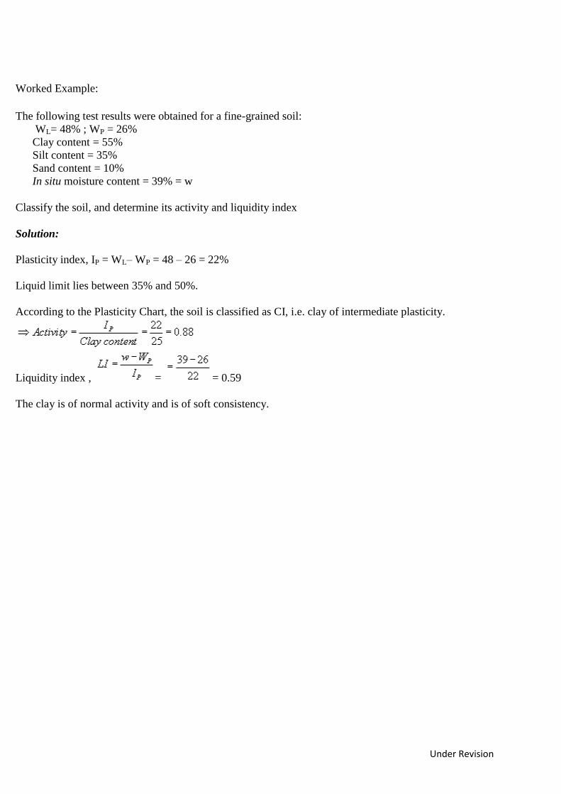
Worked Example:
The following test results were obtained for a fine-grained soil:
WL= 48% ; WP = 26%
Clay content = 55%
Silt content = 35%
Sand content = 10%
In situ moisture content = 39% = w
Classify the soil, and determine its activity and liquidity index
Solution:
Plasticity index, IP = WL– WP = 48 – 26 = 22%
Liquid limit lies between 35% and 50%.
According to the Plasticity Chart, the soil is classified as CI, i.e. clay of intermediate plasticity.
Liquidity index , = = 0.59
The clay is of normal activity and is of soft consistency.
Under Revision
LECTURE 7
Formation of Clay Minerals:
A soil particle may be a mineral or a rock fragment. A mineral is a chemical compound formed in nature during a
geological process, whereas a rock fragment has a combination of one or more minerals. Based on the nature of
atoms, minerals are classified as silicates, aluminates, oxides, carbonates and phosphates.
Out of these, silicate minerals are the most important as they influence the properties of clay soils. Different
arrangements of atoms in the silicate minerals give rise to different silicate structures.
Basic Structural Units
Soil minerals are formed from two basic structural units: tetrahedral and octahedral. Considering the valencies of the
atoms forming the units, it is clear that the units are not electrically neutral and as such do not exist as single units.
The basic units combine to form sheets in which the oxygen or hydroxyl ions are shared among adjacent units. Three
types of sheets are thus formed, namely silica sheet, gibbsite sheet and brucite sheet.
Isomorphous substitution is the replacement of the central atom of the tetrahedral or octahedral unit by another atom
during the formation of the sheets.
The sheets then combine to form various two-layer or three-layer sheet minerals. As the basic units of clay minerals
are sheet-like structures, the particle formed from stacking of the basic units is also plate-like. As a result, the surface
area per unit mass becomes very large.
Under Revision
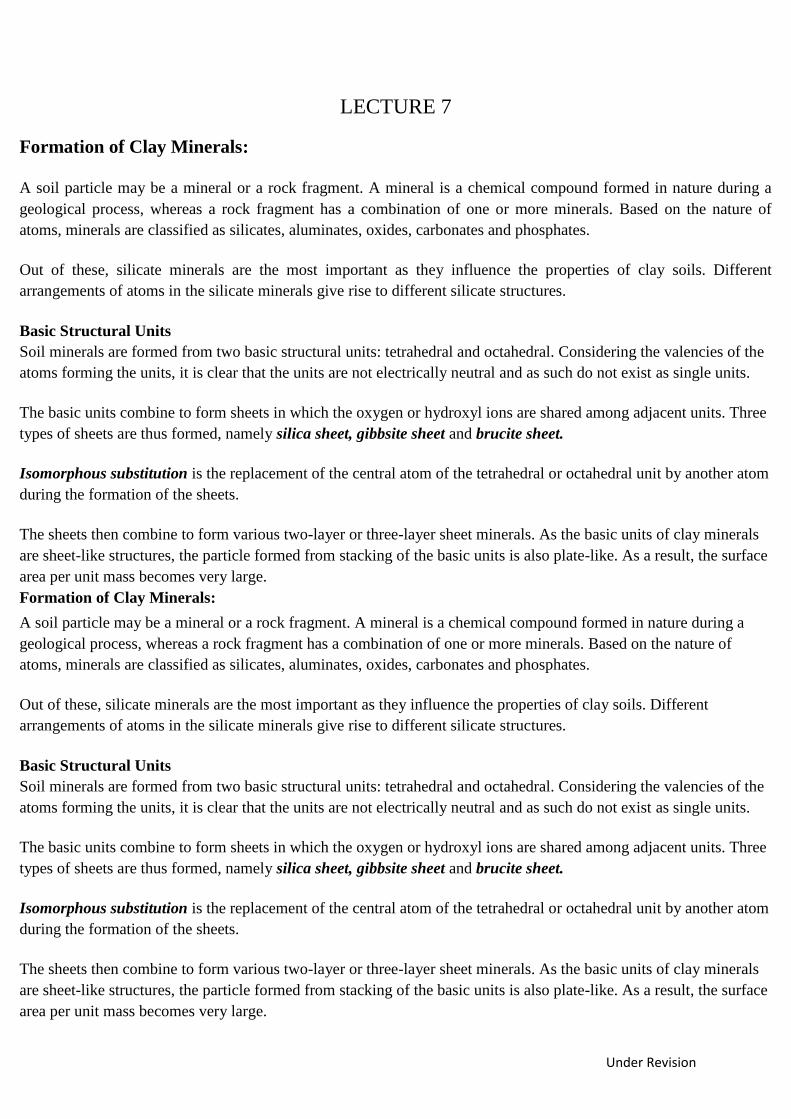
Structure of Clay Minerals:
A tetrahedral unit consists of a central silicon atom that is surrounded by four oxygen atoms located at the corners of
a tetrahedron. A combination of tetrahedrons forms a silica sheet.
An octahedral unit consists of a central ion, either aluminium or magnesium, that is surrounded by six hydroxyl ions
located at the corners of an octahedron. A combination of aluminium-hydroxyl octahedrons forms a gibbsite sheet,
whereas a combination of magnesium-hydroxyl octahedrons forms a brucite sheet.
Two-layer Sheet Minerals:
Kaolinite and halloysite clay minerals are the most common.
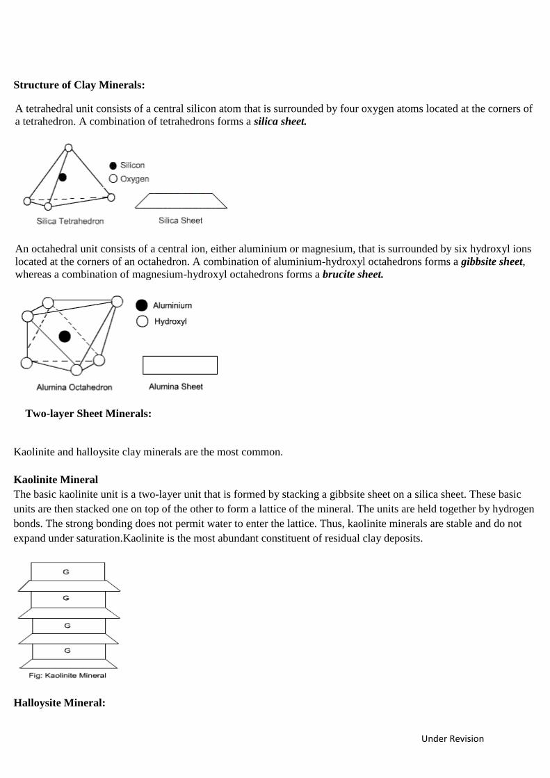
Kaolinite Mineral
The basic kaolinite unit is a two-layer unit that is formed by stacking a gibbsite sheet on a silica sheet. These basic
units are then stacked one on top of the other to form a lattice of the mineral. The units are held together by hydrogen
bonds. The strong bonding does not permit water to enter the lattice. Thus, kaolinite minerals are stable and do not
expand under saturation.Kaolinite is the most abundant constituent of residual clay deposits.
Halloysite Mineral:
Under Revision
The basic unit is also a two-layer sheet similar to that of kaolinite except for the presence of water between the
sheets.
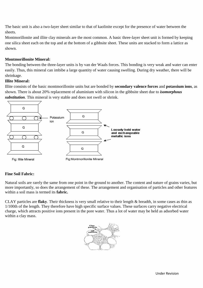
Montmorillonite and illite clay minerals are the most common. A basic three-layer sheet unit is formed by keeping
one silica sheet each on the top and at the bottom of a gibbsite sheet. These units are stacked to form a lattice as
shown.
Montmorillonite Mineral:
The bonding between the three-layer units is by van der Waals forces. This bonding is very weak and water can enter
easily. Thus, this mineral can imbibe a large quantity of water causing swelling. During dry weather, there will be
shrinkage.
Illite Mineral:
Illite consists of the basic montmorillonite units but are bonded by secondary valence forces and potassium ions, as
shown. There is about 20% replacement of aluminium with silicon in the gibbsite sheet due to isomorphous
substitution. This mineral is very stable and does not swell or shrink.
Fine Soil Fabric:
Natural soils are rarely the same from one point in the ground to another. The content and nature of grains varies, but
more importantly, so does the arrangement of these. The arrangement and organisation of particles and other features
within a soil mass is termed its fabric.
CLAY particles are flaky. Their thickness is very small relative to their length & breadth, in some cases as thin as
1/100th of the length. They therefore have high specific surface values. These surfaces carry negative electrical
charge, which attracts positive ions present in the pore water. Thus a lot of water may be held as adsorbed water
within a clay mass.
Under Revision
LECTURE 8
Stresses in the Ground:
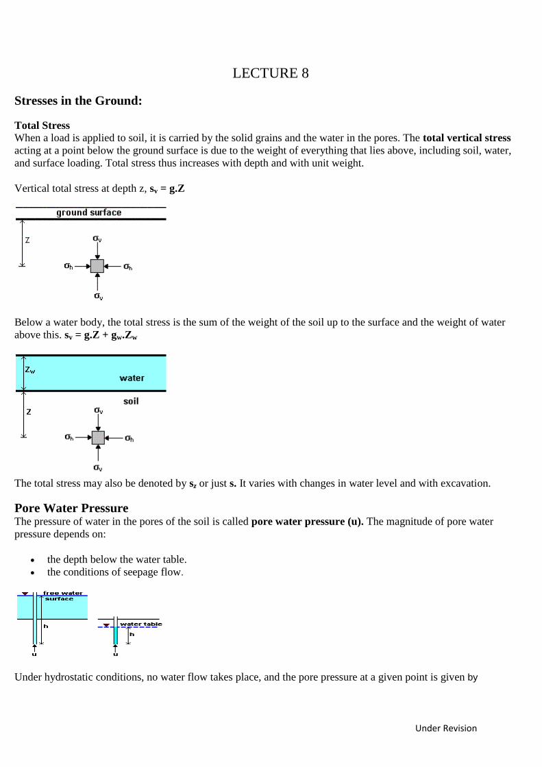
Total Stress When a load is applied to soil, it is carried by the solid grains and the water in the pores. The total vertical stress
acting at a point below the ground surface is due to the weight of everything that lies above, including soil, water,
and surface loading. Total stress thus increases with depth and with unit weight.
Vertical total stress at depth z, sv = g.Z
Below a water body, the total stress is the sum of the weight of the soil up to the surface and the weight of water
above this. sv = g.Z + gw.Zw
The total stress may also be denoted by sz or just s. It varies with changes in water level and with excavation.
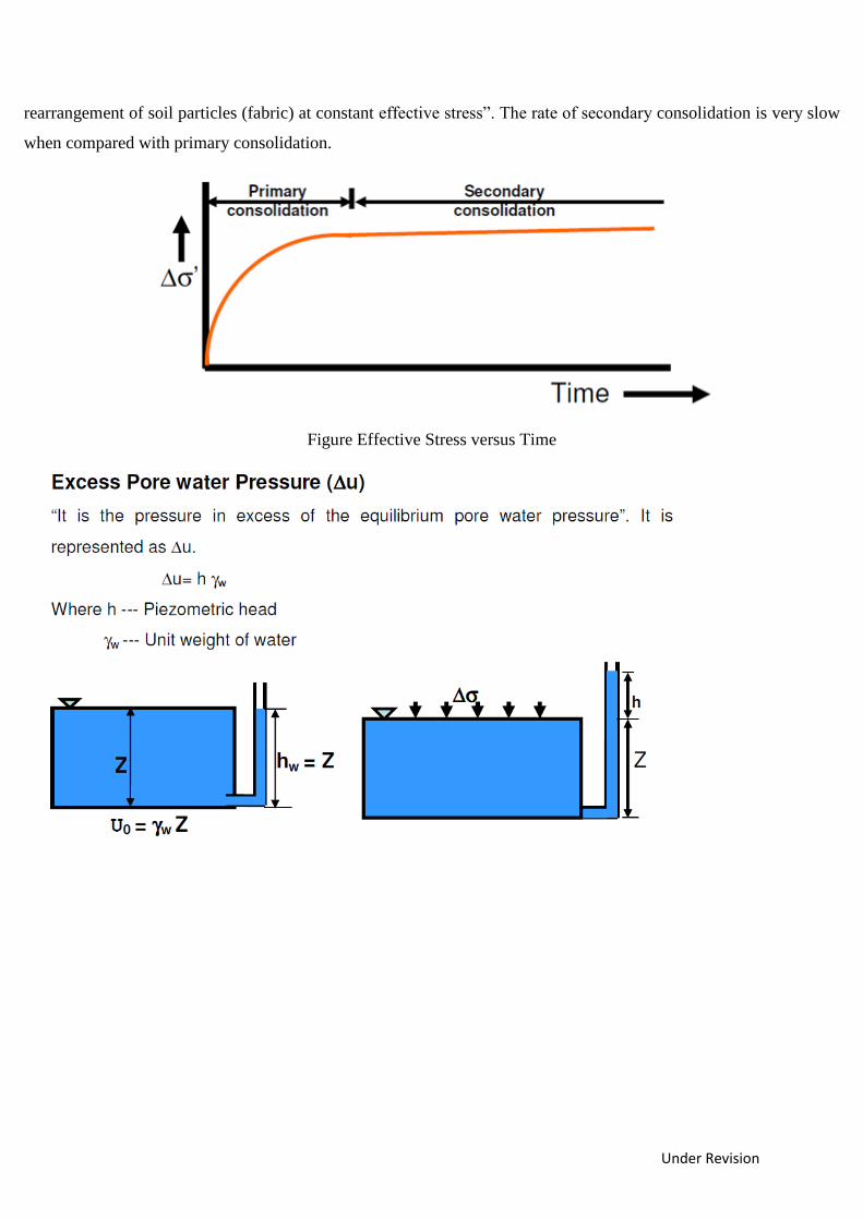
Pore Water Pressure
The pressure of water in the pores of the soil is called pore water pressure (u). The magnitude of pore water
pressure depends on:
the depth below the water table.
the conditions of seepage flow.
Under hydrostatic conditions, no water flow takes place, and the pore pressure at a given point is given by
Under Revision
u = w.h
where h = depth below water table or overlying water surface
It is convenient to think of pore water pressure as the pressure exerted by a column of water in an imaginary
standpipe inserted at the given point.
The natural level of ground water is called the water table or the phreatic surface. Under conditions of no seepage
flow, the water table is horizontal. The magnitude of the pore water pressure at the water table is zero. Below the
water table, pore water pressures are positive.
The principle of effective stress was enunciated by Karl Terzaghi in the year 1936. This principle is valid only for
saturated soils, and consists of two parts:
1. At any point in a soil mass, the effective stress (represented by or σ' ) is related to total stress (σ) and pore water
pressure (u) as
= σ - u
Both the total stress and pore water pressure can be measured at any point.
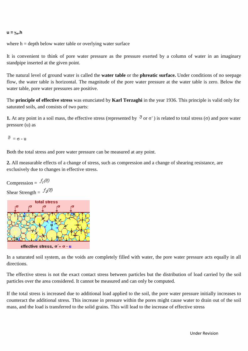
2. All measurable effects of a change of stress, such as compression and a change of shearing resistance, are
exclusively due to changes in effective stress.
Compression =
Shear Strength =
In a saturated soil system, as the voids are completely filled with water, the pore water pressure acts equally in all
directions.
The effective stress is not the exact contact stress between particles but the distribution of load carried by the soil
particles over the area considered. It cannot be measured and can only be computed.
If the total stress is increased due to additional load applied to the soil, the pore water pressure initially increases to
counteract the additional stress. This increase in pressure within the pores might cause water to drain out of the soil
mass, and the load is transferred to the solid grains. This will lead to the increase of effective stress
Under Revision
.
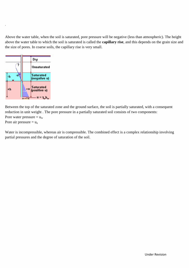
Above the water table, when the soil is saturated, pore pressure will be negative (less than atmospheric). The height
above the water table to which the soil is saturated is called the capillary rise, and this depends on the grain size and
the size of pores. In coarse soils, the capillary rise is very small.
Between the top of the saturated zone and the ground surface, the soil is partially saturated, with a consequent
reduction in unit weight . The pore pressure in a partially saturated soil consists of two components:
Pore water pressure = uw
Pore air pressure = ua
Water is incompressible, whereas air is compressible. The combined effect is a complex relationship involving
partial pressures and the degree of saturation of the soil.
Under Revision
LECTURE 9
Effective stress under Hydrodynamic Conditions:
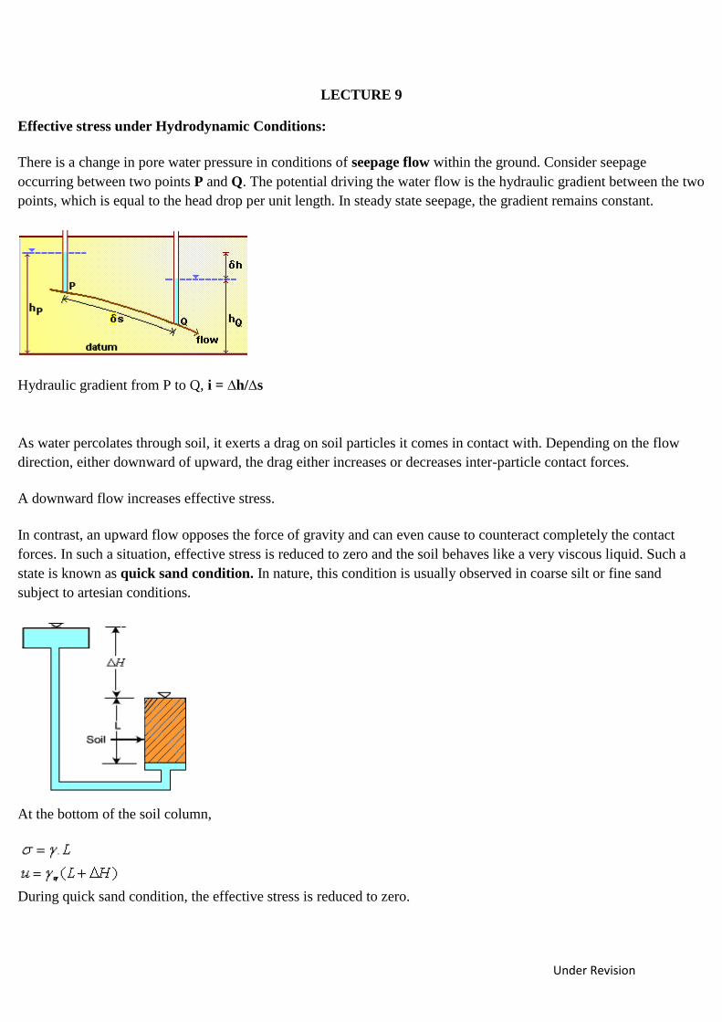
There is a change in pore water pressure in conditions of seepage flow within the ground. Consider seepage
occurring between two points P and Q. The potential driving the water flow is the hydraulic gradient between the two
points, which is equal to the head drop per unit length. In steady state seepage, the gradient remains constant.
Hydraulic gradient from P to Q, i = ∆h/∆s
As water percolates through soil, it exerts a drag on soil particles it comes in contact with. Depending on the flow
direction, either downward of upward, the drag either increases or decreases inter-particle contact forces.
A downward flow increases effective stress.
In contrast, an upward flow opposes the force of gravity and can even cause to counteract completely the contact
forces. In such a situation, effective stress is reduced to zero and the soil behaves like a very viscous liquid. Such a
state is known as quick sand condition. In nature, this condition is usually observed in coarse silt or fine sand
subject to artesian conditions.
At the bottom of the soil column,
During quick sand condition, the effective stress is reduced to zero.
Under Revision
where icr = critical hydraulic gradient
This shows that when water flows upward under a hydraulic gradient of about 1, it completely neutralizes the force
on account of the weight of particles, and thus leaves the particles suspended in water.
Importance of Effective stress:
At any point within the soil mass, the magitudes of both total stress and pore water pressure are dependent on the
ground water position. With a shift in the water table due to seasonal fluctuations, there is a resulting change in the
distribution in pore water pressure with depth.
Changes in water level below ground result in changes in effective stresses below the water table. A rise increases
the pore water pressure at all elevations thus causing a decrease in effective stress. In contrast, a fall in the water
table produces an increase in the effective stress.
Changes in water level above ground do not cause changes in effective stresses in the ground below. A rise above
ground surface increases both the total stress and the pore water pressure by the same amount, and consequently
effective stress is not altered.
In some analyses it is better to work with the changes of quantity, rather than in absolute quantities. The effective
stress expression then becomes:
σ' = σ - u
If both total stress and pore water pressure change by the same amount, the effective stress remains constant.
Total and effective stresses must be distinguishable in all calculations. Ground movements and instabilities can be
caused by changes in total stress, such as caused by loading by foundations and unloading due to excavations. They
can also be caused by changes in pore water pressures, such as failure of slopes after rainfall.
Under Revision
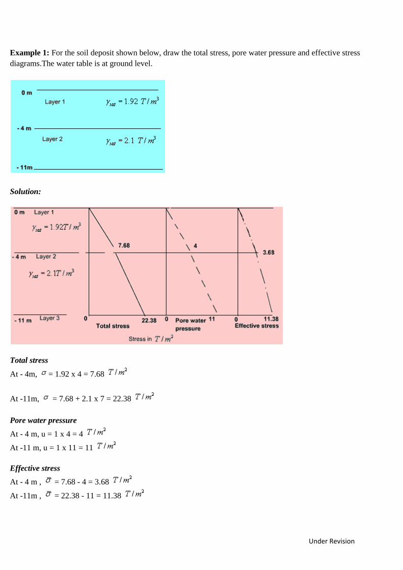
Example 1: For the soil deposit shown below, draw the total stress, pore water pressure and effective stress
diagrams.The water table is at ground level.
Solution:
Total stress
At - 4m, = 1.92 x 4 = 7.68
At -11m, = 7.68 + 2.1 x 7 = 22.38
Pore water pressure
At - 4 m, u = 1 x 4 = 4
At -11 m, u = 1 x 11 = 11
Effective stress
At - 4 m , = 7.68 - 4 = 3.68
At -11m , = 22.38 - 11 = 11.38
Under Revision
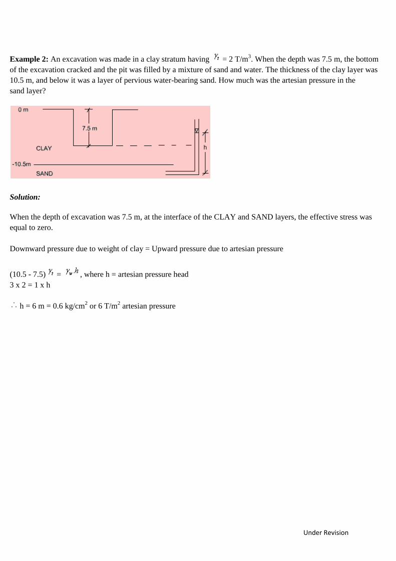
Example 2: An excavation was made in a clay stratum having = 2 T/m3. When the depth was 7.5 m, the bottom
of the excavation cracked and the pit was filled by a mixture of sand and water. The thickness of the clay layer was
10.5 m, and below it was a layer of pervious water-bearing sand. How much was the artesian pressure in the
sand layer?
Solution:
When the depth of excavation was 7.5 m, at the interface of the CLAY and SAND layers, the effective stress was
equal to zero.
Downward pressure due to weight of clay = Upward pressure due to artesian pressure
(10.5 - 7.5) = , where h = artesian pressure head
3 x 2 = 1 x h
h = 6 m = 0.6 kg/cm2 or 6 T/m
2 artesian pressure
Under Revision
LECTURE 10
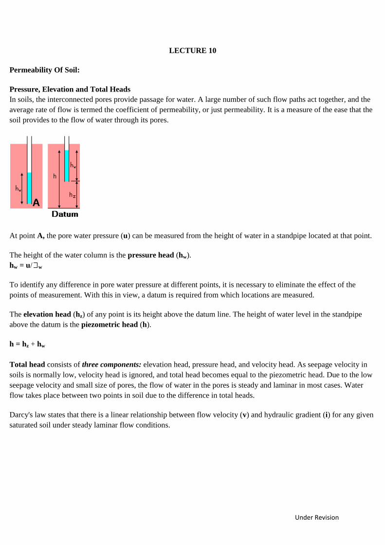
Permeability Of Soil:
Pressure, Elevation and Total Heads
In soils, the interconnected pores provide passage for water. A large number of such flow paths act together, and the
average rate of flow is termed the coefficient of permeability, or just permeability. It is a measure of the ease that the
soil provides to the flow of water through its pores.
At point A, the pore water pressure (u) can be measured from the height of water in a standpipe located at that point.
The height of the water column is the pressure head (hw).
hw = u/ w
To identify any difference in pore water pressure at different points, it is necessary to eliminate the effect of the
points of measurement. With this in view, a datum is required from which locations are measured.
The elevation head (hz) of any point is its height above the datum line. The height of water level in the standpipe
above the datum is the piezometric head (h).
h = hz + hw
Total head consists of three components: elevation head, pressure head, and velocity head. As seepage velocity in
soils is normally low, velocity head is ignored, and total head becomes equal to the piezometric head. Due to the low
seepage velocity and small size of pores, the flow of water in the pores is steady and laminar in most cases. Water
flow takes place between two points in soil due to the difference in total heads.
Darcy's law states that there is a linear relationship between flow velocity (v) and hydraulic gradient (i) for any given
saturated soil under steady laminar flow conditions.
Under Revision
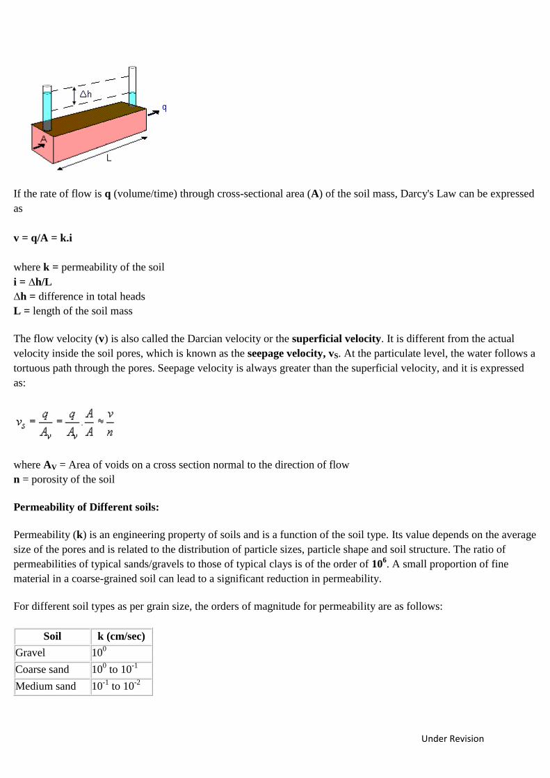
If the rate of flow is q (volume/time) through cross-sectional area (A) of the soil mass, Darcy's Law can be expressed
as
v = q/A = k.i
where k = permeability of the soil
i = ∆h/L
∆h = difference in total heads
L = length of the soil mass
The flow velocity (v) is also called the Darcian velocity or the superficial velocity. It is different from the actual
velocity inside the soil pores, which is known as the seepage velocity, vS. At the particulate level, the water follows a
tortuous path through the pores. Seepage velocity is always greater than the superficial velocity, and it is expressed
as:
where AV = Area of voids on a cross section normal to the direction of flow
n = porosity of the soil
Permeability of Different soils:
Permeability (k) is an engineering property of soils and is a function of the soil type. Its value depends on the average
size of the pores and is related to the distribution of particle sizes, particle shape and soil structure. The ratio of
permeabilities of typical sands/gravels to those of typical clays is of the order of 106. A small proportion of fine
material in a coarse-grained soil can lead to a significant reduction in permeability.
For different soil types as per grain size, the orders of magnitude for permeability are as follows:
Soil k (cm/sec)
Gravel 100
Coarse sand 100 to 10
-1
Medium sand 10-1
to 10-2
Under Revision
Fine sand 10-2
to 10-3
Silty sand 10-3
to 10-4
Silt 1 x 10⁻⁵
Clay 10-7
to 10-9
In soils, the permeant or pore fluid is mostly water whose variation in property is generally very less. Permeability of
all soils is strongly influenced by the density of packing of the soil particles, which can be represented by void ratio
(e) or porosity (n).
For Sands
In sands, permeability can be empirically related to the square of some representative grain size from its grain-size
distribution. For filter sands, Allen Hazen in 1911 found that k 100 (D10)2 cm/s where D10= effective grain size in
cm.
Different relationships have been attempted relating void ratio and permeability, such as k e3/(1+e), and k
2.
They have been obtained from the Kozeny-Carman equation for laminar flow in saturated soils.
where ko and kT are factors depending on the shape and tortuosity of the pores respectively, SS is the surface area of
w and are unit weight and viscosity of the pore water.
The equation can be reduced to a simpler form as
For Silts and Clays
For silts and clays, the Kozeny-Carman equation does not work well, and log k versus e plot has been found to
indicate a linear relationship.
For clays, it is typically found that
where Ckis the permeability change index and ek is a reference void ratio.
Under Revision
LECTURE 11
Laboratory Measurement of Permeability:
Constant Head Flow
Constant head permeameter is recommended for coarse-grained soils only since for such soils, flow rate is
measurable with adequate precision. As water flows through a sample of cross-section area A, steady total head
drop h is measured across length L.
Permeability k is obtained from:
Falling Head Flow:
Falling head permeameter is recommended for fine-grained soils.
Total head h in standpipe of area a is allowed to fall. Hydraulic gradient varies with time. Heads h1 and h2 are
measured at times t1 and t2. At any time t, flow through the soil sample of cross-sectional area A is
--------------------- (1)
Flow in unit time through the standpipe of cross-sectional area a is
Under Revision
= ----------------- (2)
Equating (1) and (2) ,
or
Integrating between the limits,
Seepage in Soils:
A rectangular soil element is shown with dimensions dx and dz in the plane, and thickness dy perpendicuar to this
plane. Consider planar flow into the rectangular soil element.
In the x-direction, the net amount of the water entering and leaving the element is
Under Revision
Similarly in the z-direction, the difference between the water inflow and outflow is
For a two-dimensional steady flow of pore water, any imbalance in flows into and out of an element in the z-direction
must be compensated by a corresponding opposite imbalance in the x-direction. Combining the above, and dividing
bydx.dy.dz , the continuity equation is expressed as
From Darcy's law, , , where h is the head causing flow.
When the continuity equation is combined with Darcy's law, the equation for flow is expressed as:
For an isotropic material in which the permeability is the same in all directions (i.e. k x= k z), the flow equation is
This is the Laplace equation governing two-dimensional steady state flow. It can be solved graphically,
analytically, numerically, or analogically.
For the more general situation involving three-dimensional steady flow, Laplace equation becomes:
Under Revision
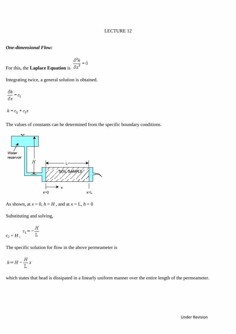
LECTURE 12
One-dimensional Flow:
For this, the Laplace Equation is
Integrating twice, a general solution is obtained.
The values of constants can be determined from the specific boundary conditions.
As shown, at x = 0, h = H , and at x = L, h = 0
Substituting and solving,
c2 = H ,
The specific solution for flow in the above permeameter is
which states that head is dissipated in a linearly uniform manner over the entire length of the permeameter.
Under Revision
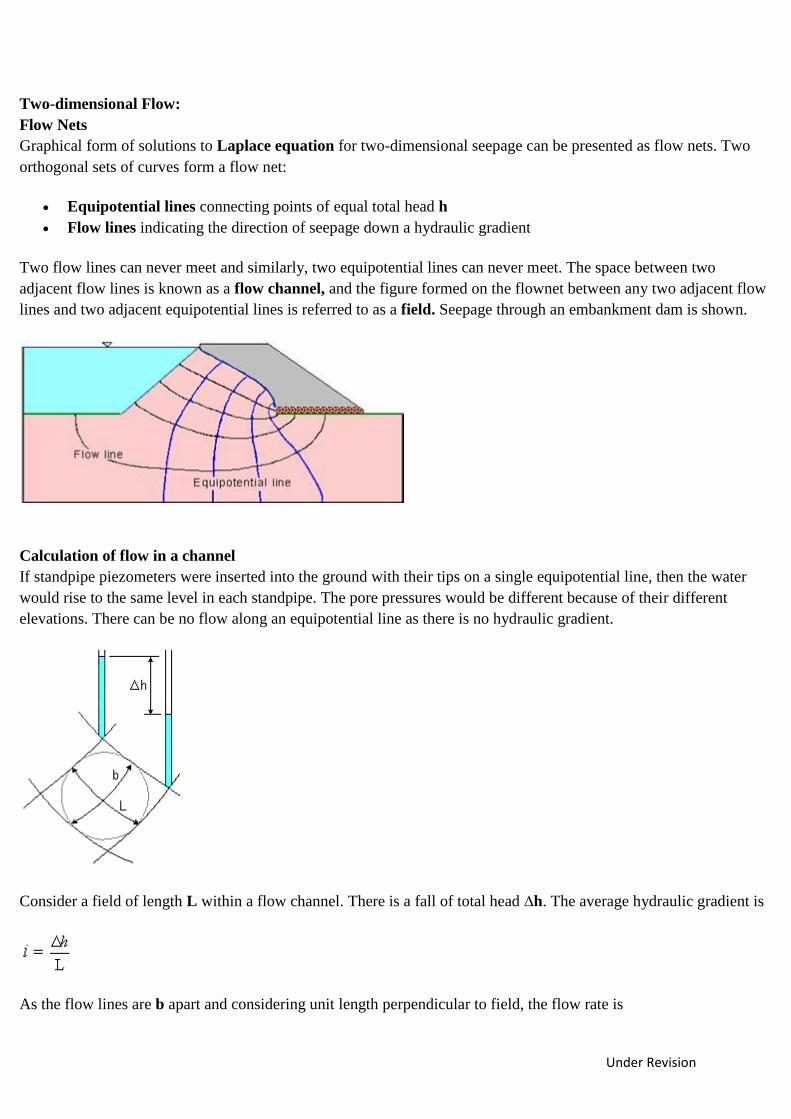
Two-dimensional Flow:
Flow Nets
Graphical form of solutions to Laplace equation for two-dimensional seepage can be presented as flow nets. Two
orthogonal sets of curves form a flow net:
Equipotential lines connecting points of equal total head h
Flow lines indicating the direction of seepage down a hydraulic gradient
Two flow lines can never meet and similarly, two equipotential lines can never meet. The space between two
adjacent flow lines is known as a flow channel, and the figure formed on the flownet between any two adjacent flow
lines and two adjacent equipotential lines is referred to as a field. Seepage through an embankment dam is shown.
Calculation of flow in a channel
If standpipe piezometers were inserted into the ground with their tips on a single equipotential line, then the water
would rise to the same level in each standpipe. The pore pressures would be different because of their different
elevations. There can be no flow along an equipotential line as there is no hydraulic gradient.
Consider a field of length L within a flow channel. There is a fall of total head ∆h. The average hydraulic gradient is
As the flow lines are b apart and considering unit length perpendicular to field, the flow rate is
Under Revision
There is an advantage in sketching flow nets in the form of curvilinear 'squares' so that a circle can be inscribed
within each four-sided figure bounded by two equipotential lines and two flow lines.
In such a square, b = L, and the flow rate is obtained as ∆q = k. ∆h
Thus the flow rate through such a flow channel is the permeability k multiplied by the uniform interval between
adjacent equipotential lines.
Calculation of total flow
For a complete problem, the flow net can be drawn with the overall head drop h divided into Nd so that ∆h = h / Nd.
If Nf is the no. of flow channels, then the total flow rate is
Under Revision
LECTURE 13
Procedure for Drawing Flow Nets:
At every point (x,z) where there is flow, there will be a value of head h(x,z). In order to represent these values,
contours of equal head are drawn.
A flow net is to be drawn by trial and error. For a given set of boundary conditions, the flow net will remain the same
even if the direction of flow is reversed. Flow nets are constructed such that the head lost between successive
equipotential lines is the same, say ∆h. It is useful in visualising the flow in a soil to plot the flow lines, as these are
lines that are tangential to the flow at any given point. The steps of construction are:
1. Mark all boundary conditions, and draw the flow cross section to some convenient scale.
2. Draw a coarse net which is consistent with the boundary conditions and which has orthogonal equipotential and
flow lines. As it is usually easier to visualise the pattern of flow, start by drawing the flow lines first.
3. Modify the mesh such that it meets the conditions outlined above and the fields between adjacent flow lines and
equipotential lines are 'square'.
4. Refine the flow net by repeating step 3.
The most common boundary conditions are:
(a) A submerged permeable soil boundary is an equipotential line. This could have been determined by considering
imaginary standpipes placed at the soil boundary, as for every point the water level in the standpipe would be the
same as the water level. (Such a boundary is marked as CD and EF in the following figure.)
(b) The boundary between permeable and impermeable soil materials is a flow line (This is marked as AB in the
same figure).
(c) Equipotential lines intersecting a phreatic surface do so at equal vertical intervals.
Under Revision
LECTURE 14
COMPACTION
Introduction:
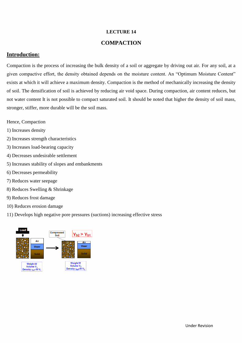
Compaction is the process of increasing the bulk density of a soil or aggregate by driving out air. For any soil, at a
given compactive effort, the density obtained depends on the moisture content. An “Optimum Moisture Content”
exists at which it will achieve a maximum density. Compaction is the method of mechanically increasing the density
of soil. The densification of soil is achieved by reducing air void space. During compaction, air content reduces, but
not water content It is not possible to compact saturated soil. It should be noted that higher the density of soil mass,
stronger, stiffer, more durable will be the soil mass.
Hence, Compaction
1) Increases density
2) Increases strength characteristics
3) Increases load-bearing capacity
4) Decreases undesirable settlement
5) Increases stability of slopes and embankments
6) Decreases permeability
7) Reduces water seepage
8) Reduces Swelling & Shrinkage
9) Reduces frost damage
10) Reduces erosion damage
11) Develops high negative pore pressures (suctions) increasing effective stress
Under Revision
Mechanism of Compaction-
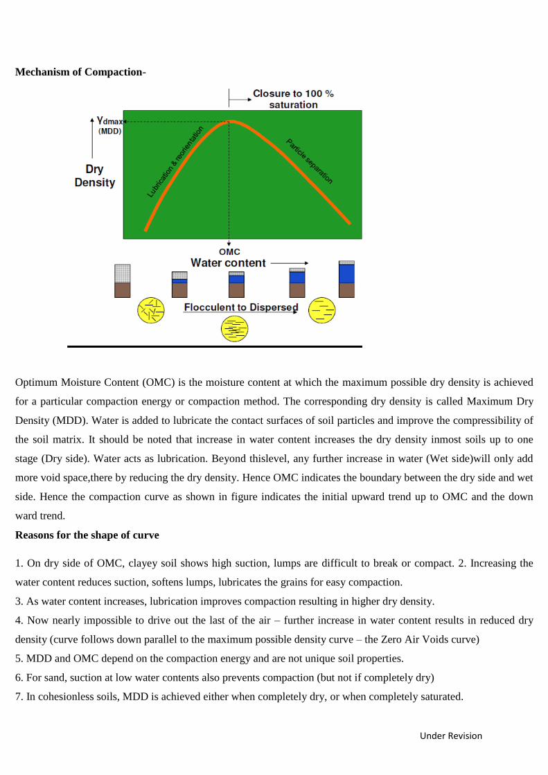
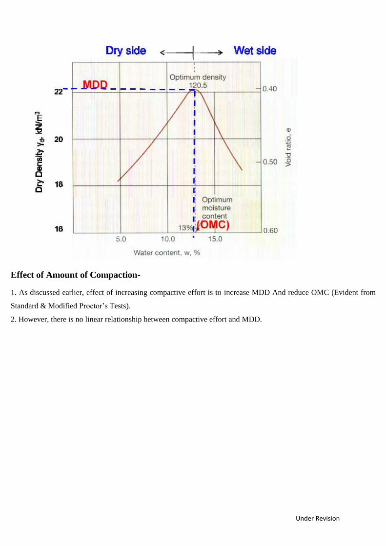
Optimum Moisture Content (OMC) is the moisture content at which the maximum possible dry density is achieved
for a particular compaction energy or compaction method. The corresponding dry density is called Maximum Dry
Density (MDD). Water is added to lubricate the contact surfaces of soil particles and improve the compressibility of
the soil matrix. It should be noted that increase in water content increases the dry density inmost soils up to one
stage (Dry side). Water acts as lubrication. Beyond thislevel, any further increase in water (Wet side)will only add
more void space,there by reducing the dry density. Hence OMC indicates the boundary between the dry side and wet
side. Hence the compaction curve as shown in figure indicates the initial upward trend up to OMC and the down
ward trend.
Reasons for the shape of curve
1. On dry side of OMC, clayey soil shows high suction, lumps are difficult to break or compact. 2. Increasing the
water content reduces suction, softens lumps, lubricates the grains for easy compaction.
3. As water content increases, lubrication improves compaction resulting in higher dry density.
4. Now nearly impossible to drive out the last of the air – further increase in water content results in reduced dry
density (curve follows down parallel to the maximum possible density curve – the Zero Air Voids curve)
5. MDD and OMC depend on the compaction energy and are not unique soil properties.
6. For sand, suction at low water contents also prevents compaction (but not if completely dry)
7. In cohesionless soils, MDD is achieved either when completely dry, or when completely saturated.
Under Revision
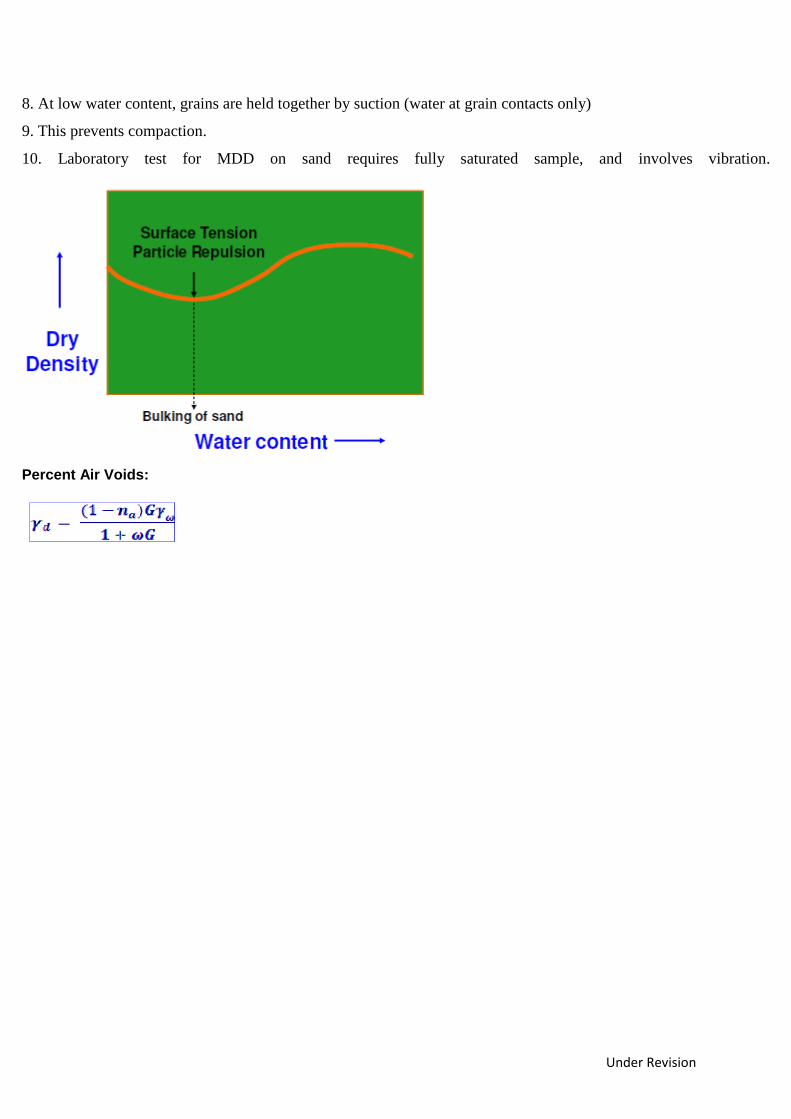
8. At low water content, grains are held together by suction (water at grain contacts only)
9. This prevents compaction.
10. Laboratory test for MDD on sand requires fully saturated sample, and involves vibration.
Percent Air Voids:
Under Revision
LECTURE 15
Factors affecting Compaction-
1. Water Content
2. Amount of Compaction
3. Method of Compaction
4. Type of Soil
5. Addition of Admixtures
Effect of Water Content-
1. With increase in water content, compacted density increases up to a stage, beyond which compacted density
decreases.
2. The maximum density achieved is called MDD and the corresponding water content is called OMC.
3. At lower water contents than OMC, soil particles are held by the force that prevents the development of diffused
double layer leading to low inter-particle repulsion.
4. Increase in water results in expansion of double layer and reduction in net attractive force between particles.
Water replaces air in void space
5. Particles slide over each other easily increasing lubrication, helping in dense packing.
6. After OMC is reached, air voids remain constant. Further increase in water, increases the void space, thereby
decreasing dry density.
Under Revision
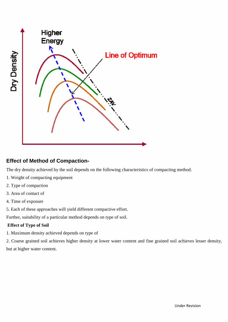
Effect of Amount of Compaction-
1. As discussed earlier, effect of increasing compactive effort is to increase MDD And reduce OMC (Evident from
Standard & Modified Proctor’s Tests).
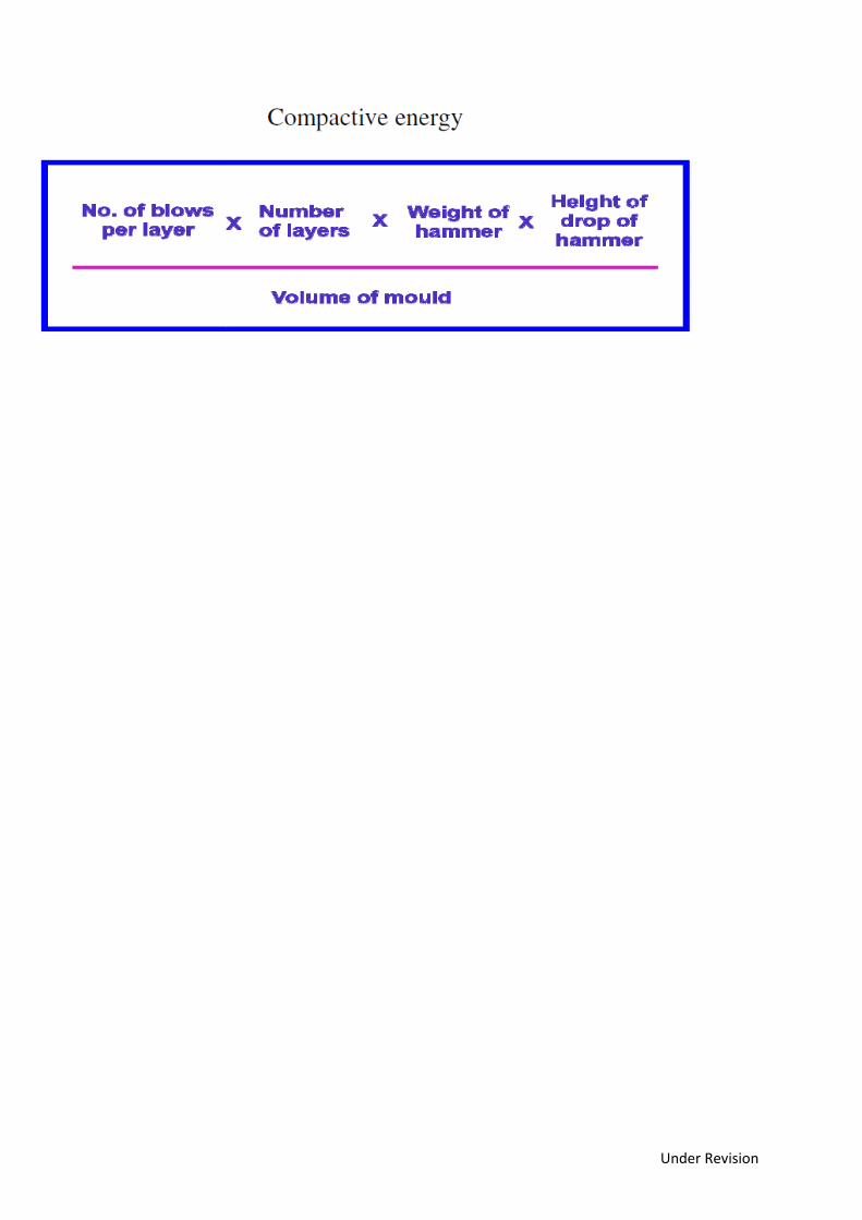
2. However, there is no linear relationship between compactive effort and MDD.
Under Revision
Effect of Method of Compaction-
The dry density achieved by the soil depends on the following characteristics of compacting method.
1. Weight of compacting equipment
2. Type of compaction
3. Area of contact of
4. Time of exposure
5. Each of these approaches will yield different compactive effort.
Further, suitability of a particular method depends on type of soil.
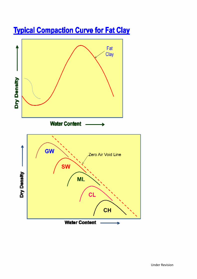
Effect of Type of Soil
1. Maximum density achieved depends on type of
2. Coarse grained soil achieves higher density at lower water content and fine grained soil achieves lesser density,
but at higher water content.
Under Revision
Under Revision
LECTURE 16
Effect of Addition of Admixtures-
1. Stabilizing agents are the admixtures added to soil.
2. The effect of adding these admixtures is to stabilize the soil.
3. In many cases they accelerate the process of densification.
Effect of compaction on soil properties-
1. Density
2. Shear strength
3. Permeability
4. Bearing Capacity
5. Settlement
6. Soil Structure
7. Pore Pressure
8. Stress Strain characteristics
9. Swelling & Shrinkage
Influence on Density:
Effect of compaction is to reduce the voids by expelling out air. This results in increasing the dry density of soil
mass.
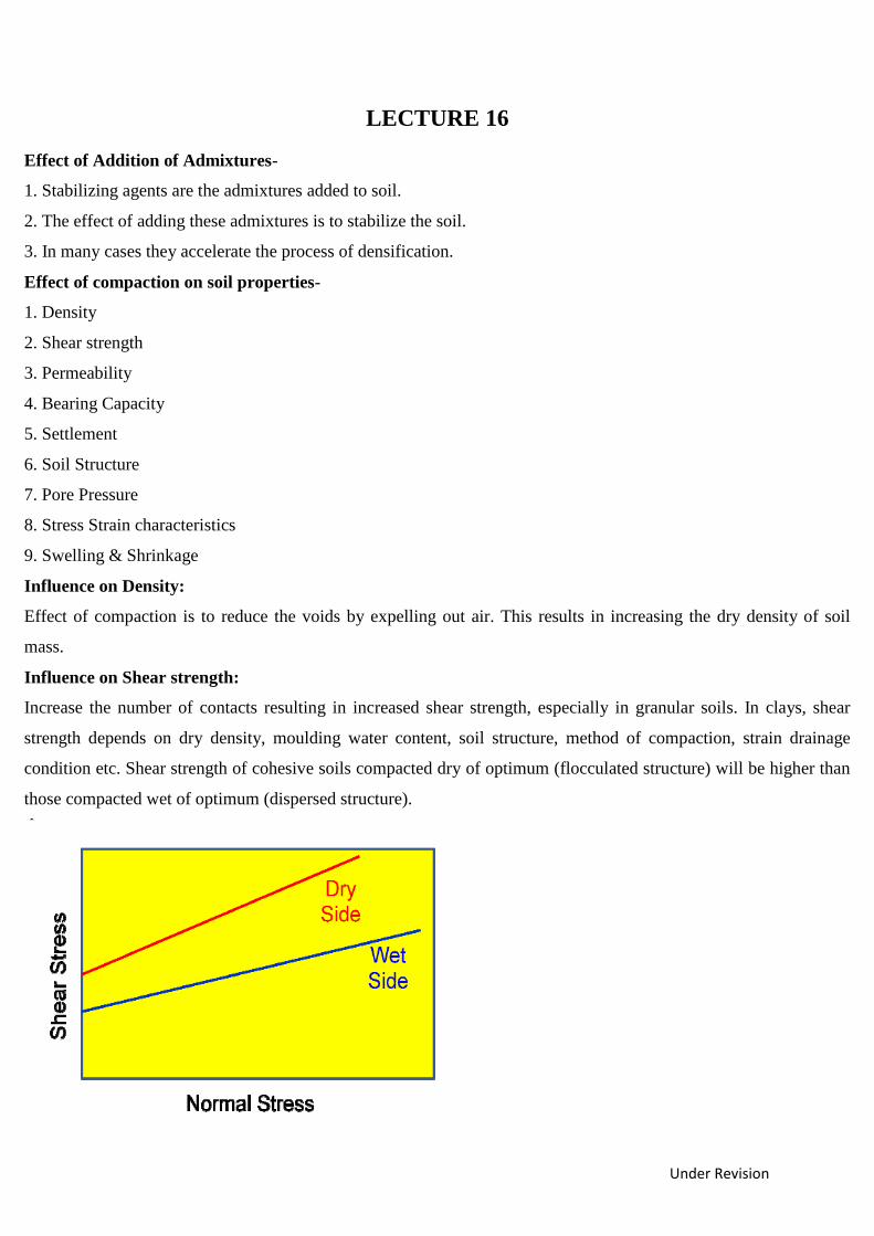
Influence on Shear strength:
Increase the number of contacts resulting in increased shear strength, especially in granular soils. In clays, shear
strength depends on dry density, moulding water content, soil structure, method of compaction, strain drainage
condition etc. Shear strength of cohesive soils compacted dry of optimum (flocculated structure) will be higher than
those compacted wet of optimum (dispersed structure).
Under Revision
Effect of compaction on permeability
1. Increased dry density, reduces the void space, thereby reducing permeability.
2. At same density, soil compacted dry of optimum is more permeable.
3. At same void ratio, soil with bigger particle size is more permeable.
4. Increased compactive effort reduces permeability.
Effect on Bearing Capacity
1. Increase in compaction increases the density and number of contacts between soil particles.
2. This results in increased
3. Hence bearing capacity increases which is a function of density and
Effect on Settlement
1. Compaction increases density and decreases void ratio.
2. This results in reduced settlement.
3. Both elastic settlement and consolidation settlement are reduced.
4. Soil compacted dry of optimum experiences greater compression than that compacted wet of optimum.
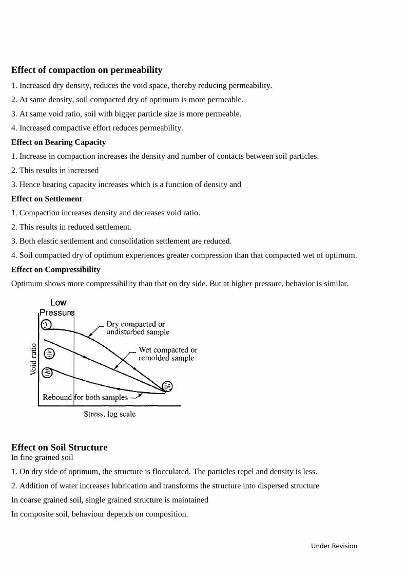
Effect on Compressibility
Optimum shows more compressibility than that on dry side. But at higher pressure, behavior is similar.
Effect on Soil Structure In fine grained soil
1. On dry side of optimum, the structure is flocculated. The particles repel and density is less.
2. Addition of water increases lubrication and transforms the structure into dispersed structure
In coarse grained soil, single grained structure is maintained
In composite soil, behaviour depends on composition.
Under Revision
Effect on Pore Pressure 1. Clayey soil compacted dry of optimum develops less pore water pressure than that compacted wet of optimum at
the same density at low strains.
2. However, at higher strains the effect is the same in both the cases.
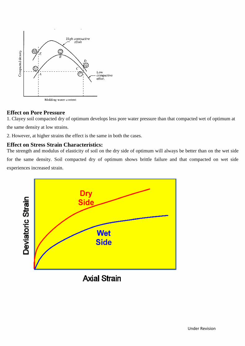
Effect on Stress Strain Characteristics:
The strength and modulus of elasticity of soil on the dry side of optimum will always be better than on the wet side
for the same density. Soil compacted dry of optimum shows brittle failure and that compacted on wet side
experiences increased strain.
Under Revision
LECTURE 17
Effect on Swell Shrink aspect
The effect of compaction is to reduce the void space. Hence the swelling and shrinkage are enormously reduced.
Further, soil compacted dry of optimum exhibits greater swell and swell pressure than that compacted on wet side
because of random orientation and deficiency in water.
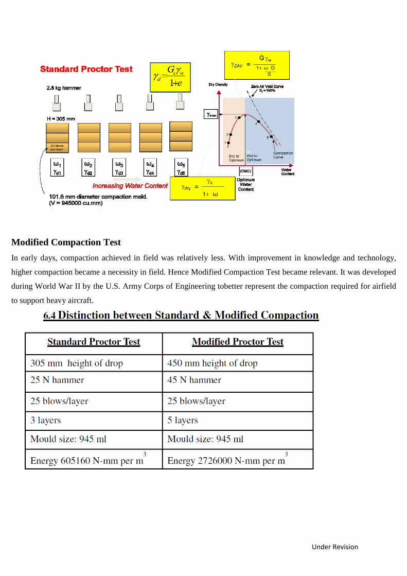
Standard Proctor’s Compaction Test
Refer IS 2720 – Part VII – 1987
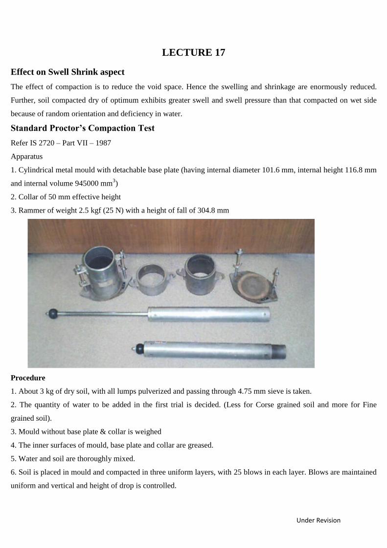
Apparatus
1. Cylindrical metal mould with detachable base plate (having internal diameter 101.6 mm, internal height 116.8 mm
and internal volume 945000 mm3)
2. Collar of 50 mm effective height
3. Rammer of weight 2.5 kgf (25 N) with a height of fall of 304.8 mm
Procedure
1. About 3 kg of dry soil, with all lumps pulverized and passing through 4.75 mm sieve is taken.
2. The quantity of water to be added in the first trial is decided. (Less for Corse grained soil and more for Fine
grained soil).
3. Mould without base plate & collar is weighed
4. The inner surfaces of mould, base plate and collar are greased.
5. Water and soil are thoroughly mixed.
6. Soil is placed in mould and compacted in three uniform layers, with 25 blows in each layer. Blows are maintained
uniform and vertical and height of drop is controlled.
Under Revision
7. After each layer, top surface is scratched to maintain integrity between layers.
8. The height of top layer is so controlled that after compaction, soil slightly protrudes in to collar.
9. Excess soil is scrapped.
10. Mould and soil are weighed (W)
11. A representative sample from the middle is kept for the determination of water content.
12. The procedure is repeated with increasing water content.
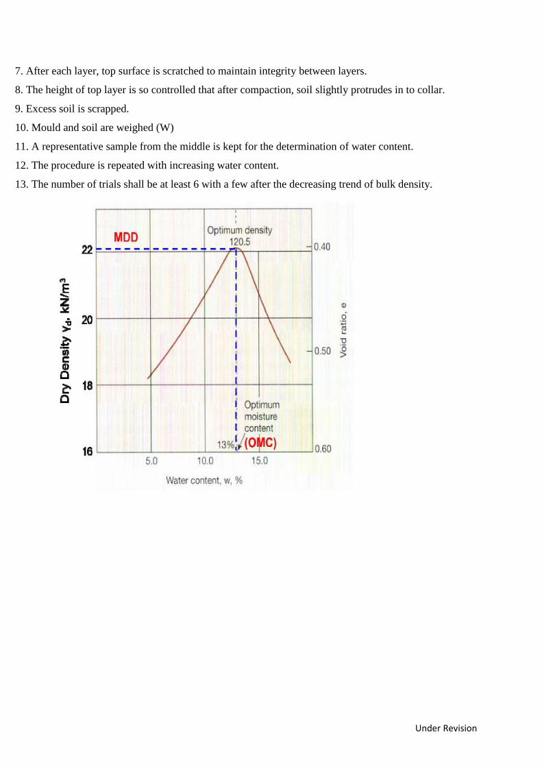
13. The number of trials shall be at least 6 with a few after the decreasing trend of bulk density.
Under Revision
Modified Compaction Test
In early days, compaction achieved in field was relatively less. With improvement in knowledge and technology,
higher compaction became a necessity in field. Hence Modified Compaction Test became relevant. It was developed
during World War II by the U.S. Army Corps of Engineering tobetter represent the compaction required for airfield
to support heavy aircraft.
Under Revision
Under Revision
LECTURE 18
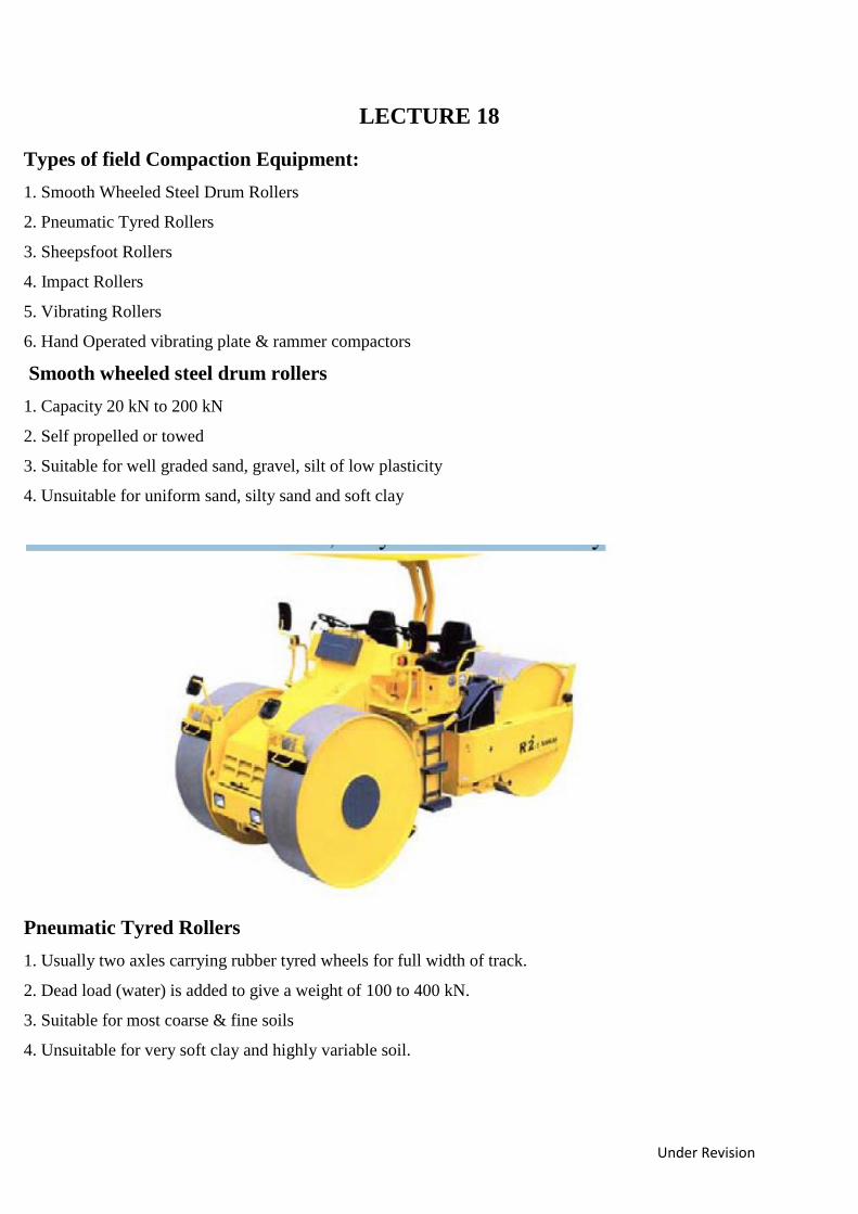
Types of field Compaction Equipment:
1. Smooth Wheeled Steel Drum Rollers
2. Pneumatic Tyred Rollers
3. Sheepsfoot Rollers
4. Impact Rollers
5. Vibrating Rollers
6. Hand Operated vibrating plate & rammer compactors
Smooth wheeled steel drum rollers
1. Capacity 20 kN to 200 kN
2. Self propelled or towed
3. Suitable for well graded sand, gravel, silt of low plasticity
4. Unsuitable for uniform sand, silty sand and soft clay
Pneumatic Tyred Rollers
1. Usually two axles carrying rubber tyred wheels for full width of track.
2. Dead load (water) is added to give a weight of 100 to 400 kN.
3. Suitable for most coarse & fine soils
4. Unsuitable for very soft clay and highly variable soil.
Under Revision
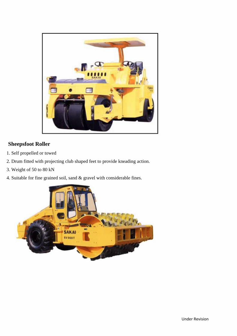
Sheepsfoot Roller
1. Self propelled or towed
2. Drum fitted with projecting club shaped feet to provide kneading action.
3. Weight of 50 to 80 kN
4. Suitable for fine grained soil, sand & gravel with considerable fines.
Under Revision
LECTURE 19
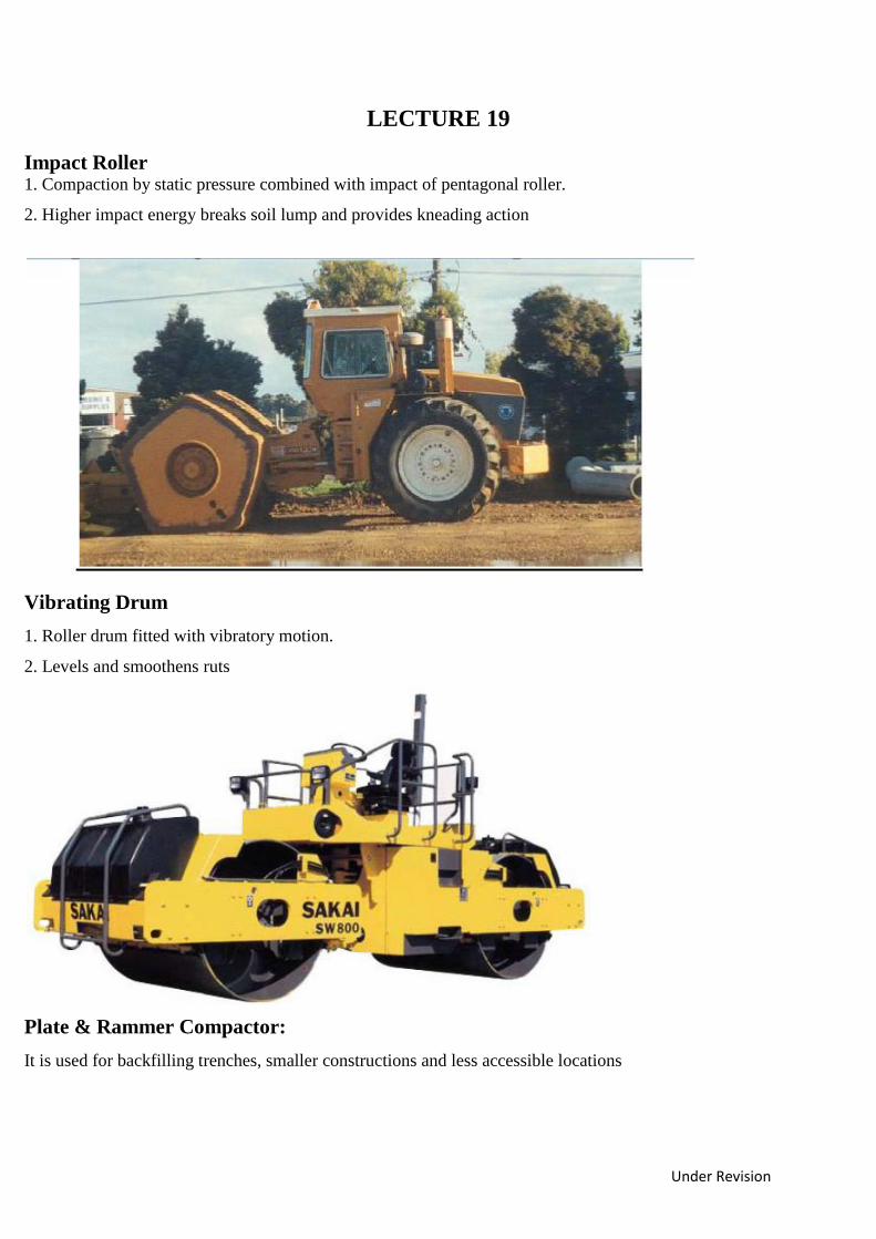
Impact Roller 1. Compaction by static pressure combined with impact of pentagonal roller.
2. Higher impact energy breaks soil lump and provides kneading action
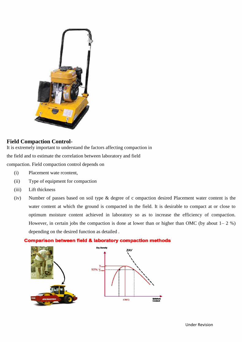
Vibrating Drum
1. Roller drum fitted with vibratory motion.
2. Levels and smoothens ruts
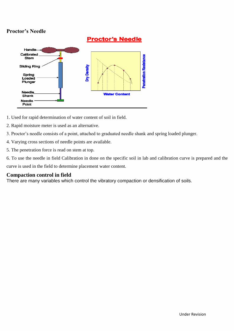
Plate & Rammer Compactor:
It is used for backfilling trenches, smaller constructions and less accessible locations
Under Revision
Field Compaction Control- It is extremely important to understand the factors affecting compaction in
the field and to estimate the correlation between laboratory and field
compaction. Field compaction control depends on
(i) Placement wate rcontent,
(ii) Type of equipment for compaction
(iii) Lift thickness
(iv) Number of passes based on soil type & degree of c ompaction desired Placement water content is the
water content at which the ground is compacted in the field. It is desirable to compact at or close to
optimum moisture content achieved in laboratory so as to increase the efficiency of compaction.
However, in certain jobs the compaction is done at lower than or higher than OMC (by about 1– 2 %)
depending on the desired function as detailed .
Under Revision
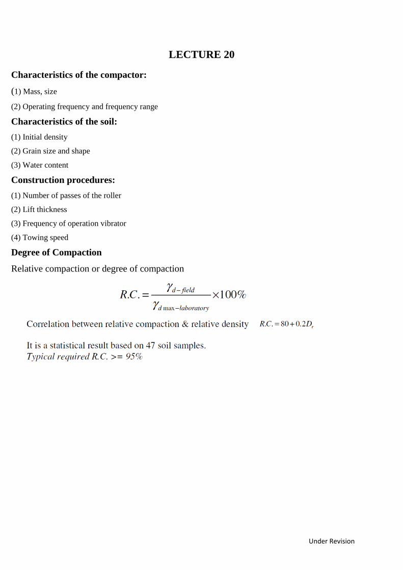
Proctor’s Needle
1. Used for rapid determination of water content of soil in field.
2. Rapid moisture meter is used as an alternative.
3. Proctor’s needle consists of a point, attached to graduated needle shank and spring loaded plunger.
4. Varying cross sections of needle points are available.
5. The penetration force is read on stem at top.
6. To use the needle in field Calibration in done on the specific soil in lab and calibration curve is prepared and the
curve is used in the field to determine placement water content.
Compaction control in field There are many variables which control the vibratory compaction or densification of soils.
Under Revision
LECTURE 20
Characteristics of the compactor:
(1) Mass, size
(2) Operating frequency and frequency range
Characteristics of the soil:
(1) Initial density
(2) Grain size and shape
(3) Water content
Construction procedures:
(1) Number of passes of the roller
(2) Lift thickness
(3) Frequency of operation vibrator
(4) Towing speed
Degree of Compaction
Relative compaction or degree of compaction
Under Revision
LECTURE 21
CONSOLIDATION Introduction
Civil Engineers build structures and the soil beneath these structures is loaded. This results in increase of stresses
resulting in strain leading to settlement of stratum. The settlement is due to decrease in volume of soil mass. When
water in the voids and soil particles are assumed as incompressible in a completely saturated soil system then -
reduction in volume takes place due to expulsion of water from the voids. There will be rearrangement of soil
particles in air voids created by the outflow of water from the voids. This rearrangement reflects as a volume change
leading to compression of saturated fine grained soil resulting in settlement. The rate of volume change is related to
the rate at which pore water moves out which in turn depends on the permeability of soil. Therefore the deformation
due to increase of stress depends on the “Compressibility of soils”
As Civil Engineers we need to provide answers for
1. Total settlement (volume change)
2. Time required for the settlement of compressible layer
The total settlement consists of three components
1. Immediate settlement.
2. Primary consolidation settlement
3. Secondary consolidation settlement (Creep settlement)
St = Si + Sc + Ssc
Elastic Settlement or Immediate Settlement
This settlement occurs immediately after the load is applied. This is due to distortion (change in shape) at constant
volume. There is negligible flow of water in less pervious soils. In case of pervious soils the flow of water is quick at
constant volume. This is determined by elastic theory.
Under Revision
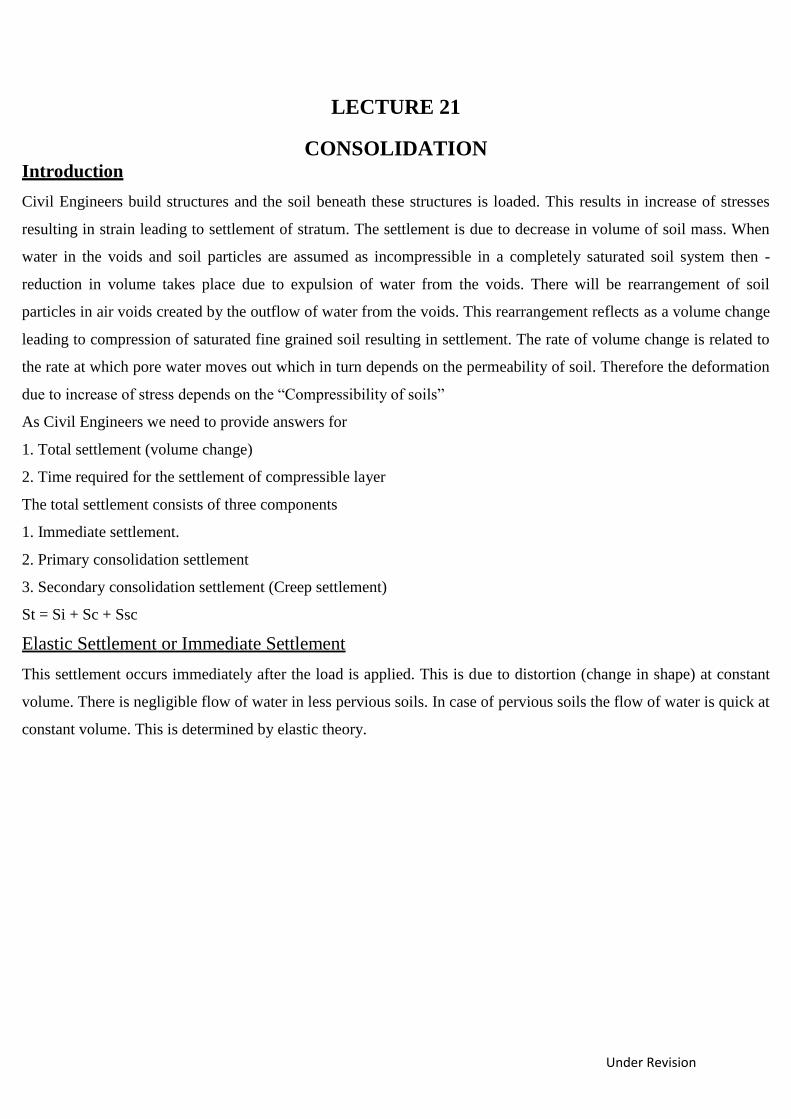
Primary Consolidation Settlement
Figure Settlement versus Time
It occurs due to expulsion of pore water from the voids of a saturated soil. In case of saturated fine grained soils, the
deformation is due to squeezing of water from the pores leading to rearrangement of soil particles. The movement
of pore water depends on the permeability and dissipation of pore water pressure. With the passage of time the
pore water pressure dissipates, the rate of flow decreases and finally the flow of water ceases. During this process
there is gradual dissipation of pore water pressure and a simultaneous increase of effective stress as shown in the
above Figure. The consolidation settlement occurs from the time water begins move out from the pores to the time
at which flow ceases from the voids. This is also the time from which the excess pore water pressure starts reducing (effective stress increase) to the time at which complete dissipation of excess pore water pressure (total
stress equal to effective stress). This time dependent compression is called “Consolidation settlement”. Primary consolidation is a major component of settlement of fine grained saturated soils and this can be estimated
from the theory of consolidation.
In case of saturated soil mass the applied stress is borne by pore water alone in the initial stages
With passage of time water starts flowing out from the voids as a result the excess pore water pressure decreases and
simultaneous increase in effective stress will takes place. The volume change is basically due to the change in
effective stress After considerable amount of time (t =0) flow from the voids ceases the effective stress stabilizes and
will be is equal to external applied total stress and this stage signifies the end of primary consolidation.
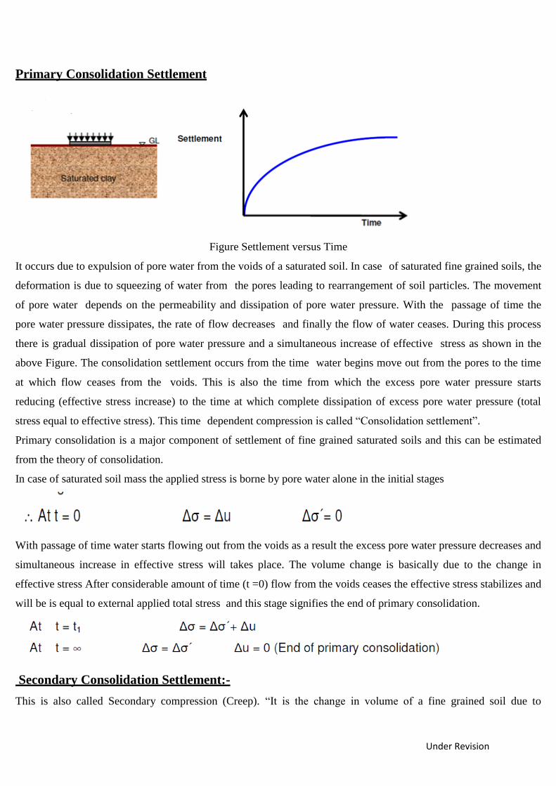
Secondary Consolidation Settlement:-
This is also called Secondary compression (Creep). “It is the change in volume of a fine grained soil due to
Under Revision
rearrangement of soil particles (fabric) at constant effective stress”. The rate of secondary consolidation is very slow
when compared with primary consolidation.
Figure Effective Stress versus Time
Under Revision
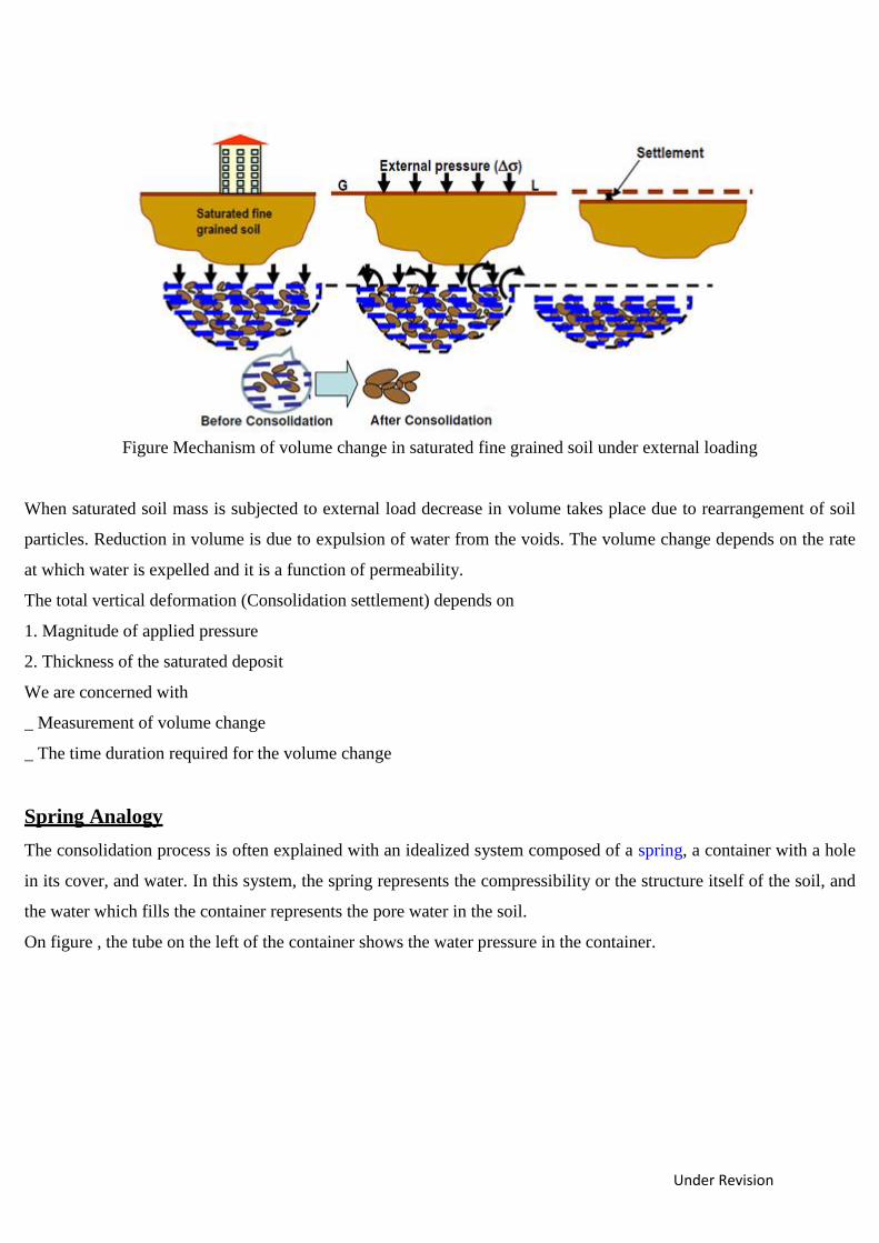
Figure Mechanism of volume change in saturated fine grained soil under external loading
When saturated soil mass is subjected to external load decrease in volume takes place due to rearrangement of soil
particles. Reduction in volume is due to expulsion of water from the voids. The volume change depends on the rate
at which water is expelled and it is a function of permeability.
The total vertical deformation (Consolidation settlement) depends on
1. Magnitude of applied pressure
2. Thickness of the saturated deposit
We are concerned with
_ Measurement of volume change
_ The time duration required for the volume change
Spring Analogy
The consolidation process is often explained with an idealized system composed of a spring, a container with a hole
in its cover, and water. In this system, the spring represents the compressibility or the structure itself of the soil, and
the water which fills the container represents the pore water in the soil.
On figure , the tube on the left of the container shows the water pressure in the container.
Under Revision
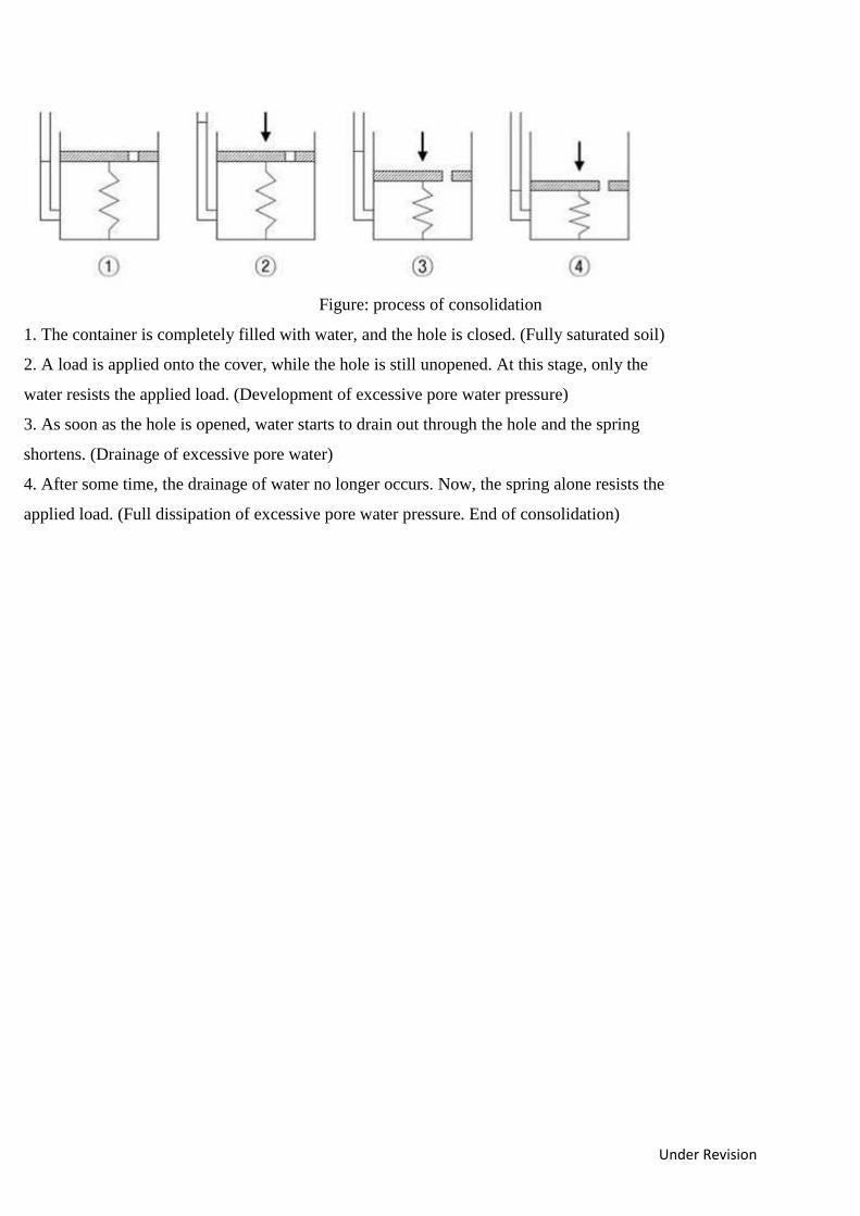
Figure: process of consolidation
1. The container is completely filled with water, and the hole is closed. (Fully saturated soil)
2. A load is applied onto the cover, while the hole is still unopened. At this stage, only the
water resists the applied load. (Development of excessive pore water pressure)
3. As soon as the hole is opened, water starts to drain out through the hole and the spring
shortens. (Drainage of excessive pore water)
4. After some time, the drainage of water no longer occurs. Now, the spring alone resists the
applied load. (Full dissipation of excessive pore water pressure. End of consolidation)
Under Revision
LECTURE 22
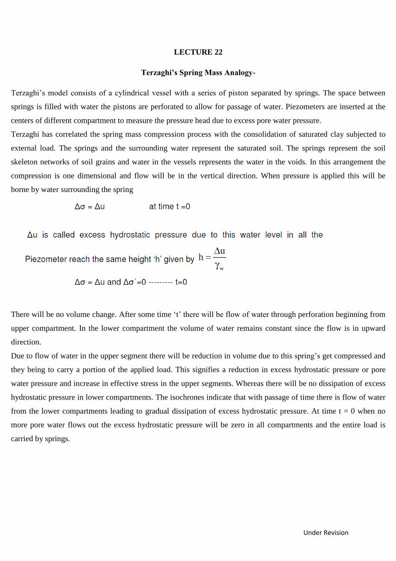
Terzaghi’s Spring Mass Analogy-
Terzaghi’s model consists of a cylindrical vessel with a series of piston separated by springs. The space between
springs is filled with water the pistons are perforated to allow for passage of water. Piezometers are inserted at the
centers of different compartment to measure the pressure head due to excess pore water pressure.
Terzaghi has correlated the spring mass compression process with the consolidation of saturated clay subjected to
external load. The springs and the surrounding water represent the saturated soil. The springs represent the soil
skeleton networks of soil grains and water in the vessels represents the water in the voids. In this arrangement the
compression is one dimensional and flow will be in the vertical direction. When pressure is applied this will be
borne by water surrounding the spring
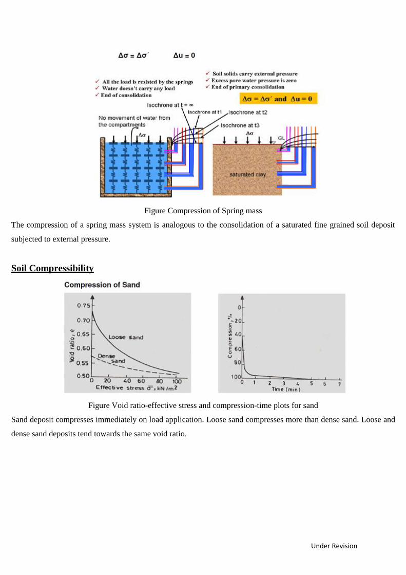
There will be no volume change. After some time ‘t’ there will be flow of water through perforation beginning from
upper compartment. In the lower compartment the volume of water remains constant since the flow is in upward
direction.
Due to flow of water in the upper segment there will be reduction in volume due to this spring’s get compressed and
they being to carry a portion of the applied load. This signifies a reduction in excess hydrostatic pressure or pore
water pressure and increase in effective stress in the upper segments. Whereas there will be no dissipation of excess
hydrostatic pressure in lower compartments. The isochrones indicate that with passage of time there is flow of water
from the lower compartments leading to gradual dissipation of excess hydrostatic pressure. At time t = 0 when no
more pore water flows out the excess hydrostatic pressure will be zero in all compartments and the entire load is
carried by springs.
Under Revision
Figure Compression of Spring mass
The compression of a spring mass system is analogous to the consolidation of a saturated fine grained soil deposit
subjected to external pressure.
Soil Compressibility
Figure Void ratio-effective stress and compression-time plots for sand
Sand deposit compresses immediately on load application. Loose sand compresses more than dense sand. Loose and
dense sand deposits tend towards the same void ratio.
Under Revision
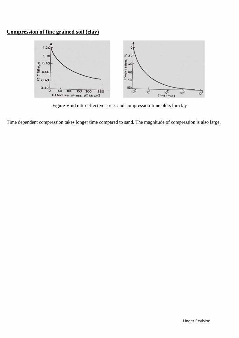
Compression of fine grained soil (clay)
Figure Void ratio-effective stress and compression-time plots for clay
Time dependent compression takes longer time compared to sand. The magnitude of compression is also large.
Under Revision
LECTURE 23
Compression of Fine Grained Soil
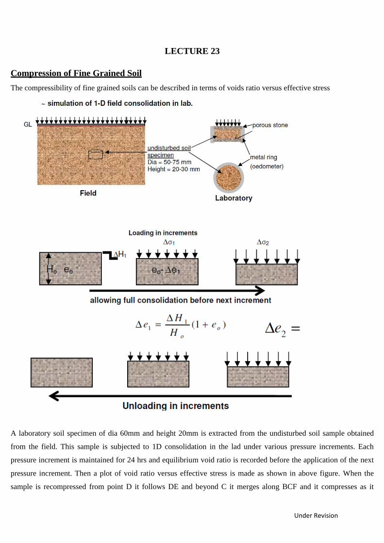
The compressibility of fine grained soils can be described in terms of voids ratio versus effective stress
A laboratory soil specimen of dia 60mm and height 20mm is extracted from the undisturbed soil sample obtained
from the field. This sample is subjected to 1D consolidation in the lad under various pressure increments. Each
pressure increment is maintained for 24 hrs and equilibrium void ratio is recorded before the application of the next
pressure increment. Then a plot of void ratio versus effective stress is made as shown in above figure. When the
sample is recompressed from point D it follows DE and beyond C it merges along BCF and it compresses as it
Under Revision
moves along BCF
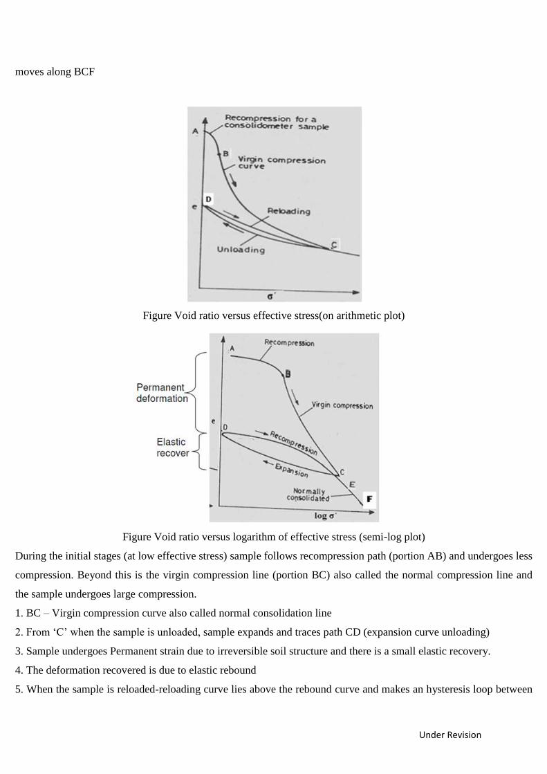
Figure Void ratio versus effective stress(on arithmetic plot)
Figure Void ratio versus logarithm of effective stress (semi-log plot)
During the initial stages (at low effective stress) sample follows recompression path (portion AB) and undergoes less
compression. Beyond this is the virgin compression line (portion BC) also called the normal compression line and
the sample undergoes large compression.
1. BC – Virgin compression curve also called normal consolidation line
2. From ‘C’ when the sample is unloaded, sample expands and traces path CD (expansion curve unloading)
3. Sample undergoes Permanent strain due to irreversible soil structure and there is a small elastic recovery.
4. The deformation recovered is due to elastic rebound
5. When the sample is reloaded-reloading curve lies above the rebound curve and makes an hysteresis loop between

Under Revision
expansion and reloading curves.
6. The reloaded soils shows less compression.
7. Loading beyond ‘C’ makes the curve to merge smoothly into portion EF as if the soil is not unloaded.
Under Revision
LECTURE 24
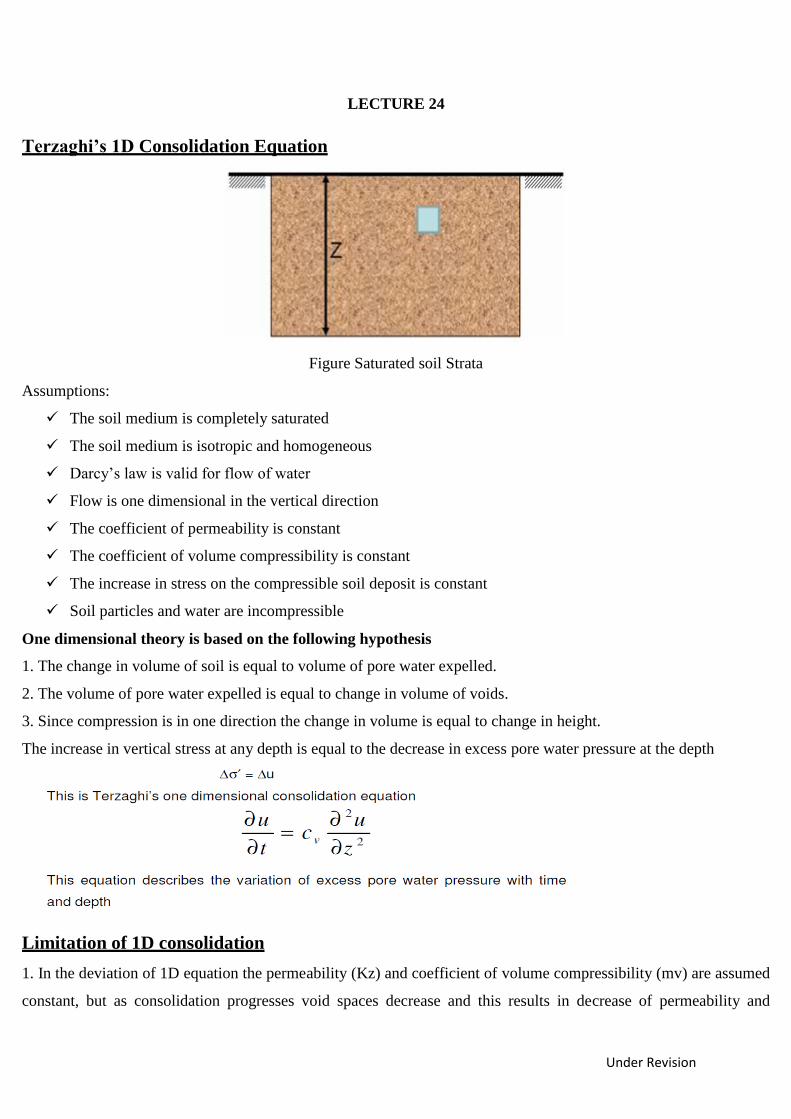
Terzaghi’s 1D Consolidation Equation
Figure Saturated soil Strata
Assumptions:
The soil medium is completely saturated
The soil medium is isotropic and homogeneous
Darcy’s law is valid for flow of water
Flow is one dimensional in the vertical direction
The coefficient of permeability is constant
The coefficient of volume compressibility is constant
The increase in stress on the compressible soil deposit is constant
Soil particles and water are incompressible
One dimensional theory is based on the following hypothesis
1. The change in volume of soil is equal to volume of pore water expelled.
2. The volume of pore water expelled is equal to change in volume of voids.
3. Since compression is in one direction the change in volume is equal to change in height.
The increase in vertical stress at any depth is equal to the decrease in excess pore water pressure at the depth
Limitation of 1D consolidation
1. In the deviation of 1D equation the permeability (Kz) and coefficient of volume compressibility (mv) are assumed
constant, but as consolidation progresses void spaces decrease and this results in decrease of permeability and
Under Revision
therefore permeability is not constant. The coefficient of volume compressibility also changes with stress level.
Therefore Cv is not constant
2. The flow is assumed to be 1D but in reality flow is three dimensional
3. The application of external load is assumed to produce excess pore water pressure over the entire soil stratum but
in some cases the excess pore water pressure does not develop over the entire clay stratum.
The solution of variation of excess pore water pressure with depth and time can be obtained for various initial
conditions.
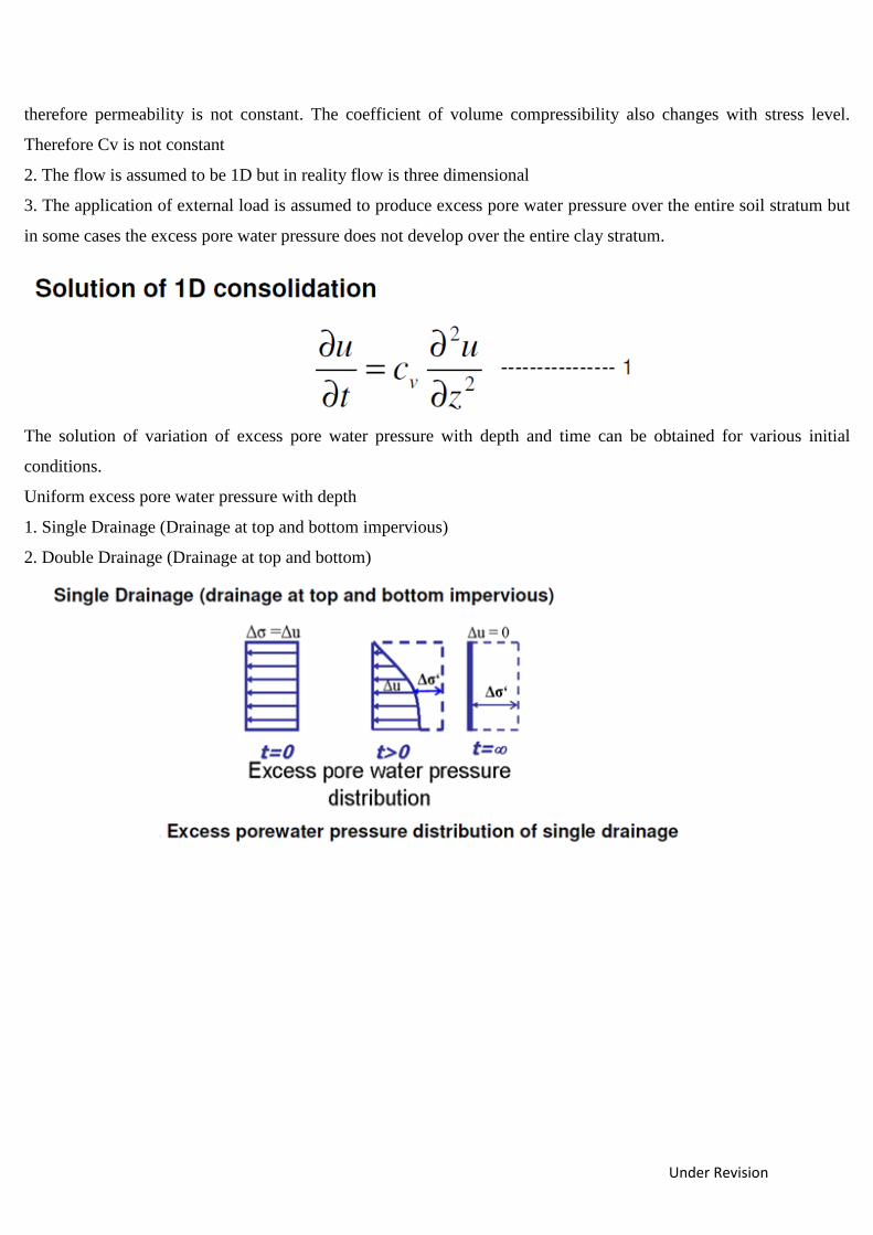
Uniform excess pore water pressure with depth
1. Single Drainage (Drainage at top and bottom impervious)
2. Double Drainage (Drainage at top and bottom)
Under Revision
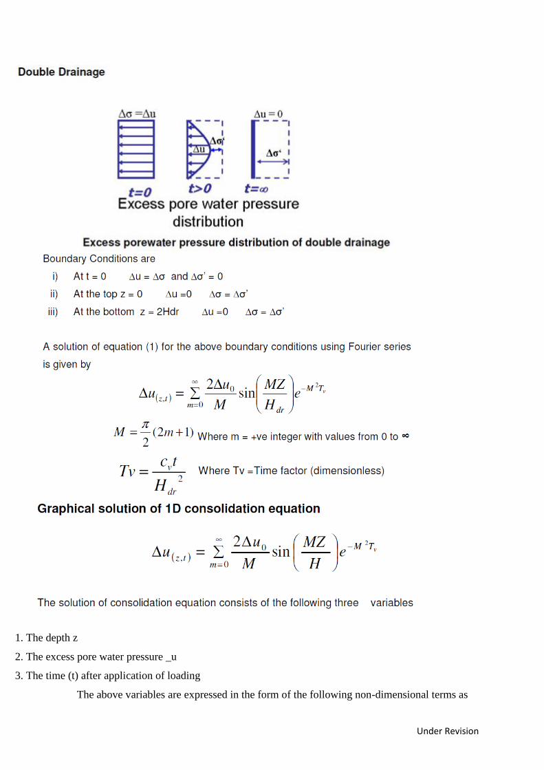
1. The depth z
2. The excess pore water pressure _u
3. The time (t) after application of loading
The above variables are expressed in the form of the following non-dimensional terms as
Under Revision
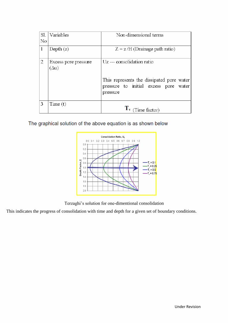
Terzaghi’s solution for one-dimentional consolidation
This indicates the progress of consolidation with time and depth for a given set of boundary conditions.
Under Revision
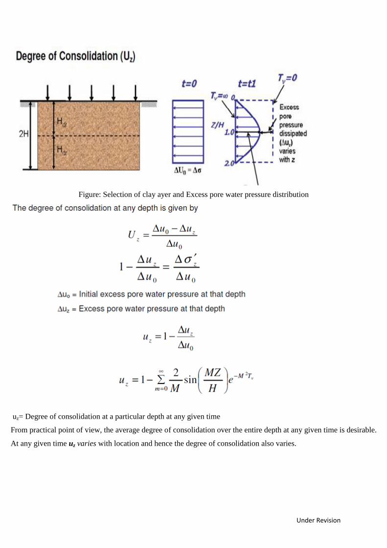
Figure: Selection of clay ayer and Excess pore water pressure distribution
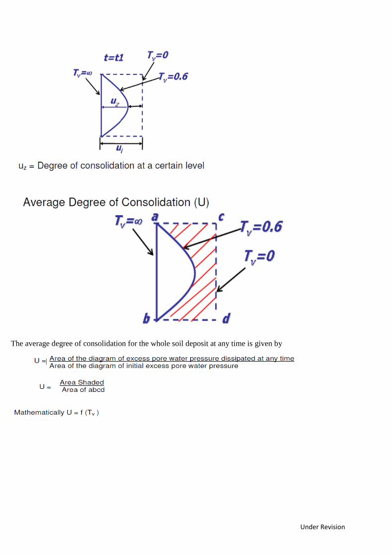
uz= Degree of consolidation at a particular depth at any given time
From practical point of view, the average degree of consolidation over the entire depth at any given time is desirable.
At any given time uz varies with location and hence the degree of consolidation also varies.
Under Revision
The average degree of consolidation for the whole soil deposit at any time is given by
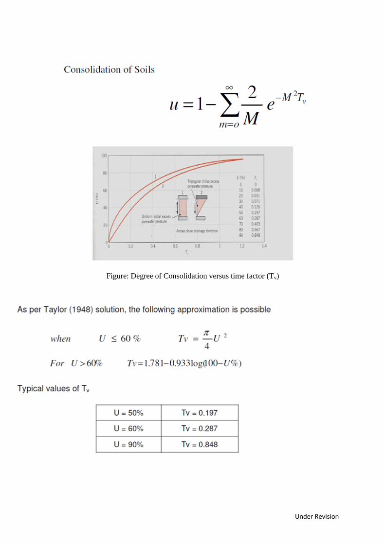
Under Revision
Figure: Degree of Consolidation versus time factor (Tv)
Under Revision
LECTURE 25
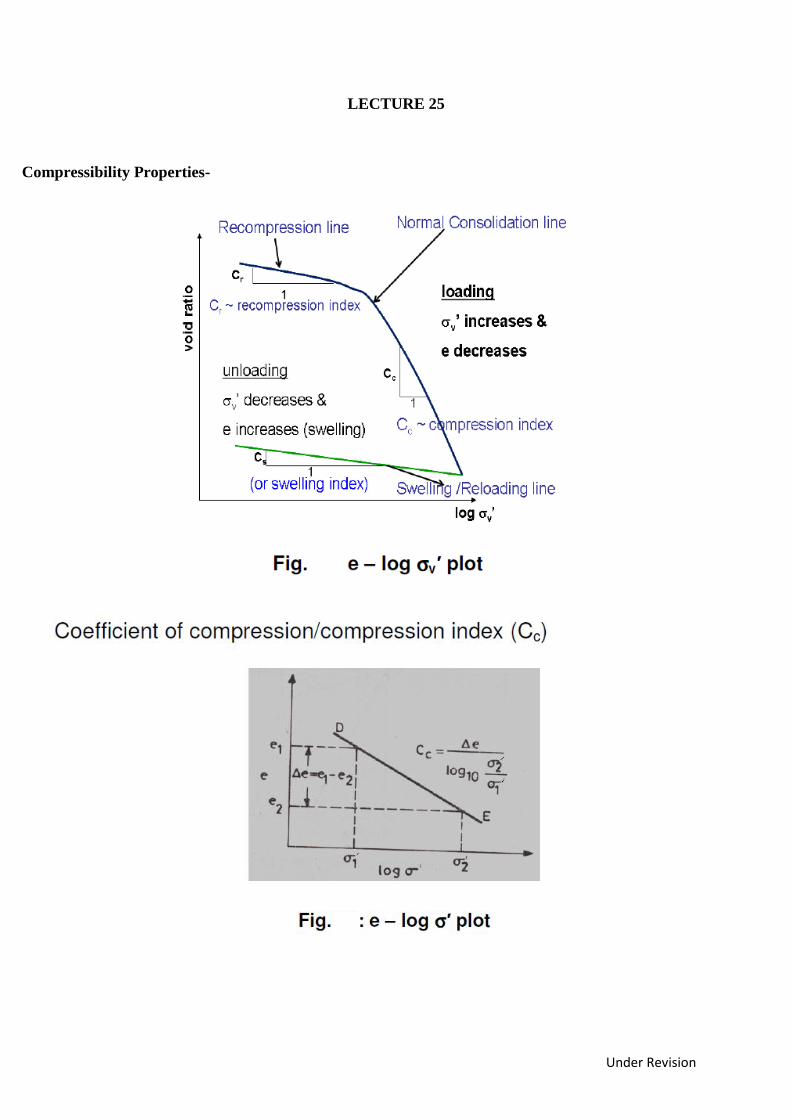
Compressibility Properties-
Under Revision
Figure: e – log σv’ plot
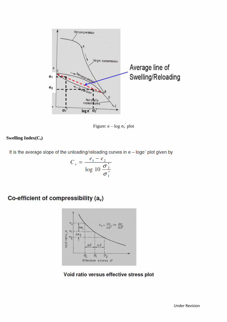
Swelling Index(Cs)
Under Revision
Under Revision
LECTURE 26
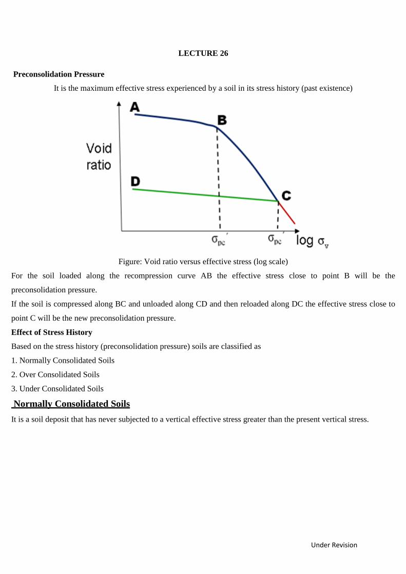
Preconsolidation Pressure
It is the maximum effective stress experienced by a soil in its stress history (past existence)
Figure: Void ratio versus effective stress (log scale)
For the soil loaded along the recompression curve AB the effective stress close to point B will be the
preconsolidation pressure.
If the soil is compressed along BC and unloaded along CD and then reloaded along DC the effective stress close to
point C will be the new preconsolidation pressure.
Effect of Stress History
Based on the stress history (preconsolidation pressure) soils are classified as
1. Normally Consolidated Soils
2. Over Consolidated Soils
3. Under Consolidated Soils
Normally Consolidated Soils
It is a soil deposit that has never subjected to a vertical effective stress greater than the present vertical stress.
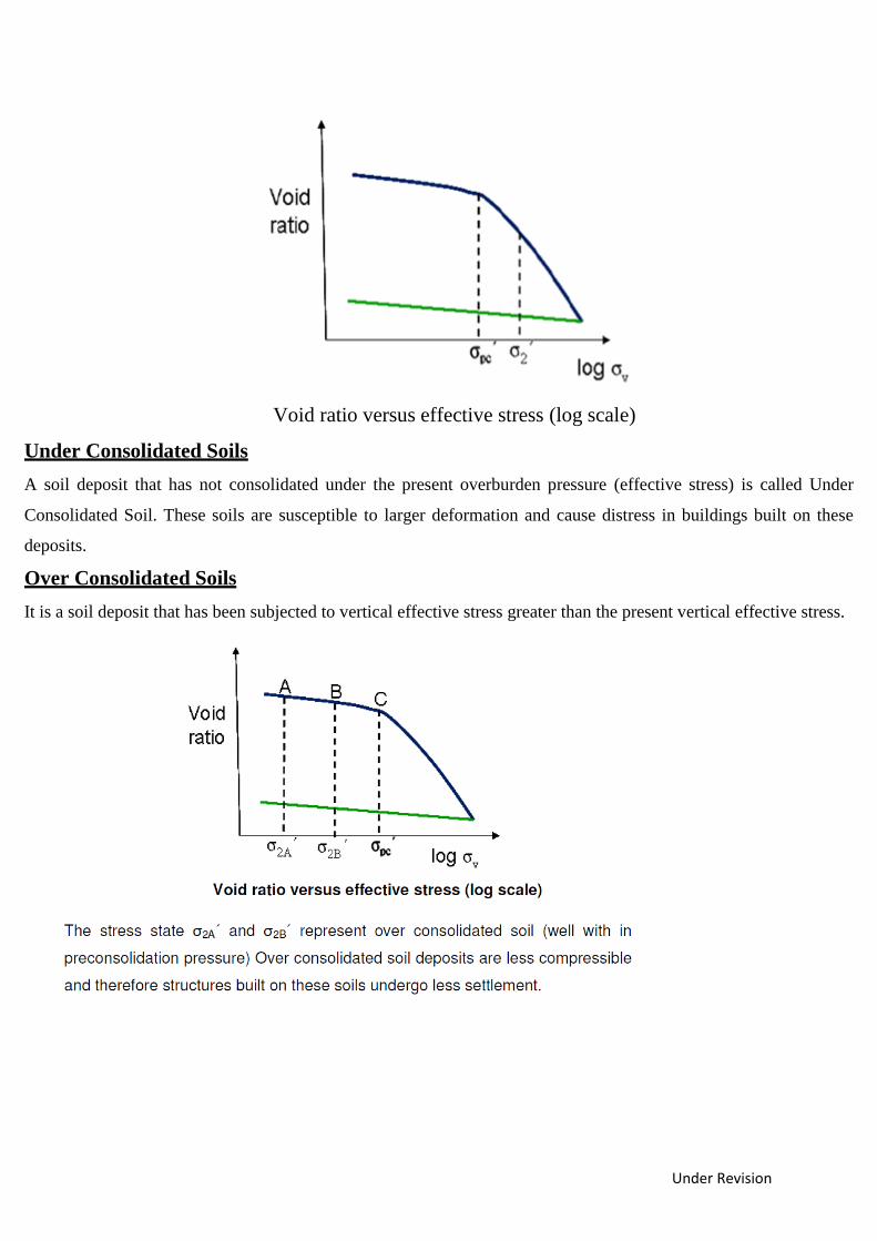
Under Revision
Void ratio versus effective stress (log scale)
Under Consolidated Soils
A soil deposit that has not consolidated under the present overburden pressure (effective stress) is called Under
Consolidated Soil. These soils are susceptible to larger deformation and cause distress in buildings built on these
deposits.
Over Consolidated Soils
It is a soil deposit that has been subjected to vertical effective stress greater than the present vertical effective stress.

Under Revision
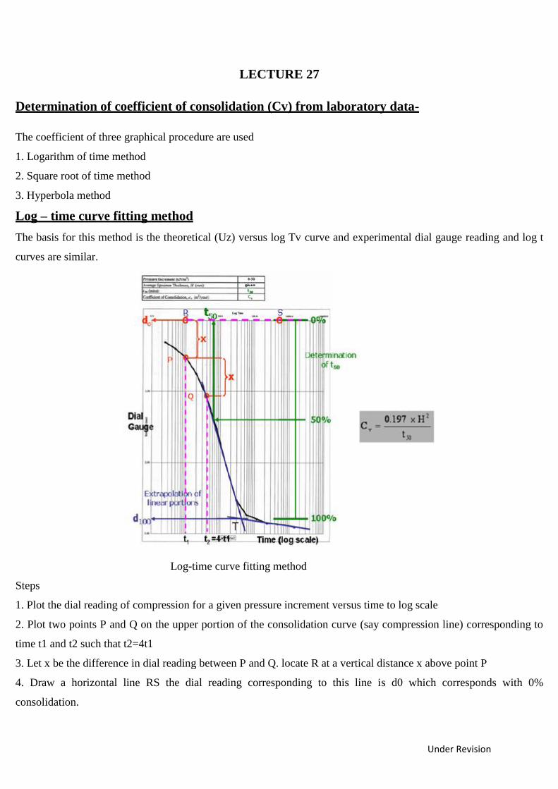
Under Revision
LECTURE 27
Determination of coefficient of consolidation (Cv) from laboratory data-
The coefficient of three graphical procedure are used
1. Logarithm of time method
2. Square root of time method
3. Hyperbola method
Log – time curve fitting method
The basis for this method is the theoretical (Uz) versus log Tv curve and experimental dial gauge reading and log t
curves are similar.
Log-time curve fitting method
Steps
1. Plot the dial reading of compression for a given pressure increment versus time to log scale
2. Plot two points P and Q on the upper portion of the consolidation curve (say compression line) corresponding to
time t1 and t2 such that t2=4t1
3. Let x be the difference in dial reading between P and Q. locate R at a vertical distance x above point P
4. Draw a horizontal line RS the dial reading corresponding to this line is d0 which corresponds with 0%
consolidation.
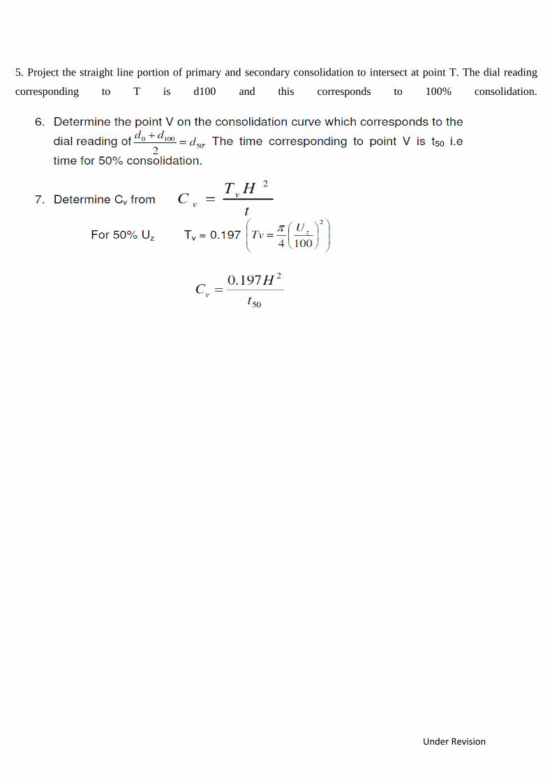
Under Revision
5. Project the straight line portion of primary and secondary consolidation to intersect at point T. The dial reading
corresponding to T is d100 and this corresponds to 100% consolidation.
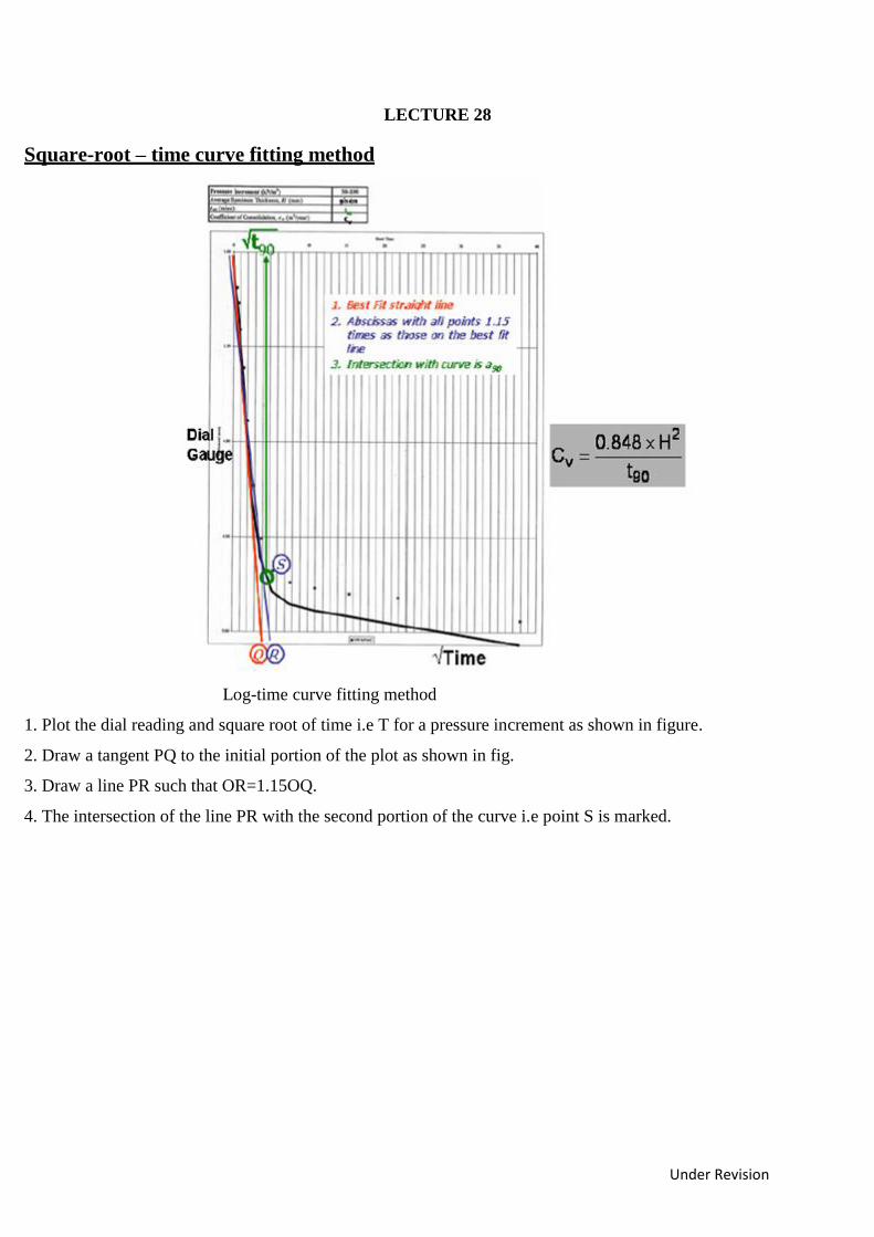
Under Revision
LECTURE 28
Square-root – time curve fitting method
Log-time curve fitting method
1. Plot the dial reading and square root of time i.e T for a pressure increment as shown in figure.
2. Draw a tangent PQ to the initial portion of the plot as shown in fig.
3. Draw a line PR such that OR=1.15OQ.
4. The intersection of the line PR with the second portion of the curve i.e point S is marked.
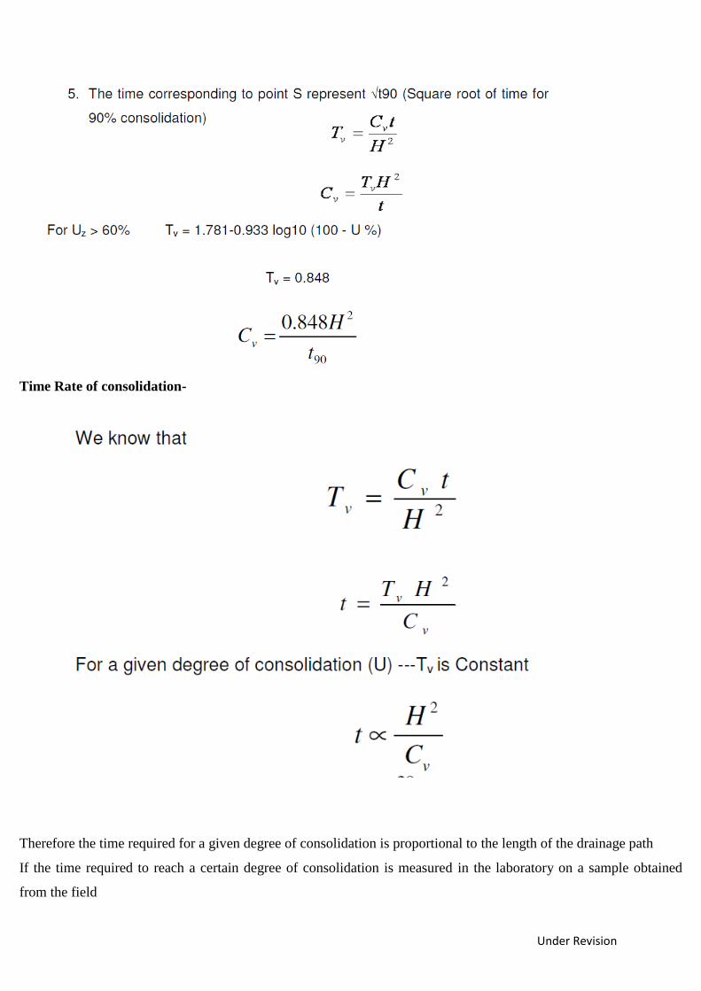
Under Revision
Time Rate of consolidation-
Therefore the time required for a given degree of consolidation is proportional to the length of the drainage path
If the time required to reach a certain degree of consolidation is measured in the laboratory on a sample obtained
from the field
Under Revision
The time taken by the field deposit of known thickness can be predicted by using
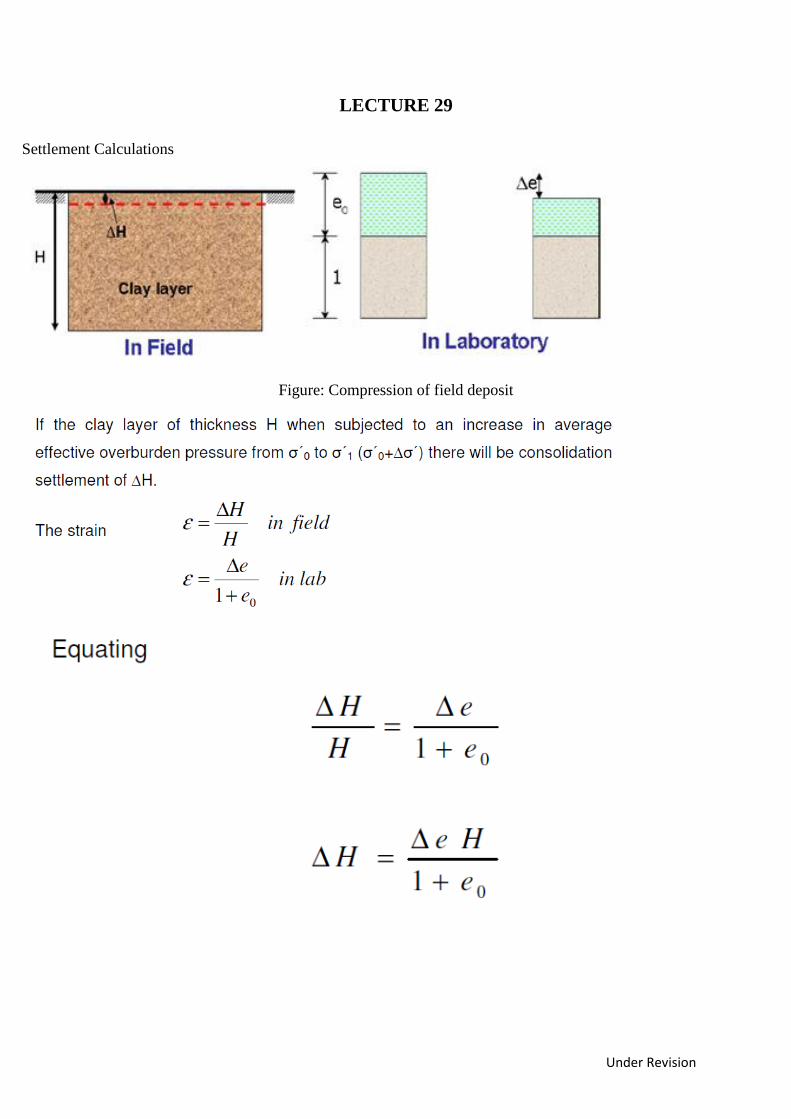
Under Revision
LECTURE 29
Settlement Calculations
Figure: Compression of field deposit
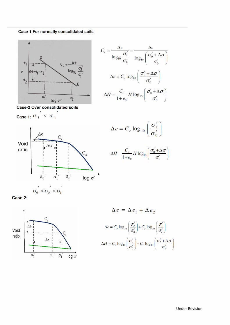
Under Revision
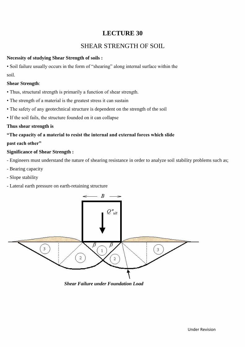
Under Revision
LECTURE 30
SHEAR STRENGTH OF SOIL
Necessity of studying Shear Strength of soils :
• Soil failure usually occurs in the form of “shearing” along internal surface within the
soil.
Shear Strength:
• Thus, structural strength is primarily a function of shear strength.
• The strength of a material is the greatest stress it can sustain
• The safety of any geotechnical structure is dependent on the strength of the soil
• If the soil fails, the structure founded on it can collapse
Thus shear strength is
“The capacity of a material to resist the internal and external forces which slide
past each other”
Significance of Shear Strength :
- Engineers must understand the nature of shearing resistance in order to analyze soil stability problems such as;
- Bearing capacity
- Slope stability
- Lateral earth pressure on earth-retaining structure
Shear Failure under Foundation Load
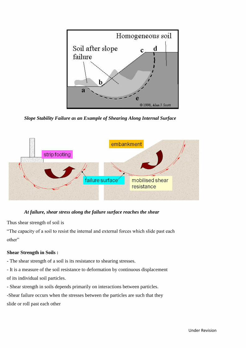
Under Revision
Slope Stability Failure as an Example of Shearing Along Internal Surface
At failure, shear stress along the failure surface reaches the shear
Thus shear strength of soil is
“The capacity of a soil to resist the internal and external forces which slide past each
other”
Shear Strength in Soils :
- The shear strength of a soil is its resistance to shearing stresses.
- It is a measure of the soil resistance to deformation by continuous displacement
of its individual soil particles.
- Shear strength in soils depends primarily on interactions between particles.
-Shear failure occurs when the stresses between the particles are such that they
slide or roll past each other
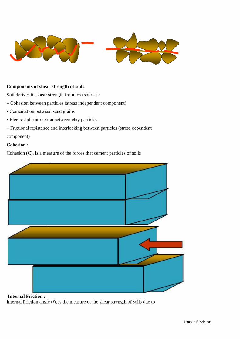
Under Revision
Components of shear strength of soils
Soil derives its shear strength from two sources:
– Cohesion between particles (stress independent component)
• Cementation between sand grains
• Electrostatic attraction between clay particles
– Frictional resistance and interlocking between particles (stress dependent
component)
Cohesion :
Cohesion (C), is a measure of the forces that cement particles of soils
Internal Friction :
Internal Friction angle (f), is the measure of the shear strength of soils due to
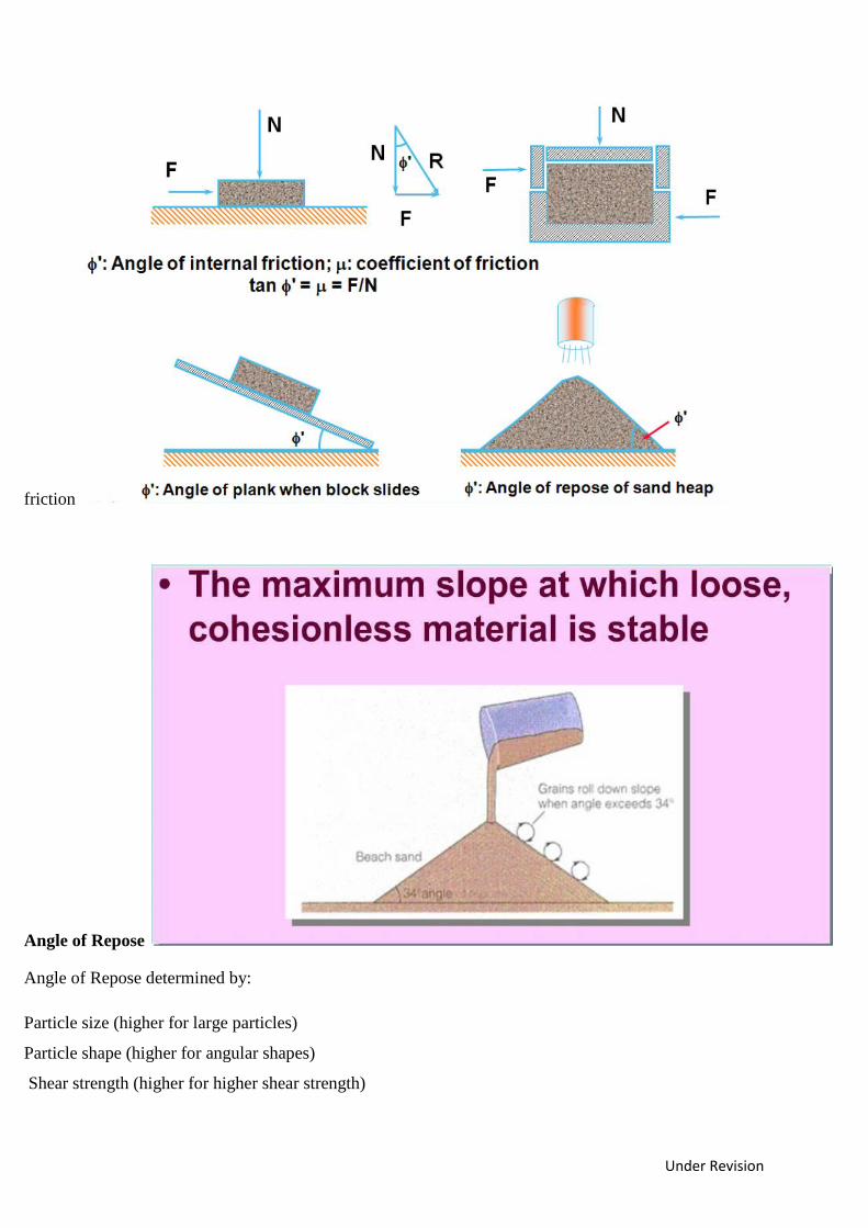
Under Revision
friction
Angle of Repose
Angle of Repose determined by:
Particle size (higher for large particles)
Particle shape (higher for angular shapes)
Shear strength (higher for higher shear strength)

Under Revision
Stresses:
Gravity generates stresses (force per unit area) in the ground at different points. Stress
on a plane at a given point is viewed in terms of two components:
Normal stress (σ) : acts normal to the plane and tends to compress soil grains
towards each other (volume change)
Shear stress (τ): acts tangential to the plane and tends to slide grains relative to each other (distortion and ultimately
sliding failure).
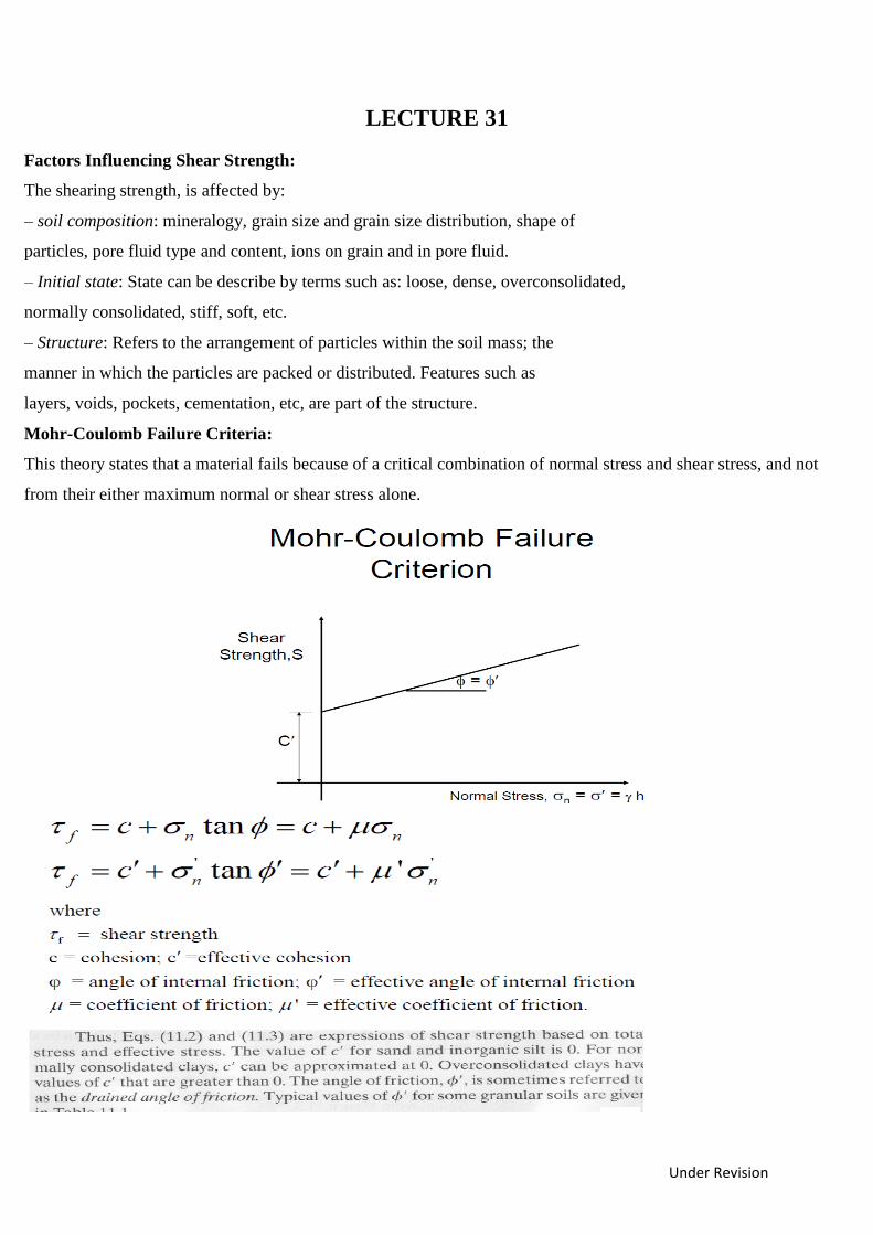
Under Revision
LECTURE 31
Factors Influencing Shear Strength:
The shearing strength, is affected by:
– soil composition: mineralogy, grain size and grain size distribution, shape of
particles, pore fluid type and content, ions on grain and in pore fluid.
– Initial state: State can be describe by terms such as: loose, dense, overconsolidated,
normally consolidated, stiff, soft, etc.
– Structure: Refers to the arrangement of particles within the soil mass; the
manner in which the particles are packed or distributed. Features such as
layers, voids, pockets, cementation, etc, are part of the structure.
Mohr-Coulomb Failure Criteria:
This theory states that a material fails because of a critical combination of normal stress and shear stress, and not
from their either maximum normal or shear stress alone.
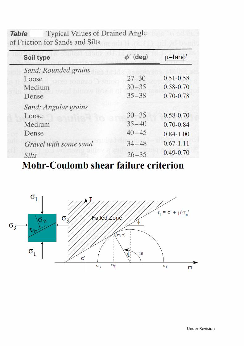
Under Revision
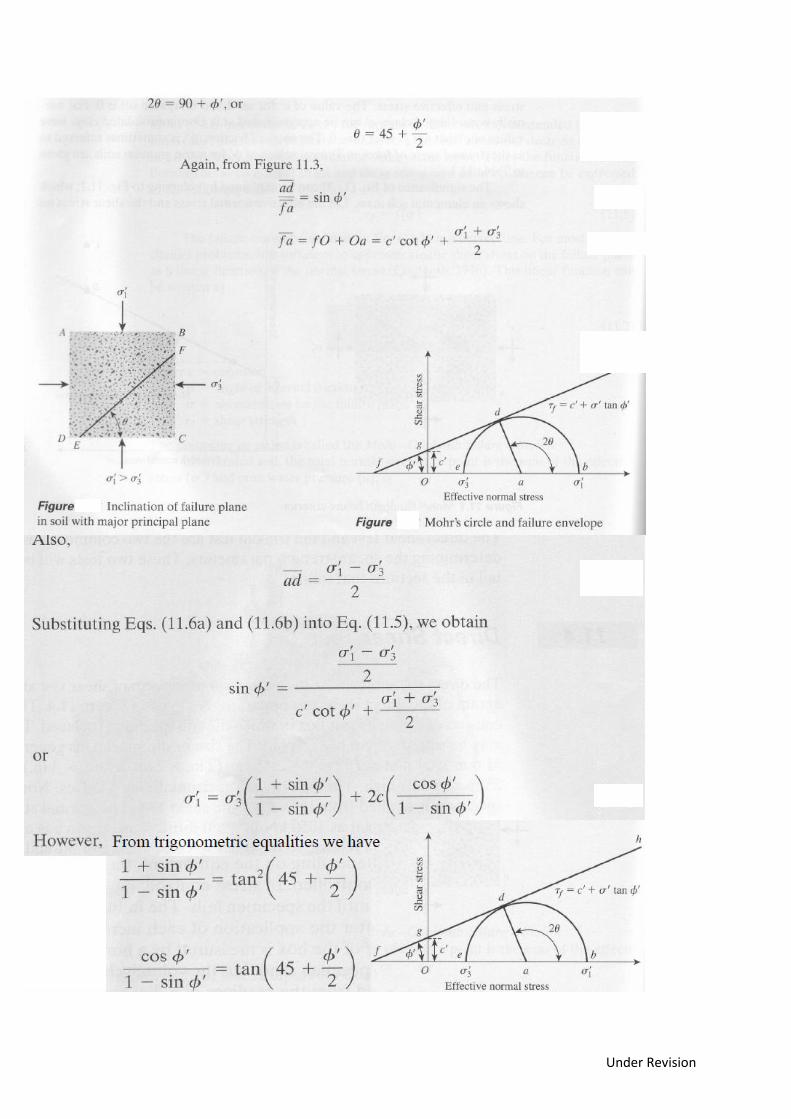
Under Revision
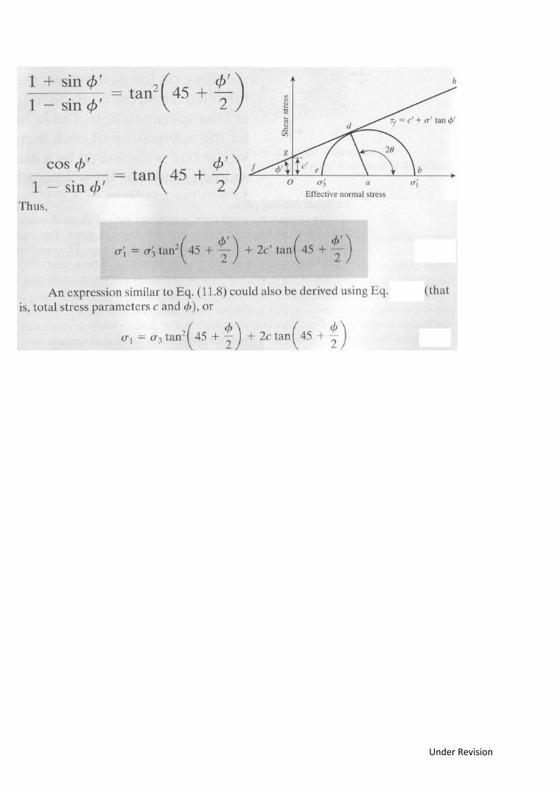
Under Revision
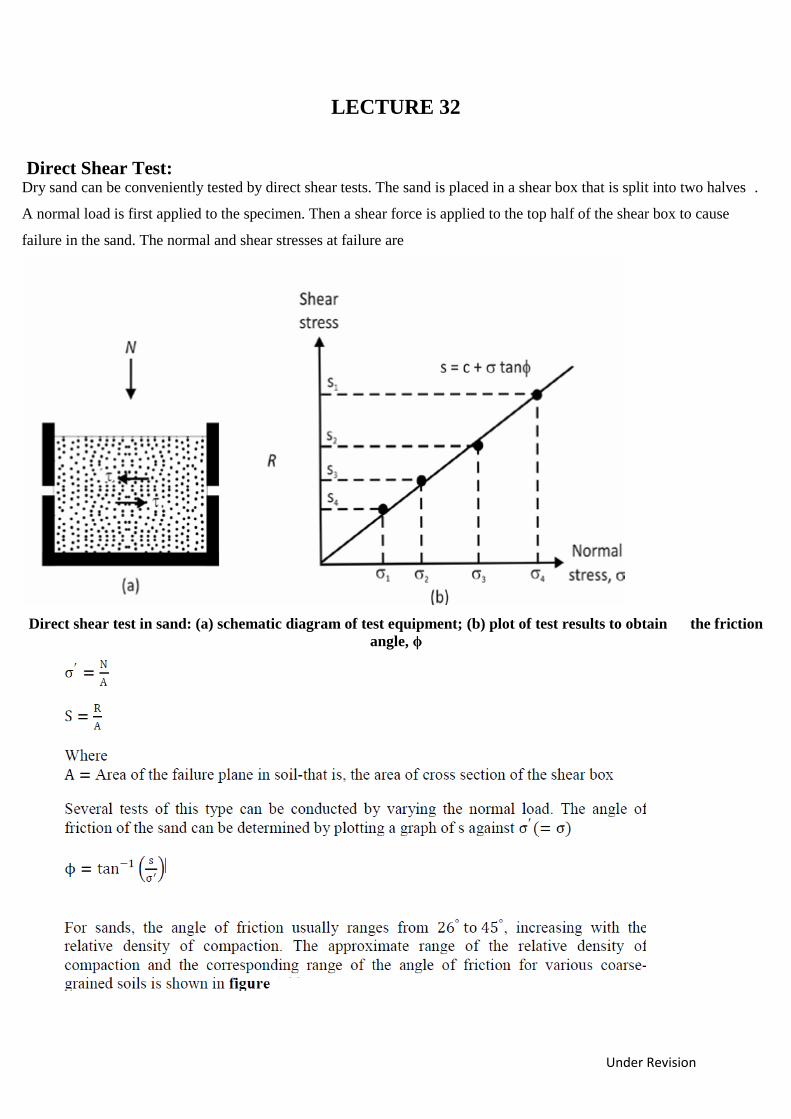
Under Revision
LECTURE 32
Direct Shear Test: Dry sand can be conveniently tested by direct shear tests. The sand is placed in a shear box that is split into two halves .
A normal load is first applied to the specimen. Then a shear force is applied to the top half of the shear box to cause
failure in the sand. The normal and shear stresses at failure are
Direct shear test in sand: (a) schematic diagram of test equipment; (b) plot of test results to obtain the friction
angle, ϕ
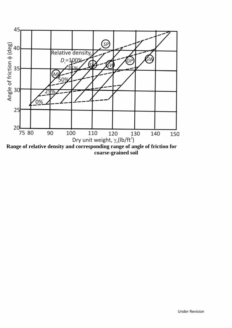
Under Revision
Range of relative density and corresponding range of angle of friction for
coarse-grained soil
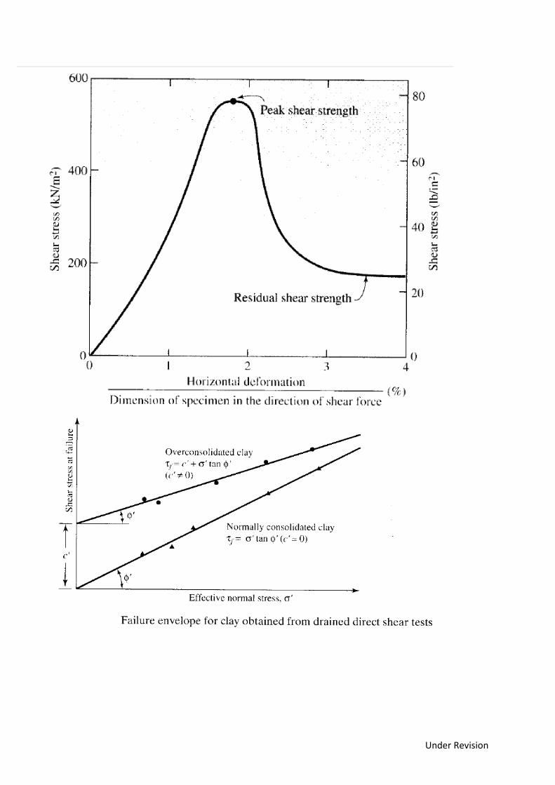
Under Revision
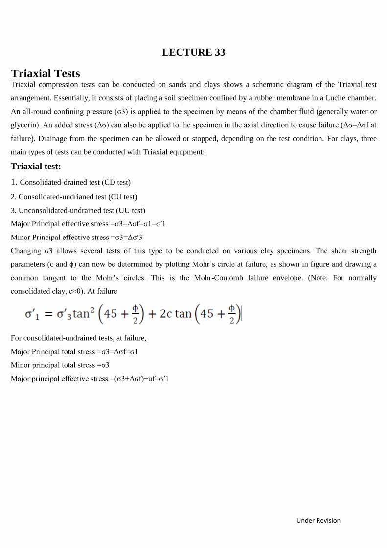
Under Revision
LECTURE 33
Triaxial Tests Triaxial compression tests can be conducted on sands and clays shows a schematic diagram of the Triaxial test
arrangement. Essentially, it consists of placing a soil specimen confined by a rubber membrane in a Lucite chamber.
An all-round confining pressure (σ3) is applied to the specimen by means of the chamber fluid (generally water or
glycerin). An added stress (Δσ) can also be applied to the specimen in the axial direction to cause failure (Δσ=Δσf at
failure). Drainage from the specimen can be allowed or stopped, depending on the test condition. For clays, three
main types of tests can be conducted with Triaxial equipment:
Triaxial test:
1. Consolidated-drained test (CD test)
2. Consolidated-undrianed test (CU test)
3. Unconsolidated-undrained test (UU test)
Major Principal effective stress =σ3=Δσf=σ1=σ′1
Minor Principal effective stress =σ3=Δσ′3
Changing σ3 allows several tests of this type to be conducted on various clay specimens. The shear strength
parameters (c and ϕ) can now be determined by plotting Mohr’s circle at failure, as shown in figure and drawing a
common tangent to the Mohr’s circles. This is the Mohr-Coulomb failure envelope. (Note: For normally
consolidated clay, c≈0). At failure
For consolidated-undrained tests, at failure,
Major Principal total stress =σ3=Δσf=σ1
Minor principal total stress =σ3
Major principal effective stress =(σ3+Δσf)−uf=σ′1
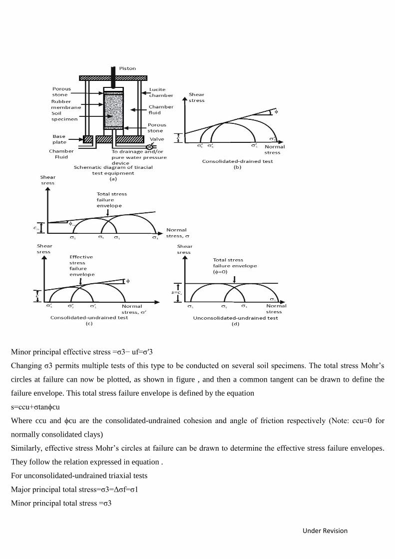
Under Revision
Minor principal effective stress =σ3− uf=σ′3
Changing σ3 permits multiple tests of this type to be conducted on several soil specimens. The total stress Mohr’s
circles at failure can now be plotted, as shown in figure , and then a common tangent can be drawn to define the
failure envelope. This total stress failure envelope is defined by the equation
s=ccu+σtanϕcu
Where ccu and ϕcu are the consolidated-undrained cohesion and angle of friction respectively (Note: ccu≈0 for
normally consolidated clays)
Similarly, effective stress Mohr’s circles at failure can be drawn to determine the effective stress failure envelopes.
They follow the relation expressed in equation .
For unconsolidated-undrained triaxial tests
Major principal total stress=σ3=Δσf=σ1
Minor principal total stress =σ3
Under Revision
The total stress Mohr’s circle at failure can now be drawn, as shown in figure. For saturated clays, the value of
σ1−σ3=Δσf is a constant, irrespective of the chamber confining pressure, σ3.The tangent to these Mohr’s circles will
be a horizontal line, called the ϕ=0 condition. The shear stress for this condition is
Where
B=Skempton′s pore pressure parameter
Similarly,the pore pressure ud is the result of added axial stress, Δσ, so
ud=A Δσ
Where
A=Skempton′s pore pressure parameter
However,
Δσ=σ1−σ3
Combining equations gives
u=ua+ud=Bσ3+Aσ1−σ3
The pore water pressure parameter B in soft saturated soils is 1, so
u=σ3+A(σ1−σ3)
The value of the pore water pressure parameter A at failure will vary with the type of soil. Following is a general
range of the values of A at failure for various types of clayey soil encountered in nature.
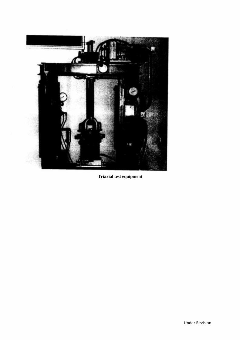
Under Revision
Triaxial test equipment
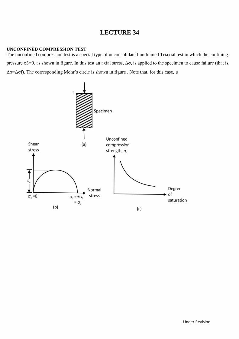
Under Revision
LECTURE 34
UNCONFINED COMPRESSION TEST
The unconfined compression test is a special type of unconsolidated-undrained Triaxial test in which the confining
pressure σ3=0, as shown in figure. In this test an axial stress, Δσ, is applied to the specimen to cause failure (that is,
Δσ=Δσf). The corresponding Mohr’s circle is shown in figure . Note that, for this case, u
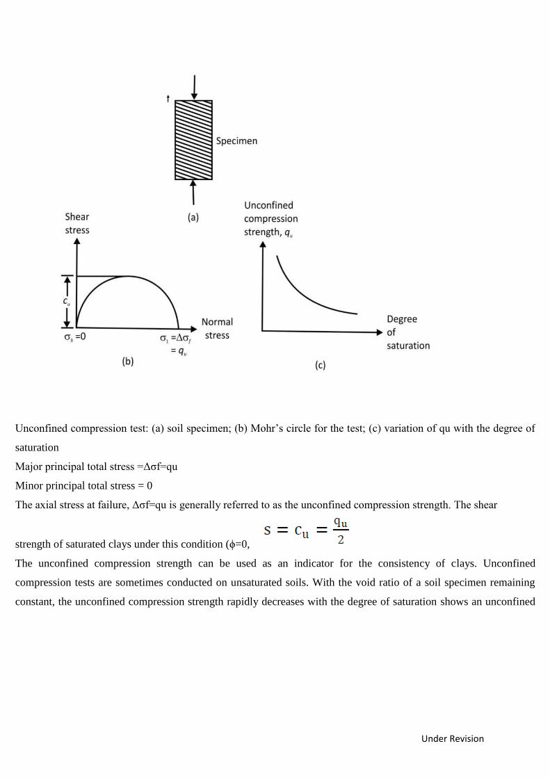
Under Revision
Unconfined compression test: (a) soil specimen; (b) Mohr’s circle for the test; (c) variation of qu with the degree of
saturation
Major principal total stress =Δσf=qu
Minor principal total stress = 0
The axial stress at failure, Δσf=qu is generally referred to as the unconfined compression strength. The shear
strength of saturated clays under this condition (ϕ=0,
The unconfined compression strength can be used as an indicator for the consistency of clays. Unconfined
compression tests are sometimes conducted on unsaturated soils. With the void ratio of a soil specimen remaining
constant, the unconfined compression strength rapidly decreases with the degree of saturation shows an unconfined
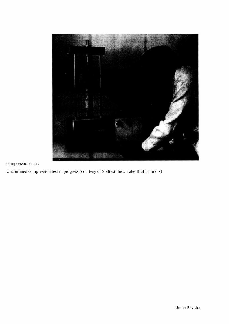
Under Revision
compression test.
Unconfined compression test in progress (courtesy of Soiltest, Inc., Lake Bluff, Illinois)
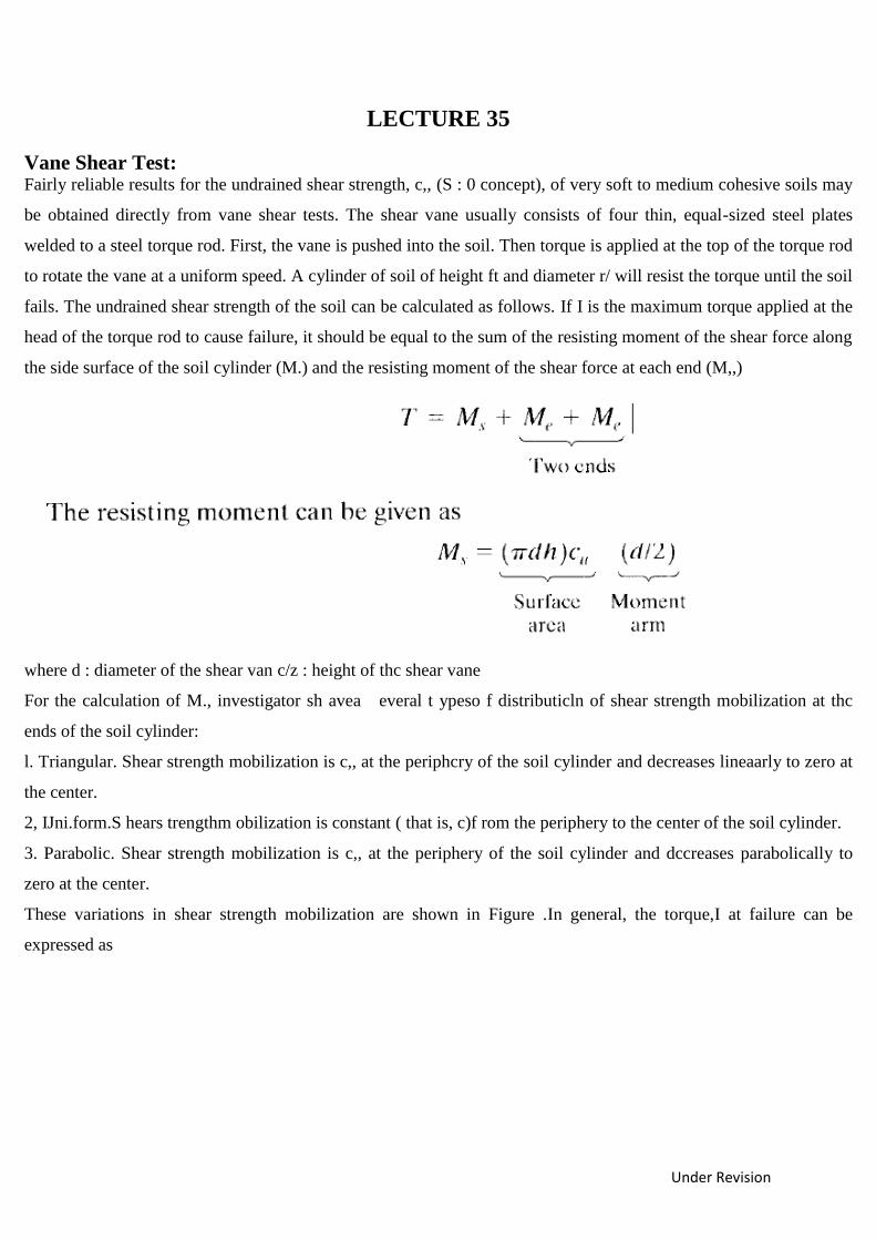
Under Revision
LECTURE 35
Vane Shear Test: Fairly reliable results for the undrained shear strength, c,, (S : 0 concept), of very soft to medium cohesive soils may
be obtained directly from vane shear tests. The shear vane usually consists of four thin, equal-sized steel plates
welded to a steel torque rod. First, the vane is pushed into the soil. Then torque is applied at the top of the torque rod
to rotate the vane at a uniform speed. A cylinder of soil of height ft and diameter r/ will resist the torque until the soil
fails. The undrained shear strength of the soil can be calculated as follows. If I is the maximum torque applied at the
head of the torque rod to cause failure, it should be equal to the sum of the resisting moment of the shear force along
the side surface of the soil cylinder (M.) and the resisting moment of the shear force at each end (M,,)
where d : diameter of the shear van c/z : height of thc shear vane
For the calculation of M., investigator sh avea everal t ypeso f distributicln of shear strength mobilization at thc
ends of the soil cylinder:
l. Triangular. Shear strength mobilization is c,, at the periphcry of the soil cylinder and decreases lineaarly to zero at
the center.
2, IJni.form.S hears trengthm obilization is constant ( that is, c)f rom the periphery to the center of the soil cylinder.
3. Parabolic. Shear strength mobilization is c,, at the periphery of the soil cylinder and dccreases parabolically to
zero at the center.
These variations in shear strength mobilization are shown in Figure .In general, the torque,I at failure can be
expressed as
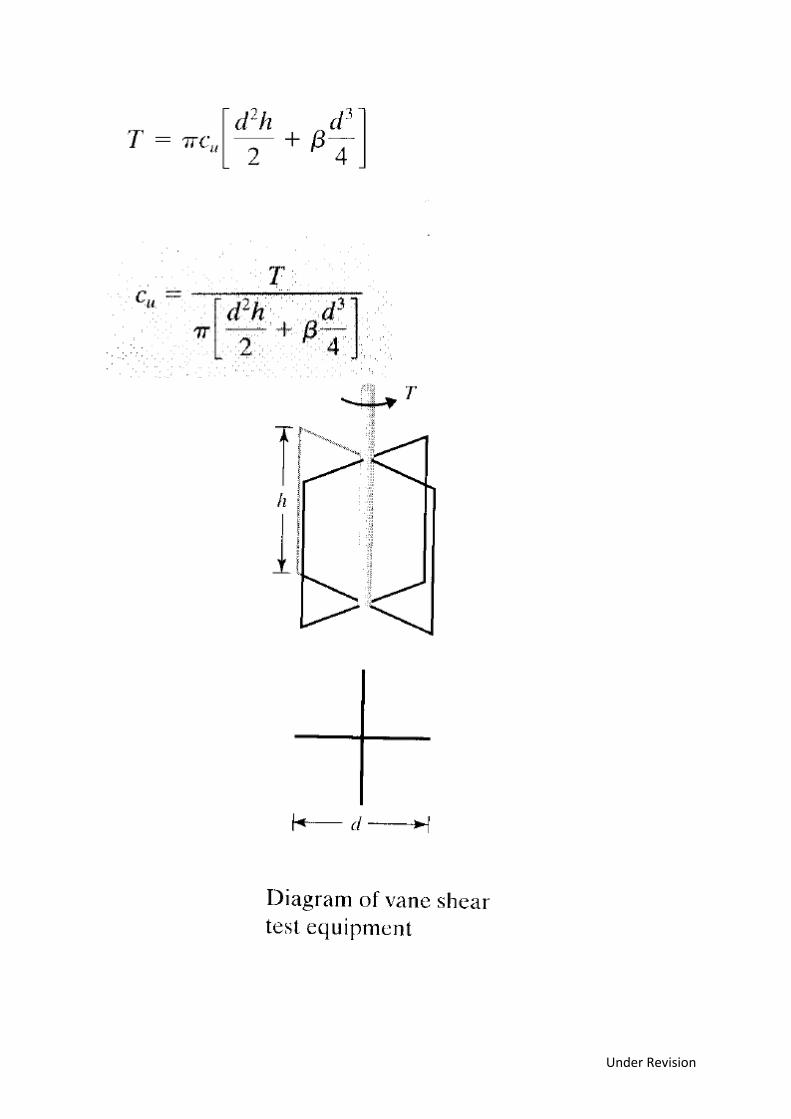
Under Revision
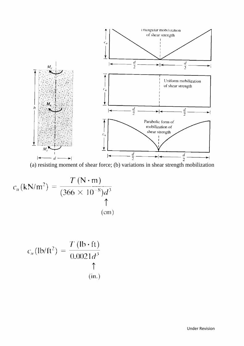
Under Revision
(a) resisting moment of shear force; (b) variations in shear strength mobilization
Under Revision
LECTURE 36 STABILIZATION OF SOIL:
It is the policy of the Indiana Department of Transportation to minimize the disruption of traffic patterns and the
delay caused today’s motorists whenever possible during the construction or reconstruction of the State’s roads and
bridges. INDOT Engineers are often faced with the problem of constructing roadbeds on or with soils, which do not
possess sufficient strength to support wheel loads imposed upon them either in construction or during the service life
of thepavement. It is, at times, necessary to treat these soils to provide a stable subgrade or a working platform for
the construction of the pavement. The result of these treatments are that less time and energy is required in the
production, handling, and placement of road and bridge fills and subgrades and therefore, less time to complete the
construction process thus reducing the disruption and delays to traffic.
These treatments are generally classified into two processes, soil modification or soil stabilization. The purpose of
subgrade modification is to create a working platform for construction equipment. No credit is accounted for in this
modification in the pavement design process. The purpose of subgrade stabilization is to enhance the strength of the
subgrade. This increased strength is then taken into account in the pavement design process. Stabilization requires
more thorough design methodology during construction than modification. The methods of subgrade modification or
stabilization include physical processes such as soil densification, blends with granular material, use of
reinforcements (Geogrids), undercutting and replacement, and chemical processes such as mixing with cement, fly
ash, lime, lime byproducts, and blends of any one of these materials. Soil properties such as strength,compressibility,
hydraulic conductivity, workability, swelling potential, and volume change tendencies may be altered by various soil
modification or stabilization methods. Subgrade modification shall be considered for all the reconstruction and new
alignment projects.
When used, modification or stabilization shall be required for the full roadbed width including shoulders or curbs.
Subgrade stabilization shall be considered for all subgrade soils with CBR of less than 2.INDOT standard
specifications provide the contractor options on construction practices to
achieve subgrade modification that includes chemical modification,replacement with aggregates, geosynthetic
reinforcement in conjunction with the aggregates, and density and moisture controls. Geotechnical designers have to
evaluate the needs of the subgrade and
include where necessary, specific treatment above and beyond the standard specifications.Various soil modification
or stabilization guidelines are discussed below. It is necessary for designers to take into consideration the local
economic factors as well as environmentalconditions and project location in order to make prudent decisions for
design.
It is important to note that modification and stabilization terms are not interchangeable.
Mechanical Stabilization: This is the process of altering soil properties by changing the gradation through mixing with other soils, densifying
the soils using compaction efforts, or undercutting the existing soils and replacing them with granular material.
A common remedial procedure for wet and soft subgrade is to cover it with granular material or to partially remove
and replace the wet subgrade with a granular material to a pre-determined depth below the grade lines. The
compacted granular layer distributes the wheel loads over a wider area and serves as a working platform.To provide
a firm-working platform with granular material, the following conditions shall be met.
1. The thickness of the granular material must be sufficient to develop acceptable pressure distribution over the wet
soils.
2. The backfill material must be able to withstand the wheel load without rutting.
3. The compaction of the backfill material should be in accordance with the Standard Specifications.
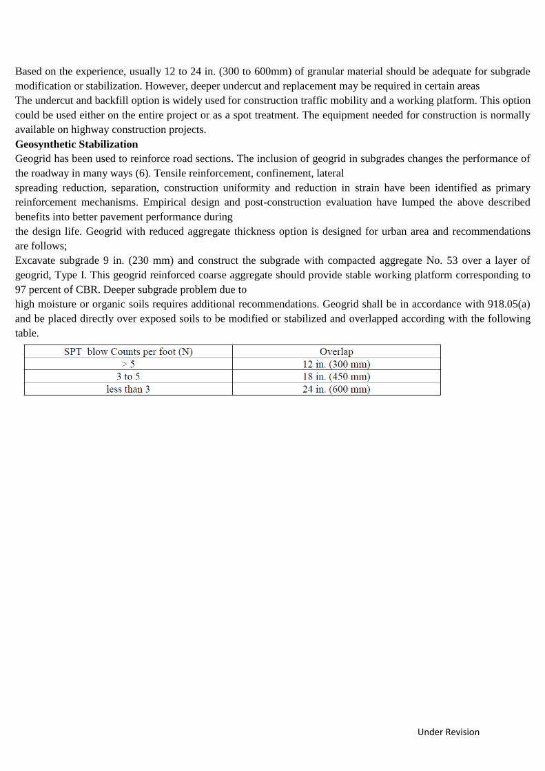
Under Revision
Based on the experience, usually 12 to 24 in. (300 to 600mm) of granular material should be adequate for subgrade
modification or stabilization. However, deeper undercut and replacement may be required in certain areas
The undercut and backfill option is widely used for construction traffic mobility and a working platform. This option
could be used either on the entire project or as a spot treatment. The equipment needed for construction is normally
available on highway construction projects.
Geosynthetic Stabilization
Geogrid has been used to reinforce road sections. The inclusion of geogrid in subgrades changes the performance of
the roadway in many ways (6). Tensile reinforcement, confinement, lateral
spreading reduction, separation, construction uniformity and reduction in strain have been identified as primary
reinforcement mechanisms. Empirical design and post-construction evaluation have lumped the above described
benefits into better pavement performance during
the design life. Geogrid with reduced aggregate thickness option is designed for urban area and recommendations
are follows;
Excavate subgrade 9 in. (230 mm) and construct the subgrade with compacted aggregate No. 53 over a layer of
geogrid, Type I. This geogrid reinforced coarse aggregate should provide stable working platform corresponding to
97 percent of CBR. Deeper subgrade problem due to
high moisture or organic soils requires additional recommendations. Geogrid shall be in accordance with 918.05(a)
and be placed directly over exposed soils to be modified or stabilized and overlapped according with the following
table.
Under Revision
LECTURE 37
Chemical Modification or Stabilization
The transformation of soil index properties by adding chemicals such as cement, fly ash, lime, or a combination of
these, often alters the physical and chemical properties of the soil including the cementation of the soil particles.
There are the two primary mechanisms by which chemicals alter the soil into a stable subgrade:
1. Increase in particle size by cementation, internal friction among the agglomerates, greater shear strength,
reduction in the plasticity index, and reduced shrink/swell potential.
2. Absorption and chemical binding of moisture that will facilitate compaction.
Design Procedures
Criteria for Chemical Selection
When the chemical stabilization or modification of subgrade soils is considered as the most economical or feasible
alternate, the following criteria should be considered for chemical selection based on index properties of the soils.
Suggested Chemical Quantities For Modification Or Stabilization-
Strength requirements for stabilization and modification
The reaction of a soil with quick lime, or cement is important for stabilization or modification and design
methodology. The methodology shall be based on an increase in the unconfined compression strength test data. To
determine the reactivity of the soils for lime stabilization, a pair of specimens measuring 2 in. (50 mm) diameter by

Under Revision
4 in. (100 mm) height (prepared by mixing at least 5% quick lime by dry weight of the natural soil) are prepared at
the optimum
moisture content and maximum dry density (AASHTO T 99). Cure the specimens for 48 hours at 120o F (50o C) in
the laboratory and test as per AASHTO T 208. The strength gain of lime soil mixture must be at least 50 psi (350
kPa) greater than the natural soils. A strength gain of 100 psi (700 kPa) for a soil-cement mixture over the natural
soil shall be considered adequate for cement stabilization with 4% cement by dry weight of the soils and tested as
described above
In the case of soil Stabilization, enhanced subgrade support is not accounted for in pavement design. However, an
approved chemical (LKD, cement, and fly ash class C) or a combination of the chemicals shall attain an increase in
strength of 30 psi over the natural soils when specimens are prepared and tested in the same manner as stabilization.
Under Revision
LECTURE 38
Lime Stabilization.
Lime reacts with medium, moderately fine and fine-grained soils to produce decreased plasticity,increased
workability, reduced swelling, and increased strength. The major soil properties and characteristics that influence the
soils ability to react with lime to produce cementitious materials are pH, organic content, natural drainage, and clay
mineralogy. As a general guide, treated soils should increase in particle size with cementation, reduction in
plasticity, increased in internal friction among the agglomerates, increased shear strength, and increased workability
due to the textural change from plastic clay to friable, sand like material.
The following procedures shall be utilized to determine the amount of lime required to stabilize the subgrade.
Hydrated or quick lime and lime by-products should be used in the range of 4 ± 0.5% and 5 ± 1% by weight of soil
for modification respectively. The following procedures shall be used to determine the optimum lime content.
Perform mechanical and physical tests on the soils.
Determine the separate pH of soil and lime samples.
Determine optimum lime content using Eades and Grim pH test.
• A sufficient amount of lime shall be added to soils to produce a pH of 12.4 or
equal to the pH of lime itself. An attached graph is plotted showing the pH as
lime content increases. The Optimum lime content shall be determined
corresponding to the maximum pH of lime-soil mixture. (See Figure 4.0 A).
• Representative samples of air-dried, minus No. 40 soil is equal to 20 g of
oven-dried soil are weighed to the nearest 0.1 g and poured into 150-ml (or
larger) plastic bottles with screw on tops.
• It is advisable to set up five bottles with lime percentages of 3, 4, 5, 6, and 7.
This will insure, in most cases, that the percentage of lime required can be
determined in one hour. Weigh the lime to the nearest 0.01 g and add it to the
soil. Shake the bottle to mix the soil and dry lime.
• Add 100 ml of CO2-free distilled water to the bottles.
• Shake the soil-lime mixture and water until there is no evidence of dry
material on the bottom. Shake for a minimum of 30 seconds.
• Shake the bottles for 30 seconds every 10 minutes.
• After one hour, transfer part of the slurry to a plastic beaker and measure the pH. The pH meter must be equipped
with a Hyalk electrode and standardized with a buffer solution having a pH of 12.00.
• Record the pH for each of the lime-soil mixtures. If the pH readings go to
12.40, then the lowest percent lime that gives a pH of 12.40 is the percentage
required to stabilize the soil. If the pH does not go beyond 12.30 and 2
percentages of lime give the same readings, the lowest percent which gives a
pH of 12.30 is the amount required to stabilize the soil. If the highest pH is
12.30 and only 1 percent lime gives a pH of 12.30, additional test bottles
should be started with larger percentages of lime.
d. Atterberg limits should be performed on the soil-lime mixtures corresponding to optimum lime content as
determined above.
e. Compaction shall be performed in accordance with AASHTO T 99 on the
optimum lime and soil mixture to evaluate the drop in maximum dry density in relation to time (depending on the
delay between the lime-soil mixing)
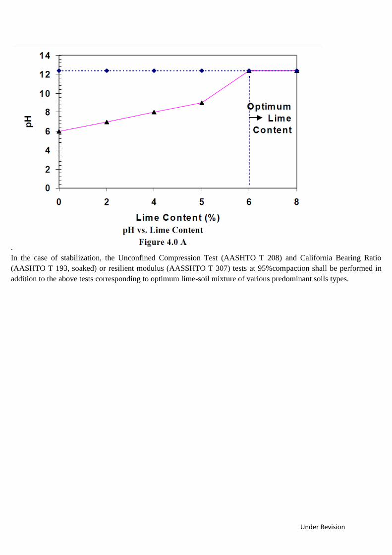
Under Revision
.
In the case of stabilization, the Unconfined Compression Test (AASHTO T 208) and California Bearing Ratio
(AASHTO T 193, soaked) or resilient modulus (AASSHTO T 307) tests at 95%compaction shall be performed in
addition to the above tests corresponding to optimum lime-soil mixture of various predominant soils types.
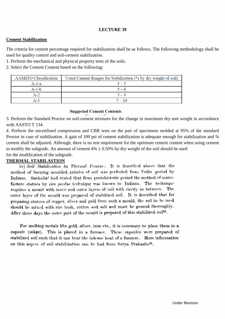
Under Revision
LECTURE 39
Cement Stabilization
The criteria for cement percentage required for stabilization shall be as follows. The following methodology shall be
used for quality control and soil-cement stabilization.
1. Perform the mechanical and physical property tests of the soils.
2. Select the Cement Content based on the following:
3. Perform the Standard Proctor on soil-cement mixtures for the change in maximum dry unit weight in accordance
with AASTO T 134.
4. Perform the unconfined compression and CBR tests on the pair of specimens molded at 95% of the standard
Proctor in case of stabilization. A gain of 100 psi of cement stabilization is adequate enough for stabilization and %
cement shall be adjusted. Although, there is no test requirement for the optimum cement content when using cement
to modify the subgrade. An amount of cement 4% ± 0.50% by dry weight of the soil should be used
for the modification of the subgrade.
THERMAL STABILASTION
Under Revision
LECTURE 40
GROUTING
The soil improvement techniques are effective for each of the allowed or required disturbance
of existing structures. The following methods, which imply a low level of vibration, are useful to
improve liquefiable ground by solidification:
(a) Compacting grouting ;
(b) Permeation grouting ;
(c) Jet grouting;
Compaction Grouting-
Compaction grouting is a soil injection with low workability cement paste that remains homogeneous without
entering in the soil pores. The cement mass extends, soil is moved and finally compacted. The liquefaction
improvement using compaction grouting divides into the
following categories:
(a)Treatment under existing structures;
(b) Treatment in urban areas with low levels of vibration and noise;
(c) Treatment in narrow areas.
The execution of compaction by injection technology using bottom-up method takes place as follows. In the first
stage, injection pipes set up on the foundation soil of the existing or future foundations using drilling machines. The
injection process begins. Mixture injected through the pipes pushes the surrounding soil; then the injection pipes
raises about 0.3-1.5 m and the process renews. The “in steps” injection process continues until the whole thickness
of the soil layer is treated. Injection stabilizes soil layer by density and pressure increasing. The injection process is
used when a controlled lifting of the soil surface or existing structures affected by local settlements are necessary
(Plescan & Rotaru, 2010; Morales & Morales, 2003; Welsh et al, 2002).
Orense et al. (2010) reported that Compaction grouting involves the injection of a very stiff grout (soil-cement-water
mixture with sufficient silt sizes to provide plasticity, together with sand and gravel sizes to develop internal
friction) that does not permeate the native soil, but
results in controlled growth of the grout bulb mass that displaces the surrounding soil. The primary purpose of
compaction grouting is to increase the density of soft, loose or disturbed soil,
typically for settlement control, structural re-leveling, increasing the soil’s bearing capacity, and mitigation of
liquefaction potential.
Also Orense (2008) had a review of two case histories on the application of compaction grouting as liquefaction
remediation was presented. One case involved the implementation in an open unrestricted space such as airport
runways, while the second one was under an existing
manufacturing plant. Based on the discussion, several important observations regarding the effectiveness of the
technique were addressed. The post-treatment data suggested that compaction grouting was capable of producing the
improvement in SPT resistance required to mitigate
liquefaction risk. The method of construction, whether “bottom-up”, “top-down” or combination of the two, affected
the level of effectiveness and the resulting ground heave. The method was most effective on sandy soil with fewer
fines content. In addition, compaction grouting also
increased the strength and the lateral earth pressure of the ground. This method is shown
Under Revision
Compaction grouting implementation (Orense, 2008).
Permeation Grouting-
Permeation grouting consists of the injection of a low-viscosity fluid in the soil pores without changes in the soil
physical structure. The main goal of permeation grouting is both to strengthen
soils through particle cementation (to stabilize the links between particles) and to waterproof ground by filling its
pores with injected fluid. This method improves the soil physical and mechanical characteristics, successfully
stabilizes the excavation walls in soft soils, controls the
groundwater migration in order to implement the underpinnings at the existing foundations and prevents the effects
of earthquakes – compaction and soil liquefaction. Permeation grouting is a
technology used to mitigate liquefaction that is suitable for un-compacted soils solidification in order to reduce the
risks of compaction and liquefaction that may occur as result of possible earthquakes (Plescan and Rotaru, 2010).
The process is quiet flexible and it can be designed with a minimal disruption at the surface and therefore, it is
advantageous for use in urban areas or areas with limited access. During grouting process, injection pressures Based
on the field trials and the soil conditions, the injection pressures and the grout volumes will be justified to meet the
intended performance.
Particulate grouts (e.g. cement or bentonite) are generally used for medium to coarse grained sands, such that the
particles in the grout easily percolate through the formation. Micro fine cement is also used for fine grained sands
where Ordinary Portland Cement cannot percolate through the formation. Chemical grouts (e.g. silicates) are used in
formations with smaller pore
spaces, but are limited to soils coarser than fine grained sands. The process of permeation grouting is schematically
shown in Figure 2. Quality Control & Quality Assurance Like any other grouting improvement process, the quality
control during permeation grouting is very important to ascertain the effectiveness of the technique. As such, the
process parameters such as grout
are usually limited to prevent fracturing or volume change in the natural soil/rock formation. injection pressures and
the grout volumes will be justified to meet the intended performance.
Particulate grouts (e.g. cement or bentonite) are generally used for medium to coarse grained sands, such that the
particles in the grout easily percolate through the formation. Micro fine
cement is also used for fine grained sands where Ordinary Portland Cement cannot percolate through the formation.
Under Revision
Chemical grouts (e.g. silicates) are used in formations with smaller pore spaces, but are limited to soils coarser than
fine grained sands. The process of permeation grouting is schematically shown in Figure 2. Quality Control &
Quality Assurance Like any other
grouting improvement process, the quality control during permeation grouting is very important to ascertain the
effectiveness of the technique. As such, the process parameters such as grout
pressure, flow rate, volume of grout for corresponding depth are monitored throughout the construction process. Post
construction in-situ permeability tests are conducted after sufficient curing period to validate the effectiveness of
permeation grouting (Raju & Valluri, 2010).
Schematic showing process of Permeation Grouting(Raju & Valluri, 2010).
A newly permeation grouting technique using a colloidal silica has been developed to prevent the liquefaction of
sandy ground beneath existing structures. In the case of cyclic torsional shear test with the treated sand, a relatively
large strain is developed in the early stage of loading;
however, both the development of shear strain and the decrease of mean effective stress resulted without any
collapse and liquefaction also the remarkable improvement of cyclic shear strength by the colloidal silica treatment
can be exhibited. This phenomenon leads to the expansion of
dilation region across which it faced the phase transformation line and the failure line. (Ohno et al, 2005)
In order to study the deformation and the strength characteristics of the treated sand with the colloidal silica, a series
of laboratory tests has been performed on the treated sand such as monotonic and cyclic torsional shear tests. In the
case of cyclic torsional shear test with the
treated sand, a relatively large strain is developed in the early stage of loading; however, both the development of
shear strain and the decrease of mean effective stress resulted without any collapse and liquefaction. As the results,
the remarkable improvement of cyclic shear strength by
the colloidal silica treatment can be exhibited. This phenomenon leads to the expansion of dilation region across
which it faced the phase transformation line and the failure line. When the performance based design for the silica-
treated ground are carried out, it is necessary for the dynamic deformation analysis to produce the appropriate
constitutive model for the treated sand
based on the test results (Oka et al. 2003). Their report indicates that the improved sand exhibited greater
liquefaction strength curves. Based on the results of laboratory studies, a cyclic elastoplastic model has been
proposed in order to describe the behavior of improved sand. Then, the cyclic elasto-plastic model has been
implemented into the fully coupled effective stress based FEM program to perform numerical analysis of
liquefaction of improved ground. It has been revealed that the improvement by permeating grouting method is very
Under Revision
effective in increasing the
resistance against liquefaction.
Jet Grouting-
Applications of the jet grouting system fall into three broad categories: underpinning or excavation support,
stabilization of soft or liquefiable soils, groundwater or pollution control. The method consists of soil injection of a
mixed fluid at high pressure forming jets that erode and
replace the existing soil with the injection mixture. In general this method begins by drilling
small-diameter holes (90-150 mm) up to the final injection depth. Cement mixture is injected into the soil with a
metal rod that runs a rotational and withdrawal motion whilst. This technology is useful to underpinnings of existing
foundations, to support excavations in cohesive less soils, to
control the groundwater migration and to improve the strength of liquefiable soil (plescan & rotaru, 2010;
Geotechnical news, 2008). This method is shown in the Figure .
Jet grouting method (Plescan & Rotaru, 2010). Cooke (2000) studied the use of jet grouting under an embankment
slope at existing highway
bridges to mitigate the risk of earthquake-induced liquefaction damage. The jet-grouted zone helped to limit
movements of the abutment by containing and limiting the shear deformations that occurred in the liquefiable soils
under the embankment that were softened due to the development
of excess pore water pressures during shaking. The limitation of the deformations was dependent on the strength and
stiffness of the jet-grouted zone, which in the cases evaluated did not fail, and its ability to resist the increased
overturning forces during shaking. The performance of a jetgrouted
zone is highly dependent on its strength. The strength assumed for the jet grouted material was high and resulted in
no material failure during shaking (Geotechnical news, 2008).
Also Geotechnical News (2008) reported from Olgun (2003), the soils were improved to
increase bearing support for shallow foundations and to reduce liquefaction potential of the sand layers. Surcharge
fills with wick drains were used to improve the soft clays, and jet-grouted columns were used to provide increased
bearing support in the clays and prevent liquefaction of
Under Revision
the loose sands. Jet-grouted column spacing and diameters were selected on the basis of footing spacing, footing
loads, floor slab loads, and judgment. A primary and secondary grid of columns was installed in a rectangular
pattern to provide blanket treatment. In addition Olgun showed that
jet grouted columns do not stiffen the ground by attracting the seismic shear stresses. they do not reduce shear
stresses on the soft ground. They may still act as vertical support if there is enough bearing capacity and side
resistance from layers that did not liquefy. It is possible rely
on jet grouted columns to provide bearing support and reduce settlements if liquefaction is limited to a specific zone.
It is clear that there could be liquefaction mitigation only if the entire liquefiable zone is treated. A total replacement
of potentially liquefiable material by jet grouting,
will avoid the liquefaction likelihood.
Yilmaz et al. (2008) performed a study on the soil improvement in Beydag dam against liquefaction of alluvium at
the dam site. Peak acceleration on rock was estimated to be 0.32 g for an earthquake having magnitude of 7.
Liquefiable soils, which consisted of two separate layers of diatomaceous silt and one layer of volcanic ash beneath
the downstream toe of Wick up Dam,
were stabilized using 4.3 m diameter jet grouting columns. These liquefiable strata extended to depths up to 26 m.
The dam had a square grid of intersecting jet grout piles at the downstream side of upstream wall having an area
replacement ratio of about 10%. Depending upon the shear
modulus ratio, G, between jet grouted column and soil, it was found that stress reduction coefficient changes with
area replacement ratio. Cyclic stress ratio (CSR) after ground improvement is calculated by multiplying stress
reduction coefficient with CSR before treatment. Thus, it was possible to calculate the area replacement ratio
required to reach the intended factor of safety. It was found that 10% area replacement ratio may reduce CSR at least
about 50%.