Towards an Arbitrage Analysis of Optimization Speculation

International Journal of Innovative Research in Advanced Engineering (IJIRAE) ISSN: 2349-2763 Issue 01, Volume 3 (January 2016) www.ijirae.com

________________________________________________________________________________________________________ IJIRAE: Impact Factor Value - ISRAJIF: 1.857 | PIF: 2.469 | Jour Info: 4.085 | Index Copernicus 2014 = 6.57

© 2014- 16, IJIRAE- All Rights Reserved Page -7

Towards an Arbitrage Analysis of Optimization Speculation

Dr.Kalyana Kumar. S Professor & Head, Department of Mathematics,

Dr.T.Thimmaiah Institute of Technology, Kolar Gold Fields- 563 120, Karnataka., India

INTRODUCTION: FINDING THE MARKETS IN THE MATH

One of the fundamental insights of mainstream neoclassical economics is the connection between competitive market prices and the Lagrange multipliers of optimization theory in mathematics. Yet this insight has not been well developed. In the standard theory of markets, competitive prices result from the equilibrium of supply and demand. But in a constrained optimization problem, there seems to be no mathematical version of supply and demand functions so that the Lagrange multipliers could be seen as equilibrium prices. How can one "Find the markets in the math" so that Lagrange multipliers will emerge as equilibrium market prices? We argue that the solution to the "Finding the markets in the math" problem is to reconceptualize equilibrium as the absence of profitable arbitrage instead of the equating of supply and demand. With each proposed solution to a classical constrained optimization problem, there is an associated market. The maximand is one commodity, and each constraint provides another commodity on this market. Given a marginal variation in one commodity, one can define the marginal change is any other given commodity so the market has a set of exchange rates between the commodities. The usual necessary conditions for the proposed solution to solve the maximization problem are the same as the conditions for this mathematically defined "market" to be arbitrage-free. The prices that emerge from the arbitrage-free system of exchange rates (normalized with the maximand as numeraire) are precisely the Lagrange multipliers. We also show the cofactors of a matrix describing the marginal variations can be taken as the prices (before being normalized) so the Lagrange multipliers can always be presented as ratios of cofactors. Starting with any square m m matrix (with rank m–1), a market can also be defined and the cofactors given a price interpretation so that an economic interpretation can be constructed for the inverse matrix and for Cramer's Rule.

The relevant mathematical result, which dates back to Augustin Cournot in 1838, is that:there exists a system of prices for the commodities such that the given exchange rates are the price ratios if and only if the exchange rates are arbitrage-free (in the sense that they multiply to one around any circle). This simple graph-theoretic theorem is known in its additive version as Kirchhoff's Voltage Law (KVL): there exists a system of potentials at the nodes of a circuit such that the voltages on the wires between the nodes are the potential differences if and only if the voltages sum to zero around any cycle. Kirchhoff's work was published in 1847, so it might be called "the Cournot-Kirchhoff law." There is also an additive version of the additive KVL. If two commodities are swapped, one unit for one unit, then usually some additional "boot" must be paid for the higher valued commodity. For each pair of goods i and j, suppose we are given an amount boot(i,j) that is the additional cash boot that needs to be paid along with one unit of good i in order to receive one unit of good j.

Then KVL takes the form: Given a system of boots for commodity swaps, there exists a set of unit prices for the goods such that the boot necessary for an exchange of units is the price difference if and only if the system of boots is arbitrage-free in the sense of summing to zero around any circle. We show that this Cournot-Kirchhoff law has many applications outside of electrical circuit theory and economics. For instance, the second law of thermodynamics can be formulated as the impossibility of a certain form of "heat arbitrage" between temperature reservoirs, and the "prices" that emerge in this case are the Kelvin absolute temperatures of the reservoirs. Yet another application of the arbitrage framework is in probability theory. Profitable arbitrage in the market for contingent commodities is called "making book." A person's subjective probability judgments satisfy the laws of probability if they are "coherent" in the sense of not allowing book to be made against the person. Thus arbitrage on the market for contingent commodities enforces the laws of probability.

Arbitrage-related concepts have been applied successfully in financial economics. Merton H. Miller and Franco Modigliani used impressive arbitrage arguments in proving their famous irrelevance theorem [1958]. Stephen A. Ross [Ross 1976a, 1976b] and his colleagues have developed Arbitrage Pricing Theory so that it is now recognized as a fundamental principle in finance theory [Varian 1987]. Our purpose here is not to use arbitrage concepts to study financial markets, but to find the mathematically defined "markets" and the related arbitrage-concepts in the mathematics of all classical constrained optimization problems.

ARBITRAGE IN GRAPH THEORY A directed graph G =(G0,G1, t,h) is given by a set G0 of nodes (numbered 0,1,...,m), a set G1 of arcs (numbered 1,2,...,b), and head and tail functions h,t:G1 G0, which indicate that arc j is directed from its tail, the t(j) node, to its head, the h(j) node.




t(j) h(j)Arc j

Figure 1. Arc j from Tail t(j) to Head h(j)

It is assumed that there are no loops at a node, i.e., h(j) t(j) for all arcs j. A path from node i to node i' is given by a sequence of arcs connected at their heads or tails that reach from node i to node i'. A graph is connected if there is a path between any two nodes. It is assumed that the graph G is connected. A closed circular path where no arc occurs more than once is a cycle [for more graph theory, see any text such as Berge and Ghouila-Houri 1965]. Let T be any group (not necessarily commutative) written multiplicatively (i.e., a set with a binary product operation defined on it, with an identity element 1 and with every element having a multiplicative inverse or reciprocal). For most of our purposes, T can be taken as R*, the multiplicative group of nonzero reals. In the motivating economic interpretation, a different commodity is associated with each node, and the arcs represent channels of exchange or transformation between the commodities at the nodes. A function r:G1 T is a rate system giving exchange or transformation rates. Given an arc j, one unit of the t(j) commodity can be transformed into r(j) = rj units of the h(j) commodity.

t(j) h(j)Arc j

Rate rj

Figure 2. Transformation Rate rj on Arc j

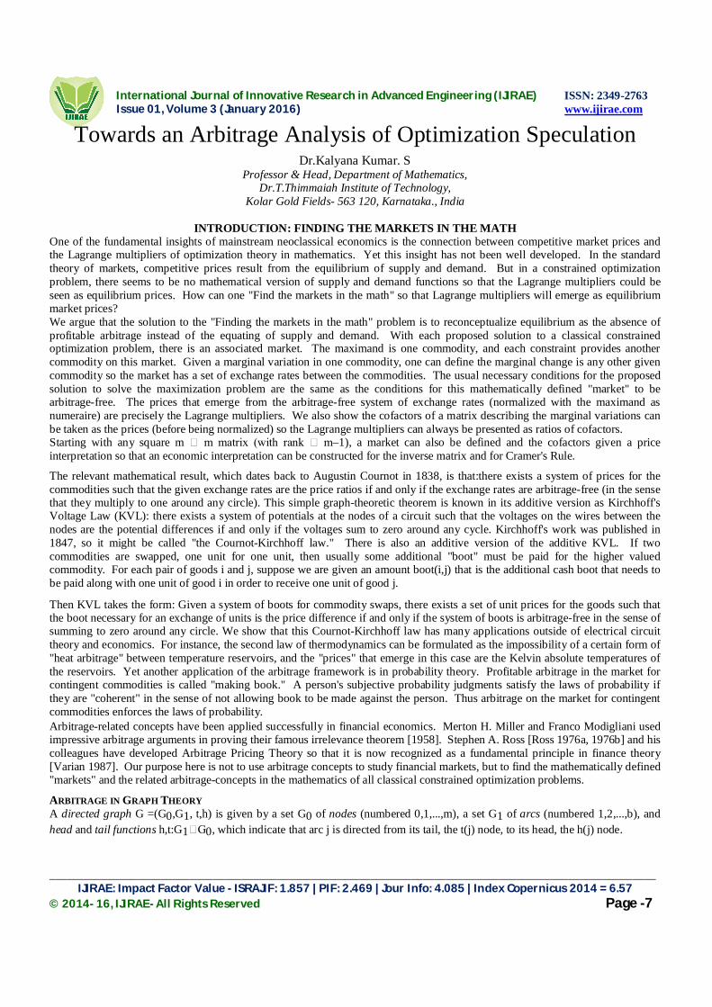
A graph (G,r) with a rate system r represents a market, so it will be called a market graph. These group-labeled graphs are also called "voltage graphs" [Gross 1974] or "group graphs" [Harary et al. 1982]. All transformations are reversible. If arc j is traversed against the arrow, the transformation rate is the reciprocal 1/rj. Given a path c from node i to i', the composite rate r[c] is the product of the rates along the path using the reciprocal rate for any arc traversed against the direction of the arrow. A function P:G0 T labeling the nodes is a price system (or absolute price system). A rate system Q(P):G1 T can be derived from a price system by taking the price ratios

Q(P)(j) = P(h(j))–1P(t(j)).

Equation 1. Derived Rate on arc j = Price at Tail Divided by Price at Head Derived rate systems have certain special properties:

1. for any path c from i to i', Q(P)[c] = P(i')–1P(i), 2. for any two paths c and c' from i to i', Q(P)[c] = Q(P)[c'], and 3. for any cycle c, Q(P)[c] = 1.

Given a market graph (G,r), the rate system r is said to be path-independent if for any two paths c and c' between the same nodes, r[c] = r[c']. The rate system is said to be arbitrage-free if for any cycle c, r[c] = 1 ["arbitrage-free" = "balanced" in much of the graph-theoretic literature following Harary 1953].

r = 1/2 r = 3

r = 3/2

r = 4/3

r = 4

r = 1/12

p = 1 p = 2 p = 6

p = 4

p = 3 p = 12

r[c] =(1/2)(1/3)(3/2)(4/3)(1/4)(12) = 1 Figure 3. An Arbitrage-Free Market Graph

In an idealized international currency exchange market with no transaction costs, if the product of the exchange rates around a circle is greater than one, profitable arbitrage is possible. If the product is less than one, then exchange around the circle in the opposite direction would be profitable arbitrage. Hence the market is arbitrage-free if the product of exchange rates around the circle is one.




A rate system derived from a price system has both the properties of being path-independent and arbitrage-free, and, in fact, the three properties are equivalent. That equivalence theorem is the finite multiplicative version of the calculus theorem about the equivalence of the conditions:

1. A vector field is the gradient of a potential function, 2. A line integral of the vector field between two points is path-independent, and 3. A line integral of the vector field around any closed path is zero.

COURNOT-KIRCHHOFF ARBITRAGE THEOREM: Let (G,r) be a market graph with r:G1 T taking values in any group T. The following conditions are equivalent: 1. There exists a price system P such that Q(P) = r, 2. The rate system r is path-independent, and 3. The rate system r is arbitrage-free. For a proof of this straightforward noncommutative generalization of Kirchhoff's Voltage Law (1847) and Cournot's earlier (1838) arbitrage-free condition, see Ellerman [1984, 1990].

EXAMPLES OF ARBITRAGE-FREE CONDITIONS KIRCHHOFF'S VOLTAGE LAW

The original "arbitrage-free" condition in electrical circuit theory is Kirchhoff's voltage law (KVL). It is the additive version of the multiplicative arbitrage principle. In economics, the commodity with the price of 1 is the numeraire. In circuit theory, the node with a potential of 0 is the "ground" or "datum" node. A real-valued function on the nodes of a graph is a "potential." The additive version of the quotient operator Q() is the difference operator, which assigns to each arrow the difference between the potentials at the tail and head of the arrow. If an assignment of reals to the arrows of the graph comes from a potential on the nodes by taking these differences, then the assignment to the arrows is called a "potential difference" or "tension." Reals assigned to the arrows can be added up around any cycle (taking care to take the negative of the number if the arrow is traversed backwards). The Arbitrage Theorem then yields:

KVL: An assignment to the arrows is a potential difference if and only if it adds to zero around any cycle.

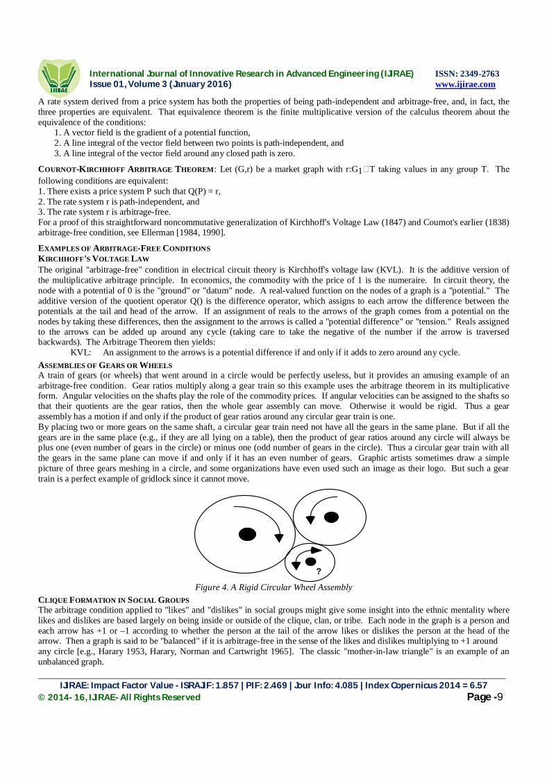
ASSEMBLIES OF GEARS OR WHEELS A train of gears (or wheels) that went around in a circle would be perfectly useless, but it provides an amusing example of an arbitrage-free condition. Gear ratios multiply along a gear train so this example uses the arbitrage theorem in its multiplicative form. Angular velocities on the shafts play the role of the commodity prices. If angular velocities can be assigned to the shafts so that their quotients are the gear ratios, then the whole gear assembly can move. Otherwise it would be rigid. Thus a gear assembly has a motion if and only if the product of gear ratios around any circular gear train is one. By placing two or more gears on the same shaft, a circular gear train need not have all the gears in the same plane. But if all the gears are in the same place (e.g., if they are all lying on a table), then the product of gear ratios around any circle will always be plus one (even number of gears in the circle) or minus one (odd number of gears in the circle). Thus a circular gear train with all the gears in the same plane can move if and only if it has an even number of gears. Graphic artists sometimes draw a simple picture of three gears meshing in a circle, and some organizations have even used such an image as their logo. But such a gear train is a perfect example of gridlock since it cannot move.

Figure 4. A Rigid Circular Wheel Assembly

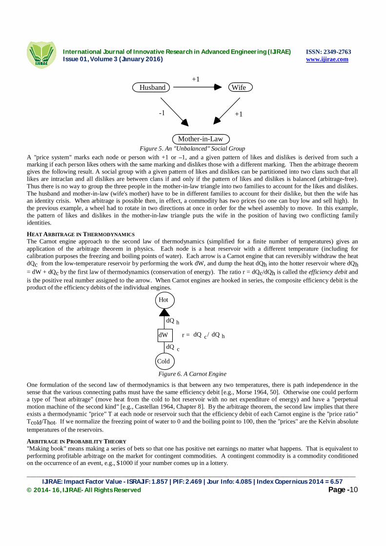
CLIQUE FORMATION IN SOCIAL GROUPS The arbitrage condition applied to "likes" and "dislikes" in social groups might give some insight into the ethnic mentality where likes and dislikes are based largely on being inside or outside of the clique, clan, or tribe. Each node in the graph is a person and each arrow has +1 or –1 according to whether the person at the tail of the arrow likes or dislikes the person at the head of the arrow. Then a graph is said to be "balanced" if it is arbitrage-free in the sense of the likes and dislikes multiplying to +1 around any circle [e.g., Harary 1953, Harary, Norman and Cartwright 1965]. The classic "mother-in-law triangle" is an example of an unbalanced graph.

?




Mother-in-Law

Husband Wife+1

+11

Figure 5. An "Unbalanced" Social Group

A "price system" marks each node or person with +1 or –1, and a given pattern of likes and dislikes is derived from such a marking if each person likes others with the same marking and dislikes those with a different marking. Then the arbitrage theorem gives the following result. A social group with a given pattern of likes and dislikes can be partitioned into two clans such that all likes are intraclan and all dislikes are between clans if and only if the pattern of likes and dislikes is balanced (arbitrage-free). Thus there is no way to group the three people in the mother-in-law triangle into two families to account for the likes and dislikes. The husband and mother-in-law (wife's mother) have to be in different families to account for their dislike, but then the wife has an identity crisis. When arbitrage is possible then, in effect, a commodity has two prices (so one can buy low and sell high). In the previous example, a wheel had to rotate in two directions at once in order for the wheel assembly to move. In this example, the pattern of likes and dislikes in the mother-in-law triangle puts the wife in the position of having two conflicting family identities.

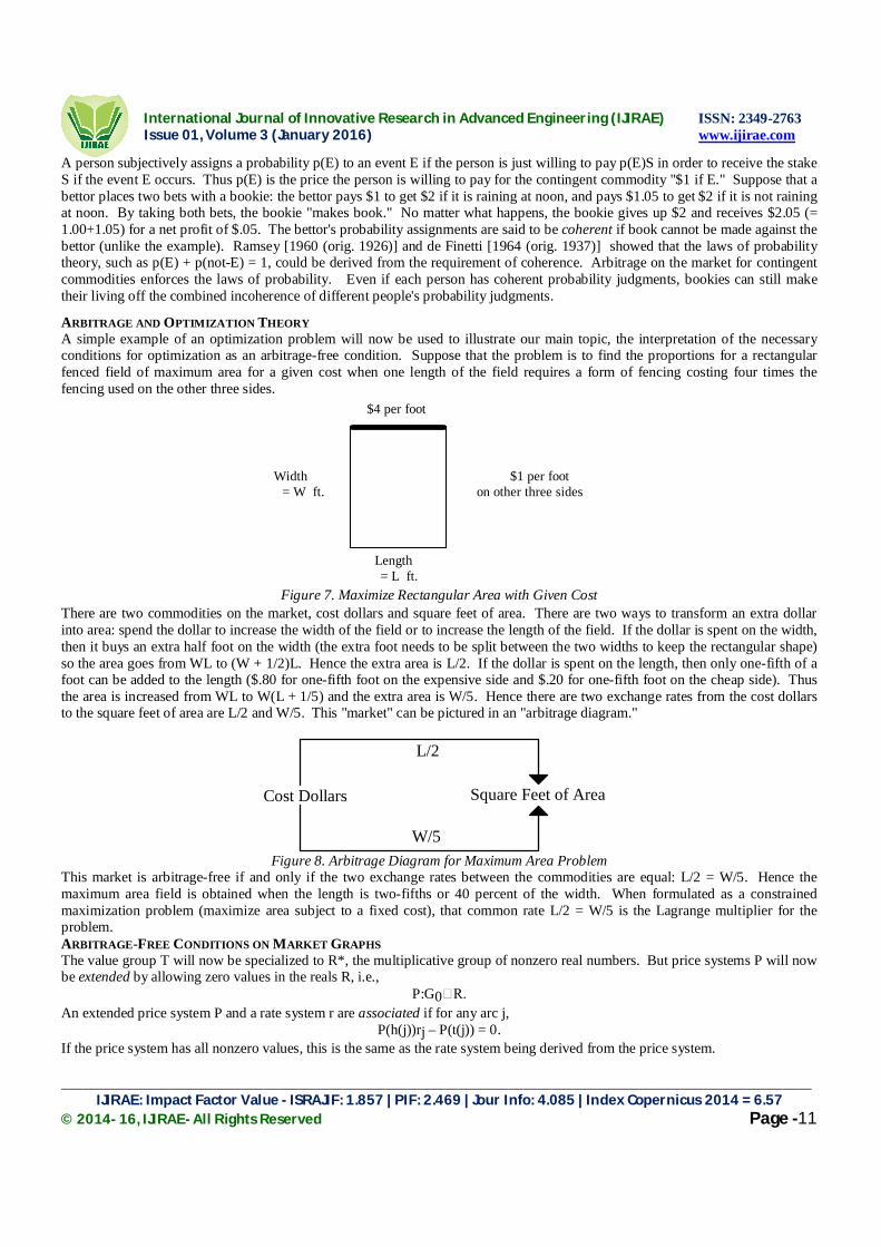
HEAT ARBITRAGE IN THERMODYNAMICS The Carnot engine approach to the second law of thermodynamics (simplified for a finite number of temperatures) gives an application of the arbitrage theorem in physics. Each node is a heat reservoir with a different temperature (including for calibration purposes the freezing and boiling points of water). Each arrow is a Carnot engine that can reversibly withdraw the heat dQc from the low-temperature reservoir by performing the work dW, and dump the heat dQh into the hotter reservoir where dQh = dW + dQc by the first law of thermodynamics (conservation of energy). The ratio r = dQc/dQh is called the efficiency debit and is the positive real number assigned to the arrow. When Carnot engines are hooked in series, the composite efficiency debit is the product of the efficiency debits of the individual engines.

Hot

Cold

dQ h

dQ c

dW dQ h dQ c r = /

Figure 6. A Carnot Engine

One formulation of the second law of thermodynamics is that between any two temperatures, there is path independence in the sense that the various connecting paths must have the same efficiency debit [e.g., Morse 1964, 50]. Otherwise one could perform a type of "heat arbitrage" (move heat from the cold to hot reservoir with no net expenditure of energy) and have a "perpetual motion machine of the second kind" [e.g., Castellan 1964, Chapter 8]. By the arbitrage theorem, the second law implies that there exists a thermodynamic "price" T at each node or reservoir such that the efficiency debit of each Carnot engine is the "price ratio" Tcold/Thot. If we normalize the freezing point of water to 0 and the boiling point to 100, then the "prices" are the Kelvin absolute temperatures of the reservoirs.

ARBITRAGE IN PROBABILITY THEORY "Making book" means making a series of bets so that one has positive net earnings no matter what happens. That is equivalent to performing profitable arbitrage on the market for contingent commodities. A contingent commodity is a commodity conditioned on the occurrence of an event, e.g., $1000 if your number comes up in a lottery.




A person subjectively assigns a probability p(E) to an event E if the person is just willing to pay p(E)S in order to receive the stake S if the event E occurs. Thus p(E) is the price the person is willing to pay for the contingent commodity "$1 if E." Suppose that a bettor places two bets with a bookie: the bettor pays $1 to get $2 if it is raining at noon, and pays $1.05 to get $2 if it is not raining at noon. By taking both bets, the bookie "makes book." No matter what happens, the bookie gives up $2 and receives $2.05 (= 1.00+1.05) for a net profit of $.05. The bettor's probability assignments are said to be coherent if book cannot be made against the bettor (unlike the example). Ramsey [1960 (orig. 1926)] and de Finetti [1964 (orig. 1937)] showed that the laws of probability theory, such as p(E) + p(not-E) = 1, could be derived from the requirement of coherence. Arbitrage on the market for contingent commodities enforces the laws of probability. Even if each person has coherent probability judgments, bookies can still make their living off the combined incoherence of different people's probability judgments.

ARBITRAGE AND OPTIMIZATION THEORY A simple example of an optimization problem will now be used to illustrate our main topic, the interpretation of the necessary conditions for optimization as an arbitrage-free condition. Suppose that the problem is to find the proportions for a rectangular fenced field of maximum area for a given cost when one length of the field requires a form of fencing costing four times the fencing used on the other three sides.

$4 per foot

$1 per foot on other three sides

Width = W ft.

Length = L ft.

Figure 7. Maximize Rectangular Area with Given Cost

There are two commodities on the market, cost dollars and square feet of area. There are two ways to transform an extra dollar into area: spend the dollar to increase the width of the field or to increase the length of the field. If the dollar is spent on the width, then it buys an extra half foot on the width (the extra foot needs to be split between the two widths to keep the rectangular shape) so the area goes from WL to (W + 1/2)L. Hence the extra area is L/2. If the dollar is spent on the length, then only one-fifth of a foot can be added to the length ($.80 for one-fifth foot on the expensive side and $.20 for one-fifth foot on the cheap side). Thus the area is increased from WL to W(L + 1/5) and the extra area is W/5. Hence there are two exchange rates from the cost dollars to the square feet of area are L/2 and W/5. This "market" can be pictured in an "arbitrage diagram."

Cost Dollars Square Feet of Area

L/2

W/5

Figure 8. Arbitrage Diagram for Maximum Area Problem This market is arbitrage-free if and only if the two exchange rates between the commodities are equal: L/2 = W/5. Hence the maximum area field is obtained when the length is two-fifths or 40 percent of the width. When formulated as a constrained maximization problem (maximize area subject to a fixed cost), that common rate L/2 = W/5 is the Lagrange multiplier for the problem. ARBITRAGE-FREE CONDITIONS ON MARKET GRAPHS The value group T will now be specialized to R*, the multiplicative group of nonzero real numbers. But price systems P will now be extended by allowing zero values in the reals R, i.e.,

P:G0 R. An extended price system P and a rate system r are associated if for any arc j,

P(h(j))rj – P(t(j)) = 0. If the price system has all nonzero values, this is the same as the rate system being derived from the price system.




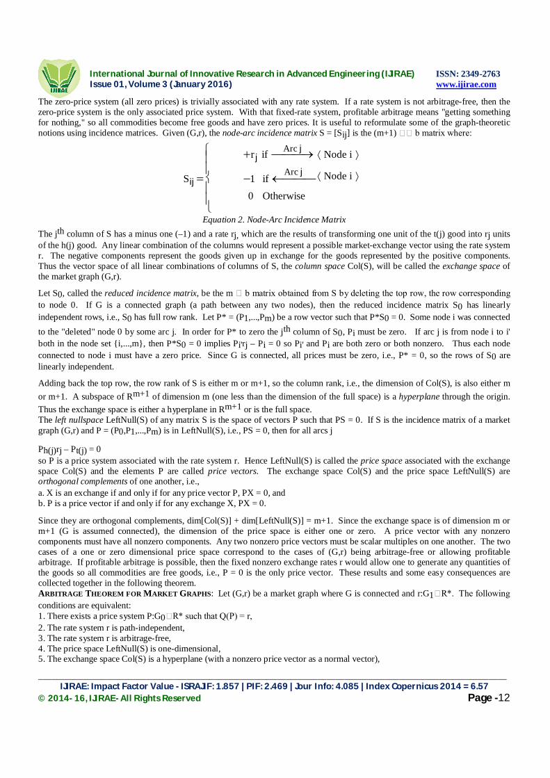
The zero-price system (all zero prices) is trivially associated with any rate system. If a rate system is not arbitrage-free, then the zero-price system is the only associated price system. With that fixed-rate system, profitable arbitrage means "getting something for nothing," so all commodities become free goods and have zero prices. It is useful to reformulate some of the graph-theoretic notions using incidence matrices. Given (G,r), the node-arc incidence matrix S = [Sij] is the (m+1) b matrix where:

S ij

r j if Arc j

1 ifArc j

0 Otherwise

Node i

Node i

Equation 2. Node-Arc Incidence Matrix

The jth column of S has a minus one (–1) and a rate rj, which are the results of transforming one unit of the t(j) good into rj units of the h(j) good. Any linear combination of the columns would represent a possible market-exchange vector using the rate system r. The negative components represent the goods given up in exchange for the goods represented by the positive components. Thus the vector space of all linear combinations of columns of S, the column space Col(S), will be called the exchange space of the market graph (G,r).

Let S0, called the reduced incidence matrix, be the m b matrix obtained from S by deleting the top row, the row corresponding to node 0. If G is a connected graph (a path between any two nodes), then the reduced incidence matrix S0 has linearly independent rows, i.e., S0 has full row rank. Let P* = (P1,...,Pm) be a row vector such that P*S0 = 0. Some node i was connected to the "deleted" node 0 by some arc j. In order for P* to zero the jth column of S0, Pi must be zero. If arc j is from node i to i' both in the node set {i,...,m}, then P*S0 = 0 implies Pi'rj – Pi = 0 so Pi' and Pi are both zero or both nonzero. Thus each node connected to node i must have a zero price. Since G is connected, all prices must be zero, i.e., P* = 0, so the rows of S0 are linearly independent.

Adding back the top row, the row rank of S is either m or m+1, so the column rank, i.e., the dimension of Col(S), is also either m or m+1. A subspace of Rm+1 of dimension m (one less than the dimension of the full space) is a hyperplane through the origin. Thus the exchange space is either a hyperplane in Rm+1 or is the full space. The left nullspace LeftNull(S) of any matrix S is the space of vectors P such that PS = 0. If S is the incidence matrix of a market graph (G,r) and P = (P0,P1,...,Pm) is in LeftNull(S), i.e., PS = 0, then for all arcs j Ph(j)rj – Pt(j) = 0 so P is a price system associated with the rate system r. Hence LeftNull(S) is called the price space associated with the exchange space Col(S) and the elements P are called price vectors. The exchange space Col(S) and the price space LeftNull(S) are orthogonal complements of one another, i.e.,

a. X is an exchange if and only if for any price vector P, PX = 0, and b. P is a price vector if and only if for any exchange X, PX = 0. Since they are orthogonal complements, dim[Col(S)] + dim[LeftNull(S)] = m+1. Since the exchange space is of dimension m or m+1 (G is assumed connected), the dimension of the price space is either one or zero. A price vector with any nonzero components must have all nonzero components. Any two nonzero price vectors must be scalar multiples on one another. The two cases of a one or zero dimensional price space correspond to the cases of (G,r) being arbitrage-free or allowing profitable arbitrage. If profitable arbitrage is possible, then the fixed nonzero exchange rates r would allow one to generate any quantities of the goods so all commodities are free goods, i.e., P = 0 is the only price vector. These results and some easy consequences are collected together in the following theorem. ARBITRAGE THEOREM FOR MARKET GRAPHS: Let (G,r) be a market graph where G is connected and r:G1 R*. The following conditions are equivalent: 1. There exists a price system P:G0 R* such that Q(P) = r, 2. The rate system r is path-independent, 3. The rate system r is arbitrage-free, 4. The price space LeftNull(S) is one-dimensional, 5. The exchange space Col(S) is a hyperplane (with a nonzero price vector as a normal vector),




6. The top row of S, s0, can be expressed as a linear combination of the bottom m rows S0 of S, i.e., there exist µ = (µ1,...,µm) such that s0 + µS0 = 0, and

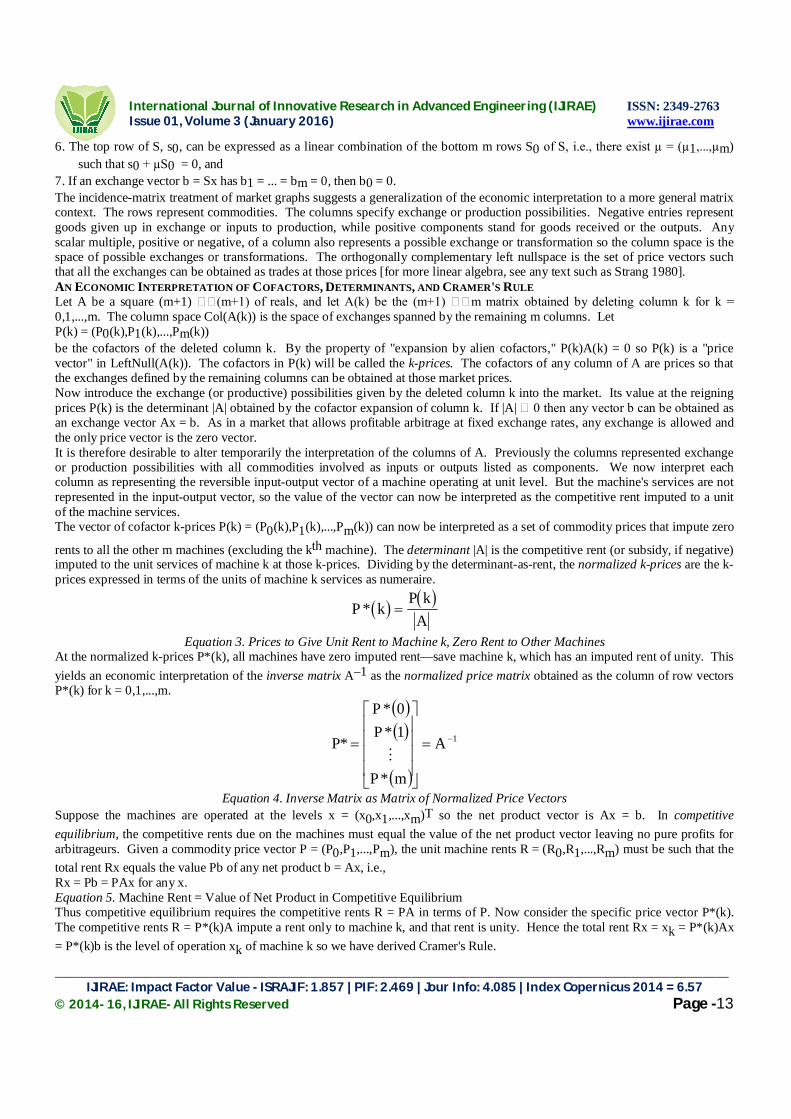
7. If an exchange vector b = Sx has b1 = ... = bm = 0, then b0 = 0. The incidence-matrix treatment of market graphs suggests a generalization of the economic interpretation to a more general matrix context. The rows represent commodities. The columns specify exchange or production possibilities. Negative entries represent goods given up in exchange or inputs to production, while positive components stand for goods received or the outputs. Any scalar multiple, positive or negative, of a column also represents a possible exchange or transformation so the column space is the space of possible exchanges or transformations. The orthogonally complementary left nullspace is the set of price vectors such that all the exchanges can be obtained as trades at those prices [for more linear algebra, see any text such as Strang 1980]. AN ECONOMIC INTERPRETATION OF COFACTORS, DETERMINANTS, AND CRAMER'S RULE Let A be a square (m+1) (m+1) of reals, and let A(k) be the (m+1) m matrix obtained by deleting column k for k = 0,1,...,m. The column space Col(A(k)) is the space of exchanges spanned by the remaining m columns. Let P(k) = (P0(k),P1(k),...,Pm(k)) be the cofactors of the deleted column k. By the property of "expansion by alien cofactors," P(k)A(k) = 0 so P(k) is a "price vector" in LeftNull(A(k)). The cofactors in P(k) will be called the k-prices. The cofactors of any column of A are prices so that the exchanges defined by the remaining columns can be obtained at those market prices. Now introduce the exchange (or productive) possibilities given by the deleted column k into the market. Its value at the reigning prices P(k) is the determinant |A| obtained by the cofactor expansion of column k. If |A| 0 then any vector b can be obtained as an exchange vector Ax = b. As in a market that allows profitable arbitrage at fixed exchange rates, any exchange is allowed and the only price vector is the zero vector. It is therefore desirable to alter temporarily the interpretation of the columns of A. Previously the columns represented exchange or production possibilities with all commodities involved as inputs or outputs listed as components. We now interpret each column as representing the reversible input-output vector of a machine operating at unit level. But the machine's services are not represented in the input-output vector, so the value of the vector can now be interpreted as the competitive rent imputed to a unit of the machine services. The vector of cofactor k-prices P(k) = (P0(k),P1(k),...,Pm(k)) can now be interpreted as a set of commodity prices that impute zero

rents to all the other m machines (excluding the kth machine). The determinant |A| is the competitive rent (or subsidy, if negative) imputed to the unit services of machine k at those k-prices. Dividing by the determinant-as-rent, the normalized k-prices are the k-prices expressed in terms of the units of machine k services as numeraire.

P kP kA

*

Equation 3. Prices to Give Unit Rent to Machine k, Zero Rent to Other Machines At the normalized k-prices P*(k), all machines have zero imputed rent—save machine k, which has an imputed rent of unity. This yields an economic interpretation of the inverse matrix A–1 as the normalized price matrix obtained as the column of row vectors P*(k) for k = 0,1,...,m.

1A

m*P

1*P0*P

*P

Equation 4. Inverse Matrix as Matrix of Normalized Price Vectors Suppose the machines are operated at the levels x = (x0,x1,...,xm)T so the net product vector is Ax = b. In competitive equilibrium, the competitive rents due on the machines must equal the value of the net product vector leaving no pure profits for arbitrageurs. Given a commodity price vector P = (P0,P1,...,Pm), the unit machine rents R = (R0,R1,...,Rm) must be such that the total rent Rx equals the value Pb of any net product b = Ax, i.e., Rx = Pb = PAx for any x. Equation 5. Machine Rent = Value of Net Product in Competitive Equilibrium Thus competitive equilibrium requires the competitive rents R = PA in terms of P. Now consider the specific price vector P*(k). The competitive rents R = P*(k)A impute a rent only to machine k, and that rent is unity. Hence the total rent Rx = xk = P*(k)Ax = P*(k)b is the level of operation xk of machine k so we have derived Cramer's Rule.




Competitive Machine Rent = xk = P*(k)b = Value of Net Product. Equation 6. Cramer's Rule as a Competitive Equilibrium Condition

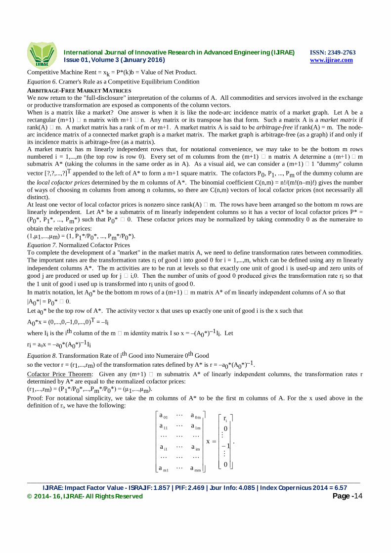
ARBITRAGE-FREE MARKET MATRICES We now return to the "full-disclosure" interpretation of the columns of A. All commodities and services involved in the exchange or productive transformation are exposed as components of the column vectors. When is a matrix like a market? One answer is when it is like the node-arc incidence matrix of a market graph. Let A be a rectangular (m+1) n matrix with m+1 n. Any matrix or its transpose has that form. Such a matrix A is a market matrix if rank(A) m. A market matrix has a rank of m or m+1. A market matrix A is said to be arbitrage-free if rank(A) = m. The node-arc incidence matrix of a connected market graph is a market matrix. The market graph is arbitrage-free (as a graph) if and only if its incidence matrix is arbitrage-free (as a matrix). A market matrix has m linearly independent rows that, for notational convenience, we may take to be the bottom m rows numbered i = 1,...,m (the top row is row 0). Every set of m columns from the (m+1) n matrix A determine a (m+1) m submatrix A* (taking the columns in the same order as in A). As a visual aid, we can consider a (m+1) 1 "dummy" column vector [?,?,...,?]T appended to the left of A* to form a m+1 square matrix. The cofactors P0, P1, ..., Pm of the dummy column are the local cofactor prices determined by the m columns of A*. The binomial coefficient C(n,m) = n!/(m!(n–m)!) gives the number of ways of choosing m columns from among n columns, so there are C(n,m) vectors of local cofactor prices (not necessarily all distinct). At least one vector of local cofactor prices is nonzero since rank(A) m. The rows have been arranged so the bottom m rows are linearly independent. Let A* be a submatrix of m linearly independent columns so it has a vector of local cofactor prices P* = (P0*, P1*, ..., Pm*) such that P0* 0. These cofactor prices may be normalized by taking commodity 0 as the numeraire to obtain the relative prices: (1,µ1,...,µm) = (1, P1*/P0*, ..., Pm*/P0*). Equation 7. Normalized Cofactor Prices To complete the development of a "market" in the market matrix A, we need to define transformation rates between commodities. The important rates are the transformation rates ri of good i into good 0 for i = 1,...,m, which can be defined using any m linearly independent columns A*. The m activities are to be run at levels so that exactly one unit of good i is used-up and zero units of good j are produced or used up for j i,0. Then the number of units of good 0 produced gives the transformation rate ri so that the 1 unit of good i used up is transformed into ri units of good 0. In matrix notation, let A0* be the bottom m rows of a (m+1) m matrix A* of m linearly independent columns of A so that |A0*| = P0* 0. Let a0* be the top row of A*. The activity vector x that uses up exactly one unit of good i is the x such that

A0*x = (0,...,0,–1,0,...,0)T = –Ii

where Ii is the ith column of the m m identity matrix I so x = –(A0*)–1Ii. Let

ri = a0x = –a0*(A0*)–1Ii

Equation 8. Transformation Rate of ith Good into Numeraire 0th Good so the vector r = (r1,...,rm) of the transformation rates defined by A* is r = –a0*(A0*)–1. Cofactor Price Theorem: Given any (m+1) m submatrix A* of linearly independent columns, the transformation rates r determined by A* are equal to the normalized cofactor prices: (r1,...,rm) = (P1*/P0*,...,Pm*/P0*) = (µ1,...,µm). Proof: For notational simplicity, we take the m columns of A* to be the first m columns of A. For the x used above in the definition of ri, we have the following:

.

0

1

0r

x

aa

aa

aaaa

i

mm1m

im1i

m111

m001




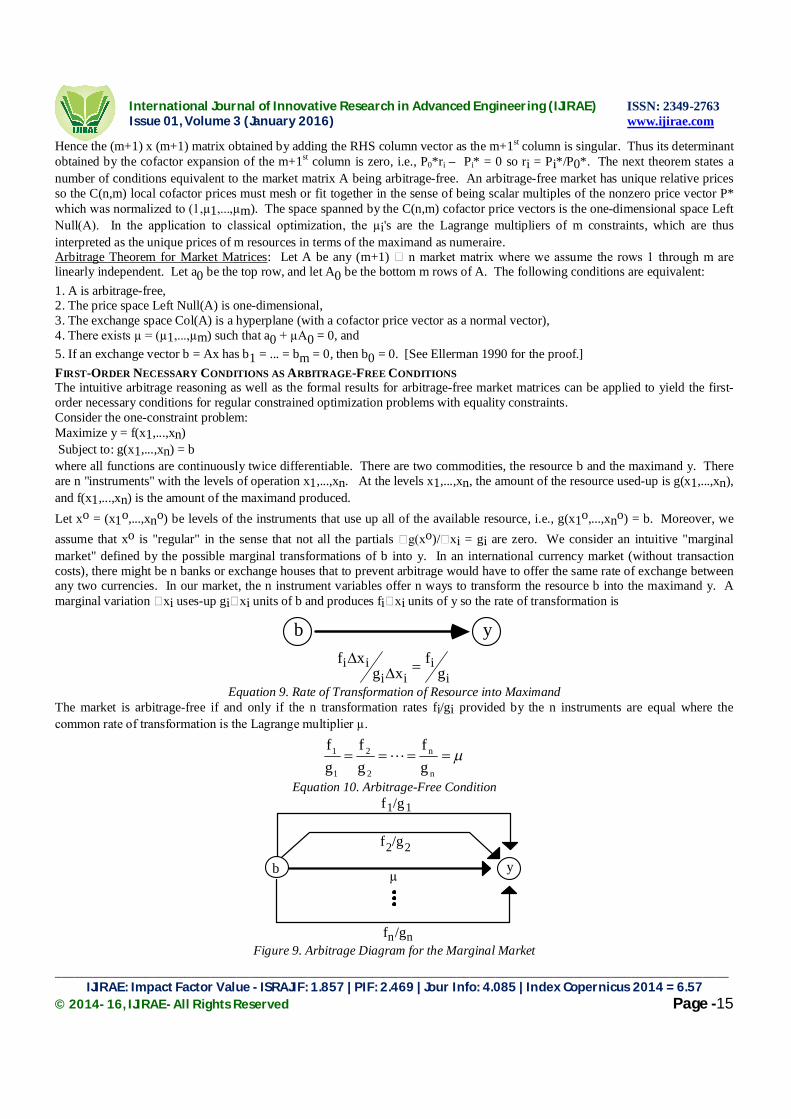
Hence the (m+1) x (m+1) matrix obtained by adding the RHS column vector as the m+1st column is singular. Thus its determinant obtained by the cofactor expansion of the m+1st column is zero, i.e., P0*ri – Pi* = 0 so ri = Pi*/P0*. The next theorem states a number of conditions equivalent to the market matrix A being arbitrage-free. An arbitrage-free market has unique relative prices so the C(n,m) local cofactor prices must mesh or fit together in the sense of being scalar multiples of the nonzero price vector P* which was normalized to (1,µ1,...,µm). The space spanned by the C(n,m) cofactor price vectors is the one-dimensional space Left Null(A). In the application to classical optimization, the µi's are the Lagrange multipliers of m constraints, which are thus interpreted as the unique prices of m resources in terms of the maximand as numeraire. Arbitrage Theorem for Market Matrices: Let A be any (m+1) n market matrix where we assume the rows 1 through m are linearly independent. Let a0 be the top row, and let A0 be the bottom m rows of A. The following conditions are equivalent: 1. A is arbitrage-free, 2. The price space Left Null(A) is one-dimensional, 3. The exchange space Col(A) is a hyperplane (with a cofactor price vector as a normal vector), 4. There exists µ = (µ1,...,µm) such that a0 + µA0 = 0, and 5. If an exchange vector b = Ax has b1 = ... = bm = 0, then b0 = 0. [See Ellerman 1990 for the proof.] FIRST-ORDER NECESSARY CONDITIONS AS ARBITRAGE-FREE CONDITIONS The intuitive arbitrage reasoning as well as the formal results for arbitrage-free market matrices can be applied to yield the first-order necessary conditions for regular constrained optimization problems with equality constraints. Consider the one-constraint problem: Maximize y = f(x1,...,xn) Subject to: g(x1,...,xn) = b where all functions are continuously twice differentiable. There are two commodities, the resource b and the maximand y. There are n "instruments" with the levels of operation x1,...,xn. At the levels x1,...,xn, the amount of the resource used-up is g(x1,...,xn), and f(x1,...,xn) is the amount of the maximand produced. Let xo = (x1o,...,xno) be levels of the instruments that use up all of the available resource, i.e., g(x1o,...,xno) = b. Moreover, we assume that xo is "regular" in the sense that not all the partials g(xo)/ xi = gi are zero. We consider an intuitive "marginal market" defined by the possible marginal transformations of b into y. In an international currency market (without transaction costs), there might be n banks or exchange houses that to prevent arbitrage would have to offer the same rate of exchange between any two currencies. In our market, the n instrument variables offer n ways to transform the resource b into the maximand y. A marginal variation xi uses-up gi xi units of b and produces fi xi units of y so the rate of transformation is

b y

f xg x

fg

i ii i

ii

Equation 9. Rate of Transformation of Resource into Maximand The market is arbitrage-free if and only if the n transformation rates fi/gi provided by the n instruments are equal where the common rate of transformation is the Lagrange multiplier µ.

n

n

2

2

1

1

gf

gf

gf

Equation 10. Arbitrage-Free Condition

y b µ

f /g1 1

n nf /g

2 2f /g

Figure 9. Arbitrage Diagram for the Marginal Market




Thus the first-order necessary conditions for xo to be a constrained maximum are equivalent to the intuitive market being arbitrage-free. To use the machinery of market matrices, let

n21

n21

gggfff

A

where –gi is used instead of +gi since g(x1,...,xn) represents the amount of the resource used up. Consider any column of this market matrix coupled with the dummy column to form a square matrix:

??

.fgi

i

The cofactors of the dummy column are the local prices Py = –gi and Pb = –fi, so (assuming gi 0) the cofactor price ratio is the transformation rate defined by the marginal variations in the instrument xi.

b y

P P f gb y i i

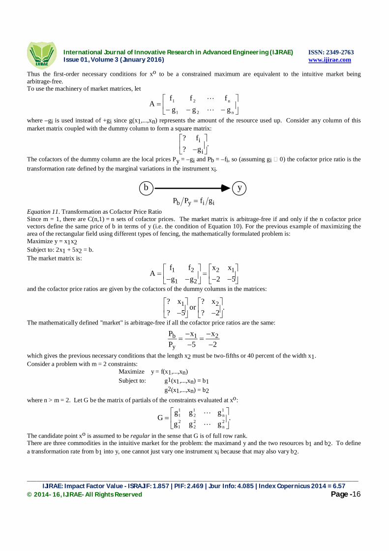
Equation 11. Transformation as Cofactor Price Ratio Since m = 1, there are C(n,1) = n sets of cofactor prices. The market matrix is arbitrage-free if and only if the n cofactor price vectors define the same price of b in terms of y (i.e. the condition of Equation 10). For the previous example of maximizing the area of the rectangular field using different types of fencing, the mathematically formulated problem is: Maximize y = x1x2 Subject to: 2x1 + 5x2 = b. The market matrix is:

Af fg g

x x

1 2

1 2

2 12 5

and the cofactor price ratios are given by the cofactors of the dummy columns in the matrices:

??

??

.x

orx1 2

5 2

The mathematically defined "market" is arbitrage-free if all the cofactor price ratios are the same:

PP

x xb

y

1 25 2

which gives the previous necessary conditions that the length x2 must be two-fifths or 40 percent of the width x1. Consider a problem with m = 2 constraints:

Maximize y = f(x1,...,xn) Subject to: g1(x1,...,xn) = b1 g2(x1,...,xn) = b2

where n > m = 2. Let G be the matrix of partials of the constraints evaluated at xo:

.gggggg

G 2n

22

21

1n

12

11

The candidate point xo is assumed to be regular in the sense that G is of full row rank. There are three commodities in the intuitive market for the problem: the maximand y and the two resources b1 and b2. To define a transformation rate from b1 into y, one cannot just vary one instrument xi because that may also vary b2.




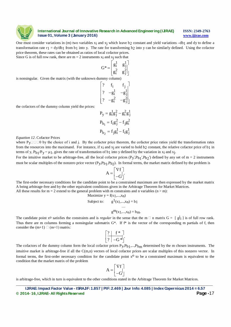
One must consider variations in (m) two variables xi and xj which leave b2 constant and yield variations –db1 and dy to define a transformation rate r1 = dy/db1 from b1 into y. The rate for transforming b2 into y can be similarly defined. Using the cofactor price theorem, these rates can be obtained as ratios of local cofactor prices. Since G is of full row rank, there are m = 2 instruments xi and xj such that

Gg gg g

i j

i j*

1 1

2 2

is nonsingular. Given the matrix (with the unknown dummy column)

?

?

?

f f

g g

g g

i j

i j

i j

1 1

2 2

the cofactors of the dummy column yield the prices:

P g g g g

P f g f g

P f g f g

y i j i j

b i j j i

b j i i j

1 2 2 1

2 2

1 11

2 Equation 12. Cofactor Prices where Py 0 by the choice of i and j. By the cofactor price theorem, the cofactor price ratios yield the transformation rates from the resources into the maximand. For instance, if xi and xj are varied to hold b2 constant, the relative cofactor price of b1 in terms of y, Pb1/Py = µ1, gives the rate of transformation of b1 into y defined by the variation in xi and xj. For the intuitive market to be arbitrage-free, all the local cofactor prices (Py',Pb1',Pb2') defined by any set of m = 2 instruments must be scalar multiples of the nonzero price vector (Py,Pb1,Pb2). In formal terms, the market matrix defined by the problem is

AfG

.

The first-order necessary conditions for the candidate point to be a constrained maximum are then expressed by the market matrix A being arbitrage-free and by the other equivalent conditions given in the Arbitrage Theorem for Market Matrices. All these results for m = 2 extend to the general problem with m constraints and n variables (n > m): Maximize y = f(x1,...,xn) Subject to: g1(x1,...,xn) = b1 … gm(x1,...,xn) = bm. The candidate point xo satisfies the constraints and is regular in the sense that the m n matrix G = [ gji ] is of full row rank. Thus there are m columns forming a nonsingular submatrix G*. If f* is the vector of the corresponding m partials of f, then consider the (m+1) (m+1) matrix:

? *? *

.fG

The cofactors of the dummy column form the local cofactor prices Py,Pb1,...,Pbm determined by the m chosen instruments. The intuitive market is arbitrage-free if all the C(m,n) vectors of local cofactor prices are scalar multiples of this nonzero vector. In formal terms, the first-order necessary condition for the candidate point xo to be a constrained maximum is equivalent to the condition that the market matrix of the problem

AfG

is arbitrage-free, which in turn is equivalent to the other conditions stated in the Arbitrage Theorem for Market Matrices.




These results point to a research program that could be developed in several directions. One direction is to show how the second-order sufficient conditions for optimality could be interpreted economically as the conditions for arbitrage to eliminate its own possibility. Preliminary results in this direction are outlined in the appendix. Another direction of development is to extend the arbitrage interpretation to other areas of optimization theory such as optimization with inequality constraints and optimal control theory.

REFERENCES [1]. Berge, Claude, and A. Ghouila-Houri, 1965. Programming, Games and Transportation Networks. John New York: Wiley

and Sons. [2]. Castellan, Gilbert. 1964. Physical Chemistry. New York: Addison-Wesley. [3]. Cournot, Augustin. 1897 (orig. 1838). Mathematical Principles of the Theory of Wealth Trans. Nathaniel Bloom. New

York: Macmillan. [4]. de Finetti, Bruno. 1964 (orig. 1937). "Foresight: Its Logical Laws, Its Subjective Sources. In Studies in Subjective

Probability ed. H. Kyburg and H. Smokler, 93-158. New York: John Wiley. [5]. Ellerman, David P. 1984. "Arbitrage Theory: A Mathematical Introduction." SIAM Review. 26: 241-61. [6]. Ellerman, David P. 1990. "An Arbitrage Interpretation of Classical Optimization." Metroeconomica 41, no. 3: 259-76. [7]. Gross, Jonathan. 1974. "Voltage graphs." Discrete Math 9: 239-46. [8]. Harary, Frank. 1953. "On the notion of balance of a signed graph." Michigan Math. J. 2: 143-46. [9]. Harary, Frank, R. Z. Norman, and D. Cartwright. 1965. Structural Models. New York: John Wiley. [10]. Harary, Frank, B. Lindstrom, and H. Zetterstrom. 1982. "On balance in group graphs." Networks 12: 317-21. [11]. Kirchhoff, G. 1847. "Über die Auflosung der Gleichungen, auf welche man dei der Untersuchung der linearen Verteilung

galvanischer Strome gefuhrt wird." Annalen der Physik und Chemie 72: 497-508. [12]. Modigliani, Franco, and Merton H. Miller. 1958. "The Cost of Capital, Corporation Finance, and the Theory of

Investment." American Economic Review 48: 261-97. [13]. Morse, Philip. 1964. Thermal Physics. New York: W. A. Benjamin. [14]. Ramsey, Frank Plumpton. 1960 (orig. 1926). Truth and probability. In The Foundations of Mathematics, ed. R. B.

Braithwaite. Paterson N.J.: Littlefield, Adams & Company. [15]. Ross, Stephen A. 1976. "The Arbitrage Theory of Capital Asset Pricing." J. Econ. Theory 13: 341-60. [16]. Ross, Stephen A. 1976. "Return, Risk and Arbitrage." In Risk and Return in Finance, ed. Irwin Friend and James L.

Bicksler. Cambridge, Mass.: Ballinger. [17]. Strang, Gilbert. 1980. Linear Algebra and its Applications. Second edition. New York: Academic Press. [18]. Varian, Hal R. 1987. "The Arbitrage Principle in Financial Economics." The Journal of Economic Perspectives 1, no. 2: 55-

72.