Eyvindson iufro

15.04.2023 1www.helsinki.fi/yliopisto

Assessment of Scenario Generation Approaches for Forest Management

Planning through Stochastic Programming

Kyle Eyvindson and Annika Kangas

Kyle Eyvindson

www.helsinki.fi/yliopisto 15.04.2023 2

• Aim is to:

• Integrate uncertainty into the development of forest plans

‒ Inventory, growth models, climate change...

• Produce a robust solution which meets the demands of the decision maker(s), and can accommodate preferences towards risks

• One method is through stochastic programming

‒ issues of tractability can become an issue

Kyle Eyvindson

Introduction


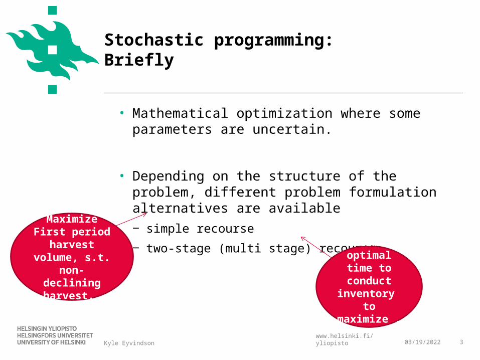
• Mathematical optimization where some parameters are uncertain.

• Depending on the structure of the problem, different problem formulation alternatives are available

‒ simple recourse

‒ two-stage (multi stage) recourse

Kyle Eyvindson

Stochastic programming:Briefly

Determine optimal time to conduct

inventory to maximize ...

Maximize First period harvest

volume, s.t. non-declining

harvest.


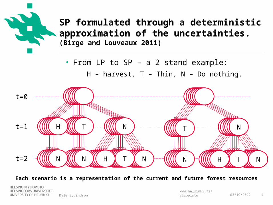
• From LP to SP – a 2 stand example:

H – harvest, T – Thin, N – Do nothing.

Kyle Eyvindson

SP formulated through a deterministic approximation of the uncertainties. (Birge and Louveaux 2011)

t=0

t=1

t=2

H NT

N N H T N

NT

N H T N

H NT

N N H T N

NT

N H T N

H NT

N N H T N

NT

N H T N

H NT

N N H T N

NT

N H T N

H NT

N N H T N

NT

N H T N

H NT

N N H T N

NT

N H T N

Each scenario is a representation of the current and future forest resources

www.helsinki.fi/yliopisto

• This requires the known (or estimated) distribution of the error.

• A number of scenarios are developed to approximate the distribution. (King and Wallace 2012)

‒ A need for balance: too many scenarios – tractability issues

too few scenarios – problem representation issues

Kyle Eyvindson

Incorporating uncertainty into the planning problem


• It depends on:

• the formulation used,

• the risk preferences involved,

• the amount of uncertainty under consideration

• the accuracy required

• One way to determine an appropriate number of scenarios is through the sample average approximation (SAA, Kleywegt et al. 2001.)

Kyle Eyvindson

How many scenarios is enough?


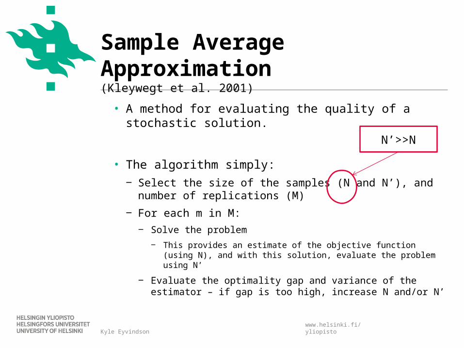
• A method for evaluating the quality of a stochastic solution.

• The algorithm simply:

‒ Select the size of the samples (N and N’), and number of replications (M)

‒ For each m in M:

‒ Solve the problem

‒ This provides an estimate of the objective function (using N), and with this solution, evaluate the problem using N’

‒ Evaluate the optimality gap and variance of the estimator – if gap is too high, increase N and/or N’

Kyle Eyvindson

Sample Average Approximation(Kleywegt et al. 2001)

N’>>N


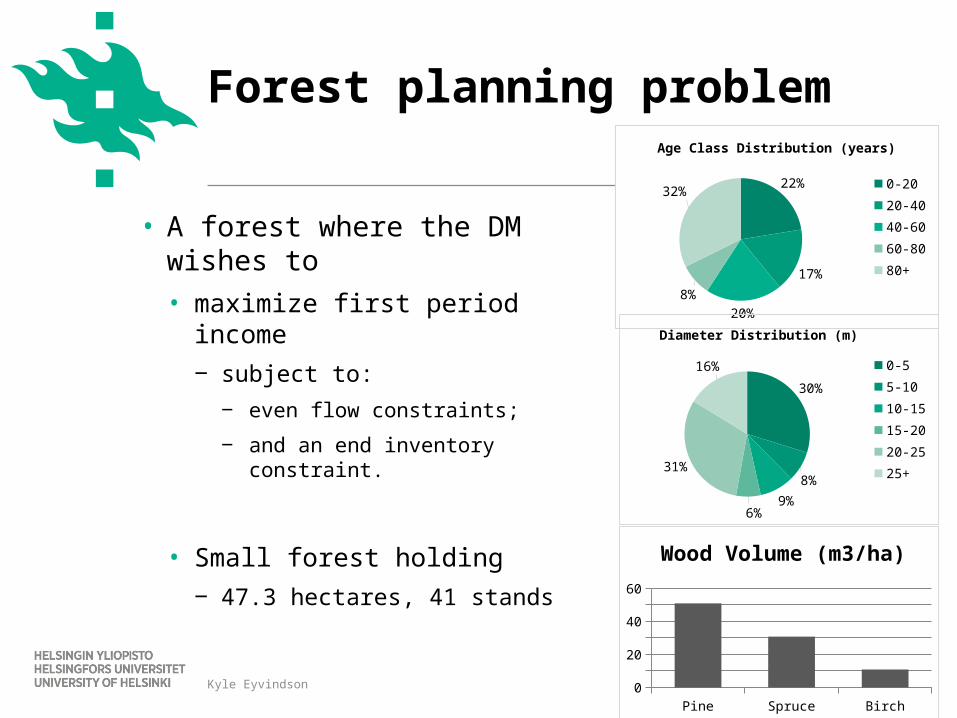
• A forest where the DM wishes to

• maximize first period income

‒ subject to:

‒ even flow constraints;

‒ and an end inventory constraint.

• Small forest holding

‒ 47.3 hectares, 41 stands

Forest planning problem

Kyle Eyvindson

22%

17%

20%

8%

32%

Age Class Distribution (years)

0-20

20-40

40-60

60-80

80+

30%

8%

9%6%

31%

16%

Diameter Distribution (m)

0-5

5-10

10-15

15-20

20-25

25+

Pine Spruce Birch0

102030405060

Wood Volume (m3/ha)

www.helsinki.fi/yliopistoKyle Eyvindson

• Two cases are studied:

• The case where only the inventory uncertainty is included

• and where both inventory uncertainty and growth model errors are included.

• A few assumptions were made:

1. A recent inventory was conducted

2. The inventory method was assumed to have an error which was normally distributed, mean zero and a standard deviation of 20% of the mean height and basal area.

Scenario generation approach:


• For each inventory error, a set of 50 growth model error scenarios were simulated.

• The growth model errors were generated using a one period autoregressive process [AR(1)], using the same models as Pietilä et al. 2010.

• Forest simulation was done using SIMO (Rasinmäki et al. 2009)

• Created a set of 528 schedules for the 41 stands (~13 schedules per stand) for each scenario.

Kyle Eyvindson

Scenario generation approach: (2)


• A standard even flow problem.

• Maximize: 1st period incomes

‒ subject to even flow and end inventory constraints Using both hard and soft constraints

• For application in a stochastic setting this problem needs slight modification:

• Maximize: Expected 1st period incomes – sum of scenario based negative deviations

‒ subject to soft even flow an end inventory constraints Having strict constraints is not the real intention behind the even-flow

problem.

The soft constraints allow for a ‘more or less’ even flow in all scenarios.

Sample problem:


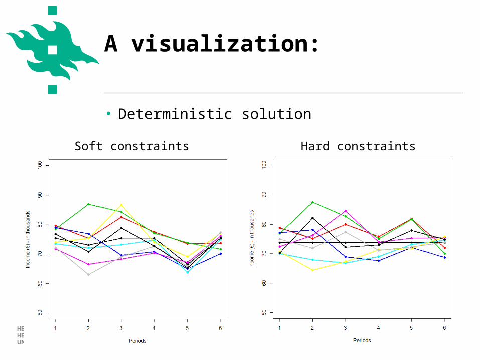
• Deterministic solution

Kyle Eyvindson

A visualization:

Soft constraints Hard constraints


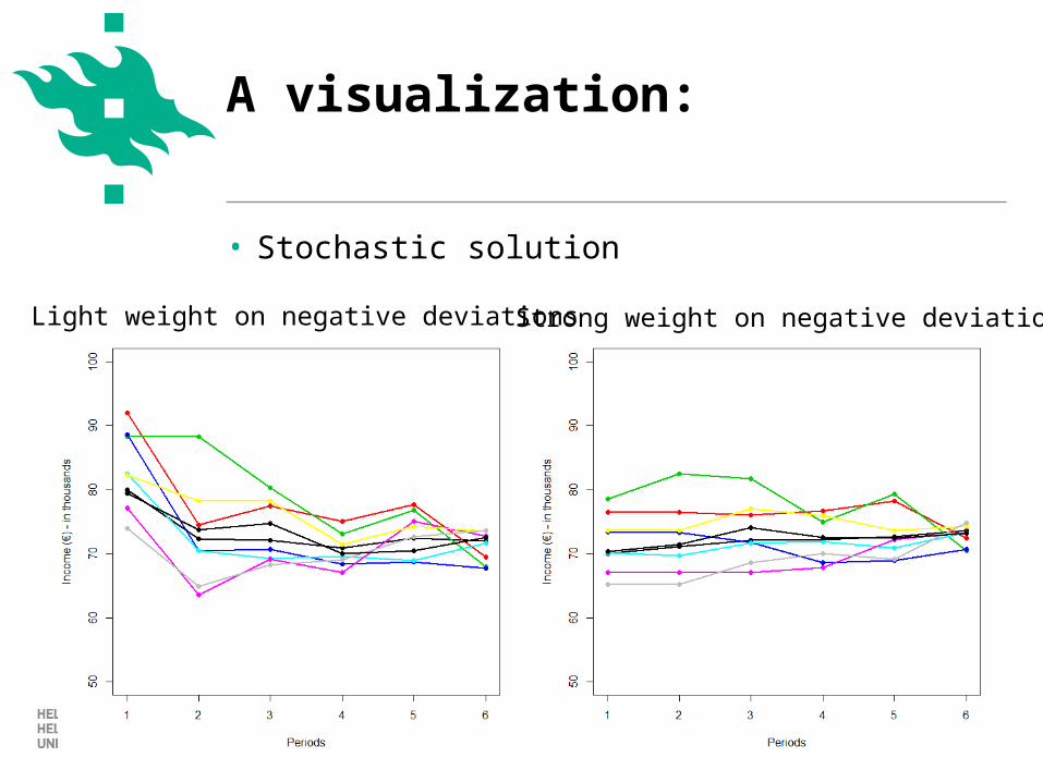
• Stochastic solution

Kyle Eyvindson

A visualization:

Light weight on negative deviations Strong weight on negative deviations


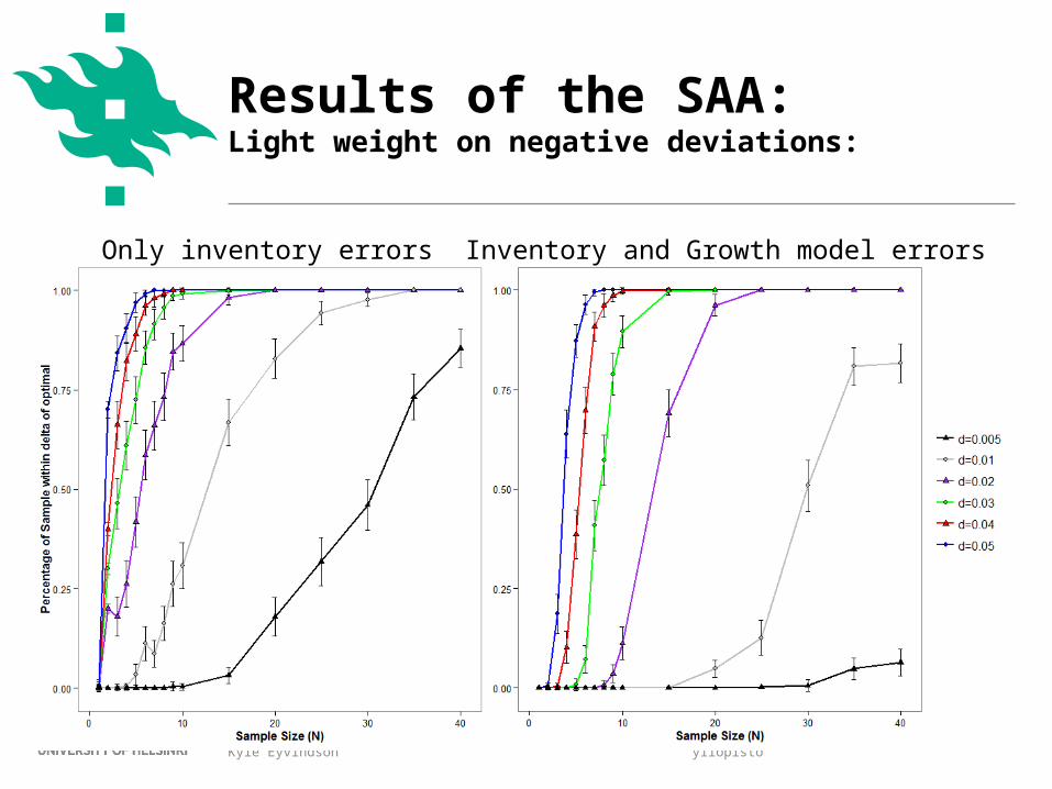
Results of the SAA:Light weight on negative deviations:

Only inventory errors Inventory and Growth model errors


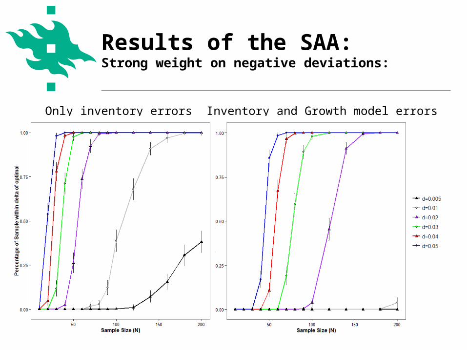
Results of the SAA:Strong weight on negative deviations:

Only inventory errors Inventory and Growth model errors


• The size of the stochastic problem need not be enormous.

• The size of the problem depends upon:

‒ the amount of uncertainty under consideration,

‒ the importance the uncertainty has in the problem formulation, and

‒ the acceptability of selecting a ‘sub-optimal’ solution.

• A stochastic program with a sizable optimality gap still outperform the deterministic equivalent.

Kyle Eyvindson

Conclusions:


• Birge, J.R., and Louveaux, F. 2011. Introduction to stochastic programming. Second edition. Springer, New York. 499 p.

• Kangas, A., Hartikainen, M., and Miettinen, K. 2013. Simultaneous optimization of harvest schedule and measurement strategy. Scand. J. Forest Res.(ahead-of-print), 1-10. doi: 10.1080/02827581.2013.823237.

• Kleywegt, Shapiro, Homem-de-Mello. 2001. The sample average approximation for stochastic discrete optimization. SIAM. J. OPTIM. (12:2) 479-502.

• King, A.J., and Wallace, S.W. 2012 Modeling with Stochastic Programming, Springer, New York

• Krzemienowski, A. & Ogryczak W. 2005. On extending the LP computable risk measures to account downside risk. Computational Optimization and Applications 32:133-160.

• Rasinmäki, J., Mäkinen, A., and Kalliovirta, J. 2009. SIMO: an adaptable simulation framework for multiscale forest resource data. Comput. Electron. Agric. 66(1): 76–84. doi: 10.1016/j.compag.2008.12.007.

• Pietilä, Kangas, Mäkinen, Mehtätalo. 2010. Influence of Growth Prediction Errors on the Expeced Loses from Forest Decisions. Silva Fennica 44(5). 829:843.

Kyle Eyvindson

References:

Environment

Eyvindson iufro