Embed Size (px)
DESCRIPTION
Resolução do livro de Eletrodinâmica
Citation preview
Contents Preface 2 1 The Wave Function 3 2 Time-Independent Schrödinger Equation 14 3 Formalism 62 4 Quantum Mechanics in Three Dimensions 87 5 Identical Particles 132 6 Time-Independent Perturbation Theory 154 7 The Variational Principle 196 8 The WKB Approximation 219 9 Time-Dependent Perturbation Theory 236 10 The Adiabatic Approximation 254 11 Scattering 268 12 Afterword 282 Appendix Linear Algebra 283 2nd Edition – 1st Edition Problem Correlation Grid 299

2
Preface
These are my own solutions to the problems in Introduction to Quantum Mechanics, 2nd ed. I have made everyeffort to insure that they are clear and correct, but errors are bound to occur, and for this I apologize in advance.I would like to thank the many people who pointed out mistakes in the solution manual for the first edition,and encourage anyone who finds defects in this one to alert me ([email protected]). I’ll maintain a list of errataon my web page (http://academic.reed.edu/physics/faculty/griffiths.html), and incorporate corrections in themanual itself from time to time. I also thank my students at Reed and at Smith for many useful suggestions,and above all Neelaksh Sadhoo, who did most of the typesetting.
At the end of the manual there is a grid that correlates the problem numbers in the second edition withthose in the first edition.
David Griffiths
c©2005 Pearson Education, Inc., Upper Saddle River, NJ. All rights reserved. This material is protected under all copyright laws as theycurrently exist. No portion of this material may be reproduced, in any form or by any means, without permission in writing from thepublisher.
CHAPTER 1. THE WAVE FUNCTION 3
Chapter 1
The Wave Function
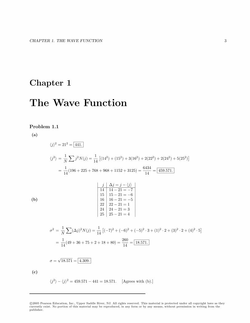
Problem 1.1
(a)
〈j〉2 = 212 = 441.
〈j2〉 =1N
∑j2N(j) =
114
[(142) + (152) + 3(162) + 2(222) + 2(242) + 5(252)
]=
114
(196 + 225 + 768 + 968 + 1152 + 3125) =643414
= 459.571.
(b)
j ∆j = j − 〈j〉14 14− 21 = −715 15− 21 = −616 16− 21 = −522 22− 21 = 124 24− 21 = 325 25− 21 = 4
σ2 =1N
∑(∆j)2N(j) =
114
[(−7)2 + (−6)2 + (−5)2 · 3 + (1)2 · 2 + (3)2 · 2 + (4)2 · 5
]=
114
(49 + 36 + 75 + 2 + 18 + 80) =26014
= 18.571.
σ =√
18.571 = 4.309.
(c)
〈j2〉 − 〈j〉2 = 459.571− 441 = 18.571. [Agrees with (b).]
c©2005 Pearson Education, Inc., Upper Saddle River, NJ. All rights reserved. This material is protected under all copyright laws as theycurrently exist. No portion of this material may be reproduced, in any form or by any means, without permission in writing from thepublisher.
4 CHAPTER 1. THE WAVE FUNCTION
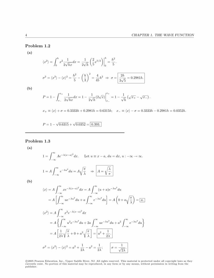
Problem 1.2
(a)
〈x2〉 =∫ h
0
x2 12√hx
dx =1
2√h
(25x5/2
)∣∣∣∣h0
=h2
5.
σ2 = 〈x2〉 − 〈x〉2 =h2
5−
(h
3
)2
=445
h2 ⇒ σ =2h
3√
5= 0.2981h.
(b)
P = 1−∫ x+
x−
12√hx
dx = 1− 12√h
(2√x)
∣∣∣∣x+
x−
= 1− 1√h
(√x+ −
√x−
).
x+ ≡ 〈x〉+ σ = 0.3333h + 0.2981h = 0.6315h; x− ≡ 〈x〉 − σ = 0.3333h− 0.2981h = 0.0352h.
P = 1−√
0.6315 +√
0.0352 = 0.393.
Problem 1.3
(a)
1 =∫ ∞−∞
Ae−λ(x−a)2dx. Let u ≡ x− a, du = dx, u : −∞→∞.
1 = A
∫ ∞−∞
e−λu2du = A
√π
λ⇒ A =
√λ
π.
(b)
〈x〉 = A
∫ ∞−∞
xe−λ(x−a)2dx = A
∫ ∞−∞
(u + a)e−λu2du
= A
[∫ ∞−∞
ue−λu2du + a
∫ ∞−∞
e−λu2du
]= A
(0 + a
√π
λ
)= a.
〈x2〉 = A
∫ ∞−∞
x2e−λ(x−a)2dx
= A
∫ ∞−∞
u2e−λu2du + 2a
∫ ∞−∞
ue−λu2du + a2
∫ ∞−∞
e−λu2du
= A
[12λ
√π
λ+ 0 + a2
√π
λ
]= a2 +
12λ
.
σ2 = 〈x2〉 − 〈x〉2 = a2 +12λ− a2 =
12λ
; σ =1√2λ
.
c©2005 Pearson Education, Inc., Upper Saddle River, NJ. All rights reserved. This material is protected under all copyright laws as theycurrently exist. No portion of this material may be reproduced, in any form or by any means, without permission in writing from thepublisher.
CHAPTER 1. THE WAVE FUNCTION 5
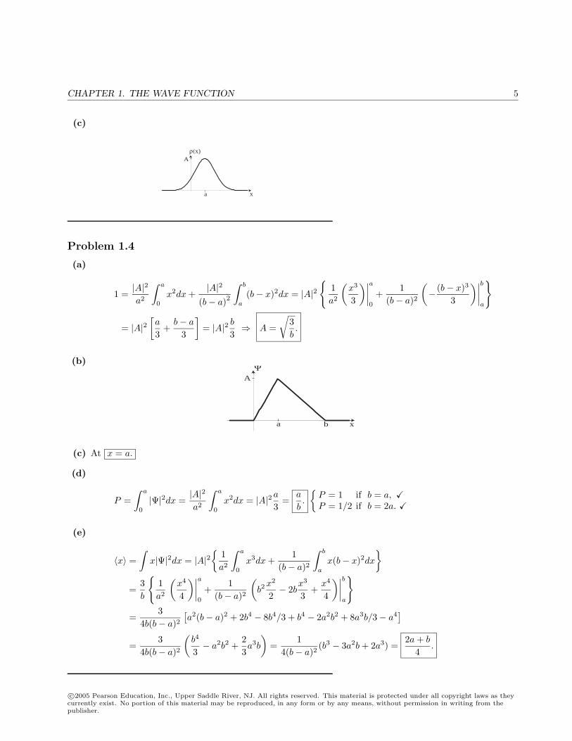
(c)
A
xa
ρ(x)
Problem 1.4
(a)
1 =|A|2a2
∫ a
0
x2dx +|A|2
(b− a)2
∫ b
a
(b− x)2dx = |A|2
1a2
(x3
3
)∣∣∣∣a0
+1
(b− a)2
(− (b− x)3
3
)∣∣∣∣ba
= |A|2[a
3+
b− a
3
]= |A|2 b
3⇒ A =
√3b.
(b)
xa
A
b
Ψ
(c) At x = a.
(d)
P =∫ a
0
|Ψ|2dx =|A|2a2
∫ a
0
x2dx = |A|2 a3
=a
b.
P = 1 if b = a, P = 1/2 if b = 2a.
(e)
〈x〉 =∫
x|Ψ|2dx = |A|2
1a2
∫ a
0
x3dx +1
(b− a)2
∫ b
a
x(b− x)2dx
=3b
1a2
(x4
4
)∣∣∣∣a0
+1
(b− a)2
(b2
x2
2− 2b
x3
3+
x4
4
)∣∣∣∣ba
=3
4b(b− a)2[a2(b− a)2 + 2b4 − 8b4/3 + b4 − 2a2b2 + 8a3b/3− a4
]=
34b(b− a)2
(b4
3− a2b2 +
23a3b
)=
14(b− a)2
(b3 − 3a2b + 2a3) =2a + b
4.
c©2005 Pearson Education, Inc., Upper Saddle River, NJ. All rights reserved. This material is protected under all copyright laws as theycurrently exist. No portion of this material may be reproduced, in any form or by any means, without permission in writing from thepublisher.
6 CHAPTER 1. THE WAVE FUNCTION
Problem 1.5
(a)
1 =∫|Ψ|2dx = 2|A|2
∫ ∞0
e−2λxdx = 2|A|2(e−2λx
−2λ
)∣∣∣∣∞0
=|A|2λ
; A =√λ.
(b)
〈x〉 =∫
x|Ψ|2dx = |A|2∫ ∞−∞
xe−2λ|x|dx = 0. [Odd integrand.]
〈x2〉 = 2|A|2∫ ∞
0
x2e−2λxdx = 2λ[
2(2λ)3
]=
12λ2
.
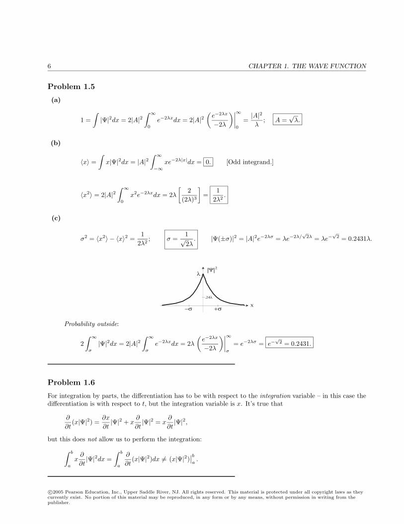
(c)
σ2 = 〈x2〉 − 〈x〉2 =1
2λ2; σ =
1√2λ
. |Ψ(±σ)|2 = |A|2e−2λσ = λe−2λ/√
2λ = λe−√
2 = 0.2431λ.
|Ψ|2λ
σ−σ +x
.24λ
Probability outside:
2∫ ∞
σ
|Ψ|2dx = 2|A|2∫ ∞
σ
e−2λxdx = 2λ(e−2λx
−2λ
)∣∣∣∣∞σ
= e−2λσ = e−√
2 = 0.2431.
Problem 1.6
For integration by parts, the differentiation has to be with respect to the integration variable – in this case thedifferentiation is with respect to t, but the integration variable is x. It’s true that
∂
∂t(x|Ψ|2) =
∂x
∂t|Ψ|2 + x
∂
∂t|Ψ|2 = x
∂
∂t|Ψ|2,
but this does not allow us to perform the integration:∫ b
a
x∂
∂t|Ψ|2dx =
∫ b
a
∂
∂t(x|Ψ|2)dx = (x|Ψ|2)
∣∣ba.
c©2005 Pearson Education, Inc., Upper Saddle River, NJ. All rights reserved. This material is protected under all copyright laws as theycurrently exist. No portion of this material may be reproduced, in any form or by any means, without permission in writing from thepublisher.
CHAPTER 1. THE WAVE FUNCTION 7
Problem 1.7
From Eq. 1.33, d〈p〉dt = −i
∫∂∂t
(Ψ∗ ∂Ψ
∂x
)dx. But, noting that ∂2Ψ
∂x∂t = ∂2Ψ∂t∂x and using Eqs. 1.23-1.24:
∂
∂t
(Ψ∗
∂Ψ∂x
)=
∂Ψ∗
∂t
∂Ψ∂x
+ Ψ∗∂
∂x
(∂Ψ∂t
)=
[− i
2m∂2Ψ∗
∂x2+
i
V Ψ∗
]∂Ψ∂x
+ Ψ∗∂
∂x
[i
2m∂2Ψ∂x2
− i
V Ψ
]=
i
2m
[Ψ∗
∂3Ψ∂x3
− ∂2Ψ∗
∂x2
∂Ψ∂x
]+
i
[V Ψ∗
∂Ψ∂x
−Ψ∗∂
∂x(V Ψ)
]The first term integrates to zero, using integration by parts twice, and the second term can be simplified toV Ψ∗ ∂Ψ
∂x −Ψ∗V ∂Ψ∂x −Ψ∗ ∂V
∂x Ψ = −|Ψ|2 ∂V∂x . So
d〈p〉dt
= −i
(i
) ∫−|Ψ|2 ∂V
∂xdx = 〈−∂V
∂x〉. QED
Problem 1.8
Suppose Ψ satisfies the Schrodinger equation without V0: i∂Ψ∂t = −
2
2m∂2Ψ∂x2 + V Ψ. We want to find the solution
Ψ0 with V0: i∂Ψ0∂t = −
2
2m∂2Ψ0∂x2 + (V + V0)Ψ0.
Claim: Ψ0 = Ψe−iV0t/.
Proof: i∂Ψ0∂t = i∂Ψ
∂t e−iV0t/ + iΨ
(− iV0
)e−iV0t/ =
[−
2
2m∂2Ψ∂x2 + V Ψ
]e−iV0t/ + V0Ψe−iV0t/
= − 2
2m∂2Ψ0∂x2 + (V + V0)Ψ0. QED
This has no effect on the expectation value of a dynamical variable, since the extra phase factor, being inde-pendent of x, cancels out in Eq. 1.36.
Problem 1.9
(a)
1 = 2|A|2∫ ∞
0
e−2amx2/dx = 2|A|2 12
√π
(2am/)= |A|2
√π
2am; A =
(2amπ
)1/4
.
(b)
∂Ψ∂t
= −iaΨ;∂Ψ∂x
= −2amx
Ψ;
∂2Ψ∂x2
= −2am
(Ψ + x
∂Ψ∂x
)= −2am
(1− 2amx2
)Ψ.
Plug these into the Schrodinger equation, i∂Ψ∂t = −
2
2m∂2Ψ∂x2 + V Ψ:
V Ψ = i(−ia)Ψ +
2
2m
(−2am
) (1− 2amx2
)Ψ
=[a− a
(1− 2amx2
)]Ψ = 2a2mx2Ψ, so V (x) = 2ma2x2.
c©2005 Pearson Education, Inc., Upper Saddle River, NJ. All rights reserved. This material is protected under all copyright laws as theycurrently exist. No portion of this material may be reproduced, in any form or by any means, without permission in writing from thepublisher.
8 CHAPTER 1. THE WAVE FUNCTION
(c)
〈x〉 =∫ ∞−∞
x|Ψ|2dx = 0. [Odd integrand.]
〈x2〉 = 2|A|2∫ ∞
0
x2e−2amx2/dx = 2|A|2 122(2am/)
√π
2am=
4am.
〈p〉 = md〈x〉dt
= 0.
〈p2〉 =∫
Ψ∗(
i
∂
∂x
)2
Ψdx = −2
∫Ψ∗
∂2Ψ∂x2
dx
= −2
∫Ψ∗
[−2am
(1− 2amx2
)Ψ
]dx = 2am
∫|Ψ|2dx− 2am
∫x2|Ψ|2dx
= 2am
(1− 2am
〈x2〉
)= 2am
(1− 2am
4am
)= 2am
(12
)= am.
(d)
σ2x = 〈x2〉 − 〈x〉2 =
4am=⇒ σx =
√
4am; σ2
p = 〈p2〉 − 〈p〉2 = am =⇒ σp =√am.
σxσp =√
4am
√am =
2 . This is (just barely) consistent with the uncertainty principle.
Problem 1.10
From Math Tables: π = 3.141592653589793238462643 · · ·
(a)P (0) = 0 P (1) = 2/25 P (2) = 3/25 P (3) = 5/25 P (4) = 3/25P (5) = 3/25 P (6) = 3/25 P (7) = 1/25 P (8) = 2/25 P (9) = 3/25
In general, P (j) = N(j)N .
(b) Most probable: 3. Median: 13 are ≤ 4, 12 are ≥ 5, so median is 4.
Average: 〈j〉 = 125 [0 · 0 + 1 · 2 + 2 · 3 + 3 · 5 + 4 · 3 + 5 · 3 + 6 · 3 + 7 · 1 + 8 · 2 + 9 · 3]
= 125 [0 + 2 + 6 + 15 + 12 + 15 + 18 + 7 + 16 + 27] = 118
25 = 4.72.
(c) 〈j2〉 = 125 [0 + 12 · 2 + 22 · 3 + 32 · 5 + 42 · 3 + 52 · 3 + 62 · 3 + 72 · 1 + 82 · 2 + 92 · 3]
= 125 [0 + 2 + 12 + 45 + 48 + 75 + 108 + 49 + 128 + 243] = 710
25 = 28.4.
σ2 = 〈j2〉 − 〈j〉2 = 28.4− 4.722 = 28.4− 22.2784 = 6.1216; σ =√
6.1216 = 2.474.
c©2005 Pearson Education, Inc., Upper Saddle River, NJ. All rights reserved. This material is protected under all copyright laws as theycurrently exist. No portion of this material may be reproduced, in any form or by any means, without permission in writing from thepublisher.
CHAPTER 1. THE WAVE FUNCTION 9
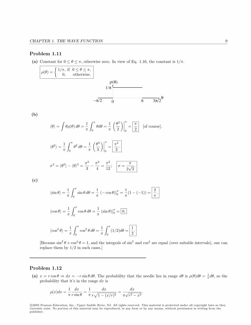
Problem 1.11
(a) Constant for 0 ≤ θ ≤ π, otherwise zero. In view of Eq. 1.16, the constant is 1/π.
ρ(θ) =
1/π, if 0 ≤ θ ≤ π,0, otherwise.
1/π
−π/2 0 π 3π/2
ρ(θ)
θ
(b)
〈θ〉 =∫
θρ(θ) dθ =1π
∫ π
0
θdθ =1π
(θ2
2
)∣∣∣∣π0
=π
2[of course].
〈θ2〉 =1π
∫ π
0
θ2 dθ =1π
(θ3
3
)∣∣∣∣π0
=π2
3.
σ2 = 〈θ2〉 − 〈θ〉2 =π2
3− π2
4=
π2
12; σ =
π
2√
3.
(c)
〈sin θ〉 =1π
∫ π
0
sin θ dθ =1π
(− cos θ)|π0 =1π
(1− (−1)) =2π
.
〈cos θ〉 =1π
∫ π
0
cos θ dθ =1π
(sin θ)|π0 = 0.
〈cos2 θ〉 =1π
∫ π
0
cos2 θ dθ =1π
∫ π
0
(1/2)dθ =12.
[Because sin2 θ + cos2 θ = 1, and the integrals of sin2 and cos2 are equal (over suitable intervals), one canreplace them by 1/2 in such cases.]
Problem 1.12
(a) x = r cos θ ⇒ dx = −r sin θ dθ. The probability that the needle lies in range dθ is ρ(θ)dθ = 1πdθ, so the
probability that it’s in the range dx is
ρ(x)dx =1π
dx
r sin θ=
1π
dx
r√
1− (x/r)2=
dx
π√r2 − x2
.
c©2005 Pearson Education, Inc., Upper Saddle River, NJ. All rights reserved. This material is protected under all copyright laws as theycurrently exist. No portion of this material may be reproduced, in any form or by any means, without permission in writing from thepublisher.
10 CHAPTER 1. THE WAVE FUNCTION
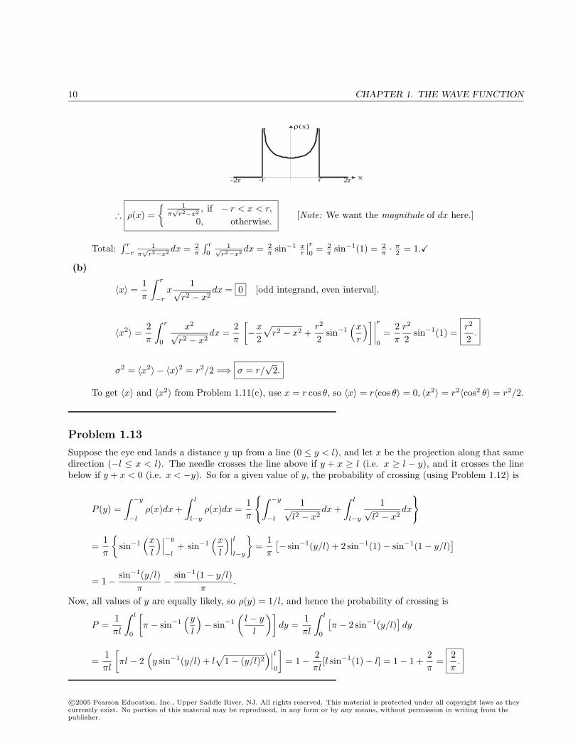
ρ(x)
xr 2r-r-2r
∴ ρ(x) = 1
π√
r2−x2 , if − r < x < r,
0, otherwise.[Note: We want the magnitude of dx here.]
Total:∫ r
−r1
π√
r2−x2 dx = 2π
∫ r
01√
r2−x2 dx = 2π sin−1 x
r
∣∣r0
= 2π sin−1(1) = 2
π · π2 = 1.
(b)
〈x〉 =1π
∫ r
−r
x1√
r2 − x2dx = 0 [odd integrand, even interval].
〈x2〉 =2π
∫ r
0
x2
√r2 − x2
dx =2π
[−x
2
√r2 − x2 +
r2
2sin−1
(x
r
)]∣∣∣∣r0
=2π
r2
2sin−1(1) =
r2
2.
σ2 = 〈x2〉 − 〈x〉2 = r2/2 =⇒ σ = r/√
2.
To get 〈x〉 and 〈x2〉 from Problem 1.11(c), use x = r cos θ, so 〈x〉 = r〈cos θ〉 = 0, 〈x2〉 = r2〈cos2 θ〉 = r2/2.
Problem 1.13
Suppose the eye end lands a distance y up from a line (0 ≤ y < l), and let x be the projection along that samedirection (−l ≤ x < l). The needle crosses the line above if y + x ≥ l (i.e. x ≥ l − y), and it crosses the linebelow if y + x < 0 (i.e. x < −y). So for a given value of y, the probability of crossing (using Problem 1.12) is
P (y) =∫ −y
−l
ρ(x)dx +∫ l
l−y
ρ(x)dx =1π
∫ −y
−l
1√l2 − x2
dx +∫ l
l−y
1√l2 − x2
dx
=1π
sin−1
(x
l
)∣∣∣−y
−l+ sin−1
(x
l
)∣∣∣ll−y
=
1π
[− sin−1(y/l) + 2 sin−1(1)− sin−1(1− y/l)
]= 1− sin−1(y/l)
π− sin−1(1− y/l)
π.
Now, all values of y are equally likely, so ρ(y) = 1/l, and hence the probability of crossing is
P =1πl
∫ l
0
[π − sin−1
(y
l
)− sin−1
(l − y
l
)]dy =
1πl
∫ l
0
[π − 2 sin−1(y/l)
]dy
=1πl
[πl − 2
(y sin−1(y/l) + l
√1− (y/l)2
)∣∣∣l0
]= 1− 2
πl[l sin−1(1)− l] = 1− 1 +
2π
=2π
.
c©2005 Pearson Education, Inc., Upper Saddle River, NJ. All rights reserved. This material is protected under all copyright laws as theycurrently exist. No portion of this material may be reproduced, in any form or by any means, without permission in writing from thepublisher.
CHAPTER 1. THE WAVE FUNCTION 11
Problem 1.14
(a) Pab(t) =∫ b
a|Ψ(x, t)2dx, so dPab
dt =∫ b
a∂∂t |Ψ|2dx. But (Eq. 1.25):
∂|Ψ|2∂t
=∂
∂x
[i
2m
(Ψ∗
∂Ψ∂x
− ∂Ψ∗
∂xΨ
)]= − ∂
∂tJ(x, t).
∴ dPab
dt= −
∫ b
a
∂
∂xJ(x, t)dx = − [J(x, t)]|ba = J(a, t)− J(b, t). QED
Probability is dimensionless, so J has the dimensions 1/time, and units seconds−1.
(b) Here Ψ(x, t) = f(x)e−iat, where f(x) ≡ Ae−amx2/, so Ψ∂Ψ∗
∂x = fe−iat dfdxe
iat = f dfdx ,
and Ψ∗ ∂Ψ∂x = f df
dx too, so J(x, t) = 0.
Problem 1.15
(a) Eq. 1.24 now reads ∂Ψ∗
∂t = − i2m
∂2Ψ∗
∂x2 + iV ∗Ψ∗, and Eq. 1.25 picks up an extra term:
∂
∂t|Ψ|2 = · · ·+ i
|Ψ|2(V ∗ − V ) = · · ·+ i
|Ψ|2(V0 + iΓ− V0 + iΓ) = · · · − 2Γ
|Ψ|2,
and Eq. 1.27 becomes dPdt = − 2Γ
∫∞−∞ |Ψ|2dx = − 2Γ
P . QED
(b)
dP
P= −2Γ
dt =⇒ lnP = −2Γ
t + constant =⇒ P (t) = P (0)e−2Γt/, so τ =
2Γ.
Problem 1.16
Use Eqs. [1.23] and [1.24], and integration by parts:
d
dt
∫ ∞−∞
Ψ∗1Ψ2 dx =∫ ∞−∞
∂
∂t(Ψ∗1Ψ2) dx =
∫ ∞−∞
(∂Ψ∗1∂t
Ψ2 + Ψ∗1∂Ψ2
∂t
)dx
=∫ ∞−∞
[(−i
2m∂2Ψ∗1∂x2
+i
V Ψ∗1
)Ψ2 + Ψ∗1
(i
2m∂2Ψ2
∂x2− i
V Ψ2
)]dx
= − i
2m
∫ ∞−∞
(∂2Ψ∗1∂x2
Ψ2 −Ψ∗1∂2Ψ2
∂x2
)dx
= − i
2m
[∂Ψ∗1∂x
Ψ2
∣∣∣∣∞−∞
−∫ ∞−∞
∂Ψ∗1∂x
∂Ψ2
∂xdx− Ψ∗1
∂Ψ2
∂x
∣∣∣∣∞−∞
+∫ ∞−∞
∂Ψ∗1∂x
∂Ψ2
∂xdx
]= 0. QED
c©2005 Pearson Education, Inc., Upper Saddle River, NJ. All rights reserved. This material is protected under all copyright laws as theycurrently exist. No portion of this material may be reproduced, in any form or by any means, without permission in writing from thepublisher.
12 CHAPTER 1. THE WAVE FUNCTION
Problem 1.17
(a)
1 = |A|2∫ a
−a
(a2 − x2
)2dx = 2|A|2
∫ a
0
(a4 − 2a2x2 + x4
)dx = 2|A|2
[a4x− 2a2x
3
3+
x5
5
]∣∣∣∣a0
= 2|A|2a5
(1− 2
3+
15
)=
1615
a5|A|2, so A =
√15
16a5.
(b)
〈x〉 =∫ a
−a
x|Ψ|2 dx = 0. (Odd integrand.)
(c)
〈p〉 =
iA2
∫ a
−a
(a2 − x2
) d
dx
(a2 − x2
)︸ ︷︷ ︸
−2x
dx = 0. (Odd integrand.)
Since we only know 〈x〉 at t = 0 we cannot calculate d〈x〉/dt directly.
(d)
〈x2〉 = A2
∫ a
−a
x2(a2 − x2
)2dx = 2A2
∫ a
0
(a4x2 − 2a2x4 + x6
)dx
= 215
16a5
[a4x
3
3− 2a2x
5
5+
x7
7
]∣∣∣∣a0
=158a5
(a7
)(13− 2
5+
17
)
=15a2
8
(35− 42 + 15
3 · 5 · 7
)=
a2
8· 87
=a2
7.
(e)
〈p2〉 = −A2
2
∫ a
−a
(a2 − x2
) d2
dx2
(a2 − x2
)︸ ︷︷ ︸
−2
dx = 2A2
22∫ a
0
(a2 − x2
)dx
= 4 · 1516a5
2
(a2x− x3
3
)∣∣∣∣a0
=152
4a5
(a3 − a3
3
)=
152
4a2· 23
=52
2
a2.
(f)
σx =√〈x2〉 − 〈x〉2 =
√17a2 =
a√7.
(g)
σp =√〈p2〉 − 〈p〉2 =
√522
a2=
√52
a.
c©2005 Pearson Education, Inc., Upper Saddle River, NJ. All rights reserved. This material is protected under all copyright laws as theycurrently exist. No portion of this material may be reproduced, in any form or by any means, without permission in writing from thepublisher.
CHAPTER 1. THE WAVE FUNCTION 13
(h)
σxσp =a√7·√
52
a=
√514 =
√107
2>
2.
Problem 1.18
h√3mkBT
> d ⇒ T <h2
3mkBd2.
(a) Electrons (m = 9.1× 10⁻³¹ kg):
T <(6.6× 10⁻³⁴)2
3(9.1× 10⁻³¹)(1.4× 10⁻²³)(3× 10⁻¹⁰)2= 1.3× 10⁵ K.
Sodium nuclei (m = 23mp = 23(1.7× 10⁻²⁷) = 3.9× 10⁻²⁶ kg):
T <(6.6× 10⁻³⁴)2
3(3.9× 10⁻²⁶)(1.4× 10⁻²³)(3× 10⁻¹⁰)2= 3.0 K.
(b) PV = NkBT ; volume occupied by one molecule (N = 1, V = d3) ⇒ d = (kBT/P )1/3.
T <h2
2mkB
(P
kBT
)2/3
⇒ T 5/3 <h2
3mP 2/3
k5/3B
⇒ T <1kB
(h2
3m
)3/5
P 2/5.
For helium (m = 4mp = 6.8× 10⁻²⁷ kg) at 1 atm = 1.0× 10⁵ N/m2:
T <1
(1.4× 10⁻²³)
((6.6× 10⁻³⁴)2
3(6.8× 10⁻²⁷)
)3/5
(1.0× 10⁵)2/5 = 2.8 K.
For hydrogen (m = 2mp = 3.4× 10⁻²⁷ kg) with d = 0.01 m:
T <(6.6× 10⁻³⁴)2
3(3.4× 10⁻²⁷)(1.4× 10⁻²³)(10−2)2= 3.1× 10⁻¹⁴ K.
At 3 K it is definitely in the classical regime.
c©2005 Pearson Education, Inc., Upper Saddle River, NJ. All rights reserved. This material is protected under all copyright laws as theycurrently exist. No portion of this material may be reproduced, in any form or by any means, without permission in writing from thepublisher.
14 CHAPTER 2. THE TIME-INDEPENDENT SCHRODINGER EQUATION
Chapter 2
Time-Independent SchrodingerEquation
Problem 2.1
(a)
Ψ(x, t) = ψ(x)e−i(E0+iΓ)t/ = ψ(x)eΓt/e−iE0t/ =⇒ |Ψ|2 = |ψ|2e2Γt/.
∫ ∞−∞
|Ψ(x, t)|2dx = e2Γt/
∫ ∞−∞
|ψ|2dx.
The second term is independent of t, so if the product is to be 1 for all time, the first term (e2Γt/) mustalso be constant, and hence Γ = 0. QED
(b) If ψ satisfies Eq. 2.5, − 2
2m∂2ψdx2 + V ψ = Eψ, then (taking the complex conjugate and noting that V and
E are real): − 2
2m∂2ψ∗
dx2 + V ψ∗ = Eψ∗, so ψ∗ also satisfies Eq. 2.5. Now, if ψ1 and ψ2 satisfy Eq. 2.5, sotoo does any linear combination of them (ψ3 ≡ c1ψ1 + c2ψ2):
− 2
2m∂2ψ3
dx2+ V ψ3 = −
2
2m
(c1
∂2ψ1
dx2+ c2
∂2ψ2
∂x2
)+ V (c1ψ1 + c2ψ2)
= c1
[−
2
2md2ψ1
dx2+ V ψ1
]+ c2
[−
2
2md2ψ2
dx2+ V ψ2
]= c1(Eψ1) + c2(Eψ2) = E(c1ψ1 + c2ψ2) = Eψ3.
Thus, (ψ + ψ∗) and i(ψ − ψ∗) – both of which are real – satisfy Eq. 2.5. Conclusion: From any complexsolution, we can always construct two real solutions (of course, if ψ is already real, the second one will bezero). In particular, since ψ = 1
2 [(ψ + ψ∗)− i(i(ψ − ψ∗))], ψ can be expressed as a linear combination oftwo real solutions. QED
(c) If ψ(x) satisfies Eq. 2.5, then, changing variables x→ −x and noting that ∂2/∂(−x)2 = ∂2/∂x2,
− 2
2m∂2ψ(−x)
dx2+ V (−x)ψ(−x) = Eψ(−x);
so if V (−x) = V (x) then ψ(−x) also satisfies Eq. 2.5. It follows that ψ+(x) ≡ ψ(x) + ψ(−x) (which iseven: ψ+(−x) = ψ+(x)) and ψ−(x) ≡ ψ(x)− ψ(−x) (which is odd: ψ−(−x) = −ψ−(x)) both satisfy Eq.
c©2005 Pearson Education, Inc., Upper Saddle River, NJ. All rights reserved. This material is protected under all copyright laws as theycurrently exist. No portion of this material may be reproduced, in any form or by any means, without permission in writing from thepublisher.
CHAPTER 2. THE TIME-INDEPENDENT SCHRODINGER EQUATION 15
2.5. But ψ(x) = 12 (ψ+(x) + ψ−(x)), so any solution can be expressed as a linear combination of even and
odd solutions. QED
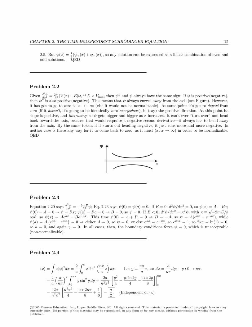
Problem 2.2
Given d2ψdx2 = 2m
2[V (x)−E]ψ, if E < Vmin, then ψ′′ and ψ always have the same sign: If ψ is positive(negative),
then ψ′′ is also positive(negative). This means that ψ always curves away from the axis (see Figure). However,it has got to go to zero as x→ −∞ (else it would not be normalizable). At some point it’s got to depart fromzero (if it doesn’t, it’s going to be identically zero everywhere), in (say) the positive direction. At this point itsslope is positive, and increasing, so ψ gets bigger and bigger as x increases. It can’t ever “turn over” and headback toward the axis, because that would requuire a negative second derivative—it always has to bend awayfrom the axis. By the same token, if it starts out heading negative, it just runs more and more negative. Inneither case is there any way for it to come back to zero, as it must (at x → ∞) in order to be normalizable.QED
x
ψ
Problem 2.3
Equation 2.20 says d2ψdx2 = − 2mE
2ψ; Eq. 2.23 says ψ(0) = ψ(a) = 0. If E = 0, d2ψ/dx2 = 0, so ψ(x) = A + Bx;
ψ(0) = A = 0 ⇒ ψ = Bx; ψ(a) = Ba = 0 ⇒ B = 0, so ψ = 0. If E < 0, d2ψ/dx2 = κ2ψ, with κ ≡√−2mE/
real, so ψ(x) = Aeκx + Be−κx. This time ψ(0) = A + B = 0 ⇒ B = −A, so ψ = A(eκx − e−κx), whileψ(a) = A
(eκa − eiκa
)= 0 ⇒ either A = 0, so ψ = 0, or else eκa = e−κa, so e2κa = 1, so 2κa = ln(1) = 0,
so κ = 0, and again ψ = 0. In all cases, then, the boundary conditions force ψ = 0, which is unacceptable(non-normalizable).
Problem 2.4
〈x〉 =∫
x|ψ|2dx =2a
∫ a
0
x sin2(nπ
ax)dx. Let y ≡ nπ
ax, so dx =
a
nπdy; y : 0→ nπ.
=2a
( a
nπ
)2∫ nπ
0
y sin2 y dy =2a
n2π2
[y2
4− y sin 2y
4− cos 2y
8
]∣∣∣∣nπ
0
=2a
n2π2
[n2π2
4− cos 2nπ
8+
18
]=
a
2. (Independent of n.)
c©2005 Pearson Education, Inc., Upper Saddle River, NJ. All rights reserved. This material is protected under all copyright laws as theycurrently exist. No portion of this material may be reproduced, in any form or by any means, without permission in writing from thepublisher.
16 CHAPTER 2. THE TIME-INDEPENDENT SCHRODINGER EQUATION
〈x2〉 =2a
∫ a
0
x2 sin2(nπ
ax)dx =
2a
( a
nπ
)3∫ nπ
0
y2 sin2 y dy
=2a2
(nπ)3
[y3
6−
(y3
4− 1
8
)sin 2y − y cos 2y
4
]nπ
0
=2a2
(nπ)3
[(nπ)3
6− nπ cos(2nπ)
4
]= a2
[13− 1
2(nπ)2
].
〈p〉 = md〈x〉dt
= 0. (Note : Eq. 1.33 is much faster than Eq. 1.35.)
〈p2〉 =∫
ψ∗n
(
i
d
dx
)2
ψn dx = −2
∫ψ∗n
(d2ψn
dx2
)dx
= (−2)(−2mEn
2
) ∫ψ∗nψn dx = 2mEn =
(nπ
a
)2
.
σ2x = 〈x2〉 − 〈x〉2 = a2
(13− 1
2(nπ)2− 1
4
)=
a2
4
(13− 2
(nπ)2
); σx =
a
2
√13− 2
(nπ)2.
σ2p = 〈p2〉 − 〈p〉2 =
(nπ
a
)2
; σp =nπ
a. ∴ σxσp =
2
√(nπ)2
3− 2.
The product σxσp is smallest for n = 1; in that case, σxσp =
2
√π2
3 − 2 = (1.136)/2 > /2.
Problem 2.5
(a)
|Ψ|2 = Ψ2Ψ = |A|2(ψ∗1 + ψ∗2)(ψ1 + ψ2) = |A|2[ψ∗1ψ1 + ψ∗1ψ2 + ψ∗2ψ1 + ψ∗2ψ2].
1 =∫|Ψ|2dx = |A|2
∫[|ψ1|2 + ψ∗1ψ2 + ψ∗2ψ1 + |ψ2|2]dx = 2|A|2 ⇒ A = 1/
√2.
(b)
Ψ(x, t) =1√2
[ψ1e−iE1t/ + ψ2e
−iE2t/]
(butEn
= n2ω)
=1√2
√2a
[sin
(π
ax)e−iωt + sin
(2πa
x
)e−i4ωt
]=
1√ae−iωt
[sin
(π
ax)
+ sin(
2πa
x
)e−3iωt
].
|Ψ(x, t)|2 =1a
[sin2
(π
ax)
+ sin(π
ax)
sin(
2πa
x
) (e−3iωt + e3iωt
)+ sin2
(2πa
x
)]=
1a
[sin2
(π
ax)
+ sin2
(2πa
x
)+ 2 sin
(π
ax)
sin(
2πa
x
)cos(3ωt)
].
c©2005 Pearson Education, Inc., Upper Saddle River, NJ. All rights reserved. This material is protected under all copyright laws as theycurrently exist. No portion of this material may be reproduced, in any form or by any means, without permission in writing from thepublisher.
CHAPTER 2. THE TIME-INDEPENDENT SCHRODINGER EQUATION 17
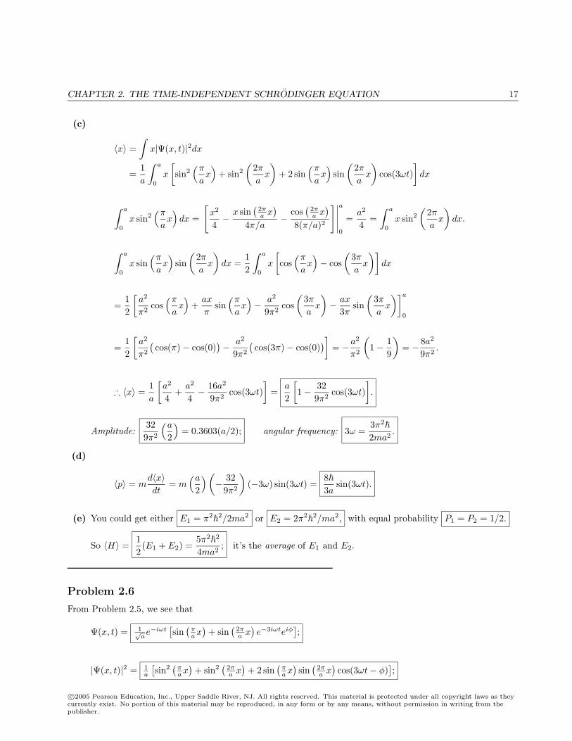
(c)
〈x〉 =∫
x|Ψ(x, t)|2dx
=1a
∫ a
0
x
[sin2
(π
ax)
+ sin2
(2πa
x
)+ 2 sin
(π
ax)
sin(
2πa
x
)cos(3ωt)
]dx
∫ a
0
x sin2(π
ax)dx =
[x2
4− x sin
(2πa x
)4π/a
− cos(
2πa x
)8(π/a)2
]∣∣∣∣∣a
0
=a2
4=
∫ a
0
x sin2
(2πa
x
)dx.
∫ a
0
x sin(π
ax)
sin(
2πa
x
)dx =
12
∫ a
0
x
[cos
(π
ax)− cos
(3πa
x
)]dx
=12
[a2
π2cos
(π
ax)
+ax
πsin
(π
ax)− a2
9π2cos
(3πa
x
)− ax
3πsin
(3πa
x
)]a
0
=12
[a2
π2
(cos(π)− cos(0)
)− a2
9π2
(cos(3π)− cos(0)
)]= −a2
π2
(1− 1
9
)= − 8a2
9π2.
∴ 〈x〉 =1a
[a2
4+
a2
4− 16a2
9π2cos(3ωt)
]=
a
2
[1− 32
9π2cos(3ωt)
].
Amplitude:329π2
(a
2
)= 0.3603(a/2); angular frequency: 3ω =
3π2
2ma2.
(d)
〈p〉 = md〈x〉dt
= m(a
2
) (− 32
9π2
)(−3ω) sin(3ωt) =
83a
sin(3ωt).
(e) You could get either E1 = π2
2/2ma2 or E2 = 2π2
2/ma2, with equal probability P1 = P2 = 1/2.
So 〈H〉 =12(E1 + E2) =
5π2
2
4ma2; it’s the average of E1 and E2.
Problem 2.6
From Problem 2.5, we see that
Ψ(x, t) = 1√ae−iωt
[sin
(πax
)+ sin
(2πa x
)e−3iωteiφ
];
|Ψ(x, t)|2 = 1a
[sin2
(πax
)+ sin2
(2πa x
)+ 2 sin
(πax
)sin
(2πa x
)cos(3ωt− φ)
];
c©2005 Pearson Education, Inc., Upper Saddle River, NJ. All rights reserved. This material is protected under all copyright laws as theycurrently exist. No portion of this material may be reproduced, in any form or by any means, without permission in writing from thepublisher.
18 CHAPTER 2. THE TIME-INDEPENDENT SCHRODINGER EQUATION
and hence 〈x〉 = a2
[1− 32
9π2 cos(3ωt− φ)]. This amounts physically to starting the clock at a different time
(i.e., shifting the t = 0 point).
If φ =π
2, so Ψ(x, 0) = A[ψ1(x) + iψ2(x)], then cos(3ωt− φ) = sin(3ωt); 〈x〉 starts at
a
2.
If φ = π, so Ψ(x, 0) = A[ψ1(x)− ψ2(x)], then cos(3ωt− φ) = − cos(3ωt); 〈x〉 starts ata
2
(1 +
329π2
).
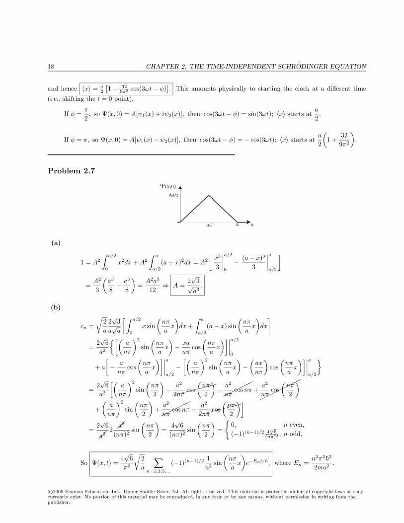
Problem 2.7
Ψ(x,0)
xaa/2
Aa/2
(a)
1 = A2
∫ a/2
0
x2dx + A2
∫ a
a/2
(a− x)2dx = A2
[x3
3
∣∣∣∣a/2
0
− (a− x)3
3
∣∣∣∣aa/2
]
=A2
3
(a3
8+
a3
8
)=
A2a3
12⇒ A =
2√
3√a3
.
(b)
cn =
√2a
2√
3a√a
[ ∫ a/2
0
x sin(nπ
ax
)dx +
∫ a
a/2
(a− x) sin(nπ
ax
)dx
]=
2√
6a2
[(a
nπ
)2
sin(nπ
ax
)− xa
nπcos
(nπ
ax
)]∣∣∣∣a/2
0
+ a
[− a
nπcos
(nπ
ax
)]∣∣∣∣aa/2
−[(
a
nπ
)2
sin(nπ
ax
)−
(ax
nπ
)cos
(nπ
ax
)]∣∣∣∣aa/2
=2√
6a2
[(a
nπ
)2
sin(nπ
2
)−
a2
2nπcos
(nπ
2
)−
a2
nπcosnπ +
a2
nπcos
(nπ
2
)+
(a
nπ
)2
sin(nπ
2
)+
a2
nπcosnπ −
a2
2nπcos
(nπ
2
)]=
2√
6
a22 a2
(nπ)2sin
(nπ
2
)=
4√
6(nπ)2
sin(nπ
2
)=
0, n even,(−1)(n−1)/2 4
√6
(nπ)2 , n odd.
So Ψ(x, t) =4√
6π2
√2a
∑n=1,3,5,...
(−1)(n−1)/2 1n2
sin(nπ
ax
)e−Ent/, where En =
n2π2
2
2ma2.
c©2005 Pearson Education, Inc., Upper Saddle River, NJ. All rights reserved. This material is protected under all copyright laws as theycurrently exist. No portion of this material may be reproduced, in any form or by any means, without permission in writing from thepublisher.
CHAPTER 2. THE TIME-INDEPENDENT SCHRODINGER EQUATION 19
(c)
P1 = |c1|2 =16 · 6π4
= 0.9855.
(d)
〈H〉 =∑
|cn|2En =96π4
π2
2
2ma2
(11
+132
+152
+172
+ · · ·︸ ︷︷ ︸π2/8
)=
482
π2ma2
π2
8=
62
ma2.
Problem 2.8
(a)
Ψ(x, 0) =
A, 0 < x < a/2;0, otherwise.
1 = A2
∫ a/2
0
dx = A2(a/2)⇒ A =
√2a.
(b) From Eq. 2.37,
c1 = A
√2a
∫ a/2
0
sin(π
ax)dx =
2a
[−a
πcos
(π
ax)] ∣∣∣∣a/2
0
= − 2π
[cos
(π
2
)− cos 0
]=
2π.
P1 = |c1|2 = (2/π)2 = 0.4053.
Problem 2.9
HΨ(x, 0) = − 2
2m∂2
∂x2[Ax(a− x)] = −A
2
2m∂
∂x(a− 2x) = A
2
m.
∫Ψ(x, 0)∗HΨ(x, 0) dx = A2
2
m
∫ a
0
x(a− x) dx = A2 2
m
(ax2
2− x3
3
) ∣∣∣∣a0
= A2 2
m
(a3
2− a3
3
)=
30a5
2
m
a3
6=
52
ma2
(same as Example 2.3).
c©2005 Pearson Education, Inc., Upper Saddle River, NJ. All rights reserved. This material is protected under all copyright laws as theycurrently exist. No portion of this material may be reproduced, in any form or by any means, without permission in writing from thepublisher.
20 CHAPTER 2. THE TIME-INDEPENDENT SCHRODINGER EQUATION
Problem 2.10
(a) Using Eqs. 2.47 and 2.59,
a+ψ0 =1√
2mω
(− d
dx+ mωx
) (mω
π
)1/4
e−mω2 x2
=1√
2mω
(mω
π
)1/4 [−
(−mω
2
)2x + mωx
]e−
mω2 x2
=1√
2mω
(mω
π
)1/4
2mωxe−mω2 x2
.
(a+)2ψ0 =1
2mω
(mω
π
)1/4
2mω
(− d
dx+ mωx
)xe−
mω2 x2
=1
(mω
π
)1/4 [−
(1− x
mω
22x
)+ mωx2
]e−
mω2 x2
=(mω
π
)1/4(
2mω
x2 − 1
)e−
mω2 x2
.
Therefore, from Eq. 2.67,
ψ2 =1√2(a+)2ψ0 =
1√2
(mω
π
)1/4(
2mω
x2 − 1
)e−
mω2 x2
.
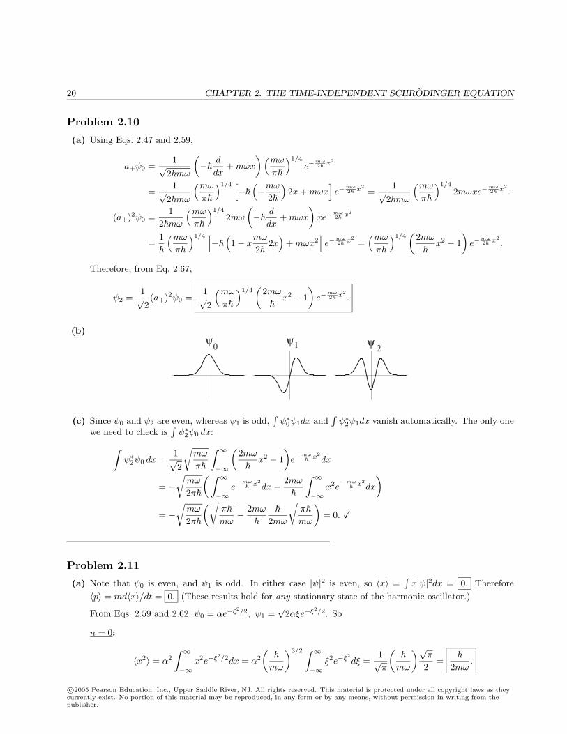
(b)ψ ψ ψ1 20
(c) Since ψ0 and ψ2 are even, whereas ψ1 is odd,∫ψ∗0ψ1dx and
∫ψ∗2ψ1dx vanish automatically. The only one
we need to check is∫ψ∗2ψ0 dx:∫
ψ∗2ψ0 dx =1√2
√mω
π
∫ ∞−∞
(2mω
x2 − 1
)e−
mω
x2dx
= −√
mω
2π
( ∫ ∞−∞
e−mω
x2dx− 2mω
∫ ∞−∞
x2e−mω
x2dx
)= −
√mω
2π
(√π
mω− 2mω
2mω
√π
mω
)= 0.
Problem 2.11
(a) Note that ψ0 is even, and ψ1 is odd. In either case |ψ|2 is even, so 〈x〉 =∫x|ψ|2dx = 0. Therefore
〈p〉 = md〈x〉/dt = 0. (These results hold for any stationary state of the harmonic oscillator.)
From Eqs. 2.59 and 2.62, ψ0 = αe−ξ2/2, ψ1 =√
2αξe−ξ2/2. So
n = 0:
〈x2〉 = α2
∫ ∞−∞
x2e−ξ2/2dx = α2
(
mω
)3/2 ∫ ∞−∞
ξ2e−ξ2dξ =
1√π
(
mω
)√π
2=
2mω.
c©2005 Pearson Education, Inc., Upper Saddle River, NJ. All rights reserved. This material is protected under all copyright laws as theycurrently exist. No portion of this material may be reproduced, in any form or by any means, without permission in writing from thepublisher.
CHAPTER 2. THE TIME-INDEPENDENT SCHRODINGER EQUATION 21
〈p2〉 =∫
ψ0
(
i
d
dx
)2
ψ0 dx = −2α2
√mω
∫ ∞−∞
e−ξ2/2
(d2
dξ2e−ξ2/2
)dξ
= −mω√π
∫ ∞−∞
(ξ2 − 1
)e−ξ2/2dξ = −mω√
π
(√π
2−√π
)=
mω
2.
n = 1:
〈x2〉 = 2α2
∫ ∞−∞
x2ξ2e−ξ2dx = 2α2
(
mω
)3/2 ∫ ∞−∞
ξ4e−ξ2dξ =
2√πmω
3√π
4=
32mω
.
〈p2〉 = −22α2
√mω
∫ ∞−∞
ξe−ξ2/2
[d2
dξ2
(ξe−ξ2/2
)]dξ
= −2mω√π
∫ ∞−∞
(ξ4 − 3ξ2
)e−ξ2
dξ = −2mω√π
(34√π − 3
√π
2
)=
3mω2
.
(b) n = 0:
σx =√〈x2〉 − 〈x〉2 =
√
2mω; σp =
√〈p2〉 − 〈p〉2 =
√mω
2;
σxσp =
√
2mω
√mω
2=
2. (Right at the uncertainty limit.)
n = 1:
σx =
√3
2mω; σp =
√3mω
2; σxσp = 3
2>
2.
(c)
〈T 〉 =1
2m〈p2〉 =
14ω (n = 0)
34ω (n = 1)
; 〈V 〉 =12mω2〈x2〉 =
14ω (n = 0)
34ω (n = 1)
.
〈T 〉+ 〈V 〉 = 〈H〉 =
12ω (n = 0) = E0
32ω (n = 1) = E1
, as expected.
Problem 2.12
From Eq. 2.69,
x =
√
2mω(a+ + a−), p = i
√mω
2(a+ − a−),
so
〈x〉 =
√
2mω
∫ψ∗n(a+ + a−)ψn dx.
c©2005 Pearson Education, Inc., Upper Saddle River, NJ. All rights reserved. This material is protected under all copyright laws as theycurrently exist. No portion of this material may be reproduced, in any form or by any means, without permission in writing from thepublisher.
22 CHAPTER 2. THE TIME-INDEPENDENT SCHRODINGER EQUATION
But (Eq. 2.66)a+ψn =
√n + 1ψn+1, a−ψn =
√nψn−1.
So
〈x〉 =
√
2mω
[√n + 1
∫ψ∗nψn+1 dx +
√n
∫ψ∗nψn−1 dx
]= 0 (by orthogonality).
〈p〉 = md〈x〉dt
= 0. x2 =
2mω(a+ + a−)2 =
2mω
(a2+ + a+a− + a−a+ + a2
−).
〈x2〉 =
2mω
∫ψ∗n
(a2+ + a+a− + a−a+ + a2
−)ψn. But
a2+ψn = a+
(√n + 1ψn+1
)=√n + 1
√n + 2ψn+2 =
√(n + 1)(n + 2)ψn+2.
a+a−ψn = a+
(√nψn−1
)=√n√nψn = nψn.
a−a+ψn = a−(√
n + 1ψn+1
)=
√n + 1)
√n + 1ψn = (n + 1)ψn.
a2−ψn = a−
(√nψn−1
)=√n√n− 1ψn−2 =
√(n− 1)nψn−2.
So
〈x2〉 =
2mω
[0 + n
∫|ψn|2dx + (n + 1)
∫|ψn|2 dx + 0
]=
2mω(2n + 1) =
(n +
12
)
mω.
p2 = −mω
2(a+ − a−)2 = −mω
2(a2+ − a+a− − a−a+ + a2
−)⇒
〈p2〉 = −mω
2[0− n− (n + 1) + 0] =
mω
2(2n + 1) =
(n +
12
)mω.
〈T 〉 = 〈p2/2m〉 =12
(n +
12
)ω .
σx =√〈x2〉 − 〈x〉2 =
√n +
12
√
mω; σp =
√〈p2〉 − 〈p〉2 =
√n +
12
√mω; σxσp =
(n +
12
) ≥
2.
Problem 2.13
(a)
1 =∫|Ψ(x, 0)|2dx = |A|2
∫ (9|ψ0|2 + 12ψ∗0ψ1 + 12ψ∗1ψ0 + 16|ψ1|2
)dx
= |A|2(9 + 0 + 0 + 16) = 25|A|2 ⇒ A = 1/5.
c©2005 Pearson Education, Inc., Upper Saddle River, NJ. All rights reserved. This material is protected under all copyright laws as theycurrently exist. No portion of this material may be reproduced, in any form or by any means, without permission in writing from thepublisher.
CHAPTER 2. THE TIME-INDEPENDENT SCHRODINGER EQUATION 23
(b)
Ψ(x, t) =15
[3ψ0(x)e−iE0t/ + 4ψ1(x)e−iE1t/
]=
15
[3ψ0(x)e−iωt/2 + 4ψ1(x)e−3iωt/2
].
(Here ψ0 and ψ1 are given by Eqs. 2.59 and 2.62; E1 and E2 by Eq. 2.61.)
|Ψ(x, t)|2 =125
[9ψ2
0 + 12ψ0ψ1eiωt/2e−3iωt/2 + 12ψ0ψ1e
−iωt/2e3iωt/2 + 16ψ21
]=
125
[9ψ2
0 + 16ψ21 + 24ψ0ψ1 cos(ωt)
].
(c)
〈x〉 =125
[9
∫xψ2
0 dx + 16∫
xψ21 dx + 24 cos(ωt)
∫xψ0ψ1 dx
].
But∫xψ2
0 dx =∫xψ2
1 dx = 0 (see Problem 2.11 or 2.12), while
∫xψ0ψ1 dx =
√mω
π
√2mω
∫xe−
mω2 x2
xe−mω2 x2
dx =
√2π
(mω
) ∫ ∞−∞
x2e−mω
x2dx
=
√2π
(mω
)2√π2
(12
√
mω
)3
=
√
2mω.
So
〈x〉 =2425
√
2mωcos(ωt); 〈p〉 = m
d
dt〈x〉 = −24
25
√mω
2sin(ωt).
(With ψ2 in place of ψ1 the frequency would be (E2 − E0)/ = [(5/2)ω − (1/2)ω]/ = 2ω.)
Ehrenfest’s theorem says d〈p〉/dt = −〈∂V/∂x〉. Here
d〈p〉dt
= −2425
√mω
2ω cos(ωt), V =
12mω2x2 ⇒ ∂V
∂x= mω2x,
so
−⟨∂V∂x
⟩= −mω2〈x〉 = −mω2 24
25
√
2mωcos(ωt) = −24
25
√mω
2ω cos(ωt),
so Ehrenfest’s theorem holds.
(d) You could get E0 = 12ω, with probability |c0|2 = 9/25, or E1 = 3
2ω, with probability |c1|2 = 16/25.
Problem 2.14
The new allowed energies are E′n = (n + 12 )ω′ = 2(n + 1
2 )ω = ω, 3ω, 5ω, . . . . So the probability ofgetting 1
2ω is zero. The probability of getting ω (the new ground state energy) is P0 = |c0|2, where c0 =∫Ψ(x, 0)ψ′0 dx, with
Ψ(x, 0) = ψ0(x) =(mω
π
)1/4
e−mω2 x2
, ψ0(x)′ =(m2ωπ
)1/4
e−m2ω2 x2
.
c©2005 Pearson Education, Inc., Upper Saddle River, NJ. All rights reserved. This material is protected under all copyright laws as theycurrently exist. No portion of this material may be reproduced, in any form or by any means, without permission in writing from thepublisher.
24 CHAPTER 2. THE TIME-INDEPENDENT SCHRODINGER EQUATION
So
c0 = 21/4
√mω
π
∫ ∞−∞
e−3mω2 x2
dx = 21/4
√mω
π2√π
(12
√2
3mω
)= 21/4
√23.
Therefore
P0 =23
√2 = 0.9428.
Problem 2.15
ψ0 =(mω
π
)1/4
e−ξ2/2, so P = 2√
mω
π
∫ ∞x0
e−ξ2dx = 2
√mω
π
√
mω
∫ ∞ξ0
e−ξ2dξ.
Classically allowed region extends out to: 12mω2x2
0 = E0 = 12ω, or x0 =
√
mω , so ξ0 = 1.
P =2√π
∫ ∞1
e−ξ2dξ = 2(1− F (
√2)) (in notation of CRC Table) = 0.157.
Problem 2.16
n = 5: j = 1 ⇒ a3 = −2(5−1)(1+1)(1+2)a1 = − 4
3a1; j = 3 ⇒ a5 = −2(5−3)(3+1)(3+2)a3 = − 1
5a3 = 415a1; j = 5 ⇒ a7 = 0. So
H5(ξ) = a1ξ − 43a1ξ
3 + 415a1ξ
5 = a115 (15ξ − 20ξ3 + 4ξ5). By convention the coefficient of ξ5 is 25, so a1 = 15 · 8,
and H5(ξ) = 120ξ − 160ξ3 + 32ξ5 (which agrees with Table 2.1).
n = 6: j = 0 ⇒ a2 = −2(6−0)(0+1)(0+2)a0 = −6a0; j = 2 ⇒ a4 = −2(6−2)
(2+1)(2+2)a2 = − 23a2 = 4a0; j = 4 ⇒ a6 =
−2(6−4)(4+1)(4+2)a4 = − 2
15a4 = − 815a0; j = 6⇒ a8 = 0. So H6(ξ) = a0 − 6a0ξ
2 + 4a0ξ4 − 8
15ξ6a0. The coefficient of ξ6
is 26, so 26 = − 815a0 ⇒ a0 = −15 · 8 = −120. H6(ξ) = −120 + 720ξ2 − 480ξ4 + 64ξ6.
Problem 2.17
(a)
d
dξ(e−ξ2
) = −2ξe−ξ2;
(d
dξ
)2
e−ξ2=
d
dξ(−2ξe−ξ2
) = (−2 + 4ξ2)e−ξ2;
(d
dξ
)3
e−ξ2=
d
dξ
[(−2 + 4ξ2)e−ξ2
]=
[8ξ + (−2 + 4ξ2)(−2ξ)
]e−ξ2
= (12ξ − 8ξ3)e−ξ2;
(d
dξ
)4
e−ξ2=
d
dξ
[(12ξ − 8ξ3)e−ξ2
]=
[12− 24ξ2 + (12ξ − 8ξ3)(−2ξ)
]e−ξ2
= (12− 48ξ2 + 16ξ4)e−ξ2.
H3(ξ) = −eξ2(
d
dξ
)3
e−ξ2= −12ξ + 8ξ3; H4(ξ) = eξ2
(d
dξ
)4
e−ξ2= 12− 48ξ2 + 16ξ4.
c©2005 Pearson Education, Inc., Upper Saddle River, NJ. All rights reserved. This material is protected under all copyright laws as theycurrently exist. No portion of this material may be reproduced, in any form or by any means, without permission in writing from thepublisher.
CHAPTER 2. THE TIME-INDEPENDENT SCHRODINGER EQUATION 25
(b)
H5 = 2ξH4 − 8H3 = 2ξ(12− 48ξ2 + 16ξ4)− 8(−12ξ + 8ξ3) = 120ξ − 160ξ3 + 32ξ5.
H6 = 2ξH5 − 10H4 = 2ξ(120ξ − 160ξ3 + 32ξ5)− 10(12− 48ξ2 + 16ξ4) = −120 + 720ξ2 − 480ξ4 + 64ξ6.
(c)
dH5
dξ= 120− 480ξ2 + 160ξ4 = 10(12− 48ξ2 + 16ξ4) = (2)(5)H4.
dH6
dξ= 1440ξ − 1920ξ3 + 384ξ5 = 12(120ξ − 160ξ3 + 32ξ5) = (2)(6)H5.
(d)
d
dz(e−z2+2zξ) = (−2z + ξ)e−z2+2zξ; setting z = 0, H0(ξ) = 2ξ.
(d
dz
)2
(e−z2+2zξ) =d
dz
[(−2z + 2ξ)e−z2+2zξ
]=
[− 2 + (−2z + 2ξ)2
]e−z2+2zξ; setting z = 0, H1(ξ) = −2 + 4ξ2.
(d
dz
)3
(e−z2+2zξ) =d
dz
[− 2 + (−2z + 2ξ)2
]e−z2+2zξ
=
2(−2z + 2ξ)(−2) +
[− 2 + (−2z + 2ξ)2
](−2z + 2ξ)
e−z2+2zξ;
setting z = 0, H2(ξ) = −8ξ + (−2 + 4ξ2)(2ξ) = −12ξ + 8ξ3.
Problem 2.18
Aeikx + Be−ikx = A(cos kx + i sin kx) + B(cos kx− i sin kx) = (A + B) cos kx + i(A−B) sin kx
= C cos kx + D sin kx, with C = A + B; D = i(A−B).
C cos kx + D sin kx = C
(eikx + e−ikx
2
)+ D
(eikx − e−ikx
2i
)=
12(C − iD)eikx +
12(C + iD)e−ikx
= Aeikx + Be−ikx, with A =12(C − iD); B =
12(C + iD).
c©2005 Pearson Education, Inc., Upper Saddle River, NJ. All rights reserved. This material is protected under all copyright laws as theycurrently exist. No portion of this material may be reproduced, in any form or by any means, without permission in writing from thepublisher.
26 CHAPTER 2. THE TIME-INDEPENDENT SCHRODINGER EQUATION
Problem 2.19
Equation 2.94 says Ψ = Aei(kx− k22m t), so
J =i
2m
(Ψ
∂Ψ∗
∂x−Ψ∗
∂Ψ∂x
)=
i
2m|A|2
[ei(kx− k22m t)(−ik)e−i(kx− k22m t) − e−i(kx− k22m t)(ik)ei(kx− k22m t)
]=
i
2m|A|2(−2ik) =
k
m|A|2.
It flows in the positive (x) direction (as you would expect).
Problem 2.20
(a)
f(x) = b0 +∞∑
n=1
an
2i
(einπx/a − e−inπx/a
)+∞∑
n=1
bn
2
(einπx/a + e−inπx/a
)= b0 +
∞∑n=1
(an
2i+
bn
2
)einπx/a +
∞∑n=1
(−an
2i+
bn
2
)e−inπx/a.
Let
c0 ≡ b0; cn = 12 (−ian + bn) , for n = 1, 2, 3, . . . ; cn ≡ 1
2 (ia−n + b−n) , for n = −1,−2,−3, . . . .
Then f(x) =∞∑
n=−∞cne
inπx/a. QED
(b) ∫ a
−a
f(x)e−imπx/adx =∞∑
n=−∞cn
∫ a
−a
ei(n−m)πx/adx. But for n = m,
∫ a
−a
ei(n−m)πx/adx =ei(n−m)πx/a
i(n−m)π/a
∣∣∣∣a−a
=ei(n−m)π − e−i(n−m)π
i(n−m)π/a=
(−1)n−m − (−1)n−m
i(n−m)π/a= 0,
whereas for n = m,∫ a
−a
ei(n−m)πx/adx =∫ a
−a
dx = 2a.
So all terms except n = m are zero, and∫ a
−a
f(x)e−imπx/a = 2acm, so cn =12a
∫ a
−a
f(x)e−inπx/adx. QED
(c)
f(x) =∞∑
n=−∞
√π
21aF (k)eikx =
1√2π
∑F (k)eikx∆k,
c©2005 Pearson Education, Inc., Upper Saddle River, NJ. All rights reserved. This material is protected under all copyright laws as theycurrently exist. No portion of this material may be reproduced, in any form or by any means, without permission in writing from thepublisher.
CHAPTER 2. THE TIME-INDEPENDENT SCHRODINGER EQUATION 27
where ∆k ≡ π
ais the increment in k from n to (n + 1).
F (k) =
√2πa
12a
∫ a
−a
f(x)e−ikxdx =1√2π
∫ a
−a
f(x)e−ikxdx.
(d) As a→∞, k becomes a continuous variable,
f(x) =1√2π
∫ ∞−∞
F (k)eikxdk; F (k) =1√2π
∫ ∞−∞
f(x)eikxdx.
Problem 2.21
(a)
1 =∫ ∞−∞
|Ψ(x, 0)|2dx = 2|A|2∫ ∞
0
e−2axdx = 2|A|2 e−2ax
−2a
∣∣∣∣∞0
=|A|2a⇒ A =
√a.
(b)
φ(k) =A√2π
∫ ∞−∞
e−a|x|e−ikx dx =A√2π
∫ ∞−∞
e−a|x|(cos kx− i sin kx)dx.
The cosine integrand is even, and the sine is odd, so the latter vanishes and
φ(k) = 2A√2π
∫ ∞0
e−ax cos kx dx =A√2π
∫ ∞0
e−ax(eikx + e−ikx
)dx
=A√2π
∫ ∞0
(e(ik−a)x + e−(ik+a)x
)dx =
A√2π
[e(ik−a)x
ik − a+
e−(ik+a)x
−(ik + a)
]∣∣∣∣∞0
=A√2π
( −1ik − a
+1
ik + a
)=
A√2π−ik − a + ik − a
−k2 − a2=
√a
2π2a
k2 + a2.
(c)
Ψ(x, t) =1√2π
2
√a3
2π
∫ ∞−∞
1k2 + a2
ei(kx− k22m t)dk =a3/2
π
∫ ∞−∞
1k2 + a2
ei(kx− k22m t)dk.
(d) For large a, Ψ(x, 0) is a sharp narrow spike whereas φ(k) ∼=√
2/πa is broad and flat; position is well-defined but momentum is ill-defined. For small a, Ψ(x, 0) is a broad and flat whereas φ(k) ∼= (
√2a3/π)/k2
is a sharp narrow spike; position is ill-defined but momentum is well-defined.
c©2005 Pearson Education, Inc., Upper Saddle River, NJ. All rights reserved. This material is protected under all copyright laws as theycurrently exist. No portion of this material may be reproduced, in any form or by any means, without permission in writing from thepublisher.
28 CHAPTER 2. THE TIME-INDEPENDENT SCHRODINGER EQUATION
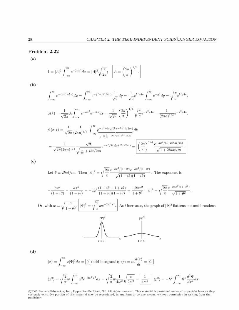
Problem 2.22
(a)
1 = |A|2∫ ∞−∞
e−2ax2dx = |A|2
√π
2a; A =
(2aπ
)1/4
.
(b) ∫ ∞−∞
e−(ax2+bx)dx =∫ ∞−∞
e−y2+(b2/4a) 1√ady =
1√aeb2/4a
∫ ∞−∞
e−y2dy =
√π
aeb2/4a.
φ(k) =1√2π
A
∫ ∞−∞
e−ax2e−ikxdx =
1√2π
(2aπ
)1/4 √π
ae−k2/4a =
1(2πa)1/4
e−k2/4a.
Ψ(x, t) =1√2π
1(2πa)1/4
∫ ∞−∞
e−k2/4aei(kx−k2t/2m)︸ ︷︷ ︸e−[( 1
4a+it/2m)k2−ixk]
dk
=1√
2π(2πa)1/4
√π√
14a + it/2m
e−x2/4( 14a+it/2m) =
(2aπ
)1/4e−ax2/(1+2iat/m)√
1 + 2iat/m.
(c)
Let θ ≡ 2at/m. Then |Ψ|2 =
√2aπ
e−ax2/(1+iθ)e−ax2/(1−iθ)√(1 + iθ)(1− iθ)
. The exponent is
− ax2
(1 + iθ)− ax2
(1− iθ)= −ax2 (1− iθ + 1 + iθ)
(1 + iθ)(1− iθ)=−2ax2
1 + θ2; |Ψ|2 =
√2aπ
e−2ax2/(1+θ2)
√1 + θ2
.
Or, with w ≡√
a
1 + θ2, |Ψ|2 =
√2πwe−2w2x2
. As t increases, the graph of |Ψ|2 flattens out and broadens.
|Ψ|2 |Ψ|2
x xt = 0 t > 0
(d)
〈x〉 =∫ ∞−∞
x|Ψ|2dx = 0 (odd integrand); 〈p〉 = md〈x〉dt
= 0.
〈x2〉 =
√2πw
∫ ∞−∞
x2e−2w2x2dx =
√2πw
14w2
√π
2w2=
14w2
. 〈p2〉 = −2
∫ ∞−∞
Ψ∗d2Ψdx2
dx.
c©2005 Pearson Education, Inc., Upper Saddle River, NJ. All rights reserved. This material is protected under all copyright laws as theycurrently exist. No portion of this material may be reproduced, in any form or by any means, without permission in writing from thepublisher.
CHAPTER 2. THE TIME-INDEPENDENT SCHRODINGER EQUATION 29
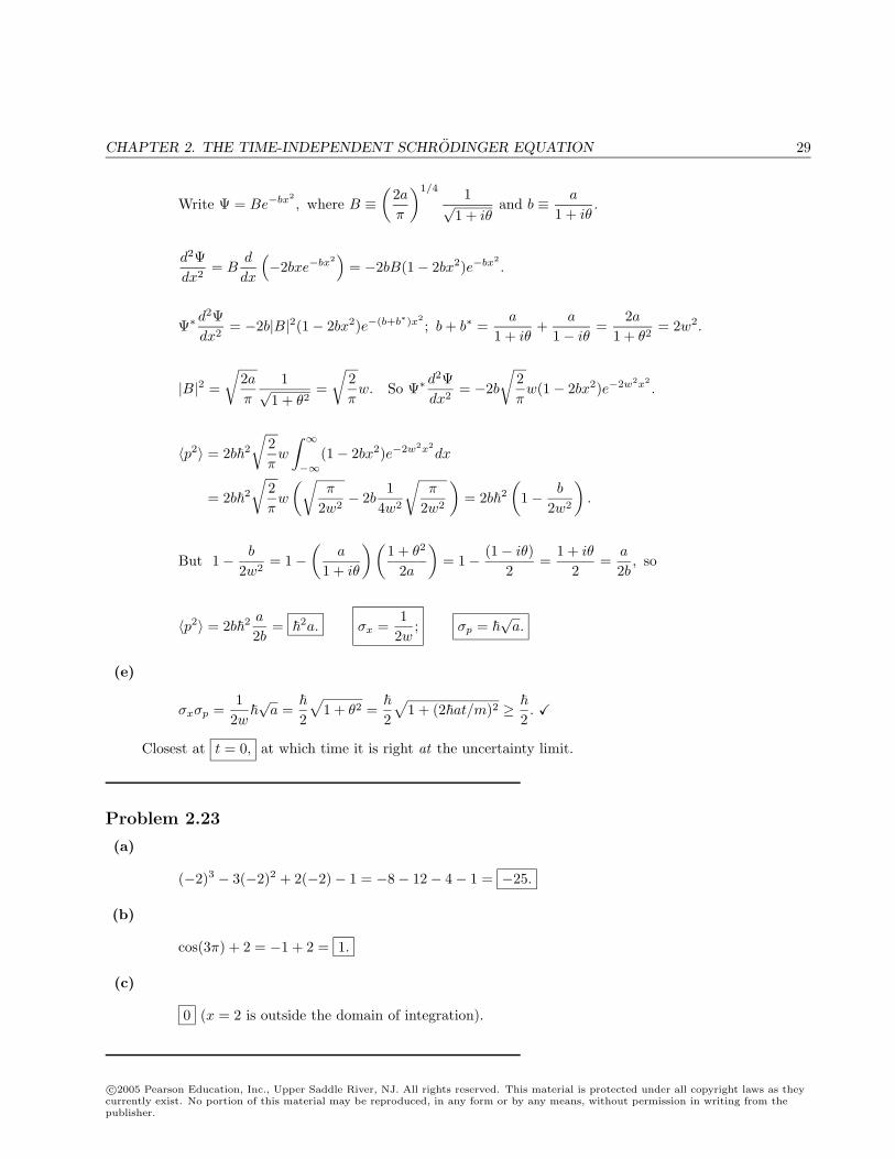
Write Ψ = Be−bx2, where B ≡
(2aπ
)1/4 1√1 + iθ
and b ≡ a
1 + iθ.
d2Ψdx2
= Bd
dx
(−2bxe−bx2
)= −2bB(1− 2bx2)e−bx2
.
Ψ∗d2Ψdx2
= −2b|B|2(1− 2bx2)e−(b+b∗)x2; b + b∗ =
a
1 + iθ+
a
1− iθ=
2a1 + θ2
= 2w2.
|B|2 =
√2aπ
1√1 + θ2
=
√2πw. So Ψ∗
d2Ψdx2
= −2b
√2πw(1− 2bx2)e−2w2x2
.
〈p2〉 = 2b2
√2πw
∫ ∞−∞
(1− 2bx2)e−2w2x2dx
= 2b2
√2πw
(√π
2w2− 2b
14w2
√π
2w2
)= 2b2
(1− b
2w2
).
But 1− b
2w2= 1−
(a
1 + iθ
) (1 + θ2
2a
)= 1− (1− iθ)
2=
1 + iθ
2=
a
2b, so
〈p2〉 = 2b2 a
2b=
2a. σx =1
2w; σp =
√a.
(e)
σxσp =1
2w√a =
2
√1 + θ2 =
2
√1 + (2at/m)2 ≥
2.
Closest at t = 0, at which time it is right at the uncertainty limit.
Problem 2.23
(a)
(−2)3 − 3(−2)2 + 2(−2)− 1 = −8− 12− 4− 1 = −25.
(b)
cos(3π) + 2 = −1 + 2 = 1.
(c)
0 (x = 2 is outside the domain of integration).
c©2005 Pearson Education, Inc., Upper Saddle River, NJ. All rights reserved. This material is protected under all copyright laws as theycurrently exist. No portion of this material may be reproduced, in any form or by any means, without permission in writing from thepublisher.
30 CHAPTER 2. THE TIME-INDEPENDENT SCHRODINGER EQUATION
Problem 2.24
(a) Let y ≡ cx, so dx =1cdy.
If c > 0, y : −∞→∞.If c < 0, y :∞→ −∞.
∫ ∞−∞
f(x)δ(cx)dx =
1c
∫∞−∞ f(y/c)δ(y)dy = 1
cf(0) (c > 0); or
1c
∫ −∞∞ f(y/c)δ(y)dy = − 1
c
∫∞−∞ f(y/c)δ(y)dy = − 1
cf(0) (c < 0).
In either case,∫ ∞−∞
f(x)δ(cx)dx =1|c|f(0) =
∫ ∞−∞
f(x)1|c|δ(x)dx. So δ(cx) =
1|c|δ(x).
(b) ∫ ∞−∞
f(x)dθ
dxdx = fθ
∣∣∣∣∞−∞
−∫ ∞−∞
df
dxθdx (integration by parts)
= f(∞)−∫ ∞
0
df
dxdx = f(∞)− f(∞) + f(0) = f(0) =
∫ ∞−∞
f(x)δ(x)dx.
So dθ/dx = δ(x). [Makes sense: The θ function is constant (so derivative is zero) except at x = 0, wherethe derivative is infinite.]
Problem 2.25
ψ(x) =√mα
e−mα|x|/2 =
√mα
e−mαx/2 , (x ≥ 0),emαx/2 , (x ≤ 0).
〈x〉 = 0 (odd integrand).
〈x2〉 =∫ ∞−∞
x2|ψ|2dx = 2mα
2
∫ ∞0
x2e−2mαx/2dx =2mα
22
(
2
2mα
)3
=
4
2m2α2; σx =
2
√2mα
.
dψ
dx=√mα
−mα2
e−mαx/2 , (x ≥ 0)
mα2
emαx/2 , (x ≤ 0)
=(√
mα
)3 [−θ(x)e−mαx/2 + θ(−x)emαx/2
].
d2ψ
dx2=
(√mα
)3 [−δ(x)e−mαx/2 +
mα
2θ(x)e−mαx/2 − δ(−x)emαx/2 +
mα
2θ(−x)emαx/2
]=
(√mα
)3 [−2δ(x) +
mα
2e−mα|x|/2
].
In the last step I used the fact that δ(−x) = δ(x) (Eq. 2.142), f(x)δ(x) = f(0)δ(x) (Eq. 2.112), and θ(−x) +θ(x) = 1 (Eq. 2.143). Since dψ/dx is an odd function, 〈p〉 = 0.
〈p2〉 = −2
∫ ∞−∞
ψd2ψ
dx2dx = −2
√mα
(√mα
)3 ∫ ∞−∞
e−mα|x|/2[−2δ(x) +
mα
2e−mα|x|/2
]dx
=(mα
)2[2− 2
mα
2
∫ ∞0
e−2mαx/2 dx
]= 2
(mα
)2[1− mα
2
2
2mα
]=
(mα
)2
.
Evidently
σp =mα
, so σxσp =
2
√2mα
mα
=√
2
2>
2.
c©2005 Pearson Education, Inc., Upper Saddle River, NJ. All rights reserved. This material is protected under all copyright laws as theycurrently exist. No portion of this material may be reproduced, in any form or by any means, without permission in writing from thepublisher.
CHAPTER 2. THE TIME-INDEPENDENT SCHRODINGER EQUATION 31
Problem 2.26
Put f(x) = δ(x) into Eq. 2.102: F (k) =1√2π
∫ ∞−∞
δ(x)e−ikxdx =1√2π
.
∴ f(x) = δ(x) =1√2π
∫ ∞−∞
1√2π
eikxdk =12π
∫ ∞−∞
eikxdk. QED
Problem 2.27
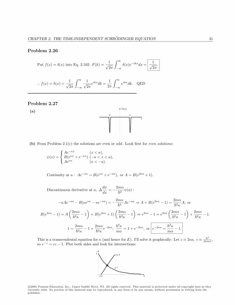
(a)V(x)
-a a
x
(b) From Problem 2.1(c) the solutions are even or odd. Look first for even solutions:
ψ(x) =
Ae−κx (x < a),B(eκx + e−κx) (−a < x < a),Aeκx (x < −a).
Continuity at a : Ae−κa = B(eκa + e−κa), or A = B(e2κa + 1).
Discontinuous derivative at a, ∆dψ
dx= −2mα
2ψ(a) :
−κAe−κa −B(κeκa − κe−κa) = −2mα
2Ae−κa ⇒ A + B(e2κa − 1) =
2mα
2κA; or
B(e2κa − 1) = A
(2mα
2κ− 1
)= B(e2κa + 1)
(2mα
2κ− 1
)⇒ e2κa − 1 = e2κa
(2mα
2κ− 1
)+
2mα
2κ− 1.
1 =2mα
2κ− 1 +
2mα
2κe−2κa;
2κ
mα= 1 + e−2κa, or e−2κa =
2κ
mα− 1.
This is a transcendental equation for κ (and hence for E). I’ll solve it graphically: Let z ≡ 2κa, c ≡ 2
2amα ,so e−z = cz − 1. Plot both sides and look for intersections:
1
z1/c
cz-1
e-z
c©2005 Pearson Education, Inc., Upper Saddle River, NJ. All rights reserved. This material is protected under all copyright laws as theycurrently exist. No portion of this material may be reproduced, in any form or by any means, without permission in writing from thepublisher.
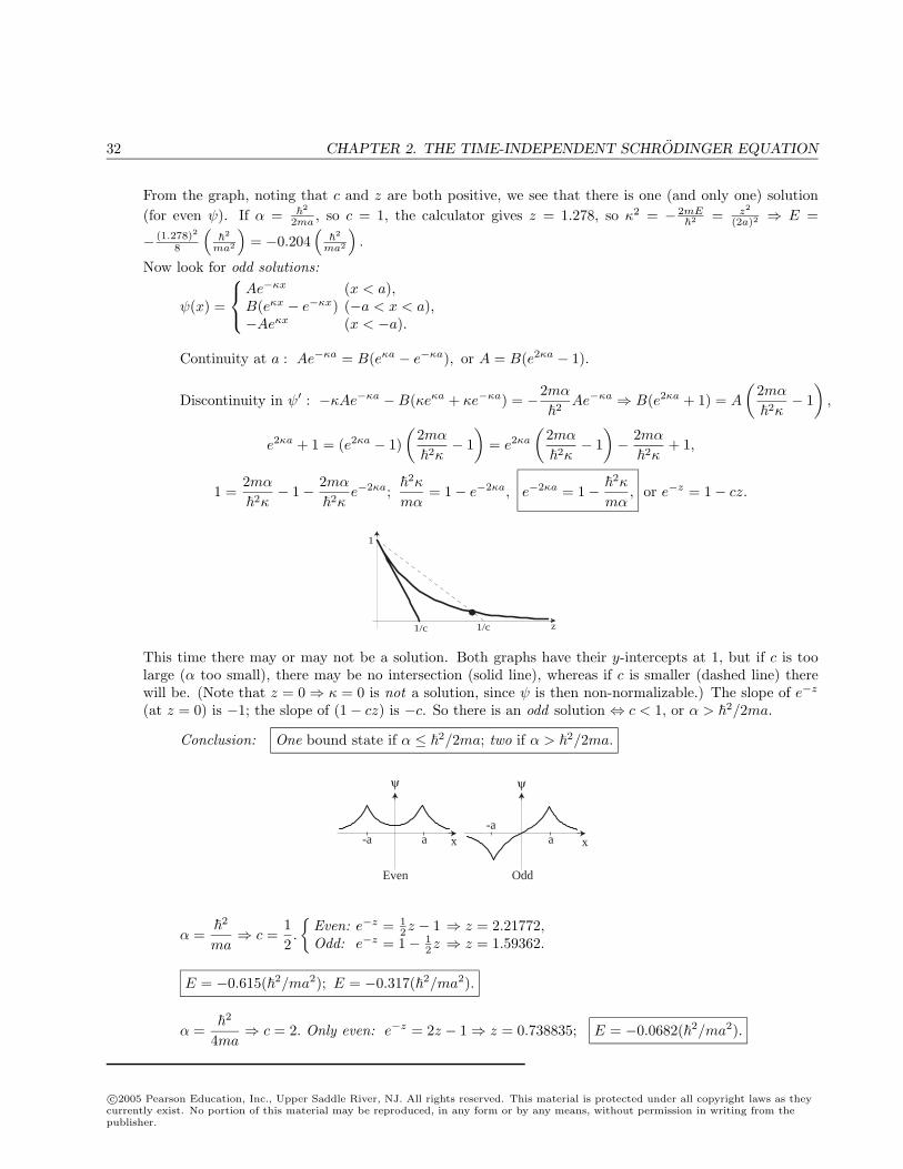
32 CHAPTER 2. THE TIME-INDEPENDENT SCHRODINGER EQUATION
From the graph, noting that c and z are both positive, we see that there is one (and only one) solution(for even ψ). If α =
2
2ma , so c = 1, the calculator gives z = 1.278, so κ2 = − 2mE2
= z2
(2a)2 ⇒ E =
− (1.278)2
8
(2
ma2
)= −0.204
(2
ma2
).
Now look for odd solutions:
ψ(x) =
Ae−κx (x < a),B(eκx − e−κx) (−a < x < a),−Aeκx (x < −a).
Continuity at a : Ae−κa = B(eκa − e−κa), or A = B(e2κa − 1).
Discontinuity in ψ′ : −κAe−κa −B(κeκa + κe−κa) = −2mα
2Ae−κa ⇒ B(e2κa + 1) = A
(2mα
2κ− 1
),
e2κa + 1 = (e2κa − 1)(
2mα
2κ− 1
)= e2κa
(2mα
2κ− 1
)− 2mα
2κ+ 1,
1 =2mα
2κ− 1− 2mα
2κe−2κa;
2κ
mα= 1− e−2κa, e−2κa = 1−
2κ
mα, or e−z = 1− cz.
1/c 1/c
1
z
This time there may or may not be a solution. Both graphs have their y-intercepts at 1, but if c is toolarge (α too small), there may be no intersection (solid line), whereas if c is smaller (dashed line) therewill be. (Note that z = 0 ⇒ κ = 0 is not a solution, since ψ is then non-normalizable.) The slope of e−z
(at z = 0) is −1; the slope of (1− cz) is −c. So there is an odd solution ⇔ c < 1, or α > 2/2ma.
Conclusion: One bound state if α ≤ 2/2ma; two if α > 2/2ma.
ψ ψ
x xa-a a-a
Even Odd
α =
2
ma⇒ c =
12.
Even: e−z = 1
2z − 1 ⇒ z = 2.21772,Odd: e−z = 1− 1
2z ⇒ z = 1.59362.
E = −0.615(2/ma2); E = −0.317(2/ma2).
α =
2
4ma⇒ c = 2. Only even: e−z = 2z − 1 ⇒ z = 0.738835; E = −0.0682(2/ma2).
c©2005 Pearson Education, Inc., Upper Saddle River, NJ. All rights reserved. This material is protected under all copyright laws as theycurrently exist. No portion of this material may be reproduced, in any form or by any means, without permission in writing from thepublisher.
CHAPTER 2. THE TIME-INDEPENDENT SCHRODINGER EQUATION 33
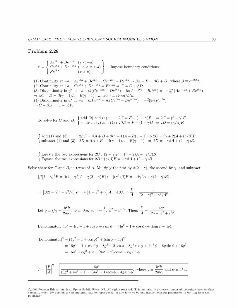
Problem 2.28
ψ =
Aeikx + Be−ikx (x < −a)Ceikx + De−ikx (−a < x < a)Feikx (x > a)
. Impose boundary conditions:
(1) Continuity at −a : Aeika + Beika = Ce−ika + Deika ⇒ βA + B = βC + D, where β ≡ e−2ika.(2) Continuity at +a : Ceika + De−ika = Feika ⇒ F = C + βD.(3) Discontinuity in ψ′ at −a : ik(Ce−ika −Deika)− ik(Ae−ika −Beika) = − 2mα
2(Ae−ika + Beika)
⇒ βC −D = β(γ + 1)A + B(γ − 1), where γ ≡ i2mα/2k.(4) Discontinuity in ψ′ at +a : ikFeika − ik(Ceika −De−ika) = − 2mα
2(Feika)
⇒ C − βD = (1− γ)F.
To solve for C and D,
add (2) and (4) : 2C = F + (1− γ)F ⇒ 2C = (2− γ)F.subtract (2) and (4) : 2βD = F − (1− γ)F ⇒ 2D = (γ/β)F.
add (1) and (3) : 2βC = βA + B + β(γ + 1)A + B(γ − 1) ⇒ 2C = (γ + 2)A + (γ/β)B.subtract (1) and (3) : 2D = βA + B − β(γ + 1)A−B(γ − 1) ⇒ 2D = −γβA + (2− γ)B.
Equate the two expressions for 2C : (2− γ)F = (γ + 2)A + (γ/β)B.Equate the two expressions for 2D : (γ/β)F = −γβA + (2− γ)B.
Solve these for F and B, in terms of A. Multiply the first by β(2− γ), the second by γ, and subtract:[β(2− γ)2F = β(4− γ2)A + γ(2− γ)B
];
[(γ2/β)F = −βγ2A + γ(2− γ)B
].
⇒[β(2− γ)2 − γ2/β
]F = β
[4− γ2 + γ
]A = 4βA⇒ F
A=
4(2− γ)2 − γ2/β2
.
Let g ≡ i/γ =
2k
2mα; φ ≡ 4ka, so γ =
i
g, β2 = e−iφ. Then:
F
A=
4g2
(2g − i)2 + eiφ.
Denominator: 4g2 − 4ig − 1 + cosφ + i sinφ = (4g2 − 1 + cosφ) + i(sinφ− 4g).
|Denominator|2 = (4g2 − 1 + cosφ)2 + (sinφ− 4g)2
= 16g4 + 1 + cos2 φ− 8g2 − 2 cosφ + 8g2 cosφ + sin2 φ− 8g sinφ + 16g2
= 16g4 + 8g2 + 2 + (8g2 − 2) cosφ− 8g sinφ.
T =∣∣∣∣FA
∣∣∣∣2 =8g4
(8g4 + 4g2 + 1) + (4g2 − 1) cosφ− 4g sinφ, where g ≡
2k
2mαand φ ≡ 4ka.
c©2005 Pearson Education, Inc., Upper Saddle River, NJ. All rights reserved. This material is protected under all copyright laws as theycurrently exist. No portion of this material may be reproduced, in any form or by any means, without permission in writing from thepublisher.
34 CHAPTER 2. THE TIME-INDEPENDENT SCHRODINGER EQUATION
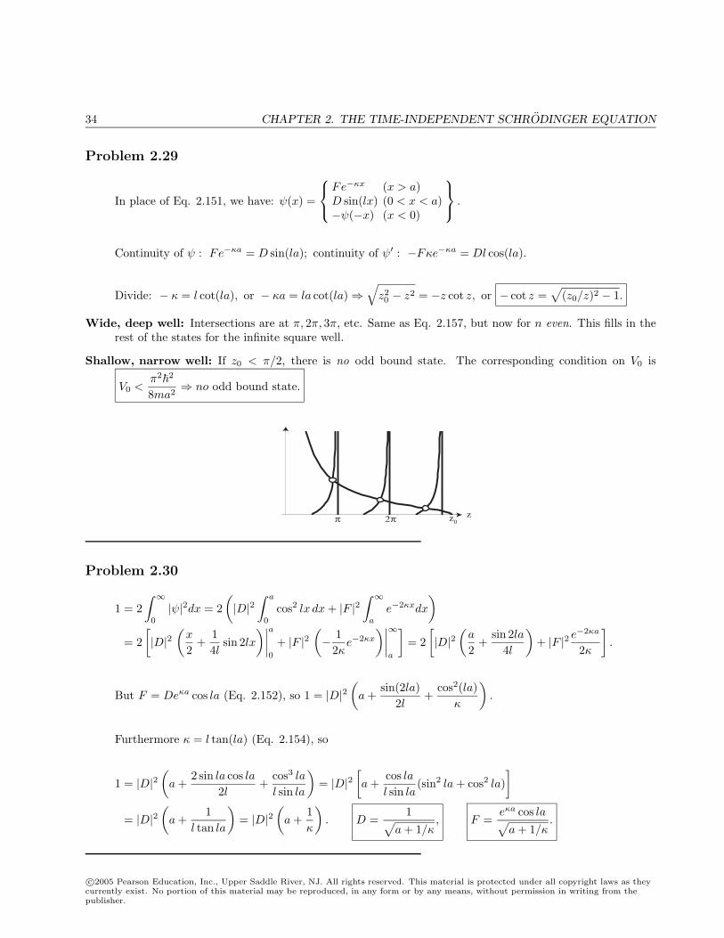
Problem 2.29
In place of Eq. 2.151, we have: ψ(x) =
Fe−κx (x > a)D sin(lx) (0 < x < a)−ψ(−x) (x < 0)
.
Continuity of ψ : Fe−κa = D sin(la); continuity of ψ′ : −Fκe−κa = Dl cos(la).
Divide: − κ = l cot(la), or − κa = la cot(la)⇒√
z20 − z2 = −z cot z, or − cot z =
√(z0/z)2 − 1.
Wide, deep well: Intersections are at π, 2π, 3π, etc. Same as Eq. 2.157, but now for n even. This fills in therest of the states for the infinite square well.
Shallow, narrow well: If z0 < π/2, there is no odd bound state. The corresponding condition on V0 is
V0 <π2
2
8ma2⇒ no odd bound state.
π 2π zz0
Problem 2.30
1 = 2∫ ∞
0
|ψ|2dx = 2(|D|2
∫ a
0
cos2 lx dx + |F |2∫ ∞
a
e−2κxdx
)= 2
[|D|2
(x
2+
14l
sin 2lx)∣∣∣∣a
0
+ |F |2(− 1
2κe−2κx
)∣∣∣∣∞a
]= 2
[|D|2
(a
2+
sin 2la4l
)+ |F |2 e
−2κa
2κ
].
But F = Deκa cos la (Eq. 2.152), so 1 = |D|2(a +
sin(2la)2l
+cos2(la)
κ
).
Furthermore κ = l tan(la) (Eq. 2.154), so
1 = |D|2(a +
2 sin la cos la2l
+cos3 la
l sin la
)= |D|2
[a +
cos lal sin la
(sin2 la + cos2 la)]
= |D|2(a +
1l tan la
)= |D|2
(a +
1κ
). D =
1√a + 1/κ
, F =eκa cos la√a + 1/κ
.
c©2005 Pearson Education, Inc., Upper Saddle River, NJ. All rights reserved. This material is protected under all copyright laws as theycurrently exist. No portion of this material may be reproduced, in any form or by any means, without permission in writing from thepublisher.
CHAPTER 2. THE TIME-INDEPENDENT SCHRODINGER EQUATION 35
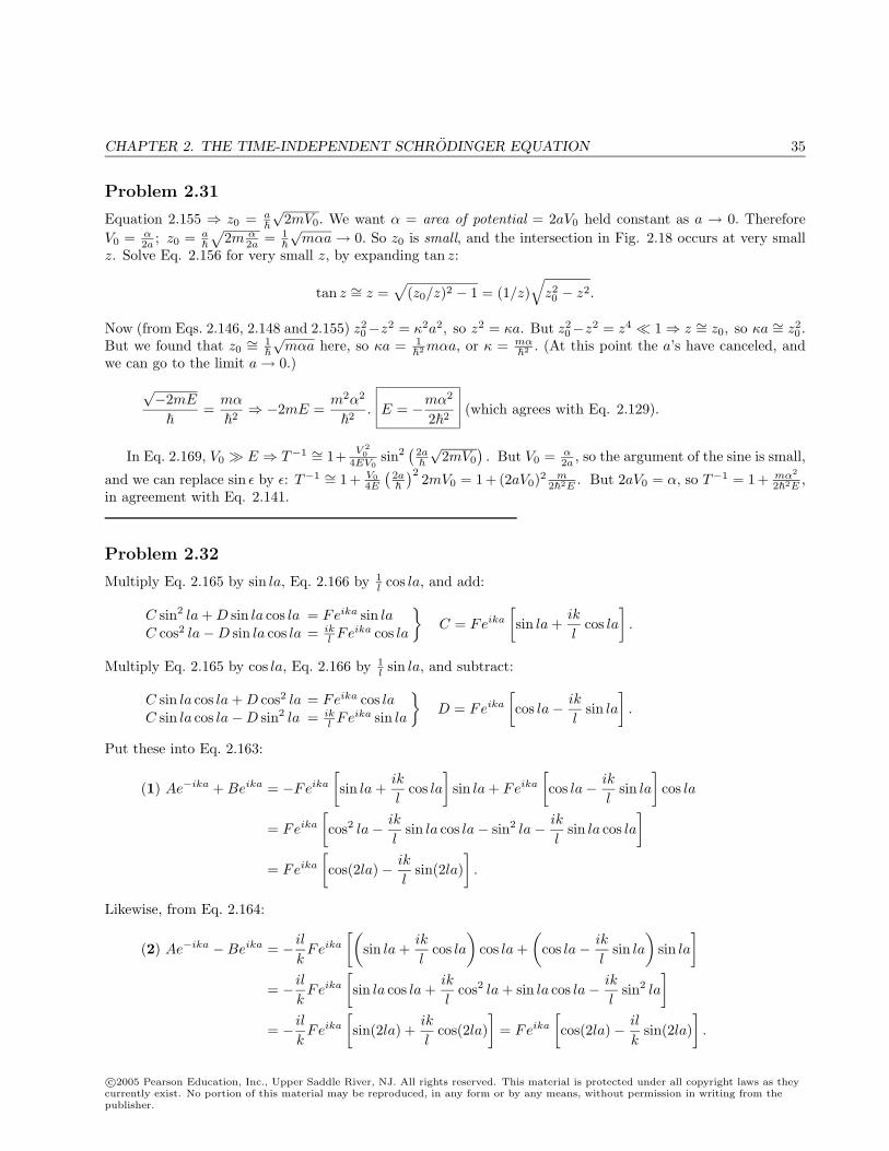
Problem 2.31
Equation 2.155 ⇒ z0 = a
√2mV0. We want α = area of potential = 2aV0 held constant as a → 0. Therefore
V0 = α2a ; z0 = a
√2m α
2a = 1
√mαa → 0. So z0 is small, and the intersection in Fig. 2.18 occurs at very small
z. Solve Eq. 2.156 for very small z, by expanding tan z:
tan z ∼= z =√
(z0/z)2 − 1 = (1/z)√
z20 − z2.
Now (from Eqs. 2.146, 2.148 and 2.155) z20−z2 = κ2a2, so z2 = κa. But z2
0−z2 = z4 1 ⇒ z ∼= z0, so κa ∼= z20 .
But we found that z0∼= 1
√mαa here, so κa = 1
2mαa, or κ = mα
2. (At this point the a’s have canceled, and
we can go to the limit a→ 0.)
√−2mE
=
mα
2⇒ −2mE =
m2α2
2. E = −mα2
22(which agrees with Eq. 2.129).
In Eq. 2.169, V0 E ⇒ T−1 ∼= 1+ V 20
4EV0sin2
(2a
√2mV0
). But V0 = α
2a , so the argument of the sine is small,
and we can replace sin ε by ε: T−1 ∼= 1+ V04E
(2a
)2 2mV0 = 1+(2aV0)2 m22E . But 2aV0 = α, so T−1 = 1+ mα2
22E ,in agreement with Eq. 2.141.
Problem 2.32
Multiply Eq. 2.165 by sin la, Eq. 2.166 by 1l cos la, and add:
C sin2 la + D sin la cos la = Feika sin laC cos2 la−D sin la cos la = ik
l Feika cos la
C = Feika
[sin la +
ik
lcos la
].
Multiply Eq. 2.165 by cos la, Eq. 2.166 by 1l sin la, and subtract:
C sin la cos la + D cos2 la = Feika cos laC sin la cos la−D sin2 la = ik
l Feika sin la
D = Feika
[cos la− ik
lsin la
].
Put these into Eq. 2.163:
(1) Ae−ika + Beika = −Feika
[sin la +
ik
lcos la
]sin la + Feika
[cos la− ik
lsin la
]cos la
= Feika
[cos2 la− ik
lsin la cos la− sin2 la− ik
lsin la cos la
]= Feika
[cos(2la)− ik
lsin(2la)
].
Likewise, from Eq. 2.164:
(2) Ae−ika −Beika = − il
kFeika
[(sin la +
ik
lcos la
)cos la +
(cos la− ik
lsin la
)sin la
]= − il
kFeika
[sin la cos la +
ik
lcos2 la + sin la cos la− ik
lsin2 la
]= − il
kFeika
[sin(2la) +
ik
lcos(2la)
]= Feika
[cos(2la)− il
ksin(2la)
].
c©2005 Pearson Education, Inc., Upper Saddle River, NJ. All rights reserved. This material is protected under all copyright laws as theycurrently exist. No portion of this material may be reproduced, in any form or by any means, without permission in writing from thepublisher.
36 CHAPTER 2. THE TIME-INDEPENDENT SCHRODINGER EQUATION
Add (1) and (2): 2Ae−ika = Feika
[2 cos(2la)− i
(k
l+
l
k
)sin(2la)
], or:
F =e−2ikaA
cos(2la)− i sin(2la)2kl (k2 + l2)
(confirming Eq. 2.168). Now subtract (2) from (1):
2Beika = Feika
[i
(l
k− k
l
)sin(2la)
]⇒ B = i
sin(2la)2kl
(l2 − k2)F (confirming Eq. 2.167).
T−1 =∣∣∣∣AF
∣∣∣∣2 =∣∣∣∣cos(2la)− i
sin(2la)2kl
(k2 + l2)∣∣∣∣2 = cos2(2la) +
sin2(2la)(2lk)2
(k2 + l2)2.
But cos2(2la) = 1− sin2(2la), so
T−1 = 1 + sin2(2la)[
(k2 + l2)2
(2lk)2− 1︸ ︷︷ ︸
1(2kl)2
[k4+2k2l2+l4−4k2l2]= 1(2kl)2
[k4−2k2l2+l4]=(k2−l2)2
(2kl)2.
]= 1 +
(k2 − l2)2
(2kl)2sin2(2la).
But k =√
2mE
, l =
√2m(E + V0)
; so (2la) =
2a
√2m(E + V0); k2 − l2 = −2mV0
2, and
(k2 − l2)2
(2kl)2=
(2m2
)2V 2
0
4(
2m2
)2E(E + V0)
=V 2
0
4E(E + V0).
∴ T−1 = 1 +V 2
0
4E(E + V0)sin2
(2a
√2m(E + V0)
), confirming Eq. 2.169.
Problem 2.33
E < V0. ψ =
Aeikx + Be−ikx (x < −a)Ceκx + De−κx (−a < x < a)Feikx (x > a)
k =√
2mE
; κ =
√2m(V0 − E)
.
(1) Continuity of ψ at −a: Ae−ika + Beika = Ce−κa + Deκa.
(2) Continuity of ψ′ at −a: ik(Ae−ika −Beika) = κ(Ce−κa −Deκa).
⇒ 2Ae−ika =(1− i
κ
k
)Ce−κa +
(1 + i
κ
k
)Deκa.
(3) Continuity of ψ at +a: Ceκa + De−κa = Feika.
(4) Continuity of ψ′ at +a: κ(Ceκa −De−κa) = ikFeika.
c©2005 Pearson Education, Inc., Upper Saddle River, NJ. All rights reserved. This material is protected under all copyright laws as theycurrently exist. No portion of this material may be reproduced, in any form or by any means, without permission in writing from thepublisher.
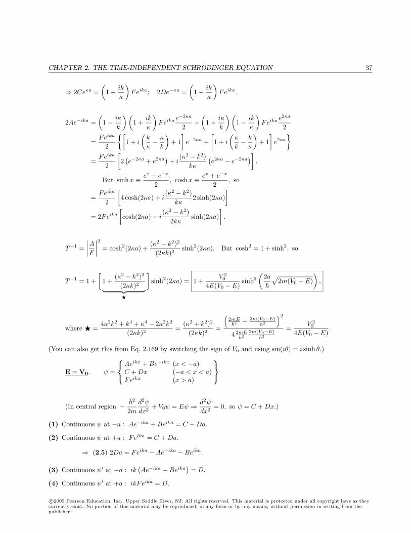
CHAPTER 2. THE TIME-INDEPENDENT SCHRODINGER EQUATION 37
⇒ 2Ceκa =(
1 +ik
κ
)Feika; 2De−κa =
(1− ik
κ
)Feika.
2Ae−ika =(
1− iκ
k
) (1 +
ik
κ
)Feika e
−2κa
2+
(1 +
iκ
k
) (1− ik
κ
)Feika e
2κa
2
=Feika
2
[1 + i
(k
κ− κ
k
)+ 1
]e−2κa +
[1 + i
(κ
k− k
κ
)+ 1
]e2κa
=
Feika
2
[2
(e−2κa + e2κa
)+ i
(κ2 − k2)kκ
(e2κa − e−2κa
)].
But sinhx ≡ ex − e−x
2, coshx ≡ ex + e−x
2, so
=Feika
2
[4 cosh(2κa) + i
(κ2 − k2)kκ
2 sinh(2κa)]
= 2Feika
[cosh(2κa) + i
(κ2 − k2)2kκ
sinh(2κa)].
T−1 =∣∣∣∣AF
∣∣∣∣2 = cosh2(2κa) +(κ2 − k2)2
(2κk)2sinh2(2κa). But cosh2 = 1 + sinh2, so
T−1 = 1 +[
1 +(κ2 − k2)2
(2κk)2︸ ︷︷ ︸
]sinh2(2κa) = 1 +
V 20
4E(V0 − E)sinh2
(2a
√2m(V0 − E)
),
where =4κ2k2 + k4 + κ4 − 2κ2k2
(2κk)2=
(κ2 + k2)2
(2κk)2=
(2mE2
+ 2m(V0−E)2
)2
4 2mE2
2m(V0−E)2
=V 2
0
4E(V0 − E).
(You can also get this from Eq. 2.169 by switching the sign of V0 and using sin(iθ) = i sinh θ.)
E = V0. ψ =
Aeikx + Be−ikx (x < −a)C + Dx (−a < x < a)Feikx (x > a)
(In central region −
2
2md2ψ
dx2+ V0ψ = Eψ ⇒ d2ψ
dx2= 0, so ψ = C + Dx.)
(1) Continuous ψ at −a : Ae−ika + Beika = C −Da.
(2) Continuous ψ at +a : Feika = C + Da.
⇒ (2.5) 2Da = Feika −Ae−ika −Beika.
(3) Continuous ψ′ at −a : ik(Ae−ika −Beika
)= D.
(4) Continuous ψ′ at +a : ikFeika = D.
c©2005 Pearson Education, Inc., Upper Saddle River, NJ. All rights reserved. This material is protected under all copyright laws as theycurrently exist. No portion of this material may be reproduced, in any form or by any means, without permission in writing from thepublisher.
38 CHAPTER 2. THE TIME-INDEPENDENT SCHRODINGER EQUATION
⇒ (4.5) Ae−2ika −B = F.
Use (4) to eliminate D in (2.5): Ae−2ika + B = F − 2aikF = (1− 2iak)F , and add to (4.5):
2Ae−2ika = 2F (1− ika), so T−1 =∣∣∣∣AF
∣∣∣∣2 = 1 + (ka)2 = 1 +2mE
2a2.
(You can also get this from Eq. 2.169 by changing the sign of V0 and taking the limit E → V0, using sin ε ∼= ε.)
E > V0. This case is identical to the one in the book, only with V0 → −V0. So
T−1 = 1 +V 2
0
4E(E − V0)sin2
(2a
√2m(E − V0)
).
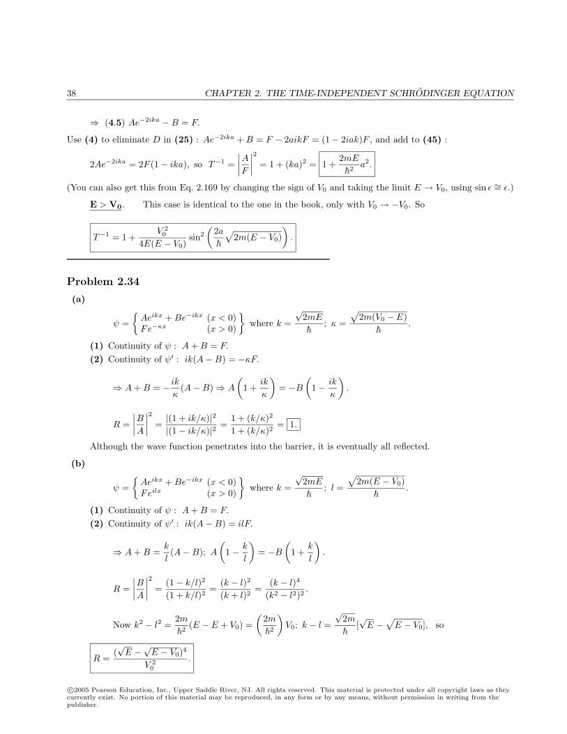
Problem 2.34
(a)
ψ =
Aeikx + Be−ikx (x < 0)Fe−κx (x > 0)
where k =
√2mE
; κ =
√2m(V0 − E)
.
(1) Continuity of ψ : A + B = F.
(2) Continuity of ψ′ : ik(A−B) = −κF.
⇒ A + B = − ik
κ(A−B)⇒ A
(1 +
ik
κ
)= −B
(1− ik
κ
).
R =∣∣∣∣BA
∣∣∣∣2 =|(1 + ik/κ)|2|(1− ik/κ)|2 =
1 + (k/κ)2
1 + (k/κ)2= 1.
Although the wave function penetrates into the barrier, it is eventually all reflected.
(b)
ψ =
Aeikx + Be−ikx (x < 0)Feilx (x > 0)
where k =
√2mE
; l =
√2m(E − V0)
.
(1) Continuity of ψ : A + B = F.
(2) Continuity of ψ′ : ik(A−B) = ilF.
⇒ A + B =k
l(A−B); A
(1− k
l
)= −B
(1 +
k
l
).
R =∣∣∣∣BA
∣∣∣∣2 =(1− k/l)2
(1 + k/l)2=
(k − l)2
(k + l)2=
(k − l)4
(k2 − l2)2.
Now k2 − l2 =2m2
(E − E + V0) =(
2m2
)V0; k − l =
√2m
[√E −
√E − V0], so
R =(√E −
√E − V0)4
V 20
.
c©2005 Pearson Education, Inc., Upper Saddle River, NJ. All rights reserved. This material is protected under all copyright laws as theycurrently exist. No portion of this material may be reproduced, in any form or by any means, without permission in writing from thepublisher.
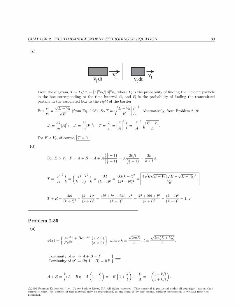
CHAPTER 2. THE TIME-INDEPENDENT SCHRODINGER EQUATION 39
(c)
vivi vt
vtdt dt
From the diagram, T = Pt/Pi = |F |2vt/|A|2vi, where Pi is the probability of finding the incident particlein the box corresponding to the time interval dt, and Pt is the probability of finding the transmittedparticle in the associated box to the right of the barrier.
Butvt
vi=√E − V0√
E(from Eq. 2.98). So T =
√E − V0
E
∣∣∣∣FA∣∣∣∣2 . Alternatively, from Problem 2.19:
Ji =k
m|A|2; Jt =
l
m|F |2; T =
Jt
Ji=
∣∣∣∣FA∣∣∣∣2 l
k=
∣∣∣∣FA∣∣∣∣2
√E − V0
E.
For E < V0, of course, T = 0.
(d)
For E > V0, F = A + B = A + A
(kl − 1
)(kl + 1
) = A2k/l(kl + 1
) =2k
k + lA.
T =∣∣∣∣FA
∣∣∣∣2 l
k=
(2k
k + l
)2l
k=
4kl(k + l)2
=4kl(k − l)2
(k2 − l2)2=
4√E√E − V0(
√E −
√E − V0)2
V 20
.
T + R =4kl
(k + l)2+
(k − l)2
(k + l)2=
4kl + k2 − 2kl + l2
(k + l)2=
k2 + 2kl + l2
(k + l)2=
(k + l)2
(k + l)2= 1.
Problem 2.35
(a)
ψ(x) =
Aeikx + Be−ikx (x < 0)Feilx (x > 0)
where k ≡
√2mE
, l ≡
√2m(E + V0)
.
Continuity of ψ ⇒ A + B = FContinuity of ψ′ ⇒ ik(A−B) = ilF
=⇒
A + B =k
l(A−B); A
(1− k
l
)= −B
(1 +
k
l
);
B
A= −
(1− k/l
1 + k/l
).
c©2005 Pearson Education, Inc., Upper Saddle River, NJ. All rights reserved. This material is protected under all copyright laws as theycurrently exist. No portion of this material may be reproduced, in any form or by any means, without permission in writing from thepublisher.
40 CHAPTER 2. THE TIME-INDEPENDENT SCHRODINGER EQUATION
R =∣∣∣∣BA
∣∣∣∣2 =(l − k
l + k
)2
=
(√E + V0 −
√E√
E + V0 +√E
)2
=
(√1 + V0/E − 1√1 + V0/E + 1
)2
=(√
1 + 3− 1√1 + 3 + 1
)2
=(
2− 12 + 1
)2
=19.
(b) The cliff is two-dimensional, and even if we pretend the car drops straight down, the potential as a functionof distance along the (crooked, but now one-dimensional) path is −mgx (with x the vertical coordinate),as shown.
V(x)
x
-V0
(c) Here V0/E = 12/4 = 3, the same as in part (a), so R = 1/9, and hence T = 8/9 = 0.8889.
Problem 2.36
Start with Eq. 2.22: ψ(x) = A sin kx + B cos kx. This time the boundary conditions are ψ(a) = ψ(−a) = 0:
A sin ka + B cos ka = 0; −A sin ka + B cos ka = 0.Subtract : A sin ka = 0⇒ ka = jπ or A = 0,Add : B cos ka = 0⇒ ka = (j − 1
2 )π or B = 0,
(where j = 1, 2, 3, . . . ).If B = 0 (so A = 0), k = jπ/a. In this case let n ≡ 2j (so n is an even integer); then k = nπ/2a,
ψ = A sin(nπx/2a). Normalizing: 1 = |A|2∫ a
−asin2(nπx/2a) dx = |A|2/2 ⇒ A =
√2.
If A = 0 (so B = 0), k = (j − 12 )π/a. In this case let n ≡ 2j − 1 (n is an odd integer); again k = nπ/2a,
ψ = B cos(nπx/2a). Normalizing: 1 = |B|2∫ a
−acos2(nπx/2a)dx = |a|2/2 ⇒ B =
√2.
In either case Eq. 2.21 yields E = 2k2
2m = n2π22
2m(2a)2 (in agreement with Eq. 2.27 for a well of width 2a).The substitution x→ (x + a)/2 takes Eq. 2.28 to
√2a
sin(nπ
a
(x + a)2
)=
√2a
sin(nπx
2a+
nπ
2
)=
(−1)n/2
√2a sin
(nπx2a
)(n even),
(−1)(n−1)/2√
2a cos
(nπx2a
)(n odd).
So (apart from normalization) we recover the results above. The graphs are the same as Figure 2.2, except thatsome are upside down (different normalization).
c©2005 Pearson Education, Inc., Upper Saddle River, NJ. All rights reserved. This material is protected under all copyright laws as theycurrently exist. No portion of this material may be reproduced, in any form or by any means, without permission in writing from thepublisher.
CHAPTER 2. THE TIME-INDEPENDENT SCHRODINGER EQUATION 41
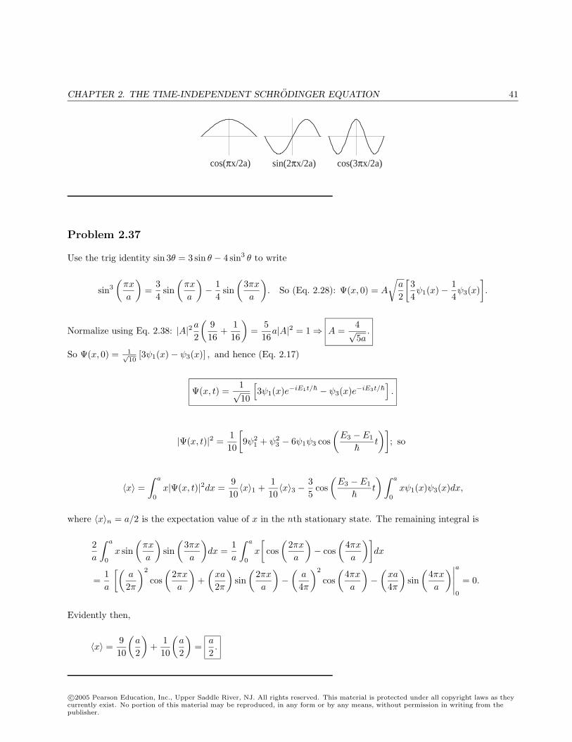
cos(πx/2a) sin(2πx/2a) cos(3πx/2a)
Problem 2.37
Use the trig identity sin 3θ = 3 sin θ − 4 sin3 θ to write
sin3
(πx
a
)=
34
sin(πx
a
)− 1
4sin
(3πxa
). So (Eq. 2.28): Ψ(x, 0) = A
√a
2
[34ψ1(x)− 1
4ψ3(x)
].
Normalize using Eq. 2.38: |A|2 a2
(916
+116
)=
516
a|A|2 = 1⇒ A =4√5a
.
So Ψ(x, 0) = 1√10
[3ψ1(x)− ψ3(x)] , and hence (Eq. 2.17)
Ψ(x, t) =1√10
[3ψ1(x)e−iE1t/ − ψ3(x)e−iE3t/
].
|Ψ(x, t)|2 =110
[9ψ2
1 + ψ23 − 6ψ1ψ3 cos
(E3 − E1
t
)]; so
〈x〉 =∫ a
0
x|Ψ(x, t)|2dx =910〈x〉1 +
110〈x〉3 −
35
cos(E3 − E1
t
) ∫ a
0
xψ1(x)ψ3(x)dx,
where 〈x〉n = a/2 is the expectation value of x in the nth stationary state. The remaining integral is
2a
∫ a
0
x sin(πx
a
)sin
(3πxa
)dx =
1a
∫ a
0
x
[cos
(2πxa
)− cos
(4πxa
)]dx
=1a
[(a
2π
)2
cos(
2πxa
)+
(xa
2π
)sin
(2πxa
)−
(a
4π
)2
cos(
4πxa
)−
(xa
4π
)sin
(4πxa
)∣∣∣∣∣a
0
= 0.
Evidently then,
〈x〉 =910
(a
2
)+
110
(a
2
)=
a
2.
c©2005 Pearson Education, Inc., Upper Saddle River, NJ. All rights reserved. This material is protected under all copyright laws as theycurrently exist. No portion of this material may be reproduced, in any form or by any means, without permission in writing from thepublisher.
42 CHAPTER 2. THE TIME-INDEPENDENT SCHRODINGER EQUATION
Problem 2.38
(a) New allowed energies: En =n2π2
2
2m(2a)2; Ψ(x, 0) =
√2a
sin(π
ax), ψn(x) =
√22a
sin(nπ
2ax).
cn =√
2a
∫ a
0
sin(π
ax)
sin(nπ
2ax)dx =
√2
2a
∫ a
0
cos
[(n
2− 1
) πx
a
]− cos
[(n
2+ 1
) πx
a
]dx.
=1√2a
sin
[(n2 − 1
)πxa
](n2 − 1
)πa
− sin[(
n2 + 1
)πxa
](n2 + 1
)πa
∣∣∣∣∣a
0
(for n = 2)
=1√2π
sin
[(n2 − 1
)π](
n2 − 1
) − sin[(
n2 + 1
)π](
n2 + 1
) =
sin[(
n2 + 1
)π]
√2π
[1(
n2 − 1
) − 1(n2 + 1
)]
=4√
2π
sin[(
n2 + 1
)π]
(n2 − 4)=
0, if n is even± 4
√2
π(n2−4) , if n is odd
.
c2 =√
2a
∫ a
0
sin2(π
ax)dx =
√2a
∫ a
0
12dx =
1√2. So the probability of getting En is
Pn = |cn|2 =
12 , if n = 2
32π2(n2−4)2 , if n is odd0, otherwise
.
Most probable: E2 =π2
2
2ma2(same as before). Probability: P2 = 1/2.
(b) Next most probable: E1 =π2
2
8ma2, with probability P1 =
329π2
= 0.36025.
(c) 〈H〉 =∫
Ψ∗HΨ dx = 2a
∫ a
0sin
(πax
) (−
2
2md2
dx2
)sin
(πax
)dx, but this is exactly the same as before the wall
moved – for which we know the answer:π2
2
2ma2.
Problem 2.39
(a) According to Eq. 2.36, the most general solution to the time-dependent Schrodinger equation for theinfinite square well is
Ψ(x, t) =∞∑
n=1
cnψn(x)e−i(n2π2/2ma2)t.
Nown2π2
2ma2T =
n2π2
2ma2
4ma2
π= 2πn2, so e−i(n2π2
/2ma2)(t+T ) = e−i(n2π2/2ma2)te−i2πn2
, and since n2 is
an integer, e−i2πn2= 1. Therefore Ψ(x, t + T ) = Ψ(x, t). QED
(b) The classical revival time is the time it takes the particle to go down and back: Tc = 2a/v, with thevelocity given by
E =12mv2 ⇒ v =
√2Em⇒ Tc = a
√2mE
.
c©2005 Pearson Education, Inc., Upper Saddle River, NJ. All rights reserved. This material is protected under all copyright laws as theycurrently exist. No portion of this material may be reproduced, in any form or by any means, without permission in writing from thepublisher.
CHAPTER 2. THE TIME-INDEPENDENT SCHRODINGER EQUATION 43
(c) The two revival times are equal if
4ma2
π= a
√2mE
, or E =π2
2
8ma2=
E1
4.
Problem 2.40
(a) Let V0 ≡ 322/ma2. This is just like the odd bound states for the finite square well, since they are theones that go to zero at the origin. Referring to the solution to Problem 2.29, the wave function is
ψ(x) =
D sin lx, l ≡
√2m(E + V0)/ (0 < x < a),
Fe−κx, κ ≡√−2mE/ (x > a),
and the boundary conditions at x = a yield
− cot z =√
(z0/z)2 − 1
with
z0 =√
2mV0
a =
√2m(322/ma2)
a = 8.
Referring to the figure (Problem 2.29), and noting that (5/2)π = 7.85 < z0 < 3π = 9.42, we see that thereare three bound states.
(b) Let
I1 ≡∫ a
0
|ψ|2dx = |D|2∫ a
0
sin2 lx dx = |D|2[x
2− 1
2lsin lx cos lx
]∣∣∣∣a0
= |D|2[a
2− 1
2lsin lz cos la
];
I2 ≡∫ ∞
a
|ψ|2dx = |F |2∫ ∞
a
e−2κx dx = |F |2[−e−2κx
2κ
]∣∣∣∣∞a
= |F |2 e−2κa
2κ.
But continuity at x = a⇒ Fe−κa = D sin la, so I2 = |D|2 sin2 la2κ .
Normalizing:
1 = I1 + I2 = |D|2[a
2− 1
2lsin la cos la +
sin2 la
2κ
]=
12κ|D|2
[κa− κ
lsin la cos la + sin2 la
]But (referring again to Problem 2.29) κ/l = − cot la, so
=12κ|D|2
[κa + cot la sin la cos la + sin2 la
]= |D|2 (1 + κa)
2κ.
So |D|2 = 2κ/(1 + κa), and the probability of finding the particle outside the well is
P = I2 =2κ
1 + κa
sin2 la
2κ=
sin2 la
1 + κa.
We can express this interms of z ≡ la and z0: κa =√
z20 − z2 (page 80),
sin2 la = sin2 z =1
1 + cot2 z=
11 + (z0/z)2 − 1
=(
z
z0
)2
⇒ P =z2
z20(1 +
√z20 − z2)
.
So far, this is correct for any bound state. In the present case z0 = 8 and z is the third solutionto − cot z =
√(8/z)2 − 1, which occurs somewhere in the interval 7.85 < z < 8. Mathematica gives
z = 7.9573 and P = 0.54204.
c©2005 Pearson Education, Inc., Upper Saddle River, NJ. All rights reserved. This material is protected under all copyright laws as theycurrently exist. No portion of this material may be reproduced, in any form or by any means, without permission in writing from thepublisher.
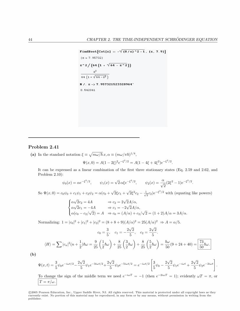
44 CHAPTER 2. THE TIME-INDEPENDENT SCHRODINGER EQUATION
Problem 2.41
(a) In the standard notation ξ ≡√
mω/x, α ≡ (mω/π)1/4,
Ψ(x, 0) = A(1− 2ξ)2e−ξ2/2 = A(1− 4ξ + 4ξ2)e−ξ2/2.
It can be expressed as a linear combination of the first three stationary states (Eq. 2.59 and 2.62, andProblem 2.10):
ψ0(x) = αe−ξ2/2, ψ1(x) =√
2αξe−ξ2/2, ψ2(x) =α√2(2ξ2 − 1)e−ξ2/2.
So Ψ(x, 0) = c0ψ0 + c1ψ1 + c2ψ2 = α(c0 +√
2ξc1 +√
2ξ2c2 − 1√2c2)e−ξ2/2 with (equating like powers)
α√
2c2 = 4A ⇒ c2 = 2√
2A/α,
α√
2c1 = −4A ⇒ c1 = −2√
2A/α,
α(c0 − c2/√
2) = A ⇒ c0 = (A/α) + c2/√
2 = (1 + 2)A/α = 3A/α.
Normalizing: 1 = |c0|2 + |c1|2 + |c2|2 = (8 + 8 + 9)(A/α)2 = 25(A/α)2 ⇒ A = α/5.
c0 =35, c1 = −2
√2
5, c2 =
2√
25
.
〈H〉 =∑
|cn|2(n +12)ω =
925
(12ω
)+
825
(32ω
)+
825
(52ω
)=ω
50(9 + 24 + 40) =
7350ω.
(b)
Ψ(x, t) =35ψ0e−iωt/2− 2
√2
5ψ1e−3iωt/2+
2√
25
ψ2e−5iωt/2 = e−iωt/2
[35ψ0 −
2√
25
ψ1e−iωt +
2√
25
ψ2e−2iωt
].
To change the sign of the middle term we need e−iωT = −1 (then e−2iωT = 1); evidently ωT = π, orT = π/ω.
c©2005 Pearson Education, Inc., Upper Saddle River, NJ. All rights reserved. This material is protected under all copyright laws as theycurrently exist. No portion of this material may be reproduced, in any form or by any means, without permission in writing from thepublisher.
CHAPTER 2. THE TIME-INDEPENDENT SCHRODINGER EQUATION 45
Problem 2.42
Everything in Section 2.3.2 still applies, except that there is an additional boundary condition: ψ(0) = 0. Thiseliminates all the even solutions (n = 0, 2, 4, . . . ), leaving only the odd solutions. So
En =(n +
12
)ω, n = 1, 3, 5, . . . .
Problem 2.43
(a) Normalization is the same as before: A =(
2aπ
)1/4.
(b) Equation 2.103 says
φ(k) =1√2π
(2aπ
)1/4 ∫ ∞−∞
e−ax2eilxe−ikxdx [same as before, only k → k − l] =
1(2πa)1/4
e−(k−l)2/4a.
Ψ(x, t) =1√2π
1(2πa)1/4
∫ ∞−∞
e−(k−l)2/4aei(kx−k2t/2m)︸ ︷︷ ︸e−l2/4ae
−[( 14a+i t2m )k2−(ix+ l
2a )k]
dk
=1√2π
1(2πa)1/4
e−l2/4a
√π(
14a + i t2m
)e(ix+l/2a)2/[4(1/4a+it/2m)]
=(
2aπ
)1/4 1√1 + 2iat/m
e−l2/4aea(ix+l/2a)2/(1+2iat/m).
(c) Let θ ≡ 2at/m, as before: |Ψ|2 =
√2aπ
1√1 + θ2
e−l2/2aea
[(ix+l/2a)2
(1+iθ) +(−ix+l/2a)2
(1−iθ)
]. Expand the term in
square brackets:
[ ] =1
1 + θ2
[(1− iθ)
(ix +
l
2a
)2
+ (1 + iθ)(−ix +
l
2a
)2]
=1
1 + θ2
[(−x2 +
ixl
a+
l2
4a2
)+
(−x2 − ixl
a+
l2
4a2
)+iθ
(x2 − ixl
a− l2
4a2
)+ iθ
(−x2 − ixl
a+
l2
4a2
)]=
11 + θ2
[−2x2 +
l2
2a2+ 2θ
xl
a
]=
11 + θ2
[−2x2 + 2θ
xl
a− θ2l2
2a2+
θ2l2
2a2+
l2
2a2
]=
−21 + θ2
(x− θl
2a
)2
+l2
2a2.
|Ψ(x, t)|2 =
√2π
√a
1 + θ2e−l2/2ae
− 2a1+θ2
(x−θl/2a)2el2/2a =
√2πwe−2w2(x−θl/2a)2 ,
c©2005 Pearson Education, Inc., Upper Saddle River, NJ. All rights reserved. This material is protected under all copyright laws as theycurrently exist. No portion of this material may be reproduced, in any form or by any means, without permission in writing from thepublisher.
46 CHAPTER 2. THE TIME-INDEPENDENT SCHRODINGER EQUATION
where w ≡√
a/(1 + θ2). The result is the same as before, except x→(x− θl
2a
)=
(x− l
m t), so |Ψ|2 has
the same (flattening Gaussian) shape – only this time the center moves at constant speed v = l/m.
(d)
〈x〉 =∫ ∞−∞
x|Ψ(x, t)|2dx. Let y ≡ x− θl/2a = x− vt, so x = y + vt.
=∫ ∞−∞
(y + vt)
√2πwe−2w2y2
dy = vt.
(The first integral is trivially zero; the second is 1 by normalization.)
=l
mt; 〈p〉 = m
d〈x〉dt
= l.
〈x2〉 =∫ ∞−∞
(y + vt)2√
2πwe−2w2y2
dy =1
4w2+ 0 + (vt)2 (the first integral is same as before).
〈x2〉 =1
4w2+
(lt
m
)2
. 〈p2〉 = −2
∫ ∞−∞
Ψ∗d2Ψdx2
dx.
Ψ =(
2aπ
)1/4 1√1 + iθ
e−l2/4aea(ix+l/2a)2/(1+iθ), sodΨdx
=2ia
(ix + l
2a
)(1 + iθ)
Ψ;
d2Ψdx2
=[2ia(ix + l/2a)
1 + iθ
]dΨdx
+2i2a
1 + iθΨ =
[−4a2 (ix + l/2a)2
(1 + iθ)2− 2a
1 + iθ
]Ψ.
〈p2〉 =4a2
2
(1 + iθ)2
∫ ∞−∞
[(ix +
l
2a
)2
+(1 + iθ)
2a
]|Ψ|2dx
=4a2
2
(1 + iθ)2
∫ ∞−∞
[−
(y + vt− il
2a
)2
+(1 + iθ)
2a
]|Ψ|2dy
=4a2
2
(1 + iθ)2
−
∫ ∞−∞
y2|Ψ|2dy − 2(vt− il
2a
) ∫ ∞−∞
y|Ψ|2dy
+
[−
(vt− il
2a
)2
+(1 + iθ)
2a
] ∫ ∞−∞
|Ψ|2dy
=4a2
2
(1 + iθ)2
[− 1
4w2+ 0−
(vt− il
2a
)2
+(1 + iθ)
2a
]
=4a2
2
(1 + iθ)2
−1 + θ2
4a−
[(−il
2a
)(1 + iθ)
]2
+(1 + iθ)
2a
=a
1 + iθ
[−(1− iθ) +
l2
a(1 + iθ) + 2
]=
a2
1 + iθ
[(1 + iθ)
(1 +
l2
a
)]=
2(a + l2).
σ2x = 〈x2〉 − 〈x〉2 =
14w2
+(lt
m
)2
−(lt
m
)2
=1
4w2⇒ σx =
12w
;
c©2005 Pearson Education, Inc., Upper Saddle River, NJ. All rights reserved. This material is protected under all copyright laws as theycurrently exist. No portion of this material may be reproduced, in any form or by any means, without permission in writing from thepublisher.
CHAPTER 2. THE TIME-INDEPENDENT SCHRODINGER EQUATION 47
σ2p = 〈p2〉 − 〈p〉2 = 2a + 2l2 − 2l2 = 2a, so σp =
√a.
(e) σx and σp are same as before, so the uncertainty principle still holds.
Problem 2.44
Equation 2.22 ⇒ ψ(x) = A sin kx + B cos kx, 0 ≤ x ≤ a, with k =√
2mE/2.Even solutions: ψ(x) = ψ(−x) = A sin(−kx) + B cos(−kx) = −A sin kx + B cos kx (−a ≤ x ≤ 0).
Boundaryconditions
ψ continuous at 0 : B = B (no new condition).ψ′ discontinuous (Eq. 2.125 with sign of α switched): Ak + Ak = 2mα
2B ⇒ B =
2kmαA.
ψ → 0 at x = a : A sin(ka) + 2k
mαA cos(ka) = 0⇒ tan(ka) = −2kmα .
ψ(x) = A
(sin kx +
2k
mαcos kx
)(0 ≤ x ≤ a); ψ(−x) = ψ(x).
π 2π 3π
tan(ka) -h kmα
2
ka
From the graph, the allowed energies are slightly above
ka =nπ
2(n = 1, 3, 5, . . . ) so En
n2π2
2
2m(2a)2(n = 1, 3, 5, . . . ).
These energies are somewhat higher than the corresponding energies for the infinite square well (Eq. 2.27, witha → 2a). As α → 0, the straight line (−2k/mα) gets steeper and steeper, and the intersections get closer tonπ/2; the energies then reduce to those of the ordinary infinite well. As α → ∞, the straight line approacheshorizontal, and the intersections are at nπ (n = 1, 2, 3, . . . ), so En → n2π2
2
2ma2 – these are the allowed energies forthe infinite square well of width a. At this point the barrier is impenetrable, and we have two isolated infinitesquare wells.
Odd solutions: ψ(x) = −ψ(−x) = −A sin(−kx)−B cos(−kx) = A sin(kx)−B cos(kx) (−a ≤ x ≤ 0).
Boundary conditions
ψ continuous at 0 : B = −B ⇒ B = 0.ψ′ discontinuous: Ak −Ak = 2mα
2(0) (no new condition).
ψ(a) = 0⇒ A sin(ka) = 0⇒ ka = nπ2 (n = 2, 4, 6, . . . ).
ψ(x) = A sin(kx), (−a < x < a); En =n2π2
2
2m(2a)2(n = 2, 4, 6, . . . ).
These are the exact (even n) energies (and wave functions) for the infinite square well (of width 2a). The pointis that the odd solutions (even n) are zero at the origin, so they never “feel” the delta function at all.
c©2005 Pearson Education, Inc., Upper Saddle River, NJ. All rights reserved. This material is protected under all copyright laws as theycurrently exist. No portion of this material may be reproduced, in any form or by any means, without permission in writing from thepublisher.
48 CHAPTER 2. THE TIME-INDEPENDENT SCHRODINGER EQUATION
Problem 2.45
− 2
2md2ψ1
dx2+ V ψ1 = Eψ1 ⇒ −
2
2mψ2
d2ψ1
dx2+ V ψ1ψ2 = Eψ1ψ2
− 2
2md2ψ2
dx2+ V ψ2 = Eψ2 ⇒ −
2
2mψ1
d2ψ2
dx2+ V ψ1ψ2 = Eψ1ψ2
⇒ − 2
2m
[ψ2
d2ψ1
dx2− ψ1
d2ψ2
dx2
]= 0.
Butd
dx
[ψ2
dψ1
dx− ψ1
dψ2
dx
]=
dψ2
dx
dψ1
dx+ ψ2
d2ψ1
dx2− dψ1
dx
dψ2
dx− ψ1
d2ψ2
dx2= ψ2
d2ψ1
dx2− ψ1
d2ψ2
dx2. Since this is
zero, it follows that ψ2dψ1
dx− ψ1
dψ2
dx= K (a constant). But ψ → 0 at ∞ so the constant must be zero. Thus
ψ2dψ1
dx= ψ1
dψ2
dx, or
1ψ1
dψ1
dx=
1ψ2
dψ2
dx, so lnψ1 = lnψ2 + constant, or ψ1 = (constant)ψ2. QED
Problem 2.46
− 2
2md2ψ
dx2= Eψ (where x is measured around the circumference), or
d2ψ
dx2= −k2ψ, with k ≡
√2mE
, so
ψ(x) = Aeikx + Be−ikx.
But ψ(x + L) = ψ(x), since x + L is the same point as x, so
AeikxeikL + Be−ikxe−ikL = Aeikx + Be−ikx,
and this is true for all x. In particular, for x = 0 :
(1) AeikL + Be−ikL = A + B. And for x =π
2k:
Aeiπ/2eikL + Be−iπ/2e−ikL = Aeiπ/2 + Be−iπ/2, or iAeikL − iBe−ikL = iA− iB, so
(2) AeikL −Be−ikL = A−B. Add (1) and (2): 2AeikL = 2A.
Either A = 0, or else eikL = 1, in which case kL = 2nπ (n = 0,±1,±2, . . . ). But if A = 0, then Be−ikL = B,leading to the same conclusion. So for every positive n there are two solutions: ψ+
n (x) = Aei(2nπx/L) andψ−n (x) = Be−i(2nπx/L) (n = 0 is ok too, but in that case there is just one solution). Normalizing:
∫ L
0|ψ±|2dx =
1 ⇒ A = B = 1/√L. Any other solution (with the same energy) is a linear combination of these.
ψ±n (x) =1√Le±i(2nπx/L); En =
2n2π2
2
mL2(n = 0, 1, 2, 3, . . . ).
The theorem fails because here ψ does not go to zero at ∞; x is restricted to a finite range, and we are unableto determine the constant K (in Problem 2.45).
Problem 2.47
(a) (i) b = 0 ⇒ ordinary finite square well. Exponential decay outside; sinusoidal inside (cos for ψ1, sin forψ2). No nodes for ψ1, one node for ψ2.
(ii) Ground state is even. Exponential decay outside, sinusoidal inside the wells, hyperbolic cosine inbarrier. First excited state is odd – hyperbolic sine in barrier. No nodes for ψ1, one node for ψ2.
c©2005 Pearson Education, Inc., Upper Saddle River, NJ. All rights reserved. This material is protected under all copyright laws as theycurrently exist. No portion of this material may be reproduced, in any form or by any means, without permission in writing from thepublisher.
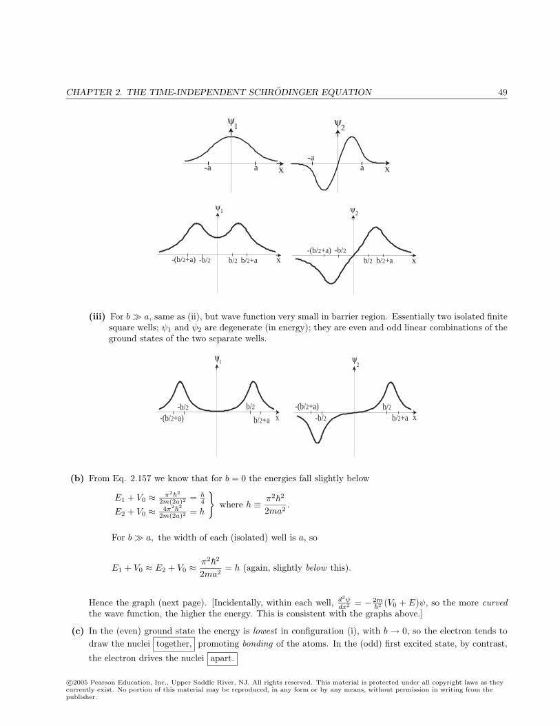
CHAPTER 2. THE TIME-INDEPENDENT SCHRODINGER EQUATION 49
x x
ψ ψ1 2
-a-a
a a
x xb/2 b/2-b/2
b/2+a-b/2-(b/2+a)
-(b/2+a) b/2+a
ψ1 2ψ
(iii) For b a, same as (ii), but wave function very small in barrier region. Essentially two isolated finitesquare wells; ψ1 and ψ2 are degenerate (in energy); they are even and odd linear combinations of theground states of the two separate wells.
ψ ψ1 2
x x-(b/2+a)
-(b/2+a)-b/2
-b/2b/2b/2
b/2+a b/2+a
(b) From Eq. 2.157 we know that for b = 0 the energies fall slightly below
E1 + V0 ≈ π22
2m(2a)2 = h4
E2 + V0 ≈ 4π22
2m(2a)2 = h
where h ≡ π2
2
2ma2.
For b a, the width of each (isolated) well is a, so
E1 + V0 ≈ E2 + V0 ≈π2
2
2ma2= h (again, slightly below this).
Hence the graph (next page). [Incidentally, within each well, d2ψdx2 = − 2m
2(V0 + E)ψ, so the more curved
the wave function, the higher the energy. This is consistent with the graphs above.]
(c) In the (even) ground state the energy is lowest in configuration (i), with b → 0, so the electron tends todraw the nuclei together, promoting bonding of the atoms. In the (odd) first excited state, by contrast,
the electron drives the nuclei apart.
c©2005 Pearson Education, Inc., Upper Saddle River, NJ. All rights reserved. This material is protected under all copyright laws as theycurrently exist. No portion of this material may be reproduced, in any form or by any means, without permission in writing from thepublisher.
50 CHAPTER 2. THE TIME-INDEPENDENT SCHRODINGER EQUATION
h
h/4
b
E+V0
E +V
E +V
0
01
2
Problem 2.48
(a)
dΨdx
=2√
3a√a·
1, (0 < x < a/2)−1, (a/2 < x < a)
=
2√
3a√a
[1− 2θ
(x− a
2
)].
(b)
d2Ψdx2
=2√
3a√a
[− 2δ
(x− a
2
)]= −4
√3
a√aδ
(x− a
2
).
(c)
〈H〉 = − 2
2m
(− 4
√3
a√a
) ∫Ψ∗δ
(x− a
2
)dx =
2√
32
ma√a
Ψ∗(a
2
)︸ ︷︷ ︸√
3/a
=2 · 3 · 2
m · a · a =62
ma2.
Problem 2.49
(a)
∂Ψ∂t
=(−mω
2
) [a2
2(−2iωe−2iωt
)+
i
m− 2ax(−iω)e−iωt
]Ψ, so
i∂Ψ∂t
=[−1
2ma2ω2e−2iωt +
12ω + maxω2e−iωt
]Ψ.
∂Ψ∂x
=[(−mω
2
) (2x− 2ae−iωt
)]Ψ = −mω
(x− ae−iωt
)Ψ;
∂2Ψ∂x2
= −mω
Ψ− mω
(x− ae−iωt
) ∂Ψ∂x
=[−mω
+
(mω
)2 (x− ae−iωt
)2]
Ψ.
c©2005 Pearson Education, Inc., Upper Saddle River, NJ. All rights reserved. This material is protected under all copyright laws as theycurrently exist. No portion of this material may be reproduced, in any form or by any means, without permission in writing from thepublisher.
CHAPTER 2. THE TIME-INDEPENDENT SCHRODINGER EQUATION 51
− 2
2m∂2Ψ∂x2
+12mω2x2Ψ = −
2
2m
[−mω
+
(mω
)2 (x− ae−iωt
)2]
Ψ +12mω2x2Ψ
=[12ω − 1
2mω2
(x2 − 2axe−iωt + a2e−2iωt
)+
12mω2x2
]Ψ
=[12ω + maxω2e−iωt − 1
2mω2a2e−2iωt
]Ψ
= i∂Ψ∂t
(comparing second line above).
(b)
|Ψ|2 =√
mω
πe−mω2
[ (x2+ a2
2 (1+e2iωt)− itm −2axeiωt)+
(x2+ a2
2 (1+e−2iωt)+ itm −2axe−iωt
) ]
=√
mω
πe−
mω2 [2x2+a2+a2 cos(2ωt)−4ax cos(ωt)]. But a2[1 + cos(2ωt)] = 2a2 cos2 ωt, so
=√
mω
πe−
mω [x2−2ax cos(ωt)+a2 cos2(ωt)] =
√mω
πe−
mω
(x−a cos ωt)2 .
The wave packet is a Gaussian of fixed shape, whose center oscillates back and forth sinusoidally, withamplitude a and angular frequency ω.
(c) Note that this wave function is correctly normalized (compare Eq. 2.59). Let y ≡ x− a cosωt :
〈x〉 =∫
x|Ψ|2dx =∫
(y + a cosωt)|Ψ|2dy = 0 + a cosωt
∫|Ψ|2dy = a cosωt.
〈p〉 = md〈x〉dt
= −maω sinωt.d〈p〉dt
= −maω2 cosωt. V =12mω2x2 =⇒ dV
dx= mω2x.
〈−dV
dx〉 = −mω2〈x〉 = −mω2a cosωt =
d〈p〉dt
, so Ehrenfest’s theorem is satisfied.
Problem 2.50
(a)
∂Ψ∂t
=[−mα
2
∂
∂t|x− vt| − i
(E + 12mv2)
]Ψ;
∂
∂t|x− vt| =
−v, if x− vt > 0v, if x− vt < 0
.
We can write this in terms of the θ-function (Eq. 2.143):
2θ(z)− 1 =
1, if z > 0−1, if z < 0
, so
∂
∂t|x− vt| = −v[2θ(x− vt)− 1].
i∂Ψ∂t
=imαv
[2θ(x− vt)− 1] + E +
12mv2
Ψ. []
c©2005 Pearson Education, Inc., Upper Saddle River, NJ. All rights reserved. This material is protected under all copyright laws as theycurrently exist. No portion of this material may be reproduced, in any form or by any means, without permission in writing from thepublisher.
52 CHAPTER 2. THE TIME-INDEPENDENT SCHRODINGER EQUATION
∂Ψ∂x
=[−mα
2
∂
∂x|x− vt|+ imv
]Ψ
∂
∂x|x− vt| = 1, if x > vt; −1, if x < vt = 2θ(x− vt)− 1.
=−mα
2[2θ(x− vt)− 1] +
imv
Ψ.
∂2Ψ∂x2
=−mα
2[2θ(x− vt)− 1] +
imv
2
Ψ− 2mα
2
[∂
∂xθ(x− vt)
]Ψ.
But (from Problem 2.24(b)) ∂∂xθ(x− vt) = δ(x− vt), so
− 2
2m∂2Ψ∂x2
− αδ(x− vt)Ψ
=
(−
2
2m
−mα
2[2θ(x− vt)− 1] +
imv
2
+ αδ(x− vt)− αδ(x− vt)
)Ψ
= − 2
2m
m2α2
4[2θ(x− vt)− 1]2︸ ︷︷ ︸
1
−m2v2
2− 2i
mv
mα
2[2θ(x− vt)− 1]
Ψ
=−mα2
22+
12mv2 + i
mvα
[2θ(x− vt)− 1]
Ψ = i
∂Ψ∂t
(compare []).
(b)
|Ψ|2 =mα
2e−2mα|y|/2 (y ≡ x− vt).
Check normalization: 2mα
2
∫ ∞0
e−2mαy/2dy =2mα
2
2
2mα= 1.
〈H〉 =∫ ∞−∞
Ψ∗HΨdx. But HΨ = i∂Ψ∂t
, which we calculated above [].
=∫
imαv
[2θ(y)− 1] + E +
12mv2
|Ψ|2dy = E +
12mv2.
(Note that [2θ(y)−1] is an odd function of y.) Interpretation: The wave packet is dragged along (at speedv) with the delta-function. The total energy is the energy it would have in a stationary delta-function(E), plus kinetic energy due to the motion (1
2mv2).
Problem 2.51
(a) Figure at top of next page.
(b)dψ0
dx= −Aa sech(ax) tanh(ax);
d2ψ0
dx2= −Aa2
[− sech(ax) tanh2(ax) + sech(ax) sech2(ax)
].
c©2005 Pearson Education, Inc., Upper Saddle River, NJ. All rights reserved. This material is protected under all copyright laws as theycurrently exist. No portion of this material may be reproduced, in any form or by any means, without permission in writing from thepublisher.
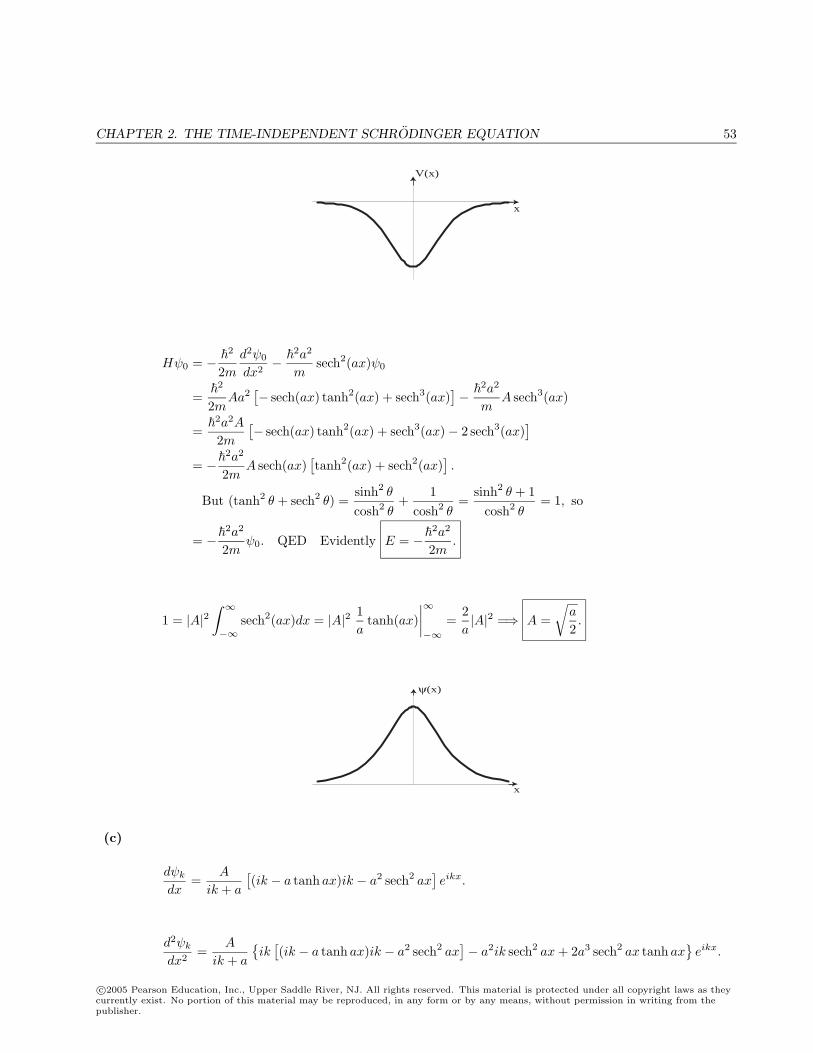
CHAPTER 2. THE TIME-INDEPENDENT SCHRODINGER EQUATION 53
V(x)
x
Hψ0 = − 2
2md2ψ0
dx2−
2a2
msech2(ax)ψ0
=
2
2mAa2
[− sech(ax) tanh2(ax) + sech3(ax)
]−
2a2
mA sech3(ax)
=
2a2A
2m[− sech(ax) tanh2(ax) + sech3(ax)− 2 sech3(ax)
]= −
2a2
2mA sech(ax)
[tanh2(ax) + sech2(ax)
].
But (tanh2 θ + sech2 θ) =sinh2 θ
cosh2 θ+
1cosh2 θ
=sinh2 θ + 1
cosh2 θ= 1, so
= −2a2
2mψ0. QED Evidently E = −
2a2
2m.
1 = |A|2∫ ∞−∞
sech2(ax)dx = |A|2 1a
tanh(ax)∣∣∣∣∞−∞
=2a|A|2 =⇒ A =
√a
2.
x
ψ(x)
(c)
dψk
dx=
A
ik + a
[(ik − a tanh ax)ik − a2 sech2 ax
]eikx.
d2ψk
dx2=
A
ik + a
ik
[(ik − a tanh ax)ik − a2 sech2 ax
]− a2ik sech2 ax + 2a3 sech2 ax tanh ax
eikx.
c©2005 Pearson Education, Inc., Upper Saddle River, NJ. All rights reserved. This material is protected under all copyright laws as theycurrently exist. No portion of this material may be reproduced, in any form or by any means, without permission in writing from thepublisher.
54 CHAPTER 2. THE TIME-INDEPENDENT SCHRODINGER EQUATION
− 2
2md2ψk
dx2+ V ψk =
A
ik + a
−2ik
2m[−k2 − iak tanh ax− a2 sech2 ax
]+
2a2
2mik sech2 ax
−2a3
msech2 ax tanh ax−
2a2
msech2 ax(ik − a tanh ax)
eikx
=Aeikx
ik + a
2
2m(ik3 − ak2 tanh ax + ia2k sech2 ax + ia2k sech2 ax
−2a3 sech2 ax tanh ax− 2ia2k sech2 ax + 2a3 sech2 ax tanh ax)
=Aeikx
ik + a
2
2mk2(ik − a tanh ax) =
2k2
2mψk = Eψk. QED
As x→ +∞, tanh ax→ +1, so ψk(x)→ A
(ik − a
ik + a
)eikx, which represents a transmitted wave.
R = 0. T =∣∣∣∣ ik − a
ik + a
∣∣∣∣2 =(−ik − a
−ik + a
) (ik − a
ik + a
)= 1.
Problem 2.52
(a) (1) From Eq. 2.133: F + G = A + B.
(2) From Eq. 2.135: F −G = (1 + 2iβ)A− (1− 2iβ)B, where β = mα/2k.
Subtract: 2G = −2iβA + 2(1− iβ)B ⇒ B =1
1− iβ(iβA + G). Multiply (1) by (1− 2iβ) and add:
2(1− iβ)F − 2iβG = 2A⇒ F =1
1− iβ(A + iβG). S =
11− iβ
(iβ 11 iβ
).
(b) For an even potential, V (−x) = V (x), scattering from the right is the same as scattering from the left, withx↔ −x, A↔ G, B ↔ F (see Fig. 2.22): F = S11G+ S12A, B = S21G+ S22A. So S11 = S22, S21 = S12.(Note that the delta-well S matrix in (a) has this property.) In the case of the finite square well, Eqs. 2.167and 2.168 give
S21 =e−2ika
cos 2la− i (k2+l2)2kl sin 2la
; S11 =i (l2−k2)
2kl sin 2la e−2ika
cos 2la− i (k2+l2)2kl sin 2la
. So
S =e−2ika
cos 2la− i (k2+l2)2kl sin 2la
(i (l2−k2)
2kl sin 2la 11 i (l2−k2)
2kl sin 2la
).
Problem 2.53
(a)
B = S11A + S12G⇒ G =1
S12(B − S11A) = M21A + M22B ⇒M21 = −S11
S12, M22 =
1S12
.
c©2005 Pearson Education, Inc., Upper Saddle River, NJ. All rights reserved. This material is protected under all copyright laws as theycurrently exist. No portion of this material may be reproduced, in any form or by any means, without permission in writing from thepublisher.
CHAPTER 2. THE TIME-INDEPENDENT SCHRODINGER EQUATION 55
F = S21A + S22B = S21A +S22
S12(B − S11A) = − (S11S22 − S12S21)
S12A +
S22
S12B = M11A + M12B.
⇒M11 = −detSS12
, M12 =S22
S12. M =
1S12
(−det(S) S22
−S11 1
). Conversely:
G = M21A + M22B ⇒ B =1
M22(G−M21A) = S11A + S12G⇒ S11 = −M21
M22; S12 =
1M22
.
F = M11A + M12B = M11A +M12
M22(G−M21A) =
(M11M22 −M12M21)M22
A +M12
M22G = S21A + S22G.
⇒ S21 =detMM22
; S22 =M12
M22. S =
1M22
(−M21 1det(M) M12
).
[It happens that the time-reversal invariance of the Schrodinger equation, plus conservation of probability,requires M22 = M∗11, M21 = M∗12, and det(M) = 1, but I won’t use this here. See Merzbacher’s QuantumMechanics. Similarly, for even potentials S11 = S22, S12 = S21 (Problem 2.52).]
Rl = |S11|2 =∣∣∣∣M21
M22
∣∣∣∣2 , Tl = |S21|2 =∣∣∣∣det(M)
M22
∣∣∣∣2 , Rr = |S22|2 =∣∣∣∣M12
M22
∣∣∣∣2 , Tr = |S12|2 =1
|M22|2.
(b)
A
B
C
D
F
G
xM M1 2
(FG
)= M2
(CD
),
(CD
)= M1
(AB
), so
(FG
)= M2M1
(AB
)= M
(AB
), with M = M2M1. QED
(c)
ψ(x) =
Aeikx + Be−ikx (x < a)Feikx + Ge−ikx (x > a)
.
Continuity of ψ : Aeika + Be−ika = Feika + Ge−ika
Discontinuity of ψ′ : ik(Feika −Ge−ika
)− ik
(Aeika −Be−ika
)= − 2mα
2ψ(a) = − 2mα
2
(Aeika + Be−ika
).
(1) Fe2ika + G = Ae2ika + B.
(2) Fe2ika −G = Ae2ika −B + i 2mα2k
(Ae2ika + B
).
c©2005 Pearson Education, Inc., Upper Saddle River, NJ. All rights reserved. This material is protected under all copyright laws as theycurrently exist. No portion of this material may be reproduced, in any form or by any means, without permission in writing from thepublisher.
56 CHAPTER 2. THE TIME-INDEPENDENT SCHRODINGER EQUATION
Add (1) and (2):
2Fe2ika = 2Ae2ika + i2mα
2k
(Ae2ika + B
)⇒ F =
(1 + i
mα
2k
)A + i
mα
2ke−2ikaB = M11A + M12B.
So M11 = (1 + iβ); M12 = iβe−2ika; β ≡ mα
2k.
Subtract (2) from (1):
2G = 2B − 2iβe2ikaA− 2iβB ⇒ G = (1− iβ)B − iβe2ikaA = M21A + M22B.
So M21 = −iβe2ika; M22 = (1− iβ). M =(
(1 + iβ) iβe−2ika
−iβe2ika (1− iβ)
).
(d)
M1 =(
(1 + iβ) iβe−2ika
−iβe2ika (1− iβ)
); to get M2, just switch the sign of a: M2 =
((1 + iβ) iβe2ika
−iβe−2ika (1− iβ)
).
M = M2M1 =(
[1 + 2iβ + β2(e4ika − 1)] 2iβ[cos 2ka + β sin 2ka]−2iβ[cos 2ka + β sin 2ka] [1− 2iβ + β2(e−4ika − 1)]
).
T = Tl = Tr =1
|M22|2⇒
T−1 = [1 + 2iβ + β2(e4ika − 1)][1− 2iβ + β2(e−4ika − 1)]
= 1− 2iβ + β2e−4ika − β2 + 2iβ + 4β2 + 2iβ3e−4ika − 2iβ3 + β2e4ika
− β2 − 2iβ3e4ika + 2iβ3 + β4(1− e4ika − e−4ika + 1)
= 1 + 2β2 + β2(e4ika + e−4ika)− 2iβ3(e4ika − e−4ika) + 2β4 − β4(e4ika + e−4ika)
= 1 + 2β2 + 2β2 cos 4ka− 2iβ32i sin 4ka + 2β4 − 2β4 cos 4ka
= 1 + 2β2(1 + cos 4ka) + 4β3 sin 4ka + 2β4(1− cos 4ka)
= 1 + 4β2 cos2 2ka + 8β3 sin 2ka cos 2ka + 4β4 sin2 2ka
T =1
1 + 4β2(cos 2ka + β sin 2ka)2
Problem 2.54
I’ll just show the first two graphs, and the last two. Evidently K lies between 0.9999 and 1.0001.
c©2005 Pearson Education, Inc., Upper Saddle River, NJ. All rights reserved. This material is protected under all copyright laws as theycurrently exist. No portion of this material may be reproduced, in any form or by any means, without permission in writing from thepublisher.
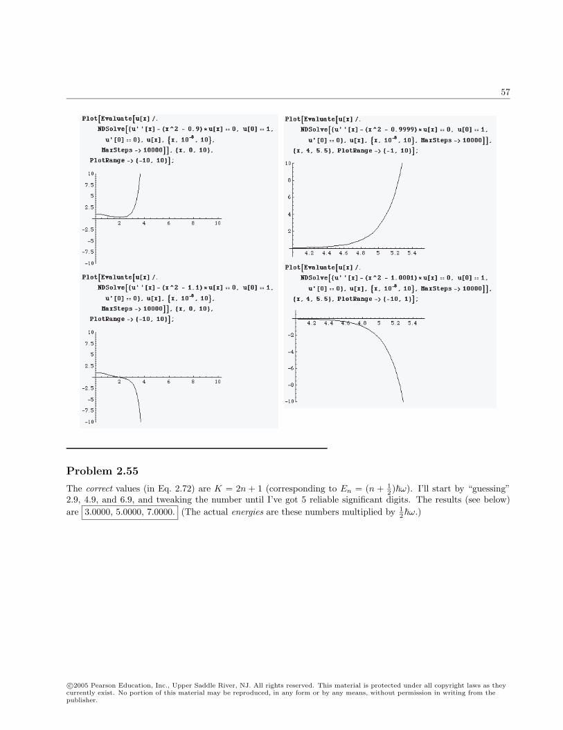
57
Problem 2.55
The correct values (in Eq. 2.72) are K = 2n + 1 (corresponding to En = (n + 12 )ω). I’ll start by “guessing”
2.9, 4.9, and 6.9, and tweaking the number until I’ve got 5 reliable significant digits. The results (see below)are 3.0000, 5.0000, 7.0000. (The actual energies are these numbers multiplied by 1
2ω.)
c©2005 Pearson Education, Inc., Upper Saddle River, NJ. All rights reserved. This material is protected under all copyright laws as theycurrently exist. No portion of this material may be reproduced, in any form or by any means, without permission in writing from thepublisher.
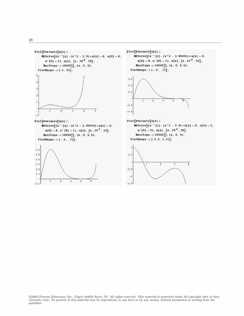
58
c©2005 Pearson Education, Inc., Upper Saddle River, NJ. All rights reserved. This material is protected under all copyright laws as theycurrently exist. No portion of this material may be reproduced, in any form or by any means, without permission in writing from thepublisher.
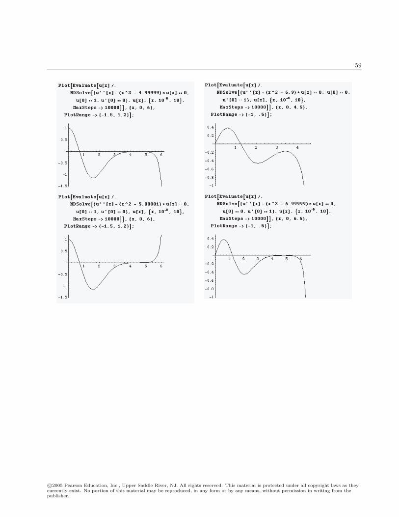
59
c©2005 Pearson Education, Inc., Upper Saddle River, NJ. All rights reserved. This material is protected under all copyright laws as theycurrently exist. No portion of this material may be reproduced, in any form or by any means, without permission in writing from thepublisher.
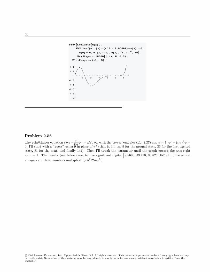
60
Problem 2.56
The Schrodinger equation says − 2
2mψ′′ = Eψ, or, with the correct energies (Eq. 2.27) and a = 1, ψ′′+(nπ)2ψ =
0. I’ll start with a “guess” using 9 in place of π2 (that is, I’ll use 9 for the ground state, 36 for the first excitedstate, 81 for the next, and finally 144). Then I’ll tweak the parameter until the graph crosses the axis rightat x = 1. The results (see below) are, to five significant digits: 9.8696, 39.478, 88.826, 157.91. (The actualenergies are these numbers multiplied by 2/2ma2.)
c©2005 Pearson Education, Inc., Upper Saddle River, NJ. All rights reserved. This material is protected under all copyright laws as theycurrently exist. No portion of this material may be reproduced, in any form or by any means, without permission in writing from thepublisher.
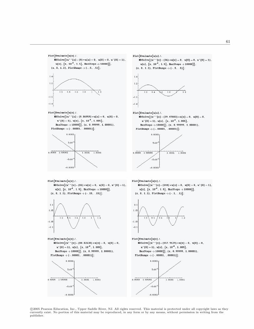
61
c©2005 Pearson Education, Inc., Upper Saddle River, NJ. All rights reserved. This material is protected under all copyright laws as theycurrently exist. No portion of this material may be reproduced, in any form or by any means, without permission in writing from thepublisher.
62 CHAPTER 3. FORMALISM
Chapter 3
Formalism
Problem 3.1
(a) All conditions are trivial except Eq. A.1: we need to show that the sum of two square-integrable functionsis itself square-integrable. Let h(x) = f(x) + g(x), so that |h|2 = (f + g)∗(f + g) = |f |2 + |g|2 + f∗g + g∗fand hence ∫
|h|2 dx =∫|f |2 dx +
∫|g|2 dx +
∫f∗g dx +
(∫f∗g dx
)∗.
If f(x) and g(x) are square-integrable, then the first two terms are finite, and (by Eq. 3.7) so too are thelast two. So
∫|h|2dx is finite. QED
The set of all normalized functions is certainly not a vector space: it doesn’t include 0, and the sum oftwo normalized functions is not (in general) normalized—in fact, if f(x) is normalized, then the squareintegral of 2f(x) is 4.
(b) Equation A.19 is trivial:
〈g|f〉 =∫ b
a
g(x)∗f(x) dx =
(∫ b
a
f(x)∗g(x) dx
)∗= 〈f |g〉∗.
Equation A.20 holds (see Eq. 3.9) subject to the understanding in footnote 6. As for Eq. A.21, this ispretty obvious:
〈f |(b|g〉+ c|h〉) =∫
f(x)∗ (bg(x) + ch(x)) dx = b
∫f∗g dx + c
∫f∗h dx = b〈f |g〉+ c〈f |h〉.
Problem 3.2
(a)
〈f |f〉 =∫ 1
0
x2ν dx =1
2ν + 1x2ν+1
∣∣∣∣10
=1
2ν + 1(1− 02ν+1
).
Now 02ν+1 is finite (in fact, zero) provided (2ν + 1) > 0, which is to say, ν > − 12 . If (2ν + 1) < 0 the
integral definitely blows up. As for the critical case ν = − 12 , this must be handled separately:
〈f |f〉 =∫ 1
0
x−1 dx = lnx∣∣10
= ln 1− ln 0 = 0 +∞.
c©2005 Pearson Education, Inc., Upper Saddle River, NJ. All rights reserved. This material is protected under all copyright laws as theycurrently exist. No portion of this material may be reproduced, in any form or by any means, without permission in writing from thepublisher.
CHAPTER 3. FORMALISM 63
So f(x) is in Hilbert space only for ν strictly greater than -1/2.
(b) For ν = 1/2, we know from (a) that f(x) is in Hilbert space: yes.
Since xf = x3/2, we know from (a) that it is in Hilbert space: yes.
For df/dx = 12x−1/2, we know from (a) that it is not in Hilbert space: no.
[Moral: Simple operations, such as differenting (or multiplying by 1/x), can carry a function out of Hilbertspace.]
Problem 3.3
Suppose 〈h|Qh〉 = 〈Qh|h〉 for all functions h(x). Let h(x) = f(x) + cg(x) for some arbitrary constant c. Then
〈h|Qh〉 = 〈(f + cg)|Q(f + cg)〉 = 〈f |Qf〉+ c〈f |Qg〉+ c∗〈g|Qf〉+ |c|2〈g|Qg〉;〈Qh|h〉 = 〈Q(f + cg)|(f + cg)〉 = 〈Qf |f〉+ c〈Qf |g〉+ c∗〈Qg|f〉+ |c|2〈Qg|g〉.
Equating the two and noting that 〈f |Qf〉 = 〈Qf |f〉 and 〈g|Qg〉 = 〈Qg|g〉 leaves
c〈f |Qg〉+ c∗〈g|Qf〉 = c〈Qf |g〉+ c∗〈Qg|f〉.In particlar, choosing c = 1:
〈f |Qg〉+ 〈g|Qf〉 = 〈Qf |g〉+ 〈Qg|f〉,whereas if c = i:
〈f |Qg〉 − 〈g|Qf〉 = 〈Qf |g〉 − 〈Qg|f〉.Adding the last two equations:
〈f |Qg〉 = 〈Qf |g〉. QED
Problem 3.4
(a) 〈f |(H + K)g〉 = 〈f |Hg〉+ 〈f |Kg〉 = 〈Hf |g〉+ 〈Kf |g〉 = 〈(H + K)f |g〉.
(b) 〈f |αQg〉 = α〈f |Qg〉; 〈αQf |g〉 = α∗〈Qf |g〉. Hermitian ⇔ α is real.
(c) 〈f |HKg〉 = 〈Hf |Kg〉 = 〈KHf |g〉, so HK is hermitian ⇔ HK = KH, or [H, K] = 0.
(d) 〈f |xg〉 =∫f∗(xg) dx =
∫(xf)∗g dx = 〈xf |g〉.
〈f |Hg〉 =∫
f∗(−
2
2md2
dx2+ V
)g dx = −
2
2m
∫f∗
d2g
dx2dx +
∫f∗V g dx.
Integrating by parts (twice):∫ ∞−∞
f∗d2g
dx2dx = f∗
dg
dx
∣∣∣∣∞−∞
−∫ ∞−∞
df∗
dx
dg
dxdx = f∗
dg
dx
∣∣∣∣∞−∞
− df∗
dxg
∣∣∣∣∞−∞
+∫ ∞−∞
d2f∗
dx2g dx.
But for functions f(x) and g(x) in Hilbert space the boundary terms vanish, so∫ ∞−∞
f∗d2g
dx2dx =
∫ ∞−∞
d2f∗
dx2g dx, and hence (assuming that V (x) is real):
〈f |Hg〉 =∫ ∞−∞
(−
2
2md2f
dx2+ V f
)∗g dx = 〈Hf |g〉.
c©2005 Pearson Education, Inc., Upper Saddle River, NJ. All rights reserved. This material is protected under all copyright laws as theycurrently exist. No portion of this material may be reproduced, in any form or by any means, without permission in writing from thepublisher.
64 CHAPTER 3. FORMALISM
Problem 3.5
(a) 〈f |xg〉 =∫f∗(xg) dx =
∫(xf)∗g dx = 〈xf |g〉, so x† = x.
〈f |ig〉 =∫f∗(ig) dx =
∫(−if)∗g dx = 〈−if |g〉, so i† = −i.
〈f |dgdx〉 =
∫ ∞−∞
f∗dg
dxdx = f∗g
∣∣∣∣∞−∞
−∫ ∞−∞
(df
dx
)∗g dx = −〈xf |g〉, so
(d
dx
)†= − d
dx.
(b) a+ =1√
2mω(−ip + mωx). But p and x are hermitian, and i† = −i, so (a+)† =
1√2mω
(ip + mωx), or
(a+)† = (a−).
(c) 〈f |(QR)g〉 = 〈Q†f |Rg〉 = 〈R†Q†f |g〉 = 〈(QR)†f |g〉, so (QR)† = R†Q†.
Problem 3.6
〈f |Qg〉 =∫ 2π
0
f∗d2g
dφ2dφ = f∗
dg
dφ
∣∣∣∣2π
0
−∫ 2π
0
df∗
dφ
dg
dφdφ = f∗
dg
dφ
∣∣∣∣2π
0
− df∗
dφg
∣∣∣∣2π
0
+∫ 2π
0
d2f∗
dφ2g dφ.
As in Example 3.1, for periodic functions (Eq. 3.26) the boundary terms vanish, and we conclude that 〈f |Qg〉 =〈Qf |g〉, so Q is hermitian: yes.
Qf = qf ⇒ d2f
dφ2= qf ⇒ f±(φ) = Ae±
√qφ.
The periodicity condition (Eq. 3.26) requires that√q(2π) = 2nπi, or
√q = in, so the eigenvalues are
q = −n2, (n = 0, 1, 2, . . . ). The spectrum is doubly degenerate; for a given n there are two eigenfunctions(the plus sign or the minus sign, in the exponent), except for the special case n = 0, which is not degenerate.
Problem 3.7
(a) Suppose Qf = qf and Qg = qg. Let h(x) = af(x) + bg(x), for arbitrary constants a and b. Then
Qh = Q(af + bg) = a(Qf) + b(Qg) = a(qf) + b(qg) = q(af + bg) = qh.
(b)d2f
dx2=
d2
dx2(ex) =
d
dx(ex) = ex = f,
d2g
dx2=
d2
dx2
(e−x
)=
d
dx
(−e−x
)= e−x = g.
So both of them are eigenfunctions, with the same eigenvalue 1. The simplest orthogonal linear combina-tions are
sinhx =12
(ex − e−x
)=
12(f − g) and coshx =
12
(ex + e−x
)=
12(f + g).
(They are clearly orthogonal, since sinhx is odd while coshx is even.)
c©2005 Pearson Education, Inc., Upper Saddle River, NJ. All rights reserved. This material is protected under all copyright laws as theycurrently exist. No portion of this material may be reproduced, in any form or by any means, without permission in writing from thepublisher.
CHAPTER 3. FORMALISM 65
Problem 3.8
(a) The eigenvalues (Eq. 3.29) are 0,±1,±2, . . . , which are obviously real. For any two eigenfunctions,f = Aqe
−iqφ and g = Aq′e−iq′φ (Eq. 3.28), we have
〈f |g〉 = A∗qAq′
∫ 2π
0
eiqφe−iq′φ dφ = A∗qAq′ei(q−q′)φ
i(q − q′)
∣∣∣∣∣2π
0
=A∗qAq′
i(q − q′)
[ei(q−q′)2π − 1
].
But q and q′ are integers, so ei(q−q′)2π = 1, and hence 〈f |g〉 = 0 (provided q = q′, so the denominator isnonzero).
(b) In Problem 3.6 the eigenvalues are q = −n2, with n = 0, 1, 2, . . . , which are obviously real. For anytwo eigenfunctions, f = Aqe
±inφ and g = Aq′e±in′φ, we have
〈f |g〉 = A∗qAq′
∫ 2π
0
e∓inφe±in′φ dφ = A∗qAq′e±i(n′−n)φ
±i(n′ − n)
∣∣∣∣∣2π
0
=A∗qAq′
±i(n′ − n)
[e±i(n′−n)2π − 1
]= 0
(provided n = n′). But notice that for each eigenvalue (i.e. each value of n) there are two eigenfunctions(one with the plus sign and one with the minus sign), and these are not orthogonal to one another.
Problem 3.9
(a) Infinite square well (Eq. 2.19).
(b) Delta-function barrier (Fig. 2.16), or the finite rectangular barrier (Prob. 2.33).
(c) Delta-function well (Eq. 2.114), or the finite square well (Eq. 2.145) or the sech2 potential (Prob. 2.51).
Problem 3.10
From Eq. 2.28, with n = 1:
p ψ1(x) =
i
d
dx
√2a
sin(π
ax)
=
i
√2a
π
acos
(π
ax)
=[−i
π
acot
(π
ax)]
ψ1(x).
Since p ψ1 is not a (constant) multiple of ψ1, ψ1 is not an eigenfunction of p: no. It’s true that the magnitudeof the momentum,
√2mE1 = π/a, is determinate, but the particle is just as likely to be found traveling to the
left (negative momentum) as to the right (positive momentum).
Problem 3.11
Ψ0(x, t) =(mω
π
)1/4
e−mω2 x2
e−iωt/2; Φ(p, t) =1√2π
(mω
π
)1/4
e−iω/2
∫ ∞−∞
e−ipx/e−mω2 x2
dx.
From Problem 2.22(b):
Φ(p, t) =1√2π
(mω
π
)1/4
e−iωt/2
√2πmω
e−p2/2mω =1
(πmω)1/4e−p2/2mωe−iωt/2.
c©2005 Pearson Education, Inc., Upper Saddle River, NJ. All rights reserved. This material is protected under all copyright laws as theycurrently exist. No portion of this material may be reproduced, in any form or by any means, without permission in writing from thepublisher.
66 CHAPTER 3. FORMALISM
|Φ(p, t)|2 =1√
πmωe−p2/mω. Maximum classical momentum:
p2
2m= E =
12ω =⇒ p =
√mω.
So the probability it’s outside classical range is:
P =∫ −√mω
−∞|Φ|2dp +
∫ ∞√
mω
|Φ|2dp = 1− 2∫ √mω
0
|Φ|2dp. Now
∫ √mω
0
|Φ|2dp =1√
πmω
∫ √mω
0
e−p2/mω dp. Let z ≡√
2mω
p, so dp =
√mω
2dz.
=1√2π
∫ √2
0
e−z2/2dz = F (√
2)− 12, in CRC Table notation.
P = 1− 2[(F (
√2)− 1
2
]= 1− 2F (
√2) + 1 = 2
[1− F (
√2)
]= 0.157.
To two digits: 0.16 (compare Prob. 2.15).
Problem 3.12
From Eq. 3.55: Ψ(x, t) =1√2π
∫ ∞−∞
eipx/Φ(p, t)dp.
〈x〉 =∫
Ψ∗xΨdx =∫ [
1√2π
∫e−ip′x/Φ∗(p′, t)dp′
]x
[1√2π
∫e+ipx/Φ(p, t)dp
]dx.
But xeipx/ = −id
dp
(eipx/
), so (integrating by parts):
x
∫eipx/Φ dp =
∫
i
d
dp
(eipx/)Φ dp =
∫eipx/
[−
i
∂
∂pΦ(p, t)
]dp.
So 〈x〉 =1
2π
∫∫∫ e−ip′x/Φ∗(p′, t)eipx/
[−
i
∂
∂pΦ(p, t)
]dp′dp dx.
Do the x integral first, letting y ≡ x/:
12π
∫e−ip′x/eipx/dx =
12π
∫ei(p−p′)ydy = δ(p− p′), (Eq. 2.144), so
〈x〉 =∫∫
Φ∗(p′, t)δ(p− p′)[−
i
∂
∂pΦ(p, t)
]dp′dp =
∫Φ∗(p, t)
[−
i
∂
∂pΦ(p, t)
]dp. QED
c©2005 Pearson Education, Inc., Upper Saddle River, NJ. All rights reserved. This material is protected under all copyright laws as theycurrently exist. No portion of this material may be reproduced, in any form or by any means, without permission in writing from thepublisher.
CHAPTER 3. FORMALISM 67
Problem 3.13
(a) [AB,C] = ABC − CAB = ABC −ACB + ACB − CAB = A[B,C] + [A,C]B.
(b) Introducing a test function g(x), as in Eq. 2.50:
[xn, p]g = xn
i
dg
dx−
i
d
dx(xng) = xn
i
dg
dx−
i
(nxn−1g + xn dg
dx
)= inxn−1g.
So, dropping the test function, [xn, p] = inxn−1.
(c) [f, p]g = f
i
dg
dx−
i
d
dx(fg) = f
i
dg
dx−
i
(df
dxg + f
dg
dx
)= i
df
dxg ⇒ [f, p] = i
df
dx.
Problem 3.14[x,
p2
2m+ V
]=
12m
[x, p2
]+ [x, V ];
[x, p2
]= xp2 − p2x = xp2 − pxp + pxp− p2x = [x, p]p + p[x, p].
Using Eq. 2.51:[x, p2
]= ip + pi = 2ip. And [x, V ] = 0, so
[x,
p2
2m+ V
]=
12m
2ip =ip
m.
The generalized uncertainty principle (Eq. 3.62) says, in this case,
σ2xσ
2H ≥
(12i
i
m〈p〉
)2
=(
2m〈p〉
)2
⇒ σxσH ≥
2m|〈p〉|. QED
For stationary states σH = 0 and 〈p〉 = 0, so it just says 0 ≥ 0.
Problem 3.15
Suppose P fn = λnfn and Qfn = µnfn (that is: fn(x) is an eigenfunction both of P and of Q), and the set fnis complete, so that any function f(x) (in Hilbert space) can be expressed as a linear combination: f =
∑cnfn.
Then
[P , Q]f = (P Q− QP )∑
cnfn = P(∑
cnµnfn
)− Q
(∑cnλnfn
)=
∑cnµnλnfn −
∑cnλnµnfn = 0.
Since this is true for any function f , it follows that [P , Q] = 0.
Problem 3.16
dΨdx
=i
(iax− ia〈x〉+ 〈p〉)Ψ =
a
(−x + 〈x〉+
i
a〈p〉
)Ψ.
dΨΨ
=a
(− x + 〈x〉+
i〈p〉a
)dx⇒ ln Ψ =
a
(− x2
2+ 〈x〉x +
i〈p〉a
x
)+ constant.
Let constant = −〈x〉2a
2+ B (B a new constant). Then ln Ψ = − a
2(x− 〈x〉)2 +
i〈p〉
x + B.
Ψ = e−a2 (x−〈x〉)2ei〈p〉x/eB = Ae−a(x−〈x〉)2/2ei〈p〉x/, where A ≡ eB .
c©2005 Pearson Education, Inc., Upper Saddle River, NJ. All rights reserved. This material is protected under all copyright laws as theycurrently exist. No portion of this material may be reproduced, in any form or by any means, without permission in writing from thepublisher.
68 CHAPTER 3. FORMALISM
Problem 3.17
(a) 1 commutes with everything, sod
dt〈Ψ|Ψ〉 = 0 (this is the conservation of normalization, which we origi-
nally proved in Eq. 1.27).
(b) Anything commutes with itself, so [H,H] = 0, and henced
dt〈H〉 = 0 (assuming H has no explicit time
dependence); this is conservation of energy, in the sense of the comment following Eq. 2.40.
(c) [H,x] = − ip
m(see Problem 3.14). So
d〈x〉dt
=i
(− i〈p〉
m
)=
〈p〉m
(Eq. 1.33).
(d) [H, p] =[p2
2m+ V, p
]= [V, p] = i
dV
dx(Problem 3.13(c)). So
d〈p〉dt
=i
(i
⟨∂V
∂x
⟩)= −
⟨∂V
∂x
⟩.
This is Ehrenfest’s theorem (Eq. 1.38).
Problem 3.18
Ψ(x, t) =1√2
(ψ1e−iE1t/ + ψ2e
−E2t/). H2Ψ =
1√2
[(H2ψ1)e−E1t/ + (H2ψ2)e−iEnt/
].
Hψ1 = E1ψ1 ⇒ H2ψ1 = E1Hψ1 = E21ψ1, and H2ψ2 = E2
2ψ2, so
〈H2〉 =12〈(ψ1e−iE1t/ + ψ2e
−iE2t/)|(E2
1ψ1e−iE1t/ + E2
2ψ2e−iE2t/
)〉
=12(〈ψ1|ψ1〉eiE1t/E2
1e−iE1t/ + 〈ψ1|ψ2〉eiE1t/E2
2e−iE2t/
+ 〈ψ2|ψ1〉eiE2t/E21e−iE1t/ + 〈ψ2|ψ2〉eiE2t/E2
2e−iE2t/
)=
12(E2
1 + E22
).
Similarly, 〈H〉 = 12 (E1 + E2) (Problem 2.5(e)).
σ2H = 〈H2〉 − 〈H〉2 =
12(E2
1 + E22
)− 1
4(E1 + E2)2 =
14(2E2
1 + 2E22 − E2
2 − E21 − 2E1E2 − E2
2
)=
14(E2
1 − 2E1E2 + E22
)=
14(E2 − E1)2. σH =
12(E2 − E1).
〈x2〉 =12[〈ψ1|x2|ψ1〉+ 〈ψ2|x2|ψ2〉+ 〈ψ1|x2|ψ2〉ei(E1−E2)t/ + 〈ψ2|x2|ψ1〉ei(E2−E1)t/
].
〈ψn|x2|ψm〉 =2a
∫ a
0
x2 sin(nπ
ax
)sin
(mπ
ax
)dx =
1a
∫ a
0
x2
[cos
(n−m
aπx
)− cos
(n + m
aπx
)]dx.
Now∫ a
0
x2 cos(k
aπx
)dx =
2a2x
k2π2cos
(k
aπx
)+
(a
kπ
)3[(kπx
a
)2
− 2]
sin(k
aπx
)∣∣∣∣∣a
0
=2a3
k2π2cos(kπ) =
2a3
k2π2(−1)k (for k = nonzero integer).
c©2005 Pearson Education, Inc., Upper Saddle River, NJ. All rights reserved. This material is protected under all copyright laws as theycurrently exist. No portion of this material may be reproduced, in any form or by any means, without permission in writing from thepublisher.
CHAPTER 3. FORMALISM 69
∴ 〈ψn|x2|ψm〉 =2a2
π2
[(−1)n−m
(n−m)2− (−1)n+m
(n + m)2
]=
2a2
π2(−1)n+m 4nm
(n2 −m2)2.
So 〈ψ1|x2|ψ2〉 = 〈ψ2|x2|ψ1〉 = −16a2
9π2. Meanwhile, from Problem 2.4, 〈ψn|x2|ψn〉 = a2
[13− 1
2(nπ)2
].
Thus 〈x2〉 =12
a2
[13− 1
2π2
]+ a2
[13− 1
8π2
]− 16a2
9π2
[ei(E2−E1)t/ + e−i(E2−E1)t/︸ ︷︷ ︸
2 cos(E2−E1
t)
].
E2 − E1
=
(4− 1)π2
2
2ma2=
3π2
2ma2= 3ω [in the notation of Problem 2.5(b)].
〈x2〉 =a2
2
[23− 5
8π2− 32
9π2cos(3ωt)
]. From Problem 2.5(c), 〈x〉 =
a
2
[1− 32
9π2cos(3ωt)
].
So σ2x = 〈x2〉 − 〈x〉2 =
a2
4
[43− 5
4π2− 64
9π2cos(3ωt)− 1 +
649π2
cos(3ωt)−(
329π2
)2
cos2(3ωt)].
σ2x =
a2
4
[13− 5
4π2−
(329π2
)2
cos2(3ωt)]. And, from Problem 2.5(d):
d〈x〉dt
=8
3masin(3ωt).
Meanwhile, the energy-time uncertainty principle (Eq. 3.72) says σ2Hσ2
x ≥
2
4
(d〈x〉dt
)2
. Here
σ2Hσ2
x =14(3ω)2
a2
4
[13− 5
4π2−
(329π2
)2
cos2(3ωt)]
= (ωa)2(
34
)2[
13− 5
4π2−
(329π2
)2
cos2(3ωt)
].
2
4
(d〈x〉dt
)2
=(
28
3ma2
)2
sin2(3ωt) =(
83π2
)2
(ωa)2 sin2(3ωt), since
ma=
2aωπ
.
So the uncertainty principle holds if(34
)2[13− 5
4π2−
(329π2
)2
cos2(3ωt)]≥
(8
3π2
)2
sin2(3ωt),
which is to say, if13− 5
4π2≥
(329π2
)2
cos2(3ωt) +(
43
83π2
)2
sin2(3ωt) =(
329π2
)2
.
Evaluating both sides:13− 5
4π2= 0.20668;
( 329π2
)2 = 0.12978. So it holds. (Whew!)
Problem 3.19
From Problem 2.43, we have:
〈x〉 =l
mt, so
d〈x〉dt
=l
m, σ2
x =1
4w2=
1 + θ2
4a, where θ =
2atm
; 〈H〉 =1
2m〈p2〉 =
12m
2(a + l2).
We need 〈H2〉 (to get σH). Now, H =p2
2m, so
〈H2〉 =1
4m2〈p4〉 =
14m2
∫ ∞−∞
p4|Φ(p, t)|2dp, where (Eq. 3.54): Φ(p, t) =1√2π
∫ ∞−∞
e−ipx/Ψ(x, t) dx.
c©2005 Pearson Education, Inc., Upper Saddle River, NJ. All rights reserved. This material is protected under all copyright laws as theycurrently exist. No portion of this material may be reproduced, in any form or by any means, without permission in writing from thepublisher.
70 CHAPTER 3. FORMALISM
From Problem 2.43: Ψ(x, t) =(
2aπ
)1/4 1√1 + iθ
e−l24a ea(ix+ l
2a )2/(1+iθ).
So Φ(p, t) =1√2π
(2aπ
)1/4 1√1 + iθ
e−l2/4a
∫ ∞−∞
e−ipx/ea(ix+ l2a )
2/(1+iθ)dx. Let y ≡ x− il
2a.
=1√2π
(2aπ
)1/4 1√1 + iθ
e−l2/4aepl/2a
∫ ∞−∞
e−ipy/e−ay2/(1+iθ)dy.
[See Prob. 2.22(a) for the integral.]
=1√2π
(2aπ
)1/4 1√1 + iθ
e−l2/4aepl/2a
√π(1 + iθ)
ae−
p2(1+iθ)4a2
=1√
(1
2aπ
)1/4
e−l24a e
pl2a e−
p2(1+iθ)4a2 .
|Φ(p, t)|2 =1√2aπ
1e−l2/2aepl/ae−p2/2a2 =
1√
2aπe
12a
(l2− 2pl
+ p2
2
)=
1√
2aπe−(l−p/)2/2a.
〈p4〉 =1
√
2aπ
∫ ∞−∞
p4e−(l−p/)2/2adp. Letp
− l ≡ z, so p = (z + l).
=1
√
2aπ
5
∫ ∞−∞
(z + l)4e−z2/2adz. Only even powers of z survive:
=
4
√2aπ
∫ ∞−∞
(z4 + 6z2l2 + l4
)e−z2/2adz =
4
√2aπ
[3(2a)2
4
√2aπ + 6l2
(2a)2
√2aπ + l4
√2aπ
]= 4
(3a2 + 6al2 + l4
). ∴ 〈H2〉 =
4
4m2
(3a2 + 6al2 + l4
).
σ2H = 〈H2〉 − 〈H〉2 =
2
4m2
(3a2 + 6al2 + l4 − a2 − 2al2 − l4
)=
4
4m2
(2a2 + 4al2
)=
4a
2m2
(a + 2l2
).
σ2Hσ2
x =
4a
2m2
(a + 2l2
) 14a
[1 +
(2atm
)2]=
4l2
4m2
(1 +
a
2l2
)[1 +
(2atm
)2]≥
4l2
4m2=
2
4
(l
m
)2
=
2
4
(d〈x〉dt
)2
, so it works.
Problem 3.20
For Q = x, Eq. 3.72 says σHσx ≥
2
∣∣∣∣d〈x〉dt
∣∣∣∣. But 〈p〉 = md〈x〉dt
, so σxσH ≥
2m|〈p〉|, which is the Griffiths
uncertainty principle of Problem 3.14.
Problem 3.21
P 2|β〉 = P (P |β〉) = P (〈α|β〉|α〉) = 〈α|β〉(P |α〉) = 〈α|β〉 〈α|α〉︸ ︷︷ ︸1
|α〉 = 〈α|β〉|α〉 = P |β〉.
c©2005 Pearson Education, Inc., Upper Saddle River, NJ. All rights reserved. This material is protected under all copyright laws as theycurrently exist. No portion of this material may be reproduced, in any form or by any means, without permission in writing from thepublisher.
CHAPTER 3. FORMALISM 71
Since P 2|β〉 = P |β〉 for any vector |β〉, P 2 = P . QED [Note: To say two operators are equal means thatthey have the same effect on all vectors.]
If |γ〉 is an eigenvector of P with eigenvalue λ, then P |γ〉 = λ|γ〉, and it follows that P 2|γ〉 = λP |γ〉 = λ2|γ〉.But P 2 = P , and |γ〉 = 0, so λ2 = λ, and hence the eigenvalues of P are 0 and 1. Any (complex) multiple of|α〉 is an eigenvector of P , with eigenvalue 1; any vector orthogonal to |α〉 is an eigenvector of P , with eigenvalue0.
Problem 3.22
(a) 〈α| = −i〈1| − 2〈2|+ i〈3|; 〈β| = −i〈1|+ 2〈3|.
(b) 〈α|β〉 = (−i〈1| − 2〈2|+ i〈3|) (i|1〉+ 2|3〉) = (−i)(i)〈1|1〉+ (i)(2)〈3|3〉 = 1 + 2i.
〈β|α〉 = (−i〈1|+ 2〈3|) (i|1〉 − 2|2〉 − i|3〉) = (−i)(i)〈1|1〉+ (2)(−i)〈3|3〉 = 1− 2i = 〈α|β〉∗.
(c)
A11 = 〈1|α〉〈β|1〉 = (i)(−i) = 1; A12 = 〈1|α〉〈β|2〉 = (i)(0) = 0; A13 = 〈1|α〉〈β|3〉 = (i)(2) = 2i;A21 = 〈2|α〉〈β|1〉 = (−2)(−i) = 2i; A22 = 〈2|α〉〈β|2〉 = (−2)(0) = 0; A23 = 〈2|α〉〈β|3〉 = (−2)(2) = −4;A31 = 〈3|α〉〈β|1〉 = (−i)(−i) = −1; A32 = 〈3|α〉〈β|2〉 = (−i)(0) = 0; A33 = 〈3|α〉〈β|3〉 = (−i)(2) = −2i.
A =
1 0 2i2i 0 −4−1 0 −2i
. No, it’s not hermitian.
Problem 3.23
Write the eigenvector as |ψ〉 = c1|1〉+ c2|2〉, and call the eigenvalue E. The eigenvalue equation is
H|ψ〉 = ε (|1〉〈1| − |2〉〈2|+ |1〉〈2|+ |2〉〈1|) (c1|1〉+ c2|2〉) = ε (c1|1〉+ c1|2〉 − c2|2〉+ c2|1〉)= ε [(c1 + c2)|1〉+ (c1 − c2)|2〉] = E|ψ〉 = E(c1|1〉+ c2|2〉).
ε(c1 + c2) = Ec1 ⇒ c2 =(E
ε− 1
)c1; ε(c1 − c2) = Ec2 ⇒ c1 =
(E
ε+ 1
)c2.
c2 =(E
ε− 1
) (E
ε+ 1
)c2 ⇒
(E
ε
)2
− 1 = 1 ⇒ E = ±√
2 ε.
The eigenvectors are: c2 = (±√
2− 1)c1 ⇒ |ψ±〉 = c1
[|1〉+ (±
√2− 1)|2〉
].
The Hamiltonian matrix is H = ε
(1 11 −1
).
Problem 3.24
|α〉 =∑
n
cn|en〉 ⇒ Q|α〉 =∑
n
cnQ|en〉 =∑
n
〈en|α〉qn|en〉 =
(∑n
qn|en〉〈en|)|α〉 ⇒ Q =
∑n
qn|en〉〈en|.
c©2005 Pearson Education, Inc., Upper Saddle River, NJ. All rights reserved. This material is protected under all copyright laws as theycurrently exist. No portion of this material may be reproduced, in any form or by any means, without permission in writing from thepublisher.
72 CHAPTER 3. FORMALISM
Problem 3.25
|e1〉 = 1; 〈e1|e1〉 =∫ 1
−1
1 dx = 2. So |e′1〉 =1√2.
|e2〉 = x; 〈e′1|e2〉 =1√2
∫ 1
−1
x dx = 0; 〈e2|e2〉 =∫ 1
−1
x2dx =x3
3
∣∣∣∣1−1
=23. So |e′2〉 =
√32x.
|e3〉 = x2; 〈e′1|e3〉 =1√2
∫ 1
−1
x2dx =1√2
23; 〈e′2|e3〉 =
√23
∫ 1
−1
x3dx = 0.
So (Problem A.4): |e′′3〉 = |e3〉 −1√2
23|e′1〉 = x2 − 1
3.
〈e′′3 |e′′3〉 =∫ 1
−1
(x2 − 1
3
)2
dx =(x5
5− 2
3· x
3
3+
x
9
)∣∣∣∣1−1
=25− 4
9+
29
=845
. So
|e′3〉 =
√458
(x2 − 1
3
)=
√52
(32x2 − 1
2
).
|e4〉 = x3. 〈e′1|e4〉 =1√2
∫ 1
−1
x3dx = 0; 〈e′2|e4〉 =
√32
∫ 1
−1
x4dx =
√32· 25;
〈e′3|e4〉 =
√52
∫ 1
−1
(32x5 − 1
2x3
)dx = 0. |e′′4〉 = |e4〉 − 〈e′2|e4〉|e′2〉 = x3 −
√32
25
√32x = x3 − 3
5x.
〈e′′4 |e′′4〉 =∫ 1
−1
(x3 − 3
5x
)2
dx =[x7
7− 2 · 3
5x5
5+
925
x3
3
]∣∣∣∣1−1
=27− 12
25+
1875
=8
7 · 25.
|e′4〉 =52
√72
(x3 − 3
5x
)=
√72
(52x3 − 3
2x
).
Problem 3.26
(a) 〈Q〉 = 〈ψ|Qψ〉 = 〈Q†ψ|ψ〉 = −〈Qψ|ψ〉 = −(〈ψ|Qψ〉)∗ = −〈Q〉∗, so 〈Q〉 is imaginary.
(b) From Problem 3.5(c) we know that (P Q)† = Q†P †, so if P = P † and Q = Q† then
[P , Q]† = (P Q− QP )† = Q†P † − P †Q† = QP − P Q = −[P , Q].
If P = −P † and Q = −Q†, then [P , Q]† = Q†P † − P †Q† = (−Q)(−P )− (−P )(−Q) = −[P , Q].
So in either case the commutator is antihermitian.
c©2005 Pearson Education, Inc., Upper Saddle River, NJ. All rights reserved. This material is protected under all copyright laws as theycurrently exist. No portion of this material may be reproduced, in any form or by any means, without permission in writing from thepublisher.
CHAPTER 3. FORMALISM 73
Problem 3.27
(a) ψ1.
(b) b1 (with probability 9/25) or b2 (with probability 16/25).
(c) Right after the measurement of B:
• With probability 9/25 the particle is in state φ1 = (3ψ1 + 4ψ2)/5; in that case the probability ofgetting a1 is 9/25.
• With probability 16/25 the particle is in state φ2 = (4ψ1 − 3ψ2)/5; in that case the probability ofgetting a1 is 16/25.
So the total probability of getting a1 is925· 925
+1625· 1625
=337625
= 0.5392.
[Note: The measurment of B (even if we don’t know the outcome of that measurement) collapses the wavefunction, and thereby alters the probabilities for the second measurment of A. If the graduate studentinadvertantly neglected to measure B, the second measurement of A would be certain to reproduce theresult a1.]
Problem 3.28
Ψn(x, t) =
√2a
sin(nπ
ax)e−iEnt/, with En =
n2π2
2
2ma2.
Φn(p, t) =1√2π
∫ ∞−∞
e−ipx/Ψn(x, t) dx =1√2π
√2ae−iEnt/
∫ a
0
e−ipx/ sin(nπ
ax)dx
=1√πa
e−iEnt/ 12i
∫ a
0
[ei(nπ/a−p/)x − ei(−nπ/a−p/)x
]dx
=1√πa
e−iEnt/ 12i
[ei(nπ/a−p/)x
i(nπ/a− p/)− ei(−nπ/a−p/)x
i(−nπ/a− p/)
]∣∣∣∣a0
=−1
2√πa
e−iEnt/
[ei(nπ−pa/) − 1(nπ/a− p/)
+e−i(nπ+pa/) − 1(nπ/a + p/)
]=
−12√πa
e−iEnt/
[(−1)ne−ipa/ − 1
(nπ − ap/)a +
(−1)ne−ipa/ − 1(nπ + ap/)
a
]= −1
2
√a
πe−iEnt/ 2nπ
(nπ)2 − (ap/)2[(−1)ne−ipa/ − 1
]=
√aπ
ne−iEnt/
(nπ)2 − (ap/)2[1− (−1)ne−ipa/
].
Noting that
1− (−1)ne−ipa/ = e−ipa/2[eipa/2 − (−1)ne−ipa/2
]= 2e−ipa/2
cos(pa/2) (n odd),i sin(pa/2) (n even),
c©2005 Pearson Education, Inc., Upper Saddle River, NJ. All rights reserved. This material is protected under all copyright laws as theycurrently exist. No portion of this material may be reproduced, in any form or by any means, without permission in writing from thepublisher.
74 CHAPTER 3. FORMALISM
we have
|Φ1(p, t)|2 =4πa
cos2(pa/2)[π2 − (pa/)2]2
, |Φ2(p, t)|2 =16πa
sin2(pa/2)[(2π)2 − (pa/)2]2
.
Mathematica has no trouble with the points p = ±nπ/a, where the denominator vanishes. The reason is thatthe numerator is also zero there, and the function as a whole is finite—in fact, the graphs show no interestingbehavior at these points.
pp
|Φ |1 222 |Φ |
〈p2〉 =∫ ∞−∞
p2|Φn(p, t)|2 dp =4n2πa
∫ ∞−∞
p2
[(nπ)2 − (ap/)2]2
cos2(pa/2)sin2(pa/2)
dp [let x ≡ ap
nπ]
=4n2
a2
∫ ∞−∞
x2
(1− x2)2Tn(x) dx =
4n2
a2In,
where
Tn(x) ≡
cos2(nπx/2), if n is odd,sin2(nπx/2), if n is even.
The integral can be evaluated by partial fractions:
x2
(x2 − 1)2=
14
[1
(x− 1)2+
1(x + 1)2
+1
(x− 1)− 1
(x + 1)
]⇒
In =14
[∫ ∞−∞
1(x− 1)2
Tn(x) dx +∫ ∞−∞
1(x + 1)2
Tn(x) dx +∫ ∞−∞
1(x− 1)
Tn(x) dx−∫ ∞−∞
1(x + 1)
Tn(x) dx].
For odd n: ∫ ∞−∞
1(x± 1)k
cos2(nπx
2
)dx =
∫ ∞−∞
1yk
cos2[nπ
2(y ∓ 1)
]dy =
∫ ∞−∞
1yk
sin2(nπy
2
)dy.
For even n: ∫ ∞−∞
1(x± 1)k
sin2(nπx
2
)dx =
∫ ∞−∞
1yk
sin2[nπ
2(y ∓ 1)
]dy =
∫ ∞−∞
1yk
sin2(nπy
2
)dy.
In either case, then,
In =12
∫ ∞−∞
1y2
sin2(nπy
2
)dy =
nπ
4
∫ ∞−∞
sin2u
u2du =
nπ2
4.
Therefore
〈p2〉 =4n2
a2In =
4n2
a2
nπ2
4=
(nπ
a
)2
(same as Problem 2.4).
c©2005 Pearson Education, Inc., Upper Saddle River, NJ. All rights reserved. This material is protected under all copyright laws as theycurrently exist. No portion of this material may be reproduced, in any form or by any means, without permission in writing from thepublisher.
CHAPTER 3. FORMALISM 75
Problem 3.29
Φ(p, 0) =1√2π
∫ ∞−∞
e−ipx/Ψ(x, 0) dx =1
2√nπλ
∫ nλ
−nλ
ei(2π/λ−p/)xdx
=1
2√nπλ
ei(2π/λ−p/)x
i(2π/λ− p/)
∣∣∣∣nλ
−nλ
=1
2√nπλ
ei2πne−ipnλ/) − e−i2πneipnλ/)
i(2π/λ− p/)
=
√λ
nπ
sin(npλ/)(pλ− 2π)
.
|Ψ(x, 0)|2 =1
2nλ(−nλ < x < nλ); |Φ(p, 0)|2 =
λ
nπ
sin2(npλ/)(pλ− 2π)2
.
|Ψ|2 |Φ|2
-nλ nλ px 2πh/λ
The width of the |Ψ|2 graph is wx = 2nλ. The |Φ|2 graph is a maximum at 2π/λ, and goes to zero on either
side at2πλ
(1± 1
2n
), so wp =
2πnλ
. As n → ∞, wx → ∞ and wp → 0; in this limit the particle has a
well-defined momentum, but a completely indeterminate position. In general,
wxwp = (2nλ)2πnλ
= 4π > /2,
so the uncertainty principle is satisfied (using the widths as a measure of uncertainty). If we try to check theuncertainty principle more rigorously, using standard deviation as the measure, we get an uninformative result,because
〈p2〉 =λ
nπ
∫ ∞−∞
p2 sin2(npλ/)(pλ− 2π)2
dp =∞.
(At large |p| the integrand is approximately (1/λ2) sin2(npλ/), so the integral blows up.) Meanwhile 〈p〉 iszero, so σp = ∞, and the uncertainty principle tells us nothing. The source of the problem is the discontinuityin Ψ at the end points; here pΨ = −i dΨ/dx picks up a delta function, and 〈Ψ|p2Ψ〉 = 〈pΨ|pΨ〉 → ∞ becausethe integral of the square of the delta function blows up. In general, if you want σp to be finite, you cannotallow discontinuities in Ψ.
Problem 3.30
(a)
1 = |A|2∫ ∞−∞
1(x2 + a2)2
dx = 2|A|2∫ ∞
0
1(x2 + a2)2
dx = 2|A|2 12a2
[x
x2 + a2+
1a
tan−1(x
a
)]∣∣∣∣∞0
=1a2|A|2 1
atan−1(∞) =
π
2a3|A|2 ⇒ A = a
√2aπ
.
c©2005 Pearson Education, Inc., Upper Saddle River, NJ. All rights reserved. This material is protected under all copyright laws as theycurrently exist. No portion of this material may be reproduced, in any form or by any means, without permission in writing from thepublisher.
76 CHAPTER 3. FORMALISM
(b)
〈x〉 = A2
∫ ∞−∞
x
(a2 + x2)2dx = 0.
〈x2〉 = 2A2
∫ ∞0
x2
(a2 + x2)2dx. [Let y ≡ x2
a2, x = a
√y, dx =
a
2√ydy.]
=2a2
π
∫ ∞0
y1/2
(1 + y)2dy =
2a2
π
Γ(3/2)Γ(1/2)Γ(2)
=2a2
π
(√π/2)(
√π)
1= a2.
σx =√〈x2〉 − 〈x〉2 = a.
(c)
Φ(p, 0) =A√2π
∫ ∞−∞
e−ipx/ 1x2 + a2
dx. [But e−ipx/ = cos(px
)− i sin
(px
), and sine is odd.]
=2A√2π
∫ ∞0
cos(px/)x2 + a2
dx =2A√2π
( π
2ae−|p|a/
)=
√a
e−|p|a/.
∫ ∞−∞
|Φ(p, 0)|2 dp =a
∫ ∞−∞
e−2|p|a/ dp =2a
(e−2pa/
−2a/
)∣∣∣∣∞0
= 1.
(d)
〈p〉 =a
∫ ∞−∞
pe−2|p|a/ dp = 0.
〈p2〉 = 2a
∫ ∞0
p2e−2pa/ dp =2a
2(
2a
)3
=
2
2a2. σp =
√〈p2〉 − 〈p〉2 =
√2 a
.
(e) σxσp = a√2 a
=√
2
2>
2.
Problem 3.31
Equation 3.71 ⇒ d
dt〈xp〉 =
i
〈[H,xp]〉; Eq. 3.64 ⇒ [H,xp] = [H,x]p + x[H, p]; Problem 3.14 ⇒ [H,x] =
− ip
m; Problem 3.17(d) ⇒ [H, p] = i
dV
dx. So
d
dt〈xp〉 =
i
[− i
m〈p2〉+ i〈xdV
dx〉]
= 2〈 p2
2m〉 − 〈xdV
dx〉 = 2〈T 〉 − 〈xdV
dx〉. QED
In a stationary state all expectation values (at least, for operators that do not depend explicitly on t) aretime-independent (see item 1 on p. 26), so d〈xp〉/dt = 0, and we are left with Eq. 3.97.
For the harmonic oscillator:
V =12mω2x2 ⇒ dV
dx= mω2x⇒ x
dV
dx= mω2x2 = 2V ⇒ 2〈T 〉 = 2〈V 〉 ⇒ 〈T 〉 = 〈V 〉. QED
In Problem 2.11(c) we found that 〈T 〉 = 〈V 〉 = 14ω (for n = 0); 〈T 〉 = 〈V 〉 = 3
4ω (for n = 1). In Problem 2.12 we found that 〈T 〉 = 1
2
(n+ 1
2
)ω, while 〈x2〉 = (n+ 1
2 )/mω, so 〈V 〉 = 12mω2〈x2〉 = 1
2 (n+ 12 )ω,
and hence 〈T 〉 = 〈V 〉 for all stationary states.
c©2005 Pearson Education, Inc., Upper Saddle River, NJ. All rights reserved. This material is protected under all copyright laws as theycurrently exist. No portion of this material may be reproduced, in any form or by any means, without permission in writing from thepublisher.
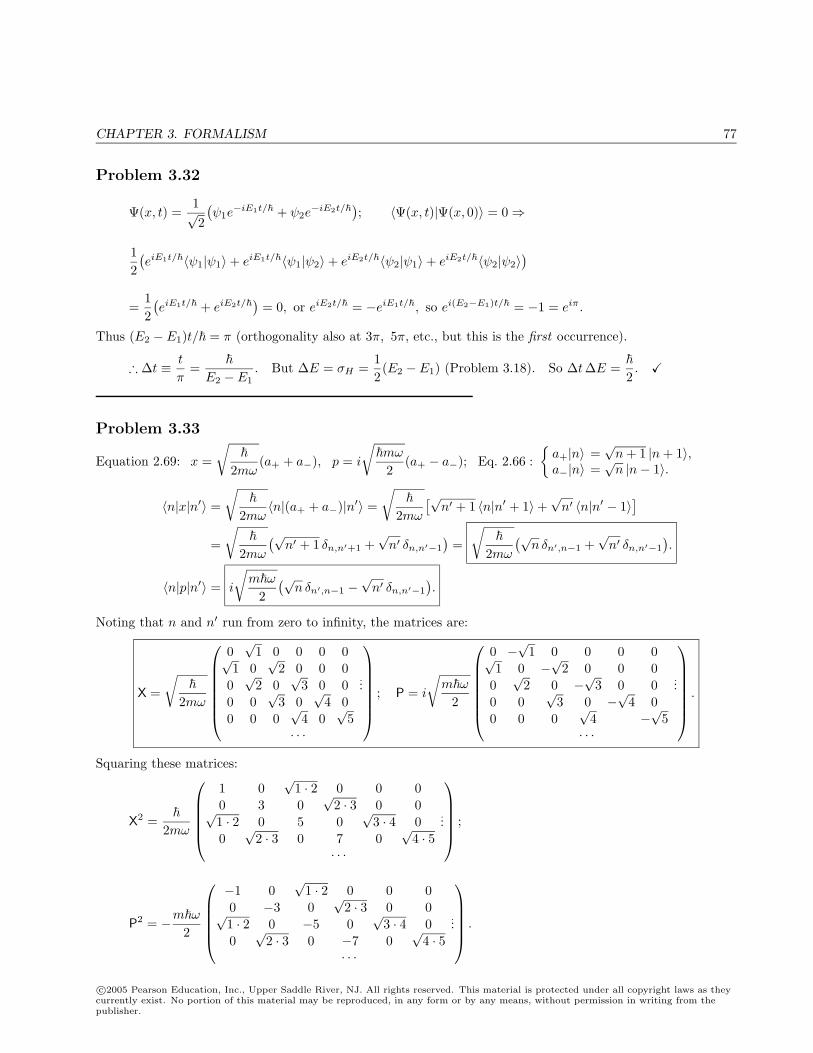
CHAPTER 3. FORMALISM 77
Problem 3.32
Ψ(x, t) =1√2
(ψ1e−iE1t/ + ψ2e
−iE2t/); 〈Ψ(x, t)|Ψ(x, 0)〉 = 0⇒
12(eiE1t/〈ψ1|ψ1〉+ eiE1t/〈ψ1|ψ2〉+ eiE2t/〈ψ2|ψ1〉+ eiE2t/〈ψ2|ψ2〉
)=
12(eiE1t/ + eiE2t/
)= 0, or eiE2t/ = −eiE1t/, so ei(E2−E1)t/ = −1 = eiπ.
Thus (E2 − E1)t/ = π (orthogonality also at 3π, 5π, etc., but this is the first occurrence).
∴ ∆t ≡ t
π=
E2 − E1. But ∆E = σH =
12(E2 − E1) (Problem 3.18). So ∆t∆E =
2.
Problem 3.33
Equation 2.69: x =
√
2mω(a+ + a−), p = i
√mω
2(a+ − a−); Eq. 2.66 :
a+|n〉 =
√n + 1 |n + 1〉,
a−|n〉 =√n |n− 1〉.
〈n|x|n′〉 =
√
2mω〈n|(a+ + a−)|n′〉 =
√
2mω
[√n′ + 1 〈n|n′ + 1〉+
√n′ 〈n|n′ − 1〉
]=
√
2mω
(√n′ + 1 δn,n′+1 +
√n′ δn,n′−1
)=
√
2mω
(√n δn′,n−1 +
√n′ δn,n′−1
).
〈n|p|n′〉 = i
√mω
2(√
n δn′,n−1 −√n′ δn,n′−1
).
Noting that n and n′ run from zero to infinity, the matrices are:
X =
√
2mω
0√
1 0 0 0 0√1 0
√2 0 0 0
0√
2 0√
3 0 0.:
0 0√
3 0√
4 00 0 0
√4 0
√5
· · ·
; P = i
√mω
2
0 −√
1 0 0 0 0√1 0 −
√2 0 0 0
0√
2 0 −√
3 0 0.:
0 0√
3 0 −√
4 00 0 0
√4 −
√5
· · ·
.
Squaring these matrices:
X2 =
2mω
1 0
√1 · 2 0 0 0
0 3 0√
2 · 3 0 0√1 · 2 0 5 0
√3 · 4 0
.:
0√
2 · 3 0 7 0√
4 · 5· · ·
;
P2 = −mω
2
−1 0
√1 · 2 0 0 0
0 −3 0√
2 · 3 0 0√1 · 2 0 −5 0
√3 · 4 0
.:
0√
2 · 3 0 −7 0√
4 · 5· · ·
.
c©2005 Pearson Education, Inc., Upper Saddle River, NJ. All rights reserved. This material is protected under all copyright laws as theycurrently exist. No portion of this material may be reproduced, in any form or by any means, without permission in writing from thepublisher.
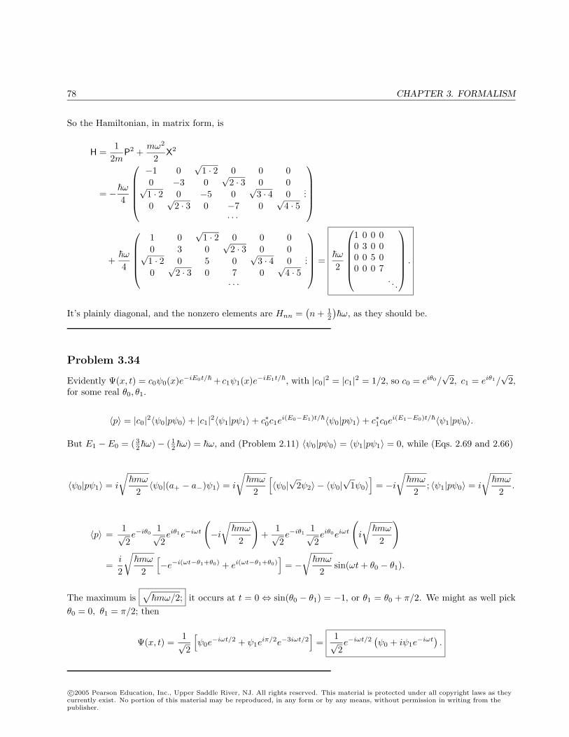
78 CHAPTER 3. FORMALISM
So the Hamiltonian, in matrix form, is
H =1
2mP2 +
mω2
2X2
= −ω4
−1 0
√1 · 2 0 0 0
0 −3 0√
2 · 3 0 0√1 · 2 0 −5 0
√3 · 4 0
.:
0√
2 · 3 0 −7 0√
4 · 5· · ·
+ω
4
1 0
√1 · 2 0 0 0
0 3 0√
2 · 3 0 0√1 · 2 0 5 0
√3 · 4 0
.:
0√
2 · 3 0 7 0√
4 · 5· · ·
=ω
2
1 0 0 00 3 0 00 0 5 00 0 0 7
. . .
.
It’s plainly diagonal, and the nonzero elements are Hnn =(n + 1
2
)ω, as they should be.
Problem 3.34
Evidently Ψ(x, t) = c0ψ0(x)e−iE0t/+ c1ψ1(x)e−iE1t/, with |c0|2 = |c1|2 = 1/2, so c0 = eiθ0/√
2, c1 = eiθ1/√
2,for some real θ0, θ1.
〈p〉 = |c0|2〈ψ0|pψ0〉+ |c1|2〈ψ1|pψ1〉+ c∗0c1ei(E0−E1)t/〈ψ0|pψ1〉+ c∗1c0e
i(E1−E0)t/〈ψ1|pψ0〉.
But E1 − E0 = ( 32ω)− ( 1
2ω) = ω, and (Problem 2.11) 〈ψ0|pψ0〉 = 〈ψ1|pψ1〉 = 0, while (Eqs. 2.69 and 2.66)
〈ψ0|pψ1〉 = i
√mω
2〈ψ0|(a+ − a−)ψ1〉 = i
√mω
2
[〈ψ0|
√2ψ2〉 − 〈ψ0|
√1ψ0〉
]= −i
√mω
2; 〈ψ1|pψ0〉 = i
√mω
2.
〈p〉 =1√2e−iθ0
1√2eiθ1e−iωt
(−i
√mω
2
)+
1√2e−iθ1
1√2eiθ0eiωt
(i
√mω
2
)
=i
2
√mω
2
[−e−i(ωt−θ1+θ0) + ei(ωt−θ1+θ0)
]= −
√mω
2sin(ωt + θ0 − θ1).
The maximum is√mω/2; it occurs at t = 0 ⇔ sin(θ0 − θ1) = −1, or θ1 = θ0 + π/2. We might as well pick
θ0 = 0, θ1 = π/2; then
Ψ(x, t) =1√2
[ψ0e−iωt/2 + ψ1e
iπ/2e−3iωt/2]
=1√2e−iωt/2
(ψ0 + iψ1e
−iωt).
c©2005 Pearson Education, Inc., Upper Saddle River, NJ. All rights reserved. This material is protected under all copyright laws as theycurrently exist. No portion of this material may be reproduced, in any form or by any means, without permission in writing from thepublisher.
CHAPTER 3. FORMALISM 79
Problem 3.35
(a) 〈x〉 = 〈α|xα〉 =
√
2mω〈α|(a+ + a−)α〉 =
√
2mω(〈a−α|α〉+ 〈α|a−α〉) =
√
2mω(α + α∗).
x2 =
2mω
(a2+ + a+a− + a−a+ + a2
−). But a−a+ = [a−, a+] + a+a− = 1 + a+a− (Eq. 2.55).
=
2mω
(a2+ + 2a+a− + 1 + a2
−).
〈x2〉 =
2mω〈α|
(a2+ + 2a+a− + 1 + a2
−)α〉 =
2mω
(〈a2−α|α〉+ 2〈a−α|a−α〉+ 〈α|α〉+ 〈α|a2
−α〉)
=
2mω
[(α∗)2 + 2(α∗)α + 1 + α2
]=
2mω
[1 + (α + α∗)2
].
〈p〉 = 〈α|pα〉 = i
√mω
2〈α|(a+ − a−)α〉 = i
√mω
2(〈a−α|α〉 − 〈α|a−α〉) = −i
√mω
2(α− α∗).
p2 = −mω
2(a2+ − a+a− − a−a+ + a2
−)
= −mω
2(a2+ − 2a+a− − 1 + a2
−).
〈p2〉 = −mω
2〈α|
(a2+ − 2a+a− − 1 + a2
−)α〉 = −mω
2(〈a2−α|α〉 − 2〈a−α|a−α〉 − 〈α|α〉+ 〈α|a2
−α〉)
= −mω
2[(α∗)2 − 2(α∗)α− 1 + α2
]=mω
2[1− (α− α∗)2
].
(b)
σ2x = 〈x2〉 − 〈x〉2 =
2mω
[1 + (α + α∗)2 − (α + α∗)2
]=
2mω;
σ2p = 〈p2〉 − 〈p〉2 =
mω
2[1− (α− α∗)2 + (α− α∗)2
]=mω
2. σxσp =
√
2mω
√mω
2=
2. QED
(c) Using Eq. 2.67 for ψn:
cn = 〈ψn|α〉 =1√n!〈(a+)nψ0|α〉 =
1√n!〈ψ0|(a−)nα〉 =
1√n!
αn〈ψ0|α〉 =αn
√n!
c0.
(d) 1 =∞∑
n=0
|cn|2 = |c0|2∞∑
n=0
|α|2n
n!= |c0|2e|α|
2 ⇒ c0 = e−|α|2/2.
(e) |α(t)〉 =∞∑
n=0
cne−iEnt/|n〉 =
∞∑n=0
αn
√n!
e−|α|2/2e−i(n+ 1
2 )ωt|n〉 = e−iωt/2∞∑
n=0
(αe−iωt
)n
√n!
e−|α|2/2|n〉.
Apart form the overall phase factor e−iωt/2 (which doesn’t affect its status as an eigenfunction of a−, orits eigenvalue), |α(t)〉 is the same as |α〉, but with eigenvalue α(t) = e−iωtα.
(f) Equation 2.58 says a−|ψ0〉 = 0, so yes, it is a coherent state, with eigenvalue α = 0.
c©2005 Pearson Education, Inc., Upper Saddle River, NJ. All rights reserved. This material is protected under all copyright laws as theycurrently exist. No portion of this material may be reproduced, in any form or by any means, without permission in writing from thepublisher.
80 CHAPTER 3. FORMALISM
Problem 3.36
(a) Equation 3.60 becomes |z|2 = [Re(z)]2 +[Im(z)]2 =[12(z + z∗)
]2
+[
12i
(z − z∗)]2
; Eq. 3.61 generalizes to
σ2Aσ2
B ≥[12
(〈f |g〉+ 〈g|f〉)]2
+[
12i
(〈f |g〉 − 〈g|f〉)]2
.
But 〈f |g〉 − 〈g|f〉 = 〈[A, B]〉 (p. 111), and, by the same argument,
〈f |g〉+ 〈g|f〉 = 〈AB〉 − 〈A〉〈B〉+ 〈BA〉 − 〈A〉〈B〉 = 〈AB + BA− 2〈A〉〈B〉〉 = 〈D〉.
So σ2Aσ2
B ≥14
(〈D〉2 + 〈C〉2
).
(b) If B = A, then C = 0, D = 2(A2 − 〈A〉2
); 〈D〉 = 2
(〈A2〉 − 〈A〉2
)= 2σ2
A. So Eq. 3.99 says
σ2Aσ2
A ≥ (1/4)4σ4A = σ4
A, which is true, but not very informative.
Problem 3.37
First find the eigenvalues and eigenvectors of the Hamiltonian. The characteristic equation says∣∣∣∣∣∣(a− E) 0 b
0 (c− E) 0b 0 (a− E)
∣∣∣∣∣∣ = (a− E)(c− E)(a− E)− b2(c− E) = (c− E)[(a− E)2 − b2
]= 0,
Either E = c, or else (a− E)2 = b2 ⇒ E = a± b. So the eigenvalues are
E1 = c, E2 = a + b, E3 = a− b.
To find the corresponding eigenvectors, writea 0 b0 c 0b 0 a
αβγ
= En
αβγ
.
(1)
aα + bγ = cα ⇒ (a− c)α + bγ = 0;cβ = cβ (redundant) ;
bα + aγ = cγ ⇒ (a− c)γ + bα = 0.
⇒[(a− c)2 − b2
]α = 0.
So (excluding the degenerate case a− c = ±b) α = 0, and hence also γ = 0.
(2)
aα + bγ = (a + b)α ⇒ α− γ = 0;cβ = (a + b)β ⇒ β = 0;
bα + aγ = (a + b)γ (redundant).
So α = γ and β = 0.
c©2005 Pearson Education, Inc., Upper Saddle River, NJ. All rights reserved. This material is protected under all copyright laws as theycurrently exist. No portion of this material may be reproduced, in any form or by any means, without permission in writing from thepublisher.
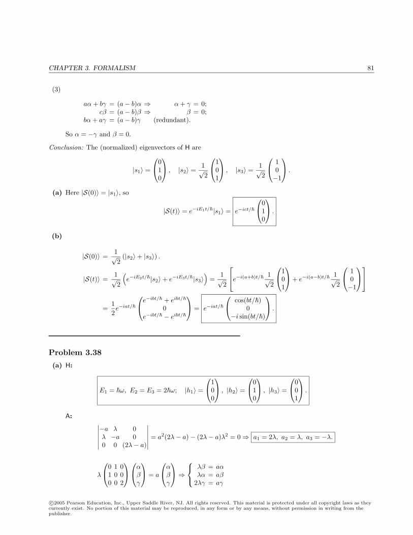
CHAPTER 3. FORMALISM 81
(3)
aα + bγ = (a− b)α ⇒ α + γ = 0;cβ = (a− b)β ⇒ β = 0;
bα + aγ = (a− b)γ (redundant).
So α = −γ and β = 0.
Conclusion: The (normalized) eigenvectors of H are
|s1〉 =
010
, |s2〉 =1√2
101
, |s3〉 =1√2
10−1
.
(a) Here |S(0)〉 = |s1〉, so
|S(t)〉 = e−iE1t/|s1〉 = e−ict/
010
.
(b)
|S(0)〉 =1√2
(|s2〉+ |s3〉) .
|S(t)〉 =1√2
(e−iE2t/|s2〉+ e−iE3t/|s3〉
)=
1√2
e−i(a+b)t/ 1√2
101
+ e−i(a−b)t/ 1√2
10−1
=
12e−iat/
e−ibt/ + eibt/
0e−ibt/ − eibt/
= e−iat/
cos(bt/)0
−i sin(bt/)
.
Problem 3.38
(a) H:
E1 = ω, E2 = E3 = 2ω; |h1〉 =
100
, |h2〉 =
010
, |h3〉 =
001
.
A: ∣∣∣∣∣∣−a λ 0λ −a 00 0 (2λ− a)
∣∣∣∣∣∣ = a2(2λ− a)− (2λ− a)λ2 = 0⇒ a1 = 2λ, a2 = λ, a3 = −λ.
λ
0 1 01 0 00 0 2
αβγ
= a
αβγ
⇒
λβ = aαλα = aβ
2λγ = aγ
c©2005 Pearson Education, Inc., Upper Saddle River, NJ. All rights reserved. This material is protected under all copyright laws as theycurrently exist. No portion of this material may be reproduced, in any form or by any means, without permission in writing from thepublisher.
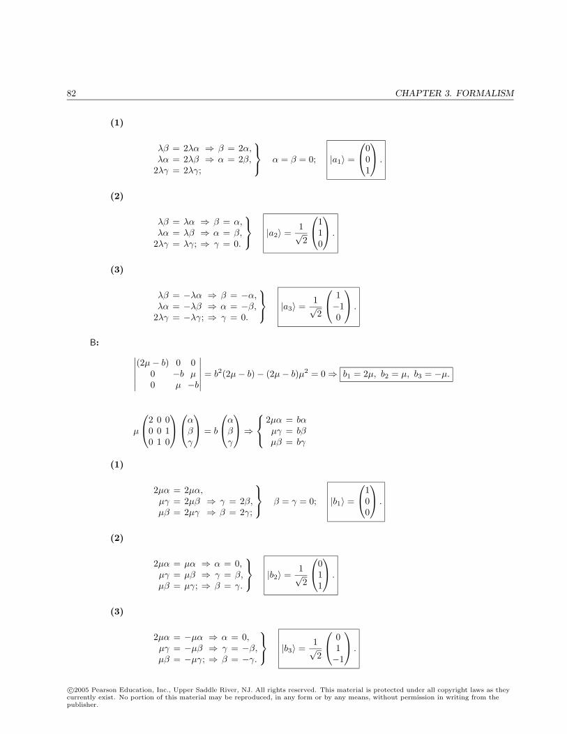
82 CHAPTER 3. FORMALISM
(1)
λβ = 2λα ⇒ β = 2α,λα = 2λβ ⇒ α = 2β,
2λγ = 2λγ;
α = β = 0; |a1〉 =
001
.
(2)
λβ = λα ⇒ β = α,λα = λβ ⇒ α = β,
2λγ = λγ; ⇒ γ = 0.
|a2〉 =1√2
110
.
(3)
λβ = −λα ⇒ β = −α,λα = −λβ ⇒ α = −β,
2λγ = −λγ; ⇒ γ = 0.
|a3〉 =1√2
1−10
.
B: ∣∣∣∣∣∣(2µ− b) 0 0
0 −b µ0 µ −b
∣∣∣∣∣∣ = b2(2µ− b)− (2µ− b)µ2 = 0⇒ b1 = 2µ, b2 = µ, b3 = −µ.
µ
2 0 00 0 10 1 0
αβγ
= b
αβγ
⇒
2µα = bαµγ = bβµβ = bγ
(1)
2µα = 2µα,µγ = 2µβ ⇒ γ = 2β,µβ = 2µγ ⇒ β = 2γ;
β = γ = 0; |b1〉 =
100
.
(2)
2µα = µα ⇒ α = 0,µγ = µβ ⇒ γ = β,µβ = µγ; ⇒ β = γ.
|b2〉 =1√2
011
.
(3)
2µα = −µα ⇒ α = 0,µγ = −µβ ⇒ γ = −β,µβ = −µγ; ⇒ β = −γ.
|b3〉 =1√2
01−1
.
c©2005 Pearson Education, Inc., Upper Saddle River, NJ. All rights reserved. This material is protected under all copyright laws as theycurrently exist. No portion of this material may be reproduced, in any form or by any means, without permission in writing from thepublisher.
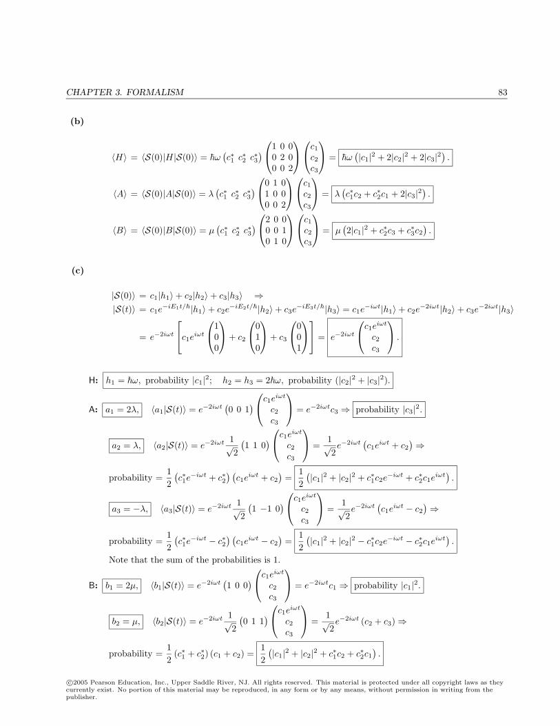
CHAPTER 3. FORMALISM 83
(b)
〈H〉 = 〈S(0)|H|S(0)〉 = ω(c∗1 c∗2 c∗3
) 1 0 00 2 00 0 2
c1c2c3
= ω(|c1|2 + 2|c2|2 + 2|c3|2
).
〈A〉 = 〈S(0)|A|S(0)〉 = λ(c∗1 c∗2 c∗3
) 0 1 01 0 00 0 2
c1c2c3
= λ(c∗1c2 + c∗2c1 + 2|c3|2
).
〈B〉 = 〈S(0)|B|S(0)〉 = µ(c∗1 c∗2 c∗3
) 2 0 00 0 10 1 0
c1c2c3
= µ(2|c1|2 + c∗2c3 + c∗3c2
).
(c)
|S(0)〉 = c1|h1〉+ c2|h2〉+ c3|h3〉 ⇒|S(t)〉 = c1e
−iE1t/|h1〉+ c2e−iE2t/|h2〉+ c3e
−iE3t/|h3〉 = c1e−iωt|h1〉+ c2e
−2iωt|h2〉+ c3e−2iωt|h3〉
= e−2iωt
c1eiωt
100
+ c2
010
+ c3
001
= e−2iωt
c1eiωt
c2c3
.
H: h1 = ω, probability |c1|2; h2 = h3 = 2ω, probability (|c2|2 + |c3|2).
A: a1 = 2λ, 〈a1|S(t)〉 = e−2iωt(0 0 1
) c1eiωt
c2c3
= e−2iωtc3 ⇒ probability |c3|2.
a2 = λ, 〈a2|S(t)〉 = e−2iωt 1√2
(1 1 0
) c1eiωt
c2c3
=1√2e−2iωt
(c1e
iωt + c2)⇒
probability =12
(c∗1e−iωt + c∗2
) (c1e
iωt + c2)
=12
(|c1|2 + |c2|2 + c∗1c2e
−iωt + c∗2c1eiωt
).
a3 = −λ, 〈a3|S(t)〉 = e−2iωt 1√2
(1 −1 0
) c1eiωt
c2c3
=1√2e−2iωt
(c1e
iωt − c2)⇒
probability =12
(c∗1e−iωt − c∗2
) (c1e
iωt − c2)
=12
(|c1|2 + |c2|2 − c∗1c2e
−iωt − c∗2c1eiωt
).
Note that the sum of the probabilities is 1.
B: b1 = 2µ, 〈b1|S(t)〉 = e−2iωt(1 0 0
) c1eiωt
c2c3
= e−2iωtc1 ⇒ probability |c1|2.
b2 = µ, 〈b2|S(t)〉 = e−2iωt 1√2
(0 1 1
) c1eiωt
c2c3
=1√2e−2iωt (c2 + c3)⇒
probability =12
(c∗1 + c∗2) (c1 + c2) =12
(|c1|2 + |c2|2 + c∗1c2 + c∗2c1
).
c©2005 Pearson Education, Inc., Upper Saddle River, NJ. All rights reserved. This material is protected under all copyright laws as theycurrently exist. No portion of this material may be reproduced, in any form or by any means, without permission in writing from thepublisher.
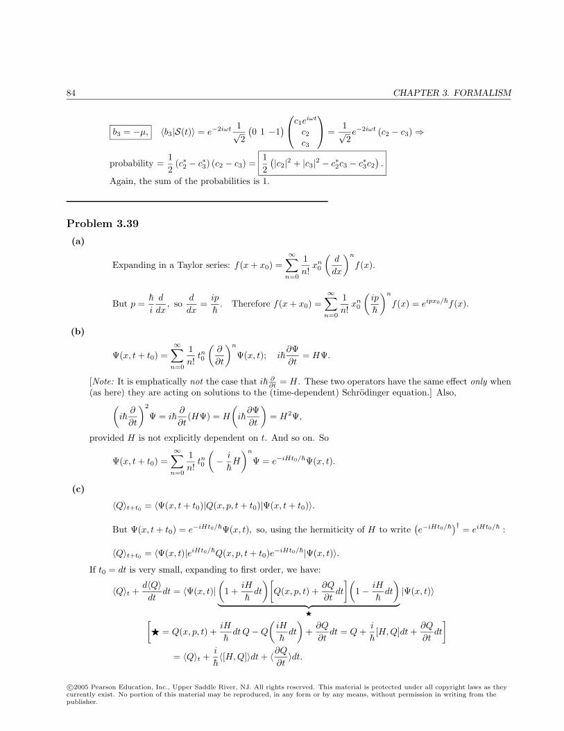
84 CHAPTER 3. FORMALISM
b3 = −µ, 〈b3|S(t)〉 = e−2iωt 1√2
(0 1 −1
) c1eiωt
c2c3
=1√2e−2iωt (c2 − c3)⇒
probability =12
(c∗2 − c∗3) (c2 − c3) =12
(|c2|2 + |c3|2 − c∗2c3 − c∗3c2
).
Again, the sum of the probabilities is 1.
Problem 3.39
(a)
Expanding in a Taylor series: f(x + x0) =∞∑
n=0
1n!
xn0
(d
dx
)n
f(x).
But p =
i
d
dx, so
d
dx=
ip
. Therefore f(x + x0) =
∞∑n=0
1n!
xn0
(ip
)n
f(x) = eipx0/f(x).
(b)
Ψ(x, t + t0) =∞∑
n=0
1n!
tn0
(∂
∂t
)n
Ψ(x, t); i∂Ψ∂t
= HΨ.
[Note: It is emphatically not the case that i ∂∂t = H. These two operators have the same effect only when
(as here) they are acting on solutions to the (time-dependent) Schrodinger equation.] Also,(i
∂
∂t
)2
Ψ = i∂
∂t(HΨ) = H
(i
∂Ψ∂t
)= H2Ψ,
provided H is not explicitly dependent on t. And so on. So
Ψ(x, t + t0) =∞∑
n=0
1n!
tn0
(− i
H
)n
Ψ = e−iHt0/Ψ(x, t).
(c)
〈Q〉t+t0 = 〈Ψ(x, t + t0)|Q(x, p, t + t0)|Ψ(x, t + t0)〉.
But Ψ(x, t + t0) = e−iHt0/Ψ(x, t), so, using the hermiticity of H to write(e−iHt0/
)† = eiHt0/ :
〈Q〉t+t0 = 〈Ψ(x, t)|eiHt0/Q(x, p, t + t0)e−iHt0/|Ψ(x, t)〉.If t0 = dt is very small, expanding to first order, we have:
〈Q〉t +d〈Q〉dt
dt = 〈Ψ(x, t)|(
1 +iH
dt
)[Q(x, p, t) +
∂Q
∂tdt
](1− iH
dt
)︸ ︷︷ ︸
|Ψ(x, t)〉
[ = Q(x, p, t) +
iH
dtQ−Q
(iH
dt
)+
∂Q
∂tdt = Q +
i
[H,Q]dt +
∂Q
∂tdt
]= 〈Q〉t +
i
〈[H,Q]〉dt + 〈∂Q
∂t〉dt.
c©2005 Pearson Education, Inc., Upper Saddle River, NJ. All rights reserved. This material is protected under all copyright laws as theycurrently exist. No portion of this material may be reproduced, in any form or by any means, without permission in writing from thepublisher.
CHAPTER 3. FORMALISM 85
∴ d〈Q〉dt
=i
〈[H,Q]〉+ 〈∂Q
∂t〉. QED
Problem 3.40
(a) For the free particle, V (x) = 0, so the time-dependent Schrodinger equation reads
i∂Ψ∂t
= − 2
2m∂2Ψ∂x2
. Ψ(x, t) =1√2π
∫ ∞−∞
eipx/Φ(p, t) dp ⇒
∂Ψ∂t
=1√2π
∫ ∞−∞
eipx/ ∂Φ∂t
dp,∂2Ψ∂x2
=1√2π
∫ ∞−∞
(−p2
2
)eipx/Φ dp. So
1√2π
∫ ∞−∞
eipx/
[i
∂Φ∂t
]dp =
1√2π
∫ ∞−∞
eipx/
[p2
2mΦ
]dp.
But two functions with the same Fourier transform are equal (as you can easily prove using Plancherel’stheorem), so
i∂Φ∂t
=p2
2mΦ.
1Φ
dΦ = − ip2
2mdt ⇒ Φ(p, t) = e−ip2t/2mΦ(p, 0).
(b)
Ψ(x, 0) = Ae−ax2eilx, A =
(2aπ
)1/4
(Problem2.43(a)).
Φ(p, 0) =1√2π
(2aπ
)1/4 ∫ ∞−∞
e−ipx/e−ax2eilx dx =
1(2πa2)1/4
e−(l−p/)2/4a (Problem2.43(b)).
Φ(p, t) =1
(2πa2)1/4e−(l−p/)2/4ae−ip2t/2m; |Φ(p, t)|2 =
1√2πa
e−(l−p/)2/2a.
(c)
〈p〉 =∫ ∞−∞
p|Φ(p, t)|2 dp =1√
2πa
∫ ∞−∞
pe−(l−p/)2/2a dp
[Let y ≡ (p/)− l, so p = (y + l) and dp = dy.]
=√2πa
∫ ∞−∞
(y + l)e−y2/2a dy [but the first term is odd]
=2l√2πa
∫ ∞0
e−y2/2a dy =2l√2πa
√πa
2= l [as in Problem 2.43(d)].
〈p2〉 =∫ ∞−∞
p2|Φ(p, t)|2 dp =1√
2πa
∫ ∞−∞
p2e−(l−p/)2/2a dp =
2
√2πa
∫ ∞−∞
(y2 + 2yl + l2)e−y2/2a dy
=22
√2πa
[∫ ∞0
y2e−y2/2a dy + l2∫ ∞
0
e−y2/2a dy
]=
22
√2πa
[2√π
(√a
2
)3
+ l2√
πa
2
]= (a + l2)2 [as in Problem 2.43(d)].
c©2005 Pearson Education, Inc., Upper Saddle River, NJ. All rights reserved. This material is protected under all copyright laws as theycurrently exist. No portion of this material may be reproduced, in any form or by any means, without permission in writing from thepublisher.
86 CHAPTER 3. FORMALISM
(d) H =p2
2m; 〈H〉 =
12m〈p2〉 =
2
2m(l2+a) =
12m〈p〉2+
2a
2m. But 〈H〉0 =
12m〈p2〉0 =
2a
2m(Problem 2.22(d)).
So 〈H〉 =1
2m〈p〉2 + 〈H〉0. QED Comment: The energy of the traveling gaussian is the energy of the
same gaussian at rest, plus the kinetic energy (〈p〉2/2m) associated with the motion of the wave packetas a whole.
c©2005 Pearson Education, Inc., Upper Saddle River, NJ. All rights reserved. This material is protected under all copyright laws as theycurrently exist. No portion of this material may be reproduced, in any form or by any means, without permission in writing from thepublisher.
CHAPTER 4. QUANTUM MECHANICS IN THREE DIMENSIONS 87
Chapter 4
Quantum Mechanics in ThreeDimensions
Problem 4.1
(a)
[x, y] = xy − yx = 0, etc., so [ri, rj ] = 0.
[px, py]f =
i
∂
∂x
(
i
∂f
∂y
)−
i
∂
∂y
(
i
∂f
∂x
)= −2
(∂2f
∂x∂y− ∂2f
∂y∂x
)= 0
(by the equality of cross-derivatives), so [pi, pj ] = 0.
[x, px]f =
i
(x∂f
∂x− ∂
∂x(xf)
)=
i
(x∂f
∂x− x
∂f
∂x− f
)= if,
so [x, px] = i (likewise [y, py] = i and [z, pz] = i).
[y, px]f =
i
(y∂f
∂x− ∂
∂x(yf)
)=
i
(y∂f
∂x− y
∂f
∂y
)= 0 (since
∂y
∂x= 0). So [y, px] = 0,
and same goes for the other “mixed” commutators. Thus [ri, pj ] = −[pj , ri] = iδij .
(b) The derivation of Eq. 3.71 (page 115) is identical in three dimensions, sod〈x〉dt
=i
〈[H,x]〉;
[H,x] =[p2
2m+ V, x
]=
12m
[p2x + p2
y + p2z, x] =
12m
[p2x, x]
=1
2m(px[px, x] + [px, x]px) =
12m
[(−i)px + (−i)px] = −i
mpx.
∴ d〈x〉dt
=i
(−i
m〈px〉
)=
1m〈px〉. The same goes for y and z, so:
d〈r〉dt
=1m〈p〉.
c©2005 Pearson Education, Inc., Upper Saddle River, NJ. All rights reserved. This material is protected under all copyright laws as theycurrently exist. No portion of this material may be reproduced, in any form or by any means, without permission in writing from thepublisher.
88 CHAPTER 4. QUANTUM MECHANICS IN THREE DIMENSIONS
d〈px〉dt
=i
〈[H, px]〉; [H, px] =
[p2
2m+ V, px
]= [V, px] = i
∂V
∂x(Eq. 3.65)
=i
(i)
⟨∂V
∂x
⟩=
⟨−∂V
∂x
⟩. Same for y and z, so:
d〈p〉dt
= 〈−∇V 〉.
(c) From Eq. 3.62: σxσpx ≥∣∣∣∣ 12i〈[x, px]〉
∣∣∣∣ =∣∣∣∣ 12i
i
∣∣∣∣ =
2. Generally, σriσpj ≥
2δij .
Problem 4.2
(a) Equation 4.8 ⇒ − 2
2m
(∂2ψ
∂x2+
∂2ψ
∂y2+
∂2ψ
∂z2
)= Eψ (inside the box). Separable solutions: ψ(x, y, z) =
X(x)Y (y)Z(z). Put this in, and divide by XY Z:
1X
d2X
dx2+
1Y
d2X
dy2+
1Z
d2Z
dz2= −2m
2E.
The three terms on the left are functions of x, y, and z, respectively, so each must be a constant. Call theseparation constants k2
x, k2y, and k2
z (as we’ll soon seen, they must be positive).
d2X
dx2= −k2
xX;d2Y
dy2= −k2
yY ;d2Z
dz2= −k2
zZ, with E =
2
2m(k2
x + k2y + k2
z).
Solution:
X(x) = Ax sin kxx + Bx cos kxx; Y (y) = Ay sin kyy + By cos kyy; Z(z) = Az sin kzz + Bz cos kzz.
But X(0) = 0, so Bx = 0; Y (0) = 0, so By = 0; Z(0) = 0, so Bz = 0. And X(a) = 0 ⇒ sin(kxa) = 0 ⇒kx = nxπ/a (nx = 1, 2, 3, . . . ). [As before (page 31), nx = 0, and negative values are redundant.] Likewiseky = nyπ/a and kz = nzπ/a. So
ψ(x, y, z) = AxAyAz sin(nxπ
ax)
sin(nyπ
ay)
sin(nzπ
az), E =
2
2mπ2
a2(n2
x + n2y + n2
z).
We might as well normalize X,Y, and Z separately: Ax = Ay = Az =√
2/a. Conclusion:
ψ(x, y, z) =(
2a
)3/2
sin(nxπ
ax)
sin(nyπ
ay)
sin(nzπ
az)
; E =π2
2
2ma2(n2
x + n2y + n2
z); nx, ny, nz = 1, 2, 3, . . .
c©2005 Pearson Education, Inc., Upper Saddle River, NJ. All rights reserved. This material is protected under all copyright laws as theycurrently exist. No portion of this material may be reproduced, in any form or by any means, without permission in writing from thepublisher.
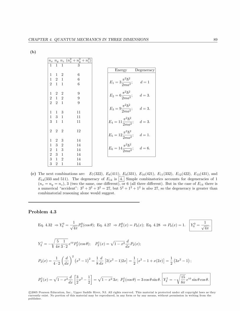
CHAPTER 4. QUANTUM MECHANICS IN THREE DIMENSIONS 89
(b)
nx ny nz (n2x + n2
y + n2z)
1 1 1 3
1 1 2 61 2 1 62 1 1 6
1 2 2 92 1 2 92 2 1 9
1 1 3 111 3 1 113 1 1 11
2 2 2 12
1 2 3 141 3 2 142 1 3 142 3 1 143 1 2 143 2 1 14
Energy Degeneracy
E1 = 3π2
2
2ma2; d = 1
E2 = 6π2
2
2ma2; d = 3.
E3 = 9π2
2
2ma2; d = 3.
E4 = 11π2
2
2ma2; d = 3.
E5 = 12π2
2
2ma2; d = 1.
E6 = 14π2
2
2ma2; d = 6.
(c) The next combinations are: E7(322), E8(411), E9(331), E10(421), E11(332), E12(422), E13(431), andE14(333 and 511). The degeneracy of E14 is 4. Simple combinatorics accounts for degeneracies of 1(nx = ny = nz), 3 (two the same, one different), or 6 (all three different). But in the case of E14 there isa numerical “accident”: 32 + 32 + 32 = 27, but 52 + 12 + 12 is also 27, so the degeneracy is greater thancombinatorial reasoning alone would suggest.
Problem 4.3
Eq. 4.32 ⇒ Y 00 =
1√4π
P 00 (cos θ); Eq. 4.27 ⇒ P 0
0 (x) = P0(x); Eq. 4.28 ⇒ P0(x) = 1. Y 00 =
1√4π
.
Y 12 = −
√54π
13 · 2 eiφP 1
2 (cos θ); P 12 (x) =
√1− x2
d
dxP2(x);
P2(x) =1
4 · 2
(d
dx
)2 (x2 − 1
)2=
18
d
dx
[2(x2 − 1)2x
]=
12
[x2 − 1 + x(2x)
]=
12
(3x2 − 1
);
P 12 (x) =
√1− x2
d
dx
[32x2 − 1
2
]=
√1− x2 3x; P 1
2 (cos θ) = 3 cos θ sin θ. Y 12 = −
√158π
eiφ sin θ cos θ.
c©2005 Pearson Education, Inc., Upper Saddle River, NJ. All rights reserved. This material is protected under all copyright laws as theycurrently exist. No portion of this material may be reproduced, in any form or by any means, without permission in writing from thepublisher.
90 CHAPTER 4. QUANTUM MECHANICS IN THREE DIMENSIONS
Normalization:∫∫
|Y 00 |2 sin θ dθ dφ =
14π
[∫ π
0
sin θ dθ
] [∫ 2π
0
dφ
]=
14π
(2)(2π) = 1.
∫∫|Y 1
2 |2 sin θ dθ dφ =158π
∫ π
0
sin2 θ cos2 θ sin θ dθ
∫ 2π
0
dφ =154
∫ π
0
cos2 θ(1− cos2 θ) sin θ dθ
=154
[−cos3 θ
3+
cos5 θ
5
]∣∣∣∣π0
=154
[23− 2
5
]=
52− 3
2= 1
Orthogonality:∫∫
Y 00∗Y 1
2 sin θ dθ dφ = − 1√4π
√158π
[ ∫ π
0
sin θ cos θ sin θ dθ︸ ︷︷ ︸(sin3 θ)/3|π0 =0
][ ∫ 2π
0
eiφdφ︸ ︷︷ ︸(eiφ)/i|2π0 =0
]= 0.
Problem 4.4
dΘdθ
=A
tan(θ/2)12
sec2(θ/2) =A
21
sin(θ/2) cos(θ/2)=
A
sin θ. Therefore
d
dθ
(sin θ
dΘdθ
)=
d
dθ(A) = 0.
With l = m = 0, Eq. 4.25 reads:d
dθ
(sin θ
dΘdθ
)= 0. So A ln[tan(θ/2)] does satisfy Eq. 4.25. However,
Θ(0) = A ln(0) = A(−∞); Θ(π) = A ln(tan
π
2
)= A ln(∞) = A(∞). Θ blows up at θ = 0 and at θ = π.
Problem 4.5
Y ll = (−1)l
√(2l + 1)
4π1
(2l)!eilφP l
l (cos θ). P ll (x) = (1− x2)l/2
(d
dx
)l
Pl(x).
Pl(x) =1
2ll!
(d
dx
)l
(x2 − 1)l, so P ll (x) =
12ll!
(1− x2)l/2
(d
dx
)2l
(x2 − 1)l.
Now (x2− 1)l = x2l + · · · , where all the other terms involve powers of x less than 2l, and hence give zero whendifferentiated 2l times. So
P ll (x) =
12ll!
(1− x2)l/2
(d
dx
)2l
x2l. But(
d
dx
)n
xn = n!, so P ll =
(2l)!2ll!
(1− x2)l/2.
∴ Y ll = (−1)l
√(2l + 1)4π(2l)!
eilφ (2l)!2ll!
(sin θ)l =1l!
√(2l + 1)!
4π
(−1
2eiφ sin θ
)l
.
c©2005 Pearson Education, Inc., Upper Saddle River, NJ. All rights reserved. This material is protected under all copyright laws as theycurrently exist. No portion of this material may be reproduced, in any form or by any means, without permission in writing from thepublisher.
CHAPTER 4. QUANTUM MECHANICS IN THREE DIMENSIONS 91
Y 23 =
√74π· 15!
e2iφP 23 (cos θ); P 2
3 (x) = (1− x2)(
d
dx
)2
P3(x); P3(x) =1
8 · 3!
(d
dx
)3
(x2 − 1)3.
P3 =1
8 · 3 · 2
(d
dx
)2 [6x(x2 − 1)2
]=
18
d
dx
[(x2 − 1)2 + 4x2(x2 − 1)
]=
18
[4x(x2 − 1) + 8x(x2 − 1) + 4x2 · 2x
]=
12
(x3 − x + 2x3 − 2x + 2x3
)=
12
(5x3 − 3x
).
P 23 (x) =
12
(1− x2
) (d
dx
)2 (5x3 − 3x
)=
12
(1− x2
) d
dx
(15x2 − 3
)=
12(1− x2)30x = 15x(1− x2).
Y 23 =
√74π
15!
15e2iφ cos θ sin2 θ =14
√1052π
e2iφ sin2 θ cos θ.
Check that Y ll satisfies Eq. 4.18: Let
1l!
√(2l + 1)!
4π
(−1
2
)l
≡ A, so Y ll = A(eiφ sin θ)l.
∂Y ll
∂θ= Aeilφl(sin θ)l−1 cos θ; sin θ
∂Y ll
∂θ= l cos θY l
l ;
sin θ∂
∂θ
(sin θ
∂Y ll
∂θ
)= l cos θ
(sin θ
∂Y ll
∂θ
)− l sin2 θY l
l =(l2 cos2 θ − l sin2 θ
)Y l
l .∂2Y l
l
∂φ2= −l2Y l
l .
So the left side of Eq. 4.18 is[l2(1− sin2 θ)− l sin2 θ − l2
]Y l
l = −l(l+1) sin2 θ Y ll , which matches the right side.
Check that Y 23 satisfies Eq. 4.18: Let B ≡ 1
4
√1052π
, so Y 23 = Be2iφ sin2 θ cos θ.
∂Y 23
∂θ= Be2iφ
(2 sin θ cos2 θ − sin3 θ
); sin θ
∂
∂θ
(sin θ
∂Y 23
∂θ
)= Be2iφ sin θ
∂
∂θ
(2 sin2 θ cos2 θ − sin4 θ
)
= Be2iφ sin θ(4 sin θ cos3 θ − 4 sin3 θ cos θ − 4 sin3 θ cos θ
)= 4Be2iφ sin2 θ cos θ
(cos2 θ − 2 sin2 θ
)= 4(cos2 θ − 2 sin2 θ)Y 2
3 .∂2Y 2
3
∂φ2= −4Y 2
3 . So the left side of Eq. 4.18 is
4(cos2 θ − 2 sin2 θ − 1)Y 23 = 4(−3 sin2 θ)Y 2
3 = −l(l + 1) sin2 θ Y 23 ,
where l = 3, so it fits the right side of Eq. 4.18.
Problem 4.6
∫ 1
−1
Pl(x)Pl′(x)dx =1
2ll!1
2l′ l′!
∫ 1
−1
[(d
dx
)l
(x2 − 1)l
] [(d
dx
)l′
(x2 − 1)l′
]dx.
c©2005 Pearson Education, Inc., Upper Saddle River, NJ. All rights reserved. This material is protected under all copyright laws as theycurrently exist. No portion of this material may be reproduced, in any form or by any means, without permission in writing from thepublisher.
92 CHAPTER 4. QUANTUM MECHANICS IN THREE DIMENSIONS
If l = l′, we may as well let l be the larger of the two (l > l′). Integrate by parts, pulling successively eachderivative off the first term onto the second:
2ll!2l′ l′!∫ 1
−1
Pl(x)Pl′(x)dx =
[(d
dx
)l−1
(x2 − 1)l
] [(d
dx
)l′
(x2 − 1)l′
]∣∣∣∣∣1
−1
−∫ 1
−1
[(d
dx
)l−1
(x2 − 1)l
] [(d
dx
)l′+1
(x2 − 1)l′
]dx
= . . . (boundary terms) . . . + (−1)l
∫ 1
−1
(x2 − 1)l
(d
dx
)l′+l
(x2 − 1)l′dx.
But (d/dx)l′+l (x2 − 1)l′ = 0, because (x2 − 1)l′ is a polynomial whose highest power is 2l′, so more than 2l′
derivatives will kill it, and l′ + l > 2l′. Now, the boundary terms are of the form:[(d
dx
)l−n
(x2 − 1)l
] [(d
dx
)l′+n−1
(x2 − 1)l′
]∣∣∣∣∣+1
−1
, n = 1, 2, 3, . . . , l.
Look at the first term: (x2 − 1)l = (x2 − 1)(x2 − 1) . . . (x2 − 1); l factors. So 0, 1, 2, . . . , l − 1 derivatives willstill leave at least one overall factor of (x2 − 1). [Zero derivatives leaves l factors; one derivative leaves l − 1 :d/dx(x2−1)l = 2lx(x2−1)l−1; two derivatives leaves l−2 : d2/dx2(x2−1)l = 2l(x2−1)l−1+2l(l−1)2x2(x2−1)l−2,and so on.] So the boundary terms are all zero, and hence
∫ 1
−1Pl(x)Pl′(x)dx = 0.
This leaves only the case l = l′. Again the boundary terms vanish, but this time the remaining integral doesnot :
(2ll!)2∫ 1
−1
[Pl(x)]2dx = (−1)l
∫ 1
−1
(x2 − 1)l
(d
dx
)2l
(x2 − 1)l︸ ︷︷ ︸(d/dx)2l(x2l)=(2l)!
dx
= (−1)l(2l)!∫ 1
−1
(x2 − 1)ldx = 2(2l)!∫ 1
0
(1− x2)ldx.
Let x ≡ cos θ, so dx = − sin θ dθ, (1− x2) = sin2 θ, θ : π/2→ 0. Then∫ 1
0
(1− x2)ldx =∫ 0
π/2
(sin θ)2l(− sin θ)dθ =∫ π/2
0
(sin θ)2l+1dθ
=(2)(4) · · · (2l)
(1)(3)(5) · · · (2l + 1)=
(2ll!)2
1 · 2 · 3 · · · · (2l + 1)=
(2ll!)2
(2l + 1)!.
∴∫ 1
−1
[Pl(x)]2dx =1
(2ll!)22(2l)!
(2ll!)2
(2l + 1)!=
22l + 1
. So∫ 1
−1
Pl(x)Pl′(x)dx =2
2l + 1δll′ . QED
Problem 4.7
(a)
n1(x) = −(−x)1x
d
dx
(cosxx
)= −cosx
x2− sinx
x.
c©2005 Pearson Education, Inc., Upper Saddle River, NJ. All rights reserved. This material is protected under all copyright laws as theycurrently exist. No portion of this material may be reproduced, in any form or by any means, without permission in writing from thepublisher.
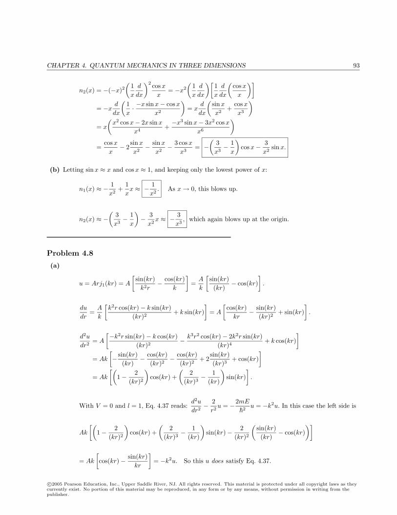
CHAPTER 4. QUANTUM MECHANICS IN THREE DIMENSIONS 93
n2(x) = −(−x)2(
1x
d
dx
)2 cosxx
= −x2
(1x
d
dx
)[1x
d
dx
(cosxx
)]= −x
d
dx
(1x· −x sinx− cosx
x2
)= x
d
dx
(sinx
x2+
cosxx3
)= x
(x2 cosx− 2x sinx
x4+−x3 sinx− 3x2 cosx
x6
)=
cosxx
− 2sinx
x2− sinx
x2− 3 cosx
x3= −
(3x3− 1
x
)cosx− 3
x2sinx.
(b) Letting sinx ≈ x and cosx ≈ 1, and keeping only the lowest power of x:
n1(x) ≈ − 1x2
+1xx ≈ − 1
x2. As x→ 0, this blows up.
n2(x) ≈ −(
3x3− 1
x
)− 3
x2x ≈ − 3
x3, which again blows up at the origin.
Problem 4.8
(a)
u = Arj1(kr) = A
[sin(kr)k2r
− cos(kr)k
]=
A
k
[sin(kr)(kr)
− cos(kr)].
du
dr=
A
k
[k2r cos(kr)− k sin(kr)
(kr)2+ k sin(kr)
]= A
[cos(kr)
kr− sin(kr)
(kr)2+ sin(kr)
].
d2u
dr2= A
[−k2r sin(kr)− k cos(kr)(kr)2
− k3r2 cos(kr)− 2k2r sin(kr)(kr)4
+ k cos(kr)]
= Ak
[− sin(kr)
(kr)− cos(kr)
(kr)2− cos(kr)
(kr)2+ 2
sin(kr)(kr)3
+ cos(kr)]
= Ak
[(1− 2
(kr)2
)cos(kr) +
(2
(kr)3− 1
(kr)
)sin(kr)
].
With V = 0 and l = 1, Eq. 4.37 reads:d2u
dr2− 2
r2u = −2mE
2u = −k2u. In this case the left side is
Ak
[(1− 2
(kr)2
)cos(kr) +
(2
(kr)3− 1
(kr)
)sin(kr)− 2
(kr)2
(sin(kr)(kr)
− cos(kr))]
= Ak
[cos(kr)− sin(kr)
kr
]= −k2u. So this u does satisfy Eq. 4.37.
c©2005 Pearson Education, Inc., Upper Saddle River, NJ. All rights reserved. This material is protected under all copyright laws as theycurrently exist. No portion of this material may be reproduced, in any form or by any means, without permission in writing from thepublisher.
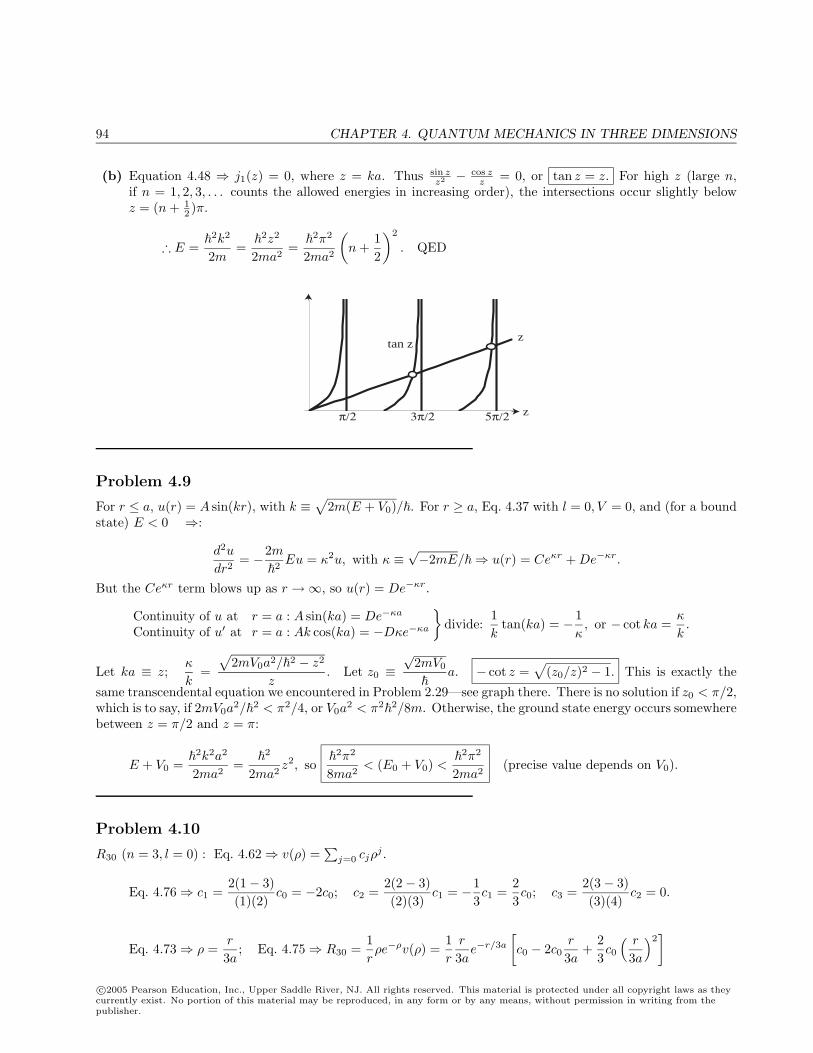
94 CHAPTER 4. QUANTUM MECHANICS IN THREE DIMENSIONS
(b) Equation 4.48 ⇒ j1(z) = 0, where z = ka. Thus sin zz2 − cos z
z = 0, or tan z = z. For high z (large n,if n = 1, 2, 3, . . . counts the allowed energies in increasing order), the intersections occur slightly belowz = (n + 1
2 )π.
∴ E =
2k2
2m=
2z2
2ma2=
2π2
2ma2
(n +
12
)2
. QED
π/2 3π/2 z5π/2
ztan z
Problem 4.9
For r ≤ a, u(r) = A sin(kr), with k ≡√
2m(E + V0)/. For r ≥ a, Eq. 4.37 with l = 0, V = 0, and (for a boundstate) E < 0 ⇒:
d2u
dr2= −2m
2Eu = κ2u, with κ ≡
√−2mE/⇒ u(r) = Ceκr + De−κr.
But the Ceκr term blows up as r →∞, so u(r) = De−κr.
Continuity of u at r = a : A sin(ka) = De−κa
Continuity of u′ at r = a : Ak cos(ka) = −Dκe−κa
divide:
1k
tan(ka) = − 1κ, or − cot ka =
κ
k.
Let ka ≡ z;κ
k=
√2mV0a2/2 − z2
z. Let z0 ≡
√2mV0
a. − cot z =
√(z0/z)2 − 1. This is exactly the
same transcendental equation we encountered in Problem 2.29—see graph there. There is no solution if z0 < π/2,which is to say, if 2mV0a
2/2 < π2/4, or V0a2 < π2
2/8m. Otherwise, the ground state energy occurs somewhere
between z = π/2 and z = π:
E + V0 =
2k2a2
2ma2=
2
2ma2z2, so
2π2
8ma2< (E0 + V0) <
2π2
2ma2(precise value depends on V0).
Problem 4.10
R30 (n = 3, l = 0) : Eq. 4.62⇒ v(ρ) =∑
j=0 cjρj .
Eq. 4.76⇒ c1 =2(1− 3)(1)(2)
c0 = −2c0; c2 =2(2− 3)(2)(3)
c1 = −13c1 =
23c0; c3 =
2(3− 3)(3)(4)
c2 = 0.
Eq. 4.73⇒ ρ =r
3a; Eq. 4.75⇒ R30 =
1rρe−ρv(ρ) =
1r
r
3ae−r/3a
[c0 − 2c0
r
3a+
23c0
( r
3a
)2]
c©2005 Pearson Education, Inc., Upper Saddle River, NJ. All rights reserved. This material is protected under all copyright laws as theycurrently exist. No portion of this material may be reproduced, in any form or by any means, without permission in writing from thepublisher.
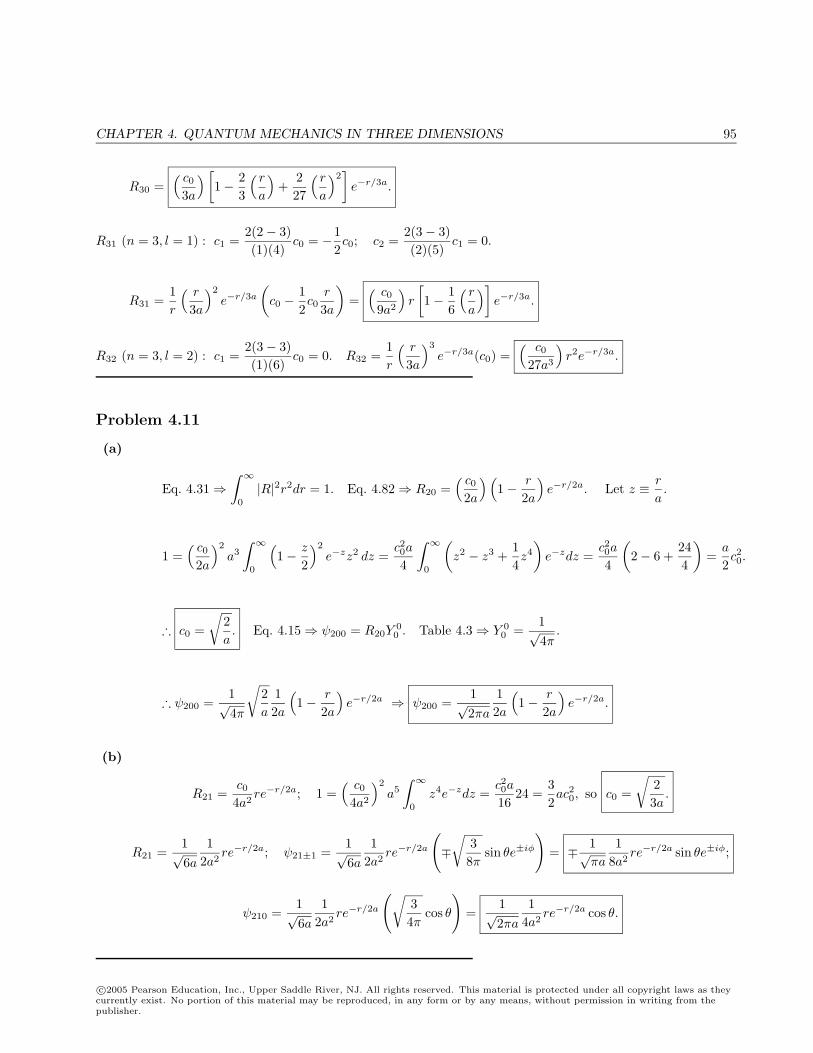
CHAPTER 4. QUANTUM MECHANICS IN THREE DIMENSIONS 95
R30 =( c0
3a
) [1− 2
3
( r
a
)+
227
( r
a
)2]e−r/3a.
R31 (n = 3, l = 1) : c1 =2(2− 3)(1)(4)
c0 = −12c0; c2 =
2(3− 3)(2)(5)
c1 = 0.
R31 =1r
( r
3a
)2
e−r/3a
(c0 −
12c0
r
3a
)=
( c09a2
)r
[1− 1
6
( r
a
)]e−r/3a.
R32 (n = 3, l = 2) : c1 =2(3− 3)(1)(6)
c0 = 0. R32 =1r
( r
3a
)3
e−r/3a(c0) =( c0
27a3
)r2e−r/3a.
Problem 4.11
(a)
Eq. 4.31⇒∫ ∞
0
|R|2r2dr = 1. Eq. 4.82⇒ R20 =( c0
2a
) (1− r
2a
)e−r/2a. Let z ≡ r
a.
1 =( c0
2a
)2
a3
∫ ∞0
(1− z
2
)2
e−zz2 dz =c20a
4
∫ ∞0
(z2 − z3 +
14z4
)e−zdz =
c20a
4
(2− 6 +
244
)=
a
2c20.
∴ c0 =
√2a. Eq. 4.15⇒ ψ200 = R20Y
00 . Table 4.3⇒ Y 0
0 =1√4π
.
∴ ψ200 =1√4π
√2a
12a
(1− r
2a
)e−r/2a ⇒ ψ200 =
1√2πa
12a
(1− r
2a
)e−r/2a.
(b)
R21 =c04a2
re−r/2a; 1 =( c0
4a2
)2
a5
∫ ∞0
z4e−zdz =c20a
1624 =
32ac20, so c0 =
√23a
.
R21 =1√6a
12a2
re−r/2a; ψ21±1 =1√6a
12a2
re−r/2a
(∓
√38π
sin θe±iφ
)= ∓ 1√
πa
18a2
re−r/2a sin θe±iφ;
ψ210 =1√6a
12a2
re−r/2a
(√34π
cos θ
)=
1√2πa
14a2
re−r/2a cos θ.
c©2005 Pearson Education, Inc., Upper Saddle River, NJ. All rights reserved. This material is protected under all copyright laws as theycurrently exist. No portion of this material may be reproduced, in any form or by any means, without permission in writing from thepublisher.
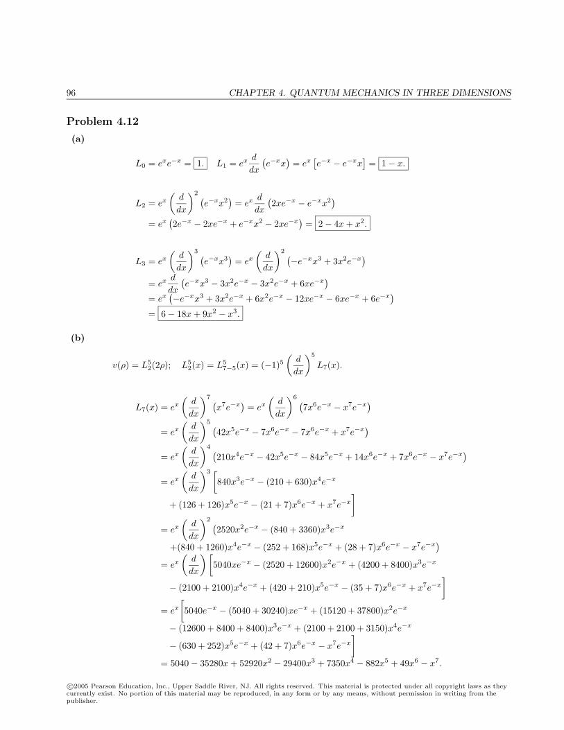
96 CHAPTER 4. QUANTUM MECHANICS IN THREE DIMENSIONS
Problem 4.12
(a)
L0 = exe−x = 1. L1 = ex d
dx
(e−xx
)= ex
[e−x − e−xx
]= 1− x.
L2 = ex
(d
dx
)2 (e−xx2
)= ex d
dx
(2xe−x − e−xx2
)= ex
(2e−x − 2xe−x + e−xx2 − 2xe−x
)= 2− 4x + x2.
L3 = ex
(d
dx
)3 (e−xx3
)= ex
(d
dx
)2 (−e−xx3 + 3x2e−x
)= ex d
dx
(e−xx3 − 3x2e−x − 3x2e−x + 6xe−x
)= ex
(−e−xx3 + 3x2e−x + 6x2e−x − 12xe−x − 6xe−x + 6e−x
)= 6− 18x + 9x2 − x3.
(b)
v(ρ) = L52(2ρ); L5
2(x) = L57−5(x) = (−1)5
(d
dx
)5
L7(x).
L7(x) = ex
(d
dx
)7 (x7e−x
)= ex
(d
dx
)6 (7x6e−x − x7e−x
)= ex
(d
dx
)5 (42x5e−x − 7x6e−x − 7x6e−x + x7e−x
)= ex
(d
dx
)4 (210x4e−x − 42x5e−x − 84x5e−x + 14x6e−x + 7x6e−x − x7e−x
)= ex
(d
dx
)3 [840x3e−x − (210 + 630)x4e−x
+ (126 + 126)x5e−x − (21 + 7)x6e−x + x7e−x
]= ex
(d
dx
)2 (2520x2e−x − (840 + 3360)x3e−x
+(840 + 1260)x4e−x − (252 + 168)x5e−x + (28 + 7)x6e−x − x7e−x)
= ex
(d
dx
) [5040xe−x − (2520 + 12600)x2e−x + (4200 + 8400)x3e−x
− (2100 + 2100)x4e−x + (420 + 210)x5e−x − (35 + 7)x6e−x + x7e−x
]= ex
[5040e−x − (5040 + 30240)xe−x + (15120 + 37800)x2e−x
− (12600 + 8400 + 8400)x3e−x + (2100 + 2100 + 3150)x4e−x
− (630 + 252)x5e−x + (42 + 7)x6e−x − x7e−x
]= 5040− 35280x + 52920x2 − 29400x3 + 7350x4 − 882x5 + 49x6 − x7.
c©2005 Pearson Education, Inc., Upper Saddle River, NJ. All rights reserved. This material is protected under all copyright laws as theycurrently exist. No portion of this material may be reproduced, in any form or by any means, without permission in writing from thepublisher.
CHAPTER 4. QUANTUM MECHANICS IN THREE DIMENSIONS 97
L52 = −
(d
dx
)5 (−882x5 + 49x6 − x7
)= −
[−882(5 · 4 · 3 · 2) + 49(6 · 5 · 4 · 3 · 2)x− 7 · 6 · 5 · 4 · 3x2
]= 60
[(882× 2)− (49× 12)x + 42x2
]= 2520(42− 14x + x2).
v(ρ) = 2520(42− 28ρ + 4ρ2) = 5040(21− 14ρ + 2ρ2
).
(c)
Eq. 4.62⇒ v(ρ) =∞∑
j=0
cjρj . Eq. 4.76⇒ c1 =
2(3− 5)(1)(6)
c0 = −23c0.
c2 =2(4− 5)(2)(7)
c1 = −17c1 =
221
c0; c3 =2(5− 5)(3)(8)
c2 = 0.
v(ρ) = c0 −23c0ρ +
221
c0ρ2 =
c021
(21− 14ρ + 2ρ2
).
Problem 4.13
(a)
ψ =1√πa3
e−r/a, so 〈rn〉 =1
πa3
∫rne−2r/a
(r2 sin θ dr dθ dφ
)=
4ππa3
∫ ∞0
rn+2e−2r/adr.
〈r〉 =4a3
∫ ∞0
r3e−2r/adr =4a3
3!(a
2
)4
=32a; 〈r2〉 =
4a3
∫ ∞0
r4e−2r/adr =4a3
4!(a
2
)5
= 3a2.
(b)
〈x〉 = 0; 〈x2〉 =13〈r2〉 = a2.
(c)
ψ211 = R21Y11 = − 1√
πa
18a2
re−r/2a sin θeiφ (Problem 4.11(b)).
〈x2〉 =1πa
1(8a2)2
∫ (r2e−r/a sin2 θ
) (r2 sin2 θ cos2 φ
)r2 sin θ dr dθ dφ
=1
64πa5
∫ ∞0
r6e−r/a dr
∫ π
0
sin5 θ dθ
∫ 2π
0
cos2 φdφ
=1
64πa5
(6!a7
) (2
2 · 41 · 3 · 5
) (12· 2π
)= 12a2.
c©2005 Pearson Education, Inc., Upper Saddle River, NJ. All rights reserved. This material is protected under all copyright laws as theycurrently exist. No portion of this material may be reproduced, in any form or by any means, without permission in writing from thepublisher.
98 CHAPTER 4. QUANTUM MECHANICS IN THREE DIMENSIONS
Problem 4.14
ψ =1√πa3
e−r/a; P = |ψ|24πr2 dr =4a3
e−2r/ar2 dr = p(r) dr; p(r) =4a3
r2e−2r/a.
dp
dr=
4a3
[2re−2r/a + r2
(−2
ae−2r/a
)]=
8ra3
e−2r/a(1− r
a
)= 0⇒ r = a.
Problem 4.15
(a) Ψ(r, t) =1√2
(ψ2 1 1e
−iE2t/ + ψ2 1−1e−iE2t/
)=
1√2
(ψ2 1 1 + ψ2 1−1) e−iE2t/; E2 =E1
4= −
2
8ma2.
From Problem 4.11(b):
ψ2 1 1 + ψ2 1−1 = − 1√πa
18a2
re−r/2a sin θ(eiφ − e−iφ
)= − i√
πa 4a2re−r/2a sin θ sinφ.
Ψ(r, t) = − i√2πa 4a2
re−r/2a sin θ sinφ e−iE2t/.
(b)
〈V 〉 =∫|Ψ|2
(− e2
4πε01r
)d3r =
1(2πa)(16a4)
(− e2
4πε0
) ∫ (r2e−r/a sin2 θ sin2 φ
) 1rr2 sin θ dr dθ dφ
=1
32πa5
(−
2
ma2
) ∫ ∞0
r3e−r/a dr
∫ π
0
sin3 θ dθ
∫ 2π
0
sin2 φdφ = − 2
32πma6
(3!a4
) (43
)(π)
= − 2
4ma2=
12E1 =
12(−13.6eV) = −6.8eV (independent of t).
Problem 4.16
En(Z) = Z2En; E1(Z) = Z2E1; a(Z) = a/Z; R(Z) = Z2R.
Lyman lines range from ni = 2 to ni =∞ (with nf = 1); the wavelengths range from1λ 2
= R
(1− 1
4
)=
34R⇒ λ2 =
43R
down to1λ 1
= R
(1− 1
∞
)= R⇒ λ1 =
1R
.
For Z = 2 : λ1 =1
4R=
14(1.097× 10⁷)
= 2.28× 10⁻⁸m to λ2 =1
3R= 3.04× 10⁻⁸ m, ultraviolet.
For Z = 3 : λ1 =1
9R= 1.01× 10⁻⁸ m to λ2 =
427R
= 1.35× 10⁻⁸ m, also ultraviolet.
Problem 4.17
(a) V (r) = −GMm
r. So
e2
4πε0→ GMm translates hydrogen results to the gravitational analogs.
c©2005 Pearson Education, Inc., Upper Saddle River, NJ. All rights reserved. This material is protected under all copyright laws as theycurrently exist. No portion of this material may be reproduced, in any form or by any means, without permission in writing from thepublisher.
CHAPTER 4. QUANTUM MECHANICS IN THREE DIMENSIONS 99
(b) Equation 4.72: a =(
4πε0e2
)
2
m, so ag =
2
GMm2
=(1.0546× 10⁻³⁴ Js)2
(6.6726× 10⁻¹¹ m3/kg · s2)(1.9892× 1030 kg)(5.98× 1024kg)2= 2.34× 10−138 m.
(c) Equation 4.70⇒ En = −[ m
22(GMm)2
] 1n2
.
Ec =12mv2 −G
Mm
ro. But G
Mm
r2o
=mv2
ro⇒ 1
2mv2 =
GMm
2ro, so
Ec = −GMm
2ro= −
[ m
22(GMm)2
] 1n2⇒ n2 =
GMm2
2ro =
ro
ag⇒ n =
√ro
ag.
ro = earth-sun distance = 1.496× 10¹¹ m ⇒ n =
√1.496× 10¹¹
2.34× 10−138= 2.53× 1074.
(d)
∆E = −[G2M2m3
22
] [1
(n + 1)2− 1
n2
].
1(n + 1)2
=1
n2(1 + 1/n)2≈ 1
n2
(1− 2
n
).
So[
1(n + 1)2
− 1n2
]≈ 1
n2
(1− 2
n− 1
)= − 2
n3; ∆E =
G2M2m3
2n3.
∆E =(6.67× 10⁻¹¹)2(1.99× 1030)2(5.98× 1024)3
(1.055× 10⁻³⁴)2(2.53×74)3= 2.09× 10−41J. Ep = ∆E = hν =
hc
λ.
λ = (3× 10⁸)(6.63× 10⁻³⁴)/(2.09× 10−41) = 9.52× 10¹⁵ m.
But 1 ly = 9.46× 10¹⁵ m. Is it a coincidence that λ ≈ 1 ly? No: From part (c), n2 = GMm2ro/2, so
λ =ch
∆E= c2π
2n3
G2M2m3= c
2π3
G2M2m3
(GMm2ro
2
)3/2
= c
(2π
√r3o
GM
).
But (from (c)) v =√
GM/ro = 2πro/T , where T is the period of the orbit (in this case one year), soT = 2π
√r3o/GM , and hence λ = cT (one light year). [Incidentally, the same goes for hydrogen: The
wavelength of the photon emitted in a transition from a highly excited state to the next lower one is equalto the distance light would travel in one orbital period.]
Problem 4.18
〈f |L±g〉 = 〈f |Lxg〉 ± i〈f |Lyg〉 = 〈Lxf |g〉 ± i〈Lyf |g〉 = 〈(Lx ∓ iLy)f |g〉 = 〈L∓f |g〉, so (L±)† = L∓.
Now, using Eq. 4.112, in the form L∓L± = L2 − L2z ∓ Lz :
〈fml |L∓L±fm
l 〉 = 〈fml |(L2 − L2
z ∓ Lz)fml 〉 = 〈fm
l |[
2l(l + 1)− 2m2 ∓ 2m]fm
l 〉= 2 [l(l + 1)−m(m± 1)] 〈fm
l |fml 〉 = 2 [l(l + 1)−m(m± 1)]
= 〈L±fml |L±fm
l 〉 = 〈Aml fm±1
l |Aml fm±1
l 〉 = |Aml |2〈fm±1
l |fm±1l 〉 = |Am
l |2.
c©2005 Pearson Education, Inc., Upper Saddle River, NJ. All rights reserved. This material is protected under all copyright laws as theycurrently exist. No portion of this material may be reproduced, in any form or by any means, without permission in writing from thepublisher.
100 CHAPTER 4. QUANTUM MECHANICS IN THREE DIMENSIONS
Conclusion: Aml =
√l(l + 1)−m(m± 1).
Problem 4.19
(a)
[Lz, x] = [xpy − ypx, x] = [xpy, x]− [ypx, x] = 0− y[px, x] = iy.
[Lz, y] = [xpy − ypx, y] = [xpy, y]− [ypx, y] = x[py, y]− 0 = −ix.
[Lz, z] = [xpy − ypx, z] = [xpy, z]− [ypx, z] = 0− 0 = 0.
[Lz, px] = [xpy − ypx, px] = [xpy, px]− [ypx, px] = py[x, px]− 0 = ipy.
[Lz, py] = [xpy − ypx, py] = [xpy, py]− [ypx, py] = 0− px[y, py] = −ipx.
[Lz, pz] = [xpy − ypx, pz] = [xpy, pz]− [ypx, pz] = 0− 0 = 0.
(b)
[Lz, Lx] = [Lz, ypz − zpy] = [Lz, ypz]− [Lz, zpy] = [Lz, y]pz − [Lz, py]z= −ixpz + ipxz = i(zpx − xpz) = iLy.
(So, by cyclic permutation of the indices, [Lx, Ly] = iLz.)
(c)
[Lz, r2] = [Lz, x
2] + [Lz, y2] + [Lz, z
2] = [Lz, x]x + x[Lz, x] + [Lz, y]y + y[Lz, y] + 0
= iyx + xiy + (−ix)y + y(−ix) = 0.
[Lz, p2] = [Lz, p
2x] + [Lz, p
2y] + [Lz, p
2z] = [Lz, px]px + px[Lz, px] + [Lz, py]py + py[Lz, py] + 0
= ipypx + pxipy + (−ipx)py + py(−ipx) = 0.
(d) It follows from (c) that all three components of L commute with r2 and p2, and hence with the wholeHamiltonian, since H = p2/2m + V (
√r2). QED
c©2005 Pearson Education, Inc., Upper Saddle River, NJ. All rights reserved. This material is protected under all copyright laws as theycurrently exist. No portion of this material may be reproduced, in any form or by any means, without permission in writing from thepublisher.
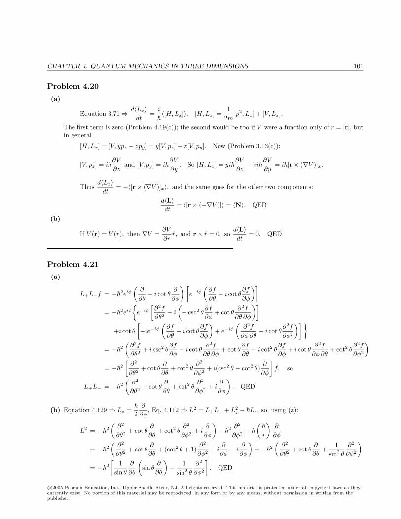
CHAPTER 4. QUANTUM MECHANICS IN THREE DIMENSIONS 101
Problem 4.20
(a)
Equation 3.71⇒ d〈Lx〉dt
=i
〈[H,Lx]〉. [H,Lx] =
12m
[p2, Lx] + [V,Lx].
The first term is zero (Problem 4.19(c)); the second would be too if V were a function only of r = |r|, butin general
[H,Lx] = [V, ypz − zpy] = y[V, pz]− z[V, py]. Now (Problem 3.13(c)):
[V, pz] = i∂V
∂zand [V, py] = i
∂V
∂y. So [H,Lx] = yi
∂V
∂z− zi
∂V
∂y= i[r× (∇V )]x.
Thusd〈Lx〉dt
= −〈[r× (∇V )]x〉, and the same goes for the other two components:
d〈L〉dt
= 〈[r× (−∇V )]〉 = 〈N〉. QED
(b)
If V (r) = V (r), then ∇V =∂V
∂rr, and r× r = 0, so
d〈L〉dt
= 0. QED
Problem 4.21
(a)
L+L−f = −2eiφ
(∂
∂θ+ i cot θ
∂
∂φ
) [e−iφ
(∂f
∂θ− i cot θ
∂f
∂φ
)]= −2eiφ
e−iφ
[∂2f
∂θ2− i
(− csc2 θ
∂f
∂φ+ cot θ
∂2f
∂θ ∂φ
)]+i cot θ
[−ie−iφ
(∂f
∂θ− i cot θ
∂f
∂φ
)+ e−iφ
(∂2f
∂φ ∂θ− i cot θ
∂2f
∂φ2
)] = −2
(∂2f
∂θ2+ i csc2 θ
∂f
∂φ− i cot θ
∂2f
∂θ ∂φ+ cot θ
∂f
∂θ− i cot2 θ
∂f
∂φ+ i cot θ
∂2f
∂φ ∂θ+ cot2 θ
∂2f
∂φ2
)= −2
[∂2
∂θ2+ cot θ
∂
∂θ+ cot2 θ
∂2
∂φ2+ i(csc2 θ − cot2 θ)
∂
∂φ
]f, so
L+L− = −2
(∂2
∂θ2+ cot θ
∂
∂θ+ cot2 θ
∂2
∂φ2+ i
∂
∂φ
). QED
(b) Equation 4.129 ⇒ Lz =
i
∂
∂φ, Eq. 4.112 ⇒ L2 = L+L− + L2
z − Lz, so, using (a):
L2 = −2
(∂2
∂θ2+ cot θ
∂
∂θ+ cot2 θ
∂2
∂φ2+ i
∂
∂φ
)− 2 ∂2
∂φ2−
(
i
)∂
∂φ
= −2
(∂2
∂θ2+ cot θ
∂
∂θ+ (cot2 θ + 1)
∂2
∂φ2+ i
∂
∂φ− i
∂
∂φ
)= −2
(∂2
∂θ2+ cot θ
∂
∂θ+
1sin2 θ
∂2
∂φ2
)= −2
[1
sin θ
∂
∂θ
(sin θ
∂
∂θ
)+
1sin2 θ
∂2
∂φ2
]. QED
c©2005 Pearson Education, Inc., Upper Saddle River, NJ. All rights reserved. This material is protected under all copyright laws as theycurrently exist. No portion of this material may be reproduced, in any form or by any means, without permission in writing from thepublisher.
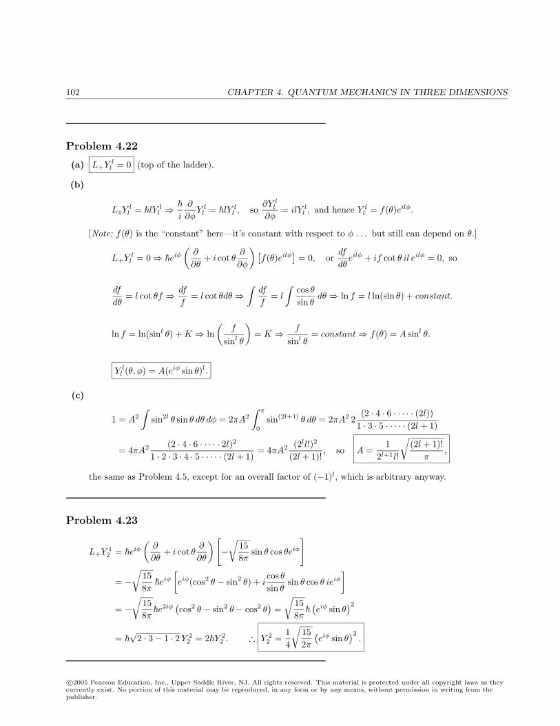
102 CHAPTER 4. QUANTUM MECHANICS IN THREE DIMENSIONS
Problem 4.22
(a) L+Y ll = 0 (top of the ladder).
(b)
LzYll = lY l
l ⇒
i
∂
∂φY l
l = lY ll , so
∂Y ll
∂φ= ilY l
l , and hence Y ll = f(θ)eilφ.
[Note: f(θ) is the “constant” here—it’s constant with respect to φ . . . but still can depend on θ.]
L+Y ll = 0⇒ eiφ
(∂
∂θ+ i cot θ
∂
∂φ
) [f(θ)eilφ
]= 0, or
df
dθeilφ + if cot θ il eilφ = 0, so
df
dθ= l cot θf ⇒ df
f= l cot θdθ ⇒
∫df
f= l
∫cos θsin θ
dθ ⇒ ln f = l ln(sin θ) + constant.
ln f = ln(sinl θ) + K ⇒ ln(
f
sinl θ
)= K ⇒ f
sinl θ= constant⇒ f(θ) = A sinl θ.
Y ll (θ, φ) = A(eiφ sin θ)l.
(c)
1 = A2
∫sin2l θ sin θ dθ dφ = 2πA2
∫ π
0
sin(2l+1) θ dθ = 2πA2 2(2 · 4 · 6 · · · · · (2l))
1 · 3 · 5 · · · · · (2l + 1)
= 4πA2 (2 · 4 · 6 · · · · · 2l)21 · 2 · 3 · 4 · 5 · · · · · (2l + 1)
= 4πA2 (2ll!)2
(2l + 1)!, so A =
12l+1l!
√(2l + 1)!
π,
the same as Problem 4.5, except for an overall factor of (−1)l, which is arbitrary anyway.
Problem 4.23
L+Y 12 = eiφ
(∂
∂θ+ i cot θ
∂
∂θ
) [−
√158π
sin θ cos θeiφ
]
= −√
158πeiφ
[eiφ(cos2 θ − sin2 θ) + i
cos θsin θ
sin θ cos θ ieiφ
]= −
√158πe2iφ
(cos2 θ − sin2 θ − cos2 θ
)=
√158π
(eiφ sin θ
)2
= √
2 · 3− 1 · 2Y 22 = 2Y 2
2 . ∴ Y 22 =
14
√152π
(eiφ sin θ
)2.
c©2005 Pearson Education, Inc., Upper Saddle River, NJ. All rights reserved. This material is protected under all copyright laws as theycurrently exist. No portion of this material may be reproduced, in any form or by any means, without permission in writing from thepublisher.
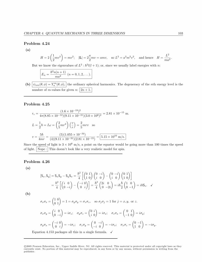
CHAPTER 4. QUANTUM MECHANICS IN THREE DIMENSIONS 103
Problem 4.24
(a)
H = 2(
12mv2
)= mv2; |L| = 2
a
2mv = amv, so L2 = a2m2v2, and hence H =
L2
ma2.
But we know the eigenvalues of L2 : 2l(l + 1); or, since we usually label energies with n:
En =
2n(n + 1)ma2
(n = 0, 1, 2, . . . ).
(b) ψnm(θ, φ) = Y mn (θ, φ), the ordinary spherical harmonics. The degeneracy of the nth energy level is the
number of m-values for given n: 2n + 1.
Problem 4.25
rc =(1.6× 10⁻¹⁹)2
4π(8.85× 10⁻¹²)(9.11× 10⁻³¹)(3.0× 10⁸)2= 2.81× 10⁻¹⁵ m.
L =12 = Iω =
(25mr2
) (v
r
)=
25mrv so
v =5
4mr=
(5)(1.055× 10⁻³⁴)(4)(9.11× 10⁻³¹)(2.81× 10⁻¹⁵)
= 5.15× 10¹⁰ m/s.
Since the speed of light is 3× 10⁸ m/s, a point on the equator would be going more than 100 times the speedof light. Nope : This doesn’t look like a very realistic model for spin.
Problem 4.26
(a)
[Sx,Sy] = SxSy − SySx =
2
4
[(0 11 0
) (0 −ii 0
)−
(0 −ii 0
) (0 11 0
)]=
2
4
[(i 00 −i
)−
(−i 00 i
)]=
2
4
(2i 00 −2i
)= i
2
(1 00 −1
)= iSz.
(b)
σxσx =(
1 00 1
)= 1 = σyσy = σzσz, so σjσj = 1 for j = x, y, or z.
σxσy =(i 00 −i
)= iσz; σyσz =
(0 ii 0
)= iσx; σzσx =
(0 1−1 0
)= iσy;
σyσx =(−i 00 i
)= −iσz; σzσy =
(0 −i−i 0
)= −iσx; σxσz =
(0 −11 0
)= −iσy.
Equation 4.153 packages all this in a single formula.
c©2005 Pearson Education, Inc., Upper Saddle River, NJ. All rights reserved. This material is protected under all copyright laws as theycurrently exist. No portion of this material may be reproduced, in any form or by any means, without permission in writing from thepublisher.
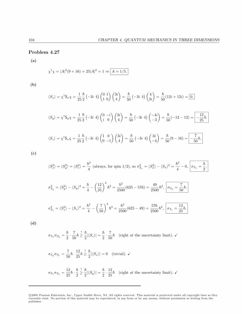
104 CHAPTER 4. QUANTUM MECHANICS IN THREE DIMENSIONS
Problem 4.27
(a)
χ†χ = |A|2(9 + 16) = 25|A|2 = 1⇒ A = 1/5.
(b)
〈Sx〉 = χ†Sxχ =125
2(−3i 4
) (0 11 0
) (3i4
)=
50(−3i 4
) (43i
)=
50(12i + 12i) = 0.
〈Sy〉 = χ†Syχ =125
2(−3i 4
) (0 −ii 0
) (3i4
)=
50(−3i 4
) (−4i−3
)=
50(−12− 12) = −12
25.
〈Sz〉 = χ†Szχ =125
2(−3i 4
) (1 00 −1
) (3i4
)=
50(−3i 4
) (3i−4
)=
50(9− 16) = − 7
50.
(c)
〈S2x〉 = 〈S2
y〉 = 〈S2z 〉 =
2
4(always, for spin 1/2), so σ2
Sx = 〈S2x〉 − 〈Sx〉2 =
2
4− 0, σSx =
2.
σ2Sy = 〈S2
y〉 − 〈Sy〉2 =
4−
(1225
)2
2 =
2
2500(625− 576) =
492500
2, σSy =
750.
σ2Sz = 〈S2
z 〉 − 〈Sz〉2 =
2
4−
(750
)2
2 =
2
2500(625− 49) =
5762500
2, σSz =
1225.
(d)
σSxσSy =
2· 750
?≥
2|〈Sz〉| =
2· 750 (right at the uncertainty limit).
σSyσSz =750 · 12
25
?≥
2|〈Sx〉| = 0 (trivial).
σSzσSx =1225 ·
2?≥
2|〈Sy〉| =
2· 1225 (right at the uncertainty limit).
c©2005 Pearson Education, Inc., Upper Saddle River, NJ. All rights reserved. This material is protected under all copyright laws as theycurrently exist. No portion of this material may be reproduced, in any form or by any means, without permission in writing from thepublisher.
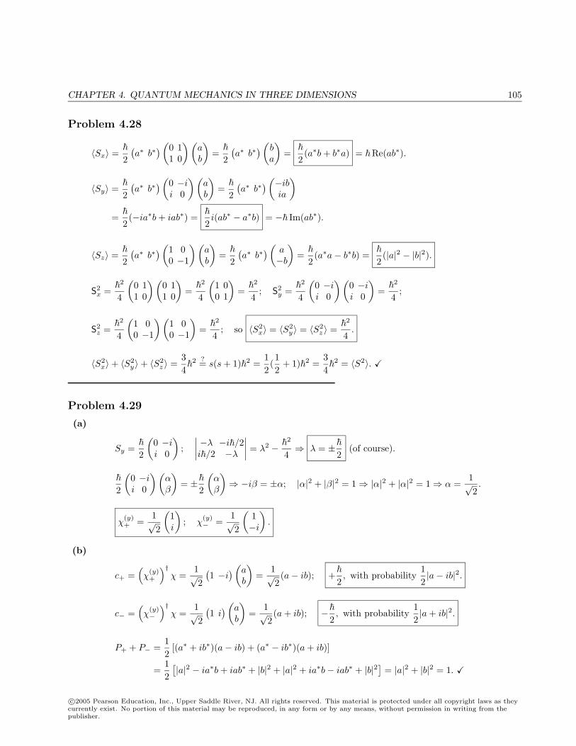
CHAPTER 4. QUANTUM MECHANICS IN THREE DIMENSIONS 105
Problem 4.28
〈Sx〉 =
2(a∗ b∗
) (0 11 0
) (ab
)=
2(a∗ b∗
) (ba
)=
2(a∗b + b∗a) = Re(ab∗).
〈Sy〉 =
2(a∗ b∗
) (0 −ii 0
) (ab
)=
2(a∗ b∗
) (−ibia
)=
2(−ia∗b + iab∗) =
2i(ab∗ − a∗b) = − Im(ab∗).
〈Sz〉 =
2(a∗ b∗
) (1 00 −1
) (ab
)=
2(a∗ b∗
) (a−b
)=
2(a∗a− b∗b) =
2(|a|2 − |b|2).
S2x =
2
4
(0 11 0
) (0 11 0
)=
2
4
(1 00 1
)=
2
4; S2
y =
2
4
(0 −ii 0
) (0 −ii 0
)=
2
4;
S2z =
2
4
(1 00 −1
) (1 00 −1
)=
2
4; so 〈S2
x〉 = 〈S2y〉 = 〈S2
z 〉 =
2
4.
〈S2x〉+ 〈S2
y〉+ 〈S2z 〉 =
34
2 ?= s(s + 1)2 =12(12
+ 1)2 =34
2 = 〈S2〉.
Problem 4.29
(a)
Sy =
2
(0 −ii 0
);
∣∣∣∣ −λ −i/2i/2 −λ
∣∣∣∣ = λ2 − 2
4⇒ λ = ±
2(of course).
2
(0 −ii 0
) (αβ
)= ±
2
(αβ
)⇒ −iβ = ±α; |α|2 + |β|2 = 1⇒ |α|2 + |α|2 = 1⇒ α =
1√2.
χ(y)+ =
1√2
(1i
); χ
(y)− =
1√2
(1−i
).
(b)
c+ =(χ
(y)+
)†χ =
1√2
(1 −i
) (ab
)=
1√2(a− ib); +
2, with probability
12|a− ib|2.
c− =(χ
(y)−
)†χ =
1√2
(1 i
) (ab
)=
1√2(a + ib); −
2, with probability
12|a + ib|2.
P+ + P− =12
[(a∗ + ib∗)(a− ib) + (a∗ − ib∗)(a + ib)]
=12
[|a|2 − ia∗b + iab∗ + |b|2 + |a|2 + ia∗b− iab∗ + |b|2
]= |a|2 + |b|2 = 1.
c©2005 Pearson Education, Inc., Upper Saddle River, NJ. All rights reserved. This material is protected under all copyright laws as theycurrently exist. No portion of this material may be reproduced, in any form or by any means, without permission in writing from thepublisher.
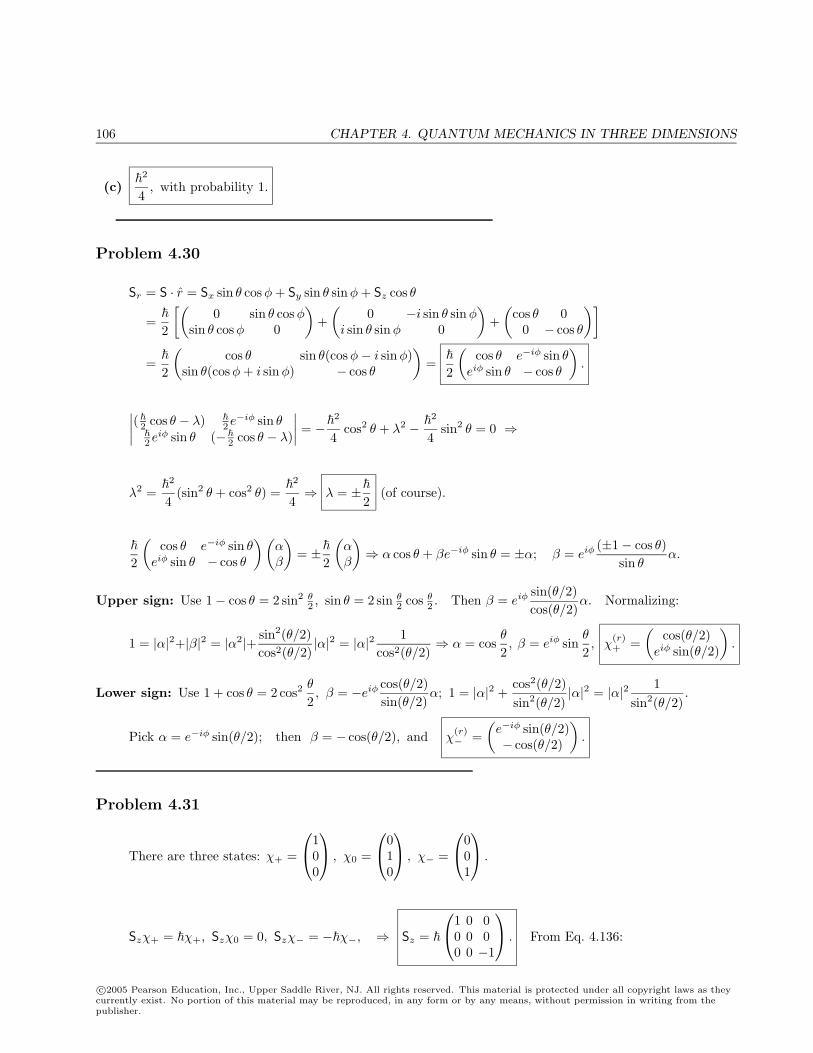
106 CHAPTER 4. QUANTUM MECHANICS IN THREE DIMENSIONS
(c)
2
4, with probability 1.
Problem 4.30
Sr = S · r = Sx sin θ cosφ + Sy sin θ sinφ + Sz cos θ
=
2
[(0 sin θ cosφ
sin θ cosφ 0
)+
(0 −i sin θ sinφ
i sin θ sinφ 0
)+
(cos θ 0
0 − cos θ
)]=
2
(cos θ sin θ(cosφ− i sinφ)
sin θ(cosφ + i sinφ) − cos θ
)=
2
(cos θ e−iφ sin θ
eiφ sin θ − cos θ
).
∣∣∣∣(2 cos θ − λ)
2 e−iφ sin θ
2 eiφ sin θ (−2 cos θ − λ)
∣∣∣∣ = −2
4cos2 θ + λ2 −
2
4sin2 θ = 0 ⇒
λ2 =
2
4(sin2 θ + cos2 θ) =
2
4⇒ λ = ±
2(of course).
2
(cos θ e−iφ sin θ
eiφ sin θ − cos θ
) (αβ
)= ±
2
(αβ
)⇒ α cos θ + βe−iφ sin θ = ±α; β = eiφ (±1− cos θ)
sin θα.
Upper sign: Use 1− cos θ = 2 sin2 θ2 , sin θ = 2 sin θ
2 cos θ2 . Then β = eiφ sin(θ/2)
cos(θ/2)α. Normalizing:
1 = |α|2+|β|2 = |α2|+ sin2(θ/2)cos2(θ/2)
|α|2 = |α|2 1cos2(θ/2)
⇒ α = cosθ
2, β = eiφ sin
θ
2, χ
(r)+ =
(cos(θ/2)
eiφ sin(θ/2)
).
Lower sign: Use 1 + cos θ = 2 cos2θ
2, β = −eiφ cos(θ/2)
sin(θ/2)α; 1 = |α|2 +
cos2(θ/2)sin2(θ/2)
|α|2 = |α|2 1sin2(θ/2)
.
Pick α = e−iφ sin(θ/2); then β = − cos(θ/2), and χ(r)− =
(e−iφ sin(θ/2)− cos(θ/2)
).
Problem 4.31
There are three states: χ+ =
100
, χ0 =
010
, χ− =
001
.
Szχ+ = χ+, Szχ0 = 0, Szχ− = −χ−, ⇒ Sz =
1 0 00 0 00 0 −1
. From Eq. 4.136:
c©2005 Pearson Education, Inc., Upper Saddle River, NJ. All rights reserved. This material is protected under all copyright laws as theycurrently exist. No portion of this material may be reproduced, in any form or by any means, without permission in writing from thepublisher.
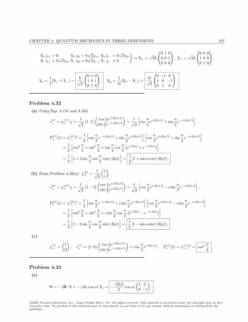
CHAPTER 4. QUANTUM MECHANICS IN THREE DIMENSIONS 107
S+χ+ = 0, S+χ0 = √
2χ+, S+χ− = √
2χ0
S−χ+ = √
2χ0, S−χ0 = √
2χ−, S−χ− = 0
⇒ S+ =
√2
0 1 00 0 10 0 0
, S− =√
2
0 0 01 0 00 1 0
.
Sx =12(S+ + S−) =
√2
0 1 01 0 10 1 0
, Sy =12i
(S+ − S−) =i√2
0 −1 01 0 −10 1 0
.
Problem 4.32
(a) Using Eqs. 4.151 and 4.163:
c(x)+ = χ
(x)†+ χ =
1√2
(1 1
) (cos α
2 eiγB0t/2
sin α2 e−iγB0t/2
)=
1√2
[cos
α
2eiγB0t/2 + sin
α
2e−iγB0t/2
].
P(x)+ (t) = |c(x)
+ |2 =12
[cos
α
2e−iγB0t/2 + sin
α
2eiγB0t/2
] [cos
α
2eiγB0t/2 + sin
α
2e−iγB0t/2
]=
12
[cos2
α
2+ sin2 α
2+ sin
α
2cos
α
2(eiγB0t + e−iγB0t
)]=
12
[1 + 2 sin
α
2cos
α
2cos(γB0t)
]=
12
[1 + sinα cos(γB0t)] .
(b) From Problem 4.29(a): χ(y)+ =
1√2
(1i
).
c(y)+ = χ
(y)†+ χ =
1√2
(1 −i
) (cos α
2 eiγB0t/2
sin α2 e
iγB0t/2
)=
1√2
[cos
α
2eiγB0t/2 − i sin
α
2e−iγB0t/2
];
P(y)+ (t) = |c(y)
+ |2 =12
[cos
α
2e−iγB0t/2 + i sin
α
2eiγB0t/2
] [cos
α
2eiγB0t/2 − i sin
α
2e−iγB0t/2
]=
12
[cos2
α
2+ sin2 α
2+ i sin
α
2cos
α
2(eiγB0t − e−iγB0t
)]=
12
[1− 2 sin
α
2cos
α
2sin(γB0t)
]=
12
[1− sinα sin(γB0t)] .
(c)
χ(z)+ =
(10
); c
(z)+ =
(1 0
) (cos α
2 eiγB0t/2
sin α2 e−iγB0t/2
)= cos
α
2eiγB0t/2; P
(z)+ (t) = |c(z)
+ |2 = cos2α
2.
Problem 4.33
(a)
H = −γB · S = −γB0 cosωt Sz = −γB0
2cosωt
(1 00 −1
).
c©2005 Pearson Education, Inc., Upper Saddle River, NJ. All rights reserved. This material is protected under all copyright laws as theycurrently exist. No portion of this material may be reproduced, in any form or by any means, without permission in writing from thepublisher.
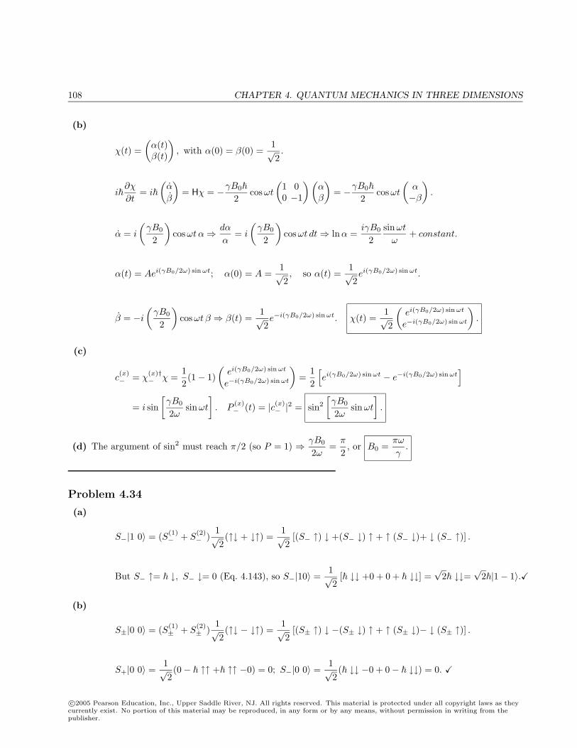
108 CHAPTER 4. QUANTUM MECHANICS IN THREE DIMENSIONS
(b)
χ(t) =(α(t)β(t)
), with α(0) = β(0) =
1√2.
i∂χ
∂t= i
(α
β
)= Hχ = −γB0
2cosωt
(1 00 −1
) (αβ
)= −γB0
2cosωt
(α−β
).
α = i
(γB0
2
)cosωtα⇒ dα
α= i
(γB0
2
)cosωt dt⇒ lnα =
iγB0
2sinωt
ω+ constant.
α(t) = Aei(γB0/2ω) sin ωt; α(0) = A =1√2, so α(t) =
1√2ei(γB0/2ω) sin ωt.
β = −i
(γB0
2
)cosωt β ⇒ β(t) =
1√2e−i(γB0/2ω) sin ωt. χ(t) =
1√2
(ei(γB0/2ω) sin ωt
e−i(γB0/2ω) sin ωt
).
(c)
c(x)− = χ
(x)†− χ =
12(1− 1)
(ei(γB0/2ω) sin ωt
e−i(γB0/2ω) sin ωt
)=
12
[ei(γB0/2ω) sin ωt − e−i(γB0/2ω) sin ωt
]= i sin
[γB0
2ωsinωt
]. P
(x)− (t) = |c(x)
− |2 = sin2
[γB0
2ωsinωt
].
(d) The argument of sin2 must reach π/2 (so P = 1) ⇒ γB0
2ω=
π
2, or B0 =
πω
γ.
Problem 4.34
(a)
S−|1 0〉 = (S(1)− + S
(2)− )
1√2(↑↓ + ↓↑) =
1√2
[(S− ↑) ↓ +(S− ↓) ↑ + ↑ (S− ↓)+ ↓ (S− ↑)] .
But S− ↑= ↓, S− ↓= 0 (Eq. 4.143), so S−|10〉 =1√2
[ ↓↓ +0 + 0 + ↓↓] =√
2 ↓↓=√
2|1− 1〉.
(b)
S±|0 0〉 = (S(1)± + S
(2)± )
1√2(↑↓ − ↓↑) =
1√2
[(S± ↑) ↓ −(S± ↓) ↑ + ↑ (S± ↓)− ↓ (S± ↑)] .
S+|0 0〉 =1√2(0− ↑↑ + ↑↑ −0) = 0; S−|0 0〉 =
1√2( ↓↓ −0 + 0− ↓↓) = 0.
c©2005 Pearson Education, Inc., Upper Saddle River, NJ. All rights reserved. This material is protected under all copyright laws as theycurrently exist. No portion of this material may be reproduced, in any form or by any means, without permission in writing from thepublisher.
CHAPTER 4. QUANTUM MECHANICS IN THREE DIMENSIONS 109
(c)
S2|1 1〉 =[(S(1))2 + (S(2))2 + 2S(1) · S(2)
]↑↑
= (S2 ↑) ↑ + ↑ (S2 ↑) + 2 [(Sx ↑)(Sx ↑) + (Sy ↑)(Sy ↑) + (Sz ↑)(Sz ↑)]
=34
2 ↑↑ +34
2 ↑↑ +2[
2↓
2↓ +
i
2↓ i
2↓ +
2↑
2↑]
=32
2 ↑↑ +2(
2
4↑↑
)= 22 ↑↑= 22|1 1〉 = (1)(1 + 1)2|1 1〉, as it should be.
S2|1 − 1〉 =[(S(1))2 + (S(2))2 + 2S(1) · S(2)
]↓↓
=32
4↓↓ +
32
4↓↓ +2 [(Sx ↓)(Sx ↓) + (Sy ↓)(Sy ↓) + (Sz ↓)(Sz ↓)]
=32
2 ↓↓ +2[(
2↑) (
2↑)
+(− i
2↑) (
− i
2↑)
+(−
2↓) (
−2↓)]
=32
2 ↓↓ +2
2
4↓↓= 22 ↓↓= 22|1 − 1〉.
Problem 4.35
(a) 1/2 and 1/2 gives 1 or zero; 1/2 and 1 gives 3/2 or 1/2; 1/2 and 0 gives 1/2 only. So baryons can havespin 3/2 or spin 1/2 (and the latter can be acheived in two distinct ways). [Incidentally, the lightest
baryons do carry spin 1/2 (proton, neutron, etc.) or 3/2 (∆,Ω−, etc.); heavier baryons can have highertotal spin, but this is because the quarks have orbital angular momentum as well.]
(b) 1/2 and 1/2 gives spin 1 or spin 0. [Again, these are the observed spins for the lightest mesons: π’s andK’s have spin 0, ρ’s and ω’s have spin 1.]
Problem 4.36
(a) From the 2× 1 Clebsch-Gordan table we get
|3 1〉 =
√115|2 2〉|1 − 1〉+
√815|2 1〉|1 0〉+
√615|2 0〉|1 1〉,
so you might get 2 (probability 1/15), (probability 8/15), or (probability 6/15).
(b) From the 1× 12 table: |1 0〉| 12 − 1
2 〉 =√
23 | 32 − 1
2 〉+√
13 | 12 − 1
2 〉. So the total is 3/2 or 1/2, with l(l+1)2 =
15/42 and 3/42, respectively. Thus you get154
2 (probability 2/3), or34
2 (probability 1/3).
c©2005 Pearson Education, Inc., Upper Saddle River, NJ. All rights reserved. This material is protected under all copyright laws as theycurrently exist. No portion of this material may be reproduced, in any form or by any means, without permission in writing from thepublisher.
110 CHAPTER 4. QUANTUM MECHANICS IN THREE DIMENSIONS
Problem 4.37
Using Eq. 4.179: [S2, S(1)z ] = [S(1)2 , S
(1)z ] + [S(2)2 , S
(1)z ] + 2[S(1) · S(2), S
(1)z ]. But [S2, Sz] = 0 (Eq. 4.102), and
anything with superscript (2) commutes with anything with superscript (1). So
[S2, S(1)z ] = 2
S(2)
x [S(1)x , S(1)
z ] + S(2)y [S(1)
y , S(1)z ] + S(2)
z [S(1)z , S(1)
z ]
= 2−iS(1)
y S(2)x + iS(1)
x S(2)y
= 2i(S(1) × S(2))z.
[S2, S(1)z ] = 2i(S(1)
x S(2)y − S(1)
y S(2)x ), and [S2,S(1)] = 2i(S(1)×S(2)). Note that [S2,S(2)] = 2i(S(2)×S(1)) =
−2i(S(1) × S(2)), so [S2, (S(1) + S(2))] = 0.]
Problem 4.38
(a)
− 2
2m
(∂2ψ
∂x2+
∂2ψ
∂y2+
∂2ψ
∂z2
)+
12mω2
(x2 + y2 + z2
)ψ = Eψ.
Let ψ(x, y, z) = X(x)Y (y)Z(z); plug it in, divide by XY Z, and collect terms:(−
2
2m1X
d2X
dx2+
12mω2x2
)+
(−
2
2m1Y
d2Y
dy2+
12mω2y2
)+
(−
2
2m1Z
d2Z
dz2+
12mω2z2
)= E.
The first term is a function only of x, the second only of y, and the third only of z. So each is a constant(call the constants Ex, Ey, Ez, with Ex + Ey + Ez = E). Thus:
− 2
2md2X
dx2+
12mω2x2X = ExX; −
2
2md2Y
dy2+
12mω2y2Y = EyY ; −
2
2md2Z
dz2+
12mω2z2Z = EzZ.
Each of these is simply the one-dimensional harmonic oscillator (Eq. 2.44). We know the allowed energies(Eq. 2.61):
Ex = (nx + 12 )ω; Ey = (ny + 1
2 )ω; Ez = (nz + 12 )ω; where nx, ny, nz = 0, 1, 2, 3, . . . .
So E = (nx + ny + ny + 32 )ω = (n + 3
2 )ω, with n ≡ nx + ny + nz.
(b) The question is: “How many ways can we add three non-negative integers to get sum n?”
If nx = n, then ny = nz = 0; one way.If nx = n− 1, then ny = 0, nz = 1, or else ny = 1, nz = 0; two ways.If nx = n− 2, then ny = 0, nz = 2, or ny = 1, nz = 1, or ny = 2, nz = 0; three ways.
And so on. Evidently d(n) = 1 + 2 + 3 + · · ·+ (n + 1) =(n + 1)(n + 2)
2.
c©2005 Pearson Education, Inc., Upper Saddle River, NJ. All rights reserved. This material is protected under all copyright laws as theycurrently exist. No portion of this material may be reproduced, in any form or by any means, without permission in writing from thepublisher.
CHAPTER 4. QUANTUM MECHANICS IN THREE DIMENSIONS 111
Problem 4.39
Eq. 4.37: − 2
2md2u
dr2+
[12mω2r2 +
2
2ml(l + 1)
r2
]u = Eu.
Following Eq. 2.71, let ξ ≡√
mω
r. Then −
2
2mmω
d2u
dξ2+
[12mω2
mωξ2 +
2
2mmω
l(l + 1)ξ2
]u = Eu,
ord2u
dξ2=
[ξ2 +
l(l + 1)ξ2
−K
]u, where K ≡ 2E
ω(as in Eq. 2.73).
At large ξ,d2u
dξ2≈ ξ2u, and u ∼ ( )e−ξ2/2 (see Eq. 2.77).
At small ξ,d2u
dξ2≈ l(l + 1)
ξ2u, and u ∼ ( )ξl+1 (see Eq. 4.59).
So let u(ξ) ≡ ξl+1e−ξ2/2v(ξ). [This defines the new function v(ξ).]
du
dξ= (l + 1)ξle−ξ2/2v − ξl+2e−ξ2/2v + ξl+1e−ξ2/2v′.
d2u
dξ2= l(l + 1)ξl−1e−ξ2/2v − (l + 1)ξl+1e−ξ2/2v + (l + 1)ξle−ξ2/2v′ − (l + 2)ξl+1e−ξ2/2v
+ ξl+3e−ξ2/2v − ξl+2e−ξ2/2v′ + (l + 1)ξle−ξ2/2v′ − ξl+2e−ξ2/2v′ + ξl+1e−ξ2/2v′′
=l(l + 1)ξl−1e−ξ2/2v − (2l + 3)ξl+1e−ξ2/2v +
ξl+3e−ξ2/2v + 2(l + 1)ξle−ξ2/2v′
− 2ξl+2e−ξ2/2v′ + ξl+1e−ξ2/2v′′ =
ξl+3e−ξ2/2v +l(l + 1)ξl−1e−ξ2/2v −Kξl+1e−ξ2/2v.
Cancelling the indicated terms, and dividing off ξl+1e−ξ2/2, we have:
v′′ + 2v′(l + 1ξ
− ξ
)+ (K − 2l − 3) v = 0.
Let v(ξ) ≡∞∑
j=0
ajξj , so v′ =
∞∑j=0
jajξj−1; v′′ =
∞∑j=2
j(j − 1)ajξj−2. Then
∞∑j=2
j(j − 1)ajξj−2 + 2(l + 2)
∞∑j=1
jajξj−2 − 2
∞∑j=1
jajξj + (K − 2l − 3)
∞∑j=0
ajξj = 0.
In the first two sums, let j → j + 2 (rename the dummy index):
∞∑j=0
(j + 2)(j + 1)aj+2ξj + 2(l + 1)
∞∑j=0
(j + 2)aj+2ξj − 2
∞∑j=0
jajξj + (K − 2l − 3)
∞∑j=0
ajξj = 0.
c©2005 Pearson Education, Inc., Upper Saddle River, NJ. All rights reserved. This material is protected under all copyright laws as theycurrently exist. No portion of this material may be reproduced, in any form or by any means, without permission in writing from thepublisher.
112 CHAPTER 4. QUANTUM MECHANICS IN THREE DIMENSIONS
Note: the second sum should start at j = −1; to eliminate this term (there is no compensating one in ξ−1) wemust take a1 = 0. Combining the terms:
∞∑j=0
[(j + 2)(j + 2l + 3)aj+2 + (K − 2j − 2l − 3)aj ] = 0, so aj+2 =(2j + 2l + 3−K)(j + 2)(j + 2l + 3)
aj .
Since a1 = 0, this gives us a single sequence: a0, a2, a4, . . . . But the series must terminate (else we get thewrong behavior as ξ →∞), so there occurs some maximal (even) number jmax such that ajmax+2 = 0. Thus
K = 2jmax + 2l + 3. But E =12ωK, so E =
(jmax + l +
32
)ω. Or, letting jmax + l ≡ n,
En = (n + 32 )ω, and n can be any nonnegative integer.
[Incidentally, we can also determine the degeneracy of En. Suppose n is even; then (since jmax is even)l = 0, 2, 4, . . . , n. For each l there are (2l + 1) values for m. So
d(n) =n∑
l=0,2,4,...
(2l + 1). Let j = l/2; then d(n) =n/2∑j=0
(4j + 1) = 4n/2∑j=0
j +n/2∑j=0
1
= 4(n
2 )(n2 + 1)2
+ (n2 + 1) = (n
2 + 1)(n + 1) =(n + 1)(n + 2)
2, as before (Problem 4.38(b)).]
Problem 4.40
(a)
d
dt〈r · p〉 =
i
〈[H, r · p]〉.
[H, r · p] =3∑
i=1
[H, ripi] =3∑
i=1
([H, ri]pi + ri[H, pi]) =3∑
i=1
(1
2m[p2, ri]pi + ri[V, pi]
).
[p2, ri] =3∑
j=1
[pjpj , ri] =3∑
j=1
(pj [pj , ri] + [pj , ri]pj) =3∑
j=1
[pj(−iδij) + (−iδij)pj ] = −2ipi.
[V, pi] = i∂V
∂ri(Problem 3.13(c)). [H, r · p] =
3∑i=1
[1
2m(−2i)pipi + ri
(i
∂V
∂ri
)]
= i
(−p2
m+ r · ∇V
).
d
dt〈r · p〉 = 〈p
2
m− r · ∇V 〉 = 2〈T 〉 − 〈r · ∇V 〉.
For stationary statesd
dt〈r · p〉 = 0, so 2〈T 〉 = 〈r · ∇V 〉. QED
(b)
V (r) = − e2
4πε01r⇒ ∇V =
e2
4πε01r2
r ⇒ r · ∇V =e2
4πε01r
= −V. So 2〈T 〉 = −〈V 〉.
But 〈T 〉 = 〈V 〉 = En, so 〈T 〉 − 2〈T 〉 = En, or 〈T 〉 = −En; 〈V 〉 = 2En. QED
c©2005 Pearson Education, Inc., Upper Saddle River, NJ. All rights reserved. This material is protected under all copyright laws as theycurrently exist. No portion of this material may be reproduced, in any form or by any means, without permission in writing from thepublisher.

CHAPTER 4. QUANTUM MECHANICS IN THREE DIMENSIONS 113
(c)
V =12mω2r2 ⇒ ∇V = mω2r r ⇒ r · ∇V = mω2r2 = 2V. So 2〈T 〉 = 2〈V 〉, or 〈T 〉 = 〈V 〉.
But 〈T 〉+ 〈V 〉 = En, so 〈T 〉 = 〈V 〉 =12En. QED
Problem 4.41
(a) ∇ · J =i
2m[∇Ψ · ∇Ψ∗ + Ψ(∇2Ψ∗)−∇Ψ∗ · ∇Ψ−Ψ∗(∇2Ψ)
]=
i
2m[Ψ(∇2Ψ∗)−Ψ∗(∇2Ψ)
].
But the Schrodinger equation says i∂Ψ∂t
= − 2
2m∇2Ψ + V Ψ, so
∇2Ψ =2m2
(V Ψ− i
∂Ψ∂t
), ∇2Ψ∗ =
2m2
(V Ψ∗ + i
∂Ψ∗
∂t
). Therefore
∇ · J =i
2m2m2
[Ψ
(V Ψ∗ + i
∂Ψ∗
∂t
)−Ψ∗
(V Ψ− i
∂Ψ∂t
)]=
i
i
(Ψ
∂Ψ∗
∂t+ Ψ∗
∂Ψ∂t
)= − ∂
∂t(Ψ∗Ψ) = − ∂
∂t|Ψ|2.
(b) From Problem 4.11(b), Ψ2 1 1 = − 1√πa
18a2
re−r/2a sin θeiφe−iE2t/. In spherical coordinates,
∇Ψ =∂Ψ∂r
r +1r
∂Ψ∂θ
θ +1
r sin θ
∂Ψ∂φ
φ, so
∇Ψ2 1 1 = − 1√πa
18a2
[(1− r
2a
)e−r/2a sin θeiφe−iE2t/ r +
1rre−r/2a cos θeiφe−iE2t/ θ
+1
r sin θre−r/2a sin θ ieiφe−iE2t/ φ
]=
[(1− r
2a
)r + cot θ θ +
i
sin θφ
]1rΨ2 1 1.
Therefore
J =i
2m
[(1− r
2a
)r + cot θ θ − i
sin θφ−
(1− r
2a
)r − cot θ θ − i
sin θφ
]1r|Ψ2 1 1|2
=i
2m(−2i)r sin θ
|Ψ2 1 1|2 φ =
m
1πa
164a4
r2e−r/a sin2 θ
r sin θφ =
64πma5re−r/a sin θ φ.
(c) Now r× J =
64πma5r2e−r/a sin θ
(r × φ
), while
(r × φ
)= −θ and z · θ = − sin θ, so
r× Jz =
64πma5r2e−r/a sin2 θ, and hence
Lz = m
64πma5
∫ (r2e−r/a sin2 θ
)r2 sin θ dr dθ dφ
=
64πa5
∫ ∞0
r4e−r/a dr
∫ π
0
sin3 θ dθ
∫ 2π
0
dφ =
64πa5
(4!a5
) (43
)(2π) = ,
c©2005 Pearson Education, Inc., Upper Saddle River, NJ. All rights reserved. This material is protected under all copyright laws as theycurrently exist. No portion of this material may be reproduced, in any form or by any means, without permission in writing from thepublisher.
114 CHAPTER 4. QUANTUM MECHANICS IN THREE DIMENSIONS
as it should be, since (Eq. 4.133) Lz = m, and m = 1 for this state.
Problem 4.42
(a)
ψ =1√πa3
e−r/a ⇒ φ(p) =1
(2π)3/2
1√πa3
∫e−ip·r/e−r/ar2 sin θ dr dθ dφ.
With axes as suggested, p · r = pr cos θ. Doing the (trivial) φ integral:
φ(p) =2π
(2πa)3/2
1√π
∫ ∞0
r2e−r/a
[∫ π
0
e−ipr cos θ/ sin θ dθ
]dr.
∫ π
0
e−ipr cos θ/ sin θ dθ =
ipre−ipr cos θ/
∣∣∣π0
=
ipr
(eipr/ − e−ipr/
)=
2pr
sin(pr
).
φ(p) =1
π√
21
(a)3/2
2p
∫ ∞0
re−r/a sin(pr
)dr.
∫ ∞0
re−r/a sin(pr
)dr =
12i
[∫ ∞0
re−r/aeipr/dr −∫ ∞
0
re−r/ae−ipr/dr
]=
12i
[1
(1/a− ip/)2− 1
(1/a + ip/)2
]=
12i
(2ip/a)2[(1/a)2 + (p/)2
]2
=(2p/)a3
[1 + (ap/)2]2.
φ(p) =
√2
1a3/2
1πp
2pa3
1[1 + (ap/)2]2
=1π
(2a
)3/2 1[1 + (ap/)2]2
.
(b) ∫|φ|2 d3p = 4π
∫ ∞0
p2|φ|2dp = 4π1π2
(2a
)3 ∫ ∞0
p2
[1 + (ap/)2]4dp.
From math tables:∫ ∞
0
x2
(m + x2)4dx =
π
32m−5/2, so
∫ ∞0
p2
[1 + (ap/)2]4dp =
(
a
)8π
32
(
a
)−5
=π
32
(
a
)3
;∫|φ|2d3p =
32π
(a
)3 π
32
(
a
)3
= 1.
c©2005 Pearson Education, Inc., Upper Saddle River, NJ. All rights reserved. This material is protected under all copyright laws as theycurrently exist. No portion of this material may be reproduced, in any form or by any means, without permission in writing from thepublisher.
CHAPTER 4. QUANTUM MECHANICS IN THREE DIMENSIONS 115
(c)
〈p2〉 =∫
p2|φ|2 d3p =1π2
(2a
)3
4π∫ ∞
0
p4
[1 + (ap/)2]4dp. From math tables:
∫ ∞0
x4
[m + x2]4dx =
( π
32
)m−3/2. So 〈p2〉 =
4π
(2a
)3 (
a
)8π
32
(
a
)−3
=
2
a2.
(d)
〈T 〉 =1
2m〈p2〉 =
12m
2
a2=
2
2mm2
4
(e2
4πε0
)2
=m
22
(e2
4πε0
)2
= −E1,
which is consistent with Eq. 4.191.
Problem 4.43
(a) From Tables 4.3 and 4.7,
ψ321 = R32Y12 =
481√
301
a3/2
( r
a
)2
e−r/3a
[−
√158π
sin θ cos θeiφ
]= − 1√
π
181a7/2
r2e−r/3a sin θ cos θeiφ.
(b) ∫|ψ|2d3r =
1π
1(81)2a7
∫ (r4e−2r/3a sin2 θ cos2 θ
)r2 sin θ dr dθ dφ
=1
π(81)2a72π
∫ ∞0
r6e−2r/3a dr
∫ π
0
(1− cos2 θ) cos2 θ sin θ dθ
=2
(81)2a7
[6!
(3a2
)7] [−cos3 θ
3+
cos5 θ
5
]∣∣∣∣π0
=2
38a76 · 5 · 4 · 3 · 237a7
27
[23− 2
5
]=
3 · 54· 415
= 1.
(c)
〈rs〉 =∫ ∞
0
rs|R32|2r2dr =(
481
)2 130
1a7
∫ ∞0
rs+6e−2r/3adr
=8
15(81)2a7(s + 6)!
(3a2
)s+7
= (s + 6)!(
3a2
)5 1720
=(s + 6)!
6!
(3a2
)3
.
Finite for s > −7 .
c©2005 Pearson Education, Inc., Upper Saddle River, NJ. All rights reserved. This material is protected under all copyright laws as theycurrently exist. No portion of this material may be reproduced, in any form or by any means, without permission in writing from thepublisher.
116 CHAPTER 4. QUANTUM MECHANICS IN THREE DIMENSIONS
Problem 4.44
(a) From Tables 4.3 and 4.7,
ψ433 = R43Y33 =
1768√
351
a3/2
( r
a
)3
e−r/4a
(−
√3564π
sin3 θ cos θe3iφ
)= − 1
6144√πa9/2
r3e−r/4a sin3 θe3iφ.
(b)
〈r〉 =∫
r|ψ|2d3r =1
(6144)2πa9
∫r(r6e−r/2a sin6 θ
)r2 sin θ dr dθ dφ
=1
(6144)2πa9
∫ ∞0
r9e−r/2a dr
∫ π
0
sin7 θ dθ
∫ 2π
0
dφ
=1
(6144)2πa9
[9!(2a)10
](22 · 4 · 63 · 5 · 7
)(2π) = 18a.
(c) Using Eq. 4.133: L2x + L2
y = L2 − L2z = 4(5)2 − (3)2 = 112, with probability 1.
Problem 4.45
(a)
P =∫|ψ|2 d3r =
4ππa3
∫ b
0
e−2r/ar2dr =4a3
[−a
2r2e−2r/a +
a3
4e−2r/a
(−2r
a− 1
)]∣∣∣∣b0
= −(
1 +2ra
+2r2
a2
)e−2r/a
∣∣∣∣b0
= 1−(
1 +2ba
+ 2b2
a2
)e−2b/a.
(b)
P = 1−(
1 + ε +12ε2
)e−ε ≈ 1−
(1 + ε +
12ε2
) (1− ε +
ε2
2− ε3
3!
)≈ 1− 1 + ε− ε2
2+
ε3
6− ε + ε2 − ε3
2− ε2
2+
ε3
2= ε3
(16− 1
2+
12
)
=16
(2ba
)3
=43
(b
a
)3
.
(c)
|ψ(0)|2 =1
πa3⇒ P ≈ 4
3πb3
1πa3
=43
(b
a
)3
.
(d)
P =43
(10−15
0.5× 10⁻¹⁰
)3
=43
(2× 10⁻⁵
)3=
43· 8× 10−15 =
323× 10−15 = 1.07× 10⁻¹⁴.
c©2005 Pearson Education, Inc., Upper Saddle River, NJ. All rights reserved. This material is protected under all copyright laws as theycurrently exist. No portion of this material may be reproduced, in any form or by any means, without permission in writing from thepublisher.
CHAPTER 4. QUANTUM MECHANICS IN THREE DIMENSIONS 117
Problem 4.46
(a) Equation 4.75 ⇒ Rn(n−1) =1rρne−ρv(ρ), where ρ ≡ r
na; Eq. 4.76 ⇒ c1 =
2(n− n)(1)(2n)
c0 = 0.
So v(ρ) = c0, and hence Rn(n−1) = Nnrn−1e−r/na, where Nn ≡
c0(na)n
.
1 =∫ ∞
0
|R|2r2dr = (Nn)2∫ ∞
0
r2ne−2r/nadr = (Nn)2(2n)!(na
2
)2n+1
; Nn =(
2na
)n√
2na(2n)!
.
(b)
〈rl〉 =∫ ∞
0
|R|2rl+2dr = N2n
∫ ∞0
r2n+le−2r/nadr.
〈r〉 =(
2na
)2n+1 1(2n)!
(2n + 1)!(na
2
)2n+2
=(n +
12
)na.
〈r2〉 =(
2na
)2n+1 1(2n)!
(2n + 2)!(na
2
)2n+3
= (2n + 2)(2n + 1)(na
2
)2
=(n +
12
)(n + 1)(na)2.
(c)
σ2r = 〈r2〉 − 〈r〉2 =
[(n +
12
)(n + 1)(na)2 −
(n +
12
)2
(na)2]
=12
(n +
12
)(na)2 =
12(n + 1/2)
〈r〉2; σr =〈r〉√
2n + 1.
r r r6aa 650a
R10 32 26 25R R
Maxima occur at:dRn,n−1
dr= 0⇒ (n− 1)rn−2e−r/na − 1
narn−1e−r/na = 0⇒ r = na(n− 1).
Problem 4.47
Here are a couple of examples: 32, 28 and 224,56; 221, 119 and 119, 91. For further discussion seeD. Wyss and W. Wyss, Foundations of Physics 23, 465 (1993).
c©2005 Pearson Education, Inc., Upper Saddle River, NJ. All rights reserved. This material is protected under all copyright laws as theycurrently exist. No portion of this material may be reproduced, in any form or by any means, without permission in writing from thepublisher.
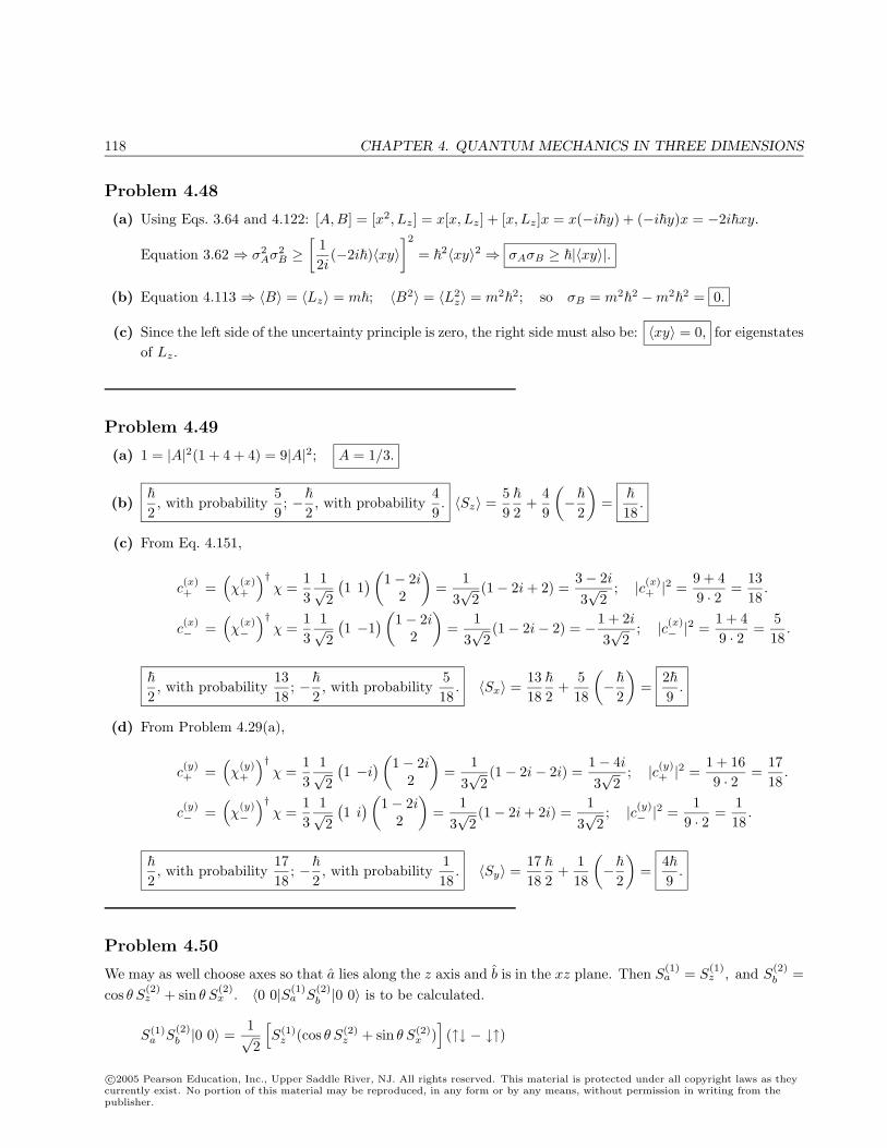
118 CHAPTER 4. QUANTUM MECHANICS IN THREE DIMENSIONS
Problem 4.48
(a) Using Eqs. 3.64 and 4.122: [A,B] = [x2, Lz] = x[x, Lz] + [x, Lz]x = x(−iy) + (−iy)x = −2ixy.
Equation 3.62 ⇒ σ2Aσ2
B ≥[
12i
(−2i)〈xy〉]2
= 2〈xy〉2 ⇒ σAσB ≥ |〈xy〉|.
(b) Equation 4.113 ⇒ 〈B〉 = 〈Lz〉 = m; 〈B2〉 = 〈L2z〉 = m2
2; so σB = m2
2 −m2
2 = 0.
(c) Since the left side of the uncertainty principle is zero, the right side must also be: 〈xy〉 = 0, for eigenstatesof Lz.
Problem 4.49
(a) 1 = |A|2(1 + 4 + 4) = 9|A|2; A = 1/3.
(b)
2, with probability
59; −
2, with probability
49. 〈Sz〉 =
59
2+
49
(−
2
)=
18.
(c) From Eq. 4.151,
c(x)+ =
(χ
(x)+
)†χ =
13
1√2
(1 1
) (1− 2i
2
)=
13√
2(1− 2i + 2) =
3− 2i3√
2; |c(x)
+ |2 =9 + 49 · 2 =
1318
.
c(x)− =
(χ
(x)−
)†χ =
13
1√2
(1 −1
) (1− 2i
2
)=
13√
2(1− 2i− 2) = −1 + 2i
3√
2; |c(x)
− |2 =1 + 49 · 2 =
518
.
2, with probability
1318
; −2, with probability
518
. 〈Sx〉 =1318
2+
518
(−
2
)=
29
.
(d) From Problem 4.29(a),
c(y)+ =
(χ
(y)+
)†χ =
13
1√2
(1 −i
) (1− 2i
2
)=
13√
2(1− 2i− 2i) =
1− 4i3√
2; |c(y)
+ |2 =1 + 169 · 2 =
1718
.
c(y)− =
(χ
(y)−
)†χ =
13
1√2
(1 i
) (1− 2i
2
)=
13√
2(1− 2i + 2i) =
13√
2; |c(y)
− |2 =1
9 · 2 =118
.
2, with probability
1718
; −2, with probability
118
. 〈Sy〉 =1718
2+
118
(−
2
)=
49
.
Problem 4.50
We may as well choose axes so that a lies along the z axis and b is in the xz plane. Then S(1)a = S
(1)z , and S
(2)b =
cos θ S(2)z + sin θ S
(2)x . 〈0 0|S(1)
a S(2)b |0 0〉 is to be calculated.
S(1)a S
(2)b |0 0〉 =
1√2
[S(1)
z (cos θ S(2)z + sin θ S(2)
x )](↑↓ − ↓↑)
c©2005 Pearson Education, Inc., Upper Saddle River, NJ. All rights reserved. This material is protected under all copyright laws as theycurrently exist. No portion of this material may be reproduced, in any form or by any means, without permission in writing from thepublisher.
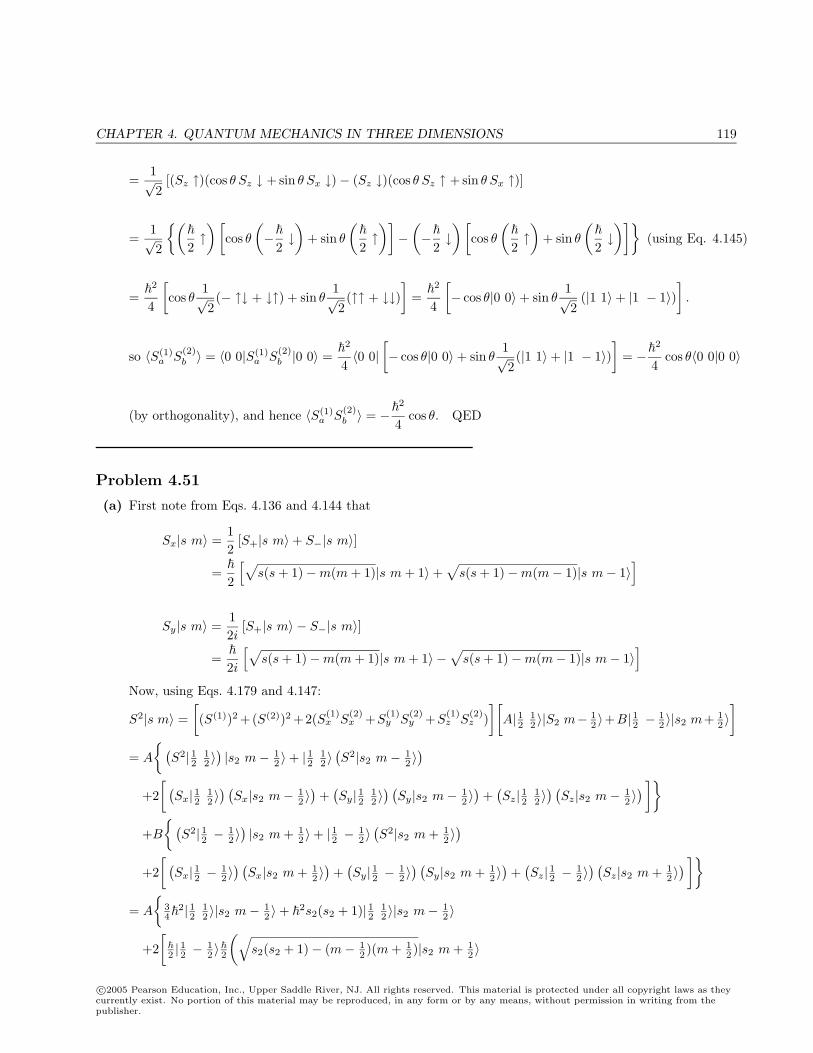
CHAPTER 4. QUANTUM MECHANICS IN THREE DIMENSIONS 119
=1√2
[(Sz ↑)(cos θ Sz ↓ + sin θ Sx ↓)− (Sz ↓)(cos θ Sz ↑ + sin θ Sx ↑)]
=1√2
(
2↑) [
cos θ(−
2↓)
+ sin θ
(
2↑)]−
(−
2↓) [
cos θ(
2↑)
+ sin θ
(
2↓)]
(using Eq. 4.145)
=
2
4
[cos θ
1√2(− ↑↓ + ↓↑) + sin θ
1√2(↑↑ + ↓↓)
]=
2
4
[− cos θ|0 0〉+ sin θ
1√2
(|1 1〉+ |1 − 1〉)].
so 〈S(1)a S
(2)b 〉 = 〈0 0|S(1)
a S(2)b |0 0〉 =
2
4〈0 0|
[− cos θ|0 0〉+ sin θ
1√2(|1 1〉+ |1 − 1〉)
]= −
2
4cos θ〈0 0|0 0〉
(by orthogonality), and hence 〈S(1)a S
(2)b 〉 = −
2
4cos θ. QED
Problem 4.51
(a) First note from Eqs. 4.136 and 4.144 that
Sx|s m〉 =12
[S+|s m〉+ S−|s m〉]
=
2
[√s(s + 1)−m(m + 1)|s m + 1〉+
√s(s + 1)−m(m− 1)|s m− 1〉
]
Sy|s m〉 =12i
[S+|s m〉 − S−|s m〉]
=
2i
[√s(s + 1)−m(m + 1)|s m + 1〉 −
√s(s + 1)−m(m− 1)|s m− 1〉
]Now, using Eqs. 4.179 and 4.147:
S2|s m〉 =[(S(1))2 +(S(2))2 +2(S(1)
x S(2)x +S
(1)y S
(2)y +S
(1)z S
(2)z )
][A| 12 1
2 〉|S2 m− 12 〉+B| 12 − 1
2 〉|s2 m+ 12 〉
]= A
(S2| 12 1
2 〉)|s2 m− 1
2 〉+ | 12 12 〉
(S2|s2 m− 1
2 〉)
+2[ (
Sx| 12 12 〉
) (Sx|s2 m− 1
2 〉)
+(Sy| 12 1
2 〉) (
Sy|s2 m− 12 〉
)+
(Sz| 12 1
2 〉) (
Sz|s2 m− 12 〉
) ]+B
(S2| 12 − 1
2 〉)|s2 m + 1
2 〉+ | 12 − 12 〉
(S2|s2 m + 1
2 〉)
+2[ (
Sx| 12 − 12 〉
) (Sx|s2 m + 1
2 〉)
+(Sy| 12 − 1
2 〉) (
Sy|s2 m + 12 〉
)+
(Sz| 12 − 1
2 〉) (
Sz|s2 m + 12 〉
) ]= A
34
2| 12 12 〉|s2 m− 1
2 〉+ 2s2(s2 + 1)| 12 12 〉|s2 m− 1
2 〉
+2[
2 | 12 − 12 〉2
(√s2(s2 + 1)− (m− 1
2 )(m + 12 )|s2 m + 1
2 〉
c©2005 Pearson Education, Inc., Upper Saddle River, NJ. All rights reserved. This material is protected under all copyright laws as theycurrently exist. No portion of this material may be reproduced, in any form or by any means, without permission in writing from thepublisher.
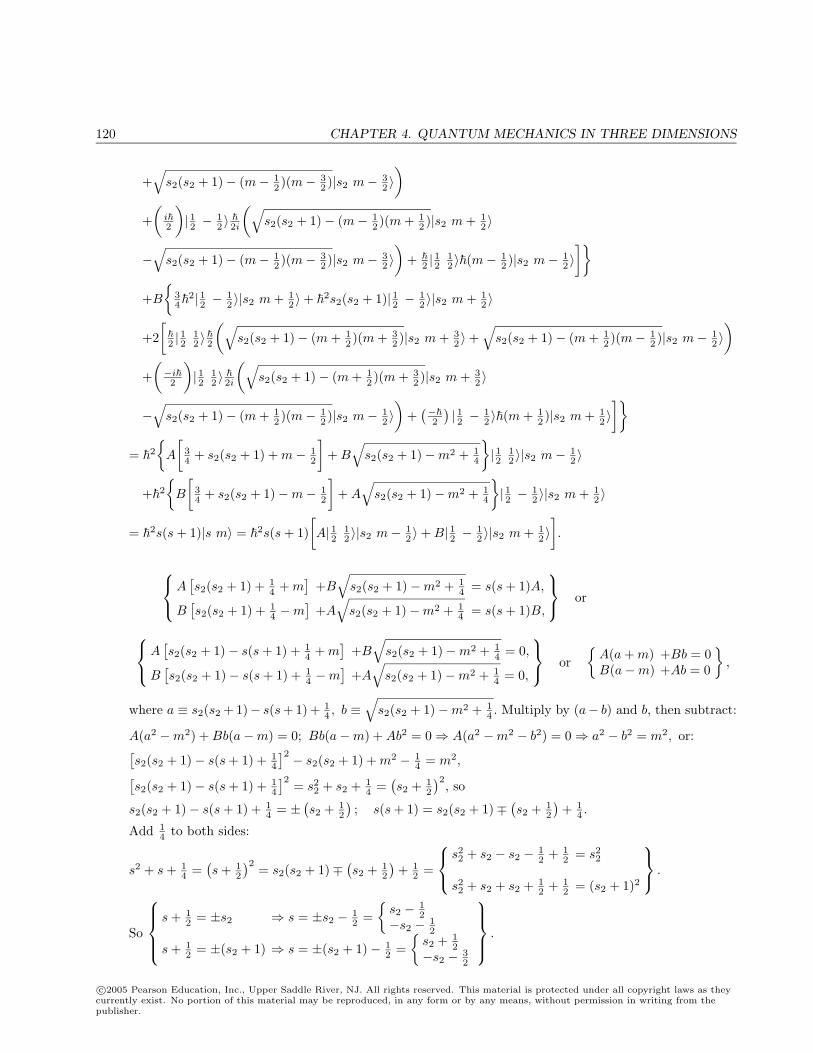
120 CHAPTER 4. QUANTUM MECHANICS IN THREE DIMENSIONS
+√
s2(s2 + 1)− (m− 12 )(m− 3
2 )|s2 m− 32 〉
)+
(i2
)| 12 − 1
2 〉 2i
(√s2(s2 + 1)− (m− 1
2 )(m + 12 )|s2 m + 1
2 〉
−√
s2(s2 + 1)− (m− 12 )(m− 3
2 )|s2 m− 32 〉
)+
2 | 12 12 〉(m− 1
2 )|s2 m− 12 〉
]+B
34
2| 12 − 12 〉|s2 m + 1
2 〉+ 2s2(s2 + 1)| 12 − 12 〉|s2 m + 1
2 〉
+2[
2 | 12 12 〉2
(√s2(s2 + 1)− (m + 1
2 )(m + 32 )|s2 m + 3
2 〉+√
s2(s2 + 1)− (m + 12 )(m− 1
2 )|s2 m− 12 〉
)+
(−i2
)| 12 1
2 〉 2i
(√s2(s2 + 1)− (m + 1
2 )(m + 32 )|s2 m + 3
2 〉
−√
s2(s2 + 1)− (m + 12 )(m− 1
2 )|s2 m− 12 〉
)+
(−2
)| 12 − 1
2 〉(m + 12 )|s2 m + 1
2 〉]
= 2
A
[34 + s2(s2 + 1) + m− 1
2
]+ B
√s2(s2 + 1)−m2 + 1
4
| 12 1
2 〉|s2 m− 12 〉
+2
B
[34 + s2(s2 + 1)−m− 1
2
]+ A
√s2(s2 + 1)−m2 + 1
4
| 12 − 1
2 〉|s2 m + 12 〉
= 2s(s + 1)|s m〉 = 2s(s + 1)[A| 12 1
2 〉|s2 m− 12 〉+ B| 12 − 1
2 〉|s2 m + 12 〉
].
A[s2(s2 + 1) + 1
4 + m]
+B√
s2(s2 + 1)−m2 + 14 = s(s + 1)A,
B[s2(s2 + 1) + 1
4 −m]
+A√
s2(s2 + 1)−m2 + 14 = s(s + 1)B,
or
A[s2(s2 + 1)− s(s + 1) + 1
4 + m]
+B√
s2(s2 + 1)−m2 + 14 = 0,
B[s2(s2 + 1)− s(s + 1) + 1
4 −m]
+A√
s2(s2 + 1)−m2 + 14 = 0,
or
A(a + m) +Bb = 0B(a−m) +Ab = 0
,
where a ≡ s2(s2 + 1)− s(s+ 1) + 14 , b ≡
√s2(s2 + 1)−m2 + 1
4 . Multiply by (a− b) and b, then subtract:
A(a2 −m2) + Bb(a−m) = 0; Bb(a−m) + Ab2 = 0⇒ A(a2 −m2 − b2) = 0⇒ a2 − b2 = m2, or:[s2(s2 + 1)− s(s + 1) + 1
4
]2 − s2(s2 + 1) + m2 − 14 = m2,[
s2(s2 + 1)− s(s + 1) + 14
]2 = s22 + s2 + 1
4 =(s2 + 1
2
)2, so
s2(s2 + 1)− s(s + 1) + 14 = ±
(s2 + 1
2
); s(s + 1) = s2(s2 + 1)∓
(s2 + 1
2
)+ 1
4 .
Add 14 to both sides:
s2 + s + 14 =
(s + 1
2
)2 = s2(s2 + 1)∓(s2 + 1
2
)+ 1
2 =
s22 + s2 − s2 − 1
2 + 12 = s2
2
s22 + s2 + s2 + 1
2 + 12 = (s2 + 1)2
.
So
s + 1
2 = ±s2 ⇒ s = ±s2 − 12 =
s2 − 1
2−s2 − 1
2
s + 12 = ±(s2 + 1) ⇒ s = ±(s2 + 1)− 1
2 =
s2 + 12
−s2 − 32
.
c©2005 Pearson Education, Inc., Upper Saddle River, NJ. All rights reserved. This material is protected under all copyright laws as theycurrently exist. No portion of this material may be reproduced, in any form or by any means, without permission in writing from thepublisher.
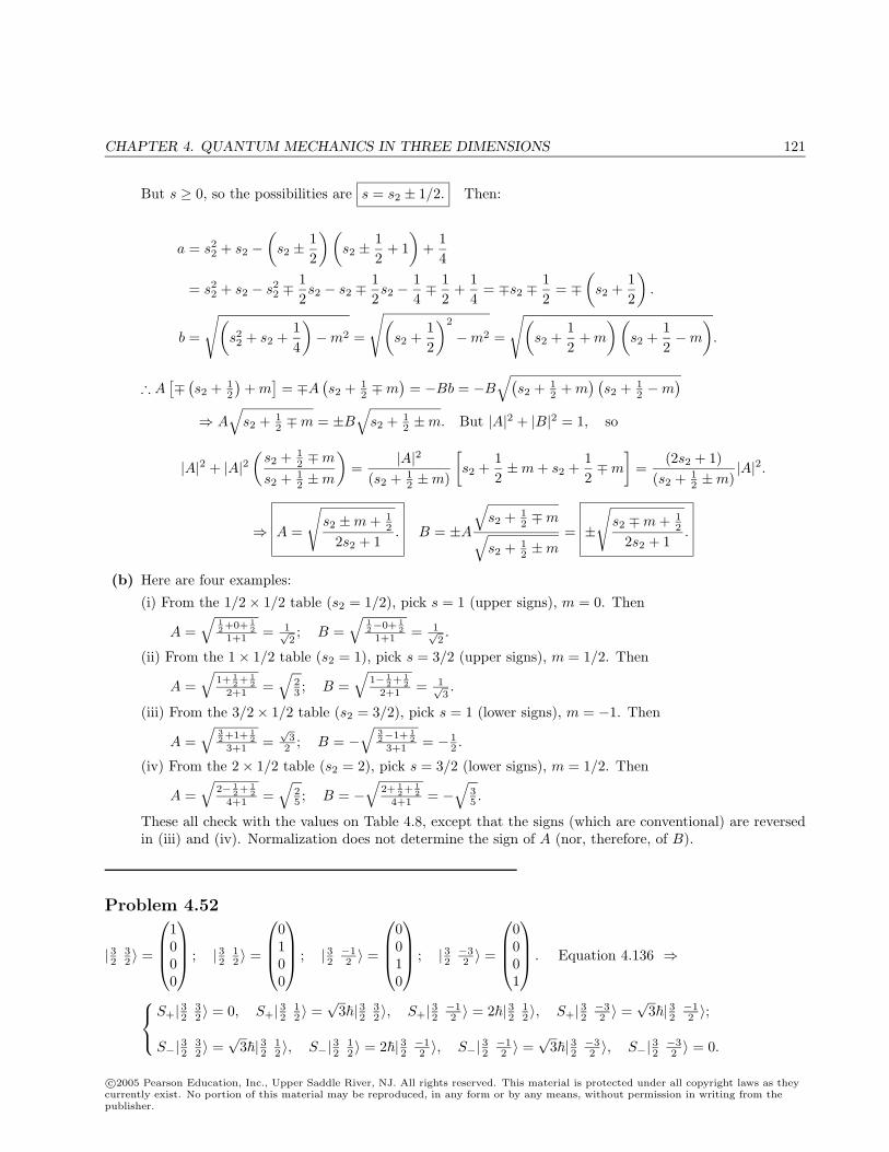
CHAPTER 4. QUANTUM MECHANICS IN THREE DIMENSIONS 121
But s ≥ 0, so the possibilities are s = s2 ± 1/2. Then:
a = s22 + s2 −
(s2 ±
12
) (s2 ±
12
+ 1)
+14
= s22 + s2 − s2
2 ∓12s2 − s2 ∓
12s2 −
14∓ 1
2+
14
= ∓s2 ∓12
= ∓(s2 +
12
).
b =
√(s22 + s2 +
14
)−m2 =
√(s2 +
12
)2
−m2 =
√(s2 +
12
+ m
) (s2 +
12−m
).
∴ A[∓
(s2 + 1
2
)+ m
]= ∓A
(s2 + 1
2 ∓m)
= −Bb = −B√(
s2 + 12 + m
) (s2 + 1
2 −m)
⇒ A√
s2 + 12 ∓m = ±B
√s2 + 1
2 ±m. But |A|2 + |B|2 = 1, so
|A|2 + |A|2(s2 + 1
2 ∓m
s2 + 12 ±m
)=
|A|2(s2 + 1
2 ±m)
[s2 +
12±m + s2 +
12∓m
]=
(2s2 + 1)(s2 + 1
2 ±m)|A|2.
⇒ A =
√s2 ±m + 1
2
2s2 + 1. B = ±A
√s2 + 1
2 ∓m√s2 + 1
2 ±m= ±
√s2 ∓m + 1
2
2s2 + 1.
(b) Here are four examples:
(i) From the 1/2× 1/2 table (s2 = 1/2), pick s = 1 (upper signs), m = 0. Then
A =√
12+0+ 1
21+1 = 1√
2; B =
√12−0+ 1
21+1 = 1√
2.
(ii) From the 1× 1/2 table (s2 = 1), pick s = 3/2 (upper signs), m = 1/2. Then
A =√
1+ 12+ 1
22+1 =
√23 ; B =
√1− 1
2+ 12
2+1 = 1√3.
(iii) From the 3/2× 1/2 table (s2 = 3/2), pick s = 1 (lower signs), m = −1. Then
A =√
32+1+ 1
23+1 =
√3
2 ; B = −√
32−1+ 1
23+1 = − 1
2 .
(iv) From the 2× 1/2 table (s2 = 2), pick s = 3/2 (lower signs), m = 1/2. Then
A =√
2− 12+ 1
24+1 =
√25 ; B = −
√2+ 1
2+ 12
4+1 = −√
35 .
These all check with the values on Table 4.8, except that the signs (which are conventional) are reversedin (iii) and (iv). Normalization does not determine the sign of A (nor, therefore, of B).
Problem 4.52
| 32 32 〉 =
1000
; | 32 12 〉 =
0100
; | 32 −12 〉 =
0010
; | 32 −32 〉 =
0001
. Equation 4.136 ⇒
S+| 32 3
2 〉 = 0, S+| 32 12 〉 =
√3| 32 3
2 〉, S+| 32 −12 〉 = 2| 32 1
2 〉, S+| 32 −32 〉 =
√3| 32 −1
2 〉;
S−| 32 32 〉 =
√3| 32 1
2 〉, S−| 32 12 〉 = 2| 32 −1
2 〉, S−| 32 −12 〉 =
√3| 32 −3
2 〉, S−| 32 −32 〉 = 0.
c©2005 Pearson Education, Inc., Upper Saddle River, NJ. All rights reserved. This material is protected under all copyright laws as theycurrently exist. No portion of this material may be reproduced, in any form or by any means, without permission in writing from thepublisher.
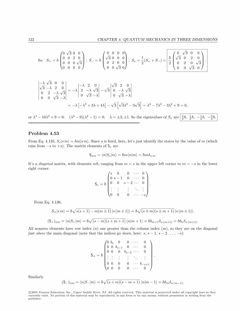
122 CHAPTER 4. QUANTUM MECHANICS IN THREE DIMENSIONS
So: S+ =
0√
3 0 00 0 2 00 0 0
√3
0 0 0 0
; S− =
0 0 0 0√3 0 0 0
0 2 0 00 0
√3 0
; Sx =12(S+ + S−) =
2
0√
3 0 0√3 0 2 0
0 2 0√
30 0
√3 0
.
∣∣∣∣∣∣∣∣−λ
√3 0 0√
3 −λ 2 00 2 −λ
√3
0 0√
3 −λ
∣∣∣∣∣∣∣∣ = −λ
∣∣∣∣∣∣−λ 2 02 −λ
√3
0√
3 −λ
∣∣∣∣∣∣−√3
∣∣∣∣∣∣√
3 2 00 −λ
√3
0√
3 −λ
∣∣∣∣∣∣= −λ
[−λ3 + 3λ + 4λ
]−√
3[√
3λ2 − 3√
3]
= λ4 − 7λ2 − 3λ2 + 9 = 0,
or λ4 − 10λ2 + 9 = 0; (λ2 − 9)(λ2 − 1) = 0; λ = ±3,±1. So the eigenvalues of Sx are 32,
12, − 1
2, − 32.
Problem 4.53
From Eq. 4.135, Sz|sm〉 = m|sm〉. Since s is fixed, here, let’s just identify the states by the value of m (whichruns from −s to +s). The matrix elements of Sz are
Snm = 〈n|Sz|m〉 = m〈n|m〉 = mδn m.
It’s a diagonal matrix, with elements m, ranging from m = s in the upper left corner to m = −s in the lowerright corner:
Sz =
s 0 0 · · · 00 s− 1 0 · · · 00 0 s− 2 · · · 0...
......
. . ....
0 0 0 · · · −s
.
From Eq. 4.136,
S±|sm〉 = √
s(s + 1)−m(m± 1) |s (m± 1)〉 = √
(s∓m)(s±m + 1) |s (m± 1)〉.
(S+)nm = 〈n|S+|m〉 = √
(s−m)(s + m + 1) 〈n|m + 1〉 = bm+1δn (m+1) = bnδn (m+1).
All nonzero elements have row index (n) one greater than the column index (m), so they are on the diagonaljust above the main diagonal (note that the indices go down, here: s, s− 1, s− 2 . . . , −s):
S+ =
0 bs 0 0 · · · 00 0 bs−1 0 · · · 00 0 0 bs−2 · · · 0...
......
.... . .
...0 0 0 0 · · · b−s+1
0 0 0 0 · · · 0
.
Similarly(S−)nm = 〈n|S−|m〉 =
√(s + m)(s−m + 1) 〈n|m− 1〉 = bmδn (m−1).
c©2005 Pearson Education, Inc., Upper Saddle River, NJ. All rights reserved. This material is protected under all copyright laws as theycurrently exist. No portion of this material may be reproduced, in any form or by any means, without permission in writing from thepublisher.
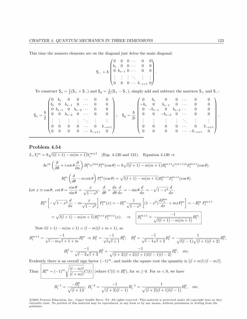
CHAPTER 4. QUANTUM MECHANICS IN THREE DIMENSIONS 123
This time the nonzero elements are on the diagonal just below the main diagonal:
S− =
0 0 0 · · · 0 0bs 0 0 · · · 0 00 bs−1 0 · · · 0 0...
......
. . ....
...0 0 0 · · · b−s+1 0
.
To construct Sx = 12 (S+ + S−) and Sy = 1
2i (S+ − S−), simply add and subtract the matrices S+ and S−:
Sx =
2
0 bs 0 0 · · · 0 0bs 0 bs−1 0 · · · 0 00 bs−1 0 bs−2 · · · 0 00 0 bs−2 0 · · · 0 0...
......
.... . .
......
0 0 0 0 · · · 0 b−s+1
0 0 0 0 · · · b−s+1 0
; Sy =
2i
0 bs 0 0 · · · 0 0−bs 0 bs−1 0 · · · 0 00 −bs−1 0 bs−2 · · · 0 00 0 −bs−2 0 · · · 0 0...
......
.... . .
......
0 0 0 0 · · · 0 b−s+1
0 0 0 0 · · · −b−s+1 0
.
Problem 4.54
L+Y ml =
√l(l + 1)−m(m + 1)Y m±1
l (Eqs. 4.120 and 121). Equation 4.130 ⇒
eiφ
(∂
∂θ+ i cot θ
∂
∂φ
)Bm
l eimφPml (cos θ) =
√l(l + 1)−m(m + 1)Bm+1
l ei(m+1)φPm+1l (cos θ).
Bml
(d
dθ−m cot θ
)Pm
l (cos θ) =√
l(l + 1)−m(m + 1)Bm+1l Pm+1
l (cos θ).
Let x ≡ cos θ; cot θ =cos θsin θ
=x√
1− x2;
d
dθ=
dx
dθ
d
dx= − sin θ
d
dx= −
√1− x2
d
dx.
Bml
[−
√1− x2
d
dx−m
x√1− x2
]Pm
l (x) = −Bml
1√1− x2
[(1− x2)
dPml
dx+ mxPm
l
]= −Bm
l Pm+1l
=√
l(l + 1)−m(m + 1)Bm+1l Pm+1
l (x). ⇒ Bm+1l =
−1√l(l + 1)−m(m + 1)
Bml .
Now l(l + 1)−m(m + 1) = (l −m)(l + m + 1), so
Bm+1l =
−1√l −m
√l + 1 + m
Bml ⇒ B1
l =−1√
l√l + 1
B0l ; B2
l =−1√
l − 1√l + 2
B1l =
1√l(l − 1)
√(l + 1)(l + 2)
B0l ;
B3l =
−1√l − 2
√l + 3
B2l =
−1√(l + 3)(l + 2)(l + 1)l(l − 1)(l − 2)
B0l , etc.
Evidently there is an overall sign factor (−1)m, and inside the square root the quantity is [(l + m)!/(l −m)!].
Thus: Bml = (−1)m
√(l −m)!(l + m)!
C(l) (where C(l) ≡ B0l ), for m ≥ 0. For m < 0, we have
B−1l =
−B0l√
(l + 1)l; B−2
l =−1√
(l + 2)(l − 1)B−1
l =1√
(l + 2)(l + 1)l(l − 1)B0
l , etc.
c©2005 Pearson Education, Inc., Upper Saddle River, NJ. All rights reserved. This material is protected under all copyright laws as theycurrently exist. No portion of this material may be reproduced, in any form or by any means, without permission in writing from thepublisher.
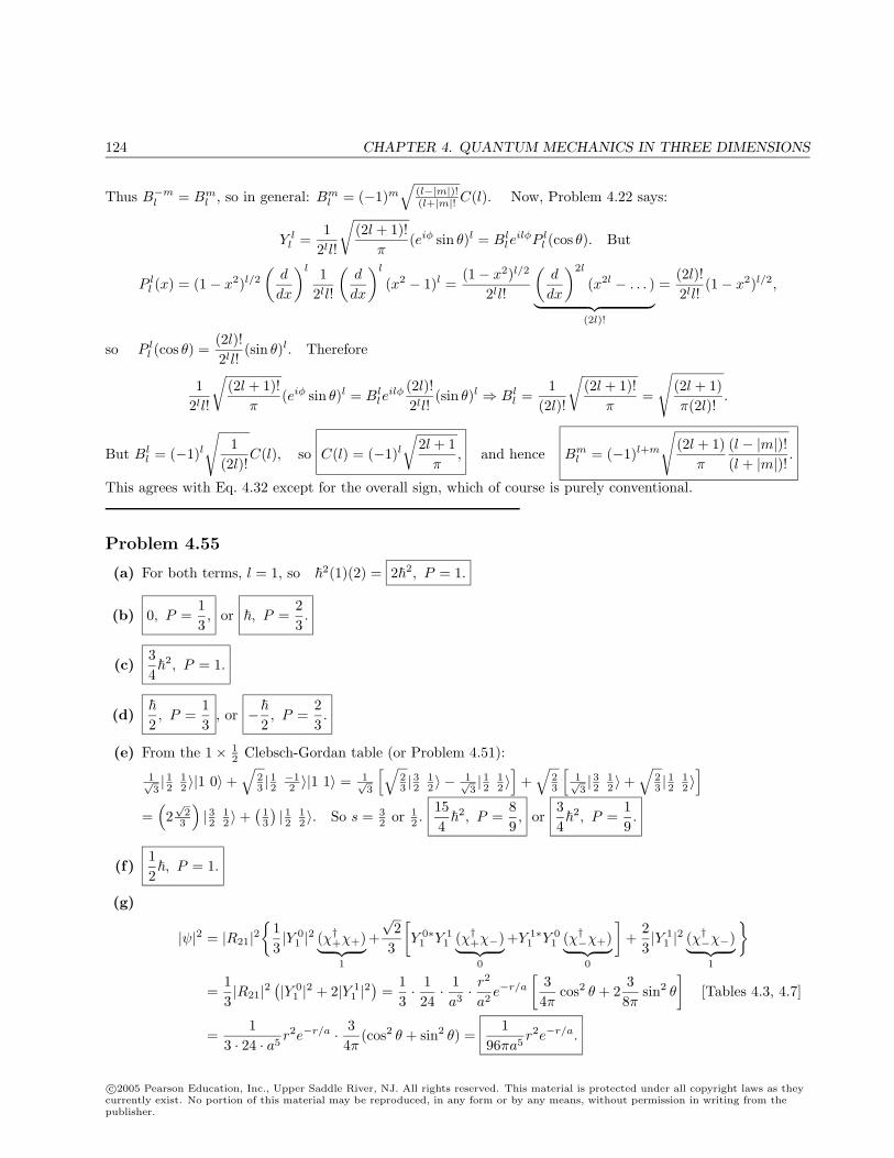
124 CHAPTER 4. QUANTUM MECHANICS IN THREE DIMENSIONS
Thus B−ml = Bm
l , so in general: Bml = (−1)m
√(l−|m|)!(l+|m|! C(l). Now, Problem 4.22 says:
Y ll =
12ll!
√(2l + 1)!
π(eiφ sin θ)l = Bl
leilφP l
l (cos θ). But
P ll (x) = (1− x2)l/2
(d
dx
)l 12ll!
(d
dx
)l
(x2 − 1)l =(1− x2)l/2
2ll!
(d
dx
)2l
(x2l − . . . )︸ ︷︷ ︸(2l)!
=(2l)!2ll!
(1− x2)l/2,
so P ll (cos θ) =
(2l)!2ll!
(sin θ)l. Therefore
12ll!
√(2l + 1)!
π(eiφ sin θ)l = Bl
leilφ (2l)!
2ll!(sin θ)l ⇒ Bl
l =1
(2l)!
√(2l + 1)!
π=
√(2l + 1)π(2l)!
.
But Bll = (−1)l
√1
(2l)!C(l), so C(l) = (−1)l
√2l + 1
π, and hence Bm
l = (−1)l+m
√(2l + 1)
π
(l − |m|)!(l + |m|)! .
This agrees with Eq. 4.32 except for the overall sign, which of course is purely conventional.
Problem 4.55
(a) For both terms, l = 1, so 2(1)(2) = 22, P = 1.
(b) 0, P =13, or , P =
23.
(c)34
2, P = 1.
(d)
2, P =
13
, or −2, P =
23.
(e) From the 1× 12 Clebsch-Gordan table (or Problem 4.51):
1√3| 12 1
2 〉|1 0〉+√
23 | 12 −1
2 〉|1 1〉 = 1√3
[√23 | 32 1
2 〉 − 1√3| 12 1
2 〉]
+√
23
[1√3| 32 1
2 〉+√
23 | 12 1
2 〉]
=(2√
23
)| 32 1
2 〉+(
13
)| 12 1
2 〉. So s = 32 or 1
2 .154
2, P =89, or
34
2, P =19.
(f)12, P = 1.
(g)
|ψ|2 = |R21|2
13|Y 0
1 |2 (χ†+χ+)︸ ︷︷ ︸1
+√
23
[Y 0∗
1 Y 11 (χ†+χ−)︸ ︷︷ ︸
0
+Y 1∗1 Y 0
1 (χ†−χ+)︸ ︷︷ ︸0
]+
23|Y 1
1 |2 (χ†−χ−)︸ ︷︷ ︸1
=13|R21|2
(|Y 0
1 |2 + 2|Y 11 |2
)=
13· 124· 1a3· r
2
a2e−r/a
[34π
cos2 θ + 238π
sin2 θ
][Tables 4.3, 4.7]
=1
3 · 24 · a5r2e−r/a · 3
4π(cos2 θ + sin2 θ) =
196πa5
r2e−r/a.
c©2005 Pearson Education, Inc., Upper Saddle River, NJ. All rights reserved. This material is protected under all copyright laws as theycurrently exist. No portion of this material may be reproduced, in any form or by any means, without permission in writing from thepublisher.
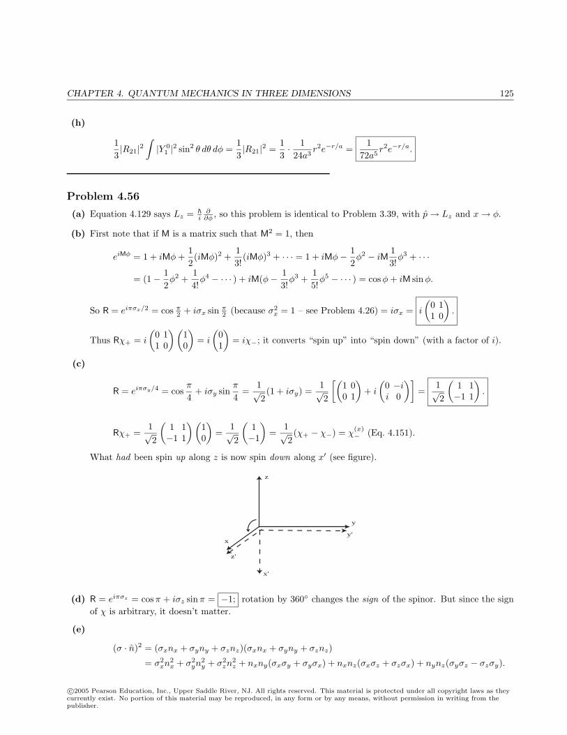
CHAPTER 4. QUANTUM MECHANICS IN THREE DIMENSIONS 125
(h)
13|R21|2
∫|Y 0
1 |2 sin2 θ dθ dφ =13|R21|2 =
13· 124a3
r2e−r/a =1
72a5r2e−r/a.
Problem 4.56
(a) Equation 4.129 says Lz =
i∂
∂φ , so this problem is identical to Problem 3.39, with p→ Lz and x→ φ.
(b) First note that if M is a matrix such that M2 = 1, then
eiMφ = 1 + iMφ +12(iMφ)2 +
13!
(iMφ)3 + · · · = 1 + iMφ− 12φ2 − iM
13!
φ3 + · · ·
= (1− 12φ2 +
14!
φ4 − · · · ) + iM(φ− 13!
φ3 +15!
φ5 − · · · ) = cosφ + iM sinφ.
So R = eiπσx/2 = cos π2 + iσx sin π
2 (because σ2x = 1 – see Problem 4.26) = iσx = i
(0 11 0
).
Thus Rχ+ = i
(0 11 0
) (10
)= i
(01
)= iχ−; it converts “spin up” into “spin down” (with a factor of i).
(c)
R = eiπσy/4 = cosπ
4+ iσy sin
π
4=
1√2(1 + iσy) =
1√2
[(1 00 1
)+ i
(0 −ii 0
)]=
1√2
(1 1−1 1
).
Rχ+ =1√2
(1 1−1 1
) (10
)=
1√2
(1−1
)=
1√2(χ+ − χ−) = χ
(x)− (Eq. 4.151).
What had been spin up along z is now spin down along x′ (see figure).
y
y'
z
x'
x
z'
(d) R = eiπσz = cosπ + iσz sinπ = −1; rotation by 360 changes the sign of the spinor. But since the signof χ is arbitrary, it doesn’t matter.
(e)
(σ · n)2 = (σxnx + σyny + σznz)(σxnx + σyny + σznz)
= σ2xn
2x + σ2
yn2y + σ2
zn2z + nxny(σxσy + σyσx) + nxnz(σxσz + σzσx) + nynz(σyσz − σzσy).
c©2005 Pearson Education, Inc., Upper Saddle River, NJ. All rights reserved. This material is protected under all copyright laws as theycurrently exist. No portion of this material may be reproduced, in any form or by any means, without permission in writing from thepublisher.
126 CHAPTER 4. QUANTUM MECHANICS IN THREE DIMENSIONS
But σ2x = σ2
y = σ2z = 1, and σxσy + σyσx = σxσz + σzσx = σyσz + σzσy = 0 (Problem 4.26), so
(σ · n)2 = n2x + n2
y + n2z = 1. So ei(σ·n)φ/2 = cos
φ
2+ i(σ · n) sin
φ
2. QED
Problem 4.57
(a)
[q1, q2] =12
[x +
(a2/
)py, x−
(a2/
)py
]= 0, because [x, py] = [x, x] = [py, py] = 0.
[p1, p2] =12
[px −
(/a2
)y, px +
(/a2
)y]
= 0, because [y, px] = [y, y] = [px, px] = 0.
[q1, p1] =12
[x +
(a2/
)py, px −
(/a2
)y]
=12
([x, px]− [py, y]) =12
[i− (−i)] = i.
[q2, p2] =12
[x−
(a2/
)py, px +
(/a2
)y]
=12
([x, px]− [py, y]) = i.
[See Eq. 4.10 for the canonical commutators.]
(b)
q21 − q2
2 =12
[x2 +
a2
(xpy + pyx) +
(a2
)2
p2y − x2 +
a2
(xpy + pyx)−
(a2
)2
p2y
]=
2a
xpy.
p21 − p2
2 =12
[p2
x −
a2(pxy + ypx) +
(
a2
)2
y2 − p2x −
a2(pxy + ypx)−
(
a2
)2
y2
]= −2
a2ypx.
So
2a2(q2
1 − q22) +
a2
2(p2
1 − p22) = xpy − ypx = Lz.
(c)
H =1
2mp2 +
12mω2x2 =
a2
2p2 +
2a2x2 = H(x, p).
Then H(q1, p1) =a2
2p21 +
2a2q21 ≡ H1, H(q2, p2) =
a2
2p22 +
2a2q22 ≡ H2; Lz = H1 −H2.
(d) The eigenvalues of H1 are (n1 + 12 ), and those of H2 are (n2 + 1
2 ), so the eigenvalues of Lz are
(n1 + 12 )− (n2 + 1
2 ) = (n1 − n2) = m, and m is an integer, because n1 and n2 are.
c©2005 Pearson Education, Inc., Upper Saddle River, NJ. All rights reserved. This material is protected under all copyright laws as theycurrently exist. No portion of this material may be reproduced, in any form or by any means, without permission in writing from thepublisher.
CHAPTER 4. QUANTUM MECHANICS IN THREE DIMENSIONS 127
Problem 4.58
From Problem 4.28 we know that in the generic state χ =(ab
)(with |a|2 + |b|2 = 1),
〈Sz〉 =
2(|a|2 − |b|2
), 〈Sx〉 = Re(ab∗), 〈Sy〉 = −Im(ab∗); 〈S2
x〉 = 〈S2y〉 =
2
4.
Writing a = |a|eiφa , b = |b|eiφb , we have ab∗ = |a||b|ei(φa−φb) = |a||b|eiθ, where θ ≡ φa − φb is the phasedifference between a and b. Then
〈Sx〉 = Re(|a||b|eiθ) = |a||b| cos θ, 〈Sy〉 = −Im(|a||b|eiθ) = −|a||b| sin θ.
σ2Sx = 〈S2
x〉 − 〈Sx〉2 =
2
4− 2|a|2|b|2 cos2 θ; σ2
Sy = 〈S2y〉 − 〈Sy〉2 =
2
4− 2|a|2|b|2 sin2 θ.
We want σ2Sxσ
2Sy =
2
4〈Sz〉2, or
2
4(1− 4|a|2|b|2 cos2 θ
) 2
4(1− 4|a|2|b|2 sin2 θ
)=
2
4
2
4(|a|2 − |b|2
)2.
1− 4|a|2|b|2(cos2 θ + sin2 θ
)+ 16|a|4|b|4 sin2 θ cos2 θ = |a|4 − 2|a|2|b|2 + |b|4.
1 + 16|a|4|b|4 sin2 θ cos2 θ = |a|4 + 2|a|2|b|2 + |b|4 =(|a|2 + |b|2
)2= 1 ⇒ |a|2|b|2 sin θ cos θ = 0.
So either θ = 0 or π, in which case a and b are relatively real, or else θ = ±π/2, in which case a and b arerelatively imaginary (these two options subsume trivially the solutions a = 0 and b = 0).
Problem 4.59
(a)
Start with Eq. 3.71:d〈r〉dt
=i
〈[H, r]〉.
H =1
2m(p− qA) · (p− qA) + qϕ =
12m
[p2 − q(p ·A + A · p) + q2A2
]+ qϕ.
[H,x] =1
2m[p2, x]− q
2m[(p ·A + A · p), x].
[p2, x] = [(p2x + p2
y + p2z), x] = [p2
x, x] = px[px, x] + [px, x]px = px(−i) + (−i)px = −2ipx.
[p ·A, x] = [(pxAx + pyAy + pzAz), x] = [pxAx, x] = px[Ax, x] + [px, x]Ax = −iAx.
[A · p, x] = [(Axpx + Aypy + Azpz), x] = [Axpx, x] = Ax[px, x] + [Ax, x]px = −iAx.
[H,x] =1
2m(−2ipx)− q
2m(−2iAx) = − i
m(px − qAx); [H, r] = − i
m(p− qA).
d〈r〉dt
=1m〈(p− qA)〉. QED
c©2005 Pearson Education, Inc., Upper Saddle River, NJ. All rights reserved. This material is protected under all copyright laws as theycurrently exist. No portion of this material may be reproduced, in any form or by any means, without permission in writing from thepublisher.
128 CHAPTER 4. QUANTUM MECHANICS IN THREE DIMENSIONS
(b)
We define the operator v ≡ 1m
(p− qA);d〈v〉dt
=i
〈[H,v]〉+ 〈∂v
∂t〉; ∂v
∂t= − q
m
∂A∂t
.
H =12mv2 + qϕ⇒ [H,v] =
m
2[v2,v] + q[ϕ,v]; [ϕ,v] =
1m
[ϕ,p].
[ϕ, px] = i∂ϕ
∂x(Eq. 3.65), so [ϕ,p] = i∇ϕ, and [ϕ,v] =
i
m∇ϕ.
[v2, vx] = [(v2x + v2
y + v2z), vx] = [v2
y, vx] + [v2z , vx] = vy[vy, vx] + [vy, vx]vy + vz[vz, vx] + [vz, vx]vz.
[vy, vx] =1m2
[(py − qAy), (px − qAx)] = − q
m2([Ay, px] + [py, Ax])
= − q
m2
(i
∂Ay
∂x− i
∂Ax
∂y
)= − iq
m2(∇×A)z = − iq
m2Bz.
[vz, vx] =1m2
[(pz − qAz), (px − qAx)] = − q
m2([Az, px] + [pz, Ax])
= − q
m2
(i
∂Az
∂x− i
∂Ax
∂y
)=
iq
m2(∇×A)y =
iq
m2By.
∴ [v2, vx] =iq
m2(−vyBz −Bzvy + vzBy + Byvz) =
iq
m2[−(v ×B)x + (B× v)x] .
[v2,v] =iq
m2[(B× v)− (v ×B)] . Putting all this together:
d〈v〉dt
=i
⟨[m
2iq
m2(B× v − v ×B) +
qi
m∇ϕ
]⟩− q
m〈∂A∂t〉.
[] md〈v〉dt
=q
2〈(v ×B)− (B× v)〉+ q
⟨−∇ϕ− ∂A
dt
⟩=
q
2〈(v ×B−B× v)〉+ q〈E〉. Or, since
v ×B−B× v =1m
[(p− qA)×B−B× (p− qA)] =1m
[p×B−B× p]− q
m[A×B−B×A] .
[Note: p does not commute with B, so the order does matter in the first term. But A commutes with B,so B×A = −A×B in the second.]
md〈v〉dt
= q〈E〉+q
2m〈p×B−B× p〉 − q2
m〈A×B〉. QED
(c) Go back to Eq. , and use 〈E〉 = E, 〈v ×B〉 = 〈v〉 ×B; 〈B× v〉 = B× 〈v〉 = −〈v〉 ×B. Then
md〈v〉dt
= q〈v〉 ×B + qE. QED
c©2005 Pearson Education, Inc., Upper Saddle River, NJ. All rights reserved. This material is protected under all copyright laws as theycurrently exist. No portion of this material may be reproduced, in any form or by any means, without permission in writing from thepublisher.
CHAPTER 4. QUANTUM MECHANICS IN THREE DIMENSIONS 129
Problem 4.60
(a)
E = −∇ϕ = −2Kzk. B = ∇×A =
∣∣∣∣∣∣i j k
∂/∂x ∂/∂y ∂/∂z−B0y/2 B0x/2 0
∣∣∣∣∣∣ = B0k.
(b) For time-independent potentials Eq. 4.205 separates in the usual way:
12m
(
i∇− qA
)·(
i∇− qA
)ψ + qϕψ = Eψ, or
− 2
2m∇2ψ+
iq
2m[∇ · (Aψ) + A · (∇ψ)]+
q2
2mA2 +qϕψ = Eψ. But ∇· (Aψ) = (∇·A)ψ+A · (∇ψ), so
− 2
2m∇2ψ +
iq
2m[2A · (∇ψ) +∇ · (Aψ)] +
(q2
2mA2 + qϕ
)ψ = Eψ.
This is the time-independent Schrodinger equation for electrodynamics. In the present case
∇ ·A = 0, A · (∇ψ) =B0
2
(x∂ψ
∂y− y
∂ψ
∂x
), A2 =
B20
4(x2 + y2
), ϕ = Kz2.
But Lz =
i
(x
∂
∂y− y
∂
∂x
), so −
2
2m∇2ψ − qB0
2mLzψ +
[q2B2
0
8m(x2 + y2
)+ qKz2
]ψ = Eψ.
Since Lz commutes with H, we may as well pick simultaneous eigenfunctions of both: Lzψ = mψ,where m = 0,±1,±2, . . . (with the overbar to distinguish the magnetic quantum number from the mass).Then [
− 2
2m∇2 +
(qB0)2
8m(x2 + y2
)+ qKz2
]ψ =
(E +
qB0
2mm
)ψ.
Now let ω1 ≡ qB0/m, ω2 ≡√
2Kq/m, and use cylindrical coordinates (r, φ, z):
− 2
2m
[1r
∂
∂r
(r∂ψ
∂r
)+
1r2
∂2ψ
∂φ2+
∂2ψ
∂z2
]+
[18mω2
1
(x2 + y2
)+
12mω2
2z2
]ψ =
(E +
12mω1
)ψ.
But Lz =
i
∂
∂φ, so
∂2ψ
∂φ2= − 1
2L2
zψ = − 12
m2
2ψ = −m2ψ. Use separation of variables: ψ(r, φ, z) =
R(r)Φ(φ)Z(z) :
− 2
2m
[ΦZ
1r
d
dr
(rdR
dr
)− m2
r2RΦZ + RΦ
d2Z
dz2
]+
(18mω2
1r2 +
12mω2
2z2
)RΦZ =
(E +
12mω1
)RΦZ.
Divide by RΦZ and collect terms:−
2
2m
[1rR
d
dr
(rdR
dr
)− m2
r2
]+
18mω2
1r2
+
−
2
2m1Z
d2Z
dz2+
12mω2
2z2
=
(E +
12mω1
).
The first term depends only on r, the second only on z, so they’re both constants; call them Er and Ez:
− 2
2m
[1r
d
dr
(rdR
dr
)− m2
r2R
]+
18mω2
1r2R = ErR; −
2
2md2Z
dz2+
12mω2
2z2Z = EzZ; E = Er+Ez−
12mω1.
c©2005 Pearson Education, Inc., Upper Saddle River, NJ. All rights reserved. This material is protected under all copyright laws as theycurrently exist. No portion of this material may be reproduced, in any form or by any means, without permission in writing from thepublisher.
130 CHAPTER 4. QUANTUM MECHANICS IN THREE DIMENSIONS
The z equation is a one-dimensional harmonic oscillator, and we can read off immediately that Ez =(n2 + 1/2)ω2, with n2 = 0, 1, 2, . . . . The r equation is actually a two-dimensional harmonic oscillator; toget Er, let u(r) ≡ √r R, and follow the method of Sections 4.1.3 and 4.2.1:
R =u√r,
dR
dr=
u′√r− u
2r3/2, r
dR
dr=√r u′ − u
2√r,
d
dr
(rdR
dr
)=√r u′′ +
u
4r3/2,
1r
d
dr
(rdR
dr
)=
u′′√r
+u
4r5/2; −
2
2m
(u′′√r
+14
u
r2
1√r− m2
r2
u√r
)+
18mω2
1r2 u√
r= Er
u√r
− 2
2m
[d2u
dr2+
(14− m2
)u
r2
]+
18mω2
1r2u = Eru.
This is identical to the equation we encountered in Problem 4.39 (the three-dimentional harmonic oscil-lator), only with ω → ω1/2, E → Er, and l(l + 1) → m2 − 1/4, which is to say, l2 + l + 1/4 = m2, or(l + 1/2)2 = m2, or l = |m| − 1/2. [Our present equation depends only on m2, and hence is the same foreither sign, but the solution to Problem 4.39 assumed l + 1/2 ≥ 0 (else u is not normalizable), so we need|m| here.] Quoting 4.39:
E = (jmax + l + 3/2)ω → Er = (jmax + |m|+ 1)ω1/2, where jmax = 0, 2, 4, . . . .
E = jmax + |m|+ 1)ω1/2 + (n2 + 1/2)ω2 − mω1/2 = (n1 + 12 )ω1 + (n2 + 1
2 )ω2,
where n1 = 0, 1, 2, . . . (if m ≥ 0, then n1 = jmax/2; if m < 0, then n1 = jmax/2− m).
Problem 4.61
(a)
B′ = ∇×A′ = ∇×A +∇× (∇λ) = ∇×A = B.
[∇×∇λ = 0, by equality of cross-derivatives: (∇×∇λ)x =∂
∂y
(∂λ
∂z
)− ∂
∂z
(∂λ
∂y
)= 0, etc.]
E′ = −∇ϕ′ − ∂A′
∂t= −∇ϕ +∇
(∂Λ∂t
)− ∂A
∂t− ∂
∂t(∇Λ) = −∇ϕ− ∂A
∂t= E.
[Again: ∇(∂Λ∂t
)=
∂
∂t(∇Λ) by the equality of cross-derivatives.]
(b) [
i∇− qA− q(∇Λ)
]eiqΛ/Ψ = q(∇Λ)eiqΛ/Ψ +
ieiqΛ/∇Ψ− qAeiqΛ/Ψ− q(∇Λ)eiqΛ/Ψ
=
ieiqΛ/∇Ψ− qAeiqΛ/Ψ.
[
i∇− qA− q(∇Λ)
]2
eiqΛ/Ψ =(
i∇− qA− q(∇Λ)
) [
ieiqΛ/∇Ψ− qAeiqΛ/Ψ
]c©2005 Pearson Education, Inc., Upper Saddle River, NJ. All rights reserved. This material is protected under all copyright laws as theycurrently exist. No portion of this material may be reproduced, in any form or by any means, without permission in writing from thepublisher.
CHAPTER 4. QUANTUM MECHANICS IN THREE DIMENSIONS 131
= −2
[iq
(∇Λ · ∇Ψ)eiqΛ/ + eiqΛ/∇2Ψ
]− q
i(∇ ·A)eiqΛ/Ψ− q2(A · ∇Λ)eiqΛ/Ψ
− q
ieiqΛ/A · (∇Ψ)− q
ieiqΛ/(A · ∇Ψ) + q2A2eiqΛ/Ψ
− q
ieiqΛ/(∇Λ · ∇Ψ) + q2(A · ∇Λ)eiqΛ/Ψ
= eiqΛ/[−2∇2Ψ + iq(∇ ·A)Ψ + 2iq(A · ∇Ψ) + q2A2Ψ
]−iq(∇Λ) · (∇Ψ)− q2(A · ∇Λ)Ψ + iq(∇Λ) · (∇Ψ) + q2(A · ∇Λ)Ψ
= eiqΛ/
[(
i∇− qA
)2
Ψ
].
So:
[1
2m
(
i∇− qA′
)2
+ qϕ′]
Ψ′ = eiqΛ/
[1
2m
(
i∇− qA
)2
+ qϕ− q∂Λ∂t
]Ψ
[using Eq. 4.205] = eiqΛ/
(i
∂Ψ∂t− q
∂Λ∂t
Ψ)
= i∂
∂t
(eiqΛ/Ψ
)= i
∂Ψ′
∂t. QED
c©2005 Pearson Education, Inc., Upper Saddle River, NJ. All rights reserved. This material is protected under all copyright laws as theycurrently exist. No portion of this material may be reproduced, in any form or by any means, without permission in writing from thepublisher.
132 CHAPTER 5. IDENTICAL PARTICLES
Chapter 5
Identical Particles
Problem 5.1
(a)
(m1 + m2)R = m1r1 + m2r2 = m1r1 + m2(r1 − r) = (m1 + m2)r1 −m2r ⇒
r1 = R +m2
m1 + m2r = R +
µ
m1r.
(m1 + m2)R = m1(r2 + r) + m2r2 = (m1 + m2)r2 + m1r⇒ r2 = R− m1
m1 + m2r = R− µ
m2r.
Let R = (X,Y, Z), r = (x, y, z).
(∇1)x =∂
∂x1=
∂X
∂x1
∂
∂X+
∂x
∂x1
∂
∂x
=(
m1
m1 + m2
)∂
∂X+ (1)
∂
∂x=
µ
m2(∇R)x + (∇r)x, so ∇1 =
µ
m2∇R +∇r.
(∇2)x =∂
∂x2=
∂X
∂x2
∂
∂X+
∂x
∂x2
∂
∂x
=(
m2
m1 + m2
)∂
∂X− (1)
∂
∂x=
µ
m1(∇R)x − (∇r)x, so ∇2 =
µ
m1∇R −∇r.
(b)
∇21ψ = ∇1 · (∇1ψ) = ∇1 ·
[µ
m2∇Rψ +∇rψ
]=
µ
m2∇R ·
(µ
m2∇Rψ +∇rψ
)+∇r ·
(µ
m2∇Rψ +∇rψ
)=
(µ
m2
)2
∇2Rψ + 2
µ
m2(∇r · ∇R)ψ +∇2
rψ.
c©2005 Pearson Education, Inc., Upper Saddle River, NJ. All rights reserved. This material is protected under all copyright laws as theycurrently exist. No portion of this material may be reproduced, in any form or by any means, without permission in writing from thepublisher.
CHAPTER 5. IDENTICAL PARTICLES 133
Likewise, ∇22ψ =
(µ
m1
)2
∇2Rψ − 2
µ
m1(∇r · ∇R) +∇2
rψ.
∴ Hψ = − 2
2m1∇2
1ψ −
2
2m2∇2
2ψ + V (r1, r2)ψ
= −2
2
(µ2
m1m22
∇2R +
2µm1m2
∇r · ∇R +1m1∇2
r +µ2
m2m21
∇2R −
2µm2m1
∇r · ∇R +1m2∇2
r
)ψ
+ V (r)ψ = −2
2
[µ2
m1m2
(1m2
+1m1
)∇2
R +(
1m1
+1m2
)∇2
r
]ψ + V (r)ψ = Eψ.
But(
1m1
+1m2
)=
m1 + m2
m1m2=
1µ, so
µ2
m1m2
(1m2
+1m1
)=
µ
m1m2=
m1m2
m1m2(m1 + m2)+
1m1 + m2
.
− 2
2(m1 + m2)∇2
Rψ − 2
2µ∇2
rψ + V (r)ψ = Eψ.
(c) Put in ψ = ψr(r)ψR(R), and divide by ψrψR:[−
2
2(m1 + m2)1ψR∇2
RψR
]+
[−
2
2µ1ψr∇2
rψr + V (r)]
= E.
The first term depends only on R, the second only on r, so each must be a constant; call them ER andEr, respectively. Then:
− 2
2(m1 + m2)∇2ψR = ERψR; −
2
2µ∇2ψr + V (r)ψr = Erψr, with ER + Er = E.
Problem 5.2
(a) From Eq. 4.77, E1 is proportional to mass, so∆E1
E1=
∆m
µ=
m− µ
µ=
m(m + M)mM
− M
M=
m
M.
The fractional error is the ratio of the electron mass to the proton mass:9.109× 10⁻³¹ kg1.673× 10−27 kg
= 5.44× 10⁻⁴. The percent error is 0.054% (pretty small).
(b) From Eq. 4.94, R is proportional to m, so∆(1/λ)(1/λ)
=∆R
R=
∆µ
µ= − (1/λ2)∆λ
(1/λ)= −∆λ
λ.
So (in magnitude) ∆λ/λ = ∆µ/µ. But µ = mM/(m + M), where m = electron mass, and M =nuclear mass.
∆µ =m(2mp)m + 2mp
− mmp
m + mp=
mmp
(m + mp)(m + 2mp)(2m + 2mp −m− 2mp)
=m2mp
(m + mp)(m + 2mp)=
mµ
m + 2mp.
c©2005 Pearson Education, Inc., Upper Saddle River, NJ. All rights reserved. This material is protected under all copyright laws as theycurrently exist. No portion of this material may be reproduced, in any form or by any means, without permission in writing from thepublisher.
134 CHAPTER 5. IDENTICAL PARTICLES
∆λ
λ=
∆µ
µ=
m
m + 2mp≈ m
2mp, so ∆λ =
m
2mpλh , where λh is the hydrogen wavelength.
1λ
= R
(14− 1
9
)536
R⇒ λ =365R
=36
5(1.097× 10⁷)m = 6.563× 10⁻⁷ m.
∴ ∆λ =9.109× 10⁻³¹
2(1.673× 10⁻²⁷)(6.563× 10⁻⁷)m = 1.79× 10⁻¹⁰ m.
(c) µ =mm
m + m=
m
2, so the energy is half what it would be for hydrogen: (13.6/2)eV = 6.8 eV.
(d) µ =mpmµ
mp + mµ; R ∝ µ, so R is changed by a factor
mpmµ
mp + mµ· mp + me
mpme=
mµ(mp + me)me(mp + mµ)
, as compared
with hydrogen. For hydrogen, 1/λ = R(1−1/4) = 34R⇒ λ = 4/3R = 4/3(1.097×107) m = 1.215×10⁻⁷ m,
and λ ∝ 1/R, so for muonic hydrogen the Lyman-alpha line is at
λ =me(mp + mµ)mµ(mp + me)
(1.215× 10⁻⁷m) =1
206.77(1.673× 10⁻²⁷ + 206.77× 9.109× 10−31)
(1.673× 10⁻²⁷ + 9.109× 10⁻³¹)(1.215× 10⁻⁷m)
= 6.54× 10⁻¹⁰ m.
Problem 5.3
The energy of the emitted photon, in a transition from vibrational state ni to state nf , isEp = (ni + 1
2 )ω − (nf + 12 )ω = nω, (where n ≡ ni − nf ). The frequency of the photon is
ν =Ep
h=
nω
2π=
n
2π
√k
µ. The splitting of this line is given by
∆ν =∣∣∣∣ n
2π
√k
(− 1
2µ3/2∆µ
)∣∣∣∣ =12
n
2π
√k
µ
∆µ
µ=
12ν
∆µ
µ.
Now
µ =mhmc
mh + mc=
11
mc+ 1
mh
⇒ ∆µ =−1(
1mc
+ 1mh
)2
(− 1
m2c
∆mc
)=
µ2
m2c
∆mc.
∆ν =12νµ∆mc
m2c
=12ν
(∆mc/mc)(1 + mc
mh
) .
Using the average value (36) for mc, we have ∆mc/mc = 2/36, and mc/mh = 36/1, so
∆ν =12
(1/18)(1 + 36)
ν =1
(36)(37)ν = 7.51× 10⁻⁴ ν.
c©2005 Pearson Education, Inc., Upper Saddle River, NJ. All rights reserved. This material is protected under all copyright laws as theycurrently exist. No portion of this material may be reproduced, in any form or by any means, without permission in writing from thepublisher.
CHAPTER 5. IDENTICAL PARTICLES 135
Problem 5.4
(a)
1 =∫|ψ±|2d3r1d3r2
= |A|2∫
[ψa(r1)ψb(r2)± ψb(r1)ψa(r2)]∗ [ψa(r1)ψb(r2)± ψb(r1)ψa(r2)] d3r1d3r2
= |A|2[∫
|ψa(r1)|2d3r1∫|ψb(r2)|2d3r2 ±
∫ψa(r1)∗ψb(r1)d3r1
∫ψb(r2)∗ψa(r2)d3r2
±∫
ψb(r1)∗ψa(r1)d3r1∫
ψa(r2)∗ψb(r2)d3r2 +∫|ψb(r1)|2d3r1
∫|ψa(r2)|2d3r2
]
= |A|2(1 · 1± 0 · 0± 0 · 0 + 1 · 1) = 2|A|2 =⇒ A = 1/√
2.
(b)
1 = |A|2∫
[2ψa(r1)ψa(r2)]∗ [2ψa(r1)ψa(r2)] d3r1d3r2
= 4|A|2∫|ψa(r1)|2d3r1
∫|ψa(r2)|2d3r2 = 4|A|2. A = 1/2.
Problem 5.5
(a)
− 2
2m∂2ψ
∂x21
− 2
2m∂2ψ
∂x22
= Eψ (for 0 ≤ x1, x2 ≤ a, otherwise ψ = 0).
ψ =√
2a
[sin
(πx1
a
)sin
(2πx2
a
)− sin
(2πx1
a
)sin
(πx2
a
)]
d2ψ
dx21
=√
2a
[−
(π
a
)2
sin(πx1
a
)sin
(2πx2
a
)+
(2πa
)2
sin(
2πx1
a
)sin
(πx2
a
)]
d2ψ
dx22
=√
2a
[−
(2πa
)2
sin(πx1
a
)sin
(2πx2
a
)+
(π
a
)2
sin(
2πx1
a
)sin
(πx2
a
)]
c©2005 Pearson Education, Inc., Upper Saddle River, NJ. All rights reserved. This material is protected under all copyright laws as theycurrently exist. No portion of this material may be reproduced, in any form or by any means, without permission in writing from thepublisher.
136 CHAPTER 5. IDENTICAL PARTICLES
(d2ψ
dx21
+d2ψ
dx22
)= −
[(π
a
)2
+(
2πa
)2]ψ = −5
π2
a2ψ,
− 2
2m
(d2ψ
dx21
+d2ψ
dx22
)=
5π2
2
2ma2ψ = Eψ, with E =
5π2
2
2ma2= 5K.
(b) Distinguishable:
ψ22 = (2/a) sin (2πx1/a) sin (2πx2/a) , with E22 = 8K (nondegenerate).
ψ13 = (2/a) sin (πx1/a) sin (3πx2/a)ψ31 = (2/a) sin (3πx1/a) sin (πx2/a)
, with E13 = E31 = 10K (doubly degenerate).
Identical Bosons:
ψ22 = (2/a) sin (2πx1/a) sin (2πx2/a), E22 = 8K (nondegenerate).
ψ13 = (√
2/a) [sin (πx1/a) sin (3πx2/a) + sin (3πx1/a) sin (πx2/a)], E13 = 10K (nondegenerate).
Identical Fermions:
ψ13 = (√
2/a)[sin
(πx1a
)sin
(3πx2
a
)− sin
(3πx1
a
)sin
(πx2a
)], E13 = 10K (nondegenerate).
ψ23 = (√
2/a)[sin
(2πx1
a
)sin
(3πx2
a
)− sin
(3πx1
a
)sin
(2πx2
a
)], E23 = 13K (nondegenerate).
Problem 5.6
(a) Use Eq. 5.19 and Problem 2.4, with 〈x〉n = a/2 and 〈x2〉n = a2(
13 − 1
2(nπ)2
).
〈(x1 − x2)2〉 = a2(
13 − 1
2(nπ)2
)+ a2
(13 − 1
2(mπ)2
)− 2 · a
2 · a2 = a2
[16− 1
2π2
(1n2
+1m2
)].
(b) 〈x〉mn = 2a
∫ a
0x sin
(mπa x
)sin
(nπa x
)dx = 1
a
∫ a
0x
[cos
((m−n)π
a x)− cos
((m+n)π
a x)]
dx
= 1a
[(a
(m−n)π
)2
cos(
(m−n)πa x
)+
(ax
(m−n)π
)sin
((m−n)π
a x)
−(
a(m+n)π
)2
cos(
(m+n)πa x
)−
(ax
(m+n)π
)sin
((m+n)π
a x)]∣∣∣∣a
0
= 1a
[(a
(m−n)π
)2
(cos[(m− n)π]− 1)−(
a(m+n)π
)2
(cos[(m + n)π]− 1)].
But cos[(m± n)π] = (−1)m+n, so
〈x〉mn =a
π2
[(−1)m+n − 1
](1
(m− n)2− 1
(m + n)2
)=
a(−8mn)
π2(m2−n2)2 , if m and n have opposite parity,0, if m and n have same parity.
So Eq. 5.21 ⇒ 〈(x1 − x2)2〉 = a2
[16− 1
2π2
(1n2
+1m2
)]− 128a2m2n2
π4(m2 − n2)4.
(The last term is present only when m, n have opposite parity.)
c©2005 Pearson Education, Inc., Upper Saddle River, NJ. All rights reserved. This material is protected under all copyright laws as theycurrently exist. No portion of this material may be reproduced, in any form or by any means, without permission in writing from thepublisher.
CHAPTER 5. IDENTICAL PARTICLES 137
(c) Here Eq. 5.21 ⇒ 〈(x1 − x2)2〉 = a2
[16− 1
2π2
(1n2
+1m2
)]+
128a2m2n2
π4(m2 − n2)4.
(Again, the last term is present only when m, n have opposite parity.)
Problem 5.7
(a) ψ(x1, x2, x3) = ψa(x1)ψb(x2)ψc(x3).
(b) ψ(x1, x2, x3) =1√6[ψa(x1)ψb(x2)ψc(x3) + ψa(x1)ψc(x2)ψb(x3) + ψb(x1)ψa(x2)ψc(x3)
+ψb(x1)ψc(x2)ψa(x3) + ψc(x1)ψb(x2)ψa(x3) + ψc(x1)ψa(x2)ψb(x3)].
(c) ψ(x1, x2, x3) =1√6[ψa(x1)ψb(x2)ψc(x3)− ψa(x1)ψc(x2)ψb(x3)− ψb(x1)ψa(x2)ψc(x3)
+ψb(x1)ψc(x2)ψa(x3)− ψc(x1)ψb(x2)ψa(x3) + ψc(x1)ψa(x2)ψb(x3)].
Problem 5.8
ψ = A[ψ(r1, r2, r3, . . . , rZ)± ψ(r2, r1, r3, . . . , rZ) + ψ(r2, r3, r1, . . . , rZ) + etc.
],
where “etc.” runs over all permutations of the arguments r1, r2, . . . , rZ , with a + sign for all even permutations(even number of transpositions ri ↔ rj , starting from r1, r2, . . . , rZ), and ± for all odd permutations (+ forbosons, − for fermions). At the end of the process, normalize the result to determine A. (Typically A = 1/
√Z!,
but this may not be right if the starting function is already symmetric under some interchanges.)
Problem 5.9
(a) The energy of each electron is E = Z2E1/n2 = 4E1/4 = E1 = −13.6eV, so the total initial energy is
2 × (−13.6) eV= −27.2 eV. One electron drops to the ground state Z2E1/1 = 4E1, so the other is leftwith 2E1 − 4E1 = −2E1 = 27.2 eV.
(b) He+ has one electron; it’s a hydrogenic ion (Problem 4.16) with Z = 2, so the spectrum is
1/λ = 4R(1/n2
f − 1/n2i
), where R is the hydrogen Rydberg constant, and ni, nf are the initial and final
quantum numbers (1, 2, 3, . . . ).
Problem 5.10
(a) The ground state (Eq. 5.30) is spatially symmetric, so it goes with the symmetric (triplet) spin configura-tion. Thus the ground state is orthohelium, and it is triply degerate. The excited states (Eq. 5.32) comein ortho (triplet) and para (singlet) form; since the former go with the symmetric spatial wave function,the orthohelium states are higher in energy than the corresponding (nondegenerate) para states.
c©2005 Pearson Education, Inc., Upper Saddle River, NJ. All rights reserved. This material is protected under all copyright laws as theycurrently exist. No portion of this material may be reproduced, in any form or by any means, without permission in writing from thepublisher.
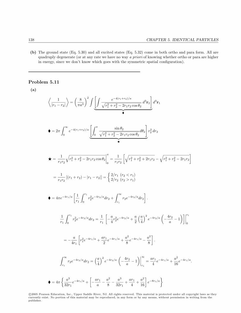
138 CHAPTER 5. IDENTICAL PARTICLES
(b) The ground state (Eq. 5.30) and all excited states (Eq. 5.32) come in both ortho and para form. All arequadruply degenerate (or at any rate we have no way a priori of knowing whether ortho or para are higherin energy, since we don’t know which goes with the symmetric spatial configuration).
Problem 5.11
(a) ⟨1
|r1 − r2|
⟩=
(8
πa3
)2 ∫ [∫e−4(r1+r2)/a√
r21 + r2
2 − 2r1r2 cos θ2
d3r2
]︸ ︷︷ ︸
d3r1
= 2π∫ ∞
0
e−4(r1+r2)/a
[∫ π
0
sin θ2√r21 + r2
2 − 2r1r2 cos θ2
dθ2
]︸ ︷︷ ︸
r22 dr2
=1
r1r2
√r21 + r2
2 − 2r1r2 cos θ2
∣∣∣∣π0
=1
r1r2
[√r21 + r2
2 + 2r1r2 −√
r21 + r2
2 − 2r1r2
]
=1
r1r2[(r1 + r2)− |r1 − r2|] =
2/r1 (r2 < r1)2/r2 (r2 > r1)
= 4πe−4r1/a
[1r1
∫ r1
0
r22e−4r2/adr2 +
∫ ∞r1
r2e−4r2/adr2
].
1r1
∫ r1
0
r22e−4r2/adr2 =
1r1
[−a
4r22e−4r2/a +
a
2
(a
4
)2
e−4r2/a
(−4r2
a− 1
)]∣∣∣∣r1
0
= − a
4r1
[r21e−4r1/a +
ar1
2e−4r1/a +
a2
8e−4r1/a − a2
8
].
∫ ∞r1
r2e−4r2/adr2 =
(a
4
)2
e−4r2/a
(−4r2
a− 1
)∣∣∣∣∞r1
=ar1
4e−4r1/a +
a2
16e−4r1/a.
= 4π
a3
32r1e−4r1/a +
[−ar1
a− a2
8− a3
32r1+
ar1
4+
a2
16
]e−8r1/a
c©2005 Pearson Education, Inc., Upper Saddle River, NJ. All rights reserved. This material is protected under all copyright laws as theycurrently exist. No portion of this material may be reproduced, in any form or by any means, without permission in writing from thepublisher.
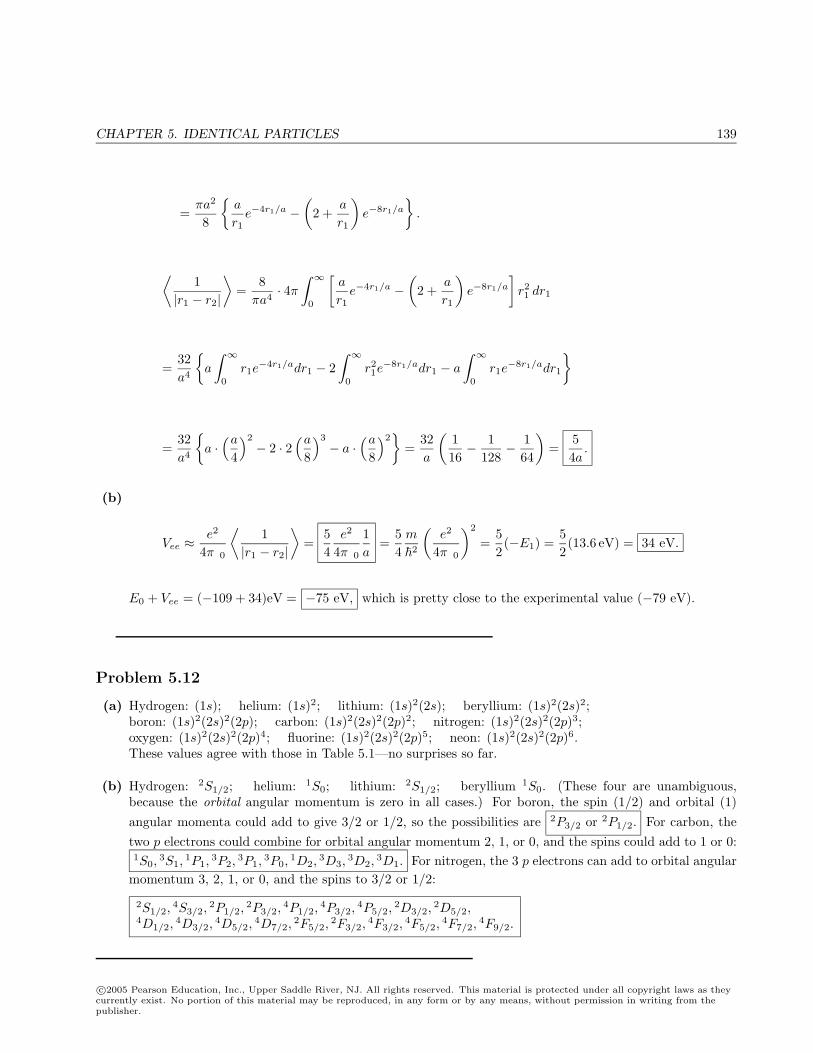
CHAPTER 5. IDENTICAL PARTICLES 139
=πa2
8
a
r1e−4r1/a −
(2 +
a
r1
)e−8r1/a
.
⟨1
|r1 − r2|
⟩=
8πa4
· 4π∫ ∞
0
[a
r1e−4r1/a −
(2 +
a
r1
)e−8r1/a
]r21 dr1
=32a4
a
∫ ∞0
r1e−4r1/adr1 − 2
∫ ∞0
r21e−8r1/adr1 − a
∫ ∞0
r1e−8r1/adr1
=32a4
a ·
(a
4
)2
− 2 · 2(a
8
)3
− a ·(a
8
)2
=32a
(116− 1
128− 1
64
)=
54a
.
(b)
Vee ≈e2
4πε0
⟨1
|r1 − r2|
⟩=
54
e2
4πε01a
=54m
2
(e2
4πε0
)2
=52(−E1) =
52(13.6 eV) = 34 eV.
E0 + Vee = (−109 + 34)eV = −75 eV, which is pretty close to the experimental value (−79 eV).
Problem 5.12
(a) Hydrogen: (1s); helium: (1s)2; lithium: (1s)2(2s); beryllium: (1s)2(2s)2;boron: (1s)2(2s)2(2p); carbon: (1s)2(2s)2(2p)2; nitrogen: (1s)2(2s)2(2p)3;oxygen: (1s)2(2s)2(2p)4; fluorine: (1s)2(2s)2(2p)5; neon: (1s)2(2s)2(2p)6.These values agree with those in Table 5.1—no surprises so far.
(b) Hydrogen: 2S1/2; helium: 1S0; lithium: 2S1/2; beryllium 1S0. (These four are unambiguous,because the orbital angular momentum is zero in all cases.) For boron, the spin (1/2) and orbital (1)angular momenta could add to give 3/2 or 1/2, so the possibilities are 2P3/2 or 2P1/2. For carbon, thetwo p electrons could combine for orbital angular momentum 2, 1, or 0, and the spins could add to 1 or 0:1S0,
3S1,1P1,
3P2,3P1,
3P0,1D2,
3D3,3D2,
3D1. For nitrogen, the 3 p electrons can add to orbital angularmomentum 3, 2, 1, or 0, and the spins to 3/2 or 1/2:
2S1/2,4S3/2,
2P1/2,2P3/2,
4P1/2,4P3/2,
4P5/2,2D3/2,
2D5/2,4D1/2,
4D3/2,4D5/2,
4D7/2,2F5/2,
2F3/2,4F3/2,
4F5/2,4F7/2,
4F9/2.
c©2005 Pearson Education, Inc., Upper Saddle River, NJ. All rights reserved. This material is protected under all copyright laws as theycurrently exist. No portion of this material may be reproduced, in any form or by any means, without permission in writing from thepublisher.
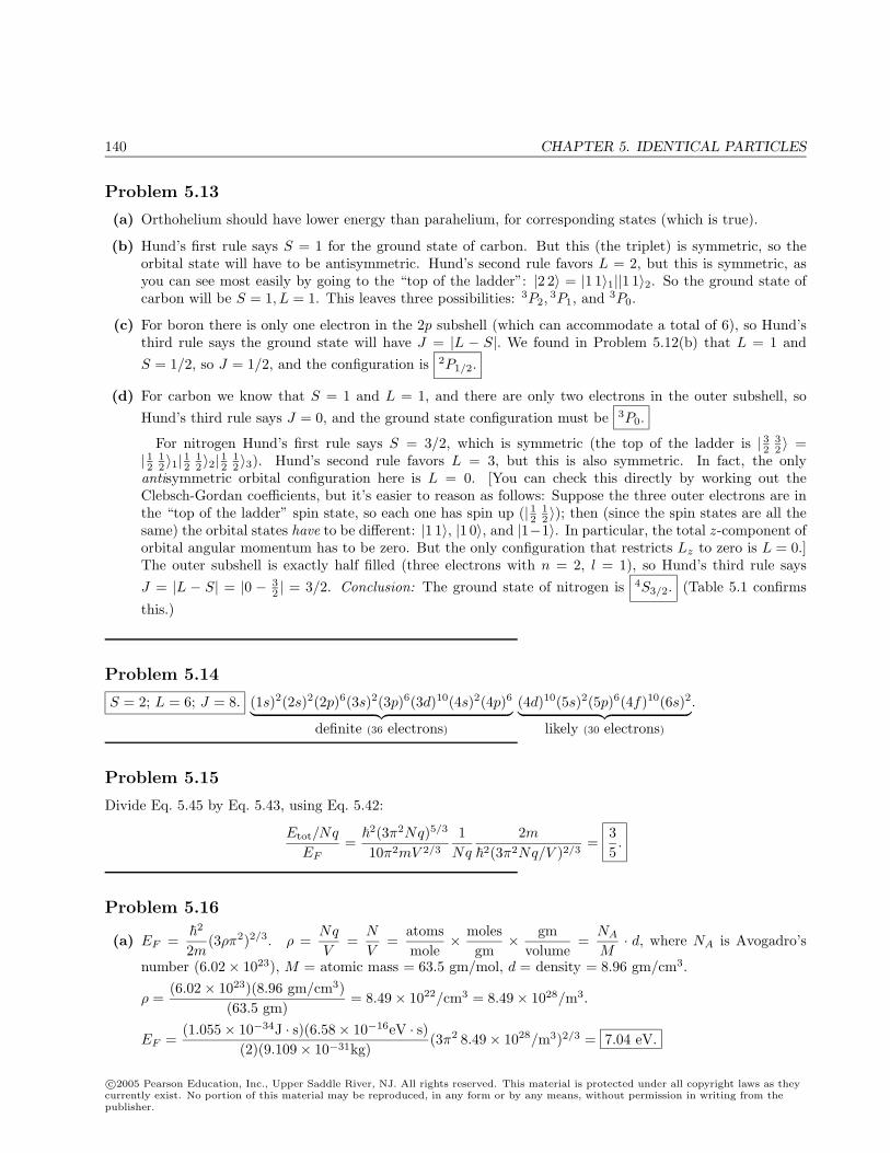
140 CHAPTER 5. IDENTICAL PARTICLES
Problem 5.13
(a) Orthohelium should have lower energy than parahelium, for corresponding states (which is true).
(b) Hund’s first rule says S = 1 for the ground state of carbon. But this (the triplet) is symmetric, so theorbital state will have to be antisymmetric. Hund’s second rule favors L = 2, but this is symmetric, asyou can see most easily by going to the “top of the ladder”: |2 2〉 = |1 1〉1||1 1〉2. So the ground state ofcarbon will be S = 1, L = 1. This leaves three possibilities: 3P2,
3P1, and 3P0.
(c) For boron there is only one electron in the 2p subshell (which can accommodate a total of 6), so Hund’sthird rule says the ground state will have J = |L − S|. We found in Problem 5.12(b) that L = 1 andS = 1/2, so J = 1/2, and the configuration is 2P1/2.
(d) For carbon we know that S = 1 and L = 1, and there are only two electrons in the outer subshell, soHund’s third rule says J = 0, and the ground state configuration must be 3P0.
For nitrogen Hund’s first rule says S = 3/2, which is symmetric (the top of the ladder is | 32 32 〉 =
| 12 12 〉1| 12 1
2 〉2| 12 12 〉3). Hund’s second rule favors L = 3, but this is also symmetric. In fact, the only
antisymmetric orbital configuration here is L = 0. [You can check this directly by working out theClebsch-Gordan coefficients, but it’s easier to reason as follows: Suppose the three outer electrons are inthe “top of the ladder” spin state, so each one has spin up (| 12 1
2 〉); then (since the spin states are all thesame) the orbital states have to be different: |1 1〉, |1 0〉, and |1−1〉. In particular, the total z-component oforbital angular momentum has to be zero. But the only configuration that restricts Lz to zero is L = 0.]The outer subshell is exactly half filled (three electrons with n = 2, l = 1), so Hund’s third rule saysJ = |L − S| = |0 − 3
2 | = 3/2. Conclusion: The ground state of nitrogen is 4S3/2. (Table 5.1 confirms
this.)
Problem 5.14
S = 2; L = 6; J = 8. (1s)2(2s)2(2p)6(3s)2(3p)6(3d)10(4s)2(4p)6︸ ︷︷ ︸definite (36 electrons)
(4d)10(5s)2(5p)6(4f)10(6s)2︸ ︷︷ ︸likely (30 electrons)
.
Problem 5.15
Divide Eq. 5.45 by Eq. 5.43, using Eq. 5.42:
Etot/Nq
EF=
2(3π2Nq)5/3
10π2mV 2/3
1Nq
2m2(3π2Nq/V )2/3
=35.
Problem 5.16
(a) EF =
2
2m(3ρπ2)2/3. ρ =
Nq
V=
N
V=
atomsmole
× molesgm
× gmvolume
=NA
M· d, where NA is Avogadro’s
number (6.02× 10²³), M = atomic mass = 63.5 gm/mol, d = density = 8.96 gm/cm3.
ρ =(6.02× 10²³)(8.96 gm/cm3)
(63.5 gm)= 8.49× 10²²/cm3 = 8.49× 1028/m3.
EF =(1.055× 10⁻³⁴J · s)(6.58× 10⁻¹⁶eV · s)
(2)(9.109× 10⁻³¹kg)(3π2 8.49× 1028/m3)2/3 = 7.04 eV.
c©2005 Pearson Education, Inc., Upper Saddle River, NJ. All rights reserved. This material is protected under all copyright laws as theycurrently exist. No portion of this material may be reproduced, in any form or by any means, without permission in writing from thepublisher.
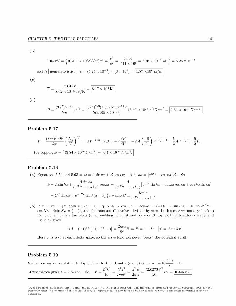
CHAPTER 5. IDENTICAL PARTICLES 141
(b)
7.04 eV =12(0.511× 10⁶eV/c2)v2 ⇒ v2
c2=
14.08.511× 106
= 2.76× 10⁻⁵ ⇒ v
c= 5.25× 10⁻³,
so it’s nonrelativistic. v = (5.25× 10−3)× (3× 108) = 1.57 ×10⁶ m/s.
(c)
T =7.04 eV
8.62× 10⁻⁵ eV/K= 8.17× 10⁴ K.
(d)
P =(3π2)2/3
2
5mρ5/3 =
(3π2)2/3(1.055× 10−34)2
5(9.109× 10⁻³¹)(8.49× 1028)5/3N/m2 = 3.84× 10¹⁰ N/m2.
Problem 5.17
P =(3π2)2/3
2
5m
(Nq
V
)5/3
= AV −5/3 ⇒ B = −VdP
dV= −V A
(−53
)V −5/3−1 =
53AV −5/3 =
53P.
For copper, B = 53 (3.84× 10¹⁰ N/m2) = 6.4× 10¹⁰ N/m2.
Problem 5.18
(a) Equations 5.59 and 5.63 ⇒ ψ = A sin kx + B cos kx; A sin ka =[eiKa − cos ka
]B. So
ψ = A sin kx +A sin ka
(eiKa − cos ka)cos kx =
A
(eiKa − cos ka)[eiKa sin kx− sin kx cos ka + cos kx sin ka
]= C
sin kx + e−iKa sin[k(a− x)]
, where C ≡ AeiKa
eiKa − cos ka.
(b) If z = ka = jπ, then sin ka = 0, Eq. 5.64 ⇒ cosKa = cos ka = (−1)j ⇒ sinKa = 0, so eiKa =cosKa + i sinKa = (−1)j , and the constant C involves division by zero. In this case we must go back toEq. 5.63, which is a tautology (0=0) yielding no constraint on A or B, Eq. 5.61 holds automatically, andEq. 5.62 gives
kA− (−1)jk[A(−1)j − 0
]=
2mα
2B ⇒ B = 0. So ψ = A sin kx.
Here ψ is zero at each delta spike, so the wave function never “feels” the potential at all.
Problem 5.19
We’re looking for a solution to Eq. 5.66 with β = 10 and z π: f(z) = cos z + 10sin z
z= 1.
Mathematica gives z = 2.62768. So E =
2k2
2m=
2z2
2ma2=
z2
2βα
a=
(2.62768)2
20eV = 0.345 eV.
c©2005 Pearson Education, Inc., Upper Saddle River, NJ. All rights reserved. This material is protected under all copyright laws as theycurrently exist. No portion of this material may be reproduced, in any form or by any means, without permission in writing from thepublisher.
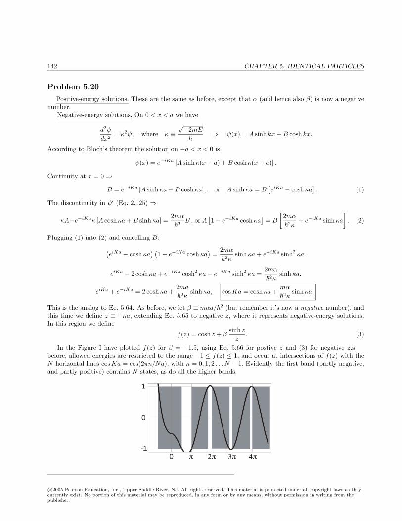
142 CHAPTER 5. IDENTICAL PARTICLES
Problem 5.20
Positive-energy solutions. These are the same as before, except that α (and hence also β) is now a negativenumber.
Negative-energy solutions. On 0 < x < a we have
d2ψ
dx2= κ2ψ, where κ ≡
√−2mE
⇒ ψ(x) = A sinh kx + B cosh kx.
According to Bloch’s theorem the solution on −a < x < 0 is
ψ(x) = e−iKa [A sinhκ(x + a) + B coshκ(x + a)] .
Continuity at x = 0⇒
B = e−iKa [A sinhκa + B coshκa] , or A sinhκa = B[eiKa − coshκa
]. (1)
The discontinuity in ψ′ (Eq. 2.125) ⇒
κA−e−iKaκ [A coshκa + B sinhκa] =2mα
2B, or A
[1− e−iKa coshκa
]= B
[2mα
2κ+ e−iKa sinhκa
]. (2)
Plugging (1) into (2) and cancelling B:(eiKa − coshκa
) (1− e−iKa coshκa
)=
2mα
2κsinhκa + e−iKa sinh2 κa.
eiKa − 2 coshκa + e−iKa cosh2 κa− e−iKa sinh2 κa =2mα
2κsinhκa.
eiKa + e−iKa = 2 coshκa +2ma
2κsinhκa, cosKa = coshκa +
mα
2κsinhκa.
This is the analog to Eq. 5.64. As before, we let β ≡ mαa/2 (but remember it’s now a negative number), andthis time we define z ≡ −κa, extending Eq. 5.65 to negative z, where it represents negative-energy solutions.In this region we define
f(z) = cosh z + βsinh z
z. (3)
In the Figure I have plotted f(z) for β = −1.5, using Eq. 5.66 for postive z and (3) for negative z. Asbefore, allowed energies are restricted to the range −1 ≤ f(z) ≤ 1, and occur at intersections of f(z) with theN horizontal lines cosKa = cos(2πn/Na), with n = 0, 1, 2 . . . N − 1. Evidently the first band (partly negative,and partly positive) contains N states, as do all the higher bands.
0
1
-10 π 2π 3π 4π
c©2005 Pearson Education, Inc., Upper Saddle River, NJ. All rights reserved. This material is protected under all copyright laws as theycurrently exist. No portion of this material may be reproduced, in any form or by any means, without permission in writing from thepublisher.
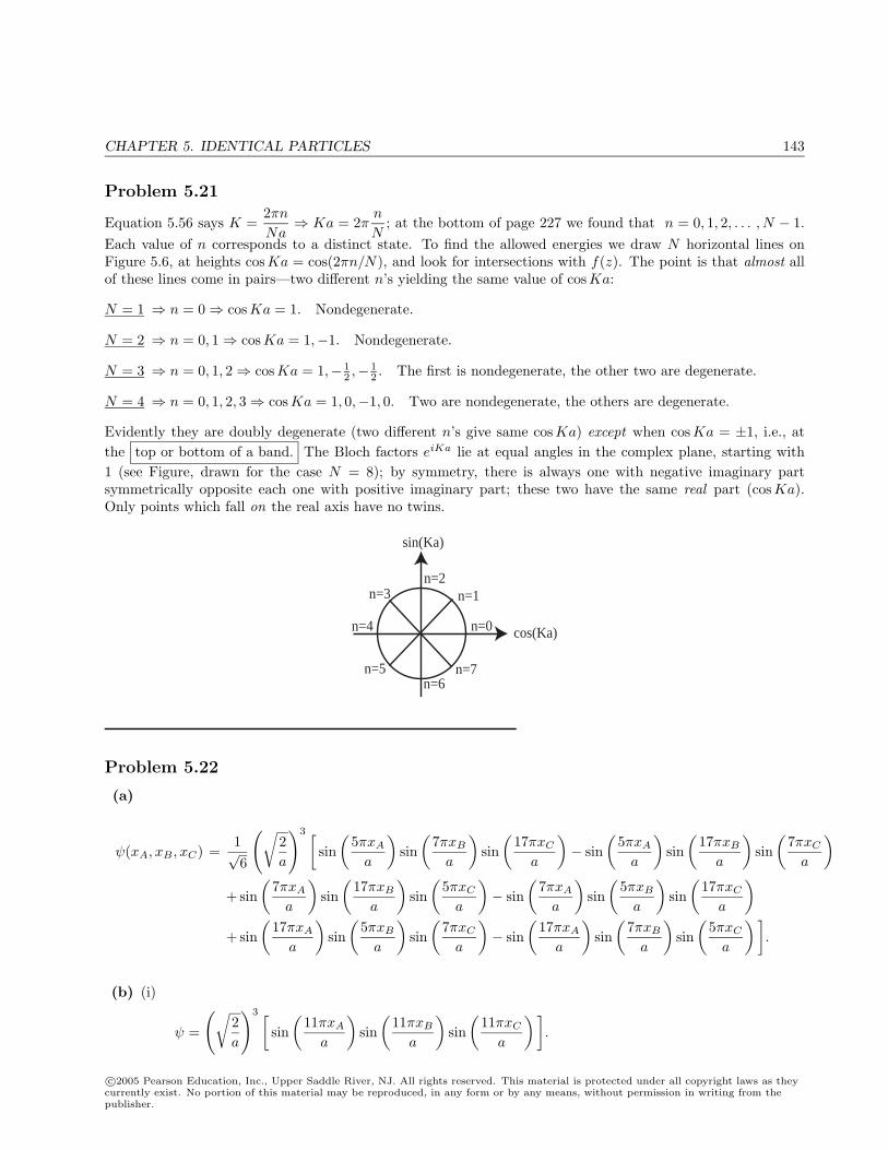
CHAPTER 5. IDENTICAL PARTICLES 143
Problem 5.21
Equation 5.56 says K =2πnNa
⇒ Ka = 2πn
N; at the bottom of page 227 we found that n = 0, 1, 2, . . . , N − 1.
Each value of n corresponds to a distinct state. To find the allowed energies we draw N horizontal lines onFigure 5.6, at heights cosKa = cos(2πn/N), and look for intersections with f(z). The point is that almost allof these lines come in pairs—two different n’s yielding the same value of cosKa:
N = 1 ⇒ n = 0⇒ cosKa = 1. Nondegenerate.
N = 2 ⇒ n = 0, 1 ⇒ cosKa = 1,−1. Nondegenerate.
N = 3 ⇒ n = 0, 1, 2 ⇒ cosKa = 1,− 12 ,− 1
2 . The first is nondegenerate, the other two are degenerate.
N = 4 ⇒ n = 0, 1, 2, 3 ⇒ cosKa = 1, 0,−1, 0. Two are nondegenerate, the others are degenerate.
Evidently they are doubly degenerate (two different n’s give same cosKa) except when cosKa = ±1, i.e., atthe top or bottom of a band. The Bloch factors eiKa lie at equal angles in the complex plane, starting with1 (see Figure, drawn for the case N = 8); by symmetry, there is always one with negative imaginary partsymmetrically opposite each one with positive imaginary part; these two have the same real part (cosKa).Only points which fall on the real axis have no twins.
n=0
n=1n=2
n=3
n=4
n=5n=6
n=7
cos(Ka)
sin(Ka)
Problem 5.22
(a)
ψ(xA, xB , xC) =1√6
(√2a
)3 [sin
(5πxA
a
)sin
(7πxB
a
)sin
(17πxC
a
)− sin
(5πxA
a
)sin
(17πxB
a
)sin
(7πxC
a
)+ sin
(7πxA
a
)sin
(17πxB
a
)sin
(5πxC
a
)− sin
(7πxA
a
)sin
(5πxB
a
)sin
(17πxC
a
)+ sin
(17πxA
a
)sin
(5πxB
a
)sin
(7πxC
a
)− sin
(17πxA
a
)sin
(7πxB
a
)sin
(5πxC
a
) ].
(b) (i)
ψ =
(√2a
)3 [sin
(11πxA
a
)sin
(11πxB
a
)sin
(11πxC
a
) ].
c©2005 Pearson Education, Inc., Upper Saddle River, NJ. All rights reserved. This material is protected under all copyright laws as theycurrently exist. No portion of this material may be reproduced, in any form or by any means, without permission in writing from thepublisher.
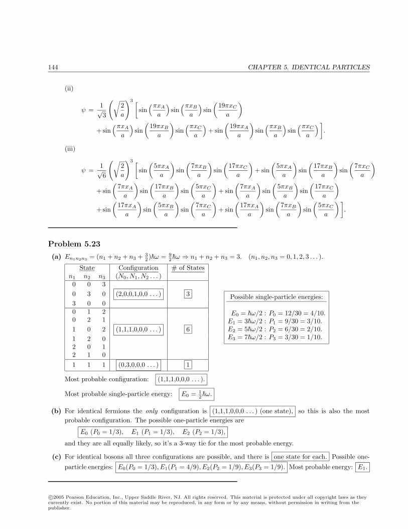
144 CHAPTER 5. IDENTICAL PARTICLES
(ii)
ψ =1√3
(√2a
)3 [sin
(πxA
a
)sin
(πxB
a
)sin
(19πxC
a
)+ sin
(πxA
a
)sin
(19πxB
a
)sin
(πxC
a
)+ sin
(19πxA
a
)sin
(πxB
a
)sin
(πxC
a
) ].
(iii)
ψ =1√6
(√2a
)3 [sin
(5πxA
a
)sin
(7πxB
a
)sin
(17πxC
a
)+ sin
(5πxA
a
)sin
(17πxB
a
)sin
(7πxC
a
)+ sin
(7πxA
a
)sin
(17πxB
a
)sin
(5πxC
a
)+ sin
(7πxA
a
)sin
(5πxB
a
)sin
(17πxC
a
)+ sin
(17πxA
a
)sin
(5πxB
a
)sin
(7πxC
a
)+ sin
(17πxA
a
)sin
(7πxB
a
)sin
(5πxC
a
) ].
Problem 5.23
(a) En1n2n3 = (n1 + n2 + n3 + 32 )ω = 9
2ω ⇒ n1 + n2 + n3 = 3. (n1, n2, n3 = 0, 1, 2, 3 . . . ).
State Configuration # of Statesn1 n2 n3 (N0, N1, N2 . . . )0 0 30 3 0 (2,0,0,1,0,0 . . . ) 33 0 00 1 20 2 11 0 2 (1,1,1,0,0,0 . . . ) 61 2 02 0 12 1 01 1 1 (0,3,0,0,0 . . . ) 1
Possible single-particle energies:
E0 = ω/2 : P0 = 12/30 = 4/10.E1 = 3ω/2 : P1 = 9/30 = 3/10.E2 = 5ω/2 : P2 = 6/30 = 2/10.E3 = 7ω/2 : P3 = 3/30 = 1/10.
Most probable configuration: (1,1,1,0,0,0 . . . ).
Most probable single-particle energy: E0 = 12ω.
(b) For identical fermions the only configuration is (1,1,1,0,0,0 . . . ) (one state), so this is also the mostprobable configuration. The possible one-particle energies are
E0 (P0 = 1/3), E1 (P1 = 1/3), E2 (P2 = 1/3),
and they are all equally likely, so it’s a 3-way tie for the most probable energy.
(c) For identical bosons all three configurations are possible, and there is one state for each. Possible one-
particle energies: E0(P0 = 1/3), E1(P1 = 4/9), E2(P2 = 1/9), E3(P3 = 1/9). Most probable energy: E1.
c©2005 Pearson Education, Inc., Upper Saddle River, NJ. All rights reserved. This material is protected under all copyright laws as theycurrently exist. No portion of this material may be reproduced, in any form or by any means, without permission in writing from thepublisher.
CHAPTER 5. IDENTICAL PARTICLES 145
Problem 5.24
Here N = 3, and dn = 1 for all states, so:
Eq. 5.74 ⇒ Q = 6
∞∏n=1
1Nn!
(distinguishable),
Eq. 5.75 ⇒ Q =∞∏
n=1
1Nn!(1−Nn)!
(fermions),
Eq. 5.77 ⇒ Q = 1 (bosons).
(In the products, most factors are 1/0! or 1/1!, both of which are 1, so I won’t write them.)
Configuration 1 (N11 = 3, others 0):
Q = 6× 1
3!= 1 (distinguishable),
Q =13!× 1
(−2)!= 0 (fermions),
Q = 1 (bosons).
Configuration 2 (N5 = 1, N13 = 2):
Q = 6× 1
1!× 1
2!= 3 (distinguishable),
Q =1
1!0!× 1
2!(−1)!= 0 (fermions),
Q = 1 (bosons).
Configuration 3 (N1 = 2, N19 = 1):
Q = 6× 1
2!× 1
1!= 3 (distinguishable),
Q =1
2!(−1)!× 1
1!0!= 0 (fermions),
Q = 1 (bosons).
Configuration 4 (N5 = N7 = N17 = 1):
Q = 6× 1
1!× 1
1!× 1
1!= 6 (distinguishable),
Q =1
1!0!× 1
1!0!× 1
1!0!= 1 (fermions),
Q = 1 (bosons).
All of these agree with what we got “by hand” at the top of page 231.
Problem 5.25
N = 1 : - can put the ball in any of d baskets, so d ways.
N = 2 :
- could put both balls in any of the d baskets : d ways, or- could put one in one basket (d ways), the other in another(d− 1) ways—but itdoesn’t matter which is which, so divide by 2.
Total: d + 12d(d− 1) = 1
2d(2 + d− 1) = 12d(d + 1) ways.
N = 3 :
- could put all three in one basket : d ways, or- 2 in one basket, one in another : d(d− 1) ways, or- 1 each in 3 baskets : d(d− 1)(d− 2)/3! ways.
Total: d + d(d− 1) + d(d− 1)(d− 2)/6 = 16d(6 + 6d− 6 + d2 − 3d + 2) = 1
6d(d2 + 3d + 2)
c©2005 Pearson Education, Inc., Upper Saddle River, NJ. All rights reserved. This material is protected under all copyright laws as theycurrently exist. No portion of this material may be reproduced, in any form or by any means, without permission in writing from thepublisher.

146 CHAPTER 5. IDENTICAL PARTICLES
=d(d + 1)(d + 2)
6ways.
N = 4 :
- all in one basket: d ways, or- 3 in one basket, 1 in another: d(d− 1) ways, or- 2 in one basket, 2 in another: d(d− 1)/2 ways, or- 2 in one basket, one each in others: d(d− 1)(d− 2)/2, or- all in different baskets: d(d− 1)(d− 2)(d− 3)/4!
Total: d + d(d− 1) + d(d− 1)/2 + d(d− 1)(d− 2)/2 + d(d− 1)(d− 2)(d− 3)/24= 1
24 (24 + 24d− 24 + 12d− 12 + 12d2 − 36d + 24 + d3 − 6d2 + 11d− 6)
= 124d(d
3 + 6d2 + 11d + 6) =d(d + 1)(d + 2)(d + 3)
24ways.
The general formula seems to be f(N, d) =d(d + 1)(d + 2) · · · (d + N − 1)
N !=
(d + N − 1)!N !(d− 1)!
=(d + N − 1
N
).
Proof: How many ways to put N identical balls in d baskets? Call it f(N, d).- Could put all of them in the first basket: 1 way.- Could put all but one in the first basket; there remains 1 ball for d− 1 baskets: f(1, d− 1) ways.- Could put all but two in the first basket; there remain 2 for d− 1 baskets: f(2, d− 1) ways....- Could put zero in the first basket, leaving N for d− 1 baskets: f(N, d− 1) ways.
Thus: f(N, d) = f(0, d−1)+f(1, d−1)+f(2, d−1)+ · · ·+f(N, d−1) =∑N
j=0 f(j, d−1) (where f(0, d) ≡ 1).It follows that f(N, d) =
∑N−1j=0 f(j, d− 1)+ f(N, d− 1) = f(N − 1, d)+ f(N, d− 1). Use this recursion relation
to confirm the conjectured formula by induction:
(d + N − 1
N
)?=
(d + N − 2N − 1
)+
(d + N − 2
N
)=
(d + N − 2)!(N − 1)!(d− 1)!
+(d + N − 2)!N !(d− 2)!
=(d + N − 2)!N !(d− 1)!
(N + d− 1) =(d + N − 1)!N !(d− 1)!
=(d + N − 1
d− 1
).
It works for N = 0 :(d−10
)= 1, and for d = 1 :
(NN
)= 1 (which is obviously correct for just one basket). QED
Problem 5.26
A(x, y) = (2x)(2y) = 4xy; maximize, subject to the constraint (x/a)2 + (y/b)2 = 1.
(x,y)
a
b
c©2005 Pearson Education, Inc., Upper Saddle River, NJ. All rights reserved. This material is protected under all copyright laws as theycurrently exist. No portion of this material may be reproduced, in any form or by any means, without permission in writing from thepublisher.
CHAPTER 5. IDENTICAL PARTICLES 147
G(x, y, λ) ≡ 4xy + λ[(x/a)2 + (y/b)2 − 1
].
∂G
∂x= 4y +
2λxa2
= 0⇒ y = − λx
2a2.
∂G
∂y= 4x +
2λyb2
= 0⇒ 4x = −2λb2
(− λx
2a2
)⇒ 4x =
λ2
a2b2x⇒ x = 0 (minimum), or else λ = ±2ab.
So y = ∓2abx2a2
= ∓ b
ax. We may as well pick x and y positive, (as in the figure); then y = (b/a)x (and
λ = −2ab).∂G
∂λ= 0⇒
(x
a
)2
+(y
b
)2
= 1 (of course), sox2
a2+
b2x2
a2b2= 1, or
2a2
x2 = 1, or x = a/√
2, and hence
y = ba/(a√
2)⇒ y = b/√
2. A = 4a√2
b√2
= 2ab.
Problem 5.27
(a) ln(10!) = ln(3628800) = 15.1044; 10 ln(10) − 10 = 23.026 − 10 = 13.0259; 15.1044 − 13.0259 =2.0785; 2.0785/15.1044 = 0.1376, or 14% .
(b) The percent error is:ln(z!)− z ln(z) + z
ln(z!)× 100.
z %20 5.7
100 0.8950 1.990 0.99685 1.0689 1.009
Since my calculator cannot compute factorials greater than 69! I used Mathematica to construct the table.Evidently, the smallest integer for which the error is < 1% is 90.
Problem 5.28
Equation 5.108 ⇒ N =V
2π2
∫ ∞0
k2n(ε) dk, where n(ε) is given (as T → 0) by Eq. 5.104.
So N =V
2π2
∫ kmax
0
k2 dk =V
2π2
k3max
3, where kmax is given by
2k2
max
2m= µ(0) = EF ⇒ kmax =
√2mEF
.
N =V
6π23(2mEF )3/2. Compare Eq. 5.43, which says
EF =
2
2m
(3π2Nq
V
)2/3
, or(2mEF )3/2
3= 3π2Nq
V, or N =
V
3π2q3(2mEF )3/2.
Here q = 1, and Eq. 5.108 needs an extra factor of 2 on the right, to account for spin, so the two formulas agree.
Equation 5.109 ⇒ Etot =V 2
4π2m
∫ kmax
0
k4 dk =V 2
4π2m
k5max
5⇒ Etot =
V
20π2m3(2mEF )5/2.
Compare Eq. 5.45, which says Etot =V 2
10π2mk5max. Again, Eq. 5.109 for electrons has an extra factor of 2, so
the two agree.
c©2005 Pearson Education, Inc., Upper Saddle River, NJ. All rights reserved. This material is protected under all copyright laws as theycurrently exist. No portion of this material may be reproduced, in any form or by any means, without permission in writing from thepublisher.
148 CHAPTER 5. IDENTICAL PARTICLES
Problem 5.29
(a) Equation 5.103, n(ε) > 0 ⇒ 1e(ε−µ)/kBT − 1
> 0 ⇒ e(ε−µ)/kBT > 1 ⇒ (ε− µ)kBT
> 0 ⇒ ε > µ(T ), for all
allowed energies ε.
(b) For a free particle gas, E =
2
2mk2 → 0 (as k → 0, in the continuum limit), so µ(T ) is always negative.
(Technically, the lowest energy is
2π2
2m
(1l2x
+1l2y
+1l2z
), but we take the dimensions lxlylz to be very large
in the continuum limit.) Equation 5.108 ⇒ N/V =1
2π2
∫ ∞0
k2
e(2k2/2m−µ)/kBT − 1dk. The integrand is
always positive, and the only T dependence is in µ(T ) and kBT . So, as T decreases, (2k2/2m) − µ(T )must also decrease, and hence −µ(T ) decreases, or µ(T ) increases (always negative).
(c)N
V=
12π2
∫ ∞0
k2
e2k2/2mkBT − 1dk. Let x ≡
2k2
2mkBT, so k =
√2mkBT
x1/2; dk =
√2mkBT
12x−1/2 dx.
N
V=
12π2
(2mkBT
2
)3/2 12
∫ ∞0
x1/2
ex − 1dx, where
∫ ∞0
x3/2−1
ex − 1dx = Γ(3/2)ζ(3/2).
Now Γ(3/2) =√π/2; ζ(3/2) = 2.61238, so
N
V= 2.612
(mkBT
2π2
)3/2
; Tc =2π2
mkB
(N
2.612V
)2/3
.
(d)
N
V=
mass/volumemass/atom
=0.15× 10³ kg/m3
4(1.67× 10⁻²⁷ kg)= 2.2× 1028/m3.
Tc =2π(1.05× 10⁻³⁴J · s)2
4(1.67× 10⁻²⁷ kg)(1.38× 10⁻²³ J/K)
(2.2× 1028
2.61 m3
)2/3
= 3.1 K.
Problem 5.30
(a)
ω = 2πν =2πcλ
, so dω = −2πcλ2
dλ, and ρ(ω) =
π2c3(2πc)3
λ3(e2πc/kBTλ − 1).
ρ(ω)|dω| = 8π1
λ3(e2πc/kBTλ − 1)
∣∣∣∣−2πcλ2
dλ
∣∣∣∣ = ρ(λ) dλ⇒ ρ(λ) =16π2
c
λ5(e2πc/kBTλ − 1).
(For density, we want only the size of the interval, not its sign.)
(b) To maximize, set dρ/dλ = 0:
0 = 16π2c
[ −5λ6(e2πc/kBTλ − 1)
− e2πc/kBTλ(2πc/kBT )λ5(e2πc/kBTλ − 1)2
(− 1
λ2
)]c©2005 Pearson Education, Inc., Upper Saddle River, NJ. All rights reserved. This material is protected under all copyright laws as theycurrently exist. No portion of this material may be reproduced, in any form or by any means, without permission in writing from thepublisher.
CHAPTER 5. IDENTICAL PARTICLES 149
1 2 3 4 5
1
2
3
4
5
5-x
5e-x
⇒ 5(e2πc/kBTλ − 1) = e2πc/kBTλ
(2πckBTλ
).
Let x ≡ 2πc/kBTλ; then 5(ex − 1) = xex; or 5(1 − e−x) = x, or 5e−x = 5 − x. From the graph, thesolution occurs slightly below x = 5.
Mathematica says x = 4.966, so λmax =2πc
(4.966)kB
1T
=(6.626× 10⁻³⁴ J · s)(2.998× 10⁸ m/s)
(4.966)(1.3807× 10⁻²³ J/K)1T
=
2.897× 10⁻³ m·K/T.
Problem 5.31
From Eq. 5.113:
E
V=
∫ ∞0
ρ(ω) dω =
π2c3
∫ ∞0
ω3
(eω/kBT − 1)dω. Let x ≡ ω
kBT. Then
E
V=
π2c3
(kBT
)4 ∫ ∞0
x3
ex − 1dx =
(kBT )4
π2c33Γ(4)ζ(4) =
(kBT )4
π2c33· 6 · π
4
90=
(π2k4
B
15c33
)T 4
=[
π2(1.3807× 10⁻²³ J/K)4
15(2.998× 10⁸ m/s)3(1.0546× 10−34 J · s)3]T 4 = 7.566× 10⁻¹⁶ J
m3K4T4. QED
Problem 5.32
From Problem 2.11(a),
〈x〉0 = 〈x〉1 = 0; 〈x2〉0 =
2mω; 〈x2〉1 =
32mω
.
From Eq. 3.98,
〈x〉01 =∫ ∞−∞
xψ0(x)ψ1(x) dx = 〈0|x|1〉 =
√
2mω
(√1 δ0 0 +
√0 δ1−1
)=
√
2mω.
(a) Equation 5.19 ⇒ 〈(x1 − x2)2〉d =
2mω+
32mω
− 0 =2mω
.
(b) Equation 5.21 ⇒ 〈(x1 − x2)2〉+ =2mω
− 2
2mω=
mω.
c©2005 Pearson Education, Inc., Upper Saddle River, NJ. All rights reserved. This material is protected under all copyright laws as theycurrently exist. No portion of this material may be reproduced, in any form or by any means, without permission in writing from thepublisher.
150 CHAPTER 5. IDENTICAL PARTICLES
(c) Equation 5.21 ⇒ 〈(x1 − x2)2〉− =2mω
+ 2
2mω=
3mω
.
Problem 5.33
(a) Each particle has 3 possible states: 3× 3× 3 = 27.
(b) All in same state: aaa, bbb, ccc ⇒ 3.
2 in one state: aab, aac, bba, bbc, cca, ccb ⇒ 6 (each symmetrized).
3 different states: abc (symmetrized) ⇒ 1.
Total: 10.
(c) Only abc (antisymmetrized) =⇒ 1.
Problem 5.34
Equation 5.39 ⇒ Enxny =π2
2
2m
(n2
x
l2x+
n2y
l2y
)=
2k2
2m, with k =
(πnx
lx,πny
ly
). Each state is represented by an
intersection on a grid in “k-space”—this time a plane—and each state occupies an area π2/lxly = π2/A (whereA ≡ lxly is the area of the well). Two electrons per state means
14πk2
F =Nq
2
(π2
A
), or kF =
(2π
Nq
A
)1/2
= (2πσ)1/2,
where σ ≡ Nq/A is the number of free electrons per unit area.
∴ EF =
2k2F
2m=
2
2m2πσ =
π2σ
m.
k
ky
x
c©2005 Pearson Education, Inc., Upper Saddle River, NJ. All rights reserved. This material is protected under all copyright laws as theycurrently exist. No portion of this material may be reproduced, in any form or by any means, without permission in writing from thepublisher.
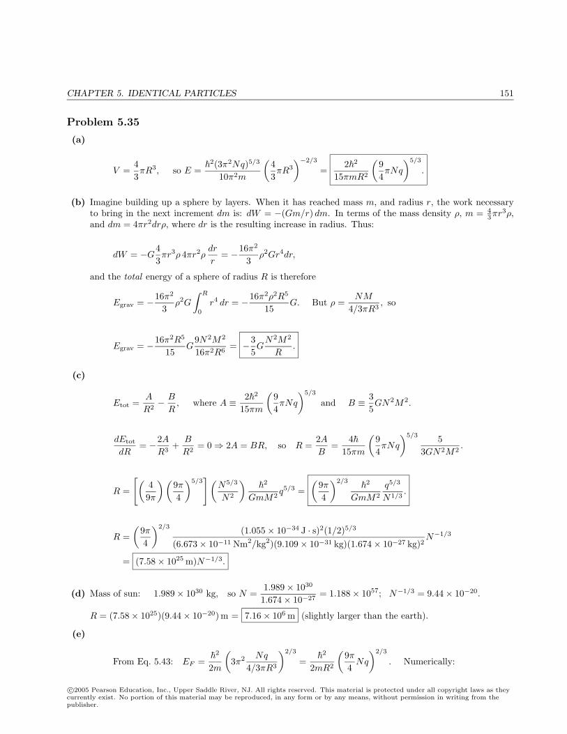
CHAPTER 5. IDENTICAL PARTICLES 151
Problem 5.35
(a)
V =43πR3, so E =
2(3π2Nq)5/3
10π2m
(43πR3
)−2/3
=22
15πmR2
(94πNq
)5/3
.
(b) Imagine building up a sphere by layers. When it has reached mass m, and radius r, the work necessaryto bring in the next increment dm is: dW = −(Gm/r) dm. In terms of the mass density ρ, m = 4
3πr3ρ,
and dm = 4πr2drρ, where dr is the resulting increase in radius. Thus:
dW = −G43πr3ρ 4πr2ρ
dr
r= −16π2
3ρ2Gr4dr,
and the total energy of a sphere of radius R is therefore
Egrav = −16π2
3ρ2G
∫ R
0
r4 dr = −16π2ρ2R5
15G. But ρ =
NM
4/3πR3, so
Egrav = −16π2R5
15G
9N2M2
16π2R6= −3
5G
N2M2
R.
(c)
Etot =A
R2− B
R, where A ≡ 22
15πm
(94πNq
)5/3
and B ≡ 35GN2M2.
dEtot
dR= −2A
R3+
B
R2= 0⇒ 2A = BR, so R =
2AB
=4
15πm
(94πNq
)5/3 53GN2M2
.
R =
[(49π
) (9π4
)5/3] (
N5/3
N2
)
2
GmM2q5/3 =
(9π4
)2/3
2
GmM2
q5/3
N1/3.
R =(
9π4
)2/3 (1.055× 10⁻³⁴ J · s)2(1/2)5/3
(6.673× 10⁻¹¹ Nm2/kg2)(9.109× 10−31 kg)(1.674× 10⁻²⁷ kg)2N−1/3
= (7.58× 1025 m)N−1/3.
(d) Mass of sun: 1.989× 1030 kg, so N =1.989× 1030
1.674× 10−27= 1.188× 1057; N−1/3 = 9.44× 10⁻²⁰.
R = (7.58× 1025)(9.44× 10⁻²⁰) m = 7.16× 10⁶ m (slightly larger than the earth).
(e)
From Eq. 5.43: EF =
2
2m
(3π2 Nq
4/3πR3
)2/3
=
2
2mR2
(9π4
Nq
)2/3
. Numerically:
c©2005 Pearson Education, Inc., Upper Saddle River, NJ. All rights reserved. This material is protected under all copyright laws as theycurrently exist. No portion of this material may be reproduced, in any form or by any means, without permission in writing from thepublisher.
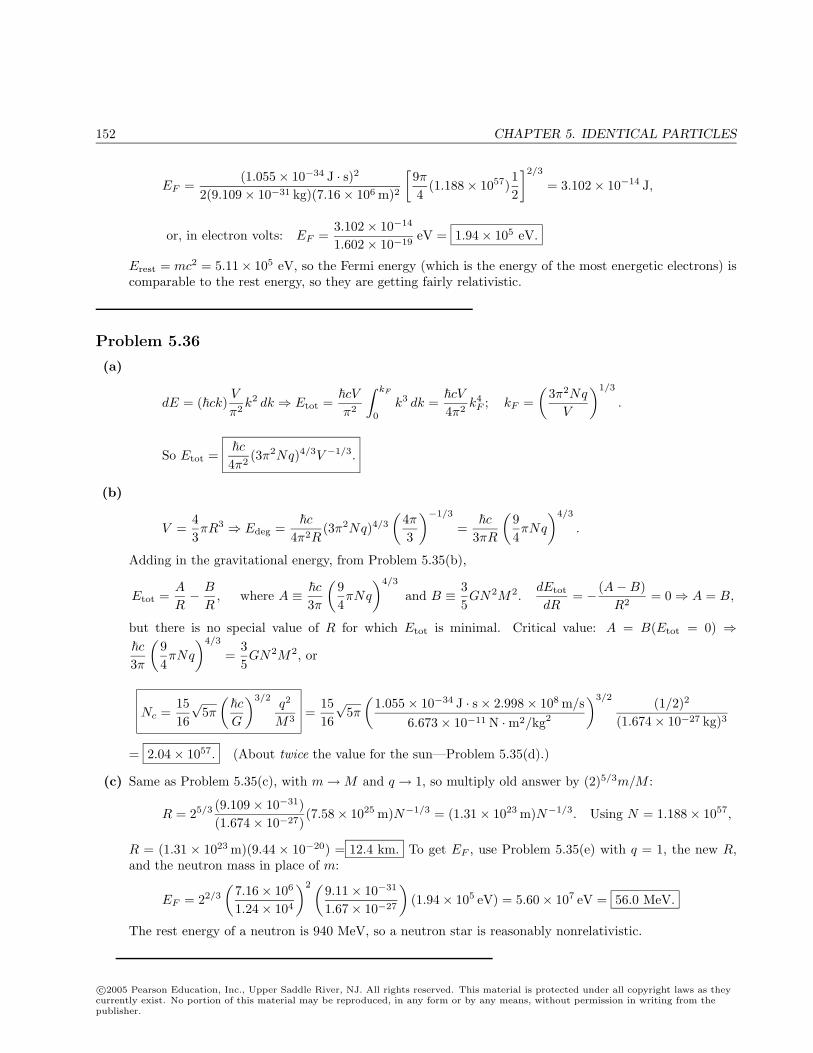
152 CHAPTER 5. IDENTICAL PARTICLES
EF =(1.055× 10⁻³⁴ J · s)2
2(9.109× 10⁻³¹ kg)(7.16× 10⁶ m)2
[9π4
(1.188× 1057)12
]2/3
= 3.102× 10⁻¹⁴ J,
or, in electron volts: EF =3.102× 10⁻¹⁴
1.602× 10⁻¹⁹eV = 1.94× 10⁵ eV.
Erest = mc2 = 5.11× 10⁵ eV, so the Fermi energy (which is the energy of the most energetic electrons) iscomparable to the rest energy, so they are getting fairly relativistic.
Problem 5.36
(a)
dE = (ck)V
π2k2 dk ⇒ Etot =
cV
π2
∫ kF
0
k3 dk =cV
4π2k4
F ; kF =(
3π2Nq
V
)1/3
.
So Etot =c
4π2(3π2Nq)4/3V −1/3.
(b)
V =43πR3 ⇒ Edeg =
c
4π2R(3π2Nq)4/3
(4π3
)−1/3
=c
3πR
(94πNq
)4/3
.
Adding in the gravitational energy, from Problem 5.35(b),
Etot =A
R− B
R, where A ≡ c
3π
(94πNq
)4/3
and B ≡ 35GN2M2.
dEtot
dR= − (A−B)
R2= 0⇒ A = B,
but there is no special value of R for which Etot is minimal. Critical value: A = B(Etot = 0) ⇒c
3π
(94πNq
)4/3
=35GN2M2, or
Nc =1516
√5π
(c
G
)3/2q2
M3=
1516
√5π
(1.055× 10⁻³⁴ J · s× 2.998× 10⁸ m/s
6.673× 10⁻¹¹ N ·m2/kg2
)3/2 (1/2)2
(1.674× 10⁻²⁷ kg)3
= 2.04× 1057. (About twice the value for the sun—Problem 5.35(d).)
(c) Same as Problem 5.35(c), with m→M and q → 1, so multiply old answer by (2)5/3m/M :
R = 25/3 (9.109× 10⁻³¹)(1.674× 10⁻²⁷)
(7.58× 1025 m)N−1/3 = (1.31× 10²³ m)N−1/3. Using N = 1.188× 1057,
R = (1.31 × 10²³ m)(9.44 × 10⁻²⁰) = 12.4 km. To get EF , use Problem 5.35(e) with q = 1, the new R,and the neutron mass in place of m:
EF = 22/3
(7.16× 10⁶
1.24× 10⁴
)2 (9.11× 10⁻³¹
1.67× 10⁻²⁷
)(1.94× 10⁵ eV) = 5.60× 10⁷ eV = 56.0 MeV.
The rest energy of a neutron is 940 MeV, so a neutron star is reasonably nonrelativistic.
c©2005 Pearson Education, Inc., Upper Saddle River, NJ. All rights reserved. This material is protected under all copyright laws as theycurrently exist. No portion of this material may be reproduced, in any form or by any means, without permission in writing from thepublisher.
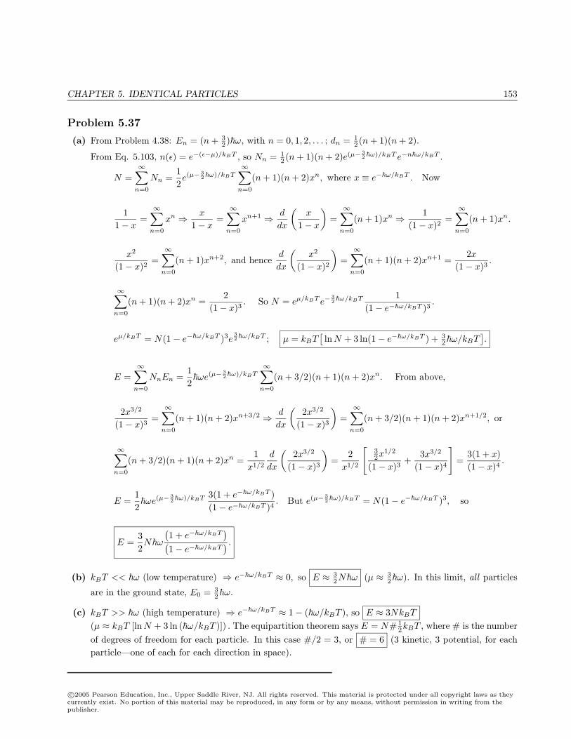
CHAPTER 5. IDENTICAL PARTICLES 153
Problem 5.37
(a) From Problem 4.38: En = (n + 32 )ω, with n = 0, 1, 2, . . . ; dn = 1
2 (n + 1)(n + 2).
From Eq. 5.103, n(ε) = e−(ε−µ)/kBT , so Nn = 12 (n + 1)(n + 2)e(µ− 3
2ω)/kBT e−nω/kBT .
N =∞∑
n=0
Nn =12e(µ− 3
2ω)/kBT∞∑
n=0
(n + 1)(n + 2)xn, where x ≡ e−ω/kBT . Now
11− x
=∞∑
n=0
xn ⇒ x
1− x=∞∑
n=0
xn+1 ⇒ d
dx
(x
1− x
)=∞∑
n=0
(n + 1)xn ⇒ 1(1− x)2
=∞∑
n=0
(n + 1)xn.
x2
(1− x)2=∞∑
n=0
(n + 1)xn+2, and henced
dx
(x2
(1− x)2
)=∞∑
n=0
(n + 1)(n + 2)xn+1 =2x
(1− x)3.
∞∑n=0
(n + 1)(n + 2)xn =2
(1− x)3. So N = eµ/kBT e−
32ω/kBT 1
(1− e−ω/kBT )3.
eµ/kBT = N(1− e−ω/kBT )3e32ω/kBT ; µ = kBT
[lnN + 3 ln(1− e−ω/kBT ) + 3
2ω/kBT].
E =∞∑
n=0
NnEn =12ωe(µ− 3
2ω)/kBT∞∑
n=0
(n + 3/2)(n + 1)(n + 2)xn. From above,
2x3/2
(1− x)3=∞∑
n=0
(n + 1)(n + 2)xn+3/2 ⇒ d
dx
(2x3/2
(1− x)3
)=∞∑
n=0
(n + 3/2)(n + 1)(n + 2)xn+1/2, or
∞∑n=0
(n + 3/2)(n + 1)(n + 2)xn =1
x1/2
d
dx
(2x3/2
(1− x)3
)=
2x1/2
[32x
1/2
(1− x)3+
3x3/2
(1− x)4
]=
3(1 + x)(1− x)4
.
E =12ωe(µ− 3
2ω)/kBT 3(1 + e−ω/kBT )(1− e−ω/kBT )4
. But e(µ− 32ω)/kBT = N(1− e−ω/kBT )3, so
E =32Nω
(1 + e−ω/kBT
)(1− e−ω/kBT
) .
(b) kBT << ω (low temperature) ⇒ e−ω/kBT ≈ 0, so E ≈ 32Nω (µ ≈ 3
2ω). In this limit, all particles
are in the ground state, E0 = 32ω.
(c) kBT >> ω (high temperature) ⇒ e−ω/kBT ≈ 1− (ω/kBT ), so E ≈ 3NkBT
(µ ≈ kBT [lnN + 3 ln (ω/kBT )]) . The equipartition theorem says E = N# 12kBT , where # is the number
of degrees of freedom for each particle. In this case #/2 = 3, or # = 6 (3 kinetic, 3 potential, for eachparticle—one of each for each direction in space).
c©2005 Pearson Education, Inc., Upper Saddle River, NJ. All rights reserved. This material is protected under all copyright laws as theycurrently exist. No portion of this material may be reproduced, in any form or by any means, without permission in writing from thepublisher.
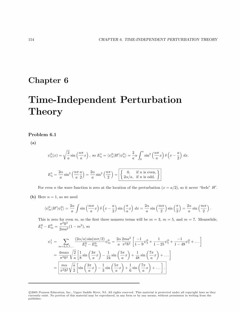
154 CHAPTER 6. TIME-INDEPENDENT PERTURBATION THEORY
Chapter 6
Time-Independent PerturbationTheory
Problem 6.1
(a)
ψ0n(x) =
√2a
sin(nπ
ax), so E1
n = 〈ψ0n|H ′|ψ0
n〉 =2aα
∫ a
0
sin2(nπ
ax)δ(x− a
2
)dx.
E1n =
2αa
sin2(nπ
a
a
2
)=
2αa
sin2(nπ
2
)=
0, if n is even,
2α/a, if n is odd.
For even n the wave function is zero at the location of the perturbation (x = a/2), so it never “feels” H ′.
(b) Here n = 1, so we need
〈ψ0m|H ′|ψ0
1〉 =2αa
∫sin
(mπ
ax)δ(x− a
2
)sin
(π
ax)
dx =2αa
sin(mπ
2
)sin
(π
2
)=
2αa
sin(mπ
2
).
This is zero for even m, so the first three nonzero terms will be m = 3, m = 5, and m = 7. Meanwhile,
E01 − E0
m =π2
2
2ma2(1−m2), so
ψ11 =
∑m=3,5,7,...
(2α/a) sin(mπ/2)E0
1 − E0m
ψ0m =
2αa
2ma2
π22
[ −11− 9
ψ03 +
11− 25
ψ05 +
−11− 49
ψ07 + . . .
]
=4maα
π22
√2a
[18
sin(
3πa
x
)− 1
24sin
(5πa
x
)+
148
sin(
7πa
x
)+ . . .
]
=mα
π22
√a
2
[sin
(3πa
x
)− 1
3sin
(5πa
x
)+
16
sin(
7πa
x
)+ . . .
].
c©2005 Pearson Education, Inc., Upper Saddle River, NJ. All rights reserved. This material is protected under all copyright laws as theycurrently exist. No portion of this material may be reproduced, in any form or by any means, without permission in writing from thepublisher.
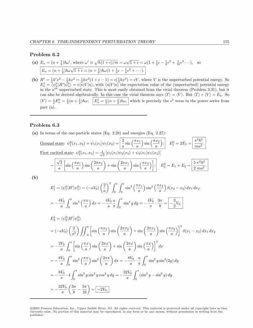
CHAPTER 6. TIME-INDEPENDENT PERTURBATION THEORY 155
Problem 6.2
(a) En = (n + 12 )ω′, where ω′ ≡
√k(1 + ε)/m = ω
√1 + ε = ω(1 + 1
2ε− 18ε
2 + 116ε
3 · · · ), so
En = (n + 12 )ω
√1 + ε = (n + 1
2 )ω(1 + 12ε− 1
8ε2 + · · · ).
(b) H ′ = 12k′x2 − 1
2kx2 = 1
2kx2(1 + ε− 1) = ε( 1
2kx2) = εV , where V is the unperturbed potential energy. So
E1n = 〈ψ0
n|H ′|ψ0n〉 = ε〈n|V |n〉, with 〈n|V |n〉 the expectation value of the (unperturbed) potential energy
in the nth unperturbed state. This is most easily obtained from the virial theorem (Problem 3.31), but itcan also be derived algebraically. In this case the virial theorem says 〈T 〉 = 〈V 〉. But 〈T 〉+ 〈V 〉 = En. So
〈V 〉 = 12E
0n = 1
2 (n + 12 )ω; E1
n = ε2 (n + 1
2 )ω, which is precisely the ε1 term in the power series from
part (a).
Problem 6.3
(a) In terms of the one-particle states (Eq. 2.28) and energies (Eq. 2.27):
Ground state: ψ01(x1, x2) = ψ1(x1)ψ1(x2) =
2a
sin(πx1
a
)sin
(πx2
a
); E0
1 = 2E1 =π2
2
ma2.
First excited state: ψ02(x1, x2) = 1√
2[ψ1(x1)ψ2(x2) + ψ2(x1)ψ1(x2)]
=√
2a
[sin
(πx1
a
)sin
(2πx2
a
)+ sin
(2πx1
a
)sin
(πx2
a
)]; E0
2 = E1 + E2 =52π2
2
ma2.
(b)
E11 = 〈ψ0
1 |H ′|ψ01〉 = (−aV0)
(2a
)2 ∫ a
0
∫ a
0
sin2(πx1
a
)sin2
(πx2
a
)δ(x2 − x2) dx1 dx2
= −4V0
a
∫ a
0
sin4(πx
a
)dx = −4V0
a
a
π
∫ π
0
sin4 y dy = −4V0
π· 3π
8= −3
2V0.
E12 = 〈ψ0
2 |H ′|ψ02〉
= (−aV0)(
2a2
) ∫∫ a
0
[sin
(πx1
a
)sin
(2πx2
a
)+ sin
(2πx1
a
)sin
(πx2
a
)]2
δ(x1 − x2) dx1 dx2
= −2V0
a
∫ a
0
[sin
(πx
a
)sin
(2πxa
)+ sin
(2πxa
)sin
(πx
a
)]2
dx
= −8V0
a
∫ a
0
sin2(πx
a
)sin2
(2πxa
)dx = −8V0
a· aπ
∫ π
0
sin2 y sin2(2y) dy
= −8V0
π· 4
∫ π
0
sin2 y sin2 y cos2 y dy = −32V0
π
∫ π
0
(sin4 y − sin6 y) dy
= −32V0
π
(3π8− 5π
16
)= −2V0.
c©2005 Pearson Education, Inc., Upper Saddle River, NJ. All rights reserved. This material is protected under all copyright laws as theycurrently exist. No portion of this material may be reproduced, in any form or by any means, without permission in writing from thepublisher.
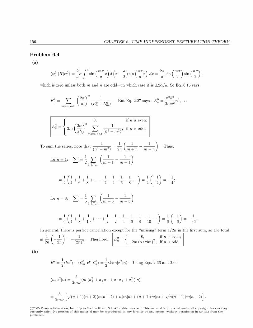
156 CHAPTER 6. TIME-INDEPENDENT PERTURBATION THEORY
Problem 6.4
(a)
〈ψ0m|H|ψ0
n〉 =2aα
∫ a
0
sin(mπ
ax)δ(x− a
2
)sin
(nπ
ax)
dx =2αa
sin(mπ
2
)sin
(nπ
2
),
which is zero unless both m and n are odd—in which case it is ±2α/a. So Eq. 6.15 says
E2n =
∑m=n, odd
(2αa
)2 1(E0
n − E0m)
. But Eq. 2.27 says E0n =
π2
2
2ma2n2, so
E2n =
0, if n is even;
2m(
2απ
)2 ∑m=n, odd
1(n2 −m2)
, if n is odd.
To sum the series, note that1
(n2 −m2)=
12n
(1
m + n− 1
m− n
). Thus,
for n = 1:∑
=12
∑3,5,7,...
(1
m + 1− 1
m− 1
)
=12
(14
+16
+18
+ · · · − 12− 1
4− 1
6− 1
8· · ·
)=
12
(−1
2
)= −1
4;
for n = 3:∑
=16
∑1,5,7,...
(1
m + 3− 1
m− 3
)
=16
(14
+18
+110
+ · · ·+ 12− 1
2− 1
4− 1
6− 1
8− 1
10· · ·
)=
16
(−1
6
)= − 1
36.
In general, there is perfect cancellation except for the “missing” term 1/2n in the first sum, so the total
is12n
(− 1
2n
)= − 1
(2n)2. Therefore: E2
n =
0, if n is even;−2m (α/πn)2 , if n is odd.
(b)
H ′ =12εkx2; 〈ψ0
m|H ′|ψ0n〉 =
12εk〈m|x2|n〉. Using Eqs. 2.66 and 2.69:
〈m|x2|n〉 =
2mω〈m|(a2
+ + a+a− + a−a+ + a2−)|n〉
=
2mω
[√(n + 1)(n + 2)〈m|n + 2〉+ n〈m|n〉+ (n + 1)〈m|n〉+
√n(n− 1)〈m|n− 2〉
].
c©2005 Pearson Education, Inc., Upper Saddle River, NJ. All rights reserved. This material is protected under all copyright laws as theycurrently exist. No portion of this material may be reproduced, in any form or by any means, without permission in writing from thepublisher.
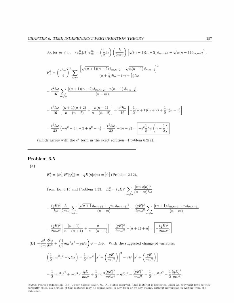
CHAPTER 6. TIME-INDEPENDENT PERTURBATION THEORY 157
So, for m = n, 〈ψ0m|H ′|ψ0
n〉 =(
12kε
) (
2mω
) [√(n + 1)(n + 2) δm,n+2 +
√n(n− 1) δm,n−2
].
E2n =
(εω
4
)2 ∑m=n
[√(n + 1)(n + 2) δm,n+2 +
√n(n− 1) δm,n−2
]2
(n + 12 )ω − (m + 1
2 )ω
=ε2ω
16
∑m=n
[(n + 1)(n + 2) δm,n+2 + n(n− 1) δm,n−2](n−m)
=ε2ω
16
[(n + 1)(n + 2)n− (n + 2)
+n(n− 1)
n− (n− 2)
]=
ε2ω
16
[−1
2(n + 1)(n + 2) +
12n(n− 1)
]
=ε2ω
32(−n2 − 3n− 2 + n2 − n
)=
ε2ω
32(−4n− 2) = −ε2
18ω
(n +
12
)(which agrees with the ε2 term in the exact solution—Problem 6.2(a)).
Problem 6.5
(a)
E1n = 〈ψ0
n|H ′|ψ0n〉 = −qE〈n|x|n〉 = 0 (Problem 2.12).
From Eq. 6.15 and Problem 3.33: E2n = (qE)2
∑m=n
|〈m|x|n〉|2(n−m)ω
=(qE)2
ω
2mω
∑m=n
[√n + 1 δm,n+1 +
√n, δm,n−1]2
(n−m)=
(qE)2
2mω2
∑m=n
[(n + 1) δm,n+1 + n δm,n−1](n−m)
=(qE)2
2mω2
[(n + 1)
n− (n + 1)+
n
n− (n− 1)
]=
(qE)2
2mω2[−(n + 1) + n] = − (qE)2
2mω2.
(b) − 2
2md2ψ
dx2+
(12mω2x2 − qEx
)ψ = Eψ. With the suggested change of variables,
(12mω2x2 − qEx
)=
12mω2
[x′ +
(qE
mω2
)]2
− qE
[x′ +
(qE
mω2
)]
=12mω2x′
2 + mω2x′qE
mω2+
12mω2 (qE)2
m2ω4− qEx′ − (qE)2
mω2=
12mω2x′
2 − 12
(qE)2
mω2.
c©2005 Pearson Education, Inc., Upper Saddle River, NJ. All rights reserved. This material is protected under all copyright laws as theycurrently exist. No portion of this material may be reproduced, in any form or by any means, without permission in writing from thepublisher.
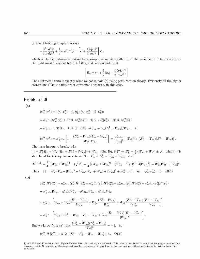
158 CHAPTER 6. TIME-INDEPENDENT PERTURBATION THEORY
So the Schrodinger equation says
− 2
2md2ψ
dx′2+
12mω2x′
2ψ =
[E +
12
(qE)2
mω2
]ψ,
which is the Schrodinger equation for a simple harmonic oscillator, in the variable x′. The constant onthe right must therefore be (n + 1
2 )ω, and we conclude that
En = (n +12)ω − 1
2(qE)2
mω2.
The subtracted term is exactly what we got in part (a) using perturbation theory. Evidently all the highercorrections (like the first-order correction) are zero, in this case.
Problem 6.6
(a)
〈ψ0+|ψ0−〉 = 〈(α+ψ0
a + β+ψ0b )|(α−ψ0
a + β−ψ0b )〉
= α∗+α−〈ψ0a|ψ0
a〉+ α∗+β−〈ψ0a|ψ0
b 〉+ β∗+α−〈ψ0b |ψ0
a〉+ β∗+β−〈ψ0b |ψ0
b 〉
= α∗+α− + β∗+β−. But Eq. 6.22 ⇒ β± = α±(E1± −Waa)/Wab, so
〈ψ0+|ψ0−〉 = α∗+α−
[1 +
(E1+ −Waa)(E1
− −Waa)Wab
∗Wab
]=
α∗+α−|Wab|2
[|Wab|2 + (E1
+ −Waa)(E1− −Waa)
].
The term in square brackets is:
[ ] = E1+E1− −Waa(E1
+ + E1−) + |Wab|2 + W 2
aa. But Eq. 6.27 ⇒ E1± = 1
2 [(Waa + Wbb)±√
], where√
isshorthand for the square root term. So E1
+ + E1− = Waa + Wbb, and
E1+E1− =
14
[(Waa + Wbb)2 − (
√)2
]=
14
[(Waa + Wbb)2 − (Waa −Wbb)2 − 4|Wab|2
]= WaaWbb − |Wab|2.
Thus [ ] = WaaWbb − |Wab|2 −Waa(Waa + Wbb) + |Wab|2 + W 2aa = 0, so 〈ψ0
+|ψ0−〉 = 0. QED
(b)
〈ψ0+|H ′|ψ0
−〉 = α∗+α−〈ψ0a|H ′|ψ0
a〉+ α∗+β−〈ψ0a|H ′|ψ0
b 〉+ β∗+α−〈ψ0b |H ′|ψ0
a〉+ β∗+β−〈ψ0b |H ′|ψ0
b 〉
= α∗+α−Waa + α∗+β−Wab + β∗+α−Wba + β∗+β−Wbb
= α∗+α−
[Waa + Wab
(E1− −Waa)Wab
+ Wba(E1
+ −Waa)W ∗ab
+ Wbb(E1
+ −Waa)W ∗ab
(E1− −Waa)Wab
]
= α∗+α−
[Waa + E1
− −Waa + E1+ −Waa + Wbb
(E1+ −Waa)(E1
− −Waa)|Wab|2
].
But we know from (a) that(E1
+ −Waa)(E1− −Waa)
|Wab|2= −1, so
〈ψ0+|H ′|ψ0
−〉 = α∗+α−[E1− + E1
+ −Waa −Wbb] = 0. QED
c©2005 Pearson Education, Inc., Upper Saddle River, NJ. All rights reserved. This material is protected under all copyright laws as theycurrently exist. No portion of this material may be reproduced, in any form or by any means, without permission in writing from thepublisher.
CHAPTER 6. TIME-INDEPENDENT PERTURBATION THEORY 159
(c)
〈ψ0±|H ′|ψ0
±〉 = α∗±α±〈ψ0a|H ′|ψ0
a〉+ α∗±β±〈ψ0a|H ′|ψ0
b 〉+ β∗±α±〈ψ0b |H ′|ψ0
a〉+ β∗±β±〈ψ0b |H ′|ψ0
b 〉
= |α±|2[Waa + Wab
(E1± −Waa)Wab
]+ |β±|2
[Wba
(E1± −Wbb)Wba
+ Wbb
](this time I used Eq. 6.24 to express α in terms of β, in the third term).
∴ 〈ψ0±|H ′|ψ0
±〉 = |α±|2(E1±) + |β±|2(E1
±) =(|α±|2 + |β±|2
)E1± = E1
±. QED
Problem 6.7
(a) See Problem 2.46.
(b) With a→ n, b→ −n, we have:
Waa = Wbb = −V0
L
∫ L/2
−L/2
e−x2/a2dx ≈ −V0
L
∫ ∞−∞
e−x2/a2dx = −V0
La√π.
Wab = −V0
L
∫ L/2
−L/2
e−x2/a2e−4πnix/Ldx ≈ −V0
L
∫ ∞−∞
e−(x2/a2+4πnix/L)dx = −V0
La√πe−(2πna/L)2 .
(We did this integral in Problem 2.22.) In this case Waa = Wbb, and Wab is real, so Eq. 6.26 ⇒
E1± = Waa ± |Wab|, or E1
± = −√πV0a
L
(1∓ e−(2πna/L)2
).
(c) Equation 6.22 ⇒ β = α(E1− −Waa)Wab
= α
[±√π(V0a/L)e−(2πna/L)2
−√π(V0a/L)e−(2πna/L)2
]= ∓α. Evidently, the “good” linear
combinations are:
ψ+ = αψn − αψ−n =1√2
1√L
[ei2πnx/L − e−i2πnx/L
]= i
√2L
sin(
2πnxL
)and
ψ− = αψn + αψ−n =
√2L
cos(
2πnxL
). Using Eq. 6.9, we have :
E1+ = 〈ψ+|H ′|ψ+〉 =
2L
(−V0)∫ L/2
−L/2
e−x2/a2sin2
(2πnxL
)dx,
E1− = 〈ψ−|H ′|ψ−〉 =
2L
(−V0)∫ L/2
−L/2
e−x2/a2cos2
(2πnxL
)dx.
c©2005 Pearson Education, Inc., Upper Saddle River, NJ. All rights reserved. This material is protected under all copyright laws as theycurrently exist. No portion of this material may be reproduced, in any form or by any means, without permission in writing from thepublisher.
160 CHAPTER 6. TIME-INDEPENDENT PERTURBATION THEORY
But sin2 θ = (1− cos 2θ)/2, and cos2 θ = (1 + cos 2θ)/2, so
E1± ≈ −
V0
L
∫ ∞−∞
e−x2/a2[1∓ cos
(4πnxL
)]dx = −V0
L
[∫ ∞−∞
e−x2/a2dx∓
∫ ∞−∞
e−x2/a2cos
(4πnxL
)dx
]
= −V0
L
[√π a∓ a
√πe−(2πna/L)2
]= −
√πV0a
L
[1∓ e−(2πna/L)2
], same as (b).
(d) Af(x) = f(−x) (the parity operator). The eigenstates are even functions (with eigenvalue +1) and oddfunctions (with eigenvalue −1). The linear combinations we found in (c) are precisely the odd and evenlinear combinations of ψn and ψ−n.
Problem 6.8
Ground state is nondegenerate; Eqs. 6.9 and 6.31 ⇒
E1 =(
2a
)3
a3V0
∫∫∫ a
0
sin2(π
ax)
sin2(π
ay)
sin2(π
az)δ(x− a
4)δ(y − a
2)δ(z − 3a
4) dx dy dz
= 8V0 sin2(π
4
)sin2
(π
2
)sin2
(3π4
)= 8V0
(12
)(1)
(12
)= 2V0.
First excited states (Eq. 6.34):
Waa = 8V0
∫∫∫sin2
(π
ax)
sin2(π
ay)
sin2
(2πa
z
)δ(x− a
4)δ(y − a
2)δ(z − 3a
4) dx dy dz
= 8V0
(12
)(1)(1) = 4V0.
Wbb = 8V0
∫∫∫sin2
(π
ax)
sin2
(2πa
y
)sin2
(π
az)δ(x− a
4)δ(y − a
2)δ(z − 3a
4) dx dy dz
= 8V0
(12
)(0)
(12
)= 0.
Wcc = 8V0
∫∫∫sin2
(2πa
x
)sin2
(π
ay)
sin2(π
az)δ(x− a
4)δ(y − a
2)δ(z − 3a
4) dx dy dz
= 8V0(1)(1)(
12
)= 4V0.
Wab = 8V0 sin2(π
4
)sin
(π
2
)sin(π) sin
(3π2
)sin
(3π4
)= 0.
Wac = 8V0 sin(π
4
)sin
(π
2
)sin2
(π
2
)sin
(3π2
)sin
(3π4
)= 8V0
(1√2
)(1)(1)(−1)
(1√2
)= −4V0.
c©2005 Pearson Education, Inc., Upper Saddle River, NJ. All rights reserved. This material is protected under all copyright laws as theycurrently exist. No portion of this material may be reproduced, in any form or by any means, without permission in writing from thepublisher.
CHAPTER 6. TIME-INDEPENDENT PERTURBATION THEORY 161
Wbc = 8V0 sin(π
4
)sin
(π
2
)sin(π) sin
(π
2
)sin
(3π4
)= 0.
W = 4V0
1 0 −10 0 0−1 0 1
= 4V0D; det(D− λ) =
∣∣∣∣∣∣(1− λ) 0 −1
0 −λ 0−1 0 (1− λ)
∣∣∣∣∣∣ = −λ(1− λ)2 + λ = 0 ⇒
λ = 0, or (1− λ)2 = 1⇒ 1− λ = ±1 ⇒ λ = 0 or λ = 2.
So the first-order corrections to the energies are 0, 0, 8V0.
Problem 6.9
(a) χ1 =
100
, eigenvalue V0; χ2 =
010
, eigenvalue V0; χ3 =
001
, eigenvalue 2V0.
(b) Characteristic equation: det(H− λ) =
∣∣∣∣∣∣[V0(1− ε)− λ] 0 0
0 [V0 − λ] εV0
0 εV0 [2V0 − λ]
∣∣∣∣∣∣ = 0;
[V0(1− ε)− λ][(V0 − λ)(2V0 − λ)− (εV0)2] = 0⇒ λ1 = V0(1− ε).
(V0 − λ)(2V0 − λ)− (εV0)2 = 0⇒ λ2 − 3V0λ + (2V 20 − ε2V 2
0 ) = 0⇒
λ =3V0 ±
√9V 2
0 − 4(2V 20 − ε2V 2
0 )2
=V0
2
[3±
√1 + 4ε2
]≈ V0
2[3± (1 + 2ε2)
].
λ2 =V0
2
(3−
√1 + 4ε2
)≈ V0(1− ε2); λ3 =
V0
2
(3 +
√1 + 4ε2
)≈ V0(2 + ε2).
(c)
H′ = εV0
−1 0 00 0 10 1 0
; E13 = 〈χ3|H ′|χ3〉 = εV0
(0 0 1
) −1 0 00 0 10 1 0
001
= εV0
(0 0 1
) 010
= 0 (no first-order correction).
E23 =
∑m=1,2
|〈χm|H ′|χ3〉|2E0
3 − E0m
; 〈χ1|H ′|χ3〉 = εV0
(1 0 0
) −1 0 00 0 10 1 0
001
= εV0
(1 0 0
) 010
= 0,
〈χ2|H ′|χ3〉 = εV0
(0 1 0
) 001
= εV0.
E03 − E0
2 = 2V0 − V0 = V0. So E23 = (εV0)2/V0 = ε2V0. Through second-order, then,
E3 = E03 + E1
3 + E23 = 2V0 + 0 + ε2V0 = V0(2 + ε2) (same as we got for λ3 in (b)).
c©2005 Pearson Education, Inc., Upper Saddle River, NJ. All rights reserved. This material is protected under all copyright laws as theycurrently exist. No portion of this material may be reproduced, in any form or by any means, without permission in writing from thepublisher.
162 CHAPTER 6. TIME-INDEPENDENT PERTURBATION THEORY
(d)
Waa = 〈χ1|H ′|χ1〉 = εV0
(1 0 0
) −1 0 00 0 10 1 0
100
= εV0
(1 0 0
) −100
= −εV0.
Wbb = 〈χ2|H ′|χ2〉 = εV0
(0 1 0
) −1 0 00 0 10 1 0
010
= εV0
(0 1 0
) 001
= 0.
Wab = 〈χ1|H ′|χ2〉 = εV0
(1 0 0
) −1 0 00 0 10 1 0
010
= εV0
(1 0 0
) 001
= 0.
Plug the expressions for Waa, Wbb, and Wab into Eq. 6.27:
E1± =
12
[−εV0 + 0±
√ε2V 2
0 + 0]
=12(−εV0 ± εV0) = 0,−εV0.
To first-order, then, E1 = V0 − εV0, E2 = V0, and these are consistent (to first order in ε) with whatwe got in (b).
Problem 6.10
Given a set of orthonornal states ψ0j that are degenerate eigenfunctions of the unperturbed Hamiltonian:
Hψ0j = E0ψ0
j , 〈ψ0j |ψ0
l 〉 = δjl,
construct the general linear combination,
ψ0 =n∑
j=1
αjψ0j .
It too is an eigenfunction of the unperturbed Hamiltonian, with the same eigenvalue:
H0ψ0 =n∑
j=1
αjH0ψ0
j = E0n∑
j=1
αjψ0j = E0ψ0.
We want to solve the Schrodinger equation Hψ = Eψ for the perturbed Hamiltonian H = H0 + λH ′.Expand the eigenvalues and eigenfunctions as power series in λ:
E = E0 + λE1 + λ2E2 + . . . , ψ = ψ0 + λψ1 + λ2ψ2 + . . . .
Plug these into the Schrodinger equation and collect like powers:
(H0 + λH ′)(ψ0 + λψ1 + λ2ψ2 + . . . ) = (E0 + λE1 + λ2E2 + . . . )(ψ0 + λψ1 + λ2ψ2 + . . . ) ⇒
H0ψ0 + λ(H0ψ1 + H ′ψ0) + . . . = E0ψ0 + λ(E0ψ1 + E1ψ0) + . . .
c©2005 Pearson Education, Inc., Upper Saddle River, NJ. All rights reserved. This material is protected under all copyright laws as theycurrently exist. No portion of this material may be reproduced, in any form or by any means, without permission in writing from thepublisher.
CHAPTER 6. TIME-INDEPENDENT PERTURBATION THEORY 163
The zeroth-order terms cancel; to first order
H0ψ1 + H ′ψ0 = E0ψ1 + E1ψ0.
Take the inner product with ψ0j :
〈ψ0j |H0ψ1〉+ 〈ψ0
j |H ′ψ0〉 = E0〈ψ0j |ψ1〉+ E1〈ψ0
j |ψ0〉.
But 〈ψ0j |H0ψ1〉 = 〈H0ψ0
j |ψ1〉 = E0〈ψ0j |ψ1〉, so the first terms cancel, leaving
〈ψ0j |H ′ψ0〉 = E1〈ψ0
j |ψ0〉.
Now use ψ0 =n∑
l=1
αlψ0l , and exploit the orthonormality of ψ0
l :
n∑l=1
αl〈ψ0j |H ′|ψ0
l 〉 = E1n∑
l=1
αl〈ψ0j |ψ0
l 〉 = E1αj ,
or, defining
Wjl ≡ 〈ψ0j |H ′|ψ0
l 〉,n∑
l=1
Wjlαl = E1αl.
This (the generalization of Eq. 6.22 for the case of n-fold degeneracy) is the eigenvalue equation for the matrixW (whose jlth element, in the ψ0
j basis, is Wjl); E1 is the eigenvalue, and the eigenvector (in the ψ0j basis)
is χj = αj . Conclusion: The first-order corrections to the energy are the eigenvalues of W. QED
Problem 6.11
(a) From Eq. 4.70: En = −[
m
22
(e2
4πε0
)2]
1n2
= −12mc2
(1c
e2
4πε0
)2 1n2
= −α2mc2
2n2.
(b) I have found a wonderful solution—unfortunately, there isn’t enough room on this page for the proof.
Problem 6.12
Equation 4.191 ⇒ 〈V 〉 = 2En, for hydrogen. V = − e2
4πε01r; En = −
[m
22
(e2
4πε0
)2]
1n2
. So
− e2
4πε0
⟨1r
⟩= −2
[m
22
(e2
4πε0
)2]
1n2
⇒⟨
1r
⟩=
(me2
4πε02
)1n2
=1
an2(Eq. 4.72). QED
c©2005 Pearson Education, Inc., Upper Saddle River, NJ. All rights reserved. This material is protected under all copyright laws as theycurrently exist. No portion of this material may be reproduced, in any form or by any means, without permission in writing from thepublisher.
164 CHAPTER 6. TIME-INDEPENDENT PERTURBATION THEORY
Problem 6.13
In Problem 4.43 we found (for n = 3, l = 2, m = 1) that 〈rs〉 =(s + 6)!
6!
(3a2
)s
.
s = 0 : 〈1〉 =6!6!
(1) = 1 (of course).
s = −1 :⟨
1r
⟩=
5!6!
(3a2
)−1
=16· 23a
=19a
(Eq. 6.55 says
132a
=19a
).
s = −2 :⟨
1r2
⟩=
4!6!
(3a2
)−2
=1
6 · 5 ·4
9a2=
2135a2
(Eq. 6.56 says
1(5/2) · 27 · a2
=2
135a2
).
s = −3 :⟨
1r3
⟩=
3!6!
(3a2
)−3
=1
6 · 5 · 4 ·8
27a3=
1405a3
(Eq. 6.64 says
12(5/2)3 · 27 · a3
=1
405a3
).
For s = −7 (or smaller) the integral does not converge: 〈1/r7〉 = ∞ in this state; this is reflected in the factthat (−1)! =∞.
Problem 6.14
Equation 6.53 ⇒ E1r = − 1
2mc2[E2 − 2E〈V 〉+ 〈V 2〉
]. Here E = (n +
12)ω, V =
12mω2x2 ⇒
E1r = − 1
2mc2
[(n +
12
)2
2ω2 − 2
(n +
12
)ω
12mω2〈x2〉+
14m2ω4〈x4〉
].
But Problem 2.12 ⇒ 〈x2〉 = (n +12)
mω, so
E1r = − 1
2mc2
[(n +
12
)2
2ω2 −
(n +
12
)2
2ω2 +
14m2ω4〈x4〉
]= −mω4
8c2〈x4〉.
From Eq. 2.69: x4 =
2
4m2ω2
(a2+ + a+a− + a−a+ + a2
−) (
a2+ + a+a− + a−a+ + a2
−),
〈x4〉 =
2
4m2ω2〈n|
(a2+a2− + a+a−a+a− + a+a−a−a+ + a−a+a+a− + a−a+a−a+ + a2
−a2+
)|n〉.
(Note that only terms with equal numbers of raising and lowering operators will survive). Using Eq. 2.66,
〈x4〉 =
2
4m2ω2〈n|
[a2+
(√n(n− 1) |n− 2〉
)+ a+a−(n |n〉) + a+a−
((n + 1) |n〉
)c©2005 Pearson Education, Inc., Upper Saddle River, NJ. All rights reserved. This material is protected under all copyright laws as theycurrently exist. No portion of this material may be reproduced, in any form or by any means, without permission in writing from thepublisher.
CHAPTER 6. TIME-INDEPENDENT PERTURBATION THEORY 165
+a−a+ (n |n〉) + a−a+
((n + 1) |n〉
)+ a2−
(√(n + 1)(n + 2) |n + 2〉
)]
=
2
4m2ω2〈n|
[√n(n− 1)
(√n(n− 1) |n〉
)+ n (n |n〉) + (n + 1) (n |n〉)
+n((n + 1) |n〉
)+ (n + 1)
((n + 1) |n〉
)+
√(n + 1)(n + 2)
(√(n + 1)(n + 2) |n〉
)]
=
2
4m2ω2
[n(n− 1) + n2 + (n + 1)n + n(n + 1) + (n + 1)2 + (n + 1)(n + 2)
]
=(
2mω
)2
(n2 − n + n2 + n2 + n + n2 + n + n2 + 2n + 1 + n2 + 3n + 2) =(
2mω
)2
(6n2 + 6n + 3).
E1r = −mω4
8c2·
2
4m2ω2· 3(3n2 + 2n + 1) = − 3
32
(
2ω2
mc2
)(2n2 + 2n + 1).
Problem 6.15
Quoting the Laplacian in spherical coordinates (Eq. 4.13), we have, for states with no dependence on θ or φ:
p2 = −2∇2 = −2
r2
d
dr
(r2 d
dr
).
Question: Is it Hermitian?Using integration by parts (twice), and test functions f(r) and g(r):
〈f |p2g〉 = −2
∫ ∞0
f1r2
d
dr
(r2 dg
dr
)4πr2 dr = −4π2
∫ ∞0
fd
dr
(r2 dg
dr
)dr
= −4π2
r2f
dg
dr
∣∣∣∞0−
∫ ∞0
r2 df
dr
dg
drdr
= −4π2
r2f
dg
dr
∣∣∣∞0− r2g
df
dr
∣∣∣∞0
+∫ ∞
0
d
dr
(r2 df
dr
)g dr
= −4π2
(r2f
dg
dr− r2g
df
dr
) ∣∣∣∣∞0
+ 〈p2f |g〉.
The boundary term at infinity vanishes for functions f(r) and g(r) that go to zero exponentially; the boundaryterm at zero is killed by the factor r2, as long as the functions (and their derivatives) are finite. So
〈f |p2g〉 = 〈p2f |g〉,
and hence p2 is Hermitian.Now we apply the same argument to
p4 =
4
r2
d
dr
r2 d
dr
[1r2
d
dr
(r2 d
dr
)],
c©2005 Pearson Education, Inc., Upper Saddle River, NJ. All rights reserved. This material is protected under all copyright laws as theycurrently exist. No portion of this material may be reproduced, in any form or by any means, without permission in writing from thepublisher.
166 CHAPTER 6. TIME-INDEPENDENT PERTURBATION THEORY
integrating by parts four times:
〈f |p4g〉 = 4π4
∫ ∞0
fd
dr
r2 d
dr
[1r2
d
dr
(r2 dg
dr
)]dr
= 4π4
r2f
d
dr
[1r2
d
dr
(r2 dg
dr
)] ∣∣∣∣∞0
−∫ ∞
0
r2 df
dr
d
dr
[1r2
d
dr
(r2 dg
dr
)]dr
= 4π4
[r2f
d
dr
[1r2
d
dr
(r2 dg
dr
)]− df
dr
d
dr
(r2 dg
dr
)] ∣∣∣∣∞0
+∫ ∞
0
1r2
d
dr
(r2 df
dr
)d
dr
(r2 dg
dr
)dr
= 4π4
[r2f
d
dr
[1r2
d
dr
(r2 dg
dr
)]− df
dr
d
dr
(r2 dg
dr
)+
d
dr
(r2 df
dr
)dg
dr
] ∣∣∣∣∞0
−∫ ∞
0
r2 d
dr
[1r2
d
dr
(r2 df
dr
)]dg
drdr
= 4π4
[r2f
d
dr
[1r2
d
dr
(r2 dg
dr
)]− df
dr
d
dr
(r2 dg
dr
)+
d
dr
(r2 df
dr
)dg
dr− r2g
d
dr
[1r2
d
dr
(r2 df
dr
)]] ∣∣∣∣∞0
+∫ ∞
0
d
dr
(r2 d
dr
[1r2
d
dr
(r2 df
dr
)])g dr
= 4π4
r2f
d
dr
[1r2
d
dr
(r2 dg
dr
)]− r2g
d
dr
[1r2
d
dr
(r2 df
dr
)] ∣∣∣∣∞0
− 4π4
df
dr
d
dr
(r2 dg
dr
)− d
dr
(r2 df
dr
)dg
dr
∣∣∣∣∞0
+ 〈p4f |g〉
This time there are four boundary terms to worry about. Infinity is no problem; the trouble comes at r = 0.If the functions f and g went to zero at the origin (as they do for states with l > 0) we’d be OK, but stateswith l = 0 go like exp(−r/na). So let’s test the boundary terms using
f(r) = e−r/na, g(r) = e−r/ma.
In this case
r2 dg
dr= − 1
mar2e−r/ma
d
dr
(r2 dg
dr
)=
1(ma)2
(r2 − 2mar
)e−r/ma
df
dr
d
dr
(r2 dg
dr
)= − 1
nae−r/na 1
(ma)2(r2 − 2mar
)e−r/ma.
This goes to zero as r → 0, so the second pair of boundary terms vanishes—but not the first pair:
1r2
d
dr
(r2 dg
dr
)=
1(ma)2
(1− 2ma
r
)e−r/ma
d
dr
[1r2
d
dr
(r2 dg
dr
)]=
1(ma)3r2
[2(ma)2 + 2mar − r2
]e−r/ma
r2fd
dr
[1r2
d
dr
(r2 dg
dr
)]=
1(ma)3
[2(ma)2 + 2mar − r2
]e−r/mae−r/na
This does not vanish as r → 0; rather, it goes to 2/ma. For these particular states, then,
〈f |p4g〉 =8π4
a
(1m− 1
n
)+ 〈p4f |g〉,
c©2005 Pearson Education, Inc., Upper Saddle River, NJ. All rights reserved. This material is protected under all copyright laws as theycurrently exist. No portion of this material may be reproduced, in any form or by any means, without permission in writing from thepublisher.
CHAPTER 6. TIME-INDEPENDENT PERTURBATION THEORY 167
or, tacking on the normalization factor,
ψn00 =1√
π (na)3/2e−r/na, 〈ψn00|p4ψm00〉 =
84
a4
(n−m)(nm)5/2
+ 〈p4ψn00|ψm00〉,
and hence p4 is not Hermitian, for such states.
Problem 6.16
(a)
[L · S, Lx] = [LxSx + LySy + LzSz, Lx] = Sx [Lx, Lx] + Sy [Ly, Lx] + Sz [Lz, Lx]
= Sx(0) + Sy(−iLz) + Sz(iLy) = i(LySz − LzSy) = i(L× S)x.
Same goes for the other two components, so [L · S,L] = i(L× S).
(b) [L · S,S] is identical, only with L↔ S: [L · S,S] = i(S× L).
(c) [L · S,J] = [L · S,L] + [L · S,S] = i(L× S + S× L) = 0.
(d) L2 commutes with all components of L (and S) , so[L · S, L2
]= 0.
(e) Likewise,[L · S, S2
]= 0.
(f)[L · S, J2
]=
[L · S, L2
]+
[L · S, S2
]+ 2 [L · S,L · S] = 0 + 0 + 0 =⇒
[L · S, J2
]= 0.
Problem 6.17
With the plus sign, j = l + 1/2 (l = j − 1/2) : Eq. 6.57⇒ E1r = − (En)2
2mc2
(4nj− 3
).
Equation 6.65⇒ E1so =
(En)2
mc2n
[j(j + 1)− (j − 1
2 )(j + 12 )− 3
4
](j − 1
2 )j(j + 12 )
=(En)2
mc2n(j2 + j − j2 + 1
4 − 34 )
(j − 12 )j(j + 1
2 )=
(En)2
mc2n
j(j + 12 )
.
E1fs = E1
r + E1so =
(En)2
2mc2
(−4n
j+ 3 +
2nj(j + 1
2 )
)
=(En)2
2mc2
3 +
2nj(j + 1
2 )
[1− 2
(j +
12
)]=
(En)2
2mc2
(3− 4n
j + 12
).
c©2005 Pearson Education, Inc., Upper Saddle River, NJ. All rights reserved. This material is protected under all copyright laws as theycurrently exist. No portion of this material may be reproduced, in any form or by any means, without permission in writing from thepublisher.
168 CHAPTER 6. TIME-INDEPENDENT PERTURBATION THEORY
With the minus sign, j = l − 1/2 (l = j + 1/2) : Eq. 6.57⇒ E1r = − (En)2
2mc2
(4n
j + 1− 3
).
Equation 6.65⇒ E1so =
(En)2
mc2n
[j(j + 1)− (j + 1
2 )(j + 32 )− 3
4
](j + 1
2 )(j + 1)(j + 32 )
=(En)2
mc2n(j2 + j − j2 − 2j − 3
4 − 34 )
(j + 12 )(j + 1)(j + 3
2 )=
(En)2
mc2−n
(j + 1)(j + 12 )
.
E1fs =
(En)2
2mc2
[− 4n
j + 1− 3 +
2n(j + 1)(j + 1
2 )
]=
(En)2
2mc2
3− 2n
(j + 1)(j + 12 )
[1 + 2
(j +
12
)]
=(En)2
2mc2
(3− 4n
j + 12
). For both signs, then, E1
fs =(En)2
2mc2
(3− 4n
j + 12
). QED
Problem 6.18
E03 − E0
2 = hν =2πcλ
= E1
(19− 1
4
)= − 5
36E1 ⇒ λ = −36
52πcE1
; E1 = −13.6 eV;
c = 1.97× 10⁻¹¹ MeV·cm; λ =365
(2π)(1.97× 10−11 × 106 eV · cm)(13.6 eV)
= 6.55× 10⁻⁵ cm= 655 nm.
ν =c
λ=
3.00× 10⁸ m/s6.55× 10−7 m
= 4.58× 10¹⁴ Hz. Equation 6.66 ⇒ E1fs =
(En)2
2mc2
(3− 4n
j + 12
):
For n = 2: l = 0 or l = 1, so j = 1/2 or 3/2. Thus n = 2 splits into two levels :
j = 1/2 : E12 =
(E2)2
2mc2
(3− 8
1
)= −5
2(E2)2
mc2= −5
2
(14
)2 (E1)2
mc2= − 5
32(13.6 eV)2
(.511× 106 eV)= −5.66× 10⁻⁵eV.
j = 3/2 : E12 =
(E2)2
2mc2
(3− 8
2
)= −1
2(E2)2
mc2= − 1
32(3.62× 10⁻⁴ eV) = −1.13× 10⁻⁵eV.
For n = 3: l = 0, 1 or 2, so j = 1/2, 3/2 or 5/2. Thus n = 3 splits into three levels :
j = 1/2 : E13 =
(E3)2
2mc2
(3− 12
1
)= −9
(E3)2
mc2= −9
2
(192
)(E1)2
mc2= − 1
18(3.62× 10⁻⁴eV) = −2.01× 10⁻⁵eV.
j = 3/2 : E13 =
(E3)2
2mc2
(3− 12
2
)= −3
2(E3)2
mc2= − 1
54(3.62× 10⁻⁴ eV) = −0.67× 10⁻⁵ eV.
j = 5/2 : E13 =
(E3)2
2mc2
(3− 12
3
)= −1
2(E3)2
mc2= − 1
162(3.62× 10⁻⁴ eV) = −0.22× 10⁻⁵ eV.
c©2005 Pearson Education, Inc., Upper Saddle River, NJ. All rights reserved. This material is protected under all copyright laws as theycurrently exist. No portion of this material may be reproduced, in any form or by any means, without permission in writing from thepublisher.
CHAPTER 6. TIME-INDEPENDENT PERTURBATION THEORY 169
E
E
0
0
3
2
1 2 3
4 5 6
5/2
3/2
1/2
3/2
1/2
j=
j=j=
j=j=
There are six transitions here; their energies are (E03 + E1
3)− (E02 + E1
2) = (E03 − E0
2) + ∆E, where∆E ≡ E1
3 − E12 . Let β ≡ (E1)2/mc2 = 3.62× 10⁻⁴ eV. Then:
(12→ 3
2) : ∆E =
[(− 1
18
)−
(− 1
32
)]β = − 7
288β = −8.80× 10⁻⁶ eV.
(32→ 3
2) : ∆E =
[(− 1
54
)−
(− 1
32
)]β =
11864
β = 4.61× 10⁻⁶ eV.
(52→ 3
2) : ∆E =
[(− 1
162
)+
(132
)]β =
652592
β = 9.08× 10⁻⁶ eV.
(12→ 1
2) : ∆E =
[(532
)−
(118
)]β =
29288
β = 36.45× 10⁻⁶ eV.
(32→ 1
2) : ∆E =
[(− 1
54
)+
(532
)]β =
119864
β = 49.86× 10⁻⁶ eV.
(52→ 1
2) : ∆E =
[(− 1
162
)+
(532
)]β =
3892592
β = 54.33× 10⁻⁶ eV.
Conclusion: There are six lines; one of them (12 → 3
2 ) has a frequency less than the unperturbed line, theother five have (slightly) higher frequencies. In order they are: 3
2 → 32 ; 5
2 → 32 ; 1
2 → 12 ; 3
2 → 12 ; 5
2 → 12 . The
frequency spacings are:
ν2 − ν1 = (∆E2 −∆E1)/2π = 3.23× 10⁹ Hzν3 − ν3 = (∆E3 −∆E2)/2π = 1.08× 10⁹ Hzν4 − ν3 = (∆E4 −∆E3)/2π = 6.60× 10⁹ Hzν5 − ν4 = (∆E5 −∆E4)/2π = 3.23× 10⁹ Hzν6 − ν5 = (∆E6 −∆E5)/2π = 1.08× 10⁹ Hz
c©2005 Pearson Education, Inc., Upper Saddle River, NJ. All rights reserved. This material is protected under all copyright laws as theycurrently exist. No portion of this material may be reproduced, in any form or by any means, without permission in writing from thepublisher.
170 CHAPTER 6. TIME-INDEPENDENT PERTURBATION THEORY
Problem 6.19
√(j +
12
)2
− α2 =(j +
12
) √1−
(α
j + 12
)2
≈(j +
12
) [1− 1
2
(α
j + 12
)2]
= (j +12)− α2
2(j + 12 )
.
α
n− (j + 12 ) +
√(j + 1
2
)2 − α2
≈ α
n−(j + 1
2
)+
(j + 1
2
)− α2
2(j+ 12 )
=α
n− α2
2(j+ 12 )
=α
n[1− α2
2n(j+ 12 )
] ≈ α
n
[1 +
α2
2n(j + 12 )
].
1 +
α
n− (j + 12 ) +
√(j + 1
2
)2 − α2
2−1/2
≈[1 +
α2
n2
(1 +
α2
n(j + 12 )
)]−1/2
≈ 1− 12α2
n2
(1 +
α2
n(j + 12 )
)+
38α4
n4= 1− α2
2n2+
α4
2n4
( −n
j + 12
+34
).
Enj ≈ mc2[1− α2
2n2+
α4
2n4
( −n
j + 12
+34
)− 1
]= −α2mc2
2n2
[1 +
α2
n2
(n
j + 12
− 34
)]
= −13.6 eVn2
[1 +
α2
n2
(n
j + 12
− 34
)], confirming Eq. 6.67.
Problem 6.20
Equation 6.59 ⇒ B =1
4πε0e
mc2r3L. Say L = , r = a; then
B =1
4πε0e
mc2a3
=(1.60× 10⁻¹⁹ C)(1.05× 10⁻³⁴ J · s)
4π(8.9× 10⁻¹² C2/N ·m2
)(9.1× 10⁻³¹ kg) (3× 10⁸ m/s)2 (0.53× 10⁻¹⁰ m)3
= 12 T.
So a “strong” Zeeman field is Bext 10 T, and a “weak” one is Bext 10 T. Incidentally, the earth’s field(10−4 T) is definitely weak.
c©2005 Pearson Education, Inc., Upper Saddle River, NJ. All rights reserved. This material is protected under all copyright laws as theycurrently exist. No portion of this material may be reproduced, in any form or by any means, without permission in writing from thepublisher.
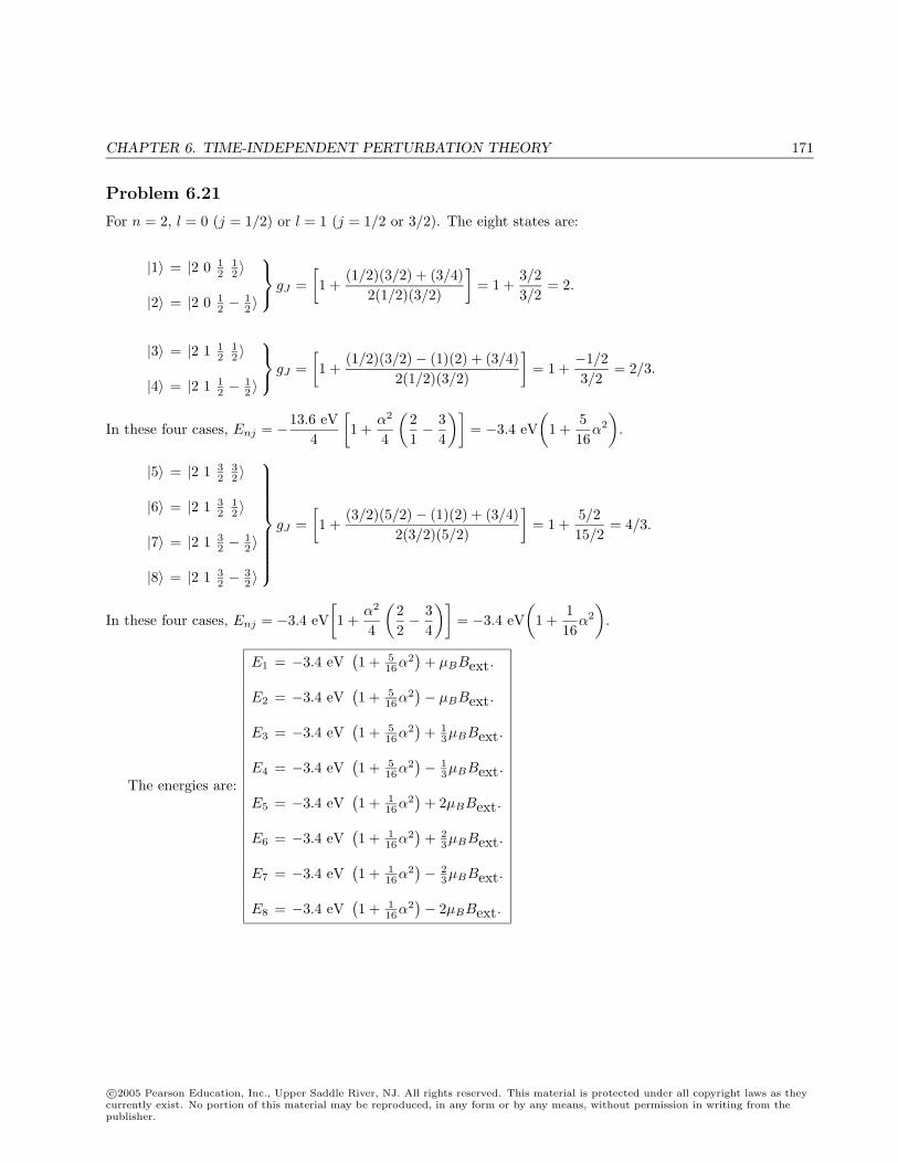
CHAPTER 6. TIME-INDEPENDENT PERTURBATION THEORY 171
Problem 6.21
For n = 2, l = 0 (j = 1/2) or l = 1 (j = 1/2 or 3/2). The eight states are:
|1〉 = |2 0 12
12 〉
|2〉 = |2 0 12 − 1
2 〉
gJ =[1 +
(1/2)(3/2) + (3/4)2(1/2)(3/2)
]= 1 +
3/23/2
= 2.
|3〉 = |2 1 12
12 〉
|4〉 = |2 1 12 − 1
2 〉
gJ =[1 +
(1/2)(3/2)− (1)(2) + (3/4)2(1/2)(3/2)
]= 1 +
−1/23/2
= 2/3.
In these four cases, Enj = −13.6 eV4
[1 +
α2
4
(21− 3
4
)]= −3.4 eV
(1 +
516
α2
).
|5〉 = |2 1 32
32 〉
|6〉 = |2 1 32
12 〉
|7〉 = |2 1 32 − 1
2 〉
|8〉 = |2 1 32 − 3
2 〉
gJ =
[1 +
(3/2)(5/2)− (1)(2) + (3/4)2(3/2)(5/2)
]= 1 +
5/215/2
= 4/3.
In these four cases, Enj = −3.4 eV[1 +
α2
4
(22− 3
4
)]= −3.4 eV
(1 +
116
α2
).
The energies are:
E1 = −3.4 eV(1 + 5
16α2)
+ µBBext.
E2 = −3.4 eV(1 + 5
16α2)− µBBext.
E3 = −3.4 eV(1 + 5
16α2)
+ 13µBBext.
E4 = −3.4 eV(1 + 5
16α2)− 1
3µBBext.
E5 = −3.4 eV(1 + 1
16α2)
+ 2µBBext.
E6 = −3.4 eV(1 + 1
16α2)
+ 23µBBext.
E7 = −3.4 eV(1 + 1
16α2)− 2
3µBBext.
E8 = −3.4 eV(1 + 1
16α2)− 2µBBext.
c©2005 Pearson Education, Inc., Upper Saddle River, NJ. All rights reserved. This material is protected under all copyright laws as theycurrently exist. No portion of this material may be reproduced, in any form or by any means, without permission in writing from thepublisher.
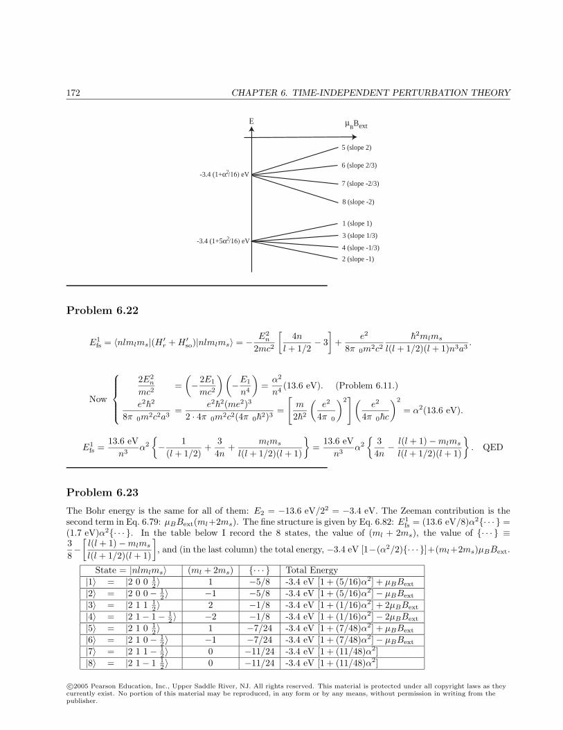
172 CHAPTER 6. TIME-INDEPENDENT PERTURBATION THEORY
E BextBµ
2 (slope -1)
4 (slope -1/3)
3 (slope 1/3)
1 (slope 1)
8 (slope -2)
7 (slope -2/3)
6 (slope 2/3)
5 (slope 2)
-3.4 (1+α /16) eV2
-3.4 (1+5α /16) eV2
Problem 6.22
E1fs = 〈nlmlms|(H ′r + H ′so)|nlmlms〉 = − E2
n
2mc2
[4n
l + 1/2− 3
]+
e2
8πε0m2c2
2mlms
l(l + 1/2)(l + 1)n3a3.
Now
2E2
n
mc2=
(− 2E1
mc2
) (−E1
n4
)=
α2
n4(13.6 eV). (Problem 6.11.)
e2
2
8πε0m2c2a3=
e2
2(me2)3
2 · 4πε0m2c2(4πε02)3=
[m
22
(e2
4πε0
)2] (
e2
4πε0c
)2
= α2(13.6 eV).
E1fs =
13.6 eVn3
α2
− 1
(l + 1/2)+
34n
+mlms
l(l + 1/2)(l + 1)
=
13.6 eVn3
α2
34n− l(l + 1)−mlms
l(l + 1/2)(l + 1)
. QED
Problem 6.23
The Bohr energy is the same for all of them: E2 = −13.6 eV/22 = −3.4 eV. The Zeeman contribution is thesecond term in Eq. 6.79: µBBext(ml+2ms). The fine structure is given by Eq. 6.82: E1
fs = (13.6 eV/8)α2· · · =(1.7 eV)α2· · · . In the table below I record the 8 states, the value of (ml + 2ms), the value of · · · ≡38−
[l(l + 1)−mlms
l(l + 1/2)(l + 1)
], and (in the last column) the total energy, −3.4 eV [1−(α2/2)· · · ]+(ml+2ms)µBBext.
State = |nlmlms〉 (ml + 2ms) · · · Total Energy|1〉 = |2 0 0 1
2 〉 1 −5/8 -3.4 eV [1 + (5/16)α2] + µBBext
|2〉 = |2 0 0− 12 〉 −1 −5/8 -3.4 eV [1 + (5/16)α2]− µBBext
|3〉 = |2 1 1 12 〉 2 −1/8 -3.4 eV [1 + (1/16)α2] + 2µBBext
|4〉 = |2 1− 1− 12 〉 −2 −1/8 -3.4 eV [1 + (1/16)α2]− 2µBBext
|5〉 = |2 1 0 12 〉 1 −7/24 -3.4 eV [1 + (7/48)α2] + µBBext
|6〉 = |2 1 0− 12 〉 −1 −7/24 -3.4 eV [1 + (7/48)α2]− µBBext
|7〉 = |2 1 1− 12 〉 0 −11/24 -3.4 eV [1 + (11/48)α2]
|8〉 = |2 1− 1 12 〉 0 −11/24 -3.4 eV [1 + (11/48)α2]
c©2005 Pearson Education, Inc., Upper Saddle River, NJ. All rights reserved. This material is protected under all copyright laws as theycurrently exist. No portion of this material may be reproduced, in any form or by any means, without permission in writing from thepublisher.
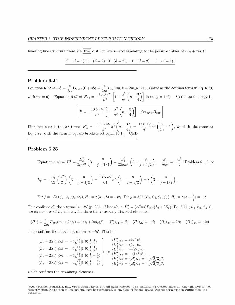
CHAPTER 6. TIME-INDEPENDENT PERTURBATION THEORY 173
Ignoring fine structure there are five distinct levels—corresponding to the possible values of (ml + 2ms):
2 (d = 1); 1 (d = 2); 0 (d = 2); −1 (d = 2); −2 (d = 1).
Problem 6.24
Equation 6.72 ⇒ E1z =
e
2mBext · 〈L+2S〉 =
e
2mBext2ms = 2msµBBext (same as the Zeeman term in Eq. 6.79,
with ml = 0). Equation 6.67 ⇒ Enj = −13.6 eVn2
[1 +
α2
n2
(n− 3
4
)](since j = 1/2). So the total energy is
E = −13.6 eVn2
[1 +
α2
n2
(n− 3
4
)]+ 2msµBBext.
Fine structure is the α2 term: E1fs = −13.6 eV
n4α2
(n− 3
4
)=
13.6 eVn3
α2
(34n− 1
), which is the same as
Eq. 6.82, with the term in square brackets set equal to 1. QED
Problem 6.25
Equation 6.66 ⇒ E1fs =
E22
2mc2
(3− 8
j + 1/2
)=
E21
32mc2
(3− 8
j + 1/2
);
E1
mc2= −α2
2(Problem 6.11), so
E1fs = −E1
32
(α2
2
) (3− 8
j + 1/2
)=
13.6 eV64
α2
(3− 8
j + 1/2
)= γ
(3− 8
j + 1/2
).
For j = 1/2 (ψ1, ψ2, ψ6, ψ8), H1fs = γ(3− 8) = −5γ. For j = 3/2 (ψ3, ψ4, ψ5, ψ7), H1
fs = γ(3− 82) = −γ.
This confirms all the γ terms in −W (p. 281). Meanwhile, H ′z = (e/2m)Bext(Lz +2Sz) (Eq. 6.71); ψ1, ψ2, ψ3, ψ4
are eigenstates of Lz and Sz; for these there are only diagonal elements:
〈H ′z〉 =e
2mBext(ml + 2ms) = (ml + 2ms)β; 〈H ′z〉11 = β; 〈H ′z〉22 = −β; 〈H ′z〉33 = 2β; 〈H ′z〉44 = −2β.
This confirms the upper left corner of −W. Finally:
(Lz + 2Sz)|ψ5〉 = +√
23 |1 0〉| 12 1
2 〉(Lz + 2Sz)|ψ6〉 = −
√13 |1 0〉| 12 1
2 〉(Lz + 2Sz)|ψ7〉 = −
√23 |1 0〉| 12 − 1
2 〉(Lz + 2Sz)|ψ8〉 = −
√13 |1 0〉| 12 − 1
2 〉
so
〈H ′z〉55 = (2/3)β,〈H ′z〉66 = (1/3)β,〈H ′z〉77 = −(2/3)β,〈H ′z〉88 = −(1/3)β,〈H ′z〉56 = 〈H ′z〉65 = −(
√2/3)β,
〈H ′z〉78 = 〈H ′z〉87 = −(√
2/3)β,
which confirms the remaining elements.
c©2005 Pearson Education, Inc., Upper Saddle River, NJ. All rights reserved. This material is protected under all copyright laws as theycurrently exist. No portion of this material may be reproduced, in any form or by any means, without permission in writing from thepublisher.
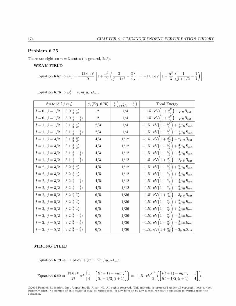
174 CHAPTER 6. TIME-INDEPENDENT PERTURBATION THEORY
Problem 6.26
There are eighteen n = 3 states (in general, 2n2).
WEAK FIELD
Equation 6.67 ⇒ E3j = −13.6 eV9
[1 +
α2
9
(3
j + 1/2− 3
4
)]= −1.51 eV
[1 +
α2
3
(1
j + 1/2− 1
4
)].
Equation 6.76 ⇒ E1z = gJmjµBBext.
State |3 l j mj〉 gJ(Eq. 6.75) 13
(1
j+1/2 − 14
)Total Energy
l = 0, j = 1/2 |3 0 12
12 〉 2 1/4 −1.51 eV
(1 + α2
4
)+ µBBext
l = 0, j = 1/2 |3 0 12 − 1
2 〉 2 1/4 −1.51 eV(1 + α2
4
)− µBBext
l = 1, j = 1/2 |3 1 12
12 〉 2/3 1/4 −1.51 eV
(1 + α2
4
)+ 1
3µBBext
l = 1, j = 1/2 |3 1 12 − 1
2 〉 2/3 1/4 −1.51 eV(1 + α2
4
)− 1
3µBBext
l = 1, j = 3/2 |3 1 32
32 〉 4/3 1/12 −1.51 eV
(1 + α2
12
)+ 2µBBext
l = 1, j = 3/2 |3 1 32
12 〉 4/3 1/12 −1.51 eV
(1 + α2
12
)+ 2
3µBBext
l = 1, j = 3/2 |3 1 32 − 1
2 〉 4/3 1/12 −1.51 eV(1 + α2
12
)− 2
3µBBext
l = 1, j = 3/2 |3 1 32 − 3
2 〉 4/3 1/12 −1.51 eV(1 + α2
12
)− 2µBBext
l = 2, j = 3/2 |3 2 32
32 〉 4/5 1/12 −1.51 eV
(1 + α2
12
)+ 6
5µBBext
l = 2, j = 3/2 |3 2 32
12 〉 4/5 1/12 −1.51 eV
(1 + α2
12
)+ 2
5µBBext
l = 2, j = 3/2 |3 2 32 − 1
2 〉 4/5 1/12 −1.51 eV(1 + α2
12
)− 2
5µBBext
l = 2, j = 3/2 |3 2 32 − 3
2 〉 4/5 1/12 −1.51 eV(1 + α2
12
)− 6
5µBBext
l = 2, j = 5/2 |3 2 52
52 〉 6/5 1/36 −1.51 eV
(1 + α2
36
)+ 3µBBext
l = 2, j = 5/2 |3 2 52
32 〉 6/5 1/36 −1.51 eV
(1 + α2
36
)+ 9
5µBBext
l = 2, j = 5/2 |3 2 52
12 〉 6/5 1/36 −1.51 eV
(1 + α2
36
)+ 3
5µBBext
l = 2, j = 5/2 |3 2 52 − 1
2 〉 6/5 1/36 −1.51 eV(1 + α2
36
)− 3
5µBBext
l = 2, j = 5/2 |3 2 52 − 3
2 〉 6/5 1/36 −1.51 eV(1 + α2
36
)− 9
5µBBext
l = 2, j = 5/2 |3 2 52 − 5
2 〉 6/5 1/36 −1.51 eV(1 + α2
36
)− 3µBBext
STRONG FIELD
Equation 6.79 ⇒ −1.51 eV + (ml + 2ms)µBBext;
Equation 6.82 ⇒ 13.6 eV27
α2
14−
[l(l + 1)−mlms
l(l + 1/2)(l + 1)
]= −1.51 eV
α2
3
[l(l + 1)−mlms
l(l + 1/2)(l + 1)− 1
4
].
c©2005 Pearson Education, Inc., Upper Saddle River, NJ. All rights reserved. This material is protected under all copyright laws as theycurrently exist. No portion of this material may be reproduced, in any form or by any means, without permission in writing from thepublisher.
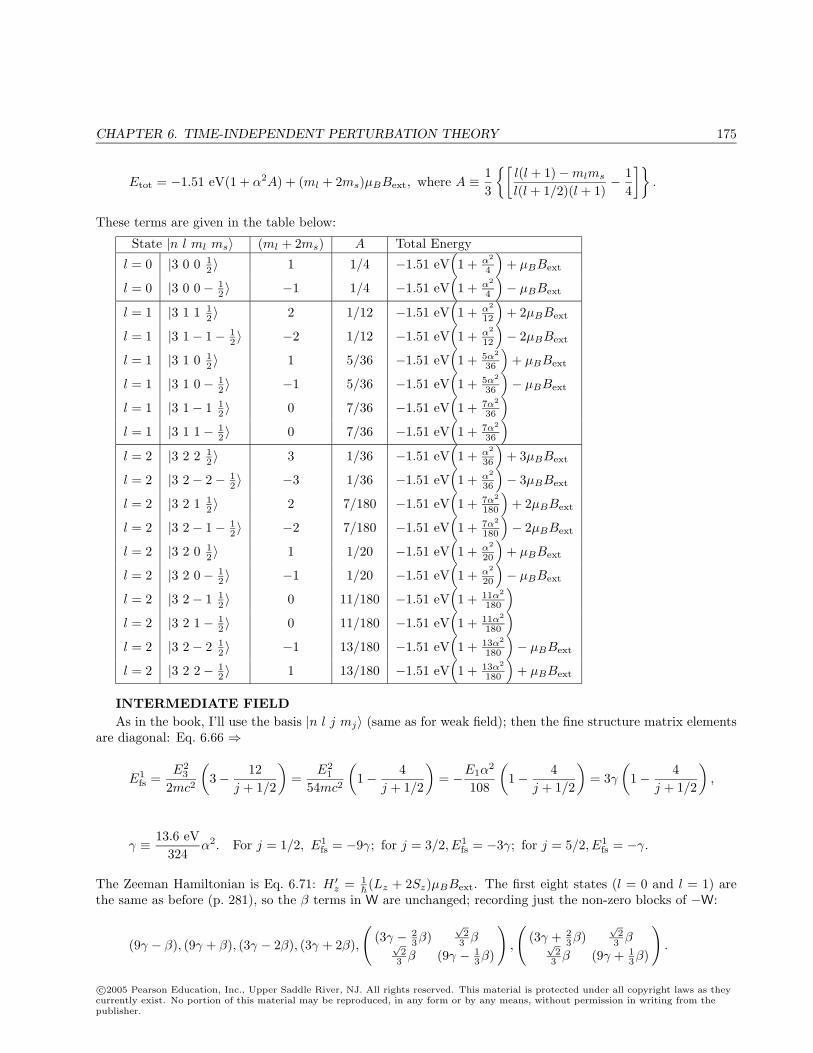
CHAPTER 6. TIME-INDEPENDENT PERTURBATION THEORY 175
Etot = −1.51 eV(1 + α2A) + (ml + 2ms)µBBext, where A ≡ 13
[l(l + 1)−mlms
l(l + 1/2)(l + 1)− 1
4
].
These terms are given in the table below:
State |n l ml ms〉 (ml + 2ms) A Total Energy
l = 0 |3 0 0 12 〉 1 1/4 −1.51 eV
(1 + α2
4
)+ µBBext
l = 0 |3 0 0− 12 〉 −1 1/4 −1.51 eV
(1 + α2
4
)− µBBext
l = 1 |3 1 1 12 〉 2 1/12 −1.51 eV
(1 + α2
12
)+ 2µBBext
l = 1 |3 1− 1− 12 〉 −2 1/12 −1.51 eV
(1 + α2
12
)− 2µBBext
l = 1 |3 1 0 12 〉 1 5/36 −1.51 eV
(1 + 5α2
36
)+ µBBext
l = 1 |3 1 0− 12 〉 −1 5/36 −1.51 eV
(1 + 5α2
36
)− µBBext
l = 1 |3 1− 1 12 〉 0 7/36 −1.51 eV
(1 + 7α2
36
)l = 1 |3 1 1− 1
2 〉 0 7/36 −1.51 eV(1 + 7α2
36
)l = 2 |3 2 2 1
2 〉 3 1/36 −1.51 eV(1 + α2
36
)+ 3µBBext
l = 2 |3 2− 2− 12 〉 −3 1/36 −1.51 eV
(1 + α2
36
)− 3µBBext
l = 2 |3 2 1 12 〉 2 7/180 −1.51 eV
(1 + 7α2
180
)+ 2µBBext
l = 2 |3 2− 1− 12 〉 −2 7/180 −1.51 eV
(1 + 7α2
180
)− 2µBBext
l = 2 |3 2 0 12 〉 1 1/20 −1.51 eV
(1 + α2
20
)+ µBBext
l = 2 |3 2 0− 12 〉 −1 1/20 −1.51 eV
(1 + α2
20
)− µBBext
l = 2 |3 2− 1 12 〉 0 11/180 −1.51 eV
(1 + 11α2
180
)l = 2 |3 2 1− 1
2 〉 0 11/180 −1.51 eV(1 + 11α2
180
)l = 2 |3 2− 2 1
2 〉 −1 13/180 −1.51 eV(1 + 13α2
180
)− µBBext
l = 2 |3 2 2− 12 〉 1 13/180 −1.51 eV
(1 + 13α2
180
)+ µBBext
INTERMEDIATE FIELDAs in the book, I’ll use the basis |n l j mj〉 (same as for weak field); then the fine structure matrix elements
are diagonal: Eq. 6.66 ⇒
E1fs =
E23
2mc2
(3− 12
j + 1/2
)=
E21
54mc2
(1− 4
j + 1/2
)= −E1α
2
108
(1− 4
j + 1/2
)= 3γ
(1− 4
j + 1/2
),
γ ≡ 13.6 eV324
α2. For j = 1/2, E1fs = −9γ; for j = 3/2, E1
fs = −3γ; for j = 5/2, E1fs = −γ.
The Zeeman Hamiltonian is Eq. 6.71: H ′z = 1(Lz + 2Sz)µBBext. The first eight states (l = 0 and l = 1) are
the same as before (p. 281), so the β terms in W are unchanged; recording just the non-zero blocks of −W:
(9γ − β), (9γ + β), (3γ − 2β), (3γ + 2β),
((3γ − 2
3β)√
23 β√
23 β (9γ − 1
3β)
),
((3γ + 2
3β)√
23 β√
23 β (9γ + 1
3β)
).
c©2005 Pearson Education, Inc., Upper Saddle River, NJ. All rights reserved. This material is protected under all copyright laws as theycurrently exist. No portion of this material may be reproduced, in any form or by any means, without permission in writing from thepublisher.
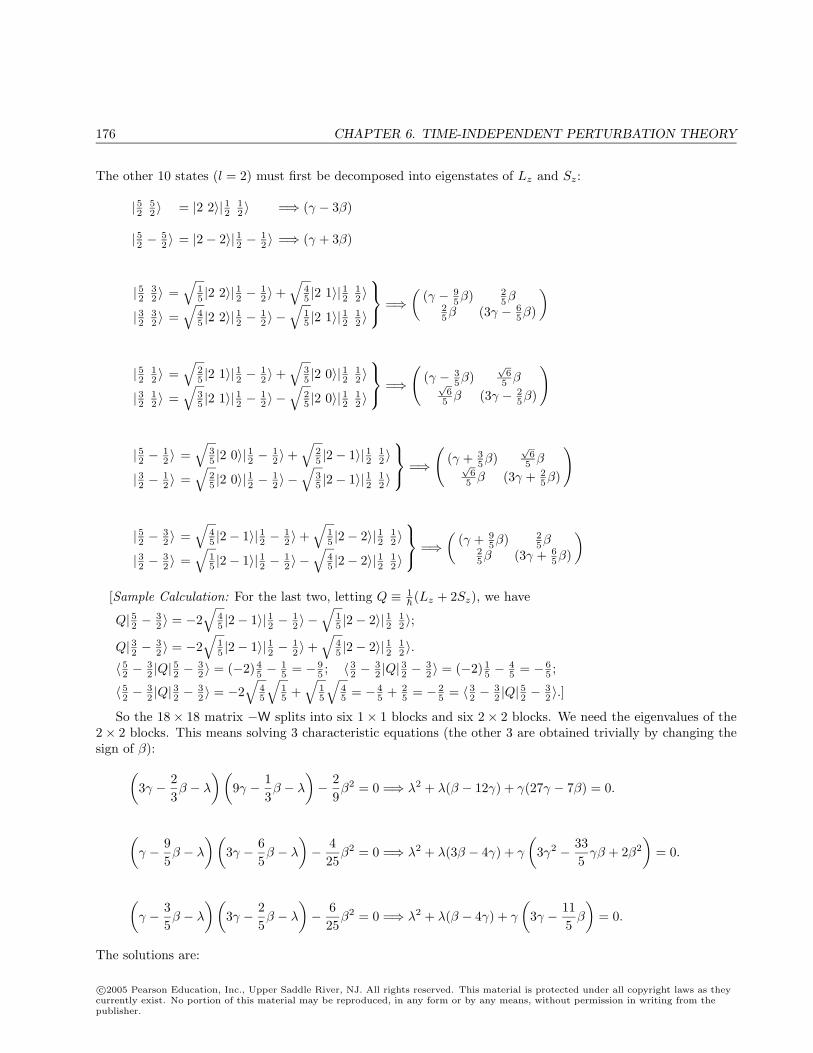
176 CHAPTER 6. TIME-INDEPENDENT PERTURBATION THEORY
The other 10 states (l = 2) must first be decomposed into eigenstates of Lz and Sz:
| 52 52 〉 = |2 2〉| 12 1
2 〉 =⇒ (γ − 3β)
| 52 − 52 〉 = |2− 2〉| 12 − 1
2 〉 =⇒ (γ + 3β)
| 52 32 〉 =
√15 |2 2〉| 12 − 1
2 〉+√
45 |2 1〉| 12 1
2 〉| 32 3
2 〉 =√
45 |2 2〉| 12 − 1
2 〉 −√
15 |2 1〉| 12 1
2 〉
=⇒(
(γ − 95β) 2
5β25β (3γ − 6
5β)
)
| 52 12 〉 =
√25 |2 1〉| 12 − 1
2 〉+√
35 |2 0〉| 12 1
2 〉| 32 1
2 〉 =√
35 |2 1〉| 12 − 1
2 〉 −√
25 |2 0〉| 12 1
2 〉
=⇒(
(γ − 35β)
√6
5 β√6
5 β (3γ − 25β)
)
| 52 − 12 〉 =
√35 |2 0〉| 12 − 1
2 〉+√
25 |2− 1〉| 12 1
2 〉| 32 − 1
2 〉 =√
25 |2 0〉| 12 − 1
2 〉 −√
35 |2− 1〉| 12 1
2 〉
=⇒(
(γ + 35β)
√6
5 β√6
5 β (3γ + 25β)
)
| 52 − 32 〉 =
√45 |2− 1〉| 12 − 1
2 〉+√
15 |2− 2〉| 12 1
2 〉| 32 − 3
2 〉 =√
15 |2− 1〉| 12 − 1
2 〉 −√
45 |2− 2〉| 12 1
2 〉
=⇒(
(γ + 95β) 2
5β25β (3γ + 6
5β)
)
[Sample Calculation: For the last two, letting Q ≡ 1(Lz + 2Sz), we have
Q| 52 − 32 〉 = −2
√45 |2− 1〉| 12 − 1
2 〉 −√
15 |2− 2〉| 12 1
2 〉;
Q| 32 − 32 〉 = −2
√15 |2− 1〉| 12 − 1
2 〉+√
45 |2− 2〉| 12 1
2 〉.〈 52 − 3
2 |Q| 52 − 32 〉 = (−2) 4
5 − 15 = − 9
5 ; 〈 32 − 32 |Q| 32 − 3
2 〉 = (−2) 15 − 4
5 = − 65 ;
〈 52 − 32 |Q| 32 − 3
2 〉 = −2√
45
√15 +
√15
√45 = − 4
5 + 25 = − 2
5 = 〈 32 − 32 |Q| 52 − 3
2 〉.]So the 18× 18 matrix −W splits into six 1× 1 blocks and six 2× 2 blocks. We need the eigenvalues of the
2× 2 blocks. This means solving 3 characteristic equations (the other 3 are obtained trivially by changing thesign of β):(
3γ − 23β − λ
) (9γ − 1
3β − λ
)− 2
9β2 = 0 =⇒ λ2 + λ(β − 12γ) + γ(27γ − 7β) = 0.
(γ − 9
5β − λ
) (3γ − 6
5β − λ
)− 4
25β2 = 0 =⇒ λ2 + λ(3β − 4γ) + γ
(3γ2 − 33
5γβ + 2β2
)= 0.
(γ − 3
5β − λ
) (3γ − 2
5β − λ
)− 6
25β2 = 0 =⇒ λ2 + λ(β − 4γ) + γ
(3γ − 11
5β
)= 0.
The solutions are:
c©2005 Pearson Education, Inc., Upper Saddle River, NJ. All rights reserved. This material is protected under all copyright laws as theycurrently exist. No portion of this material may be reproduced, in any form or by any means, without permission in writing from thepublisher.
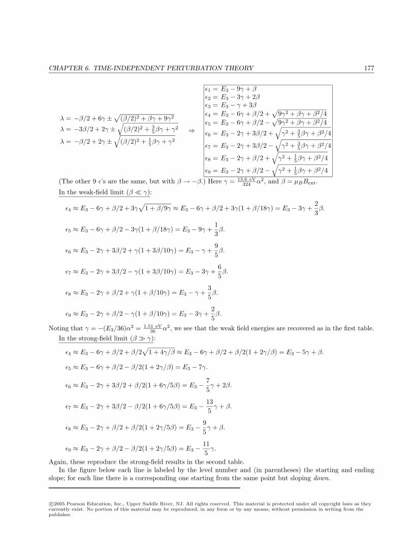
CHAPTER 6. TIME-INDEPENDENT PERTURBATION THEORY 177
λ = −β/2 + 6γ ±√
(β/2)2 + βγ + 9γ2
λ = −3β/2 + 2γ ±√
(β/2)2 + 35βγ + γ2
λ = −β/2 + 2γ ±√
(β/2)2 + 15βγ + γ2
⇒
ε1 = E3 − 9γ + βε2 = E3 − 3γ + 2βε3 = E3 − γ + 3βε4 = E3 − 6γ + β/2 +
√9γ2 + βγ + β2/4
ε5 = E3 − 6γ + β/2−√
9γ2 + βγ + β2/4
ε6 = E3 − 2γ + 3β/2 +√
γ2 + 35βγ + β2/4
ε7 = E3 − 2γ + 3β/2−√
γ2 + 35βγ + β2/4
ε8 = E3 − 2γ + β/2 +√
γ2 + 15βγ + β2/4
ε9 = E3 − 2γ + β/2−√
γ2 + 15βγ + β2/4
(The other 9 ε’s are the same, but with β → −β.) Here γ = 13.6 eV324 α2, and β = µBBext.
In the weak-field limit (β γ):
ε4 ≈ E3 − 6γ + β/2 + 3γ√
1 + β/9γ ≈ E3 − 6γ + β/2 + 3γ(1 + β/18γ) = E3 − 3γ +23β.
ε5 ≈ E3 − 6γ + β/2− 3γ(1 + β/18γ) = E3 − 9γ +13β.
ε6 ≈ E3 − 2γ + 3β/2 + γ(1 + 3β/10γ) = E3 − γ +95β.
ε7 ≈ E3 − 2γ + 3β/2− γ(1 + 3β/10γ) = E3 − 3γ +65β.
ε8 ≈ E3 − 2γ + β/2 + γ(1 + β/10γ) = E3 − γ +35β.
ε9 ≈ E3 − 2γ + β/2− γ(1 + β/10γ) = E3 − 3γ +25β.
Noting that γ = −(E3/36)α2 = 1.51 eV36 α2, we see that the weak field energies are recovered as in the first table.
In the strong-field limit (β γ):
ε4 ≈ E3 − 6γ + β/2 + β/2√
1 + 4γ/β ≈ E3 − 6γ + β/2 + β/2(1 + 2γ/β) = E3 − 5γ + β.
ε5 ≈ E3 − 6γ + β/2− β/2(1 + 2γ/β) = E3 − 7γ.
ε6 ≈ E3 − 2γ + 3β/2 + β/2(1 + 6γ/5β) = E3 −75γ + 2β.
ε7 ≈ E3 − 2γ + 3β/2− β/2(1 + 6γ/5β) = E3 −135γ + β.
ε8 ≈ E3 − 2γ + β/2 + β/2(1 + 2γ/5β) = E3 −95γ + β.
ε9 ≈ E3 − 2γ + β/2− β/2(1 + 2γ/5β) = E3 −115γ.
Again, these reproduce the strong-field results in the second table.In the figure below each line is labeled by the level number and (in parentheses) the starting and ending
slope; for each line there is a corresponding one starting from the same point but sloping down.
c©2005 Pearson Education, Inc., Upper Saddle River, NJ. All rights reserved. This material is protected under all copyright laws as theycurrently exist. No portion of this material may be reproduced, in any form or by any means, without permission in writing from thepublisher.
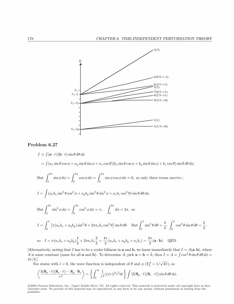
178 CHAPTER 6. TIME-INDEPENDENT PERTURBATION THEORY
E
Ε3
Ε3
Ε3−3γ
−γΕ3
−9γ
3(3)
6(9/5−> 2)
8(3/5−>1)2(2)7(6/5−>1)4(2/5−>1)
9(2/5−>0)
1(1)
5(1/3−>0)
Problem 6.27
I ≡∫
(a · r)(b · r) sin θ dθ dφ
=∫
(ax sin θ cosφ + ay sin θ sinφ + az cos θ)(bx sin θ cosφ + by sin θ sinφ + bz cos θ) sin θ dθ dφ.
But∫ 2π
0
sinφdφ =∫ 2π
0
cosφdφ =∫ 2π
0
sinφ cosφdφ = 0, so only three terms survive :
I =∫
(axbx sin2 θ cos2 φ + ayby sin2 θ sin2 φ + azbz cos2 θ) sin θ dθ dφ.
But∫ 2π
0
sin2 φdφ =∫ 2π
0
cos2 φdφ = π,
∫ 2π
0
dφ = 2π, so
I =∫ π
0
[π(axbx + ayby) sin2 θ + 2πazbz cos2 θ
]sin θ dθ. But
∫ π
0
sin3 θ dθ =43,
∫ π
0
cos2 θ sin θ dθ =23,
so I = π(axbx + ayby)43
+ 2πazbz23
=4π3
(axbx + ayby + azbz) =4π3
(a · b). QED
[Alternatively, noting that I has to be a scalar bilinear in a and b, we know immediately that I = A(a·b), whereA is some constant (same for all a and b). To determine A, pick a = b = k; then I = A =
∫cos2 θ sin θ dθ dφ =
4π/3.]For states with l = 0, the wave function is independent of θ and φ (Y 0
0 = 1/√
4π), so⟨3(Sp · r)(Se · r)− Sp · Se
r3
⟩=
∫ ∞0
1r3|ψ(r)|2r2dr
∫[3(Sp · r)(Se · r)] sin θ dθ dφ.
c©2005 Pearson Education, Inc., Upper Saddle River, NJ. All rights reserved. This material is protected under all copyright laws as theycurrently exist. No portion of this material may be reproduced, in any form or by any means, without permission in writing from thepublisher.
CHAPTER 6. TIME-INDEPENDENT PERTURBATION THEORY 179
The first angular integral is 3(4π/3)(Sp · Se) = 4π(Sp · Se), while the second is −(Sp · Se)∫
sin θ dθ dφ =−4π(Sp · Se), so the two cancel, and the result is zero. QED [Actually, there is a little sleight-of-hand here,since for l = 0, ψ → constant as r → 0, and hence the radial integral diverges logarithmically at the origin.Technically, the first term in Eq. 6.86 is the field outside an infinitesimal sphere; the delta-function gives thefield inside. For this reason it is correct to do the angular integral first (getting zero) and not worry about theradial integral.]
Problem 6.28
From Eq. 6.89 we see that ∆E ∝(
g
mpmea3
); we want reduced mass in a, but not in mpme (which come from
Eq. 6.85); the notation in Eq. 6.93 obscures this point.
(a) g and mp are unchanged; me → mµ = 207me, and a→ aµ. From Eq. 4.72, a ∝ 1/m, so
a
aµ=
mµ(reduced)me
=mµmp
mµ + mp· 1me
=207
1 + 207(me/mp)=
207
1 + 207 (9.11×10⁻³¹)1.67×10⁻²⁷)
=2071.11
= 186.
∆E = (5.88× 10⁻⁶ eV) (1/207) (186)3 = 0.183 eV.
(b) g : 5.59→ 2; mp → me;a
ap=
mp(reduced)me
=m2
e
me + me· 1me
=12.
∆E = (5.88× 10⁻⁶ eV)(
25.59
) (1.67× 10⁻²⁷
9.11× 10⁻³¹
) (12
)3
= 4.82 ×10⁻⁴ eV.
(c) g : 5.59→ 2; mp → mµ;a
am=
mm(reduced)me
=memµ
me + mµ· 1me
=207208
.
∆E = (5.88× 10⁻⁶)(
25.59
) (1.67× 10⁻²⁷
(207)(9.11× 10⁻³¹)
) (207208
)3
= 1.84×10⁻⁵ eV.
Problem 6.29
Use perturbation theory:
H ′ = − e2
4πε0
(1b− 1
r
), for 0 < r < b. ∆E = 〈ψ|H ′|ψ〉, with ψ ≡ 1√
πa3e−r/a.
∆E = − e2
4πε01
πa34π
∫ b
0
(1b− 1
r
)e−2r/ar2dr = − e2
πε0a3
(1b
∫ b
0
r2e−2r/adr −∫ b
0
re−2r/adr
)
= − e2
πε0a3
1b
[− a
2r2e−2r/a + a
(a
2
)2
e−2r/a
(− 2r
a− 1
)]−
[(a
2
)2
e−2r/a
(− 2r
a− 1
)]∣∣∣∣∣b
0
= − e2
πε0a3
[− a
2bb2e−2b/a +
a3
4be−2b/a
(− 2b
a− 1
)− a2
4e−2b/a
(− 2b
a− 1
)+
a3
4b− a2
4
]= − e2
πε0a3
[e−2b/a
(− ab
2− a2
2− a3
4b+
ab
2+
a2
4
)+
a2
4
(a
b− 1
)]= − e2
πε0a3
[e−2b/a
(− a2
4
)(a
b+ 1
)+
a2
4
(a
b− 1
)]=
e2
4πε0a
[(1− a
b
)+
(1 +
a
b
)e−2b/a
].
c©2005 Pearson Education, Inc., Upper Saddle River, NJ. All rights reserved. This material is protected under all copyright laws as theycurrently exist. No portion of this material may be reproduced, in any form or by any means, without permission in writing from thepublisher.
180 CHAPTER 6. TIME-INDEPENDENT PERTURBATION THEORY
Let +2b/a = ε (very small). Then the term in square brackets is:(1− 2
ε
)+
(1 +
2ε
)(1− ε +
ε2
2− ε3
6+ · · ·
)= 1−
2ε
+ 1 +2ε− ε− 2 +
ε2
2+ ε−
ε3
6− ε2
3+ ( )ε3 + · · · = ε2
6+ ( )ε3 + ( )ε4 · · ·
To leading order, then, ∆E =e2
4πε01a
4b2
6a2.
E = E1 = − me4
2(4πε0)22; a =
4πε02
me2; so Ea = − e2
2(4πε0).
∆E
E=
e2
4πε0
(− 2(4πε0)
e2
)2b2
3a2= −4
3
(b
a
)2
.
Putting in a = 5× 10⁻¹¹ m:
∆E
E= −4
3
(10−15
5× 10⁻¹¹
)= −16
3× 10⁻¹⁰ ≈ −5× 10⁻¹⁰.
By contrast,
fine structure: ∆E/E ≈ α2 = (1/137)2 = 5× 10⁻⁵,hyperfine structure: ∆E/E ≈ (me/mp)α2 = (1/1800)(1/137)2 = 3× 10⁻⁸.
So the correction for the finite size of the nucleus is much smaller (about 1% of hyperfine).
Problem 6.30
(a) In terms of the one-dimensional harmonic oscillator states ψn(x), the unperturbed ground state is
|0〉 = ψ0(x)ψ0(y)ψ0(z).
E10 = 〈0|H ′|0〉 = 〈ψ0(x)ψ0(y)ψ0(z)|λx2yz|ψ0(x)ψ0(y)ψ0(z)〉 = λ〈x2〉0〈y〉0〈z〉0.
But 〈y〉0 = 〈z〉0 = 0. So there is no change, in first order.
(b) The (triply degenerate) first excited states are|1〉 = ψ0(x)ψ0(y)ψ1(z)|2〉 = ψ0(x)ψ1(y)ψ0(z)|3〉 = ψ1(x)ψ0(y)ψ0(z)
In this basis the perturbation matrix is Wij = 〈i|H ′|j〉, i = 1, 2, 3.
〈1|H ′|1〉 = 〈ψ0(x)ψ0(y)ψ1(z)|λx2yz|ψ0(x)ψ0(y)ψ1(z)〉 = λ〈x2〉0〈y〉0〈z〉1 = 0,
〈2|H ′|2〉 = 〈ψ0(x)ψ1(y)ψ0(z)|λx2yz|ψ0(x)ψ1(y)ψ0(z)〉 = λ〈x2〉0〈y〉1〈z〉0 = 0,
〈3|H ′|3〉 = 〈ψ1(x)ψ0(y)ψ0(z)|λx2yz|ψ1(x)ψ0(y)ψ0(z)〉 = λ〈x2〉1〈y〉0〈z〉0 = 0,
〈1|H ′|2〉 = 〈ψ0(x)ψ0(y)ψ1(z)|λx2yz|ψ0(x)ψ1(y)ψ0(z)〉 = λ〈x2〉0〈0|y|1〉〈1|z|0〉
= λ
2mω|〈0|x|1〉|2 = λ
(
2mω
)2
[using Problems 2.11 and 3.33].
〈1|H ′|3〉 = 〈ψ0(x)ψ0(y)ψ1(z)|λx2yz|ψ1(x)ψ0(y)ψ0(z)〉 = λ〈0|x2|1〉〈y〉0〈1|z|0〉 = 0,
〈2|H ′|3〉 = 〈ψ0(x)ψ1(y)ψ0(z)|λx2yz|ψ1(x)ψ0(y)ψ0(z)〉 = λ〈0|x2|1〉〈1|y|0〉0〈z〉0 = 0.
c©2005 Pearson Education, Inc., Upper Saddle River, NJ. All rights reserved. This material is protected under all copyright laws as theycurrently exist. No portion of this material may be reproduced, in any form or by any means, without permission in writing from thepublisher.
CHAPTER 6. TIME-INDEPENDENT PERTURBATION THEORY 181
W =
0 a 0a 0 00 0 0
, where a ≡ λ
(
2mω
)2
.
Eigenvalues of W :
∣∣∣∣∣∣−E a 0a −E 00 0 −E
∣∣∣∣∣∣ = −E3 + Ea2 = 0⇒ E = 0,±a = 0, ±λ
(
2mω
)2
.
Problem 6.31
(a) The first term is the nucleus/nucleus interaction, the second is the interaction between the nucleus ofatom 2 and the electron in atom 1, the third is between nucleus 1 and electron 2, and the last term is theinteraction between the electrons.
1R− x
=1R
(1− x
R
)−1
=1R
[1 +
( x
R
)+
( x
R
)2
+ . . .
],
so
H ′ ∼= 14πε0
e2
R
1−
[1 +
(x1
R
)+
(x1
R
)2]−
[1−
(x2
R
)+
(x2
R
)2]
+
[1 +
(x1 − x2
R
)+
(x1 − x2
R
)2]
≈ 14πε0
e2
R
(−2x1x2
R2
)= − e2x1x2
2πε0R3.
(b) Expanding Eq. 6.99:
H =1
2m(p2+ + p2
−)
+12k
(x2
+ + x2−
)− e2
4πε0R3
(x2
+ − x2−
)=
12m
(p21 + p2
2
)+
12k
(x2
1 + x22
)− e2
4πε0R3(2x1x2) = H0 + H ′ (Eqs. 6.96 and 6.98).
(c)
ω± =
√k
m
(1∓ e2
2πε0R3k
)1/2
∼= ω0
[1∓ 1
2
(e2
2πε0R3mω20
)− 1
8
(e2
2πε0R3mω20
)2
+ . . .
].
∆V ∼= 12ω0
[1− 1
2
(e2
2πε0R3mω20
)− 1
8
(e2
2πε0R3mω20
)2
+
1 +12
(e2
2πε0R3mω20
)− 1
8
(e2
2πε0R3mω20
)2 ]− ω0
=1
2ω0
(−1
4
) (e2
2πε0R3mω20
)2
= −18
m2ω30
(e2
2πε0
)2 1R6
.
(d) In first order:
E10 = 〈0|H ′|0〉 = − e2
2πε0R3〈ψ0(x1)ψ0(x2)|x1x2|ψ0(x1)ψ0(x2)〉 = − e2
2πε0R3〈x〉0〈x〉0 = 0.
c©2005 Pearson Education, Inc., Upper Saddle River, NJ. All rights reserved. This material is protected under all copyright laws as theycurrently exist. No portion of this material may be reproduced, in any form or by any means, without permission in writing from thepublisher.
182 CHAPTER 6. TIME-INDEPENDENT PERTURBATION THEORY
In second order:
E20 =
∞∑n=1
|〈ψn|H ′|ψ0〉|2E0 − En
. Here |ψ0〉 = |0〉|0〉, |ψn〉 = |n1〉|n2〉, so
=(
e2
2πε0R3
)2 ∞∑n1=1
∞∑n2=1
|〈n1|x1|0〉|2 |〈n2|x2|0〉|2E0,0 − En1,n2
[use Problem 3.33]
=(
e2
2πε0R3
)2 |〈1|x|0〉|2 |〈1|x|0〉|2( 12ω0 + 1
2ω0)− ( 32ω0 + 3
2ω0)[zero unless n1 = n2 = 1]
=(
e2
2πε0R3
)2 (− 1
2ω0
) (
2mω0
)2
= −
8m2ω30
(e2
2πε0
)2 1R6
.
Problem 6.32
(a) Let the unperturbed Hamiltonian be H(λ0), for some fixed value λ0. Now tweak λ to λ0 + dλ. Theperturbing Hamiltonian is H ′ = H(λ0 + dλ)−H(λ0) = (∂H/∂λ) dλ (derivative evaluated at λ0).
The change in energy is given by Eq. 6.9:
dEn = E1n = 〈ψ0
n|H ′|ψ0n〉 = 〈ψn|
∂H
∂λ|ψn〉 dλ (all evaluated at λ0); so
∂En
∂λ= 〈ψn|
∂H
∂λ|ψn〉.
[Note: Even though we used perturbation theory, the result is exact, since all we needed (to calculate thederivative) was the infinitesimal change in En.]
(b) En = (n + 12 )ω; H = −
2
2md2
dx2+
12mω2x2.
(i)
∂En
∂ω= (n +
12);
∂H
∂ω= mωx2; so F-H ⇒ (n +
12) = 〈n|mωx2|n〉. But
V =12mω2x2, so 〈V 〉 = 〈n|1
2mω2x2|n〉 =
12ω(n +
12); 〈V 〉 = 1
2 (n + 12 )ω.
(ii)
∂En
∂= (n +
12)ω;
∂H
∂= −
m
d2
dx2=
2
(−
2
2md2
dx2
)=
2T ;
so F-H ⇒ (n +12)ω =
2〈n|T |n〉, or 〈T 〉 = 1
2 (n + 12 )ω.
(iii)
∂En
∂m= 0;
∂H
∂m=
2
2m2
d2
dx2+
12ω2x2 = − 1
m
(−
2
2md2
dx2
)+
1m
(12mω2x2
)= − 1
mT +
1m
V.
So F-H ⇒ 0 = − 1m〈T 〉+
1m〈V 〉, or 〈T 〉 = 〈V 〉. These results are consistent with what we found in
Problems 2.12 and 3.31.
c©2005 Pearson Education, Inc., Upper Saddle River, NJ. All rights reserved. This material is protected under all copyright laws as theycurrently exist. No portion of this material may be reproduced, in any form or by any means, without permission in writing from thepublisher.
CHAPTER 6. TIME-INDEPENDENT PERTURBATION THEORY 183
Problem 6.33
(a)
∂En
∂e= − 4me3
32π2ε202(jmax + l + 1)2
=4eEn;
∂H
∂e= − 2e
4πε01r. So the F-H theorem says:
4eEn = − e
2πε0
⟨1r
⟩, or
⟨1r
⟩= −8πε0
e2En = −8πε0E1
e2n2= −8πε0
e2
[− m
22
(e2
4πε0
)2]
1n2
=e2m
4πε02
1n2
.
But4πε02
me2= a (by Eq. 4.72), so
⟨1r
⟩=
1n2a
. (Agrees with Eq. 6.55.)
(b)
∂En
∂l=
2me4
32π2ε202(jmax + l + 1)3
= −2En
n;
∂H
∂l=
2
2mr2(2l + 1); so F-H says
−2En
n=
2(2l + 1)2m
⟨1r2
⟩, or
⟨1r2
⟩= − 4mEn
n(2l + 1)2= − 4mE1
n3(2l + 1)2.
But − 4mE1
2=
2a2
, so⟨
1r2
⟩=
1n3(l + 1
2 )a2. (Agrees with Eq. 6.56.)
Problem 6.34
Equation 4.53 ⇒ u′′ =[l(l + 1)
r2− 2mEn
2− 2m2
(e2
4πε0
)1r
]u.
Butme2
4πε02=
1a
(Eq. 4.72), and − 2mEn
2=
2m2
m
22
(e2
4πε0
)2 1n2
=1
a2n2. So
u′′ =[l(l + 1)
r2− 2
ar+
1n2a2
]u.
∴∫
(ursu′′) dr =∫
urs
[l(l + 1)
r2− 2
ar+
1n2a2
]u dr = l(l + 1)〈rs−2〉 − 2
a〈rs−1〉+
1n2a2
〈rs〉
= −∫
d
dr(urs)u′ dr = −
∫(u′rsu′) dr − s
∫(urs−1u′) dr.
c©2005 Pearson Education, Inc., Upper Saddle River, NJ. All rights reserved. This material is protected under all copyright laws as theycurrently exist. No portion of this material may be reproduced, in any form or by any means, without permission in writing from thepublisher.
184 CHAPTER 6. TIME-INDEPENDENT PERTURBATION THEORY
Lemma 1:∫
(ursu′) dr = −∫
d
dr(urs)u dr = −
∫(u′rsu) dr − s
∫urs−1u dr ⇒
2∫
(ursu′) dr = −s〈rs−1〉, or∫
(ursu′) dr = −s
2〈rs−1〉.
Lemma 2:∫
(u′′rs+1u′) dr = −∫
u′d
dr(rs+1u′) dr = −(s + 1)
∫(u′rsu′) dr −
∫(u′rs+1u′′) dr.
2∫
(u′′rs+1u′) dr = −(s + 1)∫
(u′rsu′) dr, or:∫
(u′rsu′) dr = − 2s + 1
∫(u′′rs+1u′) dr.
Lemma 3: Use in Lemma 2, and exploit Lemma 1:
∫(u′rsu′) dr = − 2
s + 1
∫ [l(l + 1)
r2− 2
ar+
1n2a2
](urs+1u′) dr
= − 2s + 1
[l(l + 1)
∫(urs−1u′) dr − 2
a
∫(ursu′) dr +
1n2a2
∫(urs+1u′) dr
]= − 2
s + 1
[l(l + 1)
(−s− 1
2〈rs−2〉
)− 2
a
(−s
2〈rs−1〉
)+
1n2a2
(−s + 1
2〈rs〉
)]= l(l + 1)
(s− 1s + 1
)〈rs−2〉 − 2
a
(s
s + 1
)〈rs−1〉+
1n2a2
〈rs〉.
Plug Lemmas 1 and 3 into :
l(l + 1)〈rs−2〉 − 2a〈rs−1〉+
1n2a2
〈rs〉
= −l(l + 1)(s− 1s + 1
)〈rs−2〉+
2a
(s
s + 1
)〈rs−1〉 − 1
n2a2〈rs〉+
s(s− 1)2
〈rs−2〉.
2n2a2
〈rs〉 − 2a
[1 +
s
s + 1
]︸ ︷︷ ︸
2s+1s+1
〈rs−1〉+l(l + 1)
[1 +
s− 1s + 1
]︸ ︷︷ ︸
2ss+1
−s(s− 1)2
〈rs−2〉 = 0.
2(s + 1)n2a2
〈rs〉 − 2a(2s + 1)〈rs−1〉+ 2s
[l2 + l − (s2 − 1)
4
]〈rs−2〉 = 0, or, finally,
(s + 1)n2
〈rs〉 − a(2s + 1)〈rs−1〉+sa2
4(4l2 + 4l + 1︸ ︷︷ ︸
(2l+1)2
−s2)〈rs−2〉 = 0. QED
c©2005 Pearson Education, Inc., Upper Saddle River, NJ. All rights reserved. This material is protected under all copyright laws as theycurrently exist. No portion of this material may be reproduced, in any form or by any means, without permission in writing from thepublisher.
CHAPTER 6. TIME-INDEPENDENT PERTURBATION THEORY 185
Problem 6.35
(a)
1n2〈1〉 − a
⟨1r
⟩+ 0 = 0⇒
⟨1r
⟩=
1n2a
.
2n2〈r〉 − 3a〈1〉+
14
[(2l + 1)2 − 1
]a2
⟨1r
⟩= 0⇒ 2
n2〈r〉 = 3a− l(l + 1)a2 1
n2a=
a
n2
[3n2 − l(l + 1)
].
〈r〉 =a
2[3n2 − l(l + 1)
].
3n2〈r2〉 − 5a〈r〉+
12
[(2l + 1)2 − 4
]a2 = 0⇒ 3
n2〈r2〉 = 5a
a
2[3n2 − l(l + 1)
]− a2
2[(2l + 1)2 − 4
]3n2〈r2〉 =
a2
2[15n2 − 5l(l + 1)− 4l(l + 1)− 1 + 4
]=
a2
2[15n2 − 9l(l + 1) + 3
]=
3a2
2[5n2 − 3l(l + 1) + 1
]; 〈r2〉 =
n2a2
2[5n2 − 3l(l + 1) + 1
].
4n2〈r3〉 − 7a〈r2〉+
34
[(2l + 1)2 − 9
]a2〈r〉 = 0 =⇒
4n2〈r3〉 = 7a
n2a2
2[5n2 − 3l(l + 1) + 1
]− 3
4[4l(l + 1)− 8] a2 a
2[3n2 − l(l + 1)
]=
a3
235n4 − 21l(l + 1)n2 + 7n2 − [3l(l + 1)− 6]
[3n2 − l(l + 1)
]=
a3
2[35n4 − 21l(l + 1)n2 + 7n2 − 9l(l + 1)n2 + 3l2(l + 1)2 + 18n2 − 6l(l + 1)
]=
a3
2[35n4 + 25n2 − 30l(l + 1)n2 + 3l2(l + 1)2 − 6l(l + 1)
].
〈r3〉 =n2a3
8[35n4 + 25n2 − 30l(l + 1)n2 + 3l2(l + 1)2 − 6l(l + 1)
].
(b)
0 + a
⟨1r2
⟩− 1
4[(2l + 1)2 − 1
]a2
⟨1r3
⟩= 0⇒
⟨1r2
⟩= al(l + 1)
⟨1r3
⟩.
(c)
al(l + 1)⟨
1r3
⟩=
1(l + 1/2)n3a2
⇒⟨
1r3
⟩=
1l(l + 1/2)(l + 1)n3a3
. Agrees with Eq. 6.64.
c©2005 Pearson Education, Inc., Upper Saddle River, NJ. All rights reserved. This material is protected under all copyright laws as theycurrently exist. No portion of this material may be reproduced, in any form or by any means, without permission in writing from thepublisher.
186 CHAPTER 6. TIME-INDEPENDENT PERTURBATION THEORY
Problem 6.36
(a)
|1 0 0〉 =1√πa3
e−r/a (Eq. 4.80), E1s = 〈1 0 0|H ′|1 0 0〉 = eEext
1πa3
∫e−2r/a(r cos θ)r2 sin θ dr dθ dφ.
But the θ integral is zero:∫ π
0
cos θ sin θ dθ =sin2 θ
2
∣∣∣∣π0
= 0. So E1s = 0. QED
(b) From Problem 4.11:
|1〉 = ψ2 0 0 =1√2πa
12a
(1− r
2a
)e−r/2a
|2〉 = ψ2 1 1 = − 1√πa
18a2
re−r/2a sin θeiφ
|3〉 = ψ2 1 0 =1√2πa
14a2
re−r/2a cos θ
|4〉 = ψ2 1−1 =1√πa
18a2
re−r/2a sin θe−iφ
〈1|H ′s|1〉 = . . . ∫ π
0
cos θ sin θ dθ = 0
〈2|H ′s|2〉 = . . . ∫ π
0
sin2 θ cos θ sin θ dθ = 0
〈3|H ′s|3〉 = . . . ∫ π
0
cos2 θ cos θ sin θ dθ = 0
〈4|H ′s|4〉 = . . . ∫ π
0
sin2 θ cos θ sin θ dθ = 0
〈1|H ′s|2〉 = . . . ∫ 2π
0
eiφ dφ = 0
〈1|H ′s|4〉 = . . . ∫ 2π
0
e−iφ dφ = 0
〈2|H ′s|3〉 = . . . ∫ 2π
0
e−iφ dφ = 0
〈2|H ′s|4〉 = . . . ∫ 2π
0
e−2iφ dφ = 0
〈3|H ′s|4〉 = . . . ∫ 2π
0
e−iφ dφ = 0
All matrix elements of H ′s are zeroexcept 〈1|H ′s|3〉 and 〈3|H ′s|1〉(which are complex conjugates,so only one needs to be evaluated).
〈1|H ′s|3〉 = eEext1√2πa
12a
1√2πa
14a2
∫ (1− r
2a
)e−r/2are−r/2a cos θ(r cos θ)r2 sin θ dr dθ dφ
=eEext
2πa8a3(2π)
[∫ π
0
cos2 θ sin θ dθ
] ∫ ∞0
(1− r
2a
)e−r/ar4 dr
=eEext
8a4
23
∫ ∞0
r4e−r/a dr − 12a
∫ ∞0
r5e−r/a dr
=
eEext
12a4
(4!a5 − 1
2a5!a6
)=
eEext
12a424a5
(1− 5
2
)= eaEext(−3) = −3aeEext.
W = −3aeEext
0 0 1 00 0 0 01 0 0 00 0 0 0
.
c©2005 Pearson Education, Inc., Upper Saddle River, NJ. All rights reserved. This material is protected under all copyright laws as theycurrently exist. No portion of this material may be reproduced, in any form or by any means, without permission in writing from thepublisher.
CHAPTER 6. TIME-INDEPENDENT PERTURBATION THEORY 187
We need the eigenvalues of this matrix. The characteristic equation is:∣∣∣∣∣∣∣∣−λ 0 1 00 −λ 0 01 0 −λ 00 0 0 −λ
∣∣∣∣∣∣∣∣ = −λ
∣∣∣∣∣∣−λ 0 00 −λ 00 0 −λ
∣∣∣∣∣∣ +
∣∣∣∣∣∣0 −λ 01 0 00 0 −λ
∣∣∣∣∣∣ = −λ(−λ)3 + (−λ2) = λ2(λ2 − 1) = 0.
The eigenvalues are 0, 0, 1, and −1, so the perturbed energies are
E2, E2, E2 + 3aeEext, E2 − 3aeEext. Three levels.
(c) The eigenvectors with eigenvalue 0 are |2〉 =
0100
and |4〉 =
0001
; the eigenvectors with eigenvalues ±1
are |±〉 ≡ 1√2
10±10
. So the “good” states are ψ2 1 1, ψ2 1−1,1√2(ψ2 0 0 + ψ2 1 0),
1√2(ψ2 0 0 − ψ2 1 0).
〈pe〉4 = −e1πa
164a4
∫r2e−r/a sin2 θ
[r sin θ cosφi + r sin θ sinφj + r cos θk
]r2 sin θ dr dθ dφ.
But∫ 2π
0
cosφdφ =∫ 2π
0
sinφdφ = 0,∫ π
0
sin3 θ cos θ dθ =∣∣∣∣ sin4 θ
4
∣∣∣∣π0
= 0, so
〈pe〉4 = 0. Likewise 〈pe〉2 = 0.
〈pe〉± = −12e
∫(ψ1 ± ψ3)2(r)r2 sin θ dr dθ dφ
= −12e
12πa
14a2
∫ [(1− r
2a
)± r
2acos θ
]2
e−r/ar(sin θ cosφ i + sin θ sinφ j + cos θ k)r2 sin θ dr dθ dφ
= −e
2k
2πa1
4a22π
∫ [(1− r
2a
)± r
2acos θ
]2
r3e−r/a cos θ sin θ dr dθ.
But∫ π
0cos θ sin θ dθ =
∫ π
0cos3 θ sin θ dθ = 0, so only the cross-term survives:
〈pe〉± = − e
8a3k
(±1
a
) ∫ (1− r
2a
)r cos θ r3e−r/a cos θ sin θ dr dθ
= ∓( e
8a4k) [∫ π
0
cos2 θ sin θ dθ
] ∫ ∞0
(1− r
2a
)r4e−r/adr = ∓
( e
8a4k) 2
3
[4!a5 − 1
2a5!a6
]= ∓ek
(1
12a4
)24a5
(1− 5
2
)= ±3aek.
Problem 6.37
(a) The nine states are:
c©2005 Pearson Education, Inc., Upper Saddle River, NJ. All rights reserved. This material is protected under all copyright laws as theycurrently exist. No portion of this material may be reproduced, in any form or by any means, without permission in writing from thepublisher.
188 CHAPTER 6. TIME-INDEPENDENT PERTURBATION THEORY
l = 0 : |3 0 0〉 = R30Y00
l = 1 : |3 1 1〉 = R31Y11
|3 1 0〉 = R31Y01
|3 1− 1〉 = R31Y−11
l = 2 : |3 2 2〉 = R32Y22
|3 2 1〉 = R32Y12
|3 2 0〉 = R32Y02
|3 2− 1〉 = R32Y−12
|3 2− 2〉 = R32Y−22
H ′s contains no φ dependence, so the φ integral will be:
〈n lm|H ′s|n′ l′m′〉 = · · · ∫ 2π
0
e−imφeim′φ dφ, which is zero unless m′ = m.
For diagonal elements: 〈n lm|H ′s|n lm〉 = · · · ∫ π
0[Pm
l (cos θ)]2 cos θ sin θ dθ. But (p. 137 in the text)Pm
l is a polynomial (even or odd) in cos θ, multiplied (if m is odd) by sin θ. Since sin2 θ = 1 − cos2 θ,[Pm
l (cos θ)]2 is a polynomial in even powers of cos θ. So the θ integral is of the form∫ π
0
(cos θ)2j+1 sin θ dθ = − (cos θ)2j+2
(2j + 2)
∣∣∣∣π0
= 0. All diagonal elements are zero.
There remain just 4 elements to calculate:
m = m′ = 0 : 〈3 0 0|H ′s|3 1 0〉, 〈3 0 0|H ′s|3 2 0〉, 〈3 1 0|H ′s|3 2 0〉; m = m′ = ±1 : 〈3 1 ± 1|H ′s|3 2 ± 1〉.
〈3 0 0|H ′s|3 1 0〉 = eEext
∫R30R31r
3dr
∫Y 0
0 Y 01 cos θ sin θ dθ dφ. From Table 4.7 :
∫R30R31r
3 dr =2√27
1a3/2
827√
61
a3/2
1a
∫ (1− 2r
3a+
2r2
27a2
)e−r/3a
(1− r
6a
)re−r/3ar3 dr.
Let x ≡ 2r/3a:
∫R30R31r
3 dr =24
35√
2a4
(3a2
)5 ∫ ∞0
(1− x +
x2
6
) (1− x
4
)x4e−xdx
=a
2√
2
∫ ∞0
(1− 5
4x +
512
x2 − 124
x3
)x4e−xdx =
a
2√
2
(4!− 5
45! +
512
6!− 124
7!)
= −9√
2a.∫Y 0
0 Y 01 cos θ sin θ dθ dφ =
1√4π
√34π
∫cos θ cos θ sin θ dθ dφ =
√3
4π2π
∫ π
0
cos3 θ sin θ dθ =√
32
23
=√
33
.
〈3 0 0|H ′s|3 1 0〉 = eEext(−9√
2a)
(√3
3
)= −3
√6aeEext.
〈3 0 0|H ′s|3 2 0〉 = eEext
∫R30R31r
3dr
∫Y 0
0 Y 02 cos θ sin θ dθ dφ.
c©2005 Pearson Education, Inc., Upper Saddle River, NJ. All rights reserved. This material is protected under all copyright laws as theycurrently exist. No portion of this material may be reproduced, in any form or by any means, without permission in writing from thepublisher.
CHAPTER 6. TIME-INDEPENDENT PERTURBATION THEORY 189
∫Y 0
0 Y 02 cos θ sin θ dθ dφ =
1√4π
√5
16π
∫(3 cos2 θ − 1) cos θ sin θ dθ dφ = 0. 〈3 0 0 |H ′s|3 2 0〉 = 0.
〈3 1 0|H ′s|3 2 0〉 = eEext
∫R31R32r
3dr
∫Y 0
1 Y 02 cos θ sin θ dθ dφ.
∫R31R32r
3dr =8
27√
61
a3/2
1a
481√
301
a3/2
1a2
∫ (1− r
6a
)re−r/3ar2e−r/3ar3dr
=24
38√
5a6
(3a2
)7 ∫ ∞0
(1− x
4
)x6e−xdx =
a
24√
5
(6!− 1
47!
)= −9
√5
2a.
∫Y 0
1 Y 02 sin θ cos θ dθ dφ =
√34π
√5
16π
∫cos θ(3 cos2 θ − 1) cos θ sin θ dθ dφ
=√
158π
2π∫ π
0
(3 cos4 θ − cos2 θ) sin θ dθ =√
154
[−3
5cos5 θ +
13
cos3 θ
]∣∣∣∣π0
=2√15
.
〈3 1 0|H ′s|3 2 0〉 = eEext
(−9√
52
a
)(2√15
)= −3
√3aeEext.
〈3 1 ± 1|H ′s|3 2 ± 1〉 = eEext
∫R31R32r
3dr
∫ (Y ±1
1
)∗Y ±1
2 cos θ sin θ dθ dφ.
∫ (Y ±1
1
)∗Y ±1
2 cos θ sin θ dθ dφ =
(∓
√38π
) (∓
√158π
)∫sin θe∓iφ sin θ cos θe±iφ cos θ sin θ dθ dφ
=3√
58π
2π∫ π
0
cos2 θ(1− cos2 θ) sin θ dθ =34
√5
(−cos3 θ
3+
cos5 θ
5
)∣∣∣∣π0
=1√5.
〈3 1 ± 1|H ′s|3 2 ± 1〉 = eEext
(−9√
52
a
)(1√5
)= −9
2aeEext.
Thus the matrix representing H ′s is (all empty boxes are zero; all numbers multiplied by −aeEext):
(b) The perturbing matrix (below) breaks into a 3×3 block, two 2× 2 blocks, and two 1× 1 blocks, so we canwork out the eigenvalues in each block separately.
3× 3 : 3√
3
0√
2 0√2 0 1
0 1 0
;
∣∣∣∣∣∣−λ
√2 0√
2 −λ 10 1 −λ
∣∣∣∣∣∣ = −λ3 + λ + 2λ = −λ(λ2 − 3) = 0;
λ = 0,±√
3 ⇒ E11 = 0, E1
2 = 9aeEext, E13 = −9aeEext.
2× 2 :92
(0 11 0
);
∣∣∣∣−λ 11 −λ
∣∣∣∣ = λ2 − 1 = 0⇒ λ = ±1.
c©2005 Pearson Education, Inc., Upper Saddle River, NJ. All rights reserved. This material is protected under all copyright laws as theycurrently exist. No portion of this material may be reproduced, in any form or by any means, without permission in writing from thepublisher.
190 CHAPTER 6. TIME-INDEPENDENT PERTURBATION THEORY
300 310 320 311 321 31-1 32-1 322 32-2
300
310
320
311
321
31-1
32-1
322
32-2
3√6
3√6
3√3
3√3
9/2
9/2
9/2
9/2
E14 =
92aeEext, E1
5 = −92aeEext. From the other 2×2 we get E1
6 = E14 , E1
7 = E15 , and from the 1×1’s we
get E18 = E1
9 = 0. Thus the perturbations to the energy (E3) are:
0 (degeneracy 3)(9/2)aeEext (degeneracy 2)−(9/2)aeEext (degeneracy 2)9aeEext (degeneracy 1)−9aeEext (degeneracy 1)
Problem 6.38
Equation 6.89 ⇒ E1hf =
µ0gde2
3πmdmea3〈Sd · Se〉; Eq. 6.91⇒ Sd · Se =
12(S2 − S2
e − S2d).
Electron has spin 12 , so S2
e = 12
(32
)
2 = 34
2; deuteron has spin 1, so S2d = 1(2)2 = 22.
Total spin could be 32 [in which case S2 = 3
2
(52
)
2 = 154
2] or 12 [in which case S2 = 3
42]. Thus
〈Sd · Se〉 =
12
(154
2 − 34
2 − 22)
= 12
2
12
(34
2 − 34
2 − 22)
= −2
; the difference is32
2, so ∆E =µ0gde
2
2
2πmdmea3.
But µ0ε0 =1c2⇒ µ0 =
1ε0c2
, so ∆E =2gde
2
2
4πε0mdmec2a3=
2gd4
mdm2ec
2a4=
32gd
gp
mp
md∆Ehydrogen (Eq. 6.98).
Now, λ =c
ν=
ch
∆E, so λd =
23gp
gd
md
mpλh, and since md = 2mp, λd =
43
(5.591.71
)(21 cm) = 92 cm.
Problem 6.39
(a) The potential energy of the electron (charge −e) at (x, y, z) due to q’s at x = ±d alone is:
V = − eq
4πε0
[1√
(x + d)2 + y2 + z2+
1√(x− d)2 + y2 + z2
]. Expanding (with d x, y, z) :
c©2005 Pearson Education, Inc., Upper Saddle River, NJ. All rights reserved. This material is protected under all copyright laws as theycurrently exist. No portion of this material may be reproduced, in any form or by any means, without permission in writing from thepublisher.
CHAPTER 6. TIME-INDEPENDENT PERTURBATION THEORY 191
1√(x± d)2 + y2 + z2
= (x2 ± 2dx + d2 + y2 + z2)−1/2 = (d2 ± 2dx + r2)−1/2 =1d
(1± 2x
d+
r2
d2
)−1/2
≈ 1d
(1∓ x
d− r2
2d2+
38
4x2
d2
)=
1d
[1∓ x
d+
12d2
(3x2 − r2)].
V = − eq
4πε0d
[1− x
d+
12d2
(3x2 − r2) + 1 +x
d+
12d2
(3x2 − r2)]
= − 2eq4πε0d
− eq
4πε0d3(3x2 − r2)
= 2βd2 + 3βx2 − βr2, where β ≡ − e
4πε0q
d3.
Thus with all six charges in place
H ′ = 2(β1d21 + β2d
22 + β3d
23) + 3(β1x
2 + β2y2 + β3z
2)− r2(β1 + β2 + β3). QED
(b) 〈1 0 0|H ′|1 0 0〉 =1
πa3
∫e−2r/aH ′r2 sin θ dr dθ dφ
= V0 +3
πa3
∫e−2r/a(β1x
2 + β2y2 + β3z
2)r2 sin θdr dθ dφ− (β1 + β2 + β3)πa3
∫r2e−2r/ar2 sin θ dr dθ dφ.
I1 ≡∫
r2e−2r/ar2 sin θ dr dθ dφ = 4π∫ ∞
0
r4e−2r/adr = 4π4!(a
2)5 = 3πa5.
I2 ≡∫
e−2r/a(β1x2 + β2y
2 + β3z2)r2 sin θ dr dθ dφ
=∫
r4e−2r/a(β1 sin2 θ cos2 φ + β2 sin2 θ sin2 φ + β3 cos2 θ) sin θ dr dθ dφ.
But∫ 2π
0
cos2 φdφ =∫ 2π
0
sin2 φdφ = π,
∫ 2π
0
dφ = 2π. So
=∫ ∞
0
r4e−2r/adr
∫ π
0
[π(β1 + β2) sin2 θ + 2πβ3 cos2 θ
]sin θ dθ.
But∫ π
0
sin3 θ dθ =43,
∫ π
0
cos2 θ sin θ dθ =23. So
= 4!(a
2
)5[4π3
(β1 + β2) +4π3
β3
]= πa5(β1 + β2 + β3).
〈1 0 0|H ′|1 0 0〉 = V0 +3
πa3πa5(β1 + β2 + β3)−
(β1 + β2 + β3)πa3
3πa5 = V0.
(c) The four states are
|2 0 0〉 = R20Y
00
|2 1 1〉 = R21Y11
|2 1− 1〉 = R21Y−11
|2 1 0〉 = R21Y01
(functional forms in Problem 4.11).
Diagonal elements: 〈n lm|H ′|n lm〉 = V0 + 3(β1〈x2〉+ β2〈y2〉+ β3〈z2〉
)− (β1 + β2 + β3)〈r2〉.
c©2005 Pearson Education, Inc., Upper Saddle River, NJ. All rights reserved. This material is protected under all copyright laws as theycurrently exist. No portion of this material may be reproduced, in any form or by any means, without permission in writing from thepublisher.
192 CHAPTER 6. TIME-INDEPENDENT PERTURBATION THEORY
For |2 0 0〉, 〈x2〉 = 〈y2〉 = 〈z2〉 = 13 〈r2〉 (Y 0
0 does not depend on φ, θ; this state has spherical symmetry),
so 〈2 0 0|H ′|2 0 0〉 = V0. (I could have used the same argument in (b).)
From Problem 6.35(a), 〈r2〉 =n2a2
2[5n2 − 3l(l + 1) + 1
], so for n = 2, l = 1 : 〈r2〉 = 30a2. Moreover,
since 〈x2〉 = . . . ∫ 2π
0
cos2 φdφ = . . . ∫ 2π
0
sin2 φdφ = 〈y2〉, and 〈x2〉 + 〈y2〉 + 〈z2〉 = 〈r2〉, it follows
that 〈x2〉 = 〈y2〉 =12(〈r2〉 − 〈z2〉) = 15a2 − 1
2〈z2〉. So all we need to calculate is 〈z2〉.
〈2 1 0|z2|2 1 0〉 =1
2πa1
16a4
∫r2e−r/a cos2 θ(r2 cos2 θ)r2 sin θ dr dθ dφ
=1
16a5
∫ ∞0
r6e−r/adr
∫ π
0
cos4 θ sin θ dθ =1
16a56!a7 2
5= 18a2; 〈x2〉 = 〈y2〉 = 15a2 − 9a2 = 6a2.
〈2 1 0|H ′|2 1 0〉 = V0 + 3(6a2β1 + 6a2β2 + 18a2β3)− 30a2(β1 + β2 + β3)
= V0 − 12a2(β1 + β2 + β3) + 36a2β3.
〈2 1 ± 1|z2|2 1 ± 1〉 =1πa
164a4
∫r2e−r/a sin2 θ(r2 cos2 θ)r2 sin θ dr dθ dφ
=1
32a5
∫ ∞0
r6e−r/adr
∫ π
0
(1− cos2 θ) cos2 θ sin θ dθ =1
32a56!a7
(23− 2
5
)= 6a2;
〈x2〉 = 〈y2〉 = 15a2 − 3a2 = 12a2.
〈2 1 ± 1|H ′|2 1 ± 1〉 = V0 + 3(12a2β1 + 12a2β2 + 6a2β3)− 30a2(β1 + β2 + β3)
= V0 + 6a2(β1 + β2 + β3)− 18a2β3.
Off-diagonal elements: We need 〈2 0 0|H ′|2 1 0〉, 〈2 0 0|H ′|2 1±1〉, 〈2 1 0|H ′|2 1±1〉, and 〈2 1−1|H ′|2 1 1〉.Now 〈n lm|V0|n′ l′m′〉 = 0, by orthogonality, and 〈n lm|r2|n′ l′m′〉 = 0, by orthogonality of Y m
l , soall we need are the matrix elements of x2 and y2 (〈|z2|〉 = −〈|x2|〉 − 〈|y2〉). For 〈2 0 0|x2|2 1 ± 1〉 and〈2 1 0|x2|2 1 ± 1〉 the φ integral is
∫ 2π
0cos2 φe±iφ dφ =
∫ 2π
0cos3 φdφ ± i
∫ 2π
0cos2 φ sinφdφ = 0, and the
same goes for y2. So 〈2 0 0|H ′|2 1± 1〉 = 〈2 1 0|H ′|2 1± 1〉 = 0.
For 〈2 0 0|x2|2 1 0〉 and 〈2 0 0|y2|2 1 0〉 the θ integral is∫ π
0cos θ(sin2 θ) sin θ dθ = sin4 θ/4
∣∣π0
= 0, so
〈2 0 0|H ′|2 1 0〉 = 0. Finally:
〈2 1− 1|x2|2 1 1〉 = − 1πa
164a4
∫r2e−r/a sin2 θe2iφ(r2 sin2 θ cos2 φ)r2 sin θ dr dθ dφ
= − 164πa5
∫ ∞0
r6e−r/adr︸ ︷︷ ︸6!a7
∫ π
0
sin5 θdθ︸ ︷︷ ︸16/15
∫ 2π
0
e2iφ cos2 φdφ︸ ︷︷ ︸π/2
= − 164πa5
6!a7 1615
π
2= −6a2.
c©2005 Pearson Education, Inc., Upper Saddle River, NJ. All rights reserved. This material is protected under all copyright laws as theycurrently exist. No portion of this material may be reproduced, in any form or by any means, without permission in writing from thepublisher.
CHAPTER 6. TIME-INDEPENDENT PERTURBATION THEORY 193
For y2, the φ integral is∫ 2π
0e2iφ sin2 φdφ = −π/2, so 〈2 1 − 1|y2|2 1 1〉 = 6a2, and 〈2 1− 1|z2|2 1 1〉 = 0.
〈2 1− 1|H ′|2 1 1〉 = 3[β1(−6a2) + β2(6a2)
]= −18a2(β1 − β2).
The perturbation matrix is:
2 0 0 2 1 0 2 1 1 2 1 -12 0 0 V0 0 0 02 1 0 0 V0 − 12a2(β1 + β2) + 24a2β3 0 02 1 1 0 0 V0 + 6a2(β1 + β2)− 12a2β3 −18a2(β1 − β2)2 1 -1 0 0 −18a2(β1 − β2) V0 + 6a2(β1 + β2)− 12a2β3
The 2×2 block has the form(
A BB A
); its characteristic equation is (A−λ)2−B2 = 0, so A−λ = ±B,
or
λ = A∓B = V0 + 6a2(β1 + β2)− 12a2β3 ± 18a2(β1 − β2) =
V0 + 24a2β1 − 12a2β2 − 12a2β3,V0 − 12a2β1 + 24a2β2 − 12a2β3.
The first-order corrections to the energy (E2) are therefore:
ε1 = V0
ε2 = V0 − 12a2(β1 + β2 − 2β3)ε3 = V0 − 12a2(−2β1 + β2 + β3)ε4 = V0 − 12a2(β1 − 2β2 + β3)
(i) If β1 = β2 = β3, then ε1 = ε2 = ε3 = ε4 = V0: one level (still 4-fold degenerate).
(ii) If β1 = β2 = β3, then ε1 = V0, ε2 = V0 − 24a2(β1 − β3), ε3 = ε4 = V0 + 12a2(β1 − β3): three levels(one remains doubly degenerate).
(iii) If all three β’s are different, there are four levels (no remaining degeneracy).
Problem 6.40
(a) (i) Equation 6.10: (H0 − E00)ψ1
0 = −(H ′ − E10)ψ0
0 .
H0 = − 2
2m∇2 − e2
4πε01r
= − 2
2m
(∇2 +
2ar
), since a =
4πε02
me2.
E00 = −
2
2ma2.
H ′ = eEextr cos θ; E10 = 0 (Problem6.36(a)).
ψ00 =
1√πa3
e−r/a; ψ10 = f(r)e−r/a cos θ.
c©2005 Pearson Education, Inc., Upper Saddle River, NJ. All rights reserved. This material is protected under all copyright laws as theycurrently exist. No portion of this material may be reproduced, in any form or by any means, without permission in writing from thepublisher.
194 CHAPTER 6. TIME-INDEPENDENT PERTURBATION THEORY
Equation 4.13 ⇒
∇2ψ10 =
cos θr2
d
dr
[r2 d
dr
(fe−r/a
)]+
fe−r/a
r2 sin θ
d
dθ
[sin θ
d
dθ(cos θ)
]=
cos θr2
d
dr
[r2
(f ′ − 1
af
)e−r/a
]+
fe−r/a
r2 sin θ
d
dθ
[− sin2 θ
]=
cos θr2
[2r
(f ′ − 1
af
)e−r/a + r2
(f ′′ − 2
af ′ +
1a2
f
)e−r/a
]− 2 cos θ
r2fe−r/a
= cos θe−r/a
[(f ′′ − 2
af ′ +
1a2
f
)+ 2
(f ′ − 1
af
)1r− 2f
1r2
].
Plug this into Eq. 6.10:
− 2
2mcos θe−r/a
[(f ′′ − 2
af ′ +
1a2
f
)+ 2
(f ′ − 1
af
)1r− 2f
1r2
+ 2f1a
1r− f
1a2
]= −eEextr cos θ
1√πa3
e−r/a,
(f ′′ − 2
af ′
)+ 2f ′
1r− 2f
1r2
=(
2meEext
2√πa3
)r =
4γa
r, where γ ≡ meEext
22√πa
.
Now let f(r) = A + Br + Cr2, so f ′ = B + 2Cr and f ′′ = 2C. Then
2C − 2a(B + 2Cr) +
2r(B + 2Cr)− 2
r2(A + Br + Cr2) =
4γa
r.
Collecting like powers of r:
r−2 : A = 0.r−1 : 2B − 2B = 0 (automatic).r0 : 2C − 2B/a + 4C − 2C = 0⇒ B = 2aC.
r1 : −4C/a = 4γ/a⇒ C = −γ.
Evidently the function suggested does satisfy Eq. 6.10, with the coefficients A = 0, B = −2aγ, C = −γ;the second-order correction to the wave function is
ψ10 = −γr(r + 2a)e−r/a cos θ.
(ii) Equation 6.11 says, in this case:
E20 = 〈ψ0
0 |H ′|ψ10〉 = − 1√
πa3
meEext
22√πa
eEext
∫e−r/a(r cos θ)r(r + 2a)e−r/a cos θ r2 sin θ dr dθ dφ
= −m(eEext)2
2πa222π
∫ ∞0
r4(r + 2a)e−2r/adr
∫ π
0
cos2 θ sin θ dθ
= −m
(eEext
a
)2 [5!
(a
2
)6
+ 2a 4!(a
2
)5] (−cos3 θ
3
) ∣∣∣∣π0
= −m
(eEext
a
)2 (278a6
)23
= −m
(3eEexta
2
2
)2
.
c©2005 Pearson Education, Inc., Upper Saddle River, NJ. All rights reserved. This material is protected under all copyright laws as theycurrently exist. No portion of this material may be reproduced, in any form or by any means, without permission in writing from thepublisher.
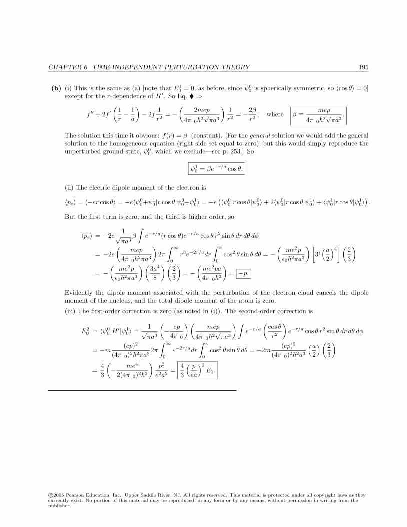
CHAPTER 6. TIME-INDEPENDENT PERTURBATION THEORY 195
(b) (i) This is the same as (a) [note that E10 = 0, as before, since ψ0
0 is spherically symmetric, so 〈cos θ〉 = 0]except for the r-dependence of H ′. So Eq. ⇒
f ′′ + 2f ′(
1r− 1
a
)− 2f
1r2
= −(
2mep
4πε02√πa3
)1r2
= −2βr2
, where β ≡ mep
4πε02√πa3
.
The solution this time it obvious: f(r) = β (constant). [For the general solution we would add the generalsolution to the homogeneous equation (right side set equal to zero), but this would simply reproduce theunperturbed ground state, ψ0
0 , which we exclude—see p. 253.] So
ψ10 = βe−r/a cos θ.
(ii) The electric dipole moment of the electron is
〈pe〉 = 〈−er cos θ〉 = −e〈ψ00+ψ1
0 |r cos θ|ψ00+ψ1
0〉 = −e(〈ψ0
0 |r cos θ|ψ00〉+ 2〈ψ0
0 |r cos θ|ψ10〉+ 〈ψ1
0 |r cos θ|ψ10〉
).
But the first term is zero, and the third is higher order, so
〈pe〉 = −2e1√πa3
β
∫e−r/a(r cos θ)e−r/a cos θ r2 sin θ dr dθ dφ
= −2e(
mep
4πε02πa3
)2π
∫ ∞0
r3e−2r/adr
∫ π
0
cos2 θ sin θ dθ = −(
me2p
ε02πa3
) [3!
(a
2
)4] (
23
)= −
(me2p
ε02πa3
) (3a4
8
) (23
)= −
(me2pa
4πε02
)= −p.
Evidently the dipole moment associated with the perturbation of the electron cloud cancels the dipolemoment of the nucleus, and the total dipole moment of the atom is zero.
(iii) The first-order correction is zero (as noted in (i)). The second-order correction is
E20 = 〈ψ0
0 |H ′|ψ10〉 =
1√πa3
(− ep
4πε0
) (mep
4πε02√πa3
) ∫e−r/a
(cos θr2
)e−r/a cos θ r2 sin θ dr dθ dφ
= −m(ep)2
(4πε0)22πa32π
∫ ∞0
e−2r/adr
∫ π
0
cos2 θ sin θ dθ = −2m(ep)2
(4πε0)22a3
(a
2
) (23
)=
43
(− me4
2(4πε0)22
)p2
e2a2=
43
( p
ea
)2
E1.
c©2005 Pearson Education, Inc., Upper Saddle River, NJ. All rights reserved. This material is protected under all copyright laws as theycurrently exist. No portion of this material may be reproduced, in any form or by any means, without permission in writing from thepublisher.
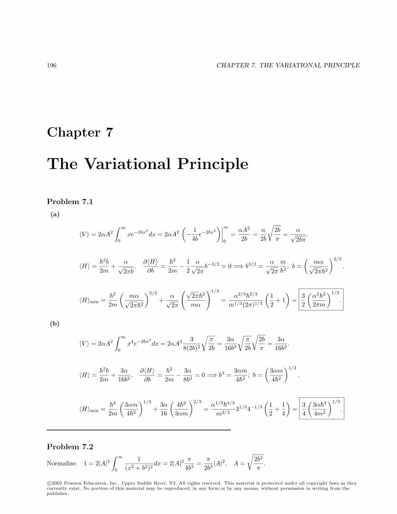
196 CHAPTER 7. THE VARIATIONAL PRINCIPLE
Chapter 7
The Variational Principle
Problem 7.1
(a)
〈V 〉 = 2αA2
∫ ∞0
xe−2bx2dx = 2αA2
(− 1
4be−2bx2
)∣∣∣∣∞0
=αA2
2b=
α
2b
√2bπ
=α√2bπ
.
〈H〉 =
2b
2m+
α√2πb
.∂〈H〉∂b
=
2
2m− 1
2α√2π
b−3/2 = 0 =⇒ b3/2 =α√2π
m
2; b =
(mα√2π2
)2/3
.
〈H〉min =
2
2m
(mα√2π2
)2/3
+α√2π
(√2π2
mα
)1/3
=α2/3
2/3
m1/3(2π)1/3
(12
+ 1)
=32
(α2
2
2πm
)1/3
.
(b)
〈V 〉 = 2αA2
∫ ∞0
x4e−2bx2dx = 2αA2 3
8(2b)2
√π
2b=
3α16b2
√π
2b
√2bπ
=3α
16b2.
〈H〉 =
2b
2m+
3α16b2
.∂〈H〉∂b
=
2
2m− 3α
8b3= 0 =⇒ b3 =
3αm42
; b =(
3αm42
)1/3
.
〈H〉min =
2
2m
(3αm42
)1/3
+3α16
(42
3αm
)2/3
=α1/3
4/3
m2/331/34−1/3
(12
+14
)=
34
(3α4
4m2
)1/3
.
Problem 7.2
Normalize: 1 = 2|A|2∫ ∞
0
1(x2 + b2)2
dx = 2|A|2 π
4b3=
π
2b3|A|2. A =
√2b3
π.
c©2005 Pearson Education, Inc., Upper Saddle River, NJ. All rights reserved. This material is protected under all copyright laws as theycurrently exist. No portion of this material may be reproduced, in any form or by any means, without permission in writing from thepublisher.
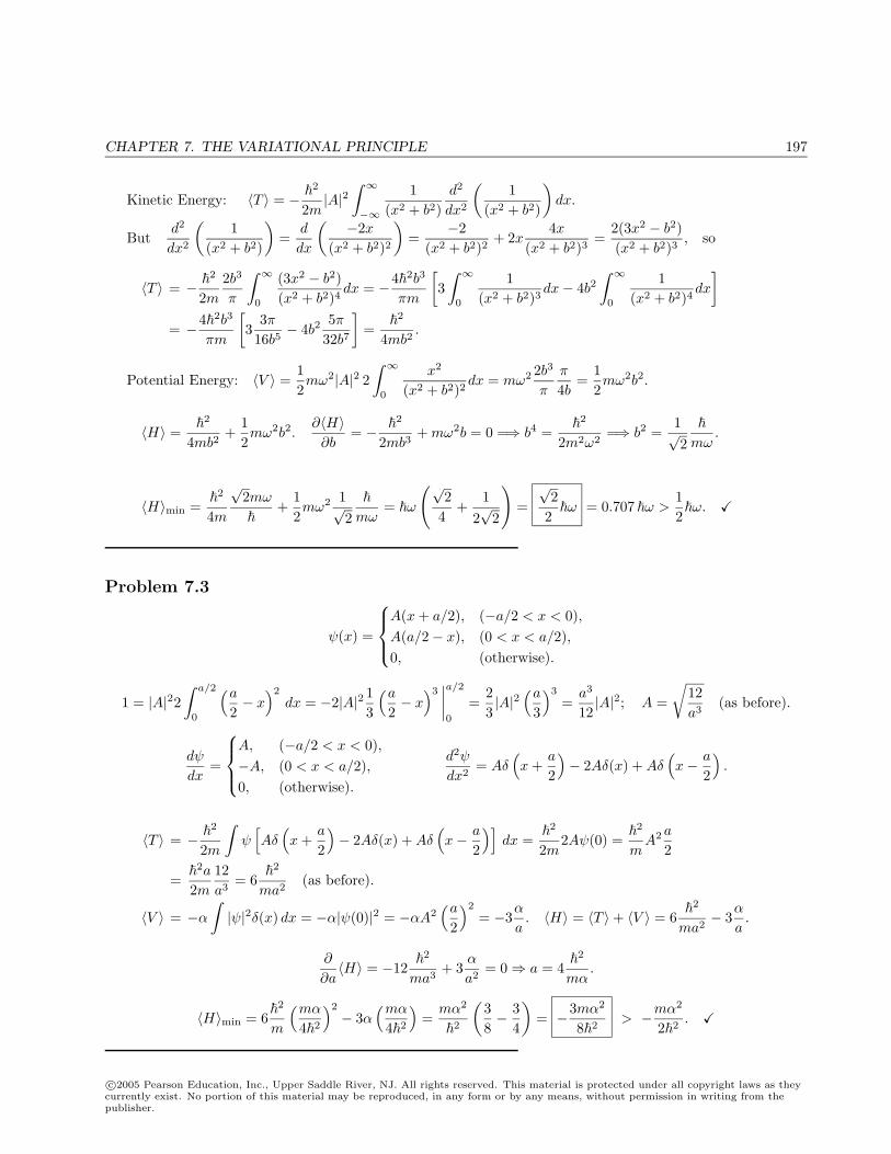
CHAPTER 7. THE VARIATIONAL PRINCIPLE 197
Kinetic Energy: 〈T 〉 = − 2
2m|A|2
∫ ∞−∞
1(x2 + b2)
d2
dx2
(1
(x2 + b2)
)dx.
Butd2
dx2
(1
(x2 + b2)
)=
d
dx
( −2x(x2 + b2)2
)=
−2(x2 + b2)2
+ 2x4x
(x2 + b2)3=
2(3x2 − b2)(x2 + b2)3
, so
〈T 〉 = − 2
2m2b3
π
∫ ∞0
(3x2 − b2)(x2 + b2)4
dx = −42b3
πm
[3
∫ ∞0
1(x2 + b2)3
dx− 4b2∫ ∞
0
1(x2 + b2)4
dx
]= −42b3
πm
[3
3π16b5
− 4b25π
32b7
]=
2
4mb2.
Potential Energy: 〈V 〉 =12mω2|A|2 2
∫ ∞0
x2
(x2 + b2)2dx = mω2 2b3
π
π
4b=
12mω2b2.
〈H〉 =
2
4mb2+
12mω2b2.
∂〈H〉∂b
= − 2
2mb3+ mω2b = 0 =⇒ b4 =
2
2m2ω2=⇒ b2 =
1√2
mω.
〈H〉min =
2
4m
√2mω
+
12mω2 1√
2
mω= ω
(√2
4+
12√
2
)=√
22ω = 0.707 ω >
12ω.
Problem 7.3
ψ(x) =
A(x + a/2), (−a/2 < x < 0),A(a/2− x), (0 < x < a/2),0, (otherwise).
1 = |A|22∫ a/2
0
(a
2− x
)2
dx = −2|A|2 13
(a
2− x
)3∣∣∣∣a/2
0
=23|A|2
(a
3
)3
=a3
12|A|2; A =
√12a3
(as before).
dψ
dx=
A, (−a/2 < x < 0),−A, (0 < x < a/2),0, (otherwise).
d2ψ
dx2= Aδ
(x +
a
2
)− 2Aδ(x) + Aδ
(x− a
2
).
〈T 〉 = − 2
2m
∫ψ
[Aδ
(x +
a
2
)− 2Aδ(x) + Aδ
(x− a
2
)]dx =
2
2m2Aψ(0) =
2
mA2 a
2
=
2a
2m12a3
= 6
2
ma2(as before).
〈V 〉 = −α
∫|ψ|2δ(x) dx = −α|ψ(0)|2 = −αA2
(a
2
)2
= −3α
a. 〈H〉 = 〈T 〉+ 〈V 〉 = 6
2
ma2− 3
α
a.
∂
∂a〈H〉 = −12
2
ma3+ 3
α
a2= 0⇒ a = 4
2
mα.
〈H〉min = 6
2
m
(mα
42
)2
− 3α(mα
42
)=
mα2
2
(38− 3
4
)= −3mα2
82> −mα2
22.
c©2005 Pearson Education, Inc., Upper Saddle River, NJ. All rights reserved. This material is protected under all copyright laws as theycurrently exist. No portion of this material may be reproduced, in any form or by any means, without permission in writing from thepublisher.
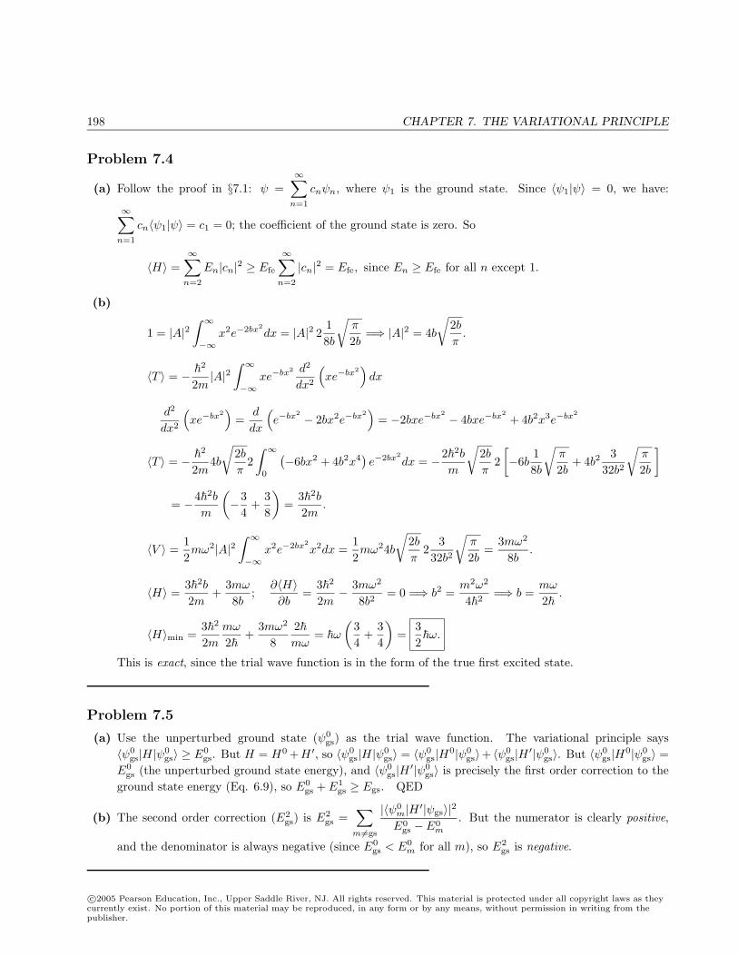
198 CHAPTER 7. THE VARIATIONAL PRINCIPLE
Problem 7.4
(a) Follow the proof in §7.1: ψ =∞∑
n=1
cnψn, where ψ1 is the ground state. Since 〈ψ1|ψ〉 = 0, we have:
∞∑n=1
cn〈ψ1|ψ〉 = c1 = 0; the coefficient of the ground state is zero. So
〈H〉 =∞∑
n=2
En|cn|2 ≥ Efe
∞∑n=2
|cn|2 = Efe, since En ≥ Efe for all n except 1.
(b)
1 = |A|2∫ ∞−∞
x2e−2bx2dx = |A|2 2
18b
√π
2b=⇒ |A|2 = 4b
√2bπ
.
〈T 〉 = − 2
2m|A|2
∫ ∞−∞
xe−bx2 d2
dx2
(xe−bx2
)dx
d2
dx2
(xe−bx2
)=
d
dx
(e−bx2 − 2bx2e−bx2
)= −2bxe−bx2 − 4bxe−bx2
+ 4b2x3e−bx2
〈T 〉 = − 2
2m4b
√2bπ
2∫ ∞
0
(−6bx2 + 4b2x4
)e−2bx2
dx = −22b
m
√2bπ
2[−6b
18b
√π
2b+ 4b2
332b2
√π
2b
]
= −42b
m
(−3
4+
38
)=
32b
2m.
〈V 〉 =12mω2|A|2
∫ ∞−∞
x2e−2bx2x2dx =
12mω24b
√2bπ
23
32b2
√π
2b=
3mω2
8b.
〈H〉 =32b
2m+
3mω
8b;
∂〈H〉∂b
=32
2m− 3mω2
8b2= 0 =⇒ b2 =
m2ω2
42=⇒ b =
mω
2.
〈H〉min =32
2mmω
2+
3mω2
82mω
= ω(
34
+34
)=
32ω.
This is exact, since the trial wave function is in the form of the true first excited state.
Problem 7.5
(a) Use the unperturbed ground state (ψ0gs) as the trial wave function. The variational principle says
〈ψ0gs|H|ψ0
gs〉 ≥ E0gs. But H = H0 +H ′, so 〈ψ0
gs|H|ψ0gs〉 = 〈ψ0
gs|H0|ψ0gs〉+ 〈ψ0
gs|H ′|ψ0gs〉. But 〈ψ0
gs|H0|ψ0gs〉 =
E0gs (the unperturbed ground state energy), and 〈ψ0
gs|H ′|ψ0gs〉 is precisely the first order correction to the
ground state energy (Eq. 6.9), so E0gs + E1
gs ≥ Egs. QED
(b) The second order correction (E2gs) is E2
gs =∑
m=gs
|〈ψ0m|H ′|ψgs〉|2E0
gs − E0m
. But the numerator is clearly positive,
and the denominator is always negative (since E0gs < E0
m for all m), so E2gs is negative.
c©2005 Pearson Education, Inc., Upper Saddle River, NJ. All rights reserved. This material is protected under all copyright laws as theycurrently exist. No portion of this material may be reproduced, in any form or by any means, without permission in writing from thepublisher.
CHAPTER 7. THE VARIATIONAL PRINCIPLE 199
Problem 7.6
He+ is a hydrogenic ion (see Problem 4.16); its ground state energy is (2)2(−13.6 eV), or −54.4 eV. It takes79.0− 54.4 = 24.6 eV to remove one electron.
Problem 7.7
I’ll do the general case of a nucleus with Z0 protons. Ignoring electron-electron repulsion altogether gives
ψ0 =Z3
0
πa3e−Z0(r1+r2)/a, (generalizing Eq. 7.17)
and the energy is 2Z20E1. 〈Vee〉 goes like 1/a (Eqs. 7.20 and 7.25), so the generalization of Eq. 7.25 is 〈Vee〉 =
− 54Z0E1, and the generalization of Eq. 7.26 is 〈H〉 = (2Z2
0 − 54Z0)E1.
If we include shielding, the only change is that (Z − 2) in Eqs. 7.28, 7.29, and 7.32 is replaced by (Z − Z0).Thus Eq. 7.32 generalizes to
〈H〉 =[2Z2 − 4Z(Z − Z0)−
54Z
]E1 =
[−2Z2 + 4ZZ0 −
54Z
]E1.
∂〈H〉∂Z
=[−4Z + 4Z0 −
54
]E1 = 0 =⇒ Z = Z0 −
516
.
〈H〉min =
[−2
(Z0 −
516
)2
+ 4(Z0 −
516
)Z0 −
54
(Z0 −
516
)]E1
=(−2Z2
0 +54Z0 −
25128
+ 4Z20 −
54Z0 −
54Z0 +
2564
)E1
=(
2Z20 −
54Z0 +
25128
)E1 =
(16Z0 − 5)2
128E1,
generalizing Eq. 7.34. The first term is the naive estimate ignoring electron-electron repulsion altogether; thesecond term is 〈Vee〉 in the unscreened state, and the third term is the effect of screening.
Z0 = 1 (H−): Z = 1− 516
=1116
= 0.688. The effective nuclear charge is less than 1, as expected.
〈H〉min =112
128E1 =
121128
E1 = −12.9 eV.
Z0 = 2 (He): Z = 2− 516
=2716
= 1.69 (as before); 〈H〉min =272
128E1 =
729128
E1 = −77.5 eV.
Z0 = 3 (Li+): Z = 3− 516
=4316
= 2.69 (somewhat less than 3); 〈H〉min =432
128E1 =
1849128
E1 = −196 eV.
Problem 7.8
D = a〈ψ0(r1)∣∣∣∣ 1r2
∣∣∣∣ψ0(r1)〉 = a〈ψ0(r2)∣∣∣∣ 1r1
∣∣∣∣ψ0(r2)〉 = a1
πa3
∫e−2r2/a 1
r1d3r
c©2005 Pearson Education, Inc., Upper Saddle River, NJ. All rights reserved. This material is protected under all copyright laws as theycurrently exist. No portion of this material may be reproduced, in any form or by any means, without permission in writing from thepublisher.
200 CHAPTER 7. THE VARIATIONAL PRINCIPLE
=1
πa3
∫e−
2a
√r2+R2−2rR cos θ 1
rr2 sin θ dr dθ dφ =
2ππa3
∫ ∞0
r
[∫ π
0
e−2a
√r2+R2−2rR cos θ sin θ dθ
]dr.
[. . . ] =1rR
∫ r+R
|r−R|e−2y/ay dy = − a
2rR
[e−2(r+R)/a
(r + R +
a
2
)− e−2|r−R|/a
(|r −R|+ a
2
)]
D =2a2
(− a
2R
) [e−2R/a
∫ ∞0
e−2r/a(r + R +
a
2
)dr
−e−2R/a
∫ R
0
e2R/a(R− r +
a
2
)dr − e2R/a
∫ ∞R
e−2r/a(r −R +
a
2
)dr
]
= − 1aR
e−2R/a
[(a
2
)2
+(R +
a
2
) (a
2
)]− e−2R/a
(R +
a
2
) (a
2e2r/a
)∣∣∣R0
+e−2R/a(a
2
)2
e2r/a
(2ra− 1
)∣∣∣∣R0
− e2R/a(−R +
a
2
) (−a
2e−2r/a
)∣∣∣∞R− e2R/a
(a
2
)2
e−2r/a
(−2r
a− 1
)∣∣∣∣∞R
= − 1aR
e−2R/a
[a2
4+
aR
2+
a2
4+
aR
2+
a2
4+
a2
4
]+
[−aR
2− a2
4+
a2
42Ra− a2
4+
aR
2− a2
4− a2
42Ra− a2
4
]
= − 1aR
[e−2R/a
(a2 + aR
)+
(−a2
)]=⇒ D =
a
R−
(1 +
a
R
)e−2R/a (confirms Eq. 7.47).
X = a〈ψ0(r1)∣∣∣∣ 1r1
∣∣∣∣ψ0(r2)〉 = a1
πa3
∫e−r1/ae−r2/a 1
r1d3r
=1
πa2
∫e−r/ae−
√r2+R2−2rR cos θ/a 1
rr2 sin θ dr dθ dφ =
2ππa2
∫ ∞0
re−r/a
[∫ π
0
e−√
r2+R2−2rR cos θ/a sin θ dθ
]dr.
[. . . ] = − a
rR
[e−(r+R)/a(r + R + a)− e−|r−R|/a(|r −R|+ a)
]
X =2a2
(− a
R
) [e−R/a
∫ ∞0
e−2r/a(r + R + a)dr
−e−R/a
∫ R
0
(R− r + a)dr − eR/a
∫ ∞R
e−2r/a(r −R + a)dr
]
= − 2aR
e−R/a
[(a
2
)2
+ (R + a)(a
2
)]− e−R/a
[(R + a)R− R2
2
]c©2005 Pearson Education, Inc., Upper Saddle River, NJ. All rights reserved. This material is protected under all copyright laws as theycurrently exist. No portion of this material may be reproduced, in any form or by any means, without permission in writing from thepublisher.
CHAPTER 7. THE VARIATIONAL PRINCIPLE 201
−eR/a(−R + a)(−a
2e−2r/a
)∣∣∣∞R− eR/a
(a
2
)2
e−2r/a
(−2r
a− 1
)∣∣∣∣∞R
= − 2aR
[e−R/a
(a2
4+
aR
2+
a2
2−R2 − aR +
R2
2+
aR
2− a2
2− a2
42Ra− a2
4
)]
= − 2aR
e−R/a
(−aR
2− R2
2
)=⇒ X = e−R/a
(1 +
R
a
)(confirms Eq. 7.48).
Problem 7.9
There are two changes: (1) the 2 in Eq. 7.38 changes sign . . . which amounts to changing the sign of I inEq. 7.43; (2) the last term in Eq. 7.44 changes sign . . . which amounts to reversing the sign of X. Thus Eq. 7.49becomes
〈H〉 =[1 + 2
D −X
1− I
]E1, and hence Eq. 7.51 becomes
F (x) =Etot
−E1=
2aR− 1− 2
D −X
1− I= −1 +
2x− 2
1/x− (1 + 1/x) e−2x − (1 + x)e−x
1− (1 + x + x2/3)e−x
= −1 +2x
[1− (1 + x + x2/3)e−x − 1 + (x + 1)e−2x + (x + x2)e−x
1− (1 + x + x2/3)e−x
]
= −1 +2x
[(1 + x)e−2x +
(23x
2 − 1)e−x
1− (1 + x + x2/3)e−x
].
The graph (with plus sign for comparison) has no minimum, and remains above −1, indicating that the energyis greater than for the proton and atom dissociated. Hence, no evidence of bonding here.
2 4 6 8
-1.1
-0.9
-0.8
-0.7
-0.6
-0.5
x
F(x)
(−)(+)
c©2005 Pearson Education, Inc., Upper Saddle River, NJ. All rights reserved. This material is protected under all copyright laws as theycurrently exist. No portion of this material may be reproduced, in any form or by any means, without permission in writing from thepublisher.
202 CHAPTER 7. THE VARIATIONAL PRINCIPLE
Problem 7.10
According to Mathematica, the minimum occurs at x = 2.493, and at this point F ′′ = 0.1257.
mω2 = V ′′ = −E1
a2F ′′, so ω =
1a
√−(0.1257)E1
m.
Here m is the reduced mass of the proton: m =mpmp
mp + mp=
12mp.
ω =3× 10⁸ m/s
(0.529× 10⁻¹⁰ m)
√(0.1257)(13.6 eV)(938× 106 eV)/2
= 3.42× 10¹⁴/s.
12ω =
12(6.58× 10⁻¹⁶ eV · s)(3.42× 10¹⁴ /s) = 0.113 eV (ground state vibrational energy).
Mathematica says that at the minimum F = −1.1297, so the binding energy is (0.1297)(13.6 eV) = 1.76 eV.Since this is substantially greater than the vibrational energy, it stays bound. The highest vibrational energy is
given by (n + 12 )ω = 1.76 eV, so n =
1.760.226
− 12
= 7.29. I estimate eight bound vibrational states (including
n = 0).
Problem 7.11
(a)
1 =∫|ψ|2 dx = |A|2
∫ a/2
−a/2
cos2(πx
a
)dx = |A|2 a
2⇒ A =
√2a.
〈T 〉 = − 2
2m
∫ψd2ψ
dx2dx =
2
2m
(π
a
)2∫
ψ2 dx =π2
2
2ma2.
〈V 〉 =12mω2
∫x2ψ2 dx =
12mω2 2
a
∫ a/2
−a/2
x2 cos2(πx
a
)dx =
mω2
a
( a
π
)3∫ π/2
−π/2
y2 cos2 y dy
=mω2a2
π3
[y3
6+
(y2
4− 1
8
)sin 2y +
y cos 2y4
] ∣∣∣∣π/2
−π/2
=mω2a2
4π2
(π2
6− 1
).
〈H〉 =π2
2
2ma2+
mω2a2
4π2
(π2
6− 1
);
∂〈H〉∂a
= −π2
2
ma3+
mω2a
2π2
(π2
6− 1
)= 0 ⇒
a = π
√
mω
(2
π2/6− 1
)1/4
.
〈H〉min =π2
2
2mπ2
mω
√π2/6− 1
2+
mω2
4π2
(π2
6− 1
)π2
mω
√2
π2/6− 1
=12ω
√π2
3− 2 =
12ω(1.136) >
12ω.
[We do not need to worry about the kink at ±a/2. It is true that d2ψ/dx2 has delta functions there, butsince ψ(±a/2) = 0 no “extra” contribution to T comes from these points.]
c©2005 Pearson Education, Inc., Upper Saddle River, NJ. All rights reserved. This material is protected under all copyright laws as theycurrently exist. No portion of this material may be reproduced, in any form or by any means, without permission in writing from thepublisher.
CHAPTER 7. THE VARIATIONAL PRINCIPLE 203
(b) Because this trial function is odd, it is orthogonal to the ground state, so by Problem 7.4 〈H〉 will givean upper bound to the first excited state.
1 =∫|ψ|2 dx = |B|2
∫ a
−a
sin2(πx
a
)dx = |B|2a ⇒ B =
1√a.
〈T 〉 = − 2
2m
∫ψd2ψ
dx2dx =
2
2m
(π
a
)2∫
ψ2 dx =π2
2
2ma2.
〈V 〉 =12mω2
∫x2ψ2 dx =
12mω2 1
a
∫ a
−a
x2 sin2(πx
a
)dx =
mω2
2a
( a
π
)3∫ π
−π
y2 sin2 y dy
=mω2a2
2π3
[y3
6−
(y2
4− 1
8
)sin 2y − y cos 2y
4
] ∣∣∣∣π−π
=mω2a2
4π2
(2π2
3− 1
).
〈H〉 =π2
2
2ma2+
mω2a2
4π2
(2π2
3− 1
);
∂〈H〉∂a
= −π2
2
ma3+
mω2a
2π2
(2π2
3− 1
)= 0 ⇒
a = π
√
mω
(2
2π2/3− 1
)1/4
.
〈H〉min =π2
2
2mπ2
mω
√2π2/3− 1
2+
mω2
4π2
(2π2
3− 1
)π2
mω
√2
2π2/3− 1
=12ω
√4π2
3− 2 =
12ω(3.341) >
32ω.
Problem 7.12
We will need the following integral repeatedly:∫ ∞0
xk
(x2 + b2)ldx =
12b2l−k−1
Γ(
k+12
)Γ
(2l−k−1
2
)Γ(l)
.
(a)
1 =∫ ∞−∞
|ψ|2 dx = 2|A|2∫ ∞
0
1(x2 + b2)2n dx =
|A|2b4n−1
Γ(
12
)Γ
(4n−1
2
)Γ(2n)
⇒ A =
√b4n−1Γ(2n)
Γ(
12
)Γ
(4n−1
2
) .〈T 〉 = −
2
2m
∫ ∞−∞
ψd2ψ
dx2dx = −
2
2mA2
∫ ∞−∞
1(x2 + b2)n
d
dx
[−2nx
(x2 + b2)n+1
]dx
=n2
mA2
∫ ∞−∞
1(x2 + b2)n
[1
(x2 + b2)n+1 −2(n + 1)x2
(x2 + b2)n+2
]dx
=2n2
mA2
[∫ ∞0
1(x2 + b2)2n+1 dx− 2(n + 1)
∫ ∞0
x2
(x2 + b2)2n+2 dx
]
=2n2
m
b4n−1Γ(2n)Γ
(12
)Γ
(4n−1
2
) [1
2b4n−1
Γ(
12
)Γ
(4n−1
2
)Γ(2n + 1)
− 2(n + 1)2b4n−1
Γ(
32
)Γ
(4n+1
2
)Γ(2n + 2)
]=
2
4mb2n(4n− 1)(2n + 1)
.
c©2005 Pearson Education, Inc., Upper Saddle River, NJ. All rights reserved. This material is protected under all copyright laws as theycurrently exist. No portion of this material may be reproduced, in any form or by any means, without permission in writing from thepublisher.
204 CHAPTER 7. THE VARIATIONAL PRINCIPLE
〈V 〉 =12mω2
∫ ∞−∞
ψ2x2 dx =12mω22A2
∫ ∞0
x2
(x2 + b2)2n dx
= mω2 b4n−1Γ(2n)Γ
(12
)Γ
(4n−1
2
) 12b4n−3
Γ(
32
)Γ
(4n−3
2
)Γ(2n)
=mω2b2
2(4n− 3).
〈H〉 =
2
4mb2n(4n− 1)(2n + 1)
+mω2b2
(4n− 3);
∂〈H〉∂b
= − 2
2mb3n(4n− 1)(2n + 1)
+mω2b
(4n− 3)= 0 ⇒
b =
√
mω
[n(4n− 1)(4n− 3)
2(2n + 1)
]1/4
.
〈H〉min =
2
4mn(4n− 1)(2n + 1)
mω
√2(2n + 1)
n(4n− 1)(4n− 3)+
mω2
2(4n− 3)
mω
√n(4n− 1)(4n− 3)
2(2n + 1)
=12ω
√2n(4n− 1)
(2n + 1)(4n− 3)=
12ω
√8n2 − 2n
8n2 − 2n− 3>
12ω.
(b)
1 = 2|B|2∫ ∞
0
x2
(x2 + b2)2n dx =|B|2b4n−3
Γ(
32
)Γ
(4n−3
2
)Γ(2n)
⇒ B =
√b4n−3Γ(2n)
Γ(
32
)Γ
(4n−3
2
) .〈T 〉 = −
2
2mB2
∫ ∞−∞
x
(x2 + b2)nd
dx
[1
(x2 + b2)n −2nx2
(x2 + b2)n+1
]dx
= −2B2
2m
∫ ∞−∞
x
(x2 + b2)n
[−2nx
(x2 + b2)n+1 −4nx
(x2 + b2)n+1 +4n(n + 1)x3
(x2 + b2)n+2
]dx
=4n2B2
2m
[3
∫ ∞0
x2
(x2 + b2)2n+1 dx− 2(n + 1)∫ ∞
0
x4
(x2 + b2)2n+2 dx
]
=2n2
m
b4n−3Γ(2n)Γ
(32
)Γ
(4n−3
2
) [3
2b4n−1
Γ(
32
)Γ
(4n−1
2
)Γ(2n + 1)
− 2(n + 1)2b4n−1
Γ(
52
)Γ
(4n−1
2
)Γ(2n + 2)
]=
32
4mb2n(4n− 3)(2n + 1)
.
〈V 〉 =12mω22B2
∫ ∞0
x4
(x2 + b2)2n dx =12mω2 b4n−3Γ(2n)
Γ(
32
)Γ
(4n−3
2
) 22b4n−5
Γ(
52
)Γ
(4n−5
2
)Γ(2n)
=32
mω2b2
(4n− 5).
〈H〉 =32
4mb2n(4n− 3)(2n + 1)
+32
mω2b2
(4n− 5);
∂〈H〉∂b
= − 32
2mb3n(4n− 3)(2n + 1)
+3mω2b
(4n− 5)= 0 ⇒
b =
√
mω
[n(4n− 3)(4n− 5)
2(2n + 1)
]1/4
.
〈H〉min =32
4mn(4n− 3)(2n + 1)
mω
√2(2n + 1)
n(4n− 3)(4n− 5)+
32
mω2
(4n− 5)
mω
√n(4n− 3)(4n− 5)
2(2n + 1)
=32ω
√2n(4n− 3)
(2n + 1)(4n− 5)=
32ω
√8n2 − 6n
8n2 − 6n− 5>
32ω.
c©2005 Pearson Education, Inc., Upper Saddle River, NJ. All rights reserved. This material is protected under all copyright laws as theycurrently exist. No portion of this material may be reproduced, in any form or by any means, without permission in writing from thepublisher.
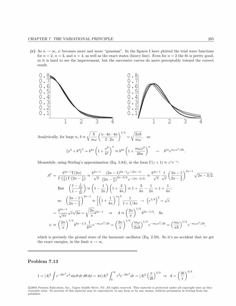
CHAPTER 7. THE VARIATIONAL PRINCIPLE 205
(c) As n → ∞, ψ becomes more and more “gaussian”. In the figures I have plotted the trial wave functionsfor n = 2, n = 3, and n = 4, as well as the exact states (heavy line). Even for n = 2 the fit is pretty good,so it is hard to see the improvement, but the successive curves do move perceptably toward the correctresult.
1 2 3 40.10.20.30.40.50.60.70.8
1 2 3 40.10.20.30.40.50.60.70.8
Analytically, for large n, b ≈√
mω
(n · 4n · 4n
2 · 2n
)1/4
=
√2nmω
, so
(x2 + b2
)n= b2n
(1 +
x2
b2
)n
≈ b2n
(1 +
mωx2
2n
)n
→ b2nemωx2/2.
Meanwhile, using Stirling’s approximation (Eq. 5.84), in the form Γ(z + 1) ≈ zze−z:
A2 =b4n−1Γ(2n)
Γ(
12
)Γ
(2n− 1
2
) ≈ b4n−1
√π
(2n− 1)2n−1e−(2n−1)(2n− 3
2
)2n−3/2e−(2n−3/2)
≈ b4n−1
√π
1√e
(2n− 12n− 3
2
)2n−1 √2n− 3/2.
But(
1− 12n
1− 34n
)≈
(1− 1
2n
) (1 +
34n
)≈ 1 +
34n− 1
2n= 1 +
14n
;
so(
2n− 12n− 3
2
)2n−1
≈[(
1 +14n
)n]2 11 + 1/4n
→(e1/4
)2
=√e.
=b4n−1
√πe
√e√
2n =
√2nπ
b4n−1 ⇒ A ≈(
2nπ
)1/4
b2n−1/2. So
ψ ≈(
2nπ
)1/4
b2n−1/2 1b2n
e−mωx2/2 =(
2nπ
)1/4 (mω
2n
)1/4
e−mωx2/2 =(mω
π
)1/4
e−mωx2/2,
which is precisely the ground state of the harmonic oscillator (Eq. 2.59). So it’s no accident that we getthe exact energies, in the limit n→∞.
Problem 7.13
1 = |A|2∫
e−2br2r2 sin θ dr dθ dφ = 4π|A|2
∫ ∞0
r2e−2br2dr = |A|2
( π
2b
)3/2
⇒ A =(
2bπ
)3/4
.
c©2005 Pearson Education, Inc., Upper Saddle River, NJ. All rights reserved. This material is protected under all copyright laws as theycurrently exist. No portion of this material may be reproduced, in any form or by any means, without permission in writing from thepublisher.
206 CHAPTER 7. THE VARIATIONAL PRINCIPLE
〈V 〉 = − e2
4πε0|A|24π
∫ ∞0
e−2br2 1rr2dr = − e2
4πε0
(2bπ
)3/2
4π14b
= − e2
4πε02
√2bπ
.
〈T 〉 = − 2
2m|A|2
∫e−br2
(∇2e−br2) r2 sin θ dr dθ dφ
But (∇2e−br2) =
1r2
d
dr
(r2 d
dre−br2
)=
1r2
d
dr
(−2br3e−br2
)=−2br2
(3r2 − 2br4
)e−br2
.
=−2
2m
(2bπ
)3/2
(4π)(−2b)∫ ∞
0
(3r2 − 2br4)e−2br2dr =
2
mπb4
(2bπ
)3/2 [3
18b
√π
2b− 2b
332b2
√π
2b
]=
2
m4πb
(2bπ
) (38b− 3
16b
)=
32b
2m.
〈H〉 =32b
2m− e2
4πε02
√2bπ
;∂〈H〉∂b
=32
2m− e2
4πε0
√2π
1√b
= 0 ⇒√b =
e2
4πε0
√2π
2m32
.
〈H〉min =32
2m
(e2
4πε0
)2 2π
4m2
94− e2
4πε02
√2π
(e2
4πε0
) √2π
2m32
=(
e2
4πε0
)2m
2
(43π− 8
3π
)= − m
22
(e2
4πε0
)2 83π
=83π
E1 = −11.5 eV.
Problem 7.14
Let ψ =1√πb3
e−r/b (same as hydrogen, but with a → b adjustable). From Eq. 4.191, we have 〈T 〉 = −E1 =
2
2ma2for hydrogen, so in this case 〈T 〉 =
2
2mb2.
〈V 〉 = − e2
4πε04ππb3
∫ ∞0
e−2r/b e−µr
rr2 dr = − e2
4πε04b3
∫ ∞0
e−(µ+2/b)rr dr = − e2
4πε04b3
1(µ + 2/b)2
= − e2
4πε01
b(1 + µb2 )2
.
〈H〉 =
2
2mb2− e2
4πε01
b(1 + µb2 )2
.
∂〈H〉∂b
= − 2
mb3+
e2
4πε0
[1
b2(1 + µb/2)2+
µ
b(1 + µb/2)3
]= −
2
mb3+
e2
4πε0(1 + 3µb/2)b2(1 + µb/2)3
= 0 ⇒
2
m
(4πε0e2
)= b
(1 + 3µb/2)(1 + µb/2)3
, or b(1 + 3µb/2)(1 + µb/2)3
= a.
This determines b, but unfortunately it’s a cubic equation. So we use the fact that µ is small to obtain a suitableapproximate solution. If µ = 0, then b = a (of course), so µa 1 =⇒ µb 1 too. We’ll expand in powers ofµb:
a ≈ b
(1 +
3µb2
) [1− 3µb
2+ 6
(µb
2
)2]≈ b
[1− 9
4(µb)2 +
64(µb)2
]= b
[1− 3
4(µb)2
].
c©2005 Pearson Education, Inc., Upper Saddle River, NJ. All rights reserved. This material is protected under all copyright laws as theycurrently exist. No portion of this material may be reproduced, in any form or by any means, without permission in writing from thepublisher.
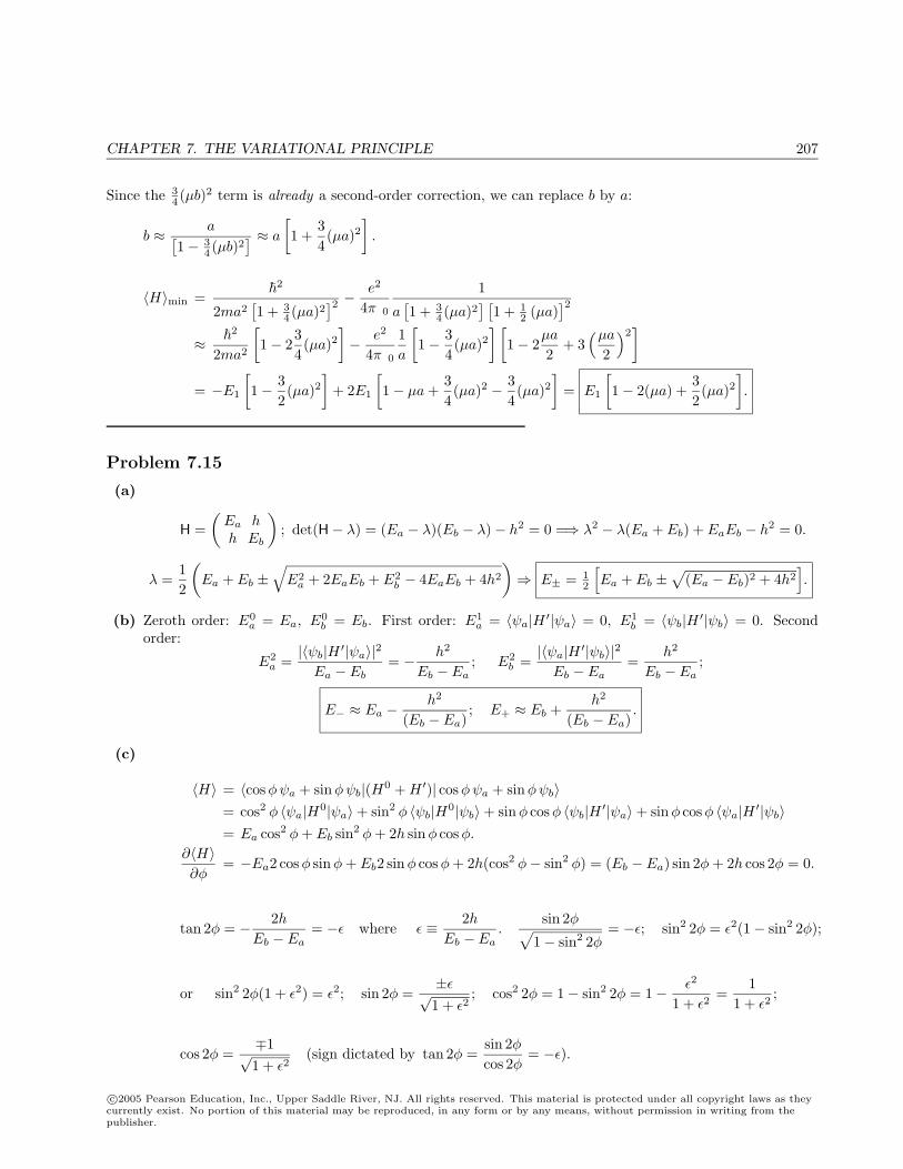
CHAPTER 7. THE VARIATIONAL PRINCIPLE 207
Since the 34 (µb)2 term is already a second-order correction, we can replace b by a:
b ≈ a[1− 3
4 (µb)2] ≈ a
[1 +
34(µa)2
].
〈H〉min =
2
2ma2[1 + 3
4 (µa)2]2 − e2
4πε01
a[1 + 3
4 (µa)2] [
1 + 12 (µa)
]2≈
2
2ma2
[1− 2
34(µa)2
]− e2
4πε01a
[1− 3
4(µa)2
] [1− 2
µa
2+ 3
(µa
2
)2]
= −E1
[1− 3
2(µa)2
]+ 2E1
[1− µa +
34(µa)2 − 3
4(µa)2
]= E1
[1− 2(µa) +
32(µa)2
].
Problem 7.15
(a)
H =(
Ea hh Eb
); det(H− λ) = (Ea − λ)(Eb − λ)− h2 = 0 =⇒ λ2 − λ(Ea + Eb) + EaEb − h2 = 0.
λ =12
(Ea + Eb ±
√E2
a + 2EaEb + E2b − 4EaEb + 4h2
)⇒ E± = 1
2
[Ea + Eb ±
√(Ea − Eb)2 + 4h2
].
(b) Zeroth order: E0a = Ea, E0
b = Eb. First order: E1a = 〈ψa|H ′|ψa〉 = 0, E1
b = 〈ψb|H ′|ψb〉 = 0. Secondorder:
E2a =
|〈ψb|H ′|ψa〉|2Ea − Eb
= − h2
Eb − Ea; E2
b =|〈ψa|H ′|ψb〉|2
Eb − Ea=
h2
Eb − Ea;
E− ≈ Ea −h2
(Eb − Ea); E+ ≈ Eb +
h2
(Eb − Ea).
(c)
〈H〉 = 〈cosφψa + sinφψb|(H0 + H ′)| cosφψa + sinφψb〉= cos2 φ 〈ψa|H0|ψa〉+ sin2 φ 〈ψb|H0|ψb〉+ sinφ cosφ 〈ψb|H ′|ψa〉+ sinφ cosφ 〈ψa|H ′|ψb〉= Ea cos2 φ + Eb sin2 φ + 2h sinφ cosφ.
∂〈H〉∂φ
= −Ea2 cosφ sinφ + Eb2 sinφ cosφ + 2h(cos2 φ− sin2 φ) = (Eb − Ea) sin 2φ + 2h cos 2φ = 0.
tan 2φ = − 2hEb − Ea
= −ε where ε ≡ 2hEb − Ea
.sin 2φ√
1− sin2 2φ= −ε; sin2 2φ = ε2(1− sin2 2φ);
or sin2 2φ(1 + ε2) = ε2; sin 2φ =±ε√1 + ε2
; cos2 2φ = 1− sin2 2φ = 1− ε2
1 + ε2=
11 + ε2
;
cos 2φ =∓1√1 + ε2
(sign dictated by tan 2φ =sin 2φcos 2φ
= −ε).
c©2005 Pearson Education, Inc., Upper Saddle River, NJ. All rights reserved. This material is protected under all copyright laws as theycurrently exist. No portion of this material may be reproduced, in any form or by any means, without permission in writing from thepublisher.
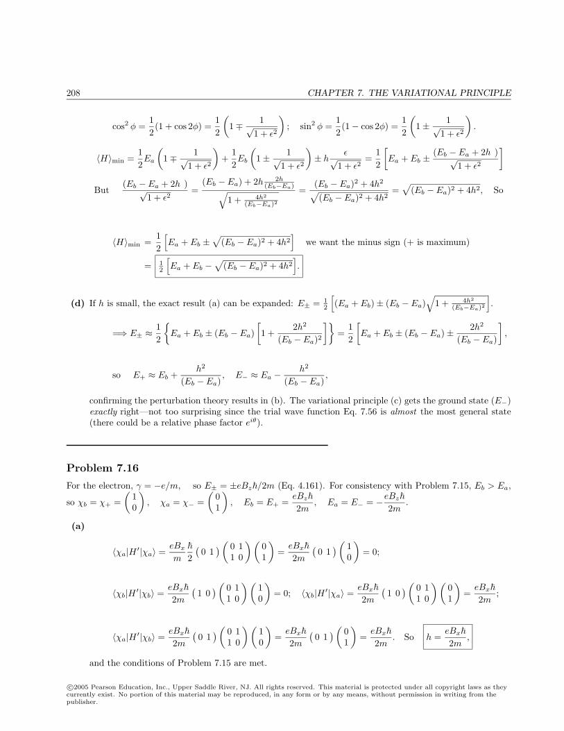
208 CHAPTER 7. THE VARIATIONAL PRINCIPLE
cos2 φ =12(1 + cos 2φ) =
12
(1∓ 1√
1 + ε2
); sin2 φ =
12(1− cos 2φ) =
12
(1± 1√
1 + ε2
).
〈H〉min =12Ea
(1∓ 1√
1 + ε2
)+
12Eb
(1± 1√
1 + ε2
)± h
ε√1 + ε2
=12
[Ea + Eb ±
(Eb − Ea + 2hε)√1 + ε2
]
But(Eb − Ea + 2hε)√
1 + ε2=
(Eb − Ea) + 2h 2h(Eb−Ea)√
1 + 4h2
(Eb−Ea)2
=(Eb − Ea)2 + 4h2√(Eb − Ea)2 + 4h2
=√
(Eb − Ea)2 + 4h2, So
〈H〉min =12
[Ea + Eb ±
√(Eb − Ea)2 + 4h2
]we want the minus sign (+ is maximum)
= 12
[Ea + Eb −
√(Eb − Ea)2 + 4h2
].
(d) If h is small, the exact result (a) can be expanded: E± = 12
[(Ea + Eb)± (Eb − Ea)
√1 + 4h2
(Eb−Ea)2
].
=⇒ E± ≈12
Ea + Eb ± (Eb − Ea)
[1 +
2h2
(Eb − Ea)2
]=
12
[Ea + Eb ± (Eb − Ea)± 2h2
(Eb − Ea)
],
so E+ ≈ Eb +h2
(Eb − Ea), E− ≈ Ea −
h2
(Eb − Ea),
confirming the perturbation theory results in (b). The variational principle (c) gets the ground state (E−)exactly right—not too surprising since the trial wave function Eq. 7.56 is almost the most general state(there could be a relative phase factor eiθ).
Problem 7.16
For the electron, γ = −e/m, so E± = ±eBz/2m (Eq. 4.161). For consistency with Problem 7.15, Eb > Ea,
so χb = χ+ =(
10
), χa = χ− =
(01
), Eb = E+ =
eBz
2m, Ea = E− = −eBz
2m.
(a)
〈χa|H ′|χa〉 =eBx
m
2(0 1
) (0 11 0
) (01
)=
eBx
2m(0 1
) (10
)= 0;
〈χb|H ′|χb〉 =eBx
2m(1 0
) (0 11 0
) (10
)= 0; 〈χb|H ′|χa〉 =
eBx
2m(1 0
) (0 11 0
) (01
)=
eBx
2m;
〈χa|H ′|χb〉 =eBx
2m(0 1
) (0 11 0
) (10
)=
eBx
2m(0 1
) (01
)=
eBx
2m. So h =
eBx
2m,
and the conditions of Problem 7.15 are met.
c©2005 Pearson Education, Inc., Upper Saddle River, NJ. All rights reserved. This material is protected under all copyright laws as theycurrently exist. No portion of this material may be reproduced, in any form or by any means, without permission in writing from thepublisher.
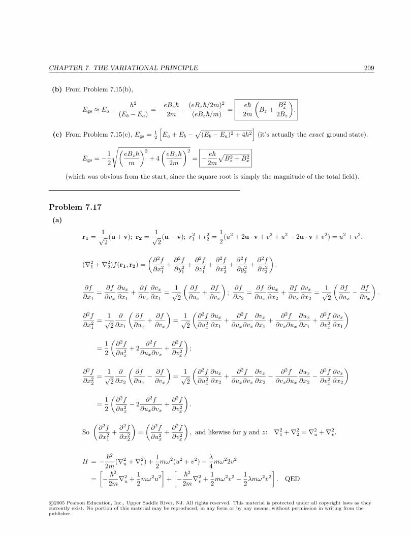
CHAPTER 7. THE VARIATIONAL PRINCIPLE 209
(b) From Problem 7.15(b),
Egs ≈ Ea −h2
(Eb − Ea)= −eBz
2m− (eBx/2m)2
(eBz/m)= − e
2m
(Bz +
B2x
2Bz
).
(c) From Problem 7.15(c), Egs = 12
[Ea + Eb −
√(Eb − Ea)2 + 4h2
](it’s actually the exact ground state).
Egs = −12
√(eBz
m
)2
+ 4(eBx
2m
)2
= − e
2m
√B2
z + B2x
(which was obvious from the start, since the square root is simply the magnitude of the total field).
Problem 7.17
(a)
r1 =1√2(u + v); r2 =
1√2(u− v); r2
1 + r22 =
12(u2 + 2u · v + v2 + u2 − 2u · v + v2) = u2 + v2.
(∇21 +∇2
2)f(r1, r2) =(∂2f
∂x21
+∂2f
∂y21
+∂2f
∂z21
+∂2f
∂x22
+∂2f
∂y22
+∂2f
∂z22
).
∂f
∂x1=
∂f
∂ux
∂ux
∂x1+
∂f
∂vx
∂vx
∂x1=
1√2
(∂f
∂ux+
∂f
∂vx
);
∂f
∂x2=
∂f
∂ux
∂ux
∂x2+
∂f
∂vx
∂vx
∂x2=
1√2
(∂f
∂ux− ∂f
∂vx
).
∂2f
∂x21
=1√2
∂
∂x1
(∂f
∂ux+
∂f
∂vx
)=
1√2
(∂2f
∂u2x
∂ux
∂x1+
∂2f
∂ux∂vx
∂vx
∂x1+
∂2f
∂vx∂ux
∂ux
∂x1+
∂2f
∂v2x
∂vx
∂x1
)
=12
(∂2f
∂u2x
+ 2∂2f
∂ux∂vx+
∂2f
∂v2x
);
∂2f
∂x22
=1√2
∂
∂x2
(∂f
∂ux− ∂f
∂vx
)=
1√2
(∂2f
∂u2x
∂ux
∂x2+
∂2f
∂ux∂vx
∂vx
∂x2− ∂2f
∂vx∂ux
∂ux
∂x2− ∂2f
∂v2x
∂vx
∂x2
)
=12
(∂2f
∂u2x
− 2∂2f
∂ux∂vx+
∂2f
∂v2x
).
So(∂2f
∂x21
+∂2f
∂x22
)=
(∂2f
∂u2x
+∂2f
∂v2x
), and likewise for y and z: ∇2
1 +∇22 = ∇2
u +∇2v.
H = − 2
2m(∇2
u +∇2v) +
12mω2(u2 + v2)− λ
4mω22v2
=[−
2
2m∇2
u +12mω2u2
]+
[−
2
2m∇2
v +12mω2v2 − 1
2λmω2v2
]. QED
c©2005 Pearson Education, Inc., Upper Saddle River, NJ. All rights reserved. This material is protected under all copyright laws as theycurrently exist. No portion of this material may be reproduced, in any form or by any means, without permission in writing from thepublisher.
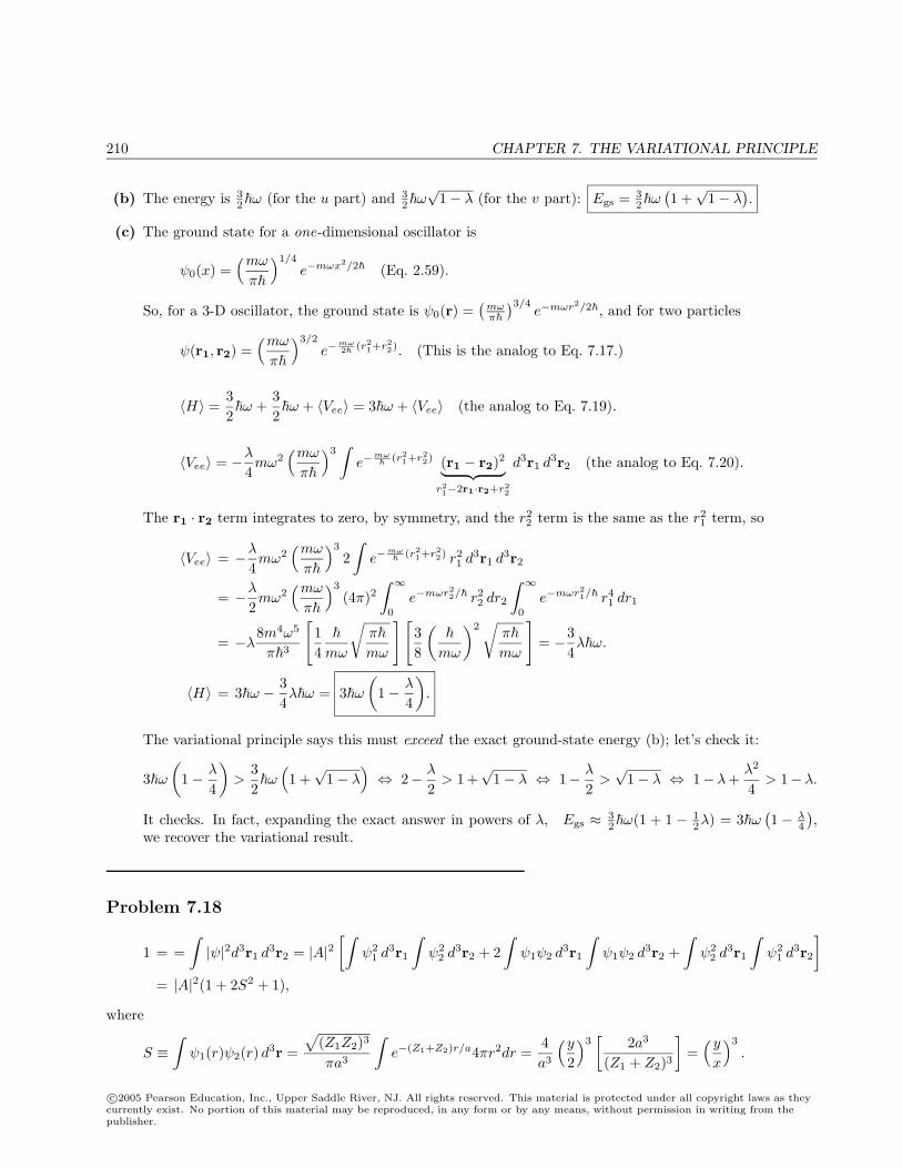
210 CHAPTER 7. THE VARIATIONAL PRINCIPLE
(b) The energy is 32ω (for the u part) and 3
2ω√
1− λ (for the v part): Egs = 32ω
(1 +
√1− λ
).
(c) The ground state for a one-dimensional oscillator is
ψ0(x) =(mω
π
)1/4
e−mωx2/2 (Eq. 2.59).
So, for a 3-D oscillator, the ground state is ψ0(r) =(
mωπ
)3/4e−mωr2/2, and for two particles
ψ(r1, r2) =(mω
π
)3/2
e−mω2 (r2
1+r22). (This is the analog to Eq. 7.17.)
〈H〉 =32ω +
32ω + 〈Vee〉 = 3ω + 〈Vee〉 (the analog to Eq. 7.19).
〈Vee〉 = −λ
4mω2
(mω
π
)3∫
e−mω
(r21+r2
2) (r1 − r2)2︸ ︷︷ ︸r21−2r1·r2+r2
2
d3r1 d3r2 (the analog to Eq. 7.20).
The r1 · r2 term integrates to zero, by symmetry, and the r22 term is the same as the r2
1 term, so
〈Vee〉 = −λ
4mω2
(mω
π
)3
2∫
e−mω
(r21+r2
2) r21 d3r1 d3r2
= −λ
2mω2
(mω
π
)3
(4π)2∫ ∞
0
e−mωr22/ r2
2 dr2
∫ ∞0
e−mωr21/ r4
1 dr1
= −λ8m4ω5
π3
[14
mω
√π
mω
] [38
(
mω
)2√
π
mω
]= −3
4λω.
〈H〉 = 3ω − 34λω = 3ω
(1− λ
4
).
The variational principle says this must exceed the exact ground-state energy (b); let’s check it:
3ω(
1− λ
4
)>
32ω
(1 +
√1− λ
)⇔ 2− λ
2> 1 +
√1− λ ⇔ 1− λ
2>√
1− λ ⇔ 1− λ+λ2
4> 1− λ.
It checks. In fact, expanding the exact answer in powers of λ, Egs ≈ 32ω(1 + 1 − 1
2λ) = 3ω(1− λ
4
),
we recover the variational result.
Problem 7.18
1 = =∫|ψ|2d3r1 d3r2 = |A|2
[∫ψ2
1 d3r1
∫ψ2
2 d3r2 + 2∫
ψ1ψ2 d3r1
∫ψ1ψ2 d3r2 +
∫ψ2
2 d3r1
∫ψ2
1 d3r2
]= |A|2(1 + 2S2 + 1),
where
S ≡∫
ψ1(r)ψ2(r) d3r =
√(Z1Z2)3
πa3
∫e−(Z1+Z2)r/a4πr2dr =
4a3
(y
2
)3[
2a3
(Z1 + Z2)3
]=
(y
x
)3
.
c©2005 Pearson Education, Inc., Upper Saddle River, NJ. All rights reserved. This material is protected under all copyright laws as theycurrently exist. No portion of this material may be reproduced, in any form or by any means, without permission in writing from thepublisher.
CHAPTER 7. THE VARIATIONAL PRINCIPLE 211
A2 =1
2[1 + (y/x)6
] .
H = − 2
2m(∇2
1 +∇22)−
e2
4πε0
(1r1
+1r2
)+
e2
4πε01
|r1 − r2|,
Hψ = A
[−
2
2m(∇2
1 +∇22)−
e2
4πε0
(Z1
r1+
Z2
r2
)]ψ1(r1)ψ2(r2)
+[−
2
2m(∇2
1 +∇22)−
e2
4πε0
(Z1
r1+
Z2
r2
)]ψ2(r1)ψ1(r2)
+Ae2
4πε0
[Z1 − 1
r1+
Z2 − 1r2
]ψ1(r1)ψ2(r2) +
[Z2 − 1
r1+
Z1 − 1r2
]ψ2(r1)ψ1(r2)
+ Veeψ,
where Vee ≡e2
4πε01
|r1 − r2|.
The term in first curly brackets is (Z21 + Z2
2 )E1ψ1(r1)ψ2(r2) + (Z22 + Z2
1 )ψ2(r1)ψ1(r2), so
Hψ = (Z21 + Z2
2 )E1ψ
+ Ae2
4πε0
[Z1 − 1
r1+
Z2 − 1r2
]ψ1(r1)ψ2(r2) +
[Z2 − 1
r1+
Z1 − 1r2
]ψ2(r1)ψ1(r2)
+ Veeψ
〈H〉 = (Z21 + Z2
2 )E1 + 〈Vee〉+ A2
(e2
4πε0
)
×〈ψ1(r1)ψ2(r2) + ψ2(r1)ψ1(r2)
∣∣∣∣([Z1 − 1
r1+
Z2 − 1r2
]∣∣∣∣ψ1(r1)ψ2(r2)〉+[Z2 − 1
r1+
Z1 − 1r2
]∣∣∣∣ψ2(r1)ψ1(r2)〉)
.
= (Z1 − 1)〈ψ1(r1)
∣∣∣∣ 1r1
∣∣∣∣ψ1(r1)〉+ (Z2 − 1)〈ψ2(r2)∣∣∣∣ 1r2
∣∣∣∣ψ2(r2)〉
+ (Z2 − 1)〈ψ1(r1)∣∣∣∣ 1r1
∣∣∣∣ψ2(r1)〉〈ψ2(r2)|ψ1(r2)〉
+ (Z1 − 1)〈ψ1(r1)|ψ2(r1)〉〈ψ2(r2)∣∣∣∣ 1r2
∣∣∣∣ψ1(r2)〉+ (Z1 − 1)〈ψ2(r1)∣∣∣∣ 1r1
∣∣∣∣ψ1(r1)〉〈ψ1(r2)|ψ2(r2)〉
+ (Z2 − 1)〈ψ2(r1)|ψ1(r1)〉〈ψ1(r2)∣∣∣∣ 1r2
∣∣∣∣ψ2(r2)〉+ (Z2 − 1)〈ψ2(r1)∣∣∣∣ 1r1
∣∣∣∣ψ2(r1)〉
+ (Z1 − 1)〈ψ1(r2)∣∣∣∣ 1r2
∣∣∣∣ψ1(r2)〉
= 2(Z1 − 1)⟨
1r
⟩1
+ 2(Z1 − 1)⟨
1r
⟩2
+ 2(Z1 − 1)〈ψ1|ψ2〉〈ψ1
∣∣∣∣1r∣∣∣∣ψ2〉+ 2(Z2 − 1)〈ψ1|ψ2〉〈ψ1
∣∣∣∣1r∣∣∣∣ψ2〉.
c©2005 Pearson Education, Inc., Upper Saddle River, NJ. All rights reserved. This material is protected under all copyright laws as theycurrently exist. No portion of this material may be reproduced, in any form or by any means, without permission in writing from thepublisher.
212 CHAPTER 7. THE VARIATIONAL PRINCIPLE
But⟨
1r
⟩1
= 〈ψ1(r)∣∣∣∣1r
∣∣∣∣ψ1(r)〉 =Z1
a;
⟨1r
⟩2
=Z2
a, so 〈H〉 = (Z2
1 + Z22 )E1
+A2
(e2
4πε0
)2
[1a(Z1 − 1)Z1 +
1a(Z2 − 1)Z2 + (Z1 + Z2 − 2)〈ψ1|ψ2〉〈ψ1
∣∣∣∣1r∣∣∣∣ψ2〉
]+ 〈Vee〉.
And 〈ψ1|ψ2〉 = S = (y/x)3 , so
〈ψ1
∣∣∣∣1r∣∣∣∣ψ2〉 =
√(Z1Z2)3
πa34π
∫e−(Z1+Z2)r/a r dr =
y3
2a3
[a
Z1 + Z2
]2
=y3
2ax2.
〈H〉 = (x2 − 12y2)E1 + A2
(e2
4πε0
)2a
[Z2
1 + Z22 − (Z1 + Z2)
]+ (x− 2)
(y
x
)3 y3
2x2
+ 〈Vee〉
= (x2 − 12y2)E1 + 4E1A
2
[x2 − 1
2y2 − x +
12(x− 2)
y6
x5
]+ 〈Vee〉.
〈Vee〉 =e2
4πε0〈ψ
∣∣∣∣ 1|r1 − r2|
∣∣∣∣ψ〉=
(e
4πε0
)A2〈ψ1(r1)ψ2(r2) + ψ2(r1) + ψ1(r2)
∣∣∣∣ 1|r1 − r2|
∣∣∣∣ψ1(r1)ψ2(r2) + ψ2(r1)ψ1(r2)〉
=(
e
4πε0
)A2
[2〈ψ1(r1)ψ2(r2)
∣∣∣∣ 1|r1 − r2|
∣∣∣∣ψ1(r1)ψ2(r2)〉+ 2〈ψ1(r1)ψ2(r2)∣∣∣∣ 1|r1 − r2|
∣∣∣∣ψ2(r1)ψ1(r2)〉]
= 2(
e
4πε0
)A2(B + C), where
B ≡ 〈ψ1(r1)ψ2(r2)∣∣∣∣ 1|r1 − r2|
∣∣∣∣ψ1(r1)ψ2(r2)〉; C ≡ 〈ψ1(r1)ψ2(r2)∣∣∣∣ 1|r1 − r2|
∣∣∣∣ψ2(r1)ψ1(r2)〉.
B =Z3
1Z32
(πa3)2
∫e−2Z1r1/ae−2Z2r2/a 1
|r1 − r2|d3r1 d3r2. As on pp 300-301, the r2 integral is
∫e−2Z2r2/a 1√
r21 + r2
2 − 2r1r2 cos θ2
d3r2
=πa3
Z32r1
[1−
(1 +
Z2r1
a
)e−2Z2r1/a
](Eq. 7.24, but with a→ 2
Z2a).
B =Z3
1Z32
(πa3)2(πa3)Z3
2
4π∫ ∞
0
e−2Z1r1/a 1r1
[1−
(1 +
Z2r1
a
)e−2Z2r1/a
]r21 dr1
=4Z3
1
a3
∫ ∞0
[r1e−2Z1r1/a − r1e
−2(Z1+Z2)r1/a − Z2
ar21e−2(Z1+Z2)r1/a
]dr1
c©2005 Pearson Education, Inc., Upper Saddle River, NJ. All rights reserved. This material is protected under all copyright laws as theycurrently exist. No portion of this material may be reproduced, in any form or by any means, without permission in writing from thepublisher.
CHAPTER 7. THE VARIATIONAL PRINCIPLE 213
=4Z3
1
a3
[(a
2Z1
)2
−(
a
2(Z1 + Z2)
)2
− Z2
a2
(a
2(Z1 + Z2)
)3]
=Z3
1
a
(1Z2
1
− 1(Z1 + Z2)2
− Z2
(Z1 + Z2)3
)
=Z1Z2
a(Z1 + Z2)
[1 +
Z1Z2
(Z1 + Z2)2
]=
y2
4ax
(1 +
y2
4x2
).
C =Z3
1Z32
(πa3)2
∫e−Z1r1/ae−Z2r2/ae−Z2r1/ae−Z1r2/a 1
|r1 − r2|d3r1 d3r2
=(Z1Z2)3
(πa3)2
∫e−(Z1+Z2)(r1+r2)/a 1
|r1 − r2|d3r1 d3r2.
The integral is the same as in Eq. 7.20, only with a→ 4Z1+Z2
a. Comparing Eqs. 7.20 and 7.25, we see that theintegral itself was
54a
(πa3
8
)2
=5
256π2a5. So C =
(Z1Z2)3
(πa3)25π2
25645a5
(Z1 + Z2)5=
20a
(Z1Z2)3
(Z1 + Z2)5=
516a
y6
x5.
〈Vee〉 = 2(
e
4πε0
)A2
[y2
4ax
(1 +
y2
4x2
)+
516a
y6
x5
]= 2A2(−2E1)
y2
4x
(1 +
y2
4x2+
5y4
4x4
).
〈H〉 = E1
x2 − 1
2y2 − 2
[1 + (y/x)6]
[x2 − 1
2y2 − x +
12(x− 2)
y6
x5
]− 2
[1 + (y/x)6]y2
4x
(1 +
y2
4x2+
5y4
4x4
)
=E1
(x6 + y6)
(x2 − 1
2y2)(x6 + y6)− 2x6
[x2 − 1
2y2 − x +
12y6
x4− y6
x5+
y2
4x+
y4
16x3+
5y6
16x5
]
=E1
(x6 + y6)
(x8 + x2y6 − 1
2x6y2 − 1
2y8 − 2x8 + x6y2 + 2x7 − x2y6 + 2xy6 − 1
2x5y2 − 1
8x3y4 − 5
8xy6
)
=E1
(x6 + y6)
(−x8 + 2x7 +
12x6y2 − 1
2x5y2 − 1
8x3y4 +
118xy6 − 1
2y8
).
Mathematica finds the minimum of 〈H〉 at x = 1.32245, y = 1.08505, corresponding to Z1 = 1.0392, Z2 =0.2832. At this point, 〈H〉min = 1.0266E1 = −13.962 eV, which is less than −13.6 eV—but not by much!
Problem 7.19
The calculation is the same as before, but with me → mµ (reduced), where
mµ(reduced) =mµmd
mµ + md=
mµ2mp
mµ + 2mp=
mµ
1 + mµ/2mp. From Problem 6.28, mµ = 207me, so
1 +mµ
2mp= 1 +
(2072
)(9.11× 10⁻³¹)(1.67× 10⁻²⁷)
= 1.056; mµ(reduced) =207me
1.056= 196me.
This shrinks the whole molecule down by a factor of almost 200, bringing the deuterons much closer together,as desired. The equilibrium separation for the electron case was 2.493 a (Problem 7.10), so for muons, R =2.493196
(0.529× 10⁻¹⁰ m) = 6.73× 10⁻¹³ m.
c©2005 Pearson Education, Inc., Upper Saddle River, NJ. All rights reserved. This material is protected under all copyright laws as theycurrently exist. No portion of this material may be reproduced, in any form or by any means, without permission in writing from thepublisher.
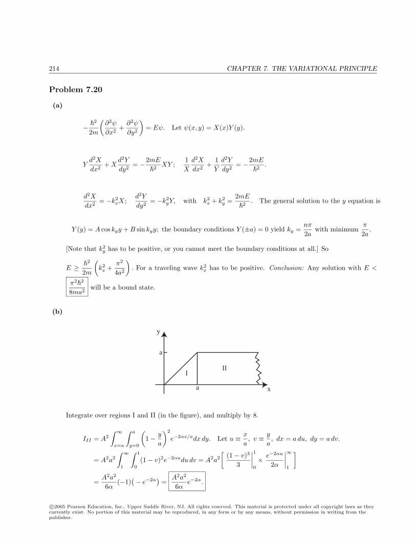
214 CHAPTER 7. THE VARIATIONAL PRINCIPLE
Problem 7.20
(a)
− 2
2m
(∂2ψ
∂x2+
∂2ψ
∂y2
)= Eψ. Let ψ(x, y) = X(x)Y (y).
Yd2X
dx2+ X
d2Y
dy2= −2mE
2XY ;
1X
d2X
dx2+
1Y
d2Y
dy2= −2mE
2.
d2X
dx2= −k2
xX;d2Y
dy2= −k2
yY, with k2x + k2
y =2mE
2. The general solution to the y equation is
Y (y) = A cos kyy + B sin kyy; the boundary conditions Y (±a) = 0 yield ky =nπ
2awith minimum
π
2a.
[Note that k2y has to be positive, or you cannot meet the boundary conditions at all.] So
E ≥ 2
2m
(k2
x +π2
4a2
). For a traveling wave k2
x has to be positive. Conclusion: Any solution with E <
π2
2
8ma2will be a bound state.
(b)
a
a
x
y
III
Integrate over regions I and II (in the figure), and multiply by 8.
III = A2
∫ ∞x=a
∫ a
y=0
(1− y
a
)2
e−2αx/adx dy. Let u ≡ x
a, v ≡ y
a, dx = a du, dy = a dv.
= A2a2
∫ ∞1
∫ 1
0
(1− v)2e−2αudu dv = A2a2
[(1− v)3
3
∣∣∣∣10
× e−2αu
2α
∣∣∣∣∞1
]
=A2a2
6α(−1)
(− e−2α
)=
A2a2
6αe−2α.
c©2005 Pearson Education, Inc., Upper Saddle River, NJ. All rights reserved. This material is protected under all copyright laws as theycurrently exist. No portion of this material may be reproduced, in any form or by any means, without permission in writing from thepublisher.
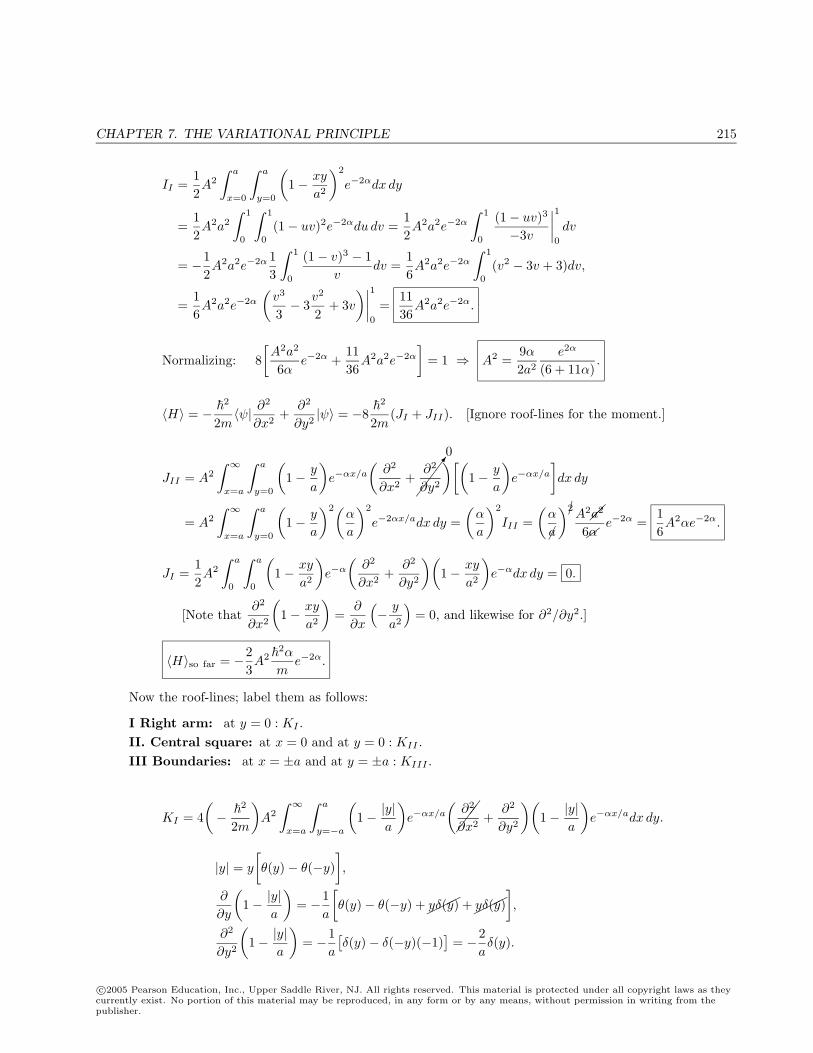
CHAPTER 7. THE VARIATIONAL PRINCIPLE 215
II =12A2
∫ a
x=0
∫ a
y=0
(1− xy
a2
)2
e−2αdx dy
=12A2a2
∫ 1
0
∫ 1
0
(1− uv)2e−2αdu dv =12A2a2e−2α
∫ 1
0
(1− uv)3
−3v
∣∣∣∣10
dv
= −12A2a2e−2α 1
3
∫ 1
0
(1− v)3 − 1v
dv =16A2a2e−2α
∫ 1
0
(v2 − 3v + 3)dv,
=16A2a2e−2α
(v3
3− 3
v2
2+ 3v
)∣∣∣∣10
=1136
A2a2e−2α.
Normalizing: 8[A2a2
6αe−2α +
1136
A2a2e−2α
]= 1 ⇒ A2 =
9α2a2
e2α
(6 + 11α).
〈H〉 = − 2
2m〈ψ| ∂
2
∂x2+
∂2
∂y2|ψ〉 = −8
2
2m(JI + JII). [Ignore roof-lines for the moment.]
JII = A2
∫ ∞x=a
∫ a
y=0
(1− y
a
)e−αx/a
(∂2
∂x2+
0∂2
∂y2
)[(1− y
a
)e−αx/a
]dx dy
= A2
∫ ∞x=a
∫ a
y=0
(1− y
a
)2(α
a
)2
e−2αx/adx dy =(α
a
)2
III =(α
a
)2A2a2
6αe−2α =
16A2αe−2α.
JI =12A2
∫ a
0
∫ a
0
(1− xy
a2
)e−α
(∂2
∂x2+
∂2
∂y2
)(1− xy
a2
)e−αdx dy = 0.
[Note that∂2
∂x2
(1− xy
a2
)=
∂
∂x
(− y
a2
)= 0, and likewise for ∂2/∂y2.]
〈H〉so far = −23A2
2α
me−2α.
Now the roof-lines; label them as follows:
I. Right arm: at y = 0 : KI .II. Central square: at x = 0 and at y = 0 : KII .III. Boundaries: at x = ±a and at y = ±a : KIII .
KI = 4(−
2
2m
)A2
∫ ∞x=a
∫ a
y=−a
(1− |y|
a
)e−αx/a
(∂2
∂x2+
∂2
∂y2
)(1− |y|
a
)e−αx/adx dy.
|y| = y
[θ(y)− θ(−y)
],
∂
∂y
(1− |y|
a
)= −1
a
[θ(y)− θ(−y) +
yδ(y) +yδ(y)
],
∂2
∂y2
(1− |y|
a
)= −1
a
[δ(y)− δ(−y)(−1)
]= −2
aδ(y).
c©2005 Pearson Education, Inc., Upper Saddle River, NJ. All rights reserved. This material is protected under all copyright laws as theycurrently exist. No portion of this material may be reproduced, in any form or by any means, without permission in writing from thepublisher.
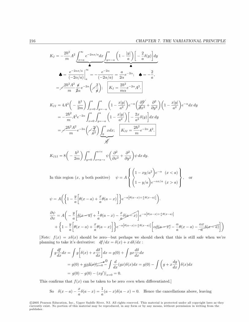
216 CHAPTER 7. THE VARIATIONAL PRINCIPLE
KI = −22
mA2
∫ ∞x=a
e−2αx/adx︸ ︷︷ ︸♣
∫ a
y=−a
(1− |y|
a
)[− 2
aδ(y)
]dy︸ ︷︷ ︸
♠
♣ =e−2αx/a
(−2α/a)
∣∣∣∣∞a
= − e−2α
(−2α/a)=
a
2αe−2α; ♠ = −2
a,
=−22A2
ma
2αe−2α
(−
2
a
); KI =
22
mαe−2αA2.
KII = 4A2
(−
2
2m
) ∫ a
x=0
∫ a
y=−a
(1− x|y|
a2
)e−α
(∂2
∂x2+
∂2
∂y2
)(1− x|y|
a2
)e−αdx dy
= −22
mA2e−2α
∫ a
x=0
∫ a
y=−a
(1− x|y|
a2
)[− 2x
a2δ(y)
]dx dy
=−22A2
me−2α
(−2a2
) ∫ a
0
xdx︸ ︷︷ ︸a22
; KII =22
me−2αA2.
KIII = 8(−
2
2m
) ∫ a
y=0
∫ a+ε
x=a−ε
ψ
(∂2
∂x2+
∂2
∂y2
)ψ dx dy.
In this region (x, y both positive) ψ = A
(
1− xy/a2
)e−α (x < a)(
1− y/a
)e−αx/a (x > a)
, or
ψ = A
(1− y
a
[θ(x− a) +
x
aθ(a− x)
]e−α[θ(a−x)+ x
a θ(x−a)]).
∂ψ
∂x= A
(− y
a
[
δ(x− a) +1aθ(a− x)−
x
aδ(a− x)
]e−α[θ(a−x)+ x
a θ(x−a)]
+
1− y
a
[θ(x− a) +
x
aθ(a− x)
]e−α[θ(a−x)+ x
a θ(x−a)][α
δ(a− x)− α
aθ(x− a)−
αx
aδ(x− a)
])[Note: f(x) = xδ(x) should be zero—but perhaps we should check that this is still safe when we’replanning to take it’s derivative: df/dx = δ(x) + x dδ/dx :∫
gdf
dxdx =
∫g
[δ(x) + x
dδ
dx
]dx = g(0) +
∫gx
dδ
dxdx
= g(0) +0
gxδ(x)|x=0 −∫
d
dx(gx)δ(x)dx = g(0)−
∫ (g + x
dg
dx
)δ(x)dx
= g(0)− g(0)− (xg′)|x=0 = 0.
This confirms that f(x) can be taken to be zero even when differentiated.]
So δ(x− a)− x
aδ(a− x) =
1a(a− x)δ(a− x) = 0. Hence the cancellations above, leaving
c©2005 Pearson Education, Inc., Upper Saddle River, NJ. All rights reserved. This material is protected under all copyright laws as theycurrently exist. No portion of this material may be reproduced, in any form or by any means, without permission in writing from thepublisher.
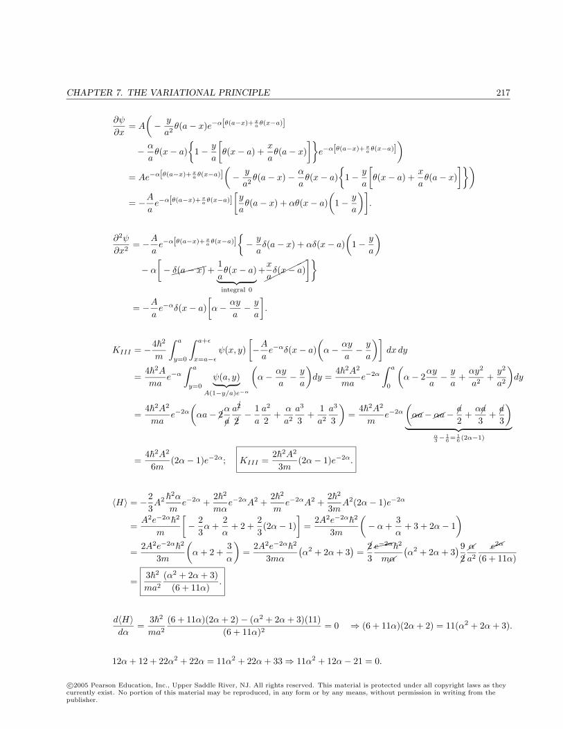
CHAPTER 7. THE VARIATIONAL PRINCIPLE 217
∂ψ
∂x= A
(− y
a2θ(a− x)e−α[θ(a−x)+ x
a θ(x−a)]
− α
aθ(x− a)
1− y
a
[θ(x− a) +
x
aθ(a− x)
]e−α[θ(a−x)+ x
a θ(x−a)])
= Ae−α[θ(a−x)+ xa θ(x−a)]
(− y
a2θ(a− x)− α
aθ(x− a)
1− y
a
[θ(x− a) +
x
aθ(a− x)
])= −A
ae−α[θ(a−x)+ x
a θ(x−a)][y
aθ(a− x) + αθ(x− a)
(1− y
a
)].
∂2ψ
∂x2= −A
ae−α[θ(a−x)+ x
a θ(x−a)]− y
aδ(a− x) + αδ(x− a)
(1− y
a
)− α
[−δ(a− x) +
1aθ(x− a)︸ ︷︷ ︸
integral 0
+
x
aδ(x− a)
]
= −A
ae−αδ(x− a)
[α− αy
a− y
a
].
KIII = −42
m
∫ a
y=0
∫ a+ε
x=a−ε
ψ(x, y)[−A
ae−αδ(x− a)
(α− αy
a− y
a
)]dx dy
=42A
mae−α
∫ a
y=0
ψ(a, y)︸ ︷︷ ︸A(1−y/a)e−α
(α− αy
a− y
a
)dy =
42A2
mae−2α
∫ a
0
(α− 2
αy
a− y
a+
αy2
a2+
y2
a2
)dy
=42A2
mae−2α
(αa− 2
α
aa2
2− 1
a
a2
2+
α
a2
a3
3+
1a2
a3
3
)=
42A2
me−2α
(αa−αa−
a
2+
αa3
+ a
3
)︸ ︷︷ ︸
α3− 1
6= 16 (2α−1)
=42A2
6m(2α− 1)e−2α; KIII =
22A2
3m(2α− 1)e−2α.
〈H〉 = −23A2
2α
me−2α +
22
mαe−2αA2 +
22
me−2αA2 +
22
3mA2(2α− 1)e−2α
=A2e−2α
2
m
[− 2
3α +
2α
+ 2 +23(2α− 1)
]=
2A2e−2α
2
3m
(− α +
3α
+ 3 + 2α− 1)
=2A2e−2α
2
3m
(α + 2 +
3α
)=
2A2e−2α
2
3mα
(α2 + 2α + 3
)=
23e−2α
2
mα
(α2 + 2α + 3
)9
2αa2
e2α
(6 + 11α)
=32
ma2
(α2 + 2α + 3)(6 + 11α)
.
d〈H〉dα
=32
ma2
(6 + 11α)(2α + 2)− (α2 + 2α + 3)(11)(6 + 11α)2
= 0 ⇒ (6 + 11α)(2α + 2) = 11(α2 + 2α + 3).
12α + 12 + 22α2 + 22α = 11α2 + 22α + 33⇒ 11α2 + 12α− 21 = 0.
c©2005 Pearson Education, Inc., Upper Saddle River, NJ. All rights reserved. This material is protected under all copyright laws as theycurrently exist. No portion of this material may be reproduced, in any form or by any means, without permission in writing from thepublisher.
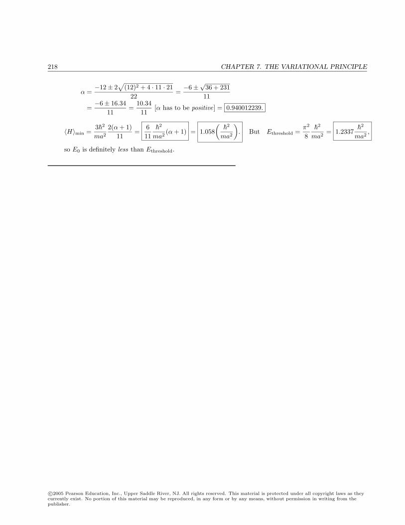
218 CHAPTER 7. THE VARIATIONAL PRINCIPLE
α =−12± 2
√(12)2 + 4 · 11 · 21
22=−6±
√36 + 23111
=−6± 16.34
11=
10.3411
[α has to be positive] = 0.940012239.
〈H〉min =32
ma2
2(α + 1)11
=611
2
ma2(α + 1) = 1.058
(
2
ma2
). But Ethreshold =
π2
8
2
ma2= 1.2337
2
ma2,
so E0 is definitely less than Ethreshold.
c©2005 Pearson Education, Inc., Upper Saddle River, NJ. All rights reserved. This material is protected under all copyright laws as theycurrently exist. No portion of this material may be reproduced, in any form or by any means, without permission in writing from thepublisher.
CHAPTER 8. THE WKB APPROXIMATION 219
Chapter 8
The WKB Approximation
Problem 8.1
∫ a
0
p(x) dx = nπ, with n = 1, 2, 3, . . . and p(x) =√
2m[E − V (x)] (Eq. 8.16).
Here∫ a
0
p(x) dx =√
2mE(a
2
)+
√2m(E − V0)
(a
2
)=√
2m(a
2
) (√E +
√E − V0
)= nπ
⇒ E + E − V0 + 2√
E(E − V0) =4
2m
(nπ
a
)2
= 4E0n; 2
√E(E − V0) = (4E0
n − 2E + V0).
Square again: 4E(E − V0) = 4E2 − 4EV0 = 16E0n
2+ 4E2 + V 2
0 − 16EE0n + 8E0
nV0 − 4EV0
⇒ 16EE0n = 16E0
n2
+ 8E0nV0 + V 2
0 ⇒ En = E0n +
V0
2+
V 20
16E0n
.
Perturbation theory gave En = E0n +
V0
2; the extra term goes to zero for very small V0 (or, since E0
n ∼ n2), forlarge n.
Problem 8.2
(a)
dψ
dx=
i
f ′eif/;
d2ψ
dx2=
i
(f ′′eif/ +
i
(f ′)2eif/
)=
[i
f ′′ − 1
2(f ′)2
]eif/.
d2ψ
dx2= −p2
2ψ =⇒
[i
f ′′ − 1
2(f ′)2
]eif/ = −p2
2eif/ =⇒ if ′′ − (f ′)2 + p2 = 0. QED
c©2005 Pearson Education, Inc., Upper Saddle River, NJ. All rights reserved. This material is protected under all copyright laws as theycurrently exist. No portion of this material may be reproduced, in any form or by any means, without permission in writing from thepublisher.
220 CHAPTER 8. THE WKB APPROXIMATION
(b) f ′ = f ′0 + f ′1 + 2f ′2 + · · · =⇒ (f ′)2 = (f ′0 + f ′1 + 2f ′2 + · · · )2 = (f ′0)2 + 2f ′0f
′1 + 2[2f ′0f
′2 + (f ′1)
2] + · · ·f ′′ = f ′′0 + f ′′1 + 2f ′′2 + · · · . i(f ′′0 + f ′′1 + 2f ′′2 )− (f ′0)
2 − 2f ′0f′1 − 2[2f ′0f
′2 + (f ′1)
2] + p2 + · · · = 0.
0 : (f ′0)
2 = p2; 1 : if ′′0 = 2f ′0f
′1;
2 : if ′′1 = 2f ′0f′2 + (f ′1)
2; . . .
(c)df0
dx= ±p =⇒ f0 = ±
∫p(x)dx + constant ;
df1
dx=
i
2f ′′0f ′0
=i
2
(±p′
±p
)=
i
2d
dxln p =⇒ f1 =
i
2ln p + const.
ψ = exp(if
)= exp
[i
(±
∫p(x) dx +
i
2ln p + K
)]= exp
(± i
∫p dx
)p−1/2eiK/
=C√p
exp(± i
∫p dx
). QED
Problem 8.3
γ =1
∫|p(x)| dx =
1
∫ 2a
0
√2m(V0 − E) dx =
2a
√2m(V0 − E). T ≈ e−4a
√2m(V0−E)/.
From Problem 2.33, the exact answer is
T =1
1 + V 20
4E(V0−E) sinh2 γ.
Now, the WKB approximation assumes the tunneling probability is small (p. 322)—which is to say that γ islarge. In this case, sinh γ = 1
2 (eγ − e−γ) ≈ 12e
γ , and sinh2 γ ≈ 14e
2γ , and the exact result reduces to
T ≈ 1
1 + V 20
16E(V0−E)e2γ≈
16E(V0 − E)
V 20
e−2γ .
The coefficient in is of order 1; the dominant dependence on E is in the exponential factor. In this senseT ≈ e−2γ (the WKB result).
Problem 8.4
I take the masses from Thornton and Rex, Modern Physics, Appendix 8. They are all atomic masses, but theelectron masses subtract out in the calculation of E. All masses are in atomic units (u): 1 u = 931 MeV/c2.The mass of He4 is 4.002602 u, and that of the α-particle is 3727 MeV/c2.
U238 : Z = 92, A = 238, m = 238.050784 u→ Th234 : m = 234.043593 u.
r1 = (1.07× 10⁻¹⁵ m)(238)1/3 = 6.63× 10⁻¹⁵ m.
E = (238.050784− 234.043593− 4.002602)(931) MeV = 4.27 MeV.
V =
√2Em
=
√(2)(4.27)
3727× 3× 108 m/s = 1.44× 10⁷ m/s.
c©2005 Pearson Education, Inc., Upper Saddle River, NJ. All rights reserved. This material is protected under all copyright laws as theycurrently exist. No portion of this material may be reproduced, in any form or by any means, without permission in writing from thepublisher.
CHAPTER 8. THE WKB APPROXIMATION 221
γ = 1.98090√4.27
− 1.485√
90(6.63) = 86.19− 36.28 = 49.9.
τ =(2)(6.63× 10⁻¹⁵)
1.44× 10⁷e98.8 s = 7.46× 10²¹ s =
7.46× 10²¹
3.15× 10⁷yr = 2.4× 10¹⁴ yrs.
Po212 : Z = 84, A = 212, m = 211.988842 u→ Pb208 : m = 207.976627 u.
r1 = (1.07× 10⁻¹⁵ m)(212)1/3 = 6.38× 10⁻¹⁵ m.
E = (211.988842− 207.976627− 4.002602)(931) MeV = 8.95 MeV.
V =
√2Em
=
√(2)(8.95)
3727× 3× 108 m/s = 2.08× 10⁷ m/s.
γ = 1.98082√8.95
− 1.485√
82(6.38) = 54.37− 33.97 = 20.4.
τ =(2)(6.38× 10⁻¹⁵)
2.08× 10⁷e40.8 s = 3.2× 10⁻⁴ s.
These results are way off—but note the extraordinary sensitivity to nuclear masses: a tiny change in E producesenormous changes in τ .
Much more impressive results are obtained when you plot the logarithm of lifetimes against 1/√E, as in
Figure 8.6. Thanks to David Rubin for pointing this out. Some experimental values are listed below (all energiesin MeV):
Uranium (Z = 92):
A E τ238 4.198 4.468× 10⁹ yr236 4.494 2.342× 10⁷ yr234 4.775 2.455× 10⁵ yr232 5.320 68.9 yr230 5.888 20.8 day228 6.680 9.1 min226 7.570 0.35 s
Protactinium (Z = 91):
A E τ224 7.488 0.79 s222 8.540 2.9 ms220 9.650 0.78 µs218 9.614 0.12 ms
Thorium (Z = 90):
A E τ232 4.012 1.405× 10¹⁰ yr230 4.687 7.538× 10⁴ yr228 5.423 1.912 yr226 6.337 30.57 min
Radium (Z = 88):
A E τ226 4.784 1600 yr224 5.685 3.66 day222 6.559 38 s220 7.455 18 ms218 8.389 25.6µs
c©2005 Pearson Education, Inc., Upper Saddle River, NJ. All rights reserved. This material is protected under all copyright laws as theycurrently exist. No portion of this material may be reproduced, in any form or by any means, without permission in writing from thepublisher.
222 CHAPTER 8. THE WKB APPROXIMATION
Problem 8.5
(a) V (x) = mgx.
(b)
− 2
2md2ψ
dx2+ mgxψ = Eψ =⇒ d2ψ
dx2=
2m2g
2
(x− E
mg
). Let y ≡ x− E
mg, and α ≡
(2m2g
2
)1/3
.
Thend2ψ
dy2= α3yψ. Let z ≡ αy = α(x − E
mg), so
d2ψ
dz2= zψ. This is the Airy equation (Eq. 8.36), and
the general solution is ψ = aAi(z) + bBi(z). However, Bi(z) blows up for large z, so b = 0 (to make ψ
normalizable). Hence ψ(x) = aAi[α(x− E
mg )].
(c) Since V (x) = ∞ for x < 0, we require ψ(0) = 0; hence Ai [α(−E/mg)] = 0. Now, the zeros of Ai arean (n = 1, 2, 3, . . . ). Abramowitz and Stegun list a1 = −2.338, a2 = −4.088, a3 = −5.521, a4 = −6.787,
etc. Here −αEn
mg= an, or En = −mg
αan = −mg
(
2
2m2g
)1/3
an, or En = −( 12mg2
2)1/3an. In this case
12mg2
2 = 1
2 (0.1 kg)(9.8 m/s2)2(1.055× 10−34J·s)2 = 5.34× 10−68 J3; ( 12mg2
2)1/3 = 3.77× 10⁻²³ J.
E1 = 8.81× 10⁻²³ J, E2 = 1.54× 10⁻²² J, E3 = 2.08× 10⁻²² J, E4 = 2.56× 10⁻²² J.
(d)
2〈T 〉 = 〈x dV
dX〉 (Eq. 3.97); here
dV
dx= mg, so 〈xdV
dx〉 = 〈mgx〉 = 〈V 〉, so 〈T 〉 =
12〈V 〉.
But 〈T 〉+ 〈V 〉 = 〈H〉 = En, so32〈V 〉 = En, or 〈V 〉 =
23En. But 〈V 〉 = mg〈x〉, so 〈x〉 =
2En
3mg.
For the electron,(
12mg2
2
)1/3
=[12(9.11× 10⁻³¹)(9.8)2(1.055× 10⁻³⁴)2
]1/3
= 7.87× 10⁻³³ J.
E1 = 1.84× 10⁻³² J = 1.15× 10⁻¹³ eV. 〈x〉 =2(1.84× 10⁻³²)
3(9.11× 10⁻³¹)(9.8)= 1.37× 10−3 = 1.37 mm.
Problem 8.6
(a)
Eq. 8.47 =⇒∫ x2
0
p(x) dx = (n− 14)π, where p(x) =
√2m(E −mgx) and E = mgx2 =⇒ x2 = E/mg.
∫ x2
0
p(x) dx =√
2m∫ x2
0
√E −mgxdx =
√2m
[− 2
3mg(E −mgx)3/2
]∣∣∣∣x2
0
= −23
√2m
1g
[(E −mgx2)3/2 − E3/2
]=
23
√2m
1gE3/2.
c©2005 Pearson Education, Inc., Upper Saddle River, NJ. All rights reserved. This material is protected under all copyright laws as theycurrently exist. No portion of this material may be reproduced, in any form or by any means, without permission in writing from thepublisher.
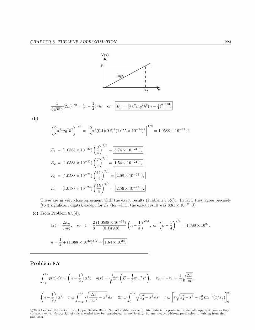
CHAPTER 8. THE WKB APPROXIMATION 223
E
V(x)
x x
mgx
2
13√mg
(2E)3/2 = (n− 14)π, or En =
[98π
2mg2
2(n− 14 )2
]1/3.
(b) (98π2mg2
2
)1/3
=[98π2(0.1)(9.8)2(1.055× 10⁻³⁴)2
]1/3
= 1.0588× 10⁻²² J.
E1 = (1.0588× 10⁻²²)(
34
)2/3
= 8.74× 10⁻²³ J,
E2 = (1.0588× 10⁻²²)(
74
)2/3
= 1.54× 10⁻²² J,
E3 = (1.0588× 10⁻²²)(
114
)2/3
= 2.08× 10⁻²² J,
E4 = (1.0588× 10⁻²²)(
154
)2/3
= 2.56× 10⁻²² J.
These are in very close agreement with the exact results (Problem 8.5(c)). In fact, they agree precisely(to 3 significant digits), except for E1 (for which the exact result was 8.81× 10⁻²³ J).
(c) From Problem 8.5(d),
〈x〉 =2En
3mg, so 1 =
23
(1.0588× 10⁻²²)(0.1)(9.8)
(n− 1
4
)2/3
, or(n− 1
4
)2/3
= 1.388× 10²².
n =14
+ (1.388× 10²²)3/2 = 1.64× 1033.
Problem 8.7
∫ x2
x1
p(x) dx =(n− 1
2
)π; p(x) =
√2m
(E − 1
2mω2x2
); x2 = −x1 =
1ω
√2Em
.
(n− 1
2
)π = mω
∫ x2
−x2
√2Emω2
− x2 dx = 2mω
∫ x2
0
√x2
2 − x2 dx = mω
[x√
x22 − x2 + x2
2 sin−1(x/x2)]x2
0
c©2005 Pearson Education, Inc., Upper Saddle River, NJ. All rights reserved. This material is protected under all copyright laws as theycurrently exist. No portion of this material may be reproduced, in any form or by any means, without permission in writing from thepublisher.
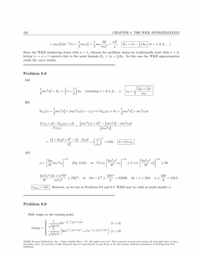
224 CHAPTER 8. THE WKB APPROXIMATION
= mωx22 sin−1(1) =
π
2mωx2
2 =π
2mω
2Emω2
=πE
ω. En =
(n− 1
2
)ω (n = 1, 2, 3, . . . )
Since the WKB numbering starts with n = 1, whereas for oscillator states we traditionally start with n = 0,letting n → n + 1 converts this to the usual formula En = (n + 1
2 )ω. In this case the WKB approximationyields the exact results.
Problem 8.8
(a)
12mω2x2
2 = En =(n +
12
)ω (counting n = 0, 1, 2, . . . ); x2 =
√(2n + 1)
mω.
(b)
Vlin(x) =12mω2x2
2 + (mω2x2)(x− x2) =⇒ Vlin(x2 + d) =12mω2x2
2 + mω2x2d.
V (x2 + d)− Vlin(x2 + d)V (x2)
=12mω2(x2 + d)2 − 1
2mω2x22 −mω2x2d
12mω2x2
2
=x2
2 + 2x2d + d2 − x22 − 2x2d
x22
=(
d
x2
)2
= 0.01. d = 0.1x2.
(c)
α =[2m2
mω2x2
]1/3
(Eq. 8.34), so 0.1x2
[2m2ω2
2x2
]1/3
≥ 5 =⇒[2m2ω2
2x4
2
]1/3
≥ 50.
2m2ω2
2
(2n + 1)22
m2ω2≥ (50)3; or (2n + 1)2 ≥ (50)3
2= 62500; 2n + 1 ≥ 250; n ≥ 249
2= 124.5.
nmin = 125. However, as we saw in Problems 8.6 and 8.7, WKB may be valid at much smaller n.
Problem 8.9
Shift origin to the turning point.
ψWKB =
1√|p(x)|
De−1
∫ 0x|p(x′)| dx′ (x < 0)
1√|p(x)|
[Be
i
∫ x0 p(x′) dx′ + Ce−
i
∫ x0 p(x′) dx′
](x > 0)
c©2005 Pearson Education, Inc., Upper Saddle River, NJ. All rights reserved. This material is protected under all copyright laws as theycurrently exist. No portion of this material may be reproduced, in any form or by any means, without permission in writing from thepublisher.
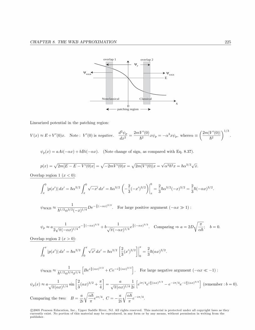
CHAPTER 8. THE WKB APPROXIMATION 225
x0
Nonclassical Classical
overlap 2overlap 1
WKB
P
ψ
ψ
WKBψ
patching region
E
Linearized potential in the patching region:
V (x) ≈ E+V ′(0)x. Note : V ′(0) is negative.d2ψp
dx2=
2mV ′(0)2
xψp = −α3xψp, whereα ≡(
2m|V ′(0)|2
)1/3
.
ψp(x) = aAi(−αx) + bBi(−αx). (Note change of sign, as compared with Eq. 8.37).
p(x) =√
2m[E − E − V ′(0)x] =√−2mV ′(0)x =
√2m|V ′(0)|x =
√α32x = α3/2
√x.
Overlap region 1 (x < 0):
∫ 0
x
|p(x′)| dx′ = α3/2
∫ 0
x
√−x′ dx′ = α3/2
(−2
3(−x′)3/2
)∣∣∣∣0x
=23α3/2(−x)3/2 =
23(−αx)3/2.
ψWKB ≈1
1/2α3/2(−x)1/4De−
23 (−αx)3/2 . For large positive argument (−αx 1) :
ψp ≈ a1
2√π(−αx)1/4
e−23 (−αx)3/2 + b
1√π(−αx)1/4
e23 (−αx)3/2 . Comparing⇒ a = 2D
√π
α; b = 0.
Overlap region 2 (x > 0):∫ x
0
|p(x′)| dx′ = α3/2
∫ x
0
√x′ dx′ = α3/2
[23(x′)3/2
]∣∣∣∣x0
=23(αx)3/2.
ψWKB ≈1
1/2α3/4x1/4
[Bei 2
3 (αx)3/2 + Ce−i 23 (αx)3/2
]. For large negative argument (−αx −1) :
ψp(x) ≈ a1√
π(αx)1/4sin
[23(αx)3/2 +
π
4
]=
a√π(αx)1/4
12i
[eiπ/4ei 2
3 (αx)3/2 − e−iπ/4e−i 23 (αx)3/2
](remember : b = 0).
Comparing the two: B =a
2i
√α
πeiπ/4, C = − a
2i
√α
πe−iπ/4.
c©2005 Pearson Education, Inc., Upper Saddle River, NJ. All rights reserved. This material is protected under all copyright laws as theycurrently exist. No portion of this material may be reproduced, in any form or by any means, without permission in writing from thepublisher.
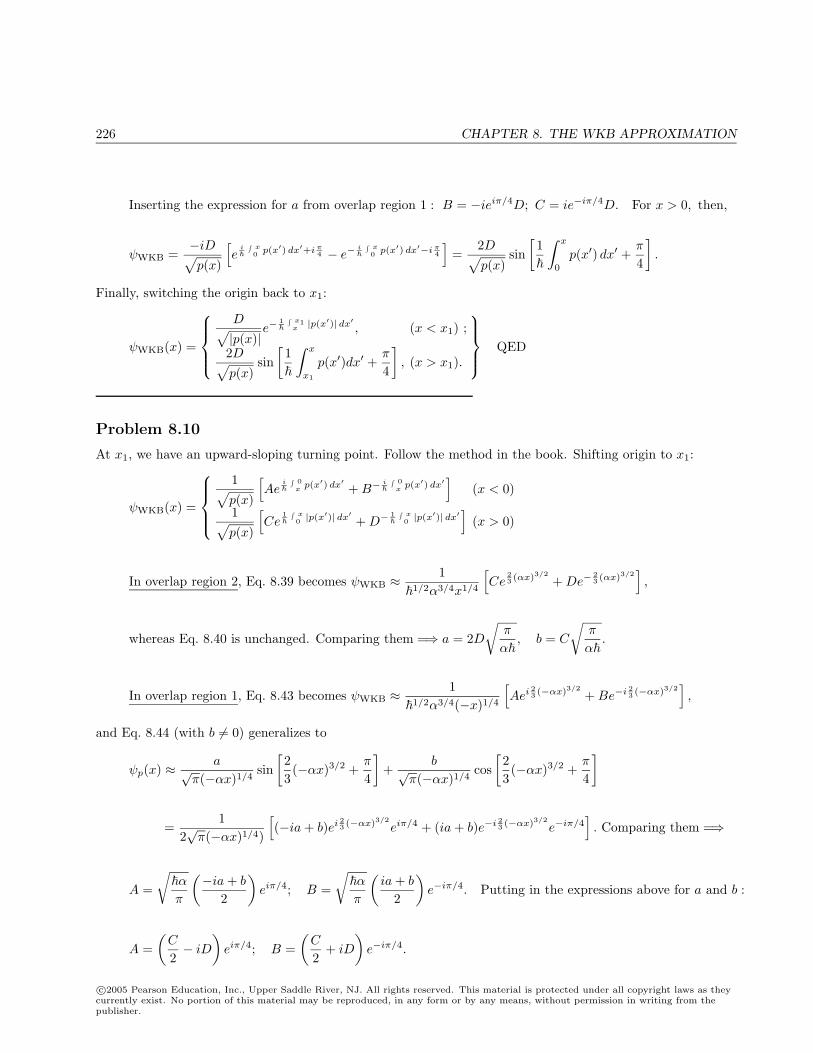
226 CHAPTER 8. THE WKB APPROXIMATION
Inserting the expression for a from overlap region 1 : B = −ieiπ/4D; C = ie−iπ/4D. For x > 0, then,
ψWKB =−iD√p(x)
[ei
∫ x0 p(x′) dx′+iπ4 − e−
i
∫ x0 p(x′) dx′−iπ4
]=
2D√p(x)
sin[
1
∫ x
0
p(x′) dx′ +π
4
].
Finally, switching the origin back to x1:
ψWKB(x) =
D√|p(x)|
e−1
∫ x1x|p(x′)| dx′ , (x < x1) ;
2D√p(x)
sin[
1
∫ x
x1
p(x′)dx′ +π
4
], (x > x1).
QED
Problem 8.10
At x1, we have an upward-sloping turning point. Follow the method in the book. Shifting origin to x1:
ψWKB(x) =
1√p(x)
[Ae
i
∫ 0x
p(x′) dx′ + B−i
∫ 0x
p(x′) dx′]
(x < 0)
1√p(x)
[Ce
1
∫ x0 |p(x′)| dx′ + D−
1
∫ x0 |p(x′)| dx′
](x > 0)
In overlap region 2, Eq. 8.39 becomes ψWKB ≈1
1/2α3/4x1/4
[Ce
23 (αx)3/2 + De−
23 (αx)3/2
],
whereas Eq. 8.40 is unchanged. Comparing them =⇒ a = 2D√
π
α, b = C
√π
α.
In overlap region 1, Eq. 8.43 becomes ψWKB ≈1
1/2α3/4(−x)1/4
[Aei 2
3 (−αx)3/2 + Be−i 23 (−αx)3/2
],
and Eq. 8.44 (with b = 0) generalizes to
ψp(x) ≈ a√π(−αx)1/4
sin[23(−αx)3/2 +
π
4
]+
b√π(−αx)1/4
cos[23(−αx)3/2 +
π
4
]
=1
2√π(−αx)1/4)
[(−ia + b)ei 2
3 (−αx)3/2eiπ/4 + (ia + b)e−i 23 (−αx)3/2e−iπ/4
]. Comparing them =⇒
A =
√α
π
(−ia + b
2
)eiπ/4; B =
√α
π
(ia + b
2
)e−iπ/4. Putting in the expressions above for a and b :
A =(C
2− iD
)eiπ/4; B =
(C
2+ iD
)e−iπ/4.
c©2005 Pearson Education, Inc., Upper Saddle River, NJ. All rights reserved. This material is protected under all copyright laws as theycurrently exist. No portion of this material may be reproduced, in any form or by any means, without permission in writing from thepublisher.
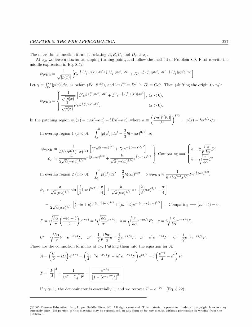
CHAPTER 8. THE WKB APPROXIMATION 227
These are the connection formulas relating A,B,C, and D, at x1.At x2, we have a downward-sloping turning point, and follow the method of Problem 8.9. First rewrite the
middle expression in Eq. 8.52:
ψWKB =1√|p(x)|
[Ce
1
∫ x2x1|p(x′)| dx′+ 1
∫ xx2|p(x′)| dx′ + De
− 1
∫ x2x1|p(x′)| dx′− 1
∫ xx2|p(x′)| dx′
].
Let γ ≡∫ x2
x1|p(x)| dx, as before (Eq. 8.22), and let C ′ ≡ De−γ , D′ ≡ Ceγ . Then (shifting the origin to x2):
ψWKB =
1√|p(x)|
[C ′e
1
∫ 0x|p(x′)| dx′ + D′e−
1
∫ 0x|p(x′)| dx′
], (x < 0);
1√p(x)
Fei
∫ x0 p(x′) dx′ , (x > 0).
In the patching region ψp(x) = aAi(−αx) + bBi(−αx), where α ≡(
2m|V ′(0)|2
)1/3
; p(x) = α3/2√x.
In overlap region 1 (x < 0):∫ 0
x
|p(x′)| dx′ = 23(−αx)3/2, so
ψWKB ≈1
1/2α3/4(−x)1/4
[C ′e
23 (−αx)3/2 + D′e−
23 (−αx)3/2
]ψp ≈
a
2√π(−αx)1/4
e−23 (−αx)3/2 +
b√π(−αx)1/4
e23 (−αx)3/2
Comparing =⇒
a = 2
√π
αD′
b =√
π
αC ′
In overlap region 2 (x > 0):∫ x
0
p(x′) dx′ =23(αx)3/2 =⇒ ψWKB ≈
11/2α3/4x1/4
Fei 23 (αx)3/2 .
ψp ≈a√
π(αx)1/4sin
[23(αx)3/2 +
π
4
]+
b√π(αx)1/4
cos[23(αx)3/2 +
π
4
]
=1
2√π(αx)1/4
[(−ia + b)eiπ4 ei 2
3 (αx)3/2 + (ia + b)e−iπ4 e−i 23 (αx)3/2
]. Comparing =⇒ (ia + b) = 0;
F =
√α
π
(−ia + b
2
)eiπ/4 = b
√α
πeiπ/4. b =
√π
αe−iπ/4F ; a = i
√π
αe−iπ/4F.
C ′ =
√α
πb = e−iπ/4F, D′ =
12
√α
πa =
i
2e−iπ/4F. D = eγe−iπ/4F ; C =
i
2e−γe−iπ/4F.
These are the connection formulas at x2. Putting them into the equation for A:
A =(C
2− iD
)eiπ/4 =
(i
4e−γe−iπ/4F − ieγe−iπ/4F
)eiπ/4 = i
(e−γ
4− eγ
)F.
T =∣∣∣∣FA
∣∣∣∣2 =1
(eγ − e−γ
4 )2=
e−2γ[1− (e−γ/2)2
]2 .
If γ 1, the denominator is essentially 1, and we recover T = e−2γ (Eq. 8.22).
c©2005 Pearson Education, Inc., Upper Saddle River, NJ. All rights reserved. This material is protected under all copyright laws as theycurrently exist. No portion of this material may be reproduced, in any form or by any means, without permission in writing from thepublisher.
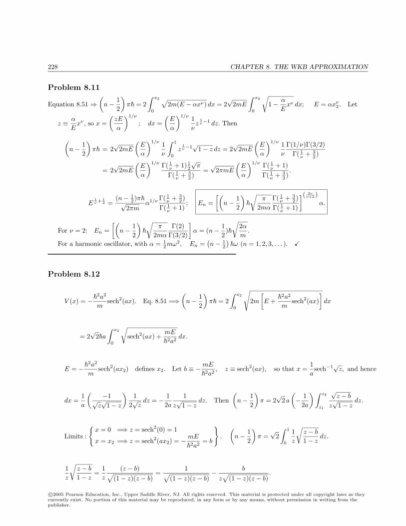
228 CHAPTER 8. THE WKB APPROXIMATION
Problem 8.11
Equation 8.51 ⇒(n− 1
2
)π = 2
∫ x2
0
√2m(E − αxν) dx = 2
√2mE
∫ x2
0
√1− α
Exν dx; E = αxν
2 . Let
z ≡ α
Exν , so x =
(zE
α
)1/ν
; dx =(E
α
)1/ν 1νz
1ν−1 dz. Then
(n− 1
2
)π = 2
√2mE
(E
α
)1/ν 1ν
∫ 1
0
z1ν−1
√1− z dz = 2
√2mE
(E
α
)1/ν 1ν
Γ(1/ν)Γ(3/2)Γ( 1
ν + 32 )
= 2√
2mE
(E
α
)1/ν Γ( 1ν + 1) 1
2
√π
Γ( 1ν + 3
2 )=√
2πmE
(E
α
)1/ν Γ( 1ν + 1)
Γ( 1ν + 3
2 ).
E1ν+ 1
2 =(n− 1
2 )π√2πm
α1/ν Γ( 1ν + 3
2 )Γ( 1
ν + 1); En =
[(n− 1
2
)
√π
2mα
Γ( 1ν + 3
2 )Γ( 1
ν + 1)
]( 2νν+2 )
α.
For ν = 2: En =[(
n− 12
)
√π
2mα
Γ(2)Γ(3/2)
]α = (n− 1
2)
√2αm
.
For a harmonic oscillator, with α = 12mω2, En =
(n− 1
2
)ω (n = 1, 2, 3, . . . ).
Problem 8.12
V (x) = −2a2
msech2(ax). Eq. 8.51 =⇒
(n− 1
2
)π = 2
∫ x2
0
√2m
[E +
2a2
msech2(ax)
]dx
= 2√
2a∫ x2
0
√sech2(ax) +
mE
2a2dx.
E = −2a2
msech2(ax2) defines x2. Let b ≡ − mE
2a2, z ≡ sech2(ax), so that x =
1asech−1√z, and hence
dx =1a
( −1√z√
1− z
)1
2√zdz = − 1
2a1
z√
1− zdz. Then
(n− 1
2
)π = 2
√2 a
(− 1
2a
) ∫ z2
z1
√z − b
z√
1− zdz.
Limits :
x = 0 =⇒ z = sech2(0) = 1
x = x2 =⇒ z = sech2(ax2) = − mE
2a2= b
.
(n− 1
2
)π =
√2
∫ 1
b
1z
√z − b
1− zdz.
1z
√z − b
1− z=
1z
(z − b)√(1− z)(z − b)
=1√
(1− z)(z − b)− b
z√
(1− z)(z − b).
c©2005 Pearson Education, Inc., Upper Saddle River, NJ. All rights reserved. This material is protected under all copyright laws as theycurrently exist. No portion of this material may be reproduced, in any form or by any means, without permission in writing from thepublisher.
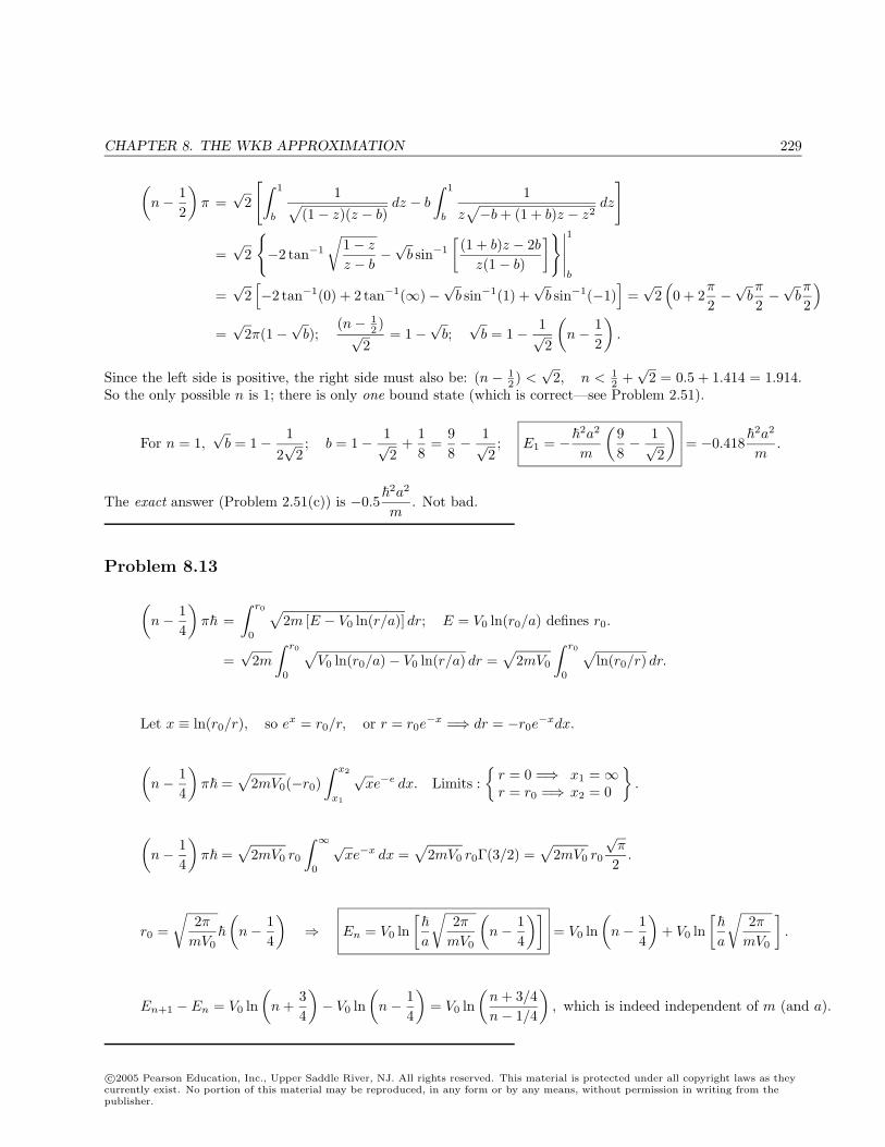
CHAPTER 8. THE WKB APPROXIMATION 229
(n− 1
2
)π =
√2
[∫ 1
b
1√(1− z)(z − b)
dz − b
∫ 1
b
1z√−b + (1 + b)z − z2
dz
]
=√
2
−2 tan−1
√1− z
z − b−√b sin−1
[(1 + b)z − 2b
z(1− b)
]∣∣∣∣∣1
b
=√
2[−2 tan−1(0) + 2 tan−1(∞)−
√b sin−1(1) +
√b sin−1(−1)
]=√
2(0 + 2
π
2−√bπ
2−√bπ
2
)=√
2π(1−√b);
(n− 12 )√
2= 1−
√b;
√b = 1− 1√
2
(n− 1
2
).
Since the left side is positive, the right side must also be: (n− 12 ) <
√2, n < 1
2 +√
2 = 0.5 + 1.414 = 1.914.So the only possible n is 1; there is only one bound state (which is correct—see Problem 2.51).
For n = 1,√b = 1− 1
2√
2; b = 1− 1√
2+
18
=98− 1√
2; E1 = −
2a2
m
(98− 1√
2
)= −0.418
2a2
m.
The exact answer (Problem 2.51(c)) is −0.5
2a2
m. Not bad.
Problem 8.13
(n− 1
4
)π =
∫ r0
0
√2m [E − V0 ln(r/a)] dr; E = V0 ln(r0/a) defines r0.
=√
2m∫ r0
0
√V0 ln(r0/a)− V0 ln(r/a) dr =
√2mV0
∫ r0
0
√ln(r0/r) dr.
Let x ≡ ln(r0/r), so ex = r0/r, or r = r0e−x =⇒ dr = −r0e
−xdx.
(n− 1
4
)π =
√2mV0(−r0)
∫ x2
x1
√xe−e dx. Limits :
r = 0 =⇒ x1 =∞r = r0 =⇒ x2 = 0
.
(n− 1
4
)π =
√2mV0 r0
∫ ∞0
√xe−x dx =
√2mV0 r0Γ(3/2) =
√2mV0 r0
√π
2.
r0 =√
2πmV0
(n− 1
4
)⇒ En = V0 ln
[
a
√2πmV0
(n− 1
4
)]= V0 ln
(n− 1
4
)+ V0 ln
[
a
√2πmV0
].
En+1 − En = V0 ln(n +
34
)− V0 ln
(n− 1
4
)= V0 ln
(n + 3/4n− 1/4
), which is indeed independent of m (and a).
c©2005 Pearson Education, Inc., Upper Saddle River, NJ. All rights reserved. This material is protected under all copyright laws as theycurrently exist. No portion of this material may be reproduced, in any form or by any means, without permission in writing from thepublisher.
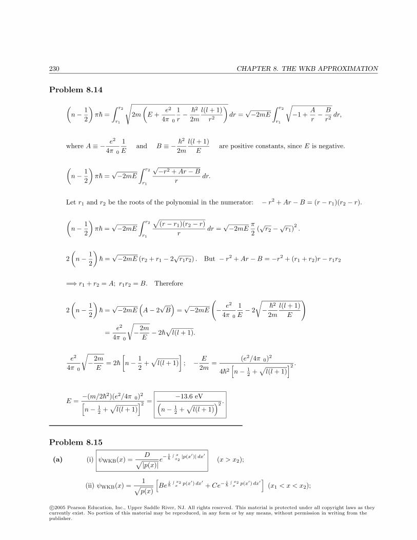
230 CHAPTER 8. THE WKB APPROXIMATION
Problem 8.14
(n− 1
2
)π =
∫ r2
r1
√2m
(E +
e2
4πε01r− 2
2ml(l + 1)
r2
)dr =
√−2mE
∫ r2
r1
√−1 +
A
r− B
r2dr,
where A ≡ − e2
4πε01E
and B ≡ − 2
2ml(l + 1)
Eare positive constants, since E is negative.
(n− 1
2
)π =
√−2mE
∫ r2
r1
√−r2 + Ar −B
rdr.
Let r1 and r2 be the roots of the polynomial in the numerator: − r2 + Ar −B = (r − r1)(r2 − r).
(n− 1
2
)π =
√−2mE
∫ r2
r1
√(r − r1)(r2 − r)
rdr =
√−2mE
π
2(√r2 −
√r1)
2.
2(n− 1
2
) =
√−2mE (r2 + r1 − 2
√r1r2) . But − r2 + Ar −B = −r2 + (r1 + r2)r − r1r2
=⇒ r1 + r2 = A; r1r2 = B. Therefore
2(n− 1
2
) =
√−2mE
(A− 2
√B
)=√−2mE
(− e2
4πε01E− 2
√−
2
2ml(l + 1)
E
)
=e2
4πε0
√−2m
E− 2
√l(l + 1).
e2
4πε0
√−2m
E= 2
[n− 1
2+
√l(l + 1)
]; − E
2m=
(e2/4πε0)2
42[n− 1
2 +√
l(l + 1)]2 .
E =−(m/22)(e2/4πε0)2[n− 1
2 +√
l(l + 1)]2 =
−13.6 eV(n− 1
2 +√
l(l + 1))2 .
Problem 8.15
(a) (i) ψWKB(x) =D√|p(x)|
e− 1
∫ xx2|p(x′)| dx′ (x > x2);
(ii) ψWKB(x) =1√p(x)
[Be
i
∫ x2x
p(x′) dx′ + Ce−i
∫ x2x
p(x′) dx′]
(x1 < x < x2);
c©2005 Pearson Education, Inc., Upper Saddle River, NJ. All rights reserved. This material is protected under all copyright laws as theycurrently exist. No portion of this material may be reproduced, in any form or by any means, without permission in writing from thepublisher.
CHAPTER 8. THE WKB APPROXIMATION 231
(iii) ψWKB(x) =1√|p(x)|
[Fe
1
∫ x1x|p(x′)| dx′ + Ge−
1
∫ x1x|p(x′)| dx′
](0 < x < x1).
Equation 8.46 =⇒ (ii) ψWKB =2D√p(x)
sin[
1
∫ x2
x
p(x′)dx′ +π
4
](x1 < x < x2).
To effect the join at x1, first rewrite (ii):
(ii) ψWKB =2D√p(x)
sin[
1
∫ x2
x1
p(x′) dx′ − 1
∫ x
x1
p(x′) dx′ +π
4
]= − 2D√
p(x)sin
[1
∫ x
x1
p(x′) dx′ − θ − π
4
],
where θ is defined in Eq. 8.58. Now shift the origin to x1:
ψWKB =
1√|p(x)|
[Fe
1
∫ 0x|p(x′)| dx′ + Ge−
1
∫ 0x|p(x′)| dx′
](x < 0)
− 2D√p(x)
sin[
1
∫ x
0
p(x′) dx′ − θ − π
4
](x > 0)
.
Following Problem 8.9: ψp(x) = aAi(−αx) + bBi(−αx), with α ≡(
2m|V ′(0)|2
)1/3
; p(x) = α3/2√x.
Overlap region 1 (x < 0):∫ 0
x
|p(x′)| dx′ = 23(−αx)3/2.
ψWKB ≈1
1/2α3/4(−x)1/4
[Fe
23 (−αx)3/2 + Ge−
23 (−αx)3/2
]ψp ≈ a
2√π(−αx)1/4
e−23 (−αx)3/2 +
b√π(−αx)1/4
e23 (−αx)3/2
=⇒ a = 2G√
π
α; b = F
√π
α.
Overlap region 2 (x > 0):∫ x
0
p(x′) dx′ =23(αx)3/2.
=⇒ ψWKB ≈ −2D
1/2α3/4x1/4sin
[23(αx)3/2 − θ − π
4
],
ψp ≈a√
π(αx)1/4sin
[23(αx)3/2 +
π
4
]+
b√π(αx)1/4
cos[23(αx)3/2 +
π
4
].
Equating the two expressions:−2D
1/2α3/4
12i
[ei 2
3 (αx)3/2e−iθe−iπ/4 − e−i 23 (αx)3/2eiθeiπ/4
]
=1√
πα1/4
a
2i
[ei 2
3 (αx)3/2eiπ/4 − e−i 23 (αx)3/2e−iπ/4
]+
b
2
[ei 2
3 (αx)3/2eiπ/4 + e−i 23 (αx)3/2e−iπ/4
]
=⇒
−2D
√π
αe−iθe−iπ/4 = (a + ib)eiπ/4, or (a + ib) = 2D
√π
αie−iθ
2D√
π
αeiθeiπ/4 = (−a + ib)e−iπ/4, or (a− ib) = −2D
√π
αieiθ
c©2005 Pearson Education, Inc., Upper Saddle River, NJ. All rights reserved. This material is protected under all copyright laws as theycurrently exist. No portion of this material may be reproduced, in any form or by any means, without permission in writing from thepublisher.
232 CHAPTER 8. THE WKB APPROXIMATION
=⇒
2a = 2D
√π
αi(e−iθ − eiθ)⇒ a = 2D
√π
αsin θ,
2ib = 2D√
π
αi(e−iθ + eiθ)⇒ b = 2D
√π
αcos θ.
Combining these with the results from overlap region 1 =⇒
2G√
π
α= 2D
√π
αsin θ, or G = D sin θ; F
√π
α= 2D
√π
αcos θ, or F = 2D cos θ.
Putting these into (iii) : ψWKB(x) =D√|p(x)|
[2 cos θe
1
∫ x1x|p(x′)| dx′ + sin θe−
1
∫ x1x|p(x′)| dx′
](0 < x < x1).
(b)
Odd(−) case: (iii) =⇒ ψ(0) = 0⇒ 2 cos θe1
∫ x10 |p(x′)| dx′ + sin θe−
1
∫ x10 |p(x′)| dx′ = 0.
1
∫ x1
0
|p(x′)| dx′ = 12φ, with φ defined by Eq. 8.60. So sin θe−φ/2 = −2 cos θeφ/2, or tan θ = −2eφ.
Even(+) case: (iii) =⇒ ψ′(0) = 0⇒ −12
D
(|p(x)|)3/2
d|p(x)|dx
∣∣∣∣0
[2 cos θeφ/2 + sin θe−φ/2
]
+D√|p(x)|
[2 cos θe
1
∫ x10 |p(x′)| dx′
(−1|p(0)|
)+ sin θe−
1
∫ x10 |p(x′)| dx′
(1|p(0)|
)]= 0.
Nowd|p(x)|
dx=
d
dx
√2m[V (x)− E] =
√2m
12
1√V − E
dV
dx, and
dV
dx
∣∣∣∣0
= 0, sod|p(x)|
dx
∣∣∣∣0
= 0.
2 cos θeφ/2 = sin θe−φ/2, or tan θ = 2eφ. Combining the two results: tan θ = ±2eφ. QED
(c)
tan θ = tan[(
n +12
)π + ε
]=
sin[(
n + 12
)π + ε
]cos
[(n + 1
2
)π + ε
] =(−1)n cos ε
(−1)n+1 sin ε= −cos ε
sin ε≈ −1
ε.
So − 1ε≈ ±2eφ, or ε ≈ ∓1
2e−φ, or θ −
(n +
12
)π ≈ ∓1
2e−φ, so θ ≈
(n +
12
)π ∓ 1
2e−φ. QED
[Note: Since θ (Eq. 8.58) is positive, n must be a non-negative integer: n = 0, 1, 2, . . . . This is likeharmonic oscillator (conventional) numbering, since it starts with n = 0.]
c©2005 Pearson Education, Inc., Upper Saddle River, NJ. All rights reserved. This material is protected under all copyright laws as theycurrently exist. No portion of this material may be reproduced, in any form or by any means, without permission in writing from thepublisher.
CHAPTER 8. THE WKB APPROXIMATION 233
a-a x x x
V(x)
1 2
(d)
θ =1
∫ x2
x1
√2m
[E − 1
2mω2(x− a)2
]dx. Let z = x− a (shifts the origin to a).
=2
∫ z2
0
√2m
[E − 1
2mω2z2
]dz, where E =
12mω2z2
2 .
=2mω
∫ z2
0
√z22 − z2 dz =
mω
[z√
z22 − z2 + z2
2 sin−1(z/z2)]∣∣∣∣z2
0
=mω
z22 sin−1(1) =
π
2mω
z22 ,
=π
2mω
2Emω2
=πE
ω.
Putting this into Eq. 8.61 yieldsπE
ω≈
(n +
12
)π ∓ 1
2e−φ, or E±n ≈
(n +
12
)ω ∓ ω
2πe−φ. QED
(e)
Ψ(x, t) =1√2
(ψ+
n e−iE+n t/ + ψ−n e−iE−n t/
)=⇒
|Ψ(x, t)|2 =12
[|ψ+
n |2 + |ψ−n |2 + ψ+n ψ−n
(ei(E−n −E+
n )t/ + e−i(E−n −E+n )t/
)].
(Note that the wave functions (i), (ii), (iii) are real). ButE−n − E+
n
≈ 12ω
2πe−φ =
ω
πe−φ, so
|Ψ(x, t)|2 =12
[ψ+
n (x)2 + ψ−n (x)2]+ ψ+
n (x)ψ−n (x) cos(ω
πe−φt
).
It oscillates back and forth, with period τ =2π
(ω/π) e−φ=
2π2
ωeφ. QED
(f)
φ = 21
∫ x1
0
√2m
[12mω2(x− a)2 − E
]dx =
2
√2mE
∫ x1
0
√mω2
2E(x− a)2 − 1 dx.
c©2005 Pearson Education, Inc., Upper Saddle River, NJ. All rights reserved. This material is protected under all copyright laws as theycurrently exist. No portion of this material may be reproduced, in any form or by any means, without permission in writing from thepublisher.
234 CHAPTER 8. THE WKB APPROXIMATION
Let z ≡√
m
2Eω(a− x), so dx = −
√2Em
1ωdz. Limits:
x = 0 =⇒ z =√
m
2Eωa ≡ z0
x = x1 =⇒ radicand = 0 =⇒ z = 1
.
φ =2
√2mE
√2Em
1ω
∫ z0
1
√z2 − 1 dz =
4Eω
∫ z0
1
√z2 − 1 dz =
4Eω
12
[z√
z2 − 1− ln(z +√
z2 − 1)]∣∣∣z0
1
=2Eω
[z0
√z20 − 1− ln
(z0 +
√z20 − 1
)],
where z0 = aω
√m
2E. V (0) = 1
2mω2a2, so V (0) E ⇒ m
2ω2a2 E ⇒ aω
√m
2E 1, or z0 1.
In that case
φ ≈ 2Eω
[z20 − ln(2z0)
]≈ 2Eω
z20 =
2Eω
a2ω2 m
2E=
mωa2
.
This, together with Eq. 8.64, gives us the period of oscillation in a double well.
Problem 8.16
(a) En ≈n2π2
2
2m(2a)2. With n = 1, E1 =
π2
2
8ma2.
(b)
V(x)
x
V0
E1
a-a
V(x)
x
E1
a-a x0
E tunneling
(c)
γ =1
∫ x0
a
|p(x)| dx. αx0 = V0 − E1 ⇒ x0 =V0 − E1
α.
p(x) =√
2m [E − V (x)]; V (x) = −αx, E = E1 − V0.
=√
2m(E1 − V0 + αx) =√
2mα√x− x0; |p(x)| =
√2mα
√x0 − x.
γ =1
√2mα
∫ x0
a
√x0 − x dx =
√2mα
[−2
3(x0 − x)3/2
] ∣∣∣∣x0
a
=23
√2mα
(x0 − a)3/2.
c©2005 Pearson Education, Inc., Upper Saddle River, NJ. All rights reserved. This material is protected under all copyright laws as theycurrently exist. No portion of this material may be reproduced, in any form or by any means, without permission in writing from thepublisher.
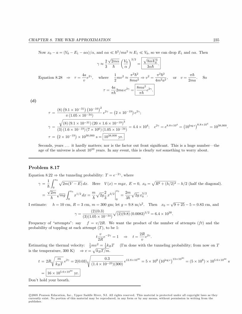
CHAPTER 8. THE WKB APPROXIMATION 235
Now x0 − a = (V0 − E1 − aα)/α, and αa 2/ma2 ≈ E1 V0, so we can drop E1 and αa. Then
γ ≈ 23
√2mα
(V0
α
)3/2
=
√8mV 3
0
3α.
Equation 8.28 ⇒ τ =4av
e2γ , where12mv2 ≈ π2
2
8ma2⇒ v2 =
π2
2
4m2a2, or v =
π
2ma. So
τ =4aπ
2mae2γ =8ma2
πe2γ .
(d)
τ =(8)
(9.1× 10⁻³¹
) (10−10
)2
π (1.05× 10⁻³⁴)e2γ =
(2× 10⁻¹⁹
)e2γ ;
γ =
√(8) (9.1× 10⁻³¹) (20× 1.6× 10−19)3
(3) (1.6× 10⁻¹⁹) (7× 10⁶) (1.05× 10⁻³⁴)= 4.4× 10⁴; e2γ = e8.8×104
=(10log e
)8.8×104
= 1038,000.
τ =(2× 10⁻¹⁹
)× 1038,000 s = 1038,000 yr.
Seconds, years . . . it hardly matters; nor is the factor out front significant. This is a huge number—theage of the universe is about 1010 years. In any event, this is clearly not something to worry about.
Problem 8.17
Equation 8.22 ⇒ the tunneling probability: T = e−2γ , where
γ =1
∫ x0
0
√2m(V − E) dx. Here V (x) = mgx, E = 0, x0 =
√R2 + (h/2)2 − h/2 (half the diagonal).
=√
2m
√mg
∫ x0
0
x1/2 dx =m
√2g
23x3/2
∣∣∣∣x0
0
=2m3
√2g x
3/20 .
I estimate: h = 10 cm, R = 3 cm, m = 300 gm; let g = 9.8 m/s2. Then x0 =√
9 + 25− 5 = 0.83 cm, and
γ =(2)(0.3)
(3)(1.05× 10⁻³⁴)
√(2)(9.8) (0.0083)3/2 = 6.4× 1030.
Frequency of “attempts”: say f = v/2R. We want the product of the number of attempts (ft) and theprobability of toppling at each attempt (T ), to be 1:
tv
2Re−2γ = 1 ⇒ t =
2Rv
e2γ .
Estimating the thermal velocity: 12mv2 = 1
2kBT (I’m done with the tunneling probability; from now on T
is the temperature, 300 K) ⇒ v =√
kBT/m.
t = 2R√
m
kBTe2γ = 2(0.03)
√0.3
(1.4× 10⁻²³)(300)e12.8×1030
= 5× 10⁸(10log e
)13×1030
= (5× 108)× 105.6×1030s
= 16× 105.6×1030yr.
Don’t hold your breath.
c©2005 Pearson Education, Inc., Upper Saddle River, NJ. All rights reserved. This material is protected under all copyright laws as theycurrently exist. No portion of this material may be reproduced, in any form or by any means, without permission in writing from thepublisher.
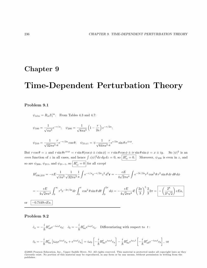
236 CHAPTER 9. TIME-DEPENDENT PERTURBATION THEORY
Chapter 9
Time-Dependent Perturbation Theory
Problem 9.1
ψnlm = RnlYml . From Tables 4.3 and 4.7:
ψ100 =1√πa3
e−r/a; ψ200 =1√
8πa3
(1− r
2a
)e−r/2a;
ψ210 =1√
32πa3
r
ae−r/2a cos θ; ψ21±1 = ∓ 1√
64πa3
r
aer/2a sin θ e±iφ.
But r cos θ = z and r sin θe±iφ = r sin θ(cosφ ± i sinφ) = r sin θ cosφ ± ir sin θ sinφ = x ± iy. So |ψ|2 is aneven function of z in all cases, and hence
∫z|ψ|2dx dy dz = 0, so H ′ii = 0. Moreover, ψ100 is even in z, and
so are ψ200, ψ211, and ψ21−1, so H ′ij = 0 for all except
H ′100,210 = −eE1√πa3
1√32πa3
1a
∫e−r/ae−r/2az2 d3r = − eE
4√
2πa4
∫e−3r/2ar2 cos2 θ r2 sin θ dr dθ dφ
= − eE
4√
2πa4
∫ ∞0
r4e−3r/2adr
∫ π
0
cos2 θ sin θ dθ
∫ 2π
0
dφ = − eE
4√
2πa44!
(2a3
)5 232π = −
(28
35√
2
)eEa,
or −0.7449 eEa.
Problem 9.2
ca = − i
H ′abe
−iω0tcb; cb = − i
H ′bae
iω0tca. Differentiating with respect to t :
cb = − i
H ′ba
[iω0e
iω0tca + eiω0tca
]= iω0
[− i
H ′bae
iω0tca
]− i
H ′bae
iωot
[− i
H ′abe
−iω0tcb
], or
c©2005 Pearson Education, Inc., Upper Saddle River, NJ. All rights reserved. This material is protected under all copyright laws as theycurrently exist. No portion of this material may be reproduced, in any form or by any means, without permission in writing from thepublisher.
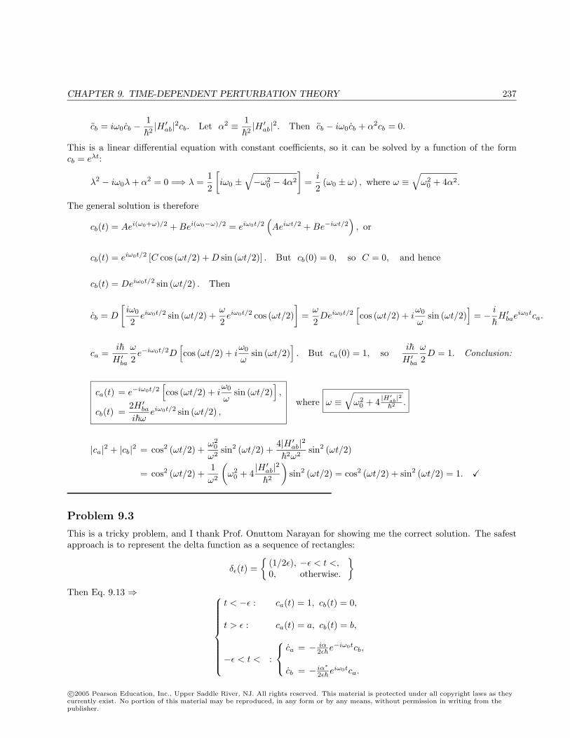
CHAPTER 9. TIME-DEPENDENT PERTURBATION THEORY 237
cb = iω0cb −12|H ′ab|2cb. Let α2 ≡ 1
2|H ′ab|2. Then cb − iω0cb + α2cb = 0.
This is a linear differential equation with constant coefficients, so it can be solved by a function of the formcb = eλt:
λ2 − iω0λ + α2 = 0 =⇒ λ =12
[iω0 ±
√−ω2
0 − 4α2
]=
i
2(ω0 ± ω) , where ω ≡
√ω2
0 + 4α2.
The general solution is therefore
cb(t) = Aei(ω0+ω)/2 + Bei(ω0−ω)/2 = eiω0t/2(Aeiωt/2 + Be−iωt/2
), or
cb(t) = eiω0t/2 [C cos (ωt/2) + D sin (ωt/2)] . But cb(0) = 0, so C = 0, and hence
cb(t) = Deiω0t/2 sin (ωt/2) . Then
cb = D
[iω0
2eiω0t/2 sin (ωt/2) +
ω
2eiω0t/2 cos (ωt/2)
]=
ω
2Deiω0t/2
[cos (ωt/2) + i
ω0
ωsin (ωt/2)
]= − i
H ′bae
iω0tca.
ca =i
H ′ba
ω
2e−iω0t/2D
[cos (ωt/2) + i
ω0
ωsin (ωt/2)
]. But ca(0) = 1, so
i
H ′ba
ω
2D = 1. Conclusion:
ca(t) = e−iω0t/2[cos (ωt/2) + i
ω0
ωsin (ωt/2)
],
cb(t) =2H ′baiω
eiω0t/2 sin (ωt/2) ,where ω ≡
√ω2
0 + 4 |H′ab|22
.
|ca|2 + |cb|2 = cos2 (ωt/2) +ω2
0
ω2sin2 (ωt/2) +
4|H ′ab|22ω2
sin2 (ωt/2)
= cos2 (ωt/2) +1ω2
(ω2
0 + 4|H ′ab|22
)sin2 (ωt/2) = cos2 (ωt/2) + sin2 (ωt/2) = 1.
Problem 9.3
This is a tricky problem, and I thank Prof. Onuttom Narayan for showing me the correct solution. The safestapproach is to represent the delta function as a sequence of rectangles:
δε(t) =
(1/2ε), −ε < t < ε,0, otherwise.
Then Eq. 9.13 ⇒
t < −ε : ca(t) = 1, cb(t) = 0,
t > ε : ca(t) = a, cb(t) = b,
−ε < t < ε :
ca = − iα
2εe−iω0tcb,
cb = − iα∗
2ε eiω0tca.
c©2005 Pearson Education, Inc., Upper Saddle River, NJ. All rights reserved. This material is protected under all copyright laws as theycurrently exist. No portion of this material may be reproduced, in any form or by any means, without permission in writing from thepublisher.
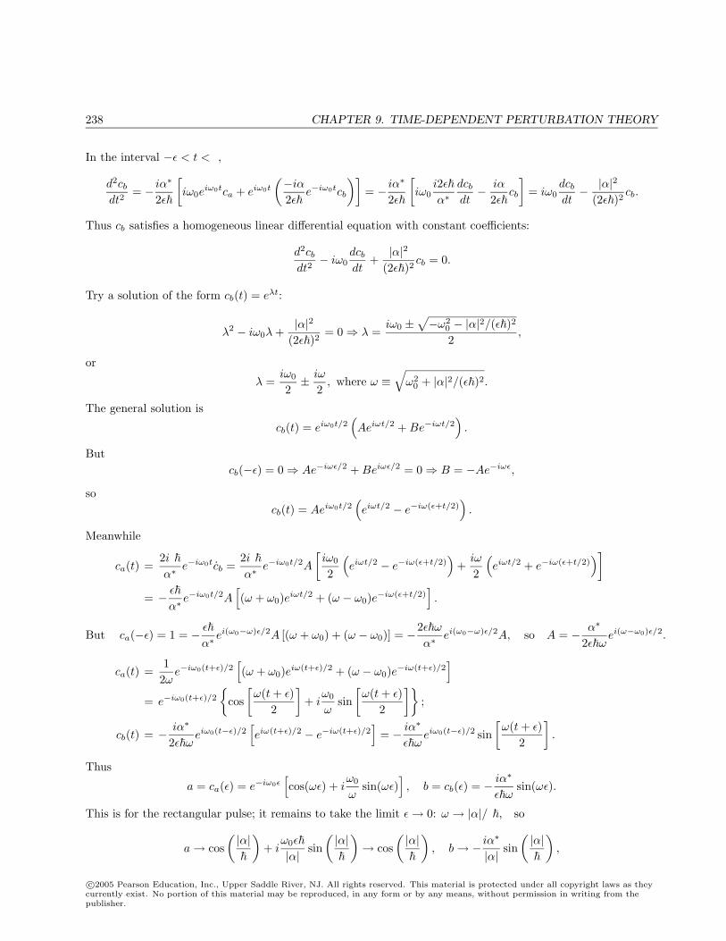
238 CHAPTER 9. TIME-DEPENDENT PERTURBATION THEORY
In the interval −ε < t < ε,
d2cb
dt2= − iα∗
2ε
[iω0e
iω0tca + eiω0t
(−iα
2εe−iω0tcb
)]= − iα∗
2ε
[iω0
i2εα∗
dcb
dt− iα
2εcb
]= iω0
dcb
dt− |α|2
(2ε)2cb.
Thus cb satisfies a homogeneous linear differential equation with constant coefficients:
d2cb
dt2− iω0
dcb
dt+
|α|2(2ε)2
cb = 0.
Try a solution of the form cb(t) = eλt:
λ2 − iω0λ +|α|2
(2ε)2= 0⇒ λ =
iω0 ±√−ω2
0 − |α|2/(ε)22
,
or
λ =iω0
2± iω
2, where ω ≡
√ω2
0 + |α|2/(ε)2.
The general solution is
cb(t) = eiω0t/2(Aeiωt/2 + Be−iωt/2
).
Butcb(−ε) = 0⇒ Ae−iωε/2 + Beiωε/2 = 0⇒ B = −Ae−iωε,
socb(t) = Aeiω0t/2
(eiωt/2 − e−iω(ε+t/2)
).
Meanwhile
ca(t) =2iεα∗
e−iω0tcb =2iεα∗
e−iω0t/2A
[iω0
2
(eiωt/2 − e−iω(ε+t/2)
)+
iω
2
(eiωt/2 + e−iω(ε+t/2)
)]= − ε
α∗e−iω0t/2A
[(ω + ω0)eiωt/2 + (ω − ω0)e−iω(ε+t/2)
].
But ca(−ε) = 1 = − ε
α∗ei(ω0−ω)ε/2A [(ω + ω0) + (ω − ω0)] = −2εω
α∗ei(ω0−ω)ε/2A, so A = − α∗
2εωei(ω−ω0)ε/2.
ca(t) =12ω
e−iω0(t+ε)/2[(ω + ω0)eiω(t+ε)/2 + (ω − ω0)e−iω(t+ε)/2
]= e−iω0(t+ε)/2
cos
[ω(t + ε)
2
]+ i
ω0
ωsin
[ω(t + ε)
2
];
cb(t) = − iα∗
2εωeiω0(t−ε)/2
[eiω(t+ε)/2 − e−iω(t+ε)/2
]= − iα∗
εωeiω0(t−ε)/2 sin
[ω(t + ε)
2
].
Thus
a = ca(ε) = e−iω0ε[cos(ωε) + i
ω0
ωsin(ωε)
], b = cb(ε) = − iα∗
εωsin(ωε).
This is for the rectangular pulse; it remains to take the limit ε→ 0: ω → |α|/ε, so
a→ cos( |α|
)+ i
ω0ε
|α| sin( |α|
)→ cos
( |α|
), b→ − iα∗
|α| sin( |α|
),
c©2005 Pearson Education, Inc., Upper Saddle River, NJ. All rights reserved. This material is protected under all copyright laws as theycurrently exist. No portion of this material may be reproduced, in any form or by any means, without permission in writing from thepublisher.
CHAPTER 9. TIME-DEPENDENT PERTURBATION THEORY 239
and we conclude that for the delta function
ca(t) =
1, t < 0,cos(|α|/), t > 0;
cb(t) =
0, t < 0,
−i
√α∗
αsin(|α|/), t > 0.
Obviously, |ca(t)|2 + |cb(t)|2 = 1 in both time periods. Finally,
Pa→b = |b|2 = sin2(|α|/).
Problem 9.4
(a)
Eq. 9.10 =⇒ ca = − i
[caH
′aa + cbH
′abe−iω0t
]Eq. 9.11 =⇒ cb = − i
[cbH
′bb + caH
′bae
iω0t]
(these are exact, and replace Eq. 9.13).
Initial conditions: ca(0) = 1, cb(0) = 0.
Zeroth order: ca(t) = 1, cb(t) = 0.
First order:
ca = − i
H ′aa =⇒
cb = − i
H ′bae
iω0t =⇒
ca(t) = 1− i
∫ t
0
H ′aa(t′) dt′
cb(t) = − i
∫ t
0
H ′ba(t′)eiω0t′dt′
|ca|2 =[1− i
∫ t
0
H ′aa(t′) dt′] [
1 +i
∫ t
0
H ′aa(t′) dt′]
= 1 +[
1
∫ t
0
H ′aa(t′) dt′]2
= 1 (to first order in H ′).
|cb|2 =[− i
∫ t
0
H ′ba(t′)eiω0t′ dt′] [
i
∫ t
0
H ′ab(t′)e−iω0t′ dt′
]= 0 (to first order in H ′).
So |ca|2 + |cb|2 = 1 (to first order).
(b)
da = ei
∫ t0 H′aa(t
′) dt′(
i
H ′aa
)ca + e
i
∫ t0 H′aa(t
′) dt′ ca. But ca = − i
[caH
′aa + cbH
′abe−iω0t
]Two terms cancel, leaving
da = − i
ei
∫ t0 H′aa(t
′) dt′cbH′abe−iω0t. But cb = e−
i
∫ t0 H′bb(t
′) dt′db.
= − i
ei
∫ t0 [H′aa(t′)−H′bb(t
′)]dt′H ′abe−iω0tdb, or da = − i
eiφH ′abe
−iω0tdb.
c©2005 Pearson Education, Inc., Upper Saddle River, NJ. All rights reserved. This material is protected under all copyright laws as theycurrently exist. No portion of this material may be reproduced, in any form or by any means, without permission in writing from thepublisher.
240 CHAPTER 9. TIME-DEPENDENT PERTURBATION THEORY
Similarly,
db = ei
∫ t0 H′bb(t
′) dt′(
i
H ′bb
)cb + e
i
∫ t0 H′bb(t
′) dt′ cb. But cb = − i
[cbH
′bb + caH
′bae
iω0t].
= − i
ei
∫ t0 H′bb(t
′) dt′caH′bae
iω0t. But ca = e−i
∫ t0 H′aa(t
′) dt′da.
= − i
ei
∫ t0 [H′bb(t′)−H′aa(t
′)]dt′H ′baeiω0tda = − i
e−iφH ′bae
iω0tda. QED
(c)
Initial conditions: ca(0) = 1 =⇒ da(0) = 1; cb(0) = 0 =⇒ db(0) = 0.
Zeroth order: da(t) = 1, db(t) = 0.
First order: da = 0 =⇒ da(t) = 1 =⇒ ca(t) = e−i
∫ t0 H′aa(t
′) dt′ .
db = − i
e−iφH ′bae
iω0t =⇒ db = − i
∫ t
0
e−iφ(t′)H ′ba(t′)eiω0t′dt′ =⇒
cb(t) = − i
e−
i
∫ t0 H′bb(t
′)dt′∫ t
0
e−iφ(t′)H ′ba(t′)eiω0t′dt′.
These don’t look much like the results in (a), but remember, we’re only working to first order in H ′,so ca(t) ≈ 1 − i
∫ t
0H ′aa(t′) dt′ (to this order), while for cb, the factor Hba in the integral means it is
already first order and hence both the exponential factor in front and e−iφ should be replaced by 1. Thencb(t) ≈ − i
∫ t
0H ′ba(t′)eiω0t′dt′, and we recover the results in (a).
Problem 9.5
Zeroth order: c(0)a (t) = a, c(0)b (t) = b.
First order:
ca = − i
H ′abe
−iω0tb =⇒ c(1)a (t) = a− ib
∫ t
0
H ′ab(t′)e−iω0t′dt′.
cb = − i
H ′bae
iω0ta =⇒ c(1)b (t) = b− ia
∫ t
0
H ′ba(t′)eiω0t′dt′.
Second order: ca = − i
H ′abe
−iω0t
[b− ia
∫ t
0
H ′ba(t′)eiω0t′dt′]
=⇒
c(2)a (t) = a− ib
∫ t
0
H ′ab(t′)e−iω0t′dt′ − a
2
∫ t
0
H ′ab(t′)e−iω0t′
[∫ t′
0
H ′ba(t′′)eiω0t′′dt′′]dt′.
To get cb, just switch a↔ b (which entails also changing the sign of ω0):
c(2)b (t) = b− ia
∫ t
0
H ′ba(t′)eiω0t′dt′ − b
2
∫ t
0
H ′ba(t′)eiω0t′
[∫ t′
0
H ′ab(t′′)e−iω0t′′dt′′
]dt′.
c©2005 Pearson Education, Inc., Upper Saddle River, NJ. All rights reserved. This material is protected under all copyright laws as theycurrently exist. No portion of this material may be reproduced, in any form or by any means, without permission in writing from thepublisher.
CHAPTER 9. TIME-DEPENDENT PERTURBATION THEORY 241
Problem 9.6
For H ′ independent of t, Eq. 9.17 =⇒ c(2)b (t) = c
(1)b (t) = − i
H ′ba
∫ t
0
eiω0t′dt′ =⇒
c(2)b (t) = − i
H ′ba
eiω0t′
iω0
∣∣∣∣∣t
0
= −H ′baω0
(eiω0t − 1
). Meanwhile Eq. 9.18 =⇒
c(2)a (t) = 1− 12|H ′ab|2
∫ t
0
e−iω0t′
[∫ t′
0
eiω0t′′dt′′]dt′ = 1− 1
2|H ′ab|2
1iω0
∫ t
0
(1− e−iω0t′
)dt′
= 1 +i
ω02|H ′ab|2
(t′ +
e−iω0t′
iω0
)∣∣∣∣∣t
0
= 1 +i
ω02|H ′ab|2
[t +
1iω0
(e−iω0t − 1
)].
For comparison with the exact answers (Problem 9.2), note first that cb(t) is already first order (because ofthe H ′ba in front), whereas ω differs from ω0 only in second order, so it suffices to replace ω → ω0 in the exactformula to get the second-order result:
cb(t) ≈2H ′baiω0
eiω0t/2 sin (ω0t/2) =2H ′baiω0
eiω0t/2 12i
(eiω0t/2 − e−iω0t/2
)= −H ′ba
ω0
(eiω0t − 1
),
in agreement with the result above. Checking ca is more difficult. Note that
ω = ω0
√1 +
4|H ′ab|2ω2
02≈ ω0
(1 + 2
|H ′ab|2ω2
02
)= ω0 + 2
|H ′ab|2ω0
2;
ω0
ω≈ 1− 2
|H ′ab|2ω2
02.
Taylor expansion:cos(x + ε) = cosx− ε sinx =⇒ cos (ωt/2) = cos
(ω0t
2+|H ′ab|2tω0
2
)≈ cos (ω0t/2)− |H
′ab|2t
ω02
sin (ω0t/2)
sin(x + ε) = sinx + ε cosx =⇒ sin (ωt/2) = sin(ω0t
2+|H ′ab|2tω0
2
)≈ sin (ω0t/2) +
|H ′ab|2tω0
2cos (ω0t/2)
ca(t) ≈ e−iω0t/2
cos
(ω0t
2
)− |H
′ab|2t
ω02
sin(ω0t
2
)+ i
(1− 2
|H ′ab|2ω2
02
) [sin
(ω0t
2
)+|H ′ab|2tω0
2cos
(ω0t
2
)]= e−iω0t/2
[cos
(ω0t
2
)+ i sin
(ω0t
2
)]− |H
′ab|2
ω02
[t
(sin
(ω0t
2
)− i cos
(ω0t
2
))+
2iω0
sin(ω0t
2
)]= e−iω0t/2
eiω0t/2 − |H
′ab|2
ω02
[−iteiω0t/2 +
2iω
12i
(eiω0t/2 − e−iω0t/2
)]= 1− |H
′ab|2
ω02
[−it +
1ω0
(1− e−iω0t
)]= 1 +
i
ω02|H ′ab|2
[t +
1iω0
(e−iω0t − 1
)], as above.
Problem 9.7
(a)
ca = − i
2Vabe
iωte−iω0tcb; cb = − i
2Vbae
−iωteiω0tca.
c©2005 Pearson Education, Inc., Upper Saddle River, NJ. All rights reserved. This material is protected under all copyright laws as theycurrently exist. No portion of this material may be reproduced, in any form or by any means, without permission in writing from thepublisher.
242 CHAPTER 9. TIME-DEPENDENT PERTURBATION THEORY
Differentiate the latter, and substitute in the former:
cb = −iVba
2
[i(ω0 − ω)ei(ω0−ω)tca + ei(ω0−ω)tca
]= i(ω0 − ω)
[−i
Vba
2ei(ω0−ω)tca
]− i
Vba
2ei(ω0−ω)t
[−i
Vab
2e−i(ω0−ω)tcb
]= i(ω0 − ω)cb −
|Vab|2(2)2
cb.
d2cb
dt2+ i(ω − ω0)
dcb
dt+|Vab|242
cb = 0. Solution is of the form cb = eλt : λ2 + i(ω − ω0)λ +|Vab|242
= 0.
λ =12
[−i(ω − ω0)±
√−(ω − ω0)2 −
|Vab|22
]= i
[− (ω − ω0)
2± ωr
], with ωr defined in Eq. 9.30.
General solution: cb(t) = Aei[− (ω−ω0)
2 +ωr]t + Be
i[− (ω−ω0)
2 +ωr]t = e−i(ω−ω0)t/2
[Aeiωrt + Be−iωrt
],
or, more conveniently: cb(t) = e−i(ω−ω0)t/2 [C cos(ωrt) + D sin(ωrt)] . But cb(0) = 0, so C = 0 :
cb(t) = Dei(ω0−ω)t/2 sin(ωrt). cb = D
[i
(ω0 − ω
2
)ei(ω0−ω)t/2 sin(ωrt) + ωre
i(ω0−ω)t/2 cos(ωrt)]
;
ca(t) = i2Vba
ei(ω−ω0)tcb = i2Vba
ei(ω−ω0)t/2D
[i
(ω0 − ω
2
)sin(ωrt) + ωr cos(ωrt)
]. But ca(0) = 1 :
1 = i2Vba
Dωr, or D =−iVba
2ωr.
cb(t) = − i
2ωrVbae
i(ω0−ω)t/2 sin(ωrt), ca(t) = ei(ω−ω0)t/2
[cos(ωrt) + i
(ω0 − ω
2ωr
)sin(ωrt)
].
(b)
Pa→b(t) = |cb(t)|2 =( |Vab|
2ωr
)2
sin2(ωrt). The largest this gets (when sin2 = 1) is|Vab|2/2
4ω2r
,
and the denominator, 4ω2r = (ω − ω0)2 + |Vab|2/2, exceeds the numerator, so P ≤ 1 (and 1 only if ω = ω0).
|ca|2 + |cb|2 = cos2(ωrt) +(ω0 − ω
2ωr
)2
sin2(ωrt) +( |Vab|
2ωr
)2
sin2(ωrt)
= cos2(ωrt) +(ω − ω0)2 + (|Vab|/)2
4ω2r
sin2(ωrt) = cos2(ωrt) + sin2(ωrt) = 1.
(c) If |Vab|2 2(ω − ω0)2, then ωr ≈ 1
2|ω − ω0|, and Pa→b ≈
|Vab|22
sin2(
ω−ω02 t
)(ω − ω0)2
, confirming
Eq. 9.28.
(d) ωrt = π =⇒ t = π/ωr.
c©2005 Pearson Education, Inc., Upper Saddle River, NJ. All rights reserved. This material is protected under all copyright laws as theycurrently exist. No portion of this material may be reproduced, in any form or by any means, without permission in writing from thepublisher.
CHAPTER 9. TIME-DEPENDENT PERTURBATION THEORY 243
Problem 9.8
Spontaneous emission rate (Eq. 9.56): A =ω3|℘|23πε0c3
. Thermally stimulated emission rate (Eq. 9.47):
R =π
3ε02|℘|2ρ(ω), with ρ(ω) =
π2c3ω3
(eω/kBT − 1)(Eq. 9.52).
So the ratio is
A
R=
ω3|℘|23πε0c3
· 3ε02
π|℘|2 ·π2c3
(eω/kBT − 1
)ω3
= eω/kBT − 1.
The ratio is a monotonically increasing function of ω, and is 1 when
eω/kbt = 2, orω
kBT= ln 2, ω =
kBT
ln 2, or ν =
ω
2π=
kBT
hln 2. For T = 300 K,
ν =(1.38× 10⁻²³ J/K)(300 K)
(6.63× 10⁻³⁴ J · s) ln 2 = 4.35× 10¹² Hz.
For higher frequencies, (including light, at 1014 Hz), spontaneous emission dominates.
Problem 9.9
(a) Simply remove the factor(eω/kBT − 1
)in the denominator of Eq. 5.113: ρ0(ω) =
ω3
π2c3.
(b) Plug this into Eq. 9.47:
Rb→a =π
3ε02|℘|2 ω
3
π2c3=
ω3|℘|23πε0c3
,
reproducing Eq. 9.56.
Problem 9.10
N(t) = e−t/τN(0) (Eqs. 9.58 and 9.59). After one half-life, N(t) = 12N(0), so 1
2 = e−t/τ , or 2 = et/τ ,so t/τ = ln 2, or t1/2 = τ ln 2.
Problem 9.11
In Problem 9.1 we calculated the matrix elements of z; all of them are zero except 〈1 0 0|z|2 1 0〉 =28
35√
2a. As
for x and y, we noted that |1 0 0〉, |2 0 0〉, and |2 1 0〉 are even (in x, y), whereas |2 1 ± 1〉 is odd. So the only
c©2005 Pearson Education, Inc., Upper Saddle River, NJ. All rights reserved. This material is protected under all copyright laws as theycurrently exist. No portion of this material may be reproduced, in any form or by any means, without permission in writing from thepublisher.
244 CHAPTER 9. TIME-DEPENDENT PERTURBATION THEORY
non-zero matrix elements are 〈1 0 0|x|2 1± 1〉 and 〈1 0 0|y|2 1± 1〉. Using the wave functions in Problem 9.1:
〈1 0 0|x|2 1± 1〉 =1√πa3
( ∓18√πa3
)1a
∫e−r/are−r/2a sin θ e±iφ(r sin θ cosφ)r2 sin θ dr dθ dφ
= ∓ 18πa4
∫ ∞0
r4e−3r/2adr
∫ π
0
sin3 θ dθ
∫ 2π
0
(cosφ± i sinφ) cosφdφ
=∓1
8πa4
[4!
(2a3
)5] (
43
)(π) = ∓27
35a.
〈1 0 0|y|2 1± 1〉 =∓1
8πa4
[4!
[2a3
)5] (
43
) ∫ 2π
0
(cosφ± i sinφ) sinφdφ
=∓1
8πa4
[4!
(2a3
)5] (
43
)(±iπ) = −i
27
35a.
〈1 0 0|r|2 0 0〉 = 0; 〈1 0 0|r|2 1 0〉 =27√
235
a k; 〈1 0 0|r|2 1± 1〉 =27
35a
(∓i− i j
), and hence
℘2 = 0 (for |2 0 0〉 → |1 0 0〉), and |℘|2 = (qa)2215
310(for |2 1 0〉 → 1 0 0〉 and |2 1± 1〉 → |1 0 0〉).
Meanwhile, ω =E2 − E1
=
1
(E1
4− E1
)= −3E1
4, so for the three l = 1 states:
A = −33E31
263
(ea)2215
310
13πε0c3
= − 29
38π
E31e
2a2
ε04c3=
210
38
(E1
mc2
)2c
a
=210
38
(13.6
0.511× 10⁶
)2 (3.00× 10⁸ m/s)(0.529× 10−10 m)
= 6.27× 10⁸/s; τ =1A
= 1.60× 10⁻⁹ s
for the three l = 1 states (all have the same lifetime); τ =∞ for the l = 0 state.
Problem 9.12
[L2, z] = [L2x, z] + [L2
y, z] + [L2z, z] = Lx[Lx, z] + [Lx, z]Lx + Ly[Ly, z] + [Ly, z]Ly + Lz[Lz, z] + [Lz, z]Lz
But
[Lx, z] = [ypz − zpy, z] = [ypz, z]− [zpy, z] = y[pz, z] = −iy,[Ly, z] = [zpx − xpz, z] = [zpx, z]− [xpz, z] = −x[pz, z] = ix,[Lz, z] = [xpy − ypx, z] = [xpy, z]− [ypx, z] = 0.
So: [L2, z] = Lx(−iy) + (−iy)Lx + Ly(ix) + (ix)Ly = i(−Lxy − yLx + Lyx + xLy).
But
Lxy = Lxy − yLx + yLx = [Lx, y] + yLx = iz + yLx,Lyx = Lyx− xLy + xLy = [Ly, x] + xLy = −iz + xLy.
c©2005 Pearson Education, Inc., Upper Saddle River, NJ. All rights reserved. This material is protected under all copyright laws as theycurrently exist. No portion of this material may be reproduced, in any form or by any means, without permission in writing from thepublisher.
CHAPTER 9. TIME-DEPENDENT PERTURBATION THEORY 245
So: [L2, z] = i(2xLy − iz − 2yLx − iz) =⇒ [L2, z] = 2i(xLy − yLx − iz).
[L2, [L2, z]
]= 2i
[L2, xLy]− [L2, yLx]− i[L2, z]
= 2i
[L2, x]Ly + x[L2, Ly]− [L2, y]Lx − y[L2, Lx]− i(L2z − zL2)
.
But [L2, Ly] = [L2, Lx] = 0 (Eq. 4.102), so[L2, [L2, z]
]= 2i
(yLz − zLy − ix)Ly − 2i (zLx − xLz − iy)Lx − i
(L2z − zL2
), or
[L2, [L2, z]
]= −22
(2yLzLy −2zL2
y − 2zL2x︸ ︷︷ ︸
−2z(L2x+L2
y+L2z)+2zL2
z
−2ixLy + 2xLzLx + 2iyLx − L2z + zL2
)
= −22(2yLzLy − 2ixLy + 2xLzLx + 2iyLx + 2zL2
z − 2zL2 − L2z + zL2)
= −22(zL2 + L2z
)− 42
[(yLz − ix)︸ ︷︷ ︸
Lzy
Ly + (xLz + iy)︸ ︷︷ ︸Lzx
Lx + zLzLz
]= 22
(zL2 + L2z
)− 42 (LzyLy + LzxLx + LzzLz)︸ ︷︷ ︸
Lz(r·L)=0
= 22(zL2 + L2z). QED
Problem 9.13
|n 0 0〉 = Rn0(r)Y 00 (θ, φ) =
1√4π
Rn0(r), so 〈n′ 0 0|r|n 0 0〉 =14π
∫Rn′0(r)Rn0(r)(x i + y j + z k) dx dy dz.
But the integrand is odd in x, y, or z, so the integral is zero.
Problem 9.14
(a)
|3 0 0〉 →
|2 1 0〉|2 1 1〉|2 1−1〉
→ |1 0 0〉. (|3 0 0〉 → |2 0 0〉 and |3 0 0〉 → |1 0 0〉 violate ∆l = ±1 rule.)
(b)
From Eq. 9.72: 〈2 1 0|r|3 0 0〉 = 〈2 1 0|z|3 0 0〉 k.
From Eq. 9.69: 〈2 1± 1|r|3 0 0〉 = 〈2 1± 1|x|3 0 0〉 i + 〈2 1± 1|y|3 0 0〉 j.
From Eq. 9.70: ± 〈2 1± 1|x|3 0 0〉 = i〈2 1± 1|y|3 0 0〉.
Thus |〈2 1 0|r|3 0 0〉|2 = |〈2 1 0|z|3 0 0〉|2 and |〈2 1± 1|r|3 0 0〉|2 = 2|〈2 1± 1|x|3 0 0〉|2,
c©2005 Pearson Education, Inc., Upper Saddle River, NJ. All rights reserved. This material is protected under all copyright laws as theycurrently exist. No portion of this material may be reproduced, in any form or by any means, without permission in writing from thepublisher.
246 CHAPTER 9. TIME-DEPENDENT PERTURBATION THEORY
so there are really just two matrix elements to calculate.
ψ21m = R21Ym1 , ψ300 = R30Y
00 . From Table 4.3:∫
Y 01 Y 0
0 cos θ sin θ dθ dφ =
√34π
√14π
∫ π
0
cos2 θ sin θ dθ
∫ 2π
0
dφ =√
34π
(−cos3 θ
3
) ∣∣∣∣π0
(2π) =√
32
(23
)=
1√3.
∫ (Y ±1
1
)∗Y 0
0 sin2 θ cosφdθ dφ = ∓√
38π
√14π
∫ π
0
sin3 θ dθ
∫ 2π
0
cosφe∓iφ dφ
= ∓ 14π
√32
(43
) [∫ 2π
0
cos2 φdφ∓ i
∫ 2π
0
cosφ sinφdφ
]= ∓ 1
π√
6(π ∓ 0) = ∓ 1√
6.
From Table 4.7:
K ≡∫ ∞
0
R21R30 r3 dr =1√
24a3/2
2√27a3/2
∫ ∞0
r
ae−r/2a
[1− 2
3r
a+
227
( r
a
)2]e−r/3ar3 dr
=1
9√
2a3a4
∫ ∞0
(1− 2
3u +
227
u2
)u4e−5u/6 du =
a
9√
2
[4!
(65
)5
− 235!
(65
)6
+227
6!(
65
)7]
=a
9√
24! 65
56
(5− 2
36 · 5 +
227
63
)=
a
9√
24! 65
56=
2734
56
√2 a.
So:
〈2 1± 1|x|3 0 0〉 =∫
R21(Y ±11 )∗(r sin θ cosφ)R30Y
00 r2 sin θ dr dθ dφ = K
(∓ 1√
6
).
〈2 1 0|z|3 0 0〉 =∫
R21Y01 (r cos θ)R30Y
00 r2 sin θ dr dθ dφ = K
(1√3
).
|〈2 1 0|r|3 0 0〉|2 = |〈2 1 0|z|3 0 0〉|2 = K2/3;
|〈2 1± 1|r|3 0 0 〉|2 = 2|〈2 1± 1|x|3 0 0 〉|2 = K2/3.
Evidently the three transition rates are equal, and hence 1/3 go by each route.
(c) For each mode, A =ω3e2|〈r〉|23πε0c3
; here ω =E3 − E2
=
1
(E1
9− E1
4
)= − 5
36E1
, so the total
decay rate is
R = 3(− 5
36E1
)3e2
3πε0c313
(2734
56
√2a
)2
= 6(
25
)9 (E1
mc2
)2 ( c
a
)= 6
(25
)9 (13.6
0.511× 10⁶
)2 (3× 10⁸
0.529× 10⁻¹⁰
)/s = 6.32× 10⁶/s. τ =
1R
= 1.58× 10⁻⁷ s.
c©2005 Pearson Education, Inc., Upper Saddle River, NJ. All rights reserved. This material is protected under all copyright laws as theycurrently exist. No portion of this material may be reproduced, in any form or by any means, without permission in writing from thepublisher.
CHAPTER 9. TIME-DEPENDENT PERTURBATION THEORY 247
Problem 9.15
(a)
Ψ(t) =∑
cn(t)e−iEnt/ψn. HΨ = i∂Ψ∂t
; H = H0 + H ′(t); H0ψn = Enψn. So
∑cne−iEnt/Enψn +
∑cne−iEnt/H ′ψn = i
∑cne−iEnt/ψn + i
(− i
) ∑cnEne
−iEnt/ψn.
The first and last terms cancel, so∑cne−iEnt/H ′ψn = i
∑cne−iEnt/ψn. Take the inner product with ψm:
∑cne−iEnt/〈ψm|H ′|ψn〉 = i
∑cne−iEnt/〈ψm|ψn〉.
Assume orthonormality of the unperturbed states, 〈ψm|ψn〉 = δmn, and define H ′mn ≡ 〈ψm|H ′|ψn〉.
∑cne−iEnt/H ′mn = i cme−iEmt/, or cm = − i
∑n
cnH′mne
i(Em−En)t/.
(b) Zeroth order: cN (t) = 1, cm(t) = 0 for m = N . Then in first order:
cN = − i
H ′NN , or cN (t) = 1− i
∫ t
0
H ′NN (t′) dt′, whereas for m = N :
cm = − i
H ′mNei(Em−EN )t/, or cm(t) = − i
∫ t
0
H ′mN (t′)ei(Em−EN )t′/ dt′.
(c)
cM (t) = − i
H ′MN
∫ t
0
ei(EM−EN )t′/ dt′ = − i
H ′MN
[ei(EM−EN )t′/
i(EM − EN )/
]∣∣∣∣∣t
0
= −H ′MN
[ei(EM−EN )t/ − 1
EM − EN
]= − H ′MN
(EM − EN )ei(EM−EN )t/2 2i sin
(EM − EN
2t
).
PN→M = |cM |2 =4|H ′MN |2
(EM − EN )2sin2
(EM − EN
2t
).
(d)
cM (t) = − i
VMN
12
∫ t
0
(eiωt′ + e−iωt′
)ei(EM−EN )t′/ dt′
= − iVMN
2
[ei(ω+EM−EN )t′/
i(ω + EM − EN )/+
ei(−ω+EM−EN )t′/
i(−ω + EM − EN )/
]∣∣∣∣∣t
0
.
c©2005 Pearson Education, Inc., Upper Saddle River, NJ. All rights reserved. This material is protected under all copyright laws as theycurrently exist. No portion of this material may be reproduced, in any form or by any means, without permission in writing from thepublisher.
248 CHAPTER 9. TIME-DEPENDENT PERTURBATION THEORY
If EM > EN , the second term dominates, and transitions occur only for ω ≈ (EM − EN )/:
cM (t) ≈ − iVMN
21
(i/)(EM − EN − ω)ei(EM−EN−ω)t/2 2i sin
(EM − EN − ω
2t
), so
PN→M = |cM |2 =|VMN |2
(EM − EN − ω)2sin2
(EM − EN − ω
2t
).
If EM < EN the first term dominates, and transitions occur only for ω ≈ (EN − EM )/:
cM (t) ≈ − iVMN
21
(i/)(EM − EN + ω)ei(EM−EN+ω)t/2 2i sin
(EM − EN + ω
2t
), and hence
PN→M =|VMN |2
(EM − EN + ω)2sin2
(EM − EN + ω
2t
).
Combining the two results, we conclude that transitions occur to states with energy EM ≈ EN ± ω, and
PN→M =|VMN |2
(EM − EN ± ω)2sin2
(EM − EN ± ω
2t
).
(e) For light, Vba = −℘E0 (Eq. 9.34). The rest is as before (Section 9.2.3), leading to Eq. 9.47:
RN→M =π
3ε02|℘|2ρ(ω), with ω = ±(EM − EN )/ (+ sign ⇒ absorption, − sign ⇒ stimulated emission).
Problem 9.16
For example (c):
cN (t) = 1− i
H ′NN t; cm(t) = −2i
H ′mN
(Em − EN )ei(Em−EN )t/2 sin
(Em − EN
2t
)(m = N).
|cN |2 = 1 +12|H ′NN |2t2, |cm|2 = 4
|H ′mN |2(Em − EN )2
sin2
(Em − EN
2t
), so
∑m
|cm|2 = 1 +t2
2|H ′NN |2 + 4
∑m=N
|H ′mN |2(Em − EN )2
sin2
(Em − EN
2t
).
This is plainly greater than 1! But remember: The c’s are accurate only to first order in H ′; to this order the|H ′|2 terms do not belong. Only if terms of first order appeared in the sum would there be a genuine problemwith normalization.
For example (d):
cN = 1− i
VNN
∫ t
0
cos(ωt′) dt′ = 1− i
VNN
sin(ωt′)ω
∣∣∣∣t0
=⇒ cN (t) = 1− i
ωVNN sin(ωt).
c©2005 Pearson Education, Inc., Upper Saddle River, NJ. All rights reserved. This material is protected under all copyright laws as theycurrently exist. No portion of this material may be reproduced, in any form or by any means, without permission in writing from thepublisher.
CHAPTER 9. TIME-DEPENDENT PERTURBATION THEORY 249
cm(t) = −VmN
2
[ei(Em−EN+ω)t/ − 1
(Em − EN + ω)+
ei(Em−EN−ω)t/ − 1(Em − EN − ω)
](m = N). So
|cN |2 = 1 +|VNN |2(ω)2
sin2(ωt); and in the rotating wave approximation
|cm|2 =|VmN |2
(Em − EN ± ω)2sin2
(Em − EN ± ω
2t
)(m = N).
Again, ostensibly∑|cm|2 > 1, but the “extra” terms are of second order in H ′, and hence do not belong (to
first order).
You would do better to use 1−∑
m=N |cm|2. Schematically: cm = a1H + a2H2 + · · · , so |cm|2 =
a21H
2 + 2a1a2H3 + · · · , whereas cN = 1 + b1H + b2H
2 + · · · , so |cN |2 = 1 + 2b1H + (2b2 + b21)H2 + · · · .
Thus knowing cm to first order (i.e., knowing a1) gets you |cm|2 to second order, but knowing cN to first order(i.e., b1) does not get you |cN |2 to second order (you’d also need b2). It is precisely this b2 term that wouldcancel the “extra” (second-order) terms in the calculations of
∑|cm|2 above.
Problem 9.17
(a)
Equation 9.82 ⇒ cm = − i
∑n
cnH′mne
i(Em−En)t/. Here H ′mn = 〈ψm|V0(t)|ψn〉 = δmnV0(t).
cm = − i
cmV0(t);
dcm
cm= − i
V0(t) dt⇒ ln cm = − i
∫V0(t′) dt′ + constant.
cm(t) = cm(0)e−i
∫ t0 V0(t
′) dt′ . Let Φ(t) ≡ −1
∫ t
0
V0(t′) dt′; cm(t) = eiΦcm(0). Hence
|cm(t)|2 = |cm(0)|2, and there are no transitions. Φ(T ) = −1
∫ T
0
V0(t) dt.
(b)
Eq. 9.84 ⇒ cN (t) ≈ 1− i
∫ t
0
V0(t′) dt = 1 + iΦ.
Eq. 9.85 ⇒ cm(t) = − i
∫ t
0
δmNV0(t′)ei(Em−EN )t′/ dt′ = 0 (m = N).
cN (t) = 1 + iΦ(t),cm(t) = 0 (m = N).
The exact answer is cN (t) = eiΦ(t), cm(t) = 0, and they are consistent, since eiΦ ≈ 1 + iΦ, to first order.
c©2005 Pearson Education, Inc., Upper Saddle River, NJ. All rights reserved. This material is protected under all copyright laws as theycurrently exist. No portion of this material may be reproduced, in any form or by any means, without permission in writing from thepublisher.
250 CHAPTER 9. TIME-DEPENDENT PERTURBATION THEORY
Problem 9.18
Use result of Problem 9.15(c). Here En =n2π2
2
2ma2, so E2 − E1 =
3π2
2
2ma2.
H ′12 =2a
∫ a/2
0
sin(π
ax)V0 sin
(2πa
x
)dx
=2V0
a
[sin
(πax
)2(π/a)
− sin(
3πa x
)2(3π/a)
]∣∣∣∣∣a/2
0
=V0
π
[sin
(π
2
)− 1
3sin
(3π2
)]=
4V0
3π.
Eq. 9.86 =⇒ P1→2 = 4(
4V0
3π
) (2ma2
3π22
)2
sin2
(3π2
4ma2t
)=
[16ma2V0
9π32sin
(3π2T
4ma2
)]2
.
[Actually, in this case H ′11 and H ′22 are nonzero:
H ′11 = 〈ψ1|H ′|ψ1〉 =2aV0
∫ a/2
0
sin2(π
ax)
dx =V0
2, H ′22 = 〈ψ2|H ′|ψ2〉 =
2aV0
∫ a/2
0
sin2
(2πa
x
)dx =
V0
2.
However, this does not affect the answer, for according to Problem 9.4, c1(t) picks up an innocuous phase factor,while c2(t) is not affected at all, in first order (formally, this is because H ′bb is multiplied by cb, in Eq. 9.11, andin zeroth order cb(t) = 0).]
Problem 9.19
Spontaneous absorption would involve taking energy (a photon) from the ground state of the electromagneticfield. But you can’t do that, because the gound state already has the lowest allowed energy.
Problem 9.20
(a)
H = −γB · S = −γ (BxSx + BySy + BzSz) ;
H = −γ
2(Bxσx + Byσy + Bzσz) = −γ
2
[Bx
(0 11 0
)+ By
(0 −ii 0
)+ Bz
(1 00 −1
)]= −γ
2
(Bz Bx − iBy
Bx + iBy −Bz
)= −γ
2
(B0 Brf(cosωt + i sinωt)
Brf(cosωt− i sinωt) −B0
)= −γ
2
(B0 Brfe
iωt
Brfe−iωt −B0
).
(b) iχ = Hχ⇒
i
(a
b
)= −γ
2
(B0 Brfe
iωt
Brfe−iωt −B0
) (ab
)= −γ
2
(B0a Brfe
iωtbBrfe
−iωta −B0b
)⇒
a = iγ
2(B0a + Brfe
iωtb)
=i
2(Ωeiωtb + ω0a
),
b = −iγ
2(B0b−Brfe
−iωta)
=i
2(Ωe−iωta− ω0b
).
c©2005 Pearson Education, Inc., Upper Saddle River, NJ. All rights reserved. This material is protected under all copyright laws as theycurrently exist. No portion of this material may be reproduced, in any form or by any means, without permission in writing from thepublisher.
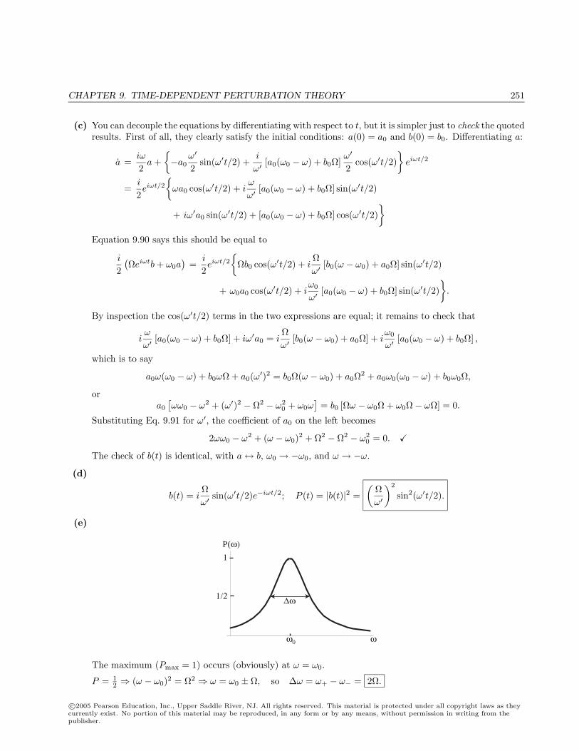
CHAPTER 9. TIME-DEPENDENT PERTURBATION THEORY 251
(c) You can decouple the equations by differentiating with respect to t, but it is simpler just to check the quotedresults. First of all, they clearly satisfy the initial conditions: a(0) = a0 and b(0) = b0. Differentiating a:
a =iω
2a +
−a0
ω′
2sin(ω′t/2) +
i
ω′[a0(ω0 − ω) + b0Ω]
ω′
2cos(ω′t/2)
eiωt/2
=i
2eiωt/2
ωa0 cos(ω′t/2) + i
ω
ω′[a0(ω0 − ω) + b0Ω] sin(ω′t/2)
+ iω′a0 sin(ω′t/2) + [a0(ω0 − ω) + b0Ω] cos(ω′t/2)
Equation 9.90 says this should be equal to
i
2(Ωeiωtb + ω0a
)=
i
2eiωt/2
Ωb0 cos(ω′t/2) + i
Ωω′
[b0(ω − ω0) + a0Ω] sin(ω′t/2)
+ ω0a0 cos(ω′t/2) + iω0
ω′[a0(ω0 − ω) + b0Ω] sin(ω′t/2)
.
By inspection the cos(ω′t/2) terms in the two expressions are equal; it remains to check that
iω
ω′[a0(ω0 − ω) + b0Ω] + iω′a0 = i
Ωω′
[b0(ω − ω0) + a0Ω] + iω0
ω′[a0(ω0 − ω) + b0Ω] ,
which is to say
a0ω(ω0 − ω) + b0ωΩ + a0(ω′)2 = b0Ω(ω − ω0) + a0Ω2 + a0ω0(ω0 − ω) + b0ω0Ω,
ora0
[ωω0 − ω2 + (ω′)2 − Ω2 − ω2
0 + ω0ω]
= b0 [Ωω − ω0Ω + ω0Ω− ωΩ] = 0.
Substituting Eq. 9.91 for ω′, the coefficient of a0 on the left becomes
2ωω0 − ω2 + (ω − ω0)2 + Ω2 − Ω2 − ω20 = 0.
The check of b(t) is identical, with a↔ b, ω0 → −ω0, and ω → −ω.
(d)
b(t) = iΩω′
sin(ω′t/2)e−iωt/2; P (t) = |b(t)|2 =(
Ωω′
)2
sin2(ω′t/2).
(e)
P(ω)
ω
1
1/2
ω0
∆ω
The maximum (Pmax = 1) occurs (obviously) at ω = ω0.
P = 12 ⇒ (ω − ω0)2 = Ω2 ⇒ ω = ω0 ± Ω, so ∆ω = ω+ − ω− = 2Ω.
c©2005 Pearson Education, Inc., Upper Saddle River, NJ. All rights reserved. This material is protected under all copyright laws as theycurrently exist. No portion of this material may be reproduced, in any form or by any means, without permission in writing from thepublisher.
252 CHAPTER 9. TIME-DEPENDENT PERTURBATION THEORY
(f) B0 = 10, 000 gauss = 1 T; Brf = 0.01 gauss = 1 × 10⁻⁶ T. ω0 = γB0. Comparing Eqs. 4.156 and6.85, γ =
gpe
2mp, where gp = 5.59. So
νres =ω0
2π=
gpe
4πmpB0 =
(5.59)(1.6× 10⁻¹⁹)4π(1.67× 10⁻²⁷)
(1) = 4.26× 10⁷ Hz.
∆ν =∆ω
2π=
Ωπ
=γ
2π2Brf = νres
2Brf
B0= (4.26× 10⁷)(2× 10⁻⁶) = 85.2 Hz.
Problem 9.21
(a)
H ′ = −qE · r = −q(E0 · r)(k · r) sin(ωt). Write E0 = E0n, k =ω
ck. Then
H ′ = −qE0ω
c(n · r)(k · r) sin(ωt). H ′ba = −qE0ω
c〈b|(n · r)(k · r)|a〉 sin(ωt).
This is the analog to Eq. 9.33: H ′ba = −qE0〈b|n · r|a〉 cosωt. The rest of the analysis is identical to thedipole case (except that it is sin(ωt) instead of cos(ωt), but this amounts to resetting the clock, and clearlyhas no effect on the transition rate). We can skip therefore to Eq. 9.56, except for the factor of 1/3, whichcame from the averaging in Eq. 9.46:
A =ω3
πε0c3q2ω2
c2|〈b|(n · r)(k · r)|a〉|2 =
q2ω5
πε0c5|〈b|(n · r)(k · r)|a〉|2.
(b) Let the oscillator lie along the x direction, so (n · r) = nxx and k · r = kxx. For a transition from n to n′,we have
A =q2ω5
πε0c5
(kxnx
)2
|〈n′|x2|n〉|2. From Example 2.5, 〈n′|x2|n〉 =
2mω〈n′|(a2
++a+a−+a−a++a2−)|n〉,
where ω is the frequency of the oscillator, not to be confused with ω, the frequency of the electromagneticwave. Now, for spontaneous emission the final state must be lower in energy, so n′ < n, and hence theonly surviving term is a2
−. Using Eq. 2.66:
〈n′|x2|n〉 =
2mω〈n′|
√n(n− 1)|n− 2〉 =
2mω
√n(n− 1) δn′,n−2.
Evidently transitions only go from |n〉 to |n− 2〉, and hence
ω =En − En−2
=
1
[(n + 1
2 )ω − (n− 2 + 12 )ω
]= 2ω.
〈n′|x2|n〉 =
mω
√n(n− 1) δn′,n−2; Rn→n−2 =
q2ω5
πε0c5(kxnx)2
2
m2ω2n(n− 1).
It remains to calculate the average of (kxnx)2. It’s easiest to reorient the oscillator along a direction r,making angle θ with the z axis, and let the radiation be incident from the z direction (so kx → kr = cos θ).
c©2005 Pearson Education, Inc., Upper Saddle River, NJ. All rights reserved. This material is protected under all copyright laws as theycurrently exist. No portion of this material may be reproduced, in any form or by any means, without permission in writing from thepublisher.
CHAPTER 9. TIME-DEPENDENT PERTURBATION THEORY 253
Averaging over the two polarizations (i and j): 〈n2r〉 = 1
2
(i2r + j2
r
)= 1
2
(sin2 θ cos2 φ + sin2 θ sin2 φ
)=
12 sin2 θ. Now average overall directions:
〈k2r n
2r〉 =
14π
∫12
sin2 θ cos2 θ sin θ dθ dφ =18π
2π∫ π
0
(1− cos2 θ) cos2 θ sin θ dθ
=14
[−cos3 θ
3+
cos5 θ
5
] ∣∣∣∣π0
=14
(23− 2
5
)=
115
.
R =115
q2ω3
πε0m2c5n(n− 1). Comparing Eq. 9.63:
R(forbidden)R(allowed)
=25(n− 1)
ω
mc2.
For a nonrelativistic system, ω mc2; hence the term “forbidden”.
(c) If both the initial state and the final state have l = 0, the wave function is independent of angle (Y 00 =
1/√
4π), and the angular part of the integral is:
〈a|(n · r)(k · r)|b〉 = · · ·∫
(n · r)(k · r) sin θ dθ dφ = · · · 4π3
(n · k) (Eq. 6.95).
But n · k = 0, since electromagnetic waves are transverse. So R = 0 in this case, both for allowed andfor forbidden transitions.
Problem 9.22
[This is done in Fermi’s Notes on Quantum Mechanics (Chicago, 1995), Section 24, but I am looking for a moreaccessible treatment.]
c©2005 Pearson Education, Inc., Upper Saddle River, NJ. All rights reserved. This material is protected under all copyright laws as theycurrently exist. No portion of this material may be reproduced, in any form or by any means, without permission in writing from thepublisher.
254 CHAPTER 10. THE ADIABATIC APPROXIMATION
Chapter 10
The Adiabatic Approximation
Problem 10.1
(a)
Let (mvx2 − 2Einat)/2w = φ(x, t). Φn =
√2w
sin(nπ
wx)eiφ, so
∂Φn
∂t=√
2(−1
21
w3/2v
)sin
(nπ
wx)eiφ +
√2w
[−nπx
w2v cos
(nπ
wx)]
eiφ +
√2w
sin(nπ
wx) (
i∂φ
∂t
)eiφ
=[− v
2w− nπxv
w2cot
(nπ
wx)
+ i∂φ
∂t
]Φn.
∂φ
∂t=
12
[−2Ei
na
w− v
w2
(mvx2 − 2Ei
nat)]
= −Eina
w− v
wφ.
i∂Φn
∂t= −i
[v
2w+
nπxv
w2cot
(nπ
wx)
+ iEi
na
w+ i
v
wφ
]Φn.
HΦn = − 2
2m∂2Φn
∂x2.
∂Φn
∂x=
√2w
[nπw
cos(nπ
wx)]
eiφ +
√2w
sin(nπ
wx)eiφ
(i∂φ
∂x
).
∂φ
∂x=
mvx
w.
∂Φn
∂x=
[nπw
cot(nπ
wx)
+ imvx
w
]Φn.
∂2Φn
∂x2=
[−
(nπ
w
)2
csc2(nπ
wx)
+imb
w
]Φn +
[nπw
cot(nπ
wx)
+ imvx
w
]2
Φn.
So the Schrodinger equation (i∂Φn/∂t = HΦn) is satisfied ⇔
−i
[v
2w+
nπxv
w2cot
(nπ
wx)
+ iEi
na
w+ i
v
wφ
]
= − 2
2m
−
(nπ
w
)2
csc2(nπ
wx)
+imv
w+
[nπw
cot(nπ
wx)
+ imvx
w
]2
c©2005 Pearson Education, Inc., Upper Saddle River, NJ. All rights reserved. This material is protected under all copyright laws as theycurrently exist. No portion of this material may be reproduced, in any form or by any means, without permission in writing from thepublisher.
CHAPTER 10. THE ADIABATIC APPROXIMATION 255
Cotangent terms: − i(nπxv
w2
)?= −
2
2m
(2nπ
wimvx
w
)= −i
nπvx
w2.
Remaining trig terms on right:
−(nπ
w
)2
csc2(nπ
wx)
+(nπ
w
)2
cot2(nπ
wx)
= −(nπ
w
)2[1− cos2 (nπx/w)
sin2 (nπx/w)
]= −
(nπ
w
)2
.
This leaves:
i
[v
2w+ i
Eina
w+ i
v
w
(mvx2 − 2Ei
nat
2w
)]?=
2m
[−
(nπ
w
)2
+imv
w− m2v2x2
2w2
]
iv2− Ei
na
−mv2x2
2w+
vEinat
w
?= −n2π2
2mw+iv2−mv2x2
2w
−Eina
w(w − vt) = −Ei
na2
w
?= −n2π2
2mw⇔ −n2π2
2
2ma2
a2
w= −n
2π2
2mw= r.h.s.
So Φn does satisfy the Schrodinger equation, and since Φn(x, t) = (· · · ) sin (nπx/w), it fits the boundaryconditions: Φn(0, t) = Φn(w, t) = 0.
(b)
Equation 10.4 =⇒ Ψ(x, 0) =∑
cnΦn(x, 0) =∑
cn
√2a
sin(nπ
ax)eimvx2/2a.
Multiply by
√2a
sin(n′π
ax
)e−imvx2/2a and integrate:
√2a
∫ a
0
Ψ(x, 0) sin(n′π
ax
)e−imvx2/2adx =
∑cn
[2a
∫ π
0
sin(nπ
ax)
sin(n′π
ax
)dx︸ ︷︷ ︸
δnn′
]= c′n.
So, in general: cn =
√2a
∫ a
0
e−imvx2/2a sin(nπ
ax)
Ψ(x, 0)dx. In this particular case,
cn =2a
∫ a
0
e−imvx2/2a sin(nπ
a
)sin
(π
ax)dx. Let
π
ax ≡ z; dx =
a
πdz;
mvx2
2a=
mvz2
2aa2
π2=
mva
2π2z2.
cn =2π
∫ π
0
e−iαz2sin(nz) sin(z) dz. QED
c©2005 Pearson Education, Inc., Upper Saddle River, NJ. All rights reserved. This material is protected under all copyright laws as theycurrently exist. No portion of this material may be reproduced, in any form or by any means, without permission in writing from thepublisher.
256 CHAPTER 10. THE ADIABATIC APPROXIMATION
(c)
w(Te) = 2a⇒ a + vTe = 2a⇒ vTe = a⇒ Tea/v; e−iE1t/ ⇒ ω =E1
⇒ Ti =
2πω
= 2π
E1, or
Ti =2ππ22
2ma2 =4π
ma2
. Ti =
4ma2
π. Adiabatic ⇒ Te Ti ⇒
a
v 4ma2
π⇒ 4
π
mav
1, or
8π( mav
2π2
)= 8πα 1, so α 1. Then cn =
2π
∫ π
0
sin(nz) sin(z)dz = δn1. Therefore
Ψ(x, t) =
√2w
sin(πx
w
)ei(mvx2−2Ei1at)/2w,
which (apart from a phase factor) is the ground state of the instantaneous well, of width w, as requiredby the adiabatic theorem. (Actually, the first term in the exponent, which is at most mva2
2a = mva2 1
and could be dropped, in the adiabatic regime.)
(d)
θ(t) = −1
(π2
2
2m
) ∫ t
0
1(a + vt′)2
dt′ = −π2
2m
[−1
v
(1
a + vt′
)]∣∣∣∣t0
= − π2
2mv
(1a− 1
w
)= − π2
2mv
(vt
aw
)= − π2
t
2maw.
So (dropping themvx2
2wterm, as explained in (c)) Ψ(x, t) =
√2w
sin(πx
w
)e−iEi1at/w can be written
(since −Ei1at
w= − π2
2
2ma2
at
w= − π2
t
2maw= θ): Ψ(x, t) =
√2w
sin(πx
w
)eiθ.
This is exactly what one would naively expect: For a fixed well (of width a) we’d have Ψ(x, t) =Ψ1(x)e−iE1t/; for the (adiabatically) expanding well, simply replace a by the (time-dependent) widthw, and integrate to get the accumulated phase factor, noting that E1 is now a function of t.
Problem 10.2
To show: i∂χ
∂t= Hχ, where χ is given by Eq. 10.31 and H is given by Eq. 10.25.
∂χ
∂t=
λ2
[− sin
(λt2
)− i (ω1−ω)
λ cos(
λt2
)]cos
(α2
)e−iωt/2 − iω
2
[cos
(λt2
)− i(ω1−ω)
λ sin(
λt2
)]cos
(α2
)e−iωt/2
λ2
[− sin
(λt2
)− i (ω1+ω)
λ cos(
λt2
)]sin
(α2
)eiωt/2 + iω
2
[cos
(λt2
)− i(ω1+ω)
λ sin(
λt2
)]sin
(α2
)eiωt/2
c©2005 Pearson Education, Inc., Upper Saddle River, NJ. All rights reserved. This material is protected under all copyright laws as theycurrently exist. No portion of this material may be reproduced, in any form or by any means, without permission in writing from thepublisher.
CHAPTER 10. THE ADIABATIC APPROXIMATION 257
Hχ =
ω1
2
cosα
[cos(λt
2 )− i (ω1−ω)λ sin(λt
2 )]cos α
2 e−iωt/2 + e−iωt sinα
[cos(λt
2 )− i(ω1+ω)λ sin(λt
2 )]sin α
2 eiωt/2
eiωt cosα[cos(λt
2 )− i (ω1−ω)λ sin(λt
2 )]cos α
2 e−iωt/2 − cosα
[cos(λt
2 )− i(ω1+ω)λ sin(λt
2 )]sin α
2 eiωt/2
(1) Upper elements:
iλ
2
[− sin
(λt
2
)− i
(ω1 − ω)λ
cos(λt
2
)]cosα
2− iω
2
[cos
(λt
2
)− i(ω1 − ω)
λsin
(λt
2
)]cosα
2
?= ω1
2
[cos
(λt
2
)− i
(ω1 − ω)λ
sin(λt
2
)]cosα
cosα
2+
[cos
(λt
2
)− i
(ω1 + ω)λ
sin(λt
2
)]sinα︸︷︷︸
sinα
2
,
where = 2 sinα
2cosα
2
The sine terms:
sin(λt
2
) [−iλ− iω(ω1 − ω)
λ+
ω1(ω1 − ω)λ
cosα +iω1(ω1 + ω)
λ2 sin2 α
2
]?= 0.
i
λsin
(λt
2
) [−ω2 − ω2
1 + 2ωω1 cosα− ωω1 +ω2 + (ω21 − ωω1) cosα + (ω2
1 + ωω1)(1− cosα)]
= − i
λsin
(λt
2
) [−ω2
1 + 2ωω1 cosα−ωω1 +
ω21 cosα− ωω1 cosα +ω
21 +ωω1 −ω2
1 cosα− ωω1 cosα]
= 0.
The cosine terms:
cos(λt
2
) [(ω1 −ω) +ω − ω1 cosα− ω1 2 sin2 α
2
]= −ω1 cos
(λt
2
)[−1 + cosα + (1− cosα)] = 0.
(2) Lower elements:
iλ
2
[− sin
(λt
2
)− i
(ω1 + ω)λ
cos(λt
2
)]
sin(α
2
)+
iω
2
[cos
(λt
2
)− i(ω1 + ω)
λsin
(λt
2
)]
sin(α
2
)?= ω1
2
[cos
(λt
2
)− i
(ω1 − ω)λ
sin(λt
2
)]2sinα
2cos2
α
2−
[cos
(λt
2
)− i(ω1 + ω)
λsin
(λt
2
)]cosα
sinα
2
.
The sine terms:
sin(λt
2
) [−iλ +
iω(ω1 + ω)λ
+iω1(ω1 − ω)
λ2 cos2
(α
2
)− iω1(ω1 + ω)
λcosα
]?= 0.
i
λsin
(λt
2
) [−ω2 − ω2
1 + 2ωω1 cosα + ωω1 +ω2 + (ω21 − ωω1)(1 + cosα)− (ω2
1 + ωω1) cosα]
=i
λsin
(λt
2
) [−ω
21 + 2ωω1 cosα +ωω1 +ω
21 −ωω1 +
ω2
1 cosα− ωω1 cosα−ω21 cosα− ωω1 cosα
]= 0.
The cosine terms:
cos(λt
2
) [(ω1 +ω)−ω − ω1 2 cos2
α
2+ ω1 cosα
]= cos
(λt
2
)[ω1 − ω1(1 + cosα) + ω1 cosα] = 0.
c©2005 Pearson Education, Inc., Upper Saddle River, NJ. All rights reserved. This material is protected under all copyright laws as theycurrently exist. No portion of this material may be reproduced, in any form or by any means, without permission in writing from thepublisher.
258 CHAPTER 10. THE ADIABATIC APPROXIMATION
As for Eq. 10.33:[cos
(λt
2
)− i
(ω1 − ω cosα)λ
sin(λt
2
)]e−iωt/2
(cos α
2eiωt sin α
2
)+ i
[ω
λsinα sin
(λt
2
)]e−iωt/2
(sin α
2−eiωt cos α
2
)
=(αβ
), with
α = [
cos(λt
2
)− iω1
λsin
(λt
2
)]cos
α
2+
iω
λ
[cosα cos
α
2+ sinα sin
α
2︸ ︷︷ ︸cos(α−α2 )=cos α2
]sin
(λt
2
) e−iωt/2
=[cos
(λt
2
)− i(ω1 − ω)
λsin
(λt
2
)]cos
α
2e−iωt/2 (confirming the top entry).
β = [
cos(λt
2
)− iω1
λsin
(λt
2
)]sin
α
2+
iω
λ
[cosα sin
α
2− sinα cos
α
2︸ ︷︷ ︸sin(α2−α)=− sin α
2
]sin
(λt
2
) eiωt/2
=[cos
(λt
2
)− i(ω1 + ω)
λsin
(λt
2
)]sin
α
2eiωt/2 (confirming the bottom entry).
|c+|2 + |c−|2 = cos2(λt
2
)+
(ω1 − ω cosα)2
λ2sin2
(λt
2
)+
ω2
λ2sin2 α sin2
(λt
2
)= cos2
(λt
2
)+
1λ2
(ω2
1 − 2ωω1 cosα + ω2 cos2 α + ω2 sin2 α︸ ︷︷ ︸ω2+ω2
1−2ωω1 cos α=λ2
)sin2
(λt
2
)
= cos2(λt
2
)+ sin2
(λt
2
)= 1.
Problem 10.3
(a)
ψn(x) =
√2w
sin(nπ
wx). In this case R = w.
∂ψn
∂R=√
2(−1
21
w3/2
)sin
(nπ
wx)
+
√2w
(−nπ
w2x)
cos(nπ
wx)
;
c©2005 Pearson Education, Inc., Upper Saddle River, NJ. All rights reserved. This material is protected under all copyright laws as theycurrently exist. No portion of this material may be reproduced, in any form or by any means, without permission in writing from thepublisher.
CHAPTER 10. THE ADIABATIC APPROXIMATION 259
⟨ψn
∣∣∣∣∂ψn
∂R
⟩=
∫ w
0
ψn∂ψn
∂Rdx
= − 1w2
∫ w
0
sin2(nπ
wx)dx− 2nπ
w3
∫ w
0
x sin(nπ
wx)
cos(nπ
wx)
︸ ︷︷ ︸12 sin( 2nπ
w x)
dx
= − 1w2
(w
2
)− nπ
w3
∫ w
0
x sin(
2nπw
x
)dx
= − 12w
− nπ
w3
[( w
2nπ
)2
sin(
2nπw
x
)− wx
2nπcos
(2nπw
x
)]∣∣∣∣w0
= − 12w
− nπ
w3
[− w2
2nπcos(2nπ)
]= − 1
2w+
12w
= 0.
So Eq. 10.42 =⇒ γn(t) = 0. (If the eigenfunctions are real, the geometric phase vanishes.)
(b)
Equation 10.39 =⇒ θn(t) =1
∫ t
0
n2π2
2
2mw2dt′ = −n2π2
2m
∫1w2
dt′
dwdw;
θn = −n2π2
2mv
∫ w2
w1
1w2
dw =n2π2
2mv
(1w
)∣∣∣∣w2
w1
=n2π2
2mv
(1w2− 1
w1
).
(c) Zero.
Problem 10.4
ψ =√mα
e−mα|x|/2 . Here R = α, so
∂ψ
∂R=√m
(12
1√α
)e−mα|x|/2 +
√mα
(−m|x|2
)e−mα|x|/2 .
ψ∂ψ
∂R=√mα
[12
√m
α− m
√mα
3|x|
]e−2mα|x|/2 =
(m
22− m2α
4|x|
)e−2mα|x|/2 .
⟨ψ
∣∣∣∣ ∂ψ∂R⟩
= 2[
m
22
∫ ∞0
e−2mαx/2dx− m2α
4
∫ ∞0
xe−2mαx/2dx
]=
m
2
(
2
2mα
)− 2m2α
4
(
2
2mα
)2
=12α− 1
2α= 0. So Eq. 10.42 =⇒ γ(t) = 0.
E = −mα2
22, so θ(t) = −1
∫ T
0
(−mα2
22
)dt′ =
m
23
∫ α2
α1
α2 dt′
dαdα =
m
23c
∫ α2
α1
α2dα =m
62c
(α3
2 − α31
).
c©2005 Pearson Education, Inc., Upper Saddle River, NJ. All rights reserved. This material is protected under all copyright laws as theycurrently exist. No portion of this material may be reproduced, in any form or by any means, without permission in writing from thepublisher.
260 CHAPTER 10. THE ADIABATIC APPROXIMATION
Problem 10.5
According to Eq. 10.44 the geometric phase is
γn(t) = i
∫ Rf
Ri
〈ψn|∇Rψn〉 · dR.
Now 〈ψn|ψn〉 = 1, so
∇R〈ψn|ψn〉 = 〈∇Rψn|ψn〉+ 〈ψn|∇Rψn〉 = 〈ψn|∇Rψn〉∗ + 〈ψn|∇Rψn〉 = 0,
and hence 〈ψn|∇Rψn〉 is pure imaginary. If ψn is real, then, 〈ψn|∇Rψn〉 must in fact be zero.Suppose we introduce a phase factor to make the (originally real) wave function complex:
ψ′n = eiφn(R)ψn, where ψn is real. Then ∇Rψ′n = eiφn∇Rψn + i(∇Rφn)eiφnψn. So
〈ψ′n|∇Rψ′n〉 = e−iφneiφn〈ψn|∇Rψn〉+ ie−iφn(∇Rφn)eiφn〈ψn|ψn〉. But 〈ψn|ψn〉 = 1, and
〈ψn|∇Rψn〉 = 0 (as we just found), so 〈ψ′n|∇Rψ′n〉 = i∇Rφn, and Eq. 10.44 =⇒
γ′n(t) = i
∫ Rf
Ri
i∇R(φn) · dR = − [φn(Rf )− φn(Ri)] , so Eq. 10.38 gives:
Ψ′n(x, t) = ψ′n(x, t)e−i
∫ t0 En(t′)dt′e−i[φn(Rf )−φn(Ri)].
The wave function picks up a (trivial) phase factor, whose only function is precisely to kill the phase factor weput in “by hand”:
Ψ′n(x, t) =[ψn(x, t)e−
i
∫ t0 En(t′)dt′
]eiφn(Ri) = Ψn(x, t)eiφn(Ri).
In particular, for a closed loop φn(Rf ) = φn(Ri), so γ′n(T ) = 0.
Problem 10.6
H =e
mB · S. Here B = B0
[sin θ cosφ i + sin θ sinφ j + cos θ k
]; take spin matrices from Problem 4.31.
H =eB0
m
√2
sin θ cosφ
0 1 01 0 10 1 0
+ sin θ sinφ
0 −i 0i 0 −i0 i 0
+ cos θ
√2 0 00 0 00 0 −
√2
=
eB0√2m
√2 cos θ e−iφ sin θ 0eiφ sin θ 0 e−iφ sin θ
0 eiφ sin θ −√
2 cos θ
.
We need the “spin up” eigenvector: Hχ+ =eB0
mχ+.
√2 cos θ e−iφ sin θ 0eiφ sin θ 0 e−iφ sin θ
0 eiφ sin θ −√
2 cos θ
abc
=√
2
abc
=⇒
(i)
√2 cos θa + e−iφ sin θb =
√2a.
(ii) eiφ sin θa + e−iφ sin θc =√
2b.(iii) eiφ sin θb−
√2 cos θc =
√2c.
c©2005 Pearson Education, Inc., Upper Saddle River, NJ. All rights reserved. This material is protected under all copyright laws as theycurrently exist. No portion of this material may be reproduced, in any form or by any means, without permission in writing from thepublisher.
CHAPTER 10. THE ADIABATIC APPROXIMATION 261
(i)⇒ b =√
2eiφ
(1− cos θ
sin θ
)a =
√2eiφ tan (θ/2) a; (iii)⇒ b =
√2e−iφ
(1 + cos θ
sin θ
)c =
√2e−iφ cot (θ/2) c.
Thus c = e2iφ tan2 (θ/2) a; (ii) is redundant. Normalize: |a|2 + 2 tan2(θ/2)|a|2 + tan4(θ/2)|a|2 = 1⇒
|a|2[1 + tan2(θ/2)
]2= |a|2
[1
cos(θ/2)
]4
= 1⇒ |a|2 = cos4 (θ/2) .
Pick a = e−iφ cos2(θ/2); then b =√
2 sin(θ/2) cos(θ/2) and c = eiφ sin2(θ/2), and
χ+ =
e−iφ cos2 (θ/2)√2 sin (θ/2) cos (θ/2)
eiφ sin2 (θ/2)
. This is the spin-1 analog to Eq. 10.57.
∇χ+ =∂χ+
∂rr +
1r
∂χ+
∂θθ +
1r sin θ
∂χ+
∂φφ
=1r
−e−iφ cos (θ/2) sin (θ/2)√2
[cos2 (θ/2)− sin2 (θ/2)
]/2
eiφ sin (θ/2) cos (θ/2)
θ +1
r sin θ
−ie−iφ cos2 (θ/2)0
ieiφ sin2 (θ/2)
φ.
〈χ+|∇χ+〉 =1r
− cos2 (θ/2) [cos (θ/2) sin (θ/2)] + sin (θ/2) cos (θ/2)
[cos2 (θ/2)− sin2 (θ/2)
]+ sin2 (θ/2) [sin (θ/2) cos (θ/2)]
θ
+1
r sin θ
cos2 (θ/2)
[−i cos2 (θ/2)
]+ sin2 (θ/2)
[i sin2 (θ/2)
]φ
=i
r sin θ
[sin4 (θ/2)− cos4 (θ/2)
]φ
=i
r sin θ
[sin2 (θ/2) + cos2 (θ/2)
] [sin2 (θ/2)− cos2 (θ/2)
]φ
=i
r sin θ(1)(− cos θ) φ = − i
rcot θ φ.
∇× 〈χ+|∇χ+〉 =1
r sin θ
∂
∂θ
[sin θ
(− i
rcot θ
)]r =
−i
r2 sin θ
∂
∂θ(cos θ) r =
i sin θ
r2 sin θr =
i
r2r.
Equation 10.51 =⇒ γ+(T ) = i
∫i
r2r2dΩ = −Ω.
Problem 10.7
(a) Giving H a test function f to act upon:
Hf =1
2m
(
i∇− qA
)·(
i∇f − qAf
)+ qϕf
=1
2m
[− 2∇ · (∇f)− q
i∇ · (Af)︸ ︷︷ ︸
(∇·A)f+A·(∇f)
−q
iA · (∇f) + q2A ·Af
]+ qϕf.
c©2005 Pearson Education, Inc., Upper Saddle River, NJ. All rights reserved. This material is protected under all copyright laws as theycurrently exist. No portion of this material may be reproduced, in any form or by any means, without permission in writing from thepublisher.
262 CHAPTER 10. THE ADIABATIC APPROXIMATION
But ∇ ·A = 0 and ϕ = 0 (see comments after Eq. 10.66), so
Hf =1
2m[−2∇2f + 2iqA · ∇f + q2A2f
], or H =
12m
[−2∇2 + q2A2 + 2iqA · ∇
]. QED
(b) Apply(
i∇− qA)· to both sides of Eq. 10.78:(
i∇− qA
)2
Ψ =(
i∇− qA
)·(
ieig∇Ψ′
)= −2∇ · (eig∇Ψ′)− q
ieigA · ∇Ψ′.
But ∇ · (eig∇Ψ′) = ieig(∇g) · (∇Ψ′) + eig∇ · (∇Ψ′) and ∇g =q
A, so the right side is
−i2 q
eigA · ∇Ψ′ − 2eig∇2Ψ′ + iqeigA · ∇Ψ′ = −2eig∇2Ψ′. QED
Problem 10.8
(a) Schrodinger equation:
− 2
2md2ψ
dx2= Eψ, or
d2ψ
dx2= −k2ψ (k ≡
√2mE/)
0 < x < 1
2a + ε,12a + ε < x < a.
Boundary conditions: ψ(0) = ψ( 12a + ε) = ψ(a) = 0.
Solution:
(1) 0 < x < 12a + ε : ψ(x) = A sin kx + B cos kx. But ψ(0) = 0⇒ B = 0, and
ψ( 12a + ε) = 0⇒
k( 1
2a + ε) = nπ (n = 1, 2, 3, . . . )⇒ En = n2π2
2/2m(a/2 + ε)2,or else A = 0.
(2) 12a + ε < x < a : ψ(x) = F sin k(a− x) + G cos k(a− x). But ψ(a) = 0⇒ G = 0, and
ψ( 12a + ε) = 0⇒
k( 1
2a− ε) = n′π (n′ = 1, 2, 3, . . . )⇒ En′ = (n′)2π2
2/2m(a/2− ε)2,or else F = 0.
The ground state energy is
either E1 =
π2
2
2m( 12a + ε)2
(n = 1), with F = 0,
or else E1′ =π2
2
2m( 12a− ε)2
(n′ = 1), with A = 0.
Both are allowed energies, but E1 is (slightly) lower (assuming ε is positive), so the ground state is
ψ(x) =
√
212 a+ε
sin(
πx12 a+ε
), 0 ≤ x ≤ 1
2a + ε;
0, 12a + ε ≤ x ≤ a.
c©2005 Pearson Education, Inc., Upper Saddle River, NJ. All rights reserved. This material is protected under all copyright laws as theycurrently exist. No portion of this material may be reproduced, in any form or by any means, without permission in writing from thepublisher.
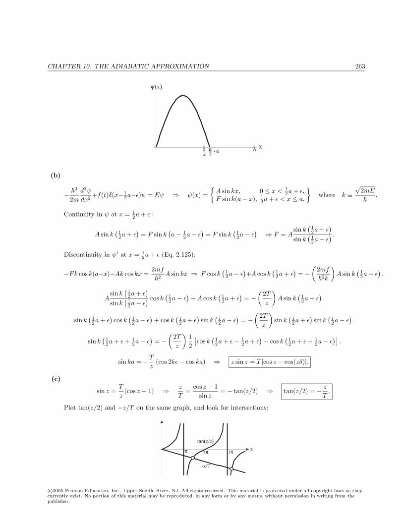
CHAPTER 10. THE ADIABATIC APPROXIMATION 263
x
ψ(x)
aa_2
_2a +ε
(b)
− 2
2md2ψ
dx2+f(t)δ(x− 1
2a−ε)ψ = Eψ ⇒ ψ(x) =
A sin kx, 0 ≤ x < 12a + ε,
F sin k(a− x), 12a + ε < x ≤ a,
where k ≡
√2mE
.
Continuity in ψ at x = 12a + ε :
A sin k(
12a + ε
)= F sin k
(a− 1
2a− ε)
= F sin k(
12a− ε
)⇒ F = A
sin k(
12a + ε
)sin k
(12a− ε
) .Discontinuity in ψ′ at x = 1
2a + ε (Eq. 2.125):
−Fk cos k(a−x)−Ak cos kx =2mf
2A sin kx ⇒ F cos k
(12a− ε
)+A cos k
(12a + ε
)= −
(2mf
2k
)A sin k
(12a + ε
).
Asin k
(12a + ε
)sin k
(12a− ε
) cos k(
12a− ε
)+ A cos k
(12a + ε
)= −
(2Tz
)A sin k
(12a + ε
).
sin k(
12a + ε
)cos k
(12a− ε
)+ cos k
(12a + ε
)sin k
(12a− ε
)= −
(2Tz
)sin k
(12a + ε
)sin k
(12a− ε
).
sin k(
12a + ε + 1
2a− ε)
= −(
2Tz
)12
[cos k
(12a + ε− 1
2a + ε)− cos k
(12a + ε + 1
2a− ε)]
.
sin ka = −T
z(cos 2kε− cos ka) ⇒ z sin z = T [cos z − cos(zδ)].
(c)
sin z =T
z(cos z − 1) ⇒ z
T=
cos z − 1sin z
= − tan(z/2) ⇒ tan(z/2) = − z
T.
Plot tan(z/2) and −z/T on the same graph, and look for intersections:
tan(z/2)
π z2π 3π
-z/T
c©2005 Pearson Education, Inc., Upper Saddle River, NJ. All rights reserved. This material is protected under all copyright laws as theycurrently exist. No portion of this material may be reproduced, in any form or by any means, without permission in writing from thepublisher.
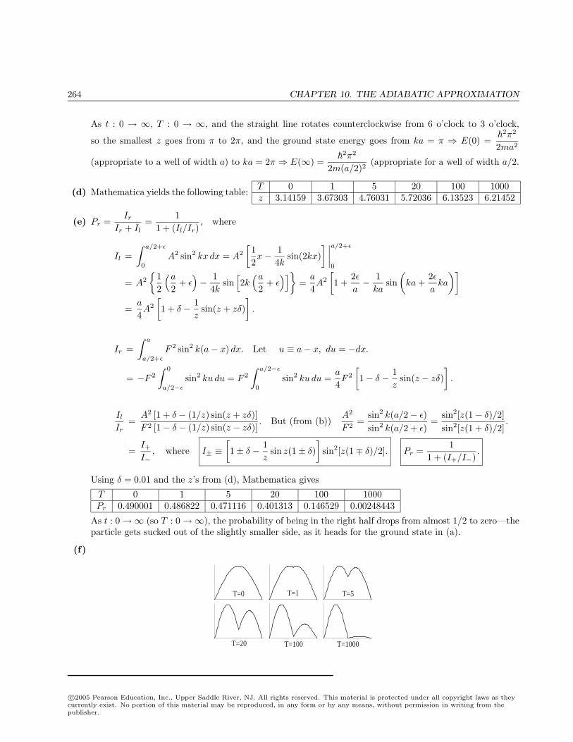
264 CHAPTER 10. THE ADIABATIC APPROXIMATION
As t : 0 → ∞, T : 0 → ∞, and the straight line rotates counterclockwise from 6 o’clock to 3 o’clock,
so the smallest z goes from π to 2π, and the ground state energy goes from ka = π ⇒ E(0) =
2π2
2ma2
(appropriate to a well of width a) to ka = 2π ⇒ E(∞) =
2π2
2m(a/2)2(appropriate for a well of width a/2.
(d) Mathematica yields the following table:T 0 1 5 20 100 1000z 3.14159 3.67303 4.76031 5.72036 6.13523 6.21452
(e) Pr =Ir
Ir + Il=
11 + (Il/Ir)
, where
Il =∫ a/2+ε
0
A2 sin2 kx dx = A2
[12x− 1
4ksin(2kx)
] ∣∣∣∣a/2+ε
0
= A2
12
(a
2+ ε
)− 1
4ksin
[2k
(a
2+ ε
)]=
a
4A2
[1 +
2εa− 1
kasin
(ka +
2εaka
)]=
a
4A2
[1 + δ − 1
zsin(z + zδ)
].
Ir =∫ a
a/2+ε
F 2 sin2 k(a− x) dx. Let u ≡ a− x, du = −dx.
= −F 2
∫ 0
a/2−ε
sin2 ku du = F 2
∫ a/2−ε
0
sin2 ku du =a
4F 2
[1− δ − 1
zsin(z − zδ)
].
Il
Ir=
A2 [1 + δ − (1/z) sin(z + zδ)]F 2 [1− δ − (1/z) sin(z − zδ)]
. But (from (b))A2
F 2=
sin2 k(a/2− ε)sin2 k(a/2 + ε)
=sin2[z(1− δ)/2]sin2[z(1 + δ)/2]
.
=I+I−
, where I± ≡[1± δ − 1
zsin z(1± δ)
]sin2[z(1∓ δ)/2]. Pr =
11 + (I+/I−)
.
Using δ = 0.01 and the z’s from (d), Mathematica gives
T 0 1 5 20 100 1000Pr 0.490001 0.486822 0.471116 0.401313 0.146529 0.00248443
As t : 0→∞ (so T : 0→∞), the probability of being in the right half drops from almost 1/2 to zero—theparticle gets sucked out of the slightly smaller side, as it heads for the ground state in (a).
(f)
T=0 T=1 T=5
T=20 T=100 T=1000
c©2005 Pearson Education, Inc., Upper Saddle River, NJ. All rights reserved. This material is protected under all copyright laws as theycurrently exist. No portion of this material may be reproduced, in any form or by any means, without permission in writing from thepublisher.
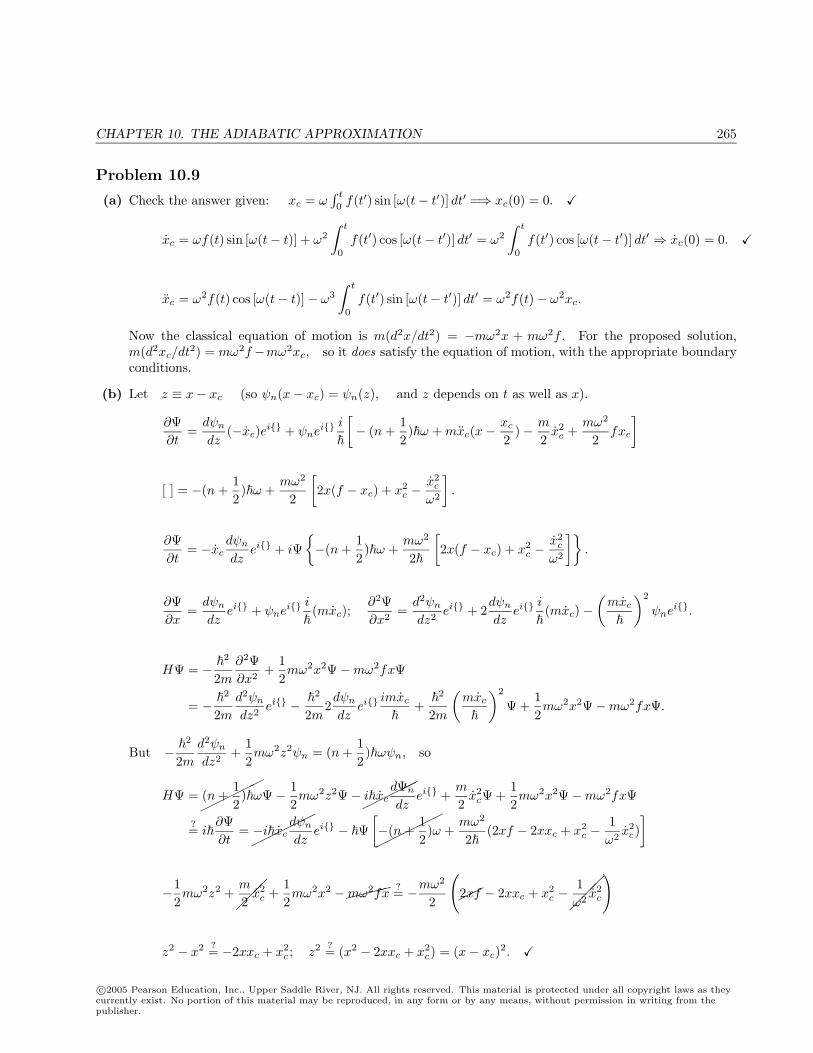
CHAPTER 10. THE ADIABATIC APPROXIMATION 265
Problem 10.9
(a) Check the answer given: xc = ω∫ t
0f(t′) sin [ω(t− t′)] dt′ =⇒ xc(0) = 0.
xc = ωf(t) sin [ω(t− t)] + ω2
∫ t
0
f(t′) cos [ω(t− t′)] dt′ = ω2
∫ t
0
f(t′) cos [ω(t− t′)] dt′ ⇒ xc(0) = 0.
xc = ω2f(t) cos [ω(t− t)]− ω3
∫ t
0
f(t′) sin [ω(t− t′)] dt′ = ω2f(t)− ω2xc.
Now the classical equation of motion is m(d2x/dt2) = −mω2x + mω2f . For the proposed solution,m(d2xc/dt
2) = mω2f−mω2xc, so it does satisfy the equation of motion, with the appropriate boundaryconditions.
(b) Let z ≡ x− xc (so ψn(x− xc) = ψn(z), and z depends on t as well as x).
∂Ψ∂t
=dψn
dz(−xc)ei + ψne
i i
[− (n +
12)ω + mxc(x−
xc
2)− m
2x2
c +mω2
2fxc
]
[ ] = −(n +12)ω +
mω2
2
[2x(f − xc) + x2
c −x2
c
ω2
].
∂Ψ∂t
= −xcdψn
dzei + iΨ
−(n +
12)ω +
mω2
2
[2x(f − xc) + x2
c −x2
c
ω2
].
∂Ψ∂x
=dψn
dzei + ψne
i i
(mxc);
∂2Ψ∂x2
=d2ψn
dz2ei + 2
dψn
dzei i
(mxc)−
(mxc
)2
ψnei.
HΨ = − 2
2m∂2Ψ∂x2
+12mω2x2Ψ−mω2fxΨ
= − 2
2md2ψn
dz2ei −
2
2m2dψn
dzei imxc
+
2
2m
(mxc
)2
Ψ +12mω2x2Ψ−mω2fxΨ.
But − 2
2md2ψn
dz2+
12mω2z2ψn = (n +
12)ωψn, so
HΨ =
(n +12)ωΨ− 1
2mω2z2Ψ−
ixcdΨn
dzei +
m
2x2
cΨ +12mω2x2Ψ−mω2fxΨ
?= i∂Ψ∂t
=
−ixcdψn
dzei − Ψ
[
−(n +12)ω +
mω2
2(2xf − 2xxc + x2
c −1ω2
x2c)
]
−12mω2z2 +
m
2x2
c +12mω2x2 −mω2fx
?= −mω2
2
(2xf − 2xxc + x2
c −
1ω2
x2c
)
z2 − x2 ?= −2xxc + x2c ; z2 ?= (x2 − 2xxc + x2
c) = (x− xc)2.
c©2005 Pearson Education, Inc., Upper Saddle River, NJ. All rights reserved. This material is protected under all copyright laws as theycurrently exist. No portion of this material may be reproduced, in any form or by any means, without permission in writing from thepublisher.
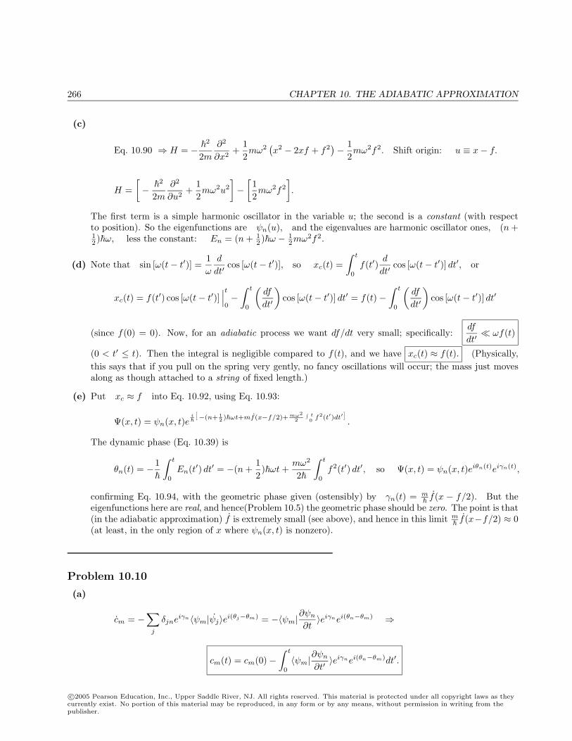
266 CHAPTER 10. THE ADIABATIC APPROXIMATION
(c)
Eq. 10.90 ⇒ H = − 2
2m∂2
∂x2+
12mω2
(x2 − 2xf + f2
)− 1
2mω2f2. Shift origin: u ≡ x− f.
H =[−
2
2m∂2
∂u2+
12mω2u2
]−
[12mω2f2
].
The first term is a simple harmonic oscillator in the variable u; the second is a constant (with respectto position). So the eigenfunctions are ψn(u), and the eigenvalues are harmonic oscillator ones, (n +12 )ω, less the constant: En = (n + 1
2 )ω − 12mω2f2.
(d) Note that sin [ω(t− t′)] =1ω
d
dt′cos [ω(t− t′)], so xc(t) =
∫ t
0
f(t′)d
dt′cos [ω(t− t′)] dt′, or
xc(t) = f(t′) cos [ω(t− t′)]∣∣∣t0−
∫ t
0
(df
dt′
)cos [ω(t− t′)] dt′ = f(t)−
∫ t
0
(df
dt′
)cos [ω(t− t′)] dt′
(since f(0) = 0). Now, for an adiabatic process we want df/dt very small; specifically:df
dt′ ωf(t)
(0 < t′ ≤ t). Then the integral is negligible compared to f(t), and we have xc(t) ≈ f(t). (Physically,this says that if you pull on the spring very gently, no fancy oscillations will occur; the mass just movesalong as though attached to a string of fixed length.)
(e) Put xc ≈ f into Eq. 10.92, using Eq. 10.93:
Ψ(x, t) = ψn(x, t)ei
[−(n+ 1
2 )ωt+mf(x−f/2)+mω22
∫ t0 f2(t′)dt′
].
The dynamic phase (Eq. 10.39) is
θn(t) = −1
∫ t
0
En(t′) dt′ = −(n +12)ωt +
mω2
2
∫ t
0
f2(t′) dt′, so Ψ(x, t) = ψn(x, t)eiθn(t)eiγn(t),
confirming Eq. 10.94, with the geometric phase given (ostensibly) by γn(t) = mf(x − f/2). But the
eigenfunctions here are real, and hence(Problem 10.5) the geometric phase should be zero. The point is that(in the adiabatic approximation) f is extremely small (see above), and hence in this limit m
f(x−f/2) ≈ 0
(at least, in the only region of x where ψn(x, t) is nonzero).
Problem 10.10
(a)
cm = −∑
j
δjneiγn〈ψm|ψj〉ei(θj−θm) = −〈ψm|
∂ψn
∂t〉eiγnei(θn−θm) ⇒
cm(t) = cm(0)−∫ t
0
〈ψm|∂ψn
∂t′〉eiγnei(θn−θm)dt′.
c©2005 Pearson Education, Inc., Upper Saddle River, NJ. All rights reserved. This material is protected under all copyright laws as theycurrently exist. No portion of this material may be reproduced, in any form or by any means, without permission in writing from thepublisher.
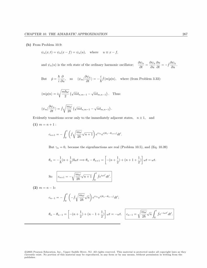
CHAPTER 10. THE ADIABATIC APPROXIMATION 267
(b) From Problem 10.9:
ψn(x, t) = ψn(x− f) = ψn(u), where u ≡ x− f,
and ψn(u) is the nth state of the ordinary harmonic oscillator;∂ψn
∂t=
∂ψn
∂u
∂u
∂t= −f
∂ψn
∂u.
But p =
i
∂
∂u, so 〈ψm|
∂ψn
∂t〉 = − i
f〈m|p|n〉, where (from Problem 3.33):
〈m|p|n〉 = i
√mω
2(√
mδn,m−1 −√nδm,n−1
). Thus:
〈ψm|∂ψn
∂t〉 = f
√mω
2(√
mδn,m−1 −√nδm,n−1
).
Evidently transitions occur only to the immediately adjacent states, n± 1, and
(1) m = n + 1 :
cn+1 = −∫ t
0
(f
√mω
2√n + 1
)eiγnei(θn−θn+1)dt′.
But γn = 0, because the eigenfunctions are real (Problem 10.5), and (Eq. 10.39)
θn = −1(n +
12)ωt =⇒ θn − θn+1 =
[−(n +
12) + (n + 1 +
12)]ωt = ωt.
So cn+1 = −√
mω
2√n + 1
∫ t
0
f eiωt′dt′.
(2) m = n− 1:
cn−1 = −∫ t
0
(−f
√mω
2√n
)eiγnei(θn−θn−1)dt′;
θn − θn−1 =[−(n +
12) + (n− 1 +
12)]ωt = −ωt. cn−1 =
√mω
2√n
∫ t
0
f e−iωt′dt′.
c©2005 Pearson Education, Inc., Upper Saddle River, NJ. All rights reserved. This material is protected under all copyright laws as theycurrently exist. No portion of this material may be reproduced, in any form or by any means, without permission in writing from thepublisher.
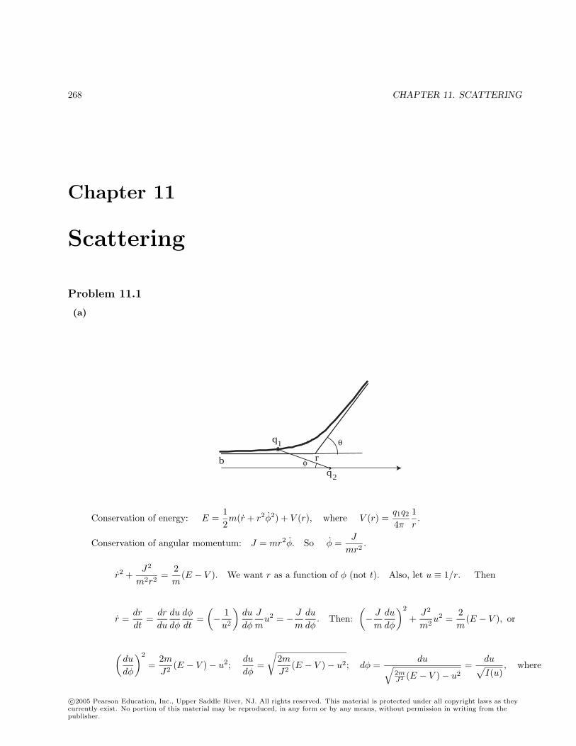
268 CHAPTER 11. SCATTERING
Chapter 11
Scattering
Problem 11.1
(a)
q
q
b r
1
2
φ
θ
Conservation of energy: E =12m(r + r2φ2) + V (r), where V (r) =
q1q2
4πε1r.
Conservation of angular momentum: J = mr2φ. So φ =J
mr2.
r2 +J2
m2r2=
2m
(E − V ). We want r as a function of φ (not t). Also, let u ≡ 1/r. Then
r =dr
dt=
dr
du
du
dφ
dφ
dt=
(− 1
u2
)du
dφ
J
mu2 = − J
m
du
dφ. Then:
(− J
m
du
dφ
)2
+J2
m2u2 =
2m
(E − V ), or
(du
dφ
)2
=2mJ2
(E − V )− u2;du
dφ=
√2mJ2
(E − V )− u2; dφ =du√
2mJ2 (E − V )− u2
=du√I(u)
, where
c©2005 Pearson Education, Inc., Upper Saddle River, NJ. All rights reserved. This material is protected under all copyright laws as theycurrently exist. No portion of this material may be reproduced, in any form or by any means, without permission in writing from thepublisher.
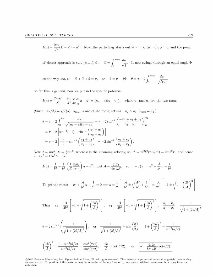
CHAPTER 11. SCATTERING 269
I(u) ≡ 2mJ2
(E − V )− u2. Now, the particle q1 starts out at r =∞ (u = 0), φ = 0, and the point
of closest approach is rmin (umax),Φ : Φ =∫ umax
0
du√I. It now swings through an equal angle Φ
on the way out, so Φ + Φ + θ = π, or θ = π − 2Φ. θ = π − 2∫ umax
0
du√I(u)
.
So far this is general ; now we put in the specific potential:
I(u) =2mE
J2− 2m
J2
q1q2
4πε0u− u2 = (u2 − u)(u− u1), where u1 and u2 are the two roots.
(Since du/dφ =√
I(u), umax is one of the roots; setting u2 > u1, umax = u2.)
θ = π − 2∫ u2
0
du√(u2 − u)(u− u1)
= π + 2 sin−1
(−2u + u1 + u2
u2 − u1
)∣∣∣∣u2
0
= π + 2[sin−1(−1)− sin−1
(u1 + u2
u2 − u1
)]= π + 2
[−π
2− sin−1
(u1 + u2
u2 − u1
)]= −2 sin−1
(u1 + u2
u2 − u1
).
Now J = mvb, E = 12mv2, where v is the incoming velocity, so J2 = m2b2(2E/m) = 2mb2E, and hence
2m/J2 = 1/b2E. So
I(u) =1b2− 1
b2
(1E
q1q2
4πε0
)u− u2. Let A ≡ q1q2
4πε0E, so − I(u) = u2 +
A
b2u− 1
b2.
To get the roots: u2 +A
b2u− 1
b2= 0 =⇒ u =
12
[−A
b2±
√A2
b4+
4b2
]=
A
2b2
−1±
√1 +
(2bA
)2 .
Thus u2 =A
2b2
−1 +
√1 +
(2bA
)2 , u1 =
A
2b2
−1−
√1 +
(2bA
)2 ;
u1 + u2
u2 − u1=
−1√1 + (2b/A)2
.
θ = 2 sin−1
1√1 + (2b/A)2
, or1√
1 + (2b/A)2= sin
(θ
2
); 1 +
(2bA
)2
=1
sin2(θ/2);
(2bA
)2
=1− sin2(θ/2)
sin2(θ/2)=
cos2(θ/2)sin2(θ/2)
;2bA
= cot(θ/2), or b =q1q2
8πε0Ecot(θ/2).
c©2005 Pearson Education, Inc., Upper Saddle River, NJ. All rights reserved. This material is protected under all copyright laws as theycurrently exist. No portion of this material may be reproduced, in any form or by any means, without permission in writing from thepublisher.
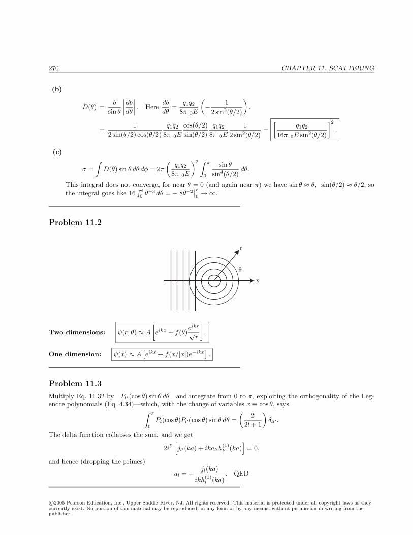
270 CHAPTER 11. SCATTERING
(b)
D(θ) =b
sin θ
∣∣∣∣dbdθ∣∣∣∣ . Here
db
dθ=
q1q2
8πε0E
(− 1
2 sin2(θ/2)
).
=1
2 sin(θ/2) cos(θ/2)q1q2
8πε0Ecos(θ/2)sin(θ/2)
q1q2
8πε0E1
2 sin2(θ/2)=
[q1q2
16πε0E sin2(θ/2)
]2
.
(c)
σ =∫
D(θ) sin θ dθ dφ = 2π(
q1q2
8πε0E
)2 ∫ π
0
sin θ
sin4(θ/2)dθ.
This integral does not converge, for near θ = 0 (and again near π) we have sin θ ≈ θ, sin(θ/2) ≈ θ/2, sothe integral goes like 16
∫ ε
0θ−3 dθ = − 8θ−2
∣∣ε0→∞.
Problem 11.2
x
r
θ
Two dimensions: ψ(r, θ) ≈ A
[eikx + f(θ)
eikr
√r
].
One dimension: ψ(x) ≈ A[eikx + f(x/|x|)e−ikx
].
Problem 11.3
Multiply Eq. 11.32 by Pl′(cos θ) sin θ dθ and integrate from 0 to π, exploiting the orthogonality of the Leg-endre polynomials (Eq. 4.34)—which, with the change of variables x ≡ cos θ, says∫ π
0
Pl(cos θ)Pl′(cos θ) sin θ dθ =(
22l + 1
)δll′ .
The delta function collapses the sum, and we get
2il′[jl′(ka) + ikal′h
(1)l′ (ka)
]= 0,
and hence (dropping the primes)
al = − jl(ka)
ikh(1)l (ka)
. QED
c©2005 Pearson Education, Inc., Upper Saddle River, NJ. All rights reserved. This material is protected under all copyright laws as theycurrently exist. No portion of this material may be reproduced, in any form or by any means, without permission in writing from thepublisher.
CHAPTER 11. SCATTERING 271
Problem 11.4
Keeping only the l = 0 terms, Eq. 11.29 says that in the exterior region:
ψ ≈ A[j0(kr) + ika0h
(1)0 (kr)
]P0(cos θ) = A
[sin(kr)
kr+ ika0
(−i
eikr
kr
)]= A
[sin(kr)
kr+ a0
eikr
r
](r > a).
In the internal region Eq. 11.18 (with nl eliminated because it blows up at the origin) yields
ψ(r) ≈ bj0(kr) = bsin(kr)
kr(r < a).
The boundary conditions hold independently for each l, as you can check by keeping the summation over l andexploiting the orthogonality of the Legendre polynomials:
(1) ψ continuous at r = a: A
[sinka
ka+ a0
eika
a
]= b
sin ka
ka.
(2) ψ′ discontinuous at r = a: Integrating the radial equation across the delta function gives
− 2
2m
∫d2u
dr2dr +
∫ [αδ(r − a) +
2
2ml(l + 1)
r2
]u dr ⇒ −
2
2m∆u′ + αu(a) = 0, or ∆u′ =
2mα
2u(a).
Now u = rR, so u′ = R+rR′; ∆u′ = ∆R+a∆R′ = a∆R′ =2mα
2aR(a), or ∆ψ′ =
2mα
2ψ(a) =
β
aψ(a).
A
ka
[k cos(ka) + a0ik
2eika]− A
ka2
[sin(ka) + a0ke
ika]− b
kak cos(ka) +
b
ka2sin ka =
β
absin(ka)
ka.
The indicated terms cancel (by (1)), leaving A[cos(ka) + ia0ke
ika]
= b
[cos(ka) +
β
kasin(ka)
].
Using (1) to eliminate b: A[cos(ka) + ia0ke
ika]
=[cot(ka) +
β
ka
] [sin(ka) + a0ke
ika]A.
cos(ka) + ia0ke
ika =cos(ka) +β
kasin(ka) + a0k cot(ka)eika + β
a0
aeika.
ia0keika
[1 + i cot(ka) + i
β
ka
]=
β
kasin(ka). But ka 1, so sin(ka) ≈ ka, and cot(ka) =
cos(ka)sin(ka)
≈ 1ka
.
ia0k(1 + ika)[1 +
i
ka(1 + β)
]= β; ia0k
[1 +
i
ka(1 + β) + ika− 1− β
]≈ ia0k
[i
ka(1 + β)
]= β.
a0 = − aβ
1 + β. Equation 11.25 ⇒ f(θ) ≈ a0 = − aβ
1 + β. Equation 11.14 ⇒ D = |f |2 =
(aβ
1 + β
)2
.
Equation 11.27 ⇒ σ = 4πD = 4π(
aβ
1 + β
)2
.
c©2005 Pearson Education, Inc., Upper Saddle River, NJ. All rights reserved. This material is protected under all copyright laws as theycurrently exist. No portion of this material may be reproduced, in any form or by any means, without permission in writing from thepublisher.
272 CHAPTER 11. SCATTERING
Problem 11.5
(a) In the region to the leftψ(x) = Aeikx + B−ikx (x ≤ −a).
In the region −a < x < 0, the Schrodinger equation gives
− h2
2md2ψ
dx2− V0ψ = Eψ ⇒ d2ψ
dx2= −k′ψ
where k′ =√
2m(E + V0)/. The general solution is
ψ = C sin(k′x) + D cos(k′x)
But ψ(0) = 0 implies D = 0, so
ψ(x) = C sin(k′x) (−a ≤ x ≤ 0).
The continuity of ψ(x) and ψ′(x) at x = −a says
Ae−ika + Beika = −C sin(k′a), ikAe−ika − ikBika = k′C cos(k′a).
Divide and solve for B:ikAe−ika − ikBeika
Ae−ika + Beika= −k′ cot(k′a),
ikAe−ika − ikBeika = −Ae−ikak′ cot(k′a)−Beikak′ cot(k′a),
Beika [−ik + k′ cot(k′a)] = Ae−ika [−ik − k′ cot(k′a)] .
B = Ae−2ika
[k − ik′ cot(k′a)k + ik′ cot(k′a)
].
(b)
|B|2 = |A|2[k − ik′ cot(k′a)k + ik′ cot(k′a)
]·[k + ik′ cot(k′a)k − ik′ cot(k′a)
]= |A|2.
(c) From part (a) the wave function for x < −a is
ψ(x) = Aeikx + Ae−2ika
[k − ik′ cot(k′a)k + ik′ cot(k′a)
]e−ikx.
But by definition of the phase shift (Eq. 11.40)
ψ(x) = A[eikx − ei(2δ−kx)
].
so
e−2ika
[k − ik′ cot(k′a)k + ik′ cot(k′a)
]= −e2iδ.
This is exact. For a very deep well, E V0, k =√
2mE/√
2m(E + V0)/ = k′, so
e−2ika
[−ik′ cot(k′a)ik′ cot(k′a)
]= −e2iδ; e−2ika = e2iδ; δ = −ka.
c©2005 Pearson Education, Inc., Upper Saddle River, NJ. All rights reserved. This material is protected under all copyright laws as theycurrently exist. No portion of this material may be reproduced, in any form or by any means, without permission in writing from thepublisher.
CHAPTER 11. SCATTERING 273
Problem 11.6
From Eq. 11.46, al =1keiδl sin δl, and Eq. 11.33, al = i
jl(ka)
kh(1)l (ka)
, it follows that eiδl sin δl = ijl(ka)
h(1)l (ka)
.
But (Eq. 11.19) h(1)l (x) = jl(x) + inl(x), so
eiδl sin δl = ijl(ka)
jl(x) + inl(x)= i
11 + i(n/j)
= i1− i(n/j)1 + (n/j)2
=(n/j) + i
1 + (n/j)2,
(writing (n/j) as shorthand for nl(ka)/jl(ka)). Equating the real and imaginary parts:
cos δl sin δl =(n/j)
1 + (n/j)2; sin2 δl =
11 + (n/j)2
.
Dividing the second by the first, I conclude that
tan δl =1
(n/j), or δl = tan−1
[jl(ka)nl(ka)
].
Problem 11.7
r > a : u(r) = A sin(kr + δ);
r < a : u(r) = B sin kr + D cos kr = B sin kr, because u(0) = 0 =⇒ D = 0.
Continuity at r = a =⇒ B sin(ka) = A sin(ka + δ) =⇒ B = Asin(ka + δ)
sin(ka). So u(r) = A
sin(ka + δ)sin(ka)
sin kr.
From Problem 11.4,
∆(du
dr
)∣∣∣∣r=a
=β
au(a)⇒ Ak cos(ka + δ)−A
sin(ka + δ)sin(ka)
k cos(ka) =β
aA sin(ka + δ).
cos(ka + δ)− sin(ka + δ)sin(ka)
cos(ka) =β
kasin(ka + δ),
sin(ka) cos(ka + δ)− sin(ka + δ) cos(ka) =β
kasin(ka + δ) sin(ka),
sin(ka− ka− δ) =β
kasin(ka) [sin(ka) cos δ + cos(ka) sin δ] ,
− sin δ = βsin2(ka)
ka[cos δ + cot(ka) sin δ] ; −1 = β
sin2(ka)ka
[cot δ + cot(ka)] .
cot δ = − cot(ka)− ka
β sin2(ka); cot δ = −
[cot(ka) +
ka
β sin2(ka)
].
c©2005 Pearson Education, Inc., Upper Saddle River, NJ. All rights reserved. This material is protected under all copyright laws as theycurrently exist. No portion of this material may be reproduced, in any form or by any means, without permission in writing from thepublisher.
274 CHAPTER 11. SCATTERING
Problem 11.8
G = −eikr
4πr=⇒ ∇G = − 1
4π
(1r∇eikr + eikr∇1
r
)=⇒
∇2G = ∇ · (∇G) = − 14π
[2
(∇1
r
)· (∇eikr) +
1r∇2(eikr) + eikr∇2
(1r
)].
But ∇1r
= − 1r2
r; ∇(eikr) = ikeikr r; ∇2eikr = ik∇ · (eikr r) = ik1r2
d
dr(r2eikr)
(see reference in footnote 12) =⇒ ∇2eikr =ik
r2(2reikr + ikr2eikr) = ikeikr
(2r
+ ik
);
∇2
(1r
)= −4πδ3(r). So ∇2G = − 1
4π
[2
(− 1
r2r
)·(ikeikr r
)+
1rikeikr
(2r
+ ik
)− 4πeikrδ3(r)
].
But eikrδ3(r) = δ3(r), so
∇2G = δ3(r)− 14π
eikr
[−2ik
r2+
2ikr2− k2
r
]= δ3(r) + k2 e
ikr
4πr= δ3(r)− k2G.
Therefore (∇2 + k2)G = δ3(r). QED
Problem 11.9
ψ =1√πa3
e−r/a; V = − e2
4πε0r= −
2
ma
1r
(Eq. 4.72); k = i
√−2mE
=
i
a.
In this case there is no “incoming” wave, and ψ0(r) = 0. Our problem is to show that
− m
2π2
∫eik|r−r0|
|r− r0|V (r0)ψ(r0) d3r0 = ψ(r).
We proceed to evaluate the left side (call it I):
I =(− m
2π2
) (−
2
ma
)1√πa3
∫e−|r−r0|/a
|r− r0|1r0
e−r0/a d3r0
=1
2πa1√πa3
∫e−√
r2+r20−2rr0 cos θ/ae−r0/a√
r2 + r20 − 2rr0 cos θ r0
r20 sin θ dr0 dθ dφ.
(I have set the z0 axis along the—fixed—direction r, for convenience.) Doing the φ integral (2π):
I =1
a√πa3
∫ ∞0
r0e−r0/a
[∫ π
0
e−√
r2+r20−2rr0 cos θ/a√
r2 + r20 − 2rr0 cos θ
sin θ dθ
]dr0. The θ integral is
c©2005 Pearson Education, Inc., Upper Saddle River, NJ. All rights reserved. This material is protected under all copyright laws as theycurrently exist. No portion of this material may be reproduced, in any form or by any means, without permission in writing from thepublisher.
CHAPTER 11. SCATTERING 275
∫ π
0
e−√
r2+r20−2rr0 cos θ/a√
r2 + r20 − 2rr0 cos θ
sin θ dθ = − a
rr0e−√
r2+r20−2rr0 cos θ/a
∣∣∣π0
= − a
rr0
[e−(r+r0)/a − e−|r−r0|/a
].
I = − 1r√πa3
∫ ∞0
e−r0/a[e−(r0+r)/a − e−|r0−r|/a
]dr0
= − 1r√πa3
[e−r/a
∫ ∞0
e−2r0/a dr0 − e−r/a
∫ r
0
dr − er/a
∫ ∞r
e−2r0/a dr0
]= − 1
r√πa3
[e−r/a
(a
2
)− e−r/a(r)− er/a
(−a
2e−2r0/a
)∣∣∣∞r
]= − 1
r√πa3
[a2e−r/a − re−r/a − a
2er/ae−2r/a
]=
1√πa3
e−r/a = ψ(r). QED
Problem 11.10
For the potential in Eq. 11.81, Eq. 11.88 =⇒
f(θ) = − 2m2κ
V0
∫ a
0
r sin(κr) dr = −2mV0
2κ
[1κ2
sin(κr)− r
κcos(κr)
]∣∣∣∣a0
= −2mV0
2κ3[sin(κa)− κa cos(κa)] ,
where (Eq. 11.89) κ = 2k sin(θ/2). For low-energy scattering (ka 1):
sin(κa) ≈ κa− 13!
(κa)3; cos(κa) = 1− 12(κa)2; so
f(θ) ≈ −2mV0
2κ3
[κa− 1
6(κa)3 − κa +
12(κa)3
]= −2
3mV0a
3
2, in agreement with Eq. 11.82.
Problem 11.11
sin(κr) =12i
(eiκr − e−iκr
), so
∫ ∞0
e−µr sin(κr) dr =12i
∫ ∞0
[e−(µ−iκ)r − e−(µ+iκ)r
]dr
=12i
[e−(µ−iκ)r
−(µ− iκ)− e−(µ+iκ)r
−(µ + iκ)
]∣∣∣∣∞0
=12i
[1
µ− iκ− 1
µ + iκ
]=
12i
(µ + iκ− µ + iκ
µ2 + κ2
)=
κ
µ2 + κ2.
So f(θ) = −2mβ
2κ
κ
µ2 + κ2= − 2mβ
2(µ2 + κ2). QED
c©2005 Pearson Education, Inc., Upper Saddle River, NJ. All rights reserved. This material is protected under all copyright laws as theycurrently exist. No portion of this material may be reproduced, in any form or by any means, without permission in writing from thepublisher.
276 CHAPTER 11. SCATTERING
Problem 11.12
Equation 11.91 =⇒ D(θ) = |f(θ)|2 =(
2mβ
2
)2 1(µ2 + κ2)2
, where Eq. 11.89⇒ κ = 2k sin(θ/2).
σ =∫
D(θ) sin θ dθ dφ = 2π(
2mβ
2
)2 1µ4
∫ π
0
1[1 + (2k/µ)2 sin2(θ/2)
]2 2 sin(θ/2) cos(θ/2) dθ.
Let2kµ
sin(θ/2) ≡ x, so 2 sin(θ/2) =µ
kx, and cos(θ/2) dθ =
µ
kdx. Then
σ = 2π(
2mβ
2
)2 1µ4
(µ
k
)2∫ x1
x0
x
(1 + x2)2dx. The limits are
θ = 0 =⇒ x = x0 = 0,θ = π =⇒ x = x1 = 2k/µ.
So
σ = 2π(
2mβ
2
)2 1(µk)2
[−1
21
(1 + x2)
]∣∣∣∣2k/µ
0
= π
(2mβ
2
)2 1(µk)2
[1− 1
1 + (2k/µ)2
]= π
(2mβ
2
)2 1(µk)2
[4(k/µ)2
1 + 4k2/µ2
]= π
(4mβ
2
)2 1µ2
1µ2 + 4k2
. But k2 =2mE
2, so
σ = π
(4mβ
µ
)2 1(µk)2 + 8mE
.
Problem 11.13
(a)
V (r) = αδ(r − a). Eq. 11.80 =⇒ f = − m
2π2
∫V (r) d3r = − m
2π2α4π
∫ ∞0
δ(r − a)r2dr.
f = −2mα
2a2; D = |f |2 =
(2mα
2a2
)2
; σ = 4πD = π
(4mα
2a2
)2
.
(b)
Eq. 11.88 =⇒ f = − 2m2κ
α
∫ ∞0
rδ(r − a) sin(κr) dr = −2mα
2κa sin(κa) (κ = 2k sin(θ/2)).
(c) Note first that (b) reduces to (a) in the low-energy regime (ka 1 =⇒ κa 1). Since Problem 11.4was also for low energy, what we must confirm is that Problem 11.4 reproduces (a) in the regime forwhich the Born approximation holds. Inspection shows that the answer to Problem 11.4 does reduce tof = −2mαa2/2 when β 1, which is to say when f/a 1. This is the appropriate condition, since(Eq. 11.12) f/a is a measure of the relative size of the scattered wave, in the interaction region.
c©2005 Pearson Education, Inc., Upper Saddle River, NJ. All rights reserved. This material is protected under all copyright laws as theycurrently exist. No portion of this material may be reproduced, in any form or by any means, without permission in writing from thepublisher.
CHAPTER 11. SCATTERING 277
Problem 11.14
F =1
4πε0q1q2
r2r; F⊥ =
14πε0
q1q2
r2cosφ; cosφ =
b
r, so F⊥ =
14πε0
q1q2b
r3; dt =
dx
v.
b
q
q
F
r
r
x
φ1
2
I⊥ =∫
F⊥dt =1
4πε0q1q2b
v
∫ ∞−∞
dx
(x2 + b2)3/2. But
∫ ∞−∞
dx
(x2 + b2)3/2= 2
∫ ∞0
dx
(x2 + b2)3/2=
2xb2√x2 + b2
∣∣∣∣∞0
=2b2
, so I⊥ =1
4πε02q1q2
bv.
tan θ =I⊥mv
=q1q2
4πε01
b( 12mv2)
=q1q2
4πε01bE
. θ = tan−1
[q1q2
4πε0bE
].
b =q1q2
4πε01
E tan θ=
(q1q2
8πε0E
)(2 cot θ).
The exact answer is the same, only with cot(θ/2) in place of 2 cot θ. So I must show that cot(θ/2) ≈ 2 cot θ,for small θ (that’s the regime in which the impulse approximation should work). Well:
cot(θ/2) =cos(θ/2)sin(θ/2)
≈ 1θ/2
=2θ, for small θ, while 2 cot θ = 2
cos θsin θ
≈ 21θ. So it works.
Problem 11.15
First let’s set up the general formalism. From Eq. 11.101:
ψ(r) = ψ0(r) +∫
g(r− r0)V (r0)ψ0(r0) d3r0 +∫
g(r− r0)V (r0)[∫
g(r0 − r1)V (r1)ψ0(r1) d3r1
]d3r0 + · · ·
Put in ψ0(r) = Aeikz, g(r) = − m
2π2
eikr
r:
ψ(r) = Aeikz − mA
2π2
∫eik|r−r0|
|r− r0|V (r0)eikz0 d3r0
+( m
2π2
)2
A
∫eik|r−r0|
|r− r0|V (r0)
[∫eik|r0−r1|
|r0 − r1|V (r1)eikz1 d3r1
]d3r0.
c©2005 Pearson Education, Inc., Upper Saddle River, NJ. All rights reserved. This material is protected under all copyright laws as theycurrently exist. No portion of this material may be reproduced, in any form or by any means, without permission in writing from thepublisher.
278 CHAPTER 11. SCATTERING
In the scattering region r r0, Eq. 11.73 =⇒ eik|r−r0|
|r− r0|≈ eikr
re−ik·r0 , with k ≡ kr, so
ψ(r) = A
eikz − m
2π2
eikr
r
∫e−ik·r0V (r0)eikz0d3r0( m
2π2
)2 eikr
r
∫e−ik·r0V (r0)
[∫eik|r0−r1|
|r0 − r1|V (r1)eikz1d3r1
]d3r0
f(θ, φ) = − m
2π2
∫ei(k′−k)·rV (r) d3r +
( m
2π2
)2∫
e−ik·rV (r)[∫
eik|r−r0|
|r− r0|V (r0)eikz0d3r0
]d3r.
I simplified the subscripts, since there is no longer any possible ambiguity. For low-energy scattering we dropthe exponentials (see p. 414):
f(θ, φ) ≈ − m
2π2
∫V (r) d3r +
( m
2π2
)2∫
V (r)[∫
1|r− r0|
V (r0) d3r0
]d3r.
Now apply this to the potential in Eq. 11.81:∫1
|r− r0|V (r0) d3r0 = V0
∫ a
0
1|r− r0|
r20 sin θ0 dr0 dθ0 dφ0.
Orient the z0 axis along r, so |r− r0| = r2 + r20 − 2rr0 cos θ0.∫
1|r− r0|
V (r0) d3r0 = V02π∫ a
0
r20
[ ∫ π
0
1√r2 + r2
0 − 2rr0 cos θ0
sin θ0 dθ0
]dr0. But
∫ π
0
1√r2 + r2
0 − 2rr0 cos θ0
sin θ0 dθ0 =1
rr0
√r2 + r2
0 − 2rr0 cos θ0
∣∣∣∣π0
=1
rr0[(r0 + r)− |r0 − r|] =
2/r, r0 < r;2/r0, r0 > r.
Here r < a (from the “outer” integral), so∫1
|r− r0|V (r0) d3r0 = 4πV0
[1r
∫ r
0
r20 dr0 +
∫ a
r
r0 dr0
]= 4πV0
[1r
r3
3+
12(a2 − r2)
]= 2πV0
(a2 − 1
3r2
).
∫V (r)
[∫1
|r− r0|V (r0) d3r0
]d3r = V0(2πV0)4π
∫ a
0
(a2 − 1
3r2
)r2dr = 8π2V 2
0
[a2 a
3
3− 1
3a5
5
]=
3215
π2V 20 a5.
f(θ) = − m
2π2V0
43πa3 +
( m
2π2
)2 3215
π2V 20 a5 = −
(2mV0a
3
32
) [1− 4
5
(mV0a
2
2
)].
Problem 11.16
(d2
dx2+ k2
)G(x) = δ(x) (analog to Eq. 11.52). G(x) =
1√2π
∫eisxg(s) ds (analog to Eq. 11.54).
c©2005 Pearson Education, Inc., Upper Saddle River, NJ. All rights reserved. This material is protected under all copyright laws as theycurrently exist. No portion of this material may be reproduced, in any form or by any means, without permission in writing from thepublisher.
CHAPTER 11. SCATTERING 279
(d2
dx2+ k2
)G =
1√2π
∫(−s2 + k2)g(s)eisxds = δ(x) =
12π
∫eisxds =⇒ g(s) =
1√2π(k2 − s2)
.
G(x) =12π
∫ ∞−∞
eisx
k2 − s2ds. Skirt the poles as in Fig. 11.10. For x > 0, close above:
G(x) = − 12π
∮ (eisx
s + k
)1
s− kds = − 1
2π2πi
(eisx
s + k
)∣∣∣∣s=k
= −ieikx
2k. For x < 0, close below:
G(x) = +12π
∮ (eisx
s− k
)1
s + kds =
12π
2πi(
eisx
s− k
)∣∣∣∣s=−k
= −ie−ikx
2k.
In either case, then, G(x) = − i
2keik|x|. (Analog to Eq. 11.65.)
ψ(x) = G(x− x0)2m2
V (x0)ψ(x0) dx0 = − i
2k2m2
∫eik|x−x0|V (x0)ψ(x0) dx0,
plus any solution ψ0(x) to the homogeneous Schrodinger equation:(d2
dx2+ k2
)ψ0(x) = 0. So:
ψ(x) = ψ0(x)− im
2k
∫ ∞−∞
eik|x−x0|V (x0)ψ(x0) dx0.
Problem 11.17
For the Born approximation let ψ0(x) = Aeikx, and ψ(x) ≈ Aeikx.
ψ(x) ≈ A
[eikx − im
2k
∫ ∞−∞
eik|x−x0|V (x0)eikx0dx0
]= A
[eikx − im
2k
∫ x
−∞eik(x−x0)V (x0)eikx0dx0 −
im
2k
∫ ∞x
eik(x0−x)V (x0)eikx0dx0
].
ψ(x) = A
[eikx − im
2keikx
∫ x
−∞V (x0) dx0 −
im
2ke−ikx
∫ ∞x
e2ikx0V (x0) dx0
].
Now assume V (x) is localized; for large positive x, the third term is zero, and
ψ(x) = Aeikx
[1− im
2k
∫ ∞−∞
V (x0) dx0
]. This is the transmitted wave.
For large negative x the middle term is zero:
ψ(x) = A
[eikx − im
2ke−ikx
∫ ∞−∞
e2ikx0V (x0)dx0
].
c©2005 Pearson Education, Inc., Upper Saddle River, NJ. All rights reserved. This material is protected under all copyright laws as theycurrently exist. No portion of this material may be reproduced, in any form or by any means, without permission in writing from thepublisher.
280 CHAPTER 11. SCATTERING
Evidently the first term is the incident wave and the second the reflected wave:
R =( m
2k
)2∣∣∣∣∫ ∞−∞
e2ikxV (x) dx∣∣∣∣2 .
If you try in the same spirit to calculate the transmission coefficient, you get
T =∣∣∣∣1− im
2k
∫ ∞−∞
V (x)dx∣∣∣∣2 = 1 +
( m
2k
)2[∫ ∞−∞
V (x)dx]2
,
which is nonsense (greater than 1). The first Born approximation gets R right, but all you can say to this orderis T ≈ 1 (you would do better using T = 1−R).
Problem 11.18
Delta function: V (x) = −αδ(x).∫ ∞−∞
e2ikxV (x) dx = −α, so R =(mα
2k
)2
,
or, in terms of energy (k2 = 2mE/2):
R =m2α2
2mE2=
mα2
22E; T = 1−R = 1− mα2
22E.
The exact answer (Eq. 2.141) is1
1 + mα2
22E
≈ 1− mα2
22E, so they agree provided E mα
22.
Finite square well: V (x) =−V0 (−a < x < a)0 (otherwise)
.∫ ∞
−∞e2ikxV (x) dx = −V0
∫ a
−a
e2ikxdx = −V0e2ikx
2ik
∣∣∣∣a−a
= −V0
k
(e2ika − e−2ika
2i
)= −V0
ksin(2ka).
So R =[ m
2k
)2(V0
ksin(2ka)
]2
. T = 1−[V0
2Esin
(2a
√2mE
)]2
.
If E V0, the exact answer (Eq. 2.169) becomes
T−1 ≈ 1 +[V0
2Esin
(2a
√2mE
)]2
=⇒ T ≈ 1−(
V0
2Esin
[2a
√2mE
)]2
,
so they agree provided E V0.
Problem 11.19
The Legendre polynomials satisfy Pl(1) = 1 (see footnote 30, p. 124), so Eq. 11.47 ⇒
f(0) =1k
∞∑l=0
(2l + 1)eiδl sin δl. Therefore Im[f(0)] =1k
∞∑l=0
(2l + 1) sin2 δl,
and hence (Eq. 11.48):
σ =4πk
Im[f(0)]. QED
c©2005 Pearson Education, Inc., Upper Saddle River, NJ. All rights reserved. This material is protected under all copyright laws as theycurrently exist. No portion of this material may be reproduced, in any form or by any means, without permission in writing from thepublisher.
CHAPTER 11. SCATTERING 281
Problem 11.20
Using Eq. 11.88 and integration by parts:
f(θ) = − 2m2κ
∫ ∞0
rAe−µr2sin(κr) dr = −2mA
2κ
∫ ∞0
d
dr
(− 1
2µe−µr2
)sin(κr) dr
=2mA
2µ2κ
e−µr2
sin(κr)∣∣∣∣∞0
−∫ ∞
0
e−µr2 d
dr[sin(κr)] dr
=
mA
µ2κ
0− κ
∫ ∞0
e−µr2cos(κr) dr
= −mA
µ2
( √π
2√µe−κ2/4µ
)= −mA
√π
22µ3/2e−κ2/4µ, where κ = 2k sin(θ/2) (Eq. 11.89).
From Eq. 11.14, then,
dσ
dΩ=
πm2A2
44µ3e−κ2/2µ,
and hence
σ =∫
dσ
dΩdΩ =
πm2A2
44µ3
∫e−4k2 sin2(θ/2)/2µ sin θ dθ dφ
=π2m2A2
24µ3
∫ π
0
e−2k2 sin2(θ/2)/µ sin θ dθ; write sin θ = 2 sin(θ/2) cos(θ/2) and let x ≡ sin(θ/2)
=π2m2A2
24µ3
∫ 1
0
e−2k2x2/µ2x 2 dx =2π2m2A2
4µ3
∫ 1
0
xe−2k2x2/µ dx
=2π2m2A2
4µ3
[− µ
4k2e−2k2x2/µ
] ∣∣∣∣10
= −π2m2A2
24µ2k2
(e−2k2/µ − 1
)=
π2m2A2
24µ2k2
(1− e−2k2/µ
).
c©2005 Pearson Education, Inc., Upper Saddle River, NJ. All rights reserved. This material is protected under all copyright laws as theycurrently exist. No portion of this material may be reproduced, in any form or by any means, without permission in writing from thepublisher.
282 CHAPTER 12. AFTERWORD
Chapter 12
Afterword
Problem 12.1
Suppose, on the contrary, that
α|φa(1)〉|φb(2)〉+ β|φb(1)〉|φa(2)〉 = |ψr(1)〉|ψs(2)〉,
for some one-particle states |ψr〉 and |ψs〉. Because |φa〉 and |φb〉 constitute a complete set of one-particle states(this is a two-level system), any other one-particle state can be expressed as a linear combination of them. Inparticular,
|ψr〉 = A|φa〉+ B|φb〉, and |ψs〉 = C|φa〉+ D|φb〉,for some complex numbers A, B, C, and D. Thus
α|φa(1)〉|φb(2)〉+ β|φb(1)〉|φa(2)〉 =[A|φa(1)〉+ B|φb(1)〉
][C|φa(2)〉+ D|φb(2)〉
]= AC|φa(1)〉|φa(2)〉+ AD|φa(1)〉|φb(2)〉+ BC|φb(1)〉|φa(2)〉+ BD|φb(1)〉|φb(2)〉.
(i) Take the inner product with 〈φa(1)|〈φb(2)|: α = AD.(ii) Take the inner product with 〈φa(1)|〈φa(2)|: 0 = AC.(iii) Take the inner product with 〈φb(1)|〈φa(2)|: β = BC.(iv) Take the inner product with 〈φb(1)|〈φb(2)|: 0 = BD.
(ii) ⇒ either A = 0 or C = 0. But if A = 0, then (i) ⇒ α = 0, which is excluded by assumption, whereas ifC = 0, then (iii) ⇒ β = 0, which is likewise excluded. Conclusion: It is impossible to express this state as aproduct of one-particle states. QED
c©2005 Pearson Education, Inc., Upper Saddle River, NJ. All rights reserved. This material is protected under all copyright laws as theycurrently exist. No portion of this material may be reproduced, in any form or by any means, without permission in writing from thepublisher.
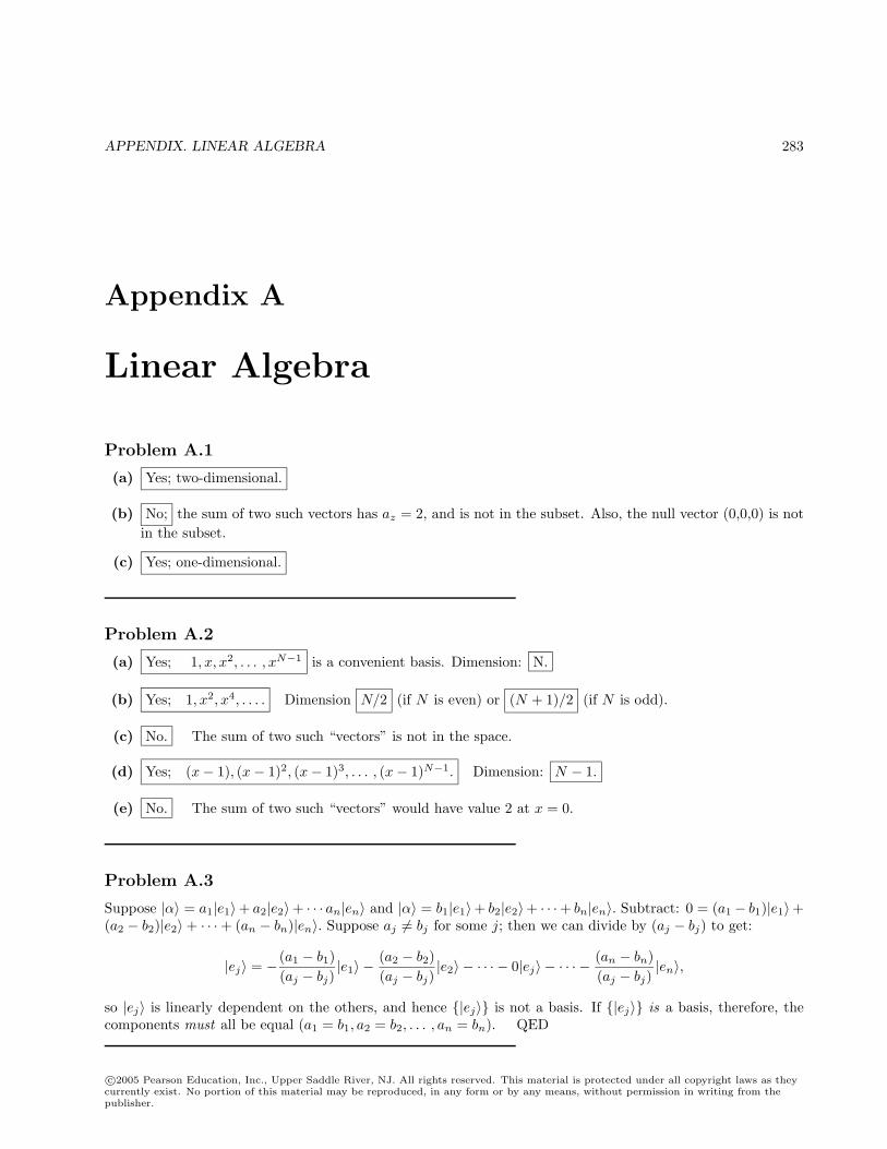
APPENDIX. LINEAR ALGEBRA 283
Appendix A
Linear Algebra
Problem A.1
(a) Yes; two-dimensional.
(b) No; the sum of two such vectors has az = 2, and is not in the subset. Also, the null vector (0,0,0) is notin the subset.
(c) Yes; one-dimensional.
Problem A.2
(a) Yes; 1, x, x2, . . . , xN−1 is a convenient basis. Dimension: N.
(b) Yes; 1, x2, x4, . . . . Dimension N/2 (if N is even) or (N + 1)/2 (if N is odd).
(c) No. The sum of two such “vectors” is not in the space.
(d) Yes; (x− 1), (x− 1)2, (x− 1)3, . . . , (x− 1)N−1. Dimension: N − 1.
(e) No. The sum of two such “vectors” would have value 2 at x = 0.
Problem A.3
Suppose |α〉 = a1|e1〉+ a2|e2〉+ · · · an|en〉 and |α〉 = b1|e1〉+ b2|e2〉+ · · ·+ bn|en〉. Subtract: 0 = (a1 − b1)|e1〉+(a2 − b2)|e2〉+ · · ·+ (an − bn)|en〉. Suppose aj = bj for some j; then we can divide by (aj − bj) to get:
|ej〉 = − (a1 − b1)(aj − bj)
|e1〉 −(a2 − b2)(aj − bj)
|e2〉 − · · · − 0|ej〉 − · · · −(an − bn)(aj − bj)
|en〉,
so |ej〉 is linearly dependent on the others, and hence |ej〉 is not a basis. If |ej〉 is a basis, therefore, thecomponents must all be equal (a1 = b1, a2 = b2, . . . , an = bn). QED
c©2005 Pearson Education, Inc., Upper Saddle River, NJ. All rights reserved. This material is protected under all copyright laws as theycurrently exist. No portion of this material may be reproduced, in any form or by any means, without permission in writing from thepublisher.
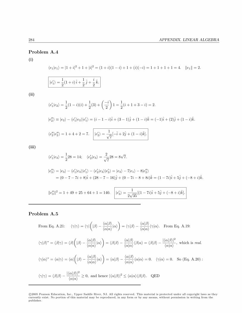
284 APPENDIX. LINEAR ALGEBRA
Problem A.4
(i)
〈e1|e1〉 = |1 + i|2 + 1 + |i|2 = (1 + i)(1− i) + 1 + (i)(−i) = 1 + 1 + 1 + 1 = 4. ‖e1‖ = 2.
|e′1〉 =12(1 + i) i +
12j +
i
2k.
(ii)
〈e′1|e2〉 =12(1− i)(i) +
12(3) +
(−i
2
)1 =
12(i + 1 + 3− i) = 2.
|e′′2〉 ≡ |e2〉 − 〈e′1|e2〉|e′1〉 = (i− 1− i)i + (3− 1)j + (1− i)k = (−1)i + (2)j + (1− i)k.
〈e′′2 |e′′2〉 = 1 + 4 + 2 = 7. |e′2〉 =1√7[−i + 2j + (1− i)k].
(iii)
〈e′1|e3〉 =1228 = 14; 〈e′2|e3〉 =
2√728 = 8
√7.
|e′′3〉 = |e3〉 − 〈e′1|e3〉|e′1〉 − 〈e′2|e3〉|e′2〉 = |e3〉 − 7|e1〉 − 8|e′′2〉= (0− 7− 7i + 8)i + (28− 7− 16)j + (0− 7i− 8 + 8i)k = (1− 7i)i + 5j + (−8 + i)k.
‖e′′3‖2 = 1 + 49 + 25 + 64 + 1 = 140. |e′3〉 =1
2√
35[(1− 7i)i + 5j + (−8 + i)k].
Problem A.5
From Eq. A.21: 〈γ|γ〉 = 〈γ|(|β〉 − 〈α|β〉〈α|α〉 |α〉
)= 〈γ|β〉 − 〈α|β〉〈α|α〉 〈γ|α〉. From Eq. A.19:
〈γ|β〉∗ = 〈β|γ〉 = 〈β|(|β〉 − 〈α|β〉〈α|α〉 |α〉
)= 〈β|β〉 − 〈α|β〉〈α|α〉 〈β|α〉 = 〈β|β〉 − |〈α|β〉|
2
〈α|α〉 , which is real.
〈γ|α〉∗ = 〈α|γ〉 = 〈α|(|β〉 − 〈α|β〉〈α|α〉 |α〉
)= 〈α|β〉 − 〈α|β〉〈α|α〉 〈α|α〉 = 0. 〈γ|α〉 = 0. So (Eq. A.20) :
〈γ|γ〉 = 〈β|β〉 − |〈α|β〉|2
〈α|α〉 ≥ 0, and hence |〈α|β〉|2 ≤ 〈α|α〉〈β|β〉. QED
c©2005 Pearson Education, Inc., Upper Saddle River, NJ. All rights reserved. This material is protected under all copyright laws as theycurrently exist. No portion of this material may be reproduced, in any form or by any means, without permission in writing from thepublisher.
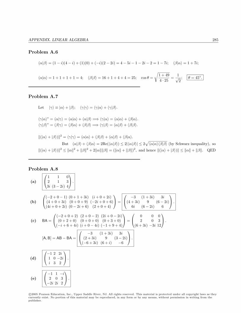
APPENDIX. LINEAR ALGEBRA 285
Problem A.6
〈α|β〉 = (1− i)(4− i) + (1)(0) + (−i)(2− 2i) = 4− 5i− 1− 2i− 2 = 1− 7i; 〈β|α〉 = 1 + 7i;
〈α|α〉 = 1 + 1 + 1 + 1 = 4; 〈β|β〉 = 16 + 1 + 4 + 4 = 25; cos θ =
√1 + 494 · 25
=1√2; θ = 45.
Problem A.7
Let |γ〉 ≡ |α〉+ |β〉; 〈γ|γ〉 = 〈γ|α〉+ 〈γ|β〉.
〈γ|α〉∗ = 〈α|γ〉 = 〈α|α〉+ 〈α|β〉 =⇒ 〈γ|α〉 = 〈α|α〉+ 〈β|α〉.〈γ|β〉∗ = 〈β|γ〉 = 〈β|α〉+ 〈β|β〉 =⇒ 〈γ|β〉 = 〈α|β〉+ 〈β|β〉.
‖(|α〉+ |β〉)‖2 = 〈γ|γ〉 = 〈α|α〉+ 〈β|β〉+ 〈α|β〉+ 〈β|α〉.But 〈α|β〉+ 〈β|α〉 = 2Re(〈α|β〉) ≤ 2|〈α|β〉| ≤ 2
√〈α|α〉〈β|β〉 (by Schwarz inequality), so
‖(|α〉+ |β〉)‖2 ≤ ‖α‖2 + ‖β‖2 + 2‖α‖‖β‖ = (‖α‖+ ‖β‖)2, and hence ‖(|α〉+ |β〉)‖ ≤ ‖α‖+ ‖β‖. QED
Problem A.8
(a)
1 1 02 1 33i (3− 2i) 4
.
(b)
(−2 + 0− 1) (0 + 1 + 3i) (i + 0 + 2i)(4 + 0 + 3i) (0 + 0 + 9) (−2i + 0 + 6)(4i + 0 + 2i) (0− 2i + 6) (2 + 0 + 4)
=
−3 (1 + 3i) 3i(4 + 3i) 9 (6− 2i)
6i (6− 2i) 6
.
(c) BA =
(−2 + 0 + 2) (2 + 0− 2) (2i + 0− 2i)(0 + 2 + 0) (0 + 0 + 0) (0 + 3 + 0)
(−i + 6 + 4i) (i + 0− 4i) (−1 + 9 + 4)
=
0 0 02 0 3
(6 + 3i) −3i 12
.
[A,B] = AB− BA =
−3 (1 + 3i) 3i(2 + 3i) 9 (3− 2i)
(−6 + 3i) (6 + i) −6
.
(d)
−1 2 2i1 0 −2ii 3 2
.
(e)
−1 1 −i2 0 3−2i 2i 2
.
c©2005 Pearson Education, Inc., Upper Saddle River, NJ. All rights reserved. This material is protected under all copyright laws as theycurrently exist. No portion of this material may be reproduced, in any form or by any means, without permission in writing from thepublisher.
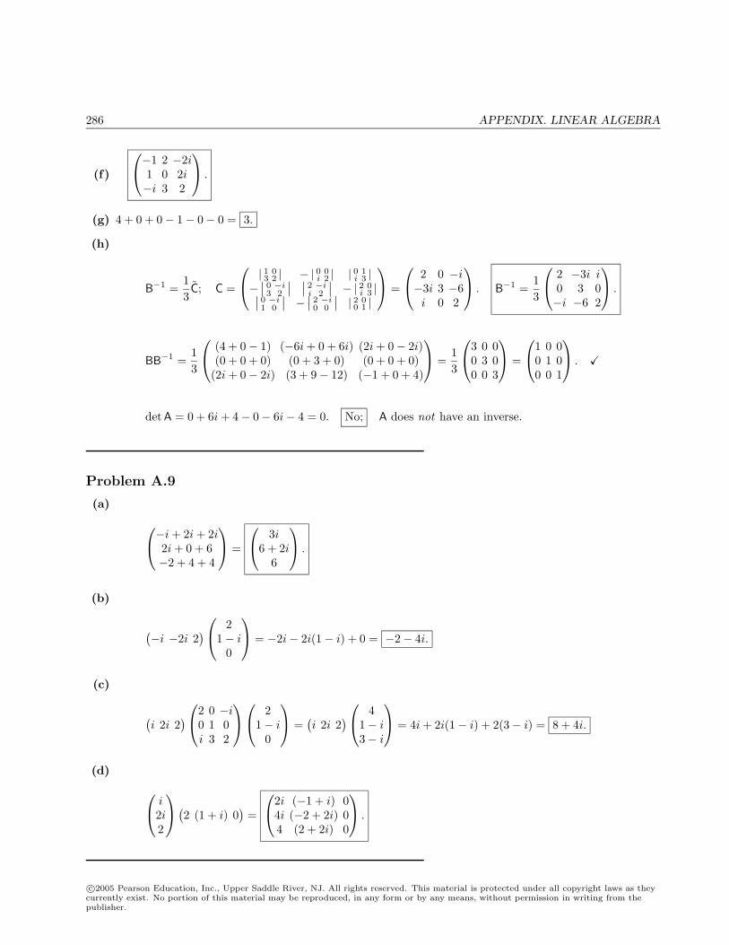
286 APPENDIX. LINEAR ALGEBRA
(f)
−1 2 −2i1 0 2i−i 3 2
.
(g) 4 + 0 + 0− 1− 0− 0 = 3.
(h)
B−1 =13C; C =
| 1 03 2 | − | 0 0
i 2 | | 0 1i 3 |
−∣∣ 0 −i3 2
∣∣ ∣∣ 2 −ii 2
∣∣ − | 2 0i 3 |∣∣ 0 −i
1 0
∣∣ −∣∣ 2 −i0 0
∣∣ | 2 00 1 |
=
2 0 −i−3i 3 −6i 0 2
. B−1 =13
2 −3i i0 3 0−i −6 2
.
BB−1 =13
(4 + 0− 1) (−6i + 0 + 6i) (2i + 0− 2i)(0 + 0 + 0) (0 + 3 + 0) (0 + 0 + 0)
(2i + 0− 2i) (3 + 9− 12) (−1 + 0 + 4)
=13
3 0 00 3 00 0 3
=
1 0 00 1 00 0 1
.
det A = 0 + 6i + 4− 0− 6i− 4 = 0. No; A does not have an inverse.
Problem A.9
(a) −i + 2i + 2i2i + 0 + 6−2 + 4 + 4
=
3i6 + 2i
6
.
(b)
(−i −2i 2
) 21− i
0
= −2i− 2i(1− i) + 0 = −2− 4i.
(c)
(i 2i 2
) 2 0 −i0 1 0i 3 2
21− i
0
=(i 2i 2
) 41− i3− i
= 4i + 2i(1− i) + 2(3− i) = 8 + 4i.
(d) i2i2
(2 (1 + i) 0
)=
2i (−1 + i) 04i (−2 + 2i) 04 (2 + 2i) 0
.
c©2005 Pearson Education, Inc., Upper Saddle River, NJ. All rights reserved. This material is protected under all copyright laws as theycurrently exist. No portion of this material may be reproduced, in any form or by any means, without permission in writing from thepublisher.
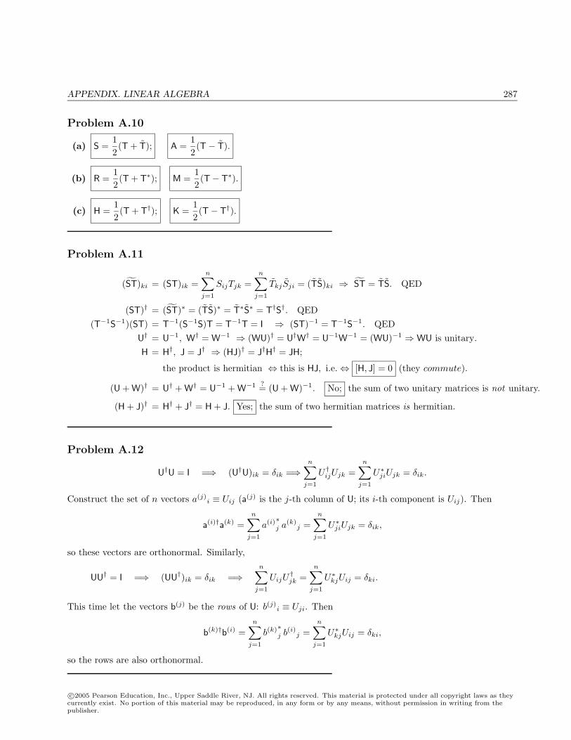
APPENDIX. LINEAR ALGEBRA 287
Problem A.10
(a) S =12(T + T); A =
12(T− T).
(b) R =12(T + T∗); M =
12(T− T∗).
(c) H =12(T + T†); K =
12(T− T†).
Problem A.11
(ST)ki = (ST)ik =n∑
j=1
SijTjk =n∑
j=1
TkjSji = (TS)ki ⇒ ST = TS. QED
(ST)† = (ST)∗ = (TS)∗ = T∗S∗ = T†S†. QED(T−1S−1)(ST) = T−1(S−1S)T = T−1T = I ⇒ (ST)−1 = T−1S−1. QED
U† = U−1, W† = W−1 ⇒ (WU)† = U†W† = U−1W−1 = (WU)−1 ⇒WU is unitary.H = H†, J = J† ⇒ (HJ)† = J†H† = JH;
the product is hermitian ⇔ this is HJ, i.e.⇔ [H, J] = 0 (they commute).
(U + W)† = U† + W† = U−1 + W−1 ?= (U + W)−1. No; the sum of two unitary matrices is not unitary.
(H + J)† = H† + J† = H + J. Yes; the sum of two hermitian matrices is hermitian.
Problem A.12
U†U = I =⇒ (U†U)ik = δik =⇒n∑
j=1
U†ijUjk =n∑
j=1
U∗jiUjk = δik.
Construct the set of n vectors a(j)i ≡ Uij (a(j) is the j-th column of U; its i-th component is Uij). Then
a(i)†a(k) =n∑
j=1
a(i)∗j a(k)
j =n∑
j=1
U∗jiUjk = δik,
so these vectors are orthonormal. Similarly,
UU† = I =⇒ (UU†)ik = δik =⇒n∑
j=1
UijU†jk =
n∑j=1
U∗kjUij = δki.
This time let the vectors b(j) be the rows of U: b(j)i ≡ Uji. Then
b(k)†b(i) =n∑
j=1
b(k)∗j b(i)j =
n∑j=1
U∗kjUij = δki,
so the rows are also orthonormal.
c©2005 Pearson Education, Inc., Upper Saddle River, NJ. All rights reserved. This material is protected under all copyright laws as theycurrently exist. No portion of this material may be reproduced, in any form or by any means, without permission in writing from thepublisher.
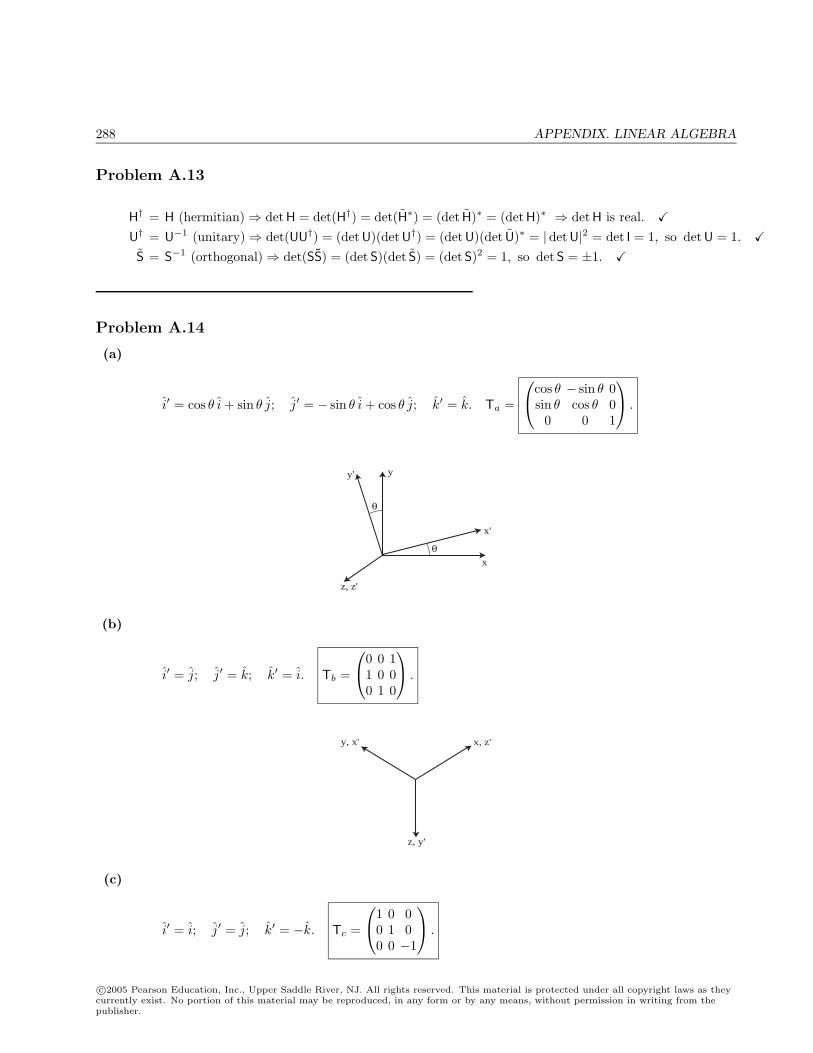
288 APPENDIX. LINEAR ALGEBRA
Problem A.13
H† = H (hermitian)⇒ detH = det(H†) = det(H∗) = (det H)∗ = (detH)∗ ⇒ det H is real. U† = U−1 (unitary)⇒ det(UU†) = (detU)(detU†) = (detU)(det U)∗ = |detU|2 = det I = 1, so det U = 1. S = S−1 (orthogonal)⇒ det(SS) = (detS)(det S) = (detS)2 = 1, so det S = ±1.
Problem A.14
(a)
i′ = cos θ i + sin θ j; j′ = − sin θ i + cos θ j; k′ = k. Ta =
cos θ − sin θ 0sin θ cos θ 0
0 0 1
.
x
z, z'
x'
yy'
θ
θ
(b)
i′ = j; j′ = k; k′ = i. Tb =
0 0 11 0 00 1 0
.
x, z'
z, y'
y, x'
(c)
i′ = i; j′ = j; k′ = −k. Tc =
1 0 00 1 00 0 −1
.
c©2005 Pearson Education, Inc., Upper Saddle River, NJ. All rights reserved. This material is protected under all copyright laws as theycurrently exist. No portion of this material may be reproduced, in any form or by any means, without permission in writing from thepublisher.
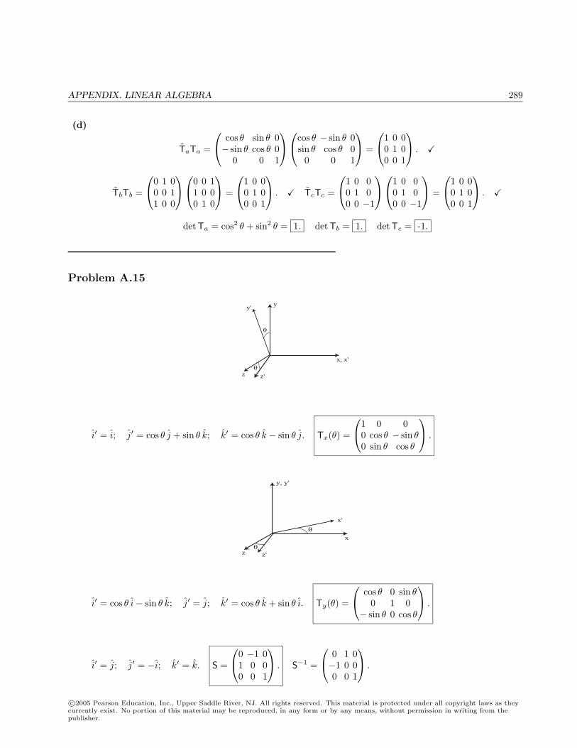
APPENDIX. LINEAR ALGEBRA 289
(d)
TaTa =
cos θ sin θ 0− sin θ cos θ 0
0 0 1
cos θ − sin θ 0sin θ cos θ 0
0 0 1
=
1 0 00 1 00 0 1
.
TbTb =
0 1 00 0 11 0 0
0 0 11 0 00 1 0
=
1 0 00 1 00 0 1
. TcTc =
1 0 00 1 00 0 −1
1 0 00 1 00 0 −1
=
1 0 00 1 00 0 1
.
detTa = cos2 θ + sin2 θ = 1. det Tb = 1. detTc = -1.
Problem A.15
x, x'
z
y
θ
θz'
y'
i′ = i; j′ = cos θ j + sin θ k; k′ = cos θ k − sin θ j. Tx(θ) =
1 0 00 cos θ − sin θ0 sin θ cos θ
.
x
z
x'
y, y'
θ
θz'
i′ = cos θ i− sin θ k; j′ = j; k′ = cos θ k + sin θ i. Ty(θ) =
cos θ 0 sin θ0 1 0
− sin θ 0 cos θ
.
i′ = j; j′ = −i; k′ = k. S =
0 −1 01 0 00 0 1
. S−1 =
0 1 0−1 0 00 0 1
.
c©2005 Pearson Education, Inc., Upper Saddle River, NJ. All rights reserved. This material is protected under all copyright laws as theycurrently exist. No portion of this material may be reproduced, in any form or by any means, without permission in writing from thepublisher.
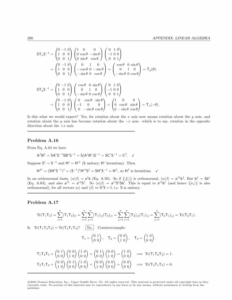
290 APPENDIX. LINEAR ALGEBRA
STxS−1 =
0 −1 01 0 00 0 1
1 0 00 cos θ − sin θ0 sin θ cos θ
0 1 0−1 0 00 0 1
=
0 −1 01 0 00 0 1
0 1 0− cos θ 0 − sin θ− sin θ 0 cos θ
=
cos θ 0 sin θ0 1 0
− sin θ 0 cos θ
= Ty(θ).
STyS−1 =
0 −1 01 0 00 0 1
cos θ 0 sin θ0 1 0
− sin θ 0 cos θ
0 1 0−1 0 00 0 1
=
0 −1 01 0 00 0 1
0 cos θ sin θ−1 0 00 − sin θ cos θ
=
1 0 00 cos θ sin θ0 − sin θ cos θ
= Tx(−θ).
Is this what we would expect? Yes, for rotation about the x axis now means rotation about the y axis, androtation about the y axis has become rotation about the −x axis—which is to say, rotation in the oppositedirection about the +x axis.
Problem A.16
From Eq. A.64 we have
AfBf = SAeS−1SBeS−1 = S(AeBe)S−1 = SCeS−1 = Cf .
Suppose S† = S−1 and He = He† (S unitary, He hermitian). Then
Hf† = (SHeS−1)† = (S−1)†He†S† = SHeS−1 = Hf , so Hf is hermitian.
In an orthonormal basis, 〈α|β〉 = a†b (Eq. A.50). So if |fi〉 is orthonormal, 〈α|β〉 = af†bf . But bf = Sbe
(Eq. A.63), and also af† = ae†S†. So 〈α|β〉 = ae†S†Sbe. This is equal to ae†be (and hence |ei〉 is alsoorthonormal), for all vectors |α〉 and |β〉 ⇔ S†S = I, i.e. S is unitary.
Problem A.17
Tr(T1T2) =n∑
i=1
(T1T2)ii =n∑
i=1
n∑j=1
(T1)ij(T2)ji =n∑
j=1
n∑i=1
(T2)ji(T1)ij =n∑
j=1
(T2T1)jj = Tr(T2T1).
Is Tr(T1T2T3) = Tr(T2T1T3)? No. Counterexample:
T1 =(
0 10 0
), T2 =
(0 01 0
), T3 =
(1 00 0
).
T1T2T3 =(
0 10 0
) (0 01 0
) (1 00 0
)=
(0 10 0
) (0 01 0
)=
(1 00 0
)=⇒ Tr(T1T2T3) = 1.
T2T1T3 =(
0 01 0
) (0 10 0
) (1 00 0
)=
(0 01 0
) (0 00 0
)=
(0 00 0
)=⇒ Tr(T2T1T3) = 0.
c©2005 Pearson Education, Inc., Upper Saddle River, NJ. All rights reserved. This material is protected under all copyright laws as theycurrently exist. No portion of this material may be reproduced, in any form or by any means, without permission in writing from thepublisher.
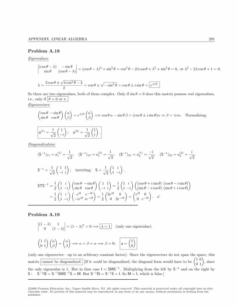
APPENDIX. LINEAR ALGEBRA 291
Problem A.18
Eigenvalues:∣∣∣∣(cos θ − λ) − sin θsin θ (cos θ − λ)
∣∣∣∣ = (cos θ − λ)2 + sin2 θ = cos2 θ − 2λ cos θ + λ2 + sin2 θ = 0, or λ2 − 2λ cos θ + 1 = 0.
λ =2 cos θ ±
√4 cos2 θ − 42
= cos θ ±√− sin2 θ = cos θ ± i sin θ = e±iθ.
So there are two eigenvalues, both of them complex. Only if sin θ = 0 does this matrix possess real eigenvalues,i.e., only if θ = 0 or π.
Eigenvectors:(cos θ − sin θsin θ cos θ
) (αβ
)= e±iθ
(αβ
)=⇒ cos θ α− sin θ β = (cos θ ± i sin θ)α⇒ β = ∓iα. Normalizing:
a(1) =1√2
(1−i
); a(2) =
1√2
(1i
).
Diagonalization:
(S−1)11 = a(1)1 =
1√2; (S−1)12 = a
(2)1 =
1√2; (S−1)21 = a
(1)2 =
−i√2; (S−1)22 = a
(2)2 =
i√2.
S−1 =1√2
(1 1−i i
); inverting: S =
1√2
(1 i1 −i
).
STS−1 =12
(1 i1 −i
) (cos θ − sin θsin θ cos θ
) (1 1−i i
)=
12
(1 i1 −i
) ((cos θ + i sin θ) (cos θ − i sin θ)(sin θ − i cos θ) (sin θ + i cos θ)
)=
12
(1 i1 −i
) (eiθ e−iθ
−ieiθ ie−iθ
)=
12
(2eiθ 00 2e−iθ
)=
(eiθ 00 e−iθ
).
Problem A.19∣∣∣∣(1− λ) 10 (1− λ)
∣∣∣∣ = (1− λ)2 = 0 =⇒ λ = 1 (only one eigenvalue).
(1 10 1
) (αβ
)=
(αβ
)=⇒ α + β = α =⇒ β = 0; a =
(10
)(only one eigenvector—up to an arbitrary constant factor). Since the eigenvectors do not span the space, this
matrix cannot be diagonalized. [If it could be diagonalized, the diagonal form would have to be(
1 00 1
), since
the only eigenvalue is 1. But in that case I = SMS−1. Multiplying from the left by S−1 and on the right byS : S−1IS = S−1SMS−1S = M. But S−1IS = S−1S = I. So M = I, which is false.]
c©2005 Pearson Education, Inc., Upper Saddle River, NJ. All rights reserved. This material is protected under all copyright laws as theycurrently exist. No portion of this material may be reproduced, in any form or by any means, without permission in writing from thepublisher.
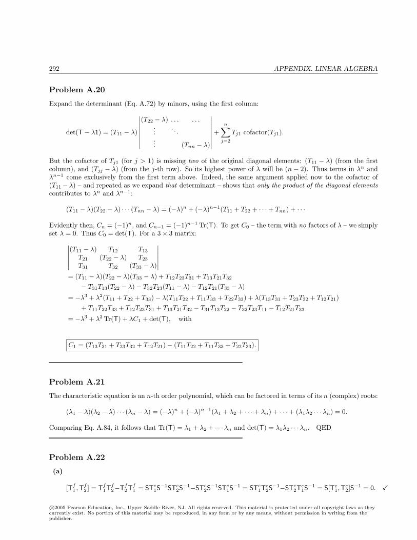
292 APPENDIX. LINEAR ALGEBRA
Problem A.20
Expand the determinant (Eq. A.72) by minors, using the first column:
det(T− λ1) = (T11 − λ)
∣∣∣∣∣∣∣∣(T22 − λ) . . . . . .
.... . .
... (Tnn − λ)
∣∣∣∣∣∣∣∣ +n∑
j=2
Tj1 cofactor(Tj1).
But the cofactor of Tj1 (for j > 1) is missing two of the original diagonal elements: (T11 − λ) (from the firstcolumn), and (Tjj − λ) (from the j-th row). So its highest power of λ will be (n − 2). Thus terms in λn andλn−1 come exclusively from the first term above. Indeed, the same argument applied now to the cofactor of(T11−λ) – and repeated as we expand that determinant – shows that only the product of the diagonal elementscontributes to λn and λn−1:
(T11 − λ)(T22 − λ) · · · (Tnn − λ) = (−λ)n + (−λ)n−1(T11 + T22 + · · ·+ Tnn) + · · ·
Evidently then, Cn = (−1)n, and Cn−1 = (−1)n−1 Tr(T). To get C0 – the term with no factors of λ – we simplyset λ = 0. Thus C0 = det(T). For a 3× 3 matrix:∣∣∣∣∣∣
(T11 − λ) T12 T13
T21 (T22 − λ) T23
T31 T32 (T33 − λ)
∣∣∣∣∣∣= (T11 − λ)(T22 − λ)(T33 − λ) + T12T23T31 + T13T21T32
− T31T13(T22 − λ)− T32T23(T11 − λ)− T12T21(T33 − λ)
= −λ3 + λ2(T11 + T22 + T33)− λ(T11T22 + T11T33 + T22T33) + λ(T13T31 + T23T32 + T12T21)+ T11T22T33 + T12T23T31 + T13T21T32 − T31T13T22 − T32T23T11 − T12T21T33
= −λ3 + λ2 Tr(T) + λC1 + det(T), with
C1 = (T13T31 + T23T32 + T12T21)− (T11T22 + T11T33 + T22T33).
Problem A.21
The characteristic equation is an n-th order polynomial, which can be factored in terms of its n (complex) roots:
(λ1 − λ)(λ2 − λ) · · · (λn − λ) = (−λ)n + (−λ)n−1(λ1 + λ2 + · · ·+ λn) + · · ·+ (λ1λ2 · · ·λn) = 0.
Comparing Eq. A.84, it follows that Tr(T) = λ1 + λ2 + · · ·λn and det(T) = λ1λ2 · · ·λn. QED
Problem A.22
(a)
[Tf1 ,T
f2 ] = Tf
1Tf2−Tf
2Tf1 = STe
1S−1STe
2S−1−STe
2S−1STe
1S−1 = STe
1Te2S−1−STe
2Te1S−1 = S[Te
1,Te2]S−1 = 0.
c©2005 Pearson Education, Inc., Upper Saddle River, NJ. All rights reserved. This material is protected under all copyright laws as theycurrently exist. No portion of this material may be reproduced, in any form or by any means, without permission in writing from thepublisher.
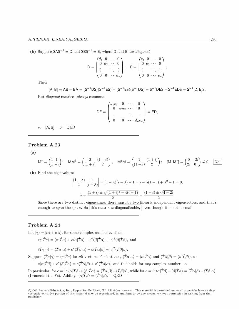
APPENDIX. LINEAR ALGEBRA 293
(b) Suppose SAS−1 = D and SBS−1 = E, where D and E are diagonal:
D =
d1 0 · · · 00 d2 · · · 0...
. . ....
0 0 · · · dn
, E =
e1 0 · · · 00 e2 · · · 0...
. . ....
0 0 · · · en
.
Then
[A,B] = AB− BA = (S−1DS)(S−1ES)− (S−1ES)(S−1DS) = S−1DES− S−1EDS = S−1[D,E]S.
But diagonal matrices always commute:
DE =
d1e1 0 · · · 0
0 d2e2 · · · 0...
. . ....
0 0 · · · dnen
= ED,
so [A,B] = 0. QED
Problem A.23
(a)
M† =(
1 11 −i
); MM† =
(2 (1− i)
(1 + i) 2
), M†M =
(2 (1 + i)
(1− i) 2
); [M,M†] =
(0 −2i2i 0
)= 0. No.
(b) Find the eigenvalues:∣∣∣∣(1− λ) 11 (i− λ)
∣∣∣∣ = (1− λ)(i− λ)− 1 = i− λ(1 + i) + λ2 − 1 = 0;
λ =(1 + i)±
√(1 + i)2 − 4(i− 1)
2=
(1 + i)±√
4− 2i2
.
Since there are two distinct eigenvalues, there must be two linearly independent eigenvectors, and that’senough to span the space. So this matrix is diagonalizable, even though it is not normal.
Problem A.24
Let |γ〉 = |α〉+ c|β〉, for some complex number c. Then
〈γ|T γ〉 = 〈α|Tα〉+ c〈α|T β〉+ c∗〈β|Tα〉+ |c|2〈β|T β〉, and
〈T γ|γ〉 = 〈Tα|α〉+ c∗〈T β|α〉+ c〈Tα|β〉+ |c|2〈T β|β〉.Suppose 〈T γ|γ〉 = 〈γ|T γ〉 for all vectors. For instance, 〈Tα|α〉 = 〈α|Tα〉 and 〈T β|β〉 = 〈β|T β〉), so
c〈α|T β〉+ c∗〈β|Tα〉 = c〈Tα|β〉+ c∗〈T β|α〉, and this holds for any complex number c.
In particular, for c = 1: 〈α|T β〉+〈β|Tα〉 = 〈Tα|β〉+〈T β|α〉, while for c = i: 〈α|T β〉−〈β|Tα〉 = 〈Tα|β〉−〈T β|α〉.(I canceled the i’s). Adding: 〈α|T β〉 = 〈Tα|β〉. QED
c©2005 Pearson Education, Inc., Upper Saddle River, NJ. All rights reserved. This material is protected under all copyright laws as theycurrently exist. No portion of this material may be reproduced, in any form or by any means, without permission in writing from thepublisher.
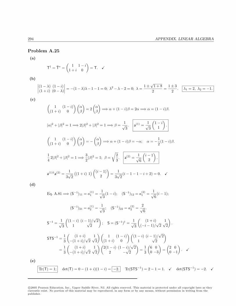
294 APPENDIX. LINEAR ALGEBRA
Problem A.25
(a)
T† = T∗ =(
1 1− i1 + i 0
)= T.
(b) ∣∣∣∣(1− λ) (1− i)(1 + i) (0− λ)
∣∣∣∣ = −(1−λ)λ− 1− 1 = 0; λ2−λ− 2 = 0; λ =1±
√1 + 8
2=
1± 32
. λ1 = 2, λ2 = −1.
(c) (1 (1− i)
(1 + i) 0
) (αβ
)= 2
(αβ
)=⇒ α + (1− i)β = 2α =⇒ α = (1− i)β.
|α|2 + |β|2 = 1 =⇒ 2|β|2 + |β|2 = 1 =⇒ β =1√3. a(1) =
1√3
(1− i
1
).
(1 (1− i)
(1 + i) 0
) (αβ
)= −
(αβ
)=⇒ α + (1− i)β = −α; α = −1
2(1− i)β.
14
2|β|2 + |β|2 = 1 =⇒ 32|β|2 = 1; β =
√23. a(2) =
1√6
(i− 1
2
).
a(1)†a(2) =1
3√
2
((1 + i) 1
) ((i− 1)
2
)=
13√
2(i− 1− 1− i + 2) = 0.
(d)
Eq. A.81 =⇒ (S−1)11 = a(1)1 =
1√3(1− i); (S−1)12 = a
(2)1 =
1√6(i− 1);
(S−1)21 = a(1)2 =
1√3; (S−1)22 = a
(2)2 =
2√6.
S−1 =1√3
((1− i) (i− 1)/
√2
1√
2
); S = (S−1)† =
1√3
((1 + i) 1
(−i− 1)/√
2√
2
).
STS−1 =13
((1 + i) 1
−(1 + i)/√
2√
2
) (1 (1− i)
(1 + i) 0
) ((1− i) (i− 1)/
√2
1√
2
)=
13
((1 + i) 1
−(1 + i)/√
2√
2
) (2(1− i) (1− i)/
√2
2 −√
2
)=
13
(6 00 −3
)=
(2 00 −1
).
(e)
Tr(T) = 1; det(T) = 0− (1 + i)(1− i) = −2. Tr(STS−1) = 2− 1 = 1. det(STS−1) = −2.
c©2005 Pearson Education, Inc., Upper Saddle River, NJ. All rights reserved. This material is protected under all copyright laws as theycurrently exist. No portion of this material may be reproduced, in any form or by any means, without permission in writing from thepublisher.
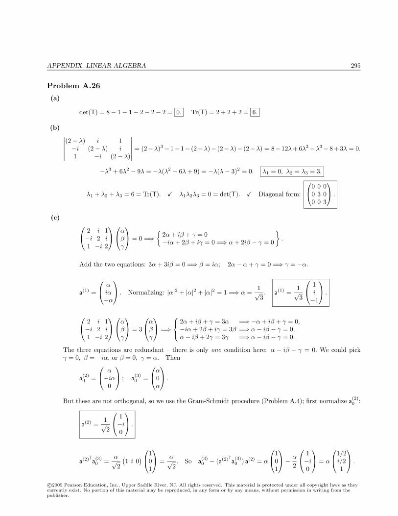
APPENDIX. LINEAR ALGEBRA 295
Problem A.26
(a)
det(T) = 8− 1− 1− 2− 2− 2 = 0. Tr(T) = 2 + 2 + 2 = 6.
(b) ∣∣∣∣∣∣(2− λ) i 1−i (2− λ) i1 −i (2− λ)
∣∣∣∣∣∣ = (2−λ)3− 1− 1− (2−λ)− (2−λ)− (2−λ) = 8− 12λ+6λ2−λ3− 8+3λ = 0.
−λ3 + 6λ2 − 9λ = −λ(λ2 − 6λ + 9) = −λ(λ− 3)2 = 0. λ1 = 0, λ2 = λ3 = 3.
λ1 + λ2 + λ3 = 6 = Tr(T). λ1λ2λ3 = 0 = det(T). Diagonal form:
0 0 00 3 00 0 3
.
(c) 2 i 1−i 2 i1 −i 2
αβγ
= 0 =⇒
2α + iβ + γ = 0−iα + 2β + iγ = 0 =⇒ α + 2iβ − γ = 0
.
Add the two equations: 3α + 3iβ = 0 =⇒ β = iα; 2α− α + γ = 0 =⇒ γ = −α.
a(1) =
αiα−α
. Normalizing: |α|2 + |α|2 + |α|2 = 1 =⇒ α =1√3. a(1) =
1√3
1i−1
.
2 i 1−i 2 i1 −i 2
αβγ
= 3
αβγ
=⇒
2α + iβ + γ = 3α =⇒ −α + iβ + γ = 0,−iα + 2β + iγ = 3β =⇒ α− iβ − γ = 0,α− iβ + 2γ = 3γ =⇒ α− iβ − γ = 0.
The three equations are redundant – there is only one condition here: α − iβ − γ = 0. We could pickγ = 0, β = −iα, or β = 0, γ = α. Then
a(2)0 =
α−iα0
; a(3)0 =
α0α
.
But these are not orthogonal, so we use the Gram-Schmidt procedure (Problem A.4); first normalize a(2)0 :
a(2) =1√2
1−i0
.
a(2)†a(3)0 =
α√2
(1 i 0
) 101
=α√2. So a
(3)0 − (a(2)†a(3)
0 ) a(2) = α
101
− α
2
1−i0
= α
1/2i/21
.
c©2005 Pearson Education, Inc., Upper Saddle River, NJ. All rights reserved. This material is protected under all copyright laws as theycurrently exist. No portion of this material may be reproduced, in any form or by any means, without permission in writing from thepublisher.

296 APPENDIX. LINEAR ALGEBRA
Normalize: |α|2(
14
+14
+ 1)
=32|α|2 = 1 =⇒ α =
√23. a(3) =
1√6
1i2
.
Check orthogonality:
a(1)†a(2) =1√6
(1 −i −1
) 1−i0
=1√6(1− 1 + 0) = 0.
a(1)†a(3) =1
3√
2
(1 −i −1
) 1i2
=1
3√
2(1 + 1− 2) = 0.
(d) S−1 is the matrix whose columns are the eigenvectors of T (Eq. A.81):
S−1 =1√6
√
2√
3 1√2 i −
√3 i i
−√
2 0 2
; S = (S−1)† =1√6
√2 −√
2 i −√
2√3√
3 i 01 −i 2
.
STS−1 =16
√2 −√
2 i −√
2√3√
3 i 01 −i 2
2 i 1−i 2 i1 −i 2
√
2√
3 1√2 i −
√3 i i
−√
2 0 2
︸ ︷︷ ︸
0 3
√3 3
0 −3√
3 i 3i0 0 6
=16
0 0 00 18 00 0 18
=
0 0 00 3 00 0 3
.
Problem A.27
(a) 〈Uα|Uβ〉 = 〈U†Uα|β〉 = 〈α|β〉.
(b) U |α〉 = λ|α〉 =⇒ 〈Uα|Uα〉 = |λ|2〈α|α〉. But from (a) this is also 〈α|α〉. So |λ| = 1.
(c) U |α〉 = λ|α〉, U |β〉 = µ|β〉 =⇒ |β〉 = µU−1|β〉, so U†|β〉 =1µ|β〉 = µ∗|β〉 (from (b)).
〈β|Uα〉 = λ〈β|α〉 = 〈U†β|α〉 = µ〈β|α〉, or (λ− µ)〈β|α〉 = 0. So if λ = µ, then 〈β|α〉 = 0. QED
Problem A.28
(a) (i)
M2 =
0 0 40 0 00 0 0
; M3 =
0 0 00 0 00 0 0
, so
c©2005 Pearson Education, Inc., Upper Saddle River, NJ. All rights reserved. This material is protected under all copyright laws as theycurrently exist. No portion of this material may be reproduced, in any form or by any means, without permission in writing from thepublisher.
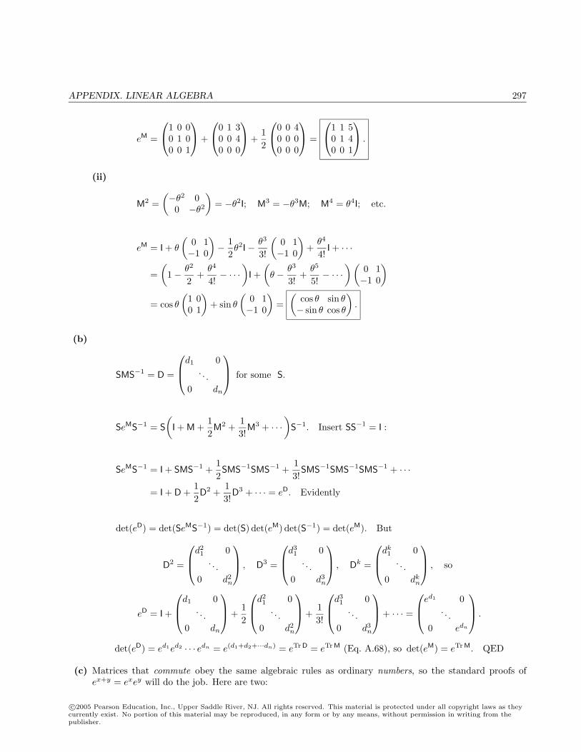
APPENDIX. LINEAR ALGEBRA 297
eM =
1 0 00 1 00 0 1
+
0 1 30 0 40 0 0
+12
0 0 40 0 00 0 0
=
1 1 50 1 40 0 1
.
(ii)
M2 =(−θ2 00 −θ2
)= −θ2I; M3 = −θ3M; M4 = θ4I; etc.
eM = I + θ
(0 1−1 0
)− 1
2θ2I− θ3
3!
(0 1−1 0
)+
θ4
4!I + · · ·
=(
1− θ2
2+
θ4
4!− · · ·
)I +
(θ − θ3
3!+
θ5
5!− · · ·
) (0 1−1 0
)= cos θ
(1 00 1
)+ sin θ
(0 1−1 0
)=
(cos θ sin θ− sin θ cos θ
).
(b)
SMS−1 = D =
d1 0. . .
0 dn
for some S.
SeMS−1 = S
(I + M +
12M2 +
13!
M3 + · · ·)
S−1. Insert SS−1 = I :
SeMS−1 = I + SMS−1 +12SMS−1SMS−1 +
13!
SMS−1SMS−1SMS−1 + · · ·
= I + D +12D2 +
13!
D3 + · · · = eD. Evidently
det(eD) = det(SeMS−1) = det(S) det(eM) det(S−1) = det(eM). But
D2 =
d21 0
. . .0 d2
n
, D3 =
d31 0
. . .0 d3
n
, Dk =
dk1 0
. . .0 dk
n
, so
eD = I +
d1 0. . .
0 dn
+12
d21 0
. . .0 d2
n
+13!
d31 0
. . .0 d3
n
+ · · · =
ed1 0. . .
0 edn
.
det(eD) = ed1ed2 · · · edn = e(d1+d2+···dn) = eTr D = eTr M (Eq. A.68), so det(eM) = eTr M. QED
(c) Matrices that commute obey the same algebraic rules as ordinary numbers, so the standard proofs ofex+y = exey will do the job. Here are two:
c©2005 Pearson Education, Inc., Upper Saddle River, NJ. All rights reserved. This material is protected under all copyright laws as theycurrently exist. No portion of this material may be reproduced, in any form or by any means, without permission in writing from thepublisher.
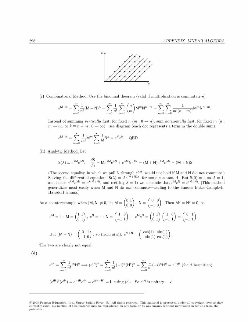
298 APPENDIX. LINEAR ALGEBRA
n
m
(i) Combinatorial Method: Use the binomial theorem (valid if multiplication is commutative):
eM+N =∞∑
n=0
1n!
(M + N)n =∞∑
n=0
1n!
n∑m=0
(n
m
)MmNn−m =
∞∑n=0
n∑m=0
1m!(n−m)!
MmNn−m.
Instead of summing vertically first, for fixed n (m : 0 → n), sum horizontally first, for fixed m (n :m→∞, or k ≡ n−m : 0→∞)—see diagram (each dot represents a term in the double sum).
eM+N =∞∑
m=0
1m!
Mm∞∑
k=0
1k!
Nk = eMeN. QED
(ii) Analytic Method: Let
S(λ) ≡ eλMeλN;dS
dλ= MeλMeλN + eλMNeλN = (M + N)eλMeλN = (M + N)S.
(The second equality, in which we pull N through eλM, would not hold if M and N did not commute.)Solving the differential equation: S(λ) = Ae(M+N)λ, for some constant A. But S(0) = I, so A = 1,and hence eλMeλN = eλ(M+N), and (setting λ = 1) we conclude that eMeN = e(M+N). [This methodgeneralizes most easily when M and N do not commute—leading to the famous Baker-Campbell-Hausdorf lemma.]
As a counterexample when [M,N] = 0, let M =(
0 10 0
), N =
(0 0−1 0
). Then M2 = N2 = 0, so
eM = I + M =(
1 10 1
), eN = I + N =
(1 0−1 1
); eMeN =
(1 10 1
) (1 0−1 1
)=
(0 1−1 1
).
But (M + N) =(
0 1−1 0
), so (from a(ii)): eM+N =
(cos(1) sin(1)− sin(1) cos(1)
).
The two are clearly not equal.
(d)
eiH =∞∑
n=0
1n!
inHn =⇒ (eiH)† =∞∑
n=0
1n!
(−i)n(H†)n =∞∑
n=0
1n!
(−i)nHn = e−iH (for H hermitian).
(eiH)†(eiH) = e−iHeiH = ei(H−H) = I, using (c). So eiH is unitary.
c©2005 Pearson Education, Inc., Upper Saddle River, NJ. All rights reserved. This material is protected under all copyright laws as theycurrently exist. No portion of this material may be reproduced, in any form or by any means, without permission in writing from thepublisher.

299
2nd Edition – 1st Edition Problem Correlation Grid N = New M = 1/e problem number (modified for 2/e) X = 2/e problem number (unchanged from 1/e)
Chapter 1 2/e 1/e
1 1
2N 3 6 4 7 5 8 6 11 7 12 8 13 9 14 10 2 11 3 12 4 13 5 14 9M 15 10
16N 17N 18N
Chapter 2 2/e 1/e
1 1 2 2 3 3 4 5 5 6M 6 7
7N 8N 9N 10 13M 11 14 12 37 13 17M
14N 15 15 16 16 17 18 18 19M
19N 20 20
21N 22 22 23 23 24 24
25N 26 25 27 26 28 27 29 28 30 29 31 30 32 31 33 32 34 33 35 41M 36 4M 37 36 38 3.48
39N 40N 41N 42 38 43 40 44 39
Chapter 2 (cont.) 2/e 1/e
45 42 46 43 47 44
48N 49 45 50 47 51 48M 52 34M, 35M 53 49
54N 55N 56N

300
2nd Edition – 1st Edition Problem Correlation Grid N = New M = 1/e problem number (modified for 2/e) (M) = 1/e problem number (distant model for 2/e) X = 2/e problem number (unchanged from 1/e)
Chapter 3 2/e 1/e
1N 2N (33M) 3N (21M) 4N (12M) 5N 6N 7N 8N 9N
10N 11 38 12 51 13 41M 14 39
15N 16 42 17 43 18 44 19 45 20 46 21 57M
22N 23N 24 57M 25 25M
26N 27N 28 52M
29N 30N 31 53 32 56 33 50 34 49M
35N 36N 37N 38N 39 55
40N
Chapter 4 2/e 1/e
1 1 2 2 3 3 4 4 5 5 6 6 7 7M 8 8 9 9M 10 10 11 11 12 12 13 13
14N 15N 16 17 17 16 18 19 19 20 20 21
21N 22 22 23 23 24 25 25 26 26 27 27 28 28 29 29 30 30 31M 31 32 32 33 33 34 34 35 35 36 36 37 37 38 38 39 39 40 40 41
41N 42 42
Chapter 4 (cont.) 2/e 1/e
43 43
44N 45 14 46 15
47N 48N 49N 50 44 51 45M 52 46
53N 54 47 55 48 56 49 57 50
58N 59 51 60 52M 61 53

301
2nd Edition – 1st Edition Problem Correlation Grid N = New M = 1/e problem number (modified for 2/e) X = 2/e problem number (unchanged from 1/e)
Chapter 5 2/e 1/e
1 1 2 2
3N 4 3 5 4 6 5 7 6 8 7 9 8 10 9 11 10 12 11M 13 11M 14 12
15N 16 13 17 14 18 15M 19 16M 20 17M 21 18 22 19M 23 20 24 21M 25 22 26 23 27 24 28 25 29 26 30 27M 31 28
32N 33 29 34 30 35 31 36 32 37 33
Chapter 6 2/e 1/e
1 1M 2 2 3 3 4 4 5 5 6 6 7 7 8 8 9 9
10N 11 10 12 11 13 12 14 13
15N 16 14 17 15 18 16 19 17 20 18 21 19 22 20 23 21 24 22 25 23 26 24 27 25 28 26
29N 30N 31N 32 27 33 28 34 29 35 30 36 31 37 32 38 33 39 34
40N
Chapter 7 2/e 1/e
1 1 2 2M 3 3M 4 4 5 5 6 6 7 7 8 8 9 9 10 10
11N 12N 13 11 14 12 15 13 16 14 17 15 18 16 19 17
20N
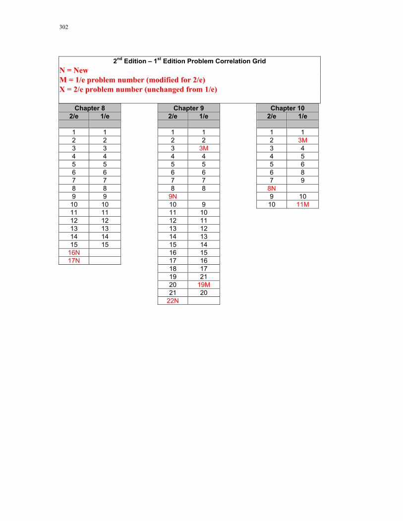
302
2nd Edition – 1st Edition Problem Correlation Grid N = New M = 1/e problem number (modified for 2/e) X = 2/e problem number (unchanged from 1/e)
Chapter 8 2/e 1/e
1 1 2 2 3 3 4 4 5 5 6 6 7 7 8 8 9 9 10 10 11 11 12 12 13 13 14 14 15 15
16N 17N
Chapter 9 2/e 1/e
1 1 2 2 3 3M 4 4 5 5 6 6 7 7 8 8
9N 10 9 11 10 12 11 13 12 14 13 15 14 16 15 17 16 18 17 19 21 20 19M 21 20
22N
Chapter 10 2/e 1/e
1 1 2 3M 3 4 4 5 5 6 6 8 7 9
8N 9 10 10 11M
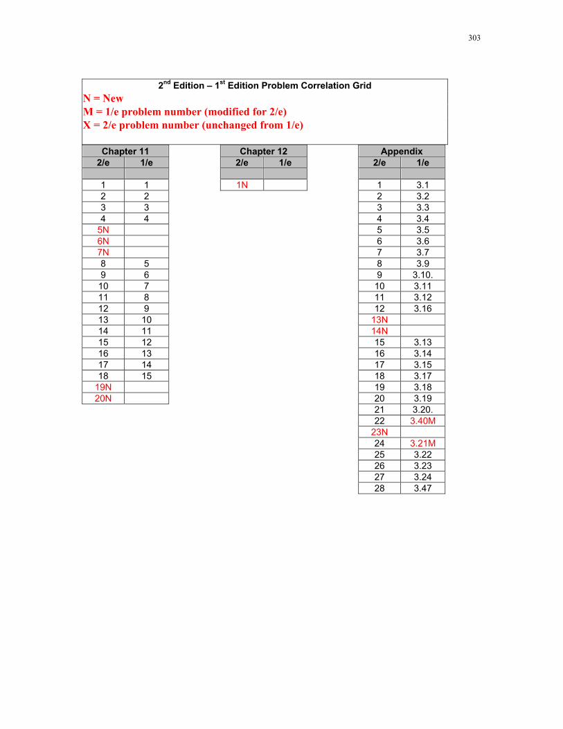
303
2nd Edition – 1st Edition Problem Correlation Grid
N = New M = 1/e problem number (modified for 2/e) X = 2/e problem number (unchanged from 1/e)
Chapter 11 2/e 1/e
1 1 2 2 3 3 4 4
5N 6N 7N 8 5 9 6 10 7 11 8 12 9 13 10 14 11 15 12 16 13 17 14 18 15
19N 20N
Chapter 12 2/e 1/e
1N
Appendix 2/e 1/e
1 3.1 2 3.2 3 3.3 4 3.4 5 3.5 6 3.6 7 3.7 8 3.9 9 3.10. 10 3.11 11 3.12 12 3.16
13N 14N 15 3.13 16 3.14 17 3.15 18 3.17 19 3.18 20 3.19 21 3.20. 22 3.40M
23N 24 3.21M 25 3.22 26 3.23 27 3.24 28 3.47