Ff tand matlab-wanjun huang

Fast Fourier Transform and MATLAB Implementation

byWanjun Huang

forforDr. Duncan L. MacFarlane

1

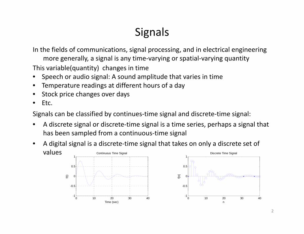
SignalsIn the fields of communications, signal processing, and in electrical engineering

more generally, a signal is any time‐varying or spatial‐varying quantityThis variable(quantity) changes in time• Speech or audio signal: A sound amplitude that varies in time• Temperature readings at different hours of a day• Stock price changes over days• Etc• Etc.

Signals can be classified by continues‐time signal and discrete‐time signal:

• A discrete signal or discrete‐time signal is a time series, perhaps a signal that h b l d f ti ti i lhas been sampled from a continuous‐time signal

• A digital signal is a discrete‐time signal that takes on only a discrete set of values

1Continuous Time Signal

1Discrete Time Signal

-0.5

0

0.5

f(t)

-0.5

0

0.5

f[n]

0 10 20 30 40-1

Time (sec)0 10 20 30 40

-1

n

2

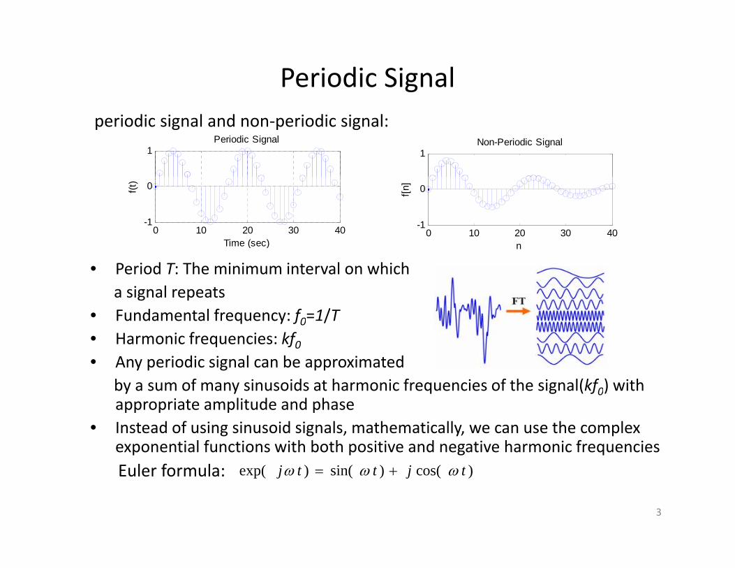
Periodic Signalperiodic signal and non‐periodic signal:

1Periodic Signal

1Non-Periodic Signal

0 10 20 30 40-1

0f(t)

Time (sec)0 10 20 30 40

-1

0f[n]

nn

• Period T: The minimum interval on which a signal repeats

• Fundamental frequency: f0=1/TFundamental frequency: f0 1/T• Harmonic frequencies: kf0• Any periodic signal can be approximated

by a sum of many sinusoids at harmonic frequencies of the signal(kf0) with y y q g ( f0)appropriate amplitude and phase

• Instead of using sinusoid signals, mathematically, we can use the complex exponential functions with both positive and negative harmonic frequencies

)cos()sin()exp( tjttj Euler formula:

3

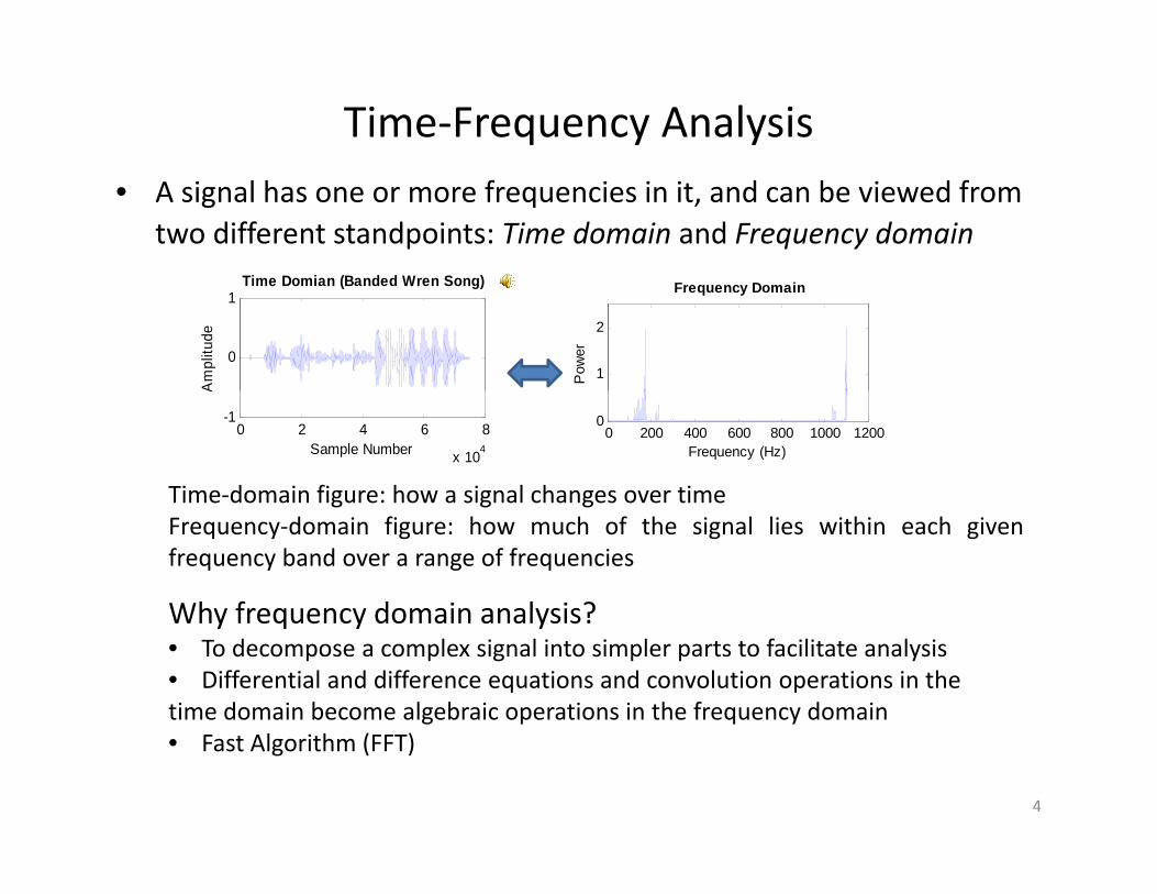
Time‐Frequency Analysis • A signal has one or more frequencies in it, and can be viewed from

two different standpoints: Time domain and Frequency domainTime Domian (Banded Wren Song)

0

1

Am

plitu

de

Time Domian (Banded Wren Song)

1

2

Pow

er

Frequency Domain

0 2 4 6 8

x 104

-1

Sample Number

A

0 200 400 600 800 1000 12000

Frequency (Hz)

Time‐domain figure: how a signal changes over time

Why frequency domain analysis?

g g gFrequency‐domain figure: how much of the signal lies within each givenfrequency band over a range of frequencies

Why frequency domain analysis?• To decompose a complex signal into simpler parts to facilitate analysis• Differential and difference equations and convolution operations in the time domain become algebraic operations in the frequency domain• Fast Algorithm (FFT)

4

Fourier TransformFourier Transform

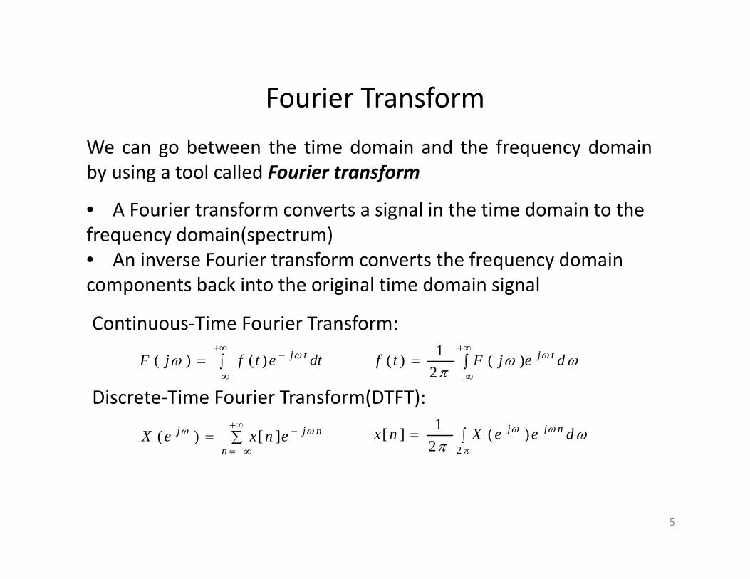
We can go between the time domain and the frequency domainby using a tool called Fourier transform

• A Fourier transform converts a signal in the time domain to the frequency domain(spectrum)

A i F i f h f d i

y g f

• An inverse Fourier transform converts the frequency domain components back into the original time domain signal

Continuous‐Time Fourier Transform:

dejFtf tj

)(

21)(

dtetfjF tj )()(

Continuous Time Fourier Transform:

Discrete‐Time Fourier Transform(DTFT):Discrete Time Fourier Transform(DTFT):

2

)(21][ deeXnx njj

n

njj enxeX ][)(

5

Fourier Representation For Four Types of SignalsFourier Representation For Four Types of Signals

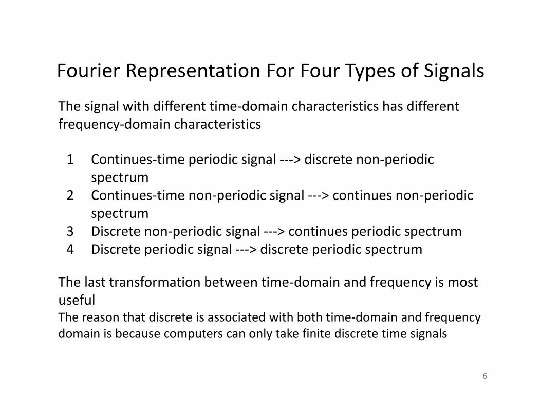
The signal with different time‐domain characteristics has different frequency‐domain characteristics

1 Continues‐time periodic signal ‐‐‐> discrete non‐periodic spectrum

q y

p2 Continues‐time non‐periodic signal ‐‐‐> continues non‐periodic

spectrum3 Discrete non‐periodic signal ‐‐‐> continues periodic spectrum3 Discrete non periodic signal > continues periodic spectrum4 Discrete periodic signal ‐‐‐> discrete periodic spectrum

The last transformation between time‐domain and frequency is most q yusefulThe reason that discrete is associated with both time‐domain and frequency domain is because computers can only take finite discrete time signalsp y g

6

Periodic SequencePeriodic Sequence

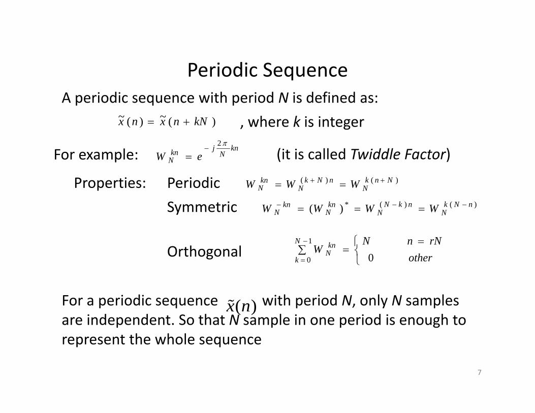
)(~)(~ kNnxnx , where k is integer

A periodic sequence with period N is defined as:

Periodic

, g

knN

jknN eW

2

For example:)()( NnknNkkn WWW

(it is called Twiddle Factor)

Properties: Periodic )()( NnkN

nNkN

knN WWW

Symmetric )()(*)( nNkN

nkNN

knN

knN WWWW

Properties:

Orthogonal

otherrNnN

WN

k

knN 0

1

0

For a periodic sequence with period N, only N samples are independent. So that N sample in one period is enough to represent the whole sequence

x(n)

represent the whole sequence

7

Discrete Fourier Series(DFS)Discrete Fourier Series(DFS)

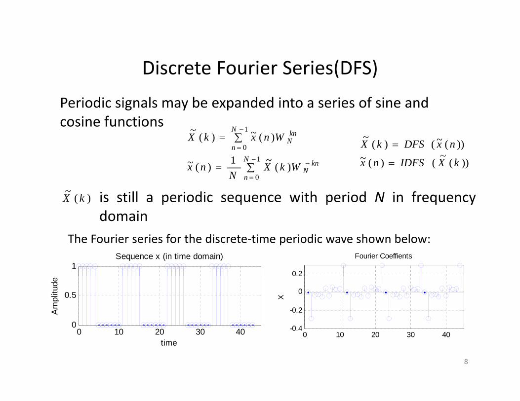
Periodic signals may be expanded into a series of sine and cosine functions

1

0

1

0

)(~1)(~

)(~)(~

N knN

N

n

knN

WkXN

nx

WnxkXcosine functions

))(~()(~))(~()(~

kXIDFSnx

nxDFSkX

0nN

is still a periodic sequence with period N in frequencydomain

)(~ kX

The Fourier series for the discrete‐time periodic wave shown below:

1Sequence x (in time domain)

0.2

Fourier Coeffients

0

0.5

Am

plitu

de

0 4

-0.2

0X

0 10 20 30 400

time0 10 20 30 40

-0.4

8

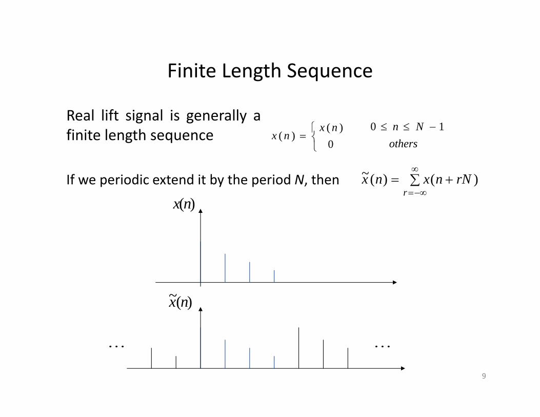
Finite Length SequenceFinite Length Sequence

)(nx Nn 10 Real lift signal is generally afi i l h

If we periodic extend it by the period N then

rNnxnx )()(~

0

)()(

nxnx

othersNn 10

finite length sequence

If we periodic extend it by the period N, then r

rNnxnx )()(

)(nx

)(~ nx

9

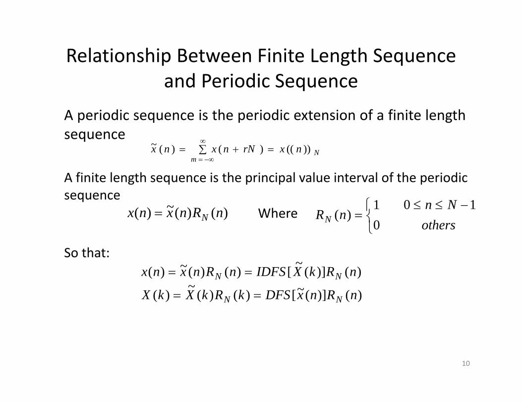
Relationship Between Finite Length Sequence d P i di Sand Periodic Sequence

A periodic sequence is the periodic extension of a finite length

A finite length sequence is the principal value interval of the periodic

sequence

mNnxrNnxnx ))(()()(~

A finite length sequence is the principal value interval of the periodic sequence

)()(~)( nRnxnx N

01

)(nRN othersNn 10

Where 0 others

So that: )()](~[)()(~)( nRkXIDFSnRnxnx NN

)()](~[)()(~)(

)()]([)()()(

nRnxDFSkRkXkX NN

NN

10

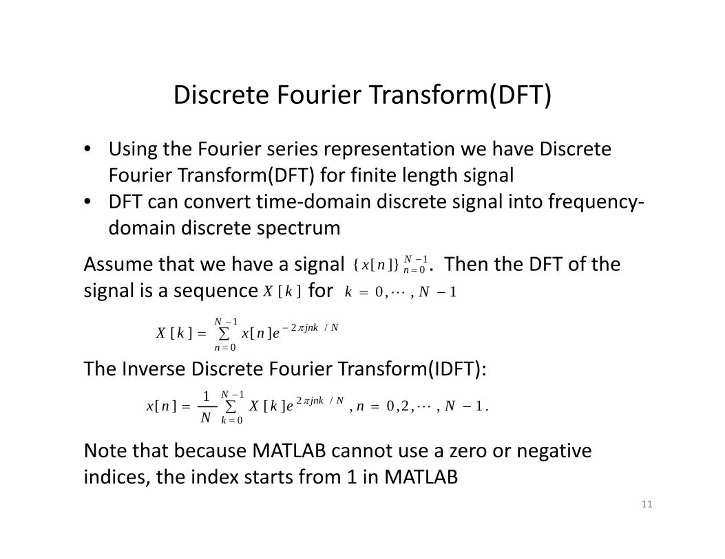
Discrete Fourier Transform(DFT)Discrete Fourier Transform(DFT)

• Using the Fourier series representation we have Discrete Fourier Transform(DFT) for finite length signalFourier Transform(DFT) for finite length signal

• DFT can convert time‐domain discrete signal into frequency‐domain discrete spectrum

Assume that we have a signal . Then the DFT of the signal is a sequence for

10]}[{

Nnnx

][ kX 1,,0 Nk

1

0

/2][][N

n

NjnkenxkX

The Inverse Discrete Fourier Transform(IDFT):

1

0

/2 .1,,2,0,][1][N

k

Njnk NnekXN

nx

Note that because MATLAB cannot use a zero or negativeNote that because MATLAB cannot use a zero or negative indices, the index starts from 1 in MATLAB

11

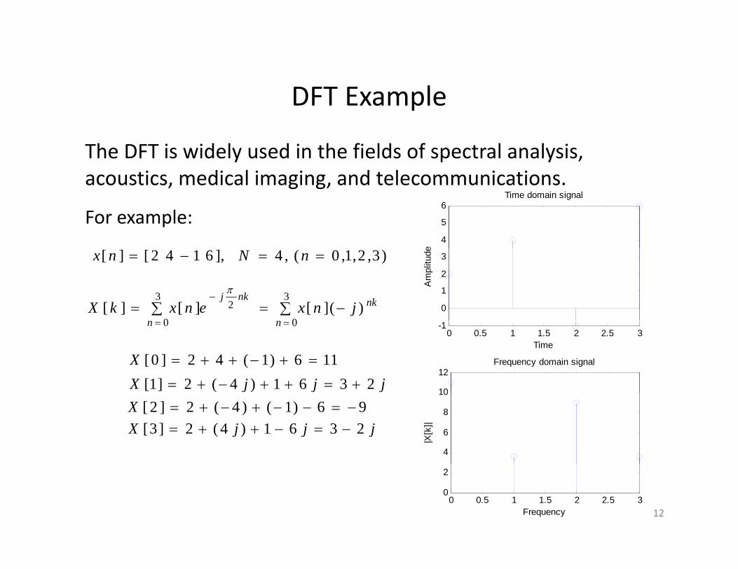
DFT ExampleDFT Example

The DFT is widely used in the fields of spectral analysis, acoustics medical imaging and telecommunicationsacoustics, medical imaging, and telecommunications.

4

5

6

e

Time domain signal

For example:

0

1

2

3

Am

plitu

de)3,2,1,0(,4],6142[][ nNnx

nknkjjnxenxkX )(][][][

3

0

23

0

0 0.5 1 1.5 2 2.5 3-1

Time

nn 00

116)1(42]0[ XjjjX 2361)4(2]1[ 10

12Frequency domain signal

96)1()4(2]2[ XjjjX 2361)4(2]3[

4

6

8

10

|X[k

]|

0 0.5 1 1.5 2 2.5 30

2

Frequency 12

Fast Fourier Transform(FFT)Fast Fourier Transform(FFT)

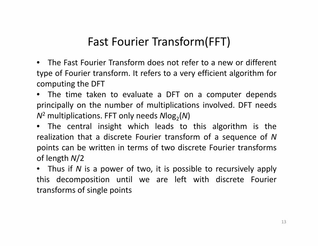
• The Fast Fourier Transform does not refer to a new or differenttype of Fourier transform. It refers to a very efficient algorithm foryp y gcomputing the DFT• The time taken to evaluate a DFT on a computer dependsprincipally on the number of multiplications involved. DFT needsprincipally on the number of multiplications involved. DFT needsN2 multiplications. FFT only needs Nlog2(N)• The central insight which leads to this algorithm is therealization that a discrete Fourier transform of a sequence of Nrealization that a discrete Fourier transform of a sequence of Npoints can be written in terms of two discrete Fourier transformsof length N/2• Thus if N is a power of two it is possible to recursively applyThus if N is a power of two, it is possible to recursively applythis decomposition until we are left with discrete Fouriertransforms of single points

13

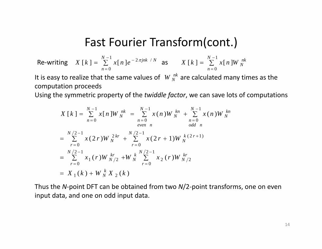
Fast Fourier Transform(cont.)Fast Fourier Transform(cont.)Re‐writing

1

0

/2][][N

n

NjnkenxkX as

1

0][][

N

n

nkNWnxkX

It is easy to realize that the same values of are calculated many times as thenkWIt is easy to realize that the same values of are calculated many times as the computation proceedsUsing the symmetric property of the twiddle factor, we can save lots of computations

NW

111 NNN

)12()2(

)()(][][

12 )12(12 2

1

0

1

0

1

0

WrxWrx

WnxWnxWnxkX

N rkN

N krN

N

noddn

knN

N

nevenn

knN

N

n

nkN

)()(

)()(

)12()2(

12

022

12

021

00

kXWkX

WrxWWrx

WrxWrx

k

N

r

krN

kN

N

r

krN

rN

rN

)()( 21 kXWkX kN

Thus the N‐point DFT can be obtained from two N/2‐point transforms, one on even input data, and one on odd input data.

14

Introduction for MATLABIntroduction for MATLAB

MATLAB is a numerical computing environment developed byMathWorks. MATLAB allows matrix manipulations, plotting ofp , p gfunctions and data, and implementation of algorithms

Getting helpGetting helpYou can get help by typing the commands help or lookfor atthe >> prompt, e.g.

>> help fft>> help fftArithmetic operatorsSymbol Operation Example

+ Addition 3 1 + 9+ Addition 3.1 + 9‐ Subtraction 6.2 – 5* Multiplication 2 * 3/ Division 5 / 2/ Division 5 / 2^ Power 3^2

15

Data Representations in MATLABData Representations in MATLABVariables: Variables are defined as the assignment operator “=” . The syntax ofvariable assignment is

i bl l ( i )variable name = a value (or an expression)For example,

>> x = 5x =

5>> y = [3*7, pi/3]; % pi is in MATLAB

Vectors/Matrices MATLAB can create and manip late arra s of 1 ( ectors) 2

Vectors/Matrices: MATLAB can create and manipulate arrays of 1 (vectors), 2(matrices), or more dimensions

row vectors: a = [1, 2, 3, 4] is a 1X4 matrixcolumn vectors: b = [5; 6; 7; 8; 9] is a 5X1 matrix, e.g.

>> A = [1 2 3; 7 8 9; 4 5 6]A = 1 2 3

7 8 94 5 64 5 6

16

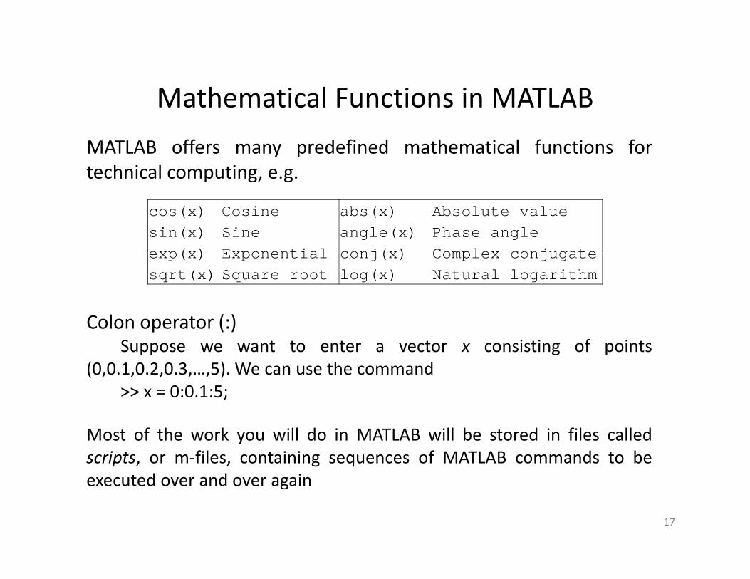
Mathematical Functions in MATLABMathematical Functions in MATLAB

MATLAB offers many predefined mathematical functions fortechnical computing, e.g.p g, g

cos(x) Cosine abs(x) Absolute valuesin(x) Sine angle(x) Phase angleexp(x) Exponential conj(x) Complex conjugate

Colon operator (:)

exp(x) Exponential conj(x) Complex conjugatesqrt(x) Square root log(x) Natural logarithm

Colon operator (:)Suppose we want to enter a vector x consisting of points

(0,0.1,0.2,0.3,…,5). We can use the command>> x = 0:0.1:5;;

Most of the work you will do in MATLAB will be stored in files calledscripts, or m‐files, containing sequences of MATLAB commands to beexecuted over and over again

17

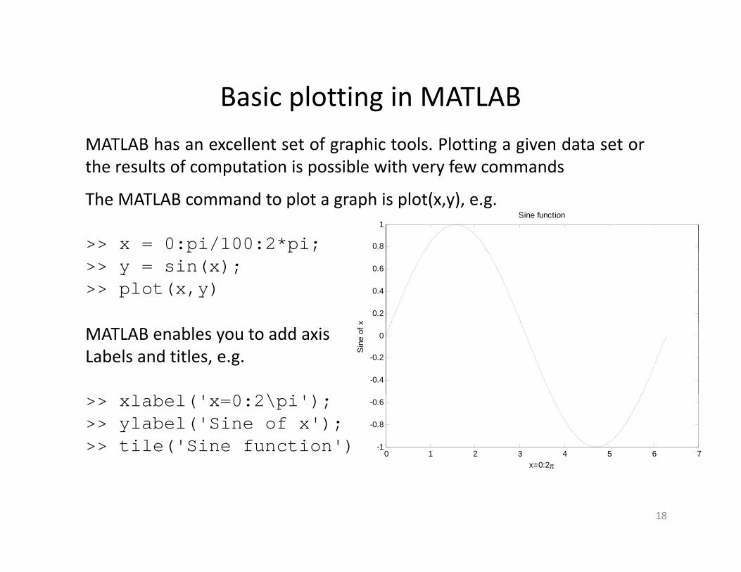
Basic plotting in MATLABBasic plotting in MATLAB

MATLAB has an excellent set of graphic tools. Plotting a given data set orthe results of computation is possible with very few commands

The MATLAB command to plot a graph is plot(x,y), e.g.

>> x = 0:pi/100:2*pi; 0.8

1Sine function

p / p ;>> y = sin(x);>> plot(x,y)

0.2

0.4

0.6

x

MATLAB enables you to add axisLabels and titles, e.g.

\ i-0.4

-0.2

0

Sin

e of

x

>> xlabel('x=0:2\pi');>> ylabel('Sine of x');>> tile('Sine function')

0 1 2 3 4 5 6 7-1

-0.8

-0.6

x=0:2x 0:2

18

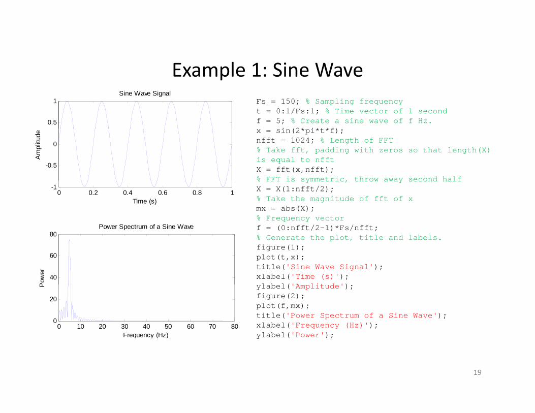
Example 1: Sine WaveExample 1: Sine Wave

0.5

1Sine Wave Signal

Fs = 150; % Sampling frequencyt = 0:1/Fs:1; % Time vector of 1 second f = 5; % Create a sine wave of f Hz.

i (2* i*t*f)

-0.5

0

Am

plitu

de

x = sin(2*pi*t*f); nfft = 1024; % Length of FFT% Take fft, padding with zeros so that length(X) is equal to nfft X = fft(x,nfft); % FFT is symmetric, throw away second half

0 0.2 0.4 0.6 0.8 1-1

Time (s)

80Power Spectrum of a Sine Wave

% FFT is symmetric, throw away second half X = X(1:nfft/2); % Take the magnitude of fft of xmx = abs(X);% Frequency vectorf = (0:nfft/2-1)*Fs/nfft;

40

60

80

Pow

er

% Generate the plot, title and labels. figure(1);plot(t,x);title('Sine Wave Signal'); xlabel('Time (s)'); l b l('A lit d ')

0 10 20 30 40 50 60 70 800

20

Frequency (Hz)

P ylabel('Amplitude'); figure(2);plot(f,mx); title('Power Spectrum of a Sine Wave'); xlabel('Frequency (Hz)'); ylabel('Power');Frequency (Hz) ylabel( Power );

19

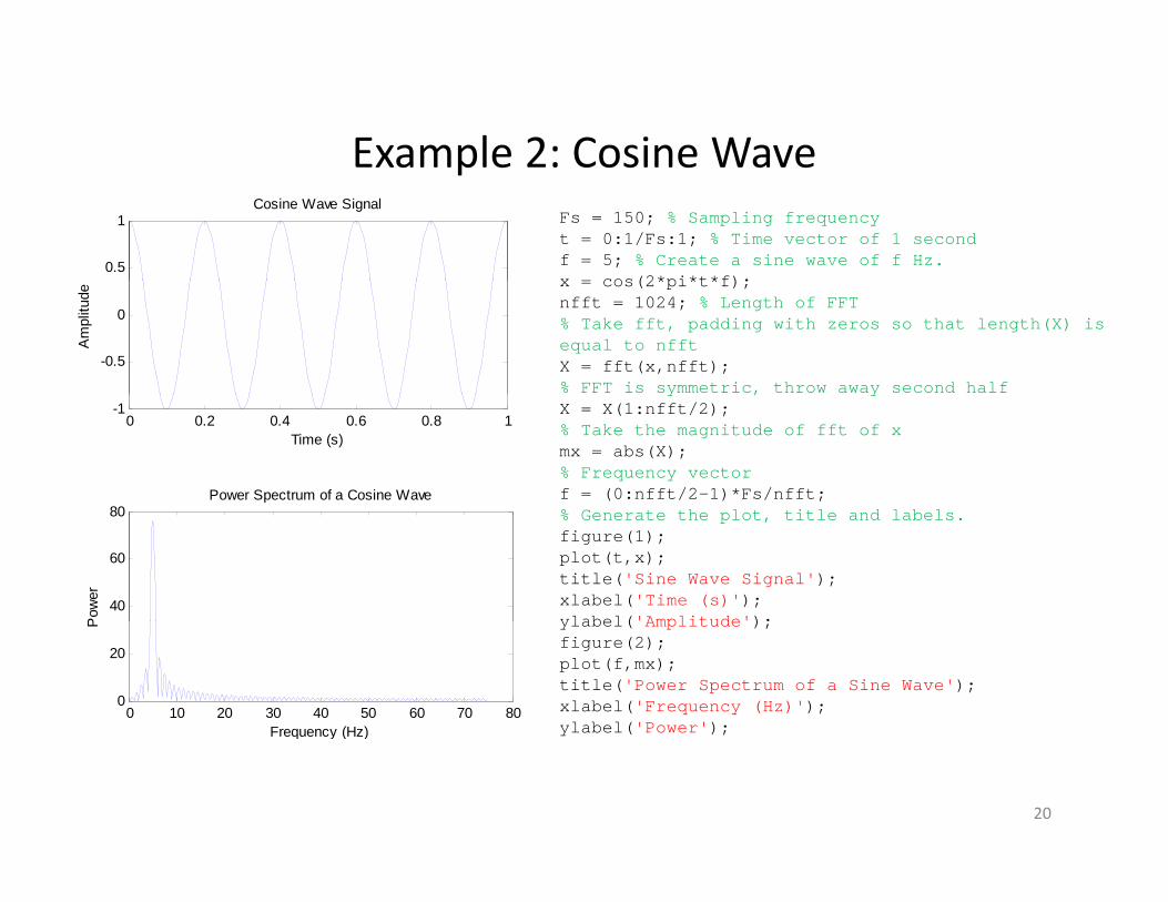
Example 2: Cosine WaveExample 2: Cosine WaveFs = 150; % Sampling frequencyt = 0:1/Fs:1; % Time vector of 1 second f = 5; % Create a sine wave of f Hz.x = cos(2*pi*t*f);

0.5

1Cosine Wave Signal

x = cos(2*pi*t*f); nfft = 1024; % Length of FFT% Take fft, padding with zeros so that length(X) is equal to nfft X = fft(x,nfft); % FFT is symmetric, throw away second half

-0.5

0

Am

plitu

de

y , yX = X(1:nfft/2); % Take the magnitude of fft of xmx = abs(X);% Frequency vectorf = (0:nfft/2-1)*Fs/nfft;

0 0.2 0.4 0.6 0.8 1-1

Time (s)

80Power Spectrum of a Cosine Wave

% Generate the plot, title and labels. figure(1);plot(t,x);title('Sine Wave Signal'); xlabel('Time (s)'); ylabel('Amplitude');

40

60

80

Pow

er

ylabel( Amplitude ); figure(2);plot(f,mx); title('Power Spectrum of a Sine Wave'); xlabel('Frequency (Hz)'); ylabel('Power');

0 10 20 30 40 50 60 70 800

20

Frequency (Hz)

P

yFrequency (Hz)

20

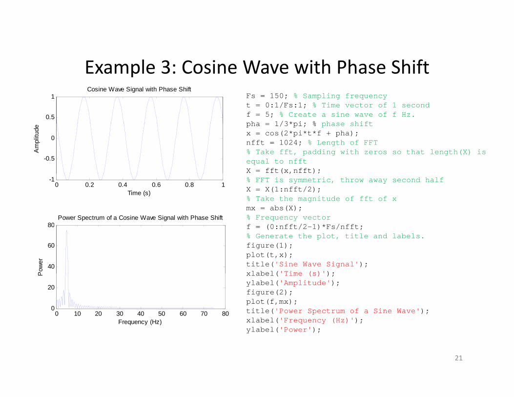
Example 3: Cosine Wave with Phase ShiftExample 3: Cosine Wave with Phase ShiftFs = 150; % Sampling frequencyt = 0:1/Fs:1; % Time vector of 1 second f = 5; % Create a sine wave of f Hz.pha = 1/3*pi; % phase shift

0.5

1Cosine Wave Signal with Phase Shift

pha = 1/3*pi; % phase shift x = cos(2*pi*t*f + pha); nfft = 1024; % Length of FFT% Take fft, padding with zeros so that length(X) is equal to nfft X = fft(x,nfft);

-0.5

0

Am

plitu

de

( , )% FFT is symmetric, throw away second half X = X(1:nfft/2); % Take the magnitude of fft of xmx = abs(X);% Frequency vector

/ /

0 0.2 0.4 0.6 0.8 1-1

Time (s)

80Power Spectrum of a Cosine Wave Signal with Phase Shift

f = (0:nfft/2-1)*Fs/nfft; % Generate the plot, title and labels. figure(1);plot(t,x);title('Sine Wave Signal'); xlabel('Time (s)');

40

60

80

Pow

er

xlabel( Time (s) ); ylabel('Amplitude'); figure(2);plot(f,mx); title('Power Spectrum of a Sine Wave'); xlabel('Frequency (Hz)');

0 10 20 30 40 50 60 70 800

20

Frequency (Hz)

P

q yylabel('Power');

Frequency (Hz)

21

Example 4: Square WaveExample 4: Square Wave

0.5

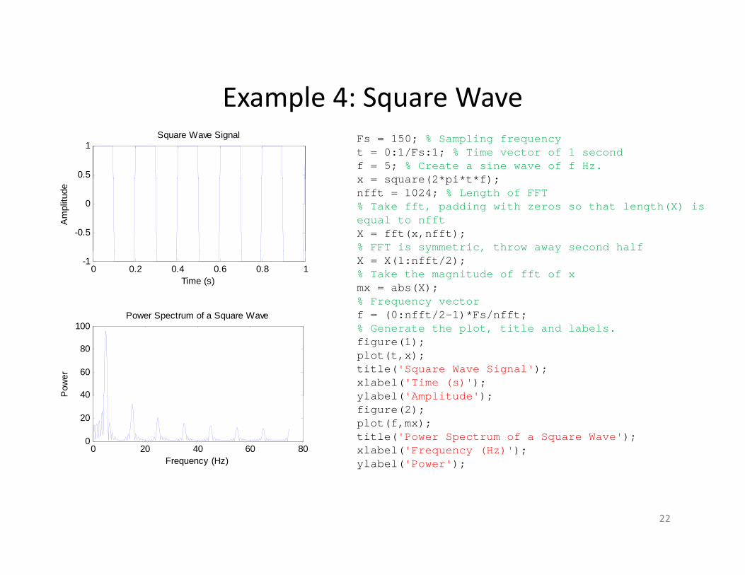
1Square Wave Signal Fs = 150; % Sampling frequency

t = 0:1/Fs:1; % Time vector of 1 second f = 5; % Create a sine wave of f Hz.x = square(2*pi*t*f);

-0.5

0

Am

plitu

de

x = square(2*pi*t*f); nfft = 1024; % Length of FFT% Take fft, padding with zeros so that length(X) is equal to nfft X = fft(x,nfft); % FFT is symmetric, throw away second half

0 0.2 0.4 0.6 0.8 1-1

Time (s)

100Power Spectrum of a Square Wave


40

60

80

100

Pow

er

% Generate the plot, title and labels. figure(1);plot(t,x);title('Square Wave Signal'); xlabel('Time (s)'); ylabel('Amplitude');

0 20 40 60 800

20

40

Frequency (Hz)

ylabel( Amplitude ); figure(2);plot(f,mx); title('Power Spectrum of a Square Wave'); xlabel('Frequency (Hz)'); ylabel('Power'); y

22

Example 5: Square PulseExample 5: Square Pulse

0.8

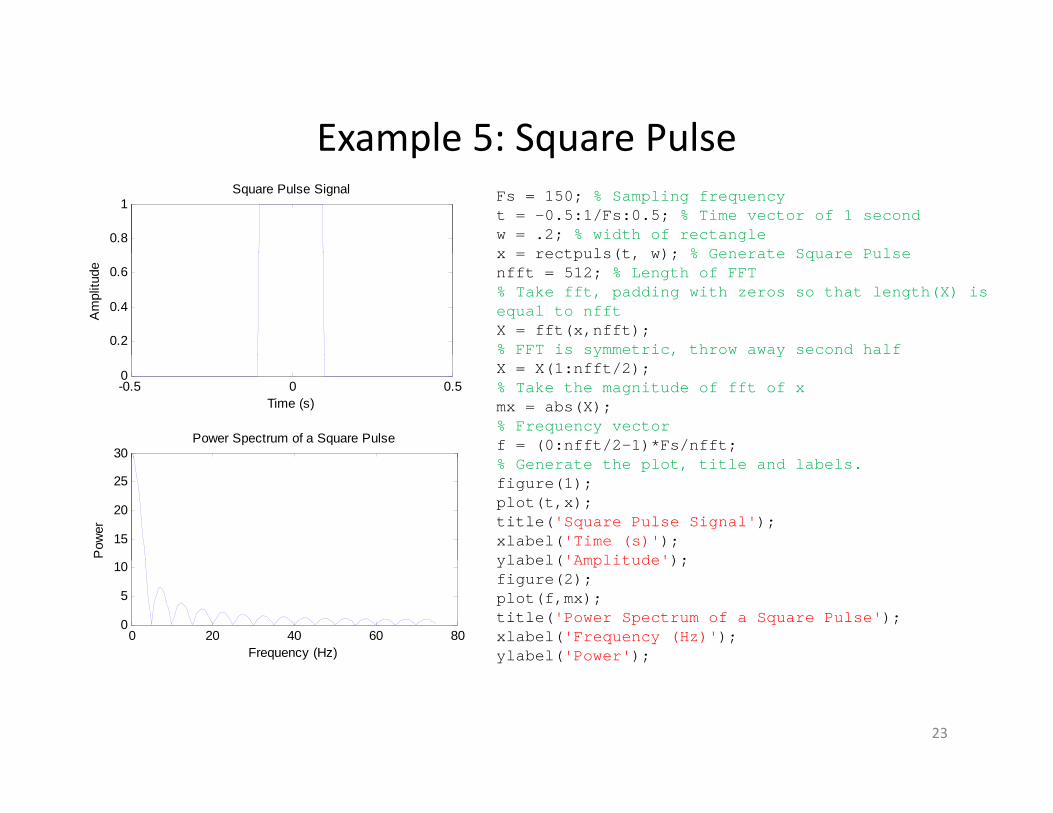
1Square Pulse Signal Fs = 150; % Sampling frequency

t = -0.5:1/Fs:0.5; % Time vector of 1 second w = .2; % width of rectanglex = rectpuls(t w); % Generate Square Pulse

0.2

0.4

0.6

Am

plitu

de

x = rectpuls(t, w); % Generate Square Pulsenfft = 512; % Length of FFT% Take fft, padding with zeros so that length(X) is equal to nfft X = fft(x,nfft); % FFT is symmetric, throw away second half

-0.5 0 0.50

Time (s)

30Power Spectrum of a Square Pulse


15

20

25

Pow

er

% Generate the plot, title and labels. figure(1);plot(t,x);title('Square Pulse Signal'); xlabel('Time (s)'); ylabel('Amplitude');

0 20 40 60 800

5

10

Frequency (Hz)

ylabel( Amplitude ); figure(2);plot(f,mx); title('Power Spectrum of a Square Pulse'); xlabel('Frequency (Hz)'); ylabel('Power'); y

23

Example 6: Gaussian PulseExample 6: Gaussian Pulse

3

4Gaussian Pulse Signal

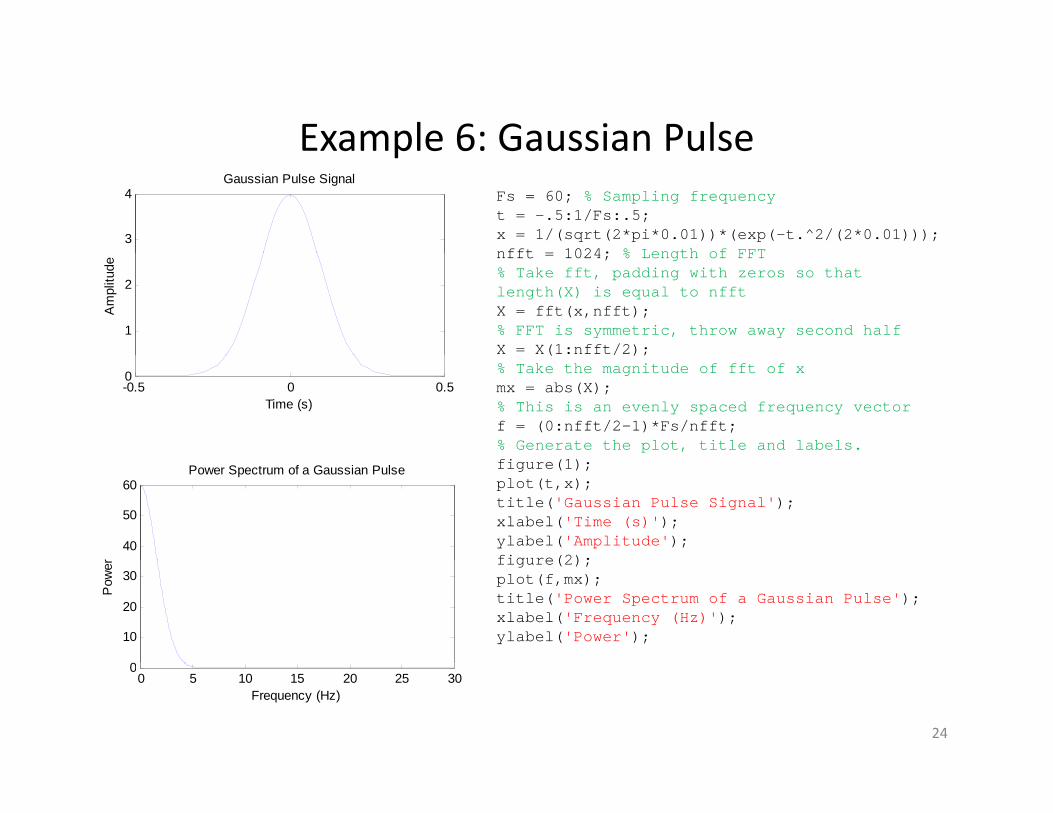
Fs = 60; % Sampling frequencyt = -.5:1/Fs:.5; x = 1/(sqrt(2*pi*0.01))*(exp(-t.^2/(2*0.01)));nfft = 1024; % Length of FFT

1

2

Am

plitu

de

nfft = 1024; % Length of FFT% Take fft, padding with zeros so that length(X) is equal to nfft X = fft(x,nfft); % FFT is symmetric, throw away second half X = X(1:nfft/2);

-0.5 0 0.50

Time (s)

( )% Take the magnitude of fft of xmx = abs(X);% This is an evenly spaced frequency vectorf = (0:nfft/2-1)*Fs/nfft; % Generate the plot, title and labels.

40

50

60Power Spectrum of a Gaussian Pulse

r

figure(1);plot(t,x);title('Gaussian Pulse Signal'); xlabel('Time (s)'); ylabel('Amplitude'); figure(2);

0

10

20

30

Pow

er figure(2);plot(f,mx); title('Power Spectrum of a Gaussian Pulse'); xlabel('Frequency (Hz)'); ylabel('Power');

0 5 10 15 20 25 300

Frequency (Hz)

24

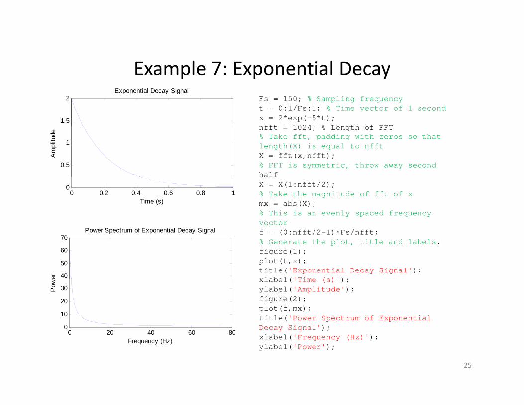
Example 7: Exponential DecayExample 7: Exponential Decay

1.5

2Exponential Decay Signal

Fs = 150; % Sampling frequencyt = 0:1/Fs:1; % Time vector of 1 second x = 2*exp(-5*t); nfft 1024 % Length of FFT

0.5

1

Am

plitu

de

nfft = 1024; % Length of FFT% Take fft, padding with zeros so that length(X) is equal to nfft X = fft(x,nfft); % FFT is symmetric, throw away second half

0 0.2 0.4 0.6 0.8 10

Time (s)

P S t f E ti l D Si l

half X = X(1:nfft/2); % Take the magnitude of fft of xmx = abs(X);% This is an evenly spaced frequency vector

40

50

60

70Power Spectrum of Exponential Decay Signal

er

f = (0:nfft/2-1)*Fs/nfft; % Generate the plot, title and labels. figure(1);plot(t,x);title('Exponential Decay Signal'); xlabel('Time (s)');

0 20 40 60 800

10

20

30Pow

e xlabel('Time (s)'); ylabel('Amplitude'); figure(2);plot(f,mx); title('Power Spectrum of Exponential Decay Signal');

0 20 40 60 80Frequency (Hz)

y g );xlabel('Frequency (Hz)'); ylabel('Power');

25

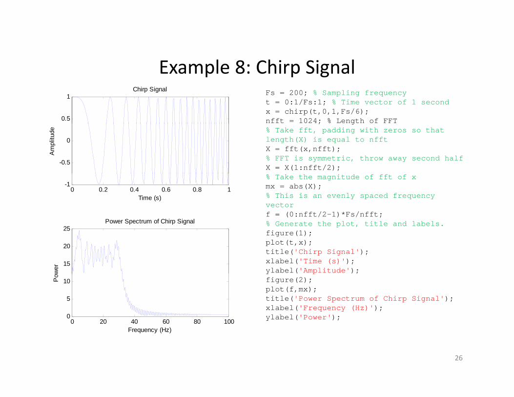
Example 8: Chirp SignalExample 8: Chirp Signal

0.5

1Chirp Signal Fs = 200; % Sampling frequency

t = 0:1/Fs:1; % Time vector of 1 second x = chirp(t,0,1,Fs/6); nfft = 1024; % Length of FFT

-0.5

0

Am

plitu

de

; g% Take fft, padding with zeros so that length(X) is equal to nfft X = fft(x,nfft); % FFT is symmetric, throw away second half X = X(1:nfft/2);

0 0.2 0.4 0.6 0.8 1-1

Time (s)

Power Spectrum of Chirp Signal

% Take the magnitude of fft of xmx = abs(X);% This is an evenly spaced frequency vectorf = (0:nfft/2-1)*Fs/nfft; % Generate the plot title and labels

15

20

25p p g

wer

% Generate the plot, title and labels. figure(1);plot(t,x);title('Chirp Signal'); xlabel('Time (s)'); ylabel('Amplitude');

0 20 40 60 80 1000

5

10Pow

y pfigure(2);plot(f,mx); title('Power Spectrum of Chirp Signal'); xlabel('Frequency (Hz)'); ylabel('Power');

Frequency (Hz)

26

Science

Ff tand matlab-wanjun huang