Embed Size (px)
Citation preview
Gunung MuluCaves as Climate RecordersKim Cobb, Georgia TechJess Adkins, CaltechJud Partin, UT AustinNele Meckler, NIODavid Lund (Sang), UConnJessica Moerman,U. MarylandStacy Carolin, OxfordShelby Ellis, Georgia Tech
• Pa
leocli
mate R
esearch • Georgia Tech •
Cobb Lab
With many thanks to:Brian Clark, Manager, Gunung Mulu National ParkSyria Lejau, Senior Guide, Gunung MuluJenny Malang, Senior Guide, Gunung MuluAndrew Tuen, Professor, UNIMAS
And with permits from:Sarawak ForestrySarawak Planning UnitMalaysia Economic Planning Unit
Moerman etal.,GRL2014
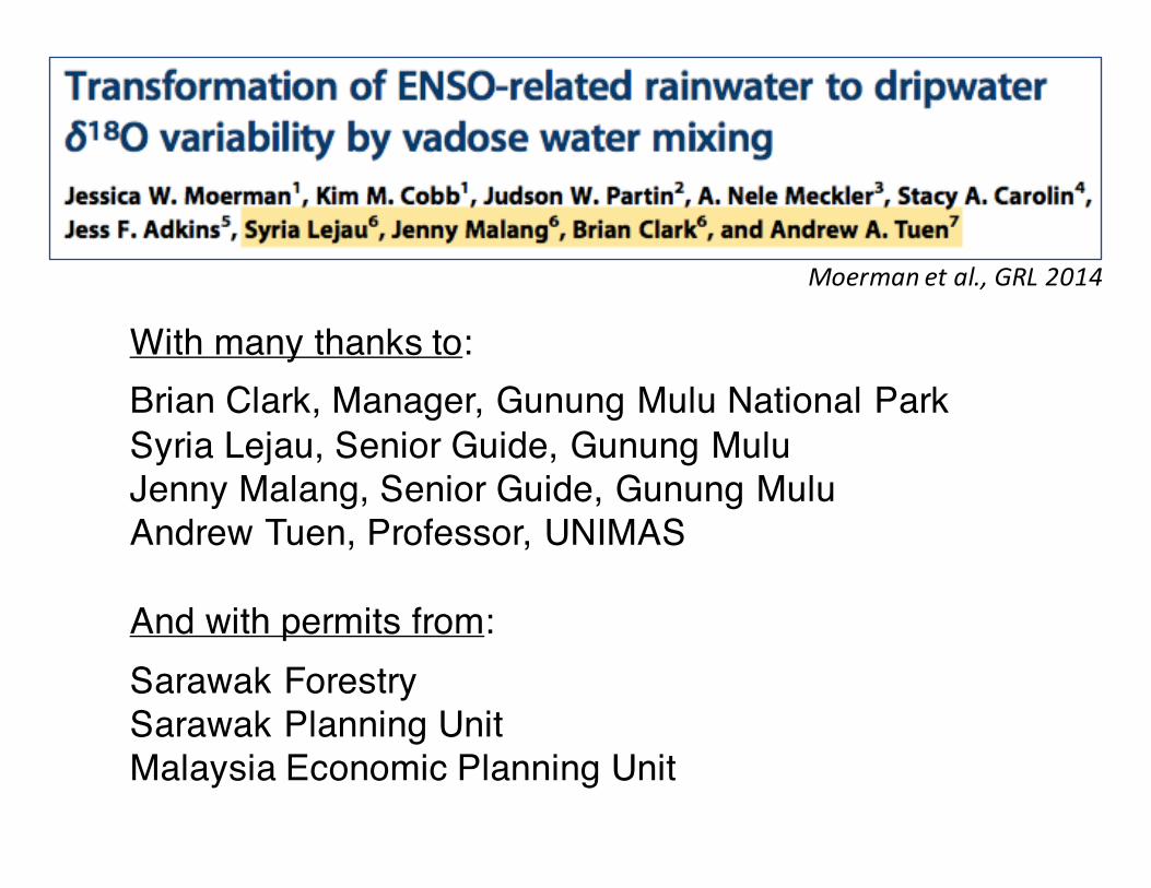
Mulu is FAMOUS for its climate records
Longest cave dripwater collectionin the world. (11yrs)
Longest daily rainwater collectionin the world. (10yrs)
One of the longest, most replicated stalagmite climate records in the world.

How do we make a climate record at Mulu?
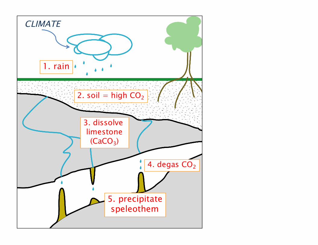
1. rain
2. soil = high CO2
3. dissolve limestone(CaCO3)
4. degas CO2
5. precipitatespeleothem
CLIMATE
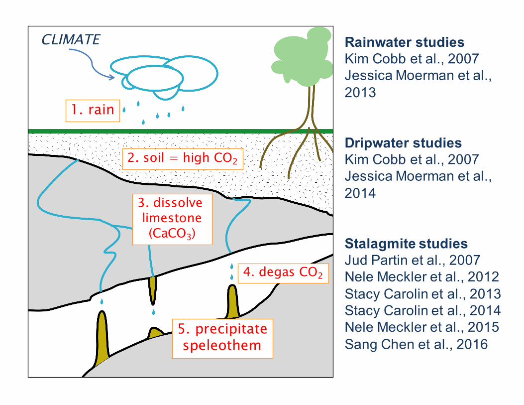
1. rain
2. soil = high CO2
3. dissolve limestone(CaCO3)
4. degas CO2
5. precipitatespeleothem
Rainwater studiesKim Cobb et al., 2007Jessica Moerman et al., 2013
Dripwater studiesKim Cobb et al., 2007Jessica Moerman et al., 2014
Stalagmite studiesJud Partin et al., 2007Nele Meckler et al., 2012Stacy Carolin et al., 2013Stacy Carolin et al., 2014Nele Meckler et al., 2015Sang Chen et al., 2016
CLIMATE
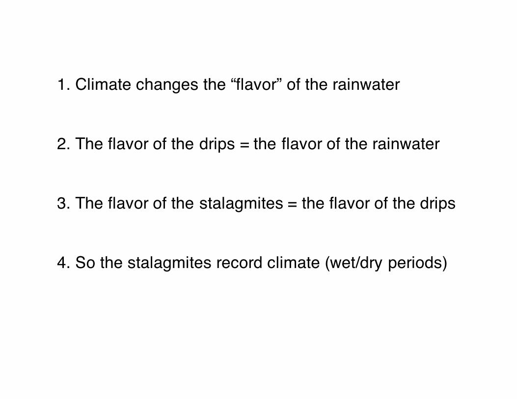
1. Climate changes the “flavor” of the rainwater
2. The flavor of the drips = the flavor of the rainwater
3. The flavor of the stalagmites = the flavor of the drips
4. So the stalagmites record climate (wet/dry periods)
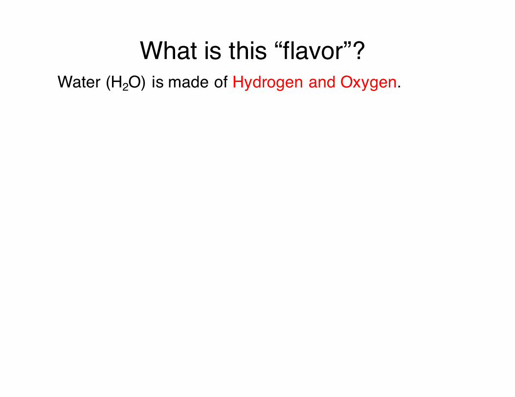
What is this “flavor”?Water (H2O) is made of Hydrogen and Oxygen.
What is this “flavor”?Water (H2O) is made of Hydrogen and Oxygen.
99.8% of Oxygen atoms have 8 protons + 8 neutrons = 160.2% of Oxygen atoms have 8 protons + 10 neutrons = 18
What is this “flavor”?Water (H2O) is made of Hydrogen and Oxygen.
99.8% of Oxygen atoms have 8 protons + 8 neutrons = 160.2% of Oxygen atoms have 8 protons + 10 neutrons = 18
“flavor” = changes in number of 18O vs 16O isotopesRainfall in every city in the world has a different value,depending on the temperature, winds, cloud types, etc.
At Mulu, dry periods and wet periods have a differentoxygen isotope value.
We can measure these changes in rainfall, dripwater, and stalagmites in my lab at Georgia Tech.
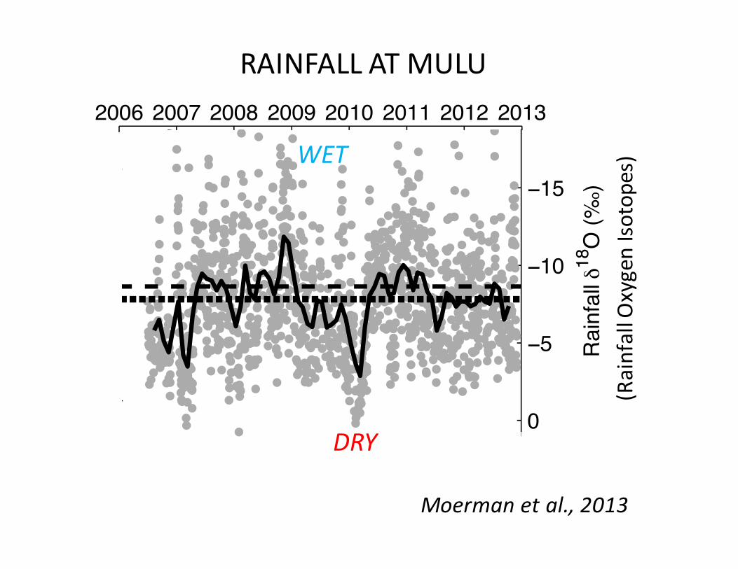
Figure 1. Comparison of Mulu dripwater δ18O to rainfall δ18O and local and regional climate variables. (a) Monthly NINO4SST anomalies [Reynolds et al., 2002]. Red and blue bars along the upper x axis represent weak-to-moderate El Niño andmoderate-to-strong La Niña events as defined by the Oceanic Niño Index (http://www.cpc.ncep.noaa.gov/products/analysis_monitoring/ensostuff/ensoyears.shtml). (b) Nonamount-weighted daily Mulu rainfall δ18O (gray circles) shownwith a 2 month running average (black line), and nonamount-weighted (dotted line) and amount-weighted (dashed line)means of the entire time series. (c) Mulu dripwater δ18O from drips WF (orange), WS (blue), and L2 (green) plotted withthe composite mean of the three dripwater δ18O time series (black line) and mean amount-weighted rainfall δ18O fromFigure 1b (dashed line). Box-and-whisker plots represent the median (bold bar), 25–75% quartile range (red box), andmaximum and minimum δ18O values (whiskers) for system-wide field expedition surveys of stalagmite-forming dripwatersconducted in August 2008 (n = 36), February–March 2010 (n = 54), and October–November 2012 (n = 135). (d) Drip ratesfrom drip sites WF (orange), WS (blue), and L2 (green). Note that WS drip rate has been shifted by +30 dpm and L2 by+20 dpm. (e) Rain gauge measurements of daily Mulu precipitation amount (gray bars) plotted with a 2 month runningaverage (black line). Y axes in Figures 1a–1c are inverted.
Geophysical Research Letters 10.1002/2014GL061696
MOERMAN ET AL. ©2014. American Geophysical Union. All Rights Reserved. 4
(RainfallO
xygenIso
topes)WET
DRY
Figure 1. Comparison of Mulu dripwater δ18O to rainfall δ18O and local and regional climate variables. (a) Monthly NINO4SST anomalies [Reynolds et al., 2002]. Red and blue bars along the upper x axis represent weak-to-moderate El Niño andmoderate-to-strong La Niña events as defined by the Oceanic Niño Index (http://www.cpc.ncep.noaa.gov/products/analysis_monitoring/ensostuff/ensoyears.shtml). (b) Nonamount-weighted daily Mulu rainfall δ18O (gray circles) shownwith a 2 month running average (black line), and nonamount-weighted (dotted line) and amount-weighted (dashed line)means of the entire time series. (c) Mulu dripwater δ18O from drips WF (orange), WS (blue), and L2 (green) plotted withthe composite mean of the three dripwater δ18O time series (black line) and mean amount-weighted rainfall δ18O fromFigure 1b (dashed line). Box-and-whisker plots represent the median (bold bar), 25–75% quartile range (red box), andmaximum and minimum δ18O values (whiskers) for system-wide field expedition surveys of stalagmite-forming dripwatersconducted in August 2008 (n = 36), February–March 2010 (n = 54), and October–November 2012 (n = 135). (d) Drip ratesfrom drip sites WF (orange), WS (blue), and L2 (green). Note that WS drip rate has been shifted by +30 dpm and L2 by+20 dpm. (e) Rain gauge measurements of daily Mulu precipitation amount (gray bars) plotted with a 2 month runningaverage (black line). Y axes in Figures 1a–1c are inverted.
Geophysical Research Letters 10.1002/2014GL061696
MOERMAN ET AL. ©2014. American Geophysical Union. All Rights Reserved. 4
Moerman etal.,2013
RAINFALLATMULU
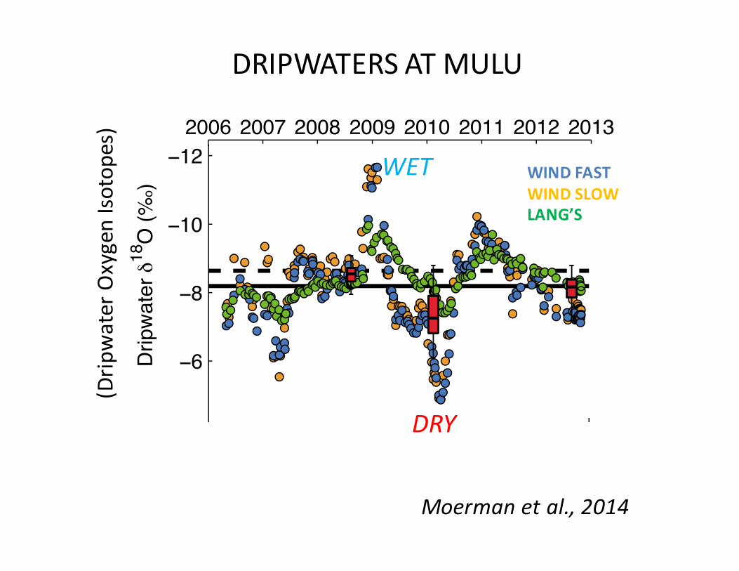
Figure 1. Comparison of Mulu dripwater δ18O to rainfall δ18O and local and regional climate variables. (a) Monthly NINO4SST anomalies [Reynolds et al., 2002]. Red and blue bars along the upper x axis represent weak-to-moderate El Niño andmoderate-to-strong La Niña events as defined by the Oceanic Niño Index (http://www.cpc.ncep.noaa.gov/products/analysis_monitoring/ensostuff/ensoyears.shtml). (b) Nonamount-weighted daily Mulu rainfall δ18O (gray circles) shownwith a 2 month running average (black line), and nonamount-weighted (dotted line) and amount-weighted (dashed line)means of the entire time series. (c) Mulu dripwater δ18O from drips WF (orange), WS (blue), and L2 (green) plotted withthe composite mean of the three dripwater δ18O time series (black line) and mean amount-weighted rainfall δ18O fromFigure 1b (dashed line). Box-and-whisker plots represent the median (bold bar), 25–75% quartile range (red box), andmaximum and minimum δ18O values (whiskers) for system-wide field expedition surveys of stalagmite-forming dripwatersconducted in August 2008 (n = 36), February–March 2010 (n = 54), and October–November 2012 (n = 135). (d) Drip ratesfrom drip sites WF (orange), WS (blue), and L2 (green). Note that WS drip rate has been shifted by +30 dpm and L2 by+20 dpm. (e) Rain gauge measurements of daily Mulu precipitation amount (gray bars) plotted with a 2 month runningaverage (black line). Y axes in Figures 1a–1c are inverted.
Geophysical Research Letters 10.1002/2014GL061696
MOERMAN ET AL. ©2014. American Geophysical Union. All Rights Reserved. 4Figure 1. Comparison of Mulu dripwater δ18O to rainfall δ18O and local and regional climate variables. (a) Monthly NINO4SST anomalies [Reynolds et al., 2002]. Red and blue bars along the upper x axis represent weak-to-moderate El Niño andmoderate-to-strong La Niña events as defined by the Oceanic Niño Index (http://www.cpc.ncep.noaa.gov/products/analysis_monitoring/ensostuff/ensoyears.shtml). (b) Nonamount-weighted daily Mulu rainfall δ18O (gray circles) shownwith a 2 month running average (black line), and nonamount-weighted (dotted line) and amount-weighted (dashed line)means of the entire time series. (c) Mulu dripwater δ18O from drips WF (orange), WS (blue), and L2 (green) plotted withthe composite mean of the three dripwater δ18O time series (black line) and mean amount-weighted rainfall δ18O fromFigure 1b (dashed line). Box-and-whisker plots represent the median (bold bar), 25–75% quartile range (red box), andmaximum and minimum δ18O values (whiskers) for system-wide field expedition surveys of stalagmite-forming dripwatersconducted in August 2008 (n = 36), February–March 2010 (n = 54), and October–November 2012 (n = 135). (d) Drip ratesfrom drip sites WF (orange), WS (blue), and L2 (green). Note that WS drip rate has been shifted by +30 dpm and L2 by+20 dpm. (e) Rain gauge measurements of daily Mulu precipitation amount (gray bars) plotted with a 2 month runningaverage (black line). Y axes in Figures 1a–1c are inverted.
Geophysical Research Letters 10.1002/2014GL061696
MOERMAN ET AL. ©2014. American Geophysical Union. All Rights Reserved. 4
WET
DRY
(Drip
water
OxygenIso
topes)
DRIPWATERSATMULU
WINDFASTWINDSLOWLANG’S
Moerman etal.,2014
While the autogenic recharge modelreproduces the timing of L2 dripwaterδ18Ominima andmaxima, it overestimatesthe amplitude of the drip’s δ18O variations(Figure 2). Amount-weighted rainfall δ18Oaveraged over the previous 42weeks(~10months) best reflects the timing ofdripwater δ18O maxima and minimaobserved in L2 (R=0.84), but the predictedvariations are roughly 1‰ higher thanobserved (Figure 2). This suggests thatthe flow pathway to this drip site is morecomplicated than that feeding WF andWS. L2’s amplitude attenuation suggestsa likely contribution from a second, well-mixed reservoir, which we model using abivariate mixing model,
XM ¼ XA 1" f Bð Þ þ XBf B (1)
where XA is the isotopic composition ofReservoir A,XB is the isotopic compositionof Reservoir B, and fB is the mixingparameter. Modeled dripwater δ18Osimulated by the autogenic rechargemodel with an ~10 month residencetime represents Reservoir A. In theinterest of simplicity, we set the isotopiccomposition of Reservoir B as amount-weighted Mulu rainfall δ18O averagedacross the study period ("8.6‰). AtfB = 0.6, the residuals between themodeled and observed L2 time seriesare minimized. With this modelconfiguration, the muted variability in L2is reproduced particularly well during
the 2009–2012 ENSO cycle (Figure 2), suggesting that two distinct reservoirs likely feed L2—one with aresidence time of ~10months that is recharged autogenically (Reservoir A) and a second with a significantlylonger residence time (Reservoir B). However, prior to 2009, the above parameters overdamp the variability,resulting in a poor fit between the modeled and observed time series. Increasing the Reservoir A flux from40% to 80% (i.e., fB = 0.2) during late 2008/early 2009 greatly improves model-data fit, suggesting anabrupt switch in flow to L2 during this period (Figure 2). Indeed, Reservoir A may represent 100% of flowin December 2008. Throughout 2008, modeled dripwater δ18O is ~0.5‰ more negative than observed L2values, indicating that either (i) the isotopic composition of Reservoir B varies over the study period and/or(ii) that our simple two-reservoir model fails to capture the complexity of flow feeding L2. Longer time seriesof rainwater and dripwater δ18O are required to differentiate between these scenarios.
The isotopic spread of hundreds of stalagmite-forming drips collected during field expeditions falls withinthe variability of the dripwater δ18O time series (Figure 1c), indicating that the three time series drips arebroadly representative of system-wide shifts in isotopic composition. The relatively small spread in both the2008 and 2012 expedition data sets (~0.3‰ (1σ)) suggests that residence times for stalagmite-forming dripsin Mulu are long enough to homogenize large intraseasonal shifts in rainfall δ18O of ~10‰ [Moerman et al.,2013], establishing a lower bound for residence times of stalagmite-forming drips of approximately 1–2months. Likewise, residence times for many stalagmite-forming drips appear to be less than 2 years, as only25% of the 2010 expedition drip distribution overlaps that of the 2008 expedition (Figure 1c). This remainstrue even when a subset of the slowest dripping samples (<2 dpm) is considered.
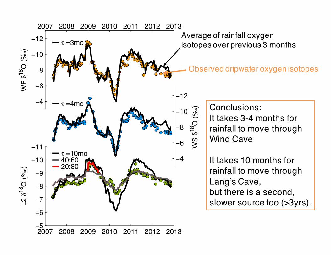
Figure 2. Observed dripwater δ18O (circles) for dripsWF (orange),WS (blue),and L2 (green) compared with best fit modeled dripwater δ18O (solid lines)using amount-weighted Mulu rainfall δ18O as input. Bold black linesrepresent dripwater simulated by the autogenic recharge model with aresidence time of ~3months for WF, ~4months for WS, and ~10monthsfor L2. Bivariate mixing model results for drip L2 modeled as 40% ofReservoir A with an ~10 month residence time and 60% of Reservoir Breflecting mean amount-weighted rainfall δ18O are plotted as a gray line.During the October 2008 to June 2009 interval, the red line reflectsmodeled dripwater δ18O assuming contributions of 20% from Reservoir Aand 80% from Reservoir B. Y axes are inverted in all panels.
Geophysical Research Letters 10.1002/2014GL061696
MOERMAN ET AL. ©2014. American Geophysical Union. All Rights Reserved. 5
Conclusions: It takes 3-4 months for rainfall to move through Wind Cave
It takes 10 months forrainfall to move through Lang’s Cave,but there is a second,slower source too (>3yrs).
Average of rainfall oxygenisotopes over previous 3 months
Observed dripwater oxygen isotopes
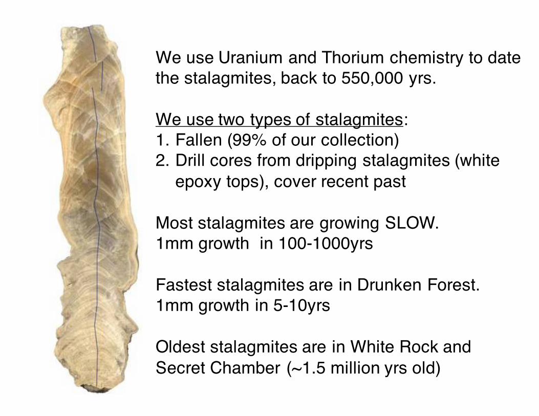
We use Uranium and Thorium chemistry to date the stalagmites, back to 550,000 yrs.
We use two types of stalagmites:1. Fallen (99% of our collection)2. Drill cores from dripping stalagmites (white
epoxy tops), cover recent past
Most stalagmites are growing SLOW.1mm growth in 100-1000yrs
Fastest stalagmites are in Drunken Forest.1mm growth in 5-10yrs
Oldest stalagmites are in White Rock andSecret Chamber (~1.5 million yrs old)
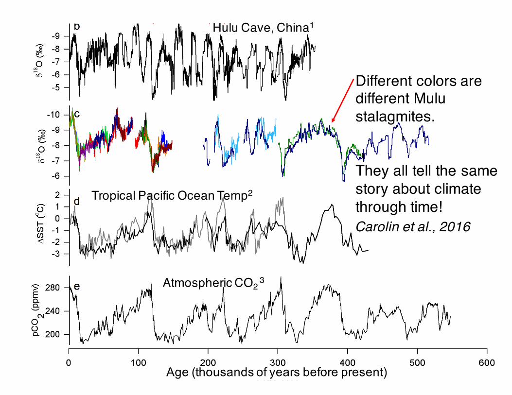
Figure 6. Comparison of 0-600 kybp global paleorecords.
Figure 6. Comparison of 0-600 kybp global paleorecords.
Different colors are different Mulustalagmites.
They all tell the samestory about climatethrough time!Carolin et al., 2016
Age (thousands of years before present)
Hulu Cave, China1
Tropical Pacific Ocean Temp2
Atmospheric CO2 3
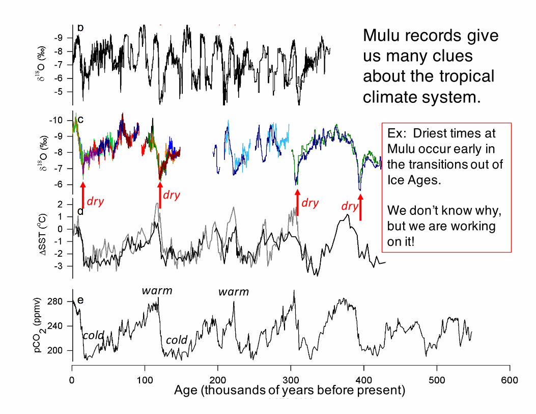
Figure 6. Comparison of 0-600 kybp global paleorecords.
Figure 6. Comparison of 0-600 kybp global paleorecords.
Mulu records give us many clues about the tropicalclimate system.
dry dry dry dry
Ex: Driest times at Mulu occur early in the transitions out of Ice Ages.
We don’t know why, but we are workingon it!
Age (thousands of years before present)
warm
coldcold
warm

2005
THANK YOU
FirstMuluExpedition,
2005
Toprow(lefttoright):
JonnyBaeiBrianClarkSueClark
SyriaLejau
Bottomrow(lefttoright):KimCobb,JudPartin,JennyMalang
Other paleoclimate records shown in slides 17-18:
1 Hulu/Sanbao stalagmite δ18O recordsWang et al., 2001; Wang et al., 2008; Cheng et al., 2009
2 Marine sediment Mg/Ca SST records (Lea et al., 2000; 2004)3 Vostok/EPICA pCO2 record (Petit et al., 1999; EPICA, 2006)