62 192-2-pb (2)

Latin American and Caribbean Journal of Engineering Education Vol. 7(1), 2013

1

Aproximate Analytic Analysis Of Annular Fins With Uniform Thickness By Way Of The Mean Value Theorem For Integration That Avoids Modified

Bessel Functions

Antonio Acosta−Iborra1, Antonio Campo2

Abstract - In the analysis of annular fins of uniform thickness, the main obstacle is without question, the variable coefficient 1 r multiplying the first order derivative temperature dT dr in the governing quasi one-dimensional heat conduction equation. A good-natured manipulation of the problematic variable coefficient 1 r is the principal objective of the present paper on engineering education. Specifically, we

seek to apply the mean value theorem for integration to 1 r , viewed as an auxiliary function in the annular

fin domain extending from the inner radius 1r to the outer radius2r . It is demonstrated in a convincing

manner that approximate analytic temperature profiles of good quality are easy to obtain without resorting to the exact analytic temperature profile embodying four modified Bessel functions. Surely, instructors and students in heat transfer courses will be the beneficiaries of this finding because of the easiness in calculating the temperatures and heat transfer rates for realistic combinations of the two controlling parameters: the normalized radii ratio and the thermo-geometric fin parameter. Keywords - annular fin with uniform thickness; mean value theorem for integration; approximate temperature distribution of simple exponential form.

Nomenclature

Bi transversal Biot number, k

ht

c normalized radii ratio, 2

1

r

r

EBi enlarged transversal Biot number, 2

2 1r rhtEBi

k t

− =

Eη relative error for the fin efficiency η

1Departamento de Ingenieria Termica y de Fluidos, Universidad Carlos III de Madrid, Madrid, Spain. [email protected]

2 Departament of Mechanical Engineering, The University of Texas at San Antonio, San Antonio, TX. USA. [email protected] Note. The manuscript for this paper was submitted for review and possible publication on November 9th, 2012; accepted on February 25th, 2013. This paper is part of the Latin American and Caribbean Journal of Engineering Education, Vol. 7, No. 1, 2013. © LACCEI, ISSN 1935-0295.


2

tE relative error for the dimensionless tip temperature (1)θ

h mean convection coefficient ……………………………………………… W m-2 K-1

vI modified Bessel function of first kind and order v

k thermal conductivity ……………………………………………………….. W m-1 K-1

vK modified Bessel function of second kind and order v

L length, 2 1r r− ……………………………………………………………….. m

MR mean value of the auxiliary function f (R) = R

1 in [ c , 1]

Q actual heat transfer ………………………………………………………….. W

iQ ideal heat transfer ……………………………………………………………. W

r radial coordinate ……………………………………………….…………...... m

1r inner radius ……………………………………………………..……………. m

2r outer radius ……………………………………………………..……………. m

R normalized radial coordinate, 2r

r

S exposed surface………………………………………………………..…. m2

t semi−thickness …………………..…………………………………………… m

T temperature …………………………………………………………………... K

bT base temperature …………………………………………………..……..…... K

Tf fluid temperature ………………………………………………..….………… K

Greek letters

β2 thermo−geometric parameter,

kt

h…………………....………………..……….. m-2

γ dimensionless group, c−1

ξ

η fin efficiency or dimensionless heat transfer, iQ

Q

θ normalized dimensionless temperature, fb

f

TT

TT

−−


3

1,2λ roots of the auxiliary equation (13)

ξ dimensionless thermo-geometric parameter, kt

hL

Subscripts

b base

i ideal

f fluid

t tip

1. INTRODUCTION

One traditional passive method for

augmenting heat transfer between hot solid

bodies and surrounding cold fluids increases the

surface area of the solid body in contact with the

fluid by attaching thin strips of material, called

extended surfaces or fins. The enlargement in

surface area of the body may be morph in the

form of spines, straight fins or annular fins with

various cross-sections. Conceptually, the

problem of determining the total heat flow in a

fin bundle attached to a solid body requires prior

knowledge of the temperature profile in a single

fin.

There are two fin shapes of paramount

importance in engineering applications, one is

the straight fin of uniform thickness and the

other is the annular fin of uniform thickness. In

the great majority of textbooks on heat transfer,

the section devoted to fin heat transfer begins

with a mathematical analysis of the straight fin

of uniform thickness that leads to exact

expressions in terms of exponentials or

equivalent hyperbolic functions for calculating

a) the temperature profile, b) the heat transfer

rate and c) the fin efficiency. However, this is

not the case with the annular fin of uniform

thickness where the cross-sectional area and the

surface area are functions of the radial

coordinate. In view of the impending difficulty,

most textbooks on heat transfer skip the

mathematical analysis and present only the fin

efficiency diagram to facilitate the calculation of

the heat transfer rate. However, there are

exceptions in the old textbooks by Boelter et al.

[1] and Jakob [2] and the new textbooks by

Mills [3] and Incropera and DeWitt [4], who do

explain in-depth the mathematical analysis that

eventually supplies exact analytic expressions

for a) the temperature profile, b) the heat

transfer rate and c) the fin efficiency. Moreover,


4

it is worth adding that the fin efficiency diagram

is included in [4], but not in [1-3]. From a

historical perspective, several exact solutions to

the heat conduction in an annular fin of constant

thickness have been developed by Harper and

Brown [5], Murray [6], Carrier and Anderson

[7] and Gardner [8]. This collection of exact

solutions is based upon the standard

assumptions of quasi one-dimensional

conduction in the radial direction of the annular

fin.

Under the prevalent quasi one-

dimensional formulation, the temperature

descend along an annular fin with uniform

cross-section is governed by a differential

equation of second order with one variable

coefficient r1 that multiplies the first order

temperature derivative drdT . The

homogeneous version of the differential

equation is named the modified Bessel equation

of zero order, wherein the variable coefficient

r1 is troublesome. A review of the heat

conduction literature reveals no previous efforts

aimed at solving this modified Bessel equation

by means of approximate analytic procedures.

The present study addresses an

elementary analytic avenue for the treatment of

annular fins of uniform thickness in an

approximate manner. The central idea is to

replace the cumbersome variable coefficient r1

by an approximate constant coefficient. Invoking

the mean value theorem for integration, one

viable avenue is to substitute r1 , viewed as an

auxiliary function in the proper fin domain

[ 1r , 2r ] by the mean value of the function. A

beneficial consequence of this approach is that

the transformed quasi one-dimensional fin

equation now holds constant coefficients. Herein,

the two controlling parameters are the

normalized radii ratio and the thermo-geometric

parameter.

It is envisioned that the analytic

approximate procedure to be delineated in the

paper on engineering education may facilitate the

quick determination of approximate analytic

temperature profiles and heat transfer rates for

annular fins of uniform thickness without the

intervention of modified Bessel functions, such

as (*)vI and (*)vK

2. Modeling and Quantities of Engineering

Interest

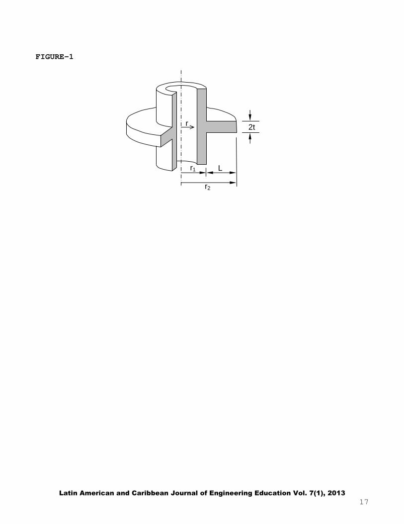
An annular fin of uniform thickness

dissipating heat by convection from a round tube

or circular rod to a surrounding fluid is sketched

in Fig. 1. The three fin dimensions are: uniform

thickness2t , inner radius 1r and outer radius 2r .


5

In the modeling, the classical Murray-Gardner

assumptions (Murray [6], Gardner [8]) are

adopted: steadiness in heat flow; constant

thermal conductivity k ; uniform heat transfer

coefficient h ; unvarying fluid temperature Tf;

prescribed fin base temperature Tb;

preponderance of radial temperature gradients

over transversal temperature gradients; negligible

heat transfer at the outermost fin section (i.e.,

adiabatic fin tip); and null heat sources or sinks.

Accordingly, the governing quasi one-

dimensional fin equation framed in cylindrical

coordinates is

21)( rrrin0 = TT rkt

h

dr

dTr

dr

d f ≤≤−−

(1)

or in an alternate expanded form

where tkh=2β is called the thermo-geometric

parameter [1]. As far as the classification of Eq.

(2) is concerned, it is a non-homogeneous

differential equation of second order with

variable coefficients, wherein the variable

coefficient r1 is of intricate form.

The proper boundary conditions implying

prescribed temperature at the fin base r1 and zero

heat loss at the fin tip r2 are

Fundamentally speaking, when a body

surface is extended by a protruding fin of any

shape, the external convective resistance Rc

decreases because the surface area is increased,

but on the other hand the internal conductive

resistance Rk increases because heat is

conducted through the fin, before being

convected to the fluid.

Calculation of the heat transfer from an annular

fin of uniform thickness to a surrounding fluid

can be carried out directly in two ways:

(1) differentiating T(r) at the fin base r = r1:

dr

rdTrtk

dr

rdTkAQ b

)(4

)( 11

11 π−=−=

(4a)

or (2) integrating T(r) over the fin surface S:

∫∫ −=−= 2

1

)(4)(2

r

r fS f drrTThdSTThQ π

(4b)

212

2)( rrrin0 = TT

dr

dT

r

1 +

dr

Td f

2

≤≤−− β

(2)

0 = dr

rdT and T = rT b

)()( 2

1

(3a, 3b)


6

Clearly, Eq. (4a) is easier to implement.

Upon introducing the normalized

dimensionless temperature ( ) ( )fbf TTTT −− and

the normalized dimensionless radial

coordinate 2rrR = , the parameter 21 rrc =

emerges as the normalized radii ratio. Thereby,

Eq. (2) is transformed to

2

21

(1 )

2

2

1 dd + = 0 in c Rd R dR cR

θ θ ξ θ− ≤ ≤−

(5)

along with the boundary conditions

(1)( )

d c = 1 and = 0

dR

θθ

(6a,6b)

Eq. (5) is named the modified Bessel equation of

zero order (Polyanin and Zaitsev [9]).

Despite that the transversal Biot number khtBi = is the natural reference parameter in fin heat transfer analysis

2

2 1r rhtEBi

k t

− =

(or 2ξ for short) seems to be a better parameter

for the annular fin of uniform thickness under

study. Herein, the fin slenderness ratio is defined

as the length 2 1L r r= − divided by the semi-

thickness t.

Conversely, the heat transfer Q from any

fin can be estimated indirectly using the concept

of dimensionless heat transfer or fin efficiency

iQQ=η as proposed by Gardner [8]. In here,

iQ is an ideal heat transfer from an identical

reference fin maintained at the base temperature

Tb (equivalent to an ideal material with infinite

thermal conductivity k →∞ ). For the specific

case of annular fins of uniform thickness, the

ideal heat transfer is given by

)()(2 21

22 fbi TThrrQ −−= π

As noted before the computation of η may be

carried out in two different ways:

(1) by differentiation of ( )Rθ at the fin

base leading to

( )1 2

2 11 ( )

1

c c d c =

c dR

θηξ

− − +

or (2) by integration of ( )Rθ over the fin

surface, resulting in


7

2 2

2( )

11

c = R R dRc

η θ ∫ −

(7b)

At the end, the magnitude of heat transfer Q is

obtainable with the expression

[ ])()(2 21

22 fbi TThrrQQ −−== πηη

(7c)

where η comes from either Eq. (7a) or (7b).

3. Exact Calculation Procedure

The exact analytic solution of Eqs. (5)

and (6) gives way to the exact dimensionless

temperature profile ( )Rθ as found in [3]:

1 0 0 1

1 0 0 1

) (I ( )K ( R I ( R)K ) (R) =

I ( )K ( c) I ( c)K ( )

γ γ γ γθγ γ γ γ

++

(8)

where (*)vI and (*)vK are the modified Bessel

functions of first and second kind, both of order

v and γ stands for the dimensionless group

)1/( c−ξ (see Nomenclature).

On the other hand, the safe-touch

temperature of hot bodies is an important issue

for the safety of technical personnel working in

plant environments (Arthur and Anderson [10]).

In this regard, the fin tips of annular fins of

uniform thickness are prone to be touched

accidentally. Because of this, the fin tip

temperature )r(T 2 is considered by design

engineers as a “parameter of relevance”.

Therefore, the exact dimensionless tip

temperature θ(1) follows from Eq. (8),

1 0 0 1

1 0 0 1

( ) ( ) ( ) ( )(1)

( ) ( ) ( ) ( )

I K I K

I K c I c K

γ γ γ γθγ γ γ γ

+=+

(9)

Further, the two η −avenues in Eqs. (7a)

and (7b) coalesce into the exact fin efficiency

1 1 1 1

1 0 0 1

1 2

1

I ( )K ( c) I ( c) K ( )c =

c I ( )K ( c) + I ( c) K ( )

γ γ γ γηξ γ γ γ γ

− +

(10)

Numerical evaluations of the sequence of Eqs.

(8)–(10) are elaborate and time-consuming, even

with contemporary symbolic algebra codes, like

Mathematica, Maple and Matlab.

4. Approximate Calculation Procedure

The idea behind the mean value theorem

for integration boils down to replacing an

auxiliary function in a certain closed interval by

an equivalent representative number. From

Differential Calculus (Stewart [11]), the mean


8

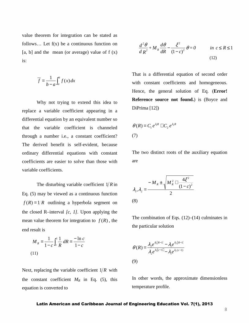
value theorem for integration can be stated as

follows… Let f(x) be a continuous function on

[a, b] and the mean (or average) value of f (x)

is:

∫−=

b

adxxf

abf )(

1

Why not trying to extend this idea to

replace a variable coefficient appearing in a

differential equation by an equivalent number so

that the variable coefficient is channeled

through a number i.e., a constant coefficient?

The derived benefit is self-evident, because

ordinary differential equations with constant

coefficients are easier to solve than those with

variable coefficients.

The disturbing variable coefficient R1 in

Eq. (5) may be viewed as a continuous function

RRf 1)( = outlining a hyperbola segment on

the closed R–interval [c, 1]. Upon applying the

mean value theorem for integration to )(Rf , the

end result is

c

cdR

RcM

cR −−=

−= ∫ 1

ln11

1 1

(11)

Next, replacing the variable coefficient R1 with

the constant coefficient MR in Eq. (5), this

equation is converted to

1)1( 2

2

≤≤−

− Rcin0 = c

dR

d M+

Rdd R2

2

θξθθ

(12)

That is a differential equation of second order

with constant coefficients and homogeneous.

Hence, the general solution of Eq. (Error!

Reference source not found.) is (Boyce and

DiPrima [12])

1 21 2( ) R RR C e C eλ λθ = +

(7)

The two distinct roots of the auxiliary equation

are

2

)1(4

,2

22

21

cMM RR −

+±−=

ξ

λλ

(8)

The combination of Eqs. (12)–(14) culminates in

the particular solution

( ) ( )

( )

1 2

1 2

1 12 1

1 ( 1)2 1

( )R R

c c

e eR

e e

λ λ

λ λ

λ λθλ λ

− −

− −

−=−

(9)

In other words, the approximate dimensionless

temperature profile.


9

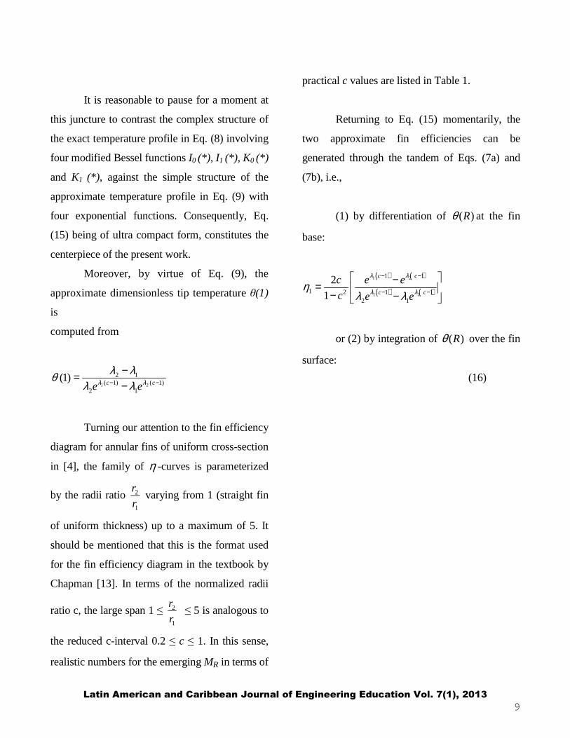
It is reasonable to pause for a moment at

this juncture to contrast the complex structure of

the exact temperature profile in Eq. (8) involving

four modified Bessel functions I0 (*), I1 (*), K0 (*)

and K1 (*), against the simple structure of the

approximate temperature profile in Eq. (9) with

four exponential functions. Consequently, Eq.

(15) being of ultra compact form, constitutes the

centerpiece of the present work.

Moreover, by virtue of Eq. (9), the

approximate dimensionless tip temperature θ(1)

is

computed from

1 2

2 1( 1) ( 1)

2 1

(1)c ce eλ λλ λθ

λ λ− −

−=−

(16)

Turning our attention to the fin efficiency

diagram for annular fins of uniform cross-section

in [4], the family of η -curves is parameterized

by the radii ratio 1

2

r

r varying from 1 (straight fin

of uniform thickness) up to a maximum of 5. It

should be mentioned that this is the format used

for the fin efficiency diagram in the textbook by

Chapman [13]. In terms of the normalized radii

ratio c, the large span 1 ≤ 1

2

r

r ≤ 5 is analogous to

the reduced c-interval 0.2 ≤ c ≤ 1. In this sense,

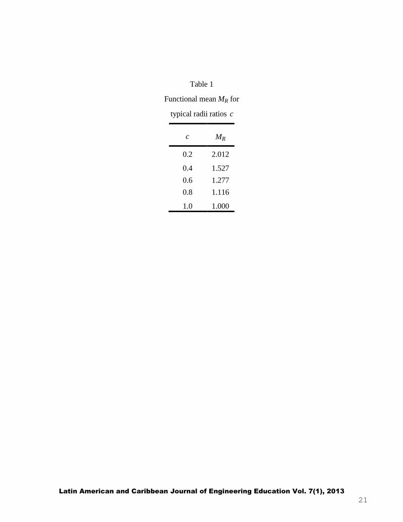
realistic numbers for the emerging MR in terms of

practical c values are listed in Table 1.

Returning to Eq. (15) momentarily, the

two approximate fin efficiencies can be

generated through the tandem of Eqs. (7a) and

(7b), i.e.,

(1) by differentiation of ( )Rθ at the fin

base:

( ) ( )

( ) ( )

1 2

1 2

1 1

1 2 1 12 1

2

1

c c

c c

c e e

c e e

λ λ

λ ληλ λ

− −

− −

−= − −

or (2) by integration of ( )Rθ over the fin

surface:


10

( ) ( ) ( ) ( )

( ) ( )

1 2

1 2

1 13 32 1 1 1 2 2

2 2 1 12 21 2 2 1

1 1 1 12

1

c c

c c

c e c e

c e e

λ λ

λ λ

λ λ λ λ λ λη

λ λ λ λ

− −

− −

− + − − − + − = − −

(17b)

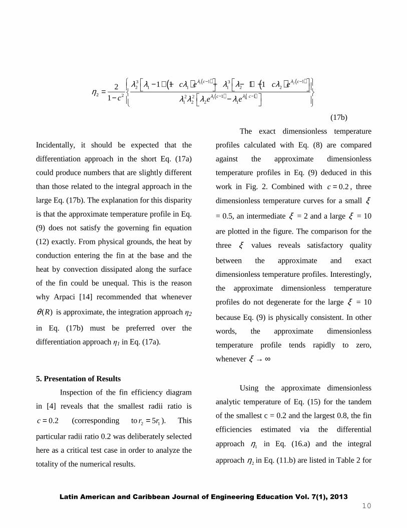
Incidentally, it should be expected that the

differentiation approach in the short Eq. (17a)

could produce numbers that are slightly different

than those related to the integral approach in the

large Eq. (17b). The explanation for this disparity

is that the approximate temperature profile in Eq.

(9) does not satisfy the governing fin equation

(12) exactly. From physical grounds, the heat by

conduction entering the fin at the base and the

heat by convection dissipated along the surface

of the fin could be unequal. This is the reason

why Arpaci [14] recommended that whenever

( )Rθ is approximate, the integration approach η2

in Eq. (17b) must be preferred over the

differentiation approach η1 in Eq. (17a).

5. Presentation of Results

Inspection of the fin efficiency diagram

in [4] reveals that the smallest radii ratio is

0.2c = (corresponding to2 15r r= ). This

particular radii ratio 0.2 was deliberately selected

here as a critical test case in order to analyze the

totality of the numerical results.

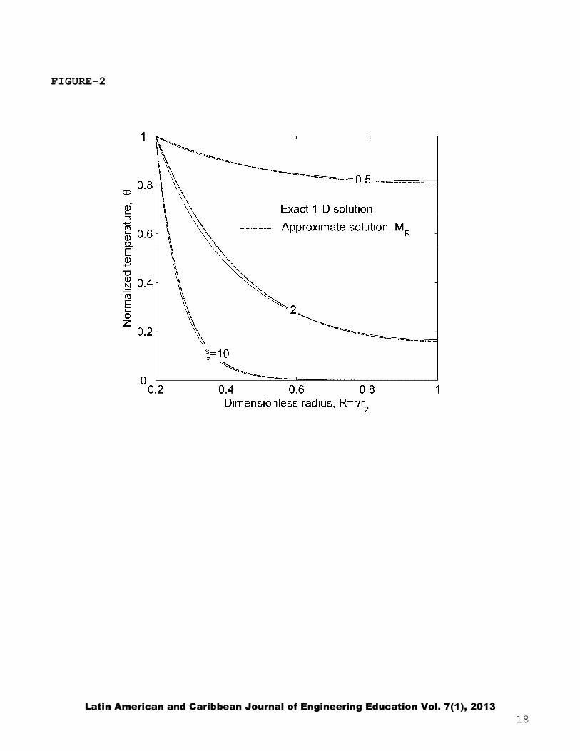
The exact dimensionless temperature

profiles calculated with Eq. (8) are compared

against the approximate dimensionless

temperature profiles in Eq. (9) deduced in this

work in Fig. 2. Combined with 0.2c = , three

dimensionless temperature curves for a small ξ

= 0.5, an intermediate ξ = 2 and a large ξ = 10

are plotted in the figure. The comparison for the

three ξ values reveals satisfactory quality

between the approximate and exact

dimensionless temperature profiles. Interestingly,

the approximate dimensionless temperature

profiles do not degenerate for the large ξ = 10

because Eq. (9) is physically consistent. In other

words, the approximate dimensionless

temperature profile tends rapidly to zero,

whenever ξ → ∞

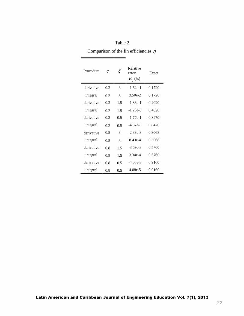
Using the approximate dimensionless

analytic temperature of Eq. (15) for the tandem

of the smallest c = 0.2 and the largest 0.8, the fin

efficiencies estimated via the differential

approach 1η in Eq. (16.a) and the integral

approach 2η in Eq. (11.b) are listed in Table 2 for


11

the trio of ξ = 0.5, 1.5 and 3. The exact fin

efficiencies η computed from Eq. (10) range

from 0.1720 for the pair c = 0.2 and ξ = 3 to

0.916 for the pair c = 0.8 and ξ = 0.5. In Table 2,

the relative error in the efficiency Eη is defined

as:

.approx exact

exact

Eη

η ηη

−=

(18)

First, for the smallest c = 0.2, the relative errors

Eη for the differential-based 1η vary from -1.62e-

1 when ξ = 3 to -1.77e-1 when ξ = 0.5. Second,

for the largest c = 0.8, the relative errors Eη for

the differential-based 1η vary from -2.88e-3

when ξ = 3 to -4.08e-1 when ξ = 0.5. Third, for

the smallest c = 0.2, the relative errors Eη for the

integral-based 2η vary from 3.5e-2 when ξ = 3

to -4.37e-3 when ξ = 0.5. Fourth, for the largest

c = 0.8, the relative errors Eη for the integral-

based 2η vary from -8.43e-4 when ξ = 3 to

4.08e-5 when ξ = 0.5. As may be seen, all

relative errors Eη are insignificant. Moreover, the

fin efficiency conveyed through the integral-

based η 2 furnishes more accurate results than the

alternate derivative-based η 1. Again, this

statement is in harmony with the

recommendations made in [Error! Reference

source not found.].

As the numbers listed in Table 2

demonstrate, the differences between the fin

efficiency results based on the integral approach

and the derivative approach diminish for large

values of c . In fact, in the limiting case

corresponding to 1c = , the approximate and the

exact predictions coincide, both magnitudes

collapsing into:

1

tanh( )c

ξηξ= =

This expression can be easily deduced from the

approximate Eqs. (11) taking into account that

the roots confirm that 1,2(1 )cλ ξ− → ± whenever

1c → . It should also be noted that Eq. (13)

stands for the fin efficiency for a longitudinal fin

of uniform thickness [3,4] and same ξ , which is

a logical similitude owing to the null curvature in

the annular fin when c tends to unity and L is

maintained constant.

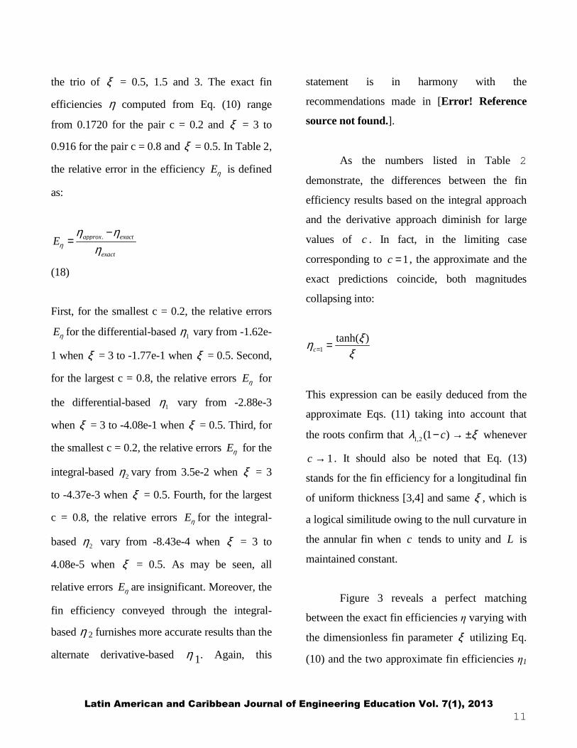
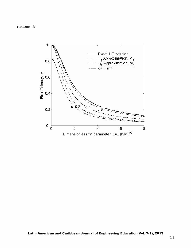
Figure 3 reveals a perfect matching

between the exact fin efficiencies η varying with

the dimensionless fin parameter ξ utilizing Eq.

(10) and the two approximate fin efficiencies η1


12

and η2 for c = 0.4 and 0.8 employing Eqs. (17a)

and (17b). However, for the smallest c = 0.2, η1

deteriorates, whereas η2 being more robust

provides good results.

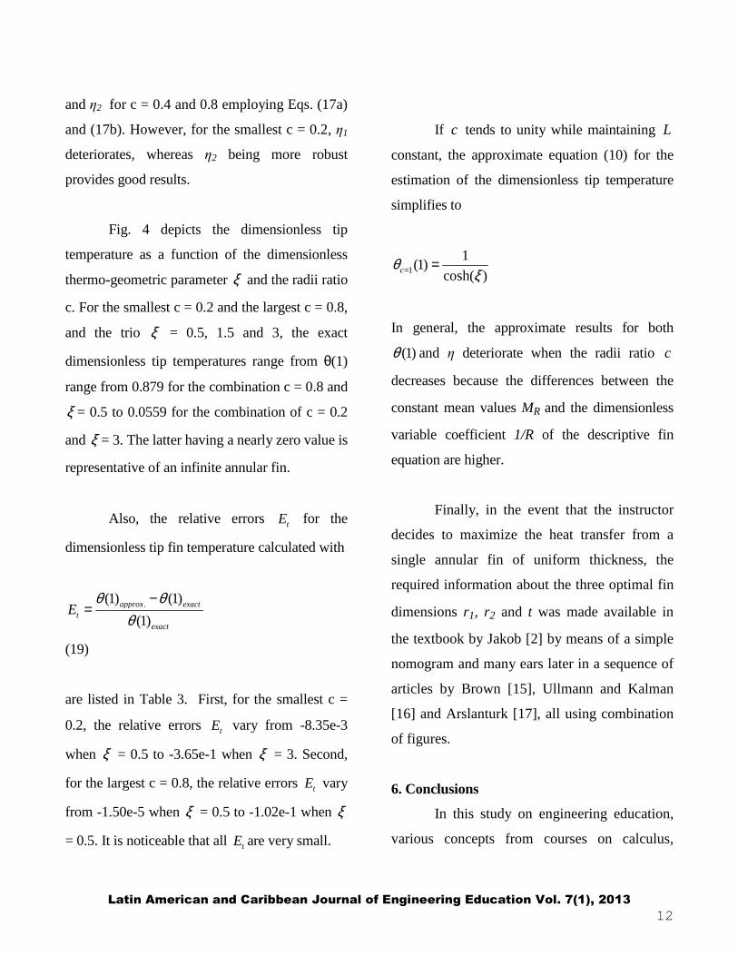
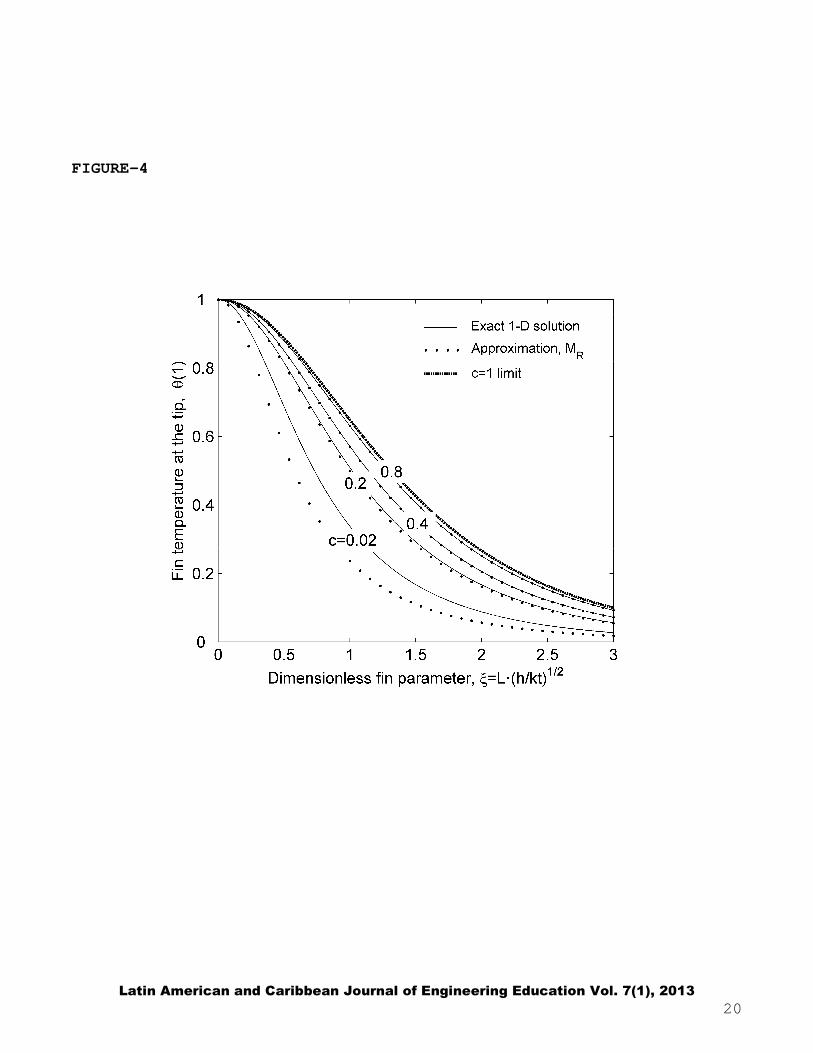
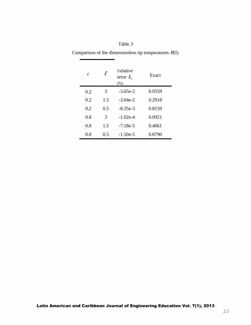
Fig. 4 depicts the dimensionless tip

temperature as a function of the dimensionless

thermo-geometric parameter ξ and the radii ratio

c. For the smallest c = 0.2 and the largest c = 0.8,

and the trio ξ = 0.5, 1.5 and 3, the exact

dimensionless tip temperatures range from θ(1)

range from 0.879 for the combination c = 0.8 and

ξ = 0.5 to 0.0559 for the combination of c = 0.2

and ξ = 3. The latter having a nearly zero value is

representative of an infinite annular fin.

Also, the relative errors tE for the

dimensionless tip fin temperature calculated with

.(1) (1)

(1)approx exact

texact

Eθ θ

θ−

=

(19)

are listed in Table 3. First, for the smallest c =

0.2, the relative errors tE vary from -8.35e-3

when ξ = 0.5 to -3.65e-1 when ξ = 3. Second,

for the largest c = 0.8, the relative errors tE vary

from -1.50e-5 when ξ = 0.5 to -1.02e-1 when ξ

= 0.5. It is noticeable that all tE are very small.

If c tends to unity while maintaining L

constant, the approximate equation (10) for the

estimation of the dimensionless tip temperature

simplifies to

1

1(1)

cosh( )cθξ= =

In general, the approximate results for both

(1)θ and η deteriorate when the radii ratio c

decreases because the differences between the

constant mean values MR and the dimensionless

variable coefficient 1/R of the descriptive fin

equation are higher.

Finally, in the event that the instructor

decides to maximize the heat transfer from a

single annular fin of uniform thickness, the

required information about the three optimal fin

dimensions r1, r2 and t was made available in

the textbook by Jakob [2] by means of a simple

nomogram and many ears later in a sequence of

articles by Brown [15], Ullmann and Kalman

[16] and Arslanturk [17], all using combination

of figures.

6. Conclusions

In this study on engineering education,

various concepts from courses on calculus,


13

ordinary differential equations and heat transfer

have been blended in a unique way. In analyzing

annular fins of uniform thickness, the mean value

theorem for integration is used for simplifying

the descriptive quasi one-dimensional fin

equation, namely the modified Bessel differential

equation. This gives way to the approximate

temperature solutions endowed with an

unsurpassed combination of accuracy and

easiness. Differences between the analytic

temperature approximations developed in the

present work and the classical exact analytic

temperature profiles relying on four modified

Bessel functions are probably below the level of

inaccuracy introduced by the Murray-Gardner

assumptions.

References

1. Boelter, L. M. K., Cherry, V. H., Johnson, H.

A. and Martinelli, R. C., Heat Transfer Notes,

pp. IIB18-IIB19, University of California Press,

Berkeley, CA and Los Angeles, CA, 1946.

2. Jakob, M., Heat Transfer, Vol. 1, pp. 232-234,

John Wiley, New York, NY, 1949.

3. Mills, A. F., Heat and Mass Transfer, 2nd

edition, pp. 90-93, Prentice-Hall, Upper Saddle

River, NJ, 1999.

4. Incropera, F.P. and DeWitt, D.P.,

Introduction to Heat Transfer, 4th edition, pp.

139-140, John Wiley, New York, NY, 2002.

5. Harper, D. R. and Brown, W. B.,

Mathematical Equations for Heat Conduction in

the Fins of Air-Cooled Engines, NACA Report

No. 158, 1922.

6. Murray, W. M., Heat dissipation through an

annular disk or fin of uniform thickness, Journal

of Applied Mechanics, Transactions of ASME,

Vol. 60, p. A-78, 1938.

7. Carrier, W. H. and Anderson, S. W., The

resistance to heat flow through finned tubing,

Heating, Piping, and Air Conditioning, Vol. 10,

pp. 304-320, 1944.

8. Gardner, K. A., Efficiency of extended

surfaces, Transactions of ASME, Vol. 67, pp.

621-631, 1945.

9. Polyanin, A. D. and Zaitsev, V. F., Handbook

of Exact Solutions for Differential Equations,

CRC Press, Boca Raton, FL, 1995.

10. Arthur, K. and Anderson, A., Too hot to

handle?: An investigation into safe touch

temperatures. In Proceedings of the ASME

International Mechanical Engineering Congress

and Exposition (IMECE), pp. 11-17, Anaheim,


14

CA, 2004.

11. Stewart, J., Single Variable Calculus, 3th

edition, Brooks/Cole, Pacific Groove, CA, 2002.

12. Boyce, W. E. and DiPrima R. C., Elementary

Differential Equations and Boundary Value

Problems, 7th edition, John Wiley, New York,

NY, 2001.

13. Chapman, A. J., Fundamentals of Heat

Transfer, 5th edition, MacMillan, New York, NY,

1987.

14. Arpaci, V., Conduction Heat Transfer,

Addison-Wesley, Reading, MA, 1966.

15. Brown, A., Optimum dimensions of uniform

annular fins, International Journal of Heat and

Mass Transfer, Vol. 8, pp. 655-662, 1965.

16. Ullmann, A. and Kalman, H., Efficiency and

optimized dimensions of annular fins of

different cross-section shapes, International

Journal of Heat and Mass Transfer, Vol. 32, pp.

1105-1110, 1989.

17. Arslanturk, C., Simple correlation equations

for optimum design of annular fins with uniform

thickness, Applied Thermal Engineering, Vol.

25, pp. 2463-2468, 2005.


15

List of Figures:

Fig. 1. Sketch of an annular fin of uniform thickness

Fig. 2. Comparison between the approximate and exact dimensionless temperature profiles for a fixed

normalized radii ratio 0.2c = when combined with three different fin parameters ξ .

Fig. 3. Comparison between the approximate and exact fin efficiencies as a function of the dimensionless

fin parameter ξ for different normalized radii ratios c .

Fig. 4. Comparison between the approximate and exact tip temperatures as a function of the dimensionless

fin parameter ξ for different normalized radii ratios c .


16

List of Tables:

Table 1. Functional mean MR in terms of the normalized radii ratio c

Table 2. Comparison of the fin efficiencies η

Table 3. Comparison of the dimensionless fin tip temperatures θ (1)


17

FIGURE-1

2t

r1

r2

L

r


18

FIGURE-2


19

FIGURE-3


20

FIGURE-4


21

Table 1

Functional mean MR for

typical radii ratios c

c MR

0.2 2.012

0.4 1.527

0.6 1.277

0.8 1.116

1.0 1.000


22

Table 2

Comparison of the fin efficiencies η

Procedure c ξ Relative error

Eη (%)

Exact

derivative 0.2 3 -1.62e-1 0.1720

integral 0.2 3 3.50e-2 0.1720

derivative 0.2 1.5 -1.83e-1 0.4020

integral 0.2 1.5 -1.25e-3 0.4020

derivative 0.2 0.5 -1.77e-1 0.8470

integral 0.2 0.5 -4.37e-3 0.8470

derivative 0.8 3 -2.88e-3 0.3068

integral 0.8 3 8.43e-4 0.3068

derivative 0.8 1.5 -3.69e-3 0.5760

integral 0.8 1.5 3.34e-4 0.5760

derivative 0.8 0.5 -4.08e-3 0.9160

integral 0.8 0.5 4.08e-5 0.9160


23

Table 3

Comparison of the dimensionless tip temperatures )1(θ

c ξ Relative error tE (%)

Exact

0.2 3 -3.65e-2 0.0559

0.2 1.5 -3.04e-2 0.2918

0.2 0.5 -8.35e-3 0.8159

0.8 3 -1.02e-4 0.0921

0.8 1.5 -7.18e-5 0.4061

0.8 0.5 -1.50e-5 0.8790

Automotive

62 192-2-pb (2)