BAYESIAN RISK ASSESSMENT OF AUTONOMOUS VEHICLES

Christos KatrakazasMohammed Quddus

Wen-Hua Chen*

Transport Studies GroupSchool of Civil and Building Engineering

*Department of Aeronautics and Automobile EngineeringLoughborough University

NORTHMOST 01: ITS-Leeds Monday 12th Dec.

Overview

Introduction to the problem

Bayesian & Dynamic Bayesian Networks (DBN)

DBN models and risk assessment of autonomous vehicles

- Variables, estimation of probabilities and inference

Preliminary findings

Potential contribution

3

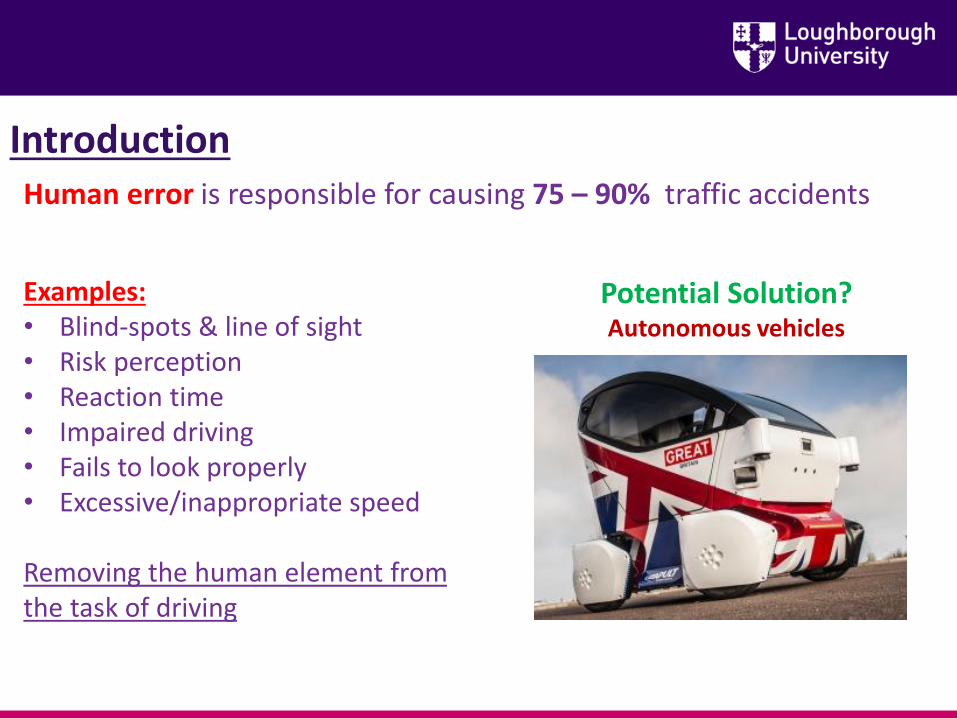
IntroductionHuman error is responsible for causing 75 – 90% traffic accidents

Examples:• Blind-spots & line of sight• Risk perception• Reaction time • Impaired driving• Fails to look properly• Excessive/inappropriate speed

Removing the human element from the task of driving

Potential Solution?Autonomous vehicles

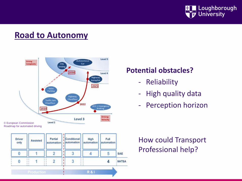
Road to Autonomy

Potential obstacles?

- Reliability

- High quality data

- Perception horizon

How could Transport Professional help?

4

© European Commission

Roadmap for automated driving

5

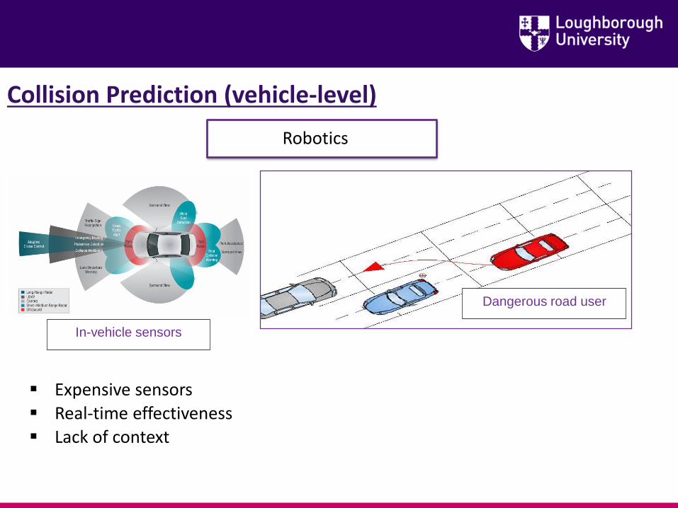
Robotics

Expensive sensors

Real-time effectiveness

Lack of context

Collision Prediction (vehicle-level)

In-vehicle sensors

Dangerous road user

6

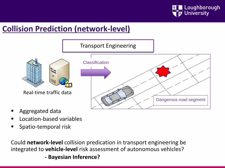
Transport Engineering

Aggregated data

Location-based variables

Spatio-temporal risk

Could network-level collision predication in transport engineering be integrated to vehicle-level risk assessment of autonomous vehicles?

- Bayesian Inference?

Collision Prediction (network-level)

Dangerous road segment

Classification

Real-time traffic data

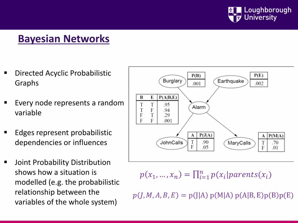
Bayesian Networks

Directed Acyclic Probabilistic Graphs

Every node represents a random variable

Edges represent probabilistic dependencies or influences

Joint Probability Distribution shows how a situation is modelled (e.g. the probabilistic relationship between the variables of the whole system)

7

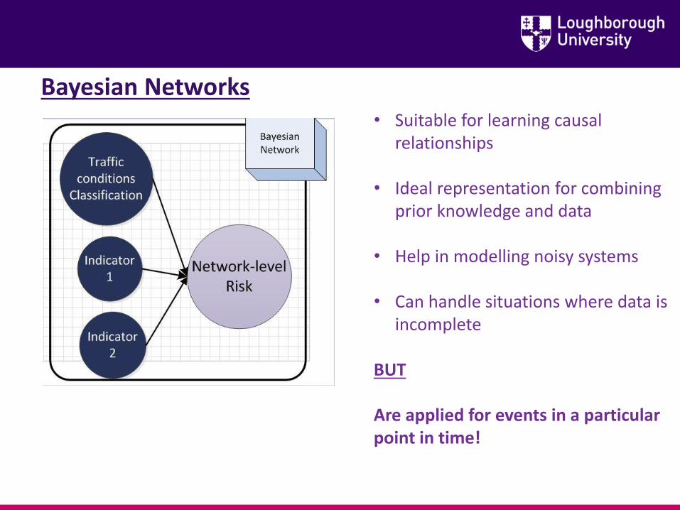
Bayesian Networks• Suitable for learning causal

relationships

• Ideal representation for combining prior knowledge and data

• Help in modelling noisy systems

• Can handle situations where data is incomplete

BUT

Are applied for events in a particular point in time!

8

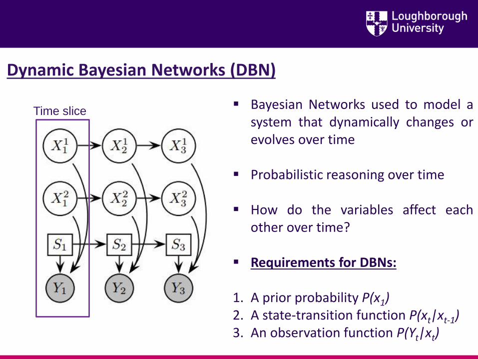
Dynamic Bayesian Networks (DBN)

Bayesian Networks used to model asystem that dynamically changes orevolves over time

Probabilistic reasoning over time

How do the variables affect eachother over time?

Requirements for DBNs:

1. A prior probability P(x1)2. A state-transition function P(xt|xt-1)3. An observation function P(Yt|xt)

Time slice

9

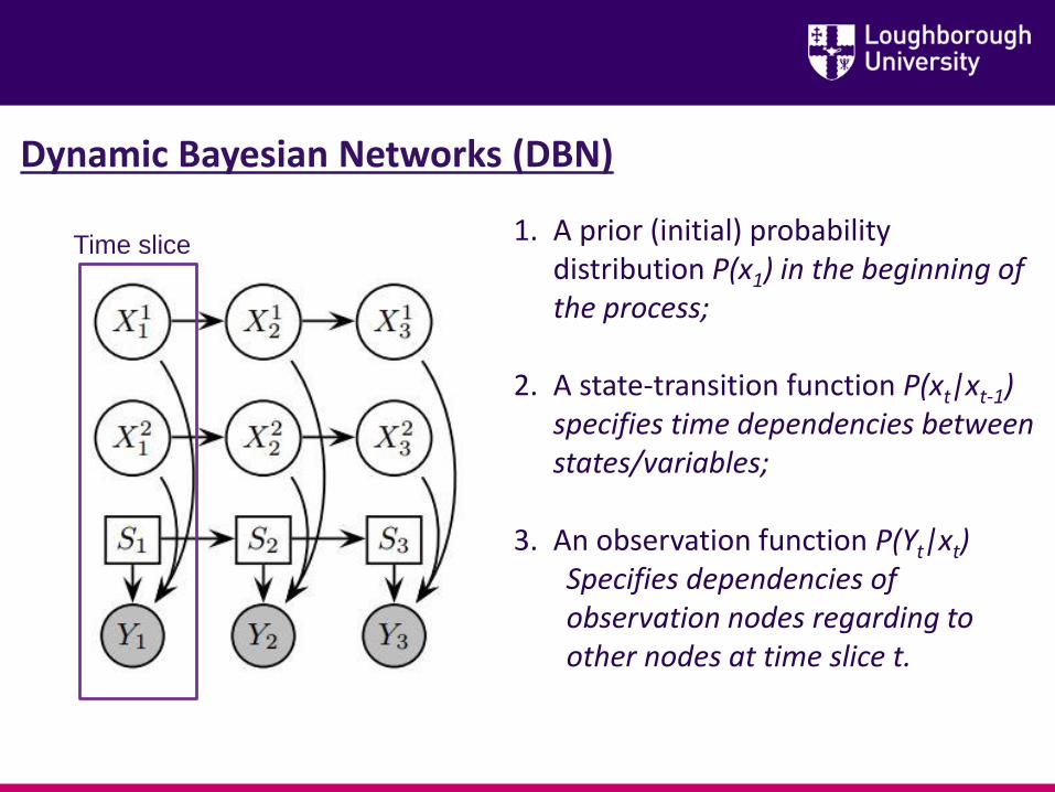
Dynamic Bayesian Networks (DBN)

1. A prior (initial) probability distribution P(x1) in the beginning of the process;

2. A state-transition function P(xt|xt-1) specifies time dependencies between states/variables;

3. An observation function P(Yt|xt)Specifies dependencies of observation nodes regarding to other nodes at time slice t.

10

Time slice

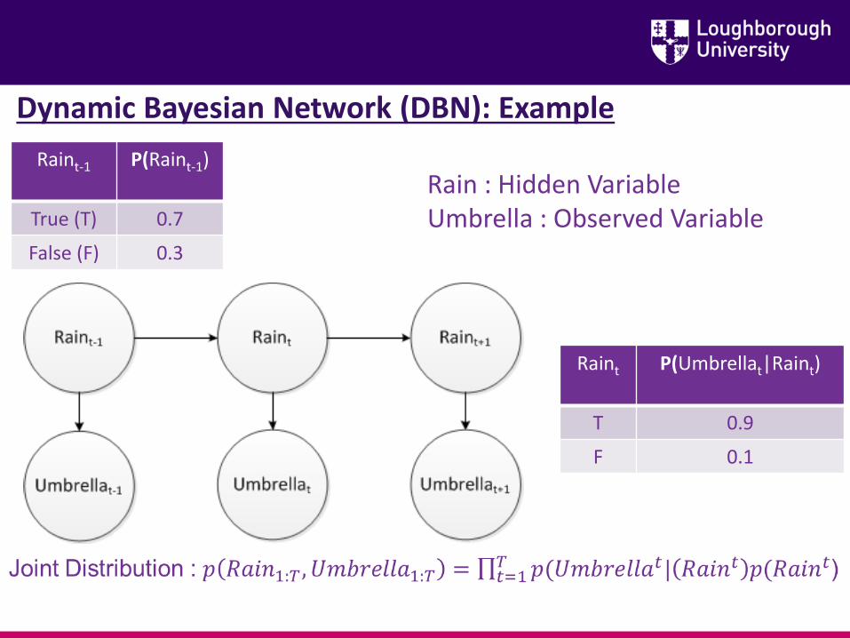
Dynamic Bayesian Network (DBN): Example

Raint-1 P(Raint-1)

True (T) 0.7

False (F) 0.3

Raint P(Umbrellat|Raint)

T 0.9

F 0.1

Rain : Hidden Variable Umbrella : Observed Variable

11

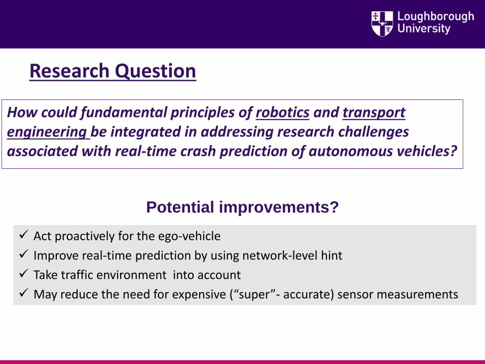
Research Question

How could fundamental principles of robotics and transport engineering be integrated in addressing research challenges associated with real-time crash prediction of autonomous vehicles?

Act proactively for the ego-vehicle

Improve real-time prediction by using network-level hint

Take traffic environment into account

May reduce the need for expensive (“super”- accurate) sensor measurements

Potential improvements?

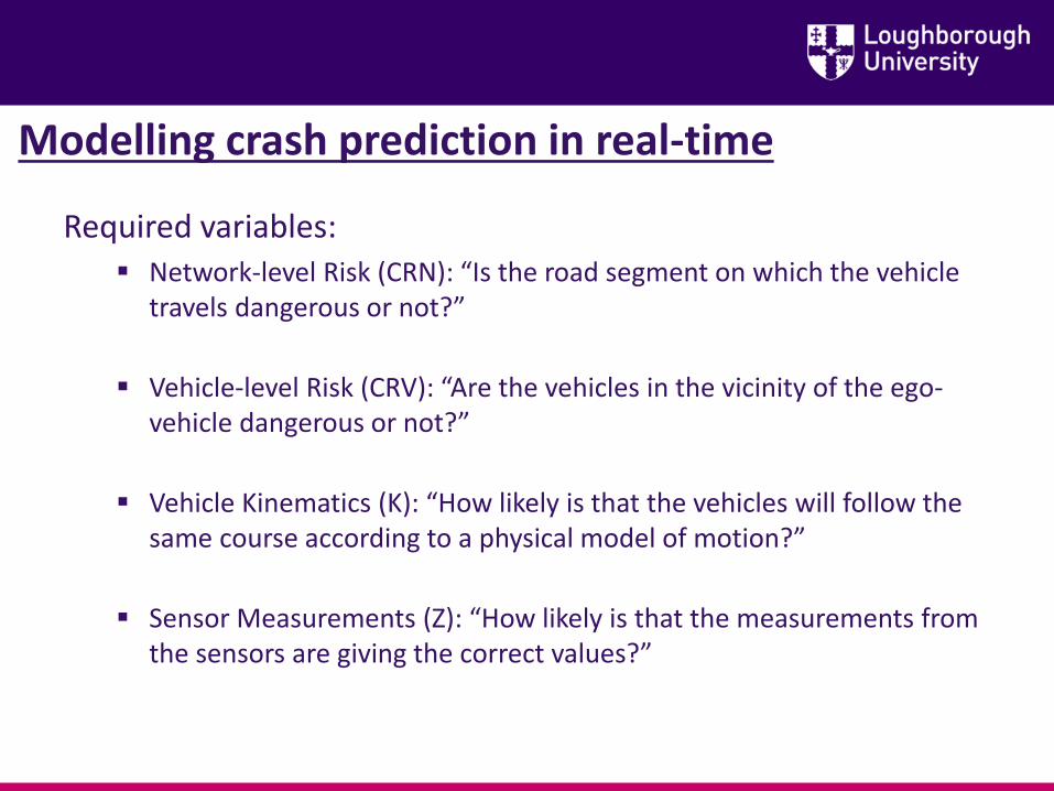
Modelling crash prediction in real-time

Required variables: Network-level Risk (CRN): “Is the road segment on which the vehicle

travels dangerous or not?”

Vehicle-level Risk (CRV): “Are the vehicles in the vicinity of the ego-vehicle dangerous or not?”

Vehicle Kinematics (K): “How likely is that the vehicles will follow the same course according to a physical model of motion?”

Sensor Measurements (Z): “How likely is that the measurements from the sensors are giving the correct values?”

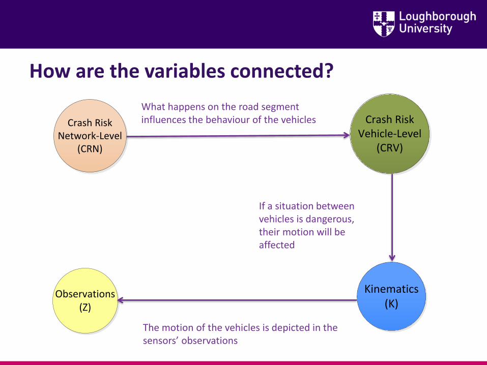
How are the variables connected?

Observations(Z)

Kinematics(K)

Crash RiskVehicle-Level

(CRV)

Crash RiskNetwork-Level

(CRN)

What happens on the road segment influences the behaviour of the vehicles

If a situation between vehicles is dangerous, their motion will be affected

The motion of the vehicles is depicted in the sensors’ observations

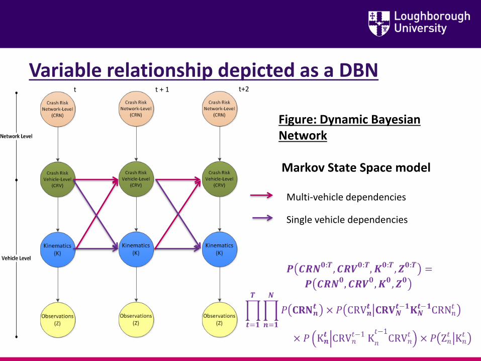
Variable relationship depicted as a DBNt t + 1 t+2

Figure: Dynamic Bayesian Network

Markov State Space model

Multi-vehicle dependencies

Single vehicle dependencies

Use traffic flow parameters to estimate the risk of an accident happening in real-time

Compare & Contrast traffic conditions just before an accident with normal conditions

Data: Highways England & DfT

• 15-min Traffic flow data (HATRIS JTDB)

• Historical Accident data (STATS 19)

• Traffic microsimulation (PTV VISSIM) -> 30second traffic data

Method : Machine learning classifiers (i.e. SVMs, RVMs, Random Forests, k-Nearest Neighbours)

Network – Level Risk

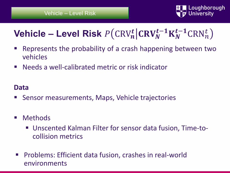
Represents the probability of a crash happening between twovehicles

Needs a well-calibrated metric or risk indicator

Data

Sensor measurements, Maps, Vehicle trajectories

Methods

Unscented Kalman Filter for sensor data fusion, Time-to-collision metrics

Problems: Efficient data fusion, crashes in real-world environments

Vehicle – Level Risk

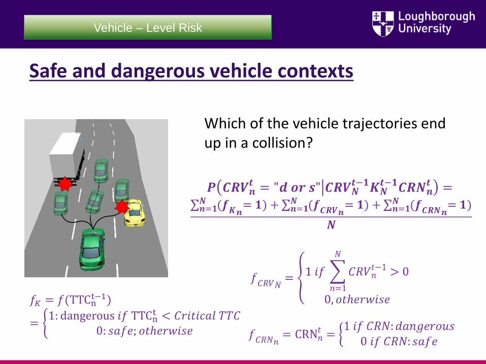
Safe and dangerous vehicle contexts

Which of the vehicle trajectories end up in a collision?

Vehicle – Level Risk

𝑓𝐾 = 𝑓(TTCnt−1)

= ቊ1: dangerous 𝑖𝑓 TTCn

t < 𝐶𝑟𝑖𝑡𝑖𝑐𝑎𝑙 𝑇𝑇𝐶0: 𝑠𝑎𝑓𝑒; 𝑜𝑡ℎ𝑒𝑟𝑤𝑖𝑠𝑒

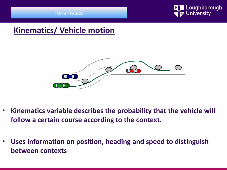
Kinematics/ Vehicle motion

Kinematics

• Kinematics variable describes the probability that the vehicle will follow a certain course according to the context.

• Uses information on position, heading and speed to distinguish between contexts

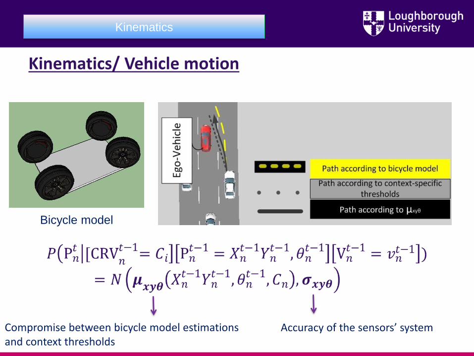
Kinematics/ Vehicle motion

Kinematics

Bicycle model

Compromise between bicycle model estimations and context thresholds

Accuracy of the sensors’ system

Sensor measurements

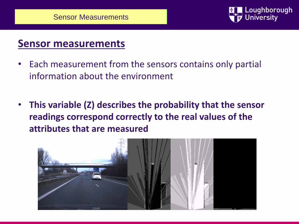
• Each measurement from the sensors contains only partial information about the environment

• This variable (Z) describes the probability that the sensor readings correspond correctly to the real values of the attributes that are measured

Sensor Measurements

Correct measurements probability

Sensor Measurements

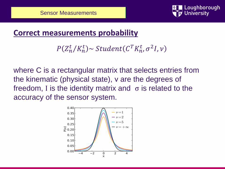
𝑃 Τ𝑍𝑛𝑡 𝐾𝑛

𝑡 ~ 𝑆𝑡𝑢𝑑𝑒𝑛𝑡 𝐶𝑇𝐾𝑛𝑡 , 𝜎2𝛪, 𝜈

where C is a rectangular matrix that selects entries from

the kinematic (physical state), ν are the degrees of

freedom, Ι is the identity matrix and σ is related to the

accuracy of the sensor system.

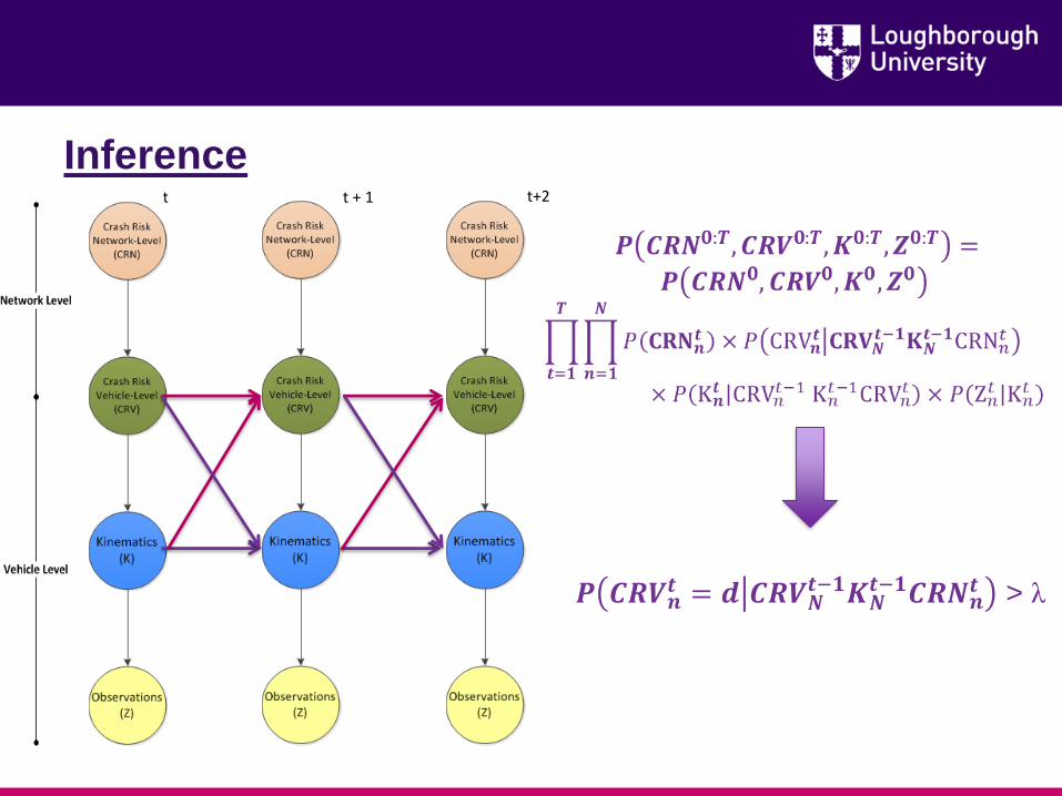
Inferencet t + 1 t+2

𝑷 𝑪𝑹𝑽𝒏𝒕 = 𝒅 𝑪𝑹𝑽𝑵

𝒕−𝟏𝑲𝑵𝒕−𝟏𝑪𝑹𝑵𝒏

𝒕 > λ

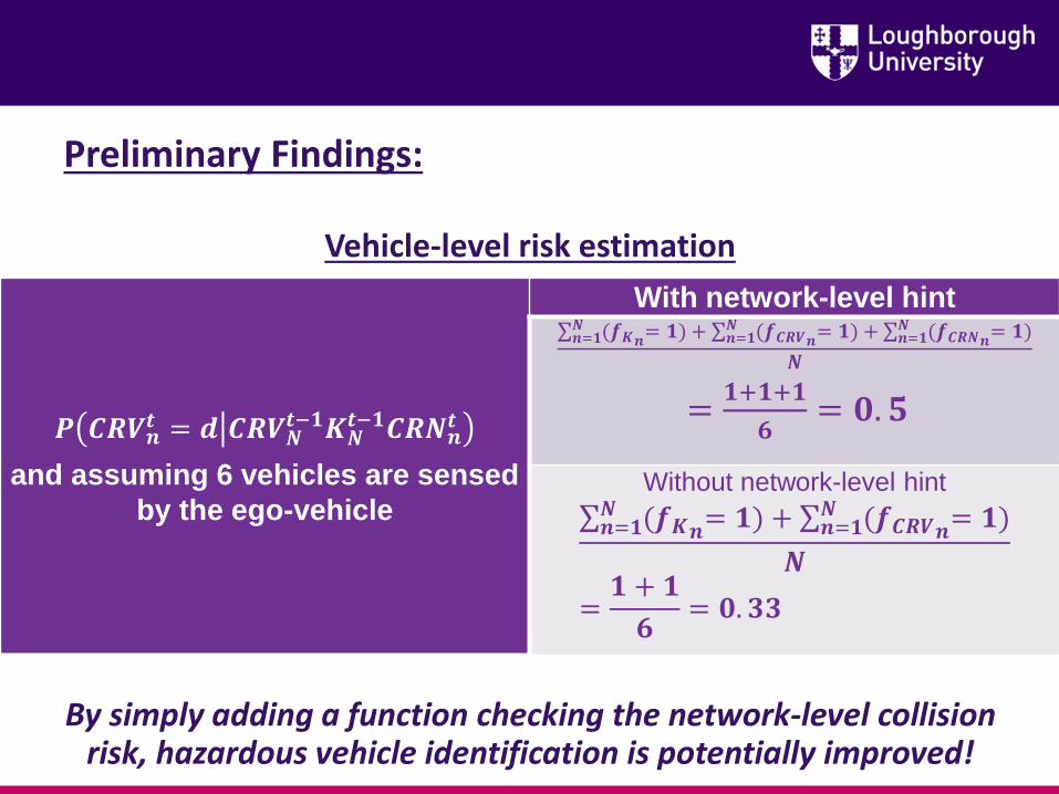
Preliminary Findings:

Vehicle-level risk estimation

𝑷 𝑪𝑹𝑽𝒏𝒕 = 𝒅 𝑪𝑹𝑽𝑵

𝒕−𝟏𝑲𝑵𝒕−𝟏𝑪𝑹𝑵𝒏

𝒕

and assuming 6 vehicles are sensed

by the ego-vehicle

With network-level hintσ𝒏=𝟏𝑵 (𝒇𝑲𝒏= 𝟏) + σ𝒏=𝟏

𝑵 (𝒇𝑪𝑹𝑽𝒏= 𝟏) + σ𝒏=𝟏𝑵 (𝒇𝑪𝑹𝑵𝒏= 𝟏)

𝑵

=𝟏+𝟏+𝟏

𝟔= 𝟎. 𝟓

Without network-level hint

σ𝒏=𝟏𝑵 (𝒇𝑲𝒏= 𝟏) + σ𝒏=𝟏

𝑵 (𝒇𝑪𝑹𝑽𝒏= 𝟏)

𝑵

=𝟏 + 𝟏

𝟔= 𝟎. 𝟑𝟑

By simply adding a function checking the network-level collision risk, hazardous vehicle identification is potentially improved!

25

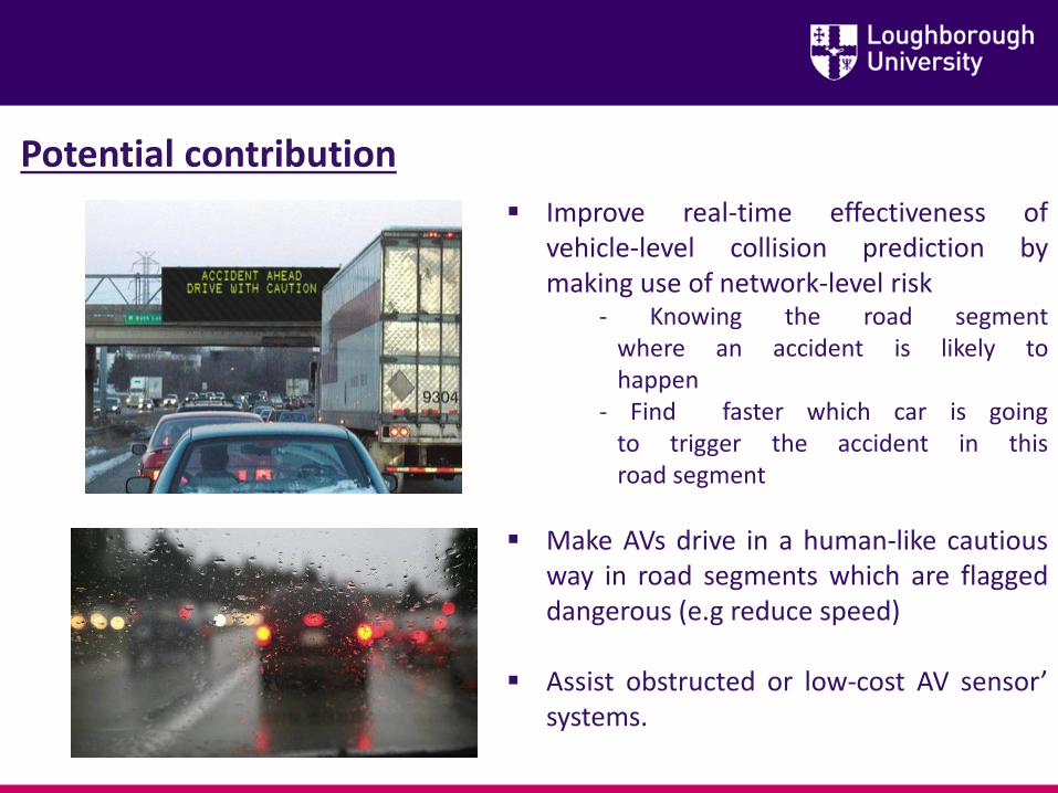
Potential contribution

Improve real-time effectiveness ofvehicle-level collision prediction bymaking use of network-level risk

- Knowing the road segmentwhere an accident is likely tohappen

- Find faster which car is goingto trigger the accident in thisroad segment

Make AVs drive in a human-like cautiousway in road segments which are flaggeddangerous (e.g reduce speed)

Assist obstructed or low-cost AV sensor’systems.

Inspiring Winners Since 1909

Thank you!

Christos Katrakazas

c.katrakazas@lboro.ac.uk