Embed Size (px)
DESCRIPTION
This topic is basically related to the econometric analysis and techniques used to develop the model for the calculation of expected stock returns taking into the account various fundamental or accounting variables of the respective stock. The model developed is basically an extension of Fama and French 3-factor model but it is for the calculation of return from individual stocks. The variables considered are all fundamental accounting variables. The technique used for the generating this proposed model is an advanced regression technique known as “panel regression technique”. To select the best model, all the four panel regression techniques i.e. Fixed One-Way, Fixed Two-Way Effect, Random One-Way and Random Two-Way Effect techniques have been used. For the development of the model, two econometrics softwares: SAS Enterprise Guide v3.0 and EVIEWS v7.0 have been used extensively. The factors affecting the return according to the model are supported by the theory also. A total of 6 fundamental factors have found to be significantly affecting the expected stock return along with the 3 factors from the Fama and French 3 factors model.
Citation preview

A REPORT
ON
DEVELOPMENT OF MARKET-WIDE STOCK
VALUATION MODEL (EXTENSION OF FAMA &
FRENCH MODEL) AND AN INDUSTRY
ANALYSIS OF IT AND CONSTRUCTION SECTOR
IN INDIA USING THIS MODEL
By
Saurabh Trivedi
10BSPHH011076

A REPORT
ON
DEVELOPMENT OF MARKET-WIDE STOCK
VALUATION MODEL (EXTENSION OF FAMA &
FRENCH MODEL) AND AN INDUSTRY ANALYSIS OF
IT AND CONSTRUCTION SECTOR IN INDIA USING
THIS MODEL
By
Saurabh Trivedi
10BSPHH011076
A report submitted in partial fulfillment of the requirements of MBA
Program of IBS Hyderabad
Submitted To
Project Guide:
Prof. Rajashekhar Reddy,
Marketing Department
Date of Submission: Friday, May 13th
, 2011

IBS HYDERABAD
CERTIFICATE
This is to certify that the thesis titled “Development Of Market-Wide Stock Valuation Model
(Extension Of Fama & French Model) And An Industry Analysis Of IT And Construction
Sector In India Using This Model” is a bonafide work done by Mr. Saurabh Trivedi,
Enrolment No. 10BSPHH011076, in partial fulfilment of the requirements for the award of any
degree and submitted to the Department of Finance & Economics, IBS Hyderabad.
This work was not submitted earlier at any other University or Institute for the award of the
degree.
Project Guide: Project Coordinator:
Prof. Rajashekhar Reddy Dr. Hilda Amalraj
Department of Marketing Dean of Academics
IBS-Hyderabad IBS-Hyderabad

SUMMER INTERNSHIP REPORT 2011
______________________________________________________________________________
IBS-Hyderabad i
I. Acknowledgement
I would take this opportunity to express my sincere gratitude to all the persons for their valuable
assistance and continuous support during my Summer Internship Program (SIP).
I would like to thank Mr. V. Rajanna, Vice President and General Manager, Tata Consultancy
Services, Hyderabad for giving me an opportunity to work with this department.
I would like to thank Dr. V.P. Gulati, Vice President and Head, TCS Business Domain
Academy, for giving me an opportunity to work with this department.
I am also thankful to Mr. J. Chandrasekhar, Academic Relationships Manager, Tata
Consultancy Services, for his helping hand throughout the internship process.
I am grateful to my company guide, Ms. Vasanta Tadimeti, Domain Consultant, TBDA, TCS
for her guidance and support during development of the project. Her inputs, motivation and
suggestions have played a crucial role at every stage in the development of the project.
I would like to thank the entire TBDA team and all my IBS colleagues at TCS who provided
their valuable inputs throughout the internship, which really helped in successful completion of
my project report.
Prof. Rajashekhar Reddy, Department of Marketing, IBS Hyderabad, my faculty guide,
with his continuous guidance throughout the program helped me to complete this project in a
timely and systematic manner.

SUMMER INTERNSHIP REPORT 2011
______________________________________________________________________________
IBS-Hyderabad ii
II. Declaration
This is to certify that the thesis titled ―Development Of Market-Wide Stock Valuation Model
(Extension Of Fama & French Model) And An Industry Analysis Of It And Construction
Sector In India Using This Model” is a bonafide work done by Mr. Saurabh Trivedi, Enrollment
No. 10BSPHH011076, in partial fulfillment of the requirements of MBA Program and submitted
to IBS Hyderabad.
I also declare that this project is a result of my own efforts and that has not been copied from
anyone and I have taken only citations from the literary resources which are mentioned in the
Bibliography/Reference section.
This work was not submitted earlier at any other university or institute for the award of the
degree.
Saurabh Trivedi,
Hyderabad

SUMMER INTERNSHIP REPORT 2011
______________________________________________________________________________
IBS-Hyderabad iii
III. Abstract
This topic is basically related to the econometric analysis and techniques used to develop the
model for the calculation of expected stock returns taking into the account various fundamental
or accounting variables of the respective stock. The model developed is basically an extension of
Fama and French 3-factor model but it is for the calculation of return from individual stocks. The
variables considered are all fundamental accounting variables. The technique used for the
generating this proposed model is an advanced regression technique known as ―panel regression
technique‖. To select the best model, all the four panel regression techniques i.e. Fixed One-
Way, Fixed Two-Way Effect, Random One-Way and Random Two-Way Effect techniques have
been used. For the development of the model, two econometrics softwares: SAS Enterprise
Guide v3.0 and EVIEWS v7.0 have been used extensively. The data sample taken for the model
development is of 42 Indian companies from various sectors have been considered. The main
finding of the project is that the models developed by all the techniques are in line with the Fama
and French 3 factor model and are consistent with each other also. The finally selected model is a
Fixed Two-Way Effect Model which tells that there can be some more fundamental accounting
variables which can be used to calculate the cost of equity or expected stock return. The factors
affecting the return according to the model are supported by the theory also. A total of 6
fundamental factors have found to be significantly affecting the expected stock return along with
the 3 factors from the Fama and French 3 factors model. The model is developed with the help of
Indian companies as the data sample. It means that it can also work for the similar developing
capital markets of other countries. Various panel data tests have been done to select the most
robust model among the 4 techniques. Then this model is used to do the valuation of 4
companies in IT and Construction Sector and it has been found that the model is working in a
fine manner. In this modeling no macroeconomic factors have been considered which can also be
considered. The industry specific models can also be developed using the Panel Regression
technique which is an advanced technique for regression. The model developed is a bit complex
as far as the calculations and time is considered. Also this model does not work for the financial
institutions and banking firms.

SUMMER INTERNSHIP REPORT 2011
______________________________________________________________________________
IBS-Hyderabad iv
Table of Contents I. Acknowledgement ................................................................................................................ i
II. Declaration ........................................................................................................................... ii
III. Abstract ............................................................................................................................... iii
IV. List of Figures ..................................................................................................................... vi
V. List of Tables ..................................................................................................................... vii
VI. List of Abbreviation .......................................................................................................... viii
VII. Company Profile ................................................................................................................. ix
1. Introduction .......................................................................................................................... 1
2. Asset Review and Learning ................................................................................................. 2
3. Asset Development .............................................................................................................. 3
4. Research Project................................................................................................................... 4
4.1 Project Title ...................................................................................................................... 4
4.2 Introduction ...................................................................................................................... 4
4.3 Literature Review ............................................................................................................. 5
4.4 Objectives of the Project .................................................................................................. 8
4.5 Fundamental Variables Identified .................................................................................... 9
4.6 Steps involved in Financial Modeling ............................................................................ 11
4.7 Data Analysis ................................................................................................................. 12
4.8 Methodology Used for Modeling ................................................................................... 16
4.8.1 Modeling Procedure Used by Fama & French ....................................................... 16
4.8.2 Modeling Procedure Used in this Project ............................................................... 16
4.9 Panel Unit Root Tests ..................................................................................................... 18
4.10 Panel Co-integration Test ............................................................................................... 20
4.11 Developing Fixed One-Way Effect Model for Stock Valuation .................................... 21
4.11.1 Introduction to Fixed One-Way Effect Model ........................................................ 21
4.11.2 Analysis and Modeling Using SAS ........................................................................ 22
4.12 Developing Fixed Two-Way Effect Model for Stock Valuation ................................... 27

SUMMER INTERNSHIP REPORT 2011
______________________________________________________________________________
IBS-Hyderabad v
4.12.1 Introduction to Fixed Two Way Effect Model ....................................................... 27
4.12.2 Analysis and Modeling Using SAS (Fixed 2-Way Effect) ..................................... 28
4.13 Developing Random One-Way Effect Model ................................................................ 35
4.13.1 Introduction to Random One-Way Effect Model ................................................... 35
4.13.2 Analysis and Modeling Using SAS (Random One-Way Effect Model) ................ 36
4.14 Developing Random 2-Way Effect Model..................................................................... 40
5. Important Findings from the Models Developed ............................................................... 42
6. Industrial Analysis ............................................................................................................. 44
6.1 Information Technology Sector ..................................................................................... 44
6.1.1 Overview of IT/Service Sector ............................................................................... 44
6.1.2 Porter‘s Five-Force Analysis for IT Sector ............................................................. 44
6.1.3 Contribution of IT Sector to GDP ........................................................................... 46
6.2 Construction Sector ........................................................................................................ 46
6.2.1 Overview of Construction Sector ............................................................................ 46
6.2.2 Porter‘s 5-Force Analysis for Construction Sector ................................................. 47
6.2.3 Contribution of Construction Sector towards GDP ................................................ 48
7. Valuation of Stocks Using the Proposed Model ................................................................ 49
8. Limitations of the Study..................................................................................................... 51
9. Conclusion and Recommendations .................................................................................... 52
10. References and Sources of Data ........................................................................................ 53

SUMMER INTERNSHIP REPORT 2011
______________________________________________________________________________
IBS-Hyderabad vi
IV. List of Figures
Figure 4-1: CAPM Regression Line ............................................................................................... 6
Figure 4-2: Steps Involved in forming an Econometric Model .................................................... 11
Figure 4-3: SAS Data Screenshot ................................................................................................. 14
Figure 4-4: Histogram Normality Test for the Residuals (Fixed 2 Way Effect) .......................... 35
Figure 6-1: IT Service Revenue Growth ....................................................................................... 45
Figure 6-2: Service Sector Growth Rate Graph ............................................................................ 46
Figure 6-3: Revenue Growth of Construction Sector ................................................................... 48

SUMMER INTERNSHIP REPORT 2011
______________________________________________________________________________
IBS-Hyderabad vii
V. List of Tables
Table 4-1: List of Sample Companies .......................................................................................... 13
Table 4-2: Data Summary Statistics ............................................................................................. 15
Table 4-3: Levin, Lin and Chu Unit Root Test ............................................................................. 20
Table 4-4: KAO Cointegration Test ............................................................................................. 21
Table 4-5: Fit Statistics for Fixed One-Way Effect Model ........................................................... 22
Table 4-6: Parameter Estimates for Fixed One Way Effect ......................................................... 25
Table 4-7: Chow Test (F-Test) for Fixed One Effect Model ........................................................ 27
Table 4-8: Redundant Fixed Effect Test ....................................................................................... 28
Table 4-9: Fit Statistics for Fixed 2-Way Effect Model ............................................................... 29
Table 4-10: Parameter Estimates for Fixed One Way Effect ....................................................... 32
Table 4-11: F-test for Fixed 2 Way Effect Model ........................................................................ 34
Table 4-12: Fit Statistics for Random 1-Way ............................................................................... 37
Table 4-13: Variance Component Estimates ................................................................................ 37
Table 4-14: Parameter Estimates for Random One Way Effect Model ........................................ 37
Table 4-15: Hausman Test for Correlated Random Effects .......................................................... 40
Table 4-16: Fit Statistics for Random 2 Way Effect Model ......................................................... 40
Table 4-17: Parameter Estimates for Random 2-Way Effect Model ............................................ 41
Table 4-18: Hausman Test for Random 2 Way Effect ................................................................. 41

SUMMER INTERNSHIP REPORT 2011
______________________________________________________________________________
IBS-Hyderabad viii
VI. List of Abbreviation
ADM Application Development and Maintenance
CAPM Capital Asset Pricing Model
FDI Foreign Direct Investment
GDP Gross Domestic Product
GLS Generalized Least Squares
LLC Levin, Lin and Chu (Test)
LSDV Least Square Dummy Variable
Mkt Market Capitalization
NSE National Stock Exchange
P/E Price to Earnings Ratio
OLS Ordinary Least Squares

SUMMER INTERNSHIP REPORT 2011
______________________________________________________________________________
IBS-Hyderabad ix
VII. Company Profile
Tata Consultancy services (TCS) is one of the leading IT Consultancy companies in the world.
TCS is providing its expertise to many of the world‘s largest companies in the areas of IT
Services, Business Solutions, Outsourcing and Consultancy. TCS provides a comprehensive
range of services & solutions for the clients to focus on their core businesses. Such engagements
require extensive and updated knowledge of client business domain.
TCS has the lineage of Tata Group, one of India‘s largest industrial conglomerates and most
respected brands. TCS offers a consulting-led, integrated portfolio of IT and IT-enabled services
delivered through its unique Global Network Delivery Model™, recognized as the benchmark of
excellence in software development. TCS has over 170,000 of the world's best trained IT
consultants in more than 50 countries. Financial Information: Revenue of over $8.2 billion (fiscal
year 2010-11).
TCS is headquartered in Mumbai, and operates in more than 50 countries and has more than 170
offices across the world. Mr. Natarajan Chandrasekaran is the Chief Executive Officer (CEO)
and Managing Director of the company. TCS is the world‘s first organization to achieve an
enterprise-wide Maturity Level 5 on CMMI® and P-CMM® based on SCAMPISM, the most
rigorous assessment methodology. TCS helps clients optimize business processes for maximum
efficiency and galvanize their IT infrastructure to be both resilient and robust. TCS offers variety
of solutions like IT Services, IT infrastructure services, Enterprise solutions, Consulting,
Business process outsourcing and Business process outsourcing.
TCS‘ global alliance mission in partnering with organizations is to ensure that TCS and the
Partner Organization derive the maximum benefit of our relationship, in terms of services and
products growth. TCS has the depth and breadth of experience and expertise that businesses need
to achieve business goals and succeed amidst fierce competition. TCS helps clients from various
industries solve complex problems, mitigate risks, and become operationally excellent. Some of
the industries it serves includes Banking and financial services, Insurance, Telecom,
Government, Media and information services.

SUMMER INTERNSHIP REPORT 2011
______________________________________________________________________________
IBS-Hyderabad x
Above 40% of the revenue generated by the gamut of services provided by TCS is contributed by
the Banking, Financial Services and Insurance (BFSI) vertical. More than 33% of the total
employees of TCS are working on the BFSI projects. Hence in view of the role of BFSI and the
employees working on such projects, Financial Technology Centre (FTC) was formed.
To build such domain knowledge, TCS piloted FTC in July 2005 focusing on Banking and
Financial Services (BFS). The success of FTC prompted expansion into other industries in mid-
2007, including Insurance, e-governance, and Telecom, Life sciences & Healthcare, Energy
resources & utilities, Retail, Manufacturing, Hi-tech, and Travel Transportation & Hospitality.
FTC got re-christened as TCS Business Domain Academy (TBDA) during April 2009 and is
now creating assets for other industry.

SUMMER INTERNSHIP REPORT 2011
__________________________________________________________________________________________
IBS-Hyderabad Page | 1
1. Introduction
This report is an analysis for all the work done at the TCS TBDA department, under the SIP
program of IBS College, Hyderabad. The report starts with discussing the working of TBDA
asset development processes. It critically highlights the important drivers of the process. The
project consists of the following three tasks:
Asset Review and Learning
Asset Development
Research Project
For doing the asset review and development stringent TCS Quality norms were followed and
there was a strict adherence to the Integrated Quality Management System (iQMS TM
). These
tasks have been carried out as per schedule.

SUMMER INTERNSHIP REPORT 2011
__________________________________________________________________________________________
IBS-Hyderabad Page | 2
2. Asset Review and Learning
In this first phase, the review of the existing Assets is done for further additions and error
rectifications, if any. Asset review requires understanding the asset in a comprehensive way.
Asset learning and related background reading is a prerequisite to asset review. The major
objective of the asset review is to check for the consistency of subject in terms of concept and
matter. Based on asset learning, further additions to the existing asset are done if any
drawback in the conceptual understanding of asset is found.
The course assigned for review is ―Program in Equity Research and Trading‖. It has been
restructured after the merger of 2 previous certification courses for the new Business
Analysis Certification Program. This course gives the basic details about the various aspects
of the Equity Research and Electronic Trading like Technical and Fundamental Analysis,
Equity Risk Management, Electronic Trading, Algorithm Trading, Accounting of Stocks,
Direct Market Access, NASDAQ and NYSE Trading, Custody and Asset Servicing,
Commodity Online Trading. A total of 17 chapters had been assigned along with their
corresponding PowerPoint Presentations for review. The list of tasks done during the Asset
Review is mentioned as below:
In most of the chapters, some modification (addition of more points) was done as per the
requirements.
The change in the sequence of the chapters in the above assigned course has been done.
A great care has been taken to remove the plagiarism. All that have been removed and
rewritten freshly to remove the plagiarism almost completely.
All the 17 Power Point Presentations for the above chapters have been reviewed.
Re-formatting of all the Chapters and the corresponding PPTs have been finished for the
above mentioned Certificate Program as per the new template of TCS Business Domain
Academy.

SUMMER INTERNSHIP REPORT 2011
__________________________________________________________________________________________
IBS-Hyderabad Page | 3
3. Asset Development
Asset development deals with developing the new certification course for the TCS
employees. A course outline for the subject is prepared and then chapters are prepared
following the course outline. The work done in this phase is the main contribution to the TCS
Business Domain Academy. Through this phase, new Assets or the certification courses are
being added in the Organization‘s already existing assets.
Following is the list of tasks performed during Asset Development Phase:
One Complete Chapter on Credit Management has been re-written completely.
The task of preparing questions for the US Mortgage Course has been completed. Four
chapters were assigned for the course. A total of 85 questions have been developed for
these chapters.
The course assigned for the Asset Development is United Kingdom Mortgage Industry. A
total of five chapters have been developed for this course.

SUMMER INTERNSHIP REPORT 2011
__________________________________________________________________________________________
IBS-Hyderabad Page | 4
4. Research Project
4.1 Project Title
Development of Market-Wide Stock Valuation Model (Extension of Fama & French Model)
and an Industry Analysis of IT and Construction Sector in India Using the Proposed Model.
4.2 Introduction
The Domain of this project is Financial Econometrics. Market Anomalies have always been
the subject of great interest of financial research scholars as these create huge opportunities
for high gains that can be earned by profitable investment decisions based on historical
information. This project also serves the same purpose and interest. The project focuses on
developing a Market-Wide Stock Valuation Model to calculate the expected return from a
stock. This project is basically an extension of Fama and French 3-factor model which itself
is an extension of Capital Asset Pricing Model (CAPM). In 2004, Fama and French suggested
that there can be various other factors which can affect the stock returns. In this project, the
focus will be to find and study the various other fundamental factors which affect the
expected return from a stock which were not taken into consideration in 3-factor model.
Financial econometrics in stock valuation is focused mainly on developing models that can
be used with same effect for all potential firms under normal financial circumstances. These
models are used to determine the stock return of a company with greater accuracy. The
approach used for the generation of model is an advanced technique used in the field of
econometrics. This approach is of panel regression technique which is used for panel data.
The panel regression technique is one of the most advanced regression technique which is
used very extensively if data allows doing so. It is still in evolving stage. In simplest terms,
―panel data‖ refers to the pooling of observations on a cross-section of households or
individuals, countries, firms over several time-periods. Panel data has lots of advantages of
simple cross-sectional data or the time-series data.
In this modeling procedure, the main objective is to develop a market-wide stock valuation
model which can calculate the expected stock return of an individual stock with the help of
various fundamental variables which will be discussed in details in the following sections.
This model will basically tell how these fundamental accounting variables of a company are
related to its expected return.

SUMMER INTERNSHIP REPORT 2011
__________________________________________________________________________________________
IBS-Hyderabad Page | 5
The model that will be developed will be actually a ―Risk-Based‖ model just like the CAPM
or Fama French 3-factor model. The coefficient or the slope attached to the independent
fundamental variables considered actually indicates about the risk involved with that variable
when an investor consider that fundamental variable for his investment decision for a
particular stock. The another category of general stock valuation model is discounted cash
flow models like dividend discount model, FCFE model, which do not consider the risk
factor.
After the development and the statistical testing of the model, the second phase of the project
is the practical implementation of the model developed. In the second part, the main objective
will be to check for the practical implementation of the proposed model. The valuation of 2
companies in 2 main Indian Sector: Information Technology and Civil Engineering
(Construction) will be done by both the models after the complete Industrial Analysis of the 2
concerned Sectors.
4.3 Literature Review
Stock valuation has primarily been focused on the use of CAPM which was developed by
William Sharpe (1964), John Lintern (1965) and others. This model used the systematic risk
i.e. variation to the market and the risk free rate to develop a simple linear model for expected
stock return.
The CAPM equation for expected stock returns is shown as below:
E (Ra) = R+ βim (E (Rm) - Rf) (Eq-4.1)
Where,
Rf = Risk Free Rate
βim = Beta of Security
E (Rm) = Expected Market Return

SUMMER INTERNSHIP REPORT 2011
__________________________________________________________________________________________
IBS-Hyderabad Page | 6
The regression function of CAPM equation is shown in following Figure 4-11:
Figure 4-1: CAPM Regression Line
Miller (1999) stated that CAPM has not only emphatically explained new and powerful
insight into the nature of the risk involved, but also through its empirical investigation
contributed to the development of the finance and to major innovation in the field of financial
econometrics.
Following the study of CAPM, there have been various empirical studies that tested this
model and in later years it has been found that there are influences beyond the market which
affect the stock returns. These studies suggested that single factor model is not that capable to
calculate and predict the expected return of an asset.
Fama and French (Journal of Finance, Vol.XLVII, No.2, June 1992) developed a 3-Factor
model in their landmark paper published in 1992. In their study, they empirically examined
the joint role of market return, firm‘s size (market capitalization), firm‘s book-to-market
equity (BE/ME) ratio, in the cross-section of average stock returns using a multifactor
approach.
Fama and French, through their Research, concluded that the systematic risk represented by
security beta (β) does not have any significant effect on the expected stock return. They
actually found in their observations and analysis that there was a simple linear relation
1 Source: www.images.google.com

SUMMER INTERNSHIP REPORT 2011
__________________________________________________________________________________________
IBS-Hyderabad Page | 7
between the average stock returns and the market β during the early periods of 1926-1968 but
this relation became very weak in the later periods of 1963-1990.
Fama and French took three main factors in their analysis. These were relative size of the
firm (market capitalization), relative book-to-market value ratio and beta of the assets. In this
paper, they showed that the relative size of the firm and the book to market ratio were highly
correlated with the expected stock returns in their considered time frame 1963-1990.
The Fama and French 3-factors model is shown as below:
E (Ra) = α+ β1 (MKT) +β2 (SMB) +β3 (HML) (Eq-4.2)
Where,
MKT =Excess Return on Market Portfolio
SMB=the difference in returns between small-capitalization stocks and large-
capitalization stocks (size)
HML=the difference between the return from High Book-to-Market Value Firms
and that from Low Book-to-Market Value Firms
Following is the brief description of SMB and HML factors:
The SMB Factor: SMB is designed to measure the additional return investors have
historically received by investing in stocks of companies with relatively small market
capitalization. This additional return is often referred to as the ―size premium.‖
The HML Factor: HML has been constructed to measure the ―value premium‖ provided
to investors for investing in companies with high book-to-market values (essentially, the
value placed on the company by accountants as a ratio relative to the value the public
markets placed on the company, commonly expressed as B/M).
At present, there is considerable evidence from other world markets in support of Fama and
French 3-Factor model. However, much of the study has been limited to developed capital
markets. Kothari, Shanken and Sloan asserted that any robust multi-factor model must be
tested to work under a variety of conditions. Hence, there is a need for sample tests,
especially for emerging capital markets like that of India. Indian capital market is grossly
under-researched as far as the applicability of these CAPM or multi-factor models are

SUMMER INTERNSHIP REPORT 2011
__________________________________________________________________________________________
IBS-Hyderabad Page | 8
concerned. There have been some empirical studies based on Fama and French model in
Indian markets. Some of these studies have suggested that Fama and French have worked
successfully in Indian context (Vaidyanathan and Chava, 1997; Marisetty and Vedpurishwar
2002; Mohanty, 1998, 2002; Sehgal, 2003; Connor and Sehgal, 2003). On the other hand, a
recent study carried by Manjunatha and Mallikakarjunappa (2006) reveal confounding
relationship among factors viz., market, size, and book-to-market (BE/ME) ratio and
portfolio return (dependent variable).
Fama and French (2004) suggest that there are multiple factors besides beta that impact stock
valuation and that are anomalous with the efficient market hypothesis.
There have been various attempts to develop a model which can be more robust and can be
used in more general sense. The more the complicate is the stock valuation model; the more
is it able to explain the complex business situations and its anomalies. A similar attempt was
made in paper named ―An Investigation of Stock Valuation Models: Market-wide & Industry
Factors” (Gary Mingle et. al, Golden Gate University, 2005).” The techniques used in this
paper were not adequate to develop a statistically justified and a more robust model.
The methodology used by Fama and French was more useful for the valuation of portfolios.
The CAPM is used extensively for individual stocks to calculate the expected stock return.
There has always been a need to develop a model which is capable of calculating the
expected stock returns from an individual stock. In a working paper on Estimation of
Expected Return: CAPM vs. Fama and French- Jan Bartholdy and Paula Peare—CAF,
2004(WP Series No.176), an attempt was made to modify the Fama and French 3-factor
model so that it can be used for individual stocks successfully.
The research on analyst forecast changes (Stickel 1991) and accruals (Sloan 1996) suggests
that there are many other factors which can act as an indication of earnings quality and are
not fully understood or factored into the valuation models as yet. These studies act as the
motivation for the base of this research project.
4.4 Objectives of the Project
The main objectives of the research project are mentioned below:
To study and identify the various fundamental variables which can or affect the expected
return of a stock.

SUMMER INTERNSHIP REPORT 2011
__________________________________________________________________________________________
IBS-Hyderabad Page | 9
To develop a quantitative panel regression model using all the 4 techniques of panel
regression.
To identify which of these factors have the most predictive and explanatory power.
To do a brief industry analysis of information technology and construction industries
taking into consideration their role in Indian economy.
To find the intrinsic value of the stock using the above developed model.
4.5 Fundamental Variables Identified
The first objective has been completed by going through the various research papers, Journals
of finance, and fundamental analyst‘s reports. Through these sources and other analytical
studies, finally eight fundamental accounting variables have been identified, which can have
some effect on the expected stock returns that will be analyzed in modeling procedure. Three
of these variables are same as that in CAPM and Fama & French 3-factor model.
The rationale behind selecting the fundamental accounting variables is that these are the
numbers which may have the direct effect on an investor‘s investment decision. These
variables actually reflect the risk involved in investing in a particular firm, though it is not
always quite obvious. The fundamental analysis is always based on these accounting
variables only.
A brief description of all these variables along with their source has been discussed below:
Size: Market Equity (ME) stands as the proxy for the size of a firm. It is also termed as
the market capitalization which is equal to the product of market price per share and
number of shares outstanding. This factor has already been researched and analyzed by
many financial researchers especially, by Fama and French in 1992. Fama and French
concluded in their studies that there is a strong negative correlation between the size of a
firm and average expected stock returns. The results of their model supported the theory
that small cap companies outperform the big cap companies as far as the average
expected return is concerned. It means that there is a negative relation between market
capitalization (size) of a firm and the average stock return from that particular stock.
Book-to-Market Ratio: The book-to-market ratio attempts to identify undervalued or
overvalued securities by taking the book value and dividing it by market value. In general

SUMMER INTERNSHIP REPORT 2011
__________________________________________________________________________________________
IBS-Hyderabad Page | 10
term, if this ratio is greater than one, then the stock is undervalued otherwise it would be
overvalued. Fama and French in their analysis showed that there seemed to be a strong
positive correlation between the average stock return and the BE/ME ratio in their
considered time-frame for the sample. This clearly supported the theory that an investor
higher returns from the value stocks (high BE/ME ratio) and this expectation is lower in
case of growth stocks (low BE/ME ratio).
Net Sales: This factor has been taken as a proxy for the prediction of average expected
stock returns by going through two or three different research papers. (i. Revenue and
Stock Returns- Narasimhan Jegadeesh & Joshua Livnat, 2004; ii. The Impact of Sales
and Income Growth on Profitability and Market Value Measures in Actual and Simulated
Industries- William C. House, University of Arkansas Michael E. Benefield, University of
Arkansas,1995). Apart from these sources, many fundamental analysts consider that the
sales growth of a company tends provide a positive impact on the expectation of an
investor from that particular stock.
P/E Ratio: When it comes to valuing a stock, the price/earnings ratio is one of the oldest
and most frequently used metrics. Although, it is a simple indicator to measure but it is
actually quite difficult to interpret. It is extremely informative in certain situations, while
it is next to meaningless other times. Fama and French suggested in their original paper
(1992) that, it can be an important accounting variable which can impact an investor‘s
expectations of return from a particular stock. There has been various research and studies
to justify it as a factor for the stock valuation.
Dividend Payout Ratio: There have been various arguments by different research
scholars regarding the effect of dividends on the stock prices. Dividend-discount models
supports the theory that the stock prices are determined by the amount of dividend paid
by a company. It is always expected by an investor that the stock of a company which is
giving high dividends must be available at discount price. A study has been conducted by
Fischer Black and Myron Scholes, Massachusetts Institute of Technology (MIT) to
develop a model which can show the effect of dividends paid by the company on its stock
price. In this project, the factor taken is dividend payout ratio rather than dividends as
dividends are absolute figures and are not comparable whereas, payout ratio can show the
relative effect and thus it is more interpretable. Lamont (1998) suggests that the dividend
payout ratio, defined as the ratio of dividends per share to earnings per share, has
SUMMER INTERNSHIP REPORT 2011
__________________________________________________________________________________________
IBS-Hyderabad Page | 11
predictive power for future stock market returns. In particular, he argues that the dividend
payout ratio should be positively correlated with future returns, since high dividends
typically forecast high returns whereas high earnings typically forecast low returns.
Leverage Effect (Debt-to-Equity Ratio): A levered company is always considered as a
risky investment by any rational investor. More the leverage of a company is, more risk is
associated with that particular stock. Due to this higher risk involved in that stock, the
investor expects higher return from the stock.
Operating Profit to Book Value: The earnings ratios have also been an indication about
the performance and financial condition of any firm. EBIT or the operating profit can be
an important factor for stock valuation. Fundamental analysts of various equity research
firms emphasize seriously on this number for any company. To make it more
interpretable, in this analysis, the ratio operating profit to book value will be considered.
Excess Return on Market: It is already a much researched variable. In CAPM model, it
was the only factor considered for calculating the expected stock return. Later, Fama and
French also included it in their 3-factors model. It is equal to the difference between the
market return and the annual risk free rate of return.
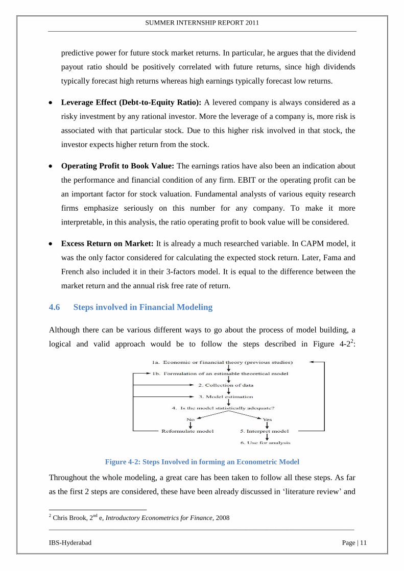
4.6 Steps involved in Financial Modeling
Although there can be various different ways to go about the process of model building, a
logical and valid approach would be to follow the steps described in Figure 4-22:
Figure 4-2: Steps Involved in forming an Econometric Model
Throughout the whole modeling, a great care has been taken to follow all these steps. As far
as the first 2 steps are considered, these have been already discussed in ‗literature review‘ and
2 Chris Brook, 2
nd e, Introductory Econometrics for Finance, 2008

SUMMER INTERNSHIP REPORT 2011
__________________________________________________________________________________________
IBS-Hyderabad Page | 12
‗fundamental variables identified‘ sub-sections. Rest of the steps will be discussed in detail in
following sections.
4.7 Data Analysis
Initially, the data for around 80-90 companies was collected from the Capitaline Database
and CMIE‘s Prowess database. The data of all the 3 financial statements (balance sheet,
income statement, and cash flows) of a company was collected for the time-frame of 10 years
from 2001-2010. The monthly data of stock prices of all these firms was also collected to
calculate the average return of that stock. The source taken for the collection of stock prices
was BSE and the yahoo finance online data.
Some of these firms whose book values were negative in any year in the considered time
frame were removed from the sample for the sake of data smoothening and better analysis.
The main reason to remove the companies with negative book value was that this model is to
be developed for normal financial situations. The firms with negative book value suggest that
their financial condition is pretty critical. Such firms could have involved the extreme values
in data points due to which these firms have not been included in final data sample. The firms
whose data was inconsistent and large number of extreme values were there have also been
removed from the final sample. The banking firms and the financial firms are also excluded
from the final sample because their fundamental variables have totally different
interpretations.
All the data used in this project is of secondary in nature and taken from public domain
sources mentioned above.

SUMMER INTERNSHIP REPORT 2011
__________________________________________________________________________________________
IBS-Hyderabad Page | 13
Following are the main points of Data Analysis:
The final Sample considered for the modeling procedure is of 42 firms and time frame of
10 years. The name of the companies is listed in following Table 4-1:
1.ACC
2.Apollo Tires
3.Ashok Leyland
4.Asian Paints
5.BEL
6.Bharti Airtel
7.BHEL
8.BPCL
9.Castrol India
10.Cipla Ltd
11.GAIL
12.Gammon India
13.GlaxoSmithKline
14.Grasim Industries
15.HCL Technologies
16.HimachalFuturistic Communications Ltd
17.Hindalco
18.HPCL
19.HUL
20.Infosys Technology
21.IOCL
22.ITC Ltd
23.Jindal Steel & Power ltd
24.Mahindra & Mahindra Ltd
25.Maruti Udyog Ltd
26.NIIT Ltd
27.NTPC Ltd
28.ONGC Ltd
29.Polaris Software Ltd
30.Ranbaxy Labs Ltd
31.RIL
32.SAIL
33.Sterlite Industries Ltd
34.Sun Pharma Ltd
35.Tata Motors
36.Tata Steel
37.TATA Teleservices
38.TCS
39.TITAN Industries Ltd
40.UNITECH Ltd
41.Wipro Ltd
42.Zee Enterprises Ltd
Table 4-1: List of Sample Companies
The calculations of all the variables as mentioned above has been done for all the
companies for each year from Jan‘01 to Dec‘10 with the help of financial statements of
these companies. The calculations of the monthly Stock Returns has also been done for
each company and then the average has been taken for each year. This Historical return is
the ―dependent variable.‖
The data that has been considered will be arranged in panel form in both the econometric
software: SAS enterprise guide v3.0 and EVIEWS v7.0.

SUMMER INTERNSHIP REPORT 2011
__________________________________________________________________________________________
IBS-Hyderabad Page | 14
The screenshot of the SAS for the data used for the analysis is shown in the following
Figure 4-3:
Figure 4-3: SAS Data Screenshot

SUMMER INTERNSHIP REPORT 2011
__________________________________________________________________________________________
IBS-Hyderabad Page | 15
Following Table 4-2 shows the Statistic summary of the data sample taken in Eviews:
Workfile Statistics
Date: 02/04/09 Time: 03:45
Name: WORKED EVIEWS FILE
Number of pages: 1
Page: Untitled
Workfile structure: Panel - Annual
Indices: CROSSID x DATEID
Panel dimension: 42 x 10
Range: 2001 2010 x 42 -- 420 obs
Object Count Data Points
Series 12 5040
Coef 1 750
Total 13 5790
Table 4-2: Data Summary Statistics
Hence, the total number of panel observations is 42*10=420 and the total data points are
420*11=4620 (including the time-series id and cross-sectional ids).
The sample size taken for the modeling is quite sufficient to run regression. The
necessary condition of Normality has been taken care in the considered sample.
The panel data that will be used for the modeling is a balanced panel data. A balanced
panel is one which has same number of time-series observations for each cross-sectional
unit.
The data was first arranged in an excel file and then it was transferred in SAS Enterprise
Guide v3.0 for the analysis. For the panel data arrangement, the time-series code and the
cross-sectional codes have also been assigned. For the time-series for the year 2001 to
2010, the time-series id assigned is from 101 to 110 respectively. For the companies, the
cross-sectional ids taken are from 1 to 42.
For some of the variables, natural log transformation has been done just to normalize the
data for all the variables. It helps in increasing the normality of data if there is lot of non-
normality amongst the variables. The variables which are transformed into their natural
log are market capitalization, net sales, book-to-market ratio and P/E ratio. Even in Fama
and French, they took the log for market capitalization and BE/ME Ratio. The variables
selected for the log transformation are being finalized by running several regressions

SUMMER INTERNSHIP REPORT 2011
__________________________________________________________________________________________
IBS-Hyderabad Page | 16
using different combination of log transformation. The better combination is finally
selected.
4.8 Methodology Used for Modeling
The technique that will be used for modeling is a bit complicated regression technique known
as panel regression technique. For generating and the testing of the model, 2 advanced
econometric software are used extensively. These are SAS Enterprise Guide v3.0 and
EVIEWS v7.0.
4.8.1 Modeling Procedure Used by Fama & French
Fama and French test involved a 2-step estimation procedure: First, they estimated the betas
(slopes or coefficients) in separate time series regressions for each firm (around 4000 firms)
and then, for each separate point in time, a cross-sectional regression of the excess returns on
the betas was conducted by them which then looked like as shown in following equation:
E (Rit) =E (R0t)+λMKTi*βMKT+λSMBi*βSMB+λHMLi*βHML (Eq-4.3)
Actually, Fama and French proposed estimating this second stage (cross-sectional) regression
separately for each time-period, and then taking the average of the parameters estimates to
conduct the hypothesis testing. It was a very cumbersome approach. The regression technique
used in their whole analysis was Ordinary Least Square (OLS) technique which is the most
basic technique of regression analysis. Though OLS is one of the most unbiased regression
techniques, there are several disadvantages when its application to panel data is concerned.
4.8.2 Modeling Procedure Used in this Project
The major and a very important part of the analysis of Fama and French 3-factor model tests
was that the betas that they used in the second stage was not the beta of the individual firms
rather it was the average beta of the portfolios that they made according to market
capitalization and book-to-market ratio. There were 6 portfolios in their analysis. Many
academicians use CAPM for calculating the returns for individual stock returns whereas for
portfolios‘ return calculation the Fama and French Model are preferred. In this paper, the
technique of panel regression will be used for modeling of Stock Valuation Equation for
Individual Stock Returns. Though, there are its own advantage of a valuation model used for
portfolios but it is always preferred that the model must be able to calculate the expected
stock return of an individual stock. There have already been some research by many scholars

SUMMER INTERNSHIP REPORT 2011
__________________________________________________________________________________________
IBS-Hyderabad Page | 17
in which they have tried to modify or interpret the Fama and French model for individual
stocks (working paper on Estimation of Expected Return: CAPM vs. Fama and French- Jan
Bartholdy and Paula Peare—CAF, 2004).
The situation often arises in financial modeling where one has data comprising both time
series and cross-sectional elements, and such a dataset would be known as a panel of data or
longitudinal data. A panel of data embodies the information across both time and space
(cross-sections).
Econometrically, the setup of panel data regression model can be represented as below:
Yit = α+∑Nk=1 βk*Xit+uit (Eq-4.4)
Where,
Yit is the dependent variable, α is the intercept term, β is a (k * 1) vector of parameters
to be estimated on the exploratory variables, and Xit is a (1 * k) vector of observations
on the explanatory variables, t= 1,…..,T; i=1,2,…….,N.
The simplest way to deal with such data would be to estimate a pooled regression, which
would involve estimating a single equation on all the data together, so that the dataset for y is
stacked up into a single column containing all the cross-sectional and time-series
observations, and similarly all of the observations on each explanatory variable would be
stacked up into single columns in the X matrix. Then this equation would be estimated in the
usual fashion using OLS.
While it is indeed a simple way to proceed, and requires the estimation of few parameters
possible, it has some severe limitations. Pooling the data in such a way implicitly assumes
that the average values of the variables and the relationships between them are constant over
time and across all of the cross-sectional units in the sample.
The approach used by the Fama and French was a 2 step process in which they separately
estimated the time-series effects for each cross-sections (firms) and then the estimated
parameters were used as the independent variables and were regressed with the same
dependent variable i.e., the historical stock returns. But it is a very tedious approach and also
the technique is OLS which is bit sub-optimal for such type of analysis. If one is fortunate

SUMMER INTERNSHIP REPORT 2011
__________________________________________________________________________________________
IBS-Hyderabad Page | 18
enough to have a panel of data at the disposal; there are important advantages to making full
use of this rich structure which are shown as below:
First, and perhaps most importantly, one can address a broader range of issues and tackle
more complex problems with panel data than would be possible with pure time-series or
pure cross-sectional data alone.
Panel data give more informative data, more variability, less collinearity among the
variables, more degrees of freedom and more efficiency.
Third, by structuring the model in an appropriate way, one can remove the impact of
certain forms of omitted variables bias in regression results.
Controlling of Individual Heterogeneity is achieved in Panel Data. Panel data suggests
that individuals, firms, states or countries are heterogeneous. Time-series and cross-
section studies not controlling this heterogeneity run the risk of obtaining biased results.
Panel data are better able to study the dynamics of adjustment. Cross-sectional
distributions that look relatively stable hide a multitude of changes. This drawback is
overcome in panel data.
Before applying any of the panel techniques, at first the data will be tested by some available
panel data test procedures which are discussed in following sections.
4.9 Panel Unit Root Tests
It is very important for any time-series data to pass this test. A unit root test tests whether a
time-series variable is non-stationary. Recent literature suggests that the panel-based unit root
tests have higher power than those based on individual time series. For the testing of the unit
root in a panel data, Levin, Lin and Chu (LLC3) Test will be used using the EVIEWS v7.0.
The null hypothesis is that each individual time series contains a unit root against the
alternative that each time series is stationary.
LLC consider the following basic Augmented Dickey-Fuller (ADF) specification:
∆yit = αyit-1+∑Pj=1 βij∆yit-j+Xit
’δ+εit (Eq-4.5)
Where the assumption is that α=ρ-1 (ρ are the autoregressive coefficients). So, the null
hypothesis of the test is written as:
3 For details, please see Baltagi, Econometric Analysis of Panel Data 3e,Willey & Sons, 2005, pp. 240

SUMMER INTERNSHIP REPORT 2011
__________________________________________________________________________________________
IBS-Hyderabad Page | 19
H0: α = 0
H1: α < 0
The LLC test is performed for each of the 9 variables (both dependent and independent).
Following Table 4-3 shows the LLC Unit Root Test Results for each of those variables:
Null Hypothesis: Unit root (common unit root process) is present.
Date: 04/29/2011 Time: 16:04
Sample: 2001 2010
Exogenous variables: Individual effects
User-specified lags: 1
Newey-West automatic bandwidth selection and Bartlett kernel
Total (balanced) observations: 336 Cross-sections included: 42
Series: RETURN Method Statistic Prob.**
Levin, Lin & Chu t* -
6.45613 0.0000
Series: ln (Book to Market value)
Method Statistic Prob.**
Levin, Lin & Chu t* -13.2298 0.0000 Series: Dividend Payout Ratio
Method Statistic Prob.**
Levin, Lin & Chu t* -
15.3991 0.0000
Series: Leverage Ratio
Method Statistic Prob.**
Levin, Lin & Chu t* -
12.4196 0.0000
Series: ln (Market Capitalization)
Method Statistic Prob.**
Levin, Lin & Chu t* -
3.95747 0.0000
Series: Operating Profit to Book Value
Method Statistic Prob.**
Levin, Lin & Chu t* -
4.37614 0.0000

SUMMER INTERNSHIP REPORT 2011
__________________________________________________________________________________________
IBS-Hyderabad Page | 20
Series: Ln (P/E Ratio)
Method Statistic Prob.**
Levin, Lin & Chu t* -
20.1611 0.0000
Series: Premium
Method Statistic Prob.**
Levin, Lin & Chu t* -
7.52612 0.0000
Series: Ln (Sales)
Method Statistic Prob.**
Levin, Lin & Chu t* -
7.83774 0.0000 ** Probabilities are computed assuming asymptotic normality
Table 4-3: Levin, Lin and Chu Unit Root Test
The above Table for the unit root test tells that No Unit Root is present in any of the variable.
It means that the data for all the 9 variables are stationary.
4.10 Panel Co-integration Test4
Though it is not much required now to check for the co-integration test as the whole data is
stationary, to be on the safe side this test has also been applied for the panel data. For panel
cointegrated regression models, the asymptotic properties of the estimators of the regression
coefficients and the associated statistical tests are different from those of the time series
cointegration regression models. Following Table 4-4 shows the panel cointegration test
using the KAO (Engle-Granger based) cointegration Tests in EVIEWS:
Kao Residual Cointegration Test
Series: RETURN PREMIUM OPBV LNSALES LNPE LNMKT LNBTM DPO
DER
Date: 29/04/2011 Time: 01:42
Sample: 2001 2010
Included observations: 420
Null Hypothesis: No cointegration
Trend assumption: No deterministic trend
User-specified lag length: 1
Newey-West automatic bandwidth selection and Bartlett kernel
t-Statistic Prob.
4 For details, please see Baltagi, Econometric Analysis of Panel Data 3e, Willey & Sons, 2005, pp. 257

SUMMER INTERNSHIP REPORT 2011
__________________________________________________________________________________________
IBS-Hyderabad Page | 21
ADF -6.532121 0.0000
Residual variance 40.79466
HAC variance 16.48424
Table 4-4: KAO Cointegration Test
It is clear from the above output Table that the null hypothesis of no cointegration is rejected.
It means that all the variables are cointegrated (alternate hypothesis accepted) and therefore,
the regression of return on the other 8 independent variables is meaningful i.e., not spurious.
There are broadly 2 types of panel estimation techniques for the financial modeling. These
are fixed-effect and random-effect technique. In this paper, both these techniques will be used
extensively for the development of required model. The better and the statistically more
significant model will be used as the final model for the calculation of expected stock return.
4.11 Developing Fixed One-Way Effect Model for Stock Valuation
4.11.1 Introduction to Fixed One-Way Effect Model5
If the specification is dependent only on the cross section to which the observation belongs,
such a model is referred to as a model with one-way effects. The term ―fixed effect‖ is due to
the fact that, although the intercept may differ across the cross-section (here 42 companies),
each cross-section‘s intercept does not vary over time i.e. it is time-invariant. It should be
noted that the Fixed-Effect model given below assumes that the (slope) coefficients of the
regressors do not vary across individuals or over time. In equation (4.4), for fixed one-way
effect model, the specifications are given as below:
uit = μi + vit (Eq-4.6)
μi is used to encapsulate all the variables that affect Yit cross-sectionally but do not vary over
time. To allow for the (fixed effect) intercept to vary between companies, differential
intercept dummies technique is used. It is also termed as the Least Square Dummy Variable
(LSDV) approach. Then the model will look like as below:
Yi t = βxit + μ1D1i + μ2D2i + μ3D3i +· · · +μNDNi + vit (Eq-4.7)
5 Chris Brook, Introductory Econometric for Finance,2
nd e, 2008

SUMMER INTERNSHIP REPORT 2011
__________________________________________________________________________________________
IBS-Hyderabad Page | 22
Where, D1i is a dummy variable that takes the value 1 for all observations on the first entity
(e.g. Company ACC) in the sample and zero otherwise and similarly for other dummies.
4.11.2 Analysis and Modeling Using SAS
For generating the Fixed-One Way Model, SAS enterprise guide v3.0 has been used. During
the process of generating the model, the intercept term has been removed. The intercept term
(α) has not been included in the analysis so as to avoid the ‘dummy-variable trap’.
The regression analysis of the panel data generated by the SAS is shown one by one as below
in the following tables. Following Table 4-5 represents the fit-statistics of fixed One-way
effect model:
Fit Statistics
SSE 9078.1349 DFE 370
MSE 24.5355 Root MSE 4.9533
R-Square 0.3671
Table 4-5: Fit Statistics for Fixed One-Way Effect Model
The correlation (R2) is 36.71% which is quite satisfactory.

SUMMER INTERNSHIP REPORT 2011
__________________________________________________________________________________________
IBS-Hyderabad Page | 23
The cross-sectional parameter estimates have also been shown in the following output Table
4-6:
Parameter Estimates
Variable DF Estimate
Standard
Error t Value Pr > |t| Label
CS1 1 -2.81729 18.9348 -0.15 0.8818 Cross Sectional Effect 1
CS2 1 -3.88115 18.3950 -0.21 0.8330 Cross Sectional Effect 2
CS3 1 1.637425 18.4094 0.09 0.9292 Cross Sectional Effect 3
CS4 1 -0.89955 19.1368 -0.05 0.9625 Cross Sectional Effect 4
CS5 1 -0.60989 18.7645 -0.03 0.9741 Cross Sectional Effect 5
CS6 1 0.204929 19.9113 0.01 0.9918 Cross Sectional Effect 6
CS7 1 -0.55332 19.8478 -0.03 0.9778 Cross Sectional Effect 7
CS8 1 -6.83975 20.8407 -0.33 0.7430 Cross Sectional Effect 8
CS9 1 -2.08924 18.6880 -0.11 0.9110 Cross Sectional Effect 9
CS10 1 -0.7814 18.8049 -0.04 0.9669 Cross Sectional Effect 10
CS11 1 -0.93704 19.8118 -0.05 0.9623 Cross Sectional Effect 11
CS12 1 -8.82817 18.4380 -0.48 0.6324 Cross Sectional Effect 12
CS13 1 1.532418 18.4531 0.08 0.9339 Cross Sectional Effect 13
CS14 1 -1.28167 19.2522 -0.07 0.9470 Cross Sectional Effect 14
CS15 1 1.878681 18.6177 0.10 0.9197 Cross Sectional Effect 15
CS16 1 -0.22525 19.3104 -0.01 0.9907 Cross Sectional Effect 16
CS17 1 3.431067 17.8516 0.19 0.8477 Cross Sectional Effect 17
CS18 1 -7.28189 20.7974 -0.35 0.7264 Cross Sectional Effect 18
CS19 1 -1.85599 20.2124 -0.09 0.9269 Cross Sectional Effect 19
CS20 1 -0.39245 19.7328 -0.02 0.9841 Cross Sectional Effect 20
CS21 1 -6.45574 21.4552 -0.30 0.7637 Cross Sectional Effect 21
CS22 1 0.471677 19.6837 0.02 0.9809 Cross Sectional Effect 22
CS23 1 3.594788 18.3705 0.20 0.8450 Cross Sectional Effect 23

SUMMER INTERNSHIP REPORT 2011
__________________________________________________________________________________________
IBS-Hyderabad Page | 24
Parameter Estimates
Variable DF Estimate
Standard
Error t Value Pr > |t| Label
CS24 1 -2.29546 19.3149 -0.12 0.9055 Cross Sectional Effect 24
CS25 1 -0.24741 19.8403 -0.01 0.9901 Cross Sectional Effect 25
CS26 1 -1.93674 17.2675 -0.11 0.9108 Cross Sectional Effect 26
CS27 1 1.735368 20.3114 0.09 0.9320 Cross Sectional Effect 27
CS28 1 -3.82409 20.7133 -0.18 0.8536 Cross Sectional Effect 28
CS29 1 -0.72479 17.6037 -0.04 0.9672 Cross Sectional Effect 29
CS30 1 -1.7701 19.1224 -0.09 0.9263 Cross Sectional Effect 30
CS31 1 -2.57113 21.0311 -0.12 0.9028 Cross Sectional Effect 31
CS32 1 -2.97284 20.1641 -0.15 0.8829 Cross Sectional Effect 32
CS33 1 -0.87976 19.0755 -0.05 0.9632 Cross Sectional Effect 33
CS34 1 2.584431 18.4323 0.14 0.8886 Cross Sectional Effect 34
CS35 1 -2.62864 19.9215 -0.13 0.8951 Cross Sectional Effect 35
CS36 1 -1.25292 19.7015 -0.06 0.9493 Cross Sectional Effect 36
CS37 1 -1.25292 19.7015 -0.06 0.9493 Cross Sectional Effect 37
CS38 1 0.52898 20.4839 0.03 0.9794 Cross Sectional Effect 38
CS39 1 -1.78398 18.3359 -0.10 0.9225 Cross Sectional Effect 39
CS40 1 1.616614 17.6167 0.09 0.9269 Cross Sectional Effect 40
CS41 1 -0.82733 19.8072 -0.04 0.9667 Cross Sectional Effect 41
CS42 1 1.977371 17.8052 0.11 0.9116 Cross Sectional Effect 42
ln Market Capitalisation 1 -2.07522 0.4337 -4.79 <.0001 ln Market Capitalisation
ln Net Sales 1 2.457405 0.8413 2.92 0.0037 ln Net Sales
ln Book to Market value 1 0.63548 0.2760 2.30 0.0219 ln Book to Market value
ln P E 1 0.779547 0.1920 4.06 <.0001 ln P E
OPBV 1 0.361881 0.2847 1.27 0.2045 OPBV
Dividend Payout 1 -0.01712 0.0144 -1.19 0.2358 Dividend Payout
SUMMER INTERNSHIP REPORT 2011
__________________________________________________________________________________________
IBS-Hyderabad Page | 25
Parameter Estimates
Variable DF Estimate
Standard
Error t Value Pr > |t| Label
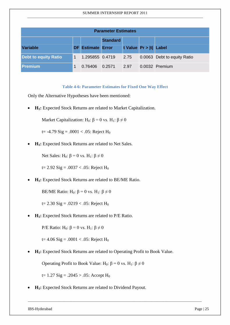
Debt to equity Ratio 1 1.295855 0.4719 2.75 0.0063 Debt to equity Ratio
Premium 1 0.76406 0.2571 2.97 0.0032 Premium
Table 4-6: Parameter Estimates for Fixed One Way Effect
Only the Alternative Hypotheses have been mentioned:
H1: Expected Stock Returns are related to Market Capitalization.
Market Capitalization: H0: β = 0 vs. H1: β ≠ 0
t= -4.79 Sig = .0001 < .05: Reject H0
H1: Expected Stock Returns are related to Net Sales.
Net Sales: H0: β = 0 vs. H1: β ≠ 0
t= 2.92 Sig = .0037 < .05: Reject H0
H1: Expected Stock Returns are related to BE/ME Ratio.
BE/ME Ratio: H0: β = 0 vs. H1: β ≠ 0
t= 2.30 Sig = .0219 < .05: Reject H0
H1: Expected Stock Returns are related to P/E Ratio.
P/E Ratio: H0: β = 0 vs. H1: β ≠ 0
t= 4.06 Sig = .0001 < .05: Reject H0
H1: Expected Stock Returns are related to Operating Profit to Book Value.
Operating Profit to Book Value: H0: β = 0 vs. H1: β ≠ 0
t= 1.27 Sig = .2045 > .05: Accept H0
H1: Expected Stock Returns are related to Dividend Payout.

SUMMER INTERNSHIP REPORT 2011
__________________________________________________________________________________________
IBS-Hyderabad Page | 26
Dividend Payout: H0: β = 0 vs. H1: β ≠ 0
t= -1.19 Sig = .2358 > .05: Accept H0
H1: Expected Stock Returns are related to Debt to Equity Ratio.
Debt to Equity Ratio: H0: β = 0 vs. H1: β ≠ 0
t= 2.75 Sig = .0063 < .05: Reject H0
H1: Expected Stock Returns are related to Premium (E (Rm) - Rf).
Premium: H0: β = 0 vs. H1: β ≠ 0
t= 2.97 Sig = .0032 < .05: Reject H0
The final Fixed-One Way Effect Model for the Stock Returns is shown as below. In this
Regression, the cross-sectional dummy variables for the companies have not been shown
(available in Table 4-6) due to very large number (42 Dummies for Cross Section). So, only
the main factors will be mentioned:
Test Statistics for the Model:
In SAS Enterprise Guide, only F-Statistics (Chow Test) is available for the Fixed One-Way
Effect Model Test. This test checks whether the panel approach is necessary at all. It involves
the restriction that all the dummy variables have the same parameter (i.e. H0: μ1 = μ2 = · ·
· = μN).
E(Rit)=-2.07522*(ln(MKTit))+2.457405*(ln(Net-Salesit))+
0.63548*(ln(BE/MEit))+0.779547*(ln(P/Eit))+1.295855*(D/Eit)+0.
76406*(Premiumit) (A)

SUMMER INTERNSHIP REPORT 2011
__________________________________________________________________________________________
IBS-Hyderabad Page | 27
The output result for this test generated by SAS is shown in the following Table 4-7:
F Test for No Fixed Effects and
No Intercept
Num DF Den DF F Value Pr > F
42 370 1.15 0.2459
Table 4-7: Chow Test (F-Test) for Fixed One Effect Model
H0: μ1 = μ2 = · · · = μN
Since, Pr (F-Stats) > 0.05 (p-value)
Therefore, H0 can’t be rejected.
Test results are not very satisfactory. It suggests that the model is not very robust.
This test suggests that simple OLS technique can also be implemented in the place of
Fixed One Way Effect.
Now referring to the steps shown in Figure 4-2, one can see that the step 4 is violated. So,
new estimation technique will be used for the modeling. There are 3 more broad techniques
left which will be used subsequently and the technique which will provide the most robust
and justifiable model will be used as the final model for the expected stock returns.
4.12 Developing Fixed Two-Way Effect Model for Stock Valuation
4.12.1 Introduction to Fixed Two Way Effect Model
A 2-way fixed effect model is the one when specification depends on both the cross section
and the time series to which the observation belongs. This technique allows for both entity-
fixed effects and the time-fixed effects within the same model. In this case the LSDV
equivalent model would contain both cross-sectional and time-dummies.
The specifications for Fixed One-Way Effect model are given as below:
uit = μi +λt+ vit (Eq-4.8)
SUMMER INTERNSHIP REPORT 2011
__________________________________________________________________________________________
IBS-Hyderabad Page | 28
Here, μi is used to encapsulate all the variables that affect Yit cross-sectionally (cross-sectional
effect) and λt is used to encapsulate all the variables that affect Yit over the period of time
(time-effect). However the number of parameters to be estimated would now be k+N+T and
it would more complex. The model will look like as below:
Yit = βxit+μ1D1i +µ2D2i +μ3D3i +· · · +μN DNi + λ1D1t+λ2D2t +λ3D3t +· · ·
+λTDTt + vit (Eq-4.9)
Where, D1i is a dummy variable that takes the value 1 for all observations on the first entity
(e.g. Company ACC) in the sample and zero otherwise and similarly for other dummies. And
D1t is a dummy variable for the years that takes value 1 for all observations on the first entity
(e.g. year 2001).
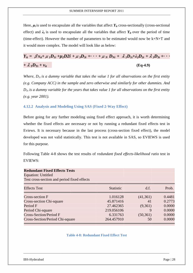
4.12.2 Analysis and Modeling Using SAS (Fixed 2-Way Effect)
Before going for any further modeling using fixed effect approach, it is worth determining
whether the fixed effects are necessary or not by running a redundant fixed effects test in
Eviews. It is necessary because in the last process (cross-section fixed effect), the model
developed was not valid statistically. This test is not available in SAS, so EVIEWS is used
for this purpose.
Following Table 4-8 shows the test results of redundant fixed effects-likelihood ratio test in
EVIEWS:
Redundant Fixed Effects Tests
Equation: Untitled
Test cross-section and period fixed effects
Effects Test Statistic d.f. Prob.
Cross-section F 1.016128 (41,361) 0.4481
Cross-section Chi-square 45.871416 41 0.2773
Period F 27.462365 (9,361) 0.0000
Period Chi-square 219.056106 9 0.0000
Cross-Section/Period F 6.331763 (50,361) 0.0000
Cross-Section/Period Chi-square 264.457910 50 0.0000
Table 4-8: Redundant Fixed Effect Test

SUMMER INTERNSHIP REPORT 2011
__________________________________________________________________________________________
IBS-Hyderabad Page | 29
From the output shown in above table, it is quite obvious that these are the time fixed-effect
which had a greater impact as compared to the cross-sectional fixed-effect. The output clearly
suggests that fixed effect model (especially time-fixed effect approach in this case) is a valid
approach rather than the pooled estimation approach.
The Table 4-9 shows the SAS outputs for the generated fixed two-way effect model:
Fit Statistics
SSE 5398.0873 DFE 361
MSE 14.9532 Root MSE 3.8669
R-Square 0.6237
Table 4-9: Fit Statistics for Fixed 2-Way Effect Model
The correlation (R2) is 62.37% which is very good if one compare it with the previous
model’s correlation. The main reason of this increased R2
is the introduction of time-effect in
the estimation.

SUMMER INTERNSHIP REPORT 2011
__________________________________________________________________________________________
IBS-Hyderabad Page | 30
The cross-sectional and time-series parameter estimates have also been shown in the
following output Table 4-10:
Parameter Estimates
Variable DF Estimate
Standard
Error t Value Pr > |t| Label
CS1 1 -33.8899 22.8094 -1.49 0.1382 Cross Sectional Effect 1
CS2 1 -34.8837 22.6737 -1.54 0.1248 Cross Sectional Effect 2
CS3 1 -30.0649 22.6489 -1.33 0.1852 Cross Sectional Effect 3
CS4 1 -32.3899 22.6833 -1.43 0.1542 Cross Sectional Effect 4
CS5 1 -32.007 22.5642 -1.42 0.1569 Cross Sectional Effect 5
CS6 1 -32.0588 23.3943 -1.37 0.1714 Cross Sectional Effect 6
CS7 1 -31.8816 23.3305 -1.37 0.1726 Cross Sectional Effect 7
CS8 1 -34.5995 23.9363 -1.45 0.1492 Cross Sectional Effect 8
CS9 1 -33.3161 22.4648 -1.48 0.1389 Cross Sectional Effect 9
CS10 1 -33.5823 22.6132 -1.49 0.1384 Cross Sectional Effect 10
CS11 1 -31.9195 23.3727 -1.37 0.1729 Cross Sectional Effect 11
CS12 1 -38.448 22.3645 -1.72 0.0864 Cross Sectional Effect 12
CS13 1 -31.4672 22.4358 -1.40 0.1616 Cross Sectional Effect 13
CS14 1 -32.6965 22.9564 -1.42 0.1552 Cross Sectional Effect 14
CS15 1 -31.1605 22.5560 -1.38 0.1680 Cross Sectional Effect 15
CS16 1 -31.9454 23.0078 -1.39 0.1659 Cross Sectional Effect 16
CS17 1 -32.2655 22.0575 -1.46 0.1444 Cross Sectional Effect 17
CS18 1 -35.0931 23.9577 -1.46 0.1438 Cross Sectional Effect 18
CS19 1 -33.2456 23.5623 -1.41 0.1591 Cross Sectional Effect 19
CS20 1 -33.3408 23.2575 -1.43 0.1526 Cross Sectional Effect 20
CS21 1 -34.5865 24.4113 -1.42 0.1574 Cross Sectional Effect 21
CS22 1 -32.1752 23.2371 -1.38 0.1670 Cross Sectional Effect 22
CS23 1 -28.9581 22.4042 -1.29 0.1970 Cross Sectional Effect 23

SUMMER INTERNSHIP REPORT 2011
__________________________________________________________________________________________
IBS-Hyderabad Page | 31
Parameter Estimates
Variable DF Estimate
Standard
Error t Value Pr > |t| Label
CS24 1 -32.9495 22.9877 -1.43 0.1526 Cross Sectional Effect 24
CS25 1 -31.4192 23.3149 -1.35 0.1786 Cross Sectional Effect 25
CS26 1 -33.9432 21.7007 -1.56 0.1187 Cross Sectional Effect 26
CS27 1 -30.2893 23.6742 -1.28 0.2016 Cross Sectional Effect 27
CS28 1 -34.1094 23.9246 -1.43 0.1548 Cross Sectional Effect 28
CS29 1 -33.0814 21.8939 -1.51 0.1317 Cross Sectional Effect 29
CS30 1 -33.9636 22.8651 -1.49 0.1383 Cross Sectional Effect 30
CS31 1 -33.0626 24.1344 -1.37 0.1716 Cross Sectional Effect 31
CS32 1 -32.9064 23.5643 -1.40 0.1634 Cross Sectional Effect 32
CS33 1 -32.1108 22.8446 -1.41 0.1607 Cross Sectional Effect 33
CS34 1 -31.2963 22.4277 -1.40 0.1637 Cross Sectional Effect 34
CS35 1 -32.7235 23.3825 -1.40 0.1625 Cross Sectional Effect 35
CS36 1 -32.1673 23.2619 -1.38 0.1676 Cross Sectional Effect 36
CS37 1 -32.1673 23.2619 -1.38 0.1676 Cross Sectional Effect 37
CS38 1 -31.6477 23.7054 -1.34 0.1827 Cross Sectional Effect 38
CS39 1 -32.2943 22.3516 -1.44 0.1494 Cross Sectional Effect 39
CS40 1 -30.5312 21.9337 -1.39 0.1648 Cross Sectional Effect 40
CS41 1 -33.4257 23.3022 -1.43 0.1523 Cross Sectional Effect 41
CS42 1 -32.098 22.0537 -1.46 0.1464 Cross Sectional Effect 42
TS1 1 -2.45853 1.1056 -2.22 0.0268 Time Series Effect 1
TS2 1 -7.94056 3.7824 -2.10 0.0365 Time Series Effect 2
TS3 1 -3.95015 4.0672 -0.97 0.3321 Time Series Effect 3
TS4 1 -7.61435 3.6999 -2.06 0.0403 Time Series Effect 4
TS5 1 -1.58197 1.4744 -1.07 0.2840 Time Series Effect 5
TS6 1 1.785411 0.9488 1.88 0.0607 Time Series Effect 6
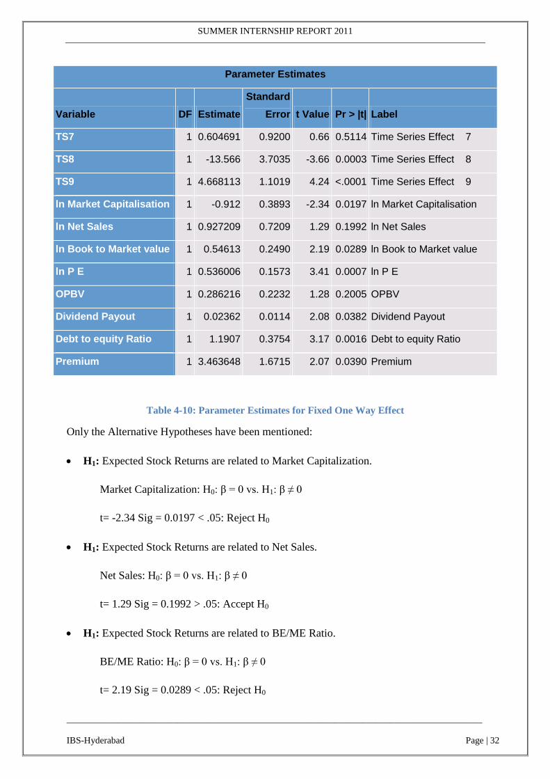
SUMMER INTERNSHIP REPORT 2011
__________________________________________________________________________________________
IBS-Hyderabad Page | 32
Parameter Estimates
Variable DF Estimate
Standard
Error t Value Pr > |t| Label
TS7 1 0.604691 0.9200 0.66 0.5114 Time Series Effect 7
TS8 1 -13.566 3.7035 -3.66 0.0003 Time Series Effect 8
TS9 1 4.668113 1.1019 4.24 <.0001 Time Series Effect 9
ln Market Capitalisation 1 -0.912 0.3893 -2.34 0.0197 ln Market Capitalisation
ln Net Sales 1 0.927209 0.7209 1.29 0.1992 ln Net Sales
ln Book to Market value 1 0.54613 0.2490 2.19 0.0289 ln Book to Market value
ln P E 1 0.536006 0.1573 3.41 0.0007 ln P E
OPBV 1 0.286216 0.2232 1.28 0.2005 OPBV
Dividend Payout 1 0.02362 0.0114 2.08 0.0382 Dividend Payout
Debt to equity Ratio 1 1.1907 0.3754 3.17 0.0016 Debt to equity Ratio
Premium 1 3.463648 1.6715 2.07 0.0390 Premium
Table 4-10: Parameter Estimates for Fixed One Way Effect
Only the Alternative Hypotheses have been mentioned:
H1: Expected Stock Returns are related to Market Capitalization.
Market Capitalization: H0: β = 0 vs. H1: β ≠ 0
t= -2.34 Sig = 0.0197 < .05: Reject H0
H1: Expected Stock Returns are related to Net Sales.
Net Sales: H0: β = 0 vs. H1: β ≠ 0
t= 1.29 Sig = 0.1992 > .05: Accept H0
H1: Expected Stock Returns are related to BE/ME Ratio.
BE/ME Ratio: H0: β = 0 vs. H1: β ≠ 0
t= 2.19 Sig = 0.0289 < .05: Reject H0

SUMMER INTERNSHIP REPORT 2011
__________________________________________________________________________________________
IBS-Hyderabad Page | 33
H1: Expected Stock Returns are related to P/E Ratio.
P/E Ratio: H0: β = 0 vs. H1: β ≠ 0
t= 3.41 Sig = 0.0007 < .05: Reject H0
H1: Expected Stock Returns are related to Operating Profit to Book Value.
Operating Profit to Book Value: H0: β = 0 vs. H1: β ≠ 0
t= 1.28 Sig = 0.2005 > .05: Accept H0
H1: Expected Stock Returns are related to Dividend Payout.
Dividend Payout: H0: β = 0 vs. H1: β ≠ 0
t= 2.08 Sig = 0.0382 < .05: Reject H0
H1: Expected Stock Returns are related to Debt to Equity Ratio.
Debt to Equity Ratio: H0: β = 0 vs. H1: β ≠ 0
t= 3.17 Sig = 0.0016 < .05: Reject H0
H1: Expected Stock Returns are related to Premium (E (Rm) - Rf).
Premium: H0: β = 0 vs. H1: β ≠ 0
t= 2.07 Sig = .039 < .05: Reject H0
From the above Hypothesis Testing Results, 6 out of the 8 considered Fundamental variables
are statistically significant. The relation of these variables with the Expected Stock Return is
supporting the theory also.
Final analysis of the model and the relationship of these variables will be discussed in detail
after selecting the final model.
The final fixed-two way effect model for the stock returns is shown as below. In this
regression, the cross-sectional and the time-series dummy variables for the companies have
not been shown (available in Table 4-10) due to very large number (42 dummies for cross
section, CS and 9 time-series dummies, TS).

SUMMER INTERNSHIP REPORT 2011
__________________________________________________________________________________________
IBS-Hyderabad Page | 34
So, only the main factors will be mentioned in the final equation shown as below:
Test Statistics for the Model:
The Table 4-11 shows the SAS output for the F-statistic for the fixed two-way effect model:
F Test for No Fixed Effects and
No Intercept
Num DF Den DF F Value Pr > F
51 362 6.36 <.0001
Table 4-11: F-test for Fixed 2 Way Effect Model
In SAS enterprise guide, only F-Statistics (Chow Test) is available for the fixed two-way
effect model test. It involves the restriction that all the dummy variables have the same
parameter (i.e. H0: μ1 = μ2 = · · · = μN and λ1 = . . . = λT−1 = 0). This test basically
tests for the presence of the individual effects (cross-sectional effect) and the time-series
effect.
H0: μ1 = μ2 = · · · = μN=0 and λ1 = . . . = λT−1 = 0
Since, Pr (F-Stats) < 0.05 (p-value)
Therefore, H0 is rejected. It means that there is a significant presence of companies’ effect
(cross-sectional effect) as well as the time-series effect. Hence this model passes the required
test of its statistical validness. This model can be used as the measure of expected stock
return.
E(Rit)=-0.912*(ln(MKTit))+0.02362*(Div-PayoutRatio)+
0.54613*(ln(BE/MEit))+0.536*(ln(P/Eit))+1.1907*(D/Eit)+3.46364
*(Premiumit) (B)

SUMMER INTERNSHIP REPORT 2011
__________________________________________________________________________________________
IBS-Hyderabad Page | 35
For more support, the histogram normality test for the residuals done in EVIEWS is also
shown as below in Figure 4-4:
Figure 4-4: Histogram Normality Test for the Residuals (Fixed 2 Way Effect)
As one can see that the null-hypothesis of non-normality of residuals has been rejected. It
means that the residuals are normally distributed.
4.13 Developing Random One-Way Effect Model
4.13.1 Introduction to Random One-Way Effect Model6
A One-way random effects model is when the specification depends only on the cross section
to which the observation belongs. In this case, the effects are random. A random effects
model is a regression with a random constant term. One way to handle the ignorance or error
is to assume that the intercept is a random outcome variable. The random outcome is a
function of a mean value plus a random error. As with fixed effects, the random effects
approach proposes different intercept terms for each entity and again these intercepts are
constant over time, with the relationships between the explanatory and explained variables
assumed to be the same both cross-sectionally and temporally.
In random effects models, the estimation framework considers that the constant term or the
intercepts for each cross-sectional unit (i.e., individual stocks) are assumed to occur from
common intercept term i.e., α plus a random variable εi that varies cross-sectionally but is
constant over time in case of one-way random effect estimation. εi measures the random
6 For Details see Baltagi (2005), Chris Brook (2008, pp.498) and Kennedy (2003, pp.315)

SUMMER INTERNSHIP REPORT 2011
__________________________________________________________________________________________
IBS-Hyderabad Page | 36
fluctuations of each entity‘s intercept term from the ‗global‘ intercept term α. random effects
panel model can be written as:
Yit = α + βXit + ωit , ωit = εi + vit (Eq-4.10)
The main required assumption of this framework is that the error term (here only cross-
sectional error term) εi has zero mean and is independent of the cross-sectional error term
(vit). Also, the variance σ2
ε is constant and error-term is independent of the explanatory
variables (Xit).
In random-effect models, a generalized least squares (GLS) method is usually used for the
estimation. The transformation used in this GLS estimation procedure is to subtract a
weighted mean of the Yit over time (i.e. part of the mean rather than the whole mean). Then,
define the ‗quasi-demeaned‘ data as Yit∗ = Yit – θYi
’ and Xit
∗ = Xit – θXi’, where Yi
’ and Xi
’ are
the means over time of the observations on Yit and Xit respectively. θ will be the function of
the variance of the entity-specific error term, σ2v , and of the variance of the entity-specific
error term, σ2
ε
(Eq-4.11)
This transformation ensures that there are no cross-correlations in the error terms, but
fortunately it will be automatically implemented by the SAS or Eviews.
4.13.2 Analysis and Modeling Using SAS (Random One-Way Effect Model)
To improve the correlation, the intercept term has been removed from the analysis and the
estimation procedure.

SUMMER INTERNSHIP REPORT 2011
__________________________________________________________________________________________
IBS-Hyderabad Page | 37
The fit statistics for random one-way model has been shown in the Table 4-12:
Fit Statistics
SSE 10152.0848 DFE 412
MSE 24.6410 Root MSE 4.9640
R-Square 0.2654
Table 4-12: Fit Statistics for Random 1-Way
The correlation (R2) is 26.54% which is bit low as compared to the previous 2 fixed effect
models.
The estimated values of the variance component have been shown in the Table 4-13:
Variance Component Estimates
Variance Component for Cross Sections 0.46908
Variance Component for Error 24.51193
Table 4-13: Variance Component Estimates
These are the error terms (εi and vit) for Cross-sectional effects.
The parameter estimate table for the random cross-sectional effect is shown below in Table 4-
14:
Parameter Estimates
Variable DF Estimate
Standard
Error t Value Pr > |t| Label
ln Market Capitalisation 1 -0.80248 0.2212 -3.63 0.0003 ln Market Capitalisation
ln Net Sales 1 0.994676 0.2407 4.13 <.0001 ln Net Sales
ln Book to Market value 1 0.5719 0.1409 4.06 <.0001 ln Book to Market value
ln P E 1 0.4803 0.1430 3.36 0.0009 ln P E
OPBV 1 -0.06077 0.1348 -0.45 0.6524 OPBV
Dividend Payout 1 0.01694 0.0102 1.66 0.0976 Dividend Payout
Debt to equity Ratio 1 1.378936 0.3602 3.83 0.0001 Debt to equity Ratio
Premium 1 0.38896 0.2111 1.84 0.0461 Premium
Table 4-14: Parameter Estimates for Random One Way Effect Model

SUMMER INTERNSHIP REPORT 2011
__________________________________________________________________________________________
IBS-Hyderabad Page | 38
Only the alternative hypotheses have been mentioned:
H1: Expected Stock Returns are related to Market Capitalization.
Market Capitalization: H0: β = 0 vs. H1: β ≠ 0
t= -3.63 Sig = 0.0003 < .05: Reject H0
H1: Expected Stock Returns are related to Net Sales.
Net Sales: H0: β = 0 vs. H1: β ≠ 0
t= 4.13 Sig = .0001 < .05: Reject H0
H1: Expected Stock Returns are related to BE/ME Ratio.
BE/ME Ratio: H0: β = 0 vs. H1: β ≠ 0
t= 4.06 Sig = .0001< .05: Reject H0
H1: Expected Stock Returns are related to P/E Ratio.
P/E Ratio: H0: β = 0 vs. H1: β ≠ 0
t = 3.36 Sig = 0.0009 < .05
H1: Expected Stock Returns are related to Operating Profit to Book Value.
Operating Profit to Book Value: H0: β = 0 vs. H1: β ≠ 0
t= -0.45 Sig = 0.6524 > .05: Accept H0
H1: Expected Stock Returns are related to Dividend Payout.
Dividend Payout: H0: β = 0 vs. H1: β ≠ 0
t= 1.66 Sig = 0.0976 > .05: Accept H0
H1: Expected Stock Returns are related to Debt to Equity Ratio.
Debt to Equity Ratio: H0: β = 0 vs. H1: β ≠ 0
t= 3.83 Sig = .0001 < .05: Reject H0
H1: Expected Stock Returns are related to Premium (E (Rm) – Rf).

SUMMER INTERNSHIP REPORT 2011
__________________________________________________________________________________________
IBS-Hyderabad Page | 39
Premium: H0: β = 0 vs. H1: β ≠ 0
t = 1.84 Sig = 0.0461 < .05: Reject H0
Following are the main points of hypothesis testing:
From the above hypothesis testing, one can see that 6 out of the 8 considered fundamental
variables are significant as far as their effect on the expected stock return is concerned.
Only 2 factors (Operating Profit to Book Value and the Dividend Payout Ratio) are
statistically non-significant.
All the rest of the factors are in line with the theory.
Also, the relationship amongst the dependent and the independent variables is consistent
with the previous 2 models (fixed effect models).
The 2 factors market capitalization and the book-to-market ratio which are taken from the
Fama and French 3-factor model are in line with the 3-factor model.
The detailed analysis of these factors will be done at the end of final model. The final random
one-way effect model for the stock returns is shown as below:
Test Statistics for the Model:
For the random effect models, Hausman Test for correlated random effects is used. A central
assumption in the random effect modeling is that the random effects are uncorrelated with the
explanatory variables. Hausman Test is used to check whether this assumption is valid or not.
If it is valid then the random effect model generated is statistically robust and valid. The
research question is whether there is significant correlation between the unobserved
individual-specific random effects and the regressors. If there is no such correlation, then the
random effects model may be more powerful and parsimonious. If there is such a correlation,
E(Rit)=-0.80248*(ln(MKTit))+0.994676*(ln(Net-Sales))+
0.5719*(ln(BE/MEit))+0.4803*(ln(P/Eit))+1.3789*(D/Eit)+0.38896
*(Premiumit) (C)

SUMMER INTERNSHIP REPORT 2011
__________________________________________________________________________________________
IBS-Hyderabad Page | 40
the random effects model would be inconsistently estimated and the fixed effects model
would be the model of choice.
The test for this correlation is a comparison of the covariance matrix of the regressors in the
LSDV model with those in the random effects model. The null hypothesis is that there is no
correlation. If there is no statistically significant difference between the covariance matrices
of the two models, then the correlations of the random effects with the regressors are
statistically insignificant. The Table 4-15 shows the SAS output for the Hausman Test for the
Random One-Way Effect Model:
Hausman Test for Random Effects
DF m Value Pr > m
8 27.75 0.0005
Table 4-15: Hausman Test for Correlated Random Effects
H0=No Correlation between the Effects Variables and the regressors
Since the probability of m-statistic (0.0005) < 0.05, the null hypothesis is rejected and hence
the Random one-way Effect model fails the Hausman Test for correlated random effects.
Hence for the given panel data, this random one-way effect model is not applicable. Other
drawback is that the correlation is on the lower side.
4.14 Developing Random 2-Way Effect Model
Random two-way effect model was also run in SAS. Though the results are consistent with
the previous models but the correlation is very poor. It is only 13.73%. In this random 2-way
effect model, the intercept is allowed to vary both cross-sectionally and over time. The output
of SAS for the random 2-Way effect has been shown in Table 4-16:
Fit Statistics
SSE 6177.4940 DFE 412
MSE 14.9939 Root MSE 3.8722
R-Square 0.1373
Table 4-16: Fit Statistics for Random 2 Way Effect Model

SUMMER INTERNSHIP REPORT 2011
__________________________________________________________________________________________
IBS-Hyderabad Page | 41
The estimated parameters for random 2-way effect models have been shown in the Table 4-
17:
Parameter Estimates
Variable DF Estimate
Standard
Error t Value Pr > |t| Label
ln Market Capitalisation 1 -0.53011 0.1869 -2.84 0.0048 ln Market Capitalisation
ln Net Sales 1 0.415231 0.1946 2.13 0.0334 ln Net Sales
ln Book to Market value 1 0.33103 0.1306 2.53 0.0116 ln Book to Market value
ln P E 1 0.347632 0.1099 3.16 0.0017 ln P E
OPBV 1 -0.04936 0.1032 -0.48 0.6326 OPBV
Dividend Payout 1 0.0207 0.00779 2.66 0.0082 Dividend Payout
Debt to equity Ratio 1 1.298293 0.2787 4.66 <.0001 Debt to equity Ratio
Premium 1 0.412065 0.3403 1.21 0.0226 Premium
Table 4-17: Parameter Estimates for Random 2-Way Effect Model
The Hausman test for the Random effects done by the SAS is shown in the following Table
4-18:
Hausman Test for Random
Effects
DF m Value Pr > m
8 14.37 0.0727
Table 4-18: Hausman Test for Random 2 Way Effect
Though this model passes the Hausman Test for the correlated random effects, the correlation
is pretty poor. This model will not be used in the final model description and analysis.

SUMMER INTERNSHIP REPORT 2011
__________________________________________________________________________________________
IBS-Hyderabad Page | 42
5. Important Findings from the Models Developed
The important findings of the Research Project are mentioned as below:
Seven out of total number of 8 Fundamental Variables taken into considered have been
found to be significantly affecting the Expected Stock Returns (combined in both the
models).
The log transformation of certain variables has improved the model significantly and also
it has helped to avoid the serial correlation within the variables as shown in tests
conducted above.
The results show that the effect of market capitalization (size factor) and BE/ME (value
factor) is in line with the Fama and French 3-factor model.
The Factors that are positively and correlated to the expected stock returns are excess
market return (premium), debt to equity ratio, net sales, P/E Ratio, BE/ME ratio and
dividend payout ratio. Only the size factor (market capitalization) is negatively correlated.
The hypothesis results for Premium, Debt to Equity Ratio, Book to Market Ratio, Net
Sales (Revenue), Dividend Payout Ratio and the Market Capitalization are also
supporting the theory of their possible effect on the expectation of stock return.
The size factor is negatively correlated with the expected stock return and according to
the theory and the Fama and French 3-factor model analysis; it is true that small cap
companies always outperform the large cap companies.
The value factor (book to market Ratio) is positively correlated with the expected stock
return which is justified in theory also as one knows that expectations of an investor from
a value firm (high book to market value i.e., undervalued stock) is always higher.
Positive growth in the revenues of a firm always indicates the positive condition of that
firm leading to the higher expectations from that stock as far as the returns are considered.
The results show that higher P/E ratio has the positive impact on the expected stock return
from that stock.

SUMMER INTERNSHIP REPORT 2011
__________________________________________________________________________________________
IBS-Hyderabad Page | 43
Dividend payout ratio is also positively related to the expected stock returns. According
to Lamont (1998) dividend payout ratio, defined as the ratio of dividends per share to
earnings per share, should be positively related to the future returns.
As per the results, leverage effect (debt to equity ratio) is positively related to the
expected stock return. If a firm is a highly levered firm, then the risk associated with it is
also high. Due to this associated risk, a rational investor expects more return from that
stock.
Instead of the coefficient generated by the 2 models for the premium (difference between
market return and the risk free rate), it is suggested to use the systematic risk i.e., beta of
the respective stock.
With the help of panel data, the models developed are bit complex but these can have
better predictive power as compared to the previously developed less complex models
like CAPM single factor model.
Fixed Effect model is showing more predictive power as compared to the random effect
model and if the dummy variables are also included in this model, then it can better
calculate the expected return of a particular stock. Only problem is that in this case, the
number of companies considered is only 42.
The residual normality test shown in Figure 4-4 and suggest that the assumption of normal
distribution of the residuals is maintained by the panel data modeling used in the analysis
in both the models. It is very important assumption in financial modeling.
All the steps of the financial modeling shown in Figure 4-2 have been followed strictly.
These steps helped to follow a logical order to develop a complex model for stock
valuation.
Now in the phase 2 of this project the remaining objectives will be considered and the
valuation of 2 companies in 2 sectors i.e., IT sector and the construction sector will be done.

SUMMER INTERNSHIP REPORT 2011
__________________________________________________________________________________________
IBS-Hyderabad Page | 44
6. Industrial Analysis
6.1 Information Technology Sector
6.1.1 Overview of IT/Service Sector7
India stands out for the size and dynamism of its Information Technology and services sector.
The contribution of the services sector to the Indian economy has been manifold: a 55.2 per
cent share in gross domestic product (GDP), growing by 10 per cent annually, contributing to
about a quarter of total employment, accounting for a high share in foreign direct investment
(FDI) inflows and over one-third of total exports, and recording very fast (27.4 per cent)
export growth through the first half of 2010-11.
In India, information technology is still the fastest growing segment, both in terms of
production and exports. With complete de-licensing of the electronics industry with the
exception of aerospace and defense electronics, and along with the liberalization in foreign
investment and export-import policies of the entire economy, this sector is not only attracting
significant attention as an enormous market but also as a potential production base by
international companies.
As a proportion of national GDP, the sector revenues have grown from 1.2 per cent in
FY1998 to an estimated 5.8 per cent in FY2009. Net value-added by this sector, to the
economy, is estimated at 3.5-4.1 per cent for FY2009.
6.1.2 Porter’s Five-Force Analysis for IT Sector
The Porter‘s five-force analysis for IT sector is as follows:
Supply: There is an abundant supply across segments, mainly towards the lower-end,
such as Application Development and Maintenance (ADM). It is lower in higher-end
areas like IT/business consulting, but the competition is very stiff in this area.
Demand: Due to the global downturn of year 2008, the global IT spending is expected to
continue to face pressure. However, growth remains good in fast-growing economies
such as India and China.
7 www.nasscom.in

SUMMER INTERNSHIP REPORT 2011
__________________________________________________________________________________________
IBS-Hyderabad Page | 45
Barriers to Entry: At the lower end, the barriers to entry are low. Especially, in the ADM
segment this is prone to easy commoditization relatively. It is high mainly in high-end
services like IT/business consulting where-in domain expertise creates a barrier. The size
of a particular company/scalability and brand-image also creates barriers to entry, as these
firms have built up long-term relationships with major clients.
Bargaining powers of Suppliers: The bargaining power of suppliers is low, due to intense
competition (oversupply), particularly in the lower-end ADM space. The scope of
differentiation is also very low which another reason for low bargaining power.
Bargaining power is high, at the higher end of the value chain.
Bargaining power of Customers: High, mainly due to intense competition among
suppliers/vendors. However, it is lower in higher-end services like consulting and
package implementation.
Competition: Competition is global in nature and stretches across boundaries and
geographies. It is expected to intensify due to the attempted replication of the Indian off
shoring model by MNC IT majors and as well as small startups. Following Figure 6-1
shows the IT/Service Sector Revenue growth in terms of export and import:
Figure 6-1: IT Service Revenue Growth8
8 Source: RBI Database, http//dmie.rbi.gov.in

SUMMER INTERNSHIP REPORT 2011
__________________________________________________________________________________________
IBS-Hyderabad Page | 46
6.1.3 Contribution of IT Sector to GDP
The share of services in India‘s GDP at factor cost (at current prices) increased rapidly:
from 30.5 per cent in 1950-51 to 55.2 per cent in 2009-10. If construction is also included,
then the share increases to 63.4 per cent in 2009-10.
The services sector growth was significantly faster than the 6.6 per cent for the combined
agriculture and industry sectors annual output growth during the same period. In 2009-10,
services growth was 10.3 per cent and in 2010-11 (advance estimates—AE) it was 10.70 percent.
India‘s services GDP growth has been continuously above overall GDP growth, pulling up the
latter since 1997-98. Following Figure 6-29 shows the Service Sector growth w.r.t. GDP
growth:
Figure 6-2: Service Sector Growth Rate Graph
6.2 Construction Sector
6.2.1 Overview of Construction Sector
The construction sector plates a pivotal role in the development of the Indian
economy. It is second only to agriculture in terms of contribution to the GDP and
employment generation. More than 8% of the GDP is contributed and is expected to cross
10% in the coming 5 years. This is because of the chain of backward and forward linkages
that the sector has with other sectors of the economy. About 250 ancillary industries such
9 Source: RBI Database, http//dmie.rbi.gov.in

SUMMER INTERNSHIP REPORT 2011
__________________________________________________________________________________________
IBS-Hyderabad Page | 47
as cement, steel, brick, building material and timber are dependent on the construction
industry. A unit increase in expenditure in this sector has a multiple effect and the capacity to
generate income as high as five times. Almost 80% of the work in the construction sector is
for housing and the rest is for commercial space, malls, hotels and hospitals.
Post the US subprime crisis and the slowdown in the economy, the real estate developers
were caught between sluggish housing demand and rising cost of capital. Due to the liquidity
crunch and slowdown in the demand led to a fall in real estate prices. However, the situation
has begun to improve recently with prices across all major metros increasing in the region of
10-30%. Nevertheless, genuine demand exists for good quality homes and the stimulus
packages offered by the government will ensure the demand sustains.
6.2.2 Porter’s 5-Force Analysis for Construction Sector
The Porter‘s 5-Force analysis for Construction Sector has been done as follows:
Supply: Past 2-3 years have seen a substantial increase in the number of contractors and
builders, especially in the housing and road construction segment.
Demand: Demand in this sector exceeds supply by a large margin. Demand for quality
infrastructure construction is mainly emanating from the housing, transportation and
urban development segments.
Barriers to entry: It is in the lower side for road and housing construction. However, due
to the high working capital requirements in this sector‘s operations, there can be growth
problems for companies with weak financial conditions.
Bargaining power of suppliers: The power of suppliers is low as far as the bargaining is
concerned. Due to the rapid increase in the number of contractors and construction
service providers, margins have been stagnant despite strong growth in volumes.
Bargaining power of customers: The bargaining power of customers is low. Our country
still lacks adequate infrastructure facilities and citizens have to pay for using public
services.
Competition: The competition is pretty stiff mainly in segments like road construction,
housing and urban infrastructure development. However, it is relatively low in airport and
port development.

SUMMER INTERNSHIP REPORT 2011
__________________________________________________________________________________________
IBS-Hyderabad Page | 48
6.2.3 Contribution of Construction Sector towards GDP
India is on the verge of witnessing a sustained investment in infrastructure build up.
With construction component accounting for 42% of the total investment in
infrastructure, the construction industry has been witness to a strong growth wave
powered by large spends in housing, road, ports, water supply and airports development.
The construction sector has grown at a CAGR of 16.5% during the last seven years and now
accounts for 6.9% of India‗s GDP compared to 5.7% in FY00. The planning commission of
India has proposed an investment of around US$ 500 Billion in the eleventh five year plan
(2007-2012), which is nearly 2.3 times more than previous five year plan. Infrastructure
investments continue to be the most important growth driver for construction companies. The
proposed increase in allocation in the eleventh five-year plan (2007-2012) will translate into a
healthy business for construction companies.
Following Figure 6-210
shows the construction sector growth w.r.t. GDP growth:
Figure 6-3: Revenue Growth of Construction Sector
10
Source: RBI Database, http//dmie.rbi.gov.in

SUMMER INTERNSHIP REPORT 2011
__________________________________________________________________________________________
IBS-Hyderabad Page | 49
7. Valuation of Stocks Using the Proposed Model
In this section, the 2 firms in both the sectors i.e. IT and construction sector will be taken into
consideration and their valuation will be done by the proposed models that were developed in
the first phase of the project. The data shown for the companies mentioned in this chapter are
from www.capitaline.com.
In construction sector, the firms considered are Gammon India Limited and Unitech Limited.
In IT sector, valuation of Infosys Technologies Limited and TCS Limited will be done.
The equation of the finally proposed fixed 2-way effects model is shown as below:
E(Rit)=-0.912*(ln(MKTit))+0.02362*(Div-PayoutRatio)
+0.54613*(ln(BE/MEit))+0.536*(ln(P/Eit))+1.1907*(D/Eit)+3.46364*(Premiumit) (Eq-B)
Infosys Technologies Limited
Actual return of Infosys in December, 2010= 2.314%
Market price of Infosys in December, 2010=Rs. 3445
On putting the values of fundamental variables mentioned in equation (B), the expected
stock return came out to be 9.415%. The proposed model suggests that the stock is
overvalued because the actual return is lesser than the expected return. It means that the
price of Infosys should come down in coming month. Calculating the price of Infosys for
next month, it is found to be 3445*(1-.09415) =3120.65. The price of Infosys in January,
2011 was Rs. 3110. It means that the model predicted almost the correct value.
TCS Limited
Actual return of TCS in December, 2010= 7.73%
Market price of TCS in December, 2010=Rs. 1,165.05
On putting the values of fundamental variables mentioned in equation (B), the expected
stock return came out to be 10.15%. It suggests that the stock was overvalued at in
December, 2010. It means that the price of TCS should have come down in coming
months. Calculating the price of TCS for next month, it is found to be 1165.05*(1-.1015)
=1046.71. The price of TCS in January, 2011 was Rs.1112.95.

SUMMER INTERNSHIP REPORT 2011
__________________________________________________________________________________________
IBS-Hyderabad Page | 50
Gammon India Limited
Actual return of Gammon India in December, 2010= 2.58%
Market price of Gammon India in December, 2010=Rs. 174.10
On putting the values of fundamental variables mentioned in equation (B), the expected
stock return came out to be 12.56%. It suggests that the stock was overvalued at in
December, 2010. It means that the price of Gammon India should have come down in
coming months. Calculating the price of Gammon India for next month, it is found to be
174.10*(1-.1256) =151. The price of Gammon India in January, 2011 was Rs.138.
Unitech Limited
Actual return of Unitech in December, 2010= 4.334%
Market price of Unitech in December, 2010=Rs. 66.20
On putting the values of fundamental variables mentioned in equation (B), the expected
stock return came out to be 16.043%. It suggests that the stock was overvalued at in
December, 2010. It means that the price of Unitech should have come down in coming
months. Calculating the price of Unitech for next month, it comes out to be 66.20*(1-
.16043) =55.60. The price of Unitech in January, 2011 was Rs.49.07.
The exercise performed above suggests that the model developed is giving good results and
thus it can be used for the calculation of expected stock return and the future intrinsic value
of a stock.

SUMMER INTERNSHIP REPORT 2011
__________________________________________________________________________________________
IBS-Hyderabad Page | 51
8. Limitations of the Study
The limitations of the model developed are shown as below:
The sample size (42 Companies) is small as compared to around more than 2000
Companies listed in NSE-India.
The proposed model does not work for the Banking Institutions and Non-Banking
Financial Institutions.
Time Frame (10 years) taken may not be very adequate.
The companies considered for this project are only those which are into existence for
more than 10 years in Indian Capital Markets. There are many companies which got listed
in NSE or BSE for last 5 or 6 years only but these are not considered in the sample due to
the constraint of time-frame considered.
The number of dummies (42) due to the 42 companies is quite large to encapsulate in the
proposed fixed 2-way effect model. It also leads to great loss of degrees of freedom for
the model.
This model works only for normal economic conditions. That is why the negative book
value firms have been excluded from the model.
Only fundamental factors have been considered but there are various macroeconomic
factors also which affect the stock return.
Due to the large number of fundamental variables involved in the proposed model, the
time and money factor also comes into play. It can be bit complicated for an investor to
calculate all those variables to use them in the model for the calculation of expected stock
return.
Most of the firms considered in the sample were having large market capitalization, so the
sample may be bit biased as far the market capitalization is concerned.
There is less number of tests that are available in SAS enterprise guide v3.0 software. The
tests that are available for panel data are not very easy to calculate and interpret.

SUMMER INTERNSHIP REPORT 2011
__________________________________________________________________________________________
IBS-Hyderabad Page | 52
9. Conclusion and Recommendations
This research paper suggests that the Fama and French 3-factor model can be improved
further by including some more fundamental variables. The model generated is for an
Individual Stock whereas the Fama and French model was for portfolios. The model used for
the 4 companies‘ valuation has shown satisfactory results. The fixed two-way effect model
has the better correlation factor and it is also quite moderate. The model was developed with
the help of Indian companies as the data sample. It means that it can also work for the similar
developing capital markets of other countries. The model involves only the fundamental
variables which are easy to calculate and can be interpreted easily. The results were quite
consistent in all the 4 panel techniques which is pretty satisfactory for any type of financial
modeling as far as the panel estimation is concerned.
Further research can be done to develop an industry-specific model using the same panel
techniques as used in this research paper. Although Asness (1999) and others have suggested
that industry normalized factors are sufficient, the breadth of the factors chosen by models
developed by industry suggest that a general model will always be less accurate than an
industry specific model.
A model can be developed using the ideas of Arbitrage Pricing Theory in which the
macroeconomic factors can also be included but by using the same estimation technique
which is used in this paper. This model would be the combination of fundamental accounting
variables and the macroeconomic variables affecting the stock returns. Then this model can
be further modified for industry specific in which only those macroeconomic factors will be
considered which affect a particular sector i.e. the variables which are more industry specific.
A model should be developed taken into consideration the banking firms and the financial
firms also.

SUMMER INTERNSHIP REPORT 2011
__________________________________________________________________________________________
IBS-Hyderabad Page | 53
10. References and Sources of Data
Baltagi H. Badi, 3rd
Edition, 2005.Econometric Analysis of Panel Data: John Willey and
Sons
Wooldridge Jeffrey M., Econometric Analysis of Cross Section and Panel Data: London:
MIT Press, Cambridge, Massachusetts
Brooks C., 2nd
Edition, 2008. Introductory Econometrics for Finance. New York:
Cambridge University Press
Gujarati Damodar N., Sangeetha., 4th
Edition, 2007. Basic Econometrics: Tata McGraw-
Hill Publishing Co.Ltd.
Fama, Eugene F., French, Kenneth R. (June, 1992). The Cross-Section of Expected Stock
Returns. The Journal of Finance-Vol. XLVII.
Fama, Eugene F. and French, Kenneth R. (June, 2005). "Profitability, Growth, and
Average Returns". CRSP Working Paper No. 558.
Sharpe, W. F (1964) Capital asset prices: A theory of market equilibrium under
conditions of risk. Journal of Finance. 19
Working Paper on Estimation of Expected Return: CAPM vs. Fama and French- Jan
Bartholdy and Paula Peare—CAF, 2004(WP Series No.176)
Fama, Eugene F., French, Kenneth R. (2004). ―The Capital Asset Pricing Model: Theory
and Evidence‖. Journal of Economic Perspectives—Volume 18, Number 3—Summer
2004
Fama, Eugene F., French, Kenneth R.(1996). ―Multifactor Explanations of Asset Pricing
Anomalies‖. The Journal of Finance-Vol.51, Issue 51
Parinya Maglin et. al, An Investigation of Stock Valuation Models: Market-wide &
Industry Factors, Golden Gate University, 2005
Cooper J. Michael, Gulen Huseyin. et. al-―Asset Growth and the Cross-Section of Stock
Returns‖.
Vaidyanathan, R. and Chava, Sudheer. ―Stock Returns and Price to Book Value Ratio‖.
The ICFAI Journal of Applied Finance-Vol.3, July 1997.
Kewei Hou, a G. Andrew Karolyi, Bong Chan Khob.‖What Fundamental Factors Drive
Global Stock Returns?‖-2006
Rahul Kumar & Dr. Chandra Prakash Gupta—“A Re-Examination Of Factors Affecting
Returns In Indian Stock Market‖.
SUMMER INTERNSHIP REPORT 2011
__________________________________________________________________________________________
IBS-Hyderabad Page | 54
Narasimhan Jegadeesh et. al, ―Revenue Surprises and Stock Returns‖, 2004
Pascal S. Froidevaux-- ―Fundamental Equity Valuation Stock Selection Based On
Discounted Cash Flow‖—Thesis Presented to the Faculty of Economics and Social
Sciences of the University of Fribourg (Switzerland) in fulfillment of the requirements for
the degree of Doctor of Economics and Social Sciences.
Zhao Sun—―The PEG Ratio and Stock Valuation Model‖—Working Paper—University
of Toronto
Fama, Eugene F. & French, Kenneth R.- Average Returns, B/M, and Share Issues (2004)
Clifford S. Asness et. al, Predicting Stock Returns Using Industry-Relative Firm
Characteristics, 2000
Andrew Ang, Using Stocks or Portfolios in Tests of Factor Models, Columbia University
and NBER, 2010
Bjorn N. Jorgensen, Jing Li, and Gil Sadka, Capacity Utilization, Pro.t Margins and Stock
Returns, 2009
Barth, M., Hutton, A.(2004 March) Forecast Revisions & Pricing of Accruals. Review of
Accounting Studies. 9.1; ABI/Inform Global. p.59.
Black, Fischer. 1993a. Beta and Return. Journal of Portfolio Management 20 (No. 1,
Fall); 8-18.
Feltham, G.A., Ohlson, J.A., (1995 Spring). Valuation and Clean Surplus Accounting for
Operating and Financial Activities. Contemporary Accounting Research. 689
Jegadeesh, N. and Titman. (1993) Returns to buying winners and selling losers:
Implications for stock market efficiency. Journal of Finance. 48(1):65-91.
Ohlson, J.A. (2001 Spring) Earnings, Book Values and Dividends in Equity Valuation:
An Emprical Perspective. Contemporary Accounting Research. 107.
Markowitz, H.M. (1991) Foundation of portfolio theory. Journal of Finance. 46(2): 469-
478
Prowess Database (CMIE)
Capitaline Database
http://in.finance.yahoo.com
http://papers.ssrn.com
http://www.bseindia.com
http://www.nseindia.com