1.Nonparam

etric(NP)estim

ation;byK.M.Abadir

A.NPdensity

estimation

Histogram

sare

themost

basicform

ofdata

summary.

However:

1.theyare

amixture

ofp.d.f.

andc.d.f.

(theyestim

atethe

probabilitythat

thedata

fallinasequence

ofintervals,rather

thanthe

probabilitymeasure

associatedwitheach

point);

2.theydonot

providesmooth

curvesthat

weare

accustomedtoseeing

asdensities

ofcontinuous

variates(for

example,the

normaldensity).

Notation:

Wedenote

adensity

(p.d.f.)by

and

adistribution

(c.d.f.)by

.If

necessarytoavoid

ambiguity,subscripts

willindicate

therandom

variable.For

example,

thedensity

ofis ()and

itsdistribution

is ()≡

Pr(≤

).

Specialcase:forN(0,1),w

ewrite

thedensity

as()and

distributionas

Φ().

Supposethat

arandom

(ori.i.d.)

sample

1

(weuse

theshorthand

{ }=1or{

}forasequence)

wasdraw

nfrom

adensity

(),orsimply

().

•Ifweknew

thatthe

datacam

efrom

anorm

aldistribution,

N(2),we

couldestim

ateitsparam

eters.Thiswould

beparam

etricestim

ation.

•But,in

general,wedonot

knowwhat

distributiongenerated

thedata.

Sohow

doweestim

atethe

densitywithout

anyparam

etricassum

ptions,that

is,howcan

weobtain

anonparam

etric(NP)density

estimator?

Assum

ethat

isacontinuous

functionwhose

functionalformisunknow

n.A

smooth

approximation

of(),say b

(),maybeobtained

fromthe

databy

usingaweighting

functioncalled

akernel

satisfying R∞−∞()d=1(the

weights

addupto100%

).Thekerneldensity

estimator

is

b()≡

1

X=1

µ−

¶= ³

−1

´

+···+

³−

´

(1)

and0isthe

smoothing

parameter

(orbandw

idthorwindow

width).

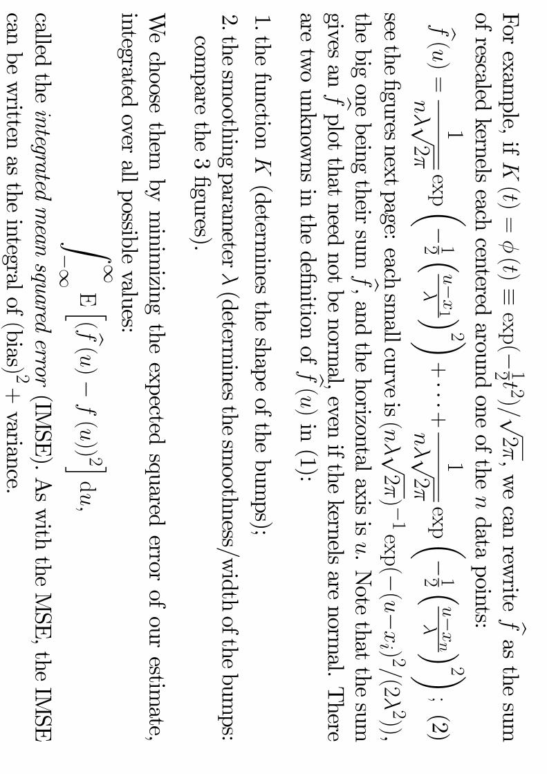
Forexam

ple,if()=()≡

exp(−12 2) √

2,wecan

rewrite b

asthe

sumofrescaled

kernelseach

centeredaround

oneofthe

data

points:

b()=

1

√2exp µ−

12 ³−

1

´2 ¶+···+

1

√2exp µ−

12 ³−

´2 ¶;(2)

seethe

figuresnextpage:

eachsmallcurve

is( √2) −1exp(−(−

) 2(2

2)),the

bigone

beingtheir

sum b,andthe

horizontalaxisis.Note

thatthe

sumgives

an bplot

thatneed

notbenorm

al,evenifthe

kernelsare

normal.There

aretwounknow

nsinthe

definitionof b

()in(1):

1.thefunction

(determ

inesthe

shapeofthe

bumps);

2.thesmoothing

parameter

(determ

inesthe

smoothness/w

idthofthe

bumps:

compare

the3figures).

Wechoose

thembyminim

izingthe

expectedsquared

errorofour

estimate,

integratedover

allpossiblevalues:

Z∞−∞E h( b

()−

()) 2 i

d

calledthe

integratedmean

squarederror

(IMSE).A

swiththe

MSE,the

IMSE

canbewritten

asthe

integralof(bias) 2

+variance.

Weshow

thisMSE

decomposition

forthe

simplest

setup.Suppose

thatwe

haveanestim

ator bofaparam

eter.

Define

≡ b−E( b)and

theestim

ator’sbias

is≡

E( b)−

.Then,

MSE( b)

=E ³(+) 2 ´

=E(2+2

+ 2)

=E(2)+E(2)

+E( 2)

Sinceisnonrandom

(thinkofE( b)asaconstant

),

MSE( b)=E(2)+2E()+ 2

Bythe

definitionofvar( b)≡

E(2),and

by

E()≡

E ³b−E( b) ´

=E( b)−

E( b)=0

weget

MSE( b)

=var( b)

+ 2.

This

proofwasconstructive

and“from

firstprinciples”.

There

isanalternative

onethat

verifiesthe

desiredresult

bymaking

useof

E(2)≡

var()+(E()) 2

Letting

≡ b−

,then

usingvar( b−

)=var( b)

(locationinvariance)

andE( b−

)=,w

eget

therequired

result.

Minim

izingthe

IMSE

when

islarge

implies

thatthe

optimalstandardized

kernelisthe

Epanechnikov

(orquadratic)

kernel

e()≡ (

34 √5 ³1−

15 2 ´(||

√5)

0(otherw

ise),(3)

andthe

mean

is0asaresult

ofthe

optimization

(notbyconstruction),w

hichiswhyeach

kernelwascentered

aroundearlier.

Nevertheless,

theincrease

inthe

optimalIMSEissmall(and

vanishesas

→∞)ifusing

()=()

instead.More

crucialisthe

choiceof

,determining

howsmooth b

is.

Thevariance

of basanestim

ateof

isthe

verticalvolatilty

ofthis

estimate

inthe

previousgraphs.

Alarger

makes

theestim

ate bless

erratic(less

volatile b)while

assigningahigher

probabilitytopoints

farfrom

thedata

(hencecausing

abias

in b);seethe

previousgraphs

&Remark

1inSection

C.

Exercise

2willgive

thebalancing

tradeoffbetw

eenbias

andvariance

of b.Section

Cwillshow

thatthe

optimal

isofthe

order −15:

doublingthe

sample

size,means

thatweneed

toreduce

byafactor

of2 −15≈

087(areduction

of13%

).Therefore,

lesssmoothing

isneeded

asthe

sample

sizeincreases

becausethere

aremore

datatofillthe

horizontalaxisinthe

graphs.

Remark

1(b)inSection

Cwillshow

thatthe

efficiency

ofthe

estimate b

isless

thanwhat

parametric

estimation

gives:the

variancedeclines

atarate

of1(

)instead

of1

,aprice

topay

forthe

flexibilityofthe

estimate b.

Apart

fromthe

usualdirect

reasonstoestim

atethe

densityofvariates

(toquantify

theirrandom

nessand

knowtheir

overallbehaviour),

thereare

otherindirect

usesfor

densitiesinfinance

andeconom

icssuch

as“hazard

rates”.They

arealso

knownas“age-related

failurerates”

iftimeisinvolved.

Forexam

ple,theprobabilities

of:

1.death,given

thatanindividual

hassurvived

untilsom

eage

(usedincalcu-

latinglife-insurance

premiainactuarialw

ork);

2.breakdownofanew

machine,given

thatithas

functioneduptosom

epoint

intime;

3.employm

ent,giventhat

aperson

hasbeen

unemployed

forsom

eperiod

(typ-ically

adim

inishingfunction

ofthis

periodasitgets

longer);

4.defaultonsom

eobligation,given

thatnodefault

hasoccurred

sofar.

Having

surviveduntil

0 ,w

hatisthe

densityfunction

ofover

therest

ofits

lifetime?Assum

ingisacontinuous

variate,thisdensity

is

|

0 ()=

()

Pr(

0 )=

()

1−(0 )

0

where

thedenom

inatorensures

thatthe

newdensity

integratesto1(the

prob-abilities

addupto100%

).

Thehazard

rateisthis

functionevaluated

at0 ,and

itgives

thedensity

offailures

at0once

thispoint

isreached.

Wehave

(0 )≡

(0 )

1−(0 )=−dlog(1−

(0 ))

d0

orequivalently

1−(0 )=exp(− R

0

0()d)if0asinthe

examples

ofthe

previousslide

(otherwisethe

lowerlimitofintegration

isdifferent).

Note:

1.thesimilarity

ofthis

exponentialtocontinuous

discountingbyaninstanta-

neousrate,used

infinance

theory;

2.wecall

1−(0 )the

survivalfunctionbecause

itequals

Pr(

0 );

3.takinglogwilltransform

absoluteinto

relativescales,so

(0 )isthe

relative(or

percentage)change

inthe

survivalfunction(1−

(0 ))as

0changes.

Let

0bearandom

variablehaving

anexponentialdensity

definedby

()=exp(−

)

0

This

implies

afixed

hazardrate

(0 )=

,regardless

ofthe

value=

0 .

(Recall

themeaning

ofthis,

fromearlier

examples

likethe

probabilityofem-

ployment.)

Other

densitiesgenerate

otherpatterns

inthe

hazardrates,

butthey

areall

restrictedbythe

specificchoice

ofadensity.

NPdensity

estimation

freesusfrom

therestrictions

thatthese

initialchoices

would

haveimposed.

Byusing

theNPestim

ate b,wecan

discoverwhether

thepattern

canbesimplified

toone

knowndensity

oranother,

butthe

resultisusually

more

generalthanthe

standardknow

ndensities

andtheir

associatedhazards.

Thesam

eideas

ofNPdensity

estimation

canbeused

formultivariate

data.When

usingNPdensity

estimation

asavisual

tool,itisbest

tolook

atthe

densityofone

ortwovariates,

conditionallyonthe

rest.For

illustrations,see

thenext

fivegraphs

fromSilverm

an(1986):

•the

firstone

showsabivariate

histogram;

•the

following

threeshow

smoothed

bivariateNPdensity

estimates;

•the

lastone

showsacontour

maporiso-probability

contoursdefined

by()=forasuccession

ofconstants

1···

0(i.e.

takea

sequenceof

slices

paralleltothe

axes

inthe

3-dimensionalgraphs.)

These

contoursare

similar

tothe

wiggly

linesinweather

maps,

where

thevalues

1

would

denoteatm

osphericpressures.

Similarly

forwalking

maps,w

ithcontours

indicatingthe

altitudealong

hillsand

mountains

(tightcontours

=steep

climb,large

gapsbetw

eencontours

=gentle

slope).Thepeaks

(ormodes)

ofare

atthe

centerofthese

contours.

Another

illustrationisinGallant,R

ossi,andTauchen

(1992,Review

ofFinan-

cialStudies);seethe

figurecontaining

4displays

onthe

nextpage.

1.Denote

logtrading

volumesby

and

conditionalchanges

inlog

pricesby

∆.Recall

thatthe

logtransform

svariables

intorelative

scales:defining

pricereturns

by ≡

( −

−1 )

−1 ,w

hereisthe

pricelevel,w

ehave

∆=

∆log

=log

−

log−1=log(

−1 )=log(1+ )≈

There

isapositive

relationbetw

eenand|∆

|.Inthe

lastdisplay

(acontour

map),as

∆becom

esnonzero

(move

awayfrom

thecenter

ofthehorizontal

axis),tends

toincrease

andthis

isreflected

bythe

widening

topofthe

triangle(this

iswhere

themost

likelycorresponding

is).

2.Therelation

isalso

asymmetric,depending

onwhether

theprices

aregoing

upordow

n.Thetilt

ofthe

triangleshow

sthat

thereismore

tradingon

theupsw

ingofprices,a

featuredetected

fromthe

NPdensity

contour(last

display)but

notdetectable

fromthe

scatterplot

(firstdisplay).

(The3-dim

ensionalgraph

inthe

thirddisplay

isthe

NPestim

ateofthe

jointdensity

∆ ,the

verticalaxisdenoting

theestim

atedvalue

of.Thecontours

areobtained

asasuccession

ofhorizontalslices.)

B.NPregression

Regression

analysiscan

beform

ulatedas

y=E(y|X)+ε≡

g(X)+ε

with by

= bg(X)asthe

estimated

(orfitted)

regressioncurve.

Forthe

bivariatenorm

aldistribution,theconditionalexpectation

g()isalinear

function,hencethe

so-calledlinear

regressionmodel.

Linearity

holdsfordistributions

havingellipticalcontours

(knownasellipticaldistributions),incl.norm

alandStudent

t,butingeneralother

functionalformsemerge

(asseen

inthe

previousslide).

Nonparam

etricregression

doesnot

presupposeafunctionalform

.Itestim

atesthe

conditionalexpectation

fromthe

nonparametric

jointdensity

estimate

ofthe

variates.This

givesrise

inthe

bivariatecase

tothe

Nadaraya-W

atsonestim

atorofE(|

=),nam

ely

b()=

X=1

with

≡

¡ −1(−

) ¢

P=1 ¡ −

1(− ) ¢

whereb

canbeseen

asaweighted

averageofthe

’s,

withweights

givenby

the ’sand

addingupto100%

.

Interpretingthis

formula

throughascatter

plot:

1.Foreach

,the ’sinasmallneighborhood

ofitprovide

thelargest

weight

tothe

averageofthe

corresponding ’s,a

localaveragingof

.

Thisisbecause

alarge

valueof|−

|corresponds

tothe

tailofthekernel;

forexam

ple,see(2).

2.Tracing

thesequence

ofsuchaverages

aschanges,w

egetthe

NPregression

curve.

Thenext

graphillustrates,

usingdata

onconsum

ption(vertical

axis)and

in-com

e(horizontalaxis).

Asincom

eincreases,consum

ptionincreases.

However,

thisdoes

nothappen

inthe

usuallinearway,but

ratherinan

-shaped

form:

1.Atlow

incomes,consum

ersborrow

tospend

more

thanthey

earn.Asincom

eincreases,the

gapfalls.

2.Forinterm

ediateincom

es,anincrease

inearnings

ismatched

byanincrease

inconsum

ption.

3.Athigh

incomes,savings

increaseand

consumption

levelsoff.

Now

considerwhat

happensas

→0or

→∞inthe

Nadaraya-W

atsonform

ula:

1.Inthe

firstcase,

thewindow

width

isshrinking

aroundeach

pointinthe

dataset,andthe

NPregression

issimply

thesequence

of-values

(assuming

thereare

noties

inthe

-values).

2.Atthe

otherextrem

e,avery

largewindow

width

means

thatthe

regressioncurve

isjust

ahorizontalline

givenbythe

averageof

.

Theoptim

albandwidth

issom

ewhere

inbetw

een,anditisfound

bythe

same

methods

asinthe

caseofNPdensity

estimation.

Wenow

turntothese

technicalities.Only

theresults

labelled“Exercise”

needtobesolved.

Therest

isacollection

ofresults

thatform

alizesom

eofthe

earlierclaim

s.They

areincluded

forreference,

butyou

arenot

requiredto

derivethem

.

C.Tech

nical

results

andExercises

Exercise

1(Kernels)

Supposethat

,=1

,are

datafrom

arandom

sampleof

,and

thathas

acontinuous

density.Wedefine

b()≡

1

X=1

µ−

¶

where

0and

wechoose

tobeaproper

densityfunction.

Write b(

)as

theaverage

ofdensities.

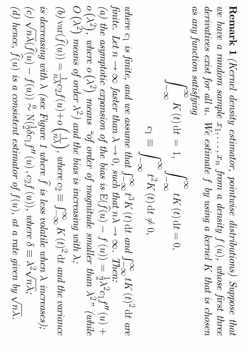
Remark

1(Kernel

densityestim

ator,pointw

isedistributions)

Supposethat

wehave

arandom

sample

1

from

adensity

(),whose

firstthree

derivativesexist

forall

.Weestim

atebyusing

akernel

that

ischosen

asany

functionsatisfyingZ∞−∞

()d=1 Z

∞−∞()d=0

1 ≡ Z

∞−∞ 2

()d6=

0

where

1isfinite,

andweassum

ethat R∞−∞

3()dand R∞−∞

() 2

dare

finite.Let

→∞faster

than→

0,such

that→

∞.Then:

(a)the

asymptotic

expansionofthe

biasisE( b(

)−())=12 21 00(

)+

¡2 ¢,

where

¡2 ¢means

“oforder

ofmagnitude

smaller

than2”(while

¡2 ¢means

oforder

2)and

thebias

isincreasing

with

;

(b)var( b(

))=

12 ()+

³1 ´,where

2 ≡ R∞−∞

() 2

dand

thevariance

isdecreasing

with

(see

Figure

1where b

isless

volatilewhen

increases);

(c) √( b(

)−())

∼N( 12

1 00()2 ()),where

≡2 √

;

(d)hence, b(

)isaconsistent

estimator

of(),atarate

givenby √

.

Exercise

2(Kernel

densityestim

ator,IMSE)Continuing

withthe

setupof

Remark

1,define

≡ Z∞−∞

00() 2d∞

Showthat:

(a)the

asymptotic

(i.e.large-

)IMSE(or

AIMSE)of b

is

421

4+

2

;

(b)the

bandwidth

thatminim

izesthis

AIMSEis

b= Ã

2

21 !

15

where

1and

2are

definedinRemark

1.[Note:

Thevalue

ofthe

minim

umAIMSE

isnot

affectedbythe

choiceof

1 ,

because2varies

accordinglytooffset

thischange.

Therefore,w

ecan

set1=1

without

lossofgenerality

inthe

formula

for bfrom

nowon.]

Remark

2(CVand

thebandw

idth)Given

thatthe

Epanechnikov

kernelisthe

optimalone,

theonly

remaining

obstacletopractical

implem

entationofthe

estimation

ofisthe

undetermined

bandwidth.

TheEpanechnikov

kernelhas

R∞−∞e() 2

d=3 ¡5 √

5 ¢,sothe

optimal b

is

b= Ã

3532

!

15≈0769

() 15

Itcontains

theunknow

n≡ R∞−∞

00() 2d.

Onepossibility

isthe

plug-inmethod,

whereby

aprelim

inaryestim

ateof

(or

somehypothesized

)issubstituted

into.

Inthis

remark,

wewillanalyze

anothermethod

thatdoes

notrequire

sucharbitrary

choices.

Least-squarescross-validation

(LSCV)optim

izesacriterion

thathas,

onaver-

age,thesam

evalue

asIMSE.It

isbased

onthefollow

ingresam

plingprocedure.

Thefirst

stepofthe

procedureistodelete

oneobservation

atatime,say

(=1

),thencalculate

theusualkernelestim

atorbased

ontherem

aining−

1data

points:

b−()=

1

(−1) X6=

µ−

¶

=1

Defining b−

1(x)≡

1 P=1 b−

¡ ¢,

where

wehave

thedata

vectorx≡

(1

) 0,the

procedureminim

izes

≡ Z

∞−∞() 2d+ Z

∞−∞ b() 2d−

2 b−1 (x)

withrespect

to.Thisprocedure

isjustified

becauseE()isthe

IMSE:

Z∞−∞E h( b

()−

()) 2 i

d=E ∙Z

∞−∞( b()−

()) 2d ¸

=E ∙Z

∞−∞() 2d+ Z

∞−∞ b() 2d−

2 Z∞−∞ b

()()d ¸

butwewon’t

provethe

equivalenceofthis

lastterm

withthe

lastone

inE().

Note

that R∞−∞() 2ddoes

notdepend

on,sothat

minim

izingwith

respectto

isequivalent

tominim

izingZ∞−∞ b(

) 2d−

2 b−1 (x)

which

containsnounknow

ns.

Exercise

3(Estim

atorofNadaraya

andWatson)

Supposethat

therandom

sample

(1

1 )(

)isdraw

nfrom

abivariate

density(),or

simply

().Defineb

()≡

1

X=1

(−

−

)

where

isascaled

bivariatekernelsuch

that

()≡ Z

∞−∞()d()≡ Z

∞−∞()d

Z∞−∞

()d=0

where

and

are

univariatekernels

(suchas

()= −1 ¡ −

1 ¢where

isasseen

earlier)and

iscentered

around0(atleast

for).

Showthat

theestim

atorofE(|

=)implied

by b()is

X=1

(−

)

P=1 ¡−

¢

Exercise

4(NPdensity

estimation,num

erical)Using

PC-GIVE,calculate

theNPkernel

densityestim

atefor

eitherinflation

orinterest

rate.Does

itlook

likeanorm

al(orlog-norm

al)?Comment

onthe

featuresofthe

density.

[Theseries

isnot

i.i.d.,but

wewilladdress

thiscom

plicationinlater

lectures.]

Exercise

5(NPregression,

numerical)

Using

PC-GIVE,calculate

theNPre-

gressionofconsum

ptiononincom

e.Comment

onthe

featuresofthe

relation.

Solution

1.Define

≡

1 µ

−

¶

=1

where

thescaling

1indicates

theconcentration

ofthe

assignedweights

aroundthe

points .Toshow

that isindeed

adensity

functionwithrespect

to,w

emust

showthat

itisnonnegative

everywhere

andthat

itintegrates

to1.Thefirst

propertyisestablished

bythe

positivityof

and

thedefinition

ofasadensity

function.Thesecond

propertyisobtained

asZ∞−∞

d= Z

∞−∞1 µ

−

¶d

= Z∞−∞

()d=1

bythe

changeofvariable

=(−

)

havingd=d.Thequantity b(

)isthen

theaverage

ofthese

,w

ithweights

1each.

Solution

2.(a)

Weknow

thatthe

MSEisthe

sumofthe

squaredbias

andthe

variance.Therefore,the

leadingterm

ofthe

MSEof b(

)is

421

4 00(

) 2+

2

()

andthe

correspondingAIMSEis

≡

421

4 Z∞−∞

00() 2d+

2

Z

∞−∞()d

=421

4+

2

(b)Minim

izingwithrespect

to,

≡321 −

2

2=0

issolved

uniquelyby b

5=2 ¡

21 ¢,and

wehave

2

2 ≡

3221 +22

30

Theoptim

alvalueistherefore

b=14 Ã

21 42

4 !

15

+ Ã21 42

4 !

15

=54 Ã

21 42

4 !

15

where

weseethat

theoptim

alsquaredbias

isofthe

sameorder

ofmagnitude

asthe

optimalvariance.

There

isabalancing

tradeoffbetw

eenbias

andvariance,

forthe

sakeofminim

izing.See

also(a)

and(b)

ofRemark

1.

Solution

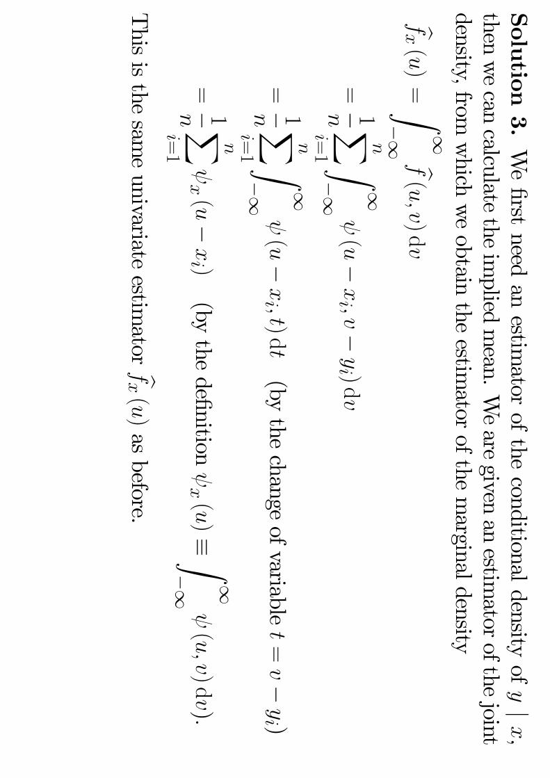
3.Wefirst

needanestim

atorofthe

conditionaldensity

of|,

thenwecan

calculatethe

implied

mean.

Weare

givenanestim

atorofthe

jointdensity,from

which

weobtain

theestim

atorofthe

marginaldensity

b()= Z

∞−∞ b()d

=1

X=1 Z∞−∞

(−

−

)d

=1

X=1 Z∞−∞

(−

)

d(by

thechange

ofvariable

=−

)

=1

X=1

(−

)

(bythe

definition()≡ Z

∞−∞()d)

Thisisthe

sameunivariate

estimator b

()asbefore.

Theestim

atorofE(|

=)istherefore

Z∞−∞

b|()d= R∞−∞

b()d

b()

= R∞−∞ P

=1(−

−

)d

P=1(−

)

=X=1 R∞−∞

(+ )(−

)

d

P=1 ¡−

¢

Theresult

followsfrom R∞−∞

(−

)

d=0and R∞−∞

(−

)

d≡

(−

).

Notice

thatthe

resultingestim

atorrequires

onlyone

marginal

kernel ,with

onlyone

smoothing

parameter,

which

issom

ethingthat

hasnot

beenimposed

atthe

outset.