Computational Finance

Computational FinanceThe design, development, testing, and implementation of software that realizes

quantitative financial models for portfolio management and trading (front office), risk management (middle office), and financial engineering and pricing (back office).

Machine LearningStatistical Inference, Inductive Reasoning,

Mathematical Optimization – derive a model from past experiences from which to understand something.

Computer ScienceHigh Performance Computing, Data

Structures, Algorithms, Simulation Methods.

Statistics & MathProbability theory, Stochastic Calculus, Optimization theory, Numerical methods.

Financial TheoryMicro and Macro

Economics, Modern Portfolio Theory, Risk

Management, and Security Analysis.

Securities include Fixed Income, Equities,

Derivatives, Structured Products, Alternatives,

Commodities, and more.

“There's no question that the computer scientist is much more highly valued today than has ever been the case.”

John Lehoczky professor of statistics at Carnegie Mellon speaking about the

future of Quantitative Finance post the 2008 financial crisis.

Source - http://www.americanbanker.com/news/bank-technology/young-quants-shift-from-risk-taking-to-risk-management-1074476-1.html

The Back Office

CompFin in the Back Office

• Financial Engineers create products and come up with models to price them. Derivatives are securities whose value depends on some underlying security.

• Many complex derivatives need to be priced using simulation methods which are computationally expensive. One solution to this is to implement the models to run on GPU’s which perform floating point and matrix operations much faster.

• How to price a derivative using simulation methods - calibrate a stochastic processes to the underlying; simulate the underlying; compute the pay-off from the derivatives for each simulation; then present value the pay-offs to today.

• Calibration is an optimization problem. Given a stochastic process (and historical data) what are the optimal parameters for the model? The more complex the model i.e. the more parameters it has, the more difficult it is to optimize.

EX 1 Model Calibration using Hill ClimbersBackground Information I

• Stochastic processes are collections of random variables which describe the evolution of a system over some period of time.

• One stochastic process is the Ornstein Uhlenbeck process. This process is mean-reverting and is sometimes used to model interest rates.

• The stochastic differential equation for the Ornstein Uhlenbeck model is:

where is the change in an interest rate; is the average interest rate over time; is the rate of mean-reversion; is volatility; and is a Wiener process. Wiener process, also called Brownian Motion, is just a normally distributed stochastic process.

EX 1 Model Calibration using Hill ClimbersBackground Information II

• So how can we find the correct values for , , and ? This is where some machine learning (optimization) can come in handy.

• From the SDE for the Ornstein Uhlenbeck process we saw that there is some relationship between the previous and the next interest rate.

• Multiple linear regression is a statistical way of expressing the linear relationship between a dependent variable and independent variables.

• Hill climbing can be used to find the optimal values for and i.e. we search for the values which minimize some objective function.

EX 1 Model Calibration using Hill ClimbersExample Output

• The relationship between and

EX 1 Model Calibration using Hill ClimbersApproach taken I

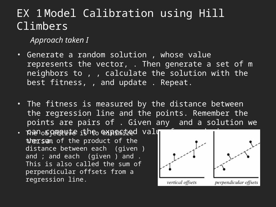
• Generate a random solution , whose value represents the vector, . Then generate a set of m neighbors to , , calculate the solution with the best fitness, , and update . Repeat.

• The fitness is measured by the distance between the regression line and the points. Remember the points are pairs of . Given any and a solution we can compute the expected value for and vice versa.

• The objective is to minimize the sum of the product of the distance between each (given ) and ; and each (given ) and . This is also called the sum of perpendicular offsets from a regression line.

EX 1 Model Calibration using Hill ClimbersExample Output I

• The result – the hill-climber algorithm finds a nice line between and

EX 1 Model Calibration using Hill ClimbersApproach Taken II

• Now using some pretty fancy mathematics which uses the horizontal, vertical, and perpendicular offsets … as well as the sum of and we can derive the approximate parameter values for the Ornstein-Uhlenbeck stochastic process. Then we have successfully calibrated the model .

• For the intrepid student here is a link to the fancy mathematics - http://www.sitmo.com/article/calibrating-the-ornstein-uhlenbeck-model/

EX 1 Model Calibration using Hill ClimbersExample Output II

• The resulting interest rates have similar statistical properties,– Known process – {, , }– Regressed values – {, , }

The Middle Office

CompFin in the Middle Office

• Quantitative Analysts in the middle office are responsible for managing financial risks, validating back-office models, and ongoing financial reporting.

• Financial risk can be broken down into many ways. One definition of risk is the factors which drive return. Factors could include market volatility, interest rate volatility, foreign exchange rate fluctuations, credit-worthiness of individuals, etc.

• The role of computational finance in this space is to build models which quantify the factors of financial risk. For example, models would answer questions like:– What is the maximum one-day loss on this portfolio within a 99% confidence interval? (VaR)– How sensitive is this portfolio / security to a one basis point increase in interest rates? (PV01)– What is the probability of our creditors defaulting within the next year? (Credit Scorecards)

• The biggest applications of machine learning in the middle office is credit risk management (default probabilities) and fraud detection (behaviour analysis).

EX 2 Credit Risk Modelling using Neural NetworksBackground Information I

• Credit risk is the risk that somebody will default on their credit. It is important for banks to predict what the probability of somebody defaulting is prior to them issuing loans. One technique for credit scoring is to use neural networks.

• The inputs into the neural network is data about the individual – age, income, net worth, etc. There are example credit data sets on the UCI machine learning page.

• A neural network is a computational model that approximates the relationship between a set of independent variables (inputs) and some dependent variable (output). In that way it is very similar to a multiple linear regression.

• In fact, neurons in a neural network are MLR’s which feed into (usually) some non-linear activation function e.g. sigmoid or tan-h. In other words, a neural network is a set of non-linear regressions between the inputs and the outputs.

EX 2 Credit Risk Modelling using Neural NetworksBackground Information II

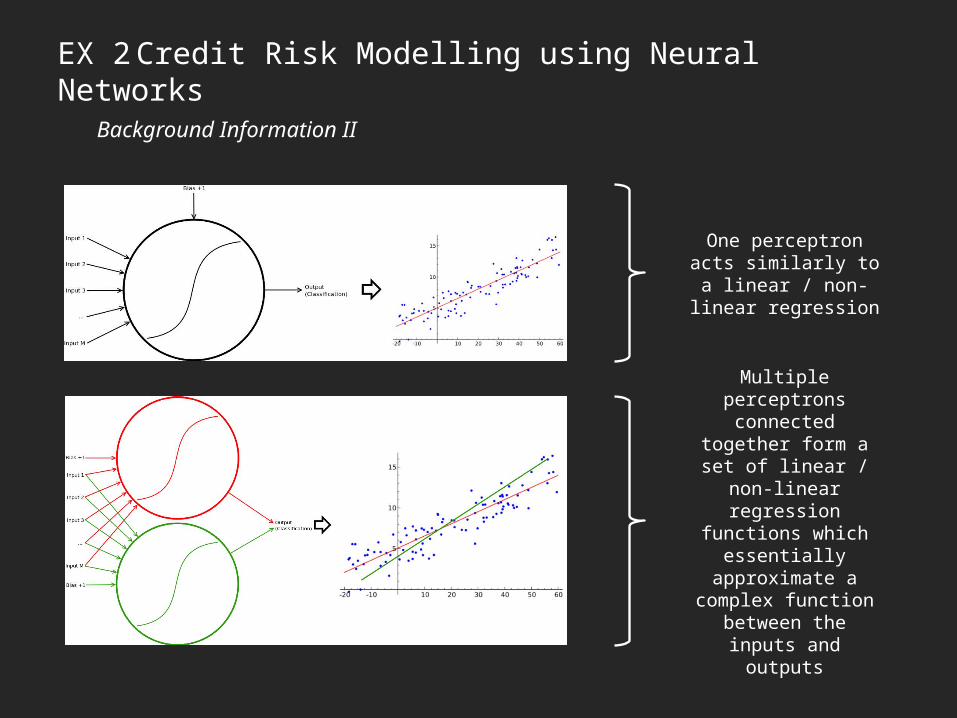
One perceptron acts similarly to a linear / non-

linear regression

Multiple perceptrons connected together form a set of linear / non-linear

regression functions which essentially

approximate a complex function between the

inputs and outputs

EX 2 Credit Risk Modelling using Neural NetworksBackground Information III

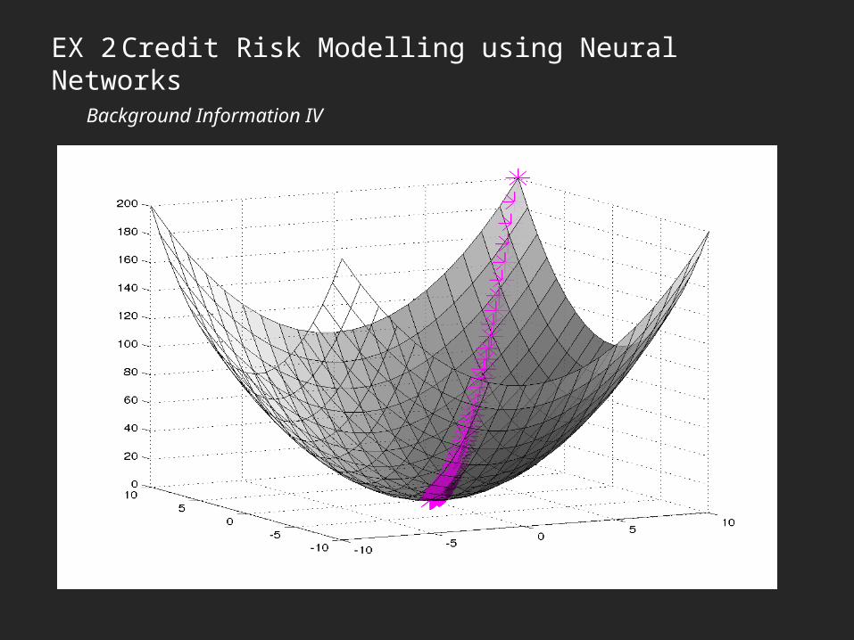
• The objective of a neural network is to optimize the weights of the inputs into each one of the perceptrons such that the error of the network is minimized. This is often done using the Back-Propagation learning algorithm (gradient descent)

• This technique works by calculating the partial derivative of the sum-squared error with respect to the weights for each neuron (automatic differentiation) and adjusting the weights by the negative gradient. Basically it goes down the hill.

Minimize the sum-squared error

(distance squared between the expected

values a.k.a targets and the output

produced by the neural network an

input pattern)

EX 2 Credit Risk Modelling using Neural NetworksBackground Information IV

EX 2 Credit Risk Modelling using Neural NetworksBackground Information V

• But … the weights in a neural network can be viewed in vector notation. As such, you can use any optimization algorithm to train a neural network including hill-climbers, particle swarm optimization, genetic algorithms, random search, etc.

EX 2 Credit Risk Modelling using Neural NetworksApproach Taken

• Download some historical credit data from the UCI Machine Learning repository online. This contains data in the form,– Attributes -> Target Value

• Wrangle the data until it is represented using values (not characters) and is within the active range of the activation functions in the NN.

• Split the data into a training and a testing (validation) set. Train the neural network on the testing set until it has learn the relationship between the input attributes and the target value (credit risk or not credit risk)

• Then test the neural network on the testing set to check for over-fitting.

EX 2 Credit Risk Modelling using Neural NetworksExample Output I

Weight Matrices are a good way to understand (non-deep) neural networksInitial Weight Matrix Final Weight Matrix

EX 2 Credit Risk Modelling using Neural NetworksExample Output II

Accuracy on Training set = 85.87896253602305 %Accuracy on Testing set = 83.5734870317003 %

Good! Not over-fitting

The Front Office

CompFin in the Front Office

• Arguably the most exciting (and best compensated) application of computational finance is the front office. Front office quantitative analysts or traders are mostly responsible for constructing portfolios and algorithmic trading strategies.

• Portfolio optimization involves trying to determine how much capital to invest into which assets in the portfolio. This involves forecasting the expected risk and return of individual assets in the portfolio (can be done using Machine Learning) and then changing the weights of the portfolio to maximize risk adjusted return.

• Quantitative trading strategies are powered by models which consider different factors such as momentum, mean reversion, quantitative value, and events to make trading decisions i.e. what to buy and when. Some firms use neural networks and other machine learning models but be-warned, markets are dynamic.

EX 3 Portfolio Optimization using PSOBackground Information I

• Portfolio optimization is the problem of apportioning a given amount of capital between the constituent assets of a portfolio such that the expected risk-adjusted return of the portfolio is maximized over some future period of time.– Inputs – future expectations of risk and return for each asset– Inputs – expected correlation matrix between each one of the assets– Outputs – the weight of capital which should be allocated to each asset– Objective – maximize the expected risk-adjusted-return of the portfolio e.g. Sharpe Ratio

• There are many different measures of risk-adjusted-return. The first phase of my Masters research involves characterizing these functions in high dimensional space (a large number of assets) under various equality and inequality constraints.

• The most popular measure of risk adjusted return is the Sharpe Ratio

EX 3 Portfolio Optimization using PSOBackground Information II

• How do you calculate the expected returns for each asset?– Option 1 – use historical mean return assuming that the distribution is stationary– Option 2 – forecast expected returns using some technique e.g. neural networks / quant method

• How do you calculate the expected risk of each asset?– Option 1 – use historical volatility again assuming that the distribution is stationary– Option 2 – use a model e.g. stochastic process to simulate how the asset evolves over time

• How do you get the expected risk and return of the portfolio?– Expected return is equal to the sum product of the expected return on the assets and the weights

– The expected risk of the portfolio is equal to the sum product of the volatilities minus diversification

EX 3 Portfolio Optimization using PSOBackground Information III

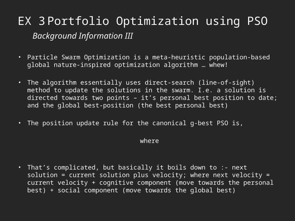
• Particle Swarm Optimization is a meta-heuristic population-based global nature-inspired optimization algorithm … whew!

• The algorithm essentially uses direct-search (line-of-sight) method to update the solutions in the swarm. I.e. a solution is directed towards two points – it’s personal best position to date; and the global best-position (the best personal best)

• The position update rule for the canonical g-best PSO is,

where

• That’s complicated, but basically it boils down to :- next solution = current solution plus velocity; where next velocity = current velocity + cognitive component (move towards the personal best) + social component (move towards the global best)

EX 3 Portfolio Optimization using PSOBackground Information IV

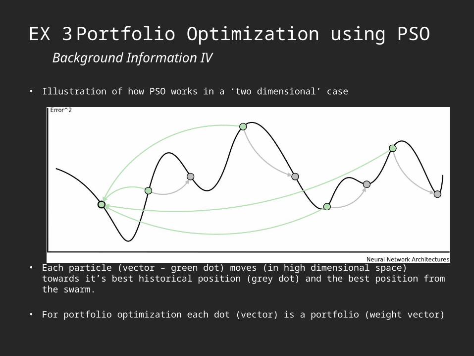
• Illustration of how PSO works in a ‘two dimensional’ case

• Each particle (vector – green dot) moves (in high dimensional space) towards it’s best historical position (grey dot) and the best position from the swarm.

• For portfolio optimization each dot (vector) is a portfolio (weight vector)

EX 3 Portfolio Optimization using PSOApproach Taken

• Download some historical JSE price data from Quandl.com for our portfolio of blue chip stocks: {SBK, ANG, BIL, SHP, WHL, VOD, MTN, DSY, SLM}

• Define a strategy for predicting what the future returns for each asset will be. Our strategy is that the previous six months = the next six months.

• Slice the data into six-monthly segments, optimize the portfolio weights on the historical six months, then calculate the returns in the next six months.

• Doing this from 2010 – 2015, 10 six-month periods, therefore results in 10 optimization problems that happen over-time. Avoid any biases!

• Compare these results to a benchmark portfolio such as an equally weighted portfolio of the stocks i.e. each stock has an equal weight.

EX 3 Portfolio Optimization using PSOExample Output

• This is the output produced from a silly trend-following strategy. Eq s = 0.0003904503493283587 r = 0.006431238387474281 f = 0.35289313566293007Op s = 0.0007074653788236298 r = 0.00875007503958214 f = 0.2548364776503159

EX 3 Portfolio Optimization using PSOProblems with Portfolio Optimization

• In this strategy the assets are expected to produce similar returns in the next six months as they did in the previous six months. As such the portfolio is optimized over historical data and the returns from this are calculated and compounded.

• The problem with portfolio optimization is that it maximizes errors. In other words, garbage-in = garbage-out. The quality of your optimized portfolio is directly proportional to the accuracy of your model and it’s predictions.

• Other problems with portfolio optimization include biases such as look-ahead bias, data-mining bias, sample selection bias, random number generator biases, etc.

For more information

• www.Quandl.com – a website with tones of free financial data and a great API.• www.QuantStart.com – a website dedicated to helping you start your quant career.• www.Quantocracy.com – an aggregation of mostly quantitative trading blogs.• www.Quantopian.com – an online python back-testing and paper trading platform.• www.StuartReid.co.za – where computer science and quantitative finance meet.

• The code used in this lecture is availablehttps://github.com/StuartGordonReid/Comp-Fin-Lecture