Flight Landing Analysis

BANA 6043 STATISTICAL COMPUTING Mid Term Project

Submitted by Tauseef Alam (M10666228)

Abstract:

Landing overrun is problem for most flight landing operations. In this report we are trying

to identify key factors affecting the landing distance of commercial flights. In order to

determine the factors and quantify the impact of factors on landing distance we created a

linear regression model keeping landing distance as dependent variable.

Landing distance is largely dependent on ground speed of aircraft, aircraft type and height

(descending order with respect to weight) of the aircraft when it passes through the

threshold of runway.

Distance= -945.4486 + 460.522*aircraft_typ + 0.27335*speed_gr_sq + 14.056*height

1. For ‘Boeing’ aircraft type the predicted landing distance would be 0.25644 points greater

than ‘Airbus’ aircraft type.

2. For every one-unit increase in square of ground speed there will be 0.92932-unit increase

in the predicted landing distance

3. For every one-unit increase in height above threshold there will be 0.15345-unit increase

in the predicted landing distance

CHAPTER 1: Data Preparation

This chapter will illustrate the step by step methods and techniques used for data

preparation. Each step will be followed by reasoning, AS code and then output of SAS

code or log file

Step1: Read landing data from the two excel files ‘FAA-1.xls’ and ‘FAA-2.xls’.

SAS Code:

PROC IMPORT OUT= FAA1 DATAFILE= "C:\Users\alamtf\Downloads\FAA1.xls"

DBMS=xls REPLACE;

SHEET="FAA1";

GETNAMES=YES;

RUN;

proc print data=FAA1;

run;

PROC IMPORT OUT= FAA2 DATAFILE= "C:\Users\alamtf\Downloads\FAA2.xls"

DBMS=xls REPLACE;

SHEET="FAA2";

GETNAMES=YES;

RUN;

proc print data=FAA2;

run;

/*deleting all missing observations from FAA2*/

data FAA2;

set FAA2;

if aircraft="" and no_pasg=. and speed_ground=. and speed_air=. and height=. and

pitch=. and distance=. then delete;

run;

data FAA1;

set FAA1;

if aircraft="" and no_pasg=. and speed_ground=. and speed_air=. and height=. and

pitch=. and distance=. then delete;

run;

Reasoning: The dataset is read from the excel files and printed to see the the

observations. This we can do in small dataset types. However, for large datasets we

cannot do this. In the last data step, we are deleting observations which are completely

blank.

Logfile output:

69 /*deleting all missing observations*/

70 data FAA2;

71 set FAA2;

72 if aircraft="" and no_pasg=. and speed_ground=. and speed_air=. and height=. and

pitch=. and

72 ! distance=. then delete;

73 run;

NOTE: There were 150 observations read from the data set WORK.FAA2.

NOTE: The data set WORK.FAA2 has 150 observations and 7 variables.

NOTE: DATA statement used (Total process time):

real time 0.00 seconds

cpu time 0.01 seconds

74 data FAA1;

75 set FAA1;

76 if aircraft="" and no_pasg=. and speed_ground=. and speed_air=. and height=. and

pitch=. and

76 ! distance=. then delete;

77 run;

NOTE: There were 800 observations read from the data set WORK.FAA1.

NOTE: The data set WORK.FAA1 has 800 observations and 8 variables.

NOTE: DATA statement used (Total process time):



Step2: Combining the datasets:

SAS Code:

data faa;

set faa1 faa2;

run;

proc print data=faa;

run;

Reasoning: The two datasets created after reading file FAA1.xls and FAA2.xls

Are appended as both are having same kind of information. FAA2 do not have variable

duration. Hence for combined file all 150 transactions from this file will be missing for

duration variable.

Output:

Step3: Check for removing duplicate observations

SAS Code:

proc sort data= faa out= faa_n nodupkey;

by aircraft no_pasg speed_ground speed_air height pitch distance;

run;

Reasoning: duplicate observations are removed from the data as they do not add any extra

information

Log File Output:

80 proc sort data= faa out= faa_n nodupkey;

81 by aircraft no_pasg speed_ground speed_air height pitch distance;

82 run;

NOTE: There were 950 observations read from the data set WORK.FAA.

NOTE: 100 observations with duplicate key values were deleted.

NOTE: The data set WORK.FAA_N has 850 observations and 8 variables.

NOTE: PROCEDURE SORT used (Total process time):



Comment: There are 850 total observations on which we will be doing our further

analysis.

Step3: Performing Completeness check for each variable: examine if missing values are

present.

SAS Code:

proc means data=faa_n n nmiss min mean p1 p5 p10 p25 p50 p75 p95 p99;

var no_pasg speed_ground speed_air height pitch distance duration;

run;

Reasoning: n and nmiss options are used in proc means to get the count of non-missing

and missing observations. The percentile distribution is check the get a feeling of

distribution of different variables:

Output:

Comments: Here we see that variable speed_air is missing for 75% of the total data and

Duration is missing for 6% of the data. Right Now we are keeping both the variables in

our further analysis. However, we may need to drop these variables or do missing value

imputation before we do our final analysis.

Step4: Removing data abnormality.

SAS code:

/*treetment to remove abnormal observations*/

data faa_fn;

set faa_n;

/*duration of normal flights is always greater than 40 min */

if duration ne . and duration < 40 then delete;

/*Speed_ground value less than 30 and more than 140 is considered abnormal*/

if speed_ground ne . and (speed_ground <30 or speed_ground > 140) then delete;

/*Speed_air value less than 30 and more than 140 is considered abnormal*/

if speed_air ne . and (speed_air < 30 or speed_air > 140) then delete;

/*height should be at least 6 meters at threshold of runway*/

if height ne . and Height < 6 then delete ;

/*distance should be less than airport run way length which is 6000 feet*/

if distance ne . and distance >6000 THEN DELETE;

run;

Reasoning: Certain checks are applied on the data to remove the abnormal observations.

These abnormality definitions are referred from Project.pdf file, which was given.

Step5: Checking the cleaned data to validate the treatment applied

proc means data=faa_fn n nmiss min mean p1 p5 p10 p25 p50 p75 p95 p99;

var no_pasg speed_ground speed_air height pitch;

run;

Proc freq data=faa_fn;

tables aircraft/missing list;

run;

SAS output:

Comment: We can see from the distribution the variables that all the abnormality is

removed. There are 831 observations remaining after removing the abnormality from the

data.

Step6: Summarization of distribution of each variable:

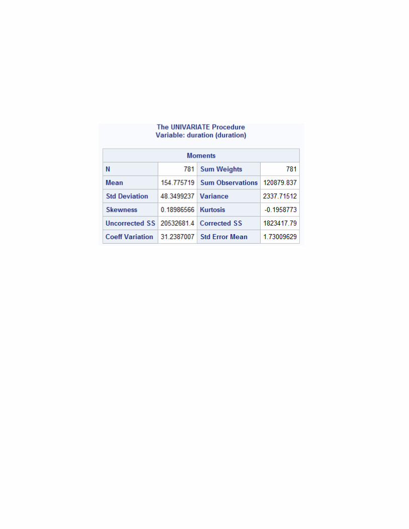
1. Duration(in minutes): Flight duration between taking off and landing. The

duration of a normal flight should always be greater than 40min.

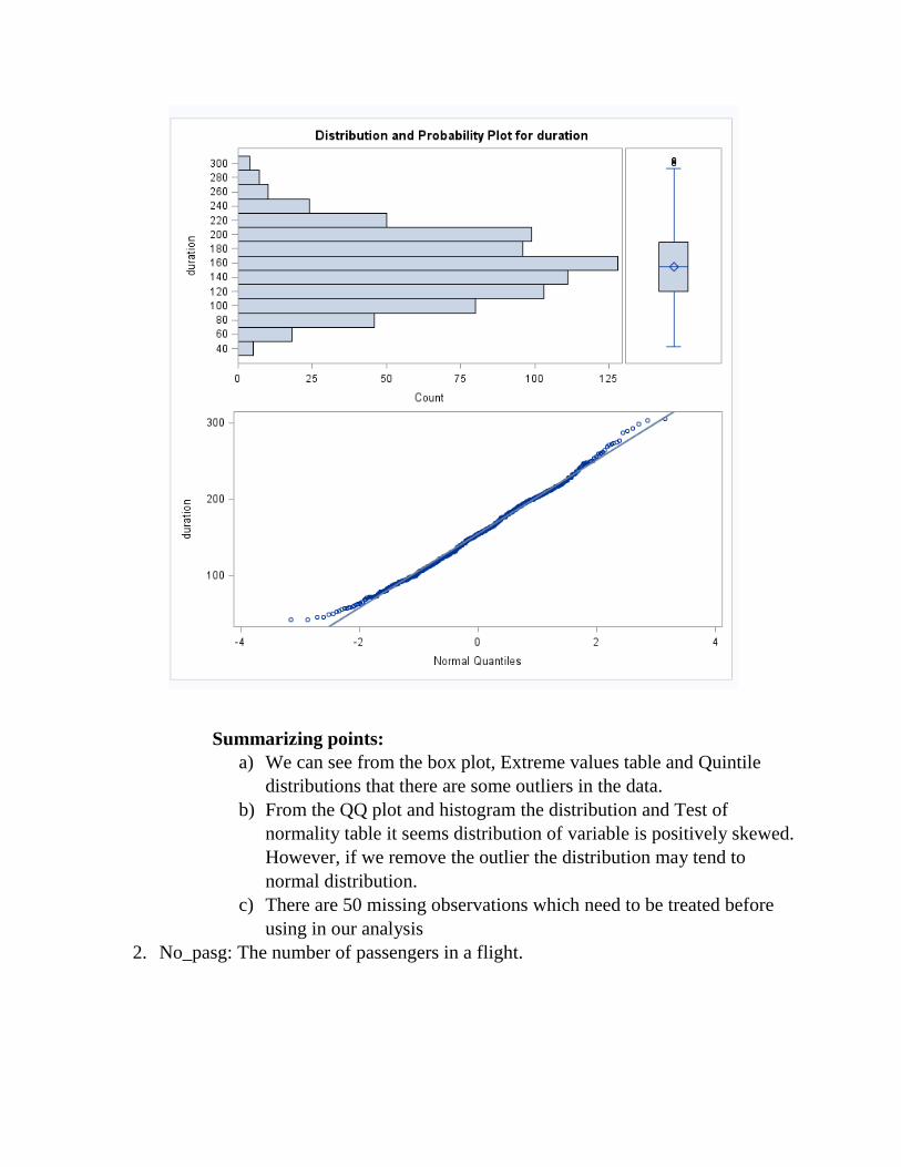
Summarizing points:

a) We can see from the box plot, Extreme values table and Quintile

distributions that there are some outliers in the data.

b) From the QQ plot and histogram the distribution and Test of

normality table it seems distribution of variable is positively skewed.

However, if we remove the outlier the distribution may tend to

normal distribution.

c) There are 50 missing observations which need to be treated before

using in our analysis

2. No_pasg: The number of passengers in a flight.

Summary of variable:

a) We can see from the box plot, Extreme values table and Quintile

distributions that there are some outliers in the data.

b) From the QQ plot and histogram the distribution seems negatively

skewed.

c) From the test of normality table. The variable fails most of the

normality tests as p value is is less than .05. hence the variable is not

normal

d) There are no missing observations.

3. Speed_ground: (in miles per hour): The ground speed of an aircraft when passing

over the threshold of the runway. If its value is less than 30MPH or greater than

140MPH, then the landing would be considered as abnormal.


a) We can see from the box plot and Quintile distributions that there

are very few outliers in the data.

b) From the QQ plot and histogram it seems distribution of variable is

positively skewed.

c) From Test of normality table, the variable passes all the normality

test as the p value for all the test is greater than .05.


4. Speed_air: (in miles per hour): The air speed of an aircraft when passing over the

threshold of the runway. If its value is less than 30MPH or greater than 140MPH,

then the landing would be considered as abnormal.


a) For 75% of the population this variable is missing.

b) We cannot interpret much about the distribution of this variable as it is filled for a

small population.

5. Height(in meters): The height of an aircraft when it is passing over the threshold

of the runway. The landing aircraft is required to be at least 6 meters high at the

threshold of the runway.


a) We can see from the box plot and Quintile distributions that there

are very few outliers in the data.

b) From the QQ plot and histogram distribution of variable is positively

skewed.

c) From the Test of normality table as the p value of all the test is

greater than .05 hence the distribution of this variable follows

normal distribution


6. Pitch (in degrees): Pitch angle of an aircraft when it is passing over the threshold

of the runway.


a) From the QQ plot and histogram it seems the variable is normal.

From the test of normality table, we can see p- value of most of the

test is greater than .05 hence the variable is normally distributed.

b) There are no missing observations.

7. Distance (in feet): The landing distance of an aircraft. More specifically, it refers

to the distance between the threshold of the runway and the point where the

aircraft can be fully stopped. The length of the airport runway is typically less than

6000 feet.


a) The distribution of the variable is positively skewed. From the qq plot and

test of normality we can say the distribution is not normal (since plave of

all the 4 test is less than .05)

b) There are some extreme values which needs to be treted before using this

variable in analysis. The extreme value table the the box plot and quntile

distribution suggest the same.

Step7: List of questions which I had during the data preparation:

a) As there are lots of missing data for Speed_air and duration variable. We need to

either delete missing values or we need to perform missing value imputation, Its

not clear to me right now which approach to take.

b) There are certain variables like no_pasg for which it was not clear whether the

distribution is normal or not as the normality test and qq plot are giving

contradicting inference.

c) Need to determine which variables need to be dropped from the analysis. For

example, speed air is missing for more than 75% of data. Hence we should drop

this.

CHAPTER 2: Data Exploration

This chapter will illustrate the step by step methods and techniques used for data

exploration. Each step will be followed by reasoning or observation, SAS code and then

output of SAS code or log file

Step1: Check the distribution of all the independent variables and dependent variable to

identify missing percentage and outliers for each variables

SAS CODE:

proc means data=faa_fn n nmiss min mean p1 p5 p10 p25 p50 p75 p95 p99;

var distance no_pasg speed_ground speed_air height pitch duration;

run;

data faa_fn1;

set faa_fn;

drop speed_air;

run;

/* there are 781 observation */

proc means data=faa_fn1 n nmiss min mean p1 p5 p10 p25 p50 p75 p95 p99;

var distance no_pasg speed_ground height pitch duration;

run;

Observation:

1. Speed_air has 76 percent of missing data hence we are dropping this variable for

our further analysis

2. Duration has 50 missing values. We are not deleting these observations as of now.

After doing the first few iterations we will see whether to keep or drop this

variable. If we drop this variable, then we will not lose information from deleting

50 observations.

Step 2: See the trend of dependent variable with each independent variable

SAS CODE:

proc plot data= faa_fn1;

plot distance*(no_pasg speed_ground height pitch duration);

run;

Output:

1. We cannot see any strong linear trend between duration and variables distance,

height, no_pasg and pitch.

2. speed_ground has a second order relationship with distance. We might need to

transform this variable to a second degree variable. We will need to see the

residual plots from our initial modelling iterations to confirm this relationship.

Step 3: Before proceeding with model building we need to check the strength of linear

relationship between independent and dependent variables. Also, we need to check which

two independent variables are highly correlated. We will only take one amongst the

correlated variable.

SAS Code:

proc corr data= faa_fn1;

run;

Output:

Observations:

1. We can see that there is no significant correlation between variables dependent

variable distance vs independent variables duration and no_pasg.( p value of

hypothesis testing that there is no correlation between variables is greater than .05

significance level)

2. There exists a strong positive correlation between speed_ground and distance.

This gives impression that it will be a strong predictor.

3. Pitch and height are had significant correlation with distance but they have a week

linear relationship with distance.

Step4: Creating binary variables for categorical variables having two levels ( for more

than two levels we need to crate level-1 number of indicators or use proc glm, right now

we will be using proc reg)

1. Variable aircraft has two values ‘boeing’ and ‘airbus’.

2. Creating variable aircraft_typ, which is set to 1 when the aircraft is ‘boeing’

SAS CODE:

data faa_fn2;

set faa_fn1;

if aircraft='boeing' then aircraft_typ=1; else aircraft_typ=0;

run;

proc freq data= faa_fn2;

tables aircraft aircraft_typ;

run;

CHAPTER 3: Data Modelling

Step1:

Run proc reg with all the variables from the end of chapter 2 step 4.

SAS Code:

proc reg data=train_faa;

model distance=aircraft_typ no_pasg pitch duration speed_ground height/vif;

output out=outp_reg r=res residual=outp_residual;

run;

Output1:

Observations:

1. There are 831 observations in training data of which 50 are missing due to missing

values in duration. These observations are not used in any of the analysis in proc

reg.

2. Analysis of Variance table shows that there is some dependability between the

independent and dependent variables. P value less than .05 significance level

indicates rejection of null hypothesis that all the coefficients of independent

variable are zero

3. R-Square and Adj-R-sq values are greater than 80% which indicates significant

variance in the dependent variable is explained by these independent variables

4. Parameter estimate table: we can see that from this run, variables such as no_pasg,

pitch and duration are not significant hence we will drop these variables in our

next iteration. (p-value > .05 indicates we can accept the null hypothesis that the

coefficient is zero)

5. Airtcraft_typ, speed_ground and height are significant variables which we will

keep in our next iteration.

6. Plot between residuals and independent variable shows that there exist a 2nd order

relationship between speed ground and distance which we also verified from

scatterplot from chapter 2.

7. 3. There is no multi-collinearity between the variables as VIF is less than 10 for all

variables

Output 2:

Observations:

Assumptions of linear regression states that the residuals should be identically distributed

and should be independent from each other.

1. Constant variance: Heteroscedasticity: The plot between standardized residuals

and predicted value should be identically distributed. Here this condition is not

met.

2. Normality Assumption: The qq plot shows the residuals are not following

normality assumption.

3. The U shaped graph between residual and predicted values shows there is some

nonlinear term in the model. Speed_ground variable which we identified above

might be the variable which is causing this non linearity.

Step2.

Re run proc reg with learnings from first iteration

SAS Code:

/* squaring variable seed_ground as per the resedual plots */

data faa_fn3;

set faa_fn2;

speed_gr_sq=speed_ground*speed_ground;

run;

proc reg data=faa_fn3 ;

model distance=aircraft_typ speed_gr_sq height/vif stb;/* for giving standardized

coefficients to report*/

output out=outp_reg r=res residual=outp_residual;

run;

Output1:

Observations:

1. After transformation R-sq adjusted jumped to 92%

2. All the variables are significant and have intuitive sign. For example, higher the

speed higher should be landing distance

3. There is no multi-collinearity between the variables as VIF is less than 10 for all

variables

Output2:

Observations and Conclusion:

1. The graph between standardized residual and predicted values have become

slightly identically distributed, which means the randomness in variance is

reduced slightly.

Step 3.

Test of normality of residuals:

SAS Code:

PROC UNIVARIATE DATA=outp_reg

NORMAL PLOT;

VAR RES;

RUN;

Output:

Observation:

1. Residuals do not have zero mean.As P value of the locationn test is less than .05

we have to reject the null hypothesis that the mean is zero.

2. Residuals fails normality test which means the reseduals are not normaly

distributed. This defies normality assumtion of linear regression.

Summary:

Landing distance is largely dependent on ground speed of aircraft, aircraft type and height

(descending order with respect to weight) of the aircraft when it passes through the

threshold of runway.

Distance= -945.4486 + 460.522*aircraft_typ + 0.27335*speed_gr_sq + 14.056*height

1. For ‘Boeing’ aircraft type(aircraft_typ) the predicted landing distance would be

460.522 points greater than ‘Airbus’ aircraft type.

2. For every one-unit increase in square of ground speed (speed_gr_sq) there will be

0.27335-unit increase in the predicted landing distance

3. For every one-unit increase in height(height) above threshold there will be 14.056-

unit increase in the predicted landing distance

Answers to qestions asked at the end

1. How many observations (flights) do you use to fit your final model? If not all 950

flights, why?

Answer: There were 831 observations used to fit the final model. 119

observations are deleted to remove the abnormal ground speed of aircrafts,

duration of flight landing, height above the threshold of runway etc.

2. What factors and how they impact the landing distance of a flight?

Answer: Landing distance is largely dependent on ground speed of aircraft,

aircraft type and height (descending order with respect to weight) of the aircraft

when it passes through the threshold of runway.

A. For ‘Boeing’ aircraft type the predicted landing distance would be 460.522

points greater than ‘Airbus’ aircraft type.

B. For every one-unit increase in square of ground speed there will be

0.27335-unit increase in the predicted landing distance

C. For every one-unit increase in height above threshold there will be 14.056-

unit increase in the predicted landing distance

3. Is there any difference between the two makes Boeing and Airbus?

Answer: Yes, there is a significant difference between the make of two

commercial aircrafts, Boeing and Airbus. From our final results of report, we can

say that:

For ‘Boeing’ aircraft type the predicted landing distance would be 460.522 points

greater than ‘Airbus’ aircraft type.

Data & Analytics

Flight Landing Analysis