Embed Size (px)
Citation preview

Test Your Hypothesis and Make the Decision
Intro to Hypothesis Testing
David Huang
Intern Data Scientist
Yoctol Info.

Review of Probability Theory
The science of uncertainty

3
A random variable 𝑿 is a real-valued function from the sample
space 𝛀 to the real line ℝ.
Random Variable 𝑿
Yoctol’s Stock Price
Real-valued functionSample Space, 𝛀
All internal and external
factors of Yoctol Info.
ℙ: probability measure
of the sample space
Real Line ℝ$100 $150
ℙ𝑋 : induced probability
measure of 𝑋
The induced probability
measure of 𝑋 is defined by
ℙ𝑋 𝑋 ∈ 𝐴 = ℙ 𝑋−1(𝐴) .

4
It’s hard to define ℙ𝑋 , so we use alternative 2 functions to
describe the probability distribution of a random variable.
Probability Density Function
The pdf of 𝑋 is a function 𝑓 such that
ℙ𝑋 𝑎 < 𝑋 ≤ 𝑏 = 𝑎𝑏𝑓 𝑥 𝑑𝑥.
Cumulative Distribution Function
The cdf of 𝑋 is a function 𝐹 such that
𝐹 𝑥 = ℙ𝑋 −∞ < 𝑋 ≤ 𝑏 .

5
Characterize a distribution by its mean and variance
Mean / Expectation (Centrality measure)
The expectation of 𝑋 is defined by
𝔼 𝑋 = 𝑋𝑑ℙ𝑋 = ∞−∞𝑥𝑓 𝑥 𝑑𝑥.
Variance (Variation measure)
The variance of 𝑋 is defined by
𝑉𝑎𝑟 𝑋 = 𝔼 𝑋 − 𝔼 𝑋 2.

6
Parametric inferential model – estimate and inference the
parameter 𝜽 ∈ 𝚯 of the assumed distribution.
Population
𝑋1 = 𝑥1 𝑋2 = 𝑥2 𝑋3 = 𝑥3 𝑋𝑛 = 𝑥𝑛
Random Sample:
𝑋1, … , 𝑋𝑛 are identically and independently distributed
from a pdf 𝑓 𝑥 𝜽 , where 𝜽 ∈ 𝚯 is the parameter.

7
3 types of traditional statistical inference problems (1)
Survey sampling – identical and independent distribution
Population
𝑋1 = 1 𝑋2 = 0 𝑋3 = 1 𝑋𝑛 = 1
𝑋𝑖 = 1 if agree
𝑋𝑖 = 0 if disagree
Random Sample:
𝑋1, … , 𝑋𝑛 are identically and independently distributed
(Here, we assume 𝑋𝑖 ~ 𝐵𝑒𝑟𝑛𝑜𝑢𝑙𝑙𝑖(𝑝).)

8
3 types of traditional statistical inference problems (2)
Multivariate analysis – relationship among variables
Population
𝑋11 = 5
𝑋21 = 3
𝑋𝑝1 = 2
Random Sample:
𝑋𝑖1, … , 𝑋𝑖𝑛 are identically and independently distributed
for all variables 𝑖 = 1,2, … , 𝑝.
𝑋12 = 1
𝑋22 = 3
𝑋𝑝2 = 4
𝑋13 = 2
𝑋23 = 1
𝑋𝑝3 = 4
𝑋1𝑛 = 5
𝑋2𝑛 = 5
𝑋𝑝𝑛 = 5
Group 1 Group 2 Group K
• Reduce the dimension
of all variables
• Extract common factors
of all variables
• Understand the effect of
the group
• Cluster individuals to
several groups
9
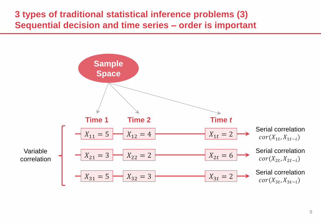
3 types of traditional statistical inference problems (3)
Sequential decision and time series – order is important
Sample
Space
Time 1
𝑋11 = 5
𝑋21 = 3
𝑋31 = 5
Time 2
𝑋12 = 4
𝑋22 = 2
𝑋32 = 3
Time t
𝑋1𝑡 = 2
𝑋2𝑡 = 6
𝑋3𝑡 = 2
Serial correlation𝑐𝑜𝑟(𝑋1𝑡 , 𝑋1𝑡−𝑖)
Serial correlation𝑐𝑜𝑟(𝑋2𝑡 , 𝑋2𝑡−𝑖)
Serial correlation𝑐𝑜𝑟(𝑋3𝑡 , 𝑋3𝑡−𝑖)
Variable
correlation

Understand Hypothesis Test Theory
What is “significantly difference?”

11
Hypothesis testing is a concept to test our “knowledge” with
empirical data sets.
Null Hypothesis
Oppose to alternative hypothesis.
𝐻0: 𝑝𝑜𝑙𝑑 ≥ 𝑝𝑛𝑒𝑤
Θ0 =𝑝𝑜𝑙𝑑 , 𝑝𝑛𝑒𝑤 :
0 < 𝑝𝑜𝑙𝑑 , 𝑝𝑛𝑒𝑤 < 1,𝑝𝑜𝑙𝑑≤ 𝑝𝑛𝑒𝑤
Parameter Space 𝚯
𝑝𝑜𝑙𝑑 , 𝑝𝑛𝑒𝑤 :0 < 𝑝𝑜𝑙𝑑 < 1, 0 < 𝑝𝑛𝑒𝑤 < 1
Alternative Hypothesis
The hypothesis we want to test.
𝐻1: 𝑝𝑜𝑙𝑑 > 𝑝𝑛𝑒𝑤
Θ1 =𝑝𝑜𝑙𝑑 , 𝑝𝑛𝑒𝑤 :
0 < 𝑝𝑜𝑙𝑑 , 𝑝𝑛𝑒𝑤 < 1,𝑝𝑜𝑙𝑑> 𝑝𝑛𝑒𝑤

12
Hypothesis testing is a concept to test our “knowledge” with
empirical data sets.
Null Hypothesis
Oppose to alternative hypothesis.
𝐻0: 𝑝𝑜𝑙𝑑 ≥ 𝑝𝑛𝑒𝑤
Θ0 =𝑝𝑜𝑙𝑑 , 𝑝𝑛𝑒𝑤 :
0 < 𝑝𝑜𝑙𝑑 , 𝑝𝑛𝑒𝑤 < 1,𝑝𝑜𝑙𝑑≤ 𝑝𝑛𝑒𝑤
Parameter Space 𝚯
𝑝𝑜𝑙𝑑 , 𝑝𝑛𝑒𝑤 :0 < 𝑝𝑜𝑙𝑑 < 1, 0 < 𝑝𝑛𝑒𝑤 < 1
Alternative Hypothesis
The hypothesis we want to test.
𝐻1: 𝑝𝑜𝑙𝑑 > 𝑝𝑛𝑒𝑤
Θ1 =𝑝𝑜𝑙𝑑 , 𝑝𝑛𝑒𝑤 :
0 < 𝑝𝑜𝑙𝑑 , 𝑝𝑛𝑒𝑤 < 1,𝑝𝑜𝑙𝑑> 𝑝𝑛𝑒𝑤

13
Two important things for a statistical hypothesis test –
“Test Statistic” and “Rejection Region”
All possible samples
Reject
𝐻0: 𝑝𝑜𝑙𝑑 ≥ 𝑝𝑛𝑒𝑤
Don’t Reject
𝐻0: 𝑝𝑜𝑙𝑑 ≥ 𝑝𝑛𝑒𝑤
Our sample give us a strong
evidence that H0 is false.
→ Our test statistic lies in RR
(rejection region)
Our sample do not give a strong
enough evidence that H0 is false.
→ Our test statistic lies in RR
(rejection region)
Question –
1. How to determine the test statistic?
2. How to determine the rejection region?

14
We commonly use likelihood ratio as the test statistic.
Our Dataset
H0 is true H0 is false
Observed
Data
Likelihood Ratio Statistics
Likelihood under H0 divided by
Likelihood under H1
Reject
Boundary
Probability
Density
15
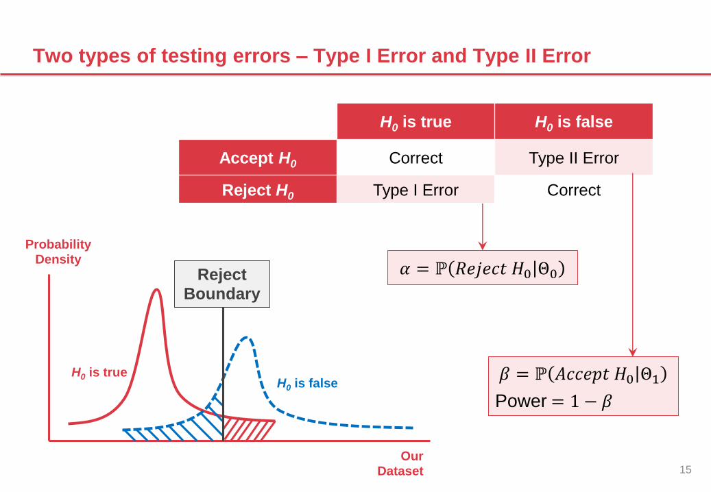
Two types of testing errors – Type I Error and Type II Error
H0 is true H0 is false
Accept H0 Correct Type II Error
Reject H0 Type I Error Correct
𝛼 = ℙ 𝑅𝑒𝑗𝑒𝑐𝑡 𝐻0 Θ0
𝛽 = ℙ 𝐴𝑐𝑐𝑒𝑝𝑡 𝐻0 Θ1
Power = 1 − 𝛽
Our Dataset
H0 is trueH0 is false
Reject
Boundary
ProbabilityDensity

16
Two types of testing errors – Type I Error and Type II Error
Our Dataset
H0 is trueH0 is false
Reject
Boundary
H0 is true H0 is false
Accept H0 Correct Type II Error
Reject H0 Type I Error Correct
𝛼 = ℙ 𝑅𝑒𝑗𝑒𝑐𝑡 𝐻0 Θ0
𝛽 = ℙ 𝐴𝑐𝑐𝑒𝑝𝑡 𝐻0 Θ1
Power = 1 − 𝛽
ProbabilityDensity

17
Neyman-Pearson Paradigm: Controlling the significance level,
i.e. false-negative probability
Our Dataset
H0 is true
H0 is false
Reject Boundary
Control the risk
𝛼 = ℙ 𝑅𝑒𝑗𝑒𝑐𝑡 𝐻0 Θ0
Probability
Density

18
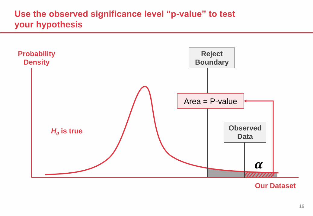
Use the observed significance level “p-value” to test
your hypothesis
Our Dataset
Probability
Density
H0 is true
Observed
Data
Reject
Boundary
Area = P-value
𝜶
19
Use the observed significance level “p-value” to test
your hypothesis
Our Dataset
H0 is true Observed
Data
Reject
Boundary
Area = P-value
𝜶
Probability
Density

Test your hypothesis – A/B Test
A very powerful tool to understand your result

New Version
21
Example: Statistical setting for A/B testing
Population
𝑋11 = 1 𝑋12 = 0 𝑋1𝑛 = 1 𝑋21 = 1 𝑋22 = 0 𝑋2𝑛 = 1
Old Version
𝑋11, … , 𝑋1𝑛 are i.i.d. from 𝐵𝑒𝑟 𝑝𝑜𝑙𝑑 𝑋21, … , 𝑋2𝑛 are i.i.d. from 𝐵𝑒𝑟 𝑝𝑛𝑒𝑤
𝑋𝑖𝑗 = 1 if click
𝑋𝑖𝑗 = 0 if not click
Randomized Control Experiment

22
Example: Why we need “statistical” hypothesis testing?
Test
Formats
Test
Algorithms
0
1
2
3
20
16
/4/4
20
16
/4/6
20
16
/4/8
20
16
/4/1
0
20
16
/4/1
2
2016/4
/14
2016/4
/16
20
16
/4/1
8
20
16
/4/2
0
20
16
/4/2
2
20
16
/4/2
4
20
16
/4/2
6
20
16
/4/2
8
20
16
/4/3
0
20
16
/5/2
20
16
/5/4
20
16
/5/6
20
16
/5/8
20
16
/5/1
0
20
16
/5/1
2
20
16
/5/1
4
20
16
/5/1
6
Relative CTR for the Recommendation System
New Version Old Version

23
The Central Limit Theorem allows as to use the “Z-test” for
the testing problem.
Assume (𝑋1, … 𝑋𝑛 ) is a random sample from a population distribution with
mean and variance exists, and denote ത𝑋𝑛 =𝑋1+ 𝑋2+⋯+𝑋𝑛
𝑛. Then, when the
sample size 𝑛 is large, ത𝑋𝑛−𝔼 𝑋𝑖
𝑉𝑎𝑟 𝑋𝑛𝑛
has an approximately N(0,1) distribution.
Central Limit Theorem
• 𝑋11, … , 𝑋1𝑛 are i.i.d. from 𝐵𝑒𝑟 𝑝𝑜𝑙𝑑 → Ƹ𝑝𝑜𝑙𝑑 =𝑋11+ 𝑋12+⋯+𝑋1𝑛
𝑛~𝐴𝑁 𝑝𝑜𝑙𝑑 ,
𝑝𝑜𝑙𝑑(1−𝑝𝑜𝑙𝑑)
𝑛
• 𝑋21, … , 𝑋2𝑛 are i.i.d. from 𝐵𝑒𝑟 𝑝𝑛𝑒𝑤 → Ƹ𝑝𝑛𝑒𝑤 =𝑋21+ 𝑋22+⋯+𝑋2𝑛
𝑛~𝐴𝑁 𝑝𝑛𝑒𝑤 ,
𝑝𝑛𝑒𝑤(1−𝑝𝑛𝑒𝑤)
𝑛
• Ƹ𝑝𝑜𝑙𝑑 − Ƹ𝑝𝑛𝑒𝑤 ~ 𝐴𝑁 0,2
𝑛Ƹ𝑝 (1 − Ƹ𝑝) , where Ƹ𝑝 =
𝑋11+ 𝑋12+⋯+𝑋1𝑛+𝑋21+ 𝑋22+⋯+𝑋2𝑛
2𝑛.
• We can use normal distribution to solve our testing problem.

24
My proposed test schema –
Two-sample Z test to understand the effect of our new version
When the null hypothesis is true, the test statistic ො𝑝𝑜𝑙𝑑− ො𝑝𝑛𝑒𝑤−0
2
𝑛ො𝑝 (1− ො𝑝)
has an approximately
standard normal distribution. So, we conduct a
Test Statistic
Alternative Hypothesis
𝐻1: 𝑝𝑜𝑙𝑑 − 𝑝𝑛𝑒𝑤 > 0
Null Hypothesis
𝐻0: 𝑝𝑜𝑙𝑑 − 𝑝𝑛𝑒𝑤 ≤ 0
Insight – During the test period (4/12 – 4/24), CTRs of the new version
are (statistically) significantly larger than those of the old version for
10 days. So we have the confidence to use new version.

Test your hypothesis – Granger Causality
Understand what is the root cause?
26
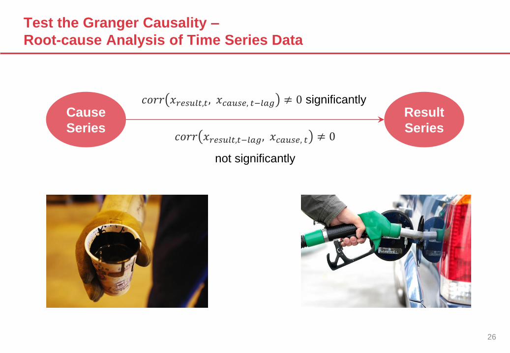
Test the Granger Causality –
Root-cause Analysis of Time Series Data
Cause
Series
Result
Series
𝑐𝑜𝑟𝑟 𝑥𝑟𝑒𝑠𝑢𝑙𝑡,𝑡, 𝑥𝑐𝑎𝑢𝑠𝑒, 𝑡−𝑙𝑎𝑔 ≠ 0 significantly
𝑐𝑜𝑟𝑟 𝑥𝑟𝑒𝑠𝑢𝑙𝑡,𝑡−𝑙𝑎𝑔, 𝑥𝑐𝑎𝑢𝑠𝑒, 𝑡 ≠ 0
not significantly

27
Example: Three Oil Spot Prices

28
Example: Hypothesis Test for Autocorrelation
• Autocorrelation Function - 𝐴𝐶𝐹 𝑙𝑎𝑔 = 𝑐𝑜𝑟𝑟 𝑜𝑡, 𝑜𝑡−𝑙𝑎𝑔
• The results show a strong “long-memory” property => nonstationary process

29
Example: log return series for 3 oil prices

30
Test the Granger Causality –
Root-cause Analysis of Time Series Data
Cause
Series
Result
Series
𝑐𝑜𝑟𝑟 𝑥𝑟𝑒𝑠𝑢𝑙𝑡,𝑡, 𝑥𝑐𝑎𝑢𝑠𝑒, 𝑡−𝑙𝑎𝑔 ≠ 0 significantly
𝑐𝑜𝑟𝑟 𝑥𝑟𝑒𝑠𝑢𝑙𝑡,𝑡−𝑙𝑎𝑔, 𝑥𝑐𝑎𝑢𝑠𝑒, 𝑡 ≠ 0
not significantly

31
Test the Granger Causality –
Impulse-response function (crude oil versus gasoline)

Thanks for your attention!
Now it’s question time!