Embed Size (px)
Citation preview

New tools from the bandit literatureto improve A/B Testing
Emilie Kaufmann,
joint work with Aurelien Garivier & Olivier Cappe
RecSys Meetup,March 23rd, 2016
Emilie Kaufmann Improved A/B Testing
Motivation
Emilie Kaufmann Improved A/B Testing

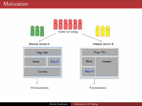
A/B Testing
A way to do A/B Testing:
allocate nA users to page A and nB users to page B
perform a statistical test of “A better than B”
A variant: fully adaptive A/B Testing
sequentially choose which version to allocate to each visitor
adaptively choose when to stop the experiment
Ü multi-armed bandit model
Emilie Kaufmann Improved A/B Testing
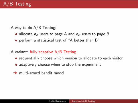
A/B/C... testing as a Best Arm Identification problem
K arms = K probability distributions (νa has mean µa)
ν1 ν2 ν3 ν4 ν5
a∗ = argmaxa=1,...,K
µa
For the t-th user,
allocate a version (arm) At ∈ {1, . . . ,K}observe a feedback Xt ∼ νAt
Goal: design
a sequential sampling rule: At+1 = Ft(A1,X1, . . . ,At ,Xt),a stopping rule τa recommendation rule aτ
such that P(aτ = a∗) ≥ 1− δ and τ is as small as possible.
Emilie Kaufmann Improved A/B Testing
Outline
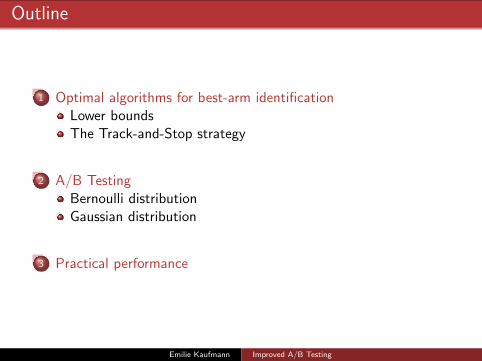
1 Optimal algorithms for best-arm identificationLower boundsThe Track-and-Stop strategy
2 A/B TestingBernoulli distributionGaussian distribution
3 Practical performance
Emilie Kaufmann Improved A/B Testing

Outline
1 Optimal algorithms for best-arm identificationLower boundsThe Track-and-Stop strategy
2 A/B TestingBernoulli distributionGaussian distribution
3 Practical performance
Emilie Kaufmann Improved A/B Testing
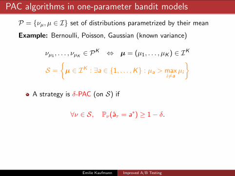
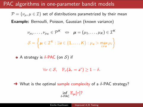
PAC algorithms in one-parameter bandit models
P = {νµ, µ ∈ I} set of distributions parametrized by their mean
Example: Bernoulli, Poisson, Gaussian (known variance)
νµ1 , . . . , νµK ∈ PK ⇔ µ = (µ1, . . . , µK ) ∈ IK
S =
{µ ∈ IK : ∃a ∈ {1, . . . ,K} : µa > max
i 6=aµi
}
A strategy is δ-PAC (on S) if
∀ν ∈ S, Pν(aτ = a∗) ≥ 1− δ.
Ü What is the optimal sample complexity of a δ-PAC strategy?
infδ-PAC
Eµ[τ ]?
Emilie Kaufmann Improved A/B Testing
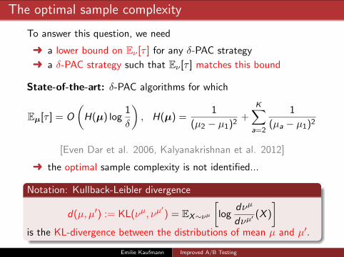
The optimal sample complexity
To answer this question, we need
Ü a lower bound on Eν [τ ] for any δ-PAC strategy
Ü a δ-PAC strategy such that Eν [τ ] matches this bound
State-of-the-art: δ-PAC algorithms for which
Eµ[τ ] = O
(H(µ) log
1
δ
), H(µ) =
1
(µ2 − µ1)2+
K∑a=2
1
(µa − µ1)2
[Even Dar et al. 2006, Kalyanakrishnan et al. 2012]
Ü the optimal sample complexity is not identified...
Notation: Kullback-Leibler divergence
d(µ, µ′) := KL(νµ, νµ′) = EX∼νµ
[log
dνµ
dνµ′(X )
]is the KL-divergence between the distributions of mean µ and µ′.
Emilie Kaufmann Improved A/B Testing
Outline
1 Optimal algorithms for best-arm identificationLower boundsThe Track-and-Stop strategy
2 A/B TestingBernoulli distributionGaussian distribution
3 Practical performance
Emilie Kaufmann Improved A/B Testing
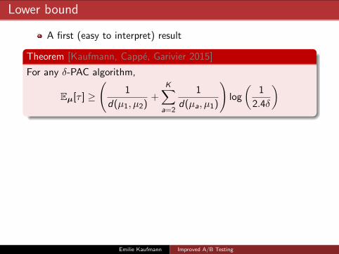
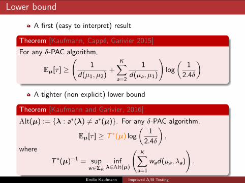
Lower bound
A first (easy to interpret) result
Theorem [Kaufmann, Cappe, Garivier 2015]
For any δ-PAC algorithm,
Eµ[τ ] ≥
(1
d(µ1, µ2)+
K∑a=2
1
d(µa, µ1)
)log
(1
2.4δ
)
A tighter (non explicit) lower bound
Theorem [Kaufmann and Garivier, 2016]
Alt(µ) := {λ : a∗(λ) 6= a∗(µ)}. For any δ-PAC algorithm,
Eµ[τ ] ≥ T ∗(µ) log
(1
2.4δ
),
where
T ∗(µ)−1 = supw∈ΣK
infλ∈Alt(µ)
(K∑
a=1
wad(µa, λa)
).
Emilie Kaufmann Improved A/B Testing
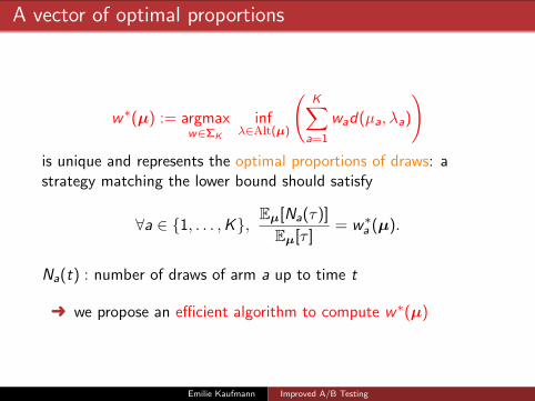
A vector of optimal proportions
w∗(µ) := argmaxw∈ΣK
infλ∈Alt(µ)
(K∑
a=1
wad(µa, λa)
)is unique and represents the optimal proportions of draws: astrategy matching the lower bound should satisfy
∀a ∈ {1, . . . ,K}, Eµ[Na(τ)]
Eµ[τ ]= w∗a (µ).
Na(t) : number of draws of arm a up to time t
Ü we propose an efficient algorithm to compute w∗(µ)
Emilie Kaufmann Improved A/B Testing
Outline
1 Optimal algorithms for best-arm identificationLower boundsThe Track-and-Stop strategy
2 A/B TestingBernoulli distributionGaussian distribution
3 Practical performance
Emilie Kaufmann Improved A/B Testing
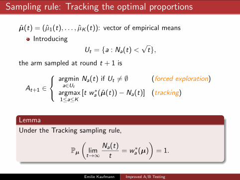
Sampling rule: Tracking the optimal proportions
µ(t) = (µ1(t), . . . , µK (t)): vector of empirical means
Introducing
Ut = {a : Na(t) <√
t},
the arm sampled at round t + 1 is
At+1 ∈
argmina∈Ut
Na(t) if Ut 6= ∅ (forced exploration)
argmax1≤a≤K
[t w∗a (µ(t))− Na(t)] (tracking)
Lemma
Under the Tracking sampling rule,
Pµ
(limt→∞
Na(t)
t= w∗a (µ)
)= 1.
Emilie Kaufmann Improved A/B Testing
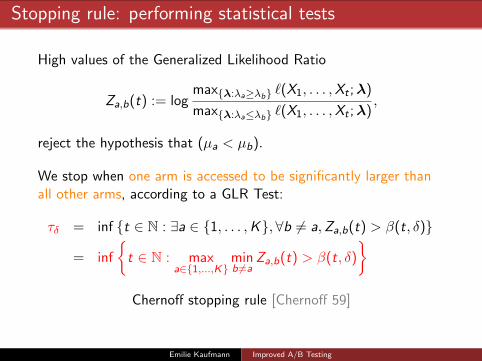
Stopping rule: performing statistical tests
High values of the Generalized Likelihood Ratio
Za,b(t) := logmax{λ:λa≥λb} `(X1, . . . ,Xt ;λ)
max{λ:λa≤λb} `(X1, . . . ,Xt ;λ),
reject the hypothesis that (µa < µb).
We stop when one arm is accessed to be significantly larger thanall other arms, according to a GLR Test:
τδ = inf {t ∈ N : ∃a ∈ {1, . . . ,K}, ∀b 6= a,Za,b(t) > β(t, δ)}
= inf
{t ∈ N : max
a∈{1,...,K}minb 6=a
Za,b(t) > β(t, δ)
}Chernoff stopping rule [Chernoff 59]
Emilie Kaufmann Improved A/B Testing
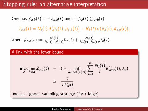
Stopping rule: an alternative interpretation
One has Za,b(t) = −Zb,a(t) and, if µa(t) ≥ µb(t),
Za,b(t) = Na(t) d(µa(t), µa,b(t)
)+ Nb(t) d
(µb(t), µa,b(t)
),
where µa,b(t) := Na(t)Na(t)+Nb(t) µa(t) + Nb(t)
Na(t)+Nb(t) µb(t).
A link with the lower bound
maxa
minb 6=a
Za,b(t) = t × infλ∈Alt(µ(t))
K∑a=1
Na(t)
td(µa(t), λa)
' t
T ∗(µ)
under a “good” sampling strategy (for t large)
Emilie Kaufmann Improved A/B Testing
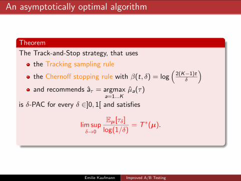
An asymptotically optimal algorithm
Theorem
The Track-and-Stop strategy, that uses
the Tracking sampling rule
the Chernoff stopping rule with β(t, δ) = log(
2(K−1)tδ
)and recommends aτ = argmax
a=1...Kµa(τ)
is δ-PAC for every δ ∈]0, 1[ and satisfies
lim supδ→0
Eµ[τδ]
log(1/δ)= T ∗(µ).
Emilie Kaufmann Improved A/B Testing

Outline
1 Optimal algorithms for best-arm identificationLower boundsThe Track-and-Stop strategy
2 A/B TestingBernoulli distributionGaussian distribution
3 Practical performance
Emilie Kaufmann Improved A/B Testing
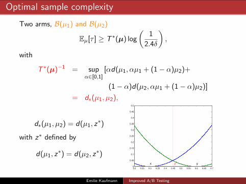
Optimal sample complexity
Two arms, B(µ1) and B(µ2)
Eµ[τ ] ≥ T ∗(µ) log
(1
2.4δ
),
with
T ∗(µ)−1 = supα∈[0,1]
[αd(µ1, αµ1 + (1− α)µ2)+
(1− α)d(µ2, αµ1 + (1− α)µ2)]
= d∗(µ1, µ2),
d∗(µ1, µ2) = d(µ1, z∗)
with z∗ defined by
d(µ1, z∗) = d(µ2, z
∗)
0.2 0.25 0.3 0.35 0.4 0.45 0.5 0.55 0.6 0.65 0.70
0.05
0.1
0.15
0.2
0.25
0.3
0.35
0.4
0.45
0.5
x yz*
Emilie Kaufmann Improved A/B Testing
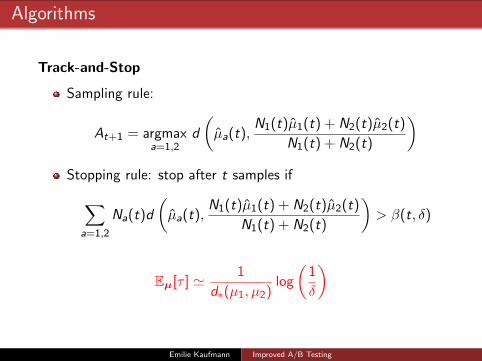
Algorithms
Track-and-Stop
Sampling rule:
At+1 = argmaxa=1,2
d
(µa(t),
N1(t)µ1(t) + N2(t)µ2(t)
N1(t) + N2(t)
)Stopping rule: stop after t samples if∑
a=1,2
Na(t)d
(µa(t),
N1(t)µ1(t) + N2(t)µ2(t)
N1(t) + N2(t)
)> β(t, δ)
Eµ[τ ] ' 1
d∗(µ1, µ2)log
(1
δ
)
Emilie Kaufmann Improved A/B Testing
Algorithms
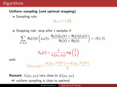
Uniform sampling (and optimal stopping)
Sampling rule:At+1 = t [2]
Stopping rule: stop after t samples if∑a=1,2
Na(t)d
(µa(t),
N1(t)µ1(t) + N2(t)µ2(t)
N1(t) + N2(t)
)> β(t, δ)
Eµ[τ ] ' 1
I∗(µ1, µ2)log
(1
δ
)with
I∗(µ1, µ2) =d(µ1,
µ1+µ22
)+ d
(µ1,
µ1+µ22
)2
.
Remark: I∗(µ1, µ2) very close to d∗(µ1, µ2)
Ü uniform sampling is close to optimalEmilie Kaufmann Improved A/B Testing

Outline
1 Optimal algorithms for best-arm identificationLower boundsThe Track-and-Stop strategy
2 A/B TestingBernoulli distributionGaussian distribution
3 Practical performance
Emilie Kaufmann Improved A/B Testing
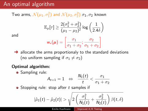
An optimal algorithm
Two arms, N (µ1, σ21) and N (µ2, σ
22) σ1, σ2 known
Eµ[τ ] ≥ 2(σ21 + σ2
2)
(µ1 − µ2)2log
(1
2.4δ
)and
w∗(µ) =
[σ1
σ1 + σ2;
σ2
σ1 + σ2
]Ü allocate the arms proportionaly to the standard deviations
(no uniform sampling if σ1 6= σ2)
Optimal algorithm:
Sampling rule:
At+1 = 1 ⇔ N1(t)
t<
σ1
σ1 + σ2
Stopping rule: stop after t samples if
|µ1(t)− µ2(t)| >
√2
(σ2
1
N1(t)+
σ22
N2(t)
)β(t, δ)
Emilie Kaufmann Improved A/B Testing

Outline
1 Optimal algorithms for best-arm identificationLower boundsThe Track-and-Stop strategy
2 A/B TestingBernoulli distributionGaussian distribution
3 Practical performance
Emilie Kaufmann Improved A/B Testing
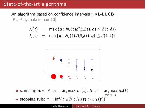
State-of-the-art algorithms
An algorithm based on confidence intervals : KL-LUCB[K., Kalyanakrishnan 13]
ua(t) = max {q : Na(t)d(µa(t), q) ≤ β(t, δ)}la(t) = min {q : Na(t)d(µa(t), q) ≤ β(t, δ)}
0
1
771 459 200 45 48 23
sampling rule: At+1 = argmaxa
µa(t), Bt+1 = argmaxb 6=At+1
ub(t)
stopping rule: τ = inf{t ∈ N : lAt (t) > uBt (t)}Emilie Kaufmann Improved A/B Testing
State-of-the-art algorithms
A Racing-type algorithm: KL-Racing [K., Kalyanakrishnan 13]
R = {1, . . . ,K} set of remaining arms.r = 0 current round
while |R| > 1
r=r+1draw each a ∈ R, compute µa,r , the empirical mean of the rsamples observed sofarcompute the empirical best and empirical worst arms:
br = argmaxa∈R
µa,r wr = argmina∈R
µa,r
Elimination step: if
lbr (r) > uwr (r),
eliminate wr : R = R\{wr}end
Outpout: a the single element in R.Emilie Kaufmann Improved A/B Testing
The Chernoff-Racing algorithm
R = {1, . . . ,K} set of remaining arms.r = 0 current roundwhile |R| > 1
r=r+1
draw each a ∈ R, compute µa,r , the empirical mean of the rsamples observed sofar
compute the empirical best and empirical worst arms:
br = argmaxa∈R
µa,r wr = argmina∈R
µa,r
Elimination step: if (Zbr ,wr (r) > β(r , δ)), or
rd
(µa,r ,
µa,r + µb,r2
)+ rd
(µb,r ,
µa,r + µb,r2
)> β(r , δ),
eliminate wr : R = R\{wr}end
Outpout: a the single element in R.Emilie Kaufmann Improved A/B Testing
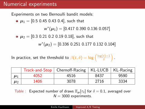
Numerical experiments
Experiments on two Bernoulli bandit models:
µ1 = [0.5 0.45 0.43 0.4], such that
w∗(µ1) = [0.417 0.390 0.136 0.057]
µ2 = [0.3 0.21 0.2 0.19 0.18], such that
w∗(µ2) = [0.336 0.251 0.177 0.132 0.104]
In practice, set the threshold to β(t, δ) = log(
log(t)+1δ
).
Track-and-Stop Chernoff-Racing KL-LUCB KL-Racing
µ1 4052 4516 8437 9590
µ2 1406 3078 2716 3334
Table : Expected number of draws Eµ[τδ] for δ = 0.1, averaged overN = 3000 experiments.
Emilie Kaufmann Improved A/B Testing
Take-home message
Useful tools for sequential A/B Testing:
stop using Sequential Generalized Likelihood Ratio tests
sample the arms to match the optimal proportions w∗(µ)
... which can be approximated by uniform sampling forBernoulli distribution
Final remark:
Good algorithms for best arm identification are very different forbandit algorithms designed for regret minimization
(UCB, Thompson Sampling)
Emilie Kaufmann Improved A/B Testing
References
This talk is based on
A. Garivier, E. Kaufmann.Optimal Best Arm Identification with Fixed Confidence,arXiv:1602.04589, 2016
E. Kaufmann, O. Cappe, A. Garivier.On the Complexity of A/B Testing. COLT, 2014
E. Kaufmann, O. Cappe, A. Garivier.On the Complexity of Best Arm Identification in Multi-ArmedBandit Models. JMLR, 2015
Emilie Kaufmann Improved A/B Testing