Zahid MianPart of the Brown-bag Series

Population Sample Variable Statistic Sample Skew

Mean Median Mode Range Percentile Variance Standard Deviation Covariance Correlation Coefficient Skewness

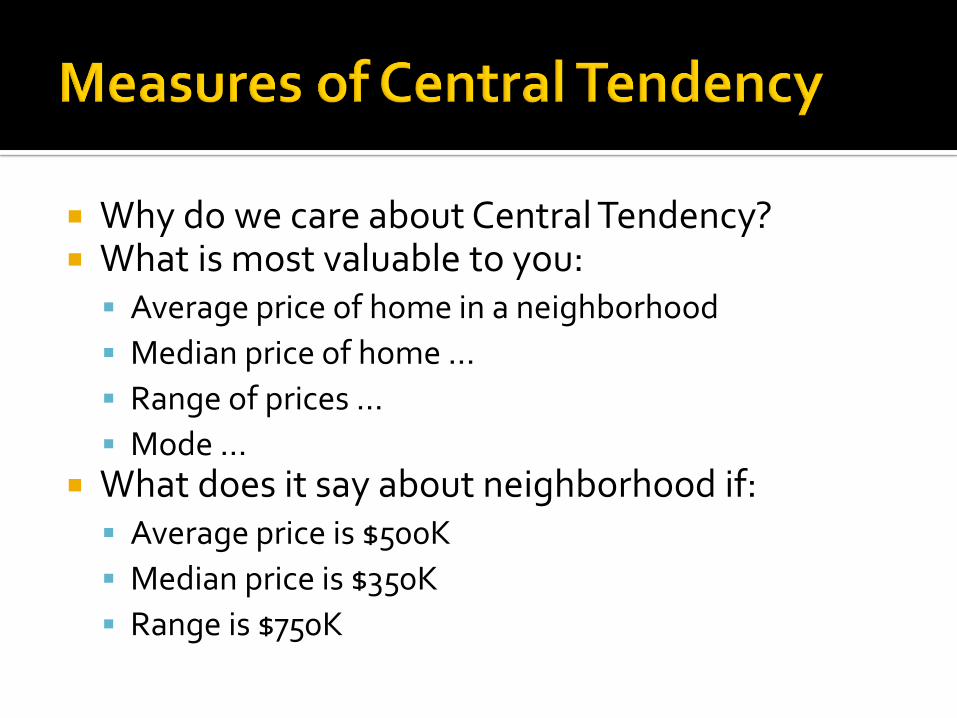
Why do we care about Central Tendency? What is most valuable to you:

Average price of home in a neighborhood

Median price of home …

Range of prices …

Mode … What does it say about neighborhood if:

Average price is $500K

Median price is $350K

Range is $750K

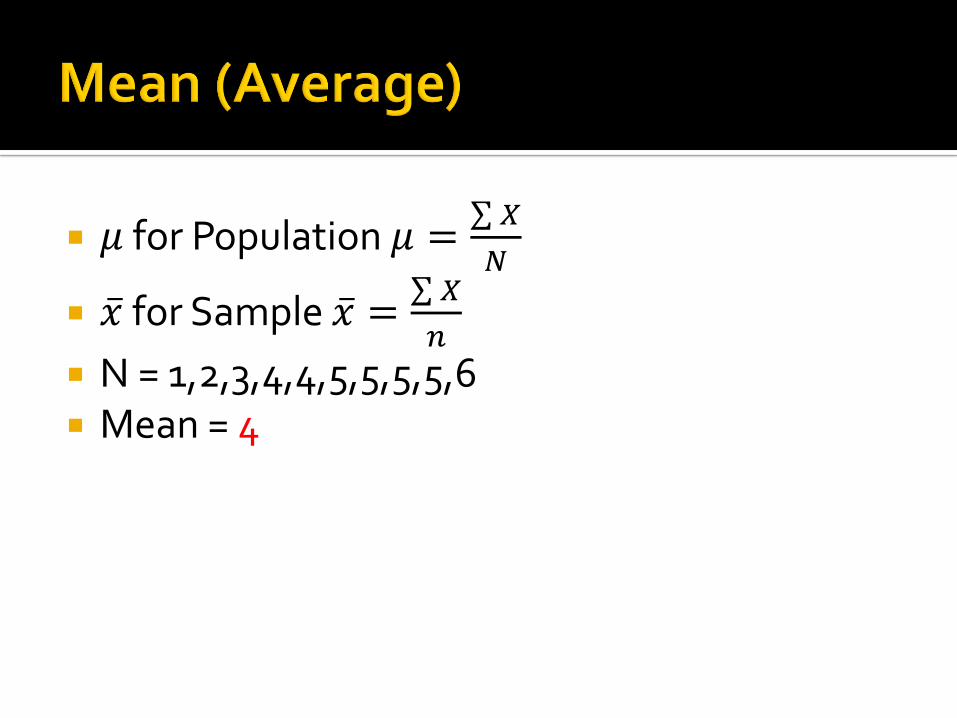
𝜇 for Population 𝜇 = 𝑋

𝑁

𝑥 for Sample 𝑥 = 𝑋

𝑛

N = 1,2,3,4,4,5,5,5,5,6 Mean = 4

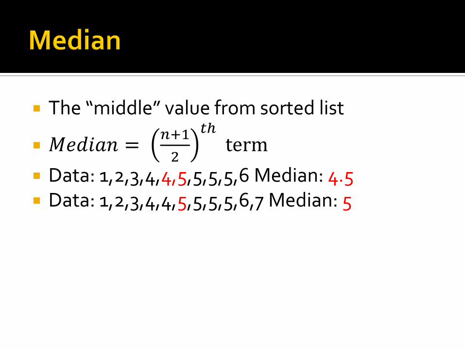
The “middle” value from sorted list

𝑀𝑒𝑑𝑖𝑎𝑛 =𝑛+1

2

𝑡ℎterm

Data: 1,2,3,4,4,5,5,5,5,6 Median: 4.5 Data: 1,2,3,4,4,5,5,5,5,6,7 Median: 5

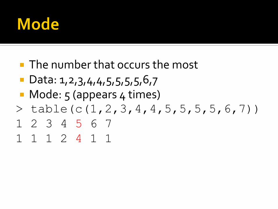
The number that occurs the most Data: 1,2,3,4,4,5,5,5,5,6,7 Mode: 5 (appears 4 times)> table(c(1,2,3,4,4,5,5,5,5,6,7))

1 2 3 4 5 6 7

1 1 1 2 4 1 1

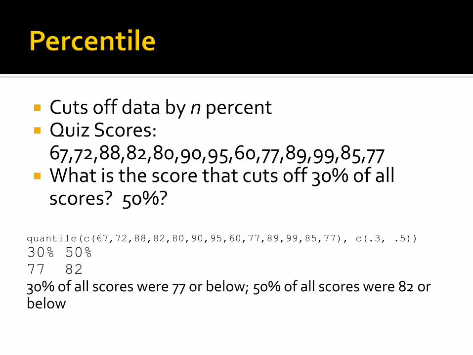
Cuts off data by n percent Quiz Scores:

67,72,88,82,80,90,95,60,77,89,99,85,77 What is the score that cuts off 30% of all

scores? 50%?

quantile(c(67,72,88,82,80,90,95,60,77,89,99,85,77), c(.3, .5))

30% 50%

77 82

30% of all scores were 77 or below; 50% of all scores were 82 or below

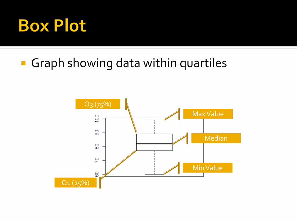
Graph showing data within quartiles

Max Value

Min Value

Median

Q3 (75%)

Q1 (25%)

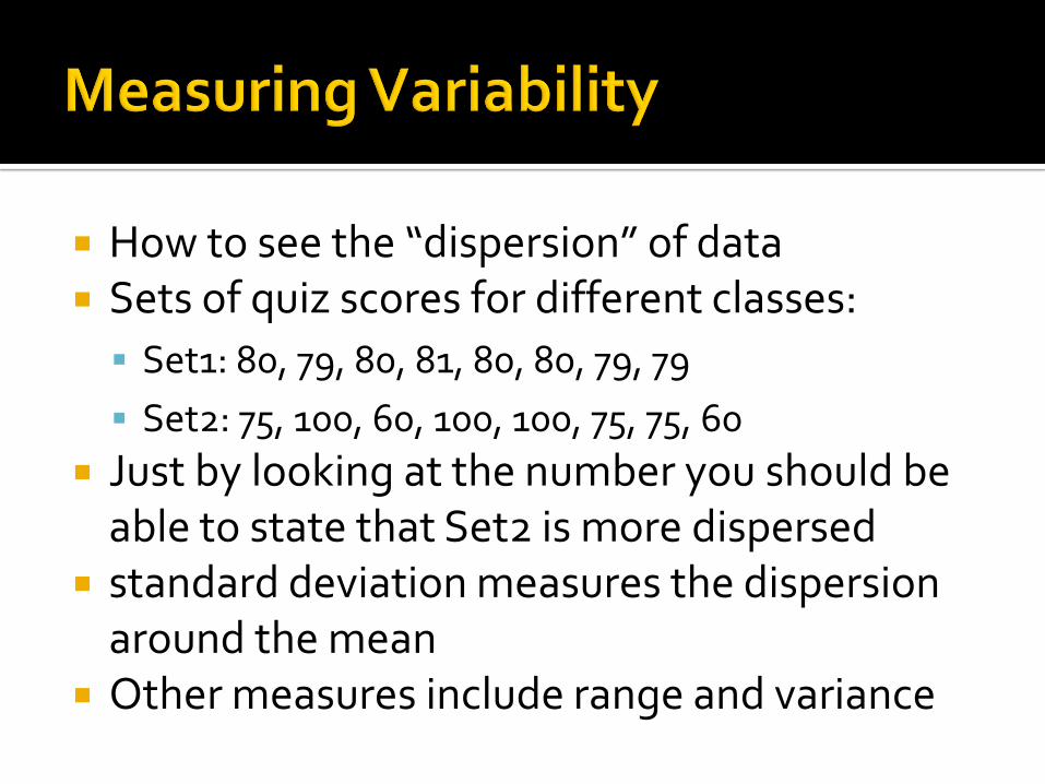
How to see the “dispersion” of data Sets of quiz scores for different classes:

Set1: 80, 79, 80, 81, 80, 80, 79, 79

Set2: 75, 100, 60, 100, 100, 75, 75, 60

Just by looking at the number you should be able to state that Set2 is more dispersed

standard deviation measures the dispersion around the mean

Other measures include range and variance

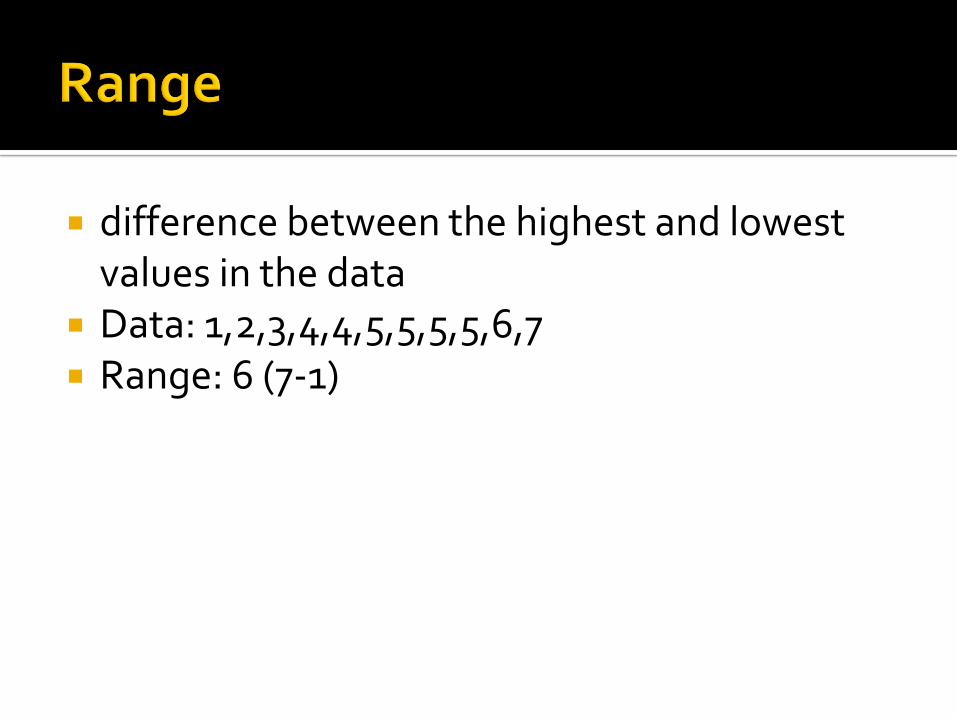
difference between the highest and lowest values in the data

Data: 1,2,3,4,4,5,5,5,5,6,7 Range: 6 (7-1)

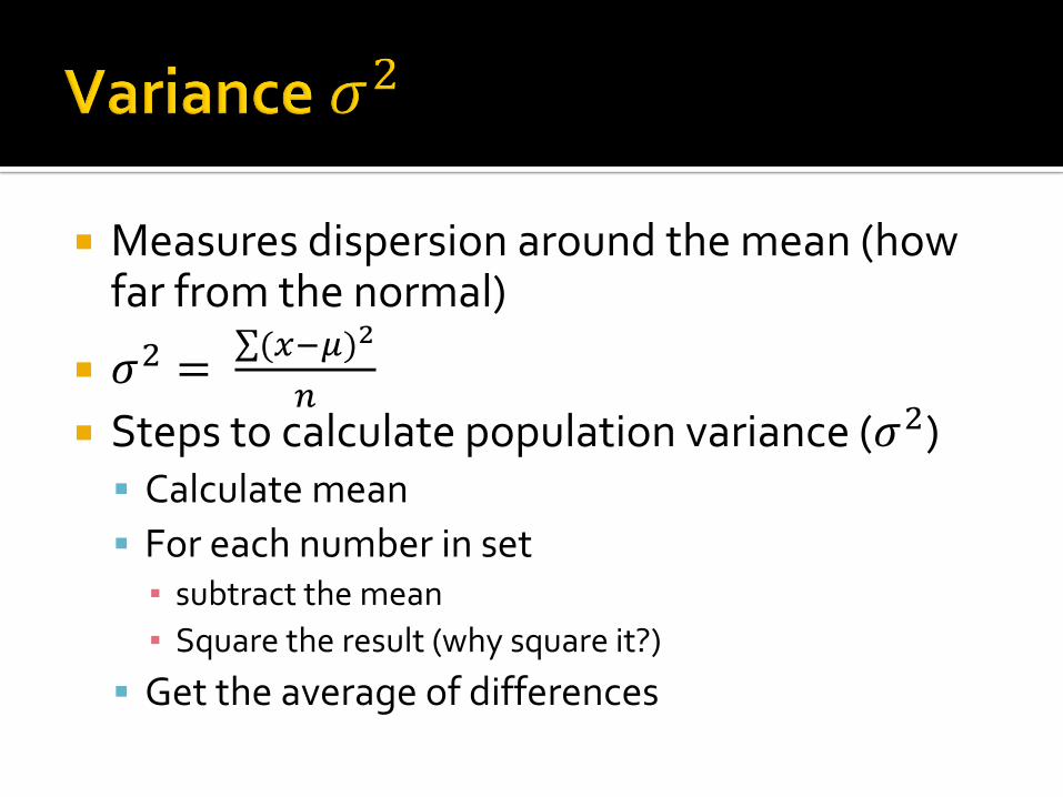
Measures dispersion around the mean (how far from the normal)

𝜎2 = (𝑥−𝜇)2

𝑛 Steps to calculate population variance (𝜎2)

Calculate mean

For each number in set ▪ subtract the mean

▪ Square the result (why square it?)

Get the average of differences

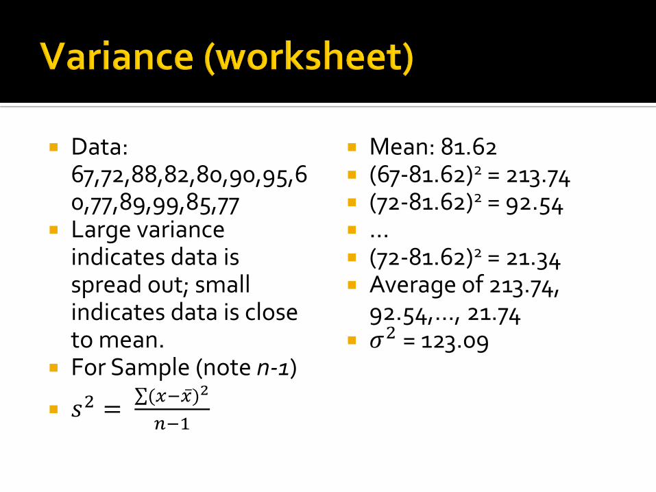
Data: 67,72,88,82,80,90,95,60,77,89,99,85,77

Large variance indicates data is spread out; small indicates data is close to mean.

For Sample (note n-1)

𝑠2 = (𝑥− 𝑥)2

𝑛−1

Mean: 81.62 (67-81.62)2 = 213.74 (72-81.62)2 = 92.54 … (72-81.62)2 = 21.34 Average of 213.74,

92.54,…, 21.74 𝜎2 = 123.09

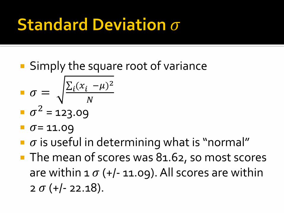
Simply the square root of variance

𝜎 = 𝑖(𝑥𝑖 −𝜇)

2

𝑁

𝜎2 = 123.09 𝜎= 11.09 𝜎 is useful in determining what is “normal” The mean of scores was 81.62, so most scores

are within 1 𝜎 (+/- 11.09). All scores are within 2 𝜎 (+/- 22.18).

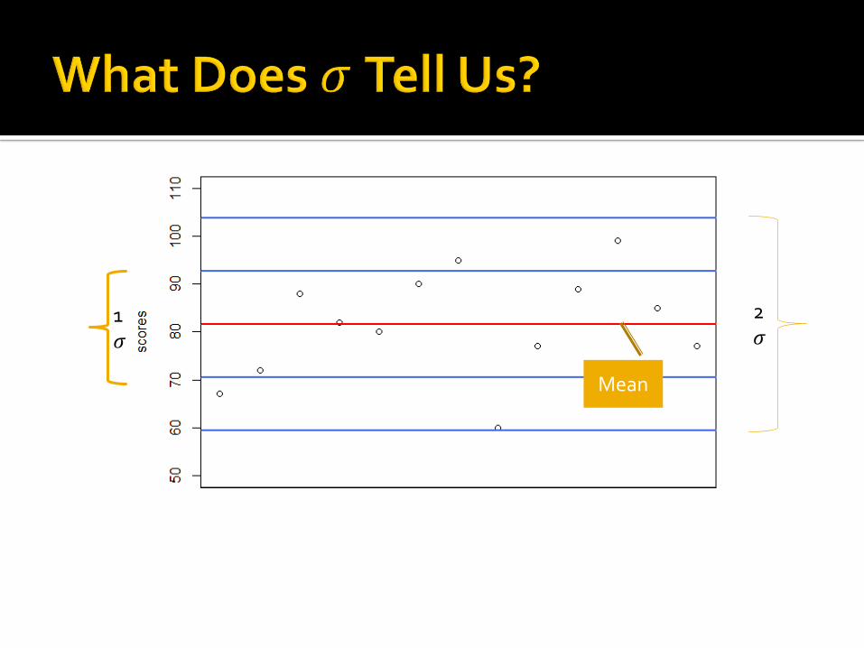
1 𝜎

Mean

2 𝜎

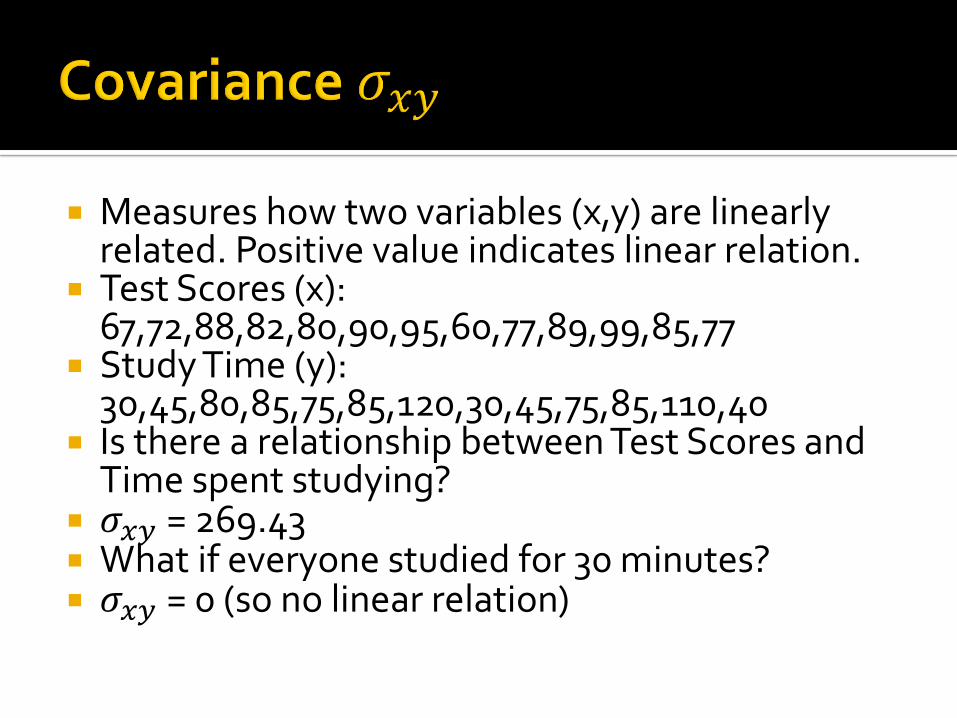
Measures how two variables (x,y) are linearly related. Positive value indicates linear relation.

Test Scores (x): 67,72,88,82,80,90,95,60,77,89,99,85,77

Study Time (y): 30,45,80,85,75,85,120,30,45,75,85,110,40

Is there a relationship between Test Scores and Time spent studying?

𝜎𝑥𝑦 = 269.43 What if everyone studied for 30 minutes? 𝜎𝑥𝑦 = 0 (so no linear relation)

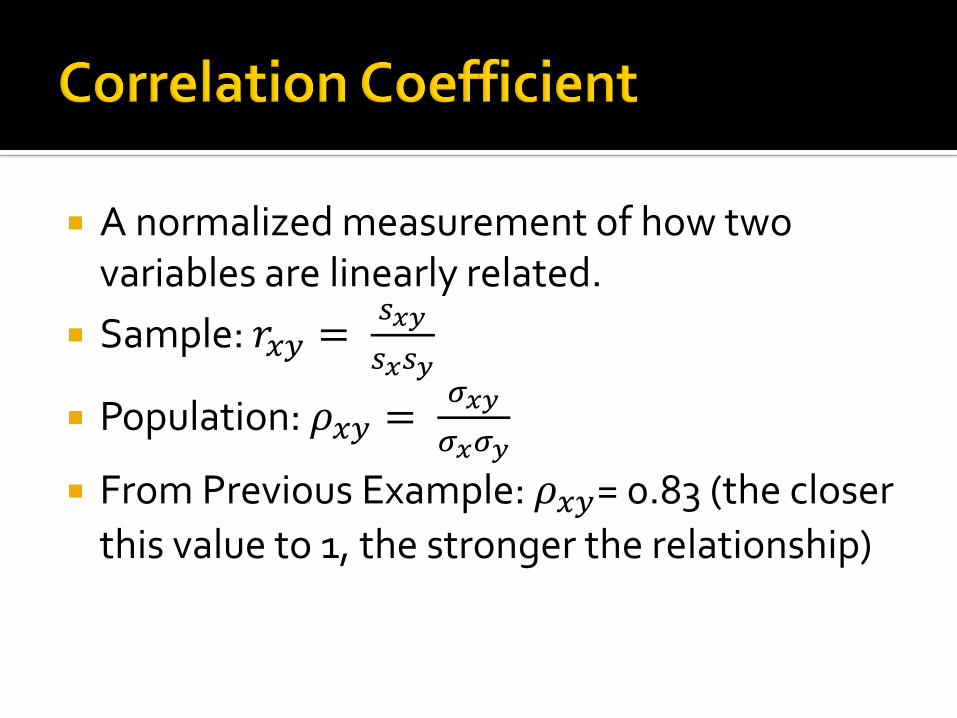
A normalized measurement of how two variables are linearly related.

Sample: 𝑟𝑥𝑦 =𝑠𝑥𝑦

𝑠𝑥𝑠𝑦

Population: 𝜌𝑥𝑦 =𝜎𝑥𝑦

𝜎𝑥𝜎𝑦

From Previous Example: 𝜌𝑥𝑦= 0.83 (the closer

this value to 1, the stronger the relationship)

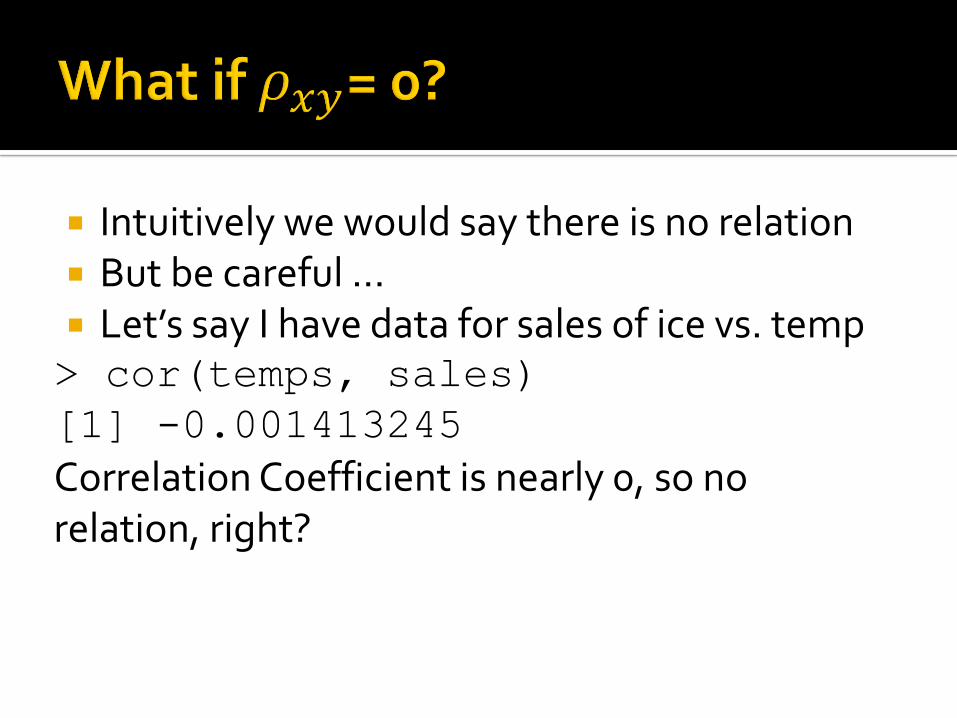
Intuitively we would say there is no relation But be careful … Let’s say I have data for sales of ice vs. temp> cor(temps, sales)

[1] -0.001413245

Correlation Coefficient is nearly 0, so no relation, right?

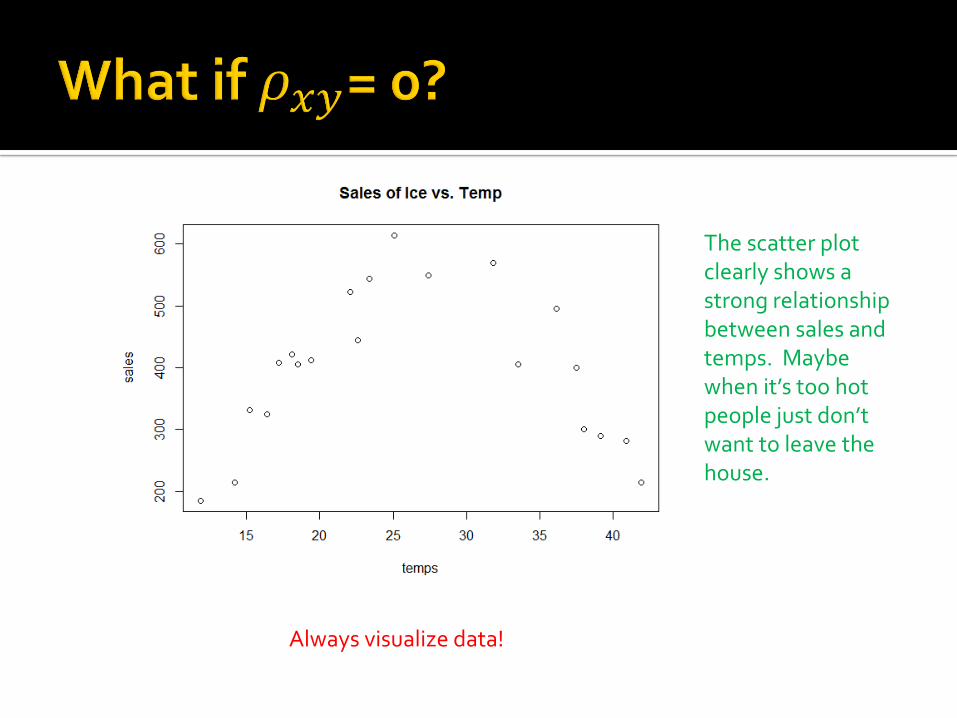
The scatter plot clearly shows a strong relationship between sales and temps. Maybe when it’s too hot people just don’t want to leave the house.

Always visualize data!

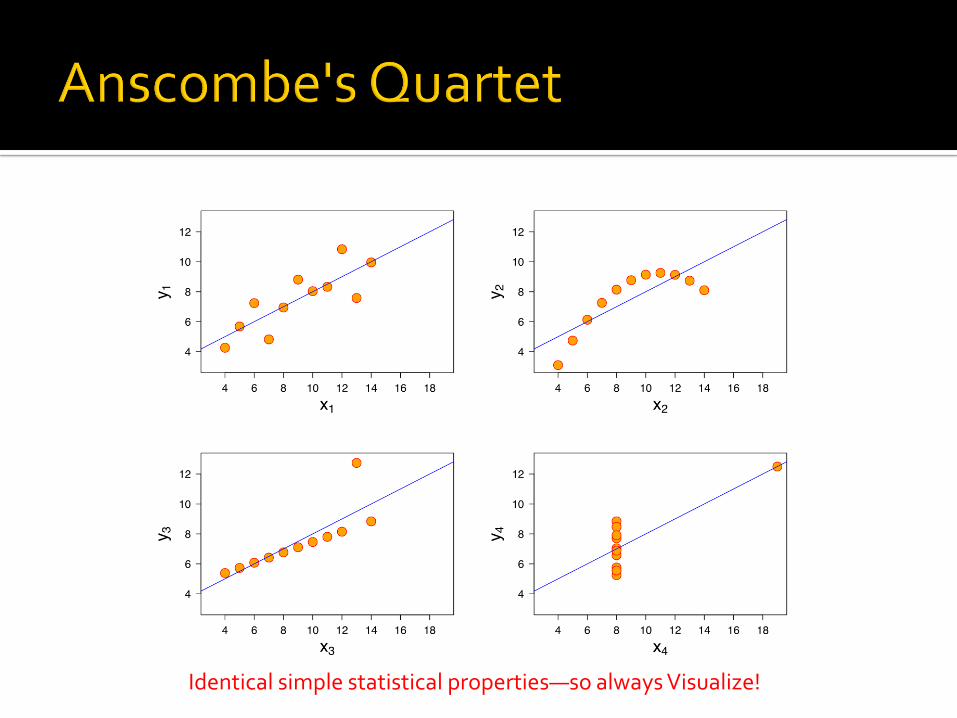
Identical simple statistical properties—so always Visualize!

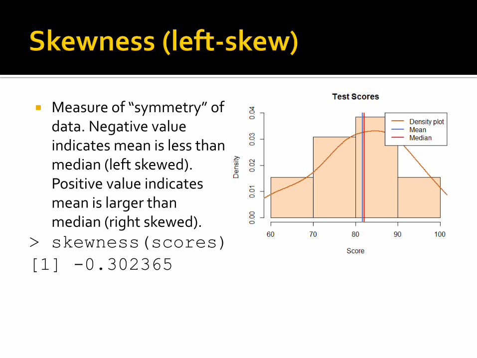
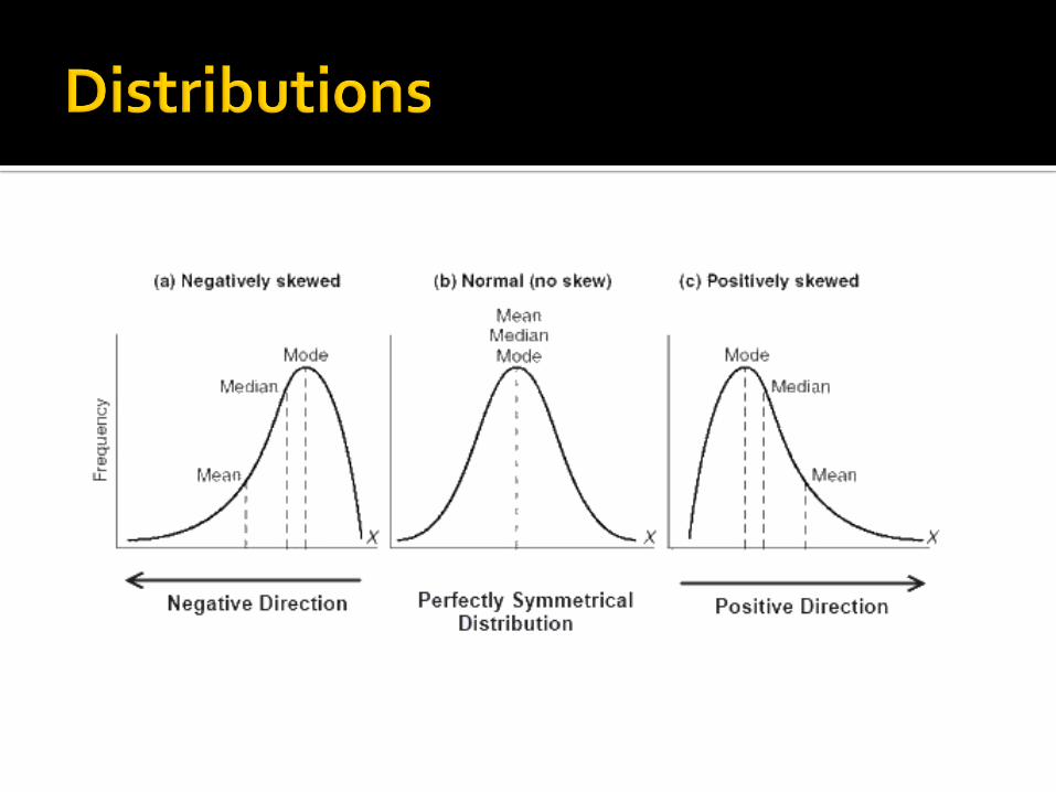
Measure of “symmetry” of data. Negative value indicates mean is less than median (left skewed). Positive value indicates mean is larger than median (right skewed).

> skewness(scores)

[1] -0.302365

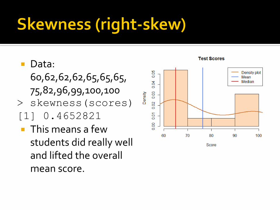
Data: 60,62,62,62,65,65,65, 75,82,96,99,100,100

> skewness(scores)

[1] 0.4652821

This means a few students did really well and lifted the overall mean score.

Mean, Median, Mode exactly at center 99.999% of all data within 3 𝜎 of mean Important for making inferences Test scores are generally normal distribution Height of humans follow normal distribution Need to be careful not to apply normal

distribution rules against non-normal data https://en.wikipedia.org/wiki/Normality_test

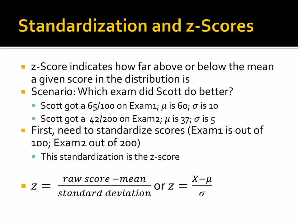
z-Score indicates how far above or below the mean a given score in the distribution is

Scenario: Which exam did Scott do better? Scott got a 65/100 on Exam1; 𝜇 is 60; 𝜎 is 10

Scott got a 42/200 on Exam2; 𝜇 is 37; 𝜎 is 5 First, need to standardize scores (Exam1 is out of

100; Exam2 out of 200) This standardization is the z-score

𝑧 =𝑟𝑎𝑤 𝑠𝑐𝑜𝑟𝑒 −𝑚𝑒𝑎𝑛

𝑠𝑡𝑎𝑛𝑑𝑎𝑟𝑑 𝑑𝑒𝑣𝑖𝑎𝑡𝑖𝑜𝑛or 𝑧 =

𝑋−𝜇

𝜎

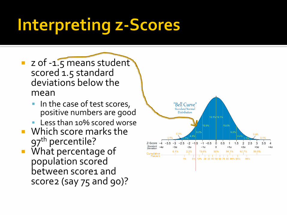
z of -1.5 means student scored 1.5 standard deviations below the mean In the case of test scores,

positive numbers are good Less than 10% scored worse

Which score marks the 97th percentile?

What percentage of population scored between score1 and score2 (say 75 and 90)?

Measurements of Central Tendency and Variability are critical to study of statistics

Central Tendency tries to provide information about the “central” value of your set

Variability tries to provide information about the dispersion of data in your set

Covariance tries to provide information about how two variables are related

z-Scores are useful with a normal distribution