[course site]

Day 1 Lecture 2

The Perceptron

Santiago Pascual

2

Outline

1. Supervised learning: Regression/Classification

2. Linear regression

3. Logistic regression

4. The Perceptron

5. Multi-class classification

6. The Neural Network

7. Metrics

3

Machine Learning techniques

We can categorize three types of learning procedures:

1. Supervised Learning:

= ƒ( )

2. Unsupervised Learning:

ƒ( )

3. Reinforcement Learning:

= ƒ( )

We have a labeled dataset with pairs (x, y), e.g. classify a signal window as containing speech or not:x1 = [x(1), x(2), …, x(T)] y1 = “no”x2 = [x(T+1), …, x(2T)] y2 = “yes”x3 = [x(2T+1), …, x(3T)] y3 = “yes”...

4

Supervised LearningBuild a function: = ƒ( ), ∈ ℝm, ∈ ℝⁿ

Depending on the type of outcome we get…

● Regression: is continous (e.g. temperature samples = {19º, 23º, 22º})

● Classification: is discrete (e.g. = {1, 2, 5, 2, 2}).

○ Beware! These are unordered categories, not numerically meaningful

outputs: e.g. code[1] = “dog”, code[2] = “cat”, code[5] = “ostrich”, ...

5

Regression motivationText to Speech: Textual features → Spectrum of speech (many coefficients)

TXTDesigned

feature extraction

ft 1

ft 2

ft 3

Regression module

s1

s2

s3

wavegen

“Hand-crafted” features

“Hand-crafted” features

6

Classification motivationAutomatic Speech Recognition: Acoustic features → Textual transcription (words)

Designedfeature

extraction

s1

s2

s3

Classifier “hola que tal”

“Hand-crafted” features

7

What “deep-models” means nowadaysLearn the representations as well, not only the final mapping → end2end

Learned extraction Classifier

Model maps raw inputs to raw outputs, no intermediate blocks.

End2end model

“hola que tal”

8

Linear RegressionFunction approximation = ω·x + β , with learnable parameters θ = {ω, β}

9

Linear RegressionWe can also make the function more complex for x being an M-dimensional set of

features: = ω1·x1 + ω2·x2 + ω3·x3 + … + ωM·xM + β

e.g. we want to predict the price of a house based on:

x1 = square-meters (sqm)

x2,3 = location (lat, lon)

x4 = year of construction (yoc)

price = ω1·(sqm) + ω2·(lat) + ω3·(lon) + ω4·(yoc) + β

● Fitting ƒ( ) means adjusting (learning) the values θ = {ω1, ω2, … , ωM, β}

○ How? Will see in training chapter, stay tunned!

10

Logistic RegressionIn the classification world we talk about Probabilities, and more concretely:

Given x input data features → Probability of y being:

● a dog P(y=dog|x) ● a cat P(y=cat|x)● a horse P(y=horse|x)● whatever P(y=whatever|x).

We achieve so with the sigmoid function!

Bounded σ(x) ∈ (0, 1)Note: This is a binary classification approach

11

Logistic RegressionInterpretation: build a delimiting boundary between our data classes + apply the

sigmoid function to estimate a probability in every point in the space.

12

The PerceptronBoth operations, linear regression and logistic regression, follow the scheme in

the Figure:

Depending on the Activation function ƒ we have a linear/non-linear behavior:

if ƒ == identity → linear regression

if ƒ == sigmoid → logistic regression

13

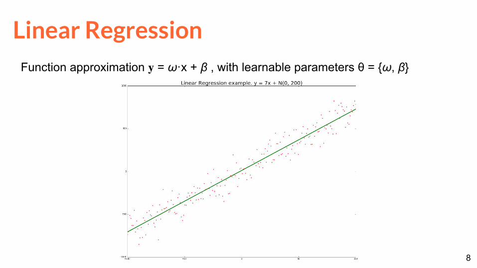
The PerceptronThe output is then derived by a weighted sum of the inputs plus a bias term.

Weights and bias are the parameters we keep (once learned) to define a neuron.

14

The PerceptronActually the artificial neuron is seen as an analogy to a biological one.

Real neuron fires an impulse once the sum of all inputs is over a threshold.

The sigmoid emulates the thresholding behavior → act like a switch.

Figure credit:Introduction to AI

15

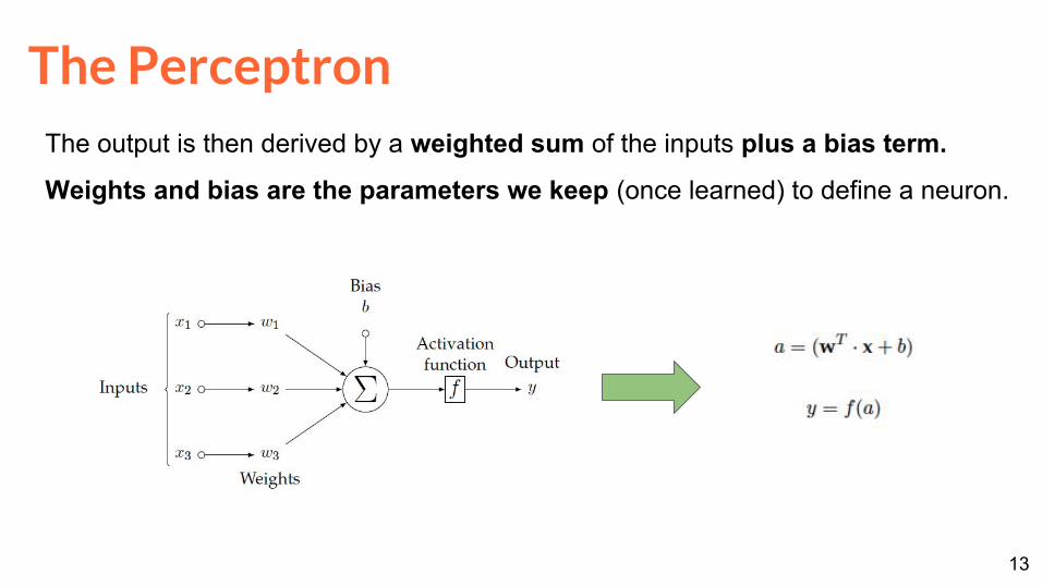
Multi-class classificationNatural extension: put many neurons in parallel, each processing its binary

output out of N possible classes.

0.3 “dog”

0.08 “cat”

0.6 “whatever”

raw pixels unrolled img

Normalization factor, remember: we want a pdf at the output! → all output P’s sum up to 1.

Softmax function

16

The Neural NetworkThe XOR problem: sometimes a single neuron is not enough → Just a single

decision split doesn’t work

17

The Neural NetworkSolution: arrange many neurons in a first intermediate non-linear mapping

(Hidden Layer), connecting everything from layer to layer in a feed-forward

fashion.

Warning! Inputs are not neurons, but they are usually depicted like neurons.

Example XOR NN

2 hidden units with sigmoid activations

output unit with sigmoid activation

The i-th layer is defined by a matrix Wi

and a vector bi, and the activation is

simply a dot product plus bi:

The Neural Network

Num parameters to learn at i-th layer:

18

The i-th layer is defined by a matrix Wi

and a vector bi, and the activation is

simply a dot product plus bi:

The Neural Network

Num parameters to learn at i-th layer:

19

Important remarks:● We can put as many hidden layers as we want whenever training can be

effectively done and we have enough data (next chapters)○ The amount of parameters to estimate grows very quickly with the

num of layers and units! → There is no formula to know the amount of units per layer nor the amount of layers, pitty...

● The power of NNets comes from non-linear mappings: hidden units must be followed by a non-linear activation!○ sigmoid, tanh, relu, leaky-relu, prelu, exp, softplus, …

20

The Neural Network

Regression metrics

In regression the metric is chosen based on the task:

● For example in TTS there are different metrics for the different predicted

parameters:

○ Mel-Cepstral Distortion, Root Mean Squared Error F0, duration, ...

21

Confusion matrices provide a by-class comparison between the results of the automatic classifications with ground truth annotations.

Classification metrics

Slide credit: Xavi Giró 22

Classification metricsCorrect classifications appear in the diagonal, while the rest of cells correspond to errors.

Prediction

Class 1 Class 2 Class 3

Ground Truth

Class 1 x(1,1) x(1,2) x(1,3)

Class 2 x(2,1) x(2,2) x(2,3)

Class 3 x(3,1) x(3,2) x(3,3)

23Slide credit: Xavi Giró

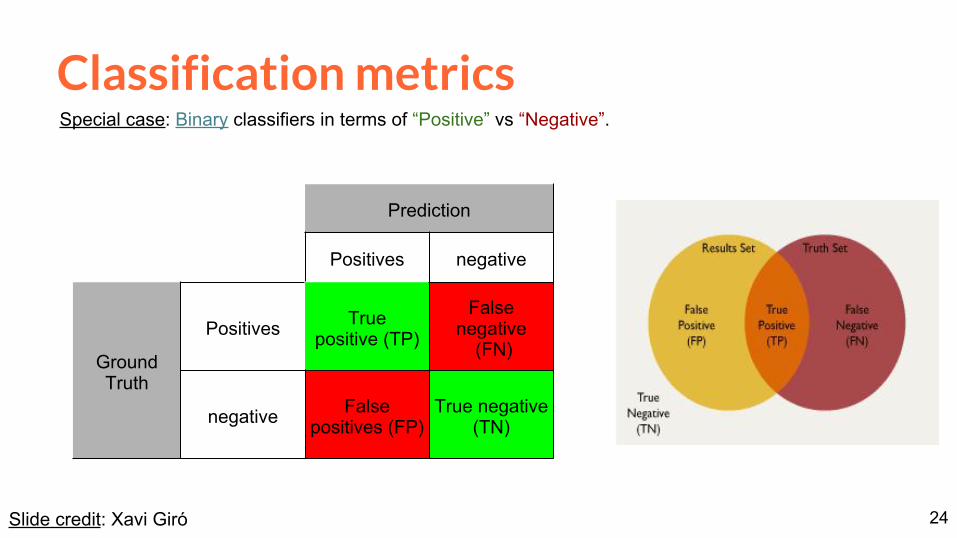
Special case: Binary classifiers in terms of “Positive” vs “Negative”.

Prediction

Positives negative

GroundTruth

Positives True positive (TP)

Falsenegative

(FN)

negative False positives (FP)

True negative(TN)

Classification metrics

24Slide credit: Xavi Giró

The “accuracy” measures the proportion of correct classifications, not distinguishing between classes.

Binary

Prediction

Class 1 Class 2 Class 3

GroundTruth

Class 1 x(1,1) x(1,2) x(1,3)

Class 2 x(2,1) x(2,2) x(2,3)

Class 3 x(3,1) x(3,2) x(3,3)

Prediction

Positives negative

GroundTruth

Positives True positive (TP)

Falsenegative

(FN)

Negative False positives (FP)

True negative(TN)

Classification metrics25

Slide credit: Xavi Giró

Given a reference class, its Precision (P) and Recall (R) are complementary measures of relevance.

Prediction

Positives Negatives

GroundTruth

PositivesTrue

positive (TP)

Falsenegative

(FN)

NegativesFalse

positives (FP)

"Precisionrecall" by Walber - Own work. Licensed under Creative Commons Attribution-Share Alike 4.0 via Wikimedia Commons - http://commons.wikimedia.org/wiki/File:Precisionrecall.svg#mediaviewer/File:Precisionrecall.svg

Example: Relevant class is “Positive” in a binary classifier.

Classification metrics26

Slide credit: Xavi Giró

Binary classification results often depend from a parameter (eg. decision threshold) whose value directly impacts precision and recall.

For this reason, in many cases a Receiver Operating Curve (ROC curve) is provided as a result.

True

Pos

itive

Rat

e

Classification metrics

27Slide credit: Xavi Giró

28

Thanks ! Q&A ?

@Santty128