Embed Size (px)
Citation preview
Strategic assessment of the risk posed to marine mammals by the use of
airguns in the Antarctic Treaty area
2009-03-27
Olaf Boebel
Monika Breitzke
Elke Burkhardt
Horst Bornemann
Alfred Wegener Institute for Polar and Marine Research, Germany
Please address all correspondence to: [email protected]

- 1 -
Content Preface ........................................................................................................................................................... 5
Summary ....................................................................................................................................................... 6
Acknowledgements ....................................................................................................................................... 7
References ..................................................................................................................................................... 7
I. Risk analysis: Survey characteristics ................................................................................ 9
1. Seismic operations .................................................................................................................... 9
Spatial distribution of seismic studies ........................................................................................................... 9
Seasonal distribution of seismic studies ...................................................................................................... 11
Recurrence of seismic measurements within certain areas .......................................................................... 14
Bathymetric domains ................................................................................................................................... 14
Sediment distribution ................................................................................................................................... 16
Output .......................................................................................................................................................... 17
2. Environment ........................................................................................................................... 18
Hydrography ................................................................................................................................................ 18
Bathymetry .................................................................................................................................................. 26
Ice conditions .............................................................................................................................................. 26
Output .......................................................................................................................................................... 27
3. Source description .................................................................................................................. 29
Seismic methods and choice of airgun configuration .................................................................................. 29
Characteristics of airguns and airgun-arrays ............................................................................................... 30
Airguns on R/V Polarstern .......................................................................................................................... 32
The Heggernes calibration survey: study site and data acquisition ............................................................. 32
The Heggernes calibration survey: data analysis and results ....................................................................... 35
Acoustic measures .................................................................................................................................. 35
Spherical spreading law .......................................................................................................................... 36
Computation of amplitude spectra .......................................................................................................... 36
Calibration of the G gun ......................................................................................................................... 38
Calibration of all airgun configurations .................................................................................................. 44
Broad-band spectral properties (0 - 80 kHz) and comparison with R/V Polarstern's self noise ............. 46
Modelling output pressure waveforms and far-field signatures ................................................................... 49
4. Sound fields ............................................................................................................................. 55
Modelling approach and model parameters ................................................................................................. 55
Model validation .......................................................................................................................................... 60
5. Sound exposure levels from multiple pulses ........................................................................ 63
6. Application to areas of interest ............................................................................................. 67
Output .......................................................................................................................................................... 71
7. References ............................................................................................................................... 72
II. Risk analysis: Species description .................................................................................. 75
1. Identification of relevant marine mammal species.............................................................. 75
2. Abundance, spatial distribution, temporal distribution, breeding grounds, migration
paths ................................................................................................................................................. 79
Blue whale (Balaenoptera musculus) .......................................................................................................... 82
Output ..................................................................................................................................................... 83
Fin whale (Balaenoptera physalus) ............................................................................................................. 84
Output ..................................................................................................................................................... 85
Sei whale (Balaenoptera borealis) .............................................................................................................. 86
Output ..................................................................................................................................................... 87
Minke whale (Balaenoptera spp.) ............................................................................................................... 88
Output ..................................................................................................................................................... 90
Humpback whale (Megaptera novaeangliae).............................................................................................. 91

- 2 -
Output ..................................................................................................................................................... 92
Southern Right whale (Eubalaena australis)............................................................................................... 93
Output ..................................................................................................................................................... 93
Sperm whale (Physeter macrocephalus) ..................................................................................................... 94
Output ..................................................................................................................................................... 95
Beaked whales ............................................................................................................................................. 96
Overall distribution ................................................................................................................................. 96
Southern bottlenose whale (Hyperoodon planiforns) ............................................................................. 97
Arnoux’s beaked whale (Berardius arnuxii) .......................................................................................... 98
Layard’s beaked whale (Mesoplodon layardii) ...................................................................................... 99
Output ................................................................................................................................................... 100
Killer whale (Orcinus orca) ...................................................................................................................... 101
Output ................................................................................................................................................... 102
Long-finned pilot whale (Globicephala melas edwardi) ........................................................................... 103
Output ................................................................................................................................................... 104
Hourglass dolphin (Lagenorhynchus cruciger) ......................................................................................... 105
Output ................................................................................................................................................... 106
Antarctic Seal species ................................................................................................................................ 107
Amundsen and Bellingshausen Seas ..................................................................................................... 109
Weddell Sea .......................................................................................................................................... 109
3. Diet ......................................................................................................................................... 111
Discussion ................................................................................................................................................. 112
Output ........................................................................................................................................................ 113
4. Mortality rates ...................................................................................................................... 114
Age ............................................................................................................................................................ 114
Diseases ..................................................................................................................................................... 114
Predation .................................................................................................................................................... 114
Stranding ................................................................................................................................................... 114
Bycatch ...................................................................................................................................................... 115
Whaling ..................................................................................................................................................... 115
Sealing ....................................................................................................................................................... 115
Shipping..................................................................................................................................................... 115
Output ........................................................................................................................................................ 125
5. Audition and vocalization .................................................................................................... 126
Audition ..................................................................................................................................................... 126
Vocalization ............................................................................................................................................... 127
Output ........................................................................................................................................................ 138
6. Diving behaviour .................................................................................................................. 139
Blue whale ................................................................................................................................................. 139
Fin whale ................................................................................................................................................... 140
Humpback whale ....................................................................................................................................... 141
Northern right whale .................................................................................................................................. 141
Sperm whale .............................................................................................................................................. 141
Beaked whales ........................................................................................................................................... 142
Antarctic fur seal ....................................................................................................................................... 143
Weddell seal .............................................................................................................................................. 143
Ross seal .................................................................................................................................................... 143
Crabeater seal ............................................................................................................................................ 144
Leopard seal .............................................................................................................................................. 144
Southern elephant seal ............................................................................................................................... 144
Output ........................................................................................................................................................ 147
7. Life history, breeding, calving, weaning ............................................................................. 148
Output ........................................................................................................................................................ 150
8. Swimming .............................................................................................................................. 151
Output ........................................................................................................................................................ 151
9. References ............................................................................................................................. 152
- 3 -
III. Risk analysis: Hazard identification ......................................................................... 165
1. Direct, immediate injury ...................................................................................................... 167
Risk criteria for direct, immediate injury................................................................................................... 168
Discussion ................................................................................................................................................. 169
Does a (single) TTS constitute an injury? ............................................................................................. 170
Can multiple TTS cause injury? ........................................................................................................... 172
Can exposures at sub-TTS levels accumulate to a TTS? ...................................................................... 174
Do Southall et al’s. TTS and PTS onset levels represent numerically conservative estimates? ........... 175
Is the scientific PTS level an appropriate injury threshold under the precautionary principle? ............ 178
Output ........................................................................................................................................................ 179
2. Indirect, immediate damage ................................................................................................ 180
Atypical mass strandings ........................................................................................................................... 180
Potential mechanisms ................................................................................................................................ 181
Behavioural response leads to potentially lethal injury independent of stranding ..................................... 181
Abetting factors of DCS scenario .............................................................................................................. 182
Sound characteristics ............................................................................................................................ 182
Herding ................................................................................................................................................. 183
Topographic conditions ........................................................................................................................ 183
Sea surface temperature and hyperthermia ........................................................................................... 183
Acoustic conditions .............................................................................................................................. 184
Species involved ................................................................................................................................... 184
Behaviour .............................................................................................................................................. 185
Discussion ................................................................................................................................................. 185
Output ........................................................................................................................................................ 187
3. Biologically significant, acoustic disturbance .................................................................... 188
Types of possible acoustically induced behavioural disturbance .............................................................. 189
Sound levels at which behavioural disturbance was observed .................................................................. 189
Biological significance of acoustic disturbance to individuals .................................................................. 190
Discussion ................................................................................................................................................. 191
Selecting a threshold of biologically significant response .................................................................... 191
Which rms integration time is appropriate in the context of behavioural responses? ........................... 195
Output ........................................................................................................................................................ 195
4. References ............................................................................................................................. 197
IV. Risk analysis: Exposure analysis .............................................................................. 203
1. Direct, immediate injury ...................................................................................................... 203
Sensitivity of critical radii to SEL threshold levels ................................................................................... 207
Output ........................................................................................................................................................ 208
2. Indirect, immediate damage ................................................................................................ 209
Sound characteristics ................................................................................................................................. 209
Herding ...................................................................................................................................................... 209
Topographic conditions ............................................................................................................................. 210
Sea surface temperature and hyperthermia ................................................................................................ 210
Acoustic conditions ................................................................................................................................... 210
Species involved ........................................................................................................................................ 210
Behaviour .................................................................................................................................................. 211
Summary ................................................................................................................................................... 212
Discussion ................................................................................................................................................. 212
Output ........................................................................................................................................................ 215
3. Biologically significant, acoustic disturbance .................................................................... 216
Migration ................................................................................................................................................... 221
Feeding ...................................................................................................................................................... 221
Breeding .................................................................................................................................................... 221
Calving/Breeding ....................................................................................................................................... 222
Nurturing and Parental Care ...................................................................................................................... 222
Predator Avoidance ................................................................................................................................... 222
Discussion ................................................................................................................................................. 224
- 4 -
Output ........................................................................................................................................................ 225
4. References ............................................................................................................................. 226
V. Risk management .......................................................................................................... 229
1. Direct, immediate injury ...................................................................................................... 229
Mitigation proposal ................................................................................................................................... 229
Definition of the exclusion zone ................................................................................................................ 230
2. Indirect, immediate damage ................................................................................................ 231
Mitigation proposal ................................................................................................................................... 231
Underlying rationale .................................................................................................................................. 231
3. Biologically significant, acoustic disturbance .................................................................... 232
Mitigation proposal ................................................................................................................................... 232
Underlying rationale .................................................................................................................................. 232
Technical aspects of ramp-up procedure ................................................................................................... 234
4. Overall Mitigation strategy ................................................................................................. 234
5. Discussion .............................................................................................................................. 235
Effectiveness of mitigation measures ........................................................................................................ 236
Use of passive acoustic methods for perimeter surveillance ..................................................................... 237
6. References ............................................................................................................................. 238
VI. Risk evaluation .......................................................................................................... 239
1. Other anthropogenic and natural risks .............................................................................. 239
2. Risks at the individual level ................................................................................................. 239
Risks without mitigation measures ............................................................................................................ 239
Residual risks under inclusion of mitigation measures.............................................................................. 240
3. Risks at the population level ................................................................................................ 241
Risk without mitigation measures ............................................................................................................. 244
Residual risks under inclusion of mitigation measures.............................................................................. 244
4. References ............................................................................................................................. 246
VII. Appendix .................................................................................................................... 247
1. Research needs ...................................................................................................................... 247
2. Impact of metrics and thresholds used on radii of concern .............................................. 251
3. References ............................................................................................................................. 257
4. List of Figures ....................................................................................................................... 259
5. List of Tables......................................................................................................................... 269
- 5 -
Preface
The goal of this study is to estimate the risk posed to marine mammals by using airguns in the Southern Ocean around Antarctica in the context of scientific, geophysical research.
In this process, evaluation criteria and associated thresholds are a prerequisite to being able to make any assessments. Yet it is not this studies’ objective to establish general recommendations of evaluation criteria and associated thresholds for the regulation of anthropogenic sound exposure to marine mammals. Rather, this assessment strives to rely on evaluation criteria and associated thresholds formulated externally in scientifically guided and multidisciplinary efforts, as compiled in recent reviews by Southall et al. (2007), Cox et al., (2006), and the National Research Council (2005).
The evaluation criteria and associated thresholds as used herein are therefore based on the current state of science, and may not necessarily coincide with criteria used by international regulatory bodies or deemed appropriate by other stakeholders under the precautionary principle. An external review of a previous version of this manuscript highlighted that some thresholds and criteria as used herein remain – particularly under the aspects of conservativeness and precaution – controversial. In this version, the concerns raised are included in summarized form and discussions of the respective topic are added where appropriate.
Throughout this study, we try to adhere to a conservative approach in our calculation and evaluation of the contingent risks. The term conservative implies that for any selection of parameters or proxies, we selected – to the extent reasonable - those that overestimated the risk on the one hand while providing increased protection for marine mammals on the other hand. In other scientific contexts, such an approach is termed “precautionary”, a term that we avoid using in this study to circumnavigate any possible confusion with its legal and regulatory implications.
- 6 -
Summary
This strategic assessment considers the risk posed to marine mammals by the use of airguns in the Antarctic Treaty area for a generic seismic survey layout. The paper is structured in seven chapters:
I. Risk analysis: Survey characteristics
This chapter combines seismic survey characteristics of 25 years (e.g. survey layout, airgun description), region and time specific environmental information (e.g. oceanography, geology, bathymetry), and state-of-the-art source and acoustic propagation modelling to develop 24 “generic” acoustic scenarios which embrace the majority of conditions under which AWI (and similarly other groups) have conducted seismic surveys in the Antarctic Treaty area.
II. Risk analysis: Species description
Herein, the current knowledge on cetaceans and pinnipeds of Antarctica to the extent relevant to this study is summarized.
III. Risk analysis: Hazard identification
Based primarily on three recent review articles by Southall et al. (2007), Cox et al. (2006) and The National Research Council (2005), this chapter develops three different risk categories: “direct, immediate injury”, “indirect, immediate damage”, and “biologically significant acoustic disturbance”. For each of these categories, a set of evaluation criteria is extracted, or – if unavailable – developed, from the aforementioned papers. With still significant gaps in the current scientific knowledge on this issue, these criteria have diverse levels of uncertainty, as emphasized by their authors. Nevertheless, at this time, they represent the state of knowledge in the field and a best-effort to develop sensible, conservative guidelines for a highly complex issue.
IV. Risk analysis: Exposure analysis
This chapter combines the numerical results of the sound propagation modelling of chapter I with the metrics developed in chapter III to independently estimate for each acoustic scenario the conditions under which an individual animal might be placed at risk under any of the three categories.
V. Risk management
Herein, suggestions are developed on how to further reduce possible impacts of scientific seismic operations, as based on the findings of chapter IV and VI.
VI. Risk evaluation
This chapter discusses separately the risks as posed with and without mitigation efforts in place, thereby distinguishing between two distinctly different types of levels: the risk for an individual and the ensuing risk for the population.
VII. Appendix
The appendix provides an overview of current research concepts and research needs in the context of this study, along with a comparison of the impact of different exposure metrics on critical radii.
The resulting evaluation matrix considers three risk categories, each with and without mitigation, for 24 acoustic scenarios, and with regard to both individual and population level
- 7 -
implications. Any of the three risks listed above depend on the condition of the mammal actually being in the vicinity of the ship and need to be weighted with the probability of a whale-ship encounter. With (German) seismic operations being conducted in Antarctica for less than 14 days per year the risk for an individual to be involved in such an encounter is small, and hence species and population level risks are significantly reduced.
Without any mitigation measure in place, the analysis reveals that – depending on the airgun cluster used – the risk of “direct, immediate injury” for marine mammals cannot –given the current state of knowledge - be excluded in the immediate to near vicinity of the acoustic source. A risk of “biologically significant acoustic disturbance”, i.e. cow/calf separation appears possible (though improbable) for cow/calf pairs when present in the near to wider vicinity of the ship. Other types of behavioural disturbances to animals in the wider vicinity of the ship are expected to be localized and short term and to not reach a level of biological significance. Similarly, the risk criterion of “indirect, immediate damage” is shown to be of marginal relevance in the context of this study.
The remaining risks of “direct, immediate injury” and of “biologically significant acoustic disturbance” via cow/calf separation for individual mammals can readily be mitigated and thereby reduced to residual levels by implementation of appropriate shut-down and ramp-up procedures. With the mitigation proposals in place, no long term or significant effects are expected on individual marine mammals.
With these risks, when mitigated, being already at a residual level, population level effects are found to be of marginal relevance for any of the risk categories and acoustic scenarios discussed. Hence, with the mitigation proposals in place, no long-term or significant effects are expected on native Antarctic marine mammal species or populations of species.
Acknowledgements
Ilse van Opzeeland provided many references on the vocalizations of marine mammals as well as helpful comments regarding the overall line of arguments. Essential input on the conduction of seismic surveys in Antarctica and on the technical implementation of mitigation measures was provided by Karsten Gohl, Wilfried Jokat and Gabriele Uenzelmann-Neben. Prompt responses by James Finneran and Paul Nachtigall helped resolving details concerning the threshold shift discussion. Douglass Wartzok, Roger Gentry and Brandon Southall provided most helpful notes on an earlier version of this study. Comments from three external reviewers helped identifying shortcomings in form and content of this earlier version The overall structure of this risk assessment was developed and refined in numerous discussions between the authors and Christoph Ruholl during the past years. Kristin Kaschner provided helpful discussions on the matter of habitat suitability models. John Diebold offered the opportunity to use the NUCLEUS software (PGS) for the calculation of the notional and far-field signatures of the airgun cluster during a stay of one of the authors at the Lamont Doherty Earth Observatory. T. Bohlen kindly provided a 2.5D finite-difference program for the numerical modelling of the sound propagation and the sound fields. The opinions and ideas of numerous colleagues working in the field of marine mammals and noise, who we shared many hours of interesting discussions with, have consciously and unconsciously found their way into this study.
References
Cox, T. M., T. J. Ragen, A. J. Read, E. Vos, R. W. Baird, K. Balcomb, J. Barlow, J. Caldwell, T. Cranford, L. Crum, A. D'Amico, G. L. D'Spain, A. Fernandez, J. Finneran, R. L. Gentry,
- 8 -
W. Gerth, F. Gulland, J. Hildebrand, D. Houser, T. Hullar, P. D. Jepson, D. R. Ketten, C. D. MacLeod, P. Miller, S. Moore, D. C. Mountain, D. Palka, P. Ponganis, S. Rommel, T. Rowles, B. Taylor, P. Tyack, D. Wartzok, R. Gisiner, J. Mead, and L. Benner (2006), Understanding the impacts of anthropogenic sound on beaked whales, Journal of Cetacean Research and Management, 7, 177-187.
National Research Council (2005), Marine mammal populations and ocean noise, 126 pp., National Academies Press, Washington.
Southall, B. L., A. E. Bowles, W. T. Ellison, J. J. Finneran, R. L. Gentry, C. R. Greene Jr., D. Kastak, D. Ketten, J. H. Miller, P. E. Nachtigall, W. J. Richardson, J. A. Thomas, and P. L. Tyack (2007), Marine mammal noise exposure criteria: Initial scientific recommendations, Aquatic Mammals, 33, 411-521.
I. Risk analysis: Survey characteristics
- 9 -
I. Risk analysis: Survey characteristics
1. Seismic operations
Spatial distribution of seismic studies
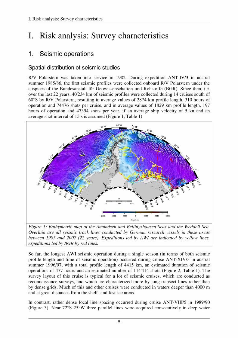
R/V Polarstern was taken into service in 1982. During expedition ANT-IV/3 in austral summer 1985/86, the first seismic profiles were collected onboard R/V Polarstern under the auspices of the Bundesanstalt für Geowissenschaften und Rohstoffe (BGR). Since then, i.e. over the last 22 years, 40'234 km of seismic profiles were collected during 14 cruises south of 60°S by R/V Polarstern, resulting in average values of 2874 km profile length, 310 hours of operation and 74476 shots per cruise, and in average values of 1829 km profile length, 197 hours of operation and 47394 shots per year, if an average ship velocity of 5 kn and an average shot interval of 15 s is assumed (Figure 1, Table 1)
Figure 1: Bathymetric map of the Amundsen and Bellingshausen Seas and the Weddell Sea. Overlain are all seismic track lines conducted by German research vessels in these areas between 1985 and 2007 (22 years). Expeditions led by AWI are indicated by yellow lines, expeditions led by BGR by red lines.
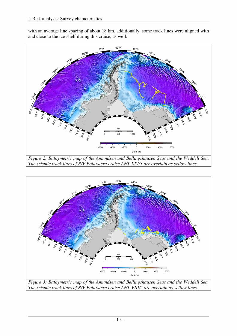
So far, the longest AWI seismic operation during a single season (in terms of both seismic profile length and time of seismic operation) occurred during cruise ANT-XIV/3 in austral summer 1996/97, with a total profile length of 4415 km, an estimated duration of seismic operations of 477 hours and an estimated number of 114'414 shots (Figure 2, Table 1). The survey layout of this cruise is typical for a lot of seismic cruises, which are conducted as reconnaissance surveys, and which are characterized more by long transect lines rather than by dense grids. Much of this and other cruises were conducted in waters deeper than 4000 m and at great distances from the shelf- and fast-ice areas.
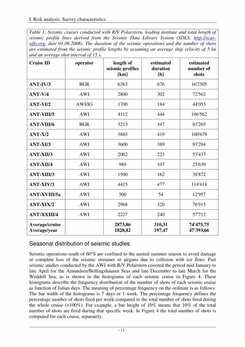
In contrast, rather dense local line spacing occurred during cruise ANT-VIII/5 in 1989/90 (Figure 3). Near 72°S 25°W three parallel lines were acquired consecutively in deep water
I. Risk analysis: Survey characteristics
- 10 -
with an average line spacing of about 18 km. additionally, some track lines were aligned with and close to the ice-shelf during this cruise, as well.
Figure 2: Bathymetric map of the Amundsen and Bellingshausen Seas and the Weddell Sea. The seismic track lines of R/V Polarstern cruise ANT-XIV/3 are overlain as yellow lines.
Figure 3: Bathymetric map of the Amundsen and Bellingshausen Seas and the Weddell Sea. The seismic track lines of R/V Polarstern cruise ANT-VIII/5 are overlain as yellow lines.
I. Risk analysis: Survey characteristics
- 11 -
Table 1: Seismic cruises conducted with R/V Polarstern, leading institute and total length of seismic profile lines derived from the Seismic Data Library System (SDLS; http://scar-sdls.org, date 01.06.2008). The duration of the seismic operations and the number of shots are estimated from the seismic profile lengths by assuming an average ship velocity of 5 kn and an average shot interval of 15 s.
Cruise ID operator length of
seismic profiles
[km]
estimated
duration
[h]
estimated
number of
shots
ANT-IV/3 BGR 6263 676 16'2305
ANT-V/4 AWI 2800 302 72'562
ANT-VI/2 AWI/IG 1700 184 44'055
ANT-VIII/5 AWI 4112 444 106'562
ANT-VIII/6 BGR 3213 347 83'265
ANT-X/2 AWI 3885 419 100'679
ANT-XI/3 AWI 3600 389 93'294
ANT-XII/3 AWI 2062 223 53'437
ANT-XII/4 AWI 989 107 25'630
ANT-XIII/3 AWI 1500 162 38'872
ANT-XIV/3 AWI 4415 477 114'414
ANT-XVIII/5a AWI 500 54 12'957
ANT-XIX/2 AWI 2968 320 76'915
ANT-XXIII/4 AWI 2227 240 57'712
Average/cruise
Average/year
2873,86
1828,82
310,31
197,47 74'475,75
47'393,66
Seasonal distribution of seismic studies
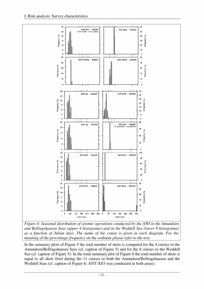
Seismic operations south of 60°S are confined to the austral summer season to avoid damage or complete loss of the seismic streamer or airguns due to collision with ice floes. Past seismic studies conducted by the AWI with R/V Polarstern covered the period mid January to late April for the Amundsen/Bellingshausen Seas and late December to late March for the Weddell Sea, as is shown in the histograms of each seismic cruise in Figure 4. These histograms describe the frequency distribution of the number of shots of each seismic cruise as function of Julian days. The meaning of percentage frequency on the ordinate is as follows: The bar width of the histograms is 7 days or 1 week. The percentage frequency defines the percentage number of shots fired per week compared to the total number of shots fired during the whole cruise (=100%). For example, a bar height of 10% means that 10% of the total number of shots are fired during that specific week. In Figure 4 the total number of shots is computed for each cruise, separately.
I. Risk analysis: Survey characteristics
- 12 -
Figure 4: Seasonal distribution of seismic operations conducted by the AWI in the Amundsen and Bellingshausen Seas (upper 4 histograms) and in the Weddell Sea (lower 8 histograms) as a function of Julian days. The name of the cruise is given in each diagram. For the meaning of the percentage frequency on the ordinate please refer to the text.
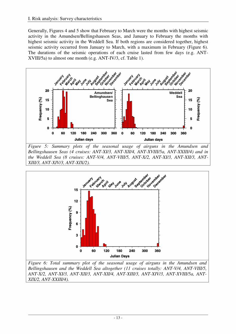
In the summary plots of Figure 5 the total number of shots is computed for the 4 cruises to the Amundsen/Bellingshausen Seas (cf. caption of Figure 5) and for the 8 cruises to the Weddell Sea (cf. caption of Figure 5). In the total summary plot of Figure 6 the total number of shots is equal to all shots fired during the 11 cruises to both the Amundsen/Bellingshausen and the Weddell Seas (cf. caption of Figure 6; ANT-XI/3 was conducted in both areas).
I. Risk analysis: Survey characteristics
- 13 -
Generally, Figures 4 and 5 show that February to March were the months with highest seismic activity in the Amundsen/Bellingshausen Seas, and January to February the months with highest seismic activity in the Weddell Sea. If both regions are considered together, highest seismic activity occurred from January to March, with a maximum in February (Figure 6). The durations of the seismic operations of each cruise lasted from few days (e.g. ANT-XVIII/5a) to almost one month (e.g. ANT-IV/3, cf. Table 1).
Figure 5: Summary plots of the seasonal usage of airguns in the Amundsen and Bellingshausen Seas (4 cruises: ANT-XI/3, ANT-XII/4, ANT-XVIII/5a, ANT-XXIII/4) and in the Weddell Sea (8 cruises: ANT-V/4, ANT-VIII/5, ANT-X/2, ANT-XI/3, ANT-XII/3, ANT-XIII/3, ANT-XIV/3, ANT-XIX/2).
Figure 6: Total summary plot of the seasonal usage of airguns in the Amundsen and Bellingshausen and the Weddell Sea altogether (11 cruises totally: ANT-V/4, ANT-VIII/5, ANT-X/2, ANT-XI/3, ANT-XII/3, ANT-XII/4, ANT-XIII/3, ANT-XIV/3, ANT-XVIII/5a, ANT-XIX/2, ANT-XXIII/4).
I. Risk analysis: Survey characteristics
- 14 -
Recurrence of seismic measurements within certain areas
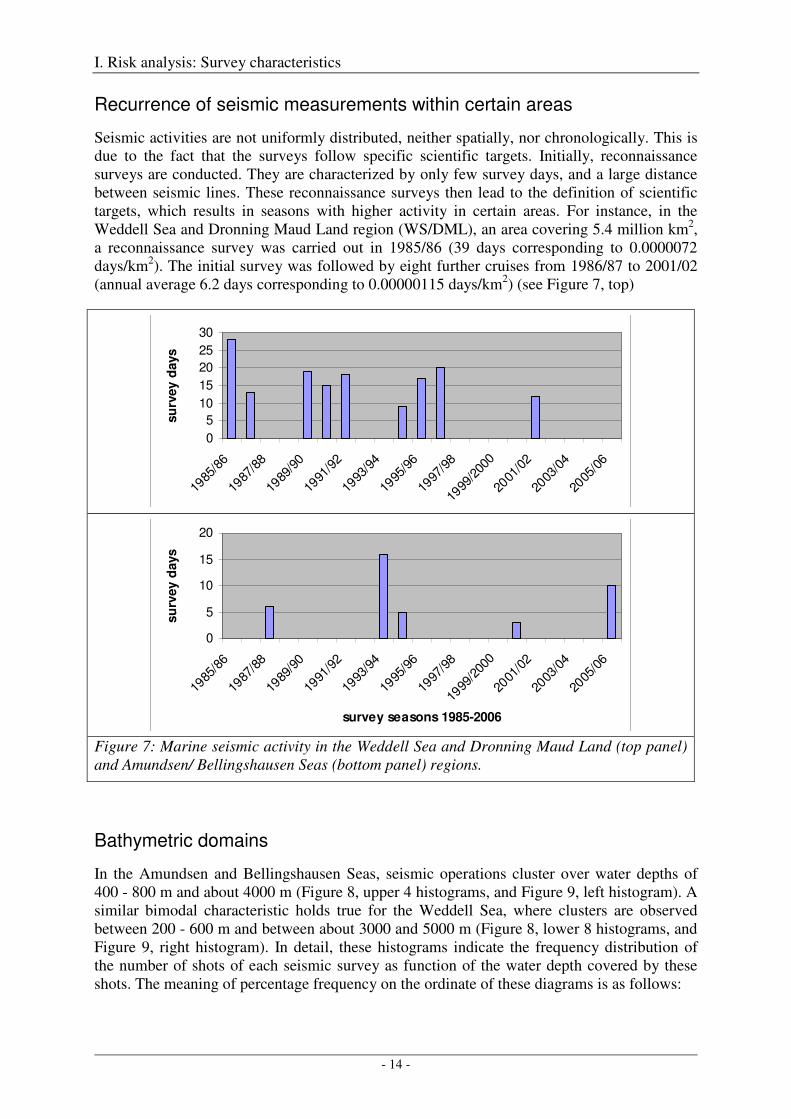
Seismic activities are not uniformly distributed, neither spatially, nor chronologically. This is due to the fact that the surveys follow specific scientific targets. Initially, reconnaissance surveys are conducted. They are characterized by only few survey days, and a large distance between seismic lines. These reconnaissance surveys then lead to the definition of scientific targets, which results in seasons with higher activity in certain areas. For instance, in the Weddell Sea and Dronning Maud Land region (WS/DML), an area covering 5.4 million km2, a reconnaissance survey was carried out in 1985/86 (39 days corresponding to 0.0000072 days/km2). The initial survey was followed by eight further cruises from 1986/87 to 2001/02 (annual average 6.2 days corresponding to 0.00000115 days/km2) (see Figure 7, top)
0
5
10
15
20
25
30
1985
/86
1987
/88
1989
/90
1991
/92
1993
/94
1995
/96
1997
/98
1999
/200
0
2001
/02
2003
/04
2005
/06
su
rvey d
ays
0
5
10
15
20
1985
/86
1987
/88
1989
/90
1991
/92
1993
/94
1995
/96
1997
/98
1999
/200
0
2001
/02
2003
/04
2005
/06
survey seasons 1985-2006
su
rvey d
ays
Figure 7: Marine seismic activity in the Weddell Sea and Dronning Maud Land (top panel) and Amundsen/ Bellingshausen Seas (bottom panel) regions.
Bathymetric domains
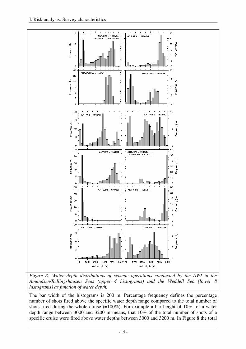
In the Amundsen and Bellingshausen Seas, seismic operations cluster over water depths of 400 - 800 m and about 4000 m (Figure 8, upper 4 histograms, and Figure 9, left histogram). A similar bimodal characteristic holds true for the Weddell Sea, where clusters are observed between 200 - 600 m and between about 3000 and 5000 m (Figure 8, lower 8 histograms, and Figure 9, right histogram). In detail, these histograms indicate the frequency distribution of the number of shots of each seismic survey as function of the water depth covered by these shots. The meaning of percentage frequency on the ordinate of these diagrams is as follows:
I. Risk analysis: Survey characteristics
- 15 -
Figure 8: Water depth distributions of seismic operations conducted by the AWI in the Amundsen/Bellingshausen Seas (upper 4 histograms) and the Weddell Sea (lower 8 histograms) as function of water depth.
The bar width of the histograms is 200 m. Percentage frequency defines the percentage number of shots fired above the specific water depth range compared to the total number of shots fired during the whole cruise (=100%). For example a bar height of 10% for a water depth range between 3000 and 3200 m means, that 10% of the total number of shots of a specific cruise were fired above water depths between 3000 and 3200 m. In Figure 8 the total
I. Risk analysis: Survey characteristics
- 16 -
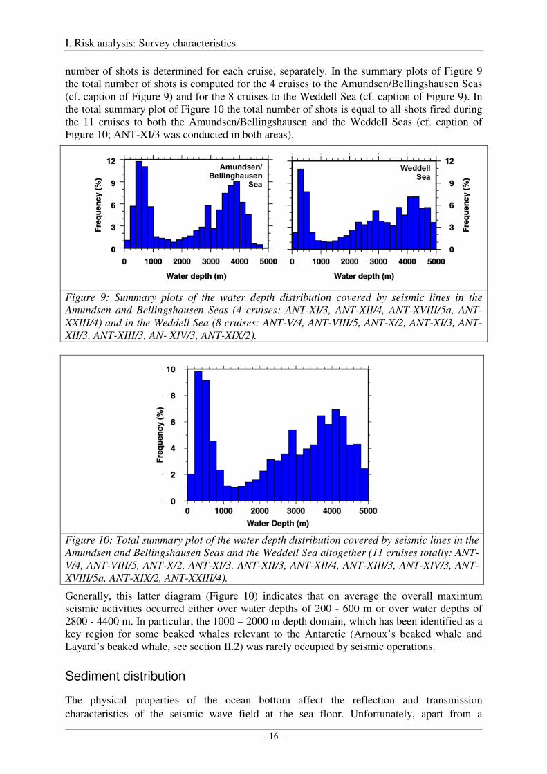
number of shots is determined for each cruise, separately. In the summary plots of Figure 9 the total number of shots is computed for the 4 cruises to the Amundsen/Bellingshausen Seas (cf. caption of Figure 9) and for the 8 cruises to the Weddell Sea (cf. caption of Figure 9). In the total summary plot of Figure 10 the total number of shots is equal to all shots fired during the 11 cruises to both the Amundsen/Bellingshausen and the Weddell Seas (cf. caption of Figure 10; ANT-XI/3 was conducted in both areas).
Figure 9: Summary plots of the water depth distribution covered by seismic lines in the Amundsen and Bellingshausen Seas (4 cruises: ANT-XI/3, ANT-XII/4, ANT-XVIII/5a, ANT-XXIII/4) and in the Weddell Sea (8 cruises: ANT-V/4, ANT-VIII/5, ANT-X/2, ANT-XI/3, ANT-XII/3, ANT-XIII/3, AN- XIV/3, ANT-XIX/2).
Figure 10: Total summary plot of the water depth distribution covered by seismic lines in the Amundsen and Bellingshausen Seas and the Weddell Sea altogether (11 cruises totally: ANT-V/4, ANT-VIII/5, ANT-X/2, ANT-XI/3, ANT-XII/3, ANT-XII/4, ANT-XIII/3, ANT-XIV/3, ANT-XVIII/5a, ANT-XIX/2, ANT-XXIII/4).
Generally, this latter diagram (Figure 10) indicates that on average the overall maximum seismic activities occurred either over water depths of 200 - 600 m or over water depths of 2800 - 4400 m. In particular, the 1000 – 2000 m depth domain, which has been identified as a key region for some beaked whales relevant to the Antarctic (Arnoux’s beaked whale and Layard’s beaked whale, see section II.2) was rarely occupied by seismic operations.
Sediment distribution
The physical properties of the ocean bottom affect the reflection and transmission characteristics of the seismic wave field at the sea floor. Unfortunately, apart from a
I. Risk analysis: Survey characteristics
- 17 -
compilation of high-resolution seismic, sediment echosounder and sediment core data for the southeastern Weddell Sea (Michels et al. 2002) detailed maps of the sediment distribution in the Amundsen and Bellingshausen Seas and in the Weddell Sea are not available. However, within the regions of concern, and according to the study of Michels et al. (2002) the sediment is expected to exhibit little variability. Furthermore, as no strong currents are known for the areas discussed herein, no sea floor areas consisting of hard rock not covered by sediment are to be expected. Hence, as a typical model, a rather soft sea floor with a P-wave velocity of 1600 m/s, an S-wave velocity of 330 m/s and a wet bulk density of 1450 kg/m³ is assumed for the modelling studies discussed later. Together with a sound velocity of 1500 m/s and a wet bulk density of 1025 kg/m³ in the sea water, this results in a normal incidence reflection coefficient of R = 0.2.
Output
All seismic profiles acquired by R/V Polarstern so far are located in the Amundsen and Bellingshausen Seas and the Weddell Sea. On average the total length of seismic profiles collected during a single expedition is about 2900 km (Table 1). This corresponds to approximately 310 h (13 days) of seismic operations and to about 74'500 seismic pulses, if a shot interval of 15 s is assumed, i.e. one pulse every 38 metres along track.
From Figures 5 - 6 it becomes evident that the peak season for seismic operations are the austral summer months January to March, while a significantly lesser amount of seismic profiles are collected during the austral spring and fall months December and April. For the rest of the year seismic operations were not conducted in Southern Ocean waters.
From Figures 8 - 10 it is evident that water depths occupied during seismic profiles cluster at 200 - 600 m and 2800 - 4400 m. Therefore, we selected an average water depth of 400 m for the shallow water modelling studies of the (propagating) sound fields, and - in order to save computation time - an average water depth of 3000 m for the deep water modelling studies. Additionally, it is worth noting that up to now only few seismic profiles were acquired in the 1000 - 2000 m depth range, which is the (hypothesized) preferential habitat of beaked whales.
As sediment parameters a P-wave velocity of vP = 1600 m/s, an S-wave velocity of vS = 330 m/s, a wet bulk density of ρ = 1450 kg/m3, and a negligible attenuation for P- and S-waves quantified by the quality factors QP = QS = 1.5 × 10⁶ were chosen for the sea floor in all further modelling studies.
I. Risk analysis: Survey characteristics
- 18 -
2. Environment
Hydrography
Based on the above analysis of spatio-temporal cruise distributions, this section focuses on the characteristics of the typical regions and seasons for AWI’s seismic operations, i.e. the Amundsen and Bellingshausen Seas and the Weddell Sea during the austral summer. Before focusing on these regions, two graphs shall exemplify the major differences between the polar and the temperate oceans with regard to sound velocity profiles and channels.
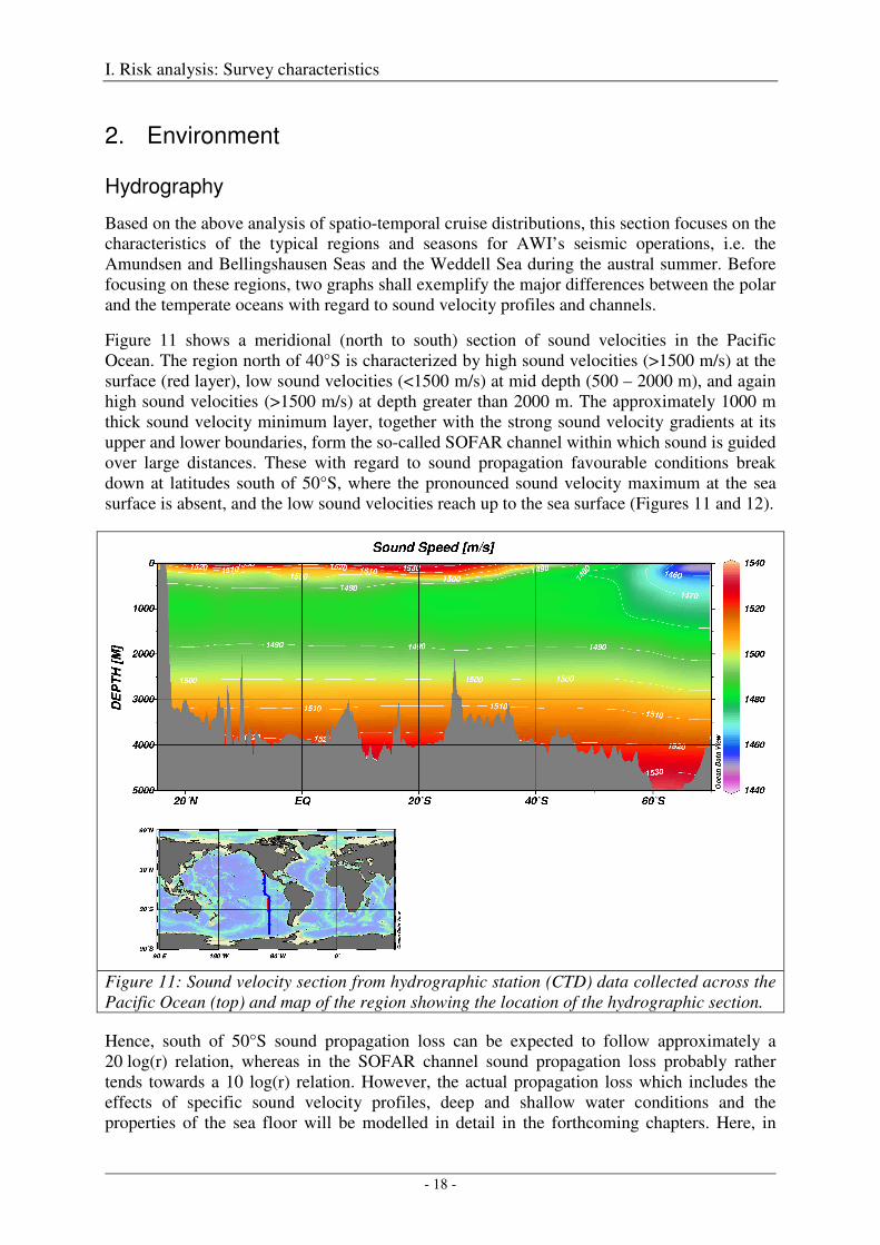
Figure 11 shows a meridional (north to south) section of sound velocities in the Pacific Ocean. The region north of 40°S is characterized by high sound velocities (>1500 m/s) at the surface (red layer), low sound velocities (<1500 m/s) at mid depth (500 – 2000 m), and again high sound velocities (>1500 m/s) at depth greater than 2000 m. The approximately 1000 m thick sound velocity minimum layer, together with the strong sound velocity gradients at its upper and lower boundaries, form the so-called SOFAR channel within which sound is guided over large distances. These with regard to sound propagation favourable conditions break down at latitudes south of 50°S, where the pronounced sound velocity maximum at the sea surface is absent, and the low sound velocities reach up to the sea surface (Figures 11 and 12).
Figure 11: Sound velocity section from hydrographic station (CTD) data collected across the Pacific Ocean (top) and map of the region showing the location of the hydrographic section.
Hence, south of 50°S sound propagation loss can be expected to follow approximately a 20 log(r) relation, whereas in the SOFAR channel sound propagation loss probably rather tends towards a 10 log(r) relation. However, the actual propagation loss which includes the effects of specific sound velocity profiles, deep and shallow water conditions and the properties of the sea floor will be modelled in detail in the forthcoming chapters. Here, in
I. Risk analysis: Survey characteristics
- 19 -
what follows the sound velocity profiles representative for the different regions will be extracted.
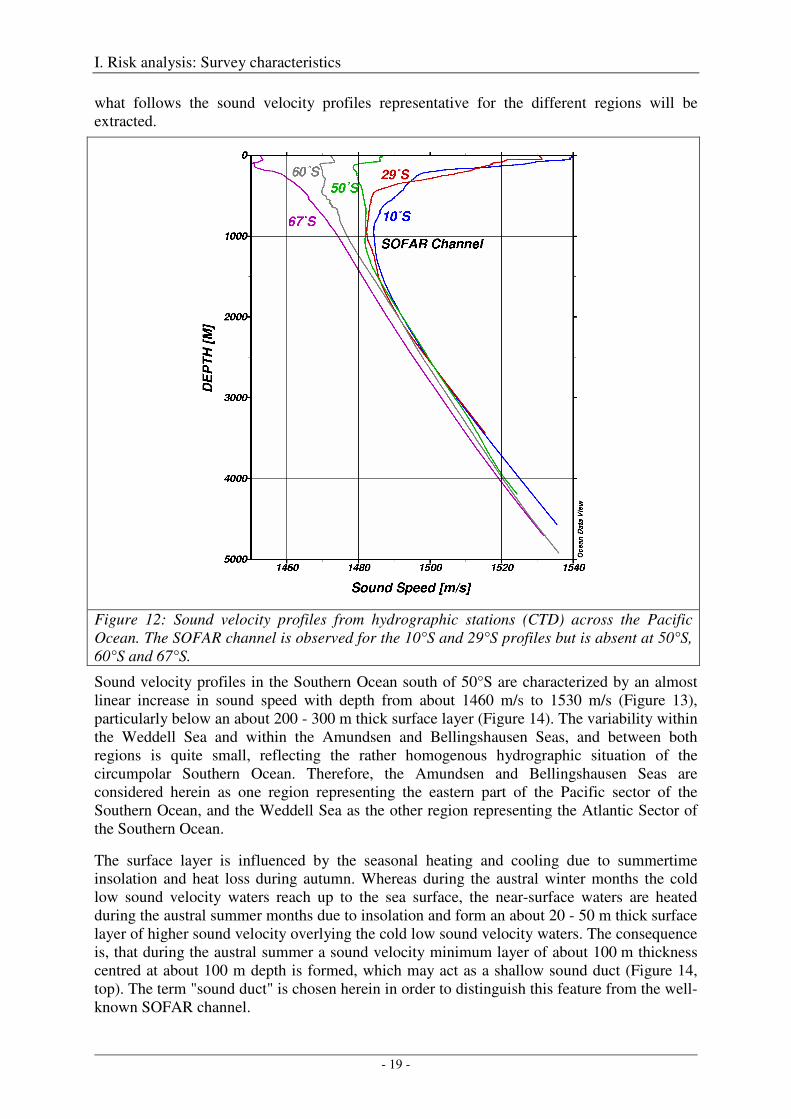
Figure 12: Sound velocity profiles from hydrographic stations (CTD) across the Pacific Ocean. The SOFAR channel is observed for the 10°S and 29°S profiles but is absent at 50°S, 60°S and 67°S.
Sound velocity profiles in the Southern Ocean south of 50°S are characterized by an almost linear increase in sound speed with depth from about 1460 m/s to 1530 m/s (Figure 13), particularly below an about 200 - 300 m thick surface layer (Figure 14). The variability within the Weddell Sea and within the Amundsen and Bellingshausen Seas, and between both regions is quite small, reflecting the rather homogenous hydrographic situation of the circumpolar Southern Ocean. Therefore, the Amundsen and Bellingshausen Seas are considered herein as one region representing the eastern part of the Pacific sector of the Southern Ocean, and the Weddell Sea as the other region representing the Atlantic Sector of the Southern Ocean.
The surface layer is influenced by the seasonal heating and cooling due to summertime insolation and heat loss during autumn. Whereas during the austral winter months the cold low sound velocity waters reach up to the sea surface, the near-surface waters are heated during the austral summer months due to insolation and form an about 20 - 50 m thick surface layer of higher sound velocity overlying the cold low sound velocity waters. The consequence is, that during the austral summer a sound velocity minimum layer of about 100 m thickness centred at about 100 m depth is formed, which may act as a shallow sound duct (Figure 14, top). The term "sound duct" is chosen herein in order to distinguish this feature from the well-known SOFAR channel.
I. Risk analysis: Survey characteristics
- 20 -
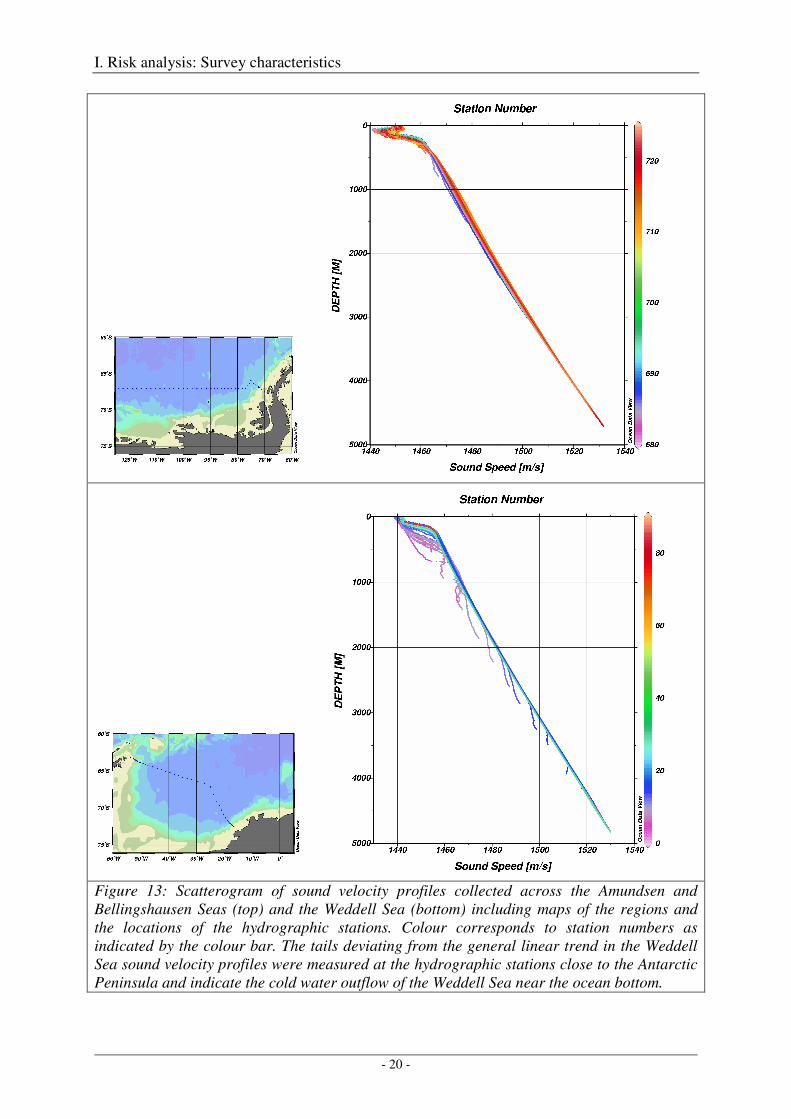
Figure 13: Scatterogram of sound velocity profiles collected across the Amundsen and Bellingshausen Seas (top) and the Weddell Sea (bottom) including maps of the regions and the locations of the hydrographic stations. Colour corresponds to station numbers as indicated by the colour bar. The tails deviating from the general linear trend in the Weddell Sea sound velocity profiles were measured at the hydrographic stations close to the Antarctic Peninsula and indicate the cold water outflow of the Weddell Sea near the ocean bottom.
I. Risk analysis: Survey characteristics
- 21 -
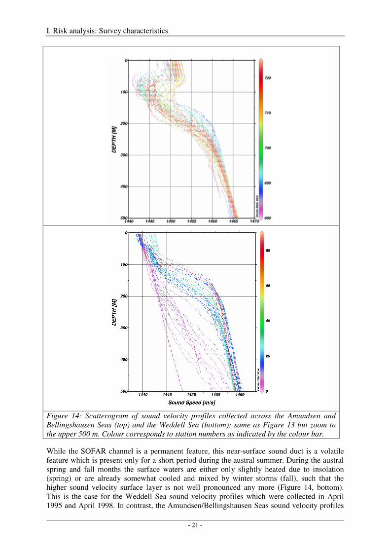
Figure 14: Scatterogram of sound velocity profiles collected across the Amundsen and Bellingshausen Seas (top) and the Weddell Sea (bottom); same as Figure 13 but zoom to the upper 500 m. Colour corresponds to station numbers as indicated by the colour bar.
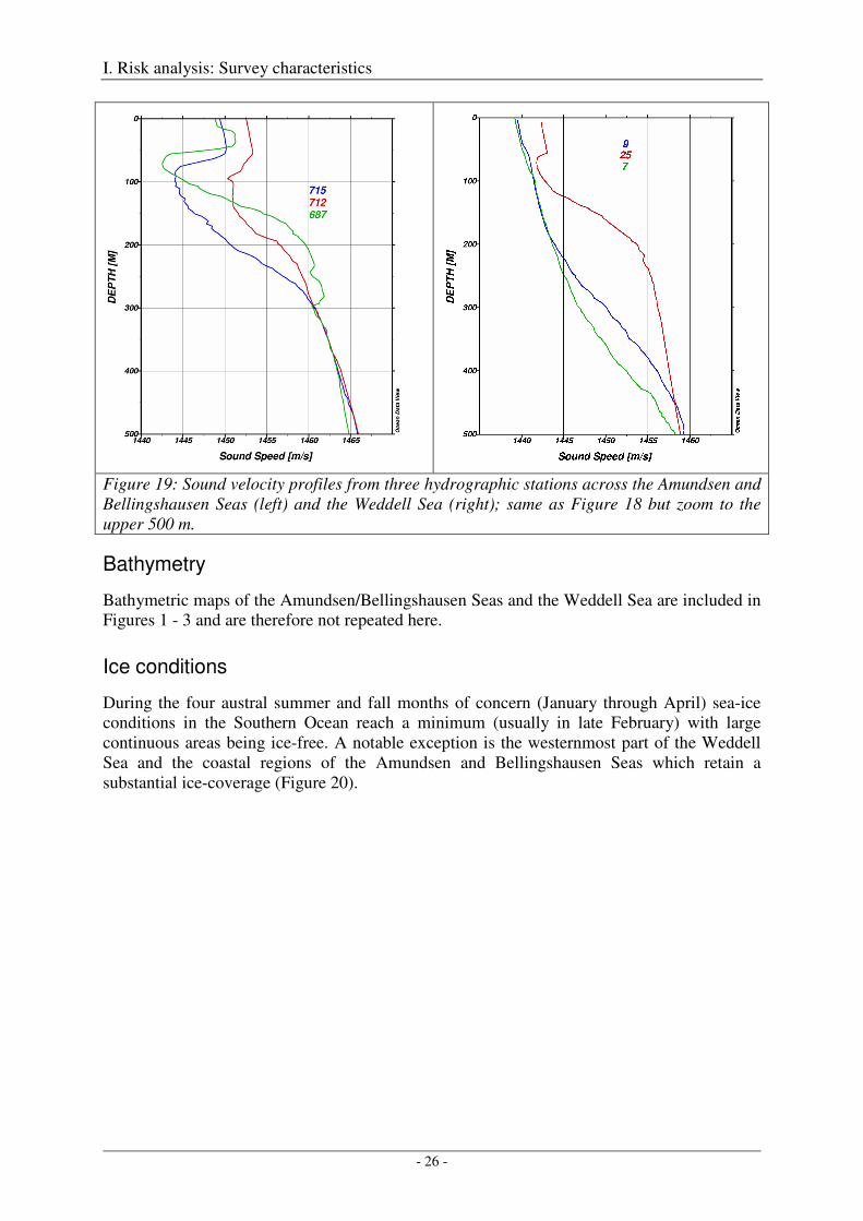
While the SOFAR channel is a permanent feature, this near-surface sound duct is a volatile feature which is present only for a short period during the austral summer. During the austral spring and fall months the surface waters are either only slightly heated due to insolation (spring) or are already somewhat cooled and mixed by winter storms (fall), such that the higher sound velocity surface layer is not well pronounced any more (Figure 14, bottom). This is the case for the Weddell Sea sound velocity profiles which were collected in April 1995 and April 1998. In contrast, the Amundsen/Bellingshausen Seas sound velocity profiles
I. Risk analysis: Survey characteristics
- 22 -
are typical for the austral summer months, because they were collected from late February to early March 1992.
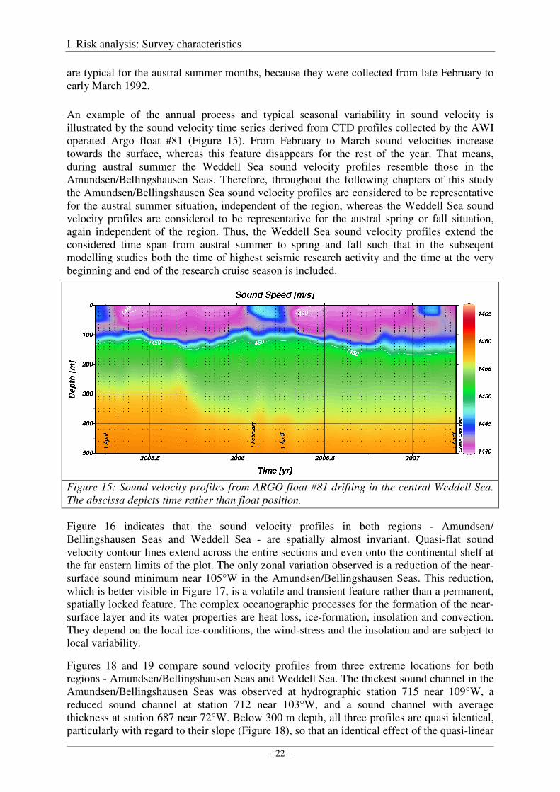
An example of the annual process and typical seasonal variability in sound velocity is illustrated by the sound velocity time series derived from CTD profiles collected by the AWI operated Argo float #81 (Figure 15). From February to March sound velocities increase towards the surface, whereas this feature disappears for the rest of the year. That means, during austral summer the Weddell Sea sound velocity profiles resemble those in the Amundsen/Bellingshausen Seas. Therefore, throughout the following chapters of this study the Amundsen/Bellingshausen Sea sound velocity profiles are considered to be representative for the austral summer situation, independent of the region, whereas the Weddell Sea sound velocity profiles are considered to be representative for the austral spring or fall situation, again independent of the region. Thus, the Weddell Sea sound velocity profiles extend the considered time span from austral summer to spring and fall such that in the subseqent modelling studies both the time of highest seismic research activity and the time at the very beginning and end of the research cruise season is included.
Figure 15: Sound velocity profiles from ARGO float #81 drifting in the central Weddell Sea. The abscissa depicts time rather than float position.
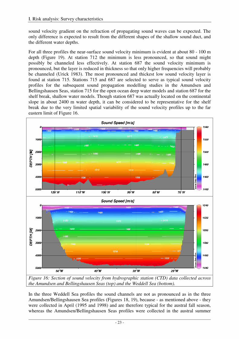
Figure 16 indicates that the sound velocity profiles in both regions - Amundsen/ Bellingshausen Seas and Weddell Sea - are spatially almost invariant. Quasi-flat sound velocity contour lines extend across the entire sections and even onto the continental shelf at the far eastern limits of the plot. The only zonal variation observed is a reduction of the near-surface sound minimum near 105°W in the Amundsen/Bellingshausen Seas. This reduction, which is better visible in Figure 17, is a volatile and transient feature rather than a permanent, spatially locked feature. The complex oceanographic processes for the formation of the near-surface layer and its water properties are heat loss, ice-formation, insolation and convection. They depend on the local ice-conditions, the wind-stress and the insolation and are subject to local variability.
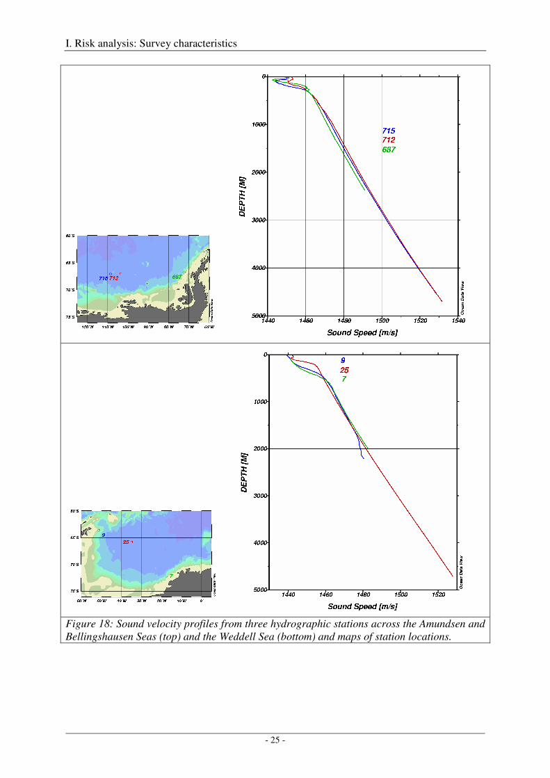
Figures 18 and 19 compare sound velocity profiles from three extreme locations for both regions - Amundsen/Bellingshausen Seas and Weddell Sea. The thickest sound channel in the Amundsen/Bellingshausen Seas was observed at hydrographic station 715 near 109°W, a reduced sound channel at station 712 near 103°W, and a sound channel with average thickness at station 687 near 72°W. Below 300 m depth, all three profiles are quasi identical, particularly with regard to their slope (Figure 18), so that an identical effect of the quasi-linear
I. Risk analysis: Survey characteristics
- 23 -
sound velocity gradient on the refraction of propagating sound waves can be expected. The only difference is expected to result from the different shapes of the shallow sound duct, and the different water depths.
For all three profiles the near-surface sound velocity minimum is evident at about 80 - 100 m depth (Figure 19). At station 712 the minimum is less pronounced, so that sound might possibly be channeled less effectively. At station 687 the sound velocity minimum is pronounced, but the layer is reduced in thickness so that only higher frequencies will probably be channeled (Urick 1983). The most pronounced and thickest low sound velocity layer is found at station 715. Stations 715 and 687 are selected to serve as typical sound velocity profiles for the subsequent sound propagation modelling studies in the Amundsen and Bellingshausen Seas, station 715 for the open ocean deep water models and station 687 for the shelf break, shallow water models. Though station 687 was actually located on the continental slope in about 2400 m water depth, it can be considered to be representative for the shelf break due to the very limited spatial variability of the sound velocity profiles up to the far eastern limit of Figure 16.
Figure 16: Section of sound velocity from hydrographic station (CTD) data collected across the Amundsen and Bellingshausen Seas (top) and the Weddell Sea (bottom).
In the three Weddell Sea profiles the sound channels are not as pronounced as in the three Amundsen/Bellingshausen Sea profiles (Figures 18, 19), because - as mentioned above - they were collected in April (1995 and 1998) and are therefore typical for the austral fall season, whereas the Amundsen/Bellingshausen Seas profiles were collected in the austral summer
I. Risk analysis: Survey characteristics
- 24 -
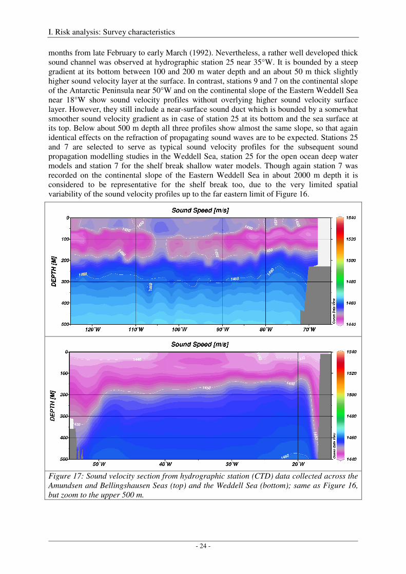
months from late February to early March (1992). Nevertheless, a rather well developed thick sound channel was observed at hydrographic station 25 near 35°W. It is bounded by a steep gradient at its bottom between 100 and 200 m water depth and an about 50 m thick slightly higher sound velocity layer at the surface. In contrast, stations 9 and 7 on the continental slope of the Antarctic Peninsula near 50°W and on the continental slope of the Eastern Weddell Sea near 18°W show sound velocity profiles without overlying higher sound velocity surface layer. However, they still include a near-surface sound duct which is bounded by a somewhat smoother sound velocity gradient as in case of station 25 at its bottom and the sea surface at its top. Below about 500 m depth all three profiles show almost the same slope, so that again identical effects on the refraction of propagating sound waves are to be expected. Stations 25 and 7 are selected to serve as typical sound velocity profiles for the subsequent sound propagation modelling studies in the Weddell Sea, station 25 for the open ocean deep water models and station 7 for the shelf break shallow water models. Though again station 7 was recorded on the continental slope of the Eastern Weddell Sea in about 2000 m depth it is considered to be representative for the shelf break too, due to the very limited spatial variability of the sound velocity profiles up to the far eastern limit of Figure 16.
Figure 17: Sound velocity section from hydrographic station (CTD) data collected across the Amundsen and Bellingshausen Seas (top) and the Weddell Sea (bottom); same as Figure 16, but zoom to the upper 500 m.
I. Risk analysis: Survey characteristics
- 25 -
Figure 18: Sound velocity profiles from three hydrographic stations across the Amundsen and Bellingshausen Seas (top) and the Weddell Sea (bottom) and maps of station locations.
I. Risk analysis: Survey characteristics
- 26 -
Figure 19: Sound velocity profiles from three hydrographic stations across the Amundsen and Bellingshausen Seas (left) and the Weddell Sea (right); same as Figure 18 but zoom to the upper 500 m.
Bathymetry
Bathymetric maps of the Amundsen/Bellingshausen Seas and the Weddell Sea are included in Figures 1 - 3 and are therefore not repeated here.
Ice conditions
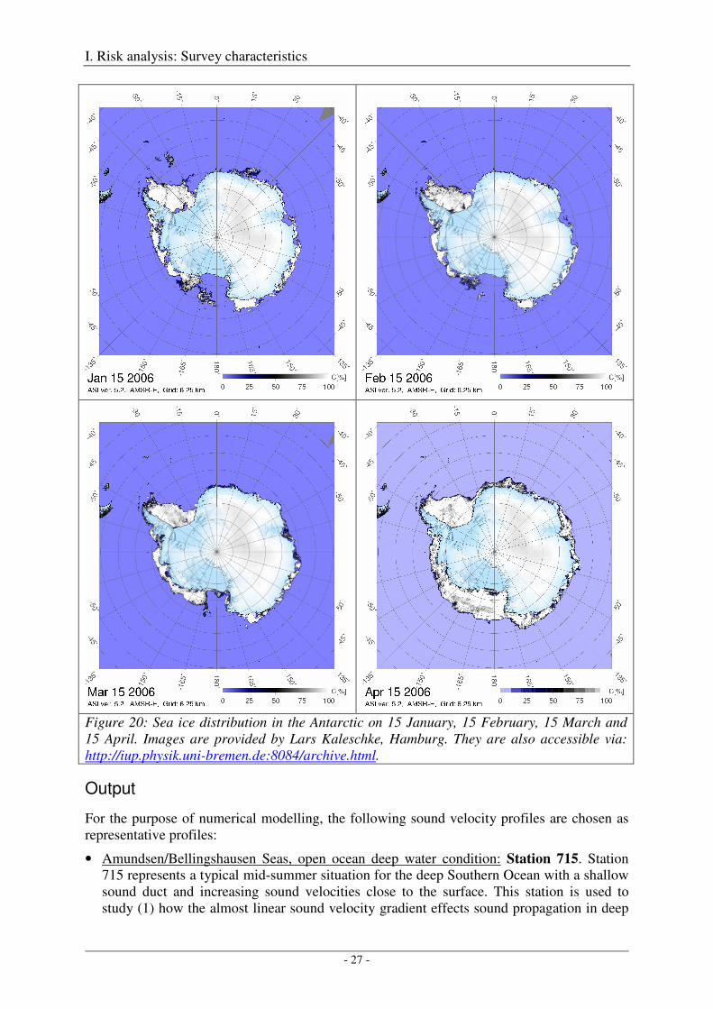
During the four austral summer and fall months of concern (January through April) sea-ice conditions in the Southern Ocean reach a minimum (usually in late February) with large continuous areas being ice-free. A notable exception is the westernmost part of the Weddell Sea and the coastal regions of the Amundsen and Bellingshausen Seas which retain a substantial ice-coverage (Figure 20).
I. Risk analysis: Survey characteristics
- 27 -
Figure 20: Sea ice distribution in the Antarctic on 15 January, 15 February, 15 March and 15 April. Images are provided by Lars Kaleschke, Hamburg. They are also accessible via: http://iup.physik.uni-bremen.de:8084/archive.html.
Output
For the purpose of numerical modelling, the following sound velocity profiles are chosen as representative profiles:
• Amundsen/Bellingshausen Seas, open ocean deep water condition: Station 715. Station 715 represents a typical mid-summer situation for the deep Southern Ocean with a shallow sound duct and increasing sound velocities close to the surface. This station is used to study (1) how the almost linear sound velocity gradient effects sound propagation in deep
I. Risk analysis: Survey characteristics
- 28 -
water, (2) if and how sound is guided in the low-velocity sound duct close to the sea surface, and (3) what are the effects on the transmission loss.
• Amundsen/Bellingshausen Seas, coastal shallow water condition: Station 687. Station 687 represents a typical mid-summer situation for the continental slope and shelf break in the Southern Ocean with a shallow sound duct of reduced thickness and increasing sound velocities close to the surface. This station is used to study (1) how the almost linear sound velocity gradient effects sound propagation in rather shallow water, (2) if and how sound is guided in the low-velocity sound duct close to the sea surface, (3) what are the effects on the transmission loss, and what are the differences compared to the deep water model of station 715.
• Weddell Sea, open ocean deep water condition: Station 25. Station 25 represents a typical late summer situation for the deep Southern Ocean in which the shallow sound duct is not as pronounced any more as during the mid-summer situation because the higher sound velocity surface layer almost disappeared. It also resembles the early summer situation.
• Weddell Sea, coastal shallow water condition: Station 7. Station 7 represents a typical late summer situation for the continental slope and shelf break in the Southern Ocean in which the higher sound velocity surface layer is not present any more. In this situation a surface duct is formed between by the sea surface and a rather steep sound velocity gradient in 400 - 500 m depth below the sea surface.
• Both Weddell Sea stations are selected to extend the considered time span for the modelling studies from the austral summer (represented by the Amundsen/Bellingshausen Seas stations) to the austral spring and/or fall months to provide additional information for the very beginning and end of the seismic research cruise season.
Together with the corresponding water depths of 3000 m (open ocean deep water) and 400 m (coastal condition shallow water) and the physical properties of the sea floor the four selected hydrographic stations define the four different so-called "environmental scenarios", hereinafter.
Considering that
• open ocean conditions (no ice) are acoustically favourable to sound propagation (i.e. no sound scattering from the rough bottom-side of an ice-cover),
• (2) sea-ice is severely diminished during austral summer, and
• (3) seismic operations are preferably conducted in open water to prevent damage to the airguns and seismic streamer,
• we assume open ocean conditions for the numerical sound propagation modelling, concordant with a conservative approach.

I. Risk analysis: Survey characteristics
- 29 -
3. Source description
Seismic methods and choice of airgun configuration
A variety of airgun configurations is used in marine seismic surveying. An airgun configuration consists of the number of airguns towed by the vessel, their type and air volume, their tow depths, their array geometries and their technical specifications. The choice of configuration is related to the target of investigation. In principle, the choice is a trade-off between source signal frequencies high enough for good vertical resolution of the subsurface and source signal frequencies low enough for deep penetration into the crust. Generally, it can be said that the larger the airgun volumes are, the lower are the source signal frequencies and the larger is the depth penetration, and vice versa. In scientific seismic surveys, three general types of investigation are common practice (Figure 21):
a) High-resolution seismic reflection surveys: The aim of this near-vertical seismic reflection technique is to image sediment layers at relatively high vertical resolution. Therefore, the airgun characteristic is such that the source signal frequency is high enough to resolve sediment layers in the order of a few tenths of metres in thickness, but still allows depth penetration of 1 - 2 km below the sea floor. Suitable airguns are GI-Guns™ operated in ‘True GI Mode’. Such airguns have two air chambers with up to 2.4 litres (150 in3) total air volume. Each chamber is operated with its own solenoid, the second chamber being fired with a time gap of a few milliseconds after the first one. This technique helps to avoid the bubble effect and generates source signals with a spectral peak level at 70 - 80 Hz for a typical towing depth of 3 - 5 m. Typically 2 - 4 GI-Guns are assembled as an array, depending on the target layer depth. They are being fired every 8 - 12 seconds.
b) Deep crustal seismic reflection surveys: A similar near-vertical seismic reflection technique is applied to obtain seismic images of the sediment sequences and a good part of the basement (or crystalline crust) beneath the sediments using large airgun arrays with a total air-chamber volume ranging between 40 and 80 litres (2400 - 4800 in3). The choice of the number and volumes of airguns depends on the expected thickness of the sediment layers and basement. Best seismic results are achieved by forming arrays of 6 - 20 airguns with 2.5 -8.5 litres (150 - 520 in3) air-chamber volume each. Suitable airguns are, for instance, G-Guns™ which are available with air-chamber volumes of up to 8.5 litres (520 in3). Their firing interval is between 12 and 20 seconds with a source signal at spectral peak level of 30-80 Hz for typical towing depths between 5 - 10 m.
c) Deep crustal seismic refraction and wide-angle reflection surveys: Only source signals with relatively low frequencies penetrate the entire Earth’s crust and return to the seismic receivers. Such deep crustal seismic surveying is commonly conducted in the form of seismic refraction and wide-angle reflection experiments in which ocean-bottom seismometers (OBS) or seismic land-recorders are deployed along a profile or an array on the sea-floor or in coastal areas, while airgun signals are being emitted from the moving vessel. At large source-receiver distances (e.g. 50 - 200 km to record signals from the crust-mantle boundary), the OBS or seismic land-recorder record the seismic wave field, which is refracted at the layer boundaries, then travels along the crustal layers and is refracted back to the surface. Wave fields reflected from layer interfaces at large source-receivers distances (so-called critical or overcritical distances) are also recorded and named ‘wide-angle reflections’. This seismic refraction and wide-angle reflection technique allows deriving information on seismic wave velocities and the layer boundary structure of the sedimentary, crustal and upper mantle
I. Risk analysis: Survey characteristics
- 30 -
zones. The low-frequency source signal is generated by a few large-volume airguns alone, or a common seismic reflection airgun array (e.g. with 8 G-Guns™ of 8.5 litres each) combined with 1 - 2 large-volume airguns in order to boost the low frequencies. The Bolt PAR CT800™ airgun with 32 litres (2000 in3) air-chamber volume is a commonly used type of large-volume airgun for this purpose. Its source signal has a spectral peak level of 25-30 Hz for typical towing depths of 5 - 10 m. Single airguns or combined arrays have firing intervals of 60 seconds in order to achieve the best data quality.
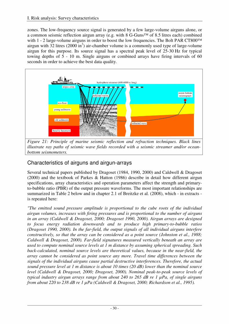
Figure 21: Principle of marine seismic reflection and refraction techniques. Black lines illustrate ray paths of seismic wave fields recorded with a seismic streamer and/or ocean-bottom seismometers.
Characteristics of airguns and airgun-arrays
Several technical papers published by Dragoset (1984, 1990, 2000) and Caldwell & Dragoset (2000) and the textbook of Parkes & Hatton (1986) describe in detail how different airgun specifications, array characteristics and operation parameters affect the strength and primary-to-bubble ratio (PBR) of the output pressure waveforms. The most important relationships are summarized in Table 2 below and in chapter 2.1 of Breitzke et al. (2008), which - in extracts - is repeated here:
"The emitted sound pressure amplitude is proportional to the cube roots of the individual airgun volumes, increases with firing pressures and is proportional to the number of airguns in an array (Caldwell & Dragoset, 2000; Dragoset 1990, 2000). Airgun arrays are designed to focus energy radiation downwards and to produce high primary-to-bubble ratios (Dragoset 1990, 2000). In the far-field, the output signals of all individual airguns interfere constructively, so that the array can be considered as a point source (Johnston et al., 1988; Caldwell & Dragoset, 2000). Far-field signatures measured vertically beneath an array are used to compute nominal source levels at 1 m distance by assuming spherical spreading. Such back-calculated, nominal source levels are theoretical values, because in the near-field, the array cannot be considered as point source any more. Travel time differences between the signals of the individual airguns cause partial destructive interferences. Therefore, the actual sound pressure level at 1 m distance is about 10 times (20 dB) lower than the nominal source level (Caldwell & Dragoset, 2000; Dragoset, 2000). Nominal peak-to-peak source levels of typical industry airgun arrays range from about 240 to 265 dB re 1 µPa, of single airguns from about 220 to 238 dB re 1 µPa (Caldwell & Dragoset, 2000; Richardson et al., 1995).
I. Risk analysis: Survey characteristics
- 31 -
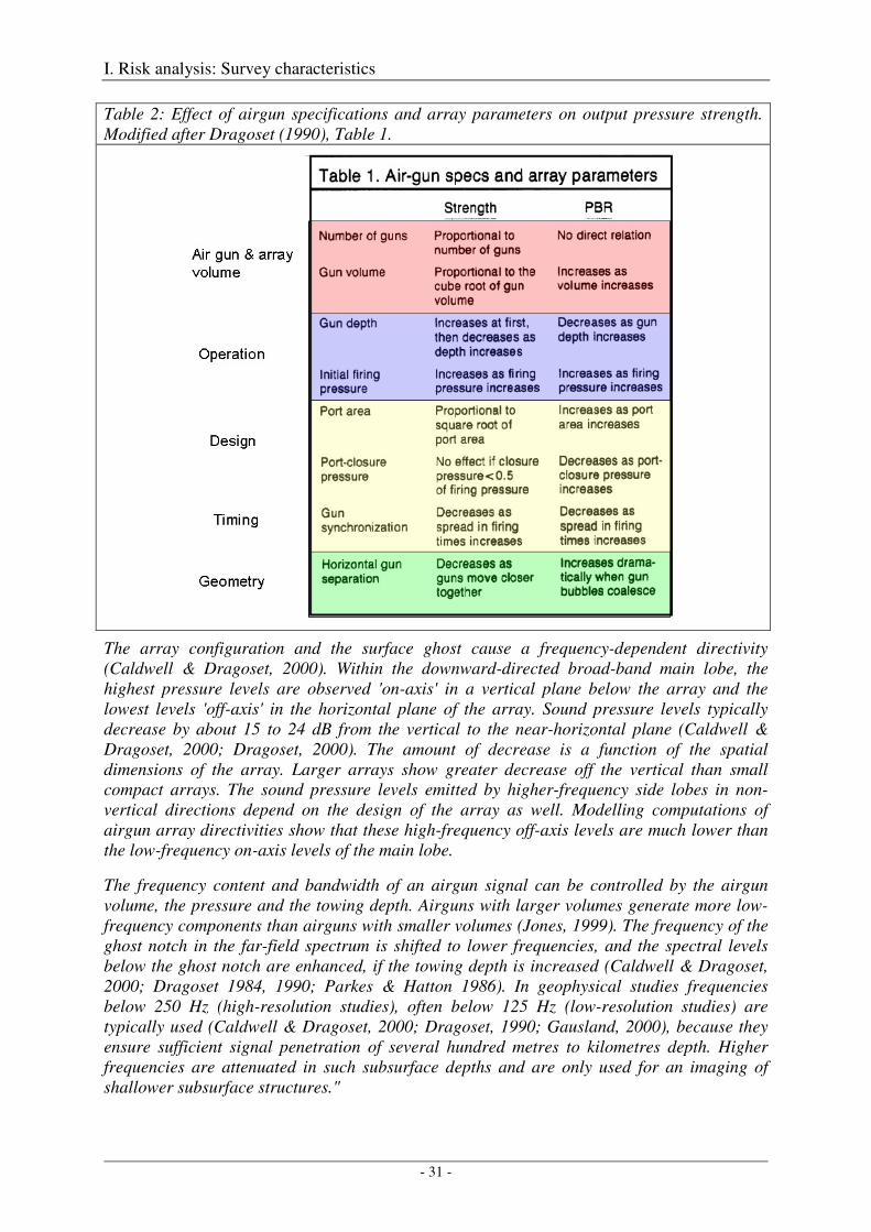
Table 2: Effect of airgun specifications and array parameters on output pressure strength. Modified after Dragoset (1990), Table 1.
The array configuration and the surface ghost cause a frequency-dependent directivity (Caldwell & Dragoset, 2000). Within the downward-directed broad-band main lobe, the highest pressure levels are observed 'on-axis' in a vertical plane below the array and the lowest levels 'off-axis' in the horizontal plane of the array. Sound pressure levels typically decrease by about 15 to 24 dB from the vertical to the near-horizontal plane (Caldwell & Dragoset, 2000; Dragoset, 2000). The amount of decrease is a function of the spatial dimensions of the array. Larger arrays show greater decrease off the vertical than small compact arrays. The sound pressure levels emitted by higher-frequency side lobes in non-vertical directions depend on the design of the array as well. Modelling computations of airgun array directivities show that these high-frequency off-axis levels are much lower than the low-frequency on-axis levels of the main lobe.
The frequency content and bandwidth of an airgun signal can be controlled by the airgun volume, the pressure and the towing depth. Airguns with larger volumes generate more low-frequency components than airguns with smaller volumes (Jones, 1999). The frequency of the ghost notch in the far-field spectrum is shifted to lower frequencies, and the spectral levels below the ghost notch are enhanced, if the towing depth is increased (Caldwell & Dragoset, 2000; Dragoset 1984, 1990; Parkes & Hatton 1986). In geophysical studies frequencies below 250 Hz (high-resolution studies), often below 125 Hz (low-resolution studies) are typically used (Caldwell & Dragoset, 2000; Dragoset, 1990; Gausland, 2000), because they ensure sufficient signal penetration of several hundred metres to kilometres depth. Higher frequencies are attenuated in such subsurface depths and are only used for an imaging of shallower subsurface structures."
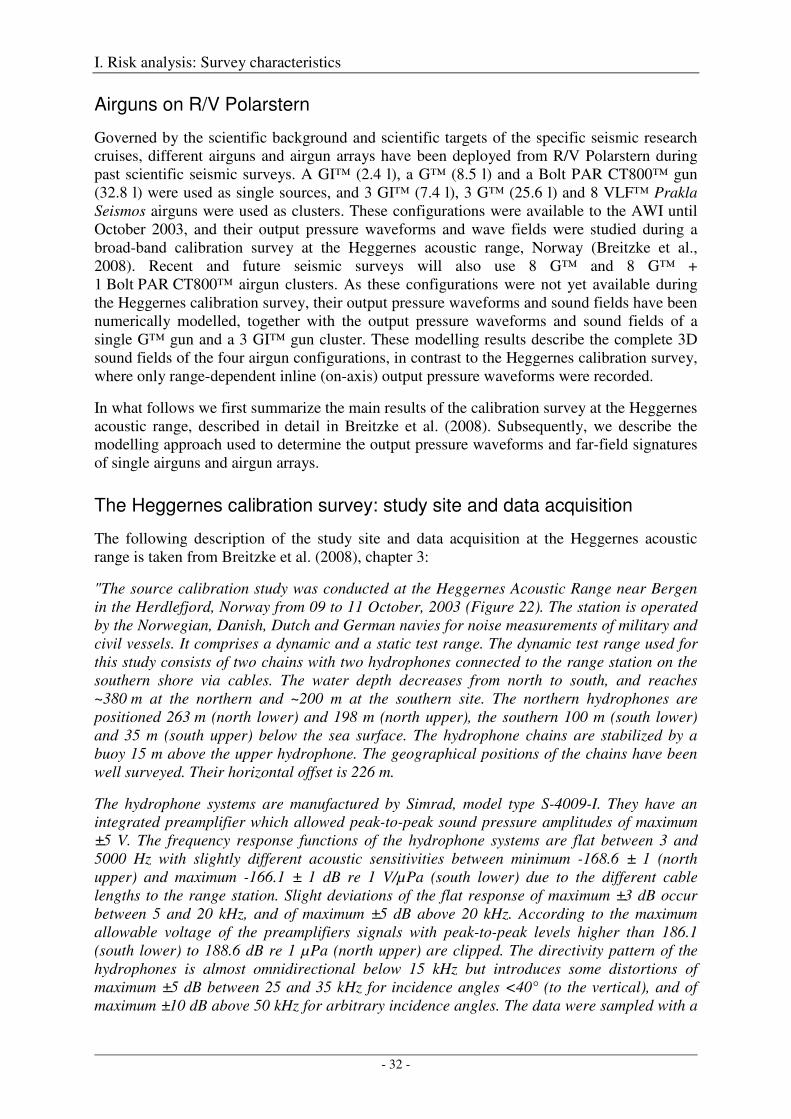
I. Risk analysis: Survey characteristics
- 32 -
Airguns on R/V Polarstern
Governed by the scientific background and scientific targets of the specific seismic research cruises, different airguns and airgun arrays have been deployed from R/V Polarstern during past scientific seismic surveys. A GI™ (2.4 l), a G™ (8.5 l) and a Bolt PAR CT800™ gun (32.8 l) were used as single sources, and 3 GI™ (7.4 l), 3 G™ (25.6 l) and 8 VLF™ Prakla Seismos airguns were used as clusters. These configurations were available to the AWI until October 2003, and their output pressure waveforms and wave fields were studied during a broad-band calibration survey at the Heggernes acoustic range, Norway (Breitzke et al., 2008). Recent and future seismic surveys will also use 8 G™ and 8 G™ + 1 Bolt PAR CT800™ airgun clusters. As these configurations were not yet available during the Heggernes calibration survey, their output pressure waveforms and sound fields have been numerically modelled, together with the output pressure waveforms and sound fields of a single G™ gun and a 3 GI™ gun cluster. These modelling results describe the complete 3D sound fields of the four airgun configurations, in contrast to the Heggernes calibration survey, where only range-dependent inline (on-axis) output pressure waveforms were recorded.
In what follows we first summarize the main results of the calibration survey at the Heggernes acoustic range, described in detail in Breitzke et al. (2008). Subsequently, we describe the modelling approach used to determine the output pressure waveforms and far-field signatures of single airguns and airgun arrays.
The Heggernes calibration survey: study site and data acquisition
The following description of the study site and data acquisition at the Heggernes acoustic range is taken from Breitzke et al. (2008), chapter 3:
"The source calibration study was conducted at the Heggernes Acoustic Range near Bergen in the Herdlefjord, Norway from 09 to 11 October, 2003 (Figure 22). The station is operated by the Norwegian, Danish, Dutch and German navies for noise measurements of military and civil vessels. It comprises a dynamic and a static test range. The dynamic test range used for this study consists of two chains with two hydrophones connected to the range station on the southern shore via cables. The water depth decreases from north to south, and reaches ~380 m at the northern and ~200 m at the southern site. The northern hydrophones are positioned 263 m (north lower) and 198 m (north upper), the southern 100 m (south lower) and 35 m (south upper) below the sea surface. The hydrophone chains are stabilized by a buoy 15 m above the upper hydrophone. The geographical positions of the chains have been well surveyed. Their horizontal offset is 226 m.
The hydrophone systems are manufactured by Simrad, model type S-4009-I. They have an integrated preamplifier which allowed peak-to-peak sound pressure amplitudes of maximum ±5 V. The frequency response functions of the hydrophone systems are flat between 3 and 5000 Hz with slightly different acoustic sensitivities between minimum -168.6 ± 1 (north upper) and maximum -166.1 ± 1 dB re 1 V/µPa (south lower) due to the different cable lengths to the range station. Slight deviations of the flat response of maximum ±3 dB occur between 5 and 20 kHz, and of maximum ±5 dB above 20 kHz. According to the maximum allowable voltage of the preamplifiers signals with peak-to-peak levels higher than 186.1 (south lower) to 188.6 dB re 1 µPa (north upper) are clipped. The directivity pattern of the hydrophones is almost omnidirectional below 15 kHz but introduces some distortions of maximum ±5 dB between 25 and 35 kHz for incidence angles <40° (to the vertical), and of maximum ±10 dB above 50 kHz for arbitrary incidence angles. The data were sampled with a
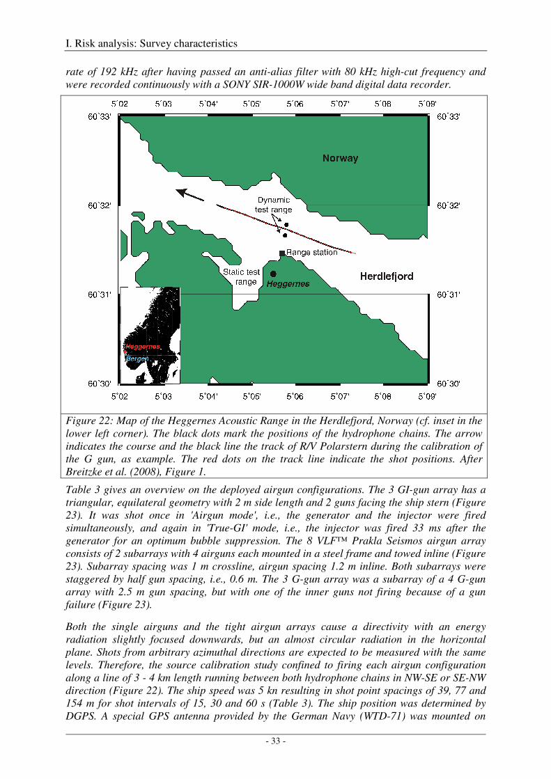
I. Risk analysis: Survey characteristics
- 33 -
rate of 192 kHz after having passed an anti-alias filter with 80 kHz high-cut frequency and were recorded continuously with a SONY SIR-1000W wide band digital data recorder.
Figure 22: Map of the Heggernes Acoustic Range in the Herdlefjord, Norway (cf. inset in the lower left corner). The black dots mark the positions of the hydrophone chains. The arrow indicates the course and the black line the track of R/V Polarstern during the calibration of the G gun, as example. The red dots on the track line indicate the shot positions. After Breitzke et al. (2008), Figure 1.
Table 3 gives an overview on the deployed airgun configurations. The 3 GI-gun array has a triangular, equilateral geometry with 2 m side length and 2 guns facing the ship stern (Figure 23). It was shot once in 'Airgun mode', i.e., the generator and the injector were fired simultaneously, and again in 'True-GI' mode, i.e., the injector was fired 33 ms after the generator for an optimum bubble suppression. The 8 VLF™ Prakla Seismos airgun array consists of 2 subarrays with 4 airguns each mounted in a steel frame and towed inline (Figure 23). Subarray spacing was 1 m crossline, airgun spacing 1.2 m inline. Both subarrays were staggered by half gun spacing, i.e., 0.6 m. The 3 G-gun array was a subarray of a 4 G-gun array with 2.5 m gun spacing, but with one of the inner guns not firing because of a gun failure (Figure 23).
Both the single airguns and the tight airgun arrays cause a directivity with an energy radiation slightly focused downwards, but an almost circular radiation in the horizontal plane. Shots from arbitrary azimuthal directions are expected to be measured with the same levels. Therefore, the source calibration study confined to firing each airgun configuration along a line of 3 - 4 km length running between both hydrophone chains in NW-SE or SE-NW direction (Figure 22). The ship speed was 5 kn resulting in shot point spacings of 39, 77 and 154 m for shot intervals of 15, 30 and 60 s (Table 3). The ship position was determined by DGPS. A special GPS antenna provided by the German Navy (WTD-71) was mounted on
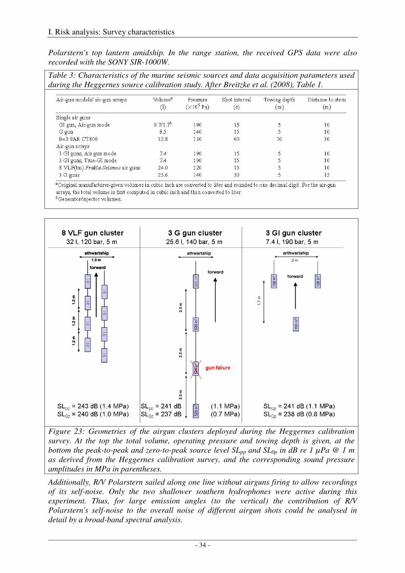
I. Risk analysis: Survey characteristics
- 34 -
Polarstern's top lantern amidship. In the range station, the received GPS data were also recorded with the SONY SIR-1000W.
Table 3: Characteristics of the marine seismic sources and data acquisition parameters used during the Heggernes source calibration study. After Breitzke et al. (2008), Table 1.
Figure 23: Geometries of the airgun clusters deployed during the Heggernes calibration survey. At the top the total volume, operating pressure and towing depth is given, at the bottom the peak-to-peak and zero-to-peak source level SLpp and SL0p in dB re 1 µPa @ 1 m as derived from the Heggernes calibration survey, and the corresponding sound pressure amplitudes in MPa in parentheses.
Additionally, R/V Polarstern sailed along one line without airguns firing to allow recordings of its self-noise. Only the two shallower southern hydrophones were active during this experiment. Thus, for large emission angles (to the vertical) the contribution of R/V Polarstern's self-noise to the overall noise of different airgun shots could be analysed in detail by a broad-band spectral analysis.
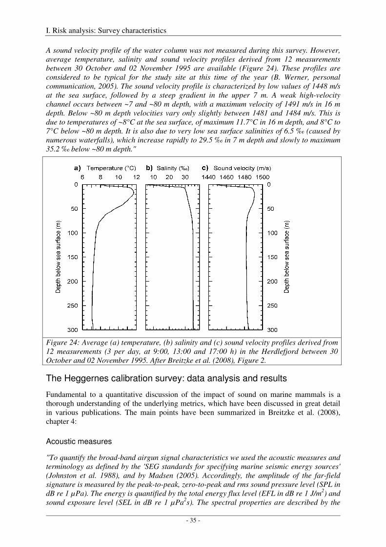
I. Risk analysis: Survey characteristics
- 35 -
A sound velocity profile of the water column was not measured during this survey. However, average temperature, salinity and sound velocity profiles derived from 12 measurements between 30 October and 02 November 1995 are available (Figure 24). These profiles are considered to be typical for the study site at this time of the year (B. Werner, personal communication, 2005). The sound velocity profile is characterized by low values of 1448 m/s at the sea surface, followed by a steep gradient in the upper 7 m. A weak high-velocity channel occurs between ~7 and ~80 m depth, with a maximum velocity of 1491 m/s in 16 m depth. Below ~80 m depth velocities vary only slightly between 1481 and 1484 m/s. This is due to temperatures of ~8°C at the sea surface, of maximum 11.7°C in 16 m depth, and 8°C to 7°C below ~80 m depth. It is also due to very low sea surface salinities of 6.5 ‰ (caused by numerous waterfalls), which increase rapidly to 29.5 ‰ in 7 m depth and slowly to maximum 35.2 ‰ below ~80 m depth."
Figure 24: Average (a) temperature, (b) salinity and (c) sound velocity profiles derived from 12 measurements (3 per day, at 9:00, 13:00 and 17:00 h) in the Herdlefjord between 30 October and 02 November 1995. After Breitzke et al. (2008), Figure 2.
The Heggernes calibration survey: data analysis and results
Fundamental to a quantitative discussion of the impact of sound on marine mammals is a thorough understanding of the underlying metrics, which have been discussed in great detail in various publications. The main points have been summarized in Breitzke et al. (2008), chapter 4:
Acoustic measures
"To quantify the broad-band airgun signal characteristics we used the acoustic measures and terminology as defined by the 'SEG standards for specifying marine seismic energy sources' (Johnston et al. 1988), and by Madsen (2005). Accordingly, the amplitude of the far-field signature is measured by the peak-to-peak, zero-to-peak and rms sound pressure level (SPL in dB re 1 µPa). The energy is quantified by the total energy flux level (EFL in dB re 1 J/m2) and sound exposure level (SEL in dB re 1 µPa2s). The spectral properties are described by the
I. Risk analysis: Survey characteristics
- 36 -
amplitude spectrum (in dB re 1 µPa/Hz), the energy flux spectral density (in dB re 1 J/m2/Hz) and the cumulative energy flux (in %) as functions of frequency. Spectral peak level, bandwidth and frequency, where the 95 percentile of the cumulative energy flux is exceeded, are used as additional parameters. In the time domain total energy flux level and sound exposure level are redundant and differ only by a scaling with the reciprocal acoustic impedance of sea water. This introduces a shift of 182 dB between both axis, if values of 1500 m/s and 1026 kg/m3 are assumed for the sound velocity and density of sea water (Johnston et al. 1988). The same applies for the amplitude spectrum and energy flux spectral density in the frequency domain. Rms sound pressure levels can be converted into sound exposure levels by SEL [dB] = SPLrms [dB] + 10 log10(T), if the same window length T (in s) is used for the computation of both parameters (Madsen 2005). This implies, that rms sound pressure and sound exposure level agree for a window length of 1 s."
Spherical spreading law
In case of a semi-infinite, completely homogeneous ocean without absorption and reflecting/ refracting boundaries the pressure amplitude decay of a propagating sound wave follows a spherical spreading law:
A(r) = A0 / r (6)
where A(r) is the sound pressure amplitude measured at distance r, and A0 is the sound pressure amplitude at the source position. On the decibel scale this spherical spreading is equivalent to a range-dependent sound pressure level decrease of 20 log (r)
SPL = SL - 20 log (r) (7)
where SPL is the sound pressure level measured at range r and SL the sound pressure source level at 1 m reference distance. Nominal, back-calculated source levels are typically derived from far-field measurements of sound pressure levels (SPL) by application of equation (7) (or equation (6) on the linear scale).
In case of a "real" ocean, i.e. if sound velocity profiles are considered this simple spreading law is modified by reflections and refractions of the propagating sound wave at the layer interfaces in the water column and ocean bottom. How pronounced these effects are in case of the Amundsen/Bellingshausen and Weddell Sea scenarios will be studied later by the finite-difference modelling approach (chapters I.4-6, chapter IV).
Computation of amplitude spectra
The most important aspect of using the 'SEG standard for specifying marine seismic energy sources' is that transient seismic (airgun) signals have zero power but finite energy. According to the prescription given in Johnston et al. (1988) the quantified energy flux spectral density is computed according to
2)m(X
c
1)m(E
ρ= , m = 0, 1, ..... , N-1 (1)
where
X(m) = )]N/mn2(iexp[)n(xt1N
0n∑
−
=
π−∆ m = 0, 1, ..... , N-1 (2)
I. Risk analysis: Survey characteristics
- 37 -
and
X(m) = Fourier coefficients, E = energy flux spectral density, x(n) = digital samples of the time series, N = number of samples in the analysis window, ρ = density of sea water c = sound speed in sea water ∆t = sample interval.
Equation (1) allows computing consistent results for transient signals, independent of the analysis window length, as long as there is no significant noise in the window. In contrast, a power spectrum P(m) = E(m)/(N·∆t) depends on the window lengths, as it includes a "normalization" by the window length N·∆t (similar to an rms value computation). Actually, transient seismic signals have zero power, because in the strict definition "power" includes an integration from minus to plus infinity. However, transient seismic signals have a finite energy (Fricke et al., 1985).
The absolute values of the Fourier coefficients in equation (2) define the amplitude spectrum. Their unit is Pa/Hz. If the coefficients of the amplitude spectrum are squared and scaled by the acoustic impedance of sea water ρc - as described in equation (1) - the coefficients E(m) define the energy flux spectral density. Their unit is J/m2/Hz. As mentioned above, on the decibel scale amplitude spectrum and energy flux spectral density have the same shape but differ by 182 dB for a sound velocity of 1500 m/s and a density of 1030 kg/m³ in sea water; i.e. 20 log10 (X(m)) = 10 log10 (E(m)) + 182.
If the energy flux spectral density is integrated (or summed-up) in the frequency domain according to
∑−
=
∆=1N
0mT )m(EfU (3)
we get the total energy flux UT (Fricke et al., 1985; Johnston et al., 1988). Its unit is J/m². On the dB scale we get the total energy flux level EFL = 10 log10 UT.
This frequency domain computation of UT is equivalent to an integration (or summation) of the squared pressure amplitudes in the time domain, scaled by the acoustic impedance of sea water (Fricke et al., 1985; Johnston et al., 1988)
U T = c
t
ρ∆∑
−
=
1N
0n
2)n(x (4)
If the scaling by the acoustic impedance of sea water ρc is omitted we get the following equivalence between time and frequency domain computations (Fricke et al., 1985; Johnston et al., 1988)
∑∑−
=
−
=
=∆=∆1N
0n
21N
0m
2SE)n(xt)m(Xf (5)
The right hand side of equation (5) is also known as sound exposure SE. On the dB scale it is well known as sound exposure level SEL = 10 log10 SE. In Fourier theory equation (5) is also termed Parseval's equation.
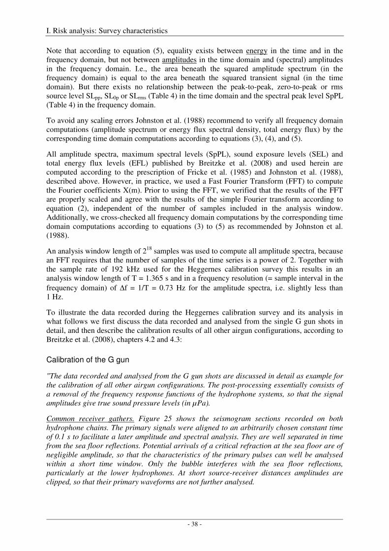
I. Risk analysis: Survey characteristics
- 38 -
Note that according to equation (5), equality exists between energy in the time and in the frequency domain, but not between amplitudes in the time domain and (spectral) amplitudes in the frequency domain. I.e., the area beneath the squared amplitude spectrum (in the frequency domain) is equal to the area beneath the squared transient signal (in the time domain). But there exists no relationship between the peak-to-peak, zero-to-peak or rms source level SLpp, SL0p or SLrms (Table 4) in the time domain and the spectral peak level SpPL (Table 4) in the frequency domain.
To avoid any scaling errors Johnston et al. (1988) recommend to verify all frequency domain computations (amplitude spectrum or energy flux spectral density, total energy flux) by the corresponding time domain computations according to equations (3), (4), and (5).
All amplitude spectra, maximum spectral levels (SpPL), sound exposure levels (SEL) and total energy flux levels (EFL) published by Breitzke et al. (2008) and used herein are computed according to the prescription of Fricke et al. (1985) and Johnston et al. (1988), described above. However, in practice, we used a Fast Fourier Transform (FFT) to compute the Fourier coefficients X(m). Prior to using the FFT, we verified that the results of the FFT are properly scaled and agree with the results of the simple Fourier transform according to equation (2), independent of the number of samples included in the analysis window. Additionally, we cross-checked all frequency domain computations by the corresponding time domain computations according to equations (3) to (5) as recommended by Johnston et al. (1988).
An analysis window length of 218 samples was used to compute all amplitude spectra, because an FFT requires that the number of samples of the time series is a power of 2. Together with the sample rate of 192 kHz used for the Heggernes calibration survey this results in an analysis window length of T = 1.365 s and in a frequency resolution (= sample interval in the frequency domain) of ∆f = 1/T = 0.73 Hz for the amplitude spectra, i.e. slightly less than 1 Hz.
To illustrate the data recorded during the Heggernes calibration survey and its analysis in what follows we first discuss the data recorded and analysed from the single G gun shots in detail, and then describe the calibration results of all other airgun configurations, according to Breitzke et al. (2008), chapters 4.2 and 4.3:
Calibration of the G gun
"The data recorded and analysed from the G gun shots are discussed in detail as example for the calibration of all other airgun configurations. The post-processing essentially consists of a removal of the frequency response functions of the hydrophone systems, so that the signal amplitudes give true sound pressure levels (in µPa).
Common receiver gathers. Figure 25 shows the seismogram sections recorded on both hydrophone chains. The primary signals were aligned to an arbitrarily chosen constant time of 0.1 s to facilitate a later amplitude and spectral analysis. They are well separated in time from the sea floor reflections. Potential arrivals of a critical refraction at the sea floor are of negligible amplitude, so that the characteristics of the primary pulses can well be analysed within a short time window. Only the bubble interferes with the sea floor reflections, particularly at the lower hydrophones. At short source-receiver distances amplitudes are clipped, so that their primary waveforms are not further analysed.
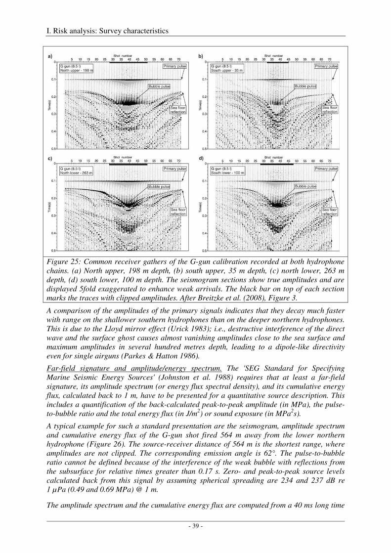
I. Risk analysis: Survey characteristics
- 39 -
Figure 25: Common receiver gathers of the G-gun calibration recorded at both hydrophone chains. (a) North upper, 198 m depth, (b) south upper, 35 m depth, (c) north lower, 263 m depth, (d) south lower, 100 m depth. The seismogram sections show true amplitudes and are displayed 5fold exaggerated to enhance weak arrivals. The black bar on top of each section marks the traces with clipped amplitudes. After Breitzke et al. (2008), Figure 3.
A comparison of the amplitudes of the primary signals indicates that they decay much faster with range on the shallower southern hydrophones than on the deeper northern hydrophones. This is due to the Lloyd mirror effect (Urick 1983); i.e., destructive interference of the direct wave and the surface ghost causes almost vanishing amplitudes close to the sea surface and maximum amplitudes in several hundred metres depth, leading to a dipole-like directivity even for single airguns (Parkes & Hatton 1986).
Far-field signature and amplitude/energy spectrum. The 'SEG Standard for Specifying Marine Seismic Energy Sources' (Johnston et al. 1988) requires that at least a far-field signature, its amplitude spectrum (or energy flux spectral density), and its cumulative energy flux, calculated back to 1 m, have to be presented for a quantitative source description. This includes a quantification of the back-calculated peak-to-peak amplitude (in MPa), the pulse-to-bubble ratio and the total energy flux (in J/m2) or sound exposure (in MPa2s).
A typical example for such a standard presentation are the seismogram, amplitude spectrum and cumulative energy flux of the G-gun shot fired 564 m away from the lower northern hydrophone (Figure 26). The source-receiver distance of 564 m is the shortest range, where amplitudes are not clipped. The corresponding emission angle is 62°. The pulse-to-bubble ratio cannot be defined because of the interference of the weak bubble with reflections from the subsurface for relative times greater than 0.17 s. Zero- and peak-to-peak source levels calculated back from this signal by assuming spherical spreading are 234 and 237 dB re 1 µPa (0.49 and 0.69 MPa) @ 1 m.
The amplitude spectrum and the cumulative energy flux are computed from a 40 ms long time
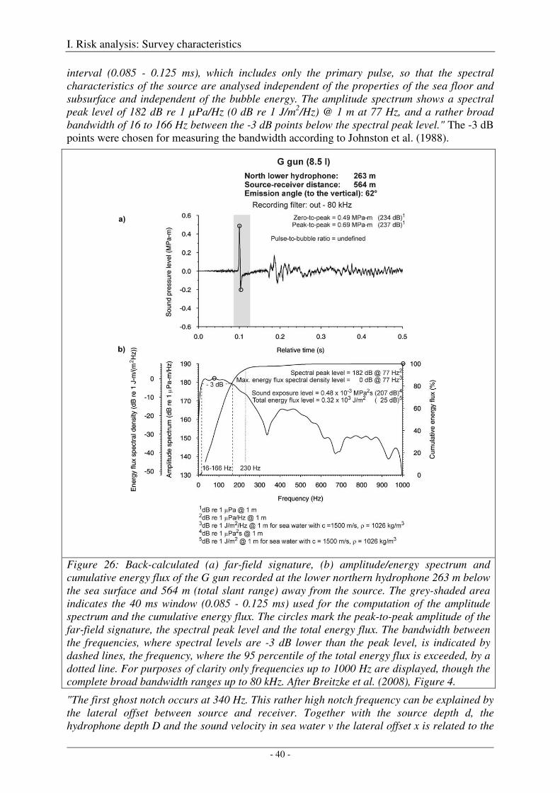
I. Risk analysis: Survey characteristics
- 40 -
interval (0.085 - 0.125 ms), which includes only the primary pulse, so that the spectral characteristics of the source are analysed independent of the properties of the sea floor and subsurface and independent of the bubble energy. The amplitude spectrum shows a spectral peak level of 182 dB re 1 µPa/Hz (0 dB re 1 J/m2/Hz) @ 1 m at 77 Hz, and a rather broad bandwidth of 16 to 166 Hz between the -3 dB points below the spectral peak level." The -3 dB points were chosen for measuring the bandwidth according to Johnston et al. (1988).
Figure 26: Back-calculated (a) far-field signature, (b) amplitude/energy spectrum and cumulative energy flux of the G gun recorded at the lower northern hydrophone 263 m below the sea surface and 564 m (total slant range) away from the source. The grey-shaded area indicates the 40 ms window (0.085 - 0.125 ms) used for the computation of the amplitude spectrum and the cumulative energy flux. The circles mark the peak-to-peak amplitude of the far-field signature, the spectral peak level and the total energy flux. The bandwidth between the frequencies, where spectral levels are -3 dB lower than the peak level, is indicated by dashed lines, the frequency, where the 95 percentile of the total energy flux is exceeded, by a dotted line. For purposes of clarity only frequencies up to 1000 Hz are displayed, though the complete broad bandwidth ranges up to 80 kHz. After Breitzke et al. (2008), Figure 4.
"The first ghost notch occurs at 340 Hz. This rather high notch frequency can be explained by the lateral offset between source and receiver. Together with the source depth d, the hydrophone depth D and the sound velocity in sea water v the lateral offset x is related to the
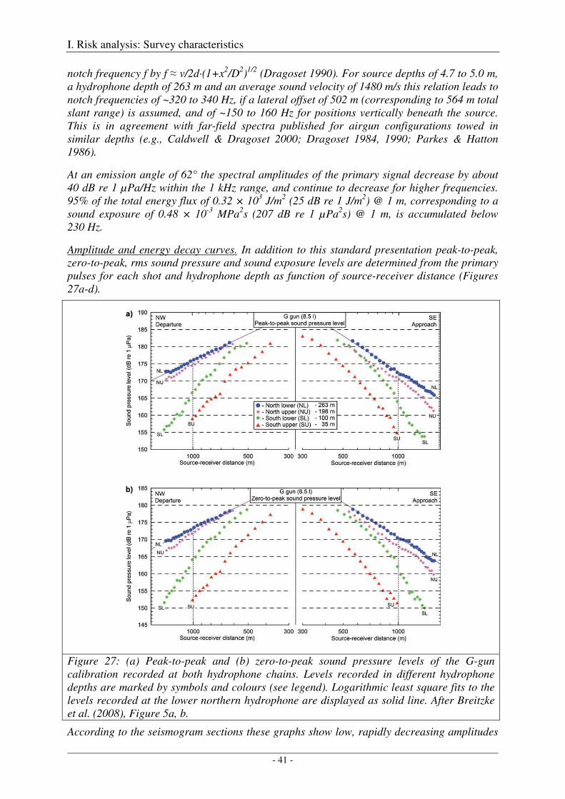
I. Risk analysis: Survey characteristics
- 41 -
notch frequency f by f ≈ v/2d·(1+x2/D2)1/2 (Dragoset 1990). For source depths of 4.7 to 5.0 m, a hydrophone depth of 263 m and an average sound velocity of 1480 m/s this relation leads to notch frequencies of ~320 to 340 Hz, if a lateral offset of 502 m (corresponding to 564 m total slant range) is assumed, and of ~150 to 160 Hz for positions vertically beneath the source. This is in agreement with far-field spectra published for airgun configurations towed in similar depths (e.g., Caldwell & Dragoset 2000; Dragoset 1984, 1990; Parkes & Hatton 1986).
At an emission angle of 62° the spectral amplitudes of the primary signal decrease by about 40 dB re 1 µPa/Hz within the 1 kHz range, and continue to decrease for higher frequencies. 95% of the total energy flux of 0.32 × 10³ J/m2 (25 dB re 1 J/m2) @ 1 m, corresponding to a sound exposure of 0.48 × 10⁻³ MPa2s (207 dB re 1 µPa2s) @ 1 m, is accumulated below 230 Hz.
Amplitude and energy decay curves. In addition to this standard presentation peak-to-peak, zero-to-peak, rms sound pressure and sound exposure levels are determined from the primary pulses for each shot and hydrophone depth as function of source-receiver distance (Figures 27a-d).
Figure 27: (a) Peak-to-peak and (b) zero-to-peak sound pressure levels of the G-gun calibration recorded at both hydrophone chains. Levels recorded in different hydrophone depths are marked by symbols and colours (see legend). Logarithmic least square fits to the levels recorded at the lower northern hydrophone are displayed as solid line. After Breitzke et al. (2008), Figure 5a, b.
According to the seismogram sections these graphs show low, rapidly decreasing amplitudes
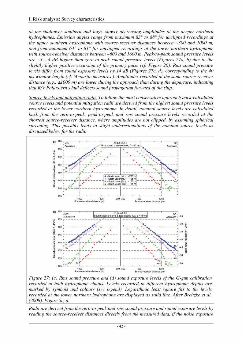
I. Risk analysis: Survey characteristics
- 42 -
at the shallower southern and high, slowly decreasing amplitudes at the deeper northern hydrophones. Emission angles range from maximum 83° to 88° for unclipped recordings at the upper southern hydrophone with source-receiver distances between ~300 and 1000 m, and from minimum 64° to 81° for unclipped recordings at the lower northern hydrophone with source-receiver distances between ~600 and 1600 m. Peak-to-peak sound pressure levels are ~3 - 4 dB higher than zero-to-peak sound pressure levels (Figures 27a, b) due to the slightly higher positive excursion of the primary pulse (cf. Figure 26). Rms sound pressure levels differ from sound exposure levels by 14 dB (Figures 27c, d), corresponding to the 40 ms window length (cf. 'Acoustic measures'). Amplitudes recorded at the same source-receiver distance (e.g., ±1000 m) are lower during the approach than during the departure, indicating that R/V Polarstern's hull deflects sound propagation forward of the ship.
Source levels and mitigation radii. To follow the most conservative approach back-calculated source levels and potential mitigation radii are derived from the highest sound pressure levels recorded at the lower northern hydrophone. In detail, nominal source levels are calculated back from the zero-to-peak, peak-to-peak and rms sound pressure levels recorded at the shortest source-receiver distance, where amplitudes are not clipped, by assuming spherical spreading. This possibly leads to slight underestimations of the nominal source levels as discussed below for the radii.
Figure 27: (c) Rms sound pressure and (d) sound exposure levels of the G-gun calibration recorded at both hydrophone chains. Levels recorded in different hydrophone depths are marked by symbols and colours (see legend). Logarithmic least square fits to the levels recorded at the lower northern hydrophone are displayed as solid line. After Breitzke et al. (2008), Figure 5c, d.
Radii are derived from the zero-to-peak and rms sound pressure and sound exposure levels by reading the source-receiver distances directly from the measured data, if the noise exposure
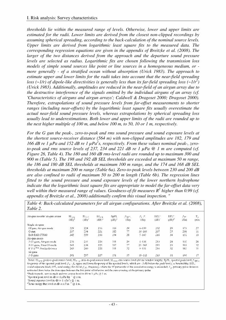
I. Risk analysis: Survey characteristics
- 43 -
thresholds lie within the measured range of levels. Otherwise, lower and upper limits are estimated for the radii. Lower limits are derived from the closest non-clipped recordings by assuming spherical spreading, according to the back-calculation of the nominal source levels. Upper limits are derived from logarithmic least square fits to the measured data. The corresponding regression equations are given in the appendix of Breitzke et al. (2008). The larger of the two distances derived from the approach and the departure sound pressure levels are selected as radius. Logarithmic fits are chosen following the transmission loss models of simple sound sources like point or line sources in a homogeneous medium, or - more generally - of a stratified ocean without absorption (Urick 1983). The approach to estimate upper and lower limits for the radii takes into account that the near-field spreading loss (~1/r) of dipole-like directivities is generally less than its far-field spreading loss (~1/r2) (Urick 1983). Additionally, amplitudes are reduced in the near-field of an airgun array due to the destructive interference of the signals emitted by the individual airguns of an array (cf. 'Characteristics of airguns and airgun arrays'; Caldwell & Dragoset 2000; Dragoset 2000). Therefore, extrapolations of sound pressure levels from far-offset measurements to shorter ranges (including near-offsets) by the logarithmic least square fits usually overestimate the actual near-field sound pressure levels, whereas extrapolations by spherical spreading loss usually lead to underestimations. Both lower and upper limits of the radii are rounded up to the next higher multiple of 100 m, and below 100 m, to 50, 10 or 1 m, respectively.
For the G gun the peak-, zero-to-peak and rms sound pressure and sound exposure levels at the shortest source-receiver distance (564 m) with non-clipped amplitudes are 182, 179 and 166 dB re 1 µPa and 152 dB re 1 µPa2s, respectively. From these values nominal peak-, zero-to-peak and rms source levels of 237, 234 and 221 dB re 1 µPa @ 1 m are computed (cf. Figure 26, Table 4). The 180 and 160 dB rms-level radii are rounded up to maximum 300 and 900 m (Table 5). The 198 and 192 dB SEL thresholds are exceeded at maximum 50 m range, the 186 and 180 dB SEL thresholds at maximum 100 m range, and the 174 and 168 dB SEL thresholds at maximum 200 m range (Table 6a). Zero-to-peak levels between 230 and 200 dB are also confined to radii of maximum 50 to 200 m length (Table 6b). The regression lines fitted to the sound pressure and sound exposure levels of the lower northern hydrophone indicate that the logarithmic least square fits are appropriate to model the far-offset data very well within their measured range of values. Goodness-of-fit measures R2 higher than 0.99 (cf. appendix of Breitzke et al., 2008) additionally confirm this visual inspection. "
Table 4: Back-calculated parameters for all airgun configurations. After Breitzke et al. (2008), Table 2.
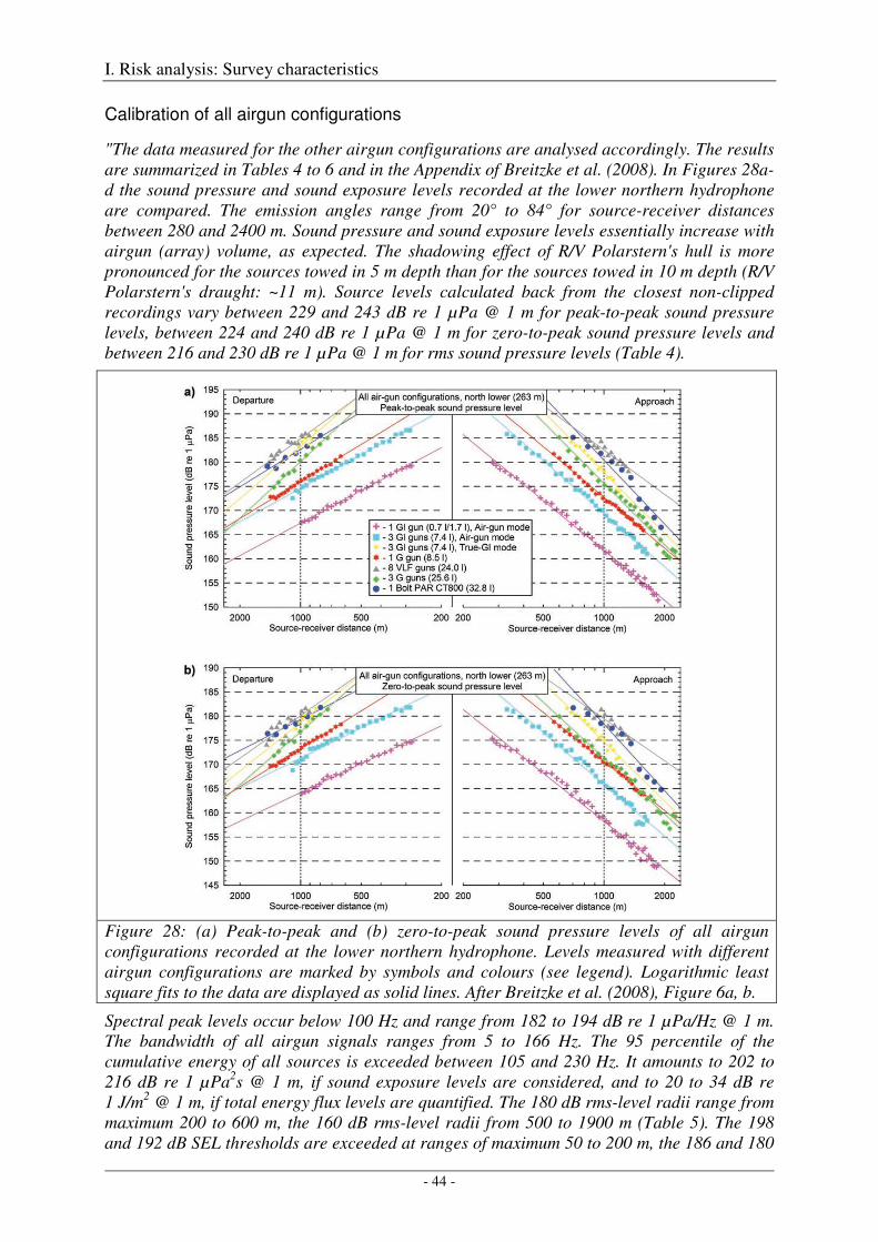
I. Risk analysis: Survey characteristics
- 44 -
Calibration of all airgun configurations
"The data measured for the other airgun configurations are analysed accordingly. The results are summarized in Tables 4 to 6 and in the Appendix of Breitzke et al. (2008). In Figures 28a-d the sound pressure and sound exposure levels recorded at the lower northern hydrophone are compared. The emission angles range from 20° to 84° for source-receiver distances between 280 and 2400 m. Sound pressure and sound exposure levels essentially increase with airgun (array) volume, as expected. The shadowing effect of R/V Polarstern's hull is more pronounced for the sources towed in 5 m depth than for the sources towed in 10 m depth (R/V Polarstern's draught: ~11 m). Source levels calculated back from the closest non-clipped recordings vary between 229 and 243 dB re 1 µPa @ 1 m for peak-to-peak sound pressure levels, between 224 and 240 dB re 1 µPa @ 1 m for zero-to-peak sound pressure levels and between 216 and 230 dB re 1 µPa @ 1 m for rms sound pressure levels (Table 4).
Figure 28: (a) Peak-to-peak and (b) zero-to-peak sound pressure levels of all airgun configurations recorded at the lower northern hydrophone. Levels measured with different airgun configurations are marked by symbols and colours (see legend). Logarithmic least square fits to the data are displayed as solid lines. After Breitzke et al. (2008), Figure 6a, b.
Spectral peak levels occur below 100 Hz and range from 182 to 194 dB re 1 µPa/Hz @ 1 m. The bandwidth of all airgun signals ranges from 5 to 166 Hz. The 95 percentile of the cumulative energy of all sources is exceeded between 105 and 230 Hz. It amounts to 202 to 216 dB re 1 µPa2s @ 1 m, if sound exposure levels are considered, and to 20 to 34 dB re 1 J/m2 @ 1 m, if total energy flux levels are quantified. The 180 dB rms-level radii range from maximum 200 to 600 m, the 160 dB rms-level radii from 500 to 1900 m (Table 5). The 198 and 192 dB SEL thresholds are exceeded at ranges of maximum 50 to 200 m, the 186 and 180
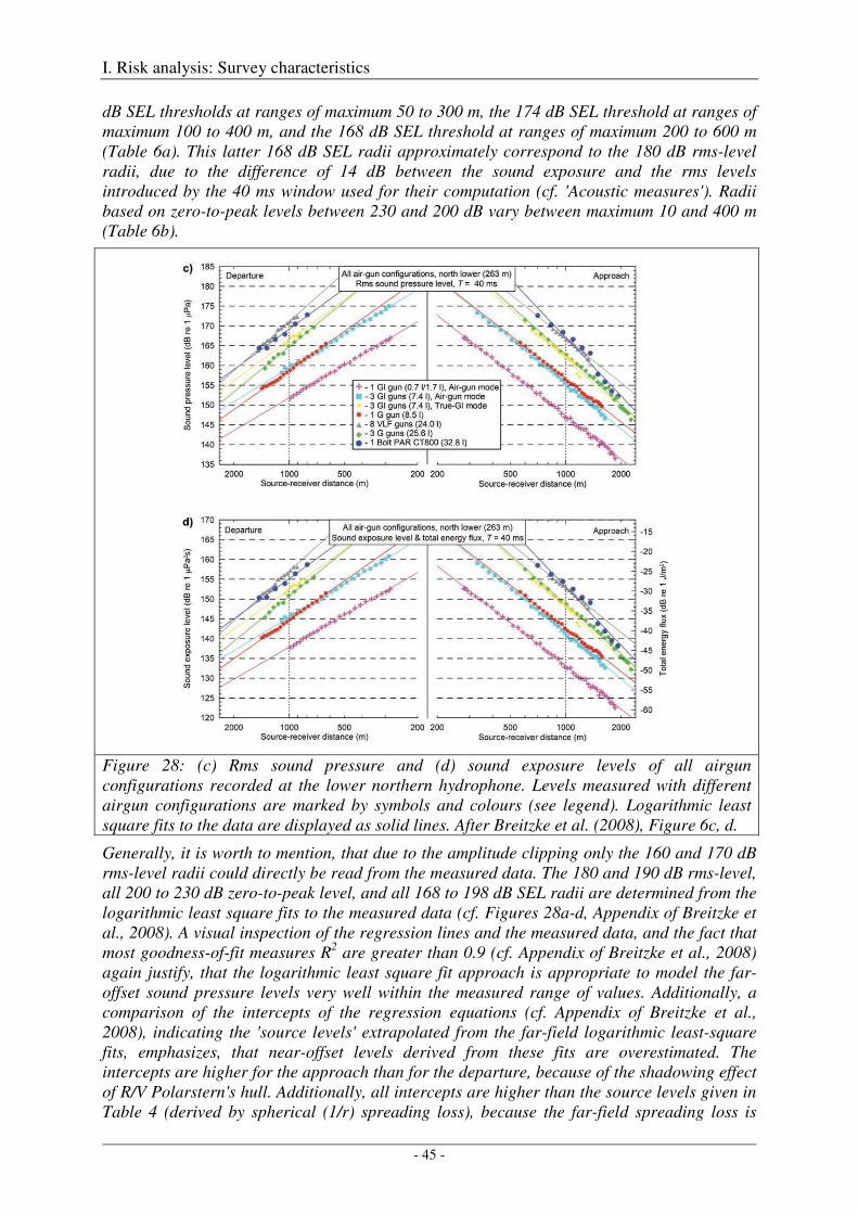
I. Risk analysis: Survey characteristics
- 45 -
dB SEL thresholds at ranges of maximum 50 to 300 m, the 174 dB SEL threshold at ranges of maximum 100 to 400 m, and the 168 dB SEL threshold at ranges of maximum 200 to 600 m (Table 6a). This latter 168 dB SEL radii approximately correspond to the 180 dB rms-level radii, due to the difference of 14 dB between the sound exposure and the rms levels introduced by the 40 ms window used for their computation (cf. 'Acoustic measures'). Radii based on zero-to-peak levels between 230 and 200 dB vary between maximum 10 and 400 m (Table 6b).
Figure 28: (c) Rms sound pressure and (d) sound exposure levels of all airgun configurations recorded at the lower northern hydrophone. Levels measured with different airgun configurations are marked by symbols and colours (see legend). Logarithmic least square fits to the data are displayed as solid lines. After Breitzke et al. (2008), Figure 6c, d.
Generally, it is worth to mention, that due to the amplitude clipping only the 160 and 170 dB rms-level radii could directly be read from the measured data. The 180 and 190 dB rms-level, all 200 to 230 dB zero-to-peak level, and all 168 to 198 dB SEL radii are determined from the logarithmic least square fits to the measured data (cf. Figures 28a-d, Appendix of Breitzke et al., 2008). A visual inspection of the regression lines and the measured data, and the fact that most goodness-of-fit measures R2 are greater than 0.9 (cf. Appendix of Breitzke et al., 2008) again justify, that the logarithmic least square fit approach is appropriate to model the far-offset sound pressure levels very well within the measured range of values. Additionally, a comparison of the intercepts of the regression equations (cf. Appendix of Breitzke et al., 2008), indicating the 'source levels' extrapolated from the far-field logarithmic least-square fits, emphasizes, that near-offset levels derived from these fits are overestimated. The intercepts are higher for the approach than for the departure, because of the shadowing effect of R/V Polarstern's hull. Additionally, all intercepts are higher than the source levels given in Table 4 (derived by spherical (1/r) spreading loss), because the far-field spreading loss is
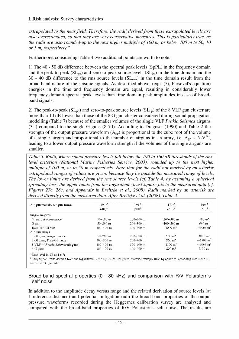
I. Risk analysis: Survey characteristics
- 46 -
extrapolated to the near field. Therefore, the radii derived from these extrapolated levels are also overestimated, so that they are very conservative measures. This is particularly true, as the radii are also rounded-up to the next higher multiple of 100 m, or below 100 m to 50, 10 or 1 m, respectively."
Furthermore, considering Table 4 two additional points are worth to note:
1) The 40 - 50 dB difference between the spectral peak levels (SpPL) in the frequency domain and the peak-to-peak (SLpp) and zero-to-peak source levels (SL0p) in the time domain and the 30 - 40 dB difference to the rms source levels (SLrms) in the time domain result from the broad-band nature of the seismic signals. As described above, (equ. (5), Parseval's equation) energies in the time and frequency domain are equal, resulting in considerably lower frequency domain spectral peak levels than time domain peak amplitudes in case of broad-band signals.
2) The peak-to-peak (SLpp) and zero-to-peak source levels (SL0p) of the 8 VLF gun cluster are more than 10 dB lower than those of the 8 G gun cluster considered during sound propagation modelling (Table 7) because of the smaller volumes of the single VLF Prakla Seismos airguns (3 l) compared to the single G guns (8.5 l). According to Dragoset (1990) and Table 2 the strength of the output pressure waveform (App) is proportional to the cube root of the volume of a single airgun and proportional to the number of airguns in an array, i.e. App ~ N·V1/3, leading to a lower output pressure waveform strength if the volumes of the single airguns are smaller.
Table 5. Radii, where sound pressure levels fall below the 190 to 160 dB thresholds of the rms-level criterion (National Marine Fisheries Service, 2003), rounded up to the next higher multiple of 100 m, or to 50 m respectively. Note that for the radii not marked by an asterisk extrapolated ranges of values are given, because they lie outside the measured range of levels. The lower limits are derived from the rms source levels (cf. Table 4) by assuming a spherical spreading loss, the upper limits from the logarithmic least square fits to the measured data (cf. Figures 27c, 28c, and Appendix in Breitzke et al., 2008). Radii marked by an asterisk are derived directly from the measured data. After Breitzke et al. (2008), Table 3.
Broad-band spectral properties (0 - 80 kHz) and comparison with R/V Polarstern's self noise
In addition to the amplitude decay versus range and the related derivation of source levels (at 1 reference distance) and potential mitigation radii the broad-band properties of the output pressure waveforms recorded during the Heggernes calibration survey are analysed and compared with the broad-band properties of R/V Polarstern's self noise. The results are
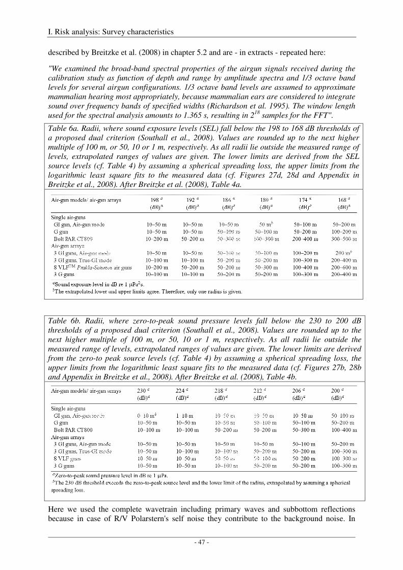
I. Risk analysis: Survey characteristics
- 47 -
described by Breitzke et al. (2008) in chapter 5.2 and are - in extracts - repeated here:
"We examined the broad-band spectral properties of the airgun signals received during the calibration study as function of depth and range by amplitude spectra and 1/3 octave band levels for several airgun configurations. 1/3 octave band levels are assumed to approximate mammalian hearing most appropriately, because mammalian ears are considered to integrate sound over frequency bands of specified widths (Richardson et al. 1995). The window length used for the spectral analysis amounts to 1.365 s, resulting in 218 samples for the FFT".
Table 6a. Radii, where sound exposure levels (SEL) fall below the 198 to 168 dB thresholds of a proposed dual criterion (Southall et al., 2008). Values are rounded up to the next higher multiple of 100 m, or 50, 10 or 1 m, respectively. As all radii lie outside the measured range of levels, extrapolated ranges of values are given. The lower limits are derived from the SEL source levels (cf. Table 4) by assuming a spherical spreading loss, the upper limits from the logarithmic least square fits to the measured data (cf. Figures 27d, 28d and Appendix in Breitzke et al., 2008). After Breitzke et al. (2008), Table 4a.
Table 6b. Radii, where zero-to-peak sound pressure levels fall below the 230 to 200 dB thresholds of a proposed dual criterion (Southall et al., 2008). Values are rounded up to the next higher multiple of 100 m, or 50, 10 or 1 m, respectively. As all radii lie outside the measured range of levels, extrapolated ranges of values are given. The lower limits are derived from the zero-to peak source levels (cf. Table 4) by assuming a spherical spreading loss, the upper limits from the logarithmic least square fits to the measured data (cf. Figures 27b, 28b and Appendix in Breitzke et al., 2008). After Breitzke et al. (2008), Table 4b.
Here we used the complete wavetrain including primary waves and subbottom reflections because in case of R/V Polarstern's self noise they contribute to the background noise. In
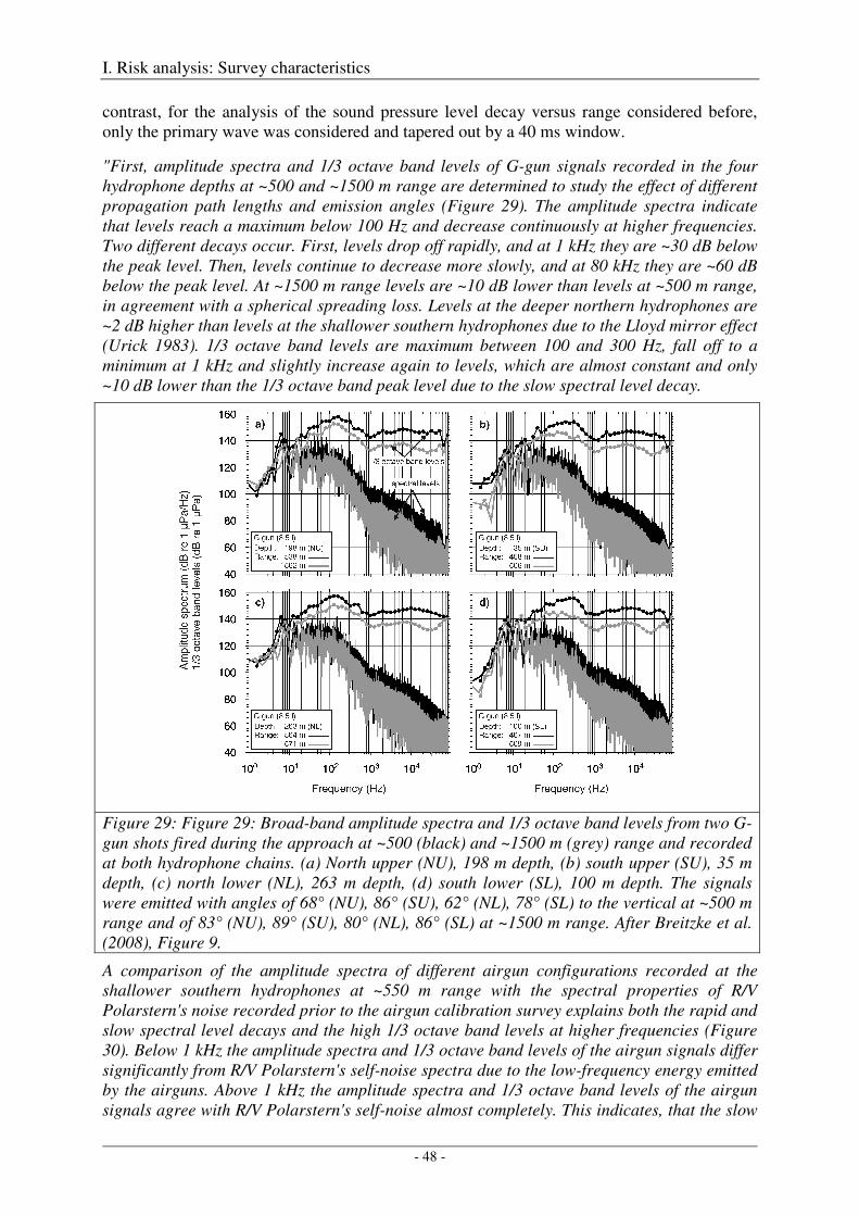
I. Risk analysis: Survey characteristics
- 48 -
contrast, for the analysis of the sound pressure level decay versus range considered before, only the primary wave was considered and tapered out by a 40 ms window.
"First, amplitude spectra and 1/3 octave band levels of G-gun signals recorded in the four hydrophone depths at ~500 and ~1500 m range are determined to study the effect of different propagation path lengths and emission angles (Figure 29). The amplitude spectra indicate that levels reach a maximum below 100 Hz and decrease continuously at higher frequencies. Two different decays occur. First, levels drop off rapidly, and at 1 kHz they are ~30 dB below the peak level. Then, levels continue to decrease more slowly, and at 80 kHz they are ~60 dB below the peak level. At ~1500 m range levels are ~10 dB lower than levels at ~500 m range, in agreement with a spherical spreading loss. Levels at the deeper northern hydrophones are ~2 dB higher than levels at the shallower southern hydrophones due to the Lloyd mirror effect (Urick 1983). 1/3 octave band levels are maximum between 100 and 300 Hz, fall off to a minimum at 1 kHz and slightly increase again to levels, which are almost constant and only ~10 dB lower than the 1/3 octave band peak level due to the slow spectral level decay.
Figure 29: Figure 29: Broad-band amplitude spectra and 1/3 octave band levels from two G-gun shots fired during the approach at ~500 (black) and ~1500 m (grey) range and recorded at both hydrophone chains. (a) North upper (NU), 198 m depth, (b) south upper (SU), 35 m depth, (c) north lower (NL), 263 m depth, (d) south lower (SL), 100 m depth. The signals were emitted with angles of 68° (NU), 86° (SU), 62° (NL), 78° (SL) to the vertical at ~500 m range and of 83° (NU), 89° (SU), 80° (NL), 86° (SL) at ~1500 m range. After Breitzke et al. (2008), Figure 9.
A comparison of the amplitude spectra of different airgun configurations recorded at the shallower southern hydrophones at ~550 m range with the spectral properties of R/V Polarstern's noise recorded prior to the airgun calibration survey explains both the rapid and slow spectral level decays and the high 1/3 octave band levels at higher frequencies (Figure 30). Below 1 kHz the amplitude spectra and 1/3 octave band levels of the airgun signals differ significantly from R/V Polarstern's self-noise spectra due to the low-frequency energy emitted by the airguns. Above 1 kHz the amplitude spectra and 1/3 octave band levels of the airgun signals agree with R/V Polarstern's self-noise almost completely. This indicates, that the slow
I. Risk analysis: Survey characteristics
- 49 -
spectral level decay and the high 1/3 octave band levels are mainly caused by ship-generated noise. Generally, the high-frequency 1/3 octave band levels are ~10 to 15 dB lower than the peak level for all airgun configurations. This means, that the low-frequency sound generated mainly by the airguns appear to marine mammals' ears with ~10 to 15 dB higher levels than the high-frequency sound generated mainly by R/V Polarstern itself. Consequently, if high-frequency off-axis components are emitted by the airgun configurations with levels considerably lower than the broad-band main lobe, and if they are transferred horizontally through the water column with reduced transmission loss, they will be largely masked by R/V Polarstern's self-noise. No evidence for high-frequency off-axis components, which exceed R/V Polarstern's self-noise, was found in any hydrophone depth or range." This fact is particularly important for the Amundsen/Bellingshausen and the Weddell Sea environmental scenarios which include a low-velocity sound channel that might trap sound energy.
Modelling output pressure waveforms and far-field signatures
In addition to the calibration survey at the Heggernes acoustic range a modelling approach was used
1.) to determine the output pressure waveform(s) emitted by a single airgun alone or by the single airguns of a cluster,
2.) to determine the far-field signature which could (theoretically) be measured vertically beneath an airgun or airgun cluster,
3.) to derive the source level @ 1 m distance of the far-field signature, and the pulse to bubble ratio.
Subsequently, the output pressure waveforms of the single airguns, or of an airgun cluster can be used as input signal(s) for sound propagation studies, which take the specific environmental conditions (e.g. sound velocity profile in the water column, bathymetry of the sea floor, physical properties of the sea floor and subsurface) of the region under consideration into account (cf. chapter I.4).
The modelling approach was applied to a single G-gun, a 3 GI-gun cluster, an 8 G-gun cluster and an 8 G +1 Bolt-gun cluster (Table 7). The modelling computations for the single G-gun (8.5 l) together with computations of the sound propagation have been compared to the corresponding measurements at the Heggernes acoustic range, allowing the validation of the modelling computations (Figure 39). The modelling computations for the 3 GI-, the 8 G-and the 8 G+ 1 Bolt gun cluster complement the Heggernes calibration survey by providing unclipped output pressure waveforms and far-field signatures for both the configurations already studied at the Heggernes acoustic range and new configurations currently in use for reflection and refraction seismic studies of the AWI.
As already described for the Heggernes calibration survey, the 3 GI-gun cluster has a triangular, equilateral geometry with 2 m side length and 7.2 l total volume (= 3 x 0.7/1.7 l generator/injector volume; Figures 23, 31). This configuration is usually towed at 5 m depth and is typically used for high-resolution seismic reflection surveys (cf. chapter I.3, Seismic methods and choice of airgun configuration, a).
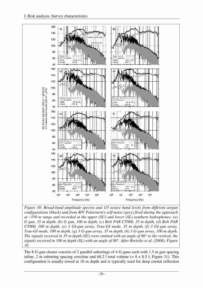
I. Risk analysis: Survey characteristics
- 50 -
Figure 30: Broad-band amplitude spectra and 1/3 octave band levels from different airgun configurations (black) and from R/V Polarstern's self-noise (grey) fired during the approach at ~550 m range and recorded at the upper (SU) and lower (SL) southern hydrophones. (a) G gun, 35 m depth, (b) G gun, 100 m depth, (c) Bolt PAR CT800, 35 m depth, (d) Bolt PAR CT800, 100 m depth, (e) 3 GI-gun array, True-GI mode, 35 m depth, (f) 3 GI-gun array, True-GI mode, 100 m depth, (g) 3 G-gun array, 35 m depth, (h) 3 G-gun array, 100 m depth. The signals received in 35 m depth (SU) were emitted with an angle of 86° to the vertical, the signals received in 100 m depth (SL) with an angle of 80°. After Breitzke et al. (2008), Figure 10.
The 8 G-gun cluster consists of 2 parallel substrings of 4 G-guns each with 1.5 m gun spacing inline, 2 m substring spacing crossline and 68.2 l total volume (= 8 x 8.5 l; Figure 31). This configuration is usually towed at 10 m depth and is typically used for deep crustal reflection
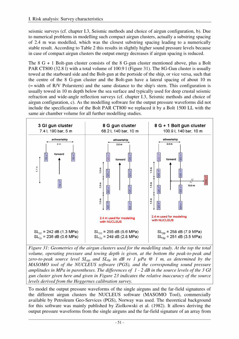
I. Risk analysis: Survey characteristics
- 51 -
seismic surveys (cf. chapter I.3, Seismic methods and choice of airgun configuration, b). Due to numerical problems in modelling such compact airgun clusters, actually a substring spacing of 2.4 m was modelled, which was the closest substring spacing leading to a numerically stable result. According to Table 2 this results in slightly higher sound pressure levels because in case of compact airgun clusters the output energy decreases if airgun spacing is reduced.
The 8 G + 1 Bolt-gun cluster consists of the 8 G-gun cluster mentioned above, plus a Bolt PAR CT800 (32.8 l) with a total volume of 100.9 l (Figure 31). The 8G-Gun cluster is usually towed at the starboard side and the Bolt-gun at the portside of the ship, or vice versa, such that the centre of the 8 G-gun cluster and the Bolt-gun have a lateral spacing of about 10 m (≈ width of R/V Polarstern) and the same distance to the ship's stern. This configuration is usually towed in 10 m depth below the sea surface and typically used for deep crustal seismic refraction and wide-angle reflection surveys (cf. chapter I.3, Seismic methods and choice of airgun configuration, c). As the modelling software for the output pressure waveforms did not include the specifications of the Bolt PAR CT800 we replaced it by a Bolt 1500 LL with the same air chamber volume for all further modelling studies.
Figure 31: Geometries of the airgun clusters used for the modelling study. At the top the total volume, operating pressure and towing depth is given, at the bottom the peak-to-peak and zero-to-peak source level SLpp and SL0p in dB re 1 µPa @ 1 m, as determined by the MASOMO tool of the NUCLEUS software (PGS), and the corresponding sound pressure amplitudes in MPa in parentheses. The differences of 1 - 2 dB in the source levels of the 3 GI gun cluster given here and given in Figure 23 indicates the relative inaccuracy of the source levels derived from the Heggernes calibration survey.
To model the output pressure waveforms of the single airguns and the far-field signatures of the different airgun clusters the NUCLEUS software (MASOMO Tool), commercially available by Petroleum Geo-Services (PGS), Norway was used. The theoretical background for this software was mainly published by Ziolkowski et al. (1982). It allows deriving the output pressure waveforms from the single airguns and the far-field signature of an array from
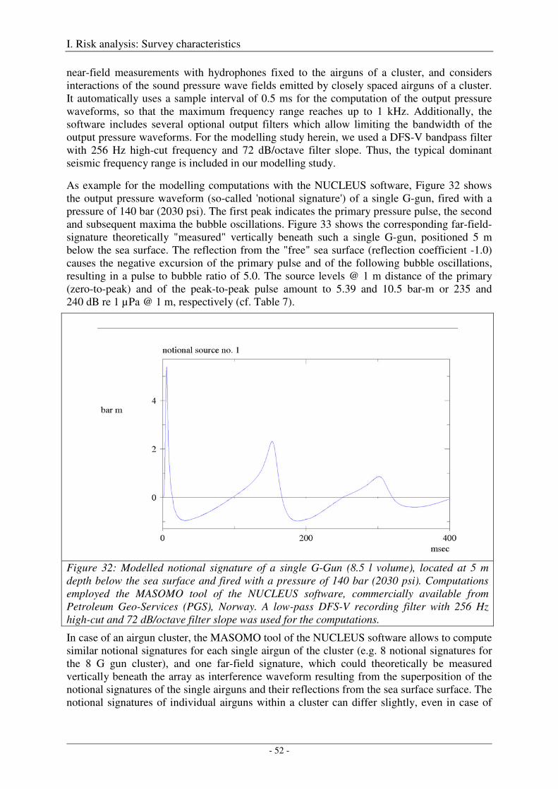
I. Risk analysis: Survey characteristics
- 52 -
near-field measurements with hydrophones fixed to the airguns of a cluster, and considers interactions of the sound pressure wave fields emitted by closely spaced airguns of a cluster. It automatically uses a sample interval of 0.5 ms for the computation of the output pressure waveforms, so that the maximum frequency range reaches up to 1 kHz. Additionally, the software includes several optional output filters which allow limiting the bandwidth of the output pressure waveforms. For the modelling study herein, we used a DFS-V bandpass filter with 256 Hz high-cut frequency and 72 dB/octave filter slope. Thus, the typical dominant seismic frequency range is included in our modelling study.
As example for the modelling computations with the NUCLEUS software, Figure 32 shows the output pressure waveform (so-called 'notional signature') of a single G-gun, fired with a pressure of 140 bar (2030 psi). The first peak indicates the primary pressure pulse, the second and subsequent maxima the bubble oscillations. Figure 33 shows the corresponding far-field-signature theoretically "measured" vertically beneath such a single G-gun, positioned 5 m below the sea surface. The reflection from the "free" sea surface (reflection coefficient -1.0) causes the negative excursion of the primary pulse and of the following bubble oscillations, resulting in a pulse to bubble ratio of 5.0. The source levels @ 1 m distance of the primary (zero-to-peak) and of the peak-to-peak pulse amount to 5.39 and 10.5 bar-m or 235 and 240 dB re 1 µPa @ 1 m, respectively (cf. Table 7).
Figure 32: Modelled notional signature of a single G-Gun (8.5 l volume), located at 5 m depth below the sea surface and fired with a pressure of 140 bar (2030 psi). Computations employed the MASOMO tool of the NUCLEUS software, commercially available from Petroleum Geo-Services (PGS), Norway. A low-pass DFS-V recording filter with 256 Hz high-cut and 72 dB/octave filter slope was used for the computations.
In case of an airgun cluster, the MASOMO tool of the NUCLEUS software allows to compute similar notional signatures for each single airgun of the cluster (e.g. 8 notional signatures for the 8 G gun cluster), and one far-field signature, which could theoretically be measured vertically beneath the array as interference waveform resulting from the superposition of the notional signatures of the single airguns and their reflections from the sea surface surface. The notional signatures of individual airguns within a cluster can differ slightly, even in case of
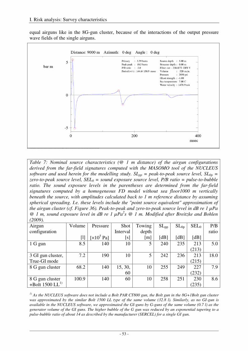
I. Risk analysis: Survey characteristics
- 53 -
equal airguns like in the 8G-gun cluster, because of the interactions of the output pressure wave fields of the single airguns.
Figure 33: Modelled far-f ield signatu re of a sing le G-Gun (8.5 l volume), located at 5 m depth be low the sea sur face and f ired with a pressu re of 140 bar (203 0 psi). Compu tations employed the MASOMO too l of the NU CLEU S sof twa re, commercially avai lable from Petro leum Geo-Services (PGS), Norwa y. A low-pass recordin g fi lter with 256 Hz high-cut a nd 72 dB /octave fi lter slope wa s used fo r the compu tations.
Table 7: Nominal source characteristics (@ 1 m distance) of the airgun configurations derived from the far-field signatures computed with the MASOMO tool of the NUCLEUS software and used herein for the modelling study. SLpp = peak-to-peak source level, SL0p = zero-to-peak source level, SEL0 = sound exposure source level, P/B ratio = pulse-to-bubble ratio. The sound exposure levels in the parentheses are determined from the far-field signatures computed by a homogeneous FD model without sea floor1000 m vertically beneath the source, with amplitudes calculated back to 1 m reference distance by assuming spherical spreading. I.e. these levels include the "point source equivalent" approximation of the airgun cluster (cf. Figure 36). Peak-to-peak and zero-to-peak source level in dB re 1 µPa @ 1 m, sound exposure level in dB re 1 µPa2s @ 1 m. Modified after Breitzke and Bohlen (2009).
Airgun configuration
Volume
[l]
Pressure
[×105 Pa]
Shot Interval
[s]
Towing depth
[m]
SLpp
[dB]
SL0p
[dB]
SEL0
[dB]
P/B ratio
1 G gun
8.5 140 10 5 240 235 213 (213)
5.0
3 GI gun cluster, True-GI mode
7.2 190 10 5 242 236 213 (215)
18.0
8 G gun cluster
68.2 140 15, 30, 60
10 255 249 227 (232)
7.9
8 G gun cluster +Bolt 1500 LL1)
100.9 140 60 10 258 251 230 (235)
8.6
1) As the NUCLEUS software does not include a Bolt PAR CT800 gun, the Bolt gun in the 8G+1Bolt gun cluster was approximated by the similar Bolt 1500 LL type of the same volume (32.8 l). Similarly, as no GI-gun is available in the NUCLEUS software, we approximated the GI-guns by G-guns of the same volume (0.7 l) as the generator volume of the GI guns. The higher bubble of the G gun was reduced by an exponential tapering to a pulse-bubble ratio of about 14 as described by the manufacturer (SERCEL) for a single GI gun.
I. Risk analysis: Survey characteristics
- 54 -
Similar notional and far-field signatures were computed for the other airgun clusters mentioned above (3 GI, 8 G, 8 G + 1 Bolt) and used as input to the subsequent sound propagation models as discussed in the subsequent chapter I.4. From the far-field signatures, the peak-to-peak and zero-to-peak source levels @ 1 m distance and pulse-to-bubble ratios were derived (Table 7). A comparison with Table 3 indicates that for the G-gun and the 3 GI-gun cluster (True-GI mode), the modelled source levels (240 and 242 dBpp re 1µPa @ 1 m, respectively) are slightly higher than the source levels measured during the Heggernes calibration survey (237 and 241 dBpp re 1µPa @ 1 m, respectively). The reason is that the source levels derived from the Heggernes calibration survey were extrapolated from the closest non-clipped recordings measured at emission angles other than directly below the source and by assuming spherical 1/r amplitude decay. By contrast, the model computes the source level directly without extrapolations. These different approaches might lead to a slight underestimation of the source levels derived from the Heggernes calibration survey, as discussed in Breitzke et al. (2008). An exception is the zero to peak source level of the 3 GI-gun cluster, where the measured, extrapolated source level (238 dB0p re. 1 µPa @ 1 m) is 2 dB higher than the modelled value (236 dB0p re 1 µPa @ 1 m). This can be explained by the fact, that the estimated accuracy of the measured, extrapolated source levels is about 1 - 2 dB.
I. Risk analysis: Survey characteristics
- 55 -
4. Sound fields
Experimental in-situ measurements along single profile lines as conducted during the calibration survey at the Heggernes acoustic range are insufficient to describe the full 3-D sound field emitted by a certain airgun configuration because the limited number of hydrophones available provide data only from certain depths and positions within a 3D-cube and for the environmental conditions (sound speed profiles, sea-floor geometry) of the test site. Furthermore, new airgun configurations like the 8 G- and 8 G + 1 Bolt-gun cluster not available during the calibration survey shall be used in future surveys. Hence, in addition to the modelling of the output pressure waveforms and far-field signatures described in the preceding chapter I.3 it is necessary to model sound propagation.
The basic concepts of the modelling approach and its validation by comparison with data collected during the Heggernes calibration study are discussed below. For illustration purposes, here the model is first applied to a semi-infinite homogenous and isotropic ocean, while section I.6 applies the method to the actual oceanic situation as encountered in the Antarctic for the different environmental scenarios.
Modelling approach and model parameters
In order to take all reflected, refracted and diffracted waves into account and to allow the incorporation of a broad range of frequencies, we used a 2.5D finite-difference model as full waveform modelling approach. The FD-code was kindly provided by Prof. Dr. T. Bohlen, Technische Universität Bergakademie Freiberg, with its main components described in Bohlen (2002). It is based on cylinder coordinates, uses 4th order operators and implicitly implies an azimuthal symmetry of the model. Compared to 2D finite difference models, this 2.5D code allows for the simulation of the spherical 1/r amplitude decay of point sources in an infinite homogeneous medium correctly, whereas 2D FD-models implicitly imply line sources (in the 3rd dimension) and simulate cylindrical 1/√r amplitude decay. Thus, the 2.5D model simulates sound propagation like a 3D model as long as the source directivity and the model parameters have an azimuthal (cylindrical) symmetry, but with the same computation time as a 2D model. By using this (computation time intensive) 2.5D FD model we put the focus on using the best full waveform sound propagation model, which also allows to include broad-band seismic source signatures without any additional computation time. Other, in ocean acoustics often applied sound propagation models like ray tracing, normal mode or parabolic equation (PE) models are usually computation time effective, but typically include approximations of the wave equation, and can therefore not be applied without restrictions to models including features like surface or sound duct.
The modelling approach works as follows (Breitzke and Bohlen, 2009) (Figure 34):
(1) The 2.5D finite-difference code (Bohlen, 2002) is used to compute synthetic seismograms for a single shot on a dense grid in the vertical x-z-plane.
(2) As the 2.5D code implies azimuthal symmetry, only point sources located on the cylinder axis (r = 0) or circular ring sources around the cylinder axis (r ≠ 0) can be realized. Therefore, to include the source signal characteristics of the airgun configurations as realistic as possible, we approximated the compact airgun clusters (cf. Figure 31, Table 7) by using the following "point source equivalent" approach:
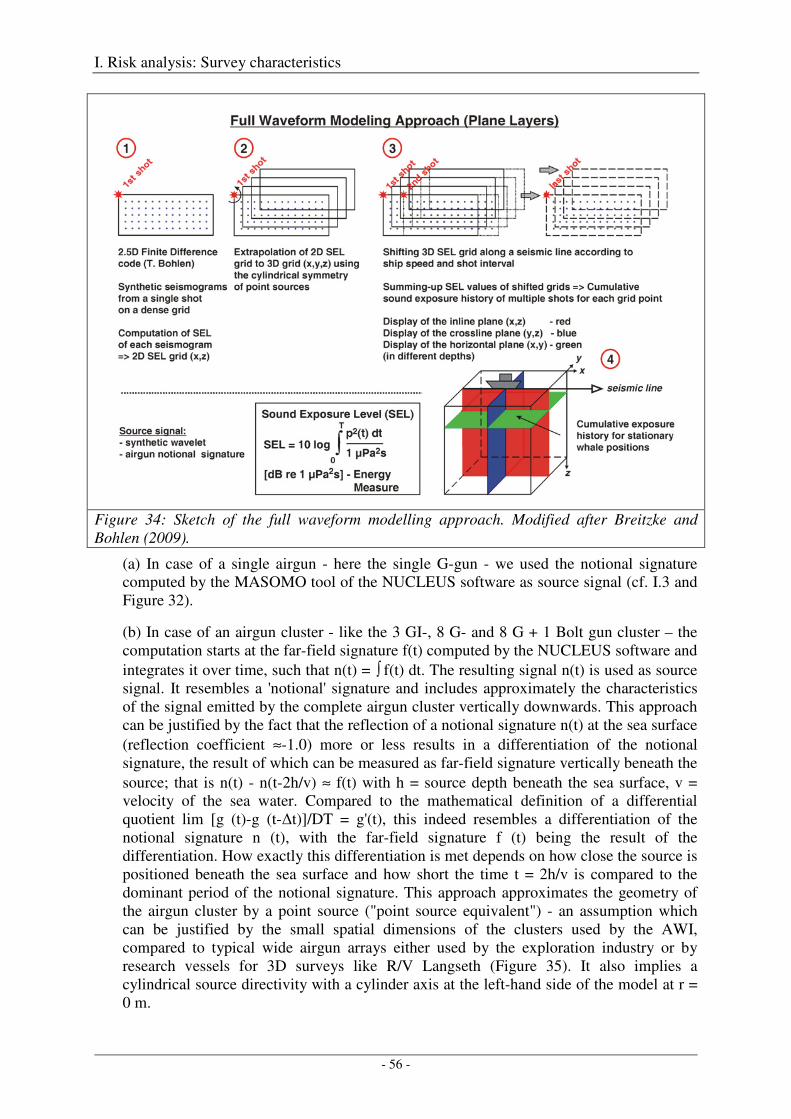
I. Risk analysis: Survey characteristics
- 56 -
Figure 34: Sketch of the full waveform modelling approach. Modified after Breitzke and Bohlen (2009).
(a) In case of a single airgun - here the single G-gun - we used the notional signature computed by the MASOMO tool of the NUCLEUS software as source signal (cf. I.3 and Figure 32).
(b) In case of an airgun cluster - like the 3 GI-, 8 G- and 8 G + 1 Bolt gun cluster – the computation starts at the far-field signature f(t) computed by the NUCLEUS software and integrates it over time, such that n(t) = ∫ f(t) dt. The resulting signal n(t) is used as source signal. It resembles a 'notional' signature and includes approximately the characteristics of the signal emitted by the complete airgun cluster vertically downwards. This approach can be justified by the fact that the reflection of a notional signature n(t) at the sea surface (reflection coefficient ≈-1.0) more or less results in a differentiation of the notional signature, the result of which can be measured as far-field signature vertically beneath the source; that is n(t) - n(t-2h/v) ≈ f(t) with h = source depth beneath the sea surface, v = velocity of the sea water. Compared to the mathematical definition of a differential quotient lim [g (t)-g (t-∆t)]/DT = g'(t), this indeed resembles a differentiation of the notional signature n (t), with the far-field signature f (t) being the result of the differentiation. How exactly this differentiation is met depends on how close the source is positioned beneath the sea surface and how short the time t = 2h/v is compared to the dominant period of the notional signature. This approach approximates the geometry of the airgun cluster by a point source ("point source equivalent") - an assumption which can be justified by the small spatial dimensions of the clusters used by the AWI, compared to typical wide airgun arrays either used by the exploration industry or by research vessels for 3D surveys like R/V Langseth (Figure 35). It also implies a cylindrical source directivity with a cylinder axis at the left-hand side of the model at r = 0 m.
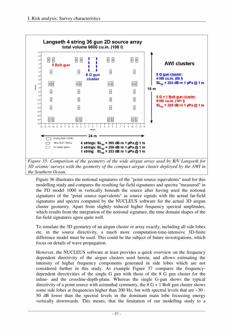
I. Risk analysis: Survey characteristics
- 57 -
Figure 35: Comparison of the geometry of the wide airgun array used by R/V Langseth for 3D seismic surveys with the geometry of the compact airgun cluster deployed by the AWI in the Southern Ocean.
Figure 36 illustrates the notional signatures of the "point source equivalents" used for this modelling study and compares the resulting far-field signatures and spectra "measured" in the FD model 1000 m vertically beneath the source after having used the notional signatures of the "point source equivalents" as source signals with the actual far-field signatures and spectra computed by the NUCLEUS software for the actual 3D airgun cluster geometry. Apart from slightly reduced higher frequency spectral amplitudes, which results from the integration of the notional signature, the time domain shapes of the far-field signatures agree quite well.
To simulate the 3D geometry of an airgun cluster or array exactly, including all side lobes etc. in the source directivity, a much more computation-time-intensive 3D-finite difference model must be used. This could be the subject of future investigations, which focus on details of wave propagation.
However, the NUCLEUS software at least provides a quick overview on the frequency dependent directivity of the airgun clusters used herein, and allows estimating the intensity of higher frequency components generated in side lobes which are not considered further in this study. As example Figure 37 compares the frequency-dependent directivities of the single G gun with those of the 8 G gun cluster for the inline- and the crossline-depth-plane. Whereas the single G-gun shows the typical directivity of a point source with azimuthal symmetry, the 8 G + 1 Bolt gun cluster shows some side lobes at frequencies higher than 200 Hz, but with spectral levels that are ~30 - 50 dB lower than the spectral levels in the dominant main lobe focussing energy vertically downwards. This means, that the limitation of our modelling study to a
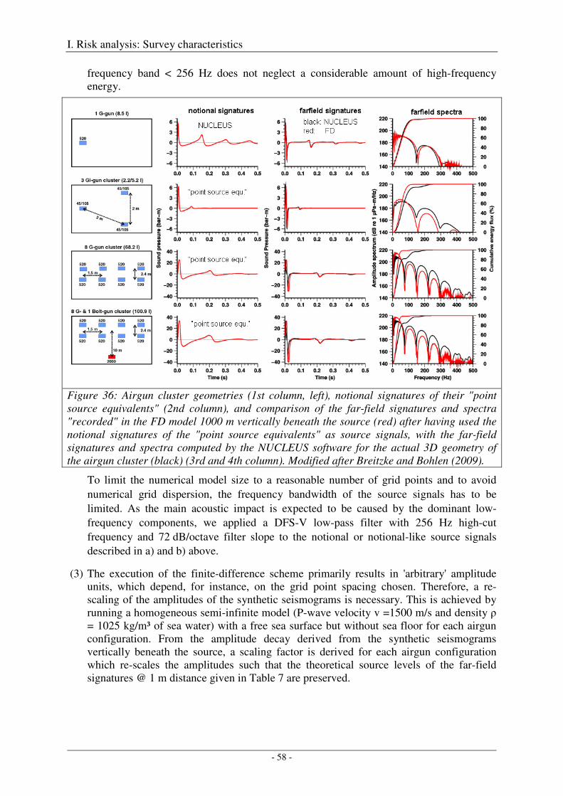
I. Risk analysis: Survey characteristics
- 58 -
frequency band < 256 Hz does not neglect a considerable amount of high-frequency energy.
Figure 36: Airgun cluster geometries (1st column, left), notional signatures of their "point source equivalents" (2nd column), and comparison of the far-field signatures and spectra "recorded" in the FD model 1000 m vertically beneath the source (red) after having used the notional signatures of the "point source equivalents" as source signals, with the far-field signatures and spectra computed by the NUCLEUS software for the actual 3D geometry of the airgun cluster (black) (3rd and 4th column). Modified after Breitzke and Bohlen (2009).
To limit the numerical model size to a reasonable number of grid points and to avoid numerical grid dispersion, the frequency bandwidth of the source signals has to be limited. As the main acoustic impact is expected to be caused by the dominant low-frequency components, we applied a DFS-V low-pass filter with 256 Hz high-cut frequency and 72 dB/octave filter slope to the notional or notional-like source signals described in a) and b) above.
(3) The execution of the finite-difference scheme primarily results in 'arbitrary' amplitude units, which depend, for instance, on the grid point spacing chosen. Therefore, a re-scaling of the amplitudes of the synthetic seismograms is necessary. This is achieved by running a homogeneous semi-infinite model (P-wave velocity v =1500 m/s and density ρ = 1025 kg/m³ of sea water) with a free sea surface but without sea floor for each airgun configuration. From the amplitude decay derived from the synthetic seismograms vertically beneath the source, a scaling factor is derived for each airgun configuration which re-scales the amplitudes such that the theoretical source levels of the far-field signatures @ 1 m distance given in Table 7 are preserved.
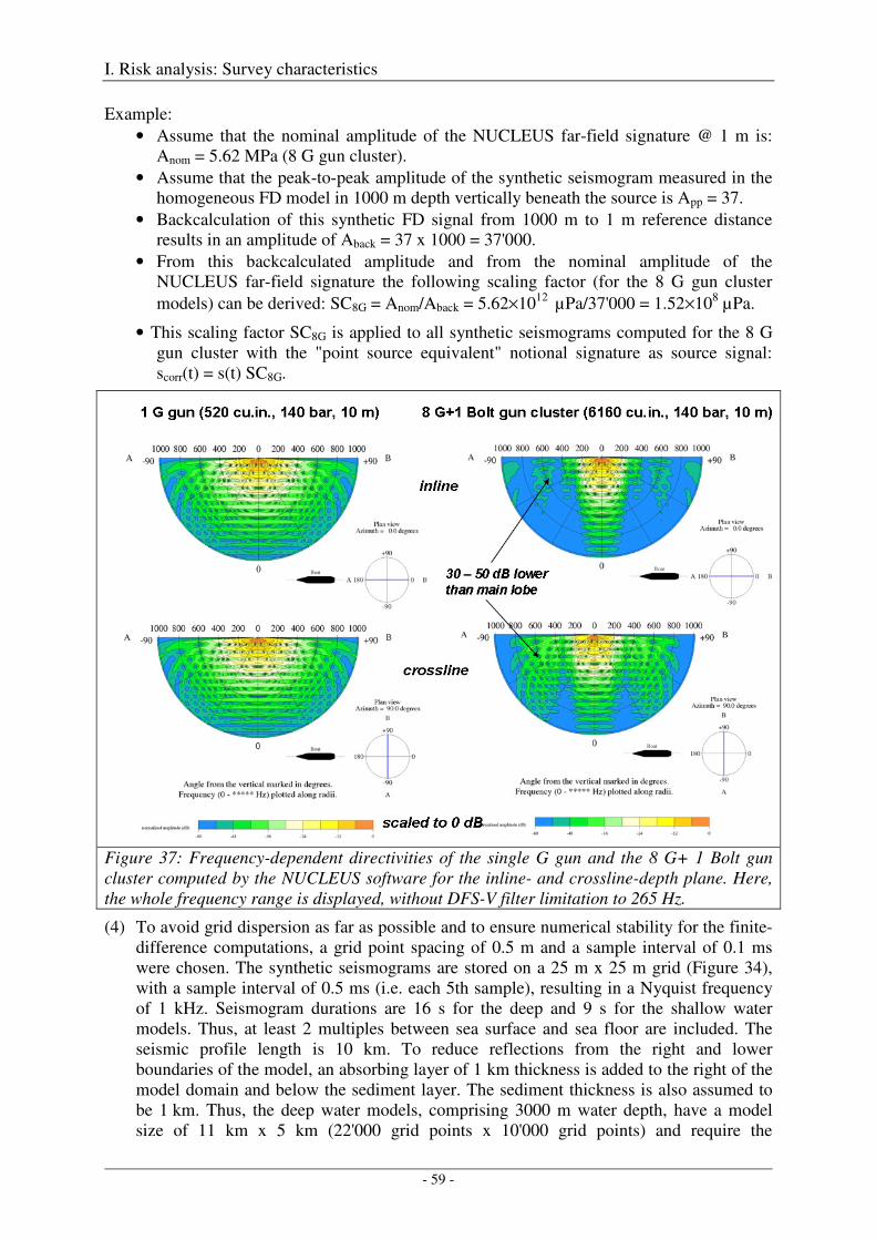
I. Risk analysis: Survey characteristics
- 59 -
Example: • Assume that the nominal amplitude of the NUCLEUS far-field signature @ 1 m is:
Anom = 5.62 MPa (8 G gun cluster). • Assume that the peak-to-peak amplitude of the synthetic seismogram measured in the
homogeneous FD model in 1000 m depth vertically beneath the source is App = 37. • Backcalculation of this synthetic FD signal from 1000 m to 1 m reference distance
results in an amplitude of Aback = 37 x 1000 = 37'000. • From this backcalculated amplitude and from the nominal amplitude of the
NUCLEUS far-field signature the following scaling factor (for the 8 G gun cluster models) can be derived: SC8G = Anom/Aback = 5.62×10¹² µPa/37'000 = 1.52×10⁸ µPa.
• This scaling factor SC8G is applied to all synthetic seismograms computed for the 8 G gun cluster with the "point source equivalent" notional signature as source signal: scorr(t) = s(t) SC8G.
Figure 37: Frequency-dependent directivities of the single G gun and the 8 G+ 1 Bolt gun cluster computed by the NUCLEUS software for the inline- and crossline-depth plane. Here, the whole frequency range is displayed, without DFS-V filter limitation to 265 Hz.
(4) To avoid grid dispersion as far as possible and to ensure numerical stability for the finite-difference computations, a grid point spacing of 0.5 m and a sample interval of 0.1 ms were chosen. The synthetic seismograms are stored on a 25 m x 25 m grid (Figure 34), with a sample interval of 0.5 ms (i.e. each 5th sample), resulting in a Nyquist frequency of 1 kHz. Seismogram durations are 16 s for the deep and 9 s for the shallow water models. Thus, at least 2 multiples between sea surface and sea floor are included. The seismic profile length is 10 km. To reduce reflections from the right and lower boundaries of the model, an absorbing layer of 1 km thickness is added to the right of the model domain and below the sediment layer. The sediment thickness is also assumed to be 1 km. Thus, the deep water models, comprising 3000 m water depth, have a model size of 11 km x 5 km (22'000 grid points x 10'000 grid points) and require the
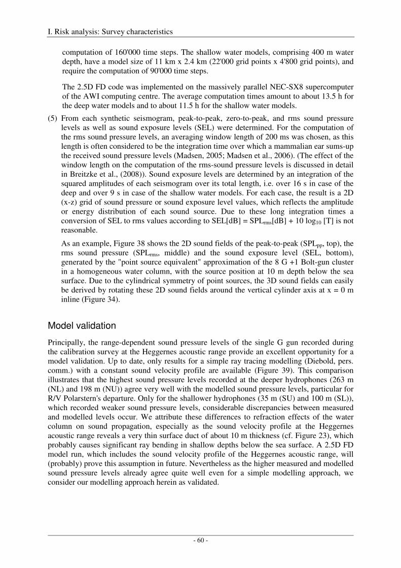
I. Risk analysis: Survey characteristics
- 60 -
computation of 160'000 time steps. The shallow water models, comprising 400 m water depth, have a model size of 11 km x 2.4 km (22'000 grid points x 4'800 grid points), and require the computation of 90'000 time steps.
The 2.5D FD code was implemented on the massively parallel NEC-SX8 supercomputer of the AWI computing centre. The average computation times amount to about 13.5 h for the deep water models and to about 11.5 h for the shallow water models.
(5) From each synthetic seismogram, peak-to-peak, zero-to-peak, and rms sound pressure levels as well as sound exposure levels (SEL) were determined. For the computation of the rms sound pressure levels, an averaging window length of 200 ms was chosen, as this length is often considered to be the integration time over which a mammalian ear sums-up the received sound pressure levels (Madsen, 2005; Madsen et al., 2006). (The effect of the window length on the computation of the rms-sound pressure levels is discussed in detail in Breitzke et al., (2008)). Sound exposure levels are determined by an integration of the squared amplitudes of each seismogram over its total length, i.e. over 16 s in case of the deep and over 9 s in case of the shallow water models. For each case, the result is a 2D (x-z) grid of sound pressure or sound exposure level values, which reflects the amplitude or energy distribution of each sound source. Due to these long integration times a conversion of SEL to rms values according to SEL[dB] = SPLrms[dB] + 10 log10 [T] is not reasonable.
As an example, Figure 38 shows the 2D sound fields of the peak-to-peak (SPLpp, top), the rms sound pressure (SPLrms, middle) and the sound exposure level (SEL, bottom), generated by the "point source equivalent" approximation of the 8 G +1 Bolt-gun cluster in a homogeneous water column, with the source position at 10 m depth below the sea surface. Due to the cylindrical symmetry of point sources, the 3D sound fields can easily be derived by rotating these 2D sound fields around the vertical cylinder axis at x = 0 m inline (Figure 34).
Model validation
Principally, the range-dependent sound pressure levels of the single G gun recorded during the calibration survey at the Heggernes acoustic range provide an excellent opportunity for a model validation. Up to date, only results for a simple ray tracing modelling (Diebold, pers. comm.) with a constant sound velocity profile are available (Figure 39). This comparison illustrates that the highest sound pressure levels recorded at the deeper hydrophones (263 m (NL) and 198 m (NU)) agree very well with the modelled sound pressure levels, particular for R/V Polarstern's departure. Only for the shallower hydrophones (35 m (SU) and 100 m (SL)), which recorded weaker sound pressure levels, considerable discrepancies between measured and modelled levels occur. We attribute these differences to refraction effects of the water column on sound propagation, especially as the sound velocity profile at the Heggernes acoustic range reveals a very thin surface duct of about 10 m thickness (cf. Figure 23), which probably causes significant ray bending in shallow depths below the sea surface. A 2.5D FD model run, which includes the sound velocity profile of the Heggernes acoustic range, will (probably) prove this assumption in future. Nevertheless as the higher measured and modelled sound pressure levels already agree quite well even for a simple modelling approach, we consider our modelling approach herein as validated.
I. Risk analysis: Survey characteristics
- 61 -
Figure 38: Sound pressure and sound exposure levels for the 8 G + 1 Bolt gun cluster. Top:
SPLpp [dB re 1 µPa], Middle: SPLrms [dB re. 1µPa], Bottom: SEL [dB re. 1µPa2s] for a single shot. All calculations are for the inline-depth plane. Modified after Breitzke and Bohlen (2009).
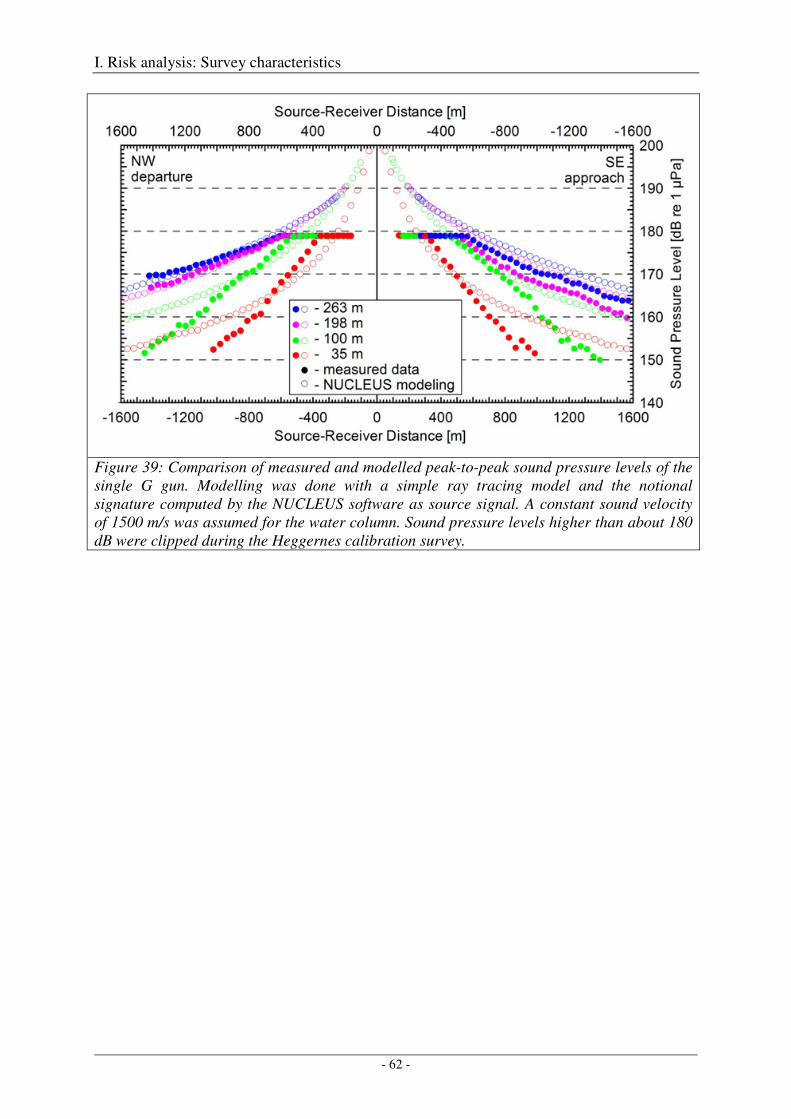
I. Risk analysis: Survey characteristics
- 62 -
Figure 39: Comparison of measured and modelled peak-to-peak sound pressure levels of the single G gun. Modelling was done with a simple ray tracing model and the notional signature computed by the NUCLEUS software as source signal. A constant sound velocity of 1500 m/s was assumed for the water column. Sound pressure levels higher than about 180 dB were clipped during the Heggernes calibration survey.
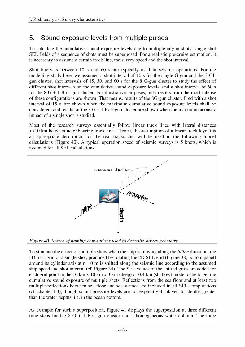
I. Risk analysis: Survey characteristics
- 63 -
5. Sound exposure levels from multiple pulses
To calculate the cumulative sound exposure levels due to multiple airgun shots, single-shot SEL fields of a sequence of shots must be superposed. For a realistic pre-cruise estimation, it is necessary to assume a certain track line, the survey speed and the shot interval.
Shot intervals between 10 s and 60 s are typically used in seismic operations. For the modelling study here, we assumed a shot interval of 10 s for the single G-gun and the 3 GI-gun cluster, shot intervals of 15, 30, and 60 s for the 8 G-gun cluster to study the effect of different shot intervals on the cumulative sound exposure levels, and a shot interval of 60 s for the 8 G + 1 Bolt-gun cluster. For illustrative purposes, only results from the most intense of these configurations are shown. That means, results of the 8G-gun cluster, fired with a shot interval of 15 s, are shown when the maximum cumulative sound exposure levels shall be considered, and results of the 8 G + 1 Bolt-gun cluster are shown when the maximum acoustic impact of a single shot is studied.
Most of the research surveys essentially follow linear track lines with lateral distances >>10 km between neighbouring track lines. Hence, the assumption of a linear track layout is an appropriate description for the real tracks and will be used in the following model calculations (Figure 40). A typical operation speed of seismic surveys is 5 knots, which is assumed for all SEL calculations.
Figure 40: Sketch of naming conventions used to describe survey geometry.
To simulate the effect of multiple shots when the ship is moving along the inline direction, the 3D SEL grid of a single shot, produced by rotating the 2D SEL grid (Figure 38, bottom panel) around its cylinder axis at r = 0 m is shifted along the seismic line according to the assumed ship speed and shot interval (cf. Figure 34). The SEL values of the shifted grids are added for each grid point in the 10 km x 10 km x 3 km (deep) or 0.4 km (shallow) model cube to get the cumulative sound exposure of multiple shots. Reflections from the sea floor and at least two multiple reflections between sea floor and sea surface are included in all SEL computations (cf. chapter I.3), though sound pressure levels are not explicitly displayed for depths greater than the water depths, i.e. in the ocean bottom.
As example for such a superposition, Figure 41 displays the superposition at three different time steps for the 8 G + 1 Bolt-gun cluster and a homogeneous water column. The three
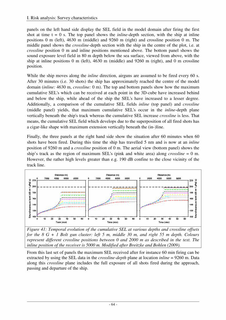
I. Risk analysis: Survey characteristics
- 64 -
panels on the left hand side display the SEL field in the model domain after firing the first shot at time t = 0 s. The top panel shows the inline-depth section, with the ship at inline positions 0 m (left), 4630 m (middle) and 9260 m (right) and crossline position 0 m. The middle panel shows the crossline-depth section with the ship in the centre of the plot, i.e. at crossline position 0 m and inline positions mentioned above. The bottom panel shows the sound exposure level field in 80 m depth below the sea surface, viewed from above, with the ship at inline positions 0 m (left), 4630 m (middle) and 9260 m (right), and 0 m crossline position.
While the ship moves along the inline direction, airguns are assumed to be fired every 60 s. After 30 minutes (i.e. 30 shots) the ship has approximately reached the centre of the model domain (inline: 4630 m, crossline: 0 m). The top and bottom panels show how the maximum cumulative SEL's which can be received at each point in the 3D-cube have increased behind and below the ship, while ahead of the ship the SEL's have increased to a lesser degree. Additionally, a comparison of the cumulative SEL fields inline (top panel) and crossline (middle panel) yields, that maximum cumulative SEL's occur in the inline-depth plane vertically beneath the ship's track whereas the cumulative SEL increase crossline is less. That means, the cumulative SEL field which develops due to the superposition of all fired shots has a cigar-like shape with maximum extension vertically beneath the (in-)line.
Finally, the three panels at the right hand side show the situation after 60 minutes when 60 shots have been fired. During this time the ship has travelled 5 nm and is now at an inline position of 9260 m and a crossline position of 0 m. The aerial view (bottom panel) shows the ship’s track as the region of maximum SEL's (pink and white area) along crossline = 0 m. However, the rather high levels greater than e.g. 190 dB confine to the close vicinity of the track line.
Figure 41: Temporal evolution of the cumulative SEL at various depths and crossline offsets for the 8 G + 1 Bolt gun cluster: left 5 m, middle 30 m, and right 55 m depth. Colours represent different crossline positions between 0 and 2000 m as described in the text. The inline position of the receiver is 5000 m. Modified after Breitzke and Bohlen (2009).
From this last set of panels the maximum SEL received after for instance 60 min firing can be extracted by using the SEL data in the crossline-depth plane at location inline = 9260 m. Data along this crossline plane includes the full exposure of all shots fired during the approach, passing and departure of the ship.
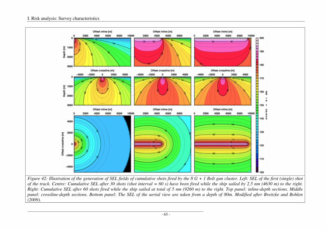
I. Risk analysis: Survey characteristics
- 65 -
Figure 42: Illustration of the generation of SEL fields of cumulative shots fired by the 8 G + 1 Bolt gun cluster. Left: SEL of the first (single) shot of the track. Centre: Cumulative SEL after 30 shots (shot interval = 60 s) have been fired while the ship sailed by 2.5 nm (4630 m) to the right. Right: Cumulative SEL after 60 shots fired while the ship sailed at total of 5 nm (9260 m) to the right. Top panel: inline-depth sections. Middle panel: crossline-depth sections. Bottom panel: The SEL of the aerial view are taken from a depth of 80m. Modified after Breitzke and Bohlen (2009).
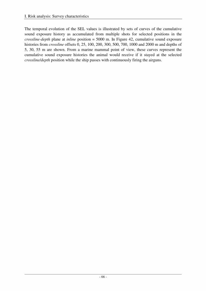
I. Risk analysis: Survey characteristics
- 66 -
The temporal evolution of the SEL values is illustrated by sets of curves of the cumulative sound exposure history as accumulated from multiple shots for selected positions in the crossline-depth plane at inline position = 5000 m. In Figure 42, cumulative sound exposure histories from crossline offsets 0, 25, 100, 200, 300, 500, 700, 1000 and 2000 m and depths of 5, 30, 55 m are shown. From a marine mammal point of view, these curves represent the cumulative sound exposure histories the animal would receive if it stayed at the selected crossline/depth position while the ship passes with continuously firing the airguns.
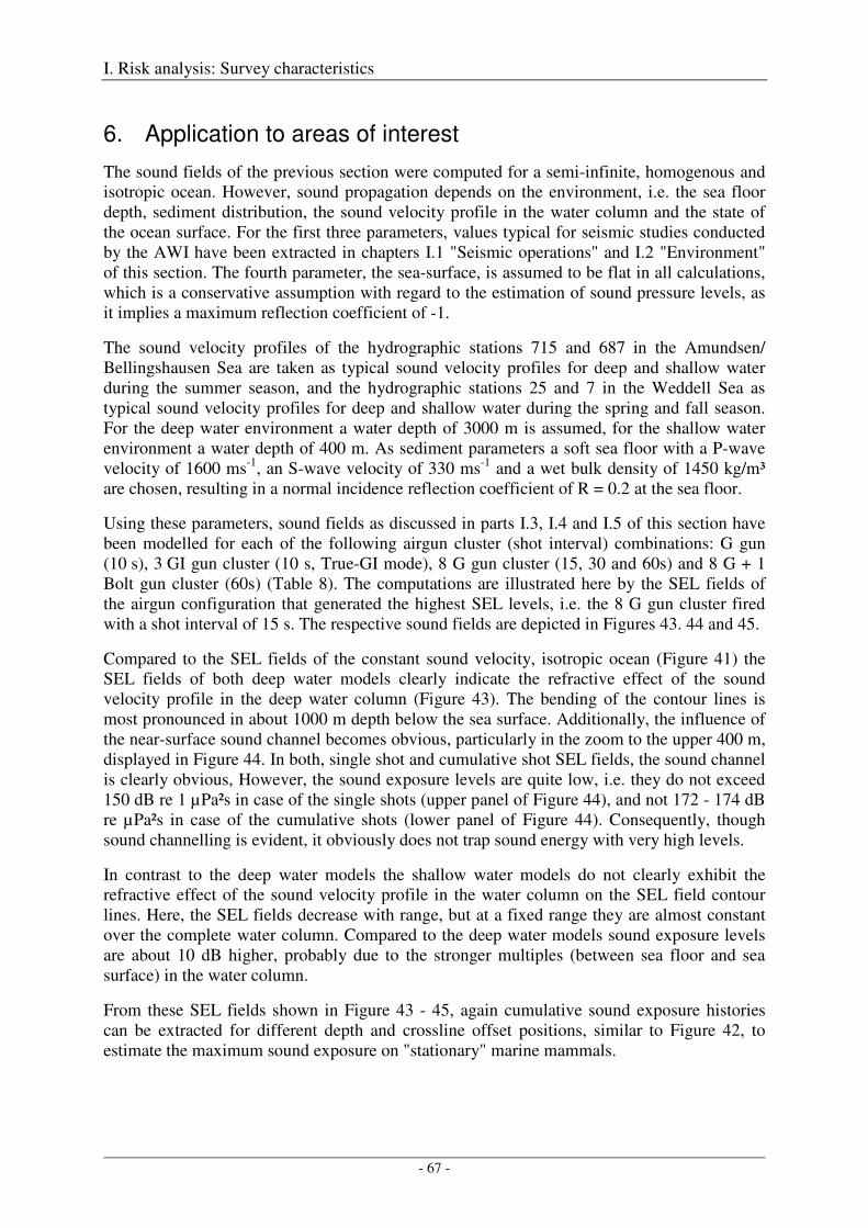
I. Risk analysis: Survey characteristics
- 67 -
6. Application to areas of interest
The sound fields of the previous section were computed for a semi-infinite, homogenous and isotropic ocean. However, sound propagation depends on the environment, i.e. the sea floor depth, sediment distribution, the sound velocity profile in the water column and the state of the ocean surface. For the first three parameters, values typical for seismic studies conducted by the AWI have been extracted in chapters I.1 "Seismic operations" and I.2 "Environment" of this section. The fourth parameter, the sea-surface, is assumed to be flat in all calculations, which is a conservative assumption with regard to the estimation of sound pressure levels, as it implies a maximum reflection coefficient of -1.
The sound velocity profiles of the hydrographic stations 715 and 687 in the Amundsen/ Bellingshausen Sea are taken as typical sound velocity profiles for deep and shallow water during the summer season, and the hydrographic stations 25 and 7 in the Weddell Sea as typical sound velocity profiles for deep and shallow water during the spring and fall season. For the deep water environment a water depth of 3000 m is assumed, for the shallow water environment a water depth of 400 m. As sediment parameters a soft sea floor with a P-wave velocity of 1600 ms-1, an S-wave velocity of 330 ms-1 and a wet bulk density of 1450 kg/m³ are chosen, resulting in a normal incidence reflection coefficient of R = 0.2 at the sea floor.
Using these parameters, sound fields as discussed in parts I.3, I.4 and I.5 of this section have been modelled for each of the following airgun cluster (shot interval) combinations: G gun (10 s), 3 GI gun cluster (10 s, True-GI mode), 8 G gun cluster (15, 30 and 60s) and 8 G + 1 Bolt gun cluster (60s) (Table 8). The computations are illustrated here by the SEL fields of the airgun configuration that generated the highest SEL levels, i.e. the 8 G gun cluster fired with a shot interval of 15 s. The respective sound fields are depicted in Figures 43. 44 and 45.
Compared to the SEL fields of the constant sound velocity, isotropic ocean (Figure 41) the SEL fields of both deep water models clearly indicate the refractive effect of the sound velocity profile in the deep water column (Figure 43). The bending of the contour lines is most pronounced in about 1000 m depth below the sea surface. Additionally, the influence of the near-surface sound channel becomes obvious, particularly in the zoom to the upper 400 m, displayed in Figure 44. In both, single shot and cumulative shot SEL fields, the sound channel is clearly obvious, However, the sound exposure levels are quite low, i.e. they do not exceed 150 dB re 1 µPa²s in case of the single shots (upper panel of Figure 44), and not 172 - 174 dB re µPa²s in case of the cumulative shots (lower panel of Figure 44). Consequently, though sound channelling is evident, it obviously does not trap sound energy with very high levels.
In contrast to the deep water models the shallow water models do not clearly exhibit the refractive effect of the sound velocity profile in the water column on the SEL field contour lines. Here, the SEL fields decrease with range, but at a fixed range they are almost constant over the complete water column. Compared to the deep water models sound exposure levels are about 10 dB higher, probably due to the stronger multiples (between sea floor and sea surface) in the water column.
From these SEL fields shown in Figure 43 - 45, again cumulative sound exposure histories can be extracted for different depth and crossline offset positions, similar to Figure 42, to estimate the maximum sound exposure on "stationary" marine mammals.
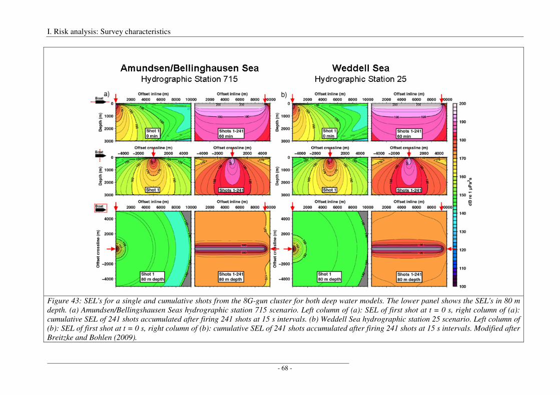
I. Risk analysis: Survey characteristics
- 68 -
Figure 43: SEL's for a single and cumulative shots from the 8G-gun cluster for both deep water models. The lower panel shows the SEL's in 80 m depth. (a) Amundsen/Bellingshausen Seas hydrographic station 715 scenario. Left column of (a): SEL of first shot at t = 0 s, right column of (a): cumulative SEL of 241 shots accumulated after firing 241 shots at 15 s intervals. (b) Weddell Sea hydrographic station 25 scenario. Left column of (b): SEL of first shot at t = 0 s, right column of (b): cumulative SEL of 241 shots accumulated after firing 241 shots at 15 s intervals. Modified after Breitzke and Bohlen (2009).
I. Risk analysis: Survey characteristics
- 69 -
Figure 44: Zoom to the upper 400 m of the SEL fields of the 8 G gun cluster shown in Figure 43. Top panel: SEL fields for a single shot. Middle panel: Cumulative SEL fields in the inline-depth plane accumulated after 60 min, or after firing 241 shots at 15 s interval. Bottom panel: Cumulative SEL fields in the crossline-depth plane accumulated after 60 min, or after firing 241 shots at 15 s interval. Modified after Breitzke and Bohlen (2009).
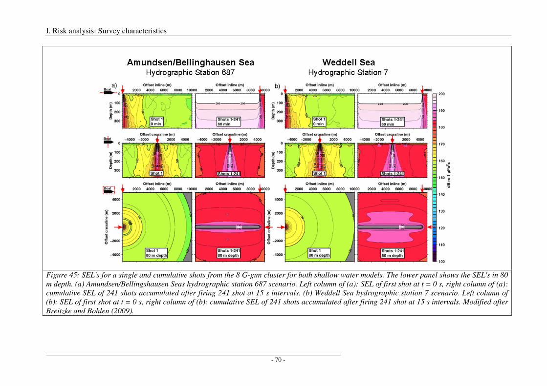
I. Risk analysis: Survey characteristics
- 70 -
Figure 45: SEL's for a single and cumulative shots from the 8 G-gun cluster for both shallow water models. The lower panel shows the SEL's in 80 m depth. (a) Amundsen/Bellingshausen Seas hydrographic station 687 scenario. Left column of (a): SEL of first shot at t = 0 s, right column of (a): cumulative SEL of 241 shots accumulated after firing 241 shot at 15 s intervals. (b) Weddell Sea hydrographic station 7 scenario. Left column of (b): SEL of first shot at t = 0 s, right column of (b): cumulative SEL of 241 shots accumulated after firing 241 shot at 15 s intervals. Modified after Breitzke and Bohlen (2009).
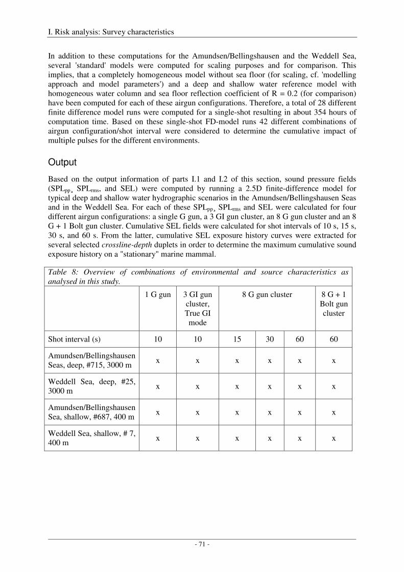
I. Risk analysis: Survey characteristics
- 71 -
In addition to these computations for the Amundsen/Bellingshausen and the Weddell Sea, several 'standard' models were computed for scaling purposes and for comparison. This implies, that a completely homogeneous model without sea floor (for scaling, cf. 'modelling approach and model parameters') and a deep and shallow water reference model with homogeneous water column and sea floor reflection coefficient of R = 0.2 (for comparison) have been computed for each of these airgun configurations. Therefore, a total of 28 different finite difference model runs were computed for a single-shot resulting in about 354 hours of computation time. Based on these single-shot FD-model runs 42 different combinations of airgun configuration/shot interval were considered to determine the cumulative impact of multiple pulses for the different environments.
Output
Based on the output information of parts I.1 and I.2 of this section, sound pressure fields (SPLpp¸ SPLrms, and SEL) were computed by running a 2.5D finite-difference model for typical deep and shallow water hydrographic scenarios in the Amundsen/Bellingshausen Seas and in the Weddell Sea. For each of these SPLpp¸ SPLrms and SEL were calculated for four different airgun configurations: a single G gun, a 3 GI gun cluster, an 8 G gun cluster and an 8 G + 1 Bolt gun cluster. Cumulative SEL fields were calculated for shot intervals of 10 s, 15 s, 30 s, and 60 s. From the latter, cumulative SEL exposure history curves were extracted for several selected crossline-depth duplets in order to determine the maximum cumulative sound exposure history on a "stationary" marine mammal.
Table 8: Overview of combinations of environmental and source characteristics as analysed in this study.
1 G gun 3 GI gun cluster, True GI mode
8 G gun cluster 8 G + 1 Bolt gun cluster
Shot interval (s) 10 10 15 30 60 60
Amundsen/Bellingshausen Seas, deep, #715, 3000 m
x x x x x x
Weddell Sea, deep, #25, 3000 m
x x x x x x
Amundsen/Bellingshausen Sea, shallow, #687, 400 m
x x x x x x
Weddell Sea, shallow, # 7, 400 m
x x x x x x
I. Risk analysis: Survey characteristics
- 72 -
7. References
Bohlen, T. (2002), Parallel 3-D viscoelastic finite-difference seismic modelling, Computers & Geosciences, 28, 887-899.
Breitzke, M., O. Boebel, S. El Naggar, W. Jokat, and B. Werner (2008), Broad-band calibration of marine seismic sources used by R/V Polarstern for academic research in polar regions, Geophysical Journal International, 174, 505-524.
Breitzke, M., and T. Bohlen (2009), Modelling acoustic wave propagation in the Southern Ocean to estimate the acoustic impact of seismic surveys on marine mammals, in prep.
Caldwell, J. & Dragoset, W., 2000. A brief overview of seismic airgun arrays, The Leading Edge, 19, 898-902.
Dragoset, W.H., 1984. A comprehensive method for evaluating the design of airguns and airgun arrays, The Leading Edge, 3, 52-61.
Dragoset, W.H., 1990. Airgun array specs: A tutorial, The Leading Edge, 9, 24-32.
Dragoset, W.H., 2000. Introduction to airguns and airgun arrays, The Leading Edge, 19, 892-897.
Fricke, J.R., Davis, J.M. & Reed, D.H., 1985. A standard quantitative calibration procedure for marine seismic sources, Geophysics, 50, 1525-1532.
Gausland, I., 2000. Impact of seismic surveys on marine life, The Leading Edge, 19, 903-905.
Johnston, R. C., D. H. Reed, and J. F. Desler (1988), Special report of the SEG Technical Standards Committee. SEG standards for specifying marine seismic energy sources, Geophysics, 53, 566-575.
Jones, E.J.W., 1999. Marine Geophysics, pp. 466, John Wiley & Sons Ltd., Chichester.
Madsen, P. T. (2005), Marine mammals and noise: Problems with root mean square sound pressure levels for transients, The Journal of the Acoustical Society of America, 117, 3952-3957.
Madsen, P. T., M. Johnson, P. J. O. Miller, N. A. Soto, J. Lynch, and P. Tyack (2006), Quantitative measures of airgun pulses recorded on sperm whales (Physeter macrocephalus) using acoustic tags during controlled exposure experiments, The Journal of the Acoustical Society of America, 120, 2366-2379.
Michels, K. H., K. G., C. D. Hillenbrand, B. Diekmann, D. K. Fütterer, H. Grobe, and G. Uenzelmann-Neben (2002), The southern Weddell Sea: combined contourite-turbidite sedimentation at the southeastern margin of the Weddell Gyre, in Deep-water contourite systems: Modern drifts and ancient series, seismic and sedimentary characteristics, edited by D. A. V. Stow, et al., pp. 305-323, Geological Society, London.
National Marine Fisheries Service, 2003. Small takes of marine mammals incidental to specified activities; marine seismic testing in the northern Gulf of Mexico, Federal Register, 68, 17773-17783.
Parkes, G., and L. Hatton (1986), The marine seismic source, 114 pp., D. Reidel Publishing Company, Dordrecht.
Richardson, W.J., Greene, C.R., Malme, C.I. & Thomson, D.H., 1995. Marine Mammals and Noise, pp. 576, Academic Press, San Diego.
I. Risk analysis: Survey characteristics
- 73 -
Southall, B.L., Bowles, A.E., Ellison, W.T., Finneran, J.J., Gentry, R.L., Greene Jr., C.R., Kastak, D., Ketten, D.R., Miller, J. H., Nachtigall, P.E., Richardson, W.J., Thomas, J.A., Tyack, P.L., 2007. Marine mammal noise exposure criteria: Initial scientific recommendations. Aquatic Mammals, 33, 411-521.
Urick, R. J. (1983), Principles of underwater sound, 3rd edition ed. ed., 423 pp., McGraw Hill, New York.
Ziolowski, A. M., G. Parkes, L. Hatton, and T. Haugland (1982), The signature of an airgun array: computation from near-field measurements including interactions, Geophysics, 47, 1413-1421.

II. Risk analysis: Species description
- 75 -
II. Risk analysis: Species description
1. Identification of relevant marine mammal species
This study is based on the review of article by Gill and Evans [2002]1 as well as the following literature databases: Scopus, Web of Science (ex Science Citation Index), Medline, Arctic and Antarctic Regions, Aquatic Science and Fisheries Abstracts (ASFA) and IWC Website. The data base query2 includes title, abstract and descriptors, and returns about 120 references between 2002 and 2006 enlarging the pool of literature of Gill and Evans [2002].
The identification of marine mammal species possibly relevant to this study was based on Gill and Evans [2002], and Boyd [2002a]. Information on the respective conservation status was taken from the IUCN red list of endangered species http://www.iucnredlist.org3.” Our selection of marine mammals is based on the compilation “Marine Mammals of the Southern Ocean” of Gill and Evans [2002] which comprises Antarctic and sub-Antarctic species. „True“ Antarctic species are defined as „those species whose populations rely on the Southern Ocean as a habitat, i.e., critical to a part of their life history, either through the provision of habitat for breeding or through the provision of the major source of food. [Boyd, 2002a]. By virtue of this definition, species that inhabit the sub-Antarctic, i.e. the islands surrounding Antarctica in the region of the polar front or the polar frontal zone itself (usually located north of 60°S), have been excluded from this study. In addition, cetaceans migrating only sporadically into the Antarctic treaty area are also excluded. The remaining 14 true Antarctic cetacean species are listed in Table 9 while those excluded are listed in Table 10
The aforementioned definition of true Antarctic species also holds valid for the six species of Antarctic seals inhabiting the Southern Ocean. There is one species from the family Otariidae (Antarctic fur seal), and there are five species from the family Phocidae (Weddell seal, Ross seal, crabeater seal, leopard seal, southern elephant seal), all of which belong to a single subfamily, the Monachinae, inhabiting the Southern Ocean [Boyd, 2002a]. Estimates of abundances and conservation status of seal species are given in Table 11. Further details on seal abundance estimates are given in Table 11.
1 Available from Bundesamt für Naturschutz, Außenstelle Insel Vilm, 18581 Putbus, Germany; (Email: [email protected]). 2 The search profile consists of the following species names arranged as (Whale* AND (beaked OR killer OR (long-finned pilot) OR sperm OR Arnoux* OR (southern bottlenose) Or (strap-tooth*) OR baleen OR (southern right) OR blue OR fin OR sei OR (dwarf minke) OR minke OR humpback OR (hourglass dolphin*) OR (Lagenorhynchus cruciger) OR (Orcinus orca) OR (Globicephala melas) OR (Physeter macrocephalus) OR (Berardius arnuxii) OR (Hyperoodon planifrons) OR (Mesoplodon layardii) OR (Eubalaena australis) OR (Balaenoptera AND (musculus OR physalus OR borealis OR acutorostrata OR bonaerensis OR noveangliae))) AND Antarctic) 3 The search used the following profile: text search “whale dolphin”, modifier “contains”, part of database “entire”, system “marine”, taxa “species”, red list category “all evaluated (incl. least concern)”, red list assigned “2006”, countries “Antarctica”, marine region “Atlantic-Antarctic, Indian Ocean-Antarctic, Pacific-Antarctic”, region of the world “Antarctic”, major habitat type “sea”, major threat type “all”
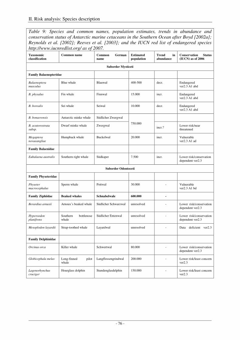
II. Risk analysis: Species description
- 76 -
Table 9: Species and common names, population estimates, trends in abundance and conservation status of Antarctic marine cetaceans in the Southern Ocean after Boyd [2002a]; Reynolds et al. [2002]; Reeves et al. [2003]; and the IUCN red list of endangered species http://www.iucnredlist.org/ as of 2007.
Taxonomic
classification
Common name Common German
name
Estimated
population
Trend in
abundance
Conservation Status
(IUCN) as of 2006
Suborder Mysticeti
Family Balaenopteridae
Balaenoptera musculus
Blue whale Blauwal 400-500 decr. Endangered ver2.3 A1 abd
B. physalus Fin whale Finnwal 15.000 incr. Endangered ver2.3 A1 abd
B. borealis Sei whale Seiwal 10.000 decr. Endangered ver2.3 A1 abd
B. bonaerensis Antarctic minke whale Südlicher Zwergwal
750.000
B. acutorostrata subsp.
Dwarf minke whale Zwergwal incr.?
Lower risk/near threatened
Megaptera novaeangliae
Humpback whale Buckelwal 20.000 incr. Vulnerable ver2.3 A1 ad
Family Balaenidae
Eubalaena australis Southern right whale Südkaper 7.500 incr. Lower risk/conservation dependent ver2.3
Suborder Odontoceti
Family Physeteridae
Physeter macrocephalus
Sperm whale Pottwal 30.000 - Vulnerable ver2.3 A1 bd
Family Ziphiidae Beaked whales Schnabelwale 600.000 -
Berardius arnuxii Arnoux’s beaked whale Südlicher Schwarzwal unresolved - Lower risk/conservation dependent ver2.3
Hyperoodon planifrons
Southern bottlenose whale
Südlicher Entenwal unresolved - Lower risk/conservation dependent ver2.3
Mesoplodon layardii Strap-toothed whale Layardwal unresolved - Data deficient ver2.3
Family Delphinidae
Orcinus orca Killer whale Schwertwal 80.000 - Lower risk/conservation dependent ver2.3
Globicephala melas Long-finned pilot whale
Langflossengrindwal 200.000 - Lower risk/least concern ver2.3
Lagenorhynchus cruciger
Hourglass dolphin Stundenglasdelphin 150.000 - Lower risk/least concern ver2.3
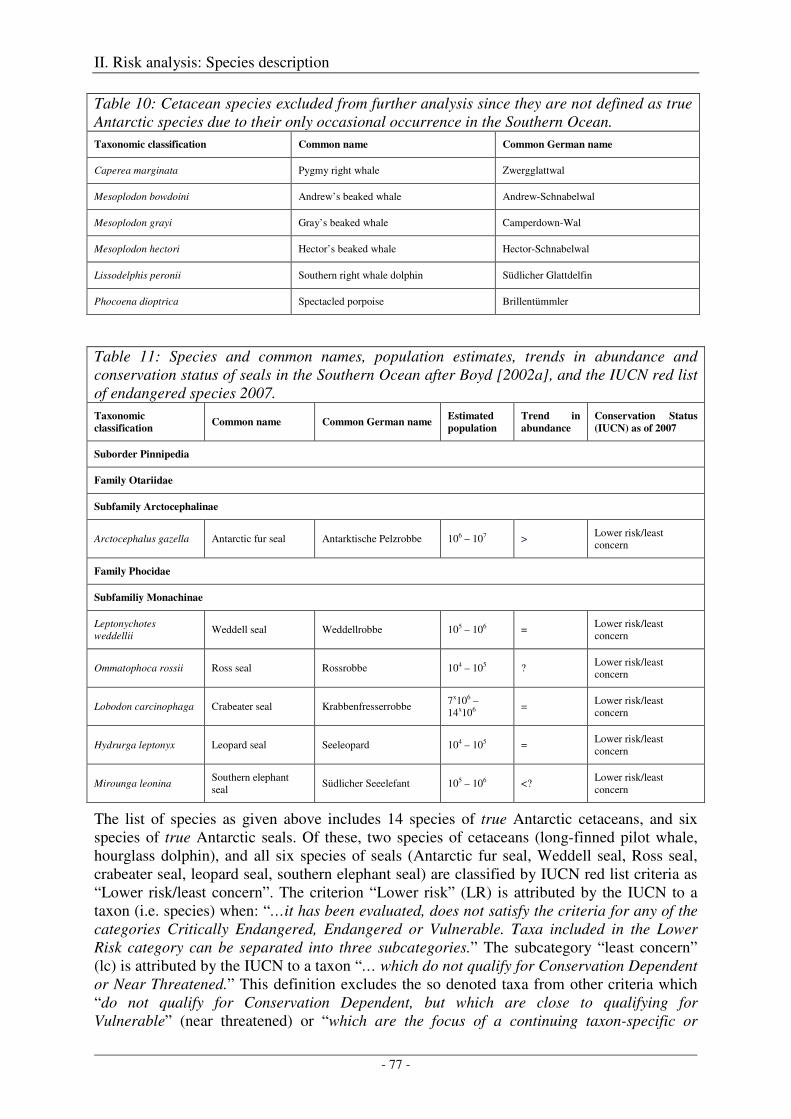
II. Risk analysis: Species description
- 77 -
Table 10: Cetacean species excluded from further analysis since they are not defined as true Antarctic species due to their only occasional occurrence in the Southern Ocean.
Taxonomic classification Common name Common German name
Caperea marginata Pygmy right whale Zwergglattwal
Mesoplodon bowdoini Andrew’s beaked whale Andrew-Schnabelwal
Mesoplodon grayi Gray’s beaked whale Camperdown-Wal
Mesoplodon hectori Hector’s beaked whale Hector-Schnabelwal
Lissodelphis peronii Southern right whale dolphin Südlicher Glattdelfin
Phocoena dioptrica Spectacled porpoise Brillentümmler
Table 11: Species and common names, population estimates, trends in abundance and conservation status of seals in the Southern Ocean after Boyd [2002a], and the IUCN red list of endangered species 2007.
Taxonomic
classification Common name Common German name
Estimated
population
Trend in
abundance
Conservation Status
(IUCN) as of 2007
Suborder Pinnipedia
Family Otariidae
Subfamily Arctocephalinae
Arctocephalus gazella Antarctic fur seal Antarktische Pelzrobbe 106 – 107 > Lower risk/least concern
Family Phocidae
Subfamiliy Monachinae
Leptonychotes weddellii
Weddell seal Weddellrobbe 105 – 106 = Lower risk/least concern
Ommatophoca rossii Ross seal Rossrobbe 104 – 105 ? Lower risk/least concern
Lobodon carcinophaga Crabeater seal Krabbenfresserrobbe 7x10⁶ – 14x106
= Lower risk/least concern
Hydrurga leptonyx Leopard seal Seeleopard 104 – 105 = Lower risk/least concern
Mirounga leonina Southern elephant seal
Südlicher Seeelefant 105 – 106 <? Lower risk/least concern
The list of species as given above includes 14 species of true Antarctic cetaceans, and six species of true Antarctic seals. Of these, two species of cetaceans (long-finned pilot whale, hourglass dolphin), and all six species of seals (Antarctic fur seal, Weddell seal, Ross seal, crabeater seal, leopard seal, southern elephant seal) are classified by IUCN red list criteria as “Lower risk/least concern”. The criterion “Lower risk” (LR) is attributed by the IUCN to a taxon (i.e. species) when: “…it has been evaluated, does not satisfy the criteria for any of the categories Critically Endangered, Endangered or Vulnerable. Taxa included in the Lower Risk category can be separated into three subcategories.” The subcategory “least concern” (lc) is attributed by the IUCN to a taxon “… which do not qualify for Conservation Dependent or Near Threatened.” This definition excludes the so denoted taxa from other criteria which “do not qualify for Conservation Dependent, but which are close to qualifying for Vulnerable” (near threatened) or “which are the focus of a continuing taxon-specific or
II. Risk analysis: Species description
- 78 -
habitat-specific conservation programme targeted towards the taxon in question, the cessation of which would result in the taxon qualifying for one of the threatened categories above within a period of five years” (see IUCN red list of endangered species http://www.iucnredlist.org/).
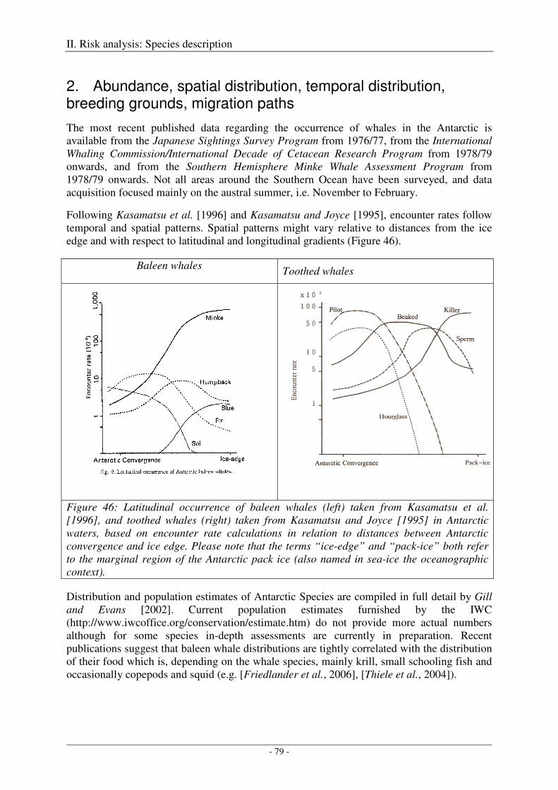
II. Risk analysis: Species description
- 79 -
2. Abundance, spatial distribution, temporal distribution, breeding grounds, migration paths
The most recent published data regarding the occurrence of whales in the Antarctic is available from the Japanese Sightings Survey Program from 1976/77, from the International Whaling Commission/International Decade of Cetacean Research Program from 1978/79 onwards, and from the Southern Hemisphere Minke Whale Assessment Program from 1978/79 onwards. Not all areas around the Southern Ocean have been surveyed, and data acquisition focused mainly on the austral summer, i.e. November to February.
Following Kasamatsu et al. [1996] and Kasamatsu and Joyce [1995], encounter rates follow temporal and spatial patterns. Spatial patterns might vary relative to distances from the ice edge and with respect to latitudinal and longitudinal gradients (Figure 46).
Baleen whales Toothed whales
Figure 46: Latitudinal occurrence of baleen whales (left) taken from Kasamatsu et al. [1996], and toothed whales (right) taken from Kasamatsu and Joyce [1995] in Antarctic waters, based on encounter rate calculations in relation to distances between Antarctic convergence and ice edge. Please note that the terms “ice-edge” and “pack-ice” both refer to the marginal region of the Antarctic pack ice (also named in sea-ice the oceanographic context).
Distribution and population estimates of Antarctic Species are compiled in full detail by Gill and Evans [2002]. Current population estimates furnished by the IWC (http://www.iwcoffice.org/conservation/estimate.htm) do not provide more actual numbers although for some species in-depth assessments are currently in preparation. Recent publications suggest that baleen whale distributions are tightly correlated with the distribution of their food which is, depending on the whale species, mainly krill, small schooling fish and occasionally copepods and squid (e.g. [Friedlander et al., 2006], [Thiele et al., 2004]).
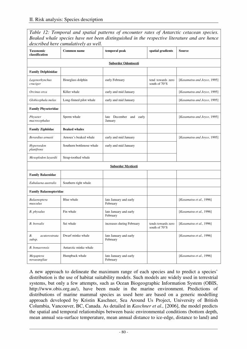
II. Risk analysis: Species description
- 80 -
Table 12: Temporal and spatial patterns of encounter rates of Antarctic cetacean species. Beaked whale species have not been distinguished in the respective literature and are hence described here cumulatively as well.
Taxonomic
classification
Common name temporal peak spatial gradients Source
Suborder Odontoceti
Family Delphinidae
Lagenorhynchus cruciger
Hourglass dolphin early February tend towards zero south of 70°S
[Kasamatsu and Joyce, 1995]
Orcinus orca Killer whale early and mid January [Kasamatsu and Joyce, 1995]
Globicephala melas Long-finned pilot whale early and mid January [Kasamatsu and Joyce, 1995]
Family Physeteridae
Physeter macrocephalus
Sperm whale late December and early January
[Kasamatsu and Joyce, 1995]
Family Ziphiidae Beaked whales
Berardius arnuxii Arnoux’s beaked whale early and mid January [Kasamatsu and Joyce, 1995]
Hyperoodon planifrons
Southern bottlenose whale early and mid January
Mesoplodon layardii Strap-toothed whale
Suborder Mysticeti
Family Balaenidae
Eubalaena australis Southern right whale
Family Balaenopteridae
Balaenoptera musculus
Blue whale late January and early February
[Kasamatsu et al., 1996]
B. physalus Fin whale late January and early February
[Kasamatsu et al., 1996]
B. borealis Sei whale increases during February tends towards zero south of 70°S
[Kasamatsu et al., 1996]
B. acutorostrata subsp.
Dwarf minke whale late January and early February
[Kasamatsu et al., 1996]
B. bonaerensis Antarctic minke whale
Megaptera novaeangliae
Humpback whale late January and early February
[Kasamatsu et al., 1996]
A new approach to delineate the maximum range of each species and to predict a species’ distribution is the use of habitat suitability models. Such models are widely used in terrestrial systems, but only a few attempts, such as Ocean Biogeographic Information System (OBIS, http://www.obis.org.au/), have been made in the marine environment. Predictions of distributions of marine mammal species as used here are based on a generic modelling approach developed by Kristin Kaschner, Sea Around Us Project, University of British Columbia, Vancouver, BC, Canada. As detailed in Kaschner et al., [2006], the model predicts the spatial and temporal relationships between basic environmental conditions (bottom depth, mean annual sea-surface temperature, mean annual distance to ice-edge, distance to land) and
II. Risk analysis: Species description
- 81 -
a given species’ presence on a global grid with cell dimensions of half a degree latitude by half a degree longitude. Although we include the resulting maps as measures of potential distributions of species, the maps represent hypotheses about the relative environmental suitability (RES) of a specific area for a specific species rather than actual densities or probabilities of occurrences. The model is currently enhanced to predict relative densities and is used by a number of institutions (and companies) like the Forschungsanstalt für Wasserschall and Geophysik, Kiel, Germany and the British Royal Navy. The advantage of using such a model would be that it could be included in the planning process and cruise tracks could be planned to cause least impact. The disadvantage of the model at the moment is the limited information about abundance of many species especially for such remote areas like the Southern Ocean.
Detailed knowledge of the stock structure is a fundamental aspect in the conservation of marine mammals, particularly with regard to their reproduction and stock trends. However, with Antarctica serving – at least for most cetacean species – as a region of transitory occupancy, The stock definition as used by the IWC [Donovan, 1991] is – solely for management purposes - in terms of feeding stocks, rather than breeding stocks and in all but few cases it is unresolved which animal from feedings stocks I-VI in the Antarctic belong to which breeding grounds in higher latitudes. More recent genetic studies (humpbacks, minkes) aim at revealing this association, but the topic is a field of ongoing research, and a detailed analysis of the current state of research regarding all species is a full field of research in itself (the IWC science committee features two main topics „Whale stocks“ and „Stock definition“ alone), and beyond the scope of this study [International Whaling Commission (IWC), 2006a; b; 2008a; b]. Current results, particularly including genetic samples from Antarctica, are yet insufficient to be used in the context of a generic risk assessment, though some aspects for specific regions might be included in concrete applications for a research permit. The topic “stock structure” as such, however, is a major, highly active research area, and is correspondingly listed in section Research Needs.
In the following section, the current state of knowledge is given for each relevant species, condensing the information provided by Gill and Evans [2002] and merging it with results from recent studies. Please note, that when referring hereinafter to a species such as the “blue whale”, it is meant to refer to the “true” Antarctic blue whale population only, rather than to the global stock. The same applies to all other species discussed.
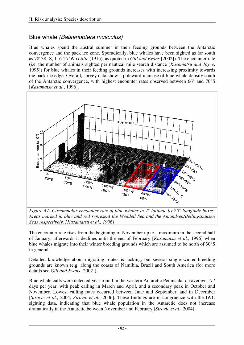
II. Risk analysis: Species description
- 82 -
Blue whale (Balaenoptera musculus)
Blue whales spend the austral summer in their feeding grounds between the Antarctic convergence and the pack ice zone. Sporadically, blue whales have been sighted as far south as 78°38’ S, 116°17’W (Lillie (1915), as quoted in Gill and Evans [2002]). The encounter rate (i.e. the number of animals sighted per nautical mile search distance [Kasamatsu and Joyce, 1995]) for blue whales in their feeding grounds increases with increasing proximity towards the pack ice edge. Overall, survey data show a poleward increase of blue whale density south of the Antarctic convergence, with highest encounter rates observed between 66° and 70°S [Kasamatsu et al., 1996].
Figure 47: Circumpolar encounter rate of blue whales in 4° latitude by 20° longitude boxes. Areas marked in blue and red represent the Weddell Sea and the Amundsen/Bellingshausen Seas respectively. [Kasamatsu et al., 1996]
The encounter rate rises from the beginning of November up to a maximum in the second half of January; afterwards it declines until the end of February [Kasamatsu et al., 1996] when blue whales migrate into their winter breeding grounds which are assumed to be north of 30°S in general.
Detailed knowledge about migrating routes is lacking, but several single winter breeding grounds are known (e.g. along the coasts of Namibia, Brazil and South America (for more details see Gill and Evans [2002]).
Blue whale calls were detected year round in the western Antarctic Peninsula, on average 177 days per year, with peak calling in March and April, and a secondary peak in October and November. Lowest calling rates occurred between June and September, and in December [Sirovic et al., 2004; Sirovic et al., 2006]. These findings are in congruence with the IWC sighting data, indicating that blue whale population in the Antarctic does not increase dramatically in the Antarctic between November and February [Sirovic et al., 2004].
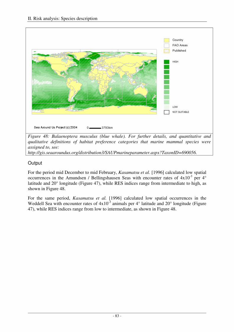
II. Risk analysis: Species description
- 83 -
Figure 48: Balaenoptera musculus (blue whale). For further details, and quantitative and qualitative definitions of habitat preference categories that marine mammal species were assigned to, see: http://gis.seaaroundus.org/distribution3/SAUPmarineparameter.aspx?TaxonID=690056.
Output
For the period mid December to mid February, Kasamatsu et al. [1996] calculated low spatial occurrences in the Amundsen / Bellingshausen Seas with encounter rates of 4x10⁻³ per 4° latitude and 20° longitude (Figure 47), while RES indices range from intermediate to high, as shown in Figure 48.
For the same period, Kasamatsu et al. [1996] calculated low spatial occurrences in the Weddell Sea with encounter rates of 4x10⁻³ animals per 4° latitude and 20° longitude (Figure 47), while RES indices range from low to intermediate, as shown in Figure 48.
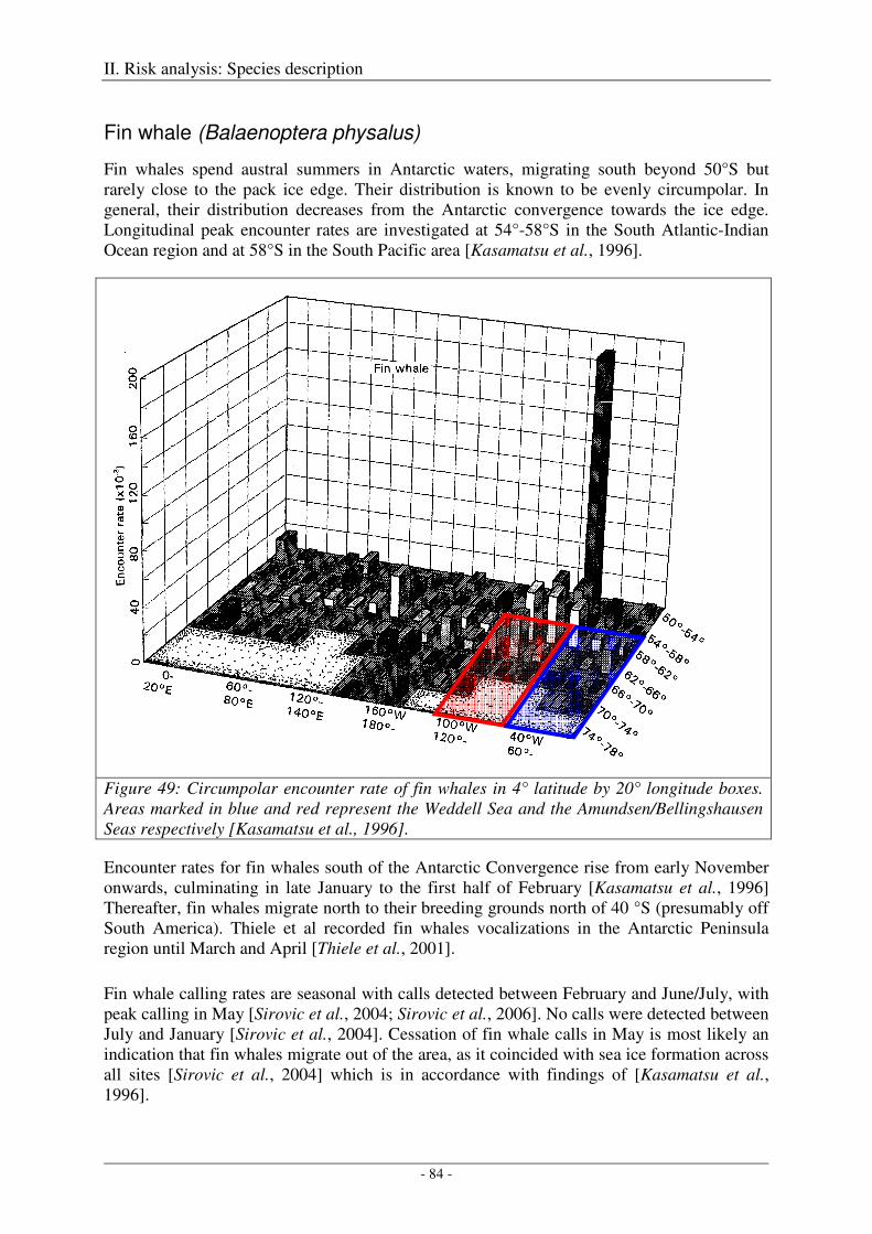
II. Risk analysis: Species description
- 84 -
Fin whale (Balaenoptera physalus)
Fin whales spend austral summers in Antarctic waters, migrating south beyond 50°S but rarely close to the pack ice edge. Their distribution is known to be evenly circumpolar. In general, their distribution decreases from the Antarctic convergence towards the ice edge. Longitudinal peak encounter rates are investigated at 54°-58°S in the South Atlantic-Indian Ocean region and at 58°S in the South Pacific area [Kasamatsu et al., 1996].
Figure 49: Circumpolar encounter rate of fin whales in 4° latitude by 20° longitude boxes. Areas marked in blue and red represent the Weddell Sea and the Amundsen/Bellingshausen Seas respectively [Kasamatsu et al., 1996].
Encounter rates for fin whales south of the Antarctic Convergence rise from early November onwards, culminating in late January to the first half of February [Kasamatsu et al., 1996] Thereafter, fin whales migrate north to their breeding grounds north of 40 °S (presumably off South America). Thiele et al recorded fin whales vocalizations in the Antarctic Peninsula region until March and April [Thiele et al., 2001].
Fin whale calling rates are seasonal with calls detected between February and June/July, with peak calling in May [Sirovic et al., 2004; Sirovic et al., 2006]. No calls were detected between July and January [Sirovic et al., 2004]. Cessation of fin whale calls in May is most likely an indication that fin whales migrate out of the area, as it coincided with sea ice formation across all sites [Sirovic et al., 2004] which is in accordance with findings of [Kasamatsu et al., 1996].
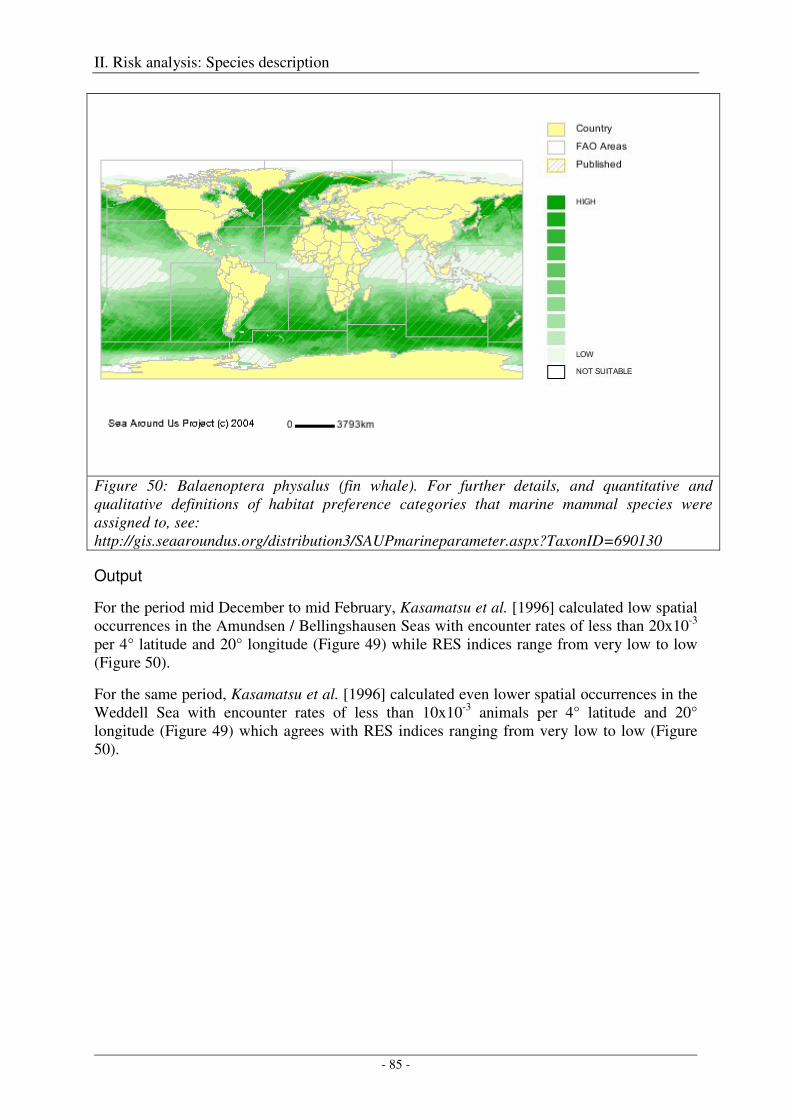
II. Risk analysis: Species description
- 85 -
Figure 50: Balaenoptera physalus (fin whale). For further details, and quantitative and qualitative definitions of habitat preference categories that marine mammal species were assigned to, see: http://gis.seaaroundus.org/distribution3/SAUPmarineparameter.aspx?TaxonID=690130
Output
For the period mid December to mid February, Kasamatsu et al. [1996] calculated low spatial occurrences in the Amundsen / Bellingshausen Seas with encounter rates of less than 20x10-3 per 4° latitude and 20° longitude (Figure 49) while RES indices range from very low to low (Figure 50).
For the same period, Kasamatsu et al. [1996] calculated even lower spatial occurrences in the Weddell Sea with encounter rates of less than 10x10-3 animals per 4° latitude and 20° longitude (Figure 49) which agrees with RES indices ranging from very low to low (Figure 50).
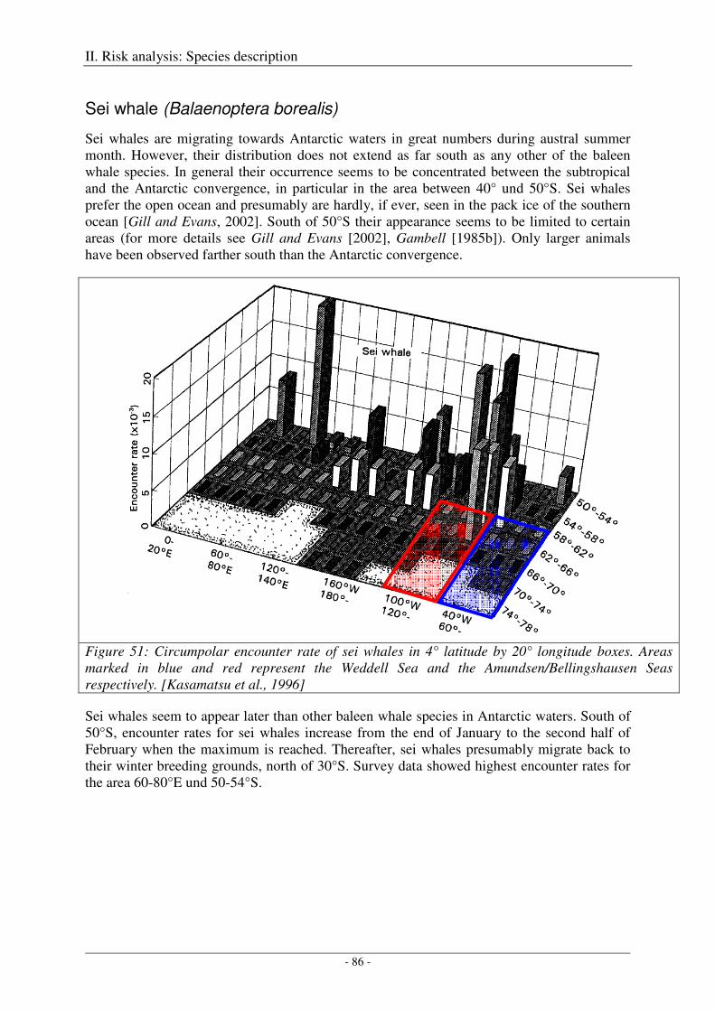
II. Risk analysis: Species description
- 86 -
Sei whale (Balaenoptera borealis)
Sei whales are migrating towards Antarctic waters in great numbers during austral summer month. However, their distribution does not extend as far south as any other of the baleen whale species. In general their occurrence seems to be concentrated between the subtropical and the Antarctic convergence, in particular in the area between 40° und 50°S. Sei whales prefer the open ocean and presumably are hardly, if ever, seen in the pack ice of the southern ocean [Gill and Evans, 2002]. South of 50°S their appearance seems to be limited to certain areas (for more details see Gill and Evans [2002], Gambell [1985b]). Only larger animals have been observed farther south than the Antarctic convergence.
Figure 51: Circumpolar encounter rate of sei whales in 4° latitude by 20° longitude boxes. Areas marked in blue and red represent the Weddell Sea and the Amundsen/Bellingshausen Seas respectively. [Kasamatsu et al., 1996]
Sei whales seem to appear later than other baleen whale species in Antarctic waters. South of 50°S, encounter rates for sei whales increase from the end of January to the second half of February when the maximum is reached. Thereafter, sei whales presumably migrate back to their winter breeding grounds, north of 30°S. Survey data showed highest encounter rates for the area 60-80°E und 50-54°S.
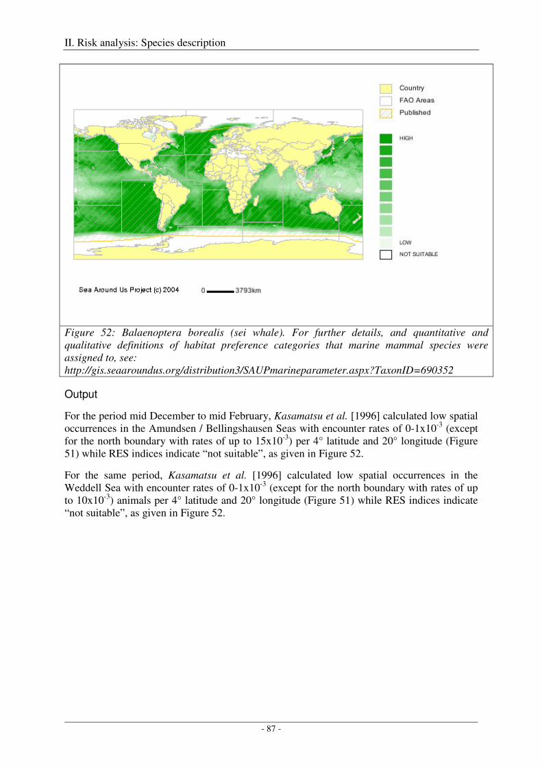
II. Risk analysis: Species description
- 87 -
Figure 52: Balaenoptera borealis (sei whale). For further details, and quantitative and qualitative definitions of habitat preference categories that marine mammal species were assigned to, see: http://gis.seaaroundus.org/distribution3/SAUPmarineparameter.aspx?TaxonID=690352
Output
For the period mid December to mid February, Kasamatsu et al. [1996] calculated low spatial occurrences in the Amundsen / Bellingshausen Seas with encounter rates of 0-1x10⁻³ (except for the north boundary with rates of up to 15x10-3) per 4° latitude and 20° longitude (Figure 51) while RES indices indicate “not suitable”, as given in Figure 52.
For the same period, Kasamatsu et al. [1996] calculated low spatial occurrences in the Weddell Sea with encounter rates of 0-1x10⁻³ (except for the north boundary with rates of up to 10x10-3) animals per 4° latitude and 20° longitude (Figure 51) while RES indices indicate “not suitable”, as given in Figure 52.
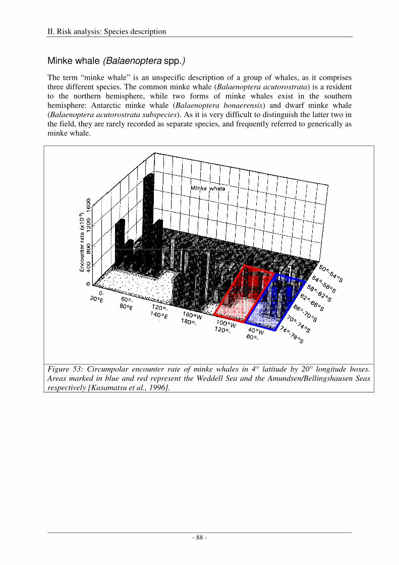
II. Risk analysis: Species description
- 88 -
Minke whale (Balaenoptera spp.)
The term “minke whale” is an unspecific description of a group of whales, as it comprises three different species. The common minke whale (Balaenoptera acutorostrata) is a resident to the northern hemisphere, while two forms of minke whales exist in the southern hemisphere: Antarctic minke whale (Balaenoptera bonaerensis) and dwarf minke whale (Balaenoptera acutorostrata subspecies). As it is very difficult to distinguish the latter two in the field, they are rarely recorded as separate species, and frequently referred to generically as minke whale.
Figure 53: Circumpolar encounter rate of minke whales in 4° latitude by 20° longitude boxes. Areas marked in blue and red represent the Weddell Sea and the Amundsen/Bellingshausen Seas respectively [Kasamatsu et al., 1996].
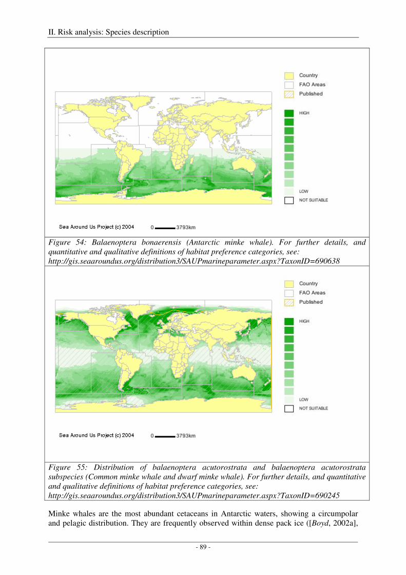
II. Risk analysis: Species description
- 89 -
Figure 54: Balaenoptera bonaerensis (Antarctic minke whale). For further details, and quantitative and qualitative definitions of habitat preference categories, see: http://gis.seaaroundus.org/distribution3/SAUPmarineparameter.aspx?TaxonID=690638
Figure 55: Distribution of balaenoptera acutorostrata and balaenoptera acutorostrata subspecies (Common minke whale and dwarf minke whale). For further details, and quantitative and qualitative definitions of habitat preference categories, see: http://gis.seaaroundus.org/distribution3/SAUPmarineparameter.aspx?TaxonID=690245
Minke whales are the most abundant cetaceans in Antarctic waters, showing a circumpolar and pelagic distribution. They are frequently observed within dense pack ice ([Boyd, 2002a],
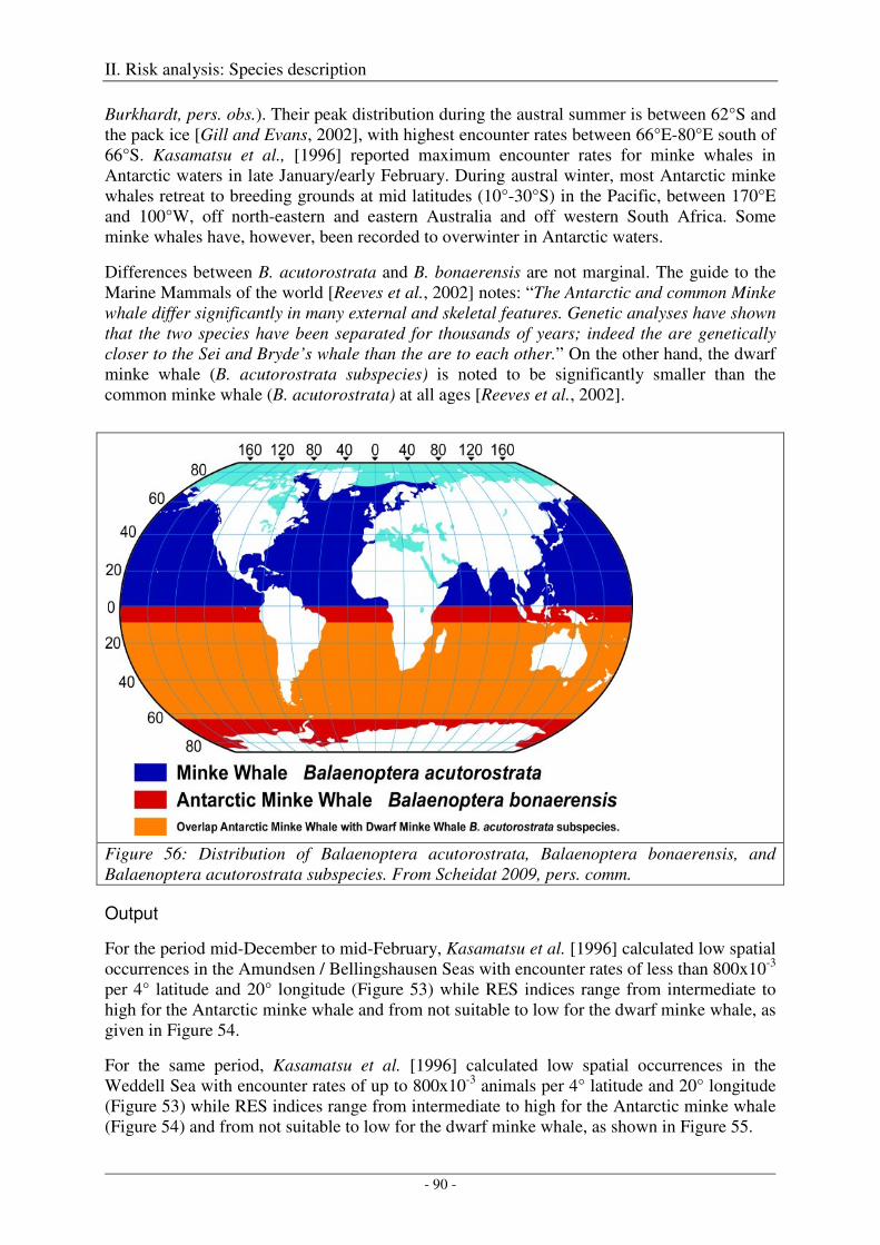
II. Risk analysis: Species description
- 90 -
Burkhardt, pers. obs.). Their peak distribution during the austral summer is between 62°S and the pack ice [Gill and Evans, 2002], with highest encounter rates between 66°E-80°E south of 66°S. Kasamatsu et al., [1996] reported maximum encounter rates for minke whales in Antarctic waters in late January/early February. During austral winter, most Antarctic minke whales retreat to breeding grounds at mid latitudes (10°-30°S) in the Pacific, between 170°E and 100°W, off north-eastern and eastern Australia and off western South Africa. Some minke whales have, however, been recorded to overwinter in Antarctic waters.
Differences between B. acutorostrata and B. bonaerensis are not marginal. The guide to the Marine Mammals of the world [Reeves et al., 2002] notes: “The Antarctic and common Minke whale differ significantly in many external and skeletal features. Genetic analyses have shown that the two species have been separated for thousands of years; indeed the are genetically closer to the Sei and Bryde’s whale than the are to each other.” On the other hand, the dwarf minke whale (B. acutorostrata subspecies) is noted to be significantly smaller than the common minke whale (B. acutorostrata) at all ages [Reeves et al., 2002].
Figure 56: Distribution of Balaenoptera acutorostrata, Balaenoptera bonaerensis, and Balaenoptera acutorostrata subspecies. From Scheidat 2009, pers. comm.
Output
For the period mid-December to mid-February, Kasamatsu et al. [1996] calculated low spatial occurrences in the Amundsen / Bellingshausen Seas with encounter rates of less than 800x10-3 per 4° latitude and 20° longitude (Figure 53) while RES indices range from intermediate to high for the Antarctic minke whale and from not suitable to low for the dwarf minke whale, as given in Figure 54.
For the same period, Kasamatsu et al. [1996] calculated low spatial occurrences in the Weddell Sea with encounter rates of up to 800x10-3 animals per 4° latitude and 20° longitude (Figure 53) while RES indices range from intermediate to high for the Antarctic minke whale (Figure 54) and from not suitable to low for the dwarf minke whale, as shown in Figure 55.
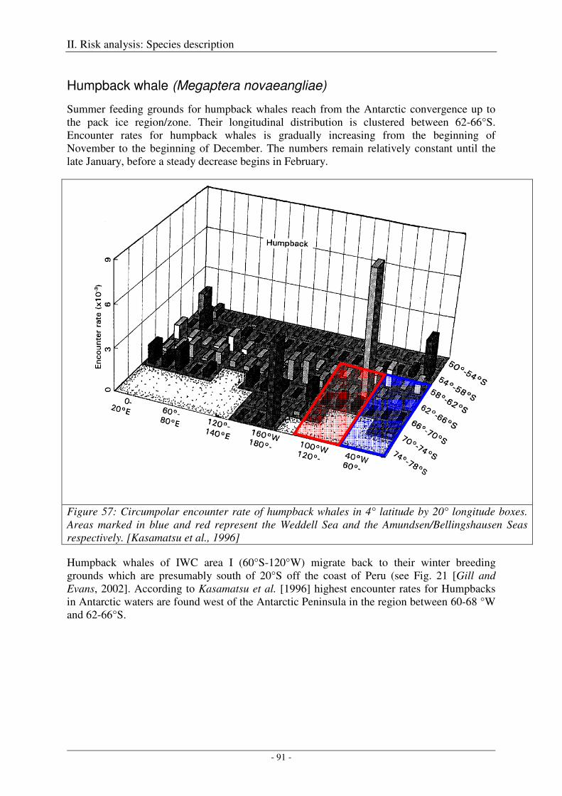
II. Risk analysis: Species description
- 91 -
Humpback whale (Megaptera novaeangliae)
Summer feeding grounds for humpback whales reach from the Antarctic convergence up to the pack ice region/zone. Their longitudinal distribution is clustered between 62-66°S. Encounter rates for humpback whales is gradually increasing from the beginning of November to the beginning of December. The numbers remain relatively constant until the late January, before a steady decrease begins in February.
Figure 57: Circumpolar encounter rate of humpback whales in 4° latitude by 20° longitude boxes. Areas marked in blue and red represent the Weddell Sea and the Amundsen/Bellingshausen Seas respectively. [Kasamatsu et al., 1996]
Humpback whales of IWC area I (60°S-120°W) migrate back to their winter breeding grounds which are presumably south of 20°S off the coast of Peru (see Fig. 21 [Gill and Evans, 2002]. According to Kasamatsu et al. [1996] highest encounter rates for Humpbacks in Antarctic waters are found west of the Antarctic Peninsula in the region between 60-68 °W and 62-66°S.
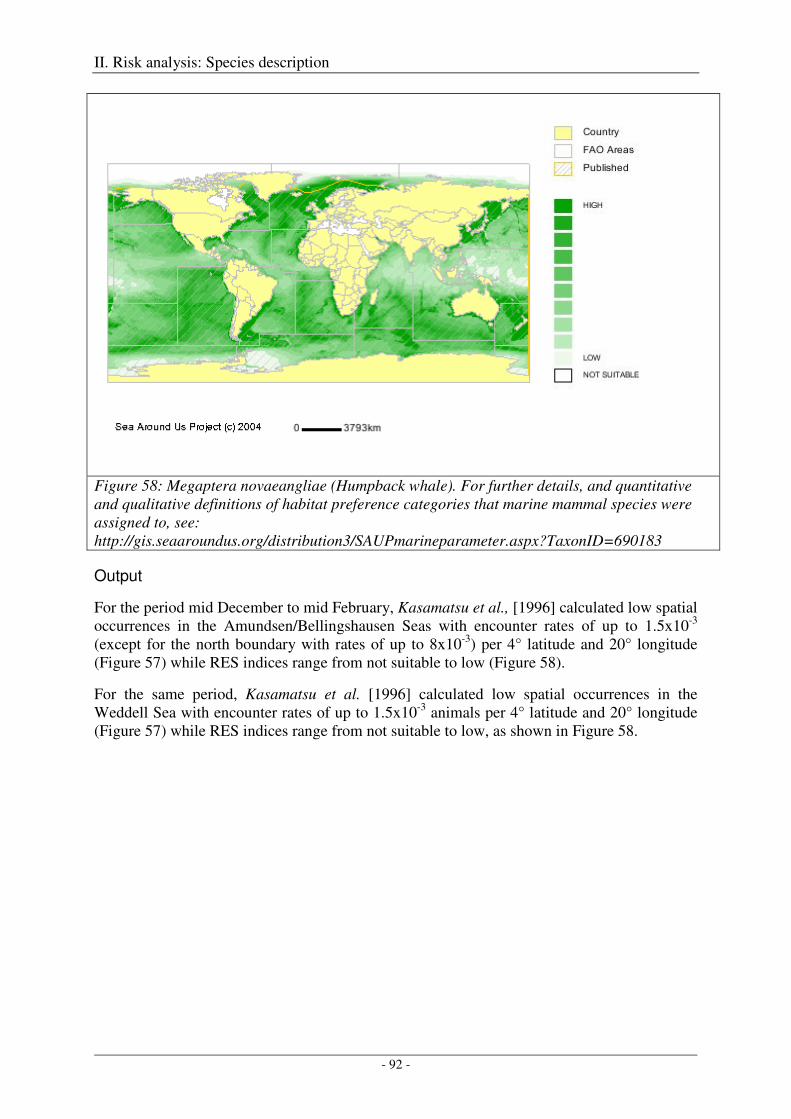
II. Risk analysis: Species description
- 92 -
Figure 58: Megaptera novaeangliae (Humpback whale). For further details, and quantitative and qualitative definitions of habitat preference categories that marine mammal species were assigned to, see: http://gis.seaaroundus.org/distribution3/SAUPmarineparameter.aspx?TaxonID=690183
Output
For the period mid December to mid February, Kasamatsu et al., [1996] calculated low spatial occurrences in the Amundsen/Bellingshausen Seas with encounter rates of up to 1.5x10⁻³ (except for the north boundary with rates of up to 8x10⁻³) per 4° latitude and 20° longitude (Figure 57) while RES indices range from not suitable to low (Figure 58).
For the same period, Kasamatsu et al. [1996] calculated low spatial occurrences in the Weddell Sea with encounter rates of up to 1.5x10⁻³ animals per 4° latitude and 20° longitude (Figure 57) while RES indices range from not suitable to low, as shown in Figure 58.
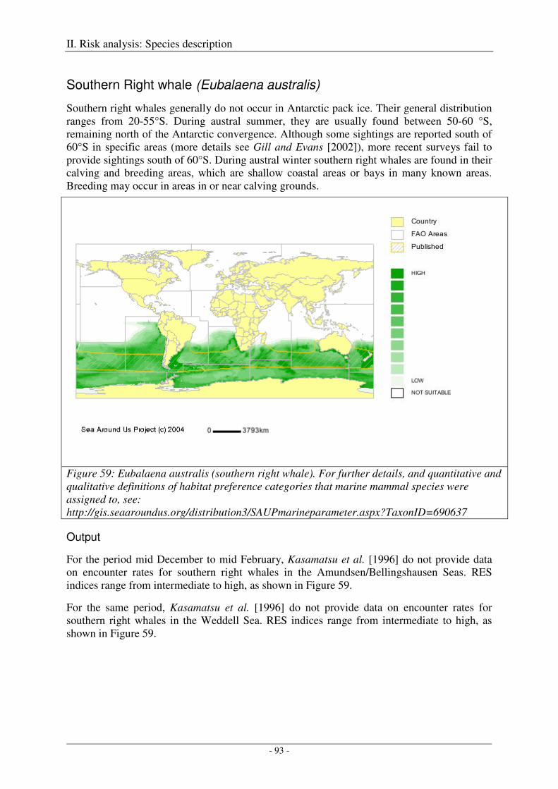
II. Risk analysis: Species description
- 93 -
Southern Right whale (Eubalaena australis)
Southern right whales generally do not occur in Antarctic pack ice. Their general distribution ranges from 20-55°S. During austral summer, they are usually found between 50-60 °S, remaining north of the Antarctic convergence. Although some sightings are reported south of 60°S in specific areas (more details see Gill and Evans [2002]), more recent surveys fail to provide sightings south of 60°S. During austral winter southern right whales are found in their calving and breeding areas, which are shallow coastal areas or bays in many known areas. Breeding may occur in areas in or near calving grounds.
Figure 59: Eubalaena australis (southern right whale). For further details, and quantitative and qualitative definitions of habitat preference categories that marine mammal species were assigned to, see: http://gis.seaaroundus.org/distribution3/SAUPmarineparameter.aspx?TaxonID=690637
Output
For the period mid December to mid February, Kasamatsu et al. [1996] do not provide data on encounter rates for southern right whales in the Amundsen/Bellingshausen Seas. RES indices range from intermediate to high, as shown in Figure 59.
For the same period, Kasamatsu et al. [1996] do not provide data on encounter rates for southern right whales in the Weddell Sea. RES indices range from intermediate to high, as shown in Figure 59.
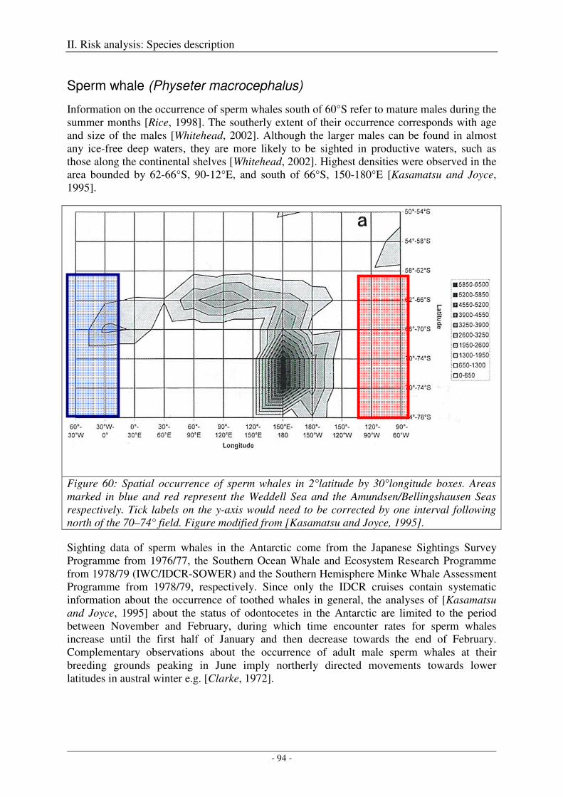
II. Risk analysis: Species description
- 94 -
Sperm whale (Physeter macrocephalus)
Information on the occurrence of sperm whales south of 60°S refer to mature males during the summer months [Rice, 1998]. The southerly extent of their occurrence corresponds with age and size of the males [Whitehead, 2002]. Although the larger males can be found in almost any ice-free deep waters, they are more likely to be sighted in productive waters, such as those along the continental shelves [Whitehead, 2002]. Highest densities were observed in the area bounded by 62-66°S, 90-12°E, and south of 66°S, 150-180°E [Kasamatsu and Joyce, 1995].
Figure 60: Spatial occurrence of sperm whales in 2°latitude by 30°longitude boxes. Areas marked in blue and red represent the Weddell Sea and the Amundsen/Bellingshausen Seas respectively. Tick labels on the y-axis would need to be corrected by one interval following north of the 70–74° field. Figure modified from [Kasamatsu and Joyce, 1995].
Sighting data of sperm whales in the Antarctic come from the Japanese Sightings Survey Programme from 1976/77, the Southern Ocean Whale and Ecosystem Research Programme from 1978/79 (IWC/IDCR-SOWER) and the Southern Hemisphere Minke Whale Assessment Programme from 1978/79, respectively. Since only the IDCR cruises contain systematic information about the occurrence of toothed whales in general, the analyses of [Kasamatsu and Joyce, 1995] about the status of odontocetes in the Antarctic are limited to the period between November and February, during which time encounter rates for sperm whales increase until the first half of January and then decrease towards the end of February. Complementary observations about the occurrence of adult male sperm whales at their breeding grounds peaking in June imply northerly directed movements towards lower latitudes in austral winter e.g. [Clarke, 1972].
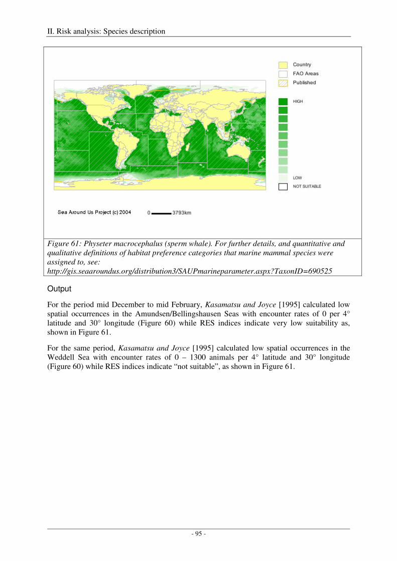
II. Risk analysis: Species description
- 95 -
Figure 61: Physeter macrocephalus (sperm whale). For further details, and quantitative and qualitative definitions of habitat preference categories that marine mammal species were assigned to, see: http://gis.seaaroundus.org/distribution3/SAUPmarineparameter.aspx?TaxonID=690525
Output
For the period mid December to mid February, Kasamatsu and Joyce [1995] calculated low spatial occurrences in the Amundsen/Bellingshausen Seas with encounter rates of 0 per 4° latitude and 30° longitude (Figure 60) while RES indices indicate very low suitability as, shown in Figure 61.
For the same period, Kasamatsu and Joyce [1995] calculated low spatial occurrences in the Weddell Sea with encounter rates of 0 – 1300 animals per 4° latitude and 30° longitude (Figure 60) while RES indices indicate “not suitable”, as shown in Figure 61.
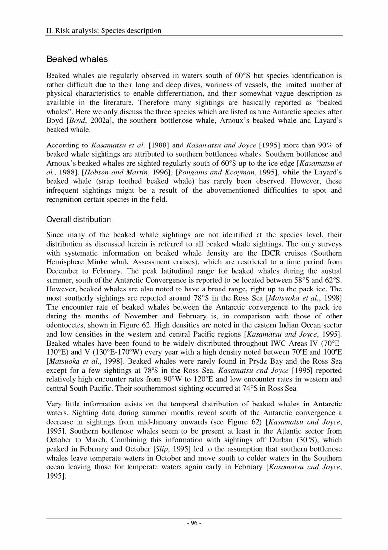
II. Risk analysis: Species description
- 96 -
Beaked whales
Beaked whales are regularly observed in waters south of 60°S but species identification is rather difficult due to their long and deep dives, wariness of vessels, the limited number of physical characteristics to enable differentiation, and their somewhat vague description as available in the literature. Therefore many sightings are basically reported as “beaked whales”. Here we only discuss the three species which are listed as true Antarctic species after Boyd [Boyd, 2002a], the southern bottlenose whale, Arnoux’s beaked whale and Layard’s beaked whale.
According to Kasamatsu et al. [1988] and Kasamatsu and Joyce [1995] more than 90% of beaked whale sightings are attributed to southern bottlenose whales. Southern bottlenose and Arnoux’s beaked whales are sighted regularly south of 60°S up to the ice edge [Kasamatsu et al., 1988], [Hobson and Martin, 1996], [Ponganis and Kooyman, 1995], while the Layard’s beaked whale (strap toothed beaked whale) has rarely been observed. However, these infrequent sightings might be a result of the abovementioned difficulties to spot and recognition certain species in the field.
Overall distribution
Since many of the beaked whale sightings are not identified at the species level, their distribution as discussed herein is referred to all beaked whale sightings. The only surveys with systematic information on beaked whale density are the IDCR cruises (Southern Hemisphere Minke whale Assessment cruises), which are restricted to a time period from December to February. The peak latitudinal range for beaked whales during the austral summer, south of the Antarctic Convergence is reported to be located between 58°S and 62°S. However, beaked whales are also noted to have a broad range, right up to the pack ice. The most southerly sightings are reported around 78°S in the Ross Sea [Matsuoka et al., 1998] The encounter rate of beaked whales between the Antarctic convergence to the pack ice during the months of November and February is, in comparison with those of other odontocetes, shown in Figure 62. High densities are noted in the eastern Indian Ocean sector and low densities in the western and central Pacific regions [Kasamatsu and Joyce, 1995]. Beaked whales have been found to be widely distributed throughout IWC Areas IV (70°E-130°E) and V (130°E-170°W) every year with a high density noted between 70ºE and 100ºE [Matsuoka et al., 1998]. Beaked whales were rarely found in Prydz Bay and the Ross Sea except for a few sightings at 78ºS in the Ross Sea. Kasamatsu and Joyce [1995] reported relatively high encounter rates from 90°W to 120°E and low encounter rates in western and central South Pacific. Their southernmost sighting occurred at 74°S in Ross Sea
Very little information exists on the temporal distribution of beaked whales in Antarctic waters. Sighting data during summer months reveal south of the Antarctic convergence a decrease in sightings from mid-January onwards (see Figure 62) [Kasamatsu and Joyce, 1995]. Southern bottlenose whales seem to be present at least in the Atlantic sector from October to March. Combining this information with sightings off Durban (30°S), which peaked in February and October [Slip, 1995] led to the assumption that southern bottlenose whales leave temperate waters in October and move south to colder waters in the Southern ocean leaving those for temperate waters again early in February [Kasamatsu and Joyce, 1995].
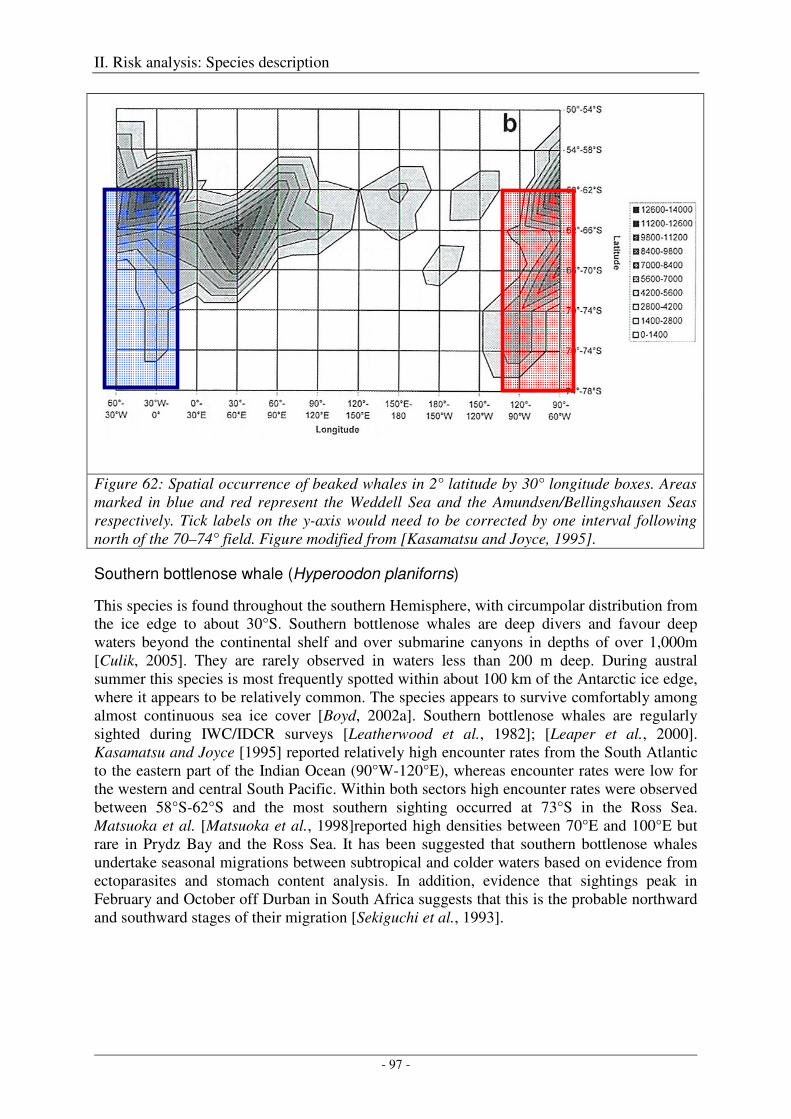
II. Risk analysis: Species description
- 97 -
Figure 62: Spatial occurrence of beaked whales in 2° latitude by 30° longitude boxes. Areas marked in blue and red represent the Weddell Sea and the Amundsen/Bellingshausen Seas respectively. Tick labels on the y-axis would need to be corrected by one interval following north of the 70–74° field. Figure modified from [Kasamatsu and Joyce, 1995].
Southern bottlenose whale (Hyperoodon planiforns)
This species is found throughout the southern Hemisphere, with circumpolar distribution from the ice edge to about 30°S. Southern bottlenose whales are deep divers and favour deep waters beyond the continental shelf and over submarine canyons in depths of over 1,000m [Culik, 2005]. They are rarely observed in waters less than 200 m deep. During austral summer this species is most frequently spotted within about 100 km of the Antarctic ice edge, where it appears to be relatively common. The species appears to survive comfortably among almost continuous sea ice cover [Boyd, 2002a]. Southern bottlenose whales are regularly sighted during IWC/IDCR surveys [Leatherwood et al., 1982]; [Leaper et al., 2000]. Kasamatsu and Joyce [1995] reported relatively high encounter rates from the South Atlantic to the eastern part of the Indian Ocean (90°W-120°E), whereas encounter rates were low for the western and central South Pacific. Within both sectors high encounter rates were observed between 58°S-62°S and the most southern sighting occurred at 73°S in the Ross Sea. Matsuoka et al. [Matsuoka et al., 1998]reported high densities between 70°E and 100°E but rare in Prydz Bay and the Ross Sea. It has been suggested that southern bottlenose whales undertake seasonal migrations between subtropical and colder waters based on evidence from ectoparasites and stomach content analysis. In addition, evidence that sightings peak in February and October off Durban in South Africa suggests that this is the probable northward and southward stages of their migration [Sekiguchi et al., 1993].
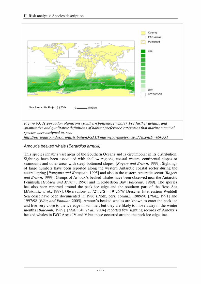
II. Risk analysis: Species description
- 98 -
Figure 63: Hyperoodon planifrons (southern bottlenose whale). For further details, and quantitative and qualitative definitions of habitat preference categories that marine mammal species were assigned to, see: http://gis.seaaroundus.org/distribution3/SAUPmarineparameter.aspx?TaxonID=690531
Arnoux’s beaked whale (Berardius arnuxii)
This species inhabits vast areas of the Southern Oceans and is circumpolar in its distribution. Sightings have been associated with shallow regions, coastal waters, continental slopes or seamounts and other areas with steep-bottomed slopes; [Rogers and Brown, 1999]. Sightings of large numbers have been reported along the western Antarctic coastal sector during the austral spring [Ponganis and Kooyman, 1995] and also in the eastern Antarctic sector [Rogers and Brown, 1999]. Groups of Arnoux’s beaked whales have been observed near the Antarctic Peninsula [Hobson and Martin, 1996] and in Robertson Bay [Balcomb, 1989]. The species has also been reported around the pack ice edge and the southern part of the Ross Sea [Matsuoka et al., 1998]. Observations at 72°52’S – 19°26’W Drescher Inlet eastern Weddell Sea coast have been documented in 1986 (Plötz, pers. comm.), 1989/90 [Plötz, 1991] and 1997/98 [Plötz and Ennulat, 2005]. Arnoux’s beaked whales are known to enter the pack ice and live very close to the ice edge in summer, but they are likely to move away in the winter months [Balcomb, 1989]. [Matsuoka et al., 2004] reported few sighting records of Arnoux’s beaked whales in IWC Areas IV and V but those occurred around the pack ice edge line.
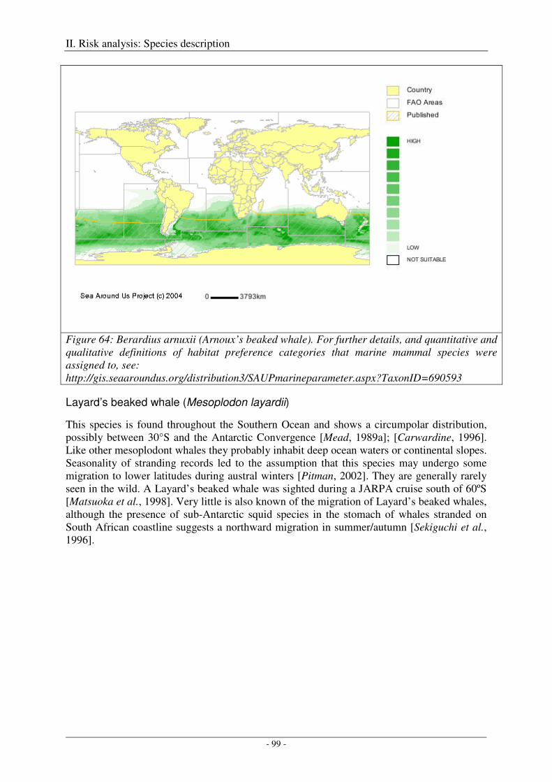
II. Risk analysis: Species description
- 99 -
Figure 64: Berardius arnuxii (Arnoux’s beaked whale). For further details, and quantitative and qualitative definitions of habitat preference categories that marine mammal species were assigned to, see: http://gis.seaaroundus.org/distribution3/SAUPmarineparameter.aspx?TaxonID=690593
Layard’s beaked whale (Mesoplodon layardii)
This species is found throughout the Southern Ocean and shows a circumpolar distribution, possibly between 30°S and the Antarctic Convergence [Mead, 1989a]; [Carwardine, 1996]. Like other mesoplodont whales they probably inhabit deep ocean waters or continental slopes. Seasonality of stranding records led to the assumption that this species may undergo some migration to lower latitudes during austral winters [Pitman, 2002]. They are generally rarely seen in the wild. A Layard’s beaked whale was sighted during a JARPA cruise south of 60ºS [Matsuoka et al., 1998]. Very little is also known of the migration of Layard’s beaked whales, although the presence of sub-Antarctic squid species in the stomach of whales stranded on South African coastline suggests a northward migration in summer/autumn [Sekiguchi et al., 1996].
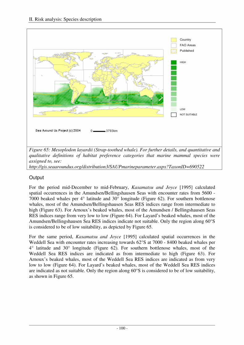
II. Risk analysis: Species description
- 100 -
Figure 65: Mesoplodon layardii (Strap-toothed whale). For further details, and quantitative and qualitative definitions of habitat preference categories that marine mammal species were assigned to, see: http://gis.seaaroundus.org/distribution3/SAUPmarineparameter.aspx?TaxonID=690522
Output
For the period mid-December to mid-February, Kasamatsu and Joyce [1995] calculated spatial occurrences in the Amundsen/Bellingshausen Seas with encounter rates from 5600 - 7000 beaked whales per 4° latitude and 30° longitude (Figure 62). For southern bottlenose whales, most of the Amundsen/Bellingshausen Seas RES indices range from intermediate to high (Figure 63). For Arnoux’s beaked whales, most of the Amundsen / Bellingshausen Seas RES indices range from very low to low (Figure 64). For Layard’s beaked whales, most of the Amundsen/Bellingshausen Sea RES indices indicate not suitable. Only the region along 60°S is considered to be of low suitability, as depicted by Figure 65.
For the same period, Kasamatsu and Joyce [1995] calculated spatial occurrences in the Weddell Sea with encounter rates increasing towards 62°S at 7000 - 8400 beaked whales per 4° latitude and 30° longitude (Figure 62). For southern bottlenose whales, most of the Weddell Sea RES indices are indicated as from intermediate to high (Figure 63). For Arnoux’s beaked whales, most of the Weddell Sea RES indices are indicated as from very low to low (Figure 64). For Layard’s beaked whales, most of the Weddell Sea RES indices are indicated as not suitable. Only the region along 60°S is considered to be of low suitability, as shown in Figure 65.
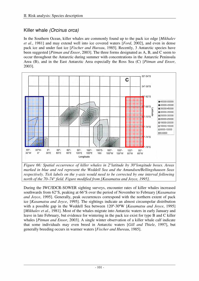
II. Risk analysis: Species description
- 101 -
Killer whale (Orcinus orca)
In the Southern Ocean, killer whales are commonly found up to the pack ice edge [Mikhalev et al., 1981] and may extend well into ice covered waters [Ford, 2002], and even in dense pack ice and under fast ice [Fischer and Hureau, 1985]. Recently, 3 Antarctic species have been suggested [Pitman and Ensor, 2003]. The three forms designated as A, B, and C seem to occur throughout the Antarctic during summer with concentrations in the Antarctic Peninsula Area (B), and in the East Antarctic Area especially the Ross Sea (C) [Pitman and Ensor, 2003].
Figure 66: Spatial occurrence of killer whales in 2°latitude by 30°longitude boxes. Areas marked in blue and red represent the Weddell Sea and the Amundsen/Bellingshausen Seas respectively. Tick labels on the y-axis would need to be corrected by one interval following north of the 70–74° field. Figure modified from [Kasamatsu and Joyce, 1995].
During the IWC/IDCR-SOWER sighting surveys, encounter rates of killer whales increased southwards from 62°S, peaking at 66°S over the period of November to February [Kasamatsu and Joyce, 1995]. Generally, peak occurrences correspond with the northern extent of pack ice [Kasamatsu and Joyce, 1995]. The sightings indicate an almost circumpolar distribution with a possible gap in the Weddell Sea between 120º-30ºW [Kasamatsu and Joyce, 1995] [Mikhalev et al., 1981]. Most of the whales migrate into Antarctic waters in early January and leave in late February, but evidence for wintering in the pack ice exist for type B and C killer whales [Pitman and Ensor, 2003]. A single winter observation of a killer whale calf indicate that some individuals may even breed in Antarctic waters [Gill and Thiele, 1997], but generally breeding occurs in warmer waters [Fischer and Hureau, 1985].
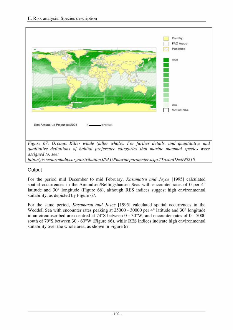
II. Risk analysis: Species description
- 102 -
Figure 67: Orcinus Killer whale (killer whale). For further details, and quantitative and qualitative definitions of habitat preference categories that marine mammal species were assigned to, see: http://gis.seaaroundus.org/distribution3/SAUPmarineparameter.aspx?TaxonID=690210
Output
For the period mid December to mid February, Kasamatsu and Joyce [1995] calculated spatial occurrences in the Amundsen/Bellingshausen Seas with encounter rates of 0 per 4° latitude and 30° longitude (Figure 66), although RES indices suggest high environmental suitability, as depicted by Figure 67.
For the same period, Kasamatsu and Joyce [1995] calculated spatial occurrences in the Weddell Sea with encounter rates peaking at 25000 - 30000 per 4° latitude and 30° longitude in an circumscribed area centred at 74°S between 0 - 30°W, and encounter rates of 0 - 5000 south of 70°S between 30 - 60°W (Figure 66), while RES indices indicate high environmental suitability over the whole area, as shown in Figure 67.
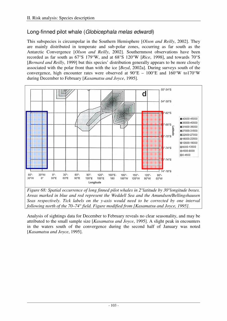
II. Risk analysis: Species description
- 103 -
Long-finned pilot whale (Globicephala melas edwardi)
This subspecies is circumpolar in the Southern Hemisphere [Olson and Reilly, 2002]. They are mainly distributed in temperate and sub-polar zones, occurring as far south as the Antarctic Convergence [Olson and Reilly, 2002]. Southernmost observations have been recorded as far south as 67°S 179°W, and at 68°S 120°W [Rice, 1998], and towards 70°S [Bernard and Reilly, 1999] but this species’ distribution generally appears to be more closely associated with the polar front than with the ice [Boyd, 2002a]. During surveys south of the convergence, high encounter rates were observed at 90°E – 100°E and 160°W to170°W during December to February [Kasamatsu and Joyce, 1995].
Figure 68: Spatial occurrence of long finned pilot whales in 2°latitude by 30°longitude boxes. Areas marked in blue and red represent the Weddell Sea and the Amundsen/Bellingshausen Seas respectively. Tick labels on the y-axis would need to be corrected by one interval following north of the 70–74° field. Figure modified from [Kasamatsu and Joyce, 1995].
Analysis of sightings data for December to February reveals no clear seasonality, and may be attributed to the small sample size [Kasamatsu and Joyce, 1995]. A slight peak in encounters in the waters south of the convergence during the second half of January was noted [Kasamatsu and Joyce, 1995].
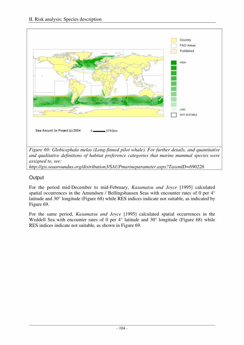
II. Risk analysis: Species description
- 104 -
Figure 69: Globicephala melas (Long-finned pilot whale). For further details, and quantitative and qualitative definitions of habitat preference categories that marine mammal species were assigned to, see: http://gis.seaaroundus.org/distribution3/SAUPmarineparameter.aspx?TaxonID=690226
Output
For the period mid-December to mid-February, Kasamatsu and Joyce [1995] calculated spatial occurrences in the Amundsen / Bellingshausen Seas with encounter rates of 0 per 4° latitude and 30° longitude (Figure 68) while RES indices indicate not suitable, as indicated by Figure 69.
For the same period, Kasamatsu and Joyce [1995] calculated spatial occurrences in the Weddell Sea with encounter rates of 0 per 4° latitude and 30° longitude (Figure 68) while RES indices indicate not suitable, as shown in Figure 69.
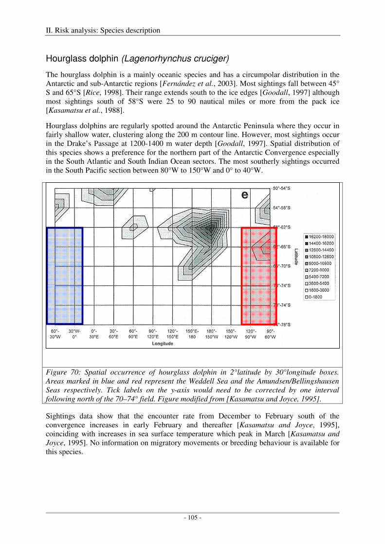
II. Risk analysis: Species description
- 105 -
Hourglass dolphin (Lagenorhynchus cruciger)
The hourglass dolphin is a mainly oceanic species and has a circumpolar distribution in the Antarctic and sub-Antarctic regions [Fernández et al., 2003]. Most sightings fall between 45° S and 65°S [Rice, 1998]. Their range extends south to the ice edges [Goodall, 1997] although most sightings south of 58°S were 25 to 90 nautical miles or more from the pack ice [Kasamatsu et al., 1988].
Hourglass dolphins are regularly spotted around the Antarctic Peninsula where they occur in fairly shallow water, clustering along the 200 m contour line. However, most sightings occur in the Drake’s Passage at 1200-1400 m water depth [Goodall, 1997]. Spatial distribution of this species shows a preference for the northern part of the Antarctic Convergence especially in the South Atlantic and South Indian Ocean sectors. The most southerly sightings occurred in the South Pacific section between 80°W to 150°W and 0° to 40°W.
Figure 70: Spatial occurrence of hourglass dolphin in 2°latitude by 30°longitude boxes. Areas marked in blue and red represent the Weddell Sea and the Amundsen/Bellingshausen Seas respectively. Tick labels on the y-axis would need to be corrected by one interval following north of the 70–74° field. Figure modified from [Kasamatsu and Joyce, 1995].
Sightings data show that the encounter rate from December to February south of the convergence increases in early February and thereafter [Kasamatsu and Joyce, 1995], coinciding with increases in sea surface temperature which peak in March [Kasamatsu and Joyce, 1995]. No information on migratory movements or breeding behaviour is available for this species.
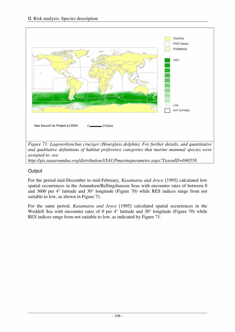
II. Risk analysis: Species description
- 106 -
Figure 71: Lagenorhynchus cruciger (Hourglass dolphin). For further details, and quantitative and qualitative definitions of habitat preference categories that marine mammal species were assigned to, see: http://gis.seaaroundus.org/distribution3/SAUPmarineparameter.aspx?TaxonID=690558
Output
For the period mid-December to mid-February, Kasamatsu and Joyce [1995] calculated low spatial occurrences in the Amundsen/Bellingshausen Seas with encounter rates of between 0 and 3600 per 4° latitude and 30° longitude (Figure 70) while RES indices range from not suitable to low, as shown in Figure 71.
For the same period, Kasamatsu and Joyce [1995] calculated spatial occurrences in the Weddell Sea with encounter rates of 0 per 4° latitude and 30° longitude (Figure 70) while RES indices range from not suitable to low, as indicated by Figure 71.
II. Risk analysis: Species description
- 107 -
Antarctic Seal species
The distribution and abundance of true Antarctic seal species (Table 11) is defined by their relationship to sea ice. Weddell seals are most associated with fast ice, Ross seals with open water and pack ice, and leopard seals are mainly associated with pack ice but patrol along shore lines north and south of the pack ice zone where colonies of penguins exist. Crabeater seals migrate extensively within the pack ice zone and some migrate over long distances potentially in excess of the total pack ice area of the Antarctic [Boyd, 2002a]. Ross seal migrations have been studied only recently, implying that they commute between pelagic and coastal pack ice areas over long distances over the course of the year [Blix and Nordøy, 2007]. Weddell seals appear to be relatively sedentary associated with coastal fast ice areas. In contrast to the ice breeding Weddell-, Ross-, leopard-, and crabeater seals, southern elephant seals and fur seals breed ashore. Elephant seals are considered to stay pelagic while foraging but the feeding grounds of certain colonies seem to be closely associated with the pack ice zone [Bornemann et al., 2000]. The animals are known to range far north of but also far south of the Antarctic Polar Front, and individuals were observed migrating between Subantarctic Islands and high Antarctic continental shelf regions [Bornemann et al., 2000]. Like southern elephant seals, Antarctic fur seals breed on Subantarctic Islands. They are sometimes found at the pack ice-open water interface, but are mainly animals of the open ocean [Boyd, 2002a].
Estimates of abundances of seal species as given in Table 11 are currently only available in orders of magnitude for the southern ocean at large [Boyd, 2002a], and will soon be or have already been determined more precisely for certain sections of the Southern Ocean by the SCAR4 Expert Group on Seals (EGS) as a result of the international Antarctic Pack Ice Seals (APIS) Program [Bester and Stewart, 2006]. The APIS Program was developed and executed by members of the SCAR Group of Specialists on Seals (GSS) and their national programs between 1995 and 2000. Since the resulting summary information on the status of Antarctic seals stocks in the Amundsen/Bellingshausen and Weddell Seas has not yet been published, pending on further analyses of the various survey data, the currently available population density information still relies on data from earlier surveys undertaken in 1972, and 1994 (United States) for the Amundsen and Bellingshausen Seas, and from those in 1968, 1969, 1983 (United States), 1991/92, 1992/93 (South Africa) for the Weddell Sea. These data on corrected population densities of lobodontine seals in the Antarctic pelagic pack ice have been compiled by the SCAR GSS in 2002 as given in Table 13, and are currently under revision, depending on addition and further analyses of data from the APIS surveys between 1995 and 2000. Although a German/South African aerial census in austral summer 1998 yielded more recent data for the Weddell Sea [Bester and Odendaal, 2000] density estimates derived from this study are disregarded here because of exceptional sea ice conditions that may have biased the census result.
4 Scientific Committee on Antarctic Research
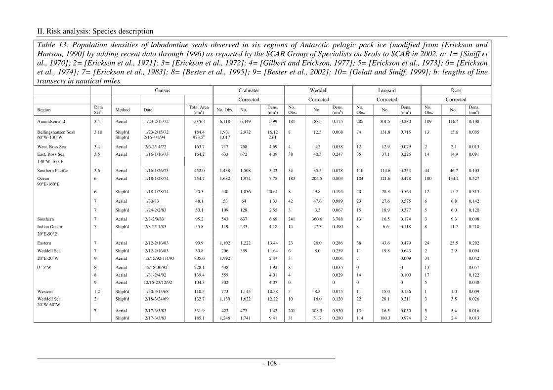
II. Risk analysis: Species description
- 108 -
Table 13: Population densities of lobodontine seals observed in six regions of Antarctic pelagic pack ice (modified from [Erickson and Hanson, 1990] by adding recent data through 1996) as reported by the SCAR Group of Specialists on Seals to SCAR in 2002. a: 1= [Siniff et al., 1970]; 2= [Erickson et al., 1971]; 3= [Erickson et al., 1972]; 4= [Gilbert and Erickson, 1977]; 5= [Erickson et al., 1973]; 6= [Erickson et al., 1974]; 7= [Erickson et al., 1983]; 8= [Bester et al., 1995]; 9= [Bester et al., 2002]; 10= [Gelatt and Siniff, 1999]; b: lengths of line transects in nautical miles.
Census Crabeater Weddell Leopard Ross
Corrected Corrected Corrected Corrected
Region Data Seta
Method Date Total Area
(nm2) No. Obs. No.
Dens. (nm2)
No. Obs.
No. Dens. (nm2)
No. Obs.
No. Dens. (nm2)
No. Obs.
No. Dens. (nm2)
Amundsen and 3,4 Aerial 1/23-2/15/72 1,076.4 6,118 6,449 5.99 181 188.1 0.175 285 301.5 0.280 109 116.4 0.108
Bellingshausen Seas 60°W-130°W
3 10
Shipb'd Shipb'd
1/23-2/15/72 2/16-4/1/94
184.4 973.5b
1,931 1,017
2,972
16.12 2.61
8
12.5
0.068
74
131.8
0.715
13
15.6
0.085
West, Ross Sea 3,4 Aerial 2/6-2/14/72 163.7 717 768 4.69 4 4.2 0.058 12 12.9 0.079 2 2.1 0.013
East, Ross Sea 3,5 Aerial 1/16-1/16/73 164.2 633 672 4.09 38 40.5 0.247 35 37.1 0.226 14 14.9 0.091
130°W-160°E
Southern Pacific 3,6 Aerial 1/16-1/26/73 452.0 1,438 1,508 3.33 34 35.5 0.078 110 114.6 0.253 44 46.7 0.103
Ocean 6 Aerial 1/18-1/28/74 254.7 1,682 1,974 7.75 183 204.5 0.803 104 121.6 0.478 100 134.2 0.527 90°E-160°E
6 Shipb'd 1/18-1/28/74 50.3 530 1,036 20.61 8 9.8 0.194 20 28.3 0.563 12 15.7 0.313
7 Aerial 1/30/83 48.1 53 64 1.33 42 47.6 0.989 23 27.6 0.575 6 6.8 0.142
7 Shipb'd 1/24-2/2/83 50.1 109 128 2.55 3 3.3 0.067 15 18.9 0.377 5 6.0 0.120
Southern 7 Aerial 2/3-2/9/83 95.2 543 637 6.69 241 360.6 3.788 13 16.5 0.174 3 9.3 0.098
Indian Ocean 7 Shipb'd 2/3-2/11/83 55.8 119 233 4.18 14 27.3 0.490 3 6.6 0.118 8 11.7 0.210
20°E-90°E
Eastern 7 Aerial 2/12-2/16/83 90.9 1,102 1,222 13.44 23 26.0 0.286 38 43.6 0.479 24 25.5 0.292
Weddell Sea 7 Shipb'd 2/12-2/16/83 30.8 206 359 11.64 6 8.0 0.259 11 19.8 0.643 2 2.9 0.094
20°E-20°W 9 Aerial 12/15/92-1/4/93 805.6 1,992 2.47 3 0.004 7 0.009 34 0.042
0°-5°W 8 Aerial 12/18-30/92 228.1 438 1.92 8 0.035 0 0 13 0.057
8 Aerial 1/31-2/4/92 139.4 559 4.01 4 0.029 14 0.100 17 0.122
9 Aerial 12/15-23/12/92 104.3 302 4.07 0 0 0 0 5 0.048
Western 1,2 Shipb'd 1/30-3/13/68 110.5 773 1,145 10.38 5 8.3 0.075 11 15.0 0.136 1 1.0 0.009
Weddell Sea 2 Shipb'd 2/18-3/24/69 132.7 1,130 1,622 12.22 10 16.0 0.120 22 28.1 0.211 3 3.5 0.026 20°W-60°W 7 Aerial 2/17-3/3/83 331.9 423 473 1.42 201 308.5 0.930 13 16.5 0.050 5 5.4 0.016
Shipb'd 2/17-3/3/83 185.1 1,248 1,741 9.41 31 51.7 0.280 114 180.3 0.974 2 2.4 0.013
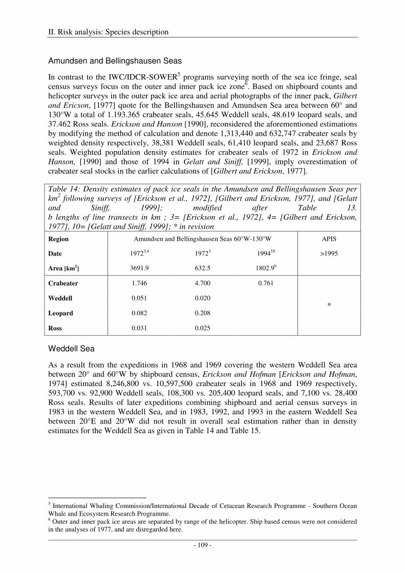
II. Risk analysis: Species description
- 109 -
Amundsen and Bellingshausen Seas
In contrast to the IWC/IDCR-SOWER5 programs surveying north of the sea ice fringe, seal census surveys focus on the outer and inner pack ice zone6. Based on shipboard counts and helicopter surveys in the outer pack ice area and aerial photographs of the inner pack, Gilbert and Ericson, [1977] quote for the Bellingshausen and Amundsen Sea area between 60° and 130°W a total of 1.193.365 crabeater seals, 45.645 Weddell seals, 48.619 leopard seals, and 37.462 Ross seals. Erickson and Hanson [1990], reconsidered the aforementioned estimations by modifying the method of calculation and denote 1,313,440 and 632,747 crabeater seals by weighted density respectively, 38,381 Weddell seals, 61,410 leopard seals, and 23,687 Ross seals. Weighted population density estimates for crabeater seals of 1972 in Erickson and Hanson, [1990] and those of 1994 in Gelatt and Siniff, [1999], imply overestimation of crabeater seal stocks in the earlier calculations of [Gilbert and Erickson, 1977].
Table 14: Density estimates of pack ice seals in the Amundsen and Bellingshausen Seas per km2 following surveys of [Erickson et al., 1972], [Gilbert and Erickson, 1977], and [Gelatt and Siniff, 1999]; modified after Table 13. b lengths of line transects in km ; 3= [Erickson et al., 1972], 4= [Gilbert and Erickson, 1977], 10= [Gelatt and Siniff, 1999]; * in revision
Region Amundsen and Bellingshausen Seas 60°W-130°W APIS
Date 19723,4 19723 199410 >1995
Area [km2] 3691.9 632.5 1802.9b
Crabeater 1.746 4.700 0.761
* Weddell 0.051 0.020
Leopard 0.082 0.208
Ross 0.031 0.025
Weddell Sea
As a result from the expeditions in 1968 and 1969 covering the western Weddell Sea area between 20° and 60°W by shipboard census, Erickson and Hofman [Erickson and Hofman, 1974] estimated 8,246,800 vs. 10,597,500 crabeater seals in 1968 and 1969 respectively, 593,700 vs. 92,900 Weddell seals, 108,300 vs. 205,400 leopard seals, and 7,100 vs. 28,400 Ross seals. Results of later expeditions combining shipboard and aerial census surveys in 1983 in the western Weddell Sea, and in 1983, 1992, and 1993 in the eastern Weddell Sea between 20°E and 20°W did not result in overall seal estimation rather than in density estimates for the Weddell Sea as given in Table 14 and Table 15.
5 International Whaling Commission/International Decade of Cetacean Research Programme - Southern Ocean Whale and Ecosystem Research Programme. 6 Outer and inner pack ice areas are separated by range of the helicopter. Ship based census were not considered in the analyses of 1977, and are disregarded here.
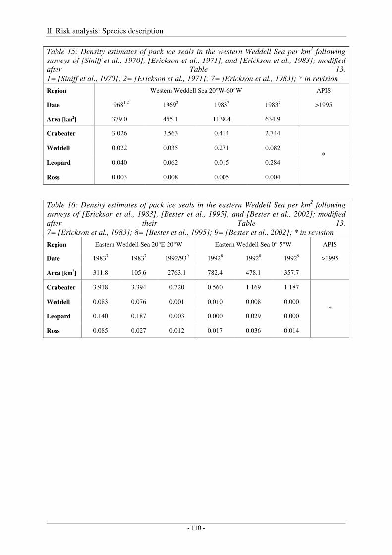
II. Risk analysis: Species description
- 110 -
Table 15: Density estimates of pack ice seals in the western Weddell Sea per km2 following surveys of [Siniff et al., 1970], [Erickson et al., 1971], and [Erickson et al., 1983]; modified after Table 13. 1= [Siniff et al., 1970]; 2= [Erickson et al., 1971]; 7= [Erickson et al., 1983]; * in revision
Region Western Weddell Sea 20°W-60°W APIS
Date 19681,2 19692 19837 19837 >1995
Area [km2] 379.0 455.1 1138.4 634.9
Crabeater 3.026 3.563 0.414 2.744
* Weddell 0.022 0.035 0.271 0.082
Leopard 0.040 0.062 0.015 0.284
Ross 0.003 0.008 0.005 0.004
Table 16: Density estimates of pack ice seals in the eastern Weddell Sea per km2 following surveys of [Erickson et al., 1983], [Bester et al., 1995], and [Bester et al., 2002]; modified after their Table 13. 7= [Erickson et al., 1983]; 8= [Bester et al., 1995]; 9= [Bester et al., 2002]; * in revision
Region Eastern Weddell Sea 20°E-20°W Eastern Weddell Sea 0°-5°W APIS
Date 19837 19837 1992/939 19928 19928 19929 >1995
Area [km2] 311.8 105.6 2763.1 782.4 478.1 357.7
Crabeater 3.918 3.394 0.720 0.560 1.169 1.187
* Weddell 0.083 0.076 0.001 0.010 0.008 0.000
Leopard 0.140 0.187 0.003 0.000 0.029 0.000
Ross 0.085 0.027 0.012 0.017 0.036 0.014
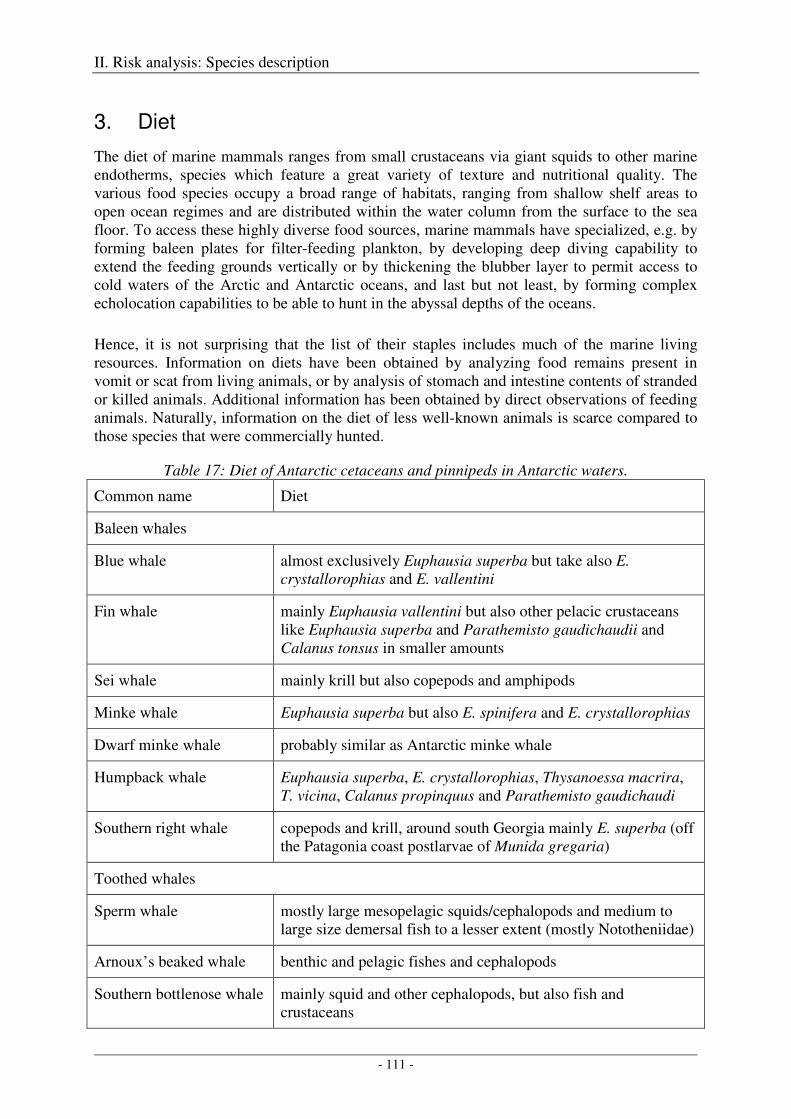
II. Risk analysis: Species description
- 111 -
3. Diet
The diet of marine mammals ranges from small crustaceans via giant squids to other marine endotherms, species which feature a great variety of texture and nutritional quality. The various food species occupy a broad range of habitats, ranging from shallow shelf areas to open ocean regimes and are distributed within the water column from the surface to the sea floor. To access these highly diverse food sources, marine mammals have specialized, e.g. by forming baleen plates for filter-feeding plankton, by developing deep diving capability to extend the feeding grounds vertically or by thickening the blubber layer to permit access to cold waters of the Arctic and Antarctic oceans, and last but not least, by forming complex echolocation capabilities to be able to hunt in the abyssal depths of the oceans.
Hence, it is not surprising that the list of their staples includes much of the marine living resources. Information on diets have been obtained by analyzing food remains present in vomit or scat from living animals, or by analysis of stomach and intestine contents of stranded or killed animals. Additional information has been obtained by direct observations of feeding animals. Naturally, information on the diet of less well-known animals is scarce compared to those species that were commercially hunted.
Table 17: Diet of Antarctic cetaceans and pinnipeds in Antarctic waters.
Common name Diet
Baleen whales
Blue whale almost exclusively Euphausia superba but take also E. crystallorophias and E. vallentini
Fin whale mainly Euphausia vallentini but also other pelacic crustaceans like Euphausia superba and Parathemisto gaudichaudii and Calanus tonsus in smaller amounts
Sei whale mainly krill but also copepods and amphipods
Minke whale Euphausia superba but also E. spinifera and E. crystallorophias
Dwarf minke whale probably similar as Antarctic minke whale
Humpback whale Euphausia superba, E. crystallorophias, Thysanoessa macrira, T. vicina, Calanus propinquus and Parathemisto gaudichaudi
Southern right whale copepods and krill, around south Georgia mainly E. superba (off the Patagonia coast postlarvae of Munida gregaria)
Toothed whales
Sperm whale mostly large mesopelagic squids/cephalopods and medium to large size demersal fish to a lesser extent (mostly Nototheniidae)
Arnoux’s beaked whale benthic and pelagic fishes and cephalopods
Southern bottlenose whale mainly squid and other cephalopods, but also fish and crustaceans
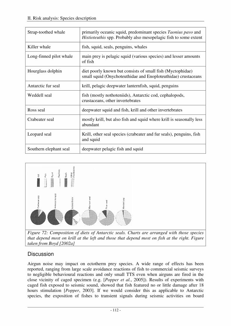
II. Risk analysis: Species description
- 112 -
Strap-toothed whale primarily oceanic squid, predominant species Taonius pavo and Histioteuthis spp. Probably also mesopelagic fish to some extent
Killer whale fish, squid, seals, penguins, whales
Long-finned pilot whale main prey is pelagic squid (various species) and lesser amounts of fish
Hourglass dolphin diet poorly known but consists of small fish (Myctophidae) small squid (Onychoteuthidae and Enoploteuthidae) crustaceans
Antarctic fur seal krill, pelagic deepwater lanternfish, squid, penguins
Weddell seal fish (mostly nothoteniids), Antarctic cod, cephalopods, crustaceans, other invertebrates
Ross seal deepwater squid and fish, krill and other invertebrates
Crabeater seal mostly krill, but also fish and squid where krill is seasonally less abundant
Leopard seal Krill, other seal species (crabeater and fur seals), penguins, fish and squid
Southern elephant seal deepwater pelagic fish and squid
Figure 72: Composition of diets of Antarctic seals. Charts are arranged with those species that depend most on krill at the left and those that depend most on fish at the right. Figure taken from Boyd [2002a]
Discussion
Airgun noise may impact on ectotherm prey species. A wide range of effects has been reported, ranging from large scale avoidance reactions of fish to commercial seismic surveys to negligible behavioural reactions and only small TTS even when airguns are fired in the close vicinity of caged specimen (e.g. [Popper et al., 2005]). Results of experiments with caged fish exposed to seismic sound, showed that fish featured no or little damage after 18 hours stimulation [Popper, 2003]. If we would consider this as applicable to Antarctic species, the exposition of fishes to transient signals during seismic activities on board
II. Risk analysis: Species description
- 113 -
“Polarstern” would remain well below the 18 hour period and hence fishes will remain principally available as prey. Other studies, considering possible conflicts between industrial seismic activities and commercial fishery [Skalski et al., 1992]; [Engas et al., 1996]; [Engas and Lokkeborg, 2002], rather than effects relevant for research seismic with respect to the Antarctic odontocetes’ and seal’s prey fishes suggest, at least for the species concerned, that fish have the potential to evade loud sounds, which may actually be judged as a species sustaining response to acoustic exposure. Other organisms such as krill or squid may be affected differently. However, in the case of krill, the current annual catch (<100.000 tons) is well below the precautionary catch limits set by CCAMLR of 4.000.000 tons in Area 48 (with a maximum of 620 000 tons per sub area), and 890.000 tons in Area 58 (440.000 tons and 450.000 tons in Divisions 58.4.1 and 58.4.2 respectively) [Hewitt et al., 2002]7. The region 88 including Amundsen and Bellingshausen Seas are negligible in terms of catches [Hewitt et al., 2002]. Any potential impact on the slowly swimming krill (migration distances seem to be 50-100 km over a few weeks [Siegel, 2005] caused by transient seismic activities of “Polarstern” would by far not reach the current annual catches, even if we would assume averaged moderate krill densities (5 krill per m2) [Atkinson et al., 2004]. Assuming a homogenous krill distribution and the (hypothesized) death of all krill organisms within a 100 m wide track, we result in a take of 1 kg krill per meter of ship track, corresponding to 1000 kg krill per kilometre seismic profile length. Thus, an average seismic profile length would amount to a take of ca 1800 t of krill, which is 2% of the current annual fishery take and 0.05% of the precautionary catch limit, an amount that hence can be considered negligible. In addition, the areas chosen for seismic surveys (Figure 1) do not match with those areas of the Southern Ocean known for high krill densities [Siegel, 2005]. The situation for squid is more difficult to evaluate, because of the scarcity of knowledge about the squids hearing abilities, and its potential reactions to seismic airgun sound. Though squid is responsive towards seismic sounds by defence and flight reactions, it is yet speculative how such responses translate to ecological implications [McCauley and Fewtrell, 2008]. At this time, this topic must be considered an emerging research field, with close to no data relevant to Antarctic ectotherm species.
Output
Noting the broad spectra of food resources used by the various cetaceans, while considering that the Southern Ocean is in generally assumed to be a highly biologically productive region and that the exploitation of living resources is regulated by the Convention on the Conservation of the Antarctic Marine Living Resources (CCAMLR) in this region, it appears unlikely that the sparse and transient seismic research operations in Antarctica have a biologically significant impact on the entirety of food resources. Therefore, this issue is not pursued further in this study. Possible effects on the predation of cetaceans by killer whales are however discussed in section III.3.
7 see http://www.ccamlr.org/pu/e/sc/fish-monit/hs-krill.htm
II. Risk analysis: Species description
- 114 -
4. Mortality rates
Apart from possible noise induced lethal impacts, mortality of marine mammals has a number of causes: age, diseases, predation, stranding, bycatch, collision with ships and boats and whaling. Table 18 gives an overview of the current knowledge on the various causes as applicable to each species.
Age
All cetaceans have long life spans, and as k-selected species they have evolved to maintain relatively stable population sizes towards the carrying capacity of their environment. Longevity estimates of odontocetes are in the order of up to seven decades (sperm whale), and for baleen whales up to 9 decades for blue whales (Table 18). Seals have shorter life spans (so far data are available) ranging from 15 (male) and 23 (female) years in southern elephant seals to up to 30 years in crabeater seals.
Diseases
A great variety of parasites has been described for cetaceans (listed in Table 18) and for pinnipeds (not listed). In general though, parasite infestation is not considered to increase mortality or serious morbidity. The principal effect of diseases on population dynamics of seal has been exemplified by [Harding, 2000].
Predation
Predation on cetaceans occurs due to attacks by sharks and killer whales [Ford and Reeves, 2008]. Killer whales are known to occasionally attack sperm and baleen whales and a variety of dolphins, porpoises and seals; the latter (mostly crabeater and fur seals) also being taken by leopard seals. Attacks by killer whales appear, however, to be rare, probably due to high risk or energetic expense involved therein [Ford and Reeves, 2008]. It is not clear if sharks attack baleen whales, though occasional incidents have been reported. Attacks by sharks will occur outside the Antarctic. While killer whales and sharks are responsible for the majority of attacks, some other delphinid species (false killer whale, pygmy killer whales and pilot whales) have been observed to attack or prey on other cetaceans. Among the species discussed herein, only the killer whale seems to experience little to no mortality due to predation.
Stranding
Strandings (or beaching) of individuals, groups or entire pods of various cetacean species have been reported for centuries. Singular (in space and time) strandings of individual whales might be in most cases attributed to dead animals drifting ashore. However, this is unlikely in the event of multiple animals stranding in a relatively close temporal and spatial context. During these “typical” strandings events, more complex mechanisms, such as sonar termination [Chambers and James, 2005], changes in the magnetic field, and social coherence in combination with diseases or poisoning of the leading or a subordinate member of the pod are suspected. In addition to these hypothesized natural causes, ensonification by tactical mid-frequency sonars has recently been indicted to have caused so-called “atypical” strandings [Cox et al., 2006], where multiple strandings of different species occur in a close temporal
II. Risk analysis: Species description
- 115 -
context, but possibly distributed across a large region. For Antarctic, only one stranding event has been reported to our knowledge (Table 18).
Bycatch
Read et al. [2006] estimated that global fisheries kill on the order of hundreds of thousands of cetaceans via bycatch each year. While the majority of the affected animals are smaller whales and dolphins, entanglement of large whales such as fin, humpback, southern right, minke and sperm whales [International Whaling Commission (IWC), 2002] has also been reported. We have no reports on bycatch of Antarctic seals, however, entanglement with lost fishing gear has been reported occasionally.
Whaling
Whaling is conducted by a number of nations within the frameworks of commercial, (so-called) scientific and traditional whaling. To our knowledge, only Japan conducts whaling operations that affect the southern hemisphere whale populations. Latest species specific numbers are given in Table 18 and described in the world wide context in Thiele [2007].
Sealing
The Convention for the Conservation of Antarctic Seals (CCAS) manages commercial sealing in the Antarctic, primarily as a precautionary measure over the potential re-initiation of pelagic commercial sealing in the region. Its objective is to “to promote and achieve the protection, scientific study and rational use of Antarctic seals, and to maintain a satisfactory balance within the ecological system of the Antarctic.” The Convention covers all species of seals in Antarctic waters. It sets conservative catch limits on crabeater, leopard and Weddell seals, and prohibits the catching of Ross, elephant and fur seals. Some few hundreds to thousands Weddell seals were likely killed as dog food (e.g. [Crawley, 1978]; [Stirling, 1968]) but here is no (commercial) sealing since sledge dogs were banned from the Antarctic in the early 1990-ies.
Shipping
Following bycatch, shipstrikes claim the second highest number of known non-natural mortalities, giving reason to estimates of 1000 strikes per year. An in-depth analysis of the incidents indicates that increases in lethal ship strikes since the 1950’s are linked to increasing ship speeds of > 14kn [Laist et al., 2001]. Contrary to bycatch, it is here that the larger cetaceans that at least become more visible in the statistic. Antarctica ranks last in a list of reported shipstrikes of large whales by region [Jensen and Silber, 2004]. However, the scarcity of reports from the southern relative to the northern hemisphere (mainly North Atlantic, Mediterranean Sea, North Pacific) may be an artefact of limited monitoring and reporting as indicated by some opportunistic observations [van Waerebeek et al., 2007]. On the other hand, predisposing factors such as the non-fatal entanglement in fishing gear or wounding caused by killer whale attacks prior to collisions or even post mortem collisions, as reported by van Waerebeek et al. [van Waerebeek et al., 2007], are indicative for the existence of false positive incidents, if they are not attributed to their primary cause. We have no reports on shipstrikes of Antarctic seals.
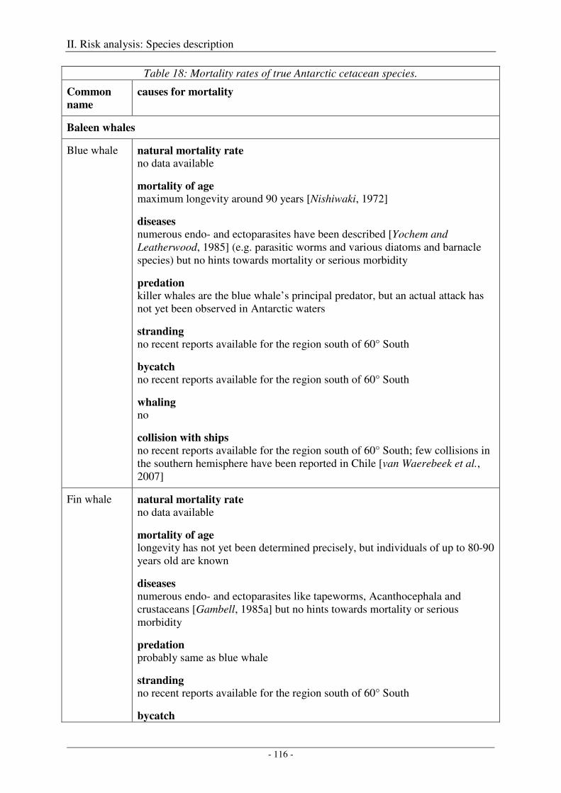
II. Risk analysis: Species description
- 116 -
Table 18: Mortality rates of true Antarctic cetacean species.
Common
name
causes for mortality
Baleen whales
Blue whale natural mortality rate no data available
mortality of age maximum longevity around 90 years [Nishiwaki, 1972]
diseases numerous endo- and ectoparasites have been described [Yochem and Leatherwood, 1985] (e.g. parasitic worms and various diatoms and barnacle species) but no hints towards mortality or serious morbidity
predation killer whales are the blue whale’s principal predator, but an actual attack has not yet been observed in Antarctic waters
stranding no recent reports available for the region south of 60° South
bycatch no recent reports available for the region south of 60° South
whaling no
collision with ships no recent reports available for the region south of 60° South; few collisions in the southern hemisphere have been reported in Chile [van Waerebeek et al., 2007]
Fin whale natural mortality rate
no data available
mortality of age longevity has not yet been determined precisely, but individuals of up to 80-90 years old are known
diseases numerous endo- and ectoparasites like tapeworms, Acanthocephala and crustaceans [Gambell, 1985a] but no hints towards mortality or serious morbidity
predation probably same as blue whale
stranding no recent reports available for the region south of 60° South
bycatch
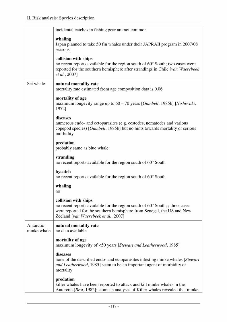
II. Risk analysis: Species description
- 117 -
incidental catches in fishing gear are not common
whaling Japan planned to take 50 fin whales under their JAPRAII program in 2007/08 seasons.
collision with ships no recent reports available for the region south of 60° South; two cases were reported for the southern hemisphere after strandings in Chile [van Waerebeek et al., 2007]
Sei whale natural mortality rate
mortality rate estimated from age composition data is 0.06
mortality of age maximum longevity range up to 60 – 70 years [Gambell, 1985b] [Nishiwaki, 1972]
diseases numerous endo- and ectoparasites (e.g. cestodes, nematodes and various copepod species) [Gambell, 1985b] but no hints towards mortality or serious morbidity
predation probably same as blue whale
stranding no recent reports available for the region south of 60° South
bycatch no recent reports available for the region south of 60° South
whaling no
collision with ships no recent reports available for the region south of 60° South; ; three cases were reported for the southern hemisphere from Senegal, the US and New Zeeland [van Waerebeek et al., 2007]
Antarctic minke whale
natural mortality rate no data available
mortality of age maximum longevity of <50 years [Stewart and Leatherwood, 1985]
diseases none of the described endo- and ectoparasites infesting minke whales [Stewart and Leatherwood, 1985] seem to be an important agent of morbidity or mortality
predation killer whales have been reported to attack and kill minke whales in the Antarctic [Best, 1982]; stomach analyses of Killer whales revealed that minke
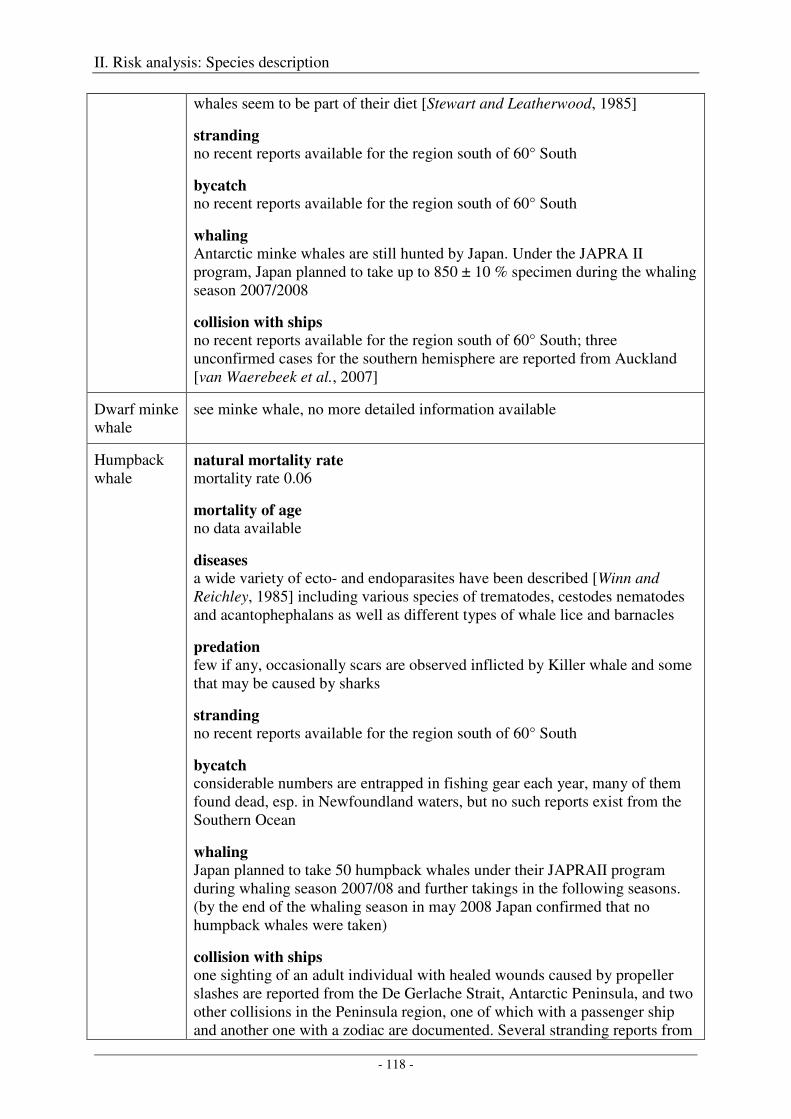
II. Risk analysis: Species description
- 118 -
whales seem to be part of their diet [Stewart and Leatherwood, 1985]
stranding no recent reports available for the region south of 60° South
bycatch no recent reports available for the region south of 60° South
whaling Antarctic minke whales are still hunted by Japan. Under the JAPRA II program, Japan planned to take up to 850 ± 10 % specimen during the whaling season 2007/2008
collision with ships no recent reports available for the region south of 60° South; three unconfirmed cases for the southern hemisphere are reported from Auckland [van Waerebeek et al., 2007]
Dwarf minke whale
see minke whale, no more detailed information available
Humpback whale
natural mortality rate mortality rate 0.06
mortality of age
no data available
diseases a wide variety of ecto- and endoparasites have been described [Winn and Reichley, 1985] including various species of trematodes, cestodes nematodes and acantophephalans as well as different types of whale lice and barnacles
predation few if any, occasionally scars are observed inflicted by Killer whale and some that may be caused by sharks
stranding no recent reports available for the region south of 60° South
bycatch considerable numbers are entrapped in fishing gear each year, many of them found dead, esp. in Newfoundland waters, but no such reports exist from the Southern Ocean
whaling Japan planned to take 50 humpback whales under their JAPRAII program during whaling season 2007/08 and further takings in the following seasons. (by the end of the whaling season in may 2008 Japan confirmed that no humpback whales were taken)
collision with ships one sighting of an adult individual with healed wounds caused by propeller slashes are reported from the De Gerlache Strait, Antarctic Peninsula, and two other collisions in the Peninsula region, one of which with a passenger ship and another one with a zodiac are documented. Several stranding reports from
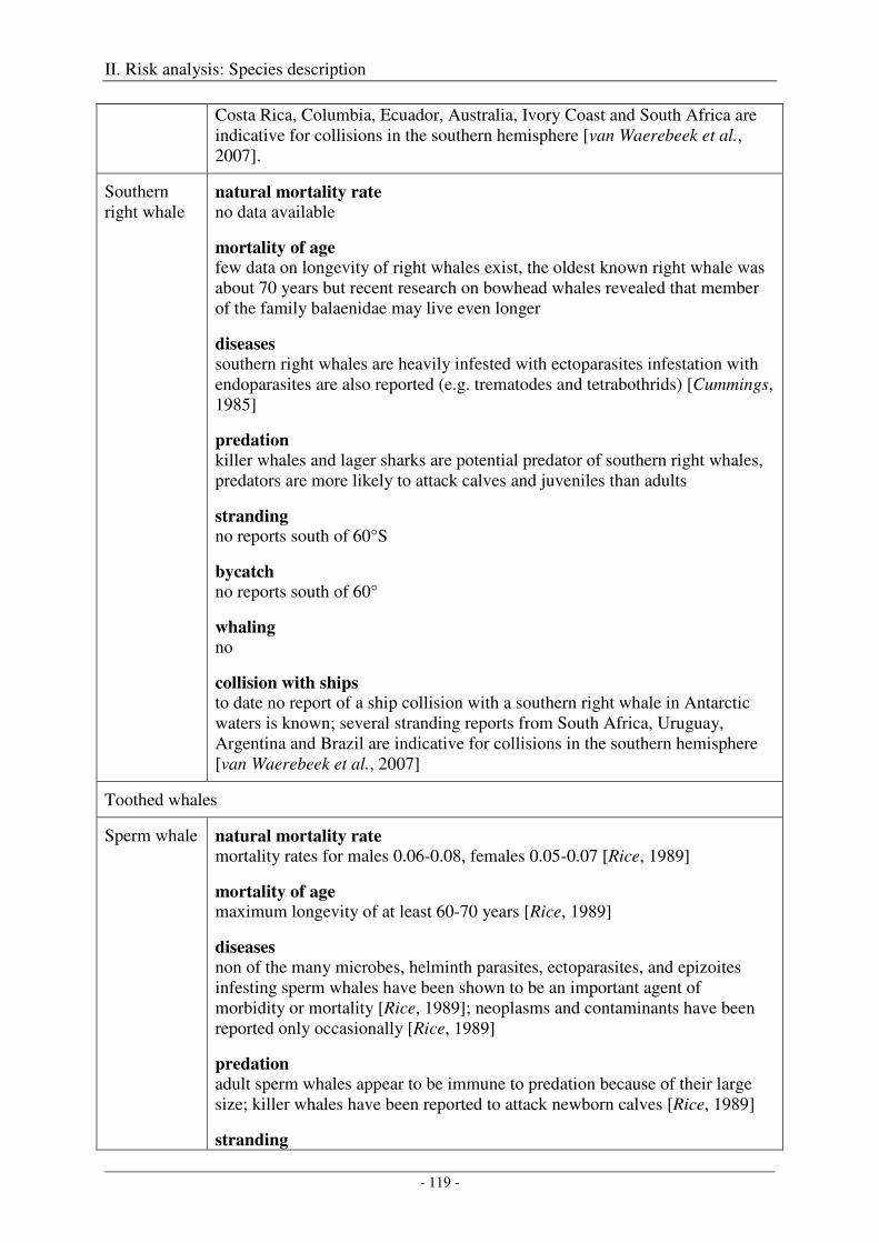
II. Risk analysis: Species description
- 119 -
Costa Rica, Columbia, Ecuador, Australia, Ivory Coast and South Africa are indicative for collisions in the southern hemisphere [van Waerebeek et al., 2007].
Southern right whale
natural mortality rate
no data available
mortality of age few data on longevity of right whales exist, the oldest known right whale was about 70 years but recent research on bowhead whales revealed that member of the family balaenidae may live even longer
diseases southern right whales are heavily infested with ectoparasites infestation with endoparasites are also reported (e.g. trematodes and tetrabothrids) [Cummings, 1985]
predation killer whales and lager sharks are potential predator of southern right whales, predators are more likely to attack calves and juveniles than adults
stranding no reports south of 60°S
bycatch no reports south of 60°
whaling
no
collision with ships to date no report of a ship collision with a southern right whale in Antarctic waters is known; several stranding reports from South Africa, Uruguay, Argentina and Brazil are indicative for collisions in the southern hemisphere [van Waerebeek et al., 2007]
Toothed whales
Sperm whale natural mortality rate mortality rates for males 0.06-0.08, females 0.05-0.07 [Rice, 1989]
mortality of age maximum longevity of at least 60-70 years [Rice, 1989]
diseases non of the many microbes, helminth parasites, ectoparasites, and epizoites infesting sperm whales have been shown to be an important agent of morbidity or mortality [Rice, 1989]; neoplasms and contaminants have been reported only occasionally [Rice, 1989]
predation adult sperm whales appear to be immune to predation because of their large size; killer whales have been reported to attack newborn calves [Rice, 1989]
stranding
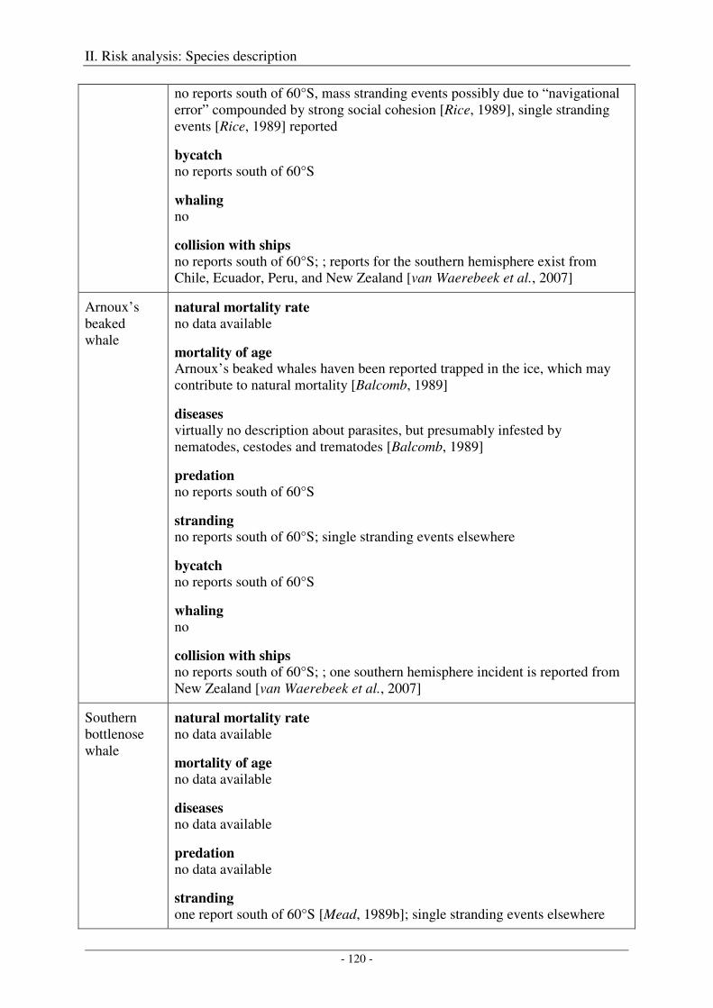
II. Risk analysis: Species description
- 120 -
no reports south of 60°S, mass stranding events possibly due to “navigational error” compounded by strong social cohesion [Rice, 1989], single stranding events [Rice, 1989] reported
bycatch no reports south of 60°S
whaling no
collision with ships no reports south of 60°S; ; reports for the southern hemisphere exist from Chile, Ecuador, Peru, and New Zealand [van Waerebeek et al., 2007]
Arnoux’s beaked whale
natural mortality rate
no data available
mortality of age Arnoux’s beaked whales haven been reported trapped in the ice, which may contribute to natural mortality [Balcomb, 1989]
diseases virtually no description about parasites, but presumably infested by nematodes, cestodes and trematodes [Balcomb, 1989]
predation no reports south of 60°S
stranding no reports south of 60°S; single stranding events elsewhere
bycatch no reports south of 60°S
whaling
no
collision with ships no reports south of 60°S; ; one southern hemisphere incident is reported from New Zealand [van Waerebeek et al., 2007]
Southern bottlenose whale
natural mortality rate no data available
mortality of age no data available
diseases no data available
predation no data available
stranding one report south of 60°S [Mead, 1989b]; single stranding events elsewhere
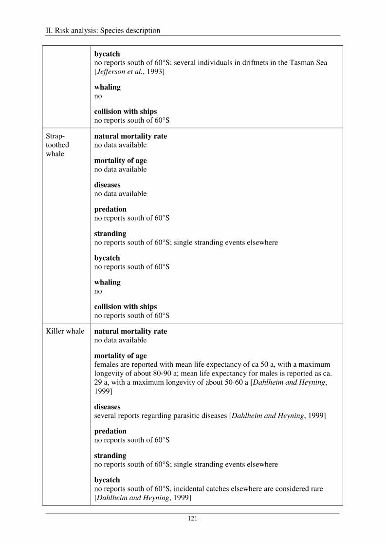
II. Risk analysis: Species description
- 121 -
bycatch no reports south of 60°S; several individuals in driftnets in the Tasman Sea [Jefferson et al., 1993]
whaling
no
collision with ships no reports south of 60°S
Strap-toothed whale
natural mortality rate no data available
mortality of age no data available
diseases no data available
predation no reports south of 60°S
stranding no reports south of 60°S; single stranding events elsewhere
bycatch no reports south of 60°S
whaling no
collision with ships no reports south of 60°S
Killer whale natural mortality rate
no data available
mortality of age females are reported with mean life expectancy of ca 50 a, with a maximum longevity of about 80-90 a; mean life expectancy for males is reported as ca. 29 a, with a maximum longevity of about 50-60 a [Dahlheim and Heyning, 1999]
diseases several reports regarding parasitic diseases [Dahlheim and Heyning, 1999]
predation no reports south of 60°S
stranding no reports south of 60°S; single stranding events elsewhere
bycatch no reports south of 60°S, incidental catches elsewhere are considered rare [Dahlheim and Heyning, 1999]
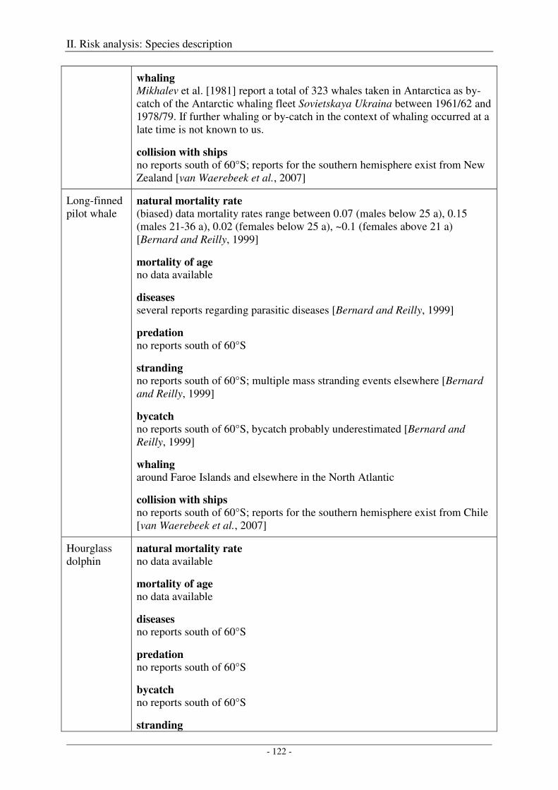
II. Risk analysis: Species description
- 122 -
whaling Mikhalev et al. [1981] report a total of 323 whales taken in Antarctica as by-catch of the Antarctic whaling fleet Sovietskaya Ukraina between 1961/62 and 1978/79. If further whaling or by-catch in the context of whaling occurred at a late time is not known to us.
collision with ships no reports south of 60°S; reports for the southern hemisphere exist from New Zealand [van Waerebeek et al., 2007]
Long-finned pilot whale
natural mortality rate (biased) data mortality rates range between 0.07 (males below 25 a), 0.15 (males 21-36 a), 0.02 (females below 25 a), ~0.1 (females above 21 a) [Bernard and Reilly, 1999]
mortality of age no data available
diseases several reports regarding parasitic diseases [Bernard and Reilly, 1999]
predation no reports south of 60°S
stranding no reports south of 60°S; multiple mass stranding events elsewhere [Bernard and Reilly, 1999]
bycatch no reports south of 60°S, bycatch probably underestimated [Bernard and Reilly, 1999]
whaling
around Faroe Islands and elsewhere in the North Atlantic
collision with ships no reports south of 60°S; reports for the southern hemisphere exist from Chile [van Waerebeek et al., 2007]
Hourglass dolphin
natural mortality rate no data available
mortality of age no data available
diseases no reports south of 60°S
predation no reports south of 60°S
bycatch no reports south of 60°S
stranding
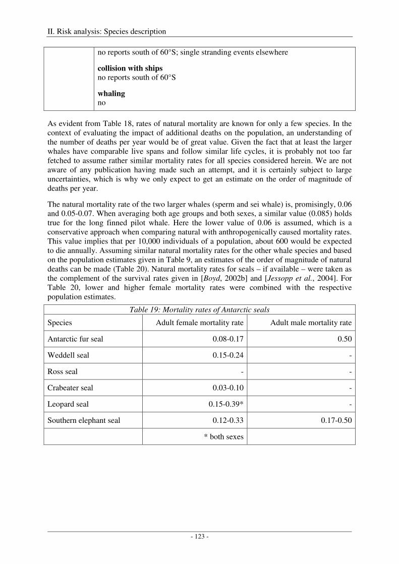
II. Risk analysis: Species description
- 123 -
no reports south of 60°S; single stranding events elsewhere
collision with ships no reports south of 60°S
whaling no
As evident from Table 18, rates of natural mortality are known for only a few species. In the context of evaluating the impact of additional deaths on the population, an understanding of the number of deaths per year would be of great value. Given the fact that at least the larger whales have comparable live spans and follow similar life cycles, it is probably not too far fetched to assume rather similar mortality rates for all species considered herein. We are not aware of any publication having made such an attempt, and it is certainly subject to large uncertainties, which is why we only expect to get an estimate on the order of magnitude of deaths per year.
The natural mortality rate of the two larger whales (sperm and sei whale) is, promisingly, 0.06 and 0.05-0.07. When averaging both age groups and both sexes, a similar value (0.085) holds true for the long finned pilot whale. Here the lower value of 0.06 is assumed, which is a conservative approach when comparing natural with anthropogenically caused mortality rates. This value implies that per 10,000 individuals of a population, about 600 would be expected to die annually. Assuming similar natural mortality rates for the other whale species and based on the population estimates given in Table 9, an estimates of the order of magnitude of natural deaths can be made (Table 20). Natural mortality rates for seals – if available – were taken as the complement of the survival rates given in [Boyd, 2002b] and [Jessopp et al., 2004]. For Table 20, lower and higher female mortality rates were combined with the respective population estimates.
Table 19: Mortality rates of Antarctic seals
Species Adult female mortality rate Adult male mortality rate
Antarctic fur seal 0.08-0.17 0.50
Weddell seal 0.15-0.24 -
Ross seal - -
Crabeater seal 0.03-0.10 -
Leopard seal 0.15-0.39* -
Southern elephant seal 0.12-0.33 0.17-0.50
* both sexes
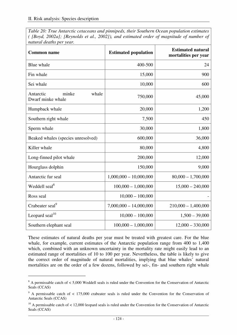
II. Risk analysis: Species description
- 124 -
Table 20: True Antarctic cetaceans and pinnipeds, their Southern Ocean population estimates ( [Boyd, 2002a]; [Reynolds et al., 2002]), and estimated order of magnitude of number of natural deaths per year.
Common name Estimated population Estimated natural
mortalities per year
Blue whale 400-500 24
Fin whale 15,000 900
Sei whale 10,000 600
Antarctic minke whale Dwarf minke whale
750,000 45,000
Humpback whale 20,000 1,200
Southern right whale 7,500 450
Sperm whale 30,000 1,800
Beaked whales (species unresolved) 600,000 36,000
Killer whale 80,000 4,800
Long-finned pilot whale 200,000 12,000
Hourglass dolphin 150,000 9,000
Antarctic fur seal 1,000,000 – 10,000,000 80,000 – 1,700,000
Weddell seal8 100,000 – 1,000,000 15,000 – 240,000
Ross seal 10,000 – 100,000 -
Crabeater seal9 7,000,000 – 14,000,000 210,000 – 1,400,000
Leopard seal10 10,000 – 100,000 1,500 – 39,000
Southern elephant seal 100,000 – 1,000,000 12,000 – 330,000
These estimates of natural deaths per year must be treated with greatest care. For the blue whale, for example, current estimates of the Antarctic population range from 400 to 1,400 which, combined with an unknown uncertainty in the mortality rate might easily lead to an estimated range of mortalities of 10 to 100 per year. Nevertheless, the table is likely to give the correct order of magnitude of natural mortalities, implying that blue whales’ natural mortalities are on the order of a few dozens, followed by sei-, fin- and southern right whale
8 A permissable catch of < 5,000 Weddell seals is ruled under the Convention for the Conservation of Antarctic Seals (CCAS) 9 A permissable catch of < 175,000 crabeater seals is ruled under the Convention for the Conservation of Antarctic Seals (CCAS) 10 A permissable catch of < 12,000 leopard seals is ruled under the Convention for the Conservation of Antarctic Seals (CCAS)
II. Risk analysis: Species description
- 125 -
mortalities on the order of several hundreds, with the remaining whales exceeding 1000 deaths per annum.
Output
With regard to causes for natural mortalities (age, diseases, predation, and typical strandings) it appears unlikely that transient seismic research operations can have a biological impact that significantly modifies the health status of Antarctic marine mammals e.g. via parasite infestation, change the environmental parameters causing typical strandings, or modify the aging process. Similarly, an effect of seismic on bycatch rates, collision with ships or whaling or sealing is not to be expected. Therefore, these issues are not pursued further in this study. However, possible effects of seismic surveys on predation and atypical stranding events are discussed in detail in the course of this study.
Of the species of concern, the blue whale, due to its low population, has the lowest number of mortalities. This implies that even singular additional kills could have a high impact on their population. All remaining species have annual mortalities of many hundreds to many thousands. In these instances, singular additional kills may be expected to only have a marginal impact on the population development.
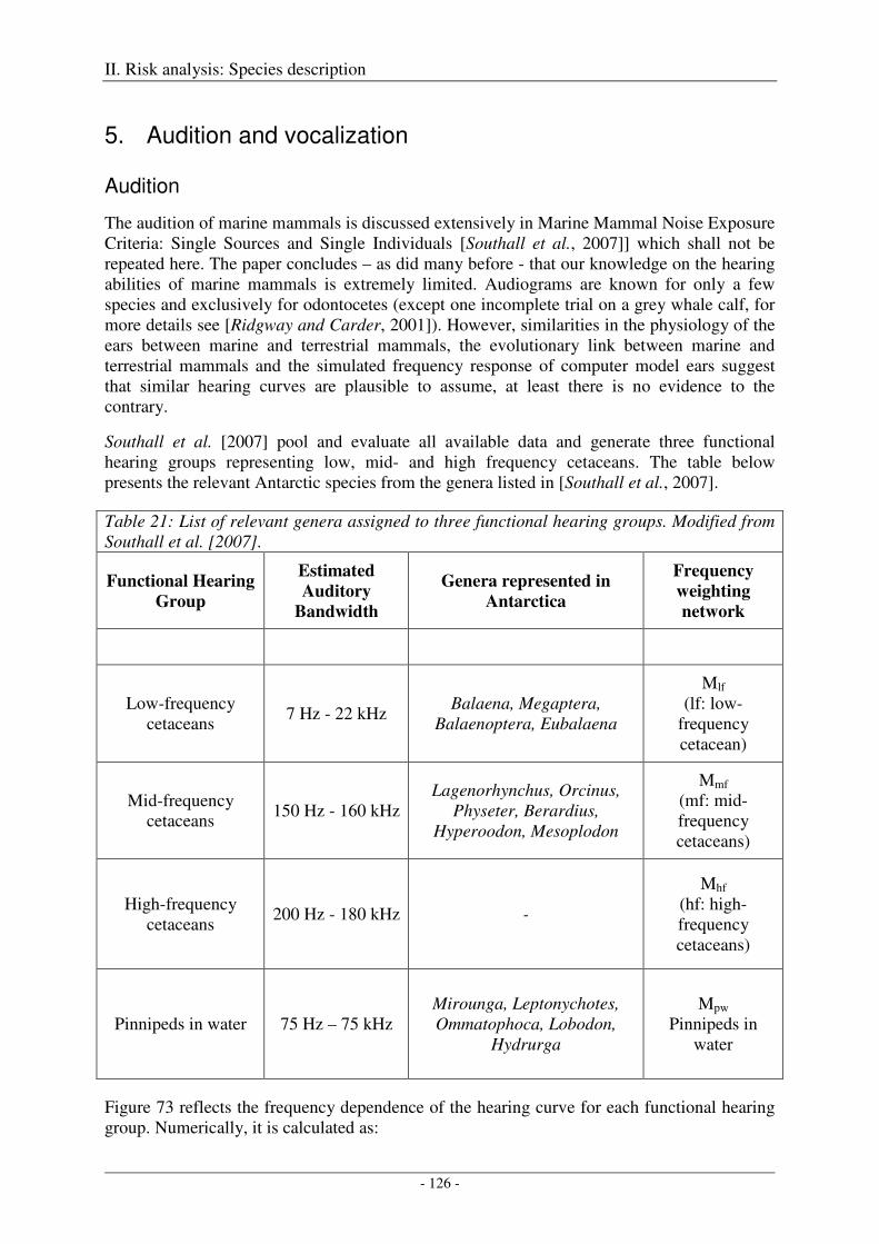
II. Risk analysis: Species description
- 126 -
5. Audition and vocalization
Audition
The audition of marine mammals is discussed extensively in Marine Mammal Noise Exposure Criteria: Single Sources and Single Individuals [Southall et al., 2007]] which shall not be repeated here. The paper concludes – as did many before - that our knowledge on the hearing abilities of marine mammals is extremely limited. Audiograms are known for only a few species and exclusively for odontocetes (except one incomplete trial on a grey whale calf, for more details see [Ridgway and Carder, 2001]). However, similarities in the physiology of the ears between marine and terrestrial mammals, the evolutionary link between marine and terrestrial mammals and the simulated frequency response of computer model ears suggest that similar hearing curves are plausible to assume, at least there is no evidence to the contrary.
Southall et al. [2007] pool and evaluate all available data and generate three functional hearing groups representing low, mid- and high frequency cetaceans. The table below presents the relevant Antarctic species from the genera listed in [Southall et al., 2007].
Table 21: List of relevant genera assigned to three functional hearing groups. Modified from Southall et al. [2007].
Functional Hearing
Group
Estimated
Auditory
Bandwidth
Genera represented in
Antarctica
Frequency
weighting
network
Low-frequency cetaceans
7 Hz - 22 kHz Balaena, Megaptera,
Balaenoptera, Eubalaena
Mlf
(lf: low-frequency cetacean)
Mid-frequency cetaceans
150 Hz - 160 kHz Lagenorhynchus, Orcinus,
Physeter, Berardius, Hyperoodon, Mesoplodon
Mmf
(mf: mid-frequency cetaceans)
High-frequency cetaceans
200 Hz - 180 kHz -
Mhf
(hf: high-frequency cetaceans)
Pinnipeds in water 75 Hz – 75 kHz Mirounga, Leptonychotes, Ommatophoca, Lobodon,
Hydrurga
Mpw Pinnipeds in
water
Figure 73 reflects the frequency dependence of the hearing curve for each functional hearing group. Numerically, it is calculated as:
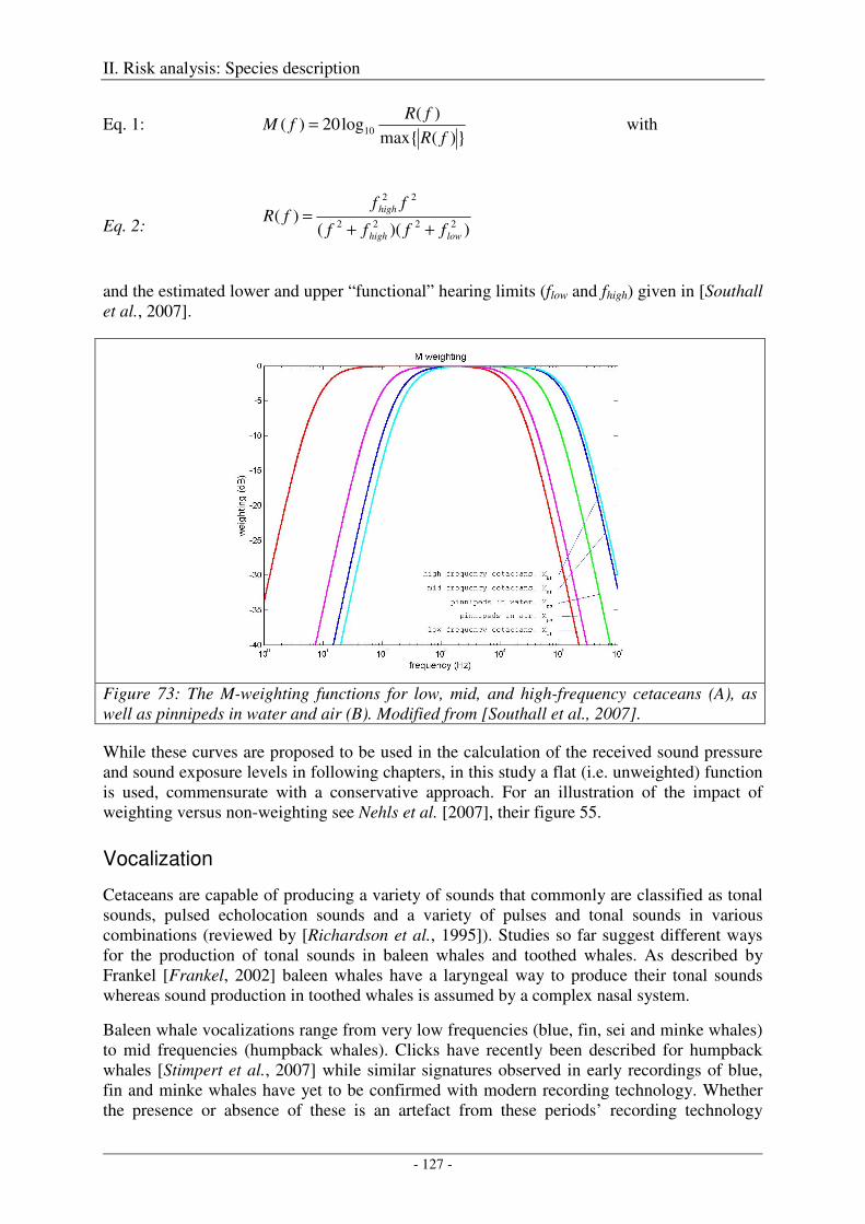
II. Risk analysis: Species description
- 127 -
Eq. 1: })(max{
)(log20)( 10
fR
fRfM = with
Eq. 2: ))(()(
2222
22
lowhigh
high
ffff
fffR
++=
and the estimated lower and upper “functional” hearing limits (flow and fhigh) given in [Southall et al., 2007].
Figure 73: The M-weighting functions for low, mid, and high-frequency cetaceans (A), as well as pinnipeds in water and air (B). Modified from [Southall et al., 2007].
While these curves are proposed to be used in the calculation of the received sound pressure and sound exposure levels in following chapters, in this study a flat (i.e. unweighted) function is used, commensurate with a conservative approach. For an illustration of the impact of weighting versus non-weighting see Nehls et al. [2007], their figure 55.
Vocalization
Cetaceans are capable of producing a variety of sounds that commonly are classified as tonal sounds, pulsed echolocation sounds and a variety of pulses and tonal sounds in various combinations (reviewed by [Richardson et al., 1995]). Studies so far suggest different ways for the production of tonal sounds in baleen whales and toothed whales. As described by Frankel [Frankel, 2002] baleen whales have a laryngeal way to produce their tonal sounds whereas sound production in toothed whales is assumed by a complex nasal system.
Baleen whale vocalizations range from very low frequencies (blue, fin, sei and minke whales) to mid frequencies (humpback whales). Clicks have recently been described for humpback whales [Stimpert et al., 2007] while similar signatures observed in early recordings of blue, fin and minke whales have yet to be confirmed with modern recording technology. Whether the presence or absence of these is an artefact from these periods’ recording technology
II. Risk analysis: Species description
- 128 -
remains open). The vocal repertoire of baleen whales varies from stereotyped repetitions of a certain call to complex songs in species, and even among species between different geographical regions. A possible theoretical depth limit of vocalisations of 30 m has been suggested by Aroyan et al., [2000] for low frequent (ca 20°Hz) vocalizations of blue whales during feeding. Vocalization events as shown in Figure 75 substantiate this hypothesis, since all vocalizations occurred in depths of less then 30 m [Calambokidis et al., 2003].
Toothed whales are in general rather vocal animals. They produce species-stereotypic broadband clicks with peak energy between 10 and 200 kHz, as well as individually variable burst pulse click trains and whistles (constant frequency or frequency modulated) within the frequency range from 4 – 16 kHz. Ultrasonic signals are used for echolocation. Two acoustic groups have been allocated on the basis of echolocation; type I (peak spectra > 100 kHz) and type II (peak spectra < 80 kHz). For further details see [Wartzok and Ketten, 1999].
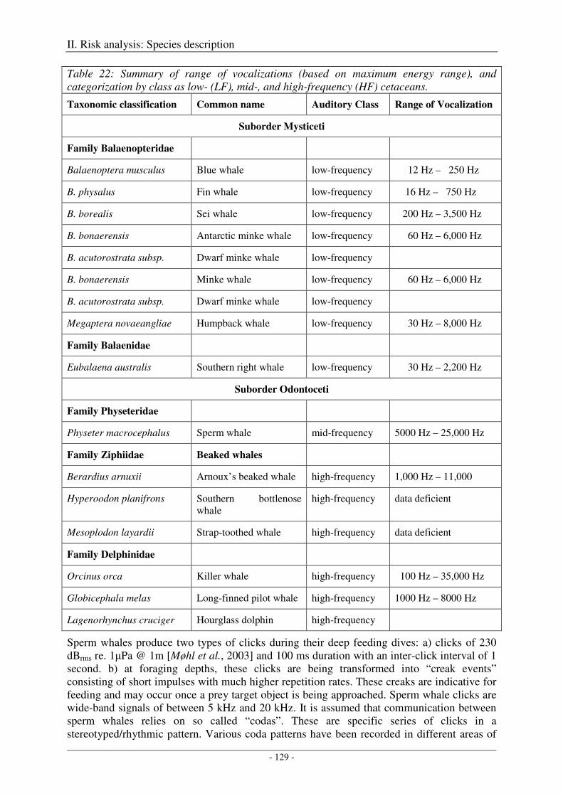
II. Risk analysis: Species description
- 129 -
Table 22: Summary of range of vocalizations (based on maximum energy range), and categorization by class as low- (LF), mid-, and high-frequency (HF) cetaceans.
Taxonomic classification Common name Auditory Class Range of Vocalization
Suborder Mysticeti
Family Balaenopteridae
Balaenoptera musculus Blue whale low-frequency 12 Hz – 250 Hz
B. physalus Fin whale low-frequency 16 Hz – 750 Hz
B. borealis Sei whale low-frequency 200 Hz – 3,500 Hz
B. bonaerensis Antarctic minke whale low-frequency 60 Hz – 6,000 Hz
B. acutorostrata subsp. Dwarf minke whale low-frequency
B. bonaerensis Minke whale low-frequency 60 Hz – 6,000 Hz
B. acutorostrata subsp. Dwarf minke whale low-frequency
Megaptera novaeangliae Humpback whale low-frequency 30 Hz – 8,000 Hz
Family Balaenidae
Eubalaena australis Southern right whale low-frequency 30 Hz – 2,200 Hz
Suborder Odontoceti
Family Physeteridae
Physeter macrocephalus Sperm whale mid-frequency 5000 Hz – 25,000 Hz
Family Ziphiidae Beaked whales
Berardius arnuxii Arnoux’s beaked whale high-frequency 1,000 Hz – 11,000
Hyperoodon planifrons Southern bottlenose whale
high-frequency data deficient
Mesoplodon layardii Strap-toothed whale high-frequency data deficient
Family Delphinidae
Orcinus orca Killer whale high-frequency 100 Hz – 35,000 Hz
Globicephala melas Long-finned pilot whale high-frequency 1000 Hz – 8000 Hz
Lagenorhynchus cruciger Hourglass dolphin high-frequency
Sperm whales produce two types of clicks during their deep feeding dives: a) clicks of 230 dBrms re. 1µPa @ 1m [Møhl et al., 2003] and 100 ms duration with an inter-click interval of 1 second. b) at foraging depths, these clicks are being transformed into “creak events” consisting of short impulses with much higher repetition rates. These creaks are indicative for feeding and may occur once a prey target object is being approached. Sperm whale clicks are wide-band signals of between 5 kHz and 20 kHz. It is assumed that communication between sperm whales relies on so called “codas”. These are specific series of clicks in a stereotyped/rhythmic pattern. Various coda patterns have been recorded in different areas of
II. Risk analysis: Species description
- 130 -
the world. The true function of codas, however, has not been elucidated yet. Vocalizations of sperm whales are unknown with the exception of rare “trumpets” [Teloni, 2005].
Pinnipeds are known to produce sounds both in-air and underwater. In-air communication occurs mainly in otariid species, whereas phocids rarely produce sounds in-air, except for mother-pup communication. The majority of phocid species are aquatic breeders and produce underwater vocalizations for mate attraction and/or male-male competition (see Van Parijs [Van Parijs, 2003] for a review. Here we focus on the underwater vocalizations of true Antarctic pinnipeds. Because of the absence of data on underwater vocalizations of Antarctic fur and southern elephant seals, in-air vocalisations are given as orientation towards their corresponding hearing range.
Pinnipeds are equipped with well-developed vocal chords, which are thought to be the prime sound production organs in pinnipeds. They are capable of producing different sounds simultaneously, which suggests that other parts of the larynx are also involved in sound production (e.g. [Norris, 1969]; [King, 1969]). Pinniped underwater vocalizations can be classified as tonal and pulsed sounds, which form in a variety of combinations and mid-frequency ranges the species-specific vocal repertoire. The size and complexity of the vocal repertoire differs strongly between species (see Table 25 and Rogers [Rogers, 2003] for an overview).
No underwater calls have been recorded for Antarctic fur seals (not for any of the fur seal spp) and in-air calls are given as a proxy for potential in-water vocalizations. Male Antarctic fur seals are known to produce in-air barks and full-threat calls (FTCs) during the breeding season which takes place from October to February. Barking consists of a series of brief, repeated calls that are thought to communicate sexual interest, affirm territory boundaries and advertise territorial status [Stirling, 1971]; [Miller, 1975]. Barks have a frequency range of approximately 100 – 8000 Hz (here the lower value is merely hypothesized and unsupported by publications or spectrograms). FTCs are used to advertise territorial status and are primarily used in male-male competition and have a frequency range between 100 – 3000 Hz [Page et al., 2002]. Female pup attraction calls are also produced in-air and have acoustic characteristics that are comparable to FTCs [Page et al., 2002].
Weddell seals are known to have a complex vocal repertoire consisting of a large number of call types that have been shown to differ between various Antarctic regions where recordings have been made [Thomas and Stirling, 1983]; [Pahl et al., 1997]; [P. et al., 2003]. The various studies that investigated Weddell seal vocalizations all use a different classification system, which in some cases complicates the comparison of call characteristics between studies. We have limited the overview of Weddell vocal repertoire to the main call types, excluding the various subtypes that have been described. The subtypes usually consist of the main call type but with a different auxiliary sound and therefore have the same frequency range as the main call types. Table 25 shows the vocal repertoire of the Weddell seal and the accompanying frequency characteristics. The majority of vocalizations occurs in the 100-8000 Hz frequency range, although one of the most predominant Weddell seal call types, the Trill, starts at 15000Hz. The period in which Weddell seals vocalize differs between locations. At some sites, Weddell seals are known to be absent in winter [Green and Burton, 1988], whereas at other sites, Weddell seal vocalizations are present almost the whole year [Rouget et al., 2007]; [van Opzeeland, pers. comm.]. Weddell seal vocalizations are thought to play a role in male-male competition, male territorial defence, and mate attraction.
Leopard seals produce sounds ranging from 35 to 6100 Hz. As leopard seals are solitary animals, they are thought to use long distance communication signals to attract mates during the breeding season, which takes place between October and January. Both male and female
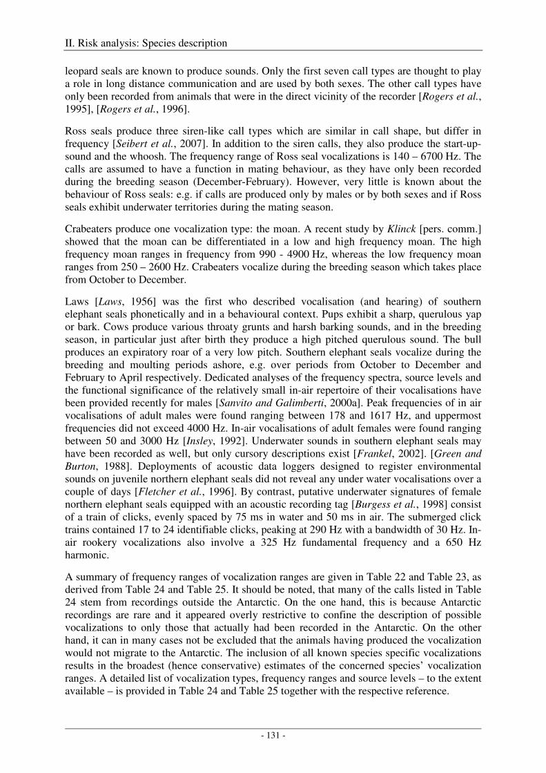
II. Risk analysis: Species description
- 131 -
leopard seals are known to produce sounds. Only the first seven call types are thought to play a role in long distance communication and are used by both sexes. The other call types have only been recorded from animals that were in the direct vicinity of the recorder [Rogers et al., 1995], [Rogers et al., 1996].
Ross seals produce three siren-like call types which are similar in call shape, but differ in frequency [Seibert et al., 2007]. In addition to the siren calls, they also produce the start-up-sound and the whoosh. The frequency range of Ross seal vocalizations is 140 – 6700 Hz. The calls are assumed to have a function in mating behaviour, as they have only been recorded during the breeding season (December-February). However, very little is known about the behaviour of Ross seals: e.g. if calls are produced only by males or by both sexes and if Ross seals exhibit underwater territories during the mating season.
Crabeaters produce one vocalization type: the moan. A recent study by Klinck [pers. comm.] showed that the moan can be differentiated in a low and high frequency moan. The high frequency moan ranges in frequency from 990 - 4900 Hz, whereas the low frequency moan ranges from 250 – 2600 Hz. Crabeaters vocalize during the breeding season which takes place from October to December.
Laws [Laws, 1956] was the first who described vocalisation (and hearing) of southern elephant seals phonetically and in a behavioural context. Pups exhibit a sharp, querulous yap or bark. Cows produce various throaty grunts and harsh barking sounds, and in the breeding season, in particular just after birth they produce a high pitched querulous sound. The bull produces an expiratory roar of a very low pitch. Southern elephant seals vocalize during the breeding and moulting periods ashore, e.g. over periods from October to December and February to April respectively. Dedicated analyses of the frequency spectra, source levels and the functional significance of the relatively small in-air repertoire of their vocalisations have been provided recently for males [Sanvito and Galimberti, 2000a]. Peak frequencies of in air vocalisations of adult males were found ranging between 178 and 1617 Hz, and uppermost frequencies did not exceed 4000 Hz. In-air vocalisations of adult females were found ranging between 50 and 3000 Hz [Insley, 1992]. Underwater sounds in southern elephant seals may have been recorded as well, but only cursory descriptions exist [Frankel, 2002]. [Green and Burton, 1988]. Deployments of acoustic data loggers designed to register environmental sounds on juvenile northern elephant seals did not reveal any under water vocalisations over a couple of days [Fletcher et al., 1996]. By contrast, putative underwater signatures of female northern elephant seals equipped with an acoustic recording tag [Burgess et al., 1998] consist of a train of clicks, evenly spaced by 75 ms in water and 50 ms in air. The submerged click trains contained 17 to 24 identifiable clicks, peaking at 290 Hz with a bandwidth of 30 Hz. In-air rookery vocalizations also involve a 325 Hz fundamental frequency and a 650 Hz harmonic.
A summary of frequency ranges of vocalization ranges are given in Table 22 and Table 23, as derived from Table 24 and Table 25. It should be noted, that many of the calls listed in Table 24 stem from recordings outside the Antarctic. On the one hand, this is because Antarctic recordings are rare and it appeared overly restrictive to confine the description of possible vocalizations to only those that actually had been recorded in the Antarctic. On the other hand, it can in many cases not be excluded that the animals having produced the vocalization would not migrate to the Antarctic. The inclusion of all known species specific vocalizations results in the broadest (hence conservative) estimates of the concerned species’ vocalization ranges. A detailed list of vocalization types, frequency ranges and source levels – to the extent available – is provided in Table 24 and Table 25 together with the respective reference.
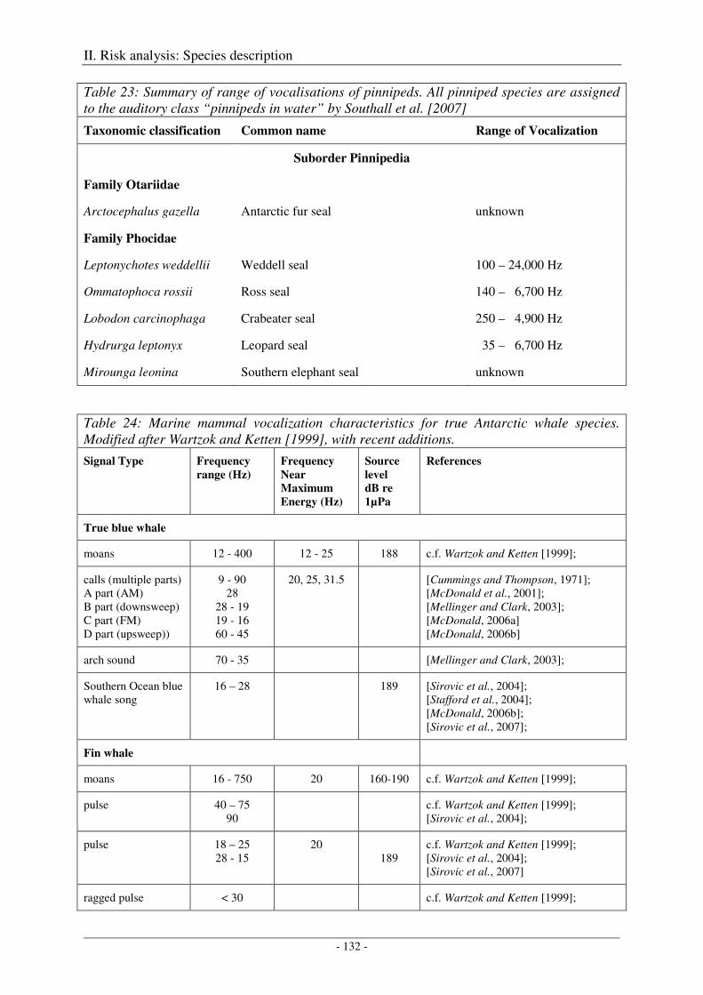
II. Risk analysis: Species description
- 132 -
Table 23: Summary of range of vocalisations of pinnipeds. All pinniped species are assigned to the auditory class “pinnipeds in water” by Southall et al. [2007]
Taxonomic classification Common name Range of Vocalization
Suborder Pinnipedia
Family Otariidae
Arctocephalus gazella Antarctic fur seal unknown
Family Phocidae
Leptonychotes weddellii Weddell seal 100 – 24,000 Hz
Ommatophoca rossii Ross seal 140 – 6,700 Hz
Lobodon carcinophaga Crabeater seal 250 – 4,900 Hz
Hydrurga leptonyx Leopard seal 035 – 6,700 Hz
Mirounga leonina Southern elephant seal unknown
Table 24: Marine mammal vocalization characteristics for true Antarctic whale species. Modified after Wartzok and Ketten [1999], with recent additions.
Signal Type Frequency
range (Hz)
Frequency
Near
Maximum
Energy (Hz)
Source
level
dB re
1µPa
References
True blue whale
moans 12 - 400 12 - 25 188 c.f. Wartzok and Ketten [1999];
calls (multiple parts) A part (AM) B part (downsweep) C part (FM) D part (upsweep))
9 - 90 28
28 - 19 19 - 16 60 - 45
20, 25, 31.5
[Cummings and Thompson, 1971]; [McDonald et al., 2001]; [Mellinger and Clark, 2003]; [McDonald, 2006a] [McDonald, 2006b]
arch sound 70 - 35 [Mellinger and Clark, 2003];
Southern Ocean blue whale song
16 – 28 189 [Sirovic et al., 2004]; [Stafford et al., 2004]; [McDonald, 2006b]; [Sirovic et al., 2007];
Fin whale
moans 16 - 750 20 160-190 c.f. Wartzok and Ketten [1999];
pulse 40 – 75 90
c.f. Wartzok and Ketten [1999]; [Sirovic et al., 2004];
pulse 18 – 25 28 - 15
20 189
c.f. Wartzok and Ketten [1999]; [Sirovic et al., 2004]; [Sirovic et al., 2007]
ragged pulse < 30 c.f. Wartzok and Ketten [1999];
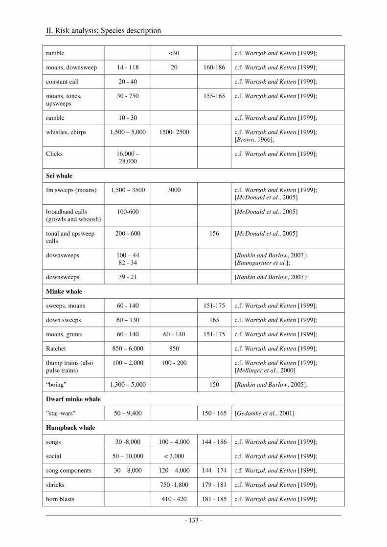
II. Risk analysis: Species description
- 133 -
rumble <30 c.f. Wartzok and Ketten [1999];
moans, downsweep 14 - 118 20 160-186 c.f. Wartzok and Ketten [1999];
constant call 20 - 40 c.f. Wartzok and Ketten [1999];
moans, tones, upsweeps
30 - 750 155-165 c.f. Wartzok and Ketten [1999];
rumble 10 - 30 c.f. Wartzok and Ketten [1999];
whistles, chirps 1,500 – 5,000 1500- 2500 c.f. Wartzok and Ketten [1999]; [Brown, 1966];
Clicks 16,000 – 28,000
c.f. Wartzok and Ketten [1999];
Sei whale
fm sweeps (moans) 1,500 – 3500 3000 c.f. Wartzok and Ketten [1999]; [McDonald et al., 2005]
broadband calls (growls and whoosh)
100-600 [McDonald et al., 2005]
tonal and upsweep calls
200 - 600 156 [McDonald et al., 2005]
downsweeps 100 – 44 82 - 34
[Rankin and Barlow, 2007]; [Baumgartner et al.];
downsweeps 39 - 21 [Rankin and Barlow, 2007];
Minke whale
sweeps, moans 60 - 140 151-175 c.f. Wartzok and Ketten [1999];
down sweeps 60 – 130 165 c.f. Wartzok and Ketten [1999];
moans, grunts 60 - 140 60 - 140 151-175 c.f. Wartzok and Ketten [1999];
Ratchet 850 – 6,000 850 c.f. Wartzok and Ketten [1999];
thump trains (also pulse trains)
100 – 2,000 100 - 200 c.f. Wartzok and Ketten [1999]; [Mellinger et al., 2000]
“boing” 1,300 – 5,000 150 [Rankin and Barlow, 2005];
Dwarf minke whale
”star-wars” 50 – 9,400 150 - 165 [Gedamke et al., 2001]
Humpback whale
songs 30 -8,000 100 – 4,000 144 - 186 c.f. Wartzok and Ketten [1999];
social 50 – 10,000 < 3,000 c.f. Wartzok and Ketten [1999];
song components 30 – 8,000 120 – 4,000 144 - 174 c.f. Wartzok and Ketten [1999];
shrieks 750 -1,800 179 - 181 c.f. Wartzok and Ketten [1999];
horn blasts 410 - 420 181 - 185 c.f. Wartzok and Ketten [1999];
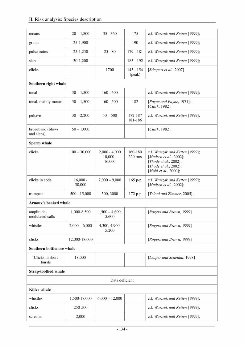
II. Risk analysis: Species description
- 134 -
moans 20 – 1,800 35 - 360 175 c.f. Wartzok and Ketten [1999];
grunts 25-1,900 190 c.f. Wartzok and Ketten [1999];
pulse trains 25-1,250 25 - 80 179 - 181 c.f. Wartzok and Ketten [1999];
slap 30-1,200 183 - 192 c.f. Wartzok and Ketten [1999];
clicks 1700 143 - 154 (peak)
[Stimpert et al., 2007]
Southern right whale
tonal 30 – 1,500 160 - 500 c.f. Wartzok and Ketten [1999];
tonal, mainly moans 30 – 1,500 160 - 500 182 [Payne and Payne, 1971]; [Clark, 1982];
pulsive 30 – 2,200 50 – 500 172-187 181-186
c.f. Wartzok and Ketten [1999];
broadband (blows and slaps)
50 – 1,000 [Clark, 1982];
Sperm whale
clicks 100 – 30,000 2,000 - 4,000 10,000 - 16,000
160-180 220 rms
c.f. Wartzok and Ketten [1999]; [Madsen et al., 2002]; [Thode et al., 2002]; [Thode et al., 2002]; [Møhl et al., 2000];
clicks in coda 16,000 - 30,000
7,000 – 9,000 165 p-p c.f. Wartzok and Ketten [1999]; [Madsen et al., 2002];
trumpets 500 - 15,000 500, 3000 172 p-p [Teloni and Zimmer, 2005];
Arnoux’s beaked whale
amplitude-modulated calls
1,000-8,500 1,500 – 4,600, 5,600
[Rogers and Brown, 1999]
whistles 2,000 – 6,000 4,300, 4,900, 5,200
[Rogers and Brown, 1999]
clicks 12,000-18,000 [Rogers and Brown, 1999]
Southern bottlenose whale
Clicks in short bursts
18,000 [Leaper and Scheidat, 1998]
Strap-toothed whale
Data deficient
Killer whale
whistles 1,500-18,000 6,000 – 12,000 c.f. Wartzok and Ketten [1999];
clicks 250-500 c.f. Wartzok and Ketten [1999];
screams 2,000 c.f. Wartzok and Ketten [1999];
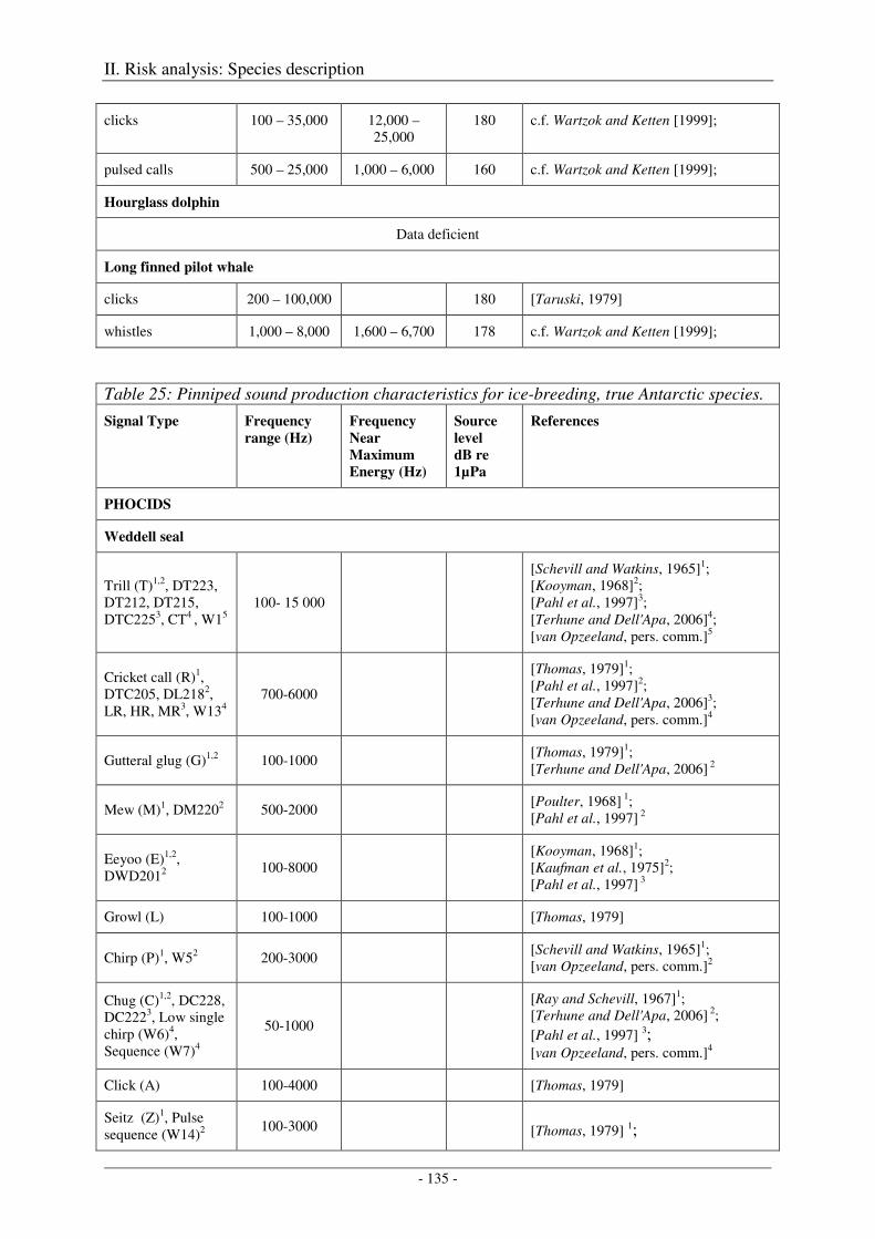
II. Risk analysis: Species description
- 135 -
clicks 100 – 35,000 12,000 – 25,000
180 c.f. Wartzok and Ketten [1999];
pulsed calls 500 – 25,000 1,000 – 6,000 160 c.f. Wartzok and Ketten [1999];
Hourglass dolphin
Data deficient
Long finned pilot whale
clicks 200 – 100,000 180 [Taruski, 1979]
whistles 1,000 – 8,000 1,600 – 6,700 178 c.f. Wartzok and Ketten [1999];
Table 25: Pinniped sound production characteristics for ice-breeding, true Antarctic species.
Signal Type Frequency
range (Hz)
Frequency
Near
Maximum
Energy (Hz)
Source
level
dB re
1µPa
References
PHOCIDS
Weddell seal
Trill (T)1,2, DT223, DT212, DT215, DTC2253, CT4 , W15
100- 15 000
[Schevill and Watkins, 1965]1; [Kooyman, 1968]2; [Pahl et al., 1997]3; [Terhune and Dell'Apa, 2006]4; [van Opzeeland, pers. comm.]5
Cricket call (R)1, DTC205, DL2182, LR, HR, MR3, W134
700-6000
[Thomas, 1979]1; [Pahl et al., 1997]2; [Terhune and Dell'Apa, 2006]3; [van Opzeeland, pers. comm.]4
Gutteral glug (G)1,2 100-1000 [Thomas, 1979]1; [Terhune and Dell'Apa, 2006] 2
Mew (M)1, DM2202 500-2000 [Poulter, 1968] 1; [Pahl et al., 1997] 2
Eeyoo (E)1,2, DWD2012
100-8000 [Kooyman, 1968]1; [Kaufman et al., 1975]2; [Pahl et al., 1997] 3
Growl (L) 100-1000 [Thomas, 1979]
Chirp (P)1, W52 200-3000 [Schevill and Watkins, 1965]1; [van Opzeeland, pers. comm.]2
Chug (C)1,2, DC228, DC2223, Low single chirp (W6)4, Sequence (W7)4
50-1000
[Ray and Schevill, 1967]1; [Terhune and Dell'Apa, 2006] 2; [Pahl et al., 1997] 3; [van Opzeeland, pers. comm.]4
Click (A) 100-4000 [Thomas, 1979]
Seitz (Z)1, Pulse sequence (W14)2
100-3000 [Thomas, 1979] 1;
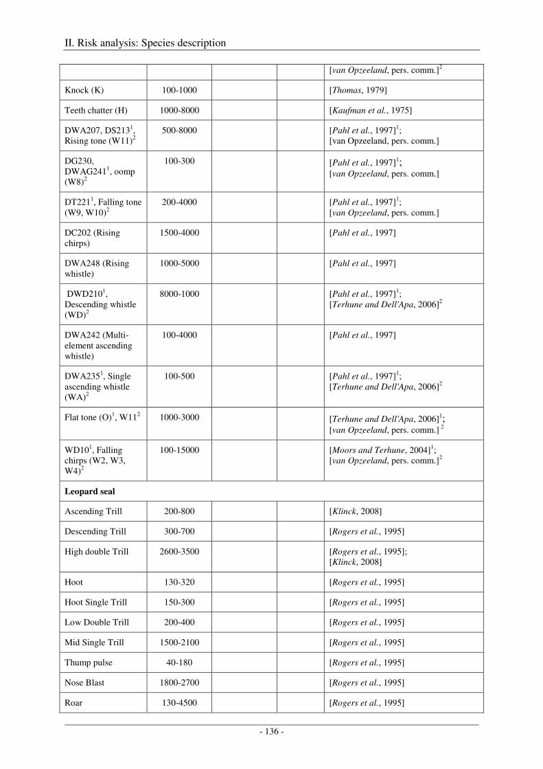
II. Risk analysis: Species description
- 136 -
[van Opzeeland, pers. comm.]2
Knock (K) 100-1000 [Thomas, 1979]
Teeth chatter (H) 1000-8000 [Kaufman et al., 1975]
DWA207, DS2131, Rising tone (W11)2
500-8000 [Pahl et al., 1997]1; [van Opzeeland, pers. comm.]
DG230, DWAG2411, oomp (W8)2
100-300 [Pahl et al., 1997]1; [van Opzeeland, pers. comm.]
DT2211, Falling tone (W9, W10)2
200-4000 [Pahl et al., 1997]1; [van Opzeeland, pers. comm.]
DC202 (Rising chirps)
1500-4000 [Pahl et al., 1997]
DWA248 (Rising whistle)
1000-5000 [Pahl et al., 1997]
DWD2101, Descending whistle (WD)2
8000-1000 [Pahl et al., 1997]1; [Terhune and Dell'Apa, 2006]2
DWA242 (Multi-element ascending whistle)
100-4000 [Pahl et al., 1997]
DWA2351, Single ascending whistle (WA)2
100-500 [Pahl et al., 1997]1; [Terhune and Dell'Apa, 2006]2
Flat tone (O)1, W112 1000-3000 [Terhune and Dell'Apa, 2006]1; [van Opzeeland, pers. comm.] 2
WD101, Falling chirps (W2, W3, W4)2
100-15000 [Moors and Terhune, 2004]1; [van Opzeeland, pers. comm.]2
Leopard seal
Ascending Trill 200-800 [Klinck, 2008]
Descending Trill 300-700 [Rogers et al., 1995]
High double Trill 2600-3500 [Rogers et al., 1995]; [Klinck, 2008]
Hoot 130-320 [Rogers et al., 1995]
Hoot Single Trill 150-300 [Rogers et al., 1995]
Low Double Trill 200-400 [Rogers et al., 1995]
Mid Single Trill 1500-2100 [Rogers et al., 1995]
Thump pulse 40-180 [Rogers et al., 1995]
Nose Blast 1800-2700 [Rogers et al., 1995]
Roar 130-4500 [Rogers et al., 1995]
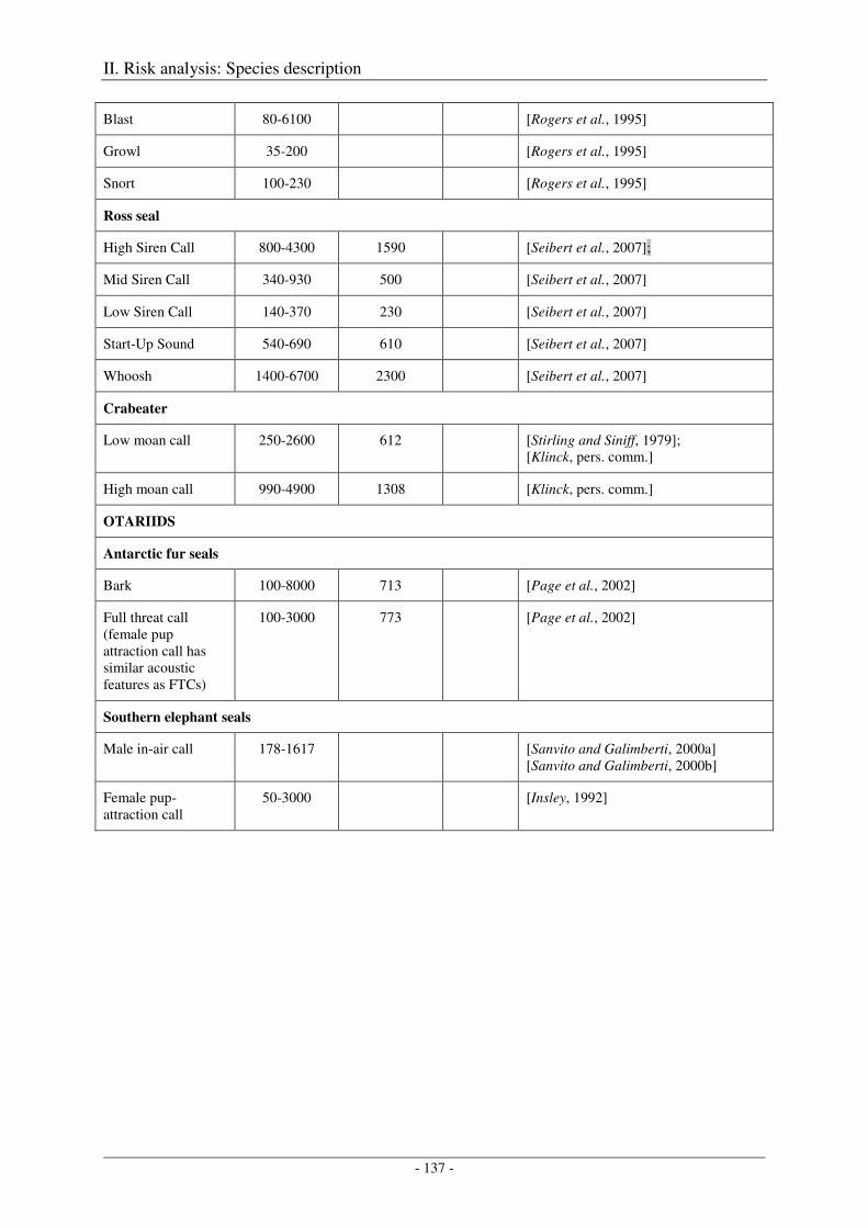
II. Risk analysis: Species description
- 137 -
Blast 80-6100 [Rogers et al., 1995]
Growl 35-200 [Rogers et al., 1995]
Snort 100-230 [Rogers et al., 1995]
Ross seal
High Siren Call 800-4300 1590 [Seibert et al., 2007];
Mid Siren Call 340-930 500 [Seibert et al., 2007]
Low Siren Call 140-370 230 [Seibert et al., 2007]
Start-Up Sound 540-690 610 [Seibert et al., 2007]
Whoosh 1400-6700 2300 [Seibert et al., 2007]
Crabeater
Low moan call 250-2600 612 [Stirling and Siniff, 1979]; [Klinck, pers. comm.]
High moan call 990-4900 1308 [Klinck, pers. comm.]
OTARIIDS
Antarctic fur seals
Bark 100-8000 713 [Page et al., 2002]
Full threat call (female pup attraction call has similar acoustic features as FTCs)
100-3000 773 [Page et al., 2002]
Southern elephant seals
Male in-air call 178-1617 [Sanvito and Galimberti, 2000a] [Sanvito and Galimberti, 2000b]
Female pup-attraction call
50-3000 [Insley, 1992]
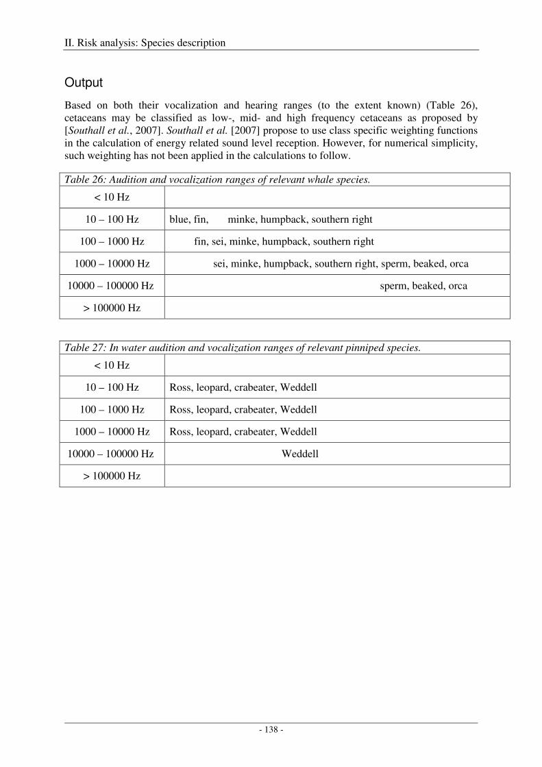
II. Risk analysis: Species description
- 138 -
Output
Based on both their vocalization and hearing ranges (to the extent known) (Table 26), cetaceans may be classified as low-, mid- and high frequency cetaceans as proposed by [Southall et al., 2007]. Southall et al. [2007] propose to use class specific weighting functions in the calculation of energy related sound level reception. However, for numerical simplicity, such weighting has not been applied in the calculations to follow.
Table 26: Audition and vocalization ranges of relevant whale species.
< 10 Hz
10 – 100 Hz blue, fin, minke, humpback, southern right
100 – 1000 Hz fin, sei, minke, humpback, southern right
1000 – 10000 Hz sei, minke, humpback, southern right, sperm, beaked, orca
10000 – 100000 Hz sperm, beaked, orca
> 100000 Hz
Table 27: In water audition and vocalization ranges of relevant pinniped species.
< 10 Hz
10 – 100 Hz Ross, leopard, crabeater, Weddell
100 – 1000 Hz Ross, leopard, crabeater, Weddell
1000 – 10000 Hz Ross, leopard, crabeater, Weddell
10000 – 100000 Hz Weddell
> 100000 Hz
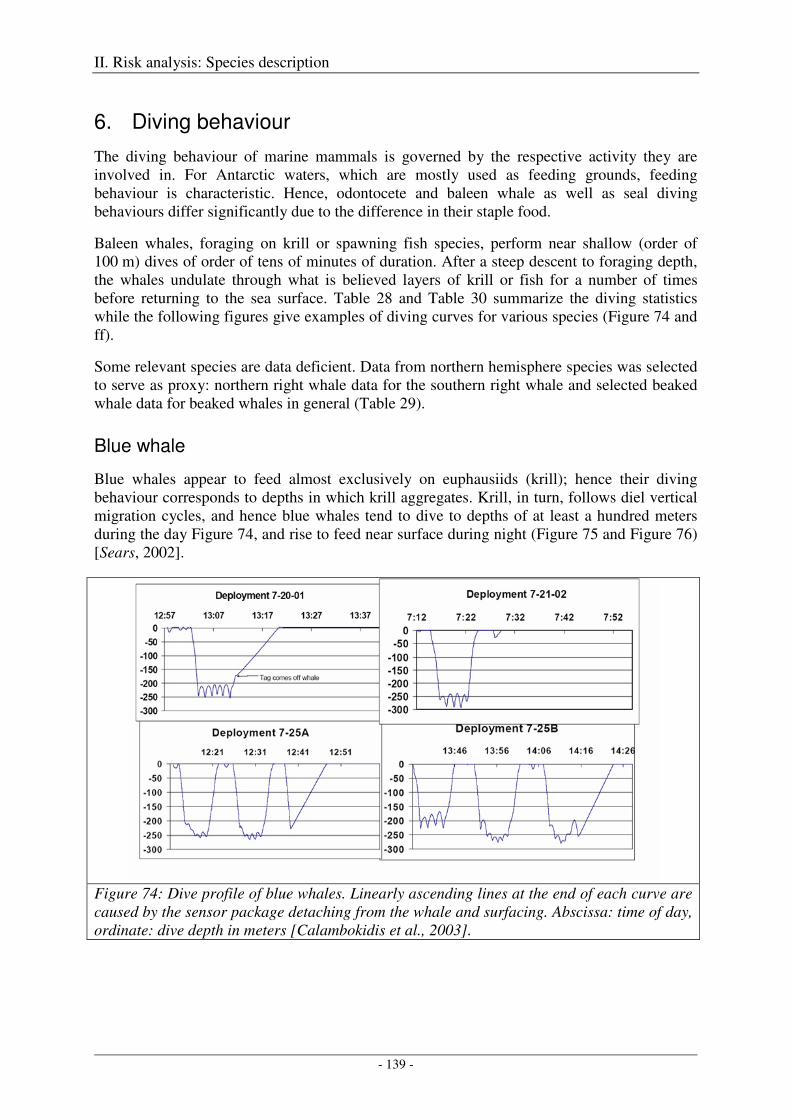
II. Risk analysis: Species description
- 139 -
6. Diving behaviour
The diving behaviour of marine mammals is governed by the respective activity they are involved in. For Antarctic waters, which are mostly used as feeding grounds, feeding behaviour is characteristic. Hence, odontocete and baleen whale as well as seal diving behaviours differ significantly due to the difference in their staple food.
Baleen whales, foraging on krill or spawning fish species, perform near shallow (order of 100 m) dives of order of tens of minutes of duration. After a steep descent to foraging depth, the whales undulate through what is believed layers of krill or fish for a number of times before returning to the sea surface. Table 28 and Table 30 summarize the diving statistics while the following figures give examples of diving curves for various species (Figure 74 and ff).
Some relevant species are data deficient. Data from northern hemisphere species was selected to serve as proxy: northern right whale data for the southern right whale and selected beaked whale data for beaked whales in general (Table 29).
Blue whale
Blue whales appear to feed almost exclusively on euphausiids (krill); hence their diving behaviour corresponds to depths in which krill aggregates. Krill, in turn, follows diel vertical migration cycles, and hence blue whales tend to dive to depths of at least a hundred meters during the day Figure 74, and rise to feed near surface during night (Figure 75 and Figure 76) [Sears, 2002].
Figure 74: Dive profile of blue whales. Linearly ascending lines at the end of each curve are caused by the sensor package detaching from the whale and surfacing. Abscissa: time of day, ordinate: dive depth in meters [Calambokidis et al., 2003].
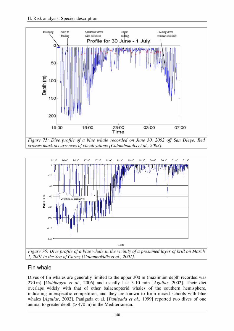
II. Risk analysis: Species description
- 140 -
Figure 75: Dive profile of a blue whale recorded on June 30, 2002 off San Diego. Red crosses mark occurrences of vocalizations [Calambokidis et al., 2003].
Figure 76: Dive profile of a blue whale in the vicinity of a presumed layer of krill on March 1, 2001 in the Sea of Cortez [Calambokidis et al., 2001].
Fin whale
Dives of fin whales are generally limited to the upper 300 m (maximum depth recorded was 270 m) [Goldbogen et al., 2006] and usually last 3-10 min [Aguilar, 2002]. Their diet overlaps widely with that of other balaenopterid whales of the southern hemisphere, indicating interspecific competition, and they are known to form mixed schools with blue whales [Aguilar, 2002]. Panigada et al. [Panigada et al., 1999] reported two dives of one animal to greater depth (> 470 m) in the Mediterranean.
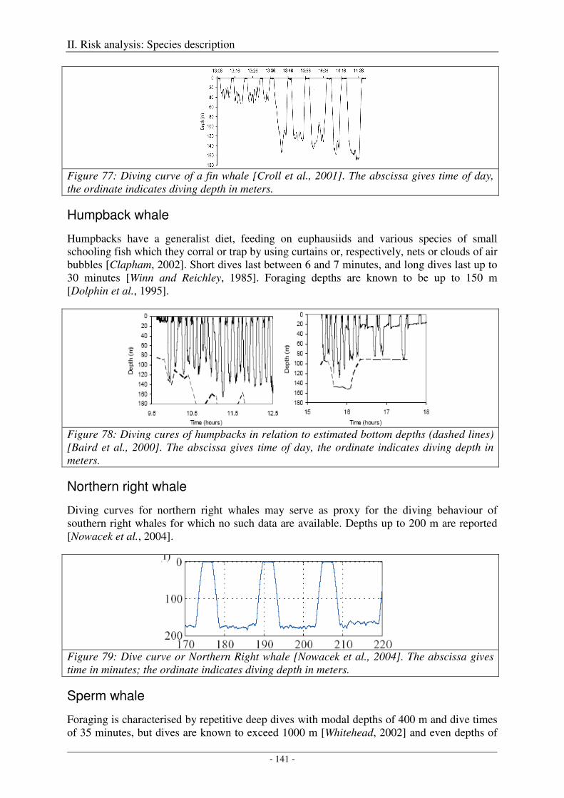
II. Risk analysis: Species description
- 141 -
Figure 77: Diving curve of a fin whale [Croll et al., 2001]. The abscissa gives time of day, the ordinate indicates diving depth in meters.
Humpback whale
Humpbacks have a generalist diet, feeding on euphausiids and various species of small schooling fish which they corral or trap by using curtains or, respectively, nets or clouds of air bubbles [Clapham, 2002]. Short dives last between 6 and 7 minutes, and long dives last up to 30 minutes [Winn and Reichley, 1985]. Foraging depths are known to be up to 150 m [Dolphin et al., 1995].
Figure 78: Diving cures of humpbacks in relation to estimated bottom depths (dashed lines) [Baird et al., 2000]. The abscissa gives time of day, the ordinate indicates diving depth in meters.
Northern right whale
Diving curves for northern right whales may serve as proxy for the diving behaviour of southern right whales for which no such data are available. Depths up to 200 m are reported [Nowacek et al., 2004].
Figure 79: Dive curve or Northern Right whale [Nowacek et al., 2004]. The abscissa gives time in minutes; the ordinate indicates diving depth in meters.
Sperm whale
Foraging is characterised by repetitive deep dives with modal depths of 400 m and dive times of 35 minutes, but dives are known to exceed 1000 m [Whitehead, 2002] and even depths of
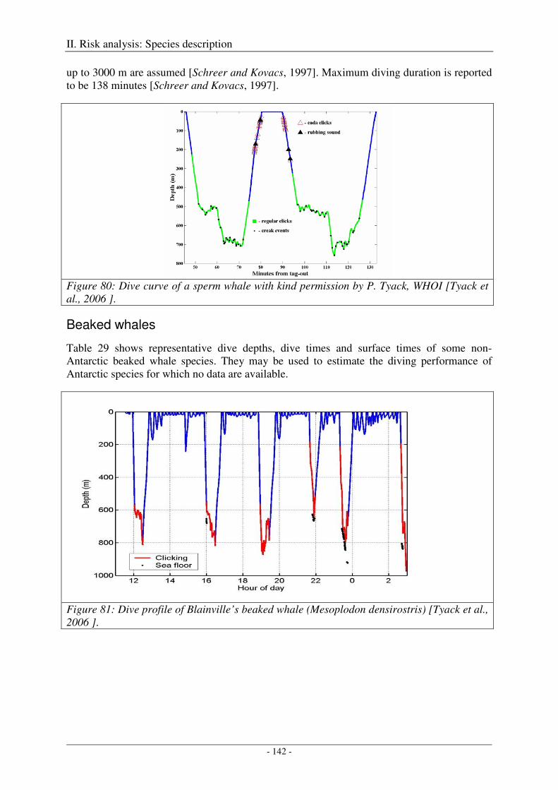
II. Risk analysis: Species description
- 142 -
up to 3000 m are assumed [Schreer and Kovacs, 1997]. Maximum diving duration is reported to be 138 minutes [Schreer and Kovacs, 1997].
Figure 80: Dive curve of a sperm whale with kind permission by P. Tyack, WHOI [Tyack et al., 2006 ].
Beaked whales
Table 29 shows representative dive depths, dive times and surface times of some non-Antarctic beaked whale species. They may be used to estimate the diving performance of Antarctic species for which no data are available.
Figure 81: Dive profile of Blainville’s beaked whale (Mesoplodon densirostris) [Tyack et al., 2006 ].
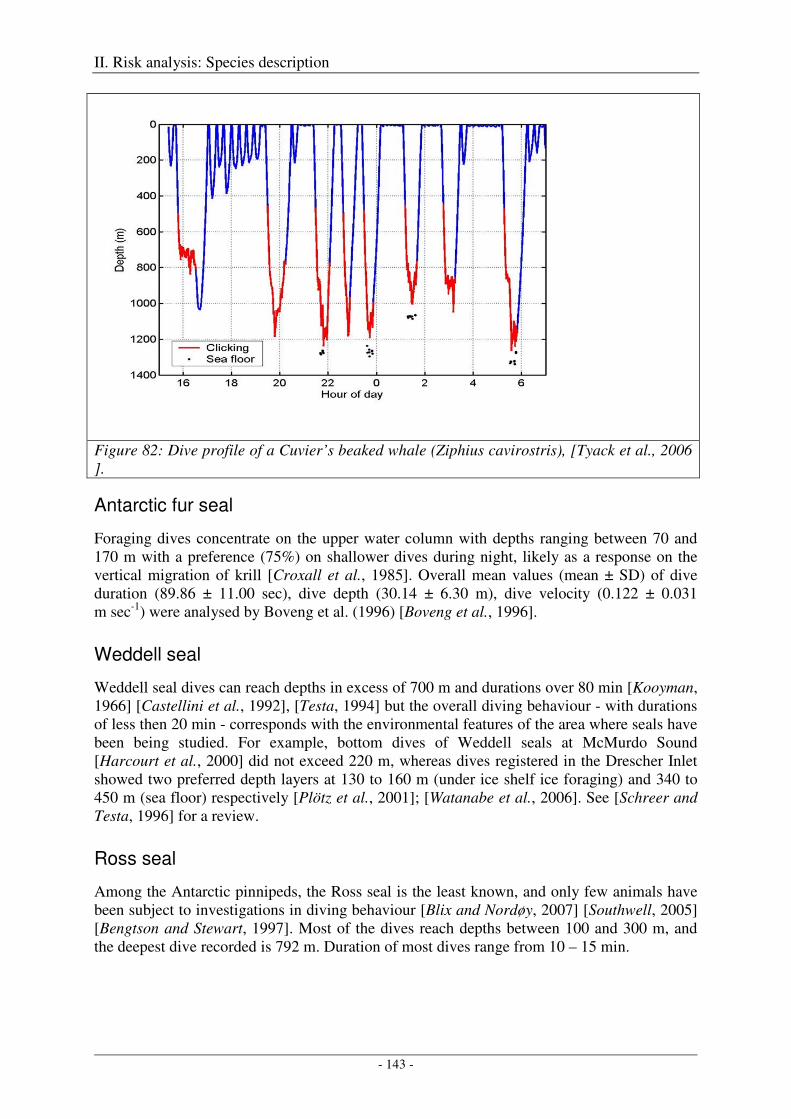
II. Risk analysis: Species description
- 143 -
Figure 82: Dive profile of a Cuvier’s beaked whale (Ziphius cavirostris), [Tyack et al., 2006 ].
Antarctic fur seal
Foraging dives concentrate on the upper water column with depths ranging between 70 and 170 m with a preference (75%) on shallower dives during night, likely as a response on the vertical migration of krill [Croxall et al., 1985]. Overall mean values (mean ± SD) of dive duration (89.86 ± 11.00 sec), dive depth (30.14 ± 6.30 m), dive velocity (0.122 ± 0.031 m sec-1) were analysed by Boveng et al. (1996) [Boveng et al., 1996].
Weddell seal
Weddell seal dives can reach depths in excess of 700 m and durations over 80 min [Kooyman, 1966] [Castellini et al., 1992], [Testa, 1994] but the overall diving behaviour - with durations of less then 20 min - corresponds with the environmental features of the area where seals have been being studied. For example, bottom dives of Weddell seals at McMurdo Sound [Harcourt et al., 2000] did not exceed 220 m, whereas dives registered in the Drescher Inlet showed two preferred depth layers at 130 to 160 m (under ice shelf ice foraging) and 340 to 450 m (sea floor) respectively [Plötz et al., 2001]; [Watanabe et al., 2006]. See [Schreer and Testa, 1996] for a review.
Ross seal
Among the Antarctic pinnipeds, the Ross seal is the least known, and only few animals have been subject to investigations in diving behaviour [Blix and Nordøy, 2007] [Southwell, 2005] [Bengtson and Stewart, 1997]. Most of the dives reach depths between 100 and 300 m, and the deepest dive recorded is 792 m. Duration of most dives range from 10 – 15 min.
II. Risk analysis: Species description
- 144 -
Crabeater seal
Foraging dives of crabeater seals concentrate on depths shallower than 50 m, and only exceptionally reach depths beyond 500 m; average dive durations are around 5 min while the longest dives last up to 11 minutes [Nordøy et al., 1995]; [Bengtson and Stewart, 1992]; [Burns et al., 2004].
Leopard seal
Data on leopard seal diving behaviour is yet only available for one juvenile and two adult individuals. Most of the dives observed in the juvenile seal were shallow with only 13% exceeding 100 m, and 2% deeper than 150 m. The maximum depth of dive recorded for this animal was 424.5 m and the mean dive duration was quite short (2 min, max = 9.35 min). [Kuhn et al., 2006]. The two adult seals made mostly short (<5 min) dives to depths of 10–50 m and only occasionally dove deeper than 200 m, the deepest dive recorded being 304 m. Short duration dives of less than 5 min dominated and contributed 70–90% of all dives. A significant proportion of dives (5–25% on a monthly basis) were of 5–10 min duration, but only one dive was longer than 15 min [Nordøy and Blix, 2008].
Southern elephant seal
The southern elephant seal has been studied to a similar extent as the Weddell seal. Overall diving behaviour of these wide-ranging and proficient deep-diving predators varies in the context of the physical environment (e.g. [Bailleul et al., 2007]; [Bennett et al., 2001]; [Hindell et al., 1991]). Deepest dives seem to extend 2,000 m and last up to 120 min, however modal depths range between 300 and 600 m with durations between 20 and 30 min.
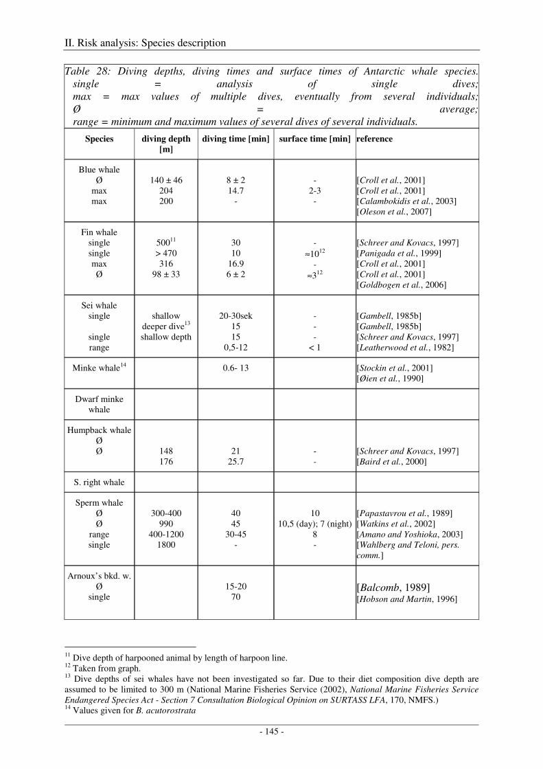
II. Risk analysis: Species description
- 145 -
Table 28: Diving depths, diving times and surface times of Antarctic whale species. single = analysis of single dives; max = max values of multiple dives, eventually from several individuals; Ø = average; range = minimum and maximum values of several dives of several individuals.
Species diving depth
[m]
diving time [min] surface time [min] reference
Blue whale Ø
max max
140 ± 46
204 200
8 ± 2 14.7
-
-
2-3 -
[Croll et al., 2001] [Croll et al., 2001] [Calambokidis et al., 2003] [Oleson et al., 2007]
Fin whale single single max Ø
50011 > 470 316
98 ± 33
30 10
16.9 6 ± 2
-
≈1012 -
≈312
[Schreer and Kovacs, 1997] [Panigada et al., 1999] [Croll et al., 2001] [Croll et al., 2001] [Goldbogen et al., 2006]
Sei whale single
single range
shallow
deeper dive13 shallow depth
20-30sek
15 15
0,5-12
- - -
< 1
[Gambell, 1985b] [Gambell, 1985b] [Schreer and Kovacs, 1997] [Leatherwood et al., 1982]
Minke whale14 0.6- 13 [Stockin et al., 2001] [Øien et al., 1990]
Dwarf minke whale
Humpback whale Ø Ø
148 176
21 25.7
- -
[Schreer and Kovacs, 1997] [Baird et al., 2000]
S. right whale
Sperm whale Ø Ø
range single
300-400
990 400-1200
1800
40 45
30-45 -
10
10,5 (day); 7 (night) 8 -
[Papastavrou et al., 1989] [Watkins et al., 2002] [Amano and Yoshioka, 2003] [Wahlberg and Teloni, pers. comm.]
Arnoux’s bkd. w. Ø
single
15-20
70
[Balcomb, 1989] [Hobson and Martin, 1996]
11 Dive depth of harpooned animal by length of harpoon line. 12 Taken from graph. 13 Dive depths of sei whales have not been investigated so far. Due to their diet composition dive depth are assumed to be limited to 300 m (National Marine Fisheries Service (2002), National Marine Fisheries Service Endangered Species Act - Section 7 Consultation Biological Opinion on SURTASS LFA, 170, NMFS.) 14 Values given for B. acutorostrata
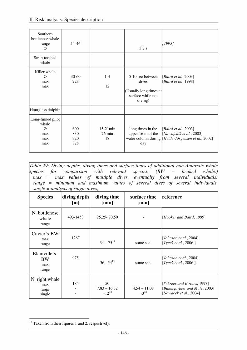
II. Risk analysis: Species description
- 146 -
Southern bottlenose whale
range Ø
11-46
3.7 s
[1995]
Strap-toothed whale
Killer whale Ø
max max
30-60 228
1-4
12
5-10 sec between
dives
(Usually long times at surface while not
diving)
[Baird et al., 2003] [Baird et al., 1998]
Hourglass dolphin
Long-finned pilot whale
Ø max max max
600 830 320 828
15-21min 26 min
18
long times in the upper 16 m of the
water column during day
[Baird et al., 2003] [Nawojchik et al., 2003] [Heide-Jørgensen et al., 2002]
Table 29: Diving depths, diving times and surface times of additional non-Antarctic whale species for comparison with relevant species. (BW = beaked whale.) max = max values of multiple dives, eventually from several individuals; range = minimum and maximum values of several dives of several individuals. single = analysis of single dives;
Species diving depth
[m]
diving time
[min]
surface time
[min]
reference
N. bottlenose whale range
493-1453
25,25- 70,50
-
[Hooker and Baird, 1999]
Cuvier’s-BW max
range
1267
34 – 7515
some sec.
[Johnson et al., 2004] [Tyack et al., 2006 ]
Blainville’s-BW max
range
975
36 - 5415
some sec.
[Johnson et al., 2004] [Tyack et al., 2006 ]
N. right whale max
range single
184
- -
50
7,83 – 16,32 ≈1212
-
4,54 – 11,08 ≈312
[Schreer and Kovacs, 1997] [Baumgartner and Mate, 2003] [Nowacek et al., 2004]
15 Taken from their figures 1 and 2, respectively.
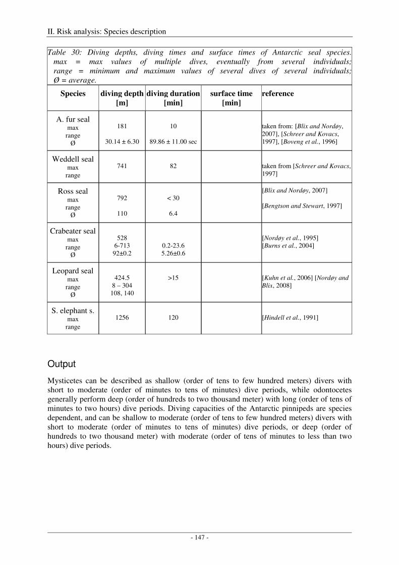
II. Risk analysis: Species description
- 147 -
Table 30: Diving depths, diving times and surface times of Antarctic seal species. max = max values of multiple dives, eventually from several individuals; range = minimum and maximum values of several dives of several individuals; Ø = average.
Species diving depth
[m]
diving duration
[min]
surface time
[min]
reference
A. fur seal max
range Ø
181
30.14 ± 6.30
10
89.86 ± 11.00 sec
taken from: [Blix and Nordøy, 2007], [Schreer and Kovacs, 1997], [Boveng et al., 1996]
Weddell seal max
range
741
82
taken from [Schreer and Kovacs, 1997]
Ross seal max
range Ø
792
110
< 30
6.4
[Blix and Nordøy, 2007] [Bengtson and Stewart, 1997]
Crabeater seal max
range Ø
528
6-713 92±0.2
0.2-23.6 5.26±0.6
[Nordøy et al., 1995] [Burns et al., 2004]
Leopard seal max
range Ø
424.5
8 – 304 108, 140
>15
[Kuhn et al., 2006] [Nordøy and Blix, 2008]
S. elephant s. max
range
1256
120
[Hindell et al., 1991]
Output
Mysticetes can be described as shallow (order of tens to few hundred meters) divers with short to moderate (order of minutes to tens of minutes) dive periods, while odontocetes generally perform deep (order of hundreds to two thousand meter) with long (order of tens of minutes to two hours) dive periods. Diving capacities of the Antarctic pinnipeds are species dependent, and can be shallow to moderate (order of tens to few hundred meters) divers with short to moderate (order of minutes to tens of minutes) dive periods, or deep (order of hundreds to two thousand meter) with moderate (order of tens of minutes to less than two hours) dive periods.
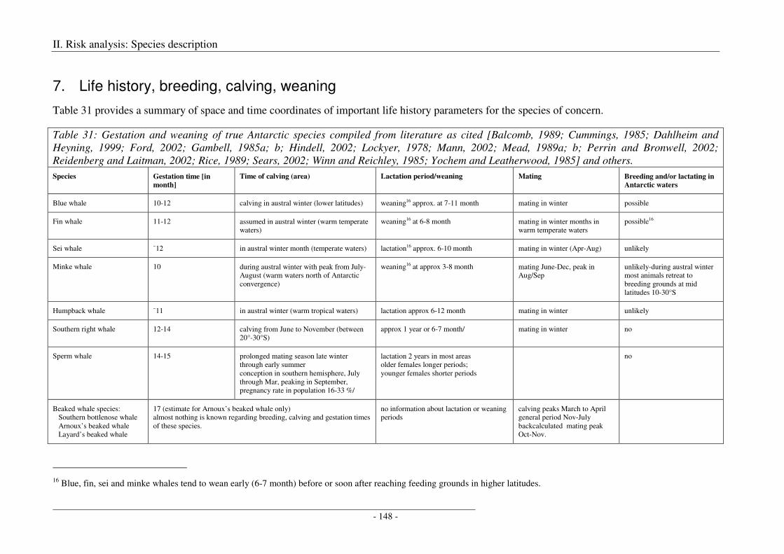
II. Risk analysis: Species description
- 148 -
7. Life history, breeding, calving, weaning
Table 31 provides a summary of space and time coordinates of important life history parameters for the species of concern.
Table 31: Gestation and weaning of true Antarctic species compiled from literature as cited [Balcomb, 1989; Cummings, 1985; Dahlheim and Heyning, 1999; Ford, 2002; Gambell, 1985a; b; Hindell, 2002; Lockyer, 1978; Mann, 2002; Mead, 1989a; b; Perrin and Bronwell, 2002; Reidenberg and Laitman, 2002; Rice, 1989; Sears, 2002; Winn and Reichley, 1985; Yochem and Leatherwood, 1985] and others.
Species Gestation time [in
month]
Time of calving (area) Lactation period/weaning Mating Breeding and/or lactating in
Antarctic waters
Blue whale 10-12 calving in austral winter (lower latitudes) weaning16 approx. at 7-11 month mating in winter possible
Fin whale 11-12 assumed in austral winter (warm temperate waters)
weaning16 at 6-8 month mating in winter months in warm temperate waters
possible16
Sei whale ~12 in austral winter month (temperate waters) lactation16 approx. 6-10 month mating in winter (Apr-Aug) unlikely
Minke whale 10 during austral winter with peak from July-August (warm waters north of Antarctic convergence)
weaning16 at approx 3-8 month mating June-Dec, peak in Aug/Sep
unlikely-during austral winter most animals retreat to breeding grounds at mid latitudes 10-30°S
Humpback whale ~11 in austral winter (warm tropical waters) lactation approx 6-12 month mating in winter unlikely
Southern right whale 12-14 calving from June to November (between 20°-30°S)
approx 1 year or 6-7 month/ mating in winter no
Sperm whale 14-15 prolonged mating season late winter through early summer conception in southern hemisphere, July through Mar, peaking in September, pregnancy rate in population 16-33 %/
lactation 2 years in most areas older females longer periods; younger females shorter periods
no
Beaked whale species: Southern bottlenose whale Arnoux’s beaked whale Layard’s beaked whale
17 (estimate for Arnoux’s beaked whale only) almost nothing is known regarding breeding, calving and gestation times of these species.
no information about lactation or weaning periods
calving peaks March to April general period Nov-July backcalculated mating peak Oct-Nov.
16 Blue, fin, sei and minke whales tend to wean early (6-7 month) before or soon after reaching feeding grounds in higher latitudes.
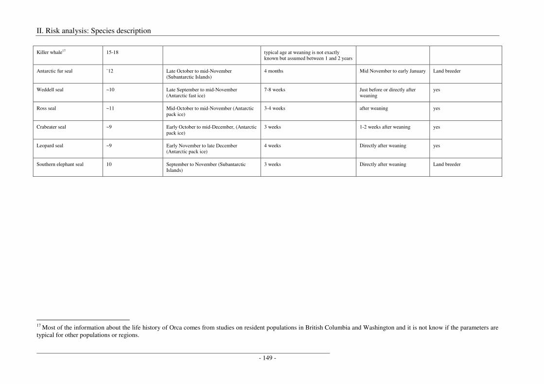
II. Risk analysis: Species description
- 149 -
Killer whale17 15-18 typical age at weaning is not exactly known but assumed between 1 and 2 years
Antarctic fur seal ~12 Late October to mid-November (Subantarctic Islands)
4 months Mid November to early January Land breeder
Weddell seal ~10 Late September to mid-November (Antarctic fast ice)
7-8 weeks Just before or directly after weaning
yes
Ross seal ~11 Mid-October to mid-November (Antarctic pack ice)
3-4 weeks after weaning yes
Crabeater seal ~9 Early October to mid-December, (Antarctic pack ice)
3 weeks 1-2 weeks after weaning yes
Leopard seal ~9 Early November to late December (Antarctic pack ice)
4 weeks Directly after weaning yes
Southern elephant seal 10 September to November (Subantarctic Islands)
3 weeks Directly after weaning Land breeder
17 Most of the information about the life history of Orca comes from studies on resident populations in British Columbia and Washington and it is not know if the parameters are typical for other populations or regions.
II. Risk Analysis: Species description
- 150 -
Output
Mating and calving in mysticetes occur in warm waters. In general only little information exists regarding mating and even less regarding their winter distribution. Gestation periods of mysticetes range from 10-13 months, and weaning of their young generally takes place within a year after birth. Blue, fin, minke and sei whale tend to wean early (6-7 month), before or soon after reaching feeding grounds while humpbacks and right whales have longer lactation periods and usually feed during later stages of nursing. Very little is known about mother-calf behaviour and association during migration.
Odontocetes have protracted breeding seasons with other activities also taking place during this period. Very little is known about the breeding site selection. Odontocete gestation periods range from 7-17 months, with longer gestation times for large whales that give birth to relatively larger calves. Lactation periods of 2-3 years are common in odontocetes and weaning is a gradual process, ranging over a period of months or years (some sperm whales).
The Antarctic ice seals (Weddell, Ross, crabeater, leopard) give birth between September and December, and lactation lasts between ca. 3 and 8 weeks. Weaning is more or less abrupt, and mating takes place immediately at around weaning. The land breeding seal species give birth between September and November, and in the case of the southern elephant seal wean and mate after a three week lactation period, and in the case of the Antarctic fur seal mate 7 to ten days after giving birth, and pups are weaned at about 4 months old.
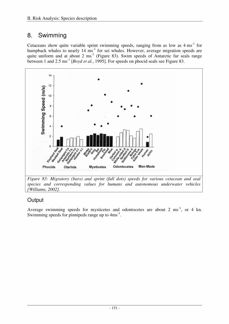
II. Risk Analysis: Species description
- 151 -
8. Swimming
Cetaceans show quite variable sprint swimming speeds, ranging from as low as 4 ms-1 for humpback whales to nearly 14 ms-1 for sei whales. However, average migration speeds are quite uniform and at about 2 ms-1 (Figure 83). Swim speeds of Antarctic fur seals range between 1 and 2.5 ms-1 [Boyd et al., 1995]. For speeds on phocid seals see Figure 83.
Figure 83: Migratory (bars) and sprint (full dots) speeds for various cetacean and seal species and corresponding values for humans and autonomous underwater vehicles [Williams, 2002].
Output
Average swimming speeds for mysticetes and odontocetes are about 2 ms-1, or 4 kn. Swimming speeds for pinnipeds range up to 4ms-1.
II. Risk Analysis: Species description
- 152 -
9. References
Aguilar, A. (2002), Fin whale Balaenoptera physalus, in Encyclopedia of Marine Mammals, edited by W. F. Perrin, et al., pp. 435-438, Academic Press, London, New York.
Amano, M., and M. Yoshioka (2003), Sperm whale diving behavior monitored using a suction-cup-attached TDR tag, Marine Ecology Progress Series, 258, 291-295.
Aroyan, J. L., et al. (2000), Acoustic models of sound production and propagation, in Hearing by Whales and Dolphins, edited by W. W. L. Au, et al., pp. pp 409-469, Springer.
Atkinson, A., et al. (2004), Long-term decline in krill stock and increase in salps within the Southern Ocean, Nature, 432(4), 100-103.
Bailleul, F., et al. (2007), Southern elephant seals from Kerguelen Islands confronted by Antarctic sea ice. Changes in movements and diving behaviour, Deep Sea Research Part II: Topical Studies in Oceanography, 54(3-4), 343-355.
Baird, R. W., et al. (1998), Diving behaviour of killer whales, paper presented at World Marine Mammal Science Conference, 9 pp, Monaco, January 1998.
Baird, R. W., et al. (2000), Sub-surface and night-time behavior of humpback whales off Maui, Hawaii: A preliminary report, 19 pp.
Baird, R. W., et al. (2003), Studies of foraging "southern resident" killer whales during July 2002: dive depth, bursts in speed, and the use of a "crittercam" system for examing sub-surface behavior, Report submitted to the National Marine Mammal Laboratory, Seattle, WA.
Balcomb, K. C. (1989), Baird's beaked whale Berardius bairdii Stejneger, 1883: Arnoux's beaked whale Berardius arnuxii Duvernoy, 1851, in Handbook of Marine Mammals, edited by S. H. Ridgway and R. Harrison, pp. 261-288, Academic Press, London.
Baumgartner, M. F., and B. R. Mate (2003), Summertime foraging ecology of North Atlantic right whales, Marine Ecology Progress Series, 264, 123.
Baumgartner, M. F., et al. (2008), Low frequency vocalizations attributed to sei whales (Balaenoptera borealis), Journal of the Acoustical Society of America, 124(2), 1339-1349.
Bengtson, J. L., and B. S. Stewart (1992), Diving and haulout behavior of crabeater seals in the Weddell Sea, Antarctica, during March 1986, Polar Biology, 12, 635-644.
Bengtson, J. L., and B. S. Stewart (1997), Diving patterns of a Ross seal (Ommatophoca rossii) near the eastern coast of the Antarctic Peninsula, Polar Biology, 18(3), 214-218.
Bennett, K. A., et al. (2001), Diurnal and seasonal variations in the duration and depth of the longest dives in southern elephant seals (Mirounga leonine): possible physiological and behavioural constraints, The Journal of Experimental Biology, 204, 649-662.
Bernard, H. J., and S. B. Reilly (1999), Pilot whales Globicephala Lesson, 1828, in Handbook of Marine Mammals, edited by S. H. Ridgeway and R. Harrison, pp. 245-279, Academic Press, London.
Best, P. B. (1982), Seasonal abundance, feeding, reproduction, age and growth in minke whales off Durban, Rep. Int. Whal. Commn., 32, 759-786.
Bester, M. N., et al. (1995), Seasonal change in the distribution and density of seals in the pack ice off Princess Martha Coast, Antarctica, Antarctic Science, 7(04), 357-364.
II. Risk Analysis: Species description
- 153 -
Bester, M. N., and P. N. Odendaal (2000), Abundance and distribution of Antarctic pack ice seals in the Weddell Sea, in Antarctic ecosystems: models for wider ecological understanding, edited by W. Davison, pp. 51-55, Caxton Press, Christchurch.
Bester, M. N., et al. (2002), Population densities of pack ice seals in the Lazarev Sea, Antarctica, Antarctic Science, 12(2), 123-127.
Bester, M. N., and B. S. Stewart (2006), The International Antarctic Pack Ice Seals (APIS) Program: Multi-disciplinary Research into the Ecology and Behavior of Antarctic Pack Ice Sea, 25 pp. (www.seals.scar.org/pdf/IntAPISSummUpdateRevis.pdf)
Blix, A. S., and E. S. Nordøy (2007), Ross seal (Ommatophoca rossii) annual distribution, diving behaviour, breeding and moulting, off Queen Maud Land, Antarctica, Polar Biology, 30(11), 1449-1458.
Bornemann, H., et al. (2000), Southern elephant seal movements and Antarctic sea ice, Antarctic Science, 12(1), 3-15.
Boveng, P., et al. (1996), Variability in Antarctic fur seal dive data: implications from TDR studies, Marine Mammal Science 12(4), 543-554.
Boyd, I. L., et al. (1995), Swimming speed and allocation of time during the dive cycle in Antarctic fur seals, Animal Behaviour, 50(3), 769-784.
Boyd, I. L. (2002a), Antarctic Marine Mammals, in Encyclopedia of Marine Mammals, edited by W. F. Perrin, et al., pp. 30-36, Academic Press, London.
Boyd, I. L. (2002b), Pinniped life history, in Encyclopedia of Marine Mammals, edited by W. F. Perrin, et al., pp. 929-934, Academic Press, London.
Brown, S. G. (1966), Whale Marks recovered in the Antarctic whaling season 1965/66, Norsk Hvalfangst-Tidende (The Norwegian whaling gazette), 10, 198-200.
Burgess, W. C., et al. (1998), A programmable acoustic recording tag and first results from free-ranging northern elephant seals, Deep Sea Research Part II: Topical Studies in Oceanography, 45(7), 1327-1351.
Burns, J. M., et al. (2004), Winter habitat use and foraging behavior of crabeater seals along the Western Antarctic Peninsula, Deep Sea Research Part II: Topical Studies in Oceanography, 51(17-19), 2279-2303.
Calambokidis, J., et al. (2001), Underwater behavior of blue whales using a suction-cup attached crittercam, 7 pp, prepared for the Office of Naval Research (ONR grant no. N00014-00-1-0942).
Calambokidis, J., et al. (2003), Research on humpback and blue whales off California, Oregon and Washington in 2002, Final Report, Cascadia Research, Olympia, WA 98501.
Carwardine, M. (1996), Whales, Dolphins and Porpoises: The visual guide to all the world's cetaceans, 256 pp., Dorling Kindersley Limited, London.
Castellini, M. A., et al. (1992), Annual cycles of diving behaviour and ecology of the Weddell seal, Bulletin of the Scripps Institution of Oceanography at the University of California, 28, 54 pp.
Chambers, S., and R. N. James (2005), Sonar termination as a cause of mass cetacean strandings in Geographe Bay, south-western Australia, paper presented at Acoustics 2005, Acoustics in a Changing Environment, 391-398 pp, Busselton, Western Australia, November 9 - 11, 2005.
Clapham, P. J. (2002), Humpback whale Megaptera novaeangliae, in Encyclopedia of Marine Mammals, edited by W. F. Perrin, et al., pp. 589-592, Academic Press, London.
II. Risk Analysis: Species description
- 154 -
Clark, C. W. (1982), The acoustic repertoire of the Southern right whale, a quantitative analysis, Animal Behaviour, 30(4), 1060-1071.
Clarke, M. R. (1972), New technique for the study of sperm whale migration, Nature, 238(5364), 405-406.
Cox, T. M., et al. (2006), Understanding the impacts of anthropogenic sound on beaked whales, Journal of Cetacean Research and Management, 7(3), 177-187.
Crawley, M. C. (1978), Weddell seal harvesting at Scott Base, McMurdo Sound, Antarctica 1970-76, New Zealand Journal of Ecology, 1, 132-137.
Croll, D. A., et al. (2001), The diving behavior of blue and fin whales: is dive duration shorter than expected based on oxygen stores?, Comparative Biochemistry and Physiology, Part A (129), 797-809.
Croxall, J. P., et al. (1985), Fur seal diving behaviour in relation to vertical distribution of krill, Journal of Animal Ecology 54(1), 1-8.
Culik, B. (2005), Review on small cetaceans: distribution, behaviour, migration and threats, 343 pp.
Cummings, W. C., and P. O. Thompson (1971), Underwater sounds from the blue whale, Balaenoptera musculus, Journal of the Acoustical Society of America, 50(4), 1193-1198.
Cummings, W. C. (1985), Right whales Eubalaena glacialis (Müller, 1776) and Eubalaena australis (Desmoulins, 1822), in Handbook of Marine Mammals: The sirenians and baleen whales, edited by S. H. Ridgway and R. Harrison, pp. 275-304, Academic Press, London.
Dahlheim, M. E., and J. E. Heyning (1999), Killer whale Orinus orca (Linnaeus, 1758), in Handbook of Marine Mammals, edited by S. H. Ridgway and R. Harrison, pp. 281-322, Academic Press, London.
Dolphin, W. F., et al. (1995), Modulation rate transfer functions to low-frequency carriers in three species of cetaceans, Journal of Comparative Physiology, A, 177(2), 235-245.
Donovan, G. P. (1991), A review of IWC stock boundaries, in Genetic ecology of whales and dolphins, edited by R. A. Hoelzel, pp. 39-68, The International Whaling Commission, Cambridge.
Engas, A., et al. (1996), Effects of seismic shooting on local abundance and catch rates of cod (Gadus morhua) and haddock (Melanogrammus aeglefinus) Canadian Journal of Fisheries and Aquatic Sciences, 53(10), 2238-2249.
Engas, A., and S. Lokkeborg (2002), Effects of seismic shooting and vessel-generated noise on fish behaviour and catch rates, Bioacoustics, 12, 313-316.
Erickson, A. W., et al. (1971), Distibutional ecology of Antarctic seals, paper presented at Symposium on Antarctic ice and water masses, 55-76 pp, SCAR, Cambridge, Tokyo, Japan, 19 September 1970.
Erickson, A. W., et al. (1972), Populations of seals, whales, and birds in the Bellingshausen and Amundsen Seas, Antarctic Journal of the United States, 70, 70-72.
Erickson, A. W., et al. (1973), Census of pelagic seals off the Oates and Gerg V Coasts, Antarctica, Antarctic Journal of the United States, 8, 191-193.
Erickson, A. W., and R. J. Hofman (1974), Antarctic seals, in Antarctic mammals, edited by V. C. Bushnell, pp. 4-13, American Geographical Society under contract with the National Science Foundation, New York.
Erickson, A. W., et al. (1974), Seal and bird populations off Adélie, Claire and Banzare coasts, Antarctic Journal of the United States, 9, 292-296.
II. Risk Analysis: Species description
- 155 -
Erickson, A. W., et al. (1983), Population densities of seals and whales observed during the 1983 cirvumnavigation of Antarctica by the USCGC Polar Star, Antarctic Journal of the United States, 18(5), 163-166.
Erickson, A. W., and M. B. Hanson (1990), Continental estimates and population trends of Antarctic ice seals, in Antarctic ecosystems - ecological change and conservation, edited by K. R. Kerry and G. Hempel, pp. 253-264, Springer - Verlag, Berlin Heidelberg.
Fernández, M., et al. (2003), Food and parasites from two hourglass dolphins Lagenorhynchus cruciger (Quoy and Gaimard, 1824), from patagonian waters, Marine Mammal Science, 19(4), 832-836.
Fischer, W., and J. C. Hureau (1985), Southern Ocean CCAMLR convention area fishing areas 48, 58 and 88, 472 pp., FAO, Rome.
Fletcher, S., et al. (1996), Onboard acoustic recording from diving northern elephant seals, The Journal of the Acoustical Society of America, 100(4), 2531-2539.
Ford, J. B. K. (2002), Killer whale Orcinus orca, in Encyclopedia of marine mammals, edited by W. F. Perrin, et al., pp. 669-676, Academic Press, London.
Ford, J. K. B., and R. R. Reeves (2008), Fight or flight: antipredator strategies of baleen whales, Mammal Review, 38(1), 50-86.
Frankel, A. S. (2002), Sound Production, in Encyclopedia of Marine Mammals, edited by W. F. Perrin, et al., p. 1414, Academic Press, London.
Friedlander, A. S., et al. (2006), Whale distribution in relation to prey abundance and oceanographic processes in shelf waters of the Western Antarctic Peninsula, Marine Ecology Progress Series, 317, 297-310.
Gambell, R. (1985a), Fin whale Balaenoptera physalus (Linnaeus 1758), in Handbook of marine mammals Vol 3: The sirenians and baleen whales, edited by S. H. Ridway and H. R., pp. 171-192, Academic Press, London.
Gambell, R. (1985b), Sei whale Balaenoptera borealis (Lesson,1828), in Handbook of Marine Mammals, Vol 3: The sirenians and baleen whales, edited by S. H. Ridgway and R. Harrison, pp. 155-170, Academic Press, London.
Gedamke, J., et al. (2001), Localization and visual verification of a complex minke whale vocalization, The Journal of the Acoustical Society of America, 109(6), 3038-3047.
Gelatt, T. S., and S. B. Siniff (1999), Line transect survey of crabeater seals in the Amundsen-Bellingshausen Seas 1994, Wildlife Society Bulletin, 27(2), 330-336.
Gilbert, J. R., and A. W. Erickson (1977), Distribution and abundance of seals in the pack ice of the Pacific Sector of the Southern Ocean, paper presented at Adaptations within Antarctic Ecosystems, 3rd SCAR Symposium on Antarctic Biology, 703-740 pp, SCAR, Smithonian Institute, Washington, D.C., August 26th-30th 1974.
Gill, A., and P. G. H. Evans (2002), Marine mammals of the Antarctic in relation to hydro-acoustic activities, 216 pp, Study on behalf of the German Federal Agency for Nature Conservation (BfN), Oxford.
Gill, P. C., and D. Thiele (1997), A winter sighting of killer whales (Orcinus orca) in Antarctic sea ice, Polar Biology, 17, 401-404.
Goldbogen, J. A., et al. (2006), Kinematics of foraging dives and lunge-feeding in fin whales, J Exp Biol, 209(7), 1231-1244.
Goodall, R. N. P. (1997), Review of sightings of the hourglass dolphin, Lagenorhynchus cruciger, in the South American Sector of the Antarctic and sub-Antarctic, 1001-1014 pp.
II. Risk Analysis: Species description
- 156 -
Green, K., and H. R. Burton (1988), Annual and diurnal variations in the underwater vocalizations of Weddell seals, Polar Biology, 8, 161-164.
Harcourt, R. G., et al. (2000), Three dimensional dive profiles of free-ranging Weddell seals, Polar Biology, 23(7), 479-487.
Harding, K. C. (2000), Population dynamics of seals: the influences of spatial and temporal structure, Dissertation thesis, 39 pp, University of Helsinki, Helsinki.
Heide-Jørgensen, M. P., et al. (2002), Diving behaviour of long-finned pilot whales Globicephala melas around the Faroe Islands, Wildlife Biology, 8(307-311).
Hewitt, R. P., et al. (2002), Setting a precautionary catch limit for Antarctic krill, Oceanography, 15(3), 26-33.
Hindell, M. A., et al. (1991), The diving behaviour of adult male and female southern elephant seals, Mirounga leonina (Pinnipedia: Phocidae). Australian Journal of Zoology, 39, 595-619.
Hindell, M. A. (2002), Breeding sites, in Encyclopedia of Marine Mammals, edited by W. F. Perrin, et al., pp. 169-171, Academic Press, London.
Hobson, R. P., and A. R. Martin (1996), Behaviour and dive times of Armoux's beaked whales, Berardius arnuxii, at narrow leads in fast ice, Canadian Journal Zoolgy, 74, 388-393.
Hooker, S. K., and R. W. Baird (1999), Deep-diving behaviour of the northern bottlenose whale, Hyperoodon ampullatus (Cetacea: Ziphiidae), Proceedings of the Royal Society, 266, 671-676.
Insley, S. J. (1992), Mother-offpring separation and acoustic stereotypy: a comparison of call morphology in two species of pinniped, Behaviour 120, 103-121.
International Whaling Commission (IWC) (2006a), Report of the sub-committee on the other southern hemisphere whale stocks, The Journal of Cetacean Research and Management, 8 (Supplement), 151-170 (Annex H).
International Whaling Commission (IWC) (2002), Report of the sub-committee on estimation of bycatch and other human-induced mortality. The Journal of Cetacean Research and Management, 4 (Supplement), 361-371.
International Whaling Commission (IWC) (2006b), Report of the working group on stock definition, The Journal of Cetacean Research and Management, 8 (Supplement), 171-176.
International Whaling Commission (IWC) (2008a), Report of the working group on stock definitions, The Journal of Cetacean Research and Management, 10 (Supplement), 225-232.
International Whaling Commission (IWC) (2008b), Report of the sub-committee on the other southern hemisphere whale stocks, The Journal of Cetacean Research and Management, 10 (Supplement), 207-224.
Jefferson, T. A., et al. (1993), Marine mammals of the world, 320 pp., FAO, Rome.
Jensen, A. S., and G. K. Silber (2004), Large whale ship strike database, NOAA Technical Memorandum NMSF-OPR, 9 pp, U.S. Department of Commerce National Oceanic and Atmospheric Administration National Marine Fisheries.
Jessopp, M. J., et al. (2004), Winter dispersal of leopard seals (Hydrurga leptonyx): Environmental factors influencing demographics and seasonal abundance, Journal of Zoology London, 263(3), 251-258.
Johnson, M., et al. (2004), Beaked whales echolocate on prey, Biology Letters, 271(Supplement 6), S383-S386.
II. Risk Analysis: Species description
- 157 -
Kasamatsu, F., et al. (1988), Distribution of cetacean sightings in the Antarctic: Results obtained from the IWC/IDCR minke whale assessment cruises, 1978/79 to 1983/84, Rep. Int.Whal. Commn., 38, 449-473.
Kasamatsu, F., and G. G. Joyce (1995), Current status of odontocetes in the Antarctic, Antarctic Science, 7(4), 365-379.
Kasamatsu, F., et al. (1996), Current occurence of baleen whales in Antarctic waters, Rep. Int. Whaling Comm., 46, 293-303.
Kaschner, K., et al. (2006), Mapping world-wide distributions of marine mammal species using a relative environmental suitability (RES) model, Marine Ecology Progress Series, 316, 285-310.
Kaufman, G. D., et al. (1975), Colony behavior of Weddell seals, Leptonychotes weddellii, at Hutton Cliffs, Antarctica, in Biology of the seal, edited by K. Ronald and A. Mansfield, pp. 228-246, Conseil International pour L'Exploration scientifique de la Mer
King, J. E. (1969), Some aspects of the anatomy of the Ross seal, British Antarctic Survey Scientific Reports, 63, 1-54.
Klinck, H. (2008), Automated passive acoustic detection, localization and identification of leopard seals: from hydro-acoustic technology to leopard seal ecology, PhD Thesis, 145 pp, Alfred Wegener Institute, Bremerhaven.
Kooyman, G. (1968), An analysis of some behavioral and physiological characteristics related to diving in the Weddell seal, Antarctic Research Series, 11, 127-144.
Kooyman, G. L. (1966), Maximum diving capacities of the Weddell seal (Leptonychotes weddellii) Science, 151, 1553-1554.
Kuhn, C. E., et al. (2006), Diving physiology and winter foraging behavior of a juvenile leopard seal (Hydrurga leptonyx), Polar Biology, 29(4), 303.
Laist, D. W., et al. (2001), Collisions between ships and whales, Marine Mammal Science, 17(1), 35.
Laws, R. M. (1956), The elephant seal (Mirounga leonina) Linn. – II. General, social, and reproductive behaviour, Falkland Islands dependencies survey scientific reports 13, 1-88.
Leaper, R., and M. Scheidat (1998), An acoustic survey for cetaceans in the Southern Ocean Sanctuary conducted from the German Government Research Vessel Polarstern, Rep. Int. Whaling Comm., 48, 431-437.
Leaper, R., et al. (2000), Results of passive acoustic surveys for odontocetes in the Southern Ocean, Journal of Cetacean Research and Management, 2(3), 187-196.
Leatherwood, S., et al. (1982), Respiration patterns and 'sightability' of whales, Rep. Int. Whal. Commn, 32, 601-613.
Lockyer, C. (1978), Growth and energy budgets of large baleen whales from the southern hemisphere, in Mammals in the sea: general papers and large cetaceans, edited, pp. 379-502, Food and Agricultural Organization of the United Nations, Rome.
Madsen, P. T., et al. (2002), Sperm whale sound production studied with ultrasound time/depth-recording tags, Journal of Experimental Biology, 205, 1899-1906.
Mann, J. (2002), Parental behavior, in Marine Mammal Encyclopedia, edited by W. F. Perrin, et al., pp. 876-882, Academic Press, London.
Matsuoka, K., et al. (1998), Abundance and distribution of sperm and beaked whales in the Antarctic areas IV and V, preliminary report (SC/50/CAWS9), 6 pp, IWC.
II. Risk Analysis: Species description
- 158 -
Matsuoka, K., et al. (2004), Development of a retrievable sonobuoy system for whale sound recording in polar region, 7 pp.
McCauley, R. D., and J. Fewtrell (2008), Marine invertebrates, intense anthropogenic noise, and squid response to seismic survey pulses, Bioacoustics, 17(1-3), 215-318.
McDonald, M., et al. (2005), Sei whale sounds recorded in the Antarctic, The Journal of the Acoustical Society of America, 118(6), 3941-3945.
McDonald, M., A. , et al. (2001), The acoustic calls of blue whales off California with gender data, The Journal of the Acoustical Society of America, 109(4), 1728-1735.
McDonald, M. A. (2006a), An acoustic survey of baleen whales off Great Barrier Island, New Zealand, New Zealand Journal of Marine and Freshwater Research, 40, 519-529.
McDonald, M. A., Mesnick, S.L., Hildebrand, J.A. (2006b), Biogeographic characterisation of blue whale song worldwide: using song to identify populations, Journal of Cetacean Research Management, 8(1), 55-65.
Mead, J. G. (1989a), Beaked whales of the genus Mesoplodon, in Handbook of Marine Mammals, edited by S. H. Ridgway and R. Harrison, Academic Press, London.
Mead, J. G. (1989b), Bottlenose whales Hyperoodon ampullatus (Forster, 1779) and Hyperoodon planifrons Flower, 1882, in Handbook of Marine Mammals, edited by S. H. Ridgway and R. Harrison, pp. 321-348, Academic Press, London.
Mellinger, D. K., et al. (2000), Characteristics of minke whale (Balaenoptera acutorostrata) pulse trains recorded near Puerto Rico Marine Mammal Science, 16(4), 739-756.
Mellinger, D. K., and C. W. Clark (2003), Blue whale (Balaenoptera musculus) sounds from the North Atlantic, Journal of the Acoustical Society of America, 114(2), 1108-1119.
Mikhalev, Y. A., et al. (1981), The distribution and biology of killer whales in the southern hemisphere, Rep. Int. Whaling Comm., 31, 551-566.
Miller, E. H. (1975), A comparative study of facial expressions of two species of pinnipeds, Behaviour, 53, 268-284.
Møhl, B., et al. (2000), Sperm whale clicks: Directionality and source level revisited, Journal of the Acoustical Society of America, 107(1), 638-648.
Møhl, B., et al. (2003), The monopulsed nature of sperm whale clicks, The Journal of the Acoustical Society of America, 114(2), 1143-1154.
Moors, H. B., and J. M. Terhune (2004), Repetition patterns in Weddell seal (Leptonychotes weddellii) underwater multiple element calls, The Journal of the Acoustical Society of America, 116(2), 1261-1270.
National Marine Fisheries Service (2002), National Marine Fisheries Service Endangered Species Act - Section 7 Consultation Biological Opinion on SURTASS LFA, 170, NMFS.
Nawojchik, R., et al. (2003), Movements and dive behavior of two stranded, rehabilitated long-finned pilot whales (Globicephala melas) in the Northwest Atlantic, Marine Mammal Science, 19, 232-239.
Nehls, G., et al. (2007), Sources of underwater noise and their implications on marine wildlife - with special emphasis on the North Sea and the Baltic Sea, final report, 123 pp, Bio Consult SH, itap.
Nishiwaki, S. (1972), General Biology, in Mammals of the sea - biology and medicine, edited by S. H. Ridgway, pp. 3-204, C. C. Thomas, Sringfield, IL.
II. Risk Analysis: Species description
- 159 -
Nordøy, E. S., et al. (1995), Distribution and diving behaviour of Crabeater seals (Lobodon carinophagus) off Queen Maud Land, Polar Biology, 15(4), 261-268.
Nordøy, E. S., and A. S. Blix (2008), Movements and dive behaviour of two leopard seals (Hydrurga leptonyx) off Queen Maud Land, Antarctica., Polar Biology, 32(3), 263-270.
Norris, K. S. (1969), The echolocation of marine mammals, in The biology of marine mammals, edited by H. Andersen, Academic Press, New York.
Nowacek, D. P., et al. (2004), North Atlantic right whales (Eubalaena glacilis) ignore ships but respond to alerting stimuli, Proceedings of the Royal Society London B, 271, 227-231.
Øien, N., et al. (1990), Dive time experiments on minke whales in Norwegian waters during the 1988 Season, Rep. Int. Whal. Commn., 40, 337-341.
Oleson, E., et al. (2007), Behavioral context of call production by eastern North Pacific blue whales, Marine Ecology Progress Series, 330, 269-284.
Olson, P. A., and S. B. Reilly (2002), Pilot whales Globicephala melas and G. macrorhynchus, in Encyclopedia of Marine Mammals, edited by W. F. Perrin, et al., Academic Press, London.
P., A., et al. (2003), Variation of Weddell seal (Leptonychotes weddellii) underwater vocalizations over mesogeographic ranges, Aquatic Mammals, 29(2), 268-277.
Page, B., et al. (2002), Interspecific differences in male vocalizations of three sympatric fur seals Arctocephalus spp., Journal of Zoology, 258(1), 49-56.
Pahl, B. C., et al. (1997), Repertoire and geographic variation in underwater vocalisations of Weddell seals (Letonychotes weddellii, Pinnipedia: Phocidae) at the Vestfold Hills, Antarctica, Australian Journal of Zoology, 45, 171-187.
Panigada, S., et al. (1999), How deep can baleen whales dive?, Marine Ecology Progress Series, 187, 209-311.
Papastavrou, V., et al. (1989), Diving behaviour of the sperm whale, Physter macrocephalus, off the Galapagos Islands, Canadian Journal of Zoology, 67, 839-846.
Payne, R. S., and K. Payne (1971), Underwater sounds of southern right whales, Zoologica, 56, 159-165.
Perrin, W. F., and J. R. L. Bronwell (2002), Minke whales Balaenoptera acutorostrata and B. bonaerensis, in Encyclopedia of Marine Mammals, edited by W. F. Perrin, et al., pp. 750-754, Academic Press, San Diego.
Pitman, R. L. (2002), Mesoplodont whales Mesoplodon ssp., in Encyclopedia of Marine Mammals, edited by W. F. Perrin, et al., pp. 738-742, Academic Press, San Diego.
Pitman, R. L., and P. Ensor (2003), Three forms of killer whales in Antarctic waters, Journal of Cetacean Research and Management, 5, 1-9.
Plötz, J. (1991), Packeis, Robben, Pinguine, p. (45min), Deutsche Welle Germany.
Plötz, J., et al. (2001), Foraging behaviour of Weddell seals, and its ecological implications, Polar Biology, 24(12), 901-909.
Plötz, J., and G. Ennulat (2005), Tiere der Antarktis - Forschungsalltag im Drescher Inlet, Germany.
Ponganis, P. J., and G. L. Kooyman (1995), Multiple sightings of Arnoux's beaked whales along the Victoria Land coast, Marine Mammal Science, 11(2), 247-250.
Popper, A. N. (2003), Effects of anthopogenic sounds on fishes, Fisheries 28(10), 24-31.
II. Risk Analysis: Species description
- 160 -
Popper, A. N., et al. (2005), Effects of exposure to seismic airgun use on hearing of three fish species, The Journal of the Acoustical Society of America, 117(6), 3958-3971.
Poulter, J. C. (1968), Underwater vocalization and behaviour of pinnipeds, in The behaviour and physiology of pinnipeds, edited by R. C. Hubbard, et al., pp. 69-84, Appelton-Century-Crofts, New York.
Rankin, S., and J. Barlow (2005), Source of the North Pacific "boing'' sound attributed to minke whales, The Journal of the Acoustical Society of America, 118(5), 3346-3351.
Rankin, S., and J. Barlow (2007), Vocalizations of the sei whale Balaenoptera borealis off the Hawaiian Islands, Bioacoustics, 16(2), 137-145.
Ray, C., and W. Schevill (1967), Social behavior and acoustics of the Weddell seal, Antarct. J. U.S., 2, 105-106.
Read, A. J., et al. (2006), Bycatch of marine mammals in the U.S. and Global Fisheries, Conservation Biology, 20(1), 163-169.
Reeves, R. R., et al. (2002), National Audeborn Society Guide to marine mammals of the world, 527 pp., Alfred A. Knopf, New York.
Reeves, R. R., et al. (Eds.) (2003), Dolphins, whales and porpoises: 2002–2010 conservation action plan for the world’s cetaceans IUCN/SSC cetacean specialist group, 139 pp., IUNC, Gland, Switzerland and Cambridge.
Reidenberg, J. S., and J. T. Laitman (2002), Prenatal development in cetaceans, in Marine Mammal Encyclopedia, edited by W. F. Perrin, et al., Academic Press, London.
Reynolds, J. E. I., et al. (2002), Endangered species and populations, in Encyclopedia of Marine Mammals, edited by W. F. Perrin, et al., pp. 373-382, Academic Press, London.
Rice, D. W. (1989), Sperm whale Physeter macrocephalus Linnaeus, 1758, in Handbook of Marine Mammals, edited by S. H. Ridgeway and R. Harrison, pp. 177-233, Academic Press, London.
Rice, D. W. (1998), Marine mammals of the world systematics and distribution, 231 pp., Society for Marine Mammalogy, Lawrence, KS.
Richardson, W. J., et al. (1995), Marine mammals and noise, 576 pp., Academic Press, San Diego.
Ridgway, S. H., and D. A. Carder (2001), Assessing hearing and sound production of cetaceans not available for behavioral audiograms: Experiences with sperm, pygmy sperm, and gray whales, Aquatic Mammals, 27(3), 267-276.
Rogers, T., et al. (1995), Underwater vocal repertoire of the leopard seal (Hydrurga leptonyx) in Prydz Bay, Antarctica, in Sensory Systems of Aquatic Mammals, edited by R. A. Kastelein, et al., pp. 223-236, De Spil Publishers, Woerden, The Netherlands.
Rogers, T. L., et al. (1996), Behavioral significance of underwater vocalizations of captive leopard seals, Hydrurga leptonyx, Marine Mammal Science, 12(3), 414-427.
Rogers, T. L., and S. M. Brown (1999), Acoustic Observations of Arnoux's Beaked Whale (Berardius Arnouxii) Off Kemp Land, Antarctica, Marine Mammal Science, 15(1), 193-198.
Rogers, T. L. (2003), Factors influencing the acoustic behaviour of male phocid seals, Aquatic Mammals, 29(2), 247-260.
Rouget, P. A., et al. (2007), Weddell seal underwater calling rates during the winter and spring near Mawson Station, Antarctica, Marine Mammal Science, 23(3), 508-523.
II. Risk Analysis: Species description
- 161 -
Sanvito, S., and F. Galimberti (2000a), Bioacoustics of southern elephant seals. I. Acoustic structure of male agressive vocalizations, Bioacoustics, 10(4), 259-285.
Sanvito, S., and F. Galimberti (2000b), Bioaccoustics of southern elephant seals. II. Individual and geographic variations in male agressive vocalizations, Bioacoustics, 10(4), 287-307.
Schevill, W. E., and W. A. Watkins (1965), Underwater calls of Leptonychotes (Weddell Seal), Zoologica: New York Zoological Society, 50(3), 45-46.
Schreer, J. F., and J. W. Testa (1996), Classification of Weddell seal diving behaviour Marine Mammal Science, 12(2), 227-250.
Schreer, J. F., and K. M. Kovacs (1997), Allometry of diving capacity in air-breathing vertebrates, Canadian Journal of Zoology, 75(3), 339-358.
Sears, R. (2002), Blue whale (Balaenoptera musculus), in Encyclopedia of Marine Mammals, edited by W. F. Perrin, et al., pp. 112-116, Academic Press, London,, New York.
Seibert, A.-M., et al. (2007), Characteristics of underwater calls of the Ross seal, paper presented at 17th Biennial Conference on the Biology of Marine Mammals Cape Town, South Africa, 29 November - 3 December 2007.
Sekiguchi, K., et al. (1993), Feeding habitats and possible movements of southern bottlenose whales (Hyperoodon planifrons), Proc. NIPR Symp. Polar Biol., 6, 84-97.
Sekiguchi, K., et al. (1996), The diet of straped-toothed whales (Mesoplodon layardii), Journal of Zoology, 239, 453-463.
Siegel, V. (2005), Distribution and population dynamics of Euphausia superba: summary of recent findings, Polar Biology, 29, 1-22.
Siniff, S. B., et al. (1970), Population densities of seals in the Weddell Sea, Antarctica, in 1968, in Antarctic Ecology, edited by M. W. Holdgate, pp. 377-394, Academic Press, London New York.
Sirovic, A., et al. (2004), Seasonality of blue and fin whale calls and the influence of sea ice in the Western Antarctic Peninsula, Deep Sea Research Part II: Topical Studies in Oceanography, 51, 2327-2344.
Sirovic, A., et al. (2006), Baleen whales in the Scotia Sea during January and February 2003, Journal of Cetacean Research and Management, 8(2), 161-171.
Sirovic, A., et al. (2007), Blue and fin whale call source levels and propagation range in the Southern Ocean, The Journal of the Acoustical Society of America, 122(2), 1208-1215.
Skalski, J. R., et al. (1992), Effects of sounds from a geophysical survey device on catch-per-unit-effort in a hook-and-line fishery for rockfish (Sebastes ssp.). Canadian Journal of Fisheries and Aquatic Sciences 49, 1357-1365.
Slip, D. J. (1995), Stomach contents of a southern bottlenose whale, Hyperoodon planifrons, stranded at Heard Island, Marine Mammal Science, 11(4), 575-584.
Southall, B. L., et al. (2007), Marine mammal noise exposure criteria: initial scientific recommendations, Aquatic Mammals, 33(4 ), 411-521.
Southwell, C. (2005), Diving behaviour of two Ross seals off east Antarctica, Wildlife Research, 32(1), 63-65.
Stafford, K. M., et al. (2004), Antarctic-type blue whale calls recorded at low latitudes in the Indian and eastern Pacific Oceans, Deep Sea Research Part I: Oceanographic Research Papers, 51(10), 1337-1346.
II. Risk Analysis: Species description
- 162 -
Stewart, B. S., and S. Leatherwood (1985), Minke whale Balaenoptera acutorostrata Lacépède, 1804, in Handbook of Marine Mammals, edited by R. S. H. and R. Harrison, pp. 91-136, Academic Press, London.
Stimpert, A. K., et al. (2007), ‘Megapclicks’: acoustic click trains and buzzes produced during night-time foraging, Biology Letters, 3(5), 467-470.
Stirling, I. (1968), Population studies on the Weddell seal, Tatura, 15(3), 133-141.
Stirling, I. (1971), Studies on the behaviour of the South Australian fur seal, Arctocephalus forsteri (Lesson). I. Annual cycle, postures and calls of adult males during the breeding season, Australian Journal of Zoology, 19(3), 243-266.
Stirling, I., and D. B. Siniff (1979), Underwater vocalizations of leopard seals (Hydrurga leptonyx) and crabeater seals (Lobodon carcinophagus) near the South Shetland Islands, Antarctica, Canadian Journal of Zoology, 57, 1244-1248.
Stockin, K., et al. (2001), Effects of diel and seasonal cycles on the dive duration of the minke whale (Balaenoptera acutorostrata), Journal of the Marine Biological Association of the United Kingdom, 81, 189-190.
Taruski, A. G. (1979), The whistle repertoire of the North Atlantic pilot whale (Globicephala melaena) and its relationship to behavior and environment, in Behavior of marine animals:current perspectives in research, edited by H. E. Winn and B. L. Olla, pp. 345-368, Plenum Press, New York.
Teloni, V. (2005), Patterns of sound production in diving sperm whales in the northwestern Mediterranean, Marine Mammal Science, 21(3), 446-457.
Teloni, V., and W. M. X. Zimmer (2005), Sperm Whale Trumpet Sounds, Bioacoustics 15, 163-174.
Terhune, J. M., and A. Dell'Apa (2006), Stereotyped calling patterns of a male Weddell seal (Leptonychotes weddellii), Aquatic Mammals, 32(2), 175-181.
Testa, J. W. (1994), Overwinter movements and diving behaviour of female Weddell seals (Leptonychotes weddellii) in the SW Ross Sea, Antarctica, Canadian Journal of Zoology, 72(10), 1700-1710.
Thiele, D., et al. (2001), Preliminary report on IWC-GLOBEC collaborative research in the Western Antarctic Peninsula Study Area March-June 2001, SC/53/E8 at IWC Scientific Committee, 10 pp.
Thiele, D., et al. (2004), Seasonal variability in whale encounters in the Western Antarctic Peninsula, Deep Sea Research Part II: Topical Studies in Oceanography, 51(17-19), 2311.
Thiele, R. (2007), Sonar: Gefahr für Wale? Eine ungewöhnliche Walstrandung löste eine genauere Untersuchung aus, Marine Forum, 3, 33-36.
Thode, A., et al. (2002), Depth-dependent acoustic features of diving sperm whales (Physeter macrocephalus) in the Gulf of Mexico, The Journal of the Acoustical Society of America, 112(1), 308.
Thomas, J. (1979), Quantitative analysis of the vocal repertoire of the Weddell seal (Leptonychotes weddellii) in McMurdo Sound, Antarctica, PhD thesis thesis, University of Minnesota, Minneapolis, MN.
Thomas, J. A., and I. Stirling (1983), Geographic variation in the underwater vocalizations of Weddel seals (Leptonychotes weddelli) from Palmer Peninsula and McMurdo Sound, Antarctica, Canadian Journal of Zoology, 61.
II. Risk Analysis: Species description
- 163 -
Tyack, P. L., et al. (2006 ), Extreme diving of beaked whales, Journal of Experimental Biology, 209 (21), 4238-4253.
Van Parijs, S. M. (2003), Aquatic mating in pinnipeds: a review, Aquatic Mammals, 29(2), 214-226.
van Waerebeek, K., et al. (2007), Vessel collisions with small cetaceans worldwide and with large whales in the southern hemisphere, an initial assessment, Latin American Journal Of Aquatic Mammals, 6(1), 43-69.
Wartzok, D., and D. R. Ketten (1999), Marine Mammal Sensory Systems, in Biology of Marine Mammals, edited by J. Reynolds III and S. A. Rommel, pp. 117-175, Smithonian Institute Press.
Watanabe, Y., et al. (2006), Seal-mounted cameras detect invertebrate fauna on the underside of an Antarctic ice shelf, Marine Ecology Progress Series, 309, 297-300.
Watkins, W. A., et al. (2002), Sperm whale dives tracked by radio tag telemetry, Marine Mammal Science, 18(1), 55-68.
Whitehead, H. (2002), Sperm whale Physeter macrocephalus, in Encyclopedia of Marine Mammals, edited by W. F. Perrin, et al., pp. 1165-1172, Academic Press, London.
Williams, T. W. (2002), Swimming, in Encyclopedia of Marine Mammals, edited by W. F. Perrin, et al., pp. 1213-1222 Academic Press, London.
Winn, H. E., and N. E. Reichley (1985), Humpback whale Megaptera novaeangliae (Borowski, 1781), in Handbook of Marine Mammals, edited by S. H. Ridgway and R. Harrison, pp. 241-273, Academic Press, London.
Yochem, P. K., and S. Leatherwood (1985), Blue whale Balaenoptera musculus (Linnaeus, 1758), in Handbook of Marine Mammals, edited by R. S. H. and R. Harrison, pp. 193-240, Academic Press, London.

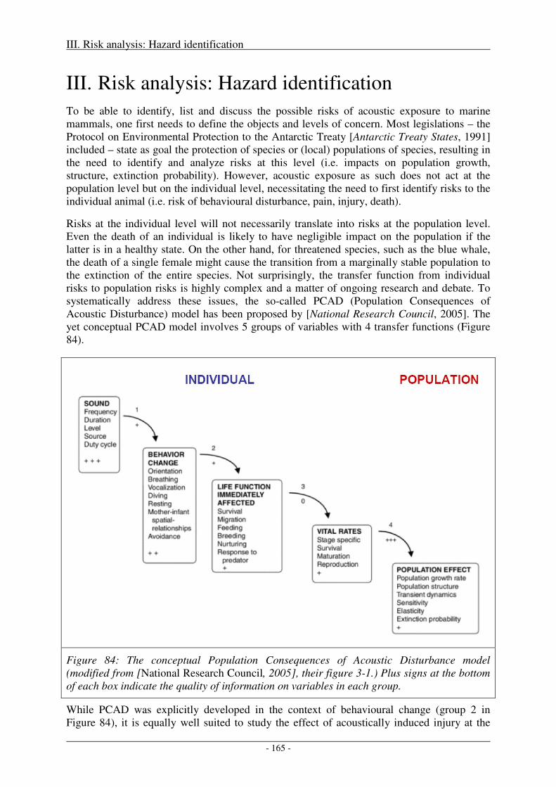
III. Risk analysis: Hazard identification
- 165 -
III. Risk analysis: Hazard identification To be able to identify, list and discuss the possible risks of acoustic exposure to marine mammals, one first needs to define the objects and levels of concern. Most legislations – the Protocol on Environmental Protection to the Antarctic Treaty [Antarctic Treaty States, 1991] included – state as goal the protection of species or (local) populations of species, resulting in the need to identify and analyze risks at this level (i.e. impacts on population growth, structure, extinction probability). However, acoustic exposure as such does not act at the population level but on the individual level, necessitating the need to first identify risks to the individual animal (i.e. risk of behavioural disturbance, pain, injury, death).
Risks at the individual level will not necessarily translate into risks at the population level. Even the death of an individual is likely to have negligible impact on the population if the latter is in a healthy state. On the other hand, for threatened species, such as the blue whale, the death of a single female might cause the transition from a marginally stable population to the extinction of the entire species. Not surprisingly, the transfer function from individual risks to population risks is highly complex and a matter of ongoing research and debate. To systematically address these issues, the so-called PCAD (Population Consequences of Acoustic Disturbance) model has been proposed by [National Research Council, 2005]. The yet conceptual PCAD model involves 5 groups of variables with 4 transfer functions (Figure 84).
Figure 84: The conceptual Population Consequences of Acoustic Disturbance model (modified from [National Research Council, 2005], their figure 3-1.) Plus signs at the bottom of each box indicate the quality of information on variables in each group.
While PCAD was explicitly developed in the context of behavioural change (group 2 in Figure 84), it is equally well suited to study the effect of acoustically induced injury at the
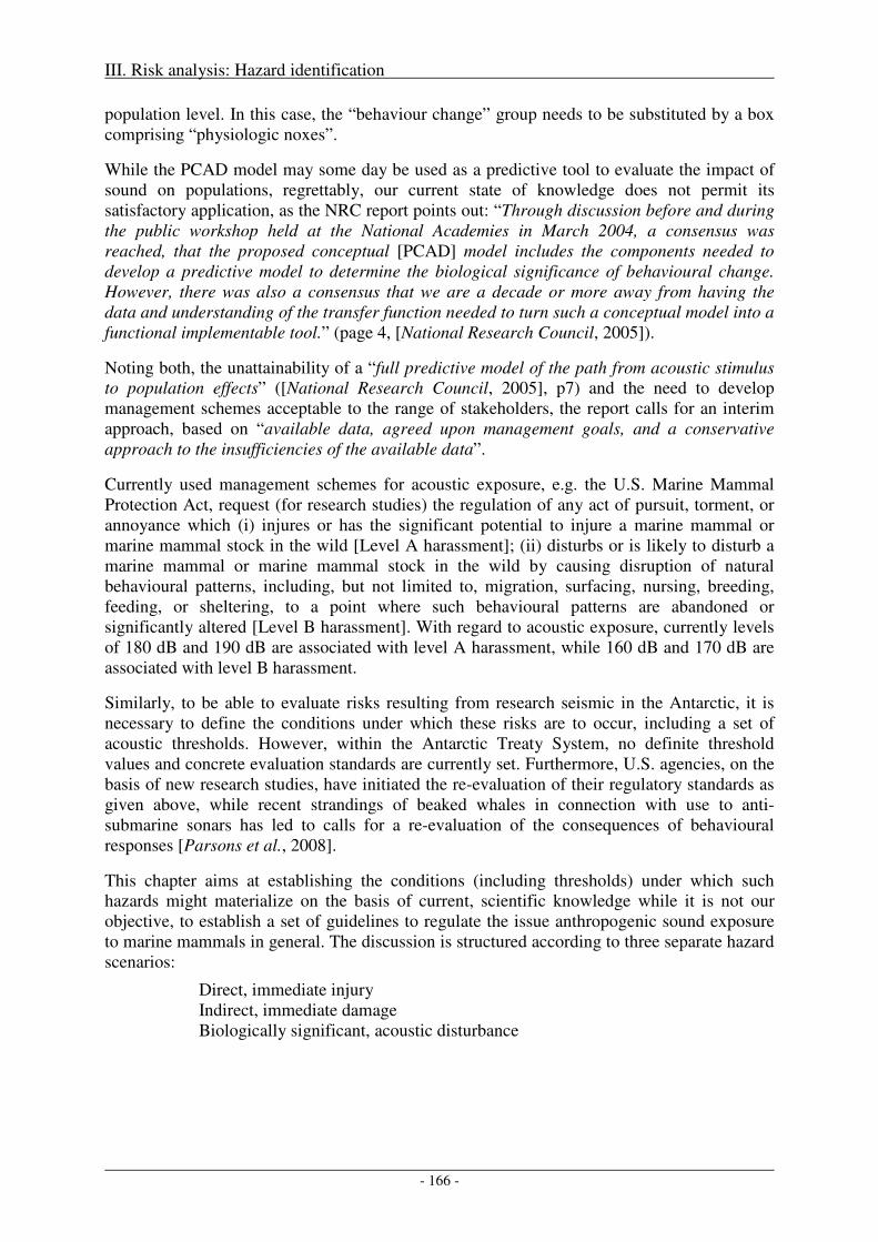
III. Risk analysis: Hazard identification
- 166 -
population level. In this case, the “behaviour change” group needs to be substituted by a box comprising “physiologic noxes”.
While the PCAD model may some day be used as a predictive tool to evaluate the impact of sound on populations, regrettably, our current state of knowledge does not permit its satisfactory application, as the NRC report points out: “Through discussion before and during the public workshop held at the National Academies in March 2004, a consensus was reached, that the proposed conceptual [PCAD] model includes the components needed to develop a predictive model to determine the biological significance of behavioural change. However, there was also a consensus that we are a decade or more away from having the data and understanding of the transfer function needed to turn such a conceptual model into a functional implementable tool.” (page 4, [National Research Council, 2005]).
Noting both, the unattainability of a “full predictive model of the path from acoustic stimulus to population effects” ([National Research Council, 2005], p7) and the need to develop management schemes acceptable to the range of stakeholders, the report calls for an interim approach, based on “available data, agreed upon management goals, and a conservative approach to the insufficiencies of the available data”.
Currently used management schemes for acoustic exposure, e.g. the U.S. Marine Mammal Protection Act, request (for research studies) the regulation of any act of pursuit, torment, or annoyance which (i) injures or has the significant potential to injure a marine mammal or marine mammal stock in the wild [Level A harassment]; (ii) disturbs or is likely to disturb a marine mammal or marine mammal stock in the wild by causing disruption of natural behavioural patterns, including, but not limited to, migration, surfacing, nursing, breeding, feeding, or sheltering, to a point where such behavioural patterns are abandoned or significantly altered [Level B harassment]. With regard to acoustic exposure, currently levels of 180 dB and 190 dB are associated with level A harassment, while 160 dB and 170 dB are associated with level B harassment.
Similarly, to be able to evaluate risks resulting from research seismic in the Antarctic, it is necessary to define the conditions under which these risks are to occur, including a set of acoustic thresholds. However, within the Antarctic Treaty System, no definite threshold values and concrete evaluation standards are currently set. Furthermore, U.S. agencies, on the basis of new research studies, have initiated the re-evaluation of their regulatory standards as given above, while recent strandings of beaked whales in connection with use to anti-submarine sonars has led to calls for a re-evaluation of the consequences of behavioural responses [Parsons et al., 2008].
This chapter aims at establishing the conditions (including thresholds) under which such hazards might materialize on the basis of current, scientific knowledge while it is not our objective, to establish a set of guidelines to regulate the issue anthropogenic sound exposure to marine mammals in general. The discussion is structured according to three separate hazard scenarios:
Direct, immediate injury Indirect, immediate damage Biologically significant, acoustic disturbance
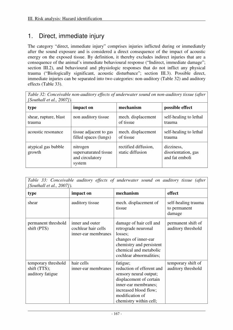
III. Risk analysis: Hazard identification
- 167 -
1. Direct, immediate injury
The category “direct, immediate injury” comprises injuries inflicted during or immediately after the sound exposure and is considered a direct consequence of the impact of acoustic energy on the exposed tissue. By definition, it thereby excludes indirect injuries that are a consequence of the animal’s immediate behavioural response (“Indirect, immediate damage”; section III.2), and behavioural and physiologic responses that do not inflict any physical trauma (“Biologically significant, acoustic disturbance”; section III.3). Possible direct, immediate injuries can be separated into two categories: non-auditory (Table 32) and auditory effects (Table 33).
Table 32: Conceivable non-auditory effects of underwater sound on non-auditory tissue (after [Southall et al., 2007]).
type impact on mechanism possible effect
shear, rupture, blast trauma
non auditory tissue mech. displacement of tissue
self-healing to lethal trauma
acoustic resonance tissue adjacent to gas filled spaces (lungs)
mech. displacement of tissue
self-healing to lethal trauma
atypical gas bubble growth
nitrogen supersaturated tissue and circulatory system
rectified diffusion, static diffusion
dizziness, disorientation, gas and fat emboli
Table 33: Conceivable auditory effects of underwater sound on auditory tissue (after [Southall et al., 2007]).
type impact on mechanism effect
shear auditory tissue mech. displacement of tissue
self-healing trauma to permanent damage
permanent threshold shift (PTS)
inner and outer cochlear hair cells inner-ear membranes
damage of hair cell and retrograde neuronal losses; changes of inner-ear chemistry and persistent chemical and metabolic cochlear abnormalities;
permanent shift of auditory threshold
temporary threshold shift (TTS); auditory fatigue
hair cells inner-ear membranes
fatigue; reduction of efferent and sensory neural output; displacement of certain inner-ear membranes; increased blood flow; modification of chemistry within cell;
temporary shift of auditory threshold
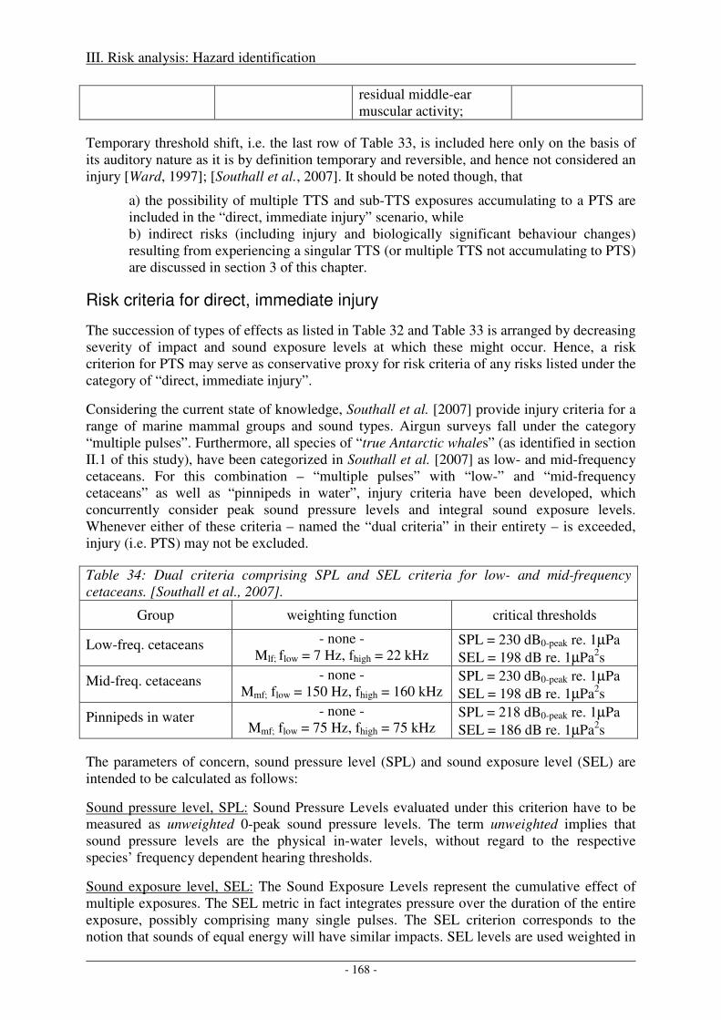
III. Risk analysis: Hazard identification
- 168 -
residual middle-ear muscular activity;
Temporary threshold shift, i.e. the last row of Table 33, is included here only on the basis of its auditory nature as it is by definition temporary and reversible, and hence not considered an injury [Ward, 1997]; [Southall et al., 2007]. It should be noted though, that
a) the possibility of multiple TTS and sub-TTS exposures accumulating to a PTS are included in the “direct, immediate injury” scenario, while b) indirect risks (including injury and biologically significant behaviour changes) resulting from experiencing a singular TTS (or multiple TTS not accumulating to PTS) are discussed in section 3 of this chapter.
Risk criteria for direct, immediate injury
The succession of types of effects as listed in Table 32 and Table 33 is arranged by decreasing severity of impact and sound exposure levels at which these might occur. Hence, a risk criterion for PTS may serve as conservative proxy for risk criteria of any risks listed under the category of “direct, immediate injury”.
Considering the current state of knowledge, Southall et al. [2007] provide injury criteria for a range of marine mammal groups and sound types. Airgun surveys fall under the category “multiple pulses”. Furthermore, all species of “true Antarctic whales” (as identified in section II.1 of this study), have been categorized in Southall et al. [2007] as low- and mid-frequency cetaceans. For this combination – “multiple pulses” with “low-” and “mid-frequency cetaceans” as well as “pinnipeds in water”, injury criteria have been developed, which concurrently consider peak sound pressure levels and integral sound exposure levels. Whenever either of these criteria – named the “dual criteria” in their entirety – is exceeded, injury (i.e. PTS) may not be excluded.
Table 34: Dual criteria comprising SPL and SEL criteria for low- and mid-frequency cetaceans. [Southall et al., 2007].
Group weighting function critical thresholds
Low-freq. cetaceans - none - Mlf; flow = 7 Hz, fhigh = 22 kHz
SPL = 230 dB0-peak re. 1µPa SEL = 198 dB re. 1µPa2s
Mid-freq. cetaceans - none - Mmf; flow = 150 Hz, fhigh = 160 kHz
SPL = 230 dB0-peak re. 1µPa SEL = 198 dB re. 1µPa2s
Pinnipeds in water - none - Mmf; flow = 75 Hz, fhigh = 75 kHz
SPL = 218 dB0-peak re. 1µPa SEL = 186 dB re. 1µPa2s
The parameters of concern, sound pressure level (SPL) and sound exposure level (SEL) are intended to be calculated as follows:
Sound pressure level, SPL: Sound Pressure Levels evaluated under this criterion have to be measured as unweighted 0-peak sound pressure levels. The term unweighted implies that sound pressure levels are the physical in-water levels, without regard to the respective species’ frequency dependent hearing thresholds.
Sound exposure level, SEL: The Sound Exposure Levels represent the cumulative effect of multiple exposures. The SEL metric in fact integrates pressure over the duration of the entire exposure, possibly comprising many single pulses. The SEL criterion corresponds to the notion that sounds of equal energy will have similar impacts. SEL levels are used weighted in
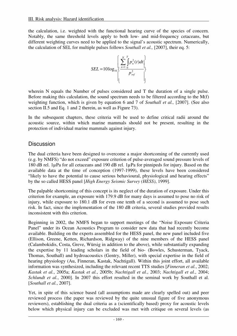
III. Risk analysis: Hazard identification
- 169 -
the calculation, i.e. weighted with the functional hearing curve of the species of concern. Notably, the same threshold levels apply to both low- and mid-frequency cetaceans, but different weighting curves need to be applied to the signal’s acoustic spectrum. Numerically, the calculation of SEL for multiple pulses follows Southall et al., [2007], their eq. 5:
=∑∫
=
2
1 0
2
10
)(
log10ref
N
n
T
n
p
dttp
SEL
wherein N equals the Number of pulses considered and T the duration of a single pulse. Before making this calculation, the sound spectrum needs to be filtered according to the M(f) weighting function, which is given by equation 6 and 7 of Southall et al., [2007]. (See also section II.5 and Eq. 1 and 2 therein, as well as Figure 73).
In the subsequent chapters, these criteria will be used to define critical radii around the acoustic source, within which marine mammals should not be present, resulting in the protection of individual marine mammals against injury.
Discussion
The dual criteria have been designed to overcome a major shortcoming of the currently used (e.g. by NMFS) “do not exceed” exposure criterion of pulse-averaged sound pressure levels of 180 dB rel. 1µPa for all cetaceans and 190 dB rel. 1µPa for pinnipeds for injury. Based on the available data at the time of conception (1997-1999), these levels have been considered “likely to have the potential to cause serious behavioural, physiological and hearing effects” by the so called HESS panel [High Energy Seismic Survey (HESS), 1999].
The palpable shortcoming of this concept is its neglect of the duration of exposure. Under this criterion for example, an exposure with 179.9 dB for many days is assumed to pose no risk of injury, while exposure to 180.1 dB for even one tenth of a second is assumed to pose such risk. In fact, since the implementation of the 180 dB criteria, several studies provided results inconsistent with this criterion.
Beginning in 2002, the NMFS began to support meetings of the “Noise Exposure Criteria Panel” under its Ocean Acoustics Program to consider new data that had recently become available. Building on the experts assembled for the HESS panel, the new panel included five (Ellison, Greene, Ketten, Richardson, Ridgway) of the nine members of the HESS panel (Calambokidis, Costa, Greve, Würsig in addition to the above), while substantially expanding the expertise by 11 leading scholars in the field of bio- (Bowles, Schusterman, Tyack, Thomas, Southall) and hydroacoustics (Gentry, Miller), with special expertise in the field of hearing physiology (Au, Finneran, Kastak, Nachtigall). Within this joint effort, all available information was synthesized, including the relevant recent TTS studies [Finneran et al., 2002; Kastak et al., 2005a; Kastak et al., 2005b; Nachtigall et al., 2003; Nachtigall et al., 2004; Schlundt et al., 2000]. In 2007 this effort resulted in the seminal work by Southall et al. [Southall et al., 2007].
Yet, in spite of this science based (all assumptions made are clearly spelled out) and peer reviewed process (the paper was reviewed by the quite unusual figure of five anonymous reviewers), establishing the dual criteria as a (scientifically based) proxy for acoustic levels below which physical injury can be excluded was met with critique on several levels (as
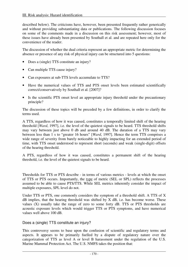
III. Risk analysis: Hazard identification
- 170 -
described below). The criticisms have, however, been presented frequently rather generically and without providing substantiating data or publications. The following discussion focuses on some of the comments made in a discussion on this risk assessment; however, most of these issues have already been presented by Southall et al. and are repeated here only for the convenience of the reader.
The discussion of whether the dual criteria represent an appropriate metric for determining the absence or presence of any risk of physical injury can be structured into 5 questions:
• Does a (single) TTS constitute an injury?
• Can multiple TTS cause injury?
• Can exposures at sub-TTS levels accumulate to TTS?
• Have the numerical values of TTS and PTS onset levels been estimated scientifically correct/conservatively by Southall et al. [2007]?
• Is the scientific PTS onset level an appropriate injury threshold under the precautionary principle?
The discussion of these topics will be preceded by a few definitions, in order to clarify the terms used.
A TTS, regardless of how it was caused, constitutes a temporally limited shift of the hearing threshold [Ward, 1997], i.e. the level of the quietest signals to be heard. TTS threshold shifts may vary between just above 0 db and around 40 dB. The duration of a TTS may vary between less than 1 s to “greater 16 hours” [Ward, 1997]. Hence the term TTS comprises a wide range of severity from barely noticeable to highly impacting for an extended period of time, with TTS onset understood to represent short (seconds) and weak (single-digit) offsets of the hearing threshold.
A PTS, regardless of how it was caused, constitutes a permanent shift of the hearing threshold, i.e. the level of the quietest signals to be heard.
Thresholds for TTS or PTS describe - in terms of various metrics - levels at which the onset of TTS or PTS occurs. Importantly, the type of metric (SEL or SPL) reflects the processes assumed to be able to cause PTS/TTS. While SEL metrics inherently consider the impact of multiple exposures, SPL level do not.
Under TTS or PTS, one commonly considers the symptom of a threshold shift. A TTS of X dB implies, that the hearing threshold was shifted by X dB, i.e. has become worse. These values (X) usually take the range of zero to some forty dB. TTS or PTS thresholds are acoustic exposure levels which would trigger TTS or PTS symptoms, and have numerical values well above 100 dB.
Does a (single) TTS constitute an injury?
This controversy seems to base upon the confusion of scientific and regulatory terms and aspects. It appears to be primarily fuelled by a dispute of regulatory nature over the categorization of TTS as level A or level B harassment under the regulation of the U.S. Marine Mammal Protection Act. The U.S. NMFS takes the position that:
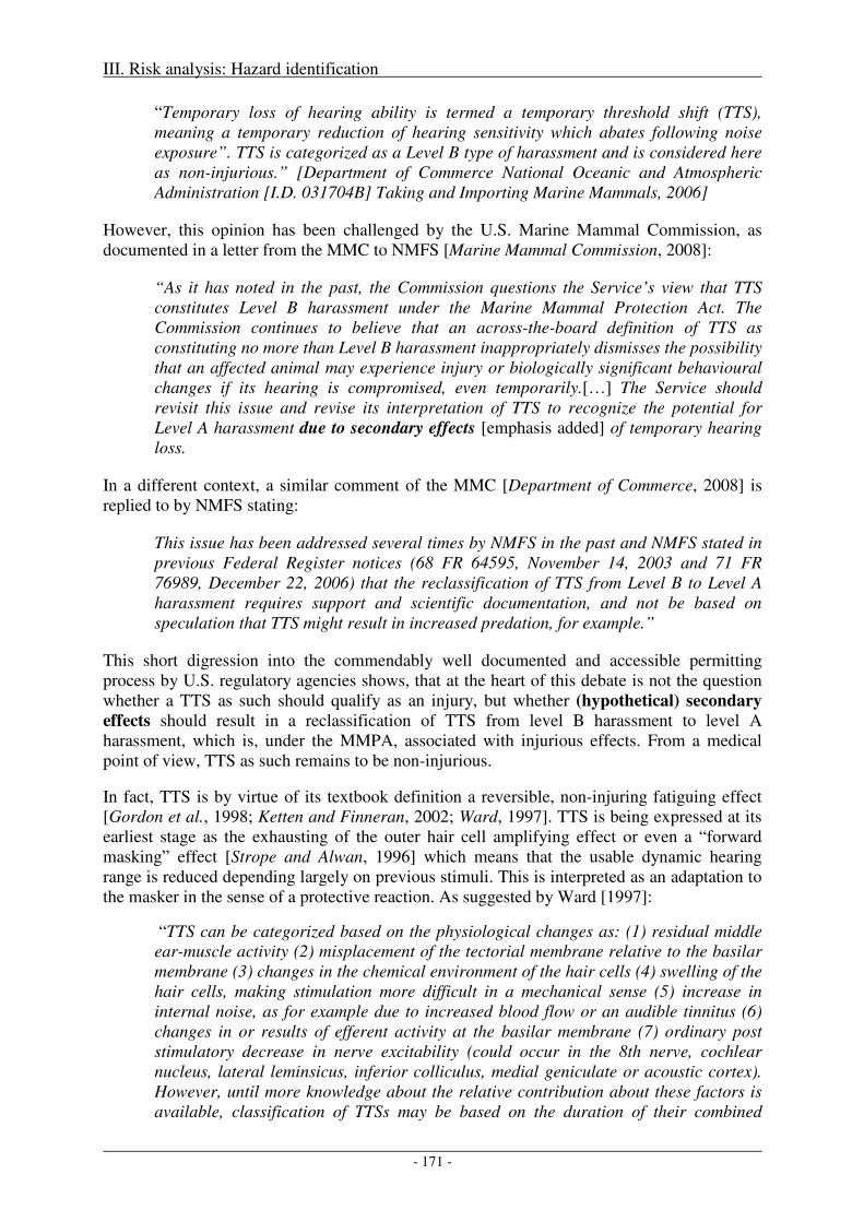
III. Risk analysis: Hazard identification
- 171 -
“Temporary loss of hearing ability is termed a temporary threshold shift (TTS), meaning a temporary reduction of hearing sensitivity which abates following noise exposure”. TTS is categorized as a Level B type of harassment and is considered here as non-injurious.” [Department of Commerce National Oceanic and Atmospheric Administration [I.D. 031704B] Taking and Importing Marine Mammals, 2006]
However, this opinion has been challenged by the U.S. Marine Mammal Commission, as documented in a letter from the MMC to NMFS [Marine Mammal Commission, 2008]:
“As it has noted in the past, the Commission questions the Service’s view that TTS constitutes Level B harassment under the Marine Mammal Protection Act. The Commission continues to believe that an across-the-board definition of TTS as constituting no more than Level B harassment inappropriately dismisses the possibility that an affected animal may experience injury or biologically significant behavioural changes if its hearing is compromised, even temporarily.[…] The Service should revisit this issue and revise its interpretation of TTS to recognize the potential for Level A harassment due to secondary effects [emphasis added] of temporary hearing loss.
In a different context, a similar comment of the MMC [Department of Commerce, 2008] is replied to by NMFS stating:
This issue has been addressed several times by NMFS in the past and NMFS stated in previous Federal Register notices (68 FR 64595, November 14, 2003 and 71 FR 76989, December 22, 2006) that the reclassification of TTS from Level B to Level A harassment requires support and scientific documentation, and not be based on speculation that TTS might result in increased predation, for example.”
This short digression into the commendably well documented and accessible permitting process by U.S. regulatory agencies shows, that at the heart of this debate is not the question whether a TTS as such should qualify as an injury, but whether (hypothetical) secondary
effects should result in a reclassification of TTS from level B harassment to level A harassment, which is, under the MMPA, associated with injurious effects. From a medical point of view, TTS as such remains to be non-injurious.
In fact, TTS is by virtue of its textbook definition a reversible, non-injuring fatiguing effect [Gordon et al., 1998; Ketten and Finneran, 2002; Ward, 1997]. TTS is being expressed at its earliest stage as the exhausting of the outer hair cell amplifying effect or even a “forward masking” effect [Strope and Alwan, 1996] which means that the usable dynamic hearing range is reduced depending largely on previous stimuli. This is interpreted as an adaptation to the masker in the sense of a protective reaction. As suggested by Ward [1997]:
“TTS can be categorized based on the physiological changes as: (1) residual middle ear-muscle activity (2) misplacement of the tectorial membrane relative to the basilar membrane (3) changes in the chemical environment of the hair cells (4) swelling of the hair cells, making stimulation more difficult in a mechanical sense (5) increase in internal noise, as for example due to increased blood flow or an audible tinnitus (6) changes in or results of efferent activity at the basilar membrane (7) ordinary post stimulatory decrease in nerve excitability (could occur in the 8th nerve, cochlear nucleus, lateral leminsicus, inferior colliculus, medial geniculate or acoustic cortex). However, until more knowledge about the relative contribution about these factors is available, classification of TTSs may be based on the duration of their combined
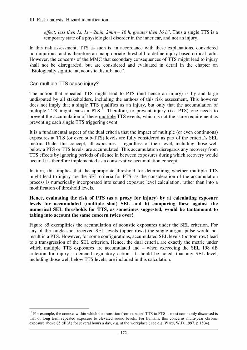
III. Risk analysis: Hazard identification
- 172 -
effect: less then 1s, 1s – 2min, 2min – 16 h, greater then 16 h”. Thus a single TTS is a temporary state of a physiological disorder in the inner ear, and not an injury.
In this risk assessment, TTS as such is, in accordance with these explanations, considered non-injurious, and is therefore an inappropriate threshold to define injury based critical radii. However, the concerns of the MMC that secondary consequences of TTS might lead to injury shall not be disregarded, but are considered and evaluated in detail in the chapter on “Biologically significant, acoustic disturbance”.
Can multiple TTS cause injury?
The notion that repeated TTS might lead to PTS (and hence an injury) is by and large undisputed by all stakeholders, including the authors of this risk assessment. This however does not imply that a single TTS qualifies as an injury, but only that the accumulation of multiple TTS might cause a PTS18. Therefore, to prevent injury (i.e. PTS) one needs to prevent the accumulation of these multiple TTS events, which is not the same requirement as preventing each single TTS triggering event.
It is a fundamental aspect of the dual criteria that the impact of multiple (or even continuous) exposures at TTS (or even sub-TTS) levels are fully considered as part of the criteria’s SEL metric. Under this concept, all exposures – regardless of their level, including those well below a PTS or TTS levels, are accumulated. This accumulation disregards any recovery from TTS effects by ignoring periods of silence in between exposures during which recovery would occur. It is therefore implemented as a conservative accumulation concept.
In turn, this implies that the appropriate threshold for determining whether multiple TTS might lead to injury are the SEL criteria for PTS, as the consideration of the accumulation process is numerically incorporated into sound exposure level calculation, rather than into a modification of threshold levels.
Hence, evaluating the risk of PTS (as a proxy for injury) by a) calculating exposure
levels for accumulated (multiple shot) SEL and b) comparing these against the
numerical SEL thresholds for TTS, as sometimes suggested, would be tantamount to
taking into account the same concern twice over!
Figure 85 exemplifies the accumulation of acoustic exposures under the SEL criterion. For any of the single shot received SEL levels (upper rows) the single airgun pulse would not result in a PTS. However, for some configurations, accumulated SEL levels (bottom row) lead to a transgression of the SEL criterion. Hence, the dual criteria are exactly the metric under which multiple TTS exposures are accumulated and – when exceeding the SEL 198 dB criterion for injury – demand regulatory action. It should be noted, that any SEL level, including those well below TTS levels, are included in this calculation.
18 For example, the context within which the transition from repeated TTS to PTS is most commonly discussed is that of long term repeated exposure to elevated sound levels. For humans, this concerns multi-year chronic exposure above 85 dB(A) for several hours a day, e.g. at the workplace ( see e.g. Ward, W.D. 1997, p 1504).
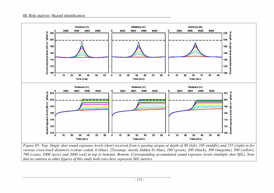
III. Risk analysis: Hazard identification
- 173 -
Figure 85: Top: Single shot sound exposure levels (dots) received from a passing airgun at depth of 80 (left), 105 (middle) and 155 (right) m for various cross-track distances (colour coded, 0 (blue), 25(orange, mostly hidden by blue), 100 (green), 200 (black), 300 (magenta), 500 (yellow), 700 (cyan), 1000 (grey) and 2000 (red) m top to bottom). Bottom: Corresponding accumulated sound exposure levels (multiple shot SEL). Note that in contrast to other figures of this study both rows here represent SEL metrics.
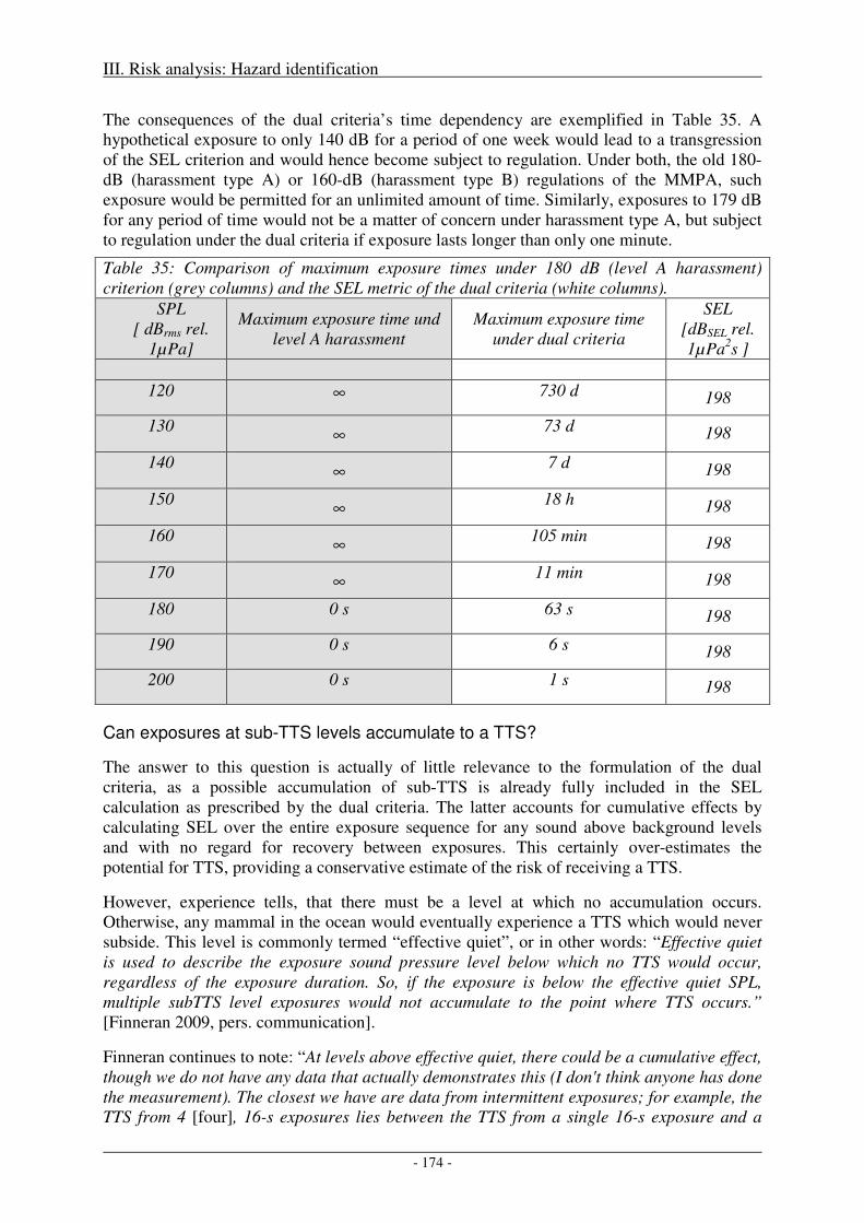
III. Risk analysis: Hazard identification
- 174 -
The consequences of the dual criteria’s time dependency are exemplified in Table 35. A hypothetical exposure to only 140 dB for a period of one week would lead to a transgression of the SEL criterion and would hence become subject to regulation. Under both, the old 180-dB (harassment type A) or 160-dB (harassment type B) regulations of the MMPA, such exposure would be permitted for an unlimited amount of time. Similarly, exposures to 179 dB for any period of time would not be a matter of concern under harassment type A, but subject to regulation under the dual criteria if exposure lasts longer than only one minute.
Table 35: Comparison of maximum exposure times under 180 dB (level A harassment) criterion (grey columns) and the SEL metric of the dual criteria (white columns).
SPL [ dBrms rel.
1µPa]
Maximum exposure time und level A harassment
Maximum exposure time under dual criteria
SEL [dBSEL rel. 1µPa2s ]
120 ∞ 730 d 198
130 ∞ 73 d 198
140 ∞ 7 d 198
150 ∞ 18 h 198
160 ∞ 105 min 198
170 ∞ 11 min 198
180 0 s 63 s 198
190 0 s 6 s 198
200 0 s 1 s 198
Can exposures at sub-TTS levels accumulate to a TTS?
The answer to this question is actually of little relevance to the formulation of the dual criteria, as a possible accumulation of sub-TTS is already fully included in the SEL calculation as prescribed by the dual criteria. The latter accounts for cumulative effects by calculating SEL over the entire exposure sequence for any sound above background levels and with no regard for recovery between exposures. This certainly over-estimates the potential for TTS, providing a conservative estimate of the risk of receiving a TTS.
However, experience tells, that there must be a level at which no accumulation occurs. Otherwise, any mammal in the ocean would eventually experience a TTS which would never subside. This level is commonly termed “effective quiet”, or in other words: “Effective quiet is used to describe the exposure sound pressure level below which no TTS would occur, regardless of the exposure duration. So, if the exposure is below the effective quiet SPL, multiple subTTS level exposures would not accumulate to the point where TTS occurs.” [Finneran 2009, pers. communication].
Finneran continues to note: “At levels above effective quiet, there could be a cumulative effect, though we do not have any data that actually demonstrates this (I don't think anyone has done the measurement). The closest we have are data from intermittent exposures; for example, the TTS from 4 [four], 16-s exposures lies between the TTS from a single 16-s exposure and a
III. Risk analysis: Hazard identification
- 175 -
single 64-s exposure. There is an increasing effect from the additional exposures, but the quiet periods between each exposure provide some opportunity for recovery.
Unfortunately though, the effective quiet level has, to our knowledge, not yet been measured in a marine mammal. For this study, effective quiet has not explicitly been defined, but implicitly (by virtue of how the calculations are performed) equals the exposure levels at the beginning and end of each simulated shot sequence as included in the calculation of the cumulative SEL levels. In Figure 85, for example, this equals SEL levels slightly below 150 dB rel. 1µPa2s.
Recovery rates depend on exposure level, exposure duration and the amount of the initial threshold shift. For long exposure durations, as measured in Kastak et al. [2005b], longer duration exposures produce bigger threshold shifts compared to shorter duration exposures with the same SEL. “Increasing the noise exposure duration and amplitude independently resulted in increases in the magnitude of the threshold shift for two of the three subjects of this experiment. Increasing the exposure duration from 25 to 50 min had a greater effect on threshold shifts than increasing the exposure level from 80 to 95 dB SL [above their auditory threshold at 2500 Hz]. These results are inconsistent with an equal energy model (3-dB exchange rate), and suggest that moderate levels of long duration sounds may have a greater impact on hearing than equal-energy sounds of greater amplitude but shorter duration sounds.” [Kastak et al., 2005b]. A similar effect could not yet be reproduced with exposures of < ~16-32 seconds duration [Finneran 2009, pers. comm.]. By comparison, 1 hour of seismic operations produce integral exposure times of the order of 10s of seconds, rendering them unlikely to qualify as “long duration” sound as described by Kastak et al. [2005b].
Do Southall et al’s. TTS and PTS onset levels represent numerically conservative estimates?
The derivation of the dual criteria by Southall et al. [2007] unavoidably had to include several extrapolations from known data, as no direct PTS measurements existed for any marine mammal, let alone for any of the large baleen whales. These extrapolations are clearly indicated in the paper, and the discerning reader might want to follow the discussions made therein. Southall et al. [2007] claim, that the extrapolations have been conducted with caution and in a conservative way throughout, an opinion we confer with.
It is worth noting, that the derivation of the dual criteria, as pointed out by the authors, is commensurate with a conservative approach. (Southall et al. use the term precautionary in place of the term „conservative“ as used in this study.) The particular assumptions and selections that have been made by Southall et al., [2007] in an effort to obtain conservative threshold levels are listed in Table 36.
While it is not the purpose of this study to repeat the arguments made in Southall et al. [2007] by again discussing each assumption and selection made in the derivation of the dual criteria, we here focus on some of the aspects specifically raised by the reviewers of this risk assessment.
One reservation that has been expressed is that no PTS measurements have actually been available for any cetacean. Southall et al.'s [2007] assumption, that a TTS with a threshold shift of 40 dB equals PTS-onset was at the time indeed based on the finding that most mammals (including humans) have full recovery from a 40 dB shift (which implies this being a conservative assumption, see Table 36). Meanwhile, additional experiments were performed to validate this assumption. Both Finneran and Reichmuth have now caused 40 dB of
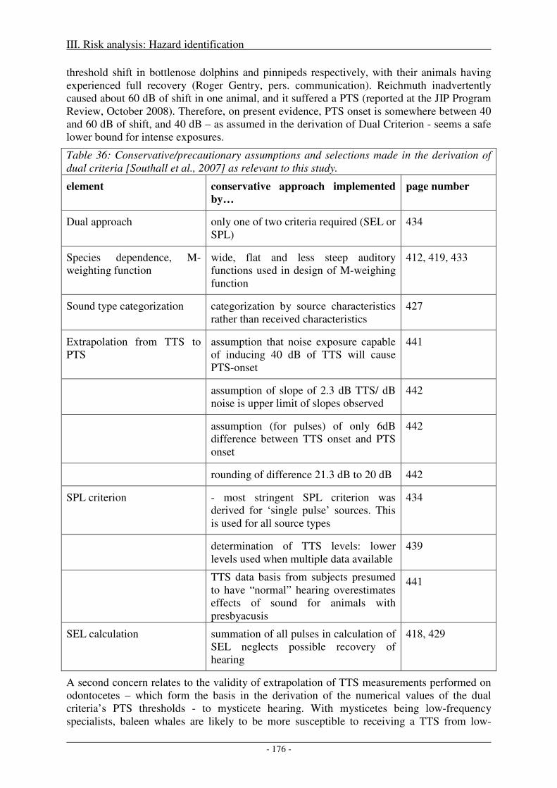
III. Risk analysis: Hazard identification
- 176 -
threshold shift in bottlenose dolphins and pinnipeds respectively, with their animals having experienced full recovery (Roger Gentry, pers. communication). Reichmuth inadvertently caused about 60 dB of shift in one animal, and it suffered a PTS (reported at the JIP Program Review, October 2008). Therefore, on present evidence, PTS onset is somewhere between 40 and 60 dB of shift, and 40 dB – as assumed in the derivation of Dual Criterion - seems a safe lower bound for intense exposures.
Table 36: Conservative/precautionary assumptions and selections made in the derivation of dual criteria [Southall et al., 2007] as relevant to this study.
element conservative approach implemented
by…
page number
Dual approach only one of two criteria required (SEL or SPL)
434
Species dependence, M-weighting function
wide, flat and less steep auditory functions used in design of M-weighing function
412, 419, 433
Sound type categorization categorization by source characteristics rather than received characteristics
427
Extrapolation from TTS to PTS
assumption that noise exposure capable of inducing 40 dB of TTS will cause PTS-onset
441
assumption of slope of 2.3 dB TTS/ dB noise is upper limit of slopes observed
442
assumption (for pulses) of only 6dB difference between TTS onset and PTS onset
442
rounding of difference 21.3 dB to 20 dB 442
SPL criterion - most stringent SPL criterion was derived for ‘single pulse’ sources. This is used for all source types
434
determination of TTS levels: lower levels used when multiple data available
439
TTS data basis from subjects presumed to have “normal” hearing overestimates effects of sound for animals with presbyacusis
441
SEL calculation summation of all pulses in calculation of SEL neglects possible recovery of hearing
418, 429
A second concern relates to the validity of extrapolation of TTS measurements performed on odontocetes – which form the basis in the derivation of the numerical values of the dual criteria’s PTS thresholds - to mysticete hearing. With mysticetes being low-frequency specialists, baleen whales are likely to be more susceptible to receiving a TTS from low-
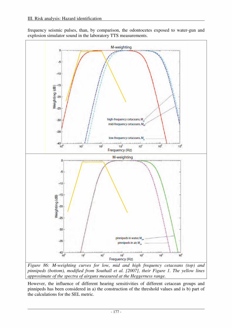
III. Risk analysis: Hazard identification
- 177 -
frequency seismic pulses, than, by comparison, the odontocetes exposed to water-gun and explosion simulator sound in the laboratory TTS measurements.
Figure 86: M-weighting curves for low, mid and high frequency cetaceans (top) and pinnipeds (bottom), modified from Southall et al. [2007], their Figure 1. The yellow lines approximate of the spectra of airguns measured at the Heggerness range.
However, the influence of different hearing sensitivities of different cetacean groups and pinnipeds has been considered in a) the construction of the threshold values and is b) part of the calculations for the SEL metric.
III. Risk analysis: Hazard identification
- 178 -
a) The first step compensates for the group (low-, mid-, and high-frequency cetaceans) dependency of the TTS measurements made. The calculation of the numerical value of the criterion thereby is based on Finneran et al. [2002] establishing onset levels of TTS with (frequency-) unweighted SEL levels of 186 dB rel. 1µPa2s. This threshold is lowered to compensate for the test animal’s (a beluga) reduced low-frequency hearing capability in accordance with its M-weighting function to 183 dB rel. 1µPa2s (see [Southall et al., 2007] page 442 for more details). Therefore, this corrected threshold is designed to be valid across all three cetacean groups (low-, mid-, and high-frequency cetaceans).
b) Southall et al. [Southall et al., 2007] then propose to apply each respective M-weighting function to the received sound spectrum, in order to properly calculate received SEL levels. This would result in a significant attenuation of acoustic energy below 100 Hz for mid-frequency cetacean and pinnipeds but little attenuation for low-frequency cetaceans. The calculations made in this study however, assume zero attenuation for computational reasons, i.e. are most conservative by assuming full hearing regardless of frequency. This induces a significant overestimation of exposure levels for mid-frequency cetacean and pinnipeds, while estimates for low-frequency cetaceans are correct.
Finally, one reviewer of this risk assessment comments, that in his opinion, an important incident relevant to this section would be described by Todd et al. [Todd et al., 1996]. The paper describes humpback whales remaining in a feeding area in Newfoundland, while seafloor blasting was being conducted. The whales showed no clear reaction to the blasting in terms of movement or residence time. However, increased entrapment in nets followed the blast exposure. Two humpback whales found trapped in the nets were dissected [Ketten et al., 1993], revealing that the temporal bones of their ears had significant blast trauma. The reviewer concludes that “this incident highlights the difficulty of using overt reactions to monitor marine mammal injury from high intensity sound”.
In appraising this comment it is important being aware that the current section topic is “direct, immediate damage”, rather than “biologically significant, acoustic disturbance”. For “direct, immediate damage”, Southall et al. [2007] in their derivation of the dual criteria, do not use any data or argument based on the observation of absence or presence of “overt reactions to […] high intensity sound”. Rather, Southall et al. [2007] use direct (acoustically evoked potentials, AEPs) and indirect (based on a behavioural response paradigm at sub-TTS levels) measurements of the hearing threshold19 itself, not the response to loud sounds. Hence their approach inherently avoids any false conclusion that could mistakenly be drawn from a lack of observation of overt responses to high intensity sound20.
Is the scientific PTS level an appropriate injury threshold under the precautionary principle?
It is not this studies’ objective to establish general recommendations on thresholds for the regulation of anthropogenic sound exposure to marine mammals. Rather, given the current state of scientific knowledge, it is this study’s goal to determine the conditions under which
19 On a side note, with the latter methodology (behavioural response paradigm), actually, the lack of response would be interpreted as lower TTS thresholds, i.e. providing a conservative estimate of TTS inducing sound exposure levels. 20 Todd et al. 1996 is relevant to the section “Biologically significant, acoustic disturbance”. Part of the considerations made there is the paper by Southall et al. which lists Todd et al. 1996 in their table 6, entry nr. 5 and discussed that paper in their “Appendix B. Studies Involving Marine Mammal Behavioral Responses to Multiple Pulses” (page 502ff). As this study forms the basis of this risk assessment’s consideration of the hazard “Biologically significant, acoustic disturbance”, the paper by Todd et al. 1996 is implicitly included in our study.
III. Risk analysis: Hazard identification
- 179 -
certain hazards (in the case of this chapter the hazard of immediate direct damage) might materialize under the given exposure scenario. The threshold used therein, being solely based on scientific findings, may not necessarily coincide with thresholds deemed appropriate under the precautionary principle. Under this principle, additional considerations might be included in threshold considerations, such as the desired level of protection or the impact of cumulative effects from risks external to acoustics, such as by-catch, whaling, and shipping. Such considerations are beyond the scope of this study.
Output
The evaluation criteria for risks of “direct, immediate injury” are the dual criteria as presented by Southall et al., [2007], using the respective numerical values given in Table 34. Based on these criteria, critical radii will be calculated, within which individuals are subject to the risk of receiving a PTS, i.e. becoming injured.
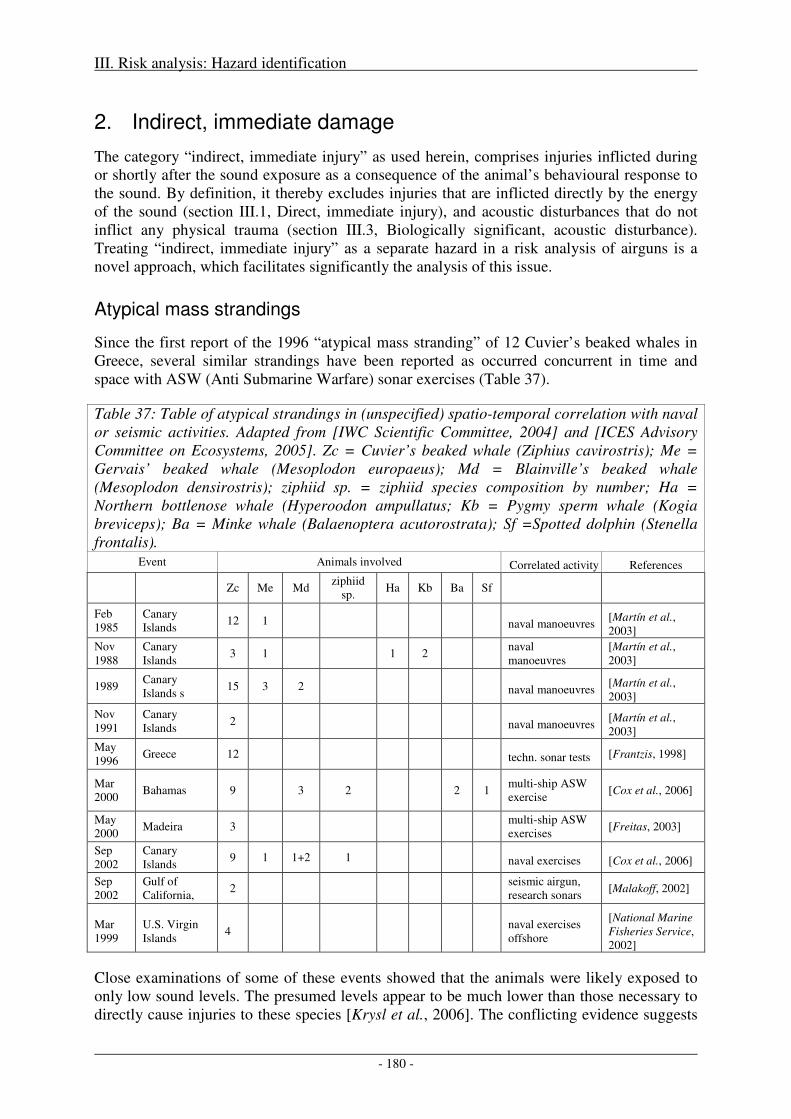
III. Risk analysis: Hazard identification
- 180 -
2. Indirect, immediate damage
The category “indirect, immediate injury” as used herein, comprises injuries inflicted during or shortly after the sound exposure as a consequence of the animal’s behavioural response to the sound. By definition, it thereby excludes injuries that are inflicted directly by the energy of the sound (section III.1, Direct, immediate injury), and acoustic disturbances that do not inflict any physical trauma (section III.3, Biologically significant, acoustic disturbance). Treating “indirect, immediate injury” as a separate hazard in a risk analysis of airguns is a novel approach, which facilitates significantly the analysis of this issue.
Atypical mass strandings
Since the first report of the 1996 “atypical mass stranding” of 12 Cuvier’s beaked whales in Greece, several similar strandings have been reported as occurred concurrent in time and space with ASW (Anti Submarine Warfare) sonar exercises (Table 37).
Table 37: Table of atypical strandings in (unspecified) spatio-temporal correlation with naval or seismic activities. Adapted from [IWC Scientific Committee, 2004] and [ICES Advisory Committee on Ecosystems, 2005]. Zc = Cuvier’s beaked whale (Ziphius cavirostris); Me = Gervais’ beaked whale (Mesoplodon europaeus); Md = Blainville’s beaked whale (Mesoplodon densirostris); ziphiid sp. = ziphiid species composition by number; Ha = Northern bottlenose whale (Hyperoodon ampullatus; Kb = Pygmy sperm whale (Kogia breviceps); Ba = Minke whale (Balaenoptera acutorostrata); Sf =Spotted dolphin (Stenella frontalis).
Event Animals involved Correlated activity References
Zc Me Md ziphiid
sp. Ha Kb Ba Sf
Feb 1985
Canary Islands
12 1 naval manoeuvres [Martín et al., 2003]
Nov 1988
Canary Islands
3 1 1 2 naval manoeuvres
[Martín et al., 2003]
1989 Canary Islands s
15 3 2 naval manoeuvres [Martín et al., 2003]
Nov 1991
Canary Islands
2 naval manoeuvres [Martín et al., 2003]
May 1996
Greece 12 techn. sonar tests [Frantzis, 1998]
Mar 2000
Bahamas 9 3 2 2 1 multi-ship ASW exercise
[Cox et al., 2006]
May 2000
Madeira 3 multi-ship ASW exercises
[Freitas, 2003]
Sep 2002
Canary Islands
9 1 1+2 1 naval exercises [Cox et al., 2006]
Sep 2002
Gulf of California,
2 seismic airgun, research sonars
[Malakoff, 2002]
Mar 1999
U.S. Virgin Islands
4 naval exercises offshore
[National Marine Fisheries Service, 2002]
Close examinations of some of these events showed that the animals were likely exposed to only low sound levels. The presumed levels appear to be much lower than those necessary to directly cause injuries to these species [Krysl et al., 2006]. The conflicting evidence suggests
III. Risk analysis: Hazard identification
- 181 -
that an indirect, alternative mechanism must have been at work in these cases, possibly triggered by the injured animals’ original behavioural response to the sound exposure. A detailed analysis of these events and the various mechanisms under discussion have been presented by Cox et al., [2006]. The results from this and related studies are presented in the following sections.
Potential mechanisms
Several mechanisms have been proposed for the observed strandings and lesions. Based on the propositions put forth by Cox et al., [2006], and augmented by the “hyperthermia” hypothesis [Cole, 2005], Peter Tyack recently summarized the list of currently discussed “possible mechanisms” during the 2nd Intergovernmental Conference in Lerici [Tyack, 2007]21:
� “Behavioural response leads directly to stranding with no injuries other than those induced by stranding.
� Behavioural response leads to potentially lethal injury independent of stranding; injured animals may strand and develop further injuries.
� Decompression sickness syndrome � Hyperthermia
� Sound triggers physiological change along with behavioural response leading to stranding
� Hemorrhagic diathesis � [Vestibular response22]
� Sound directly causes injury, followed by behavioural response leading to stranding � Acoustically mediated bubble growth � Tissue shear/acoustic resonance”
After detailed analysis of these mechanisms, Cox et al. [2006] conclude: ” We highlight gas bubble formation mediated through a behavioural response as plausible [mechanism]…” which again is emphasized in the paper’s abstract “gas-bubble disease, induced in supersaturated tissue by a behavioural response to acoustic exposure, is a plausible pathologic mechanism for the morbidity and mortality seen in cetaceans associated with sonar exposure”. In the following, this scenario shall hence be discussed in detail.
Behavioural response leads to potentially lethal injury independent of stranding
Based on the hypotheses and research conclusions listed by Cox et al., [2006], Zimmer and Tyack studied the dynamics of nitrogen und bubbles in marine mammal tissues [Zimmer and Tyack, 2007] and provide the following summary of this scenario:
“We suggest that the report of gas bubble lesions in stranded beaked whales (…) might be explained if the whales were travelling with repetitive dives of short to medium surfacing durations and without exceeding the depth of alveolar collapse.” The “modelling of simulated dive profiles suggests that beaked whales would increase the risk for DCS by undertaking [such a] long series of short repetitive shallow dives, where they do not exceed
21 The last two items in this list are included here for the sake of complete quoting, but are already included in the discussion of the previous section (see Table 32). 22 Added by the authors, based on Cox et al. [2006].
III. Risk analysis: Hazard identification
- 182 -
the depth of alveolar collapse.23” This atypical behaviour is assumed to be a consequence of the ensonification: “…The sonar sound generates [the abovementioned] avoidance reaction. The dive pattern is repeated until the sound that generated the avoidance reaction no longer elicits the response or the animal enters water too shallow to support the dive…” The reason for this avoidance reaction is sought in the sound type: “Signals from [AWS] midfrequency sonar are … similar to the stereotyped calls of killer whales, [the beaked whales’] primary predator […]. If beaked whales respond to a predator by surfacing, […] then a risk for DCS might stem from repeated shallow dives that follow the surfacing in order to leave the area […]. Shallow dives may … maximize horizontal distance travelled, [or] whales may swim deeper than 25 m or so because their primary predators are near-surface […].” First preliminary results from a controlled exposure experiment aimed to test this scenario have recently been published [Boyd et al., 2007].
It is worth noting that Zimmer and Tyack clearly distinguish between the risks induced by repeated shallow dives and those induced by simple surfacing, even at high vertical velocities. [Zimmer and Tyack, 2007] conclude: „… beaked whales, being repetitive breath-hold divers, can hardly be put to higher-than normal risk by a single interruption of their regular dive behaviour“ as it was originally hypothesized by Jepson [2003].
In the following, we attempt to develop a list of empirical similarities of some of the abovementioned strandings as well as of abetting factors and consequences of this scenario, in an attempt to provide a list of criteria that can be used to evaluate the risk of similar events in other contexts.
Abetting factors of DCS scenario
Sound characteristics
The primary acoustic sources used in connection with atypical beaked whale strandings are Anti Submarine Warfare (ASW) sonars, tactical mid-frequency sonars in particular. Details of their acoustic properties and deployment for the Greece 1996, Bahamas 2000 and Canary Islands 2002 events24 are given in D'Spain et al., [2005], who also noted a number of commonalities of acoustic and environmental parameters of these events.
The duration of deployment in all cases was on the order of several hours (per day). Individual signals were frequency modulated (FM) continuous waves (CW) of 1 s to 4 s durations, repeated at repetition rates of 10 to 60 seconds, resulting in duty cycles between 4% and 8%. All systems generated significant energy in the mid-frequency (1-10 kHz) band. The sonar systems were designed to focus acoustic energy horizontally. For all events, sources were deployed in acoustic waveguides; a shallow but subsurface guide in the case of the Greece event, and so-called surface ducts in the case of the Bahamas and Canary Islands 2002 events [D'Spain et al., 2005]. These waveguides were of appropriate thickness to trap sound of mid-frequency range.
The preferable sound spreading conditions in these waveguides, in combination with reverberations [Fromm and McEachern, 2000] might have caused a quasi-continuous, long lasting soundscape similar to that produced by killer whales. The sound levels as presumably 23 Which is calculated to be 72 m for Ziphius cavirostris by Zimmer and Tyack (Zimmer, W. M. X., and P. L. Tyack (2007), Repetitive shallow dives pose decompression risk in deep-diving beaked whales, Marine Mammal Science, 23(4), 888-925.) 24 To our current knowledge, the Greece 1996 and Bahamas 2000 events are the only atypical beaked whale stranding events for which retrospective modelling of the sound fields has been undertaken.
III. Risk analysis: Hazard identification
- 183 -
received by the animals are relatively low, i.e. 130-140 dB re. 1µPa for the Greece stranding [Zimmer, 2007].
In conclusion, empirical evidence suggests that exposure for prolonged periods (order of hours) to ASW sonar-like signals increases the risk of behaviourally induced injury, even at relatively low sound intensity levels of order 130-140 dB re. 1µPa.
Herding
Many of the atypical beaked whale strandings (Table 37) occurred in the context of naval ASW exercises involving multiple ships with ASW sonar. (An exception to this observation is the Greece (single ship) event). For distributed acoustic sources with reverberations, it might become difficult for a whale to locate the sources’ position and their respective direction of motion, which might trigger a flight response away from the source(s) for an extended period. This assumption is supported by the fact that the stranded whales were dispersed over dozens of kilometres of beach. With naval ships involved in an ASW manoeuvre moving relatively fast (10-15 knots), even above the maximum sustained speed of some species, escape efforts might require a parforce exercise of the whale(s), probably causing significant physical stress.
In conclusion, reasoning suggests that distributed sources in combination with high
source speeds are likely to form an abetting factor of the DCS scenario.
Topographic conditions
D’Spain et al. [2005] note that all strandings analyzed in their paper happened at locations where relatively deep water (>1km) occurs close to coast. However, the implication of this notion is unclear as:
- “proximity to land is a requisite for strandings to occur”;
- may “simply be the preferred habitats for beaked whales”;
- could “accentuate the effects of the sounds through reflection and reverberation from the bathymetry”.
The only obvious conclusion that can be derived from these empirical observations is that acoustic operations in regions where beaked whale habitats are close to the coast may possibly carry a higher risk of injuring these animals.
Sea surface temperature and hyperthermia
Many stranded beaked whales were found alive (for details see e.g. [Cox et al., 2006]; [ICES Advisory Committee on Ecosystems, 2005]), implicating that these animals fled several dozens of kilometres from their typical slope habitat to the beach. According to the DCS scenario, this flight would have occurred in warm waters near the surface (shallow dives). Combined with prolonged exercise during a flight response, and in light of the whales’ thick blubber layer to protect them from the cold deep waters they forage in, hyperthermia and associated symptoms such as confusion, disorientation and failure of internal organs might be an abetting, if not major, injuring factor.
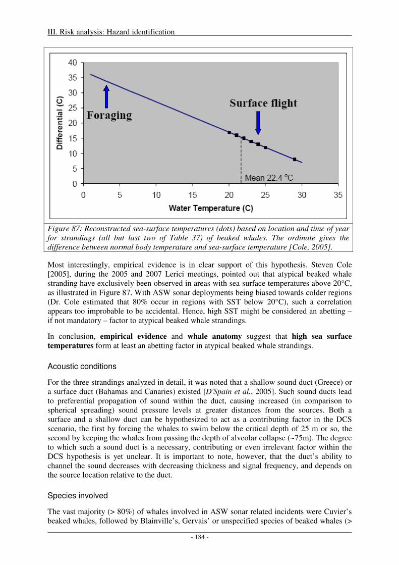
III. Risk analysis: Hazard identification
- 184 -
Figure 87: Reconstructed sea-surface temperatures (dots) based on location and time of year for strandings (all but last two of Table 37) of beaked whales. The ordinate gives the difference between normal body temperature and sea-surface temperature [Cole, 2005].
Most interestingly, empirical evidence is in clear support of this hypothesis. Steven Cole [2005], during the 2005 and 2007 Lerici meetings, pointed out that atypical beaked whale stranding have exclusively been observed in areas with sea-surface temperatures above 20°C, as illustrated in Figure 87. With ASW sonar deployments being biased towards colder regions (Dr. Cole estimated that 80% occur in regions with SST below 20°C), such a correlation appears too improbable to be accidental. Hence, high SST might be considered an abetting – if not mandatory – factor to atypical beaked whale strandings.
In conclusion, empirical evidence and whale anatomy suggest that high sea surface
temperatures form at least an abetting factor in atypical beaked whale strandings.
Acoustic conditions
For the three strandings analyzed in detail, it was noted that a shallow sound duct (Greece) or a surface duct (Bahamas and Canaries) existed [D'Spain et al., 2005]. Such sound ducts lead to preferential propagation of sound within the duct, causing increased (in comparison to spherical spreading) sound pressure levels at greater distances from the sources. Both a surface and a shallow duct can be hypothesized to act as a contributing factor in the DCS scenario, the first by forcing the whales to swim below the critical depth of 25 m or so, the second by keeping the whales from passing the depth of alveolar collapse (~75m). The degree to which such a sound duct is a necessary, contributing or even irrelevant factor within the DCS hypothesis is yet unclear. It is important to note, however, that the duct’s ability to channel the sound decreases with decreasing thickness and signal frequency, and depends on the source location relative to the duct.
Species involved
The vast majority (> 80%) of whales involved in ASW sonar related incidents were Cuvier’s beaked whales, followed by Blainville’s, Gervais’ or unspecified species of beaked whales (>
III. Risk analysis: Hazard identification
- 185 -
10%) with only a small fraction (6 %, incidentally also equalling 6 individuals) of other whale species. Pinnipeds have not been mentioned in this context.
Beaked whale diving behaviour (at least to the extent examined) clearly differs from that of other odontocetes and mysticetes in that it involves very long, deep dives, frequently followed by hitherto unknown bounce dives and relatively short surface periods. However, the extent to which individual elements of this behaviour are critical to the DCS scenario is not yet known. Rather, any whale, if forced to parforce swimming for extended period of times without diving below its lung collapse, appears to be subject to the possibility of DCS like symptoms. Tyack in particular stated during the Lerici 2007 meeting that all whales may experience DCS, provided they follow a sequence of long shallow dives interrupted by short surfacing events. However, the qualifiers “long”, “shallow” and “short” might dependent on species, context and the individual.
Hence, based on empirical evidence, one can state that beaked whales (Cuvier’s in
particular) appear to be the group of whales most affected by ASW sonars, while other species do not appear to form high risk groups. The reasons for this particular susceptibility of beaked whales are yet unknown.
Behaviour
Noise of a passing ship has been observed to disrupt a deep foraging dive of a tagged Ziphius cavirostris [Aguilar Soto et al., 2006]. However, no further interruption of the „normal“ behaviour was triggered by this transient exposure, i.e. no flight response or behavioural change beyond the initial surfacing response was observed for this beaked whale. It resumed its normal dive pattern shortly after it had surfaced and the acoustic exposure had vanished.
Moreover, Zimmer and Tyack [Zimmer and Tyack, 2007] point out that even if, due to modified diving behaviour, the formation of gas-bubbles has taken place, a single deep dive below the depth of alveolar collapse would result in the reabsorption of these gas-bubbles in the circulatory system and tissues, compensating the DCS problem.
In conclusion, experimental evidence and physiological modelling show that a single
interruption and fast surfacing is insufficient to necessarily cause DCS and related symptoms. Rather, physiological modelling suggests that prolonged shallow dives and contingent impossibility of compensating deep dives act as abetting – if not necessary – factor to the occurrence of DCS.
Discussion
In the above derivation of abetting factors, airgun signals (multiple pulses) have not been included. This was criticized by one reviewer, pointing out that the Gulf of California beaked whale stranding event [Malakoff, 2002] (see also Table 37, one but last row,), in his opinion, cannot be dismissed.
D’Spain et al., [2005] compared the Gulf of California beaked whale stranding event (GCE) with the abovementioned ASW-related incidents. While they find some similarities in the presence of a surface duct and the pulse repetition rate, many parameters are noted to differ significantly (pulse duration, directionality, spectral distribution, signal type, inability of wave guide to trap low-frequency waves). Cox et al. [Cox et al., 2006], in their review article on beaked whale standings, find that the causal connection between the seismic operations and the strandings is unresolved due to the small number of animals involved, the lack of any
III. Risk analysis: Hazard identification
- 186 -
necropsy, and an unclear spatio-temporal correlation (p 179). Brownell et al. [2004], seeking an acoustic cause of 20 historical strandings of beaked whales, propose a link to Navy activities only, while not mentioning any seismic activities. Even a recent article [Parsons et al., 2008], which urges a review of regulatory and mitigation standards for the general scenario of “indirect, immediate damage”, mentions the GCE not once, but exclusively focuses on the impact naval sonars, as for example in the initial sentence of the abstract: “Cetacean mass stranding events associated with naval mid-frequency sonar use have raised considerable conservation concerns.”
In our opinion the GCE appears to generate several internal inconsistencies as well as in the context with other observations:
a) for several decades now extensive seismic explorations have been performed in the northern Gulf of Mexico, which is known to serve as key habitat for Cuviers’ (Zc), Blainville’s (Md) and Gervais’ (Me) beaked whales [MacLeod and Mitchell, 2005/6], without – to our knowledge – atypical beaked whale strandings having been reported. It might be argued that beaked whales in this region might have habituated to airgun noise, however, with stranding reports reaching back many decades into the past, the onset of seismic exploration in the Gulf of Mexico – if it were to induce beaked whale stranding - should not have gone unnoticed.
b) An additional, atypical stranding of Baird’s beaked whales has occurred in the Gulf of California [Urbán et al., 2006], but without acoustic airguns or ASW sonars having been reported to have been operated in the area, pointing towards alternative causes. In fact, one reviewer hypothesizes that other noise producing activities - with similar acoustic characteristics as airguns, like dynamite fisheries - might have been involved. However, such considerations do equally apply to the GCE, exemplifying that a wide range of causes (other noise sources, diseases, environmental influences) could have triggered either of the events.
c) It has also been pointed out, that the R/V Ewing’s concurrent use of airguns and research echosounders (operated at 3.5 kHz and at 15 kHz) might have been instrumental in the GCE, a feature that sets it apart from conventional oil exploration surveys, such as those conducted in the Gulf of Mexico. (By making this statements, the proponents of the GCE in fact acknowledge, that the lack of mass strandings in the Gulf of Mexico are puzzling when attributing seismic to the GCE). However, the GCE proponents’ ad-lib use of either airgun or research sonar signals (or the combination) as cause for the presumed flight response of the two whales found dead in the GCE in fact further reduces the underlying hypothesis credibility: If lack of sonar is quoted as reason why no strandings occur in the Gulf of Mexico, while the presence of sonar is supposedly the reason for the GCE, why then did the Baird’s beaked whale stranding event take place when there was no sonar around? On the other hand, if seismic alone triggers stranding, why are there only few reported incidents of strandings in the Gulf of Mexico while this is among the leading regions of oil exploration?
Hence, the singular observation of a temporal coincidence of two whales being found stranded and a seismic survey having been conducted in the wider area is in our opinion insufficient evidence as to warrant including airgun like signals in the list of abetting factors (contrasting the inclusion of ASW mid-frequency and orca like signals, for which clear and multiple evidence exists).
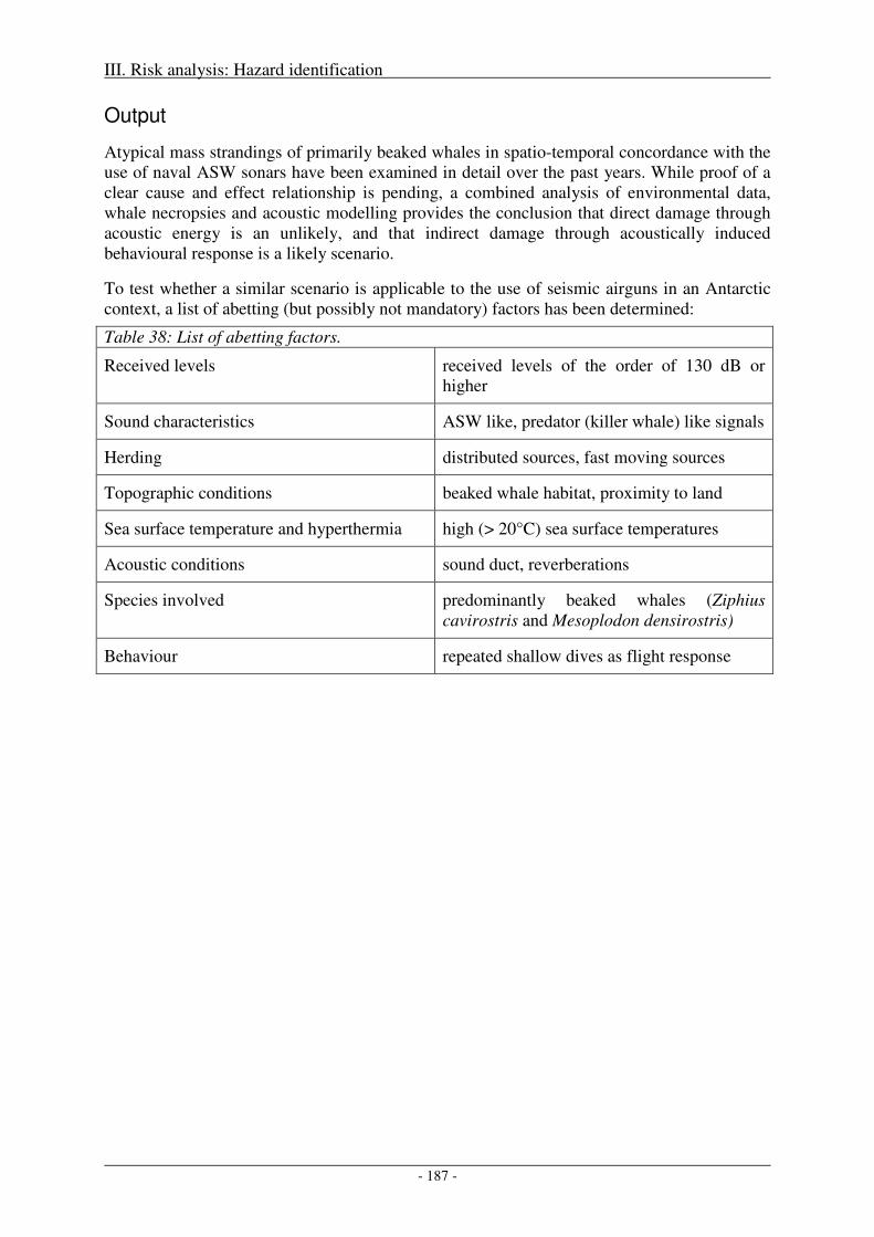
III. Risk analysis: Hazard identification
- 187 -
Output
Atypical mass strandings of primarily beaked whales in spatio-temporal concordance with the use of naval ASW sonars have been examined in detail over the past years. While proof of a clear cause and effect relationship is pending, a combined analysis of environmental data, whale necropsies and acoustic modelling provides the conclusion that direct damage through acoustic energy is an unlikely, and that indirect damage through acoustically induced behavioural response is a likely scenario.
To test whether a similar scenario is applicable to the use of seismic airguns in an Antarctic context, a list of abetting (but possibly not mandatory) factors has been determined:
Table 38: List of abetting factors.
Received levels received levels of the order of 130 dB or higher
Sound characteristics ASW like, predator (killer whale) like signals
Herding distributed sources, fast moving sources
Topographic conditions beaked whale habitat, proximity to land
Sea surface temperature and hyperthermia high (> 20°C) sea surface temperatures
Acoustic conditions sound duct, reverberations
Species involved predominantly beaked whales (Ziphius cavirostris and Mesoplodon densirostris)
Behaviour repeated shallow dives as flight response
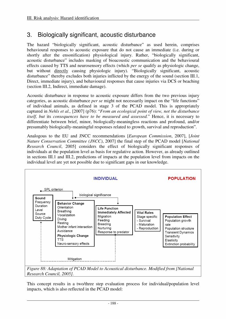
III. Risk analysis: Hazard identification
- 188 -
3. Biologically significant, acoustic disturbance
The hazard “biologically significant, acoustic disturbance” as used herein, comprises behavioural responses to acoustic exposure that do not cause an immediate (i.e. during or shortly after the ensonification) physiological injury. Rather, “biologically significant, acoustic disturbance” includes masking of bioacoustic communication and the behavioural effects caused by TTS and neurosensory effects (which per se qualify as physiologic change, but without directly causing physiologic injury). “Biologically significant, acoustic disturbance” thereby excludes both injuries inflicted by the energy of the sound (section III.1, Direct, immediate injury), and behavioural responses that cause injuries via DCS or beaching (section III.2, Indirect, immediate damage).
Acoustic disturbance in response to acoustic exposure differs from the two previous injury categories, as acoustic disturbance per se might not necessarily impact on the “life functions” of individual animals, as defined in stage 3 of the PCAD model. This is appropriately captured in Nehls et al., [2007] (p76): “From an ecological point of view, not the disturbance itself, but its consequences have to be measured and assessed.” Hence, it is necessary to differentiate between brief, minor, biologically-meaningless reactions and profound, and/or presumably biologically-meaningful responses related to growth, survival and reproduction”.
Analogous to the EU and JNCC recommendations [European Commission, 2007], [Joint Nature Conservation Committee (JNCC), 2007] the final step of the PCAD model [National Research Council, 2005] considers the effect of biologically significant responses of individuals at the population level as basis for regulative action. However, as already outlined in sections III.1 and III.2, predictions of impacts at the population level from impacts on the individual level are yet not possible due to significant gaps in our knowledge.
Figure 88: Adaptation of PCAD Model to Acoustical disturbance. Modified from [National Research Council, 2005].
This concept results in a two/three step evaluation process for individual/population level impacts, which is also reflected in the PCAD model:
III. Risk analysis: Hazard identification
- 189 -
1) The determination of areas within which a disturbance might be expected.
2.) The examination whether such a disturbance might have biologically significant impacts on the individual level.
3.) The prognoses whether the individual effect might have an effect at the population level.
However, due to the described limitations in our scientific knowledge, examination of all three points is characterized by large uncertainties.
Types of possible acoustically induced behavioural disturbance
Acoustic disturbance might elicit a number of behavioural responses as listed below. The underlying mechanisms – whether due to neurosensory effects or cognitive responses – are completely unknown. Hence the following list simply provides mostly hypothesized and few empirically observed behavioural responses:
• avoidance behaviour
• prolongation or interruption of migration
• interruption of feeding
• interruption of breeding
• disturbance of calving
• interruption of nurturing and parental care
• interference with predator avoidance
• acoustic interference (masking, change of vocalization patterns, impairment of hearing by masking, TTS or neurosensory effects)
Several reports exist on both presence and absence of such behavioural responses of marine mammals to sound. Summaries are given e.g. in [Richardson et al., 1995], [Southall et al., 2007] and [Nowacek et al., 2007]. However, the available data are yet too sparse to obtain species specific information for each of the type of behavioural response as listed above. In fact, some of these have not even been documented in the field and are based on mere reasoning. To our knowledge, the only response documented in the field is avoidance, which hence necessarily serves as a proxy for any kind of behavioural response. Focusing on the context of this study, particular interest lies in studies considering responses to what is defined by [Southall et al., 2007] as “behavioural disturbance from multiple pulses”.
Sound levels at which behavioural disturbance was observed
Southall et al., [2007], after reviewing the current literature, conclude that the data available are insufficient to arrive at an unambiguous quantitative approach (of whatever metric) to describe the magnitude and severity of possible behavioural effects. Because “SPL is the metric that has most often been measured or estimated during disturbance studies” (p 447) they suggest that SPL currently is “the best metric with which to assess the available behavioural response data”. However they recommend alterantive metrics that should be used in future studies to end this reliance on SPL.
III. Risk analysis: Hazard identification
- 190 -
After reviewing the current body of knowledge, they arrive at the conclusion that for low-frequency cetaceans (with the exception of migrating bowhead whales), the onset of significant25 behavioural disturbance (which presumably corresponds to classes 4-9 of the response severity scale as defined in Southall et al. (their table 4)) from exposure to multiple pulses occurred at RLs of 140 to 160 dBrms rel. 1µPa or perhaps higher [Southall et al., 2007] (p 452). By contrast, they report that for mid-frequency cetaceans RLs in the 120-180 dB range failed to elicit a clear response from a significant percentage of individuals.
Considering both low- and mid-frequency data in an earlier study, Gordon et al. [1998] summarize observations of behavioural changes in marine mammals in response to airguns and seismic surveys. Analysis of those of their data that concern true Antarctic species produces received levels of 160 -170 dB as the dominant RLs at which avoidance reactions have been observed. For pinnipeds in water, Southall et al. [2007] note: “…exposures in the
∼150 to 180 dB re: 1µPa range (rms over pulse duration) generally have limited potential to induce avoidance behaviour in pinnipeds, whereas RLs exceeding 190 dB re: 1µPa are likely to elicit responses, at least in some ringed seals …“.
For the purpose of estimating the range and duration within which behavioural responses may be expected, we here select the value of 160 dBrms, which appears to be the centroid of values reported across most studies and relevant species.
Based on the threshold level of 160 dBrms rel. 1µPa, distances (and areas) may be calculated for a given sound field, within which this level is exceeded. The areas – which will be calculated for the systems under consideration in section IV.3 - will provide the first step of the abovementioned two/three-step approach for individual/population effects. The second step considers the biological significance of the presumed behavioural disturbances, with the corresponding criteria being identified in the following two sections.
Biological significance of acoustic disturbance to individuals
To determine whether behavioural responses are of biological significance, the following criteria have been proposed by [National Research Council, 2005]:
Migration
• Neither path length nor duration of migration should be increased into upper quartile of the normal time or distance of migration.
Feeding
• Disturbance shall not decrease energy reserves into the lower quartile of normal variation, as measured during a period appropriate for the proposed activity and season and the species affected.
Breeding
• Disruption of male breeding behaviour should not reduce the pool of potential mates from which females can choose by more than 25%.
• Low tolerances to disturbance of females with regard to their ability to select a mate, breed, gestate, and give birth to a viable offspring.
25 It should be noted that the term „significant“ as used above must not to be confused with „biologically significant.
III. Risk analysis: Hazard identification
- 191 -
Calving
• Low tolerance to disturbance of calving.
Nurturing and Parental Care
• Lactation: the nutrition of a calf should not be reduced into the lower quartile of normal.
• Low tolerance to disturbance that might separate a dependant infant from its caregivers.
Predator Avoidance
• Low thresholds are recommended if there is the chance that the disruption will increase the vulnerability of the animal to predation.
However, much of the data required to be able to provide the detailed statistical measures proposed above are not currently available (e.g. the distribution of migration paths of sperm whales to and from Antarctica.) Noting the importance of diel patterns in many behavioural activities, Southall et al. [2007] put forth a somewhat simplified metric to evaluate the biological significance of at least the first two of the abovementioned behavioural responses: “…a reaction lasting less than 24 hours and not recurring on subsequent days is not regarded as particularly severe unless it could directly affect survival or reproduction” [Southall et al., 2007] (p448).
Discussion
Selecting a threshold of biologically significant response
The previous sections directly address one of the most controversially discussed questions in the area of marine mammals and noise: What is the appropriate threshold level at which biologically significant behavioural effects (either at the individual of population level) set in. Actually, the question itself might be ill posed, as it is unclear whether a single value exists across all species, sexes, age groups and for different behavioural context or even individuals [McCauley et al., 2000]. However, charged with the necessity of producing such value(s) to be able to quantify risks and define management schemes under which the hazard of biological significant behavioural response may be mitigated, one is left with the problem of producing a suitable and preferable singular metric from a sparse and inhomogeneous body of research.
It is important to understand, that the purpose of this risk assessment is not to write yet another review article on the few available original papers on this matter. Rather, the goal is to determine the risk specific to seismic research studies in the Antarctic from a scientific point of view. We hence attempted to rely on review papers from independent, external sources to obtain such criteria. For this reason, this risk assessment examined three review papers [Southall et al., 2007], [Gordon et al., 1998] and [Nowacek et al., 2007], which, to our knowledge, include all relevant original papers on this topic. An overview of the available original literature on cetaceans, as used by theses reviews is listed in Table 39. However, a detailed discussion of these papers seems to be repeating of what others already have done, why it should not be repeated here.
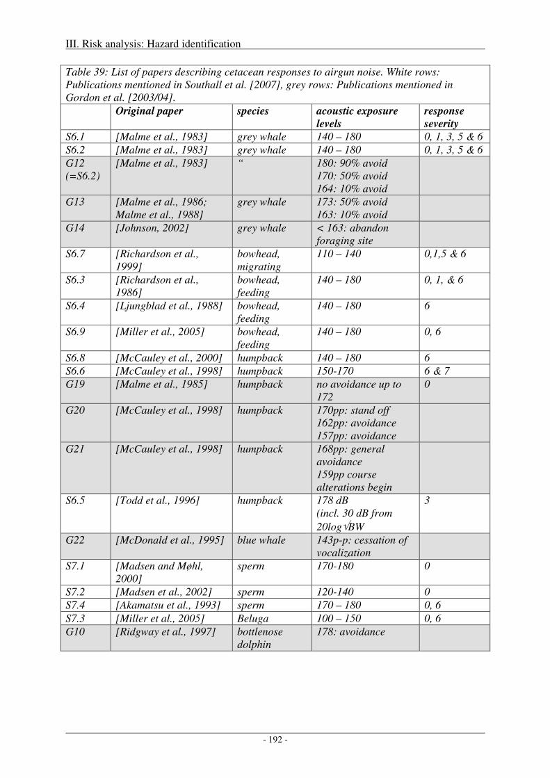
III. Risk analysis: Hazard identification
- 192 -
Table 39: List of papers describing cetacean responses to airgun noise. White rows: Publications mentioned in Southall et al. [2007], grey rows: Publications mentioned in Gordon et al. [2003/04].
Original paper species acoustic exposure
levels
response
severity
S6.1 [Malme et al., 1983] grey whale 140 – 180 0, 1, 3, 5 & 6
S6.2 [Malme et al., 1983] grey whale 140 – 180 0, 1, 3, 5 & 6
G12 (=S6.2)
[Malme et al., 1983] “ 180: 90% avoid 170: 50% avoid 164: 10% avoid
G13 [Malme et al., 1986; Malme et al., 1988]
grey whale 173: 50% avoid 163: 10% avoid
G14 [Johnson, 2002] grey whale < 163: abandon foraging site
S6.7 [Richardson et al., 1999]
bowhead, migrating
110 – 140 0,1,5 & 6
S6.3 [Richardson et al., 1986]
bowhead, feeding
140 – 180 0, 1, & 6
S6.4 [Ljungblad et al., 1988] bowhead, feeding
140 – 180 6
S6.9 [Miller et al., 2005] bowhead, feeding
140 – 180 0, 6
S6.8 [McCauley et al., 2000] humpback 140 – 180 6
S6.6 [McCauley et al., 1998] humpback 150-170 6 & 7
G19 [Malme et al., 1985] humpback no avoidance up to 172
0
G20 [McCauley et al., 1998] humpback 170pp: stand off 162pp: avoidance 157pp: avoidance
G21 [McCauley et al., 1998] humpback 168pp: general avoidance 159pp course alterations begin
S6.5 [Todd et al., 1996] humpback 178 dB (incl. 30 dB from
20log√BW
3
G22 [McDonald et al., 1995] blue whale 143p-p: cessation of vocalization
S7.1 [Madsen and Møhl, 2000]
sperm 170-180 0
S7.2 [Madsen et al., 2002] sperm 120-140 0
S7.4 [Akamatsu et al., 1993] sperm 170 – 180 0, 6
S7.3 [Miller et al., 2005] Beluga 100 – 150 0, 6
G10 [Ridgway et al., 1997] bottlenose dolphin
178: avoidance
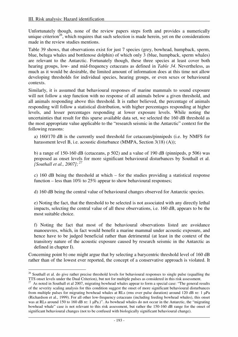
III. Risk analysis: Hazard identification
- 193 -
Unfortunately though, none of the review papers steps forth and provides a numerically unique criterion26, which requires that such selection is made herein, yet on the considerations made in the review studies mentions.
Table 39 shows, that observations exist for just 7 species (grey, bowhead, humpback, sperm, blue, beluga whales and bottlenose dolphin) of which only 3 (blue, humpback, sperm whales) are relevant to the Antarctic. Fortunately though, these three species at least cover both hearing groups, low- and mid-frequency cetaceans as defined in Table 34. Nevertheless, as much as it would be desirable, the limited amount of information does at this time not allow developing thresholds for individual species, hearing groups, or even sexes or behavioural contexts.
Similarly, it is assumed that behavioural responses of marine mammals to sound exposure will not follow a step function with no response of all animals below a given threshold, and all animals responding above this threshold. It is rather believed, the percentage of animals responding will follow a statistical distribution, with higher percentages responding at higher levels, and lesser percentages responding at lower exposure levels. While noting the uncertainties that result for this sparse available data set, we selected the 160 dB threshold as the most appropriate value applicable to the “research seismic in the Antarctic” context for the following reasons:
a) 160/170 dB is the currently used threshold for cetaceans/pinnipeds (i.e. by NMFS for harassment level B, i.e. acoustic disturbance (MMPA, Section 3(18) (A)); b) a range of 150-160 dB (cetaceans, p 502) and a value of 190 dB (pinnipeds, p 506) was proposed as onset levels for more significant behavioural disturbances by Southall et al. [Southall et al., 2007]; 27 c) 160 dB being the threshold at which – for the studies providing a statistical response function – less than 10% to 25% appear to show behavioural responses; d) 160 dB being the central value of behavioural changes observed for Antarctic species. e) Noting the fact, that the threshold to be selected is not associated with any directly lethal impacts, selecting the central value of all these observations, i.e. 160 dB, appears to be the most suitable choice. f) Noting the fact that most of the behavioural observations listed are avoidance manoeuvres, which, in fact would benefit a marine mammal under acoustic exposure, and hence have to be judged beneficial rather than detrimental (at least in the context of the transitory nature of the acoustic exposure caused by research seismic in the Antarctic as defined in chapter I).
Concerning point b) one might argue that by selecting a barycentric threshold level of 160 dB rather than of the lowest ever reported, the concept of a conservative approach is violated. It
26 Southall et al. do give rather precise threshold levels for behavioural responses to single pulse (equalling the TTS onset levels under the Dual Criterion), but not for multiple pulses as considered in this risk assessment. 27 As noted in Southall et al 2007, migrating bowhead whales appear to form a special case: “The general results of the severity scaling analysis for this condition suggest the onset of more significant behavioural disturbances from multiple pulses for migrating bowhead whales at RLs (rms over pulse duration) around 120 dB re: 1 µPa (Richardson et al., 1999). For all other low-frequency cetaceans (including feeding bowhead whales), this onset was at RLs around 150 to 160 dB re: 1 µPa.)”. As bowhead whales do not occur in the Antarctic, the “migrating bowhead whale” case is not relevant to this risk assessment, but rather the 150-160 dB range for the onset of significant behavioural changes (not to be confused with biologically significant behavioural change).
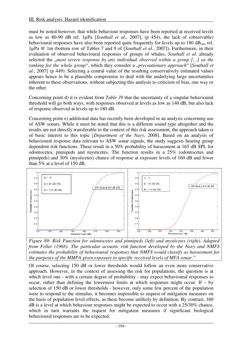
III. Risk analysis: Hazard identification
- 194 -
must be noted however, that while behaviour responses have been reported at received levels as low as 80-90 dB rel. 1µPa [Southall et al., 2007], (p 454), the lack of (observable) behavioural responses have also been reported quite frequently for levels up to 180 dBrms rel. 1µPa @ 1m (bottom row of Tables 7 and 9 of [Southall et al., 2007]). Furthermore, in their evaluation of observed behavioural responses of groups of whales, Southall et al. already selected the „most severe response by any individual observed within a group […] as the ranking for the whole group“, which they consider a „precautionary approach“ [Southall et al., 2007] (p 449). Selecting a central value of the resulting conservatively estimated values appears hence to be a plausible compromise to deal with the underlying large uncertainties inherent to these observations, without subjecting this analysis to criticism of bias, one way or the other.
Concerning point d) it is evident from Table 39 that the uncertainty of a singular behavioural threshold will go both ways, with responses observed at levels as low as 140 dB, but also lack of response observed at levels up to 180 dB.
Concerning point e) additional data has recently been developed in an analysis concerning use of ASW sonars. While it must be noted that this is a different sound type altogether and the results are not directly transferable to the context of this risk assessment, the approach taken is of basic interest to this topic [Department of the Navy, 2008]. Based on an analysis of behavioural response data relevant to ASW sonar signals, the study suggests hearing group dependent risk functions. These result in a 50% probability of harassment at 165 dB SPL for odontocetes, pinnipeds and mysticetes. The function results in a 25% (odontocetes and pinnipeds) and 30% (mysticetes) chance of response at exposure levels of 160 dB and fewer than 5% at a level of 150 dB.
Figure 89: Risk Function for odontocetes and pinnipeds (left) and mysticetes (right). Adapted from Feller (1968): The particular acoustic risk function developed by the Navy and NMFS estimates the probability of behavioural responses that NMFS would classify as harassment for the purposes of the MMPA given exposure to specific received levels of MFA sonar.”
Of course, selecting 150 dB or lower thresholds would follow an even more conservative approach. However, in the context of assessing the risk for populations, the question is at which level one - with a certain degree of probability - may expect behavioural responses to occur, rather than defining the lowermost limits at which responses might occur. If – by selection of 150 dB or lower thresholds - however, only some few percent of the population were to respond to the stimulus, it becomes impossible to request of mitigation measures on the basis of population level effects, as these become unlikely by definition. By contrast, 160 dB is a level at which behaviour responses might be expected to occur with a 25/30% chance, which in turn warrants the request for mitigation measures if significant biological behavioural responses are to be expected.
III. Risk analysis: Hazard identification
- 195 -
Which rms integration time is appropriate in the context of behavioural responses?
The calculation of rms sound pressure levels depends on the length of a chosen averaging window. This might vary between 40 ms (the typical duration of the primary seismic pulse) and 200 ms (the auditory integration timescale and also including the reception of reverberations). The difference between the two may amount to 7 dB (10 log (200 ms/40 ms)).
In this risk assessment, rms sound pressure levels are used exclusively in conjunction with the discussion of behavioural responses, i.e. the hazards of “indirect, immediate damage” and “biologically significant, acoustic disturbance” (see also page 189). A conversion of these rms values to SEL values, would be preferable, but as Southall et al. [2007] note, the entire current literature on behavioural responses is currently providing – at the most – rms values, rather than SPL0-p or SEL metrics. Until such more appropriate metrics are used in the description of behavioural response, the use of SPLrms remains unavoidable.
For the consideration of rms values in the context of behavioural response, it seems appropriate to define this metric in a way, which actually reflects the sound’s perception by the animal, rather than any characteristic specific to the sound signal itself. Hence the 200 ms averaging window, which describes the auditory integration time [Madsen, 2005], [Madsen et al., 2006], appears the appropriate choice for a discussion of these issues.
By contrast, for the discussion of “direct, immediate damage”, we use the SPL0-peak and SEL metrics, which reflect the peak pressure and energy of the pulse (which is the most appropriate metric for this issue). Rms levels represent a metric that numerically lie between SPL0-p (which indicates the peak (and hence highest) and SEL (which considers the long term energy flux). If one were to replace the 200 ms averaging time with a window only comprising the primary pulse (typically 40 ms), as suggested by one reviewer, one would basically duplicate the information inherent to the 0-peak value, while on the other hand, neglecting the additional energy contributed by e.g. bottom and surface reflections. The effect of these latter contributions to the sound field – which are modelled in detail in this study - have been a central issue of previous concerns raised with regard to the validity of sound propagation models.
It should be noted, that the rms values data calculated as part the Heggerness paper [Breitzke et al., 2008] and presented herein are based on a 40 ms integration window. This is appropriate, as this study aims at deriving source levels (SL) rather than received levels, and due to experimental constraints, i.e. having to avoid inclusion reflections resulting for the narrow fjord walls, which would not occur in the open ocean. However, the Heggerness rms based data, while presented herein (along with p-p, 0-p other metrics) does not enter the calculation of this risk-assessment and has hence no impact on our findings.
Output
To discuss the possible biological effects of behavioural response, a two-step analytic process will be used:
1) The area within which received SPL exceeds 160 dBrms rel. 1µPa will be calculated together with the time an animal is expected to spend therein.
2.) Considering the exposure time and expected time of disturbance, it will be evaluated whether a response will lead to biologically significant consequences for the individual.
III. Risk analysis: Hazard identification
- 196 -
3.) The final step required under PCAD, the transition from individual effects to population level effects is, commensurate with a highly conservative approach, omitted due to lacking scientific concepts.
III. Risk analysis: Hazard identification
- 197 -
4. References
Aguilar Soto, N., et al. (2006), Does intense ship noise disrupt foraging in deep-diving Cuvier's beaked whales (Ziphius cavirostris)?, Marine Mammal Science, 22(3), 690-699.
Akamatsu, T., et al. (1993), Effects of pulse sounds on escape behavior of false killer whales, Bulletin of the Japanese Society of Scientific Fisheries, 59, 1297-1303.
Antarctic Treaty States (1991), Protocol on environmental protection to the Antarctic treaty, 42 pp.
Boyd, I., et al. (2007), Behavioral Response Study-2007 (BSR-07), Cruise report.
Breitzke, M., et al. (2008), Broadband calibration of marine seismic sources used by R/V Polarstern for academic research in polar regions, Geophysical Journal International, 174(2), 505-524.
Bronwell jr., R. L., et al. (2004), Mass strandings of Cuvier's beaked whales in Japan: U. S. Naval accoustic link?, paper presented at IWC 56th Annual Meeting, 10 pp, Sorrento, Italy, 19-22 July 2004.
Cole, S. (2005), Military exercises and marine mammal strandings - a stressful issue?, paper presented at 1st Intergovernmental Conference on Effects of Sound on Marine MammalsNato Undersea Research Center, Lerici, Italy, 2-5 May 2005.
Cox, T. M., et al. (2006), Understanding the impacts of anthropogenic sound on beaked whales, Journal of Cetacean Research and Management, 7(3), 177-187.
D'Spain, G. L., et al. (2005), Properties of the underwater sound fields during some well documented beaked whale mass stranding events, Journal of Cetacean Research Management, 7(3), 223-238.
Department of Commerce, National Oceanic and Atmospheric Administration (NOAA), (2008), Incidental Takes of Marine Mammals During Specified Activities; Beach Boulevard AICWW Bridge Blasting Project, Duval County, FL, Federal Register, 73(234), 73913-73922.
Department of Commerce National Oceanic and Atmospheric Administration [I.D. 031704B] Taking and Importing Marine Mammals (2006), Taking Marine Mammals Incidental to Conducting Air-to-Surface Gunnery Missions in the Gulf of Mexico Federal Register, 71(14), 3480.
Department of the Navy (2008), Final environmental impact statement / overseas environmental impact statement Southern California Range Complex, 1 of 2, 1026, Department of the Navy.
European Commission (2007), Guidance document on the strict protection of animal species of community interest under the Habitats Directive 92/43/EEC.
Finneran, J. J., et al. (2002), Temporary shift in masked hearing thresholds in odontocetes after exposure to single underwater impulses from a seismic watergun, Journal of the Acoustical Society of America, 111(6), 2929-2939.
Frantzis, A. (1998), Does acoustic testing strand whales?, Nature, 392, 29.
Freitas, L. (2003), The stranding of three Cuvier's beaked whales Ziphius cavirostris in Madeira Archipelago-May 2000, paper presented at Workshop on active sonar and cetaceans held at the European Cetacean Society's 17th annual conference, 28-32 pp, ECS Newsletter 42-Special Issue, Las Palmas, Gran Canaria, March 8, 2003.
III. Risk analysis: Hazard identification
- 198 -
Fromm, D. M., and J. McEachern (2000), Acoustic modelling results of the New Providence Channel for 15 March 2000, 57 pp, NRL,, ONR.
Gordon, J., et al. (2003/04), A review of the effects of seismic surveys on marine mammals, Marine Technology Society Journal, 37, 16-34.
Gordon, J. C. D., et al. (1998), The effects of seismic activity on marine mammals paper presented at Seismic and Marine Mammals Workshop (UKOOA), 16- pp, Proceedings of the seismic and marine mammal workshop London 23-25 June 1998., London, June 23-25.
High Energy Seismic Survey (HESS) (1999), Seismic Survey review process and interim operational guidelines for marine surveys offshore Southern California. Report from HESS Team for California State Lands Commission and U.S. Minerals Management Service. Retrieved 22 October 2007 from www.mms.gov/omm/pacific/lease/fullhessrept.pdf., 39 pp, Camarillo.
ICES Advisory Committee on Ecosystems (2005), Report of the ad-hoc group on the impact of sonar on cetaceans and fish (AGISC) - By Correspondence, 41 pp, ICES.
IWC Scientific Committee (2004), Anthropogenic noise, section 12.2.5., scientific report 5pp, Sorrento, Italy.
Jepson, P. D., et al. (2003), Gas-bubble lesions in stranded cetaceans, Nature, 425.
Johnson, S. R. (2002), Marine mammal mitigation and monitoring program for the 2001 Odoptu 3-D seismic survey, Sakhalin Island, Russia: Executive summary, 49 pp, LGL Limited for Exxon Neftegas Limited, Sidney, BC, Canada.
Joint Nature Conservation Committee (JNCC) (2007), The deliberate disturbance of marine European Protected Species. Iterim guidance for English and Welsh territorial waters and the UK offshore marine area.
Kastak, D., et al. (2005a), Underwater temporary threshold shift in pinnipeds: Effects of noise level and duration, The Journal of the Acoustical Society of America, 118(5), 3154-3163.
Kastak, D., et al. (2005b), Underwater temporary threshold shift in pinnipeds: effects of noise level and duration, Journal of the Acoustical Society of America, 118(5), 3154-3163.
Ketten, D. (2002), Physische Effekte / körperliche Schädigung, in Ergebnisprotokoll der Tagung "Offshore windmills - sound emissions and marine mammals, p. 14, Forschungs- und Technologiezentrum Westküste, Büsum, Germany.
Ketten, D. R., et al. (1993), Blast injury in humpback whale ears: Evidence and implications, The Journal of the Acoustical Society of America, 94(3), 1849-1850.
Krysl, P., et al. (2006), Simulating the effect of high-intensity sound on cetaceans: Modeling approach and a case study for Cuvier's beaked whale (Ziphius cavirostris), The Journal of the Acoustical Society of America, 120(4), 2328.
Ljungblad, D. K., et al. (1988), Observations on the behavioral response of bowhead whales (Balaena mysticetus) to active geophysical vessels in the Alaskan Beaufort Sea, Arctic, 3, 183-194.
MacLeod, C. D., and G. Mitchell (2005/6), Key areas for beaked whales worldwide, Journal of Cetacean Research Management, 7(3), 309-322.
Madsen, P. T., and B. Møhl (2000), Sperm whales (Physeter catodon L. 1758) do not react to sounds from detonators, Journal of the Acoustical Society of America, 107(1), 668-671.
Madsen, P. T., et al. (2002), Sperm whale sound production studied with ultrasound time/depth-recording tags, Journal of Experimental Biology, 205, 1899-1906.
III. Risk analysis: Hazard identification
- 199 -
Madsen, P. T. (2005), Marine mammals and noise: Problems with root mean square sound pressure levels for transients, The Journal of the Acoustical Society of America, 117(6), 3952-3957.
Madsen, P. T., et al. (2006), Quantitative measures of airgun pulses recorded on sperm whales (Physeter macrocephalus) using acoustic tags during controlled exposure experiments, The Journal of the Acoustical Society of America, 120(4), 2366.
Malakoff, D. (2002), Suit ties whale deaths to research cruise, Science (Washington), 298(5594), 722-723.
Malme, C. I., et al. (1983), Investigations of the potential effects of underwater noise from petroleum industy activities on migrating gray whale behavior, prepared for the Department of the Interior, 407 pp, Bolt Beranek and Newmann Inc.
Malme, C. I., et al. (1985), Investigation of the potential effects of underwater noise from petroleum industry activities on feeding humpback whale behavior, 205 pp, Bolt Beranek and Newman Inc.
Malme, C. I., et al. (1986), Behavioral responses of gray whales to industrial noise: feeding observations and predictive modeling.
Malme, C. I., et al. (1988), Observations of feeding gray whale responses to controlled industrial noise exposure in Port and Ocean Engineering Under Arctic Conditions, edited by W. M. Sackinger, pp. 55-73, University of Alaska, Fairbanks, AK.
Marine Mammal Commission (2008), Written statement of the Marine Mammal Commission regarding the Department of the Navy's request for a Letter of Authorization to take small numbers of marine mammals incidental to shock-testing the Mesa Verde 70 km (38 nmi) off Mayport, Florida and the NMFS 11 April 2008 Federal Register notice proposing regulations to authorize and govern the requested taking, p. 2, Marine Mammal Commission, Bethesda, MD.
Martín, V., et al. (2003), Mass stranding of beaked whales in the Canary Islands, paper presented at Workshop on active sonar and cetaceans held at the European Cetacean Society's 17th annual conference, 33-36 pp, ECS Newsletter 42-Special Issue
Las Palmas, Gran Canaria, March 8, 2003.
McCauley, R. D., et al. (1998), The response of humpack whales (Megaptera novaeangliae) to offshore seismic survey noise: Preliminary results of observations about a working seismic vessel and experimantal exposures, APPEA Journal, 38(1), 692-707.
McCauley, R. D., et al. (2000), Marine seismic surveys - a study of environmental implications, APPEA Journal, 40, 692-708.
McDonald, M. A., et al. (1995), Blue and fin whales observed on a seafloor array in the Northeast Pacific, The Journal of the Acoustical Society of America, 98(2), 712-721.
Miller, G. W., et al. (2005), Monitoring seismic effects on marine mammals - southeastern Beaufort Sea, 2001-2002, in Offshore oil and gas environmental effects monitoring: Approaches and technologies, edited by S. L. Armsworthy, et al., pp. 511-542, C Battelle Press, Columbus, OH.
Nachtigall, P. E., et al. (2003), Temporary threshold shifts and recovery following noise exposure in the Atlantic bottlenosed dolphin (Tursiops truncatus), Journal of the Acoustical Society of America, 113(6), 3425-3429.
Nachtigall, P. E., et al. (2004), Temporary threshold shift after noise exposure in the bottlenose dolphin (Tursiopsis truncatus) measured using evoked auditory potentials Marine Mammal Science, 20(4), 673-687.
III. Risk analysis: Hazard identification
- 200 -
National Marine Fisheries Service (2002), National Marine Fisheries Service Endangered Species Act - Section 7 Consultation Biological Opinion on SURTASS LFA, 170, NMFS.
National Research Council (2005), Marine mammal populations and ocean noise - determining when noise causes biologically significant effects, 126 pp., National Academies Press, Washington.
Nehls, G., et al. (2007), Sources of underwater noise and their implications on marine wildlife - with special emphasis on the North Sea and the Baltic Sea, final report, 123 pp, Bio Consult SH, itap.
Nowacek, D. P., et al. (2007), Responses of cetaceans to anthropogenic noise, Mammal Review, 37(2), 81-115.
Parsons, E. C. M., et al. (2008), Navy sonar and cetaceans: Just how much does the gun need to smoke before we act?, Marine Pollution Bulletin, 56(7), 1248-1257.
Richardson, W. J., et al. (1986), Reactions of bowhead whales, Balaena mysticetus, to seismic exploration in the Canadian Beaufort Sea, The Journal of the Acoustical Society of America, 79(4), 1117-1128.
Richardson, W. J., et al. (1995), Marine mammals and noise, 576 pp., Academic Press, San Diego.
Richardson, W. J., et al. (1999), Displacement of migrating bowhead whales by sounds from seismic surveys in shallow waters of the Beaufort Sea, Journal of the Acoustical Society of America, 106, 2281.
Ridgway, S. H., et al. (1997), Behavioral responses and temporary shift in masked hearing thresholds of bottelnose dolphin, tursiopsis truncatus, to 1-second tones of 141 to 201 dB re 1µPa, 16 pp.
Schlundt, C. E., et al. (2000), Temporary shift in masked hearing thresholds of bottlenose dolphins, Tursiops truncatus, and white whales, Delphinapterus leucas, after exposure to intense tones, Journal of the Acoustical Society of America, 107(6), 3496-3508.
Southall, B. L., et al. (2007), Marine mammal noise exposure criteria: initial scientific recommendations, Aquatic Mammals, 33(4 ), 411-521.
Strope, B., and A. Alwan (1996), A model of dynamic auditory perception and its application to robust speech recognition., IEEE International Conference on Acoustics, Speech, and Signal Processing, Vol. 1, 37-40.
Todd, S., et al. (1996), Behavioural effects of exposure to underwater explosions in humpack whales (Megaptera novaeangliae), Canadian Journal of Zoology, 74, 1661-1672.
Tyack, P. L. (2007), Study on behavioral responses of tagged beaked whales to anthropogenic and natural sounds, in 2nd Intergovernmental Conference on Effects of Sound on Marine Mammals, Nato Undersea Research Center, Lerici, Italy.
Urbán, J. R., et al. (2006), Varamiento de diez zifidos de Baird, Berardius bairdii, en la isla San Jose, B.C.S., 10 pp, UNIVERSIDAD AUTÓNOMA DE BAJA CALIFOIRNIA SUR,, Programa de Investigación de Mamíferos Marinos,, La Paz, México.
Ward, W. D. (1997), Effects of high intensity-sound, in Encyclopedia of Acoustics, edited by M. J. Crocker, pp. 1497-1507, John Wiley and Sons, Inc., New York.
Zimmer, W. M. X. (2007), 11 years after Kiparissiakos bay. What may have happened and what to do about it, in 2nd Intergovernmental Conference on Effects of Sound on Marine Mammals, Lerici, Italy.
III. Risk analysis: Hazard identification
- 201 -
Zimmer, W. M. X., and P. L. Tyack (2007), Repetitive shallow dives pose decompression risk in deep-diving beaked whales, Marine Mammal Science, 23(4), 888-925.

IV. Risk analysis: Exposure analysis
- 203 -
IV. Risk analysis: Exposure analysis
1. Direct, immediate injury
Based on the output from section III.1, critical radii were calculated. The calculations provide cumulative exposure levels as exemplified in Figure 90 (representative for 24 such plots (not shown) for the various combinations of environmental and source characteristics, see Table 8. The top panels of Figure 90 show the zero to peak sound pressure levels as emitted by the single shots of an airgun moving along the seismic line, corresponding to the dual criteria’s SPL0-p metric. The bottom panels show the cumulative SEL values as received by a hypothetical, stationary whale at a depth of 5 (left), 30 (middle) and 55 (right) meters. Calculations are performed for various cross-track offsets (symbol color, see figure caption) and an inline position at 5000 m (i.e. in the center of the model domain). Dashed lines indicate the zero-to-peak and SEL thresholds of the dual criteria. As soon as either of the dashed lines (i.e. either zero-to-peak or SEL) is exceeded, a violation of the dual criteria occurs.
It should be emphasized, that in the calculation of accumulated SEL values, any acoustic exposure, including sub-PTS and sub-TTS exposures are included and added linearly. This approach neglects the possibility of any abating effect, resulting in a (conservative) maximum estimation of the exposure levels. The only constraint in the execution of the accumulation process is the size of the model domain, which limits the lowest SEL included to those occurring at the model boundary. Figure 90 for example, shows the inclusion of all exposures with single shot SEL values greater ca. 150 dB re. 1µPa2s. An inclusion of additional lower single-shot SEL values would in fact not contribute significantly to the accumulated SEL, as the latter is dominated by the contributions of shots in the near vicinity of the animal.
A second conservative approximation is taken for reasons of computational simplification by disregarding any frequency weighting in the calculation of the respective single shot SELs, implying a flat weighting equaling “one”, in contrast to the hearing group specific M-weighting curves, cf. section III.1).
The graphs indicates that high SELs occur for cross-track offsets = 0 m (blue curves), i.e. vertically beneath the seismic line, with highest values reached when the whale is located at 30 m depth. Changing to another depth level would result in smaller received SPL and SEL (Figure 90). Hence exposure data for the selection of the 30 m data may serve (in this specific case) as a conservative proxy for any other constant depth or depth profiles that one wishes to assume for the whale to follow.
The colored lines indicate that a whale residing at 30 m depth, 0 m cross-track offset, would receive SEL higher than permitted under the dual criteria as soon as the ship passes overhead (centre panel, blue curve). The same applies for the situation when the whale is located 25 m cross-track (orange curve). However, if the whale would stay at a cross-track distance of 100m or greater from the ship (green curve), the dual criteria will not be exceeded at any time of the transect.
Once the ship has passed the whale’s position, SEL values become nearly constant. This is due to the fact that while the ship is departing from the whale, received SPL and single-shot SEL levels decrease. The logarithmic addition of increasingly lower single-shot SELs results in only minor changes to the cumulative SEL. In fact, the values on the far right of each plot approximate the ‘infinite’ accumulation of SEL for a ship approaching from infinity and
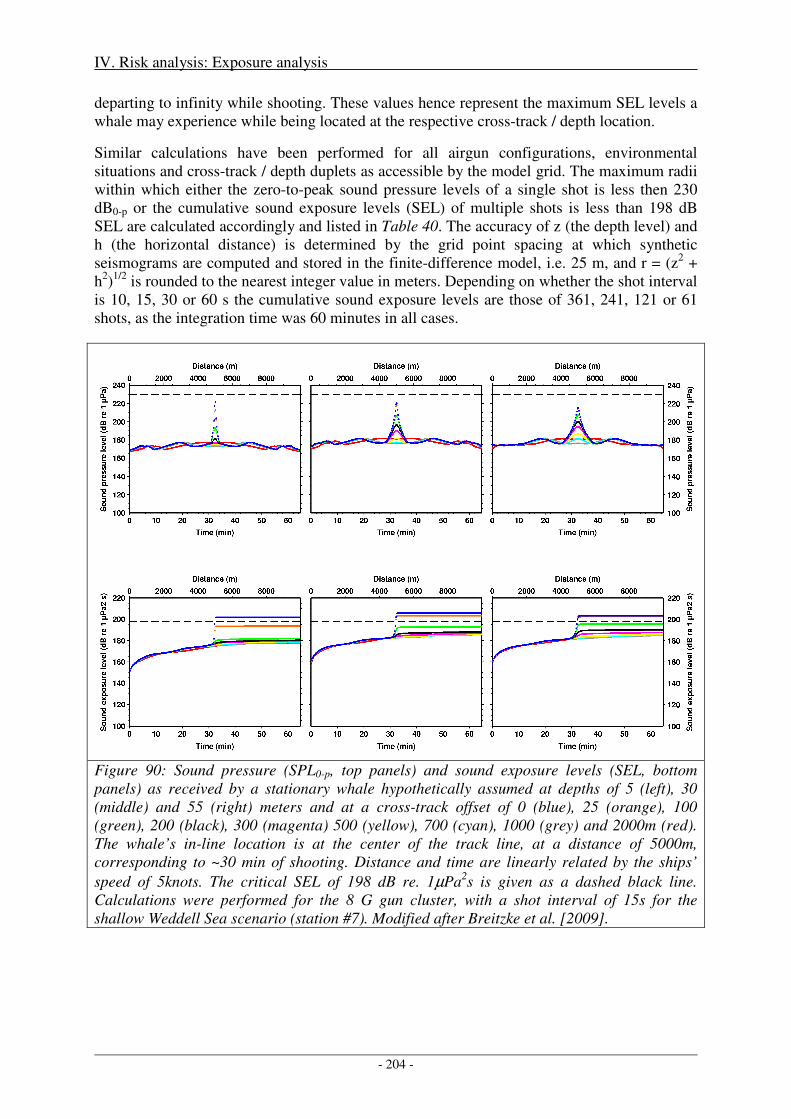
IV. Risk analysis: Exposure analysis
- 204 -
departing to infinity while shooting. These values hence represent the maximum SEL levels a whale may experience while being located at the respective cross-track / depth location.
Similar calculations have been performed for all airgun configurations, environmental situations and cross-track / depth duplets as accessible by the model grid. The maximum radii within which either the zero-to-peak sound pressure levels of a single shot is less then 230 dB0-p or the cumulative sound exposure levels (SEL) of multiple shots is less than 198 dB SEL are calculated accordingly and listed in Table 40. The accuracy of z (the depth level) and h (the horizontal distance) is determined by the grid point spacing at which synthetic seismograms are computed and stored in the finite-difference model, i.e. 25 m, and r = (z2 + h2)1/2 is rounded to the nearest integer value in meters. Depending on whether the shot interval is 10, 15, 30 or 60 s the cumulative sound exposure levels are those of 361, 241, 121 or 61 shots, as the integration time was 60 minutes in all cases.
Figure 90: Sound pressure (SPL0-p, top panels) and sound exposure levels (SEL, bottom panels) as received by a stationary whale hypothetically assumed at depths of 5 (left), 30 (middle) and 55 (right) meters and at a cross-track offset of 0 (blue), 25 (orange), 100 (green), 200 (black), 300 (magenta) 500 (yellow), 700 (cyan), 1000 (grey) and 2000m (red). The whale’s in-line location is at the center of the track line, at a distance of 5000m, corresponding to ~30 min of shooting. Distance and time are linearly related by the ships’
speed of 5knots. The critical SEL of 198 dB re. 1µPa2s is given as a dashed black line. Calculations were performed for the 8 G gun cluster, with a shot interval of 15s for the shallow Weddell Sea scenario (station #7). Modified after Breitzke et al. [2009].
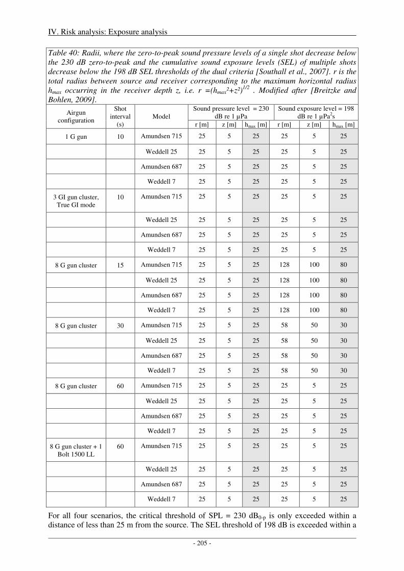
IV. Risk analysis: Exposure analysis
- 205 -
Table 40: Radii, where the zero-to-peak sound pressure levels of a single shot decrease below the 230 dB zero-to-peak and the cumulative sound exposure levels (SEL) of multiple shots decrease below the 198 dB SEL thresholds of the dual criteria [Southall et al., 2007]. r is the total radius between source and receiver corresponding to the maximum horizontal radius hmax occurring in the receiver depth z, i.e. r =(hmax²+z²)1/2 . Modified after [Breitzke and Bohlen, 2009].
Airgun configuration
Shot interval
(s) Model
Sound pressure level = 230 dB re 1 µPa
Sound exposure level = 198 dB re 1 µPa2s
r [m] z [m] hmax [m] r [m] z [m] hmax [m]
1 G gun 10 Amundsen 715 25 5 25 25 5 25
Weddell 25 25 5 25 25 5 25
Amundsen 687 25 5 25 25 5 25
Weddell 7 25 5 25 25 5 25
3 GI gun cluster, True GI mode
10 Amundsen 715 25 5 25 25 5 25
Weddell 25 25 5 25 25 5 25
Amundsen 687 25 5 25 25 5 25
Weddell 7 25 5 25 25 5 25
8 G gun cluster 15 Amundsen 715 25 5 25 128 100 80
Weddell 25 25 5 25 128 100 80
Amundsen 687 25 5 25 128 100 80
Weddell 7 25 5 25 128 100 80
8 G gun cluster 30 Amundsen 715 25 5 25 58 50 30
Weddell 25 25 5 25 58 50 30
Amundsen 687 25 5 25 58 50 30
Weddell 7 25 5 25 58 50 30
8 G gun cluster 60 Amundsen 715 25 5 25 25 5 25
Weddell 25 25 5 25 25 5 25
Amundsen 687 25 5 25 25 5 25
Weddell 7 25 5 25 25 5 25
8 G gun cluster + 1 Bolt 1500 LL
60 Amundsen 715 25 5 25 25 5 25
Weddell 25 25 5 25 25 5 25
Amundsen 687 25 5 25 25 5 25
Weddell 7 25 5 25 25 5 25
For all four scenarios, the critical threshold of SPL = 230 dB0-p is only exceeded within a distance of less than 25 m from the source. The SEL threshold of 198 dB is exceeded within a
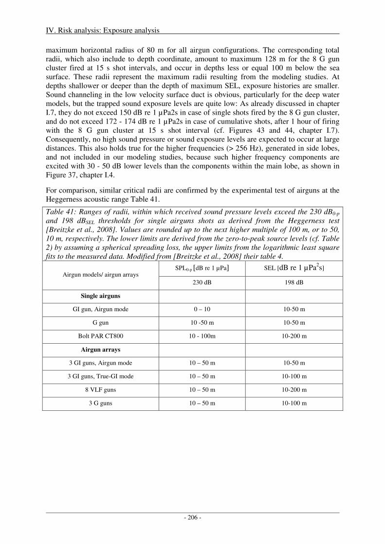
IV. Risk analysis: Exposure analysis
- 206 -
maximum horizontal radius of 80 m for all airgun configurations. The corresponding total radii, which also include to depth coordinate, amount to maximum 128 m for the 8 G gun cluster fired at 15 s shot intervals, and occur in depths less or equal 100 m below the sea surface. These radii represent the maximum radii resulting from the modeling studies. At depths shallower or deeper than the depth of maximum SEL, exposure histories are smaller. Sound channeling in the low velocity surface duct is obvious, particularly for the deep water models, but the trapped sound exposure levels are quite low: As already discussed in chapter I.7, they do not exceed 150 dB re 1 µPa2s in case of single shots fired by the 8 G gun cluster, and do not exceed 172 - 174 dB re 1 µPa2s in case of cumulative shots, after 1 hour of firing with the 8 G gun cluster at 15 s shot interval (cf. Figures 43 and 44, chapter I.7). Consequently, no high sound pressure or sound exposure levels are expected to occur at large distances. This also holds true for the higher frequencies (> 256 Hz), generated in side lobes, and not included in our modeling studies, because such higher frequency components are excited with 30 - 50 dB lower levels than the components within the main lobe, as shown in Figure 37, chapter I.4.
For comparison, similar critical radii are confirmed by the experimental test of airguns at the Heggerness acoustic range Table 41.
Table 41: Ranges of radii, within which received sound pressure levels exceed the 230 dB0-p and 198 dBSEL thresholds for single airguns shots as derived from the Heggerness test [Breitzke et al., 2008]. Values are rounded up to the next higher multiple of 100 m, or to 50, 10 m, respectively. The lower limits are derived from the zero-to-peak source levels (cf. Table 2) by assuming a spherical spreading loss, the upper limits from the logarithmic least square fits to the measured data. Modified from [Breitzke et al., 2008] their table 4.
Airgun models/ airgun arrays SPL0-p [dB re 1 µPa] SEL [dB re 1 µPa2s]
230 dB 198 dB
Single airguns
GI gun, Airgun mode 0 – 10 10-50 m
G gun 10 -50 m 10-50 m
Bolt PAR CT800 10 - 100m 10-200 m
Airgun arrays
3 GI guns, Airgun mode 10 – 50 m 10-50 m
3 GI guns, True-GI mode 10 – 50 m 10-100 m
8 VLF guns 10 – 50 m 10-200 m
3 G guns 10 – 50 m 10-100 m
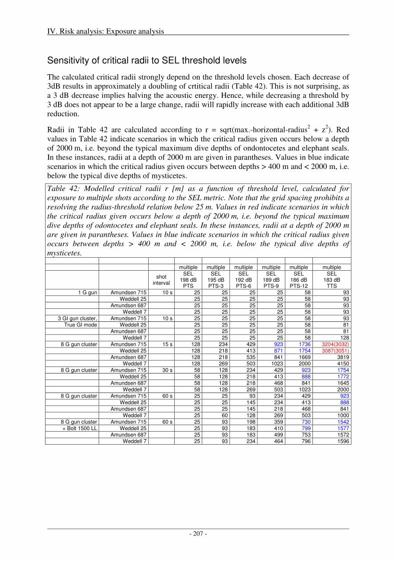
IV. Risk analysis: Exposure analysis
- 207 -
Sensitivity of critical radii to SEL threshold levels
The calculated critical radii strongly depend on the threshold levels chosen. Each decrease of 3dB results in approximately a doubling of crtitical radii (Table 42). This is not surprising, as a 3 dB decrease implies halving the acoustic energy. Hence, while decreasing a threshold by 3 dB does not appear to be a large change, radii will rapidly increase with each additional 3dB reduction.
Radii in Table 42 are calculated according to r = sqrt(max.-horizontal-radius2 + z2). Red values in Table 42 indicate scenarios in which the critical radius given occurs below a depth of 2000 m, i.e. beyond the typical maximum dive depths of ondontocetes and elephant seals. In these instances, radii at a depth of 2000 m are given in parantheses. Values in blue indicate scenarios in which the critical radius given occurs between depths > 400 m and < 2000 m, i.e. below the typical dive depths of mysticetes.
Table 42: Modelled critical radii r [m] as a function of threshold level, calculated for exposure to multiple shots according to the SEL metric. Note that the grid spacing prohibits a resolving the radius-threshold relation below 25 m. Values in red indicate scenarios in which the critical radius given occurs below a depth of 2000 m, i.e. beyond the typical maximum dive depths of odontocetes and elephant seals. In these instances, radii at a depth of 2000 m are given in parantheses. Values in blue indicate scenarios in which the critical radius given occurs between depths > 400 m and < 2000 m, i.e. below the typical dive depths of mysticetes.
multiple multiple multiple multiple multiple multiple
shot
interval
SEL 198 dB
PTS
SEL 195 dB PTS-3
SEL 192 dB PTS-6
SEL 189 dB PTS-9
SEL 186 dB PTS-12
SEL 183 dB
TTS
1 G gun Amundsen 715 10 s 25 25 25 25 58 93
Weddell 25 25 25 25 25 58 93
Amundsen 687 25 25 25 25 58 93
Weddell 7 25 25 25 25 58 93
3 GI gun cluster, Amundsen 715 10 s 25 25 25 25 58 93 True GI mode Weddell 25 25 25 25 25 58 81
Amundsen 687 25 25 25 25 58 81
Weddell 7 25 25 25 25 58 128
8 G gun cluster Amundsen 715 15 s 128 234 429 923 1736 3204(3032)
Weddell 25 128 218 413 871 1754 3087(3051)
Amundsen 687 128 218 535 841 1669 3819 Weddell 7 128 269 503 1023 2000 4150
8 G gun cluster Amundsen 715 30 s 58 128 234 429 923 1754
Weddell 25 58 128 218 413 888 1772
Amundsen 687 58 128 218 468 841 1645
Weddell 7 58 128 269 503 1023 2000 8 G gun cluster Amundsen 715 60 s 25 25 93 234 429 923
Weddell 25 25 25 145 234 413 888
Amundsen 687 25 25 145 218 468 841
Weddell 7 25 60 128 269 503 1000
8 G gun cluster Amundsen 715 60 s 25 93 198 359 730 1542
+ Bolt 1500 LL Weddell 25 25 93 183 410 799 1577 Amundsen 687 25 93 183 499 753 1572
Weddell 7 25 93 234 464 796 1596
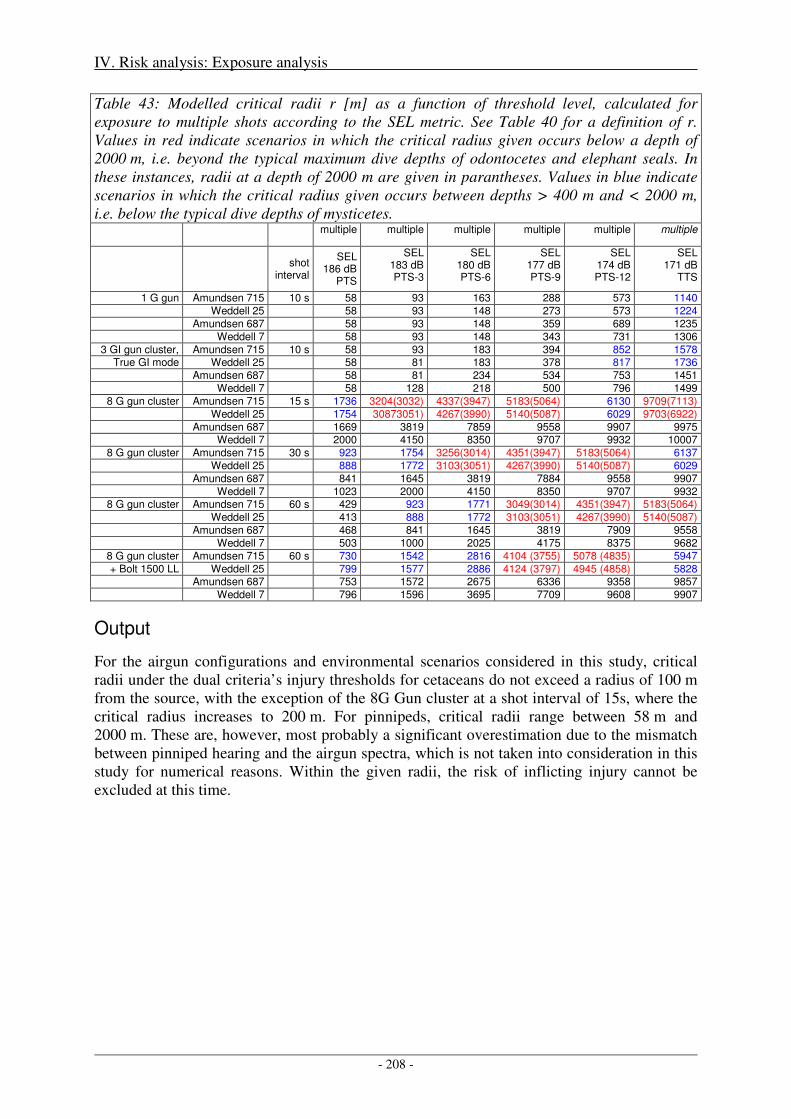
IV. Risk analysis: Exposure analysis
- 208 -
Table 43: Modelled critical radii r [m] as a function of threshold level, calculated for exposure to multiple shots according to the SEL metric. See Table 40 for a definition of r. Values in red indicate scenarios in which the critical radius given occurs below a depth of 2000 m, i.e. beyond the typical maximum dive depths of odontocetes and elephant seals. In these instances, radii at a depth of 2000 m are given in parantheses. Values in blue indicate scenarios in which the critical radius given occurs between depths > 400 m and < 2000 m, i.e. below the typical dive depths of mysticetes.
multiple multiple multiple multiple multiple multiple
shot
interval
SEL 186 dB
PTS
SEL 183 dB PTS-3
SEL 180 dB PTS-6
SEL 177 dB PTS-9
SEL 174 dB PTS-12
SEL 171 dB
TTS
1 G gun Amundsen 715 10 s 58 93 163 288 573 1140
Weddell 25 58 93 148 273 573 1224
Amundsen 687 58 93 148 359 689 1235
Weddell 7 58 93 148 343 731 1306
3 GI gun cluster, Amundsen 715 10 s 58 93 183 394 852 1578 True GI mode Weddell 25 58 81 183 378 817 1736
Amundsen 687 58 81 234 534 753 1451
Weddell 7 58 128 218 500 796 1499
8 G gun cluster Amundsen 715 15 s 1736 3204(3032) 4337(3947) 5183(5064) 6130 9709(7113)
Weddell 25 1754 30873051) 4267(3990) 5140(5087) 6029 9703(6922)
Amundsen 687 1669 3819 7859 9558 9907 9975 Weddell 7 2000 4150 8350 9707 9932 10007
8 G gun cluster Amundsen 715 30 s 923 1754 3256(3014) 4351(3947) 5183(5064) 6137
Weddell 25 888 1772 3103(3051) 4267(3990) 5140(5087) 6029
Amundsen 687 841 1645 3819 7884 9558 9907
Weddell 7 1023 2000 4150 8350 9707 9932 8 G gun cluster Amundsen 715 60 s 429 923 1771 3049(3014) 4351(3947) 5183(5064)
Weddell 25 413 888 1772 3103(3051) 4267(3990) 5140(5087)
Amundsen 687 468 841 1645 3819 7909 9558
Weddell 7 503 1000 2025 4175 8375 9682
8 G gun cluster Amundsen 715 60 s 730 1542 2816 4104 (3755) 5078 (4835) 5947
+ Bolt 1500 LL Weddell 25 799 1577 2886 4124 (3797) 4945 (4858) 5828 Amundsen 687 753 1572 2675 6336 9358 9857
Weddell 7 796 1596 3695 7709 9608 9907
Output
For the airgun configurations and environmental scenarios considered in this study, critical radii under the dual criteria’s injury thresholds for cetaceans do not exceed a radius of 100 m from the source, with the exception of the 8G Gun cluster at a shot interval of 15s, where the critical radius increases to 200 m. For pinnipeds, critical radii range between 58 m and 2000 m. These are, however, most probably a significant overestimation due to the mismatch between pinniped hearing and the airgun spectra, which is not taken into consideration in this study for numerical reasons. Within the given radii, the risk of inflicting injury cannot be excluded at this time.
IV. Risk analysis: Exposure analysis
- 209 -
2. Indirect, immediate damage
The DCS/hyperthermia scenario described in detail in chapter III.2 is the currently the accepted working hypothesis for the cause and effect that led to atypical beaked whale strandings in the context of ASW maneuvers. The hypothesis necessitates a number of abetting, if not mandatory factors, as listed in Table 38. Here it is examined to which degree these factors are applicable to Antarctic waters and the use of airguns in this ocean region.
Sound characteristics
Stranded whales have presumably been subjected to ASW sonar signals at received levels not higher than 130-140 dB re. 1µPa. For the use of the airguns studied herein, such levels are exceeded (i.e. [Breitzke et al., 2008], by extrapolation of their Figure 4c) within a few kilometers to several tens of kilometers from the source. Hence, the critical range as ensonified by airguns is comparable to the critical ranges as ensonified by ASW sonars.
Frequency range and pulse duration of airgun pulses (hundreds of Hertz, milliseconds) are distinctly different from those of ASW sonars (3-10 kHz, seconds) and of Killer whale calls (see Table 24). Airgun signals rather resemble, with respect to both spectral content and temporal evolution, the acoustic signatures of calving shelf ice, which dominates the abiotic soundscape of Antarctica [Boebel et al., 2008]. It appears unlikely that the ubiquitous acoustic signature of ice calving should trigger a flight response similar to that presumably elicited by Killer whale vocalizations (which are much less frequent). Hence, airguns signals, by virtue of their spectral and temporal characteristics (and due to the absence of noted beaked whale strandings in the Gulf of Mexico) are not expected to trigger similarly critical behavioural responses in beaked whales.
Herding
Herding, particularly in the context of multiple ship ASW operations, has been identified as an abetting factor. Scientific (and as a matter of fact, commercial) seismic surveys however operate airguns from only one ship without exception. In open waters, single ship operations are unlikely to cause herding as nearly any flight direction will lead to a reduction of the received sound pressure levels.
Occasionally, dual ship surveys occur, but the second ship only serves to tow a streamer (receiver) and not a concurrent second source. In these instances, both ships operate inline, i.e. one behind the other.
However, herding was observed by one of the authors in response to an approaching ship in ice-covered waters with few open leads. In the observed instance, minke whales attempted to outswim the approaching ship (with no scientific sonars operational) while following the leads.
A second aspect concerns the ship’s speed. In contrast to naval ASW vessels involved in ASW exercises, seismic operations are performed at a low speed of 5 knots, a speed significantly below the observed maximum sustained speeds of Antarctic whale species (Figure 83). Hence whales are easily capable of outswimming the seismic vessel if they wish, and hence can avoid herding, even if fleeing in the same direction as the ship’s course.
IV. Risk analysis: Exposure analysis
- 210 -
Topographic conditions
With southern bottlenose whales preferring regions beyond the continental shelf and Arnoux’s beaked whales being associated with shallow regions, beaked whales might be encountered throughout any of the seismic cruises shown in Figure 1.
Sea surface temperature and hyperthermia
Sea surface temperatures in Antarctica vary between -2°C and less than 5°C. They are significantly colder than the waters within which atypical strandings have been observed. Antarctic waters are even colder than those waters within which no atypical strandings have been observed, in spite of heavy use of ATW sonars [Cole, 2005]. It is hence highly unlikely that hyperthermia could be a contributory abetting factor in Antarctica.
Acoustic conditions
Both a surface and subsurface sound ducts have been identified in the context of atypical beaked whale strandings. Whether or not such ducts carry a significant role in the DCS/hyperthermia scenarios is yet unclear, but it is suspected that either the increased range or the existence of a subsurface SPL maximum might influence the diving behaviour.
Sound field models for all four Antarctic scenarios show an increase in sound pressure levels within the first 20 to 100m depth (Figure 95 and Figure 96). The effect is present for both the Amundsen/Bellingshausen station # 715 (with a subsurface duct) and the Weddell Sea station #25 (without a duct), and it is hence probably less a consequence of the structure of the sound speed profile than of the reflections of the signal at the sea-surface and seafloor.
Therefore, while the underlying physics might be different, for both the use of airguns in Antarctica and ASW sonar deployments at lower latitudes, sound pressure fields might exhibit a sub-surface intensification at depths around the lung-collapse depth of cetaceans.
Species involved
None of the species involved so far in ASW sonar related strandings occur in the Antarctic28. Of the true Antarctic cetacean species, three belong to the group of beaked whales. The southern bottlenose whale is most abundant, with RES indices ranging from intermediate to high (see section II.2) for both Weddell and Amundsen/Bellingshausen Seas, and are known to favor deep waters. The Arnoux’s beaked whale by contrast appears to favor shallow and slope regions while RES indices range from low to very low. For Layard’s beaked whale, the
28 Minke whales, stranded during the Bahamas event, and displayed a behavioural reaction to sonar during the USS Shoup incident in the Puget Sound region*). However, the term “minke whale” is an unspecific description of a group of whales, as it comprises three different species. The two minke whales that stranded at Eleuthera (Bahamas) were common minke whales (Balaenoptera acutorostrata), a species that occurs in the Northern Hemisphere only. By contrast, minke whales that occur in the Antarctic are the Antarctic minke whale (Balaenoptera bonaerensis) and the dwarf minke whale, an unnamed species (Balaenoptera acutorostrata subspecies). Hence the Antarctic species’ and the species involved in the Northern Hemisphere stranding are not the same. In fact, the differences between B. acutorostrata and B. bonaerensis are not marginal, see chapter II, Species Description. *) Assessment of Acoustic Exposures on Marine Mammals in Conjunction with USS Shoup Active Sonar Transmissions in the Eastern Strait of Juan de Fuca and Haro Strait, Washington ~ 5 May 2003 ~ National Marine Fisheries Service, Office of Protected Resources, January 21, 2005 - available online).
IV. Risk analysis: Exposure analysis
- 211 -
Antarctic Ocean south of 60°S is by and large considered not suitable, with only the region along 60°S having low suitability RES index.
Therefore, encounters with - and consequently a possible impact on - this latter species appear unlikely. While Mesoplodon layardii is listed “data deficient”, Berardius arnuxii and Hyperoodon planifrons are listed “lower risk/conservation dependent”. The cumulative beaked whale population is reported at 600,000 individuals, which suggests that even in the event of a fatal incident, detrimental effects to the survivability of the entire species are unlikely.
Behaviour
Central to the DCS/hyperthermia hypothesis is the notion that the whales need to swim for a sustained period of time at relatively high speed and are unable to dive below the depth of lung collapse (order of 70m) at the end of this flight. However, seismic surveys rarely enter waters (Figure 9) so shallow, that water depth of 70 m occur within the 130-140 dB rel. 1µPa range of up to some tens of kilometers from the source. It is hence unlikely that whales could be driven into waters that shallow that deep recovery dives would not be possible at the end of a possible flight response. Particularly, in many regions of the Weddell and Amundsen/Bellingshausen Seas, the shelf ice extends seaward out to regions with water depths of several hundred meters.
It should be noted, that the consideration above does not state that the (entire) flight response has to happen in shallow water. What it states is that the water depth end of the flight response, when the whale has the opportunity to resume normal diving, is of crucial importance to the possible outcome of the event. Zimmer and Tyack note, that the DCS symptoms (ensuing from the flight response) could easily be reversed if the whale were to dive only once below its lung-collapse depth. As it is plausible to assume that the whales may resume regular diving when beyond the “scaring” radius, the risk of developing an eventually fatal DCS is reduced in open waters, where whales can take recovery dives at the time and location of their choice. Such a ‘recovery’ response has recently been observed on a tagged beaked whale, that resumed deep dives shortly after having aborted a feeding dive presumably due to ship noise [Aguilar Soto et al., 2006]. If however, the water depths at the location of a possible recovery dive happens to be too shallow for such a dive (i.e. the whales were herded into shallow water), recovery dives are impeded and an increased risk of substantiating the DCS occurs.
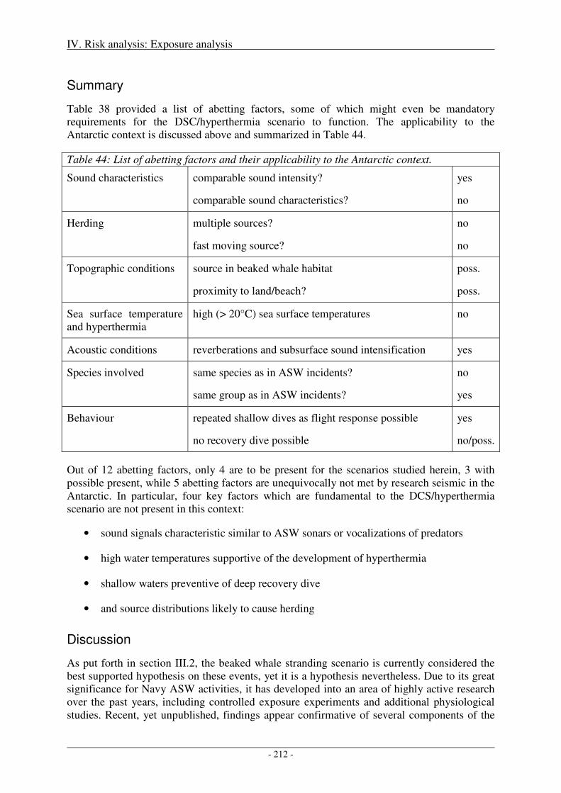
IV. Risk analysis: Exposure analysis
- 212 -
Summary
Table 38 provided a list of abetting factors, some of which might even be mandatory requirements for the DSC/hyperthermia scenario to function. The applicability to the Antarctic context is discussed above and summarized in Table 44.
Table 44: List of abetting factors and their applicability to the Antarctic context.
Sound characteristics comparable sound intensity?
comparable sound characteristics?
yes
no
Herding multiple sources?
fast moving source?
no
no
Topographic conditions source in beaked whale habitat
proximity to land/beach?
poss.
poss.
Sea surface temperature and hyperthermia
high (> 20°C) sea surface temperatures no
Acoustic conditions reverberations and subsurface sound intensification yes
Species involved same species as in ASW incidents?
same group as in ASW incidents?
no
yes
Behaviour repeated shallow dives as flight response possible
no recovery dive possible
yes
no/poss.
Out of 12 abetting factors, only 4 are to be present for the scenarios studied herein, 3 with possible present, while 5 abetting factors are unequivocally not met by research seismic in the Antarctic. In particular, four key factors which are fundamental to the DCS/hyperthermia scenario are not present in this context:
• sound signals characteristic similar to ASW sonars or vocalizations of predators
• high water temperatures supportive of the development of hyperthermia
• shallow waters preventive of deep recovery dive
• and source distributions likely to cause herding
Discussion
As put forth in section III.2, the beaked whale stranding scenario is currently considered the best supported hypothesis on these events, yet it is a hypothesis nevertheless. Due to its great significance for Navy ASW activities, it has developed into an area of highly active research over the past years, including controlled exposure experiments and additional physiological studies. Recent, yet unpublished, findings appear confirmative of several components of the
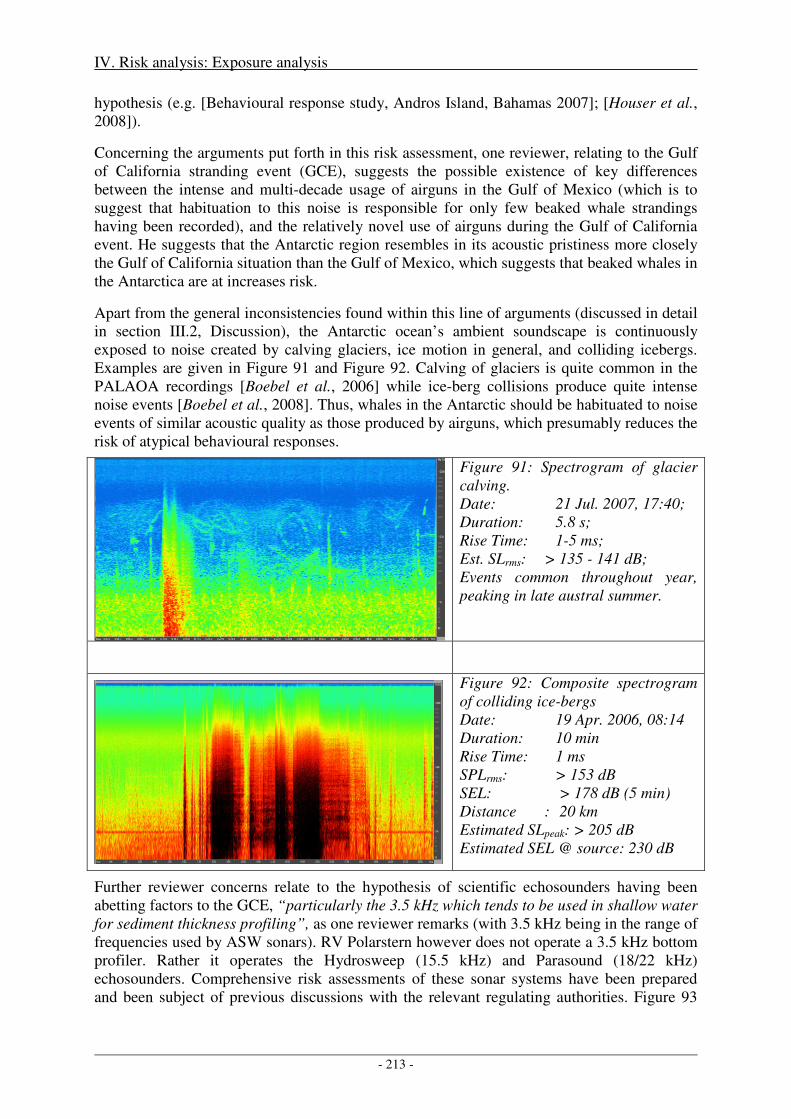
IV. Risk analysis: Exposure analysis
- 213 -
hypothesis (e.g. [Behavioural response study, Andros Island, Bahamas 2007]; [Houser et al., 2008]).
Concerning the arguments put forth in this risk assessment, one reviewer, relating to the Gulf of California stranding event (GCE), suggests the possible existence of key differences between the intense and multi-decade usage of airguns in the Gulf of Mexico (which is to suggest that habituation to this noise is responsible for only few beaked whale strandings having been recorded), and the relatively novel use of airguns during the Gulf of California event. He suggests that the Antarctic region resembles in its acoustic pristiness more closely the Gulf of California situation than the Gulf of Mexico, which suggests that beaked whales in the Antarctica are at increases risk.
Apart from the general inconsistencies found within this line of arguments (discussed in detail in section III.2, Discussion), the Antarctic ocean’s ambient soundscape is continuously exposed to noise created by calving glaciers, ice motion in general, and colliding icebergs. Examples are given in Figure 91 and Figure 92. Calving of glaciers is quite common in the PALAOA recordings [Boebel et al., 2006] while ice-berg collisions produce quite intense noise events [Boebel et al., 2008]. Thus, whales in the Antarctic should be habituated to noise events of similar acoustic quality as those produced by airguns, which presumably reduces the risk of atypical behavioural responses.
Figure 91: Spectrogram of glacier calving. Date: 21 Jul. 2007, 17:40; Duration: 5.8 s; Rise Time: 1-5 ms; Est. SLrms: > 135 - 141 dB; Events common throughout year, peaking in late austral summer.
Figure 92: Composite spectrogram of colliding ice-bergs Date: 19 Apr. 2006, 08:14 Duration: 10 min Rise Time: 1 ms SPLrms: > 153 dB SEL: > 178 dB (5 min) Distance : 20 km Estimated SLpeak: > 205 dB Estimated SEL @ source: 230 dB
Further reviewer concerns relate to the hypothesis of scientific echosounders having been abetting factors to the GCE, “particularly the 3.5 kHz which tends to be used in shallow water for sediment thickness profiling”, as one reviewer remarks (with 3.5 kHz being in the range of frequencies used by ASW sonars). RV Polarstern however does not operate a 3.5 kHz bottom profiler. Rather it operates the Hydrosweep (15.5 kHz) and Parasound (18/22 kHz) echosounders. Comprehensive risk assessments of these sonar systems have been prepared and been subject of previous discussions with the relevant regulating authorities. Figure 93
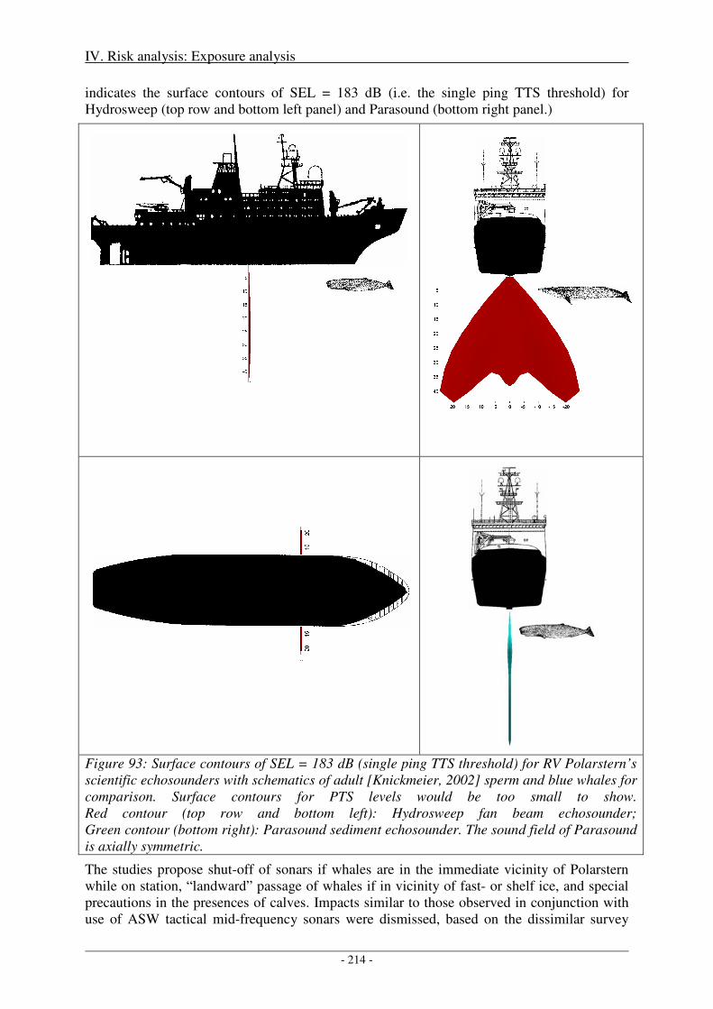
IV. Risk analysis: Exposure analysis
- 214 -
indicates the surface contours of SEL = 183 dB (i.e. the single ping TTS threshold) for Hydrosweep (top row and bottom left panel) and Parasound (bottom right panel.)
Figure 93: Surface contours of SEL = 183 dB (single ping TTS threshold) for RV Polarstern’s scientific echosounders with schematics of adult [Knickmeier, 2002] sperm and blue whales for comparison. Surface contours for PTS levels would be too small to show. Red contour (top row and bottom left): Hydrosweep fan beam echosounder; Green contour (bottom right): Parasound sediment echosounder. The sound field of Parasound is axially symmetric.
The studies propose shut-off of sonars if whales are in the immediate vicinity of Polarstern while on station, “landward” passage of whales if in vicinity of fast- or shelf ice, and special precautions in the presences of calves. Impacts similar to those observed in conjunction with use of ASW tactical mid-frequency sonars were dismissed, based on the dissimilar survey
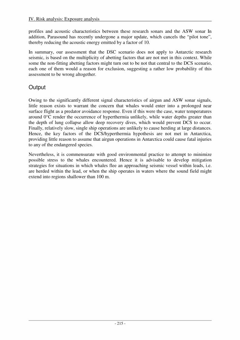
IV. Risk analysis: Exposure analysis
- 215 -
profiles and acoustic characteristics between these research sonars and the ASW sonar In addition, Parasound has recently undergone a major update, which cancels the “pilot tone”, thereby reducing the acoustic energy emitted by a factor of 10.
In summary, our assessment that the DSC scenario does not apply to Antarctic research seismic, is based on the multiplicity of abetting factors that are not met in this context. While some the non-fitting abetting factors might turn out to be not that central to the DCS scenario, each one of them would a reason for exclusion, suggesting a rather low probability of this assessment to be wrong altogether.
Output
Owing to the significantly different signal characteristics of airgun and ASW sonar signals, little reason exists to warrant the concern that whales would enter into a prolonged near surface flight as a predator avoidance response. Even if this were the case, water temperatures around 0°C render the occurrence of hyperthermia unlikely, while water depths greater than the depth of lung collapse allow deep recovery dives, which would prevent DCS to occur. Finally, relatively slow, single ship operations are unlikely to cause herding at large distances. Hence, the key factors of the DCS/hyperthermia hypothesis are not met in Antarctica, providing little reason to assume that airgun operations in Antarctica could cause fatal injuries to any of the endangered species.
Nevertheless, it is commensurate with good environmental practice to attempt to minimize possible stress to the whales encountered. Hence it is advisable to develop mitigation strategies for situations in which whales flee an approaching seismic vessel within leads, i.e. are herded within the lead, or when the ship operates in waters where the sound field might extend into regions shallower than 100 m.
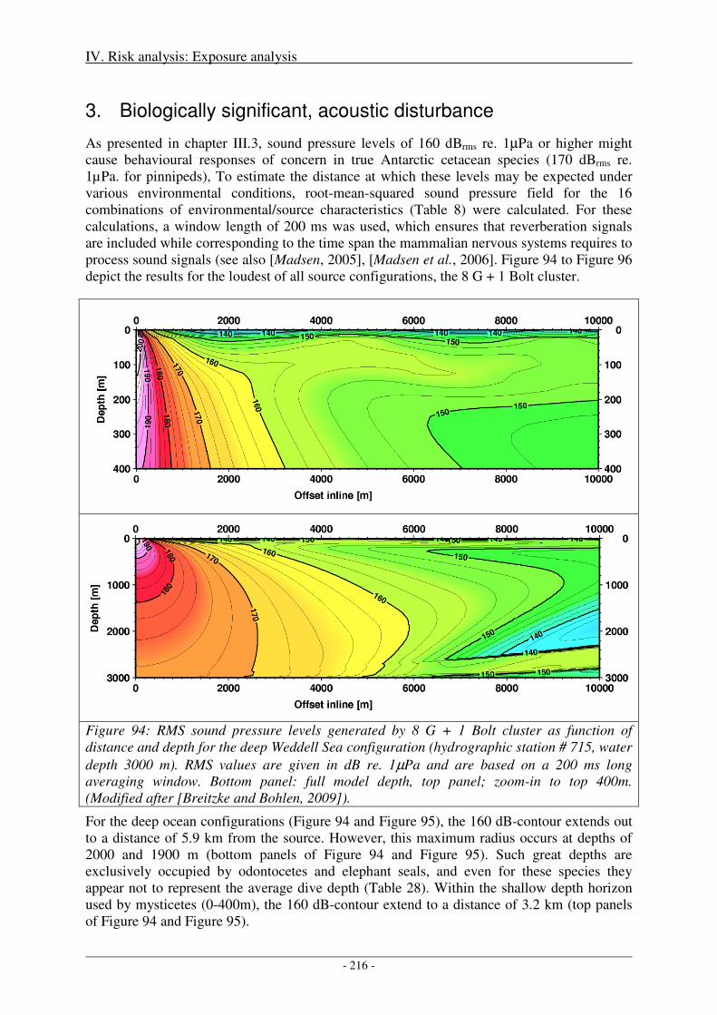
IV. Risk analysis: Exposure analysis
- 216 -
3. Biologically significant, acoustic disturbance
As presented in chapter III.3, sound pressure levels of 160 dBrms re. 1µPa or higher might cause behavioural responses of concern in true Antarctic cetacean species (170 dBrms re. 1µPa. for pinnipeds), To estimate the distance at which these levels may be expected under various environmental conditions, root-mean-squared sound pressure field for the 16 combinations of environmental/source characteristics (Table 8) were calculated. For these calculations, a window length of 200 ms was used, which ensures that reverberation signals are included while corresponding to the time span the mammalian nervous systems requires to process sound signals (see also [Madsen, 2005], [Madsen et al., 2006]. Figure 94 to Figure 96 depict the results for the loudest of all source configurations, the 8 G + 1 Bolt cluster.
Figure 94: RMS sound pressure levels generated by 8 G + 1 Bolt cluster as function of distance and depth for the deep Weddell Sea configuration (hydrographic station # 715, water
depth 3000 m). RMS values are given in dB re. 1µPa and are based on a 200 ms long averaging window. Bottom panel: full model depth, top panel; zoom-in to top 400m. (Modified after [Breitzke and Bohlen, 2009]).
For the deep ocean configurations (Figure 94 and Figure 95), the 160 dB-contour extends out to a distance of 5.9 km from the source. However, this maximum radius occurs at depths of 2000 and 1900 m (bottom panels of Figure 94 and Figure 95). Such great depths are exclusively occupied by odontocetes and elephant seals, and even for these species they appear not to represent the average dive depth (Table 28). Within the shallow depth horizon used by mysticetes (0-400m), the 160 dB-contour extend to a distance of 3.2 km (top panels of Figure 94 and Figure 95).
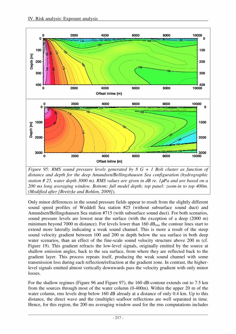
IV. Risk analysis: Exposure analysis
- 217 -
Figure 95: RMS sound pressure levels generated by 8 G + 1 Bolt cluster as function of distance and depth for the deep Amundsen/Bellingshausen Sea configuration (hydrographic
station # 25, water depth 3000 m). RMS values are given in dB re. 1µPa and are based on a 200 ms long averaging window. Bottom: full model depth; top panel: zoom-in to top 400m. (Modified after [Breitzke and Bohlen, 2009]).
Only minor differences in the sound pressure fields appear to result from the slightly different sound speed profiles of Weddell Sea station #25 (without subsurface sound duct) and Amundsen/Bellingshausen Sea station #715 (with subsurface sound duct). For both scenarios, sound pressure levels are lowest near the surface (with the exception of a deep (2000 m) minimum beyond 7000 m distance). For levels lower than 160 dBrms the contour lines start to extend more laterally indicating a weak sound channel. This is more a result of the steep sound velocity gradient between 100 and 200 m depth below the sea surface in both deep water scenarios, than an effect of the fine-scale sound velocity structure above 200 m (cf. Figure 19). This gradient refracts the low-level signals, originally emitted by the source at shallow emission angles, back to the sea surface, from where they are reflected back to the gradient layer. This process repeats itself, producing the weak sound channel with some transmission loss during each reflection/refraction at the gradient zone. In contrast, the higher-level signals emitted almost vertically downwards pass the velocity gradient with only minor losses.
For the shallow regimes (Figure 96 and Figure 97), the 160 dB-contour extends out to 7.5 km from the sources through most of the water column (0-400m). Within the upper 20 m of the water column, rms levels drop below 160 dB already at a distance of only 0.4 km. Up to this distance, the direct wave and the (multiple) seafloor reflections are well separated in time. Hence, for this region, the 200 ms averaging window used for the rms computations includes
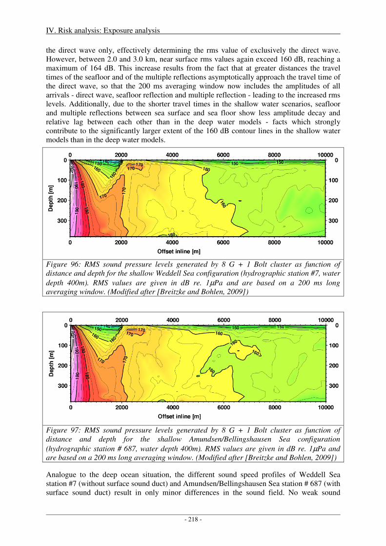
IV. Risk analysis: Exposure analysis
- 218 -
the direct wave only, effectively determining the rms value of exclusively the direct wave. However, between 2.0 and 3.0 km, near surface rms values again exceed 160 dB, reaching a maximum of 164 dB. This increase results from the fact that at greater distances the travel times of the seafloor and of the multiple reflections asymptotically approach the travel time of the direct wave, so that the 200 ms averaging window now includes the amplitudes of all arrivals - direct wave, seafloor reflection and multiple reflection - leading to the increased rms levels. Additionally, due to the shorter travel times in the shallow water scenarios, seafloor and multiple reflections between sea surface and sea floor show less amplitude decay and relative lag between each other than in the deep water models - facts which strongly contribute to the significantly larger extent of the 160 dB contour lines in the shallow water models than in the deep water models.
Figure 96: RMS sound pressure levels generated by 8 G + 1 Bolt cluster as function of distance and depth for the shallow Weddell Sea configuration (hydrographic station #7, water
depth 400m). RMS values are given in dB re. 1µPa and are based on a 200 ms long averaging window. (Modified after [Breitzke and Bohlen, 2009])
Figure 97: RMS sound pressure levels generated by 8 G + 1 Bolt cluster as function of distance and depth for the shallow Amundsen/Bellingshausen Sea configuration
(hydrographic station # 687, water depth 400m). RMS values are given in dB re. 1µPa and are based on a 200 ms long averaging window. (Modified after [Breitzke and Bohlen, 2009])
Analogue to the deep ocean situation, the different sound speed profiles of Weddell Sea station #7 (without surface sound duct) and Amundsen/Bellingshausen Sea station # 687 (with surface sound duct) result in only minor differences in the sound field. No weak sound
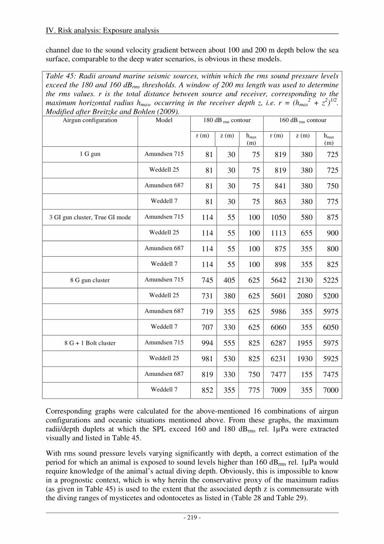
IV. Risk analysis: Exposure analysis
- 219 -
channel due to the sound velocity gradient between about 100 and 200 m depth below the sea surface, comparable to the deep water scenarios, is obvious in these models.
Table 45: Radii around marine seismic sources, within which the rms sound pressure levels exceed the 180 and 160 dBrms thresholds. A window of 200 ms length was used to determine the rms values. r is the total distance between source and receiver, corresponding to the maximum horizontal radius hmax, occurring in the receiver depth z, i.e. r = (hmax
2 + z2)1/2. Modified after Breitzke and Bohlen (2009).
Airgun configuration Model 180 dB rms contour 160 dB rms contour
r (m) z (m) hmax (m)
r (m) z (m) hmax (m)
1 G gun Amundsen 715 81 30 75 819 380 725
Weddell 25 81 30 75 819 380 725
Amundsen 687 81 30 75 841 380 750
Weddell 7 81 30 75 863 380 775
3 GI gun cluster, True GI mode Amundsen 715 114 55 100 1050 580 875
Weddell 25 114 55 100 1113 655 900
Amundsen 687 114 55 100 875 355 800
Weddell 7 114 55 100 898 355 825
8 G gun cluster Amundsen 715 745 405 625 5642 2130 5225
Weddell 25 731 380 625 5601 2080 5200
Amundsen 687 719 355 625 5986 355 5975
Weddell 7 707 330 625 6060 355 6050
8 G + 1 Bolt cluster Amundsen 715 994 555 825 6287 1955 5975
Weddell 25 981 530 825 6231 1930 5925
Amundsen 687 819 330 750 7477 155 7475
Weddell 7 852 355 775 7009 355 7000
Corresponding graphs were calculated for the above-mentioned 16 combinations of airgun configurations and oceanic situations mentioned above. From these graphs, the maximum radii/depth duplets at which the SPL exceed 160 and 180 dBrms rel. 1µPa were extracted visually and listed in Table 45.
With rms sound pressure levels varying significantly with depth, a correct estimation of the period for which an animal is exposed to sound levels higher than 160 dBrms rel. 1µPa would require knowledge of the animal’s actual diving depth. Obviously, this is impossible to know in a prognostic context, which is why herein the conservative proxy of the maximum radius (as given in Table 45) is used to the extent that the associated depth z is commensurate with the diving ranges of mysticetes and odontocetes as listed in (Table 28 and Table 29).
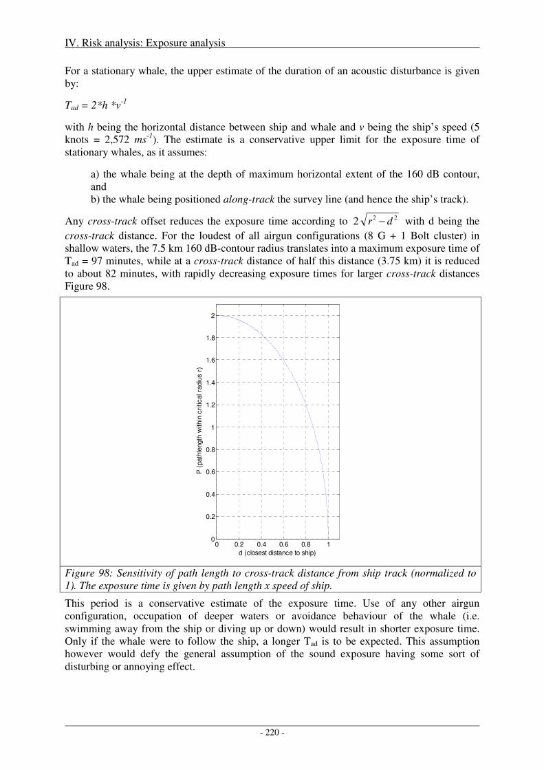
IV. Risk analysis: Exposure analysis
- 220 -
For a stationary whale, the upper estimate of the duration of an acoustic disturbance is given by:
Tad = 2*h *v-1
with h being the horizontal distance between ship and whale and v being the ship’s speed (5 knots = 2,572 ms-1). The estimate is a conservative upper limit for the exposure time of stationary whales, as it assumes:
a) the whale being at the depth of maximum horizontal extent of the 160 dB contour, and b) the whale being positioned along-track the survey line (and hence the ship’s track).
Any cross-track offset reduces the exposure time according to 222 dr − with d being the cross-track distance. For the loudest of all airgun configurations (8 G + 1 Bolt cluster) in shallow waters, the 7.5 km 160 dB-contour radius translates into a maximum exposure time of Tad = 97 minutes, while at a cross-track distance of half this distance (3.75 km) it is reduced to about 82 minutes, with rapidly decreasing exposure times for larger cross-track distances Figure 98.
0 0.2 0.4 0.6 0.8 10
0.2
0.4
0.6
0.8
1
1.2
1.4
1.6
1.8
2
d (closest distance to ship)
P (
path
length
within
cri
tical ra
diu
s r
)
Figure 98: Sensitivity of path length to cross-track distance from ship track (normalized to 1). The exposure time is given by path length x speed of ship.
This period is a conservative estimate of the exposure time. Use of any other airgun configuration, occupation of deeper waters or avoidance behaviour of the whale (i.e. swimming away from the ship or diving up or down) would result in shorter exposure time. Only if the whale were to follow the ship, a longer Tad is to be expected. This assumption however would defy the general assumption of the sound exposure having some sort of disturbing or annoying effect.
IV. Risk analysis: Exposure analysis
- 221 -
In accordance with the three step analysis process described in chapter III.3, the impact of an acoustic disturbance of 97 minutes duration needs to be discussed in the light of its biological significance.
Migration
As shown by Table 12, encounter rates for all whale species peak between late December and early February. Migration on latitudinal gradients mainly occurs outside this time frame. While seismic activities may partly coincide with peak encounter rates, the majority of seismic operation is not concurrent with timing of migration (Table 12).
If, though, longitudinal or latitudinal migratory movements should be affected by the seismic study, the potential response period (disturbance period plus lag period) of less than a few hours would not interfere with overall migratory patterns which occur on seasonal time scales of between several weeks to months, and is thus negligible due time differences in orders of magnitude.
More quantitatively, a potential interruption of migration by order of a few hours would not qualify as biologically significant according to the 24-hour rule, as it is of less then 24 h duration and not recurring on subsequent days (see section III.3).
Feeding
The Antarctic waters are feeding grounds for the cetacean species addressed here. Their distribution is tightly correlated with the distribution of their food. As illustrated in Figure 76, data on diving behaviour used as a proxy for feeding, can follow diel cycles and continues on extended time scales. Since the relevant species spend the austral summer or even longer in Antarctic waters, it appears unlikely that a transitory exposure of less than two hours and a possible behavioural disruption of a few hours can cause energy depletion into the lower quartile of normal. Here again, the potential interruption of feeding by order of a few hours would not qualify as biologically significant, as it is less then 24h and not recurring on subsequent days (see section III.3). The same argument applies to a possible temporary decrease in foraging efficiency du to the prey’s reaction to sound.
While the above concerns all true Antarctic cetaceans, an interesting secondary argument concerns the killer whales. The low frequency sound of the ship would mask low frequency communication of mysticetes (cow/calf pairs in particular) and hence hide their presence from killer whales. Thus a point could be made that ship operations (including seismic studies) would reduce the attack opportunities for killer whales by means of masking. Nevertheless, such interruptions would last a few hours at the most (see above), which again is an insignificant period of time with regard to the overall feeding activity of killer whales, which encompasses the entire period of stay in the Antarctic.
Breeding
According to Table 31 breeding does not or is unlikely to occur in Antarctic waters from mysticetes and the sperm whale, and hence seismic activities cannot interfere with breeding as shown in Figure 6. Corresponding information is lacking for beaked whales and Killer whales.
IV. Risk analysis: Exposure analysis
- 222 -
Calving/Breeding
With the exception of possibly beaked whales and killer whales, calving occurs outside Antarctic waters. However, for all species calving occurs at a time of the year (austral winter) irrelevant to seismic operations in Antarctica (Figure 6). Pinnipeds give birth on ice or land.
Nurturing and Parental Care
Phocids and southern elephant seal mother/pub pairs wean abruptly and separate shortly after, and fur seal pups do not follow their mothers on foraging excursions during the extended lactation period. Lactation in Antarctic cetacean species covers a period of between several months and up to two years (see Table 31). It hence appears unlikely that a transitory exposure of a few hours can reduce nutrition into the lower quartile of normal.
We cannot disprove that any potential alteration of behaviour could have an effect towards increasing the likelihood that a dependant infant could be separated from its caregivers. However, all but one of the observed behavioural responses for low- and mid-frequency cetaceans report behavioural response severity scores of class 6 or lower. Class 6 is defined to represent i.a. “Brief or minor separation of females and dependent offspring” while class 7 states “moderate separation of females and dependent offspring”, which implies a cow/calf reunification within a finite period. Qualifying the effects observed at exposure levels of 160 dBrms or lower as biologically significant impact is hence not expedient. However, at higher ensonification levels, even if shorter in duration, a biologically significant impact cannot be excluded.
Predator Avoidance
We can neither disprove nor prove that any potential alteration of behaviour, can increase the likelihood of predation, however, it appears to be an unlikely scenario for the following reasons:
Cetaceans and pinnipeds in the Antarctic are exclusively subject to predation by killer whales. Even short periods of acoustic disturbance may increase the vulnerability of animals to predation. The killer whale, however, preys primarily on fish, squid, seals and penguins with other cetaceans being only attacked rarely. The scenario of predation advantage for killer whales due to acoustic disturbance would involve the assumption that the predator is not disturbed by the acoustics while the prey is, which appears rather implausible. Furthermore, killer whale clicks and vocalizations would not be masked by the low-frequency, pulsed sounds of airgun, and are hence likely to remain audible to the target species.
Exposing marine mammals to airgun noise might result in causing TTS in the exposed animals. During this duration of the TTS, the animals’ awareness of a possible predator by means of hearing sensation might be reduced.
For cetaceans, the range within which TTS might be expected is given in Table 46. The maximum radius of 4.2 km corresponds to an exposure time (calculated as outlined above) of 54 minutes. Depending on the amount of TTS triggered, recovery times will vary between minutes [Finneran et al., 2002] for small threshold shifts up to 2-4 days after having received large threshold shifts of 50 dB [Ketten and Finneran, 2004]. As the given threshold levels describe the onset of TTS, only small threshold shifts are to be expected at these levels, with relatively short recovery times. Hence, when judging by the exposure level solely, killer whales might, for a duration of several hours, gain some advantage in their pursuit of prey
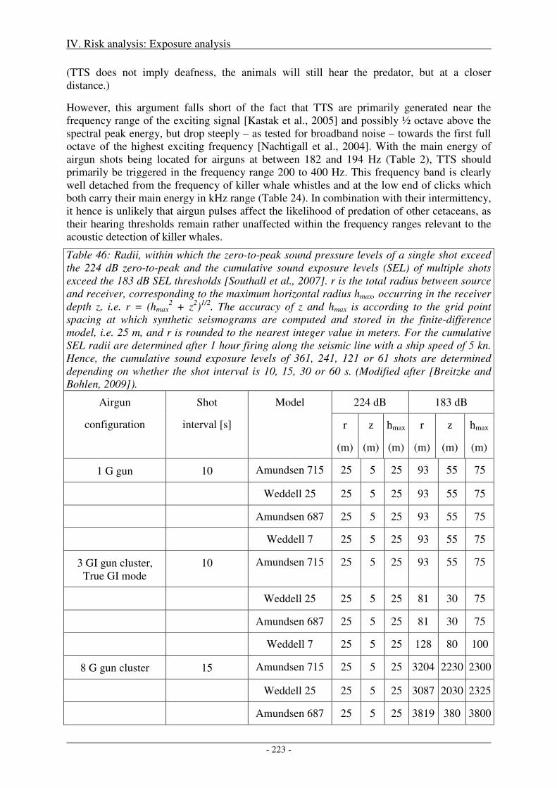
IV. Risk analysis: Exposure analysis
- 223 -
(TTS does not imply deafness, the animals will still hear the predator, but at a closer distance.)
However, this argument falls short of the fact that TTS are primarily generated near the frequency range of the exciting signal [Kastak et al., 2005] and possibly ½ octave above the spectral peak energy, but drop steeply – as tested for broadband noise – towards the first full octave of the highest exciting frequency [Nachtigall et al., 2004]. With the main energy of airgun shots being located for airguns at between 182 and 194 Hz (Table 2), TTS should primarily be triggered in the frequency range 200 to 400 Hz. This frequency band is clearly well detached from the frequency of killer whale whistles and at the low end of clicks which both carry their main energy in kHz range (Table 24). In combination with their intermittency, it hence is unlikely that airgun pulses affect the likelihood of predation of other cetaceans, as their hearing thresholds remain rather unaffected within the frequency ranges relevant to the acoustic detection of killer whales.
Table 46: Radii, within which the zero-to-peak sound pressure levels of a single shot exceed the 224 dB zero-to-peak and the cumulative sound exposure levels (SEL) of multiple shots exceed the 183 dB SEL thresholds [Southall et al., 2007]. r is the total radius between source and receiver, corresponding to the maximum horizontal radius hmax, occurring in the receiver depth z, i.e. r = (hmax
2 + z2)1/2. The accuracy of z and hmax is according to the grid point spacing at which synthetic seismograms are computed and stored in the finite-difference model, i.e. 25 m, and r is rounded to the nearest integer value in meters. For the cumulative SEL radii are determined after 1 hour firing along the seismic line with a ship speed of 5 kn. Hence, the cumulative sound exposure levels of 361, 241, 121 or 61 shots are determined depending on whether the shot interval is 10, 15, 30 or 60 s. (Modified after [Breitzke and Bohlen, 2009]).
Airgun
configuration
Shot
interval [s]
Model 224 dB 183 dB
r
(m)
z
(m)
hmax
(m)
r
(m)
z
(m)
hmax
(m)
1 G gun 10 Amundsen 715 25 5 25 93 55 75
Weddell 25 25 5 25 93 55 75
Amundsen 687 25 5 25 93 55 75
Weddell 7 25 5 25 93 55 75
3 GI gun cluster, True GI mode
10 Amundsen 715 25 5 25 93 55 75
Weddell 25 25 5 25 81 30 75
Amundsen 687 25 5 25 81 30 75
Weddell 7 25 5 25 128 80 100
8 G gun cluster 15 Amundsen 715 25 5 25 3204 2230 2300
Weddell 25 25 5 25 3087 2030 2325
Amundsen 687 25 5 25 3819 380 3800
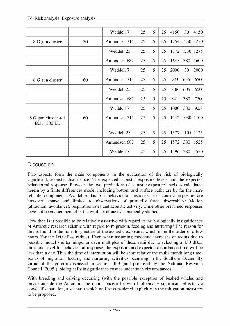
IV. Risk analysis: Exposure analysis
- 224 -
Weddell 7 25 5 25 4150 30 4150
8 G gun cluster 30 Amundsen 715 25 5 25 1754 1230 1250
Weddell 25 25 5 25 1772 1230 1275
Amundsen 687 25 5 25 1645 380 1600
Weddell 7 25 5 25 2000 30 2000
8 G gun cluster 60 Amundsen 715 25 5 25 923 655 650
Weddell 25 25 5 25 888 605 650
Amundsen 687 25 5 25 841 380 750
Weddell 7 25 5 25 1000 380 925
8 G gun cluster + 1 Bolt 1500 LL
60 Amundsen 715 25 5 25 1542 1080 1100
Weddell 25 25 5 25 1577 1105 1125
Amundsen 687 25 5 25 1572 380 1525
Weddell 7 25 5 25 1596 380 1550
Discussion
Two aspects form the main components in the evaluation of the risk of biologically significant, acoustic disturbance: The expected acoustic exposure levels and the expected behavioural response. Between the two, predictions of acoustic exposure levels as calculated herein by a finite differences model including bottom and surface paths are by far the more reliable component. Available data on behavioural responses to acoustic exposure are however, sparse and limited to observations of primarily three observables: Motion (attraction, avoidance), respiration rates and acoustic activity, while other presumed responses have not been documented in the wild, let alone systematically studied.
How then is it possible to be relatively assertive with regard to the biologically insignificance of Antarctic research seismic with regard to migration, feeding and nurturing? The reason for this is found in the transitory nature of the acoustic exposure, which is on the order of a few hours (for the 160 dBrms radius). Even when assuming moderate increases of radius due to possible model shortcomings, or even multiples of these radii due to selecting a 150 dBrms threshold level for behavioural response, the exposure and expected disturbance time will be less than a day. Thus the time of interruption will be short relative the multi-month long time-scales of migration, feeding and nurturing activities occurring in the Southern Ocean. By virtue of the criteria discussed in section III.3 (and proposed by the National Research Council [2005]), biologically insignificance ensues under such circumstances.
With breeding and calving occurring (with the possible exception of beaked whales and orcas) outside the Antarctic, the main concern lie with biologically significant effects via cow/calf separation, a scenario which will be considered explicitly in the mitigation measures to be proposed.
IV. Risk analysis: Exposure analysis
- 225 -
It should be emphasized, however, that confining the survey to a small – possibly biologically important area – would likely result in a significantly different evaluation. However, with regard to the generic seismic research study as defined in section I, the evaluations made herein appear appropriate, rather than overly bold – as suggested by one reviewer – to us.
Output
Acoustic disturbance through operation of airguns in a linear survey layout will be biologically insignificant with regard to migration, feeding and nurturing due to the shortness of acoustic exposure. Calving and breeding activities of true Antarctic species lie either outside the range or the time of Antarctic airgun surveys and are hence not subject to alteration. Reduced predator avoidance due to behavioural responses (distraction, masking) is implausible, while TTS is unlikely to gain biological significance as it occurs in frequency band irrelevant to predator detection.
Based on the current level of knowledge, it cannot be excluded that cow/calf pairs might be separated by airgun noise of amplitude 160 dBrms rel. 1µPa. At these levels, the separation has been classified as brief or minor and is hence unlikely to be biologically significant. At higher exposure levels, however, a biologically significant impact cannot be excluded at the individual (i.e. calf) level. Special attention will be given to this issue in the subsequent chapter on mitigation approaches.
It should be noted, that these results are dependent on the survey design. A survey with dense line spacing in a biological area of critical significance for an extended period of time would result in a significantly different evaluation of its biological significance. For such a survey layout, the preparation of a specific (rather than generic) environmental impact statement appears appropriate.
IV. Risk analysis: Exposure analysis
- 226 -
4. References
Aguilar Soto, N., M. Johnson, P. T. Madsen, P. L. Tyack, A. Bocconcelli, and J. Fabrizio Borsani (2006), Does intense ship noise disrupt foraging in deep-diving Cuvier's beaked whales (Ziphius cavirostris)? Marine Mammal Science, 22, 690-699.
Boebel, O., L. Kindermann, H. Klinck, H. Bornemann, J. Plötz, D. Steinhage, S. Riedel, and E. Burkhardt (2006), Acoustic Observatory Provides Real-Time Underwater Sounds from the Antarctic Ocean, EOS, 87, 361-372.
Boebel, O., H. Klinck, L. Kindermann, and S. El Naggar (2008), PALAOA: Broadband recordings of the Antarctic coastal soundscape, Bioacoustics, 17, 19-21.
Breitzke, M., O. Boebel, S. El Naggar, W. Jokat, and B. Werner (2008), Broadband calibration of marine seismic sources used by R/V Polarstern for academic research in polar regions, Geophysical Journal International, 174, 505-524.
Breitzke, M., and T. Bohlen (2009), Modeling acoustic wave propagation in the Southern Ocean to estimate the acoustic impact of seismic surveys on marine mammals, in prep.
Cole, S. (2005), Military exercises and marine mammal strandings - a stressful issue? paper presented at 1st Intergovernmental Conference on Effects of Sound on Marine Mammals, Nato Undersea Research Center, Lerici, Italy, 2-5 May 2005.
Finneran, J. J., C. E. Schlundt, R. Dear, D. A. Cader, and S. H. Ridgeway (2002), Temporary shift in masked hearing thresholds in odontocetes after exposure to single underwater impulses from a seismic watergun, Journal of the Acoustical Society of America, 111, 2929-2939.
Houser, D. S., P. J. Ponganis, T. K. Stockard, L. A. Dankiewicz (2008), Blood Nitrogen Uptake and Distribution During Diving in Bottlenose Dolphins, paper presented at Joint Industry Programme (JIP) Review Meeting, Wednesday, October 29, 2008 * 8:50 AM.
Kastak, D., B. L. Southall, R. J. Schustermann, and C. J. Reichmuth Kastak (2005), Underwater temporary threshold shift in pinnipeds: effects of noise level and duration, Journal of the Acoustical Society of America, 118, 3154-3163.
Ketten, D. and Finneran, J., (2004), Noise Exposure Criteria: “Injury (PTS) Criteria”, http://www.mmc.gov/sound/plenary2/pdf/gentryetal.pdf.
Knickmeier, K. (2002), Gutachten zur Populationsproblematik von Meeressäugern und tauchenden Vögeln in der Antarktis gemäß Umweltschutzprotokoll-Ausführungsgesetz (AUG), Berlin.
Madsen, P. T. (2005), Marine mammals and noise: Problems with root mean square sound pressure levels for transients, The Journal of the Acoustical Society of America, 117, 3952-3957.
Madsen, P. T., M. Johnson, P. J. O. Miller, N. Aguilar Soto, J. Lynch, and P. Tyack (2006), Quantitative measures of airgun pulses recorded on sperm whales (Physeter macrocephalus) using acoustic tags during controlled exposure experiments, The Journal of the Acoustical Society of America, 120, 2366.
Nachtigall, P. E., A. Y. Supin, J. Pawloski, and W. W. L. Au (2004), Temporary threshold shift after noise exposure in the bottlenose dolphin (Tursiopsis truncatus) measured using evoked auditory potentials, Marine Mammal Science, 20, 673-687.
IV. Risk analysis: Exposure analysis
- 227 -
National Research Council (2005), Marine mammal populations and ocean noise - determining when noise causes biologically significant effects, 126 pp., National Academies Press, Washington.
Southall, B. L., A. E. Bowles, W. T. Ellison, J. J. Finneran, R. L. Gentry, C. R. Greene Jr., D. Kastak, D. Ketten, J. H. Miller, P. E. Nachtigall, W. J. Richardson, J. A. Thomas, and P. L. Tyack (2007), Marine mammal noise exposure criteria: initial scientific recommendations, Aquatic Mammals, 33, 411-521.

V. Risk management
- 229 -
V. Risk management Focusing on the three different risk types described in the previous sections, the following paragraphs discuss various mitigation measures in their respective context. The resulting three sets of recommended mitigation measures are, however, intended to be used concurrently and as a single entity.
The necessity and extent of the mitigation proposals are based on the output of chapter IV “Risk analysis: Exposure analysis” and considerations made in the following chapter VI “Risk evaluation”. (This unusual order was chosen in order to be able to present risk evaluations with and without mitigation measures back to back in chapter VI, rather than with this chapter tugged in between). Noting the special concern regarding species and populations of species within the Environmental Protocol to the Antarctic Treaty, the mitigation proposals focus in particular, but not exclusively, on the protection of the twelve cetacean species that have been denoted to be of higher concern than “Lower risk/least concern” Table 9.
1. Direct, immediate injury
In the following text we distinguish between the critical radius (the distance from the airgun within which injury cannot be excluded) and the exclusion zone, which is the critical radius plus an additional safety zone to allow for timely shutdown of the airguns.
Mitigation proposal
1. To minimize the possibility of direct, immediate injury of individuals, airgun operations will be shut down when marine mammals are about to enter the exclusion zone.
2. To ensure that marine mammals are sighted with high reliability during the operation of airguns, a continuous monitoring of the ship’s perimeter will be conducted by two members of the scientific team who will be placed on the ship’s bridge, one on the starboard, one on the port side. This marine mammal watch is responsible for scanning the perimeter of the ship for whales, deciding whether a whale is about to enter the exclusion zone, and informing the airgun operators to shut down the sources.
3. The marine mammal watch will be present on the bridge regardless of conditions of visibility whenever airguns are operated. During periods of low visibility, airgun operations may proceed without restrictions. However, such periods should be minimized during the planning phase by choosing appropriate seasons and course tracks.
4. Once the animals leave the exclusion zone, the marine mammal watch informs the airgun operators that firing of the guns may be resumed. If, however, the marine mammals have been identified as cow/calf pairs or blue whales (CC/B), a ramp-up procedure will be initiated (see section V.3).
5. The ramp-up commences when the animals’ last known position is 1000 m or farther from the ship and continues according the process described in V.3.
6. Special considerations apply during the initial and subsequent startups of airguns. However, these procedures are governed by considering risks of the category
V. Risk management
- 230 -
“Biologically significant, acoustic disturbance”, which is why they will be described in detailed in section V.3.
Definition of the exclusion zone
Based on a ship speed of 5 kn (2.7 ms-1), a typical cetacean migration speeds of 2 ms-1 (c.f. chapter II.8), and the conservative assumption that whale and ship are approaching each other head-on, the distance between whale and ship would be reduced by 282 m within a reaction / shutdown time of 1 minute. Hence, when marine mammals are sighted in the water within the critical radius + 282 m ≈ 500 m distance from the ship, with the marine mammal not clearly swimming away from the ship, a shut down should be issued to avoid a possible violation of the dual criteria. The area within a 500m radius around the bridge is called exclusion zone.
One might consider the option of requesting a shut-down of airgun operations during periods of low visibility or nighttime, when it is not possible to visually scan the 500 m mitigation radius reliably. However, given the fact that whale-ship encounters within the critical radii of 100 m or 200 m are rare and that avoidance reactions can be expected at larger radii for most species, it appears sensible to accept this small risk in light of balancing advantages by avoiding additional cruises and their environmental impacts (fuel, additional noise) that would become necessary in order to fill gaps of scientific data which would be caused by extended shut-down periods.
V. Risk management
- 231 -
2. Indirect, immediate damage
As discussed in the previous and the following chapters, little reason exists to assume that the beaked whale scenario applies to the context of this study. Nevertheless, it is in accordance with good environmental practice to attempt to minimize even the possibility of harming the encountered whales. Hence, it is advisable to develop mitigation strategies for situations in which whales are herded within leads ahead of the ship or the seismic survey is conducted in regions where the sound field might extend with moderate sound pressure levels into regions shallower than 100 m, with the possible consequence of preventing deep recovery dives.
Mitigation proposal
1. The cruise track should be planned so as to avoid ensonification of regions shallower than 100 m with SPL levels higher than 140 dBrms to the extent possible.
2. If this cannot be achieved, seismic operations should be conducted in such a way that the acoustic source is moving down-slope or along-slope.
3. The GEBCO (http://www.gebco.net/) topography should be used for the determination of isobath orientation.
4. The respective pre-cruise planning will be documented accordingly.
Underlying rationale
This approach minimizes the possibility of herding marine mammals into shallow regions, within which deep recovery dives might not be possible. A sound pressure level 140 dBrms is selected as it represents the centroid of the lower range of received sound pressure levels during atypical stranding events (c.f. section III.2). The depth of 100 m is a conservative proxy for lung collapse depths as given for some cetaceans [Zimmer and Tyack, 2007]. GEBCO data is the only global high-resolution data set, including data of the high Antarctic Ocean.
Mitigation against a possible noise induced herding of whales in leads ahead of the ship is already implicitly included in the proposed shut-off of airguns as suggested in the previous section.
V. Risk management
- 232 -
3. Biologically significant, acoustic disturbance
As discussed in section IV.3, the main concern for acoustically induced biologically significant effects would be the separation of cow/calf pairs as a response to exposure levels higher than 160 dBrms rel. 1µPa. Special consideration is thereby given to blue whale cow/calf pairs due to this species’ critical population status and depleted population.
Mitigation proposal
1. By developing appropriate cruise plans, possible sites of known blue whale “hot spots” should be avoided in space or time, possibly under consideration of the overall migratory behaviour of blue whales. Based on the information given in section II.2, surveys should be designed to avoid the pack-ice edge as much as possible and be conducted preferably in late summer (i.e. from February onwards).
2. At the startup of airguns, a ramp-up procedure shall be implemented, with ramp-up times chosen according to the specific array, i.e. 15 minutes for the single G-gun and 3 GI-gun cluster, and 60 minutes for the 8 G-gun and 8 G-gun + Bolt clusters (c.f. Table 47).
3. If the airguns are shut-off for technical reasons, the ramp-up process should be initiated again if the shut-off period exceeds half the ramp-up time. If the shut-off period is shorter, seismic operations may resume at the same level as prior to the shut-down.
4. Prior to the ramp-up, the whale watch should monitor the ship’s perimeter and report all whales sighted within the 500 m radius. Ramp-up can only commence if no whales are within this radius. If whales enter this radius, ramp-up must be interrupted and may only be resumed when the whales leave the 500 m radius.
5. When cow/calf pairs of blue whales (CC/B) have been identified within the respective 160 dBrms radius (Table 47), a shut-down of airguns should be issued. A ramp-up should be initiated when the last known position of the cow/calf pair or the blue whale is at a distance of 1000m from the ship.
Underlying rationale
To minimize the risk of cow/calf separations (particularly for blue whales), a multiple level approach is chosen, involving both the planning and operational stage.
In the planning of the experiment, possible blue whale aggregations shall be avoided in a spatio-temporal context. Such an overall avoidance approach is accepted throughout the community as the most effective mitigation measure.
As seismic operations presumably cause an aversive behaviour in whales, it is reasonable to assume that cows would lead their calves away from the source of annoyance [McCauley et al., 2000]. Blue whales, for example, migrate at a speed of 2 ms-1, with sprint speed around 9 ms-1 (Figure 83). With seismic operations being audible to whales over tens of kilometers, and seismic surveys being conducted at 5 kn = 2,7 ms-1, whales are easily capable of circumnavigating the acoustic source at distances much larger than the 160 dBrms radii (Table 47).
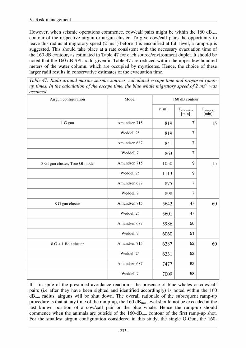
V. Risk management
- 233 -
However, when seismic operations commence, cow/calf pairs might be within the 160 dBrms contour of the respective airgun or airgun cluster. To give cow/calf pairs the opportunity to leave this radius at migratory speed (2 ms-1) before it is ensonified at full level, a ramp-up is suggested. This should take place at a rate consistent with the necessary evacuation time of the 160 dB contour, as estimated in Table 47 for each source/environment duplet. It should be noted that the 160 dB SPL radii given in Table 47 are reduced within the upper few hundred meters of the water column, which are occupied by mysticetes. Hence, the choice of these larger radii results in conservative estimates of the evacuation time.
Table 47: Radii around marine seismic sources, calculated escape time and proposed ramp-up times. In the calculation of the escape time, the blue whale migratory speed of 2 ms-1 was assumed.
Airgun configuration Model 160 dB contour
r [m] Tevacuation [min]
T ramp-up
[min]
1 G gun Amundsen 715 819 7 15
Weddell 25 819 7
Amundsen 687 841 7
Weddell 7 863 7
3 GI gun cluster, True GI mode Amundsen 715 1050 9 15
Weddell 25 1113 9
Amundsen 687 875 7
Weddell 7 898 7
8 G gun cluster Amundsen 715 5642 47 60
Weddell 25 5601 47
Amundsen 687 5986 50
Weddell 7 6060 51
8 G + 1 Bolt cluster Amundsen 715 6287 52 60
Weddell 25 6231 52
Amundsen 687 7477 62
Weddell 7 7009 58
If – in spite of the presumed avoidance reaction - the presence of blue whales or cow/calf pairs (i.e after they have been sighted and identified accordingly) is noted within the 160 dBrms radius, airguns will be shut down. The overall rationale of the subsequent ramp-up procedure is that at any time of the ramp-up, the 160 dBrms level should not be exceeded at the last known position of a cow/calf pair or the blue whale. Hence the ramp-up should commence when the animals are outside of the 160-dBrms contour of the first ramp-up shot. For the smallest airgun configuration considered in this study, the single G-Gun, the 160-
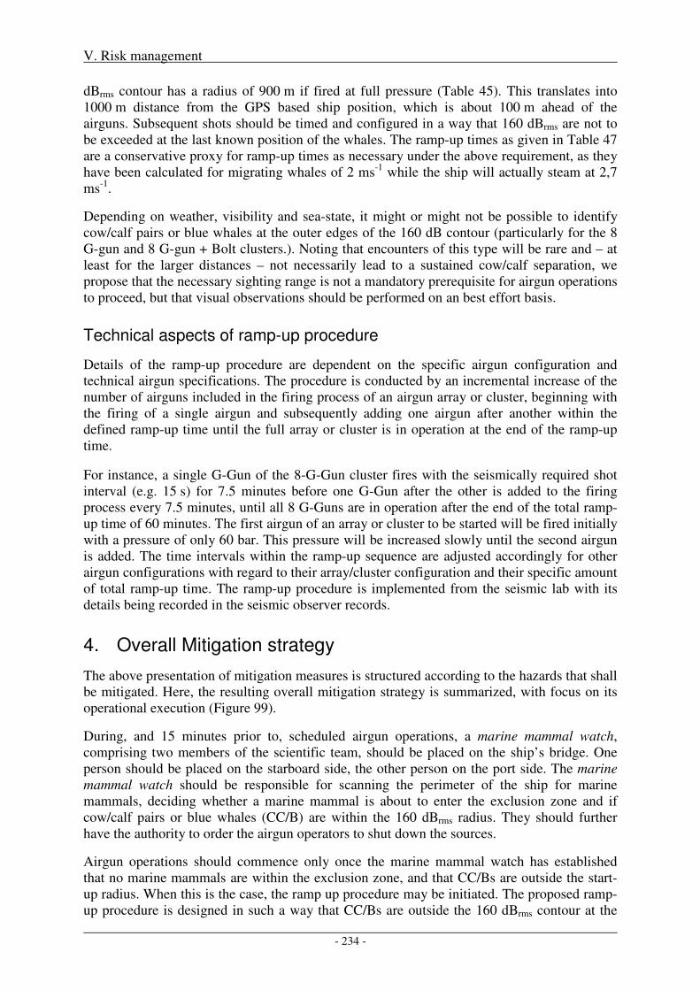
V. Risk management
- 234 -
dBrms contour has a radius of 900 m if fired at full pressure (Table 45). This translates into 1000 m distance from the GPS based ship position, which is about 100 m ahead of the airguns. Subsequent shots should be timed and configured in a way that 160 dBrms are not to be exceeded at the last known position of the whales. The ramp-up times as given in Table 47 are a conservative proxy for ramp-up times as necessary under the above requirement, as they have been calculated for migrating whales of 2 ms-1 while the ship will actually steam at 2,7 ms-1.
Depending on weather, visibility and sea-state, it might or might not be possible to identify cow/calf pairs or blue whales at the outer edges of the 160 dB contour (particularly for the 8 G-gun and 8 G-gun + Bolt clusters.). Noting that encounters of this type will be rare and – at least for the larger distances – not necessarily lead to a sustained cow/calf separation, we propose that the necessary sighting range is not a mandatory prerequisite for airgun operations to proceed, but that visual observations should be performed on an best effort basis.
Technical aspects of ramp-up procedure
Details of the ramp-up procedure are dependent on the specific airgun configuration and technical airgun specifications. The procedure is conducted by an incremental increase of the number of airguns included in the firing process of an airgun array or cluster, beginning with the firing of a single airgun and subsequently adding one airgun after another within the defined ramp-up time until the full array or cluster is in operation at the end of the ramp-up time.
For instance, a single G-Gun of the 8-G-Gun cluster fires with the seismically required shot interval (e.g. 15 s) for 7.5 minutes before one G-Gun after the other is added to the firing process every 7.5 minutes, until all 8 G-Guns are in operation after the end of the total ramp-up time of 60 minutes. The first airgun of an array or cluster to be started will be fired initially with a pressure of only 60 bar. This pressure will be increased slowly until the second airgun is added. The time intervals within the ramp-up sequence are adjusted accordingly for other airgun configurations with regard to their array/cluster configuration and their specific amount of total ramp-up time. The ramp-up procedure is implemented from the seismic lab with its details being recorded in the seismic observer records.
4. Overall Mitigation strategy
The above presentation of mitigation measures is structured according to the hazards that shall be mitigated. Here, the resulting overall mitigation strategy is summarized, with focus on its operational execution (Figure 99).
During, and 15 minutes prior to, scheduled airgun operations, a marine mammal watch, comprising two members of the scientific team, should be placed on the ship’s bridge. One person should be placed on the starboard side, the other person on the port side. The marine mammal watch should be responsible for scanning the perimeter of the ship for marine mammals, deciding whether a marine mammal is about to enter the exclusion zone and if cow/calf pairs or blue whales (CC/B) are within the 160 dBrms radius. They should further have the authority to order the airgun operators to shut down the sources.
Airgun operations should commence only once the marine mammal watch has established that no marine mammals are within the exclusion zone, and that CC/Bs are outside the start-up radius. When this is the case, the ramp up procedure may be initiated. The proposed ramp-up procedure is designed in such a way that CC/Bs are outside the 160 dBrms contour at the
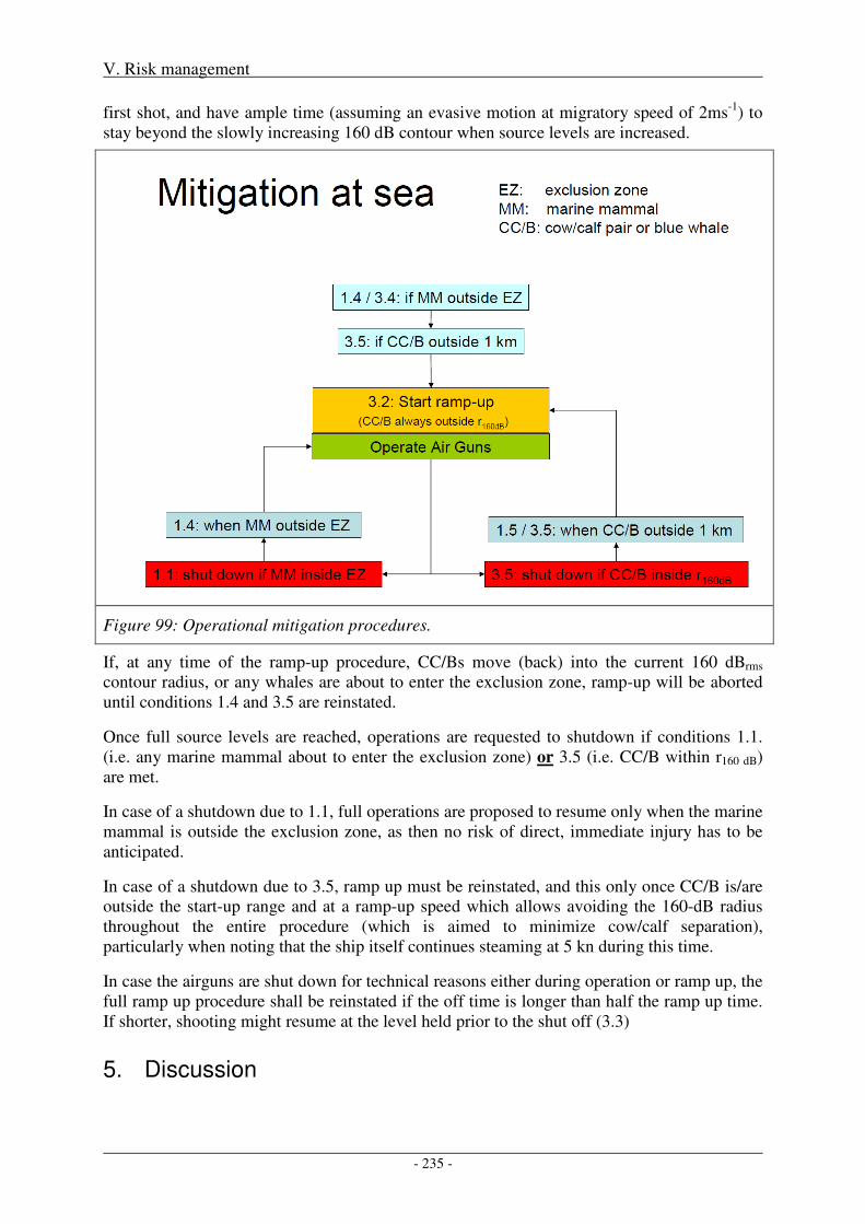
V. Risk management
- 235 -
first shot, and have ample time (assuming an evasive motion at migratory speed of 2ms-1) to stay beyond the slowly increasing 160 dB contour when source levels are increased.
Figure 99: Operational mitigation procedures.
If, at any time of the ramp-up procedure, CC/Bs move (back) into the current 160 dBrms contour radius, or any whales are about to enter the exclusion zone, ramp-up will be aborted until conditions 1.4 and 3.5 are reinstated.
Once full source levels are reached, operations are requested to shutdown if conditions 1.1. (i.e. any marine mammal about to enter the exclusion zone) or 3.5 (i.e. CC/B within r160 dB) are met.
In case of a shutdown due to 1.1, full operations are proposed to resume only when the marine mammal is outside the exclusion zone, as then no risk of direct, immediate injury has to be anticipated.
In case of a shutdown due to 3.5, ramp up must be reinstated, and this only once CC/B is/are outside the start-up range and at a ramp-up speed which allows avoiding the 160-dB radius throughout the entire procedure (which is aimed to minimize cow/calf separation), particularly when noting that the ship itself continues steaming at 5 kn during this time.
In case the airguns are shut down for technical reasons either during operation or ramp up, the full ramp up procedure shall be reinstated if the off time is longer than half the ramp up time. If shorter, shooting might resume at the level held prior to the shut off (3.3)
5. Discussion
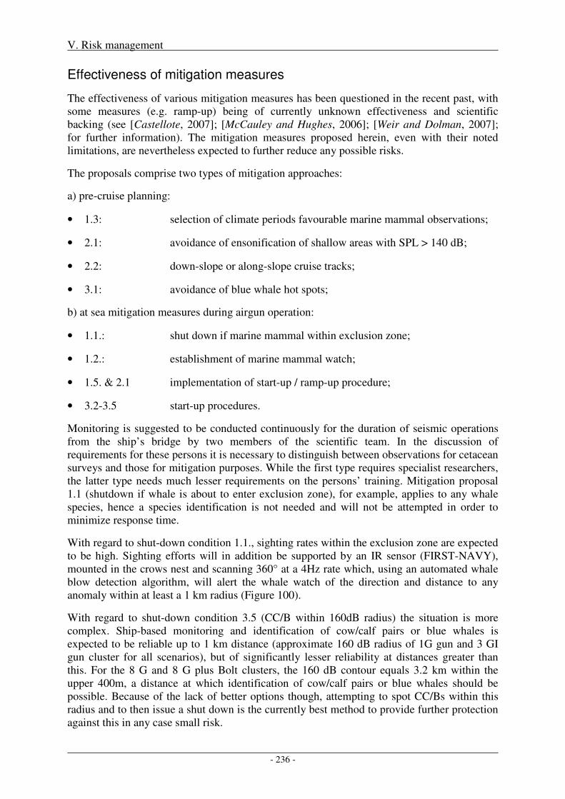
V. Risk management
- 236 -
Effectiveness of mitigation measures
The effectiveness of various mitigation measures has been questioned in the recent past, with some measures (e.g. ramp-up) being of currently unknown effectiveness and scientific backing (see [Castellote, 2007]; [McCauley and Hughes, 2006]; [Weir and Dolman, 2007]; for further information). The mitigation measures proposed herein, even with their noted limitations, are nevertheless expected to further reduce any possible risks.
The proposals comprise two types of mitigation approaches:
a) pre-cruise planning:
• 1.3: selection of climate periods favourable marine mammal observations;
• 2.1: avoidance of ensonification of shallow areas with SPL > 140 dB;
• 2.2: down-slope or along-slope cruise tracks;
• 3.1: avoidance of blue whale hot spots;
b) at sea mitigation measures during airgun operation:
• 1.1.: shut down if marine mammal within exclusion zone;
• 1.2.: establishment of marine mammal watch;
• 1.5. & 2.1 implementation of start-up / ramp-up procedure;
• 3.2-3.5 start-up procedures.
Monitoring is suggested to be conducted continuously for the duration of seismic operations from the ship’s bridge by two members of the scientific team. In the discussion of requirements for these persons it is necessary to distinguish between observations for cetacean surveys and those for mitigation purposes. While the first type requires specialist researchers, the latter type needs much lesser requirements on the persons’ training. Mitigation proposal 1.1 (shutdown if whale is about to enter exclusion zone), for example, applies to any whale species, hence a species identification is not needed and will not be attempted in order to minimize response time.
With regard to shut-down condition 1.1., sighting rates within the exclusion zone are expected to be high. Sighting efforts will in addition be supported by an IR sensor (FIRST-NAVY), mounted in the crows nest and scanning 360° at a 4Hz rate which, using an automated whale blow detection algorithm, will alert the whale watch of the direction and distance to any anomaly within at least a 1 km radius (Figure 100).
With regard to shut-down condition 3.5 (CC/B within 160dB radius) the situation is more complex. Ship-based monitoring and identification of cow/calf pairs or blue whales is expected to be reliable up to 1 km distance (approximate 160 dB radius of 1G gun and 3 GI gun cluster for all scenarios), but of significantly lesser reliability at distances greater than this. For the 8 G and 8 G plus Bolt clusters, the 160 dB contour equals 3.2 km within the upper 400m, a distance at which identification of cow/calf pairs or blue whales should be possible. Because of the lack of better options though, attempting to spot CC/Bs within this radius and to then issue a shut down is the currently best method to provide further protection against this in any case small risk.
V. Risk management
- 237 -
Figure 100: IR images by an experimental setup using FLIR Thermacam A40M with 12° lense prior (left) and during the peak (right) of a Minke whale blow. The image to the right was taken 0.24s after image to the left. The blow was visible for the duration of 8 frames, which corresponds to about 0.56s. The distance to the blow is estimated to be 1164 ± 40 m. Dark areas are covered by sea ice, brighter areas represent (partially) open water.
Use of passive acoustic methods for perimeter surveillance
Real-time, passive acoustic monitoring is frequently proposed as an alternative method to visual observations to determine the presence of marine mammals in the vicinity of a ship or as a support of the visual search effort by providing acoustic bearings of detected vocalizations. Passive acoustic detection has been attempted extensively from onboard Polarstern during four independent cruises (e.g. [Leaper and Scheidat, 1998]; [Kindermann et al., 2006]) using three different designs of dedicated streamers (e.g. 600m long, 15 hydrophones, 8 channels recorded, 5 Hz to 192 kHz sampling rate). However, ship noise prohibited detection of any marine mammal vocalization in all cases other than sperm whale clicks, with the possible exception of two Fin whales vocalizing within the immediate vicinity of the active streamer segments. By contrast, using the AWI streamer on the RV Alliance during a beaked whale tagging cruise in the Mediterranean Sea proved highly effective.
Figure 101: AWI streamer winch and streamer (total length 600m), 3 segments with 5 hydrophones each.
Additional efforts with helicopter-borne sonobuoys and PALAOA-s stations (deployed some 80 nm ahead of the approaching ship) showed masking of seal vocalizations at great distances (> 10 nm) from the ship. Hence, a real time passive acoustic monitoring appears unpractical from onboard Polarstern.
V. Risk management
- 238 -
6. References
Castellote, M. (2007), General review of protocols and guidelines for minimizing acoustic disturbance to marine mammals from seismic surveys, Journal of International Wildlife Law & Policy, 10, 273-288.
Kindermann, L., H. Klinck, and O. Boebel (2006), Automatic Detection of Marine Mammals in the Vicinity of RV Polarstern, Reports on Polar and Marine Research / Berichte zur Polar- und Meeresforschung: The Expedition ANTARKTIS-XXII/3 of the Research Vessel Polarstern, 533, 68-76.
Leaper, R., and M. Scheidat (1998), An acoustic survey for cetaceans in the Southern Ocean Sanctuary conducted from the German Government Research Vessel Polarstern, Rep. Int. Whaling Comm., 48, 431-437.
McCauley, R. D., J. Fewtrell, A. J. Duncan, C. Jenner, M.-N. Jenner, J. D. Penrose, R. I. T. Prince, A. Adhitya, J. Murdoch, and K. McCabe (2000), Marine seismic surveys - a study of environmental implications, APPEA Journal, 40, 692-708. McCauley, R. D., and J. R. Hughes (2006), Marine seismic mitigation measures-perspectives in 2006, (SC/58/E44), paper presented at IWC 58th Annual Meeting, 10 pp, St. Kitts.
Weir, C. R., and S. J. Dolman (2007), Comparative Review of the Regional Marine Mammal Mitigation Guidelines Implemented During Industrial Seismic Surveys, and Guidance Towards a Worldwide Standard, Journal of International Wildlife Law & Policy, 10, 1 - 27.
Zimmer, W. M. X., and P. L. Tyack (2007), Repetitive shallow dives pose decompression risk in deep-diving beaked whales, Marine Mammal Science, 23, 888-925.
VI. Risk evaluation
- 239 -
VI. Risk evaluation
1. Other anthropogenic and natural risks
Through their annual migrations, cetaceans are subject to significant anthropogenic risks, most of which are located outside Antarctica. These risks form an integral component of their life cycles, at least for those species that migrate annually to lower latitudes. Pinniped movements are by and large of limited extend and do usually not extend beyond the Southern Ocean.
In order of significance, the risks posed to whales are (see section II.4) bycatch (estimated hundreds of thousands annually), whaling (> 1,000 annually), and collision with ships or boats (estimated at order of 1,000 annually). The quoted numbers are based on worldwide estimates, with significant uncertainties (most likely underestimates) and might not concern populations of the southern hemisphere as much as northern hemisphere populations, as anthropogenic activities are greatly reduced in the oceanic regions of the southern hemisphere.
Other anthropogenic risks, such as bioaccumulation of pesticides or other man-made chemicals as well as changes in food supplies due to fisheries are unquantified but may also be substantial in areas other than Antarctic waters. Oceanic changes, as a response to climate change, may be possible, but research into this matter is only just commencing.
Natural risk, such as predation (see Chapter II), diseases and parasites are as yet unquantified as well and appear to be influenced little by man. Particular attention has been given to natural changes which might cause mass strandings [Bradshaw et al., 2006], such as sonar termination [Chambers and James, 2005], changes in the magnetic field [Vanselow and Ricklefs, 2005], or displacements of oceanic fronts [Learmonth et al., 2006]. Most of these effects are by definition associated with coastal regions. Resulting mortalities in these cases are rather a consequence of the stranding proper, than of the cause leading to the stranding, which is why these natural risks are of lesser concern for the open Antarctic waters with little access to beaches.
Within the coastal regime, calving of shelf ice and collisions of ice bergs produce sound pressure levels of comparable magnitude to those generated by airguns. During late austral summer, calving produces a quasi-continuous background noise [Boebel et al., 2006]. Ice berg collision produce on occasion continuous noise for the durations of tens of minutes associated with estimated SEL levels in excess of those produced by seismic airguns [Boebel et al., 2008].
Species specific quantitative information on these risks on the individual level is to our knowledge not available. However, population estimates and classifications according to the IUCN Red List provide a good measure of the communities’ estimate of how critically the sum of all these risks poses a threat to a certain species.
2. Risks at the individual level
Risks without mitigation measures
Direct, immediate injury
For the airgun configurations and environmental scenarios considered in this study, critical radii for cetaceans do not exceed 100 m from the source, with the exception of the 8G Gun cluster at a shot interval of 15s, where the critical radius increases to 200 m. Due to these small critical
VI. Risk evaluation
- 240 -
radii, and the likelihood of avoidance reactions to the approaching ship by at least some species, the risk of inflicting injury to an individual whale seems low. Nevertheless, within these ranges, the risk of inflicting injury to low- or mid-frequency cetaceans or to pinnipeds cannot be excluded.
Indirect, immediate damage
As discussed in section IV.2, the three key abetting factors of the DCS/hyperthermia hypothesis are not present in the Antarctic context. Owing to the significantly different signal characteristics of airgun and ASW sonar signals, little reason exists to warrant the concern that whales would enter into a prolonged near surface flight as a predator avoidance response. Even if this would be the case, water temperatures around 0°C render the occurrence of hyperthermia unlikely, while water depths greater than the depth of lung collapse allow deep recovery dives, which would prevent DCS to occur. Finally, relatively slow, single ship operations are unlikely to cause herding at large distances. Hence, the key factors of the DCS/hyperthermia hypothesis are not met for the context of research seismic in the Antarctic, providing little reason to assume that airgun operations in Antarctica could cause fatal injuries to any individual of the endangered species.
Biologically significant, acoustic disturbance
Acoustic disturbance through operation of airguns in a linear survey layout in Antarctica most likely has only biologically insignificant implications with regard to migration, feeding and nurturing due to the shortness of acoustic exposure. Furthermore, calving and breeding activities of true Antarctic cetaceans lie either outside the range or time of Antarctic airgun surveys and are hence not affected. Reduced predator avoidance due to behavioural response (masking and TTS) is unlikely to gain biological significance, as it would occur in a frequency band irrelevant to predator detection (any injurious effects due to cumulative TTS are included under direct, immediate damage).
However, based on the current level of knowledge, it cannot be excluded that cow-calf pairs might be separated by airgun noise of amplitude 160 dBrms rel. 1µPa. Up to these levels, the separation has been classified as brief or minor and is hence unlikely to be biologically significant. At higher exposure levels (i.e. within the 160 dBrms rel. 1µPa radius), however, a biologically significant impact, i.e. the separation of the calf from the cow, cannot be excluded at the individual level. A similar scenario is unlikely to apply to ice breeding phocids and southern elephant seals, as mother/pub pairs wean abruptly and separate shortly after, and fur seal pups do not follow their mothers on foraging excursions during the extended lactation period.
Residual risks under inclusion of mitigation measures
Direct, immediate injury
The implementation of mitigation measures 1.1 – 1.5, i.e. monitoring and implementation of an exclusion zone, is aimed at minimizing the risk of possibly injuring an (individual) marine mammal. Given the slow motion of the ship and the fact that mysticetes perform rather short (order of 10 min) and relatively shallow dives, this should allow detecting the majority of mysticetes in due time when in the vicinity of the ship. Odontocetes and pinnipeds however, perform longer and deeper dive cycles. While on the one hand this implies a higher probability of being unnoticed by the marine mammal watch, it on the other hand also reduces the possibility of a mammal surfacing within exclusion zone. With these mitigation measures in place, the risk of injuring a marine mammal of any species is reduced to the minimum level.
VI. Risk evaluation
- 241 -
Indirect, immediate damage
The risk of inducing a beaked whale type of stranding event in the context of this risk assessment is already considered negligible for the reasons given above. Nevertheless, for reasons of good environmental practice, the implementation of mitigation measures 2.1 and 2.2 are aimed at minimizing any residual risk for any individual whale further. Therefore, the per se already highly unlikely risk of incidental injury is further minimized.
Biologically significant, acoustic disturbance
The implementation of mitigation measures 3.2 and 3.5 is aimed at reducing the risk of a possible separation of cow/calf pairs, which is considered the only behavioural response with possible biologically significant impact. The proposal calls for a shut-down of acoustic sources if cow/calf pairs are sighted within the 160rms dB radius. Depending on the acoustic scenario (source and environment), this radius varies between 700m and 5600 – 7000m for the loudest sources in shallow water (Table 45). While at the larger of these distances, a positive identification of cow/calf pairs is unlikely, it should nevertheless be attempted, as even detections and resulting shut-downs at shorter distances are expected to reduce the possible risk of separation, thereby reducing the overall risk of biologically significant, acoustic disturbance to a minimum. Furthermore, with increasing cross-track distance, the exposure time decreases significantly (Figure 98), while at shorter cross-track distances the sighting probability increases, eventually leading to shut downs. Hence, for both situations, the overall exposure time is to be expected to be significantly shortened, presumably resulting in a reduced risk of separation.
3. Risks at the population level
As already stated in chapter III (Hazard Identification), risks at the individual level will not necessarily translate into risks at the population level. Even the death of an individual is likely to have negligible impact on the population if the latter is in a healthy state. On the other hand, for highly endangered species, such as the blue whale, the death of a single female might cause the transition from a marginally stable population to the extinction of the entire species.
A discussion of population level effects best commences with a consideration of the conservation status of each species, as this (independent) evaluation already includes all additional anthropogenic and non-anthropogenic risks. Of the various true Antarctic whale species (Table 3), three species (blue, fin, and sei whale) are listed as endangered (IUCN ver 2.3 A1 abd) and further two species (humpback and sperm whale) are listed as vulnerable (IUCN ver 2.3 A1 ad/bd), while all other cetaceans and pinnipeds are categorized as lower risk/least concern or respectively data deficient (Antarctic minke whale). Southern Ocean populations of the three endangered and two vulnerable species are in the range of 10,000-30,000 individuals, with the exception of the blue whale which is listed as 400-500, while recent stock estimates reaching 1,400. Population level effects are unlikely to occur, if the number of impacted individuals is much smaller than the number of natural deaths, which is why for population level effects, species classified as endangered or vulnerable are of primary concern.
To understand the dimension of a possible population impact of anthropogenic activities, it is useful to compare the number of possibly injured or biologically significantly disturbed individuals with the natural mortality of the species. Assuming (a conservatively selected) lower value of 0.06 for cetacean mortality rates, the annual natural number of deaths is calculated in Table 20.
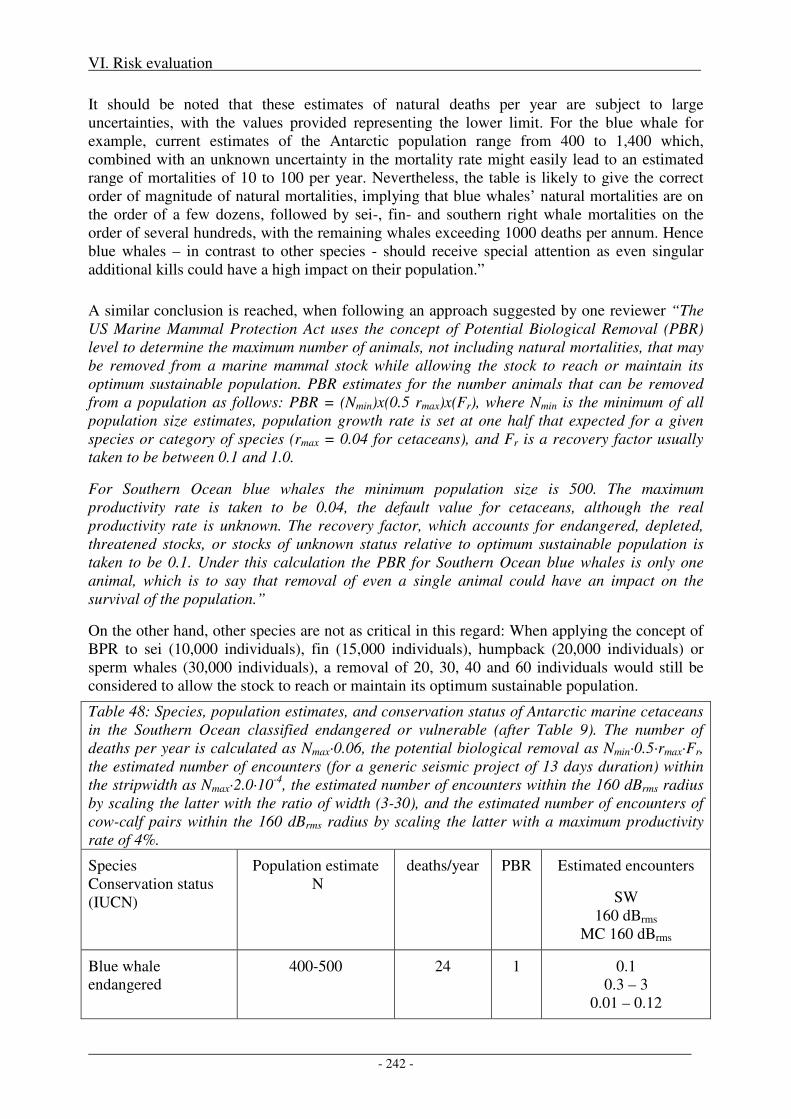
VI. Risk evaluation
- 242 -
It should be noted that these estimates of natural deaths per year are subject to large uncertainties, with the values provided representing the lower limit. For the blue whale for example, current estimates of the Antarctic population range from 400 to 1,400 which, combined with an unknown uncertainty in the mortality rate might easily lead to an estimated range of mortalities of 10 to 100 per year. Nevertheless, the table is likely to give the correct order of magnitude of natural mortalities, implying that blue whales’ natural mortalities are on the order of a few dozens, followed by sei-, fin- and southern right whale mortalities on the order of several hundreds, with the remaining whales exceeding 1000 deaths per annum. Hence blue whales – in contrast to other species - should receive special attention as even singular additional kills could have a high impact on their population.”
A similar conclusion is reached, when following an approach suggested by one reviewer “The US Marine Mammal Protection Act uses the concept of Potential Biological Removal (PBR) level to determine the maximum number of animals, not including natural mortalities, that may be removed from a marine mammal stock while allowing the stock to reach or maintain its optimum sustainable population. PBR estimates for the number animals that can be removed from a population as follows: PBR = (Nmin)x(0.5 rmax)x(Fr), where Nmin is the minimum of all population size estimates, population growth rate is set at one half that expected for a given species or category of species (rmax = 0.04 for cetaceans), and Fr is a recovery factor usually taken to be between 0.1 and 1.0.
For Southern Ocean blue whales the minimum population size is 500. The maximum productivity rate is taken to be 0.04, the default value for cetaceans, although the real productivity rate is unknown. The recovery factor, which accounts for endangered, depleted, threatened stocks, or stocks of unknown status relative to optimum sustainable population is taken to be 0.1. Under this calculation the PBR for Southern Ocean blue whales is only one animal, which is to say that removal of even a single animal could have an impact on the survival of the population.”
On the other hand, other species are not as critical in this regard: When applying the concept of BPR to sei (10,000 individuals), fin (15,000 individuals), humpback (20,000 individuals) or sperm whales (30,000 individuals), a removal of 20, 30, 40 and 60 individuals would still be considered to allow the stock to reach or maintain its optimum sustainable population.
Table 48: Species, population estimates, and conservation status of Antarctic marine cetaceans in the Southern Ocean classified endangered or vulnerable (after Table 9). The number of deaths per year is calculated as Nmax·0.06, the potential biological removal as Nmin·0.5·rmax·Fr, the estimated number of encounters (for a generic seismic project of 13 days duration) within the stripwidth as Nmax·2.0·10-4, the estimated number of encounters within the 160 dBrms radius by scaling the latter with the ratio of width (3-30), and the estimated number of encounters of cow-calf pairs within the 160 dBrms radius by scaling the latter with a maximum productivity rate of 4%.
Species Conservation status (IUCN)
Population estimate N
deaths/year
PBR
Estimated encounters
SW 160 dBrms
MC 160 dBrms
Blue whale endangered
400-500 24 1 0.1 0.3 – 3
0.01 – 0.12
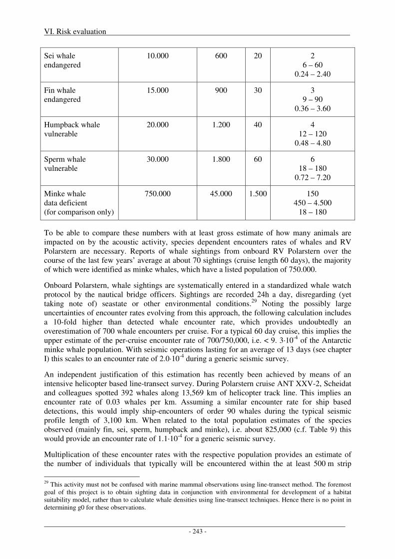
VI. Risk evaluation
- 243 -
Sei whale endangered
10.000 600 20 2 6 – 60
0.24 – 2.40
Fin whale endangered
15.000 900 30 3 9 – 90
0.36 – 3.60
Humpback whale vulnerable
20.000 1.200 40 4 12 – 120
0.48 – 4.80
Sperm whale vulnerable
30.000 1.800 60 6 18 – 180
0.72 – 7.20
Minke whale data deficient (for comparison only)
750.000 45.000 1.500 150 450 – 4.500
18 – 180
To be able to compare these numbers with at least gross estimate of how many animals are impacted on by the acoustic activity, species dependent encounters rates of whales and RV Polarstern are necessary. Reports of whale sightings from onboard RV Polarstern over the course of the last few years’ average at about 70 sightings (cruise length 60 days), the majority of which were identified as minke whales, which have a listed population of 750.000.
Onboard Polarstern, whale sightings are systematically entered in a standardized whale watch protocol by the nautical bridge officers. Sightings are recorded 24h a day, disregarding (yet taking note of) seastate or other environmental conditions.29 Noting the possibly large uncertainties of encounter rates evolving from this approach, the following calculation includes a 10-fold higher than detected whale encounter rate, which provides undoubtedly an overestimation of 700 whale encounters per cruise. For a typical 60 day cruise, this implies the upper estimate of the per-cruise encounter rate of 700/750,000, i.e. < 9. 3·10-4 of the Antarctic minke whale population. With seismic operations lasting for an average of 13 days (see chapter I) this scales to an encounter rate of 2.0·10-4 during a generic seismic survey.
An independent justification of this estimation has recently been achieved by means of an intensive helicopter based line-transect survey. During Polarstern cruise ANT XXV-2, Scheidat and colleagues spotted 392 whales along 13,569 km of helicopter track line. This implies an encounter rate of 0.03 whales per km. Assuming a similar encounter rate for ship based detections, this would imply ship-encounters of order 90 whales during the typical seismic profile length of 3,100 km. When related to the total population estimates of the species observed (mainly fin, sei, sperm, humpback and minke), i.e. about 825,000 (c.f. Table 9) this would provide an encounter rate of 1.1·10-4 for a generic seismic survey.
Multiplication of these encounter rates with the respective population provides an estimate of the number of individuals that typically will be encountered within the at least 500 m strip
29 This activity must not be confused with marine mammal observations using line-transect method. The foremost goal of this project is to obtain sighting data in conjunction with environmental for development of a habitat suitability model, rather than to calculate whale densities using line-transect techniques. Hence there is no point in determining g0 for these observations.
VI. Risk evaluation
- 244 -
widths of the above sightings. This results in encounter rates that are a factor of 10 less than the PBR. With the exclusion zone being equal or smaller to the strip width, it further gives an estimate on how many individuals may – in an statistical sense – enter the exclusion zone during a generic seismic survey.
These evaluations might be scaled to the number of encounters with the 160 dBrms radius. Using the half stripwidth (250 m) in relation to the range 700 m to 7,500 m for the 160 dB rms contour, this relates to a scaling factor of 3 to 30. The resulting estimates of numbers of animals’ ensonified per generic seismic survey are given in Table 48.
It should be noted though, that the above considerations are of statistical nature only. Due to the patchiness of whale distributions, encounter rates might fluctuate significantly, with direct impact on the estimated risks.
Risk without mitigation measures
Direct, immediate injury
Even though a detrimental impact on the individual level was not to be excluded, statistically about 2·10-4 of a given cetacean population might encounter in the vicinity of the exclusion zone during the course of the survey. While this implies a statistical possibility of impact on individuals, a population level impact under this scenario is unlikely as encounter rates are one order of magnitude smaller that the PBR values and more than two orders of magnitude smaller than the natural mortality rate.
Indirect, immediate damage
Population level effects are, under this scenario, highly unlikely, as already impacts on the individual level are unlikely.
Biologically significant, acoustic disturbance
As indicated in the section on individual level effects, the only behavioural response with concern for biological significant effects would be an acoustically induced cow calf separation. While the estimated possible per-transect encounter rates with the 160dBrms ranges being between 3-30 x 2·10-4 of the overall population, encounters with cow/calf pairs are reduced to about 4 % of the population (based on a maximum productivity rate of 0.04, the default value for cetaceans - [Wade and Angliss, 1997]). This implies cow-calf encounter rates to be one order of magnitude smaller than the PBR estimate and more then two orders of magnitude smaller than the natural mortality rate. Hence, in a statistical sense, the risk of population level consequences can be excludes, thought a residual risk remains due to the possibility of encounters with patches of increased whale densities.
Residual risks under inclusion of mitigation measures
Direct, immediate injury
Inclusion of mitigation measures 1.1 – 1.5, i.e. monitoring and implementation of an exclusion zone, leads to a significant reduction – if not overall avoidance - of injury to cetaceans. Under consideration of the already small encounter rate/BPR ratio, this should in fact annihilate any possibility of a population effect under this scenario.
Indirect, immediate damage
VI. Risk evaluation
- 245 -
Population level effects are, under this scenario, highly unlikely, as already impacts on the individual level are unlikely. The proposed mitigation measures minimize any residual risk that should derive from the currently incomplete knowledge.
Biologically significant, acoustic disturbance
As indicated in the paragraphs above on individual and population level effects, this scenario might result in an ensonification of cow/calf pairs with at least one order of magnitude less than respective PBR estimates and more than two orders of magnitude less than the natural mortality rates, which makes, in a statistical sense, a population level effect highly unlikely.
However, the possibility of encounters with patches of increased whale densities cannot be excluded. The proposed mitigation measure reduces this residual risk further. For the smaller airguns, the mitigation measure is expected to be rather effective as the detection probability is high, but detection probabilities will decrease with increasing radii. However noting the presumed dispersing character of the acoustic exposure, the observation that cow/calf pairs are more likely to exhibit an avoidance response [McCauley et al., 2000], the rather reduced presence of calves south of 60°S (with most surveys being located south of 70°S, cf. Figure 1), and the fact that patches of whales are more likely to be spotted than singular animals, population level effects under inclusion of mitigation measures 3.2 and 3.5, i.e. the shut-off of airguns when cow/calf pairs are detected, are unlikely to materialize.
VI. Risk evaluation
- 246 -
4. References
Boebel, O., et al. (2006), Acoustic Observatory Provides Real-Time Underwater Sounds from the Antarctic Ocean, EOS, 87, 361-372.
Boebel, O., et al. (2008), PALAOA: Broadband recordings of the Antarctic coastal soundscape, Bioacoustics, 17, 19-21.
Bradshaw, C. J. A., et al. (2006), Mass Cetacean Strandings—a Plea for Empiricism, Conservation Biology, 20(2), 584-586.
Chambers, S., and R. N. James (2005), Sonar termination as a cause of mass cetacean strandings in Geographe Bay, south-western Australia, paper presented at Acoustics 2005, Acoustics in a Changing Environment, 391-398 pp, Busselton, Western Australia, November 9 - 11, 2005.
Learmonth, J. A., et al. (2006), Potential effects of climate change on marine mammals, in Oceanography And Marine Biology - An Annual Review, Vol 44, edited, pp. 431-464, CRC Press-Taylor & Francis Group, Boca Raton, FL.
McCauley, R. D., et al. (2000), Marine seismic surveys - a study of environmental implications, APPEA Journal, 40, 692-708.
Vanselow, K. H., and K. Ricklefs (2005), Are solar activity and sperm whale Physeter macrocephalus strandings around the North Sea related?, Journal of Sea Research, 53(4), 319-327.
Wade, P. R., and R. P. Angliss (1997), Guidelines for assessing marine mammal stocks: Report of the GAMMS Workshop, 93 pp, Seattle, WA.
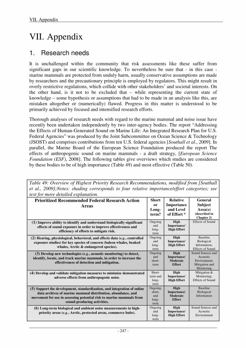
VII. Appendix
- 247 -
VII. Appendix
1. Research needs
It is unchallenged within the community that risk assessments like these suffer from significant gaps in our scientific knowledge. To nevertheless be sure that - in this case - marine mammals are protected from unduly harm, usually conservative assumptions are made by researchers and the precautionary principle is employed by regulators. This might result in overly restrictive regulations, which collide with other stakeholders’ and societal interests. On the other hand, is it not to be excluded that – while representing the current state of knowledge – some hypothesis or assumptions that had to be made in an analysis like this, are mistaken altogether or (numerically) flawed. Progress in this matter is understood to be primarily achieved by focused and intensified research efforts.
Thorough analyses of research needs with regard to the marine mammal and noise issue have recently been undertaken independently by two inter-agency bodies. The report “Addressing the Effects of Human-Generated Sound on Marine Life: An Integrated Research Plan for U.S. Federal Agencies” was produced by the Joint Subcommittee on Ocean Science & Technology (JSOST) and comprises contributions from ten U.S. federal agencies [Southall et al., 2009]. In parallel, the Marine Board of the European Science Foundation produced the report The effects of anthropogenic sound on marine mammals - a draft strategy, [European Science Foundation (ESF), 2008]. The following tables give overviews which studies are considered by these bodies to be of high importance (Table 49) and most effective (Table 50).
Table 49: Overview of Highest Priority Research Recommendations, modified from [Southall et al., 2009];Notes: shading corresponds to four relative importance/effort categories; see text for more detailed explanation.
Prioritized Recommended Federal Research Action
Areas Short
or
Long-
term?
Relative
Importance
and Level
of Effort *
General
Subject
Area(s) (described in
Chapter 2)
(1) Improve ability to identify and understand biologically-significant
effects of sound exposure in order to improve effectiveness and
efficiency of efforts to mitigate risk.
Ongoing and
long-term
High
Importance/ High Effort
Effects of Sound
(2) Hearing, physiological, behavioral, and effects data (e.g., controlled
exposure studies) for key species of concern (baleen whales, beaked
whales, Arctic & endangered species).
Ongoing and
long-term
High
Importance/ High Effort
Baseline Biological
Information; Effects of Sound
(3) Develop new technologies (e.g., acoustic monitoring) to detect,
identify, locate, and track marine mammals, in order to increase the
effectiveness of detection and mitigation.
Ongoing and
short-term
High
Importance/ Moderate
Effort
Sound Sources and Acoustic
Environment; Mitigation and
Monitoring
(4) Develop and validate mitigation measures to minimize demonstrated
adverse effects from anthropogenic noise.
Short-term and
long-term
High
Importance/ High Effort
Mitigation & Monitoring;
Effects of Sound
(5) Support the development, standardization, and integration of online
data archives of marine mammal distribution, abundance, and
movement for use in assessing potential risk to marine mammals from
sound-producing activities.
Ongoing, short, and
long-term
High
Importance/ Moderate
Effort
Baseline Biological
Information
(6) Long-term biological and ambient noise measurements in high-
priority areas (e.g., Arctic, protected areas, commerce hubs).
Ongoing and
long-term
High
Importance/ High Effort
Sound Sources and Acoustic
Environment
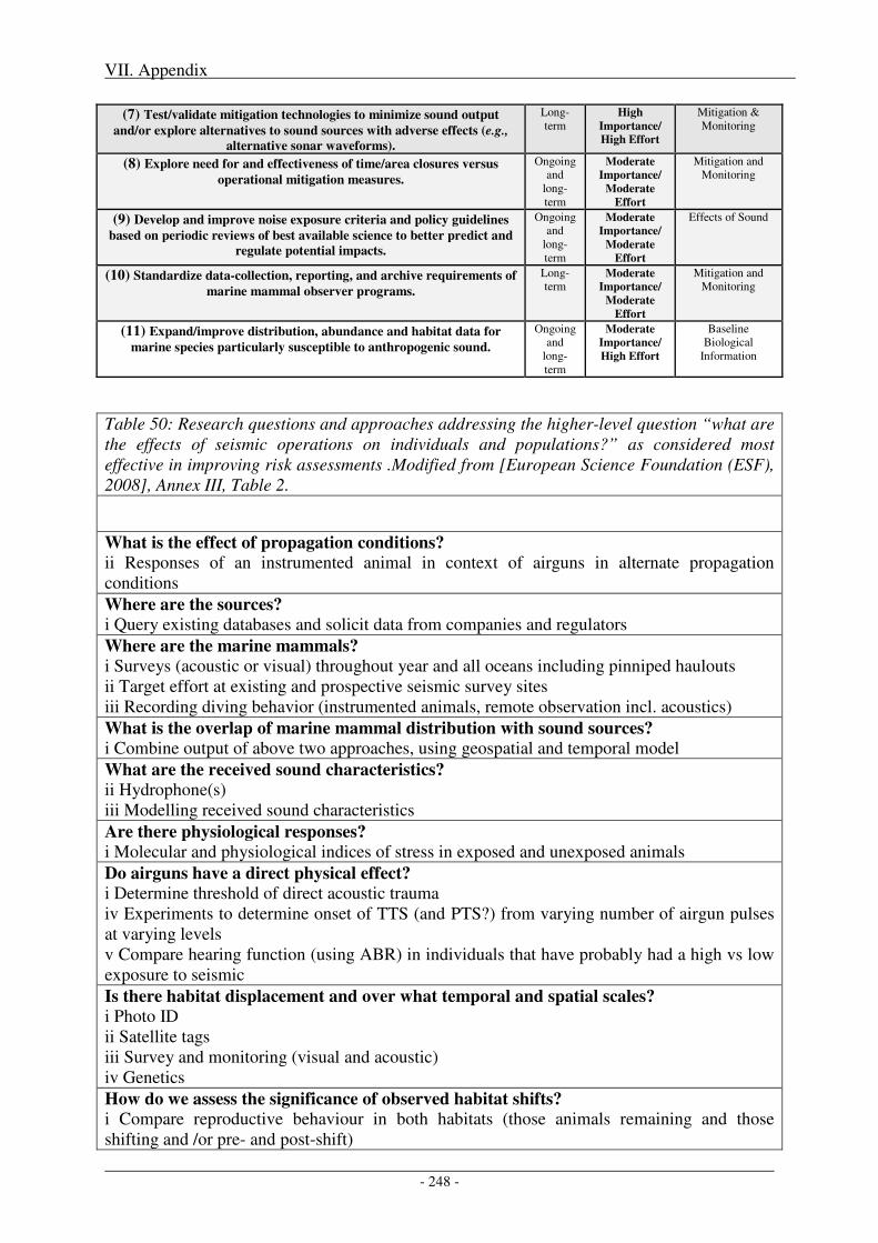
VII. Appendix
- 248 -
(7) Test/validate mitigation technologies to minimize sound output
and/or explore alternatives to sound sources with adverse effects (e.g.,
alternative sonar waveforms).
Long-term
High
Importance/ High Effort
Mitigation & Monitoring
(8) Explore need for and effectiveness of time/area closures versus
operational mitigation measures.
Ongoing and
long-term
Moderate
Importance/ Moderate
Effort
Mitigation and Monitoring
(9) Develop and improve noise exposure criteria and policy guidelines
based on periodic reviews of best available science to better predict and
regulate potential impacts.
Ongoing and
long-term
Moderate
Importance/ Moderate
Effort
Effects of Sound
(10) Standardize data-collection, reporting, and archive requirements of
marine mammal observer programs.
Long-term
Moderate
Importance/ Moderate
Effort
Mitigation and Monitoring
(11) Expand/improve distribution, abundance and habitat data for
marine species particularly susceptible to anthropogenic sound.
Ongoing and
long-term
Moderate
Importance/ High Effort
Baseline Biological
Information
Table 50: Research questions and approaches addressing the higher-level question “what are the effects of seismic operations on individuals and populations?” as considered most effective in improving risk assessments .Modified from [European Science Foundation (ESF), 2008], Annex III, Table 2.
What is the effect of propagation conditions?
ii Responses of an instrumented animal in context of airguns in alternate propagation conditions Where are the sources?
i Query existing databases and solicit data from companies and regulators Where are the marine mammals?
i Surveys (acoustic or visual) throughout year and all oceans including pinniped haulouts ii Target effort at existing and prospective seismic survey sites iii Recording diving behavior (instrumented animals, remote observation incl. acoustics) What is the overlap of marine mammal distribution with sound sources?
i Combine output of above two approaches, using geospatial and temporal model What are the received sound characteristics?
ii Hydrophone(s) iii Modelling received sound characteristics Are there physiological responses?
i Molecular and physiological indices of stress in exposed and unexposed animals Do airguns have a direct physical effect?
i Determine threshold of direct acoustic trauma iv Experiments to determine onset of TTS (and PTS?) from varying number of airgun pulses at varying levels v Compare hearing function (using ABR) in individuals that have probably had a high vs low exposure to seismic Is there habitat displacement and over what temporal and spatial scales?
i Photo ID ii Satellite tags iii Survey and monitoring (visual and acoustic) iv Genetics How do we assess the significance of observed habitat shifts?
i Compare reproductive behaviour in both habitats (those animals remaining and those shifting and /or pre- and post-shift)
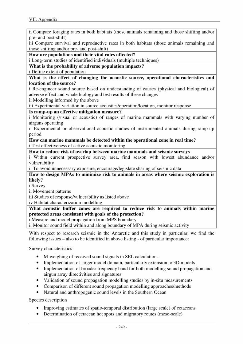
VII. Appendix
- 249 -
ii Compare foraging rates in both habitats (those animals remaining and those shifting and/or pre- and post-shift) iii Compare survival and reproductive rates in both habitats (those animals remaining and those shifting and/or pre- and post-shift) How are populations and their vital rates affected?
i Long-term studies of identified individuals (multiple techniques) What is the probability of adverse population impacts?
i Define extent of population What is the effect of changing the acoustic source, operational characteristics and
location of the source?
i Re-engineer sound source based on understanding of causes (physical and biological) of adverse effect and whale biology and test results of these changes ii Modelling informed by the above iii Experimental variation in source acoustics/operation/location, monitor response Is ramp-up an effective mitigation measure?
i Monitoring (visual or acoustic) of ranges of marine mammals with varying number of airguns operating ii Experimental or observational acoustic studies of instrumented animals during ramp-up period How can marine mammals be detected within the operational zone in real time?
i Test effectiveness of active acoustic monitoring How to reduce risk of overlap between marine mammals and seismic surveys
i Within current prospective survey area, find season with lowest abundance and/or vulnerability ii To avoid unnecessary exposure, encourage/legislate sharing of seismic data How to design MPAs to minimize risk to animals in areas where seismic exploration is
likely?
i Survey ii Movement patterns iii Studies of response/vulnerability as listed above iv Habitat characterization modelling What acoustic buffer zones are required to reduce risk to animals within marine
protected areas consistent with goals of the protection?
i Measure and model propagation from MPS boundary ii Monitor sound field within and along boundary of MPA during seismic activity
With respect to research seismic in the Antarctic and this study in particular, we find the following issues – also to be identified in above listing - of particular importance:
Survey characteristics
• M-weighing of received sound signals in SEL calculations • Implementation of larger model domain, particularly extension to 3D models • Implementation of broader frequency band for both modelling sound propagation and
airgun array directivities and signatures • Validation of sound propagation modelling studies by in-situ measurements • Comparison of different sound propagation modelling approaches/methods • Natural and anthropogenic sound levels in the Southern Ocean
Species description
• Improving estimates of spatio-temporal distribution (large scale) of cetaceans • Determination of cetacean hot spots and migratory routes (meso-scale)
VII. Appendix
- 250 -
• Determination of relationship between cetacean breeding and feeding stocks • Determination of hearing curves and TTS levels of Antarctic species (ongoing AWI
research)
Hazard identification
• Determination of behavioural responses and thresholds at which they occur
Exposure analysis
• Combination of statistical models and (3D) sound propagation models, including dynamic whales and distributions of PTS-thresholds
Risk management
• Testing of effectiveness of visual detection effort (part of ongoing AWI project) • Development of automated detection technology (part of ongoing AWI projects)
Risk evaluation
• Validation of encounter rates (part of ongoing AWI projects)
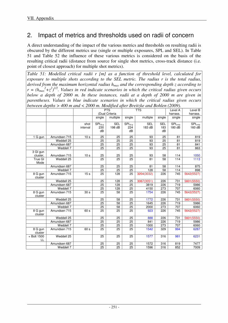
VII. Appendix
- 251 -
2. Impact of metrics and thresholds used on radii of concern
A direct understanding of the impact of the various metrics and thresholds on resulting radii is obscured by the different metrics use (single or multiple exposures, SPL and SEL). In Table 51 and Table 52 the influence of these various metrics is considered on the basis of the resulting critical radii (distance from source for single shot metrics, cross-track distance (i.e. point of closest approach) for multiple shot metrics).
Table 51: Modelled critical radii r [m] as a function of threshold level, calculated for exposure to multiple shots according to the SEL metric. The radius r is the total radius, derived from the maximum horizontal radius hmax and the corresponding depth z according to r = (hmax
2+z2)1/2. Values in red indicate scenarios in which the critical radius given occurs below a depth of 2000 m. In these instances, radii at a depth of 2000 m are given in parentheses. Values in blue indicate scenarios in which the critical radius given occurs between depths > 400 m and < 2000 m. Modified after Breitzke and Bohlen (2009).
PTS (Dual Criteria
TTS Level A harrass.
Level B harrass.
single multiple single multiple single single single
shot interval
SPL0-p
230 dB
SEL 198 dB
SPL0-p 224 dB
SEL 183 dB
SEL 183 dB
SPLrms 180 dB
SPLrms 160 dB
1 G gun Amundsen 715 10 s 25 25 25 93 25 81 819
Weddell 25 25 25 25 93 25 81 819
Amundsen 687 25 25 25 93 25 81 841 Weddell 7 25 25 25 93 25 81 863
3 GI gun cluster, Amundsen 715 10 s 25 25 25 93 58 114 1050
True GI Mode
Weddell 25 25 25 25 81 58 114 1113
Amundsen 687 25 25 25 81 58 114 875
Weddell 7 25 25 25 128 58 114 898
8 G gun cluster
Amundsen 715 15 s 25 128 25 3204(3032) 226 745 5642(5527)
Weddell 25 25 128 25 3087(3051) 226 731 5601(5550)
Amundsen 687 25 128 25 3819 226 719 5986
Weddell 7 25 128 25 4150 273 707 6060
8 G gun cluster
Amundsen 715 30 s 25 58 25 1754 226 745 5642(5527)
Weddell 25 25 58 25 1772 226 731 5601(5550)
Amundsen 687 25 58 25 1645 226 719 5986
Weddell 7 25 58 25 2000 273 707 6060
8 G gun cluster
Amundsen 715 60 s 25 25 25 923 226 745 5642(5527)
Weddell 25 25 25 25 888 226 731 5601(5550)
Amundsen 687 25 25 25 841 226 719 5986
Weddell 7 25 25 25 1000 273 707 6060
8 G gun cluster
Amundsen 715 60 s 25 25 25 1542 329 994 6287
+ Bolt 1500 LL
Weddell 25 25 25 25 1577 316 981 6231
Amundsen 687 25 25 25 1572 316 819 7477 Weddell 7 25 25 25 1596 316 852 7009
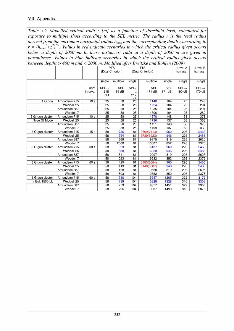
VII. Appendix
- 252 -
Table 52: Modelled critical radii r [m] as a function of threshold level, calculated for exposure to multiple shots according to the SEL metric. The radius r is the total radius derived from the maximum horizontal radius hmax and the corresponding depth z according to r = (hmax
2+z2)1/2. Values in red indicate scenarios in which the critical radius given occurs below a depth of 2000 m. In these instances, radii at a depth of 2000 m are given in parantheses. Values in blue indicate scenarios in which the critical radius given occurs between depths > 400 m and < 2000 m. Modified after Breitzke and Bohlen (2009).
PTS (Dual Criterion)
TTS (Dual Criterion)
Level A harrass.
Level B harrass.
single multiple single multiple single single single
shot interval
SPL0-p
218 dB
SEL 186 dB
SPL0-
p 212 dB
SEL 171 dB
SEL 171 dB
SPLrms 190 dB
SPLrms 170 dB
1 G gun Amundsen 715 10 s 25 58 25 1140 104 25 248
Weddell 25 25 58 25 1224 104 25 294
Amundsen 687 25 58 25 1235 104 25 294
Weddell 7 25 58 25 1306 104 25 282
3 GI gun cluster Amundsen 715 10 s 25 58 25 1578 148 58 378
True GI Mode Weddell 25 25 58 25 1736 137 58 363 Amundsen 687 25 58 25 1451 148 58 378
Weddell 7 25 58 25 1499 137 58 363
8 G gun cluster Amundsen 715 15 s 58 1736 81 9709(7113) 960 226 2468
Weddell 25 58 1754 81 9730(6922) 946 226 2488
Amundsen 687 58 1669 81 9975 819 226 2625
Weddell 7 58 2000 81 10007 852 226 2375 8 G gun cluster Amundsen 715 30 s 58 923 81 6137 960 226 2468
Weddell 25 58 888 81 6029 946 226 2488
Amundsen 687 58 841 81 9907 819 226 2625
Weddell 7 58 1023 81 9932 852 226 2375
8 G gun cluster Amundsen 715 60 s 58 429 81 5183(5064) 960 226 2468 Weddell 25 58 413 81 5140(5087) 946 226 2488
Amundsen 687 58 468 81 9558 819 226 2625
Weddell 7 58 503 81 9682 852 226 2375
8 G gun cluster Amundsen 715 60 s 58 730 104 5947 1265 329 3179
+ Bolt 1500 LL Weddell 25 58 799 104 5828 1328 316 3308
Amundsen 687 58 753 104 9857 1451 329 2900 Weddell 7 58 796 104 9907 1499 316 2875
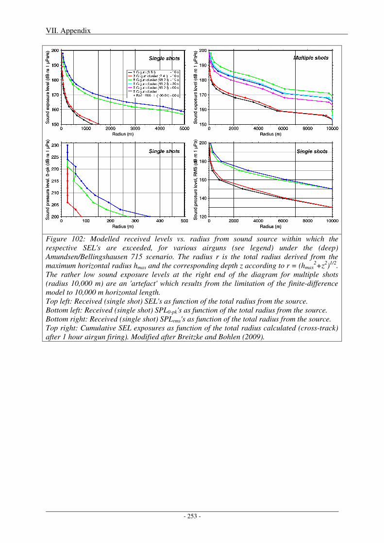
VII. Appendix
- 253 -
Figure 102: Modelled received levels vs. radius from sound source within which the respective SEL's are exceeded, for various airguns (see legend) under the (deep) Amundsen/Bellingshausen 715 scenario. The radius r is the total radius derived from the maximum horizontal radius hmax and the corresponding depth z according to r = (hmax
2+z2)1/2. The rather low sound exposure levels at the right end of the diagram for multiple shots (radius 10,000 m) are an 'artefact' which results from the limitation of the finite-difference model to 10,000 m horizontal length. Top left: Received (single shot) SEL's as function of the total radius from the source. Bottom left: Received (single shot) SPL0-pk's as function of the total radius from the source. Bottom right: Received (single shot) SPLrms's as function of the total radius from the source. Top right: Cumulative SEL exposures as function of the total radius calculated (cross-track) after 1 hour airgun firing). Modified after Breitzke and Bohlen (2009).
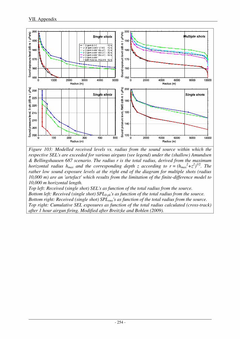
VII. Appendix
- 254 -
Figure 103: Modelled received levels vs. radius from the sound source within which the respective SEL's are exceeded for various airguns (see legend) under the (shallow) Amundsen & Bellingshausen 687 scenario. The radius r is the total radius, derived from the maximum horizontal radius hmax and the corresponding depth z according to r = (hmax
2+z2)1/2. The rather low sound exposure levels at the right end of the diagram for multiple shots (radius 10,000 m) are an 'artefact' which results from the limitation of the finite-difference model to 10,000 m horizontal length. Top left: Received (single shot) SEL's as function of the total radius from the source. Bottom left: Received (single shot) SPL0-pk's as function of the total radius from the source. Bottom right: Received (single shot) SPLrms's as function of the total radius from the source. Top right: Cumulative SEL exposures as function of the total radius calculated (cross-track) after 1 hour airgun firing. Modified after Breitzke and Bohlen (2009).
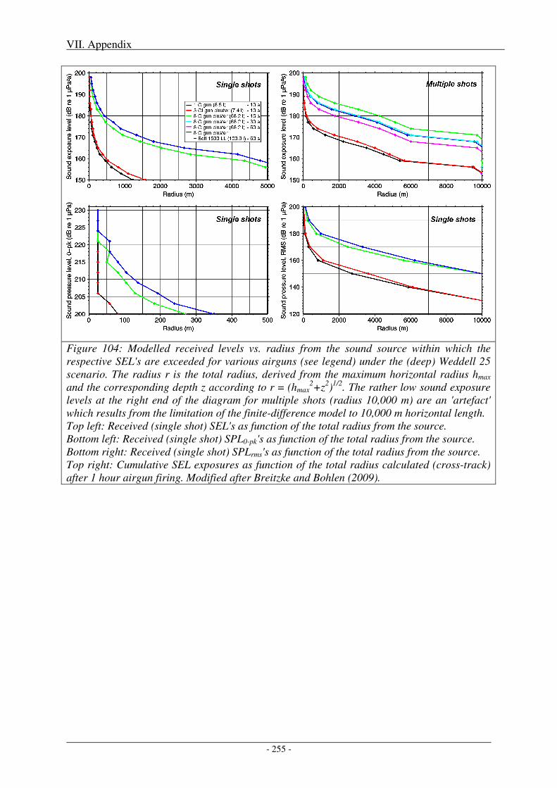
VII. Appendix
- 255 -
Figure 104: Modelled received levels vs. radius from the sound source within which the respective SEL's are exceeded for various airguns (see legend) under the (deep) Weddell 25 scenario. The radius r is the total radius, derived from the maximum horizontal radius hmax and the corresponding depth z according to r = (hmax
2+z2)1/2. The rather low sound exposure levels at the right end of the diagram for multiple shots (radius 10,000 m) are an 'artefact' which results from the limitation of the finite-difference model to 10,000 m horizontal length. Top left: Received (single shot) SEL's as function of the total radius from the source. Bottom left: Received (single shot) SPL0-pk's as function of the total radius from the source. Bottom right: Received (single shot) SPLrms's as function of the total radius from the source. Top right: Cumulative SEL exposures as function of the total radius calculated (cross-track) after 1 hour airgun firing. Modified after Breitzke and Bohlen (2009).
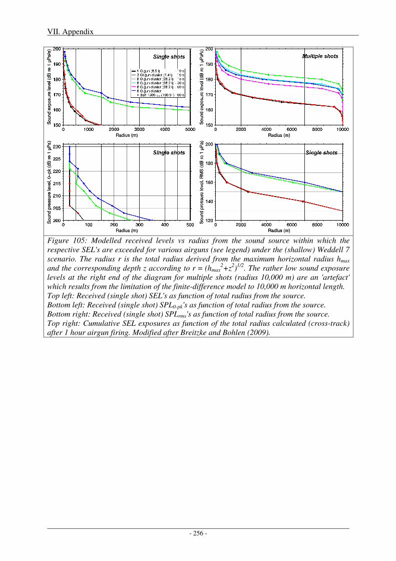
VII. Appendix
- 256 -
Figure 105: Modelled received levels vs radius from the sound source within which the respective SEL's are exceeded for various airguns (see legend) under the (shallow) Weddell 7 scenario. The radius r is the total radius derived from the maximum horizontal radius hmax and the corresponding depth z according to r = (hmax
2+z2)1/2. The rather low sound exposure levels at the right end of the diagram for multiple shots (radius 10,000 m) are an 'artefact' which results from the limitation of the finite-difference model to 10,000 m horizontal length. Top left: Received (single shot) SEL's as function of total radius from the source. Bottom left: Received (single shot) SPL0-pk's as function of total radius from the source. Bottom right: Received (single shot) SPLrms's as function of total radius from the source. Top right: Cumulative SEL exposures as function of the total radius calculated (cross-track) after 1 hour airgun firing. Modified after Breitzke and Bohlen (2009).
VII. Appendix
- 257 -
3. References
Breitzke, M., O. Boebel, S. El Naggar, W. Jokat, and B. Werner (2008), Broadband calibration of marine seismic sources used by R/V Polarstern for academic research in polar regions, Geophysical Journal International, 174, 505-524.
Breitzke, M., and T. Bohlen (2009), Modelling acoustic wave propagation in the Southern Ocean to estimate the acoustic impact of seismic surveys on marine mammals, in prep.
European Science Foundation (ESF) (2008), The effects of anthropogenic sound on marine mammals - a draft strategy, 96 pp, European Science Foundation.
Southall, B., J. Berkson, D. Bowen, R. Brake, J. Eckman, J. Field, R. Gisiner, S. Gregerson, W. Lang, J. Lewandoski, J. Wilson, and R. Winokur (2009), Addressing the Effects of Human-Generated Sound on Marine Life: An Integrated Research Plan for U.S. federal agencies, Interagency Task Force on Anthropogenic Sound and the Marine Environment of the Joint Subcommittee on Ocean Science and Technology, Washington, DC.

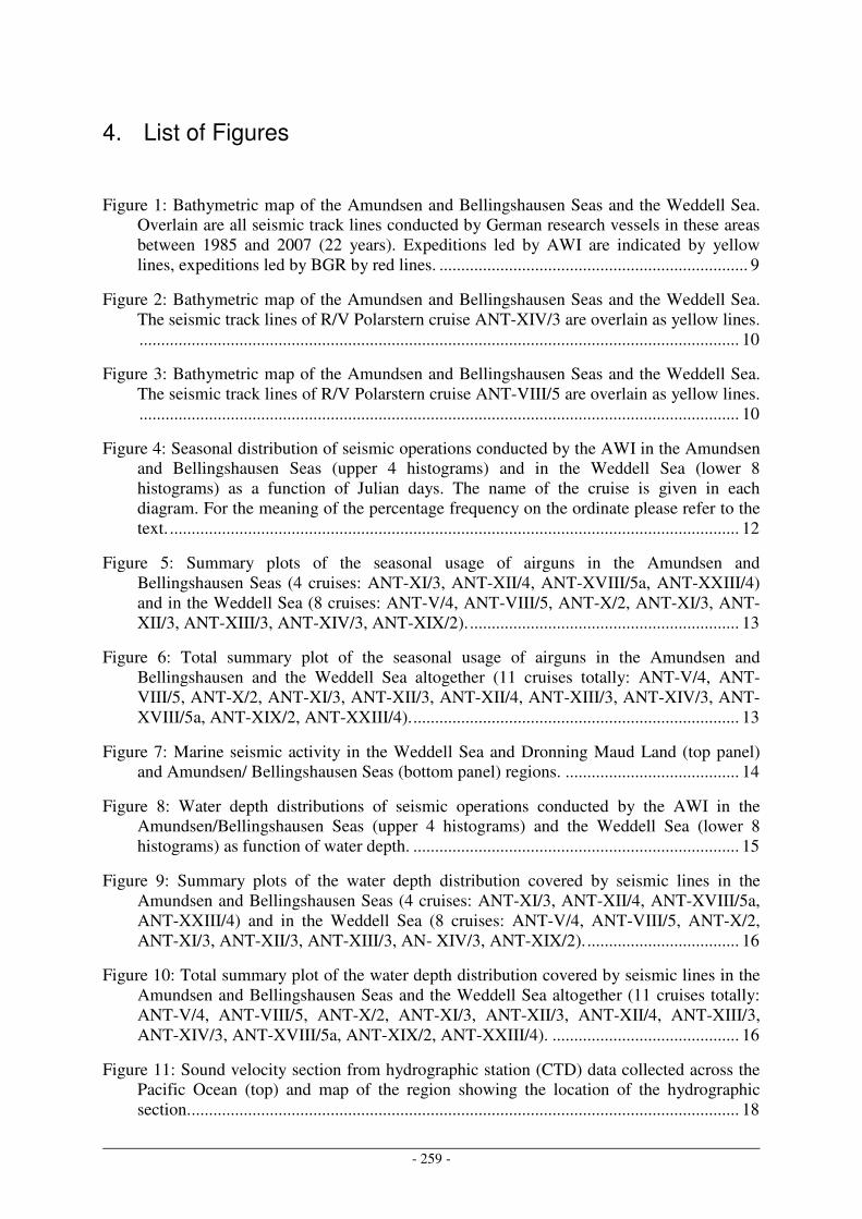
- 259 -
4. List of Figures
Figure 1: Bathymetric map of the Amundsen and Bellingshausen Seas and the Weddell Sea. Overlain are all seismic track lines conducted by German research vessels in these areas between 1985 and 2007 (22 years). Expeditions led by AWI are indicated by yellow lines, expeditions led by BGR by red lines. ....................................................................... 9
Figure 2: Bathymetric map of the Amundsen and Bellingshausen Seas and the Weddell Sea. The seismic track lines of R/V Polarstern cruise ANT-XIV/3 are overlain as yellow lines. .......................................................................................................................................... 10
Figure 3: Bathymetric map of the Amundsen and Bellingshausen Seas and the Weddell Sea. The seismic track lines of R/V Polarstern cruise ANT-VIII/5 are overlain as yellow lines. .......................................................................................................................................... 10
Figure 4: Seasonal distribution of seismic operations conducted by the AWI in the Amundsen and Bellingshausen Seas (upper 4 histograms) and in the Weddell Sea (lower 8 histograms) as a function of Julian days. The name of the cruise is given in each diagram. For the meaning of the percentage frequency on the ordinate please refer to the text. ................................................................................................................................... 12
Figure 5: Summary plots of the seasonal usage of airguns in the Amundsen and Bellingshausen Seas (4 cruises: ANT-XI/3, ANT-XII/4, ANT-XVIII/5a, ANT-XXIII/4) and in the Weddell Sea (8 cruises: ANT-V/4, ANT-VIII/5, ANT-X/2, ANT-XI/3, ANT-XII/3, ANT-XIII/3, ANT-XIV/3, ANT-XIX/2). .............................................................. 13
Figure 6: Total summary plot of the seasonal usage of airguns in the Amundsen and Bellingshausen and the Weddell Sea altogether (11 cruises totally: ANT-V/4, ANT-VIII/5, ANT-X/2, ANT-XI/3, ANT-XII/3, ANT-XII/4, ANT-XIII/3, ANT-XIV/3, ANT-XVIII/5a, ANT-XIX/2, ANT-XXIII/4). ........................................................................... 13
Figure 7: Marine seismic activity in the Weddell Sea and Dronning Maud Land (top panel) and Amundsen/ Bellingshausen Seas (bottom panel) regions. ........................................ 14
Figure 8: Water depth distributions of seismic operations conducted by the AWI in the Amundsen/Bellingshausen Seas (upper 4 histograms) and the Weddell Sea (lower 8 histograms) as function of water depth. ........................................................................... 15
Figure 9: Summary plots of the water depth distribution covered by seismic lines in the Amundsen and Bellingshausen Seas (4 cruises: ANT-XI/3, ANT-XII/4, ANT-XVIII/5a, ANT-XXIII/4) and in the Weddell Sea (8 cruises: ANT-V/4, ANT-VIII/5, ANT-X/2, ANT-XI/3, ANT-XII/3, ANT-XIII/3, AN- XIV/3, ANT-XIX/2). ................................... 16
Figure 10: Total summary plot of the water depth distribution covered by seismic lines in the Amundsen and Bellingshausen Seas and the Weddell Sea altogether (11 cruises totally: ANT-V/4, ANT-VIII/5, ANT-X/2, ANT-XI/3, ANT-XII/3, ANT-XII/4, ANT-XIII/3, ANT-XIV/3, ANT-XVIII/5a, ANT-XIX/2, ANT-XXIII/4). ........................................... 16
Figure 11: Sound velocity section from hydrographic station (CTD) data collected across the Pacific Ocean (top) and map of the region showing the location of the hydrographic section. .............................................................................................................................. 18
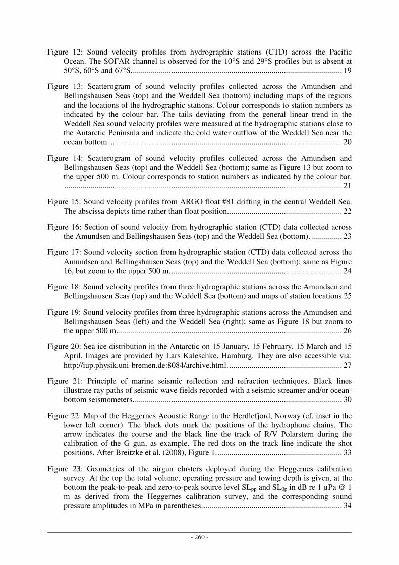
- 260 -
Figure 12: Sound velocity profiles from hydrographic stations (CTD) across the Pacific Ocean. The SOFAR channel is observed for the 10°S and 29°S profiles but is absent at 50°S, 60°S and 67°S. ........................................................................................................ 19
Figure 13: Scatterogram of sound velocity profiles collected across the Amundsen and Bellingshausen Seas (top) and the Weddell Sea (bottom) including maps of the regions and the locations of the hydrographic stations. Colour corresponds to station numbers as indicated by the colour bar. The tails deviating from the general linear trend in the Weddell Sea sound velocity profiles were measured at the hydrographic stations close to the Antarctic Peninsula and indicate the cold water outflow of the Weddell Sea near the ocean bottom. ................................................................................................................... 20
Figure 14: Scatterogram of sound velocity profiles collected across the Amundsen and Bellingshausen Seas (top) and the Weddell Sea (bottom); same as Figure 13 but zoom to the upper 500 m. Colour corresponds to station numbers as indicated by the colour bar. .......................................................................................................................................... 21
Figure 15: Sound velocity profiles from ARGO float #81 drifting in the central Weddell Sea. The abscissa depicts time rather than float position. ........................................................ 22
Figure 16: Section of sound velocity from hydrographic station (CTD) data collected across the Amundsen and Bellingshausen Seas (top) and the Weddell Sea (bottom). ............... 23
Figure 17: Sound velocity section from hydrographic station (CTD) data collected across the Amundsen and Bellingshausen Seas (top) and the Weddell Sea (bottom); same as Figure 16, but zoom to the upper 500 m. ..................................................................................... 24
Figure 18: Sound velocity profiles from three hydrographic stations across the Amundsen and Bellingshausen Seas (top) and the Weddell Sea (bottom) and maps of station locations.25
Figure 19: Sound velocity profiles from three hydrographic stations across the Amundsen and Bellingshausen Seas (left) and the Weddell Sea (right); same as Figure 18 but zoom to the upper 500 m. ............................................................................................................... 26
Figure 20: Sea ice distribution in the Antarctic on 15 January, 15 February, 15 March and 15 April. Images are provided by Lars Kaleschke, Hamburg. They are also accessible via: http://iup.physik.uni-bremen.de:8084/archive.html. ........................................................ 27
Figure 21: Principle of marine seismic reflection and refraction techniques. Black lines illustrate ray paths of seismic wave fields recorded with a seismic streamer and/or ocean-bottom seismometers. ....................................................................................................... 30
Figure 22: Map of the Heggernes Acoustic Range in the Herdlefjord, Norway (cf. inset in the lower left corner). The black dots mark the positions of the hydrophone chains. The arrow indicates the course and the black line the track of R/V Polarstern during the calibration of the G gun, as example. The red dots on the track line indicate the shot positions. After Breitzke et al. (2008), Figure 1. .............................................................. 33
Figure 23: Geometries of the airgun clusters deployed during the Heggernes calibration survey. At the top the total volume, operating pressure and towing depth is given, at the bottom the peak-to-peak and zero-to-peak source level SLpp and SL0p in dB re 1 µPa @ 1 m as derived from the Heggernes calibration survey, and the corresponding sound pressure amplitudes in MPa in parentheses. ..................................................................... 34
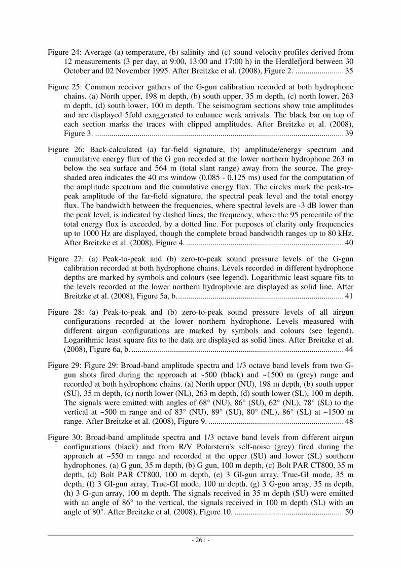
- 261 -
Figure 24: Average (a) temperature, (b) salinity and (c) sound velocity profiles derived from 12 measurements (3 per day, at 9:00, 13:00 and 17:00 h) in the Herdlefjord between 30 October and 02 November 1995. After Breitzke et al. (2008), Figure 2. ........................ 35
Figure 25: Common receiver gathers of the G-gun calibration recorded at both hydrophone chains. (a) North upper, 198 m depth, (b) south upper, 35 m depth, (c) north lower, 263 m depth, (d) south lower, 100 m depth. The seismogram sections show true amplitudes and are displayed 5fold exaggerated to enhance weak arrivals. The black bar on top of each section marks the traces with clipped amplitudes. After Breitzke et al. (2008), Figure 3. ........................................................................................................................... 39
Figure 26: Back-calculated (a) far-field signature, (b) amplitude/energy spectrum and cumulative energy flux of the G gun recorded at the lower northern hydrophone 263 m below the sea surface and 564 m (total slant range) away from the source. The grey-shaded area indicates the 40 ms window (0.085 - 0.125 ms) used for the computation of the amplitude spectrum and the cumulative energy flux. The circles mark the peak-to-peak amplitude of the far-field signature, the spectral peak level and the total energy flux. The bandwidth between the frequencies, where spectral levels are -3 dB lower than the peak level, is indicated by dashed lines, the frequency, where the 95 percentile of the total energy flux is exceeded, by a dotted line. For purposes of clarity only frequencies up to 1000 Hz are displayed, though the complete broad bandwidth ranges up to 80 kHz. After Breitzke et al. (2008), Figure 4. .............................................................................. 40
Figure 27: (a) Peak-to-peak and (b) zero-to-peak sound pressure levels of the G-gun calibration recorded at both hydrophone chains. Levels recorded in different hydrophone depths are marked by symbols and colours (see legend). Logarithmic least square fits to the levels recorded at the lower northern hydrophone are displayed as solid line. After Breitzke et al. (2008), Figure 5a, b. .................................................................................. 41
Figure 28: (a) Peak-to-peak and (b) zero-to-peak sound pressure levels of all airgun configurations recorded at the lower northern hydrophone. Levels measured with different airgun configurations are marked by symbols and colours (see legend). Logarithmic least square fits to the data are displayed as solid lines. After Breitzke et al. (2008), Figure 6a, b. ......................................................................................................... 44
Figure 29: Figure 29: Broad-band amplitude spectra and 1/3 octave band levels from two G-gun shots fired during the approach at ~500 (black) and ~1500 m (grey) range and recorded at both hydrophone chains. (a) North upper (NU), 198 m depth, (b) south upper (SU), 35 m depth, (c) north lower (NL), 263 m depth, (d) south lower (SL), 100 m depth. The signals were emitted with angles of 68° (NU), 86° (SU), 62° (NL), 78° (SL) to the vertical at ~500 m range and of 83° (NU), 89° (SU), 80° (NL), 86° (SL) at ~1500 m range. After Breitzke et al. (2008), Figure 9. ................................................................... 48
Figure 30: Broad-band amplitude spectra and 1/3 octave band levels from different airgun configurations (black) and from R/V Polarstern's self-noise (grey) fired during the approach at ~550 m range and recorded at the upper (SU) and lower (SL) southern hydrophones. (a) G gun, 35 m depth, (b) G gun, 100 m depth, (c) Bolt PAR CT800, 35 m depth, (d) Bolt PAR CT800, 100 m depth, (e) 3 GI-gun array, True-GI mode, 35 m depth, (f) 3 GI-gun array, True-GI mode, 100 m depth, (g) 3 G-gun array, 35 m depth, (h) 3 G-gun array, 100 m depth. The signals received in 35 m depth (SU) were emitted with an angle of 86° to the vertical, the signals received in 100 m depth (SL) with an angle of 80°. After Breitzke et al. (2008), Figure 10. ...................................................... 50
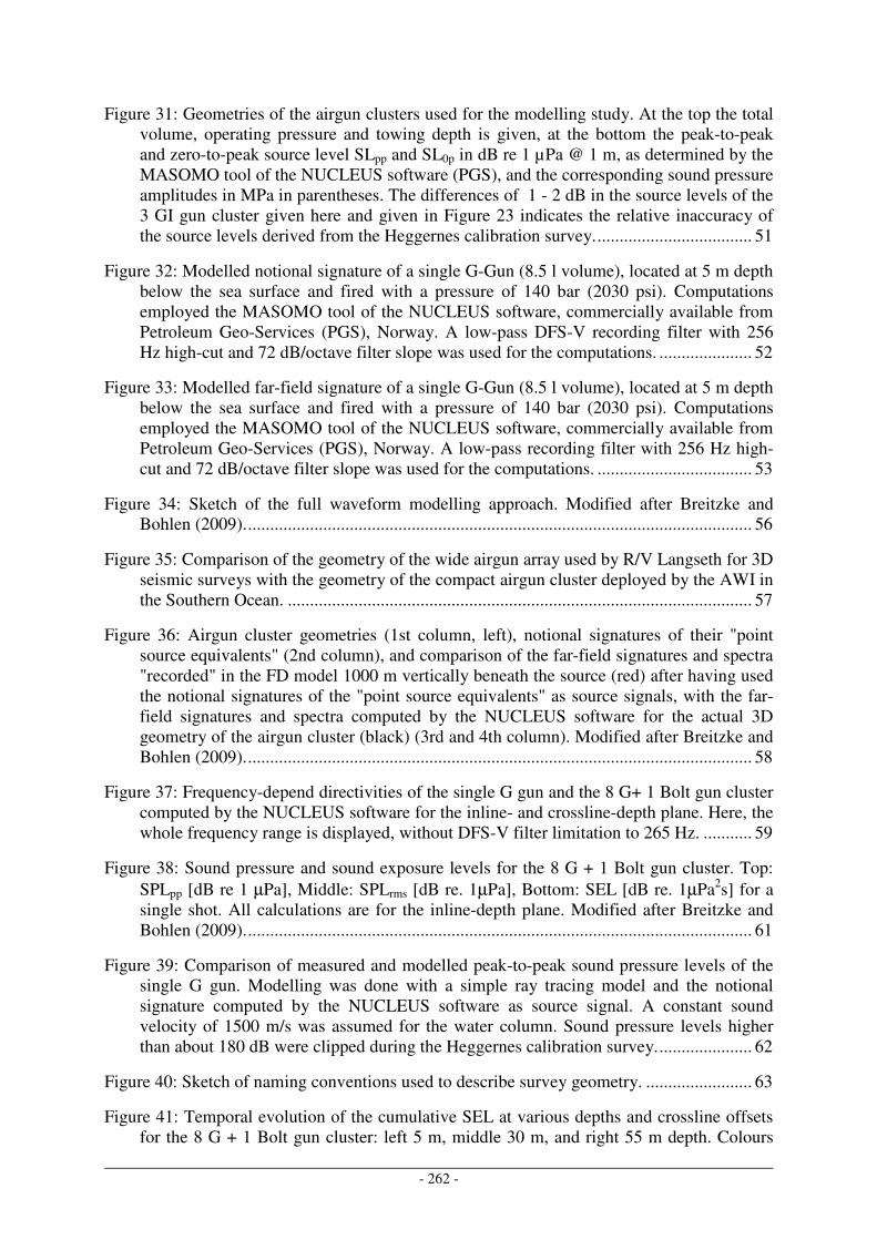
- 262 -
Figure 31: Geometries of the airgun clusters used for the modelling study. At the top the total volume, operating pressure and towing depth is given, at the bottom the peak-to-peak and zero-to-peak source level SLpp and SL0p in dB re 1 µPa @ 1 m, as determined by the MASOMO tool of the NUCLEUS software (PGS), and the corresponding sound pressure amplitudes in MPa in parentheses. The differences of 1 - 2 dB in the source levels of the 3 GI gun cluster given here and given in Figure 23 indicates the relative inaccuracy of the source levels derived from the Heggernes calibration survey. ................................... 51
Figure 32: Modelled notional signature of a single G-Gun (8.5 l volume), located at 5 m depth below the sea surface and fired with a pressure of 140 bar (2030 psi). Computations employed the MASOMO tool of the NUCLEUS software, commercially available from Petroleum Geo-Services (PGS), Norway. A low-pass DFS-V recording filter with 256 Hz high-cut and 72 dB/octave filter slope was used for the computations. ..................... 52
Figure 33: Modelled far-field signature of a single G-Gun (8.5 l volume), located at 5 m depth below the sea surface and fired with a pressure of 140 bar (2030 psi). Computations employed the MASOMO tool of the NUCLEUS software, commercially available from Petroleum Geo-Services (PGS), Norway. A low-pass recording filter with 256 Hz high-cut and 72 dB/octave filter slope was used for the computations. ................................... 53
Figure 34: Sketch of the full waveform modelling approach. Modified after Breitzke and Bohlen (2009). .................................................................................................................. 56
Figure 35: Comparison of the geometry of the wide airgun array used by R/V Langseth for 3D seismic surveys with the geometry of the compact airgun cluster deployed by the AWI in the Southern Ocean. ......................................................................................................... 57
Figure 36: Airgun cluster geometries (1st column, left), notional signatures of their "point source equivalents" (2nd column), and comparison of the far-field signatures and spectra "recorded" in the FD model 1000 m vertically beneath the source (red) after having used the notional signatures of the "point source equivalents" as source signals, with the far-field signatures and spectra computed by the NUCLEUS software for the actual 3D geometry of the airgun cluster (black) (3rd and 4th column). Modified after Breitzke and Bohlen (2009). .................................................................................................................. 58
Figure 37: Frequency-depend directivities of the single G gun and the 8 G+ 1 Bolt gun cluster computed by the NUCLEUS software for the inline- and crossline-depth plane. Here, the whole frequency range is displayed, without DFS-V filter limitation to 265 Hz. ........... 59
Figure 38: Sound pressure and sound exposure levels for the 8 G + 1 Bolt gun cluster. Top: SPLpp [dB re 1 µPa], Middle: SPLrms [dB re. 1µPa], Bottom: SEL [dB re. 1µPa2s] for a single shot. All calculations are for the inline-depth plane. Modified after Breitzke and Bohlen (2009). .................................................................................................................. 61
Figure 39: Comparison of measured and modelled peak-to-peak sound pressure levels of the single G gun. Modelling was done with a simple ray tracing model and the notional signature computed by the NUCLEUS software as source signal. A constant sound velocity of 1500 m/s was assumed for the water column. Sound pressure levels higher than about 180 dB were clipped during the Heggernes calibration survey. ..................... 62
Figure 40: Sketch of naming conventions used to describe survey geometry. ........................ 63
Figure 41: Temporal evolution of the cumulative SEL at various depths and crossline offsets for the 8 G + 1 Bolt gun cluster: left 5 m, middle 30 m, and right 55 m depth. Colours
- 263 -
represent different crossline positions between 0 and 2000 m as described in the text. The inline position of the receiver is 5000 m. Modified after Breitzke and Bohlen (2009). .. 64
Figure 42: Illustration of the generation of SEL fields of cumulative shots fired by the 8 G + 1 Bolt gun cluster. Left: SEL of the first (single) shot of the track. Centre: Cumulative SEL after 30 shots (shot interval = 60 s) have been fired while the ship sailed by 2.5 nm (4630 m) to the right. Right: Cumulative SEL after 60 shots fired while the ship sailed at total of 5 nm (9260 m) to the right. Top panel: inline-depth sections. Middle panel: crossline-depth sections. Bottom panel: The SEL of the aerial view are taken from a depth of 80m. Modified after Breitzke and Bohlen (2009). .................................................................... 65
Figure 43: SEL's for a single and cumulative shots from the 8G-gun cluster for both deep water models. The lower panel shows the SEL's in 80 m depth. (a) Amundsen/Bellingshausen Seas hydrographic station 715 scenario. Left column of (a): SEL of first shot at t = 0 s, right column of (a): cumulative SEL of 241 shots accumulated after firing 241 shots at 15 s intervals. (b) Weddell Sea hydrographic station 25 scenario. Left column of (b): SEL of first shot at t = 0 s, right column of (b): cumulative SEL of 241 shots accumulated after firing 241 shots at 15 s intervals. Modified after Breitzke and Bohlen (2009). .................................................................... 68
Figure 44: Zoom to the upper 400 m of the SEL fields of the 8 G gun cluster shown in Figure 43. Top panel: SEL fields for a single shot. Middle panel: Cumulative SEL fields in the inline-depth plane accumulated after 60 min, or after firing 241 shots at 15 s interval. Bottom panel: Cumulative SEL fields in the crossline-depth plane accumulated after 60 min, or after firing 241 shots at 15 s interval. Modified after Breitzke and Bohlen (2009). .............................................................................................................................. 69
Figure 45: SEL's for a single and cumulative shots from the 8 G-gun cluster for both shallow water models. The lower panel shows the SEL's in 80 m depth. (a) Amundsen/Bellingshausen Seas hydrographic station 687 scenario. Left column of (a): SEL of first shot at t = 0 s, right column of (a): cumulative SEL of 241 shots accumulated after firing 241 shot at 15 s intervals. (b) Weddell Sea hydrographic station 7 scenario. Left column of (b): SEL of first shot at t = 0 s, right column of (b): cumulative SEL of 241 shots accumulated after firing 241 shot at 15 s intervals. Modified after Breitzke and Bohlen (2009). .................................................................... 70
Figure 46: Latitudinal occurrence of baleen whales (left) taken from Kasamatsu et al. [1996], and toothed whales (right) taken from Kasamatsu and Joyce [1995] in Antarctic waters, based on encounter rate calculations in relation to distances between Antarctic convergence and ice edge. Please note that the terms “ice-edge” and “pack-ice” both refer to the marginal region of the Antarctic pack ice (also named in sea-ice the oceanographic context). ................................................................................................... 79
Figure 47: Circumpolar encounter rate of blue whales in 4° latitude by 20° longitude boxes. Areas marked in blue and red represent the Weddell Sea and the Amundsen/Bellingshausen Seas respectively. [Kasamatsu et al., 1996] ......................... 82
Figure 48: Balaenoptera musculus (blue whale). For further details, and quantitative and qualitative definitions of habitat preference categories that marine mammal species were assigned to, see: ................................................................................................................ 83
- 264 -
Figure 49: Circumpolar encounter rate of fin whales in 4° latitude by 20° longitude boxes. Areas marked in blue and red represent the Weddell Sea and the Amundsen/Bellingshausen Seas respectively [Kasamatsu et al., 1996]. ......................... 84
Figure 50: Balaenoptera physalus (fin whale). For further details, and quantitative and qualitative definitions of habitat preference categories that marine mammal species were assigned to, see: ................................................................................................................ 85
Figure 51: Circumpolar encounter rate of sei whales in 4° latitude by 20° longitude boxes. Areas marked in blue and red represent the Weddell Sea and the Amundsen/Bellingshausen Seas respectively. [Kasamatsu et al., 1996] ......................... 86
Figure 52: Balaenoptera borealis (sei whale). For further details, and quantitative and qualitative definitions of habitat preference categories that marine mammal species were assigned to, see: ................................................................................................................ 87
Figure 53: Circumpolar encounter rate of minke whales in 4° latitude by 20° longitude boxes. Areas marked in blue and red represent the Weddell Sea and the Amundsen/Bellingshausen Seas respectively [Kasamatsu et al., 1996]. ......................... 88
Figure 54: Balaenoptera bonaerensis (Antarctic minke whale). For further details, and quantitative and qualitative definitions of habitat preference categories, see: ................. 89
Figure 55: Distribution of balaenoptera acutorostrata and balaenoptera acutorostrata subspecies (Common minke whale and dwarf minke whale). For further details, and quantitative and qualitative definitions of habitat preference categories, see: ................. 89
Figure 56: Distribution of Balaenoptera acutorostrata, Balaenoptera bonaerensis, and Balaenoptera acutorostrata subspecies. From Scheidat 2009, pers. comm. ..................... 90
Figure 57: Circumpolar encounter rate of humpback whales in 4° latitude by 20° longitude boxes. Areas marked in blue and red represent the Weddell Sea and the Amundsen/Bellingshausen Seas respectively. [Kasamatsu et al., 1996] ......................... 91
Figure 58: Megaptera novaeangliae (Humpback whale). For further details, and quantitative and qualitative definitions of habitat preference categories that marine mammal species were assigned to, see: http://gis.seaaroundus.org/distribution3/SAUPmarineparameter.aspx?TaxonID=690183 .......................................................................................................................................... 92
Figure 59: Eubalaena australis (southern right whale). For further details, and quantitative and qualitative definitions of habitat preference categories that marine mammal species were assigned to, see: http://gis.seaaroundus.org/distribution3/SAUPmarineparameter.aspx?TaxonID=690637 .......................................................................................................................................... 93
Figure 60: Spatial occurrence of sperm whales in 2°latitude by 30°longitude boxes. Areas marked in blue and red represent the Weddell Sea and the Amundsen/Bellingshausen Seas respectively. Tick labels on the y-axis would need to be corrected by one interval following north of the 70–74° field. Figure modified from [Kasamatsu and Joyce, 1995]. .......................................................................................................................................... 94
Figure 61: Physeter macrocephalus (sperm whale). For further details, and quantitative and qualitative definitions of habitat preference categories that marine mammal species were
- 265 -
assigned to, see: http://gis.seaaroundus.org/distribution3/SAUPmarineparameter.aspx?TaxonID=690525 .......................................................................................................................................... 95
Figure 62: Spatial occurrence of beaked whales in 2° latitude by 30° longitude boxes. Areas marked in blue and red represent the Weddell Sea and the Amundsen/Bellingshausen Seas respectively. Tick labels on the y-axis would need to be corrected by one interval following north of the 70–74° field. Figure modified from [Kasamatsu and Joyce, 1995]. .......................................................................................................................................... 97
Figure 63: Hyperoodon planifrons (southern bottlenose whale). For further details, and quantitative and qualitative definitions of habitat preference categories that marine mammal species were assigned to, see: http://gis.seaaroundus.org/distribution3/SAUPmarineparameter.aspx?TaxonID=690531 .......................................................................................................................................... 98
Figure 64: Berardius arnuxii (Arnoux’s beaked whale). For further details, and quantitative and qualitative definitions of habitat preference categories that marine mammal species were assigned to, see: ....................................................................................................... 99
Figure 65: Mesoplodon layardii (Strap-toothed whale). For further details, and quantitative and qualitative definitions of habitat preference categories that marine mammal species were assigned to, see: ..................................................................................................... 100
Figure 66: Spatial occurrence of killer whales in 2°latitude by 30°longitude boxes. Areas marked in blue and red represent the Weddell Sea and the Amundsen/Bellingshausen Seas respectively. Tick labels on the y-axis would need to be corrected by one interval following north of the 70–74° field. Figure modified from [Kasamatsu and Joyce, 1995]. ........................................................................................................................................ 101
Figure 67: Orcinus Killer whale (killer whale). For further details, and quantitative and qualitative definitions of habitat preference categories that marine mammal species were assigned to, see: .............................................................................................................. 102
Figure 68: Spatial occurrence of long finned pilot whales in 2°latitude by 30°longitude boxes. Areas marked in blue and red represent the Weddell Sea and the Amundsen/Bellingshausen Seas respectively. Tick labels on the y-axis would need to be corrected by one interval following north of the 70–74° field. Figure modified from [Kasamatsu and Joyce, 1995]. ........................................................................................ 103
Figure 69: Globicephala melas (Long-finned pilot whale). For further details, and quantitative and qualitative definitions of habitat preference categories that marine mammal species were assigned to, see: ..................................................................................................... 104
Figure 70: Spatial occurrence of hourglass dolphin in 2°latitude by 30°longitude boxes. Areas marked in blue and red represent the Weddell Sea and the Amundsen/Bellingshausen Seas respectively. Tick labels on the y-axis would need to be corrected by one interval following north of the 70–74° field. Figure modified from [Kasamatsu and Joyce, 1995]. ........................................................................................................................................ 105
Figure 71: Lagenorhynchus cruciger (Hourglass dolphin). For further details, and quantitative and qualitative definitions of habitat preference categories that marine mammal species were assigned to, see: ..................................................................................................... 106
- 266 -
Figure 72: Composition of diets of Antarctic seals. Charts are arranged with those species that depend most on krill at the left and those that depend most on fish at the right. Figure taken from Boyd [2002a] ............................................................................................... 112
Figure 73: The M-weighting functions for low, mid, and high-frequency cetaceans (A), as well as pinnipeds in water and air (B). Modified from [Southall et al., 2007]. ............. 127
Figure 74: Dive profile of blue whales. Linearly ascending lines at the end of each curve are caused by the sensor package detaching from the whale and surfacing. Abscissa: time of day, ordinate: dive depth in meters [Calambokidis et al., 2003]. ................................... 139
Figure 75: Dive profile of a blue whale recorded on June 30, 2002 off San Diego. Red crosses mark occurrences of vocalizations [Calambokidis et al., 2003]. ................................... 140
Figure 76: Dive profile of a blue whale in the vicinity of a presumed layer of krill on March 1, 2001 in the Sea of Cortez [Calambokidis et al., 2001]................................................... 140
Figure 77: Diving curve of a fin whale [Croll et al., 2001]. The abscissa gives time of day, the ordinate indicates diving depth in meters. ...................................................................... 141
Figure 78: Diving cures of humpbacks in relation to estimated bottom depths (dashed lines) [Baird et al., 2000]. The abscissa gives time of day, the ordinate indicates diving depth in meters. ............................................................................................................................ 141
Figure 79: Dive curve or Northern Right whale [Nowacek et al., 2004]. The abscissa gives time in minutes; the ordinate indicates diving depth in meters. ..................................... 141
Figure 80: Dive curve of a sperm whale with kind permission by P. Tyack, WHOI [Tyack et al., 2006]. ........................................................................................................................ 142
Figure 81: Dive profile of Blainville’s beaked whale (Mesoplodon densirostris) [Tyack et al., 2006]. .............................................................................................................................. 142
Figure 82: Dive profile of a Cuvier’s beaked whale (Ziphius cavirostris), [Tyack et al., 2006]. ........................................................................................................................................ 143
Figure 83: Migratory (bars) and sprint (full dots) speeds for various cetacean and seal species and corresponding values for humans and autonomous underwater vehicles [Williams, 2002]. .............................................................................................................................. 151
Figure 84: The conceptual Population Consequences of Acoustic Disturbance model (modified from [National Research Council, 2005], their figure 3-1.) Plus signs at the bottom of each box indicate the quality of information on variables in each group. ..... 165
Figure 85: Top: Single shot sound exposure levels (dots) received from a passing airgun at depth of 80 (left), 105 (middle) and 155 (right) m for various cross-track distances (colour coded, 0 (blue), 25(orange, mostly hidden by blue), 100 (green), 200 (black), 300 (magenta), 500 (yellow), 700 (cyan), 1000 (grey) and 2000 (red) m top to bottom). Bottom: Corresponding accumulated sound exposure levels (multiple shot SEL). Note that in contrast to other figures of this study both rows here represent SEL metrics. .... 173
Figure 86: M-weighting curves for low, mid and high frequency cetaceans (top) and pinnipeds (bottom), modified from Southall et al. [2007], their Figure 1. The yellow lines approximate of the spectra of airguns measured at the Heggerness range. .................... 177
- 267 -
Figure 87: Reconstructed sea-surface temperatures (dots) based on location and time of year for strandings (all but last two of Table 37) of beaked whales. The ordinate gives the difference between normal body temperature and sea-surface temperature [Cole, 2005]. ........................................................................................................................................ 184
Figure 88: Adaptation of PCAD Model to Acoustical disturbance. Modified from [National Research Council, 2005]. ............................................................................................... 188
Figure 89: Risk Function for odontocetes and pinnipeds (left) and mysticetes (right). Adapted from Feller (1968): The particular acoustic risk function developed by the Navy and NMFS estimates the probability of behavioral responses that NMFS would classify as harassment for the purposes of the MMPA given exposure to specific received levels of MFA sonar.” ................................................................................................................... 194
Figure 90: Sound pressure (SPL0-p, top panels) and sound exposure levels (SEL, bottom panels) as received by a stationary whale hypothetically assumed at depths of 5 (left), 30 (middle) and 55 (right) meters and at a cross-track offset of 0 (blue), 25 (orange), 100 (green), 200 (black), 300 (magenta) 500 (yellow), 700 (cyan), 1000 (grey) and 2000m (red). The whale’s in-line location is at the center of the track line, at a distance of 5000m, corresponding to ~30 min of shooting. Distance and time are linearly related by the ships’ speed of 5knots. The critical SEL of 198 dB re. 1µPa2s is given as a dashed black line. Calculations were performed for the 8 G gun cluster, with a shot interval of 15s for the shallow Weddell Sea scenario (station #7). Modified after Breitzke et al. [2009]. ............................................................................................................................ 204
Figure 91: Spectrogram of glacier calving. ............................................................................ 213
Figure 92: Composite spectrogram of colliding ice-bergs ..................................................... 213
Figure 93: Surface contours of SEL = 183 dB (single ping TTS threshold) for RV Polarstern’s scientific echosounders with schematics of adult [Knickmeier, 2002] sperm and blue whales for comparison. Surface contours for PTS levels would be too small to show. Red contour (top row and bottom left): Hydrosweep fan beam echosounder; Green contour (bottom right): Parasound sediment echosounder. The sound field of Parasound is axially symmetric. ...................................................................................................................... 214
Figure 94: RMS sound pressure levels generated by 8 G + 1 Bolt cluster as function of distance and depth for the deep Weddell Sea configuration (hydrographic station # 715, water depth 3000 m). RMS values are given in dB re. 1µPa and are based on a 200 ms long averaging window. Bottom panel: full model depth, top panel; zoom-in to top 400m. (Modified after [Breitzke and Bohlen, 2009]). ................................................... 216
Figure 95: RMS sound pressure levels generated by 8 G + 1 Bolt cluster as function of distance and depth for the deep Amundsen/Bellingshausen Sea configuration (hydrographic station # 25, water depth 3000 m). RMS values are given in dB re. 1µPa and are based on a 200 ms long averaging window. Bottom: full model depth; top panel: zoom-in to top 400m. (Modified after [Breitzke and Bohlen, 2009]). ........................... 217
Figure 96: RMS sound pressure levels generated by 8 G + 1 Bolt cluster as function of distance and depth for the shallow Weddell Sea configuration (hydrographic station #7, water depth 400m). RMS values are given in dB re. 1µPa and are based on a 200 ms long averaging window. (Modified after [Breitzke and Bohlen, 2009]) ................................ 218
- 268 -
Figure 97: RMS sound pressure levels generated by 8 G + 1 Bolt cluster as function of distance and depth for the shallow Amundsen/Bellingshausen Sea configuration (hydrographic station # 687, water depth 400m). RMS values are given in dB re. 1µPa and are based on a 200 ms long averaging window. (Modified after [Breitzke and Bohlen, 2009]) ................................................................................................................ 218
Figure 98: Sensitivity of path length to cross-track distance from ship track (normalized to 1). The exposure time is given by path length x speed of ship. ........................................... 220
Figure 99: Operational mitigation procedures. ...................................................................... 235
Figure 100: IR images by an experimental setup using FLIR Thermacam A40M with 12° lense prior (left) and during peak (right) of Minke whale blow. The image to the right was taken 0.24s after image to the left. The blow was visible for the duration of 8 frames, which corresponds to about 0.56s. The distance to the blow is estimated to be 1164 ± 40 m. Dark areas are covered by sea ice, brighter areas represent (partially) open water. . 237
Figure 101: AWI streamer winch and streamer (total length 600m), 3 segments with 5 hydrophones each. .......................................................................................................... 237
Figure 102: Modelled received levels vs. radius from sound source within which the respective SEL's are exceeded, for various airguns (see legend) under the (deep) Amundsen/Bellingshausen 715 scenario. The radius r is the total radius derived from the maximum horizontal radius hmax and the corresponding depth z according to r = (hmax
2+z2)1/2. The rather low sound exposure levels at the right end of the diagram for multiple shots (radius 10,000 m) are an 'artefact' which results from the limitation of the finite-difference model to 10,000 m horizontal length................................................... 253
Figure 103: Modelled received levels vs. radius from the sound source within which the respective SEL's are exceeded for various airguns (see legend) under the (shallow) Amundsen & Bellingshausen 687 scenario. The radius r is the total radius, derived from the maximum horizontal radius hmax and the corresponding depth z according to r = (hmax
2+z2)1/2. The rather low sound exposure levels at the right end of the diagram for multiple shots (radius 10,000 m) are an 'artefact' which results from the limitation of the finite-difference model to 10,000 m horizontal length................................................... 254
Figure 104: Modelled received levels vs. radius from the sound source within which the respective SEL's are exceeded for various airguns (see legend) under the (deep) Weddell 25 scenario. The radius r is the total radius, derived from the maximum horizontal radius hmax and the corresponding depth z according to r = (hmax
2+z2)1/2. The rather low sound exposure levels at the right end of the diagram for multiple shots (radius 10,000 m) are an 'artefact' which results from the limitation of the finite-difference model to 10,000 m horizontal length. ............................................................................................................ 255
Figure 105: Modelled received levels vs radius from the sound source within which the respective SEL's are exceeded for various airguns (see legend) under the (shallow) Weddell 7 scenario. The radius r is the total radius derived from the maximum horizontal radius hmax and the corresponding depth z according to r = (hmax
2+z2)1/2. The rather low sound exposure levels at the right end of the diagram for multiple shots (radius 10,000 m) are an 'artefact' which results from the limitation of the finite-difference model to 10,000 m horizontal length. ............................................................................................ 256
- 269 -
5. List of Tables
Table 1: Seismic cruises conducted with R/V Polarstern, leading institute and total length of seismic profile lines derived from the Seismic Data Library System (SDLS; http://scar-sdls.org, date 01.06.2008). The duration of the seismic operations and the number of shots are estimated from the seismic profile lengths by assuming an average ship velocity of 5 kn and an average shot interval of 15 s. .................................................................... 11
Table 2: Effect of airgun specifications and array parameters on output pressure strength. Modified after Dragoset (1990), Table 1.......................................................................... 31
Table 3: Characteristics of the marine seismic sources and data acquisition parameters used during the Heggernes source calibration study. After Breitzke et al. (2008), Table 1. .... 34
Table 4: Back-calculated parameters for all airgun configurations. After Breitzke et al. (2008), Table 2. ............................................................................................................................. 43
Table 5. Radii, where sound pressure levels fall below the 190 to 160 dB thresholds of the rms-level criterion (National Marine Fisheries Service, 2003), rounded up to the next higher multiple of 100 m, or to 50 m respectively. Note that for the radii not marked by an asterisk extrapolated ranges of values are given, because they lie outside the measured range of levels. The lower limits are derived from the rms source levels (cf. Table 4) by assuming a spherical spreading loss, the upper limits from the logarithmic least square fits to the measured data (cf. Figures 27c, 28c, and Appendix in Breitzke et al., 2008). Radii marked by an asterisk are derived directly from the measured data. After Breitzke et al. (2008), Table 3. ....................................................................................................... 46
Table 6a. Radii, where sound exposure levels (SEL) fall below the 198 to 168 dB thresholds of a proposed dual criterion (Southall et al., 2008). Values are rounded up to the next higher multiple of 100 m, or 50, 10 or 1 m, respectively. As all radii lie outside the measured range of levels, extrapolated ranges of values are given. The lower limits are derived from the SEL source levels (cf. Table 4) by assuming a spherical spreading loss, the upper limits from the logarithmic least square fits to the measured data (cf. Figures 27d, 28d and Appendix in Breitzke et al., 2008). After Breitzke et al. (2008), Table 4a. 47
Table 7: Nominal source characteristics (@ 1 m distance) of the airgun configurations derived from the far-field signatures computed with the MASOMO tool of the NUCLEUS software and used herein for the modelling study. SLpp = peak-to-peak source level, SL0p = zero-to-peak source level, SEL0 = sound exposure source level, P/B ratio = pulse-to-bubble ratio. The sound exposure levels in the parentheses are determined from the far-field signatures computed by a homogeneous FD model without sea floor1000 m vertically beneath the source, with amplitudes calculated back to 1 m reference distance by assuming spherical spreading. I.e. these levels include the "point source equivalent" approximation of the airgun cluster (cf. Figure 36). Peak-to-peak and zero-to-peak source level in dB re 1 µPa @ 1 m, sound exposure level in dB re 1 µPa2s @ 1 m. Modified after Breitzke and Bohlen (2009). .................................................................................... 53
Table 8: Overview of combinations of environmental and source characteristics as analysed in this study. ......................................................................................................................... 71
- 270 -
Table 9: Species and common names, population estimates, trends in abundance and conservation status of Antarctic marine cetaceans in the Southern Ocean after Boyd [2002a]; Reynolds et al. [2002]; Reeves et al. [2003]; and the IUCN red list of endangered species http://www.iucnredlist.org/ as of 2007. ............................................ 76
Table 10: Cetacean species excluded from further analysis since they are not defined as true Antarctic species due to their only occasional occurrence in the Southern Ocean. ......... 77
Table 11: Species and common names, population estimates, trends in abundance and conservation status of seals in the Southern Ocean after Boyd [2002a], and the IUCN red list of endangered species 2007. ....................................................................................... 77
Table 12: Temporal and spatial patterns of encounter rates of Antarctic cetacean species. Beaked whale species have not been distinguished in the respective literature and are hence described here cumulatively as well. ..................................................................... 80
Table 13: Population densities of lobodontine seals observed in six regions of Antarctic pelagic pack ice (modified from [Erickson and Hanson, 1990] by adding recent data through 1996) as reported by the SCAR Group of Specialists on Seals to SCAR in 2002. a: 1= [Siniff et al., 1970]; 2= [Erickson et al., 1971]; 3= [Erickson et al., 1972]; 4= [Gilbert and Erickson, 1977]; 5= [Erickson et al., 1973]; 6= [Erickson et al., 1974]; 7= [Erickson et al., 1983]; 8= [Bester et al., 1995]; 9= [Bester et al., 2002]; 10= [Gelatt and Siniff, 1999]; b: lengths of line transects in nautical miles. ........................................... 108
Table 14: Density estimates of pack ice seals in the Amundsen and Bellingshausen Seas per km2 following surveys of [Erickson et al., 1972], [Gilbert and Erickson, 1977], and [Gelatt and Siniff, 1999]; modified after Table 13. b lengths of line transects in km ; 3= [Erickson et al., 1972], 4= [Gilbert and Erickson, 1977], 10= [Gelatt and Siniff, 1999]; * in revision ....................................................................................................................... 109
Table 15: Density estimates of pack ice seals in the western Weddell Sea per km2 following surveys of [Siniff et al., 1970], [Erickson et al., 1971], and [Erickson et al., 1983]; modified after Table 13. 1= [Siniff et al., 1970]; 2= [Erickson et al., 1971]; 7= [Erickson et al., 1983]; * in revision ............................................................................................... 110
Table 16: Density estimates of pack ice seals in the eastern Weddell Sea per km2 following surveys of [Erickson et al., 1983], [Bester et al., 1995], and [Bester et al., 2002]; modified after their Table 13. 7= [Erickson et al., 1983]; 8= [Bester et al., 1995]; 9= [Bester et al., 2002]; * in revision .................................................................................. 110
Table 17: Diet of Antarctic cetaceans and pinnipeds in Antarctic waters. ............................ 111
Table 18: Mortality rates of true Antarctic cetacean species. ................................................ 116
Table 19: Mortality rates of Antarctic seals ........................................................................... 123
Table 20: True Antarctic cetaceans and pinnipeds, their Southern Ocean population estimates ( [Boyd, 2002a]; [Reynolds et al., 2002]), and estimated order of magnitude of number of natural deaths per year. ................................................................................................... 124
Table 21: List of relevant genera assigned to three functional hearing groups. Modified from Southall et al. [2007]. ..................................................................................................... 126
Table 22: Summary of range of vocalizations (based on maximum energy range), and categorization by class as low- (LF), mid-, and high-frequency (HF) cetaceans. .......... 129
- 271 -
Table 23: Summary of range of vocalisations of pinnipeds. All pinniped species are assigned to the auditory class “pinnipeds in water” by Southall et al. [2007] .............................. 132
Table 24: Marine mammal vocalization characteristics for true Antarctic whale species. Modified after Wartzok and Ketten [1999], with recent additions. ............................... 132
Table 25: Pinniped sound production characteristics for ice-breeding, true Antarctic species. ........................................................................................................................................ 135
Table 26: Audition and vocalization ranges of relevant whale species. ................................ 138
Table 27: In water audition and vocalization ranges of relevant pinniped species. ............... 138
Table 28: Diving depths, diving times and surface times of Antarctic whale species. single = analysis of single dives; max = max values of multiple dives, eventually from several individuals; Ø = average; range = minimum and maximum values of several dives of several individuals. ......................................................................................................... 145
Table 29: Diving depths, diving times and surface times of additional non-Antarctic whale species for comparison with relevant species. (BW = beaked whale.) max = max values of multiple dives, eventually from several individuals; range = minimum and maximum values of several dives of several individuals. single = analysis of single dives; .............................................................................................................................. 146
Table 30: Diving depths, diving times and surface times of Antarctic seal species. max = max values of multiple dives, eventually from several individuals; range = minimum and maximum values of several dives of several individuals; Ø = average. .............. 147
Table 31: Gestation and weaning of true Antarctic species compiled from literature as cited [Balcomb, 1989; Cummings, 1985; Dahlheim and Heyning, 1999; Ford, 2002; Gambell, 1985a; b; Hindell, 2002; Lockyer, 1978; Mann, 2002; Mead, 1989a; b; Perrin and Bronwell, 2002; Reidenberg and Laitman, 2002; Rice, 1989; Sears, 2002; Winn and Reichley, 1985; Yochem and Leatherwood, 1985] and others. ..................................... 148
Table 32: Conceivable non-auditory effects of underwater sound on non-auditory tissue (after [Southall et al., 2007]). ................................................................................................... 167
Table 33: Conceivable auditory effects of underwater sound on auditory tissue (after [Southall et al., 2007]). .................................................................................................................. 167
Table 34: Dual criteria comprising SPL and SEL criteria for low- and mid-frequency cetaceans. [Southall et al., 2007]. ................................................................................... 168
Table 35: Comparison of maximum exposure times under 180 dB (level A harassment) criterion (grey columns) and the SEL metric of the dual criteria (white columns)........ 174
Table 36: Conservative/precautionary assumptions and selections made in the derivation of dual criteria [Southall et al., 2007] as relevant to this study. ......................................... 176
Table 37: Table of atypical strandings in (unspecified) spatio-temporal correlation with naval or seismic activities. Adapted from [IWC Scientific Committee, 2004] and [ICES Advisory Committee on Ecosystems, 2005]. Zc = Cuvier’s beaked whale (Ziphius cavirostris); Me = Gervais’ beaked whale (Mesoplodon europaeus); Md = Blainville’s beaked whale (Mesoplodon densirostris); ziphiid sp. = ziphiid species composition by number; Ha = Northern bottlenose whale (Hyperoodon ampullatus; Kb = Pygmy sperm
- 272 -
whale (Kogia breviceps); Ba = Minke whale (Balaenoptera acutorostrata); Sf =Spotted dolphin (Stenella frontalis). ............................................................................................ 180
Table 38: List of abetting factors. .......................................................................................... 187
Table 39: List of papers describing cetacean responses to airgun noise. White rows: Publications mentioned in Southall et al. [2007], grey rows: Publications mentioned in Gordon et al. [1998] ....................................................................................................... 192
Table 40: Radii, where the zero-to-peak sound pressure levels of a single shot decrease below the 230 dB zero-to-peak and the cumulative sound exposure levels (SEL) of multiple shots decrease below the 198 dB SEL thresholds of the dual criteria [Southall et al., 2007]. r is the total radius between source and receiver corresponding to the maximum horizontal radius hmax occurring in the receiver depth z, i.e. r =(hmax²+z²)1/2 . Modified after [Breitzke and Bohlen, 2009]. ................................................................................. 205
Table 41: Ranges of radii, within which received sound pressure levels exceed the 230 dB0-p and 198 dBSEL thresholds for single airguns shots as derived from the Heggerness test [Breitzke et al., 2008]. Values are rounded up to the next higher multiple of 100 m, or to 50, 10 m, respectively. The lower limits are derived from the zero-to-peak source levels (cf. Table 2) by assuming a spherical spreading loss, the upper limits from the logarithmic least square fits to the measured data. Modified from [Breitzke et al., 2008] their table 4. .................................................................................................................... 206
Table 42: Modelled critical radii r [m] as a function of threshold level, calculated for exposure to multiple shots according to the SEL metric. Note that the grid spacing prohibits a resolving the radius-threshold relation below 25 m. Values in red indicate scenarios in which the critical radius given occurs below a depth of 2000 m, i.e. beyond the typical maximum dive depths of odontocetes and elephant seals. In these instances, radii at a depth of 2000 m are given in parantheses. Values in blue indicate scenarios in which the critical radius given occurs between depths > 400 m and < 2000 m, i.e. below the typical dive depths of mysticetes. .............................................................................................. 207
Table 43: Modelled critical radii r [m] as a function of threshold level, calculated for exposure to multiple shots according to the SEL metric. See Table 40 for a definition of r. Values in red indicate scenarios in which the critical radius given occurs below a depth of 2000 m, i.e. beyond the typical maximum dive depths of odontocetes and elephant seals. In these instances, radii at a depth of 2000 m are given in parantheses. Values in blue indicate scenarios in which the critical radius given occurs between depths > 400 m and < 2000 m, i.e. below the typical dive depths of mysticetes. ........................................... 208
Table 44: List of abetting factors and their applicability to the Antarctic context. ................ 212
Table 45: Radii around marine seismic sources, within which the rms sound pressure levels exceed the 180 and 160 dBrms thresholds. A window of 200 ms length was used to determine the rms values. r is the total distance between source and receiver, corresponding to the maximum horizontal radius hmax, occurring in the receiver depth z, i.e. r = (hmax
2 + z2)1/2. Modified after Breitzke and Bohlen (2009). ............................... 219
Table 46: Radii, within which the zero-to-peak sound pressure levels of a single shot exceed the 224 dB zero-to-peak and the cumulative sound exposure levels (SEL) of multiple shots exceed the 183 dB SEL thresholds [Southall et al., 2007]. r is the total radius between source and receiver, corresponding to the maximum horizontal radius hmax, occurring in the receiver depth z, i.e. r = (hmax
2 + z2)1/2. The accuracy of z and hmax is
- 273 -
according to the grid point spacing at which synthetic seismograms are computed and stored in the finite-difference model, i.e. 25 m, and r is rounded to the nearest integer value in meters. For the cumulative SEL radii are determined after 1 hour firing along the seismic line with a ship speed of 5 kn. Hence, the cumulative sound exposure levels of 361, 241, 121 or 61 shots are determined depending on whether the shot interval is 10, 15, 30 or 60 s. (Modified after [Breitzke and Bohlen, 2009]). ....................................... 223
Table 47: Radii around marine seismic sources, calculated escape time and proposed ramp-up times. In the calculation of the escape time, the blue whale migratory speed of 2 ms-1 was assumed. ......................................................................................................................... 233
Table 48: Species, population estimates, and conservation status of Antarctic marine cetaceans in the Southern Ocean classified endangered or vulnerable (after Table 9). The number of deaths per year is calculated as Nmax·0.06, the potential biological removal as Nmin·0.5·rmax·Fr, the estimated number of encounters (for a generic seismic project of 13 days duration) within the stripwidth as Nmax·2.0·10-4, the estimated number of encounters within the 160 dBrms radius by scaling the latter with the ratio of width (3-30), and the estimated number of encounters of cow-calf pairs within the 160 dBrms radius by scaling the latter with a maximum productivity rate of 4%. ...................................................... 242
Table 49: Overview of Highest Priority Research Recommendations, modified from [Southall et al., 2009];Notes: shading corresponds to four relative importance/effort categories; see text for more detailed explanation. ................................................................................. 247
Table 50: Research questions and approaches addressing the higher-level question “what are the effects of seismic operations on individuals and populations?” as considered most effective in improving risk assessments .Modified from [European Science Foundation (ESF), 2008], Annex III, Table 2. .................................................................................. 248
Table 51: Modelled critical radii r [m] as a function of threshold level, calculated for exposure to multiple shots according to the SEL metric. The radius r is the total radius, derived from the maximum horizontal radius hmax and the corresponding depth z according to r = (hmax
2+z2)1/2. Values in red indicate scenarios in which the critical radius given occurs below a depth of 2000 m. In these instances, radii at a depth of 2000 m are given in parentheses. Values in blue indicate scenarios in which the critical radius given occurs between depths > 400 m and < 2000 m. Modified after Breitzke and Bohlen (2009). .. 251
Table 52: Modelled critical radii r [m] as a function of threshold level, calculated for exposure to multiple shots according to the SEL metric. The radius r is the total radius derived from the maximum horizontal radius hmax and the corresponding depth z according to r = (hmax
2+z2)1/2. Values in red indicate scenarios in which the critical radius given occurs below a depth of 2000 m. In these instances, radii at a depth of 2000 m are given in parantheses. Values in blue indicate scenarios in which the critical radius given occurs between depths > 400 m and < 2000 m. Modified after Breitzke and Bohlen (2009). .. 252


