Embed Size (px)
Citation preview
e-ISSN: 2708-521X Vo. 43 No. 2
www.at-spectrosc.com
ISSN: 0195-5373
MAR/APR 2022
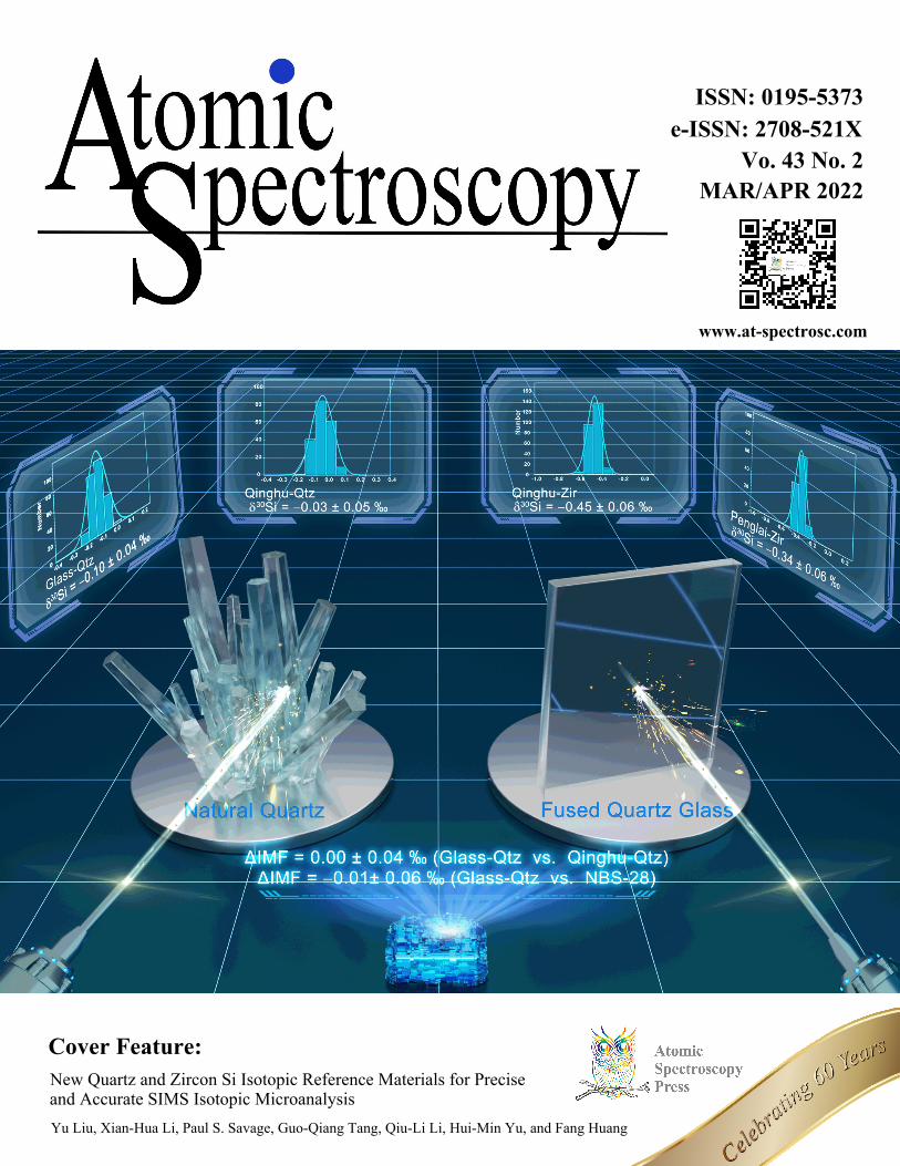
Cover Feature:New Quartz and Zircon Si Isotopic Reference Materials for Precise and Accurate SIMS Isotopic MicroanalysisYu Liu, Xian-Hua Li, Paul S. Savage, Guo-Qiang Tang, Qiu-Li Li, Hui-Min Yu, and Fang Huang

Journal Overview
The Atomic Spectroscopy
(ISSN 0195−5373; e-ISSN
2708-521X)
is a
peer-reviewed international journal started in 1962 by Dr. Walter Slavin. It
is
dedicated to advancing the analytical methodology & applications,
instrumentation & fundamentals, and the science of reference materials in the
fields of atomic spectroscopy. Publishing frequency:
Six
issues per year.
Editor in Chief
Xian-Hua Li (China)
Executive Editor
Wei Guo (China)
Associate Editors
Michael Dürr (Germany)
Wei Hang (China)
Zhaochu Hu (China)
Editorial Assistants
Anneliese Lust (USA)
Fadi. Abou-Shakra (USA)
Kenneth R. Neubauer (USA)
Ming Li (China)
Editorial Office
Address: No. 68 Jincheng Street, East Lake
High-tech Development Zone, Wuhan,
430078, P. R. China.
Tell: +8627-67883452
Fax: +8627-67883456
E-mail: [email protected]
Homepage: http://www.at-spectrosc.com
Paper Submission
Submission by
Online System: www.at-spectrosc.com
E-mail: [email protected]
Subscription/Claims
Printed Copy: U.S. $600.00 per year
E-mail: [email protected]
Article Indexing Services
Indexed in Web of Science & Scopus
2020 SCI Journal Impact Factor: 2.04
Publisher
Atomic Spectroscopy Press Limited (ASPL)
Flat H29, 1/F, Phase 2 Kwai Shing Ind. Bldg.,
No. 42-46 Tai Lin Pai Road, Kwai Chung, N.T.,
999077, Hong Kong, P.R. China
Editorial Board
Beibei Chen (Wuhan University, China)
Biyang Deng (Guangxi Normal University,
China)
Carsten Engelhard (University of Siegen,
Germany)
Chao Li (National Research Center for
Geoanalysis, China)
Chao Wei (National Institute of Metrology,
China)
Chaofeng Li (Institute of Geology and
Geophysics, CAS, China)
Chengbin Zheng (Sichuan University, China)
Diane Beauchemin (Queen's University, Canada)
Érico M. M. Flores (Universidade Federal de
Santa Maria, Brazil)
Fuyi Wang (Institute of Chemistry, CAS, China)
Haizhen Wei (Nanjing University, China)
Honglin Yuan (Northwest University, China)
Ignazio Allegretta (Università degli Studi di
Bari, Italy)
Jacob T. Shelley (Rensselaer Polytechnic
Institute, NY, USA)
Jan Kratzer (Academy of Sciences of the Czech
Republic, Czech)
Jianbo Shi (Research Center for
Eco-Environmental Sciences, CAS, China)
Jianfeng Gao (Institute of Geochemistry, CAS,
China)
Jing Liang (Beijing Haiguang Instrument Co.,
LTD., China)
Kazuaki Wagatsuma (Tohoku University,
Japan)
Ke Huang (Sichuan Norman University, China)
Kelly LeBlanc (National Research Council
Canada, Canada)
Lianbo Guo (Huazhong University of Science
and Technology, China)
Liang Fu (Chongqing University, China)
Lu Yang (National Research Council Canada,
Canada)
Luyuan Zhang (Institute of Earth Environment,
CAS, China)
Man He (Wuhan University, China)
Meirong Dong (South China University of
Technology, China)
Meng Wang (Institute of High Energy Physics,
CAS, China)
Miguel Ángel Aguirre Pastor (Universidad de
Alicante, Spain)
Mingli Chen (Northeastern University, China)
Ming Xu (Research Center for Eco-Environmental
Sciences, CAS, China)
Muharrem INCE (Munzur University, Turkey)
Mustafa Soylak (Erciyes University, Turkey)
Qian Liu (Research Center for
Eco-Environmental Sciences, CAS, China)
Qiu-Li Li (Institute of Geology and Geophysics,
CAS, China)
Rong Qian (Shanghai Institute of Ceramics, CAS,
China)
Rui Liu (Sichuan University, China)
Stefano Pagnotta (University of Pisa, Italy)
Steven Ray (State University of New York at
Buffalo, USA)
Svetlana Avtaeva (Institute of Laser Physics SB
RAS, Russia)
Taicheng Duan (Changchun Institute of Applied
Chemistry, CAS, China)
Wen Zhang (China University of Geosciences,
China)
Xiaodong Wen (Dali University, China)
Xiaomin Jiang (Sichuan University, China)
Xiaowen Yan (Xiamen University, China)
Xuefei Mao (Chinese Academy of Agricultural
Sciences, China)
Yan Luo (University of Alberta, Canada)
Yanbei Zhu (National Metrology Institute of
Japan, Japan)
Ying Gao (Chengdu University of Technology,
China)
Yongliang Yu (Northeastern University, China)
Yongguang Yin (Research Center for
Eco-Environmental Sciences, CAS, China)
Yueheng Yang (Institute of Geology and
Geophysics, CAS, China)
Yu-Feng Li (Institute of High Energy Physics,
CAS, China)
Zheng Wang (Shanghai Institute of Ceramics,
CAS, China)
Zhenli Zhu (China University of Geosciences,
China)
Zhi Xing (Tsinghua University, China)
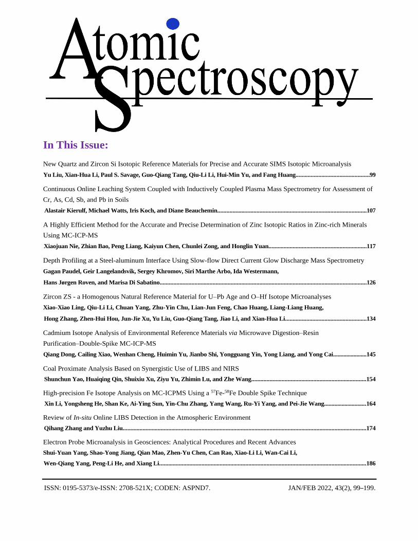
In This Issue:
New Quartz and Zircon Si Isotopic Reference Materials for Precise and Accurate SIMS Isotopic Microanalysis
Yu Liu, Xian-Hua Li, Paul S. Savage, Guo-Qiang Tang, Qiu-Li Li, Hui-Min Yu, and Fang Huang.................................................99
Continuous Online Leaching System Coupled with Inductively Coupled Plasma Mass Spectrometry for Assessment of
Cr, As, Cd, Sb, and Pb in Soils
Alastair Kierulf, Michael Watts, Iris Koch, and Diane Beauchemin...................................................................................................107
A Highly Efficient Method for the Accurate and Precise Determination of Zinc Isotopic Ratios in Zinc-rich Minerals
Using MC-ICP-MS
Xiaojuan Nie, Zhian Bao, Peng Liang, Kaiyun Chen, Chunlei Zong, and Honglin Yuan.................................................................117
Depth Profiling at a Steel-aluminum Interface Using Slow-flow Direct Current Glow Discharge Mass Spectrometry
Gagan Paudel, Geir Langelandsvik, Sergey Khromov, Siri Marthe Arbo, Ida Westermann,
Hans Jørgen Roven, and Marisa Di Sabatino.........................................................................................................................................126
Zircon ZS - a Homogenous Natural Reference Material for U–Pb Age and O–Hf Isotope Microanalyses
Xiao-Xiao Ling, Qiu-Li Li, Chuan Yang, Zhu-Yin Chu, Lian-Jun Feng, Chao Huang, Liang-Liang Huang,
Hong Zhang, Zhen-Hui Hou, Jun-Jie Xu, Yu Liu, Guo-Qiang Tang, Jiao Li, and Xian-Hua Li......................................................134
Cadmium Isotope Analysis of Environmental Reference Materials via Microwave Digestion–Resin
Purification–Double-Spike MC-ICP-MS
Qiang Dong, Cailing Xiao, Wenhan Cheng, Huimin Yu, Jianbo Shi, Yongguang Yin, Yong Liang, and Yong Cai.......................145
Coal Proximate Analysis Based on Synergistic Use of LIBS and NIRS
Shunchun Yao, Huaiqing Qin, Shuixiu Xu, Ziyu Yu, Zhimin Lu, and Zhe Wang............................................................................154
High-precision Fe Isotope Analysis on MC-ICPMS Using a 57Fe-58Fe Double Spike Technique
Xin Li, Yongsheng He, Shan Ke, Ai-Ying Sun, Yin-Chu Zhang, Yang Wang, Ru-Yi Yang, and Pei-Jie Wang.............................164
Review of In-situ Online LIBS Detection in the Atmospheric Environment
Qihang Zhang and Yuzhu Liu.................................................................................................................................................................174
Electron Probe Microanalysis in Geosciences: Analytical Procedures and Recent Advances
Shui-Yuan Yang, Shao-Yong Jiang, Qian Mao, Zhen-Yu Chen, Can Rao, Xiao-Li Li, Wan-Cai Li,
Wen-Qiang Yang, Peng-Li He, and Xiang Li.........................................................................................................................................186
ISSN: 0195-5373/e-ISSN: 2708-521X; CODEN: ASPND7. JAN/FEB 2022, 43(2), 99–199.
Guidelines for Authors
Scope: The ATOMIC SPECTROSCOPY (AS) is a peer-reviewed international journal started in 1962 by Dr. Walter
Slavin and now is published by Atomic Spectroscopy Press Limited (ASPL), Hongkong, P.R. China. It is intended for
the rapid publication of original Articles, Reviews, and Letters/Editorials in the fields of elements, elemental
speciation and isotopic analysis by AAS, AFS, ICP-OES, ICP-MS, GD-MS, TIMS, SIMS, AMS, LIBS, XRF,
SEM-EDX, EMPA, NNA, and SR-related techniques. Manuscripts dealing with (i) instrumentation & fundamentals,
(ii) methodology development & applications, and (iii) standard reference materials (SRMs) development can be
submitted for publication.
Preparation of Manuscript: The manuscript should include the text, tables, figures, and graphic abstracts, use SI
units throughout and adhere to the latest ISO and IUPAC approved terminology. Authors should study a recent issue
of Atomic Spectroscopy to ensure that papers correspond in format and style with the Journal issues after Volume 43(1)
JAN/FEB, 2022. For detailed requirements, please go to http://www.at-spectrosc.com
Text should be formatted at US letter size, with sufficient margins on either side, and all pages numbered sequentially.
The lines should be double spaced, in a single, left justified, column. Special characters, chemical formulae or
mathematical equations should be carefully typeset. Spelling should follow the conventions of British or American
English, but not a mixture of these. All tables and figure captions to be added at the end of the text.
Figures and Graphic Abstract submitted separate from the text. Since most graphs/charts/diagrams will be reduced
for publication to a single column width, authors should ensure that a sufficiently large point size is chosen for
symbols, annotation, and weight of lines so that these features will be distinguishable in the reduced version. Use a
TIFF or JPEG file (resolution > 300 dpi, size < 2 M) as the image for the figure and graphic Abstract.
Reference style:
1. T. Luo, Z. C. Hu, W. Zhang, Y. S. Liu, K. Q. Zong, L. Zhou, J. F. Zhang, and S. S. Hu, Anal. Chem., 2018, 90,
9016–9024. https://doi.org/10.1021/acs.analchem.8b01231
2. N. Dauphas and O. Rouxel, Mass Spectrom. Rev., 2006, 25, 515–550. https://doi.org/10.1002/mas.20078
3. H. Z. Lu and H. R. Fan, Fluid Inclusion. Beijing, Science Press, 2004.
Referencing templates: Endnote style files
You can automatically format references from your Endnote citation manager using our style files
(www.at-spectrosc.com/as/site/menus/20200506091044001). Files are compatible with both Windows and Macintosh.
Paper Submission: Submissions to Atomic Spectroscopy are made by Online System (http://www.at-spectrosc.com)
or by e-mail: [email protected]
Copyright
Copyright: Atomic Spectroscopy Press Limited (ASPL) holds copyright to all material published in Atomic
Spectroscopy unless otherwise noted on the first page of the paper. As soon as an article is accepted for publication,
authors will be requested to assign copyright of the article to the publisher. More information about copyright
regulations for this journal is available at http://www.at-spectrosc.com
www.at-spectrosc.com/as/article/pdf/20211110 99 At. Spectrosc. 2022, 43(2), 99–106.
New Quartz and Zircon Si Isotopic Reference Materials for
Precise and Accurate SIMS Isotopic Microanalysis
Yu Liu,a Xian-Hua Li,a,b,* Paul S. Savage,c Guo-Qiang Tang,a,b Qiu-Li Li,a,b Hui-Min Yu,d,e and Fang Huangd,e a State Key Laboratory of Lithospheric Evolution, Institute of Geology and Geophysics, Chinese Academy of Sciences, Beijing 100029, P. R. China
b College of Earth and Planetary Sciences, University of Chinese Academy of Sciences, Beijing 100049, P. R. China
c School of Earth and Environmental Sciences, University of St Andrews, Bute Building, Queen’s Terrace, St Andrews, KY16 9TS, United Kingdom
d CAS Key Laboratory of Crust-Mantle Materials and Environments, School of Earth and Space Sciences, University of Science and Technology of China,
Hefei 230026, P. R. China
e CAS Center for Excellence in Comparative Planetology, University of Science and Technology of China, Hefei 230026, P. R. China
Received: November 24, 2021; Revised: April 17, 2022; Accepted: April 23, 2022; Available online: April 25, 2022.
DOI: 10.46770/AS.2021.1110
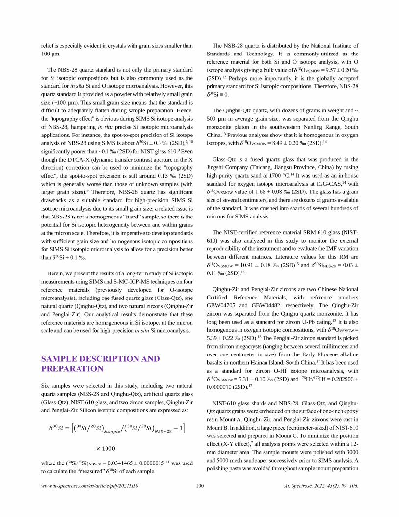
ABSTRACT: Here we report the Si isotope compositions of four potential reference materials, including one fused quartz
glass (Glass-Qtz), one natural quartz (Qinghu-Qtz), and two natural zircons (Qinghu-Zir and Penglai-Zir), suitable for in-situ Si
isotopic microanalysis. Repeated SIMS (Secondary Ion Mass Spectrometry) analyses demonstrate that these materials are more
homogeneous in Si isotopes (with the spot-to-spot uncertainty of 0.090-0.102‰), compared with the widely used NIST RM 8546
(previously NBS-28) quartz standard (with the spot-to-spot uncertainty poorer
than 0.16‰). Based on the solution-MC-ICP-MS determination, the
recommended 𝛿30Si values are −0.10 ± 0.04 ‰ (2SD), −0.03 ± 0.05 ‰ (2SD),
−0.45 ± 0.06 ‰ (2SD), and −0.34 ± 0.06 ‰ (2SD), for Glass-Qtz, Qinghu-Qtz,
Qinghu-Zir, and Penglai-Zir, respectively. Our results reveal no detectable matrix
effect on SIMS Si isotopic microanalysis between the fused quartz glass (Glass-
Qtz) and natural quartz (Qinghu-Qtz) standards. Therefore, we propose that this
synthetic quartz glass may be used as an alternative, more homogenous standard
for SIMS Si isotopic microanalysis of natural quartz samples.
INTRODUCTION
Silicon (Si) has three stable isotopes (28Si, 92.23% abundance; 29Si,
4.68%; and 30Si, 3.09%), and variations in Si isotopic composition
are typically expressed as 𝛿30SiNBS-28, which is the permil deviation
of 30Si/28Si ratio relative to the NSB-28 quartz reference standard
(N.B. NBS-28 is the historical name, and it is now referred to as
NIST RM 8546; see section 2 for the mathematical definition).
Following the pioneering works of Reynolds and Verhoogen1 and
Allenby2 in the 1950s, and the development and application of
MC-ICP-MS,3 Si isotopes have been widely used to address
various problems in Earth sciences.4 More recently, the application
of microbeam techniques such as SIMS and laser ablation (LA)-
MC-ICP-MS to Si isotopic analysis has allowed for the
investigation of Si isotopic variations at the micron scale,
significantly improving our knowledge of metal-silicate
differentiation of planetary bodies, the biogeochemical cycle of
silicon, and plate tectonics in the Early Earth.5, 6
Compared with bulk analytical methods such as Solution (S)-
MC-ICP-MS (where samples are homogenized during dissolution
and matrix elements are chemically removed prior to analysis),
well-characterized, homogeneous (to the micron scale), matrix-
matched reference materials (RMs) are prerequisites for high-
precision isotopic microanalysis using SIMS and LA-MC-ICP-
MS. Additionally, for SIMS analysis, the so-called "topography
effect"7-9 introduces extra instrument mass fraction (IMF) due to
the sample surface elevation and tilt. Thus, the surface of the
analytical targets should be sufficiently flat. However, due to the
hardness difference between the samples (usually mineral crystals)
and the epoxy resin matrix, the sample grains such as quartz and
zircon typically protrude from the epoxy resin after polishing. This
www.at-spectrosc.com/as/article/pdf/20211110 At. Spectrosc. 2022, 43(2), 99–106.
relief is especially evident in crystals with grain sizes smaller than
100 µm.
The NBS-28 quartz standard is not only the primary standard
for Si isotopic compositions but is also commonly used as the
standard for in situ Si and O isotope microanalysis. However, this
quartz standard is provided as a powder with relatively small grain
size (~100 µm). This small grain size means that the standard is
difficult to adequately flatten during sample preparation. Hence,
the "topography effect" is obvious during SIMS Si isotope analysis
of NBS-28, hampering in situ precise Si isotopic microanalysis
applications. For instance, the spot-to-spot precision of Si isotope
analysis of NBS-28 using SIMS is about 𝛿30Si ± 0.3 ‰ (2SD),9, 10
significantly poorer than ~0.1 ‰ (2SD) for NIST glass 610.9 Even
though the DTCA-X (dynamic transfer contrast aperture in the X
direction) correction can be used to minimize the "topography
effect", the spot-to-spot precision is still around 0.15 ‰ (2SD)
which is generally worse than those of unknown samples (with
larger grain sizes).9 Therefore, NBS-28 quartz has significant
drawbacks as a suitable standard for high-precision SIMS Si
isotope microanalysis due to its small grain size; a related issue is
that NBS-28 is not a homogeneous “fused” sample, so there is the
potential for Si isotopic heterogeneity between and within grains
at the micron scale. Therefore, it is imperative to develop standards
with sufficient grain size and homogenous isotopic compositions
for SIMS Si isotopic microanalysis to allow for a precision better
than 𝛿30Si ± 0.1 ‰.
Herein, we present the results of a long-term study of Si isotopic
measurements using SIMS and S-MC-ICP-MS techniques on four
reference materials (previously developed for O-isotope
microanalysis), including one fused quartz glass (Glass-Qtz), one
natural quartz (Qinghu-Qtz), and two natural zircons (Qinghu-Zir
and Penglai-Zir). Our analytical results demonstrate that these
reference materials are homogeneous in Si isotopes at the micron
scale and can be used for high-precision in situ Si microanalysis.
SAMPLE DESCRIPTION AND
PREPARATION
Six samples were selected in this study, including two natural
quartz samples (NBS-28 and Qinghu-Qtz), artificial quartz glass
(Glass-Qtz), NIST-610 glass, and two zircon samples, Qinghu-Zir
and Penglai-Zir. Silicon isotopic compositions are expressed as:
𝛿 𝑆𝑖30 = [( 𝑆𝑖30 𝑆𝑖28⁄ )𝑆𝑎𝑚𝑝𝑙𝑒
( 𝑆𝑖30 𝑆𝑖28⁄ )𝑁𝐵𝑆−28
⁄ − 1]
× 1000
where the (30Si/28Si)NBS-28 = 0.0341465 ± 0.0000015 11 was used
to calculate the “measured” 𝛿30Si of each sample.
The NSB-28 quartz is distributed by the National Institute of
Standards and Technology. It is commonly-utilized as the
reference material for both Si and O isotope analysis, with O
isotope analysis giving a bulk value of 𝛿18OVSMOW = 9.57 ± 0.20 ‰
(2SD).12 Perhaps more importantly, it is the globally accepted
primary standard for Si isotopic compositions. Therefore, NBS-28
𝛿30Si ≡ 0.
The Qinghu-Qtz quartz, with dozens of grams in weight and ~
500 µm in average grain size, was separated from the Qinghu
monzonite pluton in the southwestern Nanling Range, South
China.13 Previous analyses show that it is homogenous in oxygen
isotopes, with 𝛿18OVSMOW = 8.49 ± 0.20 ‰ (2SD).14
Glass-Qtz is a fused quartz glass that was produced in the
Jingshi Company (Taicang, Jiangsu Province, China) by fusing
high-purity quartz sand at 1700 °C.14 It was used as an in-house
standard for oxygen isotope microanalysis at IGG-CAS,14 with
𝛿18OVSMOW value of 1.68 ± 0.08 ‰ (2SD). The glass has a grain
size of several centimeters, and there are dozens of grams available
of the standard. It was crushed into shards of several hundreds of
microns for SIMS analysis.
The NIST-certified reference material SRM 610 glass (NIST-
610) was also analyzed in this study to monitor the external
reproducibility of the instrument and to evaluate the IMF variation
between different matrices. Literature values for this RM are
𝛿18OVSMOW = 10.91 ± 0.18 ‰ (2SD)15 and 𝛿30SiNBS-28 = 0.03 ±
0.11 ‰ (2SD).16
Qinghu-Zir and Penglai-Zir zircons are two Chinese National
Certified Reference Materials, with reference numbers
GBW04705 and GBW04482, respectively. The Qinghu-Zir
zircon was separated from the Qinghu quartz monzonite. It has
long been used as a standard for zircon U-Pb dating.13 It is also
homogenous in oxygen isotopic compositions, with 𝛿18OVSMOW =
5.39 ± 0.22 ‰ (2SD).13 The Penglai-Zir zircon standard is picked
from zircon megacrysts (ranging between several millimeters and
over one centimeter in size) from the Early Pliocene alkaline
basalts in northern Hainan Island, South China.17 It has been used
as a standard for zircon O-Hf isotope microanalysis, with
𝛿18OVSMOW = 5.31 ± 0.10 ‰ (2SD) and 176Hf/177Hf = 0.282906 ±
0.0000010 (2SD).17
NIST-610 glass shards and NBS-28, Glass-Qtz, and Qinghu-
Qtz quartz grains were embedded on the surface of one-inch epoxy
resin Mount A. Qinghu-Zir, and Penglai-Zir zircons were cast in
Mount B. In addition, a large piece (centimeter-sized) of NIST-610
was selected and prepared in Mount C. To minimize the position
effect (X-Y effect),7 all analysis points were selected within a 12-
mm diameter area. The sample mounts were polished with 3000
and 5000 mesh sandpaper successively prior to SIMS analysis. A
polishing paste was avoided throughout sample mount preparation
100
www.at-spectrosc.com/as/article/pdf/20211110 At. Spectrosc. 2022, 43(2), 99–106.
to reduce the "topography effect” influence. The polished mounts
were cleaned several times using alcohol and deionized water.
Afterward, the mounts were dried and gold-coated under vacuum,
then placed in the vacuum chamber of the SIMS for ~ 24 hours
before analysis to reduce the interference of hydrides.
EXPERIMENTAL METHODS
In situ Si isotope measurements using SIMS. In situ Si isotope
measurements in this study were conducted on the Cameca IMS-
1280 Large geometry Multi-Collector SIMS, located at the
Institute of Geology and Geophysics, Chinese Academy of
Sciences, in Beijing.
To overcome the low yield of silicon signal from quartz and
zircon in SIMS analysis, a ~15 µm Cs+ primary beam with an
intensity of 7 to 12 nA was tuned at the potential of +10 kV. A ~20
µm raster size was employed to avoid a deep crater. A high-density
electron beam from a normal incidence electron gun (NEG) was
tuned to obtain a maxim emission current of ~2.3 mA. During
analysis, the entrance slit of 200 µm and field aperture of 5500 µm
were used. Two Faraday cups located at the L'2 and H1 positions
of the multi-collector system were used to measure the 28Si and 30Si signals simultaneously, connected to the pre-amplifiers with
resistors of 1010 and 1012 Ω, respectively. Both detectors were
equipped with a ~700 µm exit slit to obtain a broad flat top mass
peak. Based on different NEG tunings, the typical secondary ion
yield of 28Si was 5.4 to 7.1×10⁷ cps/nA for quartz samples and 3.6
to 4.4×10⁷ cps/nA for the zircon samples, respectively.
With a data integration time of 120 s, the total analytical time of
each analysis was ~ 4.5 min, which included a pre-sputtering of 30
s to ensure a stable secondary ion intensity. Before data acquisition,
the secondary ion beam centering procedure, including the
dynamic transfer field aperture (DTFA-X and DTFA-Y) and the
DTCA-X, was applied automatically to minimize the influence of
the "topography effect". Drift correction against time and DTCA-
X correction9 were performed when necessary. Our previous
study9 showed that using the linear relationship between the
measured 𝛿30Si value and the DTCA-X parameters in the same
session to correct the obtained Si-isotope data can effectively
improve the accuracy and precision of in situ Si isotope analysis.
Specific principles and detailed correction methods can be found
in Liu et al.9 Our measured Si isotopic compositions were
normalized to the value from the S-MC-ICP-MS analysis to
compare the results from different analytical sessions.
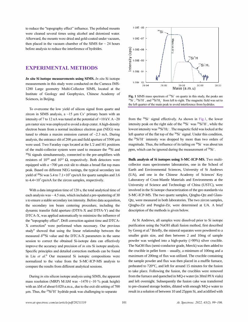
During in situ silicon isotope analysis using SIMS, the apparent
mass resolution (MRP) M/∆M was ~1470 (~10 % peak height)
with an ∆M of about 0.020 a.m.u., due to the exit slit setting of 700
µm. Thus, the 29Si1H− hydride peak was challenging to separate
Fig. 1 SIMS mass spectrum of 30Si−
on quartz in this study, the peaks are
30Si−, 29Si1H−, and 28Si1H2−
from left to right. The magnetic field was set to
the left quarter of the main peak to avoid interference from hydrides.
from the 30Si− signal effectively. As shown in Fig.1, the lower
intensity peak on the right side of the 30Si− was 29Si1H−, while the
lowest intensity was 28Si1H2−. The magnetic field was locked at the
left quarter of the flat top of the 30Si− signal. Under this condition,
the 29Si1H− intensity was dropped by more than two orders of
magnitude. Thus, the influence of its tailing on 30Si− was about ten
ppm, which can be ignored during the measurement of 30Si−.
Bulk analysis of Si isotopes using S-MC-ICP-MS. Two multi-
collector mass spectrometer laboratories, one in the School of
Earth and Environmental Sciences, University of St Andrews
(UA), and one in the Chinese Academy of Sciences' Key
Laboratory of Crust-Mantle Materials and Environments at the
University of Science and Technology of China (USTC), were
involved in the Si isotope characterization of the geo standards via
S-MC-ICP-MS. The two quartz samples, Qinghu-Qtz and Glass-
Qtz, were measured in both laboratories. The two zircon samples,
Qinghu-Zir and Penglai-Zir, were determined at UA. A brief
description of the methods is given below.
At St Andrews, all samples were dissolved prior to Si isotope
purification using the NaOH alkali fusion method, first described
by Georg et al.3 Briefly, the mineral separates were powdered to a
smaller grain size, and then between 2 and 10mg of sample
powder was weighed into a high-purity (>99%) silver crucible.
The NaOH flux (semi-conductor grade, Merck) was then added to
the crucible in pellet form – usually, a minimum of 100mg and a
maximum of 200mg of flux was utilized. The crucible containing
the sample powder and flux was then placed in a muffle furnace,
preheated to 720°C, and left for around 15 minutes for the fusion
to take place. Following the fusion, the crucibles were removed
from the furnace and quenched in MQ-e water (in 30ml PFA vials)
and left overnight. Subsequently the fusion cake was transferred
to pre-cleaned storage bottles, diluted with enough MQ-e water to
result in a solution of between 10 and 25ppm Si, and acidified with
101
www.at-spectrosc.com/as/article/pdf/20211110 At. Spectrosc. 2022, 43(2), 99–106.
enough conc. high purity HNO3 to both neutralize the NaOH and
reduce the pH of the solution to ~ 2.
The sample Si was purified for S-MC-ICP-MS analysis using
the single-stage cation exchange procedure first described in
Georg et al.3 and further discussed in Savage and Moynier
(2013).18 Here, enough sample solution containing 20µg of Si was
loaded into a BioRad Polyprep column containing 1.8 mL of
precleaned AG50W-X12, 200–400 mesh cation exchange resin,
Bio-Rad, USA. The Si, at low pH, is in the neutral H4SiO4 or
anionic H3SiO4− forms and so can be eluted immediately using
5ml of MQ-e water (whereas matrix cations are retained on the
resin). Once the Si was eluted, it was acidified to 0.22M HNO3
before MC-ICPMS analysis. Silicon yield from the columns is
always >99% and total procedural blanks are ≤ 50ng of Si, which
is negligible compared to the 20µg of Si in sample.
Si isotopes were measured on a Thermo-Fischer Neptune-Plus
MC-ICP-MS instrument. Samples were introduced into the
instrument via an ESI PFA 75µl min-1 Microflow nebulizer, into
the Thermo SIS spray chamber. The instrument was fitted with
nickel “Jet” sampler and H-skimmer cones and operated at
medium mass resolution (M/∆M ≈ 7500) to resolve the large
molecular interferences on the 29Si and 30Si isotope beams. Sample
isotope ratios were measured using the “sample-standard
bracketing" procedure, using NBS-28 as the bracketing standard.
Isotope beams were measured in the L3 (28Si), C (29Si), and H3
(30Si) Faraday collectors and with 25 cycles of ~8 sec integrations,
bracketed by on-peak blank measurements. The blank corrections,
isotope ratios and δ30Si and δ29Si values were calculated offline.
At USTC, the sample powder mixed with high purity NaOH
powder was heated in a silver crucible at 720 for 10 min to
produce a water-soluble metastable silicate. The crucible was kept
at the temperature of 80 for 12 h on a hotplate. Nitric acid was
added to the sample solution to attain a solution acidity of 1%
HNO3 (v/v) for column chemistry. A cation exchange resin (2 mL
of AG50W-X12, 200–400 mesh, Bio-Rad, USA) was used to
purify Si. The sample solution, containing ~30 μg of Si, went
through the column after the resin was sequentially cleaned with 3
mol L−1 HNO3, 6 mol L−1 HNO3, and 6 mol L−1 HCl and then
conditioned with water. Silicon was collected right after the
sample solution was loaded and was further eluted with 6 mL of
water. The yield of Si was >99%, and the total procedural blank
was ~20 ng, which is negligible relative to the ~30 μg of Si loaded
into the column.
Silicon isotope ratios were analyzed with an MC-ICP-MS
instrument (Neptune Plus from Thermo-Fisher Scientific). During
analysis, nickel cones (H skimmer and Jet sampler, Thermo-Fisher
Scientific) were used. Three stable isotopes of Si (28Si, 29Si, and 30Si) were collected using FCs on L3, C, and H3, respectively, at
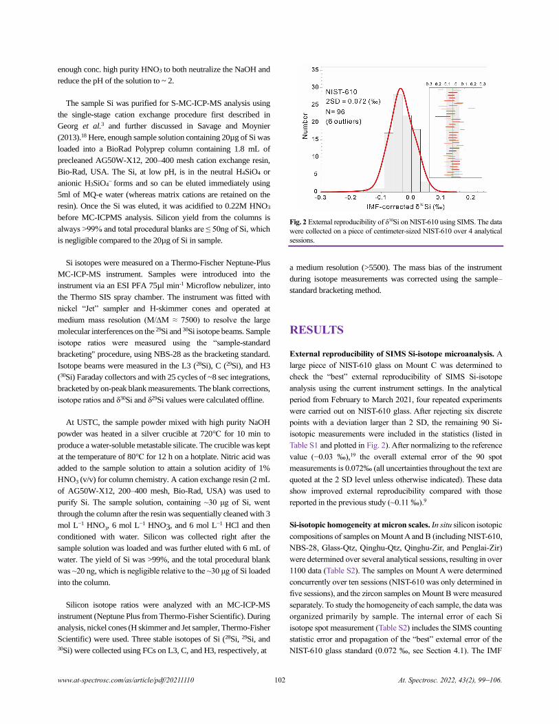
Fig. 2 External reproducibility of δ30Si on NIST-610 using SIMS. The data
were collected on a piece of centimeter-sized NIST-610 over 4 analytical
sessions.
a medium resolution (>5500). The mass bias of the instrument
during isotope measurements was corrected using the sample–
standard bracketing method.
RESULTS
External reproducibility of SIMS Si-isotope microanalysis. A
large piece of NIST-610 glass on Mount C was determined to
check the “best” external reproducibility of SIMS Si-isotope
analysis using the current instrument settings. In the analytical
period from February to March 2021, four repeated experiments
were carried out on NIST-610 glass. After rejecting six discrete
points with a deviation larger than 2 SD, the remaining 90 Si-
isotopic measurements were included in the statistics (listed in
Table S1 and plotted in Fig. 2). After normalizing to the reference
value (−0.03 ‰),19 the overall external error of the 90 spot
measurements is 0.072‰ (all uncertainties throughout the text are
quoted at the 2 SD level unless otherwise indicated). These data
show improved external reproducibility compared with those
reported in the previous study (~0.11 ‰).9
Si-isotopic homogeneity at micron scales. In situ silicon isotopic
compositions of samples on Mount A and B (including NIST-610,
NBS-28, Glass-Qtz, Qinghu-Qtz, Qinghu-Zir, and Penglai-Zir)
were determined over several analytical sessions, resulting in over
1100 data (Table S2). The samples on Mount A were determined
concurrently over ten sessions (NIST-610 was only determined in
five sessions), and the zircon samples on Mount B were measured
separately. To study the homogeneity of each sample, the data was
organized primarily by sample. The internal error of each Si
isotope spot measurement (Table S2) includes the SIMS counting
statistic error and propagation of the “best” external error of the
NIST-610 glass standard (0.072 ‰, see Section 4.1). The IMF
102
www.at-spectrosc.com/as/article/pdf/20211110 At. Spectrosc. 2022, 43(2), 99–106.
Table 1. Summary of SIMS 𝛿30Si homogeneity check of the six samples
Sample
Primary
beam
(nA)
Sessions n 2SD (‰)
over all
2SD (‰)
range in each
session
Glass-Qtz 7.3-10.9 10 234 (-7) 0.090 0.06-0.13
Qinghu-Qtz 7.4-10.9 10 207 (-6) 0.102 0.06-0.14
NBS-28 7.4-10.1 10 181(-7) 0.160 0.11-0.31
NIST-610 9.4-10.7 5 85(-4) 0.112 0.07-0.12
Qinghu-Zir 6.0-13.1 7 260 (-4) 0.094 0.07-0.13
Penglai-Zir 8.1-15.7 5 148 (-3) 0.096 0.08-0.10
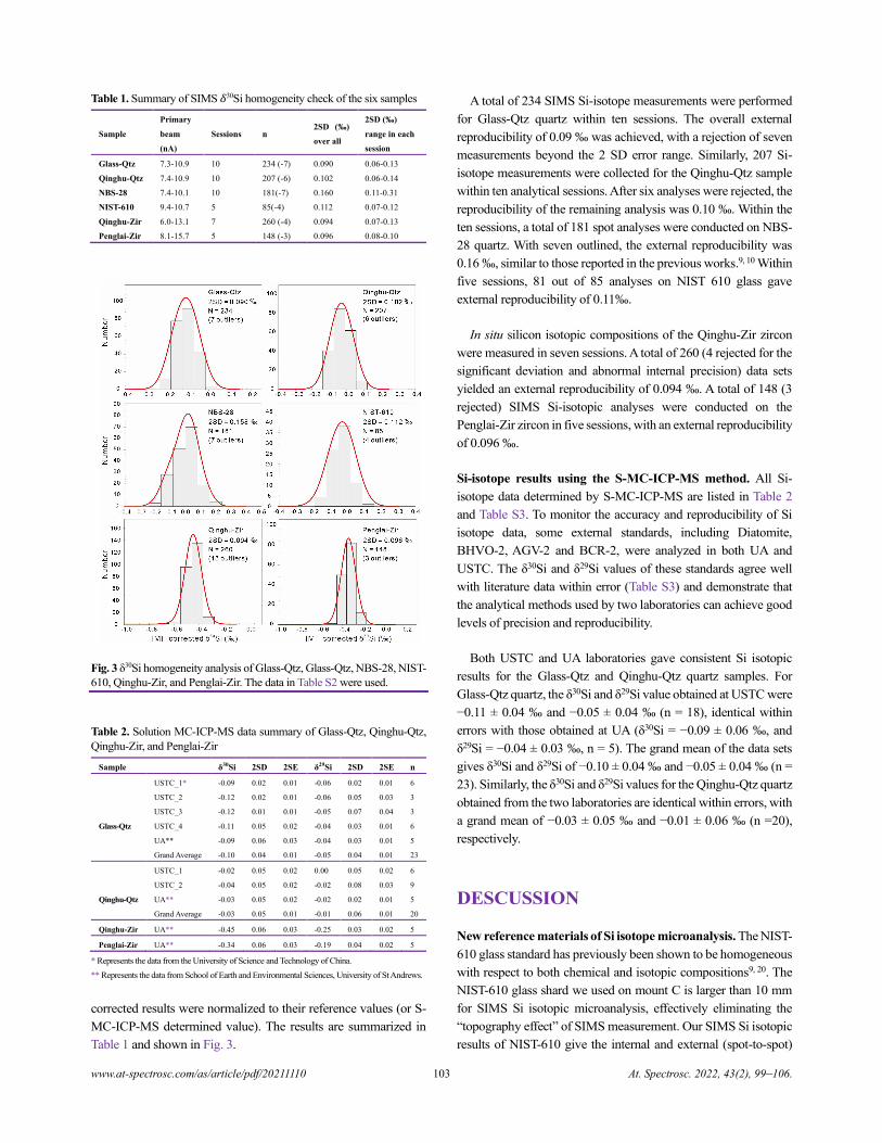
Fig. 3 δ30Si homogeneity analysis of Glass-Qtz, Glass-Qtz, NBS-28, NIST-
610, Qinghu-Zir, and Penglai-Zir. The data in Table S2 were used.
Table 2. Solution MC-ICP-MS data summary of Glass-Qtz, Qinghu-Qtz,
Qinghu-Zir, and Penglai-Zir
Sample δ30Si 2SD 2SE δ29Si 2SD 2SE n
Glass-Qtz
USTC_1* -0.09 0.02 0.01 -0.06 0.02 0.01 6
USTC_2 -0.12 0.02 0.01 -0.06 0.05 0.03 3
USTC_3 -0.12 0.01 0.01 -0.05 0.07 0.04 3
USTC_4 -0.11 0.05 0.02 -0.04 0.03 0.01 6
UA** -0.09 0.06 0.03 -0.04 0.03 0.01 5
Grand Average -0.10 0.04 0.01 -0.05 0.04 0.01 23
Qinghu-Qtz
USTC_1 -0.02 0.05 0.02 0.00 0.05 0.02 6
USTC_2 -0.04 0.05 0.02 -0.02 0.08 0.03 9
UA** -0.03 0.05 0.02 -0.02 0.02 0.01 5
Grand Average -0.03 0.05 0.01 -0.01 0.06 0.01 20
Qinghu-Zir UA** -0.45 0.06 0.03 -0.25 0.03 0.02 5
Penglai-Zir UA** -0.34 0.06 0.03 -0.19 0.04 0.02 5
* Represents the data from the University of Science and Technology of China.
** Represents the data from School of Earth and Environmental Sciences, University of St Andrews.
corrected results were normalized to their reference values (or S-
MC-ICP-MS determined value). The results are summarized in
Table 1 and shown in Fig. 3.
A total of 234 SIMS Si-isotope measurements were performed
for Glass-Qtz quartz within ten sessions. The overall external
reproducibility of 0.09 ‰ was achieved, with a rejection of seven
measurements beyond the 2 SD error range. Similarly, 207 Si-
isotope measurements were collected for the Qinghu-Qtz sample
within ten analytical sessions. After six analyses were rejected, the
reproducibility of the remaining analysis was 0.10 ‰. Within the
ten sessions, a total of 181 spot analyses were conducted on NBS-
28 quartz. With seven outlined, the external reproducibility was
0.16 ‰, similar to those reported in the previous works.9, 10 Within
five sessions, 81 out of 85 analyses on NIST 610 glass gave
external reproducibility of 0.11‰.
In situ silicon isotopic compositions of the Qinghu-Zir zircon
were measured in seven sessions. A total of 260 (4 rejected for the
significant deviation and abnormal internal precision) data sets
yielded an external reproducibility of 0.094 ‰. A total of 148 (3
rejected) SIMS Si-isotopic analyses were conducted on the
Penglai-Zir zircon in five sessions, with an external reproducibility
of 0.096 ‰.
Si-isotope results using the S-MC-ICP-MS method. All Si-
isotope data determined by S-MC-ICP-MS are listed in Table 2
and Table S3. To monitor the accuracy and reproducibility of Si
isotope data, some external standards, including Diatomite,
BHVO-2, AGV-2 and BCR-2, were analyzed in both UA and
USTC. The δ30Si and δ29Si values of these standards agree well
with literature data within error (Table S3) and demonstrate that
the analytical methods used by two laboratories can achieve good
levels of precision and reproducibility.
Both USTC and UA laboratories gave consistent Si isotopic
results for the Glass-Qtz and Qinghu-Qtz quartz samples. For
Glass-Qtz quartz, the δ30Si and δ29Si value obtained at USTC were
−0.11 ± 0.04 ‰ and −0.05 ± 0.04 ‰ (n = 18), identical within
errors with those obtained at UA (δ30Si = −0.09 ± 0.06 ‰, and
δ29Si = −0.04 ± 0.03 ‰, n = 5). The grand mean of the data sets
gives δ30Si and δ29Si of −0.10 ± 0.04 ‰ and −0.05 ± 0.04 ‰ (n =
23). Similarly, the δ30Si and δ29Si values for the Qinghu-Qtz quartz
obtained from the two laboratories are identical within errors, with
a grand mean of −0.03 ± 0.05 ‰ and −0.01 ± 0.06 ‰ (n =20),
respectively.
DESCUSSION
New reference materials of Si isotope microanalysis. The NIST-
610 glass standard has previously been shown to be homogeneous
with respect to both chemical and isotopic compositions9, 20. The
NIST-610 glass shard we used on mount C is larger than 10 mm
for SIMS Si isotopic microanalysis, effectively eliminating the
“topography effect” of SIMS measurement. Our SIMS Si isotopic
results of NIST-610 give the internal and external (spot-to-spot)
103
www.at-spectrosc.com/as/article/pdf/20211110 At. Spectrosc. 2022, 43(2), 99–106.
precision of ~0.05 ‰ and ~0.07 ‰ (Fig. 2), respectively,
representing the current “highest level” of precision and accuracy
of SIMS Si microanalysis.
Figure 3 summarizes the Si-isotope homogeneity of different
samples at micron scales using SIMS analysis, including two
quartz crystals, one fused glass O-isotope standard, the NIST-610
glass, and two zircon age and O-Hf isotope standards. All analyses
of six standards show Gaussian distributions, suggesting they are
homogeneous in Si isotopes. The Glass-Qtz, Qinghu-Qtz, Qinghu-
Zir, Penglai-Zir, and NIST-610 standards have the external
precision of 0.090 ‰, 0.102 ‰, 0.094 ‰, 0.096 ‰, and 0.112 ‰,
respectively, suggesting that all of them are suitable for the Si
isotope microanalysis. Among them, the Glass-Qtz quartz has the
best level of homogeneity of Si isotopes. Based on S-MC-ICP-MS
analyses, the δ30Si value of −0.10 ± 0.04 ‰ (2SD), −0.03 ± 0.05 ‰
(2SD), −0.45 ± 0.06 ‰ (2SD), and −0.34 ± 0.06 ‰ (2SD) are
recommended for Glass-Qtz, Qinghu-Qtz, Qinghu-Zir, and
Penglai-Zir, respectively. Considering Qinghu-Qtz quartz and
Qinghu-Zir zircon are separated from the same rock, we can
calculate Si-isotope fractionation between quartz and zircon:
δ30Si(qtz) – δ30Si(zir) = ∆30Si(qtz-zir) = 0.42 ± 0.06 ‰, which
corresponds to ~671 oC based on the first‑principles calculation of
equilibrium fractionation of Si isotopes in quartz and zircon
system.21 This Si-isotope thermometry result agrees with the O-
isotope equilibrium temperature of 656 ± 62 oC in quartz and
zircon,22 further supporting the reliability of our Si isotope results.
Compared with the NIST-610 glass standard, quartz, and zircon
standards described above, our NBS-28 quartz analyses provide a
much poorer external precision of about 0.16 ‰ for Si isotopes at
the micron scale, similar to those reported in previous works9, 10.
Therefore, we posit that NBS-28 is not an ideal standard for high-
precision Si isotopic microanalysis; although it is likely
homogeneous in Si isotopes at the milligram level typically
processed for S-MC-ICPMS measurements, we suggest that a
suite of well-characterized standards (such as those described
above) that are homogeneous at the micron level vs. NBS-28 in
terms of its Si isotope composition are more ideal for SIMS 𝛿30Si
and 𝛿29Si measurements.
Glass-Qtz as an alternative standard for precise SIMS quartz
Si isotopic microanalysis. Our SIMS analytical results
demonstrate that the Glass-Qtz quartz has excellent homogeneous
Si-isotopic compositions. However, it is noteworthy that the
structure of synthetic uncrystallized quartz glass is different from
that of natural crystallized quartz crystals. Therefore, when
assessing the use of a synthetic quartz standard (such as Glass-Qtz
quartz) for bracketing natural SIMS quartz Si-isotope analysis, we
must consider the potential for a matrix effect between the two. As
described in experimental section, all quartz standards Glass-Qtz,
Qinghu-Qtz, NBS-28, and NIST-610 were concurrently measured
using SIMS. These analytical results can be used to investigate the
Table 3. The IMF determination between the natural quartz samples and
the synthetic samples in ten sessions
Sample
name
Mean value of
𝛿30Si
Calculated
IMF
ΔIMF 2SD
Session 1
25/08/2020
Glass-Qtz -0.30 -0.20 0.00 0.06
NBS28 -0.18 -0.18 0.02 0.13
Qinghu -0.22 -0.19 0.00 0.11
Session 2
28/08/2020
Glass-Qtz -0.15 -0.05 0.00 0.11
NBS28 -0.09 -0.09 -0.04 0.11
Qinghu -0.08 -0.05 0.01 0.12
Session 3
06/10/2020
Glass-Qtz -0.01 0.09 0.00 0.08
NBS28 0.07 0.07 -0.01 0.15
Qinghu 0.02 0.05 -0.04 0.11
Session 4
7/16/2020
Glass-Qtz -0.70 -0.60 0.00 0.13
NBS28 -0.59 -0.59 0.02 0.14
Qinghu -0.51 -0.48 0.13 0.14
Session 5
31/01/2021
Glass-Qtz 0.38 0.48 0.00 0.11
NBS28 0.45 0.45 -0.03 0.22
Qinghu 0.47 0.50 0.02 0.12
NIST610 8.05 8.08 7.60 0.12
Session 6
06/02/2021
Glass-Qtz -0.11 -0.01 0.00 0.08
NBS28 -0.09 -0.09 -0.08 0.19
Qinghu -0.05 -0.02 -0.01 0.10
NIST610 7.49 7.52 7.53 0.11
Session 7
07/02/2021
Glass-Qtz -0.76 -0.66 0.00 0.10
NBS28 -0.68 -0.68 -0.03 0.18
Qinghu -0.66 -0.63 0.03 0.10
Session 8
24/02/2021
Glass-Qtz -0.13 -0.03 0.00 0.06
NBS28 -0.02 -0.02 0.00 0.15
Qinghu -0.07 -0.04 -0.02 0.06
NIST610 7.58 7.55 7.57 0.08
Session 9
25/02/2021
Glass-Qtz 0.02 0.12 0.00 0.08
NBS28 0.14 0.14 0.02 0.15
Qinghu 0.09 0.12 0.00 0.08
NIST610 7.84 7.87 7.75 0.12
Session 10
18/03/2021
Glass-Qtz 0.12 0.22 0.00 0.08
NBS28 0.20 0.20 -0.02 0.11
Qinghu 0.18 0.21 0.00 0.11
NIST610 7.94 7.97 7.75 0.07
feasibility of using Glass-Qtz quartz glass as an alternative
standard for precise SIMS quartz Si isotopic microanalysis.
Reference values of NBS-28 (𝛿30Si = 0 ‰) and NIST-610 glass
(−0.03 ‰)19, and our newly obtained 𝛿30Si values for Qinghu-Qtz
(−0.03 ‰) and Glass-Qtz (−0.10 ‰) are used as recommended
values. The difference between the calculated IMF and the
reference value (IMFSIMS− IMFRef) was defined as ΔIMF hereafter.
Taking the IMF value of Glass-Qtz as the benchmark (ΔIMF=0)
and the external standard deviation as the corresponding ΔIMF
error, the ∆IMFs of the other three standards were calculated.
Analytical data can be found in Table S4, and the results are
summarized in Table 3 and plotted in Fig. 4. According to the
calculated results of data sets from 10 sessions, the SIMS Si-
isotope values of Qinghu-Qtz and NBS-28 natural quartzes are
consistent within analytical errors with those obtained by the S-
MC-ICP-MS method. The average ∆IMF of Qinghu-Qtz and
NBS-28 were 0.00 ± 0.04 ‰ (with session four rejected) and
−0.01 ± 0.06 ‰, respectively, which indicates that no matrix effect
between quartz glass (Glass-Qtz) and natural quartz crystal can be
detected under current external reproducibility (~0.1 ‰,2SD) of
104
www.at-spectrosc.com/as/article/pdf/20211110 At. Spectrosc. 2022, 43(2), 99–106.
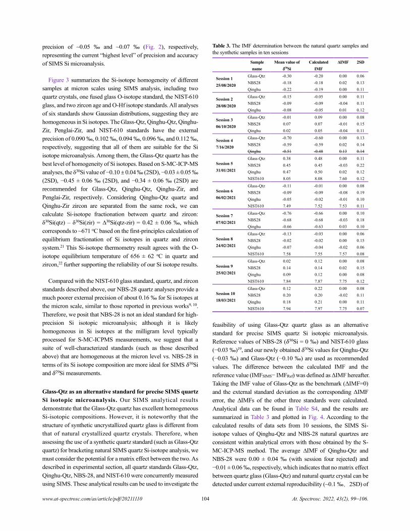
Fig. 4 The ΔIMFSi of the silicon isotope compositions between quartz and
glass were determined in ten sessions using SIMS. There is no detectable
matrix effects between the synthetic quartz glass (Glass-Qtz) and two
natural quartz samples (NBS-28 and Qinghu-Qtz) within the external
precisions.
SIMS Si-isotope analysis.
On the contrary, the NIST-610 glass has an ∆IMF value ranging
from 7.53 to 7.75 ‰, which is neither close to zero nor constant.
Although NIST-610 glass is considerably homogenous in Si
isotopes on the micron scale, it is not suitable as an RM for SIMS
Si isotope microanalysis.
CONCLUSIONS
In this study, we improve the external reproducibility of SIMS Si-
isotope microanalysis from 0.11 ‰ (2SD)9 to 0.07 ‰ (2SD) for
large shards of NIST 610 glass. Four standards previously utilized
for SIMS O-isotope microanalysis, including Glass-Qtz, Qinghu-
Qtz, Qinghu-Zir, and Penglai-Zir, are herein proved to be
homogeneous in their Si-isotopic compositions at the micron scale,
and their Si-isotopes have been precisely determined by S-MC-
ICP-MS. Thus, they can be used as standards for both O- and Si-
isotope microanalysis, allowing the SIMS isotope data to be recast
relative to VSMOW and NBS-28. We also demonstrate that there
is no detectable matrix effect of SIMS Si isotope microanalysis
between the synthetic quartz (Glass-Qtz) and natural quartz
standards at the 0.1‰ precision level. Therefore, the synthetic
Glass-Qtz quartz glass can be used as an alternative RM for precise
SIMS quartz Si isotope analysis.
ASSOCIATED CONTENT
The supporting information (Tables S1-S4) is available at www.at-
spectrosc.com/as/home
AUTHOR INFORMATION
Xian-Hua Li received his BSc in 1983
from the University of Science and
Technology of China, and PhD in 1988
from the Institute of Geochemistry,
Chinese Academy of Sciences (CAS).
He is a research professor of
geochemistry at the Institute of Geology
and Geophysics, CAS and the chief
professor of geochemistry in the
University of CAS. His major research
interests are isotope geochronology,
geochemistry, isotopic microanalysis and
their applications to igneous petrogenesis,
chemical geodynamics and evolution of Earth and Moon. He has been
working as editor-in-chief of Atomic Spectroscopy, associate editor of
Precambrian Research, Geological Magazine, and American Journal of
Science, and member of editorial committee in many other academic
journals. Xian-Hua Li is author or co-author of over 400 articles published
in peer-reviewed scientific journals, with an h-index of 101 (Web of
Science). He was elected as a Fellow of the Geological Society of America
in 2007, Academician of CAS in 2019, and named as Clarivate Analytics
Global Highly Cited Scientist, ESI Global Highly Cited Scholar and
Elsevier China Highly Cited Scholar.
Corresponding Author
*X.-H. Li
Email address: [email protected]
Notes
The authors declare no competing financial interest.
ACKNOWLEDGMENTS
We thank Hong-Xia Ma for her excellent sample preparation work.
We also thank two anonymous reviewers for their helpful
comments, which greatly improved this manuscript. This work
was financially supported by the National Key R&D Program of
China (2018YFA0702600) and National Science Foundation of
China (41890831).
REFERENCES
1. J. H. Reynolds and J. Verhoogen, Geochim. Cosmochim. Ac.,
1953, 3, 224–234. https://doi.org/10.1016/0016-7037(53)90041-6
2. R. Allenby, Geochim. Cosmochim. Ac., 1954, 5, 40–48.
https://doi.org/10.1016/0016-7037(54)90060-5
3. R. B. Georg, B. C. Reynolds, M. Frank, and A. N. Halliday,
Chem. Geol., 2006, 235, 95–104.
https://doi.org/10.1016/j.chemgeo.2006.06.006
105
www.at-spectrosc.com/as/article/pdf/20211110 At. Spectrosc. 2022, 43(2), 99–106.
4. F. Poitrasson, Rev. Mineral. Geochem., 2017, 82, 289–344.
https://doi.org/10.2138/rmg.2017.82.8
5. D. Trail, P. Boehnke, P. S. Savage, M.-C. Liu, M. L. Miller, and
I. Bindeman, P. Natl. Acad. Sci. USA, 2018, 115, 10287–10292.
https://doi.org/10.1073/pnas.1808335115
6. M. Guitreau, A. Gannoun, Z. Deng, M. Chaussidon, F. Moynier,
B. Barbarin, and J. Marin-Carbonne, Geochim. Cosmochim. Ac.,
2022, 316, 273–294. https://doi.org/10.1016/j.gca.2021.09.029
7. N. T. Kita, T. Ushikubo, B. Fu, and J. W. Valley, Chem. Geol.,
2009, 264, 43–57. https://doi.org/10.1016/j.chemgeo.2009.02.012
8. G.-Q. Tang, X.-H. Li, Q.-L. Li, Y. Liu, X.-X. Ling, and Q.-Z. Yin,
J. Anal. At. Spectrom., 2015, 30, 950–956.
https://doi.org/10.1039/C4JA00458B
9. Y. Liu, X.-H. Li, G.-Q. Tang, Q.-L. Li, X.-C. Liu, H.-M. Yu, and
F. Huang, J. Anal. At. Spectrom., 2019, 34, 906–914.
https://doi.org/10.1039/C8JA00431E
10. P. R. Heck, J. M. Huberty, N. T. Kita, T. Ushikubo, R. Kozdon,
and J. W. Valley, Geochim. Cosmochim. Ac., 2011, 75,
5879–5891. https://doi.org/10.1016/j.gca.2011.07.023
11. T. Ding, D. Wan, R. Bai, Z. Zhang, Y. Shen, and R. Meng,
Geochim. Cosmochim. Ac., 2005, 69, 5487–5494.
https://doi.org/10.1016/j.gca.2005.06.015
12. M. Kusakabe and Y. Matsuhisa, Geochem. J., 2008, 42, 309–317.
https://doi.org/10.2343/geochemj.42.309
13. X. H. Li, G. Q. Tang, B. Gong, Y. H. Yang, K. J. Hou, Z. C. Hu,
Q. L. Li, Y. Liu, and W. X. Li, Chinese Science Bulletin, 2013, 58,
4647–4654. https://doi.org/10.1007/s11434-013-5932-x
14. G.-Q. Tang, Y. Liu, Q.-L. Li, L.-J. Feng, G.-J. Wei, W. Su, Y. Li,
G.-H. Ren, and X.-H. Li, At. Spectrosc., 2020, 41, 188–193.
https://doi.org/10.46770/AS.2020.05.002
15. S. Kasemann, A. Meixner, A. Rocholl, T. Vennemann, M. Rosner,
A. K. Schmitt, and M. Wiedenbeck, Geostandard. Newslett.,
2001, 25, 405–416. https://doi.org/10.1111/j.1751-
908X.2001.tb00615.x
16. D. A. Frick, J. A. Schuessler, and F. von Blanckenburg,
Anal. Chim. Acta, 2016, 938, 33–43.
https://doi.org/10.1016/j.aca.2016.08.029
17. X.-H. Li, W.-G. Long, Q.-L. Li, Y. Liu, Y.-F. Zheng, Y.-H. Yang,
K. R. Chamberlain, D.-F. Wan, C.-H. Guo, X.-C. Wang, and
H. Tao, Geostandard. Geoanal. Res., 2010, 34, 117–134.
https://doi.org/10.1111/j.1751-908X.2010.00036.x
18. P. S. Savage and F. Moynier, Earth Planet. Sc. Lett., 2013, 361,
487–496. https://doi.org/10.1016/j.epsl.2012.11.016
19. J. A. Schuessler and F. von Blanckenburg, Spectrochim. Acta Part
B., 2014, 98, 1–18. https://doi.org/10.1016/j.sab.2014.05.002
20. E. Dubinina, A. Borisov, M. Wiedenbeck, and A. Rocholl,
Chem. Geol., 2021, 578, 120322.
https://doi.org/10.1016/j.chemgeo.2021.120322
21. T. Qin, F. Wu, Z. Wu, and F. Huang, Contrib. Mineral. Petr.,
2016, 171, 91. https://doi.org/10.1007/s00410-016-1303-3
22. Y. Li, G.-Q. Tang, Y. Liu, S. He, B. Chen, Q.-L. Li, and X.-H. Li,
Chem. Geol., 2021, 582, 120445.
https://doi.org/10.1016/j.chemgeo.2021.120445
106
www.at-spectrosc.com/as/article/pdf/2021827 107 At. Spectrosc. 2022, 43(2), 107–116.
Continuous Online Leaching System Coupled with Inductively
Coupled Plasma Mass Spectrometry for Assessment of Cr, As, Cd,
Sb, and Pb in Soils
Alastair Kierulf,a Michael Watts,b Iris Koch,c and Diane Beauchemina,*
aDepartment of Chemistry, 90 Bader Lane, Queen’s University, Kingston, Ontario, K7L 3N6, Canada
bInorganic Geochemistry, Centre for Environmental Geochemistry, British Geological Survey, Nottingham, NG12 5GG, UK
cDepartment Chemistry and Chemical Engineering, Royal Military College of Canada, 12 Verité Avenue, P.O. Box 17000 Station Forces, Kingston, ON,
Canada
Received: August 20, 2021; Revised: October 29 2021; Accepted: November 01, 2021; Available online: November 08, 2021.
DOI: 10.46770/AS.2021.827
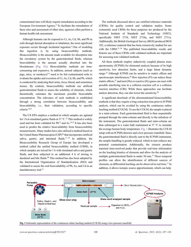
ABSTRACT: Incidental ingestion of soil containing Cr, As, Cd, Sb, and Pb has been attracting global attention as it can
significantly impact human health. Many bioaccessibility methods have been developed to simulate the amount of contaminants
extracted by gastrointestinal fluids following incidental ingestion. Although the continuous online leaching method (COLM) offers
various advantages over conventional batch bioaccessibility methods, such as reduced analysis time, elemental source apportionment,
and isotopic analysis, it has not yet been applied to soil and directly compared to validated, published methods. This study uses the
COLM with simulated gastrointestinal fluids from the United States Environmental Protection Agency (US EPA), United States
Pharmacopeia (USP), and unified bioaccessibility method (UBM) to measure the bioaccessibility of Cr, As, Cd, Sb, and Pb in NIST
2710, NIST 2710a, NIST 2711a, and BGS 102. When the US EPA gastrointestinal fluid was used, no significant difference was
observed between the COLM bioaccessible + residual, aqua regia extraction, or certificate concentrations for all the elements and
soils studied. Furthermore, COLM bioaccessibility was within the
acceptable range of control limits and bioavailability (animal)
studies for most reference materials. In addition, no statistically
significant difference was observed between either the US EPA
batch method or the stomach phase of the UBM batch method and
the stomach stage of the COLM, indicating that the COLM could
be incorporated into current bioaccessibility analyses to improve
soil contamination characterization in the future.
INTRODUCTION
Cr, As, Cd, Sb, and Pb can be toxic, carcinogenic, or have other
neurological or adverse health effects, and therefore, their presence
in soil can adversely affect humans, other animals, and the natural
environment.1 Cd, for instance, can cause nephrotoxicity in
humans. Cr and Sb have been observed to have adverse health
effects in rats. Pb can cause neurotoxicity in children. As is a
known carcinogen.1 In addition, Sb and Cr have been recognized
as risk drivers in human health risk assessment. Various methods
have been validated to determine As, Pb, and Cd in soils. Some
soil types are naturally rich in one or more of these elements, while
others can be contaminated with these elements through human
activities. Therefore, the United Nations Sustainable Development
Goals aim to reduce illness and death resulting from hazardous soil
pollution and contamination (Target 3.9),2 provide access to safe
green and public spaces (Target 11.7), reduce the release of
chemicals into soil and their adverse impacts on the human health
and environment (Target 12.4), and restore degraded land and soil
to achieve a land degradation-neutral world (Target 15.3). Over
1300 active contaminated Superfund sites have been identified by
the United States Environmental Protection Agency (US EPA).3
The Federal Contaminated Sites Action Plan has identified 4982
active contaminated sites in Canada.4 Across Europe, 340,000
www.at-spectrosc.com/as/article/pdf/2021827 108 At. Spectrosc. 2022, 43(2), 107–116.
contaminated sites will likely require remediation according to the
European Environment Agency.5 To facilitate the remediation of
these sites and assessment of other sites, agencies often perform a
human health risk assessment.
Although humans can be exposed to Cr, As, Cd, Sb, and Pb in
soils through dermal absorption or inhalation, the most significant
exposure occurs through incidental ingestion.6 One of modeling
this ingestion is by using bioaccessibility methods.
Bioaccessibility is the amount made available for absorption into
the circulatory system by the gastrointestinal fluids, whereas
bioavailability is the amount actually absorbed into the
bloodstream (Fig. S1). Bioavailability methods are time-
consuming and expensive. In addition, animal subjects (such as
pigs, mice, or monkeys)7-9 need to be fed contaminated soils to
evaluate the uptake and excretion of Cr, As, Cd, Sb, and Pb, which
is conducted by analyzing their urine, feces, blood, and sometimes
tissues. By contrast, bioaccessibility methods use artificial
gastrointestinal fluids to assess the solubility of elements, which
theoretically estimates the maximum possible bioavailable
concentration. The relevance of such methods is established
through a strong correlation between bioaccessibility and
bioavailability, i.e., their validation, according to specific
criteria.10,11
The US EPA employs a method in which samples are agitated
for 1 h in simulated gastric fluids at 37 °C.12 This method is widely
used and has been validated for Pb13 and As.14,15 It has also been
used to predict the relative bioavailability from bioaccessibility
measurements. Many studies have also utilized a method based on
the United States Pharmacopeia (USP)16 that incorporates artificial
saliva, gastric, and intestinal fluids.17–19 In addition, the
Bioaccessibility Research Group of Europe has developed a
method called the unified bioaccessibility method (UBM), in
which samples are mixed for 1 h with simulated saliva and gastric
fluids, and then subjected to an additional 4 h of mixing in
duodenal and bile fluids.20 This method has also been adopted by
the International Organization of Standardization (ISO) and
validated to assess the oral bioavailability of Pb, As, and Cd in an
interlaboratory trial.21
The methods discussed above use certified reference materials
(CRMs) for quality control and validation studies. Some
commonly used CRMs for these purposes are produced by the
National Institute of Standards and Technology (NIST),
specifically NIST 2710, NIST 2710a, and NIST 2711a.
Additionally, the British Geological Survey (BGS) produced BGS
102, a reference material that has been extensively studied for use
with the UBM.21–24 The published bioavailability results and
historic use of these CRMs with validated methods are important
for assessing non-validated methods.
All these methods employ inductively coupled plasma mass
spectrometry (ICPMS) for elemental analysis because of its high
sensitivity, low detection limits, and a large linear dynamic
range.25 Although ICPMS can be sensitive to matrix effects and
spectroscopic interferences,26 flow injection (FI) can reduce these
matrix effects,27 and inert (He) or reactive (H2) gases can react with
possible interfering ions in a collision reaction cell or a collision
reaction interface (CRI). While these approaches can facilitate
analyte detection, they can also lower the sensitivity.28
A significant drawback of the aforementioned bioaccessibility
methods is that they require a long extraction time prior to ICPMS
analysis, which can be avoided by using the continuous online
leaching method (COLM). To use the COLM, the sample is placed
in a mini-column. Each gastrointestinal fluid is then sequentially
pumped through the mini-column and directly to the nebulizer of
the instrument. The gastrointestinal fluids and mini-column are
then submerged in a water bath maintained at 37 °C to simulate
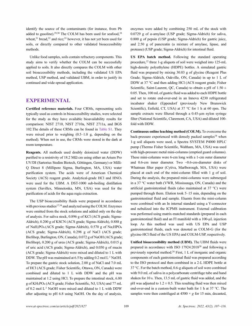
the average human body temperature. Fig. 1 illustrates the COLM
setup with an ICPMS detector and a low-pressure manifold. Since
the gastrointestinal fluid is directly sent to the ICPMS instrument,
the sample-handling is greatly reduced, which in turn reduces any
potential contamination. Additionally, the extracts produce
transient time-resolved peaks that provide real-time information
on the leaching kinetics of elements and allow for the analysis of
multiple gastrointestinal fluids in under 30 min.17 These temporal
profiles can allow the identification of different sources of
elements, as differential leaching can be observed in real time.17 In
addition, it allows isotopic source apportionment, which can help
Fig. 1 Schematic representation of the continuous online leaching method (COLM) using a low-pressure manifold.
www.at-spectrosc.com/as/article/pdf/2021827 109 At. Spectrosc. 2022, 43(2), 107–116.
identify the source of the contaminants (for instance, from Pb
added to gasoline).29,30 The COLM has been used for seafood,18
wheat,31 bread,32 and rice;33 however, it has not yet been used for
soils, or directly compared to other validated bioaccessibility
methods.
Unlike food samples, soils contain refractory components. This
study aims to verify whether the COLM can be successfully
applied to soils. It also directly compares the COLM with other
soil bioaccessibility methods, including the validated US EPA
method, USP method, and validated UBM, in order to justify its
continued and wide-spread application.
EXPERIMENTAL
Certified reference materials. Four CRMs, representing soils
typically used as controls in bioaccessibility studies, were selected
for the study as they have available bioavailability results for
comparison: NIST 2710, NIST 2710a, NIST 2711a, and BGS
102.The details of these CRMs can be found in Table S1. They
were mixed prior to weighing (0.5–1.0 g, depending on the
method). When not in use, the CRMs were stored in the dark at
room temperature.
Reagents. All methods used doubly deionized water (DDW)
purified to a resistivity of 18.2 MΩ cm using either an Arium Pro
UV/DI (Sartorius Stedim Biotech, Göttingen, Germany) or Milli-
Q Direct 8 (Millipore Sigma, Burlington, MA, USA) water
purification system. The acids were of American Chemical
Society (ACS) reagent grade. Analytical-grade HCl and HNO3
were used for the UBM. A DST-1000 sub-boiling distillation
system (Savillex, Minnetonka, MN, USA) was used for the
purification of acids for the aqua regia extraction.
The USP bioaccessibility fluids were prepared in accordance
with previous studies17,34 and analyzed using the COLM. Enzymes
were omitted from the stock solutions and added only on the day
of analysis. For saliva stock, 0.896 g of KCl (ACS grade; Sigma-
Aldrich), 0.200 g of KSCN (ACS grade; Sigma-Aldrich), 0.888 g
of NaH2PO4 (ACS grade; Sigma-Aldrich), 0.570 g of Na2HPO4
(ACS grade; Sigma-Aldrich), 0.298 g of NaCl (ACS grade;
BioShop, Burlington, ON, Canada), 0.072 g of NaOH (ACS grade;
BioShop), 0.200 g of urea (ACS grade; Sigma-Aldrich), 0.015 g
of uric acid (ACS grade; Sigma-Aldrich), and 0.050 g of mucin
(ACS grade; Sigma-Aldrich) were mixed and diluted to 1 L with
DDW. The pH was maintained at 6.5 by adding 0.2 mol L-1 NaOH.
To prepare the gastric stock solution, 2.00 g of NaCl and 7.0 mL
of HCl (ACS grade; Fisher Scientific, Ottawa, ON, Canada) were
combined and diluted to 1 L with DDW and the pH was
maintained at 1.2 using HCl. To prepare the intestinal stock, 6.80
g of KH2PO4 (ACS grade; Fisher Scientific, NJ, USA) and 77 mL
of 0.2 mol L-1 NaOH were mixed and diluted to 1 L with DDW
after adjusting to pH 6.8 using NaOH. On the day of analysis,
enzymes were added by combining 250 mL of the stock with
0.0729 g of ɑ-amylase (USP grade; Sigma-Aldrich) for saliva,
0.800 g of pepsin (USP grade; Sigma-Aldrich) for gastric juice,
and 2.50 g of pancreatin (a mixture of amylase, lipase, and
protease) (USP grade; Sigma-Aldrich) for intestinal fluid.
US EPA batch method. Following the standard operating
procedure,12 three 1-g aliquots of soil were weighed into 125-mL
high-density polyethylene (HDPE) bottles. A simulated gastric
fluid was prepared by mixing 30.03 g of glycine (Reagent Plus
Grade; Sigma-Aldrich, Oakville, ON, Canada) in up to 1 L of
DDW at 37 °C and then adding HCl (ACS reagent grade; Fisher
Scientific, Saint-Laurent, QC, Canada) to obtain a pH of 1.50 ±
0.05. Then, 100 mL of gastric fluid was added to each HDPE bottle
and set to rotate end-over-end in an Innova 4230 refrigerated
incubator shaker (Eppendorf (previously New Brunswick
Scientific), Enfield, CT, USA) at 37 °C for 1 h at 60 rpm. The
sample extracts were filtered through a 0.45-µm nylon syringe
filter (National Scientific, Claremont, CA, USA) and diluted 100-
fold with DDW.
Continuous online leaching method (COLM). To overcome the
back-pressure experienced with densely packed samples18 when
1-g soil aliquots were used, a Spectra SYSTEM P4000 HPLC
pump (Thermo Fisher Scientific, Waltham, MA, USA) was used
with high-pressure metal mini-columns (emptied guard columns).
These mini-columns were 6-cm long with a 1-cm outer diameter
and 0.6-cm inner diameter. Two ~0.6-cm-diameter disks of
Whatman filter paper (Cytiva, Marlborough, MA, USA) were
placed at each end of the mini-column filled with 1 g of soil.
During the analysis, the prepared mini-columns were submerged
in a 37 °C water bath (VWR, Mississauga, ON, Canada) and the
artificial gastrointestinal fluids (also maintained at 37 °C) were
pumped through them. Elution took 5–15 min, depending on the
gastrointestinal fluid and sample. Eluents from the mini-column
were combined with an In internal standard using a Y-connector
and nebulized into the ICPMS instrument. External calibration
was performed using matrix-matched standards (prepared in each
gastrointestinal fluid) and an FI manifold with a 100-µL injection
loop. As this method was used with US EPA and USP
gastrointestinal fluids, each was denoted as COLM-G (for the
glycine-HCl fluid of the US EPA) and COLM-USP, respectively.
Unified bioaccessibility method (UBM). The UBM fluids were
prepared in accordance with ISO 17924:201820 and following a
previously reported method.24 First, 1 L of inorganic and organic
components of each gastrointestinal fluid was prepared according
to the ISO protocol and then combined in a 2-L HDPE bottle at
37 °C. For the batch method, 0.6-g aliquots of soil were combined
with 9.0 mL of saliva in a polycarbonate centrifuge tube and hand
shaken for 10 s. Then, 13.5 mL of gastric fluid was added, and the
pH was adjusted to 1.2 ± 0.5. This resulting fluid was then mixed
end-over-end in a custom-built water bath for 1 h at 37 °C. The
samples were then centrifuged at 4500 × g for 15 min, decanted,
www.at-spectrosc.com/as/article/pdf/2021827 110 At. Spectrosc. 2022, 43(2), 107–116.
and acidified with 9.0 mL of 0.1 M HNO3 for storage prior to
analysis. This made up the “stomach” phase. For the “stomach +
intestinal” phase, the same steps were followed as above; however,
after rotation for 1 h, the pH was maintained between 1.2 and 1.5.
Then, 27 mL of the duodenal fluid and 9 mL of the bile fluid were
added, and the pH was adjusted to 6.3 ± 0.5 by adding 37% (v/v)
HCl or 1 M NaOH dropwise. The samples were then mixed for
another 4 h in a water bath at 37 °C. Finally, the pH was recorded,
the samples were centrifuged at 4500 × g for 15 min, decanted,
and acidified with 9.0 mL of 0.1 M HNO3 for storage. All samples
were diluted 10-fold prior to the ICPMS analysis.
For the COLM-UBM, a mini-column was prepared following a
method described in previous studies. Low-pressure
polytetrafluoroethylene (PTFE) tubing, a peristaltic pump, and a
FI manifold31 were used. To reduce the back-pressure, 0.6 g soil
was used. Each mini-column had an inner diameter of 7 mm, an
outer diameter of 8 mm, and a length of 5 cm. Glass wool (Acros
Organics, Fair Lawn, NJ, USA) was cleaned overnight in 10%
(v/v) HNO3, soaked in artificial saliva to matrix-match, dried in air,
and then stored in an airtight bag. The mini-columns were
prepared by rolling 0.6 g of soil in glass wool and inserting it into
the tubing. A glass wool plug was inserted at each end to secure
the sample in place. Three blank mini-columns were prepared by
inserting glass wool without any samples. Saliva, gastric juice,
duodenal fluid, and bile fluid were sequentially pumped through
the mini-columns while continuously monitoring the eluted
elements by ICPMS.
Aqua regia extraction. Residual soil CRM from each mini-
column was placed in a PTFE digestion vessel (Savillex) and dried.
Additionally, 1 g of fresh CRM (matching that of the residual) was
weighed into a separate digestion vessel to determine the total
extractable concentration of each element. Then, 5 mL of aqua
regia (3:1 v/v HCl: HNO3) was made fresh daily and added to each
digestion vessel. Aqua regia was also added to one blank vessel
without soil. These vessels were sealed and extracted on a hotplate
at ~180 °C for 2 h. The samples were then transferred to Falcon
tubes, filtered through a 0.45-µm hydrophilic polyvinylidene
fluoride filter (Foxx Life Sciences, Salem, NH, USA), and diluted
1000-fold with DDW.
Instrumentation. Samples, excluding those extracted with the
UBM, were analyzed using a Varian 820MS quadrupole-based
ICPMS instrument equipped with a Pt sampler cone with a 0.9-
mm diameter opening and a CRI Ni skimmer cone with a 0.4-mm
diameter opening. The samples were introduced into a PTFE
concentric nebulizer and a Peltier-cooled Scott-type double-pass
spray chamber maintained at 3 °C. Torch alignment was
conducted each day using 5 µg L-1 of a tuning solution containing
Be, Mg, Co, In, Ce, Pb, and Ba in 1% HNO3. Batch
bioaccessibility, total concentrations, and residual data were
acquired in the steady-state mode with five points per peak, 20
scans per replicate, and five replicates per sample, whereas the
COLM data were acquired in the time-resolved mode with three
points per peak, one scan per replicate, and a dwell time of 80 ms.
Other operating conditions are summarized in Table S2. The
samples were analyzed with a 5 µg L-1 In internal standard added
online using a Y-connector and matrix-matched external
calibration.
Samples extracted using the UBM were analyzed with an
Agilent 7500 quadrupole-based ICPMS instrument equipped with
Ni cones and an octupole collision reaction system using He and
H2 gases for interference reduction. The samples were introduced
using a SeaSpray glass concentric nebulizer (AMETEK UK,
Leicester, UK) and a quartz Scott-type spray chamber. Torch
alignment and tuning were conducted daily using aqueous multi-
element solutions. Batch UBM samples were analyzed in the
steady-state mode and COLM-UBM data were acquired in the
time-resolved mode with 50-ms measurements and a sample-
uptake rate of 1 mL min-1. The samples were analyzed by adding
5 µg L-1 of In internal standard to the nebulizer using a T-connector
and matrix-matched external calibrations. For the UBM batch
method, 25 µg L-1 of multi-element standard solution and a major
elemental solution were analyzed at the beginning and end of the
analysis daily and after every 20 samples.
Data processing. All data were imported into Microsoft Excel
(Microsoft, Redmond, WA, USA) for further processing. For the
data acquired in the steady-state mode, the samples were internally
standard-corrected, converted from count-per-second (c/s) to mg
L-1 using external calibration, blank subtracted, and converted to
mg kg-1 using the dilution factors and original sample masses. For
all the data acquired in the time-resolved mode, elution profiles
were internal standard corrected by dividing the analyte signal by
the In signal point by point, baseline-corrected by taking an
average of the baseline on either side of the peak and subtracting
from the points along the peak. The peak areas were computed
using the following modified trapezoidal equations:35
𝑇𝑛 = ∆𝑋 [∑ 𝑓(𝑥𝑖)
𝑛
𝑖=0
−𝑓(𝑥0)
2−
𝑓(𝑥𝑛)
2]
Where ∆𝑋 = (𝑏 − 𝑎)/𝑛, Tn is the peak area, f(x0) is the signal
at the onset of the peak, f(xi) is the signal at point i along the peak,
f(xn) is the signal at the end of the peak, a is the first time point of
the trapezoid, b is the last time point of the trapezoid, and n is the
number of equally spaced trapezoids under the peak. A peak area
was obtained for each extraction, which was then converted to mg
kg-1 using external calibration and sample masses.
The percent bioaccessibility was calculated by dividing the total
bioaccessible concentration with the total concentration extracted
by aqua regia. To compare the data sets, an F test for variance was
first performed to compute the appropriate Student’s t-tests. Next,
analysis of variance (ANOVA) was conducted using the XLSTAT
add-on in Microsoft Excel.36
www.at-spectrosc.com/as/article/pdf/2021827 111 At. Spectrosc. 2022, 43(2), 107–116.
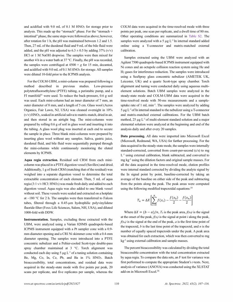
Table 1. Bioaccessible concentrations in mg kg-1 (mean ± standard Deviation, n=3) of Cr, As, Cd, Sb, and Pb in the stomach-equivalent phase of all
bioaccessibility methods
CRM Method Cr As Cd Sb Pb
NIST 2710 USEPA batch 0.019 ± 0.024 195.8 ± 2.0 19.69 ± 0.50 3.81 ± 0.26 4362 ± 54
COLM-G 0.019 ± 0.013 195 ± 27 19.9 ± 7.0 3.91 ± 0.55 4500 ± 2200
NIST 2710a USEPA batch 0.26 ± 0.22 309 ± 41 7.48 ± 0.98 9.9 ± 1.1 3165 ± 540
COLM-G 0.27 ± 0.46 318 ± 540 7.5 ± 6.7 10 ± 14 3400 ± 3400
NIST 2711a USEPA batch 0.072 ± 0.039 33.00 ± 0.35 57.5 ± 1.6 3.94 ± 0.46 1204 ± 23
COLM-G 0.072 ± 0.017 33.8 ± 6.0 47.5 ± 4.2 3.89 ± 0.16 1213 ± 301
BGS 102
USEPA batch 3.58 ± 0.28 1.51 ± 0.61 0.319 ± 0.058 0.91 ± 0.14 35 ± 36
COLM-G 3.6 ± 3.9 1.50 ± 0.22 0.32 ± 0.27 0.92 ± 0.29 35 ± 14
COLM-USP 29 ± 40 4.5 ± 6.1 0.14 ± 0.18 0.13 ± 0.18 11.3 ± 8.7
UBM batch 35.66 ± 0.65 3.90 ± 0.22 0.2177 ± 0.0073 0.0325 ± 0.0062 17.2 ± 2.6
COLM-UBM 34.652 ± 0.033 4.2955 ±
0.0037 0.21787 ± 0.00021 0.032435 ± 0.000035 11.535 ± 0.039
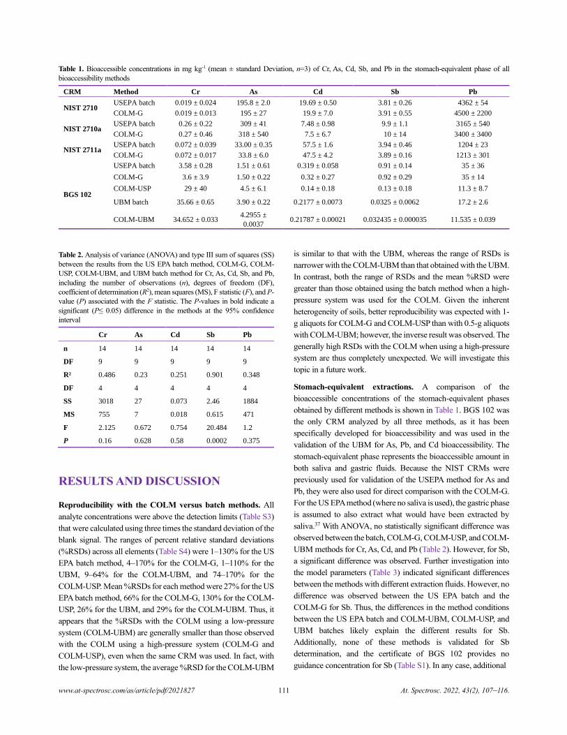
Table 2. Analysis of variance (ANOVA) and type III sum of squares (SS)
between the results from the US EPA batch method, COLM-G, COLM-
USP, COLM-UBM, and UBM batch method for Cr, As, Cd, Sb, and Pb,
including the number of observations (n), degrees of freedom (DF),
coefficient of determination (R2), mean squares (MS), F statistic (F), and P-
value (P) associated with the F statistic. The P-values in bold indicate a
significant (P≤ 0.05) difference in the methods at the 95% confidence
interval
Cr As Cd Sb Pb
n 14 14 14 14 14
DF 9 9 9 9 9
R² 0.486 0.23 0.251 0.901 0.348
DF 4 4 4 4 4
SS 3018 27 0.073 2.46 1884
MS 755 7 0.018 0.615 471
F 2.125 0.672 0.754 20.484 1.2
P 0.16 0.628 0.58 0.0002 0.375
RESULTS AND DISCUSSION
Reproducibility with the COLM versus batch methods. All
analyte concentrations were above the detection limits (Table S3)
that were calculated using three times the standard deviation of the
blank signal. The ranges of percent relative standard deviations
(%RSDs) across all elements (Table S4) were 1–130% for the US
EPA batch method, 4–170% for the COLM-G, 1–110% for the
UBM, 9–64% for the COLM-UBM, and 74–170% for the
COLM-USP. Mean %RSDs for each method were 27% for the US
EPA batch method, 66% for the COLM-G, 130% for the COLM-
USP, 26% for the UBM, and 29% for the COLM-UBM. Thus, it
appears that the %RSDs with the COLM using a low-pressure
system (COLM-UBM) are generally smaller than those observed
with the COLM using a high-pressure system (COLM-G and
COLM-USP), even when the same CRM was used. In fact, with
the low-pressure system, the average %RSD for the COLM-UBM
is similar to that with the UBM, whereas the range of RSDs is
narrower with the COLM-UBM than that obtained with the UBM.
In contrast, both the range of RSDs and the mean %RSD were
greater than those obtained using the batch method when a high-
pressure system was used for the COLM. Given the inherent
heterogeneity of soils, better reproducibility was expected with 1-
g aliquots for COLM-G and COLM-USP than with 0.5-g aliquots
with COLM-UBM; however, the inverse result was observed. The
generally high RSDs with the COLM when using a high-pressure
system are thus completely unexpected. We will investigate this
topic in a future work.
Stomach-equivalent extractions. A comparison of the
bioaccessible concentrations of the stomach-equivalent phases
obtained by different methods is shown in Table 1. BGS 102 was
the only CRM analyzed by all three methods, as it has been
specifically developed for bioaccessibility and was used in the
validation of the UBM for As, Pb, and Cd bioaccessibility. The
stomach-equivalent phase represents the bioaccessible amount in
both saliva and gastric fluids. Because the NIST CRMs were
previously used for validation of the USEPA method for As and
Pb, they were also used for direct comparison with the COLM-G.
For the US EPA method (where no saliva is used), the gastric phase
is assumed to also extract what would have been extracted by
saliva.37 With ANOVA, no statistically significant difference was
observed between the batch, COLM-G, COLM-USP, and COLM-
UBM methods for Cr, As, Cd, and Pb (Table 2). However, for Sb,
a significant difference was observed. Further investigation into
the model parameters (Table 3) indicated significant differences
between the methods with different extraction fluids. However, no
difference was observed between the US EPA batch and the
COLM-G for Sb. Thus, the differences in the method conditions
between the US EPA batch and COLM-UBM, COLM-USP, and
UBM batches likely explain the different results for Sb.
Additionally, none of these methods is validated for Sb
determination, and the certificate of BGS 102 provides no
guidance concentration for Sb (Table S1). In any case, additional
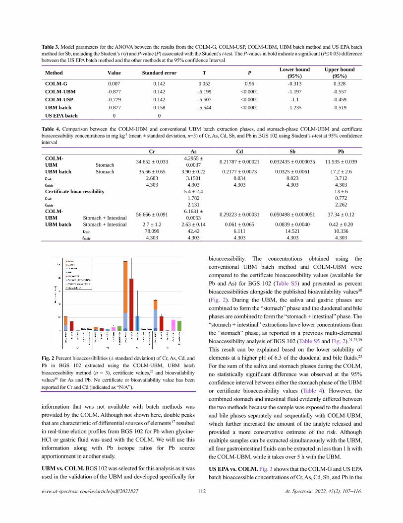
www.at-spectrosc.com/as/article/pdf/2021827 112 At. Spectrosc. 2022, 43(2), 107–116.
Table 3. Model parameters for the ANOVA between the results from the COLM-G, COLM-USP, COLM-UBM, UBM batch method and US EPA batch
method for Sb, including the Student’s t (t) and P-value (P) associated with the Student’s t-test. The P-values in bold indicate a significant (P≤ 0.05) difference
between the US EPA batch method and the other methods at the 95% confidence Interval
Method Value Standard error T P Lower bound
(95%)
Upper bound
(95%)
COLM-G 0.007 0.142 0.052 0.96 -0.313 0.328
COLM-UBM -0.877 0.142 -6.199 <0.0001 -1.197 -0.557
COLM-USP -0.779 0.142 -5.507 <0.0001 -1.1 -0.459
UBM batch -0.877 0.158 -5.544 <0.0001 -1.235 -0.519
US EPA batch 0 0
Table 4. Comparison between the COLM-UBM and conventional UBM batch extraction phases, and stomach-phase COLM-UBM and certificate
bioaccessibility concentrations in mg kg-1 (mean ± standard deviation, n=3) of Cr, As, Cd, Sb, and Pb in BGS 102 using Student’s t-test at 95% confidence
interval
Cr As Cd Sb Pb
COLM-
UBM Stomach 34.652 ± 0.033
4.2955 ±
0.0037 0.21787 ± 0.00021 0.032435 ± 0.000035 11.535 ± 0.039
UBM batch Stomach 35.66 ± 0.65 3.90 ± 0.22 0.2177 ± 0.0073 0.0325 ± 0.0061 17.2 ± 2.6
tcalc 2.683 3.1501 0.034 0.023 3.712
ttable 4.303 4.303 4.303 4.303 4.303
Certificate bioaccessibility 5.4 ± 2.4 13 ± 6
tcalc 1.782 0.772
ttable 2.131 2.262
COLM-
UBM Stomach + Intestinal 56.666 ± 0.091
6.1631 ±
0.0053 0.29223 ± 0.00031 0.050498 ± 0.000051 37.34 ± 0.12
UBM batch Stomach + Intestinal 2.7 ± 1.2 2.63 ± 0.14 0.061 ± 0.065 0.0839 ± 0.0040 0.42 ± 0.20
tcalc 78.099 42.42 6.111 14.521 10.336
ttable 4.303 4.303 4.303 4.303 4.303
Fig. 2 Percent bioaccessibilities (± standard deviation) of Cr, As, Cd, and
Pb in BGS 102 extracted using the COLM-UBM, UBM batch
bioaccessibility method (n = 3), certificate values,22 and bioavailability
values40 for As and Pb. No certificate or bioavailability value has been
reported for Cr and Cd (indicated as “N/A”).
information that was not available with batch methods was
provided by the COLM. Although not shown here, double peaks
that are characteristic of differential sources of elements17 resulted
in real-time elution profiles from BGS 102 for Pb when glycine-
HCl or gastric fluid was used with the COLM. We will use this
information along with Pb isotope ratios for Pb source
apportionment in another study.
UBM vs. COLM. BGS 102 was selected for this analysis as it was
used in the validation of the UBM and developed specifically for
bioaccessibility. The concentrations obtained using the
conventional UBM batch method and COLM-UBM were
compared to the certificate bioaccessibility values (available for
Pb and As) for BGS 102 (Table S5) and presented as percent
bioaccessibilities alongside the published bioavailability values38
(Fig. 2). During the UBM, the saliva and gastric phases are
combined to form the “stomach” phase and the duodenal and bile
phases are combined to form the “stomach + intestinal” phase. The
“stomach + intestinal” extractions have lower concentrations than
the “stomach” phase, as reported in a previous multi-elemental
bioaccessibility analysis of BGS 102 (Table S5 and Fig. 2).21,23,39
This result can be explained based on the lower solubility of
elements at a higher pH of 6.3 of the duodenal and bile fluids.23
For the sum of the saliva and stomach phases during the COLM,
no statistically significant difference was observed at the 95%
confidence interval between either the stomach phase of the UBM
or certificate bioaccessibility values (Table 4). However, the
combined stomach and intestinal fluid evidently differed between
the two methods because the sample was exposed to the duodenal
and bile phases separately and sequentially with COLM-UBM,
which further increased the amount of the analyte released and
provided a more conservative estimate of the risk. Although
multiple samples can be extracted simultaneously with the UBM,
all four gastrointestinal fluids can be extracted in less than 1 h with
the COLM-UBM, while it takes over 5 h with the UBM.
US EPA vs. COLM. Fig. 3 shows that the COLM-G and US EPA
batch bioaccessible concentrations of Cr, As, Cd, Sb, and Pb in the
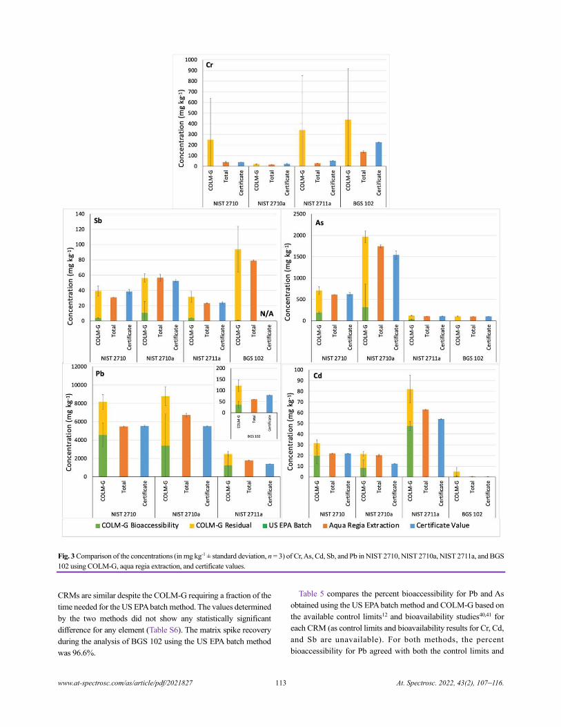
www.at-spectrosc.com/as/article/pdf/2021827 113 At. Spectrosc. 2022, 43(2), 107–116.
Fig. 3 Comparison of the concentrations (in mg kg-1 ± standard deviation, n = 3) of Cr, As, Cd, Sb, and Pb in NIST 2710, NIST 2710a, NIST 2711a, and BGS
102 using COLM-G, aqua regia extraction, and certificate values.
CRMs are similar despite the COLM-G requiring a fraction of the
time needed for the US EPA batch method. The values determined
by the two methods did not show any statistically significant
difference for any element (Table S6). The matrix spike recovery
during the analysis of BGS 102 using the US EPA batch method
was 96.6%.
Table 5 compares the percent bioaccessibility for Pb and As
obtained using the US EPA batch method and COLM-G based on
the available control limits12 and bioavailability studies40,41 for
each CRM (as control limits and bioavailability results for Cr, Cd,
and Sb are unavailable). For both methods, the percent
bioaccessibility for Pb agreed with both the control limits and
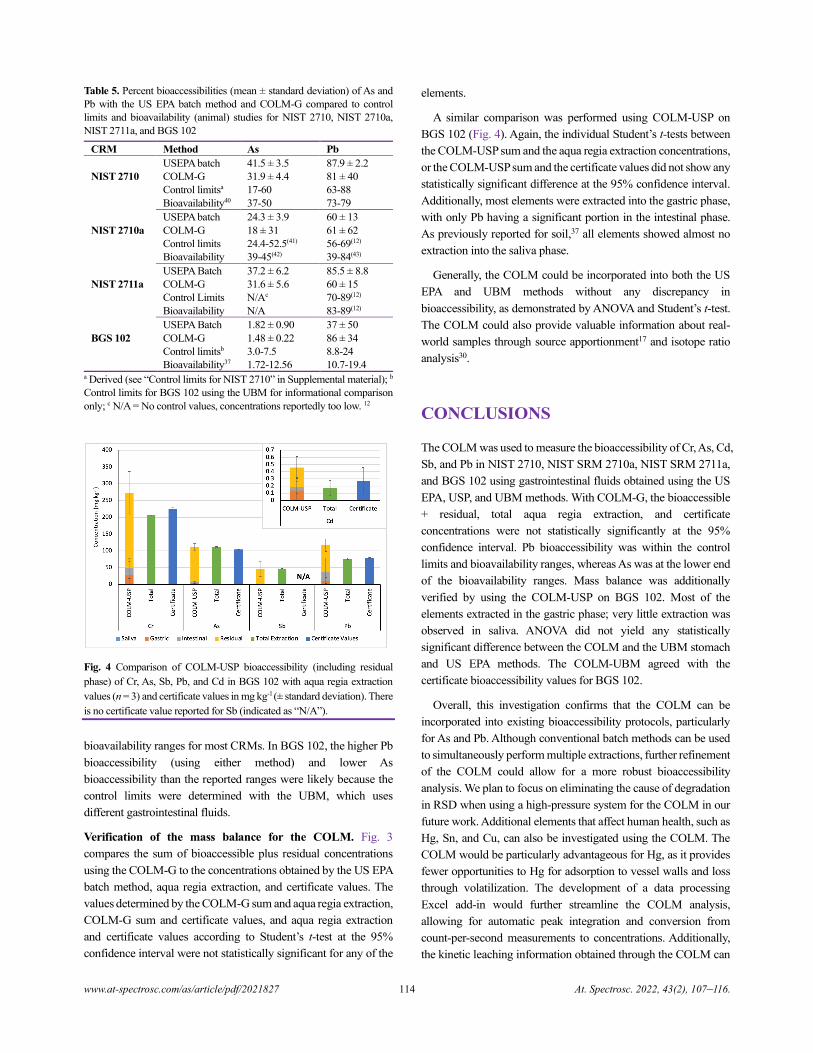
www.at-spectrosc.com/as/article/pdf/2021827 114 At. Spectrosc. 2022, 43(2), 107–116.
Table 5. Percent bioaccessibilities (mean ± standard deviation) of As and
Pb with the US EPA batch method and COLM-G compared to control
limits and bioavailability (animal) studies for NIST 2710, NIST 2710a,
NIST 2711a, and BGS 102
CRM Method As Pb
NIST 2710
USEPA batch 41.5 ± 3.5 87.9 ± 2.2
COLM-G 31.9 ± 4.4 81 ± 40
Control limitsa 17-60 63-88
Bioavailability40 37-50 73-79
NIST 2710a
USEPA batch 24.3 ± 3.9 60 ± 13
COLM-G 18 ± 31 61 ± 62
Control limits 24.4-52.5(41) 56-69(12)
Bioavailability 39-45(42) 39-84(43)
NIST 2711a
USEPA Batch 37.2 ± 6.2 85.5 ± 8.8
COLM-G 31.6 ± 5.6 60 ± 15
Control Limits N/Ac 70-89(12)
Bioavailability N/A 83-89(12)
BGS 102
USEPA Batch 1.82 ± 0.90 37 ± 50
COLM-G 1.48 ± 0.22 86 ± 34
Control limitsb 3.0-7.5 8.8-24
Bioavailability37 1.72-12.56 10.7-19.4 a Derived (see “Control limits for NIST 2710” in Supplemental material); b
Control limits for BGS 102 using the UBM for informational comparison
only; c N/A = No control values, concentrations reportedly too low. 12
Fig. 4 Comparison of COLM-USP bioaccessibility (including residual
phase) of Cr, As, Sb, Pb, and Cd in BGS 102 with aqua regia extraction
values (n = 3) and certificate values in mg kg-1 (± standard deviation). There
is no certificate value reported for Sb (indicated as “N/A”).
bioavailability ranges for most CRMs. In BGS 102, the higher Pb
bioaccessibility (using either method) and lower As
bioaccessibility than the reported ranges were likely because the
control limits were determined with the UBM, which uses
different gastrointestinal fluids.
Verification of the mass balance for the COLM. Fig. 3
compares the sum of bioaccessible plus residual concentrations
using the COLM-G to the concentrations obtained by the US EPA
batch method, aqua regia extraction, and certificate values. The
values determined by the COLM-G sum and aqua regia extraction,
COLM-G sum and certificate values, and aqua regia extraction
and certificate values according to Student’s t-test at the 95%
confidence interval were not statistically significant for any of the
elements.
A similar comparison was performed using COLM-USP on
BGS 102 (Fig. 4). Again, the individual Student’s t-tests between
the COLM-USP sum and the aqua regia extraction concentrations,
or the COLM-USP sum and the certificate values did not show any
statistically significant difference at the 95% confidence interval.
Additionally, most elements were extracted into the gastric phase,
with only Pb having a significant portion in the intestinal phase.
As previously reported for soil,37 all elements showed almost no
extraction into the saliva phase.
Generally, the COLM could be incorporated into both the US
EPA and UBM methods without any discrepancy in
bioaccessibility, as demonstrated by ANOVA and Student’s t-test.
The COLM could also provide valuable information about real-
world samples through source apportionment17 and isotope ratio
analysis30.
CONCLUSIONS
The COLM was used to measure the bioaccessibility of Cr, As, Cd,
Sb, and Pb in NIST 2710, NIST SRM 2710a, NIST SRM 2711a,
and BGS 102 using gastrointestinal fluids obtained using the US
EPA, USP, and UBM methods. With COLM-G, the bioaccessible
+ residual, total aqua regia extraction, and certificate
concentrations were not statistically significantly at the 95%
confidence interval. Pb bioaccessibility was within the control
limits and bioavailability ranges, whereas As was at the lower end
of the bioavailability ranges. Mass balance was additionally
verified by using the COLM-USP on BGS 102. Most of the
elements extracted in the gastric phase; very little extraction was
observed in saliva. ANOVA did not yield any statistically
significant difference between the COLM and the UBM stomach
and US EPA methods. The COLM-UBM agreed with the
certificate bioaccessibility values for BGS 102.
Overall, this investigation confirms that the COLM can be
incorporated into existing bioaccessibility protocols, particularly
for As and Pb. Although conventional batch methods can be used
to simultaneously perform multiple extractions, further refinement
of the COLM could allow for a more robust bioaccessibility
analysis. We plan to focus on eliminating the cause of degradation
in RSD when using a high-pressure system for the COLM in our
future work. Additional elements that affect human health, such as
Hg, Sn, and Cu, can also be investigated using the COLM. The
COLM would be particularly advantageous for Hg, as it provides
fewer opportunities to Hg for adsorption to vessel walls and loss
through volatilization. The development of a data processing
Excel add-in would further streamline the COLM analysis,
allowing for automatic peak integration and conversion from
count-per-second measurements to concentrations. Additionally,
the kinetic leaching information obtained through the COLM can
www.at-spectrosc.com/as/article/pdf/2021827 115 At. Spectrosc. 2022, 43(2), 107–116.
be used for source apportionment, which is not possible with batch
bioaccessibility methods. We will analyze soils with known
contaminant sources (such as Pb from gasoline) in our future work
to identify different sources of elements and isotopic source
apportionment, as it would allow for a more comprehensive soil
analysis.
ASSOCIATED CONTENT
Supporting Information
The Supporting Information (Table S1-S6, Fig S1, and Control
limits for NIST 2710) is available at www.at-
spectrosc.com/as/home
AUTHOR INFORMATION
Diane Beauchemin received her Ph.D.
in 1984 from Université de Montréal.
She is a professor (Full) and
Undergraduate Chair at Queen’s
University. Her research efforts are
focused on inductively coupled plasma
mass spectrometry (ICPMS) and ICP
optical emission spectrometry (OES)
from both fundamental and application
perspectives, and expanding the range
of application of ICPMS/OES to
geochemical exploration, risk assessment of food safety, characterization of
nanoparticles, and forensic analysis. She has been working as member of
editorial board for Atomic Spectroscopy. Diane Beauchemin won the Alan
Date Memorial Award (1988) from VG Elemental, the Distinguished
Service Award (2001) from Spectroscopy Society of Canada, the Maxxam
Award (2017) and Clara Benson Award (2019) from Canadian Society for
Chemistry, and the Gerhard Herzberg Award (2018) from the Canadian
Society for Analytical Sciences and Spectroscopy. She is author or co-
author of over 100 articles published in peer-reviewed scientific journals.
Corresponding Author
*D. Beauchemin
Email address: [email protected]
Notes
The authors declare no competing financial interest.
ACKNOWLEDGMENTS
The authors would like to gratefully acknowledge the Natural
Sciences and Engineering Research Council of Canada for
funding (RGPNM 39487-2018 to DB and RGPIN 2018-04885 to
IK). AK also thanks David Patch for training, Queen’s University
School of Graduate Studies for graduate awards, and Mitacs
Globallink for funding (FR38334).
REFERENCES
1. Health Canada, Federal Contaminated Site Risk Assessments in
Canada: Toxicological Reference Values (TRVs), Ottawa (ON),
3.0., 2021.
2. United Nations Department of Economic and Social Affairs,
https://sdgs.un.org/goals, (accessed 1 June 2021).
3. US Environmental Protection Agency,
https://cumulis.epa.gov/supercpad/cursites/srchrslt.cfm?start=1,
(accessed 17 May 2021).
4. Government of Canada, https://www.tbs-sct.gc.ca/fcsi-
rscf/classification-eng.aspx, (accessed 17 May 2021).
5. A. Payá Pérez and N. Rodríguez Eugenio, Status of local soil
contamination in Europe, Brussels (BE), 2018.
6. Health Canada, Federal Contaminated Site Risk Assessment in
Canada: Guidance on Human Health Preliminary Quantitative Risk
Assessment (PQRA), Ottawa (ON), 2021, vol. 3.0.
7. S. W. Casteel, C. P. Weis, G. M. Henningsen, and W. J. Brattin,
Environ. Health Persp., 2006, 114, 1162-1171.
https://doi.org/10.1289/ehp.8852
8. J. C. Ng, S. M. Kratzmann, L. Qi, H. Crawley, B. Chiswell,
and M. R. Moore, Analyst, 1998, 123, 889-892.
https://doi.org/10.1039/a707728i
9. S. M. Roberts, J. W. Munson, Y. W. Lowney, and M. V. Ruby,
Toxicol. Sci., 2007, 95, 281-288.
https://doi.org/10.1093/toxsci/kfl117
10. A. L. Juhasz, N. T. Basta, and E. Smith, Environ. Pollut., 2013, 180,
372-375. https://doi.org/10.1016/j.envpol.2013.05.008
11. Health Canada, Federal Contaminated Site Risk Assessment in
Canada: Supplemental Guidance on Human Health Risk
Assessment of Oral Bioavailability of Substances in Soil and Soil-
Like Media - Canada.ca, Ottawa (ON), 2017.
12. US Environmental Protection Agency, Standard Operating
Procedure for an In Vitro Bioaccessibility Assay for Lead and
Arsenic in Soil, Washington D.C., 2017.
13. US Environmental Protection Agency, Estimation of relative
bioavailability of lead in soil and soil-like materials using in vivo
and in vitro methods, Washington D.C., 2007.
14. G. L. Diamond, K. D. Bradham, W. J. Brattin, M. Burgess, S.
Griffin, C. A. Hawkins, A. L. Juhasz, J. M. Klotzbach, C. Nelson,
Y. W. Lowney, K. G. Scheckel, and D. J. Thomas, J. Toxicol. Env.
Heal. A, 2016, 79, 165-173.
https://doi.org/10.1080/15287394.2015.1134038
15. US Environmental Protection Agency, Validation Assessment of In
Vitro Arsenic Bioaccessibility Assay for Predicting Relative
Bioavailability of Arsenic in Soils and Soil-like Materials at
Superfund Sites. Office of Land and Emergency Management.
OLEM 9355.4-29, Washington D.C., 2017.
16. The United States Pharmacopeia, in The United States
Pharmacopeia and National Formulary, 32nd edn., 2014, p. 344.
17. R. A. Althobiti and D. Beauchemin, J. Anal. At. Spectrom., 2021,
36, 622-629. https://doi.org/10.1039/d0ja00447b
www.at-spectrosc.com/as/article/pdf/2021827 116 At. Spectrosc. 2022, 43(2), 107–116.
18. A. Leufroy, L. Noël, D. Beauchemin, and T. Guérin,
Anal. Bioanal. Chem., 2012, 402, 2849-2859.
https://doi.org/10.1007/s00216-012-5774-4
19. N. W. Sadiq, "Multi-Elemental Risk Assessment of Rice Products
Using On-Line Continuous Leaching and Ion Exchange
Chromatography Coupled to Inductively Coupled Plasma Mass
Spectrometry for the Speciation Analysis of Bio-Accessible
Elements", Thesis, Queen’s University, Kingston, ON, 2016.
20. International Organization for Standardization, "Soil quality-
Assessment of human exposure from ingestion of soil and soil
material — Procedure for the estimation of the human
bioaccessibility/bioavailability of metals in soil", Report,
International Organization for Standardization (ISO), 2018, 1-28.
21. J. Wragg, M. Cave, N. Basta, E. Brandon, S. Casteel, S. Denys, C.
Gron, A. Oomen, K. Reimer, K. Tack, and T. Van de Wiele, Sci.
Total Environ., 2011, 409, 4016-4030.
https://doi.org/10.1016/j.scitotenv.2011.05.019
22. British Geological Survey, "BGS Guidance Material 102 - Ironstone
Soil", Report, British Geological Survey (BGS), 2009, vol. 1.
23. E. M. Hamilton, T. S. Barlow, C. J. B. Gowing, and M. J. Watts,
Microchem. J., 2015, 123, 131-138.
https://doi.org/10.1016/j.microc.2015.06.001
24. BARGE - INERIS, "UBM procedure for the measurement of
inorganic contaminant bioaccessibility from solid matrices.", Report,
Bioaccessibility Research Group of Europe (BARGE), Nottingham,
UK, 2011, 1-10.
25. M. Intawongse and J. R. Dean, TRAC-Trend. Anal. Chem., 2006,
25, 876-886. https://doi.org/10.1016/j.trac.2006.03.010
26. C. Moor, T. Lymberopoulou, and V. J. Dietrich, Microchim. Acta,
2001, 136, 123-128. https://doi.org/10.1007/s006040170041
27. R. Teuma-Castelletti and D. Beauchemin, J. Anal. At. Spectrom.,
2020, 35, 2820-2825. https://doi.org/10.1039/d0ja00275e
28. R. A. Althobiti, N. W. Sadiq, and D. Beauchemin, Food Chem.,
2018, 257, 230-236.
https://doi.org/10.1016/j.foodchem.2018.03.015
29. M. Chu and D. Beauchemin, J. Anal. At. Spectrom., 2004, 19, 1213-
1216. https://doi.org/10.1039/b403215b
30. R. A. Althobiti and D. Beauchemin, J. Anal. At. Spectrom., 2021,
42, 271-277. https://doi.org/ 10.46770/AS.2021.708
31. R. A. Althobiti and D. Beauchemin, J. Anal. At. Spectrom., 2018,
33, 642-648. https://doi.org/10.1039/c8ja00047f
32. R. P. Lamsal and D. Beauchemin, Anal. Chim. Acta, 2015, 867, 9-
17. https://doi.org/10.1016/j.aca.2015.02.047
33. N. S. Horner and D. Beauchemin, Anal. Chim. Acta, 2013, 758, 28-
35. https://doi.org/10.1016/j.aca.2012.11.011
34. The United States Pharmacopeia, in The United States
Pharmacopeia, United States Pharmacopeia, Rockville, MD, NF
XVII., 1990, p. 1788.
35. W. L. Chiou, Critical Evaluation of the Potential Error in
Pharmacokinetic Studies of Using the Linear Trapezoidal Rule
Method for the Calculation of the Area Under the Plasma Level-
Time Curve, 1978, vol. 6.
36. Addinsoft, "XLSTAT statistical and data analysis solution.",
Computer Program, New York, NY, 2021.
37. A. L. Juhasz, J. Weber, and E. Smith, J. Hazard. Mater., 2011, 197,
161-168. https://doi.org/10.1016/j.jhazmat.2011.09.068
38. H. B. Li, H. Ning, S. W. Li, J. Li, R. Y. Xue, M. Y. Li, M. Y. Wang,
J. H. Liang, A. L. Juhasz, and L. Q. Ma, J. Toxicol. Env. Heal. A,
2021, 84, 593-607. https://doi.org/10.1080/15287394.2021.1919947
39. S. Denys, J. Caboche, K. Tack, G. Rychen, J. Wragg, M. Cave,
C. Jondreville, and C. Feidt, Environ. Sci. Technol., 2012, 46, 6252–
6260. https://doi.org/10.1021/es3006942
40. I. Koch, K. J. Reimer, M. I. Bakker, N. T. Basta, M. R. Cave,
S. S. Denys, M. Dodd, B. A. Hale, R. Irwin, Y. W. Lowney,
M. M. Moore, V. Paquin, P. E. Rasmussen, T. Repaso-Subang,
G. L. Stephenson, S. D. Siciliano, J. Wragg, and G. J. Zagury,
J. Environ. Sci. Heal. A, 2013, 48, 641-655.
https://doi.org/10.1080/10934529.2013.731817
41. US Environmental Protection Agency, IN VITRO
BIOACCESSIBILITY REFERENCE MATERIALS FOR LEAD
and ARSENIC ROUND ROBIN STUDY REPORT, Washington
D.C., 2017.
42. US Environmental Protection Agency, Compilation and Review of
Data on Relative Bioavailability of Arsenic in Soil, Washington
D.C., 2012.
43. S. W. Casteel, D. Genny Fent, D. Lee Myoungheon, W. J. Brattin,
and P. Hunter, Relative Bioavailability of Arsenic and Lead in the
Nist 2710a Soil Standard, Src Tr-09-0951, 2010.
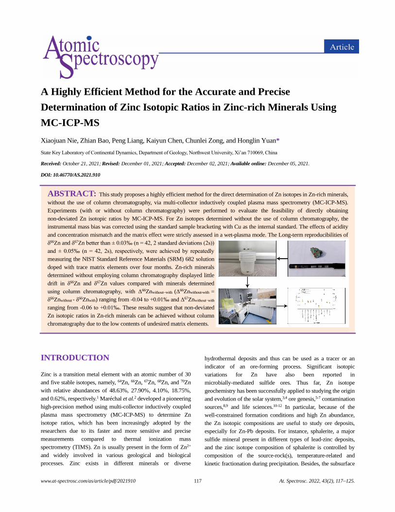
www.at-spectrosc.com/as/article/pdf/2021910 117 At. Spectrosc. 2022, 43(2), 117–125.
A Highly Efficient Method for the Accurate and Precise
Determination of Zinc Isotopic Ratios in Zinc-rich Minerals Using
MC-ICP-MS
Xiaojuan Nie, Zhian Bao, Peng Liang, Kaiyun Chen, Chunlei Zong, and Honglin Yuan*
State Key Laboratory of Continental Dynamics, Department of Geology, Northwest University, Xi’an 710069, China
Received: October 21, 2021; Revised: December 01, 2021; Accepted: December 02, 2021; Available online: December 05, 2021.
DOI: 10.46770/AS.2021.910
ABSTRACT: This study proposes a highly efficient method for the direct determination of Zn isotopes in Zn-rich minerals,
without the use of column chromatography, via multi-collector inductively coupled plasma mass spectrometry (MC-ICP-MS).
Experiments (with or without column chromatography) were performed to evaluate the feasibility of directly obtaining
non-deviated Zn isotopic ratios by MC-ICP-MS. For Zn isotopes determined without the use of column chromatography, the
instrumental mass bias was corrected using the standard sample bracketing with Cu as the internal standard. The effects of acidity
and concentration mismatch and the matrix effect were strictly assessed in a wet-plasma mode. The Long-term reproducibilities of
δ66Zn and δ67Zn better than ± 0.03‰ (n = 42, 2 standard deviations (2s))
and ± 0.05‰ (n = 42, 2s), respectively, were achieved by repeatedly
measuring the NIST Standard Reference Materials (SRM) 682 solution
doped with trace matrix elements over four months. Zn-rich minerals
determined without employing column chromatography displayed little
drift in δ66Zn and δ67Zn values compared with minerals determined
using column chromatography, with Δ66Znwithout−with (Δ66Znwithout-with =
δ66Znwithout - δ66Znwith) ranging from -0.04 to +0.01‰ and Δ67Znwithout−with
ranging from -0.06 to +0.01‰. These results suggest that non-deviated
Zn isotopic ratios in Zn-rich minerals can be achieved without column
chromatography due to the low contents of undesired matrix elements.
INTRODUCTION
Zinc is a transition metal element with an atomic number of 30
and five stable isotopes, namely, 64Zn, 66Zn, 67Zn, 68Zn, and 70Zn
with relative abundances of 48.63%, 27.90%, 4.10%, 18.75%,
and 0.62%, respectively.1 Maréchal et al.2 developed a pioneering
high-precision method using multi-collector inductively coupled
plasma mass spectrometry (MC-ICP-MS) to determine Zn
isotope ratios, which has been increasingly adopted by the
researchers due to its faster and more sensitive and precise
measurements compared to thermal ionization mass
spectrometry (TIMS). Zn is usually present in the form of Zn2+
and widely involved in various geological and biological
processes. Zinc exists in different minerals or diverse
hydrothermal deposits and thus can be used as a tracer or an
indicator of an ore-forming process. Significant isotopic
variations for Zn have also been reported in
microbially-mediated sulfide ores. Thus far, Zn isotope
geochemistry has been successfully applied to studying the origin
and evolution of the solar system,3,4 ore genesis,5-7 contamination
sources,8,9 and life sciences.10-12 In particular, because of the
well-constrained formation conditions and high Zn abundance,
the Zn isotopic compositions are useful to study ore deposits,
especially for Zn-Pb deposits. For instance, sphalerite, a major
sulfide mineral present in different types of lead-zinc deposits,
and the zinc isotope composition of sphalerite is controlled by
composition of the source-rock(s), temperature-related and
kinetic fractionation during precipitation. Besides, the subsurface
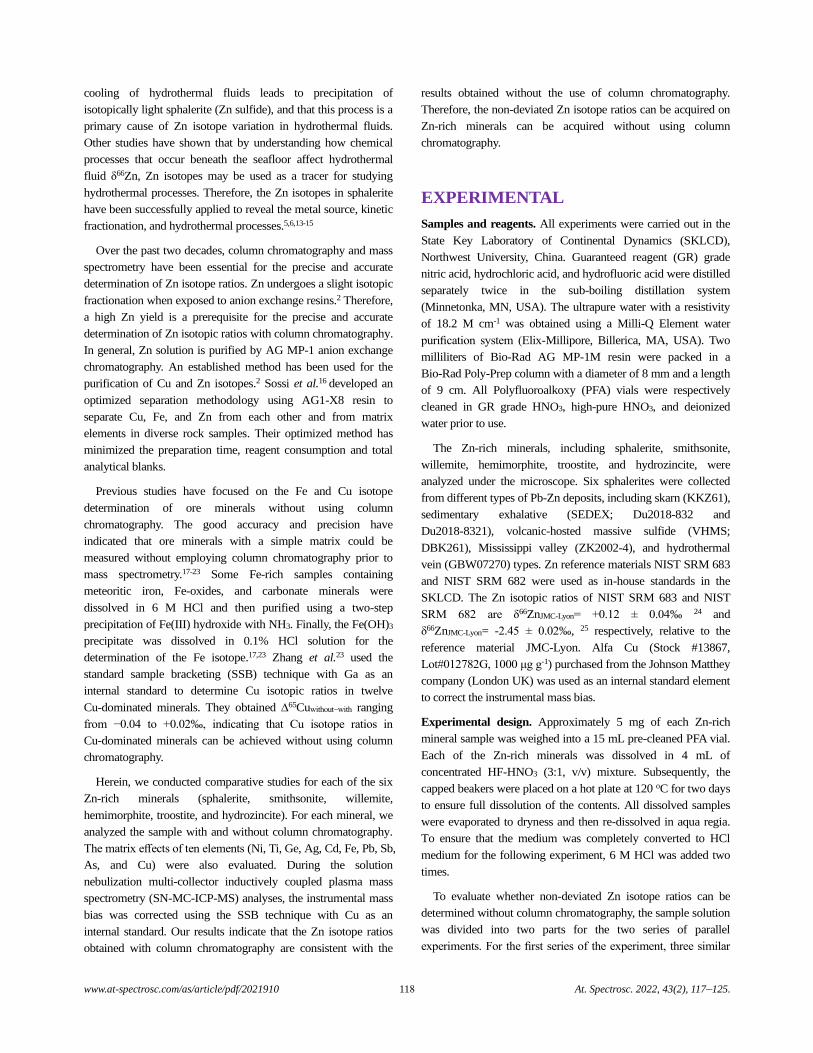
www.at-spectrosc.com/as/article/pdf/2021910 118 At. Spectrosc. 2022, 43(2), 117–125.
cooling of hydrothermal fluids leads to precipitation of
isotopically light sphalerite (Zn sulfide), and that this process is a
primary cause of Zn isotope variation in hydrothermal fluids.
Other studies have shown that by understanding how chemical
processes that occur beneath the seafloor affect hydrothermal
fluid δ66Zn, Zn isotopes may be used as a tracer for studying
hydrothermal processes. Therefore, the Zn isotopes in sphalerite
have been successfully applied to reveal the metal source, kinetic
fractionation, and hydrothermal processes.5,6,13-15
Over the past two decades, column chromatography and mass
spectrometry have been essential for the precise and accurate
determination of Zn isotope ratios. Zn undergoes a slight isotopic
fractionation when exposed to anion exchange resins.2 Therefore,
a high Zn yield is a prerequisite for the precise and accurate
determination of Zn isotopic ratios with column chromatography.
In general, Zn solution is purified by AG MP-1 anion exchange
chromatography. An established method has been used for the
purification of Cu and Zn isotopes.2 Sossi et al.16 developed an
optimized separation methodology using AG1-X8 resin to
separate Cu, Fe, and Zn from each other and from matrix
elements in diverse rock samples. Their optimized method has
minimized the preparation time, reagent consumption and total
analytical blanks.
Previous studies have focused on the Fe and Cu isotope
determination of ore minerals without using column
chromatography. The good accuracy and precision have
indicated that ore minerals with a simple matrix could be
measured without employing column chromatography prior to
mass spectrometry.17-23 Some Fe-rich samples containing
meteoritic iron, Fe-oxides, and carbonate minerals were
dissolved in 6 M HCl and then purified using a two-step
precipitation of Fe(III) hydroxide with NH3. Finally, the Fe(OH)3
precipitate was dissolved in 0.1% HCl solution for the
determination of the Fe isotope.17,23 Zhang et al.23 used the
standard sample bracketing (SSB) technique with Ga as an
internal standard to determine Cu isotopic ratios in twelve
Cu-dominated minerals. They obtained 65Cuwithout−with ranging
from −0.04 to +0.02‰, indicating that Cu isotope ratios in
Cu-dominated minerals can be achieved without using column
chromatography.
Herein, we conducted comparative studies for each of the six
Zn-rich minerals (sphalerite, smithsonite, willemite,
hemimorphite, troostite, and hydrozincite). For each mineral, we
analyzed the sample with and without column chromatography.
The matrix effects of ten elements (Ni, Ti, Ge, Ag, Cd, Fe, Pb, Sb,
As, and Cu) were also evaluated. During the solution
nebulization multi-collector inductively coupled plasma mass
spectrometry (SN-MC-ICP-MS) analyses, the instrumental mass
bias was corrected using the SSB technique with Cu as an
internal standard. Our results indicate that the Zn isotope ratios
obtained with column chromatography are consistent with the
results obtained without the use of column chromatography.
Therefore, the non-deviated Zn isotope ratios can be acquired on
Zn-rich minerals can be acquired without using column
chromatography.
EXPERIMENTAL
Samples and reagents. All experiments were carried out in the
State Key Laboratory of Continental Dynamics (SKLCD),
Northwest University, China. Guaranteed reagent (GR) grade
nitric acid, hydrochloric acid, and hydrofluoric acid were distilled
separately twice in the sub-boiling distillation system
(Minnetonka, MN, USA). The ultrapure water with a resistivity
of 18.2 M cm-1 was obtained using a Milli-Q Element water
purification system (Elix-Millipore, Billerica, MA, USA). Two
milliliters of Bio-Rad AG MP-1M resin were packed in a
Bio-Rad Poly-Prep column with a diameter of 8 mm and a length
of 9 cm. All Polyfluoroalkoxy (PFA) vials were respectively
cleaned in GR grade HNO3, high-pure HNO3, and deionized
water prior to use.
The Zn-rich minerals, including sphalerite, smithsonite,
willemite, hemimorphite, troostite, and hydrozincite, were
analyzed under the microscope. Six sphalerites were collected
from different types of Pb-Zn deposits, including skarn (KKZ61),
sedimentary exhalative (SEDEX; Du2018-832 and
Du2018-8321), volcanic-hosted massive sulfide (VHMS;
DBK261), Mississippi valley (ZK2002-4), and hydrothermal
vein (GBW07270) types. Zn reference materials NIST SRM 683
and NIST SRM 682 were used as in-house standards in the
SKLCD. The Zn isotopic ratios of NIST SRM 683 and NIST
SRM 682 are δ66ZnJMC-Lyon= +0.12 ± 0.04‰ 24 and
δ66ZnJMC-Lyon= -2.45 ± 0.02‰, 25 respectively, relative to the
reference material JMC-Lyon. Alfa Cu (Stock #13867,
Lot#012782G, 1000 μg g-1) purchased from the Johnson Matthey
company (London UK) was used as an internal standard element
to correct the instrumental mass bias.
Experimental design. Approximately 5 mg of each Zn-rich
mineral sample was weighed into a 15 mL pre-cleaned PFA vial.
Each of the Zn-rich minerals was dissolved in 4 mL of
concentrated HF-HNO3 (3:1, v/v) mixture. Subsequently, the
capped beakers were placed on a hot plate at 120 oC for two days
to ensure full dissolution of the contents. All dissolved samples
were evaporated to dryness and then re-dissolved in aqua regia.
To ensure that the medium was completely converted to HCl
medium for the following experiment, 6 M HCl was added two
times.
To evaluate whether non-deviated Zn isotope ratios can be
determined without column chromatography, the sample solution
was divided into two parts for the two series of parallel
experiments. For the first series of the experiment, three similar
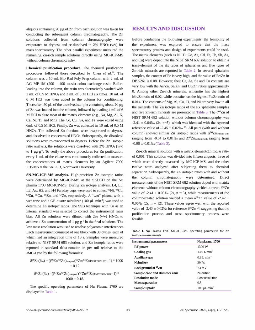
www.at-spectrosc.com/as/article/pdf/2021910 119 At. Spectrosc. 2022, 43(2), 117–125.
aliquots containing 20 µg of Zn from each solution was taken for
conducting the subsequent column chromatography. The Zn
solutions collected from column chromatography were
evaporated to dryness and re-dissolved in 2% HNO3 (v/v) for
mass spectrometry. The other parallel experiment measured the
remaining Zn-rich sample solutions directly using MC-ICP-MS
without column chromatography.
Chemical purification procedure. The chemical purification
procedures followed those described by Chen et al.26. The
column was a 10 mL Bio-Rad Poly-Prep column with 2 mL of
AG MP-1M (200 – 400 mesh) anion exchange resin. Before
loading into the column, the resin was alternatively washed with
2 mL of 0.5 M HNO3 and 2 mL of 6 M HCl six times. 10 mL of
6 M HCl was then added to the column for conditioning.
Thereafter, 50 μL of the dissolved sample containing about 20 µg
of Zn was loaded into the column, followed by loading 4 mL of 6
M HCl to elute most of the matrix elements (e.g., Na, Mg, Al, K,
Ca, Ni, Ti, and Mn). The Co, Cu, Ga, and Fe were eluted using
6mL of 0.5 M HCl. Finally, Zn was collected in 10 mL of 0.5 M
HNO3. The collected Zn fractions were evaporated to dryness
and dissolved in concentrated HNO3. Subsequently, the dissolved
solutions were re-evaporated to dryness. Before the Zn isotopic
ratio analysis, the solutions were dissolved with 2% HNO3 (v/v)
to 1 µg g-1. To verify the above procedures for Zn purification,
every 1 mL of the eluate was continuously collected to measure
the concentrations of matrix elements by an Agilent 7900
ICP-MS at the SKLCD, Northwest University.
SN-MC-ICP-MS analysis. High-precision Zn isotopic ratios
were determined by MC-ICP-MS at the SKLCD on the Nu
plasma 1700 MC-ICP-MS. During Zn isotope analysis, L4, L3,
L2, Ax, H2, and H4 Faraday cups were used to collect 62Ni, 63Cu, 64Zn, 65Cu, 66Zn, and 67Zn, respectively. A “wet” plasma with a
wet cone and a GE quartz nebulizer (100 μL min-1) was used to
determine Zn isotopic ratios. The SSB technique with Cu as an
internal standard was selected to correct the instrumental mass
bias. All Zn solutions were diluted with 2% (v/v) HNO3 to
achieve a Zn concentration of 1 μg g-1 in the final solutions. The
low mass resolution was used to resolve polyatomic interferences.
Each measurement consisted of one block with 30 cycles, each of
which had an integration time of 10 s. Samples were measured
relative to NIST SRM 683 solution, and Zn isotopic ratios were
reported in standard delta-notation in per mil relative to the
JMC-Lyon by the following formulas:
δ66Zn(‰) = ((66Zn/64Zn)sample/(66Zn/64Zn)NIST SRM 683 - 1) * 1000
+ 0.12
δ67Zn(‰) =((67Zn/64Zn)sample/ (67Zn/64Zn) NIST SRM 683 - 1) *
1000 + 0.18.
The specific operating parameters of Nu Plasma 1700 are
displayed in Table 1.
RESULTS AND DISCUSSION
Before conducting the following experiments, the feasibility of
the experiment was explored to ensure that the mass
spectrometry process and design of experiments could be used.
The matrix elements (such as Ni, Ti, Ge, Ag, Cd, Fe, Pb, Sb, As,
and Cu) were doped into the NIST SRM 682 solution to obtain a
trace-element of the six types of sphalerites and five types of
Zn-rich minerals are reported in Table 2. In several sphalerite
samples, the content of Fe is very high, and the value of Fe/Zn in
DBK261 is 0.08. However, their Ca, As, Se and Cu contents are
very low with the As/Zn, Se/Zn, and Cu/Zn ratios approximately
0. Among other Zn-rich minerals, willemite has the highest
Mn/Zn ratio of 0.02, while troostite has the highest Fe/Zn ratio of
0.014. The contents of Mg, Al, Cu, Ti, and Ni are very low in all
the minerals. The Zn isotope ratios of the six sphalerite samples
and five Zn-rich minerals are presented in Table 3. The δ66Zn of
NIST SRM 682 solution without column chromatography was
-2.41 ± 0.04‰ (2s, n=3), which was identical with the reported
reference value of -2.45 ± 0.02‰ 25. All pairs (with and without
column) showed similar Zn isotopic ratios with Δ66Znwithout-with
ranging from -0.04 to 0.01‰ and Δ67Znwithout-with ranging from
-0.06 to 0.01‰ (Table 3).
Zn-rich mineral solution with a matrix element/Zn molar ratio
of 0.001. This solution was divided into fifteen aliquots, three of
which were directly measured by MC-ICP-MS, and the other
twelve were analyzed after subjecting them to chemical
separation. Subsequently, the Zn isotopic ratios with and without
the column chromatography were determined. Direct
measurements of the NIST SRM 682 solution doped with matrix
elements without column chromatography yielded a mean δ66Zn
value of -2.41 ± 0.05‰ (2s, n = 3), while measurements of the
column-treated solution yielded a mean δ66Zn value of -2.42 ±
0.05‰ (2s, n = 12). These values agree well with the reported
value of -2.45 ± 0.02‰ for reference δ66Zn 25, suggesting that the
purification process and mass spectrometry process were
feasible.
Table 1. Nu Plasma 1700 MC-ICP-MS operating parameters for Zn
isotope measurements
Instrumental parameters Nu plasma 1700
RF power 1300 W
Cooling gas 13.0 L min-1
Auxiliary gas 0.8 L min-1
Nebulizer 39 Psi
Background of 64Zn <3 mV
Sample cone and skimmer cone Ni orifice
Resolution mode Low resolution
Mass separation 0.5
Sample uptake 100 μL min-1
www.at-spectrosc.com/as/article/pdf/2021910 120 At. Spectrosc. 2022, 43(2), 117–125.
Table 2. Selected trace element compositions of Zn-rich minerals
Minerals Ca/Zn Fe/Zn Ti/Zn Ni/Zn As/Zn Se/Zn Mg/Zn Cd/Zn Cu/Zn
Sphalerite (KKZ61) 0.003 0.021 0 0 0.001 0.002 0 0.011 0
Sphalerite (Du2018-832) 0.001 0.031 0 0 0.001 0.001 0 0.002 0.001
Sphalerite (Du2018-8321) 0.001 0.013 0 0 0.001 0.001 0 0.002 0.001
Sphalerite (DBK261) 0.003 0.08 0 0 0.003 0.006 0 0.005 0.001
Sphalerite (ZK2002-4) 0.001 - - 0 0 0 0.017 0 0
Sphalerite (GBW07270) 0.005 0.031 0 0 0 0 0.018 0.002 0.002
Smithsonite 0.017 0.003 0 0 - - 0 - 0
Willemite 0.001 0.007 0 0 - - 0.002 - 0
Hemimorphite 0.003 0 0 0 - - 0 - 0.002
Troostite 0.002 0.014 0 0 - - 0 - 0
Hydrozincite 0.01 0 0 0 0 - 0.014 0 0
“-” denotes elements that could not be detected by Agilent 7900 ICP-MS due to their low signal intensities.
Table 3. Zinc isotope ratios of sphalerite samples and other types of Zn-rich minerals with/without column chromatography
Minerals δ66Znwithout (‰) 2s n δ66Znwith (‰) 2s n Δ66Znwithout-with (‰)
Sphalerite (KKZ61) 0.21 0.02 3 0.23 0.06 3 -0.02
Sphalerite (Du2018-832) -0.07 0.02 3 -0.04 0.04 3 -0.03
Sphalerite (Du2018-8321) 0.13 0.02 3 0.17 0.04 3 -0.04
Sphalerite (DBK261) 0.13 0.03 3 0.15 0.03 3 -0.02
Sphalerite (ZK2002-4) 0.20 0.03 3 0.22 0.03 3 -0.02
Sphalerite (GBW07270) -0.05 0.01 3 -0.03 0.03 3 -0.02
Smithsonite -0.27 0.01 3 -0.26 0.04 3 -0.01
Willemite 0.26 0.07 3 0.26 0.02 3 0.00
Hemimorphite 0.96 0.05 3 0.96 0.02 3 0.00
Troostite 0.09 0.05 3 0.11 0.01 3 -0.02
Hydrozincite 0.04 0.02 3 0.03 0.01 3 0.01
Minerals δ67Znwithout (‰) 2s n δ67Znwith (‰) 2s n Δ67Znwithout-with (‰)
Sphalerite (KKZ61) 0.31 0.04 3 0.35 0.06 3 -0.04
Sphalerite (Du2018-832) -0.09 0.02 3 -0.07 0.05 3 -0.02
Sphalerite (Du2018-8321) 0.21 0.04 3 0.27 0.09 3 -0.06
Sphalerite (DBK261) 0.21 0.06 3 0.23 0.06 3 -0.02
Sphalerite (ZK2002-4) 0.33 0.06 3 0.35 0.07 3 -0.02
Sphalerite (GBW07270) -0.08 0.01 3 -0.05 0.07 3 -0.03
Smithsonite -0.38 0.01 3 -0.38 0.06 3 0.00
Willemite 0.41 0.13 3 0.40 0.04 3 0.01
Hemimorphite 1.43 0.10 3 1.42 0.04 3 0.01
Troostite 0.13 0.05 3 0.15 0.04 3 -0.02
Hydrozincite 0.04 0.03 3 0.05 0.01 3 -0.01
Note: δZnwith and δZnwithout denote Zn isotope ratios of minerals that were processed with column and without column, respectively; 2s refers to 2 standard
deviations. Column “n” represents the total number of repeat analyses. Δ66Znwithout-with=δ66Znwithout-δ66Znwith, Δ
67Znwithout-with=δ67Znwithout-δ67Znwith.
Effects of acidity and concentration mismatch. Previous
studies have shown that the stable isotopic deviation of Zn can be
caused by the concentration and acidity mismatches during mass
spectrometry.26-28 In this study, we used 1.0 μg g-1 of Alfa Zn
solution diluted with 2.0% (v/v) HNO3 as the medium for the Zn
isotopic analyses. The effects of acidity mismatch between the
sample and the standard were tested using a series of 1.0 μg g-1
Alfa Zn solutions diluted with 1.5 to 2.4% (v/v) HNO3. The SSB
www.at-spectrosc.com/as/article/pdf/2021910 121 At. Spectrosc. 2022, 43(2), 117–125.
Fig. 1 Effects of different acidities of Alfa Zn solution on δ66Zn and
δ67Zn.Precisions are expressed as 2 standard deviations (2s), which are
calculated based on four repeated measurements. Dotted line indicates the
reference value. Grey area represents the 2s deviation range (0.05‰).
Fig. 2 Zn isotope ratio variations of Alfa Zn solution with different Zn
concentrations from 0.5 to 2.0 μg g-1. Errors are presented at the 2s level
obtained by four repeated measurements. Dotted line indicates the
reference value. Grey region expresses the 2s deviation range (0.05‰).
method with Cu as an internal standard was used to correct the
instrument mass bias in the zinc isotope analysis. The lesser the
effects of acidity mismatch on the test, the closer the values of
δ66ZnAlfa Zn and δ67ZnAlfa Zn should be to 0. Fig. 1 shows that the
differences in acidities between the sample and standard have a
significant influence on the Zn isotopic compositions during
mass spectrometry. When the difference in acidities between the
sample and standard is within 10%, the obtained δ66ZnAlfa Zn and
δ67ZnAlfa Zn values were within a deviation of 0.05‰. When the
difference is ≥ 20%, the offset in δ67ZnAlfa Zn can be up to 0.10‰,
which is significant. To eliminate the possible effects of the
acidity mismatch, all dried samples were diluted using 2.0% (v/v)
HNO3 to ensure acceptable acidity differences (<10%) before
conducting mass spectrometry.
Fixing the Zn concentration of the bracketing standard at 1.0
μg g-1, we measured a series of Alfa Zn solutions with different
Zn concentrations ranging from 0.5 to 2.0 μg g-1 to investigate the
effects of the concentration mismatch between the sample and
the standard. The lesser the effects of the concentration mismatch,
the closer the values of δ66ZnAlfa Zn and δ67ZnAlfa Zn should be to 0.
Our results indicate that the differences in concentrations do not
have a significant influence on the Zn isotopic compositions for
the wet plasma method (Fig. 2). For a Csample/Cstandard ratio
ranging from 0.5 to 2.0, the δ66ZnAlfa Zn and δ67ZnAlfa Zn values of
all samples agree well within the 0.05‰ deviation. To guarantee
the precision and accuracy of Zn isotopic ratios, the
Csample/Cstandard ratio was kept at less than ± 20% during mass
spectrometry.
Effects of matrix elements. Natural sphalerite minerals usually
comprise some trace elements, such as Ni, Ti, Ge, Ag, Cd, Fe, Pb,
Sb, As, and Cu, which remain in the Zn solutions that are not
subjected to column chromatography. The presence of these
residual matrix elements can potentially affect the accuracy and
precision of Zn isotopic analysis. In this study, we quantitatively
assessed the potential effects of the ten matrix elements (Ni, Ti,
Ge, Ag, Cd, Fe, Pb, Sb, As, and Cu) on Zn isotope measurements.
These matrix elements of different concentrations were doped
into 1.0 μg g-1 Alfa Zn standard solutions and bracketed using the
same pure Zn standard without any doping. The results of these
analyses were plotted in Fig. 3. For most matrix elements with
matrix element/Zn molar ratios up to 0.1, the δ66ZnAlfa Zn and
δ67ZnAlfa Zn values were consistent with the true value within the
0.05‰ deviation, suggesting that the influence of these elements
can be ignored during the measurements. When the molar ratio
of Cu/Zn ranged from 0.25 to 3, Zn isotopic ratios showed no
difference. Therefore, the addition of Cu in the sample would not
affect the results of Zn isotope ratio measurements, it is feasible
to use Cu as the internal standard.
However, small amounts of Ti and Ni residues in the Zn
solutions will affect Zn isotopic ratios because 64Ni+ and 48Ti16O+
can produce intense isobaric interferences on 64Zn+. The matrix
effects of Ti and Ni on Zn isotope ratios are also shown in Fig. 3.
When the Ti/Zn ratio is less than 0.01, δ66ZnAlfa Zn and δ67ZnAlfa Zn
values can be accurately obtained within the 0.05‰ deviation.
When the Ni/Zn ratio is less than 0.005, δ66ZnAlfa Zn and δ67ZnAlfa
Zn values with better accuracies can be obtained within the 0.05‰
deviation. Owing the low Ti and Ni contents in Zn-rich minerals
(Ti or Ni/Zn <0.001), the Ti polyatomic and Ni interferences are
negligible when the Zn isotope ratios are measured without
column chromatography.
Quality control of the Zn isotope ratios of samples. The NIST
SRM 682 solution doped with trace matrix elements was
repeatedly measured at different periods by MC-ICP-MS for
quality control. A total of 42 tests were conducted in December
2020, January 2021 and March 2021. Fig. 4 shows that the
variations of Zn isotope ratios of NIST SRM 682 solutions were
small within the four months, and the long-term precision of the
δ66Zn was ±0.03‰. The NIST SRM 682 solutions possessed a
mean δ66Zn of -2.41 ± 0.03‰ (2s, n = 42) over the four months,
which was consistent with the reference value within 2s deviation.
The results confirm that our method was useful to determine the
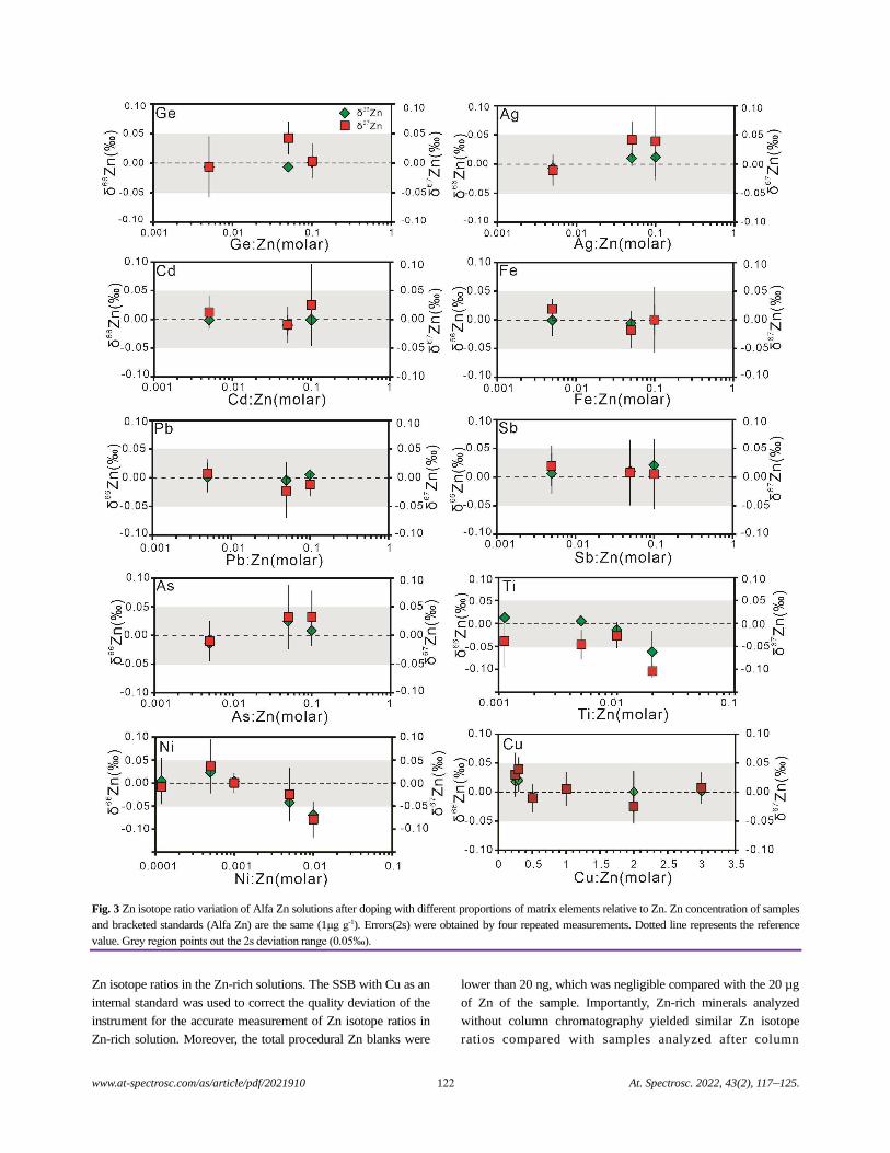
www.at-spectrosc.com/as/article/pdf/2021910 122 At. Spectrosc. 2022, 43(2), 117–125.
Fig. 3 Zn isotope ratio variation of Alfa Zn solutions after doping with different proportions of matrix elements relative to Zn. Zn concentration of samples
and bracketed standards (Alfa Zn) are the same (1μg g-1). Errors(2s) were obtained by four repeated measurements. Dotted line represents the reference
value. Grey region points out the 2s deviation range (0.05‰).
Zn isotope ratios in the Zn-rich solutions. The SSB with Cu as an
internal standard was used to correct the quality deviation of the
instrument for the accurate measurement of Zn isotope ratios in
Zn-rich solution. Moreover, the total procedural Zn blanks were
lower than 20 ng, which was negligible compared with the 20 µg
of Zn of the sample. Importantly, Zn-rich minerals analyzed
without column chromatography yielded similar Zn isotope
ratios compared with samples analyzed after column
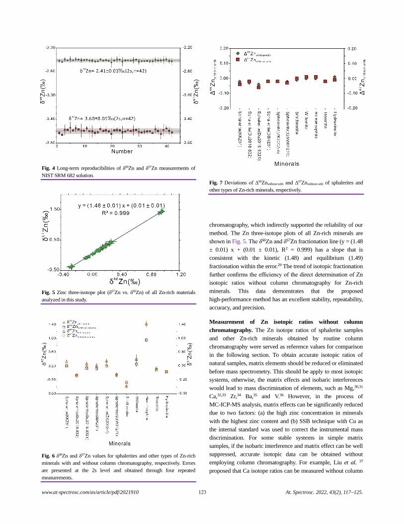
www.at-spectrosc.com/as/article/pdf/2021910 123 At. Spectrosc. 2022, 43(2), 117–125.
Fig. 4 Long-term reproducibilities of δ66Zn and δ67Zn measurements of
NIST SRM 682 solution.
Fig. 5 Zinc three-isotope plot (δ67Zn
vs. δ66Zn) of all Zn-rich materials
analyzed in this study.
Fig. 6 δ66Zn and δ67Zn values for sphalerites and other types of Zn-rich
minerals with and without column chromatography, respectively. Errors
are presented at the 2s level and obtained through four repeated
measurements.
Fig. 7
Deviations of Δ66Znwithout-with
and Δ67Znwithout-with
of sphalerites and
other types of Zn-rich minerals, respectively.
chromatography, which indirectly supported the reliability of our
method. The Zn three-isotope plots of all Zn-rich minerals are
shown in Fig. 5. The δ66Zn and δ67Zn fractionation line (y = (1.48
± 0.01) x + (0.01 ± 0.01), R2 = 0.999) has a slope that is
consistent with the kinetic (1.48) and equilibrium (1.49)
fractionation within the error.29 The trend of isotopic fractionation
further confirms the efficiency of the direct determination of Zn
isotopic ratios without column chromatography for Zn-rich
minerals. This data demonstrates that the proposed
high-performance method has an excellent stability, repeatability,
accuracy, and precision.
Measurement of Zn isotopic ratios without column
chromatography. The Zn isotope ratios of sphalerite samples
and other Zn-rich minerals obtained by routine column
chromatography were served as reference values for comparison
in the following section. To obtain accurate isotopic ratios of
natural samples, matrix elements should be reduced or eliminated
before mass spectrometry. This should be apply to most isotopic
systems, otherwise, the matrix effects and isobaric interferences
would lead to mass discrimination of elements, such as Mg,30,31
Ca,32,33 Zr,34 Ba,35 and V.36 However, in the process of
MC-ICP-MS analysis, matrix effects can be significantly reduced
due to two factors: (a) the high zinc concentration in minerals
with the highest zinc content and (b) SSB technique with Cu as
the internal standard was used to correct the instrumental mass
discrimination. For some stable systems in simple matrix
samples, if the isobaric interference and matrix effect can be well
suppressed, accurate isotopic data can be obtained without
employing column chromatography. For example, Liu et al. 37
proposed that Ca isotope ratios can be measured without column
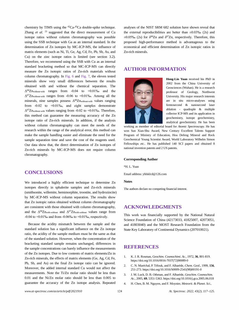
www.at-spectrosc.com/as/article/pdf/2021910 124 At. Spectrosc. 2022, 43(2), 117–125.
chemistry by TIMS using the 42Ca-43Ca double-spike technique.
Zhang et al. 23 suggested that the direct measurement of Cu
isotope ratios without column chromatography was possible
using the SSB technique with Ga as an internal standard. In the
determination of Zn isotopes by MC-ICP-MS, the influence of
matrix elements (such as Ni, Ti, Ge, Ag, Cd, Fe, Pb, Sb, As, and
Cu) on the zinc isotope ratios is limited (see section 3.2).
Therefore, we recommend using the SSB with Cu as an internal
standard bracketing method so that MC-ICP-MS can directly
measure the Zn isotopic ratios of Zn-rich materials without
column chromatography. In Fig. 6 and Fig. 7, the eleven tested
minerals show very small differences between the results
obtained with and without the chemical separation. The
Δ66Znwithout-with ranges from -0.04 to +0.01‰ and the
Δ67Znwithout-with ranges from -0.06 to +0.01‰. Among all the
minerals, nine samples possess Δ66Znwithout-with values ranging
from -0.02 to +0.01‰, and eight samples demonstrate
Δ67Znwithout-with values ranging from -0.02 to +0.01‰. Therefore,
this method can guarantee the measuring accuracy of the Zn
isotope ratio of Zn-rich minerals. In addition, if the analysis
without column chromatography can meet the needs of the
research within the range of the analytical error, this method can
make the sample handling easier and eliminate the need for the
sample separation time and save the cost of the reagents used.
Our data show that, the direct determination of Zn isotopes of
Zn-rich minerals by MC-ICP-MS does not require column
chromatography.
CONCLUSIONS
We introduced a highly efficient technique to determine Zn
isotopes directly in sphalerite samples and Zn-rich minerals
(smithsonite, willemite, hemimorphite, troostite, and hydrozincite)
by MC-ICP-MS without column separation. The results show
that Zn isotopic ratios obtained without column chromatography
are consistent with those obtained with column chromatography,
and the Δ66Znwith-without and Δ67Znwith-without values range from
-0.04 to +0.01‰ and from -0.06‰ to +0.01‰, respectively.
Because the acidity mismatch between the sample and the
standard solution has a significant influence on the Zn isotope
ratio, the acidity of the sample medium must be the same as that
of the standard solution. However, when the concentration of the
bracketing standard sample remains unchanged, differences in
the sample concentrations can barely influence the measurements
of the Zn isotopes. Due to low contents of matrix elements/Zn in
Zn-rich minerals, the effects of matrix elements (Ge, Ag, Cd, Fe,
Pb, Sb, and As) on the final Zn isotope ratio can be ignored.
Moreover, the added internal standard Cu would not affect the
measurements. Note the Ti/Zn molar ratio should be less than
0.01 and the Ni/Zn molar ratio should be less than 0.005 to
guarantee the accuracy of the Zn isotope analysis. Repeated
analyses of the NIST SRM 682 solution have shown reveal that
the external reproducibilities are better than ±0.03‰ (2s) and
±0.05‰ (2s) for δ66Zn and δ67Zn, respectively. Therefore, this
proposed high-performance method is advantageous to the
economical and efficient determination of Zn isotopic ratios in
Zn-rich minerals.
AUTHOR INFORMATION
Hong-Lin Yuan received his PhD in
2002 from the China University of
Geosciences (Wuhan). He is a research
professor of Geology, Northwest
University. His major research interests
are in situ micro-analyses using
femtosecond & nanosecond laser
ablation - quadruple & multiple
collector ICP-MS and its application in
geochemistry, isotope geochemistry,
analytical geochemistry. He has been
working as member of editorial board for Atomic Spectroscopy. He has
won Sun Xian-Shu Award, New Century Excellent Talents Support
Program of Ministry of Education, Hou Defeng Mineral and Rock
Geochemical Young Scientist Award, World Laboratory Wilhelm Simon
Fellowships etc.. He has published 140 SCI papers and obtained 8
national invention patents and 2 US patents.
Corresponding Author
*H. L. Yuan
Email address: [email protected]
Notes
The authors declare no competing financial interest.
ACKNOWLEDGMENTS
This work was financially supported by the National Natural
Science Foundation of China (42173033, 41825007, 42073051,
and 41803040) and the MOST Research Foundation from the
State Key Laboratory of Continental Dynamics (207010021).
REFERENCES
1. K. J. R. Rosman, Geochim. Cosmochimi. Ac., 1972, 36, 801-819.
https://doi.org/10.1016/0016-7037(72)90089-0
2. C. N. Maréchal, P. Télouk, and F. Albarède, Chem. Geol., 1999, 156,
251-273. https://doi.org/10.1016/S0009-2541(98)00191-0
3. J. M. Luck, D. B. Othman, and F. Albarède, Geochim. Cosmochim.
Ac., 2005, 69, 5351-5363. https://doi.org/10.1016/j.gca.2005.06.018
4. H. Chen, B. M. Nguyen, and F. Moynier, Meteorit. & Planet. Sci.,
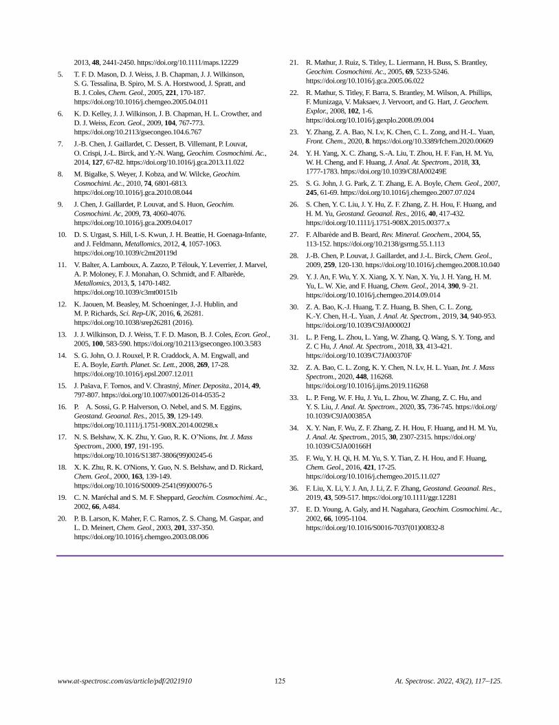
www.at-spectrosc.com/as/article/pdf/2021910 125 At. Spectrosc. 2022, 43(2), 117–125.
2013, 48, 2441-2450. https://doi.org/10.1111/maps.12229
5. T. F. D. Mason, D. J. Weiss, J. B. Chapman, J. J. Wilkinson,
S. G. Tessalina, B. Spiro, M. S. A. Horstwood, J. Spratt, and
B. J. Coles, Chem. Geol., 2005, 221, 170-187.
https://doi.org/10.1016/j.chemgeo.2005.04.011
6. K. D. Kelley, J. J. Wilkinson, J. B. Chapman, H. L. Crowther, and
D. J. Weiss, Econ. Geol., 2009, 104, 767-773.
https://doi.org/10.2113/gsecongeo.104.6.767
7. J.-B. Chen, J. Gaillardet, C. Dessert, B. Villemant, P. Louvat,
O. Crispi, J.-L. Birck, and Y.-N. Wang, Geochim. Cosmochimi. Ac.,
2014, 127, 67-82. https://doi.org/10.1016/j.gca.2013.11.022
8. M. Bigalke, S. Weyer, J. Kobza, and W. Wilcke, Geochim.
Cosmochimi. Ac., 2010, 74, 6801-6813.
https://doi.org/10.1016/j.gca.2010.08.044
9. J. Chen, J. Gaillardet, P. Louvat, and S. Huon, Geochim.
Cosmochimi. Ac, 2009, 73, 4060-4076.
https://doi.org/10.1016/j.gca.2009.04.017
10. D. S. Urgast, S. Hill, I.-S. Kwun, J. H. Beattie, H. Goenaga-Infante,
and J. Feldmann, Metallomics, 2012, 4, 1057-1063.
https://doi.org/10.1039/c2mt20119d
11. V. Balter, A. Lamboux, A. Zazzo, P. Télouk, Y. Leverrier, J. Marvel,
A. P. Moloney, F. J. Monahan, O. Schmidt, and F. Albarède,
Metallomics, 2013, 5, 1470-1482.
https://doi.org/10.1039/c3mt00151b
12. K. Jaouen, M. Beasley, M. Schoeninger, J.-J. Hublin, and
M. P. Richards, Sci. Rep-UK, 2016, 6, 26281. https://doi.org/10.1038/srep26281 (2016).
13. J. J. Wilkinson, D. J. Weiss, T. F. D. Mason, B. J. Coles, Econ. Geol.,
2005, 100, 583-590. https://doi.org/10.2113/gsecongeo.100.3.583
14. S. G. John, O. J. Rouxel, P. R. Craddock, A. M. Engwall, and
E. A. Boyle, Earth. Planet. Sc. Lett., 2008, 269, 17-28.
https://doi.org/10.1016/j.epsl.2007.12.011
15. J. Pašava, F. Tornos, and V. Chrastný, Miner. Deposita., 2014, 49,
797-807. https://doi.org/10.1007/s00126-014-0535-2
16. P. A. Sossi, G. P. Halverson, O. Nebel, and S. M. Eggins,
Geostand. Geoanal. Res., 2015, 39, 129-149.
https://doi.org/10.1111/j.1751-908X.2014.00298.x
17. N. S. Belshaw, X. K. Zhu, Y. Guo, R. K. O’Nions, Int. J. Mass
Spectrom., 2000, 197, 191-195.
https://doi.org/10.1016/S1387-3806(99)00245-6
18. X. K. Zhu, R. K. O'Nions, Y. Guo, N. S. Belshaw, and D. Rickard,
Chem. Geol., 2000, 163, 139-149.
https://doi.org/10.1016/S0009-2541(99)00076-5
19. C. N. Maréchal and S. M. F. Sheppard, Geochim. Cosmochimi. Ac.,
2002, 66, A484.
20. P. B. Larson, K. Maher, F. C. Ramos, Z. S. Chang, M. Gaspar, and
L. D. Meinert, Chem. Geol., 2003, 201, 337-350.
https://doi.org/10.1016/j.chemgeo.2003.08.006
21. R. Mathur, J. Ruiz, S. Titley, L. Liermann, H. Buss, S. Brantley,
Geochim. Cosmochimi. Ac., 2005, 69, 5233-5246.
https://doi.org/10.1016/j.gca.2005.06.022
22. R. Mathur, S. Titley, F. Barra, S. Brantley, M. Wilson, A. Phillips,
F. Munizaga, V. Maksaev, J. Vervoort, and G. Hart, J. Geochem.
Explor., 2008, 102, 1-6.
https://doi.org/10.1016/j.gexplo.2008.09.004
23. Y. Zhang, Z. A. Bao, N. Lv, K. Chen, C. L. Zong, and H.-L. Yuan,
Front. Chem., 2020, 8. https://doi.org/10.3389/fchem.2020.00609
24. Y. H. Yang, X. C. Zhang, S.-A. Liu, T. Zhou, H. F. Fan, H. M. Yu,
W. H. Cheng, and F. Huang, J. Anal. At. Spectrom., 2018, 33,
1777-1783. https://doi.org/10.1039/C8JA00249E
25. S. G. John, J. G. Park, Z. T. Zhang, E. A. Boyle, Chem. Geol., 2007,
245, 61-69. https://doi.org/10.1016/j.chemgeo.2007.07.024
26. S. Chen, Y. C. Liu, J. Y. Hu, Z. F. Zhang, Z. H. Hou, F. Huang, and
H. M. Yu, Geostand. Geoanal. Res., 2016, 40, 417-432. https://doi.org/10.1111/j.1751-908X.2015.00377.x
27. F. Albarède and B. Beard, Rev. Mineral. Geochem., 2004, 55,
113-152. https://doi.org/10.2138/gsrmg.55.1.113
28. J.-B. Chen, P. Louvat, J. Gaillardet, and J.-L. Birck, Chem. Geol.,
2009, 259, 120-130. https://doi.org/10.1016/j.chemgeo.2008.10.040
29. Y. J. An, F. Wu, Y. X. Xiang, X. Y. Nan, X. Yu, J. H. Yang, H. M.
Yu, L. W. Xie, and F. Huang, Chem. Geol., 2014, 390, 9–21.
https://doi.org/10.1016/j.chemgeo.2014.09.014
30. Z. A. Bao, K.-J. Huang, T. Z. Huang, B. Shen, C. L. Zong,
K.-Y. Chen, H.-L. Yuan, J. Anal. At. Spectrom., 2019, 34, 940-953.
https://doi.org/10.1039/C9JA00002J
31. L. P. Feng, L. Zhou, L. Yang, W. Zhang, Q. Wang, S. Y. Tong, and
Z. C Hu, J. Anal. At. Spectrom., 2018, 33, 413-421.
https://doi.org/10.1039/C7JA00370F
32. Z. A. Bao, C. L. Zong, K. Y. Chen, N. Lv, H. L. Yuan, Int. J. Mass
Spectrom., 2020, 448, 116268.
https://doi.org/10.1016/j.ijms.2019.116268
33. L. P. Feng, W. F. Hu, J. Yu, L. Zhou, W. Zhang, Z. C. Hu, and
Y. S. Liu, J. Anal. At. Spectrom., 2020, 35, 736-745. https://doi.org/
10.1039/C9JA00385A
34. X. Y. Nan, F. Wu, Z. F. Zhang, Z. H. Hou, F. Huang, and H. M. Yu,
J. Anal. At. Spectrom., 2015, 30, 2307-2315. https://doi.org/
10.1039/C5JA00166H
35. F. Wu, Y. H. Qi, H. M. Yu, S. Y. Tian, Z. H. Hou, and F. Huang,
Chem. Geol., 2016, 421, 17-25.
https://doi.org/10.1016/j.chemgeo.2015.11.027
36. F. Liu, X. Li, Y. J. An, J. Li, Z. F. Zhang, Geostand. Geoanal. Res.,
2019, 43, 509-517. https://doi.org/10.1111/ggr.12281
37. E. D. Young, A. Galy, and H. Nagahara, Geochim. Cosmochimi. Ac.,
2002, 66, 1095-1104.
https://doi.org/10.1016/S0016-7037(01)00832-8
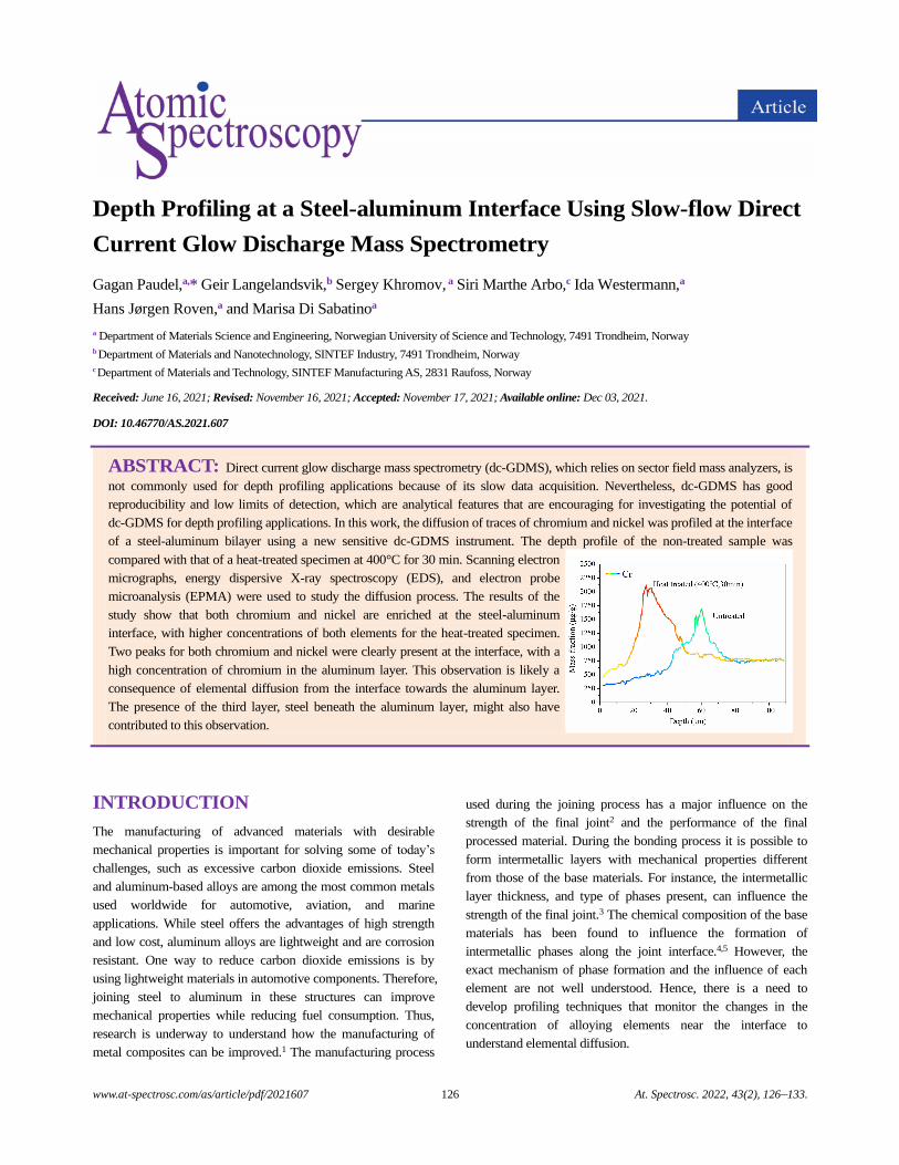
www.at-spectrosc.com/as/article/pdf/2021607 126 At. Spectrosc. 2022, 43(2), 126–133.
Depth Profiling at a Steel-aluminum Interface Using Slow-flow Direct
Current Glow Discharge Mass Spectrometry
Gagan Paudel,a,* Geir Langelandsvik,b Sergey Khromov, a Siri Marthe Arbo,c Ida Westermann,a
Hans Jørgen Roven,a and Marisa Di Sabatinoa
a Department of Materials Science and Engineering, Norwegian University of Science and Technology, 7491 Trondheim, Norway
b Department of Materials and Nanotechnology, SINTEF Industry, 7491 Trondheim, Norway
c Department of Materials and Technology, SINTEF Manufacturing AS, 2831 Raufoss, Norway
Received: June 16, 2021; Revised: November 16, 2021; Accepted: November 17, 2021; Available online: Dec 03, 2021.
DOI: 10.46770/AS.2021.607
ABSTRACT: Direct current glow discharge mass spectrometry (dc-GDMS), which relies on sector field mass analyzers, is
not commonly used for depth profiling applications because of its slow data acquisition. Nevertheless, dc-GDMS has good
reproducibility and low limits of detection, which are analytical features that are encouraging for investigating the potential of
dc-GDMS for depth profiling applications. In this work, the diffusion of traces of chromium and nickel was profiled at the interface
of a steel-aluminum bilayer using a new sensitive dc-GDMS instrument. The depth profile of the non-treated sample was
compared with that of a heat-treated specimen at 400°C for 30 min. Scanning electron
micrographs, energy dispersive X-ray spectroscopy (EDS), and electron probe
microanalysis (EPMA) were used to study the diffusion process. The results of the
study show that both chromium and nickel are enriched at the steel-aluminum
interface, with higher concentrations of both elements for the heat-treated specimen.
Two peaks for both chromium and nickel were clearly present at the interface, with a
high concentration of chromium in the aluminum layer. This observation is likely a
consequence of elemental diffusion from the interface towards the aluminum layer.
The presence of the third layer, steel beneath the aluminum layer, might also have
contributed to this observation.
INTRODUCTION
The manufacturing of advanced materials with desirable
mechanical properties is important for solving some of today’s
challenges, such as excessive carbon dioxide emissions. Steel
and aluminum-based alloys are among the most common metals
used worldwide for automotive, aviation, and marine
applications. While steel offers the advantages of high strength
and low cost, aluminum alloys are lightweight and are corrosion
resistant. One way to reduce carbon dioxide emissions is by
using lightweight materials in automotive components. Therefore,
joining steel to aluminum in these structures can improve
mechanical properties while reducing fuel consumption. Thus,
research is underway to understand how the manufacturing of
metal composites can be improved.1 The manufacturing process
used during the joining process has a major influence on the
strength of the final joint2 and the performance of the final
processed material. During the bonding process it is possible to
form intermetallic layers with mechanical properties different
from those of the base materials. For instance, the intermetallic
layer thickness, and type of phases present, can influence the
strength of the final joint.3 The chemical composition of the base
materials has been found to influence the formation of
intermetallic phases along the joint interface.4,5 However, the
exact mechanism of phase formation and the influence of each
element are not well understood. Hence, there is a need to
develop profiling techniques that monitor the changes in the
concentration of alloying elements near the interface to
understand elemental diffusion.
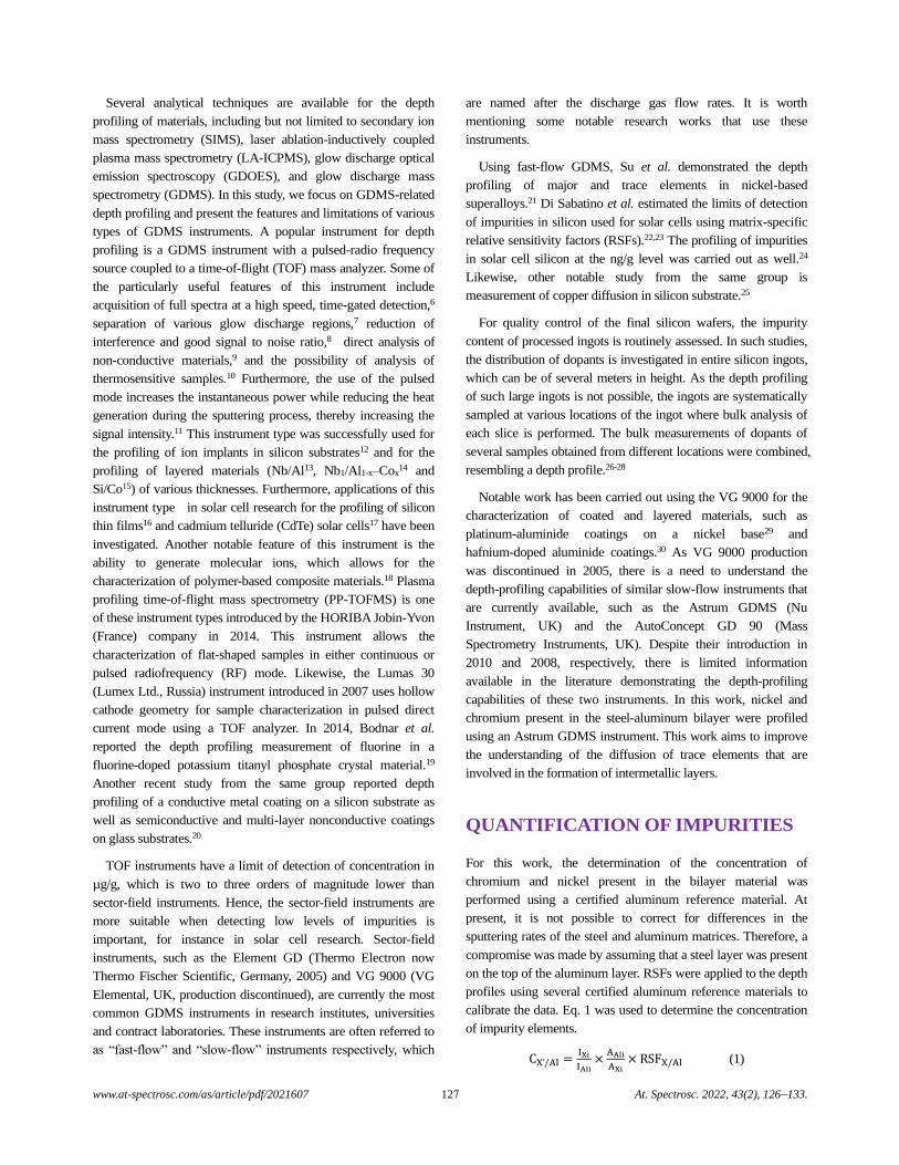
www.at-spectrosc.com/as/article/pdf/2021607 127 At. Spectrosc. 2022, 43(2), 126–133.
Several analytical techniques are available for the depth
profiling of materials, including but not limited to secondary ion
mass spectrometry (SIMS), laser ablation-inductively coupled
plasma mass spectrometry (LA-ICPMS), glow discharge optical
emission spectroscopy (GDOES), and glow discharge mass
spectrometry (GDMS). In this study, we focus on GDMS-related
depth profiling and present the features and limitations of various
types of GDMS instruments. A popular instrument for depth
profiling is a GDMS instrument with a pulsed-radio frequency
source coupled to a time-of-flight (TOF) mass analyzer. Some of
the particularly useful features of this instrument include
acquisition of full spectra at a high speed, time-gated detection,6
separation of various glow discharge regions,7 reduction of
interference and good signal to noise ratio,8 direct analysis of
non-conductive materials,9 and the possibility of analysis of
thermosensitive samples.10 Furthermore, the use of the pulsed
mode increases the instantaneous power while reducing the heat
generation during the sputtering process, thereby increasing the
signal intensity.11 This instrument type was successfully used for
the profiling of ion implants in silicon substrates12 and for the
profiling of layered materials (Nb/Al13, Nb1/Al1-x–Cox14 and
Si/Co15) of various thicknesses. Furthermore, applications of this
instrument type in solar cell research for the profiling of silicon
thin films16 and cadmium telluride (CdTe) solar cells17 have been
investigated. Another notable feature of this instrument is the
ability to generate molecular ions, which allows for the
characterization of polymer-based composite materials.18 Plasma
profiling time-of-flight mass spectrometry (PP-TOFMS) is one
of these instrument types introduced by the HORIBA Jobin-Yvon
(France) company in 2014. This instrument allows the
characterization of flat-shaped samples in either continuous or
pulsed radiofrequency (RF) mode. Likewise, the Lumas 30
(Lumex Ltd., Russia) instrument introduced in 2007 uses hollow
cathode geometry for sample characterization in pulsed direct
current mode using a TOF analyzer. In 2014, Bodnar et al.
reported the depth profiling measurement of fluorine in a
fluorine-doped potassium titanyl phosphate crystal material.19
Another recent study from the same group reported depth
profiling of a conductive metal coating on a silicon substrate as
well as semiconductive and multi-layer nonconductive coatings
on glass substrates.20
TOF instruments have a limit of detection of concentration in
µg/g, which is two to three orders of magnitude lower than
sector-field instruments. Hence, the sector-field instruments are
more suitable when detecting low levels of impurities is
important, for instance in solar cell research. Sector-field
instruments, such as the Element GD (Thermo Electron now
Thermo Fischer Scientific, Germany, 2005) and VG 9000 (VG
Elemental, UK, production discontinued), are currently the most
common GDMS instruments in research institutes, universities
and contract laboratories. These instruments are often referred to
as “fast-flow” and “slow-flow” instruments respectively, which
are named after the discharge gas flow rates. It is worth
mentioning some notable research works that use these
instruments.
Using fast-flow GDMS, Su et al. demonstrated the depth
profiling of major and trace elements in nickel-based
superalloys.21 Di Sabatino et al. estimated the limits of detection
of impurities in silicon used for solar cells using matrix-specific
relative sensitivity factors (RSFs).22,23 The profiling of impurities
in solar cell silicon at the ng/g level was carried out as well.24
Likewise, other notable study from the same group is
measurement of copper diffusion in silicon substrate.25
For quality control of the final silicon wafers, the impurity
content of processed ingots is routinely assessed. In such studies,
the distribution of dopants is investigated in entire silicon ingots,
which can be of several meters in height. As the depth profiling
of such large ingots is not possible, the ingots are systematically
sampled at various locations of the ingot where bulk analysis of
each slice is performed. The bulk measurements of dopants of
several samples obtained from different locations were combined,
resembling a depth profile.26-28
Notable work has been carried out using the VG 9000 for the
characterization of coated and layered materials, such as
platinum-aluminide coatings on a nickel base29 and
hafnium-doped aluminide coatings.30 As VG 9000 production
was discontinued in 2005, there is a need to understand the
depth-profiling capabilities of similar slow-flow instruments that
are currently available, such as the Astrum GDMS (Nu
Instrument, UK) and the AutoConcept GD 90 (Mass
Spectrometry Instruments, UK). Despite their introduction in
2010 and 2008, respectively, there is limited information
available in the literature demonstrating the depth-profiling
capabilities of these two instruments. In this work, nickel and
chromium present in the steel-aluminum bilayer were profiled
using an Astrum GDMS instrument. This work aims to improve
the understanding of the diffusion of trace elements that are
involved in the formation of intermetallic layers.
QUANTIFICATION OF IMPURITIES
For this work, the determination of the concentration of
chromium and nickel present in the bilayer material was
performed using a certified aluminum reference material. At
present, it is not possible to correct for differences in the
sputtering rates of the steel and aluminum matrices. Therefore, a
compromise was made by assuming that a steel layer was present
on the top of the aluminum layer. RSFs were applied to the depth
profiles using several certified aluminum reference materials to
calibrate the data. Eq. 1 was used to determine the concentration
of impurity elements.
CXˈ/Al =IXi
IAli×
AAli
AXi× RSFX/Al (1)
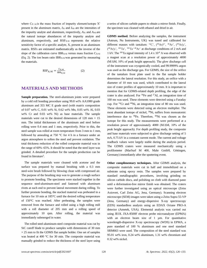
www.at-spectrosc.com/as/article/pdf/2021607 128 At. Spectrosc. 2022, 43(2), 126–133.
where CXˈ/Al is the mass fraction of impurity element/isotope Xʹ
present in the aluminum matrix, IXi and IAli are the intensities of
the impurity analyte and aluminum, respectively, AXi and AAli are
the natural isotope abundances of the impurity analyte and
aluminum, respectively, and RSFX/Al represents the relative
sensitivity factor of a specific analyte, X, present in an aluminum
matrix. RSFs are estimated mathematically as the inverse of the
slope of the calibration curve IBRX/Al versus mass fraction CX/Al
(Eq. 2). The ion beam ratio IBRX/Al was generated by measuring
the materials.
RSFX/Al =𝐶X/Al
IBRX/Al (2)
MATERIALS AND METHODS
Sample preparation. The steel-aluminum joints were prepared
by a cold roll bonding procedure using 99.8 wt% AA1080 grade
aluminum and 355 MC E grade steel (with matrix composition
of 0.07 wt% C, 0.01 wt% Si, 0.62 wt% Mn, 0.05 wt% Al, 0.03
wt% Cr and 0.03 wt% Ni) as base materials. The sample
materials were cut to the desired dimensions of 120 mm × 15
mm. The initial thicknesses of the aluminum and steel before
rolling were 0.4 mm and 1 mm, respectively. Prior to this, the
steel sample was rolled at room temperature from 3 mm to 1 mm,
followed by annealing at 750 °C for 4 h in a furnace under an
argon atmosphere to soften the steel and prevent oxidation. The
total thickness reduction of the rolled composite material was in
the range of 60%–65%. It should be noted that the steel layer was
grinded. A detailed procedure for the sample production can be
found in literature3.
The sample materials were cleaned with acetone and the
surface was prepared by manual brushing with a 0.3 mm
steel-wire brush followed by blowing clean with compressed air.
The purpose of the brushing step was to generate a rough surface
to promote bonding. The specimens were stacked together in the
sequence steel-aluminum-steel and fastened with aluminum
rivets at each end to prevent lateral movement during rolling. To
further promote bonding, the stacked material was preheated in a
furnace for 10 min at 185°C until the desired rolling temperature
of 150°C was reached. After preheating, the samples were
removed from the furnace and rolled using a high rolling mill
with a roll diameter of 205 mm and a rolling speed of
approximately 10 rpm. After rolling, the material was
immediately submerged in water.
The rolled steel-aluminum-steel composite material was cut by
SiC cutoff blade to produce samples with dimensions of 30 mm
× 25 mm to fit the GDMS flat sample holder. One set of samples
was heated at 400 °C for 30 min. The composite material was
manually grinded to reduce the thickness of the steel layer using
a series of silicon carbide papers to obtain a mirror finish. Finally,
the specimen was cleaned with ethanol and dried in air.
GDMS method. Before analyzing the samples, the instrument
(Astrum, Nu Instruments, UK) was tuned and calibrated for
different masses with tantalum: 12C+, (40Ar)2+, 36Ar+, (40Ar)2+,
(40Ar)3+, 181Ta+, 181Ta+ 40Ar+ at discharge conditions of 2 mA and
1 kV. The 181Ta signal intensity of 1.4 x 10⁻⁹ A was observed with
a magnet scan at a resolution power of approximately 4000
(M/ΔM, 10% of peak height approach). The glow discharge cell
of the instrument was cryogenically cooled, and 99.9999% argon
was used as the discharge gas. For GDMS, the size of the orifice
of the tantalum front plate used in the flat sample holder
determines the lateral resolution. For this study, an orifice with a
diameter of 10 mm was used, which contributed to the lateral
size of crater profiles of approximately 10 mm. It is important to
mention that for GDMS-related depth profiling, the edge of the
crater is also analyzed. For 56Fe and 27Al, an integration time of
160 ms was used. These elements were detected using a Faraday
cup. For 52Cr and 60Ni, an integration time of 80 ms was used.
These elements were detected using an electron multiplier. The
most abundant isotope of nickel, 58Ni, suffers from monoatomic
interference due to 58Fe. Therefore, 60Ni was chosen as the
isotope for this study. The measurements were performed at a
resolution power of approximately 4000 (M/ΔM, 10% of the
peak height approach). For depth profiling study, the composite
and base materials were subjected to glow discharge setting of 5
mA, 0.75 kV in a constant current mode. The current and voltage
readback values were largely stable during the analysis period.
The GDMS craters were measured mechanically using a
profilometer (MarSurf M 400, Mahr GmbH, Göttingen,
Germany) immediately after the sputtering event.
Other complimentary techniques. After GDMS analysis, the
composite materials were cut in half and immobilized on a
substrate using epoxy resin. The samples were prepared by
standard metallographic procedures, involving grinding on
silicon carbide discs, and polishing on cloth with diamond paste
until a deformation-free mirror finish was obtained. The craters
were further investigated using an optical microscope (Zeiss
Axiovert, Carl Zeiss AG, Jena, Germany). Scanning electron
microscope (SEM) images were taken using a Zeiss Supra 55-VP
(Jena, Germany) and energy-dispersive X-ray spectroscopy
(EDS) standardless analysis using an EDAX Octane PRO-A
detector (Ametek, USA). Elemental analysis was carried out
using JEOL JXA-8500F electron probe microanalyzer (EPMA)
with an electron beam size of 1 µm. For quantitative
wavelength-dispersive X-ray spectroscopy (WDS) in EPMA, a
pure standard of 100 % aluminum and one steel standard
SRM663 were used. The composition of the steel standard was
95.01 wt% iron, 0.24 wt% aluminum, 1.31 wt% chromium and
0.32 wt% nickel.
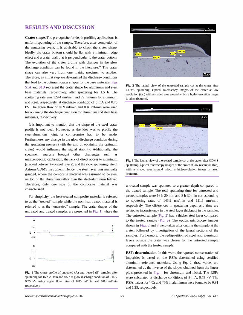
www.at-spectrosc.com/as/article/pdf/2021607 129 At. Spectrosc. 2022, 43(2), 126–133.
RESULTS AND DISCUSSION
Crater shape. The prerequisite for depth profiling applications is
uniform sputtering of the sample. Therefore, after completion of
the sputtering event, it is advisable to check the crater shape.
Ideally, the crater bottom should be flat with a minimum edge
effect and a crater wall that is perpendicular to the crater bottom.
The evolution of the crater profile with changes in the glow
discharge condition can be found in the literature.31 The crater
shape can also vary from one matrix specimen to another.
Therefore, as a first step we determined the discharge conditions
that lead to the optimum crater shapes for the base materials. Figs.
S1A and S1B represent the crater shape for aluminum and steel
base materials, respectively, after sputtering for 1.5 h. The
sputtering rate was 129.4 nm/min and 79 nm/min for aluminum
and steel, respectively, at discharge condition of 5 mA and 0.75
kV. The argon flow of 0.69 ml/min and 0.48 ml/min were used
for obtaining the discharge condition for aluminum and steel base
materials, respectively.
It is important to mention that the shape of the steel crater
profile is not ideal. However, as the idea was to profile the
steel-aluminum joint, a compromise had to be made.
Furthermore, any change in the glow discharge condition during
the sputtering process (with the aim of obtaining the optimum
crater) would influence the signal stability. Additionally, the
specimen analysis brought other challenges such as
matrix-specific calibration, the lack of direct access to aluminum
(stacked between two steel layers), and the slow sputtering rate of
Astrum GDMS instrument. Hence, the steel layer was manually
grinded, where the composite material was assumed to be steel
on top of the aluminum rather than the steel-aluminum bilayer.
Therefore, only one side of the composite material was
characterized.
For simplicity, the heat-treated composite material is referred
to as the “treated” sample while the non-heat-treated material is
referred to as the “untreated” sample. The crater shapes of the
untreated and treated samples are presented in Fig. 1, where the
Fig. 1 The crater profile of untreated (A) and treated (B) samples after
sputtering for 16 h 20 min and 8.5 h at glow discharge condition of 5 mA,
0.75 kV using argon flow rates of 0.85 ml/min and 0.83 ml/min
respectively.
Fig. 2 The lateral view of the untreated sample cut at the crater after
GDMS sputtering. Optical microscopy images of the crater at low
resolution (top) with a shaded area around which a high- resolution image
is taken (bottom).
Fig. 3 The lateral view of the treated sample cut at the crater after GDMS
sputtering. Optical microscopy images of the crater at low resolution (top)
with a shaded area around which a high-resolution image is taken
(bottom).
untreated sample was sputtered to a greater depth compared to
the treated sample. The total sputtering time for untreated and
treated samples were 16 h 20 min and 8 h 30 min corresponding
to sputtering rates of 143.9 nm/min and 111.3 nm/min,
respectively. The differences in sputtering depth and time are
related to inconsistency in the steel layer thickness in the samples.
The untreated sample (Fig. 2) had a thicker steel layer compared
to the treated sample (Fig. 3). The optical microscopy images
shown in Figs. 2 and 3 were taken after cutting the sample at the
crater, followed by investigation of the lateral sections of the
samples. Furthermore, the redisposition of steel and aluminum
layers outside the crater was clearer for the untreated sample
compared with the treated sample.
RSFs determination. In this work, the reported concentration of
impurities is based on the RSFs determined using certified
aluminum reference materials. Using Eq. 2, these values are
determined as the inverse of the slopes obtained from the linear
plots presented in Fig. 4 for chromium and nickel. The RSFs
were calculated at discharge conditions of 5 mA, 0.75 kV. The
RSFs values for 52Cr and 60Ni in aluminum were found to be 0.91
and 1.25, respectively.
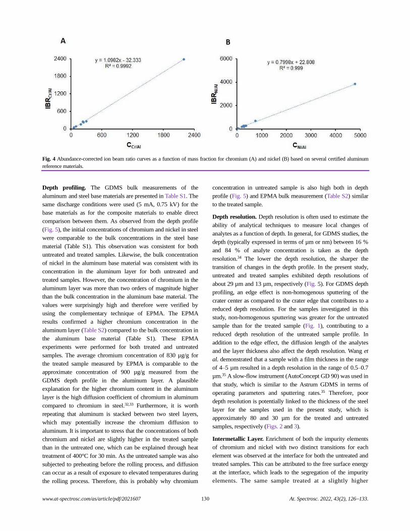
www.at-spectrosc.com/as/article/pdf/2021607 130 At. Spectrosc. 2022, 43(2), 126–133.
Fig. 4 Abundance-corrected ion beam ratio curves as a function of mass fraction for chromium (A) and nickel (B) based on several
certified aluminum
reference materials.
Depth profiling. The GDMS bulk measurements of the
aluminum and steel base materials are presented in Table S1. The
same discharge conditions were used (5 mA, 0.75 kV) for the
base materials as for the composite materials to enable direct
comparison between them. As observed from the depth profile
(Fig. 5), the initial concentrations of chromium and nickel in steel
were comparable to the bulk concentrations in the steel base
material (Table S1). This observation was consistent for both
untreated and treated samples. Likewise, the bulk concentration
of nickel in the aluminum base material was consistent with its
concentration in the aluminum layer for both untreated and
treated samples. However, the concentration of chromium in the
aluminum layer was more than two orders of magnitude higher
than the bulk concentration in the aluminum base material. The
values were surprisingly high and therefore were verified by
using the complementary technique of EPMA. The EPMA
results confirmed a higher chromium concentration in the
aluminum layer (Table S2) compared to the bulk concentration in
the aluminum base material (Table S1). These EPMA
experiments were performed for both treated and untreated
samples. The average chromium concentration of 830 µg/g for
the treated sample measured by EPMA is comparable to the
approximate concentration of 900 µg/g measured from the
GDMS depth profile in the aluminum layer. A plausible
explanation for the higher chromium content in the aluminum
layer is the high diffusion coefficient of chromium in aluminum
compared to chromium in steel.32,33 Furthermore, it is worth
repeating that aluminum is stacked between two steel layers,
which may potentially increase the chromium diffusion to
aluminum. It is important to stress that the concentrations of both
chromium and nickel are slightly higher in the treated sample
than in the untreated one, which can be explained through heat
treatment of 400°C for 30 min. As the untreated sample was also
subjected to preheating before the rolling process, and diffusion
can occur as a result of exposure to elevated temperatures during
the rolling process. Therefore, this is probably why chromium
concentration in untreated sample is also high both in depth
profile (Fig. 5) and EPMA bulk measurement (Table S2) similar
to the treated sample.
Depth resolution. Depth resolution is often used to estimate the
ability of analytical techniques to measure local changes of
analytes as a function of depth. In general, for GDMS studies, the
depth (typically expressed in terms of µm or nm) between 16 %
and 84 % of analyte concentration is taken as the depth
resolution.34 The lower the depth resolution, the sharper the
transition of changes in the depth profile. In the present study,
untreated and treated samples exhibited depth resolutions of
about 29 µm and 13 µm, respectively (Fig. 5). For GDMS depth
profiling, an edge effect is non-homogenous sputtering of the
crater center as compared to the crater edge that contributes to a
reduced depth resolution. For the samples investigated in this
study, non-homogenous sputtering was greater for the untreated
sample than for the treated sample (Fig. 1), contributing to a
reduced depth resolution of the untreated sample profile. In
addition to the edge effect, the diffusion length of the analytes
and the layer thickness also affect the depth resolution. Wang et
al. demonstrated that a sample with a film thickness in the range
of 4–5 µm resulted in a depth resolution in the range of 0.5–0.7
µm.35 A slow-flow instrument (AutoConcept GD 90) was used in
that study, which is similar to the Astrum GDMS in terms of
operating parameters and sputtering rates.35 Therefore, poor
depth resolution is potentially linked to the thickness of the steel
layer for the samples used in the present study, which is
approximately 80 and 30 µm for the treated and untreated
samples, respectively (Figs. 2 and 3).
Intermetallic Layer. Enrichment of both the impurity elements
of chromium and nickel with two distinct transitions for each
element was observed at the interface for both the untreated and
treated samples. This can be attributed to the free surface energy
at the interface, which leads to the segregation of the impurity
elements. The same sample treated at a slightly higher
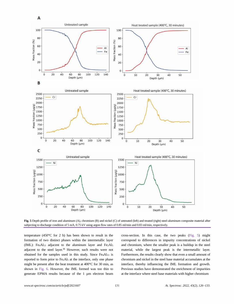
www.at-spectrosc.com/as/article/pdf/2021607 131 At. Spectrosc. 2022, 43(2), 126–133.
Fig. 5 Depth profile of iron and aluminum (A), chromium (B) and nickel (C) of untreated (left) and treated (right) steel-aluminum composite material after
subjecting to discharge condition of 5 mA, 0.75 kV using argon flow rates of 0.85 ml/min and 0.83 ml/min, respectively.
temperature (450°C for 2 h) has been shown to result in the
formation of two distinct phases within the intermetallic layer
(IML): Fe4Al13 adjacent to the aluminum layer and Fe2Al5
adjacent to the steel layer.36 However, such results were not
obtained for the samples used in this study. Since Fe4Al13 is
reported to form prior to Fe2Al5 at the interface, only one phase
might be present after the heat treatment at 400°C for 30 min, as
shown in Fig. 6. However, the IML formed was too thin to
generate EPMA results because of the 1 µm electron beam
cross-section. In this case, the two peaks (Fig. 5) might
correspond to differences in impurity concentrations of nickel
and chromium, where the smaller peak is a buildup in the steel
material, while the largest peak is the intermetallic layer.
Furthermore, the results clearly show that even a small amount of
chromium and nickel in the steel base material accumulates at the
interface, thereby influencing the IML formation and growth.
Previous studies have demonstrated the enrichment of impurities
at the interface where steel base materials with higher chromium
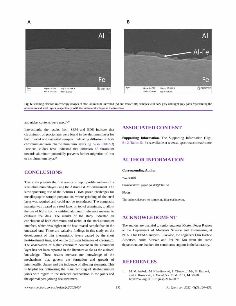
www.at-spectrosc.com/as/article/pdf/2021607 132 At. Spectrosc. 2022, 43(2), 126–133.
Fig.
6
Scanning electron microscopy images of steel-aluminum untreated (A) and treated (B) samples with dark grey and light grey parts representing the
aluminum and steel layers, respectively, with the intermetallic layer at the interface.
and nickel contents were used.5,37
Interestingly, the results from SEM and EDS indicate that
chromium-iron precipitates were found in the aluminum layer for
both treated and untreated samples, indicating diffusion of both
chromium and iron into the aluminum layer (Fig. S2 & Table S3).
Previous studies have indicated that diffusion of chromium
towards aluminum potentially prevents further migration of iron
to the aluminum layer.36
CONCLUSIONS
This study presents the first results of depth profile analysis of a
steel-aluminum bilayer using the Astrum GDMS instrument. The
slow sputtering rate of the Astrum GDMS posed challenges for
metallographic sample preparation, where grinding of the steel
layer was required and could not be reproduced. The composite
material was treated as a steel layer on top of aluminum, to allow
the use of RSFs from a certified aluminum reference material to
calibrate the data. The results of the study indicated an
enrichment of both chromium and nickel at the steel-aluminum
interface, which was higher in the heat-treated sample than in the
untreated one. There are valuable findings in this study on the
development of thin intermetallic layers caused by the short
heat-treatment time, and on the diffusion behavior of chromium.
The observation of higher chromium content in the aluminum
layer has not been reported in the literature as far as the authors’
knowledge. These results increase our knowledge of the
mechanisms that govern the formation and growth of
intermetallic phases and the influence of alloying elements. This
is helpful for optimizing the manufacturing of steel-aluminum
joints with regard to the material composition in the joints and
the optimal post-joining heat treatment.
ASSOCIATED CONTENT
Supporting Information. The Supporting Information (Figs.
S1-2, Tables S1-3) is available at www.at-spectrosc.com/as/home
AUTHOR INFORMATION
Corresponding Author
*G. Paudel
Email address: [email protected]
Notes
The authors declare no competing financial interest.
ACKNOWLEDGMENT
The authors are thankful to senior engineer Morten Peder Raanes
at the Department of Materials Science and Engineering at
NTNU for EPMA analysis. Likewise, the engineers Elin Harboe
Albertsen, Anita Storsve and Pei Na Kui from the same
department are thanked for continuous support in the laboratory.
REFERENCES
1. M. M. Atabaki, M. Nikodinovski, P. Chenier, J. Ma, M. Harooni,
and R. Kovacevic, J. Manuf. Sci. Prod., 2014, 14. 59-78.
https://doi.org/10.1515/jmsp-2014-0007
www.at-spectrosc.com/as/article/pdf/2021607 133 At. Spectrosc. 2022, 43(2), 126–133.
2. C. X. Huang, Y. F. Wang, X. L. Ma, S. Yin, H. W. Höppel,
M. Göken, X. L. Wu, H. J. Gao, and Y. T. Zhu, Mater. Today,
2018, 21, 713-719. https://doi.org/10.1016/j.mattod.2018.03.006
3. S. M. Arbo, T. Bergh, B. Holmedal, P. E. Vullum, and
I. Westermann, Metals, 2019, 9, 827.
https://doi.org/10.3390/met9080827
4. S. M. Arbo, T. Bergh, H. Solhaug, I. Westermann, and
B. Holmedal, Procedia Manufacturing, 2018, 15, 152-160.
https://doi.org/10.1016/j.promfg.2018.07.189
5. V. I. Dybkov, J.. Mater. Sci., 1990, 25, 3615-3633.
https://doi.org/10.1007/BF00575397
6. C. L. Lewis, E. S. Oxley, C. K. Pan, R. E. Steiner, and F. L. King,
Anal. Chem., 1999, 71, 230-234.
https://doi.org/10.1021/ac9806916
7. L. Li, J. T. Millay, J. P. Turner, and F. L. King,
J. Am. Soc. Mass Spectrom., 2004, 15, 87-102.
https://doi.org/10.1016/j.jasms.2003.09.004
8. E. Oxley, C. Yang, J. Liu, and W. W. Harrison, Anal. Chem., 2003,
75, 6478-6484. https://doi.org/10.1021/ac0346398
9. M. Bouza, R. Pereiro, N. Bordel, A. Sanz-Medel, and
B. Fernández, J. Anal. At. Spectrom., 2015, 30, 1108-1116.
https://doi.org/10.1039/C4JA00474D
10. N. Tuccitto, L. Lobo, A. Tempez, I. Delfanti, P. Chapon,
S. Canulescu, N. Bordel, J. Michler, and A. Licciardello, Rapid
Commun. Mass Sp., 2009, 23, 549-556.
https://doi.org/10.1002/rcm.3906
11. A. C. Muñiz, J. Pisonero, L. Lobo, C. Gonzalez, N. Bordel,
R. Pereiro, A. Tempez, P. Chapon, N. Tuccitto, A. Licciardello,
and A. Sanz-Medel, J. Anal. At. Spectrom., 2008, 23, 1239-1246.
https://doi.org/10.1039/B804169P
12. J. Pisonero, L. Lobo, N. Bordel, A. Tempez, A. Bensaoula,
N. Badi, and A. Sanz-Medel, Sol. Energ. Mat. . Sol. C., 2010, 94,
1352-1357. https://doi.org/10.1016/j.solmat.2010.04.002
13. R. Valledor, J. Pisonero, N. Bordel, J. I. Martín, C. Quirós,
A. Tempez, and A. Sanz-Medel, Anal. Bioanal. Chem., 2010, 396,
2881-2887. https://doi.org/10.1007/s00216-009-3382-8
14. J. Pisonero, A. Licciardello, A. Hierro-Rodríguez, C. Quirós,
A. Sanz-Medel, and N. Bordel, J. Anal. At. Spectrom., 2011, 26,
1604-1609. https://doi.org/10.1039/C1JA10075K
15. J. Pisonero, R. Valledor, A. Licciardello, C. Quirós, J. I. Martín,
A. Sanz-Medel, and N. Bordel, Anal. Bioanal. Chem., 2012, 403,
2437-2448. https://doi.org/10.1007/s00216-011-5601-3
16. A. Alvarez-Toral, P. Sanchez, A. Menéndez, R. Pereiro,
A. Sanz-Medel, and B. Fernández, J. Am. Soc. Mass Spectr., 2015,
26, 305-314. https://doi.org/10.1021/jasms.8b04956
17. C. Gonzalez-Gago, J. Pisonero, N. Bordel, A. Sanz-Medel,
N. J. Tibbetts, and V. S. Smentkowski, J. Vac. Sci. Technol. A,
2013, 31, 06F106. https://doi.org/10.1116/1.4824164
18. C. González-Gago, J. Pisonero, R. Sandín, J. F. Fuertes,
A. Sanz-Medel, and N. Bordel, J. Anal. Atom. Spectro., 2016, 31,
288-296. https://doi.org/10.1039/C5JA00104H
19. V. Bodnar, A. Ganeev, A. Gubal, N. Solovyev, O. Glumov,
V. Yakobson, and I. Murin, Spectrochim. Acta B, 2018, 145,
20-28. https://doi.org/10.1016/j.sab.2018.04.002
20. A. Gubal, V. Chuchina, Y. Lyalkin, V. Mikhailovskii,
V. Yakobson, N. Solovyev, and A. Ganeev, J. Anal. At. Spectrom.,
2020, 35, 1587-1596. https://doi.org/10.1039/D0JA00088D
21. K. Su, X. Wang, and K. Putyera, Yejin Fenxi/Metallurgical
Analysis, 2010, Vol 30 Suppl.1, 165.
22. M. Di Sabatino, Measurement, 2014, 50, 135-140.
https://doi.org/10.1016/j.measurement.2013.12.024
23. M. Di Sabatino, A. L. Dons, J. Hinrichs, and L. Arnberg,
Spectrochim. Acta B, 2011, 66, 144-148.
https://doi.org/10.1016/j.sab.2011.01.004
24. M. Di Sabatino, C. Modanese, and L. Arnberg, J. Anal. At.
Spectrom., 2014, 29, 2072-2077.
https://doi.org/10.1039/C4JA00175C
25. C. Modanese, G. Gaspar, L. Arnberg, and M. Di Sabatino,
Anal. Bioanal. Chem., 2014, 406, 7455-7462.
https://doi.org/10.1007/s00216-014-8105-0
26. X. Wang, K. Putyera, J. Liu, and D. Leblanc, Distribution
Measurements of Dopants in Compensated Silicon Ingots by
Fast-Flow High Resolution Glow Discharge Mass Spectrometry.
2011.
27. C. Modanese, M. Di Sabatino, A.-K. Søiland, K. Peter, and
L. Arnberg, Prog. Photovolt.: Res. Appl., 2011, 19. 45-53.
https://doi.org/10.1002/pip.986
28. C. Modanese, L. Arnberg, and M. Di Sabatino, Mater. Sci.
Eng.B-Adv., 2014, 180, 27-32.
https://doi.org/10.1016/j.mseb.2013.10.010
29. I. T. Spitsberg and K. Putyera, Surf. Coat. Tech., 2001, 139, 35-43.
https://doi.org/10.1016/S0257-8972(00)01162-2
30. L. M. He, J. D. Meyer, W. Y. Lee, K. Putyera, and L. R. Walker,
Metall. Mater. Trans. A, 2002, 33, 3578-3582.
https://doi.org/10.1007/s11661-002-0348-2
31. A. Bogaerts, W. Verscharen, and E. Steers, Spectrochim. Acta B,
2004, 59, 1403-1411. https://doi.org/10.1016/j.sab.2004.06.005
32. Y. Du, Y. A. Chang, B. Y. Huang, W. P. Gong, Z. P. Jin, H. H. Xu,
Z. H. Yuan, Y. Liu, Y. H. He, and F. Y. Xie, Mater. Sci.
Eng.A-Struct., 2003, 363, 140-151.
https://doi.org/10.1016/S0921-5093(03)00624-5
33. R. Braun and M. Feller-Kniepmeier, Phys. Status solidi (a), 1985,
90, 553-561. https://doi.org/10.1002/pssa.2210900219
34. A. Raith, R. C. Hutton, and J. C. Huneke, J. Anal. At. Spectrom.,
1993, 8, 867-873. https://doi.org/10.1039/JA9930800867
35. M. L. Wang, B. Zhuo, S. J. Zhuo, Y. Q. Zhu, L. Huang, and
R. Qian, At. Spectrosc., 2021, 42, 183-189.
https://doi.org/10.46770/AS.2021.070
36. S. M. Arbo. Cold welding of steel and aluminum alloys - Joining
processes, intermetallic phases and bond strength. Norwegian
University of Science and Technology, Trondheim, 2020.
37. Y. X. Li, Q. Jia, Z. T. Zhu, W. Gao, and H. Chen, Surf. Rev. Lett.,
2017, 24, 1750046. https://doi.org/10.1142/s0218625x17500469
www.at-spectrosc.com/as/article/pdf/2022033 134 At. Spectrosc. 2022, 43(2), 134–144.
Zircon ZS - a Homogenous Natural Reference Material for U–Pb
Age and O–Hf Isotope Microanalyses
Xiao-Xiao Ling,a Qiu-Li Li,a,b,* Chuan Yang,c Zhu-Yin Chu,a Lian-Jun Feng,a Chao Huang,a
Liang-Liang Huang,a Hong Zhang,d Zhen-Hui Hou,e Jun-Jie Xu,a Yu Liu,a Guo-Qiang Tang,a,b Jiao Li,a and
Xian-Hua Li a,b a State Key Laboratory of Lithospheric Evolution, Institute of Geology and Geophysics, Chinese Academy of Sciences, Beijing 100029, P. R. China
b College of Earth and Planetary Sciences, University of Chinese Academy of Sciences, Beijing 100049, P. R. China
c British Geological Survey, Keyworth, NG12 5GG, UK
d State Key Laboratory of Continental Dynamics, Northwest University, Xi’an 710069, P. R. China
e School of Earth and Space Sciences, University of Science and Technology of China, Hefei 230026, P. R. China
Received: January 17, 2022; Revised: April 01, 2022; Accepted: April 01, 2022; Available online: April 06, 2022.
DOI: 10.46770/AS.2022.033
ABSTRACT: A well-formed natural zircon crystal ~10 g in weight from Sri Lanka was introduced as a reference material
for the geochemical microanalysis of U–Pb–O–Hf isotopes. For the U–Pb system, a total of 96 secondary ion mass spectrometry
(SIMS) and 174 laser-ablation inductively coupled plasma mass spectrometry analyses showed that zircon ZS was homogeneous
within a ~20 μm area level. According to chemical abrasion isotope dilution thermal ionization mass spectrometry, the U–Pb system
is concordant within the uncertainties, yielding a weighted mean 206Pb/238U age of 560.6 ± 1.3 Ma (2 standard deviation (SD), n =
18) and a weighted mean 207Pb/206Pb age of 561.1 ± 3.5 Ma (2SD, n = 18).
The U and Th concentrations were 570 ± 40 μg g-1 (1SD) and 132 ± 28 μg
g-1 (1SD), respectively. The homogeneity of the O isotopes was confirmed
by 261 SIMS analyses, and that of Hf isotopes was determined by 100 laser-
ablation multi-collector inductively coupled plasma mass spectrometry
(MC–ICP–MS) analyses. A weighted mean δ18O value of 13.69‰ ± 0.11‰
(2SD, n = 12) obtained by laser fluorination isotope ratio mass spectrometry
(IRMS) and a weighted mean 176Hf/177Hf value of 0.281668 ± 0.000010
(2SD, n = 7) by solution MC–ICP–MS are recommended as the best
reference values for zircon ZS.
INTRODUCTION
Zircon (ZrSiO4) is commonly found in various types of
intermediate-acid igneous rocks, metamorphic rocks, and
sedimentary rocks.1-5 The in-situ U–Pb age, Hf–O isotopes, and
geochemical composition of zircon can be obtained through the
use of microbeam analysis techniques such as secondary ion mass
spectrometry (SIMS) and laser-ablation inductively coupled
plasma mass spectrometry (LA–ICP–MS), which have a broad
range of applications in isotope geochronology and geochemical
tracer research.6-10 The matrix effect is one of the main concerns
that need to be considered during SIMS and LA–ICP–MS
microanalyses. Matrix-matched reference materials are key to
overcoming the matrix effect and obtaining accurate results. More
than 20 zircon age standards have been reported,11 with several
zircons such as SA01,12 Tanz,13 and SA02 serving as good
standards.14 However, qualified zircon reference materials are still
rare because they need to meet the following criteria: (1)
uniformity in radiogenic 207Pb/206Pb, 206Pb/238U, and 207Pb/235U; (2)
isotopic concordance; (3) a negligible concentration of initial Pb;
and (4) sufficient radiogenic Pb concentration.15 The first SIMS
zircon standard SL3, which has a high U content, can introduce
matrix effects during the SIMS calibration procedure.16 The low
radiogenic Pb makes it difficult for the widely used zircon standard
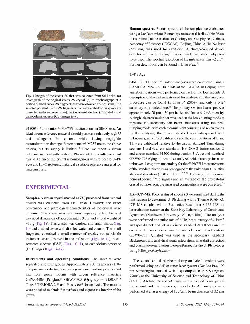
www.at-spectrosc.com/as/article/pdf/2022033 135 At. Spectrosc. 2022, 43(2), 134–144.
Fig. 1 Images of the zircon ZS that was collected from Sri Lanka. (a)
Photograph of the original zircon ZS crystal. (b) Microphotograph of a
portion of small zircon ZS fragments that were obtained after crushing. The
selected polished zircon ZS fragments that were embedded in epoxy are
presented in the reflection (c–e), back-scattered electron (BSE) (f–h), and
cathodoluminescence (CL) images (i–k).
9150017, 18 to monitor 207Pb/206Pb fractionations in SIMS tests. An
ideal zircon reference material should possess a relatively high U
and radiogenic Pb content while having negligible
metamictization damage. Zircon standard M257 meets the above
criteria, but its supply is limited.19 Here, we report a zircon
reference material with moderate Pb content. The results show that
this ~10 g zircon ZS crystal is homogenous with respect to U–Pb
ages and Hf–O isotopes, making it a suitable reference material for
microanalysis.
EXPERIMENTAL
Samples. A zircon crystal (named as ZS) purchased from mineral
dealers was collected from Sri Lanka. However, the exact
provenance and petrological characteristics of the crystal were
unknown. The brown, semitransparent mega-crystal had the most
extended dimension of approximately 3 cm and a total weight of
~10 g (Fig. 1a). This crystal was crushed into small shards (Fig.
1b) and cleaned twice with distilled water and ethanol. The small
fragments contained a small number of cracks, but no visible
inclusions were observed in the reflection (Figs. 1c–1e), back-
scattered electron (BSE) (Figs. 1f–1h), or cathodoluminescence
(CL) images (Figs. 1i–1k).
Instruments and operating conditions. The samples were
separated into four groups. Approximately 200 fragments (150–
300 μm) were selected from each group and randomly distributed
into four epoxy mounts with zircon reference materials
GBW04409 (Penglai),20 GBW04705 (Qinghu),21,22 91500,17,18
Tanz,13 TEMORA 2,23 and Plesovice24 for analysis. The mounts
were polished to obtain flat surfaces and expose the interior of the
grains.
Raman spectra. Raman spectra of the samples were obtained
using a LabRam micro-Raman spectrometer (Horiba Jobin Yvon,
Paris, France) at the Institute of Geology and Geophysics, Chinese
Academy of Sciences (IGGCAS), Beijing, China. A He–Ne laser
(532 nm) was used for excitation. A charge-coupled device
detector with a 50× magnification working-distance objective
were used. The spectral resolution of the instrument was ~2 cm–1.
Further description can be found in Ling et al. 25
U–Pb Age
SIMS. U, Th, and Pb isotope analyses were conducted using a
CAMECA IMS-1280HR SIMS at the IGGCAS in Beijing. Four
analytical sessions were performed on each of the four mounts. A
description of the instruments used for analyses and the analytical
procedure can be found in Li et al. (2009), and only a brief
summary is provided here.26 The primary O2– ion beam spot was
approximately 20 μm 30 μm in size and had a 6–9 nA intensity.
A single electron multiplier was used in the ion-counting mode to
measure the secondary ion beam intensities using the peak
jumping mode, with each measurement consisting of seven cycles.
In the analyses, the zircon standard was interspersed with
unknown grains. Pb/U calibration and the concentrations of U and
Th were calibrated relative to the zircon standard Tanz during
sessions 1 and 4, zircon standard TEMORA 2 during session 2,
and zircon standard 91500 during session 3. A second standard,
GBW04705 (Qinghu), was also analyzed with zircon grains as an
unknown. Long-term uncertainty for the 206Pb/238U measurements
of the standard zircons was propagated to the unknowns (1 relative
standard deviation (RSD) = 1.5%).27, 28 By using the measured
non-radiogenic 204Pb signals and an average of the present-day
crustal composition, the measured compositions were corrected.29
LA–ICP–MS. Forty grains of zircon ZS were analyzed during the
first session to determine U–Pb dating with a Thermo iCAP RQ
ICP–MS coupled with a Resonetics Resolution S-155 193 nm
laser ablation system at the State Key Laboratory of Continental
Dynamics (Northwest University. Xi’an, China). The analyses
were performed at a pulse rate of 6 Hz, beam energy of 4 J/cm2,
and spot diameter of 30 μm. Zircon standard 91500 was used to
calibrate the mass discrimination and elemental fractionation.
GBW04705 (Qinghu) was used as the secondary standard.
Background and analytical signal integration, time-drift correction,
and quantitative calibration were performed for the U–Pb isotopes
using Iolite_v4.0 software.30
The second and third zircon dating analytical sessions were
performed using an ArF excimer laser system (GeoLas Pro, 193
nm wavelength) coupled with a quadrupole ICP–MS (Agilent
7700e) at the University of Science and Technology of China
(USTC). A total of 26 and 59 grains were subjected to analyses in
the second and third sessions, respectively. All analyses were
performed at a laser energy of 10 J/cm2, beam diameter of 32 μm,
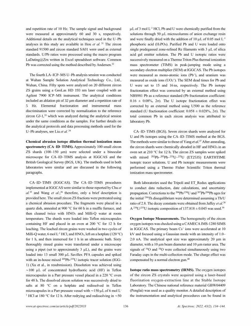
www.at-spectrosc.com/as/article/pdf/2022033 136 At. Spectrosc. 2022, 43(2), 134–144.
and repetition rate of 10 Hz. The sample signal and background
were measured at approximately 60 and 30 s, respectively.
Additional details on the analytical techniques used in the U–Pb
analyses in this study are available in Hou et al. 31 The zircon
standard 91500 and zircon standard SA01 were used as external
standards. U/Pb ratios were processed using the macro program
LaDating@Zrn written in Excel spreadsheet software. Common
Pb was corrected using the method described by Andersen.32
The fourth LA–ICP–MS U–Pb analysis session was conducted
at Wuhan Sample Solution Analytical Technology Co., Ltd.,
Wuhan, China. Fifty spots were analyzed on 20 different zircon
ZS grains using a GeoLas HD 193 nm laser coupled with an
Agilent 7900 ICP–MS instrument. The analytical conditions
included an ablation pit of 32 µm diameter and a repetition rate of
5 Hz. Elemental fractionation and instrumental mass
discrimination were corrected by normalization to the reference
zircon GJ-1,33 which was analyzed during the analytical session
under the same conditions as the samples. For further details on
the analytical protocols and data processing methods used for the
U–Pb analyses, see Liu et al. 34
Chemical abrasion isotope dilution thermal ionization mass
spectrometry (CA–ID–TIMS). Approximately 100 small zircon
ZS shards (100–150 μm) were selected under a binocular
microscope for CA–ID–TIMS analysis at IGGCAS and the
British Geological Survey (BGS, UK). The methods used in both
laboratories were similar and are discussed in the following
paragraphs.
CA–ID–TIMS (IGGCAS). The CA–ID–TIMS procedures
implemented at IGGCAS were similar to those reported by Chu et
al.35 and Wang et al.;36 therefore, only a brief description is
provided here. The small zircon ZS fractions were pretreated using
a chemical abrasion procedure. The fragments were placed in a
quartz dish, annealed at 900 °C for 60 h in a muffle furnace, and
then cleaned twice with HNO3 and Milli-Q water at room
temperature. The shards were loaded into Teflon microcapsules
containing HF and placed in an oven at 200 °C for 12 h for
leaching. The leached zircon grains were washed in two cycles of
Milli-Q water, 6 mol L-1 HCl, and HNO3, left on a hotplate (120 °C)
for 1 h, and then immersed for 1 h in an ultrasonic bath. Sixty
thoroughly rinsed grains were transferred under a microscope
using a pipet (set to approximately 3 µL), and the grains were
loaded into 13 small 300 L Savillex PFA capsules and spiked
with an in-house mixed 205Pb-235U isotopic tracer solution (IGG-
1) (Xu et al., in resubmission). Dissolution was achieved using
∼100 L of concentrated hydrofluoric acid (HF) in Teflon
microcapsules in a Parr pressure vessel placed in a 220 °C oven
for 48 h. The dissolved zircon solution was successively dried to
salts at 80 °C on a hotplate and redissolved in Teflon
microcapsules in a Parr pressure vessel with ∼150 L of 6 mol L-
1 HCl at 180 °C for 12 h. After redrying and redissolving in ∼50
L of 3 mol L-1 HCl, Pb and U were chemically purified from the
solutions through 50 L microcolumns of anion exchange resin
and were finally dried with the addition of 10 L of 0.05 mol L-1
phosphoric acid (H3PO4). Purified Pb and U were loaded onto
single predegassed zone-refined Re filaments with 3 µL of silica
acid gel emitter solution. The Pb and U isotopic ratios were
successively measured on a Thermo Triton Plus thermal ionization
mass spectrometer (TIMS) in peak-jumping mode using a
secondary electron multiplier (SEM) at IGGCAS. The Pb isotopes
were measured as mono-atomic ions (Pb+), and uranium was
measured as oxide ions (UO2+). The SEM dead times for Pb and
U were set to 15 and 16 ns, respectively. The Pb isotope
fractionation effect was corrected by an external method using
NBS981 Pb as a reference standard (Pb fractionation coefficient:
0.16 ± 0.08%, 2σ). The U isotope fractionation effect was
corrected by an external method using U500 as the reference
standard (U fractionation coefficient: 0.058 ± 0.028%, 2σ). The
total common Pb in each zircon analysis was attributed to
laboratory Pb.
CA–ID–TIMS (BGS). Seven zircon shards were analyzed for
U and Pb isotopes using the CA–ID–TIMS method at the BGS.
The methods were similar to those of Yang et al.37 After annealing,
the zircon shards were chemically abraded in HF and HNO3 in an
oven set at 210 °C for 12 h. The zircon ZS samples were spiked
with mixed 202Pb–205Pb–233U–235U (ET2535) EARTHTIME
isotopic tracer solutions. U and Pb isotopic measurements were
performed using a Thermo Fisher Scientific Triton thermal
ionization mass spectrometer.
Both laboratories used the Tripoli and ET_Redux applications
to conduct data reduction, date calculations, and uncertainty
propagation. Corrections to the 206Pb/238U and 207Pb/206Pb ages for
the initial 230Th disequilibrium were determined assuming a Th/U
ratio of 2.8. The decay constants were obtained from Jaffey et al.38
A 238U/235U isotopic composition of 137.818 ± 0.045 was used.39
Oxygen Isotope Measurements. The homogeneity of the zircon
oxygen isotopes was checked using a CAMECA IMS-1280 SIMS
in IGGCAS. The primary beam Cs+ ions were accelerated at 10
kV and focused using a Gaussian mode with an intensity of 1.0–
2.0 nA. The analytical spot size was approximately 20 μm in
diameter, with a 10 µm beam diameter and 10 µm raster area. The
signals of 16O and 18O were collected simultaneously using two
Faraday cups in the multi-collection mode. The charge effect was
compensated by a normal electron gun.40
Isotope ratio mass spectrometry (IRMS). The oxygen isotopes
of the zircon ZS crystals were acquired using a laser-based
fluorination oxygen-extraction line at the Stable Isotope
Laboratory. The Chinese national reference material GBW04409
(Penglai) was used as a quality monitor. A detailed description of
the instrumentation and analytical procedures can be found in
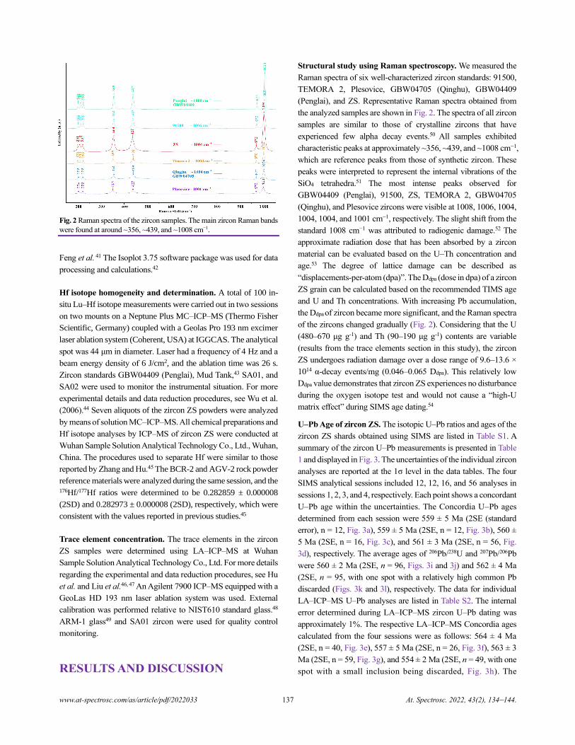
www.at-spectrosc.com/as/article/pdf/2022033 137 At. Spectrosc. 2022, 43(2), 134–144.
Fig. 2 Raman spectra of the zircon samples. The main zircon Raman bands
were found at around ~356, ~439, and ~1008 cm−1.
Feng et al. 41 The Isoplot 3.75 software package was used for data
processing and calculations.42
Hf isotope homogeneity and determination. A total of 100 in-
situ Lu–Hf isotope measurements were carried out in two sessions
on two mounts on a Neptune Plus MC–ICP–MS (Thermo Fisher
Scientific, Germany) coupled with a Geolas Pro 193 nm excimer
laser ablation system (Coherent, USA) at IGGCAS. The analytical
spot was 44 μm in diameter. Laser had a frequency of 4 Hz and a
beam energy density of 6 J/cm2, and the ablation time was 26 s.
Zircon standards GBW04409 (Penglai), Mud Tank,43 SA01, and
SA02 were used to monitor the instrumental situation. For more
experimental details and data reduction procedures, see Wu et al.
(2006).44 Seven aliquots of the zircon ZS powders were analyzed
by means of solution MC–ICP–MS. All chemical preparations and
Hf isotope analyses by ICP–MS of zircon ZS were conducted at
Wuhan Sample Solution Analytical Technology Co., Ltd., Wuhan,
China. The procedures used to separate Hf were similar to those
reported by Zhang and Hu.45 The BCR-2 and AGV-2 rock powder
reference materials were analyzed during the same session, and the 176Hf/177Hf ratios were determined to be 0.282859 ± 0.000008
(2SD) and 0.282973 ± 0.000008 (2SD), respectively, which were
consistent with the values reported in previous studies.45
Trace element concentration. The trace elements in the zircon
ZS samples were determined using LA–ICP–MS at Wuhan
Sample Solution Analytical Technology Co., Ltd. For more details
regarding the experimental and data reduction procedures, see Hu
et al. and Liu et al.46, 47 An Agilent 7900 ICP–MS equipped with a
GeoLas HD 193 nm laser ablation system was used. External
calibration was performed relative to NIST610 standard glass.48
ARM-1 glass49 and SA01 zircon were used for quality control
monitoring.
RESULTS AND DISCUSSION
Structural study using Raman spectroscopy. We measured the
Raman spectra of six well-characterized zircon standards: 91500,
TEMORA 2, Plesovice, GBW04705 (Qinghu), GBW04409
(Penglai), and ZS. Representative Raman spectra obtained from
the analyzed samples are shown in Fig. 2. The spectra of all zircon
samples are similar to those of crystalline zircons that have
experienced few alpha decay events.50 All samples exhibited
characteristic peaks at approximately ~356, ~439, and ~1008 cm−1,
which are reference peaks from those of synthetic zircon. These
peaks were interpreted to represent the internal vibrations of the
SiO4 tetrahedra.51 The most intense peaks observed for
GBW04409 (Penglai), 91500, ZS, TEMORA 2, GBW04705
(Qinghu), and Plesovice zircons were visible at 1008, 1006, 1004,
1004, 1004, and 1001 cm−1, respectively. The slight shift from the
standard 1008 cm−1 was attributed to radiogenic damage.52 The
approximate radiation dose that has been absorbed by a zircon
material can be evaluated based on the U–Th concentration and
age.53 The degree of lattice damage can be described as
“displacements-per-atom (dpa)”. The Ddpa (dose in dpa) of a zircon
ZS grain can be calculated based on the recommended TIMS age
and U and Th concentrations. With increasing Pb accumulation,
the Ddpa of zircon became more significant, and the Raman spectra
of the zircons changed gradually (Fig. 2). Considering that the U
(480–670 μg g-1) and Th (90–190 μg g-1) contents are variable
(results from the trace elements section in this study), the zircon
ZS undergoes radiation damage over a dose range of 9.6–13.6 ×
1014 α-decay events/mg (0.046–0.065 Ddpa). This relatively low
Ddpa value demonstrates that zircon ZS experiences no disturbance
during the oxygen isotope test and would not cause a “high-U
matrix effect” during SIMS age dating.54
U–Pb Age of zircon ZS. The isotopic U–Pb ratios and ages of the
zircon ZS shards obtained using SIMS are listed in Table S1. A
summary of the zircon U–Pb measurements is presented in Table
1 and displayed in Fig. 3. The uncertainties of the individual zircon
analyses are reported at the 1σ level in the data tables. The four
SIMS analytical sessions included 12, 12, 16, and 56 analyses in
sessions 1, 2, 3, and 4, respectively. Each point shows a concordant
U–Pb age within the uncertainties. The Concordia U–Pb ages
determined from each session were 559 ± 5 Ma (2SE (standard
error), n = 12, Fig. 3a), 559 ± 5 Ma (2SE, n = 12, Fig. 3b), 560 ±
5 Ma (2SE, n = 16, Fig. 3c), and 561 ± 3 Ma (2SE, n = 56, Fig.
3d), respectively. The average ages of 206Pb/238U and 207Pb/206Pb
were 560 ± 2 Ma (2SE, n = 96, Figs. 3i and 3j) and 562 ± 4 Ma
(2SE, n = 95, with one spot with a relatively high common Pb
discarded (Figs. 3k and 3l), respectively. The data for individual
LA–ICP–MS U–Pb analyses are listed in Table S2. The internal
error determined during LA–ICP–MS zircon U–Pb dating was
approximately 1%. The respective LA–ICP–MS Concordia ages
calculated from the four sessions were as follows: 564 ± 4 Ma
(2SE, n = 40, Fig. 3e), 557 ± 5 Ma (2SE, n = 26, Fig. 3f), 563 ± 3
Ma (2SE, n = 59, Fig. 3g), and 554 ± 2 Ma (2SE, n = 49, with one
spot with a small inclusion being discarded, Fig. 3h). The
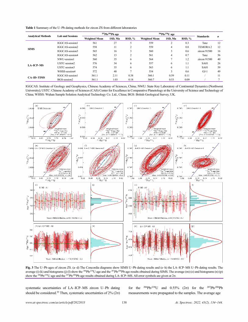
www.at-spectrosc.com/as/article/pdf/2022033 138 At. Spectrosc. 2022, 43(2), 134–144.
Table 1 Summary of the U–Pb dating methods for zircon ZS from different laboratories
Analytical Methods Lab and Sessions 207Pb/206Pb age 206Pb/238U age
Standards n Weighted Mean 1SD, Ma RSD, % Weighted Mean 1SD, Ma RSD, %
SIMS
IGGCAS-session1 561 27 5 559 2 0.3 Tanz 12
IGGCAS-session2 558 11 2 559 4 0.8 TEMORA 2 12
IGGCAS-session3 565 16 3 560 3 0.6 zircon 91500 16
IGGCAS-session4 562 13 2 561 4 0.7 Tanz 56
LA–ICP–MS
NWU-session1 560 35 6 564 7 1.2 zircon 91500 40
USTC-session2 576 34 6 557 6 1.1 SA01 26
USTC-session3 574 35 6 563 6 1.1 SA01 59
WHSS-session4 572 40 7 554 3 0.6 GJ-1 49
CA–ID–TIMS IGGCAS-session1 561.1 2.11 0.38 560.1 0.59 0.11 / 11
BGS-session2 561.1 1.03 0.18 560.7 0.53 0.09 / 7
IGGCAS: Institute of Geology and Geophysics, Chinese Academy of Sciences, China; NWU: State Key Laboratory of Continental Dynamics (Northwest
University); USTC: Chinese Academy of Sciences (CAS) Center for Excellence in Comparative Planetology at the University of Science and Technology of
China; WHSS: Wuhan Sample Solution Analytical Technology Co. Ltd., China; BGS: British Geological Survey, UK.
Fig. 3 The U–Pb ages of zircon ZS. (a–d) The Concordia diagrams show SIMS U–Pb dating results and (e–h) the LA–ICP–MS U–Pb dating results. The
average (i) (k) and histograms (j) (l) show the 206Pb/238U age and the 207Pb/206Pb age results obtained during SIMS. The average (m) (o) and histograms (n) (p)
show the 206Pb/238U age and the 207Pb/206Pb age results obtained during LA–ICP–MS. All error symbols are given at 2σ.
systematic uncertainties of LA–ICP–MS zircon U–Pb dating
should be considered.55 Then, systematic uncertainties of 2% (2σ)
for the 206Pb/238U and 0.55% (2σ) for the 207Pb/206Pb
measurements were propagated to the samples. The average age
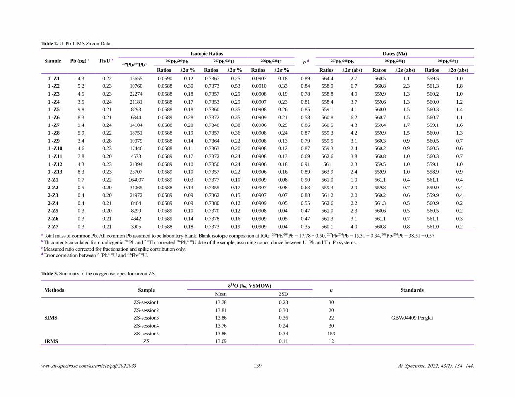
www.at-spectrosc.com/as/article/pdf/2022033 139 At. Spectrosc. 2022, 43(2), 134–144.
Table 2. U–Pb TIMS Zircon Data
Sample Pb (pg) a Th/U b
Isotopic Ratios
ρd
Dates (Ma)
206Pb/204Pb c 207Pb/206Pb 207Pb/235U 206Pb/238U 207Pb/206Pb 207Pb/235U 206Pb/238U
Ratios ±2σ % Ratios ±2σ % Ratios ±2σ % Ratios ±2σ (abs) Ratios ±2σ (abs) Ratios ±2σ (abs)
1 -Z1 4.3 0.22 15655 0.0590 0.12 0.7367 0.25 0.0907 0.18 0.89 564.4 2.7 560.5 1.1 559.5 1.0
1 -Z2 5.2 0.23 10760 0.0588 0.30 0.7373 0.53 0.0910 0.33 0.84 558.9 6.7 560.8 2.3 561.3 1.8
1 -Z3 4.5 0.23 22274 0.0588 0.18 0.7357 0.29 0.0908 0.19 0.78 558.8 4.0 559.9 1.3 560.2 1.0
1 -Z4 3.5 0.24 21181 0.0588 0.17 0.7353 0.29 0.0907 0.23 0.81 558.4 3.7 559.6 1.3 560.0 1.2
1 -Z5 9.8 0.21 8293 0.0588 0.18 0.7360 0.35 0.0908 0.26 0.85 559.1 4.1 560.0 1.5 560.3 1.4
1 -Z6 8.3 0.21 6344 0.0589 0.28 0.7372 0.35 0.0909 0.21 0.58 560.8 6.2 560.7 1.5 560.7 1.1
1 -Z7 9.4 0.24 14104 0.0588 0.20 0.7348 0.38 0.0906 0.29 0.86 560.5 4.3 559.4 1.7 559.1 1.6
1 -Z8 5.9 0.22 18751 0.0588 0.19 0.7357 0.36 0.0908 0.24 0.87 559.3 4.2 559.9 1.5 560.0 1.3
1 -Z9 3.4 0.28 10079 0.0588 0.14 0.7364 0.22 0.0908 0.13 0.79 559.5 3.1 560.3 0.9 560.5 0.7
1 -Z10 4.6 0.23 17446 0.0588 0.11 0.7363 0.20 0.0908 0.12 0.87 559.3 2.4 560.2 0.9 560.5 0.6
1 -Z11 7.8 0.20 4573 0.0589 0.17 0.7372 0.24 0.0908 0.13 0.69 562.6 3.8 560.8 1.0 560.3 0.7
1 -Z12 4.3 0.23 21394 0.0589 0.10 0.7350 0.24 0.0906 0.18 0.91 561 2.3 559.5 1.0 559.1 1.0
1 -Z13 8.3 0.23 23707 0.0589 0.10 0.7357 0.22 0.0906 0.16 0.89 563.9 2.4 559.9 1.0 558.9 0.9
2-Z1 0.7 0.22 164007 0.0589 0.03 0.7377 0.10 0.0909 0.08 0.90 561.0 1.0 561.1 0.4 561.1 0.4
2-Z2 0.5 0.20 31065 0.0588 0.13 0.7355 0.17 0.0907 0.08 0.63 559.3 2.9 559.8 0.7 559.9 0.4
2-Z3 0.4 0.20 21972 0.0589 0.09 0.7362 0.15 0.0907 0.07 0.88 561.2 2.0 560.2 0.6 559.9 0.4
2-Z4 0.4 0.21 8464 0.0589 0.09 0.7380 0.12 0.0909 0.05 0.55 562.6 2.2 561.3 0.5 560.9 0.2
2-Z5 0.3 0.20 8299 0.0589 0.10 0.7370 0.12 0.0908 0.04 0.47 561.0 2.3 560.6 0.5 560.5 0.2
2-Z6 0.3 0.21 4642 0.0589 0.14 0.7378 0.16 0.0909 0.05 0.47 561.3 3.1 561.1 0.7 561.1 0.3
2-Z7 0.3 0.21 3005 0.0588 0.18 0.7373 0.19 0.0909 0.04 0.35 560.1 4.0 560.8 0.8 561.0 0.2
a Total mass of common Pb. All common Pb assumed to be laboratory blank. Blank isotopic composition at IGG: 206Pb/204Pb = 17.78 ± 0.50, 207Pb/204Pb = 15.31 ± 0.34, 208Pb/204Pb = 38.51 ± 0.57. b Th contents calculated from radiogenic 208Pb and 230Th-corrected 206Pb/238U date of the sample, assuming concordance between U–Pb and Th–Pb systems. c Measured ratio corrected for fractionation and spike contribution only. d Error correlation between 207Pb/235U and 206Pb/238U.
Table 3. Summary of the oxygen isotopes for zircon ZS
Methods Sample δ18O (‰, VSMOW)
n Standards Mean 2SD
SIMS
ZS-session1 13.78 0.23 30
GBW04409 Penglai
ZS-session2 13.81 0.30 20
ZS-session3 13.86 0.36 22
ZS-session4 13.76 0.24 30
ZS-session5 13.86 0.34 159
IRMS ZS 13.69 0.11 12
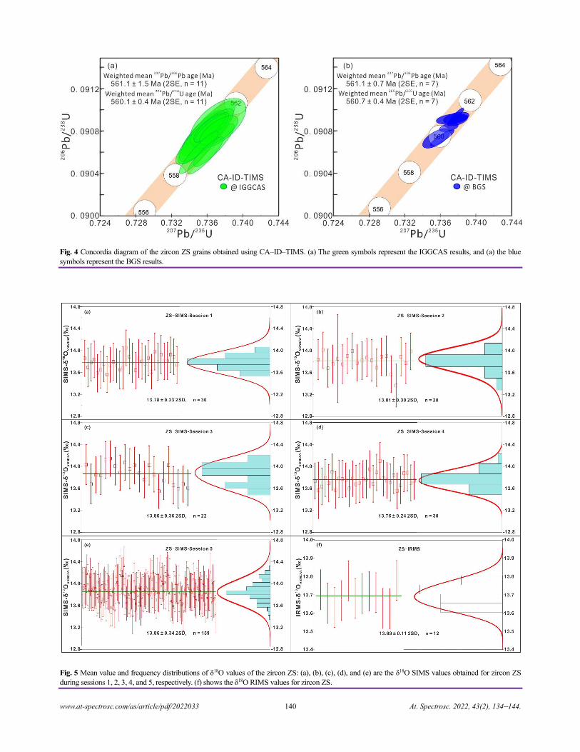
www.at-spectrosc.com/as/article/pdf/2022033 140 At. Spectrosc. 2022, 43(2), 134–144.
Fig. 4 Concordia diagram of the zircon ZS grains obtained using CA–ID–TIMS. (a) The green symbols represent the IGGCAS results, and (a) the blue
symbols represent the BGS results.
Fig. 5 Mean value and frequency distributions of δ18O values of the zircon ZS: (a), (b), (c), (d), and (e) are the δ18O SIMS values obtained for zircon ZS
during sessions 1, 2, 3, 4, and 5, respectively. (f) shows the δ18O RIMS values for zircon ZS.
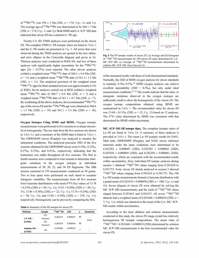
www.at-spectrosc.com/as/article/pdf/2022033 141 At. Spectrosc. 2022, 43(2), 134–144.
of 206Pb/238U was 558 ± 2 Ma (2SE, n = 174; Figs. 3m and 3n).
The average age of 207Pb/206Pb was determined to be 564 ± 7 Ma
(2SE, n = 174; Figs. 3o and 3p). Both SIMS and LA–ICP–MS data
indicated that zircon ZS has a uniform U–Pb age.
Twenty CA–ID–TIMS analyses were performed on the zircon
ZS. The complete TIMS U–Pb isotopic ratios are listed in Table 2
and the U–Pb results are presented in Fig. 4. All errors that were
observed during the TIMS analyses are quoted in the text, tables,
and error ellipses in the Concordia diagram and given at 2σ.
Thirteen analyses were conducted at IGGCAS, and two of these
analyses with significantly higher uncertainty for the 206Pb/238U
ages (2σ > 0.25%) were rejected. The other eleven analyses
yielded a weighted mean 206Pb/238U date of 560.1 ± 0.4 Ma (2SE,
n = 11) and a weighted mean 207Pb/206Pb date of 561.1± 1.5 Ma
(2SE, n = 11). The analytical precision of the weighted mean 206Pb/238U ages for these standard zircons was approximately 0.1%
(2 RSE). Seven analyses carried out at BGS yielded a weighted
mean 206Pb/238U date of 560.7 ± 0.4 Ma (2SE, n = 7) and a
weighted mean 207Pb/206Pb date of 561.1 ± 0.7 Ma (2SE, n = 7).
By combining all the above analyses, the recommended 206Pb/238U
age of the zircon ZS and the 207Pb/206Pb age were obtained as 560.6
± 1.3 Ma (2SD, n = 18) and 561.1 ± 3.5 Ma (2SD, n = 18),
respectively.
Oxygen Isotopes Using SIMS and IRMS. Oxygen isotopic
measurements were performed in five sessions to evaluate micron-
level homogeneity. The raw data from the five sessions are shown
in Table S3, and a summary of the SIMS data is listed in Table 3.
The GBW04409 zircon (Penglai) was analyzed to monitor the
instrument conditions. The analytical precision 2SD of the five
sessions obtained for the GBW04409 zircon were 0.14‰, 0.23‰,
0.27‰, 0.33‰, and 0.41‰, respectively, indicating that the
instrument was stable throughout all five sessions. The first to
fourth sessions were conducted in four mounts to determine inter-
grain variations in the oxygen isotopes as individual
measurements of 30, 20, 22, and 30 ZS fragments. The fifth
session consisted of 159 measurements conducted on 50 grains.
Two to four spots were performed on each shard to examine
intragrain variability. The measurements from all five sessions
form Gaussian distributions with mean δ18O (‰) values of 13.78
± 0.23‰ (2SD, n = 30; Fig. 5a), 13.81 ± 0.30‰ (2SD, n = 20; Fig.
5b), 13.86 ± 0.36‰ (2SD, n = 22; Fig. 5c), 13.76 ± 0.24‰ (2SD,
n = 30; Fig. 5d), and 13.86 ± 0.34‰ (2SD, n = 159; Fig. 5e),
respectively. Homogeneity can be proven by comparing the SDs
Table 4. Summary of the Hf isotopes for zircon ZS
Methods Sample 176Hf/177Hf 2SD n Standards
LA–MC–
ICPMS
ZS-
Session1 0.281674 0.000047 60
SA01 ZS-
Session2 0.281678 0.000054 40
Solution MC–
ICPMS ZS
0.281668 0.000010 7 /
Fig. 6 The Hf isotopic results of zircon ZS. (a) Average and (b) histogram
of 176Hf⁄177Hf measurements for 100 zircon ZS spots determined by LA–
MC–ICP–MS. (c) Average of 176Hf⁄177Hf measurements determined by
solution MC–ICP–MS. Error bars are 2σ.
of the measured results with those of well-demonstrated standards.
Normally, the 2SD of SIMS oxygen analysis for zircon standards
is routinely 0.3‰–0.5‰.56 SIMS oxygen analysis can achieve
excellent repeatability (2SD < 0.3‰), but only under ideal
measurement conditions.57, 58 The results indicate that the intra- or
intergrain variations observed in the oxygen isotopes are
sufficiently small to show the homogeneity of the zircon ZS. The
oxygen isotope compositions obtained using IRMS are
summarized in Table 3. The recommended value for zircon ZS
was 13.69 ± 0.11‰ (2SD, n = 12; Fig. 5f) based on 12 analyses.
The δ18O value determined by SIMS was consistent with that
determined by IRMS within uncertainty.
MC–ICP–MS Hf isotope data. The complete isotopic ratios of
Lu–Hf are listed in Table S4. A summary of these analyses is
provided in Table 4. The mean Lu–Hf isotopic results for SA01,
Mud tank, GBW04409 (Penglai), and SA02 zircon reference
materials under the same conditions were determined to be
0.282282 ± 0.000047 (2SD), 0.282502 ± 0.000042 (2SD),
0.282928 ± 0.000049 (2SD), and 0.282294 ± 0.000061 (2SD),
respectively, which are consistent with the recommended results
within uncertainties. Sixty individual Hf isotope analyses during
session 1 obtained 176Hf⁄177Hf values ranging from 0.281620 to
0.281753. Forty zircon ZS shards analyzed in session 2 showed 176Hf⁄177Hf values ranging from 0.281618 to 0.281732. The 100
Lu–Hf isotope measurements formed a Gaussian distribution with
a grand mean of 0.281676 ± 0.000050 (2SD, n = 100; Figs. 6a and
6b). Seven aliquots of zircon ZS were obtained by solving the
MC–ICP–MS measurements, and the yield of 176Hf/177Hf values
ranged between 0.281663 and 0.281675. All seven 176Hf/177Hf
datasets had a weighted mean of 0.281668 ± 0.000010 (2SD, n =
7; Fig. 6c), which was identical to the mean of the LA–MC–ICP–
MS results within uncertainties.
According to the laser ablation and solution measurements
conducted in this study, the zircon ZS mega crystal has relatively
homogeneous Hf isotopic compositions. The mean value of 176Hf/177Hf = 0.281668 ± 0.000010 (2SD) determined by solution
MC–ICP–MS measurements is the best recommended value for
zircon ZS.
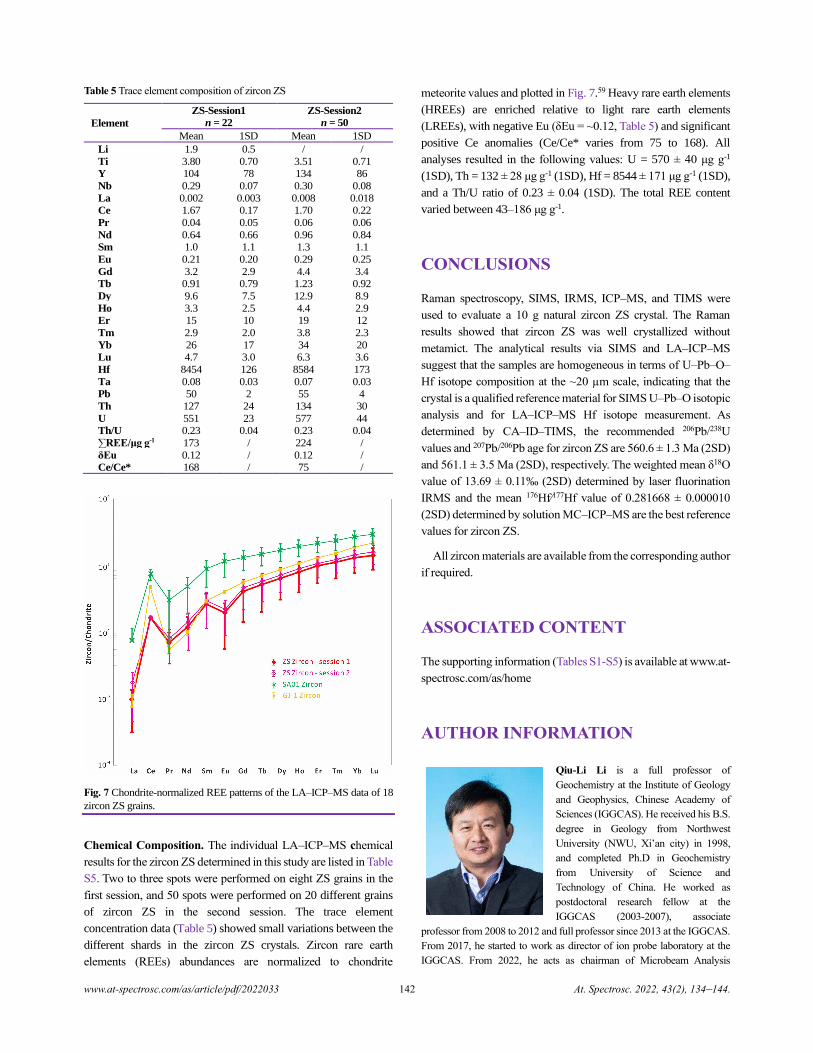
www.at-spectrosc.com/as/article/pdf/2022033 142 At. Spectrosc. 2022, 43(2), 134–144.
Table 5 Trace element composition of zircon ZS
Element
ZS-Session1
n = 22
ZS-Session2
n = 50
Mean 1SD Mean 1SD
Li 1.9 0.5 / /
Ti 3.80 0.70 3.51 0.71 Y 104 78 134 86
Nb 0.29 0.07 0.30 0.08
La 0.002 0.003 0.008 0.018 Ce 1.67 0.17 1.70 0.22
Pr 0.04 0.05 0.06 0.06
Nd 0.64 0.66 0.96 0.84 Sm 1.0 1.1 1.3 1.1
Eu 0.21 0.20 0.29 0.25
Gd 3.2 2.9 4.4 3.4 Tb 0.91 0.79 1.23 0.92
Dy 9.6 7.5 12.9 8.9
Ho 3.3 2.5 4.4 2.9 Er 15 10 19 12
Tm 2.9 2.0 3.8 2.3
Yb 26 17 34 20 Lu 4.7 3.0 6.3 3.6
Hf 8454 126 8584 173
Ta 0.08 0.03 0.07 0.03 Pb 50 2 55 4
Th 127 24 134 30
U 551 23 577 44 Th/U 0.23 0.04 0.23 0.04
∑REE/μg g-1 173 / 224 /
δEu 0.12 / 0.12 / Ce/Ce* 168 / 75 /
Fig. 7 Chondrite-normalized REE patterns of the LA–ICP–MS data of 18
zircon ZS grains.
Chemical Composition. The individual LA–ICP–MS chemical
results for the zircon ZS determined in this study are listed in Table
S5. Two to three spots were performed on eight ZS grains in the
first session, and 50 spots were performed on 20 different grains
of zircon ZS in the second session. The trace element
concentration data (Table 5) showed small variations between the
different shards in the zircon ZS crystals. Zircon rare earth
elements (REEs) abundances are normalized to chondrite
meteorite values and plotted in Fig. 7.59 Heavy rare earth elements
(HREEs) are enriched relative to light rare earth elements
(LREEs), with negative Eu (δEu = ~0.12, Table 5) and significant
positive Ce anomalies (Ce/Ce* varies from 75 to 168). All
analyses resulted in the following values: U = 570 ± 40 μg g-1
(1SD), Th = 132 ± 28 μg g-1 (1SD), Hf = 8544 ± 171 μg g-1 (1SD),
and a Th/U ratio of 0.23 ± 0.04 (1SD). The total REE content
varied between 43–186 μg g-1.
CONCLUSIONS
Raman spectroscopy, SIMS, IRMS, ICP–MS, and TIMS were
used to evaluate a 10 g natural zircon ZS crystal. The Raman
results showed that zircon ZS was well crystallized without
metamict. The analytical results via SIMS and LA–ICP–MS
suggest that the samples are homogeneous in terms of U–Pb–O–
Hf isotope composition at the ~20 µm scale, indicating that the
crystal is a qualified reference material for SIMS U–Pb–O isotopic
analysis and for LA–ICP–MS Hf isotope measurement. As
determined by CA–ID–TIMS, the recommended 206Pb/238U
values and 207Pb/206Pb age for zircon ZS are 560.6 ± 1.3 Ma (2SD)
and 561.1 ± 3.5 Ma (2SD), respectively. The weighted mean δ18O
value of 13.69 ± 0.11‰ (2SD) determined by laser fluorination
IRMS and the mean 176Hf⁄177Hf value of 0.281668 ± 0.000010
(2SD) determined by solution MC–ICP–MS are the best reference
values for zircon ZS.
All zircon materials are available from the corresponding author
if required.
ASSOCIATED CONTENT
The supporting information (Tables S1-S5) is available at www.at-
spectrosc.com/as/home
AUTHOR INFORMATION
Qiu-Li Li is a full professor of
Geochemistry at the Institute of Geology
and Geophysics, Chinese Academy of
Sciences (IGGCAS). He received his B.S.
degree in Geology from Northwest
University (NWU, Xi’an city) in 1998,
and completed Ph.D in Geochemistry
from University of Science and
Technology of China. He worked as
postdoctoral research fellow at the
IGGCAS (2003-2007), associate
professor from 2008 to 2012 and full professor since 2013 at the IGGCAS.
From 2017, he started to work as director of ion probe laboratory at the
IGGCAS. From 2022, he acts as chairman of Microbeam Analysis
www.at-spectrosc.com/as/article/pdf/2022033 143 At. Spectrosc. 2022, 43(2), 134–144.
Professional Committee of Chinese society for mineralogy petrology and
geochemistry. His research focused on micro area isotope geochemistry.
Based on the ion probe platform, he has developed a variety of in-situ U-
Th-Pb dating methods for many accessary minerals, which provides
effective dating means for solving geological chronological problems such
as ultra-alkaline rocks, carbonates, clastic sedimentary rocks, medium and
low temperature metamorphic rocks, low-temperature deposits and
extraterrestrial samples; Through the analysis of small beam spots of
zirconium containing minerals, he accurately determined that the Chang'e-
5 basalt was formed 2 billion years ago. He has been working as member
of editorial board for Atomic Spectroscopy. Qiu-Li Li published more than
50 SCI papers of the first or corresponding author in journals such as Nature,
Nature Communications and EPSL, and other more than 180 cooperative
papers.
Corresponding Author
*Q.-L. Li
Email address: [email protected]
Notes
The authors declare no competing financial interest.
ACKNOWLEDGMENTS
The authors gratefully thank the National Key Research and
Development Plan (2018YFA0702600) and the National Natural
Science Foundation of China (41773044, 41773047, and
42173037) for financially supporting this work. We thank Anton
Azaro for providing the zircon materials. We also appreciate
technical assistance from Hongxia Ma, Lanzhen Guo, Hongwei Li,
Zheng Liu, Lu Chen, and Wenquan Fan. Lastly, the authors
gratefully acknowledge the detailed reviews from the editors and
the reviewers.
REFERENCES
1. T. M. Will, C. Gaucher, X.-X. Ling, X.-H. Li, Q.-L. Li, and
H. E. Frimmel, Precambrian Res., 2019, 320, 303–322.
https://doi.org/10.1016/j.precamres.2018.11.004
2. E. Schmadicke, T. M. Will, X.-X. Ling, X.-H. Li, and Q.-L. Li,
Lithos, 2018, 322, 250–267.
https://doi.org/10.1016/j.lithos.2018.10.017
3. X.-H. Li, M. Tatsumoto, W. R. Premo, and X.-T. Gui, Geology,
1989, 17, 395–399. https://doi.org/10.1130/0091-
7613(1989)017<0395:AAOOTT>2.3.CO;2
4. Q.-L. Li, Y. Liu, G.-Q. Tang, K.-Y. Wang, X.-X. Ling, and J. Li,
J. Anal. At. Spectrom., 2018, 33, 1536–1544.
https://doi.org/10.1039/c8ja00125a
5. H.-Q. Huang, X.-H. Li, W.-X. Li, and Z.-X. Li, Geology, 2011, 39,
903–906. https://doi.org/10.1130/G32080.1
6. Y. A. El-Rahman, M. A. Anbar, X.-H. Li, J. Li, X.-X. Ling,
L.-G. Wu, and A. E. Masoud, Precambrian Res., 2019, 320, 46–62.
https://doi.org/10.1016/j.precamres.2018.10.011
7. X.-H. Li, Y. Chen, J. P. Tchouankoue, C.-Z. Liu, J. Li, X.-X. Ling,
G.-Q. Tang, and Y. Liu, Precambrian Res., 2017, 294, 307–321.
https://doi.org/10.1016/j.precamres.2017.04.006
8. H. S. Moghadam, X.-H. Li, X.-X. Ling, J. F. Santos, R. J. Stern,
Q.-L. Li, and G. Ghorbani, Lithos, 2015, 216, 118–135.
https://doi.org/10.1016/j.lithos.2014.12.012
9. M. Putis, X.-H. Li, Y.-H. Yang, Q.-L. Li, O. Nemec, X.-X. Ling,
F. Koller, and D. Balen, Lithos, 2018, 314, 165–186.
https://doi.org/10.1016/j.lithos.2018.05.030
10. F. Shakerardakani, X.-H. Li, F. Neubauer, X.-X. Ling, J. Li,
B. Monfaredi, and L.-G. Wu, Lithos, 2020, 352-353, 105330.
https://doi.org/10.1016/j.lithos.2019.105330
11. T. Luo, Q.-L. Li, X.-X. Ling, Y. Li, C. Yang, H.-L. Wang, X. Xia,
S.-B. Zhang, L. Xu, X.-M. Liu, X.-D. Deng, and Z. Hu,
J. Anal. At. Spectrom., 2021, 36, 2216–2226.
https://doi.org/10.1039/d1ja00258a
12. C. Huang, H. Wang, J.-H. Yang, J. Ramezani, C. Yang, S.-B. Zhang,
Y.-H. Yang, X.-P. Xia, L.-J. Feng, J. Lin, T.-T. Wang, Q. Ma,
H.-Y. He, L.-W. Xie, and S.-T. Wu, Geostand. Geoanal. Res., 2019,
44, 103–123. https://doi.org/10.1111/ggr.12307
13. Z.-C. Hu, X.-H. Li, T. Luo, W. Zhang, J. Crowley, Q.-L. Li,
X.-X. Ling, C. Yang, Y. Li, L. Feng, X. Xia, S.-B. Zhang,
Z.-C. Wang, J.-L. Guo, L. Xu, J. Lin, X.-M. Liu, Z.-A. Bao, Y.-S.
Liu, K.-Q. Zong, W. Chen, and S.-H. Hu, J. Anal. At. Spectrom.,
2021, 36, 2715–2734. https://doi.org/10.1039/d1ja00311a
14. C. Huang, H. Wang, J.-H. Yang, C. Yang, Z.-X. Li, Y.-H. Yang,
L.-J. Feng, L.-W. Xie, and S.-T. Wu, J. Anal. At. Spectrom., 2021, 36,
368–374. https://doi.org/10.1039/d0ja00409j
15. T. R. Ireland and I. S. Williams, Rev. Mineral. Geochem., 2003, 53,
215–241. https://doi.org/10.2113/0530215
16. A. C. Mclaren, J. D. Fitz Gerald, and I. S. Williams,
Geochim. Cosmochim. Acta, 1994, 58, 993–1005.
https://doi.org/10.1016/0016-7037(94)90521-5
17. M. Wiedenbeck, P. AllÉ, F. Corfu, W. L. Griffin, M. Meier,
F. Oberli, A. V. Quadt, J. C. Roddick, and W. Spiegel,
Geostand. Geoanal. Res., 1995, 19, 1–23.
https://doi.org/10.1111/j.1751-908X.1995.tb00147.x
18. M. Wiedenbeck, J. M. Hanchar, W. H. Peck, P. Sylvester, J. Valley,
M. Whitehouse, A. Kronz, Y. Morishita, L. Nasdala, J. Fiebig,
I. Franchi, J. P. Girard, R. C. Greenwood, R. Hinton, N. Kita,
P. R. D. Mason, M. Norman, M. Ogasawara, P. M. Piccoli,
D. Rhede, H. Satoh, B. Schulz-Dobrick, O. Skar, M. J. Spicuzza,
K. Terada, A. Tindle, S. Togashi, T. Vennemann, Q. Xie, and
Y.-F. Zheng, Geostand. Geoanal. Res., 2004, 28, 9–39.
https://doi.org/10.1111/j.1751-908X.2004.tb01041.x
19. L. Nasdala, W. Hofmeister, N. Norberg, J. M. Mattinson, F. Corfu,
W. Dörr, S. L. Kamo, A. K. Kennedy, A. Kronz, P. W. Reiners,
D. Frei, J. Kosler, Y.-S. Wan, J. Götze, T. Häger, A. Kröner, and
J. W. Valley, Geostand. Geoanal. Res., 2008, 32, 247–265.
https://doi.org/10.1111/j.1751-908X.2008.00914.x
20. X.-H. Li, W.-G. Long, Q.-L. Li, Y. Liu, Y.-F. Zheng, Y.-H. Yang,
K. R. Chamberlain, D.-F. Wan, C.-H. Guo, X.-C. Wang, and H. Tao,
Geostand. Geoanal. Res., 2010, 34, 117–134.
https://doi.org/10.1111/j.1751-908X.2010.00036.x
21. Y.-Y. Gao, X.-H. Li, W. L. Griffin, Y.-J. Tang, N. J. Pearson, Y. Liu,
M.-F. Chu, Q.-L. Li, G.-Q. Tang, and S. Y. O'Reilly, Sci. Rep., 2015,
5, 16878. https://doi.org/10.1038/srep16878
22. X.-H. Li, G.-Q. Tang, B. Gong, Y.-H. Yang, K.-J. Hou, Z.-C. Hu,
Q.-L. Li, Y. Liu, and W.-X. Li, Chin. Sci. Bull., 2013, 58,
4647–4654. https://doi.org/10.1007/s11434-013-5932-x
www.at-spectrosc.com/as/article/pdf/2022033 144 At. Spectrosc. 2022, 43(2), 134–144.
23. L. P. Black, S. L. Kamo, C. M. Allen, D. W. Davis, J. N. Aleinikoff,
J. W. Valley, R. Mundil, I. H. Campbell, R. J. Korsch, I. S. Williams,
and C. Foudoulis, Chem. Geol., 2004, 205, 115–140.
https://doi.org/10.1016/j.chemgeo.2004.01.003
24. J. Sláma, J. Košler, D. J. Condon, J. L. Crowley, A. Gerdes,
J. M. Hanchar, M. S. A. Horstwood, G. A. Morris, L. Nasdala,
N. Norberg, U. Schaltegger, B. Schoene, M. N. Tubrett, and
M. J. Whitehouse, Chem. Geol., 2008, 249, 1–35.
https://doi.org/10.1016/j.chemgeo.2007.11.005
25. X.-X. Ling, Q.-L. Li, L.-J. Feng, D. Zhang, Y. Liu, G.-Q. Tang, J. Li,
S.-T. Wu, L.-L. Huang, T.-J. Li, Y. Liu, R. Werner, and X.-H. Li,
Crystals, 2021, 11, 1322. https://doi.org/10.3390/cryst11111322
26. X.-H. Li, Y. Liu, Q.-L. Li, C.-H. Guo, and K. R. Chamberlain,
Geochem. Geophys. Geosyst., 2009, 10, Q04010.
https://doi.org/10.1029/2009gc002400
27. Q.-L. Li, X.-H. Li, Y. Liu, G.-Q. Tang, J.-H. Yang, and W.-G. Zhu,
J. Anal. At. Spectrom., 2010, 25, 1107–1113.
https://doi.org/10.1039/b923444f
28. W.-H. Zhao, Q.-L. Li, Y. Liu, G.-Q. Tang, X.-X. Ling, J. Li, and
X.-H. Li, J. Earth Sci., 2022, 33, 17–24.
https://doi.org/10.1007/s12583-021-1549-1
29. J. S. Stacey and J. D. Kramers, Earth Planet. Sci. Lett., 1975, 26,
207-221. https://doi.org/10.1016/0012-821x(75)90088-6
30. C. Paton, J. Hellstrom, B. Paul, J. Woodhead, and J. Hergt,
J. Anal. At. Spectrom., 2011, 26, 2508–2518.
https://doi.org/10.1039/c1ja10172b
31. Z.-H. Hou, Y.-L. Xiao, J. Shen, and C.-L. Yu, J. Asian Earth Sci.,
2020, 192, 104261. https://doi.org/10.1016/j.jseaes.2020.104261
32. T. Andersen, Chem. Geol., 2002, 192, 59–79.
https://doi.org/10.1016/s0009-2541(02)00195-x
33. M. L. A. Morel, O. Nebel, Y. J. Nebel-Jacobsen, J. S. Miller, and
P. Z. Vroon, Chem. Geol., 2008, 255, 231–235.
https://doi.org/10.1016/j.chemgeo.2008.06.040
34. Y.-S. Liu, S. Gao, Z.-C. Hu, C.-G. Gao, K.-Q. Zong, and
D.-B. Wang, J. Petrol., 2010, 51, 537–571.
https://doi.org/10.1093/petrology/egp082
35. Z.-Y. Chu, J.-J. Xu, Z. Chen, C.-F. Li, X.-H. Li, H.-Y. He, X.-H. Li,
and J.-H. Guo, Chin. Sci. Bull., 2016, 61, 1121–1129.
https://doi.org/10.1360/n972015-01048
36. W. Wang, M.-Z. Zhou, Z.-Y. Chu, J.-J. Xu, C.-F. Li, T.-Y. Luo, and
J.-H. Guo, Science China-Earth Sciences, 2020, 63, 1176–1187.
https://doi.org/10.1007/s11430-019-9590-0
37. C. Yang, A. D. Rooney, D. J. Condon, X.-H. Li, D. V. Grazhdankin,
F. T. Bowyer, C. Hu, F. A. Macdonald, and M.-Y. Zhu, Sci. Adv.,
2021, 7, eabi9643. https://doi.org/10.1126/sciadv.abi9643
38. A. H. Jaffey, K. F. Flynn, L. E. Glendenin, W. C. Bentley, and
A. M. Essling, Physical Review C, 1971, 4, 1889–1906.
https://doi.org/10.1103/PhysRevC.4.1889
39. J. Hiess, D. J. Condon, N. McLean, and S. R. Noble, Science, 2012,
335, 1610–1614. https://doi.org/10.1126/science.1215507
40. G.-Q. Tang, Y. Liu, Q.-L. Li, L.-J. Feng, G.-J. Wei, W. Su, Y. Li,
G.-H. Ren, and X.-H. Li, At. Spectrosc., 2020, 41, 188–193.
https://doi.org/10.46770/As.2020.05.002
41. L.-J. Feng, H.-W. Li, and T.-J. Li, Minerals, 2020, 10, 987.
https://doi.org/10.3390/min10110987
42. K. R. Ludwig, User’s Manual for Isoplot 3.75, A Geochronological
Tooklit for Microsoft Excel, Berkeley Geochronology Center Special
Publication, Berkeley, CA, USA, 2012.
43. S. E. M. Gain, Y. Greau, H. Henry, E. Belousova, I. Dainis,
W. L. Griffin, and S. Y. O'Reilly, Geostand. Geoanal. Res., 2019, 43,
339–354. https://doi.org/10.1111/ggr.12265
44. F.-Y. Wu, Y.-H. Yang, L.-W. Xie, J.-H. Yang, and P. Xu,
Chem. Geol., 2006, 234, 105–126.
https://doi.org/10.1016/j.chemgeo.2006.05.003
45. W. Zhang, and Z.-C. Hu, At. Spectrosc., 2020, 41, 93–102.
https://doi.org/10.46770/As.2020.03.001
46. Z.-C. Hu, W. Zhang, Y.-S. Liu, S. Gao, M. Li, K.-Q. Zong,
H.-H. Chen, and S.-H. Hu, Anal. Chem., 2015, 87, 1152–1157.
https://doi.org/10.1021/ac503749k
47. Y.-S. Liu, Z.-C. Hu, S. Gao, D. Günther, J. Xu, C.-G. Gao, and
H.-H. Chen, Chem. Geol., 2008, 257, 34–43.
https://doi.org/10.1016/j.chemgeo.2008.08.004
48. R. W. Hinton, Geostand. Geoanal. Res., 1999, 23, 197–207.
https://doi.org/10.1111/j.1751-908X.1999.tb00574.x
49. S.-T. Wu, G. Worner, K. P. Jochum, B. Stoll, K. Simon, and
A. Kronz, Geostand. Geoanal. Res., 2019, 43, 567–584.
https://doi.org/10.1111/ggr.12301
50. M. Zhang, E. K. H. Salje, G. C. Capitani, H. Leroux, A. M. Clark,
J. Schluter, and R. C. Ewing, J. Phys. Condens. Mat., 2000, 12,
3131–3148. https://doi.org/10.1088/0953-8984/12/13/321
51. L. Nasdala, M. Zhang, U. Kempe, G. Panczer, M. Gaft, M. Andrut,
and M. Plotze, Rev. Mineral. Geochem., 2003, 53, 427–467.
https://doi.org/10.2113/0530427
52. L. Nasdala, M. Wenzel, G. Vavra, G. Irmer, T. Wenzel, and
B. Kober, Contrib. Mineral. Petrol., 2001, 141, 125–144.
https://doi.org/10.1007/s004100000235
53. C. S. Palenik, L. Nasdala, and R. C. Ewing, Am. Mineral., 2003, 88,
770–781. https://doi.org/10.2138/am-2003-5-606
54. Y.-Y. Gao, X.-H. Li, W. L. Griffin, S. Y. O'Reilly, and Y.-F. Wang,
Lithos, 2014, 192, 180–191.
https://doi.org/10.1016/j.lithos.2014.02.002
55. M. S. A. Horstwood, J. Kosler, G. Gehrels, S. E. Jackson,
N. M. McLean, C. Paton, N. J. Pearson, K. Sircombe, P. Sylvester,
P. Vermeesch, J. F. Bowring, D. J. Condon, and B. Schoene,
Geostand. Geoanal. Res., 2016, 40, 311–332.
https://doi.org/10.1111/j.1751-908X.2016.00379.x
56. G.-Q. Tang, X.-H. Li, X. H. Li, Q.-L. Li, Y. Liu, X.-X. Ling, and
Q.-Z. Yin, J. Anal. At. Spectrom., 2015, 30, 950–956.
https://doi.org/10.1039/c4ja00458b
57. P. Peres, N. T. Kita, J. W. Valley, F. Fernandes, and
M. Schuhmacher, Surf. Interface Anal., 2012, 45, 553–556.
https://doi.org/10.1002/sia.5061
58. P. C. Treble, A. K. Schmitt, R. L. Edwards, K. D. McKeegan,
T. M. Harrison, M. Grove, H. Cheng, and Y. J. Wang, Chem. Geol.,
2007, 238, 197–212. https://doi.org/10.1016/j.chemgeo.2006.11.009
59. W. F. McDonough and S. S. Sun, Chem. Geol., 1995, 120, 223–253.
https://doi.org/10.1016/0009-2541(94)00140-4
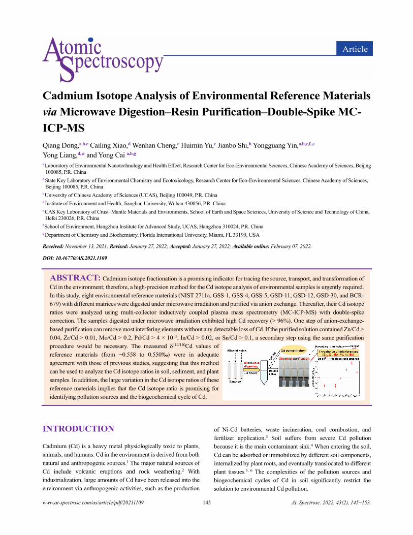
www.at-spectrosc.com/as/article/pdf/20211109 145 At. Spectrosc. 2022, 43(2), 145–153.
Cadmium Isotope Analysis of Environmental Reference Materials
via Microwave Digestion–Resin Purification–Double-Spike MC-
ICP-MS
Qiang Dong,a,b,c Cailing Xiao,d Wenhan Cheng,e Huimin Yu,e Jianbo Shi,b Yongguang Yin,a,b,c,f,*
Yong Liang,d,* and Yong Cai a,b,g a Laboratory of Environmental Nanotechnology and Health Effect, Research Center for Eco-Environmental Sciences, Chinese Academy of Sciences, Beijing
100085, P.R. China
b State Key Laboratory of Environmental Chemistry and Ecotoxicology, Research Center for Eco-Environmental Sciences, Chinese Academy of Sciences,
Beijing 100085, P.R. China
c University of Chinese Academy of Sciences (UCAS), Beijing 100049, P.R. China
d Institute of Environment and Health, Jianghan University, Wuhan 430056, P.R. China
e CAS Key Laboratory of Crust–Mantle Materials and Environments, School of Earth and Space Sciences, University of Science and Technology of China,
Hefei 230026, P.R. China
f School of Environment, Hangzhou Institute for Advanced Study, UCAS, Hangzhou 310024, P.R. China
g Department of Chemistry and Biochemistry, Florida International University, Miami, FL 33199, USA
Received: November 13, 2021; Revised: January 27, 2022; Accepted: January 27, 2022; Available online: February 07, 2022.
DOI: 10.46770/AS.2021.1109
ABSTRACT: Cadmium isotope fractionation is a promising indicator for tracing the source, transport, and transformation of
Cd in the environment; therefore, a high-precision method for the Cd isotope analysis of environmental samples is urgently required.
In this study, eight environmental reference materials (NIST 2711a, GSS-1, GSS-4, GSS-5, GSD-11, GSD-12, GSD-30, and BCR-
679) with different matrices were digested under microwave irradiation and purified via anion exchange. Thereafter, their Cd isotope
ratios were analyzed using multi-collector inductively coupled plasma mass spectrometry (MC-ICP-MS) with double-spike
correction. The samples digested under microwave irradiation exhibited high Cd recovery (> 96%). One step of anion-exchange-
based purification can remove most interfering elements without any detectable loss of Cd. If the purified solution contained Zn/Cd >
0.04, Zr/Cd > 0.01, Mo/Cd > 0.2, Pd/Cd > 4 × 10⁻⁵, In/Cd > 0.02, or Sn/Cd > 0.1, a secondary step using the same purification
procedure would be necessary. The measured δ114/110Cd values of
reference materials (from −0.558 to 0.550‰) were in adequate
agreement with those of previous studies, suggesting that this method
can be used to analyze the Cd isotope ratios in soil, sediment, and plant
samples. In addition, the large variation in the Cd isotope ratios of these
reference materials implies that the Cd isotope ratio is promising for
identifying pollution sources and the biogeochemical cycle of Cd.
INTRODUCTION
Cadmium (Cd) is a heavy metal physiologically toxic to plants,
animals, and humans. Cd in the environment is derived from both
natural and anthropogenic sources.1 The major natural sources of
Cd include volcanic eruptions and rock weathering.2 With
industrialization, large amounts of Cd have been released into the
environment via anthropogenic activities, such as the production
of Ni-Cd batteries, waste incineration, coal combustion, and
fertilizer application.3 Soil suffers from severe Cd pollution
because it is the main contaminant sink.4 When entering the soil,
Cd can be adsorbed or immobilized by different soil components,
internalized by plant roots, and eventually translocated to different
plant tissues.5, 6 The complexities of the pollution sources and
biogeochemical cycles of Cd in soil significantly restrict the
solution to environmental Cd pollution.
www.at-spectrosc.com/as/article/pdf/20211109 146 At. Spectrosc. 2022, 43(2), 145–153.
Cd has eight stable isotopes with mass numbers in the range of
106–116. Cd isotope fractionation has been shown to occur during
the evaporation/condensation and biological cycling of Cd.7, 8
Recent studies have reported a significantly large degree of Cd
isotope fractionation among the products and waste produced
during coal combustion, metal smelting/refining, and metal
coating,9-12 which implies that isotope fractionation can be used to
identify Cd pollution sources.13 Researchers have identified the
main Cd sources and their contribution to Cd pollution by
determining the Cd isotope ratios of various sources and
contaminated receptors (e.g., soil and sediments).14-17 Cd isotope
fractionation also occurs during its adsorption-desorption between
the solid and liquid phases18-20 and translocation to different plant
tissues (e.g., roots, shoots, and grains).21, 22 These observations
have demonstrated that Cd isotope analysis is a promising tool for
tracing the sources of Cd in contaminated sites and can also be
used as an indicator for probing the behavior of Cd in the
environment.
In early research, Cd isotope analysis was typically accomplished
using thermal ionization mass spectroscopy.23 With improvements
in mass spectroscopy, the use of multi-collector inductively
coupled plasma mass spectrometry (MC-ICP-MS) for metal
isotope analysis became practical.24 Since MC-ICP-MS can easily
overcome the first ionization potential of Cd via plasma ionization,
it is currently the dominant technique for Cd isotope analysis.23 To
accurately determine Cd isotope ratios, possible interfering
substances must be removed from samples, which requires the
samples to be completely digested, purified, and recovered. For
environmental sample digestion, the most widely used protocol is
to sequentially add sample and mineral acids (e.g., HNO3 and HF)
to high-pressure bombs or perfluoroalkoxy (PFA) vials. Digestion
is then performed using an oven or a hot plate for tens of hours.25-
28 Although these methods can completely digest samples, they are
time-consuming and exhibit poor organic matter removal
performance due to the incomplete oxidation of carbon.
Unfortunately, most environmental samples, such as agricultural
soils and plants, contain large amounts of organic matter that can
significantly affect the analytical accuracy of Cd isotope ratios.11
Due to the increasing use of Cd isotope fractionation in
environmental research, establishing an effective and efficient
digestion method for environmental samples has become
necessary. In addition, most soil samples contain interfering
elements (e.g., Zn, Zr, Mo, In, and Sn) in amounts that are 1–2
orders of magnitude higher than that of Cd. Thus, it also becomes
necessary to evaluate whether current purification processes can
effectively remove the matrix and interfering elements in a single
operation, and if not, whether the content of interfering elements
in the Cd sample solution can meet the requirements for Cd
isotope analysis. Furthermore, if the Cd sample solution does not
meet the test requirements, the performance of the secondary
purification procedure needs to be evaluated.
Therefore, eight environmental reference materials, including
soil, sediments, and plants, were tested to evaluate the use of
microwave digestion and anion-exchange-based chemical
purification procedures using double-spike MC-ICP-MS for Cd
isotope analysis. In addition, the effects of isobaric (Pd, In, and Sn)
and polyatomic (Zn, Zr, and Mo) interferences on Cd isotope
analysis were evaluated and discussed.
EXPERIMENTAL
Reagents, standard solutions, and samples. TraceMetalTM grade
HNO3 and hydrochloric acid (HCl) were procured from Thermo
Fisher Scientific (Waltham, MA). Analytical-grade HF and
hydrogen peroxide (H2O2) were procured from Beijing Chemicals
(Beijing, China). HNO3 and HCl were distilled twice using a
Savillex™ DST-1000 sub-boiling acid system. The 111Cd-113Cd
double-spike solution used in this study was prepared using the
enriched 111Cd (purity of 96.00%) and 113Cd isotopes (purity of
94.90%) from Isotopes for Science, Medicine, and Industry (San
Francisco, CA). Briefly, the enriched 111Cd and 113Cd isotopes
were individually dissolved in 2 mol L−1 HNO3, and suitable
volumes of the individual isotope solutions were weighed and
mixed to obtain a double-spike solution with a 111Cd-to-113Cd ratio
≈ 1, which could then provide high precision for the double-spike
method.25, 29 Finally, after the double-spike solution was stabilized
for 12 h, it was diluted to 10 µg g−1. An AG-MP-1M ion-exchange
resin (100–200 dry mesh size, Bio-Rad Laboratories AB, Solna,
Sweden) was used for sample purification. Milli-Q water (18.2
MΩ cm−1) was used in all experimental procedures.
Four mono-elemental Cd solutions were used to validate the
method: (1) an NIST SRM3108 Cd solution, a common reference
material for Cd isotope studies (Lot 130116);30 (2) AAS-Cd, a
commercial ICP standard solution (Lot 1797541);25 (3) Thermo-
Cd, a commercial ICP standard solution (Lot 9158147) (Alfa
Aesar, Thermo Fisher Scientific, Leicestershire, United Kingdom);
and (4) GSB-Cd, a mono-elemental Cd standard solution (GSB
04-1721-2004) (Iron and Steel Research Institute, Beijing, China).
Other mono-elemental (Mg, Ca, Mn, Cu, Zn, Zr, Mo, Pd, In, Sn,
and Pb) standard solutions used in this study were also procured
from the Iron and Steel Research Institute (Beijing, China).
Eight environmental reference materials with certified Cd
concentrations and isotopic compositions were used to evaluate
treatment processes, including four soil reference materials (NIST
2711a, GSS-1, GSS-4, and GSS-5), three stream sediment
reference materials (GSD-11, GSD-12, and GSD-30), and one
plant reference material (BCR-679).
Sample digestion. Samples were digested using microwaves. For
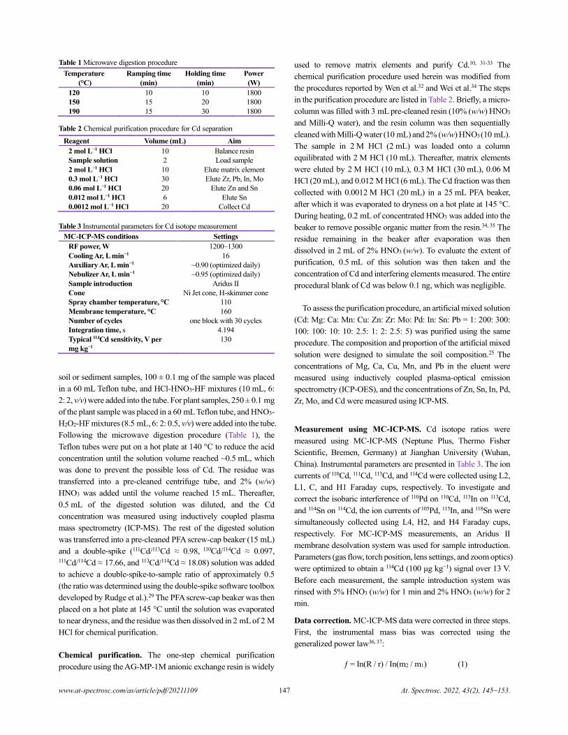
www.at-spectrosc.com/as/article/pdf/20211109 147 At. Spectrosc. 2022, 43(2), 145–153.
Table 1 Microwave digestion procedure
Temperature
(°C)
Ramping time
(min)
Holding time
(min)
Power
(W)
120 10 10 1800
150 15 20 1800
190 15 30 1800
Table 2 Chemical purification procedure for Cd separation
Reagent Volume (mL) Aim
2 mol L−1 HCl 10 Balance resin
Sample solution 2 Load sample
2 mol L−1 HCl 10 Elute matrix element
0.3 mol L−1 HCl 30 Elute Zr, Pb, In, Mo
0.06 mol L−1 HCl 20 Elute Zn and Sn
0.012 mol L−1 HCl 6 Elute Sn
0.0012 mol L−1 HCl 20 Collect Cd
Table 3 Instrumental parameters for Cd isotope measurement
MC-ICP-MS conditions Settings
RF power, W 1200–1300
Cooling Ar, L min−1 16
Auxiliary Ar, L min−1 ~0.90 (optimized daily)
Nebulizer Ar, L min−1 ~0.95 (optimized daily)
Sample introduction Aridus II
Cone Ni Jet cone, H-skimmer cone
Spray chamber temperature, °C 110
Membrane temperature, °C 160
Number of cycles
Integration time, s
one block with 30 cycles
4.194
Typical 114Cd sensitivity, V per
mg kg−1
130
soil or sediment samples, 100 ± 0.1 mg of the sample was placed
in a 60 mL Teflon tube, and HCl-HNO3-HF mixtures (10 mL, 6:
2: 2, v/v) were added into the tube. For plant samples, 250 ± 0.1 mg
of the plant sample was placed in a 60 mL Teflon tube, and HNO3-
H2O2-HF mixtures (8.5 mL, 6: 2: 0.5, v/v) were added into the tube.
Following the microwave digestion procedure (Table 1), the
Teflon tubes were put on a hot plate at 140 °C to reduce the acid
concentration until the solution volume reached ~0.5 mL, which
was done to prevent the possible loss of Cd. The residue was
transferred into a pre-cleaned centrifuge tube, and 2% (w/w)
HNO3 was added until the volume reached 15 mL. Thereafter,
0.5 mL of the digested solution was diluted, and the Cd
concentration was measured using inductively coupled plasma
mass spectrometry (ICP-MS). The rest of the digested solution
was transferred into a pre-cleaned PFA screw-cap beaker (15 mL)
and a double-spike (111Cd/113Cd ≈ 0.98, 110Cd/114Cd ≈ 0.097, 111Cd/114Cd ≈ 17.66, and 113Cd/114Cd ≈ 18.08) solution was added
to achieve a double-spike-to-sample ratio of approximately 0.5
(the ratio was determined using the double-spike software toolbox
developed by Rudge et al.).29 The PFA screw-cap beaker was then
placed on a hot plate at 145 °C until the solution was evaporated
to near dryness, and the residue was then dissolved in 2 mL of 2 M
HCl for chemical purification.
Chemical purification. The one-step chemical purification
procedure using the AG-MP-1M anionic exchange resin is widely
used to remove matrix elements and purify Cd.10, 31-33 The
chemical purification procedure used herein was modified from
the procedures reported by Wen et al.32 and Wei et al.34 The steps
in the purification procedure are listed in Table 2. Briefly, a micro-
column was filled with 3 mL pre-cleaned resin (10% (w/w) HNO3
and Milli-Q water), and the resin column was then sequentially
cleaned with Milli-Q water (10 mL) and 2% (w/w) HNO3 (10 mL).
The sample in 2 M HCl (2 mL) was loaded onto a column
equilibrated with 2 M HCl (10 mL). Thereafter, matrix elements
were eluted by 2 M HCl (10 mL), 0.3 M HCl (30 mL), 0.06 M
HCl (20 mL), and 0.012 M HCl (6 mL). The Cd fraction was then
collected with 0.0012 M HCl (20 mL) in a 25 mL PFA beaker,
after which it was evaporated to dryness on a hot plate at 145 °C.
During heating, 0.2 mL of concentrated HNO3 was added into the
beaker to remove possible organic matter from the resin.34, 35 The
residue remaining in the beaker after evaporation was then
dissolved in 2 mL of 2% HNO3 (w/w). To evaluate the extent of
purification, 0.5 mL of this solution was then taken and the
concentration of Cd and interfering elements measured. The entire
procedural blank of Cd was below 0.1 ng, which was negligible.
To assess the purification procedure, an artificial mixed solution
(Cd: Mg: Ca: Mn: Cu: Zn: Zr: Mo: Pd: In: Sn: Pb = 1: 200: 300:
100: 100: 10: 10: 2.5: 1: 2: 2.5: 5) was purified using the same
procedure. The composition and proportion of the artificial mixed
solution were designed to simulate the soil composition.25 The
concentrations of Mg, Ca, Cu, Mn, and Pb in the eluent were
measured using inductively coupled plasma-optical emission
spectrometry (ICP-OES), and the concentrations of Zn, Sn, In, Pd,
Zr, Mo, and Cd were measured using ICP-MS.
Measurement using MC-ICP-MS. Cd isotope ratios were
measured using MC-ICP-MS (Neptune Plus, Thermo Fisher
Scientific, Bremen, Germany) at Jianghan University (Wuhan,
China). Instrumental parameters are presented in Table 3. The ion
currents of 110Cd, 111Cd, 113Cd, and 114Cd were collected using L2,
L1, C, and H1 Faraday cups, respectively. To investigate and
correct the isobaric interference of 110Pd on 110Cd, 113In on 113Cd,
and 114Sn on 114Cd, the ion currents of 105Pd, 115In, and 118Sn were
simultaneously collected using L4, H2, and H4 Faraday cups,
respectively. For MC-ICP-MS measurements, an Aridus II
membrane desolvation system was used for sample introduction.
Parameters (gas flow, torch position, lens settings, and zoom optics)
were optimized to obtain a 114Cd (100 μg kg−1) signal over 13 V.
Before each measurement, the sample introduction system was
rinsed with 5% HNO3 (w/w) for 1 min and 2% HNO3 (w/w) for 2
min.
Data correction. MC-ICP-MS data were corrected in three steps.
First, the instrumental mass bias was corrected using the
generalized power law36, 37:
ƒ = In(R / r) / In(m2 / m1) (1)
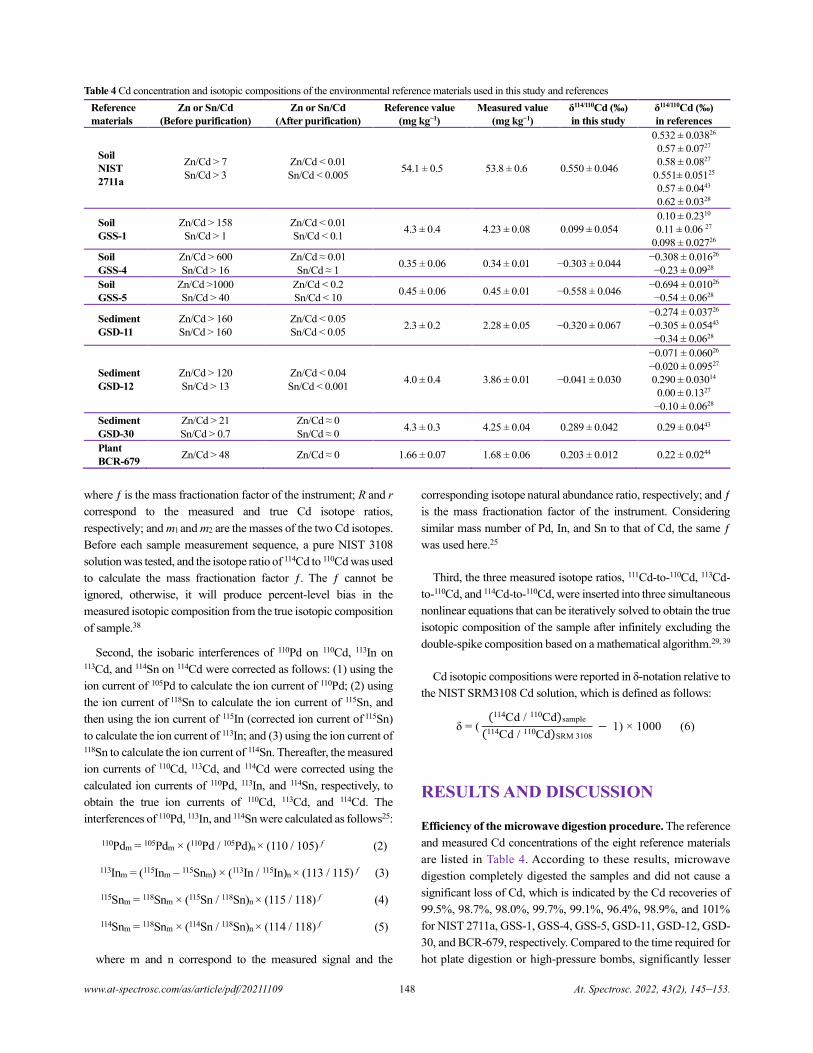
www.at-spectrosc.com/as/article/pdf/20211109 148 At. Spectrosc. 2022, 43(2), 145–153.
Table 4 Cd concentration and isotopic compositions of the environmental reference materials used in this study and references
where ƒ is the mass fractionation factor of the instrument; R and r
correspond to the measured and true Cd isotope ratios,
respectively; and m1 and m2 are the masses of the two Cd isotopes.
Before each sample measurement sequence, a pure NIST 3108
solution was tested, and the isotope ratio of 114Cd to 110Cd was used
to calculate the mass fractionation factor ƒ. The ƒ cannot be
ignored, otherwise, it will produce percent-level bias in the
measured isotopic composition from the true isotopic composition
of sample.38
Second, the isobaric interferences of 110Pd on 110Cd, 113In on 113Cd, and 114Sn on 114Cd were corrected as follows: (1) using the
ion current of 105Pd to calculate the ion current of 110Pd; (2) using
the ion current of 118Sn to calculate the ion current of 115Sn, and
then using the ion current of 115In (corrected ion current of 115Sn)
to calculate the ion current of 113In; and (3) using the ion current of
118Sn to calculate the ion current of 114Sn. Thereafter, the measured
ion currents of 110Cd, 113Cd, and 114Cd were corrected using the
calculated ion currents of 110Pd, 113In, and 114Sn, respectively, to
obtain the true ion currents of 110Cd, 113Cd, and 114Cd. The
interferences of 110Pd, 113In, and 114Sn were calculated as follows25:
110Pdm = 105Pdm × (110Pd / 105Pd)n × (110 / 105) f (2)
113Inm = (115Inm – 115Snm) × (113In / 115In)n × (113 / 115) f (3)
115Snm = 118Snm × (115Sn / 118Sn)n × (115 / 118) f (4)
114Snm = 118Snm × (114Sn / 118Sn)n × (114 / 118) f (5)
where m and n correspond to the measured signal and the
corresponding isotope natural abundance ratio, respectively; and ƒ
is the mass fractionation factor of the instrument. Considering
similar mass number of Pd, In, and Sn to that of Cd, the same ƒ
was used here.25
Third, the three measured isotope ratios, 111Cd-to-110Cd, 113Cd-
to-110Cd, and 114Cd-to-110Cd, were inserted into three simultaneous
nonlinear equations that can be iteratively solved to obtain the true
isotopic composition of the sample after infinitely excluding the
double-spike composition based on a mathematical algorithm.29, 39
Cd isotopic compositions were reported in δ-notation relative to
the NIST SRM3108 Cd solution, which is defined as follows:
δ = ((114Cd / 110Cd)sample
(114Cd / 110Cd)SRM 3108 − 1) × 1000 (6)
RESULTS AND DISCUSSION
Efficiency of the microwave digestion procedure. The reference
and measured Cd concentrations of the eight reference materials
are listed in Table 4. According to these results, microwave
digestion completely digested the samples and did not cause a
significant loss of Cd, which is indicated by the Cd recoveries of
99.5%, 98.7%, 98.0%, 99.7%, 99.1%, 96.4%, 98.9%, and 101%
for NIST 2711a, GSS-1, GSS-4, GSS-5, GSD-11, GSD-12, GSD-
30, and BCR-679, respectively. Compared to the time required for
hot plate digestion or high-pressure bombs, significantly lesser
Reference
materials
Zn or Sn/Cd
(Before purification)
Zn or Sn/Cd
(After purification)
Reference value
(mg kg−1)
Measured value
(mg kg−1)
δ114/110Cd (‰)
in this study
δ114/110Cd (‰)
in references
Soil
NIST
2711a
Zn/Cd > 7
Sn/Cd > 3
Zn/Cd < 0.01
Sn/Cd < 0.005 54.1 ± 0.5 53.8 ± 0.6 0.550 ± 0.046
0.532 ± 0.03826
0.57 ± 0.0727
0.58 ± 0.0827
0.551± 0.05125
0.57 ± 0.0443
0.62 ± 0.0328
Soil
GSS-1
Zn/Cd > 158
Sn/Cd > 1
Zn/Cd < 0.01
Sn/Cd < 0.1 4.3 ± 0.4 4.23 ± 0.08 0.099 ± 0.054
0.10 ± 0.2310
0.11 ± 0.06 27
0.098 ± 0.02726
Soil
GSS-4
Zn/Cd > 600
Sn/Cd > 16
Zn/Cd ≈ 0.01
Sn/Cd ≈ 1 0.35 ± 0.06 0.34 ± 0.01 −0.303 ± 0.044
−0.308 ± 0.01626
−0.23 ± 0.0928
Soil
GSS-5
Zn/Cd >1000
Sn/Cd > 40
Zn/Cd < 0.2
Sn/Cd < 10 0.45 ± 0.06 0.45 ± 0.01 −0.558 ± 0.046
−0.694 ± 0.01026
−0.54 ± 0.0628
Sediment
GSD-11
Zn/Cd > 160
Sn/Cd > 160
Zn/Cd < 0.05
Sn/Cd < 0.05 2.3 ± 0.2 2.28 ± 0.05 −0.320 ± 0.067
−0.274 ± 0.03726
−0.305 ± 0.05443
−0.34 ± 0.0628
Sediment
GSD-12
Zn/Cd > 120
Sn/Cd > 13
Zn/Cd < 0.04
Sn/Cd < 0.001 4.0 ± 0.4 3.86 ± 0.01 −0.041 ± 0.030
−0.071 ± 0.06026
−0.020 ± 0.09527
0.290 ± 0.03014
0.00 ± 0.1327
−0.10 ± 0.0628
Sediment
GSD-30
Zn/Cd > 21
Sn/Cd > 0.7
Zn/Cd ≈ 0
Sn/Cd ≈ 0 4.3 ± 0.3 4.25 ± 0.04 0.289 ± 0.042 0.29 ± 0.0443
Plant
BCR-679 Zn/Cd > 48 Zn/Cd ≈ 0 1.66 ± 0.07 1.68 ± 0.06 0.203 ± 0.012 0.22 ± 0.0244
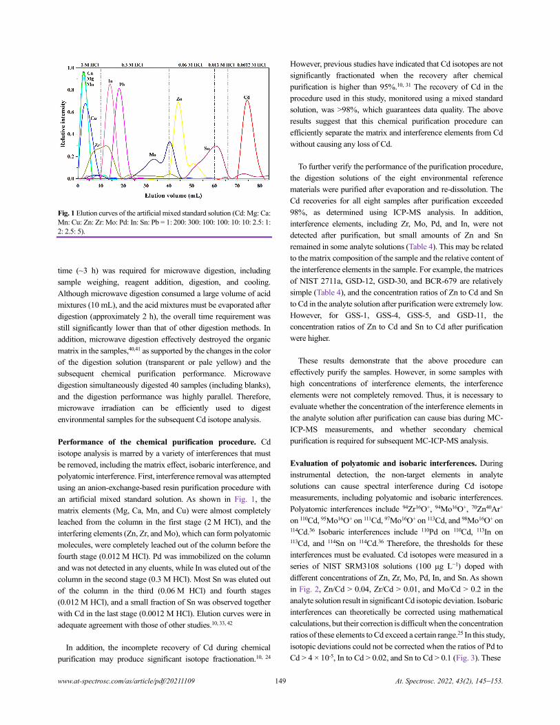
www.at-spectrosc.com/as/article/pdf/20211109 149 At. Spectrosc. 2022, 43(2), 145–153.
Fig. 1
Elution curves of the artificial mixed standard solution (Cd: Mg: Ca:
Mn:
Cu:
Zn:
Zr:
Mo:
Pd:
In:
Sn:
Pb = 1:
200:
300:
100:
100:
10:
10:
2.5:
1:
2:
2.5:
5).
time (~3 h) was required for microwave digestion, including
sample weighing, reagent addition, digestion, and cooling.
Although microwave digestion consumed a large volume of acid
mixtures (10 mL), and the acid mixtures must be evaporated after
digestion (approximately 2 h), the overall time requirement was
still significantly lower than that of other digestion methods. In
addition, microwave digestion effectively destroyed the organic
matrix in the samples,40,41 as supported by the changes in the color
of the digestion solution (transparent or pale yellow) and the
subsequent chemical purification performance. Microwave
digestion simultaneously digested 40 samples (including blanks),
and the digestion performance was highly parallel. Therefore,
microwave irradiation can be efficiently used to digest
environmental samples for the subsequent Cd isotope analysis.
Performance of the chemical purification procedure. Cd
isotope analysis is marred by a variety of interferences that must
be removed, including the matrix effect, isobaric interference, and
polyatomic interference. First, interference removal was attempted
using an anion-exchange-based resin purification procedure with
an artificial mixed standard solution. As shown in Fig. 1, the
matrix elements (Mg, Ca, Mn, and Cu) were almost completely
leached from the column in the first stage (2 M HCl), and the
interfering elements (Zn, Zr, and Mo), which can form polyatomic
molecules, were completely leached out of the column before the
fourth stage (0.012 M HCl). Pd was immobilized on the column
and was not detected in any eluents, while In was eluted out of the
column in the second stage (0.3 M HCl). Most Sn was eluted out
of the column in the third (0.06 M HCl) and fourth stages
(0.012 M HCl), and a small fraction of Sn was observed together
with Cd in the last stage (0.0012 M HCl). Elution curves were in
adequate agreement with those of other studies.10, 33, 42
In addition, the incomplete recovery of Cd during chemical
purification may produce significant isotope fractionation.10, 24
However, previous studies have indicated that Cd isotopes are not
significantly fractionated when the recovery after chemical
purification is higher than 95%.10, 31 The recovery of Cd in the
procedure used in this study, monitored using a mixed standard
solution, was >98%, which guarantees data quality. The above
results suggest that this chemical purification procedure can
efficiently separate the matrix and interference elements from Cd
without causing any loss of Cd.
To further verify the performance of the purification procedure,
the digestion solutions of the eight environmental reference
materials were purified after evaporation and re-dissolution. The
Cd recoveries for all eight samples after purification exceeded
98%, as determined using ICP-MS analysis. In addition,
interference elements, including Zr, Mo, Pd, and In, were not
detected after purification, but small amounts of Zn and Sn
remained in some analyte solutions (Table 4). This may be related
to the matrix composition of the sample and the relative content of
the interference elements in the sample. For example, the matrices
of NIST 2711a, GSD-12, GSD-30, and BCR-679 are relatively
simple (Table 4), and the concentration ratios of Zn to Cd and Sn
to Cd in the analyte solution after purification were extremely low.
However, for GSS-1, GSS-4, GSS-5, and GSD-11, the
concentration ratios of Zn to Cd and Sn to Cd after purification
were higher.
These results demonstrate that the above procedure can
effectively purify the samples. However, in some samples with
high concentrations of interference elements, the interference
elements were not completely removed. Thus, it is necessary to
evaluate whether the concentration of the interference elements in
the analyte solution after purification can cause bias during MC-
ICP-MS measurements, and whether secondary chemical
purification is required for subsequent MC-ICP-MS analysis.
Evaluation of polyatomic and isobaric interferences. During
instrumental detection, the non-target elements in analyte
solutions can cause spectral interference during Cd isotope
measurements, including polyatomic and isobaric interferences.
Polyatomic interferences include 94Zr16O+, 94Mo16O+, 70Zn40Ar+
on 110Cd, 95Mo16O+ on 111Cd, 97Mo16O+ on 113Cd, and 98Mo16O+ on 114Cd.36 Isobaric interferences include 110Pd on 110Cd, 113In on 113Cd, and 114Sn on 114Cd.36 Therefore, the thresholds for these
interferences must be evaluated. Cd isotopes were measured in a
series of NIST SRM3108 solutions (100 μg L−1) doped with
different concentrations of Zn, Zr, Mo, Pd, In, and Sn. As shown
in Fig. 2, Zn/Cd > 0.04, Zr/Cd > 0.01, and Mo/Cd > 0.2 in the
analyte solution result in significant Cd isotopic deviation. Isobaric
interferences can theoretically be corrected using mathematical
calculations, but their correction is difficult when the concentration
ratios of these elements to Cd exceed a certain range.25 In this study,
isotopic deviations could not be corrected when the ratios of Pd to
Cd > 4 × 10⁻⁵, In to Cd > 0.02, and Sn to Cd > 0.1 (Fig. 3). These
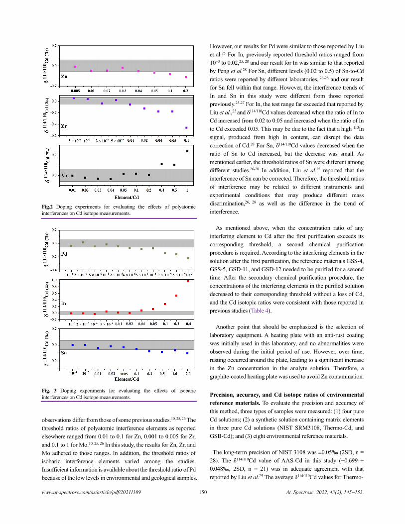
www.at-spectrosc.com/as/article/pdf/20211109 150 At. Spectrosc. 2022, 43(2), 145–153.
Fig.2
Doping experiments for evaluating the effects of polyatomic
interferences on Cd isotope measurements.
Fig. 3 Doping experiments for evaluating the effects of isobaric
interferences on Cd isotope measurements.
observations differ from those of some previous studies.10, 25, 26 The
threshold ratios of polyatomic interference elements as reported
elsewhere ranged from 0.01 to 0.1 for Zn, 0.001 to 0.005 for Zr,
and 0.1 to 1 for Mo.10, 25, 26 In this study, the results for Zn, Zr, and
Mo adhered to those ranges. In addition, the threshold ratios of
isobaric interference elements varied among the studies.
Insufficient information is available about the threshold ratio of Pd
because of the low levels in environmental and geological samples.
However, our results for Pd were similar to those reported by Liu
et al.25 For In, previously reported threshold ratios ranged from
10−3 to 0.02,25, 28 and our result for In was similar to that reported
by Peng et al.28 For Sn, different levels (0.02 to 0.5) of Sn-to-Cd
ratios were reported by different laboratories, 26-28 and our result
for Sn fell within that range. However, the interference trends of
In and Sn in this study were different from those reported
previously.25-27 For In, the test range far exceeded that reported by
Liu et al.,25 and δ114/110Cd values decreased when the ratio of In to
Cd increased from 0.02 to 0.05 and increased when the ratio of In
to Cd exceeded 0.05. This may be due to the fact that a high 113In
signal, produced from high In content, can disrupt the data
correction of Cd.28 For Sn, δ114/110Cd values decreased when the
ratio of Sn to Cd increased, but the decrease was small. As
mentioned earlier, the threshold ratios of Sn were different among
different studies.26-28 In addition, Liu et al.25 reported that the
interference of Sn can be corrected. Therefore, the threshold ratios
of interference may be related to different instruments and
experimental conditions that may produce different mass
discrimination,26, 28 as well as the difference in the trend of
interference.
As mentioned above, when the concentration ratio of any
interfering element to Cd after the first purification exceeds its
corresponding threshold, a second chemical purification
procedure is required. According to the interfering elements in the
solution after the first purification, the reference materials GSS-4,
GSS-5, GSD-11, and GSD-12 needed to be purified for a second
time. After the secondary chemical purification procedure, the
concentrations of the interfering elements in the purified solution
decreased to their corresponding threshold without a loss of Cd,
and the Cd isotopic ratios were consistent with those reported in
previous studies (Table 4).
Another point that should be emphasized is the selection of
laboratory equipment. A heating plate with an anti-rust coating
was initially used in this laboratory, and no abnormalities were
observed during the initial period of use. However, over time,
rusting occurred around the plate, leading to a significant increase
in the Zn concentration in the analyte solution. Therefore, a
graphite-coated heating plate was used to avoid Zn contamination.
Precision, accuracy, and Cd isotope ratios of environmental
reference materials. To evaluate the precision and accuracy of
this method, three types of samples were measured: (1) four pure
Cd solutions; (2) a synthetic solution containing matrix elements
in three pure Cd solutions (NIST SRM3108, Thermo-Cd, and
GSB-Cd); and (3) eight environmental reference materials.
The long-term precision of NIST 3108 was ±0.05‰ (2SD, n =
28). The δ114/110Cd value of AAS-Cd in this study (−0.699 ±
0.048‰, 2SD, n = 21) was in adequate agreement with that
reported by Liu et al.25 The average δ114/110Cd values for Thermo-
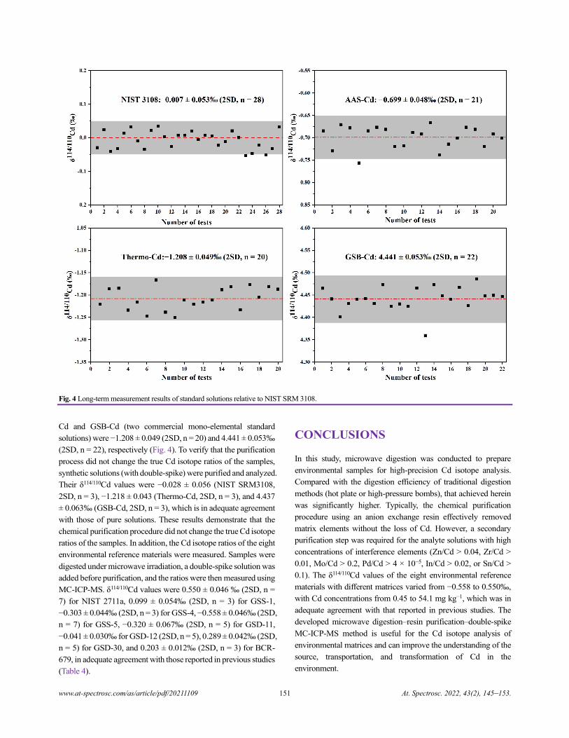
www.at-spectrosc.com/as/article/pdf/20211109 151 At. Spectrosc. 2022, 43(2), 145–153.
Fig. 4 Long-term measurement results of standard solutions relative to NIST SRM 3108.
Cd and GSB-Cd (two commercial mono-elemental standard
solutions) were −1.208 ± 0.049 (2SD, n = 20) and 4.441 ± 0.053‰
(2SD, n = 22), respectively (Fig. 4). To verify that the purification
process did not change the true Cd isotope ratios of the samples,
synthetic solutions (with double-spike) were purified and analyzed.
Their δ114/110Cd values were −0.028 ± 0.056 (NIST SRM3108,
2SD, n = 3), −1.218 ± 0.043 (Thermo-Cd, 2SD, n = 3), and 4.437
± 0.063‰ (GSB-Cd, 2SD, n = 3), which is in adequate agreement
with those of pure solutions. These results demonstrate that the
chemical purification procedure did not change the true Cd isotope
ratios of the samples. In addition, the Cd isotope ratios of the eight
environmental reference materials were measured. Samples were
digested under microwave irradiation, a double-spike solution was
added before purification, and the ratios were then measured using
MC-ICP-MS. δ114/110Cd values were 0.550 ± 0.046 ‰ (2SD, n =
7) for NIST 2711a, 0.099 ± 0.054‰ (2SD, n = 3) for GSS-1,
−0.303 ± 0.044‰ (2SD, n = 3) for GSS-4, −0.558 ± 0.046‰ (2SD,
n = 7) for GSS-5, −0.320 ± 0.067‰ (2SD, n = 5) for GSD-11,
−0.041 ± 0.030‰ for GSD-12 (2SD, n = 5), 0.289 ± 0.042‰ (2SD,
n = 5) for GSD-30, and 0.203 ± 0.012‰ (2SD, n = 3) for BCR-
679, in adequate agreement with those reported in previous studies
(Table 4).
CONCLUSIONS
In this study, microwave digestion was conducted to prepare
environmental samples for high-precision Cd isotope analysis.
Compared with the digestion efficiency of traditional digestion
methods (hot plate or high-pressure bombs), that achieved herein
was significantly higher. Typically, the chemical purification
procedure using an anion exchange resin effectively removed
matrix elements without the loss of Cd. However, a secondary
purification step was required for the analyte solutions with high
concentrations of interference elements (Zn/Cd > 0.04, Zr/Cd >
0.01, Mo/Cd > 0.2, Pd/Cd > 4 × 10⁻⁵, In/Cd > 0.02, or Sn/Cd >
0.1). The δ114/110Cd values of the eight environmental reference
materials with different matrices varied from −0.558 to 0.550‰,
with Cd concentrations from 0.45 to 54.1 mg kg−1, which was in
adequate agreement with that reported in previous studies. The
developed microwave digestion–resin purification–double-spike
MC-ICP-MS method is useful for the Cd isotope analysis of
environmental matrices and can improve the understanding of the
source, transportation, and transformation of Cd in the
environment.
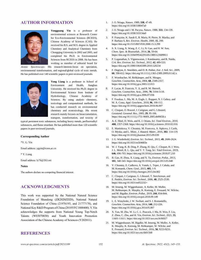
www.at-spectrosc.com/as/article/pdf/20211109 152 At. Spectrosc. 2022, 43(2), 145–153.
AUTHOR INFORMATION
Yongguang Yin is a professor of
environmental sciences at Research Center
for Eco-Environmental Sciences (RCEES),
Chinese Academy of Sciences (CAS). He
received his B.S. and M.S. degree in Applied
Chemistry and Analytical Chemistry from
Chongqing University in 2002 and 2005, and
completed his Ph.D. in Environmental
Sciences from RCEES in 2008. He has been
working as member of editorial board for
Atomic Spectroscopy. His research interests focus on speciation,
environmental transformation, and regional/global cycle of toxic metals.
He has published over 140 scientific papers in peer-reviewed journals.
Yong Liang is a professor in School of
Environment and Health, Jianghan
University. He received his Ph.D. degree in
Environmental Science from Institute of
Hydrobiology, Chinese Academy of
Sciences. By using analytic chemistry,
toxicology and computational methods, he
has conducted research on environmental
chemistry and ecotoxicology. His recent
research mainly focuses on bioaccumulation,
transport, transformation, and toxicity of
typical persistent toxic substances, including heavy metals, perfluoroalkyl
substances, and flame retardant. He has published more than 120 scientific
papers in peer-reviewed journals.
Corresponding Author
*Y. G. Yin
Email address: [email protected]
* Y. Liang
Email address: [email protected]
Notes
The authors declare no competing financial interest.
ACKNOWLEDGMENTS
This work was supported by the National Natural Science
Foundation of Shandong (ZR2020ZD20), National Natural
Science Foundation of China (21976193, and 21777178), and
National Key R&D Program of China (2018YFC1800400). Y. Yin
acknowledges the supports from National Young Top-Notch
Talents (W03070030) and Youth Innovation Promotion
Association of the Chinese Academy of Sciences (Y202011).
REFERENCES
1. J. O. Nriagu, Nature, 1989, 338, 47-49.
https://doi.org/10.1038/338047a0
2. J. O. Nriagu and J. M. Pacyna, Nature, 1988, 333, 134-139.
https://doi.org/10.1038/333134a0
3. P. Françoise, K. Sarah E, B. Maria, H. Pierre, B. Marika, and
P. Barbara S, Rev. Environ. Health, 2000, 15, 299.
https://doi.org/10.1515/REVEH.2000.15.3.299
4. S. X. Liang, X. Wang, Z. C. Li, N. Gao, and H. W. Sun,
Chem. Spec. & Bioavailab., 2014, 26, 59-64.
https://doi.org/10.3184/095422914X13885123689811
5. P. Loganathan, S. Vigneswaran, J. Kandasamy, and R. Naidu,
Crit. Rev. Environ. Sci. Technol., 2012, 42, 489-533.
https://doi.org/10.1080/10643389.2010.520234
6. F. Degryse, E. Smolders, and D. R. Parker, Eur. J. Soil. Sci., 2009,
60, 590-612. https://doi.org/10.1111/j.1365-2389.2009.01142.x
7. F. Wombacher, M. Rehkämper, and K. Mezger,
Geochim. Cosmochim. Acta, 2004, 68, 2349-2357.
https://doi.org/10.1016/j.gca.2003.12.013
8. F. Lacan, R. Francois, Y. Ji, and R. M. Sherrell,
Geochim. Cosmochim. Acta., 2006, 70, 5104-5118.
https://doi.org/10.1016/j.gca.2006.07.036
9. F. Fouskas, L. Ma, M. A. Engle, L. Ruppert, N. J. Geboy, and
M. A. Costa, Appl. Geochem., 2018, 96, 100-112.
https://doi.org/10.1016/j.apgeochem.2018.06.007
10. C. Cloquet, O. Rouxel, J. Carignan, and G. Libourel,
Geostand. Geoanal. Res., 2005, 29, 95-106.
https://doi.org/10.1111/j.1751-908X.2005.tb00658.x
11. A. E. Shiel, D. Weis, and K. J. Orians, Sci. Total Environ., 2010,
408, 2357-2368. https://doi.org/10.1016/j.scitotenv.2010.02.016
12. E. Martinkova, V. Chrastny, M. Francova, A. Sipkova, J. Curik,
O. Myska, and L. Mizic, J. Hazard. Mater., 2016, 302. 114-119.
https://doi.org/10.1016/j.jhazmat.2015.09.039
13. J. G. Wiederhold, Environ. Sci. Technol., 2015, 49, 2606-2624.
https://doi.org/10.1021/es504683e
14. W. J. Yang, K. B. Ding, P. Zhang, H. Qiu, C. Cloquet, H. J. Wen,
J. L. Morel, R. L. Qiu, and Y. T. Tang, Sci. Total Environ., 2019,
646, 696-703. https://doi.org/10.1016/j.scitotenv.2018.07.210
15. B. Gao, H. Zhou, X. Liang, and X. Tu, Environ. Pollut., 2013,
181, 340-343. https://doi.org/10.1016/j.envpol.2013.05.048
16. V. Chrastny, E. Cadkova, A. Vanek, L. Teper, J. Cabala, and
M. Komarek, Chem. Geol., 2015, 405, 1-9.
https://doi.org/10.1016/j.chemgeo.2015.04.002
17. C. Cloquet, J. Carignan, G. Libourel, T. Sterckeman, and
E. Perdrix, Environ. Sci. Technol., 2006, 40, 2525-2530.
https://doi.org/10.1021/es052232+
18. M. Imseng, M. Wiggenhauser, A. Keller, M. Muller,
M. Rehkamper, K. Murphy, K. Kreissig, E. Frossard, W. Wilcke,
and M. Bigalke, Environ. Pollut., 2019, 244, 834-844.
https://doi.org/10.1016/j.envpol.2018.09.149
19. L. E. Wasylenki, J. W. Swihart, and S. J. Romaniello,
Geochim. Cosmochim. Acta, 2014, 140, 212-226.
https://doi.org/10.1016/j.gca.2014.05.007
20. X. Yan, M. Zhu, W. Li, C. L. Peacock, J. Ma, H. Wen, F. Liu,
Z. Zhou, C. Zhu, and H. Yin, Environ. Sci. Technol., 2021, 55,
11601-11611. https://doi.org/10.1021/acs.est.0c06927
21. M. Wiggenhauser, M. Bigalke, M. Imseng, M. Muller, A. Keller,
K. Murphy, K. Kreissig, M. Rehkamper, W. Wilcke, and
E. Frossard, Environ. Sci. Technol., 2016, 50, 9223-9231.
https://doi.org/10.1021/acs.est.6b01568
www.at-spectrosc.com/as/article/pdf/20211109 153 At. Spectrosc. 2022, 43(2), 145–153.
22. M. Imseng, M. Wiggenhauser, A. Keller, M. Muller,
M. Rehkamper, K. Murphy, K. Kreissig, E. Frossard, W. Wilcke,
and M. Bigalke, Environ. Sci. Technol., 2018, 52, 1919-1928.
https://doi.org/10.1021/acs.est.7b05439
23. M. Rehkämper, F. Wombacher, T. J. Horner, and Z. Xue, in
Handbook of Environmental Isotope Geochemistry: Vol I, ed.
M. Baskaran. Springer Berlin Heidelberg: Berlin, Heidelberg, pp
125-154, 2012.
24. F. Wombacher, M. Rehkamper, K. Mezger, and C. Munker,
Geochim. Cosmochim. Acta, 2003, 67, 4639-4654.
https://doi.org/10.1016/s0016-7037(03)00389-2
25. M. S. Liu, Q. Zhang, Y. N. Zhang, Z. F. Zhang, F. Huang, and
H. M. Yu, Geostand. Geoanal. Res., 2020, 44, 169-182.
https://doi.org/10.1111/ggr.12291
26. D. C. Tan, J. M. Zhu, X. L. Wang, G. L. Han, Z. Lu, and
W. P. Xu, J. Anal. At. Spectrom., 2020, 35, 713-727.
https://doi.org/10.1039/C9JA00397E
27. D. D. Li, M. L. Li, W. R. Liu, Z. Z. Qin, and S. A. Liu,
Geostand. Geoanal. Res., 2018, 42, 593-605.
https://doi.org/10.1111/ggr.12236
28. H. Peng, D. He, R. Guo, X. Liu, N. S. Belshaw, H. T. Zheng,
S. H. Hu, and Z. L. Zhu, J. Anal. At. Spectrom., 2021, 36, 390-398.
https://doi.org/10.1039/D0JA00424C
29. J. F. Rudge, B. C. Reynolds, and B. Bourdon, Chem. Geol., 2009,
265, 420-431. https://doi.org/10.1016/j.chemgeo.2009.05.010
30. W. Abouchami, S. J. G. Galer, T. J. Horner, M. Rehkämper,
F. Wombacher, Z. Xue, M. Lambelet, M. Gault-Ringold,
C. H. Stirling, M. Schönbächler, A. E. Shiel, D. Weis, and
P. F. Holdship, Geostand. Geoanal. Res., 2013, 37, 5-17.
https://doi.org/10.1111/j.1751-908X.2012.00175.x
31. B. Gao, Y. Liu, K. Sun, X. Liang, P. Peng, G. Sheng, and J. Fu,
Anal. Chim. Acta, 2008, 612, 114-120.
https://doi.org/10.1016/j.aca.2008.02.020
32. H. J. Wen, Y. X. Zhang, C. Cloquet, C. W. Zhu, H. F. Fan, and
C. G. Luo, Appl. Geochem., 2015, 52, 147-154.
https://doi.org/10.1016/j.apgeochem.2014.11.025
33. Y. X. Zhang, H. J. Wen, H. F. Fan, J. S. Wang, and J. R. Zhang,
J. Instrum. Anal., 2010, 29, 633-637 (in Chinese).
34. R. Wei, Q. Guo, H. Wen, J. Yang, M. Peters, C. Zhu, J. Ma,
G. Zhu, H. Zhang, L. Tian, C. Wang, and Y. Wan, Anal. Methods,
2015, 7, 2479-2487. https://doi.org/10.1039/C4AY02435D
35. S. Ripperger and M. Rehkamper, Geochim. Cosmochim. Acta,
2007, 71, 631-642. https://doi.org/10.1016/j.gca.2006.10.005
36. T. J. Horner, M. Schönbächler, M. Rehkämper, S. G. Nielsen,
H. Williams, A. N. Halliday, Z. Xue, and J. R. Hein,
Geochem., Geophys. Geosyst., 2010, 11, Q04001.
https://doi.org/10.1029/2009GC002987
37. C. N. Maréchal, P. Télouk, and F. Albarède, Chem. Geol., 1999,
156, 251-273. https://doi.org/10.1016/S0009-2541(98)00191-0
38. M. Gault-Ringold and C. H. Stirling, J. Anal. At. Spectrom., 2012,
27, 449-459. https://doi.org/10.1039/C2JA10360E
39. Q. Zhang and L. P. Qin, Geochimica, 2017, 46, 15-21.
https://doi.org/10.19700/j.0379-1726.2017.01.002
40. A. Turek, K. Wieczorek, and W. M. Wolf, Sustainability, 2019,
11, 1753. https://doi.org/10.3390/su11061753
41. N. Pallavicini, E. Engstrom, D. C. Baxter, B. Ohlander, J. Ingri,
and I. Rodushkin, J. Anal. At. Spectrom., 2014, 29, 1570-1584.
https://doi.org/10.1039/c4ja00125g
42. R. F. Wei, Q. J. Guo, H. J. Wen, M. Peters, J. X. Yang, L. Y. Tian,
and X. K. Han, Anal. Sci., 2017, 33, 335-341.
https://doi.org/10.2116/analsci.33.335
43. W. X. Lv, H. M. Yin, M. S. Liu, F. Huang, and H. M. Yu,
Geostand. Geoanal. Res., 2021, 45, 245-256.
https://doi.org/10.1111/ggr.12357
44. M. Wiggenhauser, A. M. Aucour, S. Bureau, S. Campillo,
P. Telouk, M. Romani, J. F. Ma, G. Landrot, and G. Sarret,
Environ. Pollut, 2021, 269, 115934.
https://10.1016/j.envpol.2020.115934
www.at-spectrosc.com/as/article/pdf/2022099 154 At. Spectrosc. 2022, 43(2), 154–163.
Coal Proximate Analysis Based on Synergistic Use of LIBS and
NIRS
Shunchun Yao,a,b,* Huaiqing Qin,a,b Shuixiu Xu,a,b Ziyu Yu,a,b Zhimin Lu,a,b and Zhe Wangc,* a School of Electric Power, South China University of Technology, Guangzhou 510640, P. R. China
b Guangdong Province Engineering Research Center of High Efficient and Low Pollution Energy Conversion, Guangzhou 510640, P. R. China
c State Key Lab of Power Systems, International Joint Laboratory on Low Carbon Clean Energy Innovation, Department of Energy and Power Engineering,
Tsinghua University, Beijing 100084, P. R. China
Received: April 13, 2022; Revised: April 28, 2022; Accepted: April 28, 2022; Available online: April 28, 2022.
DOI: 10.46770/AS.2022.099
ABSTRACT: Rapid and accurate analysis of the coal properties is essential for its clean and efficient utilization. However,
the complexity of the physical-chemical characteristics of coal complicates accurate quantification of its properties using rapid
spectroscopic technologies. Herein, a synergistic method is proposed to achieve optimum
results for coal proximate analysis using spectra obtained via laser-induced breakdown
spectroscopy (LIBS) and near-infrared reflectance spectroscopy (NIRS). Firstly, the ash
content was analyzed by LIBS, and the moisture content was analyzed by NIRS. The
calorific value and volatile content were then analyzed using the fusion data obtained from
LIBS and NIRS, combined with the ash and moisture results. Finally, the fixed carbon
content was calculated by subtracting the mass percentage fractions of ash, moisture, and
volatile matter from 100%. The results indicated that the proposed method achieved good
quantitative performance for coal proximate analysis. The root mean square errors of
prediction for ash, moisture, calorific value, volatile matter, and fixed carbon were 0.743%,
0.304%, 0.187 MJ/kg, 0.662% and 0.972%, respectively. Thus, we believe that the
proposed method based on the synergy of LIBS and NIRS opens avenues for efficient
prospective analysis of coal properties.
INTRODUCTION
Coal is the primary source of energy worldwide. According to the
BP Statistical review of World Energy 2021, the global coal
consumption in 2020 is 151.42 EJ.1 Such a large volume of coal
consumption contributes to high carbon emissions. However, to
achieve the goals stated in the Paris Agreement, carbon emissions
must be reduced.2 The clean and efficient utilization of coal,
assisted by intelligent burner operation, is vital for reducing carbon
emissions, and therefore, online measurements of multiple coal
properties are essential. Currently, some rapid analysis techniques
for coal properties, such as prompt gamma neutron activation
analysis (PGNAA)3 and X-ray fluorescence (XRF)4 analysis, have
been put into practice. However, PGNAA machine is bulky and
needs to be strictly regulated because its neutron source has
potential health and environmental hazards.5 XRF is not capable
of detecting light elements, such as C and H.6 These disadvantages
limit the wider application of PGNAA and XRF in coal property
analysis.
Laser-induced breakdown spectroscopy (LIBS) is a promising
technique for coal analysis7–9 and demonstrates advantages such
as effortless sample preparation, real-time detection, and
capability to detect all elements. Gaft et al.10 first applied LIBS to
online analysis of ash content and the results were in good
agreement with those from an existing online PGNAA machine.
Ctvrtnickova et al.11,12 used LIBS to measure ash in coal, and they
established calibration curves for the elements contained in ash,
demonstrating excellent correlation between element
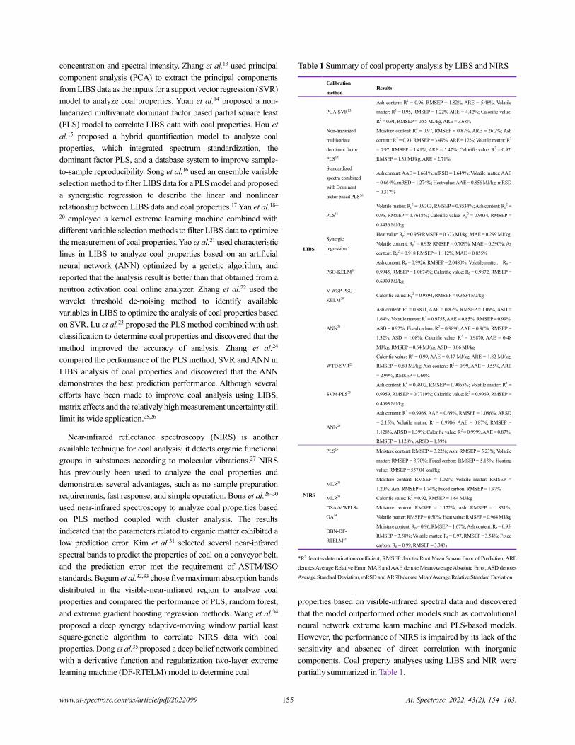
www.at-spectrosc.com/as/article/pdf/2022099 155 At. Spectrosc. 2022, 43(2), 154–163.
concentration and spectral intensity. Zhang et al.13 used principal
component analysis (PCA) to extract the principal components
from LIBS data as the inputs for a support vector regression (SVR)
model to analyze coal properties. Yuan et al.14 proposed a non-
linearized multivariate dominant factor based partial square least
(PLS) model to correlate LIBS data with coal properties. Hou et
al.15 proposed a hybrid quantification model to analyze coal
properties, which integrated spectrum standardization, the
dominant factor PLS, and a database system to improve sample-
to-sample reproducibility. Song et al.16 used an ensemble variable
selection method to filter LIBS data for a PLS model and proposed
a synergistic regression to describe the linear and nonlinear
relationship between LIBS data and coal properties.17 Yan et al.18–
20 employed a kernel extreme learning machine combined with
different variable selection methods to filter LIBS data to optimize
the measurement of coal properties. Yao et al.21 used characteristic
lines in LIBS to analyze coal properties based on an artificial
neural network (ANN) optimized by a genetic algorithm, and
reported that the analysis result is better than that obtained from a
neutron activation coal online analyzer. Zhang et al.22 used the
wavelet threshold de-noising method to identify available
variables in LIBS to optimize the analysis of coal properties based
on SVR. Lu et al.23 proposed the PLS method combined with ash
classification to determine coal properties and discovered that the
method improved the accuracy of analysis. Zhang et al.24
compared the performance of the PLS method, SVR and ANN in
LIBS analysis of coal properties and discovered that the ANN
demonstrates the best prediction performance. Although several
efforts have been made to improve coal analysis using LIBS,
matrix effects and the relatively high measurement uncertainty still
limit its wide application.25,26
Near-infrared reflectance spectroscopy (NIRS) is another
available technique for coal analysis; it detects organic functional
groups in substances according to molecular vibrations.27 NIRS
has previously been used to analyze the coal properties and
demonstrates several advantages, such as no sample preparation
requirements, fast response, and simple operation. Bona et al.28–30
used near-infrared spectroscopy to analyze coal properties based
on PLS method coupled with cluster analysis. The results
indicated that the parameters related to organic matter exhibited a
low prediction error. Kim et al.31 selected several near-infrared
spectral bands to predict the properties of coal on a conveyor belt,
and the prediction error met the requirement of ASTM/ISO
standards. Begum et al.32,33 chose five maximum absorption bands
distributed in the visible-near-infrared region to analyze coal
properties and compared the performance of PLS, random forest,
and extreme gradient boosting regression methods. Wang et al.34
proposed a deep synergy adaptive-moving window partial least
square-genetic algorithm to correlate NIRS data with coal
properties. Dong et al.35 proposed a deep belief network combined
with a derivative function and regularization two-layer extreme
learning machine (DF-RTELM) model to determine coal
Table 1 Summary of coal property analysis by LIBS and NIRS
Calibration
method Results
LIBS
PCA-SVR13
Ash content: R2 = 0.96, RMSEP = 1.82%, ARE = 5.48%; Volatile
matter: R2 = 0.95, RMSEP = 1.22% ARE = 4.42%; Calorific value:
R2 = 0.91, RMSEP = 0.85 MJ/kg, ARE = 3.68%
Non-linearized
multivariate
dominant factor
PLS14
Moisture content: R2 = 0.97, RMSEP = 0.87%, ARE = 26.2%; Ash
content: R2 = 0.93, RMSEP = 3.49%, ARE = 12%; Volatile matter: R
2
= 0.97, RMSEP = 1.41%, ARE = 5.47%; Calorific value: R2 = 0.97,
RMSEP = 1.33 MJ/kg, ARE = 2.71%
Standardized
spectra combined
with Dominant
factor based PLS36
Ash content: AAE = 1.661%, mRSD = 1.649%; Volatile matter: AAE
= 0.664%, mRSD = 1.274%; Heat value: AAE = 0.856 MJ/kg, mRSD
= 0.317%
PLS16
Volatile matter: Rp2 = 0.9303, RMSEP = 0.8534%; Ash content: Rp
2 =
0.96, RMSEP = 1.7618%; Calorific value: Rp2 = 0.9034, RMSEP =
0.8436 MJ/kg
Synergic
regression17
Heat value: Rp2 = 0.959 RMSEP = 0.373 MJ/kg, MAE = 0.299 MJ/kg;
Volatile content: Rp2 = 0.938 RMSEP = 0.709%, MAE = 0.590%; As
content: Rp2 = 0.918 RMSEP = 1.112%, MAE = 0.855%
PSO-KELM18
Ash content: Rp = 0.9926, RMSEP = 2.0480%; Volatile matter: Rp =
0.9945, RMSEP = 1.0874%; Calorific value: Rp = 0.9872, RMSEP =
0.6999 MJ/kg
V-WSP-PSO-
KELM20
Calorific value: Rp
2 = 0.9894, RMSEP = 0.3534 MJ/kg
ANN21
Ash content: R2 = 0.9871, AAE = 0.82%, RMSEP = 1.09%, ASD =
1.64%; Volatile matter: R2 = 0.9755, AAE = 0.85%, RMSEP = 0.99%,
ASD = 0.92%; Fixed carbon: R2 = 0.9890, AAE = 0.96%, RMSEP =
1.32%, ASD = 1.08%; Calorific value: R2 = 0.9870, AAE = 0.48
MJ/kg, RMSEP = 0.64 MJ/kg, ASD = 0.86 MJ/kg
WTD-SVR22
Calorific value: R2 = 0.99, AAE = 0.47 MJ/kg, ARE = 1.82 MJ/kg,
RMSEP = 0.80 MJ/kg; Ash content: R2 = 0.99, AAE = 0.55%, ARE
= 2.99%, RMSEP = 0.60%
SVM-PLS23
Ash content: R2 = 0.9972, RMSEP = 0.9065%; Volatile matter: R
2 =
0.9959, RMSEP = 0.7719%; Calorific value: R2 = 0.9969, RMSEP =
0.4093 MJ/kg
ANN24
Ash content: R2 = 0.9968, AAE = 0.69%, RMSEP = 1.086%, ARSD
= 2.15%; Volatile matter: R2 = 0.9986, AAE = 0.87%, RMSEP =
1.128%, ARSD = 1.39%; Calorific value: R2 = 0.9999, AAE = 0.87%,
RMSEP = 1.128%, ARSD = 1.39%
NIRS
PLS29
Moisture content: RMSEP = 3.22%; Ash: RMSEP = 5.23%; Volatile
matter: RMSEP = 3.70%; Fixed carbon: RMSEP = 5.13%; Heating
value: RMSEP = 557.04 kcal/kg
MLR31
Moisture content: RMSEP = 1.02%; Volatile matter: RMSEP =
1.20%; Ash: RMSEP = 1.74%; Fixed carbon: RMSEP = 1.97%
MLR33
Calorific value: R2 = 0.92, RMSEP = 1.64 MJ/kg
DSA-MWPLS-
GA34
Moisture content: RMSEP = 1.172%; Ash: RMSEP = 1.851%;
Volatile matter: RMSEP = 0.50%; Heat value: RMSEP = 0.964 MJ/kg
DBN-DF-
RTELM35
Moisture content: Rp = 0.96, RMSEP = 1.67%; Ash content: Rp = 0.95,
RMSEP = 3.58%; Volatile matter: Rp = 0.97, RMSEP = 3.54%; Fixed
carbon: Rp = 0.99, RMSEP = 3.34%
*R2 denotes determination coefficient, RMSEP denotes Root Mean Square Error of Prediction, ARE
denotes Average Relative Error, MAE and AAE denote Mean/Average Absolute Error, ASD denotes
Average Standard Deviation, mRSD and ARSD denote Mean/Average Relative Standard Deviation.
properties based on visible-infrared spectral data and discovered
that the model outperformed other models such as convolutional
neural network extreme learn machine and PLS-based models.
However, the performance of NIRS is impaired by its lack of the
sensitivity and absence of direct correlation with inorganic
components. Coal property analyses using LIBS and NIR were
partially summarized in Table 1.
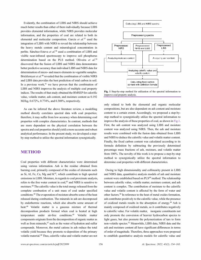
www.at-spectrosc.com/as/article/pdf/2022099 156 At. Spectrosc. 2022, 43(2), 154–163.
Evidently, the combination of LIBS and NIRS should achieve
much better results than either of them individually because LIBS
provides elemental information, while NIRS provides molecular
information, and the properties of coal are related to both its
elemental and molecular composition. Garcia et al.37 used the
integration of LIBS with NIRS to reveal the relationship between
the heavy metals content and mineralogical concentration in
perlite. Sánchez-Esteva et al.38 used a combination of LIBS and
visible near-infrared spectroscopy to improve soil phosphorus
determination based on the PLS method. Oliveira et al.39
discovered that the fusion of LIBS and NIRS data demonstrates
better predictive accuracy than individual LIBS and NIRS data for
determination of micro- and macro elements in vegetable samples.
Bricklemyer et al.40 revealed that the combination of visible NIRS
and LIBS data provides the best prediction of total carbon in soil.
In a previous work,41 we have proven that the combination of
LIBS and NIRS improves the analysis of multiple coal property
indices. The results of that study obtained the RMSEP for calorific
value, volatile matter, ash content, and moisture content as 0.192
MJ/kg, 0.672%, 0.774%, and 0.308%, respectively.
As can be inferred the above literature review, a modelling
method directly correlates spectral data with coal properties;
therefore, it may suffer from low accuracy when determining coal
properties with complex characteristics. In contrast, methods that
are more dependent on the physical correlation between the
spectra and coal properties should yield a more accurate and robust
analytical performance. In the present study, we developed a step-
by-step method to utilize the spectral information synergistically.
METHOD
Coal properties with different characteristics were determined
using various information. Ash is the residue obtained from
burning coal, primarily composed of the oxides of elements such
as Si, Al, Fe, Ca, Mg and K42, which contribute to high spectral
emissions in LIBS. Moisture, in regards to coal proximate analysis,
refers to the free water content in coal,43 and NIRS is sensitive to
moisture.44 The calorific value is the total energy released from the
complete combustion of a unit mass of coal under specified
conditions.45 The evaporation of moisture absorbs some of the heat
released during combustion. The minerals in ash are decomposed
by endothermic reactions, which also absorbs some amount of
heat.46 Volatile matter is a gaseous mixture of thermal
decomposition products formed when coal is heated at high
temperature under air-free conditions.45 Volatile matter
components originate from the decomposition of organic matter as
well as from minerals,47 such as the water of hydration and sulfur
compounds. Moreover, the metal cations in ash reduce the total
volatile yield because they promote re-deposition of the primary
volatile material.48 Thus, calorific value and volatile matter are not
Fig. 1 Step-by-step method for utilization of the spectral information to
improve coal property analysis.
only related to both the elemental and organic molecular
compositions, but are also dependent on ash content and moisture
content to a certain extent. Accordingly, we proposed a step-by-
step method to synergistically utilize the spectral information to
improve the analysis of these properties of coal, as shown in Fig.1.
First, the ash content was analyzed using LIBS and moisture
content was analyzed using NIRS. Then, the ash and moisture
results were combined with the fusion data obtained from LIBS
and NIRS to deduce the calorific value and volatile matter content.
Finally, the fixed carbon content was calculated according to its
formula definition by subtracting the previously determined
percentage mass fractions of ash, moisture, and volatile matter
from 100%. The novelty of this work is to propose a step-by-step
method to synergistically utilize the spectral information to
determine coal properties with different characteristics.
Owing to high dimensionality and collinearity present in LIBS
and NIRS data, quantitative analysis models of ash and moisture
content were established based on PLS49 method. The relationship
between calorific value, volatile matter, moisture content, and ash
content is complex. The contribution of moisture to the calorific
value and volatile content is affected by the form of water and
other factors.50 In reference to the heat of metal oxides formation,
ash contributes positively to the calorific value, while the presence
of oxidized metals results in the absorption of energy.46 Ash is
mainly composed of oxidized metals, so it contributes negatively
to calorific value. For volatile matter, inorganic constituents not
only promote the conversion of heavier hydrocarbon species to
light gases, but also promote the polymerization of tars to form
non-volatile species.51 Meanwhile, LIBS data, NIRS data and the
ash and moisture content all have significant differences in terms
of order of magnitude. Therefore, three approaches were proposed
to establish quantitative analysis models for calorific value and
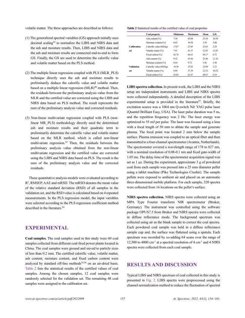
www.at-spectrosc.com/as/article/pdf/2022099 157 At. Spectrosc. 2022, 43(2), 154–163.
volatile matter. The three approaches are described as follows:
(1) The generalized spectral variables (GS) approach initially uses
decimal scaling52 to normalize the LIBS and NIRS data and
the ash and moisture results. Then, LIBS and NIRS data and
the ash and moisture results are connected end-to-end to form
GS. Finally, the GS are used to determine the calorific value
and volatile matter based on the PLS method.
(2) The multiple linear regression coupled with PLS (MLR_PLS)
technique directly uses the ash and moisture results to
preliminarily deduce the calorific value and volatile matter
based on a multiple linear regression (MLR)49 method. Then,
the residuals between the preliminary analysis value from the
MLR and the certified value are corrected using the LIBS and
NIRS data based on PLS method. The result represents the
sum of the preliminary analysis value and corrected residuals.
(3) Non-linear multivariate regression coupled with PLS (non-
linear MR_PLS) methodology directly used the determined
ash and moisture results and their quadratic term to
preliminarily determine the calorific value and volatile matter
based on the MLR method, which is called non-linear
multivariate regression.53 Then, the residuals between the
preliminary analysis value obtained from the non-linear
multivariate regression and the certified value are corrected
using the LIBS and NIRS data based on PLS. The result is the
sum of the preliminary analysis value and the corrected
residuals.
These quantitative analysis models were evaluated according to
R2, RMSEP, AAE and mRSD. The mRSD denotes the mean value
of the relative standard deviation (RSD) of all samples in the
validation set, and the RSD value is calculated based on 4 repeated
measurements. In the PLS regression model, the input variables
were selected according to the PLS regression coefficient method
described in the literature.54
EXPERIMENTAL
Coal samples. The coal samples used in this study were 60 coal
samples collected from different coal-fired power plants located in
China. The coal samples were ground and sieved to particle sizes
of less than 0.2 mm. The certified calorific value, volatile matter,
ash content, moisture content, and fixed carbon content were
analyzed by standard off-line methods55,56 on an air-dried basis.
Table 2 lists the statistical results of the certified values of coal
samples. Among the chosen samples, 12 coal samples were
randomly selected for the validation set. The remaining 48 coal
samples were assigned to the calibration set.
Table 2 Statistical results of the certified value of coal properties
Coal property Minimum Maximum Mean S.D.
Calibration
set
Ash content (%) 7.30 43.04 23.54 10.58
Moisture content (%) 0.43 10.58 3.38 3.08
Calorific value (MJ/kg) 17.87 27.85 23.65 2.29
Volatile matter (%) 7.91 41.37 22.92 11.03
Fixed carbon (%) 42.76 66.63 50.17 6.72
Validation
set
Ash content (%) 9.32 41.84 25.46 11.16
Moisture content (%) 0.64 9.72 3.56 3.50
Calorific value (MJ/kg) 18.38 25.92 22.89 2.22
Volatile matter (%) 9.44 37.39 22.32 10.52
Fixed carbon (%) 43.85 61.67 48.67 6.19
LIBS spectra collection. In present work, the LIBS and the NIRS
setup are independent instruments and LIBS and NIRS spectra
were collected independently. A detailed description of the LIBS
experimental setup is provided in the literature57. Briefly, the
excitation source was a 1064 nm Q-switch Nd: YAG pulse laser
(Quantel Brilliant Easy, USA). The laser pulse duration was 5 ns,
and the repetition frequency was 2 Hz. The laser energy was
optimized to 55 mJ per pulse. The laser was focused using a lens
with a focal length of 50 mm to ablate the sample and generate
plasma. The focal point was located 2 mm below the sample
surface. Plasma emission was coupled to an optical fiber and then
transmitted to a four-channel spectrometer (Avantes, Netherlands).
The spectrometer covered a wavelength range of 178 to 827 nm,
with a nominal resolution of 0.08-0.1 nm and fixed gate-width of
1.05 ms. The delay time of the spectrometer acquisition signal was
set as 1 μs. During the experiment, approximate 3 g of powdered
coal from each sample was pressed into a 25 mm diameter pellet
using a tablet machine (Pike Technologies Crushir). The sample
pellets were exposed to ambient air and placed on an automatic
three-dimensional mobile platform. For each sample, 320 spectra
were collected from 16 locations on the pellet’s surface.
NIRS spectra collection. NIRS spectra were collected using an
MPA Type Fourier transform NIR spectrometer (Bruker,
Germany). The instrument was controlled using the software
package OPUS7.5 from Bruker and NIRS spectra were collected
in diffuse reflectance mode. The background spectrum was
collected using air as the blank sample to correct the coal spectra.
Each powdered coal sample was held in a diffuse reflectance
sample cup and, the surface was flattened using a spatula. Each
spectrum was recorded by co-adding 64 scans over the range of
12,500 to 4000 cm-1 at a spectral resolution of 4 cm-1 and 4 NIRS
spectra were collected from each coal sample.
RESULTS AND DISCUSSION
Typical LIBS and NIRS spectrum of coal collected in this study is
presented in Fig. 2. LIBS spectra were preprocessed using the
channel normalization method to reduce the fluctuation of spectral
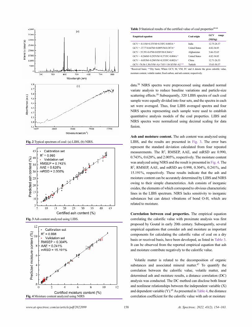
www.at-spectrosc.com/as/article/pdf/2022099 158 At. Spectrosc. 2022, 43(2), 154–163.
Fig. 2 Typical spectrum of coal: (a) LIBS, (b) NIRS.
Fig. 3 Ash content analyzed using LIBS.
Fig. 4 Moisture content analyzed using NIRS
Table 3 Statistical results of the certified value of coal properties60-64
Empirical equation Coal origin GCV range
(MJ/kg)
GCV = -0.11M+0.33VM+0.35FC-0.003A * India 12.75-28.37
GCV = -37.77-0.647M+0.089VM-0.387A* United States 4.82-34.85
GCV = 35.391-0.47M-0.028VM-0.364A * Afghanistan 3.66-32.65
GCV = -0.266M+0.293VM+0.371FC-0.004A * United States 4.82-34.85
GCV = -0.053M+0.296VM+0.353FC-0.002A * China 12.71-26.53
GCV =76.56-1.30 (VM+A)+7.03×10⁻³(VM+A2 ** Turkish 15.63-30.37
*Received basis; **Dry basis; Where GCV, M, VM, FC and A denote the gross calorific value,
moisture content, volatile matter, fixed carbon, and ash content, respectively.
data.58 NIRS spectra were preprocessed using standard normal
variate analysis to reduce baseline variations and particle-size
scattering effects.59 Subsequently, 320 LIBS spectra of each coal
sample were equally divided into four sets, and the spectra in each
set were averaged. Thus, four LIBS averaged spectra and four
NIRS spectra representing each sample were used to establish
quantitative analysis models of the coal properties. LIBS and
NIRS spectra were normalized using decimal scaling for data
fusion.
Ash and moisture content. The ash content was analyzed using
LIBS, and the results are presented in Fig. 3. The error bars
represent the standard deviation calculated from four repeated
measurements. The R2, RMSEP, AAE, and mRSD are 0.990,
0.743%, 0.628%, and 2.005%, respectively. The moisture content
was analyzed using NIRS and the result is presented in Fig. 4. The
R2, RMSEP, AAE, and mRSD are 0.998, 0.304%, 0.241%, and
15.191%, respectively. These results indicate that the ash and
moisture content can be accurately determined by LIBS and NIRS
owing to their simple characteristics. Ash consists of inorganic
oxides, the elements of which correspond to obvious characteristic
lines in the LIBS spectrum. NIRS lacks sensitivity to inorganic
substances but can detect vibrations of bond O-H, which are
related to moisture.
Correlation between coal properties. The empirical equation
correlating the calorific value with proximate analysis was first
proposed by Goutal in early 20th century. Subsequently, several
empirical equations that consider ash and moisture as important
components for calculating the calorific value of coal on a dry
basis or received basis, have been developed, as listed in Table 3.
It can be observed from the reported empirical equation that ash
and moisture contribute negatively to the calorific value.
Volatile matter is related to the decomposition of organic
substances and associated mineral matter.47 To quantify the
correlation between the calorific value, volatile matter, and
determined ash and moisture results, a distance correlation (DC)
analysis was conducted. The DC method can disclose both linear
and nonlinear relationships between the independent variable (X)
and dependent variable (Y).65 As presented in Table 4, the distance
correlation coefficient for the calorific value with ash or moisture
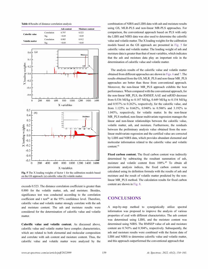
www.at-spectrosc.com/as/article/pdf/2022099 159 At. Spectrosc. 2022, 43(2), 154–163.
Table 4 Results of distance correlation analysis
Ash content Moisture content
Calorific value Correlation 0.797 0.523
Sig. <0.05 <0.05
Volatile matter Correlation 0.905 0.912
Sig. <0.05 <0.05
Fig. 5 The X loading weights of factor 1 for the calibration models based
on the GS approach: (a) calorific value (b) volatile matter.
exceeds 0.523. The distance correlation coefficient is greater than
0.880 for the volatile matter, ash, and moisture. Besides,
significance test was conducted according to the correlation
coefficient and t test66 at the 95% confidence level. Therefore,
calorific value and volatile matter strongly correlate with the ash
and moisture content. The ash and moisture results were
considered for the determination of calorific value and volatile
matter.
Calorific value and volatile content. As discussed above,
calorific value and volatile matter have complex characteristics,
which are related to both elemental and molecular composition
and correlate with ash content and moisture content. Thus, the
calorific value and volatile matter were analyzed by the
combination of NIRS and LIBS data with ash and moisture results
using GS, MLR-PLS and non-linear MR-PLS approaches. For
comparison, the conventional approach based on PLS with only
the LIBS and NIRS data was also used to determine the calorific
value and volatile matter. The X loading weights for the calibration
models based on the GS approach are presented in Fig. 5 for
calorific value and volatile matter. The loading weight of ash and
moisture data is greater than that of most variables, which indicates
that the ash and moisture data play an important role in the
determination of calorific value and volatile matter.
The analysis results of the calorific value and volatile matter
obtained from different approaches are shown in Figs. 6 and 7. The
results obtained from the GS, MLR_PLS and non-linear MR_PLS
approaches are better than those from conventional approach.
Moreover, the non-linear MR_PLS approach exhibits the best
performance. When compared with the conventional approach, for
the non-linear MR_PLS, the RMSEP, AAE and mRSD decrease
from 0.536 MJ/kg to 0.187 MJ/kg, 0.449 MJ/kg to 0.154 MJ/kg
and 0.937% to 0.262%, respectively, for the calorific value, and
from 1.125% to 0.662%, 0.940% to 0.506% and 3.192% to
1.045%, respectively, for volatile matter. In the non-linear
MR_PLS method, non-linear multivariate regression manages the
linear and non-linear relationships between the calorific value,
volatile matter, ash, and moisture. Furthermore, the residuals
between the preliminary analysis value obtained from the non-
linear multivariate regression and the certified value are corrected
by LIBS and NIRS data, which provides abundant elemental and
molecular information related to the calorific value and volatile
content.41
Fixed carbon content. The fixed carbon content was indirectly
determined by subtracting the resultant summation of ash,
moisture and volatile content from 100%.45 To obtain all
proximate analysis indices, the fixed carbon content was
calculated using its definition formula with the results of ash and
moisture and the result of volatile matter predicted by the non-
linear MR_PLS method. The calculation results for fixed carbon
content are shown in Fig. 8.
CONCLUSIONS
A step-by-step method to synergistically utilize spectral
information was proposed to improve the analysis of various
properties of coal with different characteristics. The ash content
was determined using LIBS, and the moisture content was
determined using NIRS. The RMSEP value of ash and moisture
content are 0.743% and 0.304%, respectively. Subsequently, the
ash and moisture results were combined with the fusion data of
LIBS and NIRS to determine calorific value and volatile matter,
and this approach outperformed the conventional approach that
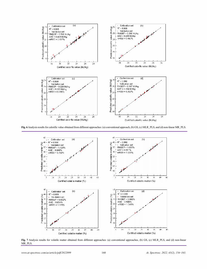
www.at-spectrosc.com/as/article/pdf/2022099 160 At. Spectrosc. 2022, 43(2), 154–163.
Fig. 6 Analysis results for calorific value obtained from different approaches: (a) conventional approach, (b) GS, (c) MLR_PLS, and (d) non-linear MR_PLS.
Fig. 7 Analysis results for volatile matter obtained from different approaches: (a) conventional approaches, (b) GS, (c) MLR_PLS, and (d) non-linear
MR_PLS.
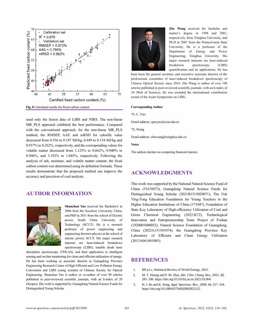
www.at-spectrosc.com/as/article/pdf/2022099 161 At. Spectrosc. 2022, 43(2), 154–163.
Fig. 8 Calculated results for fixed carbon content.
used only the fusion data of LIBS and NIRS. The non-linear
MR_PLS approach exhibited the best performance. Compared
with the conventional approach, for the non-linear MR_PLS
method, the RMSEP, AAE and mRSD for calorific value
decreased from 0.536 to 0.187 MJ/kg, 0.449 to 0.154 MJ/kg and
0.937% to 0.262%, respectively, and the corresponding values for
volatile matter decreased from 1.125% to 0.662%, 0.940% to
0.506%, and 3.192% to 1.045%, respectively. Following the
analysis of ash, moisture, and volatile matter content, the fixed
carbon content was determined using its definition formula. These
results demonstrate that the proposed method can improve the
accuracy and precision of coal analysis.
AUTHOR INFORMATION
Shunchun Yao received his Bachelor's in
2006 from the Soochow University, China,
and PhD in 2011 from the school of Electric
power, South China University of
Technology (SCUT). He is a research
professor of power engineering and
engineering thermos-physics at the school of
electric power, SCUT. His major research
interests are laser-induced breakdown
spectroscopy (LIBS), tunable diode laser
absorption spectroscopy (TDLAS), and their application to intelligent
sensing and on-line monitoring for clean and efficient utilization of energy.
He has been working as associate director in Guangdong Province
Engineering Research Center of High Efficient and Low Pollution Energy
Conversion and LIBS young scientist of Chinese Society for Optical
Engineering. Shunchun Yao is author or co-author of over 90 articles
published in peer-reviewed scientific journals, with an h-index of 20
(Scopus). His work is supported by Guangdong Natural Science Funds for
Distinguished Young Scholar.
Zhe Wang received his bachelor and
master’s degree in 1998 and 2001,
respectively, from Tsinghua University, and
Ph.D in 2007 from the Pennsylvania State
University. He is a professor of the
Department of Energy and Power
Engineering, Tsinghua University. His
major research interests are laser-induced
breakdown spectroscopy (LIBS)
quantification and its applications. He has
been been the general secretary and executive associate director of the
professional committee of laser-induced breakdown spectroscopy of
Chinese Optical Society since 2016. Zhe Wang is author of over 100
articles published in peer-reviewed scientific journals, with an h-index of
34 (Web of Science). He was awarded the international contribution
award of the Asian Symposium on LIBS.
Corresponding Author
*S. C. Yao
Email address: [email protected]
*Z. Wang
Email address: [email protected]
Notes
The authors declare no competing financial interest.
ACKNOWLEDGMENTS
This work was supported by the National Natural Science Fund of
China (51676073), Guangdong Natural Science Funds for
Distinguished Young Scholar (2021B1515020071), The Fok
Ying-Tong Education Foundation for Young Teachers in the
Higher Education Institutions of China (171047), Foundation of
State Key Laboratory of High-efficiency Utilization of Coal and
Green Chemical Engineering (2022-K72), Technological
Innovation and Entrepreneurship Team Project of Foshan
(1920001000052), Natural Science Foundation of Guangdong,
China (2022A151501074), the Guangdong Province Key
Laboratory of Efficient and Clean Energy Utilization
(2013A061401005).
REFERENCES
1. BP p.l.c, Statistical Review of World Energy, 2021.
2. M. T. Huang and P. M. Zhai, Adv. Clim. Chang. Res., 2021, 12,
281–286. https://doi.org/10.1016/j.accre.2021.03.004
3. H. J. Im and K. Song, Appl. Spectrosc. Rev., 2009, 44, 317–334.
https://doi.org/10.1080/05704920902852125
www.at-spectrosc.com/as/article/pdf/2022099 162 At. Spectrosc. 2022, 43(2), 154–163.
4. Z. Yan, Z. Xinlei, J. Wenbao, S. Qing, L. Yongsheng, H. Daqian,
and C. Da, Appl. Spectrosc., 2016, 70, 272–278.
https://doi.org/10.1177/0003702815620129
5. M. Gaft, L. Nagli, Y. Groisman, and A. Barishnikov, Appl.
Spectrosc., 2015, 68, 1004–1015.
https://doi.org/10.1366/13-07382
6. D. Redoglio, E. Golinelli, S. Musazzi, U. Perini and F. Barberis,
Spectrochim. Acta - Part B At. Spectrosc., 2016, 116, 46–50.
https://doi.org/10.1016/j.sab.2015.11.005
7. Z. Hou, Z. Wang, L. Li, X. Yu, T. Li, H. Yao, G. Yan, Q. Ye,
Z. Liu, and H. Zheng, Spectrochim. Acta Part B At. Spectrosc.,
2022, 191, 106406. https://doi.org/10.1016/j.sab.2022.106406
8. S. Sheta, M. S. Afgan, Z. Hou, S. C. Yao, L. Zhang, Z. Li, and
Z. Wang, J. Anal. At. Spectrom., 2019, 34, 1047–1082.
https://doi.org/10.1039/c9ja00016j
9. L. B. Guo, D. Zhang, L. X. Sun, S. C. Yao, L. Zhang,
Z. Z. Wang, Q. Q. Wang, H. Bin Ding, Y. Lu, Z. Y. Hou, and
Z. Wang, Front. Phys., 2021, 16, 22500.
https://doi.org/10.1007/s11467-020-1007-z
10. M. Gaft, E. Dvir, H. Modiano, and U. Schone,
Spectrochim. Acta - Part B At. Spectrosc., 2008, 63, 1177–1182.
https://doi.org/10.1016/j.sab.2008.06.007
11. T. Ctvrtnickova, M. P. Mateo, A. Yañez, and G. Nicolas,
Spectrochim. Acta - Part B At. Spectrosc., 2009, 64, 1093–1097.
https://doi.org/10.1016/j.sab.2009.07.032
12. T. Ctvrtnickova, M. P. Mateo, A. Yañez, and G. Nicolas,
Spectrochim. Acta - Part B At. Spectrosc., 2010, 65, 734–737.
https://doi.org/10.1016/j.sab.2010.04.020
13. L. Zhang, Y. Gong, Y. Li, X. Wang, J. Fan, L. Dong, W. Ma,
W. Yin, and S. Jia, Spectrochim. Acta - Part B At. Spectrosc.,
2015, 113, 167–173. https://doi.org/10.1016/j.sab.2015.09.021
14. T. Yuan, Z. Wang, S. L. Lui, Y. Fu, Z. Li, J. Liu and W. Ni,
J. Anal. At. Spectrom., 2013, 28, 1045–1053.
https://doi.org/10.1039/c3ja50097g
15. Z. Hou, Z. Wang, T. Yuan, J. Liu, Z. Li, and W. Ni,
J. Anal. At. Spectrom., 2016, 31, 722–736.
https://doi.org/10.1039/c5ja00475f
16. W. Song, Z. Hou, M. S. Afgan, W. Gu, H. Wang, J. Cui,
Z. Wang, and Y. Wang, J. Anal. At. Spectrom., 2021, 36,
111–119. http://doi.org/10.1039/d0ja00386g
17. W. Song, Z. Hou, W. Gu, H. Wang, J. Cui, Z. Zhou, G. Yan,
Q. Ye, Z. Li, and Z. Wang, Fuel, 2021, 306, 1–10.
https://doi.org/10.1016/j.fuel.2021.121667
18. C. Yan, J. Qi, J. Liang, T. Zhang, and H. Li,
J. Anal. At. Spectrom., 2018, 33, 2089–2097.
https://doi.org/10.1039/c8ja00284c
19. C. Yan, T. Zhang, Y. Sun, H. Tang, and H. Li,
Spectrochim. Acta - Part B At. Spectrosc., 2019, 154, 75–81.
https://doi.org/10.1016/j.sab.2019.02.007
20. C. Yan, J. Liang, M. Zhao, X. Zhang, T. Zhang, and H. Li, Anal.
Chim. Acta, 2019, 1080, 35–42.
https://doi.org/10.1016/j.aca.2019.07.012
21. S. Yao, J. Mo, J. Zhao, Y. Li, X. Zhang, W. Lu, and Z. Lu, Appl.
Spectrosc., 2018, 72, 1225–1233.
https://doi.org/10.1177/0003702818772856
22. Y. Zhang, M. Dong, L. Cheng, L. Wei, J. Cai, and J. Lu,
J. Anal. At. Spectrom., 2020, 35, 810–818.
https://doi.org/10.1039/c9ja00429g
23. W. Zhang, Z. Zhuo, P. Lu, J. Tang, H. Tang, J. Lu, T. Xing, and
Y. Wang, J. Anal. At. Spectrom., 2020, 35, 1621–1631.
https://doi.org/10.1039/d0ja00186d
24. Y. Zhang, Z. Xiong, Y. Ma, C. Zhu, R. Zhou, X. Li, Q. Li, and
Q. Zeng, Anal. Methods, 2020, 12, 3530–3536.
https://doi.org/10.1039/d0ay00905a
25. Z. Wang, M. S. Afgan, W. Gu, Y. Song, Y. Wang, Z. Hou,
W. Song, and Z. Li, Trends Analyt. Chem., 2021, 143, 116385.
https://doi.org/10.1016/j.trac.2021.116385
26. W. Gu, Z. Hou, W. Song, L. Li, X. Yu, J. Liu, Y. Song,
M. S. Afgan, Z. Li, Z. Liu, and Z. Wang, Anal. Chim. Acta, 2022,
1205, 339752. https://doi.org/10.1016/j.aca.2022.339752
27. Y. Okazaki, Anal. Chem., 2012, 28, 545–562.
https://doi.org/doi.org/10.2116/analsci.28.545
28. M. T. Bona and J. M. Andrés, Talanta, 2007, 72, 1423–1431.
https://doi.org/10.1016/j.talanta.2007.01.050
29. J. M. Andrés and M. T. Bona, Anal. Chim. Acta, 2005, 535,
123–132. https://doi.org/10.1016/j.aca.2004.12.007
30. J. M. Andrés and M. T. Bona, Talanta, 2006, 70, 711–719.
https://doi.org/10.1016/j.talanta.2006.05.034.
31. D. W. Kim, J. M. Lee, and J. S. Kim, Korean J. Chem. Eng.,
2009, 26, 489–495. https://doi.org/10.1007/s11814-009-0083-0
32. N. Begum, D. Chakravarty, and B. S. Das, Int. J. Coal Prep. Util.,
2019. https://doi.org/10.1080/19392699.2019.1621301
33. N. Begum, A. Maiti, D. Chakravarty, and B. S. Das, Fuel, 2020,
280, 1–10. https://doi.org/10.1016/j.fuel.2020.118676.
34. S. H. Wang,, Y. Zhao, R. Hu, Y. Y. Zhang, and X. H. Han,
Chin. J. Anal. Chem., 2019, 47, e19034–e19044.
https://doi.org/10.1016/S1872-2040(19)61150-3
35. D. Xiao and B. T. Le, Microchem. J., 2020, 157, 1–8.
https://doi.org/10.1016/j.microc.2020.104880
36. Z. Hou, Z. Wang, T. Yuan, J. Liu, Z. Li, and W. Ni,
J. Anal. At. Spectrom., 2016, 31, 722–736.
https://doi.org/10.1039/c5ja00475f
37. A. Guatame-Garcia and M. Buxton, 7th International Conference
on sensor-based sorting and control, 2016, pp. 195–208.
38. S. Sánchez-Esteva, M. Knadel, S. Kucheryavskiy,
L. W. de Jonge, G. H. Rubæk, C. Hermansen, and G. Heckrath,
Sensors (Basel), 2020, 20, 1–19.
https://doi.org/10.3390/s20185419
39. D. M. de Oliveira, L. M. Fontes, and C. Pasquini,
Anal. Chim. Acta, 2019, 1062, 28–36.
https://doi.org/10.1016/j.aca.2019.02.043.
40. R. S. Bricklemyer, D. J. Brown, P. J. Turk, and S. Clegg,
Soil Sci. Soc. Am. J., 2018, 82, 1482–1496.
http://doi.org/10.2136/sssaj2017.09.0332
41. S. Yao, H. Qin, Q. Wang, Z. Lu, X. Yao, Z. Yu, X. Chen,
L. Zhang, and J. Lu,
Spectrochim. Acta Part A Mol. Biomol. Spectrosc., 2020, 239,
118492. https://doi.org/10.1016/j.saa.2020.118492
42. H. Lim, L. Shagdarsuren, C. H. Oh, B. H. Lee, and C. H. Jeon,
J. Mech. Sci. Technol., 2016, 30, 3393–3400.
https://doi.org/10.1007/s12206-016-0648-x
43. T. Yuan, Z. Wang, S. L. Lui, Y. Fu, Z. Li, J. Liu, and W. Ni,
J. Anal. At. Spectrom., 2013, 28, 1045–1053.
https://doi.org/10.1039/c3ja50097g
44. Y. Wang, M. Yang, G. Wei, R. Hu, Z. Luo, and G. Li,
Sensor. Actuat. B-Chem., 2014, 193, 723–729.
https://doi.org/10.1016/j.snb.2013.12.028.
www.at-spectrosc.com/as/article/pdf/2022099 163 At. Spectrosc. 2022, 43(2), 154–163.
45. Q. Zhu, Coal Geology, Third Edition, Chapter 5: Coal Sampling
and Analysis, 2014.
https://doi.org/10.1002/9781119424307.ch5
46. W. W. Go, R. C. Agapay, Y. H. Ju, and A. T. Conag, Combust.
Sci. Technol., 2020, 192, 1449–1474.
https://doi.org/10.1080/00102202.2019.1617705
47. A. Scholz, Fuel, 1980, 59, 197–200.
https://doi.org/10.1016/0016-2361(80)90166-0
48. M. E. Morgan and R. G. Jenkins, Fuel, 1986, 65, 757–763.
https://doi.org/10.1016/0016-2361(86)90064-5
49. R. G. Brereton, Analyst, 2000, 125, 2125–2154.
https://doi.org/10.1039/b003805i
50. P. Kumari, A. K. Singh, D. A. Wood, and B. Hazra,
J. Geol. Soc. India, 2019, 93, 437–442.
https://doi.org/10.1007/s12594-019-1198-5
51. P. R. Solomon, M. A. Serio, and E. M. Suuberg, Prog. Energy
Combust. Sci., 1992, 18, 133–220.
https://doi.org/10.1016/0360-1285(92)90021-R
52. S. G. K. Patro and K. K. sahu, Iarjset, 2015, 2, 20–22.
http://doi.org/10.17148/iarjset.2015.2305
53. J. Feng, Z. Wang, L. Li, Z. Li, and W. Ni, Appl. Spectrosc., 2013,
67, 291–300. http://doi.org/10.1366/11-06393
54. F. B. Gonzaga and C. Pasquini, Spectrochim. Acta Part B At.
Spectrosc., 2012, 69, 20–24.
http://doi.org/10.1016/j.sab.2012.02.007.
55. GB/T213-2008, National standards of the people's Republic of
China: Determination of calorific value of coal, 2008.
56. GB/T212-2008, National standards of the people's Republic of
China: Proximate analysis of coal, 2008.
57. S. Yao, J. Zhao, Z. Wang, Y. Deguchi, Z. Lu, and J. Lu,
Spectrochim. Acta Part B At. Spectrosc., 2018, 149, 249–255.
https://doi.org/10.1016/j.sab.2018.09.002
58. P. Lu, Z. Zhuo, W. Zhang, J. Tang, T. Xing, Y. Wang, T. Sun,
and J. Lu, Appl. Phys. B Lasers Opt., 2021, 127, 1–15.
https://doi.org/10.1007/s00340-021-07626-5
59. Y. Liu, Y. Liu, Y. Chen, Y. Zhang, T. Shi, J. Wang, Y. Hong,
T. Fei and Y. Zhang, Remote Sens., 2019, 11, 1–16.
https://doi.org/10.3390/rs11040450
60. A. K. Majumder, R. Jain, P. Banerjee, and J. P. Barnwal, Fuel,
2008, 87, 3077–3081. https://doi.org/10.1016/j.fuel.2008.04.008
61. S. Mesroghli, E. Jorjani, and S. C. Chelgani, Int. J. Coal Geol.,
2009, 79, 49–54. http://doi.org/10.1016/j.coal.2009.04.002
62. S. C. Chelgani and S. Makaremi, Fuel Process. Technol., 2013,
110, 79–85. https://doi.org/10.1016/j.fuproc.2012.11.005
63. P. Tan, C. Zhang, J. Xia, Q. Y. Fang, and G. Chen, Fuel Process.
Technol., 2015, 138, 298–304.
https://doi.org/10.1016/j.fuproc.2015.06.013
64. S. Küçükbayrak, B. Dürüs, A. E. Meríçboyu, and E. Kadioglu,
Fuel, 1991, 70, 979–981.
http://doi.org/10.1016/0016-2361(91)90054-E
65. G. J. Székely, M. L. Rizzo, and N. K. Bakirov, Ann. Stat., 2007,
35, 2769–2794. https://doi.org/10.1214/009053607000000505
66. E. Ogus, A. C. Yazici, and F. Gurbuz, Commun. Stat. Simul.
Comput., 2007, 36, 847–854.
http://doi.org/10.1080/03610910701418028
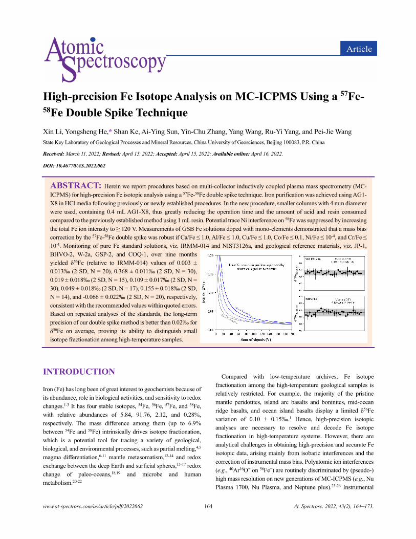
www.at-spectrosc.com/as/article/pdf/2022062 164 At. Spectrosc. 2022, 43(2), 164–173.
High-precision Fe Isotope Analysis on MC-ICPMS Using a 57Fe-58Fe Double Spike Technique
Xin Li, Yongsheng He,* Shan Ke, Ai-Ying Sun, Yin-Chu Zhang, Yang Wang, Ru-Yi Yang, and Pei-Jie Wang
State Key Laboratory of Geological Processes and Mineral Resources, China University of Geosciences, Beijing 100083, P.R. China
Received: March 11, 2022; Revised: April 15, 2022; Accepted: April 15, 2022; Available online: April 16, 2022.
DOI: 10.46770/AS.2022.062
ABSTRACT: Herein we report procedures based on multi-collector inductively coupled plasma mass spectrometry (MC-
ICPMS) for high-precision Fe isotopic analysis using a 57Fe-58Fe double spike technique. Iron purification was achieved using AG1-
X8 in HCl media following previously or newly established procedures. In the new procedure, smaller columns with 4 mm diameter
were used, containing 0.4 mL AG1-X8, thus greatly reducing the operation time and the amount of acid and resin consumed
compared to the previously established method using 1 mL resin. Potential trace Ni interference on 58Fe was suppressed by increasing
the total Fe ion intensity to ≥ 120 V. Measurements of GSB Fe solutions doped with mono-elements demonstrated that a mass bias
correction by the 57Fe-58Fe double spike was robust if Ca/Fe ≤ 1.0, Al/Fe ≤ 1.0, Cu/Fe ≤ 1.0, Co/Fe ≤ 0.1, Ni/Fe ≤ 10-4, and Cr/Fe ≤
10-4. Monitoring of pure Fe standard solutions, viz. IRMM-014 and NIST3126a, and geological reference materials, viz. JP-1,
BHVO-2, W-2a, GSP-2, and COQ-1, over nine months
yielded δ56Fe (relative to IRMM-014) values of 0.003 ±
0.013‰ (2 SD, N = 20), 0.368 ± 0.011‰ (2 SD, N = 30),
0.019 ± 0.018‰ (2 SD, N = 15), 0.109 ± 0.017‰ (2 SD, N =
30), 0.049 ± 0.018‰ (2 SD, N = 17), 0.155 ± 0.018‰ (2 SD,
N = 14), and -0.066 ± 0.022‰ (2 SD, N = 20), respectively,
consistent with the recommended values within quoted errors.
Based on repeated analyses of the standards, the long-term
precision of our double spike method is better than 0.02‰ for
δ56Fe on average, proving its ability to distinguish small
isotope fractionation among high-temperature samples.
INTRODUCTION
Iron (Fe) has long been of great interest to geochemists because of
its abundance, role in biological activities, and sensitivity to redox
changes.1-3 It has four stable isotopes, 54Fe, 56Fe, 57Fe, and 58Fe,
with relative abundances of 5.84, 91.76, 2.12, and 0.28%,
respectively. The mass difference among them (up to 6.9%
between 54Fe and 58Fe) intrinsically drives isotope fractionation,
which is a potential tool for tracing a variety of geological,
biological, and environmental processes, such as partial melting,4,5
magma differentiation,6-11 mantle metasomatism,12-14 and redox
exchange between the deep Earth and surficial spheres,15-17 redox
change of paleo-oceans,18,19 and microbe and human
metabolism.20-22
Compared with low-temperature archives, Fe isotope
fractionation among the high-temperature geological samples is
relatively restricted. For example, the majority of the pristine
mantle peridotites, island arc basalts and boninites, mid-ocean
ridge basalts, and ocean island basalts display a limited δ56Fe
variation of 0.10 0.15‰.1 Hence, high-precision isotopic
analyses are necessary to resolve and decode Fe isotope
fractionation in high-temperature systems. However, there are
analytical challenges in obtaining high-precision and accurate Fe
isotopic data, arising mainly from isobaric interferences and the
correction of instrumental mass bias. Polyatomic ion interferences
(e.g., 40Ar16O+ on 56Fe+) are routinely discriminated by (pseudo-)
high mass resolution on new generations of MC-ICPMS (e.g., Nu
Plasma 1700, Nu Plasma, and Neptune plus).23-26 Instrumental
www.at-spectrosc.com/as/article/pdf/2022062 165 At. Spectrosc. 2022, 43(2), 164–173.
mass bias can be corrected using standard sample bracketing
(SSB),23-25 element doping,8, 25-28 and double spike techniques.29-31
The SSB method is used widely and assumes mass bias during
sample measurements to be the same as that of bracketing standard
measurements. Validation of this assumption requires a well-
controlled laboratory environment (e.g., temperature, humidity,
and air exhaust rate), instrument stability, and a highly matched
matrix (1 and the references therein).The element doping method
assumes that the isotopes of the doped element exhibit an isotope
fractionation behavior similar to those isotopes of the element of
interest and helps to overcome mass bias fluctuations.1, 32
Nevertheless, the doped element and the element of interest (e.g.,
Ni and Fe) could exhibit different isotope fractionation behaviors
during measurements.31 In an optimized case, a long-term
precision (2 SD) for 56Fe/54Fe better than 0.03‰ can be routinely
achieved, provided that each sample is measured nine times by
MC-ICPMS.23, 25, 31
Theoretically, the double spike technique can be used to
accurately correct instrumental mass bias and yield high-precision
isotopic data.33 Millet et al.30 reported a procedure to measure Fe
isotope ratios using a 57Fe-58Fe double spike and demonstrated that
the external reproducibility could be as good as 0.02‰ for δ56Fe.
Nevertheless, isobaric interferences (e.g., trace 58Ni+ on 58Fe+ and
polyatomic interferences) may hinder accurate analyses.29,30 In
particular, 58Ni is an abundant isotope (~68.08% 34), whereas 58Fe
is a trace isotope (~0.28% 35). The improper correction of trace 58Ni+ interference using 60Ni+ routinely monitored on a Faraday
cup may cause significant uncertainty in the deduced 56Fe/54Fe
using the double spike method (namely, the trace Ni correction
problem).29 Finlayson et al.29 illustrated that the precision of δ56Fe
can be improved three-fold from ±0.145 to ± 0.052‰ when 60Ni+
is monitored on an ion counter instead of a Faraday cup, allowing
improved correction of 58Ni+ interference.
In this study, we developed an improved purification procedure
to efficiently separate Fe from the sample matrix and present high-
precision Fe isotope ratio measurements utilizing a 57Fe-58Fe
double spike. The on-peak-zero fluctuations (partially contributed
by tails of polyatomic ions) and trace Ni correction problems were
suppressed by increasing the signal-to-noise ratio. The robustness
of this method was demonstrated by repeated measurements of
solutions (GSB Fe, IRMM-014, and NIST3126a) and geological
standards (JP-1, BHVO-2, W-2a, GSP-2, and COQ-1), indicating
a 2 SD reproducibility and accuracy for δ56Fe better than 0.020‰.
Fe isotopic analyses of such high precision can help distinguish
limited Fe isotope fractionation during high-temperature processes.
THEORETICAL OPTIMIZATION
Iron isotopic analyses using a 57Fe-58Fe double spike on MC-
ICPMS have been previously attempted in Zhu et al.31 In this early
study, δ56Fe was measured at low signals (i.e., a 56Fe signal within
15 5 V), yielding a long-term precision of 0.10‰ for single time
measurements and showing no superiority in precision or accuracy
compared to that of the SSB method using element doping.31 The
merits of the double spike technique in accurate mass bias
correction may have been counteracted by the trace Ni correction
problem stemming from the introduction of the trace isotope 58Fe
into data deduction.29 The trace Ni correction problem was
previously overcome by monitoring 60Ni on an ion counter.
However, this required the measurements to be in dynamic
mode.29 Herein, we evaluate the trace Ni correction problem via
Monte Carlo calculations for measurements using Faraday cups
only. Theoretical runs were simulated for a spiked standard with
δ56Fe = 0, an optimized 57Fe-58Fe double spike proportion31,33
(referred to as q hereafter) of 0.457 and a mass bias (referred to as
β hereafter) of -1.5. Internal errors from counting statistics and
Johnson noise of the measured ratios during data acquisition were
calculated based on equations listed by Lehn et al.36 using an
integration time of 4.194 s; 1011 Ω resistors were adopted for all
Faraday cups, except that a 1010 Ω resistor was used for 56Fe when
its signal was > 40 V. To account for the trace Ni correction
problem, trace Ni (60Ni/58Fe = 10-7) was introduced. Despite being
theoretically negligible, it could cause a problem during
measurements. The non-linear behavior of Faraday cups
connected with the 1011 Ω resistors has been previously observed
for signals below 1 mV on the Nu instrument29, and the hardware
manual for Neptune plus suggests that 1011 Ω resistors may not
accurately measure signals < 0.1 mV. A limit (e.g., 0.1 mV, 0.2 mV,
and 0.3 mV) was set, and for a signal below this limit (i.e., 60Ni in
this study), the relative error from Johnson noise (σjn) contributed
by this signal was calculated by dividing the value of the limit with
that of the signal, i.e., [limit]/[signal]. Compared to the theoretical
value of 0.02 mV for 4.194 s of integration on 1011 Ω resistors,36
this assumption experientially enlarged the Johnson noise of the
trace 60Ni signal to examine the non-linear and inaccurate behavior
during data acquisition. Measured ratios were randomly obtained
for 40 cycles by setting normally distributed errors around
theoretical values, and then the mean δ56Fe and two standard errors
(2 SE) were deduced using equations listed in He et al.37 The
calculation was performed and repeated 1000 times for the sum of
the signals ranging from 2 to 200 V with an increment of 2 V. The
results are illustrated in Fig. 1 and show considerable extra errors
from the correction of trace Ni interference being propagated to
the deduced mean δ56Fe, particularly at a low sum of signals. For
example, for a sum of signals of 10 V, the internal error for δ56Fe
is 0.099‰, 0.162‰, and 0.235‰ when the trace signal limit is set
to 0.1 mV, 0.2 mV, and 0.3 mV, respectively, compared to the case
(~0.064‰) without Ni correction. Internal errors for δ56Fe with or
without the trace Ni correction problem converge at a high sum of
signals, and the trace Ni correction problem can be suppressed by
an increased signal-to-noise ratio or with a sum of signals >120 V.
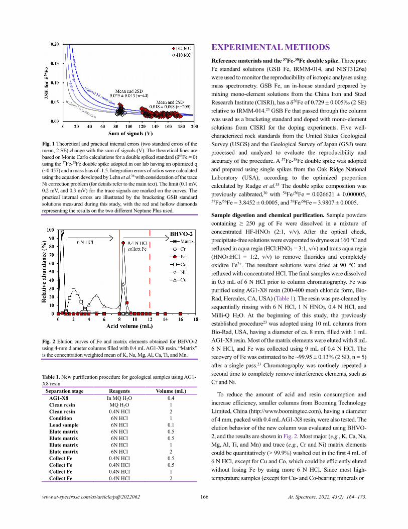
www.at-spectrosc.com/as/article/pdf/2022062 166 At. Spectrosc. 2022, 43(2), 164–173.
Fig. 1 Theoretical and practical internal errors (two standard errors of the
mean, 2 SE) change with the sum of signals (V). The theoretical lines are
based on Monte Carlo calculations for a double spiked standard (δ56Fe = 0)
using the 57Fe-58Fe double spike adopted in our lab having an optimized q
(~0.457) and a mass bias of -1.5. Integration errors of ratios were calculated
using the equation developed by Lehn et al.36
with consideration of the trace
Ni correction problem (for details refer to the main text). The limit (0.1 mV,
0.2 mV, and 0.3 mV) for the trace signals are marked on the curves. The
practical internal errors are illustrated by the bracketing GSB standard
solutions measured during this study, with the red and hollow diamonds
representing the results on the two different Neptune Plus used.
Fig. 2 Elution curves of Fe and matrix elements obtained for BHVO-2
using 4-mm diameter columns filled with 0.4 mL AG1-X8 resin. “Matrix”
is the concentration weighted mean of K, Na, Mg, Al, Ca, Ti, and Mn.
Table 1. New purification procedure for geological samples using AG1-
X8 resin
Separation stage Reagents Volume (mL)
AG1-X8 In MQ H2O 0.4
Clean resin MQ H2O 1
Clean resin 0.4N HCl 2
Condition 6N HCl 1
Load sample 6N HCl 0.1
Elute matrix 6N HCl 0.5
Elute matrix 6N HCl 0.5
Elute matrix 6N HCl 1
Elute matrix 6N HCl 2
Collect Fe 0.4N HCl 0.5
Collect Fe 0.4N HCl 0.5
Collect Fe 0.4N HCl 1
Collect Fe 0.4N HCl 2
EXPERIMENTAL METHODS
Reference materials and the 57Fe-58Fe double spike. Three pure
Fe standard solutions (GSB Fe, IRMM-014, and NIST3126a)
were used to monitor the reproducibility of isotopic analyses using
mass spectrometry. GSB Fe, an in-house standard prepared by
mixing mono-element solutions from the China Iron and Steel
Research Institute (CISRI), has a δ56Fe of 0.729 0.005‰ (2 SE)
relative to IRMM-014.23 GSB Fe that passed through the column
was used as a bracketing standard and doped with mono-element
solutions from CISRI for the doping experiments. Five well-
characterized rock standards from the United States Geological
Survey (USGS) and the Geological Survey of Japan (GSJ) were
processed and analyzed to evaluate the reproducibility and
accuracy of the procedure. A 57Fe-58Fe double spike was adopted
and prepared using single spikes from the Oak Ridge National
Laboratory (USA), according to the optimized proportion
calculated by Rudge et al.33 The double spike composition was
previously calibrated,30 with 54Fe/56Fe = 0.026621 ± 0.000005, 57Fe/56Fe = 3.8452 ± 0.0005, and 58Fe/56Fe = 3.9807 ± 0.0005.
Sample digestion and chemical purification. Sample powders
containing ≥ 250 μg of Fe were dissolved in a mixture of
concentrated HF-HNO3 (2:1, v/v). After the optical check,
precipitate-free solutions were evaporated to dryness at 160 °C and
refluxed in aqua regia (HCl:HNO3 = 3:1, v/v) and trans aqua regia
(HNO3:HCl = 1:2, v/v) to remove fluorides and completely
oxidize Fe2+. The resultant solutions were dried at 90 °C and
refluxed with concentrated HCl. The final samples were dissolved
in 0.5 mL of 6 N HCl prior to column chromatography. Fe was
purified using AG1-X8 resin (200-400 mesh chloride form, Bio-
Rad, Hercules, CA, USA) (Table 1). The resin was pre-cleaned by
sequentially rinsing with 6 N HCl, 1 N HNO3, 0.4 N HCl, and
Milli-Q H2O. At the beginning of this study, the previously
established procedure23 was adopted using 10 mL columns from
Bio-Rad, USA, having a diameter of ca. 8 mm, filled with 1 mL
AG1-X8 resin. Most of the matrix elements were eluted with 8 mL
6 N HCl, and Fe was collected using 9 mL of 0.4 N HCl. The
recovery of Fe was estimated to be ~99.95 ± 0.13% (2 SD, n = 5)
after a single pass.23 Chromatography was routinely repeated a
second time to completely remove interference elements, such as
Cr and Ni.
To reduce the amount of acid and resin consumption and
increase efficiency, smaller columns from Booming Technology
Limited, China (http://www.boomingtec.com), having a diameter
of 4 mm, packed with 0.4 mL AG1-X8 resin, were also tested. The
elution behavior of the new column was evaluated using BHVO-
2, and the results are shown in Fig. 2. Most major (e.g., K, Ca, Na,
Mg, Al, Ti, and Mn) and trace (e.g., Cr and Ni) matrix elements
could be quantitatively (> 99.9%) washed out in the first 4 mL of
6 N HCl, except for Cu and Co, which could be efficiently eluted
without losing Fe by using more 6 N HCl. Since most high-
temperature samples (except for Cu- and Co-bearing minerals or
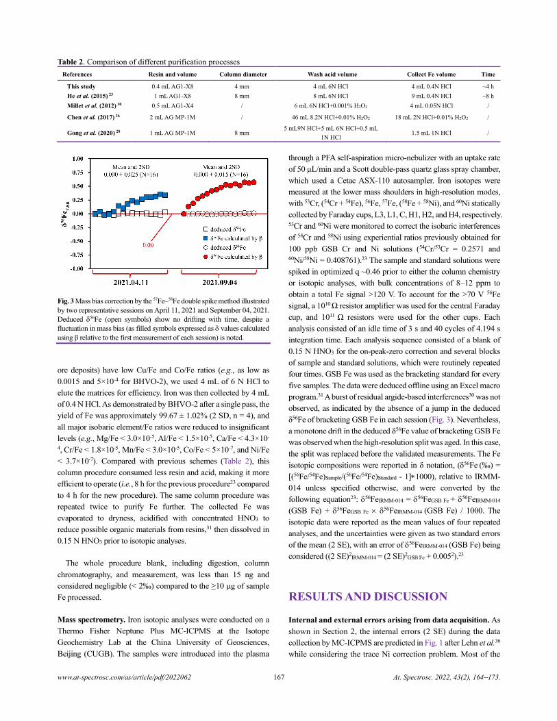
www.at-spectrosc.com/as/article/pdf/2022062 167 At. Spectrosc. 2022, 43(2), 164–173.
Table 2. Comparison of different purification processes
References Resin and volume Column diameter Wash acid volume Collect Fe volume Time
This study 0.4 mL AG1-X8 4 mm 4 mL 6N HCl 4 mL 0.4N HCl ~4 h
He et al. (2015) 23 1 mL AG1-X8 8 mm 8 mL 6N HCl 9 mL 0.4N HCl ~8 h
Millet et al. (2012) 30 0.5 mL AG1-X4 / 6 mL 6N HCl+0.001% H2O2 4 mL 0.05N HCl /
Chen et al. (2017) 26 2 mL AG MP-1M / 46 mL 8.2N HCl+0.01% H2O2 18 mL 2N HCl+0.01% H2O2 /
Gong et al. (2020) 28 1 mL AG MP-1M 8 mm 5 mL9N HCl+5 mL 6N HCl+0.5 mL
1N HCl 1.5 mL 1N HCl /
Fig. 3 Mass bias correction by the 57Fe–58Fe double spike method illustrated
by two representative sessions on April 11, 2021 and September 04, 2021.
Deduced 56Fe (open symbols) show no drifting with time, despite a
fluctuation in mass bias (as filled symbols expressed as values calculated
using β relative to the first measurement of each session) is noted.
ore deposits) have low Cu/Fe and Co/Fe ratios (e.g., as low as
0.0015 and 5×10⁻⁴ for BHVO-2), we used 4 mL of 6 N HCl to
elute the matrices for efficiency. Iron was then collected by 4 mL
of 0.4 N HCl. As demonstrated by BHVO-2 after a single pass, the
yield of Fe was approximately 99.67 ± 1.02% (2 SD, n = 4), and
all major isobaric element/Fe ratios were reduced to insignificant
levels (e.g., Mg/Fe < 3.0×10⁻⁵, Al/Fe < 1.5×10⁻⁵, Ca/Fe < 4.3×10-
4, Cr/Fe < 1.8×10⁻⁵, Mn/Fe < 3.0×10⁻⁵, Co/Fe < 5×10⁻⁷, and Ni/Fe
< 3.7×10⁻⁷). Compared with previous schemes (Table 2), this
column procedure consumed less resin and acid, making it more
efficient to operate (i.e., 8 h for the previous procedure23 compared
to 4 h for the new procedure). The same column procedure was
repeated twice to purify Fe further. The collected Fe was
evaporated to dryness, acidified with concentrated HNO3 to
reduce possible organic materials from resins,31 then dissolved in
0.15 N HNO3 prior to isotopic analyses.
The whole procedure blank, including digestion, column
chromatography, and measurement, was less than 15 ng and
considered negligible (< 2‰) compared to the ≥10 μg of sample
Fe processed.
Mass spectrometry. Iron isotopic analyses were conducted on a
Thermo Fisher Neptune Plus MC-ICPMS at the Isotope
Geochemistry Lab at the China University of Geosciences,
Beijing (CUGB). The samples were introduced into the plasma
through a PFA self-aspiration micro-nebulizer with an uptake rate
of 50 μL/min and a Scott double-pass quartz glass spray chamber,
which used a Cetac ASX-110 autosampler. Iron isotopes were
measured at the lower mass shoulders in high-resolution modes,
with 53Cr, (54Cr + 54Fe), 56Fe, 57Fe, (58Fe + 58Ni), and 60Ni statically
collected by Faraday cups, L3, L1, C, H1, H2, and H4, respectively. 53Cr and 60Ni were monitored to correct the isobaric interferences
of 54Cr and 58Ni using experiential ratios previously obtained for
100 ppb GSB Cr and Ni solutions (54Cr/53Cr = 0.2571 and 60Ni/58Ni = 0.408761).23 The sample and standard solutions were
spiked in optimized q ~0.46 prior to either the column chemistry
or isotopic analyses, with bulk concentrations of 8–12 ppm to
obtain a total Fe signal >120 V. To account for the >70 V 56Fe
signal, a 1010 Ω resistor amplifier was used for the central Faraday
cup, and 1011 Ω resistors were used for the other cups. Each
analysis consisted of an idle time of 3 s and 40 cycles of 4.194 s
integration time. Each analysis sequence consisted of a blank of
0.15 N HNO3 for the on-peak-zero correction and several blocks
of sample and standard solutions, which were routinely repeated
four times. GSB Fe was used as the bracketing standard for every
five samples. The data were deduced offline using an Excel macro
program.31 A burst of residual argide-based interferences30 was not
observed, as indicated by the absence of a jump in the deduced
δ56Fe of bracketing GSB Fe in each session (Fig. 3). Nevertheless,
a monotone drift in the deduced δ56Fe value of bracketing GSB Fe
was observed when the high-resolution split was aged. In this case,
the split was replaced before the validated measurements. The Fe
isotopic compositions were reported in δ notation, (56Fe (‰) =
[(56Fe/54Fe)Sample/(56Fe/54Fe)Standard - 1]1000), relative to IRMM-
014 unless specified otherwise, and were converted by the
following equation23: 56FeIRMM-014 = 56FeGSB Fe + 56FeIRMM-014
(GSB Fe) + 56FeGSB Fe 56FeIRMM-014 (GSB Fe) / 1000. The
isotopic data were reported as the mean values of four repeated
analyses, and the uncertainties were given as two standard errors
of the mean (2 SE), with an error of 56FeIRMM-014 (GSB Fe) being
considered ((2 SE)2IRMM-014 = (2 SE)2
GSB Fe + 0.0052).23
RESULTS AND DISCUSSION
Internal and external errors arising from data acquisition. As
shown in Section 2, the internal errors (2 SE) during the data
collection by MC-ICPMS are predicted in Fig. 1 after Lehn et al.36
while considering the trace Ni correction problem. Most of the
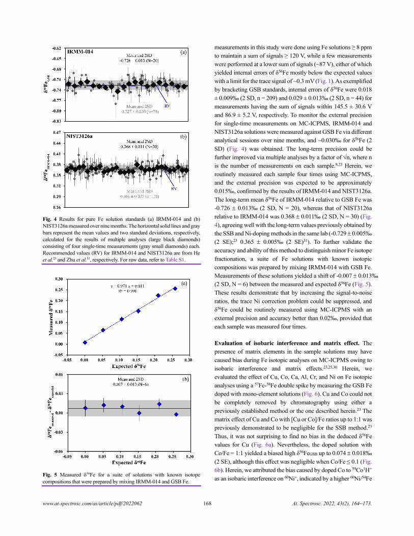
www.at-spectrosc.com/as/article/pdf/2022062 168 At. Spectrosc. 2022, 43(2), 164–173.
Fig. 4
Results for pure Fe solution standards (a) IRMM-014 and (b)
NIST3126a measured over nine months. The horizontal solid lines and gray
bars represent the mean values and two standard deviations, respectively,
calculated for the results of multiple analyses (large black diamonds)
consisting of four single-time measurements (gray small diamonds) each.
Recommended values (RV) for IRMM-014 and NIST3126a are from He
et al.23
and Zhu
et al.31, respectively. For raw data, refer to Table S1.
Fig. 5 Measured 56Fe for a suite of solutions with known isotope
compositions that were prepared by mixing IRMM-014 and GSB Fe.
measurements in this study were done using Fe solutions ≥ 8 ppm
to maintain a sum of signals ≥ 120 V, while a few measurements
were performed at a lower sum of signals (~87 V), either of which
yielded internal errors of δ56Fe mostly below the expected values
with a limit for the trace signal of ~0.3 mV (Fig. 1). As exemplified
by bracketing GSB standards, internal errors of δ56Fe were 0.018
± 0.009‰ (2 SD, n = 209) and 0.029 ± 0.013‰ (2 SD, n = 44) for
measurements having the sum of signals within 145.5 ± 30.6 V
and 86.9 ± 5.2 V, respectively. To monitor the external precision
for single-time measurements on MC-ICPMS, IRMM-014 and
NIST3126a solutions were measured against GSB Fe via different
analytical sessions over nine months, and ~0.030‰ for δ56Fe (2
SD) (Fig. 4) was obtained. The long-term precision could be
further improved via multiple analyses by a factor of n, where n
is the number of measurements on each sample.8,23 Herein, we
routinely measured each sample four times using MC-ICPMS,
and the external precision was expected to be approximately
0.015‰, confirmed by the results of IRMM-014 and NIST3126a.
The long-term mean δ56Fe of IRMM-014 relative to GSB Fe was
-0.726 0.013‰ (2 SD, N = 20), whereas that of NIST3126a
relative to IRMM-014 was 0.368 0.011‰ (2 SD, N = 30) (Fig.
4), agreeing well with the long-term values previously obtained by
the SSB and Ni-doping methods in the same lab (-0.729 0.005‰
(2 SE);23 0.365 0.005‰ (2 SE)31). To further validate the
accuracy and ability of this method to distinguish minor Fe isotope
fractionation, a suite of Fe solutions with known isotopic
compositions was prepared by mixing IRMM-014 with GSB Fe.
Measurements of these solutions yielded a shift of -0.007 0.013‰
(2 SD, N = 6) between the measured and expected δ56Fe (Fig. 5).
These results demonstrate that by increasing the signal-to-noise
ratios, the trace Ni correction problem could be suppressed, and
δ56Fe could be routinely measured using MC-ICPMS with an
external precision and accuracy better than 0.02‰, provided that
each sample was measured four times.
Evaluation of isobaric interference and matrix effect. The
presence of matrix elements in the sample solutions may have
caused bias during Fe isotopic analyses on MC-ICPMS owing to
isobaric interference and matrix effects.23,25,30 Herein, we
evaluated the effect of Cu, Co, Ca, Al, Cr, and Ni on Fe isotopic
analyses using a 57Fe-58Fe double spike by measuring the GSB Fe
doped with mono-element solutions (Fig. 6). Cu and Co could not
be completely removed by chromatography using either a
previously established method or the one described herein.23 The
matrix effect of Cu and Co with [Cu or Co]/Fe ratios up to 1:1 was
previously demonstrated to be negligible for the SSB method.23
Thus, it was not surprising to find no bias in the deduced δ56Fe
values for Cu (Fig. 6a). Nevertheless, the doped solution with
Co/Fe = 1:1 yielded a biased high δ56FeGSB up to 0.074 0.018‰
(2 SE), although this effect was negligible when Co/Fe ≤ 0.1 (Fig.
6b). Herein, we attributed the bias caused by doped Co to 59Co1H+
as an isobaric interference on 60Ni+, indicated by a higher 60Ni/54Fe
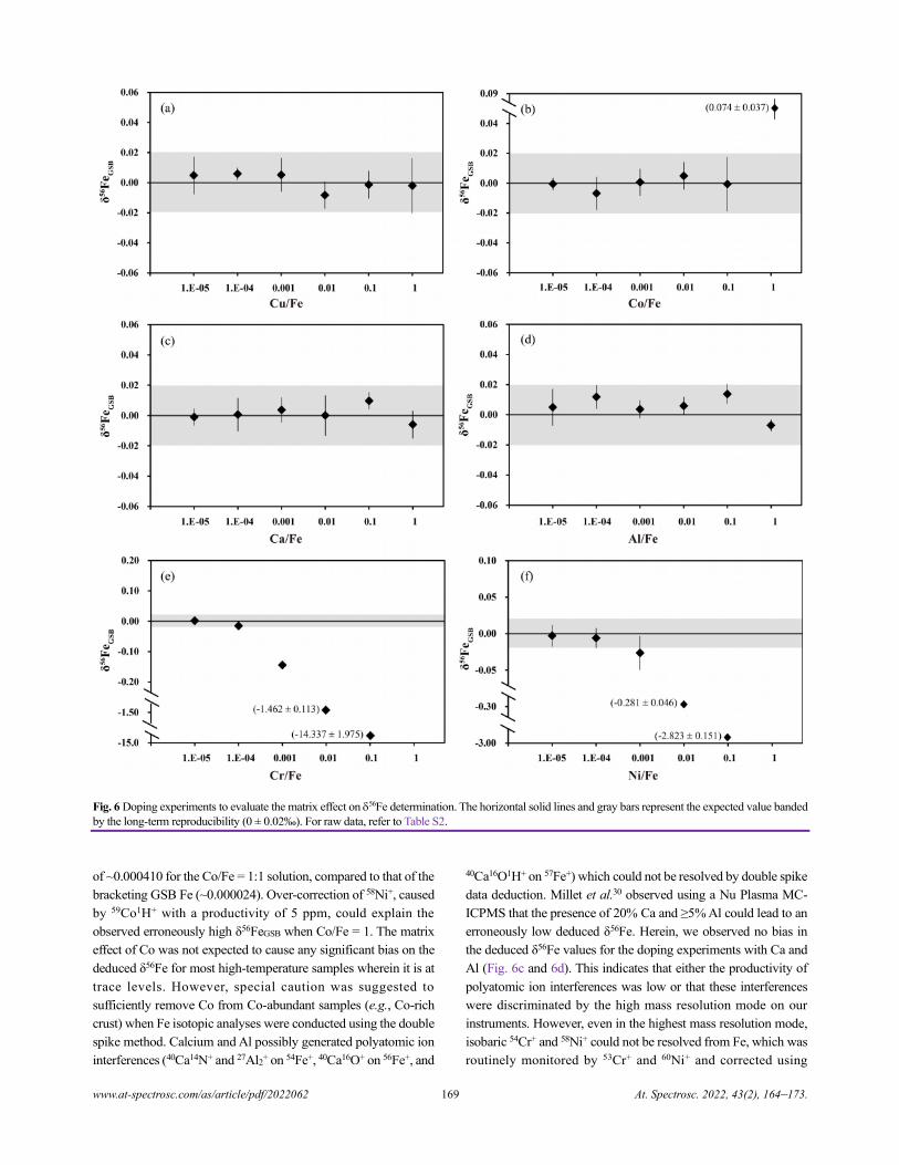
www.at-spectrosc.com/as/article/pdf/2022062 169 At. Spectrosc. 2022, 43(2), 164–173.
Fig. 6 Doping experiments to evaluate the matrix effect on 56Fe determination. The horizontal solid lines and gray bars represent the expected value banded
by the long-term reproducibility (0 ± 0.02‰). For raw data, refer to Table S2.
of ~0.000410 for the Co/Fe = 1:1 solution, compared to that of the
bracketing GSB Fe (~0.000024). Over-correction of 58Ni+, caused
by 59Co1H+ with a productivity of 5 ppm, could explain the
observed erroneously high δ56FeGSB when Co/Fe = 1. The matrix
effect of Co was not expected to cause any significant bias on the
deduced δ56Fe for most high-temperature samples wherein it is at
trace levels. However, special caution was suggested to
sufficiently remove Co from Co-abundant samples (e.g., Co-rich
crust) when Fe isotopic analyses were conducted using the double
spike method. Calcium and Al possibly generated polyatomic ion
interferences (40Ca14N+ and 27Al2+ on 54Fe+, 40Ca16O+ on 56Fe+, and
40Ca16O1H+ on 57Fe+) which could not be resolved by double spike
data deduction. Millet et al.30 observed using a Nu Plasma MC-
ICPMS that the presence of 20% Ca and ≥5% Al could lead to an
erroneously low deduced δ56Fe. Herein, we observed no bias in
the deduced δ56Fe values for the doping experiments with Ca and
Al (Fig. 6c and 6d). This indicates that either the productivity of
polyatomic ion interferences was low or that these interferences
were discriminated by the high mass resolution mode on our
instruments. However, even in the highest mass resolution mode,
isobaric 54Cr+ and 58Ni+ could not be resolved from Fe, which was
routinely monitored by 53Cr+ and 60Ni+ and corrected using
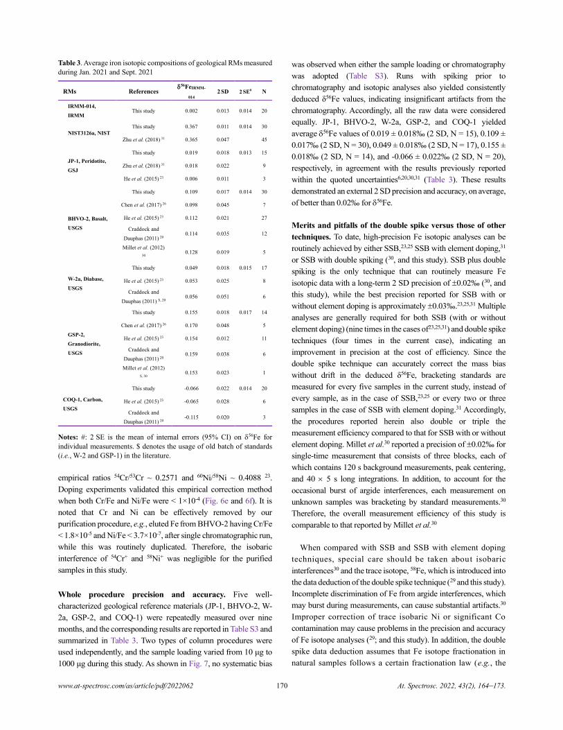
www.at-spectrosc.com/as/article/pdf/2022062 170 At. Spectrosc. 2022, 43(2), 164–173.
Table 3. Average iron isotopic compositions of geological RMs measured
during Jan. 2021 and Sept. 2021
RMs References 56FeIRMM-
014 2 SD 2 SE# N
IRMM-014,
IRMM This study 0.002 0.013 0.014 20
NIST3126a, NIST
This study 0.367 0.011 0.014 30
Zhu et al. (2018) 31 0.365 0.047 45
JP-1, Peridotite,
GSJ
This study 0.019 0.018 0.013 15
Zhu et al. (2018) 31 0.018 0.022 9
He et al. (2015) 23 0.006 0.011 3
BHVO-2, Basalt,
USGS
This study 0.109 0.017 0.014 30
Chen et al. (2017) 26 0.098 0.045 7
He et al. (2015) 23 0.112 0.021 27
Craddock and
Dauphas (2011) 20 0.114 0.035 12
Millet et al. (2012)
30 0.128 0.019 5
W-2a, Diabase,
USGS
This study 0.049 0.018 0.015 17
He et al. (2015) 23 0.053 0.025 8
Craddock and
Dauphas (2011) $, 20 0.056 0.051 6
GSP-2,
Granodiorite,
USGS
This study 0.155 0.018 0.017 14
Chen et al. (2017) 26 0.170 0.048 5
He et al. (2015) 23 0.154 0.012 11
Craddock and
Dauphas (2011) 20 0.159 0.038 6
Millet et al. (2012)
$, 30 0.153 0.023 1
COQ-1, Carbon,
USGS
This study -0.066 0.022 0.014 20
He et al. (2015) 23 -0.065 0.028 6
Craddock and
Dauphas (2011) 20 -0.115 0.020 3
Notes: #: 2 SE is the mean of internal errors (95% CI) on 56Fe for
individual measurements. $ denotes the usage of old batch of standards
(i.e., W-2 and GSP-1) in the literature.
empirical ratios 54Cr/53Cr ~ 0.2571 and 60Ni/58Ni ~ 0.4088 23.
Doping experiments validated this empirical correction method
when both Cr/Fe and Ni/Fe were < 1×10⁻⁴ (Fig. 6e and 6f). It is
noted that Cr and Ni can be effectively removed by our
purification procedure, e.g., eluted Fe from BHVO-2 having Cr/Fe
< 1.8×10⁻⁵ and Ni/Fe < 3.7×10⁻⁷, after single chromatographic run,
while this was routinely duplicated. Therefore, the isobaric
interference of 54Cr+ and 58Ni+ was negligible for the purified
samples in this study.
Whole procedure precision and accuracy. Five well-
characterized geological reference materials (JP-1, BHVO-2, W-
2a, GSP-2, and COQ-1) were repeatedly measured over nine
months, and the corresponding results are reported in Table S3 and
summarized in Table 3. Two types of column procedures were
used independently, and the sample loading varied from 10 μg to
1000 μg during this study. As shown in Fig. 7, no systematic bias
was observed when either the sample loading or chromatography
was adopted (Table S3). Runs with spiking prior to
chromatography and isotopic analyses also yielded consistently
deduced δ56Fe values, indicating insignificant artifacts from the
chromatography. Accordingly, all the raw data were considered
equally. JP-1, BHVO-2, W-2a, GSP-2, and COQ-1 yielded
average 56Fe values of 0.019 ± 0.018‰ (2 SD, N = 15), 0.109 ±
0.017‰ (2 SD, N = 30), 0.049 ± 0.018‰ (2 SD, N = 17), 0.155 ±
0.018‰ (2 SD, N = 14), and -0.066 ± 0.022‰ (2 SD, N = 20),
respectively, in agreement with the results previously reported
within the quoted uncertainties6,20,30,31 (Table 3). These results
demonstrated an external 2 SD precision and accuracy, on average,
of better than 0.02‰ for 56Fe.
Merits and pitfalls of the double spike versus those of other
techniques. To date, high-precision Fe isotopic analyses can be
routinely achieved by either SSB,23,25 SSB with element doping,31
or SSB with double spiking (30, and this study). SSB plus double
spiking is the only technique that can routinely measure Fe
isotopic data with a long-term 2 SD precision of 0.02‰ (30, and
this study), while the best precision reported for SSB with or
without element doping is approximately 0.03‰.23,25,31 Multiple
analyses are generally required for both SSB (with or without
element doping) (nine times in the cases of23,25,31) and double spike
techniques (four times in the current case), indicating an
improvement in precision at the cost of efficiency. Since the
double spike technique can accurately correct the mass bias
without drift in the deduced δ56Fe, bracketing standards are
measured for every five samples in the current study, instead of
every sample, as in the case of SSB,23,25 or every two or three
samples in the case of SSB with element doping.31 Accordingly,
the procedures reported herein also double or triple the
measurement efficiency compared to that for SSB with or without
element doping. Millet et al.30 reported a precision of 0.02‰ for
single-time measurement that consists of three blocks, each of
which contains 120 s background measurements, peak centering,
and 40 5 s long integrations. In addition, to account for the
occasional burst of argide interferences, each measurement on
unknown samples was bracketing by standard measurements.30
Therefore, the overall measurement efficiency of this study is
comparable to that reported by Millet et al.30
When compared with SSB and SSB with element doping
techniques, special care should be taken about isobaric
interferences30 and the trace isotope, 58Fe, which is introduced into
the data deduction of the double spike technique (29 and this study).
Incomplete discrimination of Fe from argide interferences, which
may burst during measurements, can cause substantial artifacts.30
Improper correction of trace isobaric Ni or significant Co
contamination may cause problems in the precision and accuracy
of Fe isotope analyses (29; and this study). In addition, the double
spike data deduction assumes that Fe isotope fractionation in
natural samples follows a certain fractionation law (e.g., the
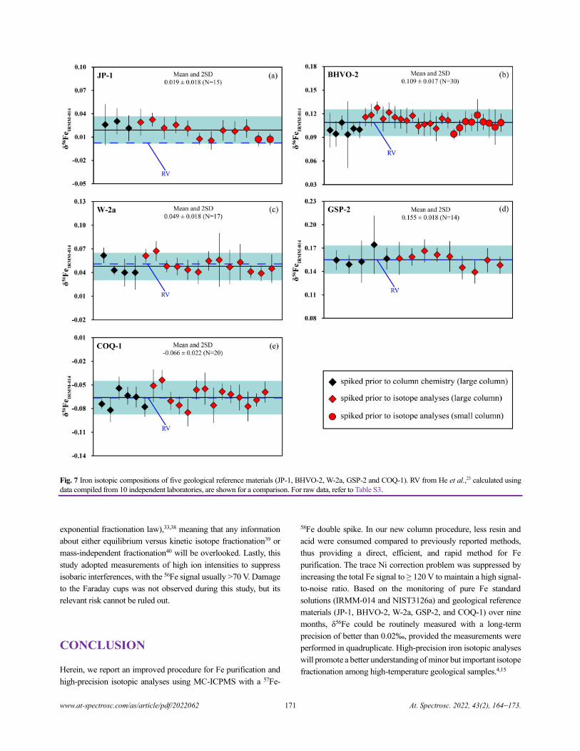
www.at-spectrosc.com/as/article/pdf/2022062 171 At. Spectrosc. 2022, 43(2), 164–173.
Fig. 7
Iron isotopic compositions of five geological reference materials (JP-1, BHVO-2, W-2a, GSP-2 and COQ-1). RV from He et al.,23
calculated using
data compiled from 10 independent laboratories, are shown for a comparison. For raw data, refer to Table S3.
exponential fractionation law),33,38 meaning that any information
about either equilibrium versus kinetic isotope fractionation39 or
mass-independent fractionation40 will be overlooked. Lastly, this
study adopted measurements of high ion intensities to suppress
isobaric interferences, with the 56Fe signal usually >70 V. Damage
to the Faraday cups was not observed during this study, but its
relevant risk cannot be ruled out.
CONCLUSION
Herein, we report an improved procedure for Fe purification and
high-precision isotopic analyses using MC-ICPMS with a 57Fe-
58Fe double spike. In our new column procedure, less resin and
acid were consumed compared to previously reported methods,
thus providing a direct, efficient, and rapid method for Fe
purification. The trace Ni correction problem was suppressed by
increasing the total Fe signal to ≥ 120 V to maintain a high signal-
to-noise ratio. Based on the monitoring of pure Fe standard
solutions (IRMM-014 and NIST3126a) and geological reference
materials (JP-1, BHVO-2, W-2a, GSP-2, and COQ-1) over nine
months, δ56Fe could be routinely measured with a long-term
precision of better than 0.02‰, provided the measurements were
performed in quadruplicate. High-precision iron isotopic analyses
will promote a better understanding of minor but important isotope
fractionation among high-temperature geological samples.4,15
www.at-spectrosc.com/as/article/pdf/2022062 172 At. Spectrosc. 2022, 43(2), 164–173.
ASSOCIATED CONTENT
The supporting information (Tables S1-S3) is available at www.at-
spectrosc.com/as/home
AUTHOR INFORMATION
Yong-Sheng He is a Professor at the
Institute of Earth Sciences, China
University of Geosciences, Beijing
(CUGB), leading a group focusing on Fe,
Ca, and Mg isotope geochemistry. He
received his B.S. (2005) and Ph.D. (2011)
degrees in geochemistry from the
University of Science and Technology of
China. After completing his Ph.D., he
came to CUGB for post-doctoral research
and joined the Isotope Geochemistry Lab
as a faculty in 2013. His main interest was petrogenesis of adakitic rocks
and their implication on evolution of orogenic crust. He currently focuses
on methodology developments on metal stable isotope geochemistry and
its application in tracing key geological and planetary processes, e.g., deep
carbon and oxygen cycles, changes in paleo-environment, and the
formation and evolution of the Moon. He has published over 50 peer-
reviewed scientific papers in ISI-indexed journals.
Corresponding Author
* Y. S. He
Email address: [email protected]
Notes
The authors declare no competing financial interest.
ACKNOWLEDGMENTS
The efficient editorial efforts by Prof. Wei Guo and constructive
comments from two anonymous reviewers are greatly appreciated.
We thank Dr. Shitou Wu and Dr. Hao Wang for their helps in
ICPMS measurements on eluates. This work is supported by the
National Key R&D Program of China (2019YFA0708403), the
National Natural Science Foundation of China (42122019), the
Fundamental Research Funds for the Central Universities (3-7-5-
2019-07), the 111 Project of the Ministry of Science and
Technology, China (BP0719021) and State Key Lab of Geological
Processes and Mineral Resources.
REFERENCES
1. N. Dauphas, S. G. John, and O. Rouxel,
Rev. Mineral. Geochem., 2017, 82, 415–510.
https://doi.org/10.2138/rmg.2017.82.11
2. C. Johnson, B. Beard, and S. Weyer, Advances in Isotope
Geochemistry, 2020, Springer, 1–360.
https://doi.org/10.1007/978-3-030-33828-2
3. Y. He, D. Hu, and C. Zhu, Earth Science Frontiers, 2015, 22, 54–71.
https://doi.org/10.13745/j.esf.2015.05.004
4. N. Dauphas, P. R. Craddock, P. D. Asimow, V. C. Bennett,
A. P. Nutman, and D. Ohnenstetter, Earth Planet. Sc. Lett., 2009,
288, 255–267. https://doi.org/10.1016/j.epsl.2009.09.029
5. S. Weyer and D. A. Ionov, Earth Planet. Sc. Lett., 2007, 259,
119–133. https://doi.org/10.1016/j.epsl.2007.04.033
6. J. Foden, P. A. Sossi, and C. M. Wawryk, Lithos, 2015, 212-215,
32–44. https://doi.org/10.1016/j.lithos.2014.10.015
7. Y. He, H. Wu, S. Ke, S.-A. Liu, and Q. Wang,
Geochim. Cosmochim. AC., 2017, 203, 89–102.
https://doi.org/10.1016/j.gca.2017.01.005
8. F. Poitrasson and R. Freydier, Chem. Geol., 2005, 222, 132–147.
https://doi.org/10.1016/j.chemgeo.2005.07.005
9. P. A. Sossi, J. D. Foden, and G. P. Halverson,
Contrib. Mineral. Petr., 2012, 164, 757–772.
https://doi.org/10.1007/s00410-012-0769-x
10. M. Telus, N. Dauphas, F. Moynier, F. L. H. Tissot, F.-Z. Teng,
P. I. Nabelek, P. R. Craddock, and L. A. Groat,
Geochim. Cosmochim. AC., 2012, 97, 247–265.
https://doi.org/10.1016/j.gca.2012.08.024
11. F.-Z. Teng, N. Dauphas, and R. T. Helz, Science, 2008, 320,
1620–1622. https://doi.org/10.1126/science.1157166
12. F. Huang, Z. Zhang, C. C. Lundstrom, and X. Zhi,
Geochim. Cosmochim. AC., 2011, 75, 3318–3334.
https://doiorg/10.1016/j.gca.2011.03.036
13. F. Poitrasson, G. Delpech, and M. Grégoire, Contrib. Mineral. Petr.,
2013, 165, 1243–1258. https://doi.org/10.1007/s00410-013-0856-7
14. X. Zhao, H. Zhang, X. Zhu, S. Tang, and B. Yan, Chem. Geol.,
2012, 292-293, 127–139.
https://doi.org/10.1016/j.chemgeo.2011.11.016
15. Y. He, X. Meng, S. Ke, H. Wu, C. Zhu, F.-Z. Teng, J. Hoefs,
J. Huang, W. Yang, L. Xu, Z. Hou, Z.-Y. Ren, and S. Li,
Earth Planet. Sc. Lett., 2019, 512, 175–183.
https://doi.org/10.1016/j.epsl.2019.02.009
16. B. Debret, M. A. Millet, M. L. Pons, P. Bouilhol, E. Inglis, and
H. Williams, Geology, 2016, 44, 215–218.
https://doi.org/10.1130/g37565.1
17. J. Deng, Y. He, R. E. Zartman, X. Yang, and W. Sun,
Earth Planet. Sc. Lett., 2022, 583, 117423.
https://doi.org/10.1016/j.epsl.2022.117423
18. O. J. Rouxel, A. Bekker, K. J. Edwards, Science. 2005, 307,
1088–1091. https://doi.org/10.1126/science.1105692
19. C. M. Johnson, B. L. Beard, and E. E. Roden,
Annu. Rev. Earth Pl. Sc., 2008, 36, 457–493.
https://doi.org/10.1146/annurev.earth.36.031207.124139
20. P. R. Craddock, N. Dauphas, Geostand. Geoanal. Res., 2011, 35,
101–123. https://doi.org/10.1111/j.1751-908X.2010.00085.x
21. A. Heimann, C. M. Johnson, B. L. Beard, J. W. Valley, E. E. Roden,
M. J. Spicuzza, and N. J. Beukes, Earth Planet. Sc. Lett., 2010, 294,
8–18. https://doi.org/10.1016/j.epsl.2010.02.015
22. Y. H. Liang, K. A. Huang, D. C. Lee, K. N. Pang, and S. H. Chen,
J Trace Elem. Med. Bio., 2020, 58, 126421.
https://doi.org/10.1016/j.jtemb.2019.126421
23. Y. He, S. Ke, F.-Z. Teng, T. Wang, H. Wu, Y. Lu, and S. Li,
Geostand. Geoanal. Res., 2015, 39, 341–356.
https://doi.org/10.1111/j.1751-908X.2014.00304.x
www.at-spectrosc.com/as/article/pdf/2022062 173 At. Spectrosc. 2022, 43(2), 164–173.
24. S. Weyer and J. B. Schwieters, Int. J. Mass Spectrom., 2003, 226,
355–368. https://doi.org/10.1016/s1387-3806(03)00078-2
25. N. Dauphas, A. Pourmand, and F.-Z. Teng, Chem. Geol., 2009, 267,
175–184. https://doi.org/10.1016/j.chemgeo.2008.12.011
26. K.-Y. Chen, H.-L. Yuan, P. Liang, Z.-A. Bao, and L. Chen,
Int. J. Mass Spectrom., 2017, 421, 196–203.
https://doi.org/10.1016/j.ijms.2017.07.002
27. P. A. Sossi, G. P. Halverson, O. Nebel, and S. M. Eggins,
Geostand. Geoanal. Res., 2015, 39, 129–149.
https://doi.org/10.1111/j.1751-908X.2014.00298.x
28. H. Gong, P. Guo, S. Chen, M. Duan, P. Sun, X. Wang, and Y. Niu,
Acta Geochim., 2020, 39, 355–364.
https://doi.org/10.1007/s11631-019-00392-4
29. V. A. Finlayson, J. G. Konter, and L. Ma,
Geochem. Geophy. Geosy., 2015, 16, 4209–4222.
https://doi.org/10.1002/2015gc006012
30. M.-A. Millet, J. A. Baker, and C. E. Payne, Chem. Geol., 2012,
304-305, 18–25. https://doi.org/10.1016/j.chemgeo.2012.01.021
31. C. Zhu, W. Lu, Y. He, S. Ke, H. Wu, and L. Zhang, Acta Geochim.,
2018, 37, 691–700. https://doi.org/10.1007/s11631-018-0284-5
32. L. Yang, S. Tong, L. Zhou, Z. Hu, Z. Mester, and J. Meija,
J. Anal. At. Spectrom., 2018, 33, 1849–1861.
https://doi.org/10.1039/c8ja00210j
33. J. F. Rudge, B. C. Reynolds, and B. Bourdon, Chem. Geol., 2009,
265, 420–431. https://doi.org/10.1016/j.chemgeo.2009.05.010
34. J. W. Gramlich, L. A. Machlan, I. L. Barnes, and P. J. Paulsen,
J. Res. Natl. Inst. Stand. Technol., 1989, 94, 347–356.
https://doi.org/10.6028/jres.094.034
35. P. D. P. Taylor, R. Maeck, and P. Debievre,
Int. J. Mass Spectrom. Ion Process, 1992, 121, 111–125.
https://doi.org/10.1016/0168-1176(92)80075-c
36. G. O. Lehn, A. D. Jacobson, and C. Holmden,
Int. J. Mass Spectrom., 2013, 351, 69–75.
https://doi.org/10.1016/j.ijms.2013.06.013
37. Y. S. He, Y. Wang, C. W. Zhu, S. C. Huang, and S. G. Li,
Geostand. Geoanal. Res., 2017, 41, 283–302.
https://doi.org/10.1111/ggr.12153
38. C. M. Johnson and B. L. Beard, Int. J. Mass Spectrom., 1999, 193,
87–99. https://doi.org/10.1016/s1387-3806(99)00158-x
39. A. W. Heard, N. Dauphas, R. Guilbaud, O. J. Rouxel, I. B. Butler,
N. X. Nie, and A. Bekker, Science, 2020, 370, 446–449.
https://doi.org/10.1126/science.aaz8821
40. M. Amor, V. Busigny, P. Louvat, A. Gélabert, P. Cartigny,
M. Durand-Dubief, G. Ona-Nguema, E. Alphandéry, I. Chebbi, and
F. Guyot, Science, 2016, 352, 705–708.
https://doi.org/10.1126/science.aad7632
www.at-spectrosc.com/as/article/pdf/2021609 174 At. Spectrosc. 2022, 43(2), 174–185.
Review of In-situ Online LIBS Detection in the Atmospheric
Environment
Qihang Zhang and Yuzhu Liu*
Jiangsu Key Laboratory for Optoelectronic Detection of Atmosphere and Ocean, Jiangsu Collaborative Innovation Center on Atmospheric Environment and
Equipment Technology (CICAEET), Nanjing University of Information Science & Technology, Nanjing 210044, P. R. China
Received: June 21, 2021; Revised: August 24, 2021; Accepted: August 25, 2021; Available online: September 11, 2021.
DOI: 10.46770/AS.2021.609
ABSTRACT: The aim of this review is to provide a brief introduction to recent research advances in in-situ online detection
of atmospheric pollutants based on laser-induced breakdown spectroscopy (LIBS) under atmospheric environments. Atmospheric
pollution has drawn much public attention, and there is increasing demand for
rapid and accurate evaluation of atmospheric environments. LIBS has the
advantages of in-situ online detection, simultaneous multi-element analysis, and
noncontact measurement, making it a highly competitive analytical technique in
the field of environmental monitoring. In terms of the different target samples,
some typical research cases, including atmospheric particulate matter,
atmospheric pollution sources, halogens in VOCs, atmospheric sulfur, and stable
isotope abundance, are presented to illustrate the current development and
problems of LIBS detection in this field.
INTRODUCTION
In recent decades, there has been ever-increasing demand for the
rapid detection of atmospheric pollutants, including volatile
organic compounds (VOCs), heavy metals, NOx, and other
hazardous substances, as the global atmospheric environment has
worsened owing to natural changes and anthropogenic activities in
many countries, and thus there has been ever-increasing demand
for the rapid detection of these atmospheric pollutants.1 The
presence of these atmospheric pollutants has caused serious
atmospheric environmental problems such as haze, increased size
of the ozone hole, and photochemical smog, and it has become a
serious threat to the global ecological environment and human
health,2,3 a problem that is gaining the attention of world
governments. To solve these environmental problems or reduce
their negative effects on the environment and human health, it is
essential to first determine the composition of the atmosphere in a
targeted area and then take specific measures after that. However,
the types and concentrations of the components in the atmosphere
vary from hour to hour with air flow. Hence, detection must be
accomplished in a very short time to ensure the validity of further
analysis and the timeliness of the measurement results, which is a
great challenge for current detection methods.
Laser-induced breakdown spectroscopy (LIBS) is a well-
known atomic emission spectroscopy (AES) technique. In LIBS
measurements, the target sample is ablated to a high-temperature
plasma by a high-intensity pulse laser, and then the atomic, ionic,
and molecular spectra containing the compositional information
emitted from the plasma are qualitatively and quantitatively
analyzed to determine all the components and their concentrations
in the sample.4 LIBS has attracted significant attention since it was
first reported at the X Colloquium Spectroscopicum Internationale
by Brech and Cross in 1962.5 Shortly thereafter, Runge et al.
established a calibration curve for quantitative analysis of target
elements based on the intensity of the characteristic line and the
plasma radiation mechanism,6 demonstrating that LIBS could be
a useful tool for spectrochemical analysis. Over the past several
decades, much scientific work covering a wide range of subjects
has been carried out by research groups worldwide,7 and the basic
theory of LIBS has gradually matured. Now, it has a wide variety
of applications in many fields, such as in material sorting,8-12 coal
analysis,13-16 food testing,17-19 medical testing,20-22 environmental
monitoring,23-26 ocean exploration,27-30 and space exploration.31-33
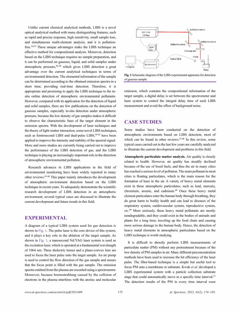
www.at-spectrosc.com/as/article/pdf/2021609 175 At. Spectrosc. 2022, 43(2), 174–185.
Unlike current chemical analytical methods, LIBS is a novel
optical analytical method with many distinguishing features, such
as rapid and precise response, high sensitivity, small sample loss,
and simultaneous multi-element analysis, and it is pollution-
free.34,35 These unique advantages make the LIBS technique an
effective method for compositional analysis. Moreover, detection
based on the LIBS technique requires no sample preparation, and
it can be performed on gaseous, liquid, and solid samples under
atmospheric pressure,36-38 which gives LIBS detection a great
advantage over the current analytical techniques in terms of
environmental detection. The elemental information of the sample
can be determined according to the obtained emission spectra in a
short time, providing real-time detection. Therefore, it is
appropriate and promising to apply the LIBS technique to the in-
situ online detection of atmospheric environmental pollutants.
However, compared with its application for the detection of liquid
and solid samples, there are few publications on the detection of
gaseous samples, especially in-situ detection under atmospheric
pressure, because the low density of gas samples makes it difficult
to observe the characteristic lines of the target element in the
emission spectra. With the development of laser techniques and
the theory of light-matter interaction, some novel LIBS techniques,
such as femtosecond LIBS and dual-pulse LIBS,39-42 have been
applied to improve the intensity and stability of the spectral signal.
More and more studies are currently being carried out to improve
the performance of the LIBS detection of gas, and the LIBS
technique is playing an increasingly important role in the detection
of atmospheric environmental pollution.
Research advances in LIBS applications in the field of
environmental monitoring have been widely reported in many
other reviews.43-46 This paper mainly introduces the development
of atmospheric environment detection based on the LIBS
technique in recent years. To adequately demonstrate the scientific
research development of LIBS detection in an atmospheric
environment, several typical cases are discussed to illustrate the
current development and future trends in this field.
EXPERIMENTAL
A diagram of a typical LIBS system used for gas detection is
shown in Fig. 1. The pulse laser is the core device of this system,
and it plays a key role in the ablation of the target sample. As
shown in Fig. 1, a nanosecond Nd:YAG laser system is used as
the excitation laser, which is operated at a fundamental wavelength
of 1064 nm. Three dielectric lenses and a plano-convex lens are
used to focus the laser pulse onto the target sample. An air pump
is used to control the flow direction of the gas sample and ensure
that the focus point is filled with the gas sample. The emission
spectra emitted from the plasma are recorded using a spectrometer.
Moreover, because bremsstrahlung caused by the collision of
electrons in the plasma interferes with the atomic and molecular
Fig. 1 Schematic diagram of the LIBS experimental apparatus for detection
of gaseous sample.
emission, which contains the compositional information of the
target sample, a digital delay is set between the spectrometer and
laser system to control the integral delay time of each LIBS
measurement and avoid the effect of background noise.
CASE STUDIES
Some studies have been conducted on the detection of
atmospheric environments based on LIBS detection, most of
which can be found in other reviews.47,48 In this review, some
typical cases carried out in the last few years are carefully analyzed
to illustrate the current development and problems in this field.
Atmospheric particulate matter analysis. Air quality is closely
related to health. However, air quality has steadily declined
because of the use of fossil fuels, and thus the air in many cities
has reached a serious level of pollution. The main pollutant in most
cities is floating particulates, which is the main reason for the
formation of haze in the air. A variety of heavy metal elements
exist in these atmospheric particulates, such as lead, mercury,
chromium, arsenic, and cadmium.49 Once these heavy metal
element particulates enter the human body through breathing, they
do great harm to bodily health and can lead to diseases of the
respiratory system, cardiovascular system, reproductive system,
etc.50 More seriously, these heavy metal pollutants are mostly
nondegradable, and they could exist in the bodies of animals and
plants for a long time, traveling up the food chain and causing
more serious damage to the human body. Hence, the detection of
heavy metal elements in atmospheric particulates based on the
LIBS technique is worth studying.
It is difficult to directly perform LIBS measurements of
particulate matter (PM) without any pretreatment because of the
low density of PM samples in air. Many different preconcentration
methods have been used to increase the hit efficiency of the laser
pulse. The filter-based technique is a simple but useful tool to
focus PM onto a membrane or substrate. Kwak et al. developed a
LIBS experimental system with a particle collection substrate
stage that could automatically move in a specific time interval.51
The detection results of the PM in every time interval were
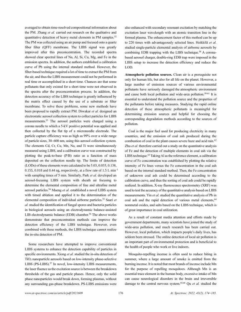
www.at-spectrosc.com/as/article/pdf/2021609 176 At. Spectrosc. 2022, 43(2), 174–185.
averaged to obtain time-resolved compositional information about
the PM. Zhang et al. carried out research on the qualitative and
quantitative detection of heavy metal elements in PM samples.52
The PM was collected using an air pump and focused onto a quartz
fiber filter (QFF) membrane. The LIBS signal was greatly
improved after this preconcentration. The recorded spectra
showed clear spectral lines of Na, Al, Si, Cu, Mg, and Fe in the
emission spectra. In addition, the authors established a calibration
curve of Pb using the internal standard method. However, the
filter-based technique required a lot of time to extract the PM from
the air, and thus the LIBS measurement could not be performed in
real time or accomplished in a short time. Chances are that some
pollutants that only existed for a short time were not observed in
the spectra after the preconcentration process. In addition, the
detection accuracy of the LIBS technique is greatly influenced by
the matrix effect caused by the use of a substrate or filter
membrane. To solve these problems, some new methods have
been proposed to rapidly extract PM. Diwakar et al. designed an
electrostatic aerosol collection system to collect particles for LIBS
measurements.53 The aerosol particles were charged using a
corona needle to which a 5-kV positive potential was applied and
then collected by the flat tip of a microneedle electrode. The
particle capture efficiency was as high as 99% over a wide range
of particle sizes, 30–600 nm, using this aerosol collection system.
The elements Cd, Cr, Cu, Mn, Na, and Ti were simultaneously
measured using LIBS, and a calibration curve was constructed by
plotting the peak-to-base (P/B) ratio as a function of mass
deposited on the collection needle tip. The limits of detection
(LODs) of these elements were calculated to be 5.03, 0.035, 0.138,
0.155, 0.018 and 0.44 ng, respectively, at a flow rate of 1.5 L min-1
with sampling times of 5 min. Similarly, Park et al. developed an
aerosol-focusing LIBS system with sheath air focusing to
determine the elemental composition of fine and ultrafine metal
aerosol particles.54 Maeng et al. established a novel LIBS system
with timed ablation and applied it to the determination of the
elemental composition of individual airborne particles.55 Saari et
al. studied the identification of fungal spores and bacteria particles
in biological aerosols using an electrodynamic balance-assisted
LIB electrodynamic balance (EDB) chamber.56 The above works
demonstrate that preconcentration methods can improve the
detection efficiency of the LIBS technique. However, even
combined with these methods, the LIBS technique cannot realize
the in-situ detection of PM.
Some researchers have attempted to improve conventional
LIBS systems to enhance the detection capability of particles in
specific environments. Xiong et al. studied the in-situ detection of
TiO2 nanoparticle aerosols based on low-intensity phase-selective
LIBS (PS-LIBS).57 In novel, low-intensity LIBS measurements,
the laser fluence as the excitation source is between the breakdown
thresholds of the gas and particle phases. Hence, only the solid
phase nanoparticles would break down, forming plasmas, without
any surrounding gas-phase breakdown. PS-LIBS emissions were
also enhanced with secondary resonant excitation by matching the
excitation laser wavelength with an atomic transition line in the
formed plasma. The enhancement factor of this method can be up
to 220 times with advantageously selected lines. Heikkilä et al.
studied single-particle elemental analysis of airborne aerosols by
combining EDB trapping with the LIBS technique.58 A corona-
based aerosol charger, double-ring EDB trap were imposed in the
LIBS setup to increase the detection efficiency and reduce the
LOD.
Atmospheric pollution sources. Clean air is a prerequisite not
only for human life, but also for all life on the planet. However, a
large number of emission sources of various environmental
pollutants have seriously damaged the atmospheric environment
and cause both local pollution and wide-area pollution.59-61 It is
essential to understand the pollution source and the properties of
the pollutants before taking measures. Studying the rapid online
detection of these atmospheric pollutants is meaningful for
determining emission sources and helpful for choosing the
corresponding degradation methods according to the sources of
pollution.
Coal is the major fuel used for producing electricity in many
countries, and the emission of coal ash produced during the
combustion of coal in the plant causes severe haze and acid rain.62
Zhu et al. therefore carried out a study on the quantitative analysis
of Fe and the detection of multiple elements in coal ash via the
LIBS technique.63 Taking Al as the reference element, a calibration
curve of Fe concentration was established by plotting the relative
intensity of Fe lines versus the Fe concentration in the coal ash
based on the internal standard method. Then, the Fe concentration
of unknown coal ash could be determined according to the
calibration curve, and thus the sorting of coal ash could be rapidly
realized. In addition, X-ray fluorescence spectrometry (XRF) was
used to test the accuracy of the quantitative analysis based on LIBS
measurements. Yin et al. studied the quantitative analysis of Pb in
coal ash and the rapid detection of various metal elements,64
nonmetal oxides, and salts based on the LIBS technique, which is
of great importance in coal utilization.
As a result of constant media attention and efforts made by
government departments, many scientists have joined the study of
wide-area pollution, and much research has been carried out.
However, local pollution, which impacts people’s daily lives, has
seldom been stressed. The online detection of local air pollution is
an important part of environmental protection and is beneficial to
the health of people who work or live indoors.
Mosquito-repelling incense is often used to reduce biting in
summer, where a large amount of smoke is emitted from the
burning incense. It is noted that most brands of incense include Mn
for the purpose of repelling mosquitoes. Although Mn is an
essential trace element in the human body, excessive intake of Mn
can cause neurological disorders in the brain and irreversible
damage to the central nervous system.65,66 Qu et al. studied the
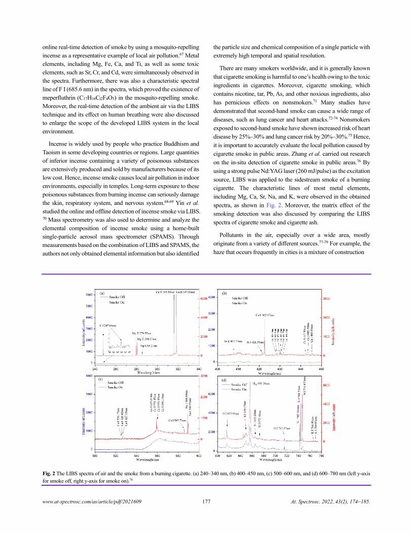
www.at-spectrosc.com/as/article/pdf/2021609 177 At. Spectrosc. 2022, 43(2), 174–185.
online real-time detection of smoke by using a mosquito-repelling
incense as a representative example of local air pollution.67 Metal
elements, including Mg, Fe, Ca, and Ti, as well as some toxic
elements, such as Sr, Cr, and Cd, were simultaneously observed in
the spectra. Furthermore, there was also a characteristic spectral
line of F I (685.6 nm) in the spectra, which proved the existence of
meperfluthrin (C17H16Cl2F4O3) in the mosquito-repelling smoke.
Moreover, the real-time detection of the ambient air via the LIBS
technique and its effect on human breathing were also discussed
to enlarge the scope of the developed LIBS system in the local
environment.
Incense is widely used by people who practice Buddhism and
Taoism in some developing countries or regions. Large quantities
of inferior incense containing a variety of poisonous substances
are extensively produced and sold by manufacturers because of its
low cost. Hence, incense smoke causes local air pollution in indoor
environments, especially in temples. Long-term exposure to these
poisonous substances from burning incense can seriously damage
the skin, respiratory system, and nervous system.68-69 Yin et al.
studied the online and offline detection of incense smoke via LIBS.
70 Mass spectrometry was also used to determine and analyze the
elemental composition of incense smoke using a home-built
single-particle aerosol mass spectrometer (SPAMS). Through
measurements based on the combination of LIBS and SPAMS, the
authors not only obtained elemental information but also identified
the particle size and chemical composition of a single particle with
extremely high temporal and spatial resolution.
There are many smokers worldwide, and it is generally known
that cigarette smoking is harmful to one’s health owing to the toxic
ingredients in cigarettes. Moreover, cigarette smoking, which
contains nicotine, tar, Pb, As, and other noxious ingredients, also
has pernicious effects on nonsmokers.71 Many studies have
demonstrated that second-hand smoke can cause a wide range of
diseases, such as lung cancer and heart attacks.72-74 Nonsmokers
exposed to second-hand smoke have shown increased risk of heart
disease by 25%–30% and lung cancer risk by 20%–30%.75 Hence,
it is important to accurately evaluate the local pollution caused by
cigarette smoke in public areas. Zhang et al. carried out research
on the in-situ detection of cigarette smoke in public areas.76 By
using a strong pulse Nd:YAG laser (260 mJ/pulse) as the excitation
source, LIBS was applied to the sidestream smoke of a burning
cigarette. The characteristic lines of most metal elements,
including Mg, Ca, Sr, Na, and K, were observed in the obtained
spectra, as shown in Fig. 2. Moreover, the matrix effect of the
smoking detection was also discussed by comparing the LIBS
spectra of cigarette smoke and cigarette ash.
Pollutants in the air, especially over a wide area, mostly
originate from a variety of different sources.77-79 For example, the
haze that occurs frequently in cities is a mixture of construction
Fig. 2 The LIBS spectra of air and the smoke from a burning cigarette. (a) 240–340 nm, (b) 400–450 nm, (c) 500–600 nm, and (d) 600–780 nm (left y-axis
for smoke off, right y-axis for smoke on).76
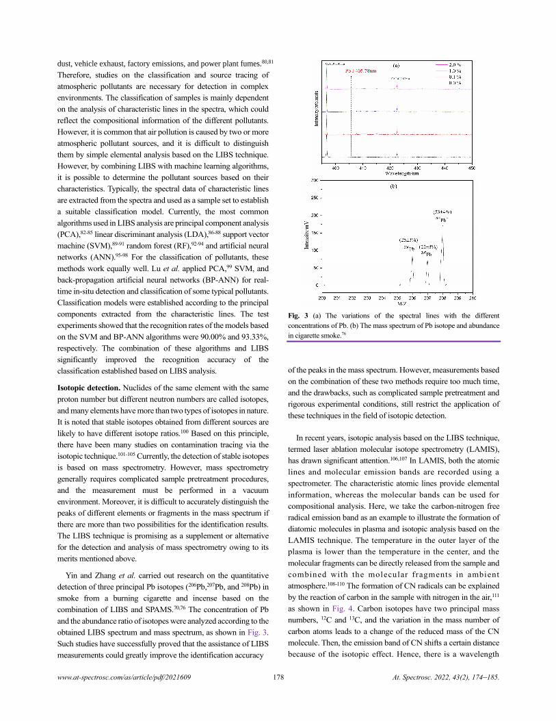
www.at-spectrosc.com/as/article/pdf/2021609 178 At. Spectrosc. 2022, 43(2), 174–185.
dust, vehicle exhaust, factory emissions, and power plant fumes.80,81
Therefore, studies on the classification and source tracing of
atmospheric pollutants are necessary for detection in complex
environments. The classification of samples is mainly dependent
on the analysis of characteristic lines in the spectra, which could
reflect the compositional information of the different pollutants.
However, it is common that air pollution is caused by two or more
atmospheric pollutant sources, and it is difficult to distinguish
them by simple elemental analysis based on the LIBS technique.
However, by combining LIBS with machine learning algorithms,
it is possible to determine the pollutant sources based on their
characteristics. Typically, the spectral data of characteristic lines
are extracted from the spectra and used as a sample set to establish
a suitable classification model. Currently, the most common
algorithms used in LIBS analysis are principal component analysis
(PCA),82-85 linear discriminant analysis (LDA),86-88 support vector
machine (SVM),89-91 random forest (RF),92-94 and artificial neural
networks (ANN).95-98 For the classification of pollutants, these
methods work equally well. Lu et al. applied PCA,99 SVM, and
back-propagation artificial neural networks (BP-ANN) for real-
time in-situ detection and classification of some typical pollutants.
Classification models were established according to the principal
components extracted from the characteristic lines. The test
experiments showed that the recognition rates of the models based
on the SVM and BP-ANN algorithms were 90.00% and 93.33%,
respectively. The combination of these algorithms and LIBS
significantly improved the recognition accuracy of the
classification established based on LIBS analysis.
Isotopic detection. Nuclides of the same element with the same
proton number but different neutron numbers are called isotopes,
and many elements have more than two types of isotopes in nature.
It is noted that stable isotopes obtained from different sources are
likely to have different isotope ratios.100 Based on this principle,
there have been many studies on contamination tracing via the
isotopic technique.101-105 Currently, the detection of stable isotopes
is based on mass spectrometry. However, mass spectrometry
generally requires complicated sample pretreatment procedures,
and the measurement must be performed in a vacuum
environment. Moreover, it is difficult to accurately distinguish the
peaks of different elements or fragments in the mass spectrum if
there are more than two possibilities for the identification results.
The LIBS technique is promising as a supplement or alternative
for the detection and analysis of mass spectrometry owing to its
merits mentioned above.
Yin and Zhang et al. carried out research on the quantitative
detection of three principal Pb isotopes (206Pb,207Pb, and 208Pb) in
smoke from a burning cigarette and incense based on the
combination of LIBS and SPAMS.70,76 The concentration of Pb
and the abundance ratio of isotopes were analyzed according to the
obtained LIBS spectrum and mass spectrum, as shown in Fig. 3.
Such studies have successfully proved that the assistance of LIBS
measurements could greatly improve the identification accuracy
Fig. 3 (a) The variations of the spectral lines with the different
concentrations of Pb. (b) The mass spectrum of Pb isotope and abundance
in cigarette smoke.76
of the peaks in the mass spectrum. However, measurements based
on the combination of these two methods require too much time,
and the drawbacks, such as complicated sample pretreatment and
rigorous experimental conditions, still restrict the application of
these techniques in the field of isotopic detection.
In recent years, isotopic analysis based on the LIBS technique,
termed laser ablation molecular isotope spectrometry (LAMIS),
has drawn significant attention.106,107 In LAMIS, both the atomic
lines and molecular emission bands are recorded using a
spectrometer. The characteristic atomic lines provide elemental
information, whereas the molecular bands can be used for
compositional analysis. Here, we take the carbon-nitrogen free
radical emission band as an example to illustrate the formation of
diatomic molecules in plasma and isotopic analysis based on the
LAMIS technique. The temperature in the outer layer of the
plasma is lower than the temperature in the center, and the
molecular fragments can be directly released from the sample and
combined with the molecular fragments in ambient
atmosphere.108-110 The formation of CN radicals can be explained
by the reaction of carbon in the sample with nitrogen in the air,111
as shown in Fig. 4. Carbon isotopes have two principal mass
numbers, 12C and 13C, and the variation in the mass number of
carbon atoms leads to a change of the reduced mass of the CN
molecule. Then, the emission band of CN shifts a certain distance
because of the isotopic effect. Hence, there is a wavelength
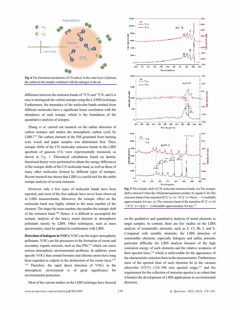
www.at-spectrosc.com/as/article/pdf/2021609 179 At. Spectrosc. 2022, 43(2), 174–185.
Fig. 4 The formation mechanism of CN radical. In the outer layer of plasma,
the carbon in the sample combined with the nitrogen in the air.
difference between the emission bands of 12CN and 13CN, and it is
easy to distinguish the carbon isotopes using the LAMIS technique.
Furthermore, the intensities of the molecular bands emitted from
different molecules have a significant linear correlation with the
abundance of each isotope, which is the foundation of the
quantitative analysis of isotopes.
Zhang et al. carried out research on the online detection of
carbon isotopes and studies the atmospheric carbon cycle by
LIBS.112 The carbon element in the PM generated from burning
coal, wood, and paper samples was determined first. Then,
isotopic shifts of the CN molecular emission bands in the LIBS
spectrum of gaseous CO2 were experimentally measured, as
shown in Fig. 5. Theoretical calculations based on density
functional theory were performed to obtain the energy differences
of the isotopic shifts of the CN molecular band, as well as those of
many other molecules formed by different types of isotopes.
Recent research has shown that LIBS is a useful tool for the stable
isotope analysis of several elements.
However, only a few types of molecular bands have been
reported, and most of the free radicals have never been observed
in LIBS measurements. Moreover, the isotopic effect on the
molecular band was highly related to the mass number of the
element. The larger the mass number, the smaller the isotopic shift
of the emission band.106 Hence, it is difficult to accomplish the
isotopic analysis of the heavy metal element in atmospheric
pollutants merely by LIBS. Other techniques, such as mass
spectrometry, must be applied in combination with LIBS.
Detection of halogens in VOCs. VOCs are the major atmospheric
pollutants. VOCs are the precursors to the formation of ozone and
secondary organic aerosols, such as fine PM,113 which can cause
serious atmospheric environmental problems. In addition, some
specific VOCs that contain bromine and chlorine atoms have long
been regarded as culprits in the destruction of the ozone layer.114-
115 Therefore, the rapid direct detection of VOCs in the
atmospheric environment is of great significance for
environmental protection.
Most of the current studies on the LIBS technique have focused
Fig. 5 The isotopic shift of CN molecular emission bands. (a) The isotopic
shift is almost 0 when the vibrational quantum number Δν equals 0. (b) The
emission band of the transition B2 Σ+ (ν=1)→X2 Σ+ (ν=0)(∆ν = +1) redshifts
approximately 0.6 nm. (c) The emission band of the transition B2 Σ+ (ν=0)
→X2 Σ+ (ν=1)(∆ν = -1) blueshifts approximately 0.8 nm.112
on the qualitative and quantitative analysis of metal elements in
target samples. In contrast, there are few studies on the LIBS
analysis of nonmetallic elements, such as F, Cl, Br, I, and S.
Compared with metallic elements, the LIBS detection of
nonmetallic elements, especially halogens and sulfur, presents
particular difficulty for LIBS analysis because of the high
ionization energy of such elements and the relative weakness of
their spectral lines,116 which is unfavorable for the appearance of
the characteristic emission lines in the measurements. Furthermore,
most of the spectral lines of such elements lie in the vacuum
ultraviolet (VUV) (110–190 nm) spectral range,117 and the
requirement for the collection of emission spectra is so robust that
it hinders the development of LIBS applications in environmental
detection.
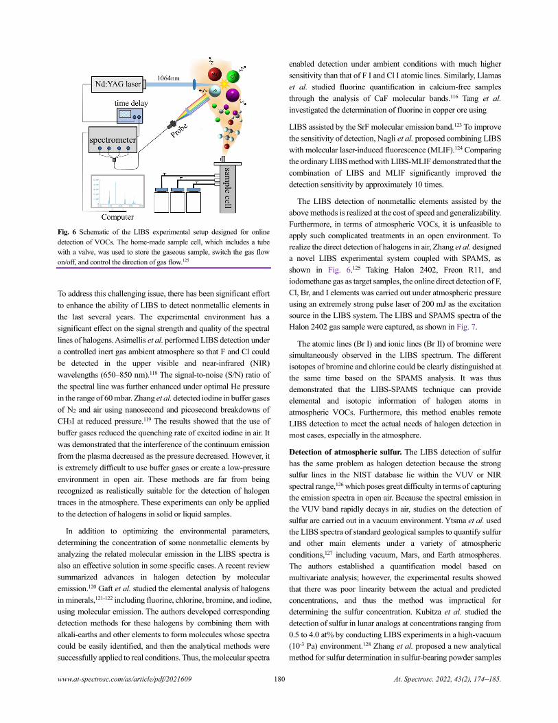
www.at-spectrosc.com/as/article/pdf/2021609 180 At. Spectrosc. 2022, 43(2), 174–185.
Fig. 6 Schematic of the LIBS experimental setup designed for online
detection of VOCs. The home-made sample cell, which includes a tube
with a valve, was used to store the gaseous sample, switch the gas flow
on/off, and control the direction of gas flow.125
To address this challenging issue, there has been significant effort
to enhance the ability of LIBS to detect nonmetallic elements in
the last several years. The experimental environment has a
significant effect on the signal strength and quality of the spectral
lines of halogens. Asimellis et al. performed LIBS detection under
a controlled inert gas ambient atmosphere so that F and Cl could
be detected in the upper visible and near-infrared (NIR)
wavelengths (650–850 nm).118 The signal-to-noise (S/N) ratio of
the spectral line was further enhanced under optimal He pressure
in the range of 60 mbar. Zhang et al. detected iodine in buffer gases
of N2 and air using nanosecond and picosecond breakdowns of
CH3I at reduced pressure.119 The results showed that the use of
buffer gases reduced the quenching rate of excited iodine in air. It
was demonstrated that the interference of the continuum emission
from the plasma decreased as the pressure decreased. However, it
is extremely difficult to use buffer gases or create a low-pressure
environment in open air. These methods are far from being
recognized as realistically suitable for the detection of halogen
traces in the atmosphere. These experiments can only be applied
to the detection of halogens in solid or liquid samples.
In addition to optimizing the environmental parameters,
determining the concentration of some nonmetallic elements by
analyzing the related molecular emission in the LIBS spectra is
also an effective solution in some specific cases. A recent review
summarized advances in halogen detection by molecular
emission.120 Gaft et al. studied the elemental analysis of halogens
in minerals,121-122 including fluorine, chlorine, bromine, and iodine,
using molecular emission. The authors developed corresponding
detection methods for these halogens by combining them with
alkali-earths and other elements to form molecules whose spectra
could be easily identified, and then the analytical methods were
successfully applied to real conditions. Thus, the molecular spectra
enabled detection under ambient conditions with much higher
sensitivity than that of F I and Cl I atomic lines. Similarly, Llamas
et al. studied fluorine quantification in calcium-free samples
through the analysis of CaF molecular bands.116 Tang et al.
investigated the determination of fluorine in copper ore using
LIBS assisted by the SrF molecular emission band.123 To improve
the sensitivity of detection, Nagli et al. proposed combining LIBS
with molecular laser-induced fluorescence (MLIF).124 Comparing
the ordinary LIBS method with LIBS-MLIF demonstrated that the
combination of LIBS and MLIF significantly improved the
detection sensitivity by approximately 10 times.
The LIBS detection of nonmetallic elements assisted by the
above methods is realized at the cost of speed and generalizability.
Furthermore, in terms of atmospheric VOCs, it is unfeasible to
apply such complicated treatments in an open environment. To
realize the direct detection of halogens in air, Zhang et al. designed
a novel LIBS experimental system coupled with SPAMS, as
shown in Fig. 6.125 Taking Halon 2402, Freon R11, and
iodomethane gas as target samples, the online direct detection of F,
Cl, Br, and I elements was carried out under atmospheric pressure
using an extremely strong pulse laser of 200 mJ as the excitation
source in the LIBS system. The LIBS and SPAMS spectra of the
Halon 2402 gas sample were captured, as shown in Fig. 7.
The atomic lines (Br I) and ionic lines (Br II) of bromine were
simultaneously observed in the LIBS spectrum. The different
isotopes of bromine and chlorine could be clearly distinguished at
the same time based on the SPAMS analysis. It was thus
demonstrated that the LIBS-SPAMS technique can provide
elemental and isotopic information of halogen atoms in
atmospheric VOCs. Furthermore, this method enables remote
LIBS detection to meet the actual needs of halogen detection in
most cases, especially in the atmosphere.
Detection of atmospheric sulfur. The LIBS detection of sulfur
has the same problem as halogen detection because the strong
sulfur lines in the NIST database lie within the VUV or NIR
spectral range,126 which poses great difficulty in terms of capturing
the emission spectra in open air. Because the spectral emission in
the VUV band rapidly decays in air, studies on the detection of
sulfur are carried out in a vacuum environment. Ytsma et al. used
the LIBS spectra of standard geological samples to quantify sulfur
and other main elements under a variety of atmospheric
conditions,127 including vacuum, Mars, and Earth atmospheres.
The authors established a quantification model based on
multivariate analysis; however, the experimental results showed
that there was poor linearity between the actual and predicted
concentrations, and thus the method was impractical for
determining the sulfur concentration. Kubitza et al. studied the
detection of sulfur in lunar analogs at concentrations ranging from
0.5 to 4.0 at% by conducting LIBS experiments in a high-vacuum
(10-3 Pa) environment.128 Zhang et al. proposed a new analytical
method for sulfur determination in sulfur-bearing powder samples
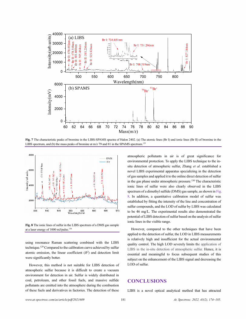
www.at-spectrosc.com/as/article/pdf/2021609 181 At. Spectrosc. 2022, 43(2), 174–185.
Fig. 7 The characteristic peaks of bromine in the LIBS-SPAMS spectra of Halon 2402. (a) The atomic lines (Br I) and ionic lines (Br II) of bromine in the
LIBS spectrum, and (b) the mass peaks of bromine at m/z 79 and 81 in the SPAMS spectrum.125
Fig. 8 The ionic lines of sulfur in the LIBS spectrum of a DMS gas sample
at a laser energy of 1000 mJ/pulse.130
using resonance Raman scattering combined with the LIBS
technique.129 Compared to the calibration curve achieved by sulfur
atomic emission, the linear coefficient (R2) and detection limit
were significantly better.
However, this method is not suitable for LIBS detection of
atmospheric sulfur because it is difficult to create a vacuum
environment for detection in air. Sulfur is widely distributed in
coal, petroleum, and other fossil fuels, and massive sulfide
pollutants are emitted into the atmosphere during the combustion
of these fuels and derivatives in factories. The detection of these
atmospheric pollutants in air is of great significance for
environmental protection. To apply the LIBS technique to the in-
situ detection of atmospheric sulfur, Zhang et al. established a
novel LIBS experimental apparatus specializing in the detection
of gas samples and applied it to the online direct detection of sulfur
in the gas phase under atmospheric pressure.130 The characteristic
ionic lines of sulfur were also clearly observed in the LIBS
spectrum of a dimethyl sulfide (DMS) gas sample, as shown in Fig.
8. In addition, a quantitative calibration model of sulfur was
established by fitting the intensity of the line and concentration of
sulfur compounds, and the LOD of sulfur by LIBS was calculated
to be 46 mg/L. The experimental results also demonstrated the
potential of LIBS detection of sulfur based on the analysis of sulfur
ionic lines in the visible range.
However, compared to the other techniques that have been
applied to the detection of sulfur, the LOD in LIBS measurements
is relatively high and insufficient for the actual environmental
quality control. The high LOD severely limits the application of
LIBS in the in-situ detection of atmospheric sulfur. Hence, it is
essential and meaningful to focus subsequent studies of this
subject on the enhancement of the LIBS signal and decreasing the
LOD of sulfur.
CONCLUSIONS
LIBS is a novel optical analytical method that has attracted
www.at-spectrosc.com/as/article/pdf/2021609 182 At. Spectrosc. 2022, 43(2), 174–185.
significant attention in recent years. Because of its unique
advantages in terms of rapid and precise response, noncontact
measurement, and simultaneous multi-element analysis, the LIBS
technique has been expected to play an important role in the field
of environment detection or even replace conventional analytical
methods under some circumstances since its inception. However,
compared with the detection of solids, liquids, and aerosols,
progress in atmospheric detection by LIBS was disappointingly
slow in the early years. As some advanced laser techniques,
including femtosecond pulse lasers, have become available, and
the fundamental theory of light-matter interaction has been
improved, development in this field has significantly increased in
the last few decades.
In this review, a brief introduction to the in-situ online detection
of the atmospheric environmental pollutants using the LIBS
technique is presented, and we have highlighted recent advances
in the research on the LIBS detection of atmospheric particulate
matter, atmospheric pollution sources, and stable isotope
abundance.
Over the past 30 years, the experimental instruments, methods,
and analytical algorithms have been greatly improved, and LIBS
detection now stands at its highest level of functionality. Our
current research on the in-situ online detection of atmospheric
environmental pollutants is focused on using LIBS to detect
pollutants with extremely low concentrations and the analysis of
the molecular structure of the organic matter.
AUTHOR INFORMATION
Yuzhu Liu is a full professor and vice director
of Jiangsu Key Laboratory for Optoelectronic
Detection of Atmosphere and Ocean at
Nanjing University of Information Science
and Technology (NUIST). He received his
PhD in physics from Wuhan institute of
Physics and Mathematics, Chinese Academy
of Sciences (June 2011). After completing his
Ph.D., he came to Paul Scherrer Institute in
Switzerland for post-doctoral research. In September 2014, he returned to
China and joined NUIST for professorship. His research interests include
laser-induced breakdown spectroscopy, Raman spectroscopy, ultrafast
molecular dynamics, photoelectron imaging technique, and time-of-flight
mass spectrometry. He is currently working on instrumentation
developments and investigations for the project of online in situ detection
of elements or pollutions in the atmosphere via LIBS. He has published
over 100 peer-reviewed scientific papers in ISI-indexed journals.
Corresponding Author
*Y. Z. Liu
Email address: [email protected]
Notes
The authors declare no competing financial interest.
ACKNOWLEDGMENTS
This work was supported by National Key R&D Program of
China (2017YFC0212700), National Natural Science Foundation
of China (U1932149), Natural Science Foundation of Jiangsu
Province (BK20191395), Key Research and Development
Program of Anhui Province (202104i07020009), and
Postgraduate Research & Practice Innovation Program of Jiangsu
Province (KYCX21_0989).
REFERENCES
1. M. Kapma and E. Castanas, Environ. Pollut., 2008, 151, 362–367.
https://doi.org/10.1016/j.envpol.2007.06.012
2. R. Atkinson, Atmos. Environ., 2000, 34, 2063–2101.
https://doi.org/10.1016/S1352-2310(99)00460-4
3. J. H. Kroll and J. H. Seinfeld, Atmos. Environ., 2008, 42,
3593–3624. https://doi.org/10.1016/j.atmosenv.2008.01.003
4. R. S. Harmon, R. E. Russo, and R. R. Hark, Spectrochim. Acta B,
2013, 87, 11–26. https://doi.org/10.1016/j.sab.2013.05.017
5. M. Baudelet and B. W. Smith, J. Anal. At. Spectrom., 2013, 28,
624–629. https://doi.org/10.1039/C3JA50027F
6. E.F. Runge, R.W. Minck, and F.R. Bryan, Spectrochim. Acta B,
1964, 20, 733–736. https://doi.org/10.1016/0371-1951(64)80070-9
7. J. El Haddad, L. Canioni, and B. Bousquet, Spectrochim. Acta B,
2014, 101, 171–182. https://doi.org/10.1016/j.sab.2014.08.039
8. S. Shin, Y. Moon, J. Lee, H. Jang, E. Hwang, and S. Jeong,
Plasma Sci. Technol., 2019, 21, 034011.
https://doi.org/10.1088/2058-6272/aaed6c
9. B. Campanella, E. Grifoni, S. Legnaioli, G. Lorenzetti, S. Pagnotta,
F. Sorrentino, and V. Palleschi, Spectrochim. Acta B, 2017, 134,
52–57. https://doi.org/10.1016/j.sab.2017.06.003
10. S. B. Roh, S. B. Park, S. K. Oh, E. K. Park, and W. Z. Choi,
J. Mater. Cycles Waste Manage., 2018, 20, 1934–1949.
https://doi.org/10.1007/s10163-018-0701-1
11. H. Jull, J. Bier, R. Künnemeyer, and P. Schaare, Spectrosc. Lett.,
2018, 51, 1–9. https://doi.org/10.1080/00387010.2018.1466806
12. C. P. M. Roux, J. Rakovský, O. Musset, F. Monna, J. F.
Buoncristiani, P. Pellenard, and C. Thomazo, Spectrochim. Acta B,
2018, 103-104, 63–69. https://doi.org/10.1016/j.sab.2014.11.013
13. S. Sheta, M. S. Afgan, Z. Y. Hou, S. C. Yao, L. Zhang, Z. Li, and
Z. Wang, J. Anal. At. Spectrom., 2019, 34, 1047–1082.
https://doi.org/10.1039/C9JA00016J
14. S. Legnaioli, B. Campanella, S. Pagnotta, F. Poggialini, and
V. Palleschi, Spectrochim. Acta B, 2019, 155, 123–126.
https://doi.org/10.1016/j.sab.2019.03.012
15. C. H. Yan, J. Qi, J. Ma, H. S. Tang, T. L. Zhang, and H. Li,
Chemom. Intell. Lab. Syst., 2017, 167, 226–231.
https://doi.org/10.1016/j.chemolab.2017.06.006
16. A. Metzinger, D. J. Palásti, É. Kovács-Széles, T. Ajtai, Z. Bozóki,
www.at-spectrosc.com/as/article/pdf/2021609 183 At. Spectrosc. 2022, 43(2), 174–185.
Z. Kónya, and G. Galbács, Energy Fuels, 2016, 30, 10306–10313.
https://doi.org/10.1021/acs.energyfuels.6b02279
17. J. Y. Peng, W. Y. Xie, J. D. Jiang, Z. F. Zhao, F. Zhou, and F. Liu,
Foods, 2020, 9, 341. https://doi.org/10.3390/foods9030341
18. F. O. Leme, D. M. Silvestre, A. N. Nascimento, and C. S. Nomura,
J. Anal. At. Spectrom., 2018, 33, 1322–1329.
https://doi.org/10.1039/C8JA00115D
19. J. Wang, P. C. Zheng, H. D. Liu, and F. Liang, Anal. Methods,
2016, 8, 3204–3209. https://doi.org/10.1039/C5AY03260A
20. J. Wu, Y. Liu, Y. W. Cui, X. H. Zhao, and D. M. Dong,
Biosens. Bioelectron., 2019, 142, 111508.
https://doi.org/10.1016/j.bios.2019.111508
21. Y. M. Moon, J. H. Han, H. H. Choi, S. Shin, Y. C. Kim, and
S. Jeong, J. Biomed. Opt., 2018, 24, 031011.
https://doi.org/10.1117/1.jbo.24.3.031011
22. N. Killiny, E. Etxeberria, A. P. Flores, P. G. Blanco, T. F. Reyes,
and L. P. Cabrera, Sci. Rep., 2019, 9, 2449.
https://doi.org/10.1038/s41598-019-39164-8
23. N. Li, J. Guo, C. Zhang, Y. Zhang, Q. Li, Y. Tian, and R. E. Zheng,
Appl. Opt., 2019, 58, 3886–3891.
https://doi.org/10.1364/ao.58.003886
24. V. K. Singh, D. K. Tripathi, X. Mao, R. Russo, and V. Zorba,
Appl. Spectrosc., 2019, 73, 387–394.
https://doi.org/10.1177/0003702819830394
25. Rehan, M. A. Gondal, and K. Rehan, Talanta, 2018, 182, 443–449.
https://doi.org/10.1016/j.talanta.2018.02.024
26. S. M. Zaytsev, I. N. Krylov, A. M. Popov, N. B. Zorov, and
T. A. Labutin, Spectrochim. Acta B, 2018, 140, 65–72.
https://doi.org/10.1016/j.sab.2017.12.005
27. J. J. Guo, A. S. Mahmoud, N. Li, J. J. Song, and R. E. Zheng,
Plasma Sci. Technol., 2018, 21, 034022.
https://doi.org/10.1088/2058-6272/aaf091
28. P. P. Sheng, L. L. Jiang, M.D. Sui, and S.L. Zhong,
Spectrochim. Acta B, 2019, 154, 1–9.
https://doi.org/10.1016/j.sab.2019.02.002
29. B. Thornton, T. Takahashi, T. Sato, T. Sakka, A. Tamura, A.
Matsumoto, T. Nozaki, T. Ohki, and K. Ohki, Deep Sea Res., Part
I., 2018, 95, 20–36. https://doi.org/10.1016/j.dsr.2014.10.006
30. S. Guirado, F. J. Fortes, V. Lazic, and J. J. Laserna,
Spectrochim. Acta B, 2012, 74-75, 137–143.
https://doi.org/10.1016/j.sab.2012.06.032
31. N. Murdoch, B. Chide, J. Lasue, A. Cadu, A. Sournac,
M. Bassas-Portús, X. Jacob, J. Merrison, J. J. Iversen, C. Moretto,
C. Velasco, L. Parès, A. Hynes, V. Godiver, R. D. Lorenz, P. Cais,
P. Bernadi, S. Maurice, R. C. Wiens, and D. Mimoun,
Planet. Space Sci., 2018, 165, 260–271.
https://doi.org/10.1016/j.pss.2018.09.009
32. D. S. Vogt, K. Rammelkamp, S. Schröder, and H.W. Hübers,
Icarus, 2018, 302, 470–482.
https://doi.org/10.1016/j.icarus.2017.12.006
33. W. Rapin, P. Y. Meslin, S. Maurice, R. C. Wiens, D. Laporte,
B. Chauviré, O. Gasnault, S. Schröder, P. Beck, S. Bender, O.
Beyssac, A. Cousin, E. Dehouck, C. Drouet, O. Forni, M. Nachon,
N. Melikechi, B. Rondeau, N. Mangold, and N. H. Thomas,
Spectrochim. Acta B, 2017, 130, 82–100.
https://doi.org/10.1016/j.sab.2017.02.007
34. Q. H. Zhang, Y. Z. Liu, W. Y. Yin, F. Jin, F. B. Zhou, and
Y. L. Zhang, Laser Phys., 2018, 28, 085703.
https://doi.org/10.1088/1555-6611/aac71c
35. L. J. Radziemski, Spectrochim. Acta B, 2002, 57, 1109–1113.
https://doi.org/10.1016/S0584-8547(02)00052-6
36. S. Moncayo, S. Manzoor, J. D. Rosales, J. Anzano, and
J. O. Caceres, Food Chem., 2017, 232, 322–328.
http://dx.doi.org/10.1016/j.foodchem.2017.04.017
37. A. Ruas, A. Matsumoto, H. Ohba, K. Akaoka, and I. Wakaida,
Spectrochim. Acta B, 2017, 131, 99–106.
https://doi.org/10.1016/j.sab.2017.03.014
38. D. A. Redoglio, N. Palazzo, F. Migliorini, R. Dondè, and
S. De Iuliis, Appl. Spectrosc., 2017, 72, 584–590.
https://doi.org/10.1177/0003702817742314
39. Y. Wang, A. M. Chen, D. Zhang, Q. Y. Wang, S. Y. Li, Y. F. Jiang,
and M. X. Jin, Phys. Plasmas., 2020, 27, 023507.
https://doi.org/10.1063/1.5131772
40. I. C. García, J. M. Vadillo, and J. J. Laserna, J. Anal. At. Spectrom.,
2019, 34, 2119–2125. https://doi.org/10.1039/c9ja00196d
41. J. Y. Peng, Y. He, Z. F. Zhao, J. D. Jiang, F. Zhou, F. Liu, and
T. T. Shen, Environ. Pollut., 2019, 252, 1125–1132.
https://doi.org/10.1016/j.envpol.2019.06.027
42. M. Burger, P. J. Skrodzki, L. A. Finney, J. Hermann, J. Nees, and
I. Jovanovic, Phys. Plasmas., 2018, 25, 083115.
https://doi.org/10.1063/1.5042665
43. R. Noll, C. F. Begemann, S. Connemann, C. Meinhardt, and
V. Sturm, J. Anal. At. Spectrom., 2018, 33, 945–956.
https://doi.org/10.1039/c8ja00076j
44. G. Galbács, Anal. Bioanal. Chem., 2015, 407, 7537–7562.
https://doi.org/10.1007/s00216-015-8855-3
45. D. W. Hahn and N. Omenetto, Appl. Spectrosc., 2010, 64,
335A–336A. https://doi.org/10.1366/000370210793561691
46. D. W. Hahn and N. Omenetto, Appl. Spectrosc., 2012, 66, 347–419.
https://doi.org/10.1366/11-06574
47. M. T. Jin, H. Yuan, B. Liu, J. J. Peng, L. P. Xu, and D. Z. Yang,
Anal. Methods, 2020, 12, 5747–5766.
https://doi.org/10.1039/D0AY01577F
48. W. T. Li, X. Y. Li, X. Li, Z. Q. Hao, Y. F. Lu, and X. Y. Zeng,
Appl. Spectrosc. Rev., 2020, 55, 1–25.
https://doi.org/10.1080/05704928.2018.1472102
49. X. Hu, Y. Zhang, Z. H. Ding, T. J. Wang, H. Z. Lian, Y. Y. Sun,
and J. C. Wu, Atmos. Environ., 2012, 57, 146–152.
https://doi.org/10.1016/j.atmosenv.2012.04.056
50. Z. J. Hu, Y. L. Shi, H. Y. Niu, and Y. Q. Cai, Atmos. Res., 2012,
104, 302–305. https://doi.org/10.1016/j.atmosres.2011.09.002
51. J. H. Kwak, G. Kim, Y. J. Kim, and K. Park, Aerosol Sci. Technol.,
2012, 46, 1079–1089.
http://dx.doi.org/10.1080/02786826.2012.692492
52. Q. H. Zhang, Y. Z. Liu, R. S. Zhu, F. Jin, F. B. Zhou, and
W. Y. Yin, Laser & Optoelectronics Progress, 2018, 55, 123002.
https://doi.org/10.3788/LOP55.123002
53. P. Diwakar, P. Kulkarni, and E. Birch, Aerosol Sci. Technol., 2012,
46, 316–332. http://dx.doi.org/10.1080/02786826.2011.625059
54. K. Park, G. Cho, and J. H. kwak. Aerosol Sci. Technol., 2009, 43,
375–386. https://doi.org/10.1080/02786820802662947
55. H. Maeng, H. Chae, H. Lee, G. Kim, H. Lee, K. Kim, J. Kwak,
G. Cho, and K. Park, Aerosol Sci. Technol., 2017, 51, 1009–1015.
https://doi.org/10.1080/02786826.2017.1344352
56. S. Saari, S. Järvinen, T. Reponen, J. M. Attipoe, P. Pasanen,
J. Toivonen, and J. Keskinen, Aerosol Sci. Technol., 2016, 50,
126–132. https://doi.org/10.1080/02786826.2015.1134764
57. G. Xiong, S. Q. Li, and S. D. Tse, Spectrochim. Acta B, 2018, 140,
13–21. https://doi.org/10.1016/j.sab.2017.11.013
www.at-spectrosc.com/as/article/pdf/2021609 184 At. Spectrosc. 2022, 43(2), 174–185.
58. P. Heikkilä, J. Rossi, A. Rostedt, J. Huhtala, A. Järvinen,
J. Toivonen, and J. Keskinen, Aerosol Sci. Technol., 2020, 54,
837–848. https://doi.org/10.1080/02786826.2020.1727408
59. S. Wang, A. Salamova, R. A. Hites, and M. Venier,
Environ. Sci. Technol., 2018, 52, 6177–6186.
https://doi.org/10.1021/acs.est.8b00123
60. Y. Guan, G. Chen, Z. Cheng, B. Yan, and L. Hou, Atmos. Environ.,
2017, 171, 155–164.
https://doi.org/10.1016/j.atmosenv.2017.10.020
61. M. Kumar, R. K. Singh, V. Murari, A. K. Singh, R. S. Singh, and
T. Banerjee, Atmos. Res., 2016, 180, 78–91.
https://doi.org/10.1016/j.atmosres.2016.05.014
62. Z. Lu, D. G. Streets, Q. Zhang, S. Wang, G. R. Carmichael,
Y. F. Cheng, C. Wei, M. Chin, T. Diehl, and Q. Tan,
Atmos. Chem. Phys., 2010, 10, 6311–6331.
https://doi.org/10.5194/acp-10-6311-2010
63. R. S. Zhu, Y. Z. Liu, Q. H. Zhang, F. B. Zhou, F. Jin, W. Y. Yin,
and X. F. Zhao, Optik, 2018, 169, 77–84.
https://doi.org/10.1016/j.ijleo.2018.05.035
64. W. Y. Yin, Y. Z. Liu, F. B. Zhou, R. S. Zhu, Q. H. Zhang, and
F. Jin, Optik, 2018, 174, 550–557.
https://doi.org/10.1016/j.ijleo.2018.08.110
65. Z. Y. Li, Z. W. Ma, T. J. Kuijp, Z. W. Yuan, and L. Huang,
Sci. Total Environ., 2014, 468-469, 843–853.
https://doi.org/10.1016/j.scitotenv.2013.08.090
66. C. G. Fraga, Mol. Aspects Med., 2005, 26, 235–244.
https://doi.org/10.1016/j.mam.2005.07.013
67. Y. F. Qu, Q. H. Zhang, W. Y. Yin, Y. C. Hu, and Y. Z. Liu,
Opt. Express, 2019, 27, A790.
https://doi.org/10.1364/OE.27.00A790
68. S. C. Kuo and Y. I. Tsai, Sci. Total Environ., 2017, 584-585,
495–504. https://doi.org/10.1016/j.scitotenv.2017.01.052
69. C. Y. Kuo, Y. H. Yang, M. R. Chao, and C. W. Hu,
Sci. Total Environ., 2008, 401, 44–50.
https://doi.org/10.1016/j.scitotenv.2008.04.018
70. W. Y. Yin, Y. Z. Liu, Q. H. Zhang, P. F. Ding, L. Li, and
G. H. Xing, Opt. Eng., 2020, 59, 026105.
https://doi.org/10.1117/1.OE.59.2.026105
71. S. S. Salvi and P. J. Barnes, Lancet, 2009, 374, 1964–1965.
https://doi.org/10.1016/S0140-6736(09)61303-9
72. S. A. Glantz and W.W. Parmley, Circulation, 1991, 83, 1–12.
https://doi.org/10.1161/01.cir.83.1.1
73. K. K. Teo, S. Ounpuu, S. Hawken, M. Pandey, V. Valentin,
D. Hunt, R. Diaz, W. Rashed, R. Freeman, L. X. Jiang, X. F. Zhang,
and S. Yusuf, Lancet, 2006, 368, 647–658.
https://doi.org/10.1016/s0140-6736(06)69249-0
74. M. Öberg, M.S. Jaakkola, A. Woodward, A. Peruga, and
A.P. Ustün, Lancet, 2011, 377, 139–146.
https://doi.org/10.1016/S0140-6736(10)61388-8
75. J. Barnoya and S.A. Glantz, Circulation., 2005, 111, 2684–2698.
https://doi.org/10.1161/circulationaha.104.492215
76. Q. H. Zhang, Y. Z. Liu, W. Y. Yin, Y. H. Yan, L. Li, and
G. H. Xing, Chemosphere., 2020, 242, 125184.
https://doi.org/10.1016/j.chemosphere.2019.125184
77. X. J. Zhao, P. S. Zhao, J. Xu, W. Meng, W. W. Pu, F. Dong, D. He,
and Q. F. Shi, Atmos. Chem. Phys., 2013, 13, 5685–5696.
https://doi.org/10.5194/acp-13-5685-2013
78. Y. L. Sun, Q. Jiang, Z. F. Wang, P. Q. Fu, J. Li, T. Yang, and
Y. Yin, J. Geophys. Res. Atmos., 2013, 119, 4380–4398.
https://doi.org/10.1002/2014JD021641
79. M. O. Andreae, O. Schmid, H. Yang, D. Chand, J. Z. Yu,
L. M. Zeng, and Y. H. Zhang, Atmos. Environ., 2008, 42,
6335–6350. https://doi.org/10.1016/j.atmosenv.2008.01.030
80. S. T. Massie, O. Torres, and S. J. Smith,
J. Geophys. Res. Atmos., 2004, 109, D18211.
https://doi.org/10.1029/2004JD004620
81. D.G. Streets and S.T. Waldhoff, Atmos. Environ., 2000, 34,
363-374. https://doi.org/10.1016/S1352-2310(99)00167-3
82. S. Chatterjee, M. Singh, B. P. Biswal, U. K. Sinha, S. Patbhaje, and
A. Sarkar, Anal. Bioanal. Chem., 2019, 411, 2855–2866.
https://doi.org/10.1007/s00216-019-01731-3
83. W. L. Liao, Q. Y. Lin, S. C. Xie, Y. He, Y. H. Tian, and
Y. X. Duan, Anal. Chim. Acta, 2018, 1043, 64–71.
https://doi.org/10.1016/j.aca.2018.06.058
84. P. Pořízka, J. Klus, E. Képeš, D. Prochazka, D. W. Hahn, and
J. Kaiser, Spectrochim. Acta B, 2018, 148, 65–82.
https://doi.org/10.1016/j.sab.2018.05.030
85. A. K. Shaik, Ajmathulla, and V. R. Soma, Opt. Lett., 2018, 43,
3465. https://doi.org/10.1364/ol.43.003465
86. Z. F. Zhao, L. Chen, F. Liu, F. Zhou, J. Y. Peng, and M. H. Sun,
Sensors, 2020, 20, 1878. https://doi.org/10.3390/s20071878
87. J. J. Yan, P. Yang, R. Zhou, S. H. Li, K. Liu, W. Zhang, X. Y. Li,
D. Z. Wang, and Y. Lu, Anal. Methods, 2019, 11, 5177–5184.
https://doi.org/10.1039/c9ay01524h
88. G. Guo, G. H. Niu, Q. Shi, Q. Y. Lin, D. Tian, and Y. X. Duan,
Anal. Methods, 2019, 11, 3006–3013.
https://doi.org/10.1039/c9ay00890j
89. O. Gazeli, E. Bellou, D. Stefas, and S. Couris, Food Chem., 2020,
302, 125329. https://doi.org/10.1016/j.foodchem.2019.125329
90. H. B. Peng, G. H. Chen, X. X. Chen, Z. M. Lu, and S. C. Yao,
Plasma Sci. Technol., 2018, 21, 034008.
https://doi.org/10.1088/2058-6272/aaebc4
91. J. Wang, L. Li, P. Yang, Y. Chen, Y. Zhu, M. Tong, Z. Q. Hao, and
X. Y. Li, Lasers Med. Sci., 2018, 33, 1381–1386.
https://doi.org/10.1007/s10103-018-2500-2
92. H. Tang, T. Zhang, X. Yang, and H. Li, Anal. Methods, 2015, 7,
9171–9176. https://doi.org/10.1039/c5ay02208h
93. N. Melikechi, Y. Markushin, D. C. Connolly, J. Lasue,
E. Ewusi-Annan, and S. Makrogiannis, Spectrochim. Acta B, 2016,
123, 33–41. https://doi.org/10.1016/j.sab.2016.07.008
94. L. Y. Zhan, X. H. Ma, W. Q. Fang, R. Wang, Z. S. Liu, Y. Song,
and H. F. Zhao, Plasma Sci. Technol., 2019, 21, 034018.
https://doi.org/10.1088/2058-6272/aaf7bf
95. J. Alvarez, M. Velásquez, A. K. Myakalwar, C. Sandoval,
R. Fuentes, R. Castillo, D. Sbarbaro, and J. Yañez,
J. Anal. At. Spectrom., 2019, 34, 2459–2468.
https://doi.org/10.1039/c9ja00271e
96. R. Junjuri and M.K. Gundawar, J. Anal. At. Spectrom., 2019, 34,
1683–1692. https://doi.org/10.1039/c9ja00102f
97. M. Yelameli, B. Thornton, T. Takahashi, T. Weerakoon, and
K. Ishii, J. Chemom., 2018, 33, 3092.
https://doi.org/10.1002/cem.3092
98. P. Yang, R. Zhou, W. Zhang, S. S. Tang, Z. Q. Hao, X. Y. Li,
Y. F. Lu, and X. Y. Zeng, Appl. Opt., 2018, 57, 8297–8302.
https://doi.org/10.1364/AO.57.008297
99. X. Lu, Y. Z. Liu, Y. B. Zhou, Q. H. Zhang, J. J. Cao, and Y. Chen,
Spectrochim. Acta B, 2020, 170, 105901.
https://doi.org/10.1016/j.sab.2020.105901
100. A. A. Bol′shakov, X. L. Mao, J. Jain, D. L. McIntyre, and
www.at-spectrosc.com/as/article/pdf/2021609 185 At. Spectrosc. 2022, 43(2), 174–185.
R. E. Russo, Spectrochim. Acta B, 2015, 113, 106–112.
https://doi.org/10.1016/j.sab.2015.08.007
101. C. S. Lee, X. D. Li, W. Z. Shi, S. C. Cheung, and I. Thornton,
Sci. Total Environ., 2006, 356, 45–61.
https://doi.org/10.1016/j.scitotenv.2005.03.024
102. H.F. Cheng and Y.N. Hu, Environ. Pollut., 2010, 158, 1134–1146.
https://doi.org/10.1016/j.envpol.2009.12.028
103. L. Hernandez, A. Probst, J. L. Probst, and E. Ulrich,
Sci. Total Environ., 2003, 312, 195–219.
https://doi.org/10.1016/S0048-9697(03)00223-7
104. C. C. M. Ip, X. D. Li, G. Zhang, O. W. H. Wai, and Y. S. Li,
Environ. Pollut., 2007, 147, 311–323.
https://doi.org/10.1016/j.envpol.2006.06.028
105. B. J. Vanderford and S. A. Snyder, Environ. Sci. Technol., 2006, 40,
7312–7320. https://doi.org/10.1021/es0613198
106. R. E. Russo, A. A. Bol'shakov, X. L. Mao, C. P. McKay,
D. L. Perry, and O. Sorkhabi, Spectrochim. Acta B, 2011, 66,
99–104. https://doi.org/10.1016/j.sab.2011.01.007
107. A. A. Bol'shakov, X. Mao, J. J. Gonz alez, and R. E. Russo,
J. Anal. At. Spectrom., 2016, 31, 119–134.
https://doi.org/10.1039/C5JA00310E
108. Z. H. Zhu, J. M. Li, Z. Q. Hao, S. S. Tang, Y. Tang, L. B. Guo,
X. Y. Li, X. Y. Zeng, and Y. F. Lu, Opt. Express, 2019, 27,
470–482. https://doi.org/10.1364/OE.27.000470
109. L. B. Guo, Z. H. Zhu, J. M. Li, Y. Tang, S. S Tang, Z. Q. Hao,
X. Y. Li, Y. F. Lu, and X. Y. Zeng, Opt. Express, 2018, 26,
2634–2642. https://doi.org/10.1364/OE.26.002634
110. S. H. Amiri, S. M. R. Darbani, and H. Saghafifar, Spectrochim. Acta B,
2018, 150, 86–91. https://doi.org/10.1016/j.sab.2018.10.012
111. A. Kushwaha and R.K. Thareja, Appl. Opt., 2008, 47, G65.
https://doi.org/10.1364/ao.47.000g65
112. Q. H. Zhang, Y. Z. Liu, W. Y. Yin, Y. H. Yan, Q. Y. Tang, and
G. H. Xing, J. Anal. At. Spectrom., 2020, 35, 341–346.
https://doi.org/10.1039/c9ja00384c
113. M. Kapma and E. Castanas, Environ. Pollution, 2008, 151,
362–367. https://doi.org/10.1016/j.envpol.2007.06.012
114. M. J. Molina and F. S. Rowland, Nature, 1974, 249, 810–812.
https://www.nature.com/articles/249810a0
115. W. R. Simpson, R. von Glasow, K. Riedel3, P. Anderson, P. Ariya,
J. Bottenheim, J. Burrows, L. J. Carpenter, U. Frieß, M. E. Goodsite,
D. Heard, M. Hutterli, H. W. Jacobi, L. Kaleschke, B. Neff, J. Plane,
U. Platt, A. Richter, H. Roscoe, R. Sander, P. Shepson, J. Sodeau,
A. Steffen, T. Wagner, and E. Wolff, Atmos. Chem. Phys., 2007, 7,
4375–4418. https://doi.org/10.5194/acp-7-4375-2007
116. C.A. Llamas, J. Pisonero, and N. Bordel, J. Anal. At. Spectrom.,
2017, 32, 162–166. https://doi.org/10.1039/c6ja00386a
117. M. Gaft, L. Nagli, Y. Raichlin, F. Pelascini, G. Panzer, and
V. Motto Ros, Spectrochim. Acta B, 2019, 157, 47–52.
https://doi.org/10.1016/j.sab.2019.05.003
118. G. Asimellis, S. Hamilton, A. Giannoudakos, and M. Kompitsas,
Spectrochim. Acta B, 2005, 60, 1132–1139.
https://doi.org/10.1016/j.sab.2005.05.035
119. X. B. Zhang, Y. Deguchi, Z. Z. Wang, J. J. Yan, and J. P. Liu,
J. Anal. At. Spectrom., 2014, 29, 1082–1089.
https://doi.org/10.1039/C4JA00044G
120. M. Gaft, L. Nagli, I. Gornushkin, and Y. Raichlin, Spectrochim.
Acta B, 2020, 173, 105989.
https://doi.org/10.1016/j.sab.2020.105989
121. M. Gaft, L. Nagli, N. Eliezer, Y. Groisman, and O. Forni,
Spectrochim. Acta B, 2014, 98, 39–47.
http://dx.doi.org/10.1016/j.sab.2014.05.011
122. M. Gaft, L. Nagli, Y. Raichlin, F. Pelascini, G. Panzer, and
V. M. Ros., Spectrochim. Acta B, 2019, 157, 47–52.
https://doi.org/10.1016/j.sab.2019.05.003
123. Z. Y. Tang, R. Zhou, Z. Q. Hao, W. Zhang, Q. Z. Li, Q. D. Zeng,
X. Y. Li, X. Y. Zeng, and Y. F. Lu, J. Anal. At. Spectrom., 2020, 35,
754–761. https://doi.org/10.1039/C9JA00407F
124. L. Nagli and M. Gaft. Appl. Spectrosc., 2016, 70, 585–592.
https://doi.org/10.1177/0003702816631292
125. Q.H. Zhang, Y.Z. Liu, Y. Chen, Y.Z. Zhangcheng, Z.M. Zhuo, and
L. Li, Opt. Express, 2020, 28, 22855.
https://doi.org/10.1364/OE.400324
126. M. Gaft, L. Nagli, I. Fasaki, M. Kompitsas, and G. Wilsch.
Spectrochim. Acta B, 2009, 64, 1098–1104.
https://doi.org/10.1016/j.sab.2009.07.010
127. C.R. Ytsma and M.D. Dyar, Spectrochim. Acta B, 2019, 162,
105715. https://doi.org/10.1016/j.sab.2019.105715
128. S. Kubitzaa, S. Schrödera, E. Dietza, S. Frohmanna, P.B. Hansena,
K. Rammelkampa, D. Sebastian, M. Genscha, and H.W. Hübersa,
Spectrochim. Acta B, 2020, 174, 105990.
https://doi.org/10.1016/j.sab.2020.105990
129. W. Zhang, R. Zhou, K. Liu, J.J. Yan, Q.Z. Li, Z.Y. Tang, X.Y. Li,
Q.D. Zeng, and X.Y. Zeng, Talanta, 2020, 216, 120968.
https://doi.org/10.1016/j.talanta.2020.120968
130. Q.H. Zhang, Y. Chen, and Y.Z. Liu, J. Anal. At. Spectrom., 2021,
36, 1028–1033. https://doi.org/10.1039/d1ja00017a
www.at-spectrosc.com/as/article/pdf/2021912 186 At. Spectrosc. 2022, 43(2), 186–200.
Electron Probe Microanalysis in Geosciences: Analytical Procedures
and Recent Advances
Shui-Yuan Yang,a,* Shao-Yong Jiang,a,b Qian Mao,c Zhen-Yu Chen,d Can Rao,e Xiao-Li Li,f Wan-Cai Li,g
Wen-Qiang Yang,h Peng-Li He,i and Xiang Lij
a State Key Laboratory of Geological Processes and Mineral Resources, China University of Geosciences, Wuhan 430074, P. R. China
b School of Earth Resources and Collaborative Innovation Center for Scarce and Strategic Mineral Resources, China University of Geosciences, Wuhan
430074, P. R. China
c State Key Laboratory of Lithospheric Evolution, Institute of Geology and Geophysics, Chinese Academy of Sciences, Beijing 100029, P. R. China
d Institute of Mineral Resources, Chinese Academy of Geological Sciences, Beijing 100037, P. R. China
e Key Laboratory of Geoscience Big Data and Deep Resource of Zhejiang Province, School of Earth Sciences, Zhejiang University, Hangzhou 310027, P.R.
China
f MOE Key Laboratory of Orogenic Belts and Crustal Evolution, School of Earth and Space Sciences, Peking University, Beijing 100871, P. R. China
g CAS Key Laboratory of Crust-Mantle Materials and Environments, School of Earth and Space Sciences, University of Science and Technology of China,
Hefei 230026, P. R. China
h State Key Laboratory of Continental Dynamics, Department of Geology, Northwest University, Xi'an, 710069, P. R. China
i State Key Laboratory of Isotope Geochemistry, Guangzhou Institute of Geochemistry, Chinese Academy of Sciences, Guangzhou 510640, P.R. China
j State Key Laboratory of Ore Deposit Geochemistry, Institute of Geochemistry, Chinese Academy of Sciences, Guiyang 550081, P. R. China
Received: October 07, 2021; Revised: December 31, 2021; Accepted: January 03, 2022; Available online: January 09, 2022.
DOI: 10.46770/AS.2021.912
ABSTRACT: Electron probe microanalysis (EPMA) is an in-situ and non-destructive analytical technique with high spatial
resolution and an increasingly important analysis tool in materials science and geosciences. This study summarizes the principles
and functions of EPMA, and the problems and difficulties, along with the recent advances in quantitative analysis of EPMA. A
routine EPMA procedure includes preparing samples, setting analytical conditions, acquiring data, and evaluating results. Caution
is required in all steps to obtain high-quality analytical results. The problems and difficulties commonly encountered in EPMA are
discussed and the corresponding measures and solutions required to resolve them are proposed. Specific analytical methods are
suggested to make accurate analysis of some
specific minerals. We also summarized the
challenges and solutions in light element
analysis, trace element analysis, EPMA U-Th-Pb
total dating, combined analysis with
wavelength- and energy-dispersive X-ray
spectroscopy, submicron spatial resolution
analysis at low accelerating voltages, iron
oxidation state analysis, and standard reference
materials.
INTRODUCTION
Electron probe microanalysis (EPMA) is a modern technique
based on the physical mechanism of electron-stimulated X-ray
emission and X-ray wavelength-dispersive spectroscopy (WDS),
which Raymond Castaing developed as part of his Doctor of
Philosophy dissertation in Paris back to 1951.1 It is one of the
most useful microanalytical methods for precise, non-destructive,
and quantitative elemental analyses of solid materials, including
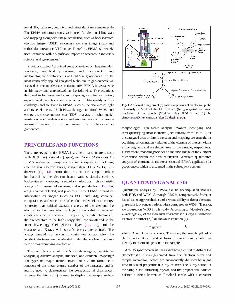
www.at-spectrosc.com/as/article/pdf/2021912 187 At. Spectrosc. 2022, 43(2), 186–200.
metal alloys, glasses, ceramics, and minerals, at micrometer scale.
The EPMA instrument can also be used for elemental line scan
and mapping along with image acquisition, such as backscattered
electron image (BSEI), secondary electron image (SEI) and
cathodoluminescence (CL) image. Therefore, EPMA is a widely
used technique with a significant impact on research in materials
science2 and geosciences.3
Previous studies2-8 provided some overviews on the principles,
functions, analytical procedures, and instrumental and
methodological developments of EPMA in geosciences. As the
most commonly applied analytical technique in geosciences, we
focused on recent advances in quantitative EPMA in geoscience
in this study and emphasized on the following: 1) precautions
that need to be considered when preparing samples and setting
experimental conditions and evaluation of data quality and 2)
challenges and solutions in EPMA, such as the analyses of light
and trace elements, U-Th-Pbtotal dating, combined WDS and
energy dispersive spectrometer (EDS) analysis, a higher spatial
resolution, iron oxidation state analysis, and standard reference
materials, aiming to further extend its applications in
geosciences.
PRINCIPLES AND FUNCTIONS
There are several major EPMA instrument manufacturers, such
as JEOL (Japan), Shimadzu (Japan), and CAMECA (France). An
EPMA instrument comprises several components, including
electron gun, electron lenses, sample stage, EDS, WDS, BSE
detector (Fig. 1a). From the area on the sample surface
bombarded by the electron beam, various signals, such as
backscattered electrons, secondary electrons, characteristic
X-rays, CL, transmitted electrons, and Auger electrons (Fig. 1b),
are generated, detected, and processed in the EPMA to produce
information on images (such as BSEI and SEI), chemical
compositions, and structures.6 When the incident electron energy
is greater than critical excitation energy of the element, the
electron in the inner electron layer of the orbit is removed,
creating an electron vacancy. Subsequently, the outer electrons of
the excited state in the high-energy shell are transferred to the
inner low-energy shell electron layer (Fig. 1c), and the
characteristic X-rays with specific energy are emitted. The
X-rays emitted are known as continuous X-rays when the
incident electrons are decelerated under the nuclear Coulomb
field without removing an electron.
The main functions of EPMA include imaging, quantitative
analysis, qualitative analysis, line scan, and elemental mapping.6
The types of images include BSEI and SEI, the former is a
function of the mean atomic number of the materials and is
mainly used to demonstrate the compositional differences,
whereas the later (SEI) is used to display the sample surface
Fig. 1 A schematic diagram of (a) basic components of an electron probe
microanalyzer (Modified after Llovet et al.2), (b) signals geted by electron
irradiation of the sample (Modified after JEOL10), and (c) the
characteristic X-ray emission (after Goldstein et al.7).
morphologies. Qualitative analysis involves identifying and
semi-quantifying most elements (theoretically from Be to U) in
the analyzed area or line. Line scan and mapping are essential in
acquiring concentration variation of the element of interest within
a line segment and a selected area in the sample, respectively.
Furthermore, mapping provides an intuitive image of the element
distribution within the area of interest. Accurate quantitative
analysis of elements is the most essential EPMA application in
geosciences, which is discussed in the subsequent section.
QUANTITATIVE ANALYSIS
Quantitative analysis by EPMA can be accomplished through
both EDS and WDS. Although EDS is comparatively faster, it
has a less energy resolution and a worse ability to detect elements
present in low concentrations when compared to WDS.2 Therefor,
we focused on WDS in this study. According to Moseley's law,9
wavelength (λ) of the elemental characteristic X-rays is related to
its atomic number (Z),7 as shown in equation (1):
𝜆 =𝐵
(𝑍−𝐶)2 (1)
where B and C are constants. Therefore, the wavelength of a
characteristic X-ray emitted from a sample can be used to
identify the elements present in the sample.
A WDS spectrometer utilizes a diffracting crystal to diffract the
characteristic X-rays generated from the electron beam and
sample interaction, which are subsequently detected by a gas
flow or sealed proportional X-ray counter. The X-ray source in
the sample, the diffracting crystal, and the proportional counter
defines a circle known as Rowland circle with a constant
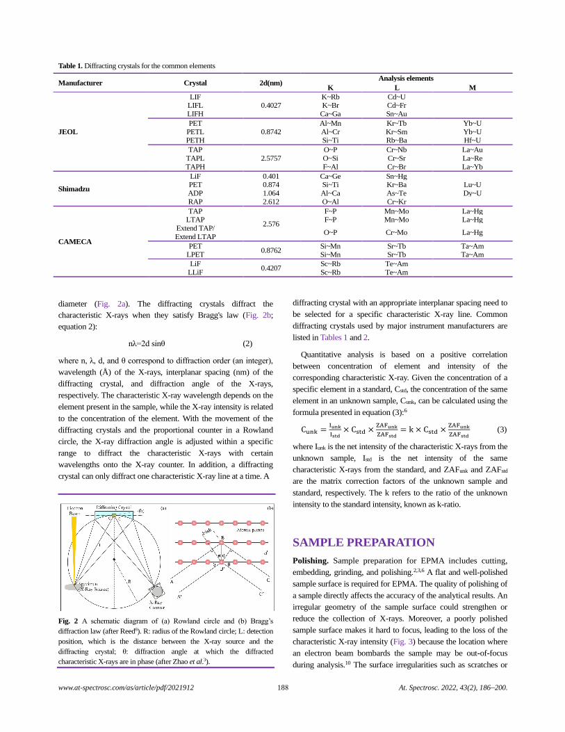
www.at-spectrosc.com/as/article/pdf/2021912 188 At. Spectrosc. 2022, 43(2), 186–200.
Table 1. Diffracting crystals for the common elements
Manufacturer Crystal 2d(nm) Analysis elements
K L M
JEOL
LIF 0.4027
K~Rb Cd~U
LIFL K~Br Cd~Fr
LIFH Ca~Ga Sn~Au
PET
0.8742
Al~Mn Kr~Tb Yb~U
PETL Al~Cr Kr~Sm Yb~U PETH Si~Ti Rb~Ba Hf~U
TAP
2.5757
O~P Cr~Nb La~Au
TAPL O~Si Cr~Sr La~Re
TAPH F~Al Cr~Br La~Yb
Shimadzu
LiF 0.401 Ca~Ge Sn~Hg
PET 0.874 Si~Ti Kr~Ba Lu~U
ADP 1.064 Al~Ca As~Te Dy~U
RAP 2.612 O~Al Cr~Kr
CAMECA
TAP
2.576
F~P Mn~Mo La~Hg LTAP F~P Mn~Mo La~Hg
Extend TAP/
Extend LTAP O~P Cr~Mo La~Hg
PET 0.8762
Si~Mn Sr~Tb Ta~Am LPET Si~Mn Sr~Tb Ta~Am
LiF 0.4207
Sc~Rb Te~Am
LLiF Sc~Rb Te~Am
diameter (Fig. 2a). The diffracting crystals diffract the
characteristic X-rays when they satisfy Bragg's law (Fig. 2b;
equation 2):
nλ=2d sinθ (2)
where n, λ, d, and θ correspond to diffraction order (an integer),
wavelength (Å) of the X-rays, interplanar spacing (nm) of the
diffracting crystal, and diffraction angle of the X-rays,
respectively. The characteristic X-ray wavelength depends on the
element present in the sample, while the X-ray intensity is related
to the concentration of the element. With the movement of the
diffracting crystals and the proportional counter in a Rowland
circle, the X-ray diffraction angle is adjusted within a specific
range to diffract the characteristic X-rays with certain
wavelengths onto the X-ray counter. In addition, a diffracting
crystal can only diffract one characteristic X-ray line at a time. A
Fig. 2 A schematic diagram of (a) Rowland circle and (b) Bragg’s
diffraction law (after Reed6). R: radius of the Rowland circle; L: detection
position, which is the distance between the X-ray source and the
diffracting crystal; θ: diffraction angle at which the diffracted
characteristic X-rays are in phase (after Zhao et al.3).
diffracting crystal with an appropriate interplanar spacing need to
be selected for a specific characteristic X-ray line. Common
diffracting crystals used by major instrument manufacturers are
listed in Tables 1 and 2.
Quantitative analysis is based on a positive correlation
between concentration of element and intensity of the
corresponding characteristic X-ray. Given the concentration of a
specific element in a standard, Cstd, the concentration of the same
element in an unknown sample, Cunk, can be calculated using the
formula presented in equation (3):6
Cunk =Iunk
Istd× Cstd ×
ZAFunk
ZAFstd= k × Cstd ×
ZAFunk
ZAFstd (3)
where Iunk is the net intensity of the characteristic X-rays from the
unknown sample, Istd is the net intensity of the same
characteristic X-rays from the standard, and ZAFunk and ZAFstd
are the matrix correction factors of the unknown sample and
standard, respectively. The k refers to the ratio of the unknown
intensity to the standard intensity, known as k-ratio.
SAMPLE PREPARATION
Polishing. Sample preparation for EPMA includes cutting,
embedding, grinding, and polishing.2,3,6 A flat and well-polished
sample surface is required for EPMA. The quality of polishing of
a sample directly affects the accuracy of the analytical results. An
irregular geometry of the sample surface could strengthen or
reduce the collection of X-rays. Moreover, a poorly polished
sample surface makes it hard to focus, leading to the loss of the
characteristic X-ray intensity (Fig. 3) because the location where
an electron beam bombards the sample may be out-of-focus
during analysis.10 The surface irregularities such as scratches or
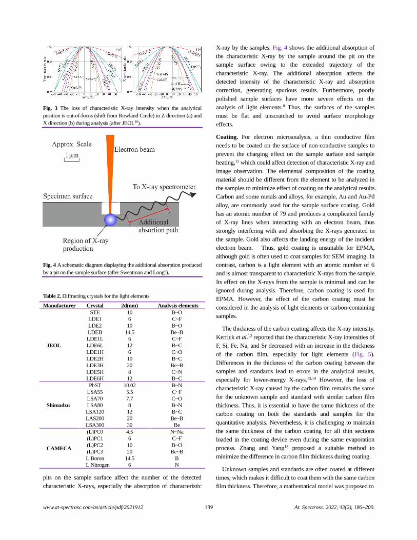
www.at-spectrosc.com/as/article/pdf/2021912 189 At. Spectrosc. 2022, 43(2), 186–200.
Fig. 3 The loss of characteristic X-ray intensity when the analytical
position is out-of-focus (shift from Rowland Circle) in Z direction (a) and
X direction (b) during analysis (after JEOL10).
Fig.
4 A schematic diagram displaying the additional absorption produced
by a pit on the sample surface (after Sweatman and Long8).
Table 2. Diffracting crystals for the light elements
Manufacturer Crystal 2d(nm) Analysis elements
JEOL
STE 10 B~O
LDE1 6 C~F
LDE2 10 B~O
LDEB 14.5 Be~B
LDE1L 6 C~F
LDE6L 12 B~C
LDE1H 6 C~O
LDE2H 10 B~C
LDE3H 20 Be~B
LDE5H 8 C~N
LDE6H 12 B~C
Shimadzu
PbST 10.02 B~N
LSA55 5.5 C~F
LSA70 7.7 C~O
LSA80 8 B~N
LSA120 12 B~C
LAS200 20 Be~B
LSA300 30 Be
CAMECA
(L)PC0 4.5 N~Na
(L)PC1 6 C~F
(L)PC2 10 B~O
(L)PC3 20 Be~B
L Boron 14.5 B
L Nitrogen 6 N
pits on the sample surface affect the number of the detected
characteristic X-rays, especially the absorption of characteristic
X-ray by the samples. Fig. 4 shows the additional absorption of
the characteristic X-ray by the sample around the pit on the
sample surface owing to the extended trajectory of the
characteristic X-ray. The additional absorption affects the
detected intensity of the characteristic X-ray and absorption
correction, generating spurious results. Furthermore, poorly
polished sample surfaces have more severe effects on the
analysis of light elements.8 Thus, the surfaces of the samples
must be flat and unscratched to avoid surface morphology
effects.
Coating. For electron microanalysis, a thin conductive film
needs to be coated on the surface of non-conductive samples to
prevent the charging effect on the sample surface and sample
heating,11 which could affect detection of characteristic X-ray and
image observation. The elemental composition of the coating
material should be different from the element to be analyzed in
the samples to minimize effect of coating on the analytical results.
Carbon and some metals and alloys, for example, Au and Au-Pd
alloy, are commonly used for the sample surface coating. Gold
has an atomic number of 79 and produces a complicated family
of X-ray lines when interacting with an electron beam, thus
strongly interfering with and absorbing the X-rays generated in
the sample. Gold also affects the landing energy of the incident
electron beam. Thus, gold coating is unsuitable for EPMA,
although gold is often used to coat samples for SEM imaging. In
contrast, carbon is a light element with an atomic number of 6
and is almost transparent to characteristic X-rays from the sample.
Its effect on the X-rays from the sample is minimal and can be
ignored during analysis. Therefore, carbon coating is used for
EPMA. However, the effect of the carbon coating must be
considered in the analysis of light elements or carbon-containing
samples.
The thickness of the carbon coating affects the X-ray intensity.
Kerrick et al.12 reported that the characteristic X-ray intensities of
F, Si, Fe, Na, and Sr decreased with an increase in the thickness
of the carbon film, especially for light elements (Fig. 5).
Differences in the thickness of the carbon coating between the
samples and standards lead to errors in the analytical results,
especially for lower-energy X-rays.13,14 However, the loss of
characteristic X-ray caused by the carbon film remains the same
for the unknown sample and standard with similar carbon film
thickness. Thus, it is essential to have the same thickness of the
carbon coating on both the standards and samples for the
quantitative analysis. Nevertheless, it is challenging to maintain
the same thickness of the carbon coating for all thin sections
loaded in the coating device even during the same evaporation
process. Zhang and Yang13 proposed a suitable method to
minimize the difference in carbon film thickness during coating.
Unknown samples and standards are often coated at different
times, which makes it difficult to coat them with the same carbon
film thickness. Therefore, a mathematical model was proposed to
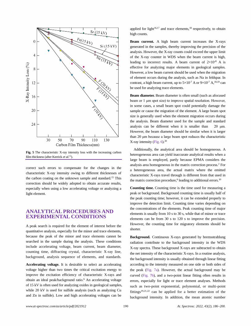
www.at-spectrosc.com/as/article/pdf/2021912 190 At. Spectrosc. 2022, 43(2), 186–200.
Fig. 5 The characteristic X-ray intensity loss with the increasing carbon
film thickness (after Kerrick et al.12).
correct such errors to compensate for the changes in the
characteristic X-ray intensity owing to different thicknesses of
the carbon coating on the unknown sample and standard.15 This
correction should be widely adopted to obtain accurate results,
especially when using a low accelerating voltage or analyzing a
light element.
ANALYTICAL PROCEDURES AND EXPERIMENTAL CONDITIONS
A peak search is required for the element of interest before the
quantitative analysis, especially for the minor and trace elements,
because the peak of the minor and trace elements cannot be
searched in the sample during the analysis. These conditions
include accelerating voltage, beam current, beam diameter,
counting time, diffracting crystal, characteristic X-ray line,
background, analysis sequence of elements, and standards.
Accelerating voltage. It is desirable to select an accelerating
voltage higher than two times the critical excitation energy to
improve the excitation efficiency of characteristic X-rays and
obtain an ideal peak/background ratio.6 An accelerating voltage
of 15 kV is often used for analyzing oxides in geological samples,
while 20 kV is used for sulfide analysis (such as analyzing Cu
and Zn in sulfide). Low and high accelerating voltages can be
applied for light16,17 and trace elements,18 respectively, to obtain
high counts.
Beam current. A high beam current increases the X-rays
generated in the samples, thereby improving the precision of the
analysis. However, the X-ray counts could exceed the upper limit
of the X-ray counter in WDS when the beam current is high,
leading to incorrect results. A beam current of 2×10⁻⁸ A is
effective for analyzing major elements in geological samples.
However, a low beam current should be used when the migration
of element occurs during the analysis, such as Na in feldspar. In
contrast, a high beam current, up to 5×10⁻⁷ A or 9×10⁻⁷ A,18,19 can
be used for analyzing trace elements.
Beam diameter. Beam diameter is often small (such as afocused
beam or 1 μm spot size) to improve spatial resolution. However,
in some cases, a small beam spot could potentially damage the
sample or cause the migration of the element. A large beam spot
size is generally used when the element migration occurs during
the analysis. Beam diameter used for the sample and standard
analysis can be different when it is smaller than 20 μm.
However, the beam diameter should be similar when it is larger
than 20 μm because a large beam spot reduces the characteristic
X-ray intensity (Fig. 6).20
Additionally, the analytical area should be homogeneous. A
heterogeneous area can yield inaccurate analytical results when a
large beam is employed, partly because EPMA considers the
analysis area homogeneous in the matrix correction process.2 For
a heterogeneous area, the actual matrix where the emitted
characteristic X-rays travel through is different from that used in
the matrix correction procedure,6 leading to additional errors.10
Counting time. Counting time is the time used for measuring a
peak or background. Background counting time is usually half of
the peak counting time; however, it can be extended properly to
improve the detection limit. Counting time varies depending on
the concentrations of the elements. Peak counting time of major
elements is usually from 10 s to 30 s, while that of minor or trace
elements can be from 30 s to 120 s to improve the precision.
However, the counting time for migratory elements should be
shorter.
Background. Continuous X-rays generated by bremsstrahlung
radiation contribute to the background intensity in the WDS
X-ray spectra. These background X-rays are subtracted to obtain
the net intensity of the characteristic X-rays. In a routine analysis,
the background intensity is usually obtained through linear fitting
according to the intensity measured on one side or both sides of
the peak (Fig. 7a). However, the actual background may be
curved (Fig. 7b), and a two-point linear fitting often results in
errors, especially for light or trace element analyses. Methods
such as two-point exponential, polynomial, or multi-point
fittings19,21,22 can be applied for a better estimation of the
background intensity. In addition, the mean atomic number
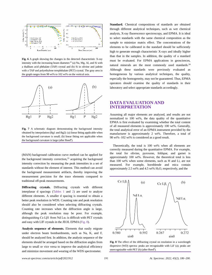
www.at-spectrosc.com/as/article/pdf/2021912 191 At. Spectrosc. 2022, 43(2), 186–200.
Fig.
6
A graph showing the changes in the detected characteristic X-ray
intensity with the increasing beam diameter.20
(a) Na, Mg, Al, and Si with
a thallium acid phthalate (TAP) crystal and (b) Si in olivine and jadeite
with a TAP and polyethylene terephthalate (PET) crystal. The gray area in
the graph ranges from 98 wt% to 102 wt% on the vertical axis.
Fig.
7
A schematic diagram demonstrating the background intensity
obtained by interpolation (Bg1 and Bg2): (a) linear fitting applicable when
the background curvature is small; (b) linear fitting not applicable when
the background curvature is large (after Reed6).
(MAN) background calibration curve method can be applied for
the background intensity correction,23 acquiring the background
intensity correction by measuring the peak intensities in a set of
standards without the element of interest. This method can avoid
the background measurement artifacts, thereby improving the
measurement precision for the trace elements compared to
traditional off-peak measurements.
Diffracting crystals. Diffracting crystals with different
interplanar d spacings (Tables 1 and 2) are used to analyze
different elements. A smaller d spacing is essential to obtain a
better peak resolution in WDS. Counting rate and peak resolution
should also be considered when selecting diffracting crystals.
Counting rate increases when the diffraction angle is large,
although the peak resolution may be poor. For example,
distinguishing Ce Lβ1 from Nd Lα1 is difficult with PET crystals
and easy with LIF crystals in the JEOL EPMA (Fig. 8).
Analysis sequence of elements. Elements that easily migrate
under electron beam bombardments, such as Na, K, and F,
should be analyzed first. In addition, the analysis sequence of the
elements should be arranged based on the diffraction angles from
large to small or vice versa to improve the analytical efficiency
and minimize movement and wearing of the WDS spectrometer.
Standard. Chemical compositions of standards are obtained
through different analytical techniques, such as wet chemical
analysis, X-ray fluorescence spectroscopy, and EPMA. It is ideal
to select standards with the same chemical composition as the
sample to minimize matrix effect. The concentrations of the
elements to be calibrated in the standard should be sufficiently
high to generate enough characteristic X-rays and ideally higher
than that in the samples. In addition, the quality of a standard
must be evaluated. For EPMA applications in geosciences,
natural minerals are the most commonly used standards.24
Although these standards were previously evaluated as
homogeneous by various analytical techniques, the quality,
especially the homogeneity, may not be guaranteed. Thus, EPMA
operators should examine the quality of standards in their
laboratory and select appropriate standards accordingly.
DATA EVALUATION AND INTERPRETATION
Assuming all major elements are analyzed, and results are not
normalized to 100 wt%, the data quality of the quantitative
EPMA is first evaluated by examining whether the total content
of all measured elements is approximately 100 wt%. Generally,
the total analytical error of an EPMA instrument provided by the
manufacturer is approximately 2 wt%. Therefore, a total of
98 wt%–102 wt% is considered as a good result.
Theoretically, the total is 100 wt% when all elements are
correctly measured during the quantitative EPMA. For example,
the total for olivine, pyroxene, feldspar, and garnet is
approximately 100 wt%. However, the theoretical total is less
than 100 wt% when some elements, such as H and Li, are not
measured. For example, hornblende and mica contain
approximately 2.5 wt% and 4.5 wt% H2O, respectively, and the
Fig. 8 The effect of the diffracting crystal on resolution in a wavelength
dispersive (WD) spectra: peaks are recognizable with LiF (a); peaks are
unrecognizable with PET (b) (after Reed6).
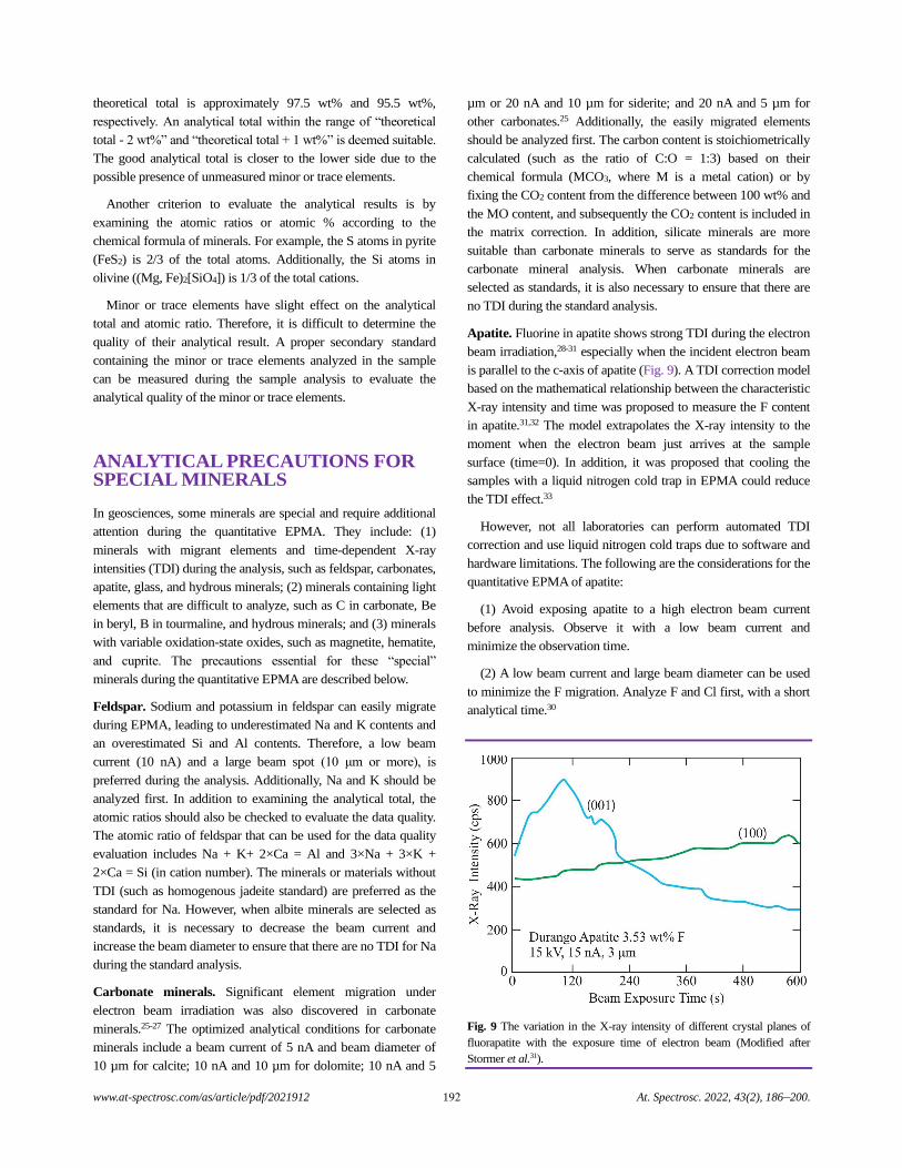
www.at-spectrosc.com/as/article/pdf/2021912 192 At. Spectrosc. 2022, 43(2), 186–200.
theoretical total is approximately 97.5 wt% and 95.5 wt%,
respectively. An analytical total within the range of “theoretical
total - 2 wt%” and “theoretical total + 1 wt%” is deemed suitable.
The good analytical total is closer to the lower side due to the
possible presence of unmeasured minor or trace elements.
Another criterion to evaluate the analytical results is by
examining the atomic ratios or atomic % according to the
chemical formula of minerals. For example, the S atoms in pyrite
(FeS2) is 2/3 of the total atoms. Additionally, the Si atoms in
olivine ((Mg, Fe)2[SiO4]) is 1/3 of the total cations.
Minor or trace elements have slight effect on the analytical
total and atomic ratio. Therefore, it is difficult to determine the
quality of their analytical result. A proper secondary standard
containing the minor or trace elements analyzed in the sample
can be measured during the sample analysis to evaluate the
analytical quality of the minor or trace elements.
ANALYTICAL PRECAUTIONS FOR SPECIAL MINERALS
In geosciences, some minerals are special and require additional
attention during the quantitative EPMA. They include: (1)
minerals with migrant elements and time-dependent X-ray
intensities (TDI) during the analysis, such as feldspar, carbonates,
apatite, glass, and hydrous minerals; (2) minerals containing light
elements that are difficult to analyze, such as C in carbonate, Be
in beryl, B in tourmaline, and hydrous minerals; and (3) minerals
with variable oxidation-state oxides, such as magnetite, hematite,
and cuprite. The precautions essential for these “special”
minerals during the quantitative EPMA are described below.
Feldspar. Sodium and potassium in feldspar can easily migrate
during EPMA, leading to underestimated Na and K contents and
an overestimated Si and Al contents. Therefore, a low beam
current (10 nA) and a large beam spot (10 μm or more), is
preferred during the analysis. Additionally, Na and K should be
analyzed first. In addition to examining the analytical total, the
atomic ratios should also be checked to evaluate the data quality.
The atomic ratio of feldspar that can be used for the data quality
evaluation includes Na + K+ 2×Ca = Al and 3×Na + 3×K +
2×Ca = Si (in cation number). The minerals or materials without
TDI (such as homogenous jadeite standard) are preferred as the
standard for Na. However, when albite minerals are selected as
standards, it is necessary to decrease the beam current and
increase the beam diameter to ensure that there are no TDI for Na
during the standard analysis.
Carbonate minerals. Significant element migration under
electron beam irradiation was also discovered in carbonate
minerals.25-27 The optimized analytical conditions for carbonate
minerals include a beam current of 5 nA and beam diameter of
10 µm for calcite; 10 nA and 10 µm for dolomite; 10 nA and 5
µm or 20 nA and 10 µm for siderite; and 20 nA and 5 µm for
other carbonates.25 Additionally, the easily migrated elements
should be analyzed first. The carbon content is stoichiometrically
calculated (such as the ratio of C:O = 1:3) based on their
chemical formula (MCO3, where M is a metal cation) or by
fixing the CO2 content from the difference between 100 wt% and
the MO content, and subsequently the CO2 content is included in
the matrix correction. In addition, silicate minerals are more
suitable than carbonate minerals to serve as standards for the
carbonate mineral analysis. When carbonate minerals are
selected as standards, it is also necessary to ensure that there are
no TDI during the standard analysis.
Apatite. Fluorine in apatite shows strong TDI during the electron
beam irradiation,28-31 especially when the incident electron beam
is parallel to the c-axis of apatite (Fig. 9). A TDI correction model
based on the mathematical relationship between the characteristic
X-ray intensity and time was proposed to measure the F content
in apatite.31,32 The model extrapolates the X-ray intensity to the
moment when the electron beam just arrives at the sample
surface (time=0). In addition, it was proposed that cooling the
samples with a liquid nitrogen cold trap in EPMA could reduce
the TDI effect.33
However, not all laboratories can perform automated TDI
correction and use liquid nitrogen cold traps due to software and
hardware limitations. The following are the considerations for the
quantitative EPMA of apatite:
(1) Avoid exposing apatite to a high electron beam current
before analysis. Observe it with a low beam current and
minimize the observation time.
(2) A low beam current and large beam diameter can be used
to minimize the F migration. Analyze F and Cl first, with a short
analytical time.30
Fig. 9 The variation in the X-ray intensity of different crystal planes of
fluorapatite with the exposure time of electron beam (Modified after
Stormer et al.31).
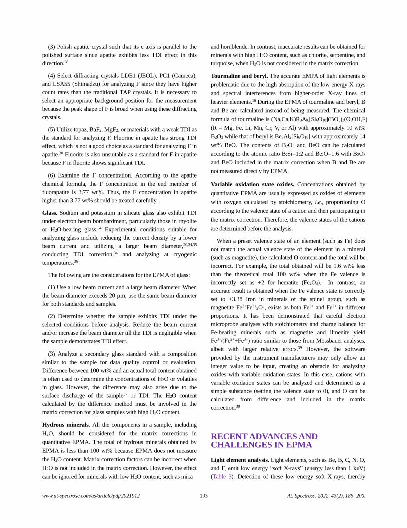
www.at-spectrosc.com/as/article/pdf/2021912 193 At. Spectrosc. 2022, 43(2), 186–200.
(3) Polish apatite crystal such that its c axis is parallel to the
polished surface since apatite exhibits less TDI effect in this
direction.28
(4) Select diffracting crystals LDE1 (JEOL), PC1 (Cameca),
and LSA55 (Shimadzu) for analyzing F since they have higher
count rates than the traditional TAP crystals. It is necessary to
select an appropriate background position for the measurement
because the peak shape of F is broad when using these diffracting
crystals.
(5) Utilize topaz, BaF2, MgF2, or materials with a weak TDI as
the standard for analyzing F. Fluorine in apatite has strong TDI
effect, which is not a good choice as a standard for analyzing F in
apatite.30 Fluorite is also unsuitable as a standard for F in apatite
because F in fluorite shows significant TDI.
(6) Examine the F concentration. According to the apatite
chemical formula, the F concentration in the end member of
fluorapatite is 3.77 wt%. Thus, the F concentration in apatite
higher than 3.77 wt% should be treated carefully.
Glass. Sodium and potassium in silicate glass also exhibit TDI
under electron beam bombardment, particularly those in rhyolite
or H2O-bearing glass.34 Experimental conditions suitable for
analyzing glass include reducing the current density by a lower
beam current and utilizing a larger beam diameter,20,34,35
conducting TDI correction,34 and analyzing at cryogenic
temperatures.36
The following are the considerations for the EPMA of glass:
(1) Use a low beam current and a large beam diameter. When
the beam diameter exceeds 20 µm, use the same beam diameter
for both standards and samples.
(2) Determine whether the sample exhibits TDI under the
selected conditions before analysis. Reduce the beam current
and/or increase the beam diameter till the TDI is negligible when
the sample demonstrates TDI effect.
(3) Analyze a secondary glass standard with a composition
similar to the sample for data quality control or evaluation.
Difference between 100 wt% and an actual total content obtained
is often used to determine the concentrations of H2O or volatiles
in glass. However, the difference may also arise due to the
surface discharge of the sample37 or TDI. The H2O content
calculated by the difference method must be involved in the
matrix correction for glass samples with high H2O content.
Hydrous minerals. All the components in a sample, including
H2O, should be considered for the matrix corrections in
quantitative EPMA. The total of hydrous minerals obtained by
EPMA is less than 100 wt% because EPMA does not measure
the H2O content. Matrix correction factors can be incorrect when
H2O is not included in the matrix correction. However, the effect
can be ignored for minerals with low H2O content, such as mica
and hornblende. In contrast, inaccurate results can be obtained for
minerals with high H2O content, such as chlorite, serpentine, and
turquoise, when H2O is not considered in the matrix correction.
Tourmaline and beryl. The accurate EMPA of light elements is
problematic due to the high absorption of the low energy X-rays
and spectral interferences from higher-order X-ray lines of
heavier elements.16 During the EPMA of tourmaline and beryl, B
and Be are calculated instead of being measured. The chemical
formula of tourmaline is (Na,Ca,K)R3Al6[Si6O18](BO3)3(O,OH,F)
(R = Mg, Fe, Li, Mn, Cr, V, or Al) with approximately 10 wt%
B2O3 while that of beryl is Be3Al2[Si6O18] with approximately 14
wt% BeO. The contents of B2O3 and BeO can be calculated
according to the atomic ratio B:Si=1:2 and Be:O=1:6 with B2O3
and BeO included in the matrix correction when B and Be are
not measured directly by EPMA.
Variable oxidation state oxides. Concentrations obtained by
quantitative EPMA are usually expressed as oxides of elements
with oxygen calculated by stoichiometry, i.e., proportioning O
according to the valence state of a cation and then participating in
the matrix correction. Therefore, the valence states of the cations
are determined before the analysis.
When a preset valence state of an element (such as Fe) does
not match the actual valence state of the element in a mineral
(such as magnetite), the calculated O content and the total will be
incorrect. For example, the total obtained will be 1.6 wt% less
than the theoretical total 100 wt% when the Fe valence is
incorrectly set as +2 for hematite (Fe2O3). In contrast, an
accurate result is obtained when the Fe valence state is correctly
set to +3.38 Iron in minerals of the spinel group, such as
magnetite Fe2+Fe3+2O4, exists as both Fe3+ and Fe2+ in different
proportions. It has been demonstrated that careful electron
microprobe analyses with stoichiometry and charge balance for
Fe-bearing minerals such as magnetite and ilmenite yield
Fe3+/(Fe2++Fe3+) ratio similar to those from Mössbauer analyses,
albeit with larger relative errors.39 However, the software
provided by the instrument manufacturers may only allow an
integer value to be input, creating an obstacle for analyzing
oxides with variable oxidation states. In this case, cations with
variable oxidation states can be analyzed and determined as a
simple substance (setting the valence state to 0), and O can be
calculated from difference and included in the matrix
correction.38
RECENT ADVANCES AND CHALLENGES IN EPMA
Light element analysis. Light elements, such as Be, B, C, N, O,
and F, emit low energy “soft X-rays” (energy less than 1 keV)
(Table 3). Detection of these low energy soft X-rays, thereby
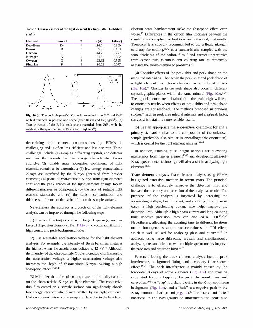
www.at-spectrosc.com/as/article/pdf/2021912 194 At. Spectrosc. 2022, 43(2), 186–200.
Table 3. Characteristics of the light element Kα lines (after Goldstein
et al.7)
Element Symbol Z λ(Å) E(keV)
Beryllium Be 4 114.0 0.109 Boron B 5 67.6 0.183
Carbon C 6 44.7 0.277
Nitrogen N 7 31.6 0.392 Oxygen O 8 23.62 0.525
Fluorine F 9 18.32 0.677
Fig. 10
(a) The peak shape of C Kα peaks recorded from SiC and Fe3C
with differences in position and shape (after Bastin and Heijligers43); (b)
Two extremes of the B Kα peak shape recorded from ZrB2 with the
rotation of the specimen (after Bastin and Heijligers44).
determining light element concentrations by EPMA is
challenging and is often less efficient and less accurate. These
challenges include: (1) samples, diffracting crystals, and detector
windows that absorb the low energy characteristic X-rays
strongly; (2) reliable mass absorption coefficients of light
elements remain to be determined; (3) low energy characteristic
X-rays are interfered by the X-rays generated from heavier
elements; (4) peaks of characteristic X-rays from light elements
shift and the peak shapes of the light elements change too in
different matrices or compounds; (5) the lack of suitable light
element standards; and (6) the carbon contamination and
thickness difference of the carbon film on the sample surface.
Nevertheless, the accuracy and precision of the light element
analysis can be improved through the following steps:
(1) Use a diffracting crystal with large d spacings, such as
layered dispersion element (LDE, Table 2), to obtain significantly
high counts and peak/background ratios.
(2) Use a suitable acceleration voltage for the light element
analyses. For example, the intensity of Be in beryllium metal is
the highest when the acceleration voltage is 12 kV.40 Although
the intensity of the characteristic X-rays increases with increasing
the acceleration voltage, a higher acceleration voltage also
increases the depth of characteristic X-rays, causing a high
absorption effect.16,40,41
(3) Minimize the effect of coating material, primarily carbon,
on the characteristic X-rays of light elements. The conductive
thin film coated on a sample surface can significantly absorb
low-energy characteristic X-rays emitted by the light elements.
Carbon contamination on the sample surface due to the heat from
electron beam bombardment make the absorption effect even
worse.15 Differences in the carbon film thickness between the
standards and samples also lead to errors in the analytical results.
Therefore, it is strongly recommended to use a liquid nitrogen
cold trap for cooling,15,42 coat standards and samples with the
same thickness of the carbon film,13 and correct uncertainties
from carbon film thickness and counting rate to effectively
alleviate the above-mentioned problems.15
(4) Consider effects of the peak shift and peak shape on the
measured intensities. Changes in the peak shift and peak shape of
a light element have been observed in a different matrix
(Fig. 10a).43 Changes in the peak shape also occur in different
crystallographic planes within the same mineral (Fig. 10b).16,44
The light element content obtained from the peak height will lead
to erroneous results when effects of peak shifts and peak shape
changes are not resolved,. The methods proposed in previous
studies,44 such as peak area integral intensity and area/peak factor,
can assist in obtaining more reliable results.
(5) Use an appropriate mass-absorption coefficient for and a
primary standard similar to the composition of the unknown
sample (preferably also similar in crystallographic orientation),
which is crucial for the light element analysis.16,44
In addition, utilizing pulse height analysis for alleviating
interference from heavier element40,45 and developing ultra-soft
X-ray spectrometer technology will also assist in analyzing light
elements.46,47
Trace element analysis. Trace element analysis using EPMA
has gained extensive attention in recent years. The principal
challenge is to effectively improve the detection limit and
increase the accuracy and precision of the analytical results. The
precision of the analysis is improved by increasing the
accelerating voltage, beam current, and counting time. In most
cases, a high accelerating voltage also helps improve the
detection limit. Although a high beam current and long counting
time improve precision, they can also cause TDI.19,48,49
Nevertheless, allocating the counting time to different locations
on the homogeneous sample surface reduces the TDI effect,
which is well utilized for analyzing glass and quartz.22,50 In
addition, using large diffracting crystals and simultaneously
analyzing the same element with multiple spectrometers improve
the precision and detection limit.22,51
Factors affecting the trace element analysis include peak
interference, background fitting, and secondary fluorescence
effect.19,21 The peak interference is mainly caused by the
low-order X-rays of some elements (Fig. 11a) and may be
separated by overlapping the peak deconvolution and
correction.30,52 A “step” is a sharp decline in the X-ray continuum
background (Fig. 11b),6 and a “hole” is a negative peak in the
X-ray continuum background (Fig. 12).22 The “steps” and “holes”
observed in the background or underneath the peak also
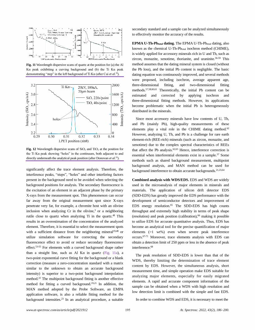
www.at-spectrosc.com/as/article/pdf/2021912 195 At. Spectrosc. 2022, 43(2), 186–200.
Fig. 11
Wavelength dispersive scans of quartz at the position for (a) the Al
Kα peak exhibiting a curving background and (b) the Ti Kα peak
demonstrating “step” in the left background of Ti Kα (after Cui et al.19).
Fig. 12 Wavelength dispersive scans of SiO2 and TiO2 at the position for
the Ti Kα peak showing “holes” in the continuum, both adjacent to and
directly underneath the analytical peak position (after Donovan et al.22).
significantly affect the trace element analysis. Therefore, the
interference peaks, “steps”, “holes” and other interfering factors
present in the background need to be avoided when selecting the
background positions for analysis. The secondary fluorescence is
the excitation of an element in an adjacent phase by the primary
X-rays from the measurement spot. This phenomenon can occur
far away from the original measurement spot since X-rays
penetrate very far, for example, a chromite host with an olivine
inclusion when analyzing Cr in the olivine,3 or a neighboring
rutile close to quartz when analyzing Ti in the quartz.48 This
results in an overestimation of the concentration of the analyzed
element. Therefore, it is essential to select the measurement spots
with a sufficient distance from the neighboring mineral19,48 or
utilize simulation software for correcting the secondary
fluorescence effect to avoid or reduce secondary fluorescence
effect.53-55 For elements with a curved background shape rather
than a straight line, such as Al Kα in quartz (Fig. 11a), a
two-point exponential curve fitting for the background or a blank
correction (measure a zero-concentration standard with a matrix
similar to the unknown to obtain an accurate background
intensity) is superior to a two-point background interpolation
method.22 The multipoint background fitting is another effective
method for fitting a curved background.19,21 In addition, the
MAN method adopted by the Probe Software, an EMPA
application software, is also a reliable fitting method for the
background intensities.23 In an analytical procedure, a suitable
secondary standard and a sample can be analyzed simultaneously
to effectively monitor the accuracy of the results.
EPMA U-Th-Pbtotal dating. The EPMA U-Th-Pbtotal dating, also
known as the chemical U-Th-Pbtotal isochron method (CHIME),
is widely applied for accessory minerals rich in U and Th, such as
zircon, monazite, xenotime, thorianite, and uraninite.56-59 This
method assumes that the dating mineral system is closed (without
the Pb loss), and the initial Pb content is negligible. The basic
dating equation was continuously improved, and several methods
were proposed, including isochron, average apparent age,
three-dimensional fitting, and two-dimensional fitting
methods.57,58,60,61 Theoretically, the initial Pb content can be
estimated and corrected by applying isochron and
three-dimensional fitting methods. However, its applications
become problematic when the initial Pb is heterogeneously
distributed in the minerals.
Since most accessory minerals have low contents of U, Th,
and Pb (mainly Pb), high-quality measurements of these
elements play a vital role in the CHIME dating method.62
However, analyzing U, Th, and Pb is a challenge for rare earth
element-rich (REE-rich) minerals (such as zircon, monazite, and
xenotime) due to the complex spectral characteristics of REEs
that affect the Pb analysis.62,63 Hence, interference correction is
essential when interferential elements exist in a sample.57 Some
methods such as shared background measurement, multipoint
background analysis, and MAN method can be used for
background interference to obtain accurate backgrounds.21,23,64
Combined analysis with WDS/EDS. EDS and WDS are widely
used in the microanalysis of major elements in minerals and
materials. The application of silicon drift detector EDS
(SDD-EDS) has greatly improved the EDS performance with the
development of semiconductor detectors and improvement of
EDS energy resolution.65 The SDD-EDS has high counts
throughput and extremely high stability in terms of peak shape
(resolution) and peak position (calibration),66 making it possible
to utilize EDS for accurate quantitative analysis. Thus, EDS has
become an analytical tool for the precise quantification of major
elements (>1 wt%) even when severe peak interference
occurs.67-71 Moreover, trace elements analysis with EDS can
obtain a detection limit of 250 ppm or less in the absence of peak
interference.68
The peak resolution of SDD-EDS is lower than that of the
WDS, thereby limiting the determination of trace element
content by EDS. However, the simultaneous analysis, short
measurement time, and simple operation make EDS suitable for
analyzing major elements, especially for easily migrated
elements. A rapid and accurate component information of the
sample can be obtained when a WDS with high resolution and
low detection limit is combined with the simple and fast EDS.
In order to combine WDS and EDS, it is necessary to meet the
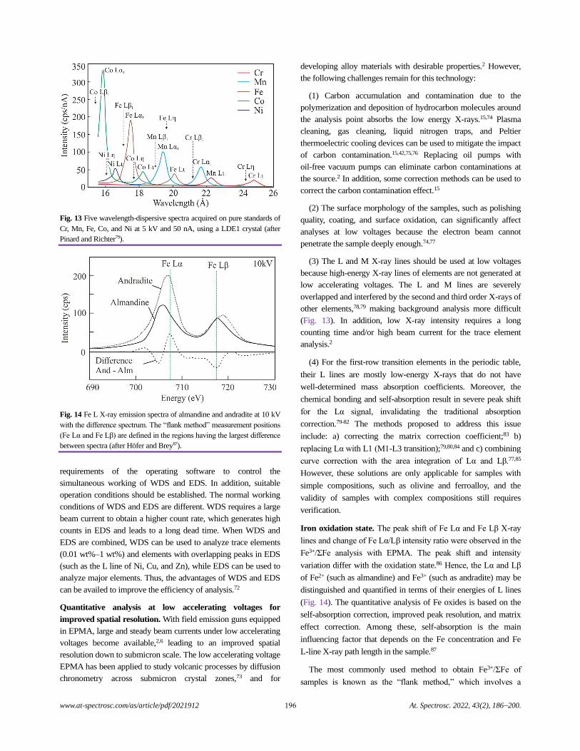
www.at-spectrosc.com/as/article/pdf/2021912 196 At. Spectrosc. 2022, 43(2), 186–200.
Fig. 13
Five wavelength-dispersive spectra acquired on pure standards of
Cr, Mn, Fe, Co, and Ni at 5 kV and 50 nA, using a LDE1 crystal (after
Pinard and Richter79).
Fig. 14 Fe L X-ray emission spectra of almandine and andradite at 10 kV
with the difference spectrum. The “flank method” measurement positions
(Fe Lα and Fe Lβ) are defined in the regions having the largest difference
between spectra (after Höfer and Brey87).
requirements of the operating software to control the
simultaneous working of WDS and EDS. In addition, suitable
operation conditions should be established. The normal working
conditions of WDS and EDS are different. WDS requires a large
beam current to obtain a higher count rate, which generates high
counts in EDS and leads to a long dead time. When WDS and
EDS are combined, WDS can be used to analyze trace elements
(0.01 wt%–1 wt%) and elements with overlapping peaks in EDS
(such as the L line of Ni, Cu, and Zn), while EDS can be used to
analyze major elements. Thus, the advantages of WDS and EDS
can be availed to improve the efficiency of analysis.72
Quantitative analysis at low accelerating voltages for
improved spatial resolution. With field emission guns equipped
in EPMA, large and steady beam currents under low accelerating
voltages become available,2,6 leading to an improved spatial
resolution down to submicron scale. The low accelerating voltage
EPMA has been applied to study volcanic processes by diffusion
chronometry across submicron crystal zones,73 and for
developing alloy materials with desirable properties.2 However,
the following challenges remain for this technology:
(1) Carbon accumulation and contamination due to the
polymerization and deposition of hydrocarbon molecules around
the analysis point absorbs the low energy X-rays.15,74 Plasma
cleaning, gas cleaning, liquid nitrogen traps, and Peltier
thermoelectric cooling devices can be used to mitigate the impact
of carbon contamination.15,42,75,76 Replacing oil pumps with
oil-free vacuum pumps can eliminate carbon contaminations at
the source.2 In addition, some correction methods can be used to
correct the carbon contamination effect.15
(2) The surface morphology of the samples, such as polishing
quality, coating, and surface oxidation, can significantly affect
analyses at low voltages because the electron beam cannot
penetrate the sample deeply enough.74,77
(3) The L and M X-ray lines should be used at low voltages
because high-energy X-ray lines of elements are not generated at
low accelerating voltages. The L and M lines are severely
overlapped and interfered by the second and third order X-rays of
other elements,78,79 making background analysis more difficult
(Fig. 13). In addition, low X-ray intensity requires a long
counting time and/or high beam current for the trace element
analysis.2
(4) For the first-row transition elements in the periodic table,
their L lines are mostly low-energy X-rays that do not have
well-determined mass absorption coefficients. Moreover, the
chemical bonding and self-absorption result in severe peak shift
for the Lα signal, invalidating the traditional absorption
correction.79-82 The methods proposed to address this issue
include: a) correcting the matrix correction coefficient;83 b)
replacing Lα with L1 (M1-L3 transition);79,80,84 and c) combining
curve correction with the area integration of Lα and Lβ.77,85
However, these solutions are only applicable for samples with
simple compositions, such as olivine and ferroalloy, and the
validity of samples with complex compositions still requires
verification.
Iron oxidation state. The peak shift of Fe Lα and Fe Lβ X-ray
lines and change of Fe Lα/Lβ intensity ratio were observed in the
Fe3+/ΣFe analysis with EPMA. The peak shift and intensity
variation differ with the oxidation state.86 Hence, the Lα and Lβ
of Fe2+ (such as almandine) and Fe3+ (such as andradite) may be
distinguished and quantified in terms of their energies of L lines
(Fig. 14). The quantitative analysis of Fe oxides is based on the
self-absorption correction, improved peak resolution, and matrix
effect correction. Among these, self-absorption is the main
influencing factor that depends on the Fe concentration and Fe
L-line X-ray path length in the sample.87
The most commonly used method to obtain Fe3+/ΣFe of
samples is known as the “flank method,” which involves a
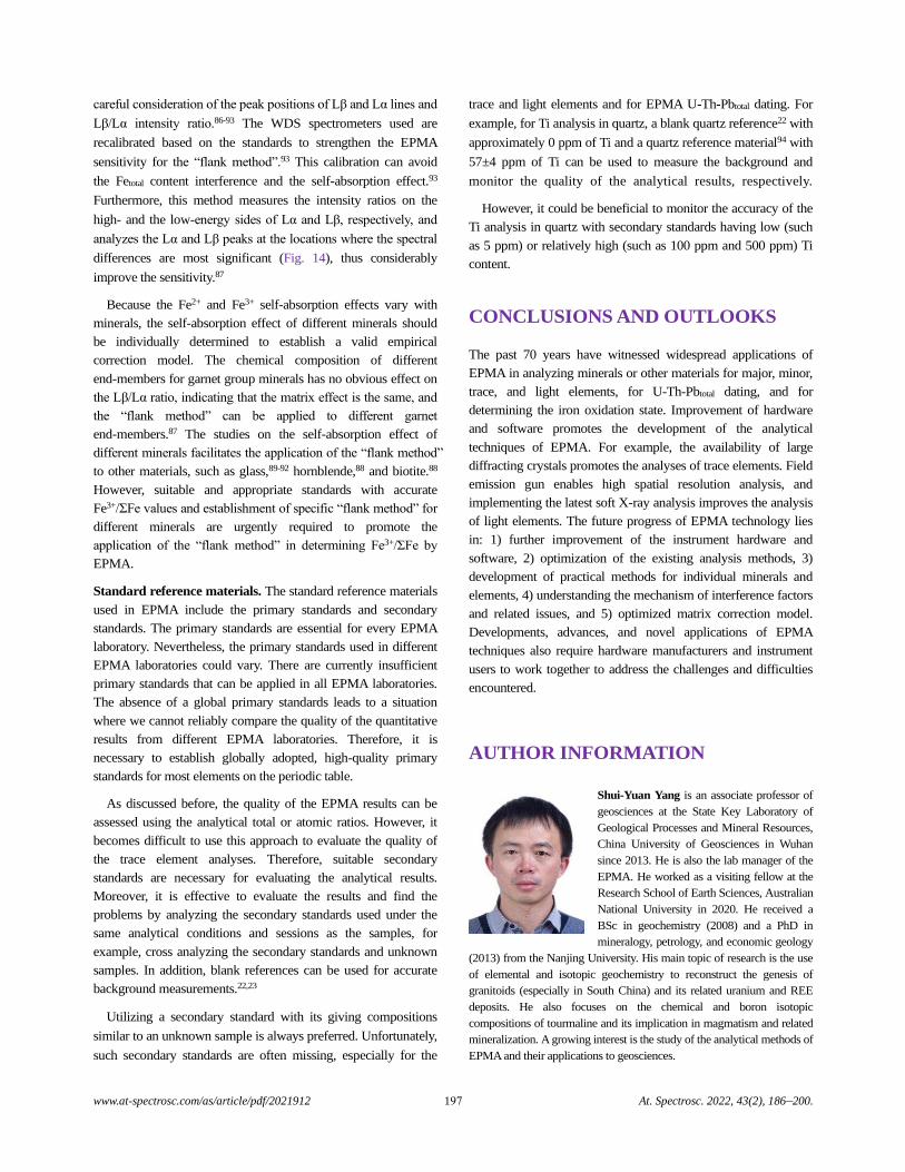
www.at-spectrosc.com/as/article/pdf/2021912 197 At. Spectrosc. 2022, 43(2), 186–200.
careful consideration of the peak positions of Lβ and Lα lines and
Lβ/Lα intensity ratio.86-93 The WDS spectrometers used are
recalibrated based on the standards to strengthen the EPMA
sensitivity for the “flank method”.93 This calibration can avoid
the Fetotal content interference and the self-absorption effect.93
Furthermore, this method measures the intensity ratios on the
high- and the low-energy sides of Lα and Lβ, respectively, and
analyzes the Lα and Lβ peaks at the locations where the spectral
differences are most significant (Fig. 14), thus considerably
improve the sensitivity.87
Because the Fe2+ and Fe3+ self-absorption effects vary with
minerals, the self-absorption effect of different minerals should
be individually determined to establish a valid empirical
correction model. The chemical composition of different
end-members for garnet group minerals has no obvious effect on
the Lβ/Lα ratio, indicating that the matrix effect is the same, and
the “flank method” can be applied to different garnet
end-members.87 The studies on the self-absorption effect of
different minerals facilitates the application of the “flank method”
to other materials, such as glass,89-92 hornblende,88 and biotite.88
However, suitable and appropriate standards with accurate
Fe3+/ΣFe values and establishment of specific “flank method” for
different minerals are urgently required to promote the
application of the “flank method” in determining Fe3+/ΣFe by
EPMA.
Standard reference materials. The standard reference materials
used in EPMA include the primary standards and secondary
standards. The primary standards are essential for every EPMA
laboratory. Nevertheless, the primary standards used in different
EPMA laboratories could vary. There are currently insufficient
primary standards that can be applied in all EPMA laboratories.
The absence of a global primary standards leads to a situation
where we cannot reliably compare the quality of the quantitative
results from different EPMA laboratories. Therefore, it is
necessary to establish globally adopted, high-quality primary
standards for most elements on the periodic table.
As discussed before, the quality of the EPMA results can be
assessed using the analytical total or atomic ratios. However, it
becomes difficult to use this approach to evaluate the quality of
the trace element analyses. Therefore, suitable secondary
standards are necessary for evaluating the analytical results.
Moreover, it is effective to evaluate the results and find the
problems by analyzing the secondary standards used under the
same analytical conditions and sessions as the samples, for
example, cross analyzing the secondary standards and unknown
samples. In addition, blank references can be used for accurate
background measurements.22,23
Utilizing a secondary standard with its giving compositions
similar to an unknown sample is always preferred. Unfortunately,
such secondary standards are often missing, especially for the
trace and light elements and for EPMA U-Th-Pbtotal dating. For
example, for Ti analysis in quartz, a blank quartz reference22 with
approximately 0 ppm of Ti and a quartz reference material94 with
57±4 ppm of Ti can be used to measure the background and
monitor the quality of the analytical results, respectively.
However, it could be beneficial to monitor the accuracy of the
Ti analysis in quartz with secondary standards having low (such
as 5 ppm) or relatively high (such as 100 ppm and 500 ppm) Ti
content.
CONCLUSIONS AND OUTLOOKS
The past 70 years have witnessed widespread applications of
EPMA in analyzing minerals or other materials for major, minor,
trace, and light elements, for U-Th-Pbtotal dating, and for
determining the iron oxidation state. Improvement of hardware
and software promotes the development of the analytical
techniques of EPMA. For example, the availability of large
diffracting crystals promotes the analyses of trace elements. Field
emission gun enables high spatial resolution analysis, and
implementing the latest soft X-ray analysis improves the analysis
of light elements. The future progress of EPMA technology lies
in: 1) further improvement of the instrument hardware and
software, 2) optimization of the existing analysis methods, 3)
development of practical methods for individual minerals and
elements, 4) understanding the mechanism of interference factors
and related issues, and 5) optimized matrix correction model.
Developments, advances, and novel applications of EPMA
techniques also require hardware manufacturers and instrument
users to work together to address the challenges and difficulties
encountered.
AUTHOR INFORMATION
Shui-Yuan Yang is an associate professor of
geosciences at the State Key Laboratory of
Geological Processes and Mineral Resources,
China University of Geosciences in Wuhan
since 2013. He is also the lab manager of the
EPMA. He worked as a visiting fellow at the
Research School of Earth Sciences, Australian
National University in 2020. He received a
BSc in geochemistry (2008) and a PhD in
mineralogy, petrology, and economic geology
(2013) from the Nanjing University. His main topic of research is the use
of elemental and isotopic geochemistry to reconstruct the genesis of
granitoids (especially in South China) and its related uranium and REE
deposits. He also focuses on the chemical and boron isotopic
compositions of tourmaline and its implication in magmatism and related
mineralization. A growing interest is the study of the analytical methods of
EPMA and their applications to geosciences.
www.at-spectrosc.com/as/article/pdf/2021912 At. Spectrosc. 2022, 43(2), 186–200.
Corresponding Author
*S.-Y. Yang
Email address: [email protected]
Notes
The authors declare no competing financial interest.
ACKNOWLEDGMENT
This research was funded by the National Key R&D Program of
China (2017YFC0601404), Natural Science Foundation of China
(41773040), and Fundamental Research Funds for the Central
University, China University of Geosciences (Wuhan)
(CUGCJ1818). We are grateful to Prof. Wei Guo and four
anonymous reviewers for providing valuable comments and
suggestions, which helped in significantly improving this
manuscript.
REFERENCES
1. R. Castaing. Application of electron probes to local chemical and
crystallographic analysis. Ph.D. Thesis, Paris, University of Paris,
1951.
2. X. Llovet, A. Moy, P. T. Pinard, and J. H. Fournelle,
Prog. Mater. Sci., 2021, 116, 100673.
https://doi.org/10.1016/j.pmatsci.2020.100673
3. Zhao, Y. Zhang, and E. J. Essene, Ore Geol. Rev., 2015, 65, 733–748.
https://doi.org/10.1016/j.oregeorev.2014.09.020
4. D. Zhang, Y. Chen, Q. Mao, B. Su, L. H. Jia, and S. Guo,
Acta Petrol. Sin., 2019, 35, 261–274.
https://doi.org/10.18654/1000-0569/2019.01.21
5. R. Rinaldi and X. Llovet, Microsc. Microanal., 2015, 21, 1053–1069.
https://doi.org/10.1017/S1431927615000409
6. S. J. B. Reed, Electron Microprobe Analysis and Scanning Electron
Microscopy in Geology, Cambridge University Press, 2005.
7. J. I. Goldstein, D. E. Newbury, P. Echlin, D. C. Joy,
Jr. A. D. Romig, C. E. Lyman, C. Fiori, and E. Lifshin, Scanning
Electron Microscopy and X-Ray Microanalysis: A Text for
Biologists, Materials Scientists, and Geologists, Plenum Press, 1992.
8. T. R. Sweatman and J. V. P. Long, J. Petrol., 1969, 10, 332–379.
https://doi.org/10.1093/petrology/10.2.332
9. H. G. J. Moseley, The London, Edinburgh, and Dublin Philosophical
Magazine and Journal of Science, 1913, 26, 1024–1034.
https://doi.org/10.1080/14786441308635052
10. JEOL Training Center. Practical Techniques for Microprobe
Analysis. 1983.
11. S. P. Limandri, A. C. Carreras, and J. C. Trincavelli,
Microsc. Microanal., 2010, 16, 583–593.
https://doi.org/10.1017/S1431927610093761
12. D. M. Kerrick, L. B. Eminhizer, and J. F. Villaume, Am. Miner.,
1973, 58, 920–925.
13. R. X. Zhang and S. Y. Yang, Microsc. Microanal., 2016, 22,
1374–1380. https://doi.org/10.1017/S143192761601182X
14. J. V. Smith, J. Geol., 1965, 73, 830–864.
15. B. Buse and S. Kearns, Microsc. Microanal., 2015, 21, 594–605.
https://doi.org/10.1017/S1431927615000288
16. M. Raudsepp, Can. Mineral., 1995, 33, 203–218.
17. J. J. McGee and L. M. Anovitz, in: Boron: Mineralogy, Petrology,
and Geochemistry, ed. L. M. Anovitz, and E. S. Grew,
Mineralogical Society of America, Washington, D.C. 1996.
18. V. G. Batanova, A. V. Sobolev, and D. V. Kuzmin, Chem. Geol.,
2015, 419, 149–157. https://doi.org/10.1016/j.chemgeo.2015.10.042
19. J. Q. Cui, S. Y. Yang, S. Y. Jiang, and J. Xie, Microsc. Microanal.,
2019, 25, 47–57. https://doi.org/10.1017/S1431927618015672
20. R. X. Zhang, S. Y. Yang, S. Y. Jiang, and J. Xie,
Microsc. Microanal., 2019, 25, 2362–2363.
https://doi.org/DOI:10.1017/S1431927619012546
21. J. M. Allaz, M. L. Williams, M. J. Jercinovic, K. Goemann,
and J. Donovan, Microsc. Microanal., 2019, 25, 30–46.
https://doi.org/10.1017/S1431927618015660
22. J. J. Donovan, H. A. Lowers, and B. G. Rusk, Am. Miner., 2011, 96,
274–282. https://doi.org/10.2138/am.2011.3631
23. J. J. Donovan, J. W. Singer, and J. T. Armstrong, Am. Miner., 2016,
101, 1839–1853. https://doi.org/10.2138/am-2016-5628
24. E. Jarosewich, J. A. Nelen, and J. A. Norberg, Geostand. Newsl.,
1980, 4, 43–47. https://doi.org/10.1111/j.1751-908X.1980.tb00273.x
25. X. Zhang, S. Y. Yang, H. Zhao, S. Y. Jiang, R. X. Zhang,
and J. Xie, J. Earth Sci-China, 2019, 30, 834–842.
https://doi.org/10.1007/s12583-017-0939-x
26. S. J. Lane and J. A. Dalton, Am. Miner., 1994, 79, 745–749.
27. E. J. Essene, Rev. Miner., 1983, 11, 77–96.
28. B. Goldoff, J. D. Webster, and D. E. Harlov, Am. Miner., 2012, 97,
1103–1115. https://doi.org/10.2138/am.2012.3812
29. M. Fialin and C. Chopin, Am. Miner., 2006, 91, 503–510.
https://doi.org/10.2138/am.2006.1926
30. J. M. Pyle, F. S. Spear, and D. A. Wark, in Phosphates: geochemical,
geobiological and materials importance, ed. M. J. Kohn, J. Rakovan,
and J. M. Hughes, Mineralogical Society of America, Washington.
2002.
31. J. C. Stormer, M. L. Pierson, and R. C. Tacker, Am. Miner., 1993, 78,
641–648.
32. F. M. McCubbin, A. Steele, H. Nekvasil, A. Schnieders,
T. Rose, M. Fries, P. K. Carpenter, and B. L. Jolliff, Am. Miner.,
2010, 95, 1141–1150. https://doi.org/10.2138/am.2010.3448
33. C. Henderson, Microsc. Microanal., 2011, 17, 588–589.
https://doi.org/10.1017/S1431927611003813
34. G. B. Morgan and D. London, Am. Miner., 1996, 81, 1176–1185.
35. G. B. Morgan and D. London, Am. Miner., 2005, 90, 1131–1138.
https://doi.org/10.2138/am.2005.1769
36. S. L. Kearns, N. Steen, and E. Erlund, Microsc. Microanal., 2002, 8,
1562–1563. https://doi.org/10.1017/S1431927602107562
37. E. C. Hughes, B. Buse, S. L. Kearns, J. D. Blundy, G. Kilgour,
and H. M. Mader, Chem. Geol., 2019, 505, 48–56.
https://doi.org/10.1016/j.chemgeo.2018.11.015
38. S. Y. Yang, R. X. Zhang, S. Y. Jiang, and J. Xie,
Geostand.Geoanal. Res., 2018, 42, 131–137.
https://doi.org/10.1111/ggr.12199
39. D. Zhao, E. J. Essene, and Y. Zhang, Earth Planet. Sci. Lett., 1999,
166, 127–137. https://doi.org/10.1016/S0012-821X(98)00281-7
198
www.at-spectrosc.com/as/article/pdf/2021912 At. Spectrosc. 2022, 43(2), 186–200.
40. R. Q. Wu, C. Rao, Q. Wang, and D. Zhang, Chin. Sci. Bull., 2020, 65,
2161–2168. https://doi.org/10.1360/TB-2020-0082
41. W. L. Zhang, X. D. Che, R. C. Wang, L. Xie, X. F. Li, and Di Zhang,
Chin. Sci. Bull., 2020, 65, 3205–3216.
https://doi.org/10.1360/TB-2020-0316
42. B. Buse, S. Kearns, C. Clapham, and D. Hawley,
Microsc.Microanal., 2016, 22, 981–986.
https://doi.org/10.1017/S1431927616011715
43. G. F. Bastin and H. J. M. Heijligers, X-Ray Spectrom., 1986, 15,
135–141.
44. G. F. Bastin and H. J. M. Heijligers, J. Solid State Chem., 2000, 154,
177–187. https://doi.org/10.1006/jssc.2000.8832
45. L. Cheng, C. Zhang, X. Li, R. R. Almeev, X. Yang, and F. Holtz,
Microsc. Microanal., 2019, 25, 874–882.
https://doi.org/10.1017/S1431927619014612
46. A. von der Handt, J. Mosenfelder, C. Dalou, and M. M. Hirschmann,
Microsc. Microanal., 2019, 25, 2320–2321.
https://doi.org/10.1017/S1431927619012339
47. T. Ogiwara, T. Kimura, S. Fukushima, K. Tsukamoto, T. Tazawa,
and S. Tanuma, Microchim. Acta, 2008, 161, 451–454.
https://doi.org/10.1007/s00604-007-0877-x
48. A. Kronz, A. M. Van den Kerkhof, and A. Müller, in Quartz:
Deposits, Mineralogy and Analytics, ed. J. Götze, and R. Möckel,
Springer, Berlin, Heidelberg. 2012.
49. M. J. Jercinovic, M. L. Williams, J. Allaz, and J. J. Donovan,
IOP Conf. Ser.: Mater. Sci. Eng., 2012, 32, 12012.
https://doi.org/10.1088/1757-899X/32/1/012012
50. M. Fialin, H. Remy, C. Richard, and C. Wagner, Am. Miner., 1999,
84, 70–77. https://doi.org/10.2138/am-1999-1-207
51. J. Q. Cui, S. B. Guo, R. X. Zhang, J. Xie, and S. Y. Yang,
Geol. J. China Univ., 2021, 27, 340–348.
https://doi.org/10.16108/j.issn1006-7493.2021035
52. M. J. Jercinovic and M. L. Williams, Am. Miner., 2005, 90, 526–546.
https://doi.org/10.2138/am.2005.1422
53. X. Llovet, J. A. Proenza, N. Pujol-Solà, J. Farré-de-Pablo,
and M. Campeny, Microsc. Microanal., 2020, 1–11.
https://doi.org/DOI: 10.1017/S1431927620024393
54. A. Y. Borisova, N. R. Zagrtdenov, M. J. Toplis, J. J. Donovan,
X. Llovet, P. D. Asimow, P. de Parseval, and S. Gouy, Chem. Geol.,
2018, 490, 22–29. https://doi.org/10.1016/j.chemgeo.2018.05.010
55. J. Fournelle, Microsc. Microanal., 2007, 13, 1390–1391.
https://doi.org/10.1017/S1431927607079354
56. M. L. Williams, M. J. Jercinovic, K. H. Mahan, and G. Dumond,
Rev. Miner. Geochem., 2017, 83, 153–182.
https://doi.org/10.2138/rmg.2017.83.5
57. K. Suzuki and T. Kato, Gondwana Res., 2008, 14, 569–586.
https://doi.org/10.1016/j.gr.2008.01.005
58. K. Suzuki and M. Adachi, Geochem. J., 1991, 25, 357–376.
59. J. F. W. Bowles, Chem. Geol., 1990, 83, 47–53.
https://doi.org/10.1016/0009-2541(90)90139-X
60. J. Montel, S. Foret, M. Veschambre, C. Nicollet, and A. Provost,
Chem. Geol., 1996, 131, 37–53.
https://doi.org/10.1016/0009-2541(96)00024-1
61. D. Rhede, I. Wendt, and H. J. Förster, Chem. Geol., 1996, 130,
247–253. https://doi.org/10.1016/0009-2541(96)00015-0
62. J. M. Allaz, M. J. Jercinovic, and M. L. Williams,
IOP Conf. Ser.: Mater. Sci. Eng., 2020, 891, 12001.
https://doi.org/10.1088/1757-899X/891/1/012001
63. J. Q. Cui, S. Y. Yang, S. Y. Jiang, and J. Xie, Microsc. Microanal.,
2019, 25, 2364–2365.
https://doi.org/DOI: 10.1017/S1431927619012558
64. P. Konečný, M. A. Kusiak, and D. J. Dunkley, Chem. Geol., 2018,
484, 22–35. https://doi.org/10.1016/j.chemgeo.2018.02.014
65. L. Strüder, C. Fiorini, E. Gatti, R. Hartmann, P. Holl, N. Krause,
P. Lechner, A. Longoni, G. Lutz, J. Kemmer, N. Meidinger, M. Popp,
H. Soltau, and C. von Zanthier. In: 5th Workshop of the
European-Microbeam-Analysis-Society on Modern, ed. G. Love,
W. A. P. Nicholsonand A. and Armigliato eds, Springer Vienna,
Vienna. 1998:11-19.
66. D. E. Newbury and N. W. M. Ritchie, J. Mater. Sci., 2015, 50,
493–518. https://doi.org/10.1007/s10853-014-8685-2
67. A. V. Villa, B. Bruck, and J. Fournelle, Microsc. Microanal., 2020,
26, 1548–1551. https://doi.org/10.1017/S1431927620018486
68. D. E. Newbury and N. W. M. Ritchie, Microsc. Microanal., 2019, 25,
1075–1105. https://doi.org/10.1017/S143192761901482X
69. E. S. Bullock, Microsc. Microanal., 2018, 24, 792–793.
https://doi.org/10.1017/S1431927618004452
70. D. E. Newbury and N. W. M. Ritchie, Scanning, 2013, 35, 141–168.
https://doi.org/10.1002/sca.21041
71. H. E. Çubukçu, O. Ersoy, E. Aydar, and U. Çakir, Micron, 2008, 39,
88–94. https://doi.org/10.1016/j.micron.2006.11.004
72. M. Briant and D. Balloy, Eur. Phys. J.-Appl. Phys., 2008, 44, 37–42.
https://doi.org/10.1051/epjap:2008146
73. K. Saunders, B. Buse, M. R. Kilburn, S. Kearns, and J. Blundy,
Chem. Geol., 2014, 364, 20–32.
https://doi.org/10.1016/j.chemgeo.2013.11.019
74. C. Merlet and X. Llovet, IOP Conf. Ser.: Mater. Sci. Eng., 2012, 32,
12016. https://doi.org/10.1088/1757-899x/32/1/012016
75. P. T. Pinard, A. Schwedt, A. Ramazani, U. Prahl, and S. Richter,
Microsc. Microanal., 2013, 19, 996–1006.
https://doi.org/10.1017/S1431927613001554
76. T. Yamashita, Y. Tanaka, M. Nagoshi, and K. Ishida, Sci. Rep., 2016,
6, 29825. https://doi.org/10.1038/srep29825
77. A. Moy, J. H. Fournelle, and A. V. D. Handt, Am. Miner., 2019, 104,
1131–1142. https://doi.org/doi:10.2138/am-2019-6865
78. V. Mikli, Microchim. Acta, 2006, 155, 205–208.
https://doi.org/10.1007/s00604-006-0544-7
79. P. T. Pinard and S. Richter, IOP Conf. Ser.: Mater. Sci. Eng., 2016,
109, 12013. https://doi.org/10.1088/1757-899x/109/1/012013
80. P. Gopon, J. Fournelle, P. E. Sobol, and X. Llovet,
Microsc.Microanal., 2013, 19, 1698–1708.
https://doi.org/10.1017/S1431927613012695
81. P. Jonnard, F. Brisset, F. Robaut, G. Wille, and J. Ruste,
X-Ray Spectrom., 2015, 44, 24–29. https://doi.org/10.1002/xrs.2573
82. X. Llovet, E. Heikinheimo, A. N. Galindo, C. Merlet, J. F. A. Bello,
S. Richter, J. Fournelle, and C. J. G. van Hoek,
IOP Conf. Ser.: Mater. Sci. Eng., 2012, 32, 12014.
https://doi.org/10.1088/1757-899x/32/1/012014
83. B. Buse and S. Kearns, Microsc. Microanal., 2018, 24, 1–7.
https://doi.org/10.1017/S1431927618000041
84. X. Llovet, P. T. Pinard, E. Heikinheimo, S. Louhenkilpi,
and S. Richter, Microsc. Microanal., 2016, 22, 1233–1243.
https://doi.org/10.1017/S1431927616011831
85. A. Moy, J. Fournelle, and A. von der Handt, Microsc. Microanal.,
2019, 25, 664–674. https://doi.org/10.1017/S1431927619000436
86. H. E. Höfer, G. P. Brey, B. Schulz-Dobrick, and R. Oberhänsli,
Eur. J. Mineral., 1994, 6, 407–418.
199
www.at-spectrosc.com/as/article/pdf/2021912 At. Spectrosc. 2022, 43(2), 186–200.
87. H. E. Höfer and G. P. Brey, Am. Miner., 2007, 92, 873–885.
https://doi.org/10.2138/am.2007.2390
88. X. Li, C. Zhang, R. R. Almeev, X. C. Zhang, X. F. Zhao, L. X. Wang,
J. Koepke, and F. Holtz, Chem. Geol., 2019, 509, 152–162.
https://doi.org/10.1016/j.chemgeo.2019.01.009
89. C. Zhang, R. R. Almeev, E. C. Hughes, A. A. Borisov, E. P. Wolff,
H. E. Höfer, R. E. Botcharnikov, and J. Koepke, Am. Miner., 2018,
103, 1445–1454. https://doi.org/10.2138/am-2018-6437
90. M. Fialin, C. Wagner, and M. L. Pascal, Mineral. Mag., 2011, 75,
347–362. https://doi.org/10.1180/minmag.2011.075.2.347
91. M. Fialin, A. Bézos, C. Wagner, V. Magnien, and E. Humler,
Am. Miner., 2004, 654-662, 654–662.
https://doi.org/10.2138/am-2004-0421
92. M. Fialin, C. Wagner, N. Métrich, E. Humler, L. Galoisy,
and A. Bézos, Am. Miner., 2001, 86, 456–465.
https://doi.org/10.2138/am-2001-0409
93. H. E. Höfer, S. Weinbruch, C. A. Mccammon, and G. P. Brey,
Eur. J. Mineral., 2000, 12, 63–71.
https://doi.org/10.1127/0935-1221/2000/0012-0063
94. A. Audétat, D. Garbe-Schönberg, A. Kronz, T. Pettke,
B. Rusk, J. J. Donovan, and H. A. Lowers, Geostand. Geoanal. Res.,
2015, 39, 171–184.
https://doi.org/10.1111/j.1751-908X.2014.00309.x
200

FOUR QsARE BETTERTHAN QQQ
Perfect for challenging applications in semiconductors, geosciences, biomonitoring, and more, the cutting-edge NexION® 5000 ICP-MS is the industry’s first four-quadrupole system, combining the simplicity of a reaction/collision cell with multi-quadrupole technology that transcends traditional triple quad. That means superior interference removal, stability, and matrix tolerance – all in a system that virtually eliminates routine maintenance, for unsurpassed instrument uptime.
The NexION 5000 multi-quadrupole ICP-MS: This is performance to the power of four.
For more information on our NexION 5000 ICP-MS, visit www.perkinelmer.com/nexion5000
Copy
right
© 2
020
Perk
inEl
mer
, Inc
. 967
03 A
ll rig
hts
rese
rved
. Per
kinE
lmer
® is
a re
gist
ered
trad
emar
k of
Per
kinE
lmer
, Inc
. All
othe
r tra
dem
arks
are
the
prop
erty
of t
heir
resp
ectiv
e ow
ners
.

Cop
yrig
ht ©
202
0 Pe
rkin
Elm
er,
Inc.
593
97_
4003
72_
02 A
ll rig
hts
rese
rved
. Pe
rkin
Elm
er®
is a
reg
iste
red
trad
emar
k of
Per
kinE
lmer
, In
c. A
ll ot
her
trad
emar
ks a
re t
he p
rope
rty
of t
heir
resp
ectiv
e ow
ners
.
For more information, visit perkinelmer.com/avio500
The New Avio 500 ICP-OES - High throughput with low cost of ownership
e Avio® 500 ICP-OES combines the productivity you need with the high-quality performance and faster return on investment your work demands. With high sensitivity and superior resolution, your lab can accomplish more, even when dealing with the most di$cult samples. And with the lowest argon consumption of any ICP, simultaneous background correction, and high throughput enabled by Dual View technology, it all comes together to expand the range of what you can accomplish. High throughput. Low cost of ownership. Superior performance. It’s everything you want in an ICP-OES system.
EXPANDYOUR RANGEEXTEND YOUR RESOURCESEXTEND YOUR RESOURCES
Avio 500 ICP-OES
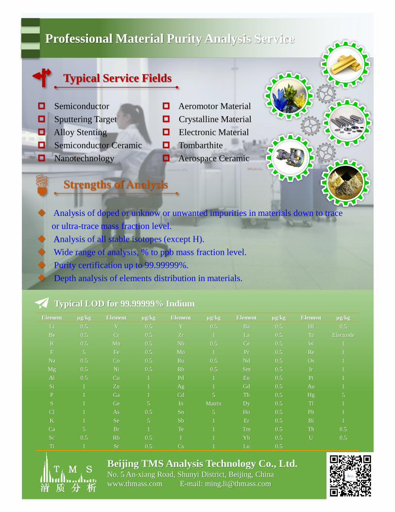
Semiconductor
Sputtering Target
Alloy Stenting
Semiconductor Ceramic
Nanotechnology
Aeromotor Material
Crystalline Material
Electronic Material
Tombarthite
Aerospace Ceramic
Typical Service Fields
Analysis of doped or unknow or unwanted impurities in materials down to trace
or ultra-trace mass fraction level.
Analysis of all stable isotopes (except H).
Wide range of analysis, % to ppb mass fraction level.
Purity certification up to 99.99999%.
Depth analysis of elements distribution in materials.
Element μg/kg Element μg/kg Element μg/kg Element μg/kg Element μg/kg
Li 0.5 V 0.5 Y 0.5 Ba 0.5 Hf 0.5
Be 0.5 Cr 0.5 Zr 1 La 0.5 Ta Electrode
B 0.5 Mn 0.5 Nb 0.5 Ce 0.5 W 1
F 5 Fe 0.5 Mo 1 Pr 0.5 Re 1
Na 0.5 Co 0.5 Ru 0.5 Nd 0.5 Os 1
Mg 0.5 Ni 0.5 Rh 0.5 Sm 0.5 Ir 1
Al 0.5 Cu 1 Pd 1 Eu 0.5 Pt 1
Si 1 Zn 1 Ag 1 Gd 0.5 Au 1
P 1 Ga 1 Cd 5 Tb 0.5 Hg 5
S 1 Ge 5 In Matrix Dy 0.5 Tl 1
Cl 1 As 0.5 Sn 5 Ho 0.5 Pb 1
K 1 Se 5 Sb 1 Er 0.5 Bi 1
Ca 5 Br 1 Te 1 Tm 0.5 Th 0.5
Sc 0.5 Rb 0.5 I 1 Yb 0.5 U 0.5
Ti 1 Sr 0.5 Cs 1 Lu 0.5
Typical LOD for 99.99999% Indium
Beijing TMS Analysis Technology Co., Ltd.No. 5 An-xiang Road, Shunyi District, Beijing, China
www.thmass.com E-mail: [email protected]
Strengths of Analysis
Professional Material Purity Analysis Service