11th International Conference onGeographic Information Science

GIScience 2021, September 27–30, 2021, Poznań, Poland(Virtual Conference)

Part II

Edited by

Krzysztof JanowiczJudith A. Verstegen

LIPIcs – Vo l . 208 – GIScience 2021 www.dagstuh l .de/ l ip i c s

Editors

Krzysztof JanowiczUniversity of California, Santa Barbara, USAjanowicz@ucsb.edu

Judith A. VerstegenWageningen University, Wageningen, The Netherlandsjudith.verstegen@wur.nl

ACM Classification 2012Information systems → Geographic information systems; Human-centered computing → Human computerinteraction (HCI); Human-centered computing → Visualization; Theory of computation → Computationalgeometry; Computing methodologies → Machine learning; Information systems → Spatial-temporalsystems

ISBN 978-3-95977-208-2

Published online and open access bySchloss Dagstuhl – Leibniz-Zentrum für Informatik GmbH, Dagstuhl Publishing, Saarbrücken/Wadern,Germany. Online available at https://www.dagstuhl.de/dagpub/978-3-95977-208-2.

Publication dateSeptember, 2021

Bibliographic information published by the Deutsche NationalbibliothekThe Deutsche Nationalbibliothek lists this publication in the Deutsche Nationalbibliografie; detailedbibliographic data are available in the Internet at https://portal.dnb.de.

LicenseThis work is licensed under a Creative Commons Attribution 4.0 International license (CC-BY 4.0):https://creativecommons.org/licenses/by/4.0/legalcode.In brief, this license authorizes each and everybody to share (to copy, distribute and transmit) the workunder the following conditions, without impairing or restricting the authors’ moral rights:

Attribution: The work must be attributed to its authors.

The copyright is retained by the corresponding authors.

Digital Object Identifier: 10.4230/LIPIcs.GIScience.2021.II.0

ISBN 978-3-95977-208-2 ISSN 1868-8969 https://www.dagstuhl.de/lipics

0:iii

LIPIcs – Leibniz International Proceedings in Informatics

LIPIcs is a series of high-quality conference proceedings across all fields in informatics. LIPIcs volumesare published according to the principle of Open Access, i.e., they are available online and free of charge.

Editorial Board

Luca Aceto (Chair, Reykjavik University, IS and Gran Sasso Science Institute, IT)Christel Baier (TU Dresden, DE)Mikolaj Bojanczyk (University of Warsaw, PL)Roberto Di Cosmo (Inria and Université de Paris, FR)Faith Ellen (University of Toronto, CA)Javier Esparza (TU München, DE)Daniel Král’ (Masaryk University - Brno, CZ)Meena Mahajan (Institute of Mathematical Sciences, Chennai, IN)Anca Muscholl (University of Bordeaux, FR)Chih-Hao Luke Ong (University of Oxford, GB)Phillip Rogaway (University of California, Davis, US)Eva Rotenberg (Technical University of Denmark, Lyngby, DK)Raimund Seidel (Universität des Saarlandes, Saarbrücken, DE and Schloss Dagstuhl – Leibniz-Zentrumfür Informatik, Wadern, DE)

ISSN 1868-8969

https://www.dagstuhl.de/lipics

GISc ience 2021

Contents

PrefaceKrzysztof Janowicz and Judith A. Verstegen . . . . . . . . . . . . . . . . . . . . . . . . . . . . . . . . . . . . . 0:vii

Conference Organization. . . . . . . . . . . . . . . . . . . . . . . . . . . . . . . . . . . . . . . . . . . . . . . . . . . . . . . . . . . . . . . . . . . . . . . . . . . . . . . . . 0:ix

List of Authors. . . . . . . . . . . . . . . . . . . . . . . . . . . . . . . . . . . . . . . . . . . . . . . . . . . . . . . . . . . . . . . . . . . . . . . . . . . . . . . . . 0:xiii

Regular Papers

Adaptive Voronoi Masking: A Method to Protect Confidential DiscreteSpatial Data

Fiona Polzin and Ourania Kounadi . . . . . . . . . . . . . . . . . . . . . . . . . . . . . . . . . . . . . . . . . . . . . . 1:1–1:17

Reproducible Research and GIScience: An Evaluation Using GIScienceConference Papers

Frank O. Ostermann , Daniel Nüst, Carlos Granell, Barbara Hofer, andMarkus Konkol . . . . . . . . . . . . . . . . . . . . . . . . . . . . . . . . . . . . . . . . . . . . . . . . . . . . . . . . . . . . . . . . . . 2:1–2:16

Comparison of Simulated Fast and Green Routes for Cyclists and PedestriansChristina Ludwig, Sven Lautenbach, Eva-Marie Schömann, and Alexander Zipf . . . 3:1–3:15

A Clustering-Based Framework for Individual Travel Behaviour Change DetectionYe Hong, Yanan Xin, Henry Martin, Dominik Bucher, and Martin Raubal . . . . . . . 4:1–4:15

Will You Take This Turn? Gaze-Based Turning Activity Recognition DuringNavigation

Negar Alinaghi, Markus Kattenbeck, Antonia Golab, and Ioannis Giannopoulos . . . 5:1–5:16

Bicriteria Aggregation of Polygons via Graph CutsPeter Rottmann, Anne Driemel, Herman Haverkort, Heiko Röglin, andJan-Henrik Haunert . . . . . . . . . . . . . . . . . . . . . . . . . . . . . . . . . . . . . . . . . . . . . . . . . . . . . . . . . . . . . 6:1–6:16

Coordinated Schematization for Visualizing Mobility Patterns on NetworksBram Custers, Wouter Meulemans, Bettina Speckmann, and Kevin Verbeek . . . . . . 7:1–7:16

Harmonious Simplification of IsolinesArthur van Goethem, Wouter Meulemans, Andreas Reimer, andBettina Speckmann . . . . . . . . . . . . . . . . . . . . . . . . . . . . . . . . . . . . . . . . . . . . . . . . . . . . . . . . . . . . . . 8:1–8:16

Navigating Your Way! Increasing the Freedom of Choice During WayfindingBartosz Mazurkiewicz, Markus Kattenbeck, and Ioannis Giannopoulos . . . . . . . . . . . . 9:1–9:16

Terrain Prickliness: Theoretical Grounds for High Complexity ViewshedsAnkush Acharyya, Ramesh K. Jallu, Maarten Löffler, Gert G.T. Meijer,Maria Saumell, Rodrigo I. Silveira, and Frank Staals . . . . . . . . . . . . . . . . . . . . . . . . . . . . 10:1–10:16

User Preferences and the Shortest PathIsabella Kreller and Bernd Ludwig . . . . . . . . . . . . . . . . . . . . . . . . . . . . . . . . . . . . . . . . . . . . . . . 11:1–11:15

11th International Conference on Geographic Information Science (GIScience 2021) – Part II.Editors: Krzysztof Janowicz and Judith A. Verstegen

Leibniz International Proceedings in InformaticsSchloss Dagstuhl – Leibniz-Zentrum für Informatik, Dagstuhl Publishing, Germany

0:vi Contents

Map Matching for Semi-Restricted TrajectoriesTimon Behr, Thomas C. van Dijk, Axel Forsch, Jan-Henrik Haunert, andSabine Storandt . . . . . . . . . . . . . . . . . . . . . . . . . . . . . . . . . . . . . . . . . . . . . . . . . . . . . . . . . . . . . . . . . 12:1–12:16

Automated Georeferencing of Antarctic SpeciesJamie Scott, Kristin Stock, Fraser Morgan, Brandon Whitehead, andDavid Medyckyj-Scott . . . . . . . . . . . . . . . . . . . . . . . . . . . . . . . . . . . . . . . . . . . . . . . . . . . . . . . . . . . . 13:1–13:16

Preface

This second volume contains the full paper proceedings of the 11th International Conferenceon Geographic Information Science (GIScience 2021) that was scheduled to be held inPoznań, Poland, 27–30 September 2021, after last year’s conference was postponed due tothe widespread outbreak of COVID-19. Given that the pandemic persisted through 2021,the organizing committee decided to hold an online conference instead.

Overall, we received 85 submissions, out of which 29 were full papers and 56 were shortpapers. While most papers received three reviews, the number of reviews varied betweentwo and four. For the full papers, the review phase was followed by a rebuttal phase inwhich the authors could react to the reviews and provide clarifications. Next, the reviewersdiscussed the reviews and rebuttals with a metareviewer, and adjusted their final assessmentwhen appropriate. The metareviewers summarized the reviews and discussion and provideda recommendation to the program chairs. One manuscript was accepted conditionally toundergo another round of editorial checks. In total, we accepted 13 full papers for this secondvolume. The short papers were in review at the time of compiling this full paper volume.

The accepted papers represent a wide range of topics in GIScience, including workon trajectory and movement analysis, computational geometry, semantics, GeoAI, andagent-based modeling.

The entire GIScience 2021 team would like to express their gratitude to all the authors,reviewers, workshop and tutorial organizers, and anybody else involved in organizing theconference. We are particularly grateful to the emergency reviewers for accepting theincreased workload and to the broader GIScience community for providing support, advice,and for their understanding during these difficult times.

The GIScience 2020/21 Organizing Team

11th International Conference on Geographic Information Science (GIScience 2021) – Part II.Editors: Krzysztof Janowicz and Judith A. Verstegen

Leibniz International Proceedings in InformaticsSchloss Dagstuhl – Leibniz-Zentrum für Informatik, Dagstuhl Publishing, Germany

Conference Organization

General ChairPiotr Jankowski, San Diego State University, USA & Adam Mickiewicz University, Poznań,Poland

Program ChairsKrzysztof Janowicz, University of California, Santa Barbara, USAJudith Verstegen, Wageningen University, The Netherlands

Local Organization ChairZbigniew Zwoliński, Adam Mickiewicz University, Poznań, Poland

Workshop and Tutorial ChairsGrant McKenzie, McGill University, CanadaMarcin Winowski, Adam Mickiewicz University, Poznań, Poland

Sponsorship ChairBernd Resch, University of Salzburg, Austria

Publicity ChairsDara Seidl, Colorado Mountain College, USAAlfred Stach, Adam Mickiewicz University, Poznań, Poland

Arrangements and LogisticsJoanna Gudowicz, Adam Mickiewicz University, Poznań, PolandRobert Kruszyk, Adam Mickiewicz University, Poznań, PolandJarosław Jasiewicz, Adam Mickiewicz University, Poznań, PolandPaweł Matulewski, Adam Mickiewicz University, Poznań, PolandMałgorzata Mazurek, Adam Mickiewicz University, Poznań, PolandAlicja Najwer, Adam Mickiewicz University, Poznań, PolandJustyna Weltrowska, Adam Mickiewicz University, Poznań, Poland

Metadata ChairsBlake Regalia, University of California, Santa Barbara, USAGengchen Mai, University of California, Santa Barbara, USALing Cai, University of California, Santa Barbara, USA

WebmasterJakub Nowosad, Adam Mickiewicz University, Poznań, Poland

11th International Conference on Geographic Information Science (GIScience 2021) – Part II.Editors: Krzysztof Janowicz and Judith A. Verstegen

Leibniz International Proceedings in InformaticsSchloss Dagstuhl – Leibniz-Zentrum für Informatik, Dagstuhl Publishing, Germany

0:x Conference Organization

Program Committee

Name University, Country

Benjamin Adams University of Canterbury, New ZeelandOla Ahlqvist The Ohio State University, USAGennady Andrienko Fraunhofer, GermanyNatalia Andrienko Fraunhofer, GermanyClio Andris Georgia Tech, USAAndrea Ballatorem Birkbeck, University of London, UKKate Beard-Tisdale University of Maine, USAItzhak Benenson Tel Aviv University, IsraelMichela Bertolotto University College Dublin, IrelandLing Bian University at Buffalo, USAJustine Blanford University of Twente, The NetherlandsThomas Blaschke University of Salzburg, AustriaBoyan Brodaric Geological Survey of Canada, CanadaChris Brunsdon National University of Ireland, Maynooth, IrelandLing Caie University of California, Santa Barbara, USAGilberto Camara INPE, BrazilChristophe Claramunt Naval Academy Research Institute, FranceEliseo Clementini University of L’Aquila, ItalyTom Cova University of Utah, USAClodoveu Davis Universidade Federal de Minas Gerais, BrazilSytze de Bruin Wageningen University, The NetherlandsSomayeh Dodge University of California, Santa Barbara, USASuzana Dragicevic Simon Fraser University, CanadaMatt Duckham RMIT University, USASara Irina Fabrikant University of Zurich, SwitzerlandSong Gao University of Wisconsin-Madison, USAAmy Griffin RMIT University, AustraliaTorsten Hahmann University of Maine, USAJan-Henrik Haunert Universität Bonn, GermanyGerard Heuvelink Wageningen University, The NetherlandsStephen Hirtle University of Pittsburgh, USAHartwig Hochmair University of Florida, USAYingjie Hum University at Buffalo, USABernhard Höfle Heidelberg University, GermanyMarta Jankowska University of California, San Diego, USABin Jiang University of Gävle, SwedenChristopher Jones Cardiff University, UKCarsten Keßler Aalborg University Copenhagen, DenmarkPeter Kiefer ETH Zurich, SwitzerlandAlexander Klippel Wageningen University, The NetherlandsJennifer Koch University of Oklahoma, USAChristian Kray University of Münster, GermanyShawn Laffan The University of New South Wales, AustraliaTobia Lakes Humboldt-Universität zu Berlin, Germany

Conference Organization 0:xi

Patrick Laube Zurich University of Applied Sciences ZHAW, SwitzerlandMichael Leitner Louisiana State University, USAWenwen Li Arizona State University, USAArika Ligmann-Zielinska Michigan State University, USAGengchen Maie University of California, Santa Barbara, USAEd Manleym University of Leeds, UKBruno Martinsm University of Lisbon, PortugalGrant McKenziem McGill University, CanadaMir Abolfazl Mostafavi Laval University, CanadaAlan Murray University of California, Santa Barbara, USAAtsushi Naram San Diego State University, USADavid O’Sullivan Victoria University of Wellington, New ZeelandEdzer Pebesma University of Münster, GermanyRoss Purves University of Zurich, SwitzerlandMartin Raubal ETH Zurich, SwitzerlandSimon Scheiderm Utrecht University, The NetherlandsOliver Schmitz Utrecht University, The NetherlandsJohannes Scholz Graz University of Technology, AustriaJohannes Schöning University of Bremen, GermanyDara Seidlm Colorado Mountain College, USARaja Sengupta McGill University, CanadaShih-Lung Shaw University of Tennessee, USATakeshi Shirabe KTH Royal Institute of Technology, SwedenAlex Singleton University of Liverpool, UKAndré Skupin San Diego State University, USASeth Spielman University of Colorado Boulder, USAKathleen Stewart University of Maryland, USAMartin Swobodzinski Portland State University, USAJean-Claude Thill Universit of North Carolina at Charlotte, USASabine Timpf University of Augsburg, GermanyMartin Tomko University of Melbourne, AustraliaMing-Hsiang Tsou San Diego State University, USANico Van de Weghe Ghent University, BelgiumMarc Van Kreveld Utrecht University, The NetherlandsJudith Verstegen Wageningen University, The NetherlandsMonica Wachowicz RMIT University, CanadaShaowen Wang University of Illinois at Urbana-Champaign, USARobert Weibel University of Zurich, SwitzerlandJohn Wilson University of Southern California, USAStephan Winter University of Melbourne, AustraliaNingchuan Xiao The Ohio State University, USAEunhye Yoo University at Buffalo, USABailang Yu East China Normal University, ChinaSisi Zlatanova University of New South Wales, Australia

e: (aditionally as) emergency reviewer, m: (aditionally as) meta reviewer

GISc ience 2021

List of Authors

Ankush Acharyya (10)The Czech Academy of Sciences,Institute of Computer Science,Prague, Czech Republic

Negar Alinaghi (5)Geoinformation, TU Wien, Austria

Timon Behr (12)University of Konstanz, Germany

Dominik Bucher (4)Institute of Cartography and Geoinformation,ETH Zurich, Switzerland

Bram Custers (7)Eindhoven University of Technology,The Netherlands

Anne Driemel (6)Hausdorff Center for Mathematics,University of Bonn, Germany

Axel Forsch (12)University of Bonn, Germany

Ioannis Giannopoulos (5, 9)Geoinformation, TU Wien, Austria;Institute of Advanced Research in ArtificialIntelligence (IARAI), Vienna, Austria

Antonia Golab (5)Geoinformation, TU Wien, Austria

Carlos Granell (2)Institute of New Imaging Technologies,Universitat Jaume I de Castellón, Spain

Jan-Henrik Haunert (6, 12)Institute of Geodesy and Geoinformation,University of Bonn, Germany

Herman Haverkort (6)Institute of Computer Science,University of Bonn, Germany

Barbara Hofer (2)Christian Doppler Laboratory GEOHUM andDepartment of Geoinformatics – Z_GIS,University of Salzburg, Austria

Ye Hong (4)Institute of Cartography and Geoinformation,ETH Zurich, Switzerland

Ramesh K. Jallu (10)The Czech Academy of Sciences,Institute of Computer Science,Prague, Czech Republic

Markus Kattenbeck (5, 9)Geoinformation, TU Wien, Austria

Markus Konkol (2)Faculty of Geo-Information Science and EarthObservation (ITC), University of Twente,Enschede, The Netherlands

Ourania Kounadi (1)Department of Geography and RegionalResearch, University of Vienna, Austria

Isabella Kreller (11)University of Regensburg, Germany

Sven Lautenbach (3)Heidelberg Institute for GeoinformationTechnology (HeiGIT) gGmbH at HeidelbergUniversity, Germany

Bernd Ludwig (11)University of Regensburg, Germany

Christina Ludwig (3)GIScience Research Group, Institute ofGeography, Heidelberg University, Germany

Maarten Löffler (10)Deptartment of Information and ComputingSciences, Utrecht University, The Netherlands

Henry Martin (4)Institute of Cartography and Geoinformation,ETH Zurich, Switzerland;Institute of Advanced Research in ArtificialIntelligence (IARAI), Austria

Bartosz Mazurkiewicz (9)Geoinformation, TU Wien, Austria

David Medyckyj-Scott (13)Manaaki Whenua Landcare Research,Auckland, New Zealand

Gert G.T. Meijer (10)Academy of ICT and Creative Technologies,NHL Stenden University of Applied Sciences,The Netherlands

Wouter Meulemans (7, 8)Eindhoven University of Technology,The Netherlands

11th International Conference on Geographic Information Science (GIScience 2021) – Part II.Editors: Krzysztof Janowicz and Judith A. Verstegen

Leibniz International Proceedings in InformaticsSchloss Dagstuhl – Leibniz-Zentrum für Informatik, Dagstuhl Publishing, Germany

0:xiv Authors

Fraser Morgan (13)Manaaki Whenua Landcare Research,Auckland, New Zealand

Daniel Nüst (2)Institute for Geoinformatics,University of Münster, Germany

Frank O. Ostermann (2)Faculty of Geo-Information Science and EarthObservation (ITC), University of Twente,Enschede, The Netherlands

Fiona Polzin (1)ITC-Faculty of Geoinformation and EarthObservation, University of Twente, Enschede,The Netherlands

Martin Raubal (4)Institute of Cartography and Geoinformation,ETH Zurich, Switzerland

Andreas Reimer (8)Eindhoven University of Technology,The Netherlands

Peter Rottmann (6)Institute of Geodesy and Geoinformation,University of Bonn, Germany

Heiko Röglin (6)Institute of Computer Science,University of Bonn, Germany

Maria Saumell (10)The Czech Academy of Sciences, Institute ofComputer Science, Prague, Czech Republic;Department of Theoretical Computer Science,Faculty of Information Technology, CzechTechnical University in Prague, Czech Republic

Eva-Marie Schömann (3)GIScience Research Group, Institute ofGeography, Heidelberg University, Germany

Jamie Scott (13)Massey University, Auckland, New Zealand

Rodrigo I. Silveira (10)Department of Mathematics,Universitat Politècnica de Catalunya,Barcelona, Spain

Bettina Speckmann (7, 8)Eindhoven University of Technology,The Netherlands

Frank Staals (10)Department of Information and ComputingSciences, Utrecht University, The Netherlands

Kristin Stock (13)Massey Geoinformatics Collaboratory,Massey University, Auckland, New Zealand

Sabine Storandt (12)University of Konstanz, Germany

Thomas C. van Dijk (12)University of Bochum, Germany

Arthur van Goethem (8)Eindhoven University of Technology,The Netherlands

Kevin Verbeek (7)Eindhoven University of Technology,The Netherlands

Brandon Whitehead (13)Manaaki Whenua Landcare Research,Auckland, New Zealand

Yanan Xin (4)Institute of Cartography and Geoinformation,ETH Zurich, Switzerland

Alexander Zipf (3)GIScience Research Group, Institute ofGeography, Heidelberg University, Germany;HeiGIT gGmbH at Heidelberg University,Germany

Adaptive Voronoi Masking: A Method to ProtectConfidential Discrete Spatial DataFiona Polzin #

ITC-Faculty of Geoinformation and Earth Observation,University of Twente, Enschede, The Netherlands

Ourania Kounadi1 # Ñ

Department of Geography and Regional Research, University of Vienna, Austria

AbstractGeomasks assure the protection of individuals in a discrete spatial point data set by aggregating,transferring or altering original points. This study develops an alternative approach, referred to asAdaptive Voronoi Masking (AVM), which is based on the concepts of Adaptive Aerial Elimination(AAE) and Voronoi Masking (VM). It considers the underlying population density by establishingareas of K-anonymity in which Voronoi polygons are created. Contrary to other geomasks, AVMconsiders the underlying topography and displaces data points to street intersections thus decreasingthe risk of false-identification since residences are not endowed with a data point.

The geomasking effects of AVM are examined by various spatial analytical results and arecompared with the outputs of AAE, VM, and Donut Masking (DM). VM attains the best efficiencyfor the mean centres whereas DM does for the median centres. Regarding the Nearest NeighbourHierarchical Cluster Analysis and Ripley’s K-function, DM demonstrates the strongest performancesince its cluster ellipsoids and clustering distance are the most similar to those of the original data.The extend of the original data is preserved the most by VM, while AVM retains the topology ofthe point pattern. Overall, AVM was ranked as 2nd in terms of data utility (i) and also outperformsall methods regarding the risk of false re-identification (ii) because no data point is moved to aresidence. Furthermore, AVM maintains the Spatial K-anonymity (iii) which is also done by AAEand partly by DM. Based on the performance combination of these factors, AVM is an advantageoustechnique to mask geodata.

2012 ACM Subject Classification Security and privacy → Privacy protections; Security and privacy→ Data anonymization and sanitization; Information systems → Geographic information systems;Mathematics of computing → Exploratory data analysis

Keywords and phrases Geoprivacy, location privacy, geomasking, Adaptive Voronoi Masking, VoronoiMasking, Adaptive Aerial Elimination, Donut Geomasking, ESDA

Digital Object Identifier 10.4230/LIPIcs.GIScience.2021.II.1

Supplementary Material The Geoprivacy Github repository contains the scripts to run AVM (AlsoAAE) as well as one of the six area data sets used in this study:Software: https://github.com/okounadi/Geoprivacy

1 Introduction

1.1 BackgroundThe advances of GIS and the interest in spatial analysis have led to an increase of thematicmaps in research and online platforms visualizing point data. However, several studies inhealth geography, reproductive and sexual health did not anonymize or aggregate data;instead, the original data were used [4, 14, 17]. Publishing an individual’s location either in

1 Corresponding author

© Fiona Polzin and Ourania Kounadi;licensed under Creative Commons License CC-BY 4.0

11th International Conference on Geographic Information Science (GIScience 2021) – Part II.Editors: Krzysztof Janowicz and Judith A. Verstegen; Article No. 1; pp. 1:1–1:17

Leibniz International Proceedings in InformaticsSchloss Dagstuhl – Leibniz-Zentrum für Informatik, Dagstuhl Publishing, Germany

1:2 Adaptive Voronoi Masking (AVM)

paper or digital form - knowingly or unknowingly - increases the risk of re-identification byand violates individual privacy. How simple the re-identification of individuals is, was alreadydemonstrated by Brownstein et al. [4]: By applying the reverse-identification method, 7% ofthe spatially coded addresses were accurately identified while all 550 of the plotted addresspoints were disclosed within 14 m of the right address. Furthermore, Kounadi and Leitner[17] exposed that within an eight-year duration, almost 70,000 home addresses had beendisclosed in academic research.

The consequences of disclosure are vast; an individual being identified as an HIV-patient- correctly or wrongly - can affect him or her by discrimination or social stigmatization [27].Identifications may cause harassment [9], unwanted advertisement or humiliation [26, 25].Kounadi and Leitner [19] criticize that general rules on privacy do not include details of thespatial re-identification risk notwithstanding the fact that relevant research and reports ongeodata exist [12, 20]. Consequently, confidential spatial data sets do not only have to bepreserved but also need to comply with present-day restrictions and regulations on the rightto privacy [19]. However, Ajayakumar et al. [1] criticized that geomasks are still unavailablefor many institutions due to the lack of expertise in geospatial proficiency although theawareness of the power of mapping has grown particularly in health organizations and clinicswhich have become spatially literate lately. The authors stress that geomasks need to becomemore of a real-world requirement.

1.2 Problem statementSome geomasks displace the points a specific distance aside from its original location (e.g.,local random rotation by Leitner and Curtis [22] and Voronoi masking (VM) by Seidl et al.[29], while others aggregate points (e.g., spatial and point aggregation by Armstrong et al.[3]). Other geomasks consider the underlying population density adapting the displacementerror such as the Donut Geomasking (DM) [15] and the Adaptive Areal Elimination (AAE)[19]. By considering the population density, the “masker” is able to determine a level ofK-anonymity in which each record (i.e. person) within a masked data set cannot be identifiedfrom at least K-1 records [24]. Regarding geodata, K-anonymity assures that every locationsuch as household, address or an individual’s location cannot be differentiated from minimumK-1 locations. This means, that spatial K-anonymity (SKA) describes the probability ofidentifying a location that can be linked to an individual by reverse geocoding. This isneeded to evaluate the degree of privacy and when measuring the degree of displacement.

A possible solution to prevent re-engineering of original locations could be points’ ag-gregation. However, when doing so, the ability to distinguish spatial relations or clustersand deriving persuasive information is decreased [30, 3, 21]. Obviously, the data becomesless useful for research purposes [30, 13]. Contrary to aggregation, geomasks that modifythe locations are preferred for analytical purposes. Nevertheless, the transferred pointscan be moved to a position which has real observations [23] or where they cannot exist [7],resulting in false identification [29]. False identification represents the incorrect linking of ahousehold or person to a data point. Contrary to that, correct identification is the correctlinkage of a household or person to a data point [29]. The consequences of identification canresult in negative effects impeding an individual’s social prominence [13]. Besides, it canunintentionally involve individuals, who were not part of the research [7]. Such limitationsinfluence both the disclosure risk and a successful investigation of spatial patterns.

Generally, there is neither a recommended nor approved geomask technique [30, 13] andeach method has disadvantages and advantages. Zandbergen [30] suggests counterbalancingdata utility and confidentiality protection. Also, not a lot of geomasks consider the underlying

F. Polzin and O. Kounadi 1:3

topography except for the Street aggregation at intersection or at midpoint [22] or the LocationSwapping method [31]. Yet these that do consider the underlying topography do not offer apredefined level of SKA. It is evident that existing techniques must be improved to overcomesuch shortcomings and also become widely accessible.

1.3 Study scope and designOur alternative approach, referred to as Adaptive Voronoi Masking (AVM), is based on theconcepts of AAE and VM. AVM shall protect the individual’s privacy based on SKA whilealso decreasing the false re-identification risk. We evaluate known geomasks, namely the VM,the AAE, and the DM, and compare them with the proposed AVM in terms of three keyaspects: a) SKA, b) false re-identification, and c) data utility.

In the next section (Methodology) we explain the two geomasks that AVM is based on(VM and AAE) and then describe the functionality of AVM. Next, we present the exploratoryspatial data analysis (ESDA) methods that are used to compare and evaluate the original datapoints with the outcome of the geomasks (i.e. masked data points). Last, we introduce thestudy area, the software, and data used. In section 3 (Results), we report the ESDA resultsand finally discuss and conclude our findings in section 4 (Conclusion). Apart from the AVM,DM, and AAE, we also evaluate the DM geomask. DM was chosen as a comparative geomasksince it is a popular technique and it has a small effect on the geographical characteristics ofthe original point pattern as highlighted in academic literature [15, 30, 2]. The algorithm forthis method was retrieved online2.

2 Methodology

2.1 Adaptive Areal Elimination (AAE)AAE assures privacy by moving the original locations within uncertainty areas. The so-calleduncertainty areas describe an area, where the masked points are displaced in, e.g. torus orcircle [19]. For instance, DM moves the original data within an uncertainty area selectedfrom a uniform distribution [15] while the population-density-based Gaussian spatial blurringdislocates points within a circle based on a normal distribution [5]. However, these geomasksassume that population is homogeneously distributed - which is not the case in most instances.This assumption can result in masked data points with a lower actual K-anonymity than theestimated K-anonymity [2]. Hence, AAE is aiming to ensure K-anonymity even when thegeomasking method and its parameters are known. K-anonymity can be measured preciselywhen uncertainty areas do not overlap and when it is applied at a lower or equal level of theavailable resolution [19].

To execute the AAE algorithm, two data sets are needed: a) a point file and b) a spatialdata set that either includes an attribute with discrete information (e.g., as administrativeunits containing an attribute field with the total households in each unit) or representsdiscrete information (e.g., point data representing households). This attribute is calledRoRi (risk of re-identification). Generally, risk of re-identification can contain informationsuch as addresses, households, or population. A disclosure value for this field predefined todescribe the minimum K-anonymity which is used to obscure confidential information. Inthe next step, the process of merging polygons starts: depending on the disclosure value,

2 https://mserre.sph.unc.edu/BMElab_web/donutGeomask/donutGeomask.htm (Last accessed on Janu-ary 22th, 2021)

GISc ience 2021

1:4 Adaptive Voronoi Masking (AVM)

every polygon containing a lower risk of re-identification value than the disclosure value, ismerged with its neighbouring polygon or polygons until each polygon has values that areeither greater than or equivalent with the disclosure value to create the K-anonymized areas.Next, original data are aggregated to the centroids of the merged polygons or randomlydisplaced within the merged polygons. Random displacement can be performed by a randomperturbation to the coordinates of each data point by a random distance and at a randomdirection (equation 1).

Xm = Xo + D ∗ cosine(Θ)Y m = Y o + D ∗ sine(Θ) (1)

where, Xo,Yo are the original coordinates of a point, Xm,Ym are the resulting maskedcoordinates, D is a random value within a predefined range, and Θ is a random angle.

In the AAE each masked point shall lie within its k-anonymized polygon. Thus, the displacedmasked point/s has to be conditioned on the boundaries of each polygon. In this study, weimplement the random displacement that yielded better performance results in the study byKounadi and Leitner (2016). When studying the outputs of AAE more closely, some maskeddata are moved further distances than necessary. This can be explained by the process ofmerging polygons that selects the neighbour with the longest boundary, which may result inK-anonymized areas that are larger than needed to ensure SKA.

2.2 Voronoi Masking (VM)VM creates Voronoi polygons around the original data points are displaced to the closestsegment (edge) of its corresponding polygon [29, 13]. The theoretical basis of creating Voronoipolygons starts with the triangulation of the original points into an irregular network thatmeets the Delaunay criterion (i.e. no point is inside the circumcircle of any triangle). Then,the perpendicular bisectors for each triangle edge are generated. These are the edges of theVoronoi polygons while the locations of the bisector’s intersections determine the vertices.Every point within each polygon is closer to the original point of its creation than to otheroriginal points.

Advantages of VM is that points in neighbouring polygons are displaced to the sameposition, enhancing their K-anonymity and that a higher point density results in smallerdistances between the original data and masked data thus giving a pattern that is similar tothe original one [29, 13]. For a small scale area or an area with a minimum of two households,VM dislocates the original data a lesser distance than compared to other geomasks thatdo not consider the underlying settlement patterns. VM is an efficient approach regardingthe preservation of the spatial point pattern as it has been proved by Seidl et al. [29] whoimplemented various methods to evaluate its performance. Finally, Seidl et al. [29] praisethat in case of applying a data set that is including all residences within the area of interest,no displaced point will be located on an actual residence and thus false identification ofresidences is not possible. Points are typically located in the centre of a parcel or at the streetsegment. VM will definitely move points away from these locations. However, this processdoes not guarantee that segments of Voronoi polygons will not cross residential parcels andtherefore VM cannot decrease the risk of false identification in this regard.

When applying VM in areas with scattered residences some data points will be dislocatedat large distances, which affect spatial patterns. Also, a smaller amount of masked datawill be depicted on the map than the original data due to the overlapping of points at the

F. Polzin and O. Kounadi 1:5

displaced locations. Although this assures a higher K-anonymity, the map viewer may notbe aware that some points represent at least two addresses, increasing the risk of spatiallyanalysing or perceiving the output differently. Last, although K-anonymity is increased,compared to other geomasks, a predefined level of SKA cannot be guaranteed.

2.3 Adaptive Voronoi Masking (AVM)AVM extracts the asset of considering the underlying population density by joining polygonsas AAE does and displaces the original data based on the concept of VM. In respect thereof,the original data are moved to the closest segment of their corresponding Voronoi polygonwhich lies within their merged AAE-polygon. In case a Voronoi segment lies outside itsdissolved polygon, the point is transferred to the boundary of the merged polygon and not tothe edge of the Voronoi polygon. Through that, AVM intends to circumvent the predicamentof moving points to a polygon containing a different population threshold thus preservingthe predefined SKA. Further, the underlying topography is considered by moving pointsto the closest street intersection that has a higher amount of surrounding buildings thanif moved to the nearest segment. Through that, AVM avoids shifting the points directlyto another residence causing false re-identification but it also prevents the displacement toinvalid locations such as water bodies or forests.

To execute AVM, the following data sets are required: a) a point file (as needed in VMand AAE), b) a polygon file including risk of re-identification information (as required inAAE), and c) a line file depicting the street network. Firstly, the data is pre-processed asdone for AAE. Subsequently, a disclosure threshold for the risk of re-identification field isselected and polygons with a smaller value than the chosen disclosure value are mergedwith its adjacent polygon until all polygons receive a value that is greater or equal to theset disclosure value. Here, the general spatial rule is applied defining that every polygon iscombined with the bordering polygon that has the longest shared border [19].

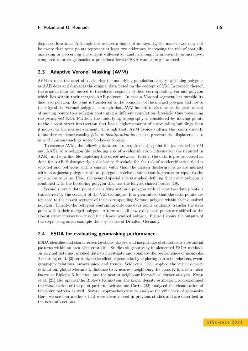
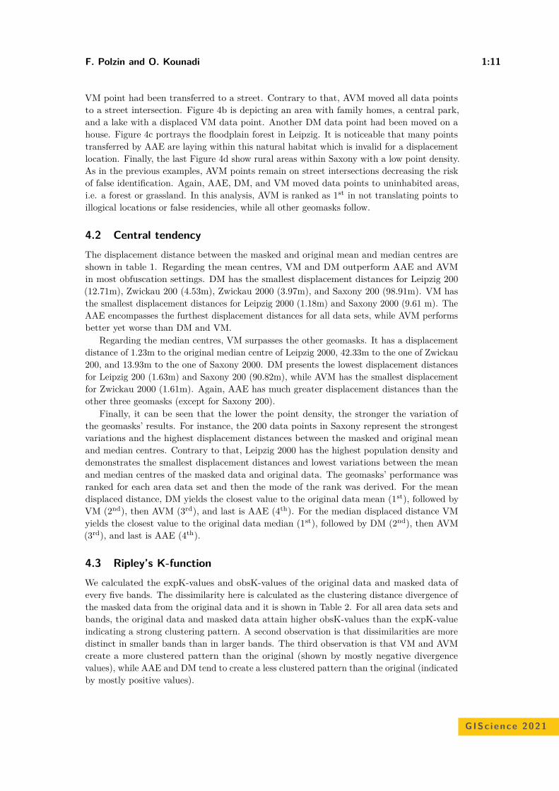
Secondly, every data point that is lying within a polygon with at least two data points istransferred by the concept of the VM technique. It is guaranteed that the data points arereplaced to the closest segment of their corresponding Voronoi polygon within their dissolvedpolygon. Thirdly, the polygons containing only one data point randomly transfer the datapoint within their merged polygon. Afterwards, all newly displaced points are shifted to theclosest street intersection inside their K-anonymized polygon. Figure 1 shows the outputs ofthe steps using as an example the city centre of Dresden, Germany.

2.4 ESDA for evaluating geomasking performanceESDA identifies and characterizes locations, shapes, and magnitudes of statistically substantialpatterns within an area of interest [10]. Studies on geoprivacy implemented ESDA methodson original data and masked data to investigate and compare the performance of geomasks.Armstrong et al. [3] scrutinized the effect of geomasks by exploring pair-wise relations, event-geography relations, anisotropies, and trends. Seidl et al. [29] applied the kernel densityestimation, global Moran’s I, distance to K-nearest neighbour, the cross K-function - alsoknown as Ripley’s K-function, and the nearest neighbour hierarchical cluster analysis. Kwanet al. [21] also applied the Ripley’s K-function, the kernel density estimation, and examinedthe visualisation of the point pattern. Leitner and Curtis [22] analysed the visualisation ofthe point pattern as well. Several approaches exist to analyse the efficiency of geomasks.Here, we use four methods that were already used in previous studies and are described inthe next subsections.

GISc ience 2021

1:6 Adaptive Voronoi Masking (AVM)

Figure 1 A visualisation of the AVM outputs in the city centre of Dresden.

2.4.1 Visualisation of point patternThis technique is used to a) scrutinize the extent of the original data and compare it withthat of the masked data and b) to investigate whether the masked data are displaced on otherresidencies increasing the risk of false re-identification or are transferred to void locationssuch as forests or lakes.

F. Polzin and O. Kounadi 1:7

2.4.2 Central tendency

The mean and median centres of the original data and the masked data are compared throughtheir distance’s divergence. This has been applied by Seidl et al. [29] and Gupta and Rao[13].

2.4.3 Ripley’s K function

Ripley’s K-function identifies whether the masked points are clustered, dispersed, or randomlydistributed and whether the point distribution between original data and masked dataremains linked or not. In the case of linked point distribution, the geomasks perform spatiallydependent on the original data. Ripley’s K-function conflates spatial dependence regardingpoint feature scattering or aggregation over a variety of distances [8], which returns a moredetailed output than other ESDA pattern detection techniques. By analysing the spatialpatterns over several lengths as well as spatial scales, the point patterns alter. Thus, itcan reflect how the scattering or aggregating of points centroids shifts when the size of theneighbourhood varies.

2.4.4 Nearest neighbour hierarchical cluster analysis

In most previous studies, the impact of geomasks on original hot spots has been probed.This is important since clustering detection plays a vital role in spatial analysis. For instance,by detecting hot spots, high concentrations of crime incidents can be explored and predictedfor future scenarios [6]. Nearest neighbour hierarchical cluster analysis allows examining andcomparing the clustering pattern of the original data with the pattern of the masked dataregarding amount of clusters, size, orientation, density.

3 Experiments’ settings

3.1 Study area

The choice of the study area is based on the availability of processed and free data. Moreover,area data sets must allow different levels of spatial granularity and population density.The chosen area is the Free State of Saxony in Eastern Germany. Saxony has 13 districtscontaining more than 4 million inhabitants3, of which more than 563,000 were registered inthe state capital Dresden. Yet, the highest population and population density are found inthe city of Leipzig with a total of 587,857 people and 1,974 inhabitants per km2. Contrary tothat, the district Nordsachsen has only 97 inhabitants per km2 - the lowest in Saxony. Hence,the State of Saxony is an explicit choice to investigate the performance of geomasks becauseit has highly populated as well as rural areas. The geomasks are applied on the State ofSaxony, the city of Leipzig because it has the most inhabitants and the highest populationdensity, and the district of Zwickau. Zwickau was chosen because when calculating theaverage inhabitants (ca. 313,685) and population density (ca. 493/km2) per district inSaxony, Zwickau has the closest values (inhabitants: 317,531; population density: 334/km2).

3 https://www.statistik.sachsen.de/(Last accessed on January 22th, 2021)

GISc ience 2021

1:8 Adaptive Voronoi Masking (AVM)

3.2 DataFor the polygon file, a line shapefile representing the street network in Saxony was derivedonline4, and used to create streets blocks. It was aimed to develop blocks which are not toocoarse but also not too small. Since the original road network file also included several streetclasses such as “footway”, “path”, or “cycleway”, all street duplicates, as well as all streetclasses except for “primary”, “secondary”, and “tertiary”, were deleted off the shapefile togeneralize the road network. Thus, an enormous amount of small blocks is avoided resultingin shorter processing times of the geomasks. Also, only single-line road features in placeof matched pairs of divided road lanes were maintained. Small and open configurations ofroads were removed. Next, polygon features were created from the remaining polylines. Anypolygons outside the study area were removed.

The same street network dataset was also used for intersection displacement step of AVM.However, in this case, it was more detailed containing also the “residential class”. Thus, asmaller but yet meaningful displacement of the data points can be achieved. More streetclasses such as “footway” or “cycleway” were not included to prevent false re-identification.

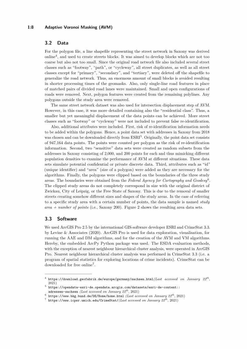
Also, additional attributes were included. First, risk of re-identification information needsto be added within the polygons. Hence, a point data set with addresses in Saxony from 2018was chosen and can be downloaded directly from ESRI5. Originally, the point data set consistsof 947,164 data points. The points were counted per polygon as the risk of re-identificationinformation. Second, two “sensitive” data sets were created as random subsets from theaddresses in Saxony consisting of 2,000, and 200 points for each and thus mimicking differentpopulation densities to examine the performance of AVM at different situations. These datasets simulate potential confidential or private discrete data. Third, attributes such as “id”(unique identifier) and “area” (size of a polygon) were added as they are necessary for thealgorithms. Finally, the polygons were clipped based on the boundaries of the three studyareas. The boundaries were obtained from the Federal Agency for Cartography and Geodesy6.The clipped study areas do not completely correspond in size with the original district ofZwickau, City of Leipzig, or the Free State of Saxony. This is due to the removal of smallerstreets creating somehow different sizes and shapes of the study areas. In the case of referringto a specific study area with a certain number of points, the data sample is named studyarea + number of points (i.e., Saxony 200). Figure 2 shows the resulting area data sets.

3.3 SoftwareWe used ArcGIS Pro 2.5 by the international GIS-software developer ESRI and CrimeStat 3.3.by Levine & Associates (2020). ArcGIS Pro is used for data exploration, visualisation, forrunning the AAE and DM algorithms, and for the creation of the AVM and VM algorithms.Hereby, the embedded ArcPy Python package was used. The ESDA evaluation methods,with the exception of nearest neighbour hierarchical cluster analysis, were operated in ArcGISPro. Nearest neighbour hierarchical cluster analysis was performed in CrimeStat 3.3 (i.e. aprogram of spatial statistics for exploring locations of crime incidents). CrimeStat can bedownloaded for free online7.

4 https://download.geofabrik.de/europe/germany/sachsen.html(Last accessed on January 22th,2021)

5 https://opendata-esri-de.opendata.arcgis.com/datasets/esri-de-content::adressen-sachsen (Last accessed on January 22th, 2021)

6 https://www.bkg.bund.de/DE/Home/home.html (Last accessed on January 22th, 2021)7 https://www.icpsr.umich.edu/CrimeStat/(Last accessed on January 22th, 2021)

F. Polzin and O. Kounadi 1:9

Figure 2 The six area data sets that are used in the study.

4 Results

AVM, AAE, and DM were applied with a SKA level of 50 addresses. VM is not an adaptivegeomask and thus a SKA level cannot be predefined and guaranteed. The four ESDA methodsare applied to the original data as well as on the masked data to examine the effects of thegeomasks on the original data. [18] and detect dissimilarities of spatial information loss andthe preservation of original data granularity [28]. In the ideal case, the spatial analysis ofthe AVM masked data will be equal to that of the original data.

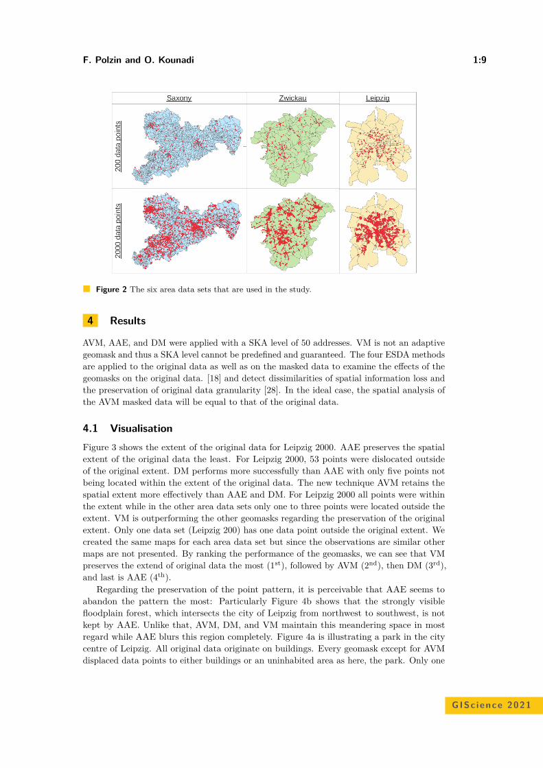
4.1 VisualisationFigure 3 shows the extent of the original data for Leipzig 2000. AAE preserves the spatialextent of the original data the least. For Leipzig 2000, 53 points were dislocated outsideof the original extent. DM performs more successfully than AAE with only five points notbeing located within the extent of the original data. The new technique AVM retains thespatial extent more effectively than AAE and DM. For Leipzig 2000 all points were withinthe extent while in the other area data sets only one to three points were located outside theextent. VM is outperforming the other geomasks regarding the preservation of the originalextent. Only one data set (Leipzig 200) has one data point outside the original extent. Wecreated the same maps for each area data set but since the observations are similar othermaps are not presented. By ranking the performance of the geomasks, we can see that VMpreserves the extend of original data the most (1st), followed by AVM (2nd), then DM (3rd),and last is AAE (4th).

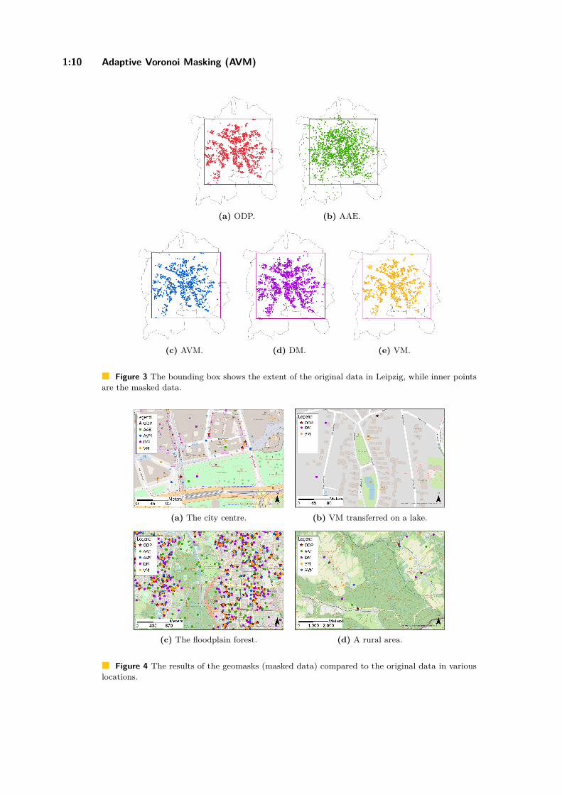
Regarding the preservation of the point pattern, it is perceivable that AAE seems toabandon the pattern the most: Particularly Figure 4b shows that the strongly visiblefloodplain forest, which intersects the city of Leipzig from northwest to southwest, is notkept by AAE. Unlike that, AVM, DM, and VM maintain this meandering space in mostregard while AAE blurs this region completely. Figure 4a is illustrating a park in the citycentre of Leipzig. All original data originate on buildings. Every geomask except for AVMdisplaced data points to either buildings or an uninhabited area as here, the park. Only one

GISc ience 2021

1:10 Adaptive Voronoi Masking (AVM)

(a) ODP. (b) AAE.

(c) AVM. (d) DM. (e) VM.

Figure 3 The bounding box shows the extent of the original data in Leipzig, while inner pointsare the masked data.

(a) The city centre. (b) VM transferred on a lake.

(c) The floodplain forest. (d) A rural area.

Figure 4 The results of the geomasks (masked data) compared to the original data in variouslocations.

F. Polzin and O. Kounadi 1:11

VM point had been transferred to a street. Contrary to that, AVM moved all data pointsto a street intersection. Figure 4b is depicting an area with family homes, a central park,and a lake with a displaced VM data point. Another DM data point had been moved on ahouse. Figure 4c portrays the floodplain forest in Leipzig. It is noticeable that many pointstransferred by AAE are laying within this natural habitat which is invalid for a displacementlocation. Finally, the last Figure 4d show rural areas within Saxony with a low point density.As in the previous examples, AVM points remain on street intersections decreasing the riskof false identification. Again, AAE, DM, and VM moved data points to uninhabited areas,i.e. a forest or grassland. In this analysis, AVM is ranked as 1st in not translating points toillogical locations or false residencies, while all other geomasks follow.

4.2 Central tendencyThe displacement distance between the masked and original mean and median centres areshown in table 1. Regarding the mean centres, VM and DM outperform AAE and AVMin most obfuscation settings. DM has the smallest displacement distances for Leipzig 200(12.71m), Zwickau 200 (4.53m), Zwickau 2000 (3.97m), and Saxony 200 (98.91m). VM hasthe smallest displacement distances for Leipzig 2000 (1.18m) and Saxony 2000 (9.61 m). TheAAE encompasses the furthest displacement distances for all data sets, while AVM performsbetter yet worse than DM and VM.

Regarding the median centres, VM surpasses the other geomasks. It has a displacementdistance of 1.23m to the original median centre of Leipzig 2000, 42.33m to the one of Zwickau200, and 13.93m to the one of Saxony 2000. DM presents the lowest displacement distancesfor Leipzig 200 (1.63m) and Saxony 200 (90.82m), while AVM has the smallest displacementfor Zwickau 2000 (1.61m). Again, AAE has much greater displacement distances than theother three geomasks (except for Saxony 200).

Finally, it can be seen that the lower the point density, the stronger the variation ofthe geomasks’ results. For instance, the 200 data points in Saxony represent the strongestvariations and the highest displacement distances between the masked and original meanand median centres. Contrary to that, Leipzig 2000 has the highest population density anddemonstrates the smallest displacement distances and lowest variations between the meanand median centres of the masked data and original data. The geomasks’ performance wasranked for each area data set and then the mode of the rank was derived. For the meandisplaced distance, DM yields the closest value to the original data mean (1st), followed byVM (2nd), then AVM (3rd), and last is AAE (4th). For the median displaced distance VMyields the closest value to the original data median (1st), followed by DM (2nd), then AVM(3rd), and last is AAE (4th).

4.3 Ripley’s K-functionWe calculated the expK-values and obsK-values of the original data and masked data ofevery five bands. The dissimilarity here is calculated as the clustering distance divergence ofthe masked data from the original data and it is shown in Table 2. For all area data sets andbands, the original data and masked data attain higher obsK-values than the expK-valueindicating a strong clustering pattern. A second observation is that dissimilarities are moredistinct in smaller bands than in larger bands. The third observation is that VM and AVMcreate a more clustered pattern than the original (shown by mostly negative divergencevalues), while AAE and DM tend to create a less clustered pattern than the original (indicatedby mostly positive values).

GISc ience 2021

1:12 Adaptive Voronoi Masking (AVM)

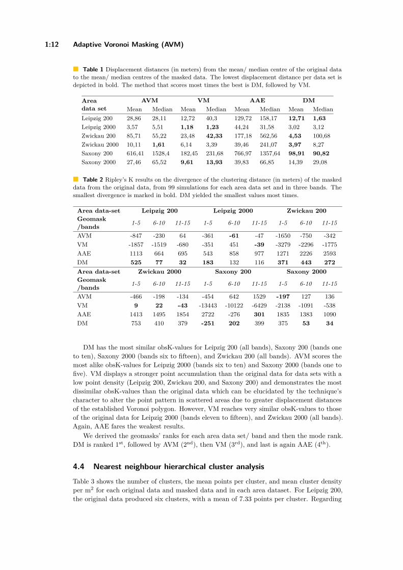
Table 1 Displacement distances (in meters) from the mean/ median centre of the original datato the mean/ median centres of the masked data. The lowest displacement distance per data set isdepicted in bold. The method that scores most times the best is DM, followed by VM.

Areadata set

AVM VM AAE DMMean Median Mean Median Mean Median Mean Median

Leipzig 200 28,86 28,11 12,72 40,3 129,72 158,17 12,71 1,63Leipzig 2000 3,57 5,51 1,18 1,23 44,24 31,58 3,02 3,12Zwickau 200 85,71 55,22 23,48 42,33 177,18 562,56 4,53 100,68Zwickau 2000 10,11 1,61 6,14 3,39 39,46 241,07 3,97 8,27Saxony 200 616,41 1528,4 182,45 231,68 766,97 1357,64 98,91 90,82Saxony 2000 27,46 65,52 9,61 13,93 39,83 66,85 14,39 29,08

Table 2 Ripley’s K results on the divergence of the clustering distance (in meters) of the maskeddata from the original data, from 99 simulations for each area data set and in three bands. Thesmallest divergence is marked in bold. DM yielded the smallest values most times.

Area data-set Leipzig 200 Leipzig 2000 Zwickau 200Geomask/bands 1-5 6-10 11-15 1-5 6-10 11-15 1-5 6-10 11-15

AVM -847 -230 64 -361 -61 -47 -1650 -750 -342VM -1857 -1519 -680 -351 451 -39 -3279 -2296 -1775AAE 1113 664 695 543 858 977 1271 2226 2593DM 525 77 32 183 132 116 371 443 272Area data-set Zwickau 2000 Saxony 200 Saxony 2000Geomask/bands 1-5 6-10 11-15 1-5 6-10 11-15 1-5 6-10 11-15

AVM -466 -198 -134 -454 642 1529 -197 127 136VM 9 22 -43 -13443 -10122 -6429 -2138 -1091 -538AAE 1413 1495 1854 2722 -276 301 1835 1383 1090DM 753 410 379 -251 202 399 375 53 34

DM has the most similar obsK-values for Leipzig 200 (all bands), Saxony 200 (bands oneto ten), Saxony 2000 (bands six to fifteen), and Zwickau 200 (all bands). AVM scores themost alike obsK-values for Leipzig 2000 (bands six to ten) and Saxony 2000 (bands one tofive). VM displays a stronger point accumulation than the original data for data sets with alow point density (Leipzig 200, Zwickau 200, and Saxony 200) and demonstrates the mostdissimilar obsK-values than the original data which can be elucidated by the technique’scharacter to alter the point pattern in scattered areas due to greater displacement distancesof the established Voronoi polygon. However, VM reaches very similar obsK-values to thoseof the original data for Leipzig 2000 (bands eleven to fifteen), and Zwickau 2000 (all bands).Again, AAE fares the weakest results.

We derived the geomasks’ ranks for each area data set/ band and then the mode rank.DM is ranked 1st, followed by AVM (2nd), then VM (3rd), and last is again AAE (4th).

4.4 Nearest neighbour hierarchical cluster analysis

Table 3 shows the number of clusters, the mean points per cluster, and mean cluster densityper m2 for each original data and masked data and in each area dataset. For Leipzig 200,the original data produced six clusters, with a mean of 7.33 points per cluster. Regarding

F. Polzin and O. Kounadi 1:13

the number of clusters, AAE, AVM, and DM are the nearest to the original data value withseven clusters. AVM has the closest mean points per cluster at 7.50 and the most similarcluster density. For Leipzig 2000, VM has the closest number of clusters as the originaldata (VM: 139; original data: 136). Regarding the mean points, original data contains 7.73points and DM reaches the nearest measure at 7.83. Also, DM has the most alike density at0.0000979 m2 (original data: 0.0001144 m2).

About Zwickau 200, the original data yielded eight clusters, mean points at 7.75, and adensity of 0.0000055 per m2. Regarding the first metric, DM has the same value. Regardingmean points, VM outperforms the other geomasks at 7.82, whilst DM shows the nearestvalue for the cluster density at 0.0000060 per m2. For Zwickau 2000, the original data yielded110 clusters, mean points of 8.70, and a density of 0.0000655 per m2. VM has 111 clustersfollowed by AVM with 112 outperforming the other geomasks. The closest mean point valuewas obtained by DM at 8.66 as well as for the mean cluster density at 0.0000598 per m2.

In Saxony 200, four clusters were generated by the original data with mean points at 6.5and a mean cluster density of zero. DM succeeded the same values as original data whereasVM indicates the most different values. For Saxony 2000, the original data demonstrates 66clusters, mean points at 7.86, and a mean cluster density at 0.0000042 per m2. Regardingthe first parameter, AVM outperforms the other methods at 63 clusters. Concerning thesecond parameter, DM reaches the closest mean points at 7.80. Finally, the most alike clusterdensity was obtained by AVM at 0.0000044 per m2. AAE fares the worst with regard to thenumber of clusters and the mean cluster density while VM demonstrates the least efficiencyfor mean points.

Last, we derived the geomasks’ ranks for each area data set/ metric and then the moderank based on the divergence value (the closer to the original data value the higher is therank). For both the mean points per cluster and mean cluster density, DM is ranked 1st,followed by AVM (2nd), then VM (3rd), and last is AAE (4th). For the cluster density, bothDM and AVM are ranked as 1st, followed by AAE (2nd), then VM (3rd).

4.5 Evaluation and comparison of geomasksIn the ESDA results subsections, we stated the ranking of each geomask. The final ranksare shown in table 4 to indicate the performance regarding data utility. AVM is ranked firstfor not displacing points to illogical locations or other residencies while VM is ranked firstfor retaining the extend of the original data. Hence, both geomasks are ranked as first forthe visualization ESDA method because there are only these two metrics. The same appliesto the central tendency (two metrics: mean and median), while for the nearest neighbourhierarchical cluster analysis we calculated the mode of the three metrics. DM is clearly thegeomask that retains the pattern of the masked data the closest to the original one, whileAAE distorts the pattern the most. Our proposed AVM method performs also very well andit is ranked as second regarding data utility.

Apart from data utility, this paper discussed the importance of preserving a level ofSKA for the derived masked data. Unfortunately, trying to anonymize data sufficiently willeventually decrease their data utility. Also, displacing points to other domiciles should beavoided to prevent false re-identification. Hence, the optimal masking solution is to findthe golden mean between these three aspects. These aspects are summarized in table 5,and compared across the geomasks. As stated before, the only method that prevents falsere-identification is AVM. DM offers the best data utility, however, it only partially preservesa certain level of SKA because it assumes that the underlying population is homogeneouslydistributed. Both AVM and AAE retain a certain level of SKA while VM performs the

GISc ience 2021

1:14 Adaptive Voronoi Masking (AVM)

worst considering all three aspects. By comparison, AVM is the optimal solution because itprevents false re-identification, offers a certain level of SKA, and is ranked second in termsof data utility.

Table 3 Nearest neighbour hierarchical cluster analysis results for each geomask and area dataset. The specific metrics are the number of clusters (number), mean points per cluster (points), andmean cluster density (density). Values closer to the original data values are marked in bold. DMhas the closest values followed by the AVM.

Geomasks/Metric

Area data setLeipzig200

Leipzig2000

Zwickau200

Zwickau2000

Saxony200

Saxony2000

Original dataNumber 6 136 8 110 4 66Points 7 .33 7 .73 7 .75 8 .7 6 .5 7 .86Density 0 .000013 0 .0001144 0 .0000055 0 .0000655 0 0 .0000042

AVMNumber 7 140 9 112 5 63Points 7 .5 8 .08 7 .44 8 .98 6 .4 7 .68Density 0 .0000113 0 .0008718 0 .0000177 0 .0004652 0 0.0000044

VMNumber 9 139 11 111 6 71Points 6 .67 8 .02 7 .82 8 .94 6 .7 8 .07Density 0 .0000221 0 .0001964 0 .0000077 0 .00010002 0 .0000002 0 .0000055

AAENumber 7 57 5 44 3 36Points 6 .43 7 .02 6 .6 8 .25 7 7 .58Density 0 .0000169 0 .0000835 0 .0000028 0 .0000511 0 0 .000003

DMNumber 7 109 8 89 4 61Points 6 .86 7 .83 7 .63 8 .66 6 .5 7 .8Density 0 .0000207 0 .0000979 0 .000006 0 .0000598 0 0 .0000037

Table 4 Ranking of geomasking techniques based on their performance on four ESDA methods(visualisation of point pattern, central tendency, Ripley’s K-function, and nearest neighbour hier-archical cluster analysis). DM retains the masked data pattern the most similar to the original data,followed by AVM.

Evaluation Method Geomask (rank)AVM VM AAE DM

Visualization 1st 1st 4th 3rdCentral tendency 3rd 1st 4th 1stRipley’s K-function 2nd 3rd 4th 1stNearest neighbour hierarchical cluster analysis 2nd 3rd 4th 1stMode Rank 2nd 3rd 4th 1st

Table 5 Evaluation of geomasking techniques based on the ability to: a) prevent the risk of falsere-identification, b) to ensure spatial K-anonymity, and c) to preserve original point pattern (datautility ranking). AVM offers the best combination of these three aspects (marked in bold).

Geomasks False re-identification Spatial K-anonymity Data UtilityAAE yes yes 4thAVM no yes 2ndDM yes partly 1stVM yes no 3rd

F. Polzin and O. Kounadi 1:15

5 Conclusion

This study presented a new geographical masking method. AVM (i) considers the underlyingpopulation density by defining a level of K-anonymity, as AAE does, (ii) displaces a partof the original data based on the concept of VM, and (iii) by considering the underlyinggeography transfers points to the closest street intersection. Thus, it decreases the risk offalse re-identification immensely and does not relocate data points to illogical positions.

The statistical analyses evidenced that AVM did not perform as well as DM regardingdata utility, yet it was ranked as second among the four examined geomasks. Adding tothat, it preserves the SKA accurately (AAE does this as well) and is the only method thatdoes not dislocate points to illogical locations and minimizes the risk of false re-identification.However, it can be argued that a map viewer will view fewer data points (due to the streetintersection aggregation) influencing the spatial perception of a phenomenon. Contraryto that, DM and VM, as well as AAE, can transfer data points to other residences orparcels increasing the risk of false re-identification. Based on three key factors (spatialK-anonymity, false re-identification, and data utility), it can be concluded that AVM is themost encouraging method in terms of the preservation of data utility and decreasing the riskof false re-identification to protect the individual’s privacy.

Still, our method is not free of constraints (just like any geomasking method). Forexample, it might be a better approach to visualize a protected version of the distributionof a point pattern, but it will be less accurate in detecting local patterns compared to DM.Even more, it is a technique that can be successfully applied to confidential spatial datapoints but not to other geodata types. Location-enabled technologies capture geodata thatare more complex and have to be treated/protected by different methods and privacy metrics[16, 20]. For instance, social media data capture, among other attributes, the spatiotemporalstamps of a user, which could be further processed to infer more than one type of spatialinformation (e.g., home or work locations). The evaluation of a method’s efficiency regardingprotection for this type of geodata should involve other measures and possibly be diversifiedby types of spatial information [11].

For the quality or information loss of masked data we applied four ESDA methods. Still,more methods can be implemented such as the global Moran’s I for spatial autocorrelationor distance to K-nearest neighbour, as well as Local Indicators of Spatial Association. Inaddition, it is of great interest to examine the performance of AVM on national data sets.Furthermore, it is recommended to juxtapose AVM with more geomasks that were not appliedhere to gather more knowledge about the new approach.

Researchers and the public are becoming more aware of the privacy risks related togeodata. However, privacy guidelines as established by Kounadi and Resch [20] as wellas the existence of geomasks have to become more well-known to researchers, institutions,companies, or the public sector. A first step to reach this goal is to make geomasks accessibleand reproducible. During this research, it was discovered that only the geomask DM isretrievable online for free. This is confounding considering the fact that many researchersstress to mask confidential discrete spatial data. Our method is available for free via theGithub repository “Geoprivacy”8. A further step is to employ geomasks for open-sourcesoftware. Through that, companies, researchers, and institutions can share their data andfindings with the public without jeopardizing individual privacy.

8 https://github.com/okounadi/Geoprivacy

GISc ience 2021

1:16 Adaptive Voronoi Masking (AVM)

References1 Jayakrishnan Ajayakumar, Andrew J Curtis, and Jacqueline Curtis. Addressing the data

guardian and geospatial scientist collaborator dilemma: how to share health records for spatialanalysis while maintaining patient confidentiality. International Journal of Health Geographics,18(1):1–12, 2019.

2 William B Allshouse, Molly K Fitch, Kristen H Hampton, Dionne C Gesink, Irene A Doherty,Peter A Leone, Marc L Serre, and William C Miller. Geomasking sensitive health data andprivacy protection: an evaluation using an e911 database. Geocarto international, 25(6):443–452, 2010.

3 Marc P Armstrong, Gerard Rushton, and Dale L Zimmerman. Geographically masking healthdata to preserve confidentiality. Statistics in medicine, 18(5):497–525, 1999.

4 John S Brownstein, Christopher A Cassa, and Kenneth D Mandl. No place to hide—reverseidentification of patients from published maps. New England Journal of Medicine, 355(16):1741–1742, 2006.

5 Christopher A Cassa, Shaun J Grannis, J Marc Overhage, and Kenneth D Mandl. A context-sensitive approach to anonymizing spatial surveillance data: impact on outbreak detection.Journal of the American Medical Informatics Association, 13(2):160–165, 2006.

6 Spencer Chainey, Lisa Tompson, and Sebastian Uhlig. The utility of hotspot mapping forpredicting spatial patterns of crime. Security journal, 21(1-2):4–28, 2008.

7 National Research Council et al. Putting people on the map: Protecting confidentiality withlinked social-spatial data. National Academies Press, 2007.

8 Philip M Dixon. R ipley’s k function. Wiley StatsRef: Statistics Reference Online, 2014.9 Matt Duckham and Lars Kulik. Location privacy and location-aware computing. Dynamic &

mobile GIS: investigating change in space and time, 3:35–51, 2006.10 Weijung J Fu, Peikun K Jiang, Guomo M Zhou, and Keli L Zhao. Using moran’s i and gis to

study the spatial pattern of forest litter carbon density in a subtropical region of southeasternchina. Biogeosciences, 11(8):2401, 2014.

11 Song Gao, Jinmeng Rao, Xinyi Liu, Yuhao Kang, Qunying Huang, and Joseph App. Exploringthe effectiveness of geomasking techniques for protecting the geoprivacy of twitter users.Journal of Spatial Information Science, 2019(19):105–129, 2019.

12 Christopher Graham. Anonymisation: managing data protection risk code of practice. In-formation Commissioner’s Office, 2012.

13 Ruchika Gupta and Udai Pratap Rao. Preserving location privacy using three layer rdvmasking in geocoded published discrete point data. World Wide Web, 23(1):175–206, 2020.

14 Danielle F Haley, Stephen A Matthews, Hannah LF Cooper, Regine Haardörfer, Adaora AAdimora, Gina M Wingood, and Michael R Kramer. Confidentiality considerations for use ofsocial-spatial data on the social determinants of health: Sexual and reproductive health casestudy. Social Science & Medicine, 166:49–56, 2016.

15 Kristen H Hampton, Molly K Fitch, William B Allshouse, Irene A Doherty, Dionne C Gesink,Peter A Leone, Marc L Serre, and William C Miller. Mapping health data: improved privacyprotection with donut method geomasking. American journal of epidemiology, 172(9):1062–1069, 2010.

16 Carsten Keßler and Grant McKenzie. A geoprivacy manifesto. Transactions in GIS, 22(1):3–19,2018.

17 Ourania Kounadi and Michael Leitner. Why does geoprivacy matter? the scientific publicationof confidential data presented on maps. Journal of Empirical Research on Human ResearchEthics, 9(4):34–45, 2014.

18 Ourania Kounadi and Michael Leitner. Spatial information divergence: Using global andlocal indices to compare geographical masks applied to crime data. Transactions in GIS,19(5):737–757, 2015.

F. Polzin and O. Kounadi 1:17

19 Ourania Kounadi and Michael Leitner. Adaptive areal elimination (aae): A transparent way ofdisclosing protected spatial datasets. Computers, Environment and Urban Systems, 57:59–67,2016.

20 Ourania Kounadi and Bernd Resch. A geoprivacy by design guideline for research campaignsthat use participatory sensing data. Journal of Empirical Research on Human Research Ethics,13(3):203–222, 2018.

21 Mei-Po Kwan, Irene Casas, and Ben Schmitz. Protection of geoprivacy and accuracy of spatialinformation: How effective are geographical masks? Cartographica: The International Journalfor Geographic Information and Geovisualization, 39(2):15–28, 2004.

22 Michael Leitner and Andrew Curtis. Cartographic guidelines for geographically masking thelocations of confidential point data. Cartographic Perspectives, (49):22–39, 2004.

23 Gerard Rushton, Marc P Armstrong, Josephine Gittler, Barry R Greene, Claire E Pavlik,Michele M West, and Dale L Zimmerman. Geocoding health data: the use of geographic codesin cancer prevention and control, research and practice. CRC Press, 2007.

24 Pierangela Samarati. Protecting respondents identities in microdata release. IEEE transactionson Knowledge and Data Engineering, 13(6):1010–1027, 2001.

25 Bill Schilit, Jason Hong, and Marco Gruteser. Wireless location privacy protection. Computer,36(12):135–137, 2003.

26 Klaus Schwab, Alan Marcus, JO Oyola, William Hoffman, and Michele Luzi. Personal data:The emergence of a new asset class. In An Initiative of the World Economic Forum, 2011.

27 Dara E Seidl, Piotr Jankowski, and Keith C Clarke. Privacy and false identification risk ingeomasking techniques. Geographical Analysis, 50(3):280–297, 2018.

28 Dara E Seidl, Piotr Jankowski, and Atsushi Nara. An empirical test of household identificationrisk in geomasked maps. Cartography and Geographic Information Science, 46(6):475–488,2019.

29 Dara E Seidl, Gernot Paulus, Piotr Jankowski, and Melanie Regenfelder. Spatial obfuscationmethods for privacy protection of household-level data. Applied Geography, 63:253–263, 2015.

30 Paul A Zandbergen. Ensuring confidentiality of geocoded health data: assessing geographicmasking strategies for individual-level data. Advances in medicine, 2014, 2014.

31 Su Zhang, Scott M Freundschuh, Kate Lenzer, and Paul A Zandbergen. The location swappingmethod for geomasking. Cartography and Geographic Information Science, 44(1):22–34, 2017.

GISc ience 2021

Reproducible Research and GIScience: AnEvaluation Using GIScience Conference PapersFrank O. Ostermann 1 #

Faculty of Geo-Information Science and Earth Observation (ITC),University of Twente, Enschede, The Netherlands

Daniel Nüst #

Institute for Geoinformatics, University of Münster, Germany

Carlos Granell #

Institute of New Imaging Technologies, Universitat Jaume I de Castellón, Spain

Barbara Hofer #

Christian Doppler Laboratory GEOHUM and Department of Geoinformatics - Z_GIS,University of Salzburg, Austria

Markus Konkol #

Faculty of Geo-Information Science and Earth Observation (ITC),University of Twente, Enschede, The Netherlands

AbstractGIScience conference authors and researchers face the same computational reproducibility challengesas authors and researchers from other disciplines who use computers to analyse data. Here, toassess the reproducibility of GIScience research, we apply a rubric for assessing the reproducibilityof 75 conference papers published at the GIScience conference series in the years 2012-2018. Sincethe rubric and process were previously applied to the publications of the AGILE conference series,this paper itself is an attempt to replicate that analysis, however going beyond the previous work byevaluating and discussing proposed measures to improve reproducibility in the specific context of theGIScience conference series. The results of the GIScience paper assessment are in line with previousfindings: although descriptions of workflows and the inclusion of the data and software suffice toexplain the presented work, in most published papers they do not allow a third party to reproducethe results and findings with a reasonable effort. We summarise and adapt previous recommendationsfor improving this situation and propose the GIScience community to start a broad discussion onthe reusability, quality, and openness of its research. Further, we critically reflect on the process ofassessing paper reproducibility, and provide suggestions for improving future assessments. The codeand data for this article are published at https://doi.org/10.5281/zenodo.4032875.

2012 ACM Subject Classification Information systems → Geographic information systems

Keywords and phrases reproducible research, open science, reproducibility, GIScience

Digital Object Identifier 10.4230/LIPIcs.GIScience.2021.II.2

Related Version Previous Version: https://doi.org/10.31223/X5ZK5V

Supplementary Material The input data for this work are the full texts of GIScience conferenceproceedings from the years 2012 to 2018 [35, 7, 20, 34]. The paper assessment results and source codeof figures are published at https://github.com/nuest/reproducible-research-at-giscience andarchived on Zenodo [27]. The used computing environment is containerised with Docker pinning theR version to 3.6.3 and R packages to the MRAN snapshot of July 5th 2019.

Funding Daniel Nüst: Project o2r , German Research Foundation, grant number PE 1632/17-1.Carlos Granell: Ramón y Cajal Programme of the Spanish government, grant number RYC-2014-16913.Markus Konkol: Project o2r , German Research Foundation, grant numbers KR 3930/8-1 andTR 864/12-1.

1 Corresponding author© Frank O. Ostermann , Daniel Nüst, Carlos Granell, Barbara Hofer, and Markus Konkol;licensed under Creative Commons License CC-BY 4.0

11th International Conference on Geographic Information Science (GIScience 2021) – Part II.Editors: Krzysztof Janowicz and Judith A. Verstegen; Article No. 2; pp. 2:1–2:16

Leibniz International Proceedings in InformaticsSchloss Dagstuhl – Leibniz-Zentrum für Informatik, Dagstuhl Publishing, Germany

2:2 Reproducible GIScience

Acknowledgements Author contributions (see CRediT): all authors contributed to conceptualisation,investigation (number of assessed papers in brackets), and writing – original draft; FO (33): writing- review & editing, software; DN (33): software, writing - review & editing, visualisation; CG (30):writing - review & editing, software; BH (21): writing - review & editing; MK (30). We thankCeleste R. Brennecka from the Scientific Editing Service of the University of Münster for her editorialsupport and the anonymous reviewers for their constructive feedback.

1 Introduction

The past two decades have seen the imperative of Open Science gain momentum acrossscientific disciplines. The adoption of Open Science practices is partially prompted by theincreasing costs of using proprietary software and subscribing to scientific journals, butmore importantly because of the increased transparency and availability of data, methods,and results, which enable reproducibility [22]. This advantage is especially relevant forthe computational and natural sciences, where sharing data and code is a prerequisite forreuse and collaboration. A large proportion of GIScience research today uses software toanalyse data on computers, meaning that many articles published in the context of theGIScience conference series2 fall into the categories of data science or computational research.Thereby, these articles face challenges of transparency and reproducibility in the sense of theClaerbout/Donoho/Peng terminology [2], where reproduction means a recreation of the sameresults using the same input data and methods, usually with the actual code created by theoriginal authors. The related concept of replication, i.e., the confirmation of insights gainedfrom a scientific study using the same method with new data, is of crucial importance toscientific progress, yet it is also frequently challenging to realise for interested readers of apublished study. So far, despite the GIScience conference series’ rigorous review process,reproducibility and replicability have not been a core concern in the contributions. Withreproducibility now being a recognised topic in the call for papers, it is time to take stockand identify possible action. In previous work [26], we assessed the reproducibility of aselection of full and short papers from the AGILE conference series3, a community conferenceorganised by member labs of the Association of Geographic Information Laboratories inEurope (AGILE). Using systematic analysis based on a rubric for reproducible research,we found that the majority of AGILE papers neither provided sufficient information for areviewer to evaluate the code and data and attempt a reproduction, nor enough material forreaders to reuse or extend data or code from the analytical workflows. This is corroboratedby research in related disciplines such as quantitative geography [3], qualitative GIS [21],geoscience [16], and e-Science [10]. The problems identified in these related research areasare transferable to the scientific discipline of GIScience, which operates at the intersectionsof aforementioned fields [11]. In any case, observations on the lack of reproducibility in allscientific fields contrast with the clear advantages and benefits of open and reproducibleresearch both for individuals and for academia as a whole (cf. for example [6, 19, 17, 5]). Asa consequence, we have initiated a process to support authors in increasing reproducibilityfor AGILE publications; as a main outcome, this initiative has produced author guidelinesas well as strategies for the AGILE conference series4.

2 https://www.giscience.org/3 https://agile-online.org/conference4 See the initiative website at https://reproducible-agile.github.io/, the author guidelines at https:

//doi.org/10.17605/OSF.IO/CB7Z8 [24] and the main OSF project with all materials https://osf.io/phmce/ [25].

F. O. Ostermann, D. Nüst, C. Granell, B. Hofer, and M. Konkol 2:3

The AGILE conference is related to GIScience conference in terms of scientific domainand contributing authors, but is different in organisational aspects. Two open questionsare thus whether the GIScience conference series faces the same issues, and whether similarstrategies could be applied successfully. To begin this investigation, we conducted a simpletext analysis of GIScience conference proceedings5 to evaluate the relevance of computationalmethods in the conference papers. The analysis searched for several word stems related toreproducibility: Generic words indicating a quantitative analysis, e.g., “data”, “software”,or “process”; specific platforms, e.g., “GitHub”; and concrete terms, e.g., words startingwith “reproduc” or “replic”. Table 1 shows the results of the search for each year analysed.The take-away message from the text analysis is that algorithms, processing, and data playan essential role in GIScience publications, but few papers mentioned code repositories orreproduction materials. Therefore, an in-depth assessment of the reproducibility of thesepublications was deemed necessary.

The main contribution of this work addresses two objectives: First, it aims to investigatethe state of reproducibility in the GIScience conference community. This investigationbroadens our knowledge base about reproducibility in the GIScience discipline and informs usabout the situation in the GIScience conference series specifically (details in section 4). Second,it aims to apply the assessment procedure used for AGILE conference papers (presentedin section 3) to the papers of the GIScience conference, so that the broader suitability ofthis procedure is evaluated using a different dataset, and thereby providing evidence of itsreplicability. Such a transfer validates the developed methodology. We discuss these findingsand present our conclusions in the final two sections (5 and 6). Together, these objectivesyield important findings for the discussion of reproducibility within the GIScience conferencecommunity and the GIScience discipline at large. We believe that GIScience as a disciplinewould greatly benefit from more studies that reproduce and replicate other studies, similarto other disciplines that are recognising the value of replication for innovating theory [23],and argue that such a replication study is not lacking innovation but is a prerequisite forinnovating community practice. Only then can a fruitful dialogue take place on whether andhow to improve reproducibility for the GIScience conference series, and whether the recentsteps taken at AGILE6 could be an inspiration for GIScience conferences as well.

2 Related work

This work builds and expands on earlier work [26], which already provides an overview ofreproducible research in general, including definitions, challenges, and shortcomings. Inthe following, we focus therefore on recently published works and briefly introduce relatedmeta-studies.

Few groups have attempted practical reproduction of computational works related toGIScience. Konkol et al. [16] conducted an in-depth examination of the computationalreproducibility of 41 geoscience papers with a focus on differences between the recreatedfigures. The set of papers was, similar to our work, drawn from a fixed group of two outlets

5 The full text analysis and the results is available in this paper’s repository in the follow-ing files: giscience-historic-text-analysis.Rmd contains the analysis code; the result dataare two tables with counts for occurrences of words respectively word stems per year inresults/text_analysis_topwordstems.csv and results/text_analysis_keywordstems.csv; a word-cloud per year is in file results/text_analysis_wordstemclouds.png.

6 See the initiative website at https://reproducible-agile.github.io/, the author guidelines at https://doi.org/10.17605/OSF.IO/CB7Z8 [24] and the main OSF project with all materials https://osf.io/phmce/ [25].

GISc ience 2021

2:4 Reproducible GIScience

Table 1 Reproducibility-related word stems in the corpus per year of proceedings.

year

words

reprod

uc..

replic

..

repeat

ab..

code

softw

are

algori

thm(s)

(pre)p

rocess

..

data.

*res

ult(s)

reposi

tory/

ies

githu

b/lab

2002 23782 6 2 0 11 61 191 150 897 129 62 02004 26728 4 1 0 34 50 138 258 849 263 4 02006 32758 6 0 0 12 32 335 250 856 164 0 02008 27356 3 6 1 3 11 331 146 854 218 17 02010 23004 3 1 0 8 16 164 276 650 162 0 0

2012 28860 2 0 0 101 27 238 190 1048 311 3 02014 29534 3 4 1 12 18 255 159 1070 228 3 02016 24838 2 0 0 23 21 333 150 1007 202 4 12018 23318 3 10 0 15 15 201 160 891 294 6 6Total 240178 32 24 2 219 251 2186 1739 8122 1971 99 7Note: The very high value for ’code’ in 2012 is due to a single paper aboutland use, for which different “land use codes” are defined, discussed and used.

(journals), but it was further limited to recent papers providing code in the R language. Themain issues raised by Konkol et al. [16] are similar to those identified in a recent report onthe reproducibility review during the AGILE conference 20207, where the reproducibilitycommittee summarised the process and documented relevant obstacles to reproducibility ofaccepted papers.

Within the geospatial domain, Kedron et al. [13] provide a recent review of opportunitiesand challenges for reproducibility and replicability. They transfer solutions from otherdomains but also discuss and conceptualise the specific nature of a reproducibility andreplicability framework when working with geospatial data, e.g., handling context, uncertaintyof spatial processes, or how to accommodate the inherent natural variability of geospatialsystems. In a similar manner, Brunsdon and Comber [4] investigate reproducibility withinspatial data science, with special attention to big spatial data. They support the needfor open tools, knowledge about code, and reproducibility editors at domain journals andconferences, but they also introduce the perspective that spatial analysis is no longerconducted only by GI/geo-scientists or geographers and connect reproducibility with criticalspatial understanding. The more conceptual work in those articles is complemented by theassessment of reproducibility conducted in this paper.

Two recent studies from distant disciplines, wildlife science [1] and hydrology [32], alsorelate to our work in this paper. Both studies investigate a random set of articles from selectedjournals and use a stepwise process of questions to determine the availability of materialsand eventually reproduce workflows if possible. Archmiller et al. [1] use a final ranking of 1to 5 to specify the degree to which a study’s conclusions were eventually reproduced. Similarto our classification scheme, their ranking models fit the general notion of a “reproducibilityspectrum” [30].

7 https://osf.io/7rjpe/

F. O. Ostermann, D. Nüst, C. Granell, B. Hofer, and M. Konkol 2:5

3 Reproducibility assessment method

3.1 Criteria

The assessment criteria used for the current study were originally defined in previous work, sowe provide only a short introduction here and refer to Nüst et al. [26] for details. The threeassessment criteria are Input Data, Methods, and Results. Input Data comprises all datasetsthat the computational analysis uses. Methods encompasses the entire computational analysisthat generates the results. Since Methods is difficult to evaluate as a whole, we split thiscriterion into three subcriteria: Preprocessing includes the steps to prepare the Input Databefore the main analysis; Methods, Analysis, Processing is the main analysis; ComputationalEnvironment addresses the description of hard- and software. Finally, the criterion Resultsrefers to the output of analysis, e.g., figures, tables, and numbers.

For each of these (sub)criteria, we assigned one of four levels unless the criterion wasnot applicable (NA). Unavailable (level 0) means that it was not possible to access thepaper’s data, methods, or results, and that it was impossible to recreate them based on thedescription in the paper. Documented (level 1) indicates that the paper still did not providedirect access to datasets, methods, or results, but that there was sufficient description ormetadata to potentially recreate them closely enough for an evaluation; yet, often a recreationwas unlikely due to the huge amount of effort needed. For example, with regard to themethods criteria, Documented means that pseudo code or a textual workflow descriptionwas provided. Available (level 2) was assigned if the paper provided direct access to thematerials (e.g., through a link to a personal or institutional website), but not in the form ofan open and permanent identifier, such as a digital object identifier (DOI). The indicationof a DOI does not apply to the methods criteria, as it is not yet common practice to makea permanent reference to code, libraries, and system environments with a single identifier.The gold standard, Available and Open (level 3), requires open and permanent access tothe materials (e.g., through public online repositories) and open licenses to allow use andextension.

Note that levels are ordinal numbers that can be compared (3 is higher than 2), butabsolute differences between numbers must not be interpreted as equals: Moving one levelup from 0 to 1 is not the same as from level 1 to level 2. While reaching level 1 is fairlystraightforward, moving to level 2 means one must create a fully reproducible paper.

3.2 Process

The overall approach to assessing the reproducibility of GIScience papers followed theprevious assessment of AGILE papers [26], and was conducted by the same persons. Contraryto the AGILE investigation, all full papers in the GIScience conference series (from the2012 to 2018 editions) were assessed. This is partly because no obvious subset exists, suchas the nominees for best papers as in the case of the AGILE conference series, but alsobecause we aimed to work with a larger dataset for potentially more informative results.Each GIScience conference paper was randomly assigned to two assessors who evaluated itqualitatively according to the reproducibility criteria. The assessors were free in the waythey approached the assigned evaluations, depending on the structure of the paper and theassessor’s familiarity with the topic. An evaluation could range from browsing the paperto identify relevant statements in case of high familiarity to a thorough reading of the fulltext. The identification of relevant content could be supported to some extent by a PDFreader with multiple highlights, using keywords like e.g., “data, software, code, download,

GISc ience 2021

2:6 Reproducible GIScience

contribution, script, workflow”. The results of the individual assessments were joined ina collaborative Google Spreadsheet. This spreadsheet also had a comments column forassessors to record relevant sources and decisions. In case of disagreement between assessors,arguments for and against a certain reproducibility level were discussed in the entire groupof five assessors until a consensus was reached. Only then were the assessments merged intoa single value. A snapshot of both the unmerged and merged values was stored as a CSV filein the collaboration repository for transparency and provenance8. Two independent assessorsper paper increased the objectivity of the final assessment. Disagreements and conductingthe assessment one year at a time, going backwards from the most recent year, were foundhelpful in aligning the interpretation of criteria and, in rare cases, led to an adjustment ofsimilar cases in other papers.

The discussion about the correct assignment of levels led to a reflection on how to applythe rubric for special situations. For the Input Data criterion, some papers had inputdata “available” at the time of writing/publication that was not available anymore at thetime of evaluation, due to broken links, changes in the URL structure of a website, orprojects and/or personal websites that were down or moved. In such cases, we gave theauthors the benefit of the doubt and assumed the data were accessible some time after thepublication of the conference proceedings. We did not give those papers an arbitrary scoreand discussed internally the best level per case; yet, such papers never earned a 3, whichwould require permanent resolving of the link. Related to this criterion, simulation data,like the specification or configuration of agents in an agent-based system, was not treatedas input data (resulting in NA if no other data was used), but as parameters of the mainanalysis, i.e., as part of the Methods, Analysis, Processing.

Preprocessing covers preparatory work for the actual analysis involving various tasks suchas data selection, cleaning, aggregation, and integration. However, the dividing line betweendata preprocessing and processing (i.e., the main analysis) proved to be often vague, andoccasionally assessors disagreed whether the preprocessing criterion should be assigned NA,Unavailable, or Documented (0 or 1, respectively). Therefore, we decided eventually to applythe Preprocessing criterion only in cases where papers specifically mentioned a preprocessingtask independent of the actual analysis or method, e.g., when clearly stated in a separatesub-section of the paper.

Lastly, human subject tests and surveys were also a special case. Human-related researchactivities were rated as 1 in the methods/analysis/processing criterion if sufficiently docu-mented; nonetheless, a sufficient documentation in these cases did not mean that originalsources were available or could be exactly recreated.

3.3 Paper corpusIn total, 87 papers from the GIScience conferences in 2012, 2014, 2016, and 2018 wereassessed. A table in the reproducibility package shows the full results of the assessment andthe included raw data provides details on assigned assessors, authors, etc. [27]. 12 papers(14%) across all years were identified as conceptual papers9 and were not included in thecorpus. The number of conceptual papers in GIScience conferences was low over the analysed

8 The assessment results are in the file results/paper_assessment.csv. As an example, commit 464e630and 2e8b1be are the pre-merge and post-merge commit after completing the assessment of the papersfrom 2014. The pre-merge commit contains the assessments including the assessors’ initials, e.g. “CG: 1,MK: 1”.

9 See [26] for a definition of “conceptual”.

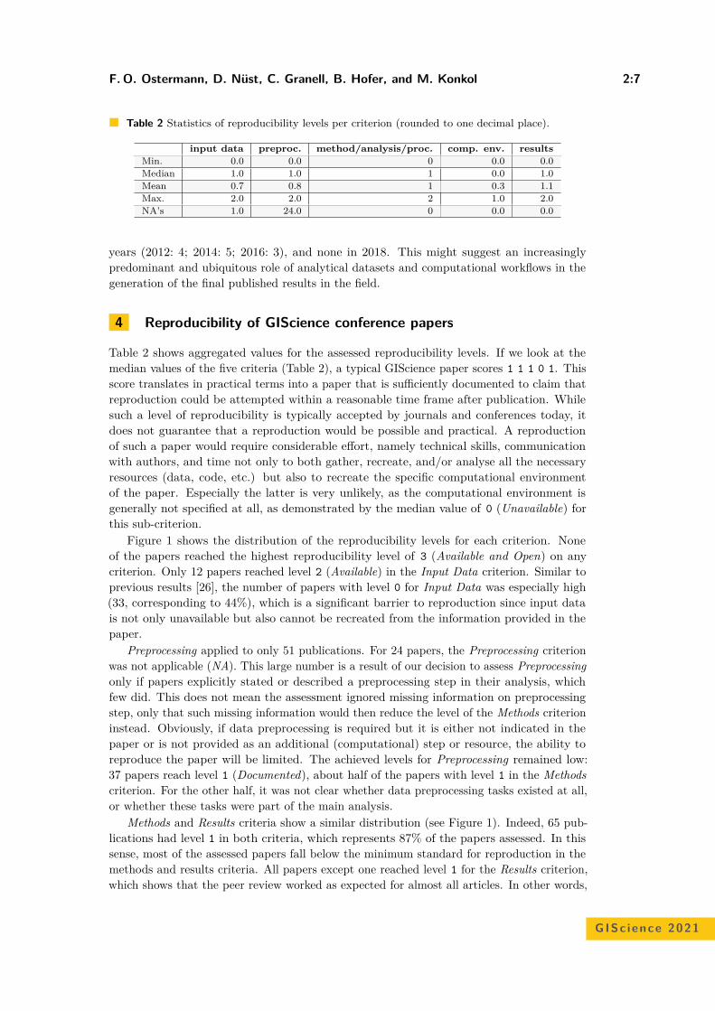
F. O. Ostermann, D. Nüst, C. Granell, B. Hofer, and M. Konkol 2:7

Table 2 Statistics of reproducibility levels per criterion (rounded to one decimal place).

input data preproc. method/analysis/proc. comp. env. resultsMin. 0.0 0.0 0 0.0 0.0Median 1.0 1.0 1 0.0 1.0Mean 0.7 0.8 1 0.3 1.1Max. 2.0 2.0 2 1.0 2.0NA’s 1.0 24.0 0 0.0 0.0

years (2012: 4; 2014: 5; 2016: 3), and none in 2018. This might suggest an increasinglypredominant and ubiquitous role of analytical datasets and computational workflows in thegeneration of the final published results in the field.

4 Reproducibility of GIScience conference papers

Table 2 shows aggregated values for the assessed reproducibility levels. If we look at themedian values of the five criteria (Table 2), a typical GIScience paper scores 1 1 1 0 1. Thisscore translates in practical terms into a paper that is sufficiently documented to claim thatreproduction could be attempted within a reasonable time frame after publication. Whilesuch a level of reproducibility is typically accepted by journals and conferences today, itdoes not guarantee that a reproduction would be possible and practical. A reproductionof such a paper would require considerable effort, namely technical skills, communicationwith authors, and time not only to both gather, recreate, and/or analyse all the necessaryresources (data, code, etc.) but also to recreate the specific computational environmentof the paper. Especially the latter is very unlikely, as the computational environment isgenerally not specified at all, as demonstrated by the median value of 0 (Unavailable) forthis sub-criterion.

Figure 1 shows the distribution of the reproducibility levels for each criterion. Noneof the papers reached the highest reproducibility level of 3 (Available and Open) on anycriterion. Only 12 papers reached level 2 (Available) in the Input Data criterion. Similar toprevious results [26], the number of papers with level 0 for Input Data was especially high(33, corresponding to 44%), which is a significant barrier to reproduction since input datais not only unavailable but also cannot be recreated from the information provided in thepaper.

Preprocessing applied to only 51 publications. For 24 papers, the Preprocessing criterionwas not applicable (NA). This large number is a result of our decision to assess Preprocessingonly if papers explicitly stated or described a preprocessing step in their analysis, whichfew did. This does not mean the assessment ignored missing information on preprocessingstep, only that such missing information would then reduce the level of the Methods criterioninstead. Obviously, if data preprocessing is required but it is either not indicated in thepaper or is not provided as an additional (computational) step or resource, the ability toreproduce the paper will be limited. The achieved levels for Preprocessing remained low:37 papers reach level 1 (Documented), about half of the papers with level 1 in the Methodscriterion. For the other half, it was not clear whether data preprocessing tasks existed at all,or whether these tasks were part of the main analysis.

Methods and Results criteria show a similar distribution (see Figure 1). Indeed, 65 pub-lications had level 1 in both criteria, which represents 87% of the papers assessed. In thissense, most of the assessed papers fall below the minimum standard for reproduction in themethods and results criteria. All papers except one reached level 1 for the Results criterion,which shows that the peer review worked as expected for almost all articles. In other words,

GISc ience 2021

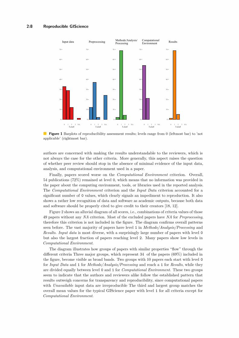
2:8 Reproducible GIScience

0

10

20

30

40

50

60

70

0 1 2 3 NALevel

Input data

0

10

20

30

40

50

60

70

0 1 2 3 NALevel

Preprocessing

0

10

20

30

40

50

60

70

0 1 2 3 NALevel

Methods/Analysis/Processing

0

10

20

30

40

50

60

70

0 1 2 3 NALevel

ComputationalEnvironment

0

10

20

30

40

50

60

70

0 1 2 3 NALevel

Results

Figure 1 Barplots of reproducibility assessment results; levels range from 0 (leftmost bar) to ’notapplicable’ (rightmost bar).

authors are concerned with making the results understandable to the reviewers, which isnot always the case for the other criteria. More generally, this aspect raises the questionof whether peer review should stop in the absence of minimal evidence of the input data,analysis, and computational environment used in a paper.

Finally, papers scored worse on the Computational Environment criterion. Overall,54 publications (72%) remained at level 0, which means that no information was provided inthe paper about the computing environment, tools, or libraries used in the reported analysis.The Computational Environment criterion and the Input Data criterion accounted for asignificant number of 0 values, which clearly signals an impediment to reproduction. It alsoshows a rather low recognition of data and software as academic outputs, because both dataand software should be properly cited to give credit to their creators [18, 12].

Figure 2 shows an alluvial diagram of all scores, i.e., combinations of criteria values of those49 papers without any NA criterion. Most of the excluded papers have NA for Preprocessing,therefore this criterion is not included in the figure. The diagram confirms overall patternsseen before. The vast majority of papers have level 1 in Methods/Analysis/Processing andResults. Input data is most diverse, with a surprisingly large number of papers with level 0but also the largest fraction of papers reaching level 2. Many papers show low levels inComputational Environment.

The diagram illustrates how groups of papers with similar properties “flow” through thedifferent criteria Three major groups, which represent 34 of the papers (69%) included inthe figure, become visible as broad bands. Two groups with 10 papers each start with level 0for Input Data and 1 for Methods/Analysis/Processing and reach a 1 for Results, while theyare divided equally between level 0 and 1 for Computational Environment. These two groupsseem to indicate that the authors and reviewers alike follow the established pattern thatresults outweigh concerns for transparency and reproducibility, since computational paperswith Unavailable input data are irreproducible The third and largest group matches theoverall mean values for the typical GIScience paper with level 1 for all criteria except forComputational Environment.

F. O. Ostermann, D. Nüst, C. Granell, B. Hofer, and M. Konkol 2:9

0

1

2

1

2

0

1

1

2

0

10

20

30

40

50

Input Data Methods/Analysis/

Processing

ComputationalEnvironment

Results

Category

Num

ber o

f pap

ers

Category levels (#)

0 0 0 1 (1)

0 1 0 1 (10)

0 1 1 1 (10)

1 1 0 0 (1)

1 1 0 1 (14)

1 1 0 2 (1)

1 1 1 1 (3)

1 2 0 1 (1)

2 1 0 1 (3)

2 1 1 1 (2)

2 1 1 2 (2)

2 2 0 2 (1)

Figure 2 Alluvial diagram of common groups of papers throughout 4 of 5 categories includingonly papers without any “not applicable” (Level NA) value; category Preprocessing was droppedbecause difficulty to clearly assess it lead to many “not applicable” values.

The diagram also shows additional interesting patterns for a few papers. The papers withthe lowest level of 0 in Results, i.e., according to the assessors the results are documentedinsufficiently and thus difficult or impossible to fully understand, actually have better values inprevious criteria. Only few papers that start with level 2 in Input Data can keep this level forMethods/Analysis/Processing, and even those who do later drop to level 0 in ComputationalEnvironment. Only one paper each shows the following surprising paths: Starting with level 1for Input Data , then moving up to level 2 in Methods, before reaching level 2 in Resultsdespite having only values of 1 or 0 in other criteria. In summary, not a single paper canreach the required levels for an immediate reproduction by ensuring that all required piecesare Available (level 2), not even considering the further challenges for reproductions, such asincomplete documentation [28]. An investigation of yearly scores to track developments overtime does not show any trend, i.e., there is little change in reproducibility over the studyperiod10. The overall low values for Computational Environment are one signal that confirmsthe growing concerns for reproducibility and reusability of computational research are notmisplaced.

5 Discussion

5.1 State of reproducibility in the GIScience conference seriesOur first research objective was to assess the state of reproducibility in the GIScienceconference series. A recurrent issue found in the analysis was the inability to access inputdata based on the information provided in the paper. Most of the links and pointers to

10 See the additional analysis and plots published at https://nuest.github.io/reproducible-research-at-giscience/giscience-reproducibility-assessment.html or in the paper’s reproducibilitypackage [27].

GISc ience 2021

2:10 Reproducible GIScience

datasets reported at the time of publication were either broken (e.g., non-existing resource,HTTP 404 error, invalid URL syntax) or not available anymore (URL works but redirects toa different generic page; specific resource from the paper no longer exists). In these cases, alevel 2 in the Input Data criterion was deserved at the time of publication; however, whenevaluating the level of reproducibility some time later, as was done in this work, level 2 is nolonger suitable for those papers. From a reproducibility point of view, the input data wastherefore not accessible, although contacting the authors could still be attempted. However,according to the meaning of the criterion and in practical terms, this is equivalent to includingthe statement “available upon request” in the paper and thereby level 0. An importantpart of reproducibility is that access to material should not degrade over time, which is bestachieved by depositing data in repositories, including sensitive data (using the appropriatemechanisms), and properly citing it. In this assessment of reproducibility, we decided to givethe authors the benefit of the doubt and awarded a value of 2 for Input Data even if wecould not conclusively determine, e.g., by using the Internet Archive’s Wayback Machine11,whether the original website ever existed.

Regarding the common situation of a paper with Documented (level 1) for all criteria, ourinterpretation is that this is indeed a regular paper that is up to current scientific standards.Does this imply that a paper with Unavailable (level 0) in any criterion should not havebeen accepted? We believe that this requires differentiation between past and future papers.The criteria used in this paper were not included in the previous call for papers or in thereviewer guidelines, and therefore received less attention from authors or reviewers. Thus,we have analysed work in a historical context when there were few concrete incentives topush these aspects, beyond the general concerns for good scientific practice. Nowadays, withawareness about reproducibility being raised through initiatives, projects, and publicationsabout it, we would expect that reproducibility levels increase, and argue that papers withUnavailable in one more criteria should not be accepted anymore without a clear and explicitjustification (e.g., sensitive data on human subjects). This does not imply that it is alwaysnecessary to achieve the gold standard of Available and Open. The overall objective shouldbe to make a paper as reproducible as possible before publication. We argue that, for mostcurrently published works at the GIScience conference, Available would have been achievableand feasible with reasonable efforts.

However, such a change in standards for paper acceptance would also mean that re-searchers, editors, and publishers might have to reevaluate their focus on publishing noveland purportedly groundbreaking results in science, and give as much weight to publishingthe full process and collection of parts that would allow readers to try to fully understandthe research. Clearly, Unavailable for Input Data is the most problematic, because withoutsufficient knowledge about the characteristics of the input data, all attempts at reproducingresults are bound to fail, even when the textual documentation of the data would potentiallyallow for an time-intensive recreation of the computational workflow.

5.2 Transferability of methodConcerning our second research objective, we can state that the overall process and theapplication of the reproducibility rubric was successfully replicated with a different dataset. This is not entirely surprising given that AGILE and GIScience conference series sharesimilarities in target audience, review process, and publication of proceedings (more on

11 https://web.archive.org/.

F. O. Ostermann, D. Nüst, C. Granell, B. Hofer, and M. Konkol 2:11

that in the following section). More importantly, the process faced similar challenges aswe recalled from its earlier application. This is crucial information, because the successfulreplication of the process, including its challenges, enables us and others to ground anychanges in solid evidence. In particular the Preprocessing criterion caused many discussionsamong the reproducibility reviewers during the assessment. It is often not clear or a matterof interpretation if a particular processing step belongs to a minor basic transformation ofinput data, if it is already part of the main analysis, and when it is a truly distinct step inthe process. The borders are vague and hence scores should be interpreted with caution.Likewise, the Computational environment is also difficult to distinguish from analysis, andtechnology and practices for the effective management of the computing environment havereached mature states relatively recently. Future reproducibility assessments of papers couldprovide a more precise definition for pre-processing, e.g., only use it if the authors use theterm, or might consider to drop the category, and benefit from rules to deal with the specificissues of older workflows, similar as discussed for input data above. Furthermore, it isimportant to remember that the levels of reproducibility are not equidistant in the sensethat a level of 2 would be twice as good as a level of 1, or that the effort needed is twiceas high. A level of 1 should be the standard for current and future peer-reviewed papers.Reaching level 2 requires several additional steps, while reaching the gold standard of 3 isagain a comparatively small step from level 2 in terms of effort - the main difference is to usepublic repositories with a DOI - yet with a high positive impact on permanent accessibility.

Although the replication was successful, the process was again labour-intensive, makingit problematic to scale it up to assess multiple years of several popular journals, for example.Further, despite our best efforts for transparency and the four-eyes principle in the assessment,the process is inherently subjective. A different group of investigators might score papersdifferently. While natural language processing techniques have made great progress in thepast decades, an automated assessment of a paper’s reproducibility still seems out-of-reach.Including important information as machine-readable metadata could allow to come closerto automation.

5.3 Comparison of conferencesGiven that we followed the same process as in [26] and demonstrated the transferabilityof the method, comparing the two conference series seems appropriate. It is importantto remember that we do not attempt such a comparison with the objective of declaring a“winner”. The published work and contributing community of the two conferences are similarenough for a comparison, yet their organisation (setup, process, geographic focus) differtoo much for a simplistic ranking. However, a comparison is required to sensibly discusswhether the guidelines developed for AGILE might also be promising for GIScience: Arethey transferable? If not, what adaptations seem necessary?

Concerning the contributing and participating academic communities, Egenhofer et al. [8]and Kemp et al. [14] both include both conferences series as outlets for GIScience research.Further, Keßler et al. [15] investigate the bibliographies of four GIScience conference series,including GIScience and AGILE for the year 2012, and identify 15 authors who have publishedin both conference series. We conducted a cursory investigation of the body of authors for fullpapers, revealing significant overlap12: Out of 571 unique AGILE and 405 unique GISciencefull paper authors, 86 published in both conferences, and this includes all 15 authors mentionedby Keßler et al. [15]. Therefore, the strong relation between the AGILE and GIScience

12 The data and code for the brief exploration into the authorship across the conferences considered inthis work can be found in the directory author_analysis of this paper’s reproducibility package [27].

GISc ience 2021

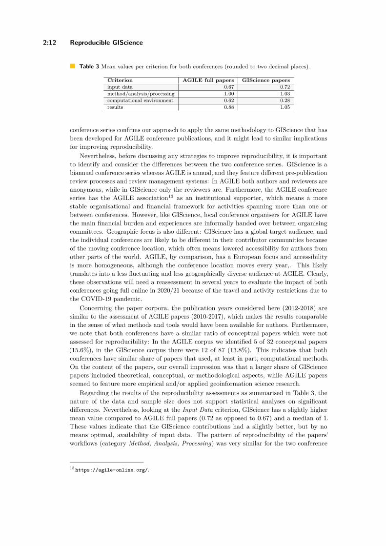
2:12 Reproducible GIScience

Table 3 Mean values per criterion for both conferences (rounded to two decimal places).

Criterion AGILE full papers GIScience papersinput data 0.67 0.72method/analysis/processing 1.00 1.03computational environment 0.62 0.28results 0.88 1.05

conference series confirms our approach to apply the same methodology to GIScience that hasbeen developed for AGILE conference publications, and it might lead to similar implicationsfor improving reproducibility.

Nevertheless, before discussing any strategies to improve reproducibility, it is importantto identify and consider the differences between the two conference series. GIScience is abiannual conference series whereas AGILE is annual, and they feature different pre-publicationreview processes and review management systems: In AGILE both authors and reviewers areanonymous, while in GIScience only the reviewers are. Furthermore, the AGILE conferenceseries has the AGILE association13 as an institutional supporter, which means a morestable organisational and financial framework for activities spanning more than one orbetween conferences. However, like GIScience, local conference organisers for AGILE havethe main financial burden and experiences are informally handed over between organisingcommittees. Geographic focus is also different: GIScience has a global target audience, andthe individual conferences are likely to be different in their contributor communities becauseof the moving conference location, which often means lowered accessibility for authors fromother parts of the world. AGILE, by comparison, has a European focus and accessibilityis more homogeneous, although the conference location moves every year,. This likelytranslates into a less fluctuating and less geographically diverse audience at AGILE. Clearly,these observations will need a reassessment in several years to evaluate the impact of bothconferences going full online in 2020/21 because of the travel and activity restrictions due tothe COVID-19 pandemic.

Concerning the paper corpora, the publication years considered here (2012-2018) aresimilar to the assessment of AGILE papers (2010-2017), which makes the results comparablein the sense of what methods and tools would have been available for authors. Furthermore,we note that both conferences have a similar ratio of conceptual papers which were notassessed for reproducibility: In the AGILE corpus we identified 5 of 32 conceptual papers(15.6%), in the GIScience corpus there were 12 of 87 (13.8%). This indicates that bothconferences have similar share of papers that used, at least in part, computational methods.On the content of the papers, our overall impression was that a larger share of GISciencepapers included theoretical, conceptual, or methodological aspects, while AGILE papersseemed to feature more empirical and/or applied geoinformation science research.

Regarding the results of the reproducibility assessments as summarised in Table 3, thenature of the data and sample size does not support statistical analyses on significantdifferences. Nevertheless, looking at the Input Data criterion, GIScience has a slightly highermean value compared to AGILE full papers (0.72 as opposed to 0.67) and a median of 1.These values indicate that the GIScience contributions had a slightly better, but by nomeans optimal, availability of input data. The pattern of reproducibility of the papers’workflows (category Method, Analysis, Processing) was very similar for the two conference

13 https://agile-online.org/.

F. O. Ostermann, D. Nüst, C. Granell, B. Hofer, and M. Konkol 2:13

series: The majority of papers achieved a level of 1, resulting in a mean of 1.03 for GIScienceand 1 for AGILE full papers. The Computational Environment category shows the largestdifference (although at overall low levels): AGILE scored better with a mean of 0.62 vs. 0.28for GIScience. The Results category scores were again slightly higher for GIScience, with amean of 1.05 vs. a mean of 0.88 for AGILE. Several papers in AGILE received a level of 0here, indicating that crucial information is missing to connect analysis outputs and presentedresults. We refrain from comparing the Preprocessing category for the reasons stated earlier.

This comparison lets us draw two main conclusions: First, we conclude that both thetarget audience and the content of the two conference series are similar enough to beafflicted with similar shortcomings in terms of reproducibility, and thus, they both likelyrespond to similar solutions. Second, we conclude that the AGILE conference series seemsstructurally better positioned to support changing culture, because of a more stable audienceand institutional support. The introduction of the AGILE reproducibility guidelines wasachieved within a short time frame and with financial support in the form of an “AGILEinitiative”, including travel funding for an in-person workshop. For GIScience, the task ofchanging the review process to foster better reproducibility falls squarely on the shoulders ofthe changing program committees. However, the initial results of AGILE’s new guidelinesshow that even small changes can lead to a significantly improved outcome.

6 Conclusions and outlook

In this work we investigated the reproducibility of several years of GIScience conferencepublications. The paper corpus is large enough for a representative sample and comparable tothat used for the AGILE assessment study due to largely overlapping time window. However,this study does not intend to make judgements on AGILE vs. GIScience conference quality,nor to question the papers’ scientific soundness or relevance, since they were accepted forpublication at a reputable conference. Instead, we investigated the papers along a singledesirable quality dimension, reproducibility, which implies requirements on openness andtransparency.

Using a similarly high bar for reproducibility as in the earlier assessment study, the resultsshow room for improvement, as none of the presented articles were readily reproducible.The majority of articles provided some information, but not to the degree required tofacilitate transparent and reusable research based on data and software. Overall, this isvery similar to the outcomes of our earlier study on AGILE papers. As part of the AGILEassessment, we described concrete recommendations for individuals and organisations toimprove paper reproducibility [26]. We have argued that AGILE and GIScience share asufficiently common domain/discipline characteristics, audience, and author community, suchthat for both communities the strategies to improve the situation should be similar. Therefore,the previously identified recommendations are transferable to the GIScience conference series,with the most important recommendations being (1) promoting outstanding reproduciblework, e.g., with awards or badges, (2) recognizing researchers’ efforts to achieve reproducibility,e.g., with a special track for reproducible papers, implementing a reproducibility review,open educational resources, and helpful author guidelines including data and softwarecitation requirements and a specific data/software repository, and (3) making an institutionalcommitment to a policy shift that goes beyond mere accessibility [33]. These changesrequire a clear roadmap with a target year, e.g., 2024, when GIScience starts to onlyaccept computationally reproducible submissions and to check reproducibility before papersare accepted. The concluding statement of Archmiller et al. [1] is directly transferable

GISc ience 2021

2:14 Reproducible GIScience

to GIScience: The challenges are not insurmountable, and increased reproducibility willensure scientific integrity. The AGILE reproducible paper guidelines [24] and the associatedreproducibility review processes as well as other community code review systems such asCODECHECK [9] are open and “ready to use”. They can also be adopted for GIScienceconferences, e.g., to suit the peer review process goals and scheduling. Kedron et al. [13]stressed the need for a comprehensive balanced approach to technical, conceptual, andpractical issues. They further pointed out that simple availability does not automaticallylead to adoption. Therefore, a broad discourse around these recommendations, tools, andconcepts would be beneficial for all members of the community, whether their work is moretowards conceptual, computational, or applied GIScience. A survey for authors, as conductedfor AGILE [26], could help identify special requirements and specific circumstances, beyondthe findings presented here and in related work.

Future work may replicate the reproducibility assessment at other major events and outletsfor GIScience research, such as GeoComputation or COSIT conferences and domain journals(cf. [8] for an extensive list), but we would not expect significantly differing results. Practicalreproductions of papers, and even more so replications of fundamental works, are promisingprojects to convincingly underpin a call for a culture change [29]. A successful reproducibilityturn would not mean that every reproducible paper would be fully reproduced, nor wouldthis be necessary. But at least for influential, e.g., highly cited papers, a validation of theirapplicability and transferability to other study areas should be possible – reproducibilityis a prerequisite for that. For example, Egenhofer et al. [8] provide for a list of the mostfrequently cited articles as potential candidates. Such a project would ideally be supportedwith proper funding. There is currently growing activity in the GIScience discipline toaddress reproducibility and replicability of geospatial research. The GIScience conferencecommunity has the opportunity to play a leading and shaping role in this process, therebyensuring its continuing attractiveness for authors to submit their work, and in consequenceits high relevance for the wider GIScience discipline. A timely adoption of the technologicaland procedural solutions may allow GIScience researchers, together with the entirety ofacademia, to level up and approach the challenges of the “second phase of reproducibleresearch” by tackling long-term funding for maintenance of code and data and buildingsupporting infrastructure for reproducible research [31].

References1 Althea A. Archmiller, Andrew D. Johnson, Jane Nolan, Margaret Edwards, Lisa H. Elliott,

Jake M. Ferguson, Fabiola Iannarilli, Juliana Vélez, Kelsey Vitense, Douglas H. Johnson, andJohn Fieberg. Computational Reproducibility in The Wildlife Society’s Flagship Journals.The Journal of Wildlife Management, 84(5):1012–1017, 2020. doi:10.1002/jwmg.21855.

2 Lorena A. Barba. Terminologies for Reproducible Research. arXiv:1802.03311 [cs], 2018.arXiv: 1802.03311. URL: https://arxiv.org/abs/1802.03311.

3 Chris Brunsdon. Quantitative methods I: Reproducible research and quantitative geography.Progress in Human Geography, 40(5):687–696, 2016. doi:10.1177/0309132515599625.

4 Chris Brunsdon and Alexis Comber. Opening practice: supporting reproducibility andcritical spatial data science. Journal of Geographical Systems, August 2020. doi:10.1007/s10109-020-00334-2.

5 Giovanni Colavizza, Iain Hrynaszkiewicz, Isla Staden, Kirstie Whitaker, and Barbara Mc-Gillivray. The citation advantage of linking publications to research data. PLOS ONE,15(4):e0230416, 2020. doi:10.1371/journal.pone.0230416.

6 David L. Donoho. An invitation to reproducible computational research. Biostatistics,11(3):385–388, July 2010. doi:10.1093/biostatistics/kxq028.

F. O. Ostermann, D. Nüst, C. Granell, B. Hofer, and M. Konkol 2:15

7 Matt Duckham, Edzer Pebesma, Kathleen Stewart, and Andrew U. Frank, editors. Geo-graphic Information Science. Springer International Publishing, 2014. doi:10.1007/978-3-319-11593-1.

8 M. Egenhofer, K. Clarke, S. Gao, Teriitutea Quesnot, W. Franklin, M. Yuan, and DavidColeman. Contributions of GIScience over the past twenty years. In Harlan Onsrud andWerner Kuhn, editors, Advancing Geographic InformationScience: The Past and Next TwentyYears. GSDI Association Press, Needham, MA, 2016. URL: http://www.gsdiassociation.org/images/publications/AdvancingGIScience.pdf.

9 Stephen Eglen and Daniel Nüst. CODECHECK: An open-science initiative to facilitate sharingof computer programs and results presented in scientific publications. Septentrio ConferenceSeries, (1), 2019. doi:10.7557/5.4910.

10 Juliana Freire, Norbert Fuhr, and Andreas Rauber. Reproducibility of Data-Oriented Ex-periments in e-Science (Dagstuhl Seminar 16041). Dagstuhl Reports, 6(1):108–159, 2016.doi:10.4230/DagRep.6.1.108.

11 Michael F. Goodchild. Geographical information science. International journal of geographicalinformation systems, 6(1):31–45, 1992. doi:10.1080/02693799208901893.

12 Daniel S. Katz, Neil P. Chue Hong, Tim Clark, August Muench, Shelley Stall, Daina Bouquin,Matthew Cannon, Scott Edmunds, Telli Faez, Patricia Feeney, Martin Fenner, MichaelFriedman, Gerry Grenier, Melissa Harrison, Joerg Heber, Adam Leary, Catriona MacCallum,Hollydawn Murray, Erika Pastrana, Katherine Perry, Douglas Schuster, Martina Stockhause,and Jake Yeston. Recognizing the value of software: a software citation guide. F1000Research,9:1257, January 2021. doi:10.12688/f1000research.26932.2.

13 Peter Kedron, Wenwen Li, Stewart Fotheringham, and Michael Goodchild. Reproducibilityand replicability: opportunities and challenges for geospatial research. International Journalof Geographical Information Science, 0(0):1–19, 2020. Publisher: Taylor & Francis _eprint:https://doi.org/10.1080/13658816.2020.1802032. doi:10.1080/13658816.2020.1802032.

14 Karen Kemp, Werner Kuhn, and Christoph Brox. Results of a survey to rate GISciencepublication outlets. Technical report, AGILE Initiative - GIScience Publication Rating, 2013.URL: https://agile-online.org/conference_paper/images/initiatives/results_of_a_survey_to_rate_giscience_publications.pdf.

15 Carsten Keßler, Krzysztof Janowicz, and Tomi Kauppinen. spatial@linkedscience – Exploringthe Research Field of GIScience with Linked Data. In Ningchuan Xiao, Mei-Po Kwan,Michael F. Goodchild, and Shashi Shekhar, editors, Geographic Information Science, LectureNotes in Computer Science, pages 102–115, Berlin, Heidelberg, 2012. Springer. doi:10.1007/978-3-642-33024-7_8.

16 Markus Konkol, Christian Kray, and Max Pfeiffer. Computational reproducibility ingeoscientific papers: Insights from a series of studies with geoscientists and a reproductionstudy. International Journal of Geographical Information Science, 33(2):408–429, February2019. doi:10.1080/13658816.2018.1508687.

17 Christian Kray, Edzer Pebesma, Markus Konkol, and Daniel Nüst. Reproducible Research inGeoinformatics: Concepts, Challenges and Benefits (Vision Paper). In Sabine Timpf, ChristophSchlieder, Markus Kattenbeck, Bernd Ludwig, and Kathleen Stewart, editors, COSIT 2019,volume 142 of LIPIcs, pages 8:1–8:13. Schloss Dagstuhl Leibniz-Zentrum für Informatik, 2019.doi:10.4230/LIPIcs.COSIT.2019.8.

18 Lawrence, Bryan, Jones, Catherine, Matthews, Brian, Pepler, Sam, and Callaghan, Sarah.Citation and Peer Review of Data: Moving Towards Formal Data Publication. InternationalJournal of Digital Curation, 6(2), 2011.

19 Florian Markowetz. Five selfish reasons to work reproducibly. Genome Biology, 16:274, 2015.doi:10.1186/s13059-015-0850-7.

20 Jennifer A. Miller, David O'Sullivan, and Nancy Wiegand, editors. Geographic InformationScience. Springer International Publishing, 2016. doi:10.1007/978-3-319-45738-3.

GISc ience 2021

2:16 Reproducible GIScience

21 Jannes Muenchow, Susann Schäfer, and Eric Krüger. Reviewing qualitative GIS re-search—Toward a wider usage of open-source GIS and reproducible research practices. Geo-graphy Compass, 13(6):e12441, 2019. doi:10.1111/gec3.12441.

22 Marcus R. Munafò, Brian A. Nosek, Dorothy V. M. Bishop, Katherine S. Button, Christopher D.Chambers, Nathalie Percie du Sert, Uri Simonsohn, Eric-Jan Wagenmakers, Jennifer J. Ware,and John P. A. Ioannidis. A manifesto for reproducible science. Nature Human Behaviour,1:0021, January 2017. doi:10.1038/s41562-016-0021.

23 Brian A. Nosek and Timothy M. Errington. What is replication? PLOS Biology, 18(3):e3000691,March 2020. doi:10.1371/journal.pbio.3000691.

24 Daniel Nüst, Frank Ostermann, Rusne Sileryte, Barbara Hofer, Carlos Granell, Marta Teperek,Anita Graser, Karl Broman, and Kristina Hettne. AGILE Reproducible Paper Guidelines,2019. doi:10.17605/OSF.IO/CB7Z8.

25 Daniel Nüst, Frank Ostermann, Rusne Sileryte, Barbara Hofer, Carlos Granell, Marta Teperek,Anita Graser, Karl Broman, and Kristina Hettne. Reproducible Publications at AGILEConferences, 2019. doi:10.17605/OSF.IO/PHMCE.

26 Daniel Nüst, Carlos Granell, Barbara Hofer, Markus Konkol, Frank O. Ostermann, RusneSileryte, and Valentina Cerutti. Reproducible research and GIScience: an evaluation usingAGILE conference papers. PeerJ, 6:e5072, 2018. doi:10.7717/peerj.5072.

27 Daniel Nüst, Frank Ostermann, Carlos Granell, and Barbara Hofer. Reproducibility packagefor "Reproducible Research and GIScience: an evaluation using GIScience conference papers",September 2020. doi:10.5281/zenodo.4032875.

28 Daniel Nüst, Frank Ostermann, Carlos Granell, and Alexander Kmoch. Improving reproducib-ility of geospatial conference papers – lessons learned from a first implementation of reprodu-cibility reviews. Septentrio Conference Series, (4), September 2020. doi:10.7557/5.5601.

29 Frank O. Ostermann. Linking Geosocial Sensing with the Socio-Demographic Fabric ofSmart Cities. ISPRS International Journal of Geo-Information, 10(2):52, January 2021.doi:10.3390/ijgi10020052.

30 Roger D. Peng. Reproducible Research in Computational Science. Science, 334(6060):1226–1227, December 2011. doi:10.1126/science.1213847.

31 Roger D. Peng and Stephanie C. Hicks. Reproducible Research: A Retrospective.arXiv:2007.12210 [stat], July 2020. arXiv: 2007.12210. URL: http://arxiv.org/abs/2007.12210.

32 James H. Stagge, David E. Rosenberg, Adel M. Abdallah, Hadia Akbar, Nour A. Attallah,and Ryan James. Assessing data availability and research reproducibility in hydrology andwater resources. Scientific Data, 6(1):190030, February 2019. Number: 1 Publisher: NaturePublishing Group. doi:10.1038/sdata.2019.30.

33 Victoria Stodden, Jennifer Seiler, and Zhaokun Ma. An empirical analysis of journal policyeffectiveness for computational reproducibility. Proceedings of the National Academy ofSciences, 115(11):2584–2589, 2018. doi:10.1073/pnas.1708290115.

34 S. Winter, A. Griffin, and M. Sester, editors. Proceedings 10th International Conferenceon Geographic Information Science (GIScience 2018), volume 114. LIPIcs, 2018. URL:http://www.dagstuhl.de/dagpub/978-3-95977-083-5.

35 Ningchuan Xiao, Mei-Po Kwan, Michael F. Goodchild, and Shashi Shekhar, editors. GeographicInformation Science. Springer Berlin Heidelberg, 2012. doi:10.1007/978-3-642-33024-7.

Comparison of Simulated Fast and Green Routesfor Cyclists and PedestriansChristina Ludwig #

GIScience Research Group, Institute of Geography, Heidelberg University, Germany

Sven Lautenbach #

Heidelberg Institute for Geoinformation Technology (HeiGIT) gGmbH at Heidelberg University,Germany

Eva-Marie Schömann #

GIScience Research Group, Institute of Geography, Heidelberg University, Germany

Alexander Zipf #

GIScience Research Group, Institute of Geography, Heidelberg University, GermanyHeiGIT gGmbH at Heidelberg University, Germany

AbstractRoutes with a high share of greenery are attractive for cyclist and pedestrians. We analyze howstrongly such green routes differ from the respective fast routes using the openrouteservice. Greennessof streets was estimated based on OpenStreetMap data in combination with Sentinel-II imagery,3d laser scan data and administrative information on trees on public ground. We assess the effectboth at the level of the individual route and at the urban level for two German cities: Dresden andHeidelberg. For individual routes, we study how strongly green routes differ from the respective fastroutes. In addition, we identify parts of the road network which represent important green corridorsas well as unattractive parts which can or cannot be avoided at the cost of reasonable detours. Inboth cities, our results show the importance of urban green spaces for the provision of attractivegreen routes and provide new insights for urban planning by identifying unvegetated bottlenecks inthe street network for which no green alternatives exist at this point.

2012 ACM Subject Classification Computing methodologies → Simulation evaluation; General andreference → Empirical studies; Applied computing → Cartography

Keywords and phrases Routing, OpenStreetMap, route choice, urban vegetation, sustainable mobility

Digital Object Identifier 10.4230/LIPIcs.GIScience.2021.II.3

Supplementary Material The source code to apply this analysis to other geographic regions can befound at https://doi.org/10.5281/zenodo.5483586.

Funding This research was funded by the German Federal Ministry of Transport and DigitalInfrastructure (BMVI) in the context of the research initiative mFUND (grant number 19F2073A).Sven Lautenbach: Acknowledges funding by the Klaus-Tschira Stiftung.

Acknowledgements We would like to thank several research assistants involved in the project,namely Anna Lausen, Pascal Wolf as well as Robert Klar and Max Girmann who wrote their thesesin the context of healthy routing. We acknowledge support by the HeiGIT openrouteservice team,especially by Adam Rousell and Andrzej Oleś as well as by the HeiGIT big spatial data team.Furthermore, we would like to thank the meinGrün project team (http://meingruen.ioer.info/)for fruitful discussions and the city administration of Dresden and Heidelberg for their support.

1 Introduction

Route preferences of pedestrians and cyclists differ from the ones of car drivers. In additionto distance and time effort, aspects such as slope, safety, aesthetics, presence of green areas,accessibility to locations of interest, avoidance of noise and air pollution, road surface andheat stress play a role [1, 30, 33, 34, 35, 38]. Several of these factors have been integrated

© Christina Ludwig, Sven Lautenbach, Eva-Marie Schömann, and Alexander Zipf;licensed under Creative Commons License CC-BY 4.0

11th International Conference on Geographic Information Science (GIScience 2021) – Part II.Editors: Krzysztof Janowicz and Judith A. Verstegen; Article No. 3; pp. 3:1–3:15

Leibniz International Proceedings in InformaticsSchloss Dagstuhl – Leibniz-Zentrum für Informatik, Dagstuhl Publishing, Germany

3:2 Green Routing

as routing weights in specialized navigation systems [41, 26, 34, 23]. We focus here ongreen routes – i.e. routes with a high share of vegetation alongside of them. Urban greenspaces have been shown to clearly benefit mental and physical well-being of city dwellers[37, 15, 12, 20, 18] in addition to providing other important ecosystem services [8] and spacefor recreational and cultural activities such as sports, experiencing nature or social exchange[5, 16, 31]. These effects are not limited to public green spaces such as parks but also includeurban greenery along roads and paths.

Including additional factors such as greenness in the route generation process will in mostsituations increase the travel distance and time, which in many situations is still the mostimportant factor in route choice. Therefore, it is necessary for the design of navigation appsand planning support systems to study these trade-offs and to adjust weighting factors sothat reasonable and attractive route recommendations are generated.

Previous studies have analyzed different routing options for pedestrians and cyclists basedon different factors such as cycling infrastructure, traffic volume or scenery [13, 21]. Novacket al [23] has analyzed one thousand randomly chosen routes with respect to detour factorswith respect to green, noise-avoiding and social routes for pedestrians at the example ofthe city of Heidelberg. We extend this work here with respect to the following aspects: i)we analyze routes for two cities – Heidelberg and Dresden –, ii) we generate a larger set ofroutes that connect different quarters of the cities and iii) we analyze detour factors both forpedestrians as well as for cyclists. In addition to the evaluation from the perspective of theindividual user (“what is the best route from A to B?”) we also analyze the routes from theperspective of city planners to identify parts of the traffic network where attractive, greenroutes exist and where they are missing.

The aims of the analysis at the example of the two cities are twofold:1. How do the green routes differ from the respective fast routes? (RQ1)2. Which parts of the citywide traffic network represent important, green corridors, which

parts can be potentially avoided due to low greenness and which parts cannot be avoidedsince no green alternatives exist? (RQ2)

We aim at a systematic analysis of the effects of greenness on the individual routes and aquantification of the availability of green routes for cyclists and pedestrians in both cities.

2 Methods and data

2.1 Study sites

The analysis was performed in two German cities: Heidelberg and Dresden. Dresden is thecapital of the federal state of Saxony and is located in the eastern part of Germany with apopulation of 563,011 (2019) and a total area of 328.8 km2. Heidelberg is smaller in size(108,8 km2) and population (160,355 in 2019). Both cities are traversed by large rivers - theElbe in Dresden and the Neckar in Heidelberg - which puts constraints on the connectivitybetween several city quarters. Restrictions also arise due to the terrain, especially in thecase of Heidelberg where the low mountain range Odenwald reaches into the city limits.Both cities provide extended green spaces such as municipal parks, floodplains along therivers, large forest areas at the city borders and private gardens within residential areas. Anestimated 74% of Heidelberg and 66% of Dresden are covered by vegetation based on landcover map by DLR (2020) [7]. As most German cities, cycling infrastructure is present andcycling is encouraged by the city administration.

C. Ludwig, S. Lautenbach, E.-M. Schömann, and A. Zipf 3:3

2.2 Methods

2.2.1 OSM Data Quality Assessment

OpenStreetMap (OSM) was used as the data source for the road network, the cyclinginfrastructure and partly for the identification of urban vegetation. Its benefits are its openlicence and its increasing availability all over the world. Since OSM data is produced bylocal and remote volunteers, the data quality varies spatially and depending on the thematicdomain. Therefore, it is important to check data quality before using it in scientific analysesand other applications. We followed an intrinsic data quality approach [32, 4, 2] and queriedcontributions for different highway categories and cycleways and studied the development ofcontributions over time. OSM history was accessed via the ohsome API that builds on theOpenStreetMap History Database (OSHDB) [28]. We analyzed the temporal evolution ofthe overall length of all OSM objects belonging to relevant highway classes. In addition, weanalyzed the number of OSM users in Heidelberg and Dresden that contributed actively inthe domain of roads and paths (highway=*). The analysis of the data quality was performedin R [27] using the packages sf [25], RCurl [36], geojsonio [3], tidyverse [40], ggplot2 [39] andggpubr [14].

2.2.2 General Routing

The pedestrian and bike routes were calculated using the openrouteservice (ORS), anopen source routing engine which is based on OSM data [22]. Its source code is publiclyavailable on Github (https://github.com/GIScience/openrouteservice) and it can beused for worldwide routing queries through its public API or web client (https://maps.openrouteservice.org). The routing function of the ORS provides different user profilessuch as car, bike or pedestrian as well as other query parameters (e.g. avoid ferries) toadapt the route to different user preferences. By integrating additional data in the routecalculation, the ORS can generate specialized routes such as green routes, which prefer pathsalong greenery, or quiet routes, which prefer paths with less traffic noise. For this study, anew instance of the ORS was created which uses region specific data for the greenness ofstreets and uses a different weighting function to balance greenness, steepness and durationof the route.

In general, routing algorithms are based on an undirected graph consisting of edgesrepresenting streets or paths and nodes representing intersections. Every edge in the graphis assigned a weight, e.g. the street length to find the shortest route or the travel time tofind the fastest route. Since the travel speeds and preferences of pedestrians and cyclistsare different, separate graphs are built for each of them. The optimal route between twopoints, e.g. the fastest or shortest, is the route with the lowest overall weight. There aredifferent algorithms to find this optimal route such as the Dijkstra’s algorithm [6], which isalso offered by the ORS but other, more efficient algorithms are preferred. In this study, theroute calculation was based on the A* algorithm [10].

The default route recommended by the ORS is the fastest route with some restrictionsbased on the street types to make the route more attractive, e.g. avoiding unpaved paths forcyclists or considering the fact that cyclists may need to dismount their bikes and walk ondesignated foot paths. In the remainder of the text we refer to this route as the fast route.The same restrictions on street or path types were considered in all our simulations - i.e. alsofor the green routes.

GISc ience 2021

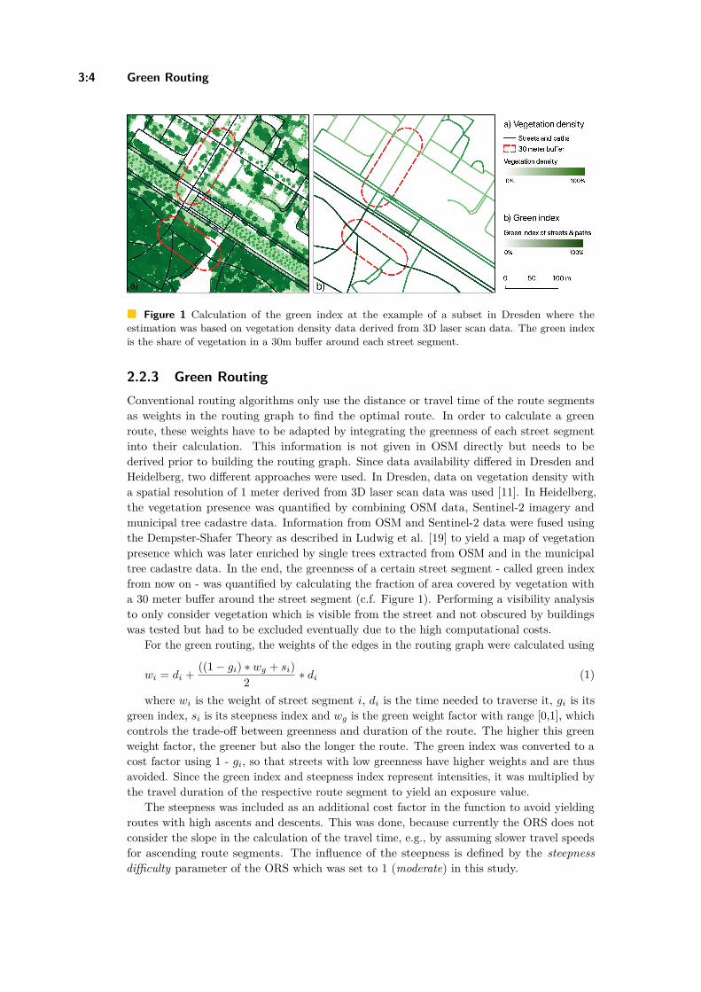
3:4 Green Routing

Figure 1 Calculation of the green index at the example of a subset in Dresden where theestimation was based on vegetation density data derived from 3D laser scan data. The green indexis the share of vegetation in a 30m buffer around each street segment.

2.2.3 Green RoutingConventional routing algorithms only use the distance or travel time of the route segmentsas weights in the routing graph to find the optimal route. In order to calculate a greenroute, these weights have to be adapted by integrating the greenness of each street segmentinto their calculation. This information is not given in OSM directly but needs to bederived prior to building the routing graph. Since data availability differed in Dresden andHeidelberg, two different approaches were used. In Dresden, data on vegetation density witha spatial resolution of 1 meter derived from 3D laser scan data was used [11]. In Heidelberg,the vegetation presence was quantified by combining OSM data, Sentinel-2 imagery andmunicipal tree cadastre data. Information from OSM and Sentinel-2 data were fused usingthe Dempster-Shafer Theory as described in Ludwig et al. [19] to yield a map of vegetationpresence which was later enriched by single trees extracted from OSM and in the municipaltree cadastre data. In the end, the greenness of a certain street segment - called green indexfrom now on - was quantified by calculating the fraction of area covered by vegetation witha 30 meter buffer around the street segment (c.f. Figure 1). Performing a visibility analysisto only consider vegetation which is visible from the street and not obscured by buildingswas tested but had to be excluded eventually due to the high computational costs.

For the green routing, the weights of the edges in the routing graph were calculated using

wi = di + ((1 − gi) ∗ wg + si)2 ∗ di (1)

where wi is the weight of street segment i, di is the time needed to traverse it, gi is itsgreen index, si is its steepness index and wg is the green weight factor with range [0,1], whichcontrols the trade-off between greenness and duration of the route. The higher this greenweight factor, the greener but also the longer the route. The green index was converted to acost factor using 1 - gi, so that streets with low greenness have higher weights and are thusavoided. Since the green index and steepness index represent intensities, it was multiplied bythe travel duration of the respective route segment to yield an exposure value.

The steepness was included as an additional cost factor in the function to avoid yieldingroutes with high ascents and descents. This was done, because currently the ORS does notconsider the slope in the calculation of the travel time, e.g., by assuming slower travel speedsfor ascending route segments. The influence of the steepness is defined by the steepnessdifficulty parameter of the ORS which was set to 1 (moderate) in this study.

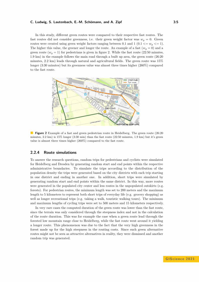
C. Ludwig, S. Lautenbach, E.-M. Schömann, and A. Zipf 3:5

In this study, different green routes were compared to their respective fast routes. Thefast routes did not consider greenness, i.e. their green weight factor was wg = 0. Greenroutes were created using green weight factors ranging between 0.1 and 1 (0.1 <= wg <= 1).The higher this value, the greener and longer the route. An example of a fast (wg = 0) and agreen route (wg = 1) for pedestrians is given in figure 2. While the fast route (22:50 minutes,1.9 km) in the example follows the main road through a built up area, the green route (26:20minutes, 2.2 km) leads through natural and agricultural fields. The green route was 15%longer (3:30 minutes) but its greenness value was almost three times higher (260%) comparedto the fast route.

Figure 2 Example of a fast and green pedestrian route in Heidelberg. The green route (26:20minutes, 2.2 km) is 15% longer (3:30 min) than the fast route (22:50 minutes, 1.9 km) but it’s greenvalue is almost three times higher (260%) compared to the fast route.

2.2.4 Route simulations

To answer the research questions, random trips for pedestrians and cyclists were simulatedfor Heidelberg and Dresden by generating random start and end points within the respectiveadministrative boundaries. To simulate the trips according to the distribution of thepopulation density the trips were generated based on the city districts with each trip startingin one district and ending in another one. In addition, short trips were simulated bygenerating random start and end points within the same district. In this way, more routeswere generated in the populated city center and less routes in the unpopulated outskirts (e.g.forests). For pedestrian routes, the minimum length was set to 200 meters and the maximumlength to 5 kilometers to represent both short trips of everyday life (e.g. grocery shopping) aswell as longer recreational trips (e.g. taking a walk, touristic walking tours). The minimumand maximum lengths of cycling trips were set to 500 meters and 15 kilometers respectively.

In very rare cases the computed duration of the green route was lower than the fast route,since the terrain was only considered through the steepness index and not in the calculationof the route duration. This was for example the case when a green route lead through theforested low mountain range close to Heidelberg, while the fast route went around it yieldinga longer route. This phenomenon was due to the fact that the very high greenness in theforest made up for the high steepness in the routing costs. Since such green alternativeroutes might not be seen as attractive alternatives in reality, they were dismissed and anotherrandom trip was generated.

GISc ience 2021

3:6 Green Routing

Two separate simulation runs were performed to answer the two research questions. Thefirst run was performed to compare the green routes to their respective fast routes in terms ofduration and similarity (RQ1). For each city, 3000 trips by bike and 3000 trips by foot weresimulated. For each trip, the fast route and 10 green routes with increasing green weightfactor wg in the range of 0.1 to 1.0 were calculated.

A second simulation run was performed to analyze the street network connectivity inregard to the exposure of cyclists and pedestrians to greenness (RQ2). This analysis wasperformed in Dresden by simulating 8858 bike trips and in Heidelberg by simulating 9024trips for pedestrians. For each trip, the fast route and an alternative green route with greenweight factor wg = 1 were calculated and compared to each other. Avoidable street segmentswere identified by extracting the route segments of the fast route which were not identicalwith the green route. Preferable street segments were identified by extracting the routesegments of the green route which were not identical with the fast route. Unavoidable routesegments were defined as streets or paths which were contained in both the fast and greenroute and showed a green index lower than 0.1. Streets where the fast and green routewere identical and which had a green index higher than 0.6 were considered as ideal routesegments, i.e. the route is both fast and green. The extracted route segments were aggregatedinto heatmaps showing avoidable, preferable, unavoidable and ideal street or path segments.The heatmaps were created using the Kernel Density Estimation module of SAGA GISversion 2.3.2 (http://www.saga-gis.org/en/index.html). Since this tool requires pointdata as input, the extracted route segments were converted from line to point geometrieswith a distance of 5 meters between the points. The rest of the analysis was implementedusing Python 3.9 (https://www.python.org/) and the openrouteservice Python package(https://pypi.org/project/openrouteservice/).

3 Results

3.1 OSM Data Quality AssessmentMost road classes in both Heidelberg and Dresden showed a contribution pattern thatindicates saturation (c.f. figure 3) – together with the constantly high user activity (c.f.figure 4) in both cities this can be taken as an indicator for high completeness of the roadnetwork. Road categories that could be assumed to be highly complete in both cities consistof: primary, secondary, tertiary, residential, unclassified and pedestrian roads. In addition,the category living_street seemed saturated in Dresden, while in Heidelberg this was true forthe category tracks .

Two road categories were declining in both cities: roads and cycleways. Roads are acategory used if a road cannot be categorized clearly into one of the other tags so a declineof this category is both expected and an indication of increasing data quality. The categorycycleway represents separate ways for cyclists. Cycleways that are not separated from aroad are usually mapped with a highway=* tag and the additional key cycleway=* thatspecifies the type of the cycleway. The use of the tag cycleway=* has evolved over timeleading to a decrease in the use of highway=cycleway. The length of ways tagged as cyclewayhas increased in both cities over time which can be taken as an indication that cycleways arerelatively complete (c.f. 5).

The road categories path, service and footway seemed not yet saturated. In Heidelberg inaddition the category living_street and in Dresden track were not saturated. The differenthighway values are explained in the OSM Wiki (https://wiki.openstreetmap.org/wiki/Key:highway).

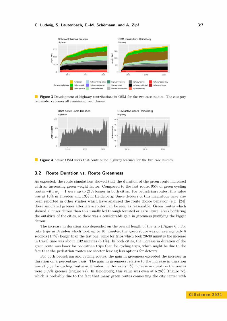
C. Ludwig, S. Lautenbach, E.-M. Schömann, and A. Zipf 3:7

0

2500

5000

7500

2010 2015 2020

Leng

th [k

m]

HighwayOSM contributions Dresden

0

500

1000

1500

2010 2015 2020

Leng

th [k

m]

HighwayOSM contributions Heidelberg

Highway categoryremainder

highway=path

highway=track

highway=living_street

highway=pedestrian

highway=footway

highway=cycleway

highway=road

highway=unclassified

highway=service

highway=residential

highway=tertiary

highway=secondary

highway=primary

Figure 3 Development of highway contributions in OSM for the two case studies. The categoryremainder captures all remaining road classes.

0

40

80

120

2010 2015 2020

Act

ive

user

s

HighwayOSM active users Dresden

0

10

20

30

40

50

2010 2015 2020

Act

ive

user

sHighwayOSM active users Heidelberg

Figure 4 Active OSM users that contributed highway features for the two case studies.

3.2 Route Duration vs. Route Greenness

As expected, the route simulations showed that the duration of the green route increasedwith an increasing green weight factor. Compared to the fast route, 95% of green cyclingroutes with wg = 1 were up to 21% longer in both cities. For pedestrian routes, this valuewas at 16% in Dresden and 13% in Heidelberg. Since detours of this magnitude have alsobeen reported in other studies which have analyzed the route choice behavior (e.g. [24])these simulated greener alternative routes can be seen as reasonable. Green routes whichshowed a longer detour than this usually led through forested or agricultural areas borderingthe outskirts of the cities, so there was a considerable gain in greenness justifying the biggerdetour.

The increase in duration also depended on the overall length of the trip (Figure 6). Forbike trips in Dresden which took up to 10 minutes, the green route was on average only 8seconds (1.7%) longer than the fast one, while for trips which took 20-30 minutes the increasein travel time was about 1:32 minutes (6.1%). In both cities, the increase in duration of thegreen route was lower for pedestrian trips than for cycling trips, which might be due to thefact that the pedestrian routes are shorter leaving less options for detours.

For both pedestrian and cycling routes, the gain in greenness exceeded the increase induration on a percentage basis. The gain in greenness relative to the increase in durationwas at 3.39 for cycling routes in Dresden, i.e. for every 1% increase in duration the routeswere 3.39% greener (Figure 7a). In Heidelberg, this value was even at 5.26% (Figure 7c),which is probably due to the fact that many green routes connecting the city center with

GISc ience 2021

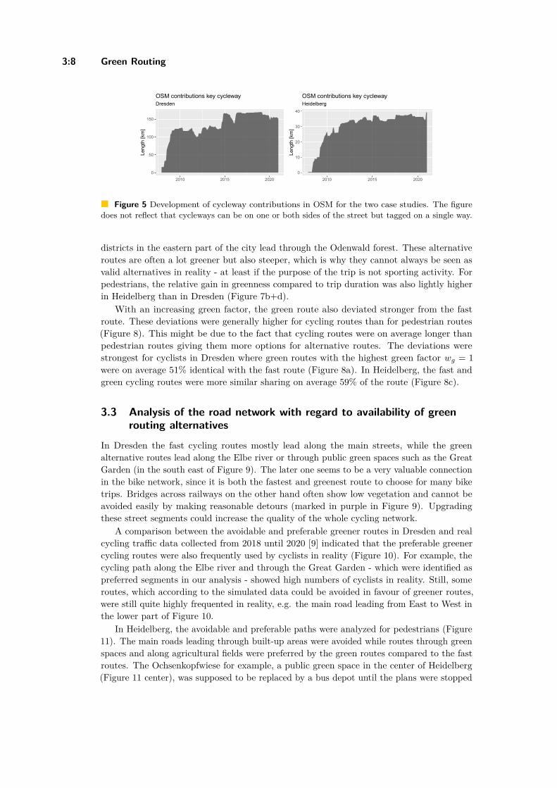
3:8 Green Routing

0

50

100

150

2010 2015 2020

Leng

th [k

m]

DresdenOSM contributions key cycleway

0

10

20

30

40

2010 2015 2020

Leng

th [k

m]

HeidelbergOSM contributions key cycleway

Figure 5 Development of cycleway contributions in OSM for the two case studies. The figuredoes not reflect that cycleways can be on one or both sides of the street but tagged on a single way.

districts in the eastern part of the city lead through the Odenwald forest. These alternativeroutes are often a lot greener but also steeper, which is why they cannot always be seen asvalid alternatives in reality - at least if the purpose of the trip is not sporting activity. Forpedestrians, the relative gain in greenness compared to trip duration was also lightly higherin Heidelberg than in Dresden (Figure 7b+d).

With an increasing green factor, the green route also deviated stronger from the fastroute. These deviations were generally higher for cycling routes than for pedestrian routes(Figure 8). This might be due to the fact that cycling routes were on average longer thanpedestrian routes giving them more options for alternative routes. The deviations werestrongest for cyclists in Dresden where green routes with the highest green factor wg = 1were on average 51% identical with the fast route (Figure 8a). In Heidelberg, the fast andgreen cycling routes were more similar sharing on average 59% of the route (Figure 8c).

3.3 Analysis of the road network with regard to availability of greenrouting alternatives

In Dresden the fast cycling routes mostly lead along the main streets, while the greenalternative routes lead along the Elbe river or through public green spaces such as the GreatGarden (in the south east of Figure 9). The later one seems to be a very valuable connectionin the bike network, since it is both the fastest and greenest route to choose for many biketrips. Bridges across railways on the other hand often show low vegetation and cannot beavoided easily by making reasonable detours (marked in purple in Figure 9). Upgradingthese street segments could increase the quality of the whole cycling network.

A comparison between the avoidable and preferable greener routes in Dresden and realcycling traffic data collected from 2018 until 2020 [9] indicated that the preferable greenercycling routes were also frequently used by cyclists in reality (Figure 10). For example, thecycling path along the Elbe river and through the Great Garden - which were identified aspreferred segments in our analysis - showed high numbers of cyclists in reality. Still, someroutes, which according to the simulated data could be avoided in favour of greener routes,were still quite highly frequented in reality, e.g. the main road leading from East to West inthe lower part of Figure 10.

In Heidelberg, the avoidable and preferable paths were analyzed for pedestrians (Figure11). The main roads leading through built-up areas were avoided while routes through greenspaces and along agricultural fields were preferred by the green routes compared to the fastroutes. The Ochsenkopfwiese for example, a public green space in the center of Heidelberg(Figure 11 center), was supposed to be replaced by a bus depot until the plans were stopped

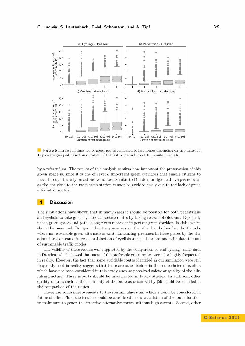
C. Ludwig, S. Lautenbach, E.-M. Schömann, and A. Zipf 3:9

0

10

20

30

40

50In

crea

se in

dur

atio

n of

g

reen

rout

e [%

]

a) Cycling - Dresden b) Pedestrian - Dresden

(0, 10] (10, 20] (20, 30] (30, 40] (40, 50]Duration of fast route [min]

0

10

20

30

40

50

Incr

ease

in d

urat

ion

of

gre

en ro

ute

[%]

c) Cycling - Heidelberg

(0, 10] (10, 20] (20, 30] (30, 40] (40, 50]Duration of fast route [min]

d) Pedestrian - Heidelberg

Figure 6 Increase in duration of green routes compared to fast routes depending on trip duration.Trips were grouped based on duration of the fast route in bins of 10 minute intervals.

by a referendum. The results of this analysis confirm how important the preservation of thisgreen space is, since it is one of several important green corridors that enable citizens tomove through the city on attractive routes. Similar to Dresden, bridges and overpasses, suchas the one close to the main train station cannot be avoided easily due to the lack of greenalternative routes.

4 Discussion

The simulations have shown that in many cases it should be possible for both pedestriansand cyclists to take greener, more attractive routes by taking reasonable detours. Especiallyurban green spaces and paths along rivers represent important green corridors in cities whichshould be preserved. Bridges without any greenery on the other hand often form bottleneckswhere no reasonable green alternatives exist. Enhancing greenness in these places by the cityadministration could increase satisfaction of cyclists and pedestrians and stimulate the useof sustainable traffic modes.

The validity of these results was supported by the comparison to real cycling traffic datain Dresden, which showed that most of the preferable green routes were also highly frequentedin reality. However, the fact that some avoidable routes identified in our simulation were stillfrequently used in reality suggests that there are other factors in the route choice of cyclistswhich have not been considered in this study such as perceived safety or quality of the bikeinfrastructure. These aspects should be investigated in future studies. In addition, otherquality metrics such as the continuity of the route as described by [29] could be included inthe comparison of the routes.

There are some improvements to the routing algorithm which should be considered infuture studies. First, the terrain should be considered in the calculation of the route durationto make sure to generate attractive alternative routes without high ascents. Second, other

GISc ience 2021

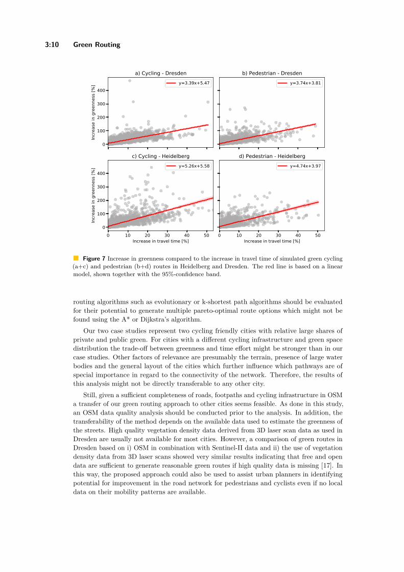
3:10 Green Routing

0

100

200

300

400In

crea

se in

gre

enne

ss [%

]

a) Cycling - Dresdeny=3.39x+5.47

b) Pedestrian - Dresdeny=3.74x+3.81

0 10 20 30 40 50Increase in travel time [%]

0

100

200

300

400

Incr

ease

in g

reen

ness

[%]

c) Cycling - Heidelbergy=5.26x+5.58

0 10 20 30 40 50Increase in travel time [%]

d) Pedestrian - Heidelbergy=4.74x+3.97

Figure 7 Increase in greenness compared to the increase in travel time of simulated green cycling(a+c) and pedestrian (b+d) routes in Heidelberg and Dresden. The red line is based on a linearmodel, shown together with the 95%-confidence band.

routing algorithms such as evolutionary or k-shortest path algorithms should be evaluatedfor their potential to generate multiple pareto-optimal route options which might not befound using the A* or Dijkstra’s algorithm.

Our two case studies represent two cycling friendly cities with relative large shares ofprivate and public green. For cities with a different cycling infrastructure and green spacedistribution the trade-off between greenness and time effort might be stronger than in ourcase studies. Other factors of relevance are presumably the terrain, presence of large waterbodies and the general layout of the cities which further influence which pathways are ofspecial importance in regard to the connectivity of the network. Therefore, the results ofthis analysis might not be directly transferable to any other city.

Still, given a sufficient completeness of roads, footpaths and cycling infrastructure in OSMa transfer of our green routing approach to other cities seems feasible. As done in this study,an OSM data quality analysis should be conducted prior to the analysis. In addition, thetransferability of the method depends on the available data used to estimate the greenness ofthe streets. High quality vegetation density data derived from 3D laser scan data as used inDresden are usually not available for most cities. However, a comparison of green routes inDresden based on i) OSM in combination with Sentinel-II data and ii) the use of vegetationdensity data from 3D laser scans showed very similar results indicating that free and opendata are sufficient to generate reasonable green routes if high quality data is missing [17]. Inthis way, the proposed approach could also be used to assist urban planners in identifyingpotential for improvement in the road network for pedestrians and cyclists even if no localdata on their mobility patterns are available.

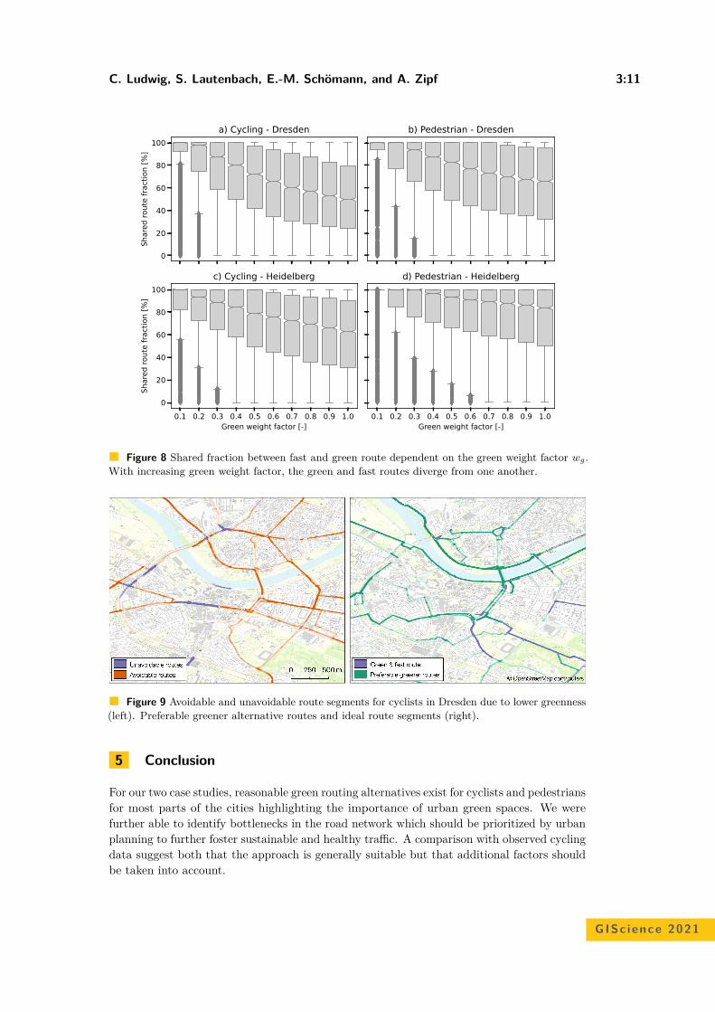
C. Ludwig, S. Lautenbach, E.-M. Schömann, and A. Zipf 3:11

0

20

40

60

80

100Sh

ared

route fra

ction [%

]a) Cycling - Dresden b) Pedestrian - Dresden

0.1 0.2 0.3 0.4 0.5 0.6 0.7 0.8 0.9 1.0Green weight factor [-]

0

20

40

60

80

100

Shar

ed ro

ute

fract

ion

[%]

c) Cycling - Heidelberg

0.1 0.2 0.3 0.4 0.5 0.6 0.7 0.8 0.9 1.0Green weight factor [-]

d) Pedestrian - Heidelberg

Figure 8 Shared fraction between fast and green route dependent on the green weight factor wg.With increasing green weight factor, the green and fast routes diverge from one another.

Figure 9 Avoidable and unavoidable route segments for cyclists in Dresden due to lower greenness(left). Preferable greener alternative routes and ideal route segments (right).

5 Conclusion

For our two case studies, reasonable green routing alternatives exist for cyclists and pedestriansfor most parts of the cities highlighting the importance of urban green spaces. We werefurther able to identify bottlenecks in the road network which should be prioritized by urbanplanning to further foster sustainable and healthy traffic. A comparison with observed cyclingdata suggest both that the approach is generally suitable but that additional factors shouldbe taken into account.

GISc ience 2021

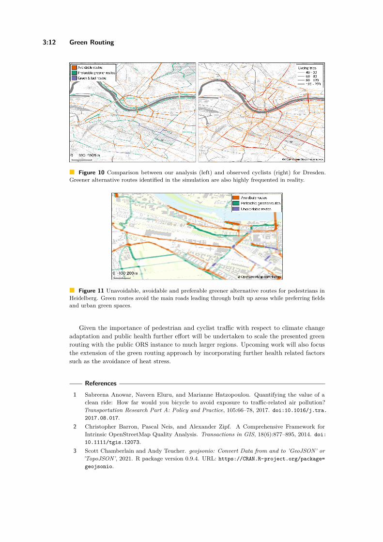
3:12 Green Routing

Figure 10 Comparison between our analysis (left) and observed cyclists (right) for Dresden.Greener alternative routes identified in the simulation are also highly frequented in reality.

Figure 11 Unavoidable, avoidable and preferable greener alternative routes for pedestrians inHeidelberg. Green routes avoid the main roads leading through built up areas while preferring fieldsand urban green spaces.

Given the importance of pedestrian and cyclist traffic with respect to climate changeadaptation and public health further effort will be undertaken to scale the presented greenrouting with the public ORS instance to much larger regions. Upcoming work will also focusthe extension of the green routing approach by incorporating further health related factorssuch as the avoidance of heat stress.

References

1 Sabreena Anowar, Naveen Eluru, and Marianne Hatzopoulou. Quantifying the value of aclean ride: How far would you bicycle to avoid exposure to traffic-related air pollution?Transportation Research Part A: Policy and Practice, 105:66–78, 2017. doi:10.1016/j.tra.2017.08.017.

2 Christopher Barron, Pascal Neis, and Alexander Zipf. A Comprehensive Framework forIntrinsic OpenStreetMap Quality Analysis. Transactions in GIS, 18(6):877–895, 2014. doi:10.1111/tgis.12073.

3 Scott Chamberlain and Andy Teucher. geojsonio: Convert Data from and to ’GeoJSON’ or’TopoJSON’, 2021. R package version 0.9.4. URL: https://CRAN.R-project.org/package=geojsonio.

C. Ludwig, S. Lautenbach, E.-M. Schömann, and A. Zipf 3:13

4 Lívia Castro Degrossi, João Porto de Albuquerque, Roberto dos Santos Rocha, and ALexanderZipf. A Framework of Quality Assessment Methods for Crowdsourced Geographic Information:a Systematic Literature Review. In Proceedings of the 14th ISCRAM Conference, pages 21–24,2017. Issue: May.

5 Dawn C Dickinson and Richard J Hobbs. Cultural ecosystem services: Characteristics,challenges and lessons for urban green space research. Ecosystem Services, 25:179–194, 2017.

6 E W Dijkstra. A note on two problems in connexion with graphs. Numerische Mathematik,1:269–271, 1959.

7 German Aerospace Center (DLR). Land Cover DE - Sentinel-2 - Germany, 2015, 2020.doi:10.15489/1ccmlap3mn39.

8 Erik Gómez-Baggethun, Åsa Gren, David N Barton, Johannes Langemeyer, Timon McPhearson,Patrick O’farrell, Erik Andersson, Zoé Hamstead, and Peleg Kremer. Urban ecosystem services.In Urbanization, biodiversity and ecosystem services: Challenges and opportunities, pages175–251. Springer, Dordrecht, 2013. doi:10.1007/978-94-007-7088-1.

9 P. Grubitzsch, S. Lißner, S. Huber, and T. Springer, 2021. Accessed: 23.4.2021.URL: https://www.mcloud.de/web/guest/suche/-/results/suche/relevance/MOVEBIS/0/detail/ECF9DF02-37DC-4268-B017-A7C2CF302006.

10 Peter E. Hart, Nils J. Nillson, and Bertram Raphael. A Formal Basis for the Heuristic Determin-ation of Minimum Cost Paths. IEEE transactions on Systems Science and Cybernetics, 4(2):100–107, 1968. URL: https://www.cs.auckland.ac.nz/compsci767s2c/projectReportExamples.d/astarNilsson.pdf.

11 Robert Hecht, Gotthard Meinel, and Manfred F Buchroithner. Estimation of urban greenvolume based on single-pulse lidar data. IEEE Transactions on Geoscience and RemoteSensing, 46(11):3832–3840, 2008. doi:10.1109/TGRS.2008.2001771.

12 Victoria Houlden, Scott Weich, João Porto de Albuquerque, Stephen Jarvis, and Karen Rees.The relationship between greenspace and the mental wellbeing of adults: A systematic review.PLOS ONE, 13(9):e0203000, September 2018. doi:10.1371/journal.pone.0203000.

13 Isaac Johnson, Jessica Henderson, Caitlin Perry, Johannes Schöning, and Brent Hecht. Beau-tiful. . . but at what cost? an examination of externalities in geographic vehicle routing.Proceedings of the ACM on Interactive, Mobile, Wearable and Ubiquitous Technologies, 1(2):1–21, 2017. doi:10.1145/3090080.

14 Alboukadel Kassambara. ggpubr: ’ggplot2’ Based Publication Ready Plots, 2020. R packageversion 0.4.0. URL: https://CRAN.R-project.org/package=ggpubr.

15 Michelle Kondo, Jaime Fluehr, Thomas McKeon, and Charles Branas. Urban green space andits impact on human health. International Journal of Environmental Research and PublicHealth, 15(3):445, 2018. doi:10.3390/ijerph15030445.

16 Kerstin Krellenberg, Juliane Welz, and Sonia Reyes-Päcke. Urban green areas and theirpotential for social interaction–a case study of a socio-economically mixed neighbourhood inSantiago de Chile. Habitat International, 44:11–21, 2014.

17 Anna Lausen. Analyse der Verwendbarkeit von OSM Daten für ein grünes Routing amBeispiel Dresden. Bachelor’s thesis, Heidelberg University, Institute of Geography, Heidelberg,Germany, January 2020.

18 Claudia Lega, Christopher Gidlow, Marc Jones, Naomi Ellis, and Gemma Hurst. Therelationship between surrounding greenness, stress and memory. Urban Forestry & UrbanGreening, 59:126974, 2021. doi:10.1016/j.ufug.2020.126974.

19 Christina Ludwig, Robert Hecht, Sven Lautenbach, Martin Schorcht, and Alexander Zipf.Mapping Public Urban Green Spaces Based on OpenStreetMap and Sentinel-2 Imagery UsingBelief Functions. ISPRS International Journal of Geo-Information, 10(4):251, April 2021.doi:10.3390/ijgi10040251.

20 J. Maas. Green space, urbanity, and health: how strong is the relation? Journal of Epidemiology& Community Health, 60(7):587–592, July 2006. doi:10.1136/jech.2005.043125.

GISc ience 2021

3:14 Green Routing

21 David Philip McArthur and Jinhyun Hong. Visualising where commuting cyclists travelusing crowdsourced data. Journal of transport geography, 74:233–241, 2019. doi:10.1016/j.jtrangeo.2018.11.018.

22 Pascal Neis and Alexander Zipf. Openrouteservice.org is three times “open”: CombiningOpenSource, OpenLS and OpenStreetMaps. In GIS Research UK (GISRUK 08). Manchester,2008.

23 Tessio Novack, Zhiyong Wang, and Alexander Zipf. A system for generating customizedpleasant pedestrian routes based on openstreetmap data. Sensors, 18(11):3794, 2018.

24 Yujin Park and Gulsah Akar. Why do bicyclists take detours? a multilevel regression modelusing smartphone gps data. Journal of transport geography, 74:191–200, 2019.

25 Edzer Pebesma. Simple Features for R: Standardized Support for Spatial Vector Data. The RJournal, 10(1):439–446, 2018. doi:10.32614/RJ-2018-009.

26 Andrea Pimpinella, Alessandro E.C. Redondi, and Matteo Cesana. Walk this way! anIoT-based urban routing system for smart cities. Computer Networks, 162:106857, 2019.doi:10.1016/j.comnet.2019.07.013.

27 R Core Team. R: A Language and Environment for Statistical Computing. R Foundation forStatistical Computing, Vienna, Austria, 2021. URL: https://www.R-project.org/.

28 Martin Raifer, Rafael Troilo, Fabian Kowatsch, Michael Auer, Lukas Loos, Sabrina Marx,Katharina Przybill, Sascha Fendrich, Franz-Benjamin Mocnik, and Alexander Zipf. OSHDB:a framework for spatio-temporal analysis of OpenStreetMap history data. Open GeospatialData, Software and Standards, 4(1), 2019. doi:10.1186/s40965-019-0061-3.

29 Karl Rehrl, Stefan Kranzinger, and Simon Gröchenig. Which quality is a route? a methodologyfor assessing route quality using spatio-temporal metrics. Transactions in GIS, 25(2):869–896,2021. doi:10.1111/tgis.12705.

30 Daniel A. Rodríguez, Louis Merlin, Carlo G. Prato, Terry L. Conway, Deborah Cohen, John P.Elder, Kelly R. Evenson, Thomas L. McKenzie, Julie L. Pickrel, and Sara Veblen-Mortenson.Influence of the built environment on pedestrian route choices of adolescent girls. Environmentand Behavior, 47(4):359–394, 2015. doi:10.1177/0013916513520004.

31 Sophie Schetke, Salman Qureshi, Sven Lautenbach, and Nadja Kabisch. What determines theuse of urban green spaces in highly urbanized areas? – Examples from two fast growing Asiancities. Urban Forestry & Urban Greening, 16:150–159, 2016. doi:10.1016/j.ufug.2016.02.009.

32 Hansi Senaratne, Amin Mobasheri, Ahmed Loai Ali, Cristina Capineri, and Morde-chai (Muki) Haklay. A review of volunteered geographic information quality assessmentmethods. International Journal of Geographical Information Science, 31(1):139–167, 2017.doi:10.1080/13658816.2016.1189556.

33 P. N. Seneviratne and J. F. Morrall. Analysis of factors affecting the choice of route ofpedestrians. Transportation Planning and Technology, 10(2):147–159, 1985. doi:10.1080/03081068508717309.

34 Monir H. Sharker and Hassan A. Karimi. Computing least air pollution exposure routes.International Journal of Geographical Information Science, 28(2):343–362, 2014. doi:10.1080/13658816.2013.841317.

35 P. Siriaraya, Y. Wang, Y. Zhang, S. Wakamiya, P. Jeszenszky, Y. Kawai, and A. Jatowt. Beyondthe shortest route: A survey on quality-aware route navigation for pedestrians. IEEE Access,8:135569–135590, 2020. Conference Name: IEEE Access. doi:10.1109/ACCESS.2020.3011924.

36 Duncan Temple Lang. RCurl: General Network (HTTP/FTP/...) Client Interface for R, 2021.R package version 1.98-1.3. URL: https://CRAN.R-project.org/package=RCurl.

37 Heike Tost, Markus Reichert, Urs Braun, Iris Reinhard, Robin Peters, Sven Lautenbach,Andreas Hoell, Emanuel Schwarz, Ulrich Ebner-Priemer, Alexander Zipf, and Andreas Meyer-Lindenberg. Neural correlates of individual differences in affective benefit of real-life urbangreen space exposure. Nature Neuroscience, 2019. doi:10.1038/s41593-019-0451-y.

C. Ludwig, S. Lautenbach, E.-M. Schömann, and A. Zipf 3:15

38 Asha Weinstein Agrawal, Marc Schlossberg, and Katja Irvin. How far, by which route andwhy? a spatial analysis of pedestrian preference. Journal of Urban Design, 13(1):81–98, 2008.doi:10.1080/13574800701804074.

39 Hadley Wickham. ggplot2: Elegant Graphics for Data Analysis. Springer-Verlag New York,2016. URL: https://ggplot2.tidyverse.org.

40 Hadley Wickham, Mara Averick, Jennifer Bryan, Winston Chang, Lucy D’Agostino McGowan,Romain François, Garrett Grolemund, Alex Hayes, Lionel Henry, Jim Hester, Max Kuhn,Thomas Lin Pedersen, Evan Miller, Stephan Milton Bache, Kirill Müller, Jeroen Ooms, DavidRobinson, Dana Paige Seidel, Vitalie Spinu, Kohske Takahashi, Davis Vaughan, Claus Wilke,Kara Woo, and Hiroaki Yutani. Welcome to the tidyverse. Journal of Open Source Software,4(43):1686, 2019. doi:10.21105/joss.01686.

41 Bin Zou, Shenxin Li, Zhong Zheng, Benjamin F. Zhan, Zhonglin Yang, and Neng Wan.Healthier routes planning: A new method and online implementation for minimizing airpollution exposure risk. Computers, Environment and Urban Systems, 80:101456, 2020.doi:10.1016/j.compenvurbsys.2019.101456.

GISc ience 2021

A Clustering-Based Framework for IndividualTravel Behaviour Change DetectionYe Hong #

Institute of Cartography and Geoinformation, ETH Zurich, Switzerland

Yanan Xin #

Institute of Cartography and Geoinformation, ETH Zurich, Switzerland

Henry Martin #

Institute of Cartography and Geoinformation, ETH Zurich, SwitzerlandInstitute of Advanced Research in Artificial Intelligence (IARAI), Austria

Dominik Bucher #

Institute of Cartography and Geoinformation, ETH Zurich, Switzerland

Martin Raubal #

Institute of Cartography and Geoinformation, ETH Zurich, Switzerland

AbstractThe emergence of passively and continuously recorded movement data offers new opportunities tostudy the long-term change of individual travel behaviour from data-driven perspectives. This studyproposes a clustering-based framework to identify travel behaviour patterns and detect potentialchange periods on the individual level. First, we extract important trips that depict individualcharacteristic movement. Then, considering trip mode, trip distance, and trip duration as travelbehaviour dimensions, we measure the similarities of trips and group them into clusters usinghierarchical clustering. The trip clusters represent dimensions of travel behaviours, and the change oftheir relative proportions over time reflect the development of travel preferences. We use two differentmethods to detect changes in travel behaviour patterns: the Herfindahl-Hirschman index-basedmethod and the sliding window-based method. The framework is tested using data from a large-scalelongitudinal GPS tracking data study in which participants had access to a Mobility-as-a-Service(MaaS) offer. The methods successfully identify significant travel behaviour changes for users.Moreover, we analyse the impact of the MaaS offer on individual travel behaviours with the obtainedchange information. The proposed framework for behaviour change detection provides valuableinsights for travel demand management and evaluating people’s reactions to sustainable mobilityoptions.

2012 ACM Subject Classification Information systems → Geographic information systems; Inform-ation systems → Clustering; Applied computing → Transportation

Keywords and phrases Human mobility, Travel behaviour, Change detection, Trip clustering

Digital Object Identifier 10.4230/LIPIcs.GIScience.2021.II.4

Supplementary MaterialSoftware (Source Code): https://github.com/mie-lab/change-detection

archived at swh:1:dir:995567f0d4599413f583b7b684a5ca7377cf7c54

Funding This research was supported by the Swiss Data Science Center (SDSC).

1 Introduction

Individual mobility is currently primarily based on the private car. Owning a car is associatedwith a high level of comfort and flexibility [39], as it is always available and can reach mostplaces while offering a safe and personal space. However, conventional car dependence isinherently unsustainable as internal combustion engine cars are a major emitter of greenhousegases [34]. Therefore, a successful transition towards a sustainable transportation systemmust find ways to reduce individual car ownership and support individuals in engaging

© Ye Hong, Yanan Xin, Henry Martin, Dominik Bucher, and Martin Raubal;licensed under Creative Commons License CC-BY 4.0

11th International Conference on Geographic Information Science (GIScience 2021) – Part II.Editors: Krzysztof Janowicz and Judith A. Verstegen; Article No. 4; pp. 4:1–4:15

Leibniz International Proceedings in InformaticsSchloss Dagstuhl – Leibniz-Zentrum für Informatik, Dagstuhl Publishing, Germany

4:2 Travel Behaviour Change Detection

in a more sustainable mobility lifestyle [42]. One of the main strategies to reduce privatecar ownership is Mobility-as-a-Service (MaaS), a concept where multiple shared modes areintegrated with public transport to facilitate intermodal travel [31]. Despite the popularity ofMaaS as a concept, there is currently only limited empirical evidence on how exactly MaaSwill influence travel behaviour [16]. To evaluate the impact of MaaS, it will be necessaryto collect substantial behavioural data and detect whether and to what extent individualschange their behaviour when exposed to a MaaS.

Travel behaviour refers to the decision-making process of individuals moving across spaceand making use of the transport facilities [12, 23]. Each individual has a set of preferredtravel behaviours, collectively forming a travel pattern that is stable over the short term andevolves over the long term [9]. To correctly evaluate MaaS as an instrument for behaviourchange, it is necessary to detect the long-term evolution of individuals’ travel behaviourpatterns. Apart from the evaluation of MaaS, detecting behaviour change on an aggregatedlevel helps transportation planners to manage travel demand, understand the impact oftransportation policies (e.g., congestion pricing, road space rationing), and evaluate people’sreactions to new transportation infrastructures [27]. At the individual service level, detectingchanges in travel patterns allows personalized location based services to adapt to individualtravel behaviour change [17], monitor mobile phone intrusions [36], and detect hidden driversfor usage-based insurance pricing [8].

Motivated by the broad applications, many researchers have focused on travel behaviourchange over the recent years [15, 20]. Studies on individual travel behaviour change mainlyemployed travel panel data and analysed the causes and directions of the behaviour change.For example, Lin et al. [24] investigated the role of social network and social environment inthe relationship between residential relocation and travel behaviour change. In their study,travel behaviours are represented by trip frequency, travel time, and modal split. A study byJain et al. [18] analysed the process of travel behaviour change associated with the adoptionof a car-sharing service, in which the travel behaviours are represented by the amount oftravel and mode choices. Overall, limited studies have focused on the detection and changingspeed of the new behaviours using panel data, partially since those discrete-time panel datawere not suitable for observing a dynamic process [22]. In the era of ubiquitous computing,billions of personal devices connect us to the web and enable the generation of data sets thatreflect large-scale human digital traces. Compared to actively obtained travel survey data,these data sets passively and continuously record the whereabouts of individuals over time,offering new opportunities for data-driven approaches to study individual travel behaviourchange.

Analysing travel behaviour and detecting its change is challenging because continuousindividual movement traces are noisy, and travel patterns are latent in the movement data.To partially mitigate this issue, previous studies most often use aggregated indexes (e.g.,total travel time per day) for describing travel behaviours [20]. Although this processingmethod can extract the essential travel behaviour, an aggregation level needs to be predefined,and some fine-grained details might be omitted during the aggregation process. Therefore,this study uses the amount of travel (trip duration and distance) and mode of transportas features to describe travel behaviours and employ clustering methods to identify travelbehaviours directly at the trip level.

We develop a clustering-based framework that utilises passively tracked data to detectchanges in individual travel behaviour patterns. Two change detection methods are proposedand analysed using a real-world, large-scale GPS tracking data set that evaluates the effect ofintroducing a MaaS offer to the study participants. The remainder of the paper is organised

Y. Hong, Y. Xin, H. Martin, D. Bucher, and M. Raubal 4:3

as follows. Section 2 reviews related work on individual travel behaviour change detection.Section 3 presents the clustering-based change detection framework developed in our study.Section 4 describes our case study data and pre-processing steps. Section 5 explains thecase study results. Section 6 summarises the main contributions of our study and highlightsfuture research directions.

2 Related work

Research on individual travel behaviour change has primarily focused on short-term changes,often called anomalies, outliers, or intrapersonal variability. A generic technique used todetect this type of change when the change is not known a priori is to model the dominantpattern from the data as a standard pattern and identify observations that deviate fromthis pattern as potential anomalies [7]. Many methods have been developed to model thedominant pattern and detect short-term travel behaviour changes, such as clustering-basedmethods, frequency pattern mining methods, and generative models. An example of usinga cluster-based method is given in [41]. The authors used a hierarchical clustering methodto identify normal clusters of trajectories and detect anomalous taxi routing patterns thatlie outside these clusters for inferring taxi fraud or traffic incidents. As a complementaryexample, a study by Sun et al. [36] utilized a frequent pattern mining technique andmodelled the mobility sequence of an individual as a mobility trie. The frequent transitionpattern between places is generated based on this mobility trie, and a less frequent travelsequence is considered abnormal. An example of using generative models is shown in [37],where a generative two-dimensional Latent Dirichlet Allocation model was developed tocapture routine patterns of individuals and predict future movements. Trajectories with lowpredictability are considered abnormal and are used to indicate potential changes in travelbehaviour patterns.

In contrast to a large number of studies in short-term pattern change detection, lessattention has been given to detecting long-term, persistent pattern changes of individualtravel behaviours. This long-term pattern change is also called structural pattern change,change point detection, or concept drift in time series analysis and has been studied in fieldssuch as statistics [25, 35], econometrics [4], and sequential pattern mining [40]. However,those methods have not been well utilized in analysing the evolution of individual travelpatterns.

Recently, a few studies explored the long-term travel pattern change of individuals.Zhao et al. [44, p. 74] defined this type of change as “abrupt, substantial, and persistentchanges in the underlying patterns of travel behavior”. To detect this pattern change, theyused a Bayesian approach to model the probability of a pattern change at any given time.The study examined the changes in three dimensions of travel behaviour: travel frequency,spatial dimension, and temporal dimension. Although the method is shown to be robust tonoisy observations of travel behaviours, it assumes that travel incidences are independentlygenerated from an underlying distribution in each dimension, thus missing the temporaldependency among one dimension and the correlation between different dimensions. Toaccount for the pattern change reflected in other dimensions of travel behaviours, Jonietzand Bucher [20] considered multiple daily and weekly aggregated mobility features, includingtravel duration, distance, speed, CO2 emission, and frequently visited places. The detectionof pattern change is based on whether each feature value deviates from the historical averagevalue by a certain threshold. The framework could signal anomalies in each feature dimensionbut failed to consider travel behaviour as a whole. By contrast, the clustering method used

GISc ience 2021

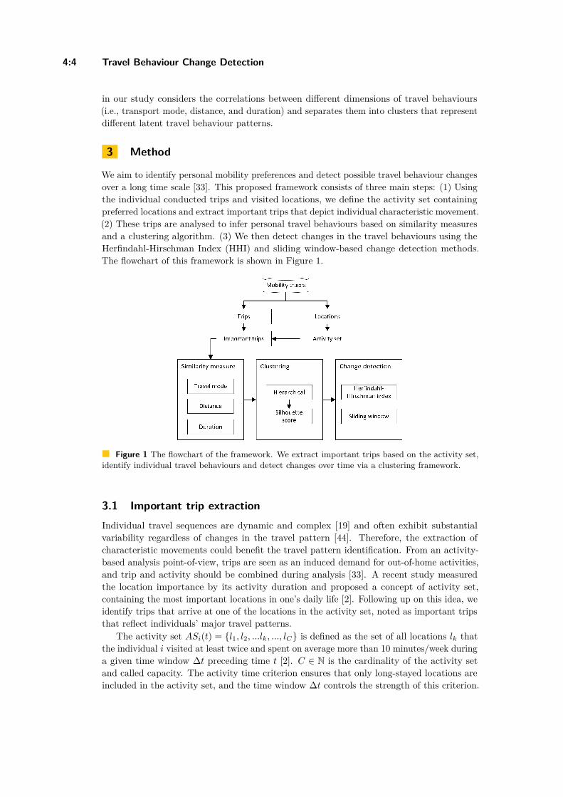
4:4 Travel Behaviour Change Detection

in our study considers the correlations between different dimensions of travel behaviours(i.e., transport mode, distance, and duration) and separates them into clusters that representdifferent latent travel behaviour patterns.

3 Method

We aim to identify personal mobility preferences and detect possible travel behaviour changesover a long time scale [33]. This proposed framework consists of three main steps: (1) Usingthe individual conducted trips and visited locations, we define the activity set containingpreferred locations and extract important trips that depict individual characteristic movement.(2) These trips are analysed to infer personal travel behaviours based on similarity measuresand a clustering algorithm. (3) We then detect changes in the travel behaviours using theHerfindahl-Hirschman Index (HHI) and sliding window-based change detection methods.The flowchart of this framework is shown in Figure 1.

Figure 1 The flowchart of the framework. We extract important trips based on the activity set,identify individual travel behaviours and detect changes over time via a clustering framework.

3.1 Important trip extractionIndividual travel sequences are dynamic and complex [19] and often exhibit substantialvariability regardless of changes in the travel pattern [44]. Therefore, the extraction ofcharacteristic movements could benefit the travel pattern identification. From an activity-based analysis point-of-view, trips are seen as an induced demand for out-of-home activities,and trip and activity should be combined during analysis [33]. A recent study measuredthe location importance by its activity duration and proposed a concept of activity set,containing the most important locations in one’s daily life [2]. Following up on this idea, weidentify trips that arrive at one of the locations in the activity set, noted as important tripsthat reflect individuals’ major travel patterns.

The activity set ASi(t) = l1, l2, ...lk, ..., lC is defined as the set of all locations lk thatthe individual i visited at least twice and spent on average more than 10 minutes/week duringa given time window ∆t preceding time t [2]. C ∈ N is the cardinality of the activity setand called capacity. The activity time criterion ensures that only long-stayed locations areincluded in the activity set, and the time window ∆t controls the strength of this criterion.

Y. Hong, Y. Xin, H. Martin, D. Bucher, and M. Raubal 4:5

We further define the important trip set ITi(t) of the individual i in week t as all trips thatarrive at any location within the activity set. We set the time window ∆t = 5 weeks in thisstudy, following an empirical study that reported that the destination-choice preferences ofan individual stabilizes after five to ten weeks [33].

3.2 Trip similarity measurement and clustering algorithmThe trips included in any important trip set ITi(t) are considered to contain informationregarding the individuals’ main travel behaviours. They are then fed into a clustering-basedframework for identifying groups of trips with similar travel choices. We focus on high-levelsemantic information attached to each trip and consider trip mode, trip distance and tripduration as features. These are essential dimensions reflecting individual travel behaviourand have been employed in various travel behaviour change studies [24, 30].

The travel mode information of trips is represented as a sequence since each trip is acombination of triplegs with a single travel mode. This property makes the travel modecomparison a sequence similarity measurement problem. Nevertheless, we are more interestedin what mode exists in a trip than the order of modes for analysing travel behaviour. Therefore,we regard travel mode sequences as sets and measure their Jaccard distance. For example,given two mode sequences, we reconstruct them into set A = modeA1, modeA2, ..., modeAiand set B = modeB1, modeB2, ..., modeBj, respectively. The Jaccard distance dJ (A, B) isthen represented as:

dJ(A, B) = 1 − J(A, B) = 1 − |A ∩ B||A ∪ B|

where J(A, B) is the Jaccard similarity coefficient, defined as taking the ratio of the intersec-tion over the union of the sets A and B. Thus, the pairwise distance matrix of trip modesDmode is constructed by calculating the Jaccard distance between each pair of trips.

Trip distance and trip duration are two features characterising the amount of travel. Wemeasure the distance and duration similarity of trips with the Euclidean distance and obtaintwo pairwise similarity measurement matrices Ddist and Ddur.

The selected semantic features are combined into the final similarity matrix Dall:

Dall = ω1Dmode + ω2Ddist + ω3Ddur

where ω1, ω2, and ω3 are the corresponding weights that control the importance of Dmode,Ddist and Ddur, respectively. The weight values can be defined equally for each of thedimensions (i.e., ω1 = ω2 = ω3 = 1

3 ), but they can also be set differently when certaindimensions need to be strengthened. To ensure consistent distance scales, each distancematrix is min-max normalized to be in the range from 0 to 1.

We perform clustering on the similarity matrix to identify the group of trips with similartravel behaviour. This is achieved using hierarchical clustering that produces a hierarchy ofclusters using agglomerative (bottom-up) or divisive (top-down) algorithms [21]. The linkagestandard that defines how the distance is measured between two clusters is the key designchoice for hierarchical clustering. Previous work reported that complete linkage is suitable fordetermining a relatively compact cluster [41, 1]. For complete linkage, the distance D(X, Y )between clusters X and Y is defined as:

D(X, Y ) = maxx∈X,y∈Y

d(x, y)

GISc ience 2021

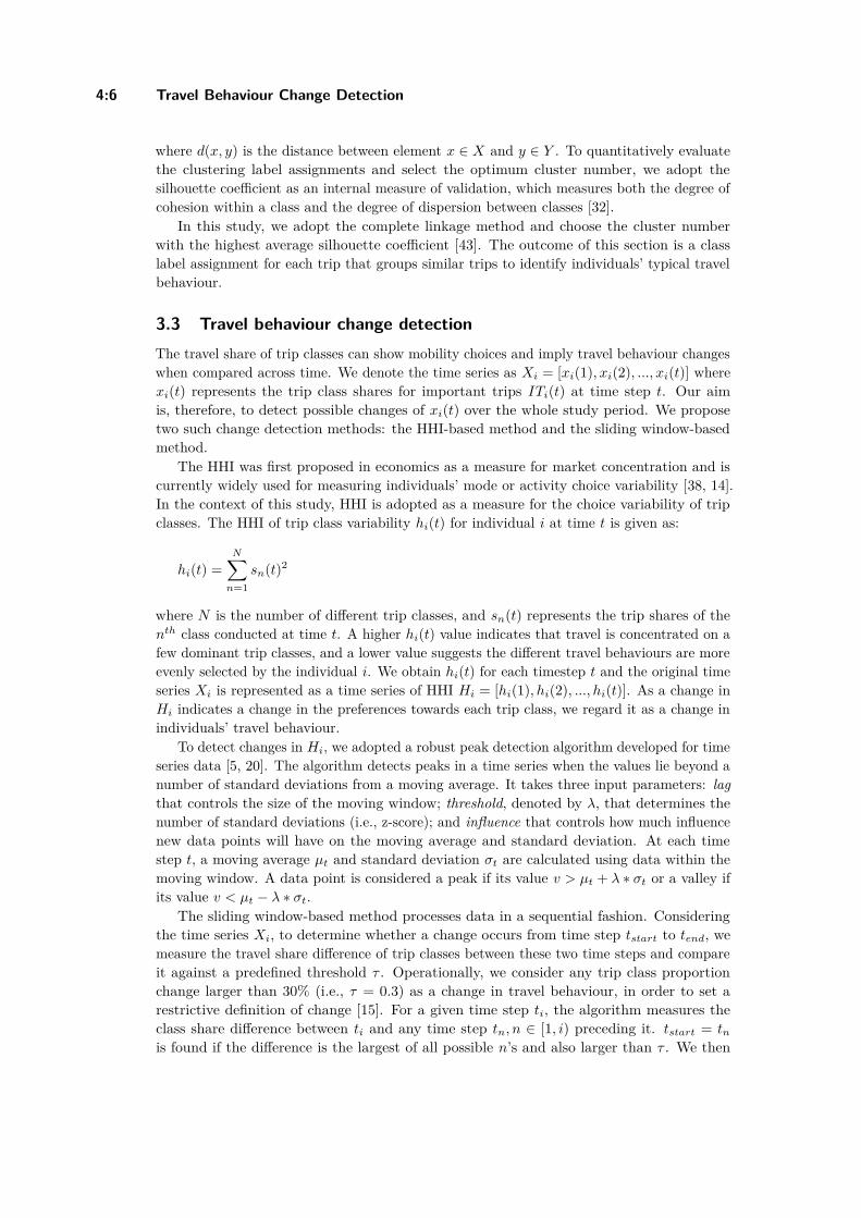
4:6 Travel Behaviour Change Detection

where d(x, y) is the distance between element x ∈ X and y ∈ Y . To quantitatively evaluatethe clustering label assignments and select the optimum cluster number, we adopt thesilhouette coefficient as an internal measure of validation, which measures both the degree ofcohesion within a class and the degree of dispersion between classes [32].

In this study, we adopt the complete linkage method and choose the cluster numberwith the highest average silhouette coefficient [43]. The outcome of this section is a classlabel assignment for each trip that groups similar trips to identify individuals’ typical travelbehaviour.

3.3 Travel behaviour change detectionThe travel share of trip classes can show mobility choices and imply travel behaviour changeswhen compared across time. We denote the time series as Xi = [xi(1), xi(2), ..., xi(t)] wherexi(t) represents the trip class shares for important trips ITi(t) at time step t. Our aimis, therefore, to detect possible changes of xi(t) over the whole study period. We proposetwo such change detection methods: the HHI-based method and the sliding window-basedmethod.

The HHI was first proposed in economics as a measure for market concentration and iscurrently widely used for measuring individuals’ mode or activity choice variability [38, 14].In the context of this study, HHI is adopted as a measure for the choice variability of tripclasses. The HHI of trip class variability hi(t) for individual i at time t is given as:

hi(t) =N∑

n=1sn(t)2

where N is the number of different trip classes, and sn(t) represents the trip shares of thenth class conducted at time t. A higher hi(t) value indicates that travel is concentrated on afew dominant trip classes, and a lower value suggests the different travel behaviours are moreevenly selected by the individual i. We obtain hi(t) for each timestep t and the original timeseries Xi is represented as a time series of HHI Hi = [hi(1), hi(2), ..., hi(t)]. As a change inHi indicates a change in the preferences towards each trip class, we regard it as a change inindividuals’ travel behaviour.

To detect changes in Hi, we adopted a robust peak detection algorithm developed for timeseries data [5, 20]. The algorithm detects peaks in a time series when the values lie beyond anumber of standard deviations from a moving average. It takes three input parameters: lagthat controls the size of the moving window; threshold, denoted by λ, that determines thenumber of standard deviations (i.e., z-score); and influence that controls how much influencenew data points will have on the moving average and standard deviation. At each timestep t, a moving average µt and standard deviation σt are calculated using data within themoving window. A data point is considered a peak if its value v > µt + λ ∗ σt or a valley ifits value v < µt − λ ∗ σt.

The sliding window-based method processes data in a sequential fashion. Consideringthe time series Xi, to determine whether a change occurs from time step tstart to tend, wemeasure the travel share difference of trip classes between these two time steps and compareit against a predefined threshold τ . Operationally, we consider any trip class proportionchange larger than 30% (i.e., τ = 0.3) as a change in travel behaviour, in order to set arestrictive definition of change [15]. For a given time step ti, the algorithm measures theclass share difference between ti and any time step tn, n ∈ [1, i) preceding it. tstart = tn

is found if the difference is the largest of all possible n’s and also larger than τ . We then

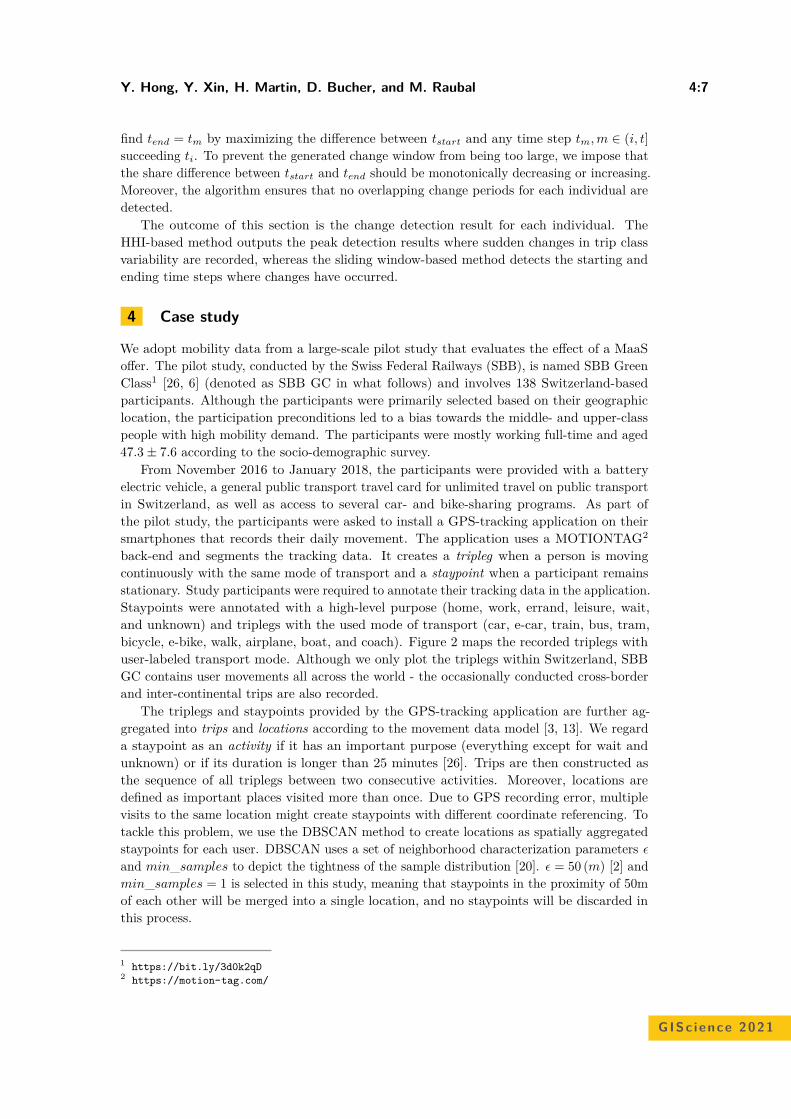
Y. Hong, Y. Xin, H. Martin, D. Bucher, and M. Raubal 4:7

find tend = tm by maximizing the difference between tstart and any time step tm, m ∈ (i, t]succeeding ti. To prevent the generated change window from being too large, we impose thatthe share difference between tstart and tend should be monotonically decreasing or increasing.Moreover, the algorithm ensures that no overlapping change periods for each individual aredetected.

The outcome of this section is the change detection result for each individual. TheHHI-based method outputs the peak detection results where sudden changes in trip classvariability are recorded, whereas the sliding window-based method detects the starting andending time steps where changes have occurred.

4 Case study

We adopt mobility data from a large-scale pilot study that evaluates the effect of a MaaSoffer. The pilot study, conducted by the Swiss Federal Railways (SBB), is named SBB GreenClass1 [26, 6] (denoted as SBB GC in what follows) and involves 138 Switzerland-basedparticipants. Although the participants were primarily selected based on their geographiclocation, the participation preconditions led to a bias towards the middle- and upper-classpeople with high mobility demand. The participants were mostly working full-time and aged47.3 ± 7.6 according to the socio-demographic survey.

From November 2016 to January 2018, the participants were provided with a batteryelectric vehicle, a general public transport travel card for unlimited travel on public transportin Switzerland, as well as access to several car- and bike-sharing programs. As part ofthe pilot study, the participants were asked to install a GPS-tracking application on theirsmartphones that records their daily movement. The application uses a MOTIONTAG2

back-end and segments the tracking data. It creates a tripleg when a person is movingcontinuously with the same mode of transport and a staypoint when a participant remainsstationary. Study participants were required to annotate their tracking data in the application.Staypoints were annotated with a high-level purpose (home, work, errand, leisure, wait,and unknown) and triplegs with the used mode of transport (car, e-car, train, bus, tram,bicycle, e-bike, walk, airplane, boat, and coach). Figure 2 maps the recorded triplegs withuser-labeled transport mode. Although we only plot the triplegs within Switzerland, SBBGC contains user movements all across the world - the occasionally conducted cross-borderand inter-continental trips are also recorded.

The triplegs and staypoints provided by the GPS-tracking application are further ag-gregated into trips and locations according to the movement data model [3, 13]. We regarda staypoint as an activity if it has an important purpose (everything except for wait andunknown) or if its duration is longer than 25 minutes [26]. Trips are then constructed asthe sequence of all triplegs between two consecutive activities. Moreover, locations aredefined as important places visited more than once. Due to GPS recording error, multiplevisits to the same location might create staypoints with different coordinate referencing. Totackle this problem, we use the DBSCAN method to create locations as spatially aggregatedstaypoints for each user. DBSCAN uses a set of neighborhood characterization parameters ϵ

and min_samples to depict the tightness of the sample distribution [20]. ϵ = 50 (m) [2] andmin_samples = 1 is selected in this study, meaning that staypoints in the proximity of 50mof each other will be merged into a single location, and no staypoints will be discarded inthis process.

1 https://bit.ly/3d0k2qD2 https://motion-tag.com/

GISc ience 2021

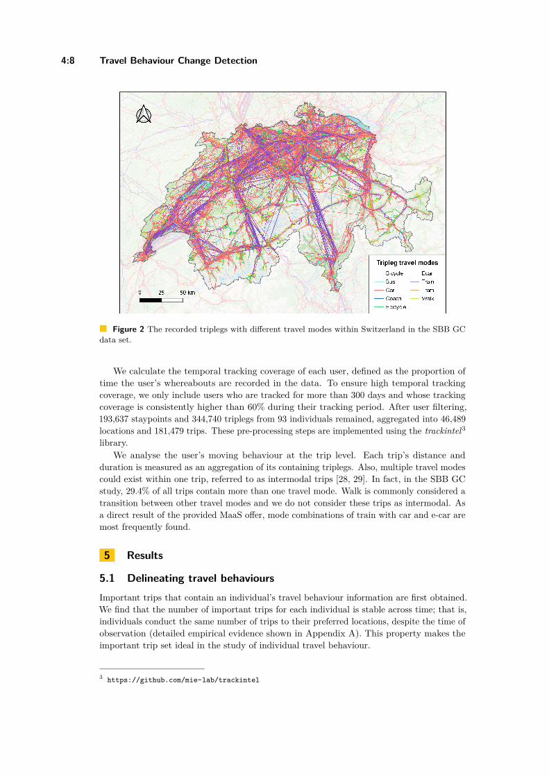
4:8 Travel Behaviour Change Detection

Figure 2 The recorded triplegs with different travel modes within Switzerland in the SBB GCdata set.

We calculate the temporal tracking coverage of each user, defined as the proportion oftime the user’s whereabouts are recorded in the data. To ensure high temporal trackingcoverage, we only include users who are tracked for more than 300 days and whose trackingcoverage is consistently higher than 60% during their tracking period. After user filtering,193,637 staypoints and 344,740 triplegs from 93 individuals remained, aggregated into 46,489locations and 181,479 trips. These pre-processing steps are implemented using the trackintel3

library.We analyse the user’s moving behaviour at the trip level. Each trip’s distance and

duration is measured as an aggregation of its containing triplegs. Also, multiple travel modescould exist within one trip, referred to as intermodal trips [28, 29]. In fact, in the SBB GCstudy, 29.4% of all trips contain more than one travel mode. Walk is commonly considered atransition between other travel modes and we do not consider these trips as intermodal. Asa direct result of the provided MaaS offer, mode combinations of train with car and e-car aremost frequently found.

5 Results

5.1 Delineating travel behavioursImportant trips that contain an individual’s travel behaviour information are first obtained.We find that the number of important trips for each individual is stable across time; that is,individuals conduct the same number of trips to their preferred locations, despite the time ofobservation (detailed empirical evidence shown in Appendix A). This property makes theimportant trip set ideal in the study of individual travel behaviour.

3 https://github.com/mie-lab/trackintel

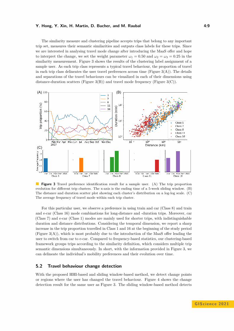
Y. Hong, Y. Xin, H. Martin, D. Bucher, and M. Raubal 4:9

The similarity measure and clustering pipeline accepts trips that belong to any importanttrip set, measures their semantic similarities and outputs class labels for these trips. Sincewe are interested in analysing travel mode change after introducing the MaaS offer and hopeto interpret the change, we set the weight parameter ω1 = 0.50 and ω2 = ω3 = 0.25 in thesimilarity measurement. Figure 3 shows the results of the clustering label assignment of asample user. As each trip class represents a typical travel behaviour, the proportion of travelin each trip class delineates the user travel preferences across time (Figure 3(A)). The detailsand separations of the travel behaviours can be visualized in each of their dimensions usingdistance-duration scatters (Figure 3(B)) and travel mode frequency (Figure 3(C)).

Figure 3 Travel preference identification result for a sample user. (A) The trip proportionevolution for different trip clusters. The x-axis is the ending time of a 5-week sliding window. (B)The distance and duration scatter plot showing each cluster’s distribution on a log-log scale. (C)The average frequency of travel mode within each trip cluster.

For this particular user, we observe a preference in using train and car (Class 8) and trainand e-car (Class 16) mode combinations for long-distance and -duration trips. Moreover, car(Class 7) and e-car (Class 1) modes are mainly used for shorter trips, with indistinguishableduration and distance distributions. Considering the temporal dimension, we report a sharpincrease in the trip proportion travelled in Class 1 and 16 at the beginning of the study period(Figure 3(A)), which is most probably due to the introduction of the MaaS offer leading theuser to switch from car to e-car. Compared to frequency-based statistics, our clustering-basedframework groups trips according to the similarity definition, which considers multiple tripsemantic dimensions simultaneously. In short, with the information provided in Figure 3, wecan delineate the individual’s mobility preferences and their evolution over time.

5.2 Travel behaviour change detectionWith the proposed HHI-based and sliding window-based method, we detect change pointsor regions where the user has changed the travel behaviour. Figure 4 shows the changedetection result for the same user as Figure 3. The sliding window-based method detects

GISc ience 2021

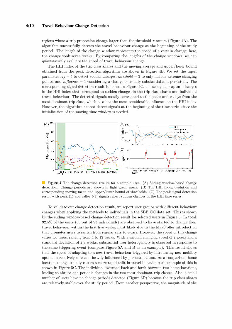
4:10 Travel Behaviour Change Detection

regions where a trip proportion change larger than the threshold τ occurs (Figure 4A). Thealgorithm successfully detects the travel behaviour change at the beginning of the studyperiod. The length of the change window represents the speed of a certain change; here,the change took seven weeks. By comparing the lengths of the change windows, we canquantitatively evaluate the speed of travel behaviour change.

The HHI index of the trip class shares and the moving average and upper/lower boundobtained from the peak detection algorithm are shown in Figure 4B. We set the inputparameter lag = 5 to detect sudden changes, threshold = 3 to only include extreme changingpoints, and influence = 1 considering a change is usually substantial and persistent. Thecorresponding signal detection result is shown in Figure 4C. These signals capture changesin the HHI index that correspond to sudden changes in the trip class shares and individualtravel behaviour. The detected signals mostly correspond to the peaks and valleys from themost dominant trip class, which also has the most considerable influence on the HHI index.However, the algorithm cannot detect signals at the beginning of the time series since theinitialization of the moving time window is needed.

Figure 4 The change detection results for a sample user. (A) Sliding window-based changedetection. Change periods are shown in light green areas. (B) The HHI index evolution andcorresponding moving mean and upper/lower bound of thresholds. (C) The peak signal detectionresult with peak (1) and valley (-1) signals reflect sudden changes in the HHI time series.

To validate our change detection result, we report user groups with different behaviourchanges when applying the methods to individuals in the SBB GC data set. This is shownby the sliding window-based change detection result for selected users in Figure 5. In total,92.5% of the users (86 out of 93 individuals) are observed to have started to change theirtravel behaviour within the first five weeks, most likely due to the MaaS offer introductionthat promotes users to switch from regular cars to e-cars. However, the speed of this changevaries for users, ranging from 4 to 13 weeks. With a median changing speed of 7 weeks and astandard deviation of 2.3 weeks, substantial user heterogeneity is observed in response tothe same triggering event (compare Figure 5A and B as an example). This result showsthat the speed of adapting to a new travel behaviour triggered by introducing new mobilityoptions is relatively slow and heavily influenced by personal factors. As a comparison, homelocation change usually causes a more rapid shift in travel behaviour; an example of this isshown in Figure 5C. The individual switched back and forth between two home locations,leading to abrupt and periodic changes in the two most dominant trip classes. Also, a smallnumber of users have no change periods detected (Figure 5D) because the trip class sharesare relatively stable over the study period. From another perspective, the magnitude of the

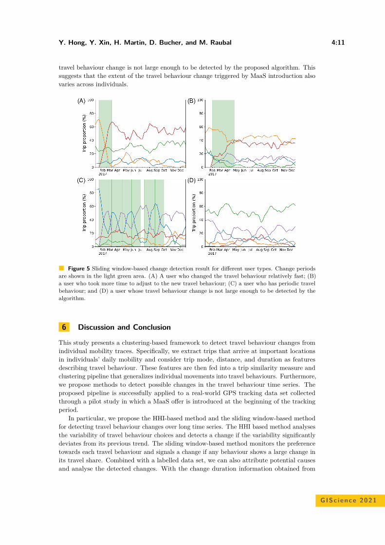
Y. Hong, Y. Xin, H. Martin, D. Bucher, and M. Raubal 4:11

travel behaviour change is not large enough to be detected by the proposed algorithm. Thissuggests that the extent of the travel behaviour change triggered by MaaS introduction alsovaries across individuals.

Figure 5 Sliding window-based change detection result for different user types. Change periodsare shown in the light green area. (A) A user who changed the travel behaviour relatively fast; (B)a user who took more time to adjust to the new travel behaviour; (C) a user who has periodic travelbehaviour; and (D) a user whose travel behaviour change is not large enough to be detected by thealgorithm.

6 Discussion and Conclusion

This study presents a clustering-based framework to detect travel behaviour changes fromindividual mobility traces. Specifically, we extract trips that arrive at important locationsin individuals’ daily mobility and consider trip mode, distance, and duration as featuresdescribing travel behaviour. These features are then fed into a trip similarity measure andclustering pipeline that generalizes individual movements into travel behaviours. Furthermore,we propose methods to detect possible changes in the travel behaviour time series. Theproposed pipeline is successfully applied to a real-world GPS tracking data set collectedthrough a pilot study in which a MaaS offer is introduced at the beginning of the trackingperiod.

In particular, we propose the HHI-based method and the sliding window-based methodfor detecting travel behaviour changes over long time series. The HHI based method analysesthe variability of travel behaviour choices and detects a change if the variability significantlydeviates from its previous trend. The sliding window-based method monitors the preferencetowards each travel behaviour and signals a change if any behaviour shows a large change inits travel share. Combined with a labelled data set, we can also attribute potential causesand analyse the detected changes. With the change duration information obtained from

GISc ience 2021

4:12 Travel Behaviour Change Detection

the sliding window-based method, we analyse the effect of the MaaS offer on the travelbehaviours in our case study. We find that these induced behaviour changes are heavilyuser-dependent. Moreover, compared to changes triggered by relocation, changes caused byadditional mobility options usually occur slower in time.

The proposed change detection method is data-driven and identifies change periodsfrom the statistical distribution of travel behaviour. We believe that this framework isgeneralisable to tracking datasets within other contexts, with flexibility given from the designchoice parameters (e.g., the weights in the similarity measurement). We see several futuredirections based on the results of this study. First, the proposed change detection pipelinecan be applied online to streaming data; however, we lack the information of whether theclustering algorithm is sensitive enough to detect newly occurred travel behaviours. Thisneeds to be tested in an online setup. Second, a sensitivity analysis on the choice of the weightparameter for each semantic feature is beneficial if the proposed pipeline is to be employed inother applications. Third, previous research has reported that residential neighbourhood hasan important impact on people’s travel behaviour [10, 11]. Combining the mobility traces ofSBB GC participants with land-use information could help validate the behaviour changedetection results with other studies. Last, the user-dependent influence of MaaS suggeststhat an analysis on the relationship between individual factors and travel behaviour changeis needed to understand the effect of MaaS offers on personal travel behaviour.

References1 Laura Alessandretti, Ulf Aslak, and Sune Lehmann. The scales of human mobility. Nature,

587(7834):402–407, 2020. doi:10.1038/s41586-020-2909-1.2 Laura Alessandretti, Piotr Sapiezynski, Vedran Sekara, Sune Lehmann, and Andrea Baronchelli.

Evidence for a conserved quantity in human mobility. Nature Human Behaviour, 2(7):485–491,2018. doi:10.1038/s41562-018-0364-x.

3 Kay W Axhausen. Definition Of Movement and Activity For Transport Modelling. InHandbook of Transport Modelling, volume 1, pages 329–343. Elsevier, 2007. doi:10.1108/9780857245670-016.

4 Jushan Bai and Pierre Perron. Computation and analysis of multiple structural change models.Journal of Applied Econometrics, 18(1):1–22, 2003. doi:10.1002/jae.659.

5 J.P.G. van Brakel. Robust peak detection algorithm (using z-scores), 2019. URL:https://stackoverflow.com/questions/22583391/peak-signal-detection-in-realtime-timeseries-data.

6 Dominik Bucher, Henry Martin, Jannik Hamper, Atefeh Jaleh, Henrik Becker, PengxiangZhao, and Martin Raubal. Exploring Factors that Influence Individuals’ Choice BetweenInternal Combustion Engine Cars and Electric Vehicles. AGILE: GIScience Series, 1:1–23,2020. doi:10.5194/agile-giss-1-2-2020.

7 Varun Chandola, Arindam Banerjee, and Vipin Kumar. Anomaly detection: A survey. ACMComputing Surveys (CSUR), 41(3):1–58, 2009. doi:10.1145/1541880.1541882.

8 Jie Chen, ZhongCheng Wu, and Jun Zhang. Driver identification based on hidden featureextraction by using adaptive nonnegativity-constrained autoencoder. Applied Soft Computing,74:1–9, 2019. doi:10.1016/j.asoc.2018.09.030.

9 MC De Haas, CE Scheepers, LWJ Harms, and M Kroesen. Travel pattern transitions: Applyinglatent transition analysis within the mobility biographies framework. Transportation ResearchPart A: Policy and Practice, 107:140–151, 2018. doi:10.1016/j.tra.2017.11.007.

10 Jonas De Vos, Dick Ettema, and Frank Witlox. Changing travel behaviour and attitudesfollowing a residential relocation. Journal of Transport Geography, 73:131–147, 2018. doi:10.1016/j.jtrangeo.2018.10.013.

Y. Hong, Y. Xin, H. Martin, D. Bucher, and M. Raubal 4:13

11 Jonas De Vos and Frank Witlox. Transportation policy as spatial planning tool; reducingurban sprawl by increasing travel costs and clustering infrastructure and public transportation.Journal of Transport Geography, 33:117–125, 2013. doi:10.1016/j.jtrangeo.2013.09.014.

12 Anne Durand, Lucas Harms, Sascha Hoogendoorn-Lanser, and Toon Zijlstra. Mobility-as-a-Service and changes in travel preferences and travel behaviour: a literature review. KiMNetherlands Institute for Transport Policy Analysis, 2018. doi:10.13140/RG.2.2.32813.33760.

13 Ramaswamy Hariharan and Kentaro Toyama. Project Lachesis: Parsing and Modeling LocationHistories. In Geographic Information Science, pages 106–124. Springer Berlin Heidelberg, 2004.doi:10.1007/978-3-540-30231-5_8.

14 Eva Heinen and Kiron Chatterjee. The same mode again? An exploration of mode choicevariability in Great Britain using the National Travel Survey. Transportation Research PartA: Policy and Practice, 78:266–282, 2015. doi:10.1016/j.tra.2015.05.015.

15 Eva Heinen and David Ogilvie. Variability in baseline travel behaviour as a predictor ofchanges in commuting by active travel, car and public transport: a natural experimental study.Journal of transport & health, 3(1):77–85, 2016. doi:10.1016/j.jth.2015.11.002.

16 David A Hensher, Corinne Mulley, Chinh Ho, Yale Wong, Göran Smith, and John D Nelson.Understanding Mobility as a Service (MaaS): Past, Present and Future. Elsevier, 2020.doi:10.1016/C2019-0-00508-0.

17 Haosheng Huang, Georg Gartner, Jukka M Krisp, Martin Raubal, and Nico Van de Weghe.Location based services: ongoing evolution and research agenda. Journal of Location BasedServices, 12(2):63–93, 2018. doi:10.1080/17489725.2018.1508763.

18 Taru Jain, Marilyn Johnson, and Geoffrey Rose. Exploring the process of travel behaviourchange and mobility trajectories associated with car share adoption. Travel Behaviour andSociety, 18:117–131, 2020. doi:10.1016/j.tbs.2019.10.006.

19 Olle Järv, Rein Ahas, and Frank Witlox. Understanding monthly variability in human activityspaces: A twelve-month study using mobile phone call detail records. Transportation ResearchPart C: Emerging Technologies, 38:122–135, 2014. doi:10.1016/j.trc.2013.11.003.

20 David Jonietz and Dominik Bucher. Continuous Trajectory Pattern Mining for MobilityBehaviour Change Detection. In Progress in Location Based Services 2018, pages 211–230.Springer International Publishing, 2018. doi:10.1007/978-3-319-71470-7_11.

21 Leonard Kaufman and Peter J Rousseeuw. Finding Groups in Data: An Introduction toCluster Analysis, volume 344. John Wiley & Sons, 2009. doi:10.1002/9780470316801.

22 Ryuichi Kitamura, Toshiyuki Yamamoto, and Satoshi Fujii. The effectiveness of panels indetecting changes in discrete travel behavior. Transportation Research Part B: Methodological,37(2):191–206, 2003. doi:10.1016/S0965-8564(01)00036-2.

23 Meng Li, Mingqiao Zou, and Huiping Li. Urban Travel Behavior Study Based on Data FusionModel. In Data-Driven Solutions to Transportation Problems, pages 111–135. Elsevier, 2019.doi:10.1016/B978-0-12-817026-7.00005-9.

24 Tao Lin, Donggen Wang, and Meng Zhou. Residential relocation and changes in travelbehavior: what is the role of social context change? Transportation Research Part A: Policyand Practice, 111:360–374, 2018. doi:10.1016/j.tra.2018.03.015.

25 Robert Lund, Xiaolan L Wang, Qi Qi Lu, Jaxk Reeves, Colin Gallagher, and Yang Feng.Changepoint Detection in Periodic and Autocorrelated Time Series. Journal of Climate,20(20):5178–5190, 2007. doi:10.1175/JCLI4291.1.

26 Henry Martin, Henrik Becker, Dominik Bucher, David Jonietz, Martin Raubal, and Kay WAxhausen. Begleitstudie SBB Green Class - Abschlussbericht. Working Paper No. 1439, Insti-tute for Transport Planning and Systems, ETH Zürich, 2019. doi:10.3929/ethz-b-000353337.

27 Famke JM Mölenberg, Jenna Panter, Alex Burdorf, and Frank J van Lenthe. A systematicreview of the effect of infrastructural interventions to promote cycling: strengthening causalinference from observational data. International Journal of Behavioral Nutrition and PhysicalActivity, 16(1):1–31, 2019. doi:10.1186/s12966-019-0850-1.

GISc ience 2021

4:14 Travel Behaviour Change Detection

28 Claudia Nobis. Multimodality: Facets and Causes of Sustainable Mobility Behavior. Trans-portation Research Record, 2010(1):35–44, 2007. doi:10.3141/2010-05.

29 Rebekka Oostendorp and Laura Gebhardt. Combining means of transport as a users’ strategyto optimize traveling in an urban context: empirical results on intermodal travel behaviorfrom a survey in Berlin. Journal of Transport Geography, 71:72–83, 2018. doi:10.1016/j.jtrangeo.2018.07.006.

30 Jan Prillwitz, Sylvia Harms, and Martin Lanzendorf. Interactions between Residential Reloca-tions, Life Course Events, and Daily Commute Distances. Transportation Research Record,2021(1):64–69, 2007. doi:10.3141/2021-08.

31 Daniel J Reck, David A Hensher, and Chinh Q Ho. MaaS bundle design. TransportationResearch Part A: Policy and Practice, 141:485–501, 2020. doi:10.1016/j.tra.2020.09.021.

32 Peter J Rousseeuw. Silhouettes: A graphical aid to the interpretation and validation ofcluster analysis. Journal of Computational and Applied Mathematics, 20:53–65, 1987. doi:10.1016/0377-0427(87)90125-7.

33 Stefan Schönfelder and Kay W Axhausen. Urban Rhythms and Travel Behaviour: Spatialand Temporal Phenomena of Daily Travel. Ashgate Publishing, Ltd., 2010. doi:10.4324/9781315548715.

34 Liridona Sopjani, Jenny Janhager Stier, Mia Hesselgren, and Sofia Ritzén. Shared mobilityservices versus private car: Implications of changes in everyday life. Journal of CleanerProduction, 259:120845, 2020. doi:10.1016/j.jclepro.2020.120845.

35 Erla Sturludottir, Helga Gunnlaugsdottir, Olafur K Nielsen, and Gunnar Stefansson. Detectionof a changepoint, a mean-shift accompanied with a trend change, in short time-series withautocorrelation. Communications in Statistics - Simulation and Computation, 46(7):5808–5818,2017. doi:10.1080/03610918.2014.1002849.

36 Bo Sun, Fei Yu, Kui Wu, and Victor CM Leung. Mobility-based anomaly detection in cellularmobile networks. In Proceedings of the 3rd ACM workshop on Wireless security, pages 61–69,2004. doi:10.1145/1023646.1023658.

37 Lijun Sun, Xinyu Chen, Zhaocheng He, and Luis F Miranda-Moreno. Routine Pattern Discoveryand Anomaly Detection in Individual Travel Behavior. Networks and Spatial Economics, 2021.doi:10.1007/s11067-021-09542-9.

38 Yusak O Susilo and Kay W Axhausen. Repetitions in individual daily activity–travel–locationpatterns: a study using the Herfindahl–Hirschman Index. Transportation, 41(5):995–1011,2014. doi:10.1007/s11116-014-9519-4.

39 Danique Ton, Lara-Britt Zomer, Florian Schneider, Sascha Hoogendoorn-Lanser, DorineDuives, Oded Cats, and Serge Hoogendoorn. Latent classes of daily mobility patterns: therelationship with attitudes towards modes. Transportation, 47(4):1843–1866, 2020. doi:10.1007/s11116-019-09975-9.

40 Chieh-Yuan Tsai and Yu-Chen Shieh. A change detection method for sequential patterns.Decision Support Systems, 46(2):501–511, 2009. doi:10.1016/j.dss.2008.09.003.

41 Yulong Wang, Kun Qin, Yixiang Chen, and Pengxiang Zhao. Detecting Anomalous Trajectoriesand Behavior Patterns Using Hierarchical Clustering from Taxi GPS Data. ISPRS InternationalJournal of Geo-Information, 7(1):25, 2018. doi:10.3390/ijgi7010025.

42 Paul Weiser, Simon Scheider, Dominik Bucher, Peter Kiefer, and Martin Raubal. Towardssustainable mobility behavior: research challenges for location-aware information and commu-nication technology. GeoInformatica, 20(2):213–239, 2016. doi:10.1007/s10707-015-0242-x.

43 Yao Yao, Ye Hong, Daiqiang Wu, Yatao Zhang, and Qingfeng Guan. Estimating the effectsof “community opening” policy on alleviating traffic congestion in large Chinese cities byintegrating ant colony optimization and complex network analyses. Computers, Environmentand Urban Systems, 70:163–174, 2018. doi:10.1016/j.compenvurbsys.2018.03.005.

44 Zhan Zhao, Haris N Koutsopoulos, and Jinhua Zhao. Detecting pattern changes in individualtravel behavior: A Bayesian approach. Transportation Research Part B: Methodological,112:73–88, 2018. doi:10.1016/j.trb.2018.03.017.

Y. Hong, Y. Xin, H. Martin, D. Bucher, and M. Raubal 4:15

A Stability of important trips

For each individual, we form the activity set at different time steps t and extract the importanttrip set ITi(t) containing trips that arrive at any location included in the activity set. Thesize of the important trip set represents the number of trips to familiar locations, which wedenote as trip capacity Ti. We are interested in the relation between Ti and t: if Ti does notdepend on the time of observation (i.e., irrespective of t), Ti is a conserved quantity overtime; otherwise, Ti is not stable and might be influenced by individual factors and seasonalityeffects [19].

We first report that on a collective level, the average trip capacity T does not depend ontime t. This is shown using a linear fit of the form T = a + b · t, and through testing thehypothesis H0 : b = 0 under independent 2-samples t-tests. Using a time window size of 5weeks, the angular coefficient b = −0.001 ± 0.007 is not significantly different from 0, andthe hypothesis H0 : b = 0 cannot be rejected (p-value: 0.86 > 0.05). This stability is testedusing the different choices of time window size ∆t, as reported in Table 1. For each choice of∆t, we find no evidence for rejecting the hypothesis that the average trip capacity does notchange in time.

At the individual level, we look at the net gain Gi(t) of the important trip set ITi(t).The net gain Gi(t) = Ai(t) − Ri(t) is defined as the difference between the number oftrips that are respectively added Ai(t) and removed Ri(t) at time t. We find that for eachindividual, the average net gain across time ⟨Gi⟩ is closer as its standard deviation σGi to0, i.e., |⟨Gi⟩| /σGi

< 1, indicating that ⟨Gi⟩ is not significantly different than 0. Therefore,for the SBB GC population, the trip capacity is stable at the individual level. This resultsuggests that individuals always conduct the same amount of travel to their importantactivity locations. Moreover, this stability is measured as roughly 23 important trips perweek for a typical user in the SBB GC data set, despite the choice of the window size ∆t

(Table 1).

Table 1 Hypotheses testing for trip capacity with different window sizes. For every window sizet, the null hypothesis H0 : b = 0 cannot be rejected (p-value > 0.05).

Window size ∆t Intercept a Slope b Standard error p-value p-value>0.05

4 23.14 -0.002 0.007 0.78 True5 23.13 -0.001 0.007 0.86 True6 23.16 -0.002 0.007 0.81 True8 23.24 -0.007 0.007 0.33 True10 23.17 -0.009 0.007 0.23 True15 22.92 -0.011 0.008 0.16 True20 22.62 -0.012 0.009 0.20 True30 22.09 -0.006 0.014 0.66 True40 21.58 0.015 0.025 0.56 True

GISc ience 2021

Will You Take This Turn? Gaze-Based TurningActivity Recognition During NavigationNegar Alinaghi #

Geoinformation, TU Wien, Austria

Markus Kattenbeck #

Geoinformation, TU Wien, Austria

Antonia Golab #

Geoinformation, TU Wien, Austria

Ioannis Giannopoulos #

Geoinformation, TU Wien, AustriaInstitute of Advanced Research in Artificial Intelligence (IARAI), Vienna, Austria

AbstractDecision making is an integral part of wayfinding and people progressively use navigation systems tofacilitate this task. The primary decision, which is also the main source of navigation error, is aboutthe turning activity, i.e., to decide either to turn left or right or continue straight forward. Thefundamental step to deal with this error, before applying any preventive approaches, e.g., providingmore information, or any compensatory solutions, e.g., pre-calculating alternative routes, could beto predict and recognize the potential turning activity. This paper aims to address this step bypredicting the turning decision of pedestrian wayfinders, before the actual action takes place, usingprimarily gaze-based features. Applying Machine Learning methods, the results of the presentedexperiment demonstrate an overall accuracy of 91% within three seconds before arriving at a decisionpoint. Beyond the application perspective, our findings also shed light on the cognitive processes ofdecision making as reflected by the wayfinder’s gaze behaviour: incorporating environmental anduser-related factors to the model, results in a noticeable change with respect to the importance ofvisual search features in turn activity recognition.

2012 ACM Subject Classification Computing methodologies → Activity recognition and under-standing; Computing methodologies → Supervised learning by classification

Keywords and phrases Activity Recognition, Wayfinding, Eye Tracking, Machine Learning

Digital Object Identifier 10.4230/LIPIcs.GIScience.2021.II.5

1 Introduction

While decision making has seen considerable research interest in various fields beyondGIScience and LBS (see e.g., [45, 38, 17]), in our domain, up until now, very few attemptshave been made to understand the behavioural correlates of decision making in humanwayfinding (see Section 2). This is in contrast to the fact that understanding these decisionmaking processes, which in wayfinding are primarily about turning activity, shows scientificand application perspectives: It can deepen the understanding of the cognitive aspects relatedto spatial decision-making and provide the grounds for engineering cognitively adequatewayfinding assistance systems, e.g., by monitoring user behaviour and detecting potentiallywrong activities before they are actually performed.

The current work takes a step into this direction: we provide evidence that the decisionmaking processes in terms of turning activity are reflected by gaze behaviour and the processesare, moreover, also highly affected by user-related and environmental factors. To this end, wereport on an in-situ pedestrian wayfinding study (N = 52) involving high precision GNSS andmobile eye tracking, and perform a turn-activity behaviour classification based on a series

© Negar Alinaghi, Markus Kattenbeck, Antonia Golab, and Ioannis Giannopoulos;licensed under Creative Commons License CC-BY 4.0

11th International Conference on Geographic Information Science (GIScience 2021) – Part II.Editors: Krzysztof Janowicz and Judith A. Verstegen; Article No. 5; pp. 5:1–5:16

Leibniz International Proceedings in InformaticsSchloss Dagstuhl – Leibniz-Zentrum für Informatik, Dagstuhl Publishing, Germany

5:2 Will You Take This Turn?

of machine learning (ML) experiments, before the actual action of taking a turn. As thereexists a vast body of literature which studies how basic eye-movement events reflect cognitiveprocesses, we deliberately trained the classifiers based on a commonly-used set of gazefeatures. In addition to that, we also selected familiarity (measured as a self-report binaryfeature indicating whether the wayfinder is familiar or unfamiliar with the environment) as asimple example of a user feature, and number and spatial arrangement of street branchesat each junction (see Section 2 for a reason) as indicators of environmental complexity. Weprovide evidence that wayfinders’ gaze behavior (and, hence, their cognitive processes) arehighly influenced by these factors while reaching a decision situation.

2 Related Work

Gaze has raised particular interest in research on cognitive load and wayfinding assistancealike. Given the aforementioned research goals, we review apt prior evidence relating to,first, gaze behaviour, cognitive load and (spatial) decision making. Second, we touch onwayfinding studies which look into gaze behaviour during this spatial activity. Third, priorwork on using machine learning methods for activity classification based on eye tracking datais reviewed in order to gain an insight which classification techniques have shown promisingresults.

2.1 Gaze Analysis in Decision Making and BeyondSince Yarbus’ seminal work [55] in the 1960s, studying gaze behaviour and understandinghow it reflects cognitive processes has drawn significant attention by researchers (see e.g., [22]for an early example, revealing that different cognitive tasks yield specific fixation patterns).In particular, the examination of eye movements in decision making and its underlyingmodels has seen a long-lasting research interest (see [35] for an overview). So far, however, itremains undecided whether gaze behaviour triggers or reflects an actual choice which hasbeen made before, and choices according to decision theory are frequently not well reflectedin gaze behaviour (see [46, p. 117] for both claims). Having said this, existing literaturepoints towards the fact that gaze bias is a good indicator for the decision to be made: Abias in gaze behavior can be observed approximately the last five seconds before we makea choice [17] and this effect is commonly referred to as the Gaze Cascade Effect [45]. Theimpact of this effect has also been studied for spatial decision making: Wiener and colleagues[53], e.g., used an eye-tracking experiment investigating the relation of gaze behavior, spatialdecision making and route learning strategies, and demonstrated the importance of visualdecision making in wayfinding performance. In another study, Wiener and colleagues [54]report on four studies, in which eye tracking was used to understand spatial decision makingduring wayfinding. Their results suggest that gaze and fixations depend on both, the task(either route learning or spatial exploration) and the environmental features.

Beyond the exploitation of fixations and saccades, however, scholars have also used pupildilation and spontaneous eye blink rate (see [10]) as higher frequency eye tracking deviceshave become increasingly widespread. Numerous studies have, thereby, linked pupillometryto cognitive effort since Hess and Polt (see [20] according to [33]) found the link betweenhigher-order cognitive processes and pupil features. Since we use a mobile eye-tracking devicein our in-situ wayfinding study, we will not use any pupil-based features in our turn-activityclassification task due to the frequency of 200Hz. Indeed, we will focus on a subset offixation- and saccade-related features suggested in the literature in order to gain an insightwhether real-time classification may come into range. Similarly, we have deliberately chosennot to exploit the gaze bias due to the sensory complexity this would have yielded.

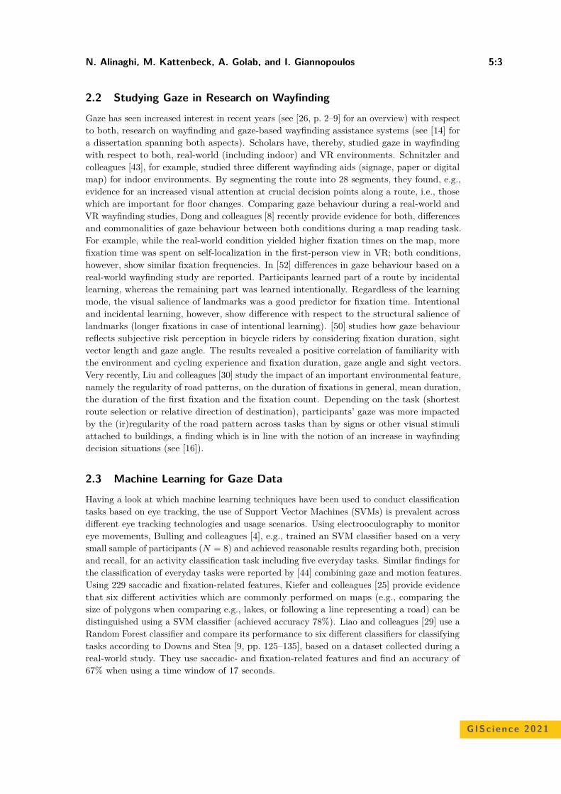
N. Alinaghi, M. Kattenbeck, A. Golab, and I. Giannopoulos 5:3

2.2 Studying Gaze in Research on Wayfinding

Gaze has seen increased interest in recent years (see [26, p. 2–9] for an overview) with respectto both, research on wayfinding and gaze-based wayfinding assistance systems (see [14] fora dissertation spanning both aspects). Scholars have, thereby, studied gaze in wayfindingwith respect to both, real-world (including indoor) and VR environments. Schnitzler andcolleagues [43], for example, studied three different wayfinding aids (signage, paper or digitalmap) for indoor environments. By segmenting the route into 28 segments, they found, e.g.,evidence for an increased visual attention at crucial decision points along a route, i.e., thosewhich are important for floor changes. Comparing gaze behaviour during a real-world andVR wayfinding studies, Dong and colleagues [8] recently provide evidence for both, differencesand commonalities of gaze behaviour between both conditions during a map reading task.For example, while the real-world condition yielded higher fixation times on the map, morefixation time was spent on self-localization in the first-person view in VR; both conditions,however, show similar fixation frequencies. In [52] differences in gaze behaviour based on areal-world wayfinding study are reported. Participants learned part of a route by incidentallearning, whereas the remaining part was learned intentionally. Regardless of the learningmode, the visual salience of landmarks was a good predictor for fixation time. Intentionaland incidental learning, however, show difference with respect to the structural salience oflandmarks (longer fixations in case of intentional learning). [50] studies how gaze behaviourreflects subjective risk perception in bicycle riders by considering fixation duration, sightvector length and gaze angle. The results revealed a positive correlation of familiarity withthe environment and cycling experience and fixation duration, gaze angle and sight vectors.Very recently, Liu and colleagues [30] study the impact of an important environmental feature,namely the regularity of road patterns, on the duration of fixations in general, mean duration,the duration of the first fixation and the fixation count. Depending on the task (shortestroute selection or relative direction of destination), participants’ gaze was more impactedby the (ir)regularity of the road pattern across tasks than by signs or other visual stimuliattached to buildings, a finding which is in line with the notion of an increase in wayfindingdecision situations (see [16]).

2.3 Machine Learning for Gaze Data

Having a look at which machine learning techniques have been used to conduct classificationtasks based on eye tracking, the use of Support Vector Machines (SVMs) is prevalent acrossdifferent eye tracking technologies and usage scenarios. Using electrooculography to monitoreye movements, Bulling and colleagues [4], e.g., trained an SVM classifier based on a verysmall sample of participants (N = 8) and achieved reasonable results regarding both, precisionand recall, for an activity classification task including five everyday tasks. Similar findings forthe classification of everyday tasks were reported by [44] combining gaze and motion features.Using 229 saccadic and fixation-related features, Kiefer and colleagues [25] provide evidencethat six different activities which are commonly performed on maps (e.g., comparing thesize of polygons when comparing e.g., lakes, or following a line representing a road) can bedistinguished using a SVM classifier (achieved accuracy 78%). Liao and colleagues [29] use aRandom Forest classifier and compare its performance to six different classifiers for classifyingtasks according to Downs and Stea [9, pp. 125–135], based on a dataset collected during areal-world study. They use saccadic- and fixation-related features and find an accuracy of67% when using a time window of 17 seconds.

GISc ience 2021

5:4 Will You Take This Turn?

Based on this evidence we conclude, first, to use features which are hand-crafted from eyemovements like all of the aforementioned studies do and deliberately choose not to use deeplearning methods. Second, regarding the reports on SVM and Random Forest algorithms inearlier studies, as well as our own pilot-test findings (see Section 4.2), we base our machinelearning experiments on tree-based techniques. Using these approaches is also in line withother machine learning literature which suggests that algorithms which split the feature spaceare considered among the best models when it comes to small-to-medium sized structured ortabular data [48].

3 Data Collection, Pre-processing and Feature Extraction

Based on our goal of turning activity recognition, this section provides information on datacollection and all data pre-processing steps, including the extraction of gaze features. We startwith a short description of the human-subject in-situ study as we use a dataset which wascollected in order to address several research problems, next to the turn activity recognition.We, then, move on to explain the synchronization of the different sensory data used. Finally,we provide details on the segmentation of the gaze data and the extraction of saccade- andfixation-related features.

3.1 Data CollectionThe data used in this paper is part of a larger data collection effort 1 addressing human spatialbehavior in real-world wayfinding scenarios2. This goal renders it also a valuable sourcefor answering other questions regarding decision-making in navigation. The data collection,which took place in 2020, required participants to walk two routes (length ranging from 0.9km

to 1.3km), one of which was located in an area they were familiar3 with, whereas they wereunfamiliar with the other. They had to find their way by means of auditory, landmark-based4,turn-by-turn route instructions, which were provided to them on demand and as many timesas they requested. We tracked participant’s behaviour using a mobile eye-tracking device(PupilLabs Invisible) recording gaze positions at 200Hz and a high precision GNSS receiver(PPM 10-xx38) tracking their position in time. In total, N = 52 people (27 female and 25males, M(age) = 26 years, SD(age) = 8.3) participated in the outdoor experiments resultingin N = 104 trials out of which N = 86 were contained for further processing5.

3.2 Data Pre-processingTo obtain the gaze-related data at each decision-point, several steps had to be taken. First,junctions had to be matched to the GPS tracks obtained in order to be able to align eye-tracking and GPS data. Subsequently, the point in time when a junction can be perceived asjunction had to be approximated.

1 This experiment has been described for the first time in [19] and here we only present the parts we usedin our analysis.

2 The data used in this paper, will be made available at https://geo.geoinfo.tuwien.ac.at/resources/(DOI: 10.5281/zenodo.4298703).

3 During an online study participants indicated areas and places therein, with which they are familiarand provided a route connecting two of these places.

4 Points of Interest were used as landmarks and chosen according to the algorithm described in [40].5 Trials had to be excluded, for example due to equipment malfunction or non-cooperative participant

behaviour.

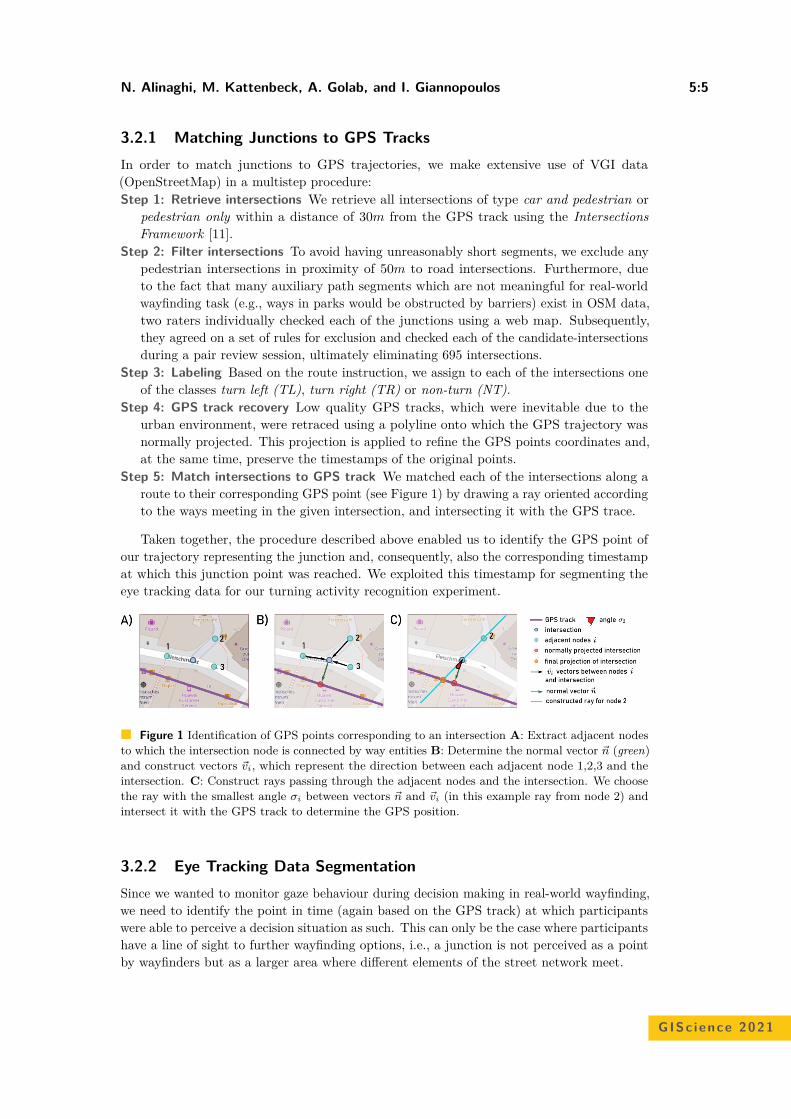
N. Alinaghi, M. Kattenbeck, A. Golab, and I. Giannopoulos 5:5

3.2.1 Matching Junctions to GPS TracksIn order to match junctions to GPS trajectories, we make extensive use of VGI data(OpenStreetMap) in a multistep procedure:Step 1: Retrieve intersections We retrieve all intersections of type car and pedestrian or

pedestrian only within a distance of 30m from the GPS track using the IntersectionsFramework [11].

Step 2: Filter intersections To avoid having unreasonably short segments, we exclude anypedestrian intersections in proximity of 50m to road intersections. Furthermore, dueto the fact that many auxiliary path segments which are not meaningful for real-worldwayfinding task (e.g., ways in parks would be obstructed by barriers) exist in OSM data,two raters individually checked each of the junctions using a web map. Subsequently,they agreed on a set of rules for exclusion and checked each of the candidate-intersectionsduring a pair review session, ultimately eliminating 695 intersections.

Step 3: Labeling Based on the route instruction, we assign to each of the intersections oneof the classes turn left (TL), turn right (TR) or non-turn (NT).

Step 4: GPS track recovery Low quality GPS tracks, which were inevitable due to theurban environment, were retraced using a polyline onto which the GPS trajectory wasnormally projected. This projection is applied to refine the GPS points coordinates and,at the same time, preserve the timestamps of the original points.

Step 5: Match intersections to GPS track We matched each of the intersections along aroute to their corresponding GPS point (see Figure 1) by drawing a ray oriented accordingto the ways meeting in the given intersection, and intersecting it with the GPS trace.

Taken together, the procedure described above enabled us to identify the GPS point ofour trajectory representing the junction and, consequently, also the corresponding timestampat which this junction point was reached. We exploited this timestamp for segmenting theeye tracking data for our turning activity recognition experiment.

Figure 1 Identification of GPS points corresponding to an intersection A: Extract adjacent nodesto which the intersection node is connected by way entities B: Determine the normal vector n (green)and construct vectors vi, which represent the direction between each adjacent node 1,2,3 and theintersection. C: Construct rays passing through the adjacent nodes and the intersection. We choosethe ray with the smallest angle σi between vectors n and vi (in this example ray from node 2) andintersect it with the GPS track to determine the GPS position.

3.2.2 Eye Tracking Data SegmentationSince we wanted to monitor gaze behaviour during decision making in real-world wayfinding,we need to identify the point in time (again based on the GPS track) at which participantswere able to perceive a decision situation as such. This can only be the case where participantshave a line of sight to further wayfinding options, i.e., a junction is not perceived as a pointby wayfinders but as a larger area where different elements of the street network meet.

GISc ience 2021

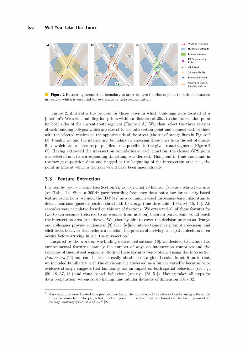
5:6 Will You Take This Turn?

Figure 2 Extracting intersection boundary in order to have the closest point to decision-situationin reality, which is essential for eye tracking data segmentation.

Figure 2, illustrates the process for those cases in which buildings were located at ajunction6: We select building footprints within a distance of 20m to the intersection pointfor both sides of the current route segment (Figure 2 A). We, then, select the three verticesof each building polygon which are closest to the intersection point and connect each of thesewith the selected vertices on the opposite side of the street (the set of orange lines in Figure 2B). Finally, we find the intersection boundary by choosing those lines from the set of orangelines which are oriented as perpendicular as possible to the given route segment (Figure 2C). Having extracted the intersection boundaries at each junction, the closest GPS pointwas selected and its corresponding timestamp was derived. This point in time was found inthe raw gaze-position data and flagged as the beginning of the intersection area, i.e., thepoint in time at which a decision would have been made already.

3.3 Feature ExtractionInspired by prior evidence (see Section 2), we extracted 28 fixation-/saccade-related features(see Table 1). Since a 200Hz gaze-recording frequency does not allow for velocity-basedfeature extractions, we used the IDT [42] as a commonly-used dispersion-based algorithm todetect fixations (gaze-dispersion threshold: 0.02 deg; time threshold: 100 ms) [15, 14]. Allsaccades were calculated based on this set of fixations. We extracted all of these features fortwo to ten seconds (referred to as window from now on) before a participant would reachthe intersection area (see above). We, thereby, aim to cover the decision process as Brunyeand colleagues provide evidence in [3] that ‘[w]hile intersections may prompt a decision, andelicit overt behavior that reflects a decision, the process of arriving at a spatial decision oftenoccurs before arriving in [sic] the intersection.’

Inspired by the work on wayfinding decision situations [16], we decided to include twoenvironmental features: namely the number of ways an intersection comprises and theskewness of these street segments. Both of these features were obtained using the IntersectionFramework [11] and can, hence, be easily obtained on a global scale. In addition to that,we included familiarity with the environment traversed as a binary variable because priorevidence strongly suggests that familiarity has an impact on both spatial behaviour (see e.g.,[50, 18, 37, 13]) and visual search behaviour (see e.g., [23, 51]). Having taken all steps fordata preparation, we ended up having nine tabular datasets of dimension 804 ∗ 32.

6 If no buildings were located at a junction, we found the boundary of the intersection by using a thresholdof 3.75seconds from the projected junction point. This resembles 5m based on the assumption of anaverage walking speed of 4.5km/h [27].

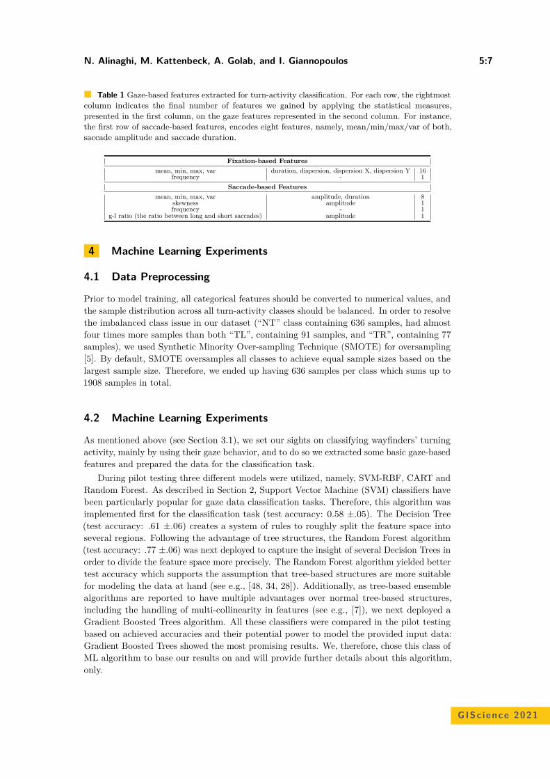
N. Alinaghi, M. Kattenbeck, A. Golab, and I. Giannopoulos 5:7

Table 1 Gaze-based features extracted for turn-activity classification. For each row, the rightmostcolumn indicates the final number of features we gained by applying the statistical measures,presented in the first column, on the gaze features represented in the second column. For instance,the first row of saccade-based features, encodes eight features, namely, mean/min/max/var of both,saccade amplitude and saccade duration.

Fixation-based Featuresmean, min, max, var duration, dispersion, dispersion X, dispersion Y 16

frequency - 1Saccade-based Features

mean, min, max, var amplitude, duration 8skewness amplitude 1frequency - 1

g-l ratio (the ratio between long and short saccades) amplitude 1

4 Machine Learning Experiments

4.1 Data Preprocessing

Prior to model training, all categorical features should be converted to numerical values, andthe sample distribution across all turn-activity classes should be balanced. In order to resolvethe imbalanced class issue in our dataset (“NT” class containing 636 samples, had almostfour times more samples than both “TL”, containing 91 samples, and “TR”, containing 77samples), we used Synthetic Minority Over-sampling Technique (SMOTE) for oversampling[5]. By default, SMOTE oversamples all classes to achieve equal sample sizes based on thelargest sample size. Therefore, we ended up having 636 samples per class which sums up to1908 samples in total.

4.2 Machine Learning Experiments

As mentioned above (see Section 3.1), we set our sights on classifying wayfinders’ turningactivity, mainly by using their gaze behavior, and to do so we extracted some basic gaze-basedfeatures and prepared the data for the classification task.

During pilot testing three different models were utilized, namely, SVM-RBF, CART andRandom Forest. As described in Section 2, Support Vector Machine (SVM) classifiers havebeen particularly popular for gaze data classification tasks. Therefore, this algorithm wasimplemented first for the classification task (test accuracy: 0.58 ±.05). The Decision Tree(test accuracy: .61 ±.06) creates a system of rules to roughly split the feature space intoseveral regions. Following the advantage of tree structures, the Random Forest algorithm(test accuracy: .77 ±.06) was next deployed to capture the insight of several Decision Trees inorder to divide the feature space more precisely. The Random Forest algorithm yielded bettertest accuracy which supports the assumption that tree-based structures are more suitablefor modeling the data at hand (see e.g., [48, 34, 28]). Additionally, as tree-based ensemblealgorithms are reported to have multiple advantages over normal tree-based structures,including the handling of multi-collinearity in features (see e.g., [7]), we next deployed aGradient Boosted Trees algorithm. All these classifiers were compared in the pilot testingbased on achieved accuracies and their potential power to model the provided input data:Gradient Boosted Trees showed the most promising results. We, therefore, chose this class ofML algorithm to base our results on and will provide further details about this algorithm,only.

GISc ience 2021

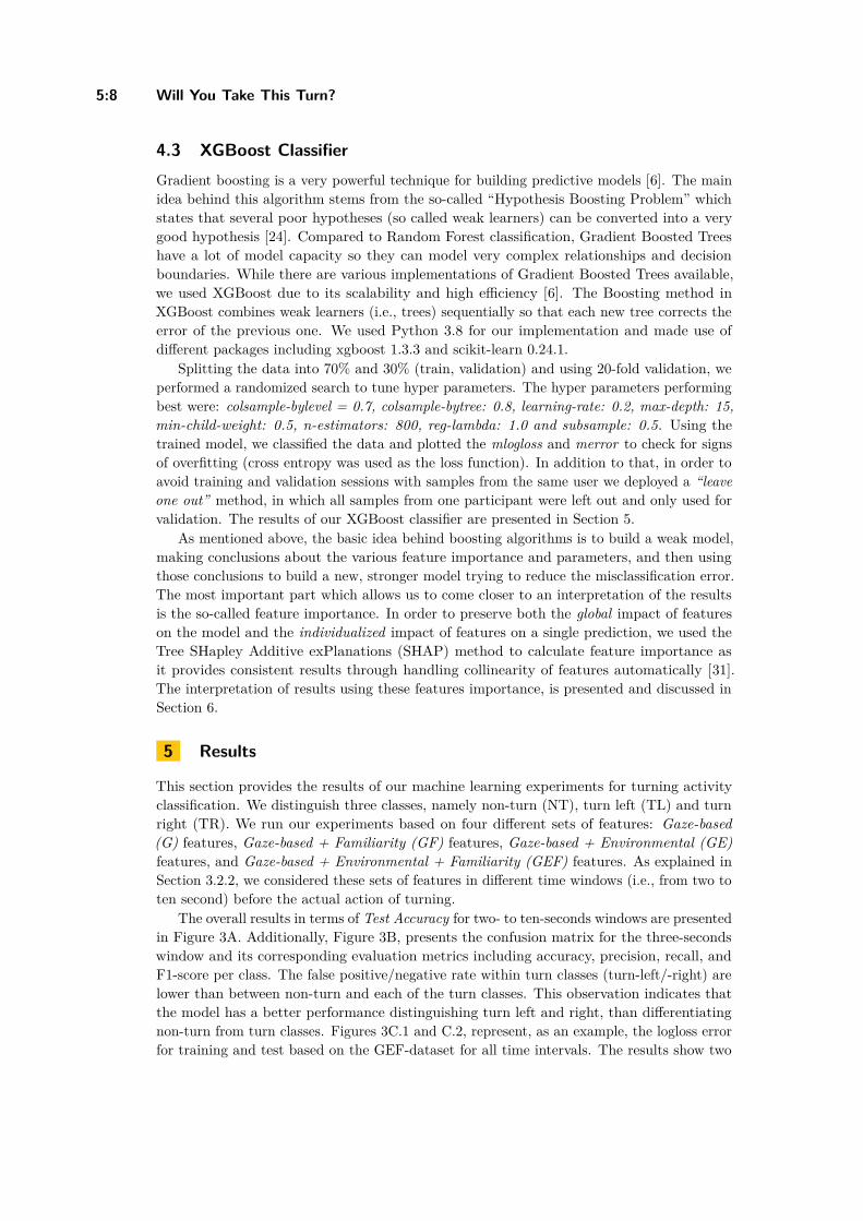
5:8 Will You Take This Turn?

4.3 XGBoost ClassifierGradient boosting is a very powerful technique for building predictive models [6]. The mainidea behind this algorithm stems from the so-called “Hypothesis Boosting Problem” whichstates that several poor hypotheses (so called weak learners) can be converted into a verygood hypothesis [24]. Compared to Random Forest classification, Gradient Boosted Treeshave a lot of model capacity so they can model very complex relationships and decisionboundaries. While there are various implementations of Gradient Boosted Trees available,we used XGBoost due to its scalability and high efficiency [6]. The Boosting method inXGBoost combines weak learners (i.e., trees) sequentially so that each new tree corrects theerror of the previous one. We used Python 3.8 for our implementation and made use ofdifferent packages including xgboost 1.3.3 and scikit-learn 0.24.1.

Splitting the data into 70% and 30% (train, validation) and using 20-fold validation, weperformed a randomized search to tune hyper parameters. The hyper parameters performingbest were: colsample-bylevel = 0.7, colsample-bytree: 0.8, learning-rate: 0.2, max-depth: 15,min-child-weight: 0.5, n-estimators: 800, reg-lambda: 1.0 and subsample: 0.5. Using thetrained model, we classified the data and plotted the mlogloss and merror to check for signsof overfitting (cross entropy was used as the loss function). In addition to that, in order toavoid training and validation sessions with samples from the same user we deployed a “leaveone out” method, in which all samples from one participant were left out and only used forvalidation. The results of our XGBoost classifier are presented in Section 5.

As mentioned above, the basic idea behind boosting algorithms is to build a weak model,making conclusions about the various feature importance and parameters, and then usingthose conclusions to build a new, stronger model trying to reduce the misclassification error.The most important part which allows us to come closer to an interpretation of the resultsis the so-called feature importance. In order to preserve both the global impact of featureson the model and the individualized impact of features on a single prediction, we used theTree SHapley Additive exPlanations (SHAP) method to calculate feature importance asit provides consistent results through handling collinearity of features automatically [31].The interpretation of results using these features importance, is presented and discussed inSection 6.

5 Results

This section provides the results of our machine learning experiments for turning activityclassification. We distinguish three classes, namely non-turn (NT), turn left (TL) and turnright (TR). We run our experiments based on four different sets of features: Gaze-based(G) features, Gaze-based + Familiarity (GF) features, Gaze-based + Environmental (GE)features, and Gaze-based + Environmental + Familiarity (GEF) features. As explained inSection 3.2.2, we considered these sets of features in different time windows (i.e., from two toten second) before the actual action of turning.

The overall results in terms of Test Accuracy for two- to ten-seconds windows are presentedin Figure 3A. Additionally, Figure 3B, presents the confusion matrix for the three-secondswindow and its corresponding evaluation metrics including accuracy, precision, recall, andF1-score per class. The false positive/negative rate within turn classes (turn-left/-right) arelower than between non-turn and each of the turn classes. This observation indicates thatthe model has a better performance distinguishing turn left and right, than differentiatingnon-turn from turn classes. Figures 3C.1 and C.2, represent, as an example, the logloss errorfor training and test based on the GEF-dataset for all time intervals. The results show two

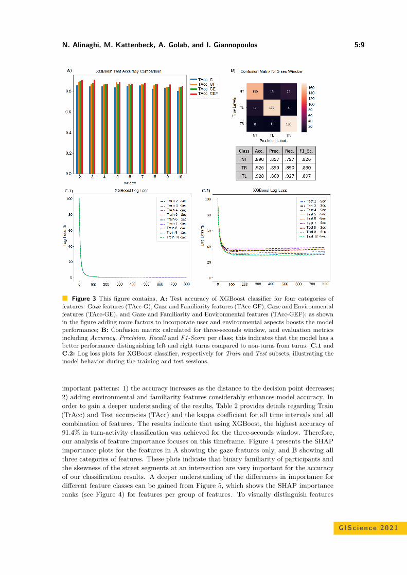
N. Alinaghi, M. Kattenbeck, A. Golab, and I. Giannopoulos 5:9

Figure 3 This figure contains, A: Test accuracy of XGBoost classifier for four categories offeatures: Gaze features (TAcc-G), Gaze and Familiarity features (TAcc-GF), Gaze and Environmentalfeatures (TAcc-GE), and Gaze and Familiarity and Environmental features (TAcc-GEF); as shownin the figure adding more factors to incorporate user and environmental aspects boosts the modelperformance; B: Confusion matrix calculated for three-seconds window, and evaluation metricsincluding Accuracy, Precision, Recall and F1-Score per class; this indicates that the model has abetter performance distinguishing left and right turns compared to non-turns from turns. C.1 andC.2: Log loss plots for XGBoost classifier, respectively for Train and Test subsets, illustrating themodel behavior during the training and test sessions.

important patterns: 1) the accuracy increases as the distance to the decision point decreases;2) adding environmental and familiarity features considerably enhances model accuracy. Inorder to gain a deeper understanding of the results, Table 2 provides details regarding Train(TrAcc) and Test accuracies (TAcc) and the kappa coefficient for all time intervals and allcombination of features. The results indicate that using XGBoost, the highest accuracy of91.4% in turn-activity classification was achieved for the three-seconds window. Therefore,our analysis of feature importance focuses on this timeframe. Figure 4 presents the SHAPimportance plots for the features in A showing the gaze features only, and B showing allthree categories of features. These plots indicate that binary familiarity of participants andthe skewness of the street segments at an intersection are very important for the accuracyof our classification results. A deeper understanding of the differences in importance fordifferent feature classes can be gained from Figure 5, which shows the SHAP importanceranks (see Figure 4) for features per group of features. To visually distinguish features

GISc ience 2021

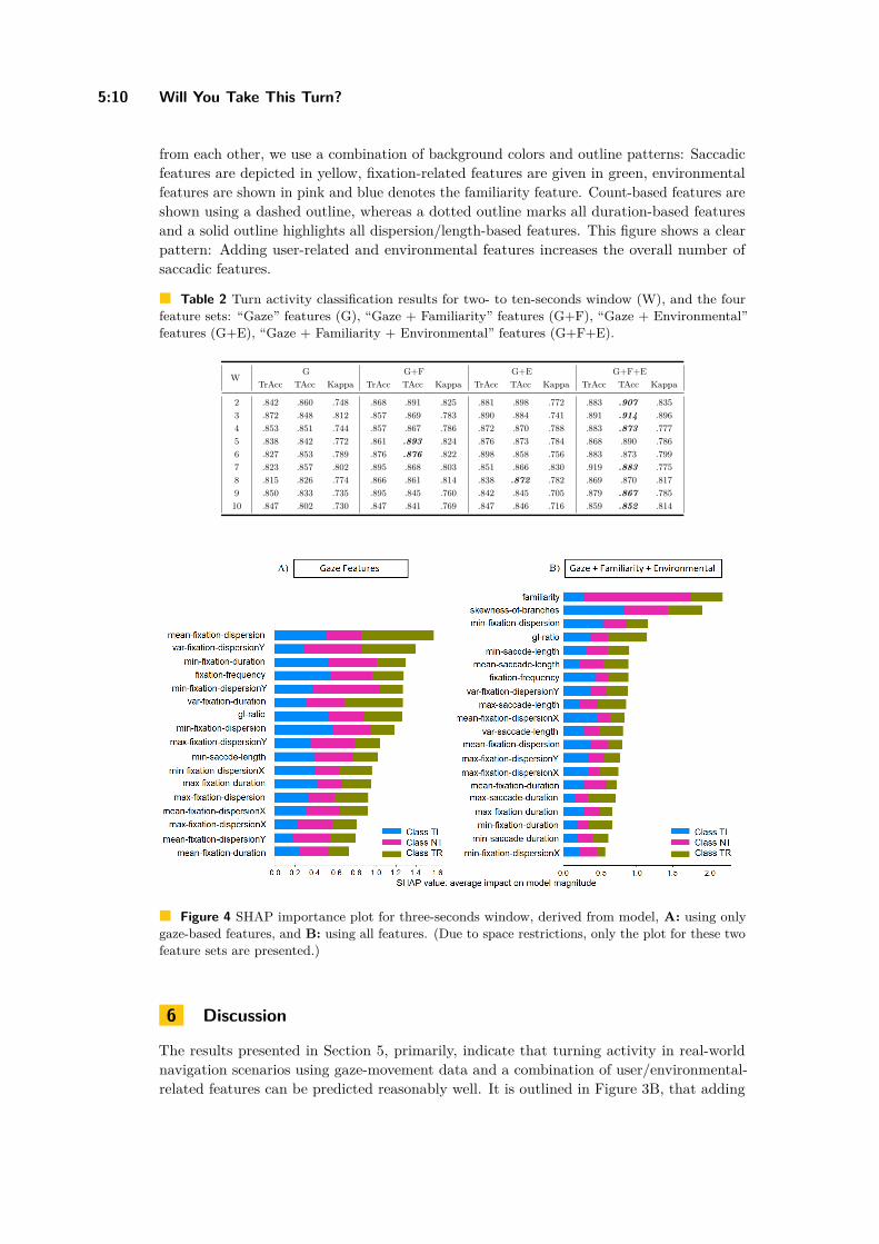
5:10 Will You Take This Turn?

from each other, we use a combination of background colors and outline patterns: Saccadicfeatures are depicted in yellow, fixation-related features are given in green, environmentalfeatures are shown in pink and blue denotes the familiarity feature. Count-based features areshown using a dashed outline, whereas a dotted outline marks all duration-based featuresand a solid outline highlights all dispersion/length-based features. This figure shows a clearpattern: Adding user-related and environmental features increases the overall number ofsaccadic features.

Table 2 Turn activity classification results for two- to ten-seconds window (W), and the fourfeature sets: “Gaze” features (G), “Gaze + Familiarity” features (G+F), “Gaze + Environmental”features (G+E), “Gaze + Familiarity + Environmental” features (G+F+E).

W G G+F G+E G+F+ETrAcc TAcc Kappa TrAcc TAcc Kappa TrAcc TAcc Kappa TrAcc TAcc Kappa

2 .842 .860 .748 .868 .891 .825 .881 .898 .772 .883 .907 .8353 .872 .848 .812 .857 .869 .783 .890 .884 .741 .891 .914 .8964 .853 .851 .744 .857 .867 .786 .872 .870 .788 .883 .873 .7775 .838 .842 .772 .861 .893 .824 .876 .873 .784 .868 .890 .7866 .827 .853 .789 .876 .876 .822 .898 .858 .756 .883 .873 .7997 .823 .857 .802 .895 .868 .803 .851 .866 .830 .919 .883 .7758 .815 .826 .774 .866 .861 .814 .838 .872 .782 .869 .870 .8179 .850 .833 .735 .895 .845 .760 .842 .845 .705 .879 .867 .78510 .847 .802 .730 .847 .841 .769 .847 .846 .716 .859 .852 .814

Figure 4 SHAP importance plot for three-seconds window, derived from model, A: using onlygaze-based features, and B: using all features. (Due to space restrictions, only the plot for these twofeature sets are presented.)

6 Discussion

The results presented in Section 5, primarily, indicate that turning activity in real-worldnavigation scenarios using gaze-movement data and a combination of user/environmental-related features can be predicted reasonably well. It is outlined in Figure 3B, that adding

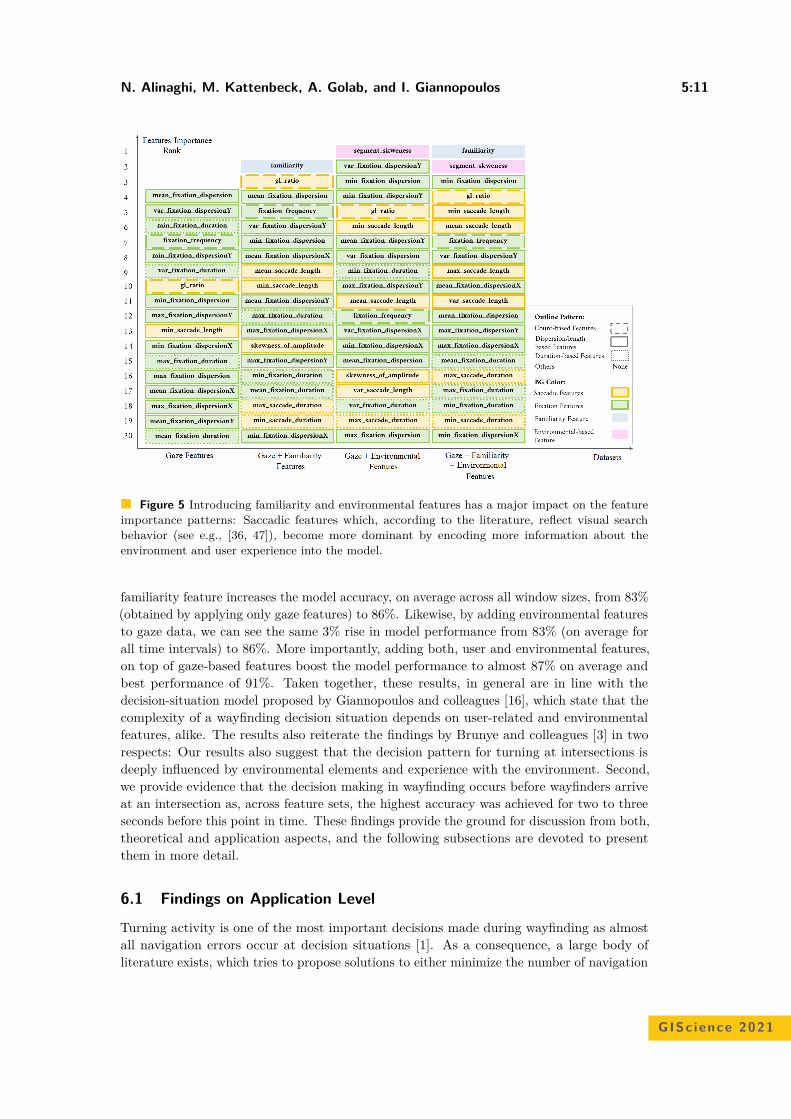
N. Alinaghi, M. Kattenbeck, A. Golab, and I. Giannopoulos 5:11

Figure 5 Introducing familiarity and environmental features has a major impact on the featureimportance patterns: Saccadic features which, according to the literature, reflect visual searchbehavior (see e.g., [36, 47]), become more dominant by encoding more information about theenvironment and user experience into the model.

familiarity feature increases the model accuracy, on average across all window sizes, from 83%(obtained by applying only gaze features) to 86%. Likewise, by adding environmental featuresto gaze data, we can see the same 3% rise in model performance from 83% (on average forall time intervals) to 86%. More importantly, adding both, user and environmental features,on top of gaze-based features boost the model performance to almost 87% on average andbest performance of 91%. Taken together, these results, in general are in line with thedecision-situation model proposed by Giannopoulos and colleagues [16], which state that thecomplexity of a wayfinding decision situation depends on user-related and environmentalfeatures, alike. The results also reiterate the findings by Brunye and colleagues [3] in tworespects: Our results also suggest that the decision pattern for turning at intersections isdeeply influenced by environmental elements and experience with the environment. Second,we provide evidence that the decision making in wayfinding occurs before wayfinders arriveat an intersection as, across feature sets, the highest accuracy was achieved for two to threeseconds before this point in time. These findings provide the ground for discussion from both,theoretical and application aspects, and the following subsections are devoted to presentthem in more detail.

6.1 Findings on Application Level

Turning activity is one of the most important decisions made during wayfinding as almostall navigation errors occur at decision situations [1]. As a consequence, a large body ofliterature exists, which tries to propose solutions to either minimize the number of navigation

GISc ience 2021

5:12 Will You Take This Turn?

errors a wayfinder makes (e.g. [41]), or to minimize the impact of these errors by, forexample, precalculating all possible routes close to the shortest path from the upcomingjunctions [1]. A system which is capable to detect potential navigation errors would be ableto pro-actively draw the wayfinders attention to this potential error and, thereby, help toavoid a wrong decision. Moreover, it has been long on debate that one of the potentialdrawbacks of wayfinding assistance systems, is their negative impact on humans spatialcognition and abilities (in long term) by constantly distracting users attention from theenvironment (see e.g. [2],[29], [39]). This detrimental effect is caused by either the need ofconstant visual interaction with the system, or by providing a more than necessary amountof information to the user. It has been suggested that gaze-based interactions in general canhelp limiting this distraction [15]. While researchers have sought for solutions to reduce thenumber of wayfinding instructions for years (e.g., [12]), our results allow for a personalizedwayfinding assistance by monitoring gaze behavior for turning activity recognition andproviding corrective instructions only if needed [32]. As an example, in case a wayfinder issupposed to continue straight ahead but shows a tendency to take a turn, the system canprovide her/him with a corrective instruction; otherwise there is no need to distract thewayfinder by repeating the same instruction).

6.2 Findings on Theoretical LevelThe findings of this paper in terms of the role of each feature in visual search behavior duringwayfinding decision situations, can deepen our understanding of decision making in real-worldwayfinding. Considering only gaze-based features (see left column of Figure 5), we observetwo patterns: First, in total 15 out of 17 most important features are fixation-related. Onepotential explanation, which is in line with the fact that fixation-related features convey signsof attention and information processing [22], is that this dominance reflects the importanceof attention at decision point. Prior evidence (see [3, 53]), suggests already that deciding totake a turn is a dynamic decision making process consisting of stimulus processing and actionpreparation which requires an attention shift. The second pattern we observe from Figure 5,relates to the equal number and importance of duration-based and dispersion-based features(note that the number of dispersion-related features are three times more than duration-basedfeatures and the same ratio holds here): Two fixation duration based features are amongthe 50% most important features, which is in line with the known positive correlation offixation duration with cognitive processing and scene perception [21]. Inline with currentevidence (see e.g., [22, 49]), these two patterns suggest that using only gaze information, theturn-activity decision is more reflected by features which are representative for cognitiveprocessing and scene perception. Adding familiarity with the environment as a user-relatedfeature (second left column of Figure 5), boosts the performance of the model and, at thesame time, increases the number of saccadic features to six. Simultaneously, the importanceof duration-based features (both fixation and saccade-related) slightly decreases. Saccadicfeatures in general represent visual search activity rather than attention or concentration,and more specifically saccade amplitude, is known to reflect search task difficulty [36] andpresence of high-frequency visual information [47]. This result can, hence, be interpretedas changing the importance of visual search in predicting a turn-activity decision. Thiswould be in line with the fact that fixation behavior is particularly biased by familiarity orlevel of expertise [50]. Adding familiarity renders itself most important; moreover, it alsoredirects the model’s attention towards saccadic features. This finding, though, leaves muchroom for further research: Arguably, familiarity somehow encapsulates most of the fixationbehavior in itself, and lets the model seek for meaningful patterns in saccadic features. This

N. Alinaghi, M. Kattenbeck, A. Golab, and I. Giannopoulos 5:13

observation requires further assessment of familiarity in order to unfold the differences ingaze behavior of familiar vs unfamiliar wayfinders. Similar to adding user-related features,an increase in presence of visual search related features (i.e., saccadic features), occurs alsowhen adding environmental factors (third left column of Figure 5). We used skewness ofstreet segments and the number of branches an intersection has, as proxy for the difficultyof the decision situation in terms of urban configuration. Due to the collinearity of bothfeatures, only skeweness is retained by the SHAP procedure. This may be an indicator forthe fact that skewness is a better (i.e., more precise than the number of branches) proxyfor the difficulty of the decision situation, with respect to environmental configuration. Themost important pattern was revealed when we added both familiarity and environmentalfeatures (right column of Figure 5). As is shown in Figure 5, familiarity remains the mostimportant feature, which can be explained by the fact that gaze-behavior is heavily biasedby user-related factors, and particularly the level of expertise of which familiarity with theenvironment is an instance of. In addition to that, a slight increase in number and importanceof saccadic features, and moreover, a sharp drop in importance for duration-based featuresarises. This observation may indicate that environmental and user-related features encodeimportant aspects of the decision situation and, thereby, redirect the model’s focus more tovisual search behavior.

7 Conclusion and Future Work

In this paper we provide evidence that it is possible to classify the turning activity ofwayfinders based on a combination of gaze-data, wayfinder familiarity (measured as a binaryvariable) and two environmental factors regarding the morphology of an intersection. To thisend, we used data collected during an in-situ wayfinding experiment and compared differenttime windows and different classification algorithms. The highest accuracy was found for anXGBoost classifier, which achieved 91% overall accuracy in turn-activity classification for awindow size of three seconds. We discussed our findings from two main perspectives: First,we shed light on the applicational prospects with respect to wayfinding assistance systemscapable to detect potential navigation errors; second, we explored which gaze features aremost important and provided explanations based on the existing literature. Taken together,these results raise further research questions. While we have deliberately used a basic set ofgaze features combined with a single user-related and two basic environmental features, itwould be interesting to see whether more sophisticated features (e.g., incorporating differentlevels of familiarity) convey even more information regarding the decision making process.Besides, according to our findings, adding user-related and environmental factors to gazefeatures, alters the pattern of fixation-related and saccadic features, in terms of the numberand importance of each gaze-event category. It is, therefore, worthwhile to disentangle therelationship between these gaze features and the familiarity/environmental factors. Anotherinteresting pattern which needs deeper exploration, relates to count-based fixation andsaccadic features. So far, these have been used mostly as an indication of semantic importanceand search-task difficulty [21]. Therefore, a future study can introduce semantic informationof areas of interest (AOI) to the model, and observe why count-based features retain theirimportance in the model. Eventually, the differences in false positive/negative rates betweendifferent classes observed in the confusion matrix, may suggest missing environmental or usercharacteristics in the model. Therefore, a future study may for instance, incorporate head/body movements to the model to see if this behavioral source of information can lead to

GISc ience 2021

5:14 Will You Take This Turn?

better classification results. In addition to that, our findings open up several other questionsregarding the general research direction of this paper:1. When is the actual onset of the decision process for turn-activity, does this point in time

vary for different phases of wayfinding (as proposed by [9]), and is this point in timestable as travel time/distance covered increases?

2. Why are some of the features more effective with respect to predicting particular classesof turn-activity? For instance, why is familiarity more effective on predicting non-turnactivity as suggested by Figure 4?

3. Does the so-called cascade effect also hold for turn-activity recognition based on gaze-behaviour in real-world navigation?

References1 D. Amores, E. Tanin, and M. Vasardani. A proactive route planning approach to navigation

errors. Int J of Geographical Information Science, pages 1–37, 2020.2 A. Brügger, K. Richter, and S. Fabrikant. How does navigation system behavior influence

human behavior? Cognitive Research: Principles and Implications, 4(1):5, December 2019.3 T. T. Brunyé, A. L. Gardony, A. Holmes, and H. A. Taylor. Spatial decision dynamics during

wayfinding: intersections prompt the decision-making process. Cognitive Research: Principlesand Implications, 3(1), 2018.

4 A. Bulling, J. A. Ward, H. Gellersen, and G. Tröster. Eye movement analysis for activityrecognition using electrooculography. IEEE Transactions on Pattern Analysis and MachineIntelligence, 33(4):741–753, 2011.

5 N. V Chawla, K. W Bowyer, L. O Hall, and W P. Kegelmeyer. Smote: synthetic minorityover-sampling technique. J of artificial intelligence research, 16:321–357, 2002.

6 T. Chen, T. He, M. Benesty, V. Khotilovich, Y. Tang, H. Cho, et al. Xgboost: extremegradient boosting. R package version 0.4-2, 1(4), 2015.

7 T. G Dietterich. Ensemble methods in machine learning. In International workshop on multipleclassifier systems, pages 1–15. Springer, 2000.

8 W. Dong, H. Liao, B. Liu, Z. Zhan, H. Liu, L. Meng, and Y. Liu. Comparing pedestrians’gaze behavior in desktop and in real Envs. Cartography and Geographic Information Science,47(5):432–451, 2020.

9 R. Downs and D. Stea. The world in the head Maps in minds: Reflections on cognitive mapping.Harper & Row, 1977.

10 M. K. Eckstein, B. Guerra-Carrillo, A. T. Miller Singley, and S. A. Bunge. Beyond eye gaze:What else can eyetracking reveal about cognition and cognitive development? DevelopmentalCognitive Neuroscience, 25:69–91, 2017.

11 P. Fogliaroni, D. Bucher, Nikola J., and I. Giannopoulos. Intersections of our world. In 10thInt Conf on Geographic Information Science, 2018.

12 A. U. Frank. Pragmatic information content—how to measure the information in a route.Foundations of geographic information science, page 47, 2003.

13 N. Gale, R. G. Golledge, W. C. Halperin, and H. Couclelis. Exploring spatial familiarity.Professional Geographer, 42(3):299–313, 1990.

14 I. Giannopoulos. Supporting Wayfinding Through Mobile Gaze-Based Interaction. PhDthesis, ETH Zurich, 2016. URL: https://www.research-collection.ethz.ch/handle/20.500.11850/116375.

15 I. Giannopoulos, P. Kiefer, and M. Raubal. Gazenav: gaze-based pedestrian navigation. InProc of MobileHCI 2015, pages 337–346, 2015.

16 I. Giannopoulos, P. Kiefer, M. Raubal, K. Richter, and T. Thrash. Wayfinding DecisionSituations: A Conceptual Model and Evaluation. In Proc of GIScience 2014, 2014.

N. Alinaghi, M. Kattenbeck, A. Golab, and I. Giannopoulos 5:15

17 K. Gidlöf, A. Wallin, R. Dewhurst, and K. Holmqvist. Using eye tracking to trace a cognitiveprocess: Gaze behaviour during decision making in a natural Env. J of Eye MovementResearch, 6(1):1–14, 2013.

18 L. Gokl, M. Mc Cutchan, B. Mazurkiewicz, P. Fogliaroni, and I. Giannopoulos. TowardsUrban Env Familiarity Prediction. Advances in Cartography and GIScience of the ICA,2(November):1–8, 2019.

19 A. Golab, M. Kattenbeck, G. Sarlas, and G. Giannopoulos. It’s also about timing! when dopedestrians want to receive navigation instructions. SPAT COGN COMPUT, 2021. acceptedfor publication.

20 E. H Hess and J. M. Polt. Pupil size as related to interest value of visual stimuli. Science,132(3423):349–350, 1960.

21 K. Holmqvist, M. Nyström, R. Andersson, R. Dewhurst, H. Jarodzka, and J. Van de Weijer.Eye tracking: A comprehensive guide to methods and measures. OUP Oxford, 2011.

22 M. Adam Just and Patricia A. C. Eye fixations and cognitive processes. Cognitive psychology,8(4):441–480, 1976.

23 A. Kafkas and D. Montaldi. Familiarity and recollection produce distinct eye movement, pupiland medial temporal lobe responses when memory strength is matched. Neuropsychologia,50(13):3080–3093, 2012.

24 M. Kearns. Thoughts on hypothesis boosting. Unpublished manuscript, 45:105, 1988.25 P. Kiefer, I. Giannopoulos, and M. Raubal. Using eye movements to recognize activities on

cartographic maps. Proc of SIGSPATIAL 2013, pages 478–481, 2013.26 P. Kiefer, I. Giannopoulos, M. Raubal, and A. Duchowski. Eye tracking for spatial research:

Cognition, computation, challenges. SPAT COGN COMPUT, 17(1-2):1–19, 2017.27 R. V Levine and A. Norenzayan. The pace of life in 31 countries. J of cross-cultural psychology,

30(2):178–205, 1999.28 B. Li, L. Peng, and B. Ramadass. Accurate and efficient processor performance prediction via

regression tree based modeling. Journal of Systems Architecture, 55(10-12):457–467, 2009.29 H. Liao, W. Dong, H. Huang, G. Gartner, and H. Liu. Inferring user tasks in pedestrian

navigation from eye movement data in real-world Envs. IJGIS, 33(4):739–763, April 2019.30 B. Liu, W. Dong, Z. Zhan, S. Wang, and L. Meng. Differences in the gaze behaviours

of pedestrians navigating between regular and irregular road patterns. ISPRS Int J ofGeo-Information, 9(1), 2020.

31 S. Lundberg and S. Lee. A unified approach to interpreting model predictions. Proc. of NIPS2017, page 4768–4777, 2017.

32 B Mazurkiewicz, M. Kattenbeck, and I Giannopoulos. Navigating your way! increasing thefreedom of choice during wayfinding. In 11th International Conference on Geographic Inform-ation Science (GIScience 2021) - Part II. Schloss Dagstuhl–Leibniz-Zentrum für Informatik,2021.

33 N. Venkata Kartheek Medathati, R. Desai, and J. Hillis. Towards inferring cognitive statechanges from pupil size variations in real world conditions. In Proc of ETRA 2020, 2020.

34 I Nitze, U Schulthess, and H Asche. Comparison of machine learning algorithms random forest,artificial neural network and support vector machine to maximum likelihood for supervisedcrop type classification. Proc. of the 4th GEOBIA, 35, 2012.

35 J. L. Orquin and S. Mueller Loose. Attention and choice: A review on eye movements indecision making. Acta Psychologica, 144(1):190–206, 2013.

36 M. H Phillips and J. A Edelman. The dependence of visual scanning performance on saccade,fixation, and perceptual metrics. Vision research, 48(7):926–936, 2008.

37 L Piccardi, M Risetti, and R Nori. Familiarity and Enval Representations of a City: ASelf-Report Study. Psychological Reports, 109(1):309–326, August 2011.

38 R. Pieters and L. Warlop. Visual attention during brand choice: The impact of time pressureand task motivation. Int J of Research in Marketing, 16(1):1–16, 1999.

GISc ience 2021

5:16 Will You Take This Turn?

39 C. A. Rothkopf, D. H. Ballard, and M. M. Hayhoe. Task and context determine where youlook. J of Vision, 7(14):1–20, 2007.

40 A. Rousell and A. Zipf. Towards a landmark-based pedestrian navigation service using OSMdata. ISPRS Int J of Geo-Information, 6(3), 2017.

41 R. A. Ruddle, E. Volkova, B. Mohler, and H. H. Bülthoff. The effect of landmark andbody-based sensory information on route knowledge. Memory & cognition, 39(4):686–699,2011.

42 D. D. Salvucci and J. H. Goldberg. Identifying fixations and saccades in eye-tracking protocols.In Proc of ETRA 2000, page 71–78, 2000.

43 V. Schnitzler, I. Giannopoulos, C. Hölscher, and I. Barisic. The interplay of pedestriannavigation, wayfinding devices, and Enval features in indoor settings. In Proc of ETRA 2016,pages 85–93, 2016.

44 Y. Shiga, T. Toyama, Y. Utsumi, K. Kise, and A. Dengel. Daily activity recognition combininggaze motion and visual features. Adjunct Proc of UbiComp 2014, pages 1103–1111, 2014.

45 S. Shimojo, C. Simion, E. Shimojo, and C. Scheier. Gaze bias both reflects and influencespreference. Nature Neuroscience, 6(12):1317–1322, 2003.

46 N. Stewart, F. Hermens, and W. J. Matthews. Eye Movements in Risky Choice. J of BehavioralDecision Making, 29(2-3):116–136, 2016.

47 B. W Tatler, R. J Baddeley, and B. T Vincent. The long and the short of it: Spatial statisticsat fixation vary with saccade amplitude and task. Vision research, 46(12):1857–1862, 2006.

48 J. Treboux, D. Genoud, and R. Ingold. Decision tree ensemble vs. nn deep learning: efficiencycomparison for a small image dataset. In Proc. of the IWBIS 2018, pages 25–30, 2018.

49 P Unema. Differences in eye movements and mental work-load between experienced andinexperienced motor vehicle drivers. Visual search, pages 193–202, 1990.

50 R. von Stülpnagel. Gaze behavior during urban cycling: Effects of subjective risk perceptionand vista space properties. Transportation Research Part F: Traffic Psychology and Behaviour,75:222–238, 2020.

51 Q. Wang, P. Cavanagh, and M. Green. Familiarity and pop-out in visual search. Perception &Psychophysics, 56(5):495–500, September 1994.

52 F. Wenczel, L. Hepperle, and R. von Stülpnagel. Gaze behavior during incidental andintentional navigation in an outdoor Env. SPAT COGN COMPUT, 17(1-2):121–142, 2017.

53 J. M. Wiener, O. de Condappa, and C. Hölscher. Do you have to look where you go? Gazebehaviour during spatial decision making. Proc of CogSci 2011, pages 1583–1588, 2011.

54 J. M. Wiener, C. Hölscher, S. Büchner, and L. Konieczny. Gaze behaviour during spaceperception and spatial decision making. Psychological Research, 76(6):713–729, 2012.

55 A. L Yarbus. Eye movements and vision. New York: Plenum Press, 1967.

Bicriteria Aggregation of Polygons via Graph CutsPeter Rottmann #

Institute of Geodesy and Geoinformation, University of Bonn, Germany

Anne Driemel #

Hausdorff Center for Mathematics, University of Bonn, Germany

Herman Haverkort #

Institute of Computer Science, University of Bonn, Germany

Heiko Röglin #

Institute of Computer Science, University of Bonn, Germany

Jan-Henrik Haunert #

Institute of Geodesy and Geoinformation, University of Bonn, Germany

AbstractWe present a new method for the task of detecting groups of polygons in a given geographic data setand computing a representative polygon for each group. This task is relevant in map generalizationwhere the aim is to derive a less detailed map from a given map. Following a classical approach, wedefine the output polygons by merging the input polygons with a set of triangles that we select froma constrained Delaunay triangulation of the input polygons’ exterior. The innovation of our methodis to compute the selection of triangles by solving a bicriteria optimization problem. While on theone hand we aim at minimizing the total area of the outputs polygons, we aim on the other hand atminimizing their total perimeter. We combine these two objectives in a weighted sum and studytwo computational problems that naturally arise. In the first problem, the parameter that balancesthe two objectives is fixed and the aim is to compute a single optimal solution. In the secondproblem, the aim is to compute a set containing an optimal solution for every possible value of theparameter. We present efficient algorithms for these problems based on computing a minimum cutin an appropriately defined graph. Moreover, we show how the result set of the second problem canbe approximated with few solutions. In an experimental evaluation, we finally show that the methodis able to derive settlement areas from building footprints that are similar to reference solutions.

2012 ACM Subject Classification Information systems → Geographic information systems; Theoryof computation → Computational geometry

Keywords and phrases map generalization, aggregation, graph cuts, bicriteria optimization

Digital Object Identifier 10.4230/LIPIcs.GIScience.2021.II.6

1 Introduction

Map generalization is the process of deriving a less detailed map from a given map. It com-prises multiple sub-tasks such as the selection, simplification, aggregation, and displacementof objects. In this paper we address the task of detecting polygon groups and aggregatingeach group to a single polygon, which we simply refer to as aggregation of polygons. Thistask is relevant, e.g., to derive settlement areas from mutually disjoint building footprints.

A popular method for the aggregation of polygons is the adopt merge amalgamationoperator proposed by Jones et al. [19], which is based on a constrained Delaunay triangulationof the space not covered by the input polygons; see Fig. 1. The approach is to select a setT ′ ⊆ T from the set T of triangles of the triangulation to glue together groups of inputpolygons. More precisely, the connected regions in the union of the triangles in T ′ and theinput polygons constitute the output polygons. We propose a new method that follows thisapproach. Our focus is to find an optimal selection of triangles, whereas Jones et al. [19]left it largely open how the selection T ′ of triangles is computed. They rather generally

© Peter Rottmann, Anne Driemel, Herman Haverkort, Heiko Röglin, and Jan-Henrik Haunert;licensed under Creative Commons License CC-BY 4.0

11th International Conference on Geographic Information Science (GIScience 2021) – Part II.Editors: Krzysztof Janowicz and Judith A. Verstegen; Article No. 6; pp. 6:1–6:16

Leibniz International Proceedings in InformaticsSchloss Dagstuhl – Leibniz-Zentrum für Informatik, Dagstuhl Publishing, Germany

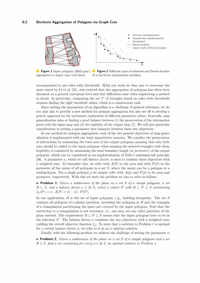
6:2 Bicriteria Aggregation of Polygons via Graph Cuts

Figure 1 Input polygons (filled gray)aggregated to larger ones (red lines).

P

A extreme nondominatednonextreme nondominateddominatedPareto-frontierconvex hull of Pareto-frontier

Figure 2 Different types of solutions and Pareto-frontierof a bicriteria optimization problem.

recommended to use rules with thresholds. With our work we thus aim to overcome theissue raised by Li et al. [21], who noticed that the aggregation of polygons has often beendiscussed on a general conceptual level and that difficulties arise when engineering a methodin detail. In particular, computing the set T ′ of triangles based on rules with thresholdsrequires finding the right threshold values, which is a cumbersome task.

Since setting the parameters of an algorithm is a challenge of general relevance, we donot only aim to provide a new method for polygon aggregation but also set off to develop ageneric approach for the systematic exploration of different parameter values. Generally, mapgeneralization aims at finding a good balance between (i) the preservation of the informationgiven with the input map and (ii) the legibility of the output map [7]. We will give particularconsideration to setting a parameter that balances between these two objectives.

In our method for polygon aggregation, each of the two general objectives of map gener-alization is implemented with one basic quantitative measure. We consider the preservationof information by minimizing the total area of the output polygons, meaning that only littlearea should be added to the input polygons when merging the selected triangles with them.Legibility is considered by minimizing the total boundary length (or perimeter) of the outputpolygons, which can be considered as an implementation of Tufte’s minimum-ink principle[38]. A parameter α, which we call balance factor, is used to combine these objectives witha weighted sum. To formalize this, we refer with A(S) to the area and with P (S) to theperimeter of the union of all polygons in a set S, where the union can be a polygon or amultipolygon. For a single polygon p we simply refer with A(p) and P (p) to its area andperimeter, respectively. With this we state the problem we aim to solve as follows.

Problem 1. Given a subdivision of the plane as a set S of n simple polygons, a setB ⊆ S, and a balance factor α ∈ [0, 1], select a subset S′ with B ⊆ S′ ⊆ S minimizingfα(S′) = α ·A(S′) + (1− α) · P (S′).

In our application, B is the set of input polygons, e.g., building footprints. The set S

contains all polygons of a planar partition, including the polygons in B and the trianglesof a triangulation partitioning the space not covered by the input polygons. Note that therestriction to a triangulation is not necessary, i.e., one may use any other partition of theplane instead. The requirement B ⊆ S′ ⊆ S means that the input polygons have to be inthe selection S′. The balance factor α combines the two objectives with a weighted sum,yielding the overall objective function fα. To state that a solution to Problem 1 is optimalfor a certain balance factor α, we refer to it as an α-optimal solution.

Finally, with the following problem we address the challenge of setting the parameter α.

Problem 2. Given a subdivision of the plane as a set S of n simple polygons and a setB ⊆ S, find a set containing for every α ∈ [0, 1] an optimal solution to Problem 1.

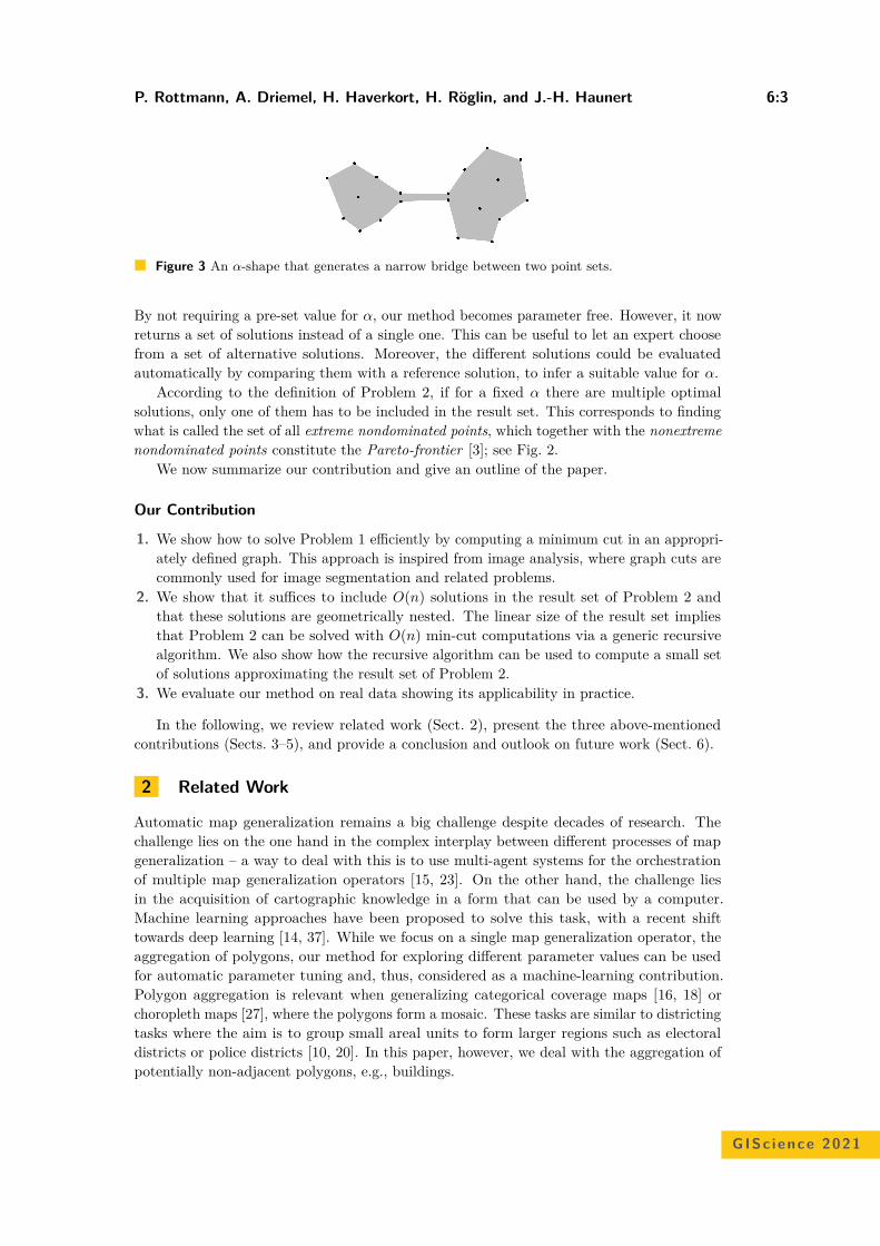
P. Rottmann, A. Driemel, H. Haverkort, H. Röglin, and J.-H. Haunert 6:3

Figure 3 An α-shape that generates a narrow bridge between two point sets.

By not requiring a pre-set value for α, our method becomes parameter free. However, it nowreturns a set of solutions instead of a single one. This can be useful to let an expert choosefrom a set of alternative solutions. Moreover, the different solutions could be evaluatedautomatically by comparing them with a reference solution, to infer a suitable value for α.

According to the definition of Problem 2, if for a fixed α there are multiple optimalsolutions, only one of them has to be included in the result set. This corresponds to findingwhat is called the set of all extreme nondominated points, which together with the nonextremenondominated points constitute the Pareto-frontier [3]; see Fig. 2.

We now summarize our contribution and give an outline of the paper.

Our Contribution

1. We show how to solve Problem 1 efficiently by computing a minimum cut in an appropri-ately defined graph. This approach is inspired from image analysis, where graph cuts arecommonly used for image segmentation and related problems.

2. We show that it suffices to include O(n) solutions in the result set of Problem 2 andthat these solutions are geometrically nested. The linear size of the result set impliesthat Problem 2 can be solved with O(n) min-cut computations via a generic recursivealgorithm. We also show how the recursive algorithm can be used to compute a small setof solutions approximating the result set of Problem 2.

3. We evaluate our method on real data showing its applicability in practice.

In the following, we review related work (Sect. 2), present the three above-mentionedcontributions (Sects. 3–5), and provide a conclusion and outlook on future work (Sect. 6).

2 Related Work

Automatic map generalization remains a big challenge despite decades of research. Thechallenge lies on the one hand in the complex interplay between different processes of mapgeneralization – a way to deal with this is to use multi-agent systems for the orchestrationof multiple map generalization operators [15, 23]. On the other hand, the challenge liesin the acquisition of cartographic knowledge in a form that can be used by a computer.Machine learning approaches have been proposed to solve this task, with a recent shifttowards deep learning [14, 37]. While we focus on a single map generalization operator, theaggregation of polygons, our method for exploring different parameter values can be usedfor automatic parameter tuning and, thus, considered as a machine-learning contribution.Polygon aggregation is relevant when generalizing categorical coverage maps [16, 18] orchoropleth maps [27], where the polygons form a mosaic. These tasks are similar to districtingtasks where the aim is to group small areal units to form larger regions such as electoraldistricts or police districts [10, 20]. In this paper, however, we deal with the aggregation ofpotentially non-adjacent polygons, e.g., buildings.

GISc ience 2021

6:4 Bicriteria Aggregation of Polygons via Graph Cuts

The aggregation of polygons is closely related to the aggregation of points. The commongoal is to find a single polygon or multiple polygons enclosing the input data. A naïve methodis to compute the convex hull of all input points. However, since this may enclose largeempty regions, generalizations of the convex hull such as α-shapes [13] have been developed.As an unwanted side effect, α-shapes tend to introduce narrow bridges between two nearbypoint sets; see Fig. 3. Such a bridge can consist of a single edge, in which case it can beeasily removed [4], but handling bridges of multiple parallel edges is not straight forward.Similar issues can arise with the concave hull introduced Moreira and Santos [26], which isbased on k-nearest neighbours clustering. In contrast, our method would never connect twopolygons with a narrow bridge as the one in Fig. 3 since not selecting the bridge would yielda solution with both a smaller perimeter and less area. Note that the parameter α of ourmethod is different from that of α-shapes. Duckham et al. [12] defined the χ(chi)-hull as afurther generalization of the convex hull. First, all points are triangulated using a Delaunaytriangulation. Then, all boundary edges that are longer than a threshold are removed. Thisprocedure always returns a single polygon without holes. This may include large emptyregions and does not separate groups of points from each other. To address the latter issue,Duckham et al. [12] suggest to identify clusters in a pre-processing step. However, this doesnot prevent the method from covering large empty regions within a cluster.

With respect to the aggregation of polygons, Jones et al. [19] proposed a method formerging polygons by selecting triangles of a constrained Delaunay triangulation, which theycall adopt merge amalgamation. They do not specify the criteria for the selection of thetriangles but generally recommend to use rules based on thresholds on the triangles’ edgelengths. Using such rules the adopt merge amalgamation operator has been implementedand experimentally evaluated by Li and Ai [22]. They showed that the method tends togenerate narrow bridges that can consist of a single triangle touching an input polygon withonly one of the triangle’s vertices. The method of Li et al. [21] overcomes this deficit byselecting sequences of triangles instead of single ones. However, the rules used to governthe selection are set up to aggregate polygons with parallel boundaries separated by longand narrow corridors. With this the method can be used to derive built-up areas from cityblocks but not, e.g., settlement areas from footprints of detached houses. Sayidov et al. [33]compute groups of polygons using a triangulation-based method and suggest to computea representative polygon for each group in a separate processing step. To accomplish thisstep, automatic typification method can be used [1, 6, 24]. Similarly, Steinger et al. [36]suggest a method that first detects groups of islands and then generates a representativepolygon for each group. They define the groups with a subgraph of a minimum spanningtree and generate for each group the convex hull. Damen et al. [9] present an approach forbuilding generalization based on morphological operators. They combine multiple closing andopening operations to simplify but also aggregate the input polygons. To retain the originalrectangular geometry that is typical for buildings they implement the closing operator witha Minkowski sum of the input polygon and a square aligned with it.

Our method for polygon aggregation computes a binary partition of the set of polygonsof a planar subdivision. For computing the binary partition we adopt a technique fromcomputer vision based on graph cuts [5]. Graph cuts are very commonly used for imagesegmentation [35, 39] or stereo matching [2]. However, most applications are concernedwith raster data. An exception is the work by Sadlacek and Zara. [34] dealing with thegeneration of polygonal objects from three-dimensional point clouds. With respect to theautomatic tuning of a parameter that balances two objectives, the work of Peng and Veksler[30] is most related to ours. While they focus on the development of quality metrics for the

P. Rottmann, A. Driemel, H. Haverkort, H. Röglin, and J.-H. Haunert 6:5

p1

p2

p3

p4

p5

p6

(a) an instance of Problem 1, where B = p1, p6;red (bold) edges delineate a solution with selec-tion S′ = p1, p3, p4, p6.

v1 v2v3

v4 v5 v6

t

s

(b) graph G for the instance in (a); red (dashed)edges show an s-t-cut modelling the solution S′.

Figure 4 Algorithmic solution of Problem 1 via a graph cut.

evaluation of image segmentation solutions, they simply use a constant step width to sampledifferent values for the parameter of a weighted-sum model. In contrast, we focus on a moresystematic exploration of different parameter values.

3 Polygon Aggregation via Minimum Cuts

For solving Problem 1 with graph cuts, we set up an undirected weighted graph G = (V, E)modeling all feasible solutions as well as our minimization goal. This approach is illustratedin Fig. 4 and described in detail in the following.

As starting point we use the adjacency graph G′ = (V ′, E′) of the planar subdivisiongiven with the set S of polygons. Assuming that the polygons are numbered in an arbitraryorder as p1, . . . , pn, we refer to the corresponding nodes in V ′ as v1, . . . , vn. The edge set E′

contains an edge vi, vj for every two polygons pi and pj whose boundaries share at leastone line segment. We define the node set of G as V = V ′ ∪ s, t, where s is a node calledsource and t a node called sink. The edge set E of G contains all edges in E′ as well as,for i = 1, . . . , n, the two edges s, vi and vi, t; see Figs. 4a and b. An s-t-cut in G is aset of edges whose removal from G causes s and t to be in different connected components.We solve Problem 1 by defining an edge weighting w : E → R≥0 and computing a minimums-t-cut in G, i.e., an s-t-cut in G of minimum total edge weight.

Formally, for any s-t-cut C ⊆ E, we define its weight as w(C) =∑

e∈C w(e) and the graphGC = (V, E \C). We call the connected component of GC containing s the source componentand the connected component of GC containing t the sink component of C. Moreover, werefer to the set of polygons represented by nodes in the source component as the solutionmodeled by C; see the red edges in Figs. 4a and b. It remains to ensure that any solutionmodeled by a minimum s-t-cut in G is feasible and optimal with respect to Problem 1. Forthis we define the edge weighting w as follows:

For every edge e = vi, vj, we set w(e) = (1− α) · ℓ(pi, pj), where ℓ(pi, pj) is the lengthof the common boundary of polygons pi and pj .For every node vi with pi ∈ B, we set w(s, vi) = 0 and w(vi, t) = α · A(pi) + (1 −α) · ℓ(pi), where ℓ(pi) is the length of the boundary between pi and the outer face (0 if pi

and the outer face are not adjacent).For every node vi with pi ∈ B, we set w(s, vi) =∞ and w(vi, t) = α ·A(pi) + (1−α) · ℓ(pi). This avoids that s, vi is selected for the cut and thus ensures that vi is inthe source component. (In practice, we use a floating-point number format with a specialvalue representing ∞.)

GISc ience 2021

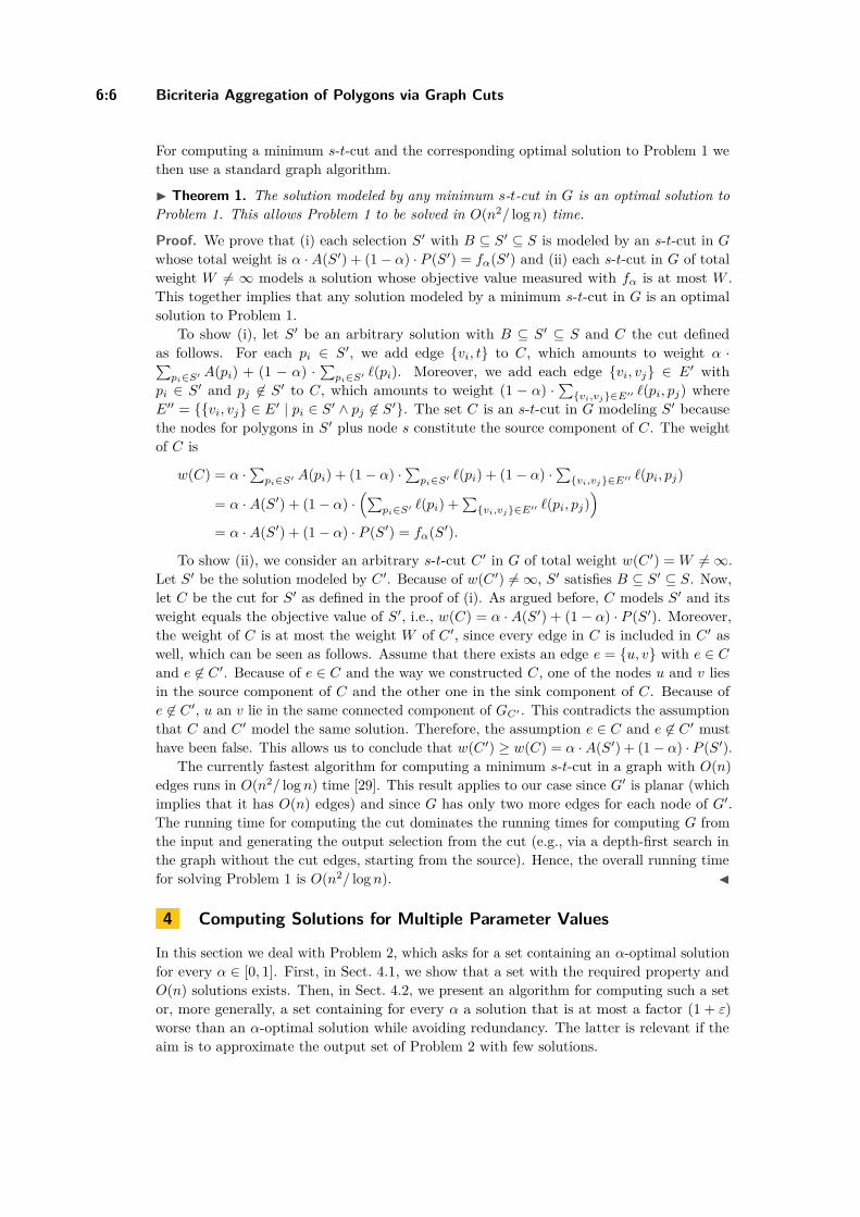
6:6 Bicriteria Aggregation of Polygons via Graph Cuts

For computing a minimum s-t-cut and the corresponding optimal solution to Problem 1 wethen use a standard graph algorithm.

Theorem 1. The solution modeled by any minimum s-t-cut in G is an optimal solution toProblem 1. This allows Problem 1 to be solved in O(n2/ log n) time.

Proof. We prove that (i) each selection S′ with B ⊆ S′ ⊆ S is modeled by an s-t-cut in G

whose total weight is α ·A(S′) + (1− α) · P (S′) = fα(S′) and (ii) each s-t-cut in G of totalweight W = ∞ models a solution whose objective value measured with fα is at most W .This together implies that any solution modeled by a minimum s-t-cut in G is an optimalsolution to Problem 1.

To show (i), let S′ be an arbitrary solution with B ⊆ S′ ⊆ S and C the cut definedas follows. For each pi ∈ S′, we add edge vi, t to C, which amounts to weight α ·∑

pi∈S′ A(pi) + (1 − α) ·∑

pi∈S′ ℓ(pi). Moreover, we add each edge vi, vj ∈ E′ withpi ∈ S′ and pj ∈ S′ to C, which amounts to weight (1 − α) ·

∑vi,vj∈E′′ ℓ(pi, pj) where

E′′ = vi, vj ∈ E′ | pi ∈ S′ ∧ pj ∈ S′. The set C is an s-t-cut in G modeling S′ becausethe nodes for polygons in S′ plus node s constitute the source component of C. The weightof C is

w(C) = α ·∑

pi∈S′ A(pi) + (1− α) ·∑

pi∈S′ ℓ(pi) + (1− α) ·∑

vi,vj∈E′′ ℓ(pi, pj)

= α ·A(S′) + (1− α) ·(∑

pi∈S′ ℓ(pi) +∑

vi,vj∈E′′ ℓ(pi, pj))

= α ·A(S′) + (1− α) · P (S′) = fα(S′).

To show (ii), we consider an arbitrary s-t-cut C ′ in G of total weight w(C ′) = W =∞.Let S′ be the solution modeled by C ′. Because of w(C ′) =∞, S′ satisfies B ⊆ S′ ⊆ S. Now,let C be the cut for S′ as defined in the proof of (i). As argued before, C models S′ and itsweight equals the objective value of S′, i.e., w(C) = α ·A(S′) + (1− α) · P (S′). Moreover,the weight of C is at most the weight W of C ′, since every edge in C is included in C ′ aswell, which can be seen as follows. Assume that there exists an edge e = u, v with e ∈ C

and e ∈ C ′. Because of e ∈ C and the way we constructed C, one of the nodes u and v liesin the source component of C and the other one in the sink component of C. Because ofe ∈ C ′, u an v lie in the same connected component of GC′ . This contradicts the assumptionthat C and C ′ model the same solution. Therefore, the assumption e ∈ C and e ∈ C ′ musthave been false. This allows us to conclude that w(C ′) ≥ w(C) = α ·A(S′) + (1− α) · P (S′).

The currently fastest algorithm for computing a minimum s-t-cut in a graph with O(n)edges runs in O(n2/ log n) time [29]. This result applies to our case since G′ is planar (whichimplies that it has O(n) edges) and since G has only two more edges for each node of G′.The running time for computing the cut dominates the running times for computing G fromthe input and generating the output selection from the cut (e.g., via a depth-first search inthe graph without the cut edges, starting from the source). Hence, the overall running timefor solving Problem 1 is O(n2/ log n).

4 Computing Solutions for Multiple Parameter Values

In this section we deal with Problem 2, which asks for a set containing an α-optimal solutionfor every α ∈ [0, 1]. First, in Sect. 4.1, we show that a set with the required property andO(n) solutions exists. Then, in Sect. 4.2, we present an algorithm for computing such a setor, more generally, a set containing for every α a solution that is at most a factor (1 + ε)worse than an α-optimal solution while avoiding redundancy. The latter is relevant if theaim is to approximate the output set of Problem 2 with few solutions.

P. Rottmann, A. Driemel, H. Haverkort, H. Röglin, and J.-H. Haunert 6:7

L13

L23L12

L03

L01

L02

A1

A2

A3

= S1

= S2

= S1 ∩ S2

= S2 \ S1

= S1 \ S2

A0

Figure 5 Schematic visualization of two α-optimal solutions S1 and S2. The labels Ai refer tothe areas and the labels Lij refer to the line lengths used in the proof of Lemma 2.

4.1 Linear number of solutionsOur argument about a sufficient size for the set requested by Problem 2 is based on thefollowing structural lemma.

Lemma 2. For an instance of Problem 1, let S1 be an α1-optimal solution and S2 be anα2-optimal solution, where α1 > α2. Then S1 ⊆ S2.

Proof. We distinguish four classes of polygons: those that are neither in S1 nor in S2; thosethat are only in S1; those that are only in S2; and those that are in S1 ∩ S2. We denotethese classes by T0 = S \ (S1 ∪ S2); T1 = S1 \ S2; T2 = S2 \ S1; and T3 = S1 ∩ S2. By Ai wedenote the area of Ti, and by Lij we denote the total length of the edges that are shared byTi and Tj ; see Fig. 5. Let α′

i be 1− αi.The α1-optimal solution S1 = T1 ∪ T3 is at least as good as S1 ∩ S2 = T3 for α = α1:

α1(A1 + A3) + α′1(L01 + L03 + L12 + L23) ≤ α1A3 + α′

1(L03 + L13 + L23)⇔ α1A1 + α′

1L12 ≤ α′1(L13 − L01). (1)

The α2-optimal solution S2 = T2 ∪ T3 is not worse than S1 ∪ S2 = T1 ∪ T2 ∪ T3 for α = α2:

α2(A2 + A3) + α′2(L02 + L03 + L12 + L13) ≤ α2(A1 + A2 + A3) + α′

2(L01 + L02 + L03)⇔ α′

2(L13 − L01) ≤ α2A1 − α′2L12. (2)

Now suppose S1 ⊈ S2, that is, A1 > 0. With α1 > α2 ≥ 0, Equation (1) then impliesL13 − L01 > 0. Since α2 < α1, we also have α′

1 < α′2. Combining this with (1) and (2) gives:

α1A1 ≤ α1A1 + α′1L12 ≤ α′

1(L13 − L01) < α′2(L13 − L01) ≤ α2A1 − α′

2L12 ≤ α2A1.

Thus, α1A1 < α2A1. However, this contradicts the assumption α2 < α1. Therefore, theassumption S1 ⊈ S2 must have been false, and we conclude S1 ⊆ S2.

Suppose that we continuously decrease α from 1 to 0 while maintaining an α-optimalsolution in a lazy fashion, meaning that we replace the current solution only if it ceasesbeing α-optimal. At the beginning of this process we have the solution containing only thepolygons in B, since for α = 1 area is all that matters. Due to Lemma 2, whenever we haveto replace the current solution, we can define the new solution by including all the polygonsselected in the current solution plus at least one additional polygon from the set S. Sincethere can be at most n− 1 such events, we can conclude the following lemma.

GISc ience 2021

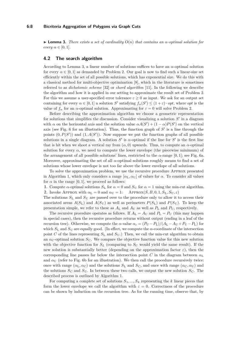
6:8 Bicriteria Aggregation of Polygons via Graph Cuts

Lemma 3. There exists a set of cardinality O(n) that contains an α-optimal solution forevery α ∈ [0, 1].

4.2 The search algorithmAccording to Lemma 3, a linear number of solutions suffices to have an α-optimal solutionfor every α ∈ [0, 1] as demanded by Problem 2. Our goal is now to find such a linear-size setefficiently within the set of all possible solutions, which has exponential size. We do this witha classical method for multi-objective optimization [8], which in the literature is sometimesreferred to as dichotomic scheme [32] or chord algorithm [11]. In the following we describethe algorithm and how it is applied in our setting to approximate the result set of Problem 2.For this we assume a user-specified error tolerance ε ≥ 0 as input. We ask for an output setcontaining for every α ∈ [0, 1] a solution S′ satisfying fα(S′) ≤ (1 + ε) · opt, where opt is thevalue of fα for an α-optimal solution. Approximating for ε = 0 will solve Problem 2.

Before describing the approximation algorithm we choose a geometric representationfor solutions that simplifies the discussion. Consider visualizing a solution S′ in a diagramwith α on the horizontal axis and the solution value αA(S′) + (1− α)P (S′) on the verticalaxis (see Fig. 6 for an illustration). Thus, the function graph of S′ is a line through thepoints (0, P (S′)) and (1, A(S′)). Now suppose we put the function graphs of all possiblesolutions in a single diagram. A solution S′ is α-optimal if the line for S′ is the first linethat is hit when we shoot a vertical ray from (α, 0) upwards. Thus, to compute an α-optimalsolution for every α, we need to compute the lower envelope (the piecewise minimum) ofthe arrangement of all possible solutions’ lines, restricted to the α-range [0, 1]; see Fig. 6a.Moreover, approximating the set of all α-optimal solutions roughly means to find a set ofsolutions whose lower envelope is not too far above the lower envelope of all solutions.

To solve the approximation problem, we use the recursive procedure Approx presentedin Algorithm 1, which only considers a range [αL, αU] of values for α. To consider all valuesfor α in the range [0, 1], we proceed as follows:1. Compute α-optimal solutions SL for α = 0 and SU for α = 1 using the min-cut algorithm.2. Invoke Approx with αL = 0 and αU = 1: Approx(S, B, 0, 1, SL, SU, ε)The solutions SL and SU are passed over to the procedure only to allow it to access theirassociated areas A(SL) and A(SU) as well as perimeters P (SL) and P (SU). To keep thepresentation simple, we refer to these as AL and AU as well as PL and PU, respectively.

The recursive procedure operates as follows. If AL = AU and PL = PU (this may happenin special cases), then the recursive procedure returns without output (ending in a leaf of therecursion tree). Otherwise, we compute the α-value αc = (PU−PL)/(AL−AU +PU−PL) forwhich SL and SU are equally good. (In effect, we compute the α-coordinate of the intersectionpoint C of the lines representing SL and SU.) Then, we call the min-cut algorithm to obtainan αC-optimal solution SC. We compare the objective function value for this new solutionwith the objective function for SL (comparing to SU would yield the same result). If thenew solution is substantially better (depending on the approximation factor ε), then thecorresponding line passes far below the intersection point C in the diagram between αLand αU (refer to Fig. 6b for an illustration). We then call the procedure recursively twice:once with range (αL, αC) and the solutions SL and SC, and once with range (αC, αU) andthe solutions SC and SU. In between these two calls, we output the new solution SC. Thedescribed process is outlined by Algorithm 1.

For computing a complete set of solutions S1, ..., Sk representing the k linear pieces thatform the lower envelope we call the algorithm with ε = 0. Correctness of the procedurecan be shown by induction on the recursion tree. As for the running time, observe that, by

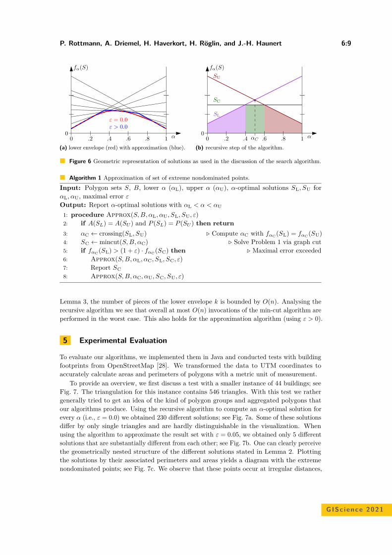
P. Rottmann, A. Driemel, H. Haverkort, H. Röglin, and J.-H. Haunert 6:9

0 .2 .4 .6 .8 1 α0

fα(S)

ε = 0.0ε > 0.0

(a) lower envelope (red) with approximation (blue).0 .2 .4 .6 .8 1 α0

SL

SC

SU

αC

fα(S)

(b) recursive step of the algorithm.

Figure 6 Geometric representation of solutions as used in the discussion of the search algorithm.

Algorithm 1 Approximation of set of extreme nondominated points.Input: Polygon sets S, B, lower α (αL), upper α (αU), α-optimal solutions SL, SU forαL, αU, maximal error ε

Output: Report α-optimal solutions with αL < α < αU

1: procedure Approx(S, B, αL, αU, SL, SU, ε)2: if A(SL) = A(SU ) and P (SL) = P (SU ) then return3: αC ← crossing(SL, SU) ▷ Compute αC with fαC(SL) = fαC(SU)4: SC ← mincut(S, B, αC) ▷ Solve Problem 1 via graph cut5: if fαC(SL) > (1 + ε) · fαC(SC) then ▷ Maximal error exceeded6: Approx(S, B, αL, αC, SL, SC, ε)7: Report SC8: Approx(S, B, αC, αU, SC, SU, ε)

Lemma 3, the number of pieces of the lower envelope k is bounded by O(n). Analysing therecursive algorithm we see that overall at most O(n) invocations of the min-cut algorithm areperformed in the worst case. This also holds for the approximation algorithm (using ε > 0).

5 Experimental Evaluation

To evaluate our algorithms, we implemented them in Java and conducted tests with buildingfootprints from OpenStreetMap [28]. We transformed the data to UTM coordinates toaccurately calculate areas and perimeters of polygons with a metric unit of measurement.

To provide an overview, we first discuss a test with a smaller instance of 44 buildings; seeFig. 7. The triangulation for this instance contains 546 triangles. With this test we rathergenerally tried to get an idea of the kind of polygon groups and aggregated polygons thatour algorithms produce. Using the recursive algorithm to compute an α-optimal solution forevery α (i.e., ε = 0.0) we obtained 230 different solutions; see Fig. 7a. Some of these solutionsdiffer by only single triangles and are hardly distinguishable in the visualization. Whenusing the algorithm to approximate the result set with ε = 0.05, we obtained only 5 differentsolutions that are substantially different from each other; see Fig. 7b. One can clearly perceivethe geometrically nested structure of the different solutions stated in Lemma 2. Plottingthe solutions by their associated perimeters and areas yields a diagram with the extremenondominated points; see Fig. 7c. We observe that these points occur at irregular distances,

GISc ience 2021

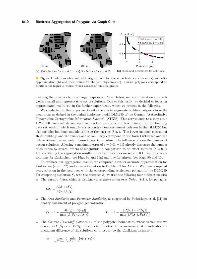
6:10 Bicriteria Aggregation of Polygons via Graph Cuts

100 m

(a) 230 solutions for ε = 0.0.

100 m

(b) 5 solutions for ε = 0.05.

2 4 6

Perimeter [km]

0.1

0.2

Area [km2]

Solutions, ε = 0.0

Solutions, ε = 0.05

(c) areas and perimeters for solutions.

Figure 7 Solutions obtained with Algorithm 1 for the same instance without (a) and withapproximation (b) and their values for the two objectives (c). Darker polygons correspond tosolutions for higher α values, which consist of multiple groups.

meaning that clusters but also larger gaps exist. Nevertheless, our approximation approachyields a small and representative set of solutions. Due to this result, we decided to focus onapproximated result sets in the further experiments, which we present in the following.

We conducted further experiments with the aim to aggregate building polygons to settle-ment areas as defined in the digital landscape model DLM250 of the German “AuthoritativeTopographic-Cartographic Information System” (ATKIS). This corresponds to a map scale1 : 250 000. We evaluate our approach on two instances of different sizes from the buildingdata set, each of which roughly corresponds to one settlement polygon in the DLM250 butalso includes buildings outside of the settlement; see Fig. 8. The larger instance consists of16881 buildings and the smaller one of 853. They correspond to the town Euskirchen and thevillage Ahrem, respectively. Figure 9 depicts for Ahrem the influence of ε on the number ofoutput solutions. Allowing a maximum error of ε = 0.01 = 1% already decreases the numberof solutions by several orders of magnitude in comparison to an exact solution (ε = 0.0).For visualizing the aggregation results of the two instances we set ε = 0.1, resulting in sixsolutions for Euskirchen (see Figs. 8a and 10a) and five for Ahrem (see Figs. 8b and 10b).

To evaluate our aggregation results, we computed a rather accurate approximation forEuskirchen (ε = 10−6) and an exact solution to Problem 2 for Ahrem. We then comparedevery solution in the result set with the corresponding settlement polygon in the DLM250.For comparing a solution S1 with the reference S2 we used the following four different metrics:

The Jaccard index, which is also known as Intersection over Union (IoU), for polygons:

IoU = A(S1 ∩ S2)A(S1 ∪ S2)

The Area Similarity and Perimeter Similarity, as suggested by Podolskaya et al. [31] forquality assessment of polygon generalization:

VA = 1− |A(S1)−A(S2)|maxA(S1), A(S2) VP = 1− |P (S1)− P (S2)|

max(P (S1), P (S2)

The discrete Hausdorff distance dH of the polygons’ boundaries, whose vertex sets wedenote as V (S1) and V (S2). It adds to the other three measure that it indicates themaximum difference of the solutions with respect to the Euclidean distance d.

dH = maxv1∈V (S1)

minv2∈V (S2)

d(v1, v2)

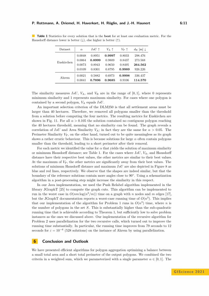
P. Rottmann, A. Driemel, H. Haverkort, H. Röglin, and J.-H. Haunert 6:11

Table 1 Statistics for every solution that is the best for at least one evaluation metric. For theHausdorff distance lower is better (↓), else higher is better (↑).

Dataset α IoU ↑ VA ↑ VP ↑ dH [m] ↓

Euskirchen

0.0048 0.8951 0.9997 0.8033 298.4760.0064 0.8999 0.9809 0.8437 273.5680.0073 0.8943 0.9650 0.8495 264.5620.0109 0.8301 0.8795 0.9989 926.226

Ahrem 0.0021 0.5882 0.6973 0.9998 336.4370.0041 0.7896 0.9685 0.9106 114.570

The similarity measures IoU , VA, and VB are in the range of [0, 1], where 0 representsminimum similarity and 1 represents maximum similarity. For cases where one polygon iscontained by a second polygon, VA equals IoU .

An important selection criterion of the DLM250 is that all settlement areas must belarger than 40 hectares. Therefore, we removed all polygons smaller than the thresholdfrom a solution before computing the four metrics. The resulting metrics for Euskirchen areshown in Fig. 11. For all α > 0.105 the solution contained no contiguous polygon reachingthe 40 hectares threshold, meaning that no similarity can be found. The graph reveals acorrelation of IoU and Area Similarity VA; in fact they are the same for α > 0.05. ThePerimeter Similarity VP, on the other hand, turned out to be quite meaningless as its graphshows a rather erratic behaviour. This is because solutions for large α often contain polygonssmaller than the threshold, leading to a short perimeter after their removal.

For each metric we identified the value for α that yields the solution of maximum similarityor minimum Hausdorff distance; see Table 1. For the cases where IoU , VA, and Hausdorffdistance have their respective best values, the other metrics are similar to their best values.At the maximum of VP, the other metrics are significantly away from their best values. Thesolutions of minimum Hausdorff distance and maximum IoU are also depicted in Figure 8 asblue and red lines, respectively. We observe that the shapes are indeed similar, but that theboundary of the reference solutions contain more angles close to 90. Using a schematizationalgorithm in a post-processing step might increase the similarity in this respect.

In our Java implementation, we used the Push Relabel algorithm implemented in thelibrary JGraphT [25] to compute the graph cuts. This algorithm can be implemented torun in the worst case in O(nm log(n2/m)) time on a graph with n nodes and m edges [17],but the JGraphT documentation reports a worst-case running time of O(n3). This impliesthat our implementation of the algorithm for Problem 1 runs in O(n3) time, where n isthe number of polygons in the set S. This is substantially higher than the sub-quadraticrunning time that is achievable according to Theorem 1, but sufficiently low to solve probleminstances as the ones we discussed above. Our implementation of the recursive algorithm forProblem 2 uses parallelization for the two recursive calls, which turned out to improve therunning time substantially. In particular, the running time improves from 79 seconds to 12seconds for ε = 10−6 (528 solutions) on the instance of Ahrem by using parallelization.

6 Conclusion and Outlook

We have presented efficient algorithms for polygon aggregation optimizing a balance betweena small total area and a short total perimeter of the output polygons. We combined the twocriteria in a weighted sum, which we parameterized with a single parameter α ∈ [0, 1]. The

GISc ience 2021

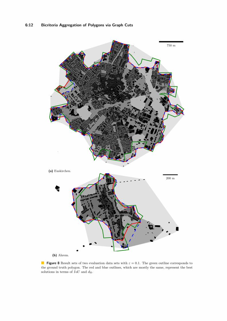
6:12 Bicriteria Aggregation of Polygons via Graph Cuts

750 m

(a) Euskirchen.

200 m

(b) Ahrem.

Figure 8 Result sets of two evaluation data sets with ε = 0.1. The green outline corresponds tothe ground truth polygon. The red and blue outlines, which are mostly the same, represent the bestsolutions in terms of IoU and dH.

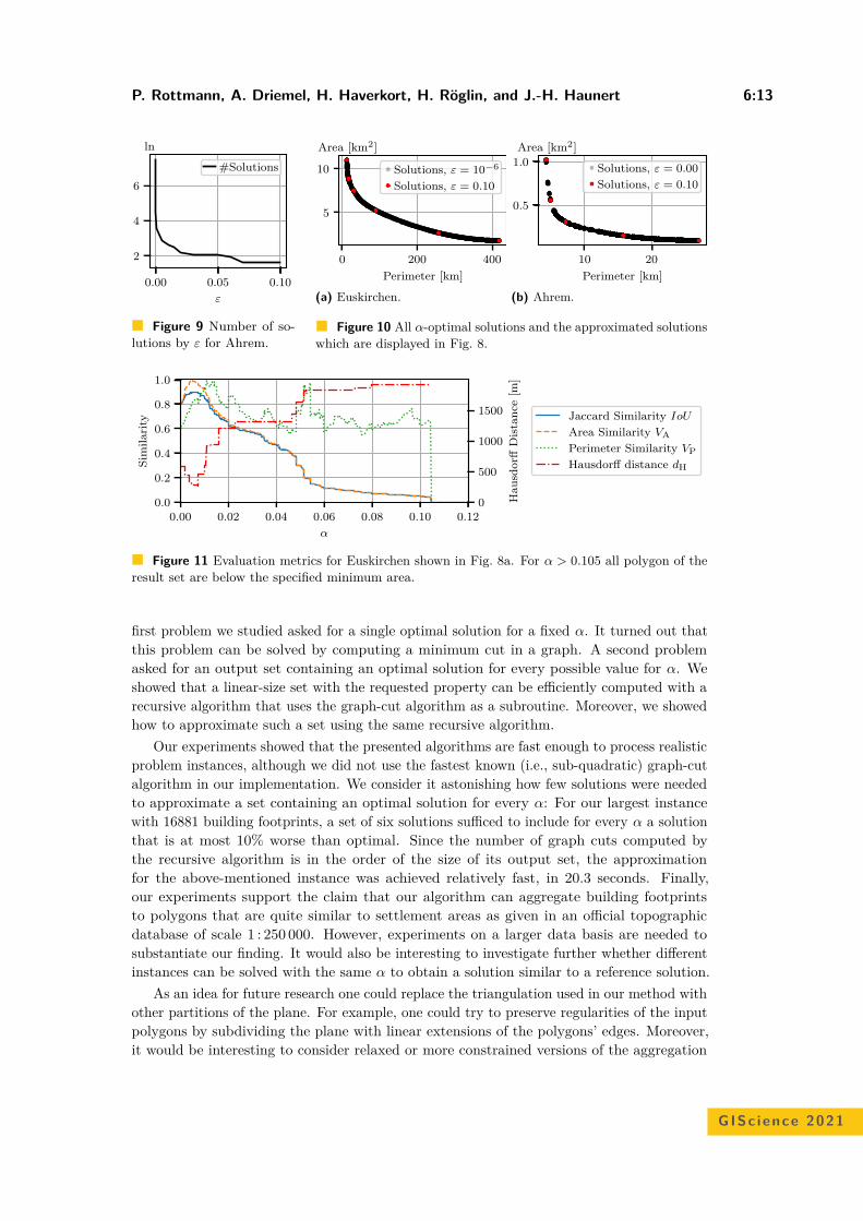
P. Rottmann, A. Driemel, H. Haverkort, H. Röglin, and J.-H. Haunert 6:13

0.00 0.05 0.10

ε

2

4

6

ln

#Solutions

Figure 9 Number of so-lutions by ε for Ahrem.

0 200 400

Perimeter [km]

5

10

Area [km2]

Solutions, ε = 10−6

Solutions, ε = 0.10

(a) Euskirchen.

10 20

Perimeter [km]

0.5

1.0

Area [km2]

Solutions, ε = 0.00

Solutions, ε = 0.10

(b) Ahrem.

Figure 10 All α-optimal solutions and the approximated solutionswhich are displayed in Fig. 8.

0.00 0.02 0.04 0.06 0.08 0.10 0.12

α

0.0

0.2

0.4

0.6

0.8

1.0

Sim

ilari

ty

0

500

1000

1500

Hau

sdorff

Dis

tan

ce[m

]

Jaccard Similarity IoU

Area Similarity VA

Perimeter Similarity VP

Hausdorff distance dH

Figure 11 Evaluation metrics for Euskirchen shown in Fig. 8a. For α > 0.105 all polygon of theresult set are below the specified minimum area.

first problem we studied asked for a single optimal solution for a fixed α. It turned out thatthis problem can be solved by computing a minimum cut in a graph. A second problemasked for an output set containing an optimal solution for every possible value for α. Weshowed that a linear-size set with the requested property can be efficiently computed with arecursive algorithm that uses the graph-cut algorithm as a subroutine. Moreover, we showedhow to approximate such a set using the same recursive algorithm.

Our experiments showed that the presented algorithms are fast enough to process realisticproblem instances, although we did not use the fastest known (i.e., sub-quadratic) graph-cutalgorithm in our implementation. We consider it astonishing how few solutions were neededto approximate a set containing an optimal solution for every α: For our largest instancewith 16881 building footprints, a set of six solutions sufficed to include for every α a solutionthat is at most 10% worse than optimal. Since the number of graph cuts computed bythe recursive algorithm is in the order of the size of its output set, the approximationfor the above-mentioned instance was achieved relatively fast, in 20.3 seconds. Finally,our experiments support the claim that our algorithm can aggregate building footprintsto polygons that are quite similar to settlement areas as given in an official topographicdatabase of scale 1 : 250 000. However, experiments on a larger data basis are needed tosubstantiate our finding. It would also be interesting to investigate further whether differentinstances can be solved with the same α to obtain a solution similar to a reference solution.

As an idea for future research one could replace the triangulation used in our method withother partitions of the plane. For example, one could try to preserve regularities of the inputpolygons by subdividing the plane with linear extensions of the polygons’ edges. Moreover,it would be interesting to consider relaxed or more constrained versions of the aggregation

GISc ience 2021

6:14 Bicriteria Aggregation of Polygons via Graph Cuts

problem. For example, one could relax the requirement to include every input polygon in theoutput and/or introduce a hard size constraint for the output polygons. Most importantly,however, we see our work as a step towards multi-criteria optimization in cartography. Asnext steps one could consider more than two criteria or look at Pareto-optimal solutionsrather than just at the extreme nondominated (i.e., α-optimal) solutions.

References1 Karl-Heinrich Anders and Monika Sester. Parameter-free cluster detection in spatial databases

and its application to typification. In Proc. 19th ISPRS Congress, volume 33 of InternationalArchives of Photogrammetry and Remote Sensing, pages 75–83, 2000.

2 Michael Bleyer and Margrit Gelautz. Graph-cut-based stereo matching using image segmen-tation with symmetrical treatment of occlusions. Signal Processing: Image Communication,22(2):127–143, 2007. doi:10.1016/j.image.2006.11.012.

3 Fritz Bökler and Petra Mutzel. Output-sensitive algorithms for enumerating the extremenondominated points of multiobjective combinatorial optimization problems. In Proc. 23rdAnnual European Symposium on Algorithms (ESA ’15), pages 288–299, 2015. doi:10.1007/978-3-662-48350-3_25.

4 Annika Bonerath, Benjamin Niedermann, and Jan-Henrik Haunert. Retrieving α-shapes andschematic polygonal approximations for sets of points within queried temporal ranges. In Proc.27th ACM SIGSPATIAL International Conference on Advances in Geographic InformationSystems (ACM SIGSPATIAL GIS ’19), pages 249–258, 2019. doi:10.1145/3347146.3359087.

5 Yuri Boykov and Olga Veksler. Graph cuts in vision and graphics: Theories and applications.In Handbook of Mathematical Models in Computer Vision, chapter 5, pages 79–96. Springer,Boston, MA, USA, 2006. doi:10.1007/0-387-28831-7_5.

6 Dirk Burghardt and Alessandro Cecconi. Mesh simplification for building typification.International Journal of Geographical Information Science, 21(3):283–298, 2007. doi:10.1080/13658810600912323.

7 Dirk Burghardt, Stefan Schmid, and Jantien Stoter. Investigations on cartographic con-straint formalisation. In Proc. 11th ICA Workshop on Generalisation and Multiple Rep-resentation, 2007. URL: https://kartographie.geo.tu-dresden.de/downloads/ica-gen/workshop2007/Burghardt-ICAWorkshop.pdf.

8 Jared L. Cohon. Multiobjective Programming and Planning. Academic Press, New York, NY,USA, 1978.

9 Jonathan Damen, Marc van Kreveld, and Bert Spaan. High quality building generalization byextending the morphological operators. In Proc. 11th ICA Workshop on Generalisation andMultiple Representation, pages 1–12, 2008. URL: https://kartographie.geo.tu-dresden.de/downloads/ica-gen/workshop2008/04_Damen_et_al.pdf.

10 Steven J. D’Amico, Shoou-Jiun Wang, Rajan Batta, and Christopher M. Rump. A simulatedannealing approach to police district design. Computers & Operations Research, 29(6):667–684,2002. doi:10.1016/S0305-0548(01)00056-9.

11 Constantinos Daskalakis, Ilias Diakonikolas, and Mihalis Yannakakis. How good is the chordalgorithm? SIAM Journal on Computing, 45(3):811–858, 2016. doi:10.1137/13093875X.

12 Matt Duckham, Lars Kulik, Mike Worboys, and Antony Galton. Efficient generation of simplepolygons for characterizing the shape of a set of points in the plane. Pattern Recognition,41(10):3224–3236, 2008. doi:10.1016/j.patcog.2008.03.023.

13 Herbert Edelsbrunner, David Kirkpatrick, and Raimund Seidel. On the shape of a setof points in the plane. IEEE Transactions on Information Theory, 29(4):551–559, 1983.doi:10.1109/TIT.1983.1056714.

14 Yu Feng, Frank Thiemann, and Monika Sester. Learning cartographic building generalizationwith deep convolutional neural networks. ISPRS International Journal of Geo-Information,8(6), 2019. doi:10.3390/ijgi8060258.

P. Rottmann, A. Driemel, H. Haverkort, H. Röglin, and J.-H. Haunert 6:15

15 Martin Galanda. Automated polygon generalization in a multi agent system. PhD thesis,University of Zurich, Zürich, 2003. doi:10.5167/uzh-163108.

16 Sven Gedicke, Johannes Oehrlein, and Jan-Henrik Haunert. Aggregating land-use polygonsconsidering line features as separating map elements. Cartography and Geographic InformationScience, 48(2):124–139, 2021. doi:10.1080/15230406.2020.1851613.

17 Andrew V. Goldberg and Robert E. Tarjan. A new approach to the maximum-flow problem.Journal of the ACM, 35(4):921–940, 1988. doi:10.1145/48014.61051.

18 Jan-Henrik Haunert and Alexander Wolff. Area aggregation in map generalisation by mixed-integer programming. International Journal of Geographical Information Science, 24(12):1871–1897, 2010. doi:10.1080/13658810903401008.

19 Christopher B. Jones, Geraint Ll. Bundy, and Mark J. Ware. Map generalization with atriangulated data structure. Cartography and Geographic Information Systems, 22(4):317–331,1995. doi:10.1559/152304095782540221.

20 Kamyoung Kim, Denis J. Dean, Hyun Kim, and Yongwan Chun. Spatial optimizationfor regionalization problems with spatial interaction: a heuristic approach. InternationalJournal of Geographical Information Science, 30(3):451–473, 2016. doi:10.1080/13658816.2015.1031671.

21 Chengming Li, Yong Yin, Xiaoli Liu, and Pengda Wu. An automated processing methodfor agglomeration areas. ISPRS International Journal of Geo-Information, 7(6):204, 2018.doi:10.3390/ijgi7060204.

22 Jingzhong Li and Tinghua Ai. A triangulated spatial model for detection of spatial character-istics of GIS data. In Proc. 2010 IEEE International Conference on Progress in Informaticsand Computing (PIC ’10), volume 1, pages 155–159, 2010. doi:10.1109/PIC.2010.5687417.

23 Adrien Maudet, Guillaume Touya, Cécile Duchêne, and Sébastien Picault. Multi-agent multi-level cartographic generalisation in CartAGen. In Proc. 12th International Conference onAdvances in Practical Applications of Heterogeneous Multi-Agent Systems (PAAMS ’14), pages355–358, 2014. doi:10.1007/978-3-319-07551-8_37.

24 Robert B. McMaster and K. Stuart Shea. Generalization in digital cartography. Associationof American Geographers, Washington, DC, USA, 1992.

25 Dimitrios Michail, Joris Kinable, Barak Naveh, and John V. Sichi. JGraphT—a Java libraryfor graph data structures and algorithms. ACM Transactions on Mathematical Software, 46(2),2020. doi:10.1145/3381449.

26 Adriano Moreira and Maribel Y. Santos. Concave hull: A k-nearest neighbours approachfor the computation of the region occupied by a set of points. In Proc. 2nd InternationalConference on Computer Graphics Theory and Applications (GRAPP ’07), pages 61–68, 2007.URL: http://hdl.handle.net/1822/6429.

27 Johannes Oehrlein and Jan-Henrik Haunert. A cutting-plane method for contiguity-constrainedspatial aggregation. Journal of Spatial Information Science, 15(1):89–120, 2017. doi:10.5311/JOSIS.2017.15.379.

28 OpenStreetMap contributors. Planet dump retrieved from https://planet.osm.org . https://www.openstreetmap.org, 2020.

29 James B. Orlin. Max flows in O(nm) time, or better. In Proc. 45th Annual ACM Symposiumon Theory of Computing (STOC ’13), page 765–774, 2013. doi:10.1145/2488608.2488705.

30 Bo Peng and Olga Veksler. Parameter selection for graph cut based image segmentation.In Proc. British Machine Vision Conference (BMVC ’08), pages 16.1–16.10, 2008. doi:10.5244/C.22.16.

31 Ekaterina S. Podolskaya, Karl-Heinrich Anders, Jan-Henrik Haunert, and Monika Sester. Qual-ity assessment for polygon generalization. In Quality Aspects in Spatial Data Mining, chapter 16,pages 211–220. CRC Press, Boca Raton, FL, USA, 2007. doi:10.1201/9781420069273.ch16.

32 Anthony Przybylski, Xavier Gandibleux, and Matthias Ehrgott. A recursive algorithm forfinding all nondominated extreme points in the outcome set of a multiobjective integerprogramme. INFORMS Journal on Computing, 22(3):371–386, 2010. doi:10.1287/ijoc.1090.0342.

GISc ience 2021

6:16 Bicriteria Aggregation of Polygons via Graph Cuts

33 Azimjon Sayidov, Robert Weibel, and Stefan Leyk. Recognition of group patterns in geologicalmaps by building similarity networks. Geocarto International, pages 1–20, 2020. doi:10.1080/10106049.2020.1730449.

34 David Sedlacek and Jiri Zara. Graph cut based point-cloud segmentation for polygonalreconstruction. In Proc. 5th International Symposium on Advances in Visual Computing(ISVC ’09), pages 218–227, 2009. doi:10.1007/978-3-642-10520-3_20.

35 Jianbo Shi and Jitendra Malik. Normalized cuts and image segmentation. IEEE Transactionson Pattern Analysis and Machine Intelligence, 22(8):888–905, 2000. doi:10.1109/34.868688.

36 Stefan Steiniger, Dirk Burghardt, and Robert Weibel. Recognition of island structures for mapgeneralization. In Proc. 14th Annual ACM International Symposium on Advances in GeographicInformation Systems (ACM GIS ’06), pages 67–74, 2006. doi:10.1145/1183471.1183484.

37 Guillaume Touya, Xiang Zhang, and Imran Lokhat. Is deep learning the new agent formap generalization? International Journal of Cartography, 5(2–3):142–157, 2019. doi:10.1080/23729333.2019.1613071.

38 Edward R. Tufte. The visual display of quantitative information. Graphics Press, Cheshire,CT, USA, 1992. doi:10.1119/1.14057.

39 Zhenyu Wu and Richard Leahy. An optimal graph theoretic approach to data clustering:theory and its application to image segmentation. IEEE Transactions on Pattern Analysisand Machine Intelligence, 15(11):1101–1113, 1993. doi:10.1109/34.244673.

Coordinated Schematization forVisualizing Mobility Patterns on NetworksBram Custers #

Eindhoven University of Technology, The Netherlands

Wouter Meulemans #

Eindhoven University of Technology, The Netherlands

Bettina Speckmann #

Eindhoven University of Technology, The Netherlands

Kevin Verbeek #

Eindhoven University of Technology, The Netherlands

AbstractGPS trajectories of vehicles moving on a road network are a valuable source of traffic information.However, the sheer volume of available data makes it challenging to identify and visualize salientpatterns. Meaningful visual summaries of trajectory collections require that both the trajectoriesand the underlying network are aggregated and simplified in a coherent manner. In this paper wepropose a coordinated fully-automated pipeline for computing a schematic overview of mobilitypatterns from a collection of trajectories on a street network. Our pipeline utilizes well-knownbuilding blocks from GIS, automated cartography, and trajectory analysis: map matching, roadselection, schematization, movement patterns, and metro-map style rendering. We showcase theresults of our pipeline on two real-world trajectory collections around The Hague and Beijing.

2012 ACM Subject Classification Theory of computation → Computational geometry

Keywords and phrases Trajectories, Visualization, Schematization

Digital Object Identifier 10.4230/LIPIcs.GIScience.2021.II.7

Supplementary Material Software (Source code): https://github.com/tue-alga/CoordinatedSchematization; archived at swh:1:dir:a04dfee52bf07c76d37ac692bc17450feec728df

Funding Bram Custers: Supported by HERE Technologies and the Dutch Research Council (NWO);628.011.005.

Acknowledgements We would like to thank HERE Technologies for providing the HR dataset.

1 Introduction

GPS tracks from moving vehicles are an important source of information for traffic analysisand urban planning. Their general ubiquity allows decision makers to understand the usageof transportation networks and urban spaces. However, the sheer volume of the data makesit challenging to render trajectory collections in a meaningful way as to show the general,overarching patterns. Simply plotting all trajectories results in the infamous “spaghettiheaps”. Heat maps [15, 19] and other aggregation techniques such as Voronoi aggregation [1]are helpful to “untangle” traffic locally, but they generally fail to capture structural patterns,such as important longer routes.

Summarizing trajectory collections visually, such that salient patterns emerge, inherentlyrequires a form of aggregation or simplification of the data. That is, the level of detailand information shown should be scale-appropriate and avoid a cognitive overload, whilestill being able to provide insight into the overall mobility. There are various techniquesto cluster trajectories and compute a representative for visualization [6, 16], or to simplify

© Bram Custers, Wouter Meulemans, Bettina Speckmann, and Kevin Verbeek;licensed under Creative Commons License CC-BY 4.0

11th International Conference on Geographic Information Science (GIScience 2021) – Part II.Editors: Krzysztof Janowicz and Judith A. Verstegen; Article No. 7; pp. 7:1–7:16

Leibniz International Proceedings in InformaticsSchloss Dagstuhl – Leibniz-Zentrum für Informatik, Dagstuhl Publishing, Germany

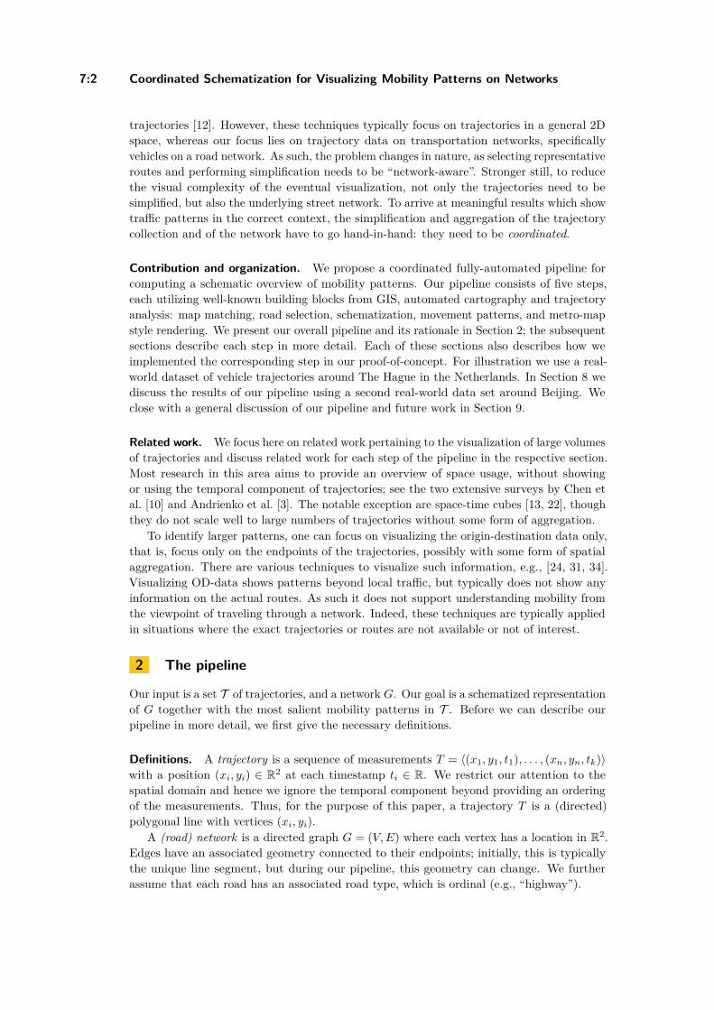
7:2 Coordinated Schematization for Visualizing Mobility Patterns on Networks

trajectories [12]. However, these techniques typically focus on trajectories in a general 2Dspace, whereas our focus lies on trajectory data on transportation networks, specificallyvehicles on a road network. As such, the problem changes in nature, as selecting representativeroutes and performing simplification needs to be “network-aware”. Stronger still, to reducethe visual complexity of the eventual visualization, not only the trajectories need to besimplified, but also the underlying street network. To arrive at meaningful results which showtraffic patterns in the correct context, the simplification and aggregation of the trajectorycollection and of the network have to go hand-in-hand: they need to be coordinated.

Contribution and organization. We propose a coordinated fully-automated pipeline forcomputing a schematic overview of mobility patterns. Our pipeline consists of five steps,each utilizing well-known building blocks from GIS, automated cartography and trajectoryanalysis: map matching, road selection, schematization, movement patterns, and metro-mapstyle rendering. We present our overall pipeline and its rationale in Section 2; the subsequentsections describe each step in more detail. Each of these sections also describes how weimplemented the corresponding step in our proof-of-concept. For illustration we use a real-world dataset of vehicle trajectories around The Hague in the Netherlands. In Section 8 wediscuss the results of our pipeline using a second real-world data set around Beijing. Weclose with a general discussion of our pipeline and future work in Section 9.

Related work. We focus here on related work pertaining to the visualization of large volumesof trajectories and discuss related work for each step of the pipeline in the respective section.Most research in this area aims to provide an overview of space usage, without showingor using the temporal component of trajectories; see the two extensive surveys by Chen etal. [10] and Andrienko et al. [3]. The notable exception are space-time cubes [13, 22], thoughthey do not scale well to large numbers of trajectories without some form of aggregation.

To identify larger patterns, one can focus on visualizing the origin-destination data only,that is, focus only on the endpoints of the trajectories, possibly with some form of spatialaggregation. There are various techniques to visualize such information, e.g., [24, 31, 34].Visualizing OD-data shows patterns beyond local traffic, but typically does not show anyinformation on the actual routes. As such it does not support understanding mobility fromthe viewpoint of traveling through a network. Indeed, these techniques are typically appliedin situations where the exact trajectories or routes are not available or not of interest.

2 The pipeline

Our input is a set T of trajectories, and a network G. Our goal is a schematized representationof G together with the most salient mobility patterns in T . Before we can describe ourpipeline in more detail, we first give the necessary definitions.

Definitions. A trajectory is a sequence of measurements T = ⟨(x1, y1, t1), . . . , (xn, yn, tk)⟩with a position (xi, yi) ∈ R2 at each timestamp ti ∈ R. We restrict our attention to thespatial domain and hence we ignore the temporal component beyond providing an orderingof the measurements. Thus, for the purpose of this paper, a trajectory T is a (directed)polygonal line with vertices (xi, yi).

A (road) network is a directed graph G = (V, E) where each vertex has a location in R2.Edges have an associated geometry connected to their endpoints; initially, this is typicallythe unique line segment, but during our pipeline, this geometry can change. We furtherassume that each road has an associated road type, which is ordinal (e.g., “highway”).

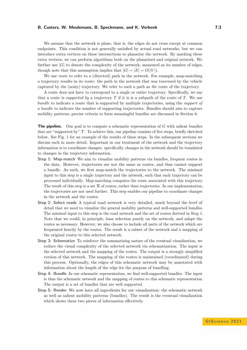
B. Custers, W. Meulemans, B. Speckmann, and K. Verbeek 7:3

We assume that the network is plane, that is, the edges do not cross except at commonendpoints. This condition is not generally satisfied by actual road networks, but we canintroduce extra vertices on these intersections to planarize the network. By marking theseextra vertices, we can perform algorithms both on the planarized and original network. Wefurther use |G| to denote the complexity of the network, measured as its number of edges,though note that this assumption implies that |G| = |E| = O(|V |).

We use route to refer to a (directed) path in the network. For example, map-matchinga trajectory results in its route: the path in the network that was traversed by the vehiclecaptured by the (noisy) trajectory. We refer to such a path as the route of the trajectory.

A route does not have to correspond to a single or entire trajectory. Specifically, we saythat a route is supported by a trajectory T if it is is a subpath of the route of T . We usebundle to indicate a route that is supported by multiple trajectories, using the support ofa bundle to indicate the number of supporting trajectories. Bundles should aim to capturemobility patterns; precise criteria to form meaningful bundles are discussed in Section 6.

The pipeline. Our goal is to compute a schematic representation of G with salient bundlesthat are “supported by” T . To achieve this, our pipeline consists of five steps, briefly sketchedbelow. See Fig. 1 for an example of the results of these steps. In the subsequent sections wediscuss each in more detail. Important in our treatment of the network and the trajectoryinformation is to coordinate changes: specifically, changes in the network should be translatedto changes in the trajectory information.Step 1: Map-match We aim to visualize mobility patterns via bundles, frequent routes in

the data. However, trajectories are not the same as routes, and thus cannot supporta bundle. As such, we first map-match the trajectories to the network. The minimalinput to this step is a single trajectory and the network, such that each trajectory can beprocessed individually. Map-matching computes the route associated with this trajectory.The result of this step is a set R of routes, rather than trajectories. In our implementation,the trajectories are not used further. This step enables our pipeline to coordinate changesin the network and the routes.

Step 2: Select roads A typical road network is very detailed, much beyond the level ofdetail that we need to visualize the general mobility patterns and well-supported bundles.The minimal input to this step is the road network and the set of routes derived in Step 1.Note that we could, in principle, base selection purely on the network, and adapt theroutes as necessary. However, we also choose to include all parts of the network which arefrequented heavily by the routes. The result is a subset of the network and a mapping ofthe original routes to this selected network.

Step 3: Schematize To reinforce the summarizing nature of the eventual visualization, wereduce the visual complexity of the selected network via schematization. The input isthe selected network and the mapping of the routes. The output is a strongly simplifiedversion of this network. The mapping of the routes is maintained (coordinated) duringthis process. Optionally, the edges of this schematic network may be annotated withinformation about the length of the edge for the purpose of bundling.

Step 4: Bundle In our schematic representation, we find well-supported bundles. The inputis thus the schematic network and the mapping of routes to this schematic representation.The output is a set of bundles that are well supported.

Step 5: Render We now have all ingredients for our visualization: the schematic networkas well as salient mobility patterns (bundles). The result is the eventual visualizationwhich shows these two pieces of information effectively.

GISc ience 2021

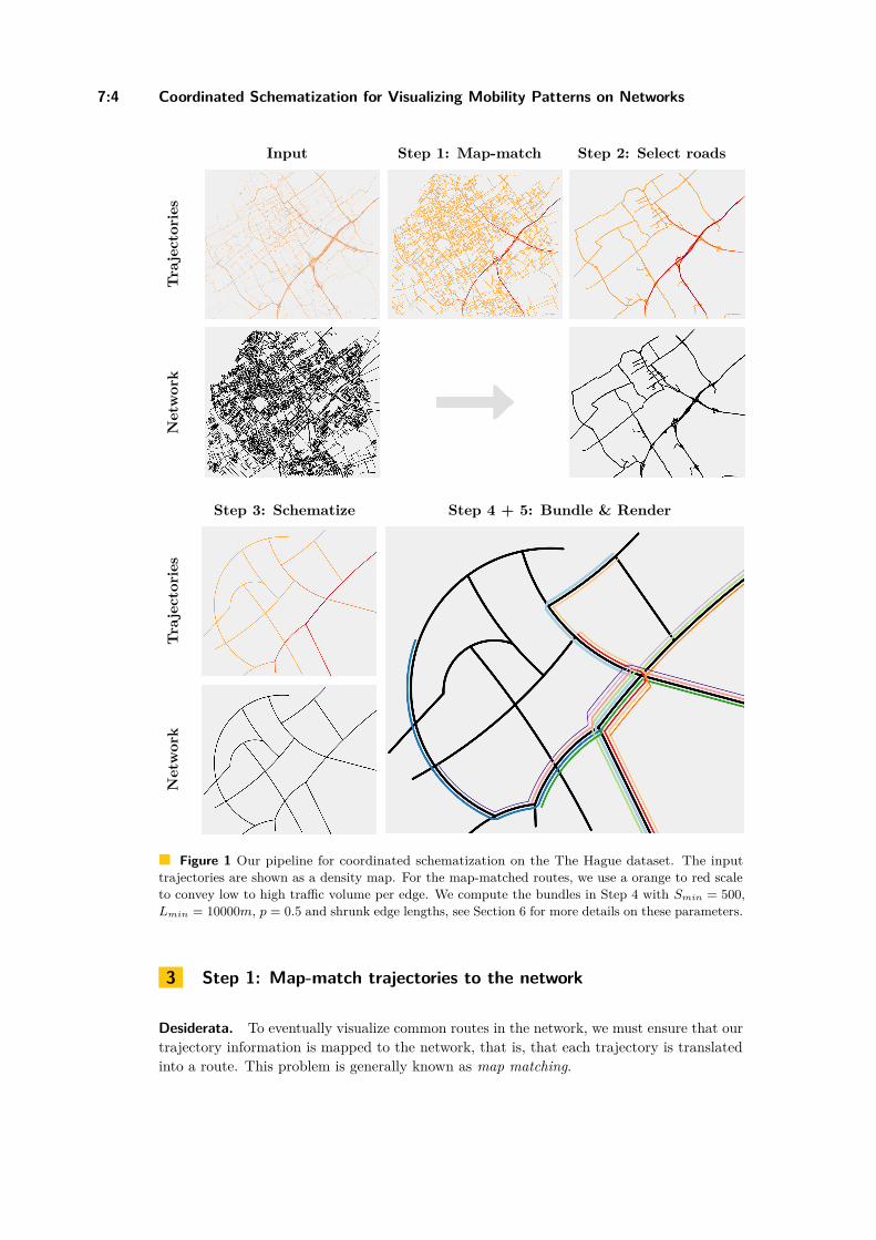
7:4 Coordinated Schematization for Visualizing Mobility Patterns on Networks

Input Step 1: Map-match Step 2: Select roadsT

raje

ctor

ies

Net

wor

k

Step 3: Schematize Step 4 + 5: Bundle & Render

Tra

ject

orie

sN

etw

ork

Figure 1 Our pipeline for coordinated schematization on the The Hague dataset. The inputtrajectories are shown as a density map. For the map-matched routes, we use a orange to red scaleto convey low to high traffic volume per edge. We compute the bundles in Step 4 with Smin = 500,Lmin = 10000m, p = 0.5 and shrunk edge lengths, see Section 6 for more details on these parameters.

3 Step 1: Map-match trajectories to the network

Desiderata. To eventually visualize common routes in the network, we must ensure that ourtrajectory information is mapped to the network, that is, that each trajectory is translatedinto a route. This problem is generally known as map matching.

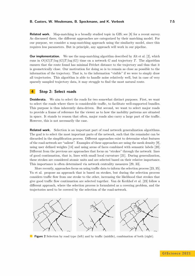
B. Custers, W. Meulemans, B. Speckmann, and K. Verbeek 7:5

Related work. Map-matching is a broadly studied topic in GIS; see [8] for a recent survey.As discussed there, the different approaches are categorized by their matching model. Forour purpose, we consider a map-matching approach using the similarity model, since thisrequires less parameters. But in principle, any approach will work in our pipeline.

Our implementation. We use the map-matching algorithm described by Alt et al. [2], whichruns in O(|G||T | log |G||T | log |G|) time on a network G and trajectory T . The algorithmensures that the route found has minimal Fréchet distance to the trajectory and thus that itis geometrically close. Our motivation for doing so is to remain as close as possible to theinformation of the trajectory. That is, to the information “visible” if we were to simply drawall trajectories. This algorithm is able to handle noise relatively well, but in case of verysparsely sampled trajectory data, it may struggle to find the most natural route.

4 Step 2: Select roads

Desiderata. We aim to select the roads for two somewhat distinct purposes. First, we wantto select the roads where there is considerable traffic, to facilitate well-supported bundles.This purpose is thus inherently data-driven. But second, we want to select major roadsto provide a frame of reference for the viewer as to how the mobility patterns are situatedin space. It stands to reason that often, major roads also carry a large part of the traffic.However, this is not necessarily the case.

Related work. Selection is an important part of road network generalization algorithms.The goal is to select the most important parts of the network, such that the remainder can bediscarded in the simplification process. Different approaches exist to determine what featuresof the road-network are “salient”. Examples of these approaches are using the mesh density [9],using user defined weights [14] and using areas of faces combined with semantic labels [20].Different from the previous are approaches that focus on “strokes” through the network: linesof good continuation, that is, lines with small local curvature [21]. During generalization,these strokes are considered atomic units and are selected based on their relative importance.This importance is often determined via network centrality measures [29, 33].

More recently, approaches focus on using traffic data to inform the selection process [23, 35].Yu et al. propose an approach that is based on strokes, but during the selection processconsiders traffic flow from one stroke to the other, increasing the likelihood that strokes thatgive good traffic flow continuation are selected together. Van de Kerkhof et al. [23] follow adifferent approach, where the selection process is formulated as a covering problem, and thetrajectories need to be covered by the selection of the road-network.

Figure 2 Selection by road type (left) and by traffic (middle), combination of both (right).

GISc ience 2021

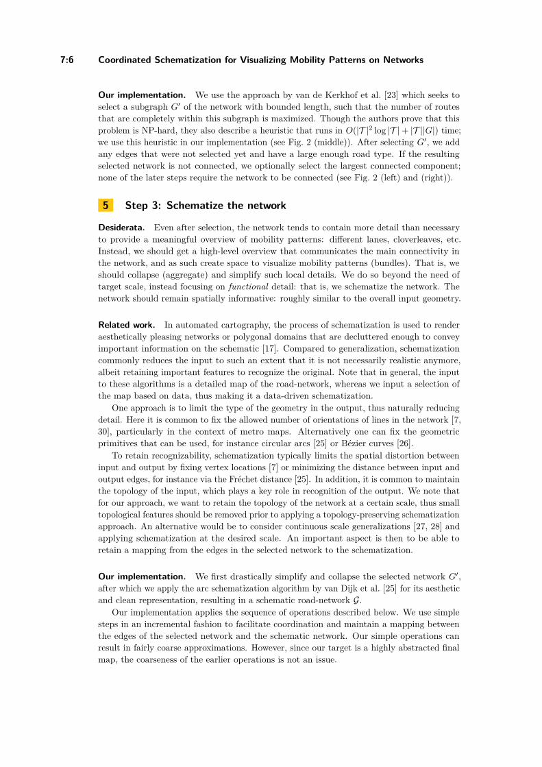
7:6 Coordinated Schematization for Visualizing Mobility Patterns on Networks

Our implementation. We use the approach by van de Kerkhof et al. [23] which seeks toselect a subgraph G′ of the network with bounded length, such that the number of routesthat are completely within this subgraph is maximized. Though the authors prove that thisproblem is NP-hard, they also describe a heuristic that runs in O(|T |2 log |T | + |T ||G|) time;we use this heuristic in our implementation (see Fig. 2 (middle)). After selecting G′, we addany edges that were not selected yet and have a large enough road type. If the resultingselected network is not connected, we optionally select the largest connected component;none of the later steps require the network to be connected (see Fig. 2 (left) and (right)).

5 Step 3: Schematize the network

Desiderata. Even after selection, the network tends to contain more detail than necessaryto provide a meaningful overview of mobility patterns: different lanes, cloverleaves, etc.Instead, we should get a high-level overview that communicates the main connectivity inthe network, and as such create space to visualize mobility patterns (bundles). That is, weshould collapse (aggregate) and simplify such local details. We do so beyond the need oftarget scale, instead focusing on functional detail: that is, we schematize the network. Thenetwork should remain spatially informative: roughly similar to the overall input geometry.

Related work. In automated cartography, the process of schematization is used to renderaesthetically pleasing networks or polygonal domains that are decluttered enough to conveyimportant information on the schematic [17]. Compared to generalization, schematizationcommonly reduces the input to such an extent that it is not necessarily realistic anymore,albeit retaining important features to recognize the original. Note that in general, the inputto these algorithms is a detailed map of the road-network, whereas we input a selection ofthe map based on data, thus making it a data-driven schematization.

One approach is to limit the type of the geometry in the output, thus naturally reducingdetail. Here it is common to fix the allowed number of orientations of lines in the network [7,30], particularly in the context of metro maps. Alternatively one can fix the geometricprimitives that can be used, for instance circular arcs [25] or Bézier curves [26].

To retain recognizability, schematization typically limits the spatial distortion betweeninput and output by fixing vertex locations [7] or minimizing the distance between input andoutput edges, for instance via the Fréchet distance [25]. In addition, it is common to maintainthe topology of the input, which plays a key role in recognition of the output. We note thatfor our approach, we want to retain the topology of the network at a certain scale, thus smalltopological features should be removed prior to applying a topology-preserving schematizationapproach. An alternative would be to consider continuous scale generalizations [27, 28] andapplying schematization at the desired scale. An important aspect is then to be able toretain a mapping from the edges in the selected network to the schematization.

Our implementation. We first drastically simplify and collapse the selected network G′,after which we apply the arc schematization algorithm by van Dijk et al. [25] for its aestheticand clean representation, resulting in a schematic road-network G.

Our implementation applies the sequence of operations described below. We use simplesteps in an incremental fashion to facilitate coordination and maintain a mapping betweenthe edges of the selected network and the schematic network. Our simple operations canresult in fairly coarse approximations. However, since our target is a highly abstracted finalmap, the coarseness of the earlier operations is not an issue.

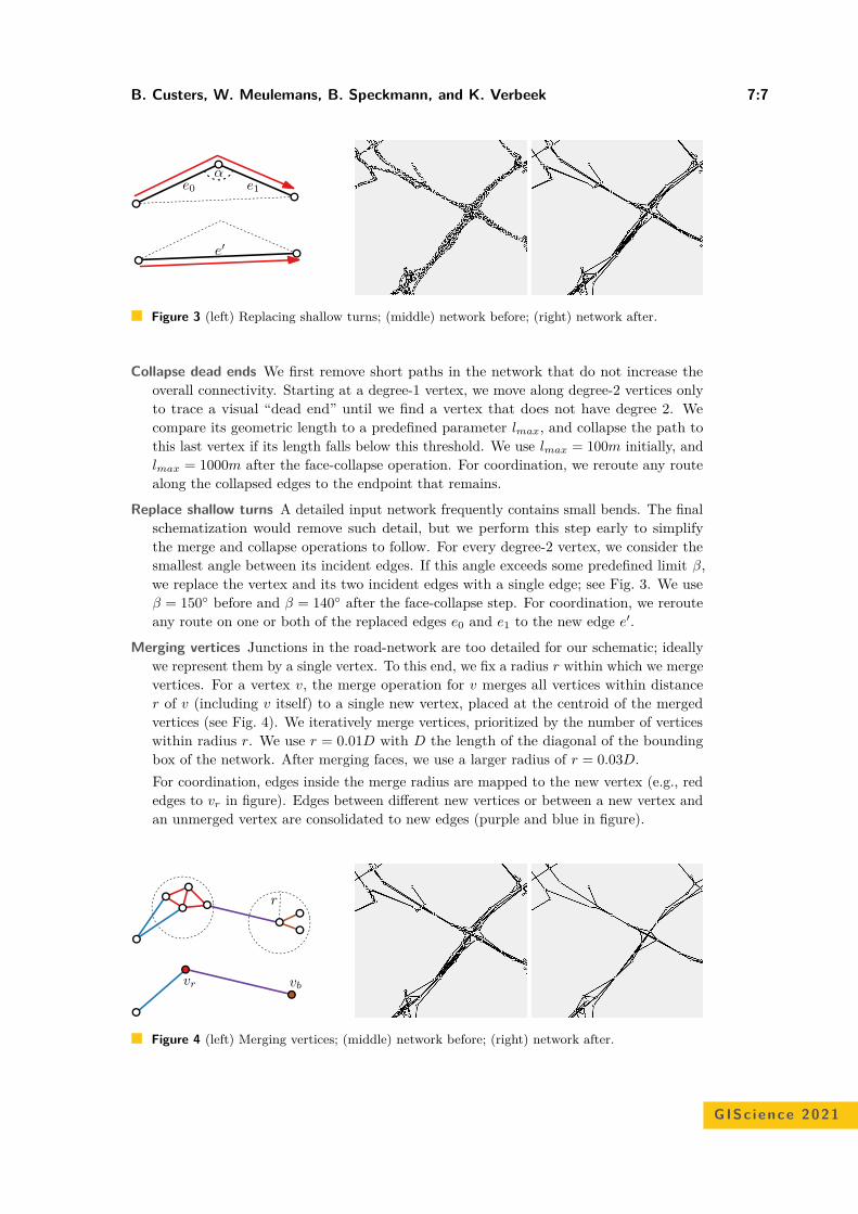
B. Custers, W. Meulemans, B. Speckmann, and K. Verbeek 7:7

e0 e1

e′

α

Figure 3 (left) Replacing shallow turns; (middle) network before; (right) network after.

Collapse dead ends We first remove short paths in the network that do not increase theoverall connectivity. Starting at a degree-1 vertex, we move along degree-2 vertices onlyto trace a visual “dead end” until we find a vertex that does not have degree 2. Wecompare its geometric length to a predefined parameter lmax, and collapse the path tothis last vertex if its length falls below this threshold. We use lmax = 100m initially, andlmax = 1000m after the face-collapse operation. For coordination, we reroute any routealong the collapsed edges to the endpoint that remains.

Replace shallow turns A detailed input network frequently contains small bends. The finalschematization would remove such detail, but we perform this step early to simplifythe merge and collapse operations to follow. For every degree-2 vertex, we consider thesmallest angle between its incident edges. If this angle exceeds some predefined limit β,we replace the vertex and its two incident edges with a single edge; see Fig. 3. We useβ = 150 before and β = 140 after the face-collapse step. For coordination, we rerouteany route on one or both of the replaced edges e0 and e1 to the new edge e′.

Merging vertices Junctions in the road-network are too detailed for our schematic; ideallywe represent them by a single vertex. To this end, we fix a radius r within which we mergevertices. For a vertex v, the merge operation for v merges all vertices within distancer of v (including v itself) to a single new vertex, placed at the centroid of the mergedvertices (see Fig. 4). We iteratively merge vertices, prioritized by the number of verticeswithin radius r. We use r = 0.01D with D the length of the diagonal of the boundingbox of the network. After merging faces, we use a larger radius of r = 0.03D.For coordination, edges inside the merge radius are mapped to the new vertex (e.g., rededges to vr in figure). Edges between different new vertices or between a new vertex andan unmerged vertex are consolidated to new edges (purple and blue in figure).

vr vb

r

Figure 4 (left) Merging vertices; (middle) network before; (right) network after.

GISc ience 2021

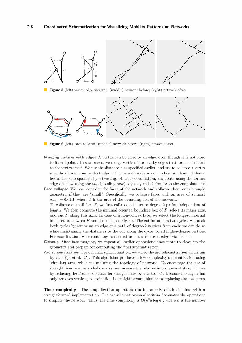
7:8 Coordinated Schematization for Visualizing Mobility Patterns on Networks

ev

e′0

e′1v

Figure 5 (left) vertex-edge merging; (middle) network before; (right) network after.

Figure 6 (left) Face collapse; (middle) network before; (right) network after.

Merging vertices with edges A vertex can be close to an edge, even though it is not closeto its endpoints. In such cases, we merge vertices into nearby edges that are not incidentto the vertex itself. We use the distance r as specified earlier, and try to collapse a vertexv to the closest non-incident edge e that is within distance r, where we demand that v

lies in the slab spanned by e (see Fig. 5). For coordination, any route using the formeredge e is now using the two (possibly new) edges e′

0 and e′1 from v to the endpoints of e.

Face collapse We now consider the faces of the network and collapse them onto a singlegeometry, if they are “small”. Specifically, we collapse faces with an area of at mostamax = 0.01A, where A is the area of the bounding box of the network.To collapse a small face F , we first collapse all interior degree-2 paths, independent oflength. We then compute the minimal oriented bounding box of F , select its major axis,and cut F along this axis. In case of a non-convex face, we select the longest internalintersection between F and the axis (see Fig. 6). The cut introduces two cycles; we breakboth cycles by removing an edge or a path of degree-2 vertices from each; we can do sowhile maintaining the distances to the cut along the cycle for all higher-degree vertices.For coordination, we reroute any route that used the removed edges via the cut.

Cleanup After face merging, we repeat all earlier operations once more to clean up thegeometry and prepare for computing the final schematization.

Arc schematization For our final schematization, we chose the arc schematization algorithmby van Dijk et al. [25]. This algorithm produces a low complexity schematization using(circular) arcs, while maintaining the topology of network. To encourage the use ofstraight lines over very shallow arcs, we increase the relative importance of straight linesby reducing the Fréchet distance for straight lines by a factor 0.3. Because this algorithmonly removes vertices, coordination is straightforward, similar to replacing shallow turns.

Time complexity. The simplification operators run in roughly quadratic time with astraightforward implementation. The arc schematization algorithm dominates the operationsto simplify the network. Thus, the time complexity is O(n2h log n), where h is the number

B. Custers, W. Meulemans, B. Speckmann, and K. Verbeek 7:9

of vertices with degree higher than three in the input simplification and n the number ofvertices, which is greatly reduced from the input at this point. Coordinating the changesbetween the road network and a trajectory T takes roughly O(|G||T |).

6 Step 4: Detect bundles

Desiderata. We aim to detect bundles that are well-supported by the routes to provideinsight into the overall mobility patterns. As such, we identify two desired properties ofa bundle. First, it has to be supported by many routes. Specifically, we do not want abundle representing a single trajectory (potentially an outlier), but rather the commonbehavior. Second, a bundle should be long in terms of (geometric) length. We aim to showmobility patterns that describe how vehicles move through the space. A long bundle ismore descriptive of behavior than a short one; in the extreme case, a short bundle (even orespecially if it is supported by many routes) may consist of one single edge (road segment),which does not help to communicate patterns beyond the existence of considerable localtraffic. That is, we want to find long bundles that are supported by many routes.

As we aim to visualize not one but multiple bundles simultaneously, we further use threecriteria to assess a set of bundles. First, we restrict our attention to maximal bundles only.That is, we consider only bundles to which we cannot add another route for its support, butspecifically also not increase its length without having to reduce its support. Second, wegenerally want to see patterns of mobility that are spatially diverse: we prefer having bundlesthrough different parts of the network, if the trajectories allow them. That is, we would liketo avoid overlap between bundles as overlap communicates the same (local) behavior.

Third, a bundle fully contained within another may not provide much extra insight intomobility beyond showing a higher support for the contained route. We call a set of bundlescontainment-free if no bundle is a subroute of another. Note that containment-free bundlesare not necessarily overlap-free and thus this is different from spatial diversity. Overlap-freebundles are containment-free, but we do not interpret spatial diversity as strict overlap-free.

In a containment-free set of maximal bundles each route may still support multiplebundles. If these are disjoint bundles, then we accept this as a bundle. However, as we are toeventually visualize the bundles, it may be misleading if well-supported bundles that sharean edge are only well-supported because they share many trajectories. Thus, we choose tocount the support for bundles in a disjoint manner: that is, routes through the overlap ofbundles can be counted to support only one of these. We refer to this as the disjoint support.

Finally, note that we consider the network bidirectional, in the sense that each edge ispresent twice, once for each direction of travel. The considerations above should consider thedirection of travel. That is, a bundle is directed and can, for example, only be supportedby routes in the same direction. Two bundles that use the same set of edges, but travel inopposite direction, would hence be considered overlap-free.

Related work. Our bundling is closely related to finding groups of trajectories and findingrepresentatives of trajectories, so-called centers. In the context of spatio-temporal data,grouping structures are used to find common patterns of mobility [5]. The groups that areconstructed essentially are trajectories that move close together for a sufficient amount oftime and with enough members in the group. Since we work with map-matched trajectories,we consider routes close when they share edges in the network, and we require bundles tohave at least some minimum length.

Note that finding a group does not directly result in finding a representation for thebehavior of the group. To represent the behavior of groups, a common approach is to clustertrajectories according to some metric, resulting in centers describing common behaviour for

GISc ience 2021

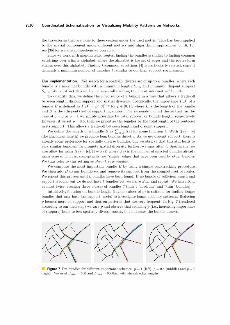
7:10 Coordinated Schematization for Visualizing Mobility Patterns on Networks

the trajectories that are close to these centers under the used metric. This has been appliedto the spatial component under different metrics and algorithmic approaches [6, 16, 18];see [36] for a more comprehensive overview.

Since we work with map-matched routes, finding the bundles is similar to finding commonsubstrings over a finite alphabet, where the alphabet is the set of edges and the routes formstrings over this alphabet. Finding k-common substrings [4] is particularly related, since itdemands a minimum number of matches k, similar to our high support requirement.

Our implementation. We search for a spatially diverse set of up to k bundles, where eachbundle is a maximal bundle with a minimum length Lmin and minimum disjoint supportSmin. We construct this set by incrementally adding the “most informative” bundle.

To quantify this, we define the importance of a bundle in a way that allows a trade-offbetween length, disjoint support and spatial diversity. Specifically, the importance I(B) of abundle B is defined as I(B) = Lp|S|1−p for p ∈ [0, 1], where L is the length of the bundleand S is the (disjoint) set of supporting routes. The rationale behind this is that, in thecase of p = 0 or p = 1 we simply prioritize by total support or bundle length, respectively.However, if we set p = 0.5, then we prioritize the bundles by the total length of the route-setin its support. This allows a trade-off between length and disjoint support.

We define the length of a bundle B as∑

e∈B ℓ(e) for some function ℓ. With ℓ(e) = |e|(the Euclidean length) we promote long bundles directly. As we use disjoint support, there isalready some preference for spatially diverse bundles, but we observe that this still leads tovery similar bundles. To promote spatial diversity further, we may alter ℓ. Specifically, wealso allow for using ℓ(e) = |e|/(1 + b(e)) where b(e) is the number of selected bundles alreadyusing edge e. That is, conceptually, we “shrink” edges that have been used by other bundles.We thus refer to this setting as shrunk edge lengths.

We compute the most important bundle B by using a simple backtracking procedure.We then add B to our bundle set and remove its support from the complete set of routes.We repeat this process until k bundles have been found. If no bundle of sufficient length andsupport is found but we do not have k bundles yet, we halve Smin and repeat. We halve Sminat most twice, creating three classes of bundles (“thick”, “medium” and “thin” bundles).

Intuitively, focusing on bundle length (higher values of p) is suitable for finding longerbundles that may have less support; useful to investigate longer mobility patterns. Reducingp focuses more on support and thus on patterns that are very frequent. In Fig. 7 (renderedaccording to our final step) we vary p and observe that reducing p (i.e., increasing importanceof support) leads to less spatially diverse routes, but increases the bundle classes.

Figure 7 Ten bundles for different importance schemes: p = 1 (left), p = 0.5 (middle) and p = 0(right). We used Smin = 500 and Lmin = 6000m, with shrunk edge lengths.

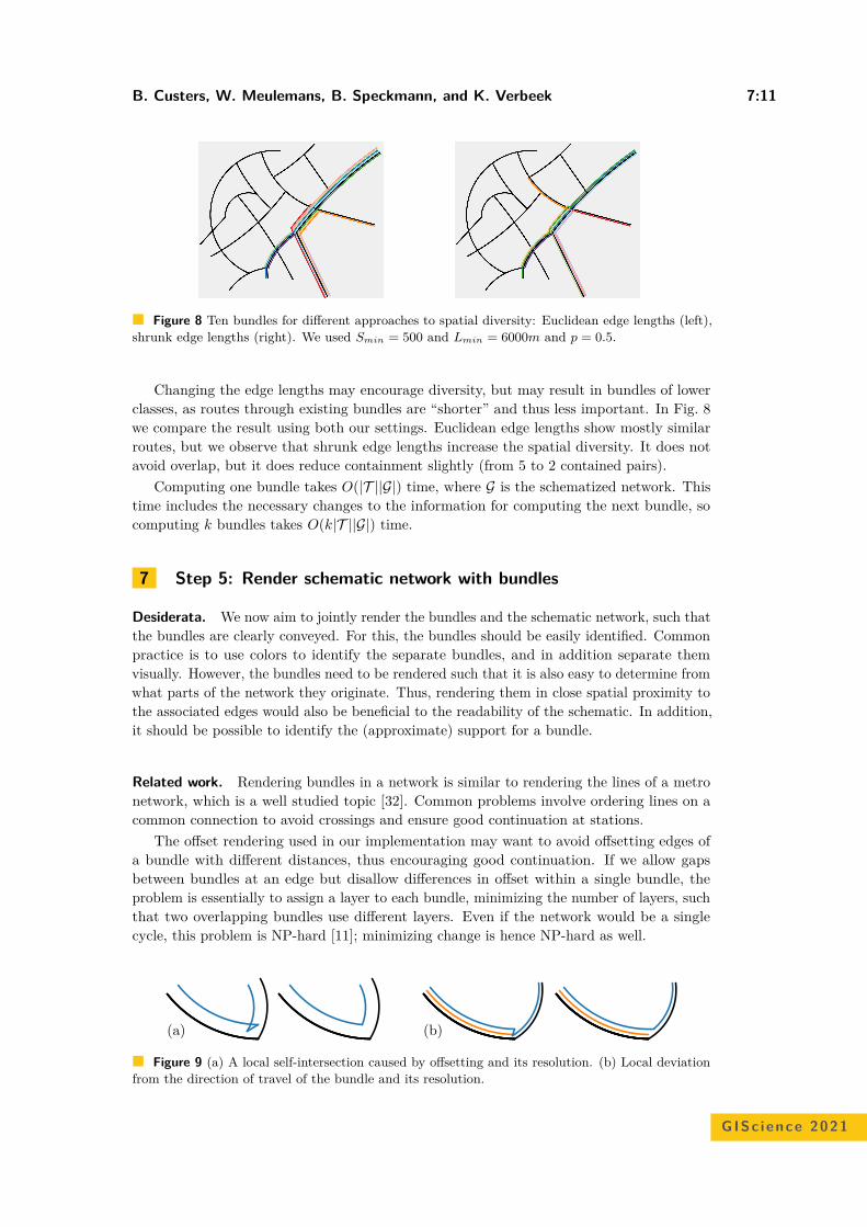
B. Custers, W. Meulemans, B. Speckmann, and K. Verbeek 7:11

Figure 8 Ten bundles for different approaches to spatial diversity: Euclidean edge lengths (left),shrunk edge lengths (right). We used Smin = 500 and Lmin = 6000m and p = 0.5.

Changing the edge lengths may encourage diversity, but may result in bundles of lowerclasses, as routes through existing bundles are “shorter” and thus less important. In Fig. 8we compare the result using both our settings. Euclidean edge lengths show mostly similarroutes, but we observe that shrunk edge lengths increase the spatial diversity. It does notavoid overlap, but it does reduce containment slightly (from 5 to 2 contained pairs).

Computing one bundle takes O(|T ||G|) time, where G is the schematized network. Thistime includes the necessary changes to the information for computing the next bundle, socomputing k bundles takes O(k|T ||G|) time.

7 Step 5: Render schematic network with bundles

Desiderata. We now aim to jointly render the bundles and the schematic network, such thatthe bundles are clearly conveyed. For this, the bundles should be easily identified. Commonpractice is to use colors to identify the separate bundles, and in addition separate themvisually. However, the bundles need to be rendered such that it is also easy to determine fromwhat parts of the network they originate. Thus, rendering them in close spatial proximity tothe associated edges would also be beneficial to the readability of the schematic. In addition,it should be possible to identify the (approximate) support for a bundle.

Related work. Rendering bundles in a network is similar to rendering the lines of a metronetwork, which is a well studied topic [32]. Common problems involve ordering lines on acommon connection to avoid crossings and ensure good continuation at stations.

The offset rendering used in our implementation may want to avoid offsetting edges ofa bundle with different distances, thus encouraging good continuation. If we allow gapsbetween bundles at an edge but disallow differences in offset within a single bundle, theproblem is essentially to assign a layer to each bundle, minimizing the number of layers, suchthat two overlapping bundles use different layers. Even if the network would be a singlecycle, this problem is NP-hard [11]; minimizing change is hence NP-hard as well.

(a) (b)

Figure 9 (a) A local self-intersection caused by offsetting and its resolution. (b) Local deviationfrom the direction of travel of the bundle and its resolution.

GISc ience 2021

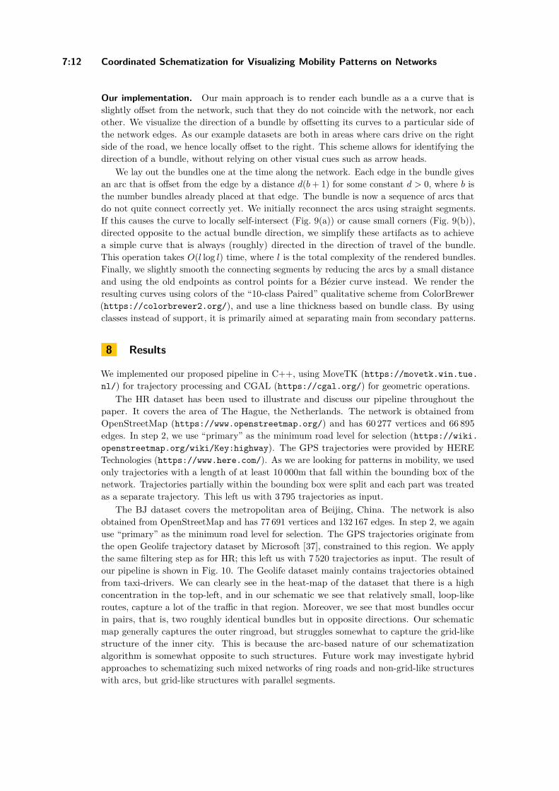
7:12 Coordinated Schematization for Visualizing Mobility Patterns on Networks

Our implementation. Our main approach is to render each bundle as a a curve that isslightly offset from the network, such that they do not coincide with the network, nor eachother. We visualize the direction of a bundle by offsetting its curves to a particular side ofthe network edges. As our example datasets are both in areas where cars drive on the rightside of the road, we hence locally offset to the right. This scheme allows for identifying thedirection of a bundle, without relying on other visual cues such as arrow heads.

We lay out the bundles one at the time along the network. Each edge in the bundle givesan arc that is offset from the edge by a distance d(b + 1) for some constant d > 0, where b isthe number bundles already placed at that edge. The bundle is now a sequence of arcs thatdo not quite connect correctly yet. We initially reconnect the arcs using straight segments.If this causes the curve to locally self-intersect (Fig. 9(a)) or cause small corners (Fig. 9(b)),directed opposite to the actual bundle direction, we simplify these artifacts as to achievea simple curve that is always (roughly) directed in the direction of travel of the bundle.This operation takes O(l log l) time, where l is the total complexity of the rendered bundles.Finally, we slightly smooth the connecting segments by reducing the arcs by a small distanceand using the old endpoints as control points for a Bézier curve instead. We render theresulting curves using colors of the “10-class Paired” qualitative scheme from ColorBrewer(https://colorbrewer2.org/), and use a line thickness based on bundle class. By usingclasses instead of support, it is primarily aimed at separating main from secondary patterns.

8 Results

We implemented our proposed pipeline in C++, using MoveTK (https://movetk.win.tue.nl/) for trajectory processing and CGAL (https://cgal.org/) for geometric operations.

The HR dataset has been used to illustrate and discuss our pipeline throughout thepaper. It covers the area of The Hague, the Netherlands. The network is obtained fromOpenStreetMap (https://www.openstreetmap.org/) and has 60 277 vertices and 66 895edges. In step 2, we use “primary” as the minimum road level for selection (https://wiki.openstreetmap.org/wiki/Key:highway). The GPS trajectories were provided by HERETechnologies (https://www.here.com/). As we are looking for patterns in mobility, we usedonly trajectories with a length of at least 10 000m that fall within the bounding box of thenetwork. Trajectories partially within the bounding box were split and each part was treatedas a separate trajectory. This left us with 3 795 trajectories as input.

The BJ dataset covers the metropolitan area of Beijing, China. The network is alsoobtained from OpenStreetMap and has 77 691 vertices and 132 167 edges. In step 2, we againuse “primary” as the minimum road level for selection. The GPS trajectories originate fromthe open Geolife trajectory dataset by Microsoft [37], constrained to this region. We applythe same filtering step as for HR; this left us with 7 520 trajectories as input. The result ofour pipeline is shown in Fig. 10. The Geolife dataset mainly contains trajectories obtainedfrom taxi-drivers. We can clearly see in the heat-map of the dataset that there is a highconcentration in the top-left, and in our schematic we see that relatively small, loop-likeroutes, capture a lot of the traffic in that region. Moreover, we see that most bundles occurin pairs, that is, two roughly identical bundles but in opposite directions. Our schematicmap generally captures the outer ringroad, but struggles somewhat to capture the grid-likestructure of the inner city. This is because the arc-based nature of our schematizationalgorithm is somewhat opposite to such structures. Future work may investigate hybridapproaches to schematizing such mixed networks of ring roads and non-grid-like structureswith arcs, but grid-like structures with parallel segments.

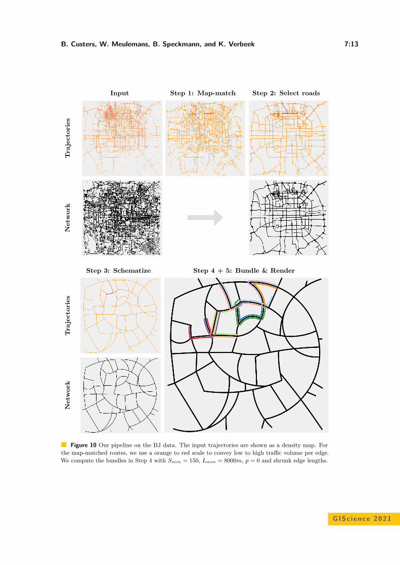
B. Custers, W. Meulemans, B. Speckmann, and K. Verbeek 7:13

Input Step 1: Map-match Step 2: Select roads

Tra

ject

orie

sN

etw

ork

Step 3: Schematize Step 4 + 5: Bundle & Render

Tra

ject

orie

sN

etw

ork

Figure 10 Our pipeline on the BJ data. The input trajectories are shown as a density map. Forthe map-matched routes, we use a orange to red scale to convey low to high traffic volume per edge.We compute the bundles in Step 4 with Smin = 150, Lmin = 8000m, p = 0 and shrunk edge lengths.

GISc ience 2021

7:14 Coordinated Schematization for Visualizing Mobility Patterns on Networks

9 Discussion and future work

We propose a coordinated pipeline to create abstract visual summaries of mobility patternsin trajectory data. Our proof-of-concept implementation shows that the pipeline is feasibleand can fully automatically compute such schematic maps. The advantage of a pipelinedapproach is that we may improve upon steps individually to improve the eventual result.Below, we reflect on our choices in the pipeline design, and discuss future work.

Step order. We could in principle also map-match (step 1) after selection (step 2). However,this would not allow for a data-driven approach for selection. Moreover, this forces all trafficto the selected roads, which may hide information on traffic that does not follow the selected(major) roads. For HR, the data-driven selection seems to not have made a large impact onthe selected network; for BJ more extensive parts of the network were added because of thedata-driven selection. We leave to future work to investigate whether inversion of these stepsis able to provide meaningful visualizations.

Similarly, we may wonder whether we would want to detect bundles (step 4) beforeschematization (step 3). As schematization reduces the network complexity, it is moreefficient to do afterwards. It may distort distances, but we can keep track of the originaldistances if desired – note that aggregation in step 3 does not make each route in theschematic network map to precisely one route in the original network. Another reasonsupporting our choice for the given order is that schematization may further aggregate denseareas of the network. By bundling afterwards, the support for such bundles grows since theyare effectively representing more traffic that generally traverses the dense area in roughly thesame way. We believe that our choice helps in promoting spatial diversity, as dense areaswith low traffic per road may reduce to a single road with higher traffic. In light of our veryspatially uneven datasets, this seems desirable. However, we leave the full exploration of theimpact of this choice as future work.

Augmenting the schematic map. We split the map-matched trajectories according towhether or not the route is on the selected network. This leaves us with parts of thetrajectories that go through unselected parts of the network and are thus dropped from theschematic map. We intend to explore ways of visualizing these dropped subroutes to provideinformation on the traffic not part of the selected network. On a computational level, anapproach we see for this is to track these subroutes relative to the faces of an embedding ofthe network. This, however, demands that we meticulously keep track of what happens tothese faces during the simplification stages. But it also requires visual design: what do wewant to show of these dropped routes, and how does that combine with the shown bundles?

While our mapping between simplifications is discrete in nature, an interesting directionof research would be to extend this to continuous mappings, where routes are also allowedto start in the middle of edges. An appropriate map-matcher should also be selected, sincethe Fréchet map-matching approach maps only to full edges, though we expect the overallimpact of allowing continuous routes here to be minor, as it is performed on the original,detailed network. The primary question is how we can alter the schematization step to allowfor high-quality continuous mapping through aggregation and simplification of the network.

Using the schematic map. In our proposed pipeline, we do not incorporate the timecomponent of the input trajectories explicitly. Given that the schematic shows stronglyaggregated data in a concise way, we can easily use our approach to show small-multiples fordifferent time frames in the data set. This leaves open the question what the best selectionmethod of the road-network is in this case, which we defer to future work.

B. Custers, W. Meulemans, B. Speckmann, and K. Verbeek 7:15

Our method hides any of the effects of sampling and noise in the data, as well as thedeformation and aggregation that occurs in our pipeline, which may be unintuitive to endusers. Though the schematic appearance aims to implicitly convey such information, it maybe communicated more explicitly with additional uncertainty visualization, albeit at the costof added visual complexity.

The final schematization is strongly influenced by the selected parameters in steps of ourpipeline. We scale parameters by a typical size (e.g. bounding box diagonal or area) to beable to assign parameters independent of scale. Nevertheless, visualizing the impact of theparameters on the end result could help users pick appropriate values for their use cases.

References1 N. Adrienko and G. Adrienko. Spatial generalization and aggregation of massive movement

data. IEEE TVCG, 17(2):205–219, 2010. doi:10.1109/TVCG.2010.44.2 H. Alt, A. Efrat, G. Rote, and C. Wenk. Matching planar maps. Journal of Algorithms,

49(2):262–283, 2003. doi:10.1016/S0196-6774(03)00085-3.3 G. Andrienko, N. Andrienko, W. Chen, R. Maciejewski, and Y. Zhao. Visual Analytics

of Mobility and Transportation: State of the Art and Further Research Directions. IEEETransactions on Intelligent Transportation Systems, 18(8):2232–2249, 2017. doi:10.1109/TITS.2017.2683539.

4 M. Arnold and E. Ohlebusch. Linear time algorithms for generalizations of the longest commonsubstring problem. Algorithmica, 60(4):806–818, 2011. doi:10.1007/s00453-009-9369-1.

5 K. Buchin, M. Buchin, M. van Kreveld, B. Speckmann, and F. Staals. Trajectory groupingstructure. In WADS, pages 219–230, 2013. doi:10.1007/978-3-642-40104-6_19.

6 K. Buchin, A. Driemel, J. Gudmundsson, M. Horton, I. Kostitsyna, M. Löffler, and M. Struijs.Approximating (k, l)-center clustering for curves. In Proc. SODA, pages 2922–2938, 2019.doi:10.1137/1.9781611975482.181.

7 S. Cabello, M. de Berg, and M. van Kreveld. Schematization of networks. ComputationalGeometry, 30(3):223–238, 2005. doi:10.1016/j.comgeo.2004.11.002.

8 P. Chao, Y. Xu, W. Hua, and X. Zhou. A survey on map-matching algorithms. In ADC, pages121–133, 2020. doi:10.1007/978-3-030-39469-1_10.

9 J. Chen, Y. Hu, Z. Li, R. Zhao, and L. Meng. Selective omission of road features basedon mesh density for automatic map generalization. IJGIS, 23(8):1013–1032, 2009. doi:10.1080/13658810802070730.

10 W. Chen, F. Guo, and F.-Y. Wang. A survey of traffic data visualization. IEEE Transactions onIntelligent Transportation Systems, 16(6):2970–2984, 2015. doi:10.1109/TITS.2015.2436897.

11 M. Garey, D. Johnson, G. Miller, and C. Papadimitriou. The complexity of coloring circulararcs and chords. SIAM Journal on Algebraic Discrete Methods, 1(2):216–227, 1980. doi:10.1137/0601025.

12 H. Imai and M. Iri. Computational-geometric methods for polygonal approximations of acurve. Computer Vision, Graphics, and Image Processing, 36(1):31–41, 1986. doi:10.1016/S0734-189X(86)80027-5.

13 M.-J. Kraak. The Space-Time cube revisited from a Geovisualization perspective. In Proc.ICC, pages 1988–1996, 2003.

14 L. Kulik, M. Duckham, and M. Egenhofer. Ontology-driven map generalization. Journal ofVisual Languages & Computing, 16(3):245–267, 2005. doi:10.1016/j.jvlc.2005.02.001.

15 O. Lampe and H. Hauser. Interactive visualization of streaming data with kernel densityestimation. In Proc. IEEE PacificVis, pages 171–178, 2011. doi:10.1109/PACIFICVIS.2011.5742387.

16 J.-G. Lee, J. Han, and K.-Y. Whang. Trajectory clustering: a partition-and-group framework.In Proc. 2007 ACM SIGMOD, pages 593–604, 2007. doi:10.1145/1247480.1247546.

17 W. Meulemans. Similarity Measures and Algorithms for Cartographic Schematization. PhDthesis, TU Eindhoven, 2014. doi:10.6100/ir777493.

GISc ience 2021

7:16 Coordinated Schematization for Visualizing Mobility Patterns on Networks

18 A. Nath and E. Taylor. k-Median clustering under discrete Fréchet and Hausdorff distances,2020. arXiv:2004.00722.

19 R. Scheepens, N. Willems, H. van de Wetering, and J. van Wijk. Interactive visualization ofmultivariate trajectory data with density maps. In IEEE PacificVis, pages 147–154, 2011.doi:10.1109/PACIFICVIS.2011.5742384.

20 R. Šuba, M. Meijers, and P. van Oosterom. Continuous road network generalization throughoutall scales. ISPRS Journal of Geo-Information, 5(8):145, 2016. doi:10.3390/ijgi5080145.

21 R. Thomson. The ’stroke’ concept in geographic network generalization and analysis. In Progressin Spatial Data Handling, pages 681–697. Springer, 2006. doi:10.1007/3-540-35589-8_43.

22 C. Tominski, H. Schumann, G. Andrienko, and N. Andrienko. Stacking-based visualization oftrajectory attribute data. IEEE TVCG, 18(12):2565–2574, 2012. doi:10.1109/TVCG.2012.265.

23 M. van de Kerkhof, I. Kostitsyna, M. van Kreveld, M. Löffler, and T. Ophelders. Route-preserving road network generalization. In Proc. ACM SIGSPATIAL, pages 381–384, 2020.doi:10.1145/3397536.3422234.

24 S. van den Elzen and J. van Wijk. Multivariate network exploration and presentation: Fromdetail to overview via selections and aggregations. IEEE TVCG, 20(12):2310–2319, 2014.doi:10.1109/TVCG.2014.2346441.

25 T. van Dijk, A. van Goethem, J.-H. Haunert, W. Meulemans, and B. Speckmann. Map schemati-zation with circular arcs. In GIScience, pages 1–17, 2014. doi:10.1007/978-3-319-11593-1_1.

26 A. van Goethem, W. Meulemans, A. Reimer, H. Haverkort, and B. Speckmann. Topologicallysafe curved schematisation. The Cartographic Journal, 50(3):276–285, 2013. doi:10.1179/1743277413Y.0000000066.

27 M. van Kreveld. Smooth generalization for continuous zooming. In IGU, pages 2180–2185,2001. URL: https://icaci.org/files/documents/ICC_proceedings/ICC2001/icc2001/file/f13042.pdf.

28 P. van Oosterom. Variable-scale topological data structures suitable for progressive datatransfer: The GAP-face tree and GAP-edge forest. Cartography and Geographic InformationScience, 32(4):331–346, 2005. doi:10.1559/152304005775194782.

29 R. Weiss and R. Weibel. Road network selection for small-scale maps using an improvedcentrality-based algorithm. Journal of Spatial Information Science, 2014(9):71–99, 2014.doi:10.5311/JOSIS.2014.9.166.

30 A. Wolff. Drawing subway maps: A survey. Informatik-Forschung und Entwicklung, 22(1):23–44,2007. doi:10.1007/s00450-007-0036-y.

31 J. Wood, J. Dykes, and A. Slingsby. Visualisation of Origins, Destinations andFlows with OD maps. The Cartographic Journal, 47(2):117–129, 2010. doi:10.1179/000870410X12658023467367.

32 H.-Y. Wu, B. Niedermann, S. Takahashi, and M. Nöllenburg. A survey on computing schematicnetwork maps: The challenge to interactivity. In Proc. Schematic Mapping Workshop, 2019.URL: https://www.cg.tuwien.ac.at/research/publications/2019/wu-2019-smw/.

33 B. Yang, X. Luan, and Q. Li. Generating hierarchical strokes from urban street networksbased on spatial pattern recognition. IJGIS, 25(12):2025–2050, 2011. doi:10.1080/13658816.2011.570270.

34 Y. Yang, T. Dwyer, S. Goodwin, and K. Marriott. Many-to-many geographically-embeddedflow visualisation: An evaluation. IEEE TVCG, 23(1):411–420, 2016. doi:10.1109/TVCG.2016.2598885.

35 W. Yu, Y. Zhang, T. Ai, Q. Guan, Z. Chen, and H. Li. Road network generalization consideringtraffic flow patterns. IJGIS, 34(1):119–149, 2020. doi:10.1080/13658816.2019.1650936.

36 G. Yuan, P. Sun, J. Zhao, D. Li, and C. Wang. A review of moving object trajectoryclustering algorithms. Artificial Intelligence Review, 47(1):123–144, 2017. doi:10.1007/s10462-016-9477-7.

37 Y. Zheng, L. Zhang, X. Xie, and W.-Y. Ma. Mining interesting locations and travel sequencesfrom GPS trajectories. In Proc. WWW, pages 791–800, 2009. doi:10.1145/1526709.1526816.

Harmonious Simplification of IsolinesArthur van Goethem #

Eindhoven University of Technology, The Netherlands

Wouter Meulemans #

Eindhoven University of Technology, The Netherlands

Andreas Reimer #

Eindhoven University of Technology, The Netherlands

Bettina Speckmann #

Eindhoven University of Technology, The Netherlands

AbstractCurrent techniques for simplification focus on reducing complexity while maintaining the geometricsimilarity to the input. For isolines that jointly describe a scalar field, however, we postulatethat geometric similarity of each isoline separately is not sufficient. Rather, we need to maintainthe harmony between these isolines to make them visually relate and describe the structures ofthe underlying terrain. Based on principles of manual cartography, we propose an algorithm forsimplifying isolines while considering harmony explicitly. Our preliminary visual and quantitativeresults suggest that our algorithm is effective.

2012 ACM Subject Classification Information systems → Geographic information systems; Theoryof computation → Computational geometry

Keywords and phrases Simplification, isolines, harmony

Digital Object Identifier 10.4230/LIPIcs.GIScience.2021.II.8

Supplementary Material Software (Source Code): https://github.com/tue-alga/harmonious-simplification

Acknowledgements DEMs provided by the Byrd Polar and Climate Research Center and the PolarGeospatial Center under NSF-OPP awards 1543501, 1810976, 1542736, 1559691, 1043681, 1541332,0753663, 1548562, 1238993 and NASA award NNX10AN61G. Computer time provided through aBlue Waters Innovation Initiative. DEMs produced using data from DigitalGlobe, Inc.

1 Introduction

Isolines are among the most common and effective cartographic techniques for visualizingscalar field-type data, such as terrain, precipitation, air pressure or, more abstractly, traveltimes. Isolines as a visualization method share and mirror an aspect of fields themselves: onlythe multitude of isolines signifies the phenomenon and the objects that it comprises. A singlespot height is insufficient to understand the lay of the land, and equally insufficient is theindividual isoline. It follows naturally, that the visual and the geometric relationships betweenindividual, pairs, and groups of isolines are essential to their cartographic effectiveness.

Geographic data need to be represented at different scales for specific tasks. The processesthat transform the visualization of geographic datasets due to scale-changes are subsumedunder the term generalization. Our approach aims to partially capture interdependencies inthe form of “harmony” of isolines while generalizing them. Visual harmony as a concept alludesto neighboring isolines behaving in a similar manner where such behavior is warranted. Incartographic practice, questions of harmony used to be addressed by the human cartographer.Nowadays isolines are usually generated automatically by interpolation processes from scalarfields, with the most common example being Digital Terrain Models (DTM) [32]. As mostprogress in automated generalization has been made for topographic maps, research inautomatization of isolines so far has concentrated on the generalization of terrains, withsystems of contour lines being one of the major outputs [16].

© Arthur van Goethem, Wouter Meulemans, Andreas Reimer, and Bettina Speckmann;licensed under Creative Commons License CC-BY 4.0

11th International Conference on Geographic Information Science (GIScience 2021) – Part II.Editors: Krzysztof Janowicz and Judith A. Verstegen; Article No. 8; pp. 8:1–8:16

Leibniz International Proceedings in InformaticsSchloss Dagstuhl – Leibniz-Zentrum für Informatik, Dagstuhl Publishing, Germany

8:2 Harmonious Simplification of Isolines

There are two main advantages to generalizing isolines instead of resampling a scalar-field (usually a DTM) and then interpolate fresh isolines: (1) the ability to directly keeprelations intact within a multi-resolution database, and (2) the avoidance of visual jumpsand resampling artifacts. Consider, for example, a river which must always run throughthe deepest part of a valley and as such must be tied to the isolines. When resampling aDTM and generalizing the drainage polylines independently, the generalized rivers mightrun over the slopes of the freshly derived contour line system [25]. Hence, until a few yearsago, many national mapping agencies either kept their manually generalized isolines for theirexisting scale ranges and did not automatically derive them for production of topographicmaps, or employed sophisticated techniques to tie freshly generated contour lines to pertinentdatabase objects and/or the DTM (such as the GAEL-model for Object-Field RelationPreservation [9]). Such conflation methods are not applicable to most other scalar fields dueto lack of ancillary data. They have also been out of reach for most GIS users, althoughsome open-source plugins for DTM-based tasks have been released recently [25, 30].

Results and organization. In this paper we propose an algorithm to simplify a whole systemof vector isolines while considering harmony explicitly. In Section 1.1 below, we presenta framework which allows us to consider harmony as an element of cartographic merit ofsystems of contour lines. We describe our harmonious simplification algorithm in Section 2and present experimental results in Section 3. Our examples focus on contour lines, but wenote that our algorithm works with any isoline vector input.

Our method allows us to apply and refine many heretofore neglected design rules (suchas those related to harmony) for isoline systems. It also naturally supports animated morphsbetween scales without loss of connections. Last but not least, since our algorithm is targetedtowards vector data, it allows us to apply locally adaptive generalization.

1.1 HarmonyWhile the word harmony has a wide range of meanings, we are concerned only with harmonyin relation to isolines. On first sight, the harmonious visual interaction between isolineslooks like a lofty or imprecise concept. However, the notion that a pleasing and informativerepetition that goes beyond mere parallelism is a crucial design goal, permeates the literature.In Swiss cartographic debates of the early 20th century, harmony was explicitly named as anintermediary design goal, which directly influenced academic and production mountain andterrain cartography [27]. To move from the qualitative and aesthetic concept of harmony toactionable requirements, we derive the pertinent design rules from cartographic examplesand cartographic literature. From those design rules, we move on to measurable qualities.

The basic idea of our approach of conceptualizing harmony is a modification of the processused by Reimer [24] for deriving and modeling harmony for chorematic diagrams. Reimerfollows Goldman [13] and observes that the general merit of a map can be operationalized bylinking objective, measurable qualities to aesthetic qualities of varying abstractness. This isdone hierarchically: the general merit of a map is a function of its accuracy, expressiveness,and beauty, with originality an optional addition that may well be zero, and is indeedzero in our case. The first three are the first tier aesthetic qualities. To each of them,Reimer [24] links a number of second tier aesthetic qualities: more precise, but still notdirectly measurable. The third hierarchical tier then links measurable qualities to the secondtier. While the first and second tier are capturing evaluative concepts which apply to everycartographic expression, the third tier is specific to a type of map or map element. That is,

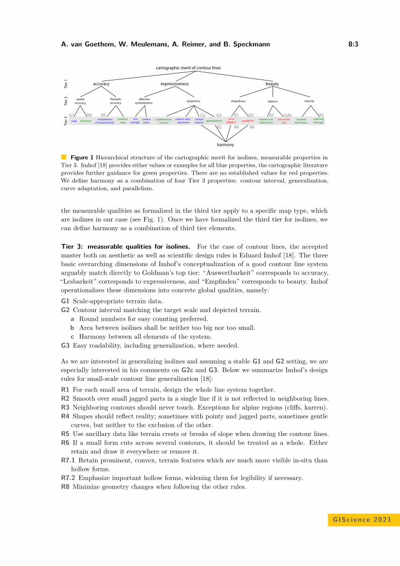
A. van Goethem, W. Meulemans, A. Reimer, and B. Speckmann 8:3

cartographic merit of contour lines

accuracy expressiveness beauty

spatialaccuracy

thematicaccuracy

poignancyeective

symbolization balanceshapeliness veracity

harmony

Tier

1Ti

er 2

Tier

3

scale distortioncompleteness

of measurementsstatistical

veritycontourinterval

contour value placement

line strength

contourcolors

curve adaption parallelism marginal

informationmatchingdrainage

area-to-lineratio

emphasis on salient forms

generalizationsupplementarycontours

G1 G2 G3 G2bR1 R2

R2

R7R5 R5

R4 R6

R8

Figure 1 Hierarchical structure of the cartographic merit for isolines, measurable properties inTier 3. Imhof [18] provides either values or examples for all blue properties, the cartographic literatureprovides further guidance for green properties. There are no established values for red properties.We define harmony as a combination of four Tier 3 properties: contour interval, generalization,curve adaptation, and parallelism.

the measurable qualities as formalized in the third tier apply to a specific map type, whichare isolines in our case (see Fig. 1). Once we have formalized the third tier for isolines, wecan define harmony as a combination of third tier elements.

Tier 3: measurable qualities for isolines. For the case of contour lines, the acceptedmaster both on aesthetic as well as scientific design rules is Eduard Imhof [18]. The threebasic overarching dimensions of Imhof’s conceptualization of a good contour line systemarguably match directly to Goldman’s top tier: “Auswertbarkeit” corresponds to accuracy,“Lesbarkeit” corresponds to expressiveness, and “Empfinden” corresponds to beauty. Imhofoperationalizes these dimensions into concrete global qualities, namely:G1 Scale-appropriate terrain data.G2 Contour interval matching the target scale and depicted terrain.

a Round numbers for easy counting preferred.b Area between isolines shall be neither too big nor too small.c Harmony between all elements of the system.

G3 Easy readability, including generalization, where needed.

As we are interested in generalizing isolines and assuming a stable G1 and G2 setting, we areespecially interested in his comments on G2c and G3. Below we summarize Imhof’s designrules for small-scale contour line generalization [18]:R1 For each small area of terrain, design the whole line system together.R2 Smooth over small jagged parts in a single line if it is not reflected in neighboring lines.R3 Neighboring contours should never touch. Exceptions for alpine regions (cliffs, karren).R4 Shapes should reflect reality; sometimes with pointy and jagged parts, sometimes gentle

curves, but neither to the exclusion of the other.R5 Use ancillary data like terrain crests or breaks of slope when drawing the contour lines.R6 If a small form cuts across several contours, it should be treated as a whole. Either

retain and draw it everywhere or remove it.R7.1 Retain prominent, convex, terrain features which are much more visible in-situ than

hollow forms.R7.2 Emphasize important hollow forms, widening them for legibility if necessary.R8 Minimize geometry changes when following the other rules.

GISc ience 2021

8:4 Harmonious Simplification of Isolines

For R3 Imhof specifically highlights that the whole line system must be brought under controland carefully adjusted, not just the overlapping pairs. This is a recurring theme with Imhof’sdesign rules which also appears in label placement. We populated Tier 3 with the measurableproperties discussed by Imhof, either in the form of rules or in the form of examples. Weadded statistical verity as well as marginal information.

Imhof does not necessarily provide evaluation functions or even parts thereof togetherwith his rules. An example would be G3b, namely the ratio of area to line, which must besomehow balanced, but no further information is provided. In Figure 1 we highlighted thoseTier 3 properties in blue for which Imhof gives sufficient guidance. We further highlightedthose properties in green for which sufficient guidance can be found in the cartographicliterature. There remain three properties for which Imhof presents rules, but not sufficientguidance, namely curve adaption, parallelism, and area to line ratio.

We are now ready to define harmony of isolines: a melange of elements of poignancyand shapeliness. Following the hierarchy, harmony is potentially measurable by evaluationfunctions for generalization solutions, curve adoption and parallelism.

1.2 Related workA very good overview until 2014 of automated terrain generalization, of which contour linegeneration is a subset, can be found in [16]. Since then, recent work was done, for example,on isobath generalization [15, 28], continuous generalization via morphing [10], improvingconflation of raster DTMs with contour lines [25, 30] and generation of supplementary contourlines [26]. These examples highlight a growing interest into automated sea-chart production,online mapping and continued support for NMA-demand via ancillary data-driven processesbased on DTMs for multiple resolution databases. Isobaths are often considered a specialcase, due to the peculiar needs for safety constraints [15] as well as being not entirely treatedas representations of a continuous scalar field but rather discrete maritime objects. Althoughdirect generalization of isobaths from other isobaths in the vector realm is more commonthan in current dry-land cartography, they are thus not too much concerned with how theindividual line shapes interact. Current morphing approaches such as [10] use a vertexmatching between origin and target scale and then interpolate on that matching, with fewregards to cartographic design rules.

Moreover, most proposed techniques for the simplification of isolines (e.g., [10, 20]) focuson individual isolines without explicitly considering the relationship between adjacent isolines.Recently, van Goethem et al. [11] proposed a technique for simultaneous simplification ofisolines with a focus on parallelism. They strengthen the paralellism between adjacent isolineswhile simplifying the input. However, the relative positions of the vertices on adjacent isolinesis not explicitly taken into account, thereby addressing but one facet of harmony.

In recent years several automated simplification approaches have been proposed thatallow the introduction of new vertex locations to more closely approximate the originalinput at lower complexity simplifications. The potential new vertex positions are usuallylimited, for example using criteria such as maintaining local topology [7, 12], interpolationbetween scales [10], or using an underlying grid [23]. An alternative criterion that is oftenused is area preservation (e.g., [6, 12, 19, 22, 29, 31]). Area preservation mandates that thearea covered by the simplified feature is exactly equal to the area covered by the originalfeature. Area preservation ensures that features can not arbitrarily increase or decrease insize during the simplification process and can be used to significantly reduce the search spacefor new vertex positions. These criteria are often combined together with a standard stepto introduce new vertices. One of the more prominent techniques used for this is the edge

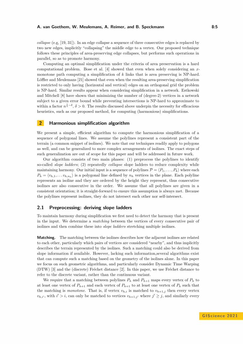
A. van Goethem, W. Meulemans, A. Reimer, and B. Speckmann 8:5

collapse (e.g, [19, 31]). In an edge collapse a sequence of three consecutive edges is replaced bytwo new edges, implicitly “collapsing” the middle edge to a vertex. Our proposed techniquefollows these principles of area-preserving edge collapses, but performs such operations inparallel, so as to promote harmony.

Computing an optimal simplification under the criteria of area preservation is a hardcomputational problem. Bose et al. [4] showed that even when solely considering an x-monotone path computing a simplification of k links that is area preserving is NP-hard.Löffler and Meulemans [21] showed that even when the resulting area-preserving simplificationis restricted to only having (horizontal and vertical) edges on an orthogonal grid the problemis NP-hard. Similar results appear when considering simplification in a network. Estkowskiand Mitchell [8] have shown that minimizing the number of (degree-2) vertices in a networksubject to a given error bound while preventing intersections is NP-hard to approximate towithin a factor n

15 −δ, δ > 0. The results discussed above underpin the necessity for efficacious

heuristics, such as our proposed method, for computing (harmonious) simplifications.

2 Harmonious simplification algorithm

We present a simple, efficient algorithm to compute the harmonious simplification of asequence of polygonal lines. We assume the polylines represent a consistent part of theterrain (a common snippet of isolines). We note that our techniques readily apply to polygonsas well, and can be generalized to more complex arrangements of isolines. The exact steps ofsuch generalization are out of scope for this paper and will be addressed in future work.

Our algorithm consists of two main phases: (1) preprocess the polylines to identifyso-called slope ladders; (2) repeatedly collapse slope ladders to reduce complexity whilemaintaining harmony. Our initial input is a sequence of polylines P = ⟨P1, . . . , Pk⟩ where eachPh = ⟨vh,1, . . . vh,nh

⟩ is a polygonal line defined by nh vertices in the plane. Each polylinerepresents an isoline and they are ordered by the height they represent, thus consecutiveisolines are also consecutive in the order. We assume that all polylines are given in aconsistent orientation; it is straight-forward to ensure this assumption is always met. Becausethe polylines represent isolines, they do not intersect each other nor self-intersect.

2.1 Preprocessing: deriving slope laddersTo maintain harmony during simplification we first need to detect the harmony that is presentin the input. We determine a matching between the vertices of every consecutive pair ofisolines and then combine these into slope ladders stretching multiple isolines.

Matching. The matching between the isolines describes how the adjacent isolines are relatedto each other, particularly which pairs of vertices are considered “nearby”, and thus implicitlydescribes the terrain represented by the isolines. Such a matching could also be derived fromslope information if available. However, lacking such information,several algorithms existthat can compute such a matching based on the geometry of the isolines alone. In this paperwe focus on such geometric algorithms, and particularly consider Dynamic Time Warping(DTW) [3] and the (discrete) Fréchet distance [2]. In this paper, we use Fréchet distance torefer to the discrete variant, rather than the continuous variant.

We require that a matching between polylines Ph and Ph+1 maps every vertex of Ph toat least one vertex of Ph+1 and each vertex of Ph+1 to at least one vertex of Ph such thatthe matching is monotone. That is, if vertex vh,i is matched to vh+1,j then every vertexvh,i′ , with i′ > i, can only be matched to vertices vh+1,j′ where j′ ≥ j, and similarly every

GISc ience 2021

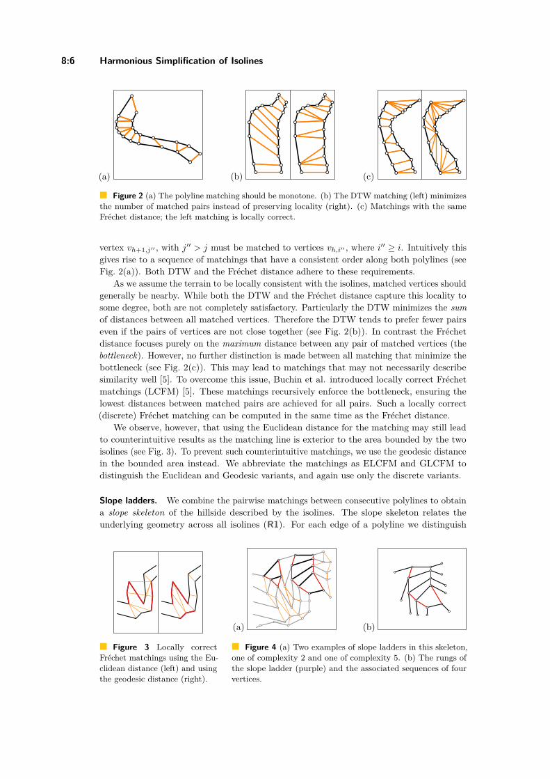
8:6 Harmonious Simplification of Isolines

(a) (b) (c)

Figure 2 (a) The polyline matching should be monotone. (b) The DTW matching (left) minimizesthe number of matched pairs instead of preserving locality (right). (c) Matchings with the sameFréchet distance; the left matching is locally correct.

vertex vh+1,j′′ , with j′′ > j must be matched to vertices vh,i′′ , where i′′ ≥ i. Intuitively thisgives rise to a sequence of matchings that have a consistent order along both polylines (seeFig. 2(a)). Both DTW and the Fréchet distance adhere to these requirements.

As we assume the terrain to be locally consistent with the isolines, matched vertices shouldgenerally be nearby. While both the DTW and the Fréchet distance capture this locality tosome degree, both are not completely satisfactory. Particularly the DTW minimizes the sumof distances between all matched vertices. Therefore the DTW tends to prefer fewer pairseven if the pairs of vertices are not close together (see Fig. 2(b)). In contrast the Fréchetdistance focuses purely on the maximum distance between any pair of matched vertices (thebottleneck). However, no further distinction is made between all matching that minimize thebottleneck (see Fig. 2(c)). This may lead to matchings that may not necessarily describesimilarity well [5]. To overcome this issue, Buchin et al. introduced locally correct Fréchetmatchings (LCFM) [5]. These matchings recursively enforce the bottleneck, ensuring thelowest distances between matched pairs are achieved for all pairs. Such a locally correct(discrete) Fréchet matching can be computed in the same time as the Fréchet distance.

We observe, however, that using the Euclidean distance for the matching may still leadto counterintuitive results as the matching line is exterior to the area bounded by the twoisolines (see Fig. 3). To prevent such counterintuitive matchings, we use the geodesic distancein the bounded area instead. We abbreviate the matchings as ELCFM and GLCFM todistinguish the Euclidean and Geodesic variants, and again use only the discrete variants.

Slope ladders. We combine the pairwise matchings between consecutive polylines to obtaina slope skeleton of the hillside described by the isolines. The slope skeleton relates theunderlying geometry across all isolines (R1). For each edge of a polyline we distinguish

Figure 3 Locally correctFréchet matchings using the Eu-clidean distance (left) and usingthe geodesic distance (right).

(a) (b)

Figure 4 (a) Two examples of slope ladders in this skeleton,one of complexity 2 and one of complexity 5. (b) The rungs ofthe slope ladder (purple) and the associated sequences of fourvertices.

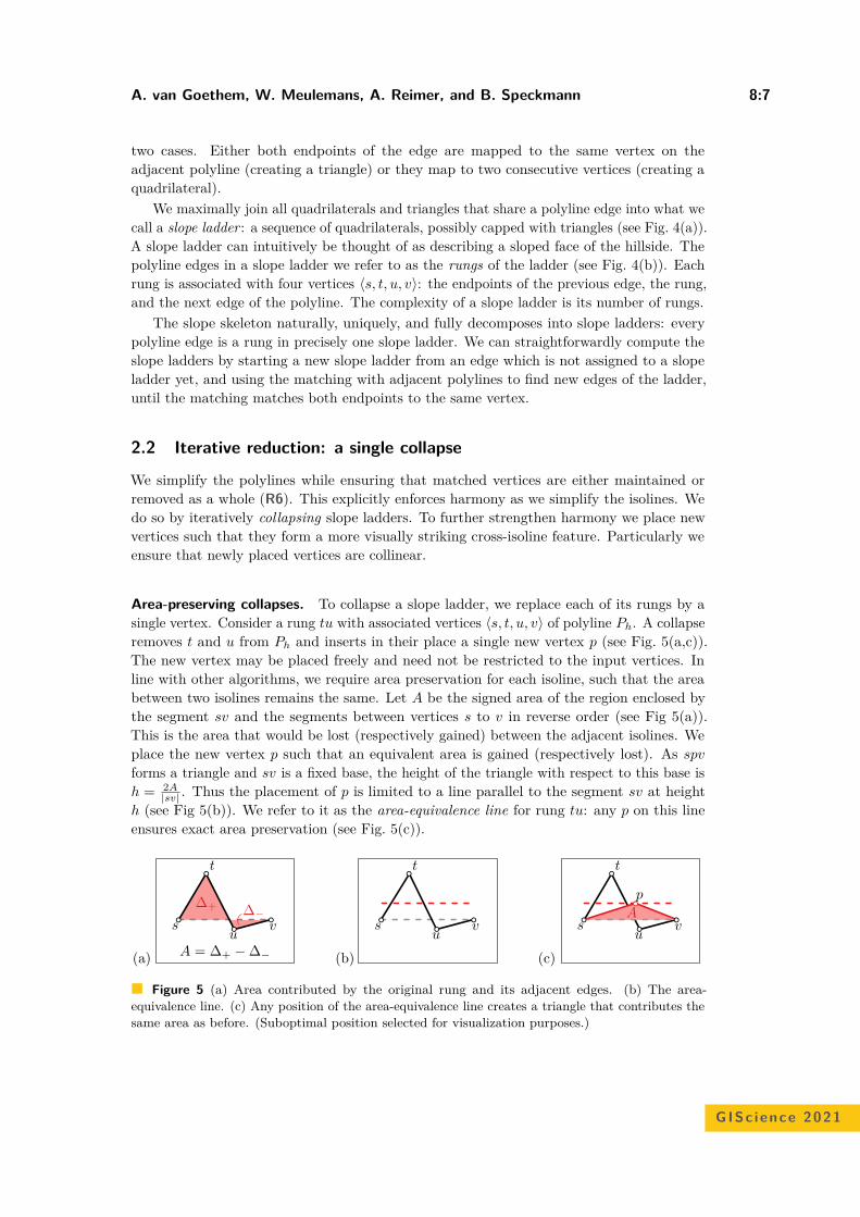
A. van Goethem, W. Meulemans, A. Reimer, and B. Speckmann 8:7

two cases. Either both endpoints of the edge are mapped to the same vertex on theadjacent polyline (creating a triangle) or they map to two consecutive vertices (creating aquadrilateral).

We maximally join all quadrilaterals and triangles that share a polyline edge into what wecall a slope ladder : a sequence of quadrilaterals, possibly capped with triangles (see Fig. 4(a)).A slope ladder can intuitively be thought of as describing a sloped face of the hillside. Thepolyline edges in a slope ladder we refer to as the rungs of the ladder (see Fig. 4(b)). Eachrung is associated with four vertices ⟨s, t, u, v⟩: the endpoints of the previous edge, the rung,and the next edge of the polyline. The complexity of a slope ladder is its number of rungs.

The slope skeleton naturally, uniquely, and fully decomposes into slope ladders: everypolyline edge is a rung in precisely one slope ladder. We can straightforwardly compute theslope ladders by starting a new slope ladder from an edge which is not assigned to a slopeladder yet, and using the matching with adjacent polylines to find new edges of the ladder,until the matching matches both endpoints to the same vertex.

2.2 Iterative reduction: a single collapse

We simplify the polylines while ensuring that matched vertices are either maintained orremoved as a whole (R6). This explicitly enforces harmony as we simplify the isolines. Wedo so by iteratively collapsing slope ladders. To further strengthen harmony we place newvertices such that they form a more visually striking cross-isoline feature. Particularly weensure that newly placed vertices are collinear.

Area-preserving collapses. To collapse a slope ladder, we replace each of its rungs by asingle vertex. Consider a rung tu with associated vertices ⟨s, t, u, v⟩ of polyline Ph. A collapseremoves t and u from Ph and inserts in their place a single new vertex p (see Fig. 5(a,c)).The new vertex may be placed freely and need not be restricted to the input vertices. Inline with other algorithms, we require area preservation for each isoline, such that the areabetween two isolines remains the same. Let A be the signed area of the region enclosed bythe segment sv and the segments between vertices s to v in reverse order (see Fig 5(a)).This is the area that would be lost (respectively gained) between the adjacent isolines. Weplace the new vertex p such that an equivalent area is gained (respectively lost). As spv

forms a triangle and sv is a fixed base, the height of the triangle with respect to this base ish = 2A

|sv| . Thus the placement of p is limited to a line parallel to the segment sv at heighth (see Fig 5(b)). We refer to it as the area-equivalence line for rung tu: any p on this lineensures exact area preservation (see Fig. 5(c)).

A = ∆+ − ∆−

s

∆+

t

uv

∆−

(a) (b)

s

t

uv

(c)

p

As

uv

t

Figure 5 (a) Area contributed by the original rung and its adjacent edges. (b) The area-equivalence line. (c) Any position of the area-equivalence line creates a triangle that contributes thesame area as before. (Suboptimal position selected for visualization purposes.)

GISc ience 2021

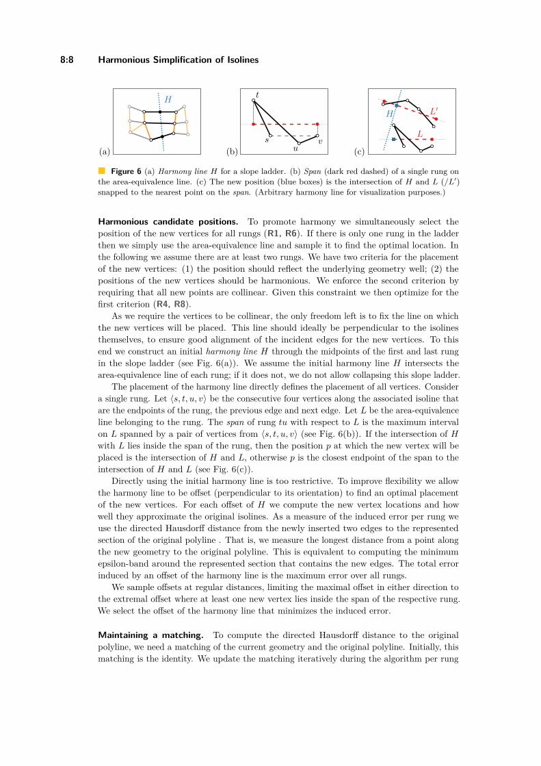
8:8 Harmonious Simplification of Isolines

(a)

H

(b)

t

uvs

(c)

L

H L′

Figure 6 (a) Harmony line H for a slope ladder. (b) Span (dark red dashed) of a single rung onthe area-equivalence line. (c) The new position (blue boxes) is the intersection of H and L (/L′)snapped to the nearest point on the span. (Arbitrary harmony line for visualization purposes.)

Harmonious candidate positions. To promote harmony we simultaneously select theposition of the new vertices for all rungs (R1, R6). If there is only one rung in the ladderthen we simply use the area-equivalence line and sample it to find the optimal location. Inthe following we assume there are at least two rungs. We have two criteria for the placementof the new vertices: (1) the position should reflect the underlying geometry well; (2) thepositions of the new vertices should be harmonious. We enforce the second criterion byrequiring that all new points are collinear. Given this constraint we then optimize for thefirst criterion (R4, R8).

As we require the vertices to be collinear, the only freedom left is to fix the line on whichthe new vertices will be placed. This line should ideally be perpendicular to the isolinesthemselves, to ensure good alignment of the incident edges for the new vertices. To thisend we construct an initial harmony line H through the midpoints of the first and last rungin the slope ladder (see Fig. 6(a)). We assume the initial harmony line H intersects thearea-equivalence line of each rung; if it does not, we do not allow collapsing this slope ladder.

The placement of the harmony line directly defines the placement of all vertices. Considera single rung. Let ⟨s, t, u, v⟩ be the consecutive four vertices along the associated isoline thatare the endpoints of the rung, the previous edge and next edge. Let L be the area-equivalenceline belonging to the rung. The span of rung tu with respect to L is the maximum intervalon L spanned by a pair of vertices from ⟨s, t, u, v⟩ (see Fig. 6(b)). If the intersection of H

with L lies inside the span of the rung, then the position p at which the new vertex will beplaced is the intersection of H and L, otherwise p is the closest endpoint of the span to theintersection of H and L (see Fig. 6(c)).

Directly using the initial harmony line is too restrictive. To improve flexibility we allowthe harmony line to be offset (perpendicular to its orientation) to find an optimal placementof the new vertices. For each offset of H we compute the new vertex locations and howwell they approximate the original isolines. As a measure of the induced error per rung weuse the directed Hausdorff distance from the newly inserted two edges to the representedsection of the original polyline . That is, we measure the longest distance from a point alongthe new geometry to the original polyline. This is equivalent to computing the minimumepsilon-band around the represented section that contains the new edges. The total errorinduced by an offset of the harmony line is the maximum error over all rungs.

We sample offsets at regular distances, limiting the maximal offset in either direction tothe extremal offset where at least one new vertex lies inside the span of the respective rung.We select the offset of the harmony line that minimizes the induced error.

Maintaining a matching. To compute the directed Hausdorff distance to the originalpolyline, we need a matching of the current geometry and the original polyline. Initially, thismatching is the identity. We update the matching iteratively during the algorithm per rung

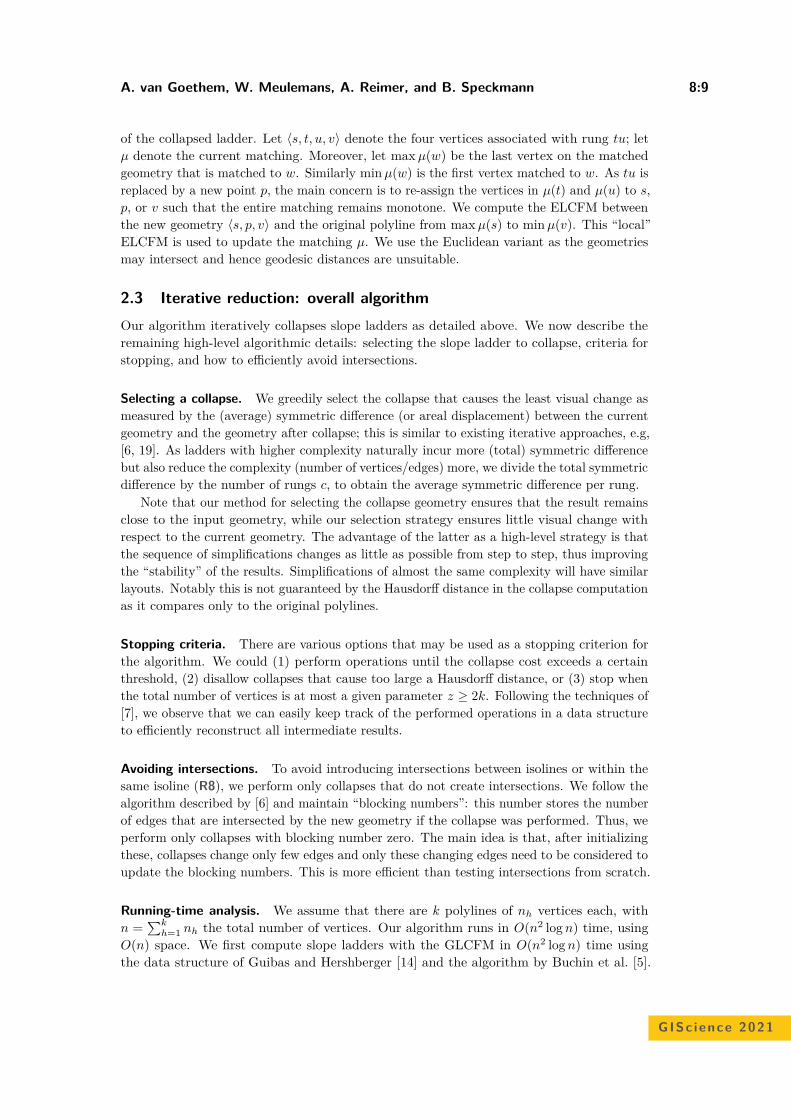
A. van Goethem, W. Meulemans, A. Reimer, and B. Speckmann 8:9

of the collapsed ladder. Let ⟨s, t, u, v⟩ denote the four vertices associated with rung tu; letµ denote the current matching. Moreover, let max µ(w) be the last vertex on the matchedgeometry that is matched to w. Similarly min µ(w) is the first vertex matched to w. As tu isreplaced by a new point p, the main concern is to re-assign the vertices in µ(t) and µ(u) to s,p, or v such that the entire matching remains monotone. We compute the ELCFM betweenthe new geometry ⟨s, p, v⟩ and the original polyline from max µ(s) to min µ(v). This “local”ELCFM is used to update the matching µ. We use the Euclidean variant as the geometriesmay intersect and hence geodesic distances are unsuitable.

2.3 Iterative reduction: overall algorithmOur algorithm iteratively collapses slope ladders as detailed above. We now describe theremaining high-level algorithmic details: selecting the slope ladder to collapse, criteria forstopping, and how to efficiently avoid intersections.

Selecting a collapse. We greedily select the collapse that causes the least visual change asmeasured by the (average) symmetric difference (or areal displacement) between the currentgeometry and the geometry after collapse; this is similar to existing iterative approaches, e.g,[6, 19]. As ladders with higher complexity naturally incur more (total) symmetric differencebut also reduce the complexity (number of vertices/edges) more, we divide the total symmetricdifference by the number of rungs c, to obtain the average symmetric difference per rung.

Note that our method for selecting the collapse geometry ensures that the result remainsclose to the input geometry, while our selection strategy ensures little visual change withrespect to the current geometry. The advantage of the latter as a high-level strategy is thatthe sequence of simplifications changes as little as possible from step to step, thus improvingthe “stability” of the results. Simplifications of almost the same complexity will have similarlayouts. Notably this is not guaranteed by the Hausdorff distance in the collapse computationas it compares only to the original polylines.

Stopping criteria. There are various options that may be used as a stopping criterion forthe algorithm. We could (1) perform operations until the collapse cost exceeds a certainthreshold, (2) disallow collapses that cause too large a Hausdorff distance, or (3) stop whenthe total number of vertices is at most a given parameter z ≥ 2k. Following the techniques of[7], we observe that we can easily keep track of the performed operations in a data structureto efficiently reconstruct all intermediate results.

Avoiding intersections. To avoid introducing intersections between isolines or within thesame isoline (R8), we perform only collapses that do not create intersections. We follow thealgorithm described by [6] and maintain “blocking numbers”: this number stores the numberof edges that are intersected by the new geometry if the collapse was performed. Thus, weperform only collapses with blocking number zero. The main idea is that, after initializingthese, collapses change only few edges and only these changing edges need to be considered toupdate the blocking numbers. This is more efficient than testing intersections from scratch.

Running-time analysis. We assume that there are k polylines of nh vertices each, withn =

∑kh=1 nh the total number of vertices. Our algorithm runs in O(n2 log n) time, using

O(n) space. We first compute slope ladders with the GLCFM in O(n2 log n) time usingthe data structure of Guibas and Hershberger [14] and the algorithm by Buchin et al. [5].

GISc ience 2021

8:10 Harmonious Simplification of Isolines

We then initialize all collapses in O(n2) using the approach of Alt et al. [1] to compute theHausdorff distance. Finally, we iteratively collapse the best slope ladder and update anyaffected ladders in total O(n2 log n) time.

3 Results and discussion

We implemented our algorithm1 and tested it with various isolines. We first qualitativelycompare the results on different sets of isolines through a visual exploration of the properties.We then quantitatively measure how well harmony is maintained using our method ofcollapsing slope ladders compared to simplifying each isoline separately.

We showcase and measure results for eight different inputs. The first are two digitizedtextbook examples, namely two sets of isolines used by Imhof to illustrate isoline generalizationpractices [18, page 155]; we denote these by IMS (slope) and IMH (hilltop). AH1 is a digitizedset of contour lines for the whole of Antarctica at 500m contour intervals. The other five aresnippets from the DEM of Antarctica [17], deriving isolines at a 150m contour interval usingQGIS v.3.16; we denote these snippets by AS1 through AS3 (slopes) and AH2 through AH3(hilltops). All inputs are illustrated in Fig. 7. The algorithm discussed considers polygonallines, hence for our experiments we open any closed isoline. Though out of scope, the conceptscan readily be extended to closed isolines and in future work this restriction will be lifted.

IMS1159 AS1442 AS21808 AS32071

IMH664 AH1584

AH21340

AH31580

Figure 7 Inputs used in this paper: four slopes (top) and four hilltops (bottom). Complexitiesrange from 442 (AS1) to 2071 (AS3). Red lines indicate where hilltops were opened into polylines.

3.1 Qualitative discussionExamples by Imhof. We start our visual investigation with IMH; see Fig. 8. We directlyobserve that the effect of harmonization is minor when the detail-level is high. Due to thelarge number of vertices in the simplification, the harmony is readily present as there aresufficient vertices to always have nearby vertices on the adjacent isoline. Isoline detail is theprimary factor. However, when we reduce the complexity further, the underlying patterns inthe isolines become emphasized through harmony. As vertices are placed at similar locations

1 https://github.com/tue-alga/harmonious-simplification (v0.1)

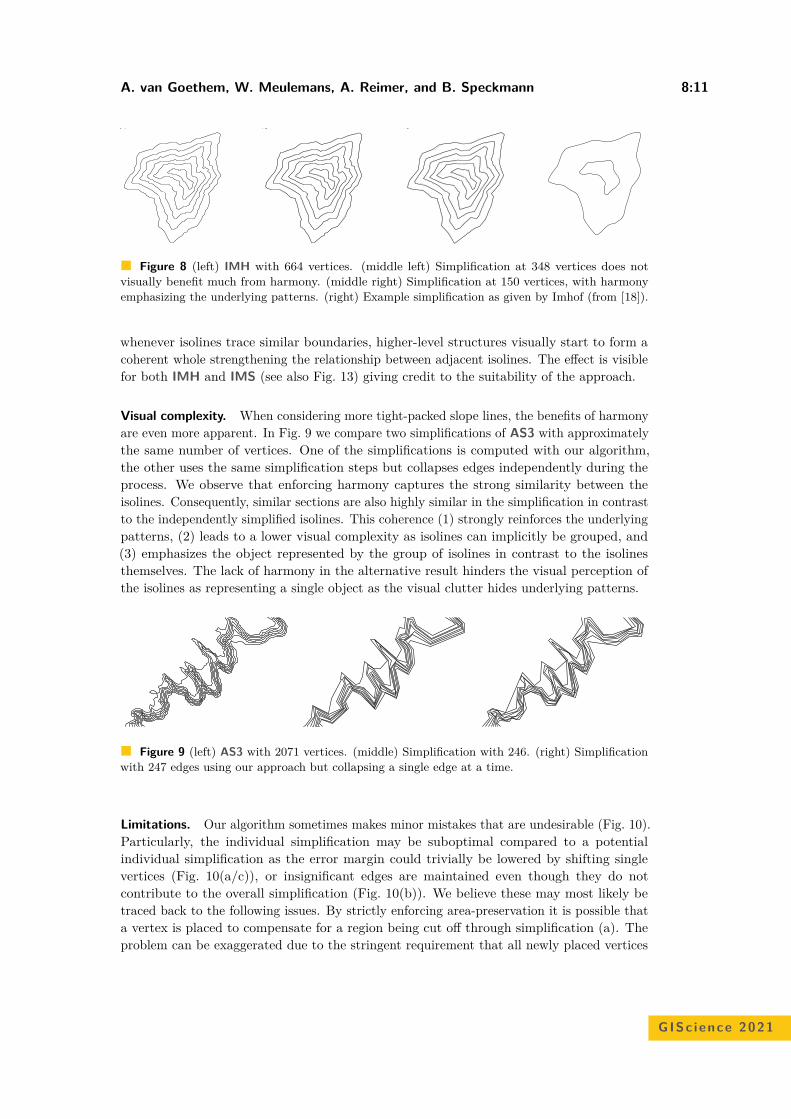
A. van Goethem, W. Meulemans, A. Reimer, and B. Speckmann 8:11

664 348 150

Figure 8 (left) IMH with 664 vertices. (middle left) Simplification at 348 vertices does notvisually benefit much from harmony. (middle right) Simplification at 150 vertices, with harmonyemphasizing the underlying patterns. (right) Example simplification as given by Imhof (from [18]).

whenever isolines trace similar boundaries, higher-level structures visually start to form acoherent whole strengthening the relationship between adjacent isolines. The effect is visiblefor both IMH and IMS (see also Fig. 13) giving credit to the suitability of the approach.

Visual complexity. When considering more tight-packed slope lines, the benefits of harmonyare even more apparent. In Fig. 9 we compare two simplifications of AS3 with approximatelythe same number of vertices. One of the simplifications is computed with our algorithm,the other uses the same simplification steps but collapses edges independently during theprocess. We observe that enforcing harmony captures the strong similarity between theisolines. Consequently, similar sections are also highly similar in the simplification in contrastto the independently simplified isolines. This coherence (1) strongly reinforces the underlyingpatterns, (2) leads to a lower visual complexity as isolines can implicitly be grouped, and(3) emphasizes the object represented by the group of isolines in contrast to the isolinesthemselves. The lack of harmony in the alternative result hinders the visual perception ofthe isolines as representing a single object as the visual clutter hides underlying patterns.

2071 246 247

Figure 9 (left) AS3 with 2071 vertices. (middle) Simplification with 246. (right) Simplificationwith 247 edges using our approach but collapsing a single edge at a time.

Limitations. Our algorithm sometimes makes minor mistakes that are undesirable (Fig. 10).Particularly, the individual simplification may be suboptimal compared to a potentialindividual simplification as the error margin could trivially be lowered by shifting singlevertices (Fig. 10(a/c)), or insignificant edges are maintained even though they do notcontribute to the overall simplification (Fig. 10(b)). We believe these may most likely betraced back to the following issues. By strictly enforcing area-preservation it is possible thata vertex is placed to compensate for a region being cut off through simplification (a). Theproblem can be exaggerated due to the stringent requirement that all newly placed vertices

GISc ience 2021

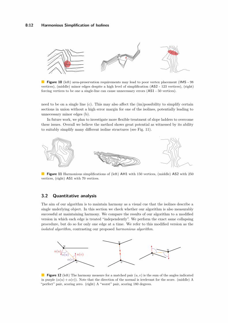
8:12 Harmonious Simplification of Isolines

Figure 10 (left) area-preservation requirements may lead to poor vertex placement (IMS - 98vertices), (middle) minor edges despite a high level of simplification (AS2 - 123 vertices), (right)forcing vertices to be one a single-line can cause unnecessary errors (AS1 - 50 vertices).

need to be on a single line (c). This may also affect the (im)possibility to simplify certainsections in union without a high error margin for one of the isolines, potentially leading tounnecessary minor edges (b).

In future work, we plan to investigate more flexible treatment of slope ladders to overcomethese issues. Overall we believe the method shows great potential as witnessed by its abilityto suitably simplify many different isoline structures (see Fig. 11).

150

250

70

Figure 11 Harmonious simplifications of (left) AH1 with 150 vertices, (middle) AS2 with 250vertices, (right) AS1 with 70 vertices.

3.2 Quantitative analysis

The aim of our algorithm is to maintain harmony as a visual cue that the isolines describe asingle underlying object. In this section we check whether our algorithm is also measurablysuccessful at maintaining harmony. We compare the results of our algorithm to a modifiedversion in which each edge is treated “independently”. We perform the exact same collapsingprocedure, but do so for only one edge at a time. We refer to this modified version as theisolated algorithm, contrasting our proposed harmonious algorithm.

n(u)n(v)

α(v)

α(u)

u

v

u

v

u

v

Figure 12 (left) The harmony measure for a matched pair (u, v) is the sum of the angles indicatedin purple (α(u) + α(v)). Note that the direction of the normal is irrelevant for the score. (middle) A“perfect” pair, scoring zero. (right) A “worst” pair, scoring 180 degrees.

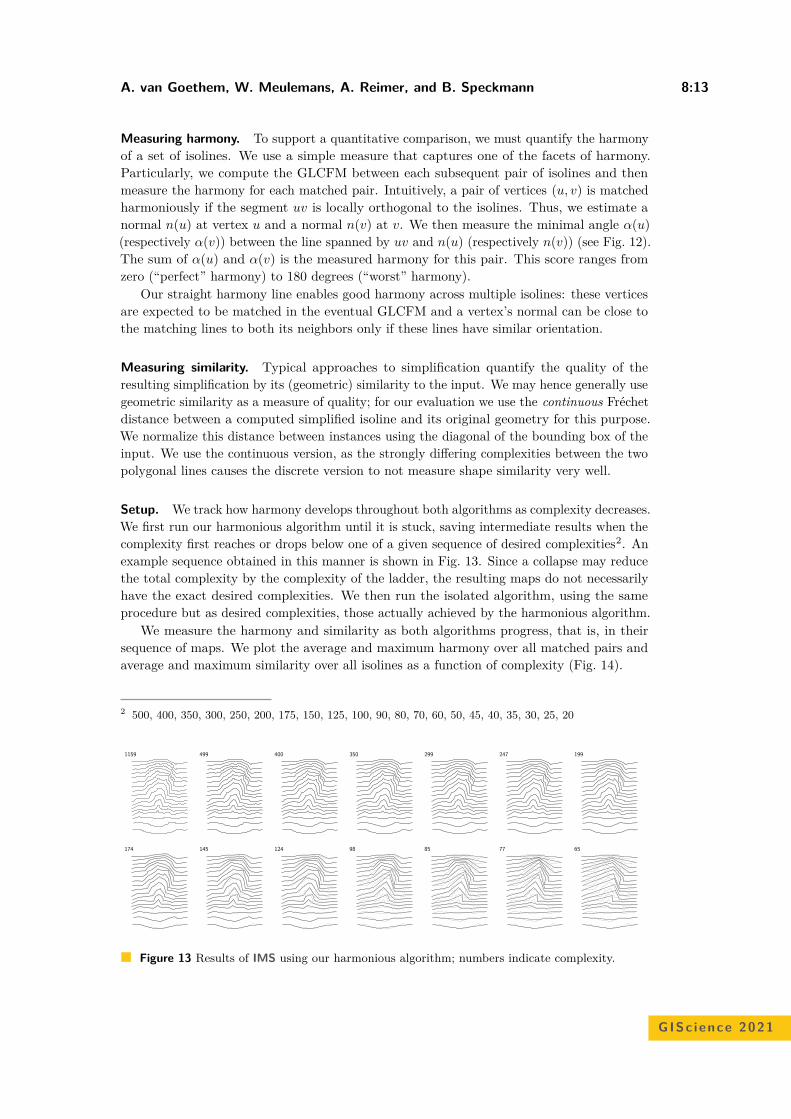
A. van Goethem, W. Meulemans, A. Reimer, and B. Speckmann 8:13

Measuring harmony. To support a quantitative comparison, we must quantify the harmonyof a set of isolines. We use a simple measure that captures one of the facets of harmony.Particularly, we compute the GLCFM between each subsequent pair of isolines and thenmeasure the harmony for each matched pair. Intuitively, a pair of vertices (u, v) is matchedharmoniously if the segment uv is locally orthogonal to the isolines. Thus, we estimate anormal n(u) at vertex u and a normal n(v) at v. We then measure the minimal angle α(u)(respectively α(v)) between the line spanned by uv and n(u) (respectively n(v)) (see Fig. 12).The sum of α(u) and α(v) is the measured harmony for this pair. This score ranges fromzero (“perfect” harmony) to 180 degrees (“worst” harmony).

Our straight harmony line enables good harmony across multiple isolines: these verticesare expected to be matched in the eventual GLCFM and a vertex’s normal can be close tothe matching lines to both its neighbors only if these lines have similar orientation.

Measuring similarity. Typical approaches to simplification quantify the quality of theresulting simplification by its (geometric) similarity to the input. We may hence generally usegeometric similarity as a measure of quality; for our evaluation we use the continuous Fréchetdistance between a computed simplified isoline and its original geometry for this purpose.We normalize this distance between instances using the diagonal of the bounding box of theinput. We use the continuous version, as the strongly differing complexities between the twopolygonal lines causes the discrete version to not measure shape similarity very well.

Setup. We track how harmony develops throughout both algorithms as complexity decreases.We first run our harmonious algorithm until it is stuck, saving intermediate results when thecomplexity first reaches or drops below one of a given sequence of desired complexities2. Anexample sequence obtained in this manner is shown in Fig. 13. Since a collapse may reducethe total complexity by the complexity of the ladder, the resulting maps do not necessarilyhave the exact desired complexities. We then run the isolated algorithm, using the sameprocedure but as desired complexities, those actually achieved by the harmonious algorithm.

We measure the harmony and similarity as both algorithms progress, that is, in theirsequence of maps. We plot the average and maximum harmony over all matched pairs andaverage and maximum similarity over all isolines as a function of complexity (Fig. 14).

2 500, 400, 350, 300, 250, 200, 175, 150, 125, 100, 90, 80, 70, 60, 50, 45, 40, 35, 30, 25, 20

1159 499 400 350 299 247 199

174 145 124 98 85 77 65

Figure 13 Results of IMS using our harmonious algorithm; numbers indicate complexity.

GISc ience 2021

8:14 Harmonious Simplification of Isolines

IMS

0

45

90

135

180

harm

ony

115965 98 174 298vertices

0.0

0.05

0.1

0.15

similarit y

AS1

44228 49 88 175vertices

AS2

180873 100 172 300vertices

AS3

2071219 300 400vertices

IMH

0

45

90

135

180

harm

ony

66441 57 90 150 247vertices

0.0

0.05

0.1

0.15

similarit y

AH1

58475 122 198 348vertices

AH2

134070 99 175 299vertices

AH3

158070 98 169 297vertices

Figure 14 Average (circles) and maximum (squares) harmony and similarity as the algorithmssimplify the input; lower values are better. Blue: harmonious algorithm; orange: isolated algorithm.Note that the horizontal axis is not linear. The maximum similarity (0.27) for the result of ourharmonious algorithm on AH3 with 81 vertices has been cropped.

Observations. First, we observe that the harmonious algorithm tends to perform better forharmony than the isolated method, but the similarity distance is typically slightly worse.This stands to reason as a collapse may sacrifice similarity to improve harmony. However,the effect on similarity is rather minor, until we reach the lower levels of complexity.

Second, the average and maximum Fréchet distance behave very similarly and tend tonot differ much until the algorithm reaches the lowest complexities. This suggests that thegeometric distortion our algorithm causes remains evenly spread between the isolines.

Third, we observe that for the isolated algorithm the average harmony tends to deteriorate.For the harmonious algorithm the harmony tends to stay roughly constant, though some ofthe slopes do show a bit of a deterioration as well (AS1–AS2 mostly).

A. van Goethem, W. Meulemans, A. Reimer, and B. Speckmann 8:15

Fourth, we observe that the isolated algorithm often is stuck earlier, never reaching thenumber of vertices that the harmonious algorithm can reach; this is the case for AS2–AS3,AH1–AS3. This may seem somewhat counterintuitive: staying closer to the original geometryshould generally help avoid intersections. There are two possible explanations here: (1) bycollapsing entire slope ladders, we may still perform a collapse, even if collapsing any of therungs in isolation would cause intersections; (2) by incorporating harmony, there is a betterrelation between the isolines and thus performing a collapse (even if in isolation) is less likelyto cause intersections. We believe the first explanation is most likely the strongest effecthere, but the second explanation may warrant further investigation in future work.

4 Conclusion and future work

We have presented an algorithm for simplifying isolines harmoniously, i.e., acknowledgingthat they describe a single object and that structures of this object should be reflected clearlyin the result. Our evaluation shows the efficacy of our method, but also marks some currentlimitations to be overcome in future work. In addition to these, we observe that simplifyinglarger features (more than a single slope or hilltop) requires more investigation. For example,if a hill has two hilltops, we may need to match the isoline that encompasses both partiallyto one hilltop and partially to the other. In similar spirit, even between two isolines, largeflat areas should possibly be omitted in the matching as maintaining harmony over a largedistance is counter to the underlying principle; again, some form of partial matching may beuseful here. As object identification in isoline systems is quite advanced and computationallyefficient via contour trees and similar Reeb-graph-like structures, the starting and end-pointproblems for partial matchings within our method remain future work.

References1 Helmut Alt, Bernd Behrends, and Johannes Blömer. Approximate matching of polygonal

shapes. Annals of Mathematics and Artificial Intelligence, 13(3):251–265, 1995.2 Helmut Alt and Michael Godau. Computing the Fréchet distance between two polygonal

curves. International Journal of Computational Geometry & Applications, 5(01n02):75–91,1995.

3 Richard Bellman and Robert Kalaba. On adaptive control processes. IRE Transactions onAutomatic Control, 4(2):1–9, 1959.

4 Prosenjit Bose, Sergio Cabello, Otfried Cheong, Joachim Gudmundsson, Marc J. van Kreveld,and Bettina Speckmann. Area-preserving approximations of polygonal paths. Journal ofDiscrete Algorithms, 4(4):554–566, 2006.

5 Kevin Buchin, Maike Buchin, Wouter Meulemans, and Bettina Speckmann. Locally correctFréchet matchings. Computational Geometry, 76:1–18, 2019.

6 Kevin Buchin, Wouter Meulemans, André Van Renssen, and Bettina Speckmann. Area-preserving simplification and schematization of polygonal subdivisions. ACM Transactions onSpatial Algorithms and Systems, 2(1):Article No. 2, 1–36, 2016.

7 Thomas C. van Dijk, Arthur van Goethem, Jan-Henrik Haunert, Wouter Meulemans, andBettina Speckmann. Map schematization with circular arcs. In Proc. International Conferenceon Geographic Information Science, pages 1–17, 2014.

8 Regina Estkowski and Joseph S. B. Mitchell. Simplifying a polygonal subdivision while keepingit simple. In Proc. 17th Symposium on Computational Geometry, pages 40–49, 2001.

9 Julien Gaffuri, Cécile Duchêne, and Anne Ruas. Object-field relationships modelling in anagent-based generalisation model. In Proc. 12th Workshop on Generalisation and MultipleRepresentation, 2008.

10 Aji Gao, Jingzhong Li, and Kai Chen. A morphing approach for continuous generalization oflinear map features. Plos one, 15(12):e0243328, 2020.

GISc ience 2021

8:16 Harmonious Simplification of Isolines

11 Arthur van Goethem, Wouter Meulemans, Andreas Reimer, and Bettina Speckmann. Sim-plification with parallelism. In Proc. 23rd ICA Workshop on Generalisation and MultipleRepresentation, 2020.

12 Arthur van Goethem, Wouter Meulemans, Bettina Speckmann, and Jo Wood. Exploring curvedschematization of territorial outlines. IEEE Transactions on Visualization and ComputerGraphics, 21(8):889–902, 2015.

13 Alan H. Goldman. Aesthetic qualities and aesthetic value. The Journal of Philosophy,87(1):23–37, 1990.

14 Leonidas J. Guibas and John Hershberger. Optimal shortest path queries in a simple polygon.Journal of Computer and System Sciences, 39(2):126–152, 1989.

15 Eric Guilbert. Feature-driven generalization of isobaths on nautical charts: A multi-agentsystem approach. Transactions in GIS, 20(1):126–143, 2016.

16 Eric Guilbert, Julien Gaffuri, and Bernhard Jenny. Terrain generalisation. In Abstractinggeographic information in a data rich world, LNCG, pages 227–258. Springer, 2014.

17 Ian M. Howat, Claire Porter, Benjamin E. Smith, Myoung-Jong Noh, and Paul Morin. Thereference elevation model of Antarctica. The Cryosphere, 13(2):665–674, 2019.

18 Eduard Imhof. Kartographische Geländedarstellung. De Gruyter, 1965.19 Barry J. Kronenfeld, Lawrence V. Stanislawski, Barbara P. Buttenfield, and Tyler Brockmeyer.

Simplification of polylines by segment collapse: Minimizing areal displacement while preservingarea. International Journal of Cartography, 6(1):22–46, 2020.

20 Zhilin Li and Haigang Sui. An integrated technique for automated generalization of contourmaps. The Cartographic Journal, 37(1):29–37, 2000.

21 Maarten Löffler and Wouter Meulemans. Discretized approaches to schematization. In Proc.29th Canadian Conference on Computational Geometry, pages 220–225, 2017.

22 Thomas Mendel. Area-preserving subdivision simplification with topology constraints: Exactlyand in practice. In Proce. 20th Workshop on Algorithm Engineering and Experiments, pages117–128, 2018.

23 Paulo Raposo. Scale-specific automated line simplification by vertex clustering on a hexagonaltessellation. Cartography and Geographic Information Science, 40(5):427–443, 2013.

24 Andreas Reimer. Cartographic modelling for automated map generation. PhD thesis, TechnischeUniversiteit Eindhoven, 2015.

25 Timofey E. Samsonov. Automated conflation of digital elevation model with reference hydro-graphic lines. ISPRS International Journal of Geo-Information, 9(5), 2020.

26 Timofey E. Samsonov, Sergey Koshel, Dmitry Walther, and Bernhard Jenny. Automatedplacement of supplementary contour lines. International Journal of Geographical InformationScience, 33(10):2072–2093, 2019.

27 Wilhelm Schüle. Zur Maßstabsfrage des neuen schweizerischen Kartenwerkes, mit einemNachtrag und Anhang zur Kurvendarstellung auf topographischen Karten. In Jahresberichtder Geographischen Gesellschaft von Bern, Bd. XXVIII, pages 31–53, 1929.

28 Andriani Skopeliti, Lysandros Tsoulos, and Shachak Pe’eri. Depth contours and coastlinegeneralization for harbour and approach nautical charts. ISPRS International Journal ofGeo-Information, 10(4):197, 2021.

29 Xiaohua Tong, Yanmin Jin, Lingyun Li, and Tinghua Ai. Area-preservation simplification ofpolygonal boundaries by the use of the structured total least squares method with constraints.Transactions in GIS, 19(5):780–799, 2015.

30 Guillaume Touya, Hugo Boulze, Anouk Schleich, and Hervé Quinquenel. Contour linesgeneration in karstic plateaus for topographic maps. In Proc. International CartographicConference, volume 2, pages 1–8, 2019.

31 Dražen Tutić and Miljenko Lapaine. Area preserving cartographic line generalizaton. Kar-tografija i geoinformacije (Cartography and Geoinformation), 8(11):84–100, 2009.

32 Dražen Tutić, Matjaž Štanfel, and Tomislav Jogun. Automation of cartographic generalisationof contour lines. In Proc. 10th ICA Mountain Cartography Workshop, pages 65–77, 2017.

Navigating Your Way! Increasing the Freedom ofChoice During WayfindingBartosz Mazurkiewicz #

Geoinformation, TU Wien, Austria

Markus Kattenbeck #

Geoinformation, TU Wien, Austria

Ioannis Giannopoulos #

Geoinformation, TU Wien, Austria

AbstractUsing navigation assistance systems has become widespread and scholars have tried to mitigatepotentially adverse effects on spatial cognition these systems may have due to the division of attentionthey require. In order to nudge the user to engage more with the environment, we propose a novelnavigation paradigm called Free Choice Navigation balancing the number of free choices, route lengthand number of instructions given. We test the viability of this approach by means of an agent-basedsimulation for three different cities. Environmental spatial abilities and spatial confidence are the twomost important modeled features of our agents. Our results are very promising: Agents could decidefreely at more than 50% of all junctions. More than 90% of the agents reached their destinationwithin an average distance of about 125% shortest path length.

2012 ACM Subject Classification Information systems → Decision support systems; Computingmethodologies → Agent / discrete models; Information systems → Location based services

Keywords and phrases Agent-based Simulation, Wayfinding, Free Choice Navigation

Digital Object Identifier 10.4230/LIPIcs.GIScience.2021.II.9

1 Introduction

Adaptive route instructions for pedestrian wayfinders have seen considerable research inter-est [7]. At the same time, empirical evidence has been collected which suggests an adverseimpact of wayfinding assistance systems on spatial cognition and knowledge acquisition(see e.g., [6]). Routing paradigms which allow wayfinders to make an increased number ofdecisions and, therefore, reduce the number of instructions given as much as reasonable wouldbe one option to remedy this effect. We explore one possible solution to this problem andpropose a pedestrian navigation paradigm which balances the number of given instructionsand the freedom of choice left to the user at junctions. We explore the feasibility of thisparadigm by means of an agent-based simulation. At the start, an agent is provided with adestination vector, similar to someone pointing to the destination when asked for instructions.Once an agent started walking they do not need to stick to a predefined route, hence theywill not suffer from on-route uncertainty [22] but are free to make their own decisions atjunctions. However, a route instruction will be provided if odds are increased that an agent,based on its current state, is likely to choose a not reasonably good branch at a given junction.The presented paradigm aims for less instructions and more free choices along the route –regardless the way instructions are phrased or the modality they are given in.

Based on a comparison of our routing paradigm (labelled free choice navigation – FCN )to the turn-by-turn (TBT) technique, which is prevalent in commercial wayfinding assistancesystems, our contribution is threefold:

© Bartosz Mazurkiewicz, Markus Kattenbeck, and Ioannis Giannopoulos;licensed under Creative Commons License CC-BY 4.0

11th International Conference on Geographic Information Science (GIScience 2021) – Part II.Editors: Krzysztof Janowicz and Judith A. Verstegen; Article No. 9; pp. 9:1–9:16

Leibniz International Proceedings in InformaticsSchloss Dagstuhl – Leibniz-Zentrum für Informatik, Dagstuhl Publishing, Germany

9:2 Navigating Your Way! Increasing the Freedom of Choice During Wayfinding

1. We present a new navigation paradigm (free choice navigation);2. We provide evidence that agents reach their destinations within a reasonable departure

from the length of the shortest path using our approach and3. We quantify the number of instructions we save/add compared to the baseline (TBT).

Successfully testing of our approach has a potentially important implication: Reducingthe number of instructions would provide users of wayfinding systems with more time toobserve the environment while, simultaneously, forcing them to engage more with it as theyhave to make their own decisions. Based on prior evidence (see e.g., [33]), this is expected toresult in increased spatial knowledge acquisition (see section 7 below). It is important tonote, though, that our approach is meant to be used in a leisure scenario, i.e. in situation inwhich wayfinders do not feel any time pressure.

2 Related Work

Given our research goal, we discuss three different branches of related work. First, literature onreducing the number of TBT navigation instructions or adapting their structure/presentationis reviewed. Second, we discuss literature using the beeline/as-the-crow-flies navigationapproach. Lastly, we review agent-based simulations modeling pedestrian behavior. Takentogether, this review reveals important factors which need to be considered when modelingagents and its accompanying mechanics (see also Section 4).

2.1 Enhancing TBT InstructionsIn recent years, evidence has been collected which suggests that the use of navigation systemsmay have an adverse impact on spatial cognition and orientation (see e.g., [6, 21]). This effectis commonly explained by the need to divide the attention between the navigation systemand the environment when following a pre-determined route (see e.g., [13]). Possible remediesregarding TBT navigation systems are enhancing instructions with additional information(see e.g., [16, 36]), reducing the number of instructions [28], combining them with differentinteraction techniques (see e.g., pointing [25]) or providing haptic or audio feedback (seee.g., [12, 14]). All these approaches assume a predefined route. This is in contrast to ourparadigm according to which users can make their own spatial decisions to a large extent.

2.2 Beeline NavigationThere are alternatives to TBT navigation approaches, e.g., using the beeline to the destination.One particularly important idea is the so-called least-angle strategy, which was for the firsttime thoroughly studied by Hochmair and Frank [20] using a simulation study. According tothis strategy a user chooses the option with the least angle with respect to the (believed)destination vector. The least-angle strategy has been studied with respect to variousimplementations: [29] and [8] report on prototype navigation systems for pedestrians which usevibro-tactile feedback devices to indicate the beeline. Either system guides users successfullyto their destination. Both systems allow for free exploration but none of them control for anupper path length limit. This is in contrast to our approach: We try to find a compromisebetween free exploration and maximum path length while determining the point in time atwhich an instruction needs to be given. Savino and colleagues [30] compare TBT and twodifferent implementations of the beeline approach for cyclists, one of which provides visualcues when the beeline differs from the shortest path branch. The latter approach enhancesuser confidence. The beeline approach was preferred for leisure scenario. This is in line with

B. Mazurkiewicz, M. Kattenbeck, and I. Giannopoulos 9:3

prior evidence suggesting that it is important for pedestrians to optimize both, distanceand angle [31] and that the environmental complexity [15] has also a major impact on routechoice behavior. Our approach takes these findings into account (see Section 4) by providingthe beeline at the starting point and providing further wayfinding assistance as needed.

2.3 Simulation Studies and Models of Pedestrian BehaviorAs mentioned above, the beeline approach was studied by Hochmair and Frank [20] using asimulation study regarding perception errors. Based on this work, Hochmair [19] analyzed theeffectiveness of the least-angle strategy with a simulation study for different transportationmodes. The results suggest a limited usability of this approach in real life (human perceptionand memory errors). Our simulation takes these findings into account by modeling humanerrors and actively supporting the user if help is needed, moreover, it incorporates environ-mental spatial abilities and spatial confidence (see Section 4). Other agent-based wayfindingstudies frequently focus on collision avoidance (see e.g., [35]), on evacuation (see e.g., [37]) oron the interplay between navigational instructions, the environment and the agent (see e.g.,[34, 22]), including research on route choice behavior based on different levels of cognitivemaps [10]. Generally speaking, the findings of these papers are based on the assumption thata path a user should follow exists. Again, this is in contrast to our approach. Neither doagents receive an instruction at every decision point, nor is there a predefined path. Ouragents are also not equipped with prior knowledge of the environment nor do they know thetrue destination direction at every junction (which is in contrast to, e.g., the models used byKneidl [23]), i.e., they are considered to be unfamiliar and, hence, have no cognitive map.

3 Simulation Preparation and Baseline Condition

In order to test1 our hypotheses (see Section 5) we run an agent-based simulation (nonmulti-agent) with two conditions. The main focus lies on whether agents do reach theirdestination with our approach. Consequently, we will not model effects on spatial cognition,e.g. spatial knowledge acquisition as this aspect will be scrutinized in a real-world study(see Section 7). The simulation study was run in three cities with three different networktypes [32], namely Djibouti City (Djibouti, type: irregular), Vienna (Austria, type: hightransit) and Mexico City (Mexico, type: checkerboard). For each city 100 random routeswith a length ranging between 500m and 5000m were chosen in order to test the approachon shorter and longer routes. We tested two conditions (TBT vs. free choice navigation):Each condition was tested with 3000 agents, i.e., there are 6000 different agents (betweensubject design). The agents are constructed based on the the so-called BDI-framework [27]for practical reasoning: The agents simulate pedestrians who have Beliefs about where theirdestination is located; agents Desire to reach their destination; and, finally, they act basedon Intentions, i.e., at each intersection they reason about which decision they need to takein order to reach their goal based on their beliefs.

3.1 Software and DataSeveral agent-based modeling and simulation frameworks exist [1]. For our approach weutilized python 3.8.8 using the package networkx (v2.5.) [17], avoiding frameworks providinggraphical interfaces since this was not relevant for the presented study. The raw network

1 The terms junction and intersection are used interchangeably, as well as option and branch are.

GISc ience 2021

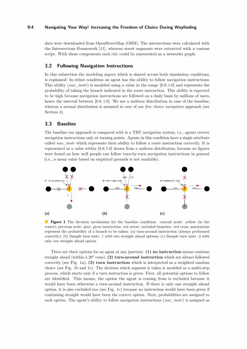
9:4 Navigating Your Way! Increasing the Freedom of Choice During Wayfinding

data were downloaded from OpenStreetMap (OSM). The intersections were calculated withthe Intersections Framework [11], whereas street segments were extracted with a customscript. With those components each city could be represented as a networkx graph.

3.2 Following Navigation InstructionsIn this subsection the modeling aspect which is shared across both simulation conditions,is explained: In either condition an agent has the ability to follow navigation instructions.This ability (nav_instr) is modeled using a value in the range [0.8; 1.0] and represents theprobability of taking the branch indicated in the route instruction. This ability is expectedto be high because navigation instructions are followed on a daily basis by millions of users,hence the interval between [0.8, 1.0]. We use a uniform distribution in case of the baseline,whereas a normal distribution is assumed in case of our free choice navigation approach (seeSection 4).

3.3 BaselineThe baseline our approach is compared with is a TBT navigation system, i.e., agents receivenavigation instructions only at turning points. Agents in this condition have a single attributecalled nav_instr which represents their ability to follow a route instruction correctly. It isrepresented as a value within [0.8; 1.0] drawn from a uniform distribution, because no figureswere found on how well people can follow turn-by-turn navigation instructions in general(i.e., a mean value based on empirical grounds is not available).

(a) (b) (c)

Figure 1 The decision mechanism for the baseline condition. current node: yellow (in thecenter); previous node: grey; given instruction: red arrow; excluded branches: red cross; annotationsrepresent the probability of a branch to be taken: (a) turn-around instruction (always performedcorrectly); (b) Sample turn instr. 1 with two straight ahead options; (c) Sample turn instr. 2 withonly one straight ahead option.

There are three options for an agent at any junction: (1) no instruction means continuestraight ahead (within a 20° cone); (2) turn-around instruction which are always followedcorrectly (see Fig. 1a); (3) turn instruction which is interpreted as a weighted randomchoice (see Fig. 1b and 1c). The decision which segment is taken is modeled as a multi-stepprocess, which starts only if a turn instruction is given: First, all potential options to followare identified. This means, the option the agent is coming from is excluded because itwould have been otherwise a turn-around instruction. If there is only one straight aheadoption, it is also excluded too (see Fig. 1c) because no instruction would have been given ifcontinuing straight would have been the correct option. Next, probabilities are assigned toeach option: The agent’s ability to follow navigation instructions (nav_instr) is assigned as

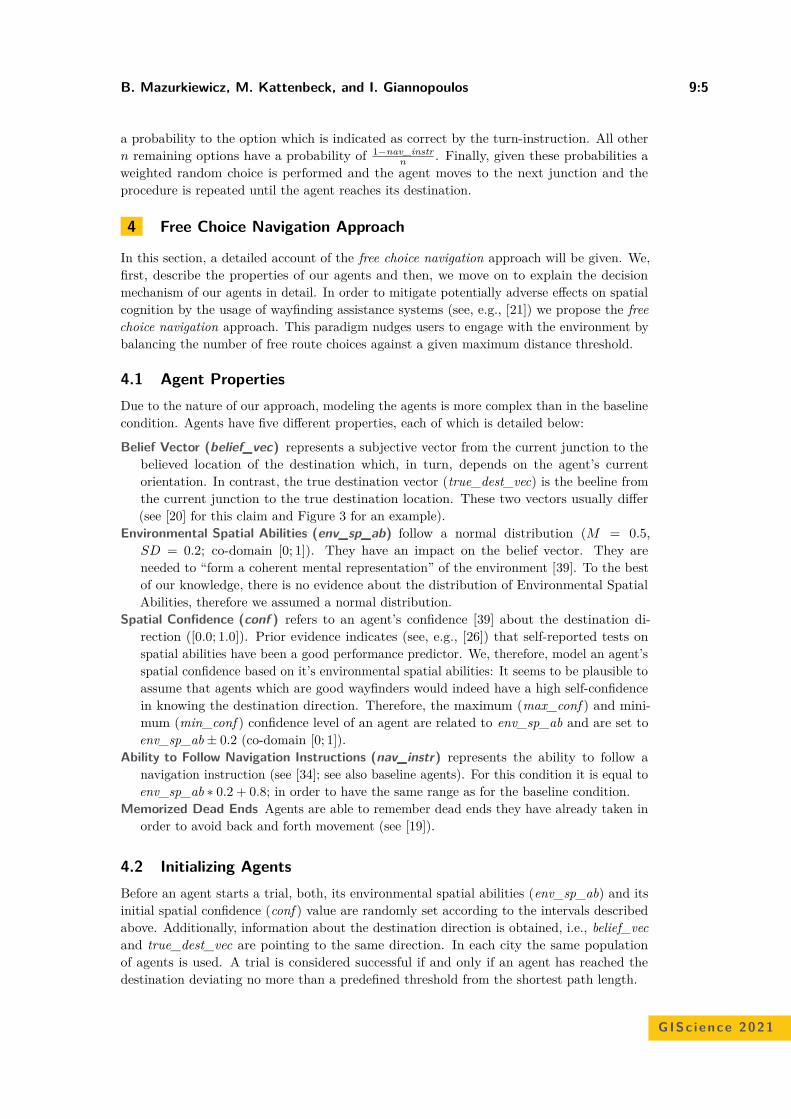
B. Mazurkiewicz, M. Kattenbeck, and I. Giannopoulos 9:5

a probability to the option which is indicated as correct by the turn-instruction. All othern remaining options have a probability of 1−nav_instr

n . Finally, given these probabilities aweighted random choice is performed and the agent moves to the next junction and theprocedure is repeated until the agent reaches its destination.

4 Free Choice Navigation Approach

In this section, a detailed account of the free choice navigation approach will be given. We,first, describe the properties of our agents and then, we move on to explain the decisionmechanism of our agents in detail. In order to mitigate potentially adverse effects on spatialcognition by the usage of wayfinding assistance systems (see, e.g., [21]) we propose the freechoice navigation approach. This paradigm nudges users to engage with the environment bybalancing the number of free route choices against a given maximum distance threshold.

4.1 Agent PropertiesDue to the nature of our approach, modeling the agents is more complex than in the baselinecondition. Agents have five different properties, each of which is detailed below:

Belief Vector (belief_vec) represents a subjective vector from the current junction to thebelieved location of the destination which, in turn, depends on the agent’s currentorientation. In contrast, the true destination vector (true_dest_vec) is the beeline fromthe current junction to the true destination location. These two vectors usually differ(see [20] for this claim and Figure 3 for an example).

Environmental Spatial Abilities (env_sp_ab) follow a normal distribution (M = 0.5,SD = 0.2; co-domain [0; 1]). They have an impact on the belief vector. They areneeded to “form a coherent mental representation” of the environment [39]. To the bestof our knowledge, there is no evidence about the distribution of Environmental SpatialAbilities, therefore we assumed a normal distribution.

Spatial Confidence (conf ) refers to an agent’s confidence [39] about the destination di-rection ([0.0; 1.0]). Prior evidence indicates (see, e.g., [26]) that self-reported tests onspatial abilities have been a good performance predictor. We, therefore, model an agent’sspatial confidence based on it’s environmental spatial abilities: It seems to be plausible toassume that agents which are good wayfinders would indeed have a high self-confidencein knowing the destination direction. Therefore, the maximum (max_conf ) and mini-mum (min_conf ) confidence level of an agent are related to env_sp_ab and are set toenv_sp_ab ± 0.2 (co-domain [0; 1]).

Ability to Follow Navigation Instructions (nav_instr) represents the ability to follow anavigation instruction (see [34]; see also baseline agents). For this condition it is equal toenv_sp_ab ∗ 0.2 + 0.8; in order to have the same range as for the baseline condition.

Memorized Dead Ends Agents are able to remember dead ends they have already taken inorder to avoid back and forth movement (see [19]).

4.2 Initializing AgentsBefore an agent starts a trial, both, its environmental spatial abilities (env_sp_ab) and itsinitial spatial confidence (conf ) value are randomly set according to the intervals describedabove. Additionally, information about the destination direction is obtained, i.e., belief_vecand true_dest_vec are pointing to the same direction. In each city the same populationof agents is used. A trial is considered successful if and only if an agent has reached thedestination deviating no more than a predefined threshold from the shortest path length.

GISc ience 2021

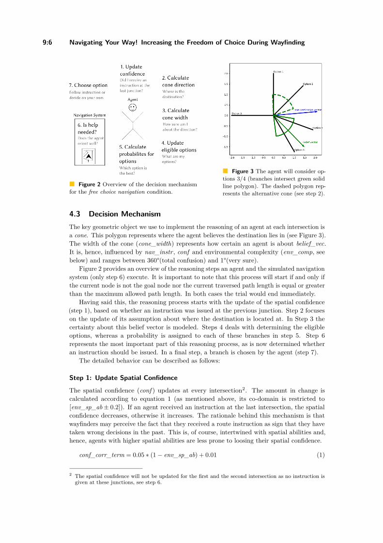
9:6 Navigating Your Way! Increasing the Freedom of Choice During Wayfinding

Figure 2 Overview of the decision mechanismfor the free choice navigation condition.

Figure 3 The agent will consider op-tions 3/4 (branches intersect green solidline polygon). The dashed polygon rep-resents the alternative cone (see step 2).

4.3 Decision MechanismThe key geometric object we use to implement the reasoning of an agent at each intersection isa cone. This polygon represents where the agent believes the destination lies in (see Figure 3).The width of the cone (cone_width) represents how certain an agent is about belief_vec.It is, hence, influenced by nav_instr , conf and environmental complexity (env_comp, seebelow) and ranges between 360°(total confusion) and 1°(very sure).

Figure 2 provides an overview of the reasoning steps an agent and the simulated navigationsystem (only step 6) execute. It is important to note that this process will start if and only ifthe current node is not the goal node nor the current traversed path length is equal or greaterthan the maximum allowed path length. In both cases the trial would end immediately.

Having said this, the reasoning process starts with the update of the spatial confidence(step 1), based on whether an instruction was issued at the previous junction. Step 2 focuseson the update of its assumption about where the destination is located at. In Step 3 thecertainty about this belief vector is modeled. Steps 4 deals with determining the eligibleoptions, whereas a probability is assigned to each of these branches in step 5. Step 6represents the most important part of this reasoning process, as is now determined whetheran instruction should be issued. In a final step, a branch is chosen by the agent (step 7).

The detailed behavior can be described as follows:

Step 1: Update Spatial Confidence

The spatial confidence (conf ) updates at every intersection2. The amount in change iscalculated according to equation 1 (as mentioned above, its co-domain is restricted to[env_sp_ab ± 0.2]). If an agent received an instruction at the last intersection, the spatialconfidence decreases, otherwise it increases. The rationale behind this mechanism is thatwayfinders may perceive the fact that they received a route instruction as sign that they havetaken wrong decisions in the past. This is, of course, intertwined with spatial abilities and,hence, agents with higher spatial abilities are less prone to loosing their spatial confidence.

conf_corr_term = 0.05 ∗ (1 − env_sp_ab) + 0.01 (1)

2 The spatial confidence will not be updated for the first and the second intersection as no instruction isgiven at these junctions, see step 6.

B. Mazurkiewicz, M. Kattenbeck, and I. Giannopoulos 9:7

Step 2: Calculate Cone Direction

The cone bisector is calculated according to the belief vector (belief_vec, see eq. 2). In linewith prior evidence [18], the agent’s orientation deteriorates with distance (the number oftraversed junctions) but less so for agents with higher env_sp_ab. For each intersection, thisbelief vector is rotated away from the true_dest_vec by random choice. The rationale forthis randomness is that there is no apriori knowledge about in which direction the erroneousbelief_vec is rotated (see Figure 3).

belief_vec = true_dest_vec ± (1 − 1#traversed_junctions

) ∗ (1 − env_sp_ab) ∗ 180° (2)

Step 3: Calculate Cone Width

The width of the cone (cone_width) represents how confident an agent is regarding thedirection to the destination. It is influenced (see eq. 3) by the agent’s spatial confidenceand the environmental complexity of the current junction (env_comp) whose impact ismoderated by the agent’s spatial abilities (the lower the environmental spatial abilities thehigher the impact environmental complexity shows on the cone width). Before the wholesimulation starts each junction in a city will be assigned a normally distributed environmentalcomplexity (env_comp, M = 0.5, SD = 0.2) which will remain unchanged during all trials. Anode for which env_comp = 0.5 is, therefore, considered as decision point having an averageenvironmental complexity. Based on the cone_width and the belief_vec the actual conegeometry is calculated (see Figure 3).

cone_width = 360° − (conf ∗ 360°) + (env_comp − 0.5) ∗ 360° ∗ (1 − env_sp_ab) (3)

Update Eligible Options (Step 4) and Calculate Probabilities for Eligible Options(Step 5)

In order to find the set of eligible branches, agents exclude any already visited dead end(memorized options) from the decision process (Step 4). Having done so, the cone is checkedfor eligible options and angles with respect to the belief_vec are calculated for each branch(Step 5). Three different cases are distinguished:

Option 1: No branch in cone All eligible options are taken into account and the anglesbetween them and the belief_vec are calculated (least-angle strategy [20]).

Option 2: Exactly one branch in cone This branch is assigned a probability of 1.0.Option 3: More than one branch in cone As in this case an agent can choose from several

branches inside the cone, angles are found for these by analogy with option 1.For options 1 and 3, these angles, denoted as opt_ang, need to be converted to probabilitiesusing three further steps.1. All angles are inverted with respect to the maximum angle within the cone which is

given by cone_width2 , thereby favoring angles which are closer to belief_vec: inv_angles =

cone_width2 − opt_ang. Subsequently, each inverted angle will be normalized (division by

the sum of all inverted angles in the list) in order to ensure that the sum of all probabilitiesequals one.

2. In order to avoid back and forth movement along the same branch (see [19]), a factorcalled already visited penalty factor (vis_pen) is applied to the probability of any edgewhich has already been visited. The lower the value the higher the penalty. Again, theprobabilities are normalized.

GISc ience 2021

9:8 Navigating Your Way! Increasing the Freedom of Choice During Wayfinding

3. A final selection step for branches is needed as several branches may show almostthe same angle to the bisector of the cone geometry, i.e., whose angles can hardly bedistinguished by humans. Therefore, only those branches with a probability greater thanmax_probability − 0.1 are selected and then the remaining probabilities are normalized.

The above procedure leads to the final set of branches FS with their final probabilitiesassigned. These will subsequently be used to decide if an agent needs an instruction or not.

Step 6: Determine Whether an Instruction is Given

Given the probabilities and several additional parameters a decision is made whether aninstruction is given to the agent3. An instruction is provided for any of the following reasons,i.e., the list of reasons is checked one-by-one in the order given below:1. The shortest path from the current junction to the destination leads over a single segment,

i.e., the instruction is given in order to support destination recognition (see [9]).2. Let sp_length denote the shortest path from the start to the destination; let further

dist_walked denote the distance an agent has walked from the start to the current junction.Finally, let max_dist denote the constant factor which determines the allowed deviationfrom sp_length still rendering a trial successful. Then, the current buffer (curr_buffer),i.e., the distance an agent can walk from the current junction to the destination in orderto still successfully finish a trial is given by equation 4.

curr_buffer = max_dist ∗ sp_length − dist_walked (4)

Let, furthermore, buff_fact (co-domain: [0; 1]) denote a factor which is used to balancethe number of given instructions against the number of agents that will arrive (giventhe presupposition that the probability of a successful trial increases for agents whoreceive more instructions). This means, this factor is used to account for the risk that theagent will exceed the available buffer: An instruction will be given if the current buffermultiplied by the buffer factor is lower than the length of the shortest path from thecurrent junction (see eq. 5).

curr_buffer ∗ buff_fact < sp_length_curr_jct (5)

3. For the same reason other branches are examined (step 2 is introduced in order to savecomputation time). We evaluate this case based on two steps. We, first, create the set ofacceptable branches AB which includes all branches which fulfill inequality 7 in whichsp_over_i denotes the sum of the length of the shortest path between the upcomingintersection i and the destination and the length of the edge from the current junction toi (see eq. 6).

sp_over_i = sp_lengthi + len(edge_to_i) (6)sp_over_i <= curr_buffer ∗ buff_fact (7)

Subsequently, we sum the probabilities of all branches b ∈ AB. If this sum is smallerthan a predefined threshold called pos_sum, which is kept constant across trials, then aninstruction is given.

3 There is no instruction given at the first two nodes the agent traverses as it is reasonable to assumethat the direction of the destination is still evident.

B. Mazurkiewicz, M. Kattenbeck, and I. Giannopoulos 9:9

4. An instruction is, furthermore, given if an edge exists in the final selection FS (see step 5above) for which the shortest path from the end node of this edge leads over the currentnode. Let the current junction be denoted as ji−1; let the upcoming junction of a branchbi which is part of the final selection set be denoted as ji. An instruction will be givenif the shortest path from ji would lead over ji−1 because this will save agents a loss ofcurr_buffer due to avoidable detours.

5. Given the fact that the number of agents with a successful trial must be maximized, aninstruction is also provided if agents have a high probability of choosing a branch whichwill be costly in terms of the consumed buffer while there would have been “cheaper”alternatives. Let rem_len_buf (Remaining Length Buffer, RLB) denote the difference(see eq. 8) between the curr_buffer and the sp_over_i (see eq. 6).

rem_len_buf = curr_buffer − sp_over_i (8)

Step 1: For all branches b ∈ FS the ratio between the RLB of the branch with thehighest probability and the RLBs of all other branches is checked. If this ratio is largerthan a threshold buff_diff , this branch will be included in set BS, because it offers abetter RLB. If |BS| = 0 no instruction is given.

Step 2: If |BS| ≥ 1: Let P (bk) denote the probability assigned to the k − th branchand MAX(P (bk)) denote the highest probability of all branches in FS (note: FS is asuperset of BS and the probabilities of branches in both sets are the same). For eachbranch in BS check whether inequality 9 holds in which prob_diff denotes a thresholdfor the ratio of the highest probability of all branches among FS and a given branchin BS.

MAX(P (bk))P (bk) > prob_diff (9)

If this inequality holds, an instruction will be given, because chances are high that theagent misses a better RLB.

If none of these cases holds for the current junction, then no instruction is given and andthe agent chooses an option (step 7) based on the probabilities (step 5) assigned to eachbranch. With those conditions we try to predict costly mistakes rather than correct thembecause some mistakes can be expensive and unrecoverable regarding the goal of reachingthe destination within a given distance threshold.

Step 7: Choose an Option

At any junction agents either choose an option by following an instruction or by making adecision without having received an instruction. In the latter case, agents choose the branchthey will continue on from the final selection set FS based on a weighted random choice.If an instruction was given, however, the same procedure as for the baseline applies (seeabove), although one important differences applies: The edge on which an agent traveledto the current junction is the only one which is excluded. Please note: Again, turn-aroundinstructions are as well followed error-free.This decision mechanism of giving an instruction remains the same for the whole route.

GISc ience 2021

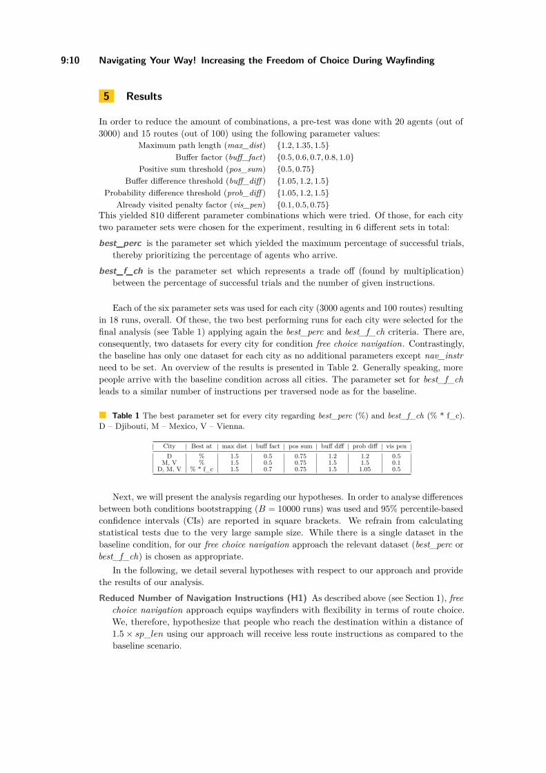
9:10 Navigating Your Way! Increasing the Freedom of Choice During Wayfinding

5 Results

In order to reduce the amount of combinations, a pre-test was done with 20 agents (out of3000) and 15 routes (out of 100) using the following parameter values:

Maximum path length (max_dist) 1.2, 1.35, 1.5Buffer factor (buff_fact) 0.5, 0.6, 0.7, 0.8, 1.0

Positive sum threshold (pos_sum) 0.5, 0.75Buffer difference threshold (buff_diff ) 1.05, 1.2, 1.5

Probability difference threshold (prob_diff ) 1.05, 1.2, 1.5Already visited penalty factor (vis_pen) 0.1, 0.5, 0.75

This yielded 810 different parameter combinations which were tried. Of those, for each citytwo parameter sets were chosen for the experiment, resulting in 6 different sets in total:best_perc is the parameter set which yielded the maximum percentage of successful trials,

thereby prioritizing the percentage of agents who arrive.best_f_ch is the parameter set which represents a trade off (found by multiplication)

between the percentage of successful trials and the number of given instructions.

Each of the six parameter sets was used for each city (3000 agents and 100 routes) resultingin 18 runs, overall. Of these, the two best performing runs for each city were selected for thefinal analysis (see Table 1) applying again the best_perc and best_f_ch criteria. There are,consequently, two datasets for every city for condition free choice navigation. Contrastingly,the baseline has only one dataset for each city as no additional parameters except nav_instrneed to be set. An overview of the results is presented in Table 2. Generally speaking, morepeople arrive with the baseline condition across all cities. The parameter set for best_f_chleads to a similar number of instructions per traversed node as for the baseline.

Table 1 The best parameter set for every city regarding best_perc (%) and best_f_ch (% * f_c).D – Djibouti, M – Mexico, V – Vienna.

City Best at max dist buff fact pos sum buff diff prob diff vis penD % 1.5 0.5 0.75 1.2 1.2 0.5

M, V % 1.5 0.5 0.75 1.5 1.5 0.1D, M, V % * f_c 1.5 0.7 0.75 1.5 1.05 0.5

Next, we will present the analysis regarding our hypotheses. In order to analyse differencesbetween both conditions bootstrapping (B = 10000 runs) was used and 95% percentile-basedconfidence intervals (CIs) are reported in square brackets. We refrain from calculatingstatistical tests due to the very large sample size. While there is a single dataset in thebaseline condition, for our free choice navigation approach the relevant dataset (best_perc orbest_f_ch) is chosen as appropriate.

In the following, we detail several hypotheses with respect to our approach and providethe results of our analysis.Reduced Number of Navigation Instructions (H1) As described above (see Section 1), free

choice navigation approach equips wayfinders with flexibility in terms of route choice.We, therefore, hypothesize that people who reach the destination within a distance of1.5 × sp_len using our approach will receive less route instructions as compared to thebaseline scenario.

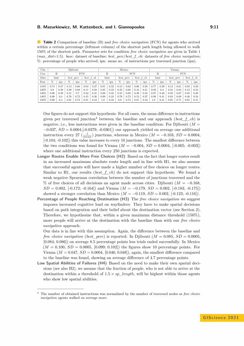
B. Mazurkiewicz, M. Kattenbeck, and I. Giannopoulos 9:11

Table 2 Comparison of baseline (B) and free choice navigation (FCN) for agents who arrivedwithin a certain percentage (leftmost column) of the shortest path length being allowed to walk150% of the shortest path. Parameter sets for condition free choice navigation are given in Table 1(max_dist=1.5). base: dataset of baseline; best_perc/best_f_ch: datasets of free choice navigation;%: percentage of people who arrived; ipn: mean no. of instructions per traversed junction (ipn).

City Djibouti Mexico ViennaCon. B FCN B FCN B FCNDset base best_perc best_f_ch base best_perc best_f_ch base best_perc best_f_chFeat. % ipn % ipn % ipn % ipn % ipn % ipn % ipn % ipn % ipn110% 0.74 0.37 0.13 0.66 0.04 0.27 0.81 0.32 0.13 0.62 0.06 0.30 0.77 0.39 0.12 0.61 0.03 0.20120% 0.9 0.39 0.30 0.68 0.11 0.28 0.95 0.33 0.32 0.66 0.16 0.31 0.92 0.4 0.34 0.64 0.12 0.24130% 0.96 0.39 0.51 0.7 0.24 0.31 0.98 0.33 0.55 0.69 0.30 0.33 0.97 0.40 0.59 0.67 0.25 0.28140% 0.98 0.4 0.76 0.72 0.45 0.36 0.99 0.33 0.78 0.72 0.52 0.37 0.99 0.41 0.83 0.69 0.48 0.34150% 0.99 0.4 0.91 0.74 0.81 0.43 1.0 0.33 0.9 0.74 0.81 0.43 1.0 0.41 0.95 0.71 0.85 0.41

Our figures do not support this hypothesis: For all cases, the mean difference in instructionsgiven per traversed junction4 between the baseline and our approach (best_f_ch) isnegative, i.e., less instructions were given in the baseline condition: For Djibouti (M =−0.037, SD = 0.0004,[-0.0379; -0.0361]) our approach yielded on average one additionalinstruction every 27 ( 1

mean ) junctions, whereas in Mexico (M = −0.103, SD = 0.0004,[-0.104; -0.102]) this value increases to every 10 junctions. The smallest difference betweenthe two conditions was found for Vienna (M = −0.004, SD = 0.0004, [-0.005; -0.003])where one additional instruction every 250 junctions is expected.

Longer Routes Enable More Free Choices (H2) Based on the fact that longer routes resultin an increased maximum absolute route length and in line with H1, we also assumethat successful agents will have made a higher number of free choices on longer routes.Similar to H1, our results (best_f_ch) do not support this hypothesis. We found aweak negative Spearman correlation between the number of junctions traversed and the% of free choices of all decisions an agent made across cities. Djibouti (M = −0.168,SD = 0.002, [-0.172; -0.164]) and Vienna (M = −0.179, SD = 0.002, [-0.183; -0.175])showed a stronger correlation than Mexico (M = −0.119, SD = 0.002, [-0.123; -0.116]).

Percentage of People Reaching Destination (H3) The free choice navigation we suggestimposes increased cognitive load on wayfinders: They have to make spatial decisionsbased on path integration and their belief about the destination vector (see Section 2).Therefore, we hypothesize that, within a given maximum distance threshold (150%),more people will arrive at the destination with the baseline than with our free choicenavigation approach.Our data is in line with this assumption. Again, the difference between the baseline andfree choice navigation (best_perc) is reported: In Djibouti (M = 0.085, SD = 0.0005,[0.084; 0.086]) on average 8.5 percentage points less trials ended successfully. In Mexico(M = 0.100, SD = 0.0005, [0.099; 0.102]) the figures show 10 percentage points. ForVienna (M = 0.047, SD = 0.0004, [0.046; 0.048]), again, the smallest difference comparedto the baseline was found, showing an average difference of 4.7 percentage points.

Low Spatial Abilities of Failures (H4) Based on the need to make their own spatial deci-sions (see also H2), we assume that the fraction of people, who is not able to arrive at thedestination within a threshold of 1.5 × sp_length, will be highest within those agentswho show low spatial abilities.

4 The number of obtained instructions was normalized by the number of traversed nodes as free choicenavigation agents walked on average more.

GISc ience 2021

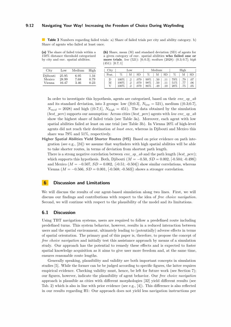
9:12 Navigating Your Way! Increasing the Freedom of Choice During Wayfinding

Table 3 Numbers regarding failed trials: a) Share of failed trials per city and ability category. b)Share of agents who failed at least once.

(a) The share of failed trials within a150% distance threshold categorizedby city and env. spatial abilities.

City Low Medium HighDjibouti 25.95 6.95 1.34Mexico 28.99 7.68 0.79Vienna 16.47 3.46 0.23

(b) Share, mean (M) and standard deviation (SD) of agents fora given category of env. spatial abilities who failed one ormore trials. low (521): [0; 0.3]; medium (2028): (0.3; 0.7]; high(451): [0.7; 1]

City Low Medium HighFeat. % M SD % M SD % M SD

D 100% .2 .079 99% .50 .11 79% .79 .07M 100% .2 .079 98% .50 .11 51% .77 .06V 100% .2 .079 86% .49 .10 20% .75 .05

In order to investigate this hypothesis, agents are categorized, based on their env_sp_aband its standard deviation, into 3 groups: low ([0;0.3], Nlow = 521), medium ((0.3;0.7],Nmed = 2028) and high ((0.7;1], Nhigh = 451). The data obtained by the simulation(best_perc) supports our assumption: Across cities (best_perc) agents with low env_sp_abshow the highest share of failed trials (see Table 3a). Moreover, each agent with lowspatial abilities failed at least on one trial (see Table 3b). In Vienna 20% of high-levelagents did not reach their destination at least once, whereas in Djibouti and Mexico thisshare was 79% and 51%, respectively.

Higher Spatial Abilities Yield Shorter Routes (H5) Based on prior evidence on path inte-gration (see e.g., [24]) we assume that wayfinders with high spatial abilities will be ableto take shorter routes, in terms of deviation from shortest path length.There is a strong negative correlation between env_sp_ab and the path length (best_perc);which supports this hypothesis. Both, Djibouti (M = −0.50, SD = 0.002, [-0.504; -0.498])and Mexico (M = −0.507, SD = 0.002, :[-0.51; -0.504]) show similar correlations, whereasVienna (M = −0.566, SD = 0.001, [-0.568; -0.563]) shows a stronger correlation.

6 Discussion and Limitations

We will discuss the results of our agent-based simulation along two lines. First, we willdiscuss our findings and contributions with respect to the idea of free choice navigation.Second, we will continue with respect to the plausibility of the model and its limitations.

6.1 DiscussionUsing TBT navigation systems, users are required to follow a predefined route includingpredefined turns. This system behavior, however, results in a reduced interaction betweenusers and the spatial environment, ultimately leading to (potentially) adverse effects in termsof spatial orientation. The primary goal of this paper is, therefore, to propose the concept offree choice navigation and initially test this assistance approach by means of a simulationstudy. Our approach has the potential to remedy these effects and is expected to fosterspatial knowledge acquisition as it aims to give user more freedom and, at the same time,ensures reasonable route lengths.

Generally speaking, plausibility and validity are both important concepts in simulationstudies [5]. While the former can be be judged according to specific figures, the latter requiresempirical evidence. Checking validity must, hence, be left for future work (see Section 7);our figures, however, indicate the plausibility of agent behavior. Our free choice navigationapproach is plausible as cities with different morphologies [32] yield different results (seeTab. 2) which is also in line with prior evidence (see e.g., [4]). This difference is also reflectedin our results regarding H1: Our approach does not yield less navigation instructions per

B. Mazurkiewicz, M. Kattenbeck, and I. Giannopoulos 9:13

traversed node compared to the baseline system. While the effect can be neglected for Vienna(average route length: 87.8 junctions, i.e., 0-1 instructions more than the baseline system)and is of low relevance for Djibouti (mean length: 67.5 junctions, i.e,. 2-3 instructions more),a considerable increase (mean length: 70.6 junctions, i.e., 7 instructions more) can be seenfor Mexico City, where 10% more instructions are needed than in the baseline condition. Thereasons as well as the impact on user experience leaves much room for further research.

The plausibility of our model is further supported by our results regarding H3, H4, H5:Less people arrived with our approach than in the baseline condition (H3), agents with lowenvironmental spatial abilities fail more often (H4) and the higher these abilities the shorterthe path taken (H5). In addition to that, each agent which has low abilities does not reach itsdestination at least once (see Table 3b). All of these results are in line with our expectationsand, taken together, suggest that environmental spatial abilities play a key role (see futurework below). Having said this, the simulation results for our free choice navigation approachyield, moreover, promising results with respect to success rate (i.e., reaching the destinationwithin 1.5 × len(shortest_path)) and distance traveled: In each city more than 90% of allagents arrive within this threshold. More importantly, on average this upper limit was notreached at all (Djibouti: M = 1.26, SD = 0.13; Mexico: M = 1.25, SD = 0.127; Vienna:M = 1.25, SD = 0.121). A mean detour of about 25% seems reasonable in a leisure scenarioand our approach yields shorter average distances than reported in other, vibro-tactile based,beeline studies (see e.g., [29] in which mean distances greater than 1.5 × len(shortest_path)are reported). While the number of route instructions issued is not less than for the baselinesystem the free choice navigation approach proposed allows for a particularly high share offree choices (Djibouti: 0.57, Mexico: 0.57, Vienna: 0.59) which results in a lot of engagementwith the spatial environment traversed. Having said this, however, our results do not supporthypothesis H2: We found a weak negative correlation between the number of traversedintersections and the share of free choices along a route (i.e., the number of intersections atwhich no route instruction is given): One possible reason for that can be that the parameterset produces an artifact in the data, hence, further research is needed. Furthermore, thehigher overall success rate and the lower share of agents with medium and high environmentalspatial abilities which did not arrive at least once (see Table 3b) suggest Vienna to be easierto navigate than Djibouti and Mexico City.

Taken together, this discussion reveals that the free choice navigation is reasonable. Atthe same time, the chosen parameters are crucial for the figures achieved. Clearly, our modelis not optimal and can, therefore, act as a baseline other researchers can compete with. Thereare several possibilities for improvement: For example, reducing the number of instructionsor increasing the percentage of arrived agents. As a consequence, the data will be publishedat https://geoinfo.geo.tuwien.ac.at/resources/

6.2 LimitationsDespite the promising results, several limitations apply. On the one hand, the environment canbe modeled more complex considering for example junction geometry [11] or environmentaldata like building footprints or points of interests. On the other hand, a more elaboratemodeling of agents is feasible, in particular with respect to interpretation of route instructions(of different types) [34] or by considering further wayfinding preferences [3]. A furtherlimitation of our work is related to the application of the introduced cone (see Section 2) forreal scenarios. We assumed to know the approximate direction that agents would follow (i.e.,the direction of the cone). To apply this to humans, it is necessary to know the direction theywill follow. Recent research in human activity recognition has shown very positive results(e.g., [38, 2]), which can be used for our purpose to determine the direction of the cone.

GISc ience 2021

9:14 Navigating Your Way! Increasing the Freedom of Choice During Wayfinding

7 Conclusion and Future Work

We introduced free choice navigation, a novel approach with the intention to increase thefreedom of choice during navigation. This approach was evaluated by means of an agent-based simulation study and compared against a TBT approach, serving as a baseline. Theagent-based model used for the simulations is a further contribution, introducing the conceptof the cone, which encodes the user’s spatial abilities and confidence. Our findings are in linewith our expectations concerning the proportion of free choices during navigation as well asthe impact of spatial abilities on the effectiveness of our approach. Furthermore, the resultsconfirm the plausibility of the introduced agent-based model.

Future human subject experiments in real-world environments are required in order toaddress a series of open research questions. First, the validity of the presented agent-basedmodel could be investigated by comparing the simulated results with the ones obtained fromhumans in a real environment. Furthermore, we expect that the free choice navigation willfoster spatial knowledge acquisition due to the increased engagement with the environment.Along the same line, also aspects concerning user experience, cognitive load, or uncertaintyshould be addressed in human subject experiments. The data and model will be madeavailable and can serve as a baseline for further development. The model and the resultscan, thus, be used by the community as a benchmark for future iterations of the model.

References1 S. Abar, G. K. Theodoropoulos, P. Lemarinier, and G. O’Hare. Agent based modelling and

simulation tools: A review of the state-of-art software. Comp. Science Review, 24:13–33, 2017.2 N. Alinaghi, M. Kattenbeck, A. Golab, and I. Giannopoulos. Will You Take this Turn? Gaze-

Based Turning Activity Recognition During Navigation. In K.Janowicz and J. A. Verstegen,editors, 11th Int. Conf. on Geographic Information Science (GIScience 2021) - Part II, 2021.

3 J. N. Bailenson, M. S. Shum, and D. H. Uttal. Road climbing: Principles governing asymmetricroute choices on maps. J. of Env. Psychology, 18(3):251–264, 1998.

4 D. Bhowmick, S. Winter, and M. Stevenxon. Comparing the costs of pedestrian wayfindingheuristics across different urban network morphologies. GeoComputation, pages 1–15, 2019.

5 L. Crociani, G. Vizzari, D. Yanagisawa, K. Nishinari, and S. Bandini. Route choice inpedestrian simulation: Design and evaluation of a model based on empirical observations.Intelligenza Artificiale, 10(2):163–182, 2016.

6 L. Dahmani and V. D. Bohbot. Habitual use of GPS negatively impacts spatial memoryduring self-guided navigation. Scientific Reports, 10(1):1–14, 2020.

7 N. Dethlefs, Y. Wu, A. Kazerani, and S. Winter. Generation of adaptive route descriptions inurban environments. SPAT COGN COMPUT, 11(2):153–177, 2011.

8 D. Dobbelstein, E. Rukzio, and P. Henzler. Unconstrained pedestrian navigation based onvibro-tactile feedback around the wristband of a smartwatch. Proc. of CHI ’16, p.2439–2445,2016.

9 R.M. Downs and D. Stea. Maps in Minds: Reflections on Cognitive Mapping. GeographySeries. Harper & Row, 1977.

10 G. Filomena, E. Manley, and J. A. Verstegen. Perception of urban subdivisions in pedestrianmovement simulation. PLoS ONE, 15(12):1–27, 2020.

11 P. Fogliaroni, D. Bucher, N. Jankovic, and I. Giannopoulos. Intersections of Our World. InWinter et al., editor, 10th Int. Conf. on Geographic Information Science, 2018.

12 D. Gallo, S. Shreepriya, and J. Willamowski. RunAhead: Exploring Head Scanning basedNavigation for Runners. In Proc. of CHI 2020., pages 1–13, 2020.

13 A. Gardony, T. Brunyé, and H. Taylor. Navigational Aids and Spatial Memory Impairment:The Role of Divided Attention. SPAT COGN COMPUT, 15(4):246–284, 2015.

B. Mazurkiewicz, M. Kattenbeck, and I. Giannopoulos 9:15

14 I. Giannopoulos, P. Kiefer, and M. Raubal. Gazenav: Gaze-based pedestrian navigation. InProc. of MobileHCI 2015, page 337–346. ACM, 2015.

15 I. Giannopoulos, P. Kiefer, M. Raubal, K. F. Richter, and T. Thrash. Wayfinding decisionsituations: A conceptual model and evaluation. In Int. Conf. on Geographic InformationScience, pages 221–234. Springer, 2014.

16 K. Gramann, P. Hoepner, and K. Karrer-Gauss. Modified navigation instructions for spatialnavigation assistance systems lead to incidental spatial learning. FRONT PSYCHOL, 8, 2017.

17 A. A. Hagberg, D. A. Schult, and P. J. Swart. Exploring network structure, dynamics, andfunction using networkx. In G. Varoquaux, T. Vaught, and J. Millman, editors, Proc. of the7th Python in Science Conf., pages 11–15, Pasadena, CA USA, 2008.

18 S. K. Harootonian, R. C. Wilson, L. Hejtmánek, E. M. Ziskin, and A. D. Ekstrom. Pathintegration in large-scale space and with novel geometries: Comparing vector addition andencoding-error models. PLoS computational biology, 16(5):e1007489, 2020.

19 H. Hochmair. Investigating the effectiveness of the least-angle strategy for wayfinding inunknown street networks. Env and Planning B: Planning and Design, 32(5):673–691, 2005.

20 H. Hochmair and A. Frank. Influence of estimation errors on wayfinding-decisions in unknownstreet networks – analyzing the least-angle strategy. SCC, 2(4):283–313, 2002.

21 T. Ishikawa. Satellite Navigation and Geospatial Awareness: Long-Term Effects of UsingNavigation Tools on Wayfinding and Spatial Orientation. Prof. Geographer, 71(2), 2019.

22 D. Jonietz and P. Kiefer. Uncertainty in Wayfinding: A Conceptual Framework and Agent-Based Model. In E. Clementini et al., editor, Proc. of COSIT 2017, pages 15:1–15:14, 2017.

23 Angelika Kneidl. Methoden zur Abbildung menschlichen Navigationsverhaltens bei der Model-lierung von Fußgängerströmen. Dissertation, Technische Universität München, 2013.

24 J. M. Loomis, R. L. Klatzky, R. G. Golledge, and J. W. Philbeck. Human navigation by pathintegration. In Wayfinding Behavior, pages 125–151. Johns Hopkins University Press, 1999.

25 C. Magnusson, K. Rassmus-Gröhn, and D. Szymczak. Navigation by pointing to GPS locations.Personal and Ubiquitous Computing, 16(8):959–971, 2012.

26 M. Pielot and S. Boll. Tactile wayfinder: Comparison of tactile waypoint navigation withcommercial pedestrian navigation systems. In P. Floréen, A. Krüger, and M. Spasojevic,editors, Proc. of the 8th Int. Conf. on Pervasive Computing, pages 76–93. Springer BerlinHeidelberg, 2010.

27 A. Rao and M. Georgeff. BDI Agents: From Theory to Practice. Proc. of ICMAS ’95, pages312–319, 1995.

28 K. F. Richter and M. Duckham. Simplest instructions: Finding easy-to-describe routes fornavigation. In T. J. Cova, H. J. Miller, K. Beard, A. U. Frank, and M. F. Goodchild, editors,Geographic Information Science, pages 274–289, Berlin, Heidelberg, 2008. Springer.

29 S. Robinson, M. Jones, P. Eslambolchilar, R. Murray-Smith, and M. Lindborg. “I Did It MyWay”: Moving Away from the Tyranny of Turn-by-Turn Pedestrian Navigation. In Proc. ofMobileHCI ’10, pages 341–344, 2010.

30 G.-L. Savino, L. Meyer, E. Schade, T. Tenbrink, and J. Schöning. Point me in the right direction:Understanding user behaviour with as-the-crow-flies navigation. In Proc. of MobileHCI ’20,pages 1–11, 2020.

31 F. Shatu, T. Yigitcanlar, and J. Bunker. Shortest path distance vs. least directional change:Empirical testing of space syntax and geographic theories concerning pedestrian route choicebehaviour. J. of Transport Geography, 74(May 2018):37–52, 2019.

32 J. Thompson, M. Stevenson, and J. S. Wijnands et al. (8). A global analysis of urban designtypes and road transport injury: an image processing study. The Lancet Planetary Health,4(1):e32–e42, 2020.

33 P. W. Thorndyke and B. Hayes-Roth. Differences in spatial knowledge acquired from mapsand navigation. Cognitive psychology, 14(4):560–589, 1982.

34 L. B. Tschander, H. R. Schmidtke, C. Eschenbach, C. Habel, and L. Kulik. A geometric agentfollowing route instructions. In Int. Conf. on Spatial Cognition, pages 89–111. Springer, 2002.

GISc ience 2021

9:16 Navigating Your Way! Increasing the Freedom of Choice During Wayfinding

35 J. M. Usher and L. Strawderman. Simulating operational behaviors of pedestrian navigation.Computers & Industrial Engineering, 59(4):736–747, 2010.

36 A. Wunderlich and K. Gramann. Electrocortical evidence for long-term incidental spatiallearning through modified navigation instructions. In Proc. of Spatial Cognition ’18, 2018.

37 D. Xu, X. Huang, J. Mango, X. Li, and Z. Li. Simulating multi-exit evacuation using deepreinforcement learning. Transactions in GIS, pages 1–23, 2021.

38 J. Ye, X. Li, X. Zhang, Q. Zhang, and W. Chen. Deep learning-based human activity real-timerecognition for pedestrian navigation. Sensors, 20(9), 2020.

39 H. D. Zimmer, S. Münzer, and J. Baus. From Resource-Adaptive Navigation Assistance toAugmented Cognition, pages 35–53. Springer Berlin Heidelberg, Berlin, Heidelberg, 2010.

Terrain Prickliness:Theoretical Grounds for High ComplexityViewshedsAnkush Acharyya #

The Czech Academy of Sciences, Institute of Computer Science, Prague, Czech Republic

Ramesh K. Jallu #

The Czech Academy of Sciences, Institute of Computer Science, Prague, Czech Republic

Maarten Löffler #

Deptartment of Information and Computing Sciences, Utrecht University, The Netherlands

Gert G.T. Meijer #

Academy of ICT and Creative Technologies,NHL Stenden University of Applied Sciences, The Netherlands

Maria Saumell #

The Czech Academy of Sciences, Institute of Computer Science, Prague, Czech RepublicDepartment of Theoretical Computer Science, Faculty of Information Technology,Czech Technical University in Prague, Czech Republic

Rodrigo I. Silveira #

Department of Mathematics, Universitat Politècnica de Catalunya, Barcelona, Spain

Frank Staals #

Department of Information and Computing Sciences, Utrecht University, The Netherlands

AbstractAn important task in terrain analysis is computing viewsheds. A viewshed is the union of all theparts of the terrain that are visible from a given viewpoint or set of viewpoints. The complexity of aviewshed can vary significantly depending on the terrain topography and the viewpoint position.

In this work we study a new topographic attribute, the prickliness, that measures the number oflocal maxima in a terrain from all possible angles of view. We show that the prickliness effectivelycaptures the potential of terrains to have high complexity viewsheds. We present near-optimalalgorithms to compute it for TIN terrains, and efficient approximate algorithms for raster DEMs.We validate the usefulness of the prickliness attribute with experiments in a large set of real terrains.

2012 ACM Subject Classification Theory of computation → Theory and algorithms for applicationdomains

Keywords and phrases Digital elevation model, Triangulated irregular network, Viewshed complexity

Digital Object Identifier 10.4230/LIPIcs.GIScience.2021.II.10

Related Version Full Version: https://arxiv.org/abs/2103.06696

Supplementary MaterialSoftware (Source Code): https://github.com/GTMeijer/Prickliness

archived at swh:1:dir:c360f8c5b838bfe88910d26aad151dee69f69364Software (Source Code): https://github.com/GTMeijer/TIN_Viewsheds

archived at swh:1:dir:911b84528046c62ddd56c32905926748dd59791e

Funding This project has received funding from the European Union’s Horizon 2020 research andinnovation programme under the Marie Skłodowska-Curie grant agreement No 734922. A. A., R. J.,and M. S. were supported by the Czech Science Foundation, grant number GJ19-06792Y, and byinstitutional support RVO: 67985807. M. L. was partially supported by the Netherlands Organizationfor Scientific Research (NWO) under project no. 614.001.504. R. S. was supported by AEI, projectPID2019-104129GB-I00/AEI/10.13039/501100011033, and Gen. Cat. DGR 2017SGR1640.

© Ankush Acharyya, Ramesh K. Jallu, Maarten Löffler, Gert G.T. Meijer, Maria Saumell,Rodrigo I. Silveira, and Frank Staals;licensed under Creative Commons License CC-BY 4.0

11th International Conference on Geographic Information Science (GIScience 2021) – Part II.Editors: Krzysztof Janowicz and Judith A. Verstegen; Article No. 10; pp. 10:1–10:16

Leibniz International Proceedings in InformaticsSchloss Dagstuhl – Leibniz-Zentrum für Informatik, Dagstuhl Publishing, Germany

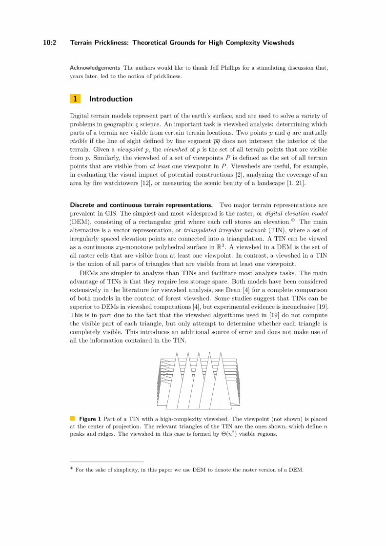
10:2 Terrain Prickliness: Theoretical Grounds for High Complexity Viewsheds

Acknowledgements The authors would like to thank Jeff Phillips for a stimulating discussion that,years later, led to the notion of prickliness.

1 Introduction

Digital terrain models represent part of the earth’s surface, and are used to solve a variety ofproblems in geographic ç science. An important task is viewshed analysis: determining whichparts of a terrain are visible from certain terrain locations. Two points p and q are mutuallyvisible if the line of sight defined by line segment pq does not intersect the interior of theterrain. Given a viewpoint p, the viewshed of p is the set of all terrain points that are visiblefrom p. Similarly, the viewshed of a set of viewpoints P is defined as the set of all terrainpoints that are visible from at least one viewpoint in P . Viewsheds are useful, for example,in evaluating the visual impact of potential constructions [2], analyzing the coverage of anarea by fire watchtowers [12], or measuring the scenic beauty of a landscape [1, 21].

Discrete and continuous terrain representations. Two major terrain representations areprevalent in GIS. The simplest and most widespread is the raster, or digital elevation model(DEM), consisting of a rectangular grid where each cell stores an elevation.① The mainalternative is a vector representation, or triangulated irregular network (TIN), where a set ofirregularly spaced elevation points are connected into a triangulation. A TIN can be viewedas a continuous xy-monotone polyhedral surface in R3. A viewshed in a DEM is the set ofall raster cells that are visible from at least one viewpoint. In contrast, a viewshed in a TINis the union of all parts of triangles that are visible from at least one viewpoint.

DEMs are simpler to analyze than TINs and facilitate most analysis tasks. The mainadvantage of TINs is that they require less storage space. Both models have been consideredextensively in the literature for viewshed analysis, see Dean [4] for a complete comparisonof both models in the context of forest viewshed. Some studies suggest that TINs can besuperior to DEMs in viewshed computations [4], but experimental evidence is inconclusive [19].This is in part due to the fact that the viewshed algorithms used in [19] do not computethe visible part of each triangle, but only attempt to determine whether each triangle iscompletely visible. This introduces an additional source of error and does not make use ofall the information contained in the TIN.

Figure 1 Part of a TIN with a high-complexity viewshed. The viewpoint (not shown) is placedat the center of projection. The relevant triangles of the TIN are the ones shown, which define n

peaks and ridges. The viewshed in this case is formed by Θ(n2) visible regions.

① For the sake of simplicity, in this paper we use DEM to denote the raster version of a DEM.

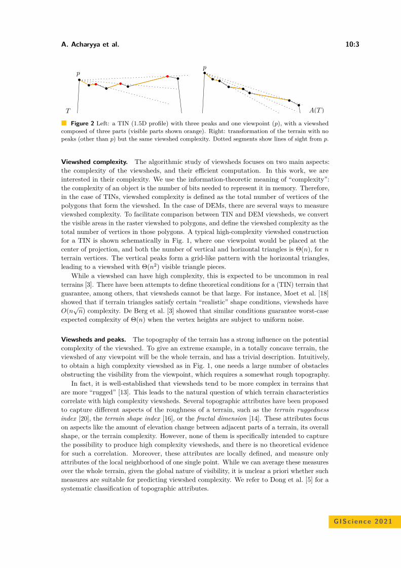
A. Acharyya et al. 10:3

p

T A(T )

p

Figure 2 Left: a TIN (1.5D profile) with three peaks and one viewpoint (p), with a viewshedcomposed of three parts (visible parts shown orange). Right: transformation of the terrain with nopeaks (other than p) but the same viewshed complexity. Dotted segments show lines of sight from p.

Viewshed complexity. The algorithmic study of viewsheds focuses on two main aspects:the complexity of the viewsheds, and their efficient computation. In this work, we areinterested in their complexity. We use the information-theoretic meaning of “complexity”:the complexity of an object is the number of bits needed to represent it in memory. Therefore,in the case of TINs, viewshed complexity is defined as the total number of vertices of thepolygons that form the viewshed. In the case of DEMs, there are several ways to measureviewshed complexity. To facilitate comparison between TIN and DEM viewsheds, we convertthe visible areas in the raster viewshed to polygons, and define the viewshed complexity as thetotal number of vertices in those polygons. A typical high-complexity viewshed constructionfor a TIN is shown schematically in Fig. 1, where one viewpoint would be placed at thecenter of projection, and both the number of vertical and horizontal triangles is Θ(n), for n

terrain vertices. The vertical peaks form a grid-like pattern with the horizontal triangles,leading to a viewshed with Θ(n2) visible triangle pieces.

While a viewshed can have high complexity, this is expected to be uncommon in realterrains [3]. There have been attempts to define theoretical conditions for a (TIN) terrain thatguarantee, among others, that viewsheds cannot be that large. For instance, Moet et al. [18]showed that if terrain triangles satisfy certain “realistic” shape conditions, viewsheds haveO(n

√n) complexity. De Berg et al. [3] showed that similar conditions guarantee worst-case

expected complexity of Θ(n) when the vertex heights are subject to uniform noise.

Viewsheds and peaks. The topography of the terrain has a strong influence on the potentialcomplexity of the viewshed. To give an extreme example, in a totally concave terrain, theviewshed of any viewpoint will be the whole terrain, and has a trivial description. Intuitively,to obtain a high complexity viewshed as in Fig. 1, one needs a large number of obstaclesobstructing the visibility from the viewpoint, which requires a somewhat rough topography.

In fact, it is well-established that viewsheds tend to be more complex in terrains thatare more “rugged” [13]. This leads to the natural question of which terrain characteristicscorrelate with high complexity viewsheds. Several topographic attributes have been proposedto capture different aspects of the roughness of a terrain, such as the terrain ruggednessindex [20], the terrain shape index [16], or the fractal dimension [14]. These attributes focuson aspects like the amount of elevation change between adjacent parts of a terrain, its overallshape, or the terrain complexity. However, none of them is specifically intended to capturethe possibility to produce high complexity viewsheds, and there is no theoretical evidencefor such a correlation. Moreover, these attributes are locally defined, and measure onlyattributes of the local neighborhood of one single point. While we can average these measuresover the whole terrain, given the global nature of visibility, it is unclear a priori whether suchmeasures are suitable for predicting viewshed complexity. We refer to Dong et al. [5] for asystematic classification of topographic attributes.

GISc ience 2021

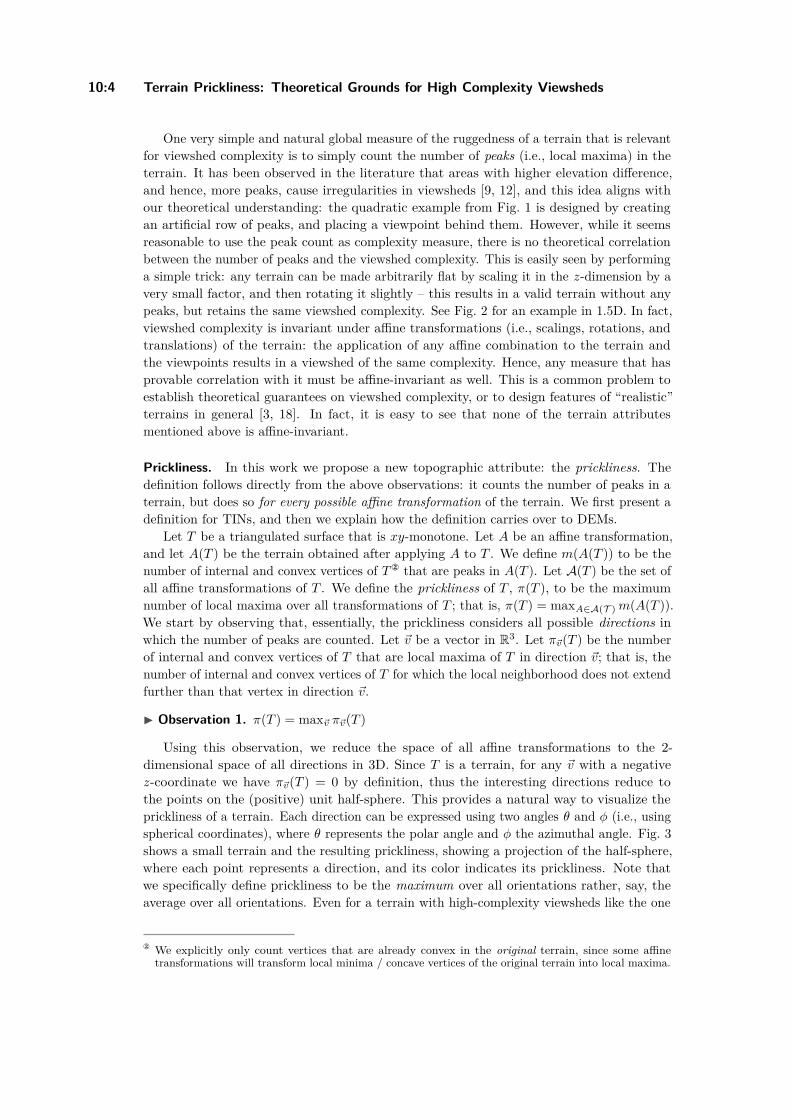
10:4 Terrain Prickliness: Theoretical Grounds for High Complexity Viewsheds

One very simple and natural global measure of the ruggedness of a terrain that is relevantfor viewshed complexity is to simply count the number of peaks (i.e., local maxima) in theterrain. It has been observed in the literature that areas with higher elevation difference,and hence, more peaks, cause irregularities in viewsheds [9, 12], and this idea aligns withour theoretical understanding: the quadratic example from Fig. 1 is designed by creatingan artificial row of peaks, and placing a viewpoint behind them. However, while it seemsreasonable to use the peak count as complexity measure, there is no theoretical correlationbetween the number of peaks and the viewshed complexity. This is easily seen by performinga simple trick: any terrain can be made arbitrarily flat by scaling it in the z-dimension by avery small factor, and then rotating it slightly – this results in a valid terrain without anypeaks, but retains the same viewshed complexity. See Fig. 2 for an example in 1.5D. In fact,viewshed complexity is invariant under affine transformations (i.e., scalings, rotations, andtranslations) of the terrain: the application of any affine combination to the terrain andthe viewpoints results in a viewshed of the same complexity. Hence, any measure that hasprovable correlation with it must be affine-invariant as well. This is a common problem toestablish theoretical guarantees on viewshed complexity, or to design features of “realistic”terrains in general [3, 18]. In fact, it is easy to see that none of the terrain attributesmentioned above is affine-invariant.

Prickliness. In this work we propose a new topographic attribute: the prickliness. Thedefinition follows directly from the above observations: it counts the number of peaks in aterrain, but does so for every possible affine transformation of the terrain. We first present adefinition for TINs, and then we explain how the definition carries over to DEMs.

Let T be a triangulated surface that is xy-monotone. Let A be an affine transformation,and let A(T ) be the terrain obtained after applying A to T . We define m(A(T )) to be thenumber of internal and convex vertices of T ② that are peaks in A(T ). Let A(T ) be the set ofall affine transformations of T . We define the prickliness of T , π(T ), to be the maximumnumber of local maxima over all transformations of T ; that is, π(T ) = maxA∈A(T ) m(A(T )).We start by observing that, essentially, the prickliness considers all possible directions inwhich the number of peaks are counted. Let v be a vector in R3. Let πv(T ) be the numberof internal and convex vertices of T that are local maxima of T in direction v; that is, thenumber of internal and convex vertices of T for which the local neighborhood does not extendfurther than that vertex in direction v.

Observation 1. π(T ) = maxv πv(T )

Using this observation, we reduce the space of all affine transformations to the 2-dimensional space of all directions in 3D. Since T is a terrain, for any v with a negativez-coordinate we have πv(T ) = 0 by definition, thus the interesting directions reduce tothe points on the (positive) unit half-sphere. This provides a natural way to visualize theprickliness of a terrain. Each direction can be expressed using two angles θ and ϕ (i.e., usingspherical coordinates), where θ represents the polar angle and ϕ the azimuthal angle. Fig. 3shows a small terrain and the resulting prickliness, showing a projection of the half-sphere,where each point represents a direction, and its color indicates its prickliness. Note thatwe specifically define prickliness to be the maximum over all orientations rather, say, theaverage over all orientations. Even for a terrain with high-complexity viewsheds like the one

② We explicitly only count vertices that are already convex in the original terrain, since some affinetransformations will transform local minima / concave vertices of the original terrain into local maxima.

A. Acharyya et al. 10:5

772 m

740 m0

8

510

1520

Figure 3 (left) A TIN T , with triangulation edges shown in black, and elevation indicated usingcolors. (right) A visualization of the prickliness of T as a function of the angles (θ, ϕ) that define eachdirection (circles indicate contour lines for θ); color indicates prickliness. The maximum pricklinessis 8, attained at a direction of roughly θ = 13 and ϕ = 60 (north-east from the origin).

in Fig. 1, the average number of peaks would still be relatively small since there are manyorientations with a small number of peaks. Hence, such a definition is unlikely to accuratelycapture the complexity of viewsheds on a terrain.

We notice that all previous notions easily translate to DEMs. The centers of the DEMcells can be seen as the vertices of the terrain, and every internal vertex of the terrain has eightneighbors given by the cell centers of the eight neighboring cells. Hence, in the definitionsfor DEMs, the notion of adjacent vertices for TINs is replaced by that of neighbors. A vertexis a local maximum for some affine transformation of the terrain if all of its neighbors have alower or equal z-coordinate. This gives an equivalent definition of π(T ) when T is a DEM.

Results and organization. The remainder of this paper is organized as follows.

In Section 2, we review existing topographic attributes in more detail, and discuss howattributes defined for DEMs can be adapted to TINs.We show in Section 3 that the viewshed complexity of a single viewpoint in a TIN terraincannot be higher than O(n · π(T )), and this is tight.In Section 4, we consider the question of how to compute prickliness. We provide an O(n2)time algorithm for TIN terrains, which is near-optimal, and an efficient approximatealgorithm for DEM terrains.In Sections 5-7, we report on experiments that measure the values of distinct topographicattributes (including the prickliness) of real terrains, and analyze their possible correlationwith viewshed complexity. From the experiments, we conclude that prickliness providessuch a correlation in the case of TIN terrains, while the other measures perform morepoorly. The situation for DEM terrains is less clear.Finally, we provide our code implementing two key algorithms for this work: an algorithmto calculate the prickliness of a TIN terrain and an algorithm to calculate the combinedviewshed originating from a set of multiple viewpoints.

2 Topographic attributes

In addition to prickliness, we consider the following topographic attributes, and their relationto viewshed complexity.

GISc ience 2021

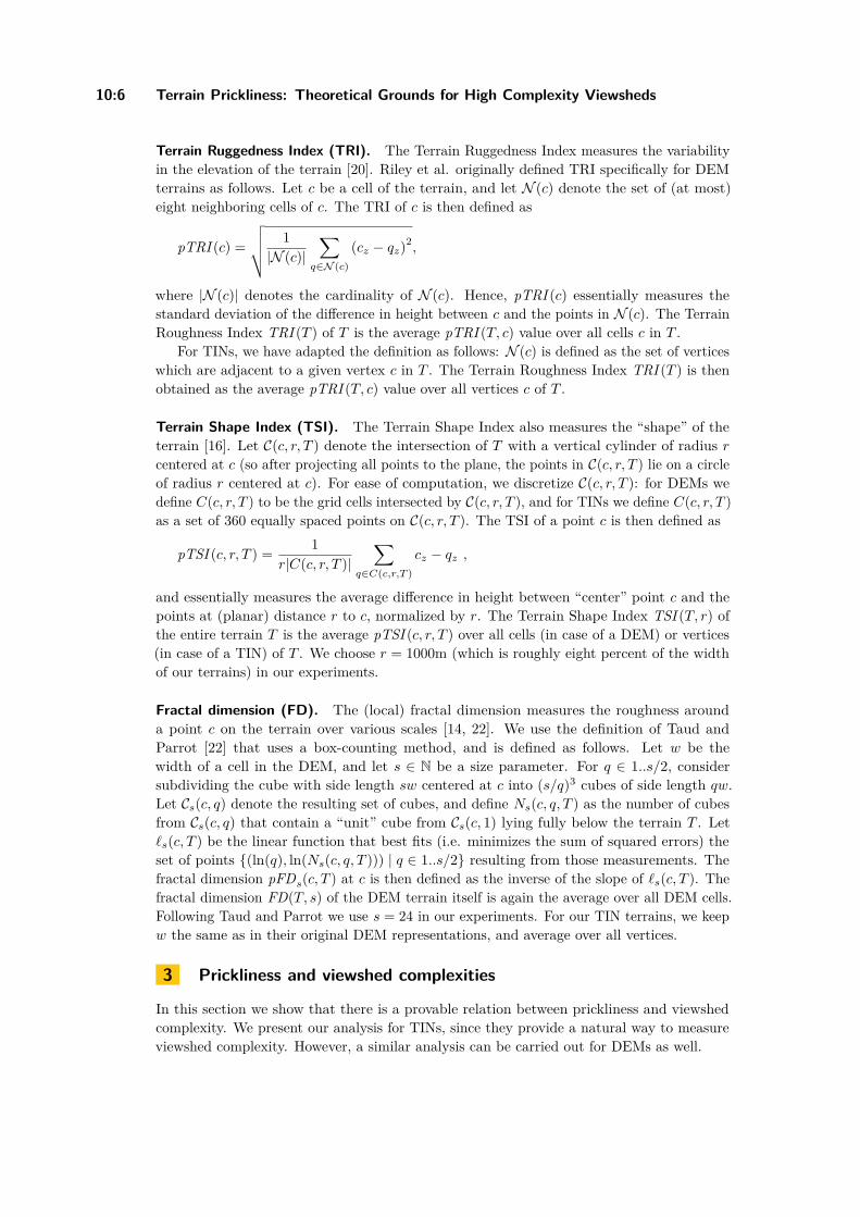
10:6 Terrain Prickliness: Theoretical Grounds for High Complexity Viewsheds

Terrain Ruggedness Index (TRI). The Terrain Ruggedness Index measures the variabilityin the elevation of the terrain [20]. Riley et al. originally defined TRI specifically for DEMterrains as follows. Let c be a cell of the terrain, and let N (c) denote the set of (at most)eight neighboring cells of c. The TRI of c is then defined as

pTRI (c) =

√√√√ 1|N (c)|

∑q∈N (c)

(cz − qz)2,

where |N (c)| denotes the cardinality of N (c). Hence, pTRI (c) essentially measures thestandard deviation of the difference in height between c and the points in N (c). The TerrainRoughness Index TRI (T ) of T is the average pTRI (T, c) value over all cells c in T .

For TINs, we have adapted the definition as follows: N (c) is defined as the set of verticeswhich are adjacent to a given vertex c in T . The Terrain Roughness Index TRI (T ) is thenobtained as the average pTRI (T, c) value over all vertices c of T .

Terrain Shape Index (TSI). The Terrain Shape Index also measures the “shape” of theterrain [16]. Let C(c, r, T ) denote the intersection of T with a vertical cylinder of radius r

centered at c (so after projecting all points to the plane, the points in C(c, r, T ) lie on a circleof radius r centered at c). For ease of computation, we discretize C(c, r, T ): for DEMs wedefine C(c, r, T ) to be the grid cells intersected by C(c, r, T ), and for TINs we define C(c, r, T )as a set of 360 equally spaced points on C(c, r, T ). The TSI of a point c is then defined as

pTSI (c, r, T ) = 1r|C(c, r, T )|

∑q∈C(c,r,T )

cz − qz ,

and essentially measures the average difference in height between “center” point c and thepoints at (planar) distance r to c, normalized by r. The Terrain Shape Index TSI (T, r) ofthe entire terrain T is the average pTSI (c, r, T ) over all cells (in case of a DEM) or vertices(in case of a TIN) of T . We choose r = 1000m (which is roughly eight percent of the widthof our terrains) in our experiments.

Fractal dimension (FD). The (local) fractal dimension measures the roughness arounda point c on the terrain over various scales [14, 22]. We use the definition of Taud andParrot [22] that uses a box-counting method, and is defined as follows. Let w be thewidth of a cell in the DEM, and let s ∈ N be a size parameter. For q ∈ 1..s/2, considersubdividing the cube with side length sw centered at c into (s/q)3 cubes of side length qw.Let Cs(c, q) denote the resulting set of cubes, and define Ns(c, q, T ) as the number of cubesfrom Cs(c, q) that contain a “unit” cube from Cs(c, 1) lying fully below the terrain T . Letℓs(c, T ) be the linear function that best fits (i.e. minimizes the sum of squared errors) theset of points (ln(q), ln(Ns(c, q, T ))) | q ∈ 1..s/2 resulting from those measurements. Thefractal dimension pFDs(c, T ) at c is then defined as the inverse of the slope of ℓs(c, T ). Thefractal dimension FD(T, s) of the DEM terrain itself is again the average over all DEM cells.Following Taud and Parrot we use s = 24 in our experiments. For our TIN terrains, we keepw the same as in their original DEM representations, and average over all vertices.

3 Prickliness and viewshed complexities

In this section we show that there is a provable relation between prickliness and viewshedcomplexity. We present our analysis for TINs, since they provide a natural way to measureviewshed complexity. However, a similar analysis can be carried out for DEMs as well.

A. Acharyya et al. 10:7

Let v be a vertex of T , and let p be a viewpoint. We denote by ↑vp the half-line with

origin at p in the direction of vector −→pv. Now, let e = uv be an edge of T . The vase of p ande, denoted ↑e

p, is the region bounded by e, ↑up , and ↑v

p (see Fig. 4).

p

e

v

u

↑up

↑vp

↑ep

Figure 4 A vase.

p

e1q

t

r

↑e2p

↑e1p

e2

Figure 5 The situation in the proof of Lemma 3.

Vertices of the viewshed of p can have three types [11]. A vertex of type 1 is a vertex ofT , of which there are clearly only n. A vertex of type 2 is the intersection of an edge of T

and a vase. A vertex of type 3 is the intersection of a triangle of T and two vases.

Lemma 2. There are at most O(n · π(T )) vertices of type 2.

Proof. Consider an edge e of T and let H be the plane spanned by e and p. Consider theviewshed of p on e. Let qr be a maximal invisible portion of e surrounded by two visibleones. Since q and r are vertices of type 2, the open segments pq and pr pass through a pointof T . On the other hand, for any point x in the open segment qr, there exist points of T

above the segment px. This implies that there is a continuous portion of T above H suchthat the vertical projection onto H of this portion lies on the triangle pqr. Such portionhas a local maximum in the direction perpendicular to H which is a convex and internalvertex of T . In consequence, each invisible portion of e surrounded by two visible ones canbe assigned to a distinct point of T that is a local maximum in the direction perpendicularto H. Hence, in the viewshed of p, e is partitioned into at most 2π(T ) + 3 parts.

Lemma 3. There are at most O(n · π(T )) vertices of type 3.

Proof. Let q be a vertex of type 3 in the viewshed of p. Point q is the intersection betweena triangle t of T and two vases, say, ↑e1

p and ↑e2p ; see Fig. 5. Let r be the ray with origin at

p and passing through q. Ray r intersects edges e1 and e2. First, we suppose that e1 ande2 do not share any vertices and, without loss of generality, we assume that r ∩ e1 is closerto p than r ∩ e2. Notice that r ∩ e2 is a vertex of type 2 because it is the intersection of e2and ↑e1

p , and ↑e1p partitions e2 into a visible and an invisible portion. Thus, we charge q to

r ∩ e2. If another vertex of type 3 was charged to r ∩ e2, then such a vertex would also lieon r. However, no point on r after q is visible from p because the visibility is blocked by t.Hence, no other vertex of type 3 is charged to r ∩ e2.

If e1 and e2 are both incident to a vertex v, since t ∩ ↑e1p ∩ ↑e2

p is a type 3 vertex, we havethat r passes through v. Therefore, q is the first intersection point between r (which can beseen as the ray with origin at p and passing through v) and the interior of some triangle inT . Therefore, any vertex v of T creates at most a unique vertex of type 3 in this way.

Theorem 4. Let T be a TIN terrain with n vertices and prickliness π(T ). The complexityof a viewshed is O(n · π(T )). This bound is asymptotically tight.

GISc ience 2021

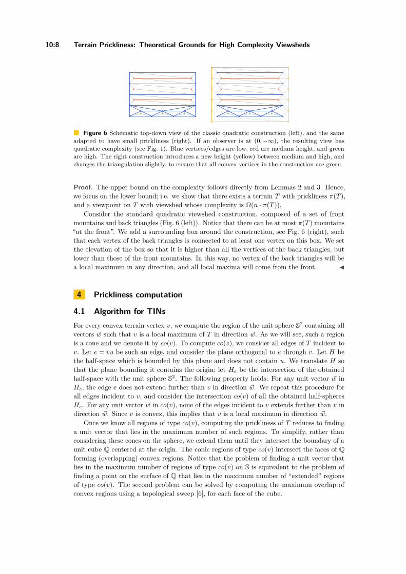
10:8 Terrain Prickliness: Theoretical Grounds for High Complexity Viewsheds

Figure 6 Schematic top-down view of the classic quadratic construction (left), and the sameadapted to have small prickliness (right). If an observer is at (0, −∞), the resulting view hasquadratic complexity (see Fig. 1). Blue vertices/edges are low, red are medium height, and greenare high. The right construction introduces a new height (yellow) between medium and high, andchanges the triangulation slightly, to ensure that all convex vertices in the construction are green.

Proof. The upper bound on the complexity follows directly from Lemmas 2 and 3. Hence,we focus on the lower bound; i.e. we show that there exists a terrain T with prickliness π(T ),and a viewpoint on T with viewshed whose complexity is Ω(n · π(T )).

Consider the standard quadratic viewshed construction, composed of a set of frontmountains and back triangles (Fig. 6 (left)). Notice that there can be at most π(T ) mountains“at the front”. We add a surrounding box around the construction, see Fig. 6 (right), suchthat each vertex of the back triangles is connected to at least one vertex on this box. We setthe elevation of the box so that it is higher than all the vertices of the back triangles, butlower than those of the front mountains. In this way, no vertex of the back triangles will bea local maximum in any direction, and all local maxima will come from the front.

4 Prickliness computation

4.1 Algorithm for TINsFor every convex terrain vertex v, we compute the region of the unit sphere S2 containing allvectors w such that v is a local maximum of T in direction w. As we will see, such a regionis a cone and we denote it by co(v). To compute co(v), we consider all edges of T incident tov. Let e = vu be such an edge, and consider the plane orthogonal to e through v. Let H bethe half-space which is bounded by this plane and does not contain u. We translate H sothat the plane bounding it contains the origin; let He be the intersection of the obtainedhalf-space with the unit sphere S2. The following property holds: For any unit vector w inHe, the edge e does not extend further than v in direction w. We repeat this procedure forall edges incident to v, and consider the intersection co(v) of all the obtained half-spheresHe. For any unit vector w in co(v), none of the edges incident to v extends further than v indirection w. Since v is convex, this implies that v is a local maximum in direction w.

Once we know all regions of type co(v), computing the prickliness of T reduces to findinga unit vector that lies in the maximum number of such regions. To simplify, rather thanconsidering these cones on the sphere, we extend them until they intersect the boundary of aunit cube Q centered at the origin. The conic regions of type co(v) intersect the faces of Qforming (overlapping) convex regions. Notice that the problem of finding a unit vector thatlies in the maximum number of regions of type co(v) on S is equivalent to the problem offinding a point on the surface of Q that lies in the maximum number of “extended” regionsof type co(v). The second problem can be solved by computing the maximum overlap ofconvex regions using a topological sweep [6], for each face of the cube.

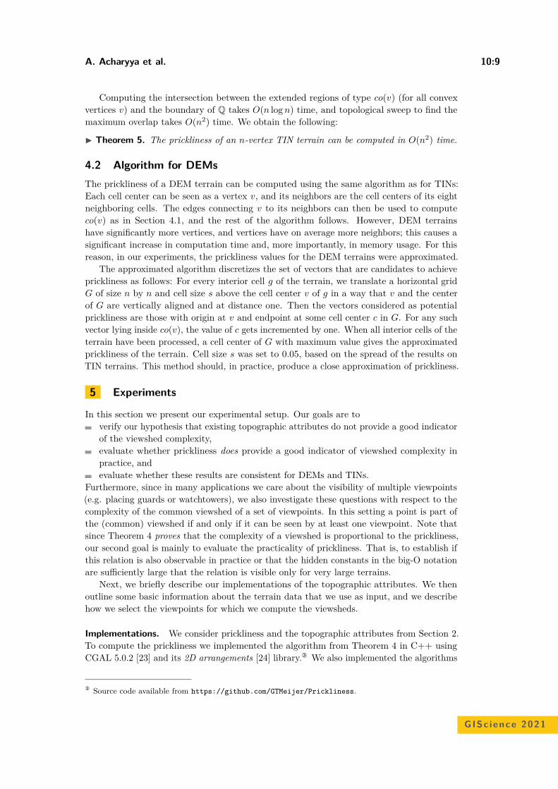
A. Acharyya et al. 10:9

Computing the intersection between the extended regions of type co(v) (for all convexvertices v) and the boundary of Q takes O(n log n) time, and topological sweep to find themaximum overlap takes O(n2) time. We obtain the following:

Theorem 5. The prickliness of an n-vertex TIN terrain can be computed in O(n2) time.

4.2 Algorithm for DEMsThe prickliness of a DEM terrain can be computed using the same algorithm as for TINs:Each cell center can be seen as a vertex v, and its neighbors are the cell centers of its eightneighboring cells. The edges connecting v to its neighbors can then be used to computeco(v) as in Section 4.1, and the rest of the algorithm follows. However, DEM terrainshave significantly more vertices, and vertices have on average more neighbors; this causes asignificant increase in computation time and, more importantly, in memory usage. For thisreason, in our experiments, the prickliness values for the DEM terrains were approximated.

The approximated algorithm discretizes the set of vectors that are candidates to achieveprickliness as follows: For every interior cell g of the terrain, we translate a horizontal gridG of size n by n and cell size s above the cell center v of g in a way that v and the centerof G are vertically aligned and at distance one. Then the vectors considered as potentialprickliness are those with origin at v and endpoint at some cell center c in G. For any suchvector lying inside co(v), the value of c gets incremented by one. When all interior cells of theterrain have been processed, a cell center of G with maximum value gives the approximatedprickliness of the terrain. Cell size s was set to 0.05, based on the spread of the results onTIN terrains. This method should, in practice, produce a close approximation of prickliness.

5 Experiments

In this section we present our experimental setup. Our goals are toverify our hypothesis that existing topographic attributes do not provide a good indicatorof the viewshed complexity,evaluate whether prickliness does provide a good indicator of viewshed complexity inpractice, andevaluate whether these results are consistent for DEMs and TINs.

Furthermore, since in many applications we care about the visibility of multiple viewpoints(e.g. placing guards or watchtowers), we also investigate these questions with respect to thecomplexity of the common viewshed of a set of viewpoints. In this setting a point is part ofthe (common) viewshed if and only if it can be seen by at least one viewpoint. Note thatsince Theorem 4 proves that the complexity of a viewshed is proportional to the prickliness,our second goal is mainly to evaluate the practicality of prickliness. That is, to establish ifthis relation is also observable in practice or that the hidden constants in the big-O notationare sufficiently large that the relation is visible only for very large terrains.

Next, we briefly describe our implementations of the topographic attributes. We thenoutline some basic information about the terrain data that we use as input, and we describehow we select the viewpoints for which we compute the viewsheds.

Implementations. We consider prickliness and the topographic attributes from Section 2.To compute the prickliness we implemented the algorithm from Theorem 4 in C++ usingCGAL 5.0.2 [23] and its 2D arrangements [24] library.③ We also implemented the algorithms

③ Source code available from https://github.com/GTMeijer/Prickliness.

GISc ience 2021

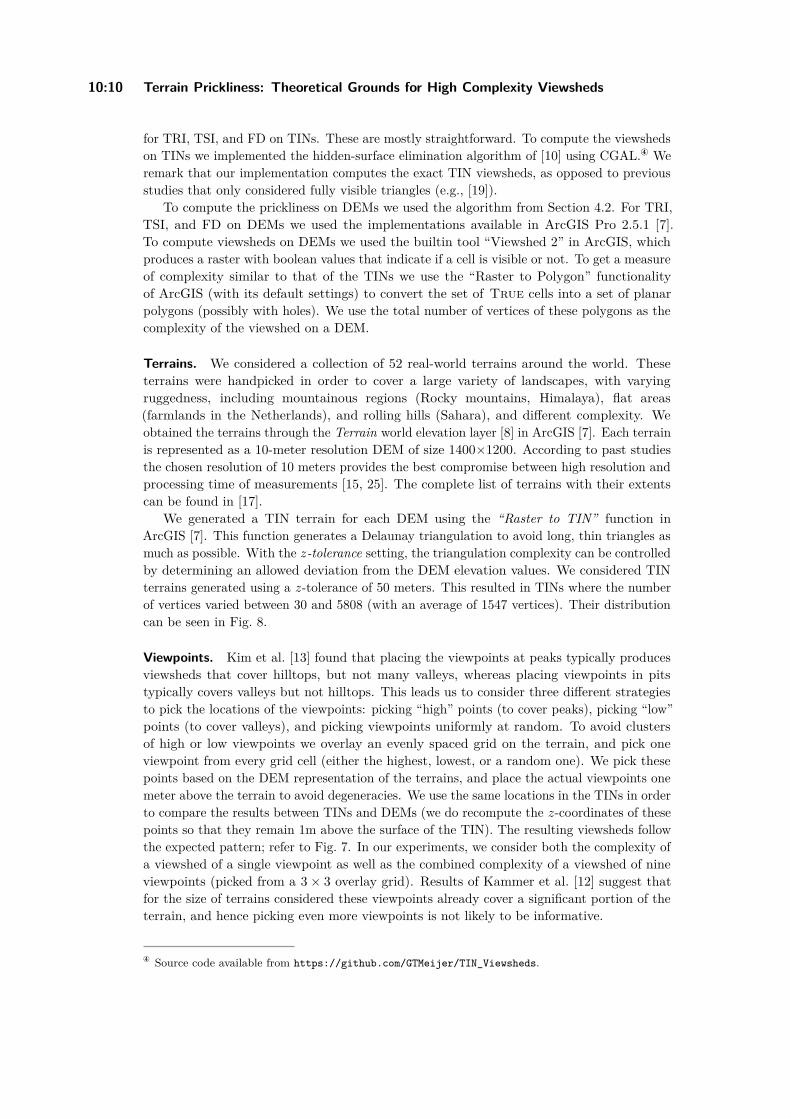
10:10 Terrain Prickliness: Theoretical Grounds for High Complexity Viewsheds

for TRI, TSI, and FD on TINs. These are mostly straightforward. To compute the viewshedson TINs we implemented the hidden-surface elimination algorithm of [10] using CGAL.④ Weremark that our implementation computes the exact TIN viewsheds, as opposed to previousstudies that only considered fully visible triangles (e.g., [19]).

To compute the prickliness on DEMs we used the algorithm from Section 4.2. For TRI,TSI, and FD on DEMs we used the implementations available in ArcGIS Pro 2.5.1 [7].To compute viewsheds on DEMs we used the builtin tool “Viewshed 2” in ArcGIS, whichproduces a raster with boolean values that indicate if a cell is visible or not. To get a measureof complexity similar to that of the TINs we use the “Raster to Polygon” functionalityof ArcGIS (with its default settings) to convert the set of True cells into a set of planarpolygons (possibly with holes). We use the total number of vertices of these polygons as thecomplexity of the viewshed on a DEM.

Terrains. We considered a collection of 52 real-world terrains around the world. Theseterrains were handpicked in order to cover a large variety of landscapes, with varyingruggedness, including mountainous regions (Rocky mountains, Himalaya), flat areas(farmlands in the Netherlands), and rolling hills (Sahara), and different complexity. Weobtained the terrains through the Terrain world elevation layer [8] in ArcGIS [7]. Each terrainis represented as a 10-meter resolution DEM of size 1400×1200. According to past studiesthe chosen resolution of 10 meters provides the best compromise between high resolution andprocessing time of measurements [15, 25]. The complete list of terrains with their extentscan be found in [17].

We generated a TIN terrain for each DEM using the “Raster to TIN” function inArcGIS [7]. This function generates a Delaunay triangulation to avoid long, thin triangles asmuch as possible. With the z-tolerance setting, the triangulation complexity can be controlledby determining an allowed deviation from the DEM elevation values. We considered TINterrains generated using a z-tolerance of 50 meters. This resulted in TINs where the numberof vertices varied between 30 and 5808 (with an average of 1547 vertices). Their distributioncan be seen in Fig. 8.

Viewpoints. Kim et al. [13] found that placing the viewpoints at peaks typically producesviewsheds that cover hilltops, but not many valleys, whereas placing viewpoints in pitstypically covers valleys but not hilltops. This leads us to consider three different strategiesto pick the locations of the viewpoints: picking “high” points (to cover peaks), picking “low”points (to cover valleys), and picking viewpoints uniformly at random. To avoid clustersof high or low viewpoints we overlay an evenly spaced grid on the terrain, and pick oneviewpoint from every grid cell (either the highest, lowest, or a random one). We pick thesepoints based on the DEM representation of the terrains, and place the actual viewpoints onemeter above the terrain to avoid degeneracies. We use the same locations in the TINs in orderto compare the results between TINs and DEMs (we do recompute the z-coordinates of thesepoints so that they remain 1m above the surface of the TIN). The resulting viewsheds followthe expected pattern; refer to Fig. 7. In our experiments, we consider both the complexity ofa viewshed of a single viewpoint as well as the combined complexity of a viewshed of nineviewpoints (picked from a 3 × 3 overlay grid). Results of Kammer et al. [12] suggest thatfor the size of terrains considered these viewpoints already cover a significant portion of theterrain, and hence picking even more viewpoints is not likely to be informative.

④ Source code available from https://github.com/GTMeijer/TIN_Viewsheds.

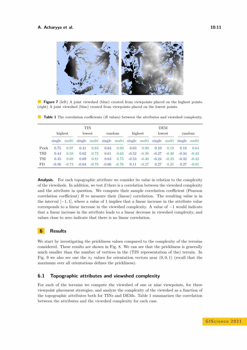
A. Acharyya et al. 10:11

Figure 7 (left) A joint viewshed (blue) created from viewpoints placed on the highest points.(right) A joint viewshed (blue) created from viewpoints placed on the lowest points.

Table 1 The correlation coefficients (R values) between the attributes and viewshed complexity.

TIN DEMhighest lowest random highest lowest random

single multi single multi single multi single multi single multi single multi

Prick 0.75 0.97 0.41 0.83 0.64 0.93 0.63 0.90 0.10 0.19 0.18 0.64TRI 0.44 0.58 0.62 0.72 0.61 0.63 -0.52 -0.38 -0.27 -0.30 -0.34 -0.43TSI 0.45 0.69 0.69 0.81 0.63 0.75 -0.53 -0.40 -0.24 -0.23 -0.32 -0.42FD -0.56 -0.73 -0.64 -0.78 -0.66 -0.76 0.11 -0.27 0.27 0.25 0.27 -0.01

Analysis. For each topographic attribute we consider its value in relation to the complexityof the viewsheds. In addition, we test if there is a correlation between the viewshed complexityand the attribute in question. We compute their sample correlation coefficient (Pearsoncorrelation coefficient) R to measure their (linear) correlation. The resulting value is inthe interval [−1, 1], where a value of 1 implies that a linear increase in the attribute valuecorresponds to a linear increase in the viewshed complexity. A value of −1 would indicatethat a linear increase in the attribute leads to a linear decrease in viewshed complexity, andvalues close to zero indicate that there is no linear correlation.

6 Results

We start by investigating the prickliness values compared to the complexity of the terrainsconsidered. These results are shown in Fig. 8. We can see that the prickliness is generallymuch smaller than the number of vertices in the (TIN representation of the) terrain. InFig. 9 we also see one the πv values for orientation vectors near (0, 0, 1) (recall that themaximum over all orientations defines the prickliness).

6.1 Topographic attributes and viewshed complexity

For each of the terrains we compute the viewshed of one or nine viewpoints, for threeviewpoint placement strategies, and analyze the complexity of the viewshed as a function ofthe topographic attributes both for TINs and DEMs. Table 1 summarizes the correlationbetween the attributes and the viewshed complexity for each case.

GISc ience 2021

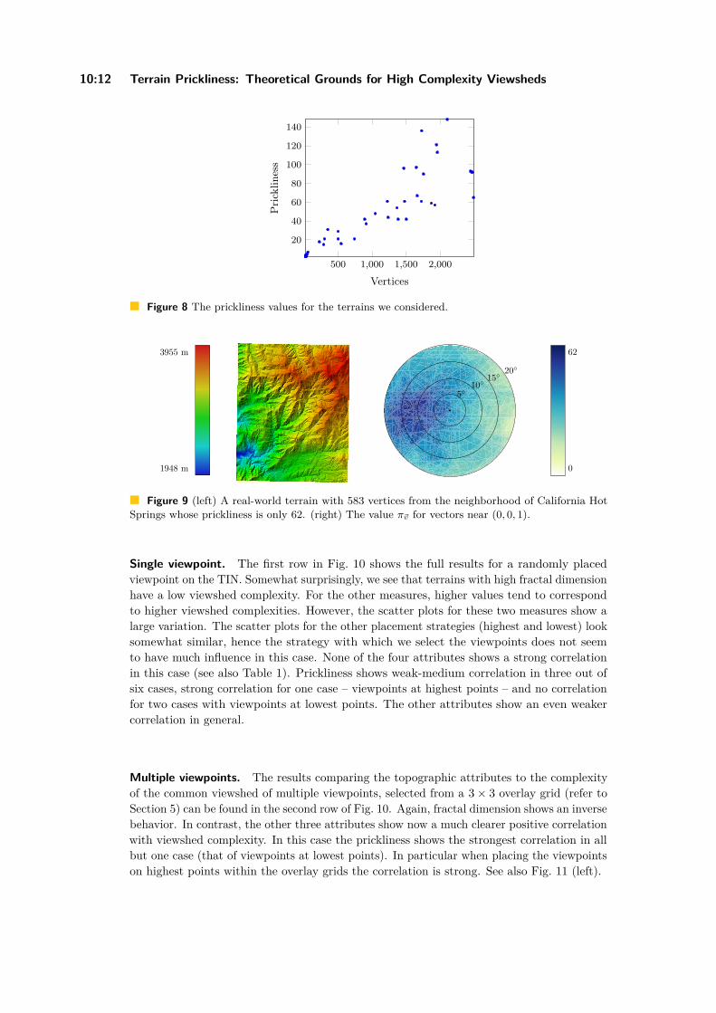
10:12 Terrain Prickliness: Theoretical Grounds for High Complexity Viewsheds

500 1,000 1,500 2,000

20

40

60

80

100

120

140

VerticesPrickliness

Terrain vertices vs. prickliness

Figure 8 The prickliness values for the terrains we considered.

3955 m

1948 m

510

1520

0

62

Figure 9 (left) A real-world terrain with 583 vertices from the neighborhood of California HotSprings whose prickliness is only 62. (right) The value πv for vectors near (0, 0, 1).

Single viewpoint. The first row in Fig. 10 shows the full results for a randomly placedviewpoint on the TIN. Somewhat surprisingly, we see that terrains with high fractal dimensionhave a low viewshed complexity. For the other measures, higher values tend to correspondto higher viewshed complexities. However, the scatter plots for these two measures show alarge variation. The scatter plots for the other placement strategies (highest and lowest) looksomewhat similar, hence the strategy with which we select the viewpoints does not seemto have much influence in this case. None of the four attributes shows a strong correlationin this case (see also Table 1). Prickliness shows weak-medium correlation in three out ofsix cases, strong correlation for one case – viewpoints at highest points – and no correlationfor two cases with viewpoints at lowest points. The other attributes show an even weakercorrelation in general.

Multiple viewpoints. The results comparing the topographic attributes to the complexityof the common viewshed of multiple viewpoints, selected from a 3 × 3 overlay grid (refer toSection 5) can be found in the second row of Fig. 10. Again, fractal dimension shows an inversebehavior. In contrast, the other three attributes show now a much clearer positive correlationwith viewshed complexity. In this case the prickliness shows the strongest correlation in allbut one case (that of viewpoints at lowest points). In particular when placing the viewpointson highest points within the overlay grids the correlation is strong. See also Fig. 11 (left).

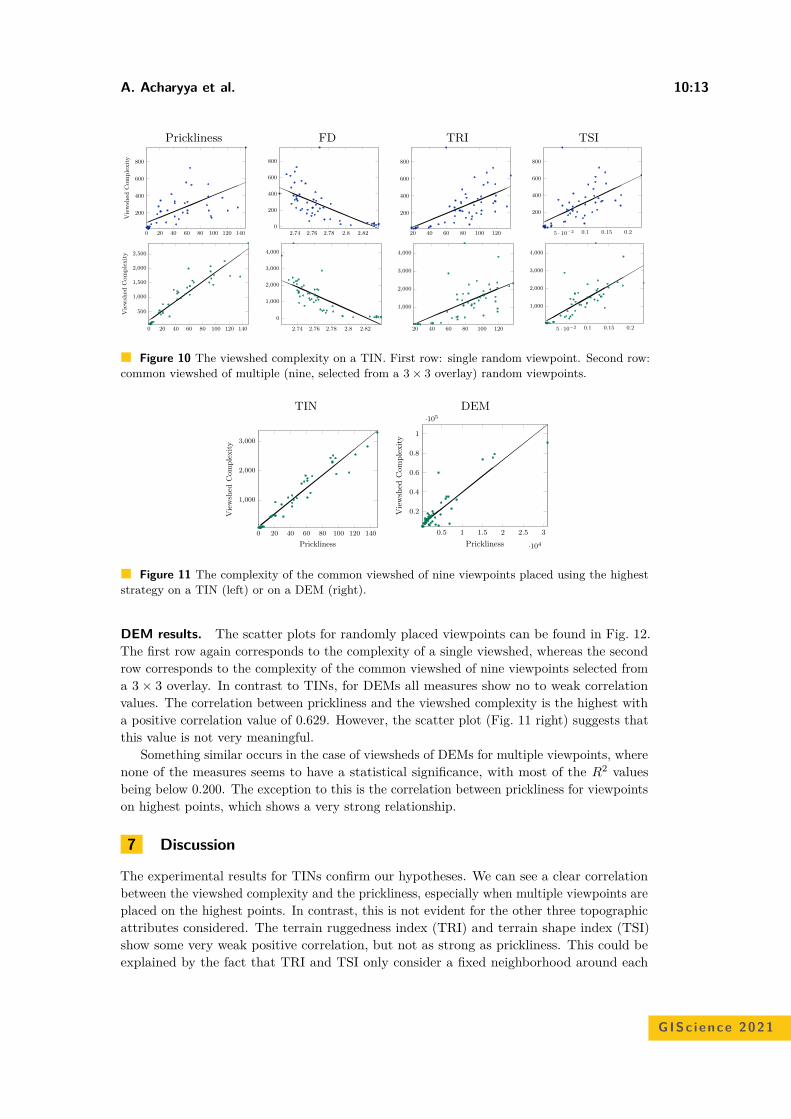
A. Acharyya et al. 10:13

Prickliness FD TRI TSI

0 20 40 60 80 100 120 140

200

400

600

800

Viewshed

Complexity

2.74 2.76 2.78 2.8 2.820

200

400

600

800

20 40 60 80 100 120

200

400

600

800

5 · 10−2 0.1 0.15 0.2

200

400

600

800

0 20 40 60 80 100 120 140

500

1,000

1,500

2,000

2,500

Viewshed

Complexity

2.74 2.76 2.78 2.8 2.82

0

1,000

2,000

3,000

4,000

20 40 60 80 100 120

1,000

2,000

3,000

4,000

5 · 10−2 0.1 0.15 0.2

1,000

2,000

3,000

4,000

Figure 10 The viewshed complexity on a TIN. First row: single random viewpoint. Second row:common viewshed of multiple (nine, selected from a 3 × 3 overlay) random viewpoints.

TIN DEM

0 20 40 60 80 100 120 140

1,000

2,000

3,000

Prickliness

Viewshed

Complexity

0.5 1 1.5 2 2.5 3

·104

0.2

0.4

0.6

0.8

1

·105

Prickliness

Viewshed

Complexity

Figure 11 The complexity of the common viewshed of nine viewpoints placed using the higheststrategy on a TIN (left) or on a DEM (right).

DEM results. The scatter plots for randomly placed viewpoints can be found in Fig. 12.The first row again corresponds to the complexity of a single viewshed, whereas the secondrow corresponds to the complexity of the common viewshed of nine viewpoints selected froma 3 × 3 overlay. In contrast to TINs, for DEMs all measures show no to weak correlationvalues. The correlation between prickliness and the viewshed complexity is the highest witha positive correlation value of 0.629. However, the scatter plot (Fig. 11 right) suggests thatthis value is not very meaningful.

Something similar occurs in the case of viewsheds of DEMs for multiple viewpoints, wherenone of the measures seems to have a statistical significance, with most of the R2 valuesbeing below 0.200. The exception to this is the correlation between prickliness for viewpointson highest points, which shows a very strong relationship.

7 Discussion

The experimental results for TINs confirm our hypotheses. We can see a clear correlationbetween the viewshed complexity and the prickliness, especially when multiple viewpoints areplaced on the highest points. In contrast, this is not evident for the other three topographicattributes considered. The terrain ruggedness index (TRI) and terrain shape index (TSI)show some very weak positive correlation, but not as strong as prickliness. This could beexplained by the fact that TRI and TSI only consider a fixed neighborhood around each

GISc ience 2021

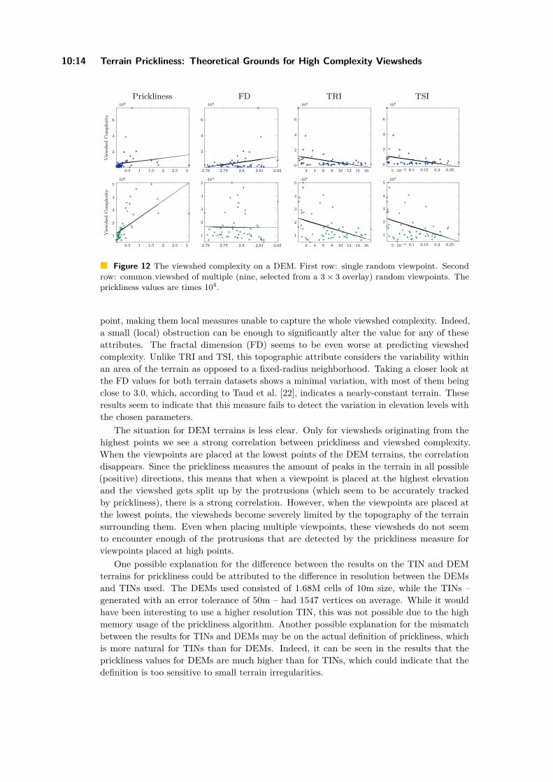
10:14 Terrain Prickliness: Theoretical Grounds for High Complexity Viewsheds

Prickliness FD TRI TSI

0.5 1 1.5 2 2.5 3

2

4

6

·104Viewshed

Complexity

2.78 2.79 2.8 2.81 2.82

2

4

6

·104

2 4 6 8 10 12 14 160

2

4

6

·104

5 · 10−2 0.1 0.15 0.2 0.25

0

2

4

6

·104

0.5 1 1.5 2 2.5 3

1

2

3

4

5·104

Viewshed

Complexity

2.78 2.79 2.8 2.81 2.82

1

2

3

4

5·104

2 4 6 8 10 12 14 16

1

2

3

4

5·104

5 · 10−2 0.1 0.15 0.2 0.25

1

2

3

4

5·104

Figure 12 The viewshed complexity on a DEM. First row: single random viewpoint. Secondrow: common viewshed of multiple (nine, selected from a 3 × 3 overlay) random viewpoints. Theprickliness values are times 104.

point, making them local measures unable to capture the whole viewshed complexity. Indeed,a small (local) obstruction can be enough to significantly alter the value for any of theseattributes. The fractal dimension (FD) seems to be even worse at predicting viewshedcomplexity. Unlike TRI and TSI, this topographic attribute considers the variability withinan area of the terrain as opposed to a fixed-radius neighborhood. Taking a closer look atthe FD values for both terrain datasets shows a minimal variation, with most of them beingclose to 3.0, which, according to Taud et al. [22], indicates a nearly-constant terrain. Theseresults seem to indicate that this measure fails to detect the variation in elevation levels withthe chosen parameters.

The situation for DEM terrains is less clear. Only for viewsheds originating from thehighest points we see a strong correlation between prickliness and viewshed complexity.When the viewpoints are placed at the lowest points of the DEM terrains, the correlationdisappears. Since the prickliness measures the amount of peaks in the terrain in all possible(positive) directions, this means that when a viewpoint is placed at the highest elevationand the viewshed gets split up by the protrusions (which seem to be accurately trackedby prickliness), there is a strong correlation. However, when the viewpoints are placed atthe lowest points, the viewsheds become severely limited by the topography of the terrainsurrounding them. Even when placing multiple viewpoints, these viewsheds do not seemto encounter enough of the protrusions that are detected by the prickliness measure forviewpoints placed at high points.

One possible explanation for the difference between the results on the TIN and DEMterrains for prickliness could be attributed to the difference in resolution between the DEMsand TINs used. The DEMs used consisted of 1.68M cells of 10m size, while the TINs –generated with an error tolerance of 50m – had 1547 vertices on average. While it wouldhave been interesting to use a higher resolution TIN, this was not possible due to the highmemory usage of the prickliness algorithm. Another possible explanation for the mismatchbetween the results for TINs and DEMs may be on the actual definition of prickliness, whichis more natural for TINs than for DEMs. Indeed, it can be seen in the results that theprickliness values for DEMs are much higher than for TINs, which could indicate that thedefinition is too sensitive to small terrain irregularities.

A. Acharyya et al. 10:15

8 Conclusion

We established that prickliness is a reasonable measure of potentially high viewshed complexity,at least for TINs, confirming our theoretical results. Moreover, prickliness shows a muchclearer correlation with viewshed complexity that the three other terrain attributes considered.

One aspect worth further investigation is its correlation for DEMs, which seems to bemuch weaker. One explanation for this might be that the definition of prickliness is morenatural for TINs than for DEMs, but there are several other possible explanations, and itwould be interesting future work to delve further into this phenomenon. Having establishedthat prickliness can be a useful terrain attribute, it remains to improve its computation time,so it can be applied to larger terrains in practice.

Finally, during our work we noticed that several of the terrain attributes are definedlocally, and are parameterized by some neighborhood size. Following previous work, weaggregated these local measures into a global measure by averaging the measurements. Itmay be worthwhile to investigate different aggregation methods as well. This also leads to amore general open question on how to “best” transform a local terrain measurement into aglobal one.

References1 Brent C. Chamberlain and Michael J. Meitner. A route-based visibility analysis for landscape

management. Landscape and Urban Planning, 111:13–24, 2013.

2 Maria Danese, Gabriele Nolè, and Beniamino Murgante. Identifying viewshed: New approachesto visual impact assessment. In Geocomputation, Sustainability and Environmental Planning,pages 73–89. Springer, 2011.

3 Mark de Berg, Herman Haverkort, and Constantinos P. Tsirogiannis. Visibility maps ofrealistic terrains have linear smoothed complexity. In Proceedings of the Twenty-Fifth AnnualSymposium on Computational Geometry, pages 163–168. ACM, 2009.

4 D J Dean. Improving the accuracy of forest viewsheds using triangulated networks and thevisual permeability method. Canadian Journal of Forest Research, 27(7):969–977, 1997.

5 Youfu Dong, Guoan Tang, and Ting Zhang. a Systematic Classification Research ofTopographic Descriptive Attribute in Digital Terrain Analysis. The International Archives ofthe Photogrammetry, Remote Sensing and Spatial Information Sciences, 37 B2:357–362, 2008.

6 Herbert Edelsbrunner and Leonidas J. Guibas. Topologically sweeping an arrangement. Journalof Computer and System Sciences, 38(1):165–194, 1989.

7 Environmental Systems Research Institute (ESRI). Arcgis pro (2.5.1), May 2020.

8 Environmental Systems Research Institute (ESRI). Terrain, scale: 10m, February 2020.

9 W. Randolph Franklin and Christian Vogt. Multiple observer siting on terrain withintervisibility or lo-res data. In XXth Congress, International Society for Photogrammetry andRemote Sensing, pages 12–23, 2004.

10 Michael T. Goodrich. A polygonal approach to hidden-line and hidden-surface elimination.CVGIP: Graphical Models and Image Processing, 54(1):1–12, January 1992.

11 Ferran Hurtado, Maarten Löffler, Inês Matos, Vera Sacristán, Maria Saumell, Rodrigo I.Silveira, and Frank Staals. Terrain visibility with multiple viewpoints. International Journalof Computational Geometry & Applications, 24(04):275–306, 2014.

12 Frank Kammer, Maarten Löffler, Paul Mutser, and Frank Staals. Practical approaches topartially guarding a polyhedral terrain. In Proc. 8th International Conference on GeographicInformation Science, LNCS 8728, pages 318–332, 2014.

GISc ience 2021

10:16 Terrain Prickliness: Theoretical Grounds for High Complexity Viewsheds

13 Young-Hoon Kim, Sanjay Rana, and Steve Wise. Exploring multiple viewshed analysis usingterrain features and optimisation techniques. Computers & Geosciences, 30(9):1019–1032,2004.

14 Benoit B Mandelbrot. The fractal geometry of nature. W.H. Freeman, New York, 1982.

15 J. J. Maynard and M. G. Johnson. Scale-dependency of LiDAR derived terrain attributesin quantitative soil-landscape modeling: Effects of grid resolution vs. neighborhood extent.Geoderma, 230-231:29–40, 2014.

16 W. Henry McNab. Terrain shape index: Quantifying effect of minor landforms on tree height.Forest Science, 35:91–104, 1989.

17 Gert Meijer. Realistic terrain features and the complexity of joint viewsheds. Master’s thesis,Utrecht University, 2020.

18 Esther Moet, Marc van Kreveld, and A. Frank van der Stappen. On realistic terrains.Computational Geometry, 41(1):48–67, 2008.

19 Philip D Riggs and Denis J Dean. An investigation into the causes of errors and inconsistenciesin predicted viewsheds. Transactions in GIS, 11(2):175–196, 2007.

20 Shawn J. Riley, Stephen D. DeGloria, and Robert Elliot. A terrain ruggedness index thatquantifies topographic heterogeneity. Journal of Science, 5:23–27, 1999.

21 Uta Schirpke, Erich Tasser, and Ulrike Tappeiner. Predicting scenic beauty of mountainregions. Landscape Urban Plan., 111:1–12, 2013.

22 Hind Taud and Jean-François Parrot. Measurement of DEM roughness using the local fractaldimension. Géomorphologie : relief, processus, environnement, 11(4):327–338, 2005.

23 The CGAL Project. CGAL User and Reference Manual. CGAL Editorial Board, 5.0.2 edition,2020.

24 Ron Wein, Eric Berberich, Efi Fogel, Dan Halperin, Michael Hemmer, Oren Salzman, andBaruch Zukerman. 2d arrangements. In CGAL User and Reference Manual. CGAL EditorialBoard, 5.0.2 edition, 2020.

25 Weihua Zhang and David R Montgomery. Digital elevation model grid size, landscaperepresentation, and hydrologic simulations. Water Resources Research, 30(4):1019–1028, 1994.

User Preferences and the Shortest PathIsabella Kreller #

University of Regensburg, Germany

Bernd Ludwig #

University of Regensburg, Germany

AbstractIndoor navigation systems leverage shortest path algorithms to calculate routes. In order to definethe “shortest path”, a cost function has to be specified based on theories and heuristics in theapplication domain. For the domain of indoor routing, we survey theories and criteria identified inthe literature as essential for human path planning. We drive quantitative definitions and integratethem into a cost function that weights each of the criteria separately. We then apply an exhaustivegrid search to find weights that lead to an ideal cost function. “Ideal” here is defined as guidingthe algorithm to plan routes that are most similar to those chosen by humans. To explore whichcriteria should be taken into account in an improved pathfinding algorithm, eleven different factorswhose favorable impact on route selection has been established in past research were considered.Each factor was included separately in the Dijkstra algorithm and the similarity of thus calculatedroutes to the actual routes chosen by students at the University of Regensburg was determined.This allows for a quantitative assessment of the factors’ impact and further constitutes a way todirectly compare them. A reduction of the number of turns, streets, revolving doors, entryways,elevators as well as the combination of the aforementioned factors was found to have a positive effectand generate paths that were favored over the shortest path. Turns and the combination of criteriaturned out to be most impactful.

2012 ACM Subject Classification Human-centered computing; Human-centered computing →Empirical studies in ubiquitous and mobile computing

Keywords and phrases Pedestrian Navigation Systems, Wayfinding, Computation of Optimal Paths,User Preferences for Best Routes

Digital Object Identifier 10.4230/LIPIcs.GIScience.2021.II.11

1 Introduction

Finding a way through their immediate environment to reach a sought destination is a taskhighly relevant to humans since they see themselves confronted with it regularly. Due to theavailable options of traveling and visiting unfamiliar cities in foreign countries, the culturaldifferences as well as the possible language barrier may further complicate wayfinding tasks.Being able to facilitate situations like these, location-based navigation services, particularlythose intended for car navigation, enjoy great popularity and have established themselves asindispensable supporting tools for navigation in the modern world, as indicated by the highusage of Google Maps [17].

Although still overshadowed by the ubiquity of outdoor navigation systems, indoorwayfinding is not anymore an obscure area of research and it might be that in this settingnavigational support might be needed most. Wayfinding, meaning the goal-oriented processof a person finding a predefined destination [2], often involving navigation through largeareas without initial perception of the target location [27], is deemed a cognitive challengingtask requiring a variety of mental resources [35].

In addition, indoor spaces exhibit structural attributes, such as the additional dimension-ality inherent in multi-storied buildings [18] or the lack of reliable methods for localization[42], which give rise to further difficulties and require current systems to be adapted to thisnavigational context.

© Isabella Kreller and Bernd Ludwig;licensed under Creative Commons License CC-BY 4.0

11th International Conference on Geographic Information Science (GIScience 2021) – Part II.Editors: Krzysztof Janowicz and Judith A. Verstegen; Article No. 11; pp. 11:1–11:15

Leibniz International Proceedings in InformaticsSchloss Dagstuhl – Leibniz-Zentrum für Informatik, Dagstuhl Publishing, Germany

11:2 User Preferences and the Shortest Path

This likewise concerns the pathfinding algorithm: due to the current lack of geospatialresearch regarding this setting, employed algorithms have shown little to no deviationfrom optimizing only in regard to the route’s efficiency disregarding human preference.Previous studies, as discussed in subsections 2.2, 2.3, and 3.3, have determined a multitudeof diverse criteria as influential to people’s path choices, yet quantification of their impactand applicability in indoor environments remain to be studied.

2 Related Work

2.1 Difficulties of Indoor NavigationThe reasons for which indoor navigation systems lack the popularity and widespread usetheir outdoor counterparts are enjoying are twofold.

Firstly, there exist additional difficulties regarding the implementation of indoor navigationsystems. The additional third dimension, the height, inherent in multi-level buildings createschallenges regarding a suitable design for the visual projection onto the small two-dimensionalscreens of smartphones [5]. This is important for providing easily comprehensible andunambiguous instructions to the user to direct them to the correct floor. Hence, conventionalvisualizations and user interfaces of map-based applications are not predestined for wayfindingsupport inside buildings.

Yet the most crucial obstacle to overcome is likely the absence of a reliable method oflocalization. Whereas the vast majority of outdoor navigation systems make use of GlobalPositioning System (GPS) signals [42], this does not constitute a viable option indoors. Thesesignals manage to pass through the walls and ceilings of buildings only sporadically, renderingit an unsatisfactory solution for optimal navigational support [42]. Although numerousalternatives, including WiFi, Bluetooth, and Infrared, have been proposed, these too entaildrawbacks regarding performance, cost, or reliability. [42]

Furthermore, human orientation may also prove more challenging in this setting. Thethird dimension, i.e. multiple stories inside buildings, creates challenges not only for thesystem’s ability to display information but for human wayfinding as well. Staircases havebeen identified as the location where mistakes are being made most frequently during awayfinding task [18]; other research supports the idea that people struggle with vertical,rather than horizontal, movement, which might be explained by the mistaken assumptionthat a building’s layout is identical across floors [43]. A restricted field of vision due to wallsand corners makes the usage of landmarks as points of reference only possible if they arelocal or in direct line of view, whereas in outdoor spaces global landmarks, such as towers orthe city skyline, can also support wayfinding. [52].

2.2 Influential FactorsThere is reason to contest and doubt that humans’ behavior is purely rational and can beexplained with conscious and deliberate reasoning alone for we are susceptible to numerousbiases in our ways of thinking and decision making [23].

The same holds for wayfinding behavior: while the most logical path to the desireddestination would generally be the shortest or least time consuming one, this does not alignwith actual human conduct or preference [3, 14, 3, 54].

Afyouni, Ray, and Claramunt [1] suggest a classification of the context in which decisionmaking takes place that can also be applied to wayfinding tasks. The user-centered contexttakes into account the navigator’s profile, such as mental capabilities of visualization [44],

I. Kreller and B. Ludwig 11:3

or rotation of objects [32], their age [45] and gender [28], or cultural background [20]. Thecontext of execution, on the other hand, describes qualities of the information systems whichaid the user; the representation of maps and real-world references used by mobile applications[38] has been found to impact navigational success, and so do conventional means of support,such as signs and paper maps to varying degrees.

What is most relevant for the adjustment of the pathfinding algorithm, however, can bedescribed by the environmental context.

According to Lynch [29], the components most crucial for the formation of mental mapsare paths, edges, districts, and landmarks, which, belonging to the same mental models, existin connection and mutual interference. This concept fits well into the research conducted,which suggests that humans mentally visualize their environment as being structurallyequivalent to a network of streets and paths [13, 27, 33].

In this sense, the definition of a path’s complexity contrived by Golledge [14] and sinceadopted into the work of many others [11, 19, 40] is to consider the number of streets orturns connecting them.

Alternative approaches [4, 12, 16, 40, 51] of achieving simplicity take into account thenumber of decision points, i.e. intersections of multiple streets, or their branching factor.It is defined by the number of streets meeting, thus considered a measure of difficulty orcomplexity of a decision point [37] and increasing the possibility of losing one’s way [2].

Rather than the number of branches, Dalton [8] found a preference for choosing themaximum, rather than mean or minimum, angles of paths available at decision points, meaningthat people were more likely to choose the way that was aligned most with from where theywere coming, presumably as a complexity-minimizing strategy. Further observations supportthe idea of people’s predilection towards maintaining linearity in their routes [7, 34, 41, 53].Similarly, another study points towards a human preference of decreasing the angular distanceto the destination (Turner, 2009) at decision points, favoring this over a reduction of theManhattan distance.

Other than a preference for simple paths, the absence or presence of certain pathentities could serve as a decisive factor. Landmarks, defined by their conspicuity andrecognizability [6, 29] commonly function as points of reference and may help reduce cognitiveload for orientation [15]. For staircases, both a preference [24] and avoidance [24, 26] havebeen identified.

2.3 Alternatives to the Shortest Path

Variants for the cost function in path planning have been proposed with different objectives inmind. Grum [16] describes a way of extending the Dijkstra algorithm so that it incorporates aweight for the risk of making a wrong decision at an intersection proportional to the distanceof the mistakenly chosen path, assuming that the navigator notices their mistake at the nextdecision point and retraces their way. In this manner, not the shortest path, but the onewith the least danger of getting lost is computed. Yet, the question remains open how therisk for wrong decisions may be estimated for arbitrary environments.

Duckham and Kulik [11] proposed a way of calculating the simplest path, using solelya measure for ease of navigation by weighting route instructions without taking distanceinto account at all. Instructions needed to navigate decision points were penalized accordingto adjusted slot values for turns and branches as proposed by Mark [31], yielding thesought-after advantages.

GISc ience 2021

11:4 User Preferences and the Shortest Path

Physically constrained people constitute a group of users which might benefit immenselyfrom adjustments to conventional navigation systems. A proposed way of achieving thisis by taking into account edge weights other than distances, thus considering specific userpreferences such as avoiding stairs or minimizing turns which can be input directly bythe user [30].

In contrast, introducing a measure of beauty as a way of suggesting short routes thatare perceived to be emotionally pleasant was accomplished by crowdsourcing of people’sjudgments of places along the dimensions beautiful, quiet, and happy, making use of picturesfrom Google Street View or taken by volunteers [39]. Such an aesthetic criterion has notbeen considered by the persons who provided us with their preferred routes, because theytried to reach their destination as quickly and easily as possible. However, [22] report thatminimizing the number of turns is a key criterion for route planning in outdoor environments.Such routes seems to be more easily perceivable and cognitively less demanding.

In our study we evaluate, whether this result can be transferred to indoor environmentsand whether other criteria (e.g. level changes or use of elevators) that result from indoorarchitectural constraints also influence human decision making for route planning.

3 Route Calculation

To operationalize the above research question, we make use of the indoor navigation systemURWalking [36, 49] (urwalking.ur.de). It implements Dijkstra’s algorithm [10] to de-termine the shortest path in terms of the distance between starting point and destinationin meters.

3.1 User Preferred Routes

Our empirical study is based on a data set of 221 routes, collected both during the summer (100paths) and winter semester (121 paths) at the University of Regensburg, thus accommodatingfor differences in weather and temperature. All participants, 129 of which were male, statedto be highly familiar with the environment and ranged in age from 19 to 33 (mean age =22.93, SD = 2.67). As means for data collection, participants were asked to walk and describetheir daily route on the campus. The university campus spans over an expanse of 1 km2 andincludes 16 buildings with a sum of 86 individual floors and 5228 rooms, encompassing bothpaths indoors and outdoors [36].

The aim of the data collection was to find out whether modifications of URWalking’s pathplanning algorithm could lead to routes users enjoy taking, so as to find a compromise betweenthe theoretically minimal walking distance and the distance of preferred paths (i.e. can weapproximately simulate human decision making using Dijkstra’s efficient algorithm?). Forthe envisioned modifications, we identified criteria in research literature that are argued toimpact human decision making during wayfinding tasks.

3.2 Criteria

The criteria that will be described in the following were chosen due to the extent of theresearch they are supported by and applied in, and also based on the feasibility of theirincorporation into the Dijkstra algorithm. The scope of literature on the measurement ofpath complexity suggests that there is no agreed-upon answer as to how to define it. Althougha few studies have suggested more elaborate ways of ruling how complex a path is, a fewelementary classifications resurface frequently across research papers. We identified 11 factors:

I. Kreller and B. Ludwig 11:5

A straightforward way to determine complexity is by considering the (1) number ofturns a route contains. Regarding the definition of what constitutes a turn in navigationthe answers once again are ambiguous. According to the Cambridge Dictionary [47], a turncan be considered “a change in the direction in which you are moving or facing”. Althoughin some studies a sufficient change in directions achieved only when the angle between twopath segments is smaller or equal to 90 degrees [19, 50], others interpret every branch at adecision point to count as a turn [11, 25].

A related factor influential to wayfinding is the (2) number of streets, meaning thepath segments separated by decision points or turns of any kind [19]. Considering only turnsup to a maximum angle of 90 degrees would not account for the number of streets whereasdisregarding the angle entirely would run the risk of accounting for turns that might not beperceived as such due to their small deviation from a linear path. For these reasons, both ofthe definitions of what constitutes a turn were examined: weighting turns regardless of theirangle will acknowledge the number of streets more completely, and following the definitionin accordance with [19] comprises a more traditional way of regarding turns and assessingtheir impact independently.

The (3) number of decision points themselves was considered for route calculation aswell. Since the number of paths at a junction demanding a decision is two in addition to thepath the navigator came from, a decision point in this study was defined as an intersection ofthree or more paths; their exact number was disregarded and every path located at a pointwhich fits this definition was penalized in the same way.

The (4) branching factor, meaning the number of intersecting paths, was regardedseparately. To weigh the paths proportionally to their quantity, every path at a decisionpoint received the additional weight times the number of intersecting paths. These weightswere taken into account only at places that qualify as decision points corresponding to theaforementioned definition.

The findings on which paths at intersections constitute the most likely choice are am-biguous, which is why two divergent findings were considered. One is the preference forselecting the path which most closely aligns with the global direction of the destination[48], being equal to the avoidance of all paths other than the one with the (5) minimumdeviation angle.

Alternatively, a preference for (6) linearity [7] might influence the person navigating tocontinue their route along the most linear path, i.e. the path with the largest angle (between0 and 180 degrees) in regard to the direction from which the navigator arrived. For this, allexcept the most linear branch at a decision point were penalized, allowing for the option ofexempting two branches in case of identical largest angles. To keep with the definition oflinearity as well as Dalton’s study [8], the condition was added that the largest angle had tospan 150 degrees or more. If there was no such angle, e.g. in a T-crossing, no weighting wascarried out.

Due to the contradictory nature of the literature regarding the preference for (7) stair-cases in routes, both a preference for and avoidance of stairs were considered. (8) Elevatorsconstituted the only alternative for changing floors at the university; hence the avoidanceof stairs, being equal to a preference for elevators, was implemented by adding weights forevery staircase and vice versa.

Another element to be taken into consideration for indoor environments exclusively isdoors. The path network used for calculating routes includes different types of nodes thatdifferentiate between (9) doorways, (10) entrances to closed premises such as offices orlecture halls, termed entryways, and (11) revolving doors. Since it has been found that

GISc ience 2021

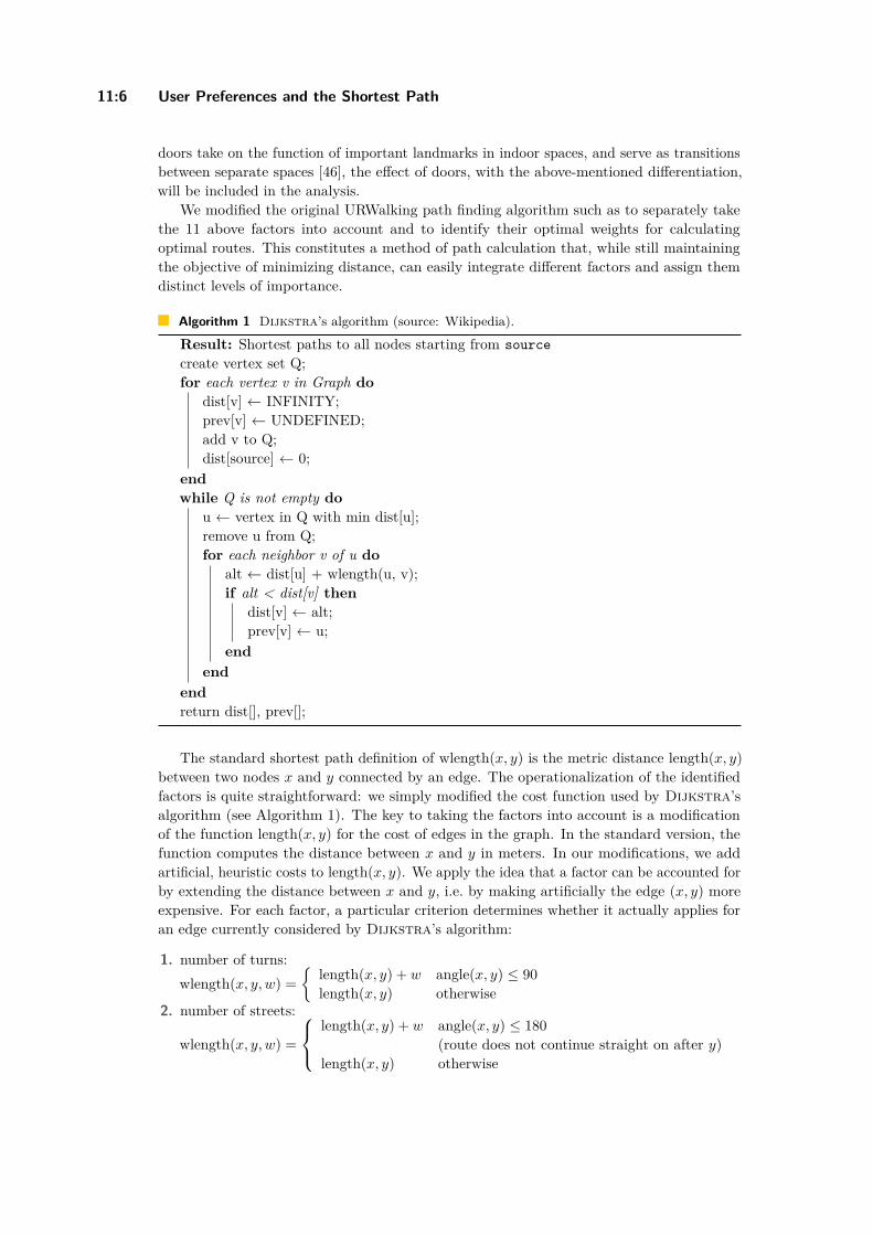
11:6 User Preferences and the Shortest Path

doors take on the function of important landmarks in indoor spaces, and serve as transitionsbetween separate spaces [46], the effect of doors, with the above-mentioned differentiation,will be included in the analysis.

We modified the original URWalking path finding algorithm such as to separately takethe 11 above factors into account and to identify their optimal weights for calculatingoptimal routes. This constitutes a method of path calculation that, while still maintainingthe objective of minimizing distance, can easily integrate different factors and assign themdistinct levels of importance.

Algorithm 1 Dijkstra’s algorithm (source: Wikipedia).

Result: Shortest paths to all nodes starting from sourcecreate vertex set Q;for each vertex v in Graph do

dist[v] ← INFINITY;prev[v] ← UNDEFINED;add v to Q;dist[source] ← 0;

endwhile Q is not empty do

u ← vertex in Q with min dist[u];remove u from Q;for each neighbor v of u do

alt ← dist[u] + wlength(u, v);if alt < dist[v] then

dist[v] ← alt;prev[v] ← u;

endend

endreturn dist[], prev[];

The standard shortest path definition of wlength(x, y) is the metric distance length(x, y)between two nodes x and y connected by an edge. The operationalization of the identifiedfactors is quite straightforward: we simply modified the cost function used by Dijkstra’salgorithm (see Algorithm 1). The key to taking the factors into account is a modificationof the function length(x, y) for the cost of edges in the graph. In the standard version, thefunction computes the distance between x and y in meters. In our modifications, we addartificial, heuristic costs to length(x, y). We apply the idea that a factor can be accounted forby extending the distance between x and y, i.e. by making artificially the edge (x, y) moreexpensive. For each factor, a particular criterion determines whether it actually applies foran edge currently considered by Dijkstra’s algorithm:

1. number of turns:wlength(x, y, w) =

length(x, y) + w angle(x, y) ≤ 90length(x, y) otherwise

2. number of streets:

wlength(x, y, w) =

length(x, y) + w angle(x, y) ≤ 180

(route does not continue straight on after y)length(x, y) otherwise

I. Kreller and B. Ludwig 11:7

3. number of decision points:

wlength(x, y, w) =

length(x, y) + w x has at least three neighbourslength(x, y) otherwise

4. branching factor:

wlength(x, y, w) =

length(x, y) + n · weight x has exactly n neighbours and n ≥ 3length(x, y) otherwise

5. minimum deviation angle:

wlength(x, y, w) =

length(x, y) + w x has at least three neighbours

and y = arg minz angle(x, z)length(x, y) otherwise

6. linearity:

wlength(x, y, w) =

length(x, y) + w x has at least three neighbours

and y = arg maxz angle(x, z)and maxz angle(x, z) ≥ 150

length(x, y) otherwise7. staircases:

wlength(x, y, w) =

length(x, y) + w y is an edge of type staircaselength(x, y) otherwise

8. elevators:wlength(x, y, w) =

length(x, y) + w y is an edge of type elevatorlength(x, y) otherwise

9. doorways:

wlength(x, y, w) =

length(x, y) + w y is of type doorwaylength(x, y) otherwise

10. entrances:wlength(x, y, w) =

length(x, y) + w y is of type entrancelength(x, y) otherwise

11. revolving doors:

wlength(x, y, w) =

length(x, y) + w y is of type revolving-doorlength(x, y) otherwise

In these definition w is a constant whose value determines by how many meters the lengthof an edge between x and y is extended. Consequentially, the shortest path gets “longer” themore instances of the respective considered factor it includes.

With this model, our main task is now to determine values of w for each factor thatmaximizes the similarity between routes calculated by URWalking and those chosen by theparticipants of our study.

3.3 Systematic Search for Optimal WeightsOur intuition is that a meaningful assessment of similarity between two routes r1 and r2reflects the length of shared path segments, i.e. edges in r1 and r2:

similarity(r1, r2) =

∑e∈r1∧e∈r2

length(e)

min(length(r1), length(r2))

with length(r) =∑

e∈r length(e) for any route r and length(e) = length(x, y) with x beingthe source node and y the sink node of any edge e.

In other words, the calculated Similarity Score similarity(r1, r2) was defined as the sum ofthe distances belonging to shared edges divided by the length of the shorter path (analogousto [21]). Following Delling et al.’s [9] approach, the mean of the similarity scores across allpath comparisons was then considered for assessment of the algorithm, i.e. each factor’sindividual impact on wayfinding.

GISc ience 2021

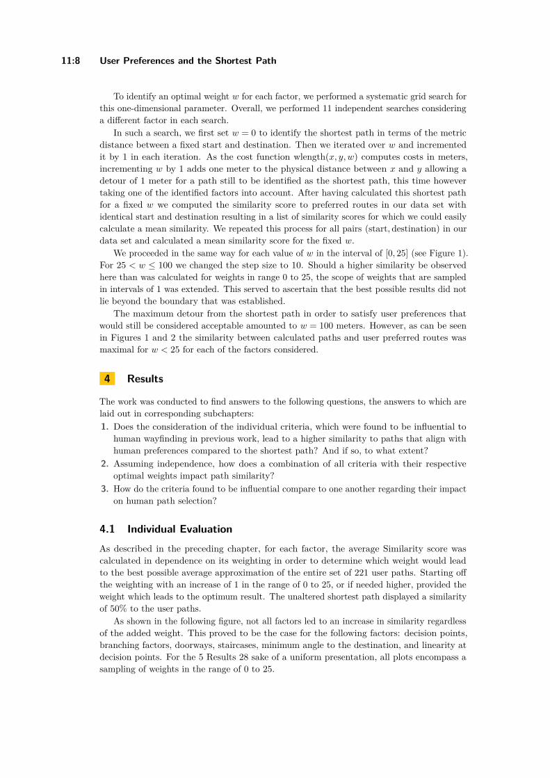
11:8 User Preferences and the Shortest Path

To identify an optimal weight w for each factor, we performed a systematic grid search forthis one-dimensional parameter. Overall, we performed 11 independent searches consideringa different factor in each search.

In such a search, we first set w = 0 to identify the shortest path in terms of the metricdistance between a fixed start and destination. Then we iterated over w and incrementedit by 1 in each iteration. As the cost function wlength(x, y, w) computes costs in meters,incrementing w by 1 adds one meter to the physical distance between x and y allowing adetour of 1 meter for a path still to be identified as the shortest path, this time howevertaking one of the identified factors into account. After having calculated this shortest pathfor a fixed w we computed the similarity score to preferred routes in our data set withidentical start and destination resulting in a list of similarity scores for which we could easilycalculate a mean similarity. We repeated this process for all pairs (start, destination) in ourdata set and calculated a mean similarity score for the fixed w.

We proceeded in the same way for each value of w in the interval of [0, 25] (see Figure 1).For 25 < w ≤ 100 we changed the step size to 10. Should a higher similarity be observedhere than was calculated for weights in range 0 to 25, the scope of weights that are sampledin intervals of 1 was extended. This served to ascertain that the best possible results did notlie beyond the boundary that was established.

The maximum detour from the shortest path in order to satisfy user preferences thatwould still be considered acceptable amounted to w = 100 meters. However, as can be seenin Figures 1 and 2 the similarity between calculated paths and user preferred routes wasmaximal for w < 25 for each of the factors considered.

4 Results

The work was conducted to find answers to the following questions, the answers to which arelaid out in corresponding subchapters:1. Does the consideration of the individual criteria, which were found to be influential to

human wayfinding in previous work, lead to a higher similarity to paths that align withhuman preferences compared to the shortest path? And if so, to what extent?

2. Assuming independence, how does a combination of all criteria with their respectiveoptimal weights impact path similarity?

3. How do the criteria found to be influential compare to one another regarding their impacton human path selection?

4.1 Individual EvaluationAs described in the preceding chapter, for each factor, the average Similarity score wascalculated in dependence on its weighting in order to determine which weight would leadto the best possible average approximation of the entire set of 221 user paths. Starting offthe weighting with an increase of 1 in the range of 0 to 25, or if needed higher, provided theweight which leads to the optimum result. The unaltered shortest path displayed a similarityof 50% to the user paths.

As shown in the following figure, not all factors led to an increase in similarity regardlessof the added weight. This proved to be the case for the following factors: decision points,branching factors, doorways, staircases, minimum angle to the destination, and linearity atdecision points. For the 5 Results 28 sake of a uniform presentation, all plots encompass asampling of weights in the range of 0 to 25.

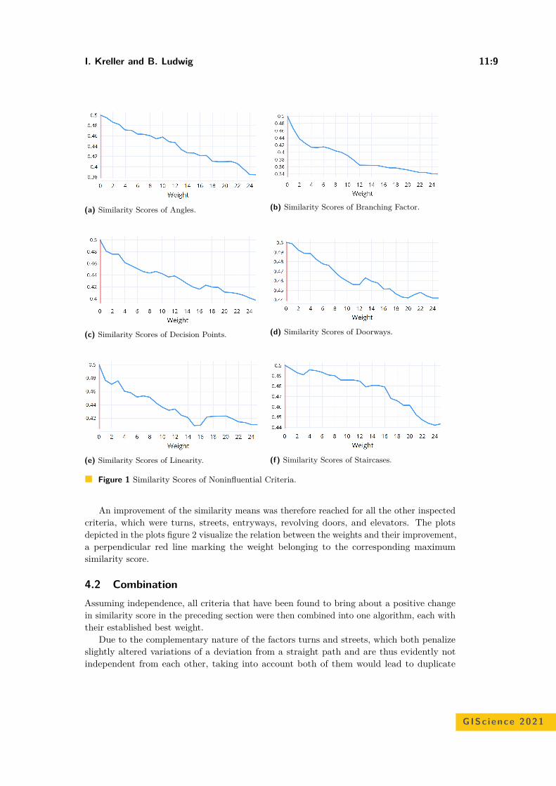
I. Kreller and B. Ludwig 11:9

(a) Similarity Scores of Angles. (b) Similarity Scores of Branching Factor.

(c) Similarity Scores of Decision Points. (d) Similarity Scores of Doorways.

(e) Similarity Scores of Linearity. (f) Similarity Scores of Staircases.

Figure 1 Similarity Scores of Noninfluential Criteria.

An improvement of the similarity means was therefore reached for all the other inspectedcriteria, which were turns, streets, entryways, revolving doors, and elevators. The plotsdepicted in the plots figure 2 visualize the relation between the weights and their improvement,a perpendicular red line marking the weight belonging to the corresponding maximumsimilarity score.

4.2 CombinationAssuming independence, all criteria that have been found to bring about a positive changein similarity score in the preceding section were then combined into one algorithm, each withtheir established best weight.

Due to the complementary nature of the factors turns and streets, which both penalizeslightly altered variations of a deviation from a straight path and are thus evidently notindependent from each other, taking into account both of them would lead to duplicate

GISc ience 2021

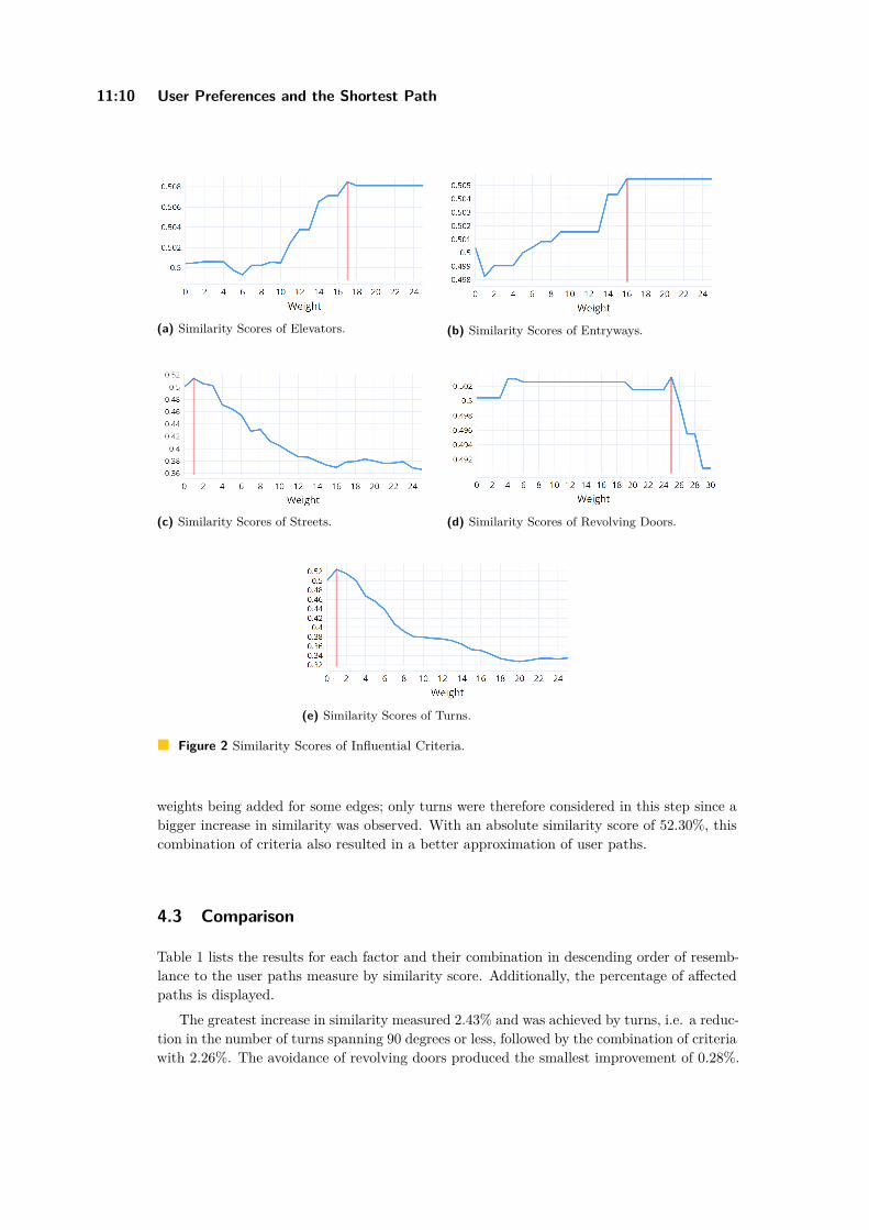
11:10 User Preferences and the Shortest Path

(a) Similarity Scores of Elevators. (b) Similarity Scores of Entryways.

(c) Similarity Scores of Streets. (d) Similarity Scores of Revolving Doors.

(e) Similarity Scores of Turns.

Figure 2 Similarity Scores of Influential Criteria.

weights being added for some edges; only turns were therefore considered in this step since abigger increase in similarity was observed. With an absolute similarity score of 52.30%, thiscombination of criteria also resulted in a better approximation of user paths.

4.3 Comparison

Table 1 lists the results for each factor and their combination in descending order of resemb-lance to the user paths measure by similarity score. Additionally, the percentage of affectedpaths is displayed.

The greatest increase in similarity measured 2.43% and was achieved by turns, i.e. a reduc-tion in the number of turns spanning 90 degrees or less, followed by the combination of criteriawith 2.26%. The avoidance of revolving doors produced the smallest improvement of 0.28%.

I. Kreller and B. Ludwig 11:11

Table 1 Sorted Table of Criteria with Scores and Percentage of Impacted Paths.

Factors Weight Similarity Score Difference to SP Impacted PathsTurns 1 52.47% 2.43% 19.91%

Combination varied 52.30% 2.26% 32.58%Streets 1 51.48% 1.38% 19.46%

Elevator 17 50.85% 0.81% 8.60%Entryway 16+ 50.55% 0.51% 11.76%

Revolving Door 25 50.32% 0.28% 2.26%

5 Discussion

In consideration of the individual factors, one must retain that not in each case it was ahigher number of occurrences that increased or decreased the assessed similarity to userpaths. Following the elaboration of the criteria’s specific implementation in 4.3, it was theiravoidance instead that was implied.

Many of the considered influential factors, previously found to be impactful, did not leadto the computation of paths that were more similar to those people prefer. This was the casefor paths that integrated the avoidance of decision points, their reduced branching factors,the avoidance of entrances to rooms, as well as staircases, and a preference for choosing pathsthat either minimized the global angular distance to the destination’s location or alignedwith the most linear path selection option. Consequently, all other factors – the avoidance ofelevators, entryways, revolving doors, turns, and streets – produced an increase in similarity.

A comparison shows that not only did the criteria’s impact on the similarity to userpaths vary, but so did the number of affected paths: the differences between the “best”factor (turns) and “worst” one (revolving doors) are almost ten-fold regarding both similarity(2.43% vs. 0.28%) as well as impacted paths (19.91% vs. 2.26%). This certainly may beexplained by the frequency with which each factor or entity occurs, for to produce significantchanges it has to be present in the paths initially suggested by the shortest path algorithm.

A preference for the most impactful factor can be reinforced by the finding that with anincreasing number of turns included in a route, the likelihood of making a mistake whilenavigating, and thus the time needed for task completion, increases [37]. The erroneousperception that routes containing more turns are longer than routes with fewer turns despitebeing equal in length (Dalton, 2003), might further explain our results.

In the cases of revolving doors, elevators, and entryways a boundless increase of theirweights lead to an improvement (Figures X), signifying that the banishing of all occurringentities would be in the interest of users. Unsurprisingly, since a study conducted on partof the same data set already discovered a significant decline in the number of entryways inpreferred routes [36], it was found that adding weights for all occurring entryways wouldimprove the similarity.

The absence of entryways in the favored paths can be understood by considering theinconvenience this would imply, for taking a shortcut through lecture halls would generallyonly serve as an option during breaks, or passing through shops or offices would be equallyunreasonable. A case against revolving doors can be made by considering that these types ofdoors are generally not barrier-free and users of wheelchairs would naturally avoid them.

The avoidance of choosing elevators as a means of transitioning to other floors impliesthat people favored the alternative option of taking stairs, which also concurs with previousfindings [24, 36].

GISc ience 2021

11:12 User Preferences and the Shortest Path

The results found are much the same for turns and streets, which can be explained withthe apparent similarities of the factors. Since turns only penalized right-angled deviations,and reducing the number of streets happened by penalizing all deviations from a straightpath, reducing the number of streets can be viewed as an extension of turns since above 90degrees (excluding 180 degrees) were also included.

Despite apparent similarities, a preference for linearity was not found and neither wasa preference for minimizing the angular distance. These results could be attributed todecision points, which by themselves, and consequently their branching factor as well, werefound ineffective. In addition, although such preferences have formerly been identified[8, 48], the environments in which the studies took place differed greatly from navigating auniversity campus.

To find the optimal integration of multiple criteria into one algorithm, their specificweights would need to be identified anew. As was expected given the incorrectly assumedindependence of the variables, the results fell short of reducing the number of turns alone. Fortaking dependencies between the factors into account, as a next step, we will train a predictorfor wlength(x, y) – i.e. a neural network that allows non-linear function approximation.

Given all these limitations and observations from our analyses, we can still claim that ouralgorithm finds a good compromise between shortest paths and user preferred routes: Theobjective of minimizing path distance, which was evident in every route calculation performed,achieved conformity with the user paths of 50% on average without further augmentation,and can therefore attest to align with human preferences. The overall results are encouragingfor the incorporation of the criteria, which were found to lead to an increase of the similarityscore, to create an algorithm able to suggest paths that humans like to follow.

6 Conclusion

This work aimed to acknowledge users as the focal point of navigational support systems andtherefore suggest paths that match with their preferences. To quantify the extent to whichthis is accomplished, a set of paths, which people take in their daily lives, was consideredrepresentative of human preferences, and similarity to these paths was treated as a measureof accomplishment. The assumption that people enjoy being suggested the same routesthat they take in well-known environments might be flawed, since aspects regarding thenavigation app, such as the ease with which instructions can be displayed and comprehended,are disregarded. Some of the factors were not found to be influential in an indoor environmentspecifically, but rather in settings whose similarity to the one considered here seems dubious.Narrowing down the findings of previous studies to research applicable to an indoor settingmight help identify influential factors more successfully. On the upside, putting these findingsinto a different context sheds light on their transferability and may offer insights into whythey have been found to impact wayfinding decisions. Future research might proceed bytaking criteria into consideration that have not been discussed and considered here, includingnot only environmental factors but more subjective criteria which might be more difficultto assess. Lastly, shedding more light on the interrelations of influential factors might benecessary for the conception of an ideal algorithm that can consider more than one elementat a time.

As far as the comparison between indoor and outdoor environments is concerned, ourstudy reproduces the results reported in [22] for indoor environments: user prefer routes witha small number of turns. However, as indoor environments are more complex that streetsoutside, also other criteria are influential. It is an interesting challenge for future work whether

I. Kreller and B. Ludwig 11:13

a transformation of a graph in which nodes actually represent actual distances physicalproperties of the environment to another model in which nodes represent inevitable choices(such as taking a turn) is feasible if multiple criteria have to be considered simultaneously.

References1 Imad Afyouni, Cyril Ray, and Claramunt Christophe. Spatial models for context-aware indoor

navigation systems: A survey. Journal of Spatial Information Science, 1(4):85–123, 2012.2 Gary L Allen. Cognitive abilities in the service of wayfinding: A functional approach. The

Professional Geographer, 51(4):555–561, 1999.3 Iro Armeni and Konstantinos Chorianopoulos. Pedestrian navigation and shortest path:

Preference versus distance. In Intelligent environments (workshops), pages 647–652, 2013.4 Michael Brown and James Pinchin. Exploring human factors in indoor navigation. In The

European Navigation Conference, 2013.5 Beatrix Brunner-Friedrich and Verena Radoczky. Active landmarks in indoor environments. In

International Conference on Advances in Visual Information Systems, pages 203–215. Springer,2005.

6 David Caduff and Sabine Timpf. On the assessment of landmark salience for human navigation.Cognitive processing, 9(4):249–267, 2008.

7 Ruth Alison Conroy. Spatial navigation in immersive virtual environments. PhD thesis,Citeseer, 2001.

8 Ruth Conroy Dalton. The secret is to follow your nose: Route path selection and angularity.Environment and Behavior, 35(1):107–131, 2003.

9 Daniel Delling, Andrew V Goldberg, Moises Goldszmidt, John Krumm, Kunal Talwar, andRenato F Werneck. Navigation made personal: Inferring driving preferences from gps traces.In Proceedings of the 23rd SIGSPATIAL international conference on advances in geographicinformation systems, pages 1–9, 2015.

10 Edsger W Dijkstra et al. A note on two problems in connexion with graphs. Numerischemathematik, 1(1):269–271, 1959.

11 Matt Duckham and Lars Kulik. “simplest” paths: automated route selection for navigation.In International Conference on Spatial Information Theory, pages 169–185. Springer, 2003.

12 Ioannis Giannopoulos, Peter Kiefer, Martin Raubal, Kai-Florian Richter, and Tyler Thrash.Wayfinding decision situations: A conceptual model and evaluation. In International Conferenceon Geographic Information Science, pages 221–234. Springer, 2014.

13 Sabine Gillner and Hanspeter A Mallot. Navigation and acquisition of spatial knowledge in avirtual maze. Journal of cognitive neuroscience, 10(4):445–463, 1998.

14 Reginald G Golledge. Path selection and route preference in human navigation: A progressreport. In International conference on spatial information theory, pages 207–222. Springer,1995.

15 Joy Goodman, Phil Gray, Kartik Khammampad, and Stephen Brewster. Using landmarks tosupport older people in navigation. In International Conference on Mobile Human-ComputerInteraction, pages 38–48. Springer, 2004.

16 E Grum and AU Frank. Risk of getting lost: Optimize a path to minimize risk. corp, vienna.Competence Center for Urban and Regional Planning, 2005.

17 Viddit Haria, Yashvi Shah, Vanya Gangwar, Vansh Chandwaney, Tarang Jain, and YashDedhia. The working of google maps, and the commercial usage of navigation systems.International Journal of Innovative Research in Technology, 6(5), 2019.

18 Christoph Hölscher, Tobias Meilinger, Georg Vrachliotis, Martin Brösamle, and MarkusKnauff. Up the down staircase: Wayfinding strategies in multi-level buildings. Journal ofEnvironmental Psychology, 26(4):284–299, 2006.

19 Christoph Hölscher, Thora Tenbrink, and Jan M Wiener. Would you follow your own routedescription? cognitive strategies in urban route planning. Cognition, 121(2):228–247, 2011.

GISc ience 2021

11:14 User Preferences and the Shortest Path

20 Alycia M Hund, Martin Schmettow, and Matthijs L Noordzij. The impact of culture andrecipient perspective on direction giving in the service of wayfinding. Journal of EnvironmentalPsychology, 32(4):327–336, 2012.

21 Oliver Jan, Alan J Horowitz, and Zhong-Ren Peng. Using global positioning system data tounderstand variations in path choice. Transportation Research Record, 1725(1):37–44, 2000.

22 Bin Jiang and Xintao Liu. Computing the fewest-turn map directions based on the connectivityof natural roads. International Journal of Geographical Information Science, 25(7):1069–1082,2011. doi:10.1080/13658816.2010.510799.

23 Daniel Kahneman. Maps of bounded rationality: Psychology for behavioral economics.American economic review, 93(5):1449–1475, 2003.

24 Panayotis Kikiras, Vassileios Tsetsos, and Stathes Hadjiefthymiades. Ontology-based usermodeling for pedestrian navigation systems. In ECAI 2006 Workshop on Ubiquitous UserModeling (UbiqUM), Riva del Garda, Italy, pages 1–6, 2006.

25 Alexander Klippel, Heike Tappe, Lars Kulik, and Paul U Lee. Wayfinding choremes—alanguage for modeling conceptual route knowledge. Journal of Visual Languages & Computing,16(4):311–329, 2005.

26 Shohei Koide and Masami Kato. 3-d human navigation system considering various transitionpreferences. In 2005 IEEE International Conference on Systems, Man and Cybernetics,volume 1, pages 859–864. IEEE, 2005.

27 Benjamin Kuipers. Modeling spatial knowledge. Cognitive science, 2(2):129–153, 1978.28 Carol A Lawton. Gender and regional differences in spatial referents used in direction giving.

Sex Roles, 44(5):321–337, 2001.29 Kevin Lynch. The image of the city (vol. 11), 1960.30 Bharadwaj RK Mantha, Carol C Menassa, Vineet R Kamat, and Clive R D’Souza. Evaluation

of preference-and constraint-sensitive path planning for assisted navigation in indoor buildingenvironments. Journal of Computing in Civil Engineering, 34(1):04019050, 2020.

31 David M Mark. Automated route selection for navigation. IEEE Aerospace and ElectronicSystems Magazine, 1(9):2–5, 1986.

32 Richar E Mayer. Visual aids to knowledge construction: Building mental representations frompictures and words. In Advances in psychology, volume 108, pages 125–138. Elsevier, 1994.

33 Tobias Meilinger, Markus Knauff, and Heinrich H Bülthoff. Working memory in wayfinding—adual task experiment in a virtual city. Cognitive Science, 32(4):755–770, 2008.

34 Daniel R Montello. Spatial orientation and the angularity of urban routes: A field study.Environment and Behavior, 23(1):47–69, 1991.

35 Daniel R Montello and Martin Raubal. Functions and applications of spatial cognition. InHandbook of Spatial Cognition, page 249–264. American Psychological Association, 2013.

36 Manuel Müller, Christina Ohm, Florin Schwappach, and Bernd Ludwig. The path of leastresistance. KI-Künstliche Intelligenz, 31(2):125–134, 2017.

37 Michael J O’Neill. Effects of familiarity and plan complexity on wayfinding in simulatedbuildings. Journal of Environmental Psychology, 12(4):319–327, 1992.

38 Arto Puikkonen, Ari-Heikki Sarjanoja, Merja Haveri, Jussi Huhtala, and Jonna Häkkilä.Towards designing better maps for indoor navigation: experiences from a case study. InProceedings of the 8th international conference on mobile and ubiquitous multimedia, pages1–4, 2009.

39 Daniele Quercia, Rossano Schifanella, and Luca Maria Aiello. The shortest path to happiness:Recommending beautiful, quiet, and happy routes in the city. In Proceedings of the 25th ACMconference on Hypertext and social media, pages 116–125, 2014.

40 Kai-Florian Richter and Alexander Klippel. You-are-here maps: Wayfinding support aslocation based service. GI-Technologien für Verkehr und Logistik. Beiträge zu den MünsteranerGI-Tagen, 20:21, 2002.

41 Edward K Sadalla and Daniel R Montello. Remembering changes in direction. Environmentand Behavior, 21(3):346–363, 1989.

I. Kreller and B. Ludwig 11:15

42 Wilson Sakpere, Michael Adeyeye-Oshin, and Nhlanhla BW Mlitwa. A state-of-the-art surveyof indoor positioning and navigation systems and technologies. South African ComputerJournal, 29(3):145–197, 2017.

43 Masashi Soeda, Noriko Kushiyama, and Ryuzo Ohno. Wayfinding in cases with vertical motion.Proceedings of MERA, 97:559–564, 1997.

44 Robert J Sternberg. Metaphors of mind: Conceptions of the nature of intelligence. CambridgeUniversity Press, 1990.

45 Mathieu Taillade, Bernard N’Kaoua, and Hélène Sauzéon. Age-related differences and cognitivecorrelates of self-reported and direct navigation performance: the effect of real and virtualtest conditions manipulation. Frontiers in Psychology, 6:2034, 2016.

46 YingLi Tian, Xiaodong Yang, Chucai Yi, and Aries Arditi. Toward a computer vision-basedwayfinding aid for blind persons to access unfamiliar indoor environments. Machine visionand applications, 24(3):521–535, 2013.

47 turn. Cambridge Dictionary. Cambridge University Press, 2021. URL: https://dictionary.cambridge.org/dictionary/english/turn.

48 Alasdair Turner. The role of angularity in route choice. In International Conference on SpatialInformation Theory, pages 489–504. Springer, 2009.

49 Manuel Ullmann. Datengetriebene optimierung präferenzadaptiver fußwegrouten durch ge-bäudekomplexe, September 2020. URL: https://epub.uni-regensburg.de/43697/.

50 Ann Vanclooster, Nina Vanhaeren, Pepijn Viaene, Kristien Ooms, Laure De Cock, Veerle Fack,Nico Van de Weghe, and Philippe De Maeyer. Turn calculations for the indoor application ofthe fewest turns path algorithm. International Journal of Geographical Information Science,33(11):2284–2304, 2019.

51 Ann Vanclooster, Pepijn Viaene, Nico Van de Weghe, Veerle Fack, and Philippe De Maeyer.Analyzing the applicability of the least risk path algorithm in indoor space. In ISPRSAcquisition and Modelling of Indoor and Enclosed Environments 2013 (Indoor 3D), volume 2,pages 19–26. International Society for Photogrammetry and Remote Sensing (ISPRS), 2013.

52 Liping Yang and Michael Worboys. Similarities and differences between outdoor and indoorspace from the perspective of navigation. Poster presented at COSIT, 2011.

53 John Zacharias. Pedestrian behavior pedestrian behavior and perception in urban walkingenvironments. Journal of planning literature, 16(1):3–18, 2001.

54 Shanjiang Zhu and David Levinson. Do people use the shortest path? an empirical test ofwardrop’s first principle. PloS one, 10(8):e0134322, 2015.

GISc ience 2021

Map Matching for Semi-Restricted TrajectoriesTimon Behr #

University of Konstanz, Germany

Thomas C. van Dijk #

University of Bochum, Germany

Axel Forsch #

University of Bonn, Germany

Jan-Henrik Haunert #

University of Bonn, Germany

Sabine Storandt #

University of Konstanz, Germany

AbstractWe consider the problem of matching trajectories to a road map, giving particular considerationto trajectories that do not exclusively follow the underlying network. Such trajectories arise, forexample, when a person walks through the inner part of a city, crossing market squares or parkinglots. We call such trajectories semi-restricted. Sensible map matching of semi-restricted trajectoriesrequires the ability to differentiate between restricted and unrestricted movement. We develop in thispaper an approach that efficiently and reliably computes concise representations of such trajectoriesthat maintain their semantic characteristics. Our approach utilizes OpenStreetMap data to not onlyextract the network but also areas that allow for free movement (as e.g. parks) as well as obstacles(as e.g. buildings). We discuss in detail how to incorporate this information in the map matchingprocess, and demonstrate the applicability of our method in an experimental evaluation on realpedestrian and bicycle trajectories.

2012 ACM Subject Classification Information systems → Geographic information systems

Keywords and phrases map matching, OpenStreetMap, GPS, trajectory, road network

Digital Object Identifier 10.4230/LIPIcs.GIScience.2021.II.12

Supplementary Material Software: https://github.com/tcvdijk/tessaarchived at swh:1:dir:265a254805a64ab73036cdebd99b59590052a471

Funding Timon Behr : DFG Grant Sto 1114/4-2 in Priority Programme 1894 “Volunteered Geo-graphic Information”.Thomas C. van Dijk: DFG Grant Di 2161/2-2 in Priority Programme 1894 “Volunteered GeographicInformation”.Axel Forsch: DFG Grant Ha 5451/7-1 in Priority Programme 1894 “Volunteered GeographicInformation”.

1 Introduction

Map matching is the process of pinpointing a trajectory (given e.g. as a sequence of GPSmeasurements) to a path in an underlying network. The goal is to find the path that explainsthe observed measurements best. Map matching is often the first step of trajectory dataprocessing as there are several benefits when dealing with paths in a known network insteadof raw location measurement data:

Both location measurements and geometric representations of roads are usually imprecise.Hence, constraining the trajectory to a path in a network is necessary to integrate theinformation given with a trajectory (e.g. recorded speed, vehicle type) with informationgiven with the road data (e.g. speed limit, road type). This is important to enableapplications as movement analysis or real-time navigation [17, 28].

© Timon Behr, Thomas C. van Dijk, Axel Forsch, Jan-Henrik Haunert, and Sabine Storandt;licensed under Creative Commons License CC-BY 4.0

11th International Conference on Geographic Information Science (GIScience 2021) – Part II.Editors: Krzysztof Janowicz and Judith A. Verstegen; Article No. 12; pp. 12:1–12:16

Leibniz International Proceedings in InformaticsSchloss Dagstuhl – Leibniz-Zentrum für Informatik, Dagstuhl Publishing, Germany

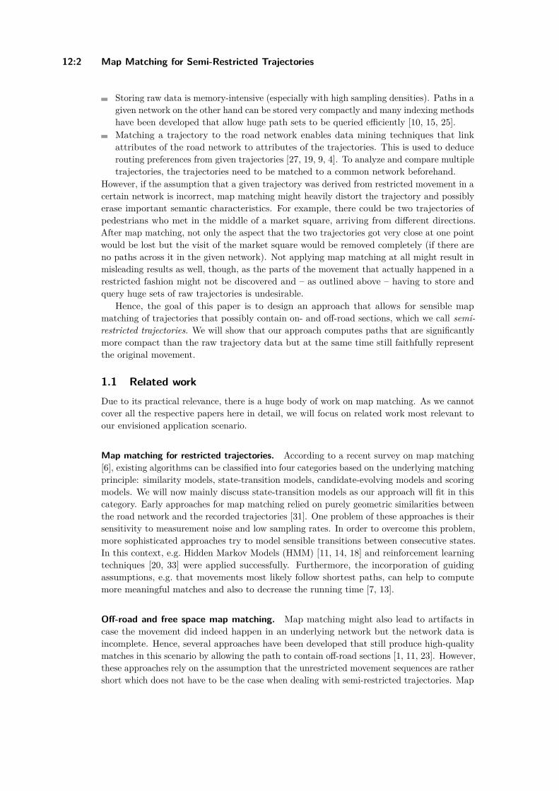
12:2 Map Matching for Semi-Restricted Trajectories

Storing raw data is memory-intensive (especially with high sampling densities). Paths in agiven network on the other hand can be stored very compactly and many indexing methodshave been developed that allow huge path sets to be queried efficiently [10, 15, 25].Matching a trajectory to the road network enables data mining techniques that linkattributes of the road network to attributes of the trajectories. This is used to deducerouting preferences from given trajectories [27, 19, 9, 4]. To analyze and compare multipletrajectories, the trajectories need to be matched to a common network beforehand.

However, if the assumption that a given trajectory was derived from restricted movement in acertain network is incorrect, map matching might heavily distort the trajectory and possiblyerase important semantic characteristics. For example, there could be two trajectories ofpedestrians who met in the middle of a market square, arriving from different directions.After map matching, not only the aspect that the two trajectories got very close at one pointwould be lost but the visit of the market square would be removed completely (if there areno paths across it in the given network). Not applying map matching at all might result inmisleading results as well, though, as the parts of the movement that actually happened in arestricted fashion might not be discovered and – as outlined above – having to store andquery huge sets of raw trajectories is undesirable.

Hence, the goal of this paper is to design an approach that allows for sensible mapmatching of trajectories that possibly contain on- and off-road sections, which we call semi-restricted trajectories. We will show that our approach computes paths that are significantlymore compact than the raw trajectory data but at the same time still faithfully representthe original movement.

1.1 Related workDue to its practical relevance, there is a huge body of work on map matching. As we cannotcover all the respective papers here in detail, we will focus on related work most relevant toour envisioned application scenario.

Map matching for restricted trajectories. According to a recent survey on map matching[6], existing algorithms can be classified into four categories based on the underlying matchingprinciple: similarity models, state-transition models, candidate-evolving models and scoringmodels. We will now mainly discuss state-transition models as our approach will fit in thiscategory. Early approaches for map matching relied on purely geometric similarities betweenthe road network and the recorded trajectories [31]. One problem of these approaches is theirsensitivity to measurement noise and low sampling rates. In order to overcome this problem,more sophisticated approaches try to model sensible transitions between consecutive states.In this context, e.g. Hidden Markov Models (HMM) [11, 14, 18] and reinforcement learningtechniques [20, 33] were applied successfully. Furthermore, the incorporation of guidingassumptions, e.g. that movements most likely follow shortest paths, can help to computemore meaningful matches and also to decrease the running time [7, 13].

Off-road and free space map matching. Map matching might also lead to artifacts incase the movement did indeed happen in an underlying network but the network data isincomplete. Hence, several approaches have been developed that still produce high-qualitymatches in this scenario by allowing the path to contain off-road sections [1, 11, 23]. However,these approaches rely on the assumption that the unrestricted movement sequences are rathershort which does not have to be the case when dealing with semi-restricted trajectories. Map

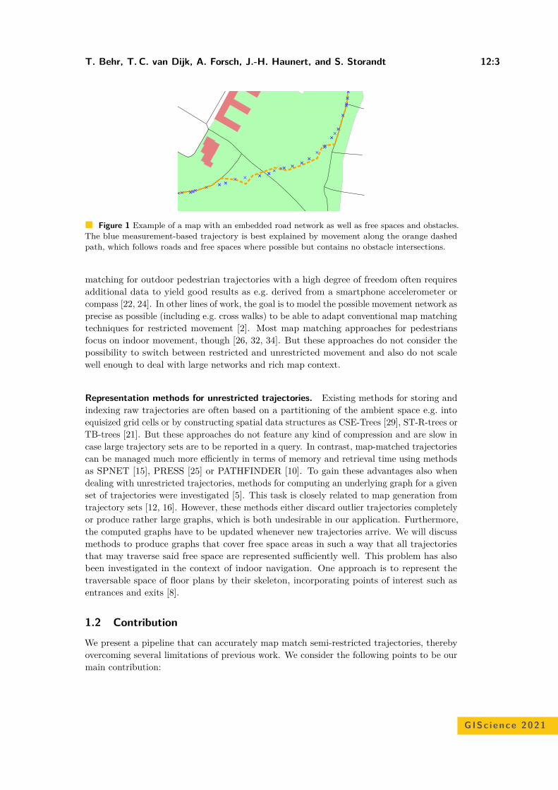
T. Behr, T. C. van Dijk, A. Forsch, J.-H. Haunert, and S. Storandt 12:3

Figure 1 Example of a map with an embedded road network as well as free spaces and obstacles.The blue measurement-based trajectory is best explained by movement along the orange dashedpath, which follows roads and free spaces where possible but contains no obstacle intersections.

matching for outdoor pedestrian trajectories with a high degree of freedom often requiresadditional data to yield good results as e.g. derived from a smartphone accelerometer orcompass [22, 24]. In other lines of work, the goal is to model the possible movement network asprecise as possible (including e.g. cross walks) to be able to adapt conventional map matchingtechniques for restricted movement [2]. Most map matching approaches for pedestriansfocus on indoor movement, though [26, 32, 34]. But these approaches do not consider thepossibility to switch between restricted and unrestricted movement and also do not scalewell enough to deal with large networks and rich map context.

Representation methods for unrestricted trajectories. Existing methods for storing andindexing raw trajectories are often based on a partitioning of the ambient space e.g. intoequisized grid cells or by constructing spatial data structures as CSE-Trees [29], ST-R-trees orTB-trees [21]. But these approaches do not feature any kind of compression and are slow incase large trajectory sets are to be reported in a query. In contrast, map-matched trajectoriescan be managed much more efficiently in terms of memory and retrieval time using methodsas SPNET [15], PRESS [25] or PATHFINDER [10]. To gain these advantages also whendealing with unrestricted trajectories, methods for computing an underlying graph for a givenset of trajectories were investigated [5]. This task is closely related to map generation fromtrajectory sets [12, 16]. However, these methods either discard outlier trajectories completelyor produce rather large graphs, which is both undesirable in our application. Furthermore,the computed graphs have to be updated whenever new trajectories arrive. We will discussmethods to produce graphs that cover free space areas in such a way that all trajectoriesthat may traverse said free space are represented sufficiently well. This problem has alsobeen investigated in the context of indoor navigation. One approach is to represent thetraversable space of floor plans by their skeleton, incorporating points of interest such asentrances and exits [8].

1.2 Contribution

We present a pipeline that can accurately map match semi-restricted trajectories, therebyovercoming several limitations of previous work. We consider the following points to be ourmain contribution:

GISc ience 2021

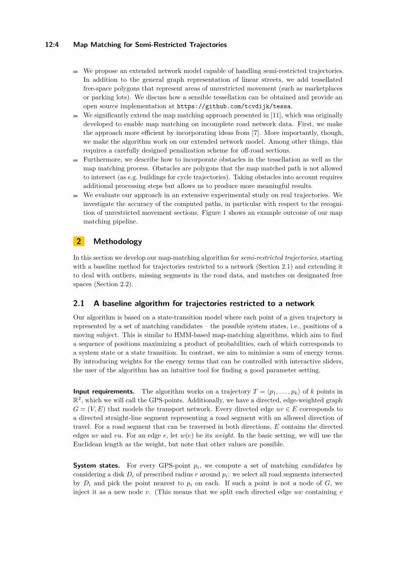
12:4 Map Matching for Semi-Restricted Trajectories

We propose an extended network model capable of handling semi-restricted trajectories.In addition to the general graph representation of linear streets, we add tessellatedfree-space polygons that represent areas of unrestricted movement (such as marketplacesor parking lots). We discuss how a sensible tessellation can be obtained and provide anopen source implementation at https://github.com/tcvdijk/tessa.We significantly extend the map matching approach presented in [11], which was originallydeveloped to enable map matching on incomplete road network data. First, we makethe approach more efficient by incorporating ideas from [7]. More importantly, though,we make the algorithm work on our extended network model. Among other things, thisrequires a carefully designed penalization scheme for off-road sections.Furthermore, we describe how to incorporate obstacles in the tessellation as well as themap matching process. Obstacles are polygons that the map matched path is not allowedto intersect (as e.g. buildings for cycle trajectories). Taking obstacles into account requiresadditional processing steps but allows us to produce more meaningful results.We evaluate our approach in an extensive experimental study on real trajectories. Weinvestigate the accuracy of the computed paths, in particular with respect to the recogni-tion of unrestricted movement sections. Figure 1 shows an example outcome of our mapmatching pipeline.

2 Methodology

In this section we develop our map-matching algorithm for semi-restricted trajectories, startingwith a baseline method for trajectories restricted to a network (Section 2.1) and extending itto deal with outliers, missing segments in the road data, and matches on designated freespaces (Section 2.2).

2.1 A baseline algorithm for trajectories restricted to a networkOur algorithm is based on a state-transition model where each point of a given trajectory isrepresented by a set of matching candidates – the possible system states, i.e., positions of amoving subject. This is similar to HMM-based map-matching algorithms, which aim to finda sequence of positions maximizing a product of probabilities, each of which corresponds toa system state or a state transition. In contrast, we aim to minimize a sum of energy terms.By introducing weights for the energy terms that can be controlled with interactive sliders,the user of the algorithm has an intuitive tool for finding a good parameter setting.

Input requirements. The algorithm works on a trajectory T = ⟨p1, . . . , pk⟩ of k points inR2, which we will call the GPS-points. Additionally, we have a directed, edge-weighted graphG = (V, E) that models the transport network. Every directed edge uv ∈ E corresponds toa directed straight-line segment representing a road segment with an allowed direction oftravel. For a road segment that can be traversed in both directions, E contains the directededges uv and vu. For an edge e, let w(e) be its weight. In the basic setting, we will use theEuclidean length as the weight, but note that other values are possible.

System states. For every GPS-point pi, we compute a set of matching candidates byconsidering a disk Di of prescribed radius r around pi: we select all road segments intersectedby Di and pick the point nearest to pi on each. If such a point is not a node of G, weinject it as a new node v. (This means that we split each directed edge uw containing v

T. Behr, T. C. van Dijk, A. Forsch, J.-H. Haunert, and S. Storandt 12:5

into two directed edges uv and vw; we distribute the weight of uw to the edges uv and vw

proportionally to their lengths.) As a consequence, the set of matching candidates for pi is aset of nodes Vi ⊆ V . If Vi is empty, we discard the GPS-point pi and do not consider it forthe matching.

State transitions. Possible transitions between candidates for two consecutive GPS-pointsare not modelled explicitly. Instead, they are implicitly modeled with the graph G byassuming that the transition between any two matching candidates u ∈ Vi and v ∈ Vi+1occurs via a minimum-weight u-v-path in G. Accordingly, the matched output path P isdefined by selecting, for i = 1, . . . , k, one candidate vi from the set Vi and connecting everypair of consecutive nodes in the sequence ⟨v1, . . . , vk⟩ via a minimum-weight path.

Energy model. To ensure that the output path P matches well to the trajectory, we setup and minimize an energy function that aggregates a state-based and a transition-basedenergy:

The state-based energy is∑k

i=1 ∥pi − vi∥2, meaning that the energy increases quadraticallywith the Euclidean distance between a GPS-point pi and the matching candidate vi

selected for it.The transition-based energy is

∑k−1i=1 w(Pi,i+1), where Pa,b is a minimum-weight va-vb-

path in G and w(P ) is the total weight of a path P (i.e., the sum of the weights of theedges of P ). For now, we use the geometric length of an edge as its weight.

The two energies are aggregated using a weighted sum, parametrized with a parameter αc.This yields our overall objective function quantifying the fit between a trajectory ⟨p1, ..., pk⟩and an output path defined with the selected sequence ⟨v1, ..., vk⟩ of nodes:

Minimize E(⟨p1, ..., pk⟩, ⟨v1, ..., vk⟩) = αc ·k∑

i=1∥pi − vi∥2 +

k−1∑i=1

w(Pi,i+1) (1)

Algorithm. An optimal solution is computed using k runs of Dijkstra’s algorithm on a graphthat results from augmenting G with a few auxiliary nodes and arcs. More precisely, we usean incremental algorithm that proceeds in k iterations. In the i-th iteration, it computes forthe sub-trajectory ⟨p1, . . . , pi⟩ of T and each matching candidate v ∈ Vi the objective valueEv

i of a solution ⟨v1, ..., vi⟩ that minimizes E(⟨p1, . . . , pi⟩, ⟨v1, . . . , vi⟩) under the restrictionthat vi = v. This computation is done as follows.

For i = 1 and any node v ∈ V1, Ev1 is simply the state-based energy for v, i.e., Ev

1 =αc · ∥p1 − v∥2.For i > 1, we introduce a dummy node si and a directed edge siu for each u ∈ Vi−1whose weight we set as Eu

i−1; see Fig. 2. With this, for any node v ∈ Vi, Evi corresponds to

the weight of a minimum-weight si-v-path in the augmented graph, plus the state-basedenergy for v. We are thus interested in finding for si and every node in Vi a minimum-weight path. All these paths can be found with one single-source shortest path querywith source si and, thus, with a single execution of Dijkstra’s algorithm.

We observe that our objective function E(⟨p1, . . . , pi⟩, ⟨v1, . . . , vi⟩) for the whole trajectoryhas the minimum value minv∈Vk

Evk and is among the values we have computed. It is not

difficult to maintain information during the run of the algorithm to enable the reconstructionof a solution attaining that value.

GISc ience 2021

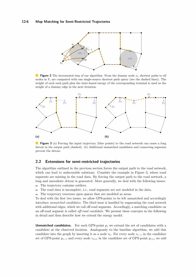
12:6 Map Matching for Semi-Restricted Trajectories

si

u

w

v

pi

pi−1

Vi

Vi−1

Figure 2 The incremental step of our algorithm. From the dummy node si, shortest paths to allnodes in Vi are computed with one single-source shortest path query (see the dashed lines). Theweight of each such path plus the state-based energy of the corresponding terminal is used as theweight of a dummy edge in the next iteration.

p1

p2 p3

p4

p5

(a)

p1

p2 p3

p4

p5

(b)

Figure 3 (a) Forcing the input trajectory (blue points) to the road network can cause a longdetour in the output path (dashed). (b) Additional unmatched candidates and connecting segmentsprevent the detour.

2.2 Extensions for semi-restricted trajectoriesThe algorithm outlined in the previous section forces the output path to the road network,which can lead to unfavorable solutions. Consider the example in Figure 3, where roadsegments are missing in the road data. By forcing the output path to the road network, along and unrealistic detour is generated. More generally, we deal with the following issues:

The trajectory contains outliers.The road data is incomplete, i.e., road segments are not modeled in the data.The trajectory traverses open spaces that are modeled as areas.

To deal with the first two issues, we allow GPS-points to be left unmatched and accordinglyintroduce unmatched candidates. The third issue is handled by augmenting the road networkwith additional edges, which we call off-road segments. Accordingly, a matching candidate onan off-road segment is called off-road candidate. We present these concepts in the followingin detail and then describe how we extend the energy model.

Unmatched candidates. For each GPS-point pi we extend the set of candidates with acandidate at the observed location. Analogously to the baseline algorithm, we add thiscandidate into the graph by inserting it as a node ui. For every node vi−1 in the candidateset of GPS-point pi−1 and every node vi+1 in the candidate set of GPS-point pi+1 we add

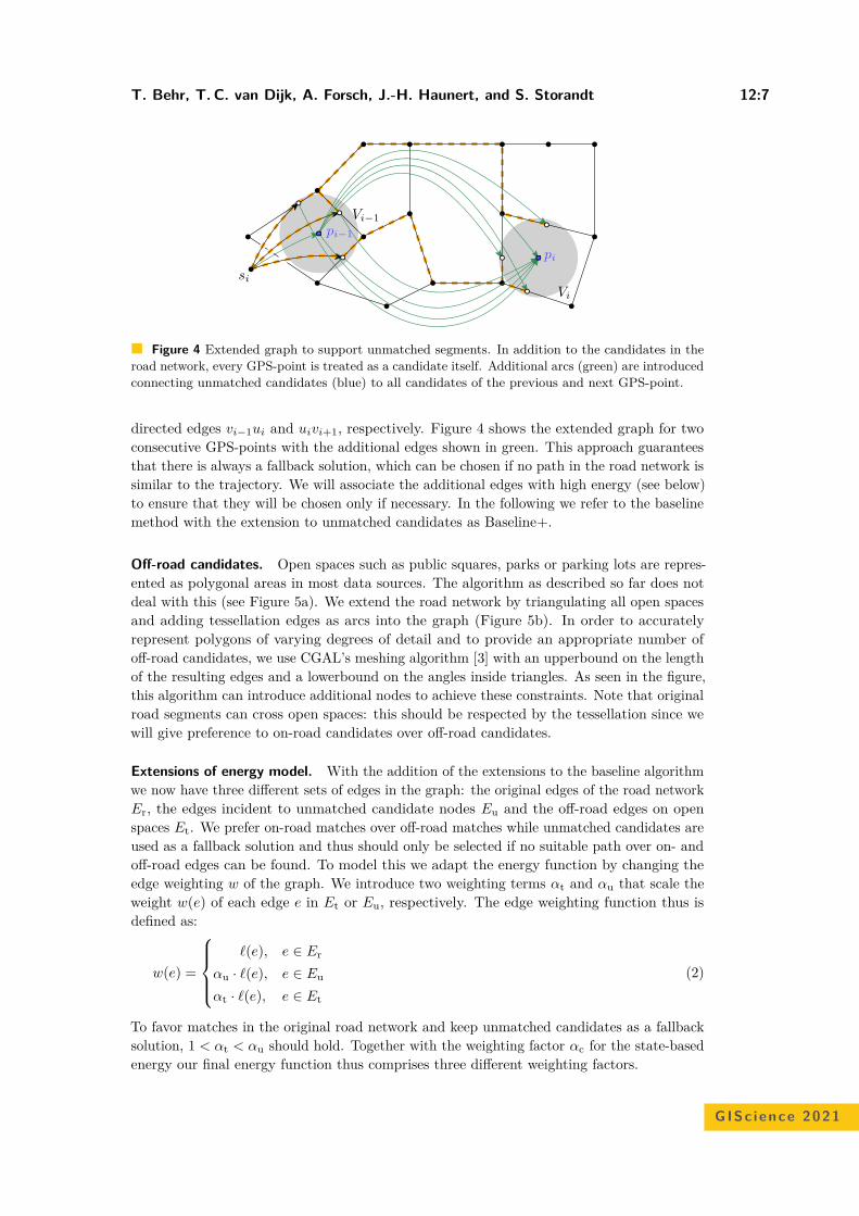
T. Behr, T. C. van Dijk, A. Forsch, J.-H. Haunert, and S. Storandt 12:7

si

pi

pi−1

Vi

Vi−1

Figure 4 Extended graph to support unmatched segments. In addition to the candidates in theroad network, every GPS-point is treated as a candidate itself. Additional arcs (green) are introducedconnecting unmatched candidates (blue) to all candidates of the previous and next GPS-point.

directed edges vi−1ui and uivi+1, respectively. Figure 4 shows the extended graph for twoconsecutive GPS-points with the additional edges shown in green. This approach guaranteesthat there is always a fallback solution, which can be chosen if no path in the road network issimilar to the trajectory. We will associate the additional edges with high energy (see below)to ensure that they will be chosen only if necessary. In the following we refer to the baselinemethod with the extension to unmatched candidates as Baseline+.

Off-road candidates. Open spaces such as public squares, parks or parking lots are repres-ented as polygonal areas in most data sources. The algorithm as described so far does notdeal with this (see Figure 5a). We extend the road network by triangulating all open spacesand adding tessellation edges as arcs into the graph (Figure 5b). In order to accuratelyrepresent polygons of varying degrees of detail and to provide an appropriate number ofoff-road candidates, we use CGAL’s meshing algorithm [3] with an upperbound on the lengthof the resulting edges and a lowerbound on the angles inside triangles. As seen in the figure,this algorithm can introduce additional nodes to achieve these constraints. Note that originalroad segments can cross open spaces: this should be respected by the tessellation since wewill give preference to on-road candidates over off-road candidates.

Extensions of energy model. With the addition of the extensions to the baseline algorithmwe now have three different sets of edges in the graph: the original edges of the road networkEr, the edges incident to unmatched candidate nodes Eu and the off-road edges on openspaces Et. We prefer on-road matches over off-road matches while unmatched candidates areused as a fallback solution and thus should only be selected if no suitable path over on- andoff-road edges can be found. To model this we adapt the energy function by changing theedge weighting w of the graph. We introduce two weighting terms αt and αu that scale theweight w(e) of each edge e in Et or Eu, respectively. The edge weighting function thus isdefined as:

w(e) =

ℓ(e), e ∈ Er

αu · ℓ(e), e ∈ Eu

αt · ℓ(e), e ∈ Et

(2)

To favor matches in the original road network and keep unmatched candidates as a fallbacksolution, 1 < αt < αu should hold. Together with the weighting factor αc for the state-basedenergy our final energy function thus comprises three different weighting factors.

GISc ience 2021

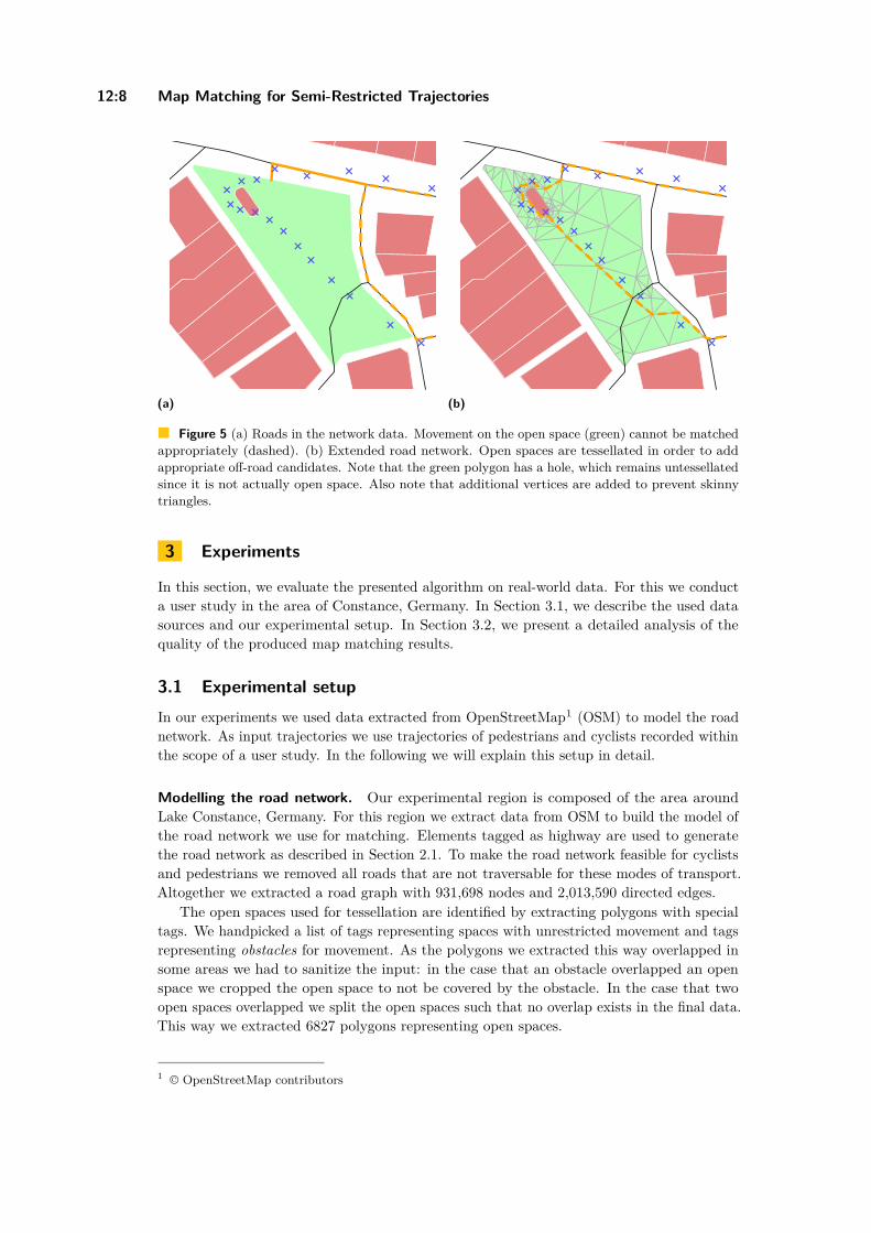
12:8 Map Matching for Semi-Restricted Trajectories

(a) (b)

Figure 5 (a) Roads in the network data. Movement on the open space (green) cannot be matchedappropriately (dashed). (b) Extended road network. Open spaces are tessellated in order to addappropriate off-road candidates. Note that the green polygon has a hole, which remains untessellatedsince it is not actually open space. Also note that additional vertices are added to prevent skinnytriangles.

3 Experiments

In this section, we evaluate the presented algorithm on real-world data. For this we conducta user study in the area of Constance, Germany. In Section 3.1, we describe the used datasources and our experimental setup. In Section 3.2, we present a detailed analysis of thequality of the produced map matching results.

3.1 Experimental setupIn our experiments we used data extracted from OpenStreetMap1 (OSM) to model the roadnetwork. As input trajectories we use trajectories of pedestrians and cyclists recorded withinthe scope of a user study. In the following we will explain this setup in detail.

Modelling the road network. Our experimental region is composed of the area aroundLake Constance, Germany. For this region we extract data from OSM to build the model ofthe road network we use for matching. Elements tagged as highway are used to generatethe road network as described in Section 2.1. To make the road network feasible for cyclistsand pedestrians we removed all roads that are not traversable for these modes of transport.Altogether we extracted a road graph with 931,698 nodes and 2,013,590 directed edges.

The open spaces used for tessellation are identified by extracting polygons with specialtags. We handpicked a list of tags representing spaces with unrestricted movement and tagsrepresenting obstacles for movement. As the polygons we extracted this way overlapped insome areas we had to sanitize the input: in the case that an obstacle overlapped an openspace we cropped the open space to not be covered by the obstacle. In the case that twoopen spaces overlapped we split the open spaces such that no overlap exists in the final data.This way we extracted 6827 polygons representing open spaces.

1 © OpenStreetMap contributors

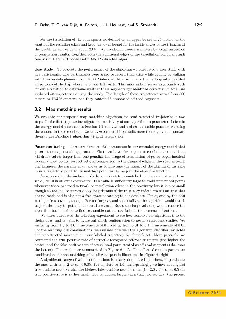
T. Behr, T. C. van Dijk, A. Forsch, J.-H. Haunert, and S. Storandt 12:9

For the tessellation of the open spaces we decided on an upper bound of 25 meters for thelength of the resulting edges and kept the lower bound for the inside angles of the triangles atthe CGAL default value of about 20.6. We decided on these parameters by visual inspectionof tessellation results. Together with the additional edges of the tessellation our final graphconsists of 1,148,213 nodes and 3,345,426 directed edges.

User study. To evaluate the performance of the algorithm we conducted a user study withfive paricipants. The participants were asked to record their trips while cycling or walkingwith their mobile phones or similar GPS-devices. After each trip, the participant annotatedall sections of the trip where he or she left roads. This information serves as ground-truthfor our evaluation to determine weather these segments got identified correctly. In total, wegathered 58 trajectories during the study. The length of these trajectories varies from 300meters to 41.3 kilometers, and they contain 66 annotated off-road segments.

3.2 Map matching resultsWe evaluate our proposed map matching algorithm for semi-restricted trajctories in twosteps: In the first step, we investigate the sensitivity of our algorithm to parameter choices inthe energy model discussed in Section 2.1 and 2.2, and deduce a sensible parameter settingthereupon. In the second step, we analyze our matching results more thoroughly and comparethem to the Baseline+ algorithm without tessellation.

Parameter tuning. There are three crucial parameters in our extended energy model thatgovern the map matching process. First, we have the edge cost coefficients αt and αu,which for values larger than one penalize the usage of tessellation edges or edges incidentto unmatched points, respectively, in comparison to the usage of edges in the road network.Furthermore, the parameter αc allows us to fine-tune the impact of the Euclidean distancefrom a trajectory point to its matched point on the map in the objective function.

As we consider the inclusion of edges incident to unmatched points as a last resort, weset αu to 10 in all our experiments. This value is sufficiently large to avoid unmatched pointswhenever there are road network or tessellation edges in the proximity but it is also smallenough to not induce unreasonably long detours if the trajectory indeed crosses an area thathas no roads and is also not a free space according to our data set. For αt and αc the bestsetting is less obvious, though. For too large αt and too small αc, the algorithm would matchtrajectories only to paths in the road network. But a too large value αc would render thealgorithm too inflexible to find reasonable paths, especially in the presence of outliers.

We hence conducted the following experiment to see how sensitive our algorithm is to thechoice of αt and αc, and to figure out which configuration to use in subsequent studies: Wevaried αt from 1.0 to 3.0 in increments of 0.1 and αc from 0.01 to 0.1 in increments of 0.01.For the resulting 310 combinations, we assessed how well the algorithm identifies restrictedand unrestricted movement in our labeled trajectory benchmark set. More precisely, wecompared the true positive rate of correctly recognized off-road segments (the higher thebetter) and the false positive rate of actual road parts treated as off-road segments (the lowerthe better). The results are summarized in Figure 6, left. The effect of certain parametercombinations for the matching of an off-road part is illustrated in Figure 6, right.

A significant range of value combinations is clearly dominated by others, in particularthe ones with αt > 2 or αc < 0.05. For αt close to 1.0, unsurprisingly, we have the highesttrue positive rate; but also the highest false positive rate for αt in [1.0, 2.0]. For αc < 0.5 thetrue positive rate is rather small. For αc chosen larger than that, we see that the precise

GISc ience 2021

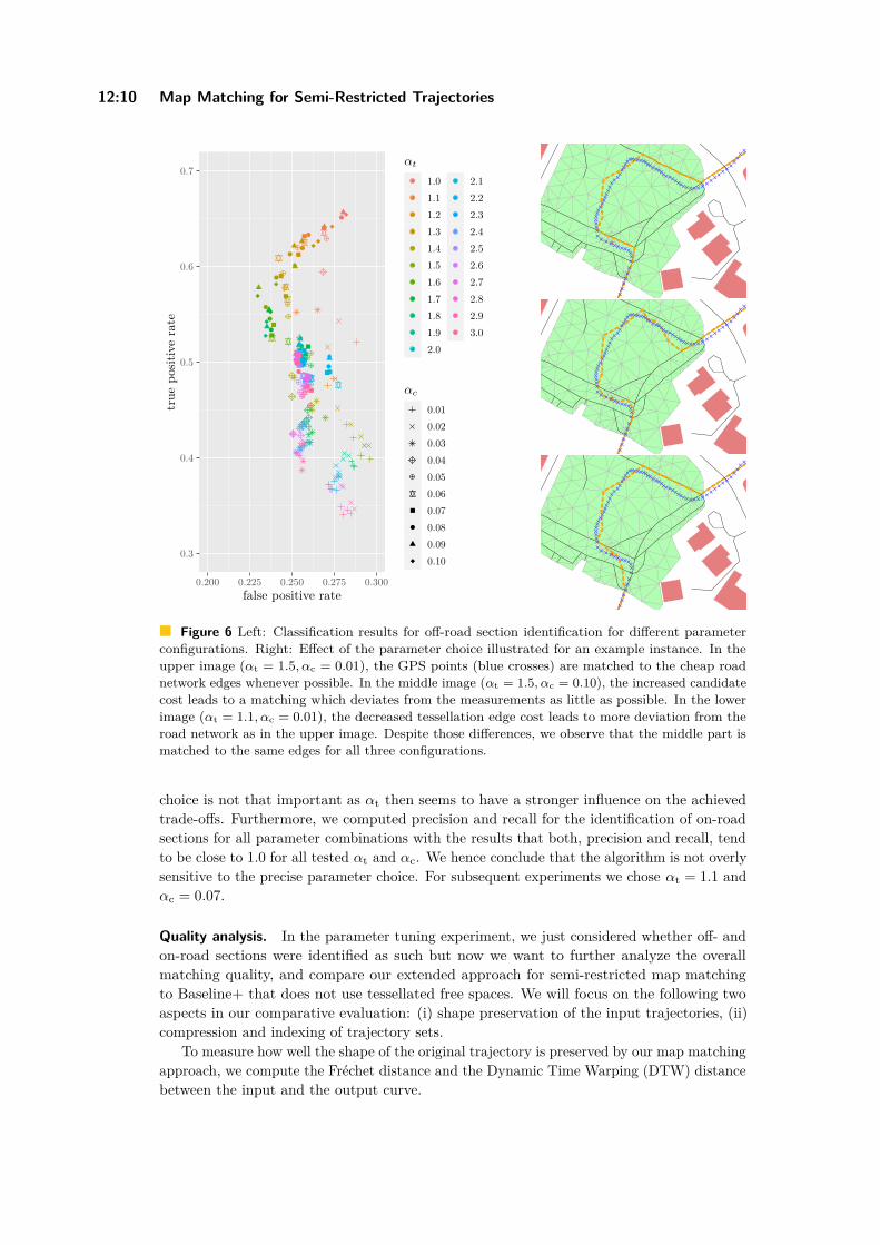
12:10 Map Matching for Semi-Restricted Trajectories

0.3

0.4

0.5

0.6

0.7

0.200 0.225 0.250 0.275 0.300false positive rate

true

posit

ive

rate

αt

1.01.11.21.31.41.51.61.71.81.92.0

2.12.22.32.42.52.62.72.82.93.0

αc

0.010.020.030.040.050.060.070.080.090.10

Figure 6 Left: Classification results for off-road section identification for different parameterconfigurations. Right: Effect of the parameter choice illustrated for an example instance. In theupper image (αt = 1.5, αc = 0.01), the GPS points (blue crosses) are matched to the cheap roadnetwork edges whenever possible. In the middle image (αt = 1.5, αc = 0.10), the increased candidatecost leads to a matching which deviates from the measurements as little as possible. In the lowerimage (αt = 1.1, αc = 0.01), the decreased tessellation edge cost leads to more deviation from theroad network as in the upper image. Despite those differences, we observe that the middle part ismatched to the same edges for all three configurations.

choice is not that important as αt then seems to have a stronger influence on the achievedtrade-offs. Furthermore, we computed precision and recall for the identification of on-roadsections for all parameter combinations with the results that both, precision and recall, tendto be close to 1.0 for all tested αt and αc. We hence conclude that the algorithm is not overlysensitive to the precise parameter choice. For subsequent experiments we chose αt = 1.1 andαc = 0.07.

Quality analysis. In the parameter tuning experiment, we just considered whether off- andon-road sections were identified as such but now we want to further analyze the overallmatching quality, and compare our extended approach for semi-restricted map matchingto Baseline+ that does not use tessellated free spaces. We will focus on the following twoaspects in our comparative evaluation: (i) shape preservation of the input trajectories, (ii)compression and indexing of trajectory sets.

To measure how well the shape of the original trajectory is preserved by our map matchingapproach, we compute the Fréchet distance and the Dynamic Time Warping (DTW) distancebetween the input and the output curve.

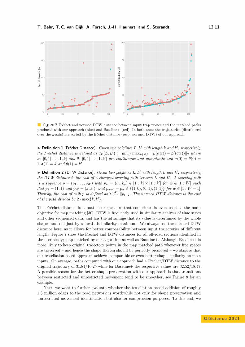
T. Behr, T. C. van Dijk, A. Forsch, J.-H. Haunert, and S. Storandt 12:11

0

50

100

150

200

0 25 50 75 100

fréch

et d

ista

nce

[m]

0

25

50

75

100

0 25 50 75 100

norm

aliz

ed d

tw [m

]

Figure 7 Fréchet and normed DTW distance between input trajectories and the matched pathsproduced with our approach (blue) and Baseline+ (red). In both cases the trajectories (distributedover the x-axis) are sorted by the fréchet distance (resp. normed DTW) of our approach.

Definition 1 (Fréchet Distance). Given two polylines L, L′ with length k and k′, respectively,the Fréchet distance is defined as dF (L, L′) := infσ,θ maxt∈[0,1] ||L(σ(t)) − L′(θ(t))||2 whereσ : [0, 1] → [1, k] and θ : [0, 1] → [1, k′] are continuous and monotonic and σ(0) = θ(0) =1, σ(1) = k and θ(1) = k′.

Definition 2 (DTW Distance). Given two polylines L, L′ with length k and k′, respectively,the DTW distance is the cost of a cheapest warping path between L and L′. A warping pathis a sequence p = (p1, . . . , pW ) with pw = (lw, l′

w) ∈ [1 : k] × [1 : k′] for w ∈ [1 : W ] suchthat p1 = (1, 1) and pW = (k, k′), and pw+1 − pw ∈ (1, 0), (0, 1), (1, 1) for w ∈ [1 : W − 1].Thereby, the cost of path p is defined as

∑Wi=1 ||pi||2. The normed DTW distance is the cost

of the path divided by 2 · maxk, k′.

The Fréchet distance is a bottleneck measure that sometimes is even used as the mainobjective for map matching [30]. DTW is frequently used in similarity analysis of time seriesand other sequenced data, and has the advantage that its value is determined by the wholeshapes and not just by a local dissimilarity maximum. We always use the normed DTWdistance here, as it allows for better comparability between input trajectories of differentlength. Figure 7 show the Fréchet and DTW distances for all off-road sections identified inthe user study; map matched by our algorithm as well as Baseline+. Although Baseline+ ismore likely to keep original trajectory points in the map matched path whenever free spacesare traversed – and hence the shape therein should be perfectly preserved – we observe thatour tessellation based approach achieves comparable or even better shape similarity on mostinputs. On average, paths computed with our approach had a Fréchet/DTW distance to theoriginal trajectory of 31.81/16.25 while for Baseline+ the respective values are 32.52/18.47.A possible reason for the better shape preservation with our approach is that transitionsbetween restricted and unrestricted movement tend to be smoother, see Figure 8 for anexample.

Next, we want to further evaluate whether the tessellation based addition of roughly1.3 million edges to the road network is worthwhile not only for shape preservation andunrestricted movement identification but also for compression purposes. To this end, we

GISc ience 2021

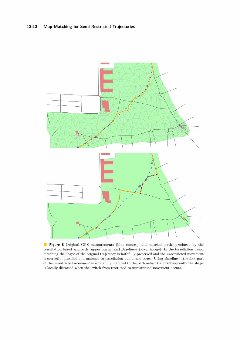
12:12 Map Matching for Semi-Restricted Trajectories

Figure 8 Original GPS measurements (blue crosses) and matched paths produced by thetessellation based approach (upper image) and Baseline+ (lower image). In the tessellation basedmatching the shape of the original trajectory is faithfully preserved and the unrestricted movementis correctly identified and matched to tessellation points and edges. Using Baseline+, the first partof the unrestricted movement is wrongfully matched to the path network and subsequently the shapeis locally distorted when the switch from restricted to unrestricted movement occurs.

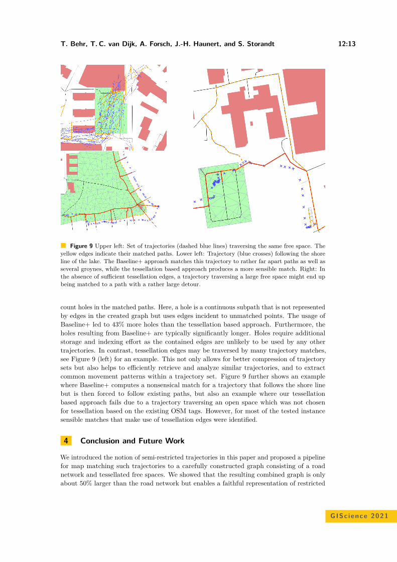
T. Behr, T. C. van Dijk, A. Forsch, J.-H. Haunert, and S. Storandt 12:13

Figure 9 Upper left: Set of trajectories (dashed blue lines) traversing the same free space. Theyellow edges indicate their matched paths. Lower left: Trajectory (blue crosses) following the shoreline of the lake. The Baseline+ approach matches this trajectory to rather far apart paths as well asseveral groynes, while the tessellation based approach produces a more sensible match. Right: Inthe absence of sufficient tessellation edges, a trajectory traversing a large free space might end upbeing matched to a path with a rather large detour.

count holes in the matched paths. Here, a hole is a continuous subpath that is not representedby edges in the created graph but uses edges incident to unmatched points. The usage ofBaseline+ led to 43% more holes than the tessellation based approach. Furthermore, theholes resulting from Baseline+ are typically significantly longer. Holes require additionalstorage and indexing effort as the contained edges are unlikely to be used by any othertrajectories. In contrast, tessellation edges may be traversed by many trajectory matches,see Figure 9 (left) for an example. This not only allows for better compression of trajectorysets but also helps to efficiently retrieve and analyze similar trajectories, and to extractcommon movement patterns within a trajectory set. Figure 9 further shows an examplewhere Baseline+ computes a nonsensical match for a trajectory that follows the shore linebut is then forced to follow existing paths, but also an example where our tessellationbased approach fails due to a trajectory traversing an open space which was not chosenfor tessellation based on the existing OSM tags. However, for most of the tested instancesensible matches that make use of tessellation edges were identified.

4 Conclusion and Future Work

We introduced the notion of semi-restricted trajectories in this paper and proposed a pipelinefor map matching such trajectories to a carefully constructed graph consisting of a roadnetwork and tessellated free spaces. We showed that the resulting combined graph is onlyabout 50% larger than the road network but enables a faithful representation of restricted

GISc ience 2021

12:14 Map Matching for Semi-Restricted Trajectories

and unrestricted movement at the same time. As evidenced in our experimental analysis,unrestricted movement is in most cases correctly identified as such by our map matchingapproach. Nevertheless, there are many interesting directions for future work that couldhelp to improve or extend our approach. For example, different tessellation variants could betested and compared. At the moment we use an upper bound for the edge length allowedin the free space triangulations and a lower bound for the angular resolution. The twobounds could be varied to achieve different precision and compression trade-offs for thematched trajectories. Other tessellation approaches, e.g. based on polygon skeletons, couldfurther help to model natural movement in free spaces. Furthermore, one could also considertrajectories that enter and exit buildings similarly and try to reliably infer the respectivetransitions from outdoor to indoor or vice versa. At the moment, we treat all buildings asobstacles, but it is also possible to apply our model to the interior of buildings to allow forindoor matching. Finally, while our approach is sufficiently fast with query times below 0.5seconds per trajectory, more efficient match computation might be possible by improvedcandidate node selection, especially within the tessellated free spaces.

References1 Priyanka Aggarwal, David Thomas, Lauro Ojeda, and Johann Borenstein. Map matching and

heuristic elimination of gyro drift for personal navigation systems in GPS-denied conditions.Measurement Science and Technology, 22(2):025205, 2011.

2 Yoonsik Bang, Jiyoung Kim, and Kiyun Yu. An improved map-matching technique based onthe Fréchet distance approach for pedestrian navigation services. Sensors, 16(10):1768, 2016.

3 Jean-Daniel Boissonnat, Olivier Devillers, Monique Teillaud, and Mariette Yvinec. Triangula-tions in CGAL. In Proc. 16th Annual Symposium on Computational Geometry (SoCG ’00),pages 11–18, 2000.

4 Anna Brauer, Ville Mäkinen, and Juha Oksanen. Characterizing cycling traffic fluency usingbig mobile activity tracking data. Computers, Environment and Urban Systems, 85:101553,2021.

5 Maike Buchin, Bernhard Kilgus, and Andrea Kölzsch. Group diagrams for representingtrajectories. International Journal of Geographical Information Science, 34(12):2401–2433,2020.

6 Pingfu Chao, Yehong Xu, Wen Hua, and Xiaofang Zhou. A survey on map-matching algorithms.In Renata Borovica-Gajic, Jianzhong Qi, and Weiqing Wang, editors, Databases Theory andApplications, pages 121–133, Cham, 2020. Springer International Publishing.

7 Jochen Eisner, Stefan Funke, Andre Herbst, Andreas Spillner, and Sabine Storandt. Algorithmsfor matching and predicting trajectories. In Proc. 13th Workshop on Algorithm Engineeringand Experiments (ALENEX ’11), pages 84–95, 2011.

8 Birgit Elias. Pedestrian navigation - creating a tailored geodatabase for routing. In 2007 4thWorkshop on Positioning, Navigation and Communication, pages 41–47, 2007.

9 Stefan Funke, Sören Laue, and Sabine Storandt. Deducing individual driving preferencesfor user-aware navigation. In Proc. 24th ACM SIGSPATIAL International Conference onAdvances in Geographic Information Systems (ACM SIGSPATIAL GIS ’16), pages 14:1–14:9,2016.

10 Stefan Funke, Tobias Rupp, André Nusser, and Sabine Storandt. PATHFINDER: storage andindexing of massive trajectory sets. In Proc. 16th International Symposium on Spatial andTemporal Databases (SSTD ’19), pages 90–99, 2019.

11 Jan-Henrik Haunert and Benedikt Budig. An algorithm for map matching given incompleteroad data. In Proc. 20th ACM SIGSPATIAL International Conference on Advances inGeographic Information Systems (ACM SIGSPATIAL GIS ’12), pages 510–513, 2012.

T. Behr, T. C. van Dijk, A. Forsch, J.-H. Haunert, and S. Storandt 12:15

12 Songtao He, Favyen Bastani, Sofiane Abbar, Mohammad Alizadeh, Hari Balakrishnan, SanjayChawla, and Sam Madden. RoadRunner: improving the precision of road network inferencefrom GPS trajectories. In Proc. 26th ACM SIGSPATIAL International Conference on Advancesin Geographic Information Systems (ACM SIGSPATIAL GIS ’18), pages 3–12, 2018.

13 George R. Jagadeesh and Thambipillai Srikanthan. Fast computation of clustered many-to-many shortest paths and its application to map matching. ACM Transactions on SpatialAlgorithms and Systems, 5(3):1–20, 2019.

14 Hannes Koller, Peter Widhalm, Melitta Dragaschnig, and Anita Graser. Fast hidden Markovmodel map-matching for sparse and noisy trajectories. In Proc. 18th IEEE InternationalConference on Intelligent Transportation Systems (ITSC ’15), pages 2557–2561. IEEE, 2015.

15 Benjamin Krogh, Christian S. Jensen, and Kristian Torp. Efficient in-memory indexing ofnetwork-constrained trajectories. In Proc. 24th ACM SIGSPATIAL international conferenceon advances in geographic information systems (ACM SIGSPATIAL GIS ’16), pages 1–10,2016.

16 Daigang Li, Junhan Li, and Juntao Li. Road network extraction from low-frequency trajectoriesbased on a road structure-aware filter. ISPRS International Journal of Geo-Information,8(9):374, 2019.

17 Yin Lou, Chengyang Zhang, Yu Zheng, Xing Xie, Wei Wang, and Yan Huang. Map-matchingfor low-sampling-rate GPS trajectories. In Proc. 17th ACM SIGSPATIAL InternationalConference on Advances in Geographic Information Systems (ACM SIGSPATIAL GIS ’09),pages 352–361. ACM, 2009.

18 Paul Newson and John Krumm. Hidden markov map matching through noise and sparse-ness. In Proc. 17th ACM SIGSPATIAL International Conference on Advances in GeographicInformation Systems (ACM SIGSPATIAL GIS ’09), pages 336–343. ACM, 2009.

19 Johannes Oehrlein, Benjamin Niedermann, and Jan-Henrik Haunert. Inferring the parametricweight of a bicriteria routing model from trajectories. In Proc. 25th ACM SIGSPATIALInternational Conference on Advances in Geographic Information Systems (ACM SIGSPATIALGIS ’17), pages 59:1–59:4, 2017.

20 Takayuki Osogami and Rudy Raymond. Map matching with inverse reinforcement learning.In Proc. 23rd International Joint Conference on Artificial Intelligence (IJCAI ’13), pages2547–2553, 2013.

21 Dieter Pfoser, Christian S. Jensen, and Yannis Theodoridis. Novel approaches to the indexingof moving object trajectories. In Proc. 26th International Conference on Very Large DataBases (VLDB ’00), pages 395–406, 2000.

22 Ming Ren and Hassan A. Karimi. Movement pattern recognition assisted map matching forpedestrian/wheelchair navigation. The Journal of Navigation, 65(4):617–633, 2012.

23 Yuya Sasaki, Jiahao Yu, and Yoshiharu Ishikawa. Road segment interpolation for incompleteroad data. In Proc. 2019 IEEE International Conference on Big Data and Smart Computing(BigComp ’19), pages 1–8, 2019.

24 Seung Hyuck Shin, Chan Gook Park, and Sangon Choi. New map-matching algorithm usingvirtual track for pedestrian dead reckoning. ETRI Journal, 32(6):891–900, 2010.

25 Renchu Song, Weiwei Sun, Baihua Zheng, and Yu Zheng. PRESS: A novel framework oftrajectory compression in road networks. Proceedings of the VLDB Endowment, 7(9), 2014.

26 Ivan Spassov, Michel Bierlaire, and Bertrand Merminod. Map-matching for pedestrians viabayesian inference. In Proc. European Navigation Conference, 2006.

27 Jody Sultan, Gev Ben-Haim, and Jan-Henrik Haunert. Extracting spatial patterns in bicycleroutes from crowdsourced data. Transactions in GIS, 21(6):1321–1340, 2017.

28 Shun Taguchi, Satoshi Koide, and Takayoshi Yoshimura. Online map matching with routeprediction. IEEE Transactions on Intelligent Transportation Systems, 20(1):338–347, 2018.

29 Longhao Wang, Yu Zheng, Xing Xie, and Wei-Ying Ma. A flexible spatio-temporal indexingscheme for large-scale GPS track retrieval. In Proc. 9th IEEE International Conference onMobile Data Management (MDM 2008), pages 1–8, 2008.

GISc ience 2021

12:16 Map Matching for Semi-Restricted Trajectories

30 Hong Wei, Yin Wang, George Forman, and Yanmin Zhu. Map matching by Fréchet distanceand global weight optimization. Technical Paper, Departement of Computer Science andEngineering, page 19, 2013.

31 Christopher E. White, David Bernstein, and Alain L. Kornhauser. Some map matchingalgorithms for personal navigation assistants. Transportation Research Part C: EmergingTechnologies, 8(1):91–108, 2000.

32 Pawel Wilk and Jaroslaw Karciarz. Optimization of map matching algorithms for indoornavigation in shopping malls. In Proc. 2014 International Conference on Indoor Positioningand Indoor Navigation (IPIN ’14), pages 661–669. IEEE, 2014.

33 Ethan Zhang and Neda Masoud. Increasing GPS localization accuracy with reinforcementlearning. IEEE Transactions on Intelligent Transportation Systems, 2020.

34 Lijia Zhang, Mo Cheng, Zhuoling Xiao, Liang Zhou, and Jun Zhou. Adaptable map matchingusing PF-net for pedestrian indoor localization. IEEE Communications Letters, 24(7):1437–1440, 2020.

Automated Georeferencing of Antarctic SpeciesJamie Scott #

Massey University, Auckland, New Zealand

Kristin Stock #

Massey Geoinformatics Collaboratory, Massey University, Auckland, New Zealand

Fraser Morgan #

Manaaki Whenua Landcare Research, Auckland, New Zealand

Brandon Whitehead #

Manaaki Whenua Landcare Research, Auckland, New Zealand

David Medyckyj-Scott #

Manaaki Whenua Landcare Research, Auckland, New Zealand

AbstractMany text documents in the biological domain contain references to the toponym of specificphenomena (e.g. species sightings) in natural language form “In <LOCATION> Garwood Valleysummer activity was 0.2% for <SPECIES> Umbilicaria aprina and 1.7% for <SPECIES> Caloplacasp. ...”

While methods have been developed to extract place names from documents, and attention hasbeen given to the interpretation of spatial prepositions, the ability to connect toponym mentions intext with the phenomena to which they refer (in this case species) has been given limited attention,but would be of considerable benefit for the task of mapping specific phenomena mentioned in textdocuments.

As part of work to create a pipeline to automate georeferencing of species within legacy documents,this paper proposes a method to: (1) recognise species and toponyms within text and (2) matcheach species mention to the relevant toponym mention. Our methods find significant promise in abespoke rules- and dictionary-based approach to recognise species within text (F1 scores up to 0.87including partial matches) but less success, as yet, recognising toponyms using multiple gazetteerscombined with an off the shelf natural language processing tool (F1 up to 0.62).

Most importantly, we offer a contribution to the relatively nascent area of matching toponymreferences to the object they locate (in our case species), including cases in which the toponym andspecies are in different sentences. We use tree-based models to achieve precision as high as 0.88 oran F1 score up to 0.68 depending on the downsampling rate. Initial results out perform previousresearch on detecting entity relationships that may cross sentence boundaries within biomedical text,and differ from previous work in specifically addressing species mapping.

2012 ACM Subject Classification Computing methodologies → Information extraction; Computingmethodologies → Classification and regression trees; Applied computing → Life and medical sciences

Keywords and phrases Named Entity Recognition (NER), Taxonomic Name Extraction, RelationExtraction, Georeferencing

Digital Object Identifier 10.4230/LIPIcs.GIScience.2021.II.13

Funding Jamie Scott: Research for this project was funded by Manaaki Whenua Landcare Research.

1 Introduction

A significant amount of biodiversity knowledge is locked up in textual descriptions withindocuments, often in free text form, without coordinates with which to georeference. Manyresearch papers in the biological domain refer to specific species and their location, and thedevelopment of methods to extract species-toponym pairs can enable biodiversity mapping,with a range of related societal and economic benefits.

© Jamie Scott, Kristin Stock, Fraser Morgan, Brandon Whitehead, and David Medyckyj-Scott;licensed under Creative Commons License CC-BY 4.0

11th International Conference on Geographic Information Science (GIScience 2021) – Part II.Editors: Krzysztof Janowicz and Judith A. Verstegen; Article No. 13; pp. 13:1–13:16

Leibniz International Proceedings in InformaticsSchloss Dagstuhl – Leibniz-Zentrum für Informatik, Dagstuhl Publishing, Germany

13:2 Automated Georeferencing of Antarctic Species

However, textual relations can be complex with one-to-many relationships between entitiesand relationships occurring sometimes across sentence boundaries, and even some distancefrom each other. To illustrate, Example 1 is a snippet from a journal article [29] containingfour relationships between four different species mentions (one just as a broader genus termand the other two in abbreviated G. species form) to the same toponym one, two or threesentences away.

Example 1. “There are also examples of growth forms that make use of the increasingprecipitation at <LOCATION> Livingston Island. Most obvious is the very extensive growthof the <SPECIES> Usnea lichens whose fruticose form allows them to benefit from both rain,snow and fog (Rundel 1978). Within the mosses, <SPECIES> A. gainii and <SPECIES>H. crispulum are able to achieve high activities by growing as clumps on the rock surfaceand storing water from precipitation, and <SPECIES> A. gainii is much warmer than otherspecies because of its darker colour.”

A significant body of work has addressed the task of extracting toponym references fromdocuments using named-entity recognition [2, 22], and then disambiguating the mentionedplace names to identify the coordinates of the named place, requiring resolution of duplicateplace names, place name abbreviations or complex place name sequences [5, 21]. Similarly,efforts have been made to develop automated methods to identify biological species in text[3, 17]. However, little attention has been given to the task of matching specific speciesmentions to their toponym references, and thus georeferencing (identifying the coordinatelocation) for specific species mentioned in text documents. Without this step, while we canmap toponyms mentioned in a document (as for example in [25] and [1]), we cannot mapspecific items mentioned in text. In the case of biological text documents, this means thatwe cannot map species distribution or conduct spatial analysis using data “locked away” intext documents.

The task of georeferencing specific phenomena in text has been addressed in someother domains, including disaster management for event georeferencing [13], and significantattention has been given to extracting spatial relations and the reference and located objectsto which they refer [18]. However, the former relies on multiple mentions of the sameevent, using clustering to converge on its probable toponym, and the latter relies on spatialprepositions to connect located and reference objects. A range of work in the relationextraction field of NLP is also relevant, but until recently the focus has been on relationshipsthat occur within the same sentence [7, 33]. Recent studies that also look for relations thatmay cross sentence boundaries [28, 8] do not include toponym or species and may have limitedtransferability, or identify relations that express location in a non-geographic context [19].

There remains a gap in solving the difficult problem of associating species mentions withlocations for georeferencing. We address this gap by proposing a method that has threesteps:– a) extracting species mentions in text; b) extracting and disambiguating toponymmentions in text and c) predicting which, if any, pairs of those species and toponyms representan actual <species> ‘present in’ or ‘found at’ <location> relationship. To perform the latterstep, we use a machine learning classifier, in which we classify all species-toponym pairs inthe document to identify those that are correct matches. We test and evaluate a range offeatures for our classifier on a corpus of seven documents (44037 tokens) from the Antarcticdomain, including a mixture of journal papers, theses and supplementary material, writtenby authors from around the world.

Preliminary results using tree-based classifiers achieved precision of up to 0.88. Thiscompares favourably to studies within the biomededical field where precision scores havevaried from 0.39 to 0.65 [27, 8, 32, 19]. Furthermore, our bespoke rules- and dictionary-basedapproach for extraction of species achieved an F1 score of 0.87 including partial matches.

J. Scott, K. Stock, F. Morgan, B. Whitehead, and D. Medyckyj-Scott 13:3

The contributions of our work are two-fold. Firstly, we apply machine learning to solvethe difficult and unaddressed problem of associating species mentions with locations forgeoreferencing. Relation extraction in natural language is regarded as a hard problemgenerally, and little progress has been made on solving it for the fundamental GIScience taskof georeferencing the detailed content of documents, with [1, p.1] pointing out that “Researchon this problem is still in its infancy”. Generic methods for relation extraction have not beenapplied to the particular problem of matching species and locations, and cannot handle textwhere the subject and object of the relation are widely separated, and that involve complexco-references. Furthermore, text that describes location differs from generic language in anumber of ways, making the challenge more difficult. Specifically:1. The ultimate goal of this work is to georeference species mentions, and thus location

mentions identified by NER must be tied to specific locations using gazetteers. However,many locations identified by NER are not found in gazetteers, and thus the textscontain many items that look like location references but are actually ‘red herrings’ (notgeoreferencable), imposing additional demands on standard relation classifiers.

2. The role of toponyms as universal labels for locations presents different language uses,including common but unusual abbreviations (e.g. MDV for McMurdo Dry Valleys), aswell as more standard forms (e.g. Mt for Mount).

3. The role of toponyms as a reference frame results in common repetition of place names(or even only once at the beginning of the paper), interspersed with other place names,and the need to disentangle the correct place name references for multiple mentions ofdifferent species is especially challenging.

Our second contribution is the method of application of machine-learning to the problem.Our contribution is in the binary classification model using pairwise matches (e.g. in contrastto dependency driven approaches), and the selection of features.

This paper is structured as follows: Section 2 reviews relevant literature, Section 3 outlinesour methodology, Section 4 presents results, which are then discussed in Section 5, beforeconclusions are summarised in section 6.

2 Related Work

2.1 Recognising Species and Toponyms as Named EntitiesThe task of detecting location mentions in text is addressed by standard named entityrecognition (NER) methods of popular modern natural language processing (NLP) Pythonpackages such as Natural Language Toolkit (NLTK)1 and spaCy2. Recent evaluation of sixNER tools on Twitter content indicates precision in the low 90s, with F1 values in the 70s (asrecall figures are typically not as high as precision) [16], with slightly lower values in a reviewon text documents [10]. Following NER, place names must also be resolved to identify thecoordinates of the places to which they refer (known as toponym resolution or disambiguation),a task that is challenging due to duplicate place names, unusual abbreviations and spellingvariations. Methods for resolving toponyms have included selecting the place with the highestpopulation on the basis that it is more likely to be the one referred to due to size; associatedplace names mentioned in surrounding text; feature types and language models [4, 15].

1 http://www.nltk.org2 https://spacy.io

GISc ience 2021

13:4 Automated Georeferencing of Antarctic Species

In contrast to location, the task of species detection is not specifically addressed instandard NER tools. The linguistic structure of taxonomic names does however, allow forthe development of automated methods to find these names within natural language text[17]. Linnaean rules for taxonomic names of organisms dictate genus names precede species(and any sub species) name with the former capitalised and all names in either Latin orGreek [17, 23]. Where abbreviated in text, the species name is preceded by the capitalisedfirst letter of the genus and then a period.

Others in the biodiversity domain have tackled the species detection challenge witha mixture of approaches based on matching terms in a dictionary of known entities, [9,20, 24], isolating taxonomic-looking strings not otherwise in a English lexicon [17, 24], ormachine learning approaches like Naïve Bayes [3] or ensemble classifiers that include neuralnetworks [24].

All those methods mentioned above focus on finding scientific names apart from [9] whichalso finds some common names with their method.

Rule and pattern-based methods can recognise new scientific names in text [17] but cangenerate false positives for non-scientific text that appears to be in a Linnaean format [24].Words found in both scientific names and vernacular text cause problems for dictionaryand machine learning approaches alike, while machine learning is sensitive to text encodingalgorithms [24].

Some dictionary approaches [20] can find new name combinations from existing termsbut all are limited by how comprehensive and up-to-date the dictionaries are at time ofuse, something especially noteworthy in the biodiversity field where thousands of species arediscovered or reclassified each year [3, 17, 24].

Recall and precision figures higher than 0.8 and up to 0.97 have been shown to be possiblewhen testing these methods on biodiversity datasets with Quaesitor[24], TaxonFinder[20],and NetiNeti[3] generally performing best in tests [24] conducted.

Despite the collective and respective informativeness of their approaches, none of theoptions reviewed were suitable for our pipeline for one or more reasons, including the following:

They were not available as an easy-to-access Python package.They returned a single instance of a species mention instead of every mention along withposition in the document.They separately annotated species and genus for combined terms.While available via an online interface or API, they were not appropriate to process entiredocuments of text, let alone a large collection, due to limits on the amount of text thatcould be parsed in each use (and while references to DOIs would remove the need toupload entire documents in some cases, a focus of our wider project is processing largebatches of legacy documents, some of which do not have DOIs).

2.2 Georeferencing Phenomena in TextThe problem of georeferencing of text has been addressed in other domains. Methods forgeoreferencing documents by identifying their geographic location have been reviewed by [25],but these methods identify a toponym for the entire document, rather than toponyms forspecific items mentioned in the document text. Methods have been developed for extractingplace mentions in a document addressing a particular topic, assuming that they describelocations relating to the topic. For example, [1] identifies locations of orchards and cancercases by extracting place names from specific portions of documents (e.g. the methodssection), [6] similarly map locations connected to specific historical events across a document,

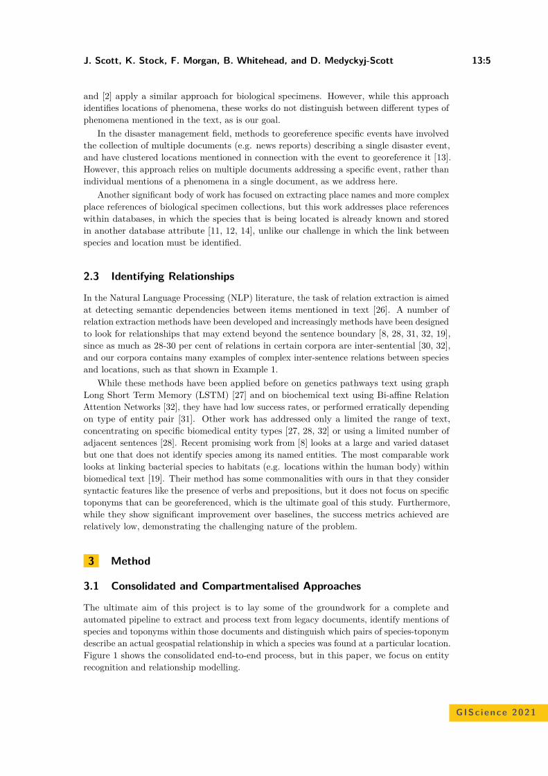
J. Scott, K. Stock, F. Morgan, B. Whitehead, and D. Medyckyj-Scott 13:5

and [2] apply a similar approach for biological specimens. However, while this approachidentifies locations of phenomena, these works do not distinguish between different types ofphenomena mentioned in the text, as is our goal.

In the disaster management field, methods to georeference specific events have involvedthe collection of multiple documents (e.g. news reports) describing a single disaster event,and have clustered locations mentioned in connection with the event to georeference it [13].However, this approach relies on multiple documents addressing a specific event, rather thanindividual mentions of a phenomena in a single document, as we address here.

Another significant body of work has focused on extracting place names and more complexplace references of biological specimen collections, but this work addresses place referenceswithin databases, in which the species that is being located is already known and storedin another database attribute [11, 12, 14], unlike our challenge in which the link betweenspecies and location must be identified.

2.3 Identifying Relationships

In the Natural Language Processing (NLP) literature, the task of relation extraction is aimedat detecting semantic dependencies between items mentioned in text [26]. A number ofrelation extraction methods have been developed and increasingly methods have been designedto look for relationships that may extend beyond the sentence boundary [8, 28, 31, 32, 19],since as much as 28-30 per cent of relations in certain corpora are inter-sentential [30, 32],and our corpora contains many examples of complex inter-sentence relations between speciesand locations, such as that shown in Example 1.

While these methods have been applied before on genetics pathways text using graphLong Short Term Memory (LSTM) [27] and on biochemical text using Bi-affine RelationAttention Networks [32], they have had low success rates, or performed erratically dependingon type of entity pair [31]. Other work has addressed only a limited the range of text,concentrating on specific biomedical entity types [27, 28, 32] or using a limited number ofadjacent sentences [28]. Recent promising work from [8] looks at a large and varied datasetbut one that does not identify species among its named entities. The most comparable worklooks at linking bacterial species to habitats (e.g. locations within the human body) withinbiomedical text [19]. Their method has some commonalities with ours in that they considersyntactic features like the presence of verbs and prepositions, but it does not focus on specifictoponyms that can be georeferenced, which is the ultimate goal of this study. Furthermore,while they show significant improvement over baselines, the success metrics achieved arerelatively low, demonstrating the challenging nature of the problem.

3 Method

3.1 Consolidated and Compartmentalised Approaches

The ultimate aim of this project is to lay some of the groundwork for a complete andautomated pipeline to extract and process text from legacy documents, identify mentions ofspecies and toponyms within those documents and distinguish which pairs of species-toponymdescribe an actual geospatial relationship in which a species was found at a particular location.Figure 1 shows the consolidated end-to-end process, but in this paper, we focus on entityrecognition and relationship modelling.

GISc ience 2021

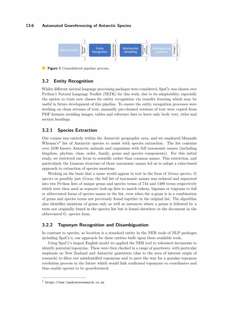
13:6 Automated Georeferencing of Antarctic Species

Figure 1 Consolidated pipeline process.

3.2 Entity RecognitionWhilst different natural language processing packages were considered, SpaCy was chosen overPython’s Natural Language Toolkit (NLTK) for this work, due to its adaptability, especiallythe option to train new classes for entity recognition via transfer learning which may beuseful in future development of this pipeline. To ensure the entity recognition processes wereworking on clean streams of text, manually pre-cleaned versions of text were copied fromPDF formats avoiding images, tables and reference lists to leave only body text, titles andsection headings.

3.2.1 Species ExtractionOur corpus was entirely within the Antarctic geographic area, and we employed ManaakiWhenua’s3 list of Antarctic species to assist with species extraction. The list containsover 2100 known Antarctic animals and organisms with full taxonomic names (includingkingdom, phylum, class, order, family, genus and species components). For this initialstudy, we restricted our focus to scientific rather than common names. This restriction, andparticularly the Linnean structure of those taxonomic names led us to adopt a rules-basedapproach to extraction of species mentions.

Working on the basis that a name would appear in text in the form of Genus species, G.species or possibly just Genus, the full list of taxonomic names was reduced and separatedinto two Python lists of unique genus and species terms of 744 and 1489 terms respectivelywhich were then used as separate look-up lists to match tokens, bigrams or trigrams to fullor abbreviated forms of species names in the list, even when the n-gram is in a combinationof genus and species terms not previously found together in the original list. The algorithmalso identifies mentions of genus only as well as instances where a genus is followed by aterm not originally found in the species list but is found elsewhere in the document in theabbreviated G. species form.

3.2.2 Toponym Recognition and DisambiguationIn contrast to species, as location is a standard entity in the NER tools of NLP packagesincluding SpaCy’s, our approach for these entities built upon these available tools.

Using SpaCy’s largest English model we applied the NER tool to tokenised documents toidentify potential toponyms. These were then checked in a range of gazetteers, with particularemphasis on New Zealand and Antarctic gazetteers (due to the area of interest origin ofresearch) to filter out misidentified toponyms and to pave the way for a genuine toponymresolution process in the future which would link confirmed toponyms to coordinates andthus enable species to be georeferenced.

3 https://www.landcareresearch.co.nz

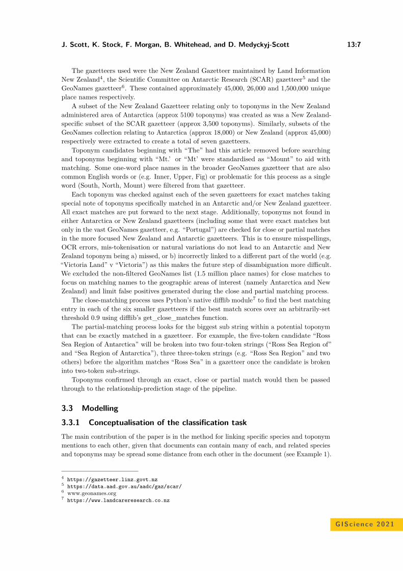
J. Scott, K. Stock, F. Morgan, B. Whitehead, and D. Medyckyj-Scott 13:7

The gazetteers used were the New Zealand Gazetteer maintained by Land InformationNew Zealand4, the Scientific Committee on Antarctic Research (SCAR) gazetteer5 and theGeoNames gazetteer6. These contained approximately 45,000, 26,000 and 1,500,000 uniqueplace names respectively.

A subset of the New Zealand Gazetteer relating only to toponyms in the New Zealandadministered area of Antarctica (approx 5100 toponyms) was created as was a New Zealand-specific subset of the SCAR gazetteer (approx 3,500 toponyms). Similarly, subsets of theGeoNames collection relating to Antarctica (approx 18,000) or New Zealand (approx 45,000)respectively were extracted to create a total of seven gazetteers.

Toponym candidates beginning with “The” had this article removed before searchingand toponyms beginning with “Mt.’ or “Mt’ were standardised as “Mount” to aid withmatching. Some one-word place names in the broader GeoNames gazetteer that are alsocommon English words or (e.g. Inner, Upper, Fig) or problematic for this process as a singleword (South, North, Mount) were filtered from that gazetteer.

Each toponym was checked against each of the seven gazetteers for exact matches takingspecial note of toponyms specifically matched in an Antarctic and/or New Zealand gazetteer.All exact matches are put forward to the next stage. Additionally, toponyms not found ineither Antarctica or New Zealand gazetteers (including some that were exact matches butonly in the vast GeoNames gazetteer, e.g. “Portugal”) are checked for close or partial matchesin the more focused New Zealand and Antarctic gazetteers. This is to ensure misspellings,OCR errors, mis-tokenisation or natural variations do not lead to an Antarctic and NewZealand toponym being a) missed, or b) incorrectly linked to a different part of the world (e.g.“Victoria Land” v “Victoria”) as this makes the future step of disambiguation more difficult.We excluded the non-filtered GeoNames list (1.5 million place names) for close matches tofocus on matching names to the geographic areas of interest (namely Antarctica and NewZealand) and limit false positives generated during the close and partial matching process.

The close-matching process uses Python’s native difflib module7 to find the best matchingentry in each of the six smaller gazetteers if the best match scores over an arbitrarily-setthreshold 0.9 using difflib’s get_close_matches function.

The partial-matching process looks for the biggest sub string within a potential toponymthat can be exactly matched in a gazetteer. For example, the five-token candidate “RossSea Region of Antarctica” will be broken into two four-token strings (“Ross Sea Region of”and “Sea Region of Antarctica”), three three-token strings (e.g. “Ross Sea Region” and twoothers) before the algorithm matches “Ross Sea” in a gazetteer once the candidate is brokeninto two-token sub-strings.

Toponyms confirmed through an exact, close or partial match would then be passedthrough to the relationship-prediction stage of the pipeline.

3.3 Modelling

3.3.1 Conceptualisation of the classification taskThe main contribution of the paper is in the method for linking specific species and toponymmentions to each other, given that documents can contain many of each, and related speciesand toponyms may be spread some distance from each other in the document (see Example 1).

4 https://gazetteer.linz.govt.nz5 https://data.aad.gov.au/aadc/gaz/scar/6 www.geonames.org7 https://www.landcareresearch.co.nz

GISc ience 2021

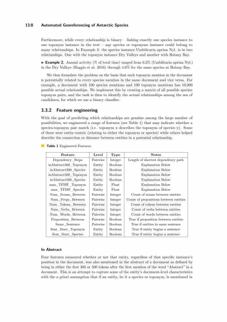
13:8 Automated Georeferencing of Antarctic Species

Furthermore, while every relationship is binary – linking exactly one species instance toone toponym instance in the text – any species or toponyms instance could belong tomany relationships. In Example 2: the species instance Umbilicaria aprina Nyl. is in tworelationships. One with the toponym instance Dry Valleys and another with Botany Bay.

Example 2. Annual activity (% of total time) ranged from 0.2% (Umbilicaria aprina Nyl.)in the Dry Valleys (Raggio et al. 2016) through 4.6% for the same species at Botany Bay.

We thus formulate the problem on the basis that each toponym mention in the documentis potentially related to every species mention in the same document and vice versa. Forexample, a document with 100 species mentions and 100 toponym mentions has 10,000possible actual relationships. We implement this by creating a matrix of all possible species-toponym pairs, and the task is then to identify the actual relationships among the sea ofcandidates, for which we use a binary classifier.

3.3.2 Feature engineeringWith the goal of predicting which relationships are genuine among the large number ofpossibilities, we engineered a range of features (see Table 1) that may indicate whether aspecies-toponym pair match (i.e. toponym x describes the toponym of species y). Someof these were entity-centric (relating to either the toponym or species) while others helpeddescribe the connection or distance between entities in a potential relationship.

Table 1 Engineered Features.

Feature Level Type NotesDependency_Steps Pairwise Integer Length of shortest dependency path

inAbstract300_Toponym Entity Boolean Explanation BelowinAbstract300_Species Entity Boolean Explanation Below

inAbstract500_Toponym Entity Boolean Explanation BelowinAbstract500_Species Entity Boolean Explanation Belowmax_TFISF_Toponym Entity Float Explanation Belowmax_TFISF_Species Entity Float Explanation Below

Num_Nouns_Between Pairwise Integer Count of nouns between entitiesNum_Preps_Between Pairwise Integer Count of prepositions between entities

Num_Tokens_Between Pairwise Integer Count of tokens between entitiesNum_Verbs_Between Pairwise Integer Count of verbs between entitiesNum_Words_Between Pairwise Integer Count of words between entitiesPreposition_Between Pairwise Boolean True if preposition between entities

Same_Sentence Pairwise Boolean True if entities in same sentenceSent_Start_Toponym Entity Boolean True if entity begins a sentenceSent_Start_Species Entity Boolean True if entity begins a sentence

In Abstract

Four features measured whether or not that entity, regardless of that specific instance’sposition in the document, was also mentioned in the abstract of a document as defined bybeing in either the first 300 or 500 tokens after the first mention of the word “Abstract” in adocument. This is an attempt to capture some of the entity’s document-level characteristicswith the a priori assumption that if an entity, be it a species or toponym, is mentioned in

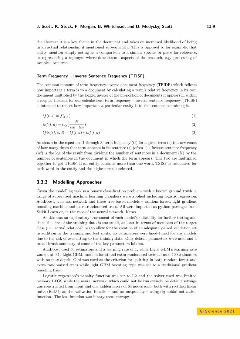
J. Scott, K. Stock, F. Morgan, B. Whitehead, and D. Medyckyj-Scott 13:9

the abstract it is a key theme in the document and takes on increased likelihood of beingin an actual relationship if mentioned subsequently. This is opposed to for example, thatentity mention simply acting as a comparison to a similar species or place for reference,or representing a toponym where downstream aspects of the research, e.g. processing ofsamples, occurred.

Term Frequency – Inverse Sentence Frequency (TFISF)

The common measure of term frequency-inverse document frequency (TFIDF) which reflectshow important a term is to a document by calculating a term’s relative frequency in its owndocument multiplied by the logged inverse of the proportion of documents it appears in withina corpus. Instead, for our calculations, term frequency – inverse sentence frequency (TFISF)is intended to reflect how important a particular entity is to the sentence containing it.

tf(t, s) = f(t,s ) (1)

isf(t, d) = log( N

sεd : tεs) (2)

tfisf(t, s, d) = tf(t, d) ∗ isf(t, d) (3)

As shown in the equations 1 through 3, term frequency (tf) for a given term (t) is a raw countof how many times that term appears in its sentence (s) (often 1) . Inverse sentence frequency(isf) is the log of the result from dividing the number of sentences in a document (N) by thenumber of sentences in the document in which the term appears. The two are multipliedtogether to get TFISF. If an entity contains more than one word, TSISF is calculated foreach word in the entity and the highest result selected.

3.3.3 Modelling Approaches

Given the modelling task is a binary classification problem with a known ground truth, arange of supervised machine learning classifiers were applied including logistic regression,AdaBoost, a neural network and three tree-based models – random forest, light gradientboosting machine and extra randomised trees. All were imported as python packages fromScikit-Learn or, in the case of the neural network, Keras.

As this was an exploratory assessment of each model’s suitability for further testing andsince the size of the training data is too small, at least in terms of members of the targetclass (i.e., actual relationships) to allow for the creation of an adequately-sized validation setin addition to the training and test splits, no parameters were fined-tuned for any modelsdue to the risk of over-fitting to the training data. Only default parameters were used and abroad-brush summary of some of the key parameters follows.

AdaBoost used 50 estimators and a learning rate of 1, while Light GBM’s learning ratewas set at 0.1. Light GBM, random forest and extra randomised trees all used 100 estimatorswith no max depth. Gini was used as the criterion for splitting in both random forest andextra randomised trees while light GBM boosting type was set to a traditional gradientboosting tree.

Logistic regression’s penalty function was set to L2 and the solver used was limitedmemory BFGS while the neural network, which could not be run entirely on default settingswas constructed from input and one hidden layers of 64 nodes each, both with rectified linearunits (ReLU) as the activation functions and an output layer using sigmoidal activationfunction. The loss function was binary cross entropy.

GISc ience 2021

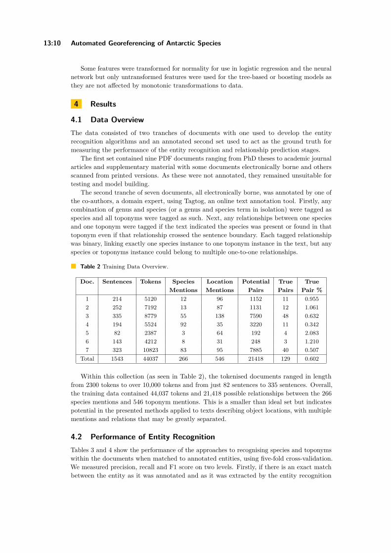
13:10 Automated Georeferencing of Antarctic Species

Some features were transformed for normality for use in logistic regression and the neuralnetwork but only untransformed features were used for the tree-based or boosting models asthey are not affected by monotonic transformations to data.

4 Results

4.1 Data OverviewThe data consisted of two tranches of documents with one used to develop the entityrecognition algorithms and an annotated second set used to act as the ground truth formeasuring the performance of the entity recognition and relationship prediction stages.

The first set contained nine PDF documents ranging from PhD theses to academic journalarticles and supplementary material with some documents electronically borne and othersscanned from printed versions. As these were not annotated, they remained unsuitable fortesting and model building.

The second tranche of seven documents, all electronically borne, was annotated by one ofthe co-authors, a domain expert, using Tagtog, an online text annotation tool. Firstly, anycombination of genus and species (or a genus and species term in isolation) were tagged asspecies and all toponyms were tagged as such. Next, any relationships between one speciesand one toponym were tagged if the text indicated the species was present or found in thattoponym even if that relationship crossed the sentence boundary. Each tagged relationshipwas binary, linking exactly one species instance to one toponym instance in the text, but anyspecies or toponyms instance could belong to multiple one-to-one relationships.

Table 2 Training Data Overview.

Doc. Sentences Tokens Species Location Potential True TrueMentions Mentions Pairs Pairs Pair %

1 214 5120 12 96 1152 11 0.9552 252 7192 13 87 1131 12 1.0613 335 8779 55 138 7590 48 0.6324 194 5524 92 35 3220 11 0.3425 82 2387 3 64 192 4 2.0836 143 4212 8 31 248 3 1.2107 323 10823 83 95 7885 40 0.507

Total 1543 44037 266 546 21418 129 0.602

Within this collection (as seen in Table 2), the tokenised documents ranged in lengthfrom 2300 tokens to over 10,000 tokens and from just 82 sentences to 335 sentences. Overall,the training data contained 44,037 tokens and 21,418 possible relationships between the 266species mentions and 546 toponym mentions. This is a smaller than ideal set but indicatespotential in the presented methods applied to texts describing object locations, with multiplementions and relations that may be greatly separated.

4.2 Performance of Entity RecognitionTables 3 and 4 show the performance of the approaches to recognising species and toponymswithin the documents when matched to annotated entities, using five-fold cross-validation.We measured precision, recall and F1 score on two levels. Firstly, if there is an exact matchbetween the entity as it was annotated and as it was extracted by the entity recognition

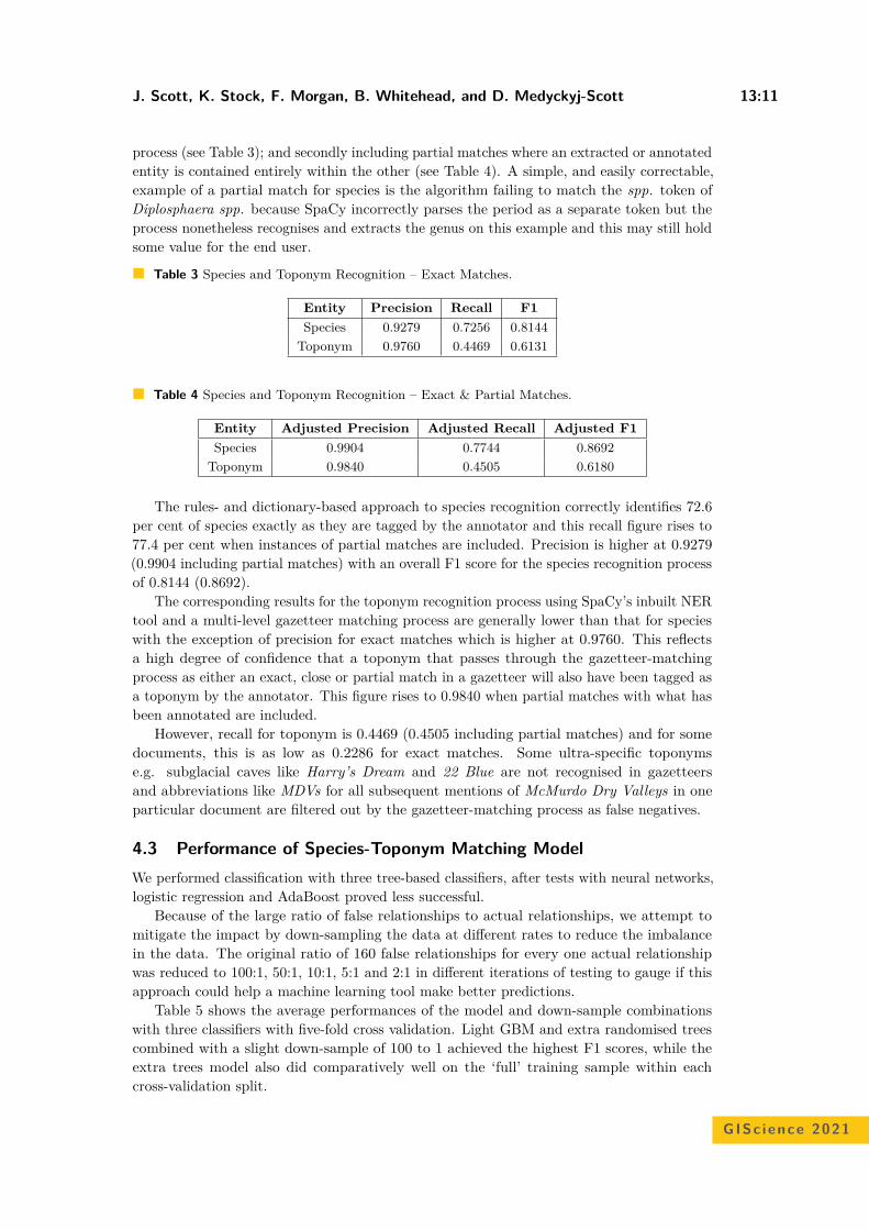
J. Scott, K. Stock, F. Morgan, B. Whitehead, and D. Medyckyj-Scott 13:11

process (see Table 3); and secondly including partial matches where an extracted or annotatedentity is contained entirely within the other (see Table 4). A simple, and easily correctable,example of a partial match for species is the algorithm failing to match the spp. token ofDiplosphaera spp. because SpaCy incorrectly parses the period as a separate token but theprocess nonetheless recognises and extracts the genus on this example and this may still holdsome value for the end user.

Table 3 Species and Toponym Recognition – Exact Matches.

Entity Precision Recall F1Species 0.9279 0.7256 0.8144

Toponym 0.9760 0.4469 0.6131

Table 4 Species and Toponym Recognition – Exact & Partial Matches.

Entity Adjusted Precision Adjusted Recall Adjusted F1Species 0.9904 0.7744 0.8692

Toponym 0.9840 0.4505 0.6180

The rules- and dictionary-based approach to species recognition correctly identifies 72.6per cent of species exactly as they are tagged by the annotator and this recall figure rises to77.4 per cent when instances of partial matches are included. Precision is higher at 0.9279(0.9904 including partial matches) with an overall F1 score for the species recognition processof 0.8144 (0.8692).

The corresponding results for the toponym recognition process using SpaCy’s inbuilt NERtool and a multi-level gazetteer matching process are generally lower than that for specieswith the exception of precision for exact matches which is higher at 0.9760. This reflectsa high degree of confidence that a toponym that passes through the gazetteer-matchingprocess as either an exact, close or partial match in a gazetteer will also have been tagged asa toponym by the annotator. This figure rises to 0.9840 when partial matches with what hasbeen annotated are included.

However, recall for toponym is 0.4469 (0.4505 including partial matches) and for somedocuments, this is as low as 0.2286 for exact matches. Some ultra-specific toponymse.g. subglacial caves like Harry’s Dream and 22 Blue are not recognised in gazetteersand abbreviations like MDVs for all subsequent mentions of McMurdo Dry Valleys in oneparticular document are filtered out by the gazetteer-matching process as false negatives.

4.3 Performance of Species-Toponym Matching ModelWe performed classification with three tree-based classifiers, after tests with neural networks,logistic regression and AdaBoost proved less successful.

Because of the large ratio of false relationships to actual relationships, we attempt tomitigate the impact by down-sampling the data at different rates to reduce the imbalancein the data. The original ratio of 160 false relationships for every one actual relationshipwas reduced to 100:1, 50:1, 10:1, 5:1 and 2:1 in different iterations of testing to gauge if thisapproach could help a machine learning tool make better predictions.

Table 5 shows the average performances of the model and down-sample combinationswith three classifiers with five-fold cross validation. Light GBM and extra randomised treescombined with a slight down-sample of 100 to 1 achieved the highest F1 scores, while theextra trees model also did comparatively well on the ‘full’ training sample within eachcross-validation split.

GISc ience 2021

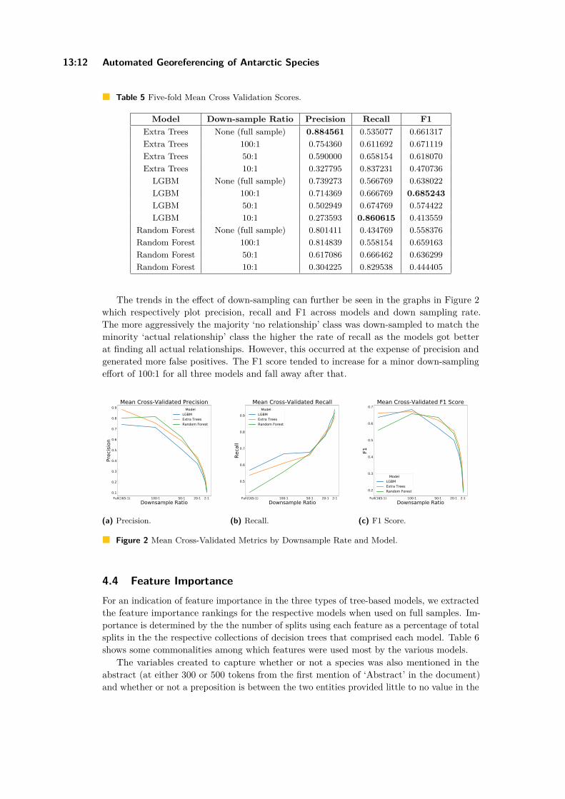
13:12 Automated Georeferencing of Antarctic Species

Table 5 Five-fold Mean Cross Validation Scores.

Model Down-sample Ratio Precision Recall F1Extra Trees None (full sample) 0.884561 0.535077 0.661317Extra Trees 100:1 0.754360 0.611692 0.671119Extra Trees 50:1 0.590000 0.658154 0.618070Extra Trees 10:1 0.327795 0.837231 0.470736

LGBM None (full sample) 0.739273 0.566769 0.638022LGBM 100:1 0.714369 0.666769 0.685243LGBM 50:1 0.502949 0.674769 0.574422LGBM 10:1 0.273593 0.860615 0.413559

Random Forest None (full sample) 0.801411 0.434769 0.558376Random Forest 100:1 0.814839 0.558154 0.659163Random Forest 50:1 0.617086 0.666462 0.636299Random Forest 10:1 0.304225 0.829538 0.444405

The trends in the effect of down-sampling can further be seen in the graphs in Figure 2which respectively plot precision, recall and F1 across models and down sampling rate.The more aggressively the majority ‘no relationship’ class was down-sampled to match theminority ‘actual relationship’ class the higher the rate of recall as the models got betterat finding all actual relationships. However, this occurred at the expense of precision andgenerated more false positives. The F1 score tended to increase for a minor down-samplingeffort of 100:1 for all three models and fall away after that.

Full(165:1) 100:1 50:1 20:1 2:1Downsample Ratio

0.1

0.2

0.3

0.4

0.5

0.6

0.7

0.8

0.9

Prec

ision

Mean Cross-Validated PrecisionModel

LGBMExtra TreesRandom Forest

(a) Precision.

Full(165:1) 100:1 50:1 20:1 2:1Downsample Ratio

0.5

0.6

0.7

0.8

0.9

Reca

ll

Mean Cross-Validated RecallModel

LGBMExtra TreesRandom Forest

(b) Recall.

Full(165:1) 100:1 50:1 20:1 2:1Downsample Ratio

0.2

0.3

0.4

0.5

0.6

0.7

F1

Mean Cross-Validated F1 Score

ModelLGBMExtra TreesRandom Forest

(c) F1 Score.

Figure 2 Mean Cross-Validated Metrics by Downsample Rate and Model.

4.4 Feature ImportanceFor an indication of feature importance in the three types of tree-based models, we extractedthe feature importance rankings for the respective models when used on full samples. Im-portance is determined by the the number of splits using each feature as a percentage of totalsplits in the the respective collections of decision trees that comprised each model. Table 6shows some commonalities among which features were used most by the various models.

The variables created to capture whether or not a species was also mentioned in theabstract (at either 300 or 500 tokens from the first mention of ‘Abstract’ in the document)and whether or not a preposition is between the two entities provided little to no value in the

J. Scott, K. Stock, F. Morgan, B. Whitehead, and D. Medyckyj-Scott 13:13

models, but the TSISF variables for both species and toponym were in the top seven featuresfor all three models and were the most important for the LGBM model, while TSISF fortoponym was also the most important for the extra randomised trees model. All of the fivenumber of <type> between distance variables rounded out the top seven in each model, andthe number of dependency steps also appeared in the top nine in each of the models.

Table 6 Most Important Features by Model Type.

Extra Random Trees Light GBM Random ForestFeature Rank Imp. Rank Imp. Rank Imp.

max_TFISF_Location 1 0.1461 1 0.2687 5 0.1222Num_Words_Between 2 0.1317 7 0.0553 1 0.1700Num_Tokens_Between 3 0.1316 4 0.1203 2 0.1530Num_Preps_Between 4 0.1217 6 0.0787 4 0.1295Num_Nouns_Between 5 0.1105 5 0.1027 3 0.1401Num_Verbs_Between 6 0.1095 3 0.1477 6 0.0901max_TFISF_Species 7 0.0657 2 0.1670 7 0.0721Dependency_Steps 8 0.0589 9 0.0113 9 0.0266

Sent_Start_Location 9 0.0491 8 0.0133 8 0.05055

5 Discussion

5.1 Entity RecognitionThe precision for both species and toponym recognition is high (>0.9 for both) and minoradjustments to the species method utilising existing SpaCy functionality such as out-of-vocabtags could help it learn to recognise species and genus names that aren’t listed in a givendictionary. This would lift the species recall figure which sits at 0.77 including partial matches.Training a NLP engine to identify species entities is another option but not tested so farwith this work due to a lack of training data.

With a recall of just 0.45, larger adjustments are required to the toponym recognitionprocess. The task of toponym extraction in these types of documents is challenging becauseof issues such as “second mentions” of place names (e.g. “McMurdo Dry Valleys”), includingpronouns (“it”), shortened forms (“the Valleys”) and acronyms (“MDVs”), and methods toaddress these through coreference resolution would improve results. Loosening the gazetteerfiltering process to allow more toponym candidates to pass through would improve recall,but at the cost of precision.

5.2 Relationship ExtractionThe performance of the relationship modelling process with limited fine-tuning of tree-basedmodels is promising. The highest precision for predicting actual relationship was 0.88 (forthe Extra Trees model with no down-sampling), and the highest recall was 0.86 (for theLGBM model with 10:1 down-sampling). The highest F1 score of 0.68 was achieved forLGBM with 100:1 down-sampling (see Table 5). Further work on larger annotated data setswould allow for validation sets to be created in addition to train/test splits and facilitatetuning of models.

Ours is an approach that has not been applied to species-toponym relationships beforeand it shows promising results when compared with other work addressing related, butdifferent problems in the biomedical fields, which use graph LTSMs [27], Bi-affine Relation

GISc ience 2021

13:14 Automated Georeferencing of Antarctic Species

Attention Networks [32], and transformer-type networks [8]. Furthermore, out work is notlimited to finding cross-sentence relations only in adjacent or near-adjacent sentences like[28]. The process has highlighted however, the potential of exploring coreference resolutionas recent studies [8, 28] have done.

While some of the engineered features, namely the two TSISF measures showed promisein the modelling process, others seemingly offered little utility. The process of engineeringand exploring new features (e.g. word vectors, sentence polarity etc) that help map therelationship of species and toponym should be explored further and may yield improvedresults as part of future work.

6 Conclusion

In this paper, we have described a method to extract mentions of species and place namesfrom text documents, and then to determine which place names describe the toponyms ofwhich species.

We have demonstrated a rules- and dictionary-based approach for the extraction of speciesin the Antarctic context, and applied existing place name extraction methods, with a setof gazetteers to identify toponyms. Our main contribution is the development of a methodthat uses tree-based classifiers to match toponyms and species mentions in order to identifythe toponym of specific species, for georeferencing and mapping, with a precision of 0.88(highest F1 of 0.68). In future work, we plan to include additional features in the model,employ a larger corpus for training and tuning; and improve efficiency through filtering somespecies-toponym combinations (those that are unlikely) before applying the classifier.

This research contributes to the goal of georeferencing text mentions of specific specieson two specific fronts. Firstly, little to no research is available on automatically extractingspecies toponyms from text documents, and the work described in this paper is among thefirst to provide a method for extracting specific mention toponyms in the biological domain.Secondly, cross-domain methods for georeferencing mentions of different kinds of phenomena(and being able to identify which kinds of phenomena are where) in a document have beenlimited thus far. While this is early work, the method shows promise, particularly for dealingwith relations that may cross sentence boundaries and contain other kinds of complexitiessuch as abbreviations and a many to many relationship between species and toponyms.

References1 Elise Acheson and Ross S. Purves. Extracting and modeling geographic information from

scientific articles. PLOS ONE, 16(1):e0244918, January 2021. doi:10.1371/journal.pone.0244918.

2 Moises Acuna-Chaves and José Araya. Extraction of geographic entities from biologicaltextual sources. In 2017 XLIII Latin American Computer Conference (CLEI), pages 1–8, 2017.doi:10.1109/CLEI.2017.8226422.

3 Lakshmi Manohar Akella, Catherine N. Norton, and Holly Miller. NetiNeti: discovery ofscientific names from text using machine learning methods. BMC Bioinformatics, 13(1):211,2012. doi:10.1186/1471-2105-13-211.

4 Ana Bárbara Cardoso, Bruno Martins, and Jacinto Estima. Using recurrent neural networksfor toponym resolution in text. In EPIA Conference on Artificial Intelligence, pages 769–780.Springer, 2019.

5 Arthur D Chapman and John R Wieczorek. Georeferencing Best Practices. GBIF Secretariat,Copenhagen, 2020. doi:10.15468/doc-gg7h-s853.

J. Scott, K. Stock, F. Morgan, B. Whitehead, and D. Medyckyj-Scott 13:15

6 Rachel Chasin, Daryl Woodward, Jeremy Witmer, and Jugal Kalita. Extracting and displayingtemporal and geospatial entities from articles on historical events. The Computer Journal,57(3):403–426, 2014.

7 Hong-Woo Chun, Yoshimasa Tsuruoka, Jin-Dong Kim, Rie Shiba, Naoki Nagata, TeruyoshiHishiki, and Jun’Ichi Tsujii. Extraction of Gene-Disease Relations from Medline using DomainDictionaries and Machine Learning. In Biocomputing 2006, pages 4–15, Maui, Hawaii, December2005. World Scientific. doi:10.1142/9789812701626_0002.

8 Markus Eberts and Adrian Ulges. An End-to-end Model for Entity-level Relation Extractionusing Multi-instance Learning. In Proceedings of the 16th Conference of the European Chapterof the Association for Computational Linguistics: Main Volume, pages 3650–3660, 2021. URL:https://www.aclweb.org/anthology/2021.eacl-main.319.

9 Martin Gerner, Goran Nenadic, and Casey M. Bergman. LINNAEUS: A species nameidentification system for biomedical literature. BMC Bioinformatics, 11(1):85, 2010. doi:10.1186/1471-2105-11-85.

10 Milan Gritta, Mohammad Taher Pilehvar, Nut Limsopatham, and Nigel Collier. What’smissing in geographical parsing? Language Resources and Evaluation, 52(2):603–623, 2018.

11 Qinghua Guo, Yu Liu, and John Wieczorek. Georeferencing locality descriptions and computingassociated uncertainty using a probabilistic approach. International Journal of GeographicalInformation Science, 22(10):1067–1090, 2008.

12 Robert P Guralnick, John Wieczorek, Reed Beaman, Robert J Hijmans, the BioGeomancerWorking Group, et al. Biogeomancer: automated georeferencing to map the world’s biodiversitydata. PLoS Biol, 4(11):e381, 2006.

13 Felix Hamborg, Corinna Breitinger, and Bela Gipp. Giveme5W1H: A Universal System forExtracting Main Events from News Articles. arXiv:1909.02766 [cs], September 2019. URL:http://arxiv.org/abs/1909.02766.

14 Andrew W Hill, Robert Guralnick, Paul Flemons, Reed Beaman, John Wieczorek, AjayRanipeta, Vishwas Chavan, and David Remsen. Location, location, location: utilizingpipelines and services to more effectively georeference the world’s biodiversity data. BMCbioinformatics, 10(14):1–9, 2009.

15 Yiting Ju, Benjamin Adams, Krzysztof Janowicz, Yingjie Hu, Bo Yan, and Grant McKenzie.Things and strings: improving place name disambiguation from short texts by combiningentity co-occurrence with topic modeling. In European Knowledge Acquisition Workshop, pages353–367. Springer, 2016.

16 Morteza Karimzadeh, Scott Pezanowski, Alan M. MacEachren, and Jan O. Wallgrün. GeoTxt:A scalable geoparsing system for unstructured text geolocation. Transactions in GIS, 23(1):118–136, 2019. doi:10.1111/tgis.12510.

17 Drew Koning, Indra Neil Sarkar, and Thomas Moritz. TaxonGrab: Extracting TaxonomicNames From Text. Biodiversity Informatics, 2, 2005. doi:10.17161/bi.v2i0.17.

18 Parisa Kordjamshidi, Martijn Otterlo, and Marie-Francine Moens. Spatial role labeling:Towards extraction of spatial relations from natural language. TSLP, 8:4, December 2011.doi:10.1145/2050104.2050105.

19 Parisa Kordjamshidi, Dan Roth, and Marie-Francine Moens. Structured learning for spatialinformation extraction from biomedical text: bacteria biotopes. BMC bioinformatics, 16:129,April 2015. doi:10.1186/s12859-015-0542-z.

20 Patrick R. Leary, David P. Remsen, Catherine N. Norton, David J. Patterson, and Indra NeilSarkar. uBioRSS: Tracking taxonomic literature using RSS. Bioinformatics, 23(11):1434–1436,2007. doi:10.1093/bioinformatics/btm109.

21 Jochen L. Leidner. Toponym resolution in text: annotation, evaluation and applications ofspatial grounding. ACM SIGIR Forum, 41(2):124–126, December 2007. doi:10.1145/1328964.1328989.

GISc ience 2021

13:16 Automated Georeferencing of Antarctic Species

22 Jochen L. Leidner and Michael D. Lieberman. Detecting geographical references in the formof place names and associated spatial natural language. SIGSPATIAL Special, 3(2):5–11, 2011.doi:10.1145/2047296.2047298.

23 Carl Linnaeus. Species Plantarum. Laurentius Salvius, Stockholm, Sweden, 1753.24 Damon P. Little. Recognition of Latin scientific names using artificial neural networks.

Applications in Plant Sciences, 8(7):e11378, 2020. doi:10.1002/aps3.11378.25 Fernando Melo and Bruno Martins. Automated Geocoding of Textual Documents: A Survey

of Current Approaches. Transactions in GIS, 21(1):3–38, 2017. doi:10.1111/tgis.12212.26 Zara Nasar, Syed Waqar Jaffry, and Muhammad Kamran Malik. Named entity recognition

and relation extraction: State-of-the-art. ACM Computing Surveys (CSUR), 54(1):1–39, 2021.27 Nanyun Peng, Hoifung Poon, Chris Quirk, Kristina Toutanova, and Wen-tau Yih. Cross-

Sentence N-ary Relation Extraction with Graph LSTMs. Transactions of the Association forComputational Linguistics, 5:101–115, 2017. doi:10.1162/tacl_a_00049.

28 Chris Quirk and Hoifung Poon. Distant Supervision for Relation Extraction beyond theSentence Boundary. In Proceedings of the 15th Conference of the European Chapter of theAssociation for Computational Linguistics: Volume 1, Long Papers, pages 1171–1182, Valencia,Spain, April 2017. Association for Computational Linguistics. URL: https://www.aclweb.org/anthology/E17-1110.

29 Burkhard Schroeter, T. G. Allan Green, Ana Pintado, Roman Türk, and Leopoldo G. Sancho.Summer activity patterns for mosses and lichens in Maritime Antarctica. Antarctic Science,29(6):517–530, December 2017. doi:10.1017/S095410201700027X.

30 Kumutha Swampillai and Mark Stevenson. Inter-sentential Relations in Information ExtractionCorpora. In Proceedings of the Seventh International Conference on Language Resources andEvaluation (LREC’10), 2010.

31 Kumutha Swampillai and Mark Stevenson. Extracting relations within and across sentences. InProceedings of the International Conference Recent Advances in Natural Language Processing2011, pages 25–32, 2011.

32 Patrick Verga, Emma Strubell, and Andrew McCallum. Simultaneously Self-Attending to AllMentions for Full-Abstract Biological Relation Extraction. In Proceedings of the 2018 Confer-ence of the North American Chapter of the Association for Computational Linguistics: HumanLanguage Technologies, Volume 1 (Long Papers), pages 872–884, New Orleans, Louisiana,June 2018. Association for Computational Linguistics. doi:10.18653/v1/N18-1080.

33 Yan Xu, Lili Mou, Ge Li, Yunchuan Chen, Hao Peng, and Zhi Jin. Classifying relations vialong short term memory networks along shortest dependency paths. In Proceedings of the2015 conference on empirical methods in natural language processing, pages 1785–1794, 2015.