Embed Size (px)
Citation preview

18th Conference of Czech and Slovak Physicistswith participation of Hungarian and Polish Physical Societies
Olomouc, Czech Republic, September 16–19, 2014
Conference Proceedings
18th Conference of Czech and Slovak Physicists with participation of Hungarian and Polish Physical Societies was organisedby the Czech Physical Society (http://www-ucjf.troja.mff.cuni.cz/cfs/) and Slovak Physical Society (http://kf.
elf.stuba.sk/~slovenska_fyzikalna_spolocnost/) in cooperation with the European Physical Society (http://www.
eps.org), Roland Eötvös Physical Society (http://www.elft.hu) and the Polish Physical Society (http://ptf.net.pl).Financial support from the European Physical Society is gratefully acknowledged.
Programme committee• Alice Valkárová (chair)
Institute of Particle and Nuclear Physics, Fac. of Mathematics and Physics, Charles University, Prague• Peter Bury
Dept. of Physics, Fac. of Electrical engineering, Žilina University• Julius Cirák
Inst. of Nuclear and Physical Engineering, Fac. of Electrical Engineering and Information technology, Slovak Universityof Technology, Bratislava
• Jan Dobeš
Nuclear Physics Institute of the ASCR, v.v.i., Řež• Miroslav Hrabovský
Joint Laboratory of Optics of Palacký University and Inst. of Phys. of the ASCR, v.v.i., Olomouc• Eduard Hulicius
Department of Semiconductors, Inst. of Phys. of the ASCR, v.v.i., Prague• Vladislav Navrátil
Dept. of Physics, Chemistry and Vocational Education, Fac. of Education, Masaryk University, Brno• Ferenc Simon
Dept. of Physics, Fac. of Natural Sciences, Budapest University of Technology and Economics• Andrzej Slebarski
Dept. of Solid State Physics, Inst. of Physics, University of Silesia, Katowice• Jaroslav Staníček
Dept. of Nuclear Physics and Biophysics, Fac. of Mathematics, Physics and Informatics, Commenius University,Bratislava
• Milan Timko
Dept. of Subnuclear Physics, Inst. of Experimental Physics, Slovak Academy of Sciences, Košice• Igor Túnyi
Geophysical Institute, Slovak Academy of Sciences, Bratislava
Organising committee• Libor Machala (chair)
Dept. of Experimental Physics, Fac. of Natural Sciences, Palacký University, Olomouc• Juraj Boháčik
Inst. of Physics, Slovak Academy of Sciences, Bratislava• Julius Cirák
Inst. of Nuclear and Physical Engineering, Fac. of Electrical Engineering and Information technology, Slovak Universityof Technology, Bratislava
• Dalibor Krúpa
Inst. of Physics, Slovak Academy of Sciences, Bratislava• Roman Kubínek
Dept. of Experimental Physics, Fac. of Natural Sciences, Palacký University, Olomouc• Marián Reiffers
Faculty of Humanities and Natural Sciences, Prešov University, Prešov• Lukáš Richterek
Dept. of Experimental Physics, Fac. of Natural Sciences, Palacký University, Olomouc• Igor Túnyi
Geophysical Institute, Slovak Academy of Sciences, Bratislava• Alice Valkárová
Institute of Particle and Nuclear Physics, Fac. of Mathematics and Physics, Charles University, Prague
No English-language editing and proofreading was done either by the publisher or by the editors, so the quality of languageof papers is under the authors’ responsibility.
Editors: Libor Machala a Lukáš RichterekExecutive Editor: Prof. RNDr. Zdeněk Dvořák, DrSc.Responsible Editor: Mgr. Jana Kreiselová
1. edition
Palacký University, Olomouc, Czech Republic 2015
ISBN 978-80-244-4725-4 (CD)ISBN 978-80-244-4726-1 (on-line)
Contents
Foreword . . . . . . . . . . . . . . . . . . . . . . . . . . . . . . . . . . . . . . . . . . . . . . . . . . . . . . . . . . . . . . . . . 5
Katz S. D.: The Phase Diagram of Quantum Chromodynamics: lattice results . . . . . . . . . . . . . . 7
Červenkov D.: Study of CP Violation and Physics Beyond the Standard Model atthe Belle experiment . . . . . . . . . . . . . . . . . . . . . . . . . . . . . . . . . . . . . . . . . . . . . . . . . . . . . 13
Chlad L. et al.: Secondary pion beam for HADES experiment at GSI . . . . . . . . . . . . . . . . . . . . 15
Čisárová J. et al.: Reentrance in an exactly soluble mixed-spin Ising model on TIT lattices . . . 17
Crkovská J. et al.: Influence of resonance decays on triangular flow in heavy-ion collisions . . . . . 19
Eyyubova G. et al.: Higher flow harmonics and ridge effect in PbPb collisions inHYDJET++ model . . . . . . . . . . . . . . . . . . . . . . . . . . . . . . . . . . . . . . . . . . . . . . . . . . . . . . 21
Fecková Z., Tomášik B.: Ideal hydrodynamic modeling of quark-gluon plasma . . . . . . . . . . . . . . 23
Federič P.: Open heavy flavor measurements at STAR . . . . . . . . . . . . . . . . . . . . . . . . . . . . . . . 25
Federič P.: Study of charge of the top quark in the ATLAS experiment . . . . . . . . . . . . . . . . . . 27
Ficker O. et al.: Unfolding of energies of fusion products measured by theactivation probe at JET . . . . . . . . . . . . . . . . . . . . . . . . . . . . . . . . . . . . . . . . . . . . . . . . . . . 29
Fodorová J. (for the STAR Collaboration): Υ production at the STAR experiment . . . . . . . . . . . . . 31
Gadomski A. et al.: Addressing nanoscale soft-matter problems by computationalphysics and physical computation – an example of facilitated lubrication in atwo-surface system with hydrodynamic interlayer . . . . . . . . . . . . . . . . . . . . . . . . . . . . . . . 33
Gadomski A., Kłos J.: Recognizing an applied-physics and physicochemicalsuccession of Jan Czochralski, an outstanding European crystal grower and personality . . . 35
Géci M. et al.: Thermodynamic Properties of Two-Dimensional System of Small Magnets . . . . 37
Gintner M., Juráň J.: The top-BESS vector resonance triplet confronted with theLHC measurements . . . . . . . . . . . . . . . . . . . . . . . . . . . . . . . . . . . . . . . . . . . . . . . . . . . . . . 39
Haverlíková V., Haverlík I.: Barriers of using models and modelling in medicalbiophysics education . . . . . . . . . . . . . . . . . . . . . . . . . . . . . . . . . . . . . . . . . . . . . . . . . . . . . 41
Haverlíková V.: Development of children’s modelling skills through non-formal activities . . . . . 43
Kladivová M. et al.: The frequency dependence of the impedance caused by asingle domain wall displacement in cylindrical magnetic wire . . . . . . . . . . . . . . . . . . . . . . . 45
Komová E. et al.: Influence of Heat Treatment on Magnetic Properties ofAmorphous Ferromagnetic Fe40Ni38Mo4B18 Microwires . . . . . . . . . . . . . . . . . . . . . . . . . . . 47
Kopečná R., Tomášik B.: Study of azimuthal anisotropy of hadron production viaMonte Carlo simulation . . . . . . . . . . . . . . . . . . . . . . . . . . . . . . . . . . . . . . . . . . . . . . . . . . . 49
Kravčák J.: Models of GMI effect in ferromagnetic microwire . . . . . . . . . . . . . . . . . . . . . . . . . . 51
Křelina M., Nemčík J.: Production of photons and hadrons on nuclear targets . . . . . . . . . . . . . . 53
Křížek F. (for the ALICE Collaboration): Study of high-pT hadron-jet correlations in ALICE . . . . 55
Kúdelčík J. et al.: Structure changes in transformer oil based magnetic fluids inmagnetic field . . . . . . . . . . . . . . . . . . . . . . . . . . . . . . . . . . . . . . . . . . . . . . . . . . . . . . . . . . 57
Lacková M., Komanický V.: Improvement of stability of platinum catalyst forhydrogen fuel cells . . . . . . . . . . . . . . . . . . . . . . . . . . . . . . . . . . . . . . . . . . . . . . . . . . . . . . . 59
Lányi Š., Nádaždy V.: Scanning Charge-Transient Microscopy/Spectroscopy . . . . . . . . . . . . . . . 61
Leja J., Gmuca Š.: The Relativistic Mean-Field Calculations of the Properties ofLight Atomic Nuclei . . . . . . . . . . . . . . . . . . . . . . . . . . . . . . . . . . . . . . . . . . . . . . . . . . . . . . 63
Liščinský M. et al.: Melting Behavior of Two-Dimensional Air-Driven System ofSmall Magnets . . . . . . . . . . . . . . . . . . . . . . . . . . . . . . . . . . . . . . . . . . . . . . . . . . . . . . . . . . 65
Lotnyk D. et al.: Photoelectric transport properties of BiOX (X = Cl, Br, I) semiconductors . . 67
3
Márkus B. G., Simon F.: Alkali Intercalation of Highly Ordered PyrolyticGraphite in Ammonia Solution . . . . . . . . . . . . . . . . . . . . . . . . . . . . . . . . . . . . . . . . . . . . . 69
Melo I., Tomášik B.: Transverse momentum spectra fits in Pb Pb collisions at√
sNN = 2.76 TeV 71
Melo I.: Cascade projects competition for high school students . . . . . . . . . . . . . . . . . . . . . . . . 73
Mikhaylov V. et al.: Anisotropic flow and the reaction plane reconstruction withthe CBM experiment . . . . . . . . . . . . . . . . . . . . . . . . . . . . . . . . . . . . . . . . . . . . . . . . . . . . . 75
Mlynáriková M.: Investigation of the Higgs boson properties . . . . . . . . . . . . . . . . . . . . . . . . . . . 77
Rodríguez-Ramos P.: Preliminary results of pion induced reaction with carbon andpolyethylene targets obtained by HADES-GSI in 2014 . . . . . . . . . . . . . . . . . . . . . . . . . . . . 79
Rusňák J.: Charged jet reconstruction in Au+Au collisions at√
sNN = 200 GeV at RHIC . . . . 81
Svoboda O. et al.: Electromagnetic Calorimeter for the HADES Spectrometer . . . . . . . . . . . . . 83
Šándor L.: Strangeness enhancements in heavy-ion collisions from SPS to LHC . . . . . . . . . . . . 85
Šimečková E. et al.: The NPI Center of Accelerators and Nuclear AnalyticalMethods (CANAM), Basic and Applied Research with Ion Beams . . . . . . . . . . . . . . . . . . . 87
Šimralová M.: CERN Programmes for Teachers . . . . . . . . . . . . . . . . . . . . . . . . . . . . . . . . . . . . 89
Štefánik M. et al.: Center of Accelerators and Nuclear Analytical Methods(CANAM): Fast Neutron Generators . . . . . . . . . . . . . . . . . . . . . . . . . . . . . . . . . . . . . . . . . 91
Štefko P.: Study of jet quenching in heavy ion collisions at LHC using ATLAS detector . . . . . 93
Tarjányi N., Mlynarčík M.: Effect of magnetic fluid layer thickness on the spectraltransmittance . . . . . . . . . . . . . . . . . . . . . . . . . . . . . . . . . . . . . . . . . . . . . . . . . . . . . . . . . . . 95
Trzeciak B. et al.: J/ψ measurements in the STAR experiment . . . . . . . . . . . . . . . . . . . . . . . . . 97
Turčičová, H. et al.: Development of high-repetition rate lasers in the HiLASE project . . . . . . . 99
Vajzer M.: Study of jet properties in p+p collisions at√
s = 7 TeV and p+Pbcollisions at
√
s = 5.02 TeV using POWHEG-Box framework . . . . . . . . . . . . . . . . . . . . . . 101
—————————
List of participants . . . . . . . . . . . . . . . . . . . . . . . . . . . . . . . . . . . . . . . . . . . . . . . . . . . . . . . . 103
4
Foreword
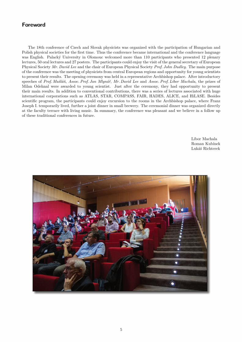
The 18th conference of Czech and Slovak physicists was organized with the participation of Hungarian andPolish physical societies for the first time. Thus the conference became international and the conference languagewas English. Palacký University in Olomouc welcomed more than 110 participants who presented 12 plenarylectures, 50 oral lectures and 27 posters. The participants could enjoy the visit of the general secretary of EuropeanPhysical Society Mr. David Lee and the chair of European Physical Society Prof. John Dudley. The main purposeof the conference was the meeting of physicists from central European regions and opportunity for young scientiststo present their results. The opening ceremony was held in a representative Archbishop palace. After introductoryspeeches of Prof. Mašláň, Assoc. Prof. Jan Mlynář, Mr. David Lee and Assoc. Prof. Libor Machala, the prizes ofMilan Odehnal were awarded to young scientist. Just after the ceremony, they had opportunity to presenttheir main results. In addition to conventional contributions, there was a series of lectures associated with hugeinternational corporations such as ATLAS, STAR, COMPASS, FAIR, HADES, ALICE, and HiLASE. Besidesscientific program, the participants could enjoy excursion to the rooms in the Archbishop palace, where FranzJoseph I. temporarily lived, further a joint dinner in small brewery. The ceremonial dinner was organized directlyat the faculty terrace with living music. In summary, the conference was pleasant and we believe in a follow upof these traditional conferences in future.
Libor MachalaRoman KubínekLukáš Richterek
5

6
18th Conference of Czech and Slovak Physicists, Olomouc, Czech Republic, September 16–19, 2014
The Phase Diagram of Quantum Chromodynamics:lattice results
Sándor D. Katz1
[email protected], Institute for Theoretical Physics, Eötvös University,MTA-ELTE Lendület Lattice Gauge Theory Research Group, Budapest, Pazmany P. setany 1/A, H-1117
Abstract. The QCD phase diagram is studied using non-perturbative lattice calculations. Resultsfor the order of the transition, the transition temperature and the equation of state are presented.At non-vanishing chemical potential, direct lattice calculations are impossible due to the signproblem. Several methods are available for moderately small chemical potentials. Results for thephase diagram and equation of state are shown.
1 Introduction
During the evolution of the universe there was a tran-sition at T ≈ 200 MeV. It is related to the spontaneousbreaking of the chiral symmetry of QCD. The natureof the QCD transition affects our understanding of theuniverse’s evolution. Extensive experimental work iscurrently being done with heavy ion collisions to studythe QCD transition. Both for the cosmological tran-sition and for high energy collisions, the net baryondensities are quite small, thus the baryonic chemicalpotentials (µ) are much less than the typical hadronmasses. A calculation at µ=0 is directly applicable forthe cosmological transition and most probably also de-termines the nature and absolute temperature of thetransition at high energy heavy ion collisions (most re-cently at LHC). The µ > 0 regime of the QCD phasediagram is relevant for lower energy collisions (e.g. atFAIR at GSI). A particularly interesting possibility isthe existence of a critical point at finite temperatureand finite µ which can be searched for by experiments.Neutron stars are described by the large µ part of thephase diagram.
Though advanced perturbative techniques can pro-vide results down to several times the transition tem-perature, the most interesting regimes of the phasediagram (i.e. around the transition line) can only beaccessed using non-perturbative techniques. Amongthese techniques, lattice QCD is the most systematicone; a short introduction will be given in the nextsection.
In this review the recent results of the Wuppertal-Budapest group are discussed. The order and the ab-solute scale of the transition. as well as the equationof state are determined using physical quark massesand a continuum extrapolation. For moderate chemi-cal potentials, results are presented for the transitionline and the equation of state. The findings are com-pared to those of the ’HotQCD’ collaboration.
2 Lattice formulation
Thermodynamical quantities can be obtained from thepartition function which can be given by a Euclideanpath-integral:
Z =∫
DUDΨDΨe−SE(U,Ψ,Ψ), (1)
where U and Ψ,Ψ are the gauge and fermionic fieldsand SE is the Euclidean action. The lattice regular-ization of this action is not unique. There are severalpossibilities to use improved actions which have thesame continuum limit as the straightforward unim-proved ones. The advantage of improved actions isthat the discretization errors are reduced and there-fore a reliable continuum extrapolation is possible al-ready from larger lattice spacings. On the other hand,calculations with improved actions are usually moreexpensive than with the unimproved one.
Usually SE can be split up as SE = Sg +Sf whereSg is the gauge action containing only the self inter-actions of the gauge fields and Sf is the fermionicpart. The gauge action has one parameter, the βgauge coupling, while the parameters of Sf are the mq
quark masses and the µq chemical potentials. Usuallythe masses of the light u,d quarks are taken equal sothere are two mass parameters, mud and ms. For thefermionic action the two most widely used discretiza-tion types are the Wilson and staggered fermions. Ourchoice is to use a tree level Symanzik improved gaugeaction for Sg and a stout improved staggered fermionaction for Sf [1]. This choice is motivated by at leasttwo reasons. It is computationally relatively cheap(comparable to the unimproved actions) and the dis-cretization effects coming from T = 0 and T > 0 sim-ulations are balanced.
For the actual calculations finite lattice sizes ofN3
sNt are used. The physical volume and the temper-ature are related to the lattice extensions as:
V = (Nsa)3, T =1
Nta. (2)
Therefore lattices with Nt ≫ Ns are referred to as zerotemperature lattices while the ones with Nt < Ns arefinite temperature lattices.
In order to carry out T > 0 simulations we have tofix the parameters of the action, the gauge couplingand the quark masses. This is usually done at zerotemperature, where the results of lattice computationscan be compared to experiments. In order to fix threeparameters, three quantities are needed. We chose touse the pion and kaon masses (mπ,mK) and the lep-tonic decay constant of the kaon (fK). These can allbe determined from T = 0 lattice simulations. Lat-tice calculations can only yield dimensionless quanti-
777
Katz S. D.: The Phase Diagram of Quantum Chromodynamics: lattice results
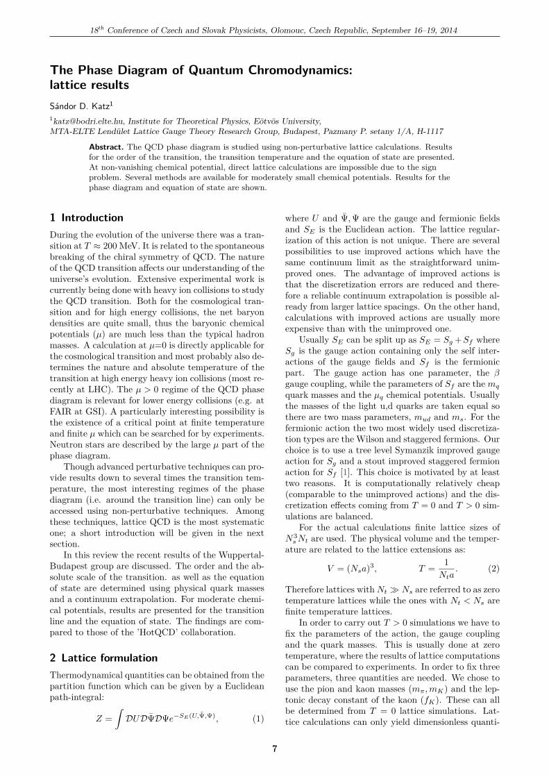
Figure 1. The volume dependence of the susceptibility peaks for pure SU(3) gauge theory (Polyakov-loopsusceptibility, left panel) and for full QCD (chiral susceptibility on Nt=4 and 6 lattices, middle and right panels,
respectively).
ties, i.e. amπ, amK and afK , where a is the latticespacing. For any value of the coupling, the mass pa-rameters can be tuned to obtain the correct ratios formπ/fK and mK/fK . These mud(β) and ms(β) func-tions are called the line of constant physics (LCP). Allfinite T simulations have to be carried out along theLCP. Different points of the LCP describe the samephysics at different lattice spacings. The lattice spac-ing can be obtained by comparing e.g. the determinedafK value to the physical fK .
A very important step of any lattice analysis is thecontinuum extrapolation. Several simulations have tobe carried out at different lattice spacings and the re-sults have to be extrapolated to the continuum. SinceT = 1/(Nta), if we are interested in a given temper-ature range (around the transition) then a decreas-ing lattice spacing corresponds to increasing Nt. Inthis paper, several different lattice resolutions are usedwhich are characterized by Nt = 4, 6, 8, 10, 12 and 16.The corresponding lattice spacings are approximately0.3 – 0.075 fm.
3 The order of the transition
In this section the nature of the QCD transition is dis-cussed. The details of the calculations can be found in[2]. In order to determine the nature of the transitionone should apply finite size scaling techniques for thechiral susceptibility χ = (T/V )·(∂2 logZ/∂m2
ud). Thisquantity shows a pronounced peak as a function of thetemperature. For a first order phase transition, suchas in the pure gauge theory, the peak of the analogousPolyakov susceptibility gets more and more singularas we increase the volume (V). The width scales with1/V the height scales with volume (see left panel ofFigure 1). A second order transition shows a similarsingular behavior with critical indices. For an ana-lytic transition (what we call a crossover) the peakwidth and height saturates to a constant value. That
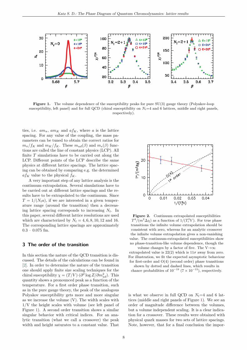
Figure 2. Continuum extrapolated susceptibilitiesT 4/(m2∆χ) as a function of 1/(T 3
c V ). For true phasetransitions the infinite volume extrapolation should beconsistent with zero, whereas for an analytic crossoverthe infinite volume extrapolation gives a non-vanishing
value. The continuum-extrapolated susceptibilities showno phase-transition-like volume dependence, though the
volume changes by a factor of five. The V→∞extrapolated value is 22(2) which is 11σ away from zero.For illustration, we fit the expected asymptotic behaviourfor first-order and O(4) (second order) phase transitions
shown by dotted and dashed lines, which results inchance probabilities of 10−19 (7 × 10⁻¹³), respectively.
is what we observe in full QCD on Nt=4 and 6 lat-tices (middle and right panels of Figure 1). We see anorder of magnitude difference between the volumes,but a volume independent scaling. It is a clear indica-tion for a crossover. These results were obtained withphysical quark masses for two sets of lattice spacings.Note, however, that for a final conclusion the impor-
8
18th Conference of Czech and Slovak Physicists, Olomouc, Czech Republic, September 16–19, 2014
tant question remains: do we get the same volumeindependent scaling in the continuum?
We carried out a finite size scaling analysis withthe continuum extrapolated height of the renormal-ized susceptibility. The renormalization of the chi-ral susceptibility can be done by taking the secondderivative of the free energy density (f) with respectto the renormalized mass (mr). The logarithm ofthe partition function contains quartic divergences.These can be removed by subtracting the free en-ergy at T = 0: f/T 4 =−N4
t ·[logZ(Ns, Nt)/(NtN3s ) −
logZ(Ns0, Nt0)/(Nt0N3s0)]. This quantity has a cor-
rect continuum limit. The subtraction term is ob-tained at T=0, for which simulations are carriedout on lattices with Ns0, Nt0 spatial and tempo-ral extensions (otherwise at the same parametersof the action). The bare light quark mass (mud)is related to mr by the mass renormalization con-stant mr=Zm·mud. Note that Zm falls out ofthe combination m2
r∂2/∂m2
r=m2ud∂
2/∂m2ud. Thus,
m2ud [χ(Ns, Nt) − χ(Ns0, Nt0)] also has a continuum
limit (for its maximum values for different Nt, andin the continuum limit we use the shorthand notationm2∆χ).
In order to carry out the finite volume scaling inthe continuum limit we took three different physicalvolumes. For these volumes we calculated the dimen-sionless combination T 4/m2∆χ at 4 different latticespacings: 0.3 fm was always off, otherwise the contin-uum extrapolations could be carried out. The volumedependence of the continuum extrapolated inverse sus-ceptibilites is shown on Figure 2.
Our result is consistent with an approximately con-stant behaviour, despite the fact that we had a factorof 5 difference in the volume. The chance probabil-ities, that statistical fluctuations changed the domi-nant behaviour of the volume dependence are negli-gible. As a conclusion we can say that the staggeredQCD transition at µ = 0 is a crossover.
! !
!
!!
!
!
!
!
!
!
!
!
!!! !!!
"
"
"
"
"
"
"
"
"
"""""" "
!
!!!
!!!
!!
!
!!!! ! ! !
#
#
#
#
#
#
##
!!
""
!!
ContinuumNt"16
Nt"12
Nt"10
Nt"8
100 120 140 160 180 200 220
0.2
0.4
0.6
0.8
1.0
T !MeV"
#l,s
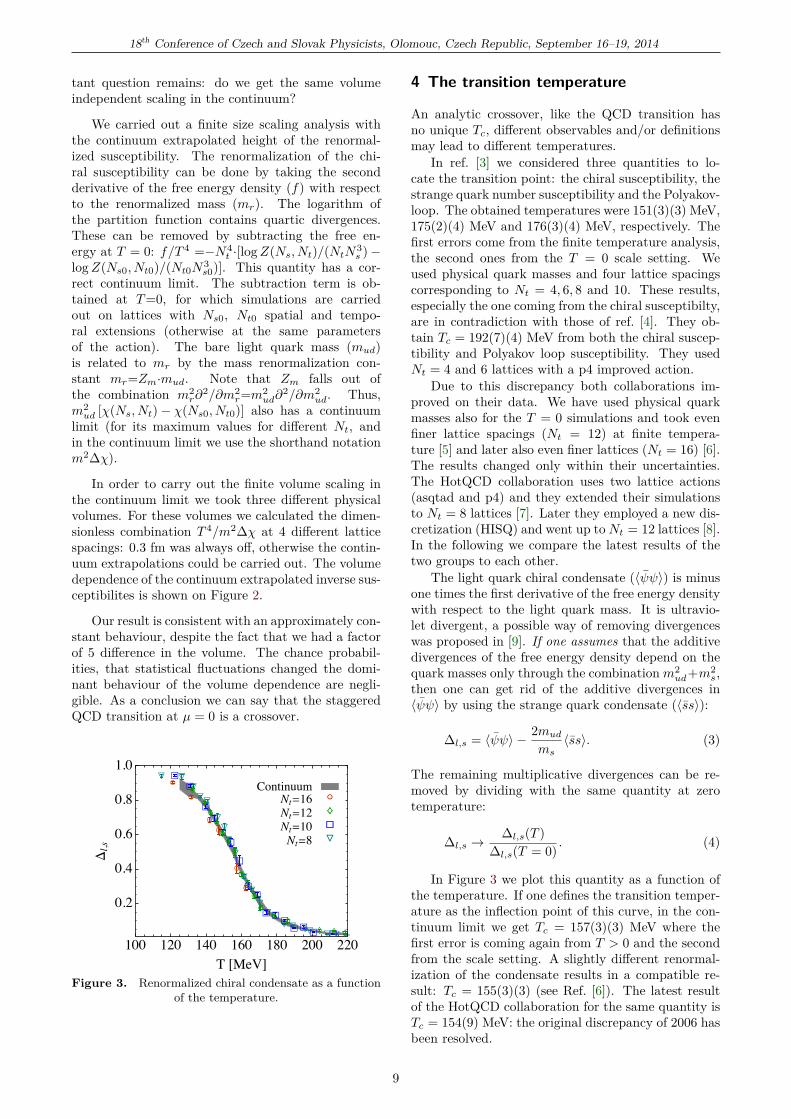
Figure 3. Renormalized chiral condensate as a functionof the temperature.
4 The transition temperature
An analytic crossover, like the QCD transition hasno unique Tc, different observables and/or definitionsmay lead to different temperatures.
In ref. [3] we considered three quantities to lo-cate the transition point: the chiral susceptibility, thestrange quark number susceptibility and the Polyakov-loop. The obtained temperatures were 151(3)(3) MeV,175(2)(4) MeV and 176(3)(4) MeV, respectively. Thefirst errors come from the finite temperature analysis,the second ones from the T = 0 scale setting. Weused physical quark masses and four lattice spacingscorresponding to Nt = 4, 6, 8 and 10. These results,especially the one coming from the chiral susceptibilty,are in contradiction with those of ref. [4]. They ob-tain Tc = 192(7)(4) MeV from both the chiral suscep-tibility and Polyakov loop susceptibility. They usedNt = 4 and 6 lattices with a p4 improved action.
Due to this discrepancy both collaborations im-proved on their data. We have used physical quarkmasses also for the T = 0 simulations and took evenfiner lattice spacings (Nt = 12) at finite tempera-ture [5] and later also even finer lattices (Nt = 16) [6].The results changed only within their uncertainties.The HotQCD collaboration uses two lattice actions(asqtad and p4) and they extended their simulationsto Nt = 8 lattices [7]. Later they employed a new dis-cretization (HISQ) and went up to Nt = 12 lattices [8].In the following we compare the latest results of thetwo groups to each other.
The light quark chiral condensate (〈ψψ〉) is minusone times the first derivative of the free energy densitywith respect to the light quark mass. It is ultravio-let divergent, a possible way of removing divergenceswas proposed in [9]. If one assumes that the additivedivergences of the free energy density depend on thequark masses only through the combination m2
ud+m2s,
then one can get rid of the additive divergences in〈ψψ〉 by using the strange quark condensate (〈ss〉):
∆l,s = 〈ψψ〉 − 2mud
ms〈ss〉. (3)
The remaining multiplicative divergences can be re-moved by dividing with the same quantity at zerotemperature:
∆l,s → ∆l,s(T )
∆l,s(T = 0). (4)
In Figure 3 we plot this quantity as a function ofthe temperature. If one defines the transition temper-ature as the inflection point of this curve, in the con-tinuum limit we get Tc = 157(3)(3) MeV where thefirst error is coming again from T > 0 and the secondfrom the scale setting. A slightly different renormal-ization of the condensate results in a compatible re-sult: Tc = 155(3)(3) (see Ref. [6]). The latest resultof the HotQCD collaboration for the same quantity isTc = 154(9) MeV: the original discrepancy of 2006 hasbeen resolved.
9
Katz S. D.: The Phase Diagram of Quantum Chromodynamics: lattice results
200 300 400 500
T[MeV]
0
1
2
3
4
5
6
p/T
4
HRG
HTL NNLO
lattice continuum limit SB
200 300 400 500
T[MeV]
0
5
10
15
20s/T
4ε/T
3
150 200 250
0.2
0.3cs
2=dp/dε
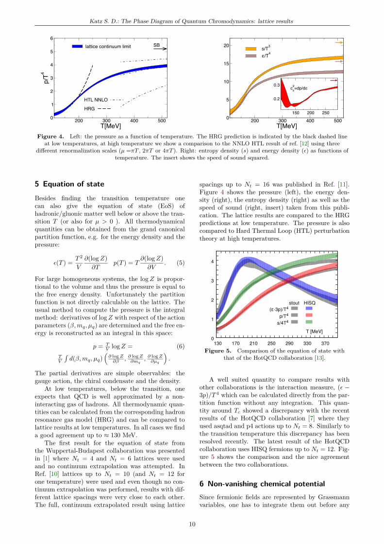
Figure 4. Left: the pressure as a function of temperature. The HRG prediction is indicated by the black dashed lineat low temperatures, at high temperature we show a comparison to the NNLO HTL result of ref. [12] using three
different renormalization scales (µ =πT , 2πT or 4πT ). Right: entropy density (s) and energy density (ǫ) as functions oftemperature. The insert shows the speed of sound squared.
5 Equation of state
Besides finding the transition temperature onecan also give the equation of state (EoS) ofhadronic/gluonic matter well below or above the tran-sition T (or also for µ > 0 ). All thermodynamicalquantities can be obtained from the grand canonicalpartition function, e.g. for the energy density and thepressure:
ǫ(T ) =T 2
V
∂(logZ)∂T
p(T ) = T∂(logZ)∂V
. (5)
For large homogeneous systems, the logZ is propor-tional to the volume and thus the pressure is equal tothe free energy density. Unfortunately the partitionfunction is not directly calculable on the lattice. Theusual method to compute the pressure is the integralmethod: derivatives of logZ with respect of the actionparameters (β,mq, µq) are determined and the free en-ergy is reconstructed as an integral in this space:
p = TV logZ = (6)
TV
∫
d(β,mq, µq)(
∂ log Z∂β , ∂ log Z
∂mq, ∂ log Z
∂µq
)
.
The partial derivatives are simple observables: thegauge action, the chiral condensate and the density.
At low temperatures, below the transition, oneexpects that QCD is well approximated by a non-interacting gas of hadrons. All thermodynamic quan-tities can be calculated from the corresponding hadronresonance gas model (HRG) and can be compared tolattice results at low temperatures. In all cases we finda good agreement up to ≈ 130 MeV.
The first result for the equation of state fromthe Wuppertal-Budapest collaboration was presentedin [1] where Nt = 4 and Nt = 6 lattices were usedand no continuum extrapolation was attempted. InRef. [10] lattices up to Nt = 10 (and Nt = 12 forone temperature) were used and even though no con-tinuum extrapolation was performed, results with dif-ferent lattice spacings were very close to each other.The full, continuum extrapolated result using lattice
spacings up to Nt = 16 was published in Ref. [11].Figure 4 shows the pressure (left), the energy den-sity (right), the entropy density (right) as well as thespeed of sound (right, insert) taken from this publi-cation. The lattice results are compared to the HRGpredictions at low temperature. The pressure is alsocompared to Hard Thermal Loop (HTL) perturbationtheory at high temperatures.
(ε-3p)/T4
p/T4
s/4T4
0
1
2
3
4
130 170 210 250 290 330 370
T [MeV]
stout HISQ
Figure 5. Comparison of the equation of state withthat of the HotQCD collaboration [13].
A well suited quantity to compare results withother collaborations is the interaction measure, (ǫ −3p)/T 4 which can be calculated directly from the par-tition function without any integration. This quan-tity around Tc showed a discrepancy with the recentresults of the HotQCD collaboration [7] where theyused asqtad and p4 actions up to Nt = 8. Similarly tothe transition temperature this discrepancy has beenresolved recently. The latest result of the HotQCDcollaboration uses HISQ fermions up to Nt = 12. Fig-ure 5 shows the comparison and the nice agreementbetween the two collaborations.
6 Non-vanishing chemical potential
Since fermionic fields are represented by Grassmannvariables, one has to integrate them out before any
10
18th Conference of Czech and Slovak Physicists, Olomouc, Czech Republic, September 16–19, 2014
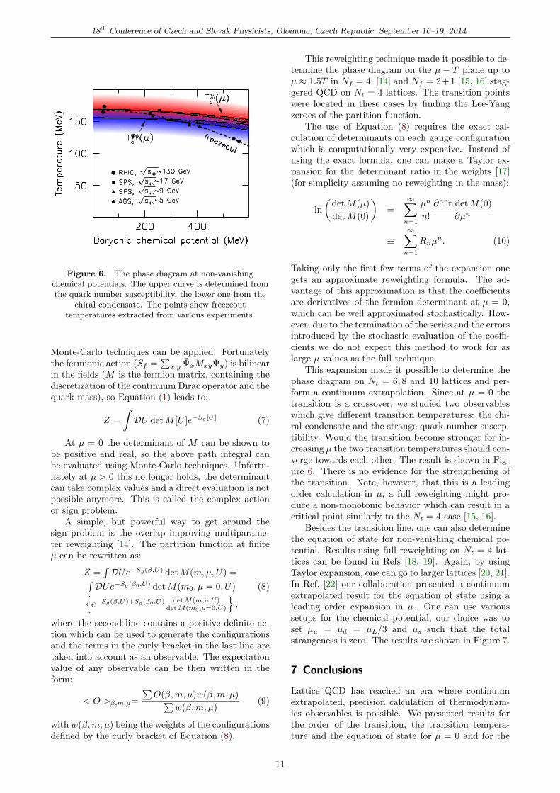
Figure 6. The phase diagram at non-vanishingchemical potentials. The upper curve is determined fromthe quark number susceptibility, the lower one from the
chiral condensate. The points show freezeouttemperatures extracted from various experiments.
Monte-Carlo techniques can be applied. Fortunatelythe fermionic action (Sf =
∑
x,y ΨxMxyΨy) is bilinearin the fields (M is the fermion matrix, containing thediscretization of the continuum Dirac operator and thequark mass), so Equation (1) leads to:
Z =
∫
DU detM [U ]e−Sg[U ] (7)
At µ = 0 the determinant of M can be shown tobe positive and real, so the above path integral canbe evaluated using Monte-Carlo techniques. Unfortu-nately at µ > 0 this no longer holds, the determinantcan take complex values and a direct evaluation is notpossible anymore. This is called the complex actionor sign problem.
A simple, but powerful way to get around thesign problem is the overlap improving multiparame-ter reweighting [14]. The partition function at finiteµ can be rewritten as:
Z =∫
DUe−Sg(β,U) detM(m,µ,U) =∫
DUe−Sg(β0,U) detM(m0, µ = 0, U) (8)
e−Sg(β,U)+Sg(β0,U) det M(m,µ,U)det M(m0,µ=0,U)
,
where the second line contains a positive definite ac-tion which can be used to generate the configurationsand the terms in the curly bracket in the last line aretaken into account as an observable. The expectationvalue of any observable can be then written in theform:
< O >β,m,µ=
∑
O(β,m, µ)w(β,m, µ)∑
w(β,m, µ)(9)
with w(β,m, µ) being the weights of the configurationsdefined by the curly bracket of Equation (8).
This reweighting technique made it possible to de-termine the phase diagram on the µ − T plane up toµ ≈ 1.5T in Nf = 4 [14] and Nf = 2+1 [15, 16] stag-gered QCD on Nt = 4 lattices. The transition pointswere located in these cases by finding the Lee-Yangzeroes of the partition function.
The use of Equation (8) requires the exact cal-culation of determinants on each gauge configurationwhich is computationally very expensive. Instead ofusing the exact formula, one can make a Taylor ex-pansion for the determinant ratio in the weights [17](for simplicity assuming no reweighting in the mass):
ln
(
detM(µ)
detM(0)
)
=
∞∑
n=1
µn
n!
∂n ln detM(0)
∂µn
≡∞∑
n=1
Rnµn. (10)
Taking only the first few terms of the expansion onegets an approximate reweighting formula. The ad-vantage of this approximation is that the coefficientsare derivatives of the fermion determinant at µ = 0,which can be well approximated stochastically. How-ever, due to the termination of the series and the errorsintroduced by the stochastic evaluation of the coeffi-cients we do not expect this method to work for aslarge µ values as the full technique.
This expansion made it possible to determine thephase diagram on Nt = 6, 8 and 10 lattices and per-form a continuum extrapolation. Since at µ = 0 thetransition is a crossover, we studied two observableswhich give different transition temperatures: the chi-ral condensate and the strange quark number suscep-tibility. Would the transition become stronger for in-creasing µ the two transition temperatures should con-verge towards each other. The result is shown in Fig-ure 6. There is no evidence for the strengthening ofthe transition. Note, however, that this is a leadingorder calculation in µ, a full reweighting might pro-duce a non-monotonic behavior which can result in acritical point similarly to the Nt = 4 case [15, 16].
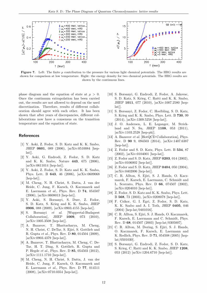
Besides the transition line, one can also determinethe equation of state for non-vanishing chemical po-tential. Results using full reweighting on Nt = 4 lat-tices can be found in Refs [18, 19]. Again, by usingTaylor expansion, one can go to larger lattices [20, 21].In Ref. [22] our collaboration presented a continuumextrapolated result for the equation of state using aleading order expansion in µ. One can use varioussetups for the chemical potential, our choice was toset µu = µd = µL/3 and µs such that the totalstrangeness is zero. The results are shown in Figure 7.
7 Conclusions
Lattice QCD has reached an era where continuumextrapolated, precision calculation of thermodynam-ics observables is possible. We presented results forthe order of the transition, the transition tempera-ture and the equation of state for µ = 0 and for the
11
Katz S. D.: The Phase Diagram of Quantum Chromodynamics: lattice results
Figure 7. Left: The finite µ contribution to the pressure for various light chemical potentials. The HRG results areshown for comparison at low temperature. Right: the energy density for two chemical potentials. The HRG results are
shown by the continuous lines.
phase diagram and the equation of state at µ > 0.Once the continuum extrapolation has been carriedout, the results are not allowed to depend on the useddiscretization. Therefore, results of different collab-oration should agree with each other. It has beenshown that after years of discrepancies, different col-laborations now have a consensus on the transitiontemperature and the equation of state.
References
[1] Y. Aoki, Z. Fodor, S. D. Katz and K. K. Szabo,JHEP 0601, 089 (2006), [arXiv:0510084 [hep-lat]].
[2] Y. Aoki, G. Endrodi, Z. Fodor, S. D. Katzand K. K. Szabo, Nature 443, 675 (2006),[arXiv:0611014 [hep-lat]].
[3] Y. Aoki, Z. Fodor, S. D. Katz and K. K. Szabo,Phys. Lett. B 643, 46 (2006), [arXiv:0609068[hep-lat]].
[4] M. Cheng, N. H. Christ, S. Datta, J. van derHeide, C. Jung, F. Karsch, O. Kaczmarek andE. Laermann et al., Phys. Rev. D 74, 054507(2006), [arXiv:0608013 [hep-lat]].
[5] Y. Aoki, S. Borsanyi, S. Durr, Z. Fodor,S. D. Katz, S. Krieg and K. K. Szabo, JHEP0906, 088 (2009), [arXiv:0903.4155 [hep-lat]].
[6] S. Borsanyi et al. [Wuppertal-BudapestCollaboration], JHEP 1009, 073 (2010),[arXiv:1005.3508 [hep-lat]].
[7] A. Bazavov, T. Bhattacharya, M. Cheng,N. H. Christ, C. DeTar, S. Ejiri, S. Gottlieb andR. Gupta et al., Phys. Rev. D 80, 014504 (2009),[arXiv:0903.4379 [hep-lat]].
[8] A. Bazavov, T. Bhattacharya, M. Cheng, C. De-Tar, H. T. Ding, S. Gottlieb, R. Gupta andP. Hegde et al., Phys. Rev. D 85, 054503 (2012),[arXiv:1111.1710 [hep-lat]].
[9] M. Cheng, N. H. Christ, S. Datta, J. van derHeide, C. Jung, F. Karsch, O. Kaczmarek andE. Laermann et al., Phys. Rev. D 77, 014511(2008), [arXiv:0710.0354 [hep-lat]].
[10] S. Borsanyi, G. Endrodi, Z. Fodor, A. Jakovac,S. D. Katz, S. Krieg, C. Ratti and K. K. Szabo,JHEP 1011, 077 (2010), [arXiv:1007.2580 [hep-lat]].
[11] S. Borsanyi, Z. Fodor, C. Hoelbling, S. D. Katz,S. Krieg and K. K. Szabo, Phys. Lett. B 730, 99(2014), [arXiv:1309.5258 [hep-lat]].
[12] J. O. Andersen, L. E. Leganger, M. Strick-land and N. Su, JHEP 1108, 053 (2011),[arXiv:1103.2528 [hep-ph]].
[13] A. Bazavov et al. [HotQCD Collaboration], Phys.Rev. D 90 9, 094503 (2014), [arXiv:1407.6387[hep-lat]].
[14] Z. Fodor and S. D. Katz, Phys. Lett. B 534, 87(2002), [arXiv:0104001 [hep-lat]].
[15] Z. Fodor and S. D. Katz, JHEP 0203, 014 (2002),[arXiv:0106002 [hep-lat]].
[16] Z. Fodor and S. D. Katz, JHEP 0404, 050 (2004),[arXiv:0402006 [hep-lat]].
[17] C. R. Allton, S. Ejiri, S. J. Hands, O. Kacz-marek, F. Karsch, E. Laermann, C. Schmidt andL. Scorzato, Phys. Rev. D 66, 074507 (2002),[arXiv:0204010 [hep-lat]].
[18] Z. Fodor, S. D. Katz and K. K. Szabo, Phys. Lett.B 568, 73 (2003), [arXiv:0208078 [hep-lat]].
[19] F. Csikor, G. I. Egri, Z. Fodor, S. D. Katz,K. K. Szabo and A. I. Toth, JHEP 0405, 046(2004) [hep-lat/0401016].
[20] C. R. Allton, S. Ejiri, S. J. Hands, O. Kaczmarek,F. Karsch, E. Laermann and C. Schmidt, Phys.Rev. D 68, 014507 (2003) [hep-lat/0305007].
[21] C. R. Allton, M. Doring, S. Ejiri, S. J. Hands,O. Kaczmarek, F. Karsch, E. Laermann andK. Redlich, Phys. Rev. D 71, 054508 (2005) [hep-lat/0501030].
[22] S. Borsanyi, G. Endrodi, Z. Fodor, S. D. Katz,S. Krieg, C. Ratti and K. K. Szabo, JHEP 1208,053 (2012) [arXiv:1204.6710 [hep-lat]].
12
18th Conference of Czech and Slovak Physicists, Olomouc, Czech Republic, September 16–19, 2014
Study of CP Violation and Physics Beyond the Standard Model at the Belleexperiment
Daniel Červenkov1
[email protected], Institute of Particle and Nuclear Physics, Faculty of Mathematics and Physics,Charles University in Prague, V Holešovičkách 2, 180 00 Prague 8, Czech Republic
Abstract. Charge-parity (CP) violation is a firmly established feature of weak interactions of theStandard Model. However, there are still many crucial open questions. E.g., the strength of CPviolation incorporated into the SM is insufficient to explain the observed cosmological matteranti-mater asymmetry by many orders of magnitude. We present a short explanation of where theStandard Model quark sector CP violation comes from and why it requires the existence of 3 quarkgenerations. We derive unitarity triangles and angles that are the actual CP violation parametersthat are usually measured. We go on to introduce the Belle experiment and some of the motivationfor the upgrade it’s currently undergoing — the lack of New Physics observation at the energyfrontier as well as several ‘anomalous’ measurements from Belle itself.
1 Introduction
Although symmetries are inseparable part of Nature,much of the texture of this world is due to symmetrybreaking. The particular case we will be discussing,CP violation, is the reason we live in a matter domi-nated universe. Without it, the world would look quitedifferent today — there wouldn’t be much of anythingexcept radiation, as most of the matter and antimatterwould have annihilated shortly after the Big Bang.
An important fact that is well worth mentioning isthat the CP violation present in the Standard Modelis not sufficient to explain the amount of matter ob-served in the universe - it can explain only about onegalactic mass. Therefore, a number of physicists arelooking for new sources of CP violation. However wewill discuss only the one that is firmly establishedwithin the Standard Model — the quark sector CPviolation.
2 Charged Current
To get a handle on CP violation we can look atthe charged current structure. Considering only twoquark generations, the structure of the charged cur-rent Lagrangian describing an up-type quark transi-tion to a down-type quark and vice versa can be seenin Equation 1 [1]. In the rightmost part, we have con-solidated the two terms from the left hand side into asingle term using matrix notation. This approach isquite useful, as examining the matrix’s properties cangive us valuable insight.
LCC ∝ uγµ 1 − γ5
2(Vudd+ Vuss)W
+µ
+ cγµ 1 − γ5
2(Vcdd+ Vcss)W
+µ + c.c. =
= (u c)γµ 1 − γ5
2
(
Vud Vus
Vcd Vcs
)(
ds
)
W+µ + c.c.
(1)Let us start by counting the number of the, so
called, mixing matrix’s parameters. In general, there
are 4 complex parameters, which is equivalent to 8real ones. However, the matrix has to be unitary —this is a very reasonable assumption as it guaranteesprobability conservation. The unitarity condition canbe expressed as V V † = I. For a 2 × 2 matrix, thistranslates to 4 constraints.
Moreover, an arbitrary complex phase can be ab-sorbed into each of the quark fields u, c, d and s, aswe have freedom in defining them. However, an over-all phase is unobservable, therefore we have only 3additional constraints.
Combining all of the above, we see that the matrixhas just 8 − 4 − 3 = 1 parameter and we can choosethe relative phases freely. A standard choice is:
(
cos θC sin θC
− sin θC cos θC
)
(2)
and it is called ‘Cabibbo matrix’.When exchanging quarks for anti-quarks in an ar-
bitrary interaction vertex, we have to look at a chargeconjugated (c.c.) part of the Lagrangian (with respectto the part describing quarks). For example:
(d s)γµ 1 − γ5
2
(
cos θC sin θC
− sin θC cos θC
)†(uc
)
W−µ =
=(d s)γµ 1 − γ5
2
(
cos θC − sin θC
sin θC cos θC
)∗(uc
)
W−µ
(3)The term that is relevant for, e.g., the u quark is:
(cos θC d+ sin θC s)γµ 1 − γ5
2uW−
µ (4)
Comparing that to the non-charge conjugated ana-logue:
uγµ 1 − γ5
2(cos θCd+ sin θCs)W
+µ (5)
we see that the amplitudes for both vertices are ex-actly the same — there is no CP violation. This isbecause the complex conjugation of the mixing ma-trix in Equation 3 is trivial as the matrix is real.
131313
Červenkov D.: Study of CP Violation and Physics Beyond the Standard Model at the Belle experiment
3 Cabibbo-Kobayashi-Maskawa Matrix
Two Japanese physicists, Kobayashi and Maskawa, ar-gued, that while no CP violation is possible within thestandard charged current with just two quark genera-tions, it arises naturally with three generations [2].
Let us repeat the previous counting exercise withthe Cabibbo-Kobayashi-Maskawa (CKM) matrix:
VCKM =
Vud Vus Vub
Vcd Vcs Vcb
Vtd Vts Vtb
(6)
In this case, there are 9 complex parameters, or 18real ones. The unitarity condition still holds, howeverfor a 3×3 matrix it is equivalent to 9 constraints. Andafter repeating the same trick with absorbing phasesinto the quark fields, we are left with 18 − 9 − 5 = 4parameters.
We may now ask ourselves, whether we can againtake VCKM real. It follows from definitions, that areal unitary matrix is actually an orthogonal matrix.In this case a member of O(3). However, it is easy toshow that an O(3) matrix has only 3 free parameters[3]. Therefore, we can conclude that VCKM invariablyhas to be complex.
The complex conjugation of the mixing matrixmentioned in the previous section is no longer triv-ial — CP violation arises and Nature treats matterand anti-matter differently!
4 Unitarity Triangle
The CP violation parameters that are actually usu-ally measured are ‘unitarity triangle angles’. As wasalready mentioned in the previous sections, the CKMmatrix is unitary and thus subject to certain con-straints. Namely elements of a unitary matrix V sat-isfy
(V †V )ij = (V V †)ij = δij . (7)
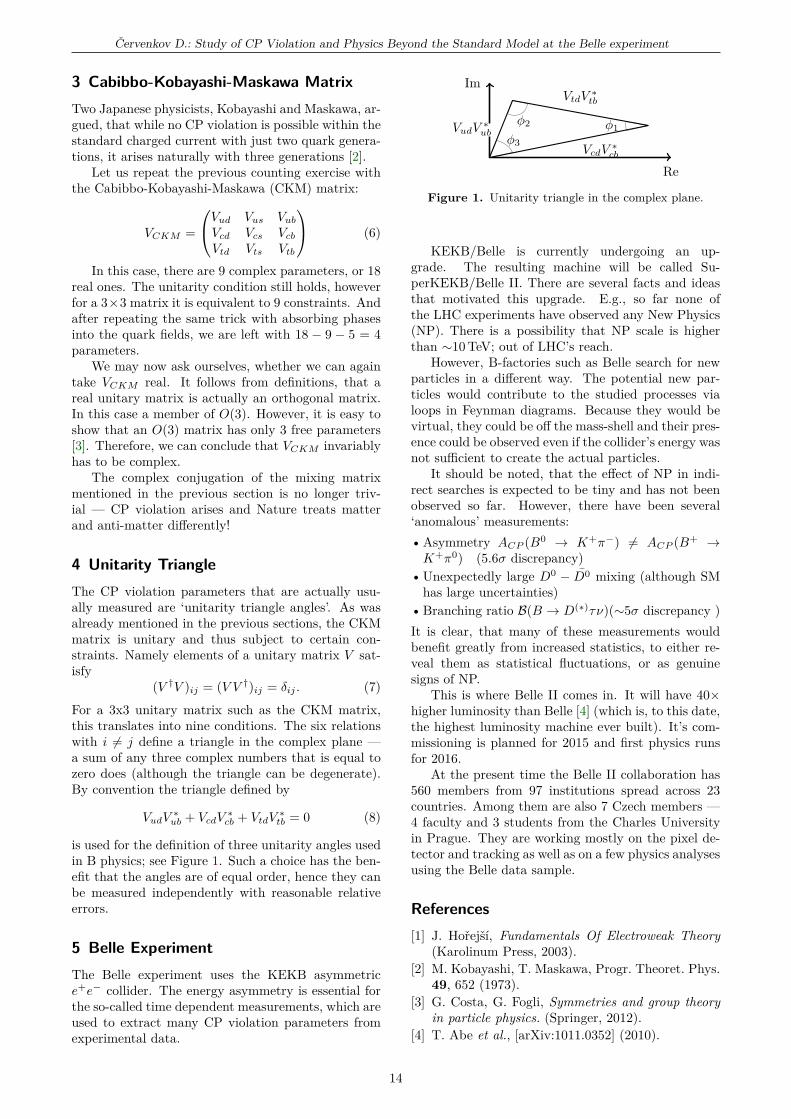
For a 3x3 unitary matrix such as the CKM matrix,this translates into nine conditions. The six relationswith i 6= j define a triangle in the complex plane —a sum of any three complex numbers that is equal tozero does (although the triangle can be degenerate).By convention the triangle defined by
VudV∗
ub + VcdV∗
cb + VtdV∗
tb = 0 (8)
is used for the definition of three unitarity angles usedin B physics; see Figure 1. Such a choice has the ben-efit that the angles are of equal order, hence they canbe measured independently with reasonable relativeerrors.
5 Belle Experiment
The Belle experiment uses the KEKB asymmetrice+e− collider. The energy asymmetry is essential forthe so-called time dependent measurements, which areused to extract many CP violation parameters fromexperimental data.
Im
Re
VcdV∗
cb
VtdV∗
tb
VudV∗
ubφ3
φ1φ2
Figure 1. Unitarity triangle in the complex plane.
KEKB/Belle is currently undergoing an up-grade. The resulting machine will be called Su-perKEKB/Belle II. There are several facts and ideasthat motivated this upgrade. E.g., so far none ofthe LHC experiments have observed any New Physics(NP). There is a possibility that NP scale is higherthan ∼10 TeV; out of LHC’s reach.
However, B-factories such as Belle search for newparticles in a different way. The potential new par-ticles would contribute to the studied processes vialoops in Feynman diagrams. Because they would bevirtual, they could be off the mass-shell and their pres-ence could be observed even if the collider’s energy wasnot sufficient to create the actual particles.
It should be noted, that the effect of NP in indi-rect searches is expected to be tiny and has not beenobserved so far. However, there have been several‘anomalous’ measurements:
•Asymmetry ACP (B0 → K+π−) 6= ACP (B+ →K+π0) (5.6σ discrepancy)
•Unexpectedly large D0 − D0 mixing (although SMhas large uncertainties)
•Branching ratio B(B → D(∗)τν)(∼5σ discrepancy )
It is clear, that many of these measurements wouldbenefit greatly from increased statistics, to either re-veal them as statistical fluctuations, or as genuinesigns of NP.
This is where Belle II comes in. It will have 40×higher luminosity than Belle [4] (which is, to this date,the highest luminosity machine ever built). It’s com-missioning is planned for 2015 and first physics runsfor 2016.
At the present time the Belle II collaboration has560 members from 97 institutions spread across 23countries. Among them are also 7 Czech members —4 faculty and 3 students from the Charles Universityin Prague. They are working mostly on the pixel de-tector and tracking as well as on a few physics analysesusing the Belle data sample.
References
[1] J. Hořejší, Fundamentals Of Electroweak Theory(Karolinum Press, 2003).
[2] M. Kobayashi, T. Maskawa, Progr. Theoret. Phys.49, 652 (1973).
[3] G. Costa, G. Fogli, Symmetries and group theoryin particle physics. (Springer, 2012).
[4] T. Abe et al., [arXiv:1011.0352] (2010).
14
18th Conference of Czech and Slovak Physicists, Olomouc, Czech Republic, September 16–19, 2014
Secondary pion beam for HADES experiment at GSI
Lukáš Chlad1,2, Jerzy Pietraszko3, and Wolfgang Koenig3
[email protected], Faculty of Mathematics and Physics, Charles University in Prague, Ke Karlovu 3, 121 16 Praha 2,Czech Republic2Nuclear Physics Institute of the ASCR, v.v.i., Řež 130, 250 68 Řež, Czech Republic3GSI Helmholtzzentrum für Schwerionenforschung GmbH, Planckstrasse 1, 642 91 Darmstadt, Germany
Abstract. During summer 2014, the HADES collaboration had the opportunity to measure pioncollisions with different nuclei. These measurements were done with two objectives. The first beingthe investigations of hadrons with strange quarks and their behaviour at normal nuclear density.The analysis of this will concentrate specifically on φ meson and Λ baryon production. The focuson properties of baryonic resonances in the region of N(1520) and N(1535) formed the secondobjective. Special emphasis is put on beamline detectors which use different particle detectiontechniques. In particular, the scintillator based Hodoscope and diamond based Start detector willbe discussed. Advantages and disadvantages of using diamond detectors will be mentioned as wellas their usage in future FAIR projects.
1 HADES experiment
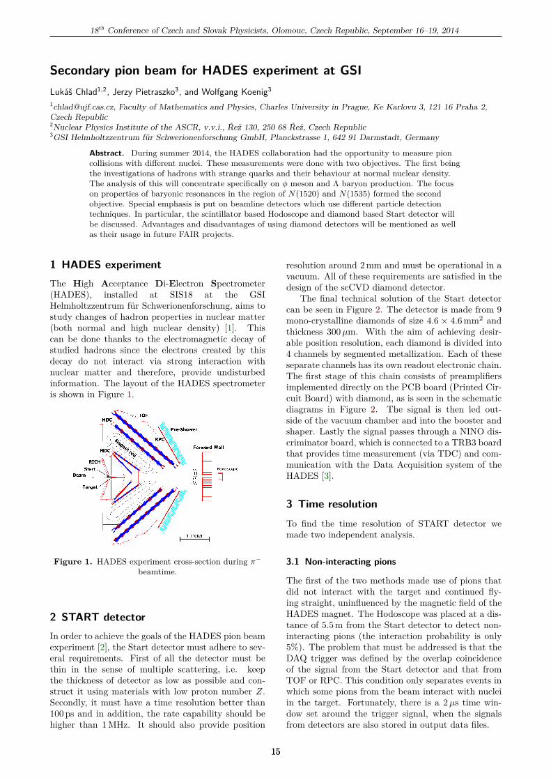
The High Acceptance Di-Electron Spectrometer(HADES), installed at SIS18 at the GSIHelmholtzzentrum für Schwerionenforschung, aims tostudy changes of hadron properties in nuclear matter(both normal and high nuclear density) [1]. Thiscan be done thanks to the electromagnetic decay ofstudied hadrons since the electrons created by thisdecay do not interact via strong interaction withnuclear matter and therefore, provide undisturbedinformation. The layout of the HADES spectrometeris shown in Figure 1.
Figure 1. HADES experiment cross-section during π−
beamtime.
2 START detector
In order to achieve the goals of the HADES pion beamexperiment [2], the Start detector must adhere to sev-eral requirements. First of all the detector must bethin in the sense of multiple scattering, i.e. keepthe thickness of detector as low as possible and con-struct it using materials with low proton number Z.Secondly, it must have a time resolution better than100 ps and in addition, the rate capability should behigher than 1 MHz. It should also provide position
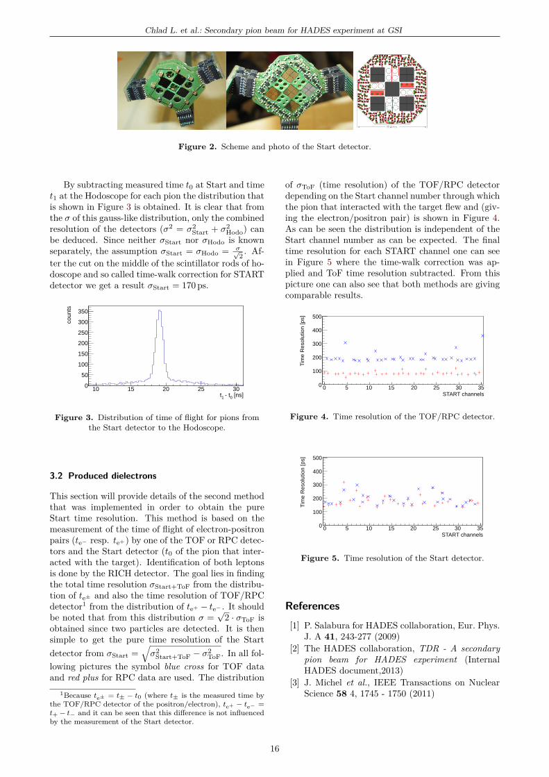
resolution around 2 mm and must be operational in avacuum. All of these requirements are satisfied in thedesign of the scCVD diamond detector.
The final technical solution of the Start detectorcan be seen in Figure 2. The detector is made from 9mono-crystalline diamonds of size 4.6 × 4.6 mm2 andthickness 300µm. With the aim of achieving desir-able position resolution, each diamond is divided into4 channels by segmented metallization. Each of theseseparate channels has its own readout electronic chain.The first stage of this chain consists of preamplifiersimplemented directly on the PCB board (Printed Cir-cuit Board) with diamond, as is seen in the schematicdiagrams in Figure 2. The signal is then led out-side of the vacuum chamber and into the booster andshaper. Lastly the signal passes through a NINO dis-criminator board, which is connected to a TRB3 boardthat provides time measurement (via TDC) and com-munication with the Data Acquisition system of theHADES [3].
3 Time resolution
To find the time resolution of START detector wemade two independent analysis.
3.1 Non-interacting pions
The first of the two methods made use of pions thatdid not interact with the target and continued fly-ing straight, uninfluenced by the magnetic field of theHADES magnet. The Hodoscope was placed at a dis-tance of 5.5 m from the Start detector to detect non-interacting pions (the interaction probability is only5%). The problem that must be addressed is that theDAQ trigger was defined by the overlap coincidenceof the signal from the Start detector and that fromTOF or RPC. This condition only separates events inwhich some pions from the beam interact with nucleiin the target. Fortunately, there is a 2µs time win-dow set around the trigger signal, when the signalsfrom detectors are also stored in output data files.
151515
Chlad L. et al.: Secondary pion beam for HADES experiment at GSI
Figure 2. Scheme and photo of the Start detector.
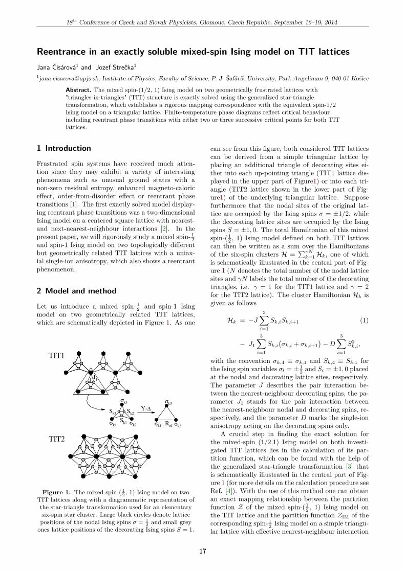
By subtracting measured time t0 at Start and timet1 at the Hodoscope for each pion the distribution thatis shown in Figure 3 is obtained. It is clear that fromthe σ of this gauss-like distribution, only the combinedresolution of the detectors (σ2 = σ2
Start + σ2Hodo) can
be deduced. Since neither σStart nor σHodo is knownseparately, the assumption σStart = σHodo = σ√
2. Af-
ter the cut on the middle of the scintillator rods of ho-doscope and so called time-walk correction for STARTdetector we get a result σStart = 170 ps.
[ns]0 - t1t10 15 20 25 30
coun
ts
0
50
100
150
200
250
300
350
Figure 3. Distribution of time of flight for pions fromthe Start detector to the Hodoscope.
3.2 Produced dielectrons
This section will provide details of the second methodthat was implemented in order to obtain the pureStart time resolution. This method is based on themeasurement of the time of flight of electron-positronpairs (te− resp. te+) by one of the TOF or RPC detec-tors and the Start detector (t0 of the pion that inter-acted with the target). Identification of both leptonsis done by the RICH detector. The goal lies in findingthe total time resolution σStart+ToF from the distribu-tion of te± and also the time resolution of TOF/RPCdetector1 from the distribution of te+ − te− . It shouldbe noted that from this distribution σ =
√2 · σToF is
obtained since two particles are detected. It is thensimple to get the pure time resolution of the Start
detector from σStart =√
σ2Start+ToF − σ2
ToF. In all fol-lowing pictures the symbol blue cross for TOF dataand red plus for RPC data are used. The distribution
1Because te± = t± − t0 (where t± is the measured time bythe TOF/RPC detector of the positron/electron), te+ − te− =t+ − t− and it can be seen that this difference is not influencedby the measurement of the Start detector.
of σToF (time resolution) of the TOF/RPC detectordepending on the Start channel number through whichthe pion that interacted with the target flew and (giv-ing the electron/positron pair) is shown in Figure 4.As can be seen the distribution is independent of theStart channel number as can be expected. The finaltime resolution for each START channel one can seein Figure 5 where the time-walk correction was ap-plied and ToF time resolution subtracted. From thispicture one can also see that both methods are givingcomparable results.
START channels0 5 10 15 20 25 30 35
Tim
e R
esol
utio
n [p
s]
0
100
200
300
400
500
Figure 4. Time resolution of the TOF/RPC detector.
START channels0 5 10 15 20 25 30 35
Tim
e R
esol
utio
n [p
s]
0
100
200
300
400
500
Figure 5. Time resolution of the Start detector.
References
[1] P. Salabura for HADES collaboration, Eur. Phys.J. A 41, 243-277 (2009)
[2] The HADES collaboration, TDR - A secondarypion beam for HADES experiment (InternalHADES document,2013)
[3] J. Michel et al., IEEE Transactions on NuclearScience 58 4, 1745 - 1750 (2011)
16
18th Conference of Czech and Slovak Physicists, Olomouc, Czech Republic, September 16–19, 2014
Reentrance in an exactly soluble mixed-spin Ising model on TIT lattices
Jana Čisárová1 and Jozef Strečka1
[email protected], Institute of Physics, Faculty of Science, P. J. Šafárik University, Park Angelinum 9, 040 01 Košice
Abstract. The mixed spin-(1/2, 1) Ising model on two geometrically frustrated lattices with"triangles-in-triangles" (TIT) structure is exactly solved using the generalized star-triangletransformation, which establishes a rigorous mapping correspondence with the equivalent spin-1/2Ising model on a triangular lattice. Finite-temperature phase diagrams reflect critical behaviourincluding reentrant phase transitions with either two or three successive critical points for both TITlattices.
1 Introduction
Frustrated spin systems have received much atten-tion since they may exhibit a variety of interestingphenomena such as unusual ground states with anon-zero residual entropy, enhanced magneto-caloriceffect, order-from-disorder effect or reentrant phasetransitions [1]. The first exactly solved model display-ing reentrant phase transitions was a two-dimensionalIsing model on a centered square lattice with nearest-and next-nearest-neighbour interactions [2]. In thepresent paper, we will rigorously study a mixed spin-1
2and spin-1 Ising model on two topologically differentbut geometrically related TIT lattices with a uniax-ial single-ion anisotropy, which also shows a reentrantphenomenon.
2 Model and method
Let us introduce a mixed spin- 12 and spin-1 Ising
model on two geometrically related TIT lattices,which are schematically depicted in Figure 1. As one
TIT2
TIT1
J1J
Sk3
Sk2
Sk1
σk3
σk2
σk1 R
efσk1 σ
k2
σk3
Y-∆
Figure 1. The mixed spin-( 12, 1) Ising model on two
TIT lattices along with a diagrammatic representation ofthe star-triangle transformation used for an elementarysix-spin star cluster. Large black circles denote latticepositions of the nodal Ising spins σ = 1
2and small grey
ones lattice positions of the decorating Ising spins S = 1.
can see from this figure, both considered TIT latticescan be derived from a simple triangular lattice byplacing an additional triangle of decorating sites ei-ther into each up-pointing triangle (TIT1 lattice dis-played in the upper part of Figure1) or into each tri-angle (TIT2 lattice shown in the lower part of Fig-ure1) of the underlying triangular lattice. Supposefurthermore that the nodal sites of the original lat-tice are occupied by the Ising spins σ = ±1/2, whilethe decorating lattice sites are occupied by the Isingspins S = ±1, 0. The total Hamiltonian of this mixedspin-( 1
2 , 1) Ising model defined on both TIT latticescan then be written as a sum over the Hamiltoniansof the six-spin clusters H =
∑γNk=1 Hk, one of which
is schematically illustrated in the central part of Fig-ure 1 (N denotes the total number of the nodal latticesites and γN labels the total number of the decoratingtriangles, i.e. γ = 1 for the TIT1 lattice and γ = 2for the TIT2 lattice). The cluster Hamiltonian Hk isgiven as follows
Hk = −J3∑
i=1
Sk,iSk,i+1 (1)
− J1
3∑
i=1
Sk,i
(
σk,i + σk,i+1
)
−D
3∑
i=1
S2k,i,
with the convention σk,4 ≡ σk,1 and Sk,4 ≡ Sk,1 forthe Ising spin variables σl = ± 1
2 and Si = ±1, 0 placedat the nodal and decorating lattice sites, respectively.The parameter J describes the pair interaction be-tween the nearest-neighbour decorating spins, the pa-rameter J1 stands for the pair interaction betweenthe nearest-neighbour nodal and decorating spins, re-spectively, and the parameter D marks the single-ionanisotropy acting on the decorating spins only.
A crucial step in finding the exact solution forthe mixed-spin (1/2,1) Ising model on both investi-gated TIT lattices lies in the calculation of its par-tition function, which can be found with the help ofthe generalized star-triangle transformation [3] thatis schematically illustrated in the central part of Fig-ure 1 (for more details on the calculation procedure seeRef. [4]). With the use of this method one can obtainan exact mapping relationship between the partitionfunction Z of the mixed spin-( 1
2 , 1) Ising model onthe TIT lattice and the partition function ZIM of thecorresponding spin- 1
2 Ising model on a simple triangu-lar lattice with effective nearest-neighbour interaction
171717
Čisárová J. et al.: Reentrance in an exactly soluble mixed-spin Ising model on TIT lattices
-0.5 0.0 0.5 1.00.0
0.2
0.4
0.6
0.8
1.0 0.0
1.0
-0.75 -0.9
-1.0
-1.7 -1.5
-1.2
D / |J1| = -0.5
J / |J1|
k
B T
c /
|J
1|
a)
-1 0 10.0
0.5
1.0
1.5
2.0
-1.0
-0.75
0.0
-1.2
-1.5
-2.0
D / |J1| = 1.0
J / |J1|
kB T
c /
|J
1|
Figure 2. Critical temperature of the mixed spin-( 12, 1)
Ising model as a function of the interaction ratio JJ1
for
several values of the single-ion anisotropy DJ1
on: (a)TIT1 lattice; (b) TIT2 lattice.
γJeff
Z(β, J, J1, D) = AγN ZIM(β, γJeff) (2)
involving the standard notation for the inverse tem-perature β = 1/(kBT ). Note that the effective in-teraction is twice as large for the TIT2 lattice thanfor the TIT1 lattice. Using the established mappingequivalence (2) between the partition functions, thecritical points of the mixed-spin Ising model on theTIT lattices can be simply located by equating the ef-fective nearest-neighbour coupling βγJeff with its crit-ical value ln 3 (for more details see Ref. [4]).
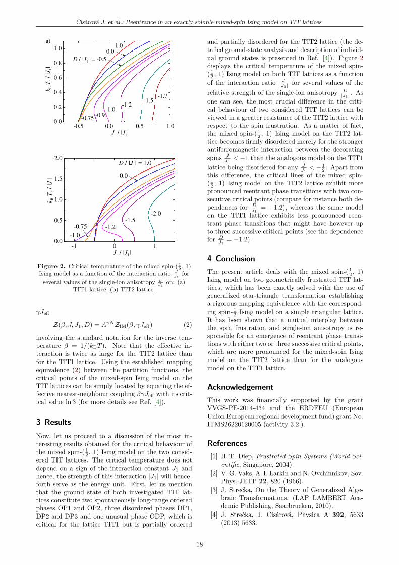
3 Results
Now, let us proceed to a discussion of the most in-teresting results obtained for the critical behaviour ofthe mixed spin-( 1
2 , 1) Ising model on the two consid-ered TIT lattices. The critical temperature does notdepend on a sign of the interaction constant J1 andhence, the strength of this interaction |J1| will hence-forth serve as the energy unit. First, let us mentionthat the ground state of both investigated TIT lat-tices constitute two spontaneously long-range orderedphases OP1 and OP2, three disordered phases DP1,DP2 and DP3 and one unusual phase ODP, which iscritical for the lattice TIT1 but is partially ordered
and partially disordered for the TIT2 lattice (the de-tailed ground-state analysis and description of individ-ual ground states is presented in Ref. [4]). Figure 2displays the critical temperature of the mixed spin-( 1
2 , 1) Ising model on both TIT lattices as a functionof the interaction ratio J
|J1| for several values of the
relative strength of the single-ion anisotropy D|J1| . As
one can see, the most crucial difference in the criti-cal behaviour of two considered TIT lattices can beviewed in a greater resistance of the TIT2 lattice withrespect to the spin frustration. As a matter of fact,the mixed spin-( 1
2 , 1) Ising model on the TIT2 lat-tice becomes firmly disordered merely for the strongerantiferromagnetic interaction between the decoratingspins J
J1< −1 than the analogous model on the TIT1
lattice being disordered for any JJ1< − 1
2 . Apart fromthis difference, the critical lines of the mixed spin-( 1
2 , 1) Ising model on the TIT2 lattice exhibit morepronounced reentrant phase transitions with two con-secutive critical points (compare for instance both de-pendences for D
J1= −1.2), whereas the same model
on the TIT1 lattice exhibits less pronounced reen-trant phase transitions that might have however upto three successive critical points (see the dependencefor D
J1= −1.2).
4 Conclusion
The present article deals with the mixed spin-( 12 , 1)
Ising model on two geometrically frustrated TIT lat-tices, which has been exactly solved with the use ofgeneralized star-triangle transformation establishinga rigorous mapping equivalence with the correspond-ing spin- 1
2 Ising model on a simple triangular lattice.It has been shown that a mutual interplay betweenthe spin frustration and single-ion anisotropy is re-sponsible for an emergence of reentrant phase transi-tions with either two or three successive critical points,which are more pronounced for the mixed-spin Isingmodel on the TIT2 lattice than for the analogousmodel on the TIT1 lattice.
Acknowledgement
This work was financially supported by the grantVVGS-PF-2014-434 and the ERDFEU (EuropeanUnion European regional development fund) grant No.ITMS26220120005 (activity 3.2.).
References
[1] H. T. Diep, Frustrated Spin Systems (World Sci-entific, Singapore, 2004).
[2] V. G. Vaks, A. I. Larkin and N. Ovchinnikov, Sov.Phys.-JETP 22, 820 (1966).
[3] J. Strečka, On the Theory of Generalized Alge-braic Transformations, (LAP LAMBERT Aca-demic Publishing, Saarbrucken, 2010).
[4] J. Strečka, J. Čisárová, Physica A 392, 5633(2013) 5633.
18
18th Conference of Czech and Slovak Physicists, Olomouc, Czech Republic, September 16–19, 2014
Influence of resonance decays on triangular flow in heavy-ion collisions
Jana Crkovská1, Larissa Bravina2, and Evgeny Zabrodin2,3
1Faculty of Nuclear Sciences and Physical Engineering, Czech Technical University in Prague, Břehová 7, Prague 110 00,Czech Republic, [email protected] of Physics, University of Oslo, P. O. Box 1048 Blindern, N-0316, Oslo, Norway3Skobeltsyn Institute of Nuclear Physics, Lomonosov Moscow State University, Leninskie Gory, GSP-1, Moscow 119991,Russian Federation
Abstract. Anisotropic flow in relativistic collisions of heavy-ions yields important information aboutthe state of the hot and dense matter created in the reactions. Study of triangular flow in Pb+Pbinteractions at LHC was performed within Monte Carlo HYDJET++ model. HYDJET++combines both parametrized hydrodynamics for soft pT particle spectra and microscopic jetquenching generator for hard pT spectra, giving a realistic prediction for vast number of hadronspecies. The model also enables study of influence of final-state interactions on flow of createdhadrons. Triangular flow patterns of pions, kaons and protons were studied at different centralities.Scaling of triangular flow with number of constituent quarks is discussed.
1 Introduction
Collective flow of particles can yield valuable informa-tion about the hot and dense medium created in rel-ativistic nucleus-nucleus collisions, known as quark-gluon plasma (QGP). The initial anisotropy of theoverlap region and the subsequent expansion of thefireball after the collision due to the pressure gradi-ents inside give rise to momentum anisotropy of out-coming particles. The azimuthal distribution of de-tected particles with respect to reaction plane ΨR canbe expanded into a Fourier series
dNdϕ
=N
2π
[
1 + 2∑
vn cos (n(ϕ− ΨR))]
, (1)
with the Fourier coefficients describing high flow har-monics
vn = 〈cos (n(ϕ− ΨR))〉 (2)
and bear the name of directed, elliptic and triangularflow for v1, v2 and v3 respectively. Measuring the mag-nitude of the flow coefficients can yield informationabout the state of the medium produced immediatelyafter the initial scattering. Elliptic flow presentedthe dominant contribution to anisotropic flow in semi-peripheral and peripheral interactions. However withenergies such as at LHC, the higher coefficients growsignificantly and become dominant at small impactparameters. Results from LHC suggest that in cen-tral collisions the main part of the anisotropic floworiginates from the triangular flow [1].
A prominent feature of elliptic flow is the number-of-constituent-quarks scaling (NCQ), first observed atRHIC [2]. The elliptic flow for identified particlesscales as v2/nq(kET /nq). Such behaviour implies for-mation of flow on partonic level, when the QGP is stillpresent, and favours coalescence formation scenario.Preliminary results from STAR experiment suggestthat v3 scales as v3/n
3/2q (kET /nq) [3].
2 HYDJET++
HYDJET++ [4] stands for HYDrodynamics withJETs and is a Monte Carlo heavy-ion event genera-
tor. It is a superposition of hydrodynamical part andjet part. These are treated independently. Amongthe advantages of this model is the possibility to studyseparately hydrodynamical behaviour and influence ofjet quenching, its efficiency, its ability to reproducerealistic shapes of distributions and that it includes avast table of resonances.
0 0.5 1 1.5 2 2.5 3 3.5 4 4.5
0.02
0.04
0.06
0.08
0.1
0.12CMS data
HYDJET++
0 0.5 1 1.5 2 2.5 3 3.5 4 4.5
3v
0.02
0.04
0.06
0.08
0.1
0.12
0 0.5 1 1.5 2 2.5 3 3.5 4 4.5
0.02
0.04
0.06
0.08
0.1
0.12
0 0.5 1 1.5 2 2.5 3 3.5 4 4.5
0.02
0.04
0.06
0.08
0.1
0.12
10-15% 15-20%
25-30%20-25%
[GeV/c]T
p
Figure 1. Triangular flow of charged particles in Pb+Pbat
√sNN = 2.76 TeV. Histograms are HYDJET++
calculations, squares are CMS data [6].
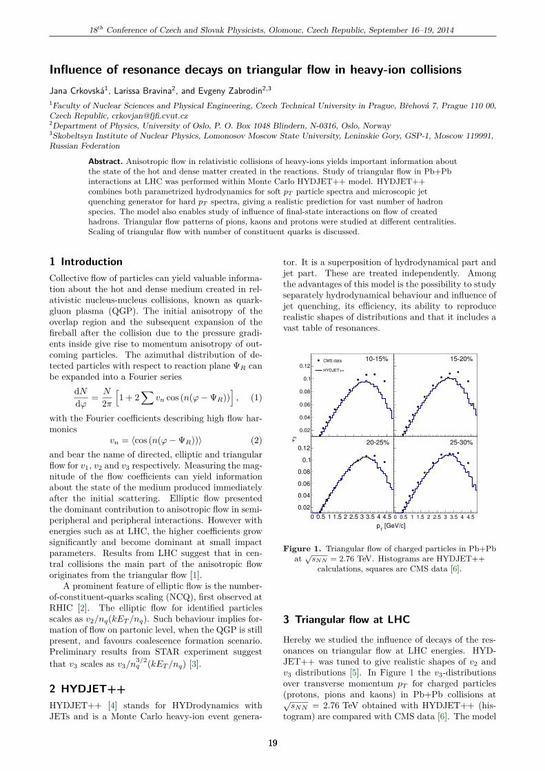
3 Triangular flow at LHC
Hereby we studied the influence of decays of the res-onances on triangular flow at LHC energies. HYD-JET++ was tuned to give realistic shapes of v2 andv3 distributions [5]. In Figure 1 the v3-distributionsover transverse momentum pT for charged particles(protons, pions and kaons) in Pb+Pb collisions at√sNN = 2.76 TeV obtained with HYDJET++ (his-
togram) are compared with CMS data [6]. The model
191919
Crkovská J. et al.: Influence of resonance decays on triangular flow in heavy-ion collisions
provides a particulary good description of data in softpT region. The overall shape of the distribution cor-responds to the trend observed in experiment as ad-vertised.
0 1 2 3 4 5 6 7 8 9
0
0.02
0.04
0.06
0.08
0.1
0.12
0 1 2 3 4 5 6 7 8 9
0
0.02
0.04
0.06
0.08
0.1
0.12
0
0.02
0.04
0.06
0.08
0.1
0.12 all hadrons
direct hadrons
0 1 2 3 4 5 6 7 8 9
3v
0
0.02
0.04
0.06
0.08
0.1
0.12
0 1 2 3 4 5 6 7 8 9
0 - 10%
20 - 30%
10 - 20%
30 - 40%
Pb+Pb at 2.76 TeV= 2.76 TeV 20-30%NNsPb+Pb
[GeV/c]T
p
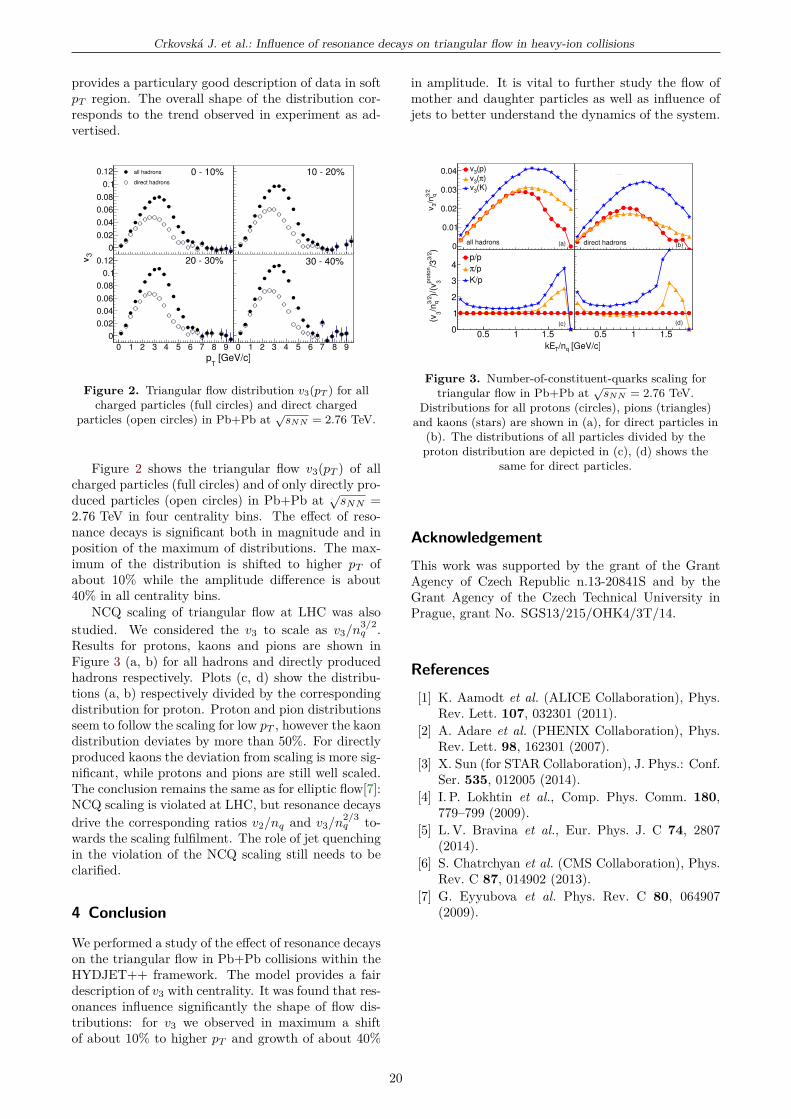
Figure 2. Triangular flow distribution v3(pT ) for allcharged particles (full circles) and direct charged
particles (open circles) in Pb+Pb at√sNN = 2.76 TeV.
Figure 2 shows the triangular flow v3(pT ) of allcharged particles (full circles) and of only directly pro-duced particles (open circles) in Pb+Pb at
√sNN =
2.76 TeV in four centrality bins. The effect of reso-nance decays is significant both in magnitude and inposition of the maximum of distributions. The max-imum of the distribution is shifted to higher pT ofabout 10% while the amplitude difference is about40% in all centrality bins.
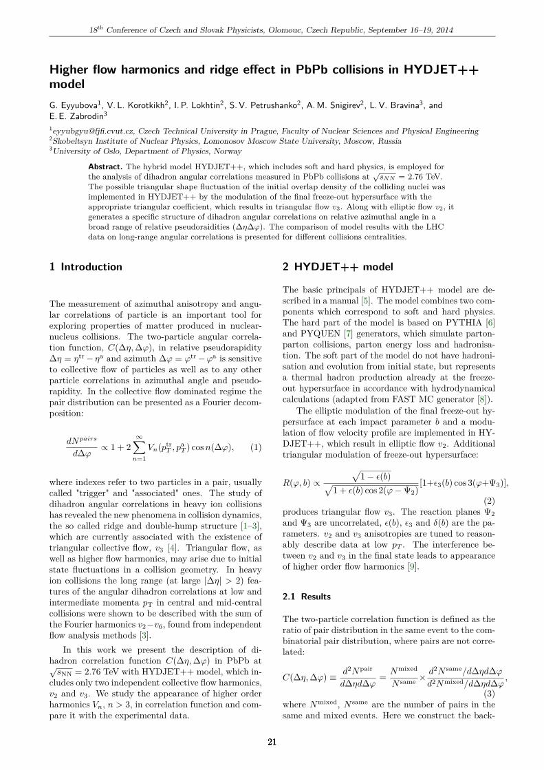
NCQ scaling of triangular flow at LHC was alsostudied. We considered the v3 to scale as v3/n
3/2q .
Results for protons, kaons and pions are shown inFigure 3 (a, b) for all hadrons and directly producedhadrons respectively. Plots (c, d) show the distribu-tions (a, b) respectively divided by the correspondingdistribution for proton. Proton and pion distributionsseem to follow the scaling for low pT , however the kaondistribution deviates by more than 50%. For directlyproduced kaons the deviation from scaling is more sig-nificant, while protons and pions are still well scaled.The conclusion remains the same as for elliptic flow[7]:NCQ scaling is violated at LHC, but resonance decaysdrive the corresponding ratios v2/nq and v3/n
2/3q to-
wards the scaling fulfilment. The role of jet quenchingin the violation of the NCQ scaling still needs to beclarified.
4 Conclusion
We performed a study of the effect of resonance decayson the triangular flow in Pb+Pb collisions within theHYDJET++ framework. The model provides a fairdescription of v3 with centrality. It was found that res-onances influence significantly the shape of flow dis-tributions: for v3 we observed in maximum a shiftof about 10% to higher pT and growth of about 40%
in amplitude. It is vital to further study the flow ofmother and daughter particles as well as influence ofjets to better understand the dynamics of the system.
0.2 0.4 0.6 0.8 1 1.2 1.4 1.6 1.8
3/2
q/n
3v
0
0.01
0.02
0.03
0.04 (p)3v
)π(3v(K)3v
(a)all hadrons
0.5 1 1.5
)3/2
/3pro
ton
3)/(v
3/2
q/n
3(v
0
1
2
3
4p/p
/pπ
K/p
(c)
0.2 0.4 0.6 0.8 1 1.2 1.4 1.6 1.8
0
0.005
0.01
0.015
0.02
0.025
0.03
0.035
0.04 = 2.76 TeV 20-30%NN
sPb+Pb
(b)direct hadrons
0.5 1 1.50
0.5
1
1.5
2
2.5
3
3.5
4
4.5
(d)
[GeV/c]q/nTkE
Figure 3. Number-of-constituent-quarks scaling fortriangular flow in Pb+Pb at
√sNN = 2.76 TeV.
Distributions for all protons (circles), pions (triangles)and kaons (stars) are shown in (a), for direct particles in
(b). The distributions of all particles divided by theproton distribution are depicted in (c), (d) shows the
same for direct particles.
Acknowledgement
This work was supported by the grant of the GrantAgency of Czech Republic n.13-20841S and by theGrant Agency of the Czech Technical University inPrague, grant No. SGS13/215/OHK4/3T/14.
References
[1] K. Aamodt et al. (ALICE Collaboration), Phys.Rev. Lett. 107, 032301 (2011).
[2] A. Adare et al. (PHENIX Collaboration), Phys.Rev. Lett. 98, 162301 (2007).
[3] X. Sun (for STAR Collaboration), J. Phys.: Conf.Ser. 535, 012005 (2014).
[4] I. P. Lokhtin et al., Comp. Phys. Comm. 180,779–799 (2009).
[5] L. V. Bravina et al., Eur. Phys. J. C 74, 2807(2014).
[6] S. Chatrchyan et al. (CMS Collaboration), Phys.Rev. C 87, 014902 (2013).
[7] G. Eyyubova et al. Phys. Rev. C 80, 064907(2009).
20
18th Conference of Czech and Slovak Physicists, Olomouc, Czech Republic, September 16–19, 2014
Higher flow harmonics and ridge effect in PbPb collisions in HYDJET++model
G. Eyyubova1, V. L. Korotkikh2, I. P. Lokhtin2, S. V. Petrushanko2, A. M. Snigirev2, L. V. Bravina3, andE. E. Zabrodin3
[email protected], Czech Technical University in Prague, Faculty of Nuclear Sciences and Physical Engineering2Skobeltsyn Institute of Nuclear Physics, Lomonosov Moscow State University, Moscow, Russia3University of Oslo, Department of Physics, Norway
Abstract. The hybrid model HYDJET++, which includes soft and hard physics, is employed forthe analysis of dihadron angular correlations measured in PbPb collisions at
√sNN = 2.76 TeV.
The possible triangular shape fluctuation of the initial overlap density of the colliding nuclei wasimplemented in HYDJET++ by the modulation of the final freeze-out hypersurface with theappropriate triangular coefficient, which results in triangular flow v3. Along with elliptic flow v2, itgenerates a specific structure of dihadron angular correlations on relative azimuthal angle in abroad range of relative pseudoraidities (∆η∆ϕ). The comparison of model results with the LHCdata on long-range angular correlations is presented for different collisions centralities.
1 Introduction
The measurement of azimuthal anisotropy and angu-lar correlations of particle is an important tool forexploring properties of matter produced in nuclear-nucleus collisions. The two-particle angular correla-tion function, C(∆η,∆ϕ), in relative pseudorapidity∆η = ηtr − ηa and azimuth ∆ϕ = ϕtr −ϕa is sensitiveto collective flow of particles as well as to any otherparticle correlations in azimuthal angle and pseudo-rapidity. In the collective flow dominated regime thepair distribution can be presented as a Fourier decom-position:
dNpairs
d∆ϕ∝ 1 + 2
∞∑
n=1
Vn(ptrT , p
aT ) cosn(∆ϕ), (1)
where indexes refer to two particles in a pair, usuallycalled "trigger" and "associated" ones. The study ofdihadron angular correlations in heavy ion collisionshas revealed the new phenomena in collision dynamics,the so called ridge and double-hump structure [1–3],which are currently associated with the existence oftriangular collective flow, v3 [4]. Triangular flow, aswell as higher flow harmonics, may arise due to initialstate fluctuations in a collision geometry. In heavyion collisions the long range (at large |∆η| > 2) fea-tures of the angular dihadron correlations at low andintermediate momenta pT in central and mid-centralcollisions were shown to be described with the sum ofthe Fourier harmonics v2−v6, found from independentflow analysis methods [3].
In this work we present the description of di-hadron correlation function C(∆η,∆ϕ) in PbPb at√sNN = 2.76 TeV with HYDJET++ model, which in-
cludes only two independent collective flow harmonics,v2 and v3. We study the appearance of higher orderharmonics Vn, n > 3, in correlation function and com-pare it with the experimental data.
2 HYDJET++ model
The basic principals of HYDJET++ model are de-scribed in a manual [5]. The model combines two com-ponents which correspond to soft and hard physics.The hard part of the model is based on PYTHIA [6]and PYQUEN [7] generators, which simulate parton-parton collisions, parton energy loss and hadronisa-tion. The soft part of the model do not have hadroni-sation and evolution from initial state, but representsa thermal hadron production already at the freeze-out hypersurface in accordance with hydrodynamicalcalculations (adapted from FAST MC generator [8]).
The elliptic modulation of the final freeze-out hy-persurface at each impact parameter b and a modu-lation of flow velocity profile are implemented in HY-DJET++, which result in elliptic flow v2. Additionaltriangular modulation of freeze-out hypersurface:
R(ϕ, b) ∝√
1 − ǫ(b)√
1 + ǫ(b) cos 2(ϕ− Ψ2)[1+ǫ3(b) cos 3(ϕ+Ψ3)],
(2)produces triangular flow v3. The reaction planes Ψ2
and Ψ3 are uncorrelated, ǫ(b), ǫ3 and δ(b) are the pa-rameters. v2 and v3 anisotropies are tuned to reason-ably describe data at low pT . The interference be-tween v2 and v3 in the final state leads to appearanceof higher order flow harmonics [9].
2.1 Results
The two-particle correlation function is defined as theratio of pair distribution in the same event to the com-binatorial pair distribution, where pairs are not corre-lated:
C(∆η,∆ϕ) ≡ d2Npair
d∆ηd∆ϕ=Nmixed
N same× d2N same/d∆ηd∆ϕd2Nmixed/d∆ηd∆ϕ
,
(3)where Nmixed, N same are the number of pairs in thesame and mixed events. Here we construct the back-
212121
Eyyubova G. et al.: Higher flow harmonics and ridge effect in PbPb collisions in HYDJET++ modelt ♦♥r♥ ♦ ③ ♥ ♦ P②ssts ♦♠♦ ③ ♣ ♣t♠r
ϕ∆-10 1 2
3 4η∆
-4-3
-2-1
01
23
4
)ϕ
∆,
η∆
C(
1
1.01
1.02
0%<2 GeV/c
a
t1<p
<4 GeV/ctr
t2<p
ϕ∆-10 1 2
3 4η∆
-4-3
-2-1
01
23
4
)ϕ
∆,
η∆
C(
1
1.01
1.02
2only v0-5%<2 GeV/c
a
t1<p
<4 GeV/ctr
t2<p
ϕ∆-10 1 2
3 4η∆
-4-3
-2-1
01
23
4
)ϕ
∆,
η∆
C(
0.99
1
1.01
1.02
1.03
0-5%<2 GeV/c
a
t1<p
<4 GeV/ctr
t2<p
r ♦rrt♦♥ ♥t♦♥ ♥ ❨ ♦r❱ ♥ ♦r ♥tr
♦s♦♥s t ♠♣t ♣r♠tr ♥trt② t ♦♥② ♥ ♥trt② t ♦t
♥ ♣rs♥t
r ♦rr r♠♦♥sr♦♠ q r ♥ rt② r♦♠
♥r r♦♥ ♦rrt♦♥s ♦♥t♥s ♣♦sst②♣s ♦ t♦ ♣rt ♦rrt♦♥s ♠♦st ♦ s♦rs♦r t♦ ♦r ♠♥②♣rt ♦rrt♦♥s s ♣rs♥t ♥t ♠♦ ♠t♦s♦♣ ♦rrt♦♥s rs♦♥♥ ②s ts ♦t ♦ ♦♥ r♥ ♦rrt♦♥s♦r ♣♣r ♥ t ♠♦ ♦♥② t♦ ♦t ♦ ♦rrt♦♥ ♥t♦♥ t ♥ ❨ ♥ PP ♦s♦♥ t ❱ ♦r
❱ ♥ s ♣rs♥t ♥ ♦r t ss ♦ ♥♦ ♦t ♦ ③r♦ ♠♣t♣r♠tr ♦♥② ♣t ♦ s tr♥ ♦♥ ♥ ♦t ♣t ♥ tr♥r ♦ r ♣rs♥t t ♣ s ② s♣♣rss t ②s t♦ t q♥♥ t♦ r♠♥♥ts ♦ t ♥ s♥ ♦r r♦ r♥ t ②s s♦s tt ♥♦ ♦♥r♥ ③♠t ♦rrt♦♥s r♣rs♥t t t ♥rs ♥ t② ♣♣r ♥ ♣rs♥ ♦♣t ♦ t t rtrst ♣ttr♥ ② r t ♥ rt ♣s♦r♣t② ♣t♦ ♦rrs♣♦♥s t♦ t ♣s♦r♣t②s♣ ♦ ♦t ♦ ♥ t ♠♦ tr♥r♦ ♥♥s ts ♥rs ♦rrt♦♥s ♦t♥ rrr s r ♥ s♦ ♠♦s ②s strtr♣r♦♥ ♦♠♣ s
♦rrt♦♥ ♥t♦♥ s t♦r ♦♥r♥ ③♠t ♦rrt♦♥s ♦r❱ ❱ ♦r r♥t ♥trts s♦s t ♦rr ♦♥ts t r♦♠ ♥ ♦♠♣rs♦♥ t t ❬❪t ♥tr ♦s♦♥s t ♦♥ts r ♦rt♥ ♥ t t ♠♥tr ♦s♦♥ srt rtr t ♣r♣r ♦s♦♥s ♥ t♠♦ s ♠ r t♥ ♥ t ♦rrs♣♦♥st♦ t t tt t ♠♦ ♦s ♥♦t sr t ♦♥ s♥♣rt ♥ t r♦♥❱ ❬❪ ❲ ♥♦t tt tr s ♥♦ ♥ t ♠♦rtss t ♦♠♣♦♥♥t ♣♣rs t♦ ♠♦♠♥t♠ ♦♥srt♦♥ ♦t♦♥ s ♥ s♥ r♦♠ r ♦rr ♦♥ts ♣♣r ♥ t♠♦ ♥ ♦♠♣♦st♦♥ t♦ t② rsr♣② t s ♦♥ts t ♦ ♥ ♦♥②♦r♥t r♦♠ ♦t ♦ ♥
r ♦rr ♦♥ts ♦r❱ ♥ ♦r r♥t ♥trts ♥
❨ ♥ ♥ t ❬❪
♦♥s♦♥s
♥ ❨ ♠♦ t ♦t ♦ ♦r ♥♦♥♥tr ♦s♦♥s s ♥tr♦ ♣t ♥ tr♥r ♠♦t♦♥ ♦ t r③♦t ♦♠ ♥ r♦tt♦♥♦ ♦ts ♦ ♠tt ♣rts s♠♣ ♠♥s♠ ♦s s t♦ sr r♦♥ ♦rrt♦♥s t♠♥tr ♦s♦♥s r ♦t ♦ ♦♠♥ts♦r tt♦♥s
s ♣t♦♥ s s♣♣♦rt ② t r♦♣♥s♦ ♥ t♥ t r♠♦r ♦ r③♥ t♣r♦t ♣♣♦rt ♦ ♥trst♦r ♠♦t② ♥ qt② ♥♥♠♥t ♦ rsr t♠s t ③ ♥❯♥rst② ♥ Pr ❩
r♥s
❬❪ r t ❬P❳ ♦♦rt♦♥❪ P②s
❬❪ r t ❬ ♦♦rt♦♥❪P②s
❬❪ ♠♦t t ❬ ♦♦rt♦♥❪ P②s tt
❬❪ r ♥ ♦♥ P②s ❬rrt♠ ❪
❬❪ P ♦t♥ ❱ ♥♥ ❱ Ptrs♥♦ ♥r rs♥ ②♦♥ ♦♠♣tP②s ♦♠♠♥
❬❪ ♦str♥ r♥♥ P ♥s P
❬❪ P ♦t♥ ♥r r P②s
❬❪ ♠♥ t P②s
❬❪ ❱ r♥ rs♠ ♦♥ss♦♥ ②②♦ ❱ ♦r♦t P ♦t♥ ❱ ♥♥ ❱ Ptrs♥♦ ♥ ♥r t r P②s
❬❪ tr②♥ t ❬ ♦♦rt♦♥❪ rP②s
(a) (b) (c)
Figure 1. 2D correlation function in HYDJET++ for2 < ptr
T < 4 GeV/c and 1 < paT < 2 for (a) central
collisions with impact parameter b = 0, (b) centrality0-5% with only v2, and (c) centrality 0-5% with both v2
and v3 present.
ground from two single particle spectra:
d2Nmixed
d∆ηd∆ϕ=∫
d2N tr
dηtrdϕtr
d2Na
dηadϕaδtr
a dηadηtrdϕadϕtr,
(4)where δtr
a = δ(ηtr − ηa)δ(ϕtr −ϕa). Fourier harmonicsVn from Eq. (1) are defined directly from C(∆ϕ):
Vn = 〈cos(∆ϕ)〉 =∑
i Ci(∆ϕi) · cos(n∆ϕi)∑
i Ci(∆ϕi). (5)
Angular dihadron correlations contains all possibletypes of two particle correlations. The most of sourcesfor two- or many-particle correlations is presented inthe model, i.e femtoscopic correlations, resonance de-cays, jets, collective flow. The long range correlationsover η appear in the model only due to collective flow.The correlation function C(∆η,∆ϕ) calculated in HY-DJET++ in PbPb collision at
√sNN = 2.76 TeV for
2 < ptrT < 4 GeV/c and 1 < pa
T < 2 is presented in Fig-ure 1 for the cases of (a) no collective flow (zero impactparameter), (b) only elliptic flow v2 is turned on and(c) both elliptic and triangular flow are present. Thejet peak is highly suppressed at away-side (∆ϕ ≈ π)due to jet quenching, though remnants of it can beseen over broad ∆η range at away-side. Figure 1 (a)shows that no long-range azimuthal correlations arepresent at the near-side and they appear in presence ofelliptic flow with the characteristic cos(2∆ϕ) pattern,Figure 1 (b). They are flat in relative pseudorapidityup to ∆η ≈ 4, which corresponds to flat pseudorapid-ity shape of collective flow in the model. The triangu-lar flow enhances these near-side correlations, often re-ferred as ridge, and also modifies away-side structure,producing double-hump (see Figure 1 (c)). The 1Dcorrelation function C(∆ϕ) was calculated for long-range azimuthal correlations for 1 < pa
T < 1.5 GeV/c,3 < ptr
T < 3.5 GeV/c for different centralities. Fig-ure 2 shows the Fourier coefficients Vn, calculated fromC(∆ϕ) in comparison with CMS data [10]. At centralcollisions all the coefficients Vn are lower than in data.At mid-central collision Vn describe data rather well.At peripheral collisions V2 in the model is much higherthan in data, which corresponds to the fact that themodel does not describe data well on single-particlev2 in the region 3 < pT < 3.5 GeV/c [9]. We note,that there is no v1 in the model. Nevertheless, the V1
component appears due to momentum conservationviolation. As can be seen from Figure 2, higher ordercoefficients Vn, n > 3 appear in the model in C(∆ϕ)
t ♦♥r♥ ♦ ③ ♥ ♦ P②ssts ♦♠♦ ③ ♣ ♣t♠r
r ♦rrt♦♥ ♥t♦♥ ♥ ❨ ♦r❱ ♥ ♦r ♥tr
♦s♦♥s t ♠♣t ♣r♠tr ♥trt② t ♦♥② ♥ ♥trt② t ♦t
♥ ♣rs♥t
r ♦rr r♠♦♥sr♦♠ q r ♥ rt② r♦♠
♥r r♦♥ ♦rrt♦♥s ♦♥t♥s ♣♦sst②♣s ♦ t♦ ♣rt ♦rrt♦♥s ♠♦st ♦ s♦rs♦r t♦ ♦r ♠♥②♣rt ♦rrt♦♥s s ♣rs♥t ♥t ♠♦ ♠t♦s♦♣ ♦rrt♦♥s rs♦♥♥ ②s ts ♦t ♦ ♦♥ r♥ ♦rrt♦♥s♦r ♣♣r ♥ t ♠♦ ♦♥② t♦ ♦t ♦ ♦rrt♦♥ ♥t♦♥ t ♥ ❨ ♥ PP ♦s♦♥ t ❱ ♦r
❱ ♥ s ♣rs♥t ♥ ♦r t ss ♦ ♥♦ ♦t ♦ ③r♦ ♠♣t♣r♠tr ♦♥② ♣t ♦ s tr♥ ♦♥ ♥ ♦t ♣t ♥ tr♥r ♦ r ♣rs♥t t ♣ s ② s♣♣rss t ②s t♦ t q♥♥ t♦ r♠♥♥ts ♦ t ♥ s♥ ♦r r♦ r♥ t ②s s♦s tt ♥♦ ♦♥r♥ ③♠t ♦rrt♦♥s r♣rs♥t t t ♥rs ♥ t② ♣♣r ♥ ♣rs♥ ♦♣t ♦ t t rtrst ♣ttr♥ ② r t ♥ rt ♣s♦r♣t② ♣t♦ ♦rrs♣♦♥s t♦ t ♣s♦r♣t②s♣ ♦ ♦t ♦ ♥ t ♠♦ tr♥r♦ ♥♥s ts ♥rs ♦rrt♦♥s ♦t♥ rrr s r ♥ s♦ ♠♦s ②s strtr♣r♦♥ ♦♠♣ s
♦rrt♦♥ ♥t♦♥ s t♦r ♦♥r♥ ③♠t ♦rrt♦♥s ♦r❱ ❱ ♦r r♥t ♥trts s♦s t ♦rr ♦♥ts t r♦♠ ♥ ♦♠♣rs♦♥ t t ❬❪t ♥tr ♦s♦♥s t ♦♥ts r ♦rt♥ ♥ t t ♠♥tr ♦s♦♥ srt rtr t ♣r♣r ♦s♦♥s ♥ t♠♦ s ♠ r t♥ ♥ t ♦rrs♣♦♥st♦ t t tt t ♠♦ ♦s ♥♦t sr t ♦♥ s♥♣rt ♥ t r♦♥❱ ❬❪ ❲ ♥♦t tt tr s ♥♦ ♥ t ♠♦rtss t ♦♠♣♦♥♥t ♣♣rs t♦ ♠♦♠♥t♠ ♦♥srt♦♥ ♦t♦♥ s ♥ s♥ r♦♠ r ♦rr ♦♥ts ♣♣r ♥ t♠♦ ♥ ♦♠♣♦st♦♥ t♦ t② rsr♣② t s ♦♥ts t ♦ ♥ ♦♥②♦r♥t r♦♠ ♦t ♦ ♥
1 2 3 4 5
0
0.001
0.002
0.003
nV
0-5% <1.5 GeV/ca
t1<p
<3.5 GeV/ctr
t3<p
1 2 3 4 5
0
0.005
0.01
0.015 10-15%
1 2 3 4 5
0
0.01
0.02
20-25%
1 2 3 4 5
0
0.01
0.02
0.03
30-35%
1 2 3 4 5
0
0.01
0.02
0.03
0.04
n
40-50%
1 2 3 4 5
0
0.02
0.04
CMS data
HYDJET++
50-60%
r ♦rr ♦♥ts ♦r❱ ♥ ♦r r♥t ♥trts ♥
❨ ♥ ♥ t ❬❪
♦♥s♦♥s
♥ ❨ ♠♦ t ♦t ♦ ♦r ♥♦♥♥tr ♦s♦♥s s ♥tr♦ ♣t ♥ tr♥r ♠♦t♦♥ ♦ t r③♦t ♦♠ ♥ r♦tt♦♥♦ ♦ts ♦ ♠tt ♣rts s♠♣ ♠♥s♠ ♦s s t♦ sr r♦♥ ♦rrt♦♥s t♠♥tr ♦s♦♥s r ♦t ♦ ♦♠♥ts♦r tt♦♥s
s ♣t♦♥ s s♣♣♦rt ② t r♦♣♥s♦ ♥ t♥ t r♠♦r ♦ r③♥ t♣r♦t ♣♣♦rt ♦ ♥trst♦r ♠♦t② ♥ qt② ♥♥♠♥t ♦ rsr t♠s t ③ ♥❯♥rst② ♥ Pr ❩
r♥s
❬❪ r t ❬P❳ ♦♦rt♦♥❪ P②s
❬❪ r t ❬ ♦♦rt♦♥❪P②s
❬❪ ♠♦t t ❬ ♦♦rt♦♥❪ P②s tt
❬❪ r ♥ ♦♥ P②s ❬rrt♠ ❪
❬❪ P ♦t♥ ❱ ♥♥ ❱ Ptrs♥♦ ♥r rs♥ ②♦♥ ♦♠♣tP②s ♦♠♠♥
❬❪ ♦str♥ r♥♥ P ♥s P
❬❪ P ♦t♥ ♥r r P②s
❬❪ ♠♥ t P②s
❬❪ ❱ r♥ rs♠ ♦♥ss♦♥ ②②♦ ❱ ♦r♦t P ♦t♥ ❱ ♥♥ ❱ Ptrs♥♦ ♥ ♥r t r P②s
❬❪ tr②♥ t ❬ ♦♦rt♦♥❪ rP②s
Figure 2. Fourier coefficients Vn for 3 < ptrT < 3.5
GeV/c and 1 < paT < 1.5 for different centralities in
HYDJET++ and in data [10].
decomposition, though they decrease rapidly with n.These coefficients at low pT can only originate fromcollective flow v2 and v3.
3 Conclusions
In HYDJET++ model the collective flow for non-central collisions is introduced via elliptic and triangu-lar modulation of the freeze-out volume and rotationof velocities of emitted particles. Such a simple mech-anism allows us to describe dihadron correlations atmid-central collisions, where collective flow dominatesover fluctuations.
This publication was supported by the Europeansocial fund within the framework of realizing theproject „Support of inter-sectoral mobility and qual-ity enhancement of research teams at Czech TechnicalUniversity in Prague“, CZ.1.07/2.3.00/30.0034.
References
[1] A. Adare et al. [PHENIX Collaboration], Phys.Rev. C 78, 014901 (2008).
[2] M. M. Aggarwal et al. [STAR Collaboration],Phys. Rev. C 82, 024912 (2010).
[3] K. Aamodt et al. [ALICE Collaboration], Phys.Rev. Lett. 107, 032301 (2011).
[4] B. Alver and G. Roland, Phys. Rev. C 81, 054905(2010) [Erratum-ibid. C 82, 039903 (2010)].
[5] I. P. Lokhtin, L. V Malinina, S. V. Petrushanko,A. M. Snigirev, I. Arsene, K. Tywoniuk, Comput.Phys. Commun. 180, 779 (2009).
[6] T. Sjostrand, S. Mrenna, P. Skands, JHEP 0605,026 (2006).
[7] I. P. Lokhtin, A.M. Snigirev, Eur. Phys. J. C 45,211 (2006).
[8] N. S. Amelin et al., Phys. Rev. C 77, 014903(2008).
[9] L. V. Bravina, B. H. Brusheim Johansson,G. K. Eyyubova, V. L. Korotkikh, I. P. Lokhtin,L. V. Malinina, S. V. Petrushanko and A. M. Sni-girev et al., Eur. Phys. J. C 74, 2807 (2014).
[10] S. Chatrchyan et al. [CMS Collaboration], Eur.Phys. J. C 72, 2012 (2012).
22
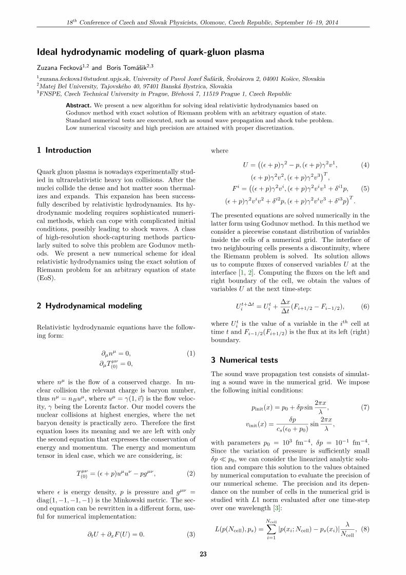
18th Conference of Czech and Slovak Physicists, Olomouc, Czech Republic, September 16–19, 2014
Ideal hydrodynamic modeling of quark-gluon plasma
Zuzana Fecková1,2 and Boris Tomášik2,3
[email protected], University of Pavol Jozef Šafárik, Šrobárova 2, 04001 Košice, Slovakia2Matej Bel University, Tajovského 40, 97401 Banská Bystrica, Slovakia3FNSPE, Czech Technical University in Prague, Břehová 7, 11519 Prague 1, Czech Republic
Abstract. We present a new algorithm for solving ideal relativistic hydrodynamics based onGodunov method with exact solution of Riemann problem with an arbitrary equation of state.Standard numerical tests are executed, such as sound wave propagation and shock tube problem.Low numerical viscosity and high precision are attained with proper discretization.
1 Introduction
Quark gluon plasma is nowadays experimentally stud-ied in ultrarelativistic heavy ion collisions. After thenuclei collide the dense and hot matter soon thermal-izes and expands. This expansion has been success-fully described by relativistic hydrodynamics. Its hy-drodynamic modeling requires sophisticated numeri-cal methods, which can cope with complicated initialconditions, possibly leading to shock waves. A classof high-resolution shock-capturing methods particu-larly suited to solve this problem are Godunov meth-ods. We present a new numerical scheme for idealrelativistic hydrodynamics using the exact solution ofRiemann problem for an arbitrary equation of state(EoS).
2 Hydrodynamical modeling
Relativistic hydrodynamic equations have the follow-ing form:
∂µnµ = 0, (1)
∂µTµν(0) = 0,
where nµ is the flow of a conserved charge. In nu-clear collision the relevant charge is baryon number,thus nµ = nBu
µ, where uµ = γ(1, ~v) is the flow veloc-ity, γ being the Lorentz factor. Our model covers thenuclear collisions at highest energies, where the netbaryon density is practically zero. Therefore the firstequation loses its meaning and we are left with onlythe second equation that expresses the conservation ofenergy and momentum. The energy and momentumtensor in ideal case, which we are considering, is:
Tµν(0) = (ǫ+ p)uµuν − pgµν , (2)
where ǫ is energy density, p is pressure and gµν =diag(1,−1,−1,−1) is the Minkowski metric. The sec-ond equation can be rewritten in a different form, use-ful for numerical implementation:
∂tU + ∂xF (U) = 0. (3)
where
U =(
(ǫ+ p)γ2 − p, (ǫ+ p)γ2v1, (4)
(ǫ+ p)γ2v2, (ǫ+ p)γ2v3)T,
F i =(
(ǫ+ p)γ2vi, (ǫ+ p)γ2viv1 + δi1p, (5)
(ǫ+ p)γ2viv2 + δi2p, (ǫ+ p)γ2viv3 + δi3p)T.
The presented equations are solved numerically in thelatter form using Godunov method. In this method weconsider a piecewise constant distribution of variablesinside the cells of a numerical grid. The interface oftwo neighbouring cells presents a discontinuity, wherethe Riemann problem is solved. Its solution allowsus to compute fluxes of conserved variables U at theinterface [1, 2]. Computing the fluxes on the left andright boundary of the cell, we obtain the values ofvariables U at the next time-step:
U t+∆ti = U t
i +∆x∆t
(Fi+1/2 − Fi−1/2), (6)
where U ti is the value of a variable in the ith cell at
time t and Fi−1/2(Fi+1/2) is the flux at its left (right)boundary.
3 Numerical tests
The sound wave propagation test consists of simulat-ing a sound wave in the numerical grid. We imposethe following initial conditions:
pinit(x) = p0 + δp sin2πxλ, (7)
vinit(x) =δp
cs(ǫ0 + p0)sin
2πxλ,
with parameters p0 = 103 fm−4, δp = 10−1 fm−4.Since the variation of pressure is sufficiently smallδp ≪ p0, we can consider the linearized analytic solu-tion and compare this solution to the values obtainedby numerical computation to evaluate the precision ofour numerical scheme. The precision and its depen-dance on the number of cells in the numerical grid isstudied with L1 norm evaluated after one time-stepover one wavelength [3]:
L(p(Ncell), ps) =Ncell∑
i=1
|p(xi;Ncell) − ps(xi)|λ
Ncell, (8)
232323
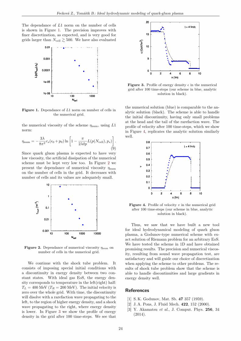
Fecková Z., Tomášik B.: Ideal hydrodynamic modeling of quark-gluon plasma
The dependance of L1 norm on the number of cellsis shown in Figure 1. The precision improves withfiner discretization, as expected, and is very good forgrids larger than Ncell & 500. We have also evaluated
Figure 1. Dependance of L1 norm on number of cells inthe numerical grid.
the numerical viscosity of the scheme ηnum, using L1norm:
ηnum = − 3λ8π2
cs(ǫ0 +p0) ln[
1 − π
2λδpL(p(Ncell), ps)
]
.
(9)Since quark gluon plasma is expected to have verylow viscosity, the artificial dissipation of the numericalscheme must be kept very low too. In Figure 2 wepresent the dependance of numerical viscosity ηnum
on the number of cells in the grid. It decreases withnumber of cells and its values are adequately small.
Figure 2. Dependance of numerical viscosity ηnum onnumber of cells in the numerical grid.
We continue with the shock tube problem. Itconsists of imposing special initial conditions witha discontinuity in energy density between two con-stant states. With ideal gas EoS, the energy den-sity corresponds to temperature in the left(right) half:TL = 400 MeV (TR = 200 MeV). The initial velocity iszero over the whole grid. With time, the discontinuitywill disolve with a rarefaction wave propagating to theleft, to the region of higher energy density, and a shockwave propagating to the right, where energy densityis lower. In Figure 3 we show the profile of energydensity in the grid after 100 time-steps. We see that
Figure 3. Profile of energy density ǫ in the numericalgrid after 100 time-steps (our scheme in blue, analytic
solution in black).
the numerical solution (blue) is comparable to the an-alytic solution (black). The scheme is able to handlethe initial discontinuity, having only small problemsat the head and the tail of the rarefaction wave. Theprofile of velocity after 100 time-steps, which we showin Figure 4, replicates the analytic solution similarlywell.
Figure 4. Profile of velocity v in the numerical gridafter 100 time-steps (our scheme in blue, analytic
solution in black).
Thus, we saw that we have built a new toolfor ideal hydrodynamical modeling of quark gluonplasma, a Godunov-type numerical scheme with ex-act solution of Riemann problem for an arbitrary EoS.We have tested the scheme in 1D and have obtainedpromising results. The precision and numerical viscos-ity, resulting from sound wave propagation test, aresatisfactory and will guide our choice of discretizationwhen applying the scheme to other problems. The re-sults of shock tube problem show that the scheme isable to handle discontinuities and large gradients inenergy density well.
References
[1] S. K. Godunov, Mat. Sb. 47 357 (1959).[2] J. A. Pons, J. Fluid Mech. 422, 152 (2000).[3] Y. Akamatsu et al., J. Comput. Phys. 256, 34
(2014).
24
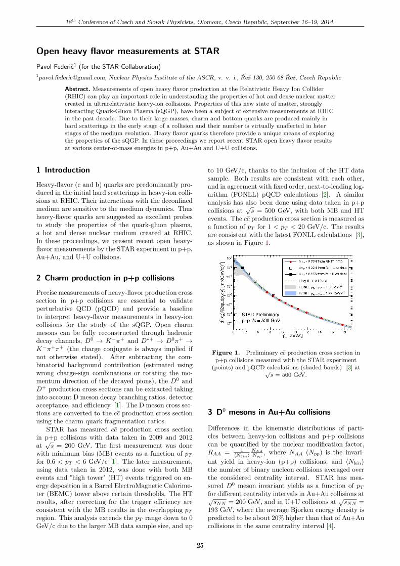
18th Conference of Czech and Slovak Physicists, Olomouc, Czech Republic, September 16–19, 2014
Open heavy flavor measurements at STAR
Pavol Federič1 (for the STAR Collaboration)[email protected], Nuclear Physics Institute of the ASCR, v. v. i., Řež 130, 250 68 Řež, Czech Republic
Abstract. Measurements of open heavy flavor production at the Relativistic Heavy Ion Collider(RHIC) can play an important role in understanding the properties of hot and dense nuclear mattercreated in ultrarelativistic heavy-ion collisions. Properties of this new state of matter, stronglyinteracting Quark-Gluon Plasma (sQGP), have been a subject of extensive measurements at RHICin the past decade. Due to their large masses, charm and bottom quarks are produced mainly inhard scatterings in the early stage of a collision and their number is virtually unaffected in laterstages of the medium evolution. Heavy flavor quarks therefore provide a unique means of exploringthe properties of the sQGP. In these proceedings we report recent STAR open heavy flavor resultsat various center-of-mass energies in p+p, Au+Au and U+U collisions.
1 Introduction
Heavy-flavor (c and b) quarks are predominantly pro-duced in the initial hard scatterings in heavy-ion colli-sions at RHIC. Their interactions with the deconfinedmedium are sensitive to the medium dynamics. Thusheavy-flavor quarks are suggested as excellent probesto study the properties of the quark-gluon plasma,a hot and dense nuclear medium created at RHIC.In these proceedings, we present recent open heavy-flavor measurements by the STAR experiment in p+p,Au+Au, and U+U collisions.
2 Charm production in p+p collisions
Precise measurements of heavy-flavor production crosssection in p+p collisions are essential to validateperturbative QCD (pQCD) and provide a baselineto interpret heavy-flavor measurements in heavy-ioncollisions for the study of the sQGP. Open charmmesons can be fully reconstructed through hadronicdecay channels, D0 → K−π+ and D∗+ → D0π+ →K−π+π+ (the charge conjugate is always implied ifnot otherwise stated). After subtracting the com-binatorial background contribution (estimated usingwrong charge-sign combinations or rotating the mo-mentum direction of the decayed pions), the D0 andD+ production cross sections can be extracted takinginto account D meson decay branching ratios, detectoracceptance, and efficiency [1]. The D meson cross sec-tions are converted to the cc production cross sectionusing the charm quark fragmentation ratios.
STAR has measured cc production cross sectionin p+p collisions with data taken in 2009 and 2012at
√s = 200 GeV. The first measurement was done
with minimum bias (MB) events as a function of pT
for 0.6 < pT < 6 GeV/c [1]. The later measurement,using data taken in 2012, was done with both MBevents and "high tower" (HT) events triggered on en-ergy deposition in a Barrel ElectroMagnetic Calorime-ter (BEMC) tower above certain thresholds. The HTresults, after correcting for the trigger efficiency areconsistent with the MB results in the overlapping pT
region. This analysis extends the pT range down to 0GeV/c due to the larger MB data sample size, and up
to 10 GeV/c, thanks to the inclusion of the HT datasample. Both results are consistent with each other,and in agreement with fixed order, next-to-leading log-arithm (FONLL) pQCD calculations [2]. A similaranalysis has also been done using data taken in p+pcollisions at
√s = 500 GeV, with both MB and HT
events. The cc production cross section is measured asa function of pT for 1 < pT < 20 GeV/c. The resultsare consistent with the latest FONLL calculations [3],as shown in Figure 1.
Figure 1. Preliminary cc production cross section inp+p collisions measured with the STAR experiment
(points) and pQCD calculations (shaded bands) [3] at√s = 500 GeV.
3 D0 mesons in Au+Au collisions
Differences in the kinematic distributions of parti-cles between heavy-ion collisions and p+p collisionscan be quantified by the nuclear modification factor,RAA = 1
〈Nbin〉NAA
Npp, where NAA (Npp) is the invari-
ant yield in heavy-ion (p+p) collisions, and 〈Nbin〉the number of binary nucleon collisions averaged overthe considered centrality interval. STAR has mea-sured D0 meson invariant yields as a function of pT
for different centrality intervals in Au+Au collisions at√sNN = 200 GeV, and in U+U collisions at
√sNN =
193 GeV, where the average Bjorken energy density ispredicted to be about 20% higher than that of Au+Aucollisions in the same centrality interval [4].
252525
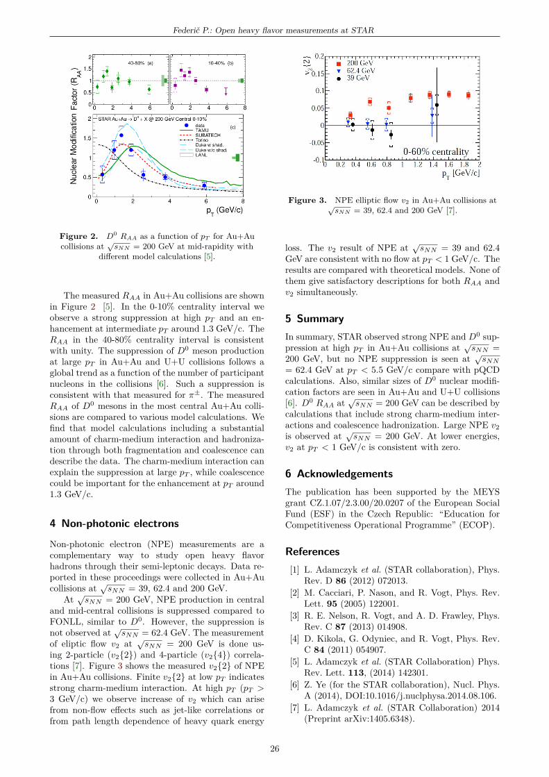
Federič P.: Open heavy flavor measurements at STAR
Figure 2. D0 RAA as a function of pT for Au+Aucollisions at
√sNN = 200 GeV at mid-rapidity with
different model calculations [5].
The measured RAA in Au+Au collisions are shownin Figure 2 [5]. In the 0-10% centrality interval weobserve a strong suppression at high pT and an en-hancement at intermediate pT around 1.3 GeV/c. TheRAA in the 40-80% centrality interval is consistentwith unity. The suppression of D0 meson productionat large pT in Au+Au and U+U collisions follows aglobal trend as a function of the number of participantnucleons in the collisions [6]. Such a suppression isconsistent with that measured for π±. The measuredRAA of D0 mesons in the most central Au+Au colli-sions are compared to various model calculations. Wefind that model calculations including a substantialamount of charm-medium interaction and hadroniza-tion through both fragmentation and coalescence candescribe the data. The charm-medium interaction canexplain the suppression at large pT , while coalescencecould be important for the enhancement at pT around1.3 GeV/c.
4 Non-photonic electrons
Non-photonic electron (NPE) measurements are acomplementary way to study open heavy flavorhadrons through their semi-leptonic decays. Data re-ported in these proceedings were collected in Au+Aucollisions at
√sNN = 39, 62.4 and 200 GeV.
At√sNN = 200 GeV, NPE production in central
and mid-central collisions is suppressed compared toFONLL, similar to D0. However, the suppression isnot observed at
√sNN = 62.4 GeV. The measurement
of eliptic flow v2 at√sNN = 200 GeV is done us-
ing 2-particle (v22) and 4-particle (v24) correla-tions [7]. Figure 3 shows the measured v22 of NPEin Au+Au collisions. Finite v22 at low pT indicatesstrong charm-medium interaction. At high pT (pT >3 GeV/c) we observe increase of v2 which can arisefrom non-flow effects such as jet-like correlations orfrom path length dependence of heavy quark energy
Figure 3. NPE elliptic flow v2 in Au+Au collisions at√sNN = 39, 62.4 and 200 GeV [7].
loss. The v2 result of NPE at√sNN = 39 and 62.4
GeV are consistent with no flow at pT < 1 GeV/c. Theresults are compared with theoretical models. None ofthem give satisfactory descriptions for both RAA andv2 simultaneously.
5 Summary
In summary, STAR observed strong NPE and D0 sup-pression at high pT in Au+Au collisions at
√sNN =
200 GeV, but no NPE suppression is seen at√sNN
= 62.4 GeV at pT < 5.5 GeV/c compare with pQCDcalculations. Also, similar sizes of D0 nuclear modifi-cation factors are seen in Au+Au and U+U collisions[6]. D0 RAA at
√sNN = 200 GeV can be described by
calculations that include strong charm-medium inter-actions and coalescence hadronization. Large NPE v2
is observed at√sNN = 200 GeV. At lower energies,
v2 at pT < 1 GeV/c is consistent with zero.
6 Acknowledgements
The publication has been supported by the MEYSgrant CZ.1.07/2.3.00/20.0207 of the European SocialFund (ESF) in the Czech Republic: “Education forCompetitiveness Operational Programme” (ECOP).
References
[1] L. Adamczyk et al. (STAR collaboration), Phys.Rev. D 86 (2012) 072013.
[2] M. Cacciari, P. Nason, and R. Vogt, Phys. Rev.Lett. 95 (2005) 122001.
[3] R. E. Nelson, R. Vogt, and A. D. Frawley, Phys.Rev. C 87 (2013) 014908.
[4] D. Kikola, G. Odyniec, and R. Vogt, Phys. Rev.C 84 (2011) 054907.
[5] L. Adamczyk et al. (STAR Collaboration) Phys.Rev. Lett. 113, (2014) 142301.
[6] Z. Ye (for the STAR collaboration), Nucl. Phys.A (2014), DOI:10.1016/j.nuclphysa.2014.08.106.
[7] L. Adamczyk et al. (STAR Collaboration) 2014(Preprint arXiv:1405.6348).
26
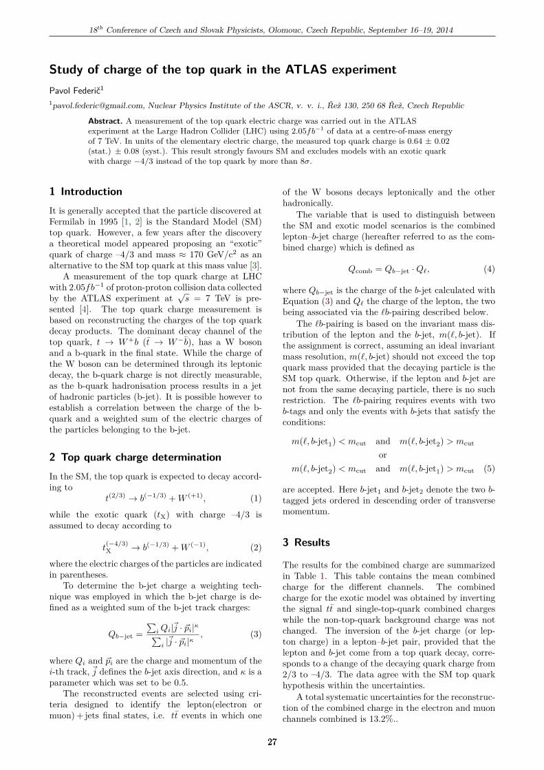
18th Conference of Czech and Slovak Physicists, Olomouc, Czech Republic, September 16–19, 2014
Study of charge of the top quark in the ATLAS experiment
Pavol Federič1
[email protected], Nuclear Physics Institute of the ASCR, v. v. i., Řež 130, 250 68 Řež, Czech Republic
Abstract. A measurement of the top quark electric charge was carried out in the ATLASexperiment at the Large Hadron Collider (LHC) using 2.05fb−1 of data at a centre-of-mass energyof 7 TeV. In units of the elementary electric charge, the measured top quark charge is 0.64 ± 0.02(stat.) ± 0.08 (syst.). This result strongly favours SM and excludes models with an exotic quarkwith charge −4/3 instead of the top quark by more than 8σ.
1 Introduction
It is generally accepted that the particle discovered atFermilab in 1995 [1, 2] is the Standard Model (SM)top quark. However, a few years after the discoverya theoretical model appeared proposing an “exotic”quark of charge –4/3 and mass ≈ 170 GeV/c2 as analternative to the SM top quark at this mass value [3].
A measurement of the top quark charge at LHCwith 2.05fb−1 of proton-proton collision data collectedby the ATLAS experiment at
√s = 7 TeV is pre-
sented [4]. The top quark charge measurement isbased on reconstructing the charges of the top quarkdecay products. The dominant decay channel of thetop quark, t → W+b (t → W−b), has a W bosonand a b-quark in the final state. While the charge ofthe W boson can be determined through its leptonicdecay, the b-quark charge is not directly measurable,as the b-quark hadronisation process results in a jetof hadronic particles (b-jet). It is possible however toestablish a correlation between the charge of the b-quark and a weighted sum of the electric charges ofthe particles belonging to the b-jet.
2 Top quark charge determination
In the SM, the top quark is expected to decay accord-ing to
t(2/3) → b(−1/3) +W (+1), (1)
while the exotic quark (tX) with charge –4/3 isassumed to decay according to
t(−4/3)X → b(−1/3) +W (−1), (2)
where the electric charges of the particles are indicatedin parentheses.
To determine the b-jet charge a weighting tech-nique was employed in which the b-jet charge is de-fined as a weighted sum of the b-jet track charges:
Qb−jet =
∑
i Qi|~j · ~pi|κ∑
i |~j · ~pi|κ, (3)
where Qi and ~pi are the charge and momentum of thei-th track, ~j defines the b-jet axis direction, and κ is aparameter which was set to be 0.5.
The reconstructed events are selected using cri-teria designed to identify the lepton(electron ormuon) + jets final states, i.e. tt events in which one
of the W bosons decays leptonically and the otherhadronically.
The variable that is used to distinguish betweenthe SM and exotic model scenarios is the combinedlepton–b-jet charge (hereafter referred to as the com-bined charge) which is defined as
Qcomb = Qb−jet ·Qℓ, (4)
where Qb−jet is the charge of the b-jet calculated withEquation (3) and Qℓ the charge of the lepton, the twobeing associated via the ℓb-pairing described below.
The ℓb-pairing is based on the invariant mass dis-tribution of the lepton and the b-jet, m(ℓ, b-jet). Ifthe assignment is correct, assuming an ideal invariantmass resolution, m(ℓ, b-jet) should not exceed the topquark mass provided that the decaying particle is theSM top quark. Otherwise, if the lepton and b-jet arenot from the same decaying particle, there is no suchrestriction. The ℓb-pairing requires events with twob-tags and only the events with b-jets that satisfy theconditions:
m(ℓ, b-jet1) < mcut and m(ℓ, b-jet2) > mcut
or
m(ℓ, b-jet2) < mcut and m(ℓ, b-jet1) > mcut (5)
are accepted. Here b-jet1 and b-jet2 denote the two b-tagged jets ordered in descending order of transversemomentum.
3 Results
The results for the combined charge are summarizedin Table 1. This table contains the mean combinedcharge for the different channels. The combinedcharge for the exotic model was obtained by invertingthe signal tt and single-top-quark combined chargeswhile the non-top-quark background charge was notchanged. The inversion of the b-jet charge (or lep-ton charge) in a lepton–b-jet pair, provided that thelepton and b-jet come from a top quark decay, corre-sponds to a change of the decaying quark charge from2/3 to –4/3. The data agree with the SM top quarkhypothesis within the uncertainties.
A total systematic uncertainties for the reconstruc-tion of the combined charge in the electron and muonchannels combined is 13.2%..
272727
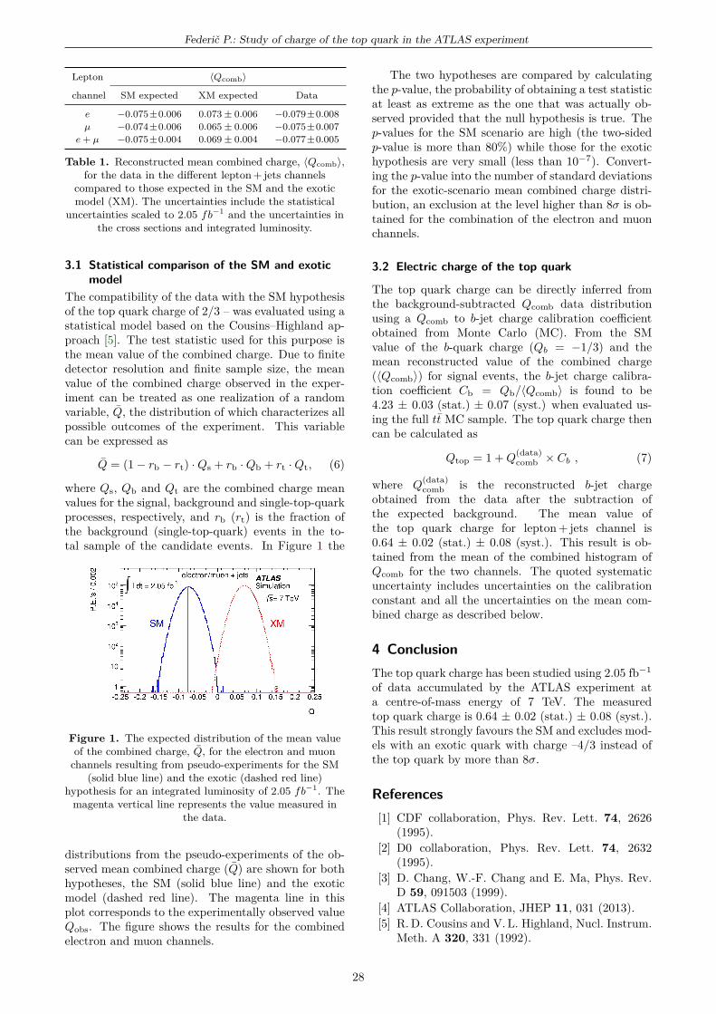
Federič P.: Study of charge of the top quark in the ATLAS experiment
Lepton 〈Qcomb〉
channel SM expected XM expected Data
e −0.075±0.006 0.073 ± 0.006 −0.079±0.008
µ −0.074±0.006 0.065 ± 0.006 −0.075±0.007
e + µ −0.075±0.004 0.069 ± 0.004 −0.077±0.005
Table 1. Reconstructed mean combined charge, 〈Qcomb〉,for the data in the different lepton + jets channels
compared to those expected in the SM and the exoticmodel (XM). The uncertainties include the statistical
uncertainties scaled to 2.05 fb−1 and the uncertainties inthe cross sections and integrated luminosity.
3.1 Statistical comparison of the SM and exoticmodel
The compatibility of the data with the SM hypothesisof the top quark charge of 2/3 – was evaluated using astatistical model based on the Cousins–Highland ap-proach [5]. The test statistic used for this purpose isthe mean value of the combined charge. Due to finitedetector resolution and finite sample size, the meanvalue of the combined charge observed in the exper-iment can be treated as one realization of a randomvariable, Q, the distribution of which characterizes allpossible outcomes of the experiment. This variablecan be expressed as
Q = (1 − rb − rt) ·Qs + rb ·Qb + rt ·Qt, (6)
where Qs, Qb and Qt are the combined charge meanvalues for the signal, background and single-top-quarkprocesses, respectively, and rb (rt) is the fraction ofthe background (single-top-quark) events in the to-tal sample of the candidate events. In Figure 1 the
Figure 1. The expected distribution of the mean valueof the combined charge, Q, for the electron and muon
channels resulting from pseudo-experiments for the SM(solid blue line) and the exotic (dashed red line)
hypothesis for an integrated luminosity of 2.05 fb−1. Themagenta vertical line represents the value measured in
the data.
distributions from the pseudo-experiments of the ob-served mean combined charge (Q) are shown for bothhypotheses, the SM (solid blue line) and the exoticmodel (dashed red line). The magenta line in thisplot corresponds to the experimentally observed valueQobs. The figure shows the results for the combinedelectron and muon channels.
The two hypotheses are compared by calculatingthe p-value, the probability of obtaining a test statisticat least as extreme as the one that was actually ob-served provided that the null hypothesis is true. Thep-values for the SM scenario are high (the two-sidedp-value is more than 80%) while those for the exotichypothesis are very small (less than 10−7). Convert-ing the p-value into the number of standard deviationsfor the exotic-scenario mean combined charge distri-bution, an exclusion at the level higher than 8σ is ob-tained for the combination of the electron and muonchannels.
3.2 Electric charge of the top quark
The top quark charge can be directly inferred fromthe background-subtracted Qcomb data distributionusing a Qcomb to b-jet charge calibration coefficientobtained from Monte Carlo (MC). From the SMvalue of the b-quark charge (Qb = −1/3) and themean reconstructed value of the combined charge(〈Qcomb〉) for signal events, the b-jet charge calibra-tion coefficient Cb = Qb/〈Qcomb〉 is found to be4.23 ± 0.03 (stat.) ± 0.07 (syst.) when evaluated us-ing the full tt MC sample. The top quark charge thencan be calculated as
Qtop = 1 +Q(data)comb × Cb , (7)
where Q(data)comb is the reconstructed b-jet charge
obtained from the data after the subtraction ofthe expected background. The mean value ofthe top quark charge for lepton + jets channel is0.64 ± 0.02 (stat.) ± 0.08 (syst.). This result is ob-tained from the mean of the combined histogram ofQcomb for the two channels. The quoted systematicuncertainty includes uncertainties on the calibrationconstant and all the uncertainties on the mean com-bined charge as described below.
4 Conclusion
The top quark charge has been studied using 2.05 fb−1
of data accumulated by the ATLAS experiment ata centre-of-mass energy of 7 TeV. The measuredtop quark charge is 0.64 ± 0.02 (stat.) ± 0.08 (syst.).This result strongly favours the SM and excludes mod-els with an exotic quark with charge –4/3 instead ofthe top quark by more than 8σ.
References
[1] CDF collaboration, Phys. Rev. Lett. 74, 2626(1995).
[2] D0 collaboration, Phys. Rev. Lett. 74, 2632(1995).
[3] D. Chang, W.-F. Chang and E. Ma, Phys. Rev.D 59, 091503 (1999).
[4] ATLAS Collaboration, JHEP 11, 031 (2013).[5] R. D. Cousins and V. L. Highland, Nucl. Instrum.
Meth. A 320, 331 (1992).
28
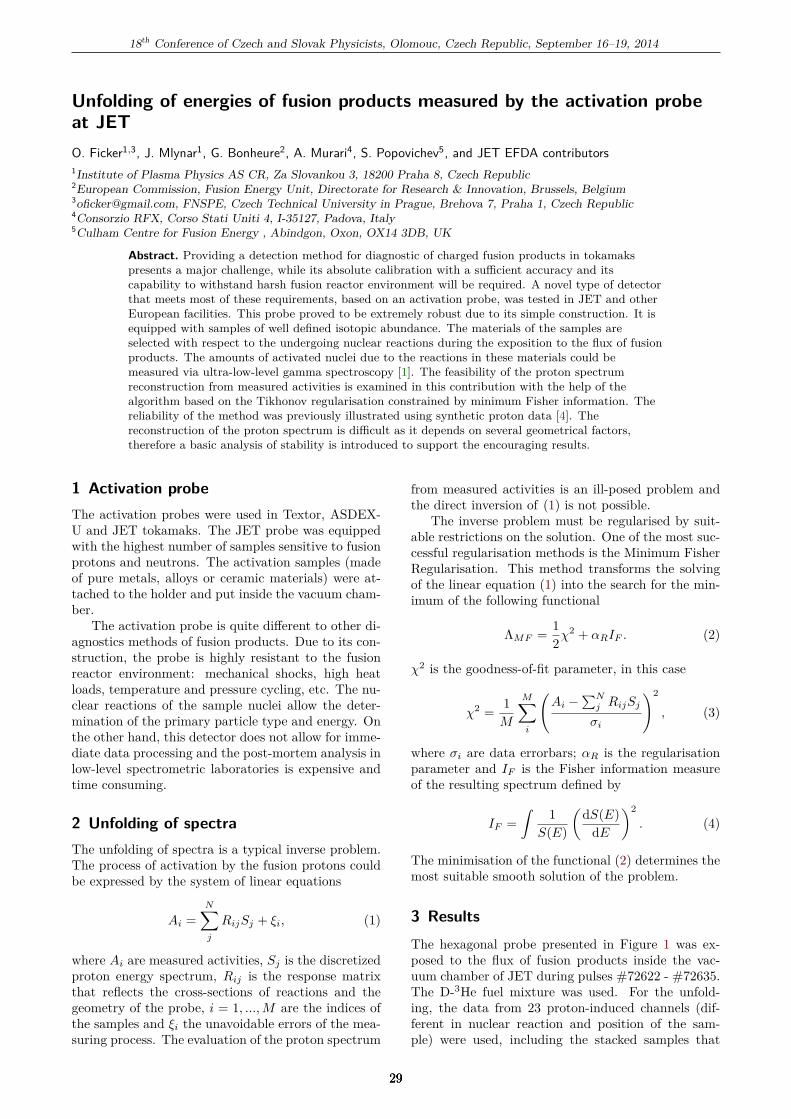
18th Conference of Czech and Slovak Physicists, Olomouc, Czech Republic, September 16–19, 2014
Unfolding of energies of fusion products measured by the activation probeat JET
O. Ficker1,3, J. Mlynar1, G. Bonheure2, A. Murari4, S. Popovichev5, and JET EFDA contributors1Institute of Plasma Physics AS CR, Za Slovankou 3, 18200 Praha 8, Czech Republic2European Commission, Fusion Energy Unit, Directorate for Research & Innovation, Brussels, [email protected], FNSPE, Czech Technical University in Prague, Brehova 7, Praha 1, Czech Republic4Consorzio RFX, Corso Stati Uniti 4, I-35127, Padova, Italy5Culham Centre for Fusion Energy , Abindgon, Oxon, OX14 3DB, UK
Abstract. Providing a detection method for diagnostic of charged fusion products in tokamakspresents a major challenge, while its absolute calibration with a sufficient accuracy and itscapability to withstand harsh fusion reactor environment will be required. A novel type of detectorthat meets most of these requirements, based on an activation probe, was tested in JET and otherEuropean facilities. This probe proved to be extremely robust due to its simple construction. It isequipped with samples of well defined isotopic abundance. The materials of the samples areselected with respect to the undergoing nuclear reactions during the exposition to the flux of fusionproducts. The amounts of activated nuclei due to the reactions in these materials could bemeasured via ultra-low-level gamma spectroscopy [1]. The feasibility of the proton spectrumreconstruction from measured activities is examined in this contribution with the help of thealgorithm based on the Tikhonov regularisation constrained by minimum Fisher information. Thereliability of the method was previously illustrated using synthetic proton data [4]. Thereconstruction of the proton spectrum is difficult as it depends on several geometrical factors,therefore a basic analysis of stability is introduced to support the encouraging results.
1 Activation probe
The activation probes were used in Textor, ASDEX-U and JET tokamaks. The JET probe was equippedwith the highest number of samples sensitive to fusionprotons and neutrons. The activation samples (madeof pure metals, alloys or ceramic materials) were at-tached to the holder and put inside the vacuum cham-ber.
The activation probe is quite different to other di-agnostics methods of fusion products. Due to its con-struction, the probe is highly resistant to the fusionreactor environment: mechanical shocks, high heatloads, temperature and pressure cycling, etc. The nu-clear reactions of the sample nuclei allow the deter-mination of the primary particle type and energy. Onthe other hand, this detector does not allow for imme-diate data processing and the post-mortem analysis inlow-level spectrometric laboratories is expensive andtime consuming.
2 Unfolding of spectra
The unfolding of spectra is a typical inverse problem.The process of activation by the fusion protons couldbe expressed by the system of linear equations
Ai =N∑
j
RijSj + ξi, (1)
where Ai are measured activities, Sj is the discretizedproton energy spectrum, Rij is the response matrixthat reflects the cross-sections of reactions and thegeometry of the probe, i = 1, ...,M are the indices ofthe samples and ξi the unavoidable errors of the mea-suring process. The evaluation of the proton spectrum
from measured activities is an ill-posed problem andthe direct inversion of (1) is not possible.
The inverse problem must be regularised by suit-able restrictions on the solution. One of the most suc-cessful regularisation methods is the Minimum FisherRegularisation. This method transforms the solvingof the linear equation (1) into the search for the min-imum of the following functional
ΛMF =12χ2 + αRIF . (2)
χ2 is the goodness-of-fit parameter, in this case
χ2 =1M
M∑
i
(
Ai −∑N
j RijSj
σi
)2
, (3)
where σi are data errorbars; αR is the regularisationparameter and IF is the Fisher information measureof the resulting spectrum defined by
IF =∫
1S(E)
(
dS(E)dE
)2
. (4)
The minimisation of the functional (2) determines themost suitable smooth solution of the problem.
3 Results
The hexagonal probe presented in Figure 1 was ex-posed to the flux of fusion products inside the vac-uum chamber of JET during pulses #72622 - #72635.The D-3He fuel mixture was used. For the unfold-ing, the data from 23 proton-induced channels (dif-ferent in nuclear reaction and position of the sam-ple) were used, including the stacked samples that
292929
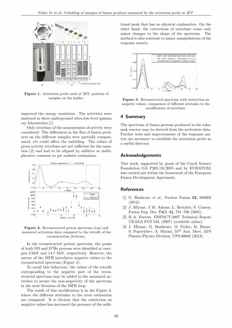
Ficker O. et al.: Unfolding of energies of fusion products measured by the activation probe at JET
Figure 1. Activation probe used at JET, position ofsamples on the holder.
improved the energy resolution. The activities wereanalysed in three underground ultra-low-level gammaray laboratories.[1]
Only errorbars of the measurement of activity wereconsidered. The differences in the flux of fusion prod-ucts on the different samples were partially compen-sated, yet could affect the unfolding. The values ofgiven activity errorbars are not sufficient for the equa-tion (2) and had to be aligned by additive or multi-plicative constant to get realistic estimation.
Figure 2. Reconstructed proton spectrum (top) andmeasured activation data compared to the retrofit of the
reconstruction (bottom).
In the reconstructed proton spectrum, the peaksof both DD and D3He protons were identified at ener-gies 3 MeV and 14.7 MeV, respectively. However, thenature of the MFR introduces negative values to thereconstructed spectrum (Figure 2).
To avoid this behaviour, the values of the retrofitcorresponding to the negative part of the recon-structed spectrum may be added to the measured ac-tivities to secure the non-negativity of the spectrumin the next iteration of the MFR loop.
The result of this modification is in the Figure 3,where the different attitudes to the error estimationare compared. It is obvious that the restriction onnegative values has increased the presence of the addi-
tional peak that has no physical explanation. On theother hand, the corrections of errorbars cause onlyminor changes to the shape of the spectrum. Themethod is also resistant to minor manipulations of theresponse matrix.
Figure 3. Reconstructed spectrum with restriction onnegative values, comparison of different attitudes to the
modification of errorbars.
4 Summary
The spectrum of fusion protons produced in the toka-mak reactor may be derived from the activation data.Further tests and improvements of the response ma-trix are necessary to establish the activation probe asa useful detector.
Acknowledgements
This work, supported by grant of the Czech ScienceFoundation GA P205/10/2055 and by EURATOM,was carried out within the framework of the EuropeanFusion Development Agreement.
References
[1] G. Bonheure et al., Nuclear Fusion 52, 083004(2012).
[2] J. Mlynar, J. M. Adams, L. Bertalot, S. Conroy,Fusion Eng. Des. 74(1–4), 781–786 (2005).
[3] R. A. Forrest, FISPACT-2007 Technical ReportUKAEA FUS 534, (2007) (available online).
[4] J. Mlynar, G. Bonheure, O. Ficker, K. Bauer,S. Popovichev, A. Murari, 55th Ann. Meet. APSPlasma Physics Division, UP8.00003 (2013).
30
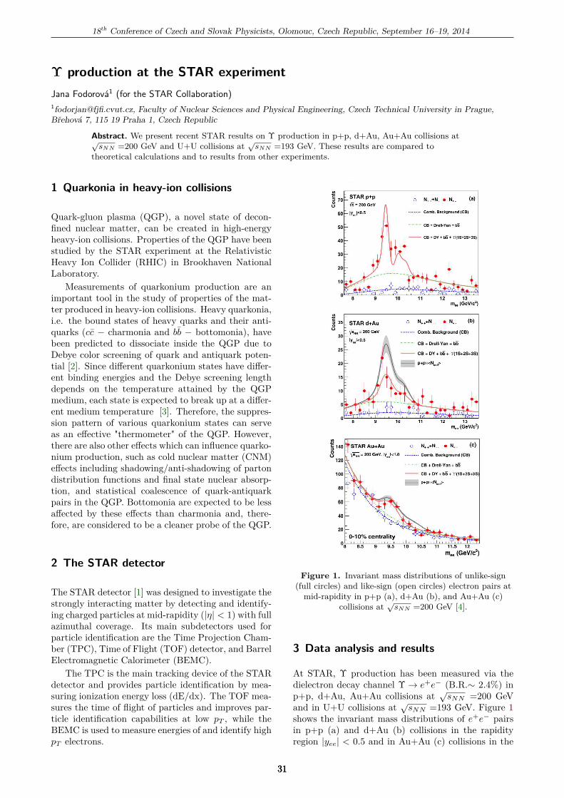
18th Conference of Czech and Slovak Physicists, Olomouc, Czech Republic, September 16–19, 2014
Υ production at the STAR experiment
Jana Fodorová1 (for the STAR Collaboration)[email protected], Faculty of Nuclear Sciences and Physical Engineering, Czech Technical University in Prague,Břehová 7, 115 19 Praha 1, Czech Republic
Abstract. We present recent STAR results on Υ production in p+p, d+Au, Au+Au collisions at√sNN =200 GeV and U+U collisions at
√sNN =193 GeV. These results are compared to
theoretical calculations and to results from other experiments.
1 Quarkonia in heavy-ion collisions
Quark-gluon plasma (QGP), a novel state of decon-fined nuclear matter, can be created in high-energyheavy-ion collisions. Properties of the QGP have beenstudied by the STAR experiment at the RelativisticHeavy Ion Collider (RHIC) in Brookhaven NationalLaboratory.
Measurements of quarkonium production are animportant tool in the study of properties of the mat-ter produced in heavy-ion collisions. Heavy quarkonia,i.e. the bound states of heavy quarks and their anti-quarks (cc − charmonia and bb − bottomonia), havebeen predicted to dissociate inside the QGP due toDebye color screening of quark and antiquark poten-tial [2]. Since different quarkonium states have differ-ent binding energies and the Debye screening lengthdepends on the temperature attained by the QGPmedium, each state is expected to break up at a differ-ent medium temperature [3]. Therefore, the suppres-sion pattern of various quarkonium states can serveas an effective "thermometer" of the QGP. However,there are also other effects which can influence quarko-nium production, such as cold nuclear matter (CNM)effects including shadowing/anti-shadowing of partondistribution functions and final state nuclear absorp-tion, and statistical coalescence of quark-antiquarkpairs in the QGP. Bottomonia are expected to be lessaffected by these effects than charmonia and, there-fore, are considered to be a cleaner probe of the QGP.
2 The STAR detector
The STAR detector [1] was designed to investigate thestrongly interacting matter by detecting and identify-ing charged particles at mid-rapidity (|η| < 1) with fullazimuthal coverage. Its main subdetectors used forparticle identification are the Time Projection Cham-ber (TPC), Time of Flight (TOF) detector, and BarrelElectromagnetic Calorimeter (BEMC).
The TPC is the main tracking device of the STARdetector and provides particle identification by mea-suring ionization energy loss (dE/dx). The TOF mea-sures the time of flight of particles and improves par-ticle identification capabilities at low pT , while theBEMC is used to measure energies of and identify highpT electrons.
Figure 1. Invariant mass distributions of unlike-sign(full circles) and like-sign (open circles) electron pairs at
mid-rapidity in p+p (a), d+Au (b), and Au+Au (c)collisions at
√sNN =200 GeV [4].
3 Data analysis and results
At STAR, Υ production has been measured via thedielectron decay channel Υ → e+e− (B.R.∼ 2.4%) inp+p, d+Au, Au+Au collisions at
√sNN =200 GeV
and in U+U collisions at√sNN =193 GeV. Figure 1
shows the invariant mass distributions of e+e− pairsin p+p (a) and d+Au (b) collisions in the rapidityregion |yee| < 0.5 and in Au+Au (c) collisions in the
313131
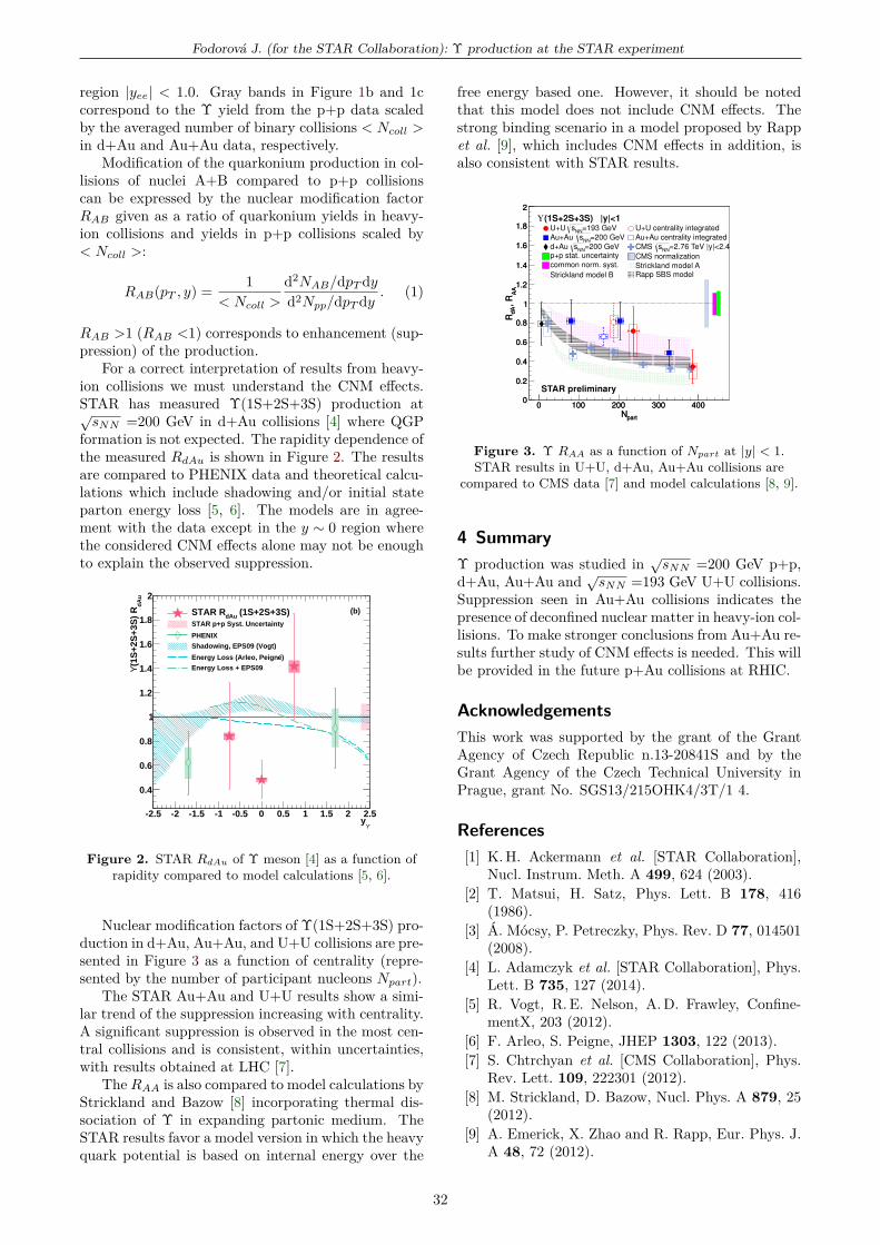
Fodorová J. (for the STAR Collaboration): Υ production at the STAR experiment
region |yee| < 1.0. Gray bands in Figure 1b and 1ccorrespond to the Υ yield from the p+p data scaledby the averaged number of binary collisions < Ncoll >in d+Au and Au+Au data, respectively.
Modification of the quarkonium production in col-lisions of nuclei A+B compared to p+p collisionscan be expressed by the nuclear modification factorRAB given as a ratio of quarkonium yields in heavy-ion collisions and yields in p+p collisions scaled by< Ncoll >:
RAB(pT , y) =1
< Ncoll >
d2NAB/dpT dyd2Npp/dpT dy
. (1)
RAB >1 (RAB <1) corresponds to enhancement (sup-pression) of the production.
For a correct interpretation of results from heavy-ion collisions we must understand the CNM effects.STAR has measured Υ(1S+2S+3S) production at√sNN =200 GeV in d+Au collisions [4] where QGP
formation is not expected. The rapidity dependence ofthe measured RdAu is shown in Figure 2. The resultsare compared to PHENIX data and theoretical calcu-lations which include shadowing and/or initial stateparton energy loss [5, 6]. The models are in agree-ment with the data except in the y ∼ 0 region wherethe considered CNM effects alone may not be enoughto explain the observed suppression.
ϒy
-2.5 -2 -1.5 -1 -0.5 0 0.5 1 1.5 2 2.5
dAu
(1S
+2S
+3S
) R
ϒ
0.4
0.6
0.8
1
1.2
1.4
1.6
1.8
2
(1S+2S+3S)dAuSTAR RSTAR p+p Syst. Uncertainty
PHENIX
Shadowing, EPS09 (Vogt)
)eEnergy Loss (Arleo, Peign
Energy Loss + EPS09
(b)
Figure 2. STAR RdAu of Υ meson [4] as a function ofrapidity compared to model calculations [5, 6].
Nuclear modification factors of Υ(1S+2S+3S) pro-duction in d+Au, Au+Au, and U+U collisions are pre-sented in Figure 3 as a function of centrality (repre-sented by the number of participant nucleons Npart).
The STAR Au+Au and U+U results show a simi-lar trend of the suppression increasing with centrality.A significant suppression is observed in the most cen-tral collisions and is consistent, within uncertainties,with results obtained at LHC [7].
The RAA is also compared to model calculations byStrickland and Bazow [8] incorporating thermal dis-sociation of Υ in expanding partonic medium. TheSTAR results favor a model version in which the heavyquark potential is based on internal energy over the
free energy based one. However, it should be notedthat this model does not include CNM effects. Thestrong binding scenario in a model proposed by Rappet al. [9], which includes CNM effects in addition, isalso consistent with STAR results.
partN0 100 200 300 400
AA
, R
dA
R
0
0.2
0.4
0.6
0.8
1
1.2
1.4
1.6
1.8
2
partN0 100 200 300 400
AA
, R
dA
R
0
0.2
0.4
0.6
0.8
1
1.2
1.4
1.6
1.8
2
=193 GeVNN
sU+U U+U centrality integrated
=200 GeVNN
sAu+Au Au+Au centrality integrated
=200 GeVNN
sd+Au =2.76 TeV |y|<2.4NN
sCMS p+p stat. uncertainty CMS normalizationcommon norm. syst. Strickland model A
Strickland model B Rapp SBS model
STAR preliminary
(1S+2S+3S) |y|<1Υ
Figure 3. Υ RAA as a function of Npart at |y| < 1.STAR results in U+U, d+Au, Au+Au collisions are
compared to CMS data [7] and model calculations [8, 9].
4 Summary
Υ production was studied in√sNN =200 GeV p+p,
d+Au, Au+Au and√sNN =193 GeV U+U collisions.
Suppression seen in Au+Au collisions indicates thepresence of deconfined nuclear matter in heavy-ion col-lisions. To make stronger conclusions from Au+Au re-sults further study of CNM effects is needed. This willbe provided in the future p+Au collisions at RHIC.
Acknowledgements
This work was supported by the grant of the GrantAgency of Czech Republic n.13-20841S and by theGrant Agency of the Czech Technical University inPrague, grant No. SGS13/215OHK4/3T/1 4.
References
[1] K. H. Ackermann et al. [STAR Collaboration],Nucl. Instrum. Meth. A 499, 624 (2003).
[2] T. Matsui, H. Satz, Phys. Lett. B 178, 416(1986).
[3] Á. Mócsy, P. Petreczky, Phys. Rev. D 77, 014501(2008).
[4] L. Adamczyk et al. [STAR Collaboration], Phys.Lett. B 735, 127 (2014).
[5] R. Vogt, R. E. Nelson, A. D. Frawley, Confine-mentX, 203 (2012).
[6] F. Arleo, S. Peigne, JHEP 1303, 122 (2013).[7] S. Chtrchyan et al. [CMS Collaboration], Phys.
Rev. Lett. 109, 222301 (2012).[8] M. Strickland, D. Bazow, Nucl. Phys. A 879, 25
(2012).[9] A. Emerick, X. Zhao and R. Rapp, Eur. Phys. J.
A 48, 72 (2012).
32
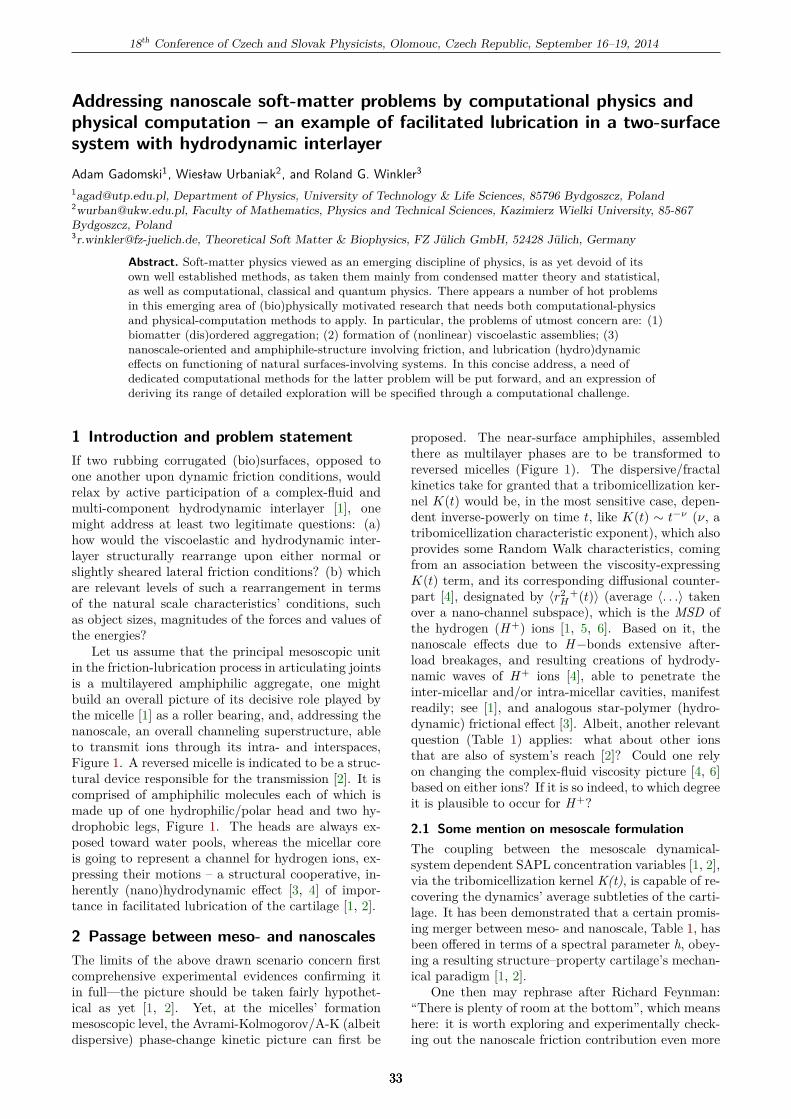
18th Conference of Czech and Slovak Physicists, Olomouc, Czech Republic, September 16–19, 2014
Addressing nanoscale soft-matter problems by computational physics andphysical computation – an example of facilitated lubrication in a two-surfacesystem with hydrodynamic interlayer
Adam Gadomski1, Wiesław Urbaniak2, and Roland G. Winkler3
[email protected], Department of Physics, University of Technology & Life Sciences, 85796 Bydgoszcz, [email protected], Faculty of Mathematics, Physics and Technical Sciences, Kazimierz Wielki University, 85-867Bydgoszcz, [email protected], Theoretical Soft Matter & Biophysics, FZ Jülich GmbH, 52428 Jülich, Germany
Abstract. Soft-matter physics viewed as an emerging discipline of physics, is as yet devoid of itsown well established methods, as taken them mainly from condensed matter theory and statistical,as well as computational, classical and quantum physics. There appears a number of hot problemsin this emerging area of (bio)physically motivated research that needs both computational-physicsand physical-computation methods to apply. In particular, the problems of utmost concern are: (1)biomatter (dis)ordered aggregation; (2) formation of (nonlinear) viscoelastic assemblies; (3)nanoscale-oriented and amphiphile-structure involving friction, and lubrication (hydro)dynamiceffects on functioning of natural surfaces-involving systems. In this concise address, a need ofdedicated computational methods for the latter problem will be put forward, and an expression ofderiving its range of detailed exploration will be specified through a computational challenge.
1 Introduction and problem statement
If two rubbing corrugated (bio)surfaces, opposed toone another upon dynamic friction conditions, wouldrelax by active participation of a complex-fluid andmulti-component hydrodynamic interlayer [1], onemight address at least two legitimate questions: (a)how would the viscoelastic and hydrodynamic inter-layer structurally rearrange upon either normal orslightly sheared lateral friction conditions? (b) whichare relevant levels of such a rearrangement in termsof the natural scale characteristics’ conditions, suchas object sizes, magnitudes of the forces and values ofthe energies?
Let us assume that the principal mesoscopic unitin the friction-lubrication process in articulating jointsis a multilayered amphiphilic aggregate, one mightbuild an overall picture of its decisive role played bythe micelle [1] as a roller bearing, and, addressing thenanoscale, an overall channeling superstructure, ableto transmit ions through its intra- and interspaces,Figure 1. A reversed micelle is indicated to be a struc-tural device responsible for the transmission [2]. It iscomprised of amphiphilic molecules each of which ismade up of one hydrophilic/polar head and two hy-drophobic legs, Figure 1. The heads are always ex-posed toward water pools, whereas the micellar coreis going to represent a channel for hydrogen ions, ex-pressing their motions – a structural cooperative, in-herently (nano)hydrodynamic effect [3, 4] of impor-tance in facilitated lubrication of the cartilage [1, 2].
2 Passage between meso- and nanoscales
The limits of the above drawn scenario concern firstcomprehensive experimental evidences confirming itin full—the picture should be taken fairly hypothet-ical as yet [1, 2]. Yet, at the micelles’ formationmesoscopic level, the Avrami-Kolmogorov/A-K (albeitdispersive) phase-change kinetic picture can first be
proposed. The near-surface amphiphiles, assembledthere as multilayer phases are to be transformed toreversed micelles (Figure 1). The dispersive/fractalkinetics take for granted that a tribomicellization ker-nel K(t) would be, in the most sensitive case, depen-dent inverse-powerly on time t, like K(t) ∼ t−ν (ν, atribomicellization characteristic exponent), which alsoprovides some Random Walk characteristics, comingfrom an association between the viscosity-expressingK(t) term, and its corresponding diffusional counter-part [4], designated by 〈r2
H+(t)〉 (average 〈. . .〉 taken
over a nano-channel subspace), which is the MSD ofthe hydrogen (H +) ions [1, 5, 6]. Based on it, thenanoscale effects due to H−bonds extensive after-load breakages, and resulting creations of hydrody-namic waves of H + ions [4], able to penetrate theinter-micellar and/or intra-micellar cavities, manifestreadily; see [1], and analogous star-polymer (hydro-dynamic) frictional effect [3]. Albeit, another relevantquestion (Table 1) applies: what about other ionsthat are also of system’s reach [2]? Could one relyon changing the complex-fluid viscosity picture [4, 6]based on either ions? If it is so indeed, to which degreeit is plausible to occur for H +?
2.1 Some mention on mesoscale formulation
The coupling between the mesoscale dynamical-system dependent SAPL concentration variables [1, 2],via the tribomicellization kernel K(t), is capable of re-covering the dynamics’ average subtleties of the carti-lage. It has been demonstrated that a certain promis-ing merger between meso- and nanoscale, Table 1, hasbeen offered in terms of a spectral parameter h, obey-ing a resulting structure–property cartilage’s mechan-ical paradigm [1, 2].
One then may rephrase after Richard Feynman:“There is plenty of room at the bottom”, which meanshere: it is worth exploring and experimentally check-ing out the nanoscale friction contribution even more
333333
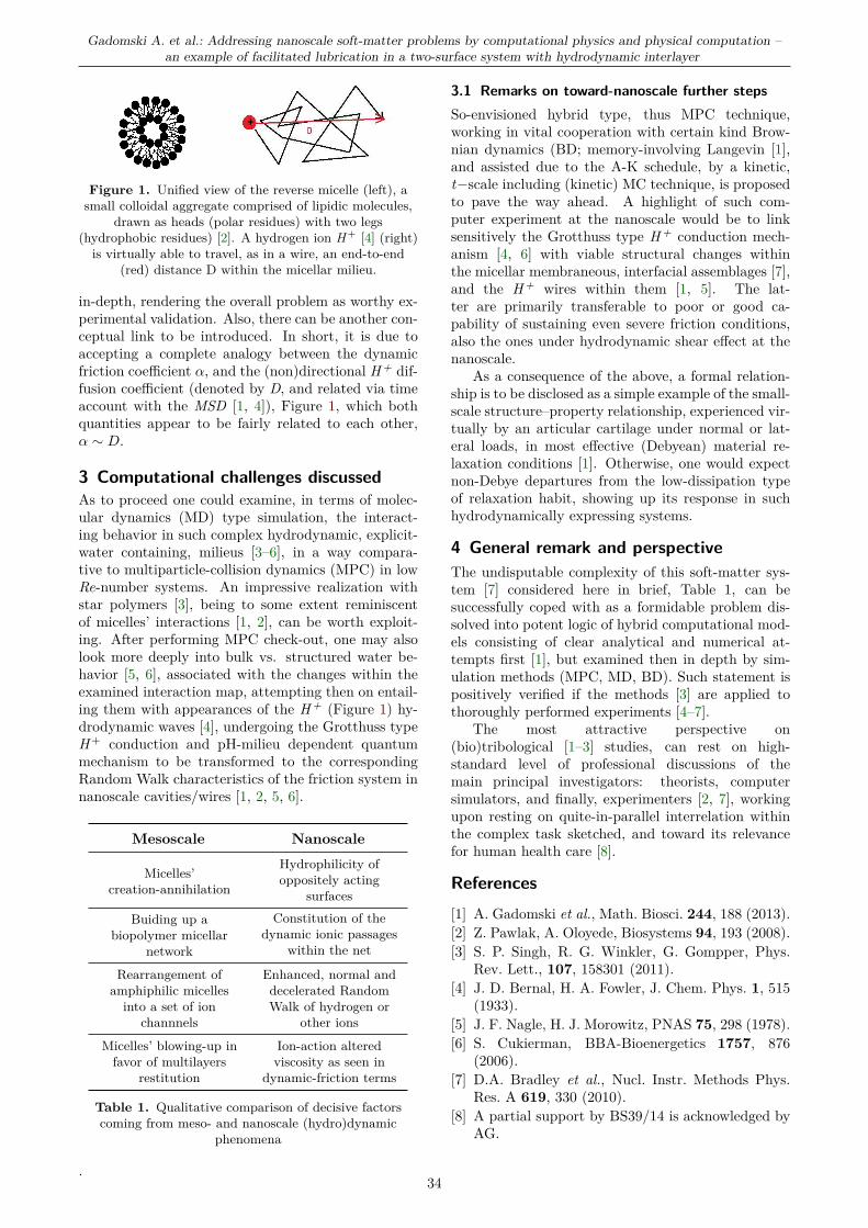
Gadomski A. et al.: Addressing nanoscale soft-matter problems by computational physics and physical computation –an example of facilitated lubrication in a two-surface system with hydrodynamic interlayer
Figure 1. Unified view of the reverse micelle (left), asmall colloidal aggregate comprised of lipidic molecules,
drawn as heads (polar residues) with two legs(hydrophobic residues) [2]. A hydrogen ion H + [4] (right)
is virtually able to travel, as in a wire, an end-to-end(red) distance D within the micellar milieu.
in-depth, rendering the overall problem as worthy ex-perimental validation. Also, there can be another con-ceptual link to be introduced. In short, it is due toaccepting a complete analogy between the dynamicfriction coefficient α, and the (non)directional H + dif-fusion coefficient (denoted by D, and related via timeaccount with the MSD [1, 4]), Figure 1, which bothquantities appear to be fairly related to each other,α ∼ D.
3 Computational challenges discussedAs to proceed one could examine, in terms of molec-ular dynamics (MD) type simulation, the interact-ing behavior in such complex hydrodynamic, explicit-water containing, milieus [3–6], in a way compara-tive to multiparticle-collision dynamics (MPC) in lowRe-number systems. An impressive realization withstar polymers [3], being to some extent reminiscentof micelles’ interactions [1, 2], can be worth exploit-ing. After performing MPC check-out, one may alsolook more deeply into bulk vs. structured water be-havior [5, 6], associated with the changes within theexamined interaction map, attempting then on entail-ing them with appearances of the H + (Figure 1) hy-drodynamic waves [4], undergoing the Grotthuss typeH + conduction and pH-milieu dependent quantummechanism to be transformed to the correspondingRandom Walk characteristics of the friction system innanoscale cavities/wires [1, 2, 5, 6].
Mesoscale Nanoscale
Micelles’creation-annihilation
Hydrophilicity ofoppositely acting
surfaces
Buiding up abiopolymer micellar
network
Constitution of thedynamic ionic passages
within the net
Rearrangement ofamphiphilic micelles
into a set of ionchannnels
Enhanced, normal anddecelerated RandomWalk of hydrogen or
other ions
Micelles’ blowing-up infavor of multilayers
restitution
Ion-action alteredviscosity as seen in
dynamic-friction terms
Table 1. Qualitative comparison of decisive factorscoming from meso- and nanoscale (hydro)dynamic
phenomena
.
3.1 Remarks on toward-nanoscale further steps
So-envisioned hybrid type, thus MPC technique,working in vital cooperation with certain kind Brow-nian dynamics (BD; memory-involving Langevin [1],and assisted due to the A-K schedule, by a kinetic,t−scale including (kinetic) MC technique, is proposedto pave the way ahead. A highlight of such com-puter experiment at the nanoscale would be to linksensitively the Grotthuss type H + conduction mech-anism [4, 6] with viable structural changes withinthe micellar membraneous, interfacial assemblages [7],and the H + wires within them [1, 5]. The lat-ter are primarily transferable to poor or good ca-pability of sustaining even severe friction conditions,also the ones under hydrodynamic shear effect at thenanoscale.
As a consequence of the above, a formal relation-ship is to be disclosed as a simple example of the small-scale structure–property relationship, experienced vir-tually by an articular cartilage under normal or lat-eral loads, in most effective (Debyean) material re-laxation conditions [1]. Otherwise, one would expectnon-Debye departures from the low-dissipation typeof relaxation habit, showing up its response in suchhydrodynamically expressing systems.
4 General remark and perspective
The undisputable complexity of this soft-matter sys-tem [7] considered here in brief, Table 1, can besuccessfully coped with as a formidable problem dis-solved into potent logic of hybrid computational mod-els consisting of clear analytical and numerical at-tempts first [1], but examined then in depth by sim-ulation methods (MPC, MD, BD). Such statement ispositively verified if the methods [3] are applied tothoroughly performed experiments [4–7].
The most attractive perspective on(bio)tribological [1–3] studies, can rest on high-standard level of professional discussions of themain principal investigators: theorists, computersimulators, and finally, experimenters [2, 7], workingupon resting on quite-in-parallel interrelation withinthe complex task sketched, and toward its relevancefor human health care [8].
References
[1] A. Gadomski et al., Math. Biosci. 244, 188 (2013).[2] Z. Pawlak, A. Oloyede, Biosystems 94, 193 (2008).[3] S. P. Singh, R. G. Winkler, G. Gompper, Phys.
Rev. Lett., 107, 158301 (2011).[4] J. D. Bernal, H. A. Fowler, J. Chem. Phys. 1, 515
(1933).[5] J. F. Nagle, H. J. Morowitz, PNAS 75, 298 (1978).[6] S. Cukierman, BBA-Bioenergetics 1757, 876
(2006).[7] D.A. Bradley et al., Nucl. Instr. Methods Phys.
Res. A 619, 330 (2010).[8] A partial support by BS39/14 is acknowledged by
AG.
34
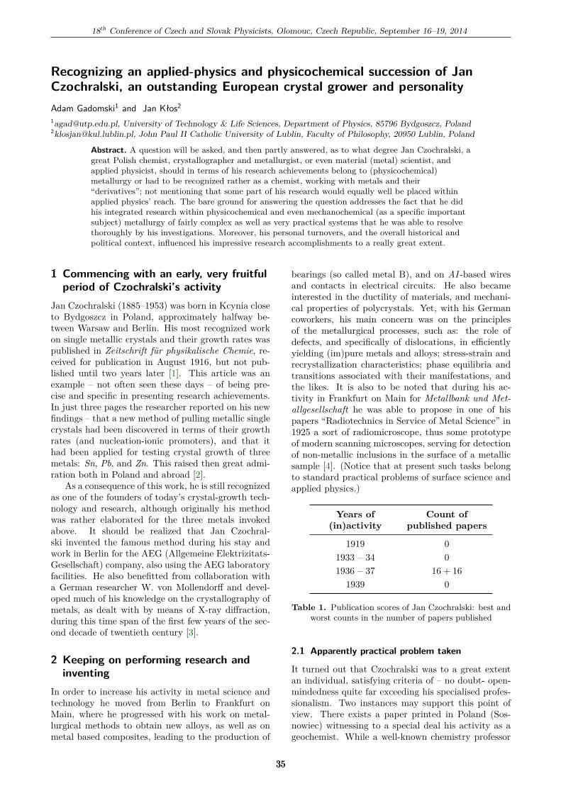
18th Conference of Czech and Slovak Physicists, Olomouc, Czech Republic, September 16–19, 2014
Recognizing an applied-physics and physicochemical succession of JanCzochralski, an outstanding European crystal grower and personality
Adam Gadomski1 and Jan Kłos2
[email protected], University of Technology & Life Sciences, Department of Physics, 85796 Bydgoszcz, [email protected], John Paul II Catholic University of Lublin, Faculty of Philosophy, 20950 Lublin, Poland
Abstract. A question will be asked, and then partly answered, as to what degree Jan Czochralski, agreat Polish chemist, crystallographer and metallurgist, or even material (metal) scientist, andapplied physicist, should in terms of his research achievements belong to (physicochemical)metallurgy or had to be recognized rather as a chemist, working with metals and their“derivatives”; not mentioning that some part of his research would equally well be placed withinapplied physics’ reach. The bare ground for answering the question addresses the fact that he didhis integrated research within physicochemical and even mechanochemical (as a specific importantsubject) metallurgy of fairly complex as well as very practical systems that he was able to resolvethoroughly by his investigations. Moreover, his personal turnovers, and the overall historical andpolitical context, influenced his impressive research accomplishments to a really great extent.
1 Commencing with an early, very fruitfulperiod of Czochralski’s activity
Jan Czochralski (1885–1953) was born in Kcynia closeto Bydgoszcz in Poland, approximately halfway be-tween Warsaw and Berlin. His most recognized workon single metallic crystals and their growth rates waspublished in Zeitschrift für physikalische Chemie, re-ceived for publication in August 1916, but not pub-lished until two years later [1]. This article was anexample – not often seen these days – of being pre-cise and specific in presenting research achievements.In just three pages the researcher reported on his newfindings – that a new method of pulling metallic singlecrystals had been discovered in terms of their growthrates (and nucleation-ionic promoters), and that ithad been applied for testing crystal growth of threemetals: Sn, Pb, and Zn. This raised then great admi-ration both in Poland and abroad [2].
As a consequence of this work, he is still recognizedas one of the founders of today’s crystal-growth tech-nology and research, although originally his methodwas rather elaborated for the three metals invokedabove. It should be realized that Jan Czochral-ski invented the famous method during his stay andwork in Berlin for the AEG (Allgemeine Elektrizitats-Gesellschaft) company, also using the AEG laboratoryfacilities. He also benefitted from collaboration witha German researcher W. von Mollendorff and devel-oped much of his knowledge on the crystallography ofmetals, as dealt with by means of X-ray diffraction,during this time span of the first few years of the sec-ond decade of twentieth century [3].
2 Keeping on performing research andinventing
In order to increase his activity in metal science andtechnology he moved from Berlin to Frankfurt onMain, where he progressed with his work on metal-lurgical methods to obtain new alloys, as well as onmetal based composites, leading to the production of
bearings (so called metal B), and on AI -based wiresand contacts in electrical circuits. He also becameinterested in the ductility of materials, and mechani-cal properties of polycrystals. Yet, with his Germancoworkers, his main concern was on the principlesof the metallurgical processes, such as: the role ofdefects, and specifically of dislocations, in efficientlyyielding (im)pure metals and alloys; stress-strain andrecrystallization characteristics; phase equilibria andtransitions associated with their manifestations, andthe likes. It is also to be noted that during his ac-tivity in Frankfurt on Main for Metallbank und Met-allgesellschaft he was able to propose in one of hispapers “Radiotechnics in Service of Metal Science” in1925 a sort of radiomicroscope, thus some prototypeof modern scanning microscopes, serving for detectionof non-metallic inclusions in the surface of a metallicsample [4]. (Notice that at present such tasks belongto standard practical problems of surface science andapplied physics.)
Years of(in)activity
Count ofpublished papers
1919 01933 – 34 01936 – 37 16 + 16
1939 0
Table 1. Publication scores of Jan Czochralski: best andworst counts in the number of papers published
2.1 Apparently practical problem taken
It turned out that Czochralski was to a great extentan individual, satisfying criteria of – no doubt- open-mindedness quite far exceeding his specialised profes-sionalism. Two instances may support this point ofview. There exists a paper printed in Poland (Sos-nowiec) witnessing to a special deal his activity as ageochemist. While a well-known chemistry professor
353535
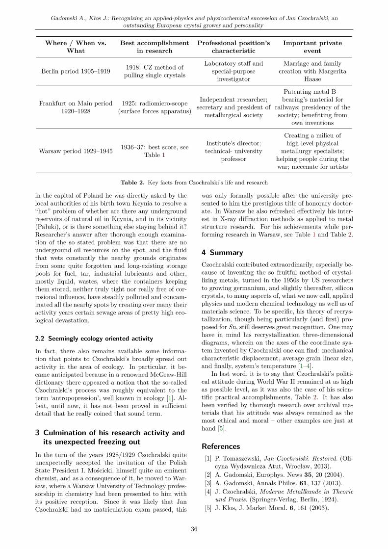
Gadomski A., Kłos J.: Recognizing an applied-physics and physicochemical succession of Jan Czochralski, anoutstanding European crystal grower and personality
Where / When vs.What
Best accomplishmentin research
Professional position’scharacteristic
Important privateevent
Berlin period 1905–19191918: CZ method of
pulling single crystals
Laboratory staff andspecial-purpose
investigator
Marriage and familycreation with Margerita
Haase
Frankfurt on Main period1920–1928
1925: radiomicro-scope(surface forces apparatus)
Independent researcher;secretary and president of
metallurgical society
Patenting metal B –bearing’s material for
railways; presidency of thesociety; benefitting from
own inventions
Warsaw period 1929–19451936–37: best score, see
Table 1
Institute’s director;technical- university
professor
Creating a milieu ofhigh-level physical
metallurgy specialists;helping people during thewar; mecenate for artists
Table 2. Key facts from Czochralski’s life and research
in the capital of Poland he was directly asked by thelocal authorities of his birth town Kcynia to resolve a“hot” problem of whether are there any undergroundreservoirs of natural oil in Kcynia, and in its vicinity(Pałuki), or is there something else staying behind it?Researcher’s answer after thorough enough examina-tion of the so stated problem was that there are nounderground oil resources on the spot, and the fluidthat wets constantly the nearby grounds originatesfrom some quite forgotten and long-existing storagepools for fuel, tar, industrial lubricants and other,mostly liquid, wastes, where the containers keepingthem stored, neither truly tight nor really free of cor-rosional influence, have steadily polluted and concam-inated all the nearby spots by creating over many theiractivity years certain sewage areas of pretty high eco-logical devastation.
2.2 Seemingly ecology oriented activity
In fact, there also remains available some informa-tion that points to Czochralski’s broadly spread outactivity in the area of ecology. In particular, it be-came anticipated because in a renowned McGraw-Hilldictionary there appeared a notion that the so-calledCzochralski’s process was roughly equivalent to theterm ‘antropopression’, well known in ecology [1]. Al-beit, until now, it has not been proved in sufficientdetail that he really coined that sound term.
3 Culmination of his research activity andits unexpected freezing out
In the turn of the years 1928/1929 Czochralski quiteunexpectedly accepted the invitation of the PolishState President I. Mościcki, himself quite an eminentchemist, and as a consequence of it, he moved to War-saw, where a Warsaw University of Technology profes-sorship in chemistry had been presented to him withits positive reception. Since it was likely that JanCzochralski had no matriculation exam passed, this
was only formally possible after the university pre-sented to him the prestigious title of honorary doctor-ate. In Warsaw he also refreshed effectively his inter-est in X-ray diffraction methods as applied to metalstructure research. For his achievements while per-forming research in Warsaw, see Table 1 and Table 2.
4 Summary
Czochralski contributed extraordinarily, especially be-cause of inventing the so fruitful method of crystal-lizing metals, turned in the 1950s by US researchersto growing germanium, and slightly thereafter, siliconcrystals, to many aspects of, what we now call, appliedphysics and modern chemical technology as well as ofmaterials science. To be specific, his theory of recrys-tallization, though being particularly (and first) pro-posed for Sn, still deserves great recognition. One mayhave in mind his recrystallization three-dimensionaldiagrams, wherein on the axes of the coordinate sys-tem invented by Czochralski one can find: mechanicalcharacteristic displacement, average grain linear size,and finally, system’s temperature [1–4].
In last word, it is to say that Czochralski’s politi-cal attitude during World War II remained at as highas possible level, as it was also the case of his scien-tific practical accomplishments, Table 2. It has alsobeen verified by thorough research over archival ma-terials that his attitude was always remained as themost ethical and moral – other examples are just athand [5].
References
[1] P. Tomaszewski, Jan Czochralski. Restored. (Ofi-cyna Wydawnicza Atut, Wrocław, 2013).
[2] A. Gadomski, Europhys. News 35, 20 (2004).[3] A. Gadomski, Annals Philos. 61, 137 (2013).[4] J. Czochralski, Moderne Metallkunde in Theorie
und Praxis. (Springer-Verlag, Berlin, 1924).[5] J. Klos, J. Market Moral. 6, 161 (2003).
36
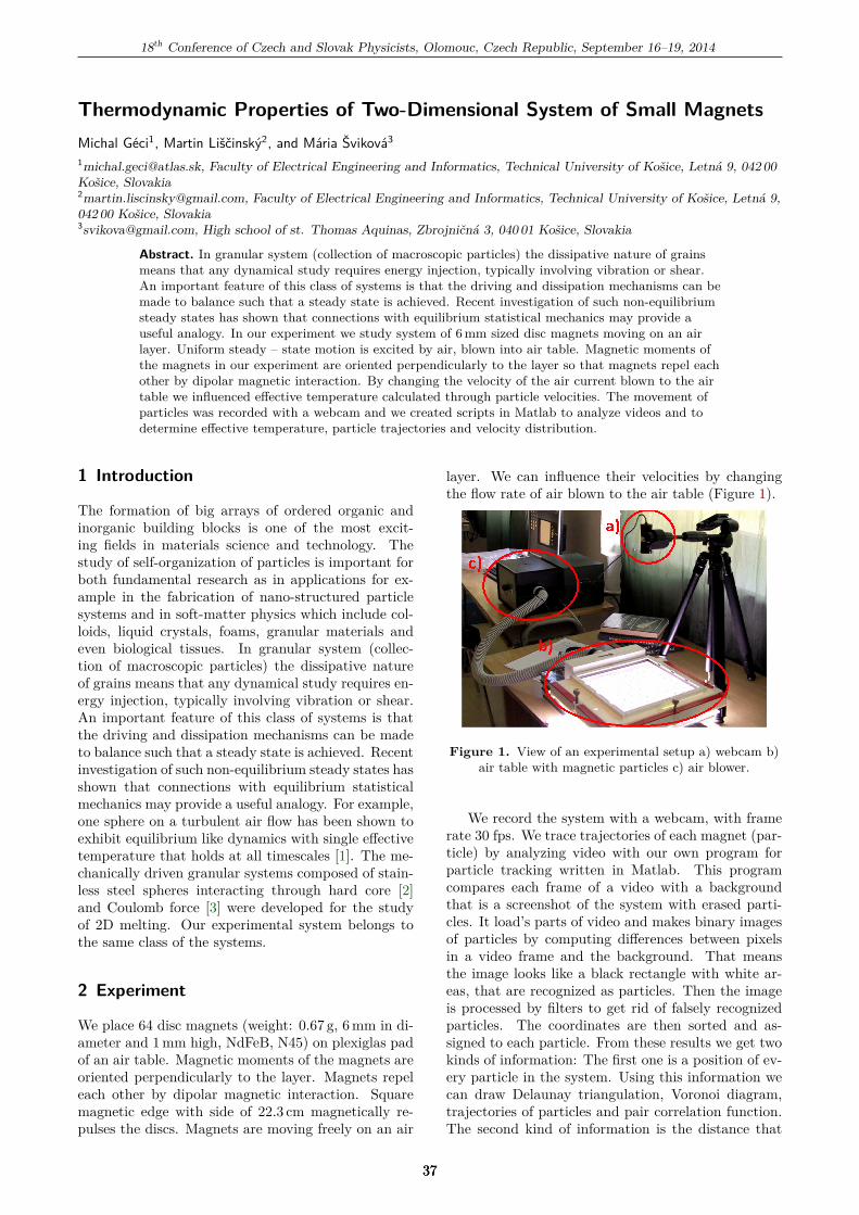
18th Conference of Czech and Slovak Physicists, Olomouc, Czech Republic, September 16–19, 2014
Thermodynamic Properties of Two-Dimensional System of Small Magnets
Michal Géci1, Martin Liščinský2, and Mária Šviková3
[email protected], Faculty of Electrical Engineering and Informatics, Technical University of Košice, Letná 9, 042 00Košice, [email protected], Faculty of Electrical Engineering and Informatics, Technical University of Košice, Letná 9,042 00 Košice, [email protected], High school of st. Thomas Aquinas, Zbrojničná 3, 040 01 Košice, Slovakia
Abstract. In granular system (collection of macroscopic particles) the dissipative nature of grainsmeans that any dynamical study requires energy injection, typically involving vibration or shear.An important feature of this class of systems is that the driving and dissipation mechanisms can bemade to balance such that a steady state is achieved. Recent investigation of such non-equilibriumsteady states has shown that connections with equilibrium statistical mechanics may provide auseful analogy. In our experiment we study system of 6 mm sized disc magnets moving on an airlayer. Uniform steady – state motion is excited by air, blown into air table. Magnetic moments ofthe magnets in our experiment are oriented perpendicularly to the layer so that magnets repel eachother by dipolar magnetic interaction. By changing the velocity of the air current blown to the airtable we influenced effective temperature calculated through particle velocities. The movement ofparticles was recorded with a webcam and we created scripts in Matlab to analyze videos and todetermine effective temperature, particle trajectories and velocity distribution.
1 Introduction
The formation of big arrays of ordered organic andinorganic building blocks is one of the most excit-ing fields in materials science and technology. Thestudy of self-organization of particles is important forboth fundamental research as in applications for ex-ample in the fabrication of nano-structured particlesystems and in soft-matter physics which include col-loids, liquid crystals, foams, granular materials andeven biological tissues. In granular system (collec-tion of macroscopic particles) the dissipative natureof grains means that any dynamical study requires en-ergy injection, typically involving vibration or shear.An important feature of this class of systems is thatthe driving and dissipation mechanisms can be madeto balance such that a steady state is achieved. Recentinvestigation of such non-equilibrium steady states hasshown that connections with equilibrium statisticalmechanics may provide a useful analogy. For example,one sphere on a turbulent air flow has been shown toexhibit equilibrium like dynamics with single effectivetemperature that holds at all timescales [1]. The me-chanically driven granular systems composed of stain-less steel spheres interacting through hard core [2]and Coulomb force [3] were developed for the studyof 2D melting. Our experimental system belongs tothe same class of the systems.
2 Experiment
We place 64 disc magnets (weight: 0.67 g, 6 mm in di-ameter and 1 mm high, NdFeB, N45) on plexiglas padof an air table. Magnetic moments of the magnets areoriented perpendicularly to the layer. Magnets repeleach other by dipolar magnetic interaction. Squaremagnetic edge with side of 22.3 cm magnetically re-pulses the discs. Magnets are moving freely on an air
layer. We can influence their velocities by changingthe flow rate of air blown to the air table (Figure 1).
Figure 1. View of an experimental setup a) webcam b)air table with magnetic particles c) air blower.
We record the system with a webcam, with framerate 30 fps. We trace trajectories of each magnet (par-ticle) by analyzing video with our own program forparticle tracking written in Matlab. This programcompares each frame of a video with a backgroundthat is a screenshot of the system with erased parti-cles. It load’s parts of video and makes binary imagesof particles by computing differences between pixelsin a video frame and the background. That meansthe image looks like a black rectangle with white ar-eas, that are recognized as particles. Then the imageis processed by filters to get rid of falsely recognizedparticles. The coordinates are then sorted and as-signed to each particle. From these results we get twokinds of information: The first one is a position of ev-ery particle in the system. Using this information wecan draw Delaunay triangulation, Voronoi diagram,trajectories of particles and pair correlation function.The second kind of information is the distance that
373737
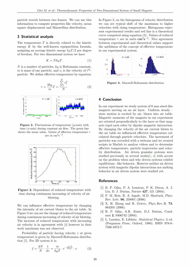
Géci M. et al.: Thermodynamic Properties of Two-Dimensional System of Small Magnets
particle travels between two frames. We can use thisinformation to compute properties like velocity, meansquare displacement and Maxwellian distribution.
3 Statistical analysis
The temperature T is directly related to the kineticenergy K by the well-known equipartition formula,assigning an average kinetic energy kBT/2 per degreeof freedom. For two dimensional system we have
K = NkBT. (1)
N is a number of particles, kB is Boltzmann constant,m is mass of one particle, and vi is the velocity of ith-particle. We define effective temperature by equation:
τ =2kB
mT =
N∑
i=1
v2i
N(2)
Figure 2. Fluctuations of temperature (y-axis) withtime (x-axis) during constant air flow. The green line
shows the mean value. Values of effective temperature τare in cm2s−2.
Figure 2. Dependence of reduced temperature withtime during continuous increasing of velocity of air
blowing.
We can influence effective temperature by changingthe intensity of air current blown to the air table. InFigure 3 we can see the change of reduced temperatureduring continuous increasing of velocity of air blowing.The increase of reduced temperature with increasingair velocity is in agreement with [4] however in theirwork maximum was not observed.
Probability of particle having velocity v at giventemperature is given by Maxwell-Boltzmann distribu-tion [5]. For 2D system it is:
f =dNN
· 1dv
=m
kBT· e− mv2
2kBT · v (3)
In Figure 3, on the histograms of velocity distributionwe can see typical shift of the maximum to highervelocities with rising temperature. Histograms repre-sent experimental results and red line is a theoreticalcurve computed using equation (3). Values of reducedtemperature τ are in units cm2s−2. Nice agreementbetween experimental and theoretical values supportthe usefulness of the concept of effective temperaturein our experimental system.
Figure 3. Maxwell-Boltzmann distribution.
4 Conclusion
In our experiment we study system of 6 mm sized discmagnets moving on an air layer. Uniform steady –state motion is excited by air, blown into air table.Magnetic moments of the magnets in our experimentare oriented perpendicularly to the layer so that mag-nets repel each other by dipolar magnetic interaction.By changing the velocity of the air current blown tothe air table we influenced effective temperature cal-culated through particle velocities. The movement ofparticles was recorded with a webcam and we createdscripts in Matlab to analyze videos and to determineeffective temperature, particle trajectories and veloc-ity distribution. Air driven granular systems werestudied previously in several works[1, 4] with accenton the problem when and why driven systems exhibitequilibrium - like behavior. However neither air drivensystem with magnetic dipolar interactions nor meltingbehavior in air driven system were studied yet.
References
[1] R. P. Ojha, P. A. Lemieux, P. K. Dixon, A. J.Liu, D. J. Durian, Nature 427, 521 (2004).
[2] P. M. Reis, R. A. Ingale, M.D. Shattuck, Phys.Rev. Lett. 96, 258001 (2006).
[3] X. H. Zheng and R. Grieve, Phys. Rev. B. 73,064205 (2006).
[4] R. P. Ojha, A.R. Abate, D.J. Durian, Cond-mat 2, 0406742 (2004).
[5] L. Landau, E. Lifshitz: Statistical Physics. 3. ed.(Pergamon Press, Oxford, 1980). ISBN 978-0-7506-3372-7.
38
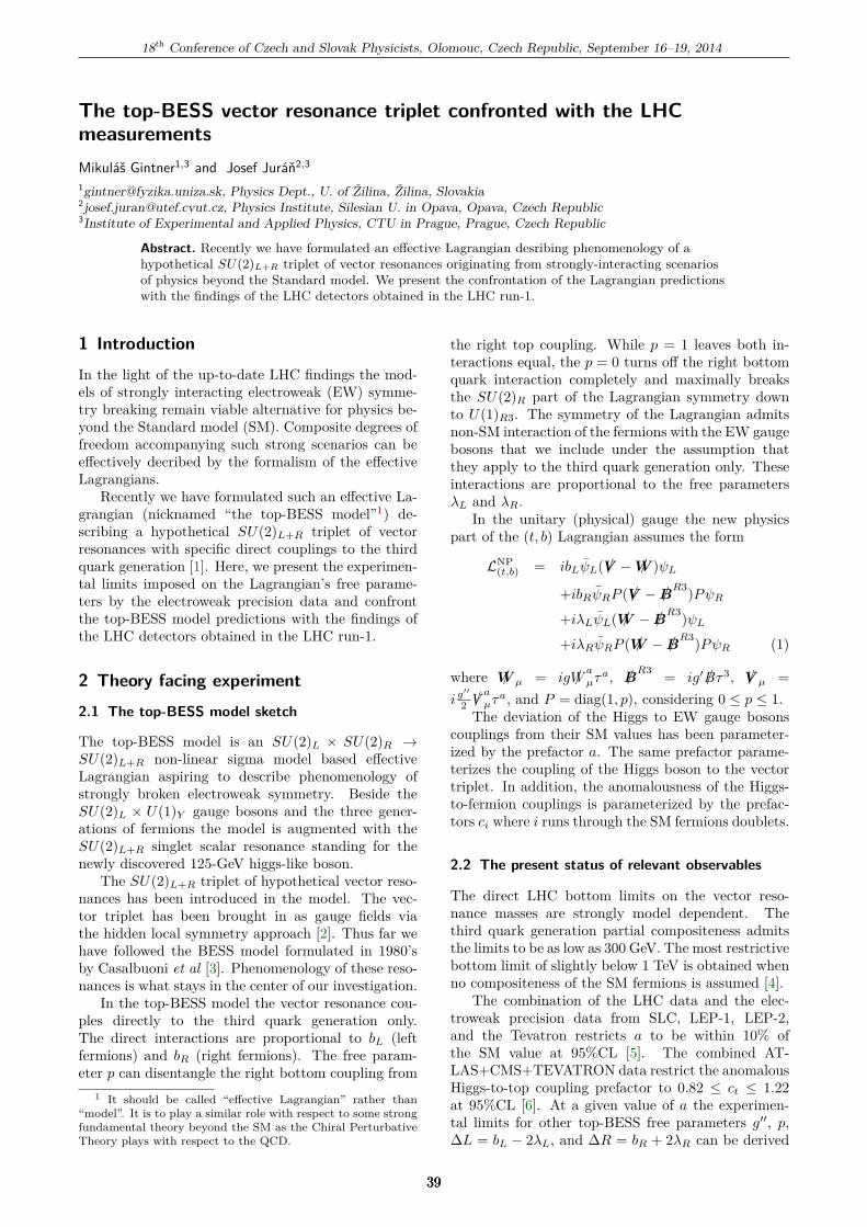
18th Conference of Czech and Slovak Physicists, Olomouc, Czech Republic, September 16–19, 2014
The top-BESS vector resonance triplet confronted with the LHCmeasurements
Mikuláš Gintner1,3 and Josef Juráň2,3
[email protected], Physics Dept., U. of Žilina, Žilina, [email protected], Physics Institute, Silesian U. in Opava, Opava, Czech Republic3Institute of Experimental and Applied Physics, CTU in Prague, Prague, Czech Republic
Abstract. Recently we have formulated an effective Lagrangian desribing phenomenology of ahypothetical SU(2)L+R triplet of vector resonances originating from strongly-interacting scenariosof physics beyond the Standard model. We present the confrontation of the Lagrangian predictionswith the findings of the LHC detectors obtained in the LHC run-1.
1 Introduction
In the light of the up-to-date LHC findings the mod-els of strongly interacting electroweak (EW) symme-try breaking remain viable alternative for physics be-yond the Standard model (SM). Composite degrees offreedom accompanying such strong scenarios can beeffectively decribed by the formalism of the effectiveLagrangians.
Recently we have formulated such an effective La-grangian (nicknamed “the top-BESS model”1) de-scribing a hypothetical SU(2)L+R triplet of vectorresonances with specific direct couplings to the thirdquark generation [1]. Here, we present the experimen-tal limits imposed on the Lagrangian’s free parame-ters by the electroweak precision data and confrontthe top-BESS model predictions with the findings ofthe LHC detectors obtained in the LHC run-1.
2 Theory facing experiment
2.1 The top-BESS model sketch
The top-BESS model is an SU(2)L × SU(2)R →SU(2)L+R non-linear sigma model based effectiveLagrangian aspiring to describe phenomenology ofstrongly broken electroweak symmetry. Beside theSU(2)L × U(1)Y gauge bosons and the three gener-ations of fermions the model is augmented with theSU(2)L+R singlet scalar resonance standing for thenewly discovered 125-GeV higgs-like boson.
The SU(2)L+R triplet of hypothetical vector reso-nances has been introduced in the model. The vec-tor triplet has been brought in as gauge fields viathe hidden local symmetry approach [2]. Thus far wehave followed the BESS model formulated in 1980’sby Casalbuoni et al [3]. Phenomenology of these reso-nances is what stays in the center of our investigation.
In the top-BESS model the vector resonance cou-ples directly to the third quark generation only.The direct interactions are proportional to bL (leftfermions) and bR (right fermions). The free param-eter p can disentangle the right bottom coupling from
1 It should be called “effective Lagrangian” rather than“model”. It is to play a similar role with respect to some strongfundamental theory beyond the SM as the Chiral PerturbativeTheory plays with respect to the QCD.
the right top coupling. While p = 1 leaves both in-teractions equal, the p = 0 turns off the right bottomquark interaction completely and maximally breaksthe SU(2)R part of the Lagrangian symmetry downto U(1)R3. The symmetry of the Lagrangian admitsnon-SM interaction of the fermions with the EW gaugebosons that we include under the assumption thatthey apply to the third quark generation only. Theseinteractions are proportional to the free parametersλL and λR.
In the unitary (physical) gauge the new physicspart of the (t, b) Lagrangian assumes the form
LNP(t,b) = ibLψL( /V − /W )ψL
+ibRψRP ( /V − /BR3
)PψR
+iλLψL( /W − /BR3
)ψL
+iλRψRP ( /W − /BR3
)PψR (1)
where /W µ = ig /Waµτ
a, /BR3
= ig′ /Bτ3, /V µ =
i g′′
2/V
aµτ
a, and P = diag(1, p), considering 0 ≤ p ≤ 1.The deviation of the Higgs to EW gauge bosons
couplings from their SM values has been parameter-ized by the prefactor a. The same prefactor parame-terizes the coupling of the Higgs boson to the vectortriplet. In addition, the anomalousness of the Higgs-to-fermion couplings is parameterized by the prefac-tors ci where i runs through the SM fermions doublets.
2.2 The present status of relevant observables
The direct LHC bottom limits on the vector reso-nance masses are strongly model dependent. Thethird quark generation partial compositeness admitsthe limits to be as low as 300 GeV. The most restrictivebottom limit of slightly below 1 TeV is obtained whenno compositeness of the SM fermions is assumed [4].
The combination of the LHC data and the elec-troweak precision data from SLC, LEP-1, LEP-2,and the Tevatron restricts a to be within 10% ofthe SM value at 95%CL [5]. The combined AT-LAS+CMS+TEVATRON data restrict the anomalousHiggs-to-top coupling prefactor to 0.82 ≤ ct ≤ 1.22at 95%CL [6]. At a given value of a the experimen-tal limits for other top-BESS free parameters g′′, p,∆L = bL − 2λL, and ∆R = bR + 2λR can be derived
393939
Gintner M., Juráň J.: The top-BESS vector resonance triplet confronted with the LHC measurements
-8
-5-4
5
10
40
1%
10%20%30%40%
48%
a=0.9DL
DR
Backin
g
pert
urba
tive
limit
20
-3.6
5 10 15 20 25 300.0
0.2
0.4
0.6
0.8
1.0
g"
p-8 -5
-4
5
20
40 49 %
1%
10%
20%
30%
40%
48%
a=1.0
-3.6
10
5 10 15 20 25 300.0
0.2
0.4
0.6
0.8
1.0
g"
p
-3.6
-8 -5
-4
5
10
2049 %
1%10%
20%30%
40%
48%
a=1.1
5 10 15 20 25 300.0
0.2
0.4
0.6
0.8
1.0
g"
p
Figure 1. The best-fit values of ∆L (dot-dashed) and ∆R (dashed) and the iso-backing contours (solid) for thepreselected values of g′′, p, and a. Sensitivity to the Higgs-to-fermion couplings is negligible. The low-energy Lagrangian
cut-off scale is Mρ ≈ Λ = 1 TeV. The naive perturbative upper limit in g′′ is indicated by the vertical solid line.
by fitting the low-energy (pseudo)observables ǫ1, ǫ2,ǫ3 [7], Γb(Z → bb) [8], and BR(B → Xsγ) [9].
The decay H → γγ is the loop level process in theSM. The dominant SM contributions to the processcome from the W± and top quark loops and they tendto cancel each other. The cancellation strengthen thesensitivity of the decay to hypothetical BSM particlesin the loop. The best-fit signal strength relative tothe standard model prediction µ(H → γγ) is 1.14+0.26
−0.23
(CMS) [10] and 1.17 ± 0.27 (ATLAS) [11].
2.3 Results and conclusions
The best fits of the top-BESS model parameters basedon fitting ǫ1, ǫ2, ǫ3, Γb(Z → bb), and BR(B → Xsγ)for three various values of a are depicted in Figure 1.The best-fit value of p found in our analysis seemsto support the assumption of some models of partialfermion compositeness that the new strong physicsresonances couple stronger to the right top quark thanto the right bottom quark.
Assuming negligible effect of the top-BESS on theHiggs production cross sections and on the total Higgswidths the relative γγ signal strength can be expressedin terms of the H → γγ decay widths
µ(H → γγ)tBESS ≈ Γ/ΓSM(h → γγ)
≈[
1 − 2
7(ct − 1) +
9
7(a− 1) +
9
8a
]2
, (2)
where the first and second terms after unit representcontributions from the anomalous couplings of theHiggs to the top quark and to the EW gauge bosons,respectively (cSM
t = aSM = 1). The last term is thecontribution from the interaction of the Higgs with thevector resonance triplet assuming the same couplingprefactor a as for the EW gauge bosons.
The most recent LHC data on µ(H → γγ) disfa-vors the top-BESS model in its presented setup; e.g.,if ct = a = 1 then µ(H → γγ)tBESS = 4.52. Never-theless, this setup could be viewed as simplistic. Forexample, the interactions of the Higgs boson to theelectroweak gauge bosons could be disentangled from
its interaction to the vector resonance. It would mod-ify (2) so that the current experimental limit couldbe satisfied. In more complex/realistic scenarios, res-onances of different kinds and more general couplingpatterns can be introduced. This is the subject of ourfurther investigation.
References
[1] M. Gintner and J. Juran, Eur. Phys. J. C 73,2577 (2013); M. Gintner, J. Juran and I. Melo,Phys. Rev. D 84, 035013 (2011).
[2] M. Bando, T. Kugo and K. Yamawaki, Phys.Rept. 164, 217 (1988).
[3] R. Casalbuoni, S. De Curtis, D. Dominici andR. Gatto, Phys. Lett. B 155, 95 (1985); Nucl.Phys. B 282, 235 (1987).
[4] B. Bellazzini, C. Csaki, J. Hubisz, J. Serra andJ. Terning, JHEP 1211, 003 (2012).
[5] A. Falkowski, F. Riva and A. Urbano, JHEP1311, 111 (2013); K. Cheung, J. S. Lee andP. Y. Tseng, arXiv:1407.8236 [hep-ph].
[6] J. Bernon, B. Dumont, S. Kraml,arXiv:1409.1588 [hep-ph].
[7] S. Schael et al., Phys. Rept. 427, 257 (2006).[8] K. Nakamura et al. (Particle Data Group Collab-
oration), J. Phys. G 37, 075021 (2010).[9] Y. Amhis et al. (Heavy Flavor Averaging Group
Collaboration), arXiv:1207.1158 [hep-ex].[10] V. Khachatryan et al. (CMS Collaboration),
arXiv:1407.0558 [hep-ex].[11] G. Aad et al. (ATLAS Collaboration),
arXiv:1408.7084 [hep-ex].
40
18th Conference of Czech and Slovak Physicists, Olomouc, Czech Republic, September 16–19, 2014
Barriers of using models and modelling in medical biophysics education
Viera Haverlíková1 and Ivan Haverlík2
[email protected], Faculty of medicine, Comenius University, Sasinkova 2, 813 72 Bratislava, [email protected], Faculty of mathematics, physics and informatics, Comenius University, Mlynská dolina,842 48 Bratislava, Slovak Republic
Abstract. Using models and modelling in medical biophysics education play increasingly importantrole. The paper presents results of two pilot research studies realised in the frame of project KEGA020UK-4/2014 “Innovation in the content, forms and methods of practical exercises of Biophysicsand Medical Biophysics to the study of Medicine and Biomedical Physics”. The research realisedwith first-year medical students was focused on students’ conceptions about models and usingelectric circuit to model blood circulation. Results show that most students think of models asphysical copies of reality, not as conceptual representations. This makes using of educational modelsineffective, if there is none or low visual similarity with investigated phenomena. Understanding thetheory of modelling was examined in survey realised with first-year-master-degree students ofbiomedical physics. One-third of respondents demonstrated serious misunderstanding of modellingprinciples and misunderstanding of relationship between original and model in science.
1 Introduction
The role of models and simulation in medical educa-tion extremely increased in recent two decades. Three-dimensional models, screen-based simulations, inter-active patient simulators and high-fidelity mannequinsare even more frequently used in training of clinicalskills and team communication, due their safety forpatients, repetitive utilisation, and financial effective-ness. These models and simulations can help studentsto develop the ability to recognise their own limita-tions and knowledge gaps.
Furthermore Evidence-Based Medicine assumesthat students understand the process of scientific re-search and the process of building the knowledge. Andthese processes are inseparably connected with modelsand modelling.
The necessity to develop understanding of modelsand modelling among medical students and studentsof biomedical physics inspired our research.
2 Goal
The general goal of realised research was to innovatethe content, forms and methods of practical exercisesof Biophysics and Medical Biophysics to the studyof Medicine and Biomedical Physics. Specific goalof presented research was to identify student’s mostcommon barriers of using models and modelling anddevelop educational activities that can overcome suchbarriers.
3 Background – student’s commonmisconception about modelling
Upper secondary students typically understand mod-els as physical copies of reality, not as conceptual rep-resentations. They do not have idea that the use-fulness of a model can be tested by comparing its
implications to actual observations of real phenom-ena/system.
Many students do not accept the explanatory roleof models, if the model shares only its abstract formwith the phenomenon. They accept this role morewillingly, if many of the material features are the samefor the model and the real phenomenon [1].
Some upper secondary students think that every-thing they learn in science classes is factual. They arenot able to distinguish observation of real phenomenaand model.
4 Research among medical students
4.1 Sample
The research was realised among 1st year medicalstudents studied general medicine at the Faculty ofmedicine, Comenius University in Bratislava in aca-demic year 2013/2014. In all phases of research 29students were involved (23 Female, 6 Male). All ofthem graduated at general upper secondary schools,none of them graduated in physics.
4.2 Methods
The research had four phases:
– Short introductory discussion.
– Anonymous written questionnaire with closed ques-tions, where students had to choose one of 3 alterna-tive answers. This questionnaire was administeredat the very beginning of practical training in bio-physics.
– Short interview and observation of students’ activityin the 5th week of semester, when students realisedthe task: Blood redistribution model [2].
– Analysis of student’s measurement protocols.
414141
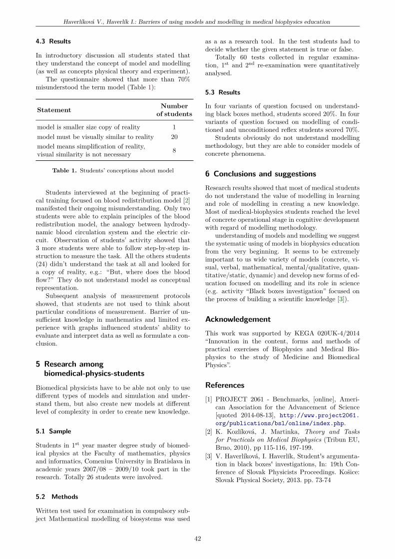
Haverlíková V., Haverlík I.: Barriers of using models and modelling in medical biophysics education
4.3 Results
In introductory discussion all students stated thatthey understand the concept of model and modelling(as well as concepts physical theory and experiment).
The questionnaire showed that more than 70%misunderstood the term model (Table 1):
StatementNumber
of students
model is smaller size copy of reality 1
model must be visually similar to reality 20model means simplification of reality,visual similarity is not necessary
8
Table 1. Students’ conceptions about model
Students interviewed at the beginning of practi-cal training focused on blood redistribution model [2]manifested their ongoing misunderstanding. Only twostudents were able to explain principles of the bloodredistribution model, the analogy between hydrody-namic blood circulation system and the electric cir-cuit. Observation of students’ activity showed that3 more students were able to follow step-by-step in-struction to measure the task. All the others students(24) didn’t understand the task at all and looked fora copy of reality, e.g.: “But, where does the bloodflow?” They do not understand model as conceptualrepresentation.
Subsequent analysis of measurement protocolsshowed, that students are not used to think aboutparticular conditions of measurement. Barrier of un-sufficient knowledge in mathematics and limited ex-perience with graphs influenced students’ ability toevaluate and interpret data as well as formulate a con-clusion.
5 Research amongbiomedical-physics-students
Biomedical physicists have to be able not only to usedifferent types of models and simulation and under-stand them, but also create new models at differentlevel of complexity in order to create new knowledge.
5.1 Sample
Students in 1st year master degree study of biomed-ical physics at the Faculty of mathematics, physicsand informatics, Comenius University in Bratislava inacademic years 2007/08 – 2009/10 took part in theresearch. Totally 26 students were involved.
5.2 Methods
Written test used for examination in compulsory sub-ject Mathematical modelling of biosystems was used
as a as a research tool. In the test students had todecide whether the given statement is true or false.
Totally 60 tests collected in regular examina-tion, 1st and 2nd re-examination were quantitativelyanalysed.
5.3 Results
In four variants of question focused on understand-ing black boxes method, students scored 20%. In fourvariants of question focused on modelling of condi-tioned and unconditioned reflex students scored 70%.
Students obviously do not understand modellingmethodology, but they are able to consider models ofconcrete phenomena.
6 Conclusions and suggestions
Research results showed that most of medical studentsdo not understand the value of modelling in learningand role of modelling in creating a new knowledge.Most of medical-biophysics students reached the levelof concrete operational stage in cognitive developmentwith regard of modelling methodology.
understanding of models and modelling we suggestthe systematic using of models in biophysics educationfrom the very beginning. It seems to be extremelyimportant to us wide variety of models (concrete, vi-sual, verbal, mathematical, mental/qualitative, quan-titative/static, dynamic) and develop new forms of ed-ucation focused on modelling and its role in science(e.g. activity “Black boxes investigation” focused onthe process of building a scientific knowledge [3]).
Acknowledgement
This work was supported by KEGA 020UK-4/2014“Innovation in the content, forms and methods ofpractical exercises of Biophysics and Medical Bio-physics to the study of Medicine and BiomedicalPhysics”.
References
[1] PROJECT 2061 - Benchmarks, [online], Ameri-can Association for the Advancement of Science[quoted 2014-08-13], http://www.project2061.
org/publications/bsl/online/index.php.[2] K. Kozlíková, J. Martinka, Theory and Tasks
for Practicals on Medical Biophysics (Tribun EU,Brno, 2010), pp 115-116, 197-199.
[3] V. Haverlíková, I. Haverlík, Student's argumenta-tion in black boxes' investigations, In: 19th Con-ference of Slovak Physicists Proceedings. Košice:Slovak Physical Society, 2013. pp. 73-74
42
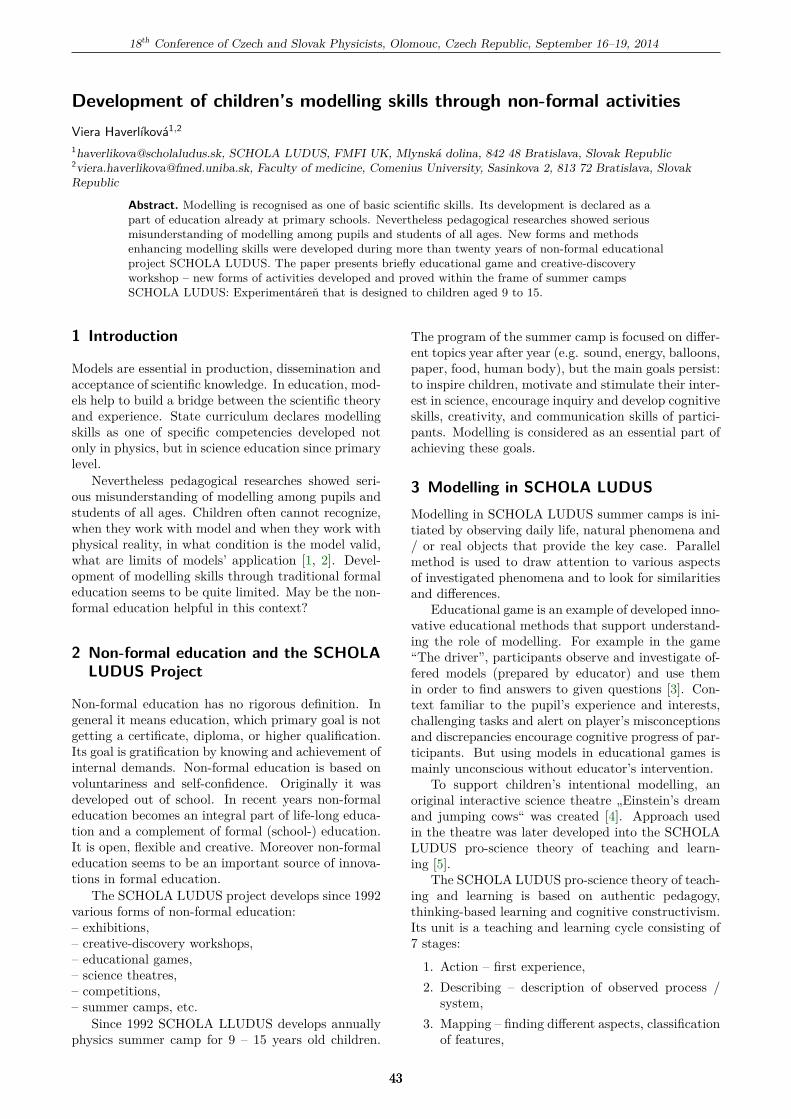
18th Conference of Czech and Slovak Physicists, Olomouc, Czech Republic, September 16–19, 2014
Development of children’s modelling skills through non-formal activities
Viera Haverlíková1,2
[email protected], SCHOLA LUDUS, FMFI UK, Mlynská dolina, 842 48 Bratislava, Slovak [email protected], Faculty of medicine, Comenius University, Sasinkova 2, 813 72 Bratislava, SlovakRepublic
Abstract. Modelling is recognised as one of basic scientific skills. Its development is declared as apart of education already at primary schools. Nevertheless pedagogical researches showed seriousmisunderstanding of modelling among pupils and students of all ages. New forms and methodsenhancing modelling skills were developed during more than twenty years of non-formal educationalproject SCHOLA LUDUS. The paper presents briefly educational game and creative-discoveryworkshop – new forms of activities developed and proved within the frame of summer campsSCHOLA LUDUS: Experimentáreň that is designed to children aged 9 to 15.
1 Introduction
Models are essential in production, dissemination andacceptance of scientific knowledge. In education, mod-els help to build a bridge between the scientific theoryand experience. State curriculum declares modellingskills as one of specific competencies developed notonly in physics, but in science education since primarylevel.
Nevertheless pedagogical researches showed seri-ous misunderstanding of modelling among pupils andstudents of all ages. Children often cannot recognize,when they work with model and when they work withphysical reality, in what condition is the model valid,what are limits of models’ application [1, 2]. Devel-opment of modelling skills through traditional formaleducation seems to be quite limited. May be the non-formal education helpful in this context?
2 Non-formal education and the SCHOLALUDUS Project
Non-formal education has no rigorous definition. Ingeneral it means education, which primary goal is notgetting a certificate, diploma, or higher qualification.Its goal is gratification by knowing and achievement ofinternal demands. Non-formal education is based onvoluntariness and self-confidence. Originally it wasdeveloped out of school. In recent years non-formaleducation becomes an integral part of life-long educa-tion and a complement of formal (school-) education.It is open, flexible and creative. Moreover non-formaleducation seems to be an important source of innova-tions in formal education.
The SCHOLA LUDUS project develops since 1992various forms of non-formal education:– exhibitions,– creative-discovery workshops,– educational games,– science theatres,– competitions,– summer camps, etc.
Since 1992 SCHOLA LLUDUS develops annuallyphysics summer camp for 9 – 15 years old children.
The program of the summer camp is focused on differ-ent topics year after year (e.g. sound, energy, balloons,paper, food, human body), but the main goals persist:to inspire children, motivate and stimulate their inter-est in science, encourage inquiry and develop cognitiveskills, creativity, and communication skills of partici-pants. Modelling is considered as an essential part ofachieving these goals.
3 Modelling in SCHOLA LUDUS
Modelling in SCHOLA LUDUS summer camps is ini-tiated by observing daily life, natural phenomena and/ or real objects that provide the key case. Parallelmethod is used to draw attention to various aspectsof investigated phenomena and to look for similaritiesand differences.
Educational game is an example of developed inno-vative educational methods that support understand-ing the role of modelling. For example in the game“The driver”, participants observe and investigate of-fered models (prepared by educator) and use themin order to find answers to given questions [3]. Con-text familiar to the pupil’s experience and interests,challenging tasks and alert on player’s misconceptionsand discrepancies encourage cognitive progress of par-ticipants. But using models in educational games ismainly unconscious without educator’s intervention.
To support children’s intentional modelling, anoriginal interactive science theatre „Einstein’s dreamand jumping cows“ was created [4]. Approach usedin the theatre was later developed into the SCHOLALUDUS pro-science theory of teaching and learn-ing [5].
The SCHOLA LUDUS pro-science theory of teach-ing and learning is based on authentic pedagogy,thinking-based learning and cognitive constructivism.Its unit is a teaching and learning cycle consisting of7 stages:
1. Action – first experience,
2. Describing – description of observed process /system,
3. Mapping – finding different aspects, classificationof features,
434343
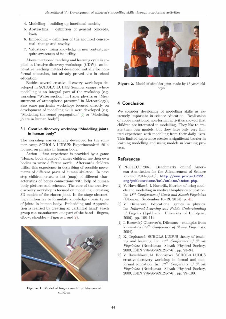
Haverlíková V.: Development of children’s modelling skills through non-formal activities
4. Modelling – building up functional models,
5. Abstracting – definition of general concepts,laws,
6. Embedding – definition of the acquired concep-tual change and novelty,
7. Valuation - using knowledge in new context, ac-quire awareness of its utility.
Above mentioned teaching and learning cycle is ap-plied in Creative-discovery workshops (CDW) - an in-novative teaching method developed initially for non-formal education, but already proved also in schooleducation.
Besides several creative-discovery workshops de-veloped in SCHOLA LUDUS Summer camps, wheremodelling is an integral part of the workshop (e.g.workshop “Water suction” in Paper physics or “Mea-surement of atmospheric pressure” in Meteorology),also some particular workshops focused directly ondevelopment of modelling skills were developed (e.g.“Modelling the sound propagation” [6] or “Modellingjoints in human body”).
3.1 Creative-discovery workshop “Modelling jointsin human body”
The workshop was originally developed for the sum-mer camp SCHOLA LUDUS: Experimentáreň 2014focused on physics in human body.
Action – first experience is provided by a game“Human body alphabet”, where children use their ownbodies to write different words. Afterwards childrenutilise this experience in describing of possible move-ments of different parts of human skeleton. In nextstep children create a list (map) of different char-acteristics of bones connections with help of humanbody pictures and schemas. The core of the creative-discovery workshop is focused on modelling – creating3D models of the chosen joint. In the stage abstract-ing children try to formulate knowledge - basic typesof joints in human body. Embedding and Apprecia-tion is realised by creating an „artificial hand“ (eachgroup can manufacture one part of the hand – fingers,elbow, shoulder – Figures 1 and 2).
Figure 1. Model of fingers made by 14-years oldchildren.
Figure 2. Model of shoulder joint made by 13-years oldboys.
4 Conclusion
We consider developing of modelling skills as ex-tremely important in science education. Realisationof above mentioned non-formal activities showed thatchildren are interested in modelling. They like to cre-ate their own models, but they have only very lim-ited experience with modelling from their daily lives.This limited experience creates a significant barrier inlearning modelling and using models in learning pro-cess.
References
[1] PROJECT 2061 – Benchmarks, [online], Ameri-can Association for the Advancement of Science[quoted 2014-08-13], http://www.project2061.
org/publications/bsl/online/index.php.[2] V. Haverlíková, I. Haverlík, Barriers of using mod-
els and modelling in medical biophysics education.In: 18th Conference of Czech and Slovak Physicists(Olomouc, September 16–19, 2014), p. 41.
[3] V. Biznárová. Educational games in physics.In: Informal Learning and Public Understandingof Physics (Ljubljana: University of Ljubljana,2006), pp. 108–114.
[4] I. Bazovský Observer's, Dilemma – examples fromkinematics (14th Conference of Slovak Physicists,2004).
[5] K. Teplanová, SCHOLA LUDUS theory of teach-ing and learning. In: 17th Conference of SlovakPhysicists (Bratislava: Slovak Physical Society,2009, ISBN 978-80-969124-7-6), pp. 93–94.
[6] V. Haverlíková, M. Hodosyová, SCHOLA LUDUScreative-discovery workshop in formal and non-formal education. In: 17th Conference of SlovakPhysicists (Bratislava: Slovak Physical Society,2009, ISBN 978-80-969124-7-6), pp. 99–100.
44
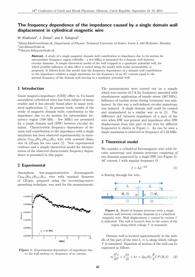
18th Conference of Czech and Slovak Physicists, Olomouc, Czech Republic, September 16–19, 2014
The frequency dependence of the impedance caused by a single domain walldisplacement in cylindrical magnetic wire
M. Kladivová1, J. Ziman2, and V. Šuhajová3
[email protected], Department of Physics, Technical University of Košice, Letná 9, 042 00 Košice, [email protected]@tuke.sk
Abstract. A study of a single magnetic domain wall contribution to impedance due to its motion forintermediate frequency region (100 kHz – a few MHz) is presented for a domain wall betweencircular domains. A simple theoretical model of the wall trapped in a quadratic potential well, forwhich possible influence of skin effect is tested using the model with scalar permeability, isproposed. It follows from this model that the frequency dependence of a domain wall contributionto the impedance exhibits a single maximum for the frequency of an AC current equal to thenatural frequency of the domain wall moving in a quadratic potential well.
1 Introduction
Giant magneto-impedance (GMI) effect in Co-basedamorphous cylindrical wires has been subject of manystudies and it has already found place in many tech-nical applications [1]. In present work, results of thestudy of magnetic domain walls contribution to theimpedance due to its motion for intermediate fre-quency region (100 kHz – few MHz) are presentedfor a single domain wall (DW) between circular do-mains. Characteristic frequency dependence of do-main wall contribution to the impedance with a singlemaximum has been observed experimentally in amor-phous Co68.2Fe4.3Si12.5B15 wire with nominal diam-eter of 125µm for two cases [2]. New experimentalevidence and a simple theoretical model for interpre-tation of the observed characteristic frequency depen-dence is presented in this paper.
2 Experimental
Amorphous low-magnetostrictive ferromagneticCo68.2Fe4.3Si12.5B15 wire with nominal diameterof 125µm, prepared using the in-rotating-water-quenching technique, was used for the measurements.
Figure 1. Experimental dependence of impedance dueto the wall motion vs. frequency of ac current.
The measurements were carried out on a samplewhich was current (0.7 A for 3 minutes) annealed withsimultaneous application of tensile stress (367 MPa).Influence of torsion stress during treatment was min-imized. In this way a well-defined circular anisotropywas induced. A single domain wall could be createdand manipulated in a similar way as in [3]. Thedifference ∆Z between impedance of a part of thewire when DW was present and impedance after DWdisplacement from this part of the wire for differentfrequencies is shown in Figure 1. As can be seen asingle maximum is observed at frequency of 1.23 MHz.
3 Theoretical model
We consider a cylindrical ferromagnetic wire with cir-cular anisotropy and domain structure consisting oftwo domains separated by a single DW (see Figure 2).AC current I with angular frequency Ω
I = I0e−iΩt (1)
is flowing through the wire.
Figure 2. Model of domain structure with a singledomain wall between circular domains in a cylindrical
magnetic wire. Wall displacement x caused by current I
is indicated. The wall is located close to the centre of theregion along which voltage V is measured.
Domain wall is located approximately in the mid-dle of the part of the wire l1 ≈ l2 along which voltageV is measured. Equation of motion of the wall can beexpressed as follows
md2x
dt2+ β
dxdt
+ kx = 2µ0MSR
3I P (R, δ) (2)
454545
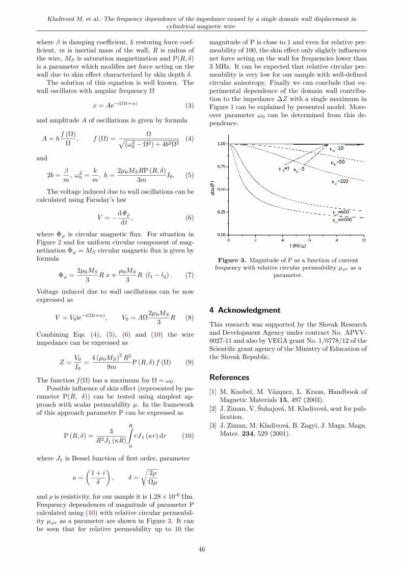
Kladivová M. et al.: The frequency dependence of the impedance caused by a single domain wall displacement incylindrical magnetic wire
where β is damping coefficient, k restoring force coef-ficient, m is inertial mass of the wall, R is radius ofthe wire, MS is saturation magnetization and P(R, δ)is a parameter which modifies net force acting on thewall due to skin effect characterized by skin depth δ.
The solution of this equation is well known. Thewall oscillates with angular frequency Ω
x = Ae−i(Ωt+α) (3)
and amplitude A of oscillations is given by formula
A = hf (Ω)
Ω, f (Ω) =
Ω√
(ω20 − Ω2) + 4b2Ω2
(4)
and
2b =β
m, ω2
0 =k
m, h =
2µ0MSRP (R, δ)3m
I0. (5)
The voltage induced due to wall oscillations can becalculated using Faraday’s law
V = −dΦϕ
dt, (6)
where Φϕ is circular magnetic flux. For situation inFigure 2 and for uniform circular component of mag-netization Φϕ = MS circular magnetic flux is given byformula
Φϕ =2µ0MS
3R x+
µ0MS
3R (l1 − l2) . (7)
Voltage induced due to wall oscillations can be nowexpressed as
V = V0ie−i(Ωt+α), V0 = AΩ2µ0MS
3R (8)
Combining Eqs. (4), (5), (6) and (10) the wireimpedance can be expressed as
Z =V0
I0=
4 (µ0MS)2R2
9mP (R, δ) f (Ω) (9)
The function f (Ω) has a maximum for Ω = ω0.Possible influence of skin effect (represented by pa-
rameter P(R, δ)) can be tested using simplest ap-proach with scalar permeability µ. In the frameworkof this approach parameter P can be expressed as
P (R, δ) =3
R2J1 (κR)
R∫
0
rJ1 (κr) dr (10)
where J1 is Bessel function of first order, parameter
κ =(
1 + i
δ
)
, δ =
√
2ρΩµ
and ρ is resistivity, for our sample it is 1.28 × 10⁻⁶ Ωm.Frequency dependences of magnitude of parameter Pcalculated using (10) with relative circular permeabil-ity µϕr as a parameter are shown in Figure 3. It canbe seen that for relative permeability up to 10 the
magnitude of P is close to 1 and even for relative per-meability of 100, the skin effect only slightly influencesnet force acting on the wall for frequencies lower than3 MHz. It can be expected that relative circular per-meability is very low for our sample with well-definedcircular anisotropy. Finally we can conclude that ex-perimental dependence of the domain wall contribu-tion to the impedance ∆Z with a single maximum inFigure 1 can be explained by presented model. More-over parameter ω0 can be determined from this de-pendence.
Figure 3. Magnitude of P as a function of currentfrequency with relative circular permeability µϕr as a
parameter.
4 Acknowledgment
This research was supported by the Slovak Researchand Development Agency under contract No. APVV-0027-11 and also by VEGA grant No. 1/0778/12 of theScientific grant agency of the Ministry of Education ofthe Slovak Republic.
References
[1] M. Knobel, M. Vázquez, L. Kraus, Handbook ofMagnetic Materials 15, 497 (2003).
[2] J. Ziman, V. Šuhajová, M. Kladivová, sent for pub-lication.
[3] J. Ziman, M. Kladivová, B. Zagyi, J. Magn. Magn.Mater. 234, 529 (2001).
46
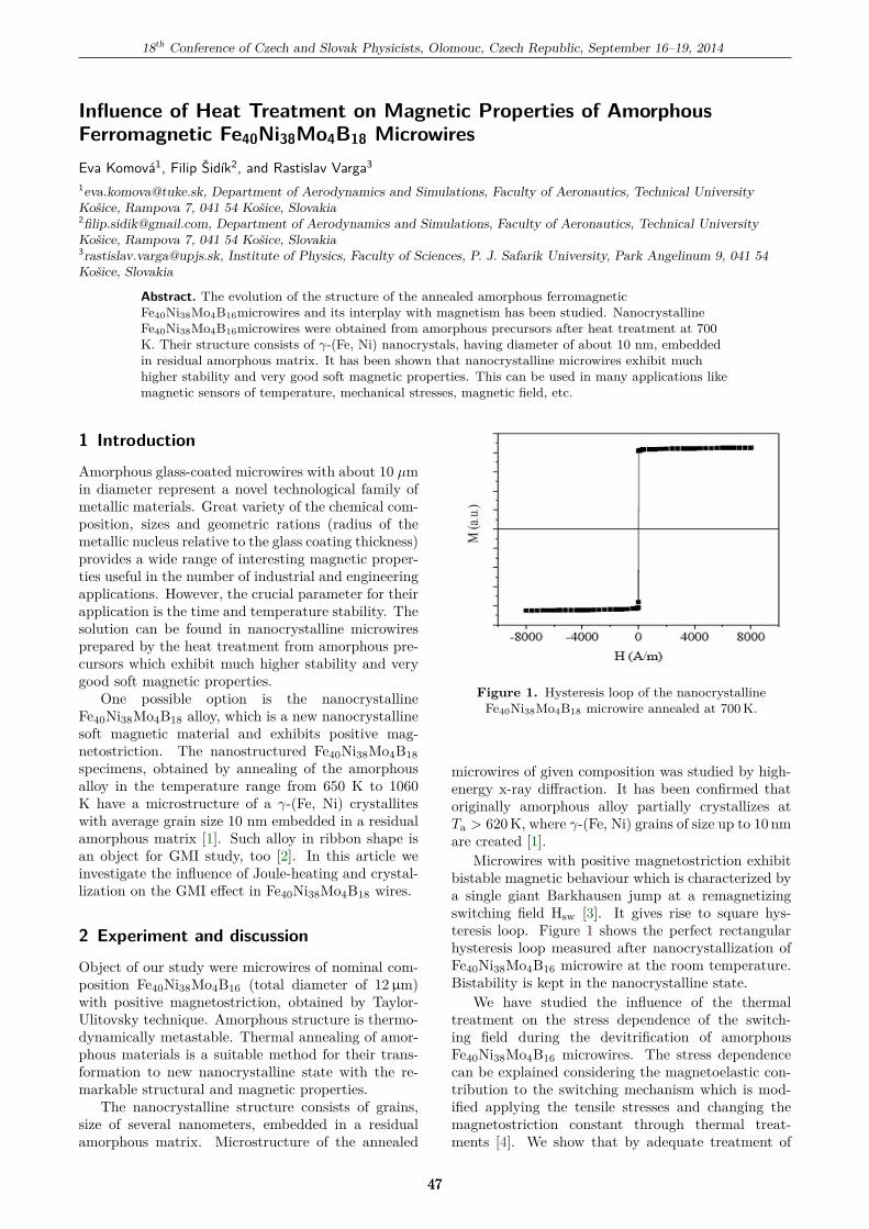
18th Conference of Czech and Slovak Physicists, Olomouc, Czech Republic, September 16–19, 2014
Influence of Heat Treatment on Magnetic Properties of AmorphousFerromagnetic Fe40Ni38Mo4B18 Microwires
Eva Komová1, Filip Šidík2, and Rastislav Varga3
[email protected], Department of Aerodynamics and Simulations, Faculty of Aeronautics, Technical UniversityKošice, Rampova 7, 041 54 Košice, [email protected], Department of Aerodynamics and Simulations, Faculty of Aeronautics, Technical UniversityKošice, Rampova 7, 041 54 Košice, [email protected], Institute of Physics, Faculty of Sciences, P. J. Safarik University, Park Angelinum 9, 041 54Košice, Slovakia
Abstract. The evolution of the structure of the annealed amorphous ferromagneticFe40Ni38Mo4B16microwires and its interplay with magnetism has been studied. NanocrystallineFe40Ni38Mo4B16microwires were obtained from amorphous precursors after heat treatment at 700K. Their structure consists of γ-(Fe, Ni) nanocrystals, having diameter of about 10 nm, embeddedin residual amorphous matrix. It has been shown that nanocrystalline microwires exhibit muchhigher stability and very good soft magnetic properties. This can be used in many applications likemagnetic sensors of temperature, mechanical stresses, magnetic field, etc.
1 Introduction
Amorphous glass-coated microwires with about 10 µmin diameter represent a novel technological family ofmetallic materials. Great variety of the chemical com-position, sizes and geometric rations (radius of themetallic nucleus relative to the glass coating thickness)provides a wide range of interesting magnetic proper-ties useful in the number of industrial and engineeringapplications. However, the crucial parameter for theirapplication is the time and temperature stability. Thesolution can be found in nanocrystalline microwiresprepared by the heat treatment from amorphous pre-cursors which exhibit much higher stability and verygood soft magnetic properties.
One possible option is the nanocrystallineFe40Ni38Mo4B18 alloy, which is a new nanocrystallinesoft magnetic material and exhibits positive mag-netostriction. The nanostructured Fe40Ni38Mo4B18
specimens, obtained by annealing of the amorphousalloy in the temperature range from 650 K to 1060K have a microstructure of a γ-(Fe, Ni) crystalliteswith average grain size 10 nm embedded in a residualamorphous matrix [1]. Such alloy in ribbon shape isan object for GMI study, too [2]. In this article weinvestigate the influence of Joule-heating and crystal-lization on the GMI effect in Fe40Ni38Mo4B18 wires.
2 Experiment and discussion
Object of our study were microwires of nominal com-position Fe40Ni38Mo4B16 (total diameter of 12µm)with positive magnetostriction, obtained by Taylor-Ulitovsky technique. Amorphous structure is thermo-dynamically metastable. Thermal annealing of amor-phous materials is a suitable method for their trans-formation to new nanocrystalline state with the re-markable structural and magnetic properties.
The nanocrystalline structure consists of grains,size of several nanometers, embedded in a residualamorphous matrix. Microstructure of the annealed
Figure 1. Hysteresis loop of the nanocrystallineFe40Ni38Mo4B18 microwire annealed at 700 K.
microwires of given composition was studied by high-energy x-ray diffraction. It has been confirmed thatoriginally amorphous alloy partially crystallizes atTa > 620 K, where γ-(Fe, Ni) grains of size up to 10 nmare created [1].
Microwires with positive magnetostriction exhibitbistable magnetic behaviour which is characterized bya single giant Barkhausen jump at a remagnetizingswitching field Hsw [3]. It gives rise to square hys-teresis loop. Figure 1 shows the perfect rectangularhysteresis loop measured after nanocrystallization ofFe40Ni38Mo4B16 microwire at the room temperature.Bistability is kept in the nanocrystalline state.
We have studied the influence of the thermaltreatment on the stress dependence of the switch-ing field during the devitrification of amorphousFe40Ni38Mo4B16 microwires. The stress dependencecan be explained considering the magnetoelastic con-tribution to the switching mechanism which is mod-ified applying the tensile stresses and changing themagnetostriction constant through thermal treat-ments [4]. We show that by adequate treatment of
474747
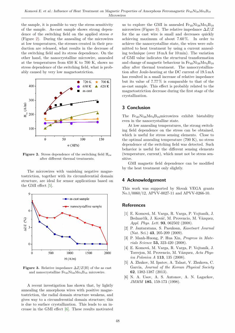
Komová E. et al.: Influence of Heat Treatment on Magnetic Properties of Amorphous Ferromagnetic Fe40Ni38Mo4B18
Microwires
the sample, it is possible to vary the stress sensitivityof the sample. As-cast sample shows strong depen-dence of the switching field on the applied stress σ(Figure 2). During the annealing of the microwiresat low temperatures, the stresses created in their pro-duction are released, what results in the decrease ofthe switching field and its stress dependence. On theother hand, the nanocrystalline microwire, annealedat the temperatures from 650 K to 700 K, shows nostress dependence of the switching field, what is prob-ably caused by very low magnetostriction.
Figure 2. Stress dependence of the switching field Hsw
after different thermal treatments.
The microwires with vanishing negative magne-tostriction, together with its circumferential domainstructure, are ideal for sensor applications based onthe GMI effect [5].
Figure 3. Relative impedance ∆Z/Z(H) of the as castand nanocrystalline Fe40Ni38Mo4B16 microwire.
A recent investigation has shown that, by lightlyannealing the amorphous wires with positive magne-tostriction, the radial domain structure weakens, andgives way to a circumferential domain structure; thisis due to surface crystallization. This leads to an in-crease in the GMI effect [6]. These results motivated
us to explore the GMI in annealed Fe40Ni38Mo4B18
microwires (Figure 3). The relative impedance ∆Z/Zfor the as cast wire is small and decreases quicklyachieving maximum of about 7.60 %. In order toachieve the nanocrystalline state, the wires were sub-mitted to heat treatment by using a current anneal-ing technique (over 18 mA for 10 min). The variationof GMI value indicates the structural transformationand change of magnetic behaviour in Fe40Ni38Mo4B18
alloy after thermal treatment. The nanocrystalliza-tion after Joule-heating at the DC current of 19.5 mAhas resulted in a small increase of relative impedancebut its value of 7.77 % is comparable to that of theas-cast sample. This effect is probably related to themagnetostriction decrease during the first stage of thecrystallization.
3 Conclusion
The Fe40Ni38Mo4B16microwires exhibit bistabilityeven in the nanocrystalline state.
At low annealing temperatures, the strong switch-ing field dependence on the stress can be obtained,which is useful for stress sensing elements. Close tothe optimal annealing temperature (700 K), no stressdependence of the switching field was detected. Suchbehavior is useful for the different sensing elements(temperature, current), which must not be stress sen-sitive.
GMI magnetic field dependence can be modifiedby the heat treatment only slightly.
4 Acknowledgement
This work was supported by Slovak VEGA grantsNo.1/0060/12, APVV-0027-11 and APVV-0266-10.
References
[1] E. Komová, M. Varga, R. Varga, P. Vojtaník, J.Bednarčík, J. Kováč, M. Provencio, M. Vázquez,Appl. Phys. Lett. 93, 062502 (2008).
[2] P. Jantaratana, S. Pasuksan, Kasetsart Journal(Nat. Sci.) 43, 205-209 (2009).
[3] P. Manh-Huong, P. Hua Xin, Progress in Mate-rials Science 53, 323-420 (2008).
[4] E. Komová, M. Varga, R. Varga, P. Vojtaník, J.Torrejon, M. Provencio, M. Vázquez, Acta Phys-ica Polonica A 113, 135 (2008).
[5] A. Zhukov, M. Ipatov, A. Talaat, V. Zhukova, C.Garcia, Journal of the Korean Physical Society62, 1382-1387 (2013).
[6] N. A. Usov, A. S. Antonov, A. N. Lagarkov,JMMM 185, 159-173 (1998).
48
18th Conference of Czech and Slovak Physicists, Olomouc, Czech Republic, September 16–19, 2014
Study of azimuthal anisotropy of hadron production via Monte Carlosimulation
Renata Kopečná1 and Boris Tomášik1,2
[email protected], FNSPE, Czech Technical University in Prague, Břehová 7, 115 19 Praha 1, Czech [email protected], Univerzita Mateja Bela, Tajovského 40, 974 01 Banská Bystrica, Slovakia
Abstract. The quark-gluon plasma (QGP) is very hot and dense form of matter, where quarks andgluons are deconfined. It can be produced in high-energy nuclear collisions, studied at facilities suchas Relativistic Heavy Ion-Collider (RHIC) or Large Hadron Collider (LHC). Important means inthe studies of QGP properties are anisotropies of the transverse collective flow of hot fireball. Theyshow up via anisotropies of hadron momentum distributions. We present simple Monte Carlo toymodel which generates hadron distributions with azimuthal anisotropy. It is used in designing andtesting analysis tools for the anisotropy coefficients.
1 Introduction
Initial conditions in heavy-ion collisions fluctuate fromevent to event. It turns out that anisotropies in thecollective flow are reflected in the particle momentumdistribution with respect to the reaction plane. Theygive us information about the initial conditions andabout the early evolution of the system, since they aredeveloped mainly in the first moments during the col-lision. However, the collisions are not ideally symmet-ric, there are quantum fluctuations, the initial nucleargeometry varies from event to event, the initial energydensity distribution is anisotropic. All these effectscause flow anisotropies. Those anisotropies are mostsignificant for non-central collisions. Studying themcan provide an insight into QGP properties. Moredetails can be found in [1].
Our goal here is to implement Monte Carlo toymodel with given profile of the azimuthal angle dis-tribution of pion transverse momenta. Next step isto extract the nth differential flows using correlationsand histograms.
2 Angle distribution
We study collective flow anisotropies via azumithaldistribution of particles. Common way of study isexpanding the distributions to Fourier series:
dNd2pT
=dN
2πpT dpT
[
1 +∞∑
n=1
2vn cos(n(Φ − Ψn))
]
.
(1)In our toy model generator we used coefficients up
to pentagonal flow: v1 = 0.1, v2 = 0.05, v3 = 0.03,v4 = 0.01 and v5 = 0.005; Ψn is generated randomlyfor every event.
3 Transverse momentum distribution
The pT distribution is expressed as
dNdpT
= CpT e− pT
T , (2)
where T is a parameter and C denotes normalizationconstant. We choose T = 400 MeV.
We cannot use the transformation method sincethe cummulative distribution function is not invert-ible. From Equation (2) the uniform random deviatex (i.e. dimensionless x ∈ 〈0, 1)) is related to pT as:
x = C
∫
dpT pT e− pT
T = −CT (T + pT )e−pT
T , (3)
where C is normalisation factor. In our case, C =−1/T 2. The required inverse function can be ex-pressed in terms of Lambert function W :
pT (x) = −T(
1 +W(x
e
))
. (4)
One way of approximatingW (x) uses the recurrentrelation
W (x) = ln
x
ln(
x
ln(
xln(...)
)
)
. (5)
This approach is simple, for small number of iter-ations it is even fast. We chose initial W0(x) and theniterate according to Wn+1(x) = ln(x/ ln(Wn(x))).The reliability of this method strongly depends on thenumber of iterations. An example is shown in Fig-ure 1 (top and middle). On the top is the histogramfor 5 iterations, the black line illustrates the desiredshape of the distribution (2) with T = 400 MeV. Itis obvious that 5 iterations are not precise enough.The big discontinuity around pt = 2T = 800 MeVis caused by a problem because of the limit of Equa-tion (5). The other histograms are fitted with the
function pT exp(
p0 + pT
p1
)
, where p0 is scale parame-ter, thus p1 should be equal to T .
Another interesting topic is the dependence onW0(x). For higher number of iteration, choosing somesmall number (0.1 is sufficient) is an approximationgood enough. It does not significantly affect the re-sulting distribution, choosing better first-guess slowsdown the computation and for 10 iteration the dif-ference is negligible. However, for 5 iterations, usingthe Branch-point expansion suggested in [2] only upto the first coefficient leads to much better results; cf.top and bottom panels of Figure 1.
494949
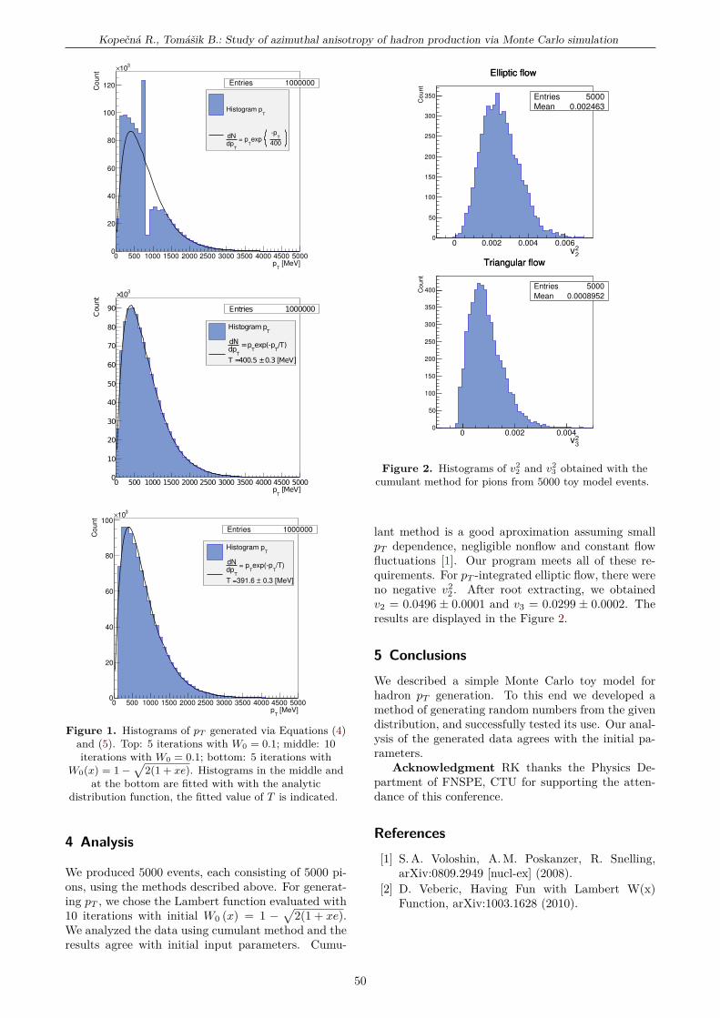
Kopečná R., Tomášik B.: Study of azimuthal anisotropy of hadron production via Monte Carlo simulation
[MeV]T
p0 500 1000 1500 2000 2500 3000 3500 4000 4500 5000
Count
0
20
40
60
80
100
120
310×
Entries 1000000
THistogram p
400T
-pexp
T= p
TdpdN
[MeV]T
p0 500 1000 1500 2000 2500 3000 3500 4000 4500 5000
Count
0
10
20
30
40
50
60
70
80
90
310×
Entries 1000000
THistogramp
0.3 [MeV]±T =400.5
/T)T
exp(-pT
=pT
dpdN
[MeV]T
p0 500 1000 1500 2000 2500 3000 3500 4000 4500 5000
Count
0
20
40
60
80
100
310×
Entries 1000000
THistogram p
0.3 [MeV]±T =391.6
/T)T
exp(-pT
= pT
dpdN
Figure 1. Histograms of pT generated via Equations (4)and (5). Top: 5 iterations with W0 = 0.1; middle: 10iterations with W0 = 0.1; bottom: 5 iterations with
W0(x) = 1 −√
2(1 + xe). Histograms in the middle andat the bottom are fitted with with the analytic
distribution function, the fitted value of T is indicated.
4 Analysis
We produced 5000 events, each consisting of 5000 pi-ons, using the methods described above. For generat-ing pT , we chose the Lambert function evaluated with10 iterations with initial W0 (x) = 1 −
√
2(1 + xe).We analyzed the data using cumulant method and theresults agree with initial input parameters. Cumu-
22 v
0 0.002 0.004 0.006
Co
un
t
0
50
100
150
200
250
300
350
Elliptic flow
Entries 5000Mean 0.002463
Elliptic flow
23 v
0 0.002 0.004
Co
un
t
0
50
100
150
200
250
300
350
400
Triangular flow
Entries 5000
Mean 0.0008952
Triangular flow
Figure 2. Histograms of v22 and v2
3 obtained with thecumulant method for pions from 5000 toy model events.
lant method is a good aproximation assuming smallpT dependence, negligible nonflow and constant flowfluctuations [1]. Our program meets all of these re-quirements. For pT -integrated elliptic flow, there wereno negative v2
2 . After root extracting, we obtainedv2 = 0.0496 ± 0.0001 and v3 = 0.0299 ± 0.0002. Theresults are displayed in the Figure 2.
5 Conclusions
We described a simple Monte Carlo toy model forhadron pT generation. To this end we developed amethod of generating random numbers from the givendistribution, and successfully tested its use. Our anal-ysis of the generated data agrees with the initial pa-rameters.
Acknowledgment RK thanks the Physics De-partment of FNSPE, CTU for supporting the atten-dance of this conference.
References
[1] S. A. Voloshin, A. M. Poskanzer, R. Snelling,arXiv:0809.2949 [nucl-ex] (2008).
[2] D. Veberic, Having Fun with Lambert W(x)Function, arXiv:1003.1628 (2010).
50
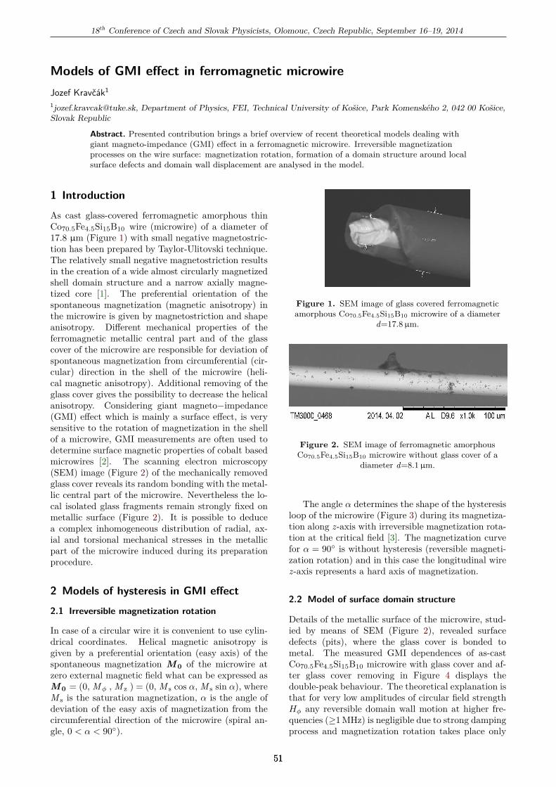
18th Conference of Czech and Slovak Physicists, Olomouc, Czech Republic, September 16–19, 2014
Models of GMI effect in ferromagnetic microwire
Jozef Kravčák1
[email protected], Department of Physics, FEI, Technical University of Košice, Park Komenského 2, 042 00 Košice,Slovak Republic
Abstract. Presented contribution brings a brief overview of recent theoretical models dealing withgiant magneto-impedance (GMI) effect in a ferromagnetic microwire. Irreversible magnetizationprocesses on the wire surface: magnetization rotation, formation of a domain structure around localsurface defects and domain wall displacement are analysed in the model.
1 Introduction
As cast glass-covered ferromagnetic amorphous thinCo70.5Fe4.5Si15B10 wire (microwire) of a diameter of17.8 µm (Figure 1) with small negative magnetostric-tion has been prepared by Taylor-Ulitovski technique.The relatively small negative magnetostriction resultsin the creation of a wide almost circularly magnetizedshell domain structure and a narrow axially magne-tized core [1]. The preferential orientation of thespontaneous magnetization (magnetic anisotropy) inthe microwire is given by magnetostriction and shapeanisotropy. Different mechanical properties of theferromagnetic metallic central part and of the glasscover of the microwire are responsible for deviation ofspontaneous magnetization from circumferential (cir-cular) direction in the shell of the microwire (heli-cal magnetic anisotropy). Additional removing of theglass cover gives the possibility to decrease the helicalanisotropy. Considering giant magneto−impedance(GMI) effect which is mainly a surface effect, is verysensitive to the rotation of magnetization in the shellof a microwire, GMI measurements are often used todetermine surface magnetic properties of cobalt basedmicrowires [2]. The scanning electron microscopy(SEM) image (Figure 2) of the mechanically removedglass cover reveals its random bonding with the metal-lic central part of the microwire. Nevertheless the lo-cal isolated glass fragments remain strongly fixed onmetallic surface (Figure 2). It is possible to deducea complex inhomogeneous distribution of radial, ax-ial and torsional mechanical stresses in the metallicpart of the microwire induced during its preparationprocedure.
2 Models of hysteresis in GMI effect
2.1 Irreversible magnetization rotation
In case of a circular wire it is convenient to use cylin-drical coordinates. Helical magnetic anisotropy isgiven by a preferential orientation (easy axis) of thespontaneous magnetization M 0 of the microwire atzero external magnetic field what can be expressed asM 0 = (0, M φ , M z ) = (0, M s cos α, M s sin α), whereM s is the saturation magnetization, α is the angle ofdeviation of the easy axis of magnetization from thecircumferential direction of the microwire (spiral an-gle, 0 < α < 90).
Figure 1. SEM image of glass covered ferromagneticamorphous Co70.5Fe4.5Si15B10 microwire of a diameter
d=17.8µm.
Figure 2. SEM image of ferromagnetic amorphousCo70.5Fe4.5Si15B10 microwire without glass cover of a
diameter d=8.1µm.
The angle α determines the shape of the hysteresisloop of the microwire (Figure 3) during its magnetiza-tion along z-axis with irreversible magnetization rota-tion at the critical field [3]. The magnetization curvefor α = 90 is without hysteresis (reversible magneti-zation rotation) and in this case the longitudinal wirez-axis represents a hard axis of magnetization.
2.2 Model of surface domain structure
Details of the metallic surface of the microwire, stud-ied by means of SEM (Figure 2), revealed surfacedefects (pits), where the glass cover is bonded tometal. The measured GMI dependences of as-castCo70.5Fe4.5Si15B10 microwire with glass cover and af-ter glass cover removing in Figure 4 displays thedouble-peak behaviour. The theoretical explanation isthat for very low amplitudes of circular field strengthHφ any reversible domain wall motion at higher fre-quencies (≥1 MHz) is negligible due to strong dampingprocess and magnetization rotation takes place only
515151
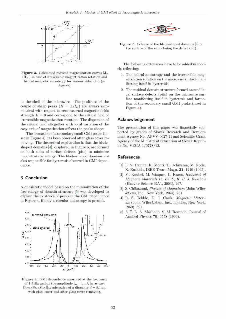
Kravčák J.: Models of GMI effect in ferromagnetic microwire
Figure 3. Calculated reduced magnetization curves Mφ
(Hφ ) in case of irreversible magnetization rotation andhelical magnetic anisotropy for various value of α (in
degrees).
in the shell of the microwire. The positions of thecouple of sharp peaks (H = ±Hm) are always sym-metrical with respect to zero external magnetic fieldsstrength H = 0 and correspond to the critical field ofirreversible magnetization rotation. The dispersion ofthe critical field altogether with local variation of theeasy axis of magnetization affects the peaks shape.
The formation of a secondary small GMI peaks (in-set in Figure 4) has been observed after glass cover re-moving. The theoretical explanation is that the blade-shaped domains [4], displayed in Figure 5, are formedon both sides of surface defects (pits) to minimizemagnetostatic energy. The blade-shaped domains arealso responsible for hysteresis observed in GMI depen-dence.
3 Conclusion
A quasistatic model based on the minimization of thefree energy of domain structure [5] was developed toexplain the existence of peaks in the GMI dependencein Figure 4, if only a circular anisotropy is present.
Figure 4. GMI dependence measured at the frequencyof 1 MHz and at the amplitude iac= 1 mA in as-cast
Co70.5Fe4.5Si15B10 microwire of a diameter d = 8.1µmwith glass cover and after glass cover removing.
Figure 5. Scheme of the blade-shaped domains [4] onthe surface of the wire closing the defect (pit).
The following extensions have to be added in mod-els reflecting:
1. The helical anisotropy and the irreversible mag-netization rotation on the microwire surface man-ifesting itself in hysteresis.
2. The residual domain structure formed around lo-cal surface defects (pits) on the microwire sur-face manifesting itself in hysteresis and forma-tion of the secondary small GMI peaks (inset inFigure 4).
Acknowledgement
The presentation of this paper was financially sup-ported by grants of Slovak Research and Develop-ment Agency No. APVV-0027-11 and Scientific GrantAgency of the Ministry of Education of Slovak Repub-lic No. VEGA-1/0778/12.
References
[1] L. V. Panina, K. Mohri, T. Uchiyama, M. Noda,K. Bushida, IEEE Trans. Magn. 31, 1249 (1995).
[2] M. Knobel, M. Vázquez, L. Kraus, Handbook ofMagnetic Materials 15, Ed. by K. H. J. Buschow(Elsevier Science B.V., 2003), 497.
[3] S. Chikazumi, Physics of Magnetism (John Wiley&Sons, Inc., New York, 1964), 281.
[4] R. S. Tebble, D. J. Craik, Magnetic Materi-als (John Wiley&Sons, Inc., London, New York,1969), 391.
[5] A F. L. A. Machado, S. M. Rezende, Journal ofApplied Physics 79, 6558 (1996).
52
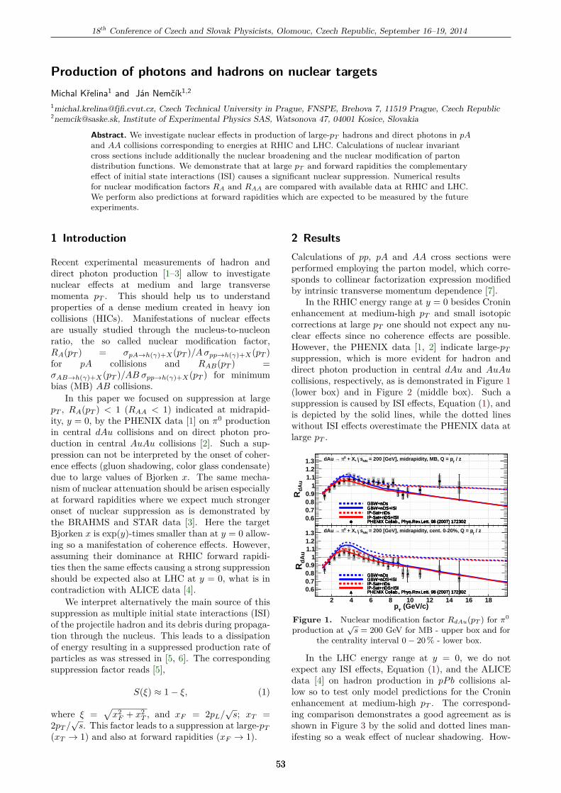
18th Conference of Czech and Slovak Physicists, Olomouc, Czech Republic, September 16–19, 2014
Production of photons and hadrons on nuclear targets
Michal Křelina1 and Ján Nemčík1,2
[email protected], Czech Technical University in Prague, FNSPE, Brehova 7, 11519 Prague, Czech [email protected], Institute of Experimental Physics SAS, Watsonova 47, 04001 Kosice, Slovakia
Abstract. We investigate nuclear effects in production of large-pT hadrons and direct photons in pAand AA collisions corresponding to energies at RHIC and LHC. Calculations of nuclear invariantcross sections include additionally the nuclear broadening and the nuclear modification of partondistribution functions. We demonstrate that at large pT and forward rapidities the complementaryeffect of initial state interactions (ISI) causes a significant nuclear suppression. Numerical resultsfor nuclear modification factors RA and RAA are compared with available data at RHIC and LHC.We perform also predictions at forward rapidities which are expected to be measured by the futureexperiments.
1 Introduction
Recent experimental measurements of hadron anddirect photon production [1–3] allow to investigatenuclear effects at medium and large transversemomenta pT . This should help us to understandproperties of a dense medium created in heavy ioncollisions (HICs). Manifestations of nuclear effectsare usually studied through the nucleus-to-nucleonratio, the so called nuclear modification factor,RA(pT ) = σpA→h(γ)+X(pT )/Aσpp→h(γ)+X(pT )for pA collisions and RAB(pT ) =σAB→h(γ)+X(pT )/AB σpp→h(γ)+X(pT ) for minimumbias (MB) AB collisions.
In this paper we focused on suppression at largepT , RA(pT ) < 1 (RAA < 1) indicated at midrapid-ity, y = 0, by the PHENIX data [1] on π0 productionin central dAu collisions and on direct photon pro-duction in central AuAu collisions [2]. Such a sup-pression can not be interpreted by the onset of coher-ence effects (gluon shadowing, color glass condensate)due to large values of Bjorken x. The same mecha-nism of nuclear attenuation should be arisen especiallyat forward rapidities where we expect much strongeronset of nuclear suppression as is demonstrated bythe BRAHMS and STAR data [3]. Here the targetBjorken x is exp(y)-times smaller than at y = 0 allow-ing so a manifestation of coherence effects. However,assuming their dominance at RHIC forward rapidi-ties then the same effects causing a strong suppressionshould be expected also at LHC at y = 0, what is incontradiction with ALICE data [4].
We interpret alternatively the main source of thissuppression as multiple initial state interactions (ISI)of the projectile hadron and its debris during propaga-tion through the nucleus. This leads to a dissipationof energy resulting in a suppressed production rate ofparticles as was stressed in [5, 6]. The correspondingsuppression factor reads [5],
S(ξ) ≈ 1 − ξ, (1)
where ξ =√
x2F + x2
T , and xF = 2pL/√s; xT =
2pT /√s. This factor leads to a suppression at large-pT
(xT → 1) and also at forward rapidities (xF → 1).
2 Results
Calculations of pp, pA and AA cross sections wereperformed employing the parton model, which corre-sponds to collinear factorization expression modifiedby intrinsic transverse momentum dependence [7].
In the RHIC energy range at y = 0 besides Croninenhancement at medium-high pT and small isotopiccorrections at large pT one should not expect any nu-clear effects since no coherence effects are possible.However, the PHENIX data [1, 2] indicate large-pT
suppression, which is more evident for hadron anddirect photon production in central dAu and AuAucollisions, respectively, as is demonstrated in Figure 1(lower box) and in Figure 2 (middle box). Such asuppression is caused by ISI effects, Equation (1), andis depicted by the solid lines, while the dotted lineswithout ISI effects overestimate the PHENIX data atlarge pT .
2 4 6 8 10 12 14 16 18
dAu
R
0.60.70.80.9
11.11.21.3 / z
T = 200 [GeV], midrapidity, MB, Q = pNNs + X, 0π →dAu
GBW+nDsGBW+nDS+ISIIP-Sat+nDsIP-Sat+nDS+ISIPHENIX Collab., Phys.Rev.Lett. 98 (2007) 172302
GBW+nDsGBW+nDS+ISIIP-Sat+nDsIP-Sat+nDS+ISIPHENIX Collab., Phys.Rev.Lett. 98 (2007) 172302
GBW+nDsGBW+nDS+ISIIP-Sat+nDsIP-Sat+nDS+ISIPHENIX Collab., Phys.Rev.Lett. 98 (2007) 172302
GBW+nDsGBW+nDS+ISIIP-Sat+nDsIP-Sat+nDS+ISIPHENIX Collab., Phys.Rev.Lett. 98 (2007) 172302
GBW+nDsGBW+nDS+ISIIP-Sat+nDsIP-Sat+nDS+ISIPHENIX Collab., Phys.Rev.Lett. 98 (2007) 172302
(GeV/c)T
p2 4 6 8 10 12 14 16 18
dAu
R
0.60.70.80.9
11.11.21.3 / z
T = 200 [GeV], midrapidity, cent. 0-20%, Q = pNNs + X, 0π →dAu
GBW+nDsGBW+nDS+ISIIP-Sat+nDsIP-Sat+nDS+ISIPHENIX Collab., Phys.Rev.Lett. 98 (2007) 172302
GBW+nDsGBW+nDS+ISIIP-Sat+nDsIP-Sat+nDS+ISIPHENIX Collab., Phys.Rev.Lett. 98 (2007) 172302
GBW+nDsGBW+nDS+ISIIP-Sat+nDsIP-Sat+nDS+ISIPHENIX Collab., Phys.Rev.Lett. 98 (2007) 172302
GBW+nDsGBW+nDS+ISIIP-Sat+nDsIP-Sat+nDS+ISIPHENIX Collab., Phys.Rev.Lett. 98 (2007) 172302
GBW+nDsGBW+nDS+ISIIP-Sat+nDsIP-Sat+nDS+ISIPHENIX Collab., Phys.Rev.Lett. 98 (2007) 172302
Figure 1. Nuclear modification factor RdAu(pT ) for π0
production at√s = 200 GeV for MB - upper box and for
the centrality interval 0 − 20 % - lower box.
In the LHC energy range at y = 0, we do notexpect any ISI effects, Equation (1), and the ALICEdata [4] on hadron production in pPb collisions al-low so to test only model predictions for the Croninenhancement at medium-high pT . The correspond-ing comparison demonstrates a good agreement as isshown in Figure 3 by the solid and dotted lines man-ifesting so a weak effect of nuclear shadowing. How-
535353
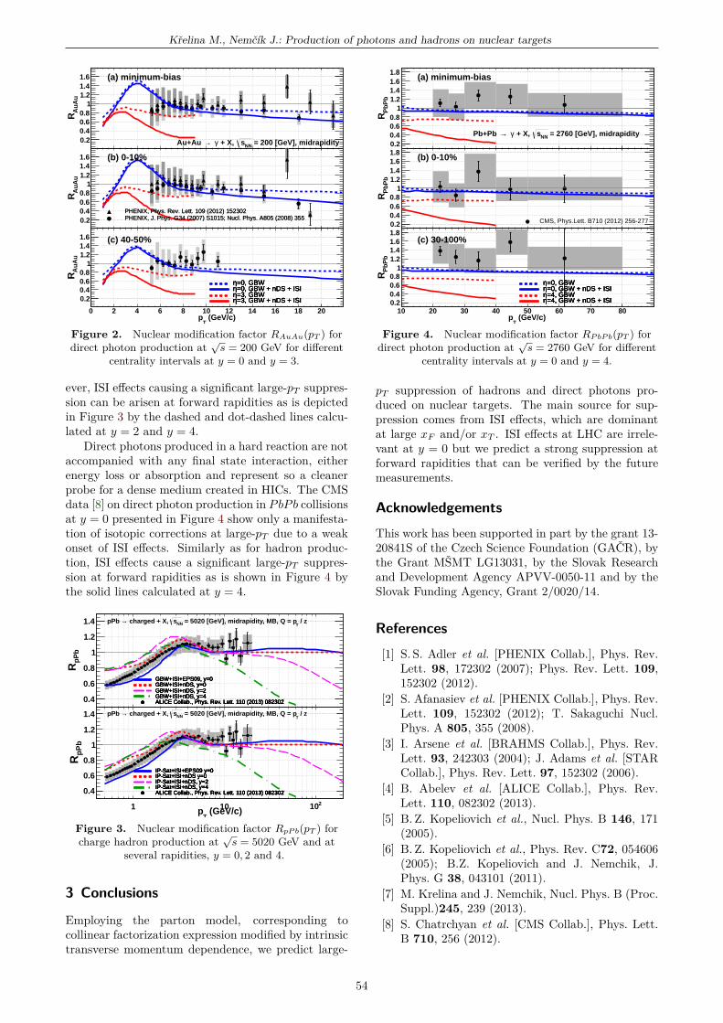
Křelina M., Nemčík J.: Production of photons and hadrons on nuclear targets
0 2 4 6 8 10 12 14 16 18 20
AuA
uR
0.20.40.60.8
11.21.41.6 (a) minimum-bias
= 200 [GeV], midrapidityNNs + X, γ →Au+Au
0 2 4 6 8 10 12 14 16 18 20
AuA
uR
0.20.40.60.8
11.21.41.6 (b) 0-10%
PHENIX, Phys. Rev. Lett. 109 (2012) 152302PHENIX, J. Phys. G34 (2007) S1015; Nucl. Phys. A805 (2008) 355PHENIX, Phys. Rev. Lett. 109 (2012) 152302PHENIX, J. Phys. G34 (2007) S1015; Nucl. Phys. A805 (2008) 355
(GeV/c)T
p0 2 4 6 8 10 12 14 16 18 20
AuA
uR
0.20.40.60.8
11.21.41.6 (c) 40-50%
=0, GBWη=0, GBW + nDS + ISIη=3, GBWη=3, GBW + nDS + ISIη
=0, GBWη=0, GBW + nDS + ISIη=3, GBWη=3, GBW + nDS + ISIη
=0, GBWη=0, GBW + nDS + ISIη=3, GBWη=3, GBW + nDS + ISIη
=0, GBWη=0, GBW + nDS + ISIη=3, GBWη=3, GBW + nDS + ISIη
Figure 2. Nuclear modification factor RAuAu(pT ) fordirect photon production at
√s = 200 GeV for different
centrality intervals at y = 0 and y = 3.
ever, ISI effects causing a significant large-pT suppres-sion can be arisen at forward rapidities as is depictedin Figure 3 by the dashed and dot-dashed lines calcu-lated at y = 2 and y = 4.
Direct photons produced in a hard reaction are notaccompanied with any final state interaction, eitherenergy loss or absorption and represent so a cleanerprobe for a dense medium created in HICs. The CMSdata [8] on direct photon production in PbPb collisionsat y = 0 presented in Figure 4 show only a manifesta-tion of isotopic corrections at large-pT due to a weakonset of ISI effects. Similarly as for hadron produc-tion, ISI effects cause a significant large-pT suppres-sion at forward rapidities as is shown in Figure 4 bythe solid lines calculated at y = 4.
pPb
R
0.4
0.6
0.8
1
1.2
1.4 / zT
= 5020 [GeV], midrapidity, MB, Q = pNNs charged + X, →pPb
GBW+ISI+EPS09, y=0GBW+ISI+nDS, y=0GBW+ISI+nDS, y=2GBW+ISI+nDS, y=4ALICE Collab., Phys. Rev. Lett. 110 (2013) 082302
GBW+ISI+EPS09, y=0GBW+ISI+nDS, y=0GBW+ISI+nDS, y=2GBW+ISI+nDS, y=4ALICE Collab., Phys. Rev. Lett. 110 (2013) 082302
GBW+ISI+EPS09, y=0GBW+ISI+nDS, y=0GBW+ISI+nDS, y=2GBW+ISI+nDS, y=4ALICE Collab., Phys. Rev. Lett. 110 (2013) 082302
GBW+ISI+EPS09, y=0GBW+ISI+nDS, y=0GBW+ISI+nDS, y=2GBW+ISI+nDS, y=4ALICE Collab., Phys. Rev. Lett. 110 (2013) 082302
GBW+ISI+EPS09, y=0GBW+ISI+nDS, y=0GBW+ISI+nDS, y=2GBW+ISI+nDS, y=4ALICE Collab., Phys. Rev. Lett. 110 (2013) 082302
(GeV/c)T
p1 10 210
pPb
R
0.4
0.6
0.8
1
1.2
1.4 / zT
= 5020 [GeV], midrapidity, MB, Q = pNNs charged + X, →pPb
IP-Sat+ISI+EPS09 y=0IP-Sat+ISI+nDS y=0IP-Sat+ISI+nDS, y=2IP-Sat+ISI+nDS, y=4ALICE Collab., Phys. Rev. Lett. 110 (2013) 082302
IP-Sat+ISI+EPS09 y=0IP-Sat+ISI+nDS y=0IP-Sat+ISI+nDS, y=2IP-Sat+ISI+nDS, y=4ALICE Collab., Phys. Rev. Lett. 110 (2013) 082302
IP-Sat+ISI+EPS09 y=0IP-Sat+ISI+nDS y=0IP-Sat+ISI+nDS, y=2IP-Sat+ISI+nDS, y=4ALICE Collab., Phys. Rev. Lett. 110 (2013) 082302
IP-Sat+ISI+EPS09 y=0IP-Sat+ISI+nDS y=0IP-Sat+ISI+nDS, y=2IP-Sat+ISI+nDS, y=4ALICE Collab., Phys. Rev. Lett. 110 (2013) 082302
IP-Sat+ISI+EPS09 y=0IP-Sat+ISI+nDS y=0IP-Sat+ISI+nDS, y=2IP-Sat+ISI+nDS, y=4ALICE Collab., Phys. Rev. Lett. 110 (2013) 082302
Figure 3. Nuclear modification factor RpP b(pT ) forcharge hadron production at
√s = 5020 GeV and at
several rapidities, y = 0, 2 and 4.
3 Conclusions
Employing the parton model, corresponding tocollinear factorization expression modified by intrinsictransverse momentum dependence, we predict large-
10 20 30 40 50 60 70 80
PbP
bR
0.20.40.60.8
11.21.41.61.8
(a) minimum-bias
= 2760 [GeV], midrapidityNNs + X, γ →Pb+Pb
10 20 30 40 50 60 70 80
PbP
bR
0.20.40.60.8
11.21.41.61.8
(b) 0-10%
CMS, Phys.Lett. B710 (2012) 256-277
(GeV/c)T
p10 20 30 40 50 60 70 80
PbP
bR
0.20.40.60.8
11.21.41.61.8
(c) 30-100%
=0, GBWη=0, GBW + nDS + ISIη=4, GBWη=4, GBW + nDS + ISIη
=0, GBWη=0, GBW + nDS + ISIη=4, GBWη=4, GBW + nDS + ISIη
=0, GBWη=0, GBW + nDS + ISIη=4, GBWη=4, GBW + nDS + ISIη
=0, GBWη=0, GBW + nDS + ISIη=4, GBWη=4, GBW + nDS + ISIη
Figure 4. Nuclear modification factor RP bP b(pT ) fordirect photon production at
√s = 2760 GeV for different
centrality intervals at y = 0 and y = 4.
pT suppression of hadrons and direct photons pro-duced on nuclear targets. The main source for sup-pression comes from ISI effects, which are dominantat large xF and/or xT . ISI effects at LHC are irrele-vant at y = 0 but we predict a strong suppression atforward rapidities that can be verified by the futuremeasurements.
Acknowledgements
This work has been supported in part by the grant 13-20841S of the Czech Science Foundation (GAČR), bythe Grant MŠMT LG13031, by the Slovak Researchand Development Agency APVV-0050-11 and by theSlovak Funding Agency, Grant 2/0020/14.
References
[1] S. S. Adler et al. [PHENIX Collab.], Phys. Rev.Lett. 98, 172302 (2007); Phys. Rev. Lett. 109,152302 (2012).
[2] S. Afanasiev et al. [PHENIX Collab.], Phys. Rev.Lett. 109, 152302 (2012); T. Sakaguchi Nucl.Phys. A 805, 355 (2008).
[3] I. Arsene et al. [BRAHMS Collab.], Phys. Rev.Lett. 93, 242303 (2004); J. Adams et al. [STARCollab.], Phys. Rev. Lett. 97, 152302 (2006).
[4] B. Abelev et al. [ALICE Collab.], Phys. Rev.Lett. 110, 082302 (2013).
[5] B. Z. Kopeliovich et al., Nucl. Phys. B 146, 171(2005).
[6] B. Z. Kopeliovich et al., Phys. Rev. C72, 054606(2005); B.Z. Kopeliovich and J. Nemchik, J.Phys. G 38, 043101 (2011).
[7] M. Krelina and J. Nemchik, Nucl. Phys. B (Proc.Suppl.)245, 239 (2013).
[8] S. Chatrchyan et al. [CMS Collab.], Phys. Lett.B 710, 256 (2012).
54
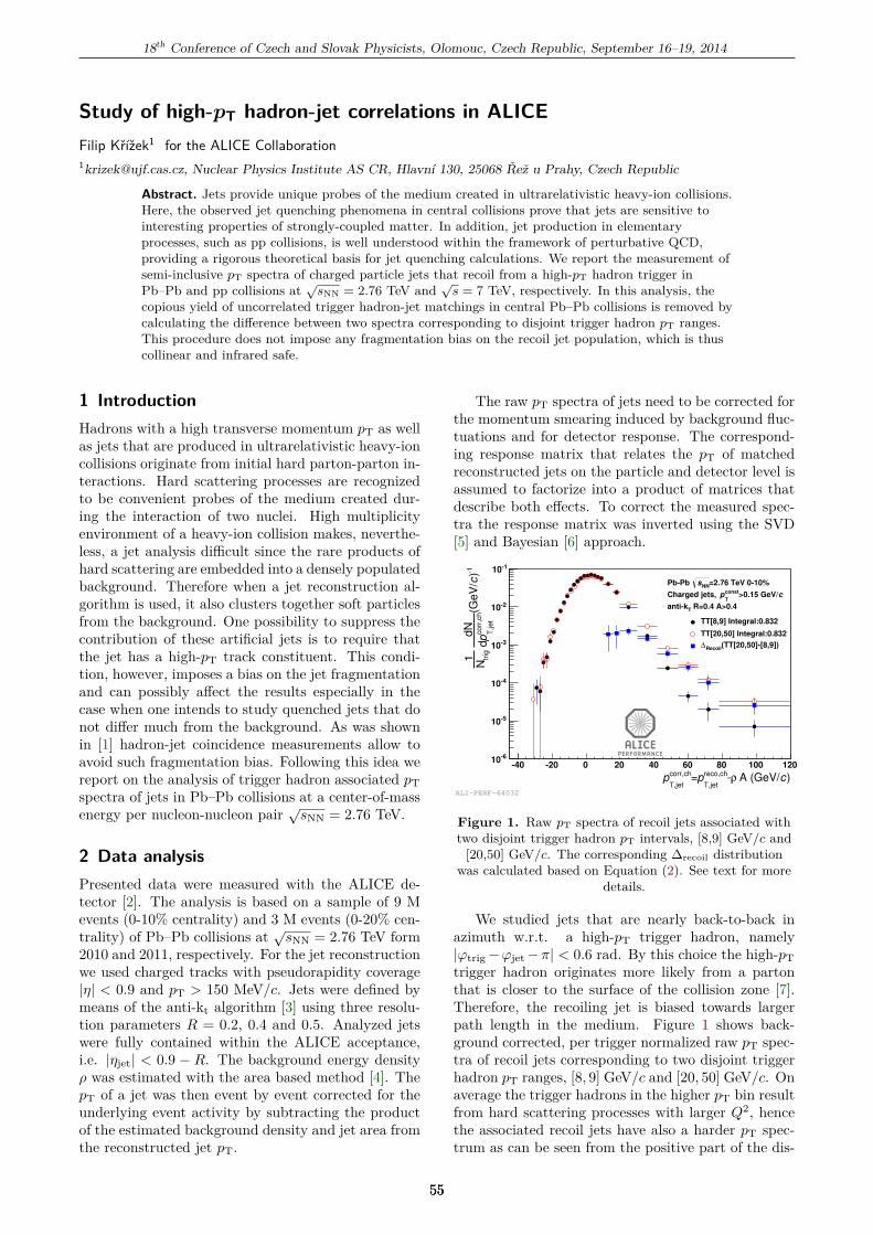
18th Conference of Czech and Slovak Physicists, Olomouc, Czech Republic, September 16–19, 2014
Study of high-pT hadron-jet correlations in ALICE
Filip Křížek1 for the ALICE [email protected], Nuclear Physics Institute AS CR, Hlavní 130, 25068 Řež u Prahy, Czech Republic
Abstract. Jets provide unique probes of the medium created in ultrarelativistic heavy-ion collisions.Here, the observed jet quenching phenomena in central collisions prove that jets are sensitive tointeresting properties of strongly-coupled matter. In addition, jet production in elementaryprocesses, such as pp collisions, is well understood within the framework of perturbative QCD,providing a rigorous theoretical basis for jet quenching calculations. We report the measurement ofsemi-inclusive pT spectra of charged particle jets that recoil from a high-pT hadron trigger inPb–Pb and pp collisions at
√sNN = 2.76 TeV and
√s = 7 TeV, respectively. In this analysis, the
copious yield of uncorrelated trigger hadron-jet matchings in central Pb–Pb collisions is removed bycalculating the difference between two spectra corresponding to disjoint trigger hadron pT ranges.This procedure does not impose any fragmentation bias on the recoil jet population, which is thuscollinear and infrared safe.
1 Introduction
Hadrons with a high transverse momentum pT as wellas jets that are produced in ultrarelativistic heavy-ioncollisions originate from initial hard parton-parton in-teractions. Hard scattering processes are recognizedto be convenient probes of the medium created dur-ing the interaction of two nuclei. High multiplicityenvironment of a heavy-ion collision makes, neverthe-less, a jet analysis difficult since the rare products ofhard scattering are embedded into a densely populatedbackground. Therefore when a jet reconstruction al-gorithm is used, it also clusters together soft particlesfrom the background. One possibility to suppress thecontribution of these artificial jets is to require thatthe jet has a high-pT track constituent. This condi-tion, however, imposes a bias on the jet fragmentationand can possibly affect the results especially in thecase when one intends to study quenched jets that donot differ much from the background. As was shownin [1] hadron-jet coincidence measurements allow toavoid such fragmentation bias. Following this idea wereport on the analysis of trigger hadron associated pT
spectra of jets in Pb–Pb collisions at a center-of-massenergy per nucleon-nucleon pair
√sNN = 2.76 TeV.
2 Data analysis
Presented data were measured with the ALICE de-tector [2]. The analysis is based on a sample of 9 Mevents (0-10% centrality) and 3 M events (0-20% cen-trality) of Pb–Pb collisions at
√sNN = 2.76 TeV form
2010 and 2011, respectively. For the jet reconstructionwe used charged tracks with pseudorapidity coverage|η| < 0.9 and pT > 150 MeV/c. Jets were defined bymeans of the anti-kt algorithm [3] using three resolu-tion parameters R = 0.2, 0.4 and 0.5. Analyzed jetswere fully contained within the ALICE acceptance,i.e. |ηjet| < 0.9 − R. The background energy densityρ was estimated with the area based method [4]. ThepT of a jet was then event by event corrected for theunderlying event activity by subtracting the productof the estimated background density and jet area fromthe reconstructed jet pT.
The raw pT spectra of jets need to be corrected forthe momentum smearing induced by background fluc-tuations and for detector response. The correspond-ing response matrix that relates the pT of matchedreconstructed jets on the particle and detector level isassumed to factorize into a product of matrices thatdescribe both effects. To correct the measured spec-tra the response matrix was inverted using the SVD[5] and Bayesian [6] approach.
)c A (GeV/ρ-reco,ch
T,jetp=corr,ch
T,jetp
-40 -20 0 20 40 60 80 100 120
-1 )c
(Ge
V/
co
rr,c
h
T,je
tp
d
dN
tr
igN
1
-610
-510
-410
-310
-210
-110
TT[8,9] Integral:0.832
TT[20,50] Integral:0.832
(TT[20,50]-[8,9])Recoil
∆
c>0.15 GeV/const
TpCharged jets,
=2.76 TeV 0-10%NN
sPb-Pb
R=0.4 A>0.4T
anti-k
ALI−PERF−64032
Figure 1. Raw pT spectra of recoil jets associated withtwo disjoint trigger hadron pT intervals, [8,9] GeV/c and
[20,50] GeV/c. The corresponding ∆recoil distributionwas calculated based on Equation (2). See text for more
details.
We studied jets that are nearly back-to-back inazimuth w.r.t. a high-pT trigger hadron, namely|ϕtrig −ϕjet −π| < 0.6 rad. By this choice the high-pT
trigger hadron originates more likely from a partonthat is closer to the surface of the collision zone [7].Therefore, the recoiling jet is biased towards largerpath length in the medium. Figure 1 shows back-ground corrected, per trigger normalized raw pT spec-tra of recoil jets corresponding to two disjoint triggerhadron pT ranges, [8, 9] GeV/c and [20, 50] GeV/c. Onaverage the trigger hadrons in the higher pT bin resultfrom hard scattering processes with larger Q2, hencethe associated recoil jets have also a harder pT spec-trum as can be seen from the positive part of the dis-
555555
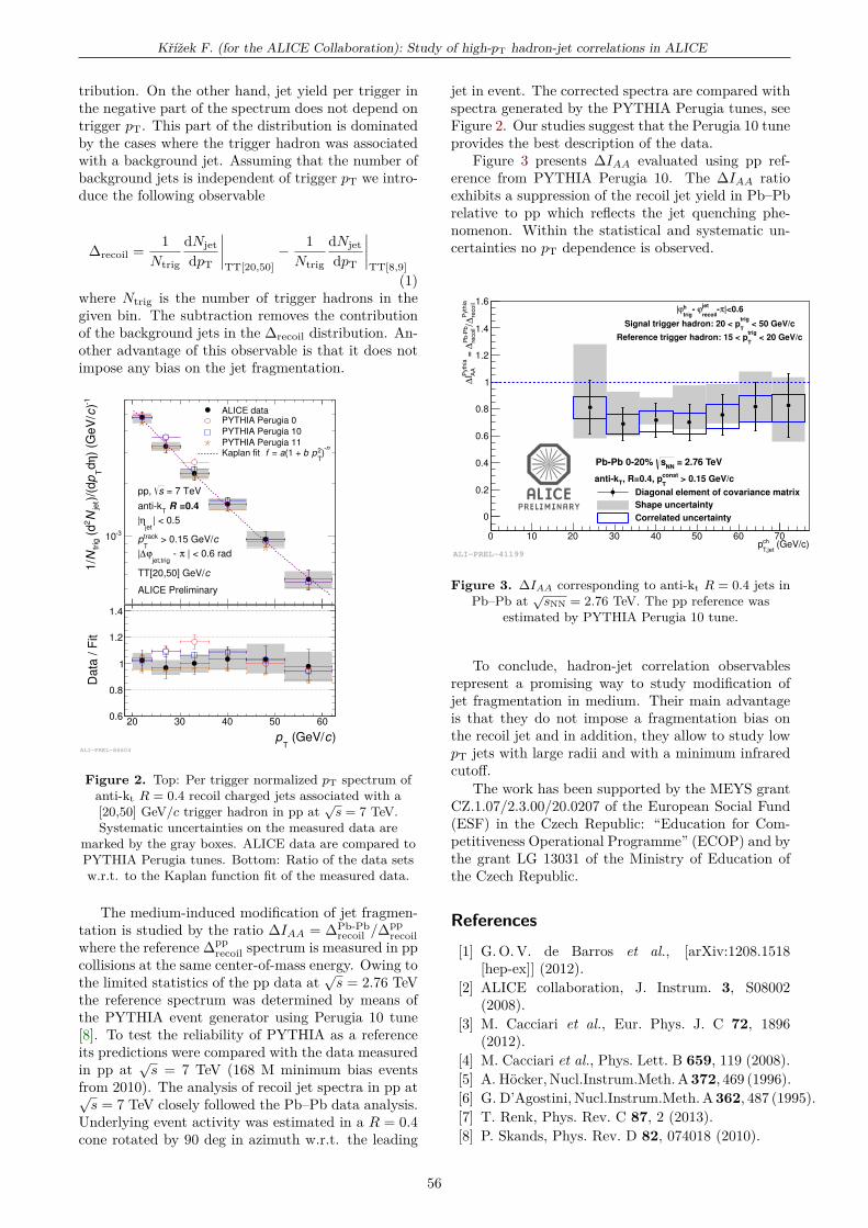
Křížek F. (for the ALICE Collaboration): Study of high-pT hadron-jet correlations in ALICE
tribution. On the other hand, jet yield per trigger inthe negative part of the spectrum does not depend ontrigger pT. This part of the distribution is dominatedby the cases where the trigger hadron was associatedwith a background jet. Assuming that the number ofbackground jets is independent of trigger pT we intro-duce the following observable
∆recoil =1
Ntrig
dNjet
dpT
∣
∣
∣
∣
TT[20,50]
− 1Ntrig
dNjet
dpT
∣
∣
∣
∣
TT[8,9]
(1)where Ntrig is the number of trigger hadrons in thegiven bin. The subtraction removes the contributionof the background jets in the ∆recoil distribution. An-other advantage of this observable is that it does notimpose any bias on the jet fragmentation.
-1 )c
) (G
eV
/η
dT
p)/
(dje
tN
2 (
dtr
igN
1/
-310
= 7 TeVspp,
=0.4R T
anti-k
| < 0.5jet
η|
c > 0.15 GeV/track
Tp
| < 0.6 radπ - jet,trig
ϕ∆|
cTT[20,50] GeV/
ALICE Preliminary
ALICE dataPYTHIA Perugia 0
PYTHIA Perugia 10
PYTHIA Perugia 11n-
)2
Tp b(1 + a = fKaplan fit
)c (GeV/T
p
20 30 40 50 60
Da
ta /
Fit
0.6
0.8
1
1.2
1.4
ALI−PREL−86604
Figure 2. Top: Per trigger normalized pT spectrum ofanti-kt R = 0.4 recoil charged jets associated with a[20,50] GeV/c trigger hadron in pp at
√s = 7 TeV.
Systematic uncertainties on the measured data aremarked by the gray boxes. ALICE data are compared toPYTHIA Perugia tunes. Bottom: Ratio of the data setsw.r.t. to the Kaplan function fit of the measured data.
The medium-induced modification of jet fragmen-tation is studied by the ratio ∆IAA = ∆Pb-Pb
recoil /∆pprecoil
where the reference ∆pprecoil spectrum is measured in pp
collisions at the same center-of-mass energy. Owing tothe limited statistics of the pp data at
√s = 2.76 TeV
the reference spectrum was determined by means ofthe PYTHIA event generator using Perugia 10 tune[8]. To test the reliability of PYTHIA as a referenceits predictions were compared with the data measuredin pp at
√s = 7 TeV (168 M minimum bias events
from 2010). The analysis of recoil jet spectra in pp at√s = 7 TeV closely followed the Pb–Pb data analysis.
Underlying event activity was estimated in a R = 0.4cone rotated by 90 deg in azimuth w.r.t. the leading
jet in event. The corrected spectra are compared withspectra generated by the PYTHIA Perugia tunes, seeFigure 2. Our studies suggest that the Perugia 10 tuneprovides the best description of the data.
Figure 3 presents ∆IAA evaluated using pp ref-erence from PYTHIA Perugia 10. The ∆IAA ratioexhibits a suppression of the recoil jet yield in Pb–Pbrelative to pp which reflects the jet quenching phe-nomenon. Within the statistical and systematic un-certainties no pT dependence is observed.
(GeV/c)ch
T,jetp
0 10 20 30 40 50 60 70
Pyth
ia
reco
il∆/
Pb
-Pb
reco
il∆
=
Pyth
ia
AA
I∆
0
0.2
0.4
0.6
0.8
1
1.2
1.4
1.6
> 0.15 GeV/cconst
T, R=0.4, p
Tanti-k
Diagonal element of covariance matrix
Shape uncertainty
Correlated uncertainty
|<0.6π-jet
recoilϕ- h
trigϕ|
< 50 GeV/ctrig
TSignal trigger hadron: 20 < p
< 20 GeV/ctrig
TReference trigger hadron: 15 < p
= 2.76 TeVNN
sPb-Pb 0-20%
ALI−PREL−41199
Figure 3. ∆IAA corresponding to anti-kt R = 0.4 jets inPb–Pb at
√sNN = 2.76 TeV. The pp reference was
estimated by PYTHIA Perugia 10 tune.
To conclude, hadron-jet correlation observablesrepresent a promising way to study modification ofjet fragmentation in medium. Their main advantageis that they do not impose a fragmentation bias onthe recoil jet and in addition, they allow to study lowpT jets with large radii and with a minimum infraredcutoff.
The work has been supported by the MEYS grantCZ.1.07/2.3.00/20.0207 of the European Social Fund(ESF) in the Czech Republic: “Education for Com-petitiveness Operational Programme” (ECOP) and bythe grant LG 13031 of the Ministry of Education ofthe Czech Republic.
References
[1] G. O. V. de Barros et al., [arXiv:1208.1518[hep-ex]] (2012).
[2] ALICE collaboration, J. Instrum. 3, S08002(2008).
[3] M. Cacciari et al., Eur. Phys. J. C 72, 1896(2012).
[4] M. Cacciari et al., Phys. Lett. B 659, 119 (2008).[5] A. Höcker, Nucl.Instrum.Meth. A 372, 469 (1996).[6] G. D’Agostini, Nucl.Instrum.Meth. A 362, 487 (1995).[7] T. Renk, Phys. Rev. C 87, 2 (2013).[8] P. Skands, Phys. Rev. D 82, 074018 (2010).
56
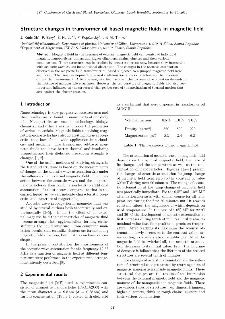
18th Conference of Czech and Slovak Physicists, Olomouc, Czech Republic, September 16–19, 2014
Structure changes in transformer oil based magnetic fluids in magnetic field
J. Kúdelčík1, P. Bury1, Š. Hardoň1, P. Kopčanský2, and M. Timko2
[email protected], Department of physics, University of Žilina, Univerzitná 1, 010 01 Žilina, Slovak Republic2Department of Magnetism, IEP SAS, Watsonova 47, 040 01 Košice, Slovak Republic
Abstract. Magnetic fluid in the presence of external magnetic field can consist of individualmagnetic nanoparticles, dimers and higher oligomers, chains, clusters and their variouscombinations. These structures can be studied by acoustic spectroscopy, because they interactionwith acoustic wave causes its additional absorption. The changes in the acoustic attenuationobserved in the magnetic fluid transformer oil based subjected to a jumped magnetic field weresignificant. The time development of acoustic attenuation allows characterizing the processesduring the measurement. After the magnetic field removal, the decrease of attenuation depends onthe lifetime of nanoparticle structures. However, the temperature of magnetic fluids had also veryimportant influence on the structural changes because of the mechanism of thermal motion thatacts against the cluster creation.
1 Introduction
Nanotechnology is very progressive research area andtheir results can be found in many parts of our dailylife. Nanoparticles are used in technology, biology,chemistry and other areas to improve the propertiesof various materials. Magnetic fluids containing mag-netic nanoparticles have also interesting physical prop-erties that have found wide application in technol-ogy and medicine. The transformer oil-based mag-netic fluids can have better thermal and insulatingproperties and their dielectric breakdown strength ischanged [1, 2].
One of the useful methods of studying changes inthe ferrofluid structure is based on the measurementsof changes in the acoustic wave attenuation ∆α underthe influence of an external magnetic field. The inter-action between the acoustic waves and the magneticnanoparticles or their combination leads to additionalattenuation of acoustic wave compared to that in thecarried liquid, so we can indicate characteristic prop-erties and structure of magnetic liquid.
Acoustic wave propagation in magnetic fluid wasstudied by several authors both theoretically and ex-perimentally [3–5]. Under the effect of an exter-nal magnetic field the nanoparticles of magnetic fluidbecome arranged into agglomeration, forming chainsstiffening the liquid structure. From computer simu-lations results that chainlike clusters are formed alongmagnetic field direction, but clusters can have variousshapes.
In the present contribution the measurements ofthe acoustic wave attenuation for the frequency 12.65MHz as a function of magnetic field at different tem-perature were performed in the experimental arrange-ment already described [6].
2 Experimental results
The magnetic fluid (MF) used in experiments con-sisted of magnetite nanoparticles (FeO.Fe2O3) withthe mean diameter d = 9.8 nm (σ = 0.28 nm) andvarious concentration (Table 1) coated with oleic acid
as a surfactant that were dispersed in transformer oilMOGUL.
Volume fraction 0.5 % 1.0 % 2.0 %
Density [g/cm3] 860 890 920
Magnetization [mT] 2.3 3.4 6.3
Table 1. The parameters of used magnetic fluid
The attenuation of acoustic wave in magnetic fluiddepends on the applied magnetic field, the rate ofits changes and the temperature as well as the con-centration of nanoparticles. Figures 1(a–c) presentthe changes of acoustic attenuation for jump changeof magnetic field from zero to the constant of value300 mT during next 60 minutes. The change of acous-tic attenuation at the jump change of magnetic fieldwas practically immediate. For the 0,5% and 1.0% MFattenuation increases with similar course for all tem-peratures during the first 50 minutes until it reachesconstant values, the magnitude of which depends onused temperature. In the case of 2.0% MF for 22 Cand 30 C the development of acoustic attenuation atfirst increases during tenth of minutes until it reachesmaximal value that time position depends on temper-ature. After reaching its maximum the acoustic at-tenuation slowly decreases to the constant value cor-responding to a new state of equilibrium. After themagnetic field is switched-off, the acoustic attenua-tion decreases to its initial value. From the longtimeof decrease it follows that the lifetimes of the createdstructures are several tenth of minutes.
The changes of acoustic attenuation are the reflec-tion of structural changes caused by rearrangement ofmagnetic nanoparticles inside magnetic fluids. Thesestructural changes are the results of the interactionbetween the external magnetic field and the magneticmoment of the nanoparticle in magnetic fluids. Thereare various types of structures like: dimers, trimmers,higher oligomers, think or rough chains, clusters andtheir various combinations.
575757
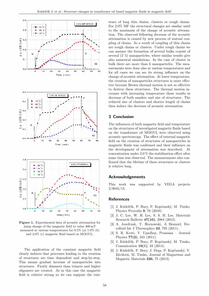
Kúdelčík J. et al.: Structure changes in transformer oil based magnetic fluids in magnetic field
Figure 1. Experimental data of acoustic attenuation forjump change of the magnetic field to value 300 mT
measured at various temperatures for 0.5% (a) 1.0% (b)and 2.0% (c) magnetic fluid based on MOGUL.
The application of the constant magnetic fieldclearly induces that processes leading to the creationof structures are time dependent and step-by-step.This means gradual increase of nanoparticles intostructures. Firstly dimmers than trimers and higheroligomers are created. As in this case the magneticfield is relative strong so we can suppose the exis-
tence of long thin chains, clusters or rough chains.For 2.0% MF the structural changes are similar untilto the maximum of the change of acoustic attenua-tion. The observed following decrease of the acousticattenuation is caused by new process of mutual cou-pling of chains. As a result of coupling of thin chainsare rough chains or clusters. Under rough chains wecan assume the formation of several bulks consist ofseveral (2–5) nanoparticles, where similar results givealso numerical simulations. In the case of cluster inbulk there are more than 6 nanoparticles. The mea-surements were done also at various temperatures andfor all cases we can see its strong influence on thechange of acoustic attenuation. At lower temperature,the creation of nanoparticles structures is more effec-tive because Brown thermal motion is not so effectiveto destroy these structures. The thermal motion in-creases with increasing temperature those results indecrease of both number and size of structures. Thereduced size of clusters and shorter length of chainsthen induce the decrease of acoustic attenuation.
3 Conclusion
The influences of both magnetic field and temperatureon the structures of investigated magnetic fluids basedon the transformer oil MOGUL were observed usingacoustic spectroscopy. The effect of external magneticfield on the creation of structures of nanoparticles inmagnetic fluids was confirmed and their influence onthe development of attenuation was described. Atconcentration under 2.0 % the stabilization effect aftersome time was observed. The measurements also con-firmed that the lifetime of these structures or clustersis relative long.
Acknowledgements
This work was supported by VEGA projects2/0045/13.
References
[1] J. Kúdelčík, P. Bury, P. Kopčanský, M. Timko,Physics Procedia 9, 78 (2010).
[2] J. C. Lee, W. H. Lee, S. S. H. Lee, MaterialsResearch Bulletin 47(10), 2984 (2012).
[3] A. Jozefczak, T. Hornowski, A Skumiel, Fer-rofluid Int J Thermophys 32, 795 (2011).
[4] S. R. Kruti, V. Upadhay, Pramana – JournalPhysics 77(2), 345 (2011).
[5] J. Kúdelčík, P. Bury, P. Kopčanský, M. Timko,Comunication 16(1), 33 (2014).
[6] J. Kúdelčík, P. Bury, J. Drga, P. Kopčanský, V.Závišová, M. Timko, Journal of Magnetism andMagnetic Materials 326, 75 (2013).
58
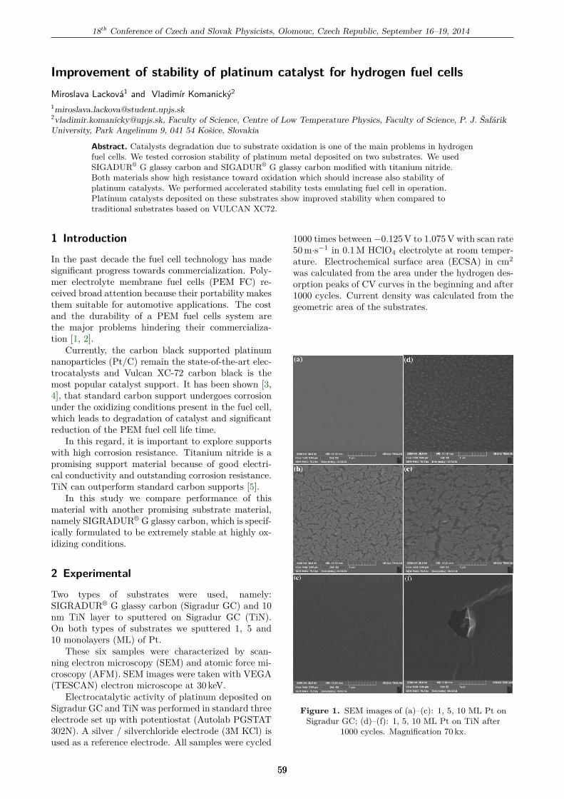
18th Conference of Czech and Slovak Physicists, Olomouc, Czech Republic, September 16–19, 2014
Improvement of stability of platinum catalyst for hydrogen fuel cells
Miroslava Lacková1 and Vladimír Komanický2
[email protected]@upjs.sk, Faculty of Science, Centre of Low Temperature Physics, Faculty of Science, P. J. ŠafárikUniversity, Park Angelinum 9, 041 54 Košice, Slovakia
Abstract. Catalysts degradation due to substrate oxidation is one of the main problems in hydrogenfuel cells. We tested corrosion stability of platinum metal deposited on two substrates. We usedSIGADUR® G glassy carbon and SIGADUR® G glassy carbon modified with titanium nitride.Both materials show high resistance toward oxidation which should increase also stability ofplatinum catalysts. We performed accelerated stability tests emulating fuel cell in operation.Platinum catalysts deposited on these substrates show improved stability when compared totraditional substrates based on VULCAN XC72.
1 Introduction
In the past decade the fuel cell technology has madesignificant progress towards commercialization. Poly-mer electrolyte membrane fuel cells (PEM FC) re-ceived broad attention because their portability makesthem suitable for automotive applications. The costand the durability of a PEM fuel cells system arethe major problems hindering their commercializa-tion [1, 2].
Currently, the carbon black supported platinumnanoparticles (Pt/C) remain the state-of-the-art elec-trocatalysts and Vulcan XC-72 carbon black is themost popular catalyst support. It has been shown [3,4], that standard carbon support undergoes corrosionunder the oxidizing conditions present in the fuel cell,which leads to degradation of catalyst and significantreduction of the PEM fuel cell life time.
In this regard, it is important to explore supportswith high corrosion resistance. Titanium nitride is apromising support material because of good electri-cal conductivity and outstanding corrosion resistance.TiN can outperform standard carbon supports [5].
In this study we compare performance of thismaterial with another promising substrate material,namely SIGRADUR® G glassy carbon, which is specif-ically formulated to be extremely stable at highly ox-idizing conditions.
2 Experimental
Two types of substrates were used, namely:SIGRADUR® G glassy carbon (Sigradur GC) and 10nm TiN layer to sputtered on Sigradur GC (TiN).On both types of substrates we sputtered 1, 5 and10 monolayers (ML) of Pt.
These six samples were characterized by scan-ning electron microscopy (SEM) and atomic force mi-croscopy (AFM). SEM images were taken with VEGA(TESCAN) electron microscope at 30 keV.
Electrocatalytic activity of platinum deposited onSigradur GC and TiN was performed in standard threeelectrode set up with potentiostat (Autolab PGSTAT302N). A silver / silverchloride electrode (3M KCl) isused as a reference electrode. All samples were cycled
1000 times between −0.125 V to 1.075 V with scan rate50 m·s−1 in 0.1 M HClO4 electrolyte at room temper-ature. Electrochemical surface area (ECSA) in cm2
was calculated from the area under the hydrogen des-orption peaks of CV curves in the beginning and after1000 cycles. Current density was calculated from thegeometric area of the substrates.
Figure 1. SEM images of (a)–(c): 1, 5, 10 ML Pt onSigradur GC; (d)–(f): 1, 5, 10 ML Pt on TiN after
1000 cycles. Magnification 70 kx.
595959
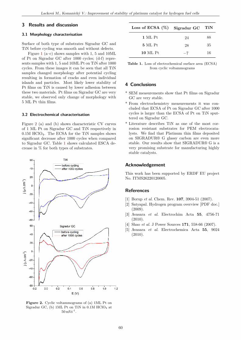
Lacková M., Komanický V.: Improvement of stability of platinum catalyst for hydrogen fuel cells
3 Results and discussion
3.1 Morphology characterisation
Surface of both type of substrates Sigradur GC andTiN before cycling was smooth and without defects.
Figure 1 (a–c) shows samples with 1, 5 and 10MLof Pt on Sigradur GC after 1000 cycles; (d-f) repre-sents samples with 1, 5 and 10ML Pt on TiN after 1000cycles. From these images it can be seen that all TiNsamples changed morphology after potential cyclingresulting in formation of cracks and even individualislands and particles. Most likely lower stability ofPt films on TiN is caused by lower adhesion betweenthese two materials. Pt films on Sigradur GC are verystable, we observed only change of morphology with5 ML Pt thin films.
3.2 Electrochemical characterisation
Figure 2 (a) and (b) shows characteristic CV curvesof 1 ML Pt on Sigradur GC and TiN respectively in0.1M HClO4. The ECSA for the TiN samples showssignificant decrease after 1000 cycles when comparedto Sigradur GC. Table 1 shows calculated ESCA de-crease in % for both types of substrates.
Figure 2. Cyclic voltammograms of (a) 1ML Pt onSigradur GC, (b) 1ML Pt on TiN in 0.1M HClO4 at
50 mVs-1.
Loss of ECSA (%) Sigradur GC TiN
1 ML Pt 24 88
5 ML Pt 28 35
10 ML Pt −7 16
Table 1. Loss of electrochemical surface area (ECSA)from cyclic voltammograms
4 Conclusions
* SEM measurements show that Pt films on SigradurGC are very stable.
* From electrochemistry measurements it was con-cluded that ECSA of Pt on Sigradur GC after 1000cycles is larger than the ECSA of Pt on TiN sput-tered on Sigradur GC.
* Literature describes TiN as one of the most cor-rosion resistant substrates for PEM electrocata-lysts. We find that Platinum thin films depositedon SIGRADUR® G glassy carbon are even morestable. Our results show that SIGRADUR® G is avery promising substrate for manufacturing highlystable catalysts.
Acknowledgement
This work has been supported by ERDF EU projectNo. ITMS26220120005.
References
[1] Borup et al. Chem. Rev. 107, 3904-51 (2007).[2] Satyapal. Hydrogen program overview [PDF doc.]
(2009).[3] Avasara et al. Electrochim Acta 55, 4756-71
(2010).[4] Shao et al. J Power Sources 171, 558-66 (2007).[5] Avasara et al. Electrochemica Acta 55, 9024
(2010).
60
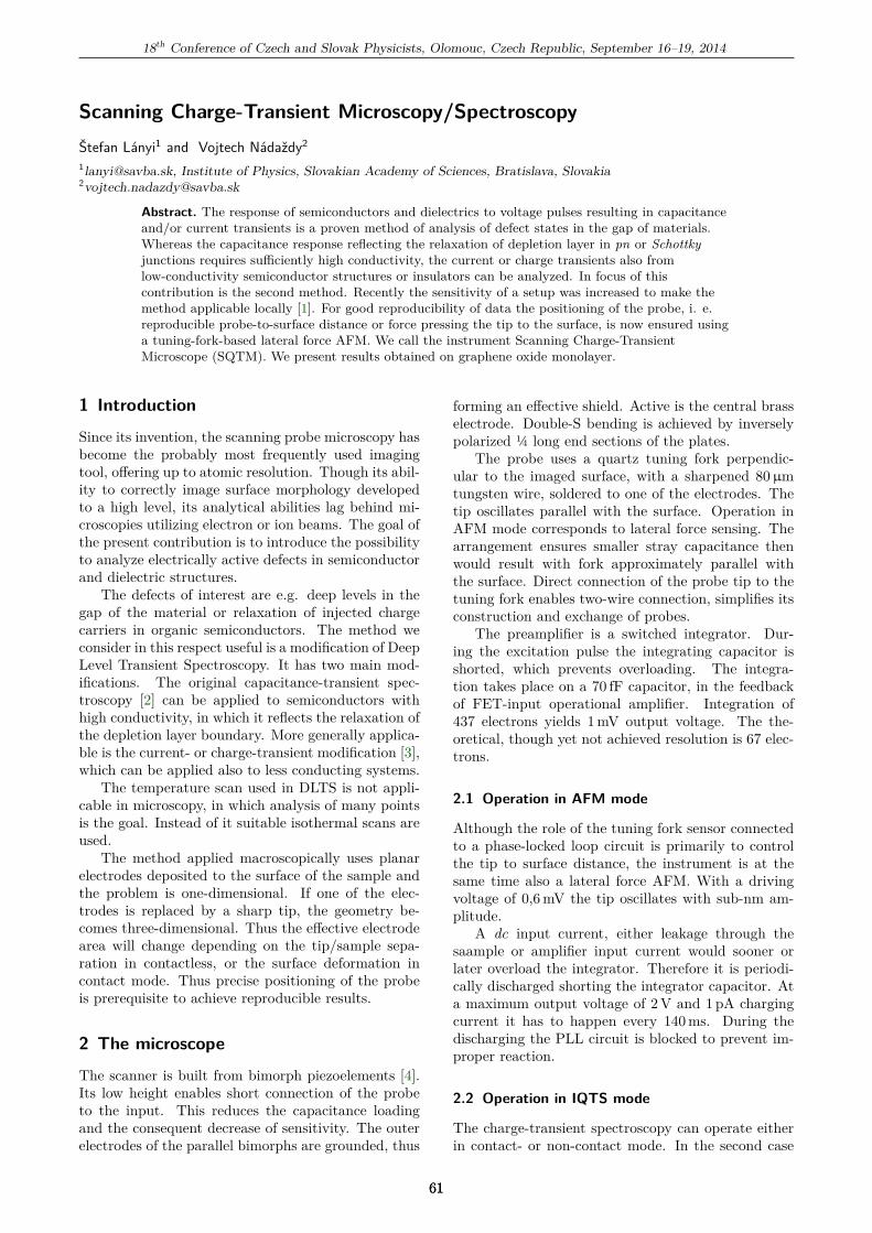
18th Conference of Czech and Slovak Physicists, Olomouc, Czech Republic, September 16–19, 2014
Scanning Charge-Transient Microscopy/Spectroscopy
Štefan Lányi1 and Vojtech Nádaždy2
[email protected], Institute of Physics, Slovakian Academy of Sciences, Bratislava, [email protected]
Abstract. The response of semiconductors and dielectrics to voltage pulses resulting in capacitanceand/or current transients is a proven method of analysis of defect states in the gap of materials.Whereas the capacitance response reflecting the relaxation of depletion layer in pn or Schottky
junctions requires sufficiently high conductivity, the current or charge transients also fromlow-conductivity semiconductor structures or insulators can be analyzed. In focus of thiscontribution is the second method. Recently the sensitivity of a setup was increased to make themethod applicable locally [1]. For good reproducibility of data the positioning of the probe, i. e.reproducible probe-to-surface distance or force pressing the tip to the surface, is now ensured usinga tuning-fork-based lateral force AFM. We call the instrument Scanning Charge-TransientMicroscope (SQTM). We present results obtained on graphene oxide monolayer.
1 Introduction
Since its invention, the scanning probe microscopy hasbecome the probably most frequently used imagingtool, offering up to atomic resolution. Though its abil-ity to correctly image surface morphology developedto a high level, its analytical abilities lag behind mi-croscopies utilizing electron or ion beams. The goal ofthe present contribution is to introduce the possibilityto analyze electrically active defects in semiconductorand dielectric structures.
The defects of interest are e.g. deep levels in thegap of the material or relaxation of injected chargecarriers in organic semiconductors. The method weconsider in this respect useful is a modification of DeepLevel Transient Spectroscopy. It has two main mod-ifications. The original capacitance-transient spec-troscopy [2] can be applied to semiconductors withhigh conductivity, in which it reflects the relaxation ofthe depletion layer boundary. More generally applica-ble is the current- or charge-transient modification [3],which can be applied also to less conducting systems.
The temperature scan used in DLTS is not appli-cable in microscopy, in which analysis of many pointsis the goal. Instead of it suitable isothermal scans areused.
The method applied macroscopically uses planarelectrodes deposited to the surface of the sample andthe problem is one-dimensional. If one of the elec-trodes is replaced by a sharp tip, the geometry be-comes three-dimensional. Thus the effective electrodearea will change depending on the tip/sample sepa-ration in contactless, or the surface deformation incontact mode. Thus precise positioning of the probeis prerequisite to achieve reproducible results.
2 The microscope
The scanner is built from bimorph piezoelements [4].Its low height enables short connection of the probeto the input. This reduces the capacitance loadingand the consequent decrease of sensitivity. The outerelectrodes of the parallel bimorphs are grounded, thus
forming an effective shield. Active is the central brasselectrode. Double-S bending is achieved by inverselypolarized ¼ long end sections of the plates.
The probe uses a quartz tuning fork perpendic-ular to the imaged surface, with a sharpened 80µmtungsten wire, soldered to one of the electrodes. Thetip oscillates parallel with the surface. Operation inAFM mode corresponds to lateral force sensing. Thearrangement ensures smaller stray capacitance thenwould result with fork approximately parallel withthe surface. Direct connection of the probe tip to thetuning fork enables two-wire connection, simplifies itsconstruction and exchange of probes.
The preamplifier is a switched integrator. Dur-ing the excitation pulse the integrating capacitor isshorted, which prevents overloading. The integra-tion takes place on a 70 fF capacitor, in the feedbackof FET-input operational amplifier. Integration of437 electrons yields 1 mV output voltage. The the-oretical, though yet not achieved resolution is 67 elec-trons.
2.1 Operation in AFM mode
Although the role of the tuning fork sensor connectedto a phase-locked loop circuit is primarily to controlthe tip to surface distance, the instrument is at thesame time also a lateral force AFM. With a drivingvoltage of 0,6 mV the tip oscillates with sub-nm am-plitude.
A dc input current, either leakage through thesaample or amplifier input current would sooner orlater overload the integrator. Therefore it is periodi-cally discharged shorting the integrator capacitor. Ata maximum output voltage of 2 V and 1 pA chargingcurrent it has to happen every 140 ms. During thedischarging the PLL circuit is blocked to prevent im-proper reaction.
2.2 Operation in IQTS mode
The charge-transient spectroscopy can operate eitherin contact- or non-contact mode. In the second case
616161
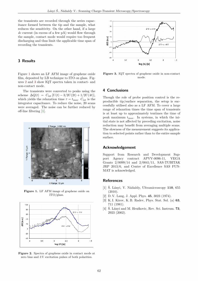
Lányi Š., Nádaždy V.: Scanning Charge-Transient Microscopy/Spectroscopy
the transients are recorded through the series capac-itance formed between the tip and the sample, whatreduces the sensitivity. On the other hand, if a largedc current (in excess of a few pA) would flow throughthe sample, contact mode would require too frequentdischarging and thus limit the applicable time span ofrecording the transients.
3 Results
Figure 1 shows an LF AFM image of graphene oxidefilm, deposited by LB technique to ITO on glass. Fig-ures 2 and 3 show IQT spectra taken in contact- andnon-contact mode.
The transients were converted to peaks using thescheme ∆Q(t) = Cint [U(t) − 3/2U(2t) + 1/2U(4t)],which yields the relaxation time τ = tmax. Cint is theintegrator capacitance. To reduce the noise, 20 scanswere averaged. The noise can be further reduced byoff-line filtering [1].
Figure 1. LF AFM image of graphene oxide onITO/glass.
Figure 2. Spectra of graphene oxide in contact mode atzero bias and 3 V excitation pulses of both polarities.
Figure 3. IQT spectra of graphene oxide in non-contactmode.
4 Conclusions
Though the role of probe position control is the re-producible tip/surface separation, the setup is suc-cessfully utilised also as a LF AFM. To cover a largerange of relaxation times the time span of transientsis at least up to approximately tentimes the time ofpeak maximum tmax. In systems, in which the ini-tial state is not affected by preceding excitation, noisereduction may benefit from averaging multiple scans.The slowness of the measurement suggests its applica-tion to selected points rather than to the entire samplesurface.
Acknowledgement
Support from Research and Development Sup-port Agency contract APVV-0096-11, VEGAGrants 2/0099/14 and 2/0041/11, SAS-TUBITAKJRP 2013/6, and Centre of Excellence SAS FUN-MAT is acknowledged.
References
[1] Š. Lányi, V. Nádaždy, Ultramicroscopy 110, 655(2010).
[2] D. V. Lang, J. Appl. Phys. 45, 3023 (1974).[3] K. I. Kirov, K. B. Radev, Phys. Stat. Sol. (a) 63,
711 (1981).[4] Š. Lányi and M. Hruškovic, Rev. Sci. Instrum. 73,
2923 (2002).
62
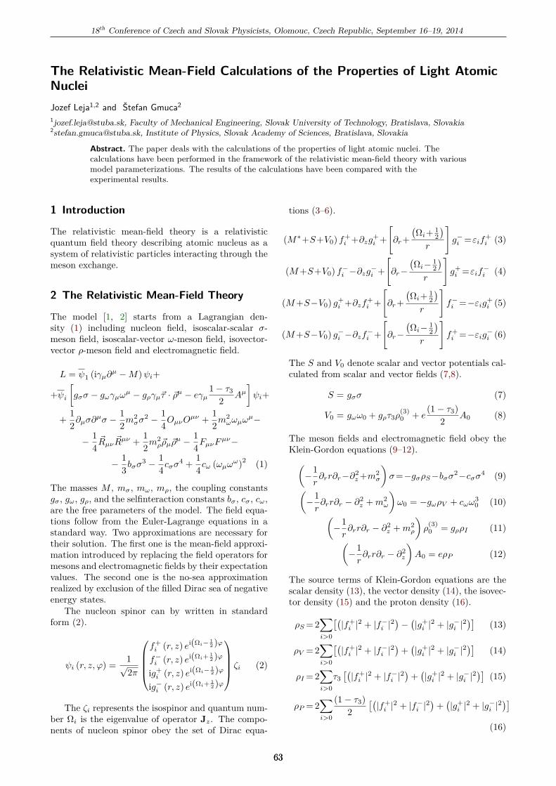
18th Conference of Czech and Slovak Physicists, Olomouc, Czech Republic, September 16–19, 2014
The Relativistic Mean-Field Calculations of the Properties of Light AtomicNuclei
Jozef Leja1,2 and Štefan Gmuca2
[email protected], Faculty of Mechanical Engineering, Slovak University of Technology, Bratislava, [email protected], Institute of Physics, Slovak Academy of Sciences, Bratislava, Slovakia
Abstract. The paper deals with the calculations of the properties of light atomic nuclei. Thecalculations have been performed in the framework of the relativistic mean-field theory with variousmodel parameterizations. The results of the calculations have been compared with theexperimental results.
1 Introduction
The relativistic mean-field theory is a relativisticquantum field theory describing atomic nucleus as asystem of relativistic particles interacting through themeson exchange.
2 The Relativistic Mean-Field Theory
The model [1, 2] starts from a Lagrangian den-sity (1) including nucleon field, isoscalar-scalar σ-meson field, isoscalar-vector ω-meson field, isovector-vector ρ-meson field and electromagnetic field.
L = ψ1 (iγµ∂µ −M)ψi+
+ψi
[
gσσ − gωγµωµ − gργµ~τ · ~ρµ − eγµ
1 − τ3
2Aµ
]
ψi+
+12∂µσ∂
µσ − 12m2
σσ2 − 1
4OµνO
µν +12m2
ωωµωµ−
− 14~Rµν
~Rµν +12m2
ρ~ρµ~ρµ − 1
4FµνF
µν−
− 13bσσ
3 − 14cσσ
4 +14cω (ωµω
ω)2 (1)
The masses M , mσ, mω, mρ, the coupling constantsgσ, gω, gρ, and the selfinteraction constants bσ, cσ, cω,are the free parameters of the model. The field equa-tions follow from the Euler-Lagrange equations in astandard way. Two approximations are necessary fortheir solution. The first one is the mean-field approxi-mation introduced by replacing the field operators formesons and electromagnetic fields by their expectationvalues. The second one is the no-sea approximationrealized by exclusion of the filled Dirac sea of negativeenergy states.
The nucleon spinor can by written in standardform (2).
ψi (r, z, ϕ) =1√2π
f+i (r, z) ei(Ωi− 1
2 )ϕ
f−i (r, z) ei(Ωi+ 1
2 )ϕ
ig+i (r, z) ei(Ωi− 1
2 )ϕ
ig−i (r, z) ei(Ωi+ 1
2 )ϕ
ζi (2)
The ζi represents the isospinor and quantum num-ber Ωi is the eigenvalue of operator Jz. The compo-nents of nucleon spinor obey the set of Dirac equa-
tions (3–6).
(M∗+S+V0) f+i +∂zg
+i +
[
∂r +
(
Ωi+ 12
)
r
]
g−i =εif
+i (3)
(M+S+V0) f−i −∂zg
−i +
[
∂r −(
Ωi− 12
)
r
]
g+i =εif
−i (4)
(M+S−V0) g+i +∂zf
+i +
[
∂r +
(
Ωi+ 12
)
r
]
f−i =−εig
+i (5)
(M+S−V0) g−i −∂zf
−i +
[
∂r −(
Ωi− 12
)
r
]
f+i =−εig
−i (6)
The S and V0 denote scalar and vector potentials cal-culated from scalar and vector fields (7,8).
S = gσσ (7)
V0 = gωω0 + gρτ3ρ(3)0 + e
(1 − τ3)2
A0 (8)
The meson fields and electromagnetic field obey theKlein-Gordon equations (9–12).(
−1r∂rr∂r −∂2
z +m2σ
)
σ=−gσρS −bσσ2−cσσ
4 (9)(
−1r∂rr∂r − ∂2
z +m2ω
)
ω0 = −gωρV + cωω30 (10)
(
−1r∂rr∂r − ∂2
z +m2ρ
)
ρ(3)0 = gρρI (11)
(
−1r∂rr∂r − ∂2
z
)
A0 = eρP (12)
The source terms of Klein-Gordon equations are thescalar density (13), the vector density (14), the isovec-tor density (15) and the proton density (16).
ρS = 2∑
i>0
[(
|f+i |2 + |f−
i |2)
−(
|g+i |2 + |g−
i |2)]
(13)
ρV = 2∑
i>0
[(
|f+i |2 + |f−
i |2)
+(
|g+i |2 + |g−
i |2)]
(14)
ρI = 2∑
i>0
τ3
[(
|f+i |2 + |f−
i |2)
+(
|g+i |2 + |g−
i |2)]
(15)
ρP = 2∑
i>0
(1 − τ3)2
[(
|f+i |2 + |f−
i |2)
+(
|g+i |2 + |g−
i |2)]
(16)
636363
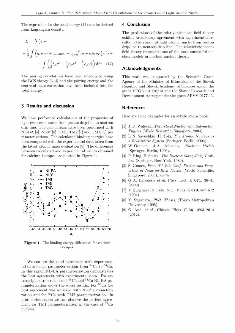
Leja J., Gmuca Š.: The Relativistic Mean-Field Calculations of the Properties of Light Atomic Nuclei
The expression for the total energy (17) can be derivedfrom Lagrangian density.
E =∑
i
εi−
− 12
∫
(
gσσρS + gωω0ρV + gρρ(3)0 ρI + eA0ρP
)
d3x+
+∫ (
13bσσ
3 +14cσσ
4 − 14cωω
40
)
d3x (17)
The pairing correlations have been introduced usingthe BCS theory [3, 4] and the pairing energy and thecentre of mass correction have been included into thetotal energy.
3 Results and discussion
We have performed calculations of the properties oflight even-even nuclei from proton drip-line to neutrondrip-line. The calculations have been performed withNL-BA [5], NL3* [6], TM1, TM2 [7] and TMA [8] pa-rameterizations. The calculated binding energies havebeen compared with the experimental data taken fromthe latest atomic mass evaluation [9]. The differencesbetween calculated and experimental values obtainedfor calcium isotopes are plotted in Figure 1.
Figure 1. The binding energy differences for calciumisotopes.
We can see the good agreement with experimen-tal data for all parameterizations from 34Ca to 54Ca.In this region NL-BA parameterization demonstratesthe best agreement with experimental data. For ex-tremely neutron-rich nuclei 56Ca and 58Ca NL-BA pa-rameterization shows the worst results. For 56Ca thebest agreement was achieved with NL3* parameteri-zation and for 58Ca with TM2 parameterization. Inproton rich region we can observe the perfect agree-ment for TM1 parameterization in the case of 34Canucleus.
4 Conclusion
The predictions of the relativistic mean-field theoryexhibit satisfactory agreement with experimental re-sults in the region of light atomic nuclei from protondrip-line to neutron-drip line. The relativistic mean-field theory represents one of the most successful nu-clear models in modern nuclear theory.
Acknowledgments
This work was supported by the Scientific GrantAgency of the Ministry of Education of the SlovakRepublic and Slovak Academy of Sciences under thegrant VEGA 2/0176/13 and the Slovak Research andDevelopment Agency under the grant APVV-0177-11.
References
Here are some examples for an article and a book:
[1] J. D. Walecka, Theoretical Nuclear and SubnuclearPhysics (World Scientific, Singapore, 2004).
[2] L. N. Savushkin, H. Toki, The Atomic Nucleus asa Relativistic System (Springer, Berlin, 2004).
[3] W. Greiner, J. A. Maruhn, Nuclear Models(Springer, Berlin, 1996).
[4] P. Ring, P. Shuck, The Nuclear Many-Body Prob-lem (Springer, New York, 1980).
[5] Š. Gmuca, Proc. 2nd Int. Conf. Fission and Prop-erties of Neutron-Rich Nuclei (World Scientific,Singapore, 2000), 75–78.
[6] G. A. Lalazissis et al. Phys. Lett. B 671, 36–41(2009).
[7] Y. Sugahara, H. Toki, Nucl. Phys. A 579, 557–572(1994).
[8] Y. Sugahara, PhD. Thesis, (Tokyo MetropolitanUniversity, 1995).
[9] G. Audi et al., Chinese Phys. C 36, 1603–2014(2012).
64
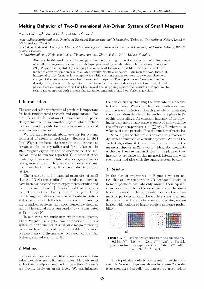
18th Conference of Czech and Slovak Physicists, Olomouc, Czech Republic, September 16–19, 2014
Melting Behavior of Two-Dimensional Air-Driven System of Small Magnets
Martin Liščinský1, Michal Géci2, and Mária Šviková3
[email protected], Faculty of Electrical Engineering and Informatics, Technical University of Košice, Letná 9,042 00 Košice, [email protected], Faculty of Electrical Engineering and Informatics, Technical University of Košice, Letná 9, 042 00Košice, [email protected], High school of st. Thomas Aquinas, Zbrojničná 3, 040 01 Košice, Slovakia
Abstract. In this work, we study configurational and melting properties of a system of finite numberof small disc magnets moving on an air layer produced by an air table to imitate two-dimensional(2D) Wigner-like crystal. By changing the velocity of the air current blown to the air table weinfluence effective temperature calculated through particle velocities. Our results show, that a 2Dhexagonal lattice forms at low temperature while with increasing temperature we can observe achange of the lattice symmetry from hexagonal to square. The dependence of averaged numberdensity of defects on the temperature exhibits sudden increase indicating transition to the liquidphase. Particle trajectories in this phase reveal the surprising square shell structure. Experimentalresults are compared with a molecular dynamics simulation based on Verlet algorithm.
1 Introduction
The study of self-organization of particles is importantfor both fundamental research and applications. Forexample in the fabrication of nano-structured parti-cle systems and in soft-matter physics which includecolloids, liquid crystals, foams, granular materials andeven biological tissues.
We are used to speak about crystals for systemscomposed of atoms or molecules. However in 1934Paul Wigner predicted theoretically that electrons atcertain conditions crystallize and form a lattice. In1979 Wigner crystallization of electrons on the sur-face of liquid helium was reported [1]. Since that otherrelated systems which exhibit Wigner crystal-like or-dering were studied. They are e.g. colloidal systems,dust particles in plasma, 2D superconducting vortexlattice.
The structural and dynamical properties of smallclassical 2D clusters confined in circular confinementhave been a subject of recent experimental studies andcomputer simulations [2]. It was found that there is acompetition between two types of ordering: orderinginto triangular lattice structure and ordering into ashell structure, which leads to clusters with interestingself-organized patterns that show concentric shells atsmall N hexagonal cores surrounded by circular outershells at large N.
In our work, we study new experimental system,where Wigner–like crystal can be observed. It is asystem of finite number of small disc magnets movingon an air layer produced by an air table. Our workis related also to thermal-like behaviour of granularsystems, studied e.g. in [3, 4].
2 Method
In our experiment we place 64 disc magnets on rectan-gular plexiglass pad with small holes. Magnets repeleach other by dipolar magnetic interaction. Magnetsare moving freely on an air layer. We can influence
their velocities by changing the flow rate of air blownto the air table. We record the system with a webcamand we trace trajectory of each particle by analyzingthe video. More details of the method are given in [5]of this proceedings. At constant intensity of air blow-ing into air table steady state is achieved and we definethe effective temperature τ =
(∑
v2i
)
/N , where vi isvelocity of i-the particle, N is the number of particles.
Second part of this work is devoted to a moleculardynamics simulation of a similar system. We used theVerlett algorithm [6] to compute the positions of themagnetic dipoles in 2D system. Magnetic momentsof the particles are perpendicular to the plane so theyinteract by repulsive dipolar magnetic interaction witheach other and also with the square system border.
3 Results
In the plot of trajectories in Figure 1 we can no-tice that at low temperature 2D hexagonal lattice isformed, particles oscillate only around their equilib-rium positions in both the experiment and the simu-lation. Increase of the temperature causes the move-ment of particles around the whole system area anddespite of that trajectories create underlying squarelattice with regions of larger particle presence proba-bility.
a) b)
Figure 1. a) Particle trajectories from the simulation.τ = 0.15 cm2s−2 (left), τ = 12 cm2s−2 (right). b) Particletrajectories from the experiment. τ = 0.6 cm2s−2 (left),
τ = 12.9 cm2s−2 (right).
The topological defects play a role in melting pro-cess. In Voronoi diagrams shown in Figure 2 the de-fects (non six-sided cells) are marked by green colour
656565
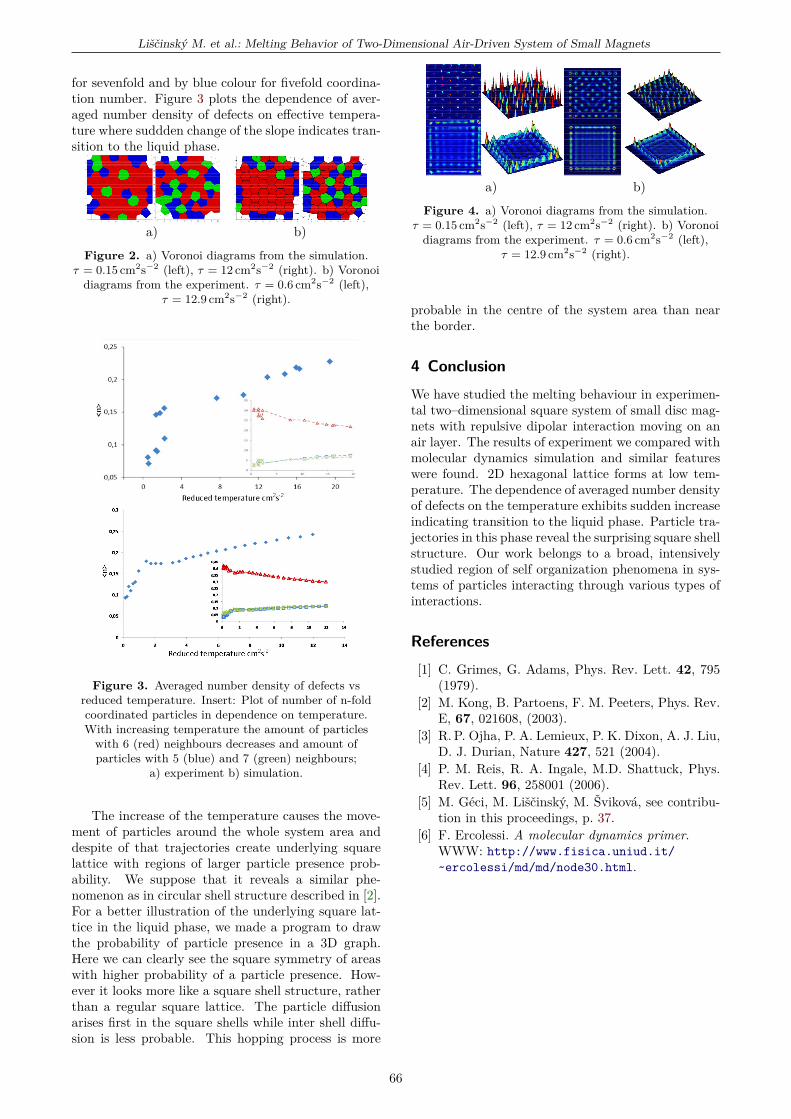
Liščinský M. et al.: Melting Behavior of Two-Dimensional Air-Driven System of Small Magnets
for sevenfold and by blue colour for fivefold coordina-tion number. Figure 3 plots the dependence of aver-aged number density of defects on effective tempera-ture where suddden change of the slope indicates tran-sition to the liquid phase.
a) b)
Figure 2. a) Voronoi diagrams from the simulation.τ = 0.15 cm2s−2 (left), τ = 12 cm2s−2 (right). b) Voronoi
diagrams from the experiment. τ = 0.6 cm2s−2 (left),τ = 12.9 cm2s−2 (right).
Figure 3. Averaged number density of defects vsreduced temperature. Insert: Plot of number of n-foldcoordinated particles in dependence on temperature.With increasing temperature the amount of particles
with 6 (red) neighbours decreases and amount ofparticles with 5 (blue) and 7 (green) neighbours;
a) experiment b) simulation.
The increase of the temperature causes the move-ment of particles around the whole system area anddespite of that trajectories create underlying squarelattice with regions of larger particle presence prob-ability. We suppose that it reveals a similar phe-nomenon as in circular shell structure described in [2].For a better illustration of the underlying square lat-tice in the liquid phase, we made a program to drawthe probability of particle presence in a 3D graph.Here we can clearly see the square symmetry of areaswith higher probability of a particle presence. How-ever it looks more like a square shell structure, ratherthan a regular square lattice. The particle diffusionarises first in the square shells while inter shell diffu-sion is less probable. This hopping process is more
a) b)
Figure 4. a) Voronoi diagrams from the simulation.τ = 0.15 cm2s−2 (left), τ = 12 cm2s−2 (right). b) Voronoi
diagrams from the experiment. τ = 0.6 cm2s−2 (left),τ = 12.9 cm2s−2 (right).
probable in the centre of the system area than nearthe border.
4 Conclusion
We have studied the melting behaviour in experimen-tal two–dimensional square system of small disc mag-nets with repulsive dipolar interaction moving on anair layer. The results of experiment we compared withmolecular dynamics simulation and similar featureswere found. 2D hexagonal lattice forms at low tem-perature. The dependence of averaged number densityof defects on the temperature exhibits sudden increaseindicating transition to the liquid phase. Particle tra-jectories in this phase reveal the surprising square shellstructure. Our work belongs to a broad, intensivelystudied region of self organization phenomena in sys-tems of particles interacting through various types ofinteractions.
References
[1] C. Grimes, G. Adams, Phys. Rev. Lett. 42, 795(1979).
[2] M. Kong, B. Partoens, F. M. Peeters, Phys. Rev.E, 67, 021608, (2003).
[3] R. P. Ojha, P. A. Lemieux, P. K. Dixon, A. J. Liu,D. J. Durian, Nature 427, 521 (2004).
[4] P. M. Reis, R. A. Ingale, M.D. Shattuck, Phys.Rev. Lett. 96, 258001 (2006).
[5] M. Géci, M. Liščinský, M. Šviková, see contribu-tion in this proceedings, p. 37.
[6] F. Ercolessi. A molecular dynamics primer.WWW: http://www.fisica.uniud.it/
~ercolessi/md/md/node30.html.
66
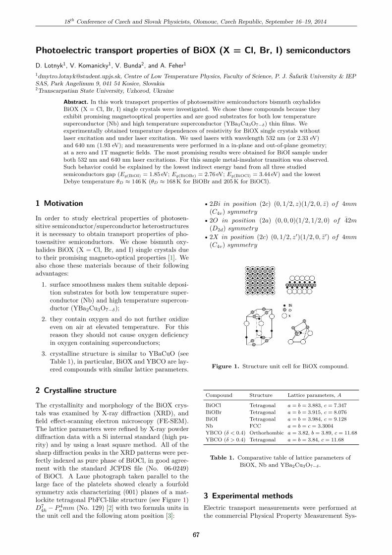
18th Conference of Czech and Slovak Physicists, Olomouc, Czech Republic, September 16–19, 2014
Photoelectric transport properties of BiOX (X = Cl, Br, I) semiconductors
D. Lotnyk1, V. Komanicky1, V. Bunda2, and A. Feher1
[email protected], Centre of Low Temperature Physics, Faculty of Science, P. J. Šafarik University & IEPSAS, Park Angelinum 9, 041 54 Kosice, Slovakia2Transcarpatian State University, Uzhorod, Ukraine
Abstract. In this work transport properties of photosensitive semiconductors bismuth oxyhalidesBiOX (X = Cl, Br, I) single crystals were investigated. We chose these compounds because theyexhibit promising magnetooptical properties and are good substrates for both low temperaturesuperconductor (Nb) and high temperature superconductor (YBa2Cu3O7−δ) thin films. Weexperimentally obtained temperature dependences of resistivity for BiOX single crystals withoutlaser excitation and under laser excitation. We used lasers with wavelength 532 nm (or 2.33 eV)and 640 nm (1.93 eV); and measurements were performed in a in-plane and out-of-plane geometry;at a zero and 1T magnetic fields. The most promising results were obtained for BiOI sample underboth 532 nm and 640 nm laser excitations. For this sample metal-insulator transition was observed.Such behavior could be explained by the lowest indirect energy band from all three studiedsemiconductors gap (Eg(BiOI) = 1.85 eV; Eg(BiOBr) = 2.76 eV; Eg(BiOCl) = 3.44 eV) and the lowestDebye temperature θD ≈ 146 K (θD ≈ 168 K for BiOBr and 205 K for BiOCl).
1 Motivation
In order to study electrical properties of photosen-sitive semiconductor/superconductor heterostructuresit is necessary to obtain transport properties of pho-tosensitive semiconductors. We chose bismuth oxy-halides BiOX (X = Cl, Br, and I) single crystals dueto their promising magneto-optical properties [1]. Wealso chose these materials because of their followingadvantages:
1. surface smoothness makes them suitable deposi-tion substrates for both low temperature super-conductor (Nb) and high temperature supercon-ductor (YBa2Cu3O7−δ);
2. they contain oxygen and do not further oxidizeeven on air at elevated temperature. For thisreason they should not cause oxygen deficiencyin oxygen containing superconductors;
3. crystalline structure is similar to YBaCuO (seeTable 1), in particular, BiOX and YBCO are lay-ered compounds with similar lattice parameters.
2 Crystalline structure
The crystallinity and morphology of the BiOX crys-tals was examined by X-ray diffraction (XRD), andfield effect-scanning electron microscopy (FE-SEM).The lattice parameters were refined by X-ray powderdiffraction data with a Si internal standard (high pu-rity) and by using a least square method. All of thesharp diffraction peaks in the XRD patterns were per-fectly indexed as pure phase of BiOCl, in good agree-ment with the standard JCPDS file (No. 06-0249)of BiOCl. A Laue photograph taken parallel to thelarge face of the platelets showed clearly a fourfoldsymmetry axis characterizing (001) planes of a mat-lockite tetragonal PbFCl-like structure (see Figure 1)D7
4h − P 4nmm (No. 129) [2] with two formula units in
the unit cell and the following atom position [3]:
•2Bi in position (2c) (0, 1/2, z)(1/2, 0, z) of 4mm(C4v) symmetry
•2O in position (2a) (0, 0, 0)(1/2, 1/2, 0) of 42m(D2d) symmetry
•2X in position (2c) (0, 1/2, z′)(1/2, 0, z′) of 4mm(C4v) symmetry
Figure 1. Structure unit cell for BiOX compound.
Compound Structure Lattice parameters, A
BiOCl Tetragonal a = b = 3.883, c = 7.347
BiOBr Tetragonal a = b = 3.915, c = 8.076
BiOI Tetragonal a = b = 3.984, c = 9.128
Nb FCC a = b = c = 3.3004
YBCO (δ < 0.4) Orthorhombic a = 3.82, b = 3.89, c = 11.68
YBCO (δ > 0.4) Tetragonal a = b = 3.84, c = 11.68
Table 1. Comparative table of lattice parameters ofBiOX, Nb and YBa2Cu3O7−δ.
3 Experimental methods
Electric transport measurements were performed atthe commercial Physical Property Measurement Sys-
676767
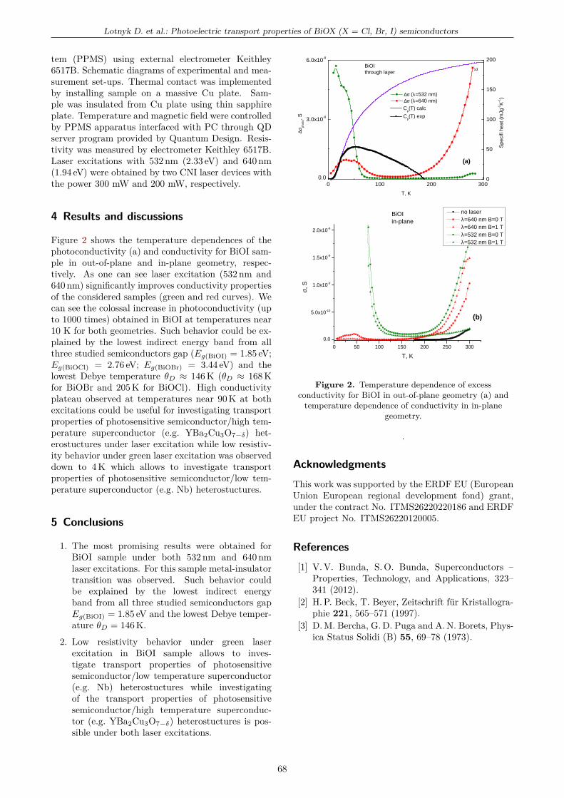
Lotnyk D. et al.: Photoelectric transport properties of BiOX (X = Cl, Br, I) semiconductors
tem (PPMS) using external electrometer Keithley6517B. Schematic diagrams of experimental and mea-surement set-ups. Thermal contact was implementedby installing sample on a massive Cu plate. Sam-ple was insulated from Cu plate using thin sapphireplate. Temperature and magnetic field were controlledby PPMS apparatus interfaced with PC through QDserver program provided by Quantum Design. Resis-tivity was measured by electrometer Keithley 6517B.Laser excitations with 532 nm (2.33 eV) and 640 nm(1.94 eV) were obtained by two CNI laser devices withthe power 300 mW and 200 mW, respectively.
4 Results and discussions
Figure 2 shows the temperature dependences of thephotoconductivity (a) and conductivity for BiOI sam-ple in out-of-plane and in-plane geometry, respec-tively. As one can see laser excitation (532 nm and640 nm) significantly improves conductivity propertiesof the considered samples (green and red curves). Wecan see the colossal increase in photoconductivity (upto 1000 times) obtained in BiOI at temperatures near10 K for both geometries. Such behavior could be ex-plained by the lowest indirect energy band from allthree studied semiconductors gap (Eg(BiOI) = 1.85 eV;Eg(BiOCl) = 2.76 eV; Eg(BiOBr) = 3.44 eV) and thelowest Debye temperature θD ≈ 146 K (θD ≈ 168 Kfor BiOBr and 205 K for BiOCl). High conductivityplateau observed at temperatures near 90 K at bothexcitations could be useful for investigating transportproperties of photosensitive semiconductor/high tem-perature superconductor (e.g. YBa2Cu3O7−δ) het-erostuctures under laser excitation while low resistiv-ity behavior under green laser excitation was observeddown to 4 K which allows to investigate transportproperties of photosensitive semiconductor/low tem-perature superconductor (e.g. Nb) heterostuctures.
5 Conclusions
1. The most promising results were obtained forBiOI sample under both 532 nm and 640 nmlaser excitations. For this sample metal-insulatortransition was observed. Such behavior couldbe explained by the lowest indirect energyband from all three studied semiconductors gapEg(BiOI) = 1.85 eV and the lowest Debye temper-ature θD = 146 K.
2. Low resistivity behavior under green laserexcitation in BiOI sample allows to inves-tigate transport properties of photosensitivesemiconductor/low temperature superconductor(e.g. Nb) heterostuctures while investigatingof the transport properties of photosensitivesemiconductor/high temperature superconduc-tor (e.g. YBa2Cu3O7−δ) heterostuctures is pos-sible under both laser excitations.
0 100 200 3000.0
3.0x10⁻⁸
6.0x10⁻⁸
∆σ (λ=532 nm) ∆σ (λ=640 nm)
∆σph
oto, S
T, K
x3
(a)
0
50
100
150
200
Cp(T) calc
Cp(T) exp
Spe
cifi
heat
(m
Jg-1K
-1)
BiOIthrough layer
0 50 100 150 200 250 300
0.0
5.0x10⁻¹⁰
1.0x10⁻⁹
1.5x10⁻⁹
2.0x10⁻⁹
σ, S
T, K
no laser λ=640 nm B=0 T λ=640 nm B=1 T λ=532 nm B=0 T λ=532 nm B=1 T
BiOIin-plane
(b)
Figure 2. Temperature dependence of excessconductivity for BiOI in out-of-plane geometry (a) and
temperature dependence of conductivity in in-planegeometry.
.
Acknowledgments
This work was supported by the ERDF EU (EuropeanUnion European regional development fond) grant,under the contract No. ITMS26220220186 and ERDFEU project No. ITMS26220120005.
References
[1] V. V. Bunda, S. O. Bunda, Superconductors –Properties, Technology, and Applications, 323–341 (2012).
[2] H. P. Beck, T. Beyer, Zeitschrift für Kristallogra-phie 221, 565–571 (1997).
[3] D. M. Bercha, G. D. Puga and A. N. Borets, Phys-ica Status Solidi (B) 55, 69–78 (1973).
68
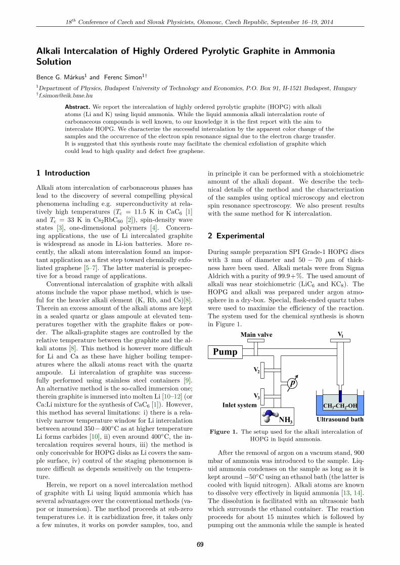
18th Conference of Czech and Slovak Physicists, Olomouc, Czech Republic, September 16–19, 2014
Alkali Intercalation of Highly Ordered Pyrolytic Graphite in AmmoniaSolution
Bence G. Márkus1 and Ferenc Simon1†
1Department of Physics, Budapest University of Technology and Economics, P.O. Box 91, H-1521 Budapest, Hungary†[email protected]
Abstract. We report the intercalation of highly ordered pyrolytic graphite (HOPG) with alkaliatoms (Li and K) using liquid ammonia. While the liquid ammonia alkali intercalation route ofcarbonaceous compounds is well known, to our knowledge it is the first report with the aim tointercalate HOPG. We characterize the successful intercalation by the apparent color change of thesamples and the occurrence of the electron spin resonance signal due to the electron charge transfer.It is suggested that this synthesis route may facilitate the chemical exfoliation of graphite whichcould lead to high quality and defect free graphene.
1 Introduction
Alkali atom intercalation of carbonaceous phases haslead to the discovery of several compelling physicalphenomena including e.g. superconductivity at rela-tively high temperatures (Tc = 11.5 K in CaC6 [1]and Tc = 33 K in Cs2RbC60 [2]), spin-density wavestates [3], one-dimensional polymers [4]. Concern-ing applications, the use of Li intercalated graphiteis widespread as anode in Li-ion batteries. More re-cently, the alkali atom intercalation found an impor-tant application as a first step toward chemically exfo-liated graphene [5–7]. The latter material is prospec-tive for a broad range of applications.
Conventional intercalation of graphite with alkaliatoms include the vapor phase method, which is use-ful for the heavier alkali element (K, Rb, and Cs)[8].Therein an excess amount of the alkali atoms are keptin a sealed quartz or glass ampoule at elevated tem-peratures together with the graphite flakes or pow-der. The alkali-graphite stages are controlled by therelative temperature between the graphite and the al-kali atoms [8]. This method is however more difficultfor Li and Ca as these have higher boiling temper-atures where the alkali atoms react with the quartzampoule. Li intercalation of graphite was success-fully performed using stainless steel containers [9].An alternative method is the so-called immersion one;therein graphite is immersed into molten Li [10–12] (orCa:Li mixture for the synthesis of CaC6 [1]). However,this method has several limitations: i) there is a rela-tively narrow temperature window for Li intercalationbetween around 350−400C as at higher temperatureLi forms carbides [10], ii) even around 400C, the in-tercalation requires several hours, iii) the method isonly conceivable for HOPG disks as Li covers the sam-ple surface, iv) control of the staging phenomenon ismore difficult as depends sensitively on the tempera-ture.
Herein, we report on a novel intercalation methodof graphite with Li using liquid ammonia which hasseveral advantages over the conventional methods (va-por or immersion). The method proceeds at sub-zerotemperatures i.e. it is carbidization free, it takes onlya few minutes, it works on powder samples, too, and
in principle it can be performed with a stoichiometricamount of the alkali dopant. We describe the tech-nical details of the method and the characterizationof the samples using optical microscopy and electronspin resonance spectroscopy. We also present resultswith the same method for K intercalation.
2 Experimental
During sample preparation SPI Grade-1 HOPG discswith 3 mm of diameter and 50 − 70 µm of thick-ness have been used. Alkali metals were from SigmaAldrich with a purity of 99.9+%. The used amount ofalkali was near stoichiometric (LiC6 and KC8). TheHOPG and alkali was prepared under argon atmo-sphere in a dry-box. Special, flask-ended quartz tubeswere used to maximize the efficiency of the reaction.The system used for the chemical synthesis is shownin Figure 1.
p
Pump
Main valve
V
NH3
V
CH -CH -OH3 2
Ultrasound bath
Inlet system
2
1
V3
Figure 1. The setup used for the alkali intercalation ofHOPG in liquid ammonia.
After the removal of argon on a vacuum stand, 900mbar of ammonia was introduced to the sample. Liq-uid ammonia condenses on the sample as long as it iskept around −50C using an ethanol bath (the latter iscooled with liquid nitrogen). Alkali atoms are knownto dissolve very effectively in liquid ammonia [13, 14].The dissolution is facilitated with an ultrasonic bathwhich surrounds the ethanol container. The reactionproceeds for about 15 minutes which is followed bypumping out the ammonia while the sample is heated
696969
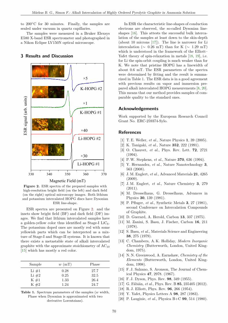
Márkus B. G., Simon F.: Alkali Intercalation of Highly Ordered Pyrolytic Graphite in Ammonia Solution
to 200C for 30 minutes. Finally, the samples aresealed under vacuum in quartz capillaries.
The samples were measured in a Bruker ElexsysE580 X-band ESR spectrometer and photographed ina Nikon Eclipse LV150N optical microscope.
3 Results and Discussion
330 340 350 360 370
K-HOPG #2
K-HOPG #1
Li-HOPG #2
Li-HOPG #1
×30
×40
×1
ESR
sign
al (a
rb. u
nits
)
Magnetic Field (mT)
×5
Figure 2. ESR spectra of the prepared samples withhigh-resolution bright field (on the left) and dark field(on the right) optical microscopy images. Both lithiumand potassium intercalated HOPG discs have Dysonian
ESR line-shape.
ESR spectra are presented on Figure 2. and theinsets show bright field (BF) and dark field (DF) im-ages. We find that lithium intercalated samples havea golden-yellow color thus identified as Stage-I LiC6.The potassium doped ones are mostly red with someyellowish parts which can be interpreted as a mix-ture of Stage-I and Stage-II systems. It is known thatthere exists a metastable state of alkali intercalatedgraphite with the approximate stoichiometry of AC10
[15] which has mostly a red color.
Sample w (mT) Phase
Li #1 0.28 27.7Li #2 0.25 32.5K #1 1.33 26.4K #2 1.24 24.7
Table 1. Spectrum parameters of the samples (w width,Phase when Dysonian is approximated with two
derivative Lorentzians).
In ESR the characteristic line-shapes of conductionelectrons are observed, the so-called Dysonian line-shapes [16]. This attests the successful bulk interca-lation of the samples at least down to the skin-depth(about 10 microns [17]). The line is narrower for Liintercalation (∼ 0.26 mT) than for K (∼ 1.29 mT)which is understood in the framework of the Elliott–Yafet theory of spin-relaxation in metals [18, 19], i.e.for Li the spin-orbit coupling is much weaker than forK. We note that pristine HOPG has a linewidth ofabout 0.6 mT. The ESR parameters of the spectrawere determined by fitting and the result is summa-rized in Table 1. The ESR data is in a good agreementwith previous results on vapor and immersion pre-pared alkali intercalated HOPG measurements [8, 20].This means that our method provides samples of com-parable quality to the standard ones.
Acknowledgements
Work supported by the European Research CouncilGrant No. ERC-259374-Sylo.
References
[1] T. E. Weller, et al., Nature Physics 1, 39 (2005).[2] K. Tanigaki, et al., Nature 352, 222 (1991).[3] O. Chauvet, et al., Phys. Rev. Lett. 72, 2721
(1994).[4] P. W. Stephens, et al., Nature 370, 636 (1994).[5] Y. Hernandez, et al., Nature Nanotechnology 3,
563 (2008).[6] J. M. Englert, et al., Advanced Materials 21, 4265
(2009).[7] J. M. Englert, et al., Nature Chemistry 3, 279
(2011).[8] M. Dresselhaus, G. Dresselhaus, Advances in
Physics 30, 139 (1981).[9] P. Pfluger, et al., Synthetic Metals 3, 27 (1981),
second Conference on Intercalation Compoundsof Graphite.
[10] D. Guerard, A. Herold, Carbon 13, 337 (1975).[11] M. Zanini, S. Basu, J. Fischer, Carbon 16, 211
(1978).[12] S. Basu, et al., Materials Science and Engineering
38, 275 (1979).[13] C. Chambers, A. K. Holliday, Modern Inorganic
Chemistry (Butterworth, London, United King-dom, 1975).
[14] N. N. Greenwood, A. Earnshaw, Chemistry of theElements (Butterworth, London, United King-dom, 1998).
[15] F. J. Salzano, S. Aronson, The Journal of Chem-ical Physics 47, 2978. (1967).
[16] F. J. Dyson, Phys. Rev. 98, 349 (1955).[17] G. Fábián, et al., Phys. Rev. B 85, 235405 (2012).[18] R. J. Elliott, Phys. Rev. 96, 266 (1954).[19] Y. Yafet, Physics Letters A 98, 287 (1983).[20] P. Lauginie, et al., Physica B+C 99, 514 (1980).
70
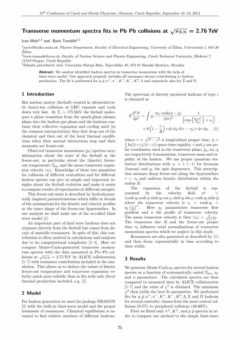
18th Conference of Czech and Slovak Physicists, Olomouc, Czech Republic, September 16–19, 2014
Transverse momentum spectra fits in Pb Pb collisions at√
sNN = 2.76 TeV
Ivan Melo1,3 and Boris Tomášik2,3
[email protected], Physics Department, Faculty of Electrical Engineering, University of Žilina, Univerzitná 1, 010 26Ž[email protected], Faculty of Nuclear Science and Physics Engineering, Czech Technical University, Břehová 7,11519 Prague, Czech Republic3Fakulta prírodných vied, Univerzita Mateja Bela, Tajovského 40, 974 01 Banská Bystrica, Slovakia
Abstract. We analyse identified hadron spectra in transverse momentum with the help ofblast-wave model. Our approach properly includes all resonance decays contributing to hadronproduction. The fit is performed for p, p, π+, π−,K+,K−,K0,Λ and separately also for Ξ and Ω.
1 Introduction
Hot nuclear matter (fireball) created in ultrarelativis-tic heavy-ion collisions at LHC expands and coolsdown very fast. At Tc ∼ 175 MeV the fireball under-goes a phase transition from the quark-gluon plasmaphase into the hadron gas phase and the hadrons con-tinue their collective expansion and cooling until (inthe common interpretation) they first drop out of thechemical and then out of the local thermal equilib-rium when their mutual interactions stop and theirmomenta are frozen-out.
Observed transverse momentum (pt) spectra carryinformation about the state of the fireball at thefreeze-out, in particular about the (kinetic) freeze-out temperature Tkin and the mean transverse expan-sion velocity 〈vt〉. Knowledge of these two quantitiesfor collisions of different centralities and for differenthadron species can give us simple and important in-sights about the fireball evolution and make it easierto compare results of experiments at different energies.
This freeze-out state is described by hydrodynam-ically inspired parametrisations which differ in detailsof the assumptions for the density and velocity profilesor the exact shape of the freeze-out hypersurface. Inour analysis we shall make use of the so-called blastwave model [1].
An important part of final state hadrons does notoriginate directly from the fireball but comes from de-cays of unstable resonances. In spite of this, this con-tribution is often omitted in calculations and analysesdue to its computational complexity [2–4]. Here wecompare Monte-Carlo-generated transverse momen-tum spectra with the data measured in Pb+Pb col-lisions at
√sNN = 2.75 TeV by ALICE collaboration
[5–7] with resonance contribution included in the sim-ulation. This allows us to deduce the values of kineticfreeze-out temperature and transverse expansion ve-locity much more reliably than in fits with only directthermal production included, e.g. [5].
2 Model
For hadron generation we used the package DRAGON[8] with the built-in blast-wave model and the propertreatment of resonances. Chemical equilibrium is as-sumed to find relative numbers of different hadrons.
The spectrum of directly produced hadrons of type iis obtained as
Ed3N
dp3=∫
gimt cosh(η − y)
(2π)3
1(
exp(
pµuµ
Tkin
)
+ si
)
× θ(
1 − r
R
)
r dr dϕ δ(τ − τ0) τ dτ dη . (1)
where τ =√t2 − z2 is longitudinal proper time, η =
12 ln((t+z)/(t−z)) space-time rapidity, r and ϕ are po-lar coordinates used in the transverse plane, pµ,mt, yare respectively 4-momentum, transverse mass and ra-pidity of the hadron. We use proper quantum sta-tistical distributions with si = 1 (−1) for fermions(bosons) and gi the spin degeneracy. This prescrip-tion assumes sharp freeze-out along the hypersurfaceτ = τ0 and uniform density distribution within theradius R.
The expansion of the fireball is rep-resented by the velocity field uµ =(cosh ηt cosh η, sinh ηt cosϕ, sinh ηt sinϕ, cosh ηt sinh η)where the transverse velocity is vt = tanh ηt =ηf
(
rR
)n. Here ηf parametrises transverse flow
gradient and n the profile of transverse velocity.The mean transverse velocity is then 〈vt〉 = 2
n+1ηf .The transverse size R and the freeze-out propertime τ0 influence total normalisations of transversemomentum spectra which we neglect in this study.
Resonances are also generated as described by (1)and then decay exponentially in time according totheir width.
3 Results
We generate Monte Carlo pt spectra for several hadronspecies as a function of systematically varied Tkin, ηf
and n parameters. The calculated spectra are thencompared to measured data by ALICE collaboration[5–7] and the value of χ2 is obtained. The minimumχ2 then yields the best fit parameters. We performedfits for p, p, π+, π−,K+,K−,K0,Λ,Ξ and Ω hadronsfor several centrality classes from the most central col-lisions (0-5%) to peripheral collisions (40-60%).
First we fitted only π±,K±, and p, p spectra in or-der to compare our method to the simple blast-wave
717171
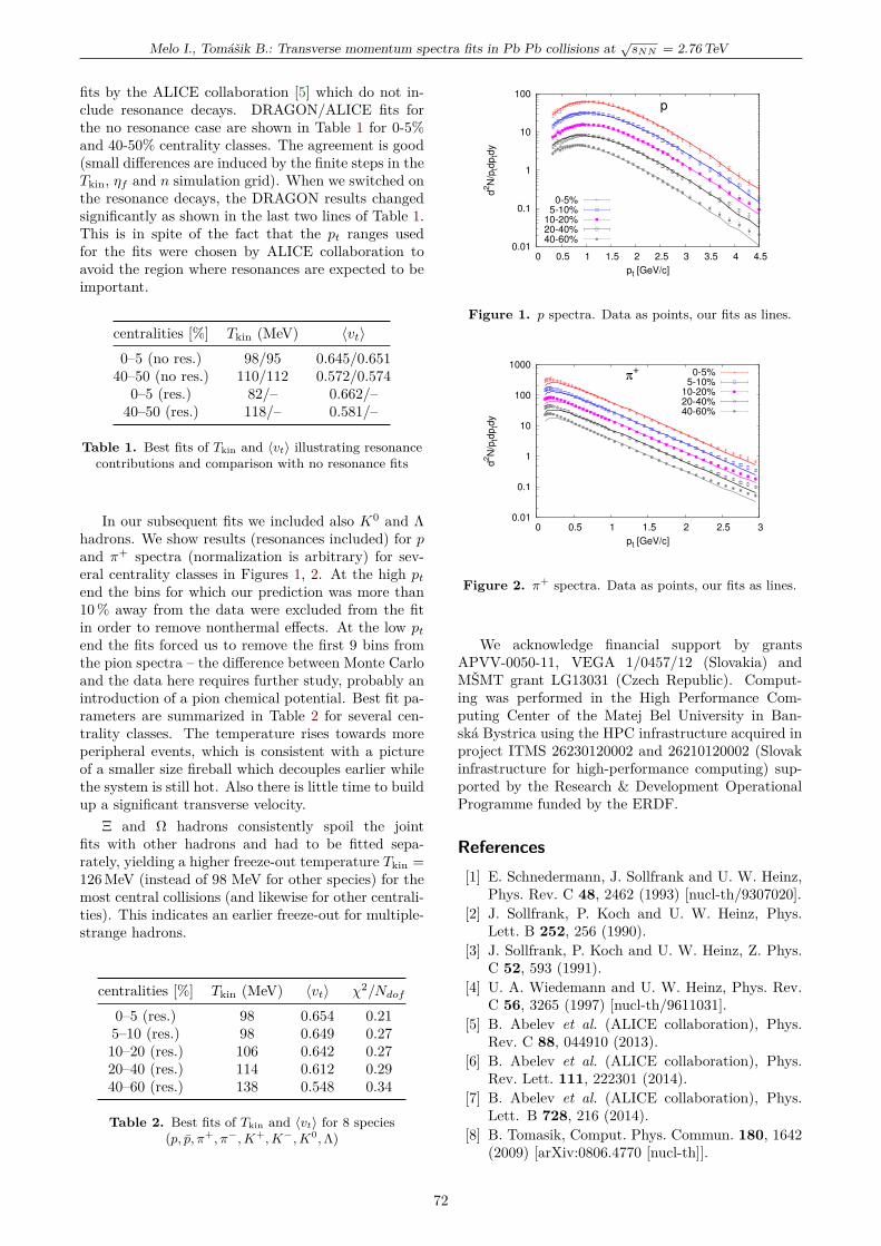
Melo I., Tomášik B.: Transverse momentum spectra fits in Pb Pb collisions at√sNN = 2.76 TeV
fits by the ALICE collaboration [5] which do not in-clude resonance decays. DRAGON/ALICE fits forthe no resonance case are shown in Table 1 for 0-5%and 40-50% centrality classes. The agreement is good(small differences are induced by the finite steps in theTkin, ηf and n simulation grid). When we switched onthe resonance decays, the DRAGON results changedsignificantly as shown in the last two lines of Table 1.This is in spite of the fact that the pt ranges usedfor the fits were chosen by ALICE collaboration toavoid the region where resonances are expected to beimportant.
centralities [%] Tkin (MeV) 〈vt〉0–5 (no res.) 98/95 0.645/0.651
40–50 (no res.) 110/112 0.572/0.5740–5 (res.) 82/– 0.662/–
40–50 (res.) 118/– 0.581/–
Table 1. Best fits of Tkin and 〈vt〉 illustrating resonancecontributions and comparison with no resonance fits
In our subsequent fits we included also K0 and Λhadrons. We show results (resonances included) for pand π+ spectra (normalization is arbitrary) for sev-eral centrality classes in Figures 1, 2. At the high pt
end the bins for which our prediction was more than10 % away from the data were excluded from the fitin order to remove nonthermal effects. At the low pt
end the fits forced us to remove the first 9 bins fromthe pion spectra – the difference between Monte Carloand the data here requires further study, probably anintroduction of a pion chemical potential. Best fit pa-rameters are summarized in Table 2 for several cen-trality classes. The temperature rises towards moreperipheral events, which is consistent with a pictureof a smaller size fireball which decouples earlier whilethe system is still hot. Also there is little time to buildup a significant transverse velocity.
Ξ and Ω hadrons consistently spoil the jointfits with other hadrons and had to be fitted sepa-rately, yielding a higher freeze-out temperature Tkin =126 MeV (instead of 98 MeV for other species) for themost central collisions (and likewise for other centrali-ties). This indicates an earlier freeze-out for multiple-strange hadrons.
centralities [%] Tkin (MeV) 〈vt〉 χ2/Ndof
0–5 (res.) 98 0.654 0.215–10 (res.) 98 0.649 0.2710–20 (res.) 106 0.642 0.2720–40 (res.) 114 0.612 0.2940–60 (res.) 138 0.548 0.34
Table 2. Best fits of Tkin and 〈vt〉 for 8 species(p, p, π+, π−,K+,K−,K0,Λ)
0.01
0.1
1
10
100
0 0.5 1 1.5 2 2.5 3 3.5 4 4.5
d2N
/ptd
ptd
y
pt [GeV/c]
p
0-5%5-10%
10-20%20-40%40-60%
Figure 1. p spectra. Data as points, our fits as lines.
0.01
0.1
1
10
100
1000
0 0.5 1 1.5 2 2.5 3
d2N
/ptd
ptd
y
pt [GeV/c]
π+ 0-5%
5-10%10-20%20-40%40-60%
Figure 2. π+ spectra. Data as points, our fits as lines.
We acknowledge financial support by grantsAPVV-0050-11, VEGA 1/0457/12 (Slovakia) andMŠMT grant LG13031 (Czech Republic). Comput-ing was performed in the High Performance Com-puting Center of the Matej Bel University in Ban-ská Bystrica using the HPC infrastructure acquired inproject ITMS 26230120002 and 26210120002 (Slovakinfrastructure for high-performance computing) sup-ported by the Research & Development OperationalProgramme funded by the ERDF.
References
[1] E. Schnedermann, J. Sollfrank and U. W. Heinz,Phys. Rev. C 48, 2462 (1993) [nucl-th/9307020].
[2] J. Sollfrank, P. Koch and U. W. Heinz, Phys.Lett. B 252, 256 (1990).
[3] J. Sollfrank, P. Koch and U. W. Heinz, Z. Phys.C 52, 593 (1991).
[4] U. A. Wiedemann and U. W. Heinz, Phys. Rev.C 56, 3265 (1997) [nucl-th/9611031].
[5] B. Abelev et al. (ALICE collaboration), Phys.Rev. C 88, 044910 (2013).
[6] B. Abelev et al. (ALICE collaboration), Phys.Rev. Lett. 111, 222301 (2014).
[7] B. Abelev et al. (ALICE collaboration), Phys.Lett. B 728, 216 (2014).
[8] B. Tomasik, Comput. Phys. Commun. 180, 1642(2009) [arXiv:0806.4770 [nucl-th]].
72
18th Conference of Czech and Slovak Physicists, Olomouc, Czech Republic, September 16–19, 2014
Cascade projects competition for high school students
Ivan Melo1
[email protected], Department of Physics, University of Žilina, Univerzitná 1, 010 26 Žilina, Slovakia
Abstract. Cascade projects is a competition for high school teams of 3–6 students. The teams withhelp from physicists work on projects from particle physics for several weeks and prepare 20 minpresentations which they deliver in their schools. They send videos of their talks to the jury whichselects the best teams. The competition is quite popular.
1 Introduction
Cascade projects spread in Slovakia through Interna-tional Particle Physics Outreach Group (IPPOG), anetwork of physicists and science educators engagedin informal science education and outreach for particlephysics [1]. IPPOG was formed in 1997. Its growingmembership currently includes representatives fromeach member state of CERN, each major experimentat CERN’s Large Hadron Collider (LHC) and severalphysics laboratories in the USA and Europe.
IPPOG's aim is to serve anyone who wants to knowmore about particle physics, especially educators andstudents (from school to university), raise standards ofglobal outreach efforts and strengthen understandingand support of particle physics and related sciencesacross the globe. IPPOG can help students tellingthem about outreach programs in their area and howto get involved and point them to recommended learn-ing resources on-line. Teachers can benefit from rec-ommended tools and materials for their classroom au-diences and scientists from recommended tools andmaterials to effectively engage young people duringtalks, presentations, and discussions.
The group meets twice each year: once at CERNand once elsewhere. First IPPOG meetings were al-most exclusively used for exchanging education andoutreach ideas and resources, where each country orexperiment presented their core activities and gainedsome insight into outreach efforts elsewhere. LaterIPPOG became more proactive organizing its own ac-tivities such as International Particle Physics Master-classes and the database of outreach material. At oneof the meetings I heard a talk about Cascade projectsin Birmingham.
2 Cascade projects
International Particle Physics Masterclasses (MC) of-fer a chance to high school students to become par-ticle physicists for one day. They come to a nearbyuniversity, listen to lectures about particles, do themeasurements on real experimental data from LHCand during final video-conference talk to other stu-dents elsewhere in the world and physicists at CERNabout their results. Masterclasses seem very success-ful in motivating high school students. However, it isonly a one day event and some of students are readyfor another adventure. Cascade projects offer a chancefor those who would like to get deeper into the realm
of particle physics. The format was developed at theUniversity of Birmingham [2].
In the Cascade competition teams of 3–6 highschool students work for several weeks on projects ontopics from particle physics and cosmology and thenmake 20 minute presentations at their schools. Theteams are helped by mentors (volunteers from the highenergy physics community) and their teachers. Teamsthen send videos of their presentations plus .ppt filesto organizers. Jury selects best teams and invitesthem to the Grand Final. The best team in the Finalwins an interesting prize, such as the trip to CERN.The recommended topics typically include:
– What are we all made of? Atoms – Quarks – ?– Particle Accelerators – How do they work?– Medical Applications of Particle Accelerators– Recreating the Early Universe at the LHC– Antimatter– Dark matter– Quantum nature of elementary particles– Neutrinos– Are there more than 3 spatial dimensions?– Search for new particles. Higgs boson– History of the Universe
Students can also come up with their own topic whichorganizers have to approve.
In Slovakia [3] we started in 2009 with 4 teams andsince then the number of participating teams quicklyrose and stabilized at 15–20 teams/year. We use an-nual International Masterclasses to advertize Cascadeprojects. Teams are usually mixed (boys and girls).Students have typically 5–6 weeks to work on theprojects. They can consult their mentor. Most teamsexchanged a few emails with mentors, some did notcontact the mentor at all.
Given the time they had, the quality of presenta-tions was good and some of them were very good andfunny. Nevertheless, many teams tried to cover toomany things and inevitably they were superficial andmade many errors. The lesson we try to teach them isthat “less is often more“.We also hope to teach themin the future by publishing best presentations on Cas-cade pages and giving them more time for the projects(3–4 months rather than 6 weeks). The winning teamin 2011, e.g., did not cover too much but they triedto be thorough and honest in each concept they in-troduced and at the same time they were original and
737373

Melo I.: Cascade projects competition for high school students
Figure 1. One of the teams at the Grand Final.
funny. As they put it, „we enjoyed it all the way“.And so did the audience.
Figure 2. Jury and audience at the Grand Final.
The format is very successful. Students enjoyworking in teams and presenting things. Masterclassesis a good springboard for Cascade. Most of the teamsare formed from Masterclass participants. The com-petition is relatively easy to organize. The first round(presentations at schools) does not require presence ofthe organizers nor judges. Grand Final is jointly or-ganized by one of the high schools and a university.Teams present their projects in front of the jury andthe high school audience.
Best Cascade projects have the qualities we hadhoped for. Solid scientific content and fresh, enter-taining presentations which are a fun to watch. Teammembers are often interested in pursuing scientific ca-reer.
3 Rules in Slovakia (short version)
1. Teams consist of 2 or 3 students. Each memberhas to contribute in a significant way.
2. The team registers by filling in the registrationform. Chosen topic must be indicated.
3. Recommended topics can be found at http://
fyzika.uniza.sk/cascade/.
4. You can choose your own topic but we have toapprove it.
5. After receiving your registration, we will assigna mentor to your team. Mentor is not your su-pervisor but rather a good friend on e-mail. Donot be afraid to ask him/her questions.
6. Your presentation should be 20 ± 2 min long.
7. Talk only about things which you understand (ofcourse, many things you will understand only toa certain level – in that case do not go beyondthat level in your presentation).
8. Presentation must include a .ppt (or .pdf or.odp) element.
9. We expect your audience to be at least 25 stu-dents 14–19 years old.
10. After the presentation at your school send usDVD with:
– video of your presentation in mp4 format– .ppt (or .pdf or .odp) file– original registration form– file with details about audience
11. Send the DVD by . . . . . . date
12. Your presentations will be judged by the jury ac-cording to these criteria:
– scientific content . . . . . . . . . . . . . . . . . . . . . . . . 50%– quality of presentation (correct explanation,
audible/entertaining, capturing audience inter-est, good .ppt . . . . . . . . . . . . . . . . . . . . . . . . . 50%
13. Best 4 teams will be invited to Grand Finalswhere they will repeat presentations in front ofjury and invited high school audience.
14. Videos of your presentations can be published onCascade web pages.
This work was supported by grant KEGA 022ŽU-4/2013.
References
[1] http://ippog.web.cern.ch
[2] http://www.hep.ph.bham.ac.uk/cascade/
[3] http://fyzika.uniza.sk/cascade/
74
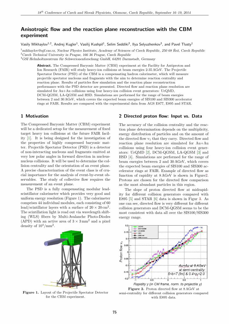
18th Conference of Czech and Slovak Physicists, Olomouc, Czech Republic, September 16–19, 2014
Anisotropic flow and the reaction plane reconstruction with the CBMexperiment
Vasily Mikhaylov1,2, Andrej Kugler1, Vasilij Kushpil1, Selim Seddiki3, Ilya Selyuzhenkov3, and Pavel Tlusty1
[email protected], Nuclear Physics Institute, Academy of Sciences of Czech Republic, 250 68 Řež, Czech Republic2Czech Technical University in Prague, 166 36 Prague, Czech Republic3GSI Helmholtzzentrum für Schwerionenforschung GmbH, 64291 Darmstadt, Germany
Abstract. The Compressed Baryonic Matter (CBM) experiment at the Facility for Antiproton andIon Research (FAIR) will study heavy-ion collisions at beam energies 2-35 AGeV. The ProjectileSpectator Detector (PSD) of the CBM is a compensating hadron calorimeter, which will measureprojectile spectator nucleons and fragments with the aim to determine reaction centrality andreaction plane. Results of particles flow simulation and the reaction plane reconstructionperformance with the PSD detector are presented. Directed flow and reaction plane resolution aresimulated for Au+Au collisions using four heavy-ion collision event generators: UrQMD,DCM-QGSM, LA-QGSM and HSD. Simulations are performed for the range of beam energiesbetween 2 and 30 AGeV, which covers the expected beam energies of SIS100 and SIS300 acceleratorrings at FAIR. Results are compared with the experimental data from AGS E877, E895 and STAR.
1 Motivation
The Compressed Baryonic Matter (CBM) experimentwill be a dedicated setup for the measurement of fixedtarget heavy ion collisions at the future FAIR facil-ity [1]. It is being designed for the investigation ofthe properties of highly compressed baryonic mat-ter. Projectile Spectator Detector (PSD) is a detectorof non-interacting nucleons and fragments emitted atvery low polar angles in forward direction in nucleus-nucleus collisions. It will be used to determine the col-lision centrality and the orientation of an event plane.A precise characterization of the event class is of cru-cial importance for the analysis of event-by-event ob-servables. The study of collective flow requires themeasurement of an event plane.
The PSD is a fully compensating modular lead-scintillator calorimeter which provides very good anduniform energy resolution (Figure 1). The calorimetercomprises 44 individual modules, each consisting of 60lead/scintillator layers with a surface of 20 × 20 cm2.The scintillation light is read out via wavelength shift-ing (WLS) fibers by Multi-Avalanche Photo-Diodes(APD) with an active area of 3 × 3 mm2 and a pixeldensity of 104/mm2.
Figure 1. Layout of the Projectile Spectator Detectorfor the CBM experiment.
2 Directed proton flow: Input vs. Data
The accuracy of the collision centrality and the reac-tion plane determination depends on the multiplicity,energy distribution of particles and on the amount ofthe directed flow v1 that they carry. Directed flow andreaction plane resolution are simulated for Au+Aucollisions using four heavy-ion collision event gener-ators: UrQMD [2], DCM-QGSM, LA-QGSM [3] andHSD [4]. Simulations are performed for the range ofbeam energies between 2 and 30 AGeV, which coversthe expected beam energies of SIS100 and SIS300 ac-celerator rings at FAIR. Example of directed flow asfunction of rapidity at 8 AGeV is shown in Figure2.Protons are chosen for the directed flow comparisonas the most abundant particles in this region.
The slope of proton directed flow at midrapid-ity for different collision generators compared withE895 [5] and STAR [6] data is shown in Figur 3. Asone can see, directed flow is very different for differentcollision generators and DCM-QGSM seems to be themost consistent with data all over the SIS100/SIS300energy range.
Figure 2. Proton directed flow at 8 AGeV atsemi-centrality for different collision generators compared
with E895 data.
757575
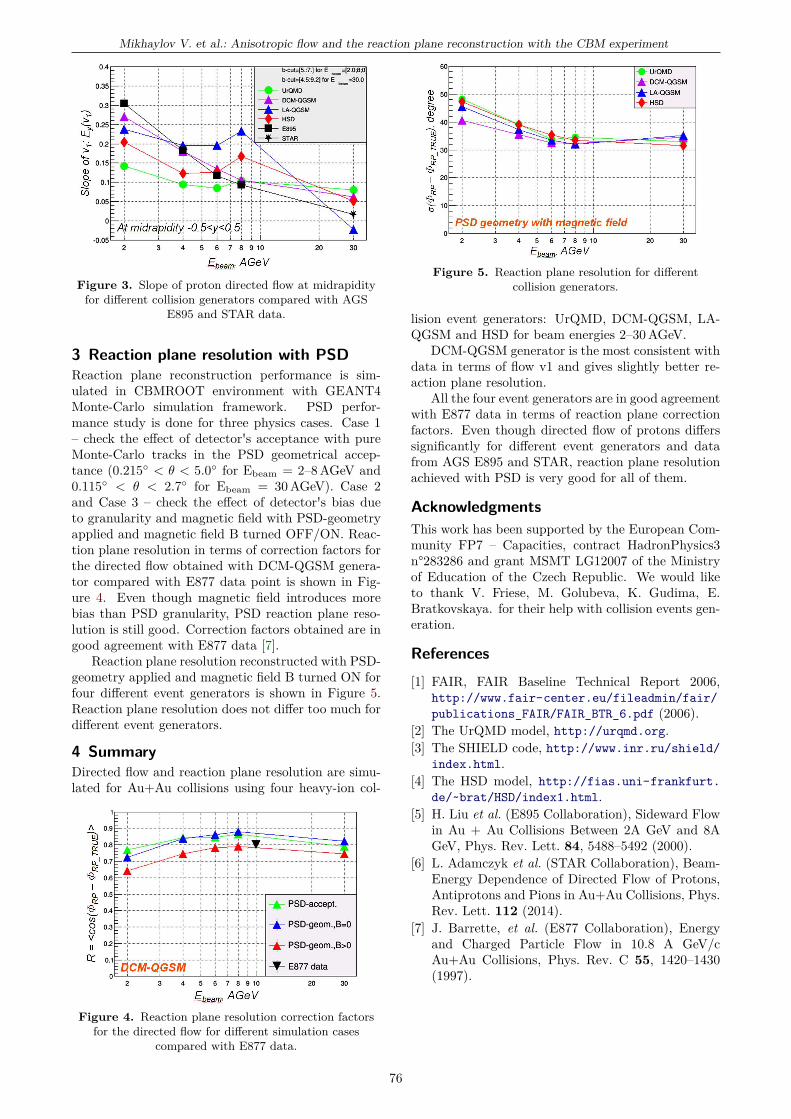
Mikhaylov V. et al.: Anisotropic flow and the reaction plane reconstruction with the CBM experiment
Figure 3. Slope of proton directed flow at midrapidityfor different collision generators compared with AGS
E895 and STAR data.
3 Reaction plane resolution with PSDReaction plane reconstruction performance is sim-ulated in CBMROOT environment with GEANT4Monte-Carlo simulation framework. PSD perfor-mance study is done for three physics cases. Case 1– check the effect of detector's acceptance with pureMonte-Carlo tracks in the PSD geometrical accep-tance (0.215 < θ < 5.0 for Ebeam = 2–8 AGeV and0.115 < θ < 2.7 for Ebeam = 30 AGeV). Case 2and Case 3 – check the effect of detector's bias dueto granularity and magnetic field with PSD-geometryapplied and magnetic field B turned OFF/ON. Reac-tion plane resolution in terms of correction factors forthe directed flow obtained with DCM-QGSM genera-tor compared with E877 data point is shown in Fig-ure 4. Even though magnetic field introduces morebias than PSD granularity, PSD reaction plane reso-lution is still good. Correction factors obtained are ingood agreement with E877 data [7].
Reaction plane resolution reconstructed with PSD-geometry applied and magnetic field B turned ON forfour different event generators is shown in Figure 5.Reaction plane resolution does not differ too much fordifferent event generators.
4 SummaryDirected flow and reaction plane resolution are simu-lated for Au+Au collisions using four heavy-ion col-
Figure 4. Reaction plane resolution correction factorsfor the directed flow for different simulation cases
compared with E877 data.
Figure 5. Reaction plane resolution for differentcollision generators.
lision event generators: UrQMD, DCM-QGSM, LA-QGSM and HSD for beam energies 2–30 AGeV.
DCM-QGSM generator is the most consistent withdata in terms of flow v1 and gives slightly better re-action plane resolution.
All the four event generators are in good agreementwith E877 data in terms of reaction plane correctionfactors. Even though directed flow of protons differssignificantly for different event generators and datafrom AGS E895 and STAR, reaction plane resolutionachieved with PSD is very good for all of them.
Acknowledgments
This work has been supported by the European Com-munity FP7 – Capacities, contract HadronPhysics3n°283286 and grant MSMT LG12007 of the Ministryof Education of the Czech Republic. We would liketo thank V. Friese, M. Golubeva, K. Gudima, E.Bratkovskaya. for their help with collision events gen-eration.
References
[1] FAIR, FAIR Baseline Technical Report 2006,http://www.fair-center.eu/fileadmin/fair/
publications_FAIR/FAIR_BTR_6.pdf (2006).[2] The UrQMD model, http://urqmd.org.[3] The SHIELD code, http://www.inr.ru/shield/
index.html.[4] The HSD model, http://fias.uni-frankfurt.
de/~brat/HSD/index1.html.[5] H. Liu et al. (E895 Collaboration), Sideward Flow
in Au + Au Collisions Between 2A GeV and 8AGeV, Phys. Rev. Lett. 84, 5488–5492 (2000).
[6] L. Adamczyk et al. (STAR Collaboration), Beam-Energy Dependence of Directed Flow of Protons,Antiprotons and Pions in Au+Au Collisions, Phys.Rev. Lett. 112 (2014).
[7] J. Barrette, et al. (E877 Collaboration), Energyand Charged Particle Flow in 10.8 A GeV/cAu+Au Collisions, Phys. Rev. C 55, 1420–1430(1997).
76
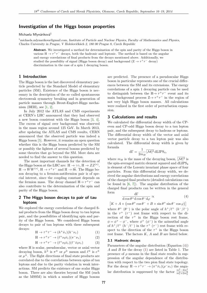
18th Conference of Czech and Slovak Physicists, Olomouc, Czech Republic, September 16–19, 2014
Investigation of the Higgs boson properties
Michaela Mlynáriková1
[email protected], Institute of Particle and Nuclear Physics, Faculty of Mathematics and Physics,Charles University in Prague, V Holešovičkách 2, 180 00 Prague 8, Czech Republic
Abstract. We investigated a method for determination of the spin and parity of the Higgs boson invarious H → τ+τ− decays, both the hadronic and leptonic. The method is based on the angularand energy correlations of final products from the decays mentioned above. Additionally, westudied the possibility of signal (Higgs boson decay) and background (Z → τ+τ− decay)discrimination in the case of a spin 1 decaying boson.
1 Introduction
The Higgs boson is the last discovered elementary par-ticle predicted by the Standard Model of elementaryparticles (SM). Existence of the Higgs boson is nec-essary in the description of the so–called spontaneouselectroweak symmetry breaking and in generation ofparticle masses through Brout-Englert-Higgs mecha-nism (BEH), see [1, 2].
In July 2012 the ATLAS and CMS experimentsat CERN’s LHC announced that they had observeda new boson consistent with the Higgs boson [3, 4].The excess of signal over background was observedin the mass region around 125 GeV. In March 2013,after updating the ATLAS and CMS results, CERNannounced that the observed particle was indeed aHiggs boson [5]. However, it remains an open questionwhether this is the Higgs boson predicted by the SMor possibly the lightest of several bosons predicted bysome theories that go beyond the SM. More data areneeded to find the answer to this question.
The most important channels for the detection ofthe Higgs boson at the LHC are: H → γγ, H → ZZ(∗),H → WW (∗), H → τ+τ− and H → bb. The Higgs bo-son decaying to a fermion-antifermion pair is of spe-cial interest, since the coupling constant depends onthe fermion mass. The decay channel H→ τ+τ− canalso contribute to the determination of the spin andparity of the Higgs boson.
2 The Higgs boson decays to pair of tauleptons
We explored the energy correlations of the charged fi-nal products from the Higgs boson decay to tau leptonpair, and the possibilities of identifying spin and par-ity of the Higgs boson. We considered Higgs bosondecays to pair of tau leptons with these subsequentdecays:
H → τ+τ− → (h+ντ )(h−ντ ) (1)
H → τ+τ− → (ℓ+νℓντ )(π−ντ ) (2)
H → τ+τ− → (ℓ+νℓντ )(ℓ−νℓντ ) (3)where H is scalar, pseudoscalar, vector or axial vectordecaying boson, h± is π± or ρ± meson and ℓ± is e±
or µ±. The flight directions of final state products arecorrelated due to the correlations between spins of tauleptons and due to the parity violation in weak inter-actions. SM predicts the existence of one scalar Higgsboson. There are also theories beyond the SM (suchas the MSSM) in which a number of Higgs bosons
are predicted. The presence of a pseudoscalar Higgsboson in particular represents one of the crucial differ-ences between the SM and its extensions. The energycorrelations of a spin 1 decaying particle can be usedto distinguish between the H→ τ+τ− event and itsmain background process Z→ τ+τ− in the region ofnot very high Higgs boson masses. All calculationswere realized in the first order of perturbation expan-sion.
3 Calculations and resultsWe calculated the differential decay width of the CP-even and CP-odd Higgs boson decay to a tau leptonpair, and the subsequent decay to hadrons or leptons.The differential decay width of the vector and axialvector particle decay to a tau lepton pair was alsocalculated. The differential decay width is given byformula
dΓ =1
2mH|M|2 dLIPS4,
where mH is the mass of the decaying boson, |M|2 isthe spin-averaged matrix element squared and dLIPS4
is element of the Lorentz invariant phase space of fourparticles. From this differential decay width, we de-rived the angular distributions and energy correlationsof the charged final products (detailed calculations canbe found in [6, 7]). The angular distribution of thecharged final products can be written in the generalform dΓ
d cos θ+d cos θ−dϕ∝ (4)
[
K +A×(
cos θ+ cos θ− +B × sin θ+ sin θ− cosϕ)]
where θ+ (θ−) is the polar angle of h+/ℓ+ (h−/ℓ−)in the τ+ (τ−) rest frame with respect to the di-rection of the τ+ in the Higgs boson rest frame,φ = φ+ − φ−, where φ+ (φ−) is the azimuthal angleof h+/ℓ+ (h−/ℓ−) in the τ+ (τ−) rest frame with re-spect to the direction of the τ+ in the Higgs bosonrest frame. The factors K, A and B are listed below.
3.1 Hadronic decays
Parameters of the angular distribution (Equation (4))A and B for the decay (1) are listed in Table 1. Thepresence of ρ mesons in the final state results in sup-pression of the angular dependence of the distribu-tion with respect to the two pion final state topology.For the decay H → τ+τ− → (π+ντ )(ρ−ντ ) the angu-
lar distribution is suppressed by the factorm2
τ −2m2ρ
m2τ +2m2
ρ
777777
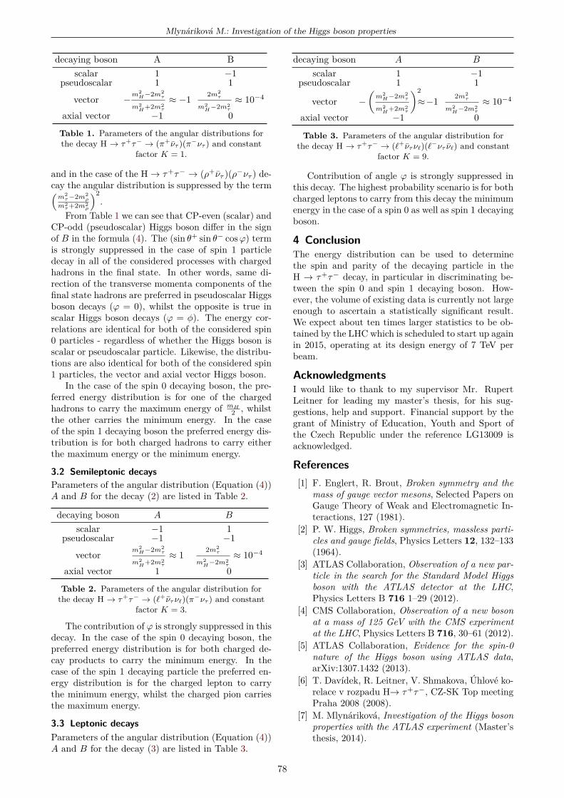
Mlynáriková M.: Investigation of the Higgs boson properties
decaying boson A B
scalar 1 −1pseudoscalar 1 1
vector − m2H −2m2
τ
m2H
+2m2τ
≈ −12m2
τ
m2H
−2m2τ
≈ 10−4
axial vector −1 0
Table 1. Parameters of the angular distributions forthe decay H → τ+τ− → (π+ντ )(π−ντ ) and constant
factor K = 1.
and in the case of the H → τ+τ− → (ρ+ντ )(ρ−ντ ) de-cay the angular distribution is suppressed by the term(
m2τ −2m2
ρ
m2τ +2m2
ρ
)2
.
From Table 1 we can see that CP-even (scalar) andCP-odd (pseudoscalar) Higgs boson differ in the signof B in the formula (4). The (sin θ+ sin θ− cosϕ) termis strongly suppressed in the case of spin 1 particledecay in all of the considered processes with chargedhadrons in the final state. In other words, same di-rection of the transverse momenta components of thefinal state hadrons are preferred in pseudoscalar Higgsboson decays (ϕ = 0), whilst the opposite is true inscalar Higgs boson decays (ϕ = φ). The energy cor-relations are identical for both of the considered spin0 particles - regardless of whether the Higgs boson isscalar or pseudoscalar particle. Likewise, the distribu-tions are also identical for both of the considered spin1 particles, the vector and axial vector Higgs boson.
In the case of the spin 0 decaying boson, the pre-ferred energy distribution is for one of the chargedhadrons to carry the maximum energy of mH
2 , whilstthe other carries the minimum energy. In the caseof the spin 1 decaying boson the preferred energy dis-tribution is for both charged hadrons to carry eitherthe maximum energy or the minimum energy.
3.2 Semileptonic decays
Parameters of the angular distribution (Equation (4))A and B for the decay (2) are listed in Table 2.
decaying boson A B
scalar −1 1pseudoscalar −1 −1
vectorm2
H −2m2τ
m2H
+2m2τ
≈ 12m2
τ
m2H
−2m2τ
≈ 10−4
axial vector 1 0
Table 2. Parameters of the angular distribution forthe decay H → τ+τ− → (ℓ+ντνℓ)(π−ντ ) and constant
factor K = 3.
The contribution of ϕ is strongly suppressed in thisdecay. In the case of the spin 0 decaying boson, thepreferred energy distribution is for both charged de-cay products to carry the minimum energy. In thecase of the spin 1 decaying particle the preferred en-ergy distribution is for the charged lepton to carrythe minimum energy, whilst the charged pion carriesthe maximum energy.
3.3 Leptonic decays
Parameters of the angular distribution (Equation (4))A and B for the decay (3) are listed in Table 3.
decaying boson A B
scalar 1 −1pseudoscalar 1 1
vector −(
m2H −2m2
τ
m2H
+2m2τ
)2
≈−12m2
τ
m2H
−2m2τ
≈ 10−4
axial vector −1 0
Table 3. Parameters of the angular distribution forthe decay H → τ+τ− → (ℓ+ντνℓ)(ℓ−ντ νℓ) and constant
factor K = 9.
Contribution of angle ϕ is strongly suppressed inthis decay. The highest probability scenario is for bothcharged leptons to carry from this decay the minimumenergy in the case of a spin 0 as well as spin 1 decayingboson.
4 ConclusionThe energy distribution can be used to determinethe spin and parity of the decaying particle in theH → τ+τ− decay, in particular in discriminating be-tween the spin 0 and spin 1 decaying boson. How-ever, the volume of existing data is currently not largeenough to ascertain a statistically significant result.We expect about ten times larger statistics to be ob-tained by the LHC which is scheduled to start up againin 2015, operating at its design energy of 7 TeV perbeam.
AcknowledgmentsI would like to thank to my supervisor Mr. RupertLeitner for leading my master’s thesis, for his sug-gestions, help and support. Financial support by thegrant of Ministry of Education, Youth and Sport ofthe Czech Republic under the reference LG13009 isacknowledged.
References
[1] F. Englert, R. Brout, Broken symmetry and themass of gauge vector mesons, Selected Papers onGauge Theory of Weak and Electromagnetic In-teractions, 127 (1981).
[2] P. W. Higgs, Broken symmetries, massless parti-cles and gauge fields, Physics Letters 12, 132–133(1964).
[3] ATLAS Collaboration, Observation of a new par-ticle in the search for the Standard Model Higgsboson with the ATLAS detector at the LHC,Physics Letters B 716 1–29 (2012).
[4] CMS Collaboration, Observation of a new bosonat a mass of 125 GeV with the CMS experimentat the LHC, Physics Letters B 716, 30–61 (2012).
[5] ATLAS Collaboration, Evidence for the spin-0nature of the Higgs boson using ATLAS data,arXiv:1307.1432 (2013).
[6] T. Davídek, R. Leitner, V. Shmakova, Úhlové ko-relace v rozpadu H→ τ+τ−, CZ-SK Top meetingPraha 2008 (2008).
[7] M. Mlynáriková, Investigation of the Higgs bosonproperties with the ATLAS experiment (Master’sthesis, 2014).
78
18th Conference of Czech and Slovak Physicists, Olomouc, Czech Republic, September 16–19, 2014
Preliminary results of pion induced reaction with carbon and polyethylenetargets obtained by HADES-GSI in 2014
Pablo Rodríguez-Ramos1,2 for the HADES [email protected], Nuclear Physics Institute, Academy of Sciences of the Czech Republic, Řež, Czech Republic2Czech Technical University in Prague, Faculty of Nuclear Sciences and Physical Engineering, Prague, Czech Republic
Abstract. In the summer of 2014 HADES was measuring with secondary pion-beam with the aim tomeasure dielepton radiation from baryonic resonances. Most of the beam time was dedicated tomeasurement of e+e− production from PolyEthylene target at pion beam momentum of 0.69GeV/c. In addition we run part of the time with pure carbon target to allow precise subtraction ofcarbon contribution to deduce the inclusive e+e− production on hydrogen.
1 Introduction
The HADES spectrometer is installed at SIS18 syn-chrotronin GSI Darmstadt, Germany. It is designedto measure systematically production of electron-positron pairs in elementary and heavy-ioncollisionsat SIS18 energy range. It covers almost full azimuthalangle and polar angle 18 − 85.
2 Motivation
A modification of hadron masses and their lifetimesin nuclear matter at normal density and zero temper-ature with respect to the values measured in vacuumhas been predicted by recent theoretical calculationsto occur as a precursor phenomenon of the chiral sym-metry restoration that should take place at high den-sity and temperature.
3 Experimental Layout
We used PE as well as Carbon targets at pion beammomentum of 656 MeV/c, 690 MeV/c, 748 MeV/c,800 MeV/c, see Table 1.
Target p[MeV/c] sum events Data
PE 690 774.7 175.56PE 748 76.5 11.61PE 656 42.4 14,08PE 800 52.4 7,48C 690 115,7 13,06C 800 41,2 6,27C 748 42,2 6,8C 656 41,9 14,75
Table 1. Collected statistics in beam time Aug14/Sep14.
3.1 Pion-Beam
The addition of a secondary pion beam to the alreadyavailable proton and heavy ion beams will allow tostudy properties of hadrons with the same detectorsystem at different nuclear matter densities producedby pion, proton and HI beams. In the first step, pionsare produced by the interaction of an intense primarybeam of N on a thick target of C. The outgoing spec-trum of pions is widely open both in momentum andin angle [1]. The pion production target is located inthe main beam-line coming from the synchrotron, see
Figure 1. A primary N beam intensity of 6.0 · 1010
pions/spill with a 10 s total spill length, producing apion beam intensity in a range of 1.2 · 105 − 4.4 · 105
pions/spill.
Figure 1. Schematic drawing of the pion beam-line.
3.2 Targets
Properties of the targets are given in Table 2. Weused it to calculate the no. of carbon atoms ineach target to further deduce a factor for subtrac-tion the C contribution from the PE=C2H4 tar-get, to obtain correct yield of reaction with hy-drogen. Using the corresponding factor f =(No. C atoms in PE/No. C atoms in C) = 0.78taken from Table 2, we can subtract finally the C con-tribution from PE using the formula: H = PE−f ·C.
Target PE= C2H4 CDiameter/cm 1.2 1.2
Length/cm 4.6 2.52M/(g/mol) 28 12
Density/(g/cm3) 0.93 1.85No. of carbon atoms 18.4 · 1022 23.4 · 1022
Table 2. Properties of the targets.
3.3 Selection of elastic events
We want to normalized the yield using the πp elas-tic scattering. In the first plot we see a mixture ofall the particles produced in the PE target, doing theproperly cuts, we select these ones in which we are in-terested, in this case we want to study the pion-protonelastic collisions from PE target, making a cut in theangle ∆φ = 180 between p and π−. We isolated thepions and the protons from elastic scattering of PEtarget to further normalize the yield with the numberof pions. Resulting plot is shown in the lower panel,see Figure 2.
797979
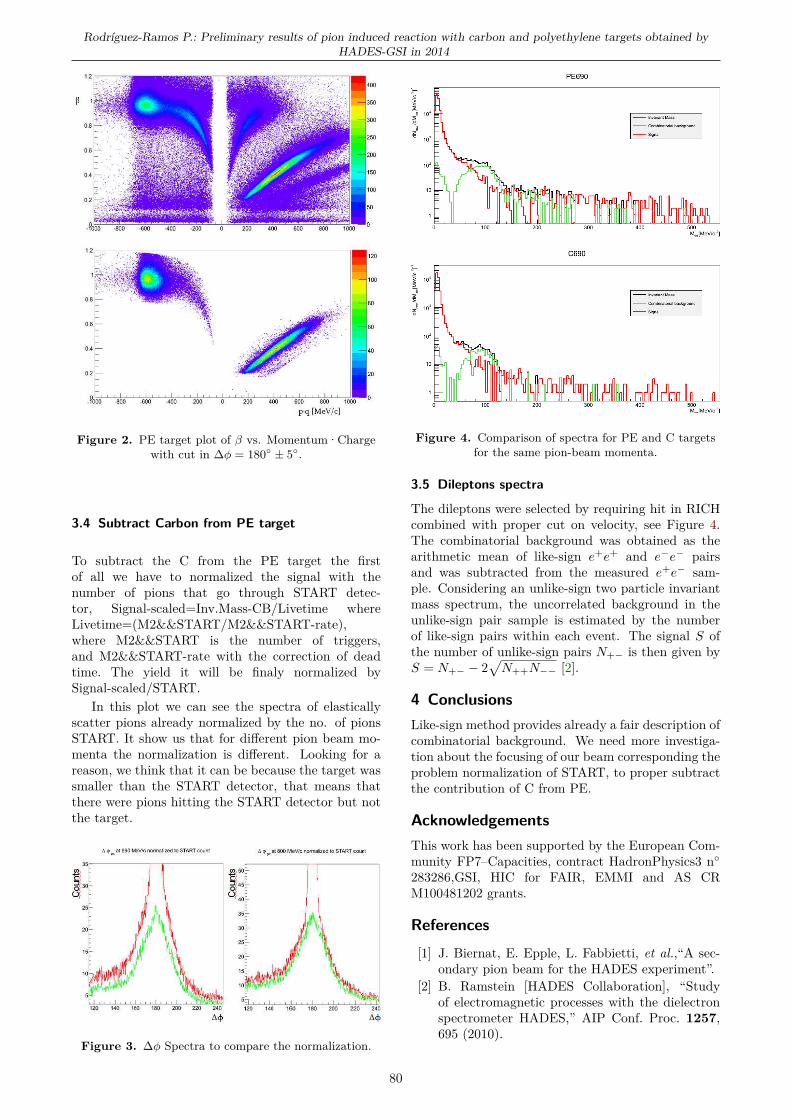
Rodríguez-Ramos P.: Preliminary results of pion induced reaction with carbon and polyethylene targets obtained byHADES-GSI in 2014
Figure 2. PE target plot of β vs. Momentum·Chargewith cut in ∆φ = 180 ± 5.
3.4 Subtract Carbon from PE target
To subtract the C from the PE target the firstof all we have to normalized the signal with thenumber of pions that go through START detec-tor, Signal-scaled=Inv.Mass-CB/Livetime whereLivetime=(M2&&START/M2&&START-rate),where M2&&START is the number of triggers,and M2&&START-rate with the correction of deadtime. The yield it will be finaly normalized bySignal-scaled/START.
In this plot we can see the spectra of elasticallyscatter pions already normalized by the no. of pionsSTART. It show us that for different pion beam mo-menta the normalization is different. Looking for areason, we think that it can be because the target wassmaller than the START detector, that means thatthere were pions hitting the START detector but notthe target.
Figure 3. ∆φ Spectra to compare the normalization.
Figure 4. Comparison of spectra for PE and C targetsfor the same pion-beam momenta.
3.5 Dileptons spectra
The dileptons were selected by requiring hit in RICHcombined with proper cut on velocity, see Figure 4.The combinatorial background was obtained as thearithmetic mean of like-sign e+e+ and e−e− pairsand was subtracted from the measured e+e− sam-ple. Considering an unlike-sign two particle invariantmass spectrum, the uncorrelated background in theunlike-sign pair sample is estimated by the numberof like-sign pairs within each event. The signal S ofthe number of unlike-sign pairs N+− is then given byS = N+− − 2
√
N++N−− [2].
4 Conclusions
Like-sign method provides already a fair description ofcombinatorial background. We need more investiga-tion about the focusing of our beam corresponding theproblem normalization of START, to proper subtractthe contribution of C from PE.
Acknowledgements
This work has been supported by the European Com-munity FP7–Capacities, contract HadronPhysics3 n
283286,GSI, HIC for FAIR, EMMI and AS CRM100481202 grants.
References
[1] J. Biernat, E. Epple, L. Fabbietti, et al.,“A sec-ondary pion beam for the HADES experiment”.
[2] B. Ramstein [HADES Collaboration], “Studyof electromagnetic processes with the dielectronspectrometer HADES,” AIP Conf. Proc. 1257,695 (2010).
80
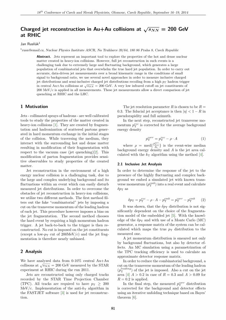
18th Conference of Czech and Slovak Physicists, Olomouc, Czech Republic, September 16–19, 2014
Charged jet reconstruction in Au+Au collisions at√
sNN = 200 GeVat RHIC
Jan Rusňák1
[email protected], Nuclear Physics Institute ASCR, Na Truhlarce 39/64, 180 86 Praha 8, Czech Republic
Abstract. Jets represent an important tool to explore the properties of the hot and dense nuclearmatter created in heavy-ion collisions. However, full jet reconstruction in such events is achallenging task due to extremely large and fluctuating background, which generates a largepopulation of combinatorial jets that overwhelm the true hard jet population. In order to carry outaccurate, data-driven jet measurements over a broad kinematic range in the conditions of smallsignal to background ratio, we use several novel approaches in order to measure inclusive chargedjet distributions and semi-inclusive charged jet distributions recoiling from a high pT hadron triggerin central Au+Au collisions at
√sNN = 200 GeV. A very low infrared cutoff on jet constituents of
200 MeV/c is applied in all measurements. These jet measurements allow a direct comparison of jetquenching at RHIC and the LHC.
1 Motivation
Jets - collimated sprays of hadrons - are well calibratedtools to study the properties of the matter created inheavy-ion collisions [1]. They are created by fragmen-tation and hadronization of scattered partons gener-ated in hard momentum exchange in the initial stagesof the collision. While traversing the medium, theyinteract with the surrounding hot and dense matterresulting in modification of their fragmentation withrespect to the vacuum case (jet quenching)[2]. Thismodification of parton fragmentation provides sensi-tive observables to study properties of the createdmatter.
Jet reconstruction in the environment of a highenergy nuclear collision is a challenging task, due tothe large and complex underlying background and itsfluctuations within an event which can easily disturbmeasured jet distributions. In order to overcome theobstacles of jet reconstruction in heavy-ion collisions,we utilize two different methods. The first method fil-ters out the fake “combinatorial” jets by imposing acut on the transverse momentum of the leading hadronof each jet. This procedure however imposes a bias onthe jet fragmentation. The second method choosesthe hard event by requiring a high momentum hadrontrigger. A jet back-to-back to the trigger is then re-constructed. No cut is imposed on the jet constituents(except a low-pT cut of 200MeV/c) and the jet frag-mentation is therefore nearly unbiased.
2 Analysis
We have analyzed data from 0-10% central Au+Aucollisons at
√sNN = 200 GeV measured by the STAR
experiment at RHIC during the run 2011.Jets are reconstructed using only charged tracks
recorded by the STAR Time Projection Chamber(TPC). All tracks are required to have pT ≥ 200MeV/c. Implementation of the anti-kT algorithm inthe FASTJET software [3] is used for jet reconstruc-tion.
The jet resolution parameter R is chosen to be R =0.3. The fiducial jet acceptance is then |η| < 1 −R inpseudorapidity and full azimuth.
In the next step, reconstructed jet transverse mo-mentum prec
T is corrected for the average backgroundenergy density
pcorrT = prec
T − ρ ·A (1)
where ρ = med precT,i
Ai is the event-wise median
background energy density and A is the jet area cal-culated with the kT algorithm using the method [4].
2.1 Inclusive Jet Analysis
In order to determine the response of the jet to thepresence of the highly fluctuating and complex back-ground we embed a simulated jet with known trans-verse momentum (pemb
T ) into a real event and calculateδpT as
δpT = precT − ρ ·A− pemb
T = pcorrT − pemb
T (2)
It was shown, that the δpT distribution is not sig-nificantly dependent on the choice of the fragmenta-tion model of the embedded jet [5]. With the knowl-edge of the δpT and with use of a Monte Carlo (MC)generator, a response matrix of the system can be cal-culated which maps the true pT distribution to themeasured one.
A jet momentum distribution is smeared not onlyby background fluctuations, but also by detector ef-fects. An MC simulation using a parametrization ofthe TPC tracking efficiency is used to calculate anapproximate detector response matrix.
In order to reduce the combinatorial background, acut on the transverse momentum of the leading hadron(pleading
T ) of the jet is imposed. Also a cut on the jetarea [4] A > 0.2 in case of R = 0.3 and A > 0.09 forR = 0.2 is applied.
In the final step, the measured pcorrT distribution
is corrected for the background and detector effectsusing an iterative unfolding technique based on Bayes’theorem [6].
818181
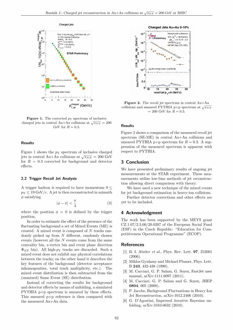
Rusňák J.: Charged jet reconstruction in Au+Au collisions at√sNN = 200 GeV at RHIC
Figure 1. The corrected pT spectrum of inclusivecharged jets in central Au+Au collisions at
√sNN = 200
GeV for R = 0.3.
Results
Figure 1 shows the pT spectrum of inclusive chargedjets in central Au+Au collisions at
√sNN = 200 GeV
for R = 0.3 corrected for background and detectoreffects.
2.2 Trigger Recoil Jet Analysis
A trigger hadron is required to have momentum 9 ≤pT ≤ 19 GeV/c. A jet is then reconstructed in azimuthφ satisfying
|φ− π| < π
4(3)
where the position φ = 0 is defined by the triggerposition.
In order to estimate the effect of the presence of thefluctuating background a set of Mixed Events (ME) iscreated. A mixed event is composed of N tracks ran-domly picked up from N different, randomly chosenevents (however all the N events come from the samecentrality bin, z-vertex bin and event plane directionΨEP bin). All high-pT tracks are discarded. Such amixed event does not exhibit any physical correlationsbetween the tracks; on the other hand it describes thekey features of the background (detector acceptanceinhomogenities, total track multiplicity, etc.). Themixed event distribution is then subtracted from the(unmixed) Same Event (SE) distribution.
Instead of correcting the results for backgroundand detector effects by means of unfolding, a simulatedPYTHIA p+p spectrum is smeared by these effects.This smeared p+p reference is then compared withthe measured Au+Au data.
Figure 2. The recoil jet spectrum in central Au+Aucollisions and smeared PYTHIA p+p spectrum at
√sNN
= 200 GeV for R = 0.3.
Results
Figure 2 shows a comparison of the measured recoil jetspectrum (SE-ME) in central Au+Au collisions andsmeared PYTHIA p+p spectrum for R = 0.3. A sup-pression of the measured spectrum is apparent withrespect to PYTHIA.
3 Conclusion
We have presented preliminary results of ongoing jetmeasurements at the STAR experiment. These mea-surements utilize low-bias methods of jet reconstruc-tion allowing direct comparison with theory.
We have used a new technique of the mixed eventsfor jet background estimation in heavy-ion collisions.
Further detector corrections and other effects areyet to be included.
4 Acknowledgment
The work has been supported by the MEYS grantCZ.1.07/2.3.00/20.0207 of the European Social Fund(ESF) in the Czech Republic: “Education for Com-petitiveness Operational Programme” (ECOP).
References
[1] B. I. Abelev et al., Phys. Rev. Lett. 97, 252001(2006).
[2] Miklos Gyulassy and Michael Plumer, Phys. Lett.B 243, 432-438 (1990).
[3] M. Cacciari, G. P. Salam, G. Soyez, FastJet usermanual, arXiv:1111.6097 (2011).
[4] M. Cacciari, G. P. Salam and G. Soyez, JHEP0804, 005 (2008).
[5] P. Jacobs, Background Fluctuations in Heavy IonJet Reconstruction, arXiv:1012.2406 (2010).
[6] G. D’Agostini, Improved iterative Bayesian un-folding, arXiv:1010.0632 (2010).
82
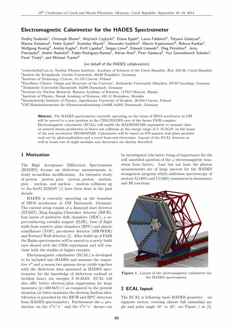
18th Conference of Czech and Slovak Physicists, Olomouc, Czech Republic, September 16–19, 2014
Electromagnetic Calorimeter for the HADES Spectrometer
Ondřej Svoboda1, Christoph Blume2, Wojciech Czyžycki3, Eliane Epple4, Laura Fabbietti4, Tetyana Galatyuk5,Marina Golubeva6, Fedor Guber6, Stanislav Hlaváč7, Alexander Ivashkin6, Marcin Kajetanowic8, Behruz Kardan2,Wolfgang Koenig9, Andrej Kugler1, Kirill Lapidus4, Sergey Linev9, Edward Lisowski3, Oleg Petukhov6, JerzyPietraszko9, Andrei Reshetin6, Pablo Rodríguez-Ramos1, Adrian Rost5, Piotr Salabura8, Yuri Gennadievich Sobolev1,Pavel Tlustý1, and Michael Traxler9
(on behalf of the HADES collaboration)[email protected], Nuclear Physics Institute, Academy of Sciences of the Czech Republic, Řež, 250 68, Czech Republic2Institut für Kernphysik, Goethe-Universität, 60438 Frankfurt, Germany3Institute of Technology Cracow, 31-155 Cracow, Poland4Excellence Cluster ‘Origin and Structure of the Universe’, Technische Universität München, 85748 Garching, Germany5Technische Universität Darmstadt, 64289 Darmstadt, Germany6Institute for Nuclear Research, Russian Academy of Sciences, 117312 Moscow, Russia7Institute of Physics, Slovak Academy of Sciences, 845 11 Bratislava, Slovakia8Smoluchowski Institute of Physics, Jagiellonian University of Kraków, 30-059 Cracow, Poland9GSI Helmholtzzentrum für Schwerionenforschung GmbH, 64291 Darmstadt, Germany
Abstract. The HADES spectrometer currently operating on the beam of SIS18 accelerator in GSIwill be moved to a new position in the CBM/HADES cave of the future FAIR complex.Electromagnetic calorimeter (ECAL) will enable the HADES@FAIR experiment to measure dataon neutral meson production in heavy ion collisions at the energy range of 2–10 AGeV on the beamof the new accelerator SIS100@FAIR. Calorimeter will be based on 978 massive lead glass modulesread out by photomultipliers and a novel front-end electronics. Layout of the ECAL detector aswell as beam test of single modules and electronics are shortly described.
1 Motivation
The High Acceptance DiElectron Spectrometer(HADES) focuses on dielectron measurements tostudy in-medium modifications. An extensive studyof proton – proton, pion – proton, proton – nucleus,pion – nucleus, and nucleus – nucleus collisions upto [email protected] [1] have been done in the pastdecade.
HADES is currently operating on the beamlineof SIS18 accelerator at GSI Darmstadt, Germany.The current setup consist of a diamond start detector(START), Ring Imaging Cherenkov detector (RICH),four layers of multiwire drift chambers (MDC), a su-perconducting toroidal magnet (ILSE), time of flightwalls from resistive plate chambers (RPC) and plasticscintillators (TOF), pre-shower detector (SHOWER)and Forward Wall detector [2]. After build-up of FAIRthe Hades spectrometer will be moved to a newly buildcave shared with the CBM experiment and will con-tinue with the studies at higher energies.
Electromagnetic calorimeter (ECAL) is developedto be included into HADES and measure the respec-tive π0 and η meson two gamma decay yields togetherwith the dielectron data measured in HADES spec-trometer for the knowledge of dielectron cocktail atincident heavy ion energies 2–10 AGeV. ECAL willalso offer better electron/pion suppression for largemomenta (p>400 MeV/c) as compared to the presentsituation (at lower momenta the electron/hadron iden-tification is provided by the RICH and RPC detectorsfrom HADES spectrometer). Furthermore the ω pro-duction via the π0π+π− and the π0e+e− decays can
be investigated (the latter being of importance for thestill unsettled question of the ω electromagnetic tran-sition form factor). Last but not least the photonmeasurements are of large interest for the HADESstrangeness program which addresses spectroscopy ofneutral Λ(1405) and Σ(1385) resonances in elementaryand HI reactions.
Figure 1. Layout of the electromagnetic calorimeter forthe HADES spectrometer.
2 ECAL layout
The ECAL is following basic HADES geometry – sixseparate sectors covering almost full azimuthal an-gle and polar angle 18 to 45, see Figure 1 or [3].
838383
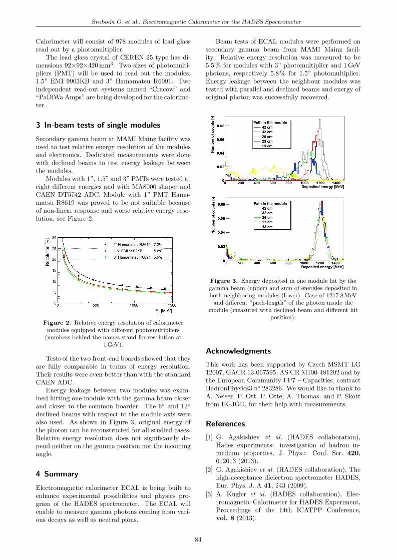
Svoboda O. et al.: Electromagnetic Calorimeter for the HADES Spectrometer
Calorimeter will consist of 978 modules of lead glassread out by a photomultiplier.
The lead glass crystal of CEREN 25 type has di-mensions 92×92×420 mm3. Two sizes of photomulti-pliers (PMT) will be used to read out the modules,1.5” EMI 9903KB and 3” Hamamatsu R6091. Twoindependent read-out systems named “Cracow” and“PaDiWa Amps” are being developed for the calorime-ter.
3 In-beam tests of single modules
Secondary gamma beam at MAMI Mainz facility wasused to test relative energy resolution of the modulesand electronics. Dedicated measurements were donewith declined beams to test energy leakage betweenthe modules.
Modules with 1”, 1.5” and 3” PMTs were tested ateight different energies and with MA8000 shaper andCAEN DT5742 ADC. Module with 1” PMT Hama-matsu R8619 was proved to be not suitable becauseof non-linear response and worse relative energy reso-lution, see Figure 2.
Figure 2. Relative energy resolution of calorimetermodules equipped with different photomultipliers
(numbers behind the names stand for resolution at1 GeV).
Tests of the two front-end boards showed that theyare fully comparable in terms of energy resolution.Their results were even better than with the standardCAEN ADC.
Energy leakage between two modules was exam-ined hitting one module with the gamma beam closerand closer to the common boarder. The 6 and 12
declined beams with respect to the module axis werealso used. As shown in Figure 3, original energy ofthe photon can be reconstructed for all studied cases.Relative energy resolution does not significantly de-pend neither on the gamma position nor the incomingangle.
4 Summary
Electromagnetic calorimeter ECAL is being built toenhance experimental possibilities and physics pro-gram of the HADES spectrometer. The ECAL willenable to measure gamma photons coming from vari-ous decays as well as neutral pions.
Beam tests of ECAL modules were performed onsecondary gamma beam from MAMI Mainz facil-ity. Relative energy resolution was measured to be5.5 % for modules with 3” photomultiplier and 1 GeVphotons, respectively 5.8 % for 1.5” photomultiplier.Energy leakage between the neighbour modules wastested with parallel and declined beams and energy oforiginal photon was successfully recovered.
Figure 3. Energy deposited in one module hit by thegamma beam (upper) and sum of energies deposited inboth neighboring modules (lower). Case of 1217.8 MeV
and different “path-length” of the photon inside themodule (measured with declined beam and different hit
position).
Acknowledgments
This work has been supported by Czech MSMT LG12007, GACR 13-067595, AS CR M100-481202 and bythe European Community FP7 – Capacities, contractHadronPhysics3 n° 283286. We would like to thank toA. Neiser, P. Ott, P. Otte, A. Thomas, and P. Skottfrom IK-JGU, for their help with measurements.
References
[1] G. Agakishiev et al. (HADES collaboration),Hades experiments: investigation of hadron in-medium properties, J. Phys.: Conf. Ser. 420,012013 (2013).
[2] G. Agakishiev et al. (HADES collaboration), Thehigh-acceptance dielectron spectrometer HADES,Eur. Phys. J. A 41, 243 (2009).
[3] A. Kugler et al. (HADES collaboration), Elec-tromagnetic Calorimeter for HADES Experiment,Proceedings of the 14th ICATPP Conference,vol. 8 (2013).
84
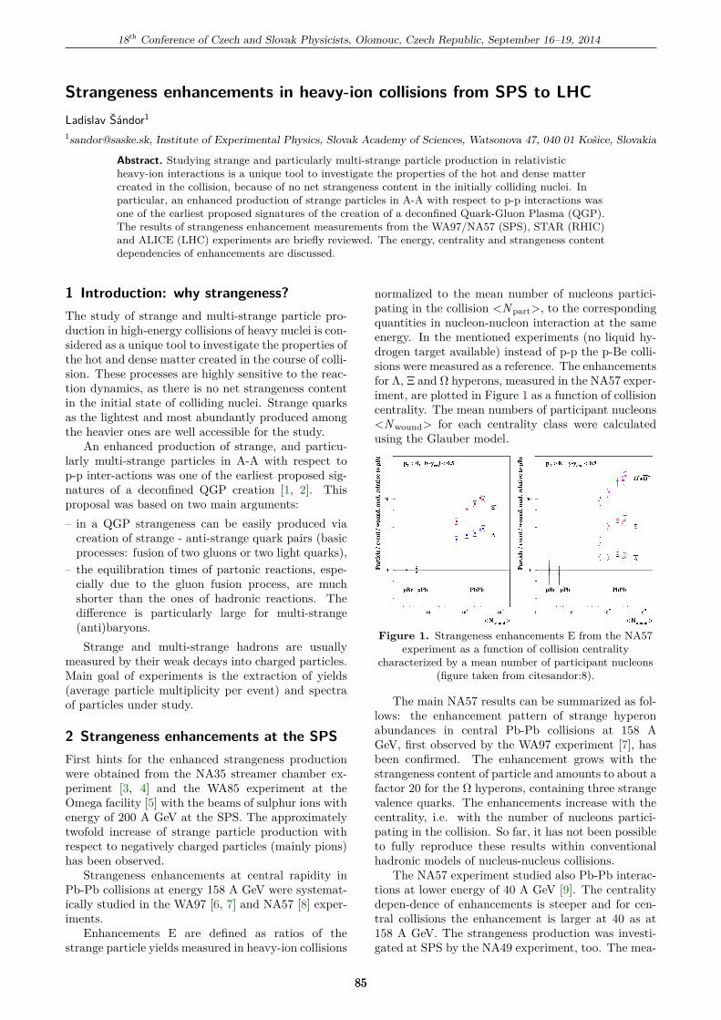
18th Conference of Czech and Slovak Physicists, Olomouc, Czech Republic, September 16–19, 2014
Strangeness enhancements in heavy-ion collisions from SPS to LHC
Ladislav Šándor1
[email protected], Institute of Experimental Physics, Slovak Academy of Sciences, Watsonova 47, 040 01 Košice, Slovakia
Abstract. Studying strange and particularly multi-strange particle production in relativisticheavy-ion interactions is a unique tool to investigate the properties of the hot and dense mattercreated in the collision, because of no net strangeness content in the initially colliding nuclei. Inparticular, an enhanced production of strange particles in A-A with respect to p-p interactions wasone of the earliest proposed signatures of the creation of a deconfined Quark-Gluon Plasma (QGP).The results of strangeness enhancement measurements from the WA97/NA57 (SPS), STAR (RHIC)and ALICE (LHC) experiments are briefly reviewed. The energy, centrality and strangeness contentdependencies of enhancements are discussed.
1 Introduction: why strangeness?
The study of strange and multi-strange particle pro-duction in high-energy collisions of heavy nuclei is con-sidered as a unique tool to investigate the properties ofthe hot and dense matter created in the course of colli-sion. These processes are highly sensitive to the reac-tion dynamics, as there is no net strangeness contentin the initial state of colliding nuclei. Strange quarksas the lightest and most abundantly produced amongthe heavier ones are well accessible for the study.
An enhanced production of strange, and particu-larly multi-strange particles in A-A with respect top-p inter-actions was one of the earliest proposed sig-natures of a deconfined QGP creation [1, 2]. Thisproposal was based on two main arguments:
– in a QGP strangeness can be easily produced viacreation of strange - anti-strange quark pairs (basicprocesses: fusion of two gluons or two light quarks),
– the equilibration times of partonic reactions, espe-cially due to the gluon fusion process, are muchshorter than the ones of hadronic reactions. Thedifference is particularly large for multi-strange(anti)baryons.
Strange and multi-strange hadrons are usuallymeasured by their weak decays into charged particles.Main goal of experiments is the extraction of yields(average particle multiplicity per event) and spectraof particles under study.
2 Strangeness enhancements at the SPS
First hints for the enhanced strangeness productionwere obtained from the NA35 streamer chamber ex-periment [3, 4] and the WA85 experiment at theOmega facility [5] with the beams of sulphur ions withenergy of 200 A GeV at the SPS. The approximatelytwofold increase of strange particle production withrespect to negatively charged particles (mainly pions)has been observed.
Strangeness enhancements at central rapidity inPb-Pb collisions at energy 158 A GeV were systemat-ically studied in the WA97 [6, 7] and NA57 [8] exper-iments.
Enhancements E are defined as ratios of thestrange particle yields measured in heavy-ion collisions
normalized to the mean number of nucleons partici-pating in the collision <N part>, to the correspondingquantities in nucleon-nucleon interaction at the sameenergy. In the mentioned experiments (no liquid hy-drogen target available) instead of p-p the p-Be colli-sions were measured as a reference. The enhancementsfor Λ, Ξ and Ω hyperons, measured in the NA57 exper-iment, are plotted in Figure 1 as a function of collisioncentrality. The mean numbers of participant nucleons<N wound> for each centrality class were calculatedusing the Glauber model.
Figure 1. Strangeness enhancements E from the NA57experiment as a function of collision centrality
characterized by a mean number of participant nucleons(figure taken from citesandor:8).
The main NA57 results can be summarized as fol-lows: the enhancement pattern of strange hyperonabundances in central Pb-Pb collisions at 158 AGeV, first observed by the WA97 experiment [7], hasbeen confirmed. The enhancement grows with thestrangeness content of particle and amounts to about afactor 20 for the Ω hyperons, containing three strangevalence quarks. The enhancements increase with thecentrality, i.e. with the number of nucleons partici-pating in the collision. So far, it has not been possibleto fully reproduce these results within conventionalhadronic models of nucleus-nucleus collisions.
The NA57 experiment studied also Pb-Pb interac-tions at lower energy of 40 A GeV [9]. The centralitydepen-dence of enhancements is steeper and for cen-tral collisions the enhancement is larger at 40 as at158 A GeV. The strangeness production was investi-gated at SPS by the NA49 experiment, too. The mea-
858585
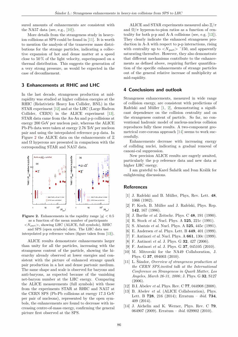
Šándor L.: Strangeness enhancements in heavy-ion collisions from SPS to LHC
sured amounts of enhancements are consistent withthe NA57 data (see, e.g., [10]).
More details from the strangeness study in heavy-ion collisions at SPS could be found in [11]. It is worthto mention the analysis of the transverse mass distri-butions for the strange particles, indicating a collec-tive expansion of hot and dense matter at a speedclose to 50 % of the light velocity, superimposed on athermal distribution. This suggests the generation ofa very strong pressure, as would be expected in thecase of deconfinement.
3 Enhancements at RHIC and LHC
In the last decade, strangeness production at mid-rapidity was studied at higher collision energies at theRHIC (Relativistic Heavy Ion Collider, BNL) in theSTAR experiment [12] and at the LHC (Large HadronCollider, CERN) in the ALICE experiment [13].STAR data came from the Au-Au and p-p collisions atenergy 200 GeV per nucleon pair, whereas the ALICEPb-Pb data were taken at energy 2.76 TeV per nucleonpair and using the interpolated reference p-p data. InFigure 2 the ALICE data on the enhancements of Ξand Ω hyperons are presented in comparison with thecorresponding STAR and NA57 data.
Figure 2. Enhancements in the rapidity range |y| < 0.5as a function of the mean number of participants
<N part>, showing LHC (ALICE, full symbols), RHICand SPS (open symbols) data. The LHC data use
interpolated p-p reference values (figure taken from [13]).
ALICE results demonstrate enhancements largerthan unity for all the particles, increasing with thestrangeness content of the particle, showing the hi-erarchy already observed at lower energies and con-sistent with the picture of enhanced strange quarkpair production in a hot and dense partonic medium.The same shape and scale is observed for baryons andanti-baryons, as expected because of the vanishingnet-baryon number at the LHC energy. Comparingthe ALICE measurements (full symbols) with thosefrom the experiments STAR at RHIC and NA57 atthe CERN SPS (Pb-Pb collisions at energy 17.3 GeVper pair of nucleons), represented by the open sym-bols, the enhancements are found to decrease with in-creasing centre-of-mass energy, confirming the generalpicture first observed at the SPS.
ALICE and STAR experiments measured also Ξ/πand Ω/π hyperon-to-pion ratios as a function of cen-trality for both p-p and A-A collisions (see, e.g. [13]).They clearly indicate the enhanced strangeness pro-duction in A-A with respect to p-p interactions, risingwith centrality up to <N part> ˜150, and apparentlysaturating thereafter. However, they also demonstratethat different mechanisms contribute to the enhance-ments as defined above, requiring further quantifica-tion of the specific enhancements of strange particlesout of the general relative increase of multiplicity atmid-rapidity.
4 Conclusions and outlook
Strangeness enhancements, measured in wide rangeof collision energy, are consistent with predictions ofRafelski and Müller [1, 2], demonstrating a signifi-cant dependence on the collision centrality and onthe strangeness content of particle. So far, no con-ventional hadronic model of nucleus-nucleus collisionreproduces fully these results. A two-component geo-metrical core-corona approach [14] seems to work suc-cessfully.
Enhancements decrease with increasing energyof colliding nuclei, indicating a gradual removal ofcanoni-cal suppression.
New precision ALICE results are eagerly awaited,particularly the p-p reference data and new data athigher LHC energy.
I am grateful to Karel Šafařík and Ivan Králik forenlightening discussions.
References
[1] J. Rafelski and B. Müller, Phys, Rev. Lett. 48,1066 (1982).
[2] P. Koch, B. Müller and J. Rafelski, Phys. Rep.142, 167 (1986).
[3] J. Bartke et al. Zeitschr. Phys. C 48, 191 (1990).[4] R. Stock et al. Nucl. Phys. A 525, 221c (1991).[5] S. Abatzis et al. Nucl. Phys. A 525, 445c (1991).[6] E. Andersen et al. Phys. Lett. B 449, 401 (1999).[7] F. Antinori et al. Nucl. Phys. A 661, 130c (1999).[8] F. Antinori et al. J. Phys. G 32, 427 (2006).[9] F. Antinori et al. J. Phys. G 37, 045105 (2010).
[10] M. Mitrovski for the NA49 Collaboration, J.Phys. G 37, 094003 (2010).
[11] L. Šándor, Overview of strangeness production atthe CERN SPS,invited talk at the InternationalConference on Strangeness in Quark Matter, LosAngeles, March 26-31, 2006 ; J. Phys. G 32, S127(2006).
[12] B.I. Abelev et al. Phys. Rev. C 77, 044908 (2008).[13] B. Abelev et al. (ALICE Collaboration), Phys.
Lett. B 728, 216 (2014); Erratum – ibid. 734,409 (2014).
[14] J. Aichelin and K. Werner, Phys. Rev. C 79,064907 (2009). Erratum – ibid. 029902 (2010).
86
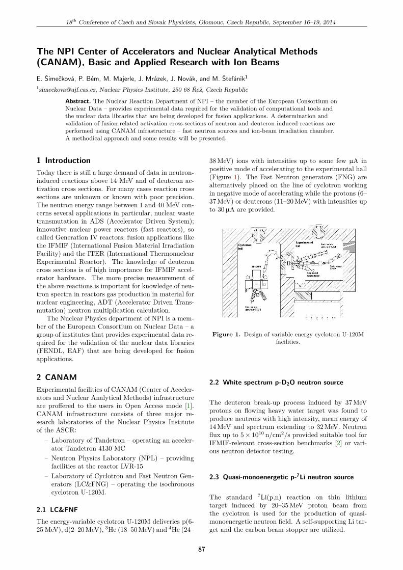
18th Conference of Czech and Slovak Physicists, Olomouc, Czech Republic, September 16–19, 2014
The NPI Center of Accelerators and Nuclear Analytical Methods(CANAM), Basic and Applied Research with Ion Beams
E. Šimečková, P. Bém, M. Majerle, J. Mrázek, J. Novák, and M. Štefánik1
[email protected], Nuclear Physics Institute, 250 68 Řež, Czech Republic
Abstract. The Nuclear Reaction Department of NPI – the member of the European Consortium onNuclear Data – provides experimental data required for the validation of computational tools andthe nuclear data libraries that are being developed for fusion applications. A determination andvalidation of fusion related activation cross-sections of neutron and deuteron induced reactions areperformed using CANAM infrastructure – fast neutron sources and ion-beam irradiation chamber.A methodical approach and some results will be presented.
1 Introduction
Today there is still a large demand of data in neutron-induced reactions above 14 MeV and of deuteron ac-tivation cross sections. For many cases reaction crosssections are unknown or known with poor precision.The neutron energy range between 1 and 40 MeV con-cerns several applications in particular, nuclear wastetransmutation in ADS (Accelerator Driven System);innovative nuclear power reactors (fast reactors), socalled Generation IV reactors; fusion applications likethe IFMIF (International Fusion Material IrradiationFacility) and the ITER (International ThermonuclearExperimental Reactor). The knowledge of deuteroncross sections is of high importance for IFMIF accel-erator hardware. The more precise measurement ofthe above reactions is important for knowledge of neu-tron spectra in reactors gas production in material fornuclear engineering, ADT (Accelerator Driven Trans-mutation) neutron multiplication calculation.
The Nuclear Physics department of NPI is a mem-ber of the European Consortium on Nuclear Data – agroup of institutes that provides experimental data re-quired for the validation of the nuclear data libraries(FENDL, EAF) that are being developed for fusionapplications.
2 CANAM
Experimental facilities of CANAM (Center of Acceler-ators and Nuclear Analytical Methods) infrastructureare proffered to the users in Open Access mode [1].CANAM infrastructure consists of three major re-search laboratories of the Nuclear Physics Instituteof the ASCR:
– Laboratory of Tandetron – operating an acceler-ator Tandetron 4130 MC
– Neutron Physics Laboratory (NPL) – providingfacilities at the reactor LVR-15
– Laboratory of Cyclotron and Fast Neutron Gen-erators (LC&FNG) – operating the isochronouscyclotron U-120M.
2.1 LC&FNF
The energy-variable cyclotron U-120M deliveries p(6-25 MeV), d(2–20 MeV), 3He (18–50 MeV) and 4He (24–
38 MeV) ions with intensities up to some few µA inpositive mode of accelerating to the experimental hall(Figure 1). The Fast Neutron generators (FNG) arealternatively placed on the line of cyclotron workingin negative mode of accelerating while the protons (6–37 MeV) or deuterons (11–20 MeV) with intensities upto 30µA are provided.
Figure 1. Design of variable energy cyclotron U-120Mfacilities.
2.2 White spectrum p-D2O neutron source
The deuteron break-up process induced by 37 MeVprotons on flowing heavy water target was found toproduce neutrons with high intensity, mean energy of14 MeV and spectrum extending to 32 MeV. Neutronflux up to 5 × 10¹⁰ n/cm2/s provided suitable tool forIFMIF-relevant cross-section benchmarks [2] or vari-ous neutron detector testing.
2.3 Quasi-monoenergetic p-7Li neutron source
The standard 7Li(p,n) reaction on thin lithiumtarget induced by 20–35 MeV proton beam fromthe cyclotron is used for the production of quasi-monoenergetic neutron field. A self-supporting Li tar-get and the carbon beam stopper are utilized.
878787
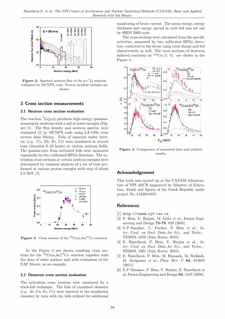
Šimečková E. et al.: The NPI Center of Accelerators and Nuclear Analytical Methods (CANAM), Basic and AppliedResearch with Ion Beams
Figure 2. Spectral neutron flux of the p+7Li reactionevaluated by MCNPX code. Proton incident energies are
shown.
3 Cross section measurements
3.1 Neutron cross section evaluation
The reaction 7Li(p,n) produces high-energy quasimo-noenergetic neutrons with a tail at lower energies (Fig-ure 2). The flux density and neutron spectra wereevaluated [3] by MCNPX code using LA-150h crosssection data library. Foils of material under inter-est (e.g. Co, Nb, Fe, Cr) were irradiated in severalruns (duration 8–10 hours) at various neutron fields.The gamma-rays from activated foils were measuredrepeatedly by two calibrated HPGe detectors. The ac-tivation cross sections at certain neutron energies weredetermined by common analysis of a set of runs per-formed at various proton energies with step of about2.5 MeV [4].
Figure 3. Cross section of the 59Co(n,3n)57Co reaction.
In the Figure 3 are shown resulting cross sec-tions for the 59Co(n,3n)57Co reaction together withthe data of other authors and with evaluation of theEAF library, as an example.
3.2 Deuteron cross section evaluation
The activation cross sections were measured by astack-foil technique. The foils of examined elements(e.g. Al, Cu, Fe, Co) were inserted in the irradiationchamber by turn with the foils utilized for additional
monitoring of beam current. The mean energy, energythickness and energy spread in each foil was set outby SRIM 2003 code.
The cross sections were calculated from the specificactivities, measured by two calibrated HPGe detec-tors, corrected to the decay using total charge and foilcharacteristic as well. The cross sections of deuteroninduced reactions on natCu [5, 6]. are shown in theFigure 4.
Figure 4. Comparison of measured data and analysisresults.
Acknowledgement
This work was carried up at the CANAM infrastruc-ture of NPI ASCR supported by Ministry of Educa-tion, Youth and Sports of the Czech Republic underproject No. LM2011019.
References
[1] http://canam.ujf.cas.cz.[2] P. Bém, V. Burjan, M. Götz et al., Fusion Engi-
neering and Design 75-79, 829 (2005).[3] S. P. Simakov, U. Fischer, P. Bém et al., In-
ter. Conf. on Nucl. Data for Sci., and Techn.,–ND2010, 1856 (Jeju, Korea, 2010).
[4] E. Šimečková, P. Bém, V. Burjan et al., In-ter. Conf. on Nucl. Data for Sci., and Techn.,–ND2010, 1801 (Jeju, Korea, 2010).
[5] E. Šimečková, P. Bém, M. Honusek, M. Štefánik,M. Avrigeanu et al., Phys. Rev. C 84, 014605(2011).
[6] S. P. Simakov, P. Bém, V. Burjan, E. Šimečková etal, Fusion Engineering and Design 83, 1547 (2008).
88
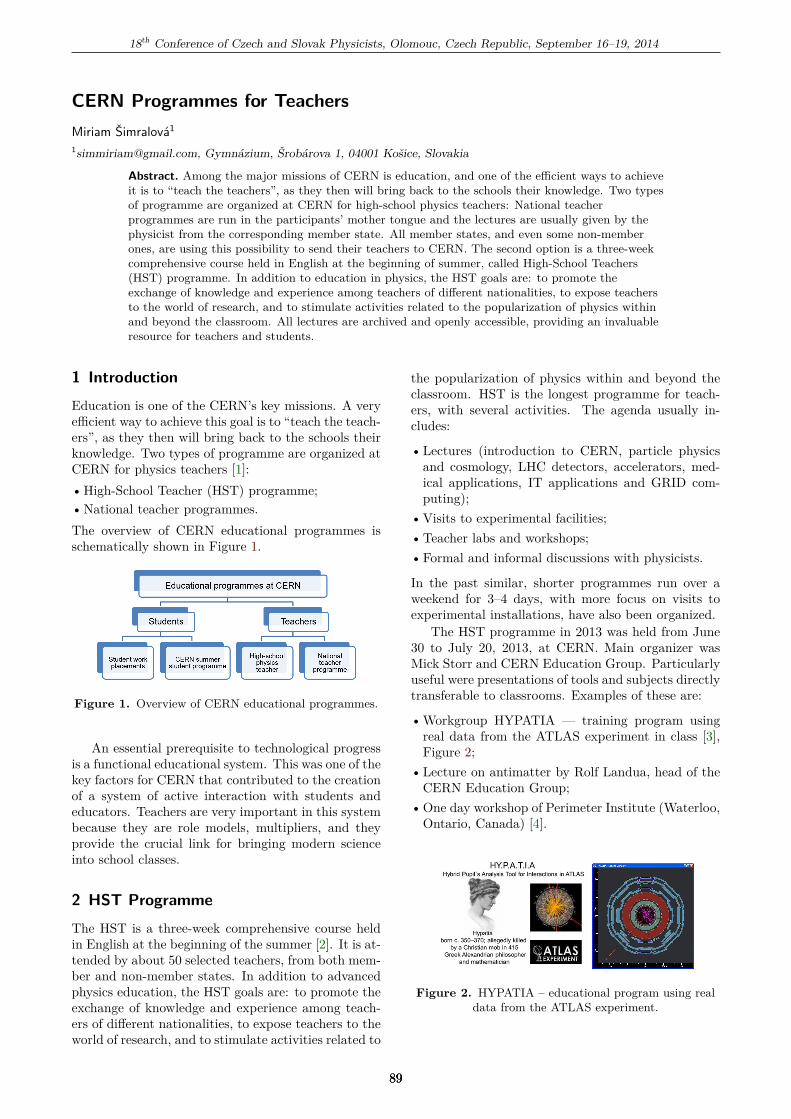
18th Conference of Czech and Slovak Physicists, Olomouc, Czech Republic, September 16–19, 2014
CERN Programmes for Teachers
Miriam Šimralová1
[email protected], Gymnázium, Šrobárova 1, 04001 Košice, Slovakia
Abstract. Among the major missions of CERN is education, and one of the efficient ways to achieveit is to “teach the teachers”, as they then will bring back to the schools their knowledge. Two typesof programme are organized at CERN for high-school physics teachers: National teacherprogrammes are run in the participants’ mother tongue and the lectures are usually given by thephysicist from the corresponding member state. All member states, and even some non-memberones, are using this possibility to send their teachers to CERN. The second option is a three-weekcomprehensive course held in English at the beginning of summer, called High-School Teachers(HST) programme. In addition to education in physics, the HST goals are: to promote theexchange of knowledge and experience among teachers of different nationalities, to expose teachersto the world of research, and to stimulate activities related to the popularization of physics withinand beyond the classroom. All lectures are archived and openly accessible, providing an invaluableresource for teachers and students.
1 Introduction
Education is one of the CERN’s key missions. A veryefficient way to achieve this goal is to “teach the teach-ers”, as they then will bring back to the schools theirknowledge. Two types of programme are organized atCERN for physics teachers [1]:
•High-School Teacher (HST) programme;
•National teacher programmes.
The overview of CERN educational programmes isschematically shown in Figure 1.
Figure 1. Overview of CERN educational programmes.
An essential prerequisite to technological progressis a functional educational system. This was one of thekey factors for CERN that contributed to the creationof a system of active interaction with students andeducators. Teachers are very important in this systembecause they are role models, multipliers, and theyprovide the crucial link for bringing modern scienceinto school classes.
2 HST Programme
The HST is a three-week comprehensive course heldin English at the beginning of the summer [2]. It is at-tended by about 50 selected teachers, from both mem-ber and non-member states. In addition to advancedphysics education, the HST goals are: to promote theexchange of knowledge and experience among teach-ers of different nationalities, to expose teachers to theworld of research, and to stimulate activities related to
the popularization of physics within and beyond theclassroom. HST is the longest programme for teach-ers, with several activities. The agenda usually in-cludes:
•Lectures (introduction to CERN, particle physicsand cosmology, LHC detectors, accelerators, med-ical applications, IT applications and GRID com-puting);
•Visits to experimental facilities;
•Teacher labs and workshops;
•Formal and informal discussions with physicists.
In the past similar, shorter programmes run over aweekend for 3–4 days, with more focus on visits toexperimental installations, have also been organized.
The HST programme in 2013 was held from June30 to July 20, 2013, at CERN. Main organizer wasMick Storr and CERN Education Group. Particularlyuseful were presentations of tools and subjects directlytransferable to classrooms. Examples of these are:
•Workgroup HYPATIA — training program usingreal data from the ATLAS experiment in class [3],Figure 2;
•Lecture on antimatter by Rolf Landua, head of theCERN Education Group;
•One day workshop of Perimeter Institute (Waterloo,Ontario, Canada) [4].
Figure 2. HYPATIA – educational program using realdata from the ATLAS experiment.
898989
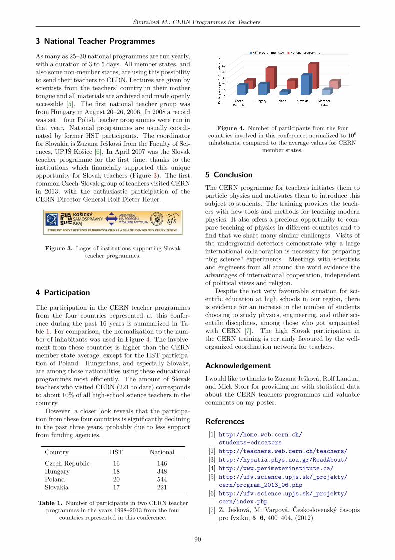
Šimralová M.: CERN Programmes for Teachers
3 National Teacher Programmes
As many as 25–30 national programmes are run yearly,with a duration of 3 to 5 days. All member states, andalso some non-member states, are using this possibilityto send their teachers to CERN. Lectures are given byscientists from the teachers’ country in their mothertongue and all materials are archived and made openlyaccessible [5]. The first national teacher group wasfrom Hungary in August 20–26, 2006. In 2008 a recordwas set – four Polish teacher programmes were run inthat year. National programmes are usually coordi-nated by former HST participants. The coordinatorfor Slovakia is Zuzana Ješková from the Faculty of Sci-ences, UPJŠ Košice [6]. In April 2007 was the Slovakteacher programme for the first time, thanks to theinstitutions which financially supported this uniqueopportunity for Slovak teachers (Figure 3). The firstcommon Czech-Slovak group of teachers visited CERNin 2013, with the enthusiastic participation of theCERN Director-General Rolf-Dieter Heuer.
Figure 3. Logos of institutions supporting Slovakteacher programmes.
4 Participation
The participation in the CERN teacher programmesfrom the four countries represented at this confer-ence during the past 16 years is summarized in Ta-ble 1. For comparison, the normalization to the num-ber of inhabitants was used in Figure 4. The involve-ment from these countries is higher than the CERNmember-state average, except for the HST participa-tion of Poland. Hungarians, and especially Slovaks,are among those nationalities using these educationalprogrammes most efficiently. The amount of Slovakteachers who visited CERN (221 to date) correspondsto about 10% of all high-school science teachers in thecountry.
However, a closer look reveals that the participa-tion from these four countries is significantly decliningin the past three years, probably due to less supportfrom funding agencies.
Country HST National
Czech Republic 16 146Hungary 18 348Poland 20 544Slovakia 17 221
Table 1. Number of participants in two CERN teacherprogrammes in the years 1998–2013 from the four
countries represented in this conference.
Figure 4. Number of participants from the fourcountries involved in this conference, normalized to 106
inhabitants, compared to the average values for CERNmember states.
5 Conclusion
The CERN programme for teachers initiates them toparticle physics and motivates them to introduce thissubject to students. The training provides the teach-ers with new tools and methods for teaching modernphysics. It also offers a precious opportunity to com-pare teaching of physics in different countries and tofind that we share many similar challenges. Visits ofthe underground detectors demonstrate why a largeinternational collaboration is necessary for preparing“big science” experiments. Meetings with scientistsand engineers from all around the word evidence theadvantages of international cooperation, independentof political views and religion.
Despite the not very favourable situation for sci-entific education at high schools in our region, thereis evidence for an increase in the number of studentschoosing to study physics, engineering, and other sci-entific disciplines, among those who got acquaintedwith CERN [7]. The high Slovak participation inthe CERN training is certainly favoured by the well-organized coordination network for teachers.
Acknowledgement
I would like to thanks to Zuzana Ješková, Rolf Landua,and Mick Storr for providing me with statistical dataabout the CERN teachers programmes and valuablecomments on my poster.
References
[1] http://home.web.cern.ch/
students-educators
[2] http://teachers.web.cern.ch/teachers/
[3] http://hypatia.phys.uoa.gr/ReadAbout/
[4] http://www.perimeterinstitute.ca/
[5] http://ufv.science.upjs.sk/_projekty/
cern/program_2013_06.php
[6] http://ufv.science.upjs.sk/_projekty/
cern/index.php
[7] Z. Ješková, M. Vargová, Československý časopispro fyziku, 5–6, 400–404, (2012)
90
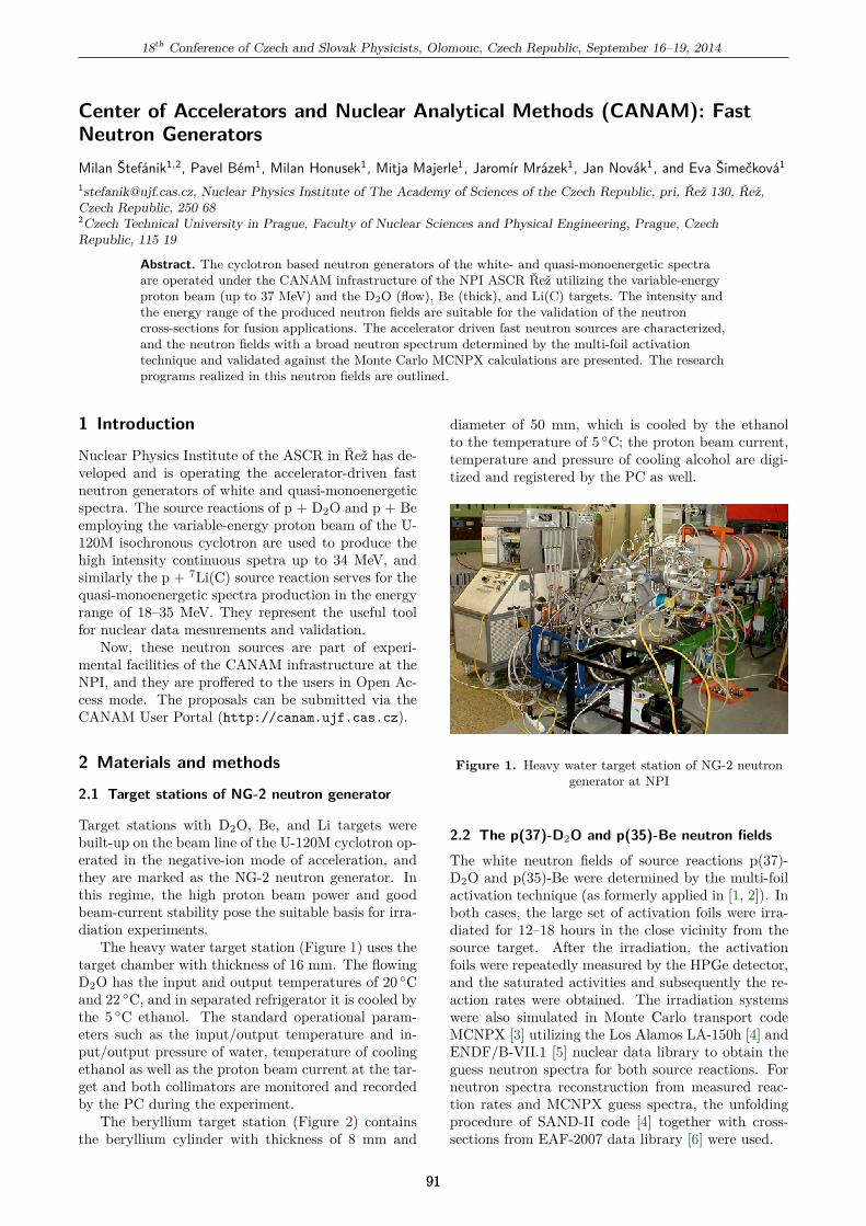
18th Conference of Czech and Slovak Physicists, Olomouc, Czech Republic, September 16–19, 2014
Center of Accelerators and Nuclear Analytical Methods (CANAM): FastNeutron Generators
Milan Štefánik1,2, Pavel Bém1, Milan Honusek1, Mitja Majerle1, Jaromír Mrázek1, Jan Novák1, and Eva Šimečková1
[email protected], Nuclear Physics Institute of The Academy of Sciences of the Czech Republic, pri, Řež 130, Řež,Czech Republic, 250 682Czech Technical University in Prague, Faculty of Nuclear Sciences and Physical Engineering, Prague, CzechRepublic, 115 19
Abstract. The cyclotron based neutron generators of the white- and quasi-monoenergetic spectraare operated under the CANAM infrastructure of the NPI ASCR Řež utilizing the variable-energyproton beam (up to 37 MeV) and the D2O (flow), Be (thick), and Li(C) targets. The intensity andthe energy range of the produced neutron fields are suitable for the validation of the neutroncross-sections for fusion applications. The accelerator driven fast neutron sources are characterized,and the neutron fields with a broad neutron spectrum determined by the multi-foil activationtechnique and validated against the Monte Carlo MCNPX calculations are presented. The researchprograms realized in this neutron fields are outlined.
1 Introduction
Nuclear Physics Institute of the ASCR in Řež has de-veloped and is operating the accelerator-driven fastneutron generators of white and quasi-monoenergeticspectra. The source reactions of p + D2O and p + Beemploying the variable-energy proton beam of the U-120M isochronous cyclotron are used to produce thehigh intensity continuous spetra up to 34 MeV, andsimilarly the p + 7Li(C) source reaction serves for thequasi-monoenergetic spectra production in the energyrange of 18–35 MeV. They represent the useful toolfor nuclear data mesurements and validation.
Now, these neutron sources are part of experi-mental facilities of the CANAM infrastructure at theNPI, and they are proffered to the users in Open Ac-cess mode. The proposals can be submitted via theCANAM User Portal (http://canam.ujf.cas.cz).
2 Materials and methods
2.1 Target stations of NG-2 neutron generator
Target stations with D2O, Be, and Li targets werebuilt-up on the beam line of the U-120M cyclotron op-erated in the negative-ion mode of acceleration, andthey are marked as the NG-2 neutron generator. Inthis regime, the high proton beam power and goodbeam-current stability pose the suitable basis for irra-diation experiments.
The heavy water target station (Figure 1) uses thetarget chamber with thickness of 16 mm. The flowingD2O has the input and output temperatures of 20 Cand 22 C, and in separated refrigerator it is cooled bythe 5 C ethanol. The standard operational param-eters such as the input/output temperature and in-put/output pressure of water, temperature of coolingethanol as well as the proton beam current at the tar-get and both collimators are monitored and recordedby the PC during the experiment.
The beryllium target station (Figure 2) containsthe beryllium cylinder with thickness of 8 mm and
diameter of 50 mm, which is cooled by the ethanolto the temperature of 5 C; the proton beam current,temperature and pressure of cooling alcohol are digi-tized and registered by the PC as well.
Figure 1. Heavy water target station of NG-2 neutrongenerator at NPI
2.2 The p(37)-D2O and p(35)-Be neutron fields
The white neutron fields of source reactions p(37)-D2O and p(35)-Be were determined by the multi-foilactivation technique (as formerly applied in [1, 2]). Inboth cases, the large set of activation foils were irra-diated for 12–18 hours in the close vicinity from thesource target. After the irradiation, the activationfoils were repeatedly measured by the HPGe detector,and the saturated activities and subsequently the re-action rates were obtained. The irradiation systemswere also simulated in Monte Carlo transport codeMCNPX [3] utilizing the Los Alamos LA-150h [4] andENDF/B-VII.1 [5] nuclear data library to obtain theguess neutron spectra for both source reactions. Forneutron spectra reconstruction from measured reac-tion rates and MCNPX guess spectra, the unfoldingprocedure of SAND-II code [4] together with cross-sections from EAF-2007 data library [6] were used.
919191
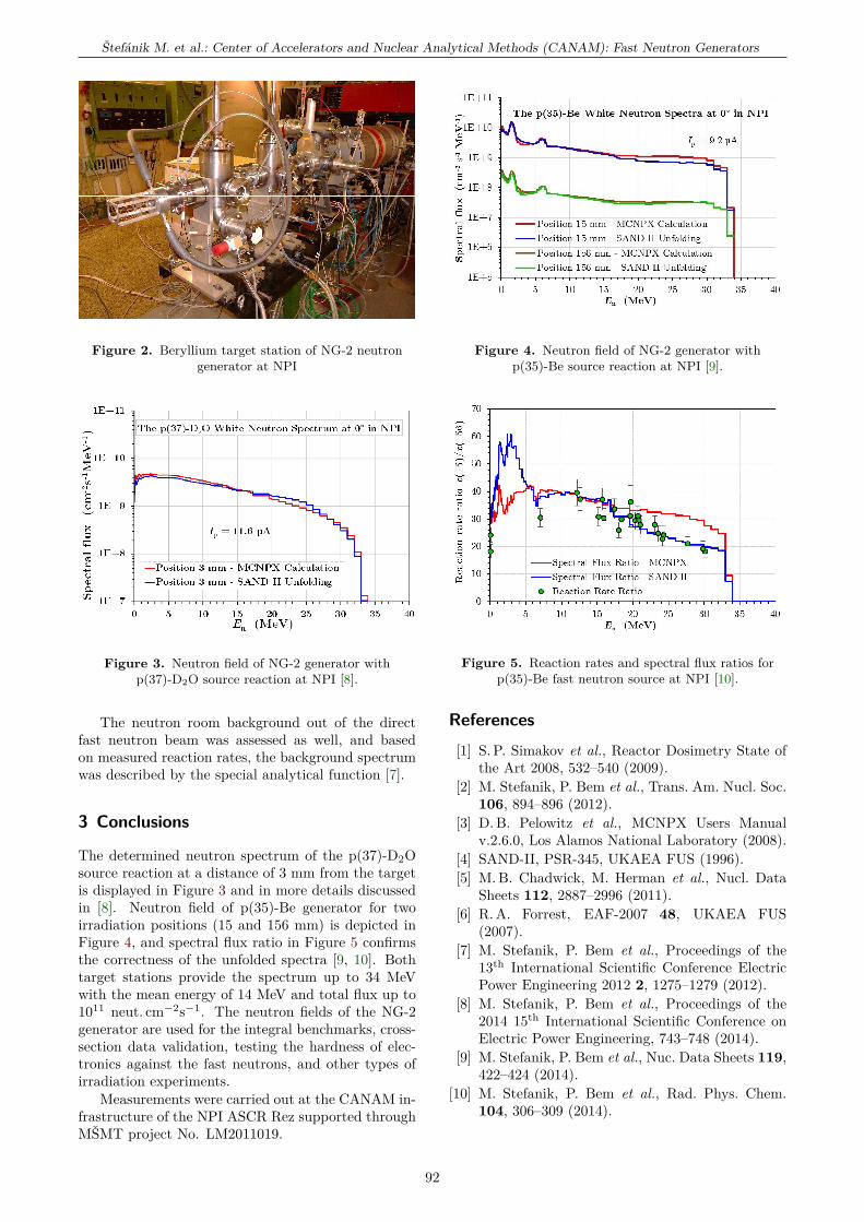
Štefánik M. et al.: Center of Accelerators and Nuclear Analytical Methods (CANAM): Fast Neutron Generators
Figure 2. Beryllium target station of NG-2 neutrongenerator at NPI
Figure 3. Neutron field of NG-2 generator withp(37)-D2O source reaction at NPI [8].
The neutron room background out of the directfast neutron beam was assessed as well, and basedon measured reaction rates, the background spectrumwas described by the special analytical function [7].
3 Conclusions
The determined neutron spectrum of the p(37)-D2Osource reaction at a distance of 3 mm from the targetis displayed in Figure 3 and in more details discussedin [8]. Neutron field of p(35)-Be generator for twoirradiation positions (15 and 156 mm) is depicted inFigure 4, and spectral flux ratio in Figure 5 confirmsthe correctness of the unfolded spectra [9, 10]. Bothtarget stations provide the spectrum up to 34 MeVwith the mean energy of 14 MeV and total flux up to1011 neut. cm−2s−1. The neutron fields of the NG-2generator are used for the integral benchmarks, cross-section data validation, testing the hardness of elec-tronics against the fast neutrons, and other types ofirradiation experiments.
Measurements were carried out at the CANAM in-frastructure of the NPI ASCR Rez supported throughMŠMT project No. LM2011019.
Figure 4. Neutron field of NG-2 generator withp(35)-Be source reaction at NPI [9].
Figure 5. Reaction rates and spectral flux ratios forp(35)-Be fast neutron source at NPI [10].
References
[1] S. P. Simakov et al., Reactor Dosimetry State ofthe Art 2008, 532–540 (2009).
[2] M. Stefanik, P. Bem et al., Trans. Am. Nucl. Soc.106, 894–896 (2012).
[3] D. B. Pelowitz et al., MCNPX Users Manualv.2.6.0, Los Alamos National Laboratory (2008).
[4] SAND-II, PSR-345, UKAEA FUS (1996).[5] M. B. Chadwick, M. Herman et al., Nucl. Data
Sheets 112, 2887–2996 (2011).[6] R. A. Forrest, EAF-2007 48, UKAEA FUS
(2007).[7] M. Stefanik, P. Bem et al., Proceedings of the
13th International Scientific Conference ElectricPower Engineering 2012 2, 1275–1279 (2012).
[8] M. Stefanik, P. Bem et al., Proceedings of the2014 15th International Scientific Conference onElectric Power Engineering, 743–748 (2014).
[9] M. Stefanik, P. Bem et al., Nuc. Data Sheets 119,422–424 (2014).
[10] M. Stefanik, P. Bem et al., Rad. Phys. Chem.104, 306–309 (2014).
92
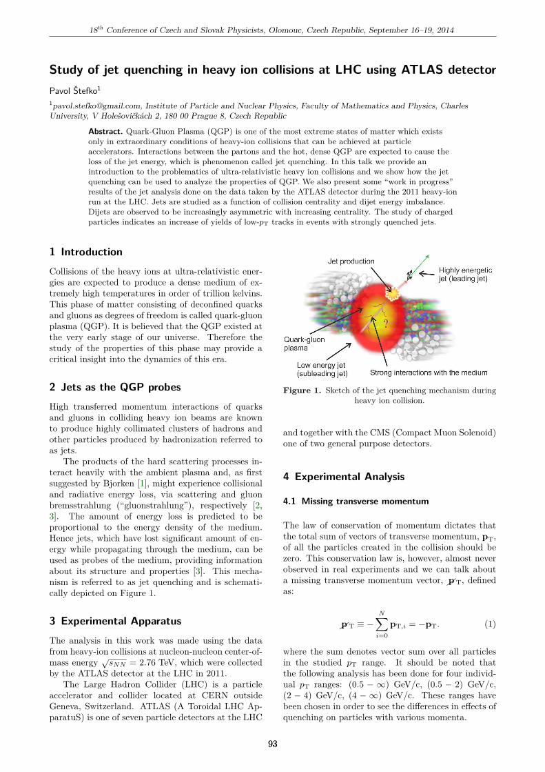
18th Conference of Czech and Slovak Physicists, Olomouc, Czech Republic, September 16–19, 2014
Study of jet quenching in heavy ion collisions at LHC using ATLAS detector
Pavol Štefko1
[email protected], Institute of Particle and Nuclear Physics, Faculty of Mathematics and Physics, CharlesUniversity, V Holešovičkách 2, 180 00 Prague 8, Czech Republic
Abstract. Quark-Gluon Plasma (QGP) is one of the most extreme states of matter which existsonly in extraordinary conditions of heavy-ion collisions that can be achieved at particleaccelerators. Interactions between the partons and the hot, dense QGP are expected to cause theloss of the jet energy, which is phenomenon called jet quenching. In this talk we provide anintroduction to the problematics of ultra-relativistic heavy ion collisions and we show how the jetquenching can be used to analyze the properties of QGP. We also present some “work in progress”results of the jet analysis done on the data taken by the ATLAS detector during the 2011 heavy-ionrun at the LHC. Jets are studied as a function of collision centrality and dijet energy imbalance.Dijets are observed to be increasingly asymmetric with increasing centrality. The study of chargedparticles indicates an increase of yields of low-pT tracks in events with strongly quenched jets.
1 Introduction
Collisions of the heavy ions at ultra-relativistic ener-gies are expected to produce a dense medium of ex-tremely high temperatures in order of trillion kelvins.This phase of matter consisting of deconfined quarksand gluons as degrees of freedom is called quark-gluonplasma (QGP). It is believed that the QGP existed atthe very early stage of our universe. Therefore thestudy of the properties of this phase may provide acritical insight into the dynamics of this era.
2 Jets as the QGP probes
High transferred momentum interactions of quarksand gluons in colliding heavy ion beams are knownto produce highly collimated clusters of hadrons andother particles produced by hadronization referred toas jets.
The products of the hard scattering processes in-teract heavily with the ambient plasma and, as firstsuggested by Bjorken [1], might experience collisionaland radiative energy loss, via scattering and gluonbremsstrahlung (“gluonstrahlung”), respectively [2,3]. The amount of energy loss is predicted to beproportional to the energy density of the medium.Hence jets, which have lost significant amount of en-ergy while propagating through the medium, can beused as probes of the medium, providing informationabout its structure and properties [3]. This mecha-nism is referred to as jet quenching and is schemati-cally depicted on Figure 1.
3 Experimental Apparatus
The analysis in this work was made using the datafrom heavy-ion collisions at nucleon-nucleon center-of-mass energy
√sNN = 2.76 TeV, which were collected
by the ATLAS detector at the LHC in 2011.The Large Hadron Collider (LHC) is a particle
accelerator and collider located at CERN outsideGeneva, Switzerland. ATLAS (A Toroidal LHC Ap-paratuS) is one of seven particle detectors at the LHC
Figure 1. Sketch of the jet quenching mechanism duringheavy ion collision.
and together with the CMS (Compact Muon Solenoid)one of two general purpose detectors.
4 Experimental Analysis
4.1 Missing transverse momentum
The law of conservation of momentum dictates thatthe total sum of vectors of transverse momentum, pT,of all the particles created in the collision should bezero. This conservation law is, however, almost neverobserved in real experiments and we can talk abouta missing transverse momentum vector, p T, definedas:
p T ≡ −N∑
i=0
pT,i = −pT. (1)
where the sum denotes vector sum over all particlesin the studied pT range. It should be noted thatthe following analysis has been done for four individ-ual pT ranges: (0.5 − ∞) GeV/c, (0.5 − 2) GeV/c,(2 − 4) GeV/c, (4 − ∞) GeV/c. These ranges havebeen chosen in order to see the differences in effects ofquenching on particles with various momenta.
939393
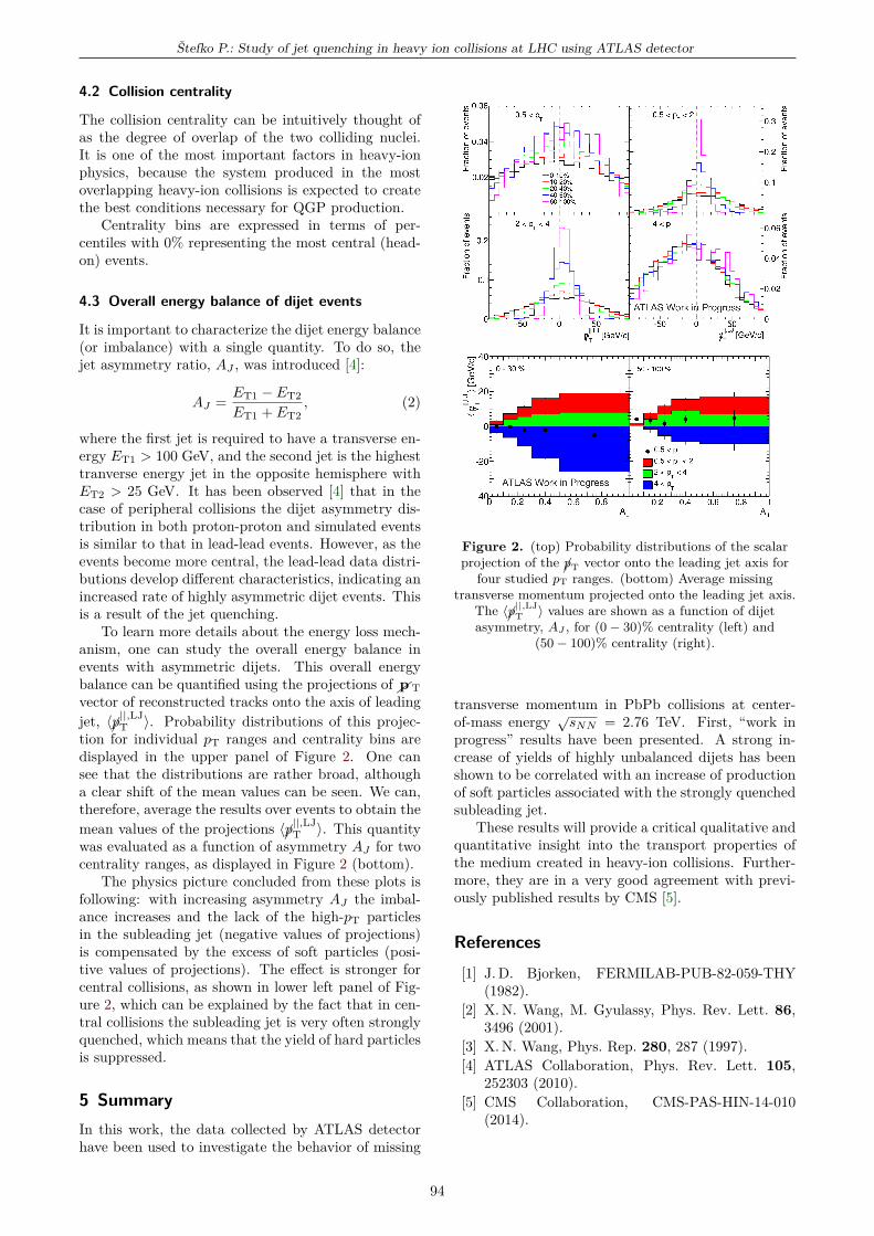
Štefko P.: Study of jet quenching in heavy ion collisions at LHC using ATLAS detector
4.2 Collision centrality
The collision centrality can be intuitively thought ofas the degree of overlap of the two colliding nuclei.It is one of the most important factors in heavy-ionphysics, because the system produced in the mostoverlapping heavy-ion collisions is expected to createthe best conditions necessary for QGP production.
Centrality bins are expressed in terms of per-centiles with 0% representing the most central (head-on) events.
4.3 Overall energy balance of dijet events
It is important to characterize the dijet energy balance(or imbalance) with a single quantity. To do so, thejet asymmetry ratio, AJ , was introduced [4]:
AJ =ET1 − ET2
ET1 + ET2, (2)
where the first jet is required to have a transverse en-ergy ET1 > 100 GeV, and the second jet is the highesttranverse energy jet in the opposite hemisphere withET2 > 25 GeV. It has been observed [4] that in thecase of peripheral collisions the dijet asymmetry dis-tribution in both proton-proton and simulated eventsis similar to that in lead-lead events. However, as theevents become more central, the lead-lead data distri-butions develop different characteristics, indicating anincreased rate of highly asymmetric dijet events. Thisis a result of the jet quenching.
To learn more details about the energy loss mech-anism, one can study the overall energy balance inevents with asymmetric dijets. This overall energybalance can be quantified using the projections of p T
vector of reconstructed tracks onto the axis of leadingjet, 〈p
||,LJT 〉. Probability distributions of this projec-
tion for individual pT ranges and centrality bins aredisplayed in the upper panel of Figure 2. One cansee that the distributions are rather broad, althougha clear shift of the mean values can be seen. We can,therefore, average the results over events to obtain themean values of the projections 〈p
||,LJT 〉. This quantity
was evaluated as a function of asymmetry AJ for twocentrality ranges, as displayed in Figure 2 (bottom).
The physics picture concluded from these plots isfollowing: with increasing asymmetry AJ the imbal-ance increases and the lack of the high-pT particlesin the subleading jet (negative values of projections)is compensated by the excess of soft particles (posi-tive values of projections). The effect is stronger forcentral collisions, as shown in lower left panel of Fig-ure 2, which can be explained by the fact that in cen-tral collisions the subleading jet is very often stronglyquenched, which means that the yield of hard particlesis suppressed.
5 Summary
In this work, the data collected by ATLAS detectorhave been used to investigate the behavior of missing
Figure 2. (top) Probability distributions of the scalarprojection of the pT vector onto the leading jet axis for
four studied pT ranges. (bottom) Average missingtransverse momentum projected onto the leading jet axis.
The 〈p||,LJT 〉 values are shown as a function of dijet
asymmetry, AJ , for (0 − 30)% centrality (left) and(50 − 100)% centrality (right).
transverse momentum in PbPb collisions at center-of-mass energy
√sNN = 2.76 TeV. First, “work in
progress” results have been presented. A strong in-crease of yields of highly unbalanced dijets has beenshown to be correlated with an increase of productionof soft particles associated with the strongly quenchedsubleading jet.
These results will provide a critical qualitative andquantitative insight into the transport properties ofthe medium created in heavy-ion collisions. Further-more, they are in a very good agreement with previ-ously published results by CMS [5].
References
[1] J. D. Bjorken, FERMILAB-PUB-82-059-THY(1982).
[2] X. N. Wang, M. Gyulassy, Phys. Rev. Lett. 86,3496 (2001).
[3] X. N. Wang, Phys. Rep. 280, 287 (1997).[4] ATLAS Collaboration, Phys. Rev. Lett. 105,
252303 (2010).[5] CMS Collaboration, CMS-PAS-HIN-14-010
(2014).
94
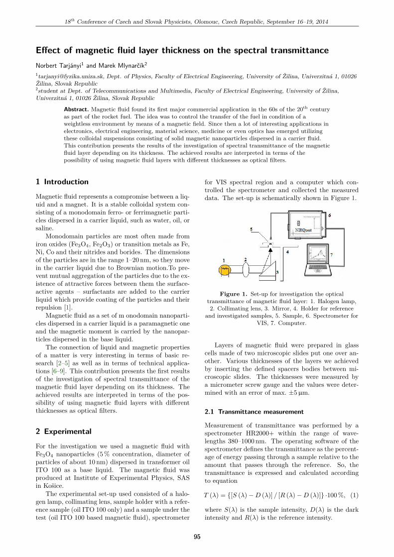
18th Conference of Czech and Slovak Physicists, Olomouc, Czech Republic, September 16–19, 2014
Effect of magnetic fluid layer thickness on the spectral transmittance
Norbert Tarjányi1 and Marek Mlynarčík2
[email protected], Dept. of Physics, Faculty of Electrical Engineering, University of Žilina, Univerzitná 1, 01026Žilina, Slovak Republic2student at Dept. of Telecommunications and Multimedia, Faculty of Electrical Engineering, University of Žilina,Univerzitná 1, 01026 Žilina, Slovak Republic
Abstract. Magnetic fluid found its first major commercial application in the 60s of the 20th centuryas part of the rocket fuel. The idea was to control the transfer of the fuel in condition of aweightless environment by means of a magnetic field. Since then a lot of interesting applications inelectronics, electrical engineering, material science, medicine or even optics has emerged utilizingthese colloidal suspensions consisting of solid magnetic nanoparticles dispersed in a carrier fluid.This contribution presents the results of the investigation of spectral transmittance of the magneticfluid layer depending on its thickness. The achieved results are interpreted in terms of thepossibility of using magnetic fluid layers with different thicknesses as optical filters.
1 Introduction
Magnetic fluid represents a compromise between a liq-uid and a magnet. It is a stable colloidal system con-sisting of a monodomain ferro- or ferrimagnetic parti-cles dispersed in a carrier liquid, such as water, oil, orsaline.
Monodomain particles are most often made fromiron oxides (Fe3O4, Fe2O3) or transition metals as Fe,Ni, Co and their nitrides and borides. The dimensionsof the particles are in the range 1–20 nm, so they movein the carrier liquid due to Brownian motion.To pre-vent mutual aggregation of the particles due to the ex-istence of attractive forces between them the surface-active agents – surfactants are added to the carrierliquid which provide coating of the particles and theirrepulsion [1].
Magnetic fluid as a set of m onodomain nanoparti-cles dispersed in a carrier liquid is a paramagnetic oneand the magnetic moment is carried by the nanopar-ticles dispersed in the base liquid.
The connection of liquid and magnetic propertiesof a matter is very interesting in terms of basic re-search [2–5] as well as in terms of technical applica-tions [6–9]. This contribution presents the first resultsof the investigation of spectral transmittance of themagnetic fluid layer depending on its thickness. Theachieved results are interpreted in terms of the pos-sibility of using magnetic fluid layers with differentthicknesses as optical filters.
2 Experimental
For the investigation we used a magnetic fluid withFe3O4 nanoparticles (5 % concentration, diameter ofparticles of about 10 nm) dispersed in transformer oilITO 100 as a base liquid. The magnetic fluid wasproduced at Institute of Experimental Physics, SASin Košice.
The experimental set-up used consisted of a halo-gen lamp, collimating lens, sample holder with a refer-ence sample (oil ITO 100 only) and a sample under thetest (oil ITO 100 based magnetic fluid), spectrometer
for VIS spectral region and a computer which con-trolled the spectrometer and collected the measureddata. The set-up is schematically shown in Figure 1.
Figure 1. Set-up for investigation the opticaltransmittance of magnetic fluid layer: 1. Halogen lamp,2. Collimating lens, 3. Mirror, 4. Holder for reference
and investigated samples, 5. Sample, 6. Spectrometer forVIS, 7. Computer.
Layers of magnetic fluid were prepared in glasscells made of two microscopic slides put one over an-other. Various thicknesses of the layers we achievedby inserting the defined spacers bodies between mi-croscopic slides. The thicknesses were measured bya micrometer screw gauge and the values were deter-mined with an error of max. ±5µm.
2.1 Transmittance measurement
Measurement of transmittance was performed by aspectrometer HR2000+ within the range of wave-lengths 380–1000 nm. The operating software of thespectrometer defines the transmittance as the percent-age of energy passing through a sample relative to theamount that passes through the reference. So, thetransmittance is expressed and calculated accordingto equation
T (λ) = [S (λ) −D (λ)] / [R (λ) −D (λ)] ·100 %, (1)
where S(λ) is the sample intensity, D(λ) is the darkintensity and R(λ) is the reference intensity.
959595
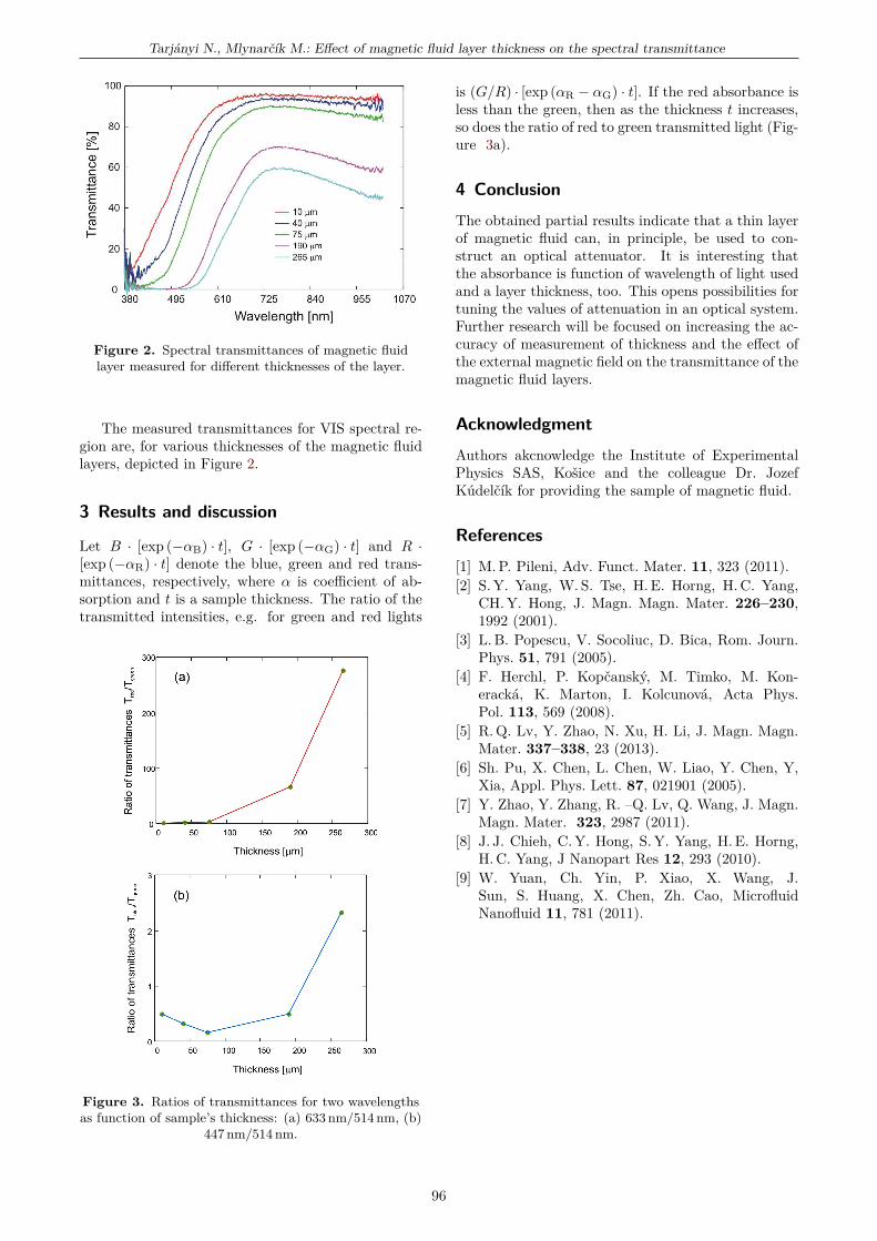
Tarjányi N., Mlynarčík M.: Effect of magnetic fluid layer thickness on the spectral transmittance
Figure 2. Spectral transmittances of magnetic fluidlayer measured for different thicknesses of the layer.
The measured transmittances for VIS spectral re-gion are, for various thicknesses of the magnetic fluidlayers, depicted in Figure 2.
3 Results and discussion
Let B · [exp (−αB) · t], G · [exp (−αG) · t] and R ·[exp (−αR) · t] denote the blue, green and red trans-mittances, respectively, where α is coefficient of ab-sorption and t is a sample thickness. The ratio of thetransmitted intensities, e.g. for green and red lights
Figure 3. Ratios of transmittances for two wavelengthsas function of sample’s thickness: (a) 633 nm/514 nm, (b)
447 nm/514 nm.
is (G/R) · [exp (αR − αG) · t]. If the red absorbance isless than the green, then as the thickness t increases,so does the ratio of red to green transmitted light (Fig-ure 3a).
4 Conclusion
The obtained partial results indicate that a thin layerof magnetic fluid can, in principle, be used to con-struct an optical attenuator. It is interesting thatthe absorbance is function of wavelength of light usedand a layer thickness, too. This opens possibilities fortuning the values of attenuation in an optical system.Further research will be focused on increasing the ac-curacy of measurement of thickness and the effect ofthe external magnetic field on the transmittance of themagnetic fluid layers.
Acknowledgment
Authors akcnowledge the Institute of ExperimentalPhysics SAS, Košice and the colleague Dr. JozefKúdelčík for providing the sample of magnetic fluid.
References
[1] M. P. Pileni, Adv. Funct. Mater. 11, 323 (2011).[2] S. Y. Yang, W. S. Tse, H. E. Horng, H. C. Yang,
CH. Y. Hong, J. Magn. Magn. Mater. 226–230,1992 (2001).
[3] L. B. Popescu, V. Socoliuc, D. Bica, Rom. Journ.Phys. 51, 791 (2005).
[4] F. Herchl, P. Kopčanský, M. Timko, M. Kon-eracká, K. Marton, I. Kolcunová, Acta Phys.Pol. 113, 569 (2008).
[5] R. Q. Lv, Y. Zhao, N. Xu, H. Li, J. Magn. Magn.Mater. 337–338, 23 (2013).
[6] Sh. Pu, X. Chen, L. Chen, W. Liao, Y. Chen, Y,Xia, Appl. Phys. Lett. 87, 021901 (2005).
[7] Y. Zhao, Y. Zhang, R. –Q. Lv, Q. Wang, J. Magn.Magn. Mater. 323, 2987 (2011).
[8] J. J. Chieh, C. Y. Hong, S. Y. Yang, H. E. Horng,H. C. Yang, J Nanopart Res 12, 293 (2010).
[9] W. Yuan, Ch. Yin, P. Xiao, X. Wang, J.Sun, S. Huang, X. Chen, Zh. Cao, MicrofluidNanofluid 11, 781 (2011).
96
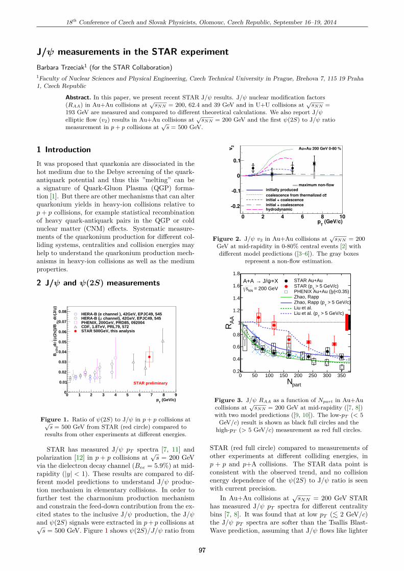
18th Conference of Czech and Slovak Physicists, Olomouc, Czech Republic, September 16–19, 2014
J/ψ measurements in the STAR experiment
Barbara Trzeciak1 (for the STAR Collaboration)1Faculty of Nuclear Sciences and Physical Engineering, Czech Technical University in Prague, Brehova 7, 115 19 Praha1, Czech Republic
Abstract. In this paper, we present recent STAR J/ψ results. J/ψ nuclear modification factors(RAA) in Au+Au collisions at
√sNN = 200, 62.4 and 39 GeV and in U+U collisions at
√sNN =
193 GeV are measured and compared to different theoretical calculations. We also report J/ψelliptic flow (v2) results in Au+Au collisions at
√sNN = 200 GeV and the first ψ(2S) to J/ψ ratio
measurement in p+ p collisions at√s = 500 GeV.
1 Introduction
It was proposed that quarkonia are dissociated in thehot medium due to the Debye screening of the quark-antiquark potential and thus this ”melting” can bea signature of Quark-Gluon Plasma (QGP) forma-tion [1]. But there are other mechanisms that can alterquarkonium yields in heavy-ion collisions relative top+ p collisions, for example statistical recombinationof heavy quark-antiquark pairs in the QGP or coldnuclear matter (CNM) effects. Systematic measure-ments of the quarkonium production for different col-liding systems, centralities and collision energies mayhelp to understand the quarkonium production mech-anisms in heavy-ion collisions as well as the mediumproperties.
2 J/ψ and ψ(2S) measurements
(GeV/c)T
p0 1 2 3 4 5 6 7 8 9
)ψ
(J/
σdψ
J/(2
s))/
Bψ('
σd(2
s)ψ
B
0
0.01
0.02
0.03
0.04
0.05
0.06
0.07
0.08HERA-B (e channel ), 42GeV, EPJC49, 545
channel), 42GeV, EPJC49, 545µHERA-B (PHENIX, 200GeV, PRD85, 092004CDF, 1.8TeV, PRL79, 572STAR 500GeV, this analysis
STAR preliminary
Figure 1. Ratio of ψ(2S) to J/ψ in p+ p collisions at√s = 500 GeV from STAR (red circle) compared to
results from other experiments at different energies.
STAR has measured J/ψ pT spectra [7, 11] andpolarization [12] in p + p collisions at
√s = 200 GeV
via the dielectron decay channel (Bee = 5.9%) at mid-rapidity (|y| < 1). These results are compared to dif-ferent model predictions to understand J/ψ produc-tion mechanism in elementary collisions. In order tofurther test the charmonium production mechanismand constrain the feed-down contribution from the ex-cited states to the inclusive J/ψ production, the J/ψand ψ(2S) signals were extracted in p+ p collisions at√s = 500 GeV. Figure 1 shows ψ(2S)/J/ψ ratio from
(GeV/c)T
p0 2 4 6 8 10
2v
-0.2
-0.1
0
0.1
maximum non-flow
initially produced
ccoalescence from thermalized cinitial + coalescence
initial + coalescencehydrodynamic
Au+Au 200 GeV 0-80 %
Figure 2. J/ψ v2 in Au+Au collisions at√sNN = 200
GeV at mid-rapidity in 0-80% central events [2] withdifferent model predictions ([3–6]). The gray boxes
represent a non-flow estimation.
partN0 50 100 150 200 250 300 350
AA
R
0.2
0.4
0.6
0.8
1
1.2
1.4
1.6
1.8
= 200 GeVNNs
+Xψ J/→A+A STAR Au+Au > 5 GeV/c)
TSTAR (pPHENIX Au+Au (|y|<0.35)Zhao, Rapp
> 5 GeV/c)T
Zhao, Rapp (pLiu et al.
> 5 GeV/c)T
Liu et al. (p
Figure 3. J/ψ RAA as a function of Npart in Au+Aucollisions at
√sNN = 200 GeV at mid-rapidity ([7, 8])
with two model predictions ([9, 10]). The low-pT (< 5GeV/c) result is shown as black full circles and the
high-pT (> 5 GeV/c) measurement as red full circles.
STAR (red full circle) compared to measurements ofother experiments at different colliding energies, inp + p and p+A collisions. The STAR data point isconsistent with the observed trend, and no collisionenergy dependence of the ψ(2S) to J/ψ ratio is seenwith current precision.
In Au+Au collisions at√sNN = 200 GeV STAR
has measured J/ψ pT spectra for different centralitybins [7, 8]. It was found that at low pT (. 2 GeV/c)the J/ψ pT spectra are softer than the Tsallis Blast-Wave prediction, assuming that J/ψ flows like lighter
979797
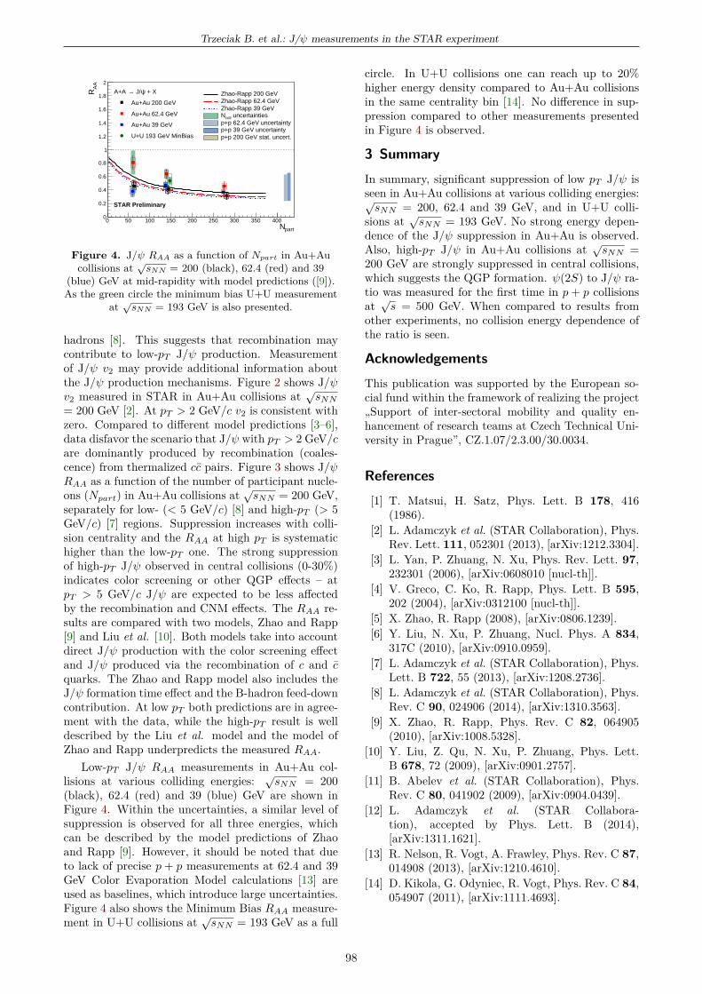
Trzeciak B. et al.: J/ψ measurements in the STAR experiment
partN0 50 100 150 200 250 300 350 400
AA
R
0
0.2
0.4
0.6
0.8
1
1.2
1.4
1.6
1.8
2
Zhao-Rapp 200 GeVZhao-Rapp 62.4 GeVZhao-Rapp 39 GeV
uncertaintiescollNp+p 62.4 GeV uncertaintyp+p 39 GeV uncertaintyp+p 200 GeV stat. uncert.
+ Xψ J/→A+A
Au+Au 200 GeV
Au+Au 62.4 GeV
Au+Au 39 GeV
U+U 193 GeV MinBias
STAR Preliminary
Figure 4. J/ψ RAA as a function of Npart in Au+Aucollisions at
√sNN = 200 (black), 62.4 (red) and 39
(blue) GeV at mid-rapidity with model predictions ([9]).As the green circle the minimum bias U+U measurement
at√sNN = 193 GeV is also presented.
hadrons [8]. This suggests that recombination maycontribute to low-pT J/ψ production. Measurementof J/ψ v2 may provide additional information aboutthe J/ψ production mechanisms. Figure 2 shows J/ψv2 measured in STAR in Au+Au collisions at
√sNN
= 200 GeV [2]. At pT > 2 GeV/c v2 is consistent withzero. Compared to different model predictions [3–6],data disfavor the scenario that J/ψ with pT > 2 GeV/care dominantly produced by recombination (coales-cence) from thermalized cc pairs. Figure 3 shows J/ψRAA as a function of the number of participant nucle-ons (Npart) in Au+Au collisions at
√sNN = 200 GeV,
separately for low- (< 5 GeV/c) [8] and high-pT (> 5GeV/c) [7] regions. Suppression increases with colli-sion centrality and the RAA at high pT is systematichigher than the low-pT one. The strong suppressionof high-pT J/ψ observed in central collisions (0-30%)indicates color screening or other QGP effects – atpT > 5 GeV/c J/ψ are expected to be less affectedby the recombination and CNM effects. The RAA re-sults are compared with two models, Zhao and Rapp[9] and Liu et al. [10]. Both models take into accountdirect J/ψ production with the color screening effectand J/ψ produced via the recombination of c and cquarks. The Zhao and Rapp model also includes theJ/ψ formation time effect and the B-hadron feed-downcontribution. At low pT both predictions are in agree-ment with the data, while the high-pT result is welldescribed by the Liu et al. model and the model ofZhao and Rapp underpredicts the measured RAA.
Low-pT J/ψ RAA measurements in Au+Au col-lisions at various colliding energies:
√sNN = 200
(black), 62.4 (red) and 39 (blue) GeV are shown inFigure 4. Within the uncertainties, a similar level ofsuppression is observed for all three energies, whichcan be described by the model predictions of Zhaoand Rapp [9]. However, it should be noted that dueto lack of precise p + p measurements at 62.4 and 39GeV Color Evaporation Model calculations [13] areused as baselines, which introduce large uncertainties.Figure 4 also shows the Minimum Bias RAA measure-ment in U+U collisions at
√sNN = 193 GeV as a full
circle. In U+U collisions one can reach up to 20%higher energy density compared to Au+Au collisionsin the same centrality bin [14]. No difference in sup-pression compared to other measurements presentedin Figure 4 is observed.
3 Summary
In summary, significant suppression of low pT J/ψ isseen in Au+Au collisions at various colliding energies:√sNN = 200, 62.4 and 39 GeV, and in U+U colli-
sions at√sNN = 193 GeV. No strong energy depen-
dence of the J/ψ suppression in Au+Au is observed.Also, high-pT J/ψ in Au+Au collisions at
√sNN =
200 GeV are strongly suppressed in central collisions,which suggests the QGP formation. ψ(2S) to J/ψ ra-tio was measured for the first time in p + p collisionsat
√s = 500 GeV. When compared to results from
other experiments, no collision energy dependence ofthe ratio is seen.
Acknowledgements
This publication was supported by the European so-cial fund within the framework of realizing the project„Support of inter-sectoral mobility and quality en-hancement of research teams at Czech Technical Uni-versity in Prague”, CZ.1.07/2.3.00/30.0034.
References
[1] T. Matsui, H. Satz, Phys. Lett. B 178, 416(1986).
[2] L. Adamczyk et al. (STAR Collaboration), Phys.Rev. Lett. 111, 052301 (2013), [arXiv:1212.3304].
[3] L. Yan, P. Zhuang, N. Xu, Phys. Rev. Lett. 97,232301 (2006), [arXiv:0608010 [nucl-th]].
[4] V. Greco, C. Ko, R. Rapp, Phys. Lett. B 595,202 (2004), [arXiv:0312100 [nucl-th]].
[5] X. Zhao, R. Rapp (2008), [arXiv:0806.1239].[6] Y. Liu, N. Xu, P. Zhuang, Nucl. Phys. A 834,
317C (2010), [arXiv:0910.0959].[7] L. Adamczyk et al. (STAR Collaboration), Phys.
Lett. B 722, 55 (2013), [arXiv:1208.2736].[8] L. Adamczyk et al. (STAR Collaboration), Phys.
Rev. C 90, 024906 (2014), [arXiv:1310.3563].[9] X. Zhao, R. Rapp, Phys. Rev. C 82, 064905
(2010), [arXiv:1008.5328].[10] Y. Liu, Z. Qu, N. Xu, P. Zhuang, Phys. Lett.
B 678, 72 (2009), [arXiv:0901.2757].[11] B. Abelev et al. (STAR Collaboration), Phys.
Rev. C 80, 041902 (2009), [arXiv:0904.0439].[12] L. Adamczyk et al. (STAR Collabora-
tion), accepted by Phys. Lett. B (2014),[arXiv:1311.1621].
[13] R. Nelson, R. Vogt, A. Frawley, Phys. Rev. C 87,014908 (2013), [arXiv:1210.4610].
[14] D. Kikola, G. Odyniec, R. Vogt, Phys. Rev. C 84,054907 (2011), [arXiv:1111.4693].
98
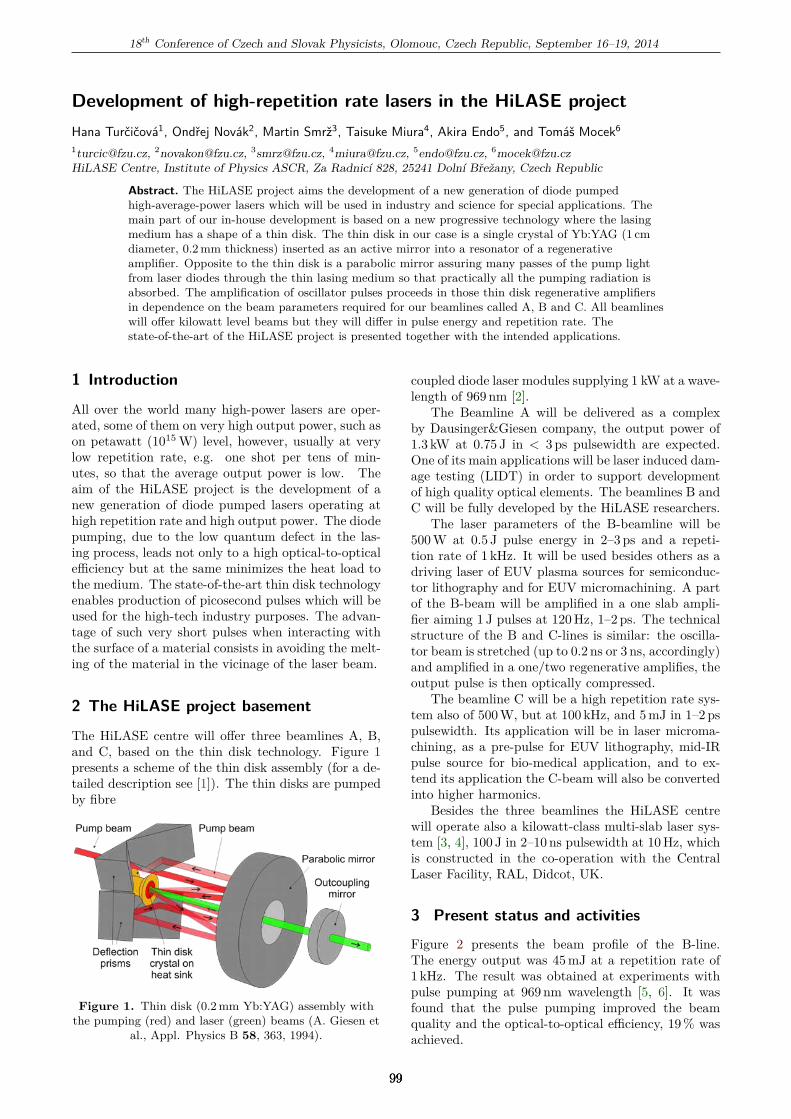
18th Conference of Czech and Slovak Physicists, Olomouc, Czech Republic, September 16–19, 2014
Development of high-repetition rate lasers in the HiLASE project
Hana Turčičová1, Ondřej Novák2, Martin Smrž3, Taisuke Miura4, Akira Endo5, and Tomáš Mocek6
[email protected], [email protected], [email protected], [email protected], [email protected], [email protected] Centre, Institute of Physics ASCR, Za Radnicí 828, 25241 Dolní Břežany, Czech Republic
Abstract. The HiLASE project aims the development of a new generation of diode pumpedhigh-average-power lasers which will be used in industry and science for special applications. Themain part of our in-house development is based on a new progressive technology where the lasingmedium has a shape of a thin disk. The thin disk in our case is a single crystal of Yb:YAG (1 cmdiameter, 0.2 mm thickness) inserted as an active mirror into a resonator of a regenerativeamplifier. Opposite to the thin disk is a parabolic mirror assuring many passes of the pump lightfrom laser diodes through the thin lasing medium so that practically all the pumping radiation isabsorbed. The amplification of oscillator pulses proceeds in those thin disk regenerative amplifiersin dependence on the beam parameters required for our beamlines called A, B and C. All beamlineswill offer kilowatt level beams but they will differ in pulse energy and repetition rate. Thestate-of-the-art of the HiLASE project is presented together with the intended applications.
1 Introduction
All over the world many high-power lasers are oper-ated, some of them on very high output power, such ason petawatt (1015 W) level, however, usually at verylow repetition rate, e.g. one shot per tens of min-utes, so that the average output power is low. Theaim of the HiLASE project is the development of anew generation of diode pumped lasers operating athigh repetition rate and high output power. The diodepumping, due to the low quantum defect in the las-ing process, leads not only to a high optical-to-opticalefficiency but at the same minimizes the heat load tothe medium. The state-of-the-art thin disk technologyenables production of picosecond pulses which will beused for the high-tech industry purposes. The advan-tage of such very short pulses when interacting withthe surface of a material consists in avoiding the melt-ing of the material in the vicinage of the laser beam.
2 The HiLASE project basement
The HiLASE centre will offer three beamlines A, B,and C, based on the thin disk technology. Figure 1presents a scheme of the thin disk assembly (for a de-tailed description see [1]). The thin disks are pumpedby fibre
Figure 1. Thin disk (0.2 mm Yb:YAG) assembly withthe pumping (red) and laser (green) beams (A. Giesen et
al., Appl. Physics B 58, 363, 1994).
coupled diode laser modules supplying 1 kW at a wave-length of 969 nm [2].
The Beamline A will be delivered as a complexby Dausinger&Giesen company, the output power of1.3 kW at 0.75 J in < 3 ps pulsewidth are expected.One of its main applications will be laser induced dam-age testing (LIDT) in order to support developmentof high quality optical elements. The beamlines B andC will be fully developed by the HiLASE researchers.
The laser parameters of the B-beamline will be500 W at 0.5 J pulse energy in 2–3 ps and a repeti-tion rate of 1 kHz. It will be used besides others as adriving laser of EUV plasma sources for semiconduc-tor lithography and for EUV micromachining. A partof the B-beam will be amplified in a one slab ampli-fier aiming 1 J pulses at 120 Hz, 1–2 ps. The technicalstructure of the B and C-lines is similar: the oscilla-tor beam is stretched (up to 0.2 ns or 3 ns, accordingly)and amplified in a one/two regenerative amplifies, theoutput pulse is then optically compressed.
The beamline C will be a high repetition rate sys-tem also of 500 W, but at 100 kHz, and 5 mJ in 1–2 pspulsewidth. Its application will be in laser microma-chining, as a pre-pulse for EUV lithography, mid-IRpulse source for bio-medical application, and to ex-tend its application the C-beam will also be convertedinto higher harmonics.
Besides the three beamlines the HiLASE centrewill operate also a kilowatt-class multi-slab laser sys-tem [3, 4], 100 J in 2–10 ns pulsewidth at 10 Hz, whichis constructed in the co-operation with the CentralLaser Facility, RAL, Didcot, UK.
3 Present status and activities
Figure 2 presents the beam profile of the B-line.The energy output was 45 mJ at a repetition rate of1 kHz. The result was obtained at experiments withpulse pumping at 969 nm wavelength [5, 6]. It wasfound that the pulse pumping improved the beamquality and the optical-to-optical efficiency, 19 % wasachieved.
999999
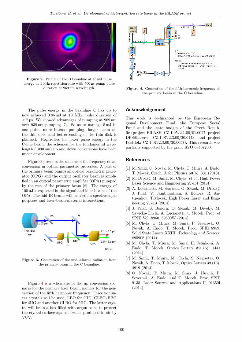
Turčičová, H. et al.: Development of high-repetition rate lasers in the HiLASE project
Figure 2. Profile of the B beamline at 45 mJ pulseenergy at 1-kHz repetition rate with 500µs pump pulse
duration at 969 nm wavelength.
The pulse energy in the beamline C has up tonow achieved 0.85 mJ at 100 kHz, pulse duration of< 2 ps. We showed advantages of pumping at 969 nmover 939 nm pumping [7]. So as to manage 5 mJ inone pulse, more intense pumping, larger beam onthe thin disk, and better cooling of the thin disk isplanned. Regardless the lower pulse energy in theC-line beam, the schemes for the fundamental wave-length (1030 nm) up and down conversions have beenunder development.
Figure 3 presents the scheme of the frequency downconversion in optical parametric processes. A part ofthe primary beam pumps an optical parametric gener-ator (OPG) and the output oscillator beam is ampli-fied in an optical parametric amplifier (OPA) pumpedby the rest of the primary beam [8]. The energy of100µJ is expected in the signal and idler beams of theOPA. The mid-IR beams will be used for spectroscopicpurposes and laser-beam-material interactions.
Figure 3. Generation of the mid-infrared radiation fromthe primary beam in the C beamline.
Figure 4 is a schematic of the up conversion sce-nario for the primary laser beam, namely for the gen-eration of the fifth harmonic frequency. Three nonlin-ear crystals will be used, LBO for 2HG, CLBO/BBOfor 4HG and another CLBO for 5HG. The latter crys-tal will be in a box filled with argon so as to protectthe crystal surface against ozone, produced in air byVUV.
Figure 4. Generation of the fifth harmonic frequency ofthe primary beam in the C beamline.
Acknowledgement
This work is co-financed by the European Re-gional Development Fund, the European SocialFund and the state budget of the Czech Repub-lic (project HiLASE: CZ.1.05/2.1.00/01.0027, projectDPSSLasers: CZ.1.07/2.3.00/20.0143, and projectPostdok: CZ.1.07/2.3.00/30.0057). This research waspartially supported by the grant RVO 68407700.
References
[1] M. Smrž, O. Novák, M. Chyla, T. Miura, A. Endo,T. Mocek, Czech. J. for Physics 63(6), 331 (2013).
[2] M. Divoký, M. Smrž, M. Chyla, et al., High PowerLaser Science and Engineering 2, e14 (2014).
[3] A. Lucianetti, M. Sawicka, O. Slezak, M. Divoký,J. Pilař, V. Jambunathan, S. Bonora, R. An-tipenkov, T.Mocek, High Power Laser and Engi-neering 2, e13 (2014).
[4] J. Pilař, S. Bonora, O. Slezák, M. Divoký, M.Sawicka-Chyla, A. Lucianetti, t. Mocek, Proc. ofSPIE Vol. 8960, 89600W (2014).
[5] M. Chyla, T. Miura, M. Smrž, P. Severová, O.Novák, A. Endo, T. Mocek, Proc. SPIE 8959,Solid State Lasers XXIII: Technology and Devices,89590S (2014).
[6] M. Chyla, T. Miura, M. Smrž, H. Jelínková, A.Endo, T. Mocek, Optics Letters 39 (6), 1441(2014).
[7] M. Smrž, T. Miura, M. Chyla, S. Nagisetty, O.Novák, A. Endo, T. Mocek, Optics Letters 39 (16),4919 (2014).
[8] O. Novák, T. Miura, M. Smrž, J. Huynh, P.Severová, A. Endo, and T. Mocek, Proc. SPIE9135, Laser Sources and Applications II, 91350I(2014).
100
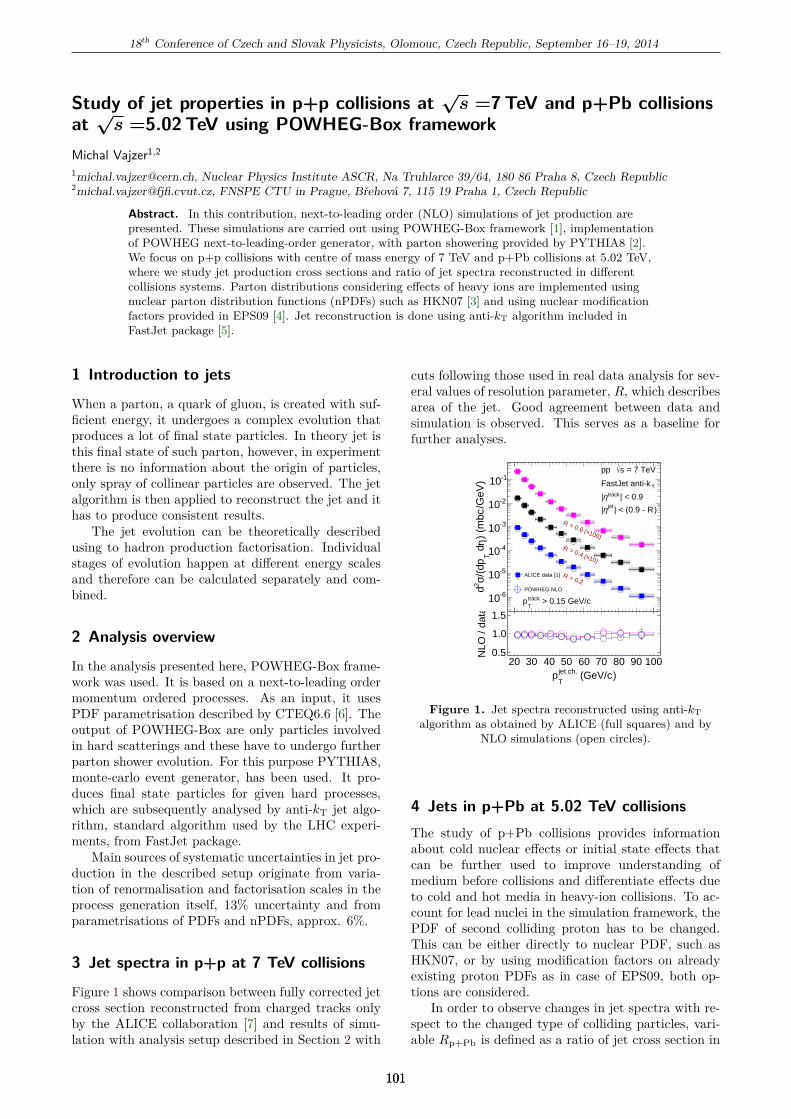
18th Conference of Czech and Slovak Physicists, Olomouc, Czech Republic, September 16–19, 2014
Study of jet properties in p+p collisions at√
s =7 TeV and p+Pb collisionsat
√
s =5.02 TeV using POWHEG-Box framework
Michal Vajzer1,2
[email protected], Nuclear Physics Institute ASCR, Na Truhlarce 39/64, 180 86 Praha 8, Czech [email protected], FNSPE CTU in Prague, Břehová 7, 115 19 Praha 1, Czech Republic
Abstract. In this contribution, next-to-leading order (NLO) simulations of jet production arepresented. These simulations are carried out using POWHEG-Box framework [1], implementationof POWHEG next-to-leading-order generator, with parton showering provided by PYTHIA8 [2].We focus on p+p collisions with centre of mass energy of 7 TeV and p+Pb collisions at 5.02 TeV,where we study jet production cross sections and ratio of jet spectra reconstructed in differentcollisions systems. Parton distributions considering effects of heavy ions are implemented usingnuclear parton distribution functions (nPDFs) such as HKN07 [3] and using nuclear modificationfactors provided in EPS09 [4]. Jet reconstruction is done using anti-kT algorithm included inFastJet package [5].
1 Introduction to jets
When a parton, a quark of gluon, is created with suf-ficient energy, it undergoes a complex evolution thatproduces a lot of final state particles. In theory jet isthis final state of such parton, however, in experimentthere is no information about the origin of particles,only spray of collinear particles are observed. The jetalgorithm is then applied to reconstruct the jet and ithas to produce consistent results.
The jet evolution can be theoretically describedusing to hadron production factorisation. Individualstages of evolution happen at different energy scalesand therefore can be calculated separately and com-bined.
2 Analysis overview
In the analysis presented here, POWHEG-Box frame-work was used. It is based on a next-to-leading ordermomentum ordered processes. As an input, it usesPDF parametrisation described by CTEQ6.6 [6]. Theoutput of POWHEG-Box are only particles involvedin hard scatterings and these have to undergo furtherparton shower evolution. For this purpose PYTHIA8,monte-carlo event generator, has been used. It pro-duces final state particles for given hard processes,which are subsequently analysed by anti-kT jet algo-rithm, standard algorithm used by the LHC experi-ments, from FastJet package.
Main sources of systematic uncertainties in jet pro-duction in the described setup originate from varia-tion of renormalisation and factorisation scales in theprocess generation itself, 13% uncertainty and fromparametrisations of PDFs and nPDFs, approx. 6%.
3 Jet spectra in p+p at 7 TeV collisions
Figure 1 shows comparison between fully corrected jetcross section reconstructed from charged tracks onlyby the ALICE collaboration [7] and results of simu-lation with analysis setup described in Section 2 with
cuts following those used in real data analysis for sev-eral values of resolution parameter, R, which describesarea of the jet. Good agreement between data andsimulation is observed. This serves as a baseline forfurther analyses.
20 30 40 50 60 70 80 90 100
/GeV
)c
) (m
bη
dT
p/(
dσ2 d
-610
-510
-410
-310
-210
-110 = 7 TeVspp
TkFastJet anti-
| < 0.9trackη|)R| < (0.9 - jetη|
c > 0.15 GeV/trackT
p
ALICE data [1]
POWHEG NLO
100)×
= 0.6 (R
10)×
= 0.4 (R
= 0.2R
)c (GeV/jet ch.
Tp
20 30 40 50 60 70 80 90 100
NLO
/ da
ta
0.5
1.0
1.5
Figure 1. Jet spectra reconstructed using anti-kT
algorithm as obtained by ALICE (full squares) and byNLO simulations (open circles).
4 Jets in p+Pb at 5.02 TeV collisions
The study of p+Pb collisions provides informationabout cold nuclear effects or initial state effects thatcan be further used to improve understanding ofmedium before collisions and differentiate effects dueto cold and hot media in heavy-ion collisions. To ac-count for lead nuclei in the simulation framework, thePDF of second colliding proton has to be changed.This can be either directly to nuclear PDF, such asHKN07, or by using modification factors on alreadyexisting proton PDFs as in case of EPS09, both op-tions are considered.
In order to observe changes in jet spectra with re-spect to the changed type of colliding particles, vari-able Rp+Pb is defined as a ratio of jet cross section in
101101101
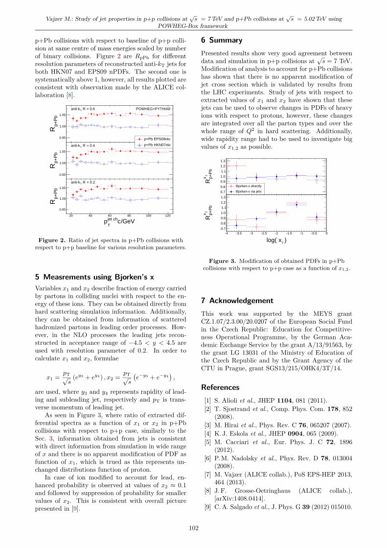
Vajzer M.: Study of jet properties in p+p collisions at√s = 7 TeV and p+Pb collisions at
√s = 5.02 TeV using
POWHEG-Box framework
p+Pb collisions with respect to baseline of p+p colli-sion at same centre of mass energies scaled by numberof binary collisions. Figure 2 are RpPb for differentresolution parameters of reconstructed anti-kT jets forboth HKN07 and EPS09 nPDFs. The second one issystematically above 1, however, all results plotted areconsistent with observation made by the ALICE col-laboration [8].
/GeVcjet ch
Tp
20 40 60 80 100 120
p+P
bR
0.95
1.00
1.05
= 0.2R Tanti-k
p+P
bR
0.95
1.00
1.05
= 0.4R Tanti-k
p+P
bR
0.95
1.00
1.05
= 0.6R Tanti-k POWHEG+PYTHIA8
p+Pb EPS09nlo
p+Pb HKN07nlo
Figure 2. Ratio of jet spectra in p+Pb collisions withrespect to p+p baseline for various resolution parameters.
5 Measrements using Bjorken’s x
Variables x1 and x2 describe fraction of energy carriedby partons in colliding nuclei with respect to the en-ergy of these ions. They can be obtained directly fromhard scattering simulation information. Additionally,they can be obtained from information of scatteredhadronized partons in leading order processes. How-ever, in the NLO processes the leading jets recon-structed in acceptance range of −4.5 < y < 4.5 areused with resolution parameter of 0.2. In order tocalculate x1 and x2, formulae
x1 =pT√s
(ey3 + ey4) , x2 =pT√s
(
e−y3 + e−y4)
,
are used, where y3 and y4 represents rapidity of lead-ing and subleading jet, respectively and pT is trans-verse momentum of leading jet.
As seen in Figure 3, where ratio of extracted dif-ferential spectra as a function of x1 or x2 in p+Pbcollisions with respect to p+p case, similarly to theSec. 3, information obtained from jets is consistentwith direct information from simulation in wide rangeof x and there is no apparent modification of PDF asfunction of x1, which is trued as this represents un-changed distributions function of proton.
In case of ion modified to account for lead, en-hanced probability is observed at values of x2 ≈ 0.1and followed by suppression of probability for smallervalues of x2. This is consistent with overall picturepresented in [9].
6 Summary
Presented results show very good agreement betweendata and simulation in p+p collisions at
√s = 7 TeV.
Modification of analysis to account for p+Pb collisionshas shown that there is no apparent modification ofjet cross section which is validated by results fromthe LHC experiments. Study of jets with respect toextracted values of x1 and x2 have shown that thesejets can be used to observe changes in PDFs of heavyions with respect to protons, however, these changesare integrated over all the parton types and over thewhole range of Q2 in hard scattering. Additionally,wide rapidity range had to be used to investigate bigvalues of x1,2 as possible.
)ixlog( -4 -3.5 -3 -2.5 -2 -1.5 -1 -0.5 0
2x p+
Pb
R
0.7
0.8
0.9
1.0
1.1
1.2
1.3
1x p+
Pb
R
0.7
0.8
0.9
1.0
1.1
1.2
1.3
Bjorken-x directly
Bjorken-x via jets
Figure 3. Modification of obtained PDFs in p+Pbcollisions with respect to p+p case as a function of x1,2.
7 Acknowledgement
This work was supported by the MEYS grantCZ.1.07/2.3.00/20.0207 of the European Social Fundin the Czech Republic: Education for Competitive-ness Operational Programme, by the German Aca-demic Exchange Service by the grant A/13/91563, bythe grant LG 13031 of the Ministry of Education ofthe Czech Republic and by the Grant Agency of theCTU in Prague, grant SGS13/215/OHK4/3T/14.
References
[1] S. Alioli et al., JHEP 1104, 081 (2011).[2] T. Sjostrand et al., Comp. Phys. Com. 178, 852
(2008).[3] M. Hirai et al., Phys. Rev. C 76, 065207 (2007).[4] K. J. Eskola et al., JHEP 0904, 065 (2009).[5] M. Cacciari et al., Eur. Phys. J. C 72, 1896
(2012).[6] P. M. Nadolsky et al., Phys. Rev. D 78, 013004
(2008).[7] M. Vajzer (ALICE collab.), PoS EPS-HEP 2013,
464 (2013).[8] J. F. Grosse-Oetringhaus (ALICE collab.),
[arXiv:1408.0414].[9] C. A. Salgado et al., J. Phys. G 39 (2012) 015010.
102
18th Conference of Czech and Slovak Physicists, Olomouc, Czech Republic, September 16–19, 2014
List of participants
1. Ing. Lucie AugustovičováCharles University, Praha, Czech Republic; [email protected]
2. Mgr. Michal BeličkaComenius University in Bratislava, Faculty of Pharmacy, Slovak Republic; [email protected]
3. Mgr. Jaroslav Bielcik, Ph.D.Czech Technical University in Prague, Czech Republic; [email protected]
4. prof. Ing. Július Cirák, CSc.Slovak Univ. of Technology in Bratislava, Fac. of El. Engineering and Inf. Technology, Slovak Republic;[email protected]
5. Jana CrkovskáCzech Technical University in Prague, Czech Republic; [email protected]
6. Szabolcs Csonka, PhD.Budapest University of Technology and Economics, Budapest, Hungary; [email protected]
7. prof. RNDr. Martin Černohorský, CSc.Masaryk University, Faculty of Science, Brno, Czech Republic; [email protected]
8. Mgr. Daniel ČervenkovCharles University, Faculty of Mathematics and Physics, Praha, Czech Republic;[email protected]
9. RNDr. Jana Čisárová, PhD.Pavol Jozef Šafárik University in Košice, Institute of Physics, Slovak Republic; [email protected]
10. RNDr. Marcel Človečko, PhD.Institute of Experimental Physics, Slovak Academy of Sciences, Košice, Slovak Republic;[email protected]
11. RNDr. Jaroslav Dittrich, CSc.Nuclear Physics Institute AS CR, v.v.i., Řež, Czech Republic; [email protected]
12. Mgr. Pavla Doškářová, PhD.Czech Technical University in Prague, Fac. of Nucl. Sciences and Phys. Eng., Czech Republic;[email protected]
13. prof. John M. DudleyUniversity of Franche-Comté, President of the European Physical Society, Besançon, France;[email protected]
14. Mr. Sami DzsaberBudapest University of Technology and Economics, Budapest, Hungary; [email protected]
15. Dr. Zoltán ElekesMTA Atomki, Debrecen, Hungary; [email protected]
16. prof. Mgr. Jiří Erhart, Ph.D.Technical University of Liberec, Department of Physics, Czech Republic; [email protected]
17. Gyulnara EyyubovaCzech Technical University in Prague, Czech Republic; [email protected]
18. Zuzana FeckováMatej Bel University, Banská Bystrica, Slovak Republic; [email protected]
19. Mgr. Pavol Federič, PhD.Nuclear Physics Institute AS CR, v.v.i., Řež, Czech Republic; [email protected]
20. Mgr. Juraj Feilhauer, PhD.Phys.-Techn. Bundesanstalt Braunschweig, Institute of Electrical Engineering, SAS, Bratislava, SlovakRepublic; [email protected]
21. Bc. Ondřej FickerCzech Technical University in Prague, Institute of Plasma Physics AS CR, v.v.i., Czech Republic;[email protected]
22. Jana FodorováCzech Technical University in Prague, Fac. of Nucl. Sciences and Phys. Eng., Czech Republic;[email protected]
103
List of participants
23. Zsolt Fülöp, D.Sc.Inst. of Nuclear Research of HAS, Debrecen, Hungary; [email protected]
24. Aurél GábrisCzech Technical University in Prague, University of Szeged, Czech Republic; [email protected]
25. prof. dr hab. Adam Gadomski, ordin. prof. physicsGroup of Modeling of Physicochemical Processes, Physics Divsion, UTP Bydgoszcz, Poland;[email protected]
26. RNDr. Lucia Gálisová, PhD.Technical University of Košice, Faculty of Mechanical Engineering, Slovak Republic;[email protected]
27. Michal GéciTechnical University of Košice, Slovak Republic; [email protected]
28. RNDr. Mikuláš Gintner, PhD.University of Žilina, Slovak Republic; [email protected]
29. doc. PaedDr. Viera Haverlíková, PhD.Comenius University in Bratislava, Faculty of Medicine, Slovak Republic;[email protected]
30. Mgr. Markéta Havrdová (Svatáková)Palacký University, Olomouc, Czech Republic; [email protected]
31. doc. RNDr. Richard Hlubina, DrSc.Comenius University in Bratislava, Fac. of Math., Physics and Informatics, Slovakia;[email protected]
32. prof. Karol HricoviniUniversité de Cergy-Pontoise, France; [email protected]
33. prof. Ing. Eduard Hulicius, CSc.Institute of Physics AS CR, v.v.i., Praha, Czech Republic; [email protected]
34. Bc. Lukáš ChladCharles University in Prague, Nuclear Physics Institute AS CR, v.v.i., Plzeň, Czech Republic;[email protected]
35. Ing. Vítězslav JarýInstitute of Physics AS CR, v.v.i., Praha, Czech Republic; [email protected]
36. RNDr. Jiří KaštilCharles University, Praha, Czech Republic; [email protected]
37. prof. Sándor Katz, PhD.Eötvös Loránd University, Budapest, Hungary; [email protected]
38. Mgr. Mária Klacsová, PhD.Comenius University in Bratislava, Faculty of Pharmacy, Slovak Republic; [email protected]
39. Mária KladivováTechnical University of Košice, Department of Physics, Slovak Republic; maria.kladivova2tuke.sk
40. Mgr. Tomáš KmječCharles University in Prague, Faculty of Mathematics and Physics, Praha, Czech Republic;[email protected]
41. Mgr. Mary KolářováPalacký University, Olomouc, Czech Republic; [email protected]
42. doc. RNDr. Eva Komová, PhD.Technical University of Košice, Faculty of Aeronautics, Slovak Republic; [email protected]
43. doc. RNDr. Peter Kopčanský, CSc.Institute of Experimental Physics, Slovak Academy of Sciences, Košice; Slovakia
44. Renata KopečnáCzech Technical University in Prague, Fac. of Nucl. Sciences and Phys. Eng., Czech Republic;[email protected]
45. RNDr. Martin Kozák, Ph.D.Charles University, Praha, Czech Republic; [email protected]
104
18th Conference of Czech and Slovak Physicists, Olomouc, Czech Republic, September 16–19, 2014
46. Dr. Jozef Kravčák, PhD.Technical University of Košice, Fac. of El. Engineering and Informatics, Slovak Republic;[email protected]
47. Ing. Michal KřelinaCzech Technical University in Prague, Fac. of Nucl. Sciences and Phys. Eng., Czech Republic;[email protected]
48. RNDr. Dalibor Krupa, CSc., DPhilInstitute of Physics, Slovak Academy of Sciences, Bratislava, Slovak Republic; [email protected]
49. RNDr. Filip Křížek, Ph.D.Nuclear Physics Institute AS CR, v.v.i., Řež, Czech Republic; [email protected]
50. doc. RNDr. Roman Kubínek, CSc.Palacký University, Olomouc, Czech Republic; [email protected]
51. doc. RNDr. Jozef Kúdelčík, PhD.University of Žilina, Slovak Republic; [email protected]
52. RNDr. Andrej Kugler, CSc.Nuclear Physics Institute AS CR, v.v.i., Řež, Czech Republic; [email protected]
53. prof. Jenö KürtiEötvös Loránd University, Department of Biological Physics, Budapest, Hungary; [email protected]
54. Mgr. Miroslava LackováPavol Jozef Šafárik University in Košice, Slovak Republic; [email protected]
55. Ing. Štefan Lányi, DrSc.Institute of Physics, Slovak Academy of Sciences, Bratislava, Slovak Republic; [email protected]
56. David LeeSecretary General, European Physical Society, Mulhouse, France; [email protected]
57. doc. Rupert Leitner, DrSc.Charles University, Faculty of Mathematics and Physics, Praha, Czech Republic;[email protected]
58. RNDr. Jozef LejaInstitute of Physics, Slovak Academy of Sciences, Bratislava, Slovak Republic; [email protected]
59. RNDr. Tomáš LešnerPhywe, Praha, Czech Republic; [email protected]
60. Miss Chiara Liberatore, MsCCzech Technical University, HiLASE Centre, Institute of Physics AS CR, Dolní Břežany, Czech Republic;[email protected]
61. Jindřich LidrychCzech Technical University in Prague, Czech Republic; [email protected]
62. Martin LiščinskýTechnical University of Košice, Slovak Republic; [email protected]
63. Mgr. Dmytro LotnykPavol Jozef Šafárik University in Košice, Slovak Republic; [email protected]
64. doc. RNDr. Libor Machala, Ph.D.Palacký University, Olomouc, Czech Republic; [email protected]
65. RNDr. Jiří J. Mareš, CSc.Institute of Physics AS CR, v.v.i., Praha, Czech Republic; [email protected]
66. Bence Gábor MárkusBudapest University of Technology, Budapest, Hungary; [email protected]
67. doc. RNDr. Ivan Melo, PhD.University of Žilina, Faculty of Electrical Engineering, Slovak Republic; [email protected]
68. Ing. Vasily MikhaylovNuclear Physics Institute AS CR, v.v.i., Řež, Czech Republic; [email protected]
69. Mgr. Martina MikováPalacký University, Olomouc, Czech Republic; [email protected]
70. Bc. Michaela MlynárikováCharles University, Faculty of Mathematics and Physics, Praha, Czech Republic;[email protected]
105
List of participants
71. doc. RNDr. Jan Mlynář, Ph.D.Institute of Plasma Physics AS CR, v.v.i., Praha, Czech Republic; [email protected]
72. prof. RNDr. Jan Novotný, CSc.Masaryk University, Faculty of Education, Brno, Czech Republic; [email protected]
73. prof. RNDr. Tomáš Opatrný, Dr.Palacký University, Olomouc, Czech Republic; [email protected]
74. Vojtěch PacíkCzech Technical University in Prague, Fac. of Nucl. Sciences and Phys. Eng., Czech Republic;[email protected]
75. Radomír PánekInstitute of Plasma Physics AS CR, v.v.i., Praha, Czech Republic; [email protected]
76. RNDr. Radek Pleskač, PhD.GSI Darmstadt, Germany; [email protected]
77. Dr. Illa Ramakanth, PhDVŠB-Technical University of Ostrava, Nanotechnology Centre, Czech Republic; [email protected]
78. prof. RNDr. Marian Reiffers, DrSc.University of Prešov in Prešov, Fac. of Humanities and Natural Sciences, Slovak Republic;[email protected]
79. Mgr. Lukáš Richterek, Ph.D.Palacký University, Olomouc, Czech Republic; [email protected]
80. Mgr. Pablo Rodríguez RamosNuclear Physics Institute AS CR, v.v.i., Řež, Czech Republic; [email protected]
81. Ing. Jan RusňákNuclear Physics Institute AS CR, v.v.i., Praha, Czech Republic; [email protected]
82. doc. Mgr. Jan Soubusta, Ph.D.Institute of Physics AS CR, v.v.i., Palacký University, Olomouc, Czech Republic; [email protected]
83. prof. Józef Spałek, Ph.D.Jagiellonian University, Krakow, Poland; [email protected],[email protected]
84. Mgr. Bohumil StoklasaPalacký University, Olomouc, Czech Republic; [email protected]
85. Ing. Ondřej Svoboda, PhD.Nuclear Physics Institute AS CR, v.v.i., Řež, Czech Republic; [email protected]
86. RNDr. Jindřiška Svobodová, Ph.D.Masaryk University, Faculty of Education, Brno, Czech Republic; [email protected]
87. Lénárd SzolnokiBudapest University of Technology and Economics, Budapest, Hungary; [email protected]
88. Karel ŠafaříkCERN, Meyrin, Geneva, Switzerland; [email protected]
89. RNDr. Ladislav Šándor, CSc.Institute of Experimental Physics, Slovak Academy of Science, Košice, Slovak Republic; [email protected]
90. Bc. Filip ŠidíkTechnical University of Košice, Faculty of Aeronautics, Slovak Republic; [email protected]
91. Mgr. Eva Šimečková, CSc.Nuclear Physics Institute AS CR, v.v.i., Řež, Czech Republic; [email protected]
92. Ing. Miroslav ŠimkoCzech Technical University in Prague, Czech Republic; [email protected]
93. RNDr. Miriam ŠimralováGrammar school, Šrobárova 1, Košice, Slovak Republic; [email protected]
94. Ing. Milan ŠtefánikNuclear Physics Institute AS CR, v.v.i., Praha, Czech Republic; [email protected]
95. Bc. Pavol ŠtefkoCharles University, Faculty of Mathematics and Physics, Praha, Czech Republic; [email protected]
96. RNDr. Mária Šviková, CSc.Grammar school of St. Thomas Aquinas, Košice, Slovak Republic; [email protected]
106
18th Conference of Czech and Slovak Physicists, Olomouc, Czech Republic, September 16–19, 2014
97. Ing. Norbert Tarjányi, PhD.University of Žilina, Slovak Republic; [email protected]
98. RNDr. Milan Timko, CSc.Institute of Experimental Physics, Slovak Academy of Sciences, Košice, Slovak Republic; [email protected]
99. Pavel TlustýNuclear Physics Institute AS CR, v.v.i., Řež, Czech Republic; [email protected]
100. dr. Barbara TrzeciakCzech Technical University in Prague, Czech Republic; [email protected]
101. RNDr. Igor Túnyi, DrSc.Geophysical Institite, Slovak Academy of Sciences, Bratislava, Slovak Republic; [email protected]
102. RNDr. Hana Turčičová, CSc.Institute of Physics AS CR, v.v.i, Praha, Czech Republic; [email protected]
103. Michal VajzerNuclear Physics Institute AS CR, v.v.i., Praha, Czech Republic; [email protected]
104. RNDr. Alice Valkárová, DrSc.Charles University, Faculty of Mathematics and Physics, Praha, Czech Republic;[email protected]
105. Mgr. František VavrekInstitute of Experimental Physics, Slovak Academy of Sciences, Košice, Slovak Republic; [email protected]
106. Mgr. Karol Vegso, PhD.Institute of Physics, Slovak Academy of Sciences, Bratislava, Slovak Republic; [email protected]
107. Mgr. Ľubomír VlčekIndependent researcher, Bardejov, Slovak Republic; [email protected]
108. Bc. Vlastimil VrbaPalacký University, Olomouc, Czech Republic; [email protected]
109. prof. RNDr. Radek Zbořil, Ph.D.Palacký University, Olomouc, Czech Republic; [email protected]
110. doc. RNDr. Ján Ziman, CSc.Technical University of Košice, Slovak Republic; [email protected]
107
Libor Machala, Lukáš Richterek (editors)
Proceedings of the 18th Conference of Czech and Slovak PhysicistsOlomouc, Czech Republic, September 16–19, 2014
Executive Editor: Prof. RNDr. Zdeněk Dvořák, DrSc.Responsible Editor: Mgr. Jana KreiselováTypeset by pdfCSLATEX: Lukáš Richterek
1. edition
No English-language editing and proofreading was done either by the publisher or by the editors, so the qualityof language of papers is under the authors’ responsibility.
Palacký University Olomouc, Křížkovského 8, CZ-771 47 Olomouc, Czech RepublicWWW: www.upol.cz/vup
E-mail: [email protected]
Olomouc 2015
Not for sale
Proceeding are available via the conference webpagehttp://jcmf.upol.cz/kcsf18/
ISBN 978-80-244-4725-4 (CD)ISBN 978-80-244-4726-1 (on-line)


