2 3 Reduction of function evaluation in differential evolution using nearest neighbor comparison

1 23

Vietnam Journal of Computer Science ISSN 2196-8888 Vietnam J Comput SciDOI 10.1007/s40595-014-0037-2

Reduction of function evaluation indifferential evolution using nearestneighbor comparison

Hoang Anh Pham

1 23

Your article is published under the Creative

Commons Attribution license which allows

users to read, copy, distribute and make

derivative works, as long as the author of

the original work is cited. You may self-

archive this article on your own website, an

institutional repository or funder’s repository

and make it publicly available immediately.

Vietnam J Comput SciDOI 10.1007/s40595-014-0037-2

REGULAR PAPER

Reduction of function evaluation in differential evolutionusing nearest neighbor comparison

Hoang Anh Pham

Received: 5 June 2014 / Accepted: 5 December 2014© The Author(s) 2014. This article is published with open access at Springerlink.com

Abstract Approximation models have recently been intro-duced to differential evolution (DE) to reduce expensive fit-ness evaluation in function optimization. These models basi-cally require additional control parameters and/or externalstorage for the learning process. Depending on the choice ofthe additional parameters, the strategies may have differentlevels of efficiency. The present paper introduces an alterna-tive way for reducing function evaluations in differential evo-lution, which does not require additional control parameterand external archive. The algorithm uses a nearest neighborin the search population to judge whether a new point is worthevaluating, so that unnecessary evaluations can be avoided.The performance of this new scheme of differential evolu-tion, known as differential evolution with nearest neighborcomparison (DE-NNC), is demonstrated and compared withthat of standard DE as well as approximation models includ-ing differential evolution using k-nearest neighbor predictor(DE-kNN), differential evolution using speeded-up k-nearestneighbor estimator (DE-EkNN) and DE with estimated com-parison method through some test functions. The results showthat DE-NNC can produce considerable reduction of actualfunction calls compared to DE and is competitive to DE-kNN, DE-EkNN and DE with estimated comparison.

Keywords Global optimization · Differential evolution ·Nearest neighbor · Function evaluation reduction

H. A. Pham (B)Department of Structural Mechanics, National University of CivilEngineering, 55 Giai Phong Road, Hanoi, Vietname-mail: [email protected]

1 Introduction

Differential evolution (DE), which was introduced by Stornand Price [1] is a population-based optimizer. DE creates atrial individual using differences within the search popula-tion. The population is then restructured by survival individu-als evolutionally. The algorithm is simple, easy to use and hasshown better global convergence and robustness than mostother genetic algorithms, suitable for various optimizationproblems [2]. However, like other population-based algo-rithms such as genetic algorithms (GA) and particle swarmoptimization (PSO), one of the main issues in applying DEis its expensive computation requirement. This is due to thefact that evolutionary algorithm (EA) often needs to evaluateobjective function thousand times to get optimal solutions. Itbecomes more pronounced when the cost of function evalu-ation becomes higher.

Research in reducing the computational burden in EAhas been focusing on using function approximations, so-called meta-model or surrogate model [3–6]. Some of thepopular approximation models in evolutionary computationare quadratic models [7], kriging models [7,8], neural net-work models [9] and radial basis function (RBF) networkmodels [10–13]. In these approximation strategies, objec-tive function is estimated by approximation model and theoptimization problem is solved utilizing the approximatedvalues. The effectiveness of this strategy depends largely onthe accuracy of the approximation model. A time-consuminglearning process is often invoked to obtain a high accuracymodel. Thus, time-efficient approximate model is particu-larly important for expensive function evaluation.

Methods using fitness approximation based on meta-model have been recently introduced to differential evolution,including DE-kNN [14] and DE-EkNN [15]. Both methodsuse k-nearest neighbor (kNN) predictor constructed through

123

Vietnam J Comput Sci

a dynamic learning to reduce the exact evaluation calls duringDE search. In the early predefined iterations, the algorithmprocesses as usual, i.e., as standard DE procedure with exactobjective function evaluations. All fitness values calculatedare stored in an archive to be reused as training population.In later iterations, prediction function value computed fromk-nearest samples in the training population is assigned toeach solution. This new population is sorted (in the order ofoptimization) based on prediction function values. A chosennumber of best solution values in the new population will bereplaced by the exact function values and then stored in thetraining population. In DE-kNN, all re-evaluated samplesare stored and the training population gradually increases.Two major differences between DE-EkNN and DE-kNN arethat a weighted average kNN is used in DE-EkNN to esti-mate the fitness value for effective prediction and the archiveis updated by selectively storing training samples for effi-ciency [15]. Thus, DE-EkNN has more compact archive thanDE-kNN. Both DE-kNN and DE-EkNN have been shownthrough benchmark test functions to be able to convergetowards the global optima with less actual evaluations. Aspointed out by Park and Lee in their paper [15], two of themajor drawbacks of the kNN predictor are the requirementof time to find the nearest neighbors and the need of memorystorage to keep samples in the archive. This tends to becomemore pronounced as the dimension of the problem and thesize of the archive increase. So the algorithms are not applica-ble to the problem whose dimension is extremely large, thereal-time application which needs rapidness or an embeddeddevice which lacks memory storage [15].

A new strategy for reducing the number of function eval-uations is the estimated comparison method introduced byTakahama and Sakai [16,17]. In their method, they utilizea rough approximation model, which is an approximationmodel with low accuracy and without learning process toapproximate the function values. The method is differentfrom the surrogate models in that the rough approximated val-ues are only used to estimate the order relation of two points.Function evaluations will be omitted if a point is judged asworse than the target point. The method of estimated com-parison was first proposed with a potential model for func-tion approximation [16] and shown to be efficient with muchless evaluations compared to DE. The method also workswell with other rough approximation models, including ker-nel average smoother and nearest neighbor smoother [17].The efficiency of the estimated comparison is influenced by aparameter for error margin: lower value of error margin para-meter can reject more trial individuals and omit a larger num-ber of function evaluations, but can also increase the possibil-ity of rejecting a good child; larger value reduces the possi-bility of rejecting a good child. However, the estimated com-parison can reject fewer children and omit a small number offunction evaluations. An improved estimated comparison is

given by the same authors in [18], in which adaptive controlwas proposed to produce proper parameters to give more effi-ciency and stability. The estimated comparison was shownto be also effective for constraint optimization problem [19].The advantage of DE with rough approximation-based com-parison is that rough approximation is not too expensive anddoes not require the learning process and archive. The roughapproximation is constructed on the current search popula-tion and only used for judgment, and the optimal solution issearched using the exact function values.

Introducing additional control parameters is required inboth DE using kNN predictor and DE with estimated com-parison method. DE-kNN and DE-EkNN need five and sevenmore parameters, respectively, whilst DE with estimatedcomparison adds one or two parameters. Proper parametersare often sought to ensure efficiency and stability. Good val-ues of parameters are obtained by hand-tuning [14,17] orin an automatically adaptive way [15,18]. Obviously, moreparameters bring more complexity to the algorithms.

The present paper proposes an alternative way to reducefunction evaluation without additional control parameter.The proposed method applies comparison to judge whetheror not a new child is worth evaluating, so that the evalua-tion of the objective function can be skipped. However, themethod is different from the estimated comparison method.It uses the readily exact function value of a nearest neigh-bor in the population of the new child to compare with thatof the parent, thus the approximation process is not neces-sary. The method is named as DE with the nearest neighborcomparison (DE-NNC) and can be viewed as another way ofrough approximation-based comparison. The performance ofDE-NNC is demonstrated through optimization of some testfunctions. The simulation results suggest that the proposedscheme is able to achieve good solutions and provide com-petitive reduction of the function evaluations compared toDE-kNN, DE-EkNN and DE with the estimated comparisonmethod.

The organization of the rest of this paper is as follows. InSect. 2, a brief introduction of DE is given. In Sect. 3, themain idea of the proposed DE-NNC is described in detailwith a concept of possibly useless trial (PUT) and a nearestneighbor comparison method. Experiment results on sometest functions are presented in Sect. 4. Finally, the conclusionis given in Sect. 5.

2 Basic of differential evolution

We search for the global optima of the objective function f (x)over a continuous space x = {xi } , xi ∈ [

xi,min, xi,max],

i = 1, 2, . . . , n. Classical differential evolution (DE) algo-rithm invented by Storn and Price [1] for this optimizationproblem is described in the following.

123


For each generation G, a population of NP parameter vec-tors xk(G), k = 1, 2, . . . , N P, is utilized. The initial popu-lation is generated as

xk,i (0) = xi,min + rand[0, 1].(xi,max − xi,min), i = 1, 2, . . . , n (1)

where rand[0,1] is a uniformly distributed random real valuein the range [0,1]. For each target vector in the populationxk(G), k = 1, 2,…, NP, a perturbed vector y is generatedaccording to

y = xr1(G) + F.[xr2(G) − xr3(G)

], (2)

with r1, r2 and r3 being randomly chosen integers and1 ≤ r1 �= r2 �= r3 �= k ≤ N P; F a real and constantfactor usually chosen in the interval [0, 1], which controls theamplification of the differential variation (xr2(G) − xr3(G)).

Crossover is introduced to increase the diversity of theparameter vectors, creating a trial vector z with its elementsdetermined by:

zi ={

yi if (rand[0, 1] ≤ Cr) or (r = i)xk,i(t) if (rand[0, 1] > Cr) and (r �= i)

(3)

Here, r is a randomly chosen integer from the interval[1, n]; Cr is a user-defined crossover constant from [0, 1].The new vector z is then compared to xk(G). If z yields abetter objective function value, then z becomes a member ofthe next generation (G + 1); otherwise, the old value xk(G)

is retained.Basically, DE calls for objective function evaluation for

every trial vector. It is desirable that trial vectors which mightproduce no better fitness should not be evaluated. In the fol-lowing parts, we introduce the concept of possibly uselesstrial and employ a nearest neighbor comparison method toreduce useless computation.

3 Differential evolution with nearest neighborcomparison (DE-NNC)

The nearest neighbor comparison has the same strategy as theestimated comparison method by Takahama and Sakai [16],[17]. In the estimated comparison, a rough approximationmodel is used to estimate the order relation of two points. Achild point z is judged better than the parent point xk if thefollowing condition is guaranteed:

f̂ (z) < f̂ (xk) + δσ, (4)

where f̂ is the estimated function of f , σ is the error estima-tion of the approximation model and δ is a margin parameterfor the approximation error. The parameter δ ≥ 0 controlsthe margin value for the approximation error. A lower valueof δ can reject more trial individuals and omit a larger number

of function evaluations, but can also increase the possibilityof rejecting a good child; a larger value of δ reduces the pos-sibility of rejecting good child. However, the estimated com-parison can reject fewer children and omit a small number offunction evaluations. Thus, the efficiency of the estimatedcomparison largely depends on the choice of the marginparameter. Different approximation models can be appliedfor estimated comparison, including the potential model andkernel smoother [17].

The nearest neighbor comparison, on the other hand,does not use function approximation and no additional con-trol parameter is introduced. The details of the method aredescribed in the following.

3.1 Concept of possibly useless trial

– A trial parameter vector with high possibility of havingfitness worse than that of the current target vector is calleda possibly useless trial vector (PUT vector).

– To judge whether a trial vector is a PUT vector, its nearestneighbor vector in the population is utilized to comparewith the target vector. This method is named as the nearestneighbor comparison (NNC).

3.2 Nearest neighbor comparison method (NNC)

The step of NNC is give below:

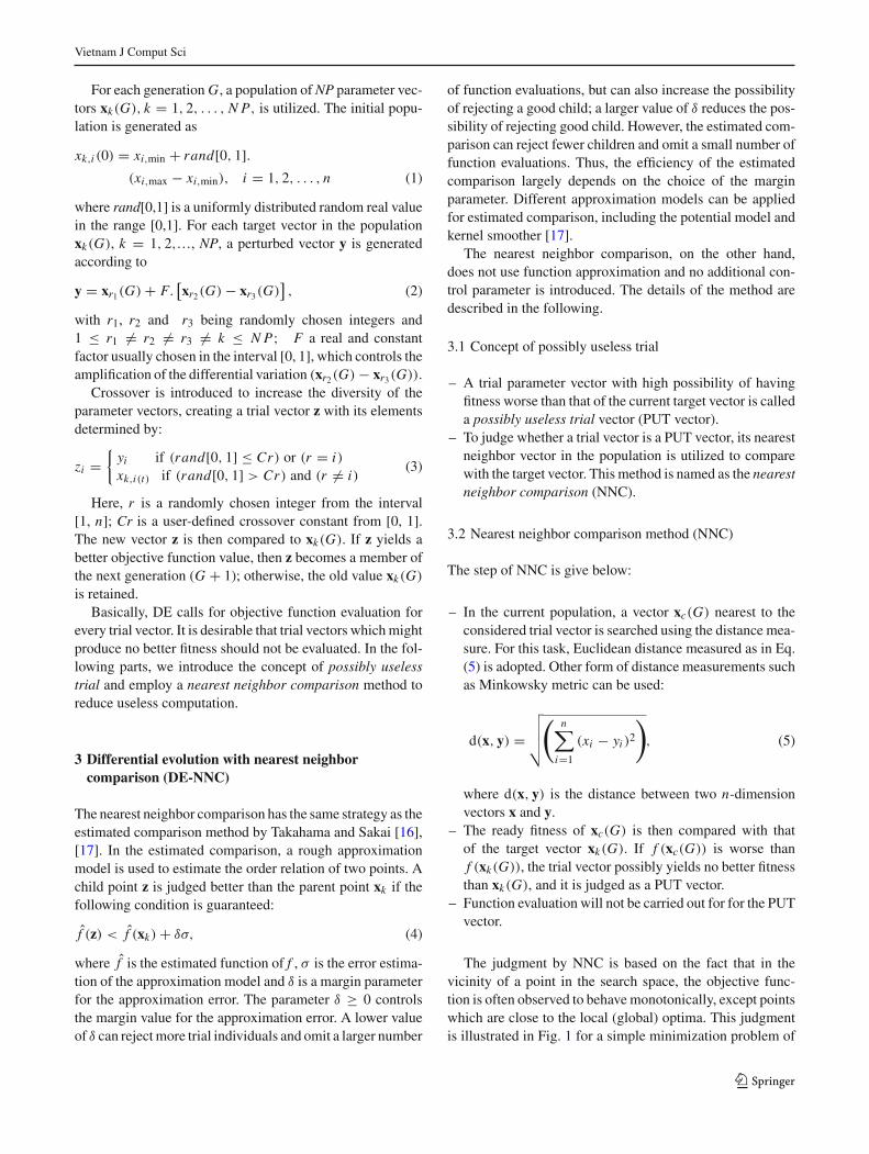
– In the current population, a vector xc(G) nearest to theconsidered trial vector is searched using the distance mea-sure. For this task, Euclidean distance measured as in Eq.(5) is adopted. Other form of distance measurements suchas Minkowsky metric can be used:

d(x, y) =√√√√

(n∑

i=1

(xi − yi )2

)

, (5)

where d(x, y) is the distance between two n-dimensionvectors x and y.

– The ready fitness of xc(G) is then compared with thatof the target vector xk(G). If f (xc(G)) is worse thanf (xk(G)), the trial vector possibly yields no better fitnessthan xk(G), and it is judged as a PUT vector.

– Function evaluation will not be carried out for for the PUTvector.

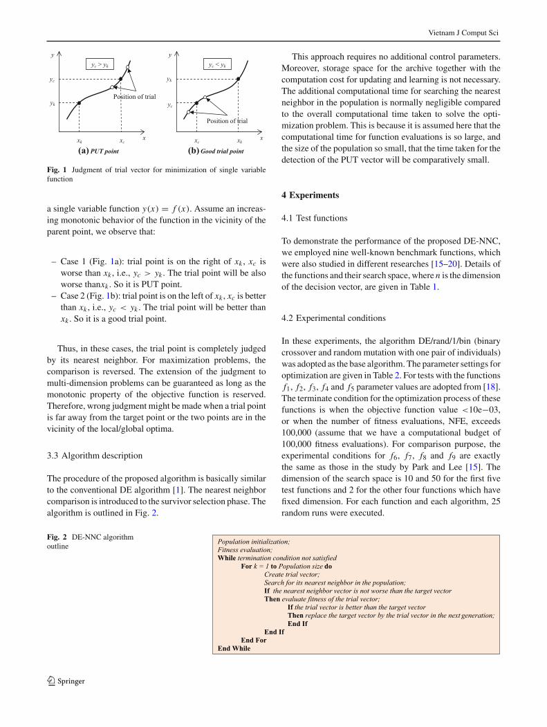
The judgment by NNC is based on the fact that in thevicinity of a point in the search space, the objective func-tion is often observed to behave monotonically, except pointswhich are close to the local (global) optima. This judgmentis illustrated in Fig. 1 for a simple minimization problem of

123


x

y

xk xc

yc

yk

yc > yk

(a) PUT point

Position of trial

x

y

xc xk

yc < yk

(b) Good trial point

Position of trial

yc

yk

Fig. 1 Judgment of trial vector for minimization of single variablefunction

a single variable function y(x) = f (x). Assume an increas-ing monotonic behavior of the function in the vicinity of theparent point, we observe that:

– Case 1 (Fig. 1a): trial point is on the right of xk , xc isworse than xk , i.e., yc > yk . The trial point will be alsoworse thanxk . So it is PUT point.

– Case 2 (Fig. 1b): trial point is on the left of xk , xc is betterthan xk , i.e., yc < yk . The trial point will be better thanxk . So it is a good trial point.

Thus, in these cases, the trial point is completely judgedby its nearest neighbor. For maximization problems, thecomparison is reversed. The extension of the judgment tomulti-dimension problems can be guaranteed as long as themonotonic property of the objective function is reserved.Therefore, wrong judgment might be made when a trial pointis far away from the target point or the two points are in thevicinity of the local/global optima.

3.3 Algorithm description

The procedure of the proposed algorithm is basically similarto the conventional DE algorithm [1]. The nearest neighborcomparison is introduced to the survivor selection phase. Thealgorithm is outlined in Fig. 2.

This approach requires no additional control parameters.Moreover, storage space for the archive together with thecomputation cost for updating and learning is not necessary.The additional computational time for searching the nearestneighbor in the population is normally negligible comparedto the overall computational time taken to solve the opti-mization problem. This is because it is assumed here that thecomputational time for function evaluations is so large, andthe size of the population so small, that the time taken for thedetection of the PUT vector will be comparatively small.

4 Experiments

4.1 Test functions

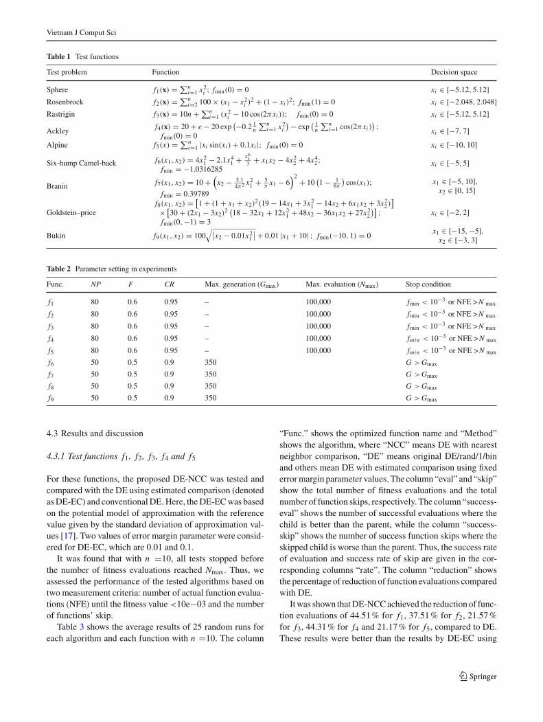
To demonstrate the performance of the proposed DE-NNC,we employed nine well-known benchmark functions, whichwere also studied in different researches [15–20]. Details ofthe functions and their search space, where n is the dimensionof the decision vector, are given in Table 1.

4.2 Experimental conditions

In these experiments, the algorithm DE/rand/1/bin (binarycrossover and random mutation with one pair of individuals)was adopted as the base algorithm. The parameter settings foroptimization are given in Table 2. For tests with the functionsf1, f2, f3, f4 and f5 parameter values are adopted from [18].The terminate condition for the optimization process of thesefunctions is when the objective function value <10e−03,or when the number of fitness evaluations, NFE, exceeds100,000 (assume that we have a computational budget of100,000 fitness evaluations). For comparison purpose, theexperimental conditions for f6, f7, f8 and f9 are exactlythe same as those in the study by Park and Lee [15]. Thedimension of the search space is 10 and 50 for the first fivetest functions and 2 for the other four functions which havefixed dimension. For each function and each algorithm, 25random runs were executed.

Fig. 2 DE-NNC algorithmoutline

Population initialization;Fitness evaluation;While termination condition not satisfied

For k = 1 to Population size doCreate trial vector;Search for its nearest neighbor in the population;If the nearest neighbor vector is not worse than the target vectorThen evaluate fitness of the trial vector;

If the trial vector is better than the target vectorThen replace the target vector by the trial vector in the next generation;End If

End IfEnd For

End While

123


Table 1 Test functions

Test problem Function Decision space

Sphere f1(x) = ∑ni=1 x2

i ; fmin(0) = 0 xi ∈ [−5.12, 5.12]

Rosenbrock f2(x) = ∑ni=2 100 × (x1 − x2

i )2 + (1 − xi )2; fmin(1) = 0 xi ∈ [−2.048, 2.048]

Rastrigin f3(x) = 10n + ∑ni=1 (x2

i − 10 cos(2πxi )); fmin(0) = 0 xi ∈ [−5.12, 5.12]

Ackleyf4(x) = 20 + e − 20 exp

(−0.2 1n

∑ni=1 x2

i

) − exp( 1

n

∑ni=1 cos(2πxi )

) ;fmin(0) = 0

xi ∈ [−7, 7]

Alpine f5(x) = ∑ni=1 |xi sin(xi ) + 0.1xi |; fmin(0) = 0 xi ∈ [−10, 10]

Six-hump Camel-back f6(x1, x2) = 4x21 − 2.1x4

1 + x613 + x1x2 − 4x2

2 + 4x42 ;

fmin = −1.0316285xi ∈ [−5, 5]

Branin f7(x1, x2) = 10 +(

x2 − 5.14π2 x2

1 + 5π

x1 − 6)2 + 10

(1 − 1

8π

)cos(x1);

fmin = 0.39789

x1 ∈ [−5, 10],x2 ∈ [0, 15]

Goldstein–pricef8(x1, x2) = [

1 + (1 + x1 + x2)2(19 − 14x1 + 3x2

1 − 14x2 + 6x1x2 + 3x22 )

]

× [30 + (2x1 − 3x2)

2(18 − 32x1 + 12x2

1 + 48x2 − 36x1x2 + 27x22

)] ;fmin(0,−1) = 3

xi ∈ [−2, 2]

Bukin f9(x1, x2) = 100√∣

∣x2 − 0.01x21

∣∣ + 0.01 |x1 + 10| ; fmin(−10, 1) = 0

x1 ∈ [−15,−5],x2 ∈ [−3, 3]

Table 2 Parameter setting in experiments

Func. NP F CR Max. generation (Gmax) Max. evaluation (Nmax) Stop condition

f1 80 0.6 0.95 – 100,000 fmin < 10−3 or NFE > N max

f2 80 0.6 0.95 – 100,000 fmin < 10−3 or NFE > N max

f3 80 0.6 0.95 – 100,000 fmin < 10−3 or NFE > N max

f4 80 0.6 0.95 – 100,000 fmin < 10−3 or NFE > N max

f5 80 0.6 0.95 – 100,000 fmin < 10−3 or NFE > N max

f6 50 0.5 0.9 350 G > Gmax

f7 50 0.5 0.9 350 G > Gmax

f8 50 0.5 0.9 350 G > Gmax

f9 50 0.5 0.9 350 G > Gmax

4.3 Results and discussion

4.3.1 Test functions f1, f2, f3, f4 and f5

For these functions, the proposed DE-NCC was tested andcompared with the DE using estimated comparison (denotedas DE-EC) and conventional DE. Here, the DE-EC was basedon the potential model of approximation with the referencevalue given by the standard deviation of approximation val-ues [17]. Two values of error margin parameter were consid-ered for DE-EC, which are 0.01 and 0.1.

It was found that with n =10, all tests stopped beforethe number of fitness evaluations reached Nmax. Thus, weassessed the performance of the tested algorithms based ontwo measurement criteria: number of actual function evalua-tions (NFE) until the fitness value <10e−03 and the numberof functions’ skip.

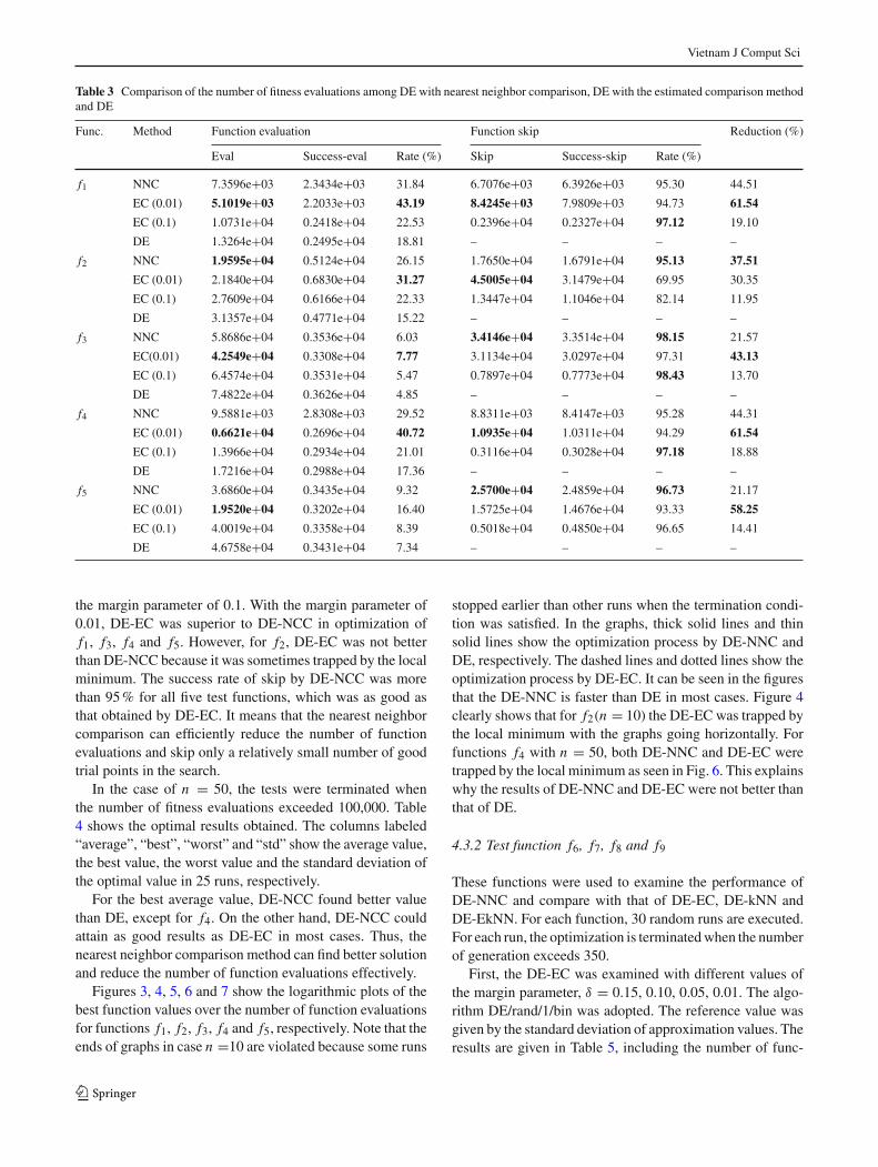
Table 3 shows the average results of 25 random runs foreach algorithm and each function with n =10. The column

“Func.” shows the optimized function name and “Method”shows the algorithm, where “NCC” means DE with nearestneighbor comparison, “DE” means original DE/rand/1/binand others mean DE with estimated comparison using fixederror margin parameter values. The column “eval” and “skip”show the total number of fitness evaluations and the totalnumber of function skips, respectively. The column “success-eval” shows the number of successful evaluations where thechild is better than the parent, while the column “success-skip” shows the number of success function skips where theskipped child is worse than the parent. Thus, the success rateof evaluation and success rate of skip are given in the cor-responding columns “rate”. The column “reduction” showsthe percentage of reduction of function evaluations comparedwith DE.

It was shown that DE-NCC achieved the reduction of func-tion evaluations of 44.51 % for f1, 37.51 % for f2, 21.57 %for f3, 44.31 % for f4 and 21.17 % for f5, compared to DE.These results were better than the results by DE-EC using

123


Table 3 Comparison of the number of fitness evaluations among DE with nearest neighbor comparison, DE with the estimated comparison methodand DE

Func. Method Function evaluation Function skip Reduction (%)

Eval Success-eval Rate (%) Skip Success-skip Rate (%)

f1 NNC 7.3596e+03 2.3434e+03 31.84 6.7076e+03 6.3926e+03 95.30 44.51

EC (0.01) 5.1019e+03 2.2033e+03 43.19 8.4245e+03 7.9809e+03 94.73 61.54

EC (0.1) 1.0731e+04 0.2418e+04 22.53 0.2396e+04 0.2327e+04 97.12 19.10

DE 1.3264e+04 0.2495e+04 18.81 – – – –

f2 NNC 1.9595e+04 0.5124e+04 26.15 1.7650e+04 1.6791e+04 95.13 37.51

EC (0.01) 2.1840e+04 0.6830e+04 31.27 4.5005e+04 3.1479e+04 69.95 30.35

EC (0.1) 2.7609e+04 0.6166e+04 22.33 1.3447e+04 1.1046e+04 82.14 11.95

DE 3.1357e+04 0.4771e+04 15.22 – – – –

f3 NNC 5.8686e+04 0.3536e+04 6.03 3.4146e+04 3.3514e+04 98.15 21.57

EC(0.01) 4.2549e+04 0.3308e+04 7.77 3.1134e+04 3.0297e+04 97.31 43.13

EC (0.1) 6.4574e+04 0.3531e+04 5.47 0.7897e+04 0.7773e+04 98.43 13.70

DE 7.4822e+04 0.3626e+04 4.85 – – – –

f4 NNC 9.5881e+03 2.8308e+03 29.52 8.8311e+03 8.4147e+03 95.28 44.31

EC (0.01) 0.6621e+04 0.2696e+04 40.72 1.0935e+04 1.0311e+04 94.29 61.54

EC (0.1) 1.3966e+04 0.2934e+04 21.01 0.3116e+04 0.3028e+04 97.18 18.88

DE 1.7216e+04 0.2988e+04 17.36 – – – –

f5 NNC 3.6860e+04 0.3435e+04 9.32 2.5700e+04 2.4859e+04 96.73 21.17

EC (0.01) 1.9520e+04 0.3202e+04 16.40 1.5725e+04 1.4676e+04 93.33 58.25

EC (0.1) 4.0019e+04 0.3358e+04 8.39 0.5018e+04 0.4850e+04 96.65 14.41

DE 4.6758e+04 0.3431e+04 7.34 – – – –

the margin parameter of 0.1. With the margin parameter of0.01, DE-EC was superior to DE-NCC in optimization off1, f3, f4 and f5. However, for f2, DE-EC was not betterthan DE-NCC because it was sometimes trapped by the localminimum. The success rate of skip by DE-NCC was morethan 95 % for all five test functions, which was as good asthat obtained by DE-EC. It means that the nearest neighborcomparison can efficiently reduce the number of functionevaluations and skip only a relatively small number of goodtrial points in the search.

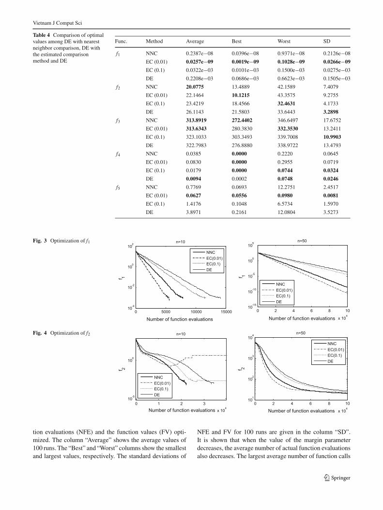
In the case of n = 50, the tests were terminated whenthe number of fitness evaluations exceeded 100,000. Table4 shows the optimal results obtained. The columns labeled“average”, “best”, “worst” and “std” show the average value,the best value, the worst value and the standard deviation ofthe optimal value in 25 runs, respectively.

For the best average value, DE-NCC found better valuethan DE, except for f4. On the other hand, DE-NCC couldattain as good results as DE-EC in most cases. Thus, thenearest neighbor comparison method can find better solutionand reduce the number of function evaluations effectively.

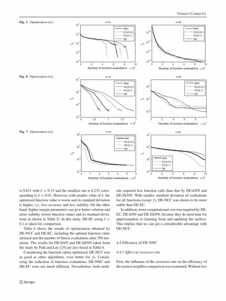
Figures 3, 4, 5, 6 and 7 show the logarithmic plots of thebest function values over the number of function evaluationsfor functions f1, f2, f3, f4 and f5, respectively. Note that theends of graphs in case n =10 are violated because some runs

stopped earlier than other runs when the termination condi-tion was satisfied. In the graphs, thick solid lines and thinsolid lines show the optimization process by DE-NNC andDE, respectively. The dashed lines and dotted lines show theoptimization process by DE-EC. It can be seen in the figuresthat the DE-NNC is faster than DE in most cases. Figure 4clearly shows that for f2(n = 10) the DE-EC was trapped bythe local minimum with the graphs going horizontally. Forfunctions f4 with n = 50, both DE-NNC and DE-EC weretrapped by the local minimum as seen in Fig. 6. This explainswhy the results of DE-NNC and DE-EC were not better thanthat of DE.

4.3.2 Test function f6, f7, f8 and f9

These functions were used to examine the performance ofDE-NNC and compare with that of DE-EC, DE-kNN andDE-EkNN. For each function, 30 random runs are executed.For each run, the optimization is terminated when the numberof generation exceeds 350.

First, the DE-EC was examined with different values ofthe margin parameter, δ = 0.15, 0.10, 0.05, 0.01. The algo-rithm DE/rand/1/bin was adopted. The reference value wasgiven by the standard deviation of approximation values. Theresults are given in Table 5, including the number of func-

123


Table 4 Comparison of optimalvalues among DE with nearestneighbor comparison, DE withthe estimated comparisonmethod and DE

Func. Method Average Best Worst SD

f1 NNC 0.2387e−08 0.0396e−08 0.9371e−08 0.2126e−08

EC (0.01) 0.0257e−09 0.0019e−09 0.1028e−09 0.0266e−09

EC (0.1) 0.0322e−03 0.0101e−03 0.1500e−03 0.0275e−03

DE 0.2208e−03 0.0686e−03 0.6623e−03 0.1505e−03

f2 NNC 20.0775 13.4889 42.1589 7.4079

EC (0.01) 22.1464 10.1215 43.3575 9.2755

EC (0.1) 23.4219 18.4566 32.4631 4.1733

DE 26.1143 21.5803 33.6443 3.2898

f3 NNC 313.8919 272.4402 346.6497 17.6752

EC (0.01) 313.6343 280.3830 332.3530 13.2411

EC (0.1) 323.1033 303.3493 339.7008 10.9903

DE 322.7983 276.8880 338.9722 13.4793

f4 NNC 0.0385 0.0000 0.2220 0.0645

EC (0.01) 0.0830 0.0000 0.2955 0.0719

EC (0.1) 0.0179 0.0000 0.0744 0.0324

DE 0.0094 0.0002 0.0748 0.0246

f5 NNC 0.7769 0.0693 12.2751 2.4517

EC (0.01) 0.0627 0.0556 0.0980 0.0081

EC (0.1) 1.4176 0.1048 6.5734 1.5970

DE 3.8971 0.2161 12.0804 3.5273

Fig. 3 Optimization of f1

0 5000 10000 1500010

-4

10-2

100

102

Number of function evaluations

f 1

n=10

NNCEC(0.01)EC(0.1)DE

0 2 4 6 8 10

x 104

10-15

10-10

10-5

100

105


f 1n=50



0 1 2 3

x 104

10-5

100


f 2

n=10


0 2 4 6 8 10

x 104

101

102

103

104


f 2

n=50


tion evaluations (NFE) and the function values (FV) opti-mized. The column “Average” shows the average values of100 runs. The “Best” and “Worst” columns show the smallestand largest values, respectively. The standard deviations of

NFE and FV for 100 runs are given in the column “SD”.It is shown that when the value of the margin parameterdecreases, the average number of actual function evaluationsalso decreases. The largest average number of function calls

123



0 2 4 6 8 10

x 104

10-4

10-2

100

102

104

Number of function evaluationsf 3

n=10


0 2 4 6 8 10

x 104

102.5

102.6

102.7

102.8


f 3

n=50



0 0.5 1 1.5 2

x 104

10-4

10-2

100

102


f 4

n=10


0 2 4 6 8

x 104

10-2

100

102


f 4

n=50



0 1 2 3 4 5 6

x 104

10-4

10-2

100

102


f 5

n=10


0 2 4 6 8 10

x 104

10-2

100

102

104


f 5

n=50


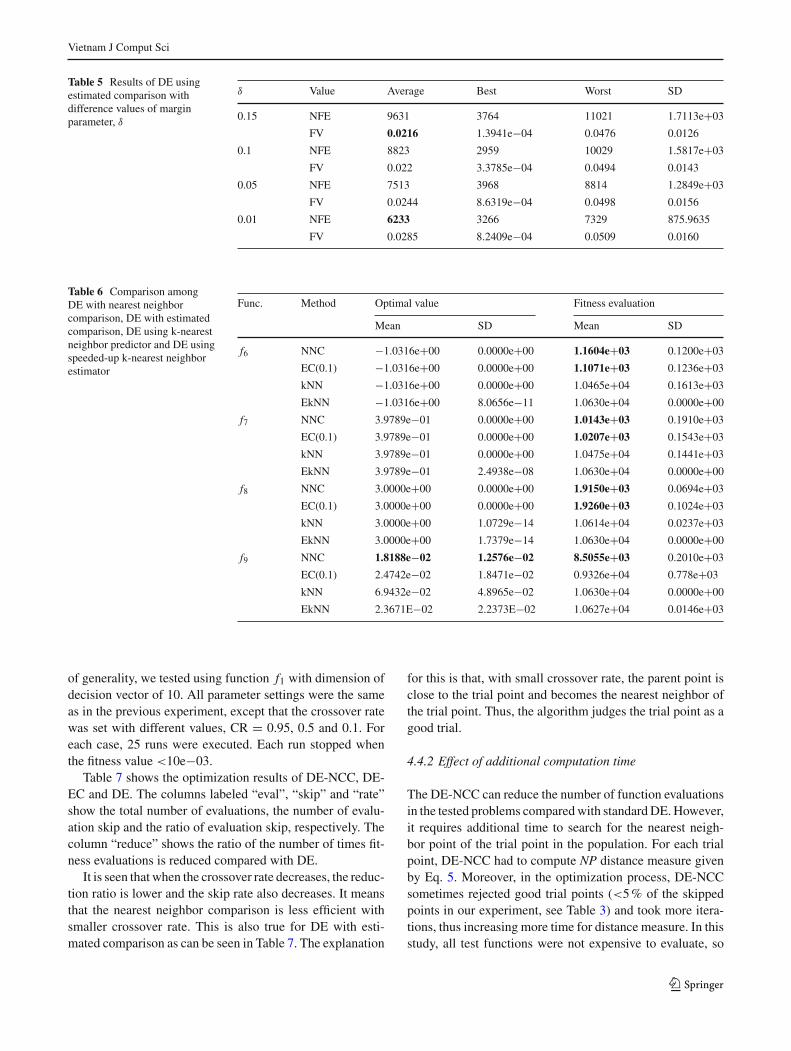
is 9,631 with δ = 0.15 and the smallest one is 6,233 corre-sponding to δ = 0.01. However, with smaller value of δ, theoptimized function value is worse and its standard deviationis higher, i.e., less accuracy and less stability. On the otherhand, higher margin parameters can give better solution andmore stability (lower function values and its standard devia-tions as shown in Table 5). In this study, DE-EC using δ =0.1 is taken for comparison.

Table 6 shows the results of optimization obtained byDE-NCC and DE-EC, including the optimal function valueattained and the number of fitness evaluations after 350 iter-ations. The results for DE-kNN and DE-EkNN taken fromthe study by Park and Lee [15] are also listed in Table 6.

Considering the function values optimized, DE-NCC wasas good as other algorithms, even better for f9. Consid-ering the reduction of function evaluations, DE-NNC andDE-EC were not much different. Nevertheless, both meth-

ods required less function calls than that by DE-kNN andDE-EkNN. With smaller standard deviation of evaluationsfor all functions except f7, DE-NCC was shown to be morestable than DE-EC.

In addition, more computational cost was required by DE-EC, DE-kNN and DE-EkNN, because they do need time forapproximation or learning from and updating the archive.This implies that we can get a considerable advantage withDE-NCC.

4.4 Efficiency of DE-NNC

4.4.1 Effect of crossover rate

First, the influence of the crossover rate on the efficiency ofthe nearest neighbor comparison was examined. Without loss

123


Table 5 Results of DE usingestimated comparison withdifference values of marginparameter, δ

δ Value Average Best Worst SD

0.15 NFE 9631 3764 11021 1.7113e+03

FV 0.0216 1.3941e−04 0.0476 0.0126

0.1 NFE 8823 2959 10029 1.5817e+03

FV 0.022 3.3785e−04 0.0494 0.0143

0.05 NFE 7513 3968 8814 1.2849e+03

FV 0.0244 8.6319e−04 0.0498 0.0156

0.01 NFE 6233 3266 7329 875.9635

FV 0.0285 8.2409e−04 0.0509 0.0160

Table 6 Comparison amongDE with nearest neighborcomparison, DE with estimatedcomparison, DE using k-nearestneighbor predictor and DE usingspeeded-up k-nearest neighborestimator

Func. Method Optimal value Fitness evaluation

Mean SD Mean SD

f6 NNC −1.0316e+00 0.0000e+00 1.1604e+03 0.1200e+03

EC(0.1) −1.0316e+00 0.0000e+00 1.1071e+03 0.1236e+03

kNN −1.0316e+00 0.0000e+00 1.0465e+04 0.1613e+03

EkNN −1.0316e+00 8.0656e−11 1.0630e+04 0.0000e+00

f7 NNC 3.9789e−01 0.0000e+00 1.0143e+03 0.1910e+03

EC(0.1) 3.9789e−01 0.0000e+00 1.0207e+03 0.1543e+03

kNN 3.9789e−01 0.0000e+00 1.0475e+04 0.1441e+03

EkNN 3.9789e−01 2.4938e−08 1.0630e+04 0.0000e+00

f8 NNC 3.0000e+00 0.0000e+00 1.9150e+03 0.0694e+03

EC(0.1) 3.0000e+00 0.0000e+00 1.9260e+03 0.1024e+03

kNN 3.0000e+00 1.0729e−14 1.0614e+04 0.0237e+03

EkNN 3.0000e+00 1.7379e−14 1.0630e+04 0.0000e+00

f9 NNC 1.8188e−02 1.2576e−02 8.5055e+03 0.2010e+03

EC(0.1) 2.4742e−02 1.8471e−02 0.9326e+04 0.778e+03

kNN 6.9432e−02 4.8965e−02 1.0630e+04 0.0000e+00

EkNN 2.3671E−02 2.2373E−02 1.0627e+04 0.0146e+03

of generality, we tested using function f1 with dimension ofdecision vector of 10. All parameter settings were the sameas in the previous experiment, except that the crossover ratewas set with different values, CR = 0.95, 0.5 and 0.1. Foreach case, 25 runs were executed. Each run stopped whenthe fitness value <10e−03.

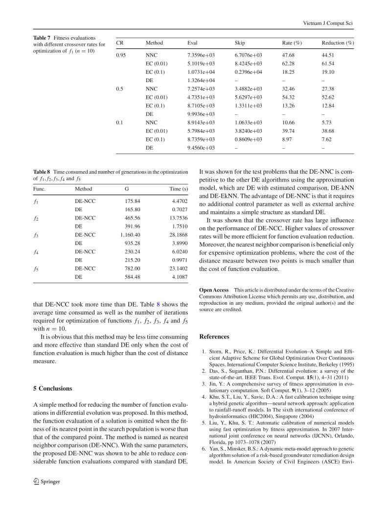
Table 7 shows the optimization results of DE-NCC, DE-EC and DE. The columns labeled “eval”, “skip” and “rate”show the total number of evaluations, the number of evalu-ation skip and the ratio of evaluation skip, respectively. Thecolumn “reduce” shows the ratio of the number of times fit-ness evaluations is reduced compared with DE.

It is seen that when the crossover rate decreases, the reduc-tion ratio is lower and the skip rate also decreases. It meansthat the nearest neighbor comparison is less efficient withsmaller crossover rate. This is also true for DE with esti-mated comparison as can be seen in Table 7. The explanation

for this is that, with small crossover rate, the parent point isclose to the trial point and becomes the nearest neighbor ofthe trial point. Thus, the algorithm judges the trial point as agood trial.

4.4.2 Effect of additional computation time

The DE-NCC can reduce the number of function evaluationsin the tested problems compared with standard DE. However,it requires additional time to search for the nearest neigh-bor point of the trial point in the population. For each trialpoint, DE-NCC had to compute NP distance measure givenby Eq. 5. Moreover, in the optimization process, DE-NCCsometimes rejected good trial points (<5 % of the skippedpoints in our experiment, see Table 3) and took more itera-tions, thus increasing more time for distance measure. In thisstudy, all test functions were not expensive to evaluate, so

123


Table 7 Fitness evaluationswith different crossover rates foroptimization of f1 (n = 10)

CR Method Eval Skip Rate (%) Reduction (%)

0.95 NNC 7.3596e+03 6.7076e+03 47.68 44.51

EC (0.01) 5.1019e+03 8.4245e+03 62.28 61.54

EC (0.1) 1.0731e+04 0.2396e+04 18.25 19.10

DE 1.3264e+04 – – –

0.5 NNC 7.2574e+03 3.4882e+03 32.46 27.38

EC (0.01) 4.7351e+03 5.6297e+03 54.32 52.62

EC (0.1) 8.7105e+03 1.3311e+03 13.26 12.84

DE 9.9936e+03 – – –

0.1 NNC 8.9143e+03 1.0633e+03 10.66 5.73

EC (0.01) 5.7984e+03 3.8240e+03 39.74 38.68

EC (0.1) 8.7359e+03 0.8609e+03 8.97 7.62

DE 9.4560e+03 – – –

Table 8 Time consumed and number of generations in the optimizationof f1, f2, f3, f4 and f5

Func. Method G Time (s)

f1 DE-NCC 175.84 4.4702

DE 165.80 0.7027

f2 DE-NCC 465.56 13.7536

DE 391.96 1.7510

f3 DE-NCC 1,160.40 28.1868

DE 935.28 3.8990

f4 DE-NCC 230.24 6.0240

DE 215.20 0.9971

f5 DE-NCC 782.00 23.1402

DE 584.48 4.1087

that DE-NCC took more time than DE. Table 8 shows theaverage time consumed as well as the number of iterationsrequired for optimization of functions f1, f2, f3, f4 and f5

with n = 10.It is obvious that this method may be less time consuming

and more effective than standard DE only when the cost offunction evaluation is much higher than the cost of distancemeasure.

5 Conclusions

A simple method for reducing the number of function evalu-ations in differential evolution was proposed. In this method,the function evaluation of a solution is omitted when the fit-ness of its nearest point in the search population is worse thanthat of the compared point. The method is named as nearestneighbor comparison (DE-NNC). With the same parameters,the proposed DE-NNC was shown to be able to reduce con-siderable function evaluations compared with standard DE.

It was shown for the test problems that the DE-NNC is com-petitive to the other DE algorithms using the approximationmodel, which are DE with estimated comparison, DE-kNNand DE-EkNN. The advantage of DE-NNC is that it requiresno additional control parameter as well as external archiveand maintains a simple structure as standard DE.

It was shown that the crossover rate has large influenceon the performance of DE-NCC. Higher values of crossoverrates will be more efficient for function evaluation reduction.Moreover, the nearest neighbor comparison is beneficial onlyfor expensive optimization problems, where the cost of thedistance measure between two points is much smaller thanthe cost of function evaluation.

Open Access This article is distributed under the terms of the CreativeCommons Attribution License which permits any use, distribution, andreproduction in any medium, provided the original author(s) and thesource are credited.

References

1. Storn, R., Price, K.: Differential Evolution–A Simple and Effi-cient Adaptive Scheme for Global Optimization Over ContinuousSpaces. International Computer Science Institute, Berkeley (1995)

2. Das, S., Suganthan, P.N.: Differential evolution: a survey of thestate-of-the-art. IEEE Trans. Evol. Comput. 15(1), 4–31 (2011)

3. Jin, Y.: A comprehensive survey of fitness approximation in evo-lutionary computation. Soft Comput. 9(1), 3–12 (2005)

4. Khu, S.T., Liu, Y., Savic, D.A.: A fast calibration technique usinga hybrid genetic algorithm—neural network approach: applicationto rainfall-runoff models. In The sixth international conference ofhydroinformatics (HIC2004), Singapore (2004)

5. Liu, Y., Khu, S. T.: Automatic calibration of numerical modelsusing fast optimization by fitness approximation. In 2007 Inter-national joint conference on neural networks (IJCNN), Orlando,Florida, pp 1073–1078 (2007)

6. Yan, S., Minsker, B.S.: A dynamic meta-model approach to geneticalgorithm solution of a risk-based groundwater remediation designmodel. In American Society of Civil Engineers (ASCE) Envi-

123


ronmental and Water Resources Institute (EWRI) world waterand environmental resources congress 2003 and related symposia,Philadelphia, PA (2003)

7. Giunta, A.A., Watson, L.T., Koehler, J.: A comparison of approxi-mation modeling techniques: polynomial versus interpolating mod-els. In Proceedings of the 7th IAA/USAF/NASA/ISSMO sympo-sium on multidisciplinary analysis and design, pp 392–404 (1998)

8. Simpson, T.W., Mauery, T.M., Korte, J.J., Mistree, F.: Comparisonof response surface and kriging models for multidisciplinary designoptimization. Am. Inst. Aeronaut. Astronaut. 98(7), 1–16 (1998)

9. Shyy, W., Tucker, P.K., Vaidyanathan, R.: Response surface andneural network techniques for rocket engine injector optimization.J. Propuls. Power 17(2), 391–401 (2001)

10. Guimaraes, F.G., Wanner, E.F., Campelo, F., Takahashi, R.H.,Igarashi, H., Lowther, D.A., Ramirez, J.A.: Local learning andsearch in memetic algorithms. In: Proceedings of the 2006 IEEECongress on Evolutionary Computation, Vancouver, BC, Canada,pp. 9841–9848 (2006)

11. Jin, Y., Sendhoff, B.. Reducing fitness evaluations using clusteringtechniques and neural network ensembles. In Genetic and Evolu-tionary Computation-GECCO 2004, Springer, Berlin Heidelberg,pp 688–699 (2004)

12. Jin, Y., Olhofer, M., Sendhoff, B. (2000). On evolutionary optimiza-tion with approximate fitness functions. In GECCO, pp 786–793

13. Jin, Y., Olhofer, M., Sendhoff, B.: A framework for evolutionaryoptimization with approximate fitness functions. IEEE Trans Evo-lution Comput 6(5), 481–494 (2002)

14. Liu, Y., Sun, F.: A fast differential evolution algorithm using k-Nearest Neighbour predictor. Expert Syst Appl 38(4), 4254–4258(2011)

15. Park, S.Y., Lee, J.J.: An efficient differential evolution usingspeeded-up k-nearest neighbor estimator. Soft Comput. 18(1), 35–49 (2014)

16. Takahama, T., Sakai, S.: Reducing function evaluations in differ-ential evolution using rough approximation-based comparison. InIEEE congress on evolutionary computation (CEC) 2008, pp 2307–2314 (2008)

17. Takahama, T., Sakai, S.: A comparative study on kernel smoothersin differential evolution with estimated comparison method forreducing function evaluations. In IEEE congress on evolutionarycomputation (CEC) 2009, pp 1367–1374 (2009)

18. Takahama, T., Sakai, S.: Reducing function evaluations using adap-tively controlled differential evolution with rough approximationmodel. In computational intelligence in expensive optimizationproblems, pp 111–129, Springer, Berlin Heidelberg (2010)

19. Takahama, T., Sakai, S.: Efficient constrained optimization by the ε

constrained differential evolution with rough approximation usingkernel regression. In IEEE congress on evolutionary computation(CEC) 2013, pp 1334–1341 (2013)

20. Neri, F., Tirronen, V.: Recent advances in differential evolution: asurvey and experimental analysis. Artif. Intel. Rev. 33(1–2), 61–106 (2010)

123

Documents

2 3 Reduction of function evaluation in differential evolution using nearest neighbor comparison