2005 Special issue

Robust self-localisation and navigation based on hippocampal place cells

Thomas Strosslin *, Denis Sheynikhovich, Ricardo Chavarriaga, Wulfram Gerstner

Laboratory of Computational Neuroscience, Brain and Mind Centre, EPFL, 1015 Lausanne, Switzerland

Abstract

A computational model of the hippocampal function in spatial learning is presented. A spatial representation is incrementally acquired during

exploration. Visual and self-motion information is fed into a network of rate-coded neurons. A consistent and stable place code emerges by

unsupervised Hebbian learning between place- and head direction cells. Based on this representation, goal-oriented navigation is learnt by

applying a reward-based learning mechanism between the hippocampus and nucleus accumbens. The model, validated on a real and simulated

robot, successfully localises itself by recalibrating its path integrator using visual input. A navigation map is learnt after about 20 trials,

comparable to rats in the water maze. In contrast to previous works, this system processes realistic visual input. No compass is needed for

localisation and the reward-based learning mechanism extends discrete navigation models to continuous space. The model reproduces

experimental findings and suggests several neurophysiological and behavioural predictions in the rat.

q 2005 Elsevier Ltd. All rights reserved.

Keywords: Spatial learning model; Hippocampus; Place cells; Head direction cells; Path integration; Calibration and drift removal; Nucleus accumbens;

Reinforcement learning in continuous space

1. Introduction

The striking discovery of place cells in the rat

hippocampus (O’Keefe & Dostrovsky, 1971) has triggered

a wave of interest on spatial learning that holds until today.

The activity of place cells is highly correlated with the

spatial location of the animal. Therefore, the hippocampus

has been suggested to mediate spatial coding (O’Keefe &

Nadel, 1978; Redish, 1999). Furthermore, neurons whose

activity is tuned to the orientation of the rat’s head in the

azimuthal plane (head direction cells) have also been found

in the hippocampal formation (Ranck, 1984; Taube, Muller,

& Ranck, 1990). It is hypothesised that place and head

direction cells together form a neural circuit for spatial

representations (Knierim, Kudrimoti, & McNaughton, 1995).

Extensive experimental evidence suggests that two types of

highly processed sensorial input influence the activity of the

location and direction sensitive cells in the hippocampal

formation: First, allothetic, i.e. external (visual, olfactory,

tactile) sensory input from cortical areas is available for

processing. It appears that visual information exerts a

0893-6080/$ - see front matter q 2005 Elsevier Ltd. All rights reserved.

doi:10.1016/j.neunet.2005.08.012

* Corresponding author. Address: Neural Computation Unit, Okinawa

Institute of Science and Technology, 12-22 Suzaki, Uruma, 904-2234 Okinawa,

Japan.

E-mail address: thomas.strosslin@a3.epfl.ch (T. Strosslin).

dominant influence compared to other modalities (Muller &

Kubie, 1987; Taube et al., 1990). Persistent location and

direction sensitivity in the absence of external stimulation

suggests that integration of idiothetic, i.e. internal self-

motion signals is another source of information processed by

the neurons in the hippocampal formation (Jeffery, 2003;

McNaughton et al., 1996). Experimental data shows that the

activities of place and head direction cells correlate with

behavioural decisions (see Jeffery, 2003 for review) and that

lesions of related brain areas impair performance in

navigational tasks where an internal space representation is

necessary.

1.1. Relation to our previous models

This work presents a biologically inspired computational

model of the rat’s hippocampus and its role in navigation to a

hidden goal location. It is based on a series of models by Arleo,

et al. (Arleo, Smeraldi & Gerstner, 2004; Arleo & Gerstner,

2000b; Arleo, Smeraldi, & Hug, 2001). As in the previous

versions, an unsupervised growing network scheme is used.

The model consists of interconnected populations of neurons

that process allothetic and idiothetic inputs to drive the firing of

simulated place cells. Visual input is represented by two-

dimensional gray-scale images. Relevant information about

current position and gaze direction is extracted from the visual

input to form allocentric location and direction estimates. Self-

motion input in the form of egocentric rotation and

Neural Networks 18 (2005) 1125–1140

www.elsevier.com/locate/neunet

T. Strosslin et al. / Neural Networks 18 (2005) 1125–11401126

displacement signals are transformed to an arbitrary allocentric

frame of reference and integrated into a position and heading

estimate. The visual and self-motion processing pathways are

then combined to form a spatial representation consisting of a

large population of place cells with overlapping receptive

fields. The synaptic efficacies between neural populations

change according to Hebbian-type learning rules. Thus without

any prior knowledge, the space code is built incrementally and

on-line from direct interactions with the environment. This

spatial representation is subsequently used for goal navigation

using reinforcement learning. The state space is represented by

the place cell population activity and locomotor neurons in

nucleus accumbens, a target structure of the hippocampus,

serve as action space.

The present model differs from previous models by Arleo

et al. in several ways. The most important improvements are:

(i) The new visual system closer emulates the visual system of

the rat in that it has a wider view field of up to 3208 (Hughes,

1977). We also propose a uniform visual filter grid in contrast

to a foveal retina. It is this rectangular grid which makes

heading discrimination much simpler. (ii) The ability to

reliably extract direction information from complex visual

input removes the need of a polarising cue (a lamp) in order to

calibrate the directional system. (iii) The former models

explicitly access the spatial variance of place cell activity in

order to recalibrate path integrator. This model combines

visual and self-motion information in a simpler and more

natural way. (iv) In previous models of learning goal-oriented

behaviour, movements were restricted to four predefined

directions. Just adding more directions would have resulted

in an increased learning time due to the lack of generalisation

in action space. The new model features a continuous action

space allowing arbitrary directions of movement. A general-

isation mechanism decouples the learning speed from the

population size.

1.2. Relation to other models

The hippocampus was modelled extensively during the last

decades due to its undisputed importance in memory and

spatial behaviour. Here, we review previous work of other

researchers which is relevant for this paper. The features of

each model are briefly outlined and compared to our proposal.

Specific similarities and differences are also mentioned in

Sections 3 and 4. A summary of our contributions is given in

Section 6.

Burgess et al. (Burgess, Recce, & O’keefe, 1994) offer a

detailed model of hippocampal place cells. It consists of

several populations, representing entorhinal cortex (EC),

hippocampus proper (HPC) and subiculum (SUB). Visual

input is based on algorithmically calculated distances to

landmarks placed near the walls. Neurons in SUB as well as

head direction (HD) cells project to goal cells (GC). Reward-

based learning is applied for navigation. This model is also

implemented on a robotic platform (Burgess, Donnett, Jeffery,

& O’Keefe, 1997; Burgess, Jackson, Hartley, & O’Keefe,

2000; Hartley, Burgess, Lever, Cacucci, & Keefe, 2000).

Unlike our proposal, their model uses simplified visual input

(distance to the walls), which is not directly available to

animals. It also suggests that the hippocampal formation is

sufficient for locale navigation. This is in contradiction to

experimental data where fornix lesions impair rats in the

hidden water maze (Eichenbaum, Stewart, & Morris, 1990;

Packard & McGaugh, 1992; Sutherland & Rodriguez, 1990).

Furthermore, their model fails in the presence of local obstacles

as well as in darkness. Finally, their learning mechanism

suffers a ‘distal reward’ problem. On the other hand, it

proposes an abstract geometrical mechanism which produces

the effect of phase precession. Our model does not address this

issue.

The model proposed by Sharp et al. (Brown; Sharp, 1991 &

Sharp, 1995) builds on visual cells that encode the agent’s

distance and bearing to several landmarks in the environment.

Subsequent layers, representing EC and HPC, combine visual

information in order to form a place code. A population of

‘motor’ cells in nucleus accumbens receives spatial infor-

mation from the hippocampal place cells. Together with a HD

system, the model learns to perform movement commands

which lead to a rewarding location. Their model relies on an

artificial local view system. In contrast, our system uses

realistic camera images. Whereas our model results in a highly

redundant and distributed place code consistent with exper-

imental data, their winner-take-all mechanism prevents all but

one place cell from firing. Their representation has no path

integration component and therefore does not support location-

specific firing in the dark. Our navigation system is similar to

theirs. However, while their model needs a long temporal trace

in order to overcome a distal reward problem, our approach

does not suffer such a limitation. On the other hand, their model

produces omnidirectional place fields in open, and uni-

directional fields in an eight-arm-maze, consistent with

experimental data. Our model’s place fields are always

omnidirectional.

The system by Redish et al. (Wan, Touretzky, & Redish,

1994; Touretzky & Redish, 1996; Redish and Touretzky

1997a,b) consists of separate populations for the local view,

head direction, path integrator and place code. All populations

interact with each other in order to form a consistent

representation of space. Algorithmically determined infor-

mation about type, distance and bearing angle to each landmark

enters the local view system. The features of this place cell

model are similar to ours. However, their neuronal model is

more abstract. Their system relies on an abstract visual input,

which features a perfect measure of the landmark type, distance

and bearing. Our model extracts low-level features from real

images. Place units in their model compute a ‘fuzzy

conjunction’ of inputs in which terms that are unavailable or

thought incorrect drop out. In contrast, we use standard neural

activation function. Finally, unlike our proposal, there is no

purely allothetic place code.

Hippocampal place cells in Abbott and colleagues’ work

(Blum & Abbott, 1996; Gerstner & Abbott, 1997) have

perfectly Gaussian tuned receptive fields prior to navigation

learning. Spike timing dependent plasticity on hippocampal

T. Strosslin et al. / Neural Networks 18 (2005) 1125–1140 1127

collateral synapses results in a goal-dependent shift of place

fields. This shift can be used for navigation. Multiple goal

locations can be represented simultaneously. Whereas our

model constructs a hippocampal place code from allothetic

cues, their approach assumes perfectly Gaussian tuned place

cells initially. In order to use the shifted place cells for

navigation, they need to explicitly compare the initial and

current place field centres. In our model, positions and actions

are implicitly coded. Their model of locale navigation is

entirely concentrated in the hippocampus. This conflicts with

experimental data showing that lesions to the fornix or nucleus

accumbens impair locale navigation (Eichenbaum et al., 1990;

Packard & McGaugh, 1992; Sutherland & Rodriguez, 1990).

On the other hand, their model can store navigation maps to

multiple goal locations at the same time whereas ours is limited

to one. Their neuron model and learning rule are also more

detailed and realistic than ours.

The model proposed by Foster, Morris, and Dayan (2000) is

based on an actor-critic architecture for temporal-difference

reinforcement learning. A layer of place cells with perfectly

tuned Gaussian receptive fields provides the navigation system

with the agent’s position within its environment. An actor

network learns selecting an appropriate direction of movement,

depending on place cell activity. In order to overcome

interference with previously learnt goal locations, their

model features a coordinate system module which learns to

transform place code activity into a Cartesian frame and stores

the goal’s coordinates. Once learnt, algorithmic vector

subtraction replaces the action selection based on learnt

place/action associations. Whereas our place fields are learnt

by experience, their model relies on a population of perfectly

Gaussian tuned place cells with no allothetic component. Like

our proposal, reinforcement learning is used between place

cells and a set of action neurons which code for the allothetic

direction of movement. Unlike our approach, however,

learning does not generalise to similar directions and does

not allow for continuous directions of movement in their

system. On the other hand, their coordinate system enables the

agent to quickly adapt to a new goal location. Our model does

not address the quick relearning of a goal location. However,

their coordinate-system module creates a global basin of

attraction. Local obstacle avoidance is then no longer possible.

Furthermore, the direction of movement is algorithmically

calculated by explicitly accessing the coordinates of the goal

location.

In the model by Gaussier et al. (Gaussier, Lepretre, Joulain,

Revel, Quoy, & Banquet, 1998; Gaussier, Joalin, Banquet,

Lepretre, & Revel, 2000; Gaussier, Revel, Banquet, & Babeau,

2002), a local view is extracted from panoramic two-

dimensional images and consists of a set of landmark bearings

and types. A landmark bearing is determined by a magnetic

compass and its type is chosen from a predefined set. A place

cell fires according to the similarity of the local views. A

population of transition cells stores all transitions from each

location (coded by a place cell) experienced in the past. This

model relies on a compass and object recognition whereas ours

works with low-level filter responses and without a compass.

Furthermore, this model uses winner-take-all mechanisms in

all populations whereas we use a more biologically plausible

distributed place code.

Being similar to these models in terms of the overall spatial

coding procedure (i.e. storage and comparison of the local

views) our model has the advantages of (i) working with

realistic visual input, (ii) having an integrated head direction

system which does not use any prior landmark information and

(iii) a navigational system which can handle a continuum of

possible actions, does not use any prior information about the

environment and is able to work in the presence of obstacles as

well as in darkness.

2. Methods

Our model consists of several interacting populations of

‘rate-coded neurons’. This artificial neural network is

synchronised by a global clock signal. During motion, a

6–12 Hz EEG oscillation called theta rhythm can be observed

in the hippocampal formation of rats (Burgess et al., 1994;

O’Keefe & Recce, 1993; Skaggs, McNaughton, Wilson, &

Barnes, 1996). Strong inhibitory input from the septal region to

the hippocampus seems to be responsible for generating these

oscillations (Buzsaki, 1984; Hasselmo & Bower, 1993; Miller,

1991; Winson, 1978). Theta is also observable during sensory

scanning (e.g. sniffing). We assume that theta serves as a clock

signal to synchronise information processing throughout the

hippocampal formation.

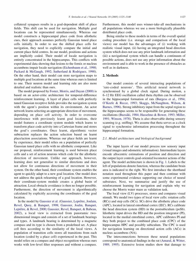
2.1. Model architecture and biological background

The input layers of our model process raw sensory input

(visual images and odometric information). Intermediate layers

encode allocentric estimations of position and direction and

the output layer controls goal-oriented locomotor actions of the

agent. The model architecture is shown in Fig. 1. Labels to the

left of populations denote function, whereas the candidate brain

area is indicated to the right. We first introduce the shorthand

notation used throughout this paper and then continue with

some experimental evidence supporting our choice of neural

substrates. Next, we summarise and justify the use of

reinforcement learning for navigation and explain why we

choose the Morris water maze as validation task.

The local view (LV) processes, stores and compares visual

stimuli. We model two types of local view cells: rotation cells

(RCs) and step cells (SCs). SCs drive the allothetic place code

(APC), located in lateral entorhinal cortex (IEC). RCs calibrate

the head direction system (HD) in the postsubiculum (poSb).

Idiothetic input drives the HD and the position integrator (PI),

located in the medial entorhinal cortex. APC calibrates PI and

they both project to the combined place code (CPC) of the

hippocampus HPC and possibly subiculum. The CPC is used

for navigation learning on directional action cells (ACs) in

nucleus accumbens (NA).

The interconnections between these neural populations

correspond to anatomical findings in the rat (Amaral, & Witter,

1989, 1995). Extensive lesion studies show that damage to

Idiothetic input

RC

SCVisual input

CPC

HD

PI

calibrate

calibrate

HPC

mEClECAPC

LV

AC

poSb

NA

Fig. 1. Model architecture. The local view (LV), embracing rotation cells (RCs)

and step cells (SCs), processes, stores and compares visual stimuli. SCs drive

the allothetic place code (APC) in the lateral entorhinal cortex (IEC) and RCs

calibrate the head direction system (HD) in the postsubiculum (poSb). Internal

odometric input drives HD and the position integrator (PI) in medial entorhinal

cortex. APC calibrates PI and they both project to the combined place code

(CPC) in the hippocampus (HPC) and subiculum. CPC is used for navigation

learning on directional action cells (ACs) in nucleus accumbens (NA).

1 The Khepera mobile robot manufactured by K-Team (http://k-team.com/)

is a modular platform popular for research and education.

T. Strosslin et al. / Neural Networks 18 (2005) 1125–11401128

brain areas containing place or direction sensitive cells, as well

as lesions of NA selectively impair rats in the hidden platform

water maze task (Packard, & McGaugh, 1992; Redish, 1999).

Additionally, NA seems to be involved in reward-

dependent learning of spatial locomotion (Whishaw, &

Mittleman, 1991). Several neurophysiological properties of

biological neurons in the hippocampus of the rat are captured

by the artificial place cells that develop in the model in an

unsupervised manner as a result of environment exploration.

The activity of the location sensitive neurons in CA3–CA1

areas of the hippocampus are shown to depend strongly on

distal visual stimuli (see (Redish, 1999) for an excellent

review). The activity of hippocampal neurons is shown to be

direction independent in an open field (Markus et al., 1994;

McNaughton, Barnes, & O’Keefe, 1983; Muller, Bostock,

Taube, & Kubie, 1994; O’Keefe, & Burgess, 1996). The

location sensitive firing persists in the absence of visual

stimulation, i.e. when the lights are turned off after

exploration (Quirk, Muller, & Kubie, 1990; Save, Nerad, &

Poucet, 2000). This suggests that integration of idiothetic

cues influence place cells. Place cells in mEC preserve firing

topology across reshaped environments. mEC cells are also

likely to be active in any environment (Quirk, Muller, Kubie,

& Ranck, 1992). This indicates that mEC might be part of a

general, environment-independent position integration

system. Little is known, however, about the lateral part of

entorhinal cortex. Electrophysiological studies are lacking for

this region. Lesion studies suggest, however, that IEC is

involved in the encoding of allothetic sensory signals (Otto,

Ding, Cousens, & Schiller, 1996). As this is the only other

pathway to HPC, we postulate that the lateral entorhinal

cortex contains an environment-dependent allothetic place

code. There is also evidence for strong synaptic innervation

from the lateral to the medial region of EC (Quirk et al.,

1992). These could convey allothetic spatial information used

to calibrate a position integrator in mEC. Cells which

respond to the allocentric head direction of rats have been

found in poSb (Ranck, 1984; Taube et al., 1990). They seem

to be heavily influenced by idiothetic and visual stimuli.

One of the existing hypotheses of how place cells can be

used for navigation employs a reinforcement learning frame-

work in order to associate place with goal information. In the

reinforcement learning theory (Sutton, & Barto, 1998), a

mapping between a state space (e.g. place cells) and an action

space (e.g. locomotor cells) is learnt via the estimation of a

state-action value function. The value function corresponds to

the expected future reward and can be learnt on-line by trial

and error based on the difference between the predicted and an

actual reward. It was found that the activity of dopaminergic

neurons in the basal ganglia is related to the errors in reward

prediction (Schultz, 1998; Schultz, Dayan, & Montague, 1997).

Furthermore, these neurons project to NA, on the same spines

as hippocampal afferents (Freund, Powell, & Smith, 1984;

Sesack, & Pickel, 1990).

The hidden platform water maze task (Morris, 1981;

Redish, 1999) is a frequently used paradigm to test

navigation capabilities. The experimental setup consists of

a circular water pool filled with opaque liquid and a small

platform located inside the pool and submerged below the

surface of the liquid. At the beginning of each trial, a rat is

placed into the pool at a random location and its task is to

find the platform. Since no visual cues directly identify the

platform and the starting locations are random, animals have

to remember the location of the hidden platform based on the

extra-pool visual features. After several trials, rats are able to

swim directly to the hidden platform from any location in the

pool. This task is known to depend on an intact

hippocampus. We therefore choose this paradigm as a

validation of our model.

2.2. Experimental setups

In order to validate our model, we also implement it on a

computer, which is connected to a Khepera1 mobile robot

(Mondada, Franzi, & Ienne, 1994). The Khepera is equipped

with a camera, odometers and proximity sensors (cf. Fig. 2(a)).

Additionally, we use a simulated Khepera robot in virtual

environments for our test experiments. The robot is controlled

by the neural model and monitored by a tracking system. We

use the term ‘agent’ throughout this article when we do not

differentiate between the real and the virtual robot. Both

emulate a rat in an experimental arena.

The experiments presented in Section 5 are run in four

different configurations. All of them are static throughout the

experiment:

Office: This setup consists of the real Khepera robot placed

in an 80 !60 cm arena on a table in a normal office

Fig. 2. (a) The Khepera robot and its sensors. (b) View of the ‘Office’ environment with the Khepera robot.

T. Strosslin et al. / Neural Networks 18 (2005) 1125–1140 1129

(cf. Fig. 2(b)). The arena is surrounded by borders

of 3 cm height. The Khepera’s camera has a view-

angle of approximately 608 (see Fig. 2). Four

pictures in directions separated by 608 are merged

into a single image I of approximately qZ2408 by

rotating the robot in-place. Note that these rotations

are only performed in order to acquire a panoramic

view.

Buildings: This and the following environments emulate the

Khepera robot in a 77!77 cm virtual world.

Images are pasted to walls placed outside of the

arena. The view of the virtual world is projected

onto a cylindrical screen which covers a view-

angle of 2808 using standard computer graphics

algorithms. In the ‘Buildings’ setup, four walls are

placed in a square around the environment and

decorated with pictures of buildings and other man-

made structures.

Davos: This natural scene contains less structure than the

man-made objects of the previous two setups.

Here, a panoramic view of the Swiss mountains is

pasted onto a big cylinder surrounding the virtual

arena.

Minimal: The previous environments all provide rich visual

stimuli. In most animal experiments, however, the

Fig. 3. Response of the artificial retina applied to a view from the ‘Buildings’ enviro

for all orientations. They indicate the direction and ‘strength’ (line length) of edge

view is restricted to a small number of well-defined

cues. In order to emulate such an impoverished

environment, four walls are placed in a square

around the arena. In the centre of each wall, one

simple geometrical object is placed. The objects

are a filled black square, a filled white circle, a

triangle and a double cross. The background of

each wall is covered with low contrast noise.

The agent constantly acquires panoramic 800!316 gray-

scale images of its environment during experiments. This high-

dimensional sensory input needs to be preprocessed before it is

passed on to the neural network model. We use a mechanism

which is inspired by neuronal properties in primary visual

cortex: The image data is represented using a set of Gabor

wavelets (Gabor, 1946). They respond to bars of different

widths (spatial frequencies) and orientations in the image much

like complex cells in visual cortex area V1 (Hubel, & Wiesel,

1962). A filter vector ðf j is calculated as the magnitude of the

complex filter responses to the image. The filter responses are

calculated on a set of sampling points in the image. These

sampling points form an artificial rectangular retina. An

example of the retinal response is shown in Fig. 3 for the

‘Buildings’ environment. The retina consists of 15 columns

and 3 rows. On each point, the filter response for the lowest

frequency (wavelength ljZ50 pixels) is represented by a black

nment. The black lines represent the weighted sum of the gabor filter responses

s near each retinal point.

T. Strosslin et al. / Neural Networks 18 (2005) 1125–11401130

line. It indicates the direction and ‘strength’ (line length) of

edges in its neighbourhood.

3. Spatial representation

Similar to (Arleo & Gerstner, 2000b; Burgess et al., 1994;

Gaussier et al., 2000; Sharp, 1991; Touretzky, & Redish, 1996),

the architecture of our localisation system (Fig. 1) is inspired

by experimental works on various levels (electrophysiology,

anatomy, behaviour, etc.) in the rat. The model consists of five

interconnected components: (i) The local view module (LV)

stores and compares visual input in rotation cells (RCs) and

step cells (SCs). (ii) The head direction system (HD)

continuously updates the agent’s sense of orientation. (iii)

The allothetic place code (APC) estimates the agent’s position

within the environment based on the local view. (iv) The

position integrator (PI) keeps track of the agent’s location

relying on odometric information. (v) The combined place

code (CPC) links the visual and odometric position estimates

and forms the output of the localisation system. It is used by the

navigation module (cf. Section 4) to learn goal-oriented

behaviours.

3.1. Local view

The local view module receives visual input from the

columns of the artificial retina. Its purpose is to store and

compare relevant information, for the construction of a spatial

representation (Touretzky & Redish, 1996). At each time step,

several view cells are recruited and tuned to the current retinal

response. We assume that there are enough recruitable neurons

and do not address the question of ‘resource management’. A

previous view stored at time tk can be compared to the current

view at time tj by defining a similarity measure between two

sets of filter activities. This measure is implemented by visual

neurons described in this section.

The choice of a comparison function depends on what

transformations the image is subject to. The agent’s local view

in an environment depends on two variables, namely position

and heading. Accordingly, we will call an agent’s movement a

‘rotation’ if it only changes the heading. If only the agent’s

position is changed by a small amount, we call it a ‘step’.

Independently of the environment, a rotation produces a

translation along the horizontal axis of the view. A step,

however, causes a complicated and environment-dependent

transformation. We assume that translations along the vertical

axis are not possible, i.e. the agent does not look up or down,

only left or right. While this holds for the mobile robot, it is

only an approximation for the rat.

One of the problems is that if the visual cues are far

away, a step produces only a small change in the view,

whereas a rotation always produces a big, but predictable

change. For a spatial representation, however, the visual

system must permit the discrimination of both heading and

position. We therefore ‘read’ the retinal information in two

ways: One neural population tries to discriminate well

between headings but not position, and vice versa for a

second population. Both should have broad tuning curves in

order to provide good generalisation of known samples to

new views.

3.1.1. Rotation cells

Rotation cells (RCs) aim at discriminating headings

regardless of position. The receptive fields should span a

large range of headings, i.e. moderate translations of the image

should not cause a drastic change in activity.

This is achieved by combining information from neighbour-

ing retinal columns. For each retinal column i positioned at xi,

the weighted sum of filter vectors ðhðxi; tkÞ at time tk, not

the filter vectors ðf ðxi; tkÞ themselves, are stored / compared:

ðhðxi; tkÞZ c0,ðf ðxi; tkÞCXdncols=2e

jZ1

cj,½ðf ðxleftði;jÞ; tkÞCðf ðxrightði;jÞ; tkÞ�

(1)

where left (i, j)ZjiKjj and right (i,j)Z(ncolsK1)KjiCjK(ncolsK1)j are the jth column indices to the left and right of the

current column i. In the centre, left (i, j)ZiKj and right (i, j)ZiCj. Near the borders, however, columns which would lie

outside of the image are mirrored on the left and right borders.

Note that vector ðf in Eq. (1) is composed of the filter responses

from all rows of column i. The weights cj are sampled from a

Gaussian Nc, the standard deviation scZ100 pixels of which

determines the amount of translation invariance.

In order to compare two views, a similarity measure must be

defined. At each time step tk, the agent takes a visual snapshot.

The image is processed as described above and encoded by a

set of RCs. For each column i, a newly recruited RC stores the

feature vector ðhðxi; tkÞ: The activity r(tjjxi,tk) of an RC

represents the similarity of a column at time tj with respect to

what the cell stored at time tk. The activation function is:

rðtjjxi; tkÞ Z exp½Kðjjðhðxi; tkÞ2ðhðxi; tjÞjj1Þ2=ð2k,s2Þ� (2)

where ðzZ ðx2ðy is the relative difference: Each element l of the

normal difference is element-wise divided by ðx, i.e.

zl Z ðxlKylÞ=xl. This is somewhat similar to a shift and scale

of the input distribution and allows sensory input from

statistically different environments be treated in the same

way, thus simulating sensitivity adaptation or habituation. k$k1

denotes the L1-norm. kZ488 is the product of the number of

rows per retina column and the number of gabor frequencies

and orientations. sZ0.25 is a hand-tuned constant. Thus, r

depends on the average relative distance between stored and

current filter activity.

3.1.2. Step cells

The second way of reading out the retinal activation helps

discriminating positions, regardless of the agent’s heading.

Suppose that two distinguishable landmarks l1 and l2 are

the only visual cues in an environment. Let us define f(P)

as the difference in the bearing angle to landmarks l1 and l2when the agent is at location P. If the agent has a field of view

of 3608, the two landmarks are visible for all agent headings

T. Strosslin et al. / Neural Networks 18 (2005) 1125–1140 1131

and the difference f(P) is independent of this heading.

However, the bearing difference depends on the agent’s

position, i.e. for most positions P1 and P2, f(P1)sf(P2).

Similar to (Touretzky, & Redish, 1996), this property is

exploited by the step cells (SCs). However, we do not really use

landmarks, but low-level Gabor filters.

At every time step tk, a variable number of SCs is recruited:

We consider two retinal columns s and sCd. If the filters of

both columns are sufficiently active, their filter vector

difference ðdðd; s; tkÞ is stored if:

d2f3;.; 6g and jjðf ðxs; tkÞjj1Oqact ! jjðf ðxsCd; tkÞjj1

ðdðd; s; tkÞ Z ðf ðxs; tkÞKðf ðxsCd; tkÞ (3)

The empirically determined activity threshold qactZ1.0 is

particularly useful in impoverished environments where most

filter columns just see plain walls. It prevents recruitment of

cells that store no relevant information.

The column distance d should ideally correspond to big

angle differences because—at least in enclosed environ-

ments—big landmark bearing differences depend more on

the agent’s position than small ones, which makes position

discrimination easier. However, if the agent’s field of view Jis smaller than 3608, a big value for d reduces the probability

that both landmarks are visible at the same time. In our

experiments, J equals 2808. We allow a range of empirically

determined column distances d2{3,.,6}. This corresponds to

bearing differences between approximately 508 and 1008.

SCs should detect at time tj if the difference of column filter

activities of a given distance d has already been seen and stored

at time tk. The comparison should be independent of the agent’s

heading, i.e. the absolute position of the two columns spaced by

d on the retina should not matter. To achieve this translation

invariance in the retinal image, ðdðd; s; tkÞ is compared with the

most similar column difference at time tj. The firing rate r(tjjd,s,tk)

of an SC which stored the difference vector ðdðd; s; tkÞ at time tk is

given by:

rðtjjd; s; tkÞ Z exp½Kðmini

jjðdðd; s; tkÞ2ðdðd; i; tjÞjj1Þ2=ð2k,s2Þ�

(4)

where k is the same normalisation factor as for RCs (Eq. (2)) and

sZ0.1 is a hand-tuned constant.

2 It is always assumed that the agent performs ‘uniform’ movements. The

movements is uniform in the sense that the angular velocity u remains constant

throughout the movement.

3.2. Head direction system

The head direction (HD) module forms the most important

part of the spatial learning model. Small rotational errors can

totally impair the system’s ability to build and maintain a

spatial representation. This section describes how the HD

system combines odometric and visual information in order to

produce a stable (non-drifting) estimate of the agent’s heading.

Similar to (Arleo, & Gerstner, 2001), a population of NhdZ120

directional neurons codes for the agent’s heading F with

respect to an arbitrary fixed compass bearing J. Without loss

of generality, we assume JZ0. Each HD neuron i represents

the heading fiZi$3608/Nhd.

The firing rates of HD cells is calculated in two stages. First,

an estimation Fhd of the agent’s real heading F is calculated as

described below. Then, a large activity profile around Fhd is

enforced in the HD system. Lateral interconnection between HD

cells could be the neuronal substrate for such activity profiles

(Boucheny, Brunel, & Arleo, 2005; Zhang, 1996). Here, we

emulate lateral interactions by enforcing a Gaussian activity

profile around Fhd. Formally, the firing rate ri of HD cell i is

ri Z exp½KðjjFhd Kfijj4Þ2=ð2s2Þ� (5)

where k$k42[0,2p] is the angular distance and s2 is the angular

variance of the Gaussian profile. In our experiments, a value of

sZ608 is used.

When the agent moves2 at time step tK1, its angular

displacement dFi(tK1) is estimated by dead-reckoning and

made available to the HD system when the movement is

completed. The new heading, estimated by idiothetic cues, is

then FiðtÞZFhdðtK1ÞCdFiðtK1Þ.

Any real-world path or heading integration system based on

dead-reckoning is subject to noise and, more importantly, to a

systematic drift. In order to keep the HD representation accurate,

the local views encountered during exploration are continuously

associated to their heading direction. In particular, all rotation

cells (RCs) are connected to all HD cells and synapses are

activated/modified at each time step as follows: If an inactive

synapse’s pre- and postsynaptic activities ri and ri are above a

threshold qactZ0.2, the synapse is activated and its strength

initialised using a one-shot Hebbian-type learning rule:

wij Z ri,rj if riOqact and rj Oqact (6)

Once activated, the synaptic efficacy is modified at each time

step:

Dwij Z h,riðrjKwijÞ (7)

where hZ0.01 is the learning rate. After each learning step,

weights are renormalised: ~wijZwij=ðP

k wikÞ. The activities of

all RCs j connected to HD cell i produce an input potential

hiZP

j ~wijrj at the HD cell i. The allothetic heading estimate Fa

is then given as a circular ‘population vector’ of the input

potentials hi:

Fa Z arctan

Pi hi sinð2pi=NhdÞPi hi cosð2pi=NhdÞ

� �(8)

Unlike the more general population vector decoding

algorithms (Georgopoulos, Schwartz, & Kettner, 1986; Salinas,

& Abbott, 1994; Sanger, 2003), this simple form does not need

the place field distribution. On the other hand, it only works well

for uniformly distributed symmetrical place cells. We still

explicitly access angular information in Eqs. (5), (8) and (9)

which seems at first sight biologically implausible. However, if

T. Strosslin et al. / Neural Networks 18 (2005) 1125–11401132

continuous attractors using lateral connections (Amari, 1977;

Boucheny et al. 2005; Zhang, 1996) or a probabilistic activity

transition matrix (Herrmann, Pawelzik, & Geisel, 1999)

between HD cells was used for implementing Eq. (5), the

recalibration could be performed without explicitly accessing

angular information. Furthermore, it has been shown that

attractor dynamics combined with basis functions can find

optimal multisensory integration (Deneve, Latham, & Pouget,

2001; Pouget, Deneve, & Duhamel, 2002).

At each time step, both idiothetic and allothetic heading

estimations are determined. Unlike (Arleo, & Gerstner, 2000a;

Gaussier et al., 2000), our system performs calibration based only

on real-world visual information. No compass or polarising cue is

needed. The total estimated heading Fhd is then calculated as:

Fhd Z FiKa,ðFiKFaÞ (9)

a2[0, 1] determines the influence of the visual estimate. A value

of zero means no visual influence at all whereas a value of one

would completely ignore odometric information.

A nice property of the idiothetic update is that it is always

smooth. There are no ‘jumps’ if the noise in the dead-reckoning

system is not too big. This smoothness is not present in the

visual heading estimation. At each time step, the previous

heading is forgotten and a new independent estimation is

performed. In other words: Odometric estimation contains

memory and visual estimation does not. For this reason, a in

Eq. (9) should be small. We use aZ0.1.

3.3. Visual place cells

In this component of the model, a spatial representation

based on visual information is constructed from experience.

Unlike (Burgess et al., 1994; Sharp, 1991; Touretzky, &

Redish, 1996), our system can deal with real-world input, much

like (Arleo, Smeraldi, & Gerstner, 2004; Gaussier et al., 2000).

In each time step, a new allothetic place cell (APC) i is

recruited. As for the local view, we assume that there are

enough recruitable cells. Neurons coding for the current local

view synapse on the new place cell i. In particular, a step cell

(SC) j connects with weight wij to place cell i if its firing rate rj

is higher than qactZ0.8:

wij Zrj ð,riÞ|ffl{zffl}

Z1

if rjOqact

0 else

8<: (10)

This is a thresholded one-shot Hebbian-type rule with learning

rate one. The newly recruited cell should represent the current

place. Therefore, it should be maximally active (riZ1) for the

current afferent SC projection. This is achieved by tuning the

parameters of the neuron’s piecewise linear activation function:

ri Z

0 if kihi!qlow

1 if kihiO1

ðkiðhiKqlowÞ=ð1KqlowÞ else

8><>: (11)

where hiZP

j wijrj is the input potential to APC neuron i, qlowZ0.2 is the minimal input to activate the neuron and kiZ1=h0

i

determines the saturation potential of neuron i, with h0i standing

for the input potential at the time when neuron i was recruited. At

the moment when the cell i is recruited, we have k$hiZ1, and

hence riZ1.For this reason, ri may be omitted in Eq. (10).

The resulting place code represents the agent’s position in

the environment. For the same reasons as in the HD system, a

simple formula is used for decoding the population activity:

Pa Z

Pi ri,xiP

i ri

(12)

where xi is the agent’s position where APC i was recruited.

3.4. Position integration

The HD system described above keeps track of the agent’s

current compass bearing. The position integrator (PI) module

presented in this section implements the memory for the

agent’s current location. Together, they work as a path

integrator, i.e. an environment-independent spatial represen-

tation. The PI system is mainly driven by idiothetic input.

Similar to (Arleo, & Gerstner, 2000b; Redish, & Touretzky,

1997a; Touretzky, & Redish, 1996), allothetic information is

used to initialise or recalibrate PI neurons.

A population of NpiZ400 simulated neurons encode the

agent’s estimated position Ppi in a Cartesian coordinate frame.

Each PI neuron j is assigned a predefined preferred position pj

such that a square region of space is uniformly covered. The

firing rate rj of cell j is a two-dimensional Gaussian with

standard deviation sZ45 mm over the euclidian distance

kPpiKpjk2:

rj Z exp½KðjjPpi Kpjjj2Þ2=ð2s2Þ� (13)

As with the HD system, such an activity profile may result

from lateral interactions between the PI neurons. Similarly to

the HD system, an idiothetic estimate Pi is calculated using

dead-reckoning (amount of displacement) as well as HD

(direction of movement) information.

In order to prevent Pi from drifting away, the representation

needs to be recalibrated using allothetic information. At each

time step, the idiothetic and allothetic position estimates Pi and

Pa are determined. The new recalibrated position estimate Ppi

is then calculated as:

Ppi Z Pi Kb,ðPiKPaÞ (14)

where b2[0,1] determines the influence of the allothetic

estimate. Similar to the HD system, a value of zero means no

allothetic influence and a value of one would completely ignore

idiothetic information. We use bZ0.1 in our experiments. As

T. Strosslin et al. / Neural Networks 18 (2005) 1125–1140 1133

in the HD system, a small value of b keeps the position

estimate smooth, while still removing systematic drifts.

Similarly to the HD system, we could associate allothetic

place cell activity to the firing of idiothetic place cells using

unsupervised Hebbian learning and use an attractor network for

implementing Eq. (13). Then, no explicit spatial information

would be needed for recalibration.

3.5. Combined visual and path integration place cells

The idiothetic and allothetic information converges in a

layer of combined place code (CPC) neurons, much like

(Arleo, & Gerstner, 2000; Touretzky, & Redish, 1996). At each

time step, a new place cell is tuned. Synapses originating in the

APC and PI layers are recruited and initialised as defined by

Eq. (10). The firing rate of CPC neuron i is given by Eq. (11).

However, the input threshold qlowZ0.3 in the CPC layer is

higher than for APC neurons. This results in a sparser

representation and smaller receptive fields. Additionally, at

each time step, weights wij of APC/CPC synapses are

modified using a Hebbian-type learning rule with learning rate

hZ0.1:

Dwij Z hriðrjKwijÞ (15)

where ri is the firing rate of CPC neuron i and rj is the firing rate

of APC neuron j.

4. Learning a navigation map

In this section, a new model of rodent navigation is presented.

In particular, we propose a locale navigation model (Redish,

1999). This type of navigation allows the animal to learn to find a

stable but hidden reward location in an environment. The

navigation system is based on the spatial representation learnt

according to Section 3. Similar to (Arleo, & Gerstner, 2000b;

Brown, & Sharp, 1995; Burgess et al., 1994; Foster et al., 2000)

and unlike (Blum, & Abbott, 1996; Gaussier et al., 2002; Redish,

& Touretzky, 1998), a navigation map is learnt outside of the

hippocampus. In particular, Q-learning, a reinforcement learning

(RL) variant (Sutton, & Barto, 1998) is applied to the HPC/NA

synapses (Arleo, & Gerstner, 2000b; Brown, & Sharp, 1995). RL

has previously been used to solve navigation tasks for

autonomous mobile agents (Arleo, & Gerstner, 2000b; Arleo,

Smeraldi, & Gerstner, 2004; Brown, & Sharp, 1995; Foster et al.,

2000). Some models operate in continuous state and / or action

spaces using function approximation. However, we are not aware

of any neural model of locale navigation where both state and

action spaces are continuous.

4.1. Action cells

A population of NacZ120 action cells (ACs) code for the

motor-commands of the agent’s next movement. Each AC i

represents a particular allocentric heading fi, which are

uniformly distributed between 0 and 2p. In each time step,

the agent gathers sensory information which activates the

simulated hippocampal place cells (CPC layer). Based on CPC

activity, the AC module selects the next action.

The AC population vector Fac is calculated according to Eq.

(8). It determines the allocentric direction of the next movement.

The egocentric rotation angle qZFhdKFac is tied to the

population vector of the head direction system (Section 3.2),

which defines the allocentric angular frame of reference.

The activity of ACs is calculated in two stages. In each

stage, ACs code for a different property:

Action-evaluation: First, each AC i receives state information

from all CPCs j and learns to attribute a

value to each action. This tells the agent

which actions are good in the current state

s. The input potential hiZP

j wij,rj to AC i

represents the estimated value Q (s,ai) for

the current state s and action ai. In

traditional Q-learning, an optimal action

is a discrete action whose Q-value is bigger

or equal than all other action values. Here,

we take a slightly different approach: In

contrast to most other models, we do not

use the max-operator to determine the

optimal action. Instead, we use the direc-

tion of the AC population vector Fac

(Eq. (8)). Fac represents the continuous

action ao which supposedly maximises the

total future reward, given the current

estimation of Q-values. This is called the

‘greedy action’ because it exploits the

current estimation of Q-values instead of

trying to improve the estimations by

exploration. In order to learn all Q-values,

we sometimes need to take non-greedy

actions. This action selection method is

briefly explained below. Here, we note that

the optimal action ao is a continuous

variable. The Q-values, however, are only

estimated for the discrete set of ACs, i.e.

Q(s, ao) is not directly accessible. It is

calculated by linear interpolation of the

Q-values of the two nearest discrete

actions.

Generalisation: As soon as an action is selected, a

generalisation mechanism is applied: A

Gaussian AC activity profile with standard

deviation sZ308 is enforced around the

selected action ax (see Eq. (5)). The firing

rates ri of the AC layer then represent the

action which was selected for execution.

Recurrent connections within nucleus

accumbens or via another population

could be responsible for the formation of

this ‘blob’ of activity. Traditional neural

implementations of RL employ a winner-

take-all mechanism which inhibits all non-

selected actions. Only the winner neuron

PC

Activity = Q Value

AC

(a)

PC

AC

Enforced activity profile

(b)

Fig. 4. (a) Action evaluation stage: The activity of action cells (visualised by their darkness) represent the Q-values of the corresponding directional movement. It

only depends on the current place cell activities and is purely feed-forward. The ‘population vector’ (thin arrow) points in the direction of the estimated optimal

action ao. (b) Generalisation stage: An action has been taken (in this case, the optimal action). Then, a Gaussian activity profile is enforced around the selected action.

This profile allows not only the selected-but also similar actions to learn and forms the basis of the generalisation capability in action space.

T. Strosslin et al. / Neural Networks 18 (2005) 1125–11401134

may refine the estimation of its Q-value. In

our model, however, many action cells are

active and thus eligible for learning. This

results in a generalisation of learning in

action space.

Fig. 4 illustrates the two-stage process. In the evaluation stage,

which is a purely feed-forward operation, only the current place

cell activities drive ACs. The current estimation of action values,

stored in the synaptic efficacies of the CPC/AC connections,

supports the selection of an appropriate next action. Once this

decision is taken, lateral interactions become effective and drive

ACs above firing threshold. In the example, the ‘greedy’ action is

taken.

The separation of the two stages of AC processing is subject to

the following constraints: First, an action selection system has to

be given enough time to read the optimal action Fac in the

evaluation stage. Secondly, in an implementation of the learning

rule with spiking neurons, the firing of ACs must closely follow

action potentials emitted by CPCs such that the pre- and

postsynaptic spikes fall into the timing window of spike timing

dependent plasticity.

These constraints require a precise timing of the system. It has

been suggested that different phases of theta activate different

processing stages in hippocampus (Hasselmo, Bodelon, &

Wyble, 2002; Koene, Gorchetchnikov, Cannon, & Hasselmo,

2003). Similarly, we propose that the theta-rhythm could provide

a separation of the two stages in nucleus accumbens: First, during

the late phase, low theta-activity allows hippocampal place cells

to fire and thus pass spatial information to nucleus accumbens.

The pathway of a recurrent loop within NA or involving another

area is disabled at this time, so as not to interfere with the

estimation of Q-values. At a later phase, when an action is

selected, the recurrent loop shapes the activity profile of the

generalisation stage.

4.2. Learning algorithm

As in all temporal-difference learning rules, the environ-

ment must be sensed before and after each action in order to

update the estimation of value functions. These sensory input

values stem from two adjacent time steps. Here we present the

algorithm from the beginning of a learning iteration to its end,

not from one time step to the next:

First, the action values Q(s(tK1), ai), i.e. the input potentials

hi to all action cells i are calculated. Next, a continuous action

ax(tK1) is selected. Most of the time, the optimal action ao(tK1),

i.e. Fac, is chosen. With a small probability 3Z0.2, however, the

new direction of movement is drawn randomly. This 3-greedy

policy balances exploration versus exploitation (Sutton, &

Barto, 1998). The action selection process is assumed to operate

on a slower time scale than the processing of sensory input. The

decision to either explore or exploit is only taken every fourth

time step, i.e. twice per second for a theta rhythm of 8 Hz. Then,

the AC activity profile is enforced around the selected action

ax(tK1) and the eligibility trace eij(tK1) is updated. Here, the

time step ends (tK1/t). In the beginning of the new time step,

the agent receives the immediate reward R(t). The agent

processes its input, i.e. the place cell activities and hi(t) are

updated. The standard reward prediction error d(t) for

Q-learning is calculated. Finally, the CPC/AC synaptic

weights wij from place cells j to action cells i are modified

using the standard RL update rule with learning rate hZ0.001.The following list briefly summarises these steps:

(1) Calculate action values: Q(s(t), ai)Zhi(t).

(2) Select action: ax(t)Zao(t) with probability 1K3 (exploita-

tion) or randomly select action with probability 3(exploration).

(3) Generalise in action space: Lateral connections impose

activity profile ri(t) around the selected action ax(t).

(4) Update eligibility trace eij(t).

(5) t/tC1.Calculate hi(tC1).

(6) Calculate reward prediction error:

dðtC1ÞZRðtC1ÞCg$QðsðtC1Þ; aoðtC1ÞÞKQðsðtÞ;

axðtÞÞ:

(7) Update synaptic strengths: DwijðtC1ÞZh$dðtC1Þ$eijðtÞ.

One problem of RL is ‘the curse of dimensionality’. When

the state—and action spaces are large, learning all parameters

is very slow. In our case, we have z1000 place cells and z100

T. Strosslin et al. / Neural Networks 18 (2005) 1125–1140 1135

action cells. However, these variables are not uncorrelated.

Due to the high overlap both in place and action cells, learning

quickly generalises in both spaces. The size of a place cell’s

receptive field has a physical meaning (a portion of the

environment). Similarly, the enforced AC activity profile’s

width s represents a range of headings. Both sizes are

independent of the number of cells, and therefore, the learning

speed is also independent of the number of cells.

5. Experiments and results

All experiments are conducted in the setups described in

Section 2. In each setup, two stages of the experiment can be

distinguished: First, the agent explores the environment and

establishes the space code in the manner described in Section 3.

Afterwards, the agent learns to find a hidden goal location

according to Section 4.

The agent’s movement consists of two primitives: (i) an in-

place rotation, the angle of which depends on the current stage

of the experiment and (ii) a forward movement of a fixed

distance d or until an obstacle is blocking the way. The step

size d is chosen so as to emulate a running rat: The rate at which

the rat processes spatial information is assumed to be related to

the theta rhythm (z8 Hz). At each cycle, the rat ‘senses’ the

world and reacts appropriately. We interpret one time step of

the model as one theta cycle. For a constant running speed of

48 cm/s, we get dZ48/8Z6 cm (Arleo & Gerstner, 2000b;

Burgess et al., 1994; Sharp, 1991; Tchernichovski, Benjamini,

& Golani, 1998).

5.1. Exploration

In each setup, the agent starts by exploring the environment

from an arbitrary location. In each time step, the agent takes a

visual snapshot and applies the processing described in Section 3.

It thus recruits cells and adapts the neurons’ tuning curves. The

agent then turns and moves a step forward. The rotation angle is

Fig. 5. Directional receptive field (RF) contour plots of (a) a typical allothetic place c

direction sensitivity and have large RFs. CPCs, in contrast are more narrowly tune

drawn from a uniform distribution between G908. The agent

continues exploration until the place cells densely cover the

entire environment, which takes approximately 1000 time steps

(z2 min). Unfortunately, completeness of exploration is

difficult to define in rodents as well as in models, so we cannot

compare the exploration time of our model to animal

experiments. After exploration, 50 randomly chosen neurons

of each the APC and the CPC population are selected and their

receptive fields are measured as follows: The environment is

covered by grid of 10!10 points such that the sampling points

are evenly spaced. At each sampling point, the agent takes eight

visual snap-shots with evenly distributed headings.

All receptive fields (RFs) have been visually inspected. In

Fig. 5, the RFs of a typical APC and CPC are visualised. They are

taken in the ‘Buildings’ environment (cf. Section 2). A cell’s

firing rate r in the contour-plots is coded by darkness. For

instance, black corresponds to rZ1.0 and white means rZ0.0.

For each cell, a block of nine contour plots is shown. Each of the

small squares represents the environment. The eight peripheral

images illustrate the receptive field when the agent is oriented

towards the corresponding direction. For instance, the top-right

image shows the receptive field when the agent is facing north-

east. The central image is the average of all directional plots. RFs

of APC neurons are rather stereotype. The cells are broadly

tuned around their preferred position. All APC cells observed

are directional, and they are all activated in a range of about 1808

around the preferred agent heading. Cells that code for positions

near the corners tend to have smaller RFs. In contrast, the

majority of combined place cells are heading independent. Place

fields are more compact than in the APC layer. Around 20% of

the observed cells are slightly directional. We observed only one

cell which does not respond to all headings.

5.2. Calibration

In this experiment, we check whether or not the model can

compensate for errors in the odometric system. Noise is

ell (APC) and (b) a typical combined place cell (CPC). All APCs show place and

d around their preferred location and are omnidirectional.

–20

0

20

40

60

80

100

120

140

0 50 100 150 200

time steps

Recalibration of odometric heading drift

Ang

ular

dis

tanc

eto

rea

l hea

ding

[deg

]

RecalibratedPure odometry

(a)

–200–100

0100200300400500600700

0 20 40 60 80 100 120 140 160 180

Tra

ckin

g er

ror

time steps

Tracking after disorientation

Heading error[deg]Position error[mm]

(b)

Fig. 6. Recalibration and localisation with noisy drifting odometry in the ‘Buildings’ environment. (a) Heading error over time for pure odometric (DFi, dashed) and

recalibrated (DFhd, solid) HD system. The systematic drift is successfully removed. (b) Position (dashed) and heading (solid) error evolution when the agent is

disoriented and inserted into the explored environment. At time step 80, the agent is again disoriented. The agent quickly localises itself.

T. Strosslin et al. / Neural Networks 18 (2005) 1125–11401136

artificially introduced in the simulated environments or the

tracker turned-off for the real robotic setup. In simulation, we

add Gaussian noise and a constant drift whenever the robot

turns or moves forward.

First, we put the agent in the explored environment and

initialise the path integrator (HD and PI cell populations) to the

real position and heading. The agent then moves randomly for

200 time steps, applying the calibration mechanism described

above (Eqs. (9) and (14)). An error histogram is computed both

for the allothetic heading and position estimates Fa and Pa. In

all setups, the mean heading errors hFaKFi are below 18 and

the mean position errors khPaKPik2 are below 1 cm.

Fig. 6(a) illustrates how the errors of the heading

estimations evolve in the ‘Buildings’ environment. The raw

odometric error (dashed) grows, as expected, linearly with time

whereas the error in the HD system (solid) remains constant

and thus effectively removes the drift. The position error

behaves similarly. The same effects are observed in all setups.

Fig. 6(b) illustrates that the agent can not only keep its error

estimation low, but it is also capable of localising itself if it is

completely disoriented. The same procedure than above is

applied, but this time, the agent is ‘disoriented’ by initialising

the path integrator to a random position and heading. At time

step 80, the agent is again disoriented. Both position (dashed)

0

20

40

60

80

100

0 5 10 15 20 25 30 35 40 45 50

time

step

s

trials

Escape latency evolution

(a) (b

Fig. 7. (a) Escape latencies (in time steps) versus number of trials for the ‘Buildings

(mean and standard deviations). Although the environments are quite different, the

and heading errors (solid) are quickly reduced as the agent

moves.

5.3. Locale navigation

Here we show that our reinforcement-based learning

mechanism between place and action cells can learn to directly

navigate to an invisible goal location. This is similar to the

Morris water maze task with a hidden platform (Morris, 1981).

As in animal experiments, the agent first explores the

environment in the manner described above. During this

period, no reward is given. Once the environment is fully

explored, i.e. place cells densely cover the whole surface, a set

of reward training trials follows.

An invisible reward is placed at a fixed location. At the

beginning of each learning trial, the agent is inserted into

the environment at a random location and with random

heading. At each time step, the agent then executes a

movement action. We use an 3-greedy policy: Every fourth

time step, either exploitation (probability 1K3) or exploration

(probability 3) is chosen. This decision is adhered to for the

following three time steps. When exploitation is chosen, the

agent follows the optional action ao. When exploration is

chosen, however, the new direction is drawn from a Gaussian

0

5

10

15

20

25

30

Office Buildings Davos Minimal

Esc

ape

late

ncy

[tim

e st

eps]

Escape latencies after 20 trials

)

’ environment. (b) Escape latencies after 20 learning trials for all environments

navigation performance after the same amount of training is roughly the same.

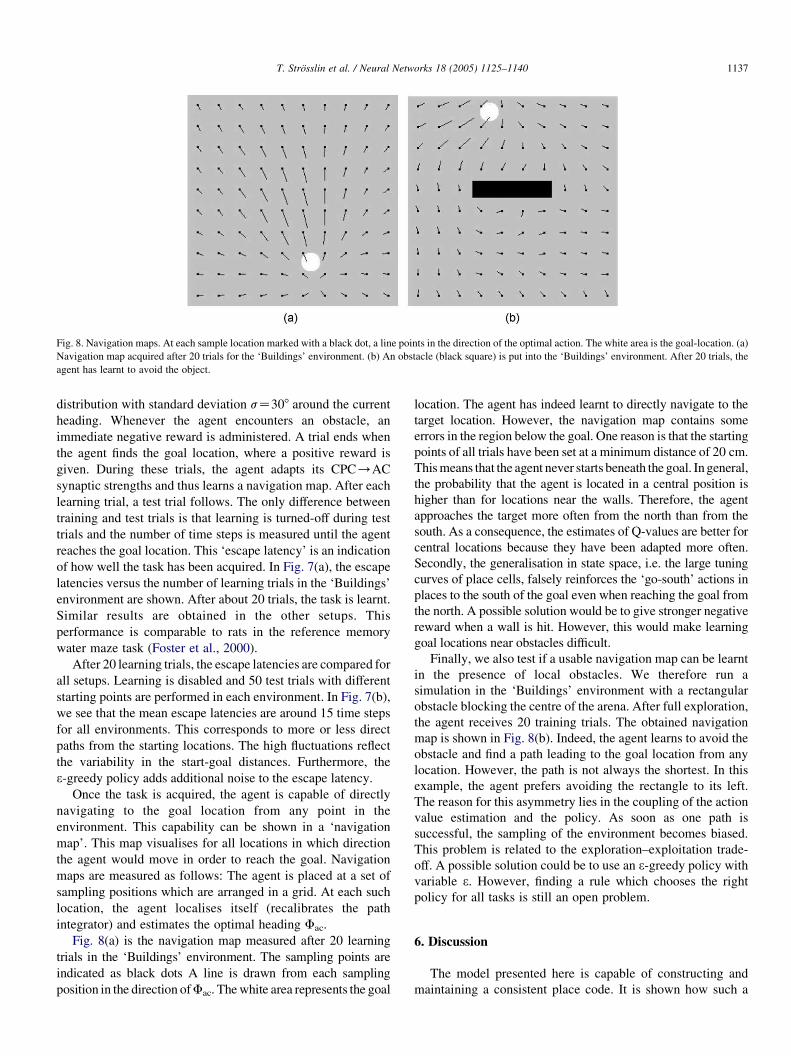
Fig. 8. Navigation maps. At each sample location marked with a black dot, a line points in the direction of the optimal action. The white area is the goal-location. (a)

Navigation map acquired after 20 trials for the ‘Buildings’ environment. (b) An obstacle (black square) is put into the ‘Buildings’ environment. After 20 trials, the

agent has learnt to avoid the object.

T. Strosslin et al. / Neural Networks 18 (2005) 1125–1140 1137

distribution with standard deviation sZ308 around the current

heading. Whenever the agent encounters an obstacle, an

immediate negative reward is administered. A trial ends when

the agent finds the goal location, where a positive reward is

given. During these trials, the agent adapts its CPC/AC

synaptic strengths and thus learns a navigation map. After each

learning trial, a test trial follows. The only difference between

training and test trials is that learning is turned-off during test

trials and the number of time steps is measured until the agent

reaches the goal location. This ‘escape latency’ is an indication

of how well the task has been acquired. In Fig. 7(a), the escape

latencies versus the number of learning trials in the ‘Buildings’

environment are shown. After about 20 trials, the task is learnt.

Similar results are obtained in the other setups. This

performance is comparable to rats in the reference memory

water maze task (Foster et al., 2000).

After 20 learning trials, the escape latencies are compared for

all setups. Learning is disabled and 50 test trials with different

starting points are performed in each environment. In Fig. 7(b),

we see that the mean escape latencies are around 15 time steps

for all environments. This corresponds to more or less direct

paths from the starting locations. The high fluctuations reflect

the variability in the start-goal distances. Furthermore, the

3-greedy policy adds additional noise to the escape latency.

Once the task is acquired, the agent is capable of directly

navigating to the goal location from any point in the

environment. This capability can be shown in a ‘navigation

map’. This map visualises for all locations in which direction

the agent would move in order to reach the goal. Navigation

maps are measured as follows: The agent is placed at a set of

sampling positions which are arranged in a grid. At each such

location, the agent localises itself (recalibrates the path

integrator) and estimates the optimal heading Fac.

Fig. 8(a) is the navigation map measured after 20 learning

trials in the ‘Buildings’ environment. The sampling points are

indicated as black dots A line is drawn from each sampling

position in the direction of Fac. The white area represents the goal

location. The agent has indeed learnt to directly navigate to the

target location. However, the navigation map contains some

errors in the region below the goal. One reason is that the starting

points of all trials have been set at a minimum distance of 20 cm.

This means that the agent never starts beneath the goal. In general,

the probability that the agent is located in a central position is

higher than for locations near the walls. Therefore, the agent

approaches the target more often from the north than from the

south. As a consequence, the estimates of Q-values are better for

central locations because they have been adapted more often.

Secondly, the generalisation in state space, i.e. the large tuning

curves of place cells, falsely reinforces the ‘go-south’ actions in

places to the south of the goal even when reaching the goal from

the north. A possible solution would be to give stronger negative

reward when a wall is hit. However, this would make learning

goal locations near obstacles difficult.

Finally, we also test if a usable navigation map can be learnt

in the presence of local obstacles. We therefore run a

simulation in the ‘Buildings’ environment with a rectangular

obstacle blocking the centre of the arena. After full exploration,

the agent receives 20 training trials. The obtained navigation

map is shown in Fig. 8(b). Indeed, the agent learns to avoid the

obstacle and find a path leading to the goal location from any

location. However, the path is not always the shortest. In this

example, the agent prefers avoiding the rectangle to its left.

The reason for this asymmetry lies in the coupling of the action

value estimation and the policy. As soon as one path is

successful, the sampling of the environment becomes biased.

This problem is related to the exploration–exploitation trade-

off. A possible solution could be to use an 3-greedy policy with

variable 3. However, finding a rule which chooses the right

policy for all tasks is still an open problem.

6. Discussion

The model presented here is capable of constructing and

maintaining a consistent place code. It is shown how such a

T. Strosslin et al. / Neural Networks 18 (2005) 1125–11401138

spatial representation can be used to solve the hidden platform

Morris water-maze task. Although comparable to previous

work, this proposal mainly adds the following contributions: (i)

real-istic input. This model relies on real visual input, just like

(Arleo, Smeraldi, & Gerstner, 2004; Gaussier et al., 2000).

However, our system does not need compass nor polarising cue

in order to maintain a stable representation. (ii) recalibration.

We show how a drifting path integrator can be recalibrated

using allothetic information. Although there are other models

which perform recalibration, our proposal has several

advantages: Firstly, this simple mechanism, unlike Bayesian

methods (Herrmann et al., 1999), can easily be implemented by

neural systems. Unlike (Arleo, & Gerstner, 2000b), neither

receptive field nor place code quality information is needed for

recalibration. Secondly, the computational cost and conver-

gence speed of our mechanism is much lower than Bayesian

methods (Herrmann et al., 1999). Lastly, our method is not

restricted to particular place field shapes (Deneve et al., 2001).

(iii)Navigation in continuous space. Reward-based learning,

as used in (Arleo, & Gerstner, 2000b; Brown, & Sharp, 1995;

Burgess et al., 1994; Foster et al., 2000; Gaussier et al., 2002),

does not scale well to bigger state and action spaces.

Additionally, actions are represented by a small discrete set

of neurons. Our model is continuous in both spaces and

features a generalisation mechanism. Therefore, the learning

speed is independent of the number of used neurons. Unlike

(Brown, & Sharp, 1995; Burgess et al., 1994), a distal reward

problem is avoided by using a temporal-difference reinforce-

ment learning algorithm. Other models (Blum, & Abbott, 1996;

Redish, & Touretzky, 1998) also operate in continuous space.

However, they model locale navigation inside the hippo-

campus, which contradicts experimental data (Eichenbaum

et al., 1990; Packard, & McGaugh, 1992; Sutherland, &

Rodriguez, 1990).

The results of the present study yields a number of

predictions. These could help designing new experiments

which in turn could confirm or disprove the proposed model.

Previous results show that postsubiculum (poSb) contains head

direction cells (HD) (Ranck, 1984; Taube et al., 1990). Similar

to others (Arleo, & Gerstner, 2001; Redish, & Touretzky,

1997a), we suggest that poSb forms the output stage of a head

direction system which combines an internal heading integrator

with visual input in order to remove a heading drift. Our work,

similar to (Arleo, & Gerstner, 2000b) proposes the lateral

entorhinal cortex (lEC) as neural substrate for a purely allothetic

place code. Consequently, poSb lesions should not affect lEC

place fields. In case of conflicting idiothetic and allothetic cues,

lEC cells should follow the allothetic cue. Furthermore, we

predict that place cells in lEC are directional. Similar to (Arleo,

& Gerstner, 2000b; Redish, & Touretzky, 1997a) and contrary to

(McNaughton et al., 1996; Samsonovich, & McNaughton,

1997), we suggest that the medial entorhinal cortex (mEC) and

possibly the subiculum (Sb) may form the neural substrate for a

position integrator. Lesions in poSb or its afferent structures,

which may provide mEC with the animal’s heading, should

produce severe inconsistencies in mEC. Indeed, it has been

shown that such lesions produce severe behavioural deficits

(Taube, Klessak, & Cotman, 1992). Furthermore, mEC place

fields are predicted to be non-directional even when the animal’s

movement is restricted. Disrupting the allothetic pathway and in

particular lesioning lEC/mEC connections should produce a

drifting position integrator. In our model, position integration in

mEC and a visual place code in lEC combine into a combined

spatial map in the hippocampal region CA1 and possibly Sb.

Lesions in mEC should leave CA1 with more broadly tuned,

purely allothetic, directional place cells. In contrast, lesions in

lEC should produce omnidirectional firing in CA1 even in cases

where these cells are normally directional. Lesions to the HD

system should disrupt place cell firing in HPC. However, joint

lesions in mEC should improve performance again (if lEC is still

intact) and leave the hippocampus with broadly tuned,

directional, allothetic place cells.

Many important issues in hippocampal function in general

and it’s significance to spatial learning in particular are yet

unanswered. Several experiments indicate that a wide range of

species use some sort of path integration (Etienne, Boulens,

Maurer, Rowe, & Siegrist, 2000; Wehner, 2003). Despite

considerable effort, however, little is known about the

underlying mechanisms. Experimental data show that hippo-

campus and fornix lesions disrupt path integration

(Maaswinkel, Jarrard, & Whishaw, 1999; Whishaw, &

Maaswinkel, 1998). However, other data also suggests that

path integration is possible without the hippocampus proper

(Alyan, & McNaughton, 1999; Alyan, Paul, Ellesworth, White,

& McNaughton, 1997). It is still unclear how these

experimental results can be reconciled. Place cells are strongly

influenced by vision. However, somatosensory, olfactive and

internal (self-motion) cues seem to contribute to the formation

and maintenance of place fields (Etienne et al., 2000; Lavenex,

& Schenk, 1998; Markus et al., 1994; Quirk et al., 1990; Save

et al., 2000). It is not yet clear how these different modalities

are integrated into one stable representation. This model could

learn to represent several environments. New place cells would

have to be recruited. Rats can, however, reuse place cells in

several environments. Their place fields in those environments

are totally unrelated (Kubie, & Ranck, 1983; Thompson, &

Best, 1989). We are not aware of any biologically plausible

place cell model which (i) depends on path integration, (ii) can

code for several environments and (iii) features totally

unrelated place fields in those environments. Indeed, the

underlying principle of these effects are still open questions.

References

Alyan, S., & McNaughton, B. L. (1999). Hippocampectomized rats are capable

of homing by path integration. Behavioral Neuroscience, 113(1), 19–31.

Alyan, S. H., Paul, B. M., Ellesworth, E., White, R. D., & McNaughton, B. L.

(1997). Is the hippocampus required for path integration? Society for

Neuroscience Abstracts, 23, 504.

Amaral, D. G., & Witter, M. P. (1989). The three-dimensional organization of

the hippocampal formation: A review of anatomical data. Neuroscience,

31(3), 571–591.

Amaral, D. G., & Witter, M. P. (1995). Hippocampal formation. In G. Paxinos

(Ed.), The Rat Nervous System (2nd ed.) (pp. 443–493). Academic Press

(Chapter 21).

T. Strosslin et al. / Neural Networks 18 (2005) 1125–1140 1139

Amari, S.-I. (1977). Dynamics of pattern formation in lateral-inhibition type

neural fields. Biological Cybernetics, 27, 77–87.

Arleo, A., & Gerstner, W. (2000a). Modeling rodent head-direction cells and

place cells for spatial learning in bio-mimetic robotics. In J.-A. Meyer, A.

Berthoz, D. Floreano, H. L. Roitblat, & S. W. Wilson (Eds.), From Animals

to Animats VI (pp. 236–245). Cambridge MA: MIT Press.

Arleo, A., & Gerstner, W. (2000b). Spatial cognition and neuro-mimetic

navigation: A model of hippocampal place cell activity. Biological

Cybernetics, Special Issue on Navigation in Biological and Artificial

Systems, 83, 287–299.

Arleo, A., & Gerstner, W. (2001). Spatial orientation in navigating agents:

Modeling head-direction cells. Neurocomputing, 38(40), 1059–1065.

Arleo, A., Smeraldi, F., & Gerstner, W. (2004). Cognitive navigation based on

nonuniform gabor space sampling, unsupervised growing networks, and

reinforcement learning. IEEE Transactions on Neural Networks, 15(3),

639–652.

Arleo, A., Smeraldi, F., Hug, S., & Gerstner, W. (2001). Place cells and spatial

navigation based on 2d visual feature extraction, path integration, and

reinforcement learning. In T. K. Leen, T. G. Dietterich, & V. Tresp (Eds.),

Advances in neural information processing systems 13 (pp. 89–95).

Cambridge MA: MIT Press.

Blum, K. I., & Abbott, L. F. (1996). A model of spatial map formation in the

hippocampus of the rat. Neural Computation, 8, 85–93.

Boucheny, C., Brunel, N., & Arleo, A. (2005). A continuous attractor network

model without recurrent excitation: Maintenance and integration in the

head direction cell system. Journal of Computational Neuroscience, 18(2),

205–227.

Brown, M. A., & Sharp, P. E. (1995). Simulation of spatial-learning in the

Morris water maze by a neural network model of the hippocampal-

formation and nucleus accumbens. Hippocampus, 5, 171–188.

Burgess, N., Donnett, J. G., Jeffery, K. J., & O’Keefe, J. (1997). Robotic and

neuronal simulation of the hippocampus and rat navigation. Philosophical

Transactions of the Royal Society London B, 352, 1535–1543.

Burgess, N., Jackson, A., Hartley, T., & O’Keefe, J. (2000). Predictions derived

from modelling the hippocampal role in navigation. Biological Cyber-

netics, 83, 301–312.

Burgess, N., Recce, M., & O’Keefe, J. (1994). A model of hippocampal

function. Neure Networks, 7, 1065–1081.

Buzsaki, G. (1984). Feed-forward inhibition in the hippocampal formation.

Progress in Neurobiology, 22, 131–153.

Deneve, S., Latham, P. E., & Pouget, A. (2001). Efficient computation and cue

integration with noisy population codes. Nature Neuroscience, 4(8), 826–

831.

Eichenbaum, H., Stewart, C., & Morris, R. G. M. (1990). Hippocampal

representation in place learning. Journal of Neuroscience, 10(11), 3531–

3542.

Etienne, A. S., Boulens, V., Maurer, R., Rowe, T., & Siegrist, C. (2000). A brief

view of known landmarks reorientates path integration in hamsters.

Naturwissenschaften, 87(11), 494–498.

Foster, D. J., Morris, R. G. M., & Dayan, P. (2000). A model of hippocampally

dependent navigation, using the temporal difference learning rule.

Hippocampus, 10(1), 1–16.

Freund, T. F., Powell, J. F., & Smith, A. D. (1984). Tyrosine hydroxylase-

immunoreactive boutons in synaptic contact with identified striatonigral

neurons, with particular reference to dendritic spines. Neuroscience, 13(4),

1189–1215.

Gabor, D. (1946). Theory of communication. Journal of the IEE, 93, 429–457.

Gaussier, P., Joulain, C., Banquet, J. P., Leprere, S., & Revel, A. (2000). The

visual homing problem: An example of robotics/biology cross fertilization.

Robotics and Autonomous Systems, 30(1-2), 155–180.

Gaussier, P., Lepretre, S., Joulain, C., Revel, A. Quoy, M., & Banquet J. P.

(1998). Animal and robot learning: Experiments and models about visual

navigation. In 7th European Workshop on Learning Robots, Edinburgh,

UK.

Gaussier, P., Revel, A., Banquet, J. P., & Babeau, V. (2002). From view cells

and place cells to cognitive map learning: Processing stages of the

hippocampal system. Biological Cybernetics, 86(1), 15–28.

Georgopoulos, A. P., Schwartz, A., & Kettner, L. E. (1986). Neuronal

population coding of movement direction. Science, 233, 1416–1419.

Gerstner, W., & Abbott, L. F. (1997). Learning navigational maps through

potentiation and modulation of hippocampal place cells. Journal of

Computational Neuroscience, 4(1), 79–94.

Hartley, T., Burgess, N., Lever, C., Cacucci, F, & O’Keefe, J. (2000). Modeling

place fields in terms of the cortical inputs to the hippocampus.

Hippocampus, 10, 369–379.

Hasselmo, M. E., Bodelon, C., & Wyble, B. P. (2002). A proposed function for

hippocampal theta rhythm: Separate phases of encoding and retrieval

enhance reversal of prior learning. Neural Computer, 14(4), 793–817.

Hasselmo, M. E., & Bower, J. M. (1993). Acetylcholine and memory. Trends in

Neurosciences, 16(6), 218–222.

Herrmann, J. M., Pawelzik, K., & Geisel, T. (1999). Self-localization of

autonomous robots by hidden representations. Autonomous Robots, 7(1),

31–40.

Hubel, D. H., & Wiesel, T. N. (1962). Receptive fields, binocular interaction

and functional architecture in the cat’s visual cortex. Journal of Physiology,

160, 106–154.

Hughes, A. (1977). The topography of visuon in mammals of contrasting life

style: Comparative optics and retinal organisation. In F. Crescitelli, The

visual system in vertebrates, Handbook of sensory physiology (Vol. 7/5)

(pp. 613–756). Berlin: Springer-Verlag (Chapter 11).

Jeffery, K. J. (Ed.). (2003). The neurobiology of spatial behavior. Oxford

University Press.

Knierim, J. J., Kudrimoti, H. S., & McNaughton, B. L. (1995). Place cells, head

direction cells, and the learning of landmark stability. Journal of

Neuroscience, 15, 1648–1659.

Koene, R. A., Gorchetchnikov, A., Cannon, R. C., & Hasselmo, M. E.

(2003). Modeling goal-directed spatial navigation in the rat based on

physiological data from the hippocampal formation. Neural Networks,

16(5-6), 577–584.

Kubie, J. L., & Ranck, J. B. (1983). Sensory-behavioral correlates in individual

hippocampus neurons in three situations: Space and context. In W. Seifert

(Ed.), Neurobiology of the Hippocampus (pp. 433–447). New York:

Academic Press.

Lavenex, P., & Schenk, F. (1998). Olfactory traces and spatial learning in rats.

Animal Behaviour, 56, 1129–1136.

Maaswinkel, H., Jarrard, L. E., & Whishaw, I. Q. (1999). Hippocampectomized

rats are impaired in homing by path integration. Hippocampus, 9(5), 553–

561.

Markus, E. J., Barnes, C. A., McNaughto, B. L., Gladden, V. L., & Skaggs,

W. E. (1994). Spatial information content and reliability of hippocampal cal

neurons: Effects of visual input. Hippocampus, 4, 410–421.

McNaughton, B. L., Barnes, C. A., Gerrard, J. L., Gothard, K., Jung, M. W.,

Knierim, J. J., et al. (1996). Deciphering the hippocampal polyglot: the

hippocampus as a path integration system. Journal of Experimental

Biology, 199(1), 173–185.

McNaughton, B. L., Barnes, C. A., & O’Keefe, J. (1983). The contributions of

position, direction, and velocity to single unit activity in the hippocampus

of freely-moving rats. Experimental Brain Research, 52, 41–49.

Miller, R. (1991). Cortico-hippocampal interplay and the representation of

contexts in the brain. Berlin: Springer.

Mondada, F., Franzi, E., & Ienne, P. (1994). Mobile robot miniaturization: A

tool for investigation in control algorithms. In T. Yoshikawa, & F.

Miyazaki (Eds.), Proceedings of the third international symposium on

experimental robotics (pp. 501–513). Tokyo: Springer.

Morris, R. G. M. (1981). Spatial localization does not require the presence of

local cues. Learning and Motivation, 12, 239–260.

Muller, R. U., Bostock, E., Taube, J. S., & Kubie, J. L. (1994). On the

directional firing properties of hippocampal place cells. Journal of

Neuroscience, 14(12), 7235–7251.

Muller, R. U., & Kubie, J. L. (1987). The effects of changes in the environment

on the spatial firing of hippocampal complex-spike cells. Journal of

Neuroscience, 7, 1951–1968.

O’Keefe, J., & Burgess, N. (1996). Geometric determinants of the place fields

of hippocampal neurons. Nature, 381, 425–428.

T. Strosslin et al. / Neural Networks 18 (2005) 1125–11401140

O’Keefe, J., & Dostrovsky, J. (1971). The hippocampus as a spatial map.

Preliminary evidence from unit activity in the freely-moving rat. Brain

Research, 34, 171–175.

O’Keefe, J., & Nadel, L. (1978). The Hippocampus as a cognitive map. Oxford:

Clarendon Press.

O’Keefe, J., & Recce, M. (1993). Phase relationship between hippocampal

place units and the EEG theta rhythm. Hippocampus, 3, 317–330.

Otto, T., Ding, C., Cousens, G., & Schiller, K. (1996). Effects of lateral vs.

medial entorhinal cortex aspiration on the acquisition of odor-place

associations. Society for Neuroscience Abstracts, 22, 1120.

Packard, M. G., & McGaugh, L. (1992). Double dissociation of fornix and

caudate nucleus lesions on acquisition of two water maze tasks: Further

evidence for multiple memory systems. Behavioral Neuroscience, 106(3),

439–446.

Pouget, A., Deneve, S., & Duhamel, J. R. (2002). A computational perspective

on the neural basis of multisensory spatial representations. Nature Review

Neuroscience, 3(9), 741–747.

Quirk, G. J., Muller, R. U., & Kubie, J. L. (1990). The firing of hippocampal

place cells in the dark depends on the rat’s recent experience. Journal of

Neuroscience, 10(6), 2008–2017.

Quirk, G. J., Muller, R. U., Kubie, J. L., & Ranck, J. B. Jr. (1992). The

positional firing properties of medial entorhinal neurons: Description and

comparison with hippocampal place cells. Journal of Neuroscience,

12(5), 1945–1963.

Ranck, J. B. Jr. (1984). Head-direction cells in the deep cell layers of dorsal

presubiculum in freely moving rats. Society for Neuroscience Abstracts, 10,

599.

Redish, A. D. (1999). Beyond the cognitive map, from place cells to episodic

memory. London: MIT Press-Bradford Books.

Redish, A. D., & Touretzky, D. S. (1997a). Cognitive maps beyond the

hippocampus. Hippocampus, 7(1), 15–35.

Redish, A. D., & Touretzky, D. S. (1997b). Navigating with landmarks:

Computing goal locations from place codes. In K. Ikeuchi, & M. Veloso

(Eds.), Symbolic visual learning (pp. 325–351). Oxford: Oxford University

Press (Chapter 12).

Redish, A. D., & Touretzky, D. S. (1998). The role of the hippocampus in

solving the morris water maze. Neural Computation, 10(1), 73–111.

Salinas, E., & Abbott, L. F. (1994). Vector reconstruction from firing rates.

Journal of Computational Neuroscience, 1, 89–107.

Samsonovich, A., & McNaughton, B. L. (1997). Path integration and cognitive

mapping in a continuous attractor neural network model. Journal of

Neuroscience, 17(15), 5900–5920.

Sanger, T. D. (2003). Neural population codes. Current Opinion Neurobiology,

13(2), 238–249.

Save, E., Nerad, L., & Poucet, B. (2000). Contribution of multiple sensory

information to place field stability in hippocampal place cells. Hippo-

campus, 10, 64–76.

Schultz, W. (1998). Predictive reward signal of dopamine neurons. Journal of

Neurophysiology, 80, 1–27.

Schultz, W., Dayan, P., & Montague, R. P. (1997). A neural substrate of

prediction and reward. Science, 275, 1593–1599.

Sesack, S. R., & Pickel, V. M. (1990). In the rat medial nucleus accumbens,

hippocampal and catecholaminergic terminals converge on spiny neurons

and are in apposition to each other. Brain Research, 527(2), 266–279.

Sharp, P. E. (1991). Computer simulation of hippocampal place cells.

Psychobiology, 19(2), 103–115.

Skaggs, W. E., McNaughton, B. L., Wilson, M. A., & Barnes, C. A. (1996).

Theta phase precession in hippocampal neuronal populations and the

compression of temporal sequences. Hippocampus, 6(2), 149–173.

Sutherland, R. J., & Rodriguez, A. J. (1990). The role of the fornix/fimbria and

some related subcortical structures in place learning and memory.

Behavioral and Brain Research, 32, 265–277.

Sutton, R., & Barto, A. G. (1998). Reinforcement learning—An introduction.

MIT Press.

Taube, J. S., Klessak, J. P., & Cotman, C. W. (1992). Lesions of the rat

postsubiculum impair performance on spatial tasks. Behavioral and Neural

Biology, 5, 131–143.

Taube, J. S., Muller, R. I., & Ranck, J. B. Jr. (1990). Head direction cells

recorded from the postsubiculum in freely moving rats. I. Description and

quantitative analysis. Journal of Neuroscience, 10, 420–435.

Tchernichovski, O., Benjamini, Y., & Golani, I. (1998). The dynamics of

long-term exploration in the rat. Part i. A phase-plane analysis of the

relationship between location and velocity. Biological Cybernetics,

78(6), 423–432.

Thompson, L. T., & Best, P. J. (1989). Place cells and silent cells in the

hippocampus of freely-behaving rats. Journal of Neuroscience, 9(7), 2382–

2390.

Touretzky, D. S., & Redish, A. D. (1996). A theory of rodent navigation based

on interacting representations of space. Hippocampus, 6(3), 247–270.

Wan, H. S., Touretzky, D. S., & Redish, A. D. (1994). Towards a computational

theory of rat navigation. In M. Mozer, P. Smolensky, D. S. Touretzky, J.

Elman, & A. Weigend (Eds.), Proceedings of the 1993 connectionist

models summer school (pp. 11–19). Hillsdale, NJ: Erlbaum.

Wehner, R. (2003). Desert ant navigation: how miniature brains solve complex

tasks. Journal of Comparative Physiology A—Neuroethology Sensory

Neural and Behavioral Physiology, 189(8), 579–588.

Whishaw, I. Q., & Maaswinkel, H. (1998). Rats with fimbria-fornix lesions are

impaired in path integration: a role for the hippocampus in sense of

direction. Journal of Neuroscience, 18(8), 3050–3058.

Whishaw, I. Q., & Mittleman, G. (1991). Hippocampal modulation of nucleus

accumbens: Behavioral evidence from amphetamine-induced activity

profiles. Behavioral and Neural Biology, 55, 289–306.

Winson, J. (1978). Loss of hippocampal theta rhythm results in spatial memory

deficits in the rat. Science, 201(160), 163.

Zhang, K. (1996). Representation of spatial orientation by the intrinsic

dynamics of the head-direction cell ensemble: A theory. Journal of

Neuroscience, 16(6), 2112–2126.