This electronic thesis or dissertation has been

downloaded from the King’s Research Portal at

https://kclpure.kcl.ac.uk/portal/

Take down policy

If you believe that this document breaches copyright please contact librarypure@kcl.ac.uk providing

details, and we will remove access to the work immediately and investigate your claim.

END USER LICENCE AGREEMENT

Unless another licence is stated on the immediately following page this work is licensed

under a Creative Commons Attribution-NonCommercial-NoDerivatives 4.0 International

licence. https://creativecommons.org/licenses/by-nc-nd/4.0/

You are free to copy, distribute and transmit the work

Under the following conditions:

Attribution: You must attribute the work in the manner specified by the author (but not in anyway that suggests that they endorse you or your use of the work).

Non Commercial: You may not use this work for commercial purposes.

No Derivative Works - You may not alter, transform, or build upon this work.

Any of these conditions can be waived if you receive permission from the author. Your fair dealings and

other rights are in no way affected by the above.

The copyright of this thesis rests with the author and no quotation from it or information derived from it

may be published without proper acknowledgement.

Economic evidence of the impact of the Dutch disease’s predictions on key labourmarket outcomes in resource-rich countriesa case study of Nigeria

Doukoure, Moustapha

Awarding institution:King's College London

Download date: 26. Aug. 2022

1

Economic Evidence of the Impact of the Dutch Disease’s Predictions on Key

Labour Market Outcomes in Resource-Rich Countries:

A Case Study of Nigeria

A Thesis submitted for the award of the degree of

DOCTOR OF PHILOSOPHY

From

King’s College London University

Department of International Development

2019

By

Moustapha Doukoure

2

Declaration

I, Moustapha Doukoure, certify that all the material in this thesis, submitted for the Doctor of

Philosophy degree, from the Department of International Development of King’s College

London University, is my original work unless specifically acknowledged and/or referenced.

Further, no material from this thesis has previously been submitted and/or approved for any other

degree to any other academic institutions.

Moustapha Doukoure

3

Acknowledgements

To my God:

“I know that all things are working for my good, You are intentional and never

failing. I can always smile because I know You are working for my good.

Through the hurt and the pain, I know You were and are working for my good”

I would like to thank my supervisor Mr. Paul Segal, who patiently guided me through the

meandering PhD process. I would like to extend my appreciation to Ms. Ekaette Ikpe, my second

supervisor. Without my supervisors’ comments and constructive criticisms, I would not have

made it through one of the most challenging academic exercises I can think of.

I also thank Michael W. and Johanne B. from the World Bank for encouraging to me to embark

on this adventure and their help in gathering some of the data. I am extending my thanks to Hayk

and Jev for sharing Matlab and Dynare tips and answering all my random questions. I will also

take the opportunity to thank Esthie and James for their editing help, as well as the staff and

colleagues from the Department of International Development for their guidance through these

PhD years.

Further, I especially feel indebted to all my friends, in particular Aarushi and Kari, for being a

source of inspiration; Kay, for all the fun and not so fun moments we shared throughout this

process; as well as Yinka and Nana for challenging me and keeping me disciplined.

My greatest appreciation goes to my family for all the support and love through these years.

Their precious care and encouragement were paramount in my completing this work. Finally, I

am grateful to Amanda - my then-girlfriend and now wife - for her patience, sense of sacrifice

and encouragement from day one of this process. To her and our future + one(s), I just want to

say I love you …

4

Abstract

The Dutch Disease framework emerged as a key mechanism through which resource revenue

impacts the economy within the larger body literature on the “natural resource curse”. On the one

hand, it is a dynamic economic adjustment from one equilibrium to another with higher real

consumption wages, owing to the fall in import prices from the inflow of resource revenue.

However, on the other, this adjustment often results in reduced investment in productive

activities and human capital development, in favour of counterproductive activities such as rent-

seeking behaviour and possible corruption; thus, it is a source of concern of many policymakers.

Building on the empirical work on Dutch Disease (DD) which presents relatively mixed

evidence, this thesis aims to investigate an area of the literature that has received less attention,

namely the impact of the DD framework predictions on labour market outcomes, such as the

employment level and wages, within a resource-rich developing country. For the purpose of this

analysis, the case of Nigeria was selected as the country showcases some of the issues related to

the resource curse and DD in particular.

This study is based on different quantitative methods, namely graphical and econometric ones, as

well as dynamic modelling. This is to bring together macroeconomic and microeconomic

evidence to unravel some of the underlying mechanisms through which oil revenue management

affects labour market outcomes. In doing so, it is suggested that resource revenue management

and the resulting policies are key factors contributing to the conversion of a “natural resource

curse” into a “natural resource blessing” – in particular, in terms of the impact of the Dutch

Disease prediction on labour market outcomes, such as employment levels and wages.

This analysis contributes to the existing literature in three different ways. It shows: 1) the

existence of a long- and short-run relationship between employment level, capital formation and

exchange rate; 2) the influence of oil revenue on wage levels and wage inequality observed in

Nigeria and 3) the impact of an oil shock on an economy with a large informal sector.

Indeed, the existence of a long-term relationship between employment, capital formation and

exchange rate, with employment levels being negatively affected by Real Effective Exchange

Rate (REER) appreciation as well as being complementary to capital has been confirmed. This

implies that an increase in capital will positively affect the level of employment. To further

5

analyse this relationship, a firm-level panel survey was used to assess firm behaviour in relation

to sector-specific exchange rates in the short term. The analysis of the survey also indicates that

the exchange rate appreciation, which is linked to possible inflows of foreign currency, will, in

the short run, negatively impact the labour market while playing a positive role in determining

the level of capital through a substitution of relatively cheaper capital for relatively more

expensive labour.

In line with this evidence, the influence of oil revenue on wage levels observed in Nigeria is

explored. Given that the oil is concentrated in a specific region of the country (i.e. the Niger

Delta region), my analysis explores the impact of fiscal federalism and oil redistribution on wage

levels and investigates if oil contributes to inequality in wage levels across the country. The

revenue sharing formula of the country implies that the resource-rich region receives significant

oil revenue. With limited mobility in the country, it was found that firms located in the oil-rich

region pay a wage premium compared to firms in other parts of the country. It was also found

that this relationship holds for assumed similar levels of productivity and across sectors with a

higher wage premium found in the services compared to the manufacturing sector. This analysis

also assesses other possible mechanisms, such as the ability to obtain government contracts and

the local price of inputs (i.e. local inflation in the oil-rich region).

Finally, to complete the picture, a DSGE model is built by considering the specificities of

Nigeria, such as its credit constraints, wage and price stickiness, as well as its large informal

sector, to assess different fiscal policy options. The analysis indicates that although the formal

and informal sector benefit from the DD’s spending effect through higher wages, the resulting

low private investment in capital may take the economy on a lower growth path. In addition,

saving options are, in the short term, mitigating the impact of the boom, even in the presence of

the informal sector. Bringing these different aspects together, it is clear that Nigeria’s oil revenue

has impacted economic and labour market outcomes. This impact has cut across different aspects

of the labour market, influencing both the employment level and labour prices in the country (i.e.

wages). This has raised several policy-related issues, such as the role of revenue sharing rules on

the country’s overall competitiveness. Further, despite the large informal sector, the saving

option still has superior outcomes compared to the spend as-you-go policy option.

6

This study concludes by arguing that to be able to better approach the adjustment process

induced by the DD and mitigate its impact on the labour market, strong institutions are required

to promote efficient and fair policies that will enable Nigeria to move away from rent-seeking

behaviour. This will help resource-rich developing countries to mitigate shocks by developing

appropriate policies responses. The lack of such policies could have lasting effects, preventing

the private sector’s capacity to sustainably generate work and decent wages.

7

Table of Contents

Declaration ...................................................................................................................................... 2

Acknowledgements ......................................................................................................................... 3

Abstract ........................................................................................................................................... 4

Table of Contents ............................................................................................................................ 7

List of Tables ................................................................................................................................ 13

List of Charts................................................................................................................................. 14

Chapter 1 Introduction .................................................................................................................. 16

1.1 Principal Research Question .......................................................................................... 19

1.2 Employment and Exchange Rates .................................................................................. 20

1.2.1 Research Question and Contribution ...................................................................... 20

1.2.2 Methodology and Data ............................................................................................ 21

1.3 Wage Determination: ..................................................................................................... 23

1.3.1 Research Question and Contribution ...................................................................... 23

1.3.2 Methodology and Data ............................................................................................ 24

1.4 Informal Sector and Fiscal policies ................................................................................ 25

1.4.1 Research question and contribution ........................................................................ 25

1.4.2 Methodology and data............................................................................................. 25

1.5 Summary of the Thesis Structure ................................................................................... 26

Chapter 2 Overarching Framework – The Dutch Disease ............................................................ 28

2.1 The Booming tradable sector and the Dutch Disease framework .................................. 36

2.1.1 The Dutch Disease’s Spending Effect .................................................................... 37

2.1.2 The Dutch Disease’s Resource movement effect ................................................... 38

2.1.3 The Dutch Disease and its economic impact .......................................................... 39

2.1.4 Alternative views on the Dutch Disease ................................................................. 40

8

2.2 Empirical Literature and Rationale for Focusing on Salient Key Relationships ........... 43

2.3 Exchange Rates and the Dutch Disease ......................................................................... 45

2.3.1 The Role of Commodities in Determining Exchange Rates ................................... 45

2.3.2 Other Channels for Exchange Rate Determination ................................................. 46

2.3.3 The determinants of the exchange rate in the Nigerian context.............................. 47

2.3.4 The chosen approach to the Exchange Rate ........................................................... 48

2.3.5 Empirical Review of the Impact of Exchange Rate movements on Employment .. 49

2.4 Wage Determination and Dutch Disease ....................................................................... 50

2.4.1 Resource Abundance and Wage Determination ..................................................... 51

2.4.2 Impact of Resource Revenue on Wages ................................................................. 51

2.4.3 Alternative Wage Determination Theories ............................................................. 52

2.4.4 Wage Determination: Empirical Literature ............................................................ 53

2.4.5 Impact of Oil on Wages at the Subnational Level .................................................. 54

2.5 Informality, Fiscal Policy and Dutch Disease ................................................................ 57

2.5.1 Fiscal Policy and the Dutch Disease framework .................................................... 57

2.5.2 DSGE modelling and developing Resource-Rich Countries’ specificities ............. 59

Chapter 3: The Nigerian Economy and Labour Market ............................................................... 64

3.1 Introduction .................................................................................................................... 64

3.2 Oil Abundance................................................................................................................ 65

3.3 Resources location within the Country .......................................................................... 68

3.4 Oil and Social Tension ................................................................................................... 69

3.5 Fiscal Policy ................................................................................................................... 72

3.6 Inflexible exchange rate policy and its impact on economic growth ............................. 76

3.7 Financial Markets and interest rate policies ................................................................... 81

3.8 Economic Growth - Gross Domestic Product ................................................................ 85

9

3.9 Composition of the Nigerian Labour Market ................................................................. 90

3.10 Labour Market and Wages ............................................................................................. 92

3.11 Regional Disparity in Terms of Economic Activities .................................................... 93

3.12 Labour Demand: A Picture of the Private Sector ........................................................... 95

3.12.1 Informality and Non-Farm Enterprises (NFE) ........................................................ 96

3.12.2 Unproductive Formal Sector ................................................................................... 98

3.13 Conclusions .................................................................................................................. 101

Chapter 4 Analytical evidence of the impact of Dutch Disease on the Labour Market: REER and

Firms ........................................................................................................................................... 104

4.1 Introduction .................................................................................................................. 104

4.2 Exchange Rate and Employment ................................................................................. 106

4.2.1 Macroeconomic Channel ...................................................................................... 106

4.2.2 Microeconomic Channels ..................................................................................... 107

4.3 Evidence of the Link between Exchange Rates Movement and Employment Levels . 108

4.4 Empirical Approach ..................................................................................................... 111

4.5 Macroeconomic Evidence in Nigeria ........................................................................... 112

4.5.1 Model Specification .............................................................................................. 113

4.5.2 Data ....................................................................................................................... 113

4.5.3 Methodology ......................................................................................................... 114

4.5.4 Empirical Implementation .................................................................................... 120

4.5.5 Conclusions ........................................................................................................... 131

4.6 Micro-level evidence on the exchange rate impact on firms ....................................... 132

4.6.1 The Employment Equation ................................................................................... 134

4.6.2 Source of Simultaneity and Endogeneity in the Wage Equation .......................... 136

4.6.3 Dynamic Panel GMM Estimation ......................................................................... 137

10

4.6.4 Data on Nigerian Manufacturing Firms ................................................................ 140

4.6.5 Empirical Evidence: The Role of the Exchange Rate on Employment ................ 148

4.6.6 Conclusions ........................................................................................................... 157

4.7 Appendices ................................................................................................................... 159

Appendix 1: The number of significant lags ........................................................................... 159

Appendix 2: Relationship between variables of interest, and past realisations ................... 160

Appendix 3: Strength of instruments ................................................................................... 162

5 Chapter 5 Oil Abundance and Inequality in Wages: A Decomposition Analysis ............... 164

5.1 Introduction .................................................................................................................. 164

5.2 Theoretical Framework and Empirical Implementation .............................................. 166

5.3 Country Background .................................................................................................... 168

5.3.1 “Point Resource” - Oil Produced in a Specific Region......................................... 168

5.3.2 Impact of Oil at the State Level ............................................................................ 168

5.4 Empirical Approach ..................................................................................................... 172

5.4.1 Wage Equation ...................................................................................................... 172

5.4.2 Calculation and Decomposition of Wage Inequality ............................................ 173

5.5 Data .............................................................................................................................. 175

5.6 Results .......................................................................................................................... 181

5.6.1 Wage Equation ...................................................................................................... 181

5.6.2 Wage Equation Robustness Check ....................................................................... 183

5.6.3 Differences between Services and Manufacturing Sectors ................................... 189

5.6.4 Wage Decomposition and Wage Inequality ......................................................... 191

5.7 Discussions ................................................................................................................... 194

5.7.1 Impact of Oil on Wage Determination .................................................................. 195

5.7.2 Discussions around observed wage inequalities ................................................... 197

11

5.8 Annexe ......................................................................................................................... 199

5.8.1 Descriptive Statistics ............................................................................................. 199

5.8.2 Wage decomposition using the total wage bill as a dependent variable ............... 200

5.8.3 Wage decomposition service sector ...................................................................... 200

5.8.4 Wage decomposition – Manufacturing firms ....................................................... 202

5.8.5 Wage decomposition – Detailed Computation ..................................................... 203

Chapter 6: Oil Shocks in a Developing Resource-Rich Economy – a DSGE Approach ........... 206

6.1 Introduction .................................................................................................................. 206

6.2 Approach ...................................................................................................................... 207

6.3 A Small Open Economy Model ................................................................................... 211

6.3.1 Details of the model .............................................................................................. 212

6.3.2 Domestic Households ........................................................................................... 215

6.3.3 Domestic Production ............................................................................................. 223

6.3.4 Foreign Sector ....................................................................................................... 227

6.3.5 Monetary Policy Rules .......................................................................................... 228

6.3.6 Fiscal Policy .......................................................................................................... 228

6.4 Model Calibration ........................................................................................................ 230

6.5 Response of Economy to Structural Shocks ................................................................ 235

6.5.1 Spending as You Go – Baseline Scenario............................................................. 236

6.5.2 Alternative Scenarios ............................................................................................ 239

6.6 Conclusions .................................................................................................................. 241

6.7 Annexe ......................................................................................................................... 243

6.7.1 Calibration Parameters .......................................................................................... 243

6.7.2 Log-Linearised Model .......................................................................................... 244

Chapter 7: Concluding remarks .................................................................................................. 252

12

7.1 Introduction .................................................................................................................. 252

7.2 Key contributions to the Literature .............................................................................. 253

7.3 Major Conclusions ....................................................................................................... 254

7.3.1 What was the Rationale for the Focus on Nigeria?............................................... 254

7.3.2 What was the Role of the RER in Explaining Employment Performance in Nigeria?

255

7.3.3 What is the Role of Oil in Wage Determination and Wage Inequality in Nigeria?

257

7.3.4 How Do Key Macroeconomic Variables Respond to Oil Shocks by Taking into

Account Formal and Informal Labour Markets? ................................................................. 259

7.4 Policy Implications ....................................................................................................... 260

7.5 Suggestions for Further Analysis ................................................................................. 262

13

List of Tables

Table 1: Summary of the Dutch Disease’s Impact ....................................................................... 40

Table 2: Share of Oil Production Per State in Nigeria in 2015 ..................................................... 69

Table 3: Composition of Output, Employment and Exports ........................................................ 88

Table 4: Augmented Dickey-Fuller Test on all Variables .......................................................... 122

Table 5: Phillips-Peron Test on all Variables ............................................................................. 122

Table 6: Lag Selection VECM .................................................................................................... 123

Table 7: Johansen’s test for Cointegration .................................................................................. 124

Table 8: Long Term Relationships Between Variables of Interest ............................................. 124

Table 9: Short-Run Dynamics Between Variables of Interest .................................................... 126

Table 10: Lagrange-multiplier test.............................................................................................. 127

Table 11: Normality Tests .......................................................................................................... 127

Table 12: Long-Run Relationship Between Total Employment and Key Variables .................. 129

Table 13: Short-Run Dynamics Between Total Employment and Key Variables ...................... 129

Table 14: Lagrange-multiplier test.............................................................................................. 130

Table 15: Normality Tests .......................................................................................................... 130

Table 16: Numbers of Observations Per Year and Sector .......................................................... 141

Table 17: Aggregate Employment Per Sector ............................................................................ 142

Table 18: Average Employment Per Sector (Log 1000s) ........................................................... 142

Table 19: Average Amount of Capital Per Sector (Log Millions of Naira) ............................... 142

Table 20: Average Log Output Per Sector (Log Millions of Naira) ........................................... 143

Table 21: Measure of Productivity - Average Output Per Worker (Log Millions of Naira) ...... 143

Table 22: Estimates of the Relationship between REER and Employment ............................... 150

Table 23: Relationship Between REER and Employment with additional control variables..... 153

Table 24: Key Relationship Estimates (GMM) .......................................................................... 155

Table 25: How Many Lags Are Significant? .............................................................................. 159

Table 26: Relationship Between Variables of Interest, and Past Realisations ........................... 160

Table 27: Do Firms’ Variables Adjust to Past Realisations? ...................................................... 162

Table 28: Level Equation (Top Part) – Difference Equation (Bottom Part) ............................... 163

14

Table 29: Estimate Log Wage Per Worker and Relevant Variables ........................................... 182

Table 30: Estimated Total Wage Bill and Relevant Variables ................................................... 183

Table 31: Estimate Using Different Proxies for oil revenue ....................................................... 184

Table 32: Estimate Including Interaction Terms Between Oil and Foreign Exposure ............... 185

Table 33: Estimate Including other costs .................................................................................... 186

Table 34: Estimate Including variable capturing government contracts .................................... 187

Table 35: Estimate for the Services Sector Only ........................................................................ 190

Table 36: Estimate for the Manufacturing Sector Only .............................................................. 191

Table 37: Wage Inequality - Gini Coefficients ........................................................................... 192

Table 38: Contribution of the Different Factors using Average Wage ....................................... 193

List of Charts

Chart1: Dutch Disease’s Spending Effect..................................................................................... 38

Chart2: Dutch Disease’s Resource effect ..................................................................................... 39

Chart 3: Share of Oil Revenue (% of Total Revenue) .................................................................. 65

Chart 4: Daily Nigerian Crude Oil production (‘000s of Barrels) ................................................ 66

Chart 5: Daily Nigerian Crude Oil production vs. Prices (US$ Per Barrel) ................................. 67

Chart 6: Oil Price vs. Nigerian government expenditure (Year on Year Change) ....................... 74

Chart 7: Average Manufacturing Capacity Utilisation (%) .......................................................... 74

Chart 8: Share of Recurrent Spending (% of Total Government Spending) ................................ 75

Chart 9: The REER (Lhs) and NER (Rhs) for the Period 1960-2014 .......................................... 80

Chart 10: Nominal exchange rate (Naira per dollar) and oil price ($ per barrel) ......................... 84

Chart 11: Oil price vs. average prime interest rate in Nigeria ...................................................... 84

Chart 12: Nominal exchange rate vs. prime interest rate .............................................................. 84

Chart 13: US Federal Reserve Bank Interest rates vs. Nigerian Interest rates ............................. 85

Chart 14: Composition of the Nigerian Labour Market in 2011/12 ............................................. 91

Chart 15: Median Wage Per Month in USD, Per Sector, 2013 .................................................... 93

Chart 16: Distribution of the Employed Labour Force, Per Type of Employer ........................... 94

Chart 17: NFE Distribution per sector and region ........................................................................ 97

15

Chart 18: Median Labour Productivity and TFP Compared to Lagos Median Firms ................. 97

Chart 19: Key Bottlenecks Faced by NFEs (LHS) and Top Three Obstacles by Zones (Rhs) .... 98

Chart 20: Median Manufacturing Firms’ TFP in Lagos v.s Regions and Comparative Countries

....................................................................................................................................................... 99

Chart 21: Nigerian Unit Labour Costs in the Manufacturing Sector vs Comparative Countries 100

Chart 22: Lagos and Other Nigerian Regions’ Unit Labour Costs in the Manufacturing Sector 100

Chart 23: Variables of Interest in Levels Compared to their First Difference............................ 120

Chart 24: Errors from the Cointegrating Equation (LHS) .......................................................... 126

Chart25: Eigenvalues (RHS)....................................................................................................... 126

Chart 26: Errors from the Cointegrating Equation (LHS) .......................................................... 130

Chart27: Eigenvalues (RHS)....................................................................................................... 130

Chart 28: Relationship Between Output Per Worker and Employment ..................................... 144

Chart 29: Employment vs. Capital Per Worker (LHS) & Output Per Worker vs. Capital Per

Worker ........................................................................................................................................ 145

Chart 30: Nominal and Real Effective Exchange Rate ............................................................... 146

Chart 31: Trade-Weighted Real Exchange Rate (Log Form) for Sectors of Interest ................. 148

Chart 32: Impact of Oil Revenue at the Subnational Level ........................................................ 169

Chart 33: Decomposition of Wage Inequality ............................................................................ 193

Chart 34: Decomposition of Firm-Level Wage Inequality: Manufacturing Firms ..................... 194

Chart 35: Decomposition of Firm-Level Wage Inequality: Services Firms ............................... 194

Chart36: Impulse Response Functions to Oil Shock .................................................................. 238

Chart 37: Selected Impulse Response Functions under Different Policy Options ..................... 240

16

Chapter 1

Introduction

Large revenue inflows from natural resources are, in theory, expected to generate wealth,

promote economic growth and enhance human development, as illustrated by the experience of

countries such as Australia, Sweden and the United States (Wright and Czelusta, 2004;

Lederman et al., 2007). These countries achieved early economic growth based on their

relatively abundant natural resource sectors. This is in line with early economic literature, which

states that economic development is limited by the amount of investment (Rostow, 1960). Thus,

natural resource revenues could play the role of triggers and provide the capital required to fast

track economic development (Sachs and Warner, 1999) and allow socio-economic growth to

accelerate. However, since the second half of the 20th century, several empirical studies have

suggested that many resource-rich countries have experienced perverse effects of natural

resource wealth, as this wealth appears to have negatively affected their economic (McKinley,

2008), social or political wellbeing (as summarised by Ross, 2014): a phenomenon known as

“the resource curse”. The first use of this term was attributed to Auty (1993), who argues in the

opening paragraph of his book that “not only do many resource-rich countries fail to benefit from

a favourable endowment, they may actually perform worse than less well-endowed countries”.

Auty (2001a, 2001b) found that some resource-rich countries, such as Nigeria, Sierra-Leone and

Angola, developed at a slower pace when compared with countries such as South Korea and

Taiwan, where resource rent represents less than 1% of GDP (World Bank database, 2019). Auty

(2007a, 2007b) observed the mechanisms of the resource curse, while Sachs and Warner (1995a,

1995b) formalised this theory by finding a negative relationship between economic growth rates

and different measures of natural resource abundance, such as mineral production or share of

primary exports, over the 1970-1989 period.

This trend has not faded, and the number of countries depending heavily on resources for over

50% of their exports has not decreased. Indeed, Dode (2012) estimated that around 75% of sub-

Saharan Africa countries and over 66% of those in Latin America, the Caribbean, North Africa

and the Middle East are still resource-dependent. Despite the significant revenue received at the

turn of the century, many resource-dependent countries are underperforming in terms of their

17

socio-economic indicators (Carneiro, 2007); they also present poor economic growth prospects

(Sachs and Warner, 2001). Despite the damning empirical evidence, Ross (1999) explains that

the resource curse’s underlying causes or transmission mechanisms are yet to be clearly

established. Nevertheless, the literature has advanced several mechanisms through which the vast

exploitation of natural resources affects the economic growth of developing countries, including

rent-seeking (Tornell et al. 1999, Auty 2001, Mehlum et al. 2006, and Robinson et al. 2006),

poor governance (see Baland et al. 2000, and Torvik 2002), political or ethnic conflict,

corruption, autocracy, (see Ross 2001, Arezki and Brückner 2011, Arezki and Gylfason 2013,

Collier et al. 2009, Tsui 2011) and excessive borrowing (see Manzano et al. 2007 and Costantini,

et al. 2006).

Among these channels, one of the key mechanisms through which natural resource wealth is

paradoxically expected to negatively affect an economy is through Dutch Disease (DD).

According to Corden and Neary (1982), Corden (1984), and Stevens (2003), DD refers to the

1960s effect that natural gas discoveries in the North Sea had on the Netherland’s manufacturing

sector. Following this discovery, the Netherlands’ income substantially increased, accompanied

by large inflows of foreign currency, resulting in: (i) the real appreciation of the exchange rate,

(ii) the decrease of non-oil exports, (iii) upward pressure on the prices of non-tradable goods, and

iv) the displacement of key production factors, mainly capital and labour, towards the gas sector

(i.e. the booming sector) and the services sector (i.e. the non-tradable sector). The trade boom

resulted in a deterioration in the production of other tradable goods and exports, as well as in an

increase in the prices of non-tradable goods. Empirical evidence related to the existence of DD

has been relatively mixed.

This, therefore, provides the rationale for the approach adopted in this thesis, which consists of

independently assessing some of the complex relationships underlying the DD framework.

Further, these predictions of DD have strong implications for resource-rich countries’ labour

markets, where empirical evidence directly assessing the underlying mechanisms remains scarce.

Indeed, despite resource revenue inflows, many resource-rich countries face difficulties in

diversifying their economies away from the resource sector, and to create much-needed

employment. For example, in Nigeria, the oil sector is estimated to employ about 300,000

persons (ILO 2005), which is small for a population of over 170 million people. The definition of

18

employment has not really evolved since the International Labour Organisation (ILO), in 1982,

defined it as “all persons above a specified age who during a specified brief period, either one

week or one day, were in the following categories: paid employment; or self-employment”.

This definition of employment is now seen as limiting in the developing country context. This is

illustrated, for example, by the concept of jobs presented by the World Bank in The Job

Challenge Report (2013, page 49), “The concept of a job is actually much broader than wage

employment. Jobs are activities that generate actual or imputed income, monetary or in-kind,

formal or informal”. This report describes jobs – including informal ones – as transformational

for three reasons. Firstly, living standards improve with job creation, thus decreasing poverty

rates. Secondly, productivity grows as efficiency increases through learning-by-doing, and

thirdly, since jobs create a sense of opportunity, social cohesion is also improved. This further

highlights the importance of jobs for developing countries, even more so in the context of

resource abundance, as it brings in the social dimension of a possible resource curse. While

acknowledging the complexity of these concepts throughout this thesis, I will mainly focus on

the level of employment (at the national and sectoral level) and wages as the key labour market

outcomes. This is mainly guided by data limitation as most datasets collect information based on

the ILO definition of employment, thus this definition remains an important indicator of interest

to policymakers.

In attempting to analyse the impact of resource revenue on labour market outcomes, Nigeria

presents itself as a good case study. This is because the country has not escaped “the curse”.

Nigeria is home to Africa’s largest economy and has been recognised as such since the GDP

rebasing exercise completed in 2014. Despite significant economic reforms placing the country

as the leading light of the “Africa rising phenomenon” (as described by Taylor, 2014), and a

return to political pluralism in 1999, Nigeria is still presented as a typical example of a country

affected by the “resource curse”, from both a political economy and economic point of view

(Mähler, 2010). Despite $1.8 trillion (in constant 2010 US$) in net income received from the sale

of oil over the last 50 years, Nigeria is struggling to significantly reduce poverty, with rates only

declining marginally from 64.2% to 62.6% between 2003/04 and 2009/10. In addition, Nigeria

has a broad-based population pyramid, with children making up 44% of the population. This

means that 4.5 million Nigerians enter the labour market each year, but only a very small number

19

are able to find formal jobs (Ufuophu-Biri 2014). These trends support arguments presenting

unemployment and underemployment as an important factor behind the emergence of terrorist

groups, especially in the poorer areas in the north of Nigeria (David et al. 2015).

This discussion highlights the fact that resource wealth does not automatically trickle down to

poorer households and may have little positive effect on employment creation. The question of

employment has long been at the centre of attention in development theory and is a key concern

of policymakers. In the context of Nigeria, as stated by Teal (2012, page 3), “governments

should undertake efforts to increase formalisation and ensure that education and skill mismatches

are addressed”. He argues that “barriers to micro and small enterprises” should be removed to

enable “them to grow” and support entrepreneurship, “while small enterprise needs to be

encouraged” (Teal, 2012 page 3). However, these recommendations appear to be disconnected

from the broader macroeconomic context dominated by the country’s resource wealth. To

address this issue, this thesis will investigate some of the economic mechanisms through which

natural resource wealth affects labour market outcomes, such as employment, through the

analysis of Nigeria as a case study, as presented in the next section.

1.1 Principal Research Question

The underlying research question of this thesis is: What is the predicted impact of Dutch Disease

symptoms on key labour market outcomes in resource-rich countries illustrated by the Nigerian

economy? Throughout this project, evidence of macro-micro linkages between the abundance of

resources and the labour market in a developing country context will be presented using some of

the predicted impacts of the Dutch Disease (DD) framework.

The relationship between resource revenue and labour market outcomes has been treated

indirectly through the impact of revenue inflows on a country’s economic performance. This

relationship is central to the existing resource curse literature (as presented in van der Ploeg,

2011; Stevens, 2003; and Frankel, 2010 literature reviews). In order to more directly assess the

relationship of interest, the DD framework presents itself as a prime candidate, through its

predictions assuming possible labour movement from tradable to non-tradable sectors, or an

upward pressure on wages in the case of limited labour mobility. However, the substantial

empirical literature has focussed on the DD’s structural impact on the economy and the

associated policy implications, such as in Corden (1984), van Wijnbergen (1984), Chatterji et al.

20

(1988), Brunstad et al. (1997), Gylfason et al. (1999), and Torvik (2002). This focus can be

explained by complex dynamics affecting the labour market, even more so as developing

countries’ markets differ with, for example, thin manufacturing sectors, large civil services, large

degrees of informality and heavy reliance on imported inputs. In addition, as highlighted by

Murshed (2008, 2011), the impact of the adjustment resulting from the inflows of resource

revenue can be mitigated by appropriate institutions and adequate policies, as illustrated by

successful resource management settings in countries as varied as Norway and Malaysia. Thus,

the roots of the resource curse may not reside in natural resource revenue inflows but may occur

due to the ability to effectively manage these revenues.

Thus, to navigate this complex nexus of interlinked relationships, the focus will be on three of

the key predictions of the DD model and, in turn, assess their impact on the labour market

outcomes of interest. In order to best unravel some of the dynamics, I have used Nigeria as a case

study within a quantitative research design. Indeed, the different datasets and analysis, as well as

interpretations, are based on a quantitative approach.

1.2 Employment and Exchange Rates

1.2.1 Research Question and Contribution

My analysis of the first key relationship underlying the DD framework will present evidence of

the relationship between real exchange rate movements (driven by oil revenue inflows) and the

level of employment in Nigeria by investigating the long-run and short-run changes in the

relative prices of capital and labour. In this section, I will answer two salient questions: What

was the role of the real exchange rate in explaining employment performance in Nigeria?; and,

How did manufacturing firms adjust to industry-specific real exchange rates?

This study is relevant as the literature has mainly focussed on the impact of the exchange rate on

macroeconomic indicators such as growth and sectoral output (Anjola et al., 2018; Ismaila, 2016;

Akinlo, 2015). Empirical evidence directly assessing the relationship between the exchange rate

and labour market outcomes in developing countries thus remains scarce (Kim, 2005; Ngandu,

2008; Hua, 2007). Most of the available studies have focused on high-income countries, with

very little attention devoted to the characteristics of developing economies. Kim (2005) argues

that since the economic structure in developing countries differs from those found in developed

countries, real exchange rate fluctuations will also have a different impact. Indeed, developing

21

countries experience higher economic growth (Mobarak, 2005) and consumption volatility

(Kose, et al. 2003), as well as an abundance of natural resources (Collier, van der Ploeg, Spence

and Venables, 2010). They also face different capital flow patterns (Gabriele et al., 2000). These

factors have significantly costlier welfare effects in developing countries compared to developed

countries (Pallage & Robe, 2003).

Departing from Frenkel and Ros’s (2006) cross-country analysis of Latin America – one of the

most noticeable empirical studies approaching part of the question at hand –this analysis will fill

a noticeable gap in the knowledge by assessing country-specific long-term relationships between

the exchange rate and the Nigerian employment level. To the best of my knowledge, the only

other study testing the direct link between exchange rate and employment level in Nigeria is

Folawewo et al.’s (2012) study, which focussed on the sectoral impact of increased aggregate

demand affecting import and export levels. This analysis differs from my own as it assesses, at

the macroeconomic level, the labour intensity transmission mechanism through which labour and

capital act as substitutes reflecting exchange rate movements. The second contribution of this

study resides in its focus on providing an assessment of the short-run dynamics of this

relationship, using the Nigerian trade-weighted industry-specific exchange rate and firm-level

panel data. This study will be the first to provide a comprehensive assessment of the exchange

rate impact on the level of employment in Nigeria.

1.2.2 Methodology and Data

The question of interest is approached from two empirical angles: first, time-series methods will

be used to analyse the macroeconomic relationship between aggregate employment and other

macroeconomic variables, including the real exchange rate and level of capital over time, and

second, micro-level data will be used to assess the short-run dynamics between the trade-

weighted industry-specific exchange rate and firm-level employment data.

To study the macroeconomic relationships and the possibility of a long-term equilibrium

relationship, a cointegration analysis will be used and Johansen’s (1991) vector error correction

model (VECM) employed. This will help address specific times series issues, such as

stationarity, that were ignored, for example, in Frenkel and Ros’s (2006) study. This method, as

discussed by Granger (1986), suggests the existence of a linear combination of non-stationary

variables that exhibit stationarity properties and thus allow for non-spurious analysis and

22

inference. This study of the relationship between employment and the exchange rate will be

based on a yearly time series from 1980 to 2010 of variables such as the real effective exchange

rate, employment, oil prices, and capital formation in order to capture macroeconomic variables

that influence the private sector’s investment, and possibly the labour/capital ratio, in Nigeria.

Although the period covered was mainly dictated to by data limitations, it nevertheless covers

key phases of the Nigerian business cycle, such as the pre- and post-structural adjustment period,

as well as the recent commodity supercycle. Most of these time series have been obtained from

the World Bank database; while the employment variable has been gleaned from the Groningen

Growth and Development Centre (GGDC) database. The GGDC data presents employment data

for ten sectors and, compared to other sources such as the ILO database, it takes into account

consistency factors such as intertemporal consistency, international consistency, and internal

consistency, meaning that these series do not present some of the structural breaks observed in

other datasets. Thus, it is best suited for my purpose.

At the micro-level, to understand some of the dynamics of adjustment, firm-level data have been

used to look at the relationship between employment and a number of variables, such as sector-

specific real exchange rates and capital formation. To assess the short-run relationship, the GMM

estimate has been used. This is the most appropriate panel econometrics method to maximise the

benefits of using a panel dataset (See Hsiao, 1986, 2007 for a discussion on benefits of panel

data). This method is applied to a panel enterprise survey which was conducted in Nigeria

between 1998 and 2003. It was collected in two successive waves by the Centre for the Study of

African Economies (Oxford) and financed by the United Nations Industrial Development

Organisation (UNIDO). The survey was completed across nine sub-sectors, including the south-

west region, eastern region and northern region of Nigeria. This survey formed the basis of

several other analyses (See Malik et al., 2008 and Aigbokhan, 2011) as it is one of the few

surveys presenting firm-level data. It will form the basis of this thesis’ analysis as it is the only

survey which was completed within the period of interest. In addition to this, and to aid the

rigour of the analysis, an industry-specific trade-weighted exchange rate, using trade data from

the World Bank database, has been built.

23

1.3 Wage Determination:

1.3.1 Research Question and Contribution

The second key relationship that this thesis investigates is the localised impact of resource

abundance revenue on wages and wage inequality. According to the DD framework, wages are

expected to be pushed upwards through aggregate demand feedback on the labour market. In

assessing this prediction, I will answer the following questions: What role does higher oil

revenue distributed to specific sub-national entities play in determining wages? How do these

determinants (including oil revenue) explain wage differentials across firms in the country?

Studies on the roots of unemployment and underemployment in Nigeria have focused mainly on

factors such as demographic trends (migration and population growth) as well as the skill

mismatch (Aigbokhan, 1988, 1992; Oni, 2006). These studies fail to acknowledge the role that

wages, and their determinants can play in influencing the employment level. This results from

the general assumption that Nigerian real wages are not very high (Adebayo, 1999) and thus,

discarding the role of wages in employers’ decisions. Within this context, the link between oil

revenue and wages at the firm level will be assessed, paying special attention to oil being

characterised as a “point resource”, meaning that the production is localised in a specific region

of the country – the South-South (i.e. the Niger Delta region). An interesting characteristic of this

region is the fact that it receives significant revenue from oil production through a revenue-

sharing arrangement determined as a part of the country’s fiscal federalism policy (Ekpo, 1994;

Aigbokhan, 1999). Such arrangements are often used to balance two potentially competing

interests, as described by Qiao et al. (2008, 1), between the notions of efficiency and equity

within the federation, and the political cohesion of the federation and assertion of entitlement to

revenues by the resource-rich regions. This very often results in oil-rich regions receiving a

significant share of the resource revenue. Such differentials in fiscal capacity, coupled with

limited labour mobility, may distort wages, affect competitiveness and motivate the adoption of

inefficient “beggar-thy-neighbour” policies by a subnational government.

To answer this question – the role of oil revenue in affecting wage level and inequalities – I will

assess the key determinants of wages by relying on efficiency wage theory, which explains how

profit-maximising firms can set wages above market-clearing levels to compensate for factors

other than human capital differences, in line with Aigbokan (2011). This class of model, which is

24

estimated through a firm-level wage equation that takes into account oil production at the

subnational level, can provide some explanation for upward wages rigidity, and possibly explain

the positive relationship between wages and unemployment. Finally, to complete this analysis, I

will assess the contribution of each of the determinants in explaining wage

differentials/inequalities across firms, as well as quantifying the pure contribution of variables

determining wages (using an equality decomposition procedure in line with Devkota et al. 2015).

1.3.2 Methodology and Data

The first step of this analysis consists of running a wage equation to identify causal effects,

following Şeker (2012), where the wage at the firm level is assumed to be determined by the size

of the firm, its exposure to international trade, and other factors including, in particular, firm-

level characteristics. The firm-specific factors provide controls that indicate whether a firm’s

age, trade union activity, share of permanent workers or if it is located in an oil-producing

region, will influence its decision to pay higher wages. This wage equation will be estimated

using OLS (see Wagstaff et al., 1991).

Then, using the Step-by-Step methodology, as described in Hosseinpoor et al. (2006), the

concept of the concentration index (CI) will be used to compute a wage Lorenz curve, and hence

a wage Gini index, to measure inequality in wages across firms. Further, applying an inequality

decomposition procedure similar to Devkota et al. (2015) allows computation of the weight of

the different determining factors, including the firm’s location in an oil-producing region, in

explaining wage inequality in the country.

To conduct this analysis, pooled cross-section data from the World Bank Enterprise Survey (ES)

2014, as well as surveys from the same source completed in 2007 and 2010, will be employed.

These surveys, based on stratified random sampling, collected a number of quantitative datasets

of information through firm-level interviews regarding the business environment the participants

faced and the productivity level of their firms. Thus, these surveys also provide information on

firm variables, such as sales, wage bills, costs of raw materials, net book values of assets, as well

as personnel data in the form of the number of permanent and temporary workers, and

production and non-production workers.

25

1.4 Informal Sector and Fiscal policies

1.4.1 Research question and contribution

The last key relationship of interest is the role of fiscal policies driven by resource revenue

inflows on labour market outcomes. This entails taking into account some features such as the

informality characterising a resource-rich developing country’s labour market. Thus, the

underlying sub-question is: How can basic fiscal policy measures affect a small oil-exporting

economy during an oil shock, taking into account the existence of a large informal sector?

An increase in natural resource exports and higher natural resource prices results in an inflow of

foreign currency, which leads to higher fiscal spending in resource-based economies (Sturm et

al., 2009). As suggested by the DD framework, the use of the influx of revenue from resources

could impact the structure of the economy as a whole, but can also make countries vulnerable to

the price volatility of exported commodities as well as the exhaustibility of natural resources.

Under these circumstances, fiscal policies are relevant for the reallocation of natural resource

revenues. To the best of my knowledge, this analysis will be the first to present a model that uses

segmented labour markets specific to resource-rich developing countries to assess the impact of

fiscal policies during a shock.

1.4.2 Methodology and data

This analysis relies on macroeconomic modelling that incorporates key characteristics of the

Nigerian labour market, including formal/informal market segmentation, as well as wage and

price stickiness, to best capture the impact of oil shocks on employment outcomes. To date, only

a few articles employ the DSGE model for oil-producing developing economies. The dynamic

stochastic general equilibrium (DSGE) model presented here will extend the work of Medina and

Soto (2007), which presents the macroeconomic dynamics of Chile, a resource-rich country. I

will enrich this model with several characteristics of a developing country, such as labour market

segmentation. The most noticeable features of this model are: (i) the assumption that variables

such as prices and wages are sticky, meaning they are partially indexed to past inflation, and (ii)

there is a persistent habit in consumption. In addition, domestic production is divided between

the formal and informal sector, similar to Ahmed’s suggestion (2012). The model also features

fiscal policy rules specific to resource-rich countries.

26

In general, DSGE models are built on microeconomic foundations. These models are dynamic

as they assign a central role to agents’ expectations and their intertemporal choices in

determining macroeconomic outcomes. DSGE models internalise the interaction between policy

decisions and agents’ behaviour, thus serving the purpose of this analysis. Finally, within such a

model, one can trace the transmission of the oil shock to the broader economy.

The DSGE model will be calibrated using Dynare and Matlab. The parameters will be calibrated

using values from the associated literature or computed, using specific data for Nigeria obtained

from sources such as the National Bureau of Statistics and, when necessary, from the literature

on emerging and low-income economies. Central Bank databases will also be used as they

include other key macroeconomic variables, such as money supply, exports, exchange rates,

imports of capital goods and gross domestic product (GDP).

1.5 Summary of the Thesis Structure

This project aims to investigate the impact of DD predictions on labour market outcomes in a

resource-rich country, using the case of Nigeria. The dissertation will be comprised of six further

chapters using various economics methods to empirically test the possible impact of oil revenue

on the labour market through the lens of the Dutch Disease framework. A brief overview of the

six following chapters is presented below.

Chapter 2 will review the existing theoretical and empirical literature on the Dutch Disease

framework’s mechanisms and predictions in general, with an emphasis on the labour market. It

will also critically assess some of the assumptions underlying the framework and review related

empirical work to show that evidence has been relatively mixed. This provides the rationale for

the approach adopted in the thesis, which consists of independently assessing some of the

complex relationships underlying the Dutch Disease framework. I will then review existing

literature around the three identified relationships/sub-problems identified in this introduction,

namely the role of the real exchange rate on the labour market; the effect and the determinants of

wages and, finally, the impact of fiscal policies on the segmented (formal vs. informal) labour

market.

Chapter 3 will assess the macroeconomic variables and the characteristics of the labour market

through the lens of the three key relationships.

27

Chapter 4 examines the impact of the exchange rate on firms’ employment decisions. This

chapter will provide an assessment of both macro and micro-economic adjustment of firms to

real exchange rate movements.

Chapter 5 looks at wage determination processes. The wage is a key mechanism through which

oil abundance can impact the economy, according to the Dutch Disease framework. This chapter

analyses the key determinants of wages and uses inequality decomposition methods to assess the

role of oil revenue in the wage determination process, and explains possible wage stickiness.

Finally, Chapter 6 analyses the impact of fiscal policy – a tool at the disposal of the government

to stabilise the economy and the labour market. To answer this question, the chapter presents a

small open economy DSGE model with labour market segmentation that will be enriched with

several fiscal and monetary features specific to resource-rich countries, taking its cue from

Medina and Soto (2007). This will be followed by a concluding chapter (Chapter 7),

summarising the key findings and policy implications of this study.

28

2 Chapter 2

Overarching Framework – The Dutch Disease

The disappointing growth performance of resource-rich economies has been a source of concern

for policymakers (Auty, 2001; Sachs and Warner, 1999, Nili and Rastad, 2007, among others).

Through the recent commodity super cycle (2000-2014), many resource-rich countries have

received significant revenues as a result of new resource discoveries and increased commodity

prices (Canuto, 2014, Erten et al., 2013). However, these economies are still struggling to

maintain sustained economic growth and enhance socio-economic development (Carneiro, 2007;

Oomes and Kalcheva, 2007; Stevens et al., 2015; Alberola et al., 2017).

As a result, a large body of literature, both theoretical and empirical, has focused on the impact

of natural resource-related activities on a number of macroeconomic variables. This literature

provides different explanations for how the “resource curse” works and manifests itself. Ranis

et al. (2000) identify six mechanisms that, through the abundance of natural resources, could

affect the achievement of sustained economic development. First, because of their over-reliance

on resource rents, resource-abundant countries tend to overlook the importance of human

development. Second, these countries adopt an import-substitution industrialisation model, with

the effect of limiting economic development. Third, limited export diversification is affected by

price volatility, which in turn affects growth. Fourth, the resource rents are often captured by an

elite class or monopoly group, resulting in greater inequality. Fifth, resource rents increase rent-

seeking activities at the expense of productivity activities. Finally, DD effects may seriously

affect a country’s non-resource tradable sector’s competitiveness (Auty, 2001).

Auty (2001) and Ranis (2000) do not provide an explanation for the underperformance of

resource-rich countries but merely reflect on other factors, such as policy choices related to the

type of political systems and the choice of the developmental strategy that a country may pursue.

These factors are the links determining the impact of natural resource endowment on a country’s

economic performance. Van der Ploeg (2011), echoed by Frankel (2010), presents a literature

review with six possible mechanisms, including: (i) a Dutch disease framework, (ii) the negative

impact through lower learning-by-doing, (iii) the role of institutions, (iv) rent-seeking behaviour

leading to corruption, (v) volatility, and (vi) inadequate public policies. For our purpose, it is

helpful to explain the natural resource curse literature by dividing it into two main categories:

29

The first category relates to the political resource curse driven by the fact that resource revenue

inflows and their redistribution create incentives for relevant actors to adopt distorting behaviour,

such as autocratic regimes, rent-seeking, corruption, and violence in the form of conflicts, as

observed in Nigeria’s history (Hausmann et al., 2003; Rodrik, 2004; Tornell et al., 1999; Jerome,

et. al. 2005).

Indeed, Collier et al. (2004) and Fearon et al. (2003) argue that there is a negative relationship

between resource production and the associated risks of conflicts, while Fearon (2005) argues

that large resource-related revenue inflows are positively related to the probability of conflicts.

Several papers argue that natural resource inflows are associated with violence through their

impact on government — either by weakening the state’s ability to fend off rebel groups, or by

increasing the value of possible reward from rebel-related activities (de Soysa, 2002, Fearon et

al., 2003,). Another strand of the literature suggests that resource revenues can result in conflicts

not through their impact on a government’s ability but through the impact on the behaviour of

rebel groups. Rebels often originate in smaller and marginalised regions which have claims to

independence based on a wish to avoid sharing locally-generated resource revenues with the rest

of the country. Similarly, rebels could be tempted to fund their activities by looting commodities

or by extorting funds from firms operating in the resource-rich regions (Collier et al., 2009; Dal

Bo and Dal Bo, 2011; Ross, 2012). Some authors, such as Besley et al. (2009 a, 2010) have

focussed on the relationship between governments and rebels by establishing a link between

resource revenue and conflicts, pending the government’s ability to negotiate peace between the

different groups. Fearon (2004) argues that the duration of conflicts is linked to the credibility of

the government to effectively redistribute resource wealth to local communities. Although Cotet

et al. (2013) indicate that oil revenue inflows are linked to conflict and Lei et al. (2014) show

that oil discovery increases the likelihood of conflict only by about 5–8 percentage points

compared to a baseline probability of about 10 percentage points; the evidence of the resource

and conflicts has been mixed as Brunnschweiler & Bulte (2009) find no correlation. Similarly,

while studies incorporating subnational data report a strong link between oil and the likelihood of

conflict (Collier & Hoeffler, 2004), others show no correlation (Bhattacharyya et al., 2019).

Further on the political aspect of the resource curse, it is thought that resource wealth stabilises

autocratic regimes, reducing the probability of a democratic transition. Authors such as Omgba

30

(2009), Cuaresma et al. (2010), Andersen et al. (2013) and Wright et al. (2015) indicate that

resource revenues are likely to allow authoritarian rulers to stay longer in office, as well as help

incumbents to retain their position against possible autocratic challengers. The literature also

points to the fact that the presence of resource revenues in autocratic regimes is associated with

less media freedom (Egorov et al. 2009) and also encourages a more authoritarian legislative

power (Gandhi et al. 2007).

The rentier effect is another at play: an increase in resource revenue can allow the incumbents to

reduce taxes and encourage rent-seeking behaviour, and thus increase the cost of possible dissent

or political change (Ross 2001a). Indeed, tax revenue is coupled with greater expectations and

accountability from citizens, while increasing rent revenue allows authoritarian regimes to lower

the need for taxes and reduce accountability expectations (Ross, 2004; Brautigam et al., 2008). In

terms of evidence, Morrison (2009) highlights how resource revenues are linked to political

stability in either democracies or autocratic regimes through different mechanisms. Those

revenues are associated with higher social spending in the case of autocracies, and lower tax

rates for elites in democratic systems. A few studies have scrutinised the rentier effect at the

subnational level. McGuirk (2013) finds strong correlations between increased resource revenues

and decreased tax mobilisation efforts, and a demand for democratic governance. The rentier

effect assumes that resource wealth has no impact on rulers’ incentives but actually impacts their

ability to finances these preferences. Robinson et al. (2006), Morrison (2007), and Caselli &

Cunningham (2009) argue that resource revenues impact the value attributed to political leaders

remaining in office, instead of their ability to do so. These authors argue that rent revenues

increase the benefits and value of incumbency, creating the incentive for the ruler to invest in

staying in power.

The debate on the role of rent on the longevity of an autocratic regime and the impact of the type

of regimes on conflicts is still ongoing. Herb (2005) and Aleex and Conrad (2009, 2011) argue

that, overall, the autocratic effect of such revenues are larger than the potential gains, resulting in

an anti-democratic impact. Many argue that this effect is conditional on a number of factors,

such as government capacity (Mehlum et al. 2006), the quality of institutions (Andersen &

Aslaksen 2008), trade-related policies (Arezki & van der Ploeg 2011) and the incentives of the

political leaders (Caselli & Cunningham 2009).

31

The second category explaining the resource curse is linked to the economic factors resulting

from the resource revenue inflows and the associated volatility forcing the growth path towards a

different equilibrium. This effect is known as the Dutch Disease. The term “Dutch Disease” was

first used in The Economist in 1977 (Corden, 1984) to describe the real exchange rate

appreciation experienced by the Netherlands in the 1960s following the gas discovery in the

North Sea. The phenomenon arises when revenue inflows result in a real exchange rate

appreciation (Corden, 1984; Stevens, 2003), followed by an increase in spending (especially by

the government) - (Wierts and Schotten, 2008; Van der Ploeg, 2011) - impacting the price of

services not internationally traded. As a result, labour and capital shift from other tradable

sectors to the more attractive booming resource and the services sectors, thus inducing a current

account deficit, fuelled by imports consumption and lower exports, and resulting in large debt

(Manzano and Rigobon, 2001). These trends are expected to impact growth negatively as the

phenomenon is thought to be negatively associated with investment in human capital. (Gylfason,

2001; Matsuyama, 1992).

As argued by Frankel (2010), the DD impact can be problematic due to the volatile nature of the

commodity prices and the difficulties in predicting them. As a result, policies supposed to

mitigate those variations such as monetary policy and fiscal policy often contribute to the boom

and bust cycles. The volatility in the price of the resource results in debt overhang and credit

constraints, and impacts negatively on the government’s capacity for or degree of financial

development (Mansano and Rigobon, 2001). Davis and Tilton (2005) and Humphreys et al.

(2007) argue that the volatility impacts the international lending patterns, with resource-rich

countries being able to borrow internationally when prices are high, thus accentuating the boom;

however, in periods of falling prices, countries find it hard to access financing. This has been

underlined by Van der Ploeg (2011) as the source of the debt crisis experienced by several

resource-rich countries in the 1980s.

This volatility is exacerbated by underdeveloped financial systems (Rose and Spiegel, 2009).

Beck et al. (2003) highlight the fact that in countries with high disease prevalence, the colonizers

failed to permanently settle, thus appropriate extractive institutions were not developed (see

Acemoglu et al., 2001). As a result, these countries inherited weak property rights and contract

enforcement, affecting negatively financial sector development. Rajan and Zingales (2006)

32

assessed that groups with vested interest, such as incumbent financiers, will use their existing

market power to hamper financial sector development in order to retain their dominant position.

Further, Bhattacharyya and Hodler (2010) argue that incumbent governments develop the

incentive to hinder the development of the financial sector by facilitating corruption and

weakening the political institutions. Thus, citizens choose to lend less capital to firms. However,

when institutions are robust, being independent of resource revenue inflows, the incumbent

government encourages development of the financial sector through strong contract enforcement.

Furthermore, volatility negatively affects growth, investment, equality patterns and educational

outcomes (Aizenman and Marion, 1999). Indeed, resource revenues negatively impact

investment in human capital through limited investment in research and development (Lee, 2011;

Papyrakis, 2011) and lower school enrolment as non-wage income is pushed upwards (Gylfason

et al., 1999; Gylfason, 2001). Auty (1998) points to the fact that the manufacturing sector

generates positive externalities through the diffusion of technology and the related learning-by-

doing effect. A reduction in the potential impact of those effects is likely to push the economy

onto a lower growth path and specialisation in a low value-added extraction process. These are

associated with increasing inequalities and the lowering of social human development levels, as

illustrated by Carmignani (2013).

The impact of volatility is also exacerbated by inappropriate economic management, reflecting

an aspect of the political curse. These resource revenues are a means of avoiding unpopular non-

resource taxes and reducing demand for political reforms. This is illustrated by Ross (2007), who

indicates that resource revenue windfalls reduce accountability, allowing the government to

postpone addressing social issues such as the supply of services, such as infrastructure, health

and education. More broadly, Chauvet and Collier (2008) highlight the fact that rent-related

revenues negatively impact the speed at which government can put a halt to inefficient policies

as resource revenue provides a cushion to maintain bad policies for a longer period.

Large resource revenue inflows and volatility impact spending patterns, such as investment

projects and the government wage bill (Frankel, 2010). This is explained by Van der Ploeg and

Venables (2011), who assessed the idea that developing economies should invest part of their

resource revenue in public capital accumulation. However, Bhattacharyya et al. (2014) claimed

that resource-rich countries appear to be experimenting in disinvestment in public capital, as the

33

capital stock is inversely related to resource revenue; they argue that this policy error is another

dimension of the resource curse. Despite such policies, resource revenue could be associated

with increasing income and economic growth as a resource-driven boom is likely to attract

foreign investment, and that may result in a misleading diagnostic of ongoing public policy and

thus result in maintaining such a policy or failing to address it. The lower capital stock observed

can be explained by public investment not reflecting development priorities, as well as often an

over-ambitious disconnect from best practices of project management, such as value for money.

Consequently, policymakers find it hard to continue financing such projects in periods of bust. In

addition, several developing resource-rich countries face a limited capacity to appraise,

implement and monitor projects; thus, a resource-driven boom results in the implementation of

unproductive investments (Hertog, 2007). This limited capacity implies increasing rent-seeking

and corruption practices, increasing more than proportionately with the resource revenue

inflows, as illustrated by Ades and Di Tella (1999), Leite and Weidman (1999), Arezki and

Bruckner (2011), and Sala-i-Martin and Subramanian (2013).

The trend in capital spending illustrates the fact that resource-rich governments adopt and

maintain sub-optimal policies (e.g., Ross, 1999). This is exacerbated by the existence of political

patronage, which accentuates the spending inefficiencies and pressures in periods of boom to the

benefit of a specific group. This distortion aims to allow the government at that time to spend

heavily in favour of a specific group and reduce the optimal amount of capital (i.e. contract too

much debt), which is then passed on to the next government (Alesina and Tabellini 1990;

Alesina and Drazen 1991). Rent revenues can be used by the incumbent government to credibly

signal its ability and willingness to continue spending in exchange for being re-elected (Besley &

Persson 2010). Increasing the wage bill goes in line with the argument that sees it as a means of

the government hiring its supporters, thus impacting negatively on the quality of the public

institutions (Robinson et al., 2006, 2014; Brollo et al. 2013). Medas and Zakharova (2009)

highlight the fact that oil revenues are often used to increase public wage bills or to increase the

number of civil servants, a type of spending hard to reverse in periods of economic downturn.

In line with the argument of economic mismanagement, the difficulties of many resource-rich

countries to diversify their economy can be added. Many resource-rich economies have

developed a specialised economic structure subjecting themselves to volatility and the inability

34

to diversify their export base. Further, as underlined by Venables (2016), several resource-rich

governments have attempted to implement several diversification strategies based on diverting

resource revenue towards sectors unconnected to the resource sector, either through development

banks or direct government industrial policy. He assesses that these have resulted in more

failures than successes; thus, he recommends that to get around these curses, saving policies and

improving the efficiency of financial markets should be the focus. However, Bahar and Santos

(2018) argue that the moment of resource discovery matters in terms of economic diversification

as countries where resources were exploited before reaching a certain level of industrialization

will present a very different economic structure and diversification trajectories than countries

that discovered their resources after this critical level had been reached. Indeed, resource

exporting countries present a high degree of non-resource export concentration, characterised by

the increased production of existing products, as opposed to adding new export lines. Beyond the

DD framework mentioned above and discussed in more detail below, the authors established that

not all the non-resource tradables are expected to shrink, but instead found that capital-intensive

goods have a higher share of non-resource exports. This reflects the fact that resource revenue

inflows drive wages upward against capital, which is freely mobile and, therefore, priced by

international markets. Such a pattern is likely to negatively impact income equality and

distribution within a country.

Most of the channels discussed above overlap each other, but the role of institutions does cut

across these mechanisms. Indeed, empirical evidence supports the role that good institutional

quality can play in turning the curse into a blessing (Mehlum et al., 2006 and Mavrotas et al.,

2011). Bulte et al. 2005 highlighted that beyond economic growth, social and human

development are also conditional on the quality of the institutional arrangement. This might be

the missing link explaining the outliers such as the Norwegian case (Larsen, 2006). For example,

Robinson et al. (2006) and Wiens (2014) highlight that in cases where institutions encourage

corruption, resource revenue negatively impacts aggregate income, and the opposite is true in the

case of efficient and transparent institutions. Part of the literature argues that institutions are

endogenous to resource endowments, as resource wealth and the efficiency of institutions are

inversely correlated (Bulte et al. 2005; Knack 2009; Anthonsen et al. 2012). This is also

observed at the subnational level, as argued by Vicente (2010), who notes that oil discovery is

associated with an increase in the perception of corruption in a number of public services

35

administrations. Similarly, Brollo et al. (2013) found in the Brazilian context that an increase in

resource transfer to municipalities is associated with a significant increase in corruption cases. In

addition, the impact of resource wealth on institutions may also be conditional on the political

system in place. This is illustrated by Andersen et al. (2012) and Bhattacharyya et al. (2010),

who have offered evidence that resource revenues are more likely to be associated with

corruption in countries described as autocratic compared to those using a democratic system.

Finally, the level of institutions is correlated to the Government’s involvement in the resource

sector, in areas such as ownership, and this is associated with weakened state institutions (Luong

& Weinthal, 2010). Another strand of the literature argues that the resource curse is linked to the

resource revenue redistribution mechanisms used for institutional arrangements. This is

illustrated by Torvik (2009), who highlights that good institutions mitigate the possible impact of

resource revenue inflows on growth. In addition, Sarmidi et al. (2014) suggest that improvements

in institutional quality would result in mitigating the negative effects of resource abundance on

growth.

Institutions matter because they guide and determine policy choices that will help play a role in

determining a government’s ability to adopt policies that will help mitigate the impact of external

shocks on the economy and maintain growth prospects (Rodrik, 2003). Indeed, resource

management is the key to making the most of the resource inflows and adopting the relevant

policies, as recommended by van Der Ploeg and Venables (2011). They argue an increase in

resource revenue leaves the government with choices regarding public debt management, public

investment and financial redistribution to citizens to enhance consumption, particularly if the

boom is thought to be temporary. These results challenge aspects of the standard advice,

consisting of building a sovereign wealth fund and limiting consumption to the interest

accumulated on this fund (e.g., Barnett and Ossowski, 2003). Developing countries have an

urgent need both for consumption to reduce poverty, and high-return domestic investment

opportunities.

Finally, El Anshasy and Katsaiti (2013) highlight that institutions are key in improving economic

growth prospects and fast-track human development. In particular, as argued by László Szalai

(2018), institutions are key in mitigating the impact at the subnational level that suffers from a

national economy affected by poor policies and the degradation of the local social tissue and

36

environmental capital. Bhattacharrya et al. (2017) argue that resource-rich countries with

democratic political institutions are more likely to opt for more fiscally decentralised policies,

while countries with centralised political institutions are more likely to reduce/control the degree

of autonomy granted to subnational units. On the one hand, resource discovery could encourage

a revenue maximising government to centralise fiscal matters. On the other hand, resource

discovery could give central government the incentive to share its power in order to either

expand political patronage or to try and improve public spending efficiency.

Turning natural wealth into a blessing is a complex issue. Common prescriptions relate to the

fundamentals of social-economic development, such as effective propriety rights and basic

access to health and education services. More specific recommendations are required concerning

the operation of the resource sector and the need for transparency and accountability

mechanisms, in particular around the use of the resource revenue. However, as illustrated by the

mixed results of the Extractive Industries Transparency Initiative (EITI) (see Williams, 2011;

Acosta, 2013), transparency seems to be a necessary but insufficient condition concerning

turning resources into blessings (Kolstad and Wiig, 2009). Such recommendations result in the

consideration of more radical solutions, such as redistributing revenues to the public (Segal,

2012; Sala-i-Martin and Subramanian,2013) or domestic private ownership of the reserves

(Weinthal and Luong, 2006). However, as highlighted by Stevens and Dietsche (2008), these

recommendations are yet to be disconnected from the mechanisms by which institutions are

formed and changed. After this broad discussion on the resource curse, the focus will now be

narrowed down to consideration of the Dutch disease.

2.1 The Booming tradable sector and the Dutch Disease framework

Dutch Disease, the underlying framework of this project, was best formalised by Corden and

Neary (1982). These scholars theorised a small open economy with three normal goods: one

tradable and booming (i.e. a resource sector, such as oil); one tradable and non-booming (i.e.

manufacturing or agriculture sectors) and one non-tradable good (the service sector). The price

of the tradable goods is fixed by international markets, while non-traded goods prices are

domestically determined. The real exchange rate is defined as the price of non-booming tradable

goods relative to the price of non-traded goods. Another key assumption of this theory is that the

different goods are produced using common factors of production. These include: a sector-

37

specific non-mobile factor (capital) and a factor of production mobile across the different sectors

(labour). The labour market can move between sectors to keep wages constant across the whole

economy.

Within this setting, in the Corden and Neary (1982) model, a boom resulting from technical

improvement in the sector, new discoveries or price increases affects the economy through the

spending and resource movement effects. This mechanism is illustrated using Chart 1 and Chart

2 below, from Ali (2011). The horizontal axis represents services output (i.e. non-tradable goods)

and the vertical axis includes oil and non-oil tradable output (i.e. tradable goods). The line SP

represents the production possibility frontier, which represents the combination of all goods

(tradable and non-tradable) possible, given the existing technology. The initial pre-boom

equilibrium is represented by point A, where SP and the aggregate demand I0 intersect. Thus, at

this point, output is equal to demand. The slope of the line AP0 corresponds to the initial real

exchange rate and the line OY0 is the combination of constant relative prices along which

national income increases. The real exchange rate in this model is defined as the relative price of

tradable goods to non-tradable goods.

An oil boom does not change the non-tradable output, but it increases the tradable output, in

particular with reference to oil. Therefore, the production frontier shifts upwards along the

vertical axis from OP to OP*.

2.1.1 The Dutch Disease’s Spending Effect

In order to isolate the spending effect, in Chart 1 below, taken from Ali (2011), it is assumed that

the demand for labour is kept constant, thus eliminating the factor of production movement (i.e.

resource movement). The expansion of the oil sector pushes the production frontier upwards to a

new aggregate production point A*, while other outputs (i.e. non-oil tradable and non-tradable

goods) are kept at A. In this new setting, A* is higher than A as the relative price of non-tradable

goods is kept constant given that AP1 is parallel to AP0. As a result of the oil boom shifting the

production frontier, demand for other goods increases, resulting in a disequilibrium with demand

(point N) exceeding the quantity of non-tradable goods that producers plan to supply (point A*).

Thus, there is a gap (MA*), which is the balance of payments.

38

To restore the equilibrium and depress the excess demand, the real exchange rate must

appreciate, and the market clearing point shift from A*to D. At this point, the push in the

production frontier from the booming oil sector results in additional demand for non-tradable

goods, but the move in the real exchange rate helps depress this demand; nevertheless, this still

results in higher demand (MN*) and higher output (T2 to T3). The opposite is true for the other

tradable goods, with the boom resulting in an increased higher demand which is further

exacerbated by the real exchange rate appreciation (MM*), which is equivalent to a fall in

domestic non-oil tradable goods (T1T4). Thus, the shortfall created in the sector is resorbed by

imports, which increase from D to D*.

Chart 1: Dutch Disease’s Spending Effect

Source: Adapted from Ali (2011)

2.1.2 The Dutch Disease’s Resource movement effect

The second effect of DD is the resource movement effect. In order to isolate this effect, which

can be described as the movement of mobile factors of production, it is assumed that there is no

change in demand for non-tradable goods in response to a change in income, as captured by

Chart 2, from Ali (2011). Thus, OY0 becomes a vertical line interacting with the new production

frontier at the point J.

The booming sector leads to a wage increase in this sector as the marginal product – labour - is

pushed upwards, thus attracting labour from other sectors. As the relative price for non-tradables

is initially kept constant, the production of other goods (non-oil and non-tradable) declines,

resulting in excess demand (point C). To restore the equilibrium, non-tradable goods’ prices will

39

increase, resulting in a real exchange rate appreciation. This results in the excess demand being

resorbed and the initiated production decline is slowed down, moving the market clearing point

to D.

In conclusion the resource movement results in a smaller amount of non-tradable goods, which

also leads to a further real exchange rate appreciation affecting negatively the production of non-

oil tradable goods.

Chart 2: Dutch Disease’s Resource effect

Source: Adapted from Ali (2011)

2.1.3 The Dutch Disease and its economic impact

As a summary following the above discussion, Corden and Neary’s (1982) model demonstrates

that under the assumption of two factors of production, one being mobile and the other not, the

combined impacts of the resource movement and spending effect are mainly twofold: 1) labour,

the factor of production considered mobile, moves away from the resource none-tradable sector;

and 2) the real exchange rate appreciates. Therefore, on the one hand, the non-resource sector is

negatively affected through a loss of competitiveness and lower output. The decline linked to the

resource movement is called “direct de-industrialisation”; while the one reflecting the spending

effect is known as “indirect de-industrialisation”.

On the other hand, the impact on the non-tradable sector is ambiguous as the spending effect

leads to higher output, while the resource movement implies the opposite. Thus, the impact on

output will depend on the inclination to consume non-tradable goods and the factor intensity of

40

the different sectors. Indeed, the former will impact on the importance of the spending effect

(Stijns, 2005), while the latter will determine the effect of the resource movement. In the case of

a Nigerian oil sector relying heavily on non-mobile factors such as capital, the spending effect

will prevail in the resource movement, resulting in a predicted increase in non-tradable output.

These impacts, including those on the level of employment and wages, are summarised in Table

1 below, adapted from Oomes and Kalcheva (2007).

Table 1: Summary of the Dutch Disease’s Impact

2.1.4 Alternative views on the Dutch Disease

From the above, the production of non-resource tradable goods is expected to decrease following

a resource boom. The predictions of the Corden and Neary (1982) model could be different if

based on another set of assumptions. In that case, the de-industrialisation, given as almost

certain, may not materialise and the DD may not exist at all.

Indeed, since the appearance of the original model, the literature has developed a number of

theoretical extensions based on a different set of assumptions and extended the basic model by

Output Employment Wage Price

Resource movement effect

Booming tradable sector (oil sector) + + + Given

Non-Booming tradable sector (manufacturing

sector) - - + Given

Non-tradable sector (services sector) - - + +

Spending effect

Booming tradable sector (oil sector) - - + Given

Non-Booming tradable sector (manufacturing

sector) - - + Given

Non-tradable sector (services sector) + + + +

Combined effect

Booming tradable sector (oil sector) + indeterminate + Given

Non-Booming tradable sector (manufacturing

sector) - - + Given

Non-tradable sector (services sector) Indeterminate indeterminate + +

Source: Adapted from Oomes and Kalcheva (2007), Diagnosing Dutch Disease, Does Russia have the symptoms?

41

including, among others, monetary policy issues, market rigidities, international factor mobility,

and knowledge spillovers - van Wijnbergen (1984), Buiter et al. (1983), Krugman (1987) and

Matsuyama (1992). Furthermore, this literature has attempted to internalise and capture some of

the effects arising from increased capital stock in non-booming sectors, and exchange rates and

fiscal policies, both in static and dynamic models (see Harvie and Maleka, 1992; Harvie, 1993;

Cox and Harvie, 2010). These multiple studies validate, in part or completely, the predictions of

the core model developed by Corden and Neary.

In line with the above, Hsieh et al. (1998) developed a model taking into account capital stock,

like many other existing studies, but they internalised the households’ labour supply trade-off

between labour and leisure. This model found that the DD effect is exacerbated and, even in the

event of non-traded goods being produced through a capital-intensive process, aggregate capital

stock does not increase if households are more willing to substitute labour for leisure. Similarly,

Hamilton and Hartwick (2008) developed a model for a small resource-rich economy open to

trade resources, producing resources and other goods. This economy also has a non-tradable

sector and it is also assumed that it imports capital. The conclusions show that DD effects still

exist, and the amount of capital imported falls following a resource boom.

Bruno and Sachs (1982), based on the basic Corden and Neary model, captured the inherent

dynamics of the DD effect on different sectors. The resource boom results in lower demand for

non-resource tradable goods and higher demand for non-tradable goods., thus shifting

profitability and capital accumulation trends from one sector to another. In their model, Bruno

and Sachs, by assuming an open economy, show how capital can move between the different

sectors, thus keeping the marginal product of capital constant. Even under this assumption of

international capital mobility, the DD effect still exists. Similarly, Buiter and Purvis (1982)

relaxed the DD model assumption by presenting a model with international capital mobility,

rational exchange-rate expectations and sticky domestic goods prices within the context of a

country that can control the price of its non-resource goods. Their model found that a resource

boom has a temporary negative impact on non-resource sectors, as non-resource prices are

predetermined and sticky; the exchange rate is likely to appreciate beyond its long-run

equilibrium value.

42

While some of the studies mentioned above confirm or partly confirm the prediction of the core

model, others invalidate the prediction. Indeed, Corden (1984) and Neary and Purvis (1981)

show that against the prediction of the Dutch Disease, in the event of large unemployment and

underutilised capital, a resource boom could boost the non-booming tradable sector output. In

addition, Kojo (2015) highlights that if factors of production are perfectly mobile internationally,

which could realistically be assumed in the long run, the resource-driven shock will not impact

the real exchange rate, and thus the DD prediction will not materialise. Under the assumption of

perfectly mobile capital and labour, the production of non-tradable goods will expand to

accommodate the increased demand by attracting international capital and labour without

negatively impacting the other sectors. With this possibly highly elastic supply of non-tradable

goods, wages will not be pushed upwards, and the world interest rate will keep capital in the

tradable sectors constant; as a result, real exchange rates could remain unchanged. Under this

assumption, outputs across the different sectors expand (see van der Ploeg et al. 2011).

Corden (2010) reinforced this argument by analysing the case study of Australia, where the

resource movement effect of the DD framework does not occur. According to Corden, the

underlying reasons for this include: (i) a labour shortage in the extractive sector (booming sector)

can be mitigated by a skilled migration program; (ii) the extractive sector often operates as an

enclave and it is not labour intensive; and iii) high capital mobility reduces the sectoral shift of

factors of production (such as labour). Indeed, Downes et al. (2014), using the case of Australia,

argue against the possible trade-off between sectors as the booming sector can drive demand in

other sectors.

An entire field of literature has been developed to address the DD framework, and to suit the

context of less developed economies. For example, in the case of Cameroon, Benjamin et al.

(1989) found that, in relation to an oil boom, in the presence of features such as the imperfect

substitutability between domestic and imported goods, the predictions of the model are likely to

be different. They found, using a general equilibrium model, little evidence of the DD occurring

in Cameroon.

To conclude, in this section, it is apparent that the theoretical literature on the DD framework

points to the existence of a de-industrialisation phenomenon, which can be defined as a shrinking

manufacturing sector resulting from a resource boom. Nevertheless, the de-industrialisation is

43

not always supplemented by the predicted real exchange rate appreciation, which can be

attenuated by internationally mobile factors of production. Thus, the DD framework is sensitive

to the underlying set of assumptions and might not exist in some contexts. This will be further

discussed in the next section reviewing the empirical evidence.

2.2 Empirical Literature and Rationale for Focusing on Salient Key Relationships

The theoretical predictions of the DD framework have attracted a lot of empirical attention, as

summarised by Stevens (2003). Although a number of theoretical studies, as presented above,

validate the prediction of the DD framework, the empirical literature is much more divided and a

source of debate, given the complexity of the underlying assumptions and the sensitivity of the

DD framework to changes in these underlying assumptions. The empirical approach to the DD

paradigm, according to Kojo (2015), can be classified into three groups: (i) a number of studies

which have based their estimations on cross-country or panel data, such as Arezki et al. (2010),

Rajan et al. (2011), and Lartey et al. (2012); (ii) others which rely on country-specific data time-

series analysis, such as Richards (1994), Oomes and Kalcheva (2007) and Algieri (2011); and

(iii) country-specific analyses using stylised facts, such as Dobrynskaya and Turkisch (2010).

Indeed, the evidence of the negative impact of an oil-related boom and real exchange rate

movement on the manufacturing sector has not been obvious, with Gelb (1988), Sala-i-Martin et

al. (2003) and Larsen (2004) finding no impact in their studies. Similarly, the existence of the

DD and the lack of firm evidence across case studies have been discussed in Stevens (2003).

However, more recent studies appear to find a negative relationship between resource wealth and

the non-resource sector, such as Harding and Venables (2010), who found that increasing

resource exports by $1 will result in a reduction of non-resource goods exports by $0.5. This

increase will also lead to higher imports (increased by $0.15) and a reduction in non-resource

exports by $0.65. Brahmbhatt, et al. (2010), in the conclusion of their study, found that in

resource-rich countries, the tradable sector output is approximately 15 percentage points smaller

than expected. Ismail (2010) estimates that an increase in oil revenue by 10% will negatively

affect manufacturing sector value-added, resulting in a falloff of about 3%. In line with these

studies, Elbadawi et al. (1997), through a study of 62 developing countries, found similar results,

and Lartey (2008,) in the case of the Philippines, found that DD predictions hold.

44

In general, the mixed empirical evidence rests on a number of factors, including the lack of a

common definition of Dutch Disease and an unclear definition of the different sectors affected

(see Kojo, 2014, Harding et al., 2013). Also, as highlighted by Kojo (2014), the underlying

mechanisms of DD can be complex. For example, the DD effect may not materialise as a

significant proportion of the resource revenue inflows is used in the form of foreign outflows to

buy imported goods and services or acquire foreign assets. Finally, country-level analyses can

shed more light on the underlying mechanisms as they capture unique factors affecting the real

exchange rate or the trade balance. They also reflect a given country’s fiscal and monetary

policies, as well as market characteristics or private sector dynamism, through the notion of

absorptive capacity.

In relation to the above, Oomes and Kalcheva (2007) investigated the determinants of real

exchange rates to assess whether the Russian economy had, from 1995 to 2005, experienced a

resource-boom related real exchange rate appreciation. The paper also focussed on the possible

contraction of the manufacturing sector through the analysis of output and employment growth

rates at the sectoral level. In sum, although they established that the Russian economy suffered

from DD, they underlined the complexity of attributing the observed trends to DD only, as they

might be confounded with other factors which were not controlled for.

Similarly, still in the Russian context, Mironov and Petronevich (2015) analysed the link

between the real exchange rate and possible structural economic changes in the Russian

economy. They found that the real exchange rate impacted negatively on the manufacturing

sector and wages between 2002 and 2013, while the return on capital was positively affected

across different sectors. Thus, this analysis, based on the standard model, found evidence of DD.

Further important country-specific empirical studies include Mogtosi (2002), Looney (1990),

Forsyth and Nicholas (1983) and Egerbt et al. (2008).

The observed lack of consistent empirical evidence could also be as a result of some of the

assumptions underlying the framework; thus, to fully assess the complex and multifaceted

relationship of interest to this thesis, I will look more closely at the country-level studies of some

of the key predictions of the framework, and assess their possible impact on the labour market.

45

2.3 Exchange Rates and the Dutch Disease

Firstly, the model developed by Corden and Neary assumes that factors of production are fully

utilised. However, responses to a resource boom in a developing country may be different from

the theoretical predictions reflecting imperfect markets, structural issues such as infrastructure

gaps or other economic policies recurrently captured within the resource curse literature. Thus,

the predicted impact on different sectors and unemployment as discussed in sector 2.1.3 is

uncertain.

In addition, the production inputs or services in many developing countries are imported, and

capturing this assumption distorts the theoretical predictions of traditional models, which rely on

the assumed comparative advantage of final goods (Kojo, 2015). For example, in the case of real

exchange rate appreciation, exports of final goods may be affected negatively, but when a

country relies on imports for intermediate goods entering its production process, final goods may

actually be cheaper. This ambiguous relationship in developing markets provides the rationale to

closely analyse the linkages between exchange rates and some of the predictions of the standard

model regarding labour market outcomes, such as employment levels.

2.3.1 The Role of Commodities in Determining Exchange Rates

As suggested by the DD framework, an oil-related boom will, in theory, impact the real

exchange rate. This theory defines the equilibrium real exchange rate (RER) as the rate reflecting

the equilibrium level of a number of internal and external factors. These factors can include

taxes, international prices, capital flows and technology (Edwards, 1989, 1994). This suggests

that the equilibrium real exchange rate is sensitive to any changes in any of the factors affecting

the economy. Thus, in a resource-rich context, movements in resource prices will affect the RER

through its effect on the terms of trade. As a result, the role of resource prices as a determinant of

RER cannot be understated, as suggested by Aron et al. (1997); however, it is not the only

possible factor.

There is a vast literature looking at the linkages between resource prices and the RER (as

illustrated by, among others, Edwards (1985); Douglas et al. (1997); Amano et al. (1998); Chen

et al. (2002); Spatafora et al. (2003); and Cashin et al. (2004)). These studies have established a

positive relationship across a number of countries. Among these studies, Cashin et al. (2004), by

assessing the determinants of RER, finds that in 15 out of 44 resource-rich countries, there is a

46

long-run relationship between resource prices and national RER. Furthermore, those prices are

key factors underlying the RER.

Similarly, Chen and Rogoff (2002) find that commodity prices have an impact on the RER of a

number of resource-rich countries, such as Australia, Canada and New Zealand – economies that

rely heavily on commodity exports. More specifically to oil-exporting countries, studies

analysing RER and real oil prices have presented mixed results. This is illustrated by Korhonen

and Juurikkala (2007), who established a link between increased oil prices and RER appreciation

in a study of nine OPEC countries, including Nigeria. These results are consistent for country-

specific analysis with, for example, Zalduendo (2006), Koranchelian (2005), Mongardini (1998),

and Oomes et al. (2007) reporting similar results for Venezuela, Algeria, Egypt and Russia.

Nevertheless, some studies have presented statistically insignificant or weak relationships

between commodities prices and RER: for example, in the case of Norway (Akram, 2004;

Bjørnland et al., 2008). Similarly, Gauthier and Tessier (2002) find that this relationship is

insignificant in their case study analysis of Canada, while, Habib et al.’s (2007) analysis of

Russia, Norway and Saudi Arabia – countries among the world’s largest oil exporters –

establishes that there is no relationship between prices and RER in Norway and Saudi Arabia, yet

this relationship turns out to be positive for Russia.

2.3.2 Other Channels for Exchange Rate Determination

As presented above, resource prices can be a key determinant of the exchange rate, but they are

not the only factor. Among other factors are the level of output, inflation, the openness of an

economy, interest rates, the domestic and foreign money supply, the exchange rate regime and

central bank independence (Stancik, 2007). The degree of the impact of each of these factors

varies and depends on a particular country’s economic condition.

There have been a number of studies, mainly using data from developed countries, on the

underlying factors affecting the RER (e.g. Williamson 1994; Isard, 1998; MacDonald, 1997;

Betts and Kehoe, 2008). Only a few of these focus on developing countries: for example, Lee et

al. (2007) use a panel cointegrating relationship for a sample of 48 countries to establish that

increases in net foreign assets and in fiscal position are key determinants of real exchange rates.

47

Zalduendo (2006), studying determinants of equilibrium RER in Venezuela, finds that other than

oil prices, declining productivity also plays a significant role in impacting the equilibrium RER.

Similarly, Bayoumi and Mhleisen (2006) present a long run and short run assessment of the

Canadian RER determinants and find that in the short run RER movements are mostly linked to

energy commodity prices. However, in the long run, through an error correction model, they

have established that non-energy commodity prices have a greater influence on the RER.

MacDonald (1997) shows that primary factors, such as private sector productivity levels and

impacts of trade, fiscal and monetary policies, have a significant bearing on determining both

long and short-run exchange rates. Similarly, Mahidhar (2006) argues macroeconomic

fundamentals and global political uncertainties are factors that cannot be ignored when looking

at exchange rate levels.

Most of these studies have used various empirical methods to assess different determinants of

Dutch Disease. These methods and determinants are summarised by Bems and de Carvalho Filho

(2009) as follows: (i) Behavioural Equilibrium Exchange Rate approaches, based on the

assumption that RER is a function of macroeconomic fundamentals, such as government

spending, trade policies, and productivity levels across sectors (i.e. the Balassa-Samuelson

effect); and (ii) quantity-based approaches that relate to the relationship between current account

positions and a number of variables including resource production and reserves, population and

fertility growth-rates, a country’s GDP, etc. In addition, as suggested by Rickne (2009), variables

reflecting the political and legal institutions of a given country can be included in these analyses.

The third determinant of DD concerns balance-sheet-based approaches, which present the RER

movement as the level that restores equilibrium in the foreign asset market.

2.3.3 The determinants of the exchange rate in the Nigerian context

The empirical evidence of the impact of commodity prices on RER determination is also

inconclusive in the Nigerian case. Olomola (2006) studied the impact of an oil price shock in

Nigeria and showed that oil prices impact the exchange rate; however, oil prices do not affect

output and inflation. Hassan and Zahid (2011) and Ozsoz and Akinkunmi (2011) also argue the

existence of a positive long-run relationship between real oil prices and the RER. However,

Coleman et al. (2012), analysing the oil-price exchange-rate relationship, did not find a

relationship between Nigerian RER and real oil prices. This is in line with Sala-i-Martin et al.

48

(2003) who could not establish any evidence of an impact of oil prices on the Nigerian RER

between 1968 and 2000 as the oil price and different measures of exchange rates were weakly

correlated. They argued that one of the key determinants was linked to political economy factors.

Thus, the evidence is mixed as exchange rates can be affected by a number of other factors.

Beyond the role of oil, several other factors can impact the exchange rate. There is a large body

of literature that assesses the possible determinants of the exchange rate in Nigeria (further

discussed in section 3.6). While these studies, using various econometrics methods and analyses,

return different opinions on the drivers of the exchange rate, they reveal that key macroeconomic

variables, such as the balance of payments driven by oil abundance, terms of trade dominated by

oil price and external debt, and the external reserve, contribute to the determination of the

exchange rate in Nigeria. The literature also indicates that the weight of these factors differs in

degrees and in different periods of Nigerian history.

Further to the macroeconomic variables, policies and management can be underlying factors

impacting the exchange rate. Indeed, as an oil-exporting country and import-dependent country,

the exchange rate is a crucial tool for protecting the economy from speculative attacks and

currency crisis, as well as achieving long-term growth. In the light of the number of changes in

exchange rate regimes in Nigeria, Eruma et al. (2018) argue that the political pressures and

interest groups have affected the management of the exchange rate there and identify politics,

institutional incentives, and group interests as some of the key drivers of Nigeria’s exchange rate

regime determination process.

2.3.4 The chosen approach to the Exchange Rate

Based on the above, empirical studies have returned mixed evidence in assessing the various

determinants of the exchange rate; however, it is evident that the determinants are not unique,

and that they contribute to different degrees and are dependent on specific situations. Thus, in

line with Ezirim (2006) and Demir (2010), it may be assumed that exchange-rate determinants

can be a set of economic and non-economic factors, such as changes in the balance of payments,

import/export interconnections, changes in foreign reserves, monetary and fiscal policies, GDP

growth, the price volatility of commodities, and socio-political factors. This thesis will not

attempt to disentangle the underlying determinants, but it will rather assume the exchange rate as

given and as reflecting policy choices made, undoubtedly, in response to the abundance of

49

resources that is clearly present within the Nigerian context. The aim of the analysis will be to

study the short and long-run dynamic evolution, and interrelationship, between the exchange rate

and employment, in line with the argument that policies resulting from revenue inflows impact

the labour market through DD.

2.3.5 Empirical Review of the Impact of Exchange Rate movements on Employment

Evidence of the direct impact of exchange rates on the level of employment remains relatively

scarce. Studies have mainly analysed the effect of RER on output at the aggregate and sectoral

level, and the evidence presented by these studies has been mixed. Existing studies assume an

inverse relationship between a currency movement and employment level. Several studies

confirm the existence of this inverse relationship, such as Alexandre et al. (2009), Demir, (2010),

Frenkel (2004), Nucci et al. (2004), Burgess et al. (1998), Revenga (1992) and Branson and

Marston (1989). In contrast, some analyses have established no relationship between the

exchange rate and employment (or a weak relationship, if present) but rather investigated more

pronounced effects on other indicators such as wages (Campa and Goldberg, 1999). Some

studies even find a positive relationship, such as those undertaken by Ngandu (2008) and

Adewuyi (2005).

There are many studies focusing on the linkages between exchange rates and employment in

developed economies such as the US. In the 1980s, one of the main challenges faced by the US

economy was associated with a possible de-industrialisation process. This strand of the literature

points to the fact that RER levels have an impact on American manufacturing employment

levels. Further, this effect is also assessed as different across sectors, with tradable goods such as

machinery and ‘hard goods’ responding negatively to a currency appreciation (see Branson and

Love, (1988); Branson and Marston, (1989)). Similarly, in the European context, Sekkat, and

Mansour (2000) claimed that the production of tradable goods is sensitive to exchange rate

movements. The study concluded that this sensitivity was driven by the European market

structure.

In the context of less developed economies, with specific market characteristics, such as a large

informal sector, underemployment and scarce capital, evidence is mixed. On the one hand, Dao

and Chen (2011), in the case of China, show that a real appreciation lowers employment growth

in tradable sectors (mostly manufacturing), as well as non-tradable sectors (i.e. transport,

50

wholesale/retail trade). Frenkel et al. (2004) establish that RER appreciation in a number of

South American countries for the period 1980-2003 resulted in a negative change in the level of

employment. Similarly, Eichengreen (2008) found in a study of 40 emerging countries that a real

exchange rate depreciation has a positive impact on the level of employment in the

manufacturing sector. On the other hand, Filiztekin (2004) concludes that in the case of Turkey,

due to the reliance on imported inputs, a real exchange rate depreciation has a negative net

impact on the level of employment. At a more sectoral level, Ngandu’s (2008) study on the

South African economy and its manufacturing sector found, using a partial equilibrium model,

that a currency appreciation impacts negatively on the level of unemployment, while a general

model indicates that an exchange rate appreciation could result in job creation through the

reallocation of labour from sectors such as leather products and chemical products through to

hiring sectors, such as mining and other services.

This discussion around the differentiated effect of RER on economic sectors reinforces the need

to focus on a country’s specific experience. Further, as such suggested by Goldberg (2001),

assessing exchange rates would require analysing industry-specific exchange rate movements. In

line with this last point, Koren (2001) used firm-specific RERs in Hungary to illustrate the

sensitivity of some sectors to exchange rate movements, thus reflecting the fact that demand and

cost factors are sector-specific. For example, this study found in the food sector that an RER

depreciation caused employment to rise. However, on an aggregate level, Koren (2001) could not

conclude on the direction of the impact between RER and labour demand. Thus, against those

mixed results, historical evidence of the effect of RER on labour demand at both the

macroeconomic and the microeconomic level, using industry-specific exchange rates, will be

provided.

2.4 Wage Determination and Dutch Disease

As discussed above, the DD framework, in its static form, predicts that the overall wage level is

expected to increase due to resource revenue inflows. However, in the context of unemployment

and/or underemployment, the boom in the resource sector can result in existing excess labour

supply being absorbed without it being drawn away from the non-booming tradable and non-

tradable sectors. In a similar manner, the non-tradable sector can hire additional labour to

respond to increased demand without pushing wages upwards. Within this setting, the DD

51

predictions, such as a real exchange rate appreciation, will not materialise. As highlighted by van

der Ploeg (2011: 409), “It is worthwhile to investigate further the effects of resource dependence

on wage formation”. This provides further support for the rationale to assess the role of oil

revenue in the wage determination process in Nigeria.

2.4.1 Resource Abundance and Wage Determination

The wage determination process is a complex process and mostly reflects labour market

characteristics, such as wage stickiness. Indeed, like standard markets, wages and any observed

wage differentials should reflect the forces of demand and supply, guided by profit-maximisation

decisions, productivity and human capital characteristics.

Further, within a competitive labour market, it is assumed that the existence of unemployment is

the result of prices, in this case wages, not reflecting market-clearing levels as a result of possible

market rigidities. In addition, wage differentials should reflect compensation for differences in

labour supply, which result in higher productivity. In the context of resource-rich countries, the

resource curse literature suggests that the over-employment of citizens in the public sector, for

example under generous conditions, is one of the main channels of mass rent circulation,

contributing to these rigidities. This could also negatively impact productive activities if wages

in the private sector are indexed to those relatively high public-sector wages (King 2009; Hertog

2016).

2.4.2 Impact of Resource Revenue on Wages

The evidence of the role of oil as a determinant of wage rates remains scarce. Many of the

existing studies cover oil and gas exporting countries in transition, such as Kazakhstan, Russia

and oil transiting country (indirect dependence) such as the Ukraine. Rahmanov (2007) finds that

oil shocks have an impact on a number of variables, including wages. Indeed, in the Ukraine and

Kazakhstan for example, oil price increases have led to an increase in real wage growth and

inflation. Similarly, Oomes and Kalcheva (2007), in the case of Russia, show that wage increases

observed across different sectors since the turn of the century, reflect the impact of DD. In

another context, Vazquez-Alvarez (2010) finds in the United Arab Emirates (UAE) a significant

wage premium, which is viewed as a transfer mechanism to redistribute resource wealth to

citizens. This premium is supposed to boost the labour supply. In addition, by keeping wages

above the market clearing level, the government can increase returns on schooling but also

52

attract a foreign labour supply, which can foster a learning-by-doing process. Finally, across

resource-rich African countries belonging to the common economic zone (CEMAC), Trevino

(2011) finds a significant increase in the wage bill related to the spending effect of DD.

2.4.3 Alternative Wage Determination Theories

Beyond the impact of resource-related wealth, the literature has developed a number of

efficiency wage frameworks to analyse the rationale behind the fact that some profit maximising

firms are paying the labour supply above the market-clearing level for reasons other than to

compensate for skills and higher productivity (World Bank, 1995:27). These frameworks provide

an explanation for sticky wages, even when structural bottlenecks such as labour unions are

accounted for. These theories approach wage efficiency from different angles, such as the

nutritional aspect (i.e. a wage level allowing workers to ensure continued labour supply); the

limiting of staff turnover; and shirking labour.

These approaches suggest that paying labour above the market clearing level reflects the

willingness to increase the monetary trade-off between employment and unemployment, and

therefore increase the probability of retaining labour, possibly leading to higher productivity

(Bulow et al., 1986; Azam et al., 1997). Another variant is the “adverse selection theory”

developed by Weiss (1980) that sees wages as a mechanism to entice the more capable candidate

with the relevant skills to apply for a job and, thus, reduce the adverse selection problem.

Groshen (1991) provides a summary of these theories by presenting a literature review on the

rationale behind wage premiums. Many of these frameworks, including the nutrition-related

theory, were established for labour markets in advanced economies, but remain relevant when

discussing developing countries.

The last variant of these theories is the rent-sharing theory, first exposed by Akerlof (1982,

1984), which argues that wages are a tool to retain employees; in return for higher wages,

employees are likely to be more productive. In this theory, loyalty is positively related to a share

of profit redistributed to employees. In the resource-rich countries context, the DD’s spending

effect on firms will act as a trigger for other firms to offer higher wages. This is to possibly

compensate for the high cost of living and/or to retain labour in the light of limited labour

mobility (at the subnational level, for example).

53

2.4.4 Wage Determination: Empirical Literature

Aighokan (2011) offers a summary of the existing empirical literature. Given the focus in this

paper on the impact of oil on wage determination, the studies in developing country contexts,

focusing on rent-sharing theory, will be highlighted.

Among these studies, a key study on a developing country is Teal’s research (2000), based on a

Ghanaian survey, which confirmed the existence of a rent-sharing mechanism at play in the

labour market in that country. The empirical approach was based on a firm-level dataset covering

the period 1991-1994 which was used to run regressions related to production and earning

functions. Further, in a previous study based on wage function, Teal (1996) found that the

existence of a rent-sharing mechanism through the role played by labour unions in the wage

determination process was pushing wages upwards – the wage premium was estimated to be over

45%. Contrary to these studies, still in the Ghanaian context but with an updated dataset,

Soderbom and Teal (2001) were unable to establish the existence of an efficiency wage

mechanism.

Soderbom and Teal (2002), using a Nigerian dataset including both manufacturing sector firms

and employees’ characteristics for the year 2000-2001, ran an earnings function. In this study,

initially focused on the wage determination process, they established that standard variables

related to employees, such as experience, age, and schooling, played a role in determining

wages. Similarly, at the firm level, variables such as the number of employees, turnover and

capital stock impacted wages offered to employees. Interestingly, although the study did not set

out to test the rent-sharing hypothesis, the analysis, surprisingly, indicates that profit per worker,

a proxy for rent-sharing, is not a key determinant of wages. Nevertheless, Soderbom and Teal

(ibid) recognised the possible existence of an efficiency-wage related mechanism manifesting

itself through wage differentials paid by firms of different sizes:

“[one] set of explanations argues that workers of the same quality do get paid more

by large firms. One of these explanations argues that monitoring of workers is more

expensive in large firms so that to ensure workers work hard the penalty from failure

to do so needs to be higher in such firms […] This is part of the efficiency wage

argument for firm size wage differentials […] There may be other explanations for

such a correlation. It may be that workers in more productive firms can obtain higher

wages, a form of rent-seeking” (Soderbom and Teal, 2002: 53).

54

This paper, however, completely ignored the possible role of resource abundance on wages, in

particular the role it plays in oil-producing regions receiving significant revenues as part of the

revenue sharing arrangement (This will be further discussed in chapter 5, by analysing the factor

contributing to wage inequality in the Nigerian context). Further, Valenchik’s (1997) research,

based on a Zimbabwean dataset, including firms’ and employees’ characteristics, tests different

variants of the rent-sharing theory. It found that rent-sharing is a key underlying factor in the

wage determination process. Furthermore, it presented the fact that rent-sharing might be the

driver of firm size, as pointed to by the theory: firms sharing profit are more likely to be more

productive and, thus, larger. Azam and Ris (2001), in the Ivorian context, point at the fact that

rent-theory and employees’ bargaining powers are more likely to be the key drivers of wage

determination, while evidence of efficiency-wage link is weak.

Overall, the existing studies point to the fact that rent-sharing is an underlying factor in wage

determination. Thus, in the context of a developing oil-rich country like Nigeria, one can expect

the abundance of resources to be a major determinant of wages, and to contribute to wage

inequality.

2.4.5 Impact of Oil on Wages at the Subnational Level

In the case of a federation and the presence of a point resource – known to affect growth

prospects more negatively than other types of natural resources (Engerman et al., 2002; Isham et

al., 2004), the DD framework, if considered at the subnational level, will have an impact. Indeed,

with significant revenue gleaned from revenue-sharing agreements, and in the absence of

migration or limited labour mobility, these dynamics are likely to impact wages at the

subnational level. This analysis will be the first to investigate such mechanisms in the case of

Nigeria.

The natural-resource wealth literature has moved away from regressions based on cross-country

data sets, as per Sachs and Warner (1995), to within-country investigations, as suggested by the

survey undertaken by Marchand and Weber (2018). A body of literature has emerged focusing

on the impact of resource revenue at the subnational level on several indicators, including wages.

In the developed country context, Papyrakis and Gerlagh (2007), in the US context and using a

subnational level dataset, established that an abundance of resources (measured by the proportion

of resource to the subnational GDP) and household incomes are negatively related. Black et al.’s

55

study (2005) established that at the local level in the US (using county-related data) the resource

boom experienced in the ‘70s and ‘80s resulted in a surge in the number of local residents, as

well as higher labour demand in non-mining sectors and increased workers’ compensation. The

opposite is true in the case of a resource-driven downturn.

More recently, Jacobsen and Parker (2016), still in the US, also established that the local

economy benefits from an increase in resource wealth as several variables, such as labour

demand and employees’ compensations, are increased; however, these impacts are only

temporary and are reversed in downturns. Jacobsen and Parker further indicated that some of

those economic variables do not return to their pre-boom levels, resulting in a long-lasting

economic downturn affecting, durably, the local economy and livelihoods. Similarly, Mamo et

al. (2019) found and quantified the impact of production and discovery of minerals on economic

development at the subnational level in Sub-Saharan Africa. Between 1992 and 2012, the

analysis of 42 districts points to the fact that mining activities resulted in increased night lights

by between 2 and 4 per cent – this is a measure of economic activity based on satellite imagery

capturing the intensity of energy consumption at night; while a new discovery leads to significant

increase in economic activity – over 55 per cent and this impact is noticeable two years prior to

effective mining production. This positive impact lasted over time as economic activities

increased by around 20 per cent by the sixth year, and about 45 per cent by the tenth year.

However, this impact quickly fell away after the end of the mining operations, thus, highlighting

the transitory impact of natural resource activities, which is consistent with the “resource curse”

result in the macro-literature.

Overall, these studies suggest that the extractive industry generates at least temporary higher

employment levels and an upward pressure on salaries. However, the empirical evidence related

to the impact of resource revenue inflows on the manufacturing sector against one of the key

predictions of the DD framework is mixed, which suggests a shrinking manufacturing sector.

Another strand of the literature concentrates on the effect of a local resource boom on

manufacturing-related activities; again, the empirical evidence is mixed, with a number of

studies presenting a negative impact on the manufacturing sector; others indicate the opposite

trend. On the one hand, increased manufacturing activities can be explained by economies of

scale and network effects, as well as increased demand resulting from the boom. On the other

56

hand, local inflationary pressures from labour costs and other services could be a drag on the

manufacturing sector. In conclusion the evidence is still inconclusive.

In addition, the underlying mechanisms through which this impact is felt at the subnational level

are intrinsically linked to the way the windfall is being used. The literature, such as that

presented by Berman et al. (2017), shows that mining activity was linked to conflict within

African countries for the capture of their resources. Contrary to this view Bhattacharyya et al.

(forthcoming) find no significant evidence of the impact of resources on the probability of

conflict. This relationship is robust and independent of a number of control factors, such as

resource type, size of discovery, and institutional quality. These results stand both at the regional

and national levels. This is in line with the argument developed by Collier et al. (1998) and

Fearon et al. (2003), which argues that resource wealth results in higher income and better

quality of life as hinted at by evidence of the improvement of night lights following the resource

discovery. Therefore, conflict comes at a greater cost to individuals and is, therefore, less likely.

Another strand of the literature approaches the question from a different angle. Caselli and

Michaels (2013), as well as Borge et al. (2015), assess the response of local politicians to

resource revenue inflows related to oil in Brazil and hydropower in Norway, using variations

across municipalities. The former finds that higher public-goods spending and resource windfalls

are not proportional, while the latter argues that increased local government wealth results in less

effective public goods delivery. In addition, Brunstad and Dyrstad (1997) analysed the resource

boom in Norway and identified the demand and cost-of-living effects as the two distinct ways

through which wages are impacted. These research efforts are important as they combine aspects

of the Dutch Disease framework and the local demand shocks literature, and provide the broad

framework for analysis in this thesis. Cust and Poelhekke (2015) summarise the literature

discussions on the topic.

Given this overview of the literature, several questions remain unanswered. For example, the

impact of the resource at the subnational level remains of interest, in particular related to the

effect of oil revenue inflows on wages in both the manufacturing and other sectors at the local

level. To answer these Dutch Disease-related questions, the use of firm-level data is still scarce.

Recent papers, such as those by Allcott and Keniston (2014), De Cavalcanti et al. (2015), and

Crust et al. (2015), provide some insight by looking at firms in the manufacturing sector. They

57

find that wages increase in response to oil discovery and exploration at the subnational level;

however, these papers pay little attention to the direct impact of resources on wage determination

at the firm level. This is surprising since the crowding-out of manufacturing described as part of

the Dutch Disease mechanism is driven by increasing wages among other factors. Further, an

important area of inquiry pertains to the fact that within firms, wage inequality may not capture

the dynamics at the national level. Indeed, firm-level approaches to inequality can result in

deepening inequality across the sector and country. Thus, for the first time in the Nigerian

context, evidence of the contribution of oil in overall wage inequality will be presented in this

thesis. This will contribute to explaining how micro-level decisions impact wages throughout a

sectoral labour market.

2.5 Informality, Fiscal Policy and Dutch Disease

Finally, government policies (i.e. fiscal policies), in response to the possible impact of resource

revenue, will have an impact on the labour market. Real appreciation, declining economic

sectors, and the possible loss of competitiveness associated with a resource-sector boom may not

be sources of concern if they reflect the transition from one equilibrium to another and do not

automatically require government intervention, unless the new equilibrium is a lower-growth

one, as van Wijnbergen (1984) proposes. Corden (2012) defends this position and argues that in

the event of DD, the optimal response should be to “do nothing” if the new equilibrium is not a

lower growth one which allows the exchange rate to appreciate and to shift consumption and

wages upwards through lower import prices. Thus, an intervention could reduce welfare and

undermine domestic investment. A better understanding is needed given the complex impact of

government policies and the fact that, in the developing country context, a number of rigidities,

such as formal-informal market segmentation, wage and price rigidities and habit formation, are

affecting the adjustment mechanisms (as described by Corden, 2012). To develop this

understanding, the DSGE approach has been adopted as it provides a sense of the interaction

between the formal and informal economy, as well as of the adjustment mechanism following a

shock.

2.5.1 Fiscal Policy and the Dutch Disease framework

The possible existence of DD is a source of concern for policymakers. This is because they are

confronted with a choice of adopting a laissez-faire approach, which will allow the booming

58

sector to expand, possibly with negative impacts on other productive sectors and generally be

associated with spending the revenue inflows (Lama et. al 2012), against an interventionist

approach that will curtail growth in the booming sector and protect the other economic sectors,

while saving part of the revenue inflows. Cespedes et al. (2014) established that most resource-

rich countries adopt the former option, which translates into economic volatility and pro-

cyclicality, while the second option is linked with imposing mechanisms to limit spending.

Further to this, Shakeri (2009), when discussing the evidence of DD, observed that it is not

generalised, as discussed in the empirical literature. He argues that, among other factors,

government intervention plays a significant role in mitigating the impact, and that it could

explain the lack of empirical evidence of the Dutch Disease phenomenon.

The use of fiscal policies within an economy possibly prone to DD has been the source of

literature debates. In cases where the government needs to intervene to curtail the resource boom,

fiscal policies are the most appropriate tools. Corden (2012) points to the fact that reducing the

deficit, and even turning it into a surplus, is an appropriate policy response as it will depress

demand and deflate prices, pushing interest rates downwards, which in turn will result in an

exchange rate depreciation. Conversely, higher government spending and larger fiscal deficit

would have the opposite effect as it aggravates the effects of Dutch Disease by accelerating

exchange rate appreciation (Orrego & Vega 2013).

Furthermore, other government interventions, such as protecting the non-booming tradable

sector, could worsen the DD impact on those sectors as such measures could result in lower

import levels, resulting in an even higher exchange rate appreciation. In addition, Corden (2012)

argues that “picking winners”, i.e. sectors that benefit from government support, could worsen

the impact on other non-protected non-resource tradable goods sectors. A contrasting view sees

fiscal policy as playing no role in mitigating DD, as Bruno and Sachs (1982) indicate that

government intervention in the long run can do very little to impact a resource boom.

In conclusion, the real exchange rate appreciation following a resource boom is just a mechanism

through which an economy moves to another equilibrium. Although, in the short run, this

transition can result in economic disruptions, the shift in medium to long run could benefit

economic growth and improve welfare. Stapledon (2013), in the case of Australia, shows that,

despite the disruption accompanying a resource boom, the economy expanded as a whole,

59

including other tradable sectors. Additionally, Matsen and Torvik (2005) argue that decisions

around windfall spending are the roots of the possible negative impacts that are associated with

DD. Their analysis indicates that lower spending, usually geared towards consumption, could

result in harnessing the positive impacts of DD. Furthermore, if an economy can ensure that

“learning by doing” results from the resource boom, it will be no worse off, but actually be on a

higher growth path. Thus, the role of government should be to assure that its interventions, like

unrestrained spending, do not aggravate economic distortions (Sachs & Warner 1997).

2.5.2 DSGE modelling and developing Resource-Rich Countries’ specificities

As discussed in the next chapter, fiscal policy has been at the heart of the management of oil

resources in Nigeria. To assess the macroeconomic dynamics underlying an oil-producing

country and the impact of fiscal policies, a DSGE model will be used to present how the fiscal

policy (i.e. doing nothing or saving) could impact several economic variables. Although DSGE

modelling for resource-rich countries has received more attention, it is still a relatively new area

of research, in particular for developing countries, given their specificities.

2.5.2.1 Developing Countries and Informality

Labour markets in the developing world often present specific characteristics, such as

segmentation, in particular in sub-Saharan Africa. Thus, to understand how a complex

phenomenon such as DD could impact the economy will require an understanding of this

segmentation to appreciate any responses to shocks.

In the sub-Saharan Africa (SSA) labour market, segmentation is along the lines of formality

versus informality, as illustrated by Kingdon et al. (2006). This assessment identified several

characteristics of SSA labour markets: (i) wage flexibility, as real wages move in the same

direction and in reaction to unemployment levels; (ii) sectoral rigidity, with the existence of

sectors paying relatively higher wages (i.e. the formal sector) against sectors characterised by

lower wages (the informal sector); and (iii) the fact that this dichotomy is particularly interesting

in the developing world as the informal sector (i.e. low paying sector) comprises the higher share

of labour. (Charmes 2000; Blunch et al. 2001).

Further, Kingdon et al. (2006) explained that in SSA, this fragmentation can be found across the

different labour markets, confirming the existence of a small formal high paying sector co-

60

existing with a large informal low paying sector. The wage differential across these sectors is

large and cannot be ignored when looking at the economic impacts of possible shocks. This is a

characteristic of the Nigerian labour market that will be modelled in this thesis.

2.5.2.2 DSGE Modelling with Labour Frictions

Until recently, dynamic stochastic general equilibrium (DSGE) models were not designed to

include key factors characterising a functioning labour market, such as unemployment or

segmentation. This shortfall was recognised by academics such as Blanchard et al. (2010) and

Gali et al. (2011). This oversight is described by Blanchard (2009 p 212) as “a striking (and

unpleasant) characteristic of the standard New Keynesian DSGE model”.

To address some of these criticisms, recent works in DSGE modelling have developed the

capacity to integrate labour market imperfections into a modelling approach as presented by

Blanchard et al. (2010), Gali (2010), Castillo et al. (2012), Christiano et al. (2010) and Mattesini

et al. (2009). Thus, many of these models include features of search and matching theory that

address some of the shortfalls of the modelling approach. In addition, the estimates in these

models also show improvements in matching data (see Christiano et al., 2011, and Gertler et al.,

2008).

Nevertheless, most of these developments fail to internalise the labour market heterogeneity.

Fields (2009) argues that modelling the labour market as a single market belies a lack of realism,

given, as discussed above, the fact that employment and labour supply are intrinsically

heterogeneous. This heterogeneity has long been acknowledged by the literature and has resulted

in developing analysis presenting, at least, a dual labour market. This is slowly transpiring into

the DGSE modelling approach, as illustrated by Mattesini and Rossi (2009). This paper has

analysed duality in the labour market reflecting a sub-market characterised by flexible wages,

while the other sub-market is affected by sticky wages reflecting structural bottlenecks, such as

labour union activities. The above authors concluded that output is determined by the interaction

and relative importance of the different sub-markets.

In line with Mattesini and Rossi (2009), Castillo and Montoro (2012) assumed that the dual

labour market is driven by the existence of formality versus informality. Furthermore, they

included labour market rigidities in their model in order to assess the linkages between the two

sub-markets and the impact of government policies, such as monetary policy. They assumed that

61

the firm hiring labour would consider the fact that the formal sector is characterised by higher

productivity while, at the same time, facing a comparatively higher degree of tightness – i.e. it is

easier to hire labour in the informal sector than in the formal sector. They concluded their study

by highlighting that an increase in aggregate demand would increase the size of the informal

sector, and by stating that the opposite is also true in the case of an economic downturn.

Other studies, such as Batini et al. (2011), introduce informality as per Zenou (2008) to analyse

the impact of shocks in the context of limited access to credit. Zenou’s (2008) work is an

extension of the Harris-Todaro model, taking into account a search-matching approach to

characterised labour fragmenting in the developing country context. The model assumes that

wages in the formal sector are the result of a bargaining process, while the informal sector’s

wages are the result of competitive processes, reflecting market forces.

Finally, studies like Conesa et al. (2002) purport that informality is introduced in a real business

cycle model by assuming a less efficient production process, resulting in the existence of a wage

premium in the formal sector. Ahmed (2012) relaxes the assumption made by Conesa et al.

(2002) regarding the indivisibility of the formal labour supply. He assumes that households have

a choice between either of the sectors, while an informal worker is assumed to prefer leisure over

a higher wage.

However, these analyses are designed within a closed economy context. Senbeta’s (2013) study,

based on a New Keynesian DSGE framework, was one of the first to address labour market

fragmentation (formal vs. informal) within an assumed open economy. Although Senbeta’s

paper relaxes the closed economy assumption, it does not include a financial sector and ignores

the capital accumulation assumption. However, these features could have significant implications

for performance, given the characteristics of the developing country’s economic structure and the

economic phenomenon of interest. Indeed, these limitations matter as the large informal sector in

developing countries is characterised by a limited access to credit, thus limiting growth and

investment. These constraints are not as stringent for formal sector firms, resulting in a higher

capital to labour ratio.

Thus, within the existing literature, the DSGE model developed in this thesis is in line with the

model presented by Conesa et al. (2002) as it introduces an informal sector using a differentiated

production process compared to the formal sector. It also includes an informal labour market.

62

Thus, the model has an informal production process and an informal labour market co-existing

with formal labour and production markets. The two sub-labour markets are differentiated on the

basis of productivity, with the formal sector assumed to be more productive than the informal

sector; as a result, the formal sector commands a wage premium. Unlike Ahmed (2012), the

mobility between both sectors is limited and households are assigned a sector and cannot move

to another sector. As a result of these assumptions, flexibility arises from households deciding on

the working hours they are willing to supply to maximise their utility function.

2.5.2.3 DSGE Modelling and Oil-Rich Countries’ Specificities

The DSGE literature capturing the characteristics of resource-rich countries is developing

relatively quickly. This body of work mostly captures standard assumptions of DSGE modelling

and adjusts them by introducing characteristics specific to resource-rich contexts. Morales and

Saez’s (2007) publication was one of the first papers to capture the dynamics of the Venezuelan

economy through a DSGE model assessing the impact of resource-driven shocks on spending

and investment. This model is an extension of the model developed by Gali and Monacelli’s

(2005) which included sticky price-determining mechanisms. In their model, Morales and Saez

departed from the standard Taylor’s rule characterising the monetary policy function to a rule

that accommodates increased government spending. Thus, they highlight the role of international

reserves to manage the exchange rate and interest rate.

Batte et al. (2008) used a DSGE model to assess the DD mechanism following positive oil

shocks within the context of Nigeria and the West African Economic and Monetary Union. They

assume that oil-related inflows are partly spent through households and partly saved in a

stabilisation fund. In conclusion, they found that without the appropriate fiscal policy, only a

flexible exchange rate policy prevents the DD from materialising. Batte et al. (ibid) also found

that a policy mix involving fiscal expansion and foreign inflow from resource revenues would

increase aggregate demand and affect negatively the private sector through the crowding-out

effect. This loss of competition is mitigated if government spending targets the stock of capital.

Along the same lines, an IMF article (Dagher et al., 2011) investigated oil price shocks on

Ghana’s economy. This model included resource revenue inflows in both the fiscal and monetary

policies by including the government and central bank constraints. In conclusion, the increased

63

spending initially had a limited effect on prices; however, gradual increases in spending on non-

tradable goods added inflationary pressure.

Further examples include studies such as Benkhodja (2014) and Allegret and Benkhodja (2015)

that analysed the welfare loss associated with a resource-driven shock. These papers investigated

the appropriate monetary policy rules that could mitigate the impact of an eventual DD effect

and concluded that a flexible exchange rate policy could lead to positive economic outcomes,

both in the case of boom and of bust. Similarly, Pieschacon (2012) studied the appropriate fiscal

policies and their impacts in the Mexican and Norwegian context. He concluded that isolating

the economy from oil revenue inflows with the appropriate fiscal policies leads to better

outcomes.

Finally, Medina and Soto (2005), in the case of Chile, developed a model to study resource price

shocks, extending the work of Gali and Monacelli (2005) and their model, which explicitly

included oil as an input for firms and as a consumption good for households. Medina and Soto

(2005) allowed for substitution between oil and other consumer goods, as well as among inputs

in the production process. These authors computed counterfactual policy responses to an oil

shock under several different monetary frameworks. They established that revenue-related

inflows result in lower aggregate output as the interest rate is pushed upwards. In addition,

alleviating wage stickiness eases the process of input reallocation, resulting in superior outcomes

compared to policy options aimed at depressing price increases.

In the same spirit, this study will rely on certain macroeconomic modelling, incorporating key

characteristics of the Nigerian labour market, such as segmentation, to capture the effects of

government macroeconomic policies on employment outcomes. Thus, a dynamic stochastic

general equilibrium (DSGE) model will be developed which follows Medina and Soto (2005) by

including labour market duality in a small open economy. This will be enriched, however, with

several fiscal features that are specific to resource-rich countries, such as an excess crude

account, which will be further discussed in the following chapter.

64

3 Chapter 3:

The Nigerian Economy and Labour Market

3.1 Introduction

In this section, the choice of Nigeria as the case study for this project is presented. One of the

central reasons for this choice is that Nigeria offers an opportunity for the different relationships

underlying the DD framework that inform this study’s focus to be analysed.

While several emerging economies, such as India and China, are making significant socio-

economic progress, Nigeria, Africa’s largest economy (since the statistical exercise leading to the

revision of its GDP base in 2014) and the fourth-fastest growing economy in the world from

2000-2010 (Chawla, 2015; Folarin et al., 2016; Ajakaiye 2015) is experiencing increasing

poverty and unemployment/underemployment. Despite the robust GDP growth of 8% observed

between 2000 and 2010, poverty levels increased in absolute terms given the population growth

rate and the marginal decrease in poverty rates between 2003-2004 and 2009-2010 (NBS data).

At the same time, the labour supply increases each year by 4.5 million (Museri, 2009; Seth et al.,

2018); however, only a very small proportion can enter the formal private sector, reflecting a

lack of dynamism of this sector, and a severe structural issue affecting formal employment

growth. Thus, unemployment has grown by over four percentage points between 2009 and 2011,

affecting almost one person out of four. This trend has mainly affected the young (15-24 age

group), where over one person out of three is estimated to be unemployed. (NBS data, Akeju

2014). These underlying trends reflect long-run demographic patterns and are thought to have

been accentuated by the recent economic downturn in 2015 and 2016, which goes beyond the

period under study.

Nigeria is rich in resources, having by 2015 received over $1.8 trillion in oil revenue (based on

the 2010 constant price). Despite significant revenue from oil, serious developmental challenges

remain, and the country is often presented as a typical example of a country affected by the

“resource curse”, from a political and an economic point of view (Collier et al., 2001; Le Billon

2005; Auty 1993). These challenges include substantial poverty, increasing inequalities, a large

agricultural workforce, spatial inequality, and conflict-prone areas (Mähler 2010; Fenske et al.,

2017; Ogbalubi 2013). The discussion below links the abundance of oil in Nigeria to a number of

65

socio-economic developments, including those in the private sector. The section thereafter

investigates some of the particular characteristics that pertain to Nigeria informed the choice to

focus on this country as a case study.

3.2 Oil Abundance

Nigeria discovered oil in 1956 and production reached commercial levels in the early 1970s.

Since then, Nigeria has earned over $1.8 trillion in oil revenues, between 1971 and 2015. This

represents almost four times the 2015 GDP (in constant 2010 USD). The sizeable oil revenue

inflows represent net wealth and thus create additional fiscal space for government spending, but

they have resulted in creating a reliance on a highly volatile commodity, thus complicating

macroeconomic policymaking (Sala-i-martin 2008). The share of natural resource mining/

drilling as a proportion of GDP rose substantially from the 1970s, to reach 50% of Nigeria’s

GDP in 2005. It also represented close to 90% of exports (Ogwumike et al., 2008) and around

80% of federally collected income (Adedipe, 2004; Adenikinju, 2006), as illustrated in Chart 3.

Chart 3: Share of Oil Revenue1 (% of Total Revenue)

Source: CBN Statistical Bulletin 2016, total oil revenue as a share of total federally collected revenue.

In 2016, Nigeria produced an estimated 2.5 million barrels of oil per day (Chart 4). It then ranked

eleventh and eighth among oil-producing and oil-exporting countries, respectively. This

difference reflects the country’s small domestic oil consumption (BP Statistics 2017). The OPEC

annual report of 2017 indicates that Nigeria currently has an estimated oil reserve of 37.4 billion

cubic metres, which makes it the second-largest reserve in Africa behind Libya with proven

1 Oil revenues consist of (i) crude export earnings of the NNPC; (ii) profit taxes and royalties of oil-producing

companies (usually joint-venture companies with a government majority ownership); and (iii) domestic crude sales

and upstream gas sales.

0%

20%

40%

60%

80%

100%

19

81

19

82

19

83

19

84

19

85

19

86

19

87

19

88

19

89

19

90

19

91

19

92

19

93

19

94

19

95

19

96

19

97

19

98

19

99

20

00

20

01

20

02

20

03

20

04

20

05

20

06

20

07

20

08

20

09

20

10

20

11

20

12

20

13

20

14

20

15

Share of Oil Revenue

66

crude oil of 48.01 billion cubic metres, and the tenth-largest reserve in the world. The country’s

gas reserve is put at 5 trillion cubic metres, compared to 6 trillion cubic metres for the United

Arab Emirates (OPEC, 2018).

Chart 4: Daily Nigerian Crude Oil production (‘000s of Barrels)

Source: Estimate from Statistical Review of World Energy 2016

As illustrated in Chart 5 below, oil prices are intrinsically volatile. The impact of price volatility

on the country’s financing is exacerbated by poor overall resource management, which, in

Nigeria, has historically been presented as ineffective, unsustainable and a source of

inefficiencies (Sala‐i‐Martin 2003).

Indeed, since the creation of the state-owned enterprise in 1977 - the Nigeria National Petroleum

Corporation (NNPC) - expensive joint venture contracts between the NNPC and multinational oil

companies have been the norm; however, this national oil company has been described as a

source of inefficiencies. Its business model implies that the company is dependent on volatile

government funding, resulting in a frequent lack of financial funding (Mähler 2010). As a result,

the NNPC, unlike similar national oil companies of its size, remains a relatively small actor in

oil-related operations, such as exploration and production. It principally acts as a regulator and

supervisor for the Nigerian oil sector. This fact has undermined the country’s capacity to build its

development around a dynamic sector fully integrated into its development plans. This, it is

argued, has deepened the sector dependency on foreign companies and has weakened Nigeria’s

capacity to capture higher margins, thus allowing significant repatriation of the sector’s profits

(Odularu, 2007).

67

Chart 5: Daily Nigerian Crude Oil production vs. Prices (US$ Per Barrel)

Source: BP Statistical Review, 2017 (for prices per barrel presented on the right-hand side) and Estimate from Statistical Review of World

Energy 2016 (for daily production in thousands of barrels per day, presented on the left-hand side).

Nevertheless, oil revenues contribute significantly to government revenue; in absolute terms, oil

sales have generated close to two trillion dollars. However, with a fast-growing population

exceeding 186 million in 2016 (NBS data), resource revenues per capita remain very low. For

example, in 2007, at the peak of the commodity super-cycle, Nigerian oil revenue per capita was

estimated at US$391, while in Saudi Arabia, this figure was close to US$8,500. This relatively

low figure partly explains the fact that in the Nigerian context, oil does not play the same

stabilising or conflict‐reducing role as it has in other top oil-exporting countries such as Saudi

Arabia, further highlighting the importance of resource management.

Furthermore, high poverty rates were already predominant before the discovery of oil; however,

they have increased drastically following the fall in oil revenues inflows in the mid-‘80s. The

resulting economic crisis and structural reforms that followed have all been linked to the

unstainable spending and management of these revenues. As a result, the country’s poverty rates

increased from 35% to 70% between the 1970s and 1990s (Sala‐i‐Martin 2003: 35). In more

recent times, these poverty rates2 declined marginally by two percentage points between 2010

and 2012, to reach 33%; however, in absolute terms, given the country’s fertility rate, the

number of Nigerians living below the poverty line has increased, and this, despite large oil

revenue inflows.

2 The Nigerian official poverty line is defined as the ability to consume at least 3000 calories per day.

0.00

20.00

40.00

60.00

80.00

100.00

120.00

-

500

1000

1500

2000

2500

3000

$ p

er b

arre

l

'00

0s

of

bar

rels

Nigeria Production Price

68

In addition, Nigeria faces large regional disparities across a number of socio-economic

indicators, including poverty rates. The South-West region, including the booming Lagos

metropolis, reduced its poverty headcount from 21% in 2007 to 8.5%, in 2012. However, in the

economically less dynamic northern part of the country, poverty remain high, at around 46% in

the North-West region and 50% in the North-East region, reflecting a number of factors, namely

relatively poor access to public goods, large infrastructure gaps, and the recent pervasive security

instability.

3.3 Resources location within the Country

The Federal Republic of Nigeria owns the country’s natural resources. The country is composed

of 37 states (including the Federal Capital Territory), each of which is divided into local

government areas. Thus, the 37 states are regrouped into six geopolitical zones and altogether

there are 775 LGAs in the country. Oil is the main source of fiscal revenue in Nigeria and it is

unevenly distributed across these geopolitical regions, with the South-South geopolitical region

producing 98% of Nigerian’s daily oil production of 2.5 million barrels in 2016. The oil

production breakdown per state is presented in Table 2 below.

The South-South region, also known as the Niger Delta region, has a very difficult landscape

composed of marshes, forests and creeks. These geographical characteristics fit the description of

a “point resource” as described by Auty (1997) and Philippot (2010). The topography of this oil-

producing region also underscores its vulnerability to oil exploitation and environmental damage,

such as oil spills, which pollute local drinking water (Ukeje 2008).

The environmental damages observed from the early years of the exploration for oil are

exacerbated by the unsustainable management of the resource and its environmental impact

caused by both the multinational oil corporations and the government. Indeed, the UNDP has

assessed that over three million barrels of oil have been spilled in the environment since the

beginning of oil exploration, and only a fraction of that amount has since been recovered.

(UNDP 2006: 76). Coupled with this is the fact that a large proportion of Nigerian gas is being

flared (Lubeck et al. 2007). As a result, Nigeria has experienced large amounts of damage to its

wildlife, as well as its local population and local economy, through air pollution, acid rain and

noise, which have destroyed farmland and fishery activities.

69

More recently, Nigeria has experienced a gradual shift in production towards offshore oil fields:

in 2016, these represented about 15% of total production (EIA,2017). Although offshore

exploitation is comparatively more expensive than onshore exploitation, it has become more

attractive to firms as they face increased risks of attacks on land-based oil facilities and overall

insecurity in the region. This shift in production could lead to a reduction of the grievance‐

related conflict potential that Nigeria currently experiences in this region.

Table 2: Share of Oil Production Per State in Nigeria in 2015

States Share of oil

production

Rivers 21.50%

Delta 21.60%

Akwa Ibom 31.40%

Bayelsa 18.40%

Ondo 3.70%

Edo 2.40%

Abia 0.65%

Imo 0.35%

Source: Revenue mobilisation and fiscal allocation commission and Ministry of finance, 2017

3.4 Oil and Social Tension

The discovery of oil exacerbated social tensions in the region as redistribution of this new source

of wealth was contentious. Its environmental impact also pushed local populations reliant on the

fishing industry into economic hardship. These precipitated claims to independence in the Biafra

region, which includes the main oil-producing states. This resulted in the Nigerian Civil War

between July 1967 and January 1970. The two and half years of conflict resulted in about

100,000 military casualties and close to two million civilians dying from starvation (ICE case

studies 1997). There are already several in‐depth analyses linking the secessionist Biafra war to

the control of oil rents, in addition to political struggles and ethnic tensions (Zinn 2005, Caselli,

2006; Kurečić, 2015). The presence of oil in this region undoubtedly contributed to this conflict

(Ross, 2003).

Beginning in 1990 and continuing through the 1990s, this region of Nigeria was again prone to

violence, (Abidoye and Cali, 2015), this time further exacerbated by the highest poverty rates in

the country (Ross, 2003). During the 2000s, violence by rebel groups emerged in relation to

demands for the control of a greater share of resource revenues. This violence was led by rebel

groups and coincided with rising oil prices (Abidoye and Calì, 2015). Further, the violence in the

70

Niger Delta is linked to weak institutions and poor policymaking, as well as the perceived unfair

treatment of the local communities in favour of foreign oil companies (Oyefusi, 2007). In

addition, low incomes and education levels in the region have increased the probability of

engaging in conflict (Oyefusi, 2007).

This development of the Nigerian political economy and its oil sector fits into the resource curse

literature, which suggests that resource income and conflicts are positively related (Collier et al.,

2004; Fearon, 2005). For instance, the literature indicates that a resource-poor country has a

0.5% probability of enduring a civil conflict; however, with an estimated share of natural

resources estimated at 25% of GDP the probability of conflict increases to 23%. Nigeria’s share

of oil in GDP, before the GDP rebasing, was estimated at 9.2 % in 1970, increasing to 19.37 %

in 1975 and reaching 37.4 % in 2009. It was averaging 12% between 2010 and 2016. This

evidence is glaring for sub-Saharan Africa as resources such as oil (Fearon and Laitin, 2003;

Ross, 2004; Humphreys, 2005), diamonds (Lujala, 2010) and other point-source resources

increase the probability of conflict as they weaken states and serve to finance rebels (Collier and

Hoeffler, 2004).

In addition, in the case of Nigeria, the race to control natural resources has been aggravated by

the tense relationship between the country’s different identity groups. The country is

heterogeneous and presents deep ethnic, religious, and regional cleavages. Nigeria is a home to

513 languages, as reported by Tar and Shettima (2005). The Muslim Hausa‐Fulani group is the

largest (30% of the population) and is primarily concentrated in the northern part of Nigeria,

followed by the Yoruba (in the south-west) comprising 20% of the population, while the

predominantly Christian Igbo (in the south-east) represent around 16% of the population (Ukiwo

(2005). The Niger Delta region (South-South) is constituted of several smaller ethnic groups,

dominated by the Ijaw ethnic group (8% of the country’s total population). It should be noted

that even during the pre-oil era, these cleavages were the source of deep internal division in

Nigeria. The resulting mistrust and lack of nationhood negatively affected Nigeria’s stability, and

its oil abundance has exacerbated this further – in particular in terms of the sharing of the

resources (the voracity effect). The impact of such diversity on driving the resource curse has

been highlighted by Di John (2007) and Rosser (2006), who also emphasised the role played in

this drive by external factors, social forces and historical aspects.

71

Nigeria also presents symptoms of the “voracity effect”, negatively affecting growth, as has been

observed following large revenue inflows from the resource sector in the context of oil-rich

economies such as Venezuela and Mexico (Lane et al., 1996; Tornell et al., 1999). This effect

can be described as the sum of rent-seeking behaviour developed in an attempt to control

resource revenues, often in the context of weak institutions and poorly-defined property rights.

The historically weak political institutions in Nigeria’s post-independence have weakened the

state’s ability to politically stabilise the country (Maehler, 2010). In addition, the already-

weakened institutions have been further affected by a series of military coups, which

strengthened the paternalistic characteristics of the political system. The military dictators,

especially during the period 1985-1993 under General Babangida and the period 1993-1998

under General Abacha, found, in oil rents, an effective means to claim political legitimacy and

assure the support of the country’s traditional rulers (for example, the chiefs or emirs), thereby

encouraging a culture of rent-seeking and corruption. These features are still present in today’s

Nigeria.

The Nigerian Federal Government collects resource revenues through the state-owned NNPC

that executes oil production contracts between the Nigerian government and private oil

companies. The voracity effect is particularly relevant here as it affects the allocation and

spending of resource revenues, around which Nigerian politics is centred (Sala-i-Martin and

Subramanian, 2013). For example, the proportion of oil revenue redistributed to producing states

has been a source of intense negotiations; the revenue allocation rules have changed 18 times

over the period 1970 to 2003, (Ross, 2003). The share of oil revenue allocated to oil-producing

states changed from 45% to 20% in 1975, the share being further reduced to 5% in 1979. In

1999, with the return to democracy, the share was revised to 13%, which has resulted in a

significant increase in revenues received by the producing states (Nigeria UNDP, 2006). This

fraction comes in addition to the portion of oil revenue redistributed to every state (oil and non-

oil-producing ones). In sum, the revenue-sharing formula indicates that close to 50% of oil

revenues are redistributed to state and local governments. Furthermore, as the Nigerian budget is

based on a reference oil price below market prices, excess proceeds over the budgeted revenue

not saved in an excess crude account are redistributed according to the same formula.

72

The evolution of the share of resources allocated to oil-producing states in the South-South

region indicates that those states were deprived of large revenues, exacerbating the already

existing resentment towards the federal government. Nevertheless, changes under the 1999

constitution, with a share revised to 13%, implies that, compared to other states, the oil-

producing states receive a disproportionally large share of the oil revenues. This revenue-sharing

formula, implying that oil-producing states receive comparatively more oil revenues, reinforces

the need to assess the local impact of oil on wages, given that oil-producing regions receive such

a large part of the revenues (this is covered in more detail in chapter 5). Further, as discussed in

the next section, the voracity effect can explain the lack of productive investment in the country,

such as in infrastructure.

The Nigerian context is similar to that of Brazil, according to the findings of Caselli and

Michaels’ (2013) research which assessed the impact of oil revenue inflows on the local

economy. Using municipality-related data, the analysis indicates that an increase of oil royalty

receipts for municipalities results in increased local public spending. However, this spending

impacts on local public goods minimally, with a limited effect on the quantity and quality of

education, health services and housing. The impact is also not statistically significant on

household revenues and population size. Caselli and Michaels concluded that an oil boom has a

limited impact on a population’s welfare; however, anecdotal evidence indicates that the

resource inflows result in increased rent-seeking, with corruption and patronage practices

increasing significantly. Brollo et al. (2013) align with these conclusions by comparing outcomes

in oil-rich and other municipalities in Brazil. They confirm that revenue windfalls in Brazil are

linked to more political corruption and embezzlement. This is very similar to the case of Nigeria,

where, as described by Maehler (2010), revenue at the subnational level has not benefitted the

population as a whole.

3.5 Fiscal Policy

The abundance of oil in Nigeria is not only affecting the political economy of the country but

also its macroeconomic fundamentals. Indeed, considering the period 1961 to 2000, Budina et al.

(2007), in an analysis covering 90 countries, found that Nigeria was amongst the most volatile

economies in terms of trade and exchange rate.

73

Nigeria’s fiscal policy can also be described as volatile, and as being dependent on oil prices and

revenues. Indeed, the share of oil revenue in federally-collected revenue increased from 26.3% in

1970 to 78.7% in 2009: this greater dependency implies greater volatility as it follows oil prices

trends. During this time, Nigeria’s public expenditure was highly correlated to revenues. Chart 6

below indicates that year-on-year expenditure growth correlates with the changes in oil prices. In

line with oil price trends, public spending as a proportion of non-oil GDP (pre-GDP rebasing)

grew significantly from 10% in 1971 to more than 60% in 1980. It then fell to around 20% in

1984 to reflect dwindling oil prices, before increasing again to 70% in 1990 and falling to around

30% in 1997. During the commodity supercycle in the 2000s, this share reached a peak of 80%,

and has since stabilised at around 60% (CBN Statistical Bulletin, 2016).

The high fiscal-policy volatility reflecting the uncertainty in oil prices is in line with the

“voracity effect” argument described above as different pressure groups will compete for their

share of resource revenues resulting in overspending in periods of boom, and are highly likely to

under-adjust in periods of bust. The different groups centred on their own interests avoid

adjustment in periods of bust, leaving the adjustment costs to others (Lane and Tornell 1995),

thus aggravating the volatility.

The volatility of expenditure is also correlated to unproductive public investments. Indeed,

projects completed in a period of high resource revenues are unlikely to reflect the country’s

capacity to absorb them, thus at the end of a boom, the government will be unable to complete or

maintain them. This has been a recurrent issue in the Nigerian context. Budina, et al. (2007), for

example, indicate that the majority of projects completed between 1975 and 1989 failed to yield

the expected returns needed to fast-track socio-economic development.

74

Chart 6: Oil Price vs. Nigerian government expenditure (Year on Year Change)

Source: BP Statistical Review, 2017 - for oil prices and CBN Statistical Bulletin (2016) – for total expenditure

A perfect illustration of this concerns the use of the oil revenue inflows in the 1970s which

financed industrialisation projects and extended health and education services delivery across

Nigeria. Unfortunately, these selected projects had a limited impact on the economic

diversification efforts of the country as they were unproductive and conceptualised as a

mechanism for spending the large inflows of revenue and to benefit certain groups close to the

country’s political circles (Mähler 2010).

This lack of productivity of investment is further reflected in capacity utilisation rates in the

manufacturing sector. This rate averaged 77% in 1975, falling to 50% in 1983 (Chart 7).

Between the period 1985 and 2000, capacity utilisation stagnated at around 45%, and it has been

hovering around 55% ever since. Given that a substantial proportion of manufacturing capacity

was owned by the government, it implies that only half of the investment in manufacturing has

been productive. In summary, the Nigerian government over-invested in unproductive physical

capital.

Chart 7: Average Manufacturing Capacity Utilisation (%)

Source: CBN Statistical Bulletin (2016)

0.0

20.0

40.0

60.0

80.0

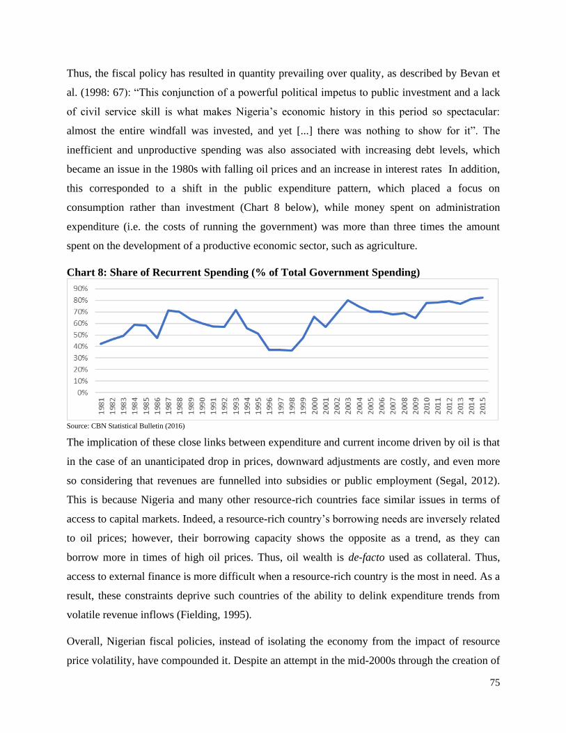
75

Thus, the fiscal policy has resulted in quantity prevailing over quality, as described by Bevan et

al. (1998: 67): “This conjunction of a powerful political impetus to public investment and a lack

of civil service skill is what makes Nigeria’s economic history in this period so spectacular:

almost the entire windfall was invested, and yet [...] there was nothing to show for it”. The

inefficient and unproductive spending was also associated with increasing debt levels, which

became an issue in the 1980s with falling oil prices and an increase in interest rates In addition,

this corresponded to a shift in the public expenditure pattern, which placed a focus on

consumption rather than investment (Chart 8 below), while money spent on administration

expenditure (i.e. the costs of running the government) was more than three times the amount

spent on the development of a productive economic sector, such as agriculture.

Chart 8: Share of Recurrent Spending (% of Total Government Spending)

Source: CBN Statistical Bulletin (2016)

The implication of these close links between expenditure and current income driven by oil is that

in the case of an unanticipated drop in prices, downward adjustments are costly, and even more

so considering that revenues are funnelled into subsidies or public employment (Segal, 2012).

This is because Nigeria and many other resource-rich countries face similar issues in terms of

access to capital markets. Indeed, a resource-rich country’s borrowing needs are inversely related

to oil prices; however, their borrowing capacity shows the opposite as a trend, as they can

borrow more in times of high oil prices. Thus, oil wealth is de-facto used as collateral. Thus,

access to external finance is more difficult when a resource-rich country is the most in need. As a

result, these constraints deprive such countries of the ability to delink expenditure trends from

volatile revenue inflows (Fielding, 1995).

Overall, Nigerian fiscal policies, instead of isolating the economy from the impact of resource

price volatility, have compounded it. Despite an attempt in the mid-2000s through the creation of

76

an excess crude account (ECA) and a sovereign wealth fund, public spending remains linked to

resource-related revenues. The ECA is a special account which was set up in 2004 to protect the

budget from unexpected shortfalls in oil prices. Thus, oil revenues in excess of the reference

price are saved, isolating, in part, the economy from external oil-price related shocks. At its

creation, the ECA was used to clear debt and reduce the required deficit in periods of bust. For

example, by 2007, the ECA had built huge reserves, close to USD 10 billion. These allowed the

government to smooth out expenditure as oil prices dropped significantly in 2007-2008. Since

then, the ECA has been depleted as the account lost its credibility when the government could

not resist political pressure to increase public spending when the oil prices recovered. The ECA

was formalised through three sovereign wealth funds meant to manage Nigeria's excess earnings

from crude oil.

In conclusion, as indicated by Budina, et al. (2007), fiscal policy has resulted in higher volatility

levels beyond the levels of observed volatility stemming from variable oil prices; in other words,

government policies have become a source of macroeconomic volatility. This excess volatility

has impacted negatively on economic growth across the country’s different sectors (oil and non-

oil).

3.6 Inflexible exchange rate policy and its impact on economic growth

Throughout Nigerian post-independence history, the impact of government spending volatility

and increased aggregate spending on economic aggregates, including growth, has been

accentuated by ineffective governmental monetary and exchange rate policies. In the Nigerian

context, exchange rates were not flexible enough and this resulted in contributing to the boom

and bust cycle which has characterised the Nigerian economy over the last 50 years, as described

by Budina et al. (2006). Indeed, the exchange policy has oscillated between a fixed and flexible

system, with capital control or government intervention playing a key role. Indeed, between 1960

and 1970, Nigeria operated under a fixed exchange rate system with a fixed parity set against the

British pound and the US dollar (Obi et al., 2016). Towards the end of the 1970s, the Nigerian

currency was tied to seven currencies, including the country’s main trading partners. The

exchange rate policy before 1985 was set up to assure an overvaluation of the naira (N), with few

restrictions on capital movement and a monetary policy used to defend the currency peg.

77

As part of the implementation of the structural adjustment programme (SAP) designed by the

International Monetary Fund (IMF), a market-based exchange rate system was introduced in

1986, under the military regime of General Babangida (1985-1993), to usher in a realistic naira

exchange rate, responding to market forces and able to stimulate non-oil exports (Mordi, 2006).

This resulted in abandoning the currency peg, a more independent monetary policy and free

capital movement. The currency depreciated quickly from 0.89 naira to one dollar in 1985 to

17.30 naira to one dollar in 1993, when Babangida left office (see Chart 9 below). In 1994, the

fixed exchange rate system was reintroduced under the military regime of General Abacha

(1993-1998). During this era (1994-1998), the currency peg was reintroduced and the naira was

fixed at N21.89/USD, even though parallel markets indicated that it was overvalued, with the

rate ranging between N56.80/ USD in 1994 and N84.70/USD at the end of Abacha’s regime in

1998. Then, with the return of democracy in 1999, different governments opted for a

guided/managed floating exchange rate system while allowing a measure of free capital

movements.

In sum, the Nigerian exchange rate can be characterised by frequent changes resulting in high

volatility, a real exchange rate overvaluation underlined by a continuous nominal depreciation,

and the continued dominance of government as the main supplier of foreign exchange. Another

key feature of the exchange rate policy is the large premium that exists between the official rate,

determined by the authorities, and the parallel market rates, which reflect market forces. As a

result, the RER was more stable during the fixed nominal exchange rate regime (1961-1985)

than under the period of liberalisation that followed. The volatility was driven by the significant

oil revenues and fiscal policy inconsistencies which were feeding high inflation (Ajao et al.,

2013).

Given this context, several studies have analysed the determinants of the exchange rate policies,

identifying a number of macroeconomic factors. Oil plays a significant role through the

exchange in terms of trade; however, even under the fixed nominal exchange rate, the rates

reflect several other factors. Sala-i-Martin et al. (2006) highlight that exchange rate movements

are not fully dictated by oil prices as the correlation between real exchange rates and oil prices

was only -0.05 over the period 1968-2000. Nwude (2013) presents a literature survey identifying

a number of variables that impact Nigeria’s short- and long-term real exchange rate. These

78

include, among others: interest rate differentials, short term capital inflows, monetary policy,

speculation, demand and supply regarding the naira, foreign exchange regulation and the general

economic environment.

Indeed, among the substantial existing literature, Oriawota et al. (2012) identified inflation rates

and capital inflow as the long-run determinants of real exchange rates, while terms of trade and

fiscal policies did not have an impact over the period 1970-2010. Obi et al. (2010), by testing the

Balassa-Samuelson hypothesis, found that increased productivity played a significant role in

determining the exchange rate between 1970 to 2007. It also indicated that prices, investment

levels and GDP are linked to exchange rate appreciation, while increased foreign reserves,

interest rate differentials and degrees of openness were related to the depreciation of the naira.

Although the macroeconomic determinants are relevant in determining short- and long-run

exchange rate levels, the role of the political economy cannot be ignored. Indeed, studies like

Ibrahim (2016), covering the period from 1960 to 2015, bring together macroeconomic variables,

such as money supply and the nominal exchange rate, as well as dummy variables representing

specific periods of Nigerian history, such as a civil rule dummy, an SAP dummy and a change to

civil rule dummy. The analysis indicates that the political regime in place is one of the major

short-run fundamentals of the exchange rate, while terms of trade, capital inflows, trade and

fiscal policies are the long-run fundamentals of the exchange rate in Nigeria.

Thus, as indicated by Sala-i-Martin (2006), the political economy factor is not negligible.

Political considerations have played a significant role in influencing exchange rate policy and

capital control measures in Nigeria. Indeed, the different, and sometimes conflicting, exchange

rate policies in the country reflect the political dynamics. For instance, from independence to

1985, Nigeria adopted a regulated economic policy, ostensibly to promote economic

development. However, this policy was in reality a mechanism to maintain low interest rates, a

fixed exchange rate, controlled credit allocation, and protectionism, all related to some rent-

seeking tendencies -(Okoye et al., 2016).

The political economy of the exchange rate also impacted the country’s trade policies. Indeed,

Nigerian exchange rate policies rested on protectionist trade policies in 1960 following the

import substitution strategy adopted by the government, coupled with a worsening of Nigeria’s

terms of trade and a drop-in commodity price. Thus, government-imposed tariffs were set at a

79

minimum of 50% on most imported goods, forcing an appreciation of the naira. In a period of

high oil prices such as 1973-1980, the government substantially reduced tariff rates and followed

an import payments policy to finance increased consumption driven by the DD's “spending

effect”. These policies resulted in a large balance of payments disequilibrium. Over the period

1973-1978, the naira continued to appreciate, reflecting the expansionary fiscal policy and the

deliberate currency appreciation policy. In the context of DD, the observed RER appreciation

within the period is an efficient economic response; however, it was not sustainable under a fixed

exchange-rate policy.

By 1980, at the end of the oil boom Nigeria had contracted a large external debt which grew

annually by 72% between 1982 and 1985, reflecting its expansionary fiscal policy. Furthermore,

to dampen demand and to maintain the appreciated exchange rate policy needed to maintain debt

contracted in foreign currency at a manageable level, tariff rates in excess of 150% were

introduced; similarly, quotas were a standard feature of trade policies. In essence, between 1960

and 1985, the RER appreciated because of the oil windfall but also because of government

policies imposing trade restrictions and its large external debt. By 1986, this position was no

longer sustainable, and Nigeria was forced to adopt a structural adjustment programme (SAP),

aimed at restructuring and redirecting the Nigerian economy, promoting competition and raising

the productivity of the real sector. However, a policy reversal occurred in 1994, as a fixed

exchange rate system was reintroduced and most of the protectionist trade policy measures were

reinstated to continue to fuel import driven consumption. With the return of democracy in 1999,

the trade policy was aimed at protecting local industry while slightly reducing tariffs on

consumer goods. This was intended to reduce smuggling and economic distortions. It resulted in

increased tariffs with lower rates for goods and inputs scarce in the domestic market, and high

rates for goods directly competing with local industry (Coste, 2014; Obinwata et al., 2016).

These trends in trade policy corresponded to a period of exchange rate depreciation as illustrated

by Obinwata et al. (2016). The naira depreciated from N21.89/USD in 1998 to N92.69/USD in

1999, followed by further depreciation to reach N133.5/USD in 2004. This depreciation was

linked to failing policies such as the creation in 1995 of a foreign exchange committee in charge

of allocating foreign exchange. The economic conditions resulted in further depreciation and the

dual exchange-rate market was reintroduced to manage this devaluation.

80

The exchange rate was relatively stable between 2004 and 2010, reflecting monetary policy

reforms, such as financial sector reforms introduced in 2004, a reduction of exchange rate

differentials between the different domestic markets, and the introduction of an effective

monetary policy rate. As presented in Chart 9 below, these reforms were supported by large oil

price increases resulting in an appreciation of from N132.15/USD in 2005 to N118.57/USD in

2008. This was followed by another depreciation driven by the financial crisis and the sharp fall

in the resulting commodity prices. These are also reflected in the REER, which assesses a

currency against a basket of other currencies. It is linked to the nominal exchange rate as

nominal depreciation of the naira translates into weaker (more competitive) REER. Chart 9

below presents the REER and NER for the period 1960-2014.

Chart 9: The REER (Lhs) and NER (Rhs) for the Period 1960-2014

In addition, as pointed by Uruma et al. (2016), exchange rate policies are likely to be affected by

varieties of political institutions, including election timing, since the real exchange rate affects

broad aggregates like the purchasing power, the growth rates, the price level, and these broad

aggregates are almost certainly relevant to elections. Indeed, governments, as in the case of

Nigeria following the return to democracy, tend to maintain appreciated currencies before

elections, delaying a depreciation/devaluation until after the election (Klein and Marion, 1997).

Given the political unpopularity of a devaluation-induced reduction in national purchasing

power, governments may face strong incentives to avoid devaluing, even when the result is a

Source: World Bank Database

Note: The REER is the nominal effective exchange rate divided by a price deflator - an increase represents an appreciation. Nominal exchange

rate refers to the exchange rate determined by legally sanctioned exchange market. It is calculated as an annual average based on monthly

averages (local currency units relative to the U.S. dollar).

81

more severe crisis than would otherwise be expected, in order not to jeopardise their electoral

fortunes.

As a summary, the exchange rate movements are linked to the multiple changes in exchange rate

and trade policies adopted by the government in their effort to manage volatile domestic

conditions linked to oil revenue inflows as well as a willingness to maintain an over-valued

exchange rate to fuel import-driven consumption and in reaction to a complex political economy

driven by rent-seeking behaviour.

3.7 Financial Markets and interest rate policies

There is a large body of literature pointing to the fact that resource-rich countries tend to have

underdeveloped financial sectors. Bhattacharyya and Hodler (2014) indicate that this is relatively

paradoxical given the large inflows of resource-related revenues. The literature has also

advanced a number of underlying mechanisms of this other dimension of the resource curse.

Hattendorff (2014) indicates that as resource-rich economies are more exposed to shocks, banks

require high interest rates to reflect the risks. This negatively impacts the availability of credit;

and, therefore, lowers financial development. Another argument relates to the fact that resource-

related operations are often enclaves, as presented by Beck (2011). He established that the

domestic banking system is underused by the resource sector as a significant proportion of their

cost is paid abroad.

Another argument presented by Beck et al. (2010) points to the use of resource revenue: as

investment in the resource sector increases, it may impact negatively on financial sector growth

and reduce the viability of skills in that sector, given that the economy will start relying on the

resource sector, which is less finance-intensive. Similarly, Nili and Rastad (2007) argue that

investment, driven by government spending, crowds out the private sector and reduces the need

for a developed financial sector. The argument that is most often put forward is presented by

LaPorta et al. (1998) and Bhattacharyya and Hodler (2014); it points to the fact that the

development of the financial sector is hindered by the quality of institutions and the ability to

enforce contracts. Thus, the governance structure around the financial sector is too weak to

favour its development. In resource-rich countries, these institutions are relatively weak, thus the

risk associated with lending operation is much higher. This reduces the banks’ willingness to

lend. In this context, an elite having access to credit could use the proceeds from these activities

82

to buy off political competitors. The resulting uncompetitive nature of politics reduces the

incentives for fostering contract enforcement, and often fosters corruption.

Against this literature, Adekunle et al., (2013) indicate that during the 1970s and early 1980s,

government intervention dominated financial sector development, which was seen as a means of

guiding economic development. This intervention took the form of the government ownership of

banks: the government controlled about 80% of assets in the commercial banks and 45% of

assets in the merchant banks (Brownbridge, 1996; Umejiaku, 2011). In that period, the financial

sector was described by Umejiaku (2011) as segmented and underdeveloped. The financial

system was considerably over-stretched as government policies to direct bank credit to certain

sectors at a concessional rate led to a distortion in the interest rate determination process, and

also impacted negatively on the banks’ balance sheets. Furthermore, the lack of appropriate

regulation and prudential norms resulted in a large portfolio of non-performing assets (Obadan

2004). Indeed, interest rates were determined administratively by the Central Bank of Nigeria,

thus failing to reflect markets forces. As a result, the correlation between the interest rate and oil

price was only around -0.15, as can be seen in Chart 11 below.

During the period of direct control of the money supply, the interest rate policy was determined

to direct financial resources at concessionary rates to the preferred sectors. On the other hand, the

non-priority sectors faced above-market rates. Further interest rate policy was aimed at

maintaining low debt service, and also to enhance output, following the devastation caused by

years of civil war. It quickly became apparent that those measures affected the efficiencies of the

sector, and resulted in financial repression, slower economic growth and credit benefiting an elite

(Abu, 2010). It also resulted in an increase of non-performing loans and risk loans as banks had

to grant credits on political rather than commercial considerations (Okonjo, 2018).This period of

financial repression, coupled with the fact that the rates were significantly below the rate of

inflation, implied that real interest rates were negative. This caused a decrease in savings,

discouraged investment, and thus impacted economic growth prospects.

Since the mid-1980s, financial sector reforms have been pursued in Nigeria aimed at stabilizing

and deepening the financial sector. A number of reforms, as highlighted by Somoye (2008),

drove the development of the sector, including deregulation of interest rates, the strengthening of

the regulatory and supervisory framework of the central bank, a review of the capital adequacy

83

ratio, Bureau-de-Change guidelines, the privatization of government-owned banks, an increase in

the range and type of bank accounts available, etc. As a result, the financial market deepened the

money supply (M2), which stood at ₦16.1 billion in 1981, then increased to ₦700 billion in

1999, to reach 24 trillion in 2017. Credit to the private sector grew from ₦8.6 billion in 1980 to

over ₦22 trillion by 2017. The deregulation of the financial sector also led to improved access to

financial services (Adegbite, 2005) as the liquidity ratio declined from 94.5% in 1970 to 61.8%

in 1972, and the lending-deposit ratio and ratio of bank credit to GDP rose from 51.3% and 6.7%

to 74.2% and 8.7%, respectively.

Despite these trends, while some analysts argue that those reforms have resulted in increased

sectorial performance and economic growth and positioned Nigeria as a competitive financial

leader in Africa (Akingbola, 2006), others are of the opinion that the financial sector has not

achieved much as the base of the industry has continued to remain fragile, playing but a

supportive role to the public and private sectors (Okafor, 2012). This latter argument is linked to

the role played by interest rates.

Indeed, interest rate policy has had an impact on the economic development of Nigeria. There

has been an underdevelopment of the real sector and it has been claimed that the reason for this

is the lack of funds from the financial sector to this sector. This ought not to be so because over

long periods, there has been in most countries a rough but unmistakable parallel between

economic growth and financial development. According to Gurley and Shaw (1967), there is

clearly a positive correlation between levels of economic development and financial

development. Among the wider literature covering Nigeria, Utile et al. (2018) found that

inflation and exchange rates have a negative and insignificant effect on GDP, while the deposit

interest rate exerted a positive and significant impact. Also, Osadume (2018) found that between

1986 and 2016, interest and monetary policy rates impacted growth both in the short and the long

run. Moreover, Udoka et al. (2012) found that an increase in the interest rate will negatively

impact GDP.

In sum, the discussion above indicates that both exchange rate and interest rate policies, to an

extent, respond to some macroeconomic variables, but that the role of government policies

cannot be understated. This can be seen in Chart 10 and Chart 11below, where interest rate and

exchange rate policies are dissociated from oil prices. Interest rates in Nigeria before 2009 did

84

not follow very closely the US federal reserve’s bank rates. Furthermore, the interest rate and

exchange rate show very little correlation, highlighting the lack of consistency of Nigerian

policies over the years. Thus, the expected mechanism through which exchange rate impacts on

growth and employment through the cost of borrowing (i.e. the interest rate) may be at play in

the context of Nigeria, but it appears to be a relatively indirect relationship that needs to be

further explored. However, this is beyond the scope of this thesis.

Chart 10: Nominal exchange rate (Naira per dollar) and oil price ($ per barrel)

Source: World Bank database, accessed, July 2018 (Naira per dollars) – presented on the left-hand side and BP Statistical Review, 2017 (for

prices per barrel presented on the right-hand side)

Chart 11: Oil price vs. average prime interest rate in Nigeria

Source: CBN, statistical Bulletin, 2016 (average prime interest rate offered by Nigerian banks) – presented on the left-hand side and BP

Statistical Review, 2017 (for prices per barrel presented on the right-hand side)

Chart 12: Nominal exchange rate vs. prime interest rate

Source: CBN, statistical Bulletin, 2016 (average prime interest rate offered by Nigerian banks) – presented on the left-hand side and World Bank

database, accessed, July 2018 (Naira per dollars) – presented on the left-hand side

-

50.0

100.0

150.0

-

100.0

200.0

300.0

400.0

19

81

19

82

19

83

19

84

19

85

19

86

19

87

19

88

19

89

19

90

19

91

19

92

19

93

19

94

19

95

19

96

19

97

19

98

19

99

20

00

20

01

20

02

20

03

20

04

20

05

20

06

20

07

20

08

20

09

20

10

20

11

20

12

20

13

20

14

20

15

20

16

20

17

Nominal Exchange rate Oil price ($ pb)

-

10.0

20.0

30.0

40.0

-

50.0

100.0

150.0

19

81

19

82

19

83

19

84

19

85

19

86

19

87

19

88

19

89

19

90

19

91

19

92

19

93

19

94

19

95

19

96

19

97

19

98

19

99

20

00

20

01

20

02

20

03

20

04

20

05

20

06

20

07

20

08

20

09

20

10

20

11

20

12

20

13

20

14

20

15

20

16

20

17

Oil price ($ pb) Prime Interest Rate

-

10.0

20.0

30.0

40.0

-

100.0

200.0

300.0

400.0

19

81

19

82

19

83

19

84

19

85

19

86

19

87

19

88

19

89

19

90

19

91

19

92

19

93

19

94

19

95

19

96

19

97

19

98

19

99

20

00

20

01

20

02

20

03

20

04

20

05

20

06

20

07

20

08

20

09

20

10

20

11

20

12

20

13

20

14

20

15

20

16

20

17

Nominal Exchange rate Prime Interest Rate

85

Chart 13: US Federal Reserve Bank Interest rates vs. Nigerian Interest rates

Source: CBN, statistical Bulletin, 2016 (average prime interest rate offered by Nigerian banks) – presented on the left-hand side and US Federal

Bank reserve interest rate, sourced from the website in July 2019 – presented on the left-hand side

3.8 Economic Growth - Gross Domestic Product

Nigerian GDP growth, like most economic variables, has been relatively volatile. Indeed,

following its independence, annual economic growth, measured by GDP, was around 3% during

the period 1960-1970. This rate grew to around 6% over the period 1970-1978: the time of early

oil production. In the early 1980s, Nigeria experienced negative growth rates, which turned

positive with the structural adjustment programme, with an average annual growth of 4%

between 1988 and 1997. Overall, despite the large revenue inflows throughout the first three

decades of oil production, Nigeria recorded an average growth of less than 3% (NPC 2004).

More recently, economic growth has accelerated significantly, as real GDP grew on average by

over 7% between 2009 and 2014. This was before the negative growth registered in 2016 as a

result of the sharp fall in commodity prices: real GDP fell from 6.23% in 2014 to -1.6% in 2016.

The composition of the Nigerian economic structure is clearly in line with the prediction of DD,

which indicates that large oil revenue inflows alter the output composition via the spending

effect, which contracts the agriculture sector; while the non-traded goods sector and the protected

(semi-traded/semi-nontraded) manufacturing sector expand. Fardermesh (1991) studied a

number of oil-rich countries, including, among others, Algeria, Nigeria and Venezuela, and

found that an oil boom similar to the one experienced in the 1970s reduced agriculture output

and resulted in an increase in non-traded goods, as well as manufacturing output (which in many

developing countries is protected and not always tradable). Conversely, an oil collapse, as the

one experienced in the 1980s, would promote agricultural activities and undermine

manufacturing output and the non-traded goods sectors.

-

5.0

10.0

15.0

20.0

25.0

30.0

35.0

0.00

5.00

10.00

15.00

20.001

98

1

19

82

19

83

19

84

19

85

19

86

19

87

19

88

19

89

19

90

19

91

19

92

19

93

19

94

19

95

19

96

19

97

19

98

19

99

20

00

20

01

20

02

20

03

20

04

20

05

20

06

20

07

20

08

20

09

20

10

20

11

20

12

20

13

20

14

20

15

20

16

20

17

Fed Interest Rates (LHS) Prime Interest Rate (Rhs)

86

Structural changes in the economy brought on by the oil sector, which rose from 10% of GDP to

31% in 2000, while it employs less than 1% of the active population, had effects on other sectors.

This is in line with the Dutch Disease prediction that the boom in the oil sector adversely affects

outputs of non-oil tradables. Thus, Nigerian data indicates that in the 1950s, the agriculture

sector accounted for 69% of GDP. The share quickly fell to about 49% and then below 20% by

1980. It has since stabilised around that mark (Sala-i-Martin et al. 2003). Before the rapid

increase in oil export revenue, the country was exporting several cash crops, including cocoa,

groundnuts, palm oil and rubber. However, production of these crops declined by over 75%

between 1970 and 1981.

The agricultural contribution to GDP between 1981 and 1990 was 18%, and it rose to 20% in the

following decade; this contribution also increased to 25% between 2001 and 2010 and decreased

to 23% in the middle of 2011 and 2015. Its share in total foreign exchange receipts dropped from

86% in 1955 (Aigbokan, 2001) to 1.8% in 1996 (Balogun, 2001). These trends were attributed to

two key factors, namely the large increase in oil prices and government policies meant to

encourage industrialisation in the ‘80s and ‘90s, which had a negative impact on the sector.

Despite the lower contribution to growth, the sector remains the largest employer of labour in the

country. In 1970 the agricultural sector accounted for about 75% of the labour force; this

gradually decreased to 59% in 1980’s and then later to represent about 57% in 2010, as

illustrated by Table 3 below.

Low productivity and low investment have, in part, driven this performance. This is illustrated

by the fact that only 34 million of an estimated 72 million hectares of potentially cultivable

Nigerian land are in use (Norton, 1993). In addition, as indicated by Oyejide (1986), the

macroeconomic developments of the country have driven this performance. Firstly, the rural-

urban migration, which was driven by higher wage offers in other sectors, has put upward

pressure on agricultural wages, resulting in sectoral wage increases in the ‘70s and ‘80s. This

continued for most of the ‘90s. This is in line with DD and its impact on the non-resource

tradable sector. In addition, trade policies, given their volatility and exchange rate policies, have

also resulted in volatility and an overvaluation of the naira, reducing the profitability of the

sector. (Kwanashie, Ajilima and Garba, 1998). The other non-oil tradable sector, the

manufacturing sector, despite being the focus of several development plans and significant

87

investment, has never really taken off (see Table 3) and has stagnated. In the Nigerian context,

this is also reflected in the county’s acute infrastructure gap crystallised by a significant lack of a

reliable power supply, causing damage to firms’ equipment. Thus, most private sector actors rely

on self-supply for most public goods, using, for example, generators, thus increasing costs of

production and negatively affecting competitiveness.

The other side of the observed decline in the agricultural sector concerns the growth of services

(including the rapid rise of government spending in ineffective service delivery). The share of

services grew from 34% in 1970 to 47% of GDP in 1980, by then the biggest contributor to

growth. The decade that followed saw a relatively large decline in this share to 38%, before

gradually increasing to 58% in 2015. Similarly, the service sector has attracted a significant share

of employment. In line with DD predictions, labour is shifting from non-resource tradable

activities to non-tradable activities.

Although in the Nigerian economic context, Dutch Disease is likely to be linked to the observed

developments, such as services output and national income being positively correlated, its impact

is potentially confounded by other factors. Take as an example the Engel effects in consumption:

according to this theory, increasing income leads to increasing demand in services, linked to

higher income elasticity of demand for services relative to agricultural products (Chenery et al.,

1975, Syrquin et al., 1986). Another explanation could be Baumol’s cost of “disease” effect:

under this theory, the fast productivity growth in a sector such as oil allows for an increase in

resources allocated to other sectors, in particular services (Baumol, 1967). Those impacts could

confound the Dutch Disease resource movement effect.

As Rodrik (2014) argued, the capital intensity of the manufacturing sector reduces this sector’s

ability to absorb the large population migrating away from the agricultural sector, characterised

by relatively low skills and low productivity. The extractive sector is capital intensive,

generating little employment and high rents. The ILO (2005)3 estimated that only 65,000 and

250,000 people respectively are working directly and indirectly in the Nigerian oil industry. The

contribution is minimal given that the population consists of 180 million people. Thus, Rodrik

(2016) argues that many developing countries are experiencing a premature de-industrialisation,

3 Fajana, Sola. "Industrial relations in the oil industry in Nigeria." (2005).

88

as most of the excess labour from the agriculture sector is finding employment in low

productivity service activities, such as retail trade or housework. This argument is central to the

academic and policy discussions surrounding the ability of a services-led development model to

provide jobs and accelerate economic development. On the one hand, Ghani and O’Connell

(2014) respond positively to this possibility, arguing that services can deliver growth, while on

the other hand, authors such as Rodrik (2016) and Kormawa and Jerome (2015) are more

sceptical about the ability of the service sector to deliver decent employment as the service sector

in developing countries operates at low margins and low levels of productivity.

Table 3: Composition of Output, Employment and Exports Share of output

Sector 1970 1980 1990 2000 2010 2015

Agriculture 49 22 18 20 24 23

Oil and mining 10 25 36 31 15 10

Manufacturing 7 6 9 6 7 10

Services 34 47 38 42 54 58

Share of employment

Sector 1970 1980 1990 2000 2010 2015

Agriculture 75 59 58 57 30.6 36.4

Oil and mining 0.2 0.4 - - - -

Manufacturing 15 17.7 9.2 9.1 14.1 11.8

Services 9.8 22.9 32.2 34 55 52

Share of exports

Sector 1970 1980 1990 2000 2010 2015

Agriculture 71.9 2.4 1.46 0.14 3.34 4.75

Oil and mining 15.4 87.5 97 99 94.4 92.2

Manufacturing 12.7 0.1 1.54 0.86 2.26 3.05

Services

Source: Computed from CBN Statistical Bulletin, 2016

The above discussion is even more applicable to the recent trends showing that Nigeria’s non-oil

sector has experienced significant growth. In the 1990s and early 2000s, the significant increase

in oil production resulted in relatively low and unproductive investment in other sectors.

Nevertheless, the data indicates that since 2003, 70% of growth originated from non-resource

sectors such as agriculture, and services such as trade-related activities. This was emphasised by

the National Bureau of Statistics (NBS) GDP rebasing exercise undertaken in 2014, which

reflected the economic transition that Nigeria had experienced, as the country became the richest

89

on the continent, with a revised GDP estimate of USD510 billion in 2013. Following this

exercise, economic activities can be seen to be more diverse, with increased contributions from

service sectors, previously largely informal and undocumented, such as the entertainment

industry. In addition, emerging services, including construction, financial intermediation, and

ICT, have also contributed significantly to economic growth, illustrating the structural

transformation and a shift of economic activities towards services – as predicted by the Dutch

Disease framework.

In conclusion, large revenue inflows have impacted on the economy, mostly in line with the

prediction of the DD framework. Oil continues to matter in the development of other sectors in

Nigeria. Indeed, Akinlo (2012) analysed the role of oil in the development of several other

economic sectors, including manufacturing, agriculture, trade & services, as well as construction,

using a multivariate vector auto-regression (VAR) model covering the years 1960 to 2009. He

concludes that the five different sectors are co-integrated and that the resource sector can

positively impact the growth of the trade sector, while this impact turns negative concerning the

manufacturing sector. This is in line with the predictions of DD.

Although oil matters, a major concern with the country’s growth pattern includes the weak

linkages between the oil sector and the rest of the economy. Ibrahim (2007) explains this lack of

integration by the lack of technological development in other sectors of the economy, further

exacerbated by weak downstream oil activities. Thus, in this context, growth differentials in oil

and non-oil sectors are inevitable, as the oil sector operates as an enclave not integrated with the

rest of the economy. Therefore, for example, it will not support the growth of the manufacturing

sector (Ibrahim, 2007).

Furthermore, employment and GDP are weakly linked. For example, agriculture represents 22%

of GDP but employs 50% of the population, while industry represented 27% of GDP in 2012 but

only employed 6% of Nigerian workers. Therefore, the current growth pattern is unlikely to

increase household incomes and reduce poverty. Indeed, being employed does not translate into

maintaining average living standards, as a large number of jobs are informal and very often

associated with low skills and productivity. These forms of employment support livelihoods but

do not provide sufficient income to reduce poverty in Nigeria, and do not support structural

transformation through productivity growth. Nor do they build self-esteem or social cohesion

90

(World Bank, 2015). The discussion below links the macroeconomic developments in Nigeria to

the structure of the labour market.

3.9 Composition of the Nigerian Labour Market

Nigeria is the continent’s most populated nation, with a population estimated at over 158 million

in 2011, of which over 50% or 87 million people are aged between 15 and 64 years old. In this

group of working-age adults, only 5% are categorised as not working but actively searching for a

job: i.e. unemployed. According to the ILO definition of unemployment4, Nigeria’s

unemployment rate is low, but this masks the fact that the labour market is dominated by very

low productivity sectors such as agriculture and services (i.e. the retail trade) (World Bank

2014). Indeed, while the total labour force rose by 3% on average between 2010 and 2014, the

share of the active population in paid employment increased on average only by 2% over the

same period, three times and eight times lower than the growth observed in underemployment

and unemployment, respectively.

In addition, according to the World Bank and the Nigeria Jobs Report (2015), the Nigerian

labour market is dominated by informality. While two-thirds of the adult population work in the

labour market, self-employment in agriculture and non-farm activities accounts for 70% of

employment. These sectors are generally described as informal sectors, where workers have no

employer and generally lack access to any form of social security. Only nine million out of a

working population of 87 million are employed in either the private or the public sector. Chart 14

below also indicates that employment patterns are slowly shifting away from agrarian self-

employment to other activities. Only one in 20 workers in agriculture are wage labourers, with

the rest being engaged in smallholder farming.

4 Nigeria’s Bureau of Statistics is using a specific definition of the employment presented as the labour force share

able and available to work, but that work was less than 39 hours in the week preceding the survey. As a result,

compared to the international definition, the unemployment rate across Nigeria has been very high.

91

Chart 14: Composition of the Nigerian Labour Market in 2011/12

Source: Adjusted from estimates World Bank based on GHS 2010/11 and GHS 2012/13. Note: Numbers in parentheses correspond to the estimates for 2010/11. Wage work Private includes private firms, NGOs, cooperatives and

international organisations. Wage work Public includes federal, state and local governments.

Despite a fall in the share of employment in agriculture, a large share of households rely on

farming for employment and income, even in peri-urban areas. However, the sector is

characterised by low productivity, with little access to agricultural inputs such as fertilisers,

pesticides or draught animals: less than 10% of workers have access to irrigation, and less than

15% benefit from agricultural advisory services. This links to Nigeria’s public expenditure

pattern, with very little investment in the productive sector (section 3.5 above). Given the low

productivity in the sector, many households cannot rely on their farming income alone (one in

five of those employed has a second job, mostly as a self-employed person). Nevertheless, 40%

of rurally based farm households are poor, compared to 19% of households who have completely

diversified out of the agricultural sector, and 31% who mix farm and non-farm activities in order

to supplement their income (Oseni et al 2014).

In addition, the country presents some strong regional disparities. The share of employment in

farming is in fact higher in the northern regions, where the semi-arid climate is less favourable

for cultivation, than in the southern regions. Conversely, one in four households in the South-

East engage in higher market value cash crop production, compared to only one in 100

households in the North-East, in line with the higher poverty rates in the northern regions as

compared to the southern region of the country.

92

Unlike many other African countries, the net effect of workers moving out of agriculture has not

led to an increase in the household enterprise sector. Instead, more jobs have been created in the

private, and especially the public, wage sectors, which constitute higher rates of employment of

non-farm workers in the formal sectors of Nigeria’s economy. Wage employment represents

18% of total employment, of which 50% are employed in the public sector. The public sector

contribution to wage-work explains why the government spends so much on recurrent

expenditure every fiscal year, and hints at the fact that the public sector is crowding out the

private sector by setting up wages and attracting the best talent, similar to the experience of the

Middle East and North-Africa regions (Segal,2012; Behar et Mok, 2013). Overall, the World

Bank World Development Indicator indicates that the size of wage work is very small compared

to other regions, such as South-East Asia, as wage sector employment in Indonesia and the

Philippines were estimated at 40% and 57% of the active population, respectively. Further,

public sector employment as a share of the active population went from 6% to 5% between 2011

and 2013 resulting from the privatisation of several sectors of the economy such as the

telecommunication, banking and energy sectors.

In terms of unemployment, the rates are higher for the more educated, reaching 10% for those

with post-secondary education. In fact, only 11% of the population has some post-secondary

training, but they account for 21% of the unemployed. As in many African countries,

unemployment is also a more significant problem for those with higher education, especially for

women, who may not be able to find jobs that match their expectations or education when

compared to those with little schooling. It follows that unemployment, unlike inactivity, is not

prevalent among the poor, who cannot afford to be unemployed. In fact, the youth belonging to

the richest 40% of the population are overrepresented among the unemployed.

3.10 Labour Market and Wages

The Nigerian labour market structure does not support poverty reduction efforts. In fact, the poor

and the non-poor are about as likely to be working and employment-to-population ratios are not

markedly different across consumption quintiles. Instead, the sector of activity is a stronger

indicator of poverty patterns, most visibly for the poorest and the richest Nigerians. Half (51%)

of those working in agriculture belong to the poorest 40% of the population (the two poorest

quintiles). They are under-represented in the non-agricultural sector, where poor workers account

for only 34% and 27% of self-employment in industry and services respectively, and only 17%

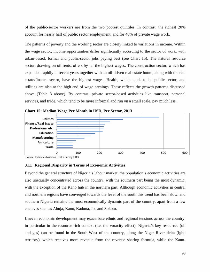
93

of the public-sector workers are from the two poorest quintiles. In contrast, the richest 20%

account for nearly half of public sector employment, and for 40% of private wage work.

The patterns of poverty and the working sector are closely linked to variations in income. Within

the wage sector, income opportunities differ significantly according to the sector of work, with

urban-based, formal and public-sector jobs paying best (see Chart 15). The natural resource

sector, drawing on oil rents, offers by far the highest wages. The construction sector, which has

expanded rapidly in recent years together with an oil-driven real estate boom, along with the real

estate/finance sector, have the highest wages. Health, which tends to be public sector, and

utilities are also at the high end of wage earnings. These reflects the growth patterns discussed

above (Table 3 above). By contrast, private sector-based activities like transport, personal

services, and trade, which tend to be more informal and run on a small scale, pay much less.

Chart 15: Median Wage Per Month in USD, Per Sector, 2013

Source: Estimates based on Health Survey 2013

3.11 Regional Disparity in Terms of Economic Activities

Beyond the general structure of Nigeria’s labour market, the population’s economic activities are

also unequally concentrated across the country, with the southern part being the most dynamic,

with the exception of the Kano hub in the northern part. Although economic activities in central

and northern regions have converged towards the level of the south this trend has been slow, and

southern Nigeria remains the most economically dynamic part of the country, apart from a few

enclaves such as Abuja, Kano, Kaduna, Jos and Sokoto.

Uneven economic development may exacerbate ethnic and regional tensions across the country,

in particular in the resource-rich context (i.e. the voracity effect). Nigeria’s key resources (oil

and gas) can be found in the South-West of the country, along the Niger River delta (Igbo

territory), which receives more revenue from the revenue sharing formula, while the Kano-

0 100 200 300 400 500 600

Trade

Agriculture

Manufacturing

Education

Professional etc.

Finance/Real Estate

Utilities

94

Kaduna axis (Hausa/Fulani territory) has long been a corridor for traders and merchants coming

from the Sahel. The South-West, meanwhile, has been driven by the megapolis of Lagos. With

the exception of these few pockets, most of the country has been economically stagnant.

The existence of a strong ethnic identity and social networks within the different ethnic groups in

Nigeria implies the existence of fragmented markets characterised by high transaction costs.

Indeed, Fenske and Zurimendi (2015) highlighted how oil prices impact populations, and a

number of socio-economic outcomes, such as education, employment, and wealth, differ

depending on ethnicity. In addition, Aker et al. (2014) point to the existence of lower business

transaction costs when traders belong to the same ethnic group. These evidences indicate that the

strong ethnic division existing in Nigeria can result in fragmented labour and supplier markets,

resulting in limited mobility. This aspect of the Nigerian labour market is particularly interesting

for studying the wage-determination process and the role of oil in this process (chapter 5)

With the main economic activities located in the South, the wage-work sector is also larger in

this region. The occupational choice of the working-age population differs by region, as shown

below. The share of wage work in total employment corresponds to 29% and 23% in the South-

South and South-West regions, respectively (Chart 16). This share is significantly higher than the

equivalent proportion in the North-East and North-West regions, estimated at 9%. Across the

different zones, the share of public sector employment has decreased; while private sector

employment has been growing in the southern regions, it is almost non-existent in the north.

Like other social and economic metrics, poverty rates are higher in the north, with an average of

67%, which is almost three times the rate in the south and more than one-and-a-half times more

than the national average of 45.3%. The poverty rate differences between the north and south

boil down to the fact that economic activities in the north are characterised by very low

productivity, low consumption levels, higher population (growth) and less industrialisation,

which is not as prevalent in the south. In sum, this makes the north region a poorer and less

productive region in comparison with the south.

Chart 16: Distribution of the Employed Labour Force, Per Type of Employer

95

3.12 Labour Demand: A Picture of the Private Sector

Nigeria is home to about 37 million enterprises, most of which are microenterprises, and about

40% of which are farms (SMEDAN, 2012). According to SMEDAN, there were also about

68,200 small firms (between 10 and 49 employees) and 4,670 medium firms (with more than 50

employees) in operation in Nigeria in 2012. This indicates that most Nigerians have informal

jobs, defined as wage-workers working without a contract, and are self-employed/household

enterprise workers in firms that are not registered with the authorities. Some 96% of the self-

employed who work on their own farms and 84% of the self-employed in the non-farm sector are

not registered with the authorities. In 2011, about five in six non-agricultural wage workers were

informally employed.

The level of informality is highest among services sector workers. While private-sector jobs are

almost exclusively (96%) informal, three out of four public sector workers are also informally

employed. Informality is “normal” at this stage of development – indeed, in many countries in

Latin America and East Asia, informal employment in fact increased with growth (OECD, 2009;

Perry et al., 2007). As such, informality is not likely to fall with economic development and the

share of informal employment will not be a good indicator of changes in job opportunities.

For wave 1(2010/11) and wave 2(2012/13)

Source: HGS survey and adjusted from World Bank (2013).

Based on answers to the question: “In your main activity, what is the employer in this job?” and “Have you received wages, salary or other

payments either in cash or in other forms from this employment for this work?”

96

3.12.1 Informality and Non-Farm Enterprises (NFE)

Another key characteristic of informal economic activities in Nigeria is the importance of non-

farm enterprises (NFEs). As in many developing economies, NFEs reflect economic needs and

the fact that the private sector fails to provide decent alternatives. Similarly, in other sub-Saharan

African countries, including Tanzania and the Republic of Congo, NFEs originate with the

inability to find wage-employment (Fox, L. & Sohnesen, 2012) and remain a major source of

income for the poorest households (Haggblade, Hazel and Reardon 2007). Household-based

activities outside of agriculture provide complementary income to rural farm-based households

and are the most important form of activity in urban areas, above wage employment. In the

South-West region, household enterprises account for more than half of all jobs; even in the

northern regions, which remain dominated by farming, one quarter of the employed are working

in a non-farm household enterprise as their primary job. In rural areas, many workers also shift

between farming and household enterprises on a seasonal basis. Overall, 63% of all households

were involved in an NFE, underlined by strong regional disparities with the South-West and

North-West geopolitical zones, accounting for over 50% of the NFEs in Nigeria. Most of these

businesses are not professionally run, and almost all operate without registration. They are also

run from home (over 50%), employ on average 1.5 persons (including the owner) and very few

of them (9%) employ labour outside of the household.

In line the with the country’s growth pattern, most of the NFEs provide services, the majority

being in retail, trade or personal services, although they are venturing into manufacturing goods

as well. NFEs cater mainly to local customers and not to other businesses. NFEs, as a whole, are

dominated by wholesale and retail services; while the manufacturing sector accounts for almost

one-fifth of NFEs, the production of food-related products dominates. The overall landscape of

NFEs varies across the country (Chart 17 below). Only 6% of these firms are registered. They

have little access to formal means of financing and rely on household savings or the extended

family for start-up capital. The median income of a household enterprise is approximately 30

USD per month (National Bureau of Statistics, 2013) – less than one-quarter of the

manufacturing median monthly wage (about 134 USD).

97

Chart 17: NFE Distribution per sector and region

Firms in the economic hub of Lagos and in the South-South geopolitical area display greater

productivity than in other parts of the country, in terms of total factor productivity (TFP) and

labour productivity (Chart 18). Firms in the North-West geopolitical region are the least

productive (displaying productivity levels of about 50% of the median firm in Lagos), while

other regions present similar levels of productivity. There is no great difference in terms of NFE

productivity between sectors; however, in line with DD, wage-per-worker in the services sector

is higher than in manufacturing.

Chart 18: Median Labour Productivity and TFP Compared to Lagos Median Firms

Part of the performance of an NFE is linked to the current business climate (see Chart 19, below).

Transport, finance and electricity were assessed as the top three obstacles to a firm’s growth,

followed by significant difficulty in gaining access to water and telecommunications. Although

the Nigerian government incurs huge expenditure every year, it is largely recurrent, and little is

Source: Estimates based on GHS 2012/13

Source: World Bank calculations based on GHS 2012/13.

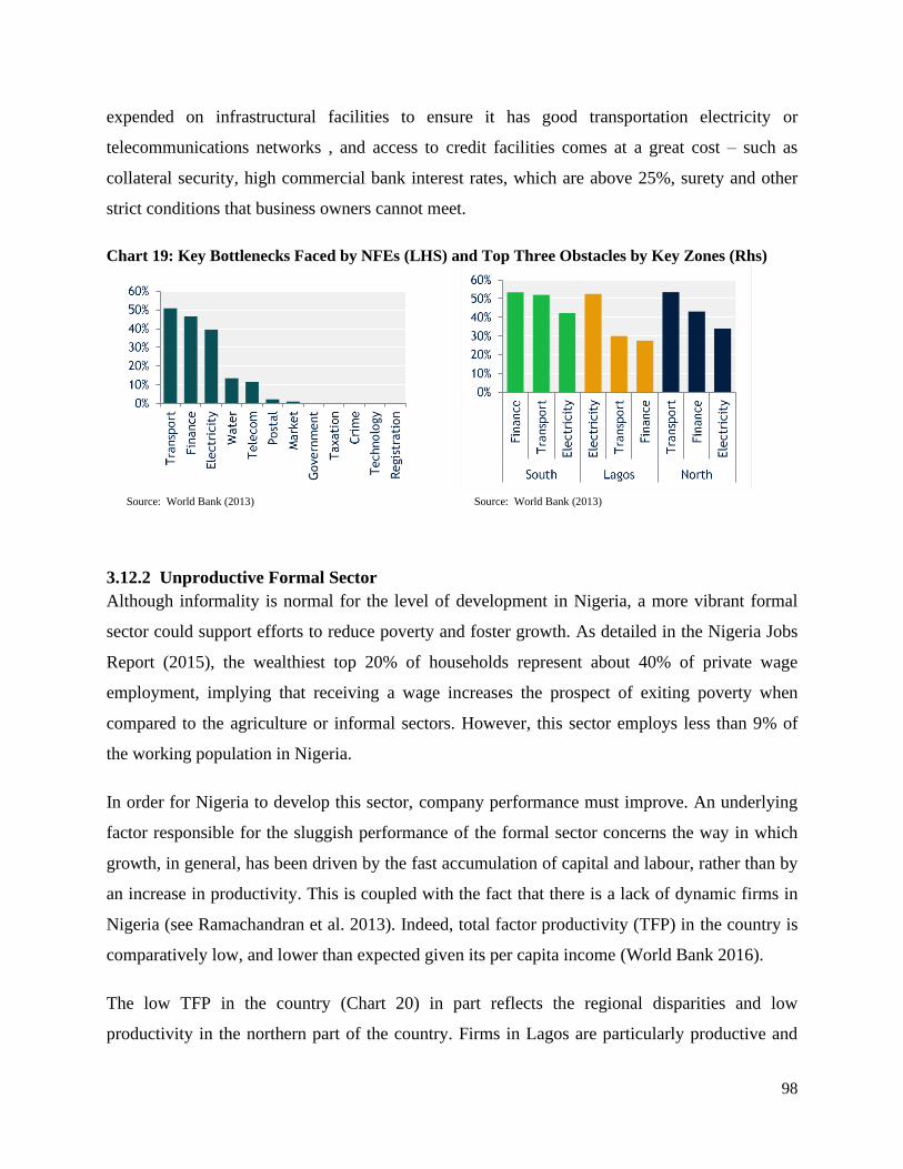
98

expended on infrastructural facilities to ensure it has good transportation electricity or

telecommunications networks , and access to credit facilities comes at a great cost – such as

collateral security, high commercial bank interest rates, which are above 25%, surety and other

strict conditions that business owners cannot meet.

Chart 19: Key Bottlenecks Faced by NFEs (LHS) and Top Three Obstacles by Key Zones (Rhs)

3.12.2 Unproductive Formal Sector

Although informality is normal for the level of development in Nigeria, a more vibrant formal

sector could support efforts to reduce poverty and foster growth. As detailed in the Nigeria Jobs

Report (2015), the wealthiest top 20% of households represent about 40% of private wage

employment, implying that receiving a wage increases the prospect of exiting poverty when

compared to the agriculture or informal sectors. However, this sector employs less than 9% of

the working population in Nigeria.

In order for Nigeria to develop this sector, company performance must improve. An underlying

factor responsible for the sluggish performance of the formal sector concerns the way in which

growth, in general, has been driven by the fast accumulation of capital and labour, rather than by

an increase in productivity. This is coupled with the fact that there is a lack of dynamic firms in

Nigeria (see Ramachandran et al. 2013). Indeed, total factor productivity (TFP) in the country is

comparatively low, and lower than expected given its per capita income (World Bank 2016).

The low TFP in the country (Chart 20) in part reflects the regional disparities and low

productivity in the northern part of the country. Firms in Lagos are particularly productive and

Source: World Bank (2013) Source: World Bank (2013)

99

compare well with firms operating in Ethiopia, Côte d’Ivoire and Ghana. Although TFP in Lagos

is lower than in India – and the other BRICS – it compares more favourably with these firms as

well. The median firms in Kana and Kaduna present productivity levels of 75% of the medium

firms in Lagos, while firms in the south stand at 62%. The difference between other northern

provinces and Lagos and other regions is more significant. TFP in the northern provinces

accounts for one-third of TFP in the southern provinces, and one-quarter of TFP in Lagos, thus,

pushing the national average downwards.

Chart 20: Median Manufacturing Firms’ TFP in Lagos against other Regions and

Comparative Countries

Firms in Nigeria remain labour intensive. Unit labour costs are high, but TFP is relatively low.

This implies that, despite the high cost of each unit of labour and high productivity of each unit

of capital, firms are still reluctant to invest in more capital and that production processes remain

labour intensive. Weak property rights, infrastructure deficiencies (such as a lack of roads and

electricity- see below) could explain why firms are reluctant to invest more in capital. In

addition, low productivity is also linked to labour productivity (Clarke, 2011). The low wage

rates in the country do not adjust to reflect the low labour productivity levels, and this results in

lower competitiveness compared to other countries. This may be due to the rigid labour market,

which forces businesses to retain poor performers. A lack of investment in human capital and/or

a skills mismatch are further possible reasons for this. This provides a further rationale to look at

the determinant of wage and wage inequality, which this project seeks to investigate.

Indeed, unit labour costs are high in Nigeria; labour costs about 31% of output. Only Côte

d’Ivoire (34%) and South Africa (45%) have higher unit labour costs (see Clarke et al., 2007).

However, Nigeria’s unit labour costs are only marginally higher than Chinese costs (27%) and

Source: adjusted from World Bank report.

100

comparable to Indian (31%).

Costs of labour display large regional disparity. In Kano and Kaduna and in the south, they are

comparable to countries with the lowest unit labour costs (see Chart 21 below), giving firms in

these locations a clear comparative advantage in the production of labour-intensive goods. In

Northern Nigeria, low productivity is met by low wages. In contrast, unit labour costs appear

relatively high in Lagos: at 57%, they are higher than other countries (see Chart 22 below).

Chapter 5 on wage determination will argue that wages could be even more competitive in the

absence of oil in the South-South region. In addition, the chapter will present evidence of the role

of oil revenue in explaining wage inequality across firms.

Chart 21: Nigerian Unit Labour Costs in the Manufacturing Sector against Comparative

Countries

Chart 22: Lagos and Other Nigerian Regions’ Unit Labour Costs in the Manufacturing Sector

Although further analysis is required for the Nigerian case, the facts presented above are in line

with those found by Gleb, Meyer and Ramachandran (2013), who compared labour costs and

productivity levels in several African countries. They presented the fact that the labour price in

African countries is more expensive than expected when compared to GDP per-capita levels.

This trend reflects the fact that in the African context, as firms grow larger and productivity

Source: Adjusted from World Bank ES (2014/15 for Nigeria.

Source: Adjusted from World Bank ES (2014/15 for Nigeria

101

increases, the related labour costs grow more than anywhere else.

Gleb et al. (2013) highlighted the need for Nigeria to invest in the infrastructure, such as power

supplies, needed to improve the business environment. In addition, their analysis shows that low

levels of income do not always translate into the ability to specialise in low wage activities.

Thus, they present that resource-rich developing countries similar to Nigeria would have a

comparative advantage in sectors immediately related to the resource endowment and not

necessarily in low-wage manufacturing activities.

Firms in Nigeria are confronted with a difficult environment. The Doing Business report (2015)

places the country 170th out of 189 globally pointing to a non-conducive investment climate that

may prevent investment; resulting in lower productivity. The last two World Bank investment

climate assessments (2009 and 2011) identified the same three constraints to private sector

activities in Nigeria. These are: a difficult access to power supply, unavailability of credit and a

poor transport network. These bottlenecks increase the operating costs of firms in Nigeria.

Indeed, it is estimated that 10% of sales are lost each year due to the poor business environment,

including the poor power supply, delays from a poor transport infrastructure, crime and

corruption. This is twice the estimated losses observed in comparative countries, such as South

Africa, Brazil, Russia and Indonesia.

3.13 Conclusions

This chapter has highlighted that oil revenue inflows have had a substantial influence on

Nigeria’s socio-economic development but shows that these impacts are compounded by several

contextual factors. These include the country’s stagnating economic development, intertwined

cultural and religious cleavages, as well as unstable institutions. Further, in line with the

resource curse literature and the definition of a point resource, oil has been a source of social

tension and conflict as populations in the Niger Delta region have felt deprived of the resource’s

revenues, while also having to deal with the negative impact of oil production on the

environment and on local livelihoods in the region . Although the country’s revenue-sharing

arrangement attempts to correct this inequality, the assumption that elites capture the benefit

instead of privileging productive reinvestment apply to Nigeria.

These dynamics having transpired in the country’s macroeconomic trends, Nigeria has not

102

escaped the perverse impacts of the abundance of oil revenue. Historically, the country’s fiscal

policies have exacerbated volatility rather than smooth it. This, coupled with inconsistent and

fairly inflexible exchange-rate policies, has created an avenue for the Dutch Disease to take root

in the country. These effects are illustrated by a gradual shift in the structure of the economy

driven by changes in relative prices. As a result, Nigeria has seen its agriculture sector (its main

non-oil tradable) shrinking, and its manufacturing sector stagnating at the expense of a growing

services sector. To mitigate these impacts, in the mid-2000s, the country attempted to reduce the

impact of oil revenue volatility on public expenditure by creating an oil fund. However, this has

been only partially successful. This is illustrated by the large amount of money that has been

wasted on low productivity capital projects and large recurrent spending driven by a large civil

service (seen as a way to redistribute oil wealth), reflecting a lack of long-term planning with

political pressures driven by the voracity effect and a poor institutional environment.

These dynamics at the macroeconomic levels have affected the structure of the labour market

and private sector activities. Government policies have resulted in a difficult business

environment, with the existence of major barriers which crowd out private sector capital

investment negatively affecting productivity. As presented above, the private sector bottlenecks

are related to ineffective government spending resulting in a large infrastructure deficit. As a

result, total factor productivity in Nigeria in key sectors such as manufacturing fails to reflect the

country’s per capita income (hinting at the oil artificially boosting this income (El-Anshasy,

2017)). Further, given the tough business environment, Nigerian manufacturing firms are not big

investors. Indeed, previous studies, such as Svensson (2003), found that corruption negatively

impacts investment as capital intensive firms are more likely to be exposed to corruption

practices than labour-intensive firms. In addition, in the context of underdeveloped financial

markets, firms are likely to underinvest as investment has to be financed internally.

Another impact of the macroeconomic dynamics is the high cost of labour, which is relatively

expensive compared to other countries. Furthermore, the wage level in the country does not

compensate for its low labour productivity. This implies that investment in labour productivity

could attract labour-intensive manufacturing sectors seeking low labour costs. Concurrently,

Nigerian value added per worker is lower than in other countries. Thus, unit labour cost (labour

costs as a percentage of value added) is one of the highest in Sub-Saharan Africa. In other words,

103

productivity does not drive wages affecting their competitiveness. This points to factors other

than productivity, such as DD, underlying the wage-determination process.

Moreover, adding to the distortions related to oil revenue inflows, Nigeria’s labour market

presents characteristics of a developing country with a large informal sector. Most people work

for themselves and informality is the norm. Indeed, only 15% of the Nigerian labour force earn a

wage. Ramachandran et al. (2013) highlight the fact that entrepreneurship is a common feature of

African economies; however, firms lack the necessary dynamism to drive aggregate productivity

and employment. These countries are characterised by a limited number of large and effective

firms, but they often benefit from protection, allowing them, in many cases, to operate as

monopolies, affecting productivity distribution.

In addition, strong social and ethnic networks in Nigeria contribute to the development of

fragmented markets characterised by high search and transaction costs. This fragmentation is

reflected in strong regional disparity in terms of socio-economic development, including labour

costs, productivity and poverty rates. The formal and informal sectors are likely to have an

impact on the way a shock (with or without mitigating fiscal policy) affects the economy.

104

4 Chapter 4

Analytical evidence of the impact of Dutch Disease on the Labour Market:

REER and Firms

4.1 Introduction

It is worth remembering that resource-rich-economies are unique since an appreciation will often

be caused by a commodity boom, and not a secular expansion in value-added exports such as

manufactured goods. An appreciation that is caused by an expansion in manufactured exports

can indicate a successful and sustainable growth path, while an appreciation caused by a

commodity boom can simply reflect the successful extraction of resources to feed global

demand, to the detriment of more value-adding exports. This mechanism underlines the possible

developmental risks associated with Dutch Disease.

The exchange rate 5 determination process is a complex mechanism, as described in section 2.3,

and it is difficult to distinguish between purely macroeconomic factors and those associated with

the resource curse literature (such as political economy or policy-related factors). In a resource-

rich developing country context, the exchange-rate determination process is undeniably linked to

the inflows of resource revenue or at least by the way they are managed, as suggested by the DD

framework. Indeed, Cashin et al. (2004) and Chen and Rogoff (2003) highlight that a commodity

price increase is linked with a real exchange-rate movement (i.e. appreciation). In addition,

Beine et al. (2012) have found a link between exchange-rate movement and manufacturing

outputs. They also found that a Canadian dollar appreciation driven by a resource boom led to

significant employment reduction in the manufacturing sector, as presented in Chapter 2.

The value and stability of a country’s currency can have an important impact on trade orientation

and industrial outcomes, and therefore on employment. The exchange rate is a central piece in

any economy, even more so in the Nigerian context; a resource-rich developing country. Nigeria

is the most populous African country, battling with issues of unemployment/underemployment.

The need to look at this relationship is necessitated by several factors, including: (i) the high

volatility of the naira relative compared to other emerging countries driven by resource revenue

5 The term exchange rate used throughout this chapter refers to the real exchange rate unless stated otherwise.

105

inflows or policies attempting to mitigate the impact, thereby reducing the ability of exporters to

plan long-term with any certainty; (ii) the exchange rate as a key economic factor; (iii) the

impact of resource prices on the exchange rate as predicted by the DD framework; (iv) the need

to inform sector strategies given the possible effect of exchange rate movements on labour

demand; and (v) the strong global evidence that points to the importance of exchange rates in

influencing employment dynamics and in enhancing a country’s growth potential.

There exist several economic channels presenting the possible impact of the exchange rate on

employment levels. Indeed, exchange rate variations impact the relative cost of production.

Changes in relative prices influence the pricing, output and employment decisions of a firm and

the relative incentive to export, to produce for the domestic market, or to import. However,

evidence of the links between employment, unemployment and the exchange rate are scarce, and

this is even more so in the context of developing countries.

Thus, this chapter aims to test the real exchange rate movement on the level of employment

predicted by DD. The underlying question is: to what extent does the RER affect the level of

employment in Nigeria? This relationship has an impact on the allocation of factors of

production, which alter patterns and levels of employment across industries. The focus of this

analysis will be narrowed to find the direct impact of exchange rate movements (independent of

their determinants) on employment levels in Nigeria, and in the manufacturing sector as a whole,

through a vector correction model analysis. Further proof of the originality of this chapter resides

in the presentation of micro-level evidence using firm-level data by employing a dynamic labour

demand equation and sector-specific RER.

The choice of exchange rate policy depends considerably on the institutional context and policy

regime. If evidence that exchange rate movements resulting from DD, or the associated measures

implemented to prevent it, have an impact on the labour market is confirmed, and policymakers

can consider that the transition to a new equilibrium has an impact on a number of

socioeconomic outcomes that need to be mitigated, policies that have been successfully

implemented in countries such as Norway can be used. These policies may include investment to

promote the non-resource tradable sector, subsidies to protect the non-booming tradable sector,

saving the resource inflows and investing in foreign assets, and limiting wage increases to reflect

106

productivity growth-rates. Thus, beyond focusing on assessing the impact of Dutch Disease, this

chapter provides some suggestions as to possible policy directions that may be taken to approach

these impacts.

4.2 Exchange Rate and Employment

The literature suggests (as discussed below) the existence of two main channels through which

employment is affected by the exchange rate: the first relates to industry-specific contexts and

the second to economy-wide behaviour.

Exchange-rate movements might affect employment levels within a country. The question

linking exchange-rate movement to employment level reflects the naira’s degree of volatility

against other developing countries’ currencies (Budina et al. 2007) and the frequent change of

nominal exchange rate regimes (Bakare 2011), which could affect labour allocation within and

across sectors through the different channels discussed below.

4.2.1 Macroeconomic Channel

Changes in aggregate demand can impact on a country’s growth potential. Under normal

circumstances, a depreciation will make domestically produced goods cheaper. This will result in

higher demand for a country’s exports as it is a component of aggregate demand. As more

exports are produced, factors of production demand will increase to meet the additional output

demand. In a case where there is unemployment, output can, among other things, be increased by

hiring more labour, while the opposite is true in the case of an appreciation. To have a higher

employment level as a result of a depreciation, the employment that is generated by the

expansion of exports needs to be greater than the amount that is lost from contracting import-

substituting industries, as long as the Marshall-Lerner condition holds, which seems to be the

case in Nigeria (Adedokun, 2016; Igue et al., 2014). The underlying assumption behind the

aggregate demand channel is that the depreciation will have an expansionary impact. Thus, the

underlying question is whether a depreciation of a currency automatically implies a rise in

employment levels and whether this change is transitory or permanent (Ngandu and

Gebreselasie, 2006). Across the whole economy context, the impact of exchange rate changes is

important since a depreciation can introduce inflationary dynamics, such as through increases in

fuel and imported inputs, which can dampen the level of domestic economic activity, depending

107

on the Marshall-Lerner condition.

A competitive exchange-rate policy coupled with an outward-looking set of industrial policies

can lead to a labour absorbing growth process. Most high-growth countries, especially the East

Asian economies, grew faster than countries with flexible exchange rates largely because of their

system of managed currencies (see Ngandu, 2005; Ito and Krueger ,1999). Further, according to

Ito and Krueger (1999), the exchange rate is a key macroeconomic variable linking domestic

markets to the global economy. Thus, the appropriate exchange policy can contribute to

developing countries’ economic growth. Indeed, exchange rate policies in several East Asian

countries were designed to promote exports. The result of this was rapid economic growth.

Thus, an effective exchange rate policy can lead to job creation, manifesting itself at the macro

level through a boost in export and aggregate demand. At the micro-level, this will manifest

itself through the channels outlined below.

4.2.2 Microeconomic Channels

(a) External Orientation Channels: As presented by Campa and Goldberg (1997, 2001), the

exchange rate affects industries differently depending on their external orientation. This is

captured by three mechanisms through which exchange rates impact employment:

(i) Export orientation. An exchange rate depreciation, for example, will facilitate exports to

foreign markets and thus positively affect labour demand for these firms. The opposite is

also true, with import-competing sectors being affected negatively.

(ii) The use of foreign-made inputs. Firms relying on imports may be affected negatively by an

exchange-rate appreciation, thus negatively affecting their demand for labour.

(iii) The labour demand of firms competing with foreign imports will also affect exchange-rate

movement. Klein et al. (2003) found, through using a model for job flows, that the

employment level’s sensitivity to exchange rate movements was contingent on economic

openness.

(b) Productivity Channel: Studies in international trade, such as Melitz (2003) and Berman et

al. (2009), have highlight the role of productivity in changes in the exchange rate. For example,

productivity levels will determine firms’ adjustment processes in response to exchange-rate

depreciations. According to Berman et al. (ibid), in response to a deprecation, most productive

108

firms will raise their price mark-up instead of increasing export levels, whereas the least

productive firms will adopt the opposite strategy.

(c) Factor Intensity Channel: As suggested by Ngandu (2008), this channel relates to the

relative prices of capital compared to labour costs. Thus, an appreciation will lead to lower prices

(in domestic terms) of imported inputs and capital goods. As a result, firms can substitute labour

with relatively cheaper imported capital goods, affecting employment levels in the non-booming

tradable sector. Overall, the strength of the impact will be a factor of the labour intensity of the

sector. Labour-intensive sectors are less sensitive to exchange rate fluctuations as they use

relatively fewer capital inputs and are less dependent on imports relative to capital intensive

sectors that use many natural resource-based inputs and import a relatively higher level of inputs.

This will be the main channel that will be assessed in the empirical sections of this study as the

existing literature has focused mainly on the external orientation channels discussed below.

The microeconomic channels presented above are conditional on a number of other factors.

Indeed, market structures and labour regulatory forces can affect output and employment

responses to exchange-rate movements. (see Federer, 1993; Pindyck et al., 1993; Aizenman et

al., 1999). This is also the case of financial sector development which, as described in section

3.7, is often underdeveloped in resource-rich country contexts (Bhattacharyya and Hodler, 2014;

Hattendorff, 2014), and which negatively impact growth prospects and, therefore, labour market

development. Thus, the oil curse could also manifest itself through an impact on the financial

market; however, in the context of Nigeria, the interest rate is mainly driven by political

economy factors as it is noticeable that interest levels in Nigeria are weakly correlated to the

exchange rate, the oil price and the US federal reserves’ interest rate.

4.3 Evidence of the Link between Exchange Rates Movement and Employment Levels

This section highlights the empirical evidence available on the relationship between exchange

rates and employment levels. It is clear that exchange rates impact employment, as illustrated by

studies on the US and Latin America; however, these studies focus on a very different context to

that of Nigeria.

It is recognised that the literature that has focused on the direct link between employment and

exchange rates is limited (Campa and Goldberg, 2001; Kim, 2005). The early studies on this

topic focused on the United States (US) and assessed the possible de-industrialisation of the US

109

economy, with attention given to the impact of dollar appreciation on manufacturing

employment in the first half of the 1980s. This strand of the literature established the fact that the

US manufacturing employment level was affected by exchange rates. (Branson and Love, 1986,

1987 and 1988). Furthermore, these papers indicated that the intensity of this relationship was

differentiated per sector, with durable goods and metal products being positively affected by an

appreciation, while non-electrical machinery output decreased. In terms of employment, similar

trends were noted. This evidence also suggests that the impact of exchange-rate movements is

differentiated across the US regions.

Another strand of the literature focused on firm-specific pricing decisions and industry

characteristics as these are influenced by the exchange rate. Most of these studies have assessed

the price adjustments resulting from exchange-rate movements. This work has focused on

business pricing, output and employment decisions in response to exchange-rate fluctuations,

given their external orientation, the share of foreign inputs and the exposure to foreign goods

competition. Campa and Goldberg (2001) highlighted a number of features affecting the

intensity of the three external orientation transmission channels, including the labour intensity of

the production process, the exposure to imports, the propensity to export and the reliance on

imported inputs.

Further, Branson and Marston (1989) highlighted that pricing and output decisions of the firm in

reaction to exchange rates will drive employment levels. They found that Japanese prices were

sensitive to exchange-rate fluctuations, implying a change in firms’ mark-ups, leaving output and

employment unchanged. This type of approach is country-specific, as underlined by Burgress

and Knetter (1998); in the case of the US, no evidence was found of firms adjusting prices in

response to exchange-rate movements. This resulted in more volatile employment and output

levels. Further, Burgress and Knetter (ibid) assessed that European employment levels were less

sensitive to exchange rates when compared to the US, Japan, and Canada.

An exchange-rate shock will impact the various sectors of the economy differently, depending on

their intrinsic characteristics. Thus, exchange-rate movements are likely to drive inter-sectoral

job reallocations, as found by Gourinchas (1999) in France. He found that firms’ profit and

entry/exit decisions are affected by exchange rates, and an appreciation of 1% impacts tradable

sector employment by - 0.95% with a two-year lag.

110

The literature has focused on high-income countries, with very little attention devoted to

developing economies; however, Kim (2005) developed the argument that, given the specific

characteristics of developing countries’ productive sectors, the effect of real exchange-rate

movement on employment levels will also differ. Kim (2005), using the case study of Korea,

presents a positive relationship between employment levels and exchange-rate shocks

(depreciation). This impact is greater for sectors with high openness and non-reliance on

imported inputs. This study also shows that, compared to the US, employment levels in Korea

were found to be more sensitive to exchange rate shocks. Similarly, Hua (2007) found in the

Chinese context that a real exchange-rate appreciation impacts negatively manufacturing

employment.

Further, in the Latin American context, Frenkel (2004) showed that the RER appreciation and

trade opening nexus negatively affected employment levels. In Argentina and Brazil, large fiscal

expansion leading to increased aggregate demand were not used to offset the impact on

employment. Ros (2004) showed that large unemployment levels in Latin America were driven

by large resources exports and real exchange-rate appreciation. Similarly, Damill et al. (2002), in

the case of Argentina, presented how changes in employment levels were driven by currency

movements. However, after the exchange-rate policy was stabilised, the level of employment

was more responsive to the output levels.

Finally, real exchange-rate impacts on the Nigerian labour market were analysed at the sectoral

level by Folawewo et al. (2012), who found that between 1970 and 2010 the labour market

adjusted to exchange-rate movements using the export orientation and import penetration

channels, as suggested by Campa and Goldberg (2001). Folawewo et al.’s (2012) analysis was

based on a vector autoregression (VAR) model and it found that, compared to the agricultural

and service sectors, the manufacturing sector is more sensitive to exchange-rate appreciation.

Similarly, Adedokun (2012) used an autoregressive conditional heteroskedastic (GARCH) model

and examined the effect of real exchange-rate variations on employment levels in the Nigerian

manufacturing sector via export orientation (which was found to be significant) and the import

penetration channel (found to be insignificant). Apart from these papers, empirical evidence

assessing the relationship between RER and employment is scarce, and evidence at the aggregate

and firm-level using industry-specific exchange rates does not exist.

111

4.4 Empirical Approach

Based on the above, the relationship between the real exchange rate and employment levels in

Nigeria will be explored. This will be achieved by analysing macro-economic data to determine

the existence of a long-run relationship at the aggregate level and for the manufacturing sector,

as well as examining short-running dynamics by analysing firm-level data.

Unlike the analysis completed by Folawewo et al. (2012), which presents evidence of the impact

of exchange rates at the sectoral levels (i.e. services, manufacturing and agriculture), it has been

found that in the agricultural sector, labour demand is linked to the sector output and oil price, as

well as the interest rate. Against expectations, output and labour demand in the agriculture sector

are inversely related. These results indicate that exchange rate movement has a greater negative

impact on the manufacturing sector labour demand than on the agricultural sector labour

demand. Additionally, manufacturing sector labour demand is positively related to the sector’s

output, the oil price and the interest rate. In contrast with these two sectors, the labour demand in

the service sector is positively impacted by the exchange rate through the export channel and

negatively through the input channel. A currency depreciation will reduce the labour demand in

the service sector through the export orientation channel. As the naira depreciates, domestic

services get relatively cheaper, thus demand increases leading to increased labour demand. In the

case of an appreciation, importing services becomes cheaper., thus local demand decreases so

does the demand for labour.

Building on that analysis, the focus will move on to assessing a different channel, the one most

relevant for the manufacturing sector as this sector is more likely to be impacted by the exchange

movement leading to a possible substitution of capital for labour. As the analysis focusses on the

sectoral level and assesses the impact of the exchange rate through the export and import

channels, both macro and firm-level aspects of the relationship of interest through a different

channel will be considered.

Thus, the main focus is to assess another channel using the underlying model drawn by Frenkel

and Ros (2006), employing a different empirical approach. Frenkel and Ros run a regression

using unemployment, GDP, lagged REER and a time trend to capture the RER impact on the

unemployment level. This study does not seem to pay attention to the possible issues that may

arise in using macroeconomic data, such as stationarity issues and cointegration. Thus, for the

112

first part of the empirical analysis in this paper, the long-run relationship between the exchange

rate and employment in Nigeria will be established; the above framework will be used but

attention will be paid to the issue of stationarity that may arise from the use of time-series data.

In the second part my analysis, the conclusions drawn from the macroeconomic analysis at the

microeconomic level will be evaluated by an examination of the firm-level data. Making use of

microeconomic data presents several advantages. Indeed, aggregate manufacturing data across

countries may fail to capture hidden intrinsic trends as sectors are heterogeneous and can vary

greatly. Microeconomic data can also help reduce the scale of measurement errors, thus

addressing data-quality issues affecting macro-level analysis.

Overall, this study is relevant as the above empirical evidence has confirmed that the literature is

inconclusive on this issue. These relationships may not have received the required attention,

given their possible importance, in explaining labour-market performance in Nigeria. This study

is an attempt at filling this noticeable gap in the literature; after presenting the macroeconomic

aspect of the relationship between exchange rates and employment, a microeconomic picture of

this adjustment using firm-level data and industry-specific exchange rates will be presented.

Although a number of studies have been completed at an aggregate level (i.e. macro and sectoral

level) based on different data and methodologies, this study will be the first to present evidence

at the firm level using panel data and trade-weighted industry-specific exchange rates.

4.5 Macroeconomic Evidence in Nigeria

This section uses macroeconomic variables to investigate the possible long-run relationship

between the level of employment (at the national and manufacturing sector level) and the

exchange rate in Nigeria (proxied by the REER). The macroeconomic analysis is completed

using Johansen’s cointegration approach and rests on the analytical model developed by Frenkel

and Ros (2006), which fits within the broader Dutch Disease literature that assumes the real

exchange rate is at the centre of economic and structural distortions resulting from resource

wealth. Standard time-series data methodologies, such as unit root tests (Augmented Dickey-

Fuller [ADF] and Phillip-Perron [PP] unit root tests), are applied to yearly data covering the

1980 – 2010 period, and the variables are found to be co-integrated of order one, suggesting the

existence of a long-run relationship between manufacturing employment, real exchange rates,

and capital formation. Similar results are found at the aggregate level of employment.

113

4.5.1 Model Specification

Firstly, the underlying Frankel and Ros (2006) model of investigating the effect of real effective

exchange-rates on unemployment in Latin America has been adjusted. In this analysis, it is

assumed that employment in Nigeria is a function of REER and capital formation.

One of the main variables of interest is capital formation, which has been linked to oil revenue.

Using the different time series of interest, the correlation coefficient between capital formation

and oil revenue is 57%, while the correlation between capital formation and government

spending is 71% (this was calculated but not included in the tables below). At the same time, oil

and government expenditure are correlated at 63%. This implies that capital formation in Nigeria

is linked to oil revenue through government spending.

This variable is particularly relevant as the intensity channel – i.e. the substitution between

labour and capital in the case of each rate movement – was tested. This fits into the broader

discussion of the nature of capital formation. Rowthron (1999) and Kapadia (2003) have studied

the relationship between capital and labour to assess if these factors are substitutes or

complements. If capital and labour are substitutes, more capital will negatively affect labour

productivity, thus lowering labour demand. Conversely, if they are complements, more capital

would result in higher labour productivity and result in higher demand.

4.5.2 Data

To study the relationship between employment variables such as total employment and

employment in the manufacturing sector and the REER relevant variable, capital formation is

added to capture other mechanisms that influence the employment decision. This is an extension

of the empirical model developed by Frankel and Ros (2006) but it takes account of possible

endogeneity between their underlying variables, such as GDP and unemployment.

In addition, for comparability purposes between micro and macro evidence, the REER – a

measure of competitiveness – will be one of the key variables in this empirical analysis. An

REER index, as the product of nominal effective exchange-rates (defined by the World Bank as

the weighted average of the naira exchange rates against the currencies of Nigeria’s main foreign

trade partners) and the ratio of the consumer price index to the weighted-average consumer price

114

index of trade partners6, was computed. According to this definition, the REER is a useful way to

assess the reallocation of production between, for example, the tradable and the non-tradable

sectors.

The accumulation of capital, as defined by the World Bank, implies enhancing productivity and

growth rates by adding to the existing stock of capital goods, notably through investing in the

industrialisation process. The capital formation variable captures all the assets added to the

economy which could lead to further investment, generates savings and/or creates wealth for

future generations.

Thus, a Vector Error Correction Model (VECM) was estimated using the variables similar to

Frankel and Ros (2006) in logarithm form, including employment in the manufacturing sector

(millions of persons); capital formation (in constant local currency (millions)) and the real

effective exchange rate index (2010 prices were used as the benchmark). Regarding the

assessment of the impact at the national level, total employment (millions of persons), capital

formation and REER were used. Most variables were obtained from the World Bank database

with the exception of the aggregate and manufacturing employment variables, which were

obtained from the Groningen Growth and Development Centre (GGDC) database. The time-

series data that are applied in this chapter are yearly data collected between 1980 and 2010.

4.5.3 Methodology

This chapter investigates the long-run linkages between REER, capital formation and

employment in the manufacturing sector and at the aggregate level, and the dynamic adjustment

of the first difference of variables, and specifically analyses the impact of REER and capital

formation at the level of employment from 1980 to 2010. To conduct this analysis, the following

time-series econometric methods were applied.

The ADF test was conducted first to assess the stationarity of the data, a condition that will

determine the subsequent approach. After testing for the stationarity of each variable, the two-

step Engle-Granger residual-based cointegration test and the Johansen trace and maximum

eigenvalue approaches were used, based on a VAR model, to measure whether the variables in

6 Other definitions are possible – e.g. price of non-tradables to tradables. Due to data limitation, I used the definition

more related to international competitiveness

115

the system were co-integrated. If so, the number of cointegrating vectors in the system can then

be identified. In the event of cointegration among the different variables, it implies that even

variables displaying non-stationarity properties have a long-run equilibrium or, to put it

differently, they are a set of variables that never drift apart in the long term.

To characterise this relationship, i.e. the impact of REER and capital formation on employment

levels, the Johansen maximum likelihood method was used to estimate the co-integrating

vectors. While the cointegration test measures the long-run dynamic linkages among different

variables, the VECM can use the first difference of variables to assess the model’s dynamic

adjustments.

4.5.3.1 Augmented Dickey‐Fuller Unit Root Test

Since most time-series econometric methodology are designed based on the underlying

assumption of stationarity, thus the prerequisite step for the analysis is to assess the properties of

the different series. A series is stationary if it exhibits a constant mean, constant variance and

constant auto-covariance for each given lag. Several tests have been defined to assess time-series

stationary properties, e.g. the ADF test and PP test, among others.

In its most complex form, assuming a constant and a deterministic time trend, the ADF assumes

the following system:

∆𝑦𝑡 = 𝛽0 + 𝛽1𝑡 + 𝛼∗𝑦𝑡−1 + ∑ 𝛼𝑖𝑝−1𝑖=1 𝑦𝑡−1 + 𝑢𝑡

where 𝑦𝑡 represents the variable value at time 𝑡 ; ∆𝑦𝑡 is the first difference expression of that

variable; 𝛽0 is a constant term; 𝑡 is a linear trend and 𝑢𝑡 is the error term. The test rests on

examining the coefficient 𝛼∗. Thus, the series presents a unit root: under the null hypothesis

𝛼∗ = 0, and under the alternative hypothesis, 𝛼∗ < 0, the series is stationary.

To validate this presence of a unit root, the following T statistic is computed 𝜏 =𝛼∗

√𝑣𝑎𝑟(𝛼∗) and

then, as suggested by the literature, compared to the corresponding critical value. The series is

said to contain a unit root (i.e. an integrated series of order one) if the null hypothesis is rejected;

otherwise, it is stationary (i.e. an integrated series of order zero).

The ADF test exists in two other forms, where 𝛽0 and 𝛽1 are equal to 0 (the unit root test) or

where 𝛽1 = 0 (the unit root test with a constant). To decide which specification to use, standard

116

practice suggests using the extended version. However, including irrelevant parameters will

weaken the test’s ability to reject the null hypothesis. Verbeek (2004) proposed a graphical

inspection to support the selection of the appropriate test. If the plot of a series indicates a clear

upward or downward trend, it is most appropriate to run the test with a time-trend term.

Another possible issue is the optimal lag-length selection of the dependent variable. One

approach is based on the lowest value of information criteria, such as the Akaike Information

Criterion (AIC), and the Schwartz Bayesian Criterion (SBIC). It is also helpful to use the SBIC

criterion in cases of conflicting results as it selects the correct model with fewer lag-lengths than

that of AIC.

4.5.3.2 Vector Autoregressive Model

The VAR model was developed by Sims (1980) as an extension of the univariate autoregressive

model in order to capture the dynamic behaviour of an economic time series in a multivariate

model. In its simplest form, the VAR model contains two variables [𝑦1𝑡, 𝑦2𝑡]. The current value

is dependent on the variable’s lagged values and some error terms, expressed as follows:

(𝑦1𝑡

𝑦2𝑡) = (

𝛽10

𝛽20) + (

𝛽11 𝛿11

𝛿21 𝛽21) (

𝑦1𝑡−1

𝑦2𝑡−1) + (

𝑢1𝑡

𝑢2𝑡)

where 𝑢1𝑡 is a white noise term with 𝐸(𝑢1𝑡) = 0 and 𝐸(𝑢1𝑡, 𝑢2𝑡) = 0 . This system indicates that

the current values are dependent on different combinations of lag variables and error terms. This

also applies to a system with more than two variables.

In order to select the optimal lag-length of the VAR model, the likelihood ratio test was used and

supported by the AIC and SBIC. As suggested by the literature, the selection of the optimal lag-

length was based on maximising LR, or minimising the information criteria. Nevertheless, Liew

(2004) indicates that the information criteria method is more powerful than LR and, among the

different information criteria methods, the AIC performs better.

4.5.3.3 Cointegration Test

A regression involving variables presenting non-stationary characteristics may result in a

spurious regression affecting inference analysis. However, if a linear combination of non-

stationary time-series variables exists, the series are cointegrated, implying the existence of a

117

long-run value towards which variables converge. This allows one to circumvent the

spuriousness-bias of possible interpretation. The literature has put forward the two-step Engle-

Granger residual-based test and the Johansen approach to assess the existence of the

cointegration relationship.

A) Granger residual Test for Cointegration

The Engle and Granger (1987) test considers the model of the form:

𝑦𝑡 = 𝛽0𝑋𝑡 + 𝑢𝑡

where 𝑦𝑡 and 𝑋𝑡 are non-stationary of order 1 (i.e. I(1)); running a simple OLS regression, the

obtained residuals are ��𝑡 and tested for the presence of the unit root

∆𝑢𝑡 = 𝛼∗𝑢𝑡−1 + ∑ 𝛼𝑖

𝑝−1

𝑖=1

𝑢𝑡−1 + 𝑣𝑡

If the null hypothesis, suggesting the existence of a unit root in the residuals, is rejected, the

system suggests the presence of a stationary linear combination of the non-stationary variables,

indicating that the variables are cointegrated and the residuals are stationary.

In the case of a multivariate model, it is possible to have several cointegrating relationships. In

such a setting, the Engle Granger approach presents some limitations which were addressed by

Johansen (1988), who developed a multivariate cointegration technique.

B) The VAR-based Johansen approach

The Johansen approach is more generally applicable as it allows for the existence of more than

one cointegrating relationship.

The tests and estimations are carried using a restricted VAR model. In the case of a model with

nonstationary variables and integrated to order one-I(1) variables (n ≥ 2) and assumed to be

cointegrated, a vector autoregressive model with k lags, including this series, can be presented as

follows:

𝑌𝑡 = 𝛽1𝑌𝑡−1 + 𝛽2𝑌𝑡−2 + ⋯ + 𝛽𝑘𝑌𝑡−𝑘 + 𝑢𝑡

118

where 𝑌𝑡 is an N ×1 column vector including the I(1) dependent variables and 𝑢𝑡 is the

innovation vector N ×1.

The underlying assumption for the use of a VAR model is that all variables exhibit stationarity

properties. Thus, to perform the Johansen test, the VAR model presented above is re-written as

VECM as it allows a nonstationary time series to be dealt with. The VECM can be written as

follows:

∆𝑌𝑡 = 𝛱𝑌𝑡−𝑘 + 𝛤1∆𝑌𝑡−1 + 𝛤2∆𝑌𝑡−2 … + 𝛤𝑘−1∆𝑌𝑡−𝑘−1 + 𝑢𝑡

Where 𝛱 = (∑ 𝛽𝑖𝑗𝑖=1 ) − 𝐼𝑛 and 𝛤𝑖 = (∑ 𝛽𝑖

𝑗𝑖=1 ) − 𝐼𝑛

The matrix 𝛱 is the matrix determining the number of cointegrating vectors, assumed to be r.

The Johansen approach is focused on examining the long-run cointegrating matrix 𝛱. This

matrix is assumed to be the product of 𝛼 (N×R) and 𝛽 (N×R) such that 𝛱 = α β′

In the case of the existence of a long equilibrium, the expression above will be reduced to

𝛱𝑌𝑡−𝑘 = 0 as the different ∆𝑌𝑡−𝑘 will be equal to zero, and the expected value of the error term

𝑢𝑡 is zero. Thus, the cointegration test entails assessing the number of eigenvalues 𝜆𝑖 different

from zero, which will determine the rank of the matrix 𝛱. In the case of cointegration, the rank

of 𝛱 will be different from zero. Johansen and Juselius (1990) proposed the following expression

for the trace test and the maximum eigenvalue t-statistics:

𝜆𝑡𝑟𝑎𝑐𝑒(𝑟) = −𝑇 ∑ ln (1 − ��𝑟)

𝑛

𝑖=𝑟+1

and, 𝜆𝑚𝑎𝑥(𝑟, 𝑟 + 1) = −𝑇 ln (1 − ��𝑟+1)

where 𝑇 is the sample size, 𝜆 represents the eigenvalues, while 𝑟 refers to the number of

cointegrating vectors. Under the Johansen test, the null hypothesis is presented as the system

having at the most r cointegrating vectors, while the alternative hypothesis of more than r

cointegrating vectors is tested by trace statistics.

A common issue faced when using the Johansen approach is related to the selection of the

deterministic elements of the model, such as including a constant or a time trend in levels of data

or cointegration equations. This aspect matters as it affects the cointegration tests and the

119

distribution of the test statistics. Other than the graphic examination of the data, as recommended

by Johansen (1992) and Irandoust and Ericsson (2004), the Pantula Principle is applied to find

the appropriate deterministic factors for the different models.

4.5.3.4 Vector Error Correction Model

The cointegration analysis ensuing a VECM allows one to assess both the long-run linkages

between the level series of variables and also the dynamic adjustments between the first

differences of the variables. This can be explained as follows:

휀𝑡 = 𝑦𝑡 − 𝛽𝑥𝑡

where 𝛽 is the cointegrating coefficient, and 휀𝑡 is the error term from the regression of 𝑦𝑡 on 𝑥𝑡 .

Then the Error Correction Model (ECM) is simply defined as:

∆𝑦𝑡 = 𝛼휀𝑡−1 + 𝛾∆𝑥𝑡 + 𝑢𝑡

where 𝑢𝑡 is i.i.d. and ∆𝑦𝑡 can be explained by 휀𝑡−1and ∆𝑥𝑡. 휀𝑡−1 is a disequilibrium error term

which has occurred in the previous period. In the presence of cointegration, the error correction

term 휀𝑡−1 indicates the speed at which the variable adjusts towards the long-run equilibrium

value.

In this chapter, there are three variables: the log real effective exchange rate (REER), the log

employment levels (Employ) and the log capital formation (Capfor) as endogenous variables.

The ECM can be expressed as follows:

∆𝑅𝐸𝐸𝑅𝑡 = 𝛼1𝐸𝐶𝑇𝑡−1 + 𝛼2∆𝐸𝑚𝑝𝑙𝑜𝑦𝑡 + 𝛼3∆𝐶𝑎𝑝𝑓𝑜𝑟𝑡 + 𝑢1𝑡

∆𝐸𝑚𝑝𝑙𝑜𝑦𝑡 = 𝛽1𝐸𝐶𝑇𝑡−1 + 𝛽2∆𝑅𝐸𝐸𝑅𝑡 + 𝛽3∆𝐶𝑎𝑝𝑓𝑜𝑟𝑡 + 𝑢2𝑡

∆𝐶𝑎𝑝𝑓𝑜𝑟𝑡 = 𝛾1𝐸𝐶𝑇𝑡−1 + 𝛾2∆𝑅𝐸𝐸𝑅𝑡 + 𝛾3∆𝐶𝑎𝑝𝑓𝑜𝑟𝑡 + 𝑢3𝑡

where 𝐸𝐶𝑇𝑡−1 is the lagged error-correction term capturing departure from the long-run

cointegrating relations between these three variables. In sum, the VECM is a VAR presented in

first difference form and including a vector of cointegrating residuals.

120

4.5.4 Empirical Implementation

In sum, a Johansen cointegration test can be performed when the different time series are

integrated of order I(1). The integration order confirms the possible existence of a long-run

relationship between the different time series. To test for cointegration, the trace statistics and

maximum eigenvalue are used to assess the number of co-integrating equations. Further, a

VECM is applied to confirm and qualify the long-run and short-run causality between the

variables. Once the existence of the long-run relationship is confirmed, an unrestricted VAR is

used to assess the short-run relationships.

4.5.4.1 Unit Root Test

Firstly, the stationarity characteristics of the different time series are assessed. This is key to

preventing inference based on spurious results that could result from not internalising the

nonstationary properties of many macroeconomic variables. In the presence of nonstationary

variables, they are differentiated to determine their order. Stationarity is tested through the ADF

and PP tests.

As the graphic inspections of the series indicates that the data does not move around a constant

and a trend, they are assumed to be nonstationary in mean (Chart 23). To make the data

stationary in mean, the series are transformed using the differencing process. The graphics below

indicate that the series of interest are not stationary in level but display stationary properties in

their first difference.

Chart 23: Variables of Interest in Levels Compared to their First Difference

10.2

10.4

10.6

10.8

11

lnE

mpl

oy

1980 1990 2000 2010Year

-.0

4-.

02

0

.02

.04

.06

Dln

Em

plo

y

1980 1990 2000 2010Year

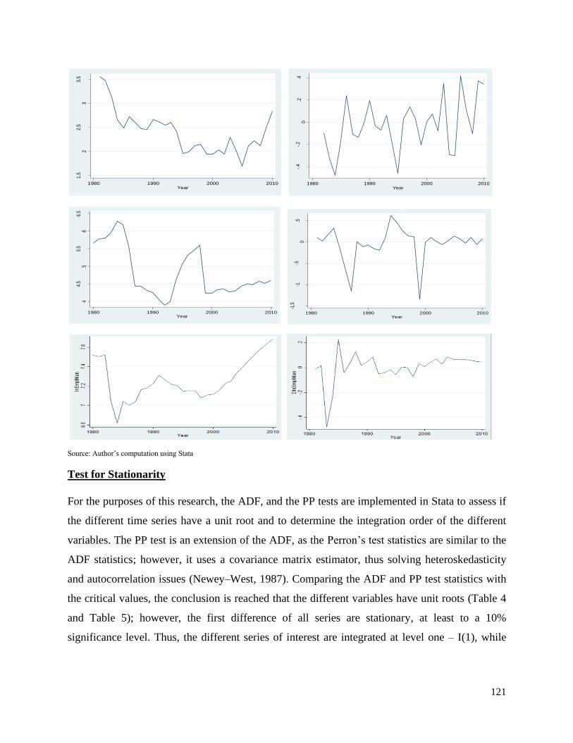
121

Source: Author’s computation using Stata

Test for Stationarity

For the purposes of this research, the ADF, and the PP tests are implemented in Stata to assess if

the different time series have a unit root and to determine the integration order of the different

variables. The PP test is an extension of the ADF, as the Perron’s test statistics are similar to the

ADF statistics; however, it uses a covariance matrix estimator, thus solving heteroskedasticity

and autocorrelation issues (Newey–West, 1987). Comparing the ADF and PP test statistics with

the critical values, the conclusion is reached that the different variables have unit roots (Table 4

and Table 5); however, the first difference of all series are stationary, at least to a 10%

significance level. Thus, the different series of interest are integrated at level one – I(1), while

1.5

22.

53

3.5

lnC

ap

1980 1990 2000 2010Year

-.4

-.2

0.2

.4

Dln

Cap

1980 1990 2000 2010Year

44.

55

5.5

66.

5

lnR

eeR

1980 1990 2000 2010Year

-1.5

-1-.5

0.5

Dln

Ree

R

1980 1990 2000 2010Year

122

their first differences are all stationary I(0). The tables below show the results of the unit-root

tests applied in this study.

Table 4: Augmented Dickey-Fuller Test on all Variables

Table 5: Phillips-Peron Test on all Variables

4.5.4.2 Cointegration Test

In the case of two or more non-stationary series, a linear combination of them is stationary if

these series are cointegrated (Harris, 1995) and related in the long run.

a) Lag length

To check for cointegration between the different variables (i.e. REER, capital and employment)

in their logarithmic forms, the Johansen method of cointegration is applied. Then, the lag length

selection is made by using information criteria, i.e. AIC, HQIC and SBIC. Table 6 shows the

different criteria informing the lag length order selection. Information criteria assess the trade-off

between fit and complexity, i.e. adding more lags reduces degrees of freedom and makes the

model more complex but might add to the statistical fit, so information criteria give the optimal

fit between these two trade-offs. The lag length is selected by minimising the information

criteria. The lag length of two is chosen using criteria based on the fact that the AIC is superior

in the case of a small sample as it minimises possible underestimation and maximises the

possibility of presenting the true lag length, as discussed by Liew (2004).

123

Table 6: Lag Selection VECM

b) Cointegration test

Johansen’s cointegration test assesses the number of long-run equilibrium relationships between

variables of interest by finding the long-run stochastic trend relating to the different series.

Johansen’s cointegration test results (Table 7) show the existence of at least one cointegrating

relationship between the three variables of interest. This suggests that there is at least one

equilibrium relationship between our variables of interest and, as Johansen (1991) shows, this

means our OLS estimation of the reduced form equation is not biased and is, in fact, “super-

consistent”.

This conclusion is based on the trace test which implies the existence of, at most, r cointegration

vectors, while the maximum eigenvalue test evaluates the hypothesis of r+1 cointegration vectors

against the hypothesis of only r cointegration vectors. As indicated in the table below, the trace

statistic of 52.6 is greater than 42.44, which is the critical value at the 5% level of significance.

This points to the existence of one possible stable long-run relationship. The exact number of

cointegrating vectors is confirmed by the maximum eigenvalue test, which leads to the rejection

of the null hypothesis of zero cointegrating vectors at the 1% level of significance. The output

below confirms that there is one cointegrating equation in the model.

124

Table 7: Johansen’s test for Cointegration

4.5.4.3 Manufacturing Sector - Error Correction Model

The long-run relationship in Nigeria between 1980 and 2010 between employment in the

manufacturing sector, aggregate capital formation and REER based on one cointegrating vector

is presented in Table 8 in the same form as equation 2:

𝑙𝑛𝐸𝑚𝑝𝑙𝑜𝑦𝑀𝑎𝑡 = −5.4 − 0.165 𝑙𝑛𝑅𝐸𝐸𝑅𝑡 + 0.358 𝑙𝑛𝐶𝑎𝑝𝑓𝑜𝑟𝑚𝑡 − 0.015𝑡

(0.507) (0.139) ( 0.006)

Table 8: Long Term Relationships Between Variables of Interest

All the coefficients have at least a 5% significance level. These results confirm the theoretical

predictions as real exchange-rate depreciation (a decline in the variable REER) is linked to

increased employment in the manufacturing sector. Thus, my estimate is consistent with the

prediction of Frankel et al.’s (2006) model. As variables were considered in logarithms, the

coefficients can be read as elasticities. This implies that, in the long run, a 1% appreciation of the

125

naira will reduce the employment level in the manufacturing sector by 0.165%. However, in the

long run, for a 1% increase in the country’s capital formation, employment in the manufacturing

sector will increase by 0.358%. This implies that firms internalise the changes in the relative

price of capital and labour, but there is no substitution between capital and labour. A

depreciation will imply that capital is relatively more expensive; thus, firms will focus on a

labour-intensive process, while an appreciation will have the opposite impact.

This analysis indicates two key points. First, in line with the DD framework, an appreciation of

the REER (driven by oil revenues or by political economy factors linked to the resource wealth)

will negatively impact employment levels in the manufacturing sector, and if this sector is

considered a driver of potential growth, it could hinder the country’s development efforts. The

second point concerns the complementary role that capital plays in the Nigerian context in the

long run. This analysis indicates that capital and employment are complementary in the sense

that capital investment will support higher employment levels in line with the findings of Dikko

(2016), who estimated that faster capital accumulation has the potential to reduce unemployment

levels in Namibia, Nigeria, and South Africa.

VECM analysis allows us to assess long- and short-run dynamics. In the estimated system, the

error correction terms capture deviation from equilibrium. In conditions of disequilibrium, the

statistically significant error-correction term indicates that 87% of disequilibrium is corrected.

Thus, LnEmployMan with lag 1 corrects for a significant part of the disequilibrium to bring the

system back in equilibrium in the long-run (see Table 9 below).

The short-run dynamics are evaluated using the Wald test to assess the significance of the

variables. The analysis indicates that in the short-run, the key variable to which the level of

employment is sensitive to is the past level of employment. This hints at certain levels of

stickiness in the sense that adjusting capital is possibly a medium-to-long-term effort. This

explains why the REER is found to have a significant impact on the employment level in the

short run, but its impact is felt in the long run. Although, these short-run dynamics indicate that

REER and capital have the opposite impact on employment than the one assessed in the long

run. These results provide a rationale for a further analysis of the relationship using firm-level

data – see section 4.6.

126

Table 9: Short-Run Dynamics Between Variables of Interest

Post-estimation Analysis

Following the estimation presented above, a number of tests are implemented to assure that the

model is adequate and not misspecified. As all the tests validate the model, the conclusion can be

reached that the model is appropriately specified.

Under the model specification, stationarity is achieved, as illustrated by the graph below. To

assess the model fit, cointegration equation errors are graphed over time (Chart 24). This is

complemented with the unit circle, in line with the theory, Chart25 indicating that the stability

conditions are met as all the eigenvalues are smaller or equal to one. Both tests indicate that

cointegration between the variables does exist and the stability check does not indicate signs of

misspecification.

Chart 24: Errors from the Cointegrating Equation (LHS)

Chart25: Eigenvalues (RHS)

Source: Author’s Computation

-.2

-.1

0.1

.2.3

Pre

dic

ted

co

inte

gra

ted e

qu

atio

n

1980 1990 2000 2010Year

-1-.

50

.51

Ima

gin

ary

-1 -.5 0 .5 1Real

The VECM specification imposes 2 unit moduli

Roots of the companion matrix

127

The Lagrange-multiplier (LM) test for autocorrelation in the residuals is then run. Table 10

below contains the results of this test:

Table 10: Lagrange-multiplier test

Relatively high p-values (Prob>chi2) show that the null hypothesis of no autocorrelation at lag

order 2 may not be rejected at 5% and 10% significance levels. This indicates that the estimated

coefficients are efficient as the minimum variance property holds.

Finally, the Jarque-Berra test is used to confirm if the VECM residuals are normally distributed.

This will help confirm that the inferences are valid. Table 11 below presents the different tests

and indicates that with the reasonable p-values the null hypothesis of normality for the key

equation central to the study, D_lnEmplMan, may not be rejected at conventional significance

levels (α=5%, 10%).

Table 11: Normality Tests

Lag Chi2 df Prob>chi2

1 11.8886 9 0.21966

2 9.8110 9 0.36600

H0 : no autocorrelation at lag order

Source: Author’s Computation

128

4.5.4.4 Total Employment – Error Correction Model

To further assess the link between real exchange rates and employment, the long-run relationship

between total employment in Nigeria (Employ – series from the GGDC which includes both

formal and informal employment), REER and total capital formation is established. Following

the same approach described above, a system cointegrated of order 1 is obtained, with a long-run

relationship (Table 12). This confirms the long-run relationship between the variables of interest

and provides evidence of the relationship between the exchange rate and the aggregate level of

employment.

In line with discussions presented by Frankel et al. (2006), the REER has an impact on the level

of employment. In addition, capital formation impact will depend of the nature of the capital in

Nigeria. The REER impact on the national level of employment is much lower than the one

observed for the manufacturing sector’s employment level. This hints at the fact that the

manufacturing sector is more sensitive to REER movement, given international trade and

competition. It also reflects the structure of the Nigerian economy, which is driven by several

sectors, such as the services sector which has less foreign exposure.

The analysis so far has indicated that capital formation has a positive impact on employment

levels in the Nigerian manufacturing sector. This is further confirmed using the total level of

employment in the country. Similar to observations made in the manufacturing sector, capital

formation is complementary to the employment level; a 1% increase in capital formation could

result in a 1.76% increase in employment. This is expected given the large infrastructure deficit

of the country. This impact is almost five times higher than the impact on the manufacturing

sector, pointing to the issue of capital formation unlocking employment in other sectors. This

also reflects the composition of the Nigerian GDP tilting towards sectors others than

manufacturing.

𝑙𝑛𝐸𝑚𝑝𝑙𝑜𝑦𝑡 = −9.955 − 0.021 𝑙𝑛𝑅𝐸𝐸𝑅𝑡 + 1.765 𝑙𝑛𝐶𝑎𝑝 − 0.026𝜙𝑡

(0.0048) (0.4555) (0.0005)

129

Table 12: Long-Run Relationship Between Total Employment and Key Variables Johansen normalisation restriction imposed

beta Coef. Std. Err. z P>|z| [95% Conf. Interval]

_cel

InEmploy

1

InReer -.0205484 .0048021 -4.28 0.000 -.0299604 -.0111364

Incap 1.76471 .4555476 3.87 0.000 .8718526 2.657566

_trend -.0265388 .0005726 -46.35 0.000 -.027661 -.0254165

_cons -9.955104

Source: Author’s Computation

The VECM analysis, Table 13 below, indicates that most variables, apart from the lagged

employment one, are found to be insignificant factors affecting employment levels, apart from

the level of capital formation.

Table 13: Short-Run Dynamics Between Total Employment and Key Variables Coef. Std. Err. z P>l z l [95% Conf. Interval]

D_InEmploy

_Cel

L1.

-.0129377

.0047015

-2.75

0.006

-.0221524

-.003723

InEmploy

LD.

.1052418

.1806194

0.58

0.560

-.2487657

.4592493

InReer

LD.

.006925

.008163

0.85

0.396

-.0090741

.0229241

Incap

LD.

.0388411

.0144194

2.69

0.007

0.105797

.0671026

_cons .0223845 .0052604 4.26 0.000 .0120743 .0326948

Source: Author’s Computation

Given the high statistical significance of regressors above, this vindicates the VAR-VECM

methodology and the presence of both the long-run equilibrium relationship and the existence of

short-run dynamics. The different post-estimation figures below (Table 14; Table 15; Chart 26;

Chart27) validate the existence of a long-run relationship between employment, REER and

capital.

130

Chart 26: Errors from the Cointegrating Equation (LHS)

Chart27: Eigenvalues (RHS)

Source: Author’s Computation

Table 14: Lagrange-multiplier test

Table 15: Normality Tests

-.2

-.1

0.1

.2.3

Pre

dic

ted

co

inte

gra

ted e

qu

atio

n

1980 1990 2000 2010Year

-1-.

50

.51

Ima

gin

ary

-1 -.5 0 .5 1Real

The VECM specification imposes 2 unit moduli

Roots of the companion matrix

131

4.5.5 Conclusions

This analysis so far has investigated for the first time in the Nigerian context the labour intensity

channel through which the exchange rate impacts employment. This has been achieved by

assuming changes in the relative price of capital and labour and concluding that they will

dampen or amplify the magnitude of exchange rate shocks on labour market outcomes. Though

the empirical literature on exchange rates and employment is still growing, existing evidence

shows that exchange rates exert a strong influence on employment. In order for the Nigerians

government’s industrial policy to achieve its goal of creating impetus for jobs, the impact of the

exchange rate on traded goods needs to be considered and addressed.

The above analysis, using macroeconomic data, assesses the impact of the REER on the

employment level in Nigeria, both in the manufacturing sector and at the aggregate level. In the

long run, an exchange-rate appreciation as indicated by the model developed by Frenkel and Ros

(2007) and suggested by the way in which the labour intensity channel decreases the

employment level in the manufacturing sector, on aggregate by 0.165% and 0.02%, respectively.

The difference in impacts between the manufacturing sector and the aggregate level is explained

by the structure of the Nigerian economy, including the small share of the manufacturing sector

in total employment. Other sectors, in particular the service and agriculture sectors (cumulatively

representing over 90% of total GDP), are less sensitive to the real exchange-rate movement.

Indeed, services are in general non-tradables, while the agricultural output has mainly focused on

132

staples crops, with only 15% of farmers focusing only on cash crops (NOI polls, 2016). Thus,

overall, in terms of employment, a depreciated REER will have an impact on employment but

not in the needed scale; however, it will support the manufacturing sector.

Furthermore, capital formation impacts positively on the level of employment. This is in line

with the level of development of the country and the large infrastructure gap it faces, illustrated

by the levels of physical capital of roads, the quality of the educational system, low production

and access to electricity, and poor access to public health services, all of which lag behind the

regional average (Brookings 2018). This implies that capital investment leads to economies of

scale and increased productivity. For example, the notorious issues of power supply in the

country will impact employment, as found in other countries. Dollar et al. (2005) discovered, for

instance, that fluctuating power supplies have a strong negative impact on production in

Bangladesh, Pakistan, India, and China. Reinikka and Svensson (2002) submitted that in

Uganda, employment, probability to export, and private investments have a negative relationship

to power losses.

Finally, although not significant, the implication of the short-run dynamic analysis could indicate

that an exchange-rate appreciation may lead to increased employment – against theoretical

predictions. This provides the rationale for the further analysis of the adjustment dynamics of

Nigerian firms to REER movements presented in the next section.

4.6 Micro-level evidence on the exchange rate impact on firms

In this section of the analysis, the short-run dynamics which appear inconclusive using a VECM

are further explored. To better assess some of the short-run dynamics and the impact of REER,

the determinants of employment at the firm level are investigated, taking into account the

possible dynamics of such relationships, as presented in the labour literature of Eisner et al.

(1963), Sargent (1978), Nickell (1986) and Hamermesh (1993) among others. The objective of

this section is to measure the impact of Nigeria’s real exchange rate on its manufacturing

employment. This is the first analysis that looks at the impact of REER from a firm perspective

using panel data from Nigeria. Another major contribution of this analysis is the construction and

use of sector-specific REER, based on the assumption that price movements affecting different

sectors of the economy will be driven by trade patterns which are intrinsic to those sectors.

133

The strand of the literature analysing the direct impact of REER movements on employment

levels in the case of developing countries is growing. For example, Koren (2001), who used

panel data for Hungarian exporting firms from 1992-1996, found that industry-specific REER

impacted employment levels in that country. Similarly, Frenkel (2004) found that REER

influenced the unemployment levels in Latin America countries such as Argentina, Brazil, Chile

and Mexico. Filiztekin (2004), in the case of Turkey, also points to the impact of the REER

exchange rate on employment levels in the manufacturing sector, using panel data covering the

period 1981-1999.

Firm-level analysis of this type needs to take into account the fact that a movement from one

equilibrium to another, in a reaction to exchange rates for example, will be affected by the type

of adjustment costs they face (see Nickell 1986; Hamermesh et al. 1996; Cooper et al. 2004;

Nilsen et al. 2007). Indeed, firms are confronted with adjustment costs that affect the level of

labour as presented by Hamermesh (1993). Firms can react to the shocks by changing input (i.e.

labour) demand. The scale of these changes is dependent on the adjustment costs they face,

which may prevent them from responding optimally. This adjustment in cost could result from a

number of factors, including institutional regulations, but also from economic or technological

obstacles. Although the key relationship of interest here is the impact of industry-specific REER

on employment, it is difficult to analyse this independently of other variables, such as capital and

wages. Further, when looking at these variables and REER, it is difficult to assess causation (e.g.

wages driving employment) or if employment levels reflect any underlying unobservable factors,

also impacting wages and capital. Thus, without specific econometric tools taking into account

the nature of these relationships, it is difficult to make an appropriate inference from the analysis.

In addition, using a panel data set with large numbers of cross-section units observed over a

relatively short period of time presents some challenges. As indicated by Bond (2002), these

characteristics often represent micro-level panel data that implies the need for specific estimation

methods that can internalise the short time period and present consistent parameter estimates.

Standard methods estimators can be inconsistent as the strict heterogeneity assumption prevents

them from capturing the possible feedback loop between current and past observations, which is

not a natural restriction when looking at the labour market and exchange rate. Thus, the

134

Generalised Method of Moments (GMM) estimators, developed by Arellano and Bond (1991,

2000) and Bond (2002) among others, are employed.

There are several reasons for preferring this method over others. The first pertains to the fact that

it is in line with the dynamic VECM approach taken in the time-series analysis; it takes into

account the dynamics flowing from lagged dependent and independent variables in the

regression of employment. The model described above is inherently dynamic; therefore, the

analysis needs to internalise this dynamic relationship between current levels of employment

observed and the past REER; ignoring these dynamics, as in the case of the traditional fixed-

effects estimators, could result in inconsistent estimates. One could have also estimated a fixed-

effects model when working with panel data, but including lagged dependent variables can result

in fixed-effect model estimates affected by a bias (see Bond, 2002 for the derivation of bias that

arises).

Secondly, contrary to the OLS and fixed-effects estimates, the GMM estimator captures the

dynamic underlying process, in this case employment on past REER, and thus allows for the

possibility of finding valid instruments originating from the variables representing the firm’s

history. This will allow one to address the simultaneity issue among the variables of interest. In

summary, the GMM estimator relies on internal instruments found in the dataset, then makes

allowances to avoid the problem of finding relevant and valid external instruments. In this

analysis, past levels of REER and employment are candidates for the role of instruments

explaining current levels of employment.

Thus, for the purpose of this paper, using a data set of 200 firms covering the period 1998 to

2000, and using a dynamic estimator, the relationship between the different determinants of

employment such as wages, capital and industry-specific REER and employment are

investigated. Secondly, the dynamic GMM estimator is employed to assess the relationship

between industry-specific REER and employment. Thirdly, the results are presented using this

method.

4.6.1 The Employment Equation

The impact of the RER on employment has received limited interest compared to the number of

studies related to developed economies, in particular when assessed from a macroeconomic

135

perspective (Ay and Ayhan 2016). Studies transposing these mechanisms at the micro-level (i.e.

firm-level) in developing contexts are also scarce. In attempting to do so, one has to consider the

fact that a number of factors related to a firm’s organisation can endogenously affect a firm’s

employment decisions.

Departing slightly from the model developed by Frenkel and Ros (2006), for this study, possible

adjustment costs are included. In line with Lichter et al. (2012), a partial adjustment model7 is

included, which assumes that due adjustment-costs prevent firms from responding optimally and,

therefore, employment levels can be sub-optimal (King and Thomas 2006) and the actual

employment level 𝐿𝑡 is affected by the optimal level of employment 𝐿𝑡∗ as well as by past levels

of employment: 𝐿𝑡−1:

𝐿𝑡 = 𝜆𝐿𝑡∗ + (1 − 𝜆)𝐿𝑡−1 (equation 1)

To make estimations using this model, the optimal value of 𝐿𝑡∗ needs to be taken into account. By

assuming a similar production function used in 2006 by Frenkel and Ros (i.e. the Cobb-Douglas

production function) and using transformed logarithms, the optimal value of employment can be

expressed as:

ln(𝐿𝑡) = 𝛿1ln (𝐿𝑡−1) + 𝛿2 ln(𝐿𝑡∗) + 𝑣𝑡 (see Nickell 1996) –(equation 2)

Without adjustment costs, firms could set employment such as ln(𝐿𝑡∗) = 𝛽0 + 𝛽1 ln(𝑤𝑡) +

𝛽2 ln(𝑘𝑡) + 𝛽3ln (𝜎𝑡), where ln(𝑤𝑡) is the logarithm form of the wage rate, ln(𝑘𝑡) is the

logarithm form of capital and ln (𝜎𝑡) is the logarithm form of expected demand. (see Layard and

Nickell 1996). Using equation 1 and 2 presented above, the following equation is obtained:

ln(𝐿𝑡) = 𝛿1ln (𝐿𝑡−1) + 𝛽0 + 𝛽1 ln(𝑤𝑡) + 𝛽2 ln(𝑘𝑡) + 𝛽3 ln(𝜎𝑡) + 𝑣𝑡

This setting captures the short-run dynamics that reflect a number of factors, including

adjustment costs, a firm’s expectations and a firm’s decision-processes. Building on this equation

are several papers, such as Layard and Nickell (1986), Nickell and Wadhwani (1989) and

Blundell and Bond (2000): see also Arrelano and Bond (1991). In line with Adam and Moutos

(2014), the equation is adjusted to include industry real-exchange rates. This equation will allow

7 Limitations of such models are discussed in Litcher et al (2012).

136

the labour-intensity channel to be tested by capturing aspects of the possible substitution of

labour for capital, as well as the impact of REER in this process. The specification arrived at is:

𝑙𝑖,𝑡 = 𝑙𝑖,𝑡−1 + 𝛽1𝑤𝑖,𝑡 + 𝛽2𝑤𝑖,𝑡−1 + 𝛽3𝑘𝑖,𝑡 + 𝛽4𝑘𝑖,𝑡−1 + 𝛽5𝑅𝐸𝐸𝑅𝑗,𝑡 + 𝛽6𝑅𝐸𝐸𝑅𝑗,𝑡−1 + 𝑑𝑖 + 𝜏𝑡 +

휀𝑖𝑡

where i represents the firms, j reflects the relevant industry and t is the observation year. di

represents the firm-fixed effects, capturing all the unobserved firm-related factors, REER is the

sector-specific real effective exchange rate and εit is the error term. Alternatively, the equation in

its reduced form becomes:

𝑙𝑖𝑡 = 𝛼 + ∑ 𝑘𝑠∆𝑙𝑖𝑡−𝑠𝑠 + 𝛽𝑋𝑖𝑡 + 𝛾𝑍𝑖𝑡 + 𝑛𝑖 + 휀𝑖𝑡 𝑠 = 1, … , 𝑝 equation. (3)

where 𝑙 represents employment, 𝑋 and 𝑍 represent REER and other characteristics of the firm

and 𝑛 captures the unobserved firms’ effects.

A key issue with such a specification is that if variables, such as capital and wages and, to a

certain extent, the sector-specific exchange rate, along with the weighted average of the trade

import and export activities of a sector, are the chosen variables, then they must be based on

some expectations of employment. This implies that any estimates based on equation 3 assume

that currents shocks are independent of past levels of any variables of interest. Further, this

assumption allows for current levels of employment to reflect current and past realisations of

variables, such as wage, capital and REER. This implies that firms can choose capital levels to

only affect current or future levels of employment. This has empirical implications.

4.6.2 Source of Simultaneity and Endogeneity in the Wage Equation

From an econometric perspective, simultaneity bias is present in equation (3) if 𝐸(휀𝑖𝑡|𝑋𝑖𝑡, 𝑍𝑖𝑡) ≠

0. Simultaneity will occur between employment and other variables of interest if, as suggested

by economic theory, firms can select a level of employment in any period to reflect an assumed

level of wages, capital and REER in that same period. While employment levels can reflect other

variables, the reverse will also be true – wages, capital and trade-weighted REER will also be

affected by employment. In this case, an estimate of equation (3) using OLS and the fixed-effects

methods will internalise a simultaneity bias.

137

A possible solution to the simultaneity bias is found in a system of equations employed to

estimate the impact of the different variables on employment levels. In this case, employment

will depend on the relevant variables. These dependent variables in the other equations of this

system, in turn, become control variables, which are allowed to be dependent on the employment

level and the other variables of interest. To gain estimates from such a system will require a set

of strictly exogenous instruments to be identified. This assumes the existence of at least one

variable in the employment equation that is not also in the REER, wage and capital equations. In

general, findings of this type, of strictly exogenous instruments, can be an arduous task, even

more so considering that the number of instruments required is proportional to the number of

equations included in the system.

In addition, using panel data implies the fact that there are a number of unobservable factors

affecting a firm’s performance and the explanatory variables of interest. These types of factors

can include the managerial ability of senior staff, which is not captured by any of the variables

but which can impact employment levels. This unobservable heterogeneity can cause an

endogeneity bias affecting the performance of an OLS regression. In theory, this bias can be

addressed by using fixed-effects or “within” estimations.

However, fixed-effects regression can be consistent and unbiased only under a number of

conditions. Indeed, estimating equation (3), using a fixed-effect approach, is only consistent

when the current level of each explanatory variable (capital, wages, etc.) is completely

independent of the dependent variable’s (i.e. employment) past levels: in other words, if

𝐸(휀𝑖𝑡|𝑋𝑖𝑡, 𝑍𝑖𝑡) = 0, ∀𝑠,𝑡.. Other than the independence from past realisations of explanatory

variables, Roodman (2009) highlights the possibility of another fixed effect bias in the context of

a dynamic relationship in which a firm’s past performance (y) affects the level of employment

(x) but the inverse, meaning x impacting y, is not true. Within this setting, a fixed-effect

regression would result in a false, but statistically significant, estimate. This form of bias is more

prominent in the case of a small length of the panel data.

4.6.3 Dynamic Panel GMM Estimation

Based on the above analysis of possible bias, to estimate the relationship between the REER and

employment level at the firm level, a dynamic GMM panel estimator will be used, in line with

Holtz-Eakin et al. (1988) and Arellano et al. (1991), who use the dynamic structure presented by

138

the dependent and explanatory variables. This method has been used to solve dynamic problems

in analysing capital investment (Whited, 1991), economic growth convergence (Caselli et al.

1996), and labour demand (Blundell et al. 1998).

The GMM estimation approach is based on two steps. The first one entails running a dynamic

model similar to equation (2) which can be written in its first-differenced form

∆𝑙𝑖𝑡 = 𝛼 + 𝑘𝑝 ∑ ∆𝑙𝑖𝑡−𝑝𝑝 + 𝛽∆𝑋𝑖𝑡 + 𝛾∆𝑍𝑖𝑡 + ∆휀𝑖𝑡, 𝑝 > 0 equation 4

Applying the first difference allows one to reduce the unobservable variables bias. Then,

equation 4 is estimated using the GMM approach. This implies considering the lagged values of

the set of explanatory variables as valid instruments for the current level of explanatory

variables.

This means that the instruments used here to estimate equation (3) and (4) are sourced from

lagged values of the variables of interest, i.e., 𝑙𝑡−𝑘 , 𝑋𝑡−𝑘, 𝑍𝑡−𝑘 , where 𝑘 > 𝑝 . Further, these

instruments are only valid if:

i) they represent a source of variation for current variables, for example 𝑍𝑡 =

𝑓(𝑙𝑡−𝑘,𝑋𝑡−𝑘, 𝑍𝑡−𝑘).

ii) the lagged levels are an exogenous factor affecting changes in the current levels of

employment. As a result, the lagged levels are not correlated with the error terms in the

employment equation – this is known as weak rational expectations.

The second condition means that shocks to explanatory variables would not have been

anticipated when the employment level was decided. As a result, p number of lags is necessary to

ensure dynamic completeness of equation 2 by assuring that p lags of the employment level

variable will capture the impact of past-performance on the present. Thus, by adding these p lags

of employment, past performance of the firms prior to p does not impact current realisation of

employment. This affirms that information beyond p is exogenous from both current and future

information.

Despite its advantages, the GMM estimator presents some shortcomings. Indeed, Beck et al.

(2000) highlight that the need to use models in their first-difference form can weaken the power

of the existing tests as this reduces the amount of information presented by the explanatory

139

variables. Further, Arellano and Bover (1995) indicate that the variables presented in their level

forms are likely to be weak instruments. Finally, Griliches and Hausman, (1986) claim that using

the first-difference forms may worsen measurement errors.

Blundell et al. (1998) developed an approach mitigating these shortcomings by allowing the

GMM estimator to include equations in their level forms. Thus, by using a “stacked” system of

equations, including levels and differences variables, variables in their first-differenced form can

be used as instruments for equations presented in following levels. As a result, a “system” GMM

estimator is obtained:

[𝑙𝑖𝑡

∆𝑙𝑖𝑡] = 𝛼 + 𝑘 [

𝑙𝑖𝑡−𝑝

∆𝑙𝑖𝑡−𝑝] + 𝛽 [

𝑋𝑖𝑡

∆𝑋𝑖𝑡] + 𝛾 [

𝑍𝑖𝑡

∆𝑍𝑖𝑡] + 휀𝑖𝑡

Despite the progress, equations in their levels form in this system will still present some

unobserved heterogeneity. To cater for this issue, it is assumed that the correlation between the

unobservable variables and the observed ones is constant over time. The literature posits that this

assumption is reasonable with data-sets covering a relatively short time period.

Thus, the GMM system estimator provides estimates addressing a number of issues faced with

dealing with panel data. These include simultaneity and the dynamic relationship between

explanatory and dependent variables, as well as time-invariant unobserved heterogeneity.

Further, this method implies that instruments are available within the systems as lagged-level

values can serve as instruments for differenced equations: for level equations, the most

appropriate instruments are lagged differences. These are only true if the assumptions of no

serial correlation in the error terms are held and if orthogonality conditions are met (see Arellano

and Bond 1991), which will be tested in the empirical approach. Further, another key underlying

assumption of the GMM estimator is the exogeneity assumption, which assumes that historical

employment levels of a given firm and other relevant characteristics are independent of current

shocks. Arellano and Bond (1991) highlight how two tests have been developed to assess this

key assumption.

The first one evaluates second-order serial correlation, allowing one to confirm if sufficient lags

were included to fully control the dynamic relationship. If this test is conclusive, any values of

the explanatory variables beyond those lags can be used as instruments, given the confirmed

140

exogeneity to level shocks. This test implies that the residuals in the first differences (AR(1)) are

expected to be correlated, while this correlation should not be found in the second differences

(AR(2)).

The second test is a Hansen test of over-identification. As the dynamic panel GMM estimator is

based on using lags as instruments, it implies that the system is over-identified, which can be

tested through the Hansen test. Under the null hypothesis of valid instruments, the test provides a

J-statistic which is distributed χ 2.

4.6.4 Data on Nigerian Manufacturing Firms

4.6.4.1 Survey

The Nigerian Manufacturing Enterprise Survey (NMES) is the panel data used for the

investigation of the relationship of interest between exchange rates and firm-level employment

contained within this thesis. The NMES survey was initially completed for the United Nations

Industrial Development Organisation (UNIDO) and the Centre for the Study of African

Economies (CSAE), based at Oxford University. At the time, the survey aimed to identify the

drivers of the performance of the Nigerian manufacturing sector. It was one of the first surveys

to attempt to use firm-level data, in contrast to the dominant use of macroeconomic data to study

African firms.

The survey applied a stratified random sampling methodology, implying that the population

firms are grouped into strata, and a random draw is completed from each stratum to select

relevant firms (NMES, 2001). Thus, the frequency distribution across sectors is non-uniform.

However, this methodology is useful as firms within a stratum are relatively homogeneous, but a

large heterogeneity can be noted among firms in different strata. As a result, it captures the fact

that the Nigerian manufacturing sector is dominated by a large number of small, homogeneous

firms, while large firms represent a significant proportion of employment created by this sector.

To capture this feature, large firms are over-represented compared to their proportion in the

actual population (NMES report, Wave 1). A major caveat of the dataset is the fact that it is not

representative of the population, which is known to include a large informal sector.

The NMES was undertaken in mid-2001 to cover the years 1998 to 2000 for the first wave; a

second wave was undertaken in 2004 to cover the years 2001 to 2003. The surveys were

141

administered to capture both current and past level-information. The surveys focused mainly on

four subsectors (i.e. food processing, textiles and garments, furniture and paper processing, and

metal, machinery and chemicals). Both waves of surveys covered specific parts of the country

judged to be the most dynamic, such as Lagos and Ibadan in the South-West; the South East,

with key cities such as Enugu, Onitsha, and Aba; and Kaduna and Kano in the north.

The timing of the survey is particularly interesting for the purpose of this research as it captures

the significant devaluation of the naira that occurred in 1999. This is elaborated upon further in

the section below.

The Sample

The Table 16 below shows a 35% loss in observations between the two waves, as observations

dropped from 180 firms included in wave 1, covering the period 1998-1999, to 117 firms

surveyed during the second wave, over the period 2001-2003. As such, this could provide an

interesting angle of analysis, which could entail identifying possible factors driving firms to drop

out of the survey (e.g. productivity, capital/labour ratios, fixed effects, etc.). However, this is not

covered by the present analysis. Table 16 below also shows the differences in the yearly number

of firms surveyed.

Table 16: Numbers of Observations Per Year and Sector

Year

Sub – Sector 1998 1999 2000 2001 2002 2003 Total

Paper Manufacture &

Products 21 21 21 12 12 12 99

Textiles 34 34 34 13 13 13 141

Chemicals 14 14 14 11 11 11 75

Food 19 19 19 15 15 15 102

Furniture 12 12 12 11 11 11 69

Garment 40 40 40 27 27 27 201

Machines 9 9 9 9 9 9 54

Metal 25 25 25 14 14 14 117

Wood 6 6 6 5 5 5 34

Total 180 180 180 117 117 117 891

Source: The NMES

142

Table 17 below presents total employment per sector of interest in the different years of interest.

Most sectors show a marginal increase or a decrease in total employment in 1999, while for most

sectors, total employment of the firms remaining in the survey show an increase in the period

2001-2003. Similarly, Table 18 below shows the average logarithms for employment per firm.

Table 19 shows the log of capital.

Table 17: Aggregate Employment Per Sector

year

Sub – Sector 1998 1999 2000 2001 2002 2003

Paper Manufacture &

Products 839 1151 1269 511 490 480

Textiles 14140 26480 28483 15991 15236 14547

Chemicals 1155 2388 7842 7893 7919 7977

Food 6443 6399 15193 9899 10258 8391

Furniture 848 865 829 719 819 902

Garment 244 256 337 429 367 324

Machines 1724 1690 2592 3642 3712 3298

Metal 1174 1187 1155 926.1 957 1142

Wood 267 300 272 373 391 387

Source: The NMES

Table 18: Average Employment Per Sector (Log 1000s)

year

Sub – Sector 1998 1999 2000 2001 2002 2003

Manufacture & Products 3.49 3.59 3.60 3.24 3.23 3.17

Textiles 5.00 5.02 5.18 5.47 5.43 5.43

Chemicals 4.38 4.58 5.05 5.13 5.08 5.06

Food 4.22 3.99 4.57 4.30 4.35 4.38

Furniture 3.74 3.32 3.07 3.22 3.32 3.20

Garment 1.92 1.82 1.74 2.18 2.00 1.91

Machines 4.54 4.47 4.71 5.12 5.08 4.99

Metal 3.44 3.47 3.13 3.20 3.55 3.64

Wood 5.59 5.70 2.99 2.24 3.09 2.82

Source: The NMES

Table 19: Average Amount of Capital Per Sector (Log Millions of Naira)

year

Sub – Sector 1998 1999 2000 2001 2002 2003

Manufacture & Products 13.84 13.66 13.65 13.46 13.58 13.64

Textiles 13.81 13.85 13.82 13.45 13.53 13.50

Chemicals 14.02 14.30 14.16 14.23 14.34 14.30

Food 13.56 12.88 13.06 12.76 12.70 12.64

Furniture 12.70 11.93 12.18 12.54 12.47 12.56

143

Garment 10.95 10.94 11.07 10.42 10.68 10.70

Machines 12.12 12.07 12.60 12.93 13.15 13.23

Metal 13.76 13.30 13.18 14.37 14.27 14.16

Wood 12.75 12.60 11.99 11.29 11.49 11.74

Source: The NMES

A number of points gleaned from the dataset need to be highlighted as they have a potential

impact on the analysis.

a) Real output during 1998-2003 did not increase (see Table 20). Irrespective of firm size, there

was no meaningful change in real output within this sample. This suggests that in the

NMES, sample firm growth is negligible. This is true for all the size categories and this

result is of no consequence in terms of rise in output. It needs to be stressed that this is a

result of this sample and that it is not representative of all firms in the Nigerian

manufacturing sector. It is probable that a large number of firms have entered and exited the

different sectors.

Table 20: Average Log Output Per Sector (Log Millions of Naira)

year

Sub – Sector 1998 1999 2000 2001 2002 2003

Paper Manufacture & Products 16.57 16.75 16.79 16.82 16.91 16.82

Textiles 18.42 18.52 18.75 19.31 19.40 19.36

Chemicals 18.87 19.35 19.66 20.39 20.40 20.54

Food 19.56 17.97 18.91 18.60 18.75 18.74

Furniture 16.86 16.91 16.60 16.95 17.16 17.15

Garment 14.32 14.40 14.07 14.45 14.50 14.53

Machines 18.18 18.29 18.71 18.80 18.95 18.95

Metal 17.69 17.80 17.13 18.01 17.90 18.06

Wood 16.00 16.52 16.45 15.99 17.32 17.55

Source: The NMES

b) Efficiency and productivity have not shown significant improvement (Table 21). Looking at

real output per employee over the period of interest, there is no major change in

productivity. Thus, the data suggests that the firms’ processes did not improve over this

period.

Table 21: Measure of Productivity - Average Output Per Worker (Log Millions of Naira)

year

Sub – Sector 1998 1999 2000 2001 2002 2003

Paper Manufacture & Products 13.34 13.40 13.40 13.58 13.56 13.40

Textiles 13.78 13.81 13.69 13.85 13.85 13.68

Chemicals 14.63 14.85 14.78 15.26 15.20 15.22

144

Food 14.43 14.22 14.52 14.30 14.27 14.11

Furniture 13.13 13.63 13.71 13.72 13.72 13.70

Garment 12.60 12.86 12.47 12.26 12.37 12.37

Machines 13.94 14.06 14.17 13.68 13.75 13.72

Metal 14.48 14.53 14.17 14.39 14.23 14.28

Wood 13.81 14.68 13.63 12.61 14.11 14.48

Source: The NMES

However, sectoral labour productivity varies greatly. In terms of labour productivity, the

chemicals, food and machines sectors are the most productive, followed by the metal, textiles

and wood sectors, while the furniture, garment and paper sectors are the least productive. The

difference between the chemicals sector and the garments sector (between the highest and lowest

productivity sectors) in their logarithm form is close to 2, indicating an extremely large

difference in levels. The scatter diagram below indicates that labour productivity increases

monotonically with size.

Chart 28: Relationship Between Output Per Worker and Employment

Source: Authors’ computation based on the NMES

c) The capital intensity of firms is one of the underlying reasons for the observed differences in

labour productivity. Capital intensity measures the relative use of capital compared to other

factors, such as labour, in the production process. Both labour productivity (see Chart 28

above) and capital intensity (Chart 29; the LHS diagram below) increase monotonically with

a firm’s size. The scatter diagram below (Chart 29; RHS) shows the relationship between

capital intensity and labour productivity.

145

Chart 29: Employment vs. Capital Per Worker (LHS) & Output Per Worker vs. Capital

Per Worker

Source: Authors’ computation based on the NMES

d) Investment and capital stock are key determinants of economic growth-rates. Moreover, the

observed volatility can explain significant short-run economic fluctuations. The data

highlights that investment is not a smooth process, with the majority of firms not investing

in any given year. In this sample, only 48% of the firms reported non-zero investments in

any given year. For the remaining 52%, the lack of investment implies that their capital

stock is actually declining as they fail to replace value lost through depreciation. The survey

also points to the fact that the average capacity utilisation is about 44%. As highlighted by

Malik et al. (2008), capacity utilisation rates in these sectors compared to international

standards are relatively low, pointing to significant excess capacity.

Based on the survey, the key variable of interest will be capital, wages and employment at the

firm level in their logarithmic forms. The employment variable – lnEmploy – is the logarithm of

the employment level in the firms in a given year. In line with an adjusted version of Arrendo

and Bond’s (1991) model, the level of employment is assumed to be determined through three

factors:

(i) Capital is the firm’s real total assets (in its logarithmic form). This controls for size

effects that possibly impact a firm’s performance, such as growth, as well as the

investment and employment levels;

(ii) Wages, which represent the logarithm of the firm’s real wages. Here, lagged values are

used to control for the possible effect of exchange rate on employment, which will

manifest itself through higher wages (Andersen and Sorensen, 1988); and

(iii) The trade-weight exchange-rate – discussed below.

146

4.6.4.2 Exchange Rate

4.6.4.2.1 Nigeria’s Historical Exchange Rates around the Period of Interest

Chapter 3 reviewed exchange-rate policy in relation to aspects of economic development, such as

oil and trade policy. Chart 30 below reminds us of the evolution of the official exchange rate

against the trade-weighted REER index, i.e. the measure of a currency against a basket of other

currencies that is linked to the nominal exchange rate. In this case, it shows that nominal

depreciation of the naira translates into weaker (more competitive) REER.

Chart 30: Nominal and Real Effective Exchange Rate

4.6.4.2.2 Industry-Specific Real Exchange Rate Construction

In addition, it is clear that price movements will not have the same impact on different sectors of

the economy as the trade patterns are likely to be different depending on the goods produced.

Thus, to capture these differences across sectors and industries, a trade-weighted real exchange-

rate specific to each industry of interest was constructed. This represents another key

contribution of this study.

To construct these industry-specific exchange rates, in line with Golbderg (2004), the different

trade partners (noted with c), both from the import and export side, were attributed a weight

based on the volume of exchanges originating from a specific industry (denoted i). On an

aggregate basis, the weights were allocated to each partner based on total trade (i.e. import and

export activity). In other words, industry-specific real exchange-rates were computed as follows:

1. Export-weighted real exchange-rate

Source: World Bank Database

Note: The REER is the nominal effective exchange rate divided by a price deflator - an increase represents an appreciation. Nominal exchange

rate refers to the exchange rate determined by legally sanctioned exchange market. It is calculated as an annual average based on monthly

averages (local currency units relative to the U.S. dollar).

147

𝑥𝑒𝑟𝑡𝑖 = ∑ 𝑥𝑡

𝑖𝑐

𝑐

. 𝑟𝑒𝑟𝑡𝑐, 𝑤ℎ𝑒𝑟𝑒 𝑥𝑡

𝑖𝑐 =𝑋𝑡

𝑖𝑐

∑ 𝑋𝑡𝑖𝑐

𝑐

2. Import-weighted real exchange-rate

𝑚𝑒𝑟𝑡𝑖 = ∑ 𝑚𝑡

𝑖𝑐

𝑐

. 𝑟𝑒𝑟𝑡𝑐, 𝑤ℎ𝑒𝑟𝑒 𝑚𝑡

𝑖𝑐 =𝑀𝑡

𝑖𝑐

∑ 𝑀𝑡𝑖𝑐

𝑐

3. Trade -weighted real exchange rate

𝑡𝑒𝑟𝑡𝑖 = ∑ ((. 5

𝑋𝑡𝑖𝑐

∑ 𝑋𝑡𝑖𝑐

𝑐

+ .5𝑀𝑡

𝑖𝑐

∑ 𝑀𝑡𝑖𝑐

𝑐

)𝑡

𝑖𝑐

)

𝑐

. 𝑟𝑒𝑟𝑡𝑐,

where 𝑟𝑒𝑟𝑡𝑐 represents the RER between Nigeria and its trading partner 𝑐, which is the product of

country 𝑐′s nominal exchange rate and the ratio of the Nigerian consumer price index against that

of country c. The index 𝑖 refers to a specific industry, while t refers to a specific year. The

analysis leads to the computation of an industry-specific export RER, an industry-specific import

RER, and the trade-average RER. An increase in the value of any of these indexes reflect a naira

real appreciation in trade-weighted terms.

4.6.4.2.3 Data

The nominal exchange rate data were taken from the World Bank database and converted to US

dollars. The foreign consumers price indexes data was extracted from the same source, while the

trade data was collected from the World Integrated Trade Solution (WITS) tool, which collects

and compiles information on trade gathered from several international organisations, including

the World Bank. Using the methodology presented above, an industry-specific exchange rate for

the different sectors included in the MNES survey was obtained. Chart 31 below indicates that

exchange-rate movement affects industries such as the food and chemical sector far less than the

garment and wood industries. Although trends are unique to each sector, they capture large

exchange rates movements, such as the 1999 naira devaluation.

148

Chart 31: Trade-Weighted Real Exchange Rate (Log Form) for Sectors of Interest

Source: Author’s computation, trade data from the World Integrated Trade Solution (WITS) for sectors using the classification HS 1988/92; the nominal exchange rate data were taken from the World Bank database and converted to US dollars. Similarly, the foreign consumers price

indexes data was sourced from the same source,

4.6.5 Empirical Evidence: The Role of the Exchange Rate on Employment

In this section, given the dynamic relationship between employment and its determinants at the

micro-level, the dynamic model developed above is used. In the next sections, the relationship

between employment and its determinants is estimated through a dynamic panel GMM

estimator. The results of this estimation are compared to static models (i.e. OLS and fixed

-1

0

1

2

3

4

5

1998 1999 2000 2001 2002 2003log

trad

e w

eitg

hed

rea

l ex

chan

ge r

ate

Food Textile Garment

0

2

4

6

8

1998 1999 2000 2001 2002 2003log

trad

e w

eitg

hed

rea

l ex

chan

ge r

ate

Chemical Metal Machines

0

1

2

3

4

5

6

7

1998 1999 2000 2001 2002 2003

log

trad

e w

eitg

hed

rea

l ex

chan

ge r

ate

Wood Paper etc Furniture

149

effects) to ascertain the bias that could result from ignoring endogeneity arising from the

dynamic characteristics of the variables.

4.6.5.1.1 Ensuring Dynamic Completeness

For the purpose of this study, it is important to evaluate the number of lags needed to capture all

the necessary information from a firm’s past performance. A failure to capture the dynamic

through which the past impact’s the present could result in misspecifying equation (2) as it may

suffer from an omitted variable bias. Furthermore, fully capturing the impact of past information

is a necessary condition to be able to use past lags as valid instruments, as it guarantees that

those past values are not related to the residuals of the present. This assumption is key as it

ensures that the dynamic panel GMM estimator is constant.

As suggested by the literature in the form of Glen et al. (2001) and Gschwandtner (2005), two

lags are expected to be sufficient to capture the persistence of most firms’ decisions. Thus,

following this recommendation, two lags are included in this analysis. To test this

recommendation ensuring dynamic completeness, a regression of employment levels at time t on

three lags of past employment levels is run. The results in Table 25 in the annexe confirm that

two lags are sufficient as the third lag is statistically insignificant.

4.6.5.1.2 Strength of the Correlation between Past and Present Variables

A key argument driving the chosen methodological approach here is that employment levels and

other variables specific to the firm are linked to the previous years’ outcomes. This assumption is

approached by using a number of tests. One of these tests involves running OLS regressions of

current employment levels on other variables in term level form. Then, OLS regressions are also

run on changes in levels on past values of variables of interest.

Table 26, in the annexe, shows that current levels and changes in REER, capital and wages are

all dynamically endogenous as they appear to be linked to previous outcomes. This underlines

how all the variables of interest - both explanatory and dependent - are endogenous.

In line with Wintoki et al. (2012), another test assessing strict exogeneity is included, using the

only test available presented by Wooldbridge (2002). The results from Table 27 in the annexe

suggest that, in line with the results presented in Table 26 in the annexe, the control variables are

endogenous.

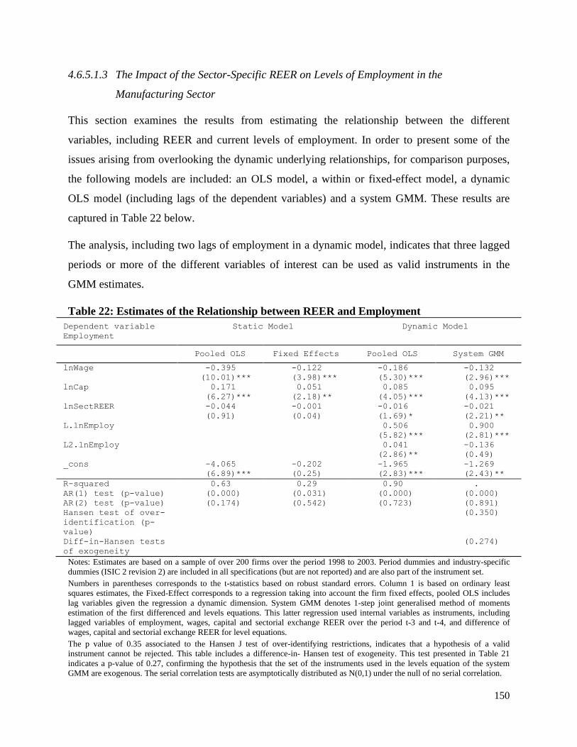
150

4.6.5.1.3 The Impact of the Sector-Specific REER on Levels of Employment in the

Manufacturing Sector

This section examines the results from estimating the relationship between the different

variables, including REER and current levels of employment. In order to present some of the

issues arising from overlooking the dynamic underlying relationships, for comparison purposes,

the following models are included: an OLS model, a within or fixed-effect model, a dynamic

OLS model (including lags of the dependent variables) and a system GMM. These results are

captured in Table 22 below.

The analysis, including two lags of employment in a dynamic model, indicates that three lagged

periods or more of the different variables of interest can be used as valid instruments in the

GMM estimates.

Table 22: Estimates of the Relationship between REER and Employment

Dependent variable

Employment

Static Model Dynamic Model

Pooled OLS Fixed Effects Pooled OLS System GMM

lnWage -0.395 -0.122 -0.186 -0.132

(10.01)*** (3.98)*** (5.30)*** (2.96)***

lnCap 0.171 0.051 0.085 0.095

(6.27)*** (2.18)** (4.05)*** (4.13)***

lnSectREER -0.044 -0.001 -0.016 -0.021

(0.91) (0.04) (1.69)* (2.21)**

L.lnEmploy 0.506 0.900

(5.82)*** (2.81)***

L2.lnEmploy 0.041 -0.136

(2.86)** (0.49)

_cons -4.065 -0.202 -1.965 -1.269

(6.89)*** (0.25) (2.83)*** (2.43)**

R-squared 0.63 0.29 0.90 .

AR(1) test (p-value) (0.000) (0.031) (0.000) (0.000)

AR(2) test (p-value) (0.174) (0.542) (0.723) (0.891)

Hansen test of over-

identification (p-

value)

(0.350)

Diff-in-Hansen tests

of exogeneity

(0.274)

Notes: Estimates are based on a sample of over 200 firms over the period 1998 to 2003. Period dummies and industry-specific

dummies (ISIC 2 revision 2) are included in all specifications (but are not reported) and are also part of the instrument set.

Numbers in parentheses corresponds to the t-statistics based on robust standard errors. Column 1 is based on ordinary least

squares estimates, the Fixed-Effect corresponds to a regression taking into account the firm fixed effects, pooled OLS includes

lag variables given the regression a dynamic dimension. System GMM denotes 1-step joint generalised method of moments

estimation of the first differenced and levels equations. This latter regression used internal variables as instruments, including

lagged variables of employment, wages, capital and sectorial exchange REER over the period t-3 and t-4, and difference of

wages, capital and sectorial exchange REER for level equations.

The p value of 0.35 associated to the Hansen J test of over-identifying restrictions, indicates that a hypothesis of a valid

instrument cannot be rejected. This table includes a difference-in- Hansen test of exogeneity. This test presented in Table 21

indicates a p-value of 0.27, confirming the hypothesis that the set of the instruments used in the levels equation of the system

GMM are exogenous. The serial correlation tests are asymptotically distributed as N(0,1) under the null of no serial correlation.

151

Standard methods such as OLS and fixed-effects regressions present a negative relation between

sector-specific exchange rates and firms’ employment levels. However, this relationship appears

to be insignificant and the magnitude of the coefficients vary greatly. In the simple OLS model,

the coefficient is of -0.044 (t=-0.91), while in the fixed-effect regression, the coefficient is -0.001

(t =- 0.04). Nevertheless, dynamic models show that these results are significant. Even in a basic

dynamic OLS estimate, the relationship between sector-specific REER and firms’ employment

levels is now statistically significant, the coefficient on REER is −0.108 (t = −3.07), compared to

its statistical insignificance under the static OLS model.

The dynamic OLS model performs better than the other models, and the inclusion of the lagged

employment variable appears to be important. Indeed, when comparing the static OLS estimation

to the dynamic one, the R squared value increased from 63% to 90%. Thus, past employment

levels explain a major part of a given firm’s current employment levels. This is clearly noted in

the VECM analysis presented above. In addition, the observed differences in the estimated

coefficients on the REER across the different specifications suggest a degree of correlation

between current REER levels and past employment – indicating a source of endogeneity. Despite

the improvement presented by the dynamic OLS model, the estimate may still suffer from some

heterogeneity bias not captured by the included lagged variables.

For this analysis, the system GMM model is the most appropriate method as it allows us to

capture the dynamic relationship between employment and REER, as well as the embedded

unobservable heterogeneity-characterising panel data. Thus, the GMM system indicates that the

industry-specific REER is significant (-0.021, t = - 2.21) at 5%.

GMM estimates show that when fixed-effects are included in a dynamic model and estimated via

the GMM system, then the coefficient of REER is now significant (-0.021, t = - 2.21) at 5%,

compared to the non-statistically significant REER coefficient (−0.001, t = −0.04) obtained

through the static fixed-effects estimate. This is consistent with Roodman’s (2006) theory, which

suggests that the OLS and fixed-effect estimators present upwards and downwards biases,

respectively. Thus, the coefficient estimate using a GMM estimate lies within the theoretical

lower and upper boundaries given by FE and OLS estimators.

The table above suggests that the exchange rate matters in determining the level of employment,

as an increase in sector-specific REER (appreciation) reduces employment by 0.021%. This

152

number is similar in size as the one in the long-run dynamics of the VECM analysis (i.e. 0.021).

However, unlike the VECM short-run dynamics, the sign is in line with the theoretical

predictions. The results point to a negative relationship between wages and employment at the

firm level (-0.132, t = 2.96), as predicted by economic theory and found in a number of prior

studies including Bangs (1942) and Welch (1997). In addition, capital is positively related to

levels of employment with a coefficient of 0.095, highlighting that for manufacturing firms, level

capital impacts positively the employment level. Finally, past levels of employment also have an

impact on employment – as identified in the VECM analysis. However, the impact using

microeconomic data is twice as large (i.e. 0.9 compared to 0.46 using the VECM). This possibly

reflects the specificity of the firms included in the survey, such as their maturity level. Indeed,

firms in the sample are growing, as illustrated by average firm output (section 4.6.5).

Table 22 presents the output of the specification tests. The AR(2) test presents a p-value of 0.89,

implying that the null hypothesis of no second-order serial correlation cannot be rejected. The p

value of 0.35 associated to the Hansen J test of over-identifying restrictions indicates that a

hypothesis of a valid instrument cannot be rejected. This table includes the exogeneity test run on

a subset of the instruments herein. As discussed in Wintoki et al. (2012), the system GMM

estimator assumes that the correlation between the variables included in the model and the

unobserved effect is constant over time. Eichenbaum et al. (1988) suggest testing this assumption

through a difference-in- Hansen test of exogeneity. This test, presented in Table 21, indicates a

p-value of 0.27, confirming the hypothesis that the set of the instruments used in the levels

equation of the system GMM are exogenous.

Assessing the strength of the set of instruments

Authors such as Bond et al. (1995) and Staiger et al. (2001) have highlighted that, in the case of

weakly correlated variables and instruments, results could be biased. Furthermore, the literature

indicates that assessing the joint strength of the instruments is difficult; however, by adjusting

the procedure developed by Staiger and Stock (1997) and Stock and Yogo (2005) to assess the

strength of a set of instruments within a two-stage least squares (2SLS) regression, the system

GMM instruments can be tested. Following the procedure described by Wintoki et al. (2012),

Table 22 shows the results of the Cragg-Donald statistic indicating that the system GMM

estimates are not affected by weak instruments.

153

Further discussion

This analysis has presented the impact of the sector-specific REER on employment. The

underlying assumption is that the firm characteristics, such as levels of capital and wages, are

determinants of one another. To further assess the mechanisms through which REER impacts

employment, the impact of REER (if any) on a set of variables including capital, output, profit

and investment will be discussed. In order to assess the potential role of these variables as

possible mechanisms underlying the relationship between exchange rate and employment, these

variables will be included in the model described in the above sections and Table 22, assessing

the role of REER on employment. The results of these regressions, based on wage per worker as

a dependent variable, are summarised in Table 23 below.

These results indicate that after adding in turn the three different variables (output, investment

and profit) acting as potential mechanisms through which REER impacts the employment level,

it can be seen that coefficients associated with output and investment are significant and positive,

while those associated with REER are relatively small compared to those in Table 22. This

points to the fact that the impact of the exchange rate on employment is potentially through

output and investment. On the other hand, the role of profit appears to be limited as the

coefficient related to REER is in line with the results of Table 22, and this coefficient is not

statistically significant. This is in line with the evidence presented by the investment climate

World Bank report (2014), where employment levels are expected to reflect the current level of

output and the sales prospects. Indeed, the report indicates that managers tend to keep their

employees waiting for economic prospects as entrepreneurs indicate that they are overstaffed in

anticipation of an economic upturn; this appears to happen at the expense of profit. Further, the

table below indicates the role of investment as an increase in investment is positively linked to

employment. This relationship also explains the fact that coefficients associated with the capital

variable is relatively lower when these additional variables are introduced.

Table 23: Relationship Between REER and Employment with additional control variables

lnEmploy lnEmploy lnEmploy lnEmploy

lnWage -0.132 -0.129 -0.089 -0.119

(2.96)*** (2.06)** (2.81)*** (2.49)**

lnCap 0.095 0.023 0.064 0.042

(4.13) *** (2.41)** (3.97)*** (2.76)**

lnSectREER -0.021 -0.014 -0.017 -0.021

154

(2.21)** (4.41)*** (3.99)*** (3.11)***

L.lnEmploy 0.900 0.707 0.957 0.839

(2.81)*** (3.94)*** (4.13)*** (3.63)***

L2.lnEmploy -0.136 -0.075 -0.185 -0.103

(0.49) (0.98) (1.33) (0.57)

lnOut 0.041

(2.05)**

lnInv 0.037

(1.66)*

lnProfit -0.007

(0.43)

_cons -1.269 -0.763 -1.124 -1.377

(2.43)** (2.51)** (1.84)* (3.86)***

AR(1) test (p-

value)

(0.00) (0.00) (0.05) (0.06)

AR(2) test (p-

value)

(0.89) (0.74) (0.51) (0.78)

Hansen test of

over-identification

(p-value)

(0.35) (0.52) (0.48) (0.46)

Diff-in-Hansen

tests of exogeneity

(p-value)

(0.27) (0.23) (0.28) (0.132)

Notes: Estimates are based on a sample of over 200 firms over the period 1998 to 2003. Period dummies and industry-specific

dummies (ISIC 2 revision 2) are included in all specifications (but are not reported) and are also part of the instrument set.

Numbers in parentheses corresponds to the t-statistics based on robust standard errors.

The system GMM corresponds to denotes 1-step joint generalised method of moments estimation of the first differenced and

levels equations. This latter regression used internal variables as instruments, including lagged variables of employment, wages,

capital and sectorial exchange the REER over the periods t-3 and t-4, to which lagged variables of output, investment and profit

are added in turn (column 2, 3 and 4 respectively), and the differentiated variables of wages, capital and sectorial exchange

REER, to which lagged variables of output, investment and profit are added in turn (column 2, 3 and 4 respectively), for level

equations.

The p value associated with the Hansen J test of over-identifying restrictions, indicates that a hypothesis of a valid instrument

cannot be rejected. This table also includes a difference-in- Hansen test of exogeneity. This test confirms the hypothesis that the

set of instruments used in the levels equation of the system GMM are exogenous. The serial correlation tests are asymptotically

distributed as N(0,1) under the null of no serial correlation.

To further assess these mechanisms, they are examined to see whether a firm’s characteristics,

such as profit, investment and output, are also determined by exchange rate movements by

applying the dynamic GMM panel estimator. The following form is an estimated empirical

model:

𝑥𝑖𝑡 = 𝛼 + ∑ 𝑘𝑠𝑥𝑖𝑡−𝑠

𝑠

+ 𝛾𝑍𝑖𝑡 + 휂𝑖 + 휀𝑖𝑡 𝑠 = 1, … , 𝑝,

where 𝑥 is a firm’s characteristics, such as profit, investment and output, and 𝑍𝑖𝑡is a vector of

these characteristics, but including employment levels. This assumed relationships takes root in

the large number of empirical studies that examine the impact of the various hypothesized

155

determinants of firm profitability, including exchange rate, employment levels, output and

capital, as presented by Nanda et al. (2018), and the level of output, as identified by Clark (2009)

and Collins (2010). This is implemented using the steps presented in the above sections; the

results are presented in Table 24, summarising the outputs of the GMM regressions.

In line with the DD framework, an exchange rate appreciation caused by a commodity boom

results in negatively affecting the rate of return of capital in the tradable sectors; this has

implications for the sector distribution of investment. Appreciation will have an impact on the

future investment response of the sector since capital might be invested in other productive

sectors of the economy. The inability of the manufacturing sector to attract investment in the

future will hamper its capacity to compete internationally. This mechanism seems to be at work

in the Nigerian manufacturing sector. Indeed, the table below indicates that profit, output and

investment are all impacted by REER.

Table 24: Key Relationship Estimates (GMM)

lnProfit lnOut lnInv

lnProfit 0.140 0.170

(3.31)*** (1.73)*

lnOut 0.408 0.051

(2.21)** (0.09)

lnInv -0.308 0.251

(2.77)** (1.92)*

lnCap 0.207 0.062 0.321

(2.58)** (1.05) (2.21)**

lnEmploy -0.280 0.356 0.476

(3.40)*** (2.17)** (3.25)***

lnSectREER -0.062 -0.080 0.067

(1.89)* (2.93)*** (2.66)**

L.lnProfit -0.006

(2.32)**

L2.lnProfit 0.372

(0.94)

L.lnOut 0.861

(2.20)**

L2.lnOut -0.213

(0.62)

L.lnInv 0.661

(2.41)**

L2.lnInv -0.166

(1.03)

AR(1) test (p-value) (0.00) (0.00) (0.00)

AR(2) test (p-value) (0.89) (0.74) (0.81)

Hansen test of over-

identification (p-

value)

(0.45) (0.52) (0.68)

Diff-in-Hansen tests

of exogeneity (p-

value)

(0.22) (0.25) (0.30)

* p<0.1; ** p<0.05; *** p<0.01

156

Source: Author’s computation

Notes: Estimates are based on a sample of over 200 firms over the period 1998, to 2003. Period dummies and industry-specific

dummies (ISIC 2 revision 2) are included in all specifications (but are not reported) and are also part of the instrument set.

Numbers in parentheses corresponds to the t-statistics based on robust standard errors.

The system GMM corresponds to denotes 1-step joint generalised method of moments estimation of the first differenced and

levels equations. These regressions used internal variables as instruments. Column 1 uses profit as a dependent variable and

lagged profit, investment, capital, employment and sector REER are independent variables form which the instruments are

sourced in the form of lagged values t-3 and t-4 of investment, capital, employment and sector REER. For the level equations,

investment, capital, employment and sector REER excluding the dependent variable are used as instruments. Similarly, column 2,

output is the dependent variable and lagged output, investment, capital, employment and sector REER are independent variables

from which the instruments are sourced in the form of lagged values t-3 and t-4 of investment, capital, employment and sector

REER. For the level equations, investment, capital, employment and sector REER excluding the dependent variable are used as

instruments. The same is applicable to investment as a dependent variable.

The p value associated to the Hansen J test of over-identifying restrictions indicates that a hypothesis of a valid instrument cannot

be rejected. This table also includes a difference-in- Hansen test of exogeneity. This test confirms the hypothesis that the set of

the instruments used in the levels equation of the system GMM are exogenous. The serial correlation tests are asymptotically

distributed as N(0,1) under the null of no serial correlation.

The sector-specific REER negatively impacts firms’ output and profit while it is positively

linked to investment. This implies that an exchange rate appreciation can affect negatively the

manufacturing sector’s profitability. As tradable goods such as manufacturing are often

competing with international goods, their relative increase in price makes them less attractive to

the external market, thus negatively affecting output. Non-exporting Firms find that their

production costs are higher than in other parts of the world and thus they face tougher

competition from imported goods at the sectorial level, as argued by Folawewo et al. (2012).

This is in line with the DD framework as investors may find tradable goods less attractive.

In addition, Table 24 column 2 above interestingly indicates that increased employment

negatively impacts profit, but it is beneficial to output. This highlights the fact that the

production process is still relatively labour-intensive, as illustrated in the previous chapter

(Chapter 3). Similarly, a large labour force is also linked to increased investment (column 3).

The table also indicates that employment has a greater role on profit than profit has on

employment. This underlines the fact that an employment decision is a medium-term decision

and, in the short run, though firms’ investments are impacted by profit, the employment decision

appears less sensitive. This is explained by the firms mainly employing labour in the network

and driving the limited labour mobility; thus, labour adjustment costs are relatively high.

Finally, investment similar to capital is positively associated with the REER and output level,

while an increase in capital and employment increases investment levels. This points to the

complementary role of labour and capital in the Nigerian context. In addition, and as expected,

an appreciation encourages investments. This is likely to operate through the relative price of

157

imported investment goods becoming cheaper. Overall, this points to the fact that REER

contributes to the substitution of labour for capital. Indeed, REER is a positive determinant of

capital levels, while this role is reversed when looking at labour.

4.6.6 Conclusions

Theoretical and empirical research at the firm level are affected by endogenous dynamic

relationships between control and dependent variables. Very often, empirical research implies

assessing the existence of a causal effect, of a firm’s characteristic (X) on some measure of

outcome such as employment level (Y); and the inference will include a number of control

variables (Z). However, such an estimate may lead to bias estimates if the variables are affected

by endogeneity. Further issues could arise with unobservable heterogeneity described as factors

affecting both control and dependent variables. Another type of bias is the simultaneity issue

arising when, for example, a firm’s current decisions impact on its performance in the following

periods, which in turn impacts on the firm’s future decision-making. In the context of the impact

of the REER on employment, the current firm’s employment levels performance will influence

capital and wage choices and, to some degree, sector-specific REER, and these may impact

expected firm employment levels.

In this chapter, first the GMM estimator was discussed and the advantages of using such methods

to assess the relationship of interest were presented. The GMM estimate is shown to be more

accurate than fixed-effects estimates, which can be biased when dependent and control variables

are dynamically linked. This technique is appropriate for estimation of the impact of sector-

specific REER on employment levels in a panel of 200 firms operating in various manufacturing

sectors over the period 1998–2003. Employment is presented as being, in part, determined by

past levels of employment, and after taking this characteristic into account, the existence of a

causal relationship between employment and the following control variables: REER, wage,

capital, and firm performance was demonstrated.

Sector-specific movement is, to an extent, linked to capital within the sector, but more

importantly, it has been shown that a 1% increase (appreciation) of sector-specific REER results

in a decrease of employment of 0.021%. This is in line with the long-run dynamic obtained with

the VECM analysis. This implies that firms react to labour costs being relatively more expensive

in the light of an appreciation against other factors of production (which is primarily imported in

158

the Nigerian context – see Kojo, (2014)). This indicates that the possible REER appreciation will

have a negative impact on the level of employment, and this is in both the short- (GMM analysis)

and long-run (VECM analysis).

Further, this analysis also indicated that capital and employment levels are complementary in the

context of the Nigerian manufacturing sector, implying that an increase of capital is beneficial

for the employment level. However, the micro-evidence indicated a small impact of capital on

employment (coefficient of 0.1), which is almost 2/3 smaller than the coefficient obtained at the

macro level. This could be explained by the fact that the sectors included in this survey (such as

paper and furniture) can easily substitute labour for capital, but it is interesting to consider that

this impact, at the micro-level, was noted over a relatively short period of time.

Thus, the analysis shows that, as predicted by the labour-intensity channel, exchange rates do

lead in the short-run, to a possible substitution of labour with capital, as they affect, positively,

capital levels and, negatively, employment. The analysis shows that REER appreciation results

in lower investment and lower profit (as margins are reduced if firms compete with imported

goods); however, capital increases as firms can take advantage of cheaper imported capital.

Taken in isolation, the first symptom of Dutch Disease has a negative impact on employment

levels as predicted by the framework. However, this could be mitigated by the role it has on the

price of capital and the fact that capital and employment are complementary in the Nigerian

formal manufacturing context. Although the composition of the economy is thought to be

different from the period 1998-2003, it still offers relevant lessons regarding the exchange-rate

volatility experienced by the country at the end of the commodity super-cycle.

From a policy perspective, if the Nigerian government is to recognise the impact and potential

benefit of the manufacturing sector on job creation and possible growth, it needs to implement

the right economic policies. Revenue inflows coupled with appropriate industrial policies can

contribute to economic diversification efforts. This can be illustrated by the experience of several

developed countries, including Australia, the United States, and Norway. Another way to foster

economic diversification is through providing tax incentives to non-resource tradable sectors.

The revenue inflows following a commodity boom can support a transfer of capital by

facilitating the import of advanced capital goods that cannot be made locally. This kind of

investment improves economic competitiveness and generates little exchange rate appreciation.

159

4.7 Appendices

Appendix 1: The number of significant lags

In column 1, lags 3 and older lags are not statistically significant contrary to the first two lags,

which are statistically significant. In column 2, the results of a regression only, including the

older lags, are presented. In both columns, the older lags are statistically significant, indicating

that these older lags contain relevant information that is captured by more recent lags.

Table 25: How Many Lags Are Significant?

The table below reports results from the following OLS model:

𝑙𝑖𝑡 = 𝛼1 + ∑ 𝐾𝑝

𝑝=4

𝑝=2

𝑙𝑖𝑡−𝑝 + 𝐾𝑍𝑖𝑡 + 𝑛𝑖 + 휀𝑖𝑡

𝑙𝑖𝑡 represents the employment level; 𝑍𝑖𝑡 includes sector-specific REER, capital and wages, all in their logarithm

form. The relevant t-statistics based on firm-clustered standard errors are reported in parentheses. Year dummies

(1998, 1999, 2000, 2001, 2002 and 2003) and industry dummies (ISIC level 2 revision 2) are included in all

specifications. Numbers in parentheses correspond to t-statistics and *, **, *** are significance levels at 10%, 5%

and 1%, respectively. The serial correlation tests are asymptotically distributed as N(0,1) under the null of no serial

correlation.

lnEmploy lnEmploy

lnEmploylag1 0.487

(14.47)***

lnEmploylag2 0.057

(1.80)*

lnEmploylag3 -0.032 0.080

(1.30) (3.72)***

lnWage -0.198 -0.406

(9.18)*** (19.14)***

lnCap 0.087 0.147

(6.02)*** (8.68)***

lnSectREER -0.032 -0.108

(0.93) (4.41)***

_cons -2.052 -4.127

(6.39)*** (13.86)***

R-squared 0.89 0.83

NT 533 580

AR(1) – p-value (0.000) (0.000)

AR(2) – p-value (0.317) (0.725)

* p<0.1; ** p<0.05; *** p<0.01

Source: Author’s computation

160

Appendix 2: Relationship between variables of interest, and past realisations

In Panel A of Table 26, OLS regression estimates of REER and other variables of interest on

lagged employment levels and firm characteristics are presented. Findings show that current

levels of employment are negatively related to lagged wages and lagged sectoral exchange-rates,

while employment is positively related to past capital levels. This is line with Frenkel (2004),

who links unemployment to lagged REER. Further, wages are positively associated to lagged

employment levels and to lagged levels of capital, while they are negatively related to the sector

exchange-rate. Similarly, the actual level of capital is positively related to past employment

levels and wages. It is also positively related to the past but not at a significant level. Finally,

given the computation of the sector-specific trade-weighted exchange rate, the assumption that

REER could be affected by the past performance of firms is possible (even more so if

government policies are sensitive to firms’ performance). Thus, sector-specific REER is

negatively related to (but not at a significant level) past levels of wages and employment, while it

is positively (at a significant level) related to lagged capital levels. Overall, the table indicates

that for firms facing an appreciated REER in the past, capital is likely to be larger today, but they

will experience a lower wage bill and employment level. This points in the direction of this

paper’s hypothesis, suggesting that REER affects the price of labour and capital encouraging a

substitution effect.

Panel B of Table 26 shows OLS estimates of employment and other variables of interest and

their lagged values. The results presented in this table are similar to the regressions using level

variables. Again, results indicate changes in employment in response to past variables such as

capital and sector-specific REER

Table 26: Relationship Between Variables of Interest, and Past Realisations This table presents the OLS regressions of current employment (lnEmploy), wages (lnWage), capital (lnCap) and sector REER

(lnSect REER) on lagged values of variables of interest. A variable name followed by “lag1” indicates the lagged value of the

variable of interest, while a variable name preceded by “D.” indicates the first difference value of the given variable. The results

are based on a sample of over 200 Nigerian firms. Regressions include time years dummy variables for the years 1998 to 2003

and industry dummies (ISIC level 2 revision 2) from the NMES, (but which are not reported). In panel A, the

dependent variables are at current levels, while in panel B, s the dependent variables are the first difference. The serial

correlation tests are asymptotically distributed as N(0,1) under the null of no serial correlation.

Panel A: Dependent variable is level at time t

lnEmploy lnWage lnCap lnSectREER

lnWagelag1 -0.306 0.319 -0.033

(10.62)*** (4.51)*** (1.21)

lnCaplag1 0.132 0.108 0.033

161

(5.53)*** (2.86)*** (1.78)*

lnSectREERlag1 -0.215 -0.238 0.023

(3.63)*** (2.72)*** (0.20)

lnEmploylag1 0.888 0.791 -0.031

(12.51)*** (7.24)*** (0.71)

_cons -2.142 10.373 7.118 3.578

(5.31)*** (18.45)*** (6.45)*** (10.61)***

NT 553 553 553 553

AR (1) – p-value (0.017) (0.000) (0.025) (0.010)

AR(2) – p-value (0.543) (0.305) (0.871) (0.789)

R-squared 0.66 0.69 0.69 0.73

* p<0.1; ** p<0.05; *** p<0.01

Panel B: Dependent variable changed from t −1 to t

DlnEmploy DlnWage DlnCap DlnSectREER

lnWagelag1 -0.087 -0.030 -0.013

(3.33)*** (0.67) (0.32)

lnCaplag1 -0.042 -0.048 -0.081

(1.96)** (1.53) (2.76)***

lnSectREERlag1 -0.166 -0.200 0.148

(3.09)*** (2.70)*** (1.91)*

lnEmploylag1 -0.158 -0.032 0.097

(2.66)*** (0.47) (1.38)

_cons 2.531 1.796 -0.669 2.202

(6.94)*** (3.77)*** (0.98) (4.15)***

NT 513 513 513 513

AR (1) – p-value (0.013) (0.754) (0.201) (0.000)

AR(2) – p-value (0.188) (0.434) (0.015) (0.910)

R-squared 0.11 0.13 0.16 0.33

* p<0.1; ** p<0.05; *** p<0.01

Source: Author’s computation

As indicated by Wintoki (2012), a test of strict exogeneity was performed. If 𝑋𝑖,𝑡 is assumed to

contain the model control variables, strict exogeneity is estimated through the following fixed-

effects model:

𝑙𝑖𝑡 = 𝛼 + 𝛽𝑋𝑖,𝑡 + 𝜑𝑊𝑖,𝑡+1 + 𝑛𝑖 + 휀𝑖𝑡

where 𝑊𝑖,𝑡+1 represents future values of the relevant variables. The null hypothesis of strict

exogeneity suggests that future realisations of control variables are independent from current

values of the dependent variables i.e. 𝜑=0.

Table 27 shows estimates with different subsets of variables, 𝑊𝑖,𝑡+1. In the different

specifications, the coefficient related to the future values of control variables, such as wages,

capital and REER, are significantly different from zero. This suggests that these variables reflect

the level of employment (i.e. they are not strictly exogenous). This is confirmed by an F-test of

162

the joint significance, confirming the theoretical predictions and the results from the OLS

regressions in Table 26 above.

Table 27: Do Firms’ Variables Adjust to Past Realisations? The table reports the fixed-effects estimates:𝑙𝑖𝑡 = 𝛼 + 𝛽𝑋𝑖,𝑡 + 𝜑𝑊𝑖,𝑡+1 + 𝑛𝑖 + 휀𝑖𝑡, , t = 1998, 1999, 2000, 2001, 2002 and 2003,

where Wit+1 includes future values of control variables, X – which includes wages (LnWage), capital (lnCap), sector REER

(lnSectREER). 𝑙 is the firm’s level of employment. 𝜑 = 0 is the null hypothesis of strict exogeneity. The analysis is based on

over 200 firms observed over the period 1998 to 2003. The data is from the NMES. All numbers in parentheses correspond to

robust standard errors. Year dummies are included in all specifications, as well as industry dummies (ISIC level 2 revision 2) -

(but are not reported). The serial correlation tests are asymptotically distributed as N(0,1) under the null of no serial correlation.

lnEmploy lnEmploy lnEmploy lnEmploy

LnWage -0.400 -0.392 -0.393 -0.395

(18.02)*** (16.75)*** (19.55)*** (15.73)***

LnCap 0.173 0.176 0.172 0.176

(9.76)*** (8.74)*** (10.25)*** (8.54)***

lnSectREER -0.049 -0.087 -0.084 -0.135

(1.07) (1.65)* (1.62) (1.83)*

LlnWage1 -0.048 -0.030

(1.78)* (2.11)**

LlnCap1 -0.040 -0.025

(1.21) (1.69)*

LlnSectREER1 0.042 0.045

(2.35)** (0.89)

_cons -4.145 -3.922 -4.012 -3.887

(10.23)*** (9.32)*** (10.52)*** (8.91)***

NT 553 553 553 553

AR (1) – p-value (0.000) (0.017) (0.012) (0.010)

AR(2) – p-value (0.111) (0.351) (0.587) (0.497)

R-squared 0.83 0.83 0.83 0.83

* p<0.1; ** p<0.05; *** p<0.01

Source: Author’s computation

Appendix 3: Strength of instruments

As described by Wintoki et al. (2012), if 𝑙 is employment and X includes all the regressors, the

system GMM involves estimating the following:

[𝑙𝑖𝑡

∆𝑙𝑖𝑡] = 𝛼 + 𝛽 [

𝑋𝑖𝑡

∆𝑋𝑖𝑡] + 휀𝑖𝑡

To assess the strength of the instruments used in this study, lagged differences as instruments in

the level equations and lagged levels as instruments in the differenced equations are separately

assessed. The equation in the levels indicates: 𝑙𝑖𝑡 = 𝛼𝑙 + 𝛽𝑙𝑋𝑖𝑡 + 𝑣𝑖𝑡 Instrument ∆𝑋𝑖𝑡−2

And the equation in differences: ∆𝑙𝑖𝑡 = 𝛼𝑑 + 𝛽𝑑∆𝑋𝑖𝑡 + 𝑣𝑖𝑡 Instrument 𝑋𝑖𝑡−3

Table 28 shows that the F-statistics results for all the first-stage regressions are significant, which

confirms the strength of the selected instruments in explaining the endogenous variables. Further,

163

the F-statistics are larger than 10, which corresponds to the critical value proposed by Staiger et

al. (2001) as a rule of thumb.

Table 28: Level Equation (Top Part) – Difference Equation (Bottom Part)

F-Statistic p-value R2

lnWage 16.17 0.00 0.3866

lnCap 18.68 0.00 0.4224

lnSectREER 24.29 0.00 0.7730

Cragg-Donald statistic: 20.5

F-Statistic p-value R2

lnWage 12.10 0.03 0.3313

lnCap 13.40 0.01 0.2327

lnSectREER 38.72 0.00 0.3979

Cragg-Donald statistic: 3.48

Source: Author’s computation

164

5 Chapter 5

Oil Abundance and Inequality in Wages: A Decomposition Analysis

5.1 Introduction

In the discussion in Chapter 4 above, wages are negatively related to employment levels. This

implies that in the Nigerian context an increase in wages impacts negatively on the level of

employment. Thus, through the lens of the DD framework, the determinants of wages and the

role potentially played by oil in determining wages will be explored. In addition, I the influence

of oil in explaining wage inequality observed across the country will be assessed. This could be

significant in quantifying - for the first time in the Nigerian context - the impact of oil on wages,

as well as in terms of policy direction regarding the country’s competitiveness (i.e. does the

country’s oil-revenue sharing formula affect its ability to compete internationally?).

Working from the assumption that the possible negative impact of resources is greater for point

resources than diffuse resources (Engerman and Sokoloff, 2002; Isham, et al. 2003) and given

their localised nature, the following analysis will focus on subnational units such as states which

have recently been the focus of a number of studies replicating growth regressions often

presented in cross-country analysis but using subnational data (see literature review in Chapter

2). Overall, these studies suggest that the extractive industry generates at least some short-run

positive effects on the employment level and wages across a number of sectors. The mechanisms

through which this impact is felt at the local level is intrinsically linked to the redistribution of

resources and their use. The literature, such as the evidence produced by Berman et al. (2017),

has shown that mining activity is linked to conflict in African countries for the capture of

resources. This is contrary to the evidence presented by Bhattacharyya et al. (forthcoming), who

find no significant evidence of the impact of resources on the probability of conflict but find a

positive impact on economic development. In the case of oil in Brazil, Caselli et al. (2013) find

that the increase in public-goods spending is not proportional to resource windfalls, while Borge

et al. (2017), in the case of hydropower in Norway, highlight that revenue inflows results in

lower public goods efficiency.

The impact of resource abundance at the local level remains of interest, in particular its impact

on the structure of the local economy, as well as on local variables such as inflation and wages,

165

as suggested by the DD framework. To answer these questions, the reliance on firm-level data in

the developing-country context is still scarce. More recent papers, such as Crust et al. (2015) in

the case of Indonesia, show that resource production has been associated with higher wages, with

districts rich in oil and gas seeing a rise in the wage rate by as much as 9.4% compared to

countries with half the amount of such resources.

Other empirical evidence of the impact of oil on wages is mainly found in analysis of the

manufacturing sector. Allcott and Keniston (2014) argue that manufacturing sector output is

reduced following a boom at the local level if local manufacturing wages rises and prices are

exogenous, i.e. they do not rise. By assessing oil-rich economies in the 1970s, Smith (2014)

underlines the impact of bust-boom cycles on the manufacturing sector. He points to the fact that

exports, productivity and employment levels increase during the boom, and the reverse is true

during a bust. Cavalcanti et al. (2015), focusing on Brazil, compared municipalities where oil

was discovered to other municipalities with drilling activities but no discovery. In doing so, they

made sure that no confounding factors, such as institutions or infrastructure that could affect both

oil production and manufacturing activity, were responsible for the difference between oil-rich

and other municipalities’ GDP. They found that oil production positively impacts GDP per capita

and the pace of urbanisation, and even has positive spillover effects on services and

manufacturing GDP. This chapter will contribute to the literature by assessing the effect of

resources inflows on wage determination at the firm level. This is highly relevant as part of the

Dutch Disease mechanism is driven by increasing wages that crowd out the tradable sector.

Thus, using Nigeria as the basis for my analysis, this chapter investigates the specific impact of

oil abundance on wage determination in an emerging resource-rich economy. My aim is to

examine whether firms in oil and gas extraction regions offer higher wages (i.e. oil revenue is a

key factor impacting the wage determination process) and thereby contribute to wage inequality

in the country. Nigeria provides an ideal setting for studying the potential impact of resource

abundance on wage determination because it is a relatively large emerging economy with oil

extraction activities concentrated in one specific region of the country (i.e. the South-South

region). In addition, the country’s fiscal-federalism policy implies that this region receives a

large proportion of oil revenue (13% of oil revenue over and above the share communally

distributed globally among the different states).

166

As far as it is known, this study is the first one to provide Nigerian firm-level evidence on the

impact of oil abundance at the subnational level on wage determination and the contribution of

resource revenues to wage inequality in the country. Existing studies on Nigerian firm-level

wage determination (Aighokan 2011; Malik et al. 2012; Söderbom et al. 2002) do not take into

account the possible role played by the abundance of oil in wage determination. Finally, beyond

the well-documented impact on the environment and/or the political economy of the region, as

illustrated by Zinn (2005) Caselli, (2006) and Kurečić (2015), this research hints at the economic

impact of the oil revenue distribution mechanism which has been a source of debate (see Ekpo

(1994) and Adedotun (1991)) on firms’ level of employment and the country’s competitiveness.

5.2 Theoretical Framework and Empirical Implementation

A number of studies related to the Dutch Disease literature have shown that countries rich in

resources experience an overall increase in wages. Through this analysis, this impact will be

demonstrated at the subnational level (i.e. the administrative division called the ‘geopolitical

level’8) for a country such as Nigeria by asking the following questions: Does the abundance of

oil, through higher receipts from the central government relative to other states, affect the wage

level? And if so, does oil abundance play a role in explaining wage inequality across Nigerian

firms?

The general literature on wage determination is rich and vast, drawing from microeconomic and

firm theory. This literature shows that wages are unequal because of variations in skill, ability,

experience, gender, race, and other characteristics of workers. Even after adjustments are made

for these differences, firm size and productivity can be important in affecting wage rates

(Akerlof, 1984; Kahn and Cume, 1987; Donohue and Heywood, 2004). A number of factors can

explain this. Experimental research conducted by Charness and Kuhn (2007) concludes that a

phenomenon of gift exchange is prevalent and strong among workers and firms as a larger wage

(a gift to labour) results in larger efforts from employees (a gift to the firm). Alternatively, larger

and more productive firms pay higher wages out of ‘fairness’ considerations (Amiti and Davis,

2012) which, in turn, succeeds in producing goods that can be exported, even after adjusting for

8 Nigeria is composed of thirty-six states which are distributed between the six geopolitical zones. These six

geopolitical zones are used to amalgamate related ethnic groups and to allocate resources (i.e. economic, political

and social resources are frequently assessed and shared across the zones).

167

skilled employment, by exporting firms (Verhoogen, 2008). As noted in Chapter 3, the South-

South region appears to be relatively more productive than other parts of the country. Thus, gift

sharing is the position from which the question of interest will be approached.

Gift sharing (i.e. higher wages) is the result of oil revenue. In the context of a country like

Nigeria, it is difficult not to consider the fact that a booming sector such as oil production and its

redistribution may affect wages (the reliance on oil revenue is presented in the fiscal section in

Chapter 2). Indeed, as presented by Brunstad and Dyrstad (1997), who analysed the resource

boom in Norway, wages in the resource-rich context are driven by the demand and cost-of-living

effects, which combines aspects of the Dutch Disease and the literature on local demand shocks.

This provides the broader framework for the analysis in this paper. This mechanism is composed

as follows:

The demand effect corresponds to the labour market impact of increased demand in sectors

providing goods and services to the resource sector. In the case of inelastic supply, the prices of

these goods will increase, adding upward pressure on wages. This is needed to attract labour to

respond to the added demand. Thus, sectors across the country with tight links to the booming

sectors will experience a wage increase, independently of their location. For example, the

booming sector can increase demand for steel; therefore, steelworkers anywhere in the country

will see a rise in demand for their labour. This causes a marked non-negative effect on wages

(similar to Dutch Disease).

Thus, the demand effect puts upward pressure on wages, while the cost-of-living effect, if

greater, can push wages in the opposite direction. This effect reflects the fact that oil production

is located in a specific region; as a result, several markets will be under pressure given limited

supply (at least in the short run), such as housing markets, in which prices will be pushed

upwards. Under this effect, local inflation is expected to increase, thus affecting the local

economy independently of specific sectors. This effect could put a downward pressure on labour

supply; thus, the higher nominal wage could be offset by lower real-wages. Reduced real wages

could result in increased supply in other sectors and other regions, generating pressures on

wages. This effect can be in specific sectors.

In the conclusion of their paper, Brunstad and Dyrstad (1997) found that demand and cost-of-

living effects originating from the resource sector can have an opposite impact on nominal wages

168

and represent a significant contributing factor to wage differentials at the occupational and

regional levels. The cost-of-living effect is likely to exert a non-negative downward pressure on

wages in the region; while the demand effect will put a non-negative upward pressure on

nominal wages. The combined effect is that the resource sector will tend to contribute to sectoral

and regional wage differentials. Nevertheless, the pass-through of increased cost of living

resulting from the boom to real wages, is likely to be smaller than nominal wage differentials,

reflecting labour supply and demand elasticities. Given the scarce data, this analysis will use a

simpler wage equation to empirically test the impact of oil in wage determination in Nigeria.

5.3 Country Background

5.3.1 “Point Resource” - Oil Produced in a Specific Region

Oil revenue, as was shown in Chapter 3, flows to the Nigerian government’s coffers through its

state-owned enterprise – the Nigerian National Petroleum Corporation - which is responsible for

enforcing the oil-production signed agreements between the government and the private oil

companies. Since the return to democracy in 1999, the Nigerian constitution indicates that at

least 13% of revenue must be transferred to the oil-producing states. (Nigeria UNDP, 2006). To

complement these revenues, these oil-producing states and local governments, like any other

states, receive a share of fifty per cent of net-revenue proceeds (after deduction of first charges).

Nigerian oil exploration and production activities are concentrated in the South-South

Geopolitical region, also known as the Niger Delta region, producing 97% of the total Nigerian

production of 2.5 million barrels per day (the remaining 2% is produced by Ondo state [included

in my dummy]). Thus, the share of Imo and Abia states, estimated at less than 15,000 barrels a

day each, is too small to impact the state in a similar fashion to other oil-producing states.

Indeed, oil production of those two states represents less than 1% of total national production,

and the associated revenue in terms of redistribution is relatively small. Revenues from

derivation represents about 15% of Imo and Abia states’ revenue respectively, compared to over

50% for the other oil-producing states.

5.3.2 Impact of Oil at the State Level

The focus here is on the effect that being located in an oil-producing region has on wages. This is

the basis for the dummy variable which is to be included in this analysis. To do this, the

169

framework of Brunstad and Dyrstad (1997) is adjusted and the hypothesis that oil revenue is

expected to affect the geopolitical region as described in Chart 32 below is tested.

Chart 32: Impact of Oil Revenue at the Subnational Level

Natural resource abundance

Increase in fiscal revenue (through revenue sharing mechanisms) spent as follows:

Salaries and personnel cost

Good and services (recurrent cost)

Capital expenditure

Increase local demand and demand for labour

Increase nominal wage

If labour force is not mobile

Increase in real wage

If labour force is mobile

Increase in population

Agglomeration impact: increase productivity

Decrease nominal wage and increase

other cost (housing)

Congestion in public services

Increase in nontradable output ambiguous impact on tradable

Chart 32 above indicates that, typically, governments in Nigeria divide their resources into two

main categories. The capital budget corresponds to a share of the national budget used to finance

the country’s development projects, such as the construction of key infrastructure, including

roads, hospitals, schools, highways, electricity and dams, as well as the purchase of machinery

and equipment. Goods and services linked to the capital budget are likely to be sourced abroad

(i.e. through the hiring of foreign firms to deliver those durable assets), thus increased demand

for these goods and services may not contribute to the local shock. By contrast, the recurrent

budget (goods, services and salaries) refers to the financing of related government operations,

such as expenditures on personnel, overheads, and infrastructure maintenance. Those

expenditures will contribute to the local economy through consumer demand and government

demand for local goods and services. Historically, since the 2000s, the capital budget represents

30% of total allocation (CBN data, Ogujiuba et al., 2014) and suffers from severe

implementation issues. Over the past decade, data from the CBN indicates that capital budget

implementation was volatile and relatively modest, averaging 50%, between 2000 and 2010.

This implies that about close to 85% of national expenditure finances salaries or government

recurrent spending.

170

Those trends observed at the federal level are also noticeable at the state level, and this

independently of the oil production level. Indeed, as presented by the World Bank report (2011),

Federal states in Nigeria have not been able to transform increased revenue received from the

federal government, reflecting increased oil revenue, into socio-economic development. This

reflects some of the resource curse challenges discussed in section 3, including weaknesses in

public expenditure management and state government delivery capacity. Indeed, as the

constitution gave greater autonomy to the states and local government and a greater share of

federal revenue (accounting for about 50% of consolidated public sector spending, which

doubled between 1999 and 2001), Nigeria has found it hard to control the increasing liquidity,

inflationary and exchange rate pressures.

Since independence, revenue increases have been generalized across states; however, they also

vary considerably in size between states. Not surprisingly, the largest oil producers in the sample

have experienced some of the highest revenue increases due, in part, to the increase in natural

resource derivation payments, from 1 per cent to 13 per cent. For example, Akwa Ibom and

Delta state, the country’s larger oil-producing states, experienced total revenue increases in real

terms of about 500 per cent a few years after the return of democracy. For the oil-producing

states, revenue from the derivation mechanism is the single largest item in their revenue profile.

In general, across all states, receipts from the states' own sources also increased, but by much

less, thus deepening their dependence on federation revenues and creating an avenue for

patronage between federal authorities and the subnational governments. On average, states

collect only 10 per cent of their revenue from their own sources; the remaining 90 per cent

comes from federally-collected revenues, compared to 28 per cent and 72 per cent respectively in

1997. These shares are highly correlated with oil revenue; thus, the recent end drop in

commodity prices drove this share to about 15 per cent. This share is consistent across all states,

with the average revenue being relatively low for the resource-rich states and relatively high for

states around the economic capital of the country Lagos, where state collected revenue are above

35 per cent.

On the expenditure side, states' expenditures increased slightly faster than revenues, rising about

330 per cent in real terms soon after the return of democracy. In line with revenue trends, oil-

producing states saw their expenditure increase significantly, reaching as high as 10-fold in states

such as Delta State compared to only 41 per cent in a Lagos state which is an outlier known for

171

relatively strong public finance systems. Across the different states, expenditure has been

dominated by recurrent expenditure on sectors such as personnel and the cost of running

government, thus reducing significantly the fiscal space needed for capital investment. On

average, recurrent expenditures have constituted 65 per cent on average of total expenditures,

and about 75 per cent for oil-producing states. Personnel outlays have accounted for a large and

growing share of recurrent expenditures, ranging on average from around 33 per cent in Lagos,

to as much as 82 per cent in Cross Rivers State. Several states are now encountering increasing

difficulties meeting their wage obligations, evidenced in mounting personnel arrears and frequent

strike action by state civil servants. This pressure is exacerbated by the fact that state civil

servants’ unions, supported by the central labour union, seek to ensure that state salaries match

the federal level. This is compounded by a significant increase in the number of civil servants (in

line with the resource curse discussion in chapter 3) or the increase in the number of parastatals.

All states, on average, have been spending more on capital investment in absolute terms;

however, it is apparent that they have been embarking on large projects, paying little attention to

economic returns and their poverty-reducing impact. In addition, there is a disconnect between

capital and recurrent spending with, overall, a limited consistency between them. To further

illustrate, the inefficient spending general administration gets the largest share of state spending,

reflecting the cost of state bureaucracy, while growth in education and health spending has

lagged behind growth in other sectors

Those trends highlight how state-level spending is fairly consistent in its composition, with the

larger revenue received by oil-producing states impacting the scale of the increase in recurrent

spending (i.e. salaries) and inefficient spending while impacting negatively revenue collection

efforts. As a result, there will be an increased demand for goods/services and labour at the local

level to respond to government-driven increased demand. This, in turn, will increase nominal

wages.

Another characteristic of importance when considering the effect of oil at the local level is the

presence of strong social networks, which can contribute to fragmented markets as well as high

search and transaction costs for firms and employees. In line with this argument, Aker et al.

(2014 page 1) argue that cross-border transaction costs are reduced when traders are from the

same ethnic group. They summarise this as follows: “having a common ethnicity reduces the

transaction costs associated with agricultural trade, especially in communications and credit

172

transactions.” Although, these findings are not directly linked to the development of the private

sector, they provide an explanation for the observed fragmented labour and supplier markets.

This points to low labour mobility, and the increase in demand driven by oil revenue given to a

state’s government is likely to have an impact locally, with limited spillover on other states, or

will be mitigated by internal migration. This argument is further confirmed by the enterprise

survey data that indicates that, on average, over 60% of firms indicate that their last recruit was

found through relatives and friends.

5.4 Empirical Approach

The analysis here uses pooled firm-level data from Nigeria covering the years 2007, 2009 and

2013 collected by the World Bank’s Enterprise Survey Unit to examine some of the factors

driving wages and to assess if oil is a key underlining factor that contributes to wage inequality.

To do so, first a wage equation at the firm level is estimated and the impact of oil on wage

determination is established. Then, wage inequality is decomposed to reflect its determinants

using the linear decomposition technique developed by Wagstaff, et al. (2003). Finally, these

results will be used to help to identify the contribution of the different variables, including oil

revenue, to firm-level wage inequality.

5.4.1 Wage Equation

Given the data available, the model developed by Teal (1996) is adjusted to reflect the

determination of the average wage level at the firm level. The standard equation starts with the

form: W = F(H, Fc, We ), where W represents a firm’s wage rate; H is the set of variables

capturing human capital characteristics; Fc is a set of firm-related characteristics; and We is

trade-off wage (i.e. wages available in other sectors).

However, given data limitation, an adjusted version of this wage equation is used here in line

with Devkota et al. (2015) and Şeker (2012). Firm-level wages are determined by the size of the

firm, its exposure to international trade, and other factors, including, in particular, firm-level

characteristics like operating in a geopolitical region receiving significant oil revenues. Firm-

specific factors provide controls that indicate whether older firms with a higher share of

permanent workers or firms with any union activity pay higher wages. This also indirectly

provides information on important labour-specific characteristics.

173

The wage equation in a linear form can thus be written as follows:

𝑤𝑖 = 𝛽0 + 𝛽1𝑓𝑖𝑟𝑚𝑠𝑖𝑧𝑒𝑖 + 𝛽2𝑓𝑥𝑝𝑜𝑠𝑢𝑟𝑒𝑖 + ∑ 𝛽𝑗𝑋𝑗𝑖

𝑘

𝑗=3

+ 𝛾𝑦𝑟𝐷𝑦𝑟 + 𝛾𝑖𝑛𝑑𝐷𝑖𝑛𝑑 + 𝛾𝑟𝑔𝑛𝐷𝑟𝑔𝑛

+ 𝛾𝑜𝑖𝑙𝐷𝑜𝑖𝑙 + 휀𝑖

where subscript i indicates a firm, w is the wage rate, and fxposr is the foreign exposure dummy

based on the fact that firms with international market-ties perform better than firms purely

focused on the domestic market, as illustrated by the World Bank Investment Climate

Assessment for Nigeria (2014). The variable Firmsize is firm size given by total sales, sales per

worker (an indirect measure for productivity: see Malik et al., 2012) or total employment.

Similarly, Dyr, Dind, and Drgn are year, industry and region dummies, respectively. Year effects

are added to the model to capture economy-wide shocks that affect wages in the country. The

industry and region effects are included to address time-invariant factors for industries and

geographic regions. The residuals are assumed to follow a normal distribution with a zero mean

and a constant variance. The definitions and descriptive statistics of the different variables of

interest are discussed in the previous section. For the purposes of this paper, all βj > 0 are

assumed, except the coefficient related to the firm’s age.

5.4.2 Calculation and Decomposition of Wage Inequality

The wage equation will help assess the role of firm location (in an oil-producing region or not)

on wages. Thus, the concentration index is used to calculate the inequality in wages and other

variables mentioned above to assess the weight of a firm’s location in explaining wage inequality

in Nigeria. This approach could allow policymakers to move from tackling average wage

problems to tackling inequalities in wages. This accounts for the diversity of a country such as

Nigeria.

This method, borrowed from the health economics literature (see Wagstaff et al. 1991, Konings

et al. 2009) allows us to assess the link between inequalities in wages and the variables of

interest. It rests on the concept of the relative concentration index (RCI), which consists of

ranking, in ascending order, the different firms using the different variables of interest (e.g. share

of permanent employees, ages, etc. but excluding wages). The concentration curve for wages

will then plot the cumulative proportions of the firms by variables of interest against the

174

cumulative proportion of wages. The concentration index corresponds to twice the area defined

by the concentration curve and the 45-degree line (i.e. the equality line).

The full details on the computation of the concentration index are presented in Konings et al.

(2009) but briefly summarised below. The starting point is a linear model of the form:

𝑤𝑖 = 𝛽0 + ∑ 𝛽𝑘𝑋𝑘𝑖𝑘 + 휀𝑖 (equation 1)

where 𝑤𝑖 is linearly associated to a number of determinants 𝑋𝑘𝑖 , where (i) means the interested

wages outcomes, 𝑋𝑘𝑖 is the explanatory variables, and 휀𝑖 is the error term. Considering the

relationship linking the variables 𝑤𝑖 and 𝑋𝑘𝑖 presented in equation 1, the wage relative

concentration index (𝑅𝐶𝐼) is as follows:

𝑅𝐶𝐼𝑦 = ∑ (𝛽𝑘��𝑘

𝜇)𝑘 𝐶𝑘 +

𝐺𝐶𝜀

𝜇 (equation 2)

where 𝜇 corresponds to the mean of 𝑤, ��𝑘 is the mean of determinant 𝑋𝑘𝑖, and Ck stands for the

RCI for 𝑋𝑘𝑖 (defined as a proportion of C, which is the sum of all the concentration indexes). In

the last term, 𝐺𝐶𝜀 corresponds to error term 휀𝑖- the generalised concentration index. This

residual is the wage inequality that is not captured by the regressors’ variations, thus cannot be

calculated. Hence, overall inequality in wages has an explained as well as an unexplained

component.

This reduces RCI to the first component of equation (2) and it is estimated through the following

equation:

𝑅𝐶𝐼𝑦 = ∑ (𝛽𝑘��𝑘

𝜇)𝑘 𝐶𝑘 (equation 3)

In equation. (3), 𝐶𝑘 can be calculated by using the covariance formula:

𝐶𝑘 =2𝑐𝑜𝑣(𝑥𝑘,𝑟)

��𝑘 (equation 4)

in which 𝑐𝑜𝑣(𝑥𝑘, 𝑟) is the covariance between the explanatory variables and the fractional rank

of the variable 𝑥𝑘.

As a result, the inequality decomposition will entail estimating equation 1 to obtain the

coefficients related to the set of explanatory variables of interest 𝛽𝑘, the average of the wage

variable 𝜇 and the average of each of the determinants variables ��𝑘 are then computed.

175

Furthermore, 𝐶𝑘 was computed for all the variables using equation (4). Computing [(𝛽𝑘��𝑘

𝜇) 𝐶𝑘]

gives the absolute contribution of each determinant to wage inequality. Finally, to obtain the

relative contribution of the different determinants of wage to the total value of C for each

variable, the contribution in C is divided by the total value of C. The analysis was computed

using Stata version 13/SE.

5.5 Data

Enterprise Survey data for Nigeria collected by the World Bank Group is used here. The survey

was conducted in the years 2007, 2009 and 2013 using stratified random sampling by location,

size, and sector. This approach allows for inferences across these different strata. This method is

standardised across all countries, thus allowing for cross-country comparisons. All three surveys,

completed through interviews, gathered qualitative and quantitative information about the

country’s overall business environment and its firms’ productivity. The information collected

covered, among others, topics such as quality of infrastructure, access to finance, regulations,

labour, crimes, and perceptions of bottlenecks related to the business environment. Using data

gleaned over the three years, a pooled cross-sectional database is constructed of firm-level

characteristics for the firms that were selected randomly from around the country. As it was not

possible to obtain data to construct firm or sector-specific price deflators, the CPI deflators for

the relevant years is used to adjust prices.

The world bank enterprise survey data has some limitations. Indeed, as it is based on interviews,

it is possible for the respondent not to communicate accurate information. It is often perceived

that survey respondents might have the incentive to under-report sales data as they may fear that

it could be used by tax authorities. On the other hand, they may over-report performance in order

not to provide information about the true state of their operation to competitors. Din et al. (2012)

and Clausen et al. (2010) show that interviewees have a tendency to under-report corruption and

over-report the obtention of the International Organization for Standardization certificates,

hinting at possible over-reporting of firms’ performances and a reluctance to be truthful about

how productive and capital intensive their firms are.

Furthermore, the survey only covers the non-agricultural, formal, private sector, thus excluding a

significant proportion of economic activity and private sector segments, such as the informal

176

sector. This limitation implies that the analysis may not be representative of economic activity as

a whole. In countries like Nigeria, the informal sector accounts for over 60% of GDP (Ogbuabor

et al., 2010). Another limitation on the data concerns the relatively low representation of services

firms. Services represented over 50% of employment in 2016 (World Bank database). The

surveys covered both services and manufacturing firms; however, some interesting modules,

such as innovation for example, were not administered to service firms in 2007.

The dependent variable corresponds to wages per-worker in its natural logarithmic form. This

was computed by using the ratio between a firm’s aggregate wage bill and its number of

workers. To test for robustness, the logarithm of wage per-worker was also used.

Several independent variables are analysed to explain wages at the firm level, as suggested by

the literature. Total sales, that is sales per worker, and total employment can all affect the wages

a firm pays out (Amiti and Davis, 2012; Egger and Kreickemeier, 2009). Sales and employment

are alternative measures of a firm’s size, and appear in their logarithmic forms. Next,

participation in international trade can also affect wages. Based on a firm’s participation in

exports or imports, a variable fxposr is constructed; this is a foreign exposure dummy which

assumes the value of 1 if the firm of interest is engaged in international trade and 0 if not.

Besides exports and imports, the surveys also provide information on whether workers at the

firm are unionised or participate in union-forming activities. Another key variable is the dummy

variable indicating if a firm is located in Nigeria’s oil-producing region. The regressions used

also control for the age of a firm, the year of a firm’s inception, and industry and region-specific

effects: see descriptive statistics in the annexe.

Chapter 3 indicates a difference in terms of productivity and TFP between firms in other parts of

Nigeria and firms in the South-South region. This chapter aims at exploring the difference in

wage determination between oil-producing states and other states in Nigeria. On that basis, the

World Bank data set for the different years indicates a number of interesting similarities between

those two groups of states. Despite significant revenue from oil sales, the Niger Delta region

remains arguably the poorest and least developed area in Nigeria, experiencing a reducing life

expectancy (UNDP, 2006: 151-159). Moreover, at a time when oil prices reached historic highs,

the power supply and infrastructure deficit remained a challenge, despite the fact that the region

is producing most of the country’s oil (Omotola, 2006; Ibeanu, 2000).

177

Indeed, when looking at variables reflecting the business environment, there are some

differences between the states of interest and the rest of the country. Using the pooled data set of

the years 2007, 2010 and 2014, it can be seen that in terms of access to power, 78% of firms in

oil-producing states consider that lack of electricity is either a severe or a major constraint to

their operations, compared to only 74% of firms in the rest of the country. This also translates

into a larger share of sales (12%) being lost in oil-producing states as a result of an unreliable

power supply compared to 9% in the rest of the country. Similarly, 59% of firms in the oil-

producing states consider that they are facing a lack of infrastructure compared to 53% in the rest

of the country. One of the most important key elements of firms’ competitiveness is

infrastructure, especially the power supply which has not improved since the late 1990s. It is also

assumed that only about 30% of roads in Nigeria are paved, and of the close to 200,000 km road

network, 67% is under the maintenance of states and local government, therefore depending on

oil revenue from the federal government (UNDP, 2006: 151-159).

In terms of access to finance, 57% of firms in oil-producing states consider it to be at least a

major constraint, compared to 49% of firms in the rest of the country. Furthermore, these firms

consider that the interest rates they face are perceived as more of a constraint than they are by

firms in the rest of the country. This results in a higher share of working capital being financed

through retained earnings or from relatives in oil-producing states (75%) against only 64% of

firms in other part of the country. Unlike the other business environment indicators,

corruption is perceived as less of an issue in the oil-producing region. Indeed, only 31% of

firms in oil-producing states consider that corruption is at least a major constraint to their

operations, against 38% in the rest of the country. Further, these firms in the South-South region

consider that only 1% of their sales goes to informal payments to government officials, against

2% in the rest of the country. This appears to be somewhat paradoxical given the number of

high-level corruption cases reported in these states.

Adeyemi (2012) and Agbiboa (2012) highlight that the Niger Delta region is prone to weak

governance by both state and local governments officials. They argue that if monthly revenue

allocation were used for the development of the region and geared towards poverty reduction

programmes, the region would have made significant socio-economic progress. They illustrate

178

this by using the example of health-related services being allocated half of the governor’s

expenditure on transportation and the purchase of two helicopters.

Two other elements often associated with weak governance corroborate these tendencies.

Access to land, as with corruption, appears to be less of an issue in oil-producing regions than in

the rest of country. This results in land, on average, being 2.5 times more expensive in the rest in

the country than in the oil-producing states. In the same vein, tax rates and tax administration are

perceived to be less of an issue in oil-producing states: 29% and 23% respectively, against 33%

and 30% in the rest of the country.

This difficult business environment impacts a number of firms’ characteristics. Indeed, on

average, firms in the oil-producing regions are about two years older than firms in the rest of the

country. This potentially reflects a number of factors, such as the ability of the entrepreneurs.

Indeed, entrepreneurs in the South-South region are marginally more experienced than in the rest

of the country: 11.5 years against 11 years. In Addition, those entrepreneurs in oil-producing

regions are, on average, more educated, with 40% of them holding at least an undergraduate

degree, against 32% in the rest of the country. In addition, entrepreneurs in the South-South

region are more likely to be in partnership: 20% against 12% in the rest of the country. Similarly,

they are more likely to have a board of directors (10% against 5%) and, unlike the rest of the

country, they are more involved in running their operations, with only 35% of firms having an

appointed manager, against 48% in other parts of the country.

On average, firms in the South-South region employ more labour than their counterpart in the

rest of the country. Indeed, the average number of full-time workers is 30.6 in the oil-producing

states, against 28.7 in the rest of the country. Similarly, the number of part-time employees is

12.1 in resource-rich states, against 10.6 in other parts of the country. The preferred hiring

method also differs across the two groups, with the firms in oil-producing states more likely to

hire through their network: 40% against 34% in the rest of the country. This recruitment

mechanism potentially explains why firms in oil-producing states are more likely to dismiss

employees for personnel reasons: 38% against 33%. Thus, labour regulations are less of a

constraint for firms in the oil-rich regions compared to the rest of the country. This could be

linked to the fact that, on average, it takes more time to fill a vacancy in the South-South region:

12 weeks against 9 weeks in other parts of Nigeria. Balancing the difficulty to fill a position, a

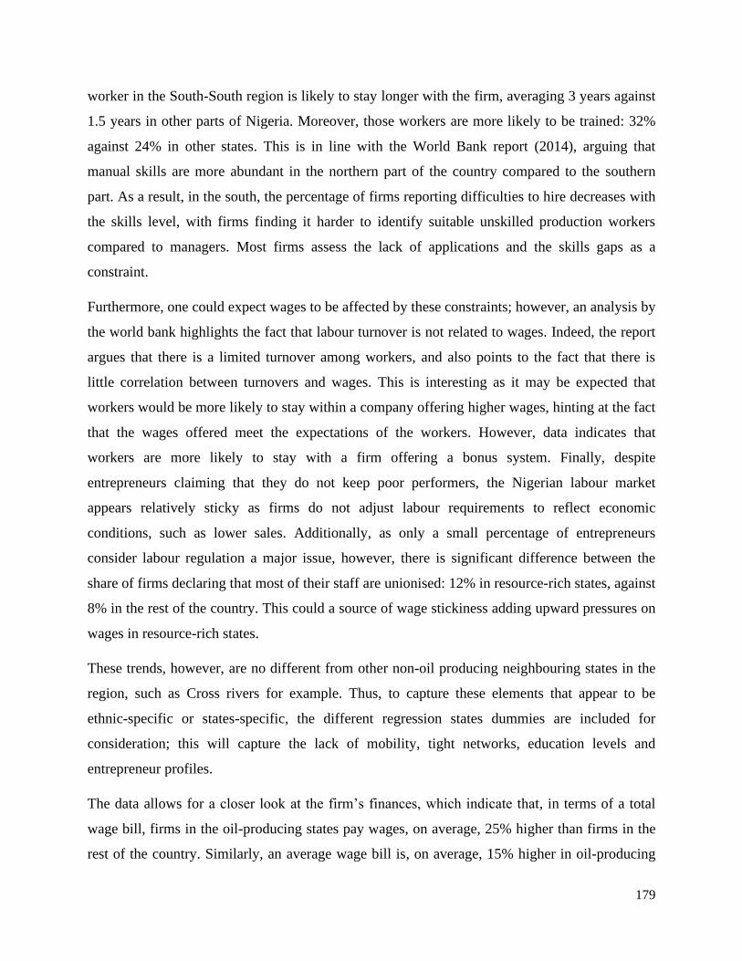
179

worker in the South-South region is likely to stay longer with the firm, averaging 3 years against

1.5 years in other parts of Nigeria. Moreover, those workers are more likely to be trained: 32%

against 24% in other states. This is in line with the World Bank report (2014), arguing that

manual skills are more abundant in the northern part of the country compared to the southern

part. As a result, in the south, the percentage of firms reporting difficulties to hire decreases with

the skills level, with firms finding it harder to identify suitable unskilled production workers

compared to managers. Most firms assess the lack of applications and the skills gaps as a

constraint.

Furthermore, one could expect wages to be affected by these constraints; however, an analysis by

the world bank highlights the fact that labour turnover is not related to wages. Indeed, the report

argues that there is a limited turnover among workers, and also points to the fact that there is

little correlation between turnovers and wages. This is interesting as it may be expected that

workers would be more likely to stay within a company offering higher wages, hinting at the fact

that the wages offered meet the expectations of the workers. However, data indicates that

workers are more likely to stay with a firm offering a bonus system. Finally, despite

entrepreneurs claiming that they do not keep poor performers, the Nigerian labour market

appears relatively sticky as firms do not adjust labour requirements to reflect economic

conditions, such as lower sales. Additionally, as only a small percentage of entrepreneurs

consider labour regulation a major issue, however, there is significant difference between the

share of firms declaring that most of their staff are unionised: 12% in resource-rich states, against

8% in the rest of the country. This could a source of wage stickiness adding upward pressures on

wages in resource-rich states.

These trends, however, are no different from other non-oil producing neighbouring states in the

region, such as Cross rivers for example. Thus, to capture these elements that appear to be

ethnic-specific or states-specific, the different regression states dummies are included for

consideration; this will capture the lack of mobility, tight networks, education levels and

entrepreneur profiles.

The data allows for a closer look at the firm’s finances, which indicate that, in terms of a total

wage bill, firms in the oil-producing states pay wages, on average, 25% higher than firms in the

rest of the country. Similarly, an average wage bill is, on average, 15% higher in oil-producing

180

states where, on average, they hire relatively fewer employees than firms in the rest of the

country. Indeed, on average, firms in non-oil-producing states hire about two people more than

firms in the South-South region. In terms of sales (in absolute numbers), on average, small and

large firms in the South-South region are performing better than firms in other parts of the

country; however, medium-size firms in the rest of country are performing much better. These

trends are maintained when sales per worker are considered.

Finally, when considering all other costs of production (excluding wages), on average, costs

faced by firms in the oil-producing region are 32% higher than in the rest of the country. These

costs are as high as 45% for small firms. This reflects the fact that the Niger delta is not on the

major commercial axis of the country, thus the price regimes for goods and services in this

geopolitical region is different from those of most other regions. Indeed, prices reflect the fact

that the Delta region is difficult to access and that communities are remote; this is compounded

by the spending by the oil and gas industry and the much higher earnings of oil sector workers.

This puts downward pressure on the average purchasing power in the region by heightening

inflation in key services, such as housing, transportation and food products. Furthermore, the oil

and gas activities have impacted farmlands and fishing grounds, negatively affecting traditional

economic occupations such as fishing and farming, as well as lowering the attractiveness of these

activities by weakening possible earnings relative to the oil sector.

This could result in rent-seeking behaviour, as illustrated by the ability to obtain government

contracts. Firms in the resource-rich states spend more time dealing with the government: 7% of

time against 5% in the rest of the country. As government spending is relatively high due to the

fiscal federalism approach, firms in the oil-producing regions are more likely to secure

government contracts: 20% against 12% in the rest of the country. To obtain this, those firms are

willing to pay a higher proportion of the contract value: 8% in the South-South region, against

5% in the rest of the country. Indeed, firms in the South-South region are more likely to obtain a

concession on the firms’ location (30% against 24%) and more likely to be owned by the

government (56% against 25%) than in the rest of the country.

From the above description of the data, a number of characteristics can be noted, intrinsic to the

region and the people within this region, particularly their approach to entrepreneurship in terms

of ownership structure as well as mechanisms used to recruit employees; thus, they are likely to

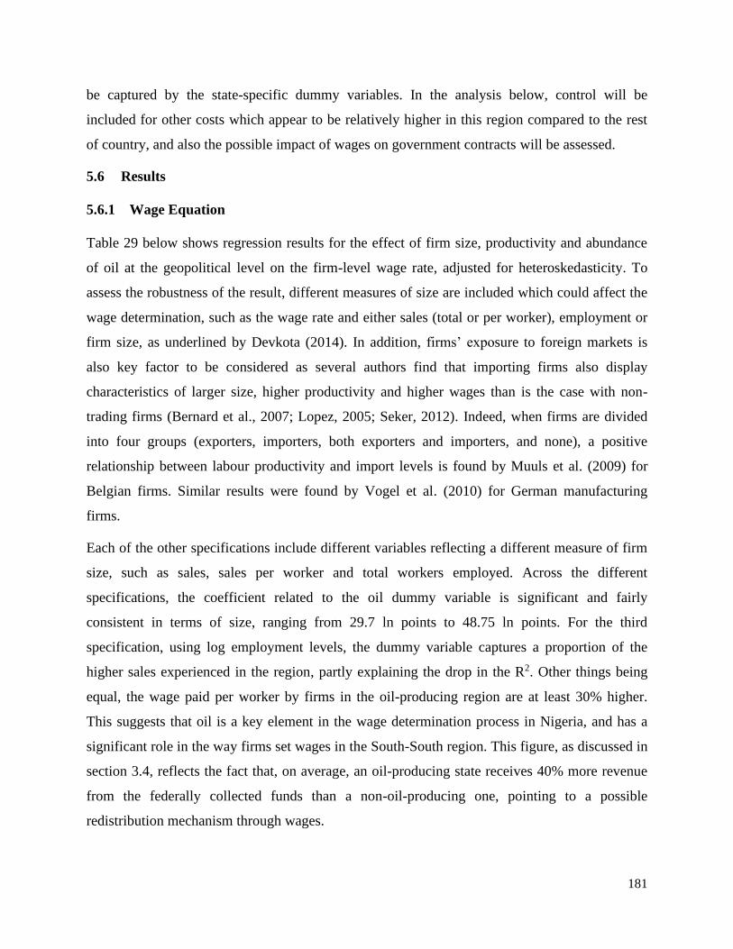
181

be captured by the state-specific dummy variables. In the analysis below, control will be

included for other costs which appear to be relatively higher in this region compared to the rest

of country, and also the possible impact of wages on government contracts will be assessed.

5.6 Results

5.6.1 Wage Equation

Table 29 below shows regression results for the effect of firm size, productivity and abundance

of oil at the geopolitical level on the firm-level wage rate, adjusted for heteroskedasticity. To

assess the robustness of the result, different measures of size are included which could affect the

wage determination, such as the wage rate and either sales (total or per worker), employment or

firm size, as underlined by Devkota (2014). In addition, firms’ exposure to foreign markets is

also key factor to be considered as several authors find that importing firms also display

characteristics of larger size, higher productivity and higher wages than is the case with non-

trading firms (Bernard et al., 2007; Lopez, 2005; Seker, 2012). Indeed, when firms are divided

into four groups (exporters, importers, both exporters and importers, and none), a positive

relationship between labour productivity and import levels is found by Muuls et al. (2009) for

Belgian firms. Similar results were found by Vogel et al. (2010) for German manufacturing

firms.

Each of the other specifications include different variables reflecting a different measure of firm

size, such as sales, sales per worker and total workers employed. Across the different

specifications, the coefficient related to the oil dummy variable is significant and fairly

consistent in terms of size, ranging from 29.7 ln points to 48.75 ln points. For the third

specification, using log employment levels, the dummy variable captures a proportion of the

higher sales experienced in the region, partly explaining the drop in the R2. Other things being

equal, the wage paid per worker by firms in the oil-producing region are at least 30% higher.

This suggests that oil is a key element in the wage determination process in Nigeria, and has a

significant role in the way firms set wages in the South-South region. This figure, as discussed in

section 3.4, reflects the fact that, on average, an oil-producing state receives 40% more revenue

from the federally collected funds than a non-oil-producing one, pointing to a possible

redistribution mechanism through wages.

182

Firm size is a key determinant of the wage level, with a coefficient ranging from 0.19 to 0.46.

This is even more of a determinant than a firm’s exposure to external markets. The different

control variables are significant under the different dependent variables, apart from age and

variable age square (age2), indicating, interestingly, that wages are independent of the firm’s age

in that older firms are not more likely to offer higher wages.

In addition, across the three specifications, the variable indicating a firm’s size is significant, and

size plays a role similar to the oil dummy. For example, a 1% increase in sales is associated with

a 0.33% higher average wage per worker or 1% increase in sales per worker leads to a 0.47%.

increase in the average wage per worker. Similarly, the average per worker wage in medium and

large firms is 21% and 53% higher than in a small firm, pointing to the profit-sharing theory

(Teal, 1995). This points to wage-sharing mechanisms being set in place to retain workers. This

is reinforced by the share of permanent employees’ positive impact on wages, as firms offer

relatively higher wages per worker to retain their labour force. In addition, the dummy for the

presence of a labour union indicates (as expected) a small upwards pressure on average wages

when significant. It is also insignificant in the first specifications. This suggests that the role

played by labour unions may not be the major factor in wage determination at the firm level.

Foreign exposure, as a proxy for productivity based on the assumption that more productive

firms will be able to withstand international competition, does not significantly impact firm

average wage per worker. When considered with total sales (model 1), it turns out to be both

significant and negative, implying that export-orientated firms have to pay a lower wage to

maintain a degree of competitiveness. Moreover, when labour employed is used to represent firm

size, we find that firms engaged in international trade provide about 27% higher wages than a

typical non-trading firm. This is in line with the theory suggesting that firms are experiencing

greater efficiency because of their ability to withstand external competition urging the payment

of higher wages. In the same specification, a 1% increase in employment leads to about a 0.2%

higher wage. Although firm exposure is likely to play a role in wage determination, its role is

ambiguous and not as clear as suggested by the literature.

Table 29: Estimate Log Wage Per Worker and Relevant Variables Estimation summary - Dependent var is ln (per worker wage cost)

Model 1

Coeff./Se.

Model 2

Coeff./Se.

Model 3

Coeff./Se.

oil_dummy 0.2975***

(0.06)

0.3050***

(0.06)

0.4875***

(0.08)

183

Fexposure -0.1084*

(0.06)

0.0470

(0.05)

0.2687***

(0.07)

Permlshr 0.0133***

(0.00)

0.0077***

(0.00)

0.0164***

(0.00)

Labunion -0.0005

(0.00)

0.0007**

(0.00)

0.0011***

(0.00)

Age -0.0024

(0.00)

0.0020

(0.00)

0.0031*

(0.00)

age^2 0.0000

(0.00)

-0.0000

(0.00)

0.0000

(0.00)

ln(sales) 0.3266***

(0.01)

ln(pw sales)

0.4683***

(0.01)

ln(labour)

0.1959***

(0.01)

_cons 5.1079***

(0.15)

4.6013***

(0.16)

9.2426***

(0.14)

Aic 7336.30 6768.05 9426.82

Bic 7698.77 7130.52 9789.29

r2 0.6050 0.6492 0.3883

N 4782 4782 4782

In all the models, dummy variables controlling for years, industry (SIC level 2,

revision 2) and states-related dummy variables are included.

Standard errors are in the parentheses and are robust.

* p<0.1, ** p<0.05, *** p<0.01

source: Author’s estimations

5.6.2 Wage Equation Robustness Check

To further asses the robustness of these results, a similar analysis was carried out using the total

wage bill as a dependent variable (see Table 30 below). This result is fairly consistent with the

size of the oil dummy, ranging from 27% to 49%. However, the size of the different parameters

presents more deviations from the values presented, as in Table 30, and they all present results in

line with theoretical expectations and are, in most cases, significant.

Table 30: Estimated Total Wage Bill and Relevant Variables Estimation summary (Dependent var is ln (Total wage cost))

Model 4

Coeff./Se.

Model 5

Coeff./Se.

Model 6

Coeff./Se.

oil_dummy 0.2734***

(0.08)

0.4833***

(0.12)

0.4875***

(0.08)

Fexposure -0.1317*

(0.08)

0.7845***

(0.14)

0.2687***

(0.07)

Permlshr 0.0011**

(0.00)

-0.0052***

(0.00)

0.0164***

(0.00)

Labunion 0.0016***

(0.00)

0.0052***

(0.00)

0.0011***

(0.00)

Age 0.0055***

(0.00)

0.0186***

(0.00)

0.0031*

(0.00)

age^2 -0.0000

(0.00)

-0.0001***

(0.00)

0.0000

(0.00)

ln(sales) 0.6847***

(0.01)

ln(pw sales) 0.5838***

(0.02)

ln(labour) 0.1959***

(0.01)

Med. 20-99

184

Large > 100

_cons 3.2107***

(0.19)

6.6515***

(0.30)

9.2426***

(0.14)

Aic 8408.55 12289.53 9426.82

Bic 8771.01 12652.00 9789.29

r2 0.8156 0.7849 0.5719

N 4782 4782 4782

In all the models, dummy variables controlling for years, industry (SIC level 2,

revision 2) and states-related dummy variables are included.

Standard errors are in parentheses.

* p<0.1, ** p<0.05, *** p<0.01

source: Author’s estimations

As before, to assess the robustness of the oil dummy, it is replaced with the amount of revenue

received by each state’s government (computed from the Central Bank Statistical Bulletin 2016).

In doing so, similar results were obtained (see Table 31), with the coefficient being positive and

significant, pointing to the role played by oil revenue in wage determination, resulting in a

premium of at least 10%. This was achieved using both average wage cost per worker (models

1.1, 2.1, 3.1) and total wages (models 4.1, 5.1 and 6.1).

Table 31: Estimate Using Different Proxies for oil revenue Estimation summary (Dependent var is ln (per worker wage cost) for model 1.1.; 2.1.and

3.1.and Dependent var is ln (Wage cost) for model 4.1; 5.1.and 6.1.

Model 1.1

Coeff./Se.

Model 2.1

Coeff./Se.

Model 3.1

Coeff./Se.

Model 4.1

Coeff./Se.

Model 5.1

Coeff./Se.

Model 6.1

Coeff./Se.

l_grants_stt 0.1486**

(0.02)

0.2341***

(0.03)

0.1032***

(0.02)

-0.0077

(0.02)

0.3430**

(0.02)

0.1032***

(0.02)

Fexposure 0.1481*

(0.08)

0.2736***

(0.14)

0.2998***

(0.07)

0.1060*

(0.06)

0.0732

(0.05)

0.2998***

(0.07)

Permlshr 0.0120**

(0.00)

-0.0089***

(0.00)

0.0169***

(0.00)

0.0131***

(0.00)

0.0072***

(0.00)

0.0169***

(0.00)

Labunion 0.0016***

(0.00)

0.0056***

(0.00)

0.0009**

(0.00)

0.0006*

(0.00)

0.0007**

(0.00)

0.0009**

(0.00)

Age 0.0047***

(0.00)

0.0168***

(0.00)

-0.0001

(0.00)

0.0036**

(0.00)

0.0011

(0.00)

-0.0001

(0.00)

age^2 -0.0000

(0.00)

-0.0000

(0.00)

0.0000*

(0.00)

0.0000

(0.00)

0.0000

(0.00)

0.0000*

(0.00)

ln(sales) 0.7090***

(0.01)

0.3416***

(0.01)

ln(pwsales) 0.6650***

(0.02)

0.4966***

(0.01)

ln(labour) 1.2635***

(0.01)

0.2635***

(0.01)

_cons 2.8244***

(0.18)

5.4585***

(0.31)

9.1247***

(0.15)

5.0466***

(0.15)

4.3349***

(0.16)

9.1247***

(0.15)

Aic 8655.28 12827.74 10008.80 7653.20 7097.61 10008.80

Bic 8797.67 12970.14 10151.20 7795.60 7240.01 10151.20

r2 0.8031 0.6287 0.7386 0.5718 0.6188 0.4993

N 4782 4782 4782 4782 4782 4782

In all the models, dummy variables controlling for years, industry (SIC level 2,

revision 2) and states-related dummy variables are included.

Standard errors are in parentheses.

* p<0.1, ** p<0.05, *** p<0.01

source; Author’s estimations

185

Overall, the obtained results align with the DD theoretical prediction as they suggest that the

mere presence of oil is in general associated with higher wages. Indeed, the total wage bill and

average wage of firms in oil and gas producing geopolitical regions is higher than other non-oil-

producing regions. This analysis also indicates that firm size plays a significant role in wage

determination. Thus, oil abundance will contribute to wage inequality across the country.

Furthermore, as presented in Chapter 3, firms in the South-South region possess greater

efficiency levels compared to firms in other parts of the country. Thus, it might be that the higher

wage is just the result of higher productivity in that region. Based on the assumption that

exporting firms are more productive, introduced into the different specifications is an interaction

dummy between foreign exposure (fexposure) and the oil dummy. Complementary to the per-

worker sales, this interaction term will capture the impact of being located in the oil-producing

region on wages paid by firms able to export, thus assumed to be more productive.

Table 32 below indicates that among exporting firms expected to be more productive, there is a

difference in wages, which is linked to the abundance of oil at the local level. The interaction

coefficient term is found to be positive and significant across the different specifications. Thus,

on average, productive firms in the South-South region pay wages depending on the

specifications, between 10% and 19% more than other exporting firms. similar results were

obtained using the total wage bill as the dependent variable (not reported).

Table 32: Estimate Including Interaction Terms Between Oil and Foreign Exposure Estimation summary (Dependent var is Ln (per worker wage cost) and interaction term

between the oil dummy and foreign exposure.

Model l.2

Coeff./Se.

Model 2.2

Coeff./Se.

Model 3.2

Coeff./Se.

oil_dummy 0.2941***

(0.06)

0.3097***

(0.06)

0.4841***

(0.08)

Fexposure -0.1218*

(0.06)

0.0654

(0.06)

0.2549***

(0.08)

Permlshr 0.0133***

(0.00)

0.0077***

(0.00)

0.0164***

(0.00)

Labunion -0.0005

(0.00)

0.0007**

(0.00)

0.0011***

(0.00)

Age -0.0024

(0.00)

0.0020

(0.00)

0.0031*

(0.00)

age^2 -0.0000

(0.00)

-0.0000

(0.00)

0.0000

(0.00)

ln (sales) 0.3267***

(0.01)

interaction 0.1547**

(0.06)

0.0960*

(0.05)

0.1919***

(0.06)

ln (pw sales) 0.4683***

(0.01)

ln (labour) 0.1961***

(0.01)

186

_cons 5.1104***

(0.15)

4.5969***

(0.16)

9.2451***

(0.14)

Aic 7338.12 6769.66 9428.70

Bic 7707.06 7138.60 9797.64

r2 0.6050 0.6492 0.3884

N 4782 4782 4782

In all the models, dummy variables controlling for years, industry (SIC level 2,

revision 2) and states-related dummy variables are included.

standard errors are in parentheses.

* p<0.1, ** p<0.05, *** p<0.01

source; Author’s estimations

In order to assess the relationship between location and price, total other costs (excluding wages)

are added to the model. This is justified by the fact that the discussion above (section 5.5) points

to the fact that prices are, on average, higher in the oil-producing region compared to the rest of

the country. Table 33 below, using average wage per worker as dependent, points to the fact that

the dummy variable captures parts of the price effect as the associated coefficient increases when

the price of other inputs is included. The upwards movement reflects the fact that other costs

have a negative impact on wages. Similarly, this additional variable absorbs part of the impact

captured by the foreign exposure dummy. This means that other total costs impact the ability of

firms to export.

Table 33: Estimate Including other costs Estimation summary (Dependent var is Ln (per worker wage cost) and additional cost

variables (excluding wages).

Model l.2

Coeff./Se.

Model 2.2

Coeff./Se.

Model 3.2

Coeff./Se.

oil_dummy 0.3350***

(0.05)

0.3590***

(0.05)

0.5547***

(0.05)

Fexposure -0.0632*

(0.04)

0.0658

(0.04)

0.0745**

(0.03)

Permlshr 0.0131***

(0.00)

0.0086***

(0.00)

0.0109***

(0.00)

Labunion -0.0007

(0.00)

0.0007**

(0.00)

0.0006***

(0.00)

Age -0.0016

(0.00)

0.0021

(0.00)

0.0017*

(0.00)

Age^2 -0.0000

(0.00)

-0.0000

(0.00)

0.0000

(0.00)

ln cost (excl.wages) -0.1018***

(0.01)

-0.0475***

(0.01)

-0.2838***

(0.00)

ln (sales) 0.3973***

(0.02)

ln (pw sales) 0.3571***

(0.01)

ln (labour) 0.1776***

(0.01)

_cons 5.5535***

(0.11)

5.470***

(0.16)

6.7561***

(0.09)

Aic 7335.32 6768.96 9427.29

Bic 7704.41 7134.81 9793.57

r2 0.6261 0.6529 0.6101

N 4782 4782 4782

187

In all the models, dummy variables controlling for years, industry (SIC level 2,

revision 2) and states-related dummy variables are included.

standard errors are in parentheses.

* p<0.1, ** p<0.05, *** p<0.01

source; Author’s estimations

Another channel that was explored from the descriptive statistics discussion in section 5.5 is the

ability of the firms to attract government contracts. In order to do so, a dummy variable is

introduced into the initial model specifications, capturing the fact that the firm bids for a

government contract. Table 34 below presents the results, using wage per worker as a dependent

variable and sales per worker as the measure of a firm’s size. These indicate that the dummy

variable is positive and significant, pointing to the fact that the ability to bid/obtain government

contracts impacts wage levels positively. When the interaction terms associating the location in

an oil-producing region and the ability to seek/obtain are introduced in the model, government

contracts, on average, offer higher wages. This is in line with the rent sharing theory that can be

associated with the DD framework.

Table 34: Estimate Including variable capturing government contracts Model 2.2

Coeff./Se.

Model 2.2

Coeff./Se.

oil_dummy 0.2875***

(0.08)

0.2529***

(0.06)

Fexposure 0.0351

(0.06)

0.0318

(0.06)

Permlshr 0.0076***

(0.00)

0.0077***

(0.00)

Labunion 0.0005**

(0.00)

0.0005**

(0.00)

Age 0.0020

(0.00)

0.0020

(0.00)

age^2 -0.0000

(0.00)

-0.0000

(0.00)

ln (pw sales) 0.4221***

(0.01)

0.4237***

(0.01)

Gov_contract 0.1371**

(0.06)

0.1287**

(0.05)

interaction 0.0860*

(0.05)

_cons 4.6418***

(0.15)

4.6969***

(0.16)

Aic 6768.96 6873.53

Bic 7135.20 7258.11

r2 0.6592 0.7214

N 4782 4782

In all the models, dummy variables controlling for years, industry

(SIC level 2, revision 2) and states related dummy variables are

included.

Standard errors are in parentheses

* p<0.1, ** p<0.05, *** p<0.01

source; Author’s estimations

188

Thus, wages and location are shown to be closely related as a wage premium is paid in the region

receiving larger revenues from the oil sector. The analysis does not allow the disentanglement of

the revenue and location impact described by Brunstad and Dyrstad (1997) but, given the limited

labour mobility across the country, wages are being pushed upwards. This is similar to Brunstad

and Dyrstad’s findings in the Norwegian case, where a booming sector was shown to impact

nominal wages through wage differentials across sectors and regions. Further, the demand effect

can potentially positively impact nominal wages across the different labour submarkets; while

the cost of living effect can put a negative pressure on regions further away from the oil-

producing zones. This analysis also points to the existence of a rent-sharing mechanism as

presented in Chapter 3, where it was established that firms in this region were among the most

productive in the country. Moreover, assuming that other than a firm’s exposure, sales per

worker captures productivity levels, thus it can be noted that higher productivity results in higher

wages paid. This in is in line with the literature produced by Charness and Kuhn (2007), who

found that a phenomenon of gift exchange does exist among workers and firms.

In addition, this analysis points to the fact that foreign exposure does not result in higher wages,

in contrast to the general prediction of the literature. However, as pointed out by Malik et al.

(2008), unlike firms in East Asia which are export-oriented, Nigerian firms are inward-looking,

targeting mainly the large domestic market. Thus, these inward-looking firms do not face the

competition of international markets and, as a result, can offer higher wages, which do not

necessarily reflect productivity levels. This observation is very much in line with the

assumptions of the Dutch Disease framework, implying a greater focus on non-tradable activities

pushing wages upwards, making the tradable sector less competitive. This will be further

explored in the next section, which looks at the difference between services and manufacturing

activities.

Finally, this analysis indicates that a firm’s size, which has been assessed by different variables,

matters more than its age in terms of wage determination. The age of a firm plays a weak role in

determining wages, while the size seems to have a stronger role in that smaller firms will pay a

relatively lower average wage per-worker compared to larger firms. This probably contributes to

wage inequality in Nigeria (assessed in the next sections) and could have interesting policy

implications. Similarly, the price of other inputs and the ability to obtain government contracts

matter for wage determination. This points to the fact that the Nigerian fiscal federalism results

189

in local inflation, and possibly encourages rent-seeking behaviour assimilated to the rent sharing

mechanisms.

5.6.3 Differences between Services and Manufacturing Sectors

It is important to note that firms in the manufacturing sector9 and firms offering services are both

affected by the presence of oil; however, the dummy coefficient in Table 35 and Table 36, when

significant, is higher for manufacturing firms. This implies that oil abundance at the geopolitical

level matters more for these firms; i.e. a manufacturing firm in the South-South region will pay a

premium of between 32% and 55% compared to a firm outside the region, while this range is of

20-42% for a services firm. This in line with the work of Brunstad and Dyrstad (1997) and the

prediction of the DD, pointing to the effect of oil revenues extending beyond the booming sector

and affecting the entire local economy, including the non-tradable sector. The impact is less

regarding the services sector as it is a relatively competitive sector and offers more homogeneous

goods.

Among the different firms, independent of the sector, size matters as larger firms offer higher

wages. This is true for the different proxy of size that was used in the different specifications.

However, the size effect is more pronounced for services firms than manufacturing firms. Again,

given the fact that firms in the tradable sector face external competition, there is a limit on the

premium they can put on wages. Thus, among firms of similar size, wages in the service sector

will be higher.

In addition, in the different sectors, the role played by labour unions seems to differ. In the

services sector, the labour union plays a more subdued role in wage determination. This could

reflect the fact that the sector is very diverse and historically less tolerant towards labour actions

(see George et al., 2012). The opposite is true of the manufacturing sector, where labour unions

do have an impact on wage determination; it is significant but with a very small coefficient of

0.002. Similarly, age is less relevant for services firms than for manufacturing ones.

Finally, looking at the issue of foreign exposure, the role of the ability to export is unclear for

services firms across the different specifications, and when significant, it has a negative impact

9 This sector includes firms in the textile, garment, food, machinery, electronics, chemicals, wood, plastic materials,

and other manufacturing. Firms in the services sectors include construction, IT services, retail and wholesale trade

and hotels and restaurants.

190

on wages. This highlights that in the Nigerian market, services allow firms to pay higher wages if

not under the pressure of having to compete internationally. Furthermore, when looking at the

interaction variable between foreign exposure and the oil sector, it is clear that firms located in

the oil-rich region pay a higher premium on wages than their counterparts in other parts of the

country. These results also point to the cost of living effect, where the abundance of oil also

impact sectors other than the oil sector. Thus, it reinforces the message that oil has an impact that

cuts across various sectors of the economy, as suggested by the DD framework.

When looking at firms in the manufacturing sector, the ability to export turns out to have a

positive impact on wages. This effect can be very significant, as illustrated by the coefficient in

Table 36, below. This corresponds with the literature, as more productive firms are then able to

share the returns of productivity with their workers. However, the location and abundance of oil

at the local level still matters as exporting firms in the South-South region pay more than similar

exporting firms in other regions.

Table 35: Estimate for the Services Sector Only Model 1.3

Coeff./Se.

Model 2.3

Coeff./Se.

Model 3.3

Coeff./Se.

Model 1.4

Coeff./Se.

Model 2.4

Coeff./Se.

Model 3.4

Coeff./Se.

oil_dummy 0.2050**

(0.09)

0.2867***

(0.09)

0.4231***

(0.11)

0.2042**

(0.09)

0.2885***

(0.09)

0.4099***

(0.11)

fexposure -0.2264**

(0.10)

-0.1241

(0.10)

0.1759

(0.14)

-0.2375**

(0.12)

-0.0992

(0.11)

0.0054

(0.15)

Permlshr 0.0135***

(0.00)

0.0077***

(0.00)

0.0178***

(0.00)

0.0135***

(0.00)

0.0077***

(0.00)

0.0177***

(0.00)

Labunion -0.0010**

(0.00)

0.0003

(0.00)

0.0001

(0.00)

-0.0010**

(0.00)

0.0003

(0.00)

0.0001

(0.00)

Age -0.0047

(0.00)

-0.0009

(0.00)

0.0004

(0.00)

-0.0047

(0.00)

-0.0009

(0.00)

0.0002

(0.00)

age^2 0.0001

(0.00)

0.0000

(0.00)

0.0000

(0.00)

0.0001

(0.00)

0.0000

(0.00)

0.0001

(0.00)

In (sales) 0.3493***

(0.01)

0.3492***

(0.01)

In (pw

sales)

0.4774***

(0.01)

0.4777***

(0.01)

In (labour) 0.2256***

(0.02)

0.2250***

(0.02)

Interaction 0.2697***

(0.07)

0.1195*

(0.07)

0.1514*

(0.08)

_cons 4.8155***

(0.15)

4.4339***

(0.16)

8.9551***

(0.13)

4.8169***

(0.15)

4.4303***

(0.16)

8.9618***

(0.13)

Aic 5134.27 4814.77 6658.85 5136.24 4816.59 6656.17

Bic 5431.85 5112.35 6956.43 5439.89 5120.25 6959.83

r2 0.6078 0.6450 0.3691 0.6078 0.6450 0.3700

N 3207 3207 3207 3207 3207 3207

In all the models, year, industry and regional effects are controlled.

Standard errors are in parentheses.

* p<0.1, ** p<0.05, *** p<0.01

source: Author’s estimations

191

Table 36: Estimate for the Manufacturing Sector Only Model 1.5

Coeff./Se.

Model 2.5

Coeff./Se.

Model 3.5

Coeff./Se.

Model 1.6

Coeff./Se.

Model 2.6

Coeff./Se.

Model 3.6

Coeff./Se.

oil_dummy 0.3861***

(0.09)

0.3165***

(0.08)

0.5194***

(0.11)

0.3929***

(0.09)

0.3256***

(0.08)

0.5539***

(0.11)

fexposure 0.0226

(0.07)

0.1445**

(0.06)

0.3171***

(0.08)

0.0366**

(0.07)

0.1628**

(0.06)

0.3885***

(0.08)

Permlshr 0.0126***

(0.00)

0.0075***

(0.00)

0.0139***

(0.00)

0.0126***

(0.00)

0.0075***

(0.00)

0.0139***

(0.00)

Labunion 0.0008

(0.00)

0.0014***

(0.00)

0.0029***

(0.00)

0.0008

(0.00)

0.0014***

(0.00)

0.0029***

(0.00)

Age -0.0004

(0.00)

0.0035**

(0.00)

0.0058**

(0.00)

-0.0004

(0.00)

0.0035**

(0.00)

0.0059***

(0.00)

age^2 0.0000

(0.00)

-0.0000*

(0.00)

0.0000

(0.00)

0.0000

(0.00)

-0.0000*

(0.00)

-0.0000

(0.00)

In (sales) 0.2710***

(0.01)

0.2706***

(0.01)

In (pw

sales)

0.4394***

(0.02)

0.4388***

(0.02)

In (labour) 0.1441***

(0.02)

0.1421***

(0.02)

Interaction 0.2125**

(0.09)

0.2580**

(0.10)

0.1873**

(0.09)

_cons 6.0901***

(0.23)

5.0044***

(0.24)

9.6994***

(0.18)

6.0921***

(0.23)

5.0065***

(0.24)

9.6895***

(0.18)

Aic 2105.87 1880.27 2638.41 2107.70 1881.92 2637.17

Bic 2368.60 2143.00 2901.15 2375.80 2150.02 2905.27

r2 0.6115 0.6633 0.4552 0.6115 0.6634 0.4563

N 1575 1575 1575 1575 1575 1575

In all the models, year, industry and regional effects are controlled.

Standard errors are in parentheses.

* p<0.1, ** p<0.05, *** p<0.01

source: Author’s estimations

To conclude, firm size, oil abundance and wages are closely related. The smaller the size of a

given firm, the lower the wage per worker, and the larger the size of a firm, the higher the wage

per worker. In addition, oil abundance undeniably affects firms, with firms in the oil-producing

geopolitical region paying a premium on labour inputs. This premium is higher for firms

operating in the manufacturing sector (i.e. tradable) than those in the services sector (i.e. non-

tradable). This indicates that oil at the local level has an impact on wages that affect the different

sectors of the economy: both the manufacturing and services sectors. This leads to a further

exploration of wage inequality and an assessment of the role played by each factor, such as oil,

in explaining wage inequality in Nigeria.

5.6.4 Wage Decomposition and Wage Inequality

5.6.4.1 Gini index

The Gini index estimated for the entire sample, and for different types of firms according to their

size, is presented below, along with the related Lorenz curves (see the annexe for the different

192

sectors). The wage inequality in Nigeria (the wage Gini), using the average log million Naira

wage per worker cost paid by firms, stands at 0.43.

Table 37 below indicates that for the whole sample, inequality is larger among large and small

firms, while medium-sized firms are less unequal in terms of wages. Looking at the different

sectors, inequalities are overall higher among the firms operating in the services sector (0.49)

when compared to the 0.38 for manufacturing firms. This reflects the heterogeneity of firms

operating in the services sector. This further explains why greater inequality exists among small

firms than among the small services firms (0.50) when compared to the figure of 0.33 among

small manufacturing firms. This trend is inverted when looking at larger firms, as inequality is

greater among large manufacturing firms (0.44) when compared to their large service

counterparts (0.33). This indicates that, as firms grow, practices homogenise, and this is notable

in terms of wages. This can be explained by larger firms being more likely to operate in the

formal sector and are thus more compliant with labour laws. However, regarding manufacturing

firms, the homogeneity of their products pushes for more standardised practices, and they are

thus relatively less informal. Greater inequality among larger manufacturing sectors could be

explained by the “efficiency wage theory”, which argues that, as firms grow, they may be

reducing their costs by increasing wages due to labour market rigidity and high search costs.

Table 37: Wage Inequality - Gini Coefficients

Average wage cost

(full sample)

Average wage cost

(services firms)

Average wage cost

(manufacturing firms)

Small (5-19) 0.4095 0.5012 0.3341

Medium (20-99) 0.3879 0.4118 0.3667

Large (100+) 0.4237 0.3320 0.4425

Total Sample 0.4255 0.4855 0.3778

source: Author’s estimations

5.6.4.2 Contribution of the Different factor: Wage Decomposition

Wage inequality can be deconstructed into the determinants of wage, as indicated by equation (1)

above and the steps described above. The decomposition is done for three separate specifications

(Model 1, 2 and 3, Table 29), the results of which appear in Table 38 and Chart 33 below. These

findings show that oil contributes to at least 6% of wage inequality observed in Nigeria (using

labour as a proxy for size). This contribution is as large as 44% when the per worker sales as

proxy per-size are used. The difference between these results can be imputed to the per worker

sales variable which “dilutes” the impact of size reduction and thus it is of relative importance

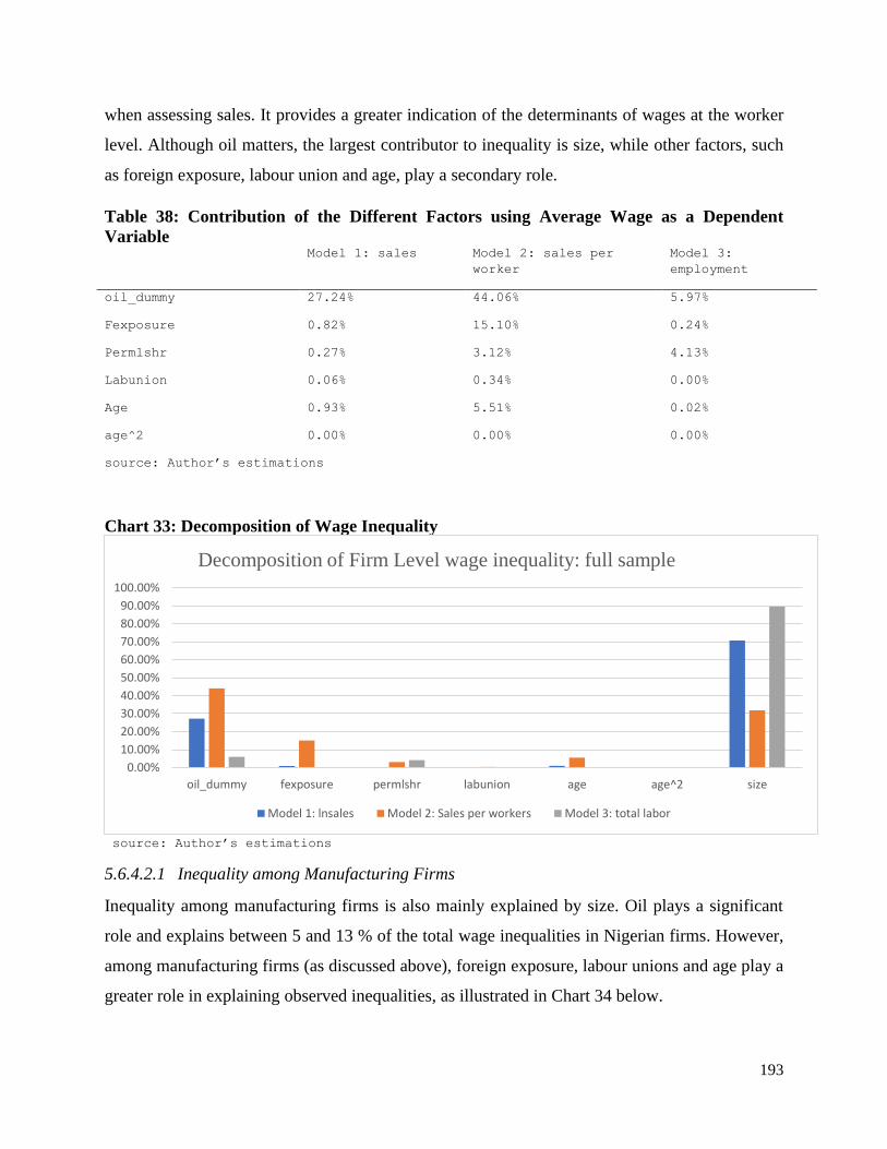
193

when assessing sales. It provides a greater indication of the determinants of wages at the worker

level. Although oil matters, the largest contributor to inequality is size, while other factors, such

as foreign exposure, labour union and age, play a secondary role.

Table 38: Contribution of the Different Factors using Average Wage as a Dependent

Variable Model 1: sales Model 2: sales per

worker

Model 3:

employment

oil_dummy 27.24% 44.06% 5.97%

Fexposure 0.82% 15.10% 0.24%

Permlshr 0.27% 3.12% 4.13%

Labunion 0.06% 0.34% 0.00%

Age 0.93% 5.51% 0.02%

age^2 0.00% 0.00% 0.00%

source: Author’s estimations

Chart 33: Decomposition of Wage Inequality

source: Author’s estimations

5.6.4.2.1 Inequality among Manufacturing Firms

Inequality among manufacturing firms is also mainly explained by size. Oil plays a significant

role and explains between 5 and 13 % of the total wage inequalities in Nigerian firms. However,

among manufacturing firms (as discussed above), foreign exposure, labour unions and age play a

greater role in explaining observed inequalities, as illustrated in Chart 34 below.

0.00%

10.00%

20.00%

30.00%

40.00%

50.00%

60.00%

70.00%

80.00%

90.00%

100.00%

oil_dummy fexposure permlshr labunion age age^2 size

Decomposition of Firm Level wage inequality: full sample

Model 1: lnsales Model 2: Sales per workers Model 3: total labor

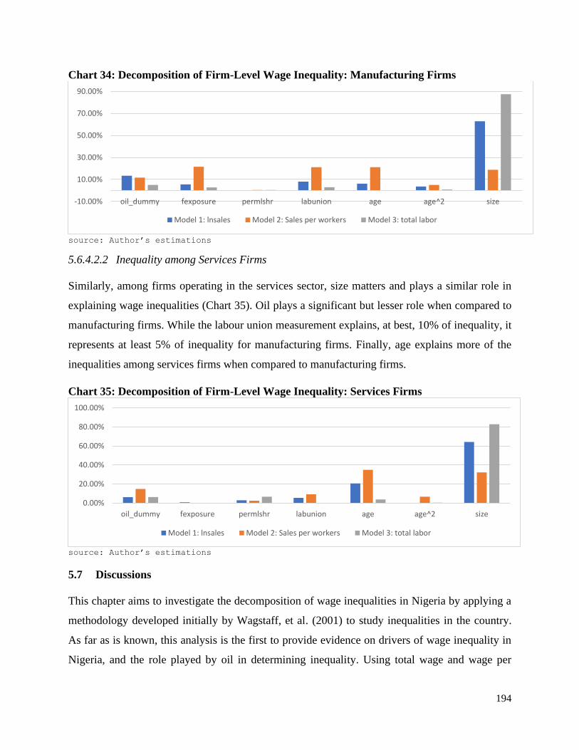
194

Chart 34: Decomposition of Firm-Level Wage Inequality: Manufacturing Firms

source: Author’s estimations

5.6.4.2.2 Inequality among Services Firms

Similarly, among firms operating in the services sector, size matters and plays a similar role in

explaining wage inequalities (Chart 35). Oil plays a significant but lesser role when compared to

manufacturing firms. While the labour union measurement explains, at best, 10% of inequality, it

represents at least 5% of inequality for manufacturing firms. Finally, age explains more of the

inequalities among services firms when compared to manufacturing firms.

Chart 35: Decomposition of Firm-Level Wage Inequality: Services Firms

source: Author’s estimations

5.7 Discussions

This chapter aims to investigate the decomposition of wage inequalities in Nigeria by applying a

methodology developed initially by Wagstaff, et al. (2001) to study inequalities in the country.

As far as is known, this analysis is the first to provide evidence on drivers of wage inequality in

Nigeria, and the role played by oil in determining inequality. Using total wage and wage per

-10.00%

10.00%

30.00%

50.00%

70.00%

90.00%

oil_dummy fexposure permlshr labunion age age^2 size

Model 1: lnsales Model 2: Sales per workers Model 3: total labor

0.00%

20.00%

40.00%

60.00%

80.00%

100.00%

oil_dummy fexposure permlshr labunion age age^2 size

Model 1: lnsales Model 2: Sales per workers Model 3: total labor

195

worker at the firm level as dependent variables, this chapter has provided new evidence on

disparities among firms in the context of an oil-rich country, where resource extraction is mainly

concentrated in one geopolitical region. In addition, this region receives relatively large shares of

revenue through the country’s revenue-sharing formula.

This chapter shows that firms in oil-rich regions are more likely to pay a premium on wages. In

Nigeria, the assumed wage determinants indicate that firms’ location in an oil-producing region

impacts wages positively and contributes to wage inequality across firms. The methodology

entails combining the marginal effect of the different explanatory variables on wages. This effect

captures the fact that a determinant is more prevalent among firms offering a relatively small

average wage or among those offering a larger average wage. For instance, part of the wage

inequality is attributed to firms being located in an oil-rich state. This results in firms in oil-rich

regions paying, on average, at least 10% more than firms in other parts of the country. Size

(assessed by different proxies) contributes most significantly to wage inequality. Thus, larger

firms will be paying larger wages, while factors such as foreign exposure, the presence of labour

unions, the permanent size of employment, and the age of a firm also have positive, but more

marginal, contributions to wage inequalities.

5.7.1 Impact of Oil on Wage Determination

The analysis above indicates, as suggested by Dutch Disease theory and the mechanisms

presented by Brunstad and Dyrstad (1997), that oil has an impact on the local economy by

affecting determinants of one of the key production inputs for firms – namely wages. The wage

offered by a firm located in the oil-producing geopolitical region of a country like Nigeria is

impacted by the inflows of oil revenue at the subnational level. Those results hold for different

measures of wages and across the full sample and across sectors. Furthermore, these results hold

for when actual revenue received by oil-rich states from the federal government (in line with the

country’s revenue sharing formula) are used as explanatory variables. The abundance of oil at

the local level also feeds wage inequality in the country. This analysis provides evidence of

another mechanism through which this region of Nigeria is affected by the abundance of oil, i.e.

higher wage levels affecting the overall competitiveness of firms.

This effect is found across firms, sectors and even across firms that are assumed to be of similar

productivity levels, given their ability to export. Indeed, even among firms facing external

196

markets, it was found that firms in the South-South region are paying a premium on wages.

Further, when looking at the difference across sectors, it becomes clear that the interaction term

between the oil dummy and foreign exposure matters. Thus, both manufacturing and service

sectors in those regions could be more cost-competitive if this premium did not exist. Indeed, in

the service sector, we find that firms exposed to international markets have to pay lower wages

to remain competitive. This points to the structure and the nature of non-tradable goods, which

allow firms to pay higher wages because they face very little external competition. Within the

manufacturing sector, exporting for an assumed similar level of productivity, firms in the South-

South region pay workers up to 55 % more. This suggests that these firms could be relatively

more competitive if this premium did not exist. This premium could be explained by several

factors, all linked directly and indirectly to the abundance of resources at the local level.

First, efficiency wage and rent-sharing theory could explain these results. The efficiency wage

hypothesis suggests that firms offering higher wages or increasing wages could, in effect, reduce

costs, as it may result in the increased productivity of workers. For similar reasons, the rent-

sharing theory or gift exchange theory (Akerlof, 1982, 1984) argues that firms, by offering

higher wages, can promote workers’ loyalty and this can result in increased productivity. The

strength of this effect will determine the extent to which firms are willing to share profits. By

extension, this bargaining can result from the threats that workers have the power to reduce profit

to zero (Azam and Ris, 2001). This could be facilitated by the fact that government revenue is

higher due to the Nigerian revenue sharing formula and, thus, increased local demand puts

pressure on the price of goods and services, thus pushing wages upwards.

Aigbokhan (2011) finds evidence of both these effects in Nigeria, which are likely to be

exacerbated in the oil-rich region, as firms with limited labour mobility in the country have to

increase wages to retain and attract skilled workers. The region is also negatively affected by the

effects of pollution on human health, and this has an impact on labour supply and productivity.

Thus, paying higher wages could be one mechanism through which firms seek to maintain

productivity and mitigate against the impact of oil (see Agbonifo, 2016; Ordinioha and Brisibe,

2013).

This evidence and the negative externalities associated with oil exploitation present a strong case

for the government to develop revenue-sharing mechanisms. However, the impact of these

197

mechanisms is mixed. This analysis indicates that oil impacts the wage determination process,

thus presenting a possible impact of such a policy affecting private sector activities through

lower international competitiveness, as well as an impact on government in terms of revenue

generation (states within that region rely less on taxes as a source of income, also pointing to

little incentive to foster a private-sector-friendly environment).

This argument is in line with the literature, as revenue sharing formulas may show some

limitations in improving local living conditions. Indeed, Aragon and Rud (2013), in the case of

Peru, doubt the ability of revenue sharing mechanisms as policy instruments to redistribute

resource wealth at the subnational level. Similarly, Loayza et al. (2013), still in the case of

resource exploitation at the subnational level in Peru, found that resource exploitation positively

impacts socioeconomic outcomes such as poverty rates and consumption, but this impact is not

as clear when government transfers are considered, underlining issues related to the quality of

expenditure. In line with these studies, Woller et al. (1998), using panel data, fail to establish a

clear relationship between fiscal decentralisation and economic growth in developing countries.

In the Nigerian context, given the fiscal federalism model, states in the resource-rich region

should consider using savings tools, such as sub-national resource funds, which will help them

smooth out the impact of oil resources, as well as support efforts to control the wage premium

potentially driven by local costs of living.

5.7.2 Discussions around observed wage inequalities

A mechanism such as the one described above will help reduce wage inequality. Nevertheless,

the main source of firm inequality is size. This can be perceived as larger firms being at the root

of wage inequality and/or smaller firms not keeping up in terms of efficiency and, thus, also

failing to keep up in terms of wages offered. Larger firms may be paying wages that do not

reflect productivity levels – reinforcing the Dutch Disease and rent-sharing hypotheses. This

could result from the higher probability of larger firms obtaining government contracts or better

access to public goods, for example. This also calls for further study of the link between public-

sector employment and wage determination in that sector, as well as its impact on the private

sector. If wages are indexed on public sector wages (which are driven by oil revenue spending,

as presented in Chapter 3), this may artificially push up wages, in turn contributing to wage

inequality.

198

At the same time, wage growth remains sluggish in smaller firms, contributing to the inequality

of wages in Nigeria. These firms are less likely to be able to manage the difficulties of the

business environment, which negatively affects their growth and, therefore, the wages they pay.

Designing effective mechanisms to boost productivity for small and medium-sized enterprises

will, therefore, be critical in raising wages and reducing wage inequalities in Nigeria. These

types of policies could be complementary to the implementation of a minimum wage to raise

workers’ incomes in small firms; thus, a gain of productivity will increase wages, while the

minimum wage measure will support a reduction in wage inequality. As indicated in Chapter 3,

wages in Nigeria (and in several sub-Saharan African countries) do not reflect productivity

levels; further increasing wages without productivity-related measures will prevent firms from

ever being competitive, internationally.

In addition, a number of other issues would require further research. These include the role of

labour mobility in the Nigerian context. Greater mobility could help control the premium paid in

oil-rich regions, which contributes to inequality. The role of unionised labour would also be

interesting to further explore, as greater unionisation, in particular among small and medium

firms, could help reduce inequality.

Finally, the difference across the manufacturing and services sector is interesting in the sense

that the services sector presents the greatest inequality due to its heterogeneous nature, as well as

its relative informality, which allows firms to pay lower wages. Thus, if Nigeria is to reduce

poverty, (assuming this can be done through wages) and given the existing GDP structure tilt

towards the services sector, more effort is needed to set standards and enforce labour laws in the

country.

This section has built on the previous chapter by assessing the fact that the exchange-rate policy

undertaken by oil-driven revenue inflows has had an impact on the employment level in the

manufacturing sector. In the next chapter, how a shock may well impact several variables,

including wages in case of a dual labour market (formal and informal), will be assessed. The way

in which a saving fund, i.e. the Sovereign Wealth Fund (as recommended at the sub-regional

level), could help smooth out the wage premium paid by firms in resource-rich regions and could

thus mitigate the impact of resource distribution on wages will be considered.

199

5.8 Annexe

5.8.1 Descriptive Statistics

Variable Size Oil Obs. Mean Std. Min Max

Total cost Small no 3019 1,696,773 3,748,441 18000 160,000,000

Yes 424 1,979,841 2,481,618 80,000 23,000,000

Medium

no 928 8,901,763 11,100,000 250,000 120,000,000

Yes 269 8,471,039 13,200,000 180,000 122,000,000

Large no 116 123,000,000 307,000,000 1,824,000 2,290,000,000

Yes 32 112,000,000 175,000,000 6,500,000 840,000,000

Total no 4063 6,808,166 55,800,000 50,000 2,290,000,000

Yes 725 9,240,933 43,300,000 80,000 840,000,000

Average cost Small no 3019 145,120 158,162 4,816 4,333,334

Yes 424 162,200 158,531 3,890 1,636,364

Medium

no 928 217,156 187,277 10,588 2,666,667

Yes 269 213,974 252,596 3,462 3,297,297

Large no 116 418,131 388,727 41,841 2,662,722

Yes 32 449,452 480,966 47,027 2,288,828

Total no 4063 169,368 183,286 4,816 4,333,334

Yes 725 194,088 227,665 3,462 3,297,297

# of employers (perm)

Small no 4483 10 15 1 19

Yes 610 7 5 1 19

Medium

no 1577 32 24 20 99

Yes 332 32 18 20 99

Large no 310 279 620 100 5,000

Yes 40 255 466 100 2,860

Total no 6370 29 149 1 5,000

Yes 982 27 105 1 2,860

# of employers (temp)

Small no 4386 1 6 0 560

Yes 606 1 3 0 30

Medium

no 1531 4 10 0 120

Yes 334 4 9 0 70

Large no 285 26 109 0 1,000

Yes 37 28 99 0 600

Total no 6202 3 26 0 1,000

Yes 977 3 20 0 600

Sales Small no 4219 232,800,000 7,398,500,000 15,000 673,000,000,000

Yes 592 282,150,000 5,926,000,000 38,000 275,000,000,000

Medium

no 1468 525,000,000 9,190,000,000 21,000 275,000,000,000

Yes 327 106,000,000 407,000,000 60,000 4,680,000,000

Large no 293 8,460,000,000 63,400,000,000 50,000 1,000,000,000,000

Yes 38 8,340,000,000 43,500,000,000 250,000 269,000,000,000

Total no 5980 834,000,000 19,000,000,000 15,000 1,000,000,000,000

Yes 957 676,000,000 12,400,000,000 38,000 275,000,000,000

PW sales Small no 4101 15,883,002 525,750,000 400 61,200,000,000

Yes 565 56,903,824 1,200,500,000 2,714 55,000,000,000

Medium

no 1422 8,794,152 122,000,000 577 2,960,000,000

Yes 317 3,275,561 19,500,000 1,714 333,000,000

Large no 251 10,100,000 39,500,000 375 459,000,000

Yes 37 68,700,000 384,000,000 174 2,340,000,000

Total no 5774 19,800,000 839,000,000 375 61,200,000,000

Yes 919 66,500,000 1,820,000,000 174 55,000,000,000

Age Small no 4380 14 10 0 105

Yes 612 12 8 1 102

Medium

no 1536 15 11 0 84

200

5.8.2 Wage decomposition using the total wage bill as a dependent variable

Gini coefficient – Total wage bill

Manufacturing Full sample Service

Total 0.8129 0.7961 0.7805

Small (5-19) 0.4687 0.5170 0.5768

Medium (20-99) 0.5090 0.5095 0.4972

Large (100+) 0.6867 0.6572 0.4810

Gini index based on total wage costs (full sample lhs and small firms rhs)

Gini index based on total wage costs for medium firms and large firms

5.8.3 Wage decomposition service sector

Lorenz curve on average wage cost per worker – Service firms

Full sample and small firm for average wage per worker

0.2

.4.6

.81

cum

ulat

ive

shar

e of

totc

ost

0 .2 .4 .6 .8 1

rank of totcost

0.2

.4.6

.81

cum

ulat

ive

shar

e of

totc

ost

0 .2 .4 .6 .8 1

rank of totcost

0.2

.4.6

.81

cum

ula

tive s

hare

of to

tcost

0 .2 .4 .6 .8 1

rank of totcost

0.2

.4.6

.81

cu

mula

tive

sh

are

of

totc

ost

0 .2 .4 .6 .8 1

rank of totcost

201

Medium and large firms for average wage cost per worker

Full sample and small firm for total wage bill

Medium and large firms for total wage bill

0.2

.4.6

.81

cum

ulat

ive

shar

e of

avc

ost

0 .2 .4 .6 .8 1

rank of avcost

0.2

.4.6

.81

cum

ulat

ive

shar

e of

avc

ost

0 .2 .4 .6 .8 1

rank of avcost

0.2

.4.6

.81

cum

ulat

ive s

hare

of a

vcos

t

0 .2 .4 .6 .8 1

rank of avcost

0.2

.4.6

.81

cum

ulat

ive

shar

e of

totc

ost

0 .2 .4 .6 .8 1

rank of totcost

0.2

.4.6

.81

cum

ulat

ive

shar

e of

totc

ost

0 .2 .4 .6 .8 1

rank of totcost

0.2

.4.6

.81

cum

ulativ

e sh

are

of to

tcos

t

0 .2 .4 .6 .8 1

rank of totcost

0.2

.4.6

.81

cum

ulativ

e sh

are

of to

tcost

0 .2 .4 .6 .8 1

rank of totcost

0.2

.4.6

.81

cum

ulat

ive

shar

e of

totc

ost

0 .2 .4 .6 .8 1

rank of totcost

202

5.8.4 Wage decomposition – Manufacturing firms

Full sample and small firm for total wage bill

Medium and large firms for average and total wage cost

Full sample and small firm for average wage per worker

Medium and large firms for average wage cost per worker

0.2

.4.6

.81

cu

mula

tive

sh

are

of

totc

ost

0 .2 .4 .6 .8 1

rank of totcost

0.2

.4.6

.81

cu

mula

tive

sh

are

of

totc

ost

0 .2 .4 .6 .8 1

rank of totcost

0.2

.4.6

.81

cu

mula

tive

sh

are

of

totc

ost

0 .2 .4 .6 .8 1

rank of totcost

0.2

.4.6

.81

cu

mula

tive

sh

are

of

totc

ost

0 .2 .4 .6 .8 1

rank of totcost

0.2

.4.6

.81

cum

ula

tive s

hare

of avcost

0 .2 .4 .6 .8 1

rank of avcost

0.2

.4.6

.81

cum

ula

tive s

hare

of avcost

0 .2 .4 .6 .8 1

rank of avcost

0.2

.4.6

.81

cum

ulat

ive

shar

e of

avc

ost

0 .2 .4 .6 .8 1

rank of avcost

0.2

.4.6

.81

cu

mula

tive

sh

are

of

avco

st

0 .2 .4 .6 .8 1

rank of avcost

203

5.8.5 Wage decomposition – Detailed Computation

Model 1 - Dependent variable is ln (Total wage cost)

Variable Marginal effects Ck. Contribution to CI Contr. % Contr. %

pc

Age 0.0693897 0.4714097 0.032710978 14.55% 14.55%

age^2 -0.009065 1.034838 -0.009380806 -4.17% -4.17%

fexposure 0.0025609 2.812975 0.007203748 3.20% 3.20%

Labunion 0.0156194 1.101927 0.017211439 7.65% 7.65%

oil_dummy 0.0411677 0.6188037 0.025474725 11.33% 11.33%

Permlshr 0.1008436 0.02110543 0.002128348 0.95% 0.95%

log(sales) 0.6847157 0.2183522 0.149509179 66.49% 66.49%

Model 2 - Dependent variable is ln(Total wage cost)

Age 0.2351895 0.4714097 0.110870612 37.12% 37.12%

age^2 -0.0213979 1.034838 -0.02214336 -7.41% -7.41%

fexposure 0.0152574 2.812975 0.042918685 14.37% 14.37%

Labunion 0.0515317 1.101927 0.056784172 19.01% 19.01%

oil_dummy 0.0727739 0.6188037 0.045032759 15.08% 15.08%

Permlshr -0.4758641 0.02110543 -0.010043316 -3.36% -3.36%

log(pw_sales) 0.5837592 0.1289419 0.07527102 25.20% 25.20%

Model 3 - Dependent variable is ln(Total wage cost)

Age 0.0389948 0.4714097 0.018382527 1.98% 1.98%

age^2 0.00506 1.034838 0.00523628 0.57% 0.57%

fexposure 0.0052248 2.812975 0.014697232 1.59% 1.59%

Labunion 0.0108535 1.101927 0.011959765 1.29% 1.29%

oil_dummy 0.0734046 0.6188037 0.045423038 4.90% 4.90%

Permlshr 1.500115 0.02110543 0.031660572 3.42% 3.42%

log(nemp) 1.195932 0.6681735 0.79909007 86.25% 86.25%

Model 4 - Dependent variable is ln(Total wage cost)

Age 0.1577432 0.4714097 0.074361675 2.21% 2.21%

age^2 -0.0098847 1.034838 -0.010229063 -0.30% -0.30%

fexposure 0.0113476 2.812975 0.031920515 0.95% 0.95%

Labunion 0.0372993 1.101927 0.041101106 1.22% 1.22%

oil_dummy 0.0695759 0.6188037 0.043053824 1.28% 1.28%

Permlshr 0.0812111 0.02110543 0.001713995 0.05% 0.05%

medium firms 1.346087 0.7193837 0.968353047 28.81% 94.59%

large firms 3.073796 0.7193837 2.21123874 65.78%

Model 5 - Dependent variable is ln(Average wage cost)

Age -0.0304181 0.3671347 -0.01116754 -5.29% -5.29%

age^2 0.0054257 0.780272 0.004233522 2.01% 2.01%

fexposure -0.0021091 2.328077 -0.004910147 -2.33% -2.33%

Labunion -0.0049164 0.6547699 -0.003219111 -1.53% -1.53%

oil_dummy 0.0447939 0.2658983 0.011910622 5.64% 5.64%

204

Permlshr 1.218483 0.1301507 0.158586415 75.13% 75.13%

log(sales) 0.3266292 0.1703608 0.055644812 26.36% 26.36%

Model 6 - Dependent variable is ln(Average wage cost)

Age 0.0253493 0.3671347 0.009306608 4.89% 4.89%

age^2 -0.0016854 0.780272 -0.00131507 -0.69% -0.69%

fexposure 0.0009149 2.328077 0.002129958 1.12% 1.12%

Labunion 0.0067089 0.6547699 0.004392786 2.31% 2.31%

oil_dummy 0.0459269 0.2658983 0.012211885 6.42% 6.42%

Permlshr 0.701457 0.1301507 0.09129512 47.96% 47.96%

log(pw_sales) 0.4682937 0.1544396 0.072323092 38.00% 38.00%

Model 7 - Dependent variable is ln(Average wage cost)

Age 0.0389948 0.3671347 0.014316344 4.75% 4.75%

age^2 0.00506 0.780272 0.003948176 1.31% 1.31%

fexposure 0.0052248 2.328077 0.012163737 4.04% 4.04%

Labunion 0.0108535 0.6547699 0.007106545 2.36% 2.36%

oil_dummy 0.0734046 0.2658983 0.019518158 6.48% 6.48%

Permlshr 1.500115 0.1301507 0.195241017 64.79% 64.79%

log(nemp) 0.1959321 0.2504599 0.049073134 16.28% 16.28%

Model 8 - Dependent variable is ln(Average wage cost)

Age 0.0585422 0.3671347 0.021492873 0.32% 0.32%

age^2 0.0023266 0.780272 0.001815381 0.03% 0.03%

fexposure 0.0061321 2.328077 0.014276001 0.21% 0.21%

Labunion 0.0150052 4.788 0.071844898 1.06% 1.06%

oil_dummy 0.0731837 4.788 0.350403556 5.17% 5.17%

Permlshr 1.268302 4.788 6.072629976 89.68% 89.68%

medium firms 0.2116483 0.3234356 0.068454595 1.01% 3.53%

large firms 0.5267266 0.3234356 0.170362134 2.52%

5.8.5.1 Summary for the whole sample Model

1

Model

2

Model

3

Model

4

Model

5

Model

6

Model

7

Model

8

oil_dummy 27.24% 44.06% 5.97% 4.14% 2.82% 0.27% 1.65% 0.32%

fexposure 0.82% 15.10% 0.24% 0.86% 0.00% 0.00% 0.01% 0.00%

Permlshr 0.27% 3.12% 4.13% 0.01% 13.83% 1.09% 6.33% 1.84%

Labunion 0.06% 0.34% 0.00% 0.02% 0.00% 0.00% 0.00% 0.00%

Age 0.93% 5.51% 0.02% 0.25% 2.91% 0.68% 3.91% 18.89%

age^2 0.00% 0.00% 0.00% 0.00% 7.77% 0.63% 3.35% 1.71%

Size 70.68% 31.87% 89.64% 94.72% 72.66% 97.33% 84.75% 77.23%

205

5.8.5.2 Summary for manufacturing firms Model

1

Model

2

Model

3

Model

4

Model

5

Model

6

Model

7

Model

8

oil_dummy 13.42% 11.68% 5.05% 1.19% 6.71% 8.21% 6.81% 4.45%

fexposure 5.57% 21.63% 2.80% 1.63% 0.68% 3.62% 6.88% 4.86%

Permlshr 0.10% 0.44% 0.40% 0.01% 66.96% 50.54% 63.73% 35.20%

Labunion 8.07% 21.22% 3.08% 1.90% 1.29% 5.55% 7.04% 5.21%

Age 6.21% 21.21% 0.33% 1.31% 5.35% 0.42% 0.85% 1.51%

age^2 3.69% 5.05% 0.89% 0.13% 1.93% 0.23% 2.17% 0.99%

Size 62.93% 18.79% 87.44% 93.83% 17.07% 31.44% 12.51% 47.78%

5.8.5.3 Summary for services firms Model

1

Model

2

Model

3

Model

4

Model

5

Model

6

Model

7

Model

8

oil_dummy 6.08% 14.72% 6.25% 2.17% 4.95% 9.85% 32.92% 24.89%

fexposure 0.70% 0.09% 0.01% 3.04% 1.14% 0.98% 0.06% 0.13%

permlshr 2.95% 2.40% 6.62% 0.28% 26.01% 16.58% 34.87% 20.52%

labunion 5.44% 9.16% 0.12% 0.61% 5.45% 1.60% 0.61% 1.51%

age 20.56% 34.90% 3.76% 3.18% 9.52% 12.94% 19.79% 20.39%

age^2 0.06% 6.57% 0.42% 0.63% 10.70% 4.74% 2.19% 0.52%

size 64.22% 32.15% 82.82% 90.08% 42.23% 53.32% 9.56% 32.04%

206

6 Chapter 6

Oil Shocks in a Developing Resource-Rich Economy – a DSGE Approach

6.1 Introduction

Chapter 4 highlighted how government policies, such as exchange rate policy, could impact the

level of employment in Nigeria and, more specifically, in the manufacturing sector. Chapter 5

further showed that oil-revenue redistribution impacts the price of labour (i.e. wages) and

contributes to wage inequality among firms. This last analytical chapter will further present the

possible distortionary role that oil, and its management, can play by assessing the impact of a

temporary shock on resources in a resource-rich developing country modelled on Nigeria. This is

achieved by considering some of the characteristics of a developing country’s labour market,

such as labour market fragmentation. Further, the discussions of this chapter will contribute to

spending/saving decisions of oil revenues by analysing fiscal policy impact on the labour market

and the economy as a whole.

Chapter 2 and 3 highlighted how natural resource revenues generate important sovereign wealth,

which is used through the national Nigerian budget to finance government expenditure.

However, natural resource management in developing countries is still a challenge with regards

to the optimal spending and investing decisions resulting from the intrinsic nature of the resource

revenue, resulting in a certain degree of volatility (see Blattman, Hwang and Williamson, 2007;

Fatás and Mihov, 2005; Baxter and Kouparitsas, 2006; and Ramey and Ramey, 1995).

Dutch Disease and other possible adverse impacts from large revenue inflows could be the result

of the inability of fiscal authorities to effectively manage political pressures - requests for higher

public spending - which adds pressure on the demand for services. Indeed, as suggested by Gelb,

(1988), and Sala-i-Martin et al., (2013), the saving option is often not seen as viable by

politicians and, in practice, hardly ever enforced in the developing economies context.

Under these circumstances, tools at the disposal of policymakers, namely monetary and fiscal

policies, can impact the reallocation of natural resource revenues. A common recommendation

(as highlighted by van de Ploeg, 2011; see also Collier et al., 2010) is for governments to

intervene by restricting fiscal spending during resource booms and to promote saving. To do so,

207

conventional wisdom requires that revenue inflows are in a fund (e.g. a sovereign wealth fund)

as highlighted in Collier et al. (2010). Unfortunately, in many developing countries, these funds

have failed to serve their purpose as shown by the performance of these funds captured by the

Natural Resource Governance Institute briefing (2018) paper on premature funds.

Within the DD framework, government policies (i.e. fiscal and monetary) that are implemented

in response to the possible impact of resource revenue will impact the labour market. Exchange

rate real appreciation may result in declining economic sectors and the possible loss of

competitiveness. These are not necessarily a source of concern if they reflect the transition from

one equilibrium to another and do not automatically require government intervention. This is

argued by Corden (2012), who suggests that the most appropriate policy answer to DD is to “do

nothing” and allow for a currency appreciation, thereby lifting real consumption and wages

through lower import prices. Under this assumption, a policy intervention could take the form of

a welfare-reducing policy resulting in possible underinvestment at home. However, in most

cases, the possible large political cost of doing nothing in the light of the changing economic

structure has encouraged government intervention.

Thus, difficulties in managing resource-revenue inflows arise at different stages. This analysis is

a contribution to the rich literature on the effects of oil windfalls and natural resources on the

main macroeconomic aggregates in resource-rich countries, while also integrating features of

developing countries which have been overlooked. The chapter will ask the following question:

How do key macroeconomic variables, including wages and employment levels, of a small open

resource-rich economy respond to shocks when labour market segmentation (i.e. the formal and

informal sectors) is taken into account? Further, taking into account those characteristics, the

chapter investigates how a temporary windfall affects the economy under various policy options.

This part of the analysis will focus on evaluating several policy options available and the choice

between spending-as-you-go or creating a sovereign wealth fund (SWF). The focus will be on

assessing the impact of these policy rules by taking into account some of the key features of

developing countries.

6.2 Approach

In order to provide an analysis accounting for the multifaceted dimensions of both government

intervention and the developments of the labour market, a dynamic stochastic general

208

equilibrium (DGSE) modelling approach will be employed. Although the implications could be

applicable to many developing resource-rich countries, the model used here is calibrated to

match the Nigerian data, which is a prime example illustrating the impact of oil-revenue inflows,

as underlined by Gelb (1988) and Sala-i-Martin et al. (2013).

DSGE modelling allows for the derivation of macroeconomic variables using microeconomic

relationships between relevant agents, as well as the incorporation of their intertemporal choices

(in response to Lucas’ critique (1976)). These models are dynamic as they allow for agents to

make current choices while internalising uncertain future outcomes; thus, the expectations of

rational agents play a crucial role in impacting the economy. In addition, the general equilibrium

aspect underlines the role that policies can have on an agent’s behaviour. In addition, these

models allow for the inclusion of shocks which can be traced through the modelled economy

specifications. Given these characteristics, the choice of a DSGE model is appropriate to assess

the central question of this chapter.

A DSGE model has been created representing a small open economy borrowing features from

several authors, including Medina et al. (2007), Berg et al. (2010), Beidas-Strom et al. (2011)

and Benkhodja (2014), all of which include key economic characteristics common to developing

economies reliant on resource-revenue inflows, such as habit formation, limited access to credit

and limited factors of production (i.e. labour and capital mobility).

Another important characteristic of the model used here is the distinction between formal and

informal labour markets. Developing countries’ labour markets can be characterised by a

significant heterogeneity in both demand and supply; however, accounting for this large

heterogeneity in a DSGE model is difficult. Thus, the model developed here will assume duality

in the labour market, as often reflected in development economics. This approach has also been

reflected in some New Keynesian DSGE models, which are capable of capturing business cycle

fluctuations for emerging economies (Batini et al. 2011; Peiris and Saxegaard 2007; Zenou 2008;

Mattesini and Rossi 2010; and Castillo and Montoro 2008).

Within the existing literature, the model presented in this chapter is closest to the one developed

by Conesa et al. (2002) and Ahmed (2002), with an informal goods-producing sector using

differentiated technology and an informal labour market. Conesa et al. (2002) included the

informal producing sector in a Real Business Cycle type of model. In this model, sector trade-off

209

is allowed through the presence of a formal sector wage premium. Furthermore, labour is

assumed to be indivisible in the formal sector. Households are assigned a probability of working

in one of the two sectors. An informal sector worker is expected to enjoy more leisure at the cost

of reduced wages.

In line with this argument, Ahmed (2012) introduced informality in the productive sector,

assuming differentiated technology and an informal labour market in a simple RBC model.

However, in this model, the same household has the possibility of working for either sector,

rather than assuming that households are assigned a sector with a set probability. Households are

differentiated based on skills, which are only recognised through a markup/premium on a wage

they can charge by working in the formal sector. In this way, Ahmed (2012) obtained a

segmented labour market analysis that showed that households choose between the number of

hours they wish to supply to each of the two sectors that maximise their utilities. In this paper’s

model, as in Conesa’s (2012), households are differentiated based on skills, but are assigned a

sector (formal or informal). Thus, a segmented labour market is created with households being

unable to choose the ir preferred sector, only being able to decide on the working hours to supply

to formal and informal sectors to maximise their overall utility.

However, unlike Conesa and Ahmed, who present a simple RBC model, this framework is based

on an open economy. This restriction was addressed in the literature by Senbeta (2013), who

investigated labour market segmentation through a DSGE model representing a developing open

economy. Although Senbeta’s paper relaxes the open economy assumption, it does not include

features such as financial market frictions and capital accumulation, which are important in the

developing country context. This will be addressed by adopting features proposed by Medina and

Soto (2005), with differentiated access to credit and to capital.

Another specific characteristic of the model used here refers to the integration of real frictions in

terms of wages and price. In line with Soto and Medina (2005), themselves inspired by, among

others, Smets et al. (2003, 2007) and Christiano et al. (2005), a DSGE model with nominal and

real frictions in terms of wages and price but also incorporating formal and informal households

and consumption is presented, designed to capture the main features of a resource-rich

developing country such as Nigeria.

210

The assumption of sticky prices, as suggested by Blanchard et al., (2005), means that expressions

of marginal costs will depend on both the variations of output and the gap between real and

equilibrium real wages. Under this assumption, a shock that affects the equilibrium real wage

also impacts price inflation as real wages may not automatically adjust to the equilibrium level.

This implies that to resolve the disequilibrium, output needs to be adjusted. Thus, with assumed

wage and price stickiness, policymakers face a trade-off between price and outputs. This

mechanism is endogenous to the model, as in Erceg, et al. (2000).

Further, a sticky-wage assumption has a welfare implication as households face changes in the

labour they supply because the marginal utility of labour is decreasing. Thus, in addition to

internalising changes in output and inflation, the policymaker has to take into account wage

inflation, which impacts the employment level (in this case the number of hours worked). Wage

and price stickiness are particularly interesting in terms of investigating the question of interest

which assesses the effect of an oil shock on wages and employment levels as a shock is expected

to affect the output level, price inflation and wage inflation of a developing country such as

Nigeria.

A third factor of importance in this model is the oil sector and its impact on the economy. The

model here assumes that the oil sector is exogenous, in line with the assumption that the resource

sector in many developing countries operates as a capital-intensive enclave that creates limited

employment (Karl, 1997). However, to reflect the specificity of the case study, the assumptions

made by Medina and Soto (2005) and Bouakez et al. (2008), who posit that oil is produced and

consumed locally, are disregarded. In this case, it is assumed that all oil production is exported

and then re-imported for domestic consumption, and thus plays a marginal role as an input of

production. This reflects the fact that ongoing electricity production issues imply that developing

countries rely on alternative sources of energy production, such as generators running on diesel,

while industrial production firms depend on their own source of energy production. Thus, oil

shocks will play an indirect role by impacting the formal firms’ activities through their access to

public goods (financed by the government) and formal households through the share of oil

revenue.

Thus, within this theoretical setting, an oil-price shock will impact income which, in turn, will

affect consumption and labour decisions. It will also indirectly impact firms' marginal costs of

211

labour. Similarly, the capital level and marginal cost of capital will be affected by government-

provided public goods, thereby affecting their pricing decisions.

Finally, the last aspect that will be considered in this model is the role of fiscal policy. The effect

of several policy recommendations often suggested to developing countries will be presented.

These include the “Bird in Hand Hypothesis” (BIH) that suggests saving resource-revenue

inflows in a Sovereign Wealth Fund (SWF) and only spending the interest accumulated on those

revenues, as suggested by Bjerkholt, (2002) and Barnett et al. (2003). This policy is often

considered very conservative as it is a practical implementation of the Permanent Income

Hypothesis (Leigh et al., 2006; Basdevant, 2008) but with the revenue not being taken into

account until it has been collected. A modified Bird in Hand rule is described as a proportion of

revenue being invested in capital and the rest being saved in a SWF. Both the PIH and the BIH

strategies consist of transferring a significant proportion of consumption increase to future

generations. This approach may be relevant for developed countries, but it is subject to debate in

the developing country context given capital scarcity, infrastructure gaps and low current

incomes. Those policies may prevent rapid growth and possible convergence. In this model,

spending-as-you-go and other fiscal policies are analysed.

6.3 A Small Open Economy Model

The foundation of the model developed in this analysis is a small domestic economy open to

trade. These assumptions imply that prices of international goods, as well as foreign interest rates

and demand, are not impacted by development in the domestic economy. In addition, domestic

prices (i.e. prices of goods and labour) are sticky, meaning that they are not frequently adjusted;

when they can be adjusted to reflect economic conditions, prices are partially indexed to past

inflation. This rigidity matters as it improves the realism of the model and, as suggested by Erceg

et al. (2000) and Blanchard et al. (2005), it ensures an adequate trade-off between inflation and

output fluctuations. Gradual wage adjustment and price rigidities better represent the actual

macroeconomic dynamics of a small oil-exporting economy, as is the case here.

212

6.3.1 Details of the model

Commodity Producer

Households

EntrepreneursRest of the world Government

Central Bank

Formal Informal

Formal Informal

Royalties

Export of oil

Oil and non-oil imports

External Borrowing

labour wagesCapital vs. Profits and rents

Flow affecting formal HH or firms only

Public goods

Rents and taxes

Transfers

Taxes and seigniorage

Interest rateShare of Dividends

The modelled economy is composed of different types of firms:

- One set of firms are considered formal sector firms that produce differentiated intermediate

tradable goods. These firms’ production process requires inputs such as labour, capital and

government public goods. As they act as monopolies over the goods they produce, prices

can be gradually adjusted and these goods are sold to assemblers that aggregate the

intermediate goods for both the domestic and international markets. For simplicity, these

assemblers have no market power and they aggregate goods at no cost.

- Similarly, another set of firms are assumed to be firms operating in the informal sector that

produce differentiated non-tradable intermediate goods or services. These firms only use

labour in the production process and they also have a monopoly over their goods, thus they

can set prices. Similar to the formal goods, these firms sell their goods to assemblers that

213

mainly sell to the domestic market; nevertheless, for increasing realism, a small proportion

of production is assumed to be exported to reflect the complexity and diversity of the

informal sector in a developing country.

- The term importing firms refers to the set of firms which can buy homogeneous foreign

goods in the world market and use similar branding technology to convert the foreign goods

into identical final imported products, which are then sold locally.

- Finally, there is a unique firm that produces the country’s main commodity, which is

exported. The firm cannot affect the international price of this commodity. This firm is

partly owned by the government and private investors (mostly foreign, with a small

proportion of domestic investors). The sector is also heavily taxed. The total stock of

resources is exogenously fixed.

Two types of households are considered: Ricardian households, which can maximise their utility

by inter-temporally choosing future consumption and savings. These households are assumed to

supply their labour to the formal sector. The second type of household is described as non-

Ricardian as they cannot save and spend all their income earned from their labour in every given

period. These households are assumed to operate in the informal sector. This model assumes that

the fraction (1-λ) of households represents the number of Ricardian households. These two sets

of households also display habit-formation in consumption in line with the framework provided

by Medina and Soto (2007), implying that next period consumption is indexed on the current

period of consumption. Also, independently of the type of households, they all consume three

types of goods: formal, informal and imported. These goods are an imperfect substitute in the

consumption basket.

It is also assumed that the labour force is divided into two sectors: non-Ricardian households

work in the informal sector to produce informal goods (services) and Ricardian households work

in the formal sector to produce formal goods. There is no substitutability in the labour force; that

is, households cannot move from one sector to another. For the purpose of this analysis, it is

assumed that the current structure of the Nigerian economy and labour market is at equilibrium

and temporal deviation from this equilibrium is assessed. This implies that the shares of the

labour force in the formal and informal sectors are given and fixed; thus, households can only

choose the number of hours/intensity at which they wish to work. This assumption reflects

empirical evidence of little movement between the formal (La Porta and Shleifer 2008, Nataraj,

214

2011) and the informal sector, which has been described as being the “new normal” (Stuart et al.

2018; Jütting 2009; Chen 2012).

In accordance with existing literature (Bargain et al., 2009), it is assumed that the differentiated

labour supply is provided by households and remunerated by the corresponding wage. The

different households have a monopolistic power over the supplied labour. Under the wage-

stickiness assumption, in each period only a (constant) fraction of households/labour types can

request and obtain an adjustment to their nominal wage. Thus, aggregate nominal wage in any

period does not reflect the economic condition; it only adjusts slowly to shocks. This slow

adjustment and the possible wage inflation resulting from a shock results in wage distortions and

a possible inefficient distribution of labour. This assumption can also be interpreted as all

households/workers that specialise in a given labour service are represented by a trade union,

with the latter setting the wage on behalf of its members. Another assumption underlying the

model is the fact that the formal sector’s productivity is higher than the informal sector’s; thus,

there is a wage premium to workers in the formal sector. Furthermore, Ricardian households own

the different firms producing formal home goods; thus, they receive these firms’ monopolistic

rents.

In this model, productivity is subjected to stochastic shocks, as is standard in DSGE models.

Monetary policy is mainly based on the choice of interest rates, and this decision reflects a

Taylor-type rule incorporating interest rate inertia as it reacts to its own lagged value as well as

inflation and GDP growth. It is also assumed that given imperfect asset substitution and the

crawling exchange rate regime, the central bank can also independently affect independent

monetary policy

The baseline fiscal policy assumes that the government spends revenue as it receives it, while

avoiding long-term debt. Under the alternative, it is assumed that government can save part of

the revenue and build reserves. Under the Bird in Hand theory, it will save the use of the interest

rates for domestic spending; under the modified Bird in Hand, it will use a proportion of revenue

for domestic spending, and under the last option, it will utilise part of the revenue to target the

output gap.

215

6.3.2 Domestic Households

The modelled economy is characterised by a continuum of heterogeneous households. These

households are indexed by j ∈ [0, 1], and the expected present value of their utility is as follows:

𝑼 = 𝒍𝒏 (𝑪𝒕(𝒋) − 𝒉 (𝟏 + 𝒈𝒚) 𝑪𝒕−𝟏(𝒋)) +𝜶

𝟏−𝝁(

𝑴𝒕(𝒋)

𝑷𝒕)

𝟏−𝝁

−𝜻𝒕

𝟏+𝝈𝑳𝑳𝒂𝒃𝒕(𝒋)𝟏+𝝈𝑳 (1)

where 𝐿𝑎𝑏𝑡(𝑗) is labour effort, 𝐶𝑡 (𝑗) corresponds to total consumption, and 𝑀𝑡 (𝑗) represents

the household’s end of previous period total nominal balances carried into period t. 𝝁 defines the

semi-elasticity of money demand in response to nominal interest rates. 𝜶 determines the weight

of nominal balances in the household’s preferences, parameter 𝜎𝐿 represents the inverse elasticity

of labour supply with respect to real wages. Productivity grows at a rate of 𝒈𝒚 in the steady state.

The parameters 𝒉(𝟏 + 𝒈𝒚) capture the habit formation in consumption, where 𝒉 corresponds to

the habit-formation parameter. This is one of the real-friction representatives of the type of

economy under study. Labour supply is affected by the preference shock captured by the

parameter 휁𝑡. This type of shock could be driven by a technological change affecting home

technology. It follows an 𝐴𝑅(1) process to be subject to i.i.d innovations.

6.3.2.1 Consumption

Independent of the status (Ricardian or non-Ricardian, as discussed below), a household’s

consumption basket is similar in its composition. It includes oil (fuel to run generators, for

example), domestics goods (from both the formal and informal sectors), as well as imported

goods. The consumption bundle of a given household is represented by:

𝑪𝒕(𝒋) = [𝜹𝟏

𝒏 (𝑪𝒐,𝒕(𝒋)) 𝒏−𝟏

𝒏+ (𝟏 − 𝜹)

𝟏

𝒏(𝑪𝒛,𝒕(𝒋))𝒏−𝟏

𝒏 ]𝒏

𝒏−𝟏 (2)

where 𝑪𝒐,𝒕 captures oil consumed, 𝑪𝒁,𝒕 is referred to as core consumption, including non-fuel

consumption, 𝒏 captures the elasticity of substitution between consumption of oil and other

goods and 𝜹 is the share of oil.

At any level of income, the different households consume a composite of home (formal and

informal) goods, foreign goods and oil. These choices are made to minimise the cost of the

households’ consumption baskets: 𝑷𝑶,𝒕𝑪𝒐,𝒕(𝒋) + 𝑷𝒁,𝒕𝑪𝒛,𝒕(𝒋) subject to equation (2), where 𝑷𝑶,𝒕 is

216

the price of oil deflator and 𝑷𝒁,𝒕 represents the core consumption deflator. Thus, the demand for

each set of goods (i.e. oil and core consumption) are as follow:

𝑪𝒛,𝒕(𝒋) = (𝟏 − 𝜹) (𝑷𝒁,𝒕

𝑷𝒕)

−𝒏

𝑪𝒕(𝒋) , and 𝑪𝒐,𝒕(𝒋) = 𝜹 (𝑷𝑶,𝒕

𝑷𝒕)

−𝒏

𝑪𝒕(𝒋) (3)

The aggregate price level is given by 𝑷𝒕 = [𝜹𝑷𝑶,𝒕𝟏−𝒏 + (𝟏 − 𝜹) 𝑷𝒛,𝒕

𝟏−𝒏]𝟏

𝟏−𝒏

Core consumption

The core consumption bundle is composed of foreign and home goods demand equations that

serve as a constraint on the cost function:

𝑪𝒛,𝒕(𝒋) = [𝜸𝟏

𝜽 (𝑪𝑭,𝒕(𝒋)) 𝜽−𝟏

𝜽+ (𝟏 − 𝜸)

𝟏

𝜽(𝑪𝑯,𝒕(𝒋))𝜽−𝟏

𝜽 ]𝜽

𝜽−𝟏 (4)

𝑪𝒛,𝒕 is the bundle of core consumption (i.e. consumption of formal and informal home goods and

foreign goods), where 𝜽 captures the elasticity of substitution between home and foreign goods

in the bundle and 𝜸 is the weight for foreign goods. The different household optimally

determines the composition of core consumption by minimising 𝑷𝑯,𝒕𝑪𝑯,𝒕(𝒋) + 𝑷𝑭,𝒕𝑪𝑭,𝒕(𝒋),

subject to (3). The demand for these goods is given by:

𝑪𝑯,𝒕(𝒋) = (𝟏 − 𝜸)𝑷𝑯,𝒕

𝑷𝒁,𝒕

−𝜽𝒁𝒕(𝒋) and 𝑪𝑭,𝒕(𝒋) = 𝜸

𝑷𝑭,𝒕

𝑷𝒁,𝒕

−𝜽𝑪𝒛,𝒕(𝒋) (5)

where 𝑃𝐻,𝑡 is the price index for home goods and 𝑃𝐹,𝑡 corresponds to the price index for foreign

goods, and 𝑃𝑍,𝑡 is the price index of the non-fuel consumption set of goods, captured by: 𝑃𝑍,𝑡 =

[𝛾𝑃𝐻,𝑡1−𝜃 + (1 − 𝛾) 𝑃𝐹,𝑡

1−𝜃]1

1−𝜃

Demand for formal and informal goods

Finally, the home consumption bundle is composed of the demand for formal and informal

goods, and it is given by:

𝑪𝑯,𝒕(𝒋) = [𝝆𝟏

𝝋 (𝑪𝒇𝒐,𝒕(𝒋)) 𝝋−𝟏

𝝋+ (𝟏 − 𝜹)

𝟏

𝝋(𝑪𝑰𝒏𝒇,𝒕(𝒋))𝝋−𝟏

𝝋 ]𝝋

𝝋−𝟏 (6)

Where 𝑪𝒇𝒐,𝒕, represents formal goods consumption, and 𝑪𝑰𝒏𝒇,𝒕 corresponds to the informal goods.

𝝋 is the elasticity of substitution between formal and informal goods, while 𝝆 reflects the weight

for formal goods.

217

Each household minimises the cost of the domestic consumption basket, 𝑷𝑭𝒐,𝒕𝑪𝑭𝒐,𝒕(𝒋) +

𝑷𝑰𝒏𝒇,𝒕𝑪𝑰𝒏𝒇,𝒕(𝒋), subject to (6). The associated demand functions for formal and informal goods

are:

𝑪𝒇𝒐,𝒕(𝒋) = (𝟏 − 𝜹)𝑷𝒇𝒐,𝒕

𝑷𝑪,𝒕

−𝜽

𝑪𝑯,𝒕(𝒋) and 𝑪𝒊𝒏𝒇,𝒕(𝒋) = 𝜸𝑷𝒊𝒏𝒇,𝒕

𝑷𝑪,𝒕

−𝜽

𝑪𝑯,𝒕(𝒋) (7)

where 𝑷𝑭𝒐,𝒕 is the price index for formal goods, while 𝑷𝑰𝒏𝒇,𝒕 corresponds to informal goods. The

consumption-based price index (CPI) is 𝑷𝑪𝑯,𝒕, while the price index of the home-produced goods

consumption is 𝑷𝑪𝑯,𝒕 = [𝝆𝑷𝑭𝒐,𝒕𝟏−𝝋 + (𝟏 − 𝝆) 𝑷𝒊𝒏𝒇,𝒕

𝟏−𝝋]𝟏

𝟏−𝝋

6.3.2.2 Ricardian Households’ Consumption and Savings Decisions

This model includes Ricardian households, which are allowed to trade in asset markets and,

therefore, smooth their consumption. It also includes non-Ricardian households, which cannot

possess any assets beyond initial endowment. Thus, they are credit-constrained and only

consume the product of their labour.

The model assumes that 𝜆𝑐 is the share of non-Ricardian households, which also corresponds

with the labour supply to the formal sector. Three types of assets are available to each Ricardian

household to smooth consumption intertemporally: money 𝑴𝒕(𝒋), one-period non-contingent

foreign bonds 𝑩𝒕,𝑭(𝒋), and 𝑫𝒕(𝒋) is a one-period domestic-contingent-bond that pays a unit of

domestic currency in a particular state. Adjustments to the portfolio are free of costs; however, a

household borrowing from abroad pays a premium on such foreign bonds. This premium is

necessary to obtain a well-defined steady state for the economy10.

The Ricardian household has an intertemporal budget constraint, expressed as follows:

𝑀𝑡(𝑗)−𝑀𝑡−1(𝑗)

𝑃𝑡+

𝐷𝑡(𝑗)−(1−𝑖) 𝐷𝑡−1(𝑗)

𝑃𝑡+

𝜖𝑡 𝐵𝑡,𝐹(𝑗)−(1−𝑖𝑡𝐹) Θ𝐵𝑡−1,𝐹(𝑗)

𝑃𝑡+ 𝐶𝑡

𝑅(𝑗) + 𝐼𝑡(𝑗) = 𝑇𝑡(𝑗) +

𝑅𝑡(𝑗)𝐾𝑡−1(𝑗) + 𝜋𝑡(𝑗) + (1 − 𝑑𝑖𝑣)Ω + 𝑊f𝑡(𝑗)(1 − 𝜆𝑐)𝐿𝑎𝑏𝑡 (8)

10 Similar to Schmitt-Grohé and Uribe (2003), when the real rate of return on the foreign bond exceeds the

subjective rate of discount, the model presents continuous positive growth. This dynamism can be eliminated by

assuming that the subjective discount rate equals the (average) real interest rate.

218

where 𝒊𝒕F captures the return on the international bond abroad, 𝝐𝒕 is the expression for the

nominal exchange rate, 𝑾𝐟𝒕(𝒋) is the household’s nominal wage, 𝑻𝒓𝒕(𝒋) refers to government

transfers to households. 𝐶𝑡𝑅(𝑗)stands for consumption specific to Ricardian households. The term

𝚯(𝝐𝒕𝑩𝒕

∗

𝑷𝑿,𝒕𝑿𝒕) is the premium paid by domestic households for borrowing abroad, with 𝑩𝒕,𝑭(𝒋) being

the aggregate net foreign asset position of the economy, and 𝑷𝑿,𝒕𝑿𝒕 represents export nominal

values. This is explained by the fact that in a steady state, the economy is projected to grow;

thus, so is the country’s net-asset position in the long-run. For the risk premium to be stationary,

it must represent the ratio between the net-asset position and a variable growing at the same rate

as the economy in steady state. In accordance with Medina and Soto (2005), exports are the

variable of choice; as in a resource-rich context, they are a form of international collateral (see

Caballero et al., 2001).

The model implicitly assumes the availability of state-contingent claims as they insure the

households against idiosyncratic wage risk, and that households will be identical in their choice

of consumption, capital accumulation, capital utilisation, and bond-holdings. They will only

differ in the wages they charge and in their labour supply in the case of preferences being

separable in leisure and consumption. This is in line with Erceg, et al. (2000).

Households take the premium 𝚯(. ) as given when assessing and choosing their optimal

portfolios. It also implies that the effect on the premium driven by households changes in their

own foreign asset positions (see Medina and Soto, 2007). In the steady state 𝚯(. ) is:

𝚯 (𝝐𝑩𝑭

𝑷𝑿𝑋) = �� and

𝚯′(𝝐𝑩𝑭

𝑷𝑿𝑋)

𝚯(𝝐𝑩𝑭

𝑷𝑿𝑋)

𝝐𝑩𝑭

𝑷𝑿X= 𝜚

Here 𝑩F is the net foreign asset position at steady state, and 𝑷𝑿𝑋 corresponds to export values at

a steady state, whereas 𝜚 is the elasticity of the upward sloping supply of international funds.

In addition, Ricardian households, as owners of the formal sector firms, receive profits 𝛑𝒕(𝒋),

and internalise the capital investment decision. They invest I𝒕 in every period and receive

R𝒕 𝐾𝑡−1 as a price for renting capital made available to firms in one period lag (i.e. t-1). Under

this framework, the household is the owner of the firms and thus investment decisions will

219

impact its consumption, through profits which depend on the price of labour and the rental price

of capital. The capital stock accumulates following a law of motion such as:

𝐾𝑡 = 𝐼𝑡 + (1 − 𝛿)𝐾𝑡−1 (9)

Where 𝛅𝐤-is depreciation, 𝐾𝑡 is the capital stock and 𝐈𝐧𝐯𝐭-is investments.

Further, it is assumed that the share of net dividend after tax goes to the formal sector in the form

of additional income.

Ricardian households’ consumption, saving and investment decisions

As indicated above, households determine their consumption and the assets they are willing to

hold by maximising (1) subject to (8) and (9).

With the complete set of contingent claims, consumption is assumed to be the same for all

Ricardian households; thus, the index j can be omitted. The resulting first-order conditions are

used to define the following Euler equation for consumption, i.e. the optimal consumption path is

given below:

1

𝐶𝑡𝑅−ℎ(1+𝑔𝑦)−𝐶𝑡−1

𝑅 − 𝛽𝐸𝑡 [1

𝐶𝑡𝑅−ℎ(1+𝑔𝑦)−𝐶𝑡−1

𝑅 ] = 𝜓𝑡 (10)

where 𝜓𝑡 is the Lagrange multiplier that can be interpreted as the shadow price of marginally

relaxing the constraint on 𝐶𝑡𝑅. Thus, in the case of a non-binding constraint (i.e.𝜓𝑡 = 0), the

Euler equation holds, and the marginal benefit of the marginal consumption interpretation is

straightforward. In the event of a binding constraint, the change in utility for an additional unit of

consumption is equivalent to the change reflecting a decrease in consumption in the next period

plus the shadow price.

The FOC with respect to foreign bond holdings is expressed as follows:

𝛽𝐸𝑡 [𝜓𝑡+1𝜖𝑡+1(1+𝑖𝑡+1

𝐹 )ΘP𝑡

𝜖𝑡P𝑡+1] = 𝜓𝑡 (11)

The foreign interest rate follows an AR (1) process subject to an independent and identically

distributed shock. In line with Medina and Soto, 2007, these shocks to 𝒊𝒕F reflect the foreign

economy’s financial factors, such as risk premium or exchange-rate arbitrage.

Capital accumulation

220

In the household maximisation problem, the value of capital investment is dependent on its

projected future value. Considering the household’s maximisation problem, we obtain the

following FOC:

𝛽𝐸𝑡 (𝑅𝑡+1𝜓𝑡+1 + 휁𝑡+1(1 − 𝛿)) = 𝜓𝑡 (12)

6.3.2.3 Non-Ricardian Households’ Consumption’s Decisions

The non-Ricardian households are not able to optimise as they do not have access to any type of

assets. This includes no shares in domestic firms. As a result, it is assumed that these households

only follow a rule of thumb approach by setting nominal consumption equal to wage income

minus net payment to the government:

𝑪𝒕𝑵𝑹(𝒋) = 𝑾𝒊𝒕𝜆𝑐𝐋𝐚𝐛𝒕(𝒋) − 𝑻𝒕 (13)

where 𝐶𝑡𝑁𝑅 is the consumption of non-Ricardian households, 𝑊𝑖𝑡 is wage paid to this type of

household, while T is tax paid. A key specificity of this model is that Ricardian and non-

Ricardian households determine different wages – discussed below. different productivity levels

between sectors (formal and informal) are also assumed, implying that the wage in the informal

sector (which operates the non-Ricardian households) is lower than the one in the formal sector.

6.3.2.4 Aggregate Labour Market

It is assumed that domestically produced goods are divided into formal and informal goods.

Furthermore, the labour force consists of two parts: people working in the informal sector (𝜆𝑐)

and people working in the formal sector (1 − 𝜆𝑐). The informal sector employers are assumed to

be non-Ricardian consumers, while the formal sector employers are Ricardian workers.

A household’s aggregate labour is a composite of both formal (𝐋𝐚𝐛𝐟𝐨,𝐭,) and informal (𝐋𝐚𝐛𝐢𝐧𝐟,𝐭)

labour. It can be expressed as: Labt = 𝐴 ∗ labinf,tλc ∗ labfo,t

(1−λc)

(14)

where 1 − 𝜆𝑐 and 𝜆𝑐 represent informal and formal labour division. Similarly, the aggregate

wage can be written as: Wt = (Winf,t

λc)

λc

(Wfo,t

1−λc)

1−λcLabt

𝐴 (15)

221

Further, within each sector, the different households (j) have monopolistic power over the

differentiated labour service they supply, in line with Dixit and Stiglitz (1977). In addition, the

economy is characterised by a set of perfectly competitive labour service assemblers that

aggregate labour supply into two sets: (𝐋𝐚𝐛𝐢𝐧𝐟,𝐭) from non-Ricardian households and (𝐋𝐚𝐛𝐟𝐨,𝐭)

from Ricardian households. These sets of labour are used by intermediate goods producers to

produce formal and informal goods.

Ricardian Households’ labour Supply and Wage

The labour service unit for formal Households is defined as:

𝐋𝐚𝐛𝐟𝐨,𝐭 = [∫ 𝐋𝐚𝐛𝐟𝐨,𝐭(𝑗)𝝐𝑙𝑎𝑏−𝟏

𝝐𝑙𝑎𝑏1

𝟎𝒅j]

𝝐𝑙𝑎𝑏𝝐𝑙𝑎𝑏−𝟏

(16)

Where parameter 𝝐𝒍𝒂𝒃 is the elasticity of substitution between the different types of labour

services. The optimal demand for labour service units is the result of a cost-minimising problem,

taking into account the differentiated wages set by each formal/Ricardian household. Indeed, the

demand for household j’s labour services will be: 𝐋𝐚𝐛𝐟𝐨,𝐭(j) = (𝐖𝐟𝐨,𝐭(j)

𝐖𝐟𝐨,𝐭)

−𝛜𝐥𝐚𝐛

(1 −

𝜆𝑐)𝐋𝐚𝐛𝐭

where 𝐖𝐟𝐨,𝐭(𝑗) corresponds to the formal household j’s wages and the aggregate wage index is

defined as: 𝐖𝐟𝐨,𝐭 = [∫ 𝐖𝐟𝐨,𝐭(j)1−𝝐𝑙𝑎𝑏𝟏

𝟎𝒅j]

𝟏

1−𝛜𝑙𝑎𝑏 (17)

Non-Ricardian Households’ labour Supply and Wage

Similar to the formal sector, the labour demand from household j in the informal sector will be:

𝐋𝐚𝐛𝐢𝐧𝐟,𝐭 = [∫ 𝐋𝐚𝐛𝐢𝐧𝐟,𝐭(𝑗)𝝐𝑙𝑎𝑏−𝟏

𝝐𝑙𝑎𝑏1

𝟎𝒅j]

𝝐𝑙𝑎𝑏𝝐𝑙𝑎𝑏−𝟏

(18)

where 𝐖𝐢𝐧𝐟,𝐭 corresponds to household j’s set wage rate in the informal sector, and is defined as:

𝐖𝐢𝐧𝐟,𝐭 = [∫ 𝐖𝐢𝐧𝐟,𝐭(j)1−𝝐𝑙𝑎𝑏,𝑖𝟏

𝟎𝒅j]

𝟏

1−𝝐𝑙𝑎𝑏,𝑖 (19)

222

6.3.2.5 Wage Setting Process

Similarly to Erceg et al. (2000), the wage-setting process internalises a Calvo-type nominal

rigidity. This affects the dynamics of the whole system of equations, and hence also affects this

model since Calvo-contracting allows a proportion of firms to reset their prices in any given

period (albeit with a constant probability). Thus, in line with the standard literature, a certain

degree of stickiness is assumed to exist among both the Ricardian and non-Ricardian households.

This implies that in every given period a proportion of households can reset their wages based on

economic conditions, such as prices, consumption, shocks, etc., while the other part is setting

wages based on past inflation. As suggested in the existing literature, it is assumed that wage

stickiness is higher among Ricardian (formal) households as they are more likely to be locked

into contracts. Thus, as soon as the household sets its wage, it must meet labour demand at that

wage.

Further, it is assumed that all households (formal or informal) follow a similar updating rule;

when a household cannot re-optimise its set wage during 𝑖 periods between 𝑡 and 𝑡 + 𝑖, the wage

is expressed as:

𝐖𝑡+𝑖(j) = 𝚪𝐰,𝐭𝐖𝐭(𝑗) (20)

where 𝚪𝐰,𝐭 is the wage adjustment rule expressed as:

𝚪𝐰,𝐭 = ∏ (𝟏 + 𝛑𝐭+𝐣−𝟏)𝛏𝐥𝐚𝐛

(𝟏 + 𝛑𝐭+𝐣 )𝟏−𝛏𝐥𝐚𝐛

(1 + 𝐠𝑦)𝐢𝐣=𝟏 (21)

This “passive” adjustment rule suggests that working households unable to optimally reset their

wages to reflect prevailing economic conditions will simply accept a wage based on a geometric

weighted average of past CPI inflation and the government inflation target captured by 𝛑𝐭+𝐣 . The

expression (1 + 𝐠𝑦) is used, as suggested by Medina and Soto (2007), to ensure that the

expression above does not diverge significantly from the economy’s steady-state growth path.

A household j that can re-optimise its wages at 𝑡 is given by solving the following

maximisation problem:

𝐦𝐚𝐱𝐖𝐭(𝑗)

𝐄,𝐭 {∑ 𝝓𝑳𝒂𝒃𝒊 𝚲𝒕,𝒕+𝟏 (

𝐖𝐭(𝐣)𝚪𝐰,𝐭

𝐏𝒕+𝟏− 𝜻𝒕(𝒍𝒂𝒃𝒕+𝒊(𝒋))

𝝈𝒍𝒂𝒃(𝑪𝒕+𝒊 − 𝒉(𝟏 + 𝐠𝑦)𝑪𝒕+𝒊−𝟏)) 𝑳𝒂𝒃 𝒕+𝒊(𝒋)∞

𝒊=𝟎 }

(22)

223

subject to the labour demand in the sector in which it is operating and the updating rule for

agents unable to reset their nominal wage defined by equation (16). Hence, wage dynamics

influence consumption through equation (18). Moreover, the variable 𝚲𝒕,𝒕+𝟏 captures the

discount over the period 𝑡 and 𝑡 + 𝑖.

6.3.3 Domestic Production

6.3.3.1 Oil sector

The oil sector is assumed to employ a marginal and fixed proportion of the labour force and

capital investment in this sector is assumed to be of foreign origin. Thus, oil production is

considered exogenous and captured by this expression:

��𝒐,𝒕

��𝒐= (

��𝒐,𝒕−𝟏

��𝒐)

𝝆𝒚𝒐

𝒆𝒙𝒑(𝜺𝒕𝒚𝒐

) (23)

where 𝜌𝑦𝑜∈ (0, 1) is an auto-regressive coefficient and 𝜺𝒕𝒚𝒐

~𝑖.𝑖.𝑑 𝑁(0, 𝝈𝒚𝒐𝟐 ) is the resource shock

related to the production process. The model also assumes that the country does not have any

market power over this commodity; thus, the price of this commodity is set internationally and

𝑷𝒐,𝒕∗ r is given, and changes, according to the expression below:

𝑷𝒐,𝒕∗

𝑷𝒐∗ = (

𝑷𝒐,𝒕−𝟏∗

𝑷𝒐∗ )

𝝆𝒑𝒐

𝒆𝒙𝒑(𝜺𝒕𝒑𝒐

) (24)

where 𝝆𝒑𝒐∈ (0, 1] is an auto-regressive coefficient and 𝜺𝒕𝒑𝒐

~𝑖.𝑖.𝑑 𝑁(0, 𝝈𝒑𝒐𝟐 ) is the oil price shock.

In addition, oil GDP expressed in units of the domestic consumption basket is:

𝒚𝒐,𝒕 = 𝛆𝒕𝑷𝒐,𝒕∗ ��𝒐,𝒕 (25)

Thus, increased oil production has a direct impact on the domestic economy through GDP. As it

is assumed that the oil sector operates as an enclave and uses no domestic inputs, the increased

production results correspond to a windfall gain. The expansion of the technological frontier is

assumed to be biased towards tradable goods; thus, an oil boom will result in an exchange-rate

appreciation. This is likely to result in higher exports, and the size of the appreciation will reflect

structural parameters capturing the degree of intra-temporal and inter-temporal substitution in

aggregate demand and production.

224

6.3.3.2 Domestic Goods - Non-Oil Sector

In this model, final formal goods are produced by using formal intermediate goods. Similarly,

informal goods are produced using inputs produced by the informal sector. Differentiated goods

are produced by the formal intermediate firms, using hired labour as well as private capital and

enhanced by better access to public goods. These goods are sold to formal-final-good-producers

operating in a monopolistically competitive market. Informal intermediate goods are produced

by only using labour as inputs. These goods are sold to informal-final-goods-producers in a

monopolistically competitive market. In both the formal and informal sectors, final goods are

produced by packaging intermediate goods at no cost and at the price of at which they are bought

from the retailers. These final goods of both sectors are sold competitively.

Domestic Retailers – Aggregating Domestic Goods

The model assumes that there is a large number of firms using CES technology to produce, under

perfect competition, formal and informal final home goods, with the intermediate goods

produced domestically. These retailing firms sell those goods domestically and internationally

(discussed below in the foreign sector section). To express this, 𝐘𝐇,𝐭 captures the quantity of

home goods sold domestically, which is the weighted sum of the formal (𝐘𝐇𝐟,𝐭) and informal

(𝐘𝐇𝐢,𝐭) goods.

The demands for particular intermediate formal and informal varieties by each set of assemblers

are given by:

𝐘𝐇𝐟,𝐭(𝐳𝐇𝐟) = 𝐘𝐇,𝐭 (𝐏𝑯𝒇,𝐭(𝐳𝐇𝐟)

𝐏𝐇𝐟,𝐭)

−𝛜𝐇

and 𝐘𝐇𝐢,𝐭(𝐳𝐇𝐢) = 𝐘𝐇,𝐭 (𝐏𝑯𝒊,𝐭(𝐳𝐇𝐢)

𝐏𝐇𝐢,𝐭)

−𝛜𝐇

(26)

where 𝐏𝑯𝒇,𝐭(𝐳𝐇𝐟) and 𝐏𝑯𝒊,𝐭(𝐳𝐇𝐢) correspond to the prices of the formal goods variety 𝐳𝐇𝐟 and

informal goods variety 𝐳𝐇𝐢 used to produce formal and informal home goods sold domestically.

𝐏𝑯𝒇,𝐭 and 𝐏𝑯𝒊,𝐭 are the corresponding aggregate-price indices.

Intermediate goods production

Home intermediate goods producers are assumed to operate under monopolistic conditions. The

model also assumes that these producers are facing sticky prices as they cannot optimally adjust

prices in every period.

225

Formal sector Intermediate goods production

Firms producing intermediate goods have monopoly power. They maximise profits by setting

prices subject to demand for their differentiated goods and the technology used. 𝐘𝐇𝐟,𝐭

corresponds to the aggregate quantity of domestically produced goods by the formal sector, also

defined as the sum of the particular variety 𝐳𝐇𝐟. Given the available technology, this takes the

general form of:

𝐘𝐇𝐟,𝐭 = 𝐴 [((1 − 𝜆𝑐)𝐿𝑎𝑏)𝛼Kβ𝑘 Kg1−𝛼−𝛽𝑘] (27)

Where 𝐋𝐚𝐛 corresponds to labour input used, and 𝐊 stands for capital used in the production

of that variety. In addition, in relation to public capital goods 𝐊𝐠, in the same spirit as Ncube et

al. (2017), it is assumed that public goods enhance formal private-sector production. 𝛼𝑁 is the

sectoral income’s labour share, and 𝛃𝒌 is the output elasticity with respect to capital, and

𝟏 − α − β𝒌 is the output elasticity with respect to public capital. Variable 𝐀𝐭 corresponds to a

productivity shock affecting firms in the model. This is similar to work done by Conesa et al.,

(2002) who were the first to differentiate between formal and informal goods production in the

labour market by assuming differentiated technology in the standard RBC model.

Given the price-setting process discussed below, the firm aims to minimise costs as follows:

𝑚𝑖𝑛{𝐾, 𝐿𝑎𝑏, 𝐾}𝑤(1 − 𝜆𝑐)𝐿𝑎𝑏 + 𝑅𝐾 + 𝑅𝑔𝐾𝑔 (28)

where 𝑹𝒕is the private capital goods’ rental price; 𝑹𝒕 corresponds to the rental price of public

goods and 𝑾𝒇𝒐,𝒕 to the wage of the formal sector. Firms assess the required quantity of inputs by

minimising production costs subject to the available technology presented in equation (23).

YHf,t = 𝐴 [((1 − 𝜆𝑐)𝐿𝑎𝑏)𝛼Kβ𝑘 Kg1−𝛼−𝛽𝑘]

From the cost minimisation problem, the following expression for the nominal marginal cost is

obtained:

MCHf = 𝑌𝑤𝛼𝑅β𝑘 Kg1−𝛼−𝛽𝑘 (

1

𝛼)

𝛼

(1

1−𝛼−𝛽𝑘)

1−𝛼−𝛽𝑘

(1

𝛽𝑘)

𝛽𝑘

(29)

226

Equation 29 indicates that the MC is defined by input prices and the technology level. Therefore,

the MC does not depend on the scale of production of a specific firm, and the cost of capital

rental is defined as:

𝑅 = 𝐴 𝛽𝑘 [((1 − 𝜆𝑐)𝐿𝑎𝑏)𝛼Kβ𝑘 Kg1−𝛼−𝛽𝑘] (30)

Informal sector

Similar to a formal firm, a representative firm from the informal sector has the following

production function, taking into account that labour is the only input. Limited access to public

goods (assumed nil) and assumed productivity in the sector is lower than in the formal sector.

Thus, the firm has to minimise costs according to wages – the only input production:

YHi,t(zHi) = At [(λcLabt(zHi)ωZ ) ] (31)

where 𝛚𝐙 acts as a penalty on productivity for operating in the informal sector. Thus, the

maximisation problem of the firm is as follows: minwage

λc Labt(zHi)ωZ Wi,t

Using the price of labour, we can write the nominal marginal cost as:

MC𝑖,t = A𝐻,𝑡−1 [ 𝑊𝑖,𝑡

ω𝑧] (32)

6.3.3.3 Price Setting

It is assumed that prices are set in a similar way in both formal and informal sectors, following

Calvo’s staggered price-setting rule, which supposes that a proportion of producers (i.e. 𝜙𝑖) can

adjust prices in any period. The value of 𝜙𝑖 will be higher for the informal sector, given that it is

more competitive than the formal sector. Those firms which do not adjust their prices

between 𝑡 𝑎𝑛𝑑 𝑡 + 𝑖, adjust their prices in 𝑡 + 𝑖 following Γ𝐻,𝑡𝑃𝐻,𝑡, where Γ𝐻 is the updating

rule.

When a firm adjusts its prices in response to shocks, then it maximises the following function:

∑ 𝛟𝐢,𝐄𝐭 {𝚲𝐭,𝐭+𝐢

(𝚪𝐢,𝐇,𝐭𝐏𝐇,𝐭𝐨𝐩

−𝐌𝐂𝐇,𝐭+𝐢)

𝐏𝐭+𝐢𝐘𝐇,𝐭+𝟏(𝐳𝐇)}∞

𝐢 (𝟑𝟑)

subject to the demand for this type of good (𝐳𝐇) being driven by:

227

𝐂𝐇,𝐭(𝐳𝐇) = (𝐏𝑯,𝐭(𝐳𝐇)

𝐏𝐇,𝐭)

𝛜𝐇

(𝐂𝐇,𝐭 + 𝑪𝑯,𝒕∗ ) (𝟑𝟒

where 𝛜𝐇 refers to the price elasticity of demand for a variety of the corresponding good 𝐳𝐇. It

indicates that the demand for product 𝐳𝐇 (formal and informal) is contingent on the domestic

consumption of home goods (formal and informal) and consumption of domestic goods by

foreign agents (to increase realism we assume that a small proportion of informal goods are

exported).

The “passive” rule for firms that cannot adjust prices between 𝑡 and 𝒕 + 𝟏 is given by: 𝚪𝐢,𝐇,𝐭 =

∏ (𝟏 + 𝛑𝐇,𝐭+𝐣−𝟏)𝛏𝐇

(𝟏 + 𝛑𝐭+𝐣)𝟏−𝛏𝐇𝐢

𝐣 (𝟑𝟓)

The parameter 𝛏𝐇 reflects the strength of “indexation”, meaning that larger values imply that past

inflation has a significant impact on the price adjustment process. This is in line with standard

Calvo staggered pricing. The expression is 𝟏 + 𝛑𝐇,𝐭= (𝑃𝐇,𝐭/𝑃𝐇,𝐭−𝟏), where 𝛑𝐭+𝐣 is the

government’s inflation target. Thus, firms that cannot optimally adjust prices consider the

inflation target (set in terms of consumer goods inflation) in their pricing decision.

6.3.4 Foreign Sector

In the model, the Nigerian economy is assumed to export only two sets of goods: formal

consumption goods and oil. For the sake of simplicity, it is assumed that the oil that is produced

is exported (see section 6.2.3.1 above). Domestic goods demand from the rest of the world is

expressed as follows:

𝐶𝐻,𝑡∗ = γ∗ (

𝐏𝑯,𝒕∗

𝐏𝑭,𝒕∗ )

−𝑛∗

𝐶𝑡∗ (36)

where γ∗ is the weight of domestically produced goods in the foreign agents’ consumption

basket, while 𝑛∗ refers to the price elasticity of demand. By assuming that domestic firms cannot

price discriminate across markets, the law of one price is set to hold for domestically produced

goods sold internationally: 𝑷𝑯,𝒕∗ =

𝐏𝑯,𝒕

𝛆𝒕

The real exchange rate is the ratio of the domestic consumption basket and price of the foreign

consumption basket in a domestic currency, expressed as 𝐑𝐄𝐑𝒕 =𝛆𝒕𝐏𝑭,𝒕

∗

𝐏𝑪,𝒕

(37)

228

6.3.5 Monetary Policy Rules

The model’s monetary policy is characterised by a simple real-interest rate feedback rule. Under

the model baseline assumptions, the country’s central bank reacts to changes in CPI inflation

away from its target, as well as the deviation growth of output from the long-run trend.

The Central Bank of Nigeria (CBN) is taken to be following a partial implementation of an

Inflation Targeting Regime, implying that CPI targets are pre-announced every year. For the

baseline analysis in this paper, the real interest rate is the key policy instrument. This chosen rule

allows the CBN to internalise changes in the desired optimal level of output at a long-run level,

thus also helping to capture the fact that the CBN also follows an exchange rate target.

Under the alternative policy, a rule-based on nominal interest rates as the key policy instrument

is specified. This adds a direct policy reaction to the oil variations.

In summary, the following rule to characterise the monetary policy has been developed:

1+𝑟𝑡

1+𝑟=

1+𝑟𝑡−1𝜌𝑖

1+𝑟(

𝑌𝑡

𝑌𝑡−1

1

1+𝑔𝑦)

(1−𝜌𝑖)𝜔𝜋

(1+𝜋𝑡

1+��𝑡)

(1−𝜌𝑖)𝜔𝜋

exp (𝑣𝑡) (38)

where 𝜋𝑡 corresponds to the inflation target set for period t and 𝑟𝑡 = (1 + 𝑖𝑡)/𝐸𝑡(𝑃𝑡+1/𝑃𝑡) − 1

is the net real interest rate. (𝑌_𝑡/𝑌_(𝑡 − 1) ∗ 1/(1 + 𝑔_𝑦 )) is the deviation from the long-run

steady-state growth rate. Variable 𝑣𝑡 captures the monetary policy shock, reflecting deviations

from the policy rule.

6.3.6 Fiscal Policy

6.3.6.1 Spend as You Go - Baseline

The model’s fiscal element is composed of the country’s national budget and the SWF.

Government spending, including both consumption and investment, is a composite of tradable

and non-tradable goods. This expenditure is financed through revenues from oil and non-oil

taxation. Furthermore, it is composed of government-received interest-income from oil revenues

saved, and from domestic and international borrowing. In each period, oil revenues in excess of

the fiscal target are saved in the SWF. In the case of fiscal deficit, the government draws from

the fund, unless the balance is below a pre-determined level. In the case of the SWF’s lower

boundary becoming a binding constraint, the gap is covered either through external borrowing,

spending or tax adjustments.

229

The government flow budget constraint is given by:

𝜏𝑌,𝑡𝑌𝑡 +𝐷𝑡−(1+𝑖)𝐷𝑡−1

𝑃𝑡+

𝑀𝑡−𝑀𝑡−1

𝑃𝑡+ 𝑅𝑡

𝑔𝐾𝑔,𝑡−1 + 𝑡𝑂,𝑡 = 𝐺𝑘,𝑡 + 𝑇 (39)

Tax revenue, new bond issues, return on public capital and oil tax revenues are sources of

income for the government, who spends it on public capital investment and transfers. Resource

revenue is defined as: 𝑡𝑂,𝑡 = 𝜏𝑂𝑃𝑂,𝑡∗ ��𝑂,𝑡 + 𝑑𝑖𝑣(1 − 𝑣𝑎𝑐𝑟𝑐𝑜 − 𝜏𝑂)𝑃𝑂,𝑡

∗ ��𝑂,𝑡 − 𝑓𝑐𝑜 ∗ 𝑦

where (1 − 𝑣𝑎𝑐𝑟𝑐𝑜 − 𝜏𝑂)𝑃𝑂,𝑡∗ ��𝑂,𝑡 − 𝑓𝑐𝑜 ∗ 𝑦 is the oil sector profit, and 𝑑𝑖𝑣 is the part of revenue

accruing to the state coffers; 𝑣𝑎𝑟𝑐𝑜 corresponds to the oil sector costs expressed as a per cent of

the resource output; 𝑓𝑐𝑜 refers to oil production’s fixed costs as a proportion of GDP and 𝜏𝑂 is a

constant royalty rate paid by firms.

The accumulation of public capital follows this rule:

𝐾𝑔,𝑡 = 𝐺𝑘,𝑡 + (1 − 𝛿)𝐾𝑔,𝑡−1

Thus, government constraint becomes:

𝜏𝑌,𝑡𝑌𝑡 +𝐷𝑡−(1+𝑖)𝐷𝑡−1

𝑃𝑡+

𝑀𝑡−𝑀𝑡−1

𝑃𝑡+ (1 + 𝑅𝑡

𝑔− 𝛿)𝐾𝑔,𝑡−1 + 𝑡𝑂,𝑡 = 𝐾𝑔,𝑡 + 𝑇 (40)

Under the baseline, government spends revenue as it receives it and adjusts expenditure

accordingly. This suggests a full oil volatility pass-through to the economy. For simplicity’s

sake, I assume that the government does not run a deficit.

Under the alternative scenario, the excess crude account is modelled whereby the government

saves part of the revenue above a certain threshold, and it has saved and spent it in the following

period if there is a shortfall in revenue (i.e. a deficit) in order to smoothen its expenditure.

6.3.6.2 Bird in Hand Rule (BIH rule)

The BIH rule implies saving all revenues accruing from the oil sector in a specific fund: a

Sovereign Wealth Fund (SWF). Then, the policy entails that the government only consumes the

interest on accumulated assets. This policy is similar to the one applied in Norway, post-1990.

Under this policy, the resource balance is 𝑅𝐵𝑡 = ε𝑡(1 + 𝑟∗)𝐹𝑡 , where (1 + 𝑟∗) is the risk-free

interest earned on the savings. 𝐹𝑡 are oil-related foreign assets (i.e. the sovereign wealth fund).

𝐸𝑡[𝑀𝑡,𝑡+1𝐹𝑡+1] = [1 − (1 + 𝑟∗)𝐹𝑡 + 𝑡𝑂,𝑡]

230

Thus, the government constraint becomes

𝜏𝑌,𝑡𝑌𝑡 +𝐷𝑡−(1+𝑖)𝐷𝑡−1

𝑃𝑡+

𝑀𝑡−𝑀𝑡−1

𝑃𝑡+ (1 + 𝑅𝑡

𝑔− 𝛿)𝐾𝑔,𝑡−1 + 𝑅𝐵𝑡 = 𝐾𝑔,𝑡 + 𝑇 (41)

6.3.6.3 Modified Bird in Hand

The modified BIH rule consists of saving all oil revenues in a SWF similar to the BIH, but

government consumes a fixed proportion of accumulated assets. In this case, the resource

balance is, 𝑅𝐵𝑡 = 𝜌𝐻𝐵𝐹𝑡 , where 𝜌𝐻𝐵 is the proportion of the sovereign wealth fund spent each

year. 𝐹𝑡 are oil-related foreign assets (i.e. the sovereign wealth fund). 𝐸𝑡[𝑀𝑡,𝑡+1𝐹𝑡+1] =

[1 − 𝜌𝐻𝐵𝐹𝑡 + 𝑡𝑂,𝑡]

So, the government constraint becomes

𝜏𝑌,𝑡𝑌𝑡 +𝐷𝑡−(1+𝑖)𝐷𝑡−1

𝑃𝑡+

𝑀𝑡−𝑀𝑡−1

𝑃𝑡+ (1 + 𝑅𝑡

𝑔− 𝛿)𝐾𝑔,𝑡−1 + 𝑅𝐵𝑡 = 𝐾𝑔,𝑡 + 𝑇 (42)

6.3.6.4 Aggregate Equilibrium

The equilibrium conditions in the home goods sector and the labour market imply:

𝑌𝐻,𝑡(𝑧𝐻) = 𝐶𝐻,𝑡 + 𝐶𝐻,𝑡∗ +𝐼𝑡 + 𝐺𝑘,𝑡 (43)

𝑙𝑡 = 𝐿𝐻,𝑡

𝑃𝑌,𝑡 denotes the implicit output deflator. Then, in the model, total GDP —at current prices— is

captured by: 𝑃𝑌,𝑡

𝑃𝑡𝑌𝑡 = 𝐶𝑡+𝐼𝑡 + 𝐺𝑘,𝑡 +

𝑃𝑋,𝑡

𝑃𝑡𝑋𝑡 −

𝑃𝑀,𝑡

𝑃𝑡𝑀𝑡 (44)

where the total value of exports is : 𝑃𝑋,𝑡

𝑃𝑡𝑋𝑡 =

𝑃𝐻,𝑡

𝑃𝑡𝐶𝐻,𝑡

∗ +𝑃𝑆,𝑡

𝑃𝑡𝑌𝑆,𝑡 +

𝑦𝑂,𝑡

𝑃𝑡 and where 𝑦𝑂,𝑡. is per

Ncube. It is assumed that domestic oil gets exported, and imports are captured as 𝑃𝑀,𝑡

𝑃𝑡𝑀𝑡 =

𝑅𝐸𝑅𝑡𝐶𝐹,𝑡 +𝜀𝑡𝑃𝑂,𝑡

∗

𝑃𝑡𝑂𝑡

Finally, the net foreign asset position is: 𝜀𝑡𝐵𝑡

∗

[1+𝑖𝑡∗]Θ(

𝜀𝑡𝐵𝑡F

𝑃𝑋,𝑡𝑋𝑡)𝑃𝑡

=𝜀𝑡𝐵𝑡−1

∗

𝑃𝑡+

𝑃𝑋,𝑡

𝑃𝑡𝑋𝑡 −

𝑃𝑀,𝑡

𝑃𝑡𝑀𝑡 (45)

6.4 Model Calibration

Although the objective is to understand the impact of an oil shock in developing resource-rich

countries with specific characteristics, as well as assessing the implications for developing

economies of resource revenue saving and spending decisions, this model is calibrated for

231

Nigeria’s economy, which, as presented throughout this study, represents a good case study of a

developing economy dependent on natural-resource revenues.

Deep parameter values are selected by matching average ratios for the period 2000-2014 and

using standard values presented in the relevant literature. Furthermore, values for some

parameters were obtained from estimated macroeconomic structural equations, while several

parameters have been based on the country’s national accounts and steady-state ratios.

Thus, for the calibration, the first step is to use the Nigerian averages in a wide range of

international data sets, such as the world economic outlook, international financial statistics and

world development indicators for the period 2000 to 2014. The imports as a share of GDP

amount to 25% of GDP (M_Y) and the export share is estimated at 37% of GDP (X_Y),

implying a trade balance of 11.4% of GDP over the period. The choice of the period is guided by

the relative economic stability and consistency in monetary and fiscal policies within that period.

Nigeria is considered to be at an advanced stage of oil production as the oil sector (O_Y)

represents 36.7% of GDP at the initial steady-state (BP Statistical Review 2014). It is also

assumed that oil produced is fully exported and represents 87% of exports (O_X). Other tradable

goods (Chstar_X) represent 13% of GDP, of which a small proportion is from informal goods –

5% of informal goods (gamma2). Out of total domestic production (excluding oil), 60% is

assumed (gamma1) to be formal goods and 40% informal.

The other components of GDP are such that consumption (C_Y) represents about 71% of core

GDP over the period, of which 80% is by Ricardian households and 20% by non-Ricardian

households. This corresponds to the consumption of the richest top 40% of the population (see

Ben E. Aigbokhan, 2017). It is assumed that the top 40% of the population is Ricardian. Fifteen

per cent of total imports is oil imported for domestic consumption, while the remaining imports

are assumed to be consumption goods. This reflects the specific situation of several oil-rich

developing countries which export oil and find themselves importing oil at a market price for

their domestic refineries, when they exist. In addition, core consumption is divided: 60% are

domestic goods (Ch_Yh) and 40% imported (gamma).

In the absence of better data on the weight of imported goods in the Nigerian CPI basket, the

imports share of GDP should better approximate the degree of pass-through. This share is not

particularly high, and, as hinted by Habib et al. (2008), it may be on the conservative side. Like

232

domestic production, it is assumed that, out of domestic consumption, 60% is the consumption of

formal goods and 40% of informal goods – this reflects the GDP production of the formal and

informal sectors, estimated by the National Bureau of Statistics (NBS).

The government expenditure averaged 26% of GDP, of which 19 percentage points represent

government consumption and 7% percentage points represent government capital investment

(KG_Y) – in line with fiscal data of the country, with capital investment representing on average

about 40% of the annual budget (see Chapter 3). Finally, private investment is presented as the

residuals.

Households and Labour:

The discount factor 𝜷 (beta), which is a benchmark of forward-looking behaviour, has been

computed to be 0.99 by taking the inverse of average long-term real interest rates. This i is

confirmed in the existing literature on developing countries and Nigeria (See Ncube et al. 2017).

The coefficient of labour supply in the utility function (sensitivity of labour supply to real wages)

is fixed at 3 for the non-Ricardian household (sigma_li) and to 1.5 for the Ricardian household

(sigma_lf), following the literature (i.e. Sembeta 2013 and Ahmed 2012). These values

correspond to similar estimates in the U.S. (Rabanal et al. 2005), Pakistan (Ahmed, 2012) and

Uganda (Zeufach, 2016). Further, it is assumed that non-Ricardian households are more sensitive

to wages than Ricardian households, given their reliance on wages. This literature finds the

unemployment elasticity of real hourly wages for informal workers to be 3.5 times the estimate

for formal workers in the context of Turkey, for example (Baltagi et al. 2012). The difference

between elasticity in the formal and informal sectors in the model represents the range of values

presented in the literature. This reflects the complexity of the informal sector, in terms of the

wide range of types of activities in the developing country setting.

Further, h, the habit formation coefficient, is estimated at 0.49, in line with the meta-analysis

conducted by Havranek et al. (2015). This estimate is in line with findings in Hungary (Jakab

and Világi, 2007); however, it is smaller than in Europe (Adolfson et al., 2007) and higher than

in Chile (Medina and Soto, 2007). The calibration choice is justified by imported oil being

included in the households’ consumption basket, with an elasticity of substitution between oil

233

and core consumption estimated at eta = 0.2 - less than one, and oil shocks, independently of

habit formation, having an impact on aggregate consumption.

The elasticity of substitution between home and foreign goods, θ, is estimated at 0.97, reflecting

the developing nature of the economy under consideration. In turn, the demand elasticity of

home goods in the foreign economy, eta_star, is estimated at 1.14 (in line with the unitary

Chilean estimate, lower than in the case of Jordan) pointing to a significant price elasticity of

foreign demand. Nigeria is not a significant exporter of non-oil tradable goods, and in terms of

oil it remains a price-taker. Finally, in line with the country’s exchange rate policy, Nigeria faces

an elasticity of risk premium on its foreign borrowing, estimated at 0.012 by the Central Bank.

The coefficient of wage indexation on the informal sector (phi_li) is estimated to be 0.619, while

the coefficient for the formal sector (phi_lf) is estimated at 0.819, suggesting a relatively high

level of wage indexation and reflecting a limited ability to absorb shocks. This reflects the

complex wage-setting process where wages in the public sector and oil sector are affecting levels

of wages in the rest of the economy. Wages in those sectors, in particular the public sector, are

rigid and impact wages in the other sectors (Stevenson, 1992). As indicated by Ramzi (2006), the

informal sector employs a significant part of the labour force in many developing countries. This

sector is defined as less organised and less regulated as minimum wage laws and other types of

regulation are either absent or weakly implemented. Thus, indexation to past inflation rates is

weaker. However, workers in the informal sector have flexible wages compared to formal sector

workers. Nevertheless, wages in the formal sector have an impact on the informal sector’s

wages.

Contrary to wage stickiness, evidence from developing countries indicate that price indexation is

relatively low - phi_h is set at 0.16. Alidou (2014) and Choudhary et al. (2011) found similar

results, which showed that firms promptly accommodate to changes in (a) cost, in particular

related to key inputs, (b) competitors’ prices and (c) the exchange rate. This implies that prices

depend less on past levels.

Also, the low degree of financial literacy and the difficult access to finance imply that a large

proportion of Nigerian households cannot access formal financial institutions. Therefore, it is

assumed that 63% of households in Nigeria behave using a rule-of-thumb rule, in line with

Ncube (2017), and data related to financial inclusion in the country, with lambdac =0.37.

234

Production

Private capital is relatively low, based on evidence from the firm-level survey indicating that

firms are labour intensive (Chapter 2), so private capital share is set at 0.2. Furthermore,

government presumably plays a role in enhancing private investment (alpha_kg) by bringing in a

share of capital to about 0.4, which is in line with Ncube (2016) and Nwafor et al. (2011). The

depreciation rate for government capital has been set at 0.07, as shown by Ncube (2017), while

the depreciation rate for private capital was set at 0.10 to reflect the fact that these goods have

higher economic obsolescence than public capital goods.

The probability of formal firms being able to reset wages (i.e. the Calvo probability) is estimated

at 0.37 and 0.54 for the informal sector – reflecting the assumption that only Ricardian

households are assumed to operate in the formal sector, and are thus more likely to be protected

by contracts. Calvo probabilities (for firms not able to reset prices) are set at 0.308 for the

informal sector against 0.17 for the formal sector. The informal sector is more competitive than

the formal sector (Ramzi, 2006). Thus, the probability of an informal firm resetting its prices is

0.9, compared to 0.7 for a formal firm. Ahmed (2012) undertook a firm-level survey in Pakistan

and found that the median price change frequency in the manufacturing sector was estimated at

6, while this figure drops to 2 for the services sector. The equivalent figures in Europe and the

US are estimated at 1 and 1.4, respectively (Jakab and Világi, 2007). In addition to the overall

low-price stickiness, the informal market Calvo parameter reflects the fact that the informal

sector is competitive, as part of the literature argues that informality results from a profit-driven

decision, allowing entrepreneurs to gain a competitive advance (Allen and Schipper 2016;

Ahmed 2011). Overall, this implies that domestic wages are not adjusted as often as home goods

prices.

The elasticity of substitution between oil and core consumption (eta) is 0.2, in line with estimates

of oil-rich developing countries such as Jordan. This elasticity is lower than the Chilean estimate

(Medina and Soto, 2007), illustrating g the historically poor performance of the power

(electricity generation) sector in Nigeria and several other developing countries, as well as

technological constraints. Additionally, elasticity of substitution of labour in oil production is

estimated at -0.207, which is relatively inelastic and in line with Soto and Medina (2007). This

parameter is important to determine the impacts of an oil-price shock on several key variables

235

such as output, marginal cost and inflation. In addition, a penalty (omega z) on labour

productivity for operating in the informal sector was assumed and linked to the difficult access to

public goods.

Policy Function

The Taylor Rule responses to inflation and output were obtained by regressing nominal interest

rates on inflation and output steady-state deviations. Thus, in line with Ireland (2004), omega_y

and omega_pi are estimated to be 0.82 and 0.07, respectively. Steady-state gross inflation has

been estimated to be 0.117 annually. These parameters are in accordance with those provided by

Adebiyi et al. (2011).

Fiscal Policy

The royalty tax rate, 𝜏𝑜, is set at 0.95 in line with Ncube (2017), which corresponds to the value

allowing for an initial steady-state ratio of natural-resource revenue to total revenue to be at 60%

of total revenues (IMF, 2014). In addition, non-resource revenue is estimated around 20% of

GDP at the initial steady-state, reflecting the implied inefficiency in revenue mobilisation.

Under the alternative scenario, it is assumed that government will seek to save about 25% of oil

revenue (res-floor). This corresponds to the average difference between market prices and

budgeted oil prices in the period 2000-2013.

Shock related process

Regarding the three shock processes, the approach developed by King and Rebelo (2000) and

presented in the annexe is followed.

6.5 Response of Economy to Structural Shocks

The model can be used for policy analysis by assessing the impulse response functions (IRF)

resulting from different exogenous structural shocks in it. IRFs are estimated and presented in

Chart 36. A shock in the model is found in the responses of endogenous variables’ to a 1

standard deviation increase in the shock parameter. Although the model allows one to analyse

several possible shocks, such as technology, interest rate and foreign demand, the rest of the

analysis will focus on the shock to the relative prices of oil.

236

6.5.1 Spending as You Go – Baseline Scenario

The oil price shock, described in Chart 36, represents 1 standard deviation increase in the

international price of oil (prostar). By assuming the law of one price, the domestic price of oil

(pro) also increases in a similar fashion. Given the increase in international oil prices, the value

of domestic oil production increases (oh). This results in higher oil royalties and, therefore, an

increase in government revenue and spending (g), given its take in the oil industry. In addition,

given that the oil produced is exported, exports (x) increase. In sum, increased exports and higher

government revenue and spending will impact the domestic economy.

The increase in exports leads to a nominal appreciation of the exchange rate (d_e). The

appreciation (higher d_e) pushes down domestic prices (in particular of non-oil tradable goods)

as formal sector firms, to remain competitive, reduce the prices of their products. However, as

discussed below, the price of non-tradable goods is increasing, reflecting the labour price which

is the sole input, and there is a gradual increase in demand for non-tradable outputs. In response,

in aggregate and given the contribution of the informal goods to the consumer basket, prices are

increasing. In response to this, the Central Bank reacts by increasing interest rates (i) to dampen

inflation, reversing initial appreciation and slowly bringing nominal exchange and prices back to

their steady states.

These dynamics will affect households and firms’ behaviour. Indeed, the initial nominal

appreciation implies that demand for domestically produced formal goods are lower (yhf). This

is further illustrated by the tradable impulse response function (IRF) (yht), which is competing

with imports (m) that are relatively cheaper, thus they are increasing. These dynamics results in

lower total tradable home goods production (yh). As part of the adjustment to tradable goods

prices, formal sector firms decrease investment (inv) and, because of price stickiness, the process

is gradual and capital stock decreases gradually over time (k), before increasing as the shocks are

being absorbed. This is confirmed by the DD framework predictions, and this is despite the

increase in government capital investment. Furthermore, if it is assumed that capital investment

contributes to “learning by doing” and thus to future growth, then the economy will be on a

different growth path – beyond the model specification. This firm-level decision also has an

impact on the labour market, with the aggregate number of hours worked initially decreasing

(lab_f).

237

The Ricardian households, operating in the formal sector, are also affected through capital

rent(q), which is initially increased to reflect the interest rate before decreasing to reflect lower

output in the formal sector. However, as formal firms are competing with the oil sector for labour

and under the assumption that the part of the increase in (g) will increase civil service wages,

wages paid to Ricardian households in the formal sector (wrf) are also increasing, despite the

lower output. This is part of the DD spending effect as the relative price of home goods rises

(prh) when the higher direct impacts of the oil boom (i.e. higher wage and profits in the resource

sector, as well as higher tax revenues) result in higher demand for non-tradable goods, assuming

that there is positive income elasticity of demand for non-tradables.

Following the price movement and the nominal exchange rate appreciation, the real exchange

rate (lower rer) appreciates. This rise in the relative price of non-tradable goods is a result of the

wage spillover from the oil-producing sector, and the increase in government spending, which is

allocated to civil servant wages. The impact of the appreciation of the RER on the non-oil

tradable sector can be aggravated by the nominal exchange rate appreciation resulting from

“petrol dollars” inflows. This results in the decline in domestic output (yhf) and employment (lf),

with wages moving in a different direction to the number of hours worked. It also points to de-

industrialisation, where the non-oil tradable sector struggles to compete. In this model, as a

particular shock fades away, output from the formal sector gradually returns to its steady state.

In addition, given the ability of Ricardian households to smoothen consumption, driven by habits

in consumption and in part by the dividend received by those households, their consumption

actually increases (cr). The size of the consumption increase is also impacted by the monetary

policy response, (i) and (r). This increase in demand also feeds increased imports, with the

consumption of home (ch) and foreign goods (cf) being higher. In contrast, demand for foreign

bonds decreases.

Concurrently, the production of informal goods (yhi) initially drops as overall wages increase,

which prices labour out of this sector as the only input for these firms is labour. However, as

demand from Ricardian households gradually increases, reflecting higher wages and lower

interest rates and boosting domestic demand for all type of goods, (yhi) increases quickly.

Informal wages (wri) (as demand from non-Ricardian households increases) also increases and

238

becomes positive. This is reflected in higher wages, resulting in higher consumption – which

gradually reduces and reverts back to equilibrium as the shock is slowly absorbed.

Chart 36: Impulse Response Functions to Oil Shock

Overall, consumption is higher under the baseline due to stronger performance of the non-

commodity sectors. The model above highlights that wages and numbers of hours worked will

move in opposite directions, as a result production of the formal/ tradable sector decreases, in

5 10 15 20 25 30 35-5

0

5g

5 10 15 20 25 30 35-1

0

1t_o

5 10 15 20 25 30 35-1

-0.5

0bstar

239

line with DD predictions. In this context, the justification for using fiscal policy tools to

consolidate the fiscal position is to depress demand and contain inflation (Corden 2012). The

lower interest rate also reflects the fact that government demand for bonds is lower, pushing

interest rates downwards (van der Ploeg 2011). Further, under these assumptions, the

government may not avoid the Dutch Disease effect given the impact on capital and investment

in the formal sector, as well as on wages and prices.

6.5.2 Alternative Scenarios

There are a number of potential fiscal rules pertaining to the relationship between resource-

revenue inflows into public spending. As presented by Kopits and Symansky, (1998), a fiscal

rule refers to a usually permanent and potentially binding constraint imposed on fiscal policy

aggregates. These constraints are numerical values imposed on fiscal/budgetary parameters, such

as revenue, debt or spending. Independently of the type of rules, they need to be supported by a

number of institutional mechanisms to ensure their enforcement. In this context, fiscal rules help

to formalise the quantum of resource revenue to be spent in any fiscal year.

Under the Bird in Hand scenario, it is assumed that the government partially smooths its

spending of a temporary windfall by only spending interest accumulated on all oil revenues

saved in a sovereign wealth fund. The BIH rule will impact the modelled economy in three

distinct phases: i) consumption increases and results in terms of trade appreciation; ii) then

government spending will only gradually rise under the BIH rule, dampening the real exchange-

rate and gradually crowding out consumption; and then iii) the terms of trade depreciate to their

new steady-state. However, compared to the other options, it has a lesser impact on capital and

investment as well as on wages – highlighting the difficult trade-off between capital investment

and keeping wages under control, given its poverty reduction potential. Further, as regards the

monetary policy implied in the model, the currency peg or the standard Taylor Rule, the rise of

government spending will create inflationary pressure; the opposite is true in the case of lower

government spending.

Similarly, the modified BIH rule implies the government will save all oil revenues in a SWF and

spend only a fixed proportion of these revenues. In Nigeria, this is similar to the oil-revenue

distribution between the national budget and the revenue stabilisation fund: in the case of

Nigeria, called the Excess Crude Account (ECA). The accrual to the ECA is based on the

240

difference between the actual international oil price and a benchmark price determined in

preparation of the yearly budget. In the Nigerian case, the ECA insulated the economy from the

recession following the slump in global oil prices in 2009. The impact in this model is half-way

between the BIH and the spending-as-you-go rules.

The Chart 37 below indicates that the alternative scenario shows that this type of rule will have a

limited impact on mitigating the cyclicality observed in many resource-rich countries. It may,

however, have some temporary welfare impact as consumption and production recover faster

through government spending, thus boosting domestic formal production. Under the alternative

scenario, the fall in investment is delayed, and thus is not as abrupt. The real exchange-rate also

returns to equilibrium faster. In sum, saving matters, in particular for mitigating the impact of oil

shocks on an informal sector.

Chart 37: Selected Impulse Response Functions under Different Policy Options

The two options presented above (BIH and the modified BIH) do not necessarily isolate the

economy from possible volatility or act as a stop-gap measure for the underlying mechanisms

leading to the manifestation of the Dutch Disease. This implies that the fiscal rule on its own

may not support efforts to mitigate the effect of oil revenues on the economy (raising the

question about the context with regards to shallow financial markets, where monetary policy may

0 10 20 30 40

-0.04

-0.02

0

De

via

tio

n fro

m S

S

Home Goods consumption

Government spends everything

Modified BIH

BIH

0 10 20 30 400

0.02

0.04

De

via

tio

n fro

m S

S

Foreign Goods consumption

0 10 20 30 40-1

0

1

De

via

tio

n fro

m S

S

Export

0 10 20 30 40-0.1

-0.05

0

De

via

tio

n fro

m S

S

Total core production

0 10 20 30 40-0.1

0

0.1

De

via

tio

n fro

m S

S

Labor force informal

0 10 20 30 40-0.05

0

0.05

De

via

tio

n fro

m S

S

Labor force formal

0 10 20 30 40-4

-2

0

Quarters

De

via

tio

n fro

m S

S

investment

0 10 20 30 40-1

-0.5

0

Quarters

De

via

tio

n fro

m S

S

capital stock

0 10 20 30 40-2

0

2

Quarters

De

via

tio

n fro

m S

S

Government spending growth

0 10 20 30 400

0.05

Quarters

De

via

tio

n fro

m S

S

wage informal

0 10 20 30 400

0.05

0.1

Quarters

De

via

tio

n fro

m S

S

wage formal

0 10 20 30 40-0.04

-0.02

0

Quarters

De

via

tio

n fro

m S

S

Real exchange rate

241

have a limited impact). Saving or spending on its own may therefore not be sustainable. Further,

as pointed to by Stiglitz (1984), beyond the DD framework, the possible destruction of firms and

banks’ informational and organisational capital as a result of a recession can have long-term

impacts.

In addition, human capital will be affected, reflecting the impact of macroeconomic volatility on

growth prospects. This volatility will also impact poverty levels, education outcomes and

inequality. Thus, extreme volatility is more likely to harm the more vulnerable strata of the

population as they have limited opportunities to smooth out consumption due to limited access to

credit, for example. The World Bank (2006) further indicates that in the absence of adequate

social safety nets, the nutritional impact on the population can be irreversible, as is usually the

case in developing countries (see World Bank, 2006).

6.6 Conclusions

In this chapter, I have developed a general equilibrium model with the inclusion of an informal

sector, wage and price stickiness, as well as credit-constrained households – a number of

characteristics that pertain to a developing country’s economy.

This study is relevant as it presents labour-market frictions within the New Keynesian

framework and includes features relevant to a developing country context, such as a dual labour

market. Only a few studies have included duality in a real business cycle model instead of in a

New Keynesian model. Thus, those models focused on a closed economy instead of an open

economy model, which describes most developing-country economies. The model employed

here introduced duality in the simple fashion; however, it did so in order to be representative of

the characteristics of the type of economy under study.

The informal labour market is considered more competitive than the formal sector. The same

was assumed for the price-setting process. In line with Senbeta (2013), it has been argued that

the whole economy presents a formal and informal sector duality. Therefore, the adjustment

through which firms can employ both types of workers is not included in this model.

The different impulse responses of the variables of interest reflect economic theory and empirical

evidence. However, the presented results do not support the conclusion of a strand of the

literature that suggests the existence of a flexible informal sector acting as a stabilising force to

242

mitigate possible shocks (see Castillo and Montoro 2012; and Ahmed 2012). This is in line with

findings from Senbeta’s study (2013).

In addition, developing countries are more volatile and less prepared to absorb shocks. To further

illustrate this point, a number of fiscal policies often recommended to resource-rich countries,

such as the Bird in Hand and an adjusted version of this policy have been considered. Although

these policies affect the intensity of the shocks and reduce the crowding-out effects on private

investment, they do not protect a developing country’s economy from volatility. Independently

of the fiscal rule, an oil shock will imply an immediate terms of trade appreciation as

consumption of private and public agents increase. Under a nominal currency peg or standard

Taylor Rule, this leads to inflation, and a recession characterised by less investment in capital.

243

6.7 Annexe

6.7.1 Calibration Parameters

Households parameters

gamma1 0.6 Formal goods share in domestic production

gamma2 0.95 Proportion of informal goods in non-tradable sector

G_Y 0.26 Govt spending in GDP

KG_Y 0.07 Govt capital investment in GDP

O_Y 0.367; Oil to GDP ratio

Ch_Yh 0.6 Domestic goods consumption in core GDP

C_Y 0.713 Consumption in GDP

X_Y 0.246 Export to GDP ratio

M_Y -0.37 Import to GDP ratio

Chstar_X 0.128 Foreign consumption of non-oil goods in export O_X 1-Chstar_X Share of Oil in total export Cf_X 0.8 Foreign goods consumption as a proportion of export

I_Y 1-G_Y-X_Y-C_Y-M_Y

Investment in GDP

Cnr_Y 0.2 Non Ricardian consumption in GDP

WL_Y 0.05 Wages of informal sector in GDP

Gamma 0.4 Share of imported goods in domestic consumption

Households- related parameters

lambdac 0.63 Informal labour share in labour force

Beta 0.99 Discount factor

sigma_lf 1.5 Inverse labour elasticity

sigma_li 3 Inverse labour elasticity

H 0.49 Habit coefficient

eps_li 4 Wage mark-ups

eps_lf 2 Wage mark-ups

Eta 0. 2 Core/oil elast. subst.

eta_star 1.14 Elast. frgn demand

Varrho 0.012 Elast. risk. Premium

Theta 0.97 Home/Foreign goods elast. substit.

phi_li 0.619 Wage rigidity

phi_lf 0.819 Wage rigidity

phi_h 0.166 Price rigidity – price stickiness of home goods

Production

delta_k 0.1 Capital depreciation rate

delta_kg 0.07 Government capital depreciation rate

omegaz 0.8 Productivity factor of informal labour

xi_li 0.108 Weight past inflation – proportion adjusting price?

xi_lf 0.308 Weight past inflation

xi_h 1-lambdac Weight past inflation – wages?

244

omega -0.207 Labour cost elasticity with respect to oil production

alpha_kg 0.2 Share of government capital input in the core production

alpha_k 0.2 Share of capital input in the core production

g_y 0.045/4 ; Annual long-run labour productivity growth

g_pi 0.117/4 The long-run annual inflation rate

chi =1/(1+g_y)/(1+g_pi)

Policy Function

omega_pi 1.5 Inf. weight pol. Rule

omega_y 0.5 Out. weight pol. Rule

omega_o 0 Oil weight pol. Rule

Fiscal Policy

tau_o 0.95 Royalty rate on natural resources production

div = 0 ; Additional dividend share by govt

T_Y G_Y Oil and non-oil government revenue to GDP ratio

varco 0 ; Cost coefficient in the oil sector

fco 0 ; Fixed cost in production of oil

res_floor 0.25 Targeted level of government reserve change

RES_Y 0.02 Marginal effect of economic growth on the changes in government reserves

Shock Related

rho_z 0.9 Labour productivity shock

rho_istar 0.991 AR frgn int. shock

rho_a 0.936 AR product. Shock

rho_zeta 0.521 AR utility shock

rho_psi 0.968 AR oil lop shock

rho_pistar 0.14 AR frgn. inflat shock

rho_cstar 0.881 AR frgn. cons. Shock

rho_s 0.917 AR exports shock

rho_prostar 0.9 Oil relative price shock in the foreign markets

rho_r 0.85 AR policy rule

rho_upsilon 0.6 AR of MP shock

rho_tau 0.9 AR gov. spending

rho_dg 0.9 AR gov. deposits

6.7.2 Log-Linearised Model

The model is log-linearised using standard Taylor expansions around the steady state. The steady

state productivity level, such as 𝐴𝐻 =𝜖𝐻

𝜖𝐻−1, and the labour disutility parameter 휁 are normalised

so real wage is 1 in the steady state. In addition to these two normalisations, the foreign currency

price level of imported goods is chosen such as all relative prices are one.

245

In line with the literature (Medina et al., 2007; Beidas-Strom et al., 2011) standard log

linearisation procedures (Sims, 2015), the variables in lower case with the symbol " ", capture

the log deviation with respect to the steady state. The real price is defined as 𝑝��𝐽,𝑡 = ��𝐽,𝑡 − ��𝑡.

Similarly, real wage is 𝑤��𝐽,𝑡 = ��𝑡 − ��𝑡 .

Consumption and Aggregate demand

The log-linearised expressions of the domestic consumption of home goods and domestic

consumption of foreign goods are:

��𝐻,𝑡 = (1 − 𝛾) (휃 − 휂) 𝑟𝑒��𝑡 − (휃(1 − 𝛾) + 𝛾휂)𝑝��𝐻,𝑡 + ��𝑡 (A1)

��𝐹,𝑡 = (1 − 𝛾) (휃 − 휂) 𝑟𝑒��𝑡 − (휃(1 − 𝛾) + 𝛾휂)𝑝��𝐻,𝑡 + ��𝑡 (A2)

��𝐶,𝑡 = −휂 𝑝��𝑂,𝑡 + ��𝑡 (A3)

Within the above equations, 𝑟𝑒��𝑡 = ��𝑡 + ��𝐹,𝑡∗ − ��𝑡, where ��𝐹,𝑡

∗ is the price of imported goods in

foreign currency. 𝑟𝑒��𝑡 is the log deviation of the real exchange rate from its steady state level.

One of the underlying assumptions is the fact that the law of one price holds for imported goods;

thus, the equation for domestic prices of foreign goods is: ��𝐹,𝑡 = ��𝑡 + ��𝐹,𝑡∗ − ��𝑡.

Using the optimal condition, the Euler equations for the different types of households (Ricardian

and non-Ricardian) are:

��𝑡𝑅 =

1

1+ℎ𝐸𝑡��𝑡+1 +

ℎ

1+ℎ��𝑡−1 −

1−ℎ

1+ℎ(𝑖�� − 𝐸𝑡��𝑡+1) (A4)

𝜓�� =𝐸𝑡[1 + ��𝑡+1] − (1 + 𝛽)ℎ(1 + ��𝑡) + ℎ((1 + ��𝑡−1)

𝐸𝑡[1 + ��𝑡+1 − ℎ(1 + ��𝑡)] − (1 + ��𝑡) − ℎ(1 + ��𝑡−1)

and from the FOC: 𝜓�� = 𝐸𝑡��𝑡+1 − 𝐸𝑡��𝑡+1 + 𝑟��

Regarding non-Ricardian consumption based on wage only, the following was obtained from

equation 13.

��𝑡𝑁𝑅 = 𝜆𝑐𝐿𝑎𝑏 + 𝑤𝑟�� (A5)

Production, Aggregate Supply and Inflation

Informal sector:

246

For the informal sector, output is defined as 𝑌𝑖𝑛𝑓,�� = ��𝐻,𝑡 + 𝜆𝑐[𝐿𝑎��𝑡 + 𝜔𝑧𝑧𝐻,��]

(A6)

where home goods technology is expressed as follows:

��𝐻,𝑡 = 𝜌𝑎��𝐻,𝑡−1 + 휀𝑎,𝑡

(A7)

and 𝑧𝐻,�� represents a productivity shock following an AR(1) process of the form:

��𝐻,𝑡 = 𝜌𝑧��𝐻,𝑡−1 + 휀𝑧,𝑡 (A8)

Furthermore, the productivity level in the informal sector is discounted by the factor

𝜔𝑧representing lower productivity in the sector.

By combining the optimal choice of wages under the existing updating rule and the aggregate

real wages, the following log-linear expression for the informal sector is obtained:

1+𝜐𝐿𝑖𝜙𝐿𝑖+𝜎𝐿𝑖𝜖𝐿𝑖(𝜐𝐿𝑖+𝜙𝐿𝑖)

1+𝜎𝐿𝑖𝜖𝐿𝑖𝑤��𝑖,𝑡 − 𝜙𝐿𝑖𝑤��𝑖,𝑡−1 − 𝜐𝐿𝑖𝐸𝑡𝑤��𝑖,𝑡+1 =

𝜔𝑧 (1−𝜐𝐿𝑖)(1−𝜙𝐿𝑖)

1+𝜎𝐿𝑖𝜖𝐿𝑖𝑚𝑟𝑠 𝑖,𝑡 −

(𝜙𝐿𝑖 + 𝜐𝐿𝑖𝜉𝐿𝑖)��𝐻𝑖,𝑡 + 𝜙𝐿𝑖𝜉𝐿𝑖��𝐻𝑖,𝑡−1 + 𝜐𝐿𝑖𝐸𝑡��𝐻𝑖,𝑡+1 + 휁��

(A9)

where 𝜐𝐿 = 𝛽𝜙𝐿 and the subscript i or l defining the sector informal or formal, respectively.

Variable 휁�� =(1−𝜐𝐿)(1−𝜙𝐿)

1+𝜎𝐿𝜖𝐿ln (

𝜁𝑡

𝜁) refers to a shock to the labour disutility parameter, which is

assumed to be expressed as:

휁𝑡 = 𝜌𝜁 휁𝑡−1 + 휀𝜁,𝑡 (A10)

The marginal rate of substitution between labour and consumption, 𝑚𝑟𝑠 𝑡, for the informal sector

is given by:

𝑚𝑟𝑠 𝑖,𝑡 = 𝜎𝐿𝑖𝜆𝑐𝐿𝑎𝑏 +1

1−ℎ��𝑡

𝑁𝑅 −ℎ

1−ℎ��𝑡−1

𝑁𝑅 (A11)

247

Formal sector:

Similar to the equations above, the following log-linear equations related to production in the

formal sector are obtained.

From the production function, the following is the log-linearised expression of output in the

domestic formal goods sector: 𝑌𝑓𝑜,𝑡 = ��𝐻,𝑡 + (1 − 𝜆𝑐)𝛼[𝐿𝑎��𝑡 + 𝑧𝐻,��] + 𝛽𝐾𝑘�� + (1 − 𝛼 −

𝛽𝐾) 𝑘𝑔,�� (A12)

where 𝑧𝐻,�� represents a productivity shock following an AR(1) process of the form: ��𝐻,𝑡 =

𝜌𝑧��𝐻,𝑡−1 + 휀𝑧,𝑡

By combining the optimal choice of wages with the updating rule and the definition of the

aggregate real wages, the following is the log-linear expression for the formal sector:

1+𝜐𝐿𝑓𝜙𝐿𝑓+𝜎𝐿𝑓𝜖𝐿𝑓(𝜐𝐿𝑓+𝜙𝐿𝑓)

1+𝜎𝐿𝑓𝜖𝐿𝑓𝑤��𝑓,𝑡 − 𝜙𝐿𝑓𝑤��𝑓,𝑡−1 − 𝜐𝐿𝑓𝐸𝑡𝑤��𝑓,𝑡+1 =

(1−𝜐𝐿𝑓)(1−𝜙𝐿𝑓)

1+𝜎𝐿𝑓𝜖𝐿𝑓𝑚𝑟𝑠 𝑓,𝑡 −

(𝜙𝐿𝑓 + 𝜐𝐿𝑓𝜉𝐿𝑓)��𝐻𝑓,𝑡 + 𝜙𝐿𝑓𝜉𝐿𝑓��𝐻𝑓,𝑡−1 + 𝜐𝐿𝑓𝐸𝑡��𝐻𝑓,𝑡+1 + 휁�� (A13)

and the formal sector marginal rate of substitution is:

𝑚𝑟𝑠 𝑓,𝑡 = 𝜎𝐿𝑓(1 − 𝜆𝑐)𝑍𝐿𝑎𝑏 +1

1−ℎ��𝑡

𝑅 −ℎ

1−ℎ��𝑡−1

𝑅

(A14)

Capital accumulation:

��𝑡 = (1 − 𝜆𝑘)��𝑡−1 + 𝜆𝑘𝑖𝑡−1 (A15)

Rental price

��𝑡 = ��𝐻,𝑡 + (1 − 𝛼)𝑍𝑙𝑎𝑏�� + (𝛽 − 1)��𝑡 + (1 − 𝛼 − 𝛽)��𝑔,𝑡 (A16)

Oil production

The evolution of commodity exports, ��𝑡 = 𝜌𝑂��𝑡−1 + 휀𝑂,𝑡 (A17)

External sector

The domestic interest rate is defined as:

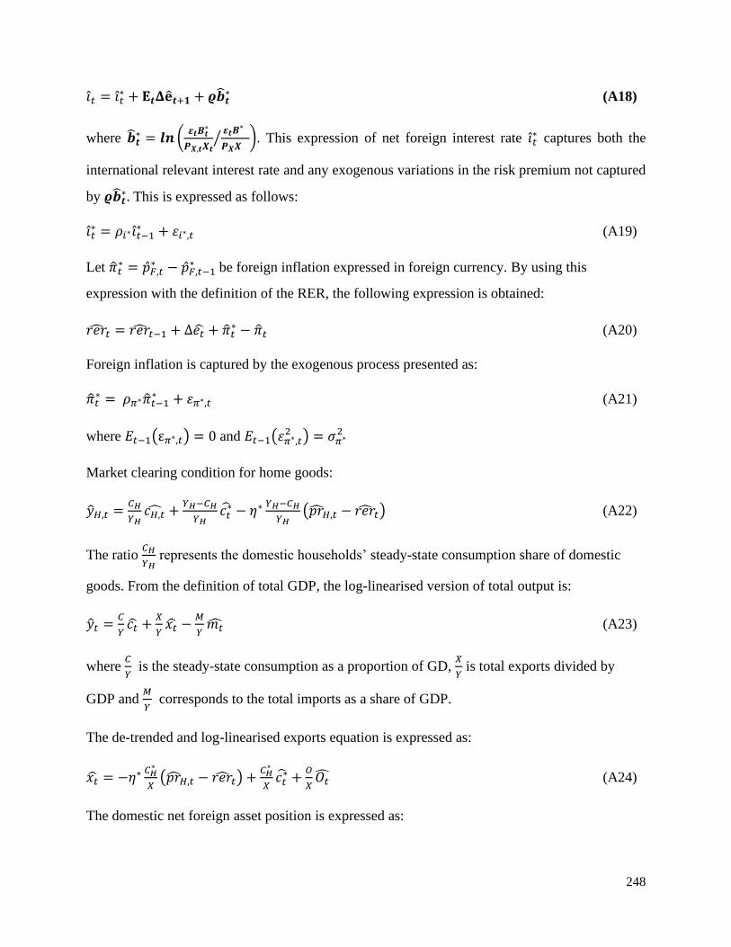
248

𝑖𝑡 = 𝑖𝑡∗ + 𝐄𝒕𝚫��𝒕+𝟏 + 𝝔��𝒕

∗ (A18)

where ��𝒕∗ = 𝒍𝒏 (

𝜺𝒕𝑩𝒕∗

𝑷𝑿,𝒕𝑿𝒕

𝜺𝒕𝑩∗

𝑷𝑿𝑿⁄ ). This expression of net foreign interest rate 𝑖𝑡

∗ captures both the

international relevant interest rate and any exogenous variations in the risk premium not captured

by 𝝔��𝒕∗. This is expressed as follows:

𝑖𝑡∗ = 𝜌𝑖∗𝑖𝑡−1

∗ + 휀𝑖∗,𝑡 (A19)

Let ��𝑡∗ = ��𝐹,𝑡

∗ − ��𝐹,𝑡−1∗ be foreign inflation expressed in foreign currency. By using this

expression with the definition of the RER, the following expression is obtained:

𝑟𝑒��𝑡 = 𝑟𝑒��𝑡−1 + Δ𝑒�� + ��𝑡∗ − ��𝑡 (A20)

Foreign inflation is captured by the exogenous process presented as:

��𝑡∗ = 𝜌𝜋∗��𝑡−1

∗ + 휀𝜋∗,𝑡 (A21)

where 𝐸𝑡−1(ε𝜋∗,𝑡) = 0 and 𝐸𝑡−1(휀𝜋∗,𝑡2 ) = 𝜎𝜋∗

2

Market clearing condition for home goods:

��𝐻,𝑡 =𝐶𝐻

𝑌𝐻𝑐𝐻,�� +

𝑌𝐻−𝐶𝐻

𝑌𝐻𝑐𝑡

∗ − 휂∗ 𝑌𝐻−𝐶𝐻

𝑌𝐻(𝑝��𝐻,𝑡 − 𝑟𝑒��𝑡) (A22)

The ratio 𝐶𝐻

𝑌𝐻 represents the domestic households’ steady-state consumption share of domestic

goods. From the definition of total GDP, the log-linearised version of total output is:

��𝑡 =𝐶

𝑌𝑐�� +

𝑋

𝑌𝑥�� −

𝑀

𝑌𝑚�� (A23)

where 𝐶

𝑌 is the steady-state consumption as a proportion of GD,

𝑋

𝑌 is total exports divided by

GDP and 𝑀

𝑌 corresponds to the total imports as a share of GDP.

The de-trended and log-linearised exports equation is expressed as:

𝑥�� = −휂∗ 𝐶𝐻∗

𝑋(𝑝��𝐻,𝑡 − 𝑟𝑒��𝑡) +

𝐶𝐻∗

𝑋𝑐𝑡

∗ +𝑂

𝑋𝑂�� (A24)

The domestic net foreign asset position is expressed as:

249

(1 − 𝜚)𝛽��𝑡∗ = 𝛽𝑖𝑡

∗ + 𝜒𝑏𝑡−1∗ + 𝜒��𝑡−1 +

𝐶𝐻∗

𝑋𝜒𝑝��𝐻,𝑡−1 + 𝜒(ΔO𝑡 − 𝜋𝑡) + (

𝑃𝑋𝑋

𝜀𝐵− 𝛽) ��𝑡 +

(𝑃𝑋𝑋

𝜀𝐵− 𝛽)

𝐶𝐻∗

𝑋𝑝��𝐻,𝑡 −

𝑃𝑋𝑋

𝜀𝐵

𝑀

𝑋��𝑡 −

𝑃𝑋𝑋

𝜀𝐵

𝐶𝐹

𝑋𝑟𝑒��𝑡 −

𝑃𝑋𝑋

𝜀𝐵

𝑂

𝑋𝑝𝑟𝑂,𝑡

∗

(A25)

where 𝜒 =1

(1+𝜋∗)(1+𝑔𝑦)

Relative Prices

By associating the optimal price-setting equation to the equation allowing for a passive price-

resetting equation (35), domestic inflation on home goods is:

𝜋𝐻,𝑡 =(1−𝜙𝐻)(1−𝛽𝜙𝐻)

𝜙𝐻(1+𝛽𝜉𝐻)(1 − 𝛼) 𝑤𝑟�� + 𝛽𝑘𝑅�� + (1 − 𝛼 − 𝛽𝑘)𝑅𝑔,�� − �� − 𝑝��𝐻,𝑡 +

𝛽

1+𝛽𝜉𝐻𝐸𝑡��𝐻,𝑡+1 +

𝜉𝐻

1+𝛽𝜉𝐻��𝐻,𝑡−1 (A26)

where 𝑤𝑟�� is the weighted average, such as 𝑤𝑟�� = 𝜆𝑐𝑤𝑟�� + (1 − 𝜆𝑐) 𝑤𝑟�� (A27)

The real price of domestic goods and oil, expressed in domestic currency, are captured by the

following equations:

𝑝��𝐻,𝑡 = 𝑝��𝐻,𝑡−1 − ��𝐻,𝑡 − ��𝑡 (A28)

𝑝��𝑂,𝑡 = 𝑟𝑒��𝑡 + 𝑝��𝑂,𝑡∗ + ��𝑡 (A29)

The international real price of oil is the international relative price of oil with respect to the

foreign price index captured by:

𝑝��𝑂,𝑡∗ = 𝜌𝑂𝑝��𝑂,𝑡−1

∗ + 휀𝑂,𝑡 (A31)

��𝑡, capturing the law of one price deviations for oil, follows an AR(1) process, such as:

��𝑡 = 𝜌𝜓��𝑡−1 + 휀𝜓,𝑡 (A32)

Furthermore, using the CPI definition and core consumption price-levels, the relationship

between the real prices of oil and domestic goods, as well as RER, is expressed as:

0 = 𝛿𝑝��𝑂,𝑡 + (1 − 𝛿)𝛾𝑝��𝐻,𝑡 + (1 − 𝛿)(1 − 𝛾)𝑟𝑒��𝑡 (A32)

Policy Rule

250

The log-linearised expression of the baseline monetary policy rule is:

��𝑡 = 𝜌��𝑡−1 + (1 − 𝜌)𝜛𝜋�� + (1 − 𝜌)𝜛𝑦(��𝑡 − ��𝑡−1) + ��𝑡 (A34)

where brt is the steady state deviation of the real interest rate such as:

��𝑡 = 𝑖��𝑡 − 𝐸𝑡��𝑡+1 (A35)

Finally, the monetary shock is given by:

𝑣�� = 𝜌𝑣𝑣𝑡−1 + 휀𝑣,𝑡 (A36)

Fiscal Rule

The Spend-it-all rule consists of spending oil revenue as it is received. In log-linear form it is

expressed as:

��𝑔,𝑡 = 𝑟𝑒��𝑡 + ��𝑟𝑜𝑡 + 𝑡��𝑡

The BIH rule involves saving all oil revenues in a SWF and spending only the interest

accumulated on the saved assets.

��𝑔,𝑡 = 𝑟𝑒��𝑡 + ��𝑡∗𝑓𝑡

where𝑓𝑡 = 𝑓𝑡−1 + 𝑡��𝑡−1

The modified BIH rule corresponds to saving all oil revenues in an SWF and consuming only a

fixed proportion of these revenues.

��𝑔,𝑡 = 𝑟𝑒��𝑡 + 𝜌𝐻𝐵𝑓𝑡

where 𝑓𝑡 = 𝑓𝑡−1 + 𝑡��𝑡−1

Market clearing:

Aggregate consumption:

��𝑡 = (1 − 𝜆𝑐)��𝑡𝑟 + 𝜆𝑐 ��𝑡

𝑛𝑟

Aggregate wages:

𝑤��𝑡 = (1 − 𝜆𝑐)𝑤��𝑓𝑜,𝑡 + 𝜆𝑐𝑤��𝑖𝑛𝑓,𝑡

Aggregate output as expressed in equation A23:

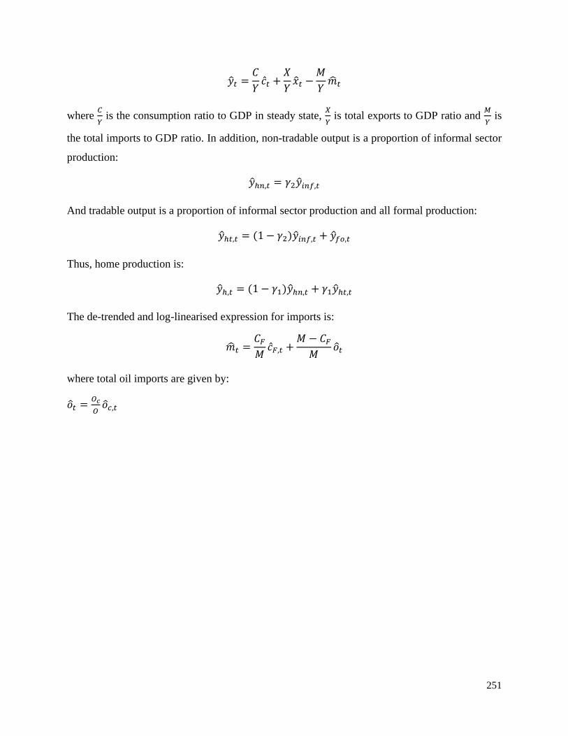
251

��𝑡 =𝐶

𝑌��𝑡 +

𝑋

𝑌��𝑡 −

𝑀

𝑌��𝑡

where 𝐶

𝑌 is the consumption ratio to GDP in steady state,

𝑋

𝑌 is total exports to GDP ratio and

𝑀

𝑌 is

the total imports to GDP ratio. In addition, non-tradable output is a proportion of informal sector

production:

��ℎ𝑛,𝑡 = 𝛾2��𝑖𝑛𝑓,𝑡

And tradable output is a proportion of informal sector production and all formal production:

��ℎ𝑡,𝑡 = (1 − 𝛾2)��𝑖𝑛𝑓,𝑡 + ��𝑓𝑜,𝑡

Thus, home production is:

��ℎ,𝑡 = (1 − 𝛾1)��ℎ𝑛,𝑡 + 𝛾1��ℎ𝑡,𝑡

The de-trended and log-linearised expression for imports is:

��𝑡 =𝐶𝐹

𝑀��𝐹,𝑡 +

𝑀 − 𝐶𝐹

𝑀��𝑡

where total oil imports are given by:

��𝑡 =𝑂𝑐

𝑂��𝑐,𝑡

252

7 Chapter 7:

Concluding remarks

7.1 Introduction

This study has analysed the impacts of the Dutch Disease’s predictions on labour market

outcomes, such as employment levels and wages, in the context of a resource-rich developing

country: in this case, Nigeria. The focus was placed on providing macroeconomic and

microeconomic evidence of the labour market adjustment related to the direct impacts of oil-

abundance and its related resource-revenue inflows, as well as related policies linked to the

management of those revenues.

Four objectives were set at the beginning of this thesis. The first was to provide a rationale for

the relevance of the study within the DD framework and the effect of oil revenues on the socio-

economic development of Nigeria – often referred to as a perfect case study for the analysis of

the resource curse. Second, given that the exchange rate is the main trigger of the DD

mechanism, an analysis was undertaken, at the macro and micro levels, of the impact of the RER

movement on the level of employment in Nigeria. Third, given the specificities of the oil-sharing

arrangement, the question of whether oil has a key role in the wage determination process was

investigated and quantification of its role in explaining wage inequality across firms in the

country was sought. Fourthly, an assessment of how the economy reacts to short term shocks,

given its large informal sector, and whether fiscal policies actually mitigate the possible impact

of shocks on the Nigerian economy was attempted.

To achieve the above objectives, a number of approaches were used to answer the research and

sub-research questions set out at the start of this thesis. First, a descriptive-analytical approach

was used in Chapters 2 and 3 to critically present the Dutch Disease framework, and the impact

of oil in the Nigerian context, using various aspects of the resource curse literature. These

aspects included resource dependence, social tension, and fiscal and monetary policies. Then,

Chapter 4 sought to present employment adjustment to real exchange rate movements (one of the

DD’s key predicted impacts) and used a VECM to assess the long-run relationship between the

253

exchange rate and employment levels in both the manufacturing sector and at the aggregate

level.

This was further complemented by panel survey analysis tools, such as GMM estimates, to

present the short-run labour adjustment at the firm level. Thirdly, OLS and wage decomposition

analysis (borrowed from the health literature) was used to assess the impact of oil-abundance in

wage determination and the contribution of oil-abundance to wage inequality in the country.

Finally, a DGSE model was built and Dynare used to evaluate the impact of shocks, in particular

oil-related ones, and the possible fiscal policies that may be implemented in Nigeria to reduce

possible economic distortions resulting from the transition to a new equilibrium.

7.2 Key contributions to the Literature

There are several studies devoted to natural resource production impacts on the growth

performance of resource-rich economies. The Dutch Disease framework remains the key

analytical tool through which to assess how the resource sector affects the economy, in particular

in the short-run, through a number of channels such as the resource movement and the spending

effect (Corden 1984, Corden and Neary 1982, and Neary et al., 1984). However, analysis of the

direct impact of some of the predictions regarding the labour market has been relatively scarce

and the empirical evidence of the existence has been inconclusive, in particular in the developing

country context due to a number of market rigidities that developing countries face (Kojo, 2015).

The proposed approach was to take some of these different predictions of the framework and

assess their impact on the labour market. Thus, this study is the first of its kind to test the real

exchange rate impact on the labour market through the labour intensity channel (i.e. a

substitution of labour for capital) in the Nigerian context. Further, it has presented both long- and

short-term adjustments in the manufacturing sector. The short-term adjustment was based on the

analysis of panel data and computed a trade-weighted exchange rate (a first in Nigeria).

The second innovation of this project lies in how it assesses the impact of oil on the wage

determination process, as well as on the quantity of the impact of oil in wage inequality, for the

first time in the Nigerian context. This contributes to the debate on the revenue sharing

arrangement of the country, and its impact on the competitiveness of the country.

254

The third aspect of this study’s innovation concerns how it introduces informality (an informal

labour supply and informal labour demand) into an open economy setting that accounts for

capital markets and assumes that oil revenue impacts the economy mainly through fiscal

spending and capital investment. In addition, evidence of short-term adjustment of the economy

to an oil shock is presented.

7.3 Major Conclusions

The thesis investigated the following main question: what is the impact of resource abundance

(i.e. oil) on the labour market of a resource-rich developing country such as Nigeria? Beyond

assessing the significance of oil revenue to the socio-economic development of Nigeria, the role

these revenues played in various aspects of the labour market, mainly employment levels and

wages, were examined through the lens of the Dutch Disease framework. The impact of the

management of these revenues on the labour market was also assessed. This analysis was

completed by assessing the impact of oil in the context of a large informal sector. Specifically,

this study aimed at quantifying the impact of DD on different aspects of the labour market of a

resource-rich developing country. The major results that were found through this study are

summarised below.

7.3.1 What was the Rationale for the Focus on Nigeria?

To analyse these sub-questions, this study reviewed the historical development of the oil sector

and its impact on a number of factors in Nigeria related to the resource curse literature, such as

resource dependence, social tensions and several macro-economic variables, including GDP, as

well as monetary and fiscal policies. These are the main points that were described:

a) This analysis emphasised that oil revenue only compounded a number of issues (such as

weak political structure, regional disparities) which existed before oil extraction began in

Nigeria.

b) The oil sector impacted the country’s economic development, with a dependence that

grew gradually from the 1970s onward. This dependence on oil has translated into

increased economic volatility and inconsistent fiscal and monetary policies.

255

c) In relation to the impact of the oil sector, this has been shown to mainly take place

through government revenue and spending, which has enabled the Nigerian government

to expand consumption (i.e. recurrent expenditure – wages and costs of running the

administration) and development (the impact of which has been limited because of a

complex political economy context)

d) Oil revenue has therefore resulted in a higher demand for tradeable and non-tradeable

goods, such as services. This has led to higher domestic price levels and an appreciation

of the RER, which was artificially maintained at a high level by various policies. Thus,

the government’s policies are likely to have been the main channel through which oil

revenue has affected the economy. Furthermore, although the oil sector is extremely

capital intensive, with a high level of labour productivity, implying that the resource

effect will be limited, it may have provided the impetus for upward-moving wages.

e) Finally, although the share of oil output as a share of GDP has been at most 30%, it has

had an impact on the development of the non-tradable sector, negatively affecting the

agriculture sector, preventing the growth of manufacturing (notably through adverse trade

and exchange policy decisions) and encouraging an oversized services sector. This hints

at the existence of the Dutch Disease effect.

7.3.2 What was the Role of the RER in Explaining Employment Performance in Nigeria?

The second main sub-question focused on the effect of REER movement (driven by oil inflows

or related policies) on the level of employment in Nigeria through changes in the labour intensity

channel (i.e. changes in the relative price of capital and labour).

7.3.2.1 What was the Role of the RER in Explaining Employment Performance in the Nigerian

Manufacturing Sector?

Using a VECM, the presence of a long-run relationship between REER, employment and capital

formation was assessed.

a) The above model used macroeconomic data to analyse the effect of the REER on the

level of employment in Nigeria, both at the aggregate level and, more specifically, in the

manufacturing sector. In the long-run, an exchange rate appreciation, as indicated by the

256

model developed by Frenkel and Ros (2007), and as suggested by the labour intensity

channel, decreased the employment level in the manufacturing sector and at the aggregate

level by 0.165% and 0.02%, respectively.

b) Further, capital formation was shown to positively affect the level of employment. This is

in line with the level of development of the country and the large infrastructure gap it

faces in the quantity of infrastructure it possesses.

c) Short-term dynamics were inconclusive using macro data within a VECM analysis.

7.3.2.2 What was the Role of the RER in Explaining Employment Performance in the Nigerian

Manufacturing Sector at the Micro-level?

Using a panel data survey and completing an analysis based on GMM estimators, the following

points were highlighted regarding an eventual short-run relationship between the level of

employment and a number of variables, including wages, sector-specific trade-weighted

exchange rates and capital:

a) From a methodological point of view, the analysis took into account the specific

characteristics of panel data. This included the simultaneity that occurs between

employment and other variables of interest impacting one another in any given period. In

this case, both OLS and fixed-effects estimates will be biased. The other issue that arose

was that of unobservable heterogeneity. These factors were addressed through the use of

a GMM estimator.

b) This study found that sector-specific exchange rate movements are linked to capital levels

within these specific sectors but, more importantly, it was found that a 1% increase

(appreciation) in the sector-specific REER will result in lower employment levels – a

reduction of 0.021%. This suggests that firms react to labour costs being relatively more

expensive in light of an appreciation against other factors of production such as capital

(which is primarily imported in the Nigerian context, according to Kojo, 2014).

257

c) The findings also suggest a negative relationship between wages and firm employment (-

0.132, t = 2.96), as predicted, ceteris paribus, by economic theory. In addition, capital is

positively related to the level of employment, highlighting that, at the manufacturing

firm-level, capital is complementary to the employment level.

d) Moreover, this analysis also indicated that capital and employment levels are

complementary in the context of the Nigerian manufacturing sector, implying that an

increase of capital is beneficial for job creation. However, the micro-evidence indicates a

small impact of capital on employment (coefficient of 0.1), which is almost 2/3 smaller

than the coefficient obtained at the macro level, reflecting the type of firms included in

the survey.

Overall, this analysis indicated that although the coefficients between macro evidence and micro

evidence differ in sizes, they confirm theoretical expectations. The difference in amplitude can

be attributed to the data, including the number of firms with an average capacity rate of only

44%. Thus, the mechanism of interest will be more subdued. Nevertheless, a possible REER

appreciation will have a negative impact on the level of employment, and this was shown to be

the case both in the short-run (GMM analysis) and long-run (VECM analysis). The mechanism

through which this can manifest itself at the firm level is through lower investment and

profitability resulting from REER appreciation; however, firms will take advantage of the

cheaper capital.

Furthermore, there does not seem to have been a substitution between capital and employment in

the short and long-run as they both moved in similar directions, possibly reflecting the fact that

the firms included in the survey mostly survived and, therefore, have growth potential in the

Nigerian context. This could be explained by the fact that the sectors included in this survey

(such as paper and furniture) can easily substitute labour for capital. However, this impact at the

micro level was observed over a relatively short period of time.

7.3.3 What is the Role of Oil in Wage Determination and Wage Inequality in Nigeria?

The second key relationship observed here was the impact of the abundance of revenue on

wages. According to the DD framework, wages are expected to be pushed upwards through

258

aggregate demand feedback on the labour market. In assessing this prediction, the following

evidence was found.

7.3.3.1 What role does higher oil revenue distributed to specific sub-national entities play in

determining wages?

Based on a wage equation using cross-sectional enterprise survey data, the analysis indicates

that:

a) In line with Dutch Disease theory and the mechanisms presented by Brunstad and

Dyrstad (1997), oil has an impact on wages. Different measures of wages (total wage

bills, wage per worker) with different specifications of the control variable, including a

dummy variable for the oil region or the amount received by each state in the region,

returned a consistent impact of oil on wages –commanding a wage premium of at least 10

% for firms located in oil-producing regions.

b) This effect was found across firms, sectors and even in firms that are assumed to be of

similar productivity levels given their ability to export. Indeed, even among firms facing

external markets, it was found that firms in the South-South region (the point-resource

region in Nigeria) are paying a premium. Further, when looking at the difference across

sectors, it was noted that the interaction term between the oil dummy and foreign

exposure matters. Thus, both the manufacturing and services sector in those regions could

be more cost-competitive if this oil premium on wages did not exist. The premium was

estimated to be up to 55% for manufacturing firms and around 30% for firms operating in

the services sector.

c) The observed differences in impact between services and manufacturing hints at a skills

gap as service-related skills are readily available and less specialised. Thus, the wage

offered is still higher in the oil-producing region, but it remains comparatively less

important than the manufacturing sector’s wage premium.

d) This premium reflects several factors, all linked directly and indirectly by the abundance

of resources at the local level. Firstly, efficiency wage and rent sharing theory could

259

explain these results, where firms can reduce costs by increasing wages. With limited

labour mobility in the country, employees are able to raise their wages through threats of

withholding labour supply, and this situation is likely to be exacerbated in the oil-rich

region. Also, higher wages could also be a way of compensating for higher costs of

living, resulting in a local Dutch Disease effect.

7.3.3.2 How Do These Determinants (including Oil Revenue) Explain Wage Differentials

across Firms?

This research project also aimed to investigate the decomposition of wage inequalities in Nigeria

by applying a methodology developed initially by Wagstaff et al. (2001) to study inequalities. As

far a is known, this analysis is the first to provide evidence on drivers of wage inequality in

Nigeria and the role played by oil in this encounter. My study found that:

a) A mechanism such as the revenue sharing formula used by Nigeria will contribute to

wage inequality in the country. This implies that after controlling for other determinants

of wages, on average, firms in oil-rich regions are at least 10% more likely to be the ones

with higher wages (or vice versa).

b) Although oil matters, the main source of inequality between firms is size. This can be

attributed to the fact that larger firms lie at the root of wage inequality. It is also possible

that smaller firms are not able to keep up in terms of efficiency and, thus, are similarly

unable to keep up in terms of wages offered. Larger firms are paying wages that do not

reflect productivity levels, reinforcing the Dutch Disease and rent sharing hypotheses.

This could be further driven by the higher probability of larger firms of obtaining

government contracts or better access to public goods, for example.

7.3.4 How Do Key Macroeconomic Variables Respond to Oil Shocks by Taking into

Account Formal and Informal Labour Markets?

The last key relationship of interest to this project was the impact on the labour market of fiscal

policy development in response to the abundance of oil, taking into consideration some of the

characteristics of a resource-rich developing country’s labour market, such as informality. The

analytical work indicated:

260

a) The DSGE model includes a number of key features, such as price and wage rigidity, an

informal labour supply, an informal production sector, public goods benefiting only the

formal sector, limited labour mobility and the fiscal sector. All these features fall within

an open economy context.

b) The analysis of the oil shocks indicated that an increase in government revenue increases

spending, pushing consumption and wages upwards, while investment decreases;

consumption of domestic goods, therefore, increases at the expense of imports, which

decrease. This leads to inflation and exchange rate appreciation.

c) The informal sector, where households rely solely on wages, having no ability to save,

does not play the role of a buffer and contributes to the Dutch Disease mechanisms (by

spending the higher wage received).

d) The policy options presented by international institutions, like the IMF, recommend

creating a savings account, such as a Sovereign Wealth Fund. Two versions of such a

mechanism (Bird in Hand and Modified Bird in Hand) were tested. In the short-run, these

were shown to have very little impact on managing short-term volatility in Nigeria. This

is because they reduce the size of the distortion and thus preserve capital investment for

future growth. All in all, informality does not have a shock-absorber role.

7.4 Policy Implications

The above discussion presenting the major results of this study demonstrates the key role that

government has to play in promoting economic development and in mitigating the impact of

Dutch Disease This entails supporting the growth of the non-oil sector, as well as generating real

income and creating much-needed jobs. This will only be made possible if effective mechanisms

are implemented to manage the impact of oil-related shocks on the labour market and non-oil

sectors.

This analysis has highlighted several policy aspects that require the attention of developing

country policymakers:

261

a) The exchange rate policy impacts the labour market, and thus an appreciation will affect

firms’ employment decisions. This means that a stable and predictable exchange rate is a

prerequisite for job creation (as it affects profits and investment decisions). An over-

valued or appreciated naira maybe be seen as a way to facilitate import-fuelled

consumption; however, Nigerian firms currently have excess capacity and will therefore

invest in little, which limits job creation. A more flexible exchange rate may increase

demand for domestic goods and reduce that excess capacity.

b) The investment policy. Given that labour and capital are deemed to be complementary

investments in well-implemented infrastructure projects, the development of a reliable

and efficient power supply network will support production efforts and increase

productivity.

c) The revenue-sharing formula in favour of oil-producing states is needed because of the

environmental damage caused by the oil sector and the impact it has on the livelihoods of

populations living in oil-producing regions. However, the current revenue-sharing model

allows for excess revenue to fuel consumption, which has an implication at the local level

through local inflation on wages, which affects the current competitiveness of firms. In

the absence of oil, wages across the country will be more equal and, therefore, will more

accurately reflect productivity levels in Nigeria.

d) The wage growth of smaller firms remains sluggish, contributing to inequality in Nigeria.

These firms are less likely to manage the difficult current “doing business environment”,

which negatively affects their growth and, therefore, wages paid. Designing effective

mechanisms to boost productivity for small and medium-sized enterprises will be critical

in raising wages and reducing wage inequalities. These types of policies could be

complementary to the implementation of a minimum wage to raise income in small firms.

Further, promoting labour mobility could also have an impact in equalising wages across

the country. Finally, the greater inequality among services firms compared to

manufacturing firms points to the role of unions and the regulation of service sector

activities.

262

e) The large informal sector is normal at this stage of Nigeria’s development; however, it

does not act as a buffer when the economy is faced with a shock. Thus, without the

appropriate mechanisms, a shock will push a major part of the population into hardship.

Therefore, an appropriate mechanism is needed. As illustrated by the analysis, traditional

recommendations may not isolate the economy from volatility, and thus the government

could consider an even more conservative approach in terms of injecting oil revenue into

the domestic economy (restrict its use to development projects alone, for example).

More generally, development in a country such as Nigeria is feasible through a consistent policy

approach aimed at using oil-revenue to develop its infrastructure. This strategy, when coupled

with more exchange rate flexibility, will offer the country the ability to both absorb shocks and

support the development of other sectors. These are not simple tasks, and the country has been

battling with these issues for the last 50 years. For change to be achieved, it will require

established institutions to reform in order to allow policymakers to develop consistent and

prudent measures in response to positive oil shocks and to stimulate socio-economic

development to avoid perverse effects, such as Dutch Disease. On the other hand, the lack of

such stable and efficient institutions in Nigeria have led, and will continue to lead, to poor

policies, deepening the negative impacts of resource abundance in the country.

In the Nigerian context, oil inflows have created rent-seeking behaviour among the various

stakeholders, resulting in policy inefficiencies. This has led to economic underdevelopment,

including the gradual collapse of the agriculture sector and low socio development indicators.

Therefore, efficient government is key to transforming the resource curse into a blessing.

7.5 Suggestions for Further Analysis

It is key to acknowledge there are areas of or perspectives regarding the various questions

presented here that have not been covered, principally due to data limitation and time constraints.

It would be helpful for these to be attended to in the future. Some possibilities for doing so

include:

a) It would be interesting to extend the analysis offered in Chapter 4 to the most recent

years over which Nigeria has experienced a depreciation of its currency as a result of an

263

oil shock. This will also fully capture the structural change suggested by the GDP

rebasing, completed in 2012. Employing a longer time series would have strengthened

the analysis in Chapter 4 using the VECM approach. Also, at the microeconomic level,

the analysis focused mainly on the formal sector; however, given the size of the informal

sector, it would be interesting to study the informal sector and the impact of REER (if

any) on this sector, in the future.

b) Concerning Chapter 5, approaching the question from the workers’ perspectives could be

interesting in the sense of where workers internalise oil revenue in their wage

determination. A deeper dive into the dynamics between small, medium and large firms

in terms of productivity, as well an investigation into the dynamics between different

regions of the country, could also be productive.

c) Incorporating the role of institutions in these different chapters could be of interest for

future researchers; they may, for example, wish to include in the wage determination

process an analysis of a variable reflecting the lack of transparency of the procurement

process. The role of unionised labour requires more attention in the analysis of

inequalities. Similarly, in the DGSE model, inefficiency in terms of fiscal policy (i.e.

implementation capacity issues) could have been included. The inclusion of this would

have affected the spending effect associated with Dutch Disease.

d) Informality in the DGSE model could also have been modelled to ensure more flexibility,

thus allowing agents to move from one sector to another or allowing agents to provide

services to both the formal and informal sector. Similarly, the formal sector could hire

informal labour. Also, explicitly modelling “learning by doing” could add value to the

DSGE model presented here. In addition, the fiscal policy presented in my model could

be made more complex by incorporating, for example, a permanent-income hypothesis

rule.

Overall, this thesis has assessed the predicted impact of Dutch Disease on labour market

outcomes in Nigeria using several techniques to best explore the data available. It has provided

salient indications and quantified – for the first time – important dimensions of these impacts by

264

using Nigeria as a case study. A number of possible policies that could affect wage and

employment level outcomes in the country have been proposed. Some of the evidence presented

here, although very specific to the Nigerian context, may provide insights into some of these

mechanisms in other developing resource-rich countries that suffer from Dutch Disease and, to a

larger extent, from the resource curse.

265

Bibliography

Abidoye, B., & Calì, M. (2015). Income shocks and conflict: Evidence from Nigeria.

Abu, N. (2010). Saving-economic growth nexus in Nigeria, 1970-2007: Granger causality and

co-integration analyses. Review of Economic and Business Studies, 5, 93–104.

Acemoglu, D., Johnson, S., & Robinson, J. A. (2001). The colonial origins of comparative

development: an empirical investigation. American Economic Review, 91, 1369–1401.

Adam, A., & Moutos, T. (2014). Industry-level labour demand elasticities across the Eurozone:

Will there be any gain after the pain of internal devaluation? (No. 4858).

Adebayo, A. (1999). Youth unemployment and the national directorate of employment self-

employment programmes. The Nigerian Journal of Economic and Social Studies, 41(1), 81–

104.

Adebiyi, M. A., & Mordi, C. N. (2011). A Dynamic Stochastic General Equilibrium (DSGE)

Model of Exchange Rate Pass-Through to Domestic Inflation in Nigeria.

Adedipe, B. (2004). The impact of oil on Nigeria’s economic policy formulation. In Overseas

Development Institute Conference in Collaboration with the Nigerian Economic Summit

Group.

Adegbite, D. E. O. (2005). Financial Sector Reforms and Economic Development in Nigeria:

The Role of Management. East Asia, 5(7).

Adekun, S. (2016). Balance of Payents Equilibrium: A test of marshall-lerner condition in

Nigeria. FUTA Journal of Management and Technology, 1(2).

Adekunle, O. A., Oluwaseyi, B., & Olusoji, S. G. (2013). The effect of the financial

liberalisation on economic growth. International Journal of Academic Research in

Economics and Management Sciences, 2(1).

Ades, A., & Tella., R. Di. (1999). Rents, competition, and corruption. American Economic

Review, 89(4), 982–993.

Adewuyi, A. O., & Akpokodje, G. (2013). Exchange Rate Volatility and Economic Activities of

Africa’s Sub-Groups. The International Trade Journal, 27(4), 349–384.

Adeyemi, O. O. (2012). Corruption and local government administration in Nigeria: A discourse

of core issues. European Journal of Sustainable Development, 1(2), 183–198.

266

Adolfson, M., Laséen, S., Lindé, J., & Villani, M. (2007). Bayesian estimation of an open

economy DSGE model with incomplete pass-through. Journal of International Economics,

72(2), 481–511.

Agbiboa, D. E. (2012). Between corruption and development: The political economy of state

robbery in Nigeria. Journal of Business Ethics, 108(3), 325–345.

Agbonifo, P. (2016). Oil spills injustices in the Niger Delta region: reflections on oil industry

failure In relation to the United Nations Environment Programme (UNEP) Report.

International Journal of Petroleum and Gas Exploration Management, 2(1), 26–37.

Ahmed, S., Ahmed, W., Khan, S., Pasha, F., & Rehman, M. (2012). Pakistan economy DSGE

model with informality.

Aigbokhan, B. E. (1988). Rural-urban migration and urban unemployment in Nigeria. Migration

World Magazine, 16(4/5), 16.

Aigbokhan, B. E. (1999). Fiscal federalism and economic growth in Nigeria. In NES selected

paper presented at the 1999 annual conference.

Aigbokhan, B. E. (2008). Growth, inequality and poverty in Nigeria. In United Nations

Economic Commission for Africa (UNECA).

Aigbokhan, B. E. (2011). Efficiency wage, rent-sharing theories and wage determination in the

manufacturing sector in Nigeria.

Aizenman, J., & Marion, N. (1999). Volatility and investment: interpreting evidence from

developing countries. Economica 66.262 (1999): 157-1179., 66(262), 157–1179.

Ajakaiye, O., Jerome, A., & Nabena, D. (2015). Understanding the relationship between growth

and employment in Nigeria (No. 2015/124).

Ajao, M. G., & Igbekoyi, O. E. (2013). The determinants of real exchange rate volatility in

Nigeria. Academic Journal of Interdisciplinary Studies, 2(1), 459–471.

Akeju, K. F., & Olanipekun, D. B. (2014). Unemployment and economic growth in Nigeria.

Journal of Economics and Sustainable Development, 5(4), 138–144.

Akerlof, G. A. (1982). Labor contracts as partial gift exchange. The Quarterly Journal of

Economics, 97(4), 543–569.

Akerlof, G. A. (1984). Gift exchange and efficiency-wage theory: Four views. The American

Economic Review, 74(2), 79–83.

Akingbola, A. A. (2006). Electronic Payment Systems and Tele-banking Services in Nigeria.

Journal of Internet Banking and Commerce, 11(3), 13–28.

267

Akinlo, O. O., & Lawal, A. Q. (2015). Impact of exchange rate on industrial production in

nigeria 1986-2010. International Business and Management, 10(1), 104–110.

Akram, Q. F. (2004). Oil prices and exchange rates: Norwegian evidence. The Econometrics

Journal, 7(2), 476–504.

Alberola, E., & Benigno, G. (2017). Revisiting the commodity curse: A financial perspective.

Journal of International Economics, 108, S87–S106.

Alege, P. O. (2012). A Business Cycle Model for Nigeria. CBN Journal of Applied Statistics,

3(1), 85–115.

Alesina, A., & Drazen, A. (1991). Why Are Stabilizations Delayed? American Economic

Review, 81(5), 1170–1188.

Alesina, A., & Tabellini, G. (1990). A positive theory of fiscal deficits and government debt. The

Review of Economic Studies, 57(3), 403–414.

Alexandre, F., Bacao, P., Cerejeira, J., & Portela, M. (2009). Employment and Exchange Rates:

The Role of Openness and Technology (No. 4191).

Alexeev, M., & Conrad, R. (2009). The elusive curse of oil 91.3 (2009): 586-598. The Review of

Economics and Statistics, 91(3), 586–598.

Alexeev, M., & Conrad, R. (2011). The natural resource curse and economic transition.

Economic Systems, 35(4), 445–461.

Algieri, B. (2011). The Dutch disease: evidences from Russia. Economic Change and

Restructuring, 44(3), 243–277.

Alidou, S. (2014). Degree of price rigidity in LICs and implication for monetary policy.

Allcott, H., & Keniston, D. (2014). Dutch Disease or Agglomeration? The Local Economic

Effects of Natural Resource Booms in North America.

Allegret, J. P., & Benkhodja, M. T. (2015). External shocks and monetary policy in an oil

exporting economy (Algeria). Journal of Policy Modeling, 37(4), 652–667.

Allen, J., Nataraj, S., & Schipper, T. C. (2018). Strict duality and overlapping productivity

distributions between formal and informal firms.

Alli, I. S. (2011). Oil Revenue and Economic Development case of the Libyan Economy (1970-

2010). Univerity of Wollongong.

Amano, R. A., & Van Norden, S. (1998). Exchange rates and oil prices. Review of International

Economics, 6(4), 683–694.

268

Amiti, M., & Davis, D. R. (2011). Trade, firms, and wages: Theory and evidence. The Review of

Economic Studies, 79(1), 1–36.

Andersen, J. J., & Aslaksen, S. (2008). Constitutions and the resource curse. Journal of

Development Economics, 87, 227–246.

Angrist, J. D., & Kugler, A. D. (2008). Rural windfall or a new resource curse? Coca, income,

and civil conflict in Colombia. The Review of Economics and Statistics, 90(2), 191–215.

Anjola, A., Kehinde, A., Oluwatobi, F., Timilehin, I. D., & Osabohien, R. (2018). Macro-

economic determinants of industrial output in Nigeria: Exchange rate and employment

dimension. International Journal of Development Research, 8(6), 21310–21316.

Apere, T. O., & Karimo, T. M. (2014). Monetary policy effectiveness, output growth and

inflation in Nigeria. International Journal, 3(6).

Aragón, F. M., & Rud, J. P. (2013). Natural resources and local communities: evidence from a

Peruvian gold mine. American Economic Journal: Economic Policy, 5(2), 1–25.

Arellano, M., & Bond, S. (1991). Some tests of specification for panel data: Monte Carlo

evidence and an application to employment equations. Review of Economic Studies, 58,

277–297.

Arellano, M., & Bond, S. R. (1991). Some tests of specification for panel data: Monte Carlo

evidence and an application to employment equations. The Review of Economic Studies,

58(2), 277–297.

Arellano, M., & Bover, O. (1995). Another look at the instrumental variable estimation of error-

components models. Journal of Econometrics, 68(1), 29–51.

Arezki, R., & Brückner, M. (2011). Oil rents, corruption, and state stability: Evidence from panel

data regressions. European Economic Review, 55(7), 955–963.

Arezki, R., & Brückner, M. (2011). Oil rents, corruption, and state stability: Evidence from panel

data regressions. European Economic Review, 55(7), 955–963.

Arezki, R., & Gylfason, T. (2013). Resource rents, democracy, corruption and conflict: Evidence

from sub-Saharan Africa. Journal of African Economies, 22(4), 552–569.

Aron, J., Elbadawi, I., & Kahn, B. (1997). Determinants of the real exchange rate in South

Africa. Centre for the Study of African Economies, Institute of Economics and Statistics,

University of Oxford.

Auty, R. (2001). Why resource endowments can undermine economic development: concepts

and case studies. In Paper Prepared for the BP-Amoco Seminar. Lincoln College Oxford

University.

269

Auty, R. (2001). The Political Economy of Resource-Driven Growth. European Economic

Review, 45(4), 839–846.

Auty, R. (2001). Resource abundance and economic development (Oxford Uni). Oxford.

Auty, R. (2007). Rent Cycling Theory, the Resource Curse, and Development Policy.

Developing Alternatives, 11(1), 7–13.

Auty, R. (1993). Sustaining Development in Mineral Economies. The Resource Curse Thesis,

London: Routledge.

Auty, R. (2007). Natural Resources, Capital Accumulation and the Resource Curse. Ecological

Economics, 61(4), 627–634.

Auty, R. (1993). Sustaining Development in Mineral Economies: The Resource Curse Thesis.

(Routledge, Ed.). London.

Ay, A., & Ayhan, F. (2016). EMPLOYMENT AND EXCHANGE RATE VOLATILITY

RELATIONSHIP: THE TURKISH CASE. Journal of Business Economics and Finance,

5(1), 108–114.

Azam, J.-P., & Lesueur, J.-Y. (1997). Efficiency Wage and Supervision: Theory and Application

to the Ivorian Manufacturing Sector. Journal of African Economies, 6(3), 445–462.

Azam, J.-P., & Ris, C. (2001). Rent Sharing, Hold Up, and Manufacturing: Wages in Côte d’

Ivoire (No. 2600).

Azfar, O., & Murrell, P. (2009). Identifying reticent respondents: Assessing the quality of survey

data on corruption and values. Economic Development and Cultural Change, 57(2), 387–

411.

Bahar, D., & Santos, M. A. (2018). One more resource curse: Dutch disease and export

concentration. Journal of Development Economics, 132, 102–114.

Bakare, A. S. (2011). The determinants and roles of capital flight in the growth process of

Nigerian economy: Vector autoregressive model approach. British Journal of Management

and Economics, 1(2), 100–113.

Baland, J.-M., & Francois, P. (2000). Rent-seeking and resource booms. Journal of Development

Economics, 61(2), 527–542.

Baltagi, B. H., Baskaya, Y. S., & Hulagu, T. (2012). The Turkish wage curve: Evidence from the

household labor force survey. Economics Letters, 114(1), 128–131.

Bangs, R. B. (1942). Wage Reductions and Employment. Journal of Political Economy, 50(2),

251–271.

270

Bargain, O., & Kwenda, P. (2009). The informal sector wage gap: new evidence using quantile

estimations on panel data (No. No. 4286).

Basdevant, O. (2008). Are diamonds forever? Using the permanent income hypothesis to analyze

Botswana’s reliance on diamond revenue.

Batini, N., Levine, P., Lotti, E., & Yang, B. (2011). Monetary and Fiscal Policy in the Presence

of Informal Labour Markets.

Batté, L., Bénassy-Quéré, A., Carton, B., & Dufrénot, G. (2009). erm of trade shocks in a

monetary union: An Application to West-Africa.

Bauer, A., & Mihalyi, D. (2018). Premature Funds: How Overenthusiasm and Bad Advice Can

Leave Countries Poorer. Retrieved August 21, 2018, from

https://resourcegovernance.org/sites/default/files/documents/premature-funds.pdf

Baumol, W. J. (1967). Macroeconomics of unbalanced growth: the anatomy of urban crisis. The

American Economic Review, 57(3), 415–426.

Baxter, M., & Kouparitsas, M. A. (2006). What can account for fluctuations in the terms of

trade? International Finance, 9(1), 63–86.

Bayoumi, T., & Mhleisen, M. (2006). Energy, the exchange rate, and the economy:

macroeconomic benefits of Canada’s oil sands production.

Beck, T. (n.d.). Finance and Oil: Is there a resource curse in financial development? (No. 2011-

004).

Beck, T., Demirgüç-Kunt, A., & Levine, R. (2010). Financial institutions and markets across

countries and over time: The updated financial development and structure database. The

World Bank Economic Review, 24(1), 77–92.

Beck, T., & Levine, R. (2005). Legal institutions and financial development. (H. of new

institutional Economics., Ed.). Springer, Boston, MA,.

Beck, T., Levine, R., & Loayza, N. (2000). Finance and the Sources of Growth. Journal of

Financial Economics, 58(1–2), 261–300.

Behar, A., & Mok, J. (2013). Does Public-Sector Employment Fully Crowd Out Private-Sector

Employment? (No. No. 13-146).

Beidas-Strom, S., & Pescatori, A. (2014). Oil Price Volatility and the Role of Speculation (No.

No. 14-218).

Beine, M., Bos, C. S., & Coulombe, S. (2012). Does the Canadian economy suffer from Dutch

disease? Resource and Energy Economics, 34(4), 468–492.

271

Benjamin, N., Devarajan, S., & Weiner, R. J. (1989). The ‘Dutch’ disease in a developing

country: Oil reserves in Cameroon. Journal of Development Economics, 30(1), 71–92.

Benkhodja, M. T. (2014). Monetary policy and the Dutch disease effect in an oil exporting

economy. International Economics, 138, 78–102.

Berg, M. A., Portillo, R., Yang, M. S.-C. S., & Zanna, L.-F. (2012). Public investment in

resource-abundant developing countries (No. No. 12-274).

Berman, N., Martin, P., & Mayer, T. (2009). How do different exporters react to exchange rate

changes? Theory, Empirics and Aggregate Implications (No. No. DP7493).

Berman, N., Couttenier, M., & Rohner, D. (2017). This mine is mine! How minerals fuel

conflicts in Africa. American Economic Review, 107(6), 1564–1610.

Bernard, A. B., Jensen, J. B., Redding, S. J., & Schott, P. K. (2007). Firms in international trade.

Journal of Economic Perspectives, 21(3), 105–130.

Besley, T., & Persson, T. (n.d.). The origins of state capacity: property rights, taxation and

politics. American Economic Review, 99(4), 1218–1244.

Besley, T., & Persson, T. (2010). State capacity, conflict, and development. Econometrica,

78(1), 1–34.

Betts, C. M., & Kehoe, T. J. (2008). Real exchange rate movements and the relative price of

non-traded goods (No. w14437).

Bevan, D., Collier, P., & Gunning, J. W. (1999). The Political Economy of Poverty, Equity, and

Growth: Nigeria and Indonesia. Oxford University Press.

Bhattacharyya, S., & Collier, P. (2014). Public capital in resource rich economies: is there a

curse? Oxford Economic Papers, 66(1), 1–24.

Bhattacharyya, S., & Hodler, R. (2014). Do natural resource revenues hinder financial

development? The role of political institutions. World Development, 57, 101–113.

Bhattacharyya, S., Conradie, L., & Arezki, R. (2017). Resource discovery and the politics of

fiscal decentralization. Journal of Comparative Economics, 45(2), 366–382.

Bhattacharyya, S., & Hodler, R. (2010). Natural resources, democracy and corruption. European

Economic Review 54.4 (2010): 608-621., 54(4), 608–621.

Bhattacharyya, S., & Mamo, N. G. (forthcoming). Resource discovery and conflict in Africa:

What do the data show?.". Economic Development and Cultural Change.

Bjerkholt, O. (2002). Fiscal rule suggestions for economies with non-renewable resources.

272

Bjørnland, H. (1998). The economic effects of North Sea oil on the manufacturing sector.

Scottish Journal of Political Economy, 45(5), 553–585.

Bjørnland, H. C. (2009). Monetary policy and exchange rate overshooting: Dornbusch was right

after all. Journal of International Economics, 79(1), 64–77.

Black, D., McKinnish, T., & Sanders, S. (2005). The economic impact of the coal boom and

bust. The Economic Journal, 115(503), 449–476.

Blanchard, O. (2009). The State of Macro. Annual Review of Economics, 1, 209–228.

Blanchard, O., & Gali, J. (2010). Labor markets and monetary policy: A New Keynesian model

with unemployment. American Economic Journal: Macroeconomics, 2(2), 1–30.

Blattman, C., Hwang, J., & Williamson, J. G. (2007). Winners and losers in the commodity

lottery: The impact of terms of trade growth and volatility in the Periphery 1870-1939.

Journal of Development Economics, 82, 156–179.

Bloom, D. E., Boersch-Supan, A., & McGee, P. (2011). Population aging: facts, challenges, and

responses. Benefits and Compensation International, 41(1), 22.

Blunch, N.-H., Canagarajah, S., & Raju, D. (2001). No Title (No. 119).

Blundell, R., & Bond, S. R. (1998). Initial conditions and moment restrictions in dynamic panel

data models. Journal of Econometrics, 87(1), 115–143.

Bond, S. R. (2002). Dynamic panel data models: a guide to micro data methods and practice.

Portuguese Economic Journal, 1(2), 141–162.

Bond, S., & Meghir, C. (1994). Dynamic investment models and the firm’s financial policy. The

Review of Economic Studies, 61(2), 197–222.

Borge, L.-E., Parmer, P., & Torvik, R. (2015). Local natural resource curse? Journal of Public

Economics, 131, 101–114.

Bouakez, H., Rebei, N., & Vencatachellum, D. (2008). Optimal pass-through of oil prices in an

economy with nominal rigidities (No. 08-31).

Bound, J., Jaeger, D. A., & Baker, R. M. (1995). Problems with instrumental variables

estimation when the correlation between the instruments and the endogenous explanatory

variable is weak. Journal of the American Statistical Association, 90(430), 443–450.

Brahmbhatt, M., Canuto, O., & Vostroknutova, E. (2010). Dealing with Dutch Disease.

Economic Premise, (16).

273

Branson, W. H., & Love, J. (1988). U.S. Manufacturing and The Real Exchange Rate. In R. C.

Marston (Ed.), Misalignment of Exchange Rates: Effects on Trade and Industry. (pp. 241–

270). Chicago: University of Chicago Pres.

Branson, W. H., & Marston, R. C. (1989). Price and output adjustment in Japanese

manufacturing (No. 2878).

Brautigam, D., & Knack, S. (2004). Foreign aid, institutions and governance in sub-Saharan

Africa. Economic Development and Cultural Change, 52(2), 255–286.

Briggs, I. N. (2007). NIGERIA: MAINSTREAMING TRADE POLICY INTO NATIONAL

DEVELOPMENT STRATEGIES (No. 52).

Brollo, F., Nannicini, T., Perotti, R., & Tabellini, G. (2013). The political resource curse.

American Economic Review, 103(5), 1759–96.

Brownbridge, M. (1996). The impact of public policy on the banking system in Nigeria.

Brunnschweiler, C., & Bulte, E. H. (2008). The natural resource curse revised and revisited: A

tale of paradoxes and red herrings,. Journal of Environmental Economics and Management,

55(3), 248–264.

Bruno, M., & Sachs, J. (1982). Energy and resource allocation: a dynamic model of the “Dutch

Disease.” The Review of Economic Studies, 49(5), 845–859.

Brunstad, R. J., & Dyrstadt, J. M. (1997). Booming sector and wage effects: An empirical

analysis on Norwegian data. Oxford Economic Papers, 49(1), 89–103.

Budina, N., Pang, G., & Wijnbergen., S. van. (2007). Nigeria’s growth record: Dutch disease or

debt overhang? World Bank Group, No. 4256.

Buiter, W. H., & Purvis, D. D. (1983). Oil, Disinflation and export Competitiveness: A moddl of

Dutch Disease. In J. Bhandari & B. Putman (Eds.), Economic Interdependence and Flexible

Exchanges Rates (pp. 221–247). Cambridge.

Bulow, J. I., & Summers, L. H. (1986). A theory of dual labor markets with application to

industrial policy, discrimination, and Keynesian unemployment. Journal of Labor

Economics, 4(3, Part 1), 376–414.

Burgess, S. M., & Knetter, M. M. (1998). An international comparison of employment

adjustment to exchange rate fluctuations. Review of International Economics, 6(1), 151–

163.

Caballero, R. J., & Krishnamurthy, A. (2001). International and domestic collateral constraints in

a model of emerging market crises. Journal of Monetary Economics, 48(3), 513–548.

274

Campa, J. M., & Goldberg, L. S. (1999). Investment, pass‐through, and exchange rates: a cross‐

country comparison. International Economic Review, 40(2), 287–314.

Campa, J. M., & Goldberg, L. S. (2001). Employment versus wage adjustment and the US dollar.

Review of Economics and Statistics, 83(3), 477–489.

Canuto, O. (2014). The Commodity super cycle: is this time different? Economic Premise, 150,

1–4.

Carmignani, F. (2013). Development outcomes, resource abundance, and the transmission

through inequality. Resource and Energy Economics, 35(3), 412–428.

Carneiro, F. (2007). Development challenges of resource-rich countries: the case of oil exporters.

In VI International Colloquium (pp. 115–140).

Carvalho Filho, I. E., & Bems, R. (2009). Exchange rate assessments: methodologies for oil

exporting countries (No. 9–281).

Caselli, F. (2006). Power struggles and the natural resource curse.

Caselli, F., & Cunningham, T. (2009). Leader behaviour and the natural resource curse. Oxford

Economic Papers, 61(4), 628–650.

Caselli, F., Esquivel, G., & Lefort, F. (1996). Reopening the convergence debate: a new look at

cross-country growth empirics. Journal of Economic Growth, 1(3), 363–389.

Caselli, F., & Michaels, G. (2013). Do oil windfalls improve living standards? Evidence from

Brazil. American Economic Journal: Applied Economics, 5(1), 208–238.

Cashin, P., Céspedes, L. F., & Sahay, R. (2004). Commodity currencies and the real exchange

rate. Journal of Development Economics, 75(1), 239–268.

Castillo, P., & Montoro, C. (2008). Monetary Policy in the Presence of Informal Labour

Markets.

Céspedes, L. F., & Velasco, A. (2014). Was this time different?: Fiscal policy in commodity

republics. Journal of Development Economics, 106, 92–106.

Charmes, J. (n.d.). The contribution of informal sector to GDP in developing countries:

Assessment, estimates, methods, orientations for the future.

Charness, G., & Kuhn, P. (2007). Does pay inequality affect worker effort? Experimental

evidence. Journal of Labor Economics, 25(4), 693–723.

Chatterji, M., & Price, S. (1988). Unions, Dutch disease and unemployment. Oxford Economic

Papers, 40(2), 302–321.

275

Chauvet, L., & Collier, P. (2008). What are the preconditions for turnarounds in failing states?

Conflict Management and Peace Science, 25(4), 332–348.

Chawla, A. (2015). Nigeria: Advertising the Economic Engine. In Conceptualising the Roles of

China and India in Africa: History, Contemporary Realities and Future Scenarios (p. 127).

Chen, M. A. (2012). The informal economy: Definitions, theories and policies (No. 26).

Chen, S.-S., & Chen, H.-C. (2007). Oil prices and real exchange rates. Energy Economics, 29(3),

390–404.

Chen, Y., & Rogoff, K. (2003). Commodity currencies. Journal of International Economics,

60(1), 133–160.

Chenery, H. B., Syrquin, M., & Elkington, H. (1975). Patterns of development, 1950-1970.

London: Oxford University Press.

Choudhary, A., Naeem, S., & Ahmed, W. (2012). Formal Sector Wage Discoveries: Evidence

from a Developing Country.

Choudhary, A., Naeem, S., Faheem, A., Hanif, N., & Pasha, F. (n.d.). Formal Sector Price

Discoveries: Preliminary Results from a Developing Country (No. No.42).

Christiano, L. J., Trabandt, M., & Walentin, K. (2010). DSGE models for monetary policy

analysis. In Handbook of monetary economics (pp. 285–367). Elsevier.

Christiano, L. J., Trabandt, M., & Walentin, K. (2011). Introducing financial frictions and

unemployment into a small open economy model. Journal of Economic Dynamics and

Control, 35(12), 1999–2041.

Clarke, G. (2009). Manufacturinggrowth: what is the path to prosperity in Africa?

Clarke, R. G., Habyarimana, J., Ingram, M., Kaplan, D., & Ramachandran, V. (2007). An

Assessment of the Investment Climate in South Africa. World Bank Publications.

Clausen, B., Kraay, A., & Murrell, P. (2010). Does respondent reticence affect the results of

corruption surveys. Evidence from the World Bank Enterprise Survey for Nigeria. (No.

5415).

Coleman, S., Cuestats, J. C., & Mourelle, E. (2012). Investigating the Oil Price Exchange Rate

Nexus: Evidence from Africa (No. 03-2012).

Collier, P., & Hoeffler, A. (2004). Greed and Grievance in Civil War. Oxford Economic Papers ,

Vol . 56 , ( 2004 ), Pp . 563-595, 56, 563–595. https://doi.org/10.1093/oep/gpf064

276

Collier, P., & Hoeffler, A. (2009). Testing the neocon agenda: democracy in resource-rich

societies. European Economic Review, 53(3), 293–308.

Collier, P., Van Der Ploeg, R., Spence, M., & Venables, A. J. (2010). Managing resource

revenues in developing economies. IMF Staff Papers, 57(1), 84–118.

Collier, P., Van Der Ploeg, R., Spence, M., & Venables, A. J. (2010). Managing resource

revenues in developing economies. IMF Staff Papers, 57(1), 84–118.

Collin, A. (2010). Testing the Law of Proportionate Effect. Journal of Industrial Economics,

27(4), 403–411.

Conesa, J. C., Diaz-Moreno, C., & Galon-Sanchez, J. E. (2002). Explaining Cross-Country

Differences in Participation Rates and Aggregate Fluctuations. Journal of Economic

Dynamics and Control, 26, 333–345.

Cooper, R. W., Haltiwanger, J. C., & Jonathan, W. (2004). Dynamics of labor demand: evidence

from plant-level observations and aggregate implications (No. w10297).

Corden, W. (1984). Booming Sector and Dutch Disease Economics: Survey and Consolidation.

Oxford Economic Papers, 36(3), 359–380.

Corden, W. (2012). Dutch disease in Australia: policy options for a three‐speed economy.

Australian Economic Review, 45(3), 290–304.

Corden, W., & Neary, J. (1982). Booming Sector and De-industrialisation in a Small Open

Economy. The Economic Journal, 92(December), 825–848.

Costantini, V., & Monni, S. (2006). Environment, Human Development and Economic Growth.

Coste, A. (2014). Domestic obstacles to trade and transport in Nigeria and their impact on

competitiveness (Polciy Note No. I(42)).

Cotet, A. M., & Tsui, K. K. (2013). Oil and conflict: what does the cross country evidence really

show? American Economic Journal: Macroeconomics, 5(1), 49–80.

Cox, G. M., & Harvie, C. (2010). Resource price turbulence and macroeconomic adjustment for

a resource exporter: A conceptual framework for policy analysis. Energy Economics, 32(2),

469–489.

Cuaresma, J. C., Oberhofer, H., & Raschky, P. A. (2011). Oil and the duration of dictatorships.

Public Choice, 148(3–4), 505–530.

Cust, J., Harding, T., & Vezina, P.-L. (2017). Dutch Disease Resistance: Evidence from

Indonesian Firms (No. 192). University of Oxfor.

277

Cust, J., & Poelhekke, S. (2015). The local economic impacts of natural resource extraction.

Annual Review of Ressource Economics, 7(1), 251–268.

Dagher, J., Gottschalk, J., & Portillo, R. (2010). Oil windfalls in Ghana: a DSGE approach (No.

No. 10-116).

Dagher, J., Gottschalk, J., & Portillo, R. (2012). The short-run impact of oil windfalls in low-

income countries: A dsge approach. Journal of African Economies, 21(3), 343–372.

Dal Bó, E., & Dal Bó, P. (2011). Workers, warriors, and criminals: social conflict in general

equilibrium. Journal of the European Economic Association, 9(4), 646–677.

Dao, M., & Chen, R. (2011). The real exchange rate and employment in China (No. 11–148).

David, O. J., Asuelime, L. E., & Onapajo, H. (2015). Boko Haram: The Socio-Economic Drivers.

Switzerland: Springer International Publishing.

Davis, G. A., & Tilton, J. E. (2005). The resource curse. Natural Resources Forum, 29(3).

Davis, J., Ossowski, R., Daniel, J., & Barnett, S. (2003). Stabilization and savings funds for

nonrenewable resources: experience and fiscal policy implications. In Fiscal policy

formulation and implementation in oil-producing countries (pp. 273–315).

De Soysa, I. (2002). Paradise is a bazaar? Greed, creed, and governance in civil war, 1989-99.

Journal of Peace Research, 39(4), 395–416.

De V. Cavalcanti, T. V., Mohaddes, K., & Raissi, M. (2015). Commodity price volatility and the

sources of growth. Journal of Applied Econometrics, 30(6), 857–873.

Demir, F. (2010). Exchange Rate Volatility and Employment Growth in Developing Countries:

Evidence from Turkey. World Development, 38(8).

Devkota, S., Kapri, K., & Upadhyay, M. (2015). Firm Size, Foreign Exposure and Inequality in

Wage: A Decomposition Analysis. Development Journal of the South, 1(1), 5.

Dhruv Gandhi. (2018). Gaps in Nigeria’s public infrastructure. Retrieved August 27, 2018, from

https://www.brookings.edu/blog/africa-in-focus/2018/03/14/figure-of-the-week-gaps-in-

nigerias-public-infrastructure/

Di John, J. (2011). Is there really a resource curse? A critical survey of theory and evidence.

Global Governance, 17(2), 167–184.

Dinh, H. T., & Clarke, G. R. (2012). Performance of manufacturing firms in Africa: An

empirical analysis.

278

Dobrynskaya, V., & Turkisch, E. (2010). Economic diversification and Dutch disease in Russia.

Post-Communist Economies, 22(3), 283–302.

Dode, R. O. (2012). The political economy of resource curse and the Niger Delta crisis in

Nigeria: Matters arising. European Journal of Sustainable Development, 1(2), 235–248.

Dollar, D., Hallward-Driemeier, M., & M., T. (2005). Business climate and firm performance in

developing countries. Economic Development and Cultural Change, 54(1), 1–31.

Donohue, S. M., & Heywood, J. S. (2004). Job satisfaction and gender: an expanded

specification from the NLSY. International Journal of Manpower, 25(2), 211–238.

Douglas, J., Thompson, H., & Downes, P. M. (1997). Modeling the Exchange Rate and

Commodity Prices in the Treasury Macroeconomic (TRYM) Model. In Conference of

Economists, University of Tasmania.

Downes, P. M. (2015). The Effect of the Mining Boom on the Australian Economy (No. 2014-

08).

Eastwood, R. K., & Venables, A. J. (1982). The macroeconomic implications of a resource

discovery in an open economy. The Economic Journal, 92(366), 285–299.

Edwards, S. (1985). Commodity Export Boom and the Real Exchange Rate: The Money-Inflation

Link (No. 1741).

Edwards, S. (1989). Real Exchange Rates, Devaluation and Adjustment : Exchange Rate Policy

in Developing Countries (MIT Press). Cambridge.

Edwards, S. (1994). Real and monetary Determinants of Real Exchange Rate Behavior : Theory

and Evidence from Developing Countries. In Estimating Equilibrium Exchange Rates (pp.

61–91). Institue for International Economics.

Egert, B., & Leonard, C. S. (2008). Dutch disease scare in Kazakhstan: Is it real? Open

Economies Review, 19(2), 147–165.

Egger, H., & Kreickemeier, U. (n.d.). Firm heterogeneity and the labor market effects of trade

liberalization. International Economic Review, 50(1), 187–216.

Egorov, G., Guriev, S., & Sonin, K. (2009). Why resource-poor dictators allow freer media: A

theory and evidence from panel data. American Political Science Review, 103(4), 645–668.

Eisner, R., & Strotz, R. (1963). Determinants of investment behavior. In Impacts of Monetary

Policy. NJ: Princeton-Hall.

Ejibunu, H. T. (2007). Nigeria’s Niger Delta crisis: root causes of peacelessness. EPU Research

Papers, 7(7), 1–41.

279

Ekpo, A. H. (1994). Fiscal federalism: Nigeria’s post-independence experience, 1960–90. World

Development, 22(8), 1129–1146.

El Anshasy, A. A., & Katsaiti., M.-S. (2013). Natural resources and fiscal performance: Does

good governance matter? Journal of Macroeconomics, 37, 285–298.

El-Anshasy, A., Mohaddes, K., & Nugent, J. B. (2017). Oil, Volatility and Institutions: Cross-

Country Evidence from Major Oil Producers (No. 1513). Cambridge.

Elbadawi, I., & Soto, R. (1999). Resource rents, political institutions and economic growth. In

Understanding and Avoiding the Oil Curse in Resource-rich Arab Economies.

Engerman, S. L., & Sokoloff, K. L. (1997). Factor endowments, institutions, and differential

paths of growth among new world economies. In How Latin America Fell Behind (pp. 260–

304).

Erceg, C., Henderson, Dale, W., & Levin, A. T. (2000). Optimal monetary policy with staggered

wage and price contracts. Journal of Monetary Economics, 46(2), 281–313.

Erten, B., & Ocampo, J. A. (2013). Super cycles of commodity prices since the mid-nineteenth

century. World Development, 44, 14–30.

Ezirim, B. C., & Muoghalu, M. I. (2006). Exchange rate determination, foreign investment

burden and exter-nal debt crisis in Less-Developed Countries: Nigeria’s experience.

International Journal of Business and Economics Perspectives, 1(1).

Fadil, F. G. (1985). Monetary management in small oil-based economies: the case of Kuwait.

University of Aberdeen.

Fatás, A., & Mihov, I. (2005). Policy volatility, institutions and economic growth (No.

Discussion Paper No. 5388). London.

Fearon, J. D. (2005). Primary commodity exports and civil war. Journal of Conflict Resolution,

49(4), 483–507.

Fearon, J. D., & Laitin, D. D. (2003). Ethnicity, insurgency, and civil war. American Political

Science Review, 97(1), 75–90.

Federer, J. (1993). The impact of uncertainty on aggregate investment spending. Journal of

Money, Credit and Banking, 25(1), 30–48.

Fenske, J., & Zurimendi, I. (2017). Oil and ethnic inequality in Nigeria. Journal of Economic

Growth, 22(4), 397–420. https://doi.org/10.1007/s10887-017-9149-8

Fielding, D. (1995). Modeling the Determinants of Government Expenditure in Sub-Saharan

Africa. Journal of African Economies, 6(3), 377–390.

280

Fields, G. S. (2009). Segmented labor market models in developing countries. In H. Kincaid &

D. Ross (Eds.), The Oxford handbook of philosophy of economics (pp. 476–510). Oxford:

Oxford.

Filiztekin, A. (2004). Exchange rates and employment in Turkish manufacturing (No. 0501004).

Folarin, S. F., Ibietan, J., & Chidozie, F. (2016). Nigeria and the BRICS: Regional Dynamics in

Emerging Economies. Journal of South African Business Research.

Folawewo, A. O., & Adedokun, A. J. (2012). Real exchange rate and sectoral employment in

Nigeria: An Empirical Analysis of Agriculture, Manufacturing and Service Sectors. In

Youth Employment and Poverty Reduction in Nigeria.

Fortsyth, P. J., & Nicholas, S. J. (1983). The Decline of Spanish Industry and the Price

Revolution: A Neoclassical Analysis. Journal of European Economic History, 12, 601–609.

Fox, L., & Sohnesen, T. P. (2012). Household Enterprises in Sub-Saharan Africa-Why They

Matter for Growth, Jobs, and Livelihoods.

Frankel, J. A. (2010). The natural resource curse: a survey (No. w15836).

Frenkel, R. (2004). Real exchange rate and employment in Argentina, Brazil, Chile and Mexico.

In G24.

Frenkel, R., & Ros, J. (2006). Unemployment and the real exchange rate in Latin America.

World Development, 34(4), 631–646.

Gabriele, A., Baratav, K., & Parikh, A. (2000). Instability and volatility of capital flows to

developing countries. World Economy, 23(8), 1031–1056.

Galí, J. (2011). The return of the wage Phillips curve. Journal of the European Economic

Association, 9(3), 436–461.

Gali, J., & Monacelli, T. (2008). Optimal monetary and fiscal policy in a currency union. Journal

of International Economics, 76(1), 116–132.

Galí, J., Smets, F., & Wouters, R. (2012). Unemployment in an estimated new keynesian model.

NBER Macroeconomics Annual, 26(1), 329–360.

Gandhi, J., & Przeworski, A. (2007). Authoritarian institutions and the survival of autocrats.

Comparative Political Studies, 40(11), 1279–1301.

Gauthier, C., & Tessier, D. (2002). Supply shocks and real exchange rate dynamics: Canadian

evidence.

Gelb, A. H. (1988). Oil windfalls: Blessing or curse? Oxford university press.

281

Gelb, A., Meyer, C., & Ramachandran, V. (2013). Does poor mean cheap? A comparative look

at Africa’s industrial labor costs (No. 325).

George, O. J., Owoyemi, O., & Onokala, U. (2012). Trade Unions and Unionism in Nigeria: A

Historical Perspective. Research in World Economy, 3(2), 68.

Gertler, M., & Trigari, A. (2009). Unemployment fluctuations with staggered Nash wage

bargaining. Journal of Political Economy, 117(1), 38–86.

Ghani, E., & O’Connell, S. D. (2014). Can service be a growth escalator in low-income

countries?

Glen, J., Lee, K., & Singh, A. (2001). Persistence of profitability and competition in emerging

markets. Economics Letters, 72(2), 247–253.

Goldberg, L. S. (2002). Industry Specific Exchange Rates for the United States.

Gourinchas, P.-O. (1999). Exchange rates do matter: French job reallocation and exchange rate

turbulence, 1984–1992. European Economic Review, 43(7), 1279–1316.

Granger, C. J. (1986). Developments in the study of cointegrated economic variables. Oxford

Bulletin of Economics and Statistics, 48(3), 213–228.

Groshen, E. L. (1991). Sources of intra-industry wage dispersion: How much do employers

matter? The Quarterly Journal of Economics, 106(3), 869–884.

Gschwandtner, A. (2005). Profit persistence in the ‘very’long run: evidence from survivors and

exiters. Applied Economics, 37(7), 793–806.

Gurley, J. G., & Shaw, E. S. (1967). Financial Structure and Economic Development.

Development and Cultural Change, 15(31), 257–268.

Gylfason, T. (2001). Natural resources, education, and economic development. European

Economic Review, 45, 847–859.

Gylfason, T., Herbertsson, T. T., & Zoega, G. (1999). A mixed blessing: natural resources and

economic growth. Macroeconomic Dynamics, 3, 204–225.

Gylfason, T. (2001). Natural Resources, Education, and Economic Development. European

Economic Review, 45(4), 847–859.

Gylfason, T. (2001). Lessons from the Dutch Disease: Causes, Treatment, and Cures.

Gylfason, T. (2001). ’Natural Resources and Economic Growth: What is the Connection?

282

Gylfason, T., Herbertsson, T. T., & Zoega, G. (1999). A mixed blessing: natural resources and

economic growth. Macroeconomic Dynamics, 3(2), 204–225.

Habib, M. M., & Kalamova, M. M. (2007). Are There Oil Currencies? The Real Exchange Rate

of Oil Exporting Countries (No. 839).

Habib, M. M., & Stráský, J. (2008). Oil exporters In search of an external anchor (No. Working

Paper series No 958).

Hamermesh, D. S. (1993). Labor demand and the source of adjustment costs (No. w4394).

Hamermesh, D. S., & Pfann, G. A. (1996). Adjustment costs in factor demand. Journal of

Economic Literature, 34(3), 1264–1292.

Hamilton, K., & Hartwick, J. (2008). Oil stock discovery and Dutch disease (No. 1163).

Harding, T., & Venables, A. J. (2016). The implications of natural resource exports for

nonresource trade. IMF Economic Review, 64(2), 268–302.

Harris, R. I. (1995). Using cointegration analysis in econometric modelling.

Harvie, C. (1993). The macroeconomic effects of oil shocks under fixed and flexible ex change

rates–a comparison. OPEC Review, 17(3), 259–278.

Harvie, C., & Maleka, P. T. (1992). Oil production, oil prices, and macroeconomic adjustment

under different wage assumptions. International Journal of Energy Research, 16(2), 139–

150.

Hassan, S., & Zahid, M. (2011). The real exchange rate of an oil exporting economy: Empirical

evidence from Nigeria.

Hattendorff, C. (2014). Natural resources, export concentration and financial development (No.

2014/34).

Hausmann, R., & Rigobon, R. (2003). An alternative interpretation of the’resource curse’:

Theory and policy implications (No. w9424). National Bureau of Economic Research.

Havranek, T., Rusnak, M., & Sokolova, A. (2017). Habit formation in consumption: A meta-

analysis. European Economic Review, 95, 142–167.

Hazell, P., Haggblade, S., & Reardon, T. (2007). Structural transformation of the rural nonfarm

economy. In S. Haggblade & T. Reardon (Eds.). Baltimore: The Johns Hopkins University

Press for IFPRI.

Herb, M. (2005). No representation without taxation? Rents, development, and democracy.

Comparative Politics, 297–316.

283

Hertog, S. (2007). Shaping the Saudi state: Human agency’s shifting role in rentier-state

formation. International Journal of Middle East Studies, 39(4), 539–563.

Hertog, S. (2016). Rent distribution, labour markets and development in high rent countries (No.

40).

Hoechle, D., Schmid, M., Walter, I., & Yermack, D. (2012). How much of the diversification

discount can be explained by poor corporate governance? Journal of Financial Economics,

103(1), 41–60.

Holtz-Eakin, D., Newey, W., & Rosen, H. S. (1998). Estimating vector autoregressions with

panel data. Econometrica: Journal of the Econometric Society, 1371–1395.

Hosseinpoor, A. R., Van Doorslaer, E., Speybroeck, N., Naghavi, M., & Mohammad, K. (2006).

Decomposing socioeconomic inequality in infant mortality in Iran. International Journal of

Epidemiology, 35(5), 1211–1219.

Hsiao, C. (1986). Analysis of Panel Data. Econometric Society Monograph, (11).

Hsiao, C. (2007). Panel data analysis—advantages and challenges. Test, 16(1), 1.

Hsieh, Y., Chang, W., & Lai, C. (1998). Endogenizing Labor-Leisure Choice: Investment and

the Relative Price of Non-traded Good. Economics Letter, 60, 105–111.

Hua, P. (2007). Real exchange rate and manufacturing employment in China. China Economic

Review, 18(3), 335–353.

Humphreys, M., Sachs, J. D., Stiglitz, J. E., & Soros, G. (2007). Escaping the resource curse.

Columbia University Press, 2007. (Columbia U).

Humphreys, M. (2005). Natural resources, conflict, and conflict resolution: Uncovering the

mechanisms. Journal of Conflict Resolution, 49(4), 508–537.

Iarossi, G., & Clarke, george R. G. (2011). Nigeria 2011: An assessment of the investment

climate in 26 states.

Iarossi, G., Mousley, P., & Radwan, I. (2009). An Assessment of the investment climate in

Nigeria.

Ibeanu, O. (2000). Oiling the friction: Environmental conflict management in the Niger Delta,

Nigeria. Environmental Change and Security Project Report, 6, 19–32.

Ibrahim, W. (2016). Econometric analysis of determinants of real effective exchange rate in

Nigeria (1960-2015). Timisoara Journal of Economics and Business, 9(1), 62–80.

284

Igue, N. N., & Ogunleye, T. S. (2014). Impact of real exchange rate on trade balance in Nigeria.

African Development Review, 26(2), 347–358.

International Labour Organization (ILO). (1982). Resolutions Concerning Economically Active

Population; Employment; Unemployment and Underemployment. In Adopted by the 13th

International Conference of Labour Statisticians (p. para.9).

Irandoust, M., & Ericsson, J. (2004). Are imports and exports cointegrated? An international

comparison. Metroeconomica, 55(1), 49–64.

Isard, P., & Farugee, H. (1998). Exchange Rate Assessment; Extension of the Macroeconomic

Balance Approach (No. 167).

Isham, J., Pritchett, L., Woolcosk, M., & Busby, G. (2004). The varieties of resource experience:

How natural resource export structures affect the political economy of economic growth.

Ismail, K. (2010). The Structural Manifestation of the 'Dutch Disease’: The Case of Oil

Exporting Countries (No. 10–103).

Ismail, K., & Arezki, M. R. (2010). Boom-bust cycle, asymmetrical fiscal response and the

Dutch disease (No. 10–94).

Ismaila, M. (2016). Exchange rate depreciation and Nigeria economic performance after

Structural Adjustment Programmes (SAPs). NG-Journal of Social Development, 5(2), 122–

132.

Ito, T., & Krueger, A. O. (2007). Changes in exchange rates in rapidly developing countries:

theory, practice, and policy issues. University of Chicago Press.

Jacobsen, G. D., & Parker, D. P. (2016). The economic aftermath of resource booms: evidence

from boomtowns in the American West. The Economic Journal, 126(593), 1092–1128.

Jakab, Z., & Világi, B. (2008). An estimated DSGE model of the Hungarian economy (No. No.

2008/9).

Jerome, A., Busari, D., & S., A. (2005). Addressing Oil Related Corruption in Africa. is the Push

for Transparency enough? Review of Human Factor Studies, 11(1), 7–32.

Johansen, S. (1991). Estimation and hypothesis testing of cointegration vectors in Gaussian

vector autoregressive models. Econometrica: Journal of the Econometric Society, 15515–

1580.

Jütting, J., & de Laiglesia, J. R. (n.d.). Is Informal Normal ?: Towards More and Better Jobs in

Developing Countries.

285

Kahn, L. M., & Cume, M. (1987). Unions and nonunion wage dispersion. The Review of

Economics and Statistics, 600–607.

Kalcheva, K., & Oomes, N. (2007). Diagnosing Dutch disease: does Russia have the symptoms?

International Monetary Fund.

Kapadia, S. (2005). The capital stock and equilibrium unemployment: a new theoretical

perspective (No. Discussion Paper 181).

Karl, T. L. (1997). The paradox of plenty: Oil booms and petro-states. University of California

Press.

Khumalo, J., & Mosiane, O. (2014). FDI-Employment short-run dynamics in South Africa:

VECM approach. Mediterranean Journal of Social Sciences, 5(20), 522.

Kim, W. (2005). Analyses of the relationship between exchange rates and employment in Korea.

Journal of Economic Development, 30(2), 131.

King, R. (2009). An institutional analysis of the resource curse in Africa: Lessons for Ghana.

Consilience, 2, 1–22.

King, R. G., & Thomas, J. K. (2006). Partial adjustment without apology. International

Economic Review, 47(3), 779–809.

Kingdon, G., Sanderfur, J., & Teal, F. (2006). Labour Market Flexibility, Wages and Incomes in

Sub‐Saharan Africa in the 1990s. African Development Review, 18(3), 392–427.

Klein, M. K., Schuch, S., & Trest, R. (2003). Job creation, job destruction and the realexchnage

rate. Journal of International Economics, 59, 239–265.

Klein, M. W., & Marion, N. P. (1997). Explaining the duration of exchange-rate pegs. Journal of

Development Economics, 54, 387–404.

Knack, S. (2009). Sovereign rents and quality of tax policy and administration. Journal of

Comparative Economics, 37(3), 359–371.

Kojo, N. C. (2014). Demystifying Dutch Disease. The World Bank.

Kolstad, I., Wiig, A. (2009). Is Transparency the Key to Reducing Corruption in Resource-Rich

Countries? World Development, 37(3), 521–532.

Koranchelian, T. (2005). The equilibrium real exchange rate in a commodity exporting country:

Algeria’s Experience (No. 5–135).

Koren, M. (2001). Employment response to real exchange rate movements: evidence from

Hungarian exporting firms.

286

Korhonen, I., & Juurikkala, T. (2009). Equilibrium exchange rates in oil-exporting countries.

Journal of Economics and Finance, 33(1), 71–79.

Kormawa, P., & Jerome, A. (2015). Renewing Industrialization Strategies in Africa. In T.

Makombe & O. Badiane (Eds.), Beyond a Middle Income Africa: Transforming African

Economies for Sustained Growth with Rising Employment and Incomes (pp. 133–155).

Washington, DC: International Food Policy Research Institute.

Kose, M. A., Prasad, E. S., & Terrones, M. E. (2003). Financial integration and macroeconomic

volatility. IMF Staff Papers, 50(1), 119–142.

Krugman, P. (1987). The narrow moving band, the Dutch disease, and the competitive

consequences of Mrs. Thatcher: Notes on trade in the presence of dynamic scale economies.

Journal of Development Economics, 27(1–2), 41–55.

Kurečić, P., Hunjet, A., & Kozina, G. (2015). The Strong Role of Natural Resources in

Secessionist Conflicts: A Comparative Analysis of Main Features. In 5th Eastern European

Economic and Social Development Conference on Social Responsibility.

Lama, R., & Medina, J. P. (2012). Is exchange rate stabilization an appropriate cure for the

Dutch disease? International Journal of Central Banking, 8(1), 5–46.

Lane, P. R., & Tornell, A. (1996). Power, growth, and the voracity effect. Journal of Economic

Growth, 1(2), 213–241.

LaPorta, R., Lopez-de-Silanes, F., Shleifer, A., & Vishny, R. (1998). Law and Finance. Journal

of Political Economy, 106, 1113–1155.

Larsen, E. R. (2004). Escaping the resource curse and the Dutch Disease?: when and why

Norway caught up with and forged ahead of its neighbors (No. 377).

Lartey, E. K., Mandelman, F. S., & Acosta, P. A. (2012). Remittances, exchange rate regimes

and the Dutch disease: A panel data analysis. Review of International Economics, 20(2),

377–395.

Le Billion, P. (2001). The political ecology of war: natural resources and armed conflicts.

Political Geography, 20(5), 561–584.

Le Billon, P. (2005). Resources and armed conflicts. The Adelphi Papers, 45(373), 29–49.

Lederman, D., & Maloney, W. F. (2008). In search of the missing resource curse. The World

Bank Group.

Lee, C. C., Chang, C.-P., & Chen, P. F. (2008). Energy-income causality in OECD countries

revisited: The key role of capital stock. Energy Economics, 30(5), 2359–2373.

287

Lee, J., & Tang, M.-K. (2007). Does productivity growth appreciate the real exchnage rate?

Review of International Economics, 15(1), 164–187.

Lei, Y.-H., & Michaels, G. (2014). Do giant oilfield discoveries fuel internal armed conflicts?

Journal of Development Economics, 110, 139–157.

Leite, C., & Weidmann, J. (1999). Does mother nature corrupt: Natural resources, corruption,

and economic growth.

Leke, A., Fiorini, R., Dobbs, R., Thompson, F., Suleiman, A., & Wright, D. (2014). Nigeria’s

renewal: Delivering inclusive growth in Africa’s largest economy. McKinsey Global

Institute.

Lichter, A., Peichl, A., & Siegloch, S. (2015). The own-wage elasticity of labor demand: A meta-

regression analysis. European Economic Review, 80, 94–119.

Liew, V. K.-S. (2004). Which lag length selection criteria should we employ? Economics

Bulletin, 3(33), 1–9.

Loayza, N., Teran, A. M. Y., & Rigolini, J. (2013). Poverty, inequality, and the local natural

resource curse.

Looney, R. E. (1990). Oil Revenues and Dutch Disease in Saudi Arabia: Differential Impacts on

Sectoral Growth. Canadian Journal of Development Studies, 11(1), 119–133.

López, R. A. (2005). Trade and growth: Reconciling the macroeconomic and microeconomic

evidence. Journal of Economic Surveys, 19(4), 623–648.

Lubeck, P., Watts, M. J., & Lipschtz, R. (2007). Convergent interests: U.S. Energy Security and

the “Securing” of Nigerian Democracy. Washington DC.

Lucas, R. E. (1976). Econometric Policy Evaluation: A Critique. In K. Brunner & A. Meltzer

(Eds.), The Phillips Curve and Labor Markets (Carnegie R, pp. 19–46). New York.

Lujala, P. (2010). The spoils of nature: Armed civil conflict and rebel access to natural resources.

Journal of Peace Research, 47(1), 15–28.

Luong, P. J., & Weinthal, E. (2010). Oil is not a curse: Ownership structure and institutions in

Soviet successor states. Cambridge University Press.

MacDonald, R. (1997). What determines Real Exchange Rates? The Long and Short of it (No.

97–21).

Mahidhar, V. (2006). Managing in the Face of Exchange-Rate Uncertainty: A Case for

Operational Hedging. Boston, MA.

288

Mähler, A. (2010). Nigeria : A Prime Example of the Resource Curse ? Revisiting the Oil-

Violence Link in the Niger Delta Annegret Mähler. GIGA Research Programme: Violence

and Security, (120), 38. Retrieved from

http://papers.ssrn.com/sol3/papers.cfm?abstract_id=1541940

Malik, A., & Teal, F. (2008). Towards a more competitive manufacturing sector. In P. Collier &

E. Al (Eds.), Economic Policy options for a prosperous Nigeria (pp. 247–275). Pagrave

McMillan.

Malik, A., Teal, F., & Baptist, S. (2012). The performance of Nigerian manufacturing firms:

report on the Nigerian manufacturing enterprise survey.

Mamo, N. G., & Bhattacharyya, Sambit Moradi, A. (2019). Intensive and extensive margins of

mining and development: evidence from Sub-Saharan Africa. Journal of Development

Economics, 139, 28–49.

Manzano, O., & Rigobon, R. (2001). Resource curse or debt overhang? National Bureau of

Economic Research, w8390.

Marchand, J., & Weber, J. (2018). Local labor markets and natural resources: A synthesis of the

literature. Journal of Economic Surveys, 32(2), 469–490.

Matsen, E., & Torvik, R. (2005). Optimal dutch disease. Journal of Development Economics,

78(2), 494–515.

Matsuyama, K. (1992). Agricultural productivity, comparative advantage, and economic growth.

Journal of Economic Theory, 58(2), 317–334.

Mattesini, F., & Rossi, L. (2009). Optimal monetary policy in economies with dual labor

markets. Journal of Economic Dynamics and Control, 33(7), 1469–1489.

Mavrotas, G., Murshed, S. M., & Torres, S. (2011). Natural resource dependence and economic

performance in the 1970–2000 period. Review of Development Economics, 15(1), 124–138.

McGuirk, E. F. (2013). The illusory leader: natural resources, taxation and accountability. Public

Choice, 154(3–4), 285–313.

McKinley, T. (2008). Resource Abundance: A Curse or a Blessing? In The Resource Curse.

Centre for Development Policy Research (CDPR) Development Digest No. 1.

Medas, P. A., & Zakharova., D. (2009). A Primer on Fiscal Analysis in Oil-Producing

Countries. (No. 9–56).

Medina, J. P., & Soto, C. (2005). Model for Analysis and Simulations (MAS): A New DSGE for

the Chilean Economy.

289

Mehlum, H., Moene, K., & Torvik, R. (2006). Institutions and the resource curse. The Economic

Journal, 116(508), 1–20.

Mejía Acosta, A. (2013). The Impact and Effectiveness of Accountability and Transparency

Initiatives: The Governance of Natural Resources. Development Policy Review, 31(1), 89–

105.

Melitz, M. J. (2003). The impact of trade on intra-industry reallocations and aggregate industry

productivity. Econometrica, 71(6), 1695–1725.

Mironov, V. V., & Petronevich, A. V. (2015). Discovering the signs of Dutch disease in Russia.

Resources Policy, 46, 97–112.

Mobarak, A. M. (2005). Democracy, volatility, and economic development. Review of

Economics and Statistics, 87(2), 348–361.

Mogotsi, I. (2002). Botswana’s diamonds boom: was there a Dutch disease? South African

Journal of Economics, 70(1), 128–155.

Mongardini, M. J. (n.d.). Estimating Egypt’s equilibrium real exchange rate. 1998.

Morales, J., & Sáez, F. (2008). A Small Open Economy DSGE model for an Oil Producer

Economy: The Case of Venezuela.

Mordi, C. N. (2006). Challenges of exchange rate volatility in economic management in Nigeria.

Morrison, K. M. (2009). Oil, nontax revenue, and the redistributional foundations of regime

stability. International Organization, 63(1), 107–138.

Murshed, S. M. (2008). Development Despite Modest Growth in the Middle East. Review of

Middle East Economics and Finance, 4(3), 1–31.

Murshed, S. M. (2011). What Turns a Blessing into a Curse? the Political Economy of Natural

Resource Wealth. The Pakistan Development Review, 46(4), 351–377.

Musari, A. (2009, March). Youth and the National Youth Employment Action Plan. Guardian

Newspapers.

Muûls, M., & Pisu, M. (2009). Imports and Exports at the Level of the Firm: Evidence from

Belgium. World Economy, 32(5), 629–734.

Nanda, S., & Panda, A. K. (2018). The determinants of corporate profitability: aninvestigation of

Indian manufacturing firms. International Journal of Emerging Markets, 13(1), 66–86.

290

Nataraj, S. (2011). The impact of trade liberalization on productivity: Evidence from India’s

formal and informal manufacturing sectors. Journal of International Economics, 85(2),

292–301.

National Bureau of Statistics of Nigeria. (2005). Poverty Profile for Nigeria.

National Bureau of Statistics of Nigeria. (2011). 2011 Annual Socio-Economic Report.

National Bureau of Statistics of Nigeria. (2012). Poverty Assessment 2010.

Ncube, M., & Balma, L. (2017). Oil Shocks, Public Investment and Macroeconomic and Fiscal

Sustainability in Nigeria: Simulations using a DSGE Model (No. 2017/01).

Neary, J. P., & Purvis, D. D. (1983). Sectoral shocks in a dependent economy: long-run

adjustment and short-run accommodation (Palgrave M). London.

Ngandu, S. (2008). Exchange rates and employment. South African Journal of Economics,

76(2008), S205–S221.

Ngandu, S., & Gebreselasie, T. (2006). When Might an Exchange Rate Depreciation be Growth

Inducing or Contractionary?

Nickell, S. J. (1986). Dynamic models of labour demand. Handbook of Labor Economics, 1,

473–522.

Nickell, S. J., Wadhwani, S., & Wall, M. (1989). Unions and productivity growth in Britain,

1974-86: evidence from UK company accounts data (No. 353).

Nickell, S., & Layard, R. (1999). Labor market institutions and economic performance.

Handbook of Labor Economics, 3, 3029–3084.

Nili, M., & Rastas, M. (2007). Addressing the growth failure of the oil economies: The role of

financial development. The Quarterly Review of Economics and Finance, 46(5), 726–740.

Noi-Polls. (2016). Nigeria’s agricultural sector still dominated by subsistence farming; as

farmers call for more support. Retrieved from http://noi-

polls.com/root/index.php?pid=410&parentid=14&ptid=1

Norton, R. D. (1993). Pricing Policy Analyses for Nigerian Agriculture.

Nucci, F., & Pozzolo, A. F. (2001). Investment and the Exchange Rate: An Analysis with Firm-

level Data. European Economic Review, 45, 259–283.

Nwafor, M., Diao, X., & Alpuerto, V. (n.d.). A 2006 Social Accounting Matrix for Nigeria:

Methodology and Results.

291

Nwude, E. C. (2012). A survey of foreign exchange rate determinants in Nigeria. European

Journal of Business and Management, 4(13).

Obadan, M. . (2004). Globalization of Finance and the Challenges of National Financial Sector

Development. Journal of Asian Economics, 17(4).

Obi, B., & Obida, G. (2010). Determinants of exchange rate in Nigeria, 1970-2007: An empirical

analysis. Indian Journal of Economics and Business, 9(1), 175.

Obinwata, I., Owuru, J., & Farayibi, A. (2016). Exchange Rate Trends and Export Performance

in Nigeria: A Descriptive Approach.

Odularu, G. O. (2008). Crude oil and the Nigerian economic performance. Oil and Gas Business,

1–29.

Ogbalubi, L. ., & Wokocha, C. . (2013). Agricultural Development and Employment Generation:

The Nigeria Experience. IOSR Journal of Agriculture and Veterinary Science, 2(2), 60–69.

Retrieved from http://www.iosrjournals.org/iosr-javs/papers/vol2-issue2/L0226069.pdf

Ogbuabor, J. E., & Malaolu, V. (2013). Size and causes of the informal sector of the Nigerian

economy: Evidence from error correction mimic model.

Ogujiuba, K. K., & Ehigiamusoe, K. (2014). Capital budget implementation in Nigeria: Evidence

from the 2012 capital budget. Contemporary Economics, 8(3), 293–314.

Ogwumike, F. O., & Ogunleye, E. K. (2008). Resource‐led Development: An Illustrative

Example from Nigeria. African Development Review, 20(2), 200–220.

Okafor, R. G. (2012). Performance evaluation of Nigerian commercial banks before and after

consolidation. IJEMR, 2(2).

Okonjo-Iweala, N. (2018). Fighting corruption is dangerous: The story behind the headlines.

MIT Press.

Okoye, L. U. ., Nwakoby, C., & Modebe, N. J. (2016). Impact of economic liberalization on the

growth of the Nigerian economy. African Banking and Finance Review, 2(2).

Olomola, P. A. (2006). Oil price shock and aggregate economic activity in Nigeria. African

Economic and Business Review, 4(2), 40–45.

Olters, M. J., & Leigh, D. (2006). Natural-Resource Depletion, Habit Formation, and

Sustainable Fiscal Policy: Lessons from Gabon (No. No. 6-193).

Omgba, L. D. (2009). On the duration of political power in Africa: the role of oil rents.

Comparative Political Studies, 42(3), 416–436.

292

Omotola, S. (2006). The next Gulf? Oil politics, environmental apocalypse and rising tension in

the Niger Delta. ACCORD Occasional Paper, 3, 1–31.

Oni, B. (2006). Employment generation: Theoretical and empirical issues. In NSE, Employment

Generation in Nigeria: Selected Papers for the 2006 Annual Conference (pp. 11–30).

OPEC. (2018). Nigeria facts and figures. Retrieved August 20, 2018, from

https://www.opec.org/opec_web/en/about_us/167.htm

Ordinioha, B., & Brisibe, S. (2013). The human health implications of crude oil spills in the

Niger delta, Nigeria: An interpretation of published studies. Nigerian Medical Journal:

Journal of the Nigeria Medical Association, 54(1), 10.

Oriavwota, V. E., & Oyovwi, D. O. (2012). The Determinants of Real Exchange Rate in Nigeria.

International Journal of Economics and Finance, 4(8), 150–160.

Orrego, F., & Vega, G. (2013). Dutch disease and fiscal policy (No. 2013-021).

Osadume, R. (2018). Effect of Interest Rate Mechanisms on the Economic Development of

Nigeria, 1986-2016. International Journal of Economics and Business Management, 4(4),

91–115.

Oseni, G., Corral, P., Goldstein, M., & Winters, P. (2014). Explaining gender differentials in

agricultural production in Nigeria.

Oyefusi, A. (2007). Oil-Dependence and Civil Conflict in Nigeria.

Ozsoz, E., & Akinkunmi, M. A. (2011). An evaluation of price based determinants of Nigeria’s

real exchange rate.

Paldam, M. (1997). Dutch disease and rent-seeking: The Greenland model. European Journal of

Political Economy, 13, 591–614.

Pallage, S., & Robe, M. A. (2003). On the welfare cost of economic fluctuations in developing

countries. International Economic Review, 44(2), 677–698.

Papyrakis, E., & Gerlagh, R. (2007). Resource abundance and economic growth in the United

States. European Economic Review, 51(4), 1011–1039.

Parker, J. A. (2006). Euler equations.

Perry, G. E., Arias, O., Fajnzylber, P., Maloney, W. F., Mason, A., & Saavedra-Chanduvi, J.

(2007). Informality: Exit and exclusion. Washington DC.

Philippot, L.-M. (2010). Are natural resources a curse for human capital accumulation.

293

Phillips, A. O. (1991). Four Decades of Fiscal Federalism in Nigeria. Publius: The Journal of

Federalism, 21, 103–111.

Pieschacón, A. (2012). The value of fiscal discipline for oil-exporting countries. Journal of

Monetary Economics, 59(3), 250–268.

Pindyck, R., & Solimano, A. (1993). Economic instability and aggregate investment. In O. J.

Blanchard & S. Fischer (Eds.), NBER Macroeconomics Annual (pp. 259–302). Cambridge:

MIT press.

Poghosyan, T., & Beidas-Strom, S. (2011). An estimated dynamic stochastic general equilibrium

model of the Jordanian economy (No. No. 11-28).

Porta, R. La, & Shleifer, A. (2008). The unofficial economy and economic development (No. No.

w14520).

Qiao, B., Shah, A., & Bishop, G. (2008). Fiscal Federalism of Non-Renewable Natural

Resources: Principles and Practices of Revenue Sharing and Equalization.

Rabanal, P., & Rubio-Ramírez, J. (2005). Comparing New Keynesian Models of the Business

Cycle: A Bayesian Approach. Journal of Monetary Economics, 52(6), 1151–1166.

Rahmanov, R. (2007). Do oil price shocks matter for transition economies? Evidence from

Kazakhistan, Russia and Ukraine.

Rajan, R. G., & Subramanian, A. (2011). Aid, Dutch disease, and manufacturing growth. Journal

of Development Economics, 94(1), 106–118.

Rajan, R. G., & Zingales., L. (2006). The persistence of underdevelopment: Institutions, human

capital or constituencies.

Ramey, G., & Ramey, V. A. (1995). Cross-country evidence on the link between volatility and

growth. American Economic Review, 85(5), 1138–1151.

Ranis, G., Stewart, F., & Ramirez, A. (2000). Economic Growth and Human Development.

World Development, 28(2), 197–219.

Razmi, A. (2006). Aspects of Informalization and Income Distribution in Developing Countries:

A Modified Specific Factors Approac (No. 2006-03).

Reinikka, R., & Svensson, J. (2002). Coping with poor public capital. Journal of Development

Economics, 69(1), 51–69.

Revenga, A. L. (1992). Exporting jobs? The impact of import competition on employment and

wages in US manufacturing. The Quarterly Journal of Economics, 107(1), 255–284.

294

Richards, D. G. (1994). Booming‐sector economic activity in Paraguay 1973–86: A case of

dutch disease? The Journal of Development Studies, 31(2), 310–333.

Rickne, J. (2009). Oil prices and real exchange rate movements in oil-exporting countries: The

role of institutions (No. 810).

Robinson, J. A., Torvik, R., & Verdier, T. (2006). Political foundations of the resource curse.

Journal of Development, 79(2), 447–468.

Robinson, J. A., Torvik, R., & Verdier, T. (2006). Political foundations of the resource curse.

Journal of Development Economics, 79(2), 447–468.

Rodrik, D. (2004). Institutions and economic performance-getting institutions right. CESifo

DICE Report, 2(2), 10–15.

Rodrik, D. (2014). The past, present, and future of economic growth. Challenge, 57(3), 5–39.

Rodrik, D. (2016). Premature deindustrialization. Journal of Economic Growth, 21(1), 1–33.

Roodman, D. (2009). How to do xtabond2: An introduction to difference and system gmm in

stata. Stata Journal, 9(1), 86–136.

Rose, A. K., & Spiegel, M. M. (2009). International financial remoteness and macroeconomic

volatility. Journal of Development Economics, 89(2), 250–257.

Ross, M. L. (1999). The Political Economy of the Resource Curse. World Politics, 51, 297–322.

Ross, M. L. (2004). How do natural resources influence civil war? Evidence from thirteen cases.

International Organization, 58(1), 35–67.

Ross, M. L. (2018). What have we learned about the resource curse? Annual Review of Political

Science, (18), 239–259.

Rosser, A. (2011). Escaping the Resource Curse. New Political Economy, 11(4), 557–570.

Rostow, W. W. (1960). The Stages of Economic Growth. Cambridge.

Rowthorn, R. (1999). Unemployment, wage bargaining and capital-labour substitution.

Cambridge Journal of Economics, 23(4), 413–425.

Sachs, J. D., & Warner, A. M. (1995). Natural Resource Abundance and Economic Growth.

National Bureau of Economic Research (Vol. 5039).

Sachs, J. D., & Warner, A. M. (1999). The Big Push, Natural Resource Booms and Growth.

Journal of Development Economics, 59(1), 43–76.

295

Sachs, J., & Warner, A. M. (2001). The curse of natural resources. European Economic Review,

45(4–6), 827–838.

Saheed, Z. S., Sani, I., & Idakwoji, B. (2015). Impact of public external debt on exchange rate in

Nigeria. International Finance and Banking, 2(1), 1–4.

Sala, L., Söderström, U., & Trigari, A. (2008). No Title. Journal of Monetary Economics, 55(5),

983–1006.

Sala-i-Martin, X., & Subramanian, A. (2013). Addressing the natural resource curse: An

illustration from Nigeria. Journal of African Economies, 22(4), 570–615.

Sargent, T. J. (1978). Estimation of dynamic labor demand schedules under rational

expectations. Journal of Political Economy, 86(6), 1009–1044.

Sarmidi, T., Law, S. H., & Jafari, Y. (2014). Resource curse: new evidence on the role of

institutions. International Economic Journal, 28(1), 191–206.

Segal, P. (2012). How to spend it: Resource wealth and the distribution of resource rents. Energy

Policy, 51, 340–348.

Şeker, M. (2012). Importing, exporting, and innovation in developing countries. Review of

International Economics, 20, 299–314.

Sekkat, K., & Mansour, J. K. (2000). Imperfect Competition and Sectoral Sensitivity to Exchange

Rate Fluctuations in Europe.

Senbeta, S. R. (2013). Informality and macroeconomic fluctuations: A small open economy New

Keynesian DSGE model with dual labour markets.

Seth, A., John, M. A., & Araf, Y. (2018). The Impact of Unemployment on Economic Growth in

Nigeria: An Application of Autoregressive Distributed Lag (ARDL) Bound Testing.

Sumerianz Journal of Business Management and Marketing, 1(2), 37–46.

Shakeri, M. (2010). Essays on Dutch disease and exchange rate pass-through: Evidence from

Canadian manufacturing industries. University of Saskatchewan.

Shapiro, C., & Stiglitz, J. E. (1984). Equilibrium unemployment as a worker discipline device.

The American Economic Review, 74(3), 433–444.

Söderbom, M., & Teal, F. (2001). Firm size and human capital as determinants of productivity

and earnings.

Söderbom, M., & Teal, F. (2002). The performance of Nigerian manufacturing firms: report on

the Nigerian manufacturing enterprise survey 2001.

296

Somoye, R. O. C. (2008). The performances of commercial banks in post-consolidation period in

Nigeria: An empirical review. European Journal of Economics, Finance and Administrative

Sciences, 14(14), 62–73.

Spatafora, N., & Stavrev, E. (2003). The equilibrium real exchange rate in a commodity

exporting country: The case of Russia.

Staiger, D., Stock, J. H., & Watson, M. W. (2001). Prices, Wages and the US NAIRU in the

1990s (No. w8320).

Stancik, J. (2007). Determinants of exchange rate volatility: The case of the new EU members.

The Czech Journal of Economics and Finance, 57(9–10), 414–432.

Stapledon, N. (2013). Australia’s Major Terms of Trade and Commodity Shocks, 1800–2013:

Sources and Impacts.

Statistics British Petroleum. (n.d.). BP Statistical Review of World Energy June 2017.

Https://Www.Bp.Com/Content/Dam/Bp/En/Corporate/Pdf/Energy-Economics/Statistical-

Review/Bp-Stats-Review-2018-Oil.Pdf. Retrieved from

https://www.bp.com/content/dam/bp/en/corporate/pdf/energy-economics/statistical-

review/bp-stats-review-2018-oil.pdf

Stevens, P. (2003). Resource impact: a curse or a blessing? Investment Policy, 22(5.6).

Stevens, P., & Dietsche, E. (2008). Resource curse: An analysis of causes, experiences and

possible ways forward. Energy Policy, 36(1), 56–65.

Stevens, P., Lahn, G., & Kooroshy, J. (2015). The resource curse revisited. Affairs, Chatham

House for the Royal Institute of International.

Stevenson, G. (1992). How public sector pay and employment affect labor markets.

Stijns, J.-P. C. (2005). Natural resource abundance and economic growth revisited. Resources

Policy, 30(2), 107–130.

Stock, J., & Yogo, M. (2005). Asymptotic distributions of instrumental variables statistics with

many instruments.

Stuart, E., Samman, E., & Hunt, A. (2018). Informal is the new normal: improving the lives of

workers at risk of being left behind.

Sturm, M., Gurtner, F. J., & Gonzalez, J. (2009). Fiscal Policy Challenges in Oil-Exporting

Countries-A Review of Key Issues (No. Occasional Paper series No 104).

Syrquin, M., & Chenery, H. B. (1989). Patterns of Development, 1950 to 1983. Washington DC:

World Bank.

297

Szalai, L. (2018). A Review on the Resource Curse. Periodica Polytechnica Social and

Management Sciences, 26(2), 179–189.

Tar, U. A., & Shettima, A. G. (2010). Endangered democracy?: The struggle over secularism

and its implications for politics and democracy in Nigeria.

Taylor, I. (2014). Africa Rising? BRICS - Diversifying Dependency. (J. Currey, Ed.). Oxford.

Teal, F. (1996). The size and sources of economic rents in a developing country manufacturing

labour market. The Econometrics Journal, 963–976.

Teal, F. (2000). Real wages and the demand for skilled and unskilled male labour in Ghana’s

manufacturing sector: 1991–1995. Journal of Development Economics, 61(2), 447–461.

Teal, F. (2012). Employment Creation, Poverty and the Structure of the Job Market in Nigeria

(No. WPS/2014-18).

Tornell, A., & Lane, P. R. (1999). The voracity effect. American Economic Review, 89(1), 22–

46.

Torvik, R. (2002). Natural resources, rent seeking and welfare. Journal of Development

Economics, 67(2), 455–470.

Treviño, J. P. (2011). Oil-Price Boom and Real Exchange Rate Appreciation: Is There Dutch

Disease in the CEMAC?

Tsui, K. K. (2011). More oil, less democracy: evidence from worldwide crude oil discoveries.

The Economic Journal, 121(551), 89–115.

Ubok-Udom, E. U. (1999). Currency depreciation and domestic output growth in Nigeria, 1971-

95. The Nigerian Journal of Economic and Social Studies, 41(1), 31–44.

Udoka, C. O., & Anyingang, R. A. (2012). The effect of interest rate fluctuation on the economic

growth of Nigeria, 1970-2010. International Journal of Business and Social Science, 3(20).

Udousung, I. . J., & Umoh, D. . (2012). Real Exchange Rate Determinants in Nigeria (1971-

2000). Global Journal of Management and Business Research, 12(20).

Ufuophu-Biri, E., & Iwu, C. G. (2014). Job motivation, job performance and gender relations in

the broadcast sector in Nigeria. Mediterranean Journal of Social Sciences, 5(16:191).

Ukeje, C. (2008). Oiling Regional Insecurity? The Implications of the Niger Delta Crisis‐ for

Security and Stability in the Gulf of Guinea and West Africa. In Paper for the 3rd Annual

Conference of the European Network of Excellence GARNET.

Ukiwo, U. (2005). The study of ethnicity in Nigeria. Oxford Development Studies, 33(1), 7–23.

298

Umejiaku, R. I. (2011). Financial reform and financial development in Nigeria: A Graphical

Analysis. African Research Review, 5(3).

United Nations Development Programme (UNDP). (2006). Niger Delta Human Development

Report. Abuja.

Urama, N. E., & Iloh, E. C. (2018). The Political Economy of Exchange Rate Policy and Capital

Control in Nigeria.

Utile, I. Ada, U., & K, A. C. (2018). Interest Rates in Nigeria: An Analytical Perspective.

Research Journal of Finance and Accounting, 2(3), 71–82.

Van der Ploeg, F. (2011). Fiscal policy and Dutch disease. International Economics and

Economic Policy, 8(2), 121–128.

Van der Ploeg, F., & Poelhekke, S. (2009). Volatility and the natural resource curse. Oxford

Economic Papers, 61(4), 727–760.

Van der Ploeg, R. (2006). Challenges and opportunities for resource rich economies (No. No

5688).

Van der Ploeg, R. (2011). Natural resources: curse or blessing? Journal of Economic Literature,

49(2), 366–420.

Van der Ploeg, R., & Venables, A. J. (2011). Harnessing Windfall Revenues: Optimal Policies

for Resource‐Rich Developing Economies. The Economic Journal, 121(551), 1–30.

Van Wijnbergen, S. (1984). The “Dutch Disease”: a disease after all? The Economic Journal,

94(373), 41–55.

Vazquez-Alvarez, R. (2010). The micro-structure of wages and wage determination in the UAE.

Dubai Economic Council.

Velenchick, A. D. (1997). Government intervention, efficiency wages, and the employer size

wage effect in Zimbabwe. Journal of Development Economics, 53(2), 305–338.

Venables, A. J. (2016). Using natural resources for development: why has it proven so difficult?

Journal of Economic Perspectives, 30(1), 161–184.

Verhoogen, E. A. (2008). Trade, quality upgrading, and wage inequality in the Mexican

manufacturing sector. The Quarterly Journal of Economics, 123(2), 489–530.

Vogel, A., & Wagner, J. (2010). Higher productivity in importing German manufacturing firms:

self-selection, learning from importing, or both? Review of World Economics, 145(4), 641–

665.

299

Wagstaff, A., Paci, P., & Van Doorslaer, E. (1991). On the measurement of inequalities in

health. Social Science & Medicine, 33(5), 545–557.

Weinthal, E., & Luong, P. J. (2006). Combating the Resource Curse: An Alternative Solution to

Managing Mineral Wealth. Perspectives on Politics, 4(1), 35–53.

Weiss, A. (1980). Job queues and layoffs in labor markets with flexible wages. Journal of

Political Economy, 88(3), 526–538.

Welch, F. (1997). Wages and participation. Journal of Labor Economics, 15(1), S77–S103.

Whited, T. M., & Wu, G. (2006). Financial constraints risk. The Review of Financial Studies,

19(2), 531–559.

Wiens, D. (2014). Natural resources and institutional development. Journal of Theoretical

Politics, 26(2), 197–221.

Wierts, P., & Schotten, G. (2008). Dutch natural gas revenues and fiscal policy: Theory versus

practice (No. 605).

Williams, A. (2011). Shining a Light on the Resource Curse: An Empirical Analysis of the

Relationship Between Natural Resources, Transparency, and Economic Growth,. World

Development, 39(4), 490–505.

Williamson, J. (1994). Estimates of FEERs. In J. Williamson (Ed.), Estimating Equilibrium

Exchange Rates. Institute for International Economics.

Woller, G. M., & Phillips, K. (1998). Fiscal decentralisation and IDC economic growth: An

empirical investigation. The Journal of Development Studies, 34(4), 139–148.

Woolbrdige, J. M. (2002). Econometric Analysis of Cross Section and Panel Data. (The MIT

Press, Ed.). Cambridge.

World Bank. (1995). Wage differences by size of enterprise in African manufacturing : further

explorations and analysis.

World Bank. (2006). Where is the Wealth of Nations - Measuring Capital for the 21st Century.

Washington DC.

World Bank. (2011). Nigeria - State Level Public Expenditure Management and Financial

Accountability Review : A synthesis Report. Public expenditure review (PER). Washington

DC.

World Bank. (2013). World Development Report 2013. Retrieved from

http://siteresources.worldbank.org/EXTNWDR2013/Resources/8258024-

1320950747192/8260293-1322665883147/Chapter-1.pdf

300

World Bank. (2013). Nigeria Where Has All the Growth Gone? Retrieved from

http://documents.worldbank.org/curated/en/470331468096576867/pdf/789080REVISED00

Box0377361B00PUBLIC0.pdf

World Bank. (2014). Nigeria economic report no. 2. Washington DC. Retrieved from

http://documents.worldbank.org/curated/en/337181468100145688/Nigeria-economic-report

World Bank. (2015). Going Beyond Efficiency. Comparing Business Regulations for domestic

firms in 189 Economies.

World Bank. (2015). Doing Business Report 2015.

World Bank. (2016). An Assessment of the Investment Climate in Nigeria : The Challenges of

Nigeria’s Private Sector. Washington DC. Retrieved from

https://openknowledge.worldbank.org/handle/10986/25767

World Bank. (n.d.). Putting Nigeria to Work: A Strategy for Employment and Growth. (V.

Treichel, Ed.). Washington DC: World Bank.

World Energy. (n.d.). Estimate from Statistical Review 2016.

Wright, G., & Jesse, C. (2004). WHY ECONOMIES SLOW: The Myth of the Resource Curse.

Challenge, 47(2), 6–38.

Wright, J., Frantz, E., & Geddes, B. (2015). Oil and autocratic regime survival. British Journal

of Political Science, 45(2), 287–306.

Zalduendo, M. J. (2006). Determinants of Venezuela’s equilibrium real exchange rate (No. 6–

74).

Zenou, Y. (2008). Job search and mobility in developing countries. Theory and policy

implications. Journal of Development Economics, 86(2), 336–355.

Zeufack, A., Kopoin, A., Nganou, J.-P., Tchana, F. T., & Kemoe, L. (2016). Optimal allocation

of natural resource surpluses in a dynamic macroeconomic framework: a DSGE analysis

with evidence from Uganda.

Zinn, A. (2005). Theory versus reality: Civil war onset and avoidance since 1960. In P. Collier &

N. Sambanis (Eds.), Understanding civil War (pp. 89–122). Washington DC: World Bank.

Country analysis briefs: Nigeria. (n.d.).