12.5D TRUE-AMPLITUDE OFFSETCONTINUATIONL. T. SANTOS, J. SCHLEICHER and M. TYGELDepartment of Applied Mathemati s, IMECC, State University of Campinas (UNICAMP), CP6065, 13081{970, Campinas (SP), Brazil.(A epted May 5, 1997)ABSTRACTCon�guration transform operations su h as o�set ontinuation have a variety of uses in seismi pro- essing. O�set ontinuation, i.e., the transformation of one ommon-o�set se tion into another an berealized as a Kir hho�-type sta king operation for 3D wave propagation in a 2D laterally inhomogeneousmedium. By appli ation of a suitable weight fun tion amplitudes of the data are transformed by repla ingthe geometri al-spreading fa tor of the input re e tions by the orre t one of the output re e tions. Thene essary weight fun tion an be omputed via 2D dynami ray tra ing in a given ma ro-velo ity modelwithout any knowledge about a possible re e tor. Numeri al examples show that su h a transformation an be realized with high a ura y.KEY WORDS: Con�guration transform, O�set ontinuation, Kir hho�-type migration.INTRODUCTIONCon�guration transforms like dip-moveout orre tion (DMO), migration to zero-o�set (MZO),shot or o�set ontinuation (SCO and OCO), and azimuth-moveout orre tion (AMO) have be- ome a �eld of great interest in exploration seismi s. The obje tive of a on�guration transformis to simulate a seismi se tion as if obtained with a ertain measurement on�guration usingthe data measured with another on�guration. This type of imaging pro ess is not only usefulin the seismi pro essing hain for an improved sta k, i.e., for data redu tion and signal-to-noise

2 Santos, S hlei her & Tygelenhan ement, but also for wave-equation-based tra e interpolation to re onstru t missing dataand for velo ity analysis. Re ent publi ations in the area, that demonstrate the use of on�gu-ration transforms for these purposes, in lude the following ones on MZO (Bleistein and Cohen,1995), OCO (Fomel and Bleistein, 1996), SCO (Bagaini and Spagnolini, 1996), AMO (Biondiet al., 1996) and DMO (Canning and Gardner, 1996; Collins, 1997).The obje tive of the true-amplitude o�set ontinuation (OCO) to be presented in this paperis to transform one ommon o�set se tion into another ommon-o�set se tion with a di�erento�set, su h that the geometri al-spreading fa tors are automati ally a ounted for. It is basedon the general 3D Kir hho�-type formula for on�guration transforms of Tygel et al. (1996).In that paper, a uni�ed approa h to amplitude-preserving seismi re e tion imaging is providedfor the ase of a 3D seismi re ord with an arbitrary measurement on�guration and assuming alaterally and verti ally inhomogeneous, isotropi ma ro-velo ity model. We onsider here a 2.5Dsituation, i.e., 3D wave propagation in a 2D (isotropi , verti ally and laterally inhomogeneous)earth model. There exist no medium variations in the out-of-plane y-dire tion perpendi ular tothe seismi line. In parti ular, all re e tors an be spe i�ed by in-plane (x; z)- urves. Moreover,all point sour es, assumed to omnidire tionally emit identi al pulses, and all re eivers, assumedto have identi al hara teristi s, are distributed along the x-axis so that only in-plane propaga-tion needs to be onsidered. For the 2.5D problem, the full 3D geometri al-spreading fa tor ofan in-plane ray an be written as produ t of in-plane and out-of-plane fa tors (Bleistein, 1986).Both quantities an be omputed using 2D dynami ray tra ing (�Cerven�y, 1987).TRUE-AMPLITUDE OFFSET CONTINUATION STACKThe ommon-o�set measurement on�gurations are parameterized by their midpoint andhalf-o�set oordinates �j and hj . The index j = 1 is related to the input ommon-o�set on�guration and j = 2 to the output on�guration. On the measurement surfa e z = 0and along the seismi line y = 0, these oordinates de�ne the lo ations of pairs of sour esSj = S(�j) = (�j � hj ; 0; 0) and re eivers Gj = G(�j) = (�j + hj ; 0; 0). At ea h re eiver positionGj , a s alar wave�eld indu ed by the orresponding point sour e at Sj is re orded. In the follow-ing, we assume that ea h (real) seismi tra e in the input se tion has already been transformedinto its orresponding analyti ( omplex) tra e by adding the Hilbert transform of the original

OFFSET CONTINUATION 3tra e as imaginary part. Therefore, the output ommon-o�set se tion will be also onsideredanalyti . The analyti tra es will be denoted by U(�j ; tj), where tj is the time oordinate of therespe tive input or output se tions. Both these se tions are then des ribed by U(�j ; tj) for a�xed hj as well as varying �j ( on�ned to some aperture Aj) and tj ( on�ned to some interval0 < tj < Tj).Sta king integralFor ea h point (�2; t2) in the output se tion to be simulated, the sta k result eU(�2; t2) willbe obtained by means of a weighted sta k of the input data, represented by the following integraleU(�2; t2) = 1p2� ZA1 d�1 W(�1; �2; t2) D1=2� [U(�1; t1)℄���t1=T (�1;�2;t2) : (1)Similar to a familiar 2.5D Kir hho�-type di�ra tion-sta k migration (Bleistein et al., 1987),the input tra es U(�1; t1) are to be weighted by a ertain fa tor W(�1; �2; t2) and then to besummed up along the sta king line t1 = T (�1; �2; t2). Both fun tions depend on the point(�2; t2) where the sta k is to be pla ed, as well as on the variable �1 that spe i�es the tra esbeing onsidered in the sta k. The (anti- ausal) time half-derivative, given byD1=2� [f(t)℄ = F�1 hj!j1=2e�i�4 sign(!)F [f(t)℄i ; (2)where F denotes the Fourier transform, is needed to orre t the pulse shape. It is a natural 2.5D ounterpart (Bleistein et al., 1987) to the full derivative that is part of a full 3D Kir hho�-typemigration s heme (Newman, 1975; S hlei her et al., 1993).The sta king line and the weight fun tion will be determined by imposing the requirementthat, asymptoti ally, the simulated re e tions must have the same geometri al-spreading fa toras orresponding true re e tions when re orded with half-o�set h2 of the output se tion. Asshown below, the weight fun tion W for whi h this true-amplitude ondition is satis�ed doesnot depend on any re e tor properties. It an be omputed for any arbitrary point (�2; t2) inthe ommon-o�set se tion to be simulated using no other information than that provided by thegiven smooth ma ro-velo ity model.

4 Santos, S hlei her & TygelSta king lineThe sta king line is onstru ted as the inplanat (Tygel et al., 1996) for the on�gurationtransform problem, whi h is de�ned as the kinemati image in the input se tion of a point inthe output se tion. To explain this onstru tion (see also Figure 1), let us start from a �xedpoint (�2; t2) in the output se tion and ompute the orresponding sta king line. The two-steppro edure is:(i) For the given point (�2; t2) draw the iso hrone in depth, z = �2(x; �2; t2). This iso hroneis impli itly de�ned by all depth points M = (x; �2(x; �2; t2)) for whi h the sum of thetraveltimes along the two ray segments S2M and MG2 onne ting M to the �xed sour e-re eiver pair (S2; G2), equals the given traveltime t2, viz.,�D(x; �2) = �(S2;M) + �(M;G2) = t2 : (3)These traveltimes �(S2;M) and �(M;G2) are to be onstru ted in the given ma ro-velo itymodel. For onstant velo ity, the resulting iso hrone is the lower half-ellipse with fo i atS2 and G2 and semiaxes a2 = vt2=2 and b2 = qa22 � h22.(ii) Treat the iso hrone (3) as a re e tor and onstru t its re e tion traveltime urve withthe input on�guration, i.e., ompute the re e tion traveltimes for all sour e-re eiver pairs(S1; G1) by forward modeling. The resulting o�set ontinuation sta king urve may thenbe written as t1 = T (�1; �2; t2) = �D(x�; �1) = �(S1;M�) + �(M�; G1) ; (4)where, for ea h lo ation parameter �1, M� = (x�; �2(x�; �2; t2)) with x� � x�(�1; �2; t2) isthe spe ular re e tion point on the iso hrone z = �2(x; �2; t2) of the sour e-re eiver pair(S1; G1) spe i�ed by �1. We assume that M� is unique. The value of x� is thus obtainedusing the stationary ondition ��x�D(x; �1)����x=x� = 0 : (5)

OFFSET CONTINUATION 5In the Appendix, the onstant-velo ity OCO sta king line t1 = T (�1; �2; t2) is a tually onstru ted following the above geometri al pres riptions. It readsT (�1; �2; t2) = 2h1v s1 + b22u2h21 ; (6)where u = 8>>>>>><>>>>>>:p(h1 + h2)2 � �2 +p(h1 � h2)2 � �22h1 ; h1 > h22h2p(h1 + h2)2 � �2 +p(h1 � h2)2 � �2 ; h1 < h2 ; (7)with � being the midpoint shift, i.e., � = �1 � �2. We see that a real sta king line exists only ifj�j = j�1 � �2j < jh1 � h2j. This gives a �rst ondition for the aperture A1 of sta k (1). We willsee later that the aperture a tually needed is even smaller.Weight fun tionAnalogously to the above, we now onsider the iso hrone of a point (�1; t1) in the input se -tion, this iso hrone being supposed to exist and being parameterized in the form z = �1(x; �1; t1).For onstant velo ity, this is the lower half-ellipse with fo i at S1 and G1 and semiaxes a1 = vt1=2and b1 = qa21 � h21. The iso hrone z = �1(x; �1; t1) is tangent to the iso hrone z = �2(x; �2; t2)at M� for arbitrarily heterogeneous ma ro-velo ity models.Let us now denote the 3D point-sour e geometri al spreading fa tors for the ray segmentsS1M� and M�G1 by LS1 and LG1, respe tively. Correspondingly, we denote the 3D point-sour e geometri al spreading fa tors for the ray segments S2M� and M�G2 by LS2 and LG2.We remark that, as is well-known, in the 2.5D ase all 3D geometri al spreading fa tors an bewritten as produ ts of in-plane and out-of-plane fa tors. Also, the velo ity at M� is denotedby v�. Moreover, let �1 denote the in ident angle between the ray S1M� and the iso hronenormal at M�. Note that this is half the angle between the ray segments S1M� and M�G1. In a orresponding way, we de�ne �2. We also need the in-plane urvaturesK1 andK2 of the ommon-o�set iso hrones z = �1(x; �1; t1) and z = �2(x; �2; t2), respe tively, at M�. Furthermore, theout-of-plane Fresnel geometri al-spreading fa tors (Tygel et al., 1994) of the rays S1MG1 andS2MG2 are denoted by LF1 and LF2, respe tively. Finally, let hB be the 2D Beylkin determinant

6 Santos, S hlei her & Tygel(Beylkin, 1985; Bleistein, 1987; Tygel et al., 1995). With the help of these quantities, the weightfun tion W(�1; �2; t2) an be expressed asW(�1; �2; t2) = �v�2 �3=2 LS1LG1LS2LG2 LF2LF1 p os �2( os �1)2 jhB jpjK1 �K2j expfi�2 k12g ; (8)where k12 = (1� sign(K1 �K2))=2. The derivation of expression (8) is fully parallel to that ofthe weight fun tion for MZO (Tygel at al., 1996) and need not be repeated here.As is shown in the Appendix, the true-amplitude OCO weight fun tion (8) redu es for a onstant velo ity v toW(�1; �2; t2) = s12 1 + �21� �2 b2a2s2�vu (1� 2)(1� �2)1=2j�2(1� �2)3=2 � ua22(1� �2)3=2j ; (9)where s12 = 1 if h1 > h2 and s12 = i if h1 < h2, � = �h1u2=h12, � = �h2=h12, = ��u=h12,� = qa22 + h12 and h12 = h21u2 � h22. Re all that u is given by equation (7).OCO apertureThe square root in equation (9) must remain real, whi h requires the ful�llment of theadditional onditions j�j < 1, j�j < 1, and j j < 1. See also the Appendix, equation (31). Ofthese onditions, the last is the most rigid one whi h implies ful�llment of the other two. Usingthe de�nition of , this yields the �nal onditionj��uj < jh12j : (10)for the OCO aperture A1 for onstant velo ity.NUMERICAL EXPERIMENTTo have a �rst he k on the validity of the OCO weight fun tion (8) for urved re e tors, weprovide a simple syntheti example. The model is shown in Figure 2. It onsists of a smoothly urved re e tor, separating two homogeneous halfspa es with v1 = 2:0 km/s in the upper andv2 = 2:5 km/s in the lower one. The density in both media is onstant. For this model, �venumeri al ommon-o�set experiments with half-o�sets h = 0, 250, 500, 750, and 1000 m wereperformed using an implementation of the 2.5D Kir hho� integral. Several spe ular re e tion

OFFSET CONTINUATION 7rays for the involved measurement on�guration for h = 500 m are plotted in Figure 2. Sour eand re eiver spa ing was 10 m and the time sampling interval was 4 ms. The real part of theanalyti sour e pulse is a zero-phase Ri ker wavelet of 72 ms duration with peak frequen y ofabout 28 Hz. The modeled ommon-o�set re e tions for h = 500 m are depi ted in Figure 3a.We applied the proposed true-amplitude o�set ontinuation to transform ea h of the ommon-o�set se tion with h = 0, 250, 750, and 1000 m into simulated se tions with h = 500 m. Toenable a better omparison between the amplitudes of the simulated and modeled ommon-o�set se tions, we refrained from using the orre t angle-dependent re e tion oeÆ ient in themodeling but omputed the ommon-o�set re e tions with a onstant unit re e tion oeÆ ient.In this way, the simulated ommon-o�set amplitudes after OCO should ideally be identi al tothose obtained from modeling.As a typi al OCO result, the simulated ommon-o�set se tion for h = 500 m obtained fromapplying the OCO integral (1) to the ommon-o�set re e tions for h = 250 m, is depi ted inFigure 3b. The simulated se tions obtained from the other o�sets look almost identi al. Thefollowing dis ussion thus applies in the same way to all of them. In Figure 3 pulse shapesand amplitudes seem very well re onstru ted. Careful examination of the se tions shows thatthe peak amplitudes of the simulated ommon-o�set re e tions are exa tly lo ated at the ray-theoreti al ommon-o�set traveltimes as should be the ase for the zero-phase Ri ker wavelet.Some di�eren es an be found at the boundaries of the se tions. As is ommon to Kir hho�-typeoperations, some boundary noise is generated by the OCO, be ause there the data overage isinsuÆ ient to a hieve omplete destru tive interferen e of the sta ked tra es. Finally, we observesome small ghosts at later traveltimes. These ghosts appear be ause of the limited spatial extentof the sta king operator and an be minimized by using a suitable taper.To enable a more quantitative analysis, the peak amplitudes along the ommon-o�set re- e tions have been pi ked for the four di�erent simulated se tions as well as for the modeledone. They are shown in Figure 4a. We see that the simulated ommon-o�set amplitudes (dashedlines) resemble the modeled ones ( ontinuous line) very well. Of ourse, at the boundaries there onstru tion is in omplete due to the well-known boundary e�e ts. In Figure 4b, the relativeerrors of the re onstru ted amplitudes are depi ted. All simulated amplitudes show more or lessthe same behaviour. Away from the boundary regions, we have a systemati underestimationof the amplitudes of about two per ent, with u tuations of about the same order. Errors an

8 Santos, S hlei her & Tygelof ourse be redu ed at the expense of omputer time by better tra e interpolations than ourquadrati one during the sta k or higher sampling rates.CONCLUSIONSIn this paper we have formulated a new Kir hho�-type approa h to a true-amplitude o�-set ontinuation (OCO) for 2.5D in-plane re e tions in 2D laterally inhomogeneous media with urved interfa es. Constru ting true OCO amplitudes (in our sense) implies that in the trans-formed ommon-o�set re e tions the geometri al-spreading fa tor of the original ommon-o�setre e tion is repla ed by the new one for the same re e tion points. This goal is a hieved bya weighted one-fold single-sta k integral in the time domain along spe i� sta king lines. Westress that the operation does not rely on any prior knowledge about the arbitrarily urvedre e tors to be imaged and is theoreti ally valid for any re e tor dip. Thus, the true amplitudeweight fun tion an be omputed by 2D dynami ray tra ing performed along ray segments thatlink the two ommon-o�set pairs of sour e and re eivers to ertain points in the ma ro-velo itymodel.First numeri al results show that a true-amplitude OCO an be realized with high a u-ra y. In this way, an amplitude-variations-with-o�set (AVO) analysis be omes possible in anyarbitrary o�set domain.ACKNOWLEDGEMENTSThe resear h of this paper has been supported partially by the Resear h Foundation ofthe State of S~ao Paulo (FAPESP), the National Resear h Coun il (CNPq) of Brazil, and thesponsors of the WIT Consortium Proje t.REFERENCES1. C. Bagaini and U. Spagnolini, 1996, 2D Continuation Operators and their Appli a-tions, Geophysi s, 61, 1846{1858.

OFFSET CONTINUATION 92. G. Beylkin, 1985, Imaging of Dis ontinuities in the Inverse S attering Problem by Inver-sion of a Generalized Radon Transform, Journal of Mathemati al Physi s, 26, 99{108.3. B.L. Biondi, S. Fomel and N. Chemingui, 1996, Appli ation of Azimuth Moveout to3D Presta k Imaging, Expanded Abstra ts of 66th SEG Meeting, Denver (USA), 431{434.4. N. Bleistein, 1986, Two-and-One-Half Dimensional In-Plane Wave Propagation, Geo-physi al Prospe ting, 34, 686{703.5. N. Bleistein, 1987, On The Imaging of Re e tors in the Earth, Geophysi s, 52, 931{942.6. N. Bleistein and J.K. Cohen, 1995, The E�e ts of Curvature on True-AmplitudeDMO: Proof of Con ept, Te hni al Report CWP, Colorado S hool of Mines, CWP-193.7. N. Bleistein, J.K. Cohen and F.G. Hagin, 1987, Two-and-One-Half DimensionalBorn Inversion with an Arbitrary Referen e, Geophysi s, 52, 26{36.8. A. Canning and G.H.F. Gardner, 1996, Regularizing 3D Data Sets with DMO, Geo-physi s, 61, 1101{1114.9. V. �Cerven�y, 1987, Ray Methods for Three-Dimensional Seismi Modeling, NorwegianInstitute for Te hnology, Petroleum Industry Course.10. C.L. Collins, 1997, Imaging in 3D DMO; Part I: Geometri al Opti s Model; Part II:Amplitude E�e ts, Geophysi s, 62, 211{244.11. S. Fomel and N. Bleistein, 1996, Amplitude Preservation for O�set Continuation: Con-�rmation for Kir hho� Data, Te hni al Report CWP, Colorado S hool of Mines, CWP-197.12. P. Newman, 1975, Amplitude and Phase Properties of a Digital Migration Pro ess, 37thAnnual International Meeting EAEG, republished 1990, First Break, 8, 397{403.13. J. S hlei her, M. Tygel and P. Hubral, 1993, 3D True-Amplitude Finite-O�setMigration, Geophysi s, 58, 1112{1126.14. M. Tygel, J. S hlei her and P. Hubral, 1994, Kir hho�-Helmholtz Theory in Mod-eling and Migration, Journal of Seismi Exploration, 3, 203{214.

10 Santos, S hlei her & Tygel15. M. Tygel, J. S hlei her and P. Hubral, 1995, Dualities Involving Re e tors andRe e tion-Time Surfa es, Journal of Seismi Exploration, 4, 123{150.16. M. Tygel, J. S hlei her and P. Hubral, 1996, A Uni�ed Approa h to 3D Seismi Re e tion Imaging - Part II: Theory, Geophysi s, 61, 759{775.17. M. Tygel, J. S hlei her, P. Hubral and L.T. Santos, 1997, 2.5D True-AmplitudeKir hho� Migration to Zero O�set in Laterally Inhomogeneous Media, submitted to Geo-physi s, under third review.APPENDIXCONSTANT-VELOCITY MEDIUMIn this Appendix, we derive the expressions (6) and (9) to the OCO sta king line and weightfun tion in a onstant-velo ity medium.OCO sta king line in a onstant velo ity mediumA point (�2; t2) in the output se tion determines in the image spa e z > 0 the iso hronez = �2(x; �2; t2), impli itly de�ned by equation (3). For a onstant velo ity v, equation (3) anbe solved for z to yield z = �2(x; �2; t2) = b2s1� (x� �2)2a22 ; (11)whi h is a half-ellipse with semiaxes a2 = vt2=2 and b2 = qa22 � h22. Therefore, the di�ra tiontraveltime �D(x; �1), whi h is the sum of the traveltimes along the (straight-line) ray segmentsfrom S1 to a point on the above iso hrone (11), i.e., M = (x; �2(x; �2; t2)) and from M to G1, an be re ast as �D(x; �1) = RS1 + RG1v ; (12)where RS1 = s(x� �1 + h1)2 + b22 �1� (x� �2)2a22 � ; (13)

OFFSET CONTINUATION 11RG1 = s(x� �1 � h1)2 + b22 �1� (x� �2)2a22 � : (14)Applying the stationary ondition (5) to equation (12) we �nd for x�, after some tedious algebrai manipulations, x�(�1; �2; t2) = �1 � ��2h12 = �2 � �a22h12 ; (15)where � = �1 � �2, h12 = h21u2 � h22, � = qa22 + h12 and u is de�ned by equation (7).Computation of RS1 and RG1 at the stationary point x�, yieldsR�S1 = �u(1 + �) and R�G1 = �u(1� �) ; (16)where � = �h1u2=h12. As a on lusion, the expression for T , as indi ated in equation (4), isgiven by T (�1; �2; t2) = �D(x�; �1) = R�S1 +R�G1v = 2�vu : (17)OCO weight fun tion in a onstant-velo ity mediumTo derive the onstant-velo ity weight fun tion (9) from its general 2.5D representation (8),we start by dis ussing several geometri features that are spe i� to onstant-velo ity OCO.Curvatures of the iso hrones. The two iso hrones of the two ommon-o�set on�gurationshave the general form z = �j(x; �j ; tj) = bjs1� (x� �j)2a2j ; (18)where aj = vtj=2 and bj = qa2j � h2j are the respe tive semiaxes (j = 1; 2). Re alling thatt1 = T , we on lude from equation (17) thata1 = vt12 = �u and b1 = b2a1� : (19)The urvatures Kj of the ellipses (18) at any point M = (x; �j(x; �j ; tj)) are given byKj = d2z=dx2[1 + (dz=dx)2℄3=2 = � bja2j 1� h2j(x� �j)2a4j !�3=2 : (20)In parti ular, at the point M�, we haveK1 = � b2u�2(1� �2)3=2 and K2 = � b2a22(1� �2)3=2 ; (21)

12 Santos, S hlei her & Tygelwhere � = �h1u2=h12 and � = �h2=h12. Let us now examine the urvature di�eren e K1 �K2,K1 �K2 = b2 " 1a22(1� �2)3=2 � u�2(1� �2)3=2 # : (22)We an verify that, ex ept at the horizontal extremes of the ellipses, the above di�eren e ispositive for h1 > h2 and negative for h1 < h2. Away from these extremes, it follows thatsign(K1 �K2) = sign(h1 � h2) and then,s12 = exp�i�2 k12� = exp�i�4 [1� sign(h1 � h2)℄� = 8><>: 1 ; h1 > h2i ; h1 < h2 : (23)Re e tion angles. To ompute the osine of re e tion angle �1, we use the well-known law of osines (see Figure 1),(2h1)2 = (R�S1)2 + (R�G1)2 � 2R�S1R�G1 os 2�1 = (R�S1 +R�G1)2 � 4R�S1R�G1( os �1)2 ; (24)where R�S1 and R�G1 are given by (16). Therefore, os �1 = b2�p1� �2 : (25)Analogously, to ompute os �2, we �rst use thatR�S2 = s(x� � �2 + h1)2 + b22 �1� (x� � �2)2a22 � = a2(1 + �) ; (26)R�G2 = s(x� � �2 � h1)2 + b22 �1� (x� � �2)2a22 � = a2(1� �) ; (27)from whi h it an be on luded that os �2 = b2a2p1� �2 : (28)Beylkin's determinant. We onsider the 2D Beylkin determinanthB = det0BBBBB� ��x�D(x; z; �1) ��z �D(x; z; �1)�2�x��1 �D(x; z; �1) �2�z��1 �D(x; z; �1)1CCCCCA ; (29)where �D(x; z; �1) = q(x� �1 + h1)2 + z2 +q(x� �1 � h1)2 + z2 : (30)

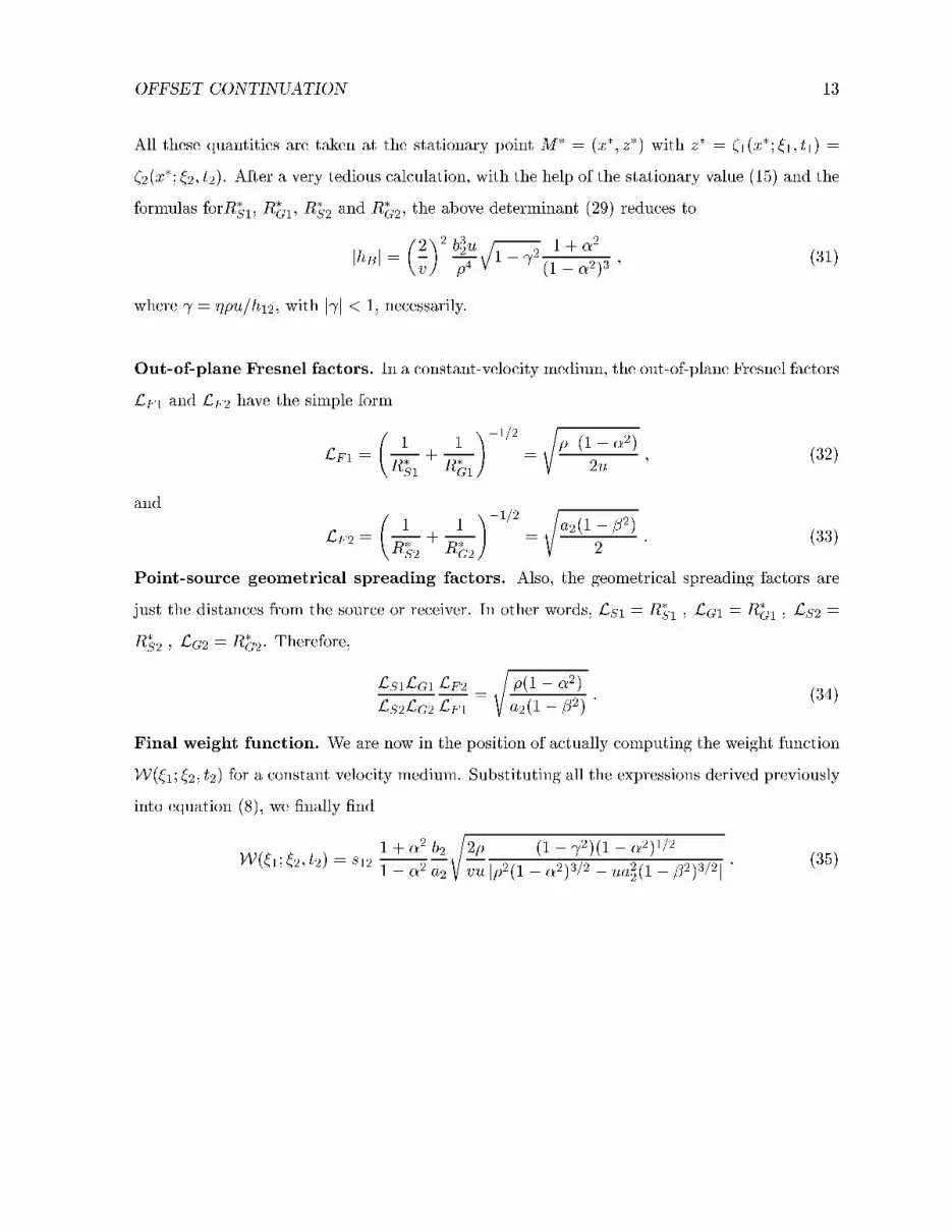
OFFSET CONTINUATION 13All these quantities are taken at the stationary point M� = (x�; z�) with z� = �1(x�; �1; t1) =�2(x�; �2; t2). After a very tedious al ulation, with the help of the stationary value (15) and theformulas forR�S1, R�G1, R�S2 and R�G2, the above determinant (29) redu es tojhB j = �2v�2 b32u�4 q1� 2 1 + �2(1� �2)3 ; (31)where = ��u=h12, with j j < 1, ne essarily.Out-of-plane Fresnel fa tors. In a onstant-velo ity medium, the out-of-plane Fresnel fa torsLF1 and LF2 have the simple formLF1 = 1R�S1 + 1R�G1!�1=2 = s� (1� �2)2u ; (32)and LF2 = 1R�S2 + 1R�G2!�1=2 = sa2(1� �2)2 : (33)Point-sour e geometri al spreading fa tors. Also, the geometri al spreading fa tors arejust the distan es from the sour e or re eiver. In other words, LS1 = R�S1 ; LG1 = R�G1 ; LS2 =R�S2 ; LG2 = R�G2. Therefore, LS1LG1LS2LG2 LF2LF1 = s �(1� �2)a2(1� �2) : (34)Final weight fun tion. We are now in the position of a tually omputing the weight fun tionW(�1; �2; t2) for a onstant velo ity medium. Substituting all the expressions derived previouslyinto equation (8), we �nally �ndW(�1; �2; t2) = s12 1 + �21� �2 b2a2s2�vu (1� 2)(1� �2)1=2j�2(1� �2)3=2 � ua22(1� �2)3=2j : (35)

14 Santos, S hlei her & TygelFIGURE CAPTIONSFig. 1: 2D laterally inhomogeneous Earth model for a 2.5D OCO. The model is assumed to beindependent of the out-of-plane y- oordinate. The two ommon-o�set on�gurations areindi ated by the sour e-re eiver pairs (S1; G1) and (S2; G2) separated by o�sets 2h1 and2h2 with midpoints at �1 and �2, respe tively.Fig. 2: Model for the the syntheti tests.Fig. 3: (a) Syntheti ommon-o�set se tion for the stru ture of Figure 2 with h= 500 m, mod-eled by a 2.5D Kir hho� integral. (b) simulated ommon-o�set se tion with h= 500 m omputed by OCO from the ommon-o�set se tion with h= 250 m. For details, pleaserefer to the text.Fig. 4: (a) Pi ked peak amplitudes along the modeled ( ontinuous line) and simulated (dashedlines) ommon-o�set re e tions for h= 500 m. (b) Relative amplitude errors of the simu-lated ommon-o�set re e tions omputed by OCO from the se tions with h= 0 m (solid),h= 250 m (dashed), h= 750 m (dotted), h= 1000 m (dash-dotted).