Embed Size (px)
Citation preview

3 AD-A274 519
It
3 An XCP User's Guide and Reference Manual
I by Thomas B. Sanford, Eric A. D'Asaro, Eric L. Kunze, John H. Dunlap,Robert G. Drever, Maureen A. Kennelly, Mark D. Prater, and Michael S. Horgan
I
DTICELECTE
JAN 0 3 1994
Technical ReportAPL-UW TR 9309
c(,o August 1993
Contracts N00014-84-C-01 11, NOOO14-87-K-O004 , and Grant NOOO14.90-J- 1100
93 1223 0.4 4-

III
i An XCP User's Guide and Reference ManualI
by Thomas B. Sanford, Eric A. D'Asaro, Eric L. Kunze, John H. Dunlap,Robert G. Drever, Maureen A. Kennelly, Mark D. Prater, and Michael S. Horgan
I
INTIS CRA&IDTIC iAS
Technical ReportDy.....ib ..ti ............. APL-UW TR 9309
....,Ia•J-,Iity Goje August 1993Av ail t•:,djor
Dist i Special
| A-1
I1.TIC QTJ ,.mLIINPCD
* Applied Physics Laboratory University of Washingtoni 1013 NE 40th Street Seattle, Washington 98105-6698
I I Contracts N00014-84-C-011 1, NOOO14-87-K.O004 , and Grant NOOO14-90-J-1 100
II

III
Acknowledgments
The XCP work done by the authors has been prinarily funded by the Office of INaval Research. We thank Mark Morehead for his valuable contributions to the OCEANSTORMS project, Art Bartlett and Pat McKeown for their contributions to the success ofmany APL-UW XCP operations, and Dicky Allison for her help in this project Wewould also like to acknowledge the support of the Oceanographer of the Navy (N096)through Ken Ferer of the Naval Research Laboratory's Tactical Oceanography Warfare ISupport Program Office (Code 7410) for development of the XCP. Publication of thiswork was funded by ONR.
IIIIIIIIIIII

IUNIVERSITY OF WASHINGTON * APPLIED PHYSICS LABORATORY
IABSTRACT
This report describes expendable current profiler (XCP) instrumentation, equipmenttesting procedures, data acquisition methods, and data processing. It also provides aguide to XCP field operations.
IIIIIIIIIIIIII
ITR9309 iii

UNIVERSITY OF WASHINGTON * APPLIED PHYSICS LABORATORY
TABLE OF CONTENTS iPage
1. Introduction .............................................................................. 1
1.1 Background ................................................................................................. I
1.2 Theory of Operation ................................................................................... 3
2. Instrumentation ............................................ 4
2.1 Probe Description ..................................................................................... . 4
2.1.1 XCPs ........................................... 4
2.1.2 AXCPs .......................................... 8
2.1.3 Slowfall AXCPs ................................................................................. 9
2.2 Data Acquisition Equipment .................................................................... 10
2.2.1 Standard Data Acquisition System .................................................. 102.2.1.1 Antennas ..................................................................................... 102.2.1.2 RF Receivers ............................................................................. 12 I2.2.1.3 Signal Processors ........................................................................ 12
2.2.1.3.1 APL-UW Signal Processor ................................................ 122.2.1.3.2 MK-10 Digital Data Interface .......................................... 12
2.2.1.3.2.1 MK-10 Modifications ................................................ 122.2.1.3.2.2 MK-10 Switch Settings ............................................. 15
2.2.1.4 Computers ................................................................................... 162.2.1.4.1 Computer Requirements ................................................... 16
2.2.1.4.2 Data Acquisition ................................................................. 172.2.1.4.3 Equipment Used During the Gulf of Cadiz Expedition ... 17
2.2.2 Backup Data Acquisition System .................................................... 192.2.2.1 Backup Media ............................................................................. 19
2.2.2.1.1 Audio Cassette Tapes ........................................................ 202.2.2.1.2 Video Cassette Tapes ......................................................... 202.2.2.1.3 Digital Audio Tapes ........................................................... 20
2.2.3 Portable Data Acquisition System .................................................... 202.2.4 Homemade Data Acquisition System .............................................. 20
3. Equipment Tests ...................................................................................................... 213.1 Playback of Standard XCP Cassette ......................................................... 21
3.1.1 Radio Transmitter Test Box Construction .................... 223.1.2 Radio Transmitter Test Procedure ..................................................... 22
3.2 Portable Receiver Test .............................................................................. 233.3 Probe Tests ................................................................................................. 23
3.3.1 Radio Frequency Test ........................................................................ 253.3.2 Audio Frequency Test ....................................................................... 263.3.3 Compass Coil Test ............................................................................. 273.3.4 Visual Examination of Agar ............................................................. 27 I
4. Sippican Probe Calibrations ................................................................................. 28
Iiv TR 9309m
UUNIVERSITY OF WASHINGTON * APPLIED PHYSICS LABORATORY
I5. Deploying XCPs ..................................................................................................... 29
5.1 Pre-Launch Considerations ........................................................................ 295.2 Acquisition Equipment Preparations ....................................................... .,305.3 XCP Preparations ...................................................................................... 315.4 XCP Launch ......................................... 315.5 XCP Operational Sequence ...................................................................... 31
6. XCP Data Processing ............................................................................................. 346.1 XCP Processing Programs ......................................................................... 346.2 XCP Depth Coefficients .................................. 366.3 New Coefficients for XCP Processing ...................................................... 396.4 Am= ................................................................. ..................................... . ... . 416.5 New C2 value for XCPs ............................................................................ 416.6 XCP Temperature Processing .................................................................... 411 7. XCP Performance near the Geomagnetic Equator ............................................... 44
8. XCP Performance near the Geomagnetic Pole .................................................... 489. Failures and Fixes ................................................................................................... 4910. Combining XCP and ADCP Data ....................................................................... 5011. Effect of Fall-Rate Variations on North Velocity ............................................... 53
11.1 Introduction ............................................................................................. 5311.2 Theoretical Source of the Error ............................ 5311.3 Effect Found in Data ................................................................................ 5411.4 Effect Explained by Model ...................................................................... 55I 12. References ............................................. 58
Appendix A, Bibliography of XCP Publications ....................................................... Al-A4Appendix B, Instrument Settings ................................................................................ B 1Appendix C, XCP Launch Checklist .......................................................................... Cl--C2Appendix D, XCP Log Sheet ...................................................................................... DAppendix E, Drop Checklist ....................................................................................... ElAppendix F, Storage Formats for XCP Data from HP-9020 Acquisition Program
1. Raw Data .................................................................................... F12. Processed Data ........................................................................... F2
Appendix G, XCP Processing Program Overview, xcpover ............................... G1-G5Appendix H, hdrmerge Documentation ..................................................................... HIAppendix I, xcpsplit Documentation .......................................................................... 11-12Appendix J, xcpftoi Documentation ........................................................................... JiAppendix K, xcpfloat Documentation ....................................................................... KIAppendix L, xcpturn Documentation ......................................................................... L1-L2Appendix M, xcpaddt Documentation ....................................................................... M1-M2Appendix N, xcpblfDocumentation ........................................................................... NIAppendix 0, xcppro Documentation .......................................................................... 01-04Appendix P, xcpgrid Documentation ...................................................................... PI-P2Appendix Q, xcpplot Documentation ......................................................................... Q1Appendix R, List of Selected Symbols and Acronyms ............................................. RI
TR9309 v

IUNIVERSITY OF WASHINGTON - APPLIED PHYSICS LABORATORY
LIST OF FIGURES 1Page
Figure 1. Locations where UW investigators have deployed XCPs .................... 2
Figure 2. XCP launch from stem of an underway vessel .................... 4 4
Figure 3. XCP schematics ....................................................................................... 5
Figure 4. Launch sequence from underway vessel and aircraft ................ 7 IFigure 5. Slowfall AXCP during launch and descent ............................................ 9
Figure 6. Configuration of MK- 10 rack during Gulf of Cadiz Expedition .......... 13 1Figure 7. Configuration of XCP/XBT/XSV acquisition system ........................... 18
Figure 8. XCP backup rack .................................................................................... 19 IFigure 9a. XCP test box containing radio transmitters for channels 12, 14,
and 16 ...................................................................................................... 21
Figure 9b. Pinouts for RF transmitter bcard on XCP ............................................. 22
Figure 10. Power supply used for XCP probe tests ............................................... 24
Figure 11. XCP power-up diagram .......................................................................... 26
Figure 12. XCP transmitter board schematic .......................................................... 29 3Figure 13. Deviation in revised XCP depth from that given by Sippican
as computed from coefficients ............................................................... 38 3Figure 14. Combined result of matching program for 67 XCP-CTD pairs,
Gulf of Cadiz ........................................................................................... 39 3Figure 15. Location of zones of small F. (magnetic equator) and small Fh
(magnetic poles) ...................................................................................... 45
Figure 16. Global chart of F/Fh ................................................................................ 46
Figure 17. Pairs of XCP and ADCP profiles of east and north velocity from theG ulf of Cadiz ........................................................................................... 52
Figure 18. North velocity and rotation frequency data from the Gulf of Cadiz ..... 54Figure 19. Model results of north velocity, corrected north velocity, and 3
rotation frequency ................................................................................. 56
II
vi TR9309 3

IUNIVERSITY OF WASHINGTON* APPLIED PHYSICS LABORATORY
I LIST OF TABLES
I Page
Table 1. Sonobuoy channels and corresponding radio frequencies ....................... 8
Table 2. Audio signals received from the XCP and their meaning ..................... 32
Table 3. XCP depth coefficients ............................................................................ 37
Table 4. Horgan's new polynomial coefficients of gain and phase ..................... 40
III
IIIIIIII
ITR9309 vii

I3 UNIVERSITY OF WASHINGTON - APPLIED PHYSICS LABORATORY
1 1. INTRODUCTIONThe expendable current profiler (XCP) manufactured by Sippican, Inc., measures
ocean velocity and temperature from the surface to a depth of 1500 m. This reportdiscusses XCP instrumentation, equipment testing procedures, data acquisition methods,and data processing and provides a guide to XCP field operations. Software methods for
fixing certain failure modes are also described.
1.1 BackgroundStudies of ocean dynamics and water transport require rapid and accurate observa-
tions of velocities. One way to measure these quantities is through naturally occurringelectric currents induced by the motion of seawater through the Earth's magnetic field.The concept of measuring ocean currents from motionally induced electromagnetic (EM)fields was first suggested by Michael Faraday in 1832. More recently (in the early
I 1970's), the EM Group* at the Woods Hole Oceanographic Institution used EM princi-ples to build a free-fall instrument called the Electro-Magnetic Velocity Profiler, orEMVP (Sanford et al., 1978). The EMVP was approximately 2.5 m long, weighed about160 kg, and could achieve a complete velocity profile in 6000 m of water in about3 hours. Experience with the EMVP suggested that a smaller, expendable version couldbe developed. In 1976, Thomas Sanford and Robert Drever began development of anexpendable temperature and velocity profiler (XTVP), initially funded by the Office ofNaval Research (ONR) and later by the Naval Ocean Research and DevelopmentActivity (now NRL at Stennis). In 1979, Sippican, Inc., began manufacturing the probesas expendable current profilers, or XCPs.
One advantage of the XCP is that it can be deployed from any sort of platform(ship, aircraft, ice, etc.), enabling rapid surveys, especially from aircraft. Moreover, itcan be launched in any weather conditions, including hurricanes.
XCPs have been used in a variety of oceanographic programs. Figure 1 shows thelocations where they have been deployed by University of Washington (UW) investiga-tors. Some of the topics investigated using XCPs include mixed-layer dynamics, geos-trophic eddies, the Mediterranean Outflow, Mediterranean Water eddies (Meddies),fronts, cold- and warm-core Gulf Stream rings, topographic interactions, near-inertialwaves, surface waves, the Equatorial Undercurrent, and benthic boundary layer dynam-ics. XCPs have been deployed at latitudes ranging from the equator to 86N. Acomprehensive bibliography listing XCP references and studies using XCPs is given inAppendix A.
I3 *Now at the Applied Physics Laboratory, University of Washington (APL-UW).
TR9309 1

2 0c bL C4
I<
m cio
e ca.T
;lo 0
P rý 0
ai 0e -
0
on in2, T 030
IUNIVERSITY OF WASHINGTON * APPLIED PHYSICS LABORATORY
I Scientific development and operation of the XCP were summarized in 1982 in areport entitled "Design, Operation and Performance of an Expendable Temperature andVelocity Profiler (XTVP)" (Sanford et al., 1982). Since then, the XCP has undergone anumber of changes: a radio link rather than a wire link is now used to transmit data fromthe surface unit to the receiving unit; the depth capability has been increased from 850 to1500 m; air-launched units (AXCPs) have been developed by packaging XCPs insonobuoy containers; a new type of AXCP, the slowfall, has been developed to enhanceobservations of surface wave oscillations in the upper 200 m of the water column; andXCP processing methods have become more sophisticated. In addition, some XCP usershave experienced difficulties in acquiring and processing their data and would havebenefited from a description of our approach. Thus, we felt it was time to compile ourrecent experiences and findings into a single volume.
1.2 Theory of OperationThe XCP provides a vertical profile of the relative horizontal velocity and tempera-
ture. Velocity determinations are based on the principles of electromagnetic inductionthat govern the weak electric currents induced by the motion of electrically conductinglayers of seawater through the Earth's magnetic field (Sanford, 1971). The magnitude ofthe electric current is related to the velocity of the conductor, its conductivity, and thestrength of the magnetic field. The XCP determines this current by measuring the vol-tage between horizontally spaced electrodes falling through the water column. An exten-sive discussion of the theory of operation is provided by Sanford et al. (1982).
IIIIIII
ITR 9309 3

IUNIVERSITY OF WASHINGTON . APPLIED PHYSICS LABORATORY
I2. INSTRUMENTATION
2.1 Probe Description
2.1.1 XCPs
A short description of the XCP is given here; more detailed information can befound in the report by Sanford et al. (1982).
The standard XCP is designed to be launched from a vessel that is under way. Theentire system-consisting of a surface float with a radio transmitter, a free-falling sensorprobe, and wire connecting the two--is simply tossed overboard (Figure 2); there is no Imechanical tether between the vessel and the sensor. The total package weighs about10 kg and is 12 cm in diameter by 100 cm long. The probe is projectile-shaped, with acruciform tail and ring shroud; it contains electrodes, a compass coil, electronics, bat-teries, a thermistor, and wire-spooling components similar to those used in expendablebathythermographs (XBTs). The probe weighs 900 g in seawater and is approximately5 cm in diameter by 42 cm long. The mechanical designs of the various XCPs (XCP,AXCP, and slowfall AXCP) are shown in Figure 3. I
II
1IFigure 2. XCP launch from stern of an underway vessel.
I4 TR9309

IUNIVERSITY OF WASHINGTON APPLIED PHYSICS LABORATORY
IParachute
Float Release Cover Wind Flap - Float Release Cover
Flotation Bag Flotation Bag
H-F Electronics RF Electronics
Seawater Battery Seawater Battery
Surface Float Surface Float
Surface Wire SpoolSurface Wire Spool
I XCP Wire Spool XCP Wire SpoolBulkheadI
Electrode Electrode
XCP Probe XCP ProbeI
I Nose Weight Nose Weight
Door Air-Launch DoorRelease Squib Sonobuoy
Canister Release Squib
(a) XCP (-Air-Canister Weight
(b) AXCP
Figure 3. XCP schematics. (a) XCP, (b) AXCP, (c) slowfall AXCP (next page).
IIII
STR9309 5

I,UNIVERSITY OF WASHINGTON. APPLIED PHYSICS LABORATORY
LAUNCH TUBEISLEEVE
DROlGUEEICOLLAR
FLOODING
PORTS
DROGUE AIRFOIL
SLOWF:ALL II
tTANDARDXCP PROBE MOOIFIED
LAUNCH TUBE
PROBEINSPECTIONPOST
NOSE BLOCK
END PLUG
LAUNCH TUBEIEND PLUG SNUBBING
SCREW
(c) Slowfall AXCP I
Figure 3, cont.
The probe contains two silver-silver chloride electrodes separated by 5 cm. Ameasured voltage of 50 nV across the electrodes equates to 1 cm s-1 of relative motion atmidlatitudes. Determination of the two horizontal components of velocity is enabled by acompass coil wound coaxially over the electrode tubes. The XCP probe spins 16 timesper second during descent. As the probe falls, the compass-coil signal is used to deter-mine the location of magnetic north once per revolution. A thermistor mounted within aflow tube on the probe provides a continuous vertical temperature profile.I
The motionally induced voltage, sensed between the silver-silver chloride elec-trodes, and the compass coil voltage are amplified separately and processed throughvoltage-to-frequency (V/F) converters. A third frequency is determined based on theresistance of the thermistor. Frequency-modulated (FM) signals are summed together fortransmission up the wire connecting the probe to the surface float and telemetered to the
6 TR9309

I
UNIVERSITY OF WASHINGTON . APPLIED PHYSICS LABORATORY
Iship via a radio frequency (RF) transmitter to a VHF radio receiver on the launchingvessel. The output of the RF receiver is amplified, demodulated, and digitized by the sig-nal processor for direct computer storage.
Deployment consists of the following series of events, which occur within 50 s ofimpact with the water's surface (see diagram in Figure 4). The XCP package, beingnegatively buoyant, sinks, flooding the interior and the seawater-activated battery con-tained therein. The battery provides power to fire a squib which punctures a CO2 car-tridge. The CO2 inflates a flotation bladder, and the system, buoyed up by the bladder,floats to the surface. About 40 s later, a timer, activated at battery power-up, fires asecond squib, which uncaps the bottom of the probe's launch tube. The probe then fallsat about 4.5 m s-1 , rotating at about 16 Hz as it descends. As it drops through the watercolumn, it trails fine, two-conductor XBT wire which deploys from spools on both theprobe and surface float. This method of deployment eliminates an increasing drag force.ýnd allows the probe to maintain a uniform descent speed. The wire has a breakingstrength of about 1 lb.
The probes currently manufactured by Sippican, Inc., are denoted as Mod 7s. TheMod 6 XCPs produced by Sippican used a wire link to transmit data from the probe allthe way to the receiving equipment on the ship and provided data to only 850 m depth.
I.
III'
canniser •,
I Figure 4. XCP launch sequence from underway vessel and aircraft.
I TR 9309 7

IUNIVERSITY OF WASHINGTON * APPLIED PHYSICS LABORATORY__
Sippican routinely manufactures probes that transmit on one of three sonobuoy RF chan- Inels: 12, 14, and 16. Table 1 lists the sonobuoy channels and their corresponding fre-quencies. With advance notice, Sippican can manufacture probes that utilize sonobuoychannel 10. However, a channel-10 radio must be installed in a MK-10 digital data inter-face to be able to receive channel-t0 data. In a two or three channel MK-1O, one of theexisting radios can simply be exchanged for a channel-10 radio, and no othermodification is needed.
Table 1. Sonobuoy channels and corresponding radio frequencies. USonobuoy Channel Radio Frequency
Channel l0 169.0 MHzChannel 12 170.5 MHzChannel 14 172.0 MHzChannel 16 173.5 MHz
2.1.2 AXCPs
The AXCP (Figure 3b) is an air-launched version of the XCP. It consists of theXCP described in the previous section with the addition of a parachute decelerating sys-tem and an outer aluminum tube. These modifications allow the system to be launched 3through normal sonobuoy launch tubes (either with a cartridge-activated device or grav-ity launched) while the radio receiver is on board the aircraft.
The entire unit is housed in a protective, A-size sonobuoy canister. Upon launch Ifrom an aircraft (Figure 4), a small wind flap deploys, pulling the parachute from the can-ister. The unit falls to the ocean surface at a rate of about 25 m s-1. As with the XCP, aseawater battery is activated upon impact, turning on the telemetry radio, firing the CO2cartridge, and inflating the flotation bladder. The pressure from the inflated bladderpushes the weight off the upper end of the sonobuoy canister, allowing the float toseparate from the canister and rise to the surface. The AXCP then performs identicallyto the XCP. According to Sippican, the AXCP can be launched at aircraft speeds up to180 knots and at altitudes up to 2000 ft. We have launched it from 10,000 ft and at air- 3craft speeds greater than 200 knots (Osse et al., 1989; D'Asaro et al., 1990). Data ameacquired and processed in the same manner as for XCPs.
II
8 TR9309 3

IUNIVERSITY OF WASHINGTON - APPLIED PHYSICS LABORATORY
2.1.3 Slowfali AXCPs
The slowfall AXCP (Figure 3c) was developed at APL-UW for the OCEANSTORMS program (Osse et al., 1988; D'Asaro et al., 1990). It is a modified version ofthe AXCP designed to improve launch stability and impact survival and to fall slowly(<1 m s-t) through the upper 200 m of the ocean to observe more cycles of surface waveoscillations. The device was based on the standard AXCP described in Section 2.1.2 butincorporates a winged drogue to slow descent over the upper ocean while maintaining asufficient rotation rate. At a preset depth, the drogue is jettisoned, and the probe revertsto its normal descent and spin rates. Figure 5 shows the unit's configuration duringlaunch, descent, and jettison of the drogue.
Forty slowfall AXCPs were deployed in late 1987 as part of the OCEAN STORMSProgram (D'Asaro et al., 1990). Nineteen units provided profile data.
Investigators have experimented with another type of slowfall AXCP obtained fromSippican, Inc., that had a smaller and lighter, square nose weight (designated the T-I 1 bySippican). The lighter nose weight caused the AXCP to fall at about half speed (i.e.,2.2 m s-1), enabling better filtering or observation of surface wave signals than with stan-dard AXCPs.I
U Figure5.
Launch Slowfall AXCP during launch and descent.Canister
I 1I
Slow-fall* .Descent
DrogueI Jettisoned
IITR 9309 9
-UNIVERSITY OF WASHINGTON * APPLIED PHYSICS LABORATORY 3
2.2 Data Acquisition Equipment i
The basic requirements for XCP data acquisition are an antenna, a receiver or signalprocessor, and a data storage device (e.g., a cassette recorder or VCR). Additional Iequipment can include multiple antennas, computers, disk drives, printers, and plotters.
For an experiment with a large XCP component, we use a full complement ofequipment, including multiple antennas at different locations on the ship, multiple ireceivers to acquire data simultaneously from two or more XCPs on different channels,and a computer equipped with floppy and hard disk drives for real-time processing anddisplay. Such an installation is described in Section 2.2.1 as our standard system. Wetypically use an independent backup system (such as that described in Section 2.2.2) withits own radios and recorders in conjunction with the standard system. I
For an experiment with only a few XCPs or occasional XCP deployments (such asin the Arctic), we use a portable system consisting of an antenna, a receiver, and a taperecorder. We recommend using digital audio tapes (DAT) or VHS tapes for data record-ing although audio cassette tapes are adequate. With the portable equipment, the data areplayed back from the magnetic tapes and transferred to computer for subsequent process-ing upon return to the laboratory. Although profiles of velocity cannot be displayed inreal time with the portable gear, headphones can be used to listen to the FM signal of theprobe as it falls. After listening to recordings of a few probes, one can differentiatebetween the signal of an XCP that is functioning properly and one that is not. This typeof system is described in Section 2.2.3. Both the standard and portable systems havebeen used successfully by APL and other investigators. In addition, an easily configured Ihomemade data acquisition system is described in Section 2.2.4.
For operations at sea or in the air, the acquisition equipment, particularly comput-ers, must be shock resistant. We have had good success in the field with Hewlett-Packard(HP) equipment. Another important consideration for field operations is "clean" power.We always use Topaz, Inc., power conditioners at sea.
2.2.1 Standard Data Acquisition System
Equipment used in ,u- standard system inc)d des antennas, a receiver or signal pro-cessor, a computer with multiple data storage media, what we call a "patch panel"which includes backup sonobuoy RF receivers and signal strength meters, and a spec-trum analyzer.
2.2.1.1 Antennas UVery high frequency (143-174 MHz) antennas are used for XCP reception. The
electric polarization must be vertical to match that of the transmitting antenna on theprobe. Some directionality helps to reduce fading due to muitipath interference from Ireflections off the ship and to increase signal strength. Too much directionality is
I10 TR9309 3

UNIVERSITY OF WASHINGTON . APPLIED PHYSICS LABORATORY
I,counterproductive because vessel pitch, yaw, and small heading adjustnents will cause
signal dropouts. We have been most pleased with Cushcraft1 Yagi antennas cutspecifically for 170 MHz, and our recommendation is to use four-element Yagi antennasthat have a beam width of about 660 and a front-to-back ratio of 18 dB. The front-to-backratio is the ratio of the forward-looking gain of the antenna to the backward-looking gain.A four-element Yagi antenna mounted with the elements vertical 15 m or more above thewater works very well at ship speeds of 6 m s71 or less.
We have experienced good performance from directional log-periodic TV antennasas well as four-element Yagi antennas. We have not had good results with the simpleomnidirectional ground-plane whip antennas that were initially supplied with the MK-10digital data interface. Sippican, Inc., now offers the user a choice between an omnidirec-tional antenna and a Yagi antenna.
Television antennas are readily available and take no particular care in tuning.However, they have several disadvantages: They require a nonconducting mast; theyproduce more wind resistance than Yagi antennas and may not be strong enough for thewinds encountered at sea; the standard mounting brackets assume horizontal polarizationwhereas XCP work requires the elements to be vertical. When using TV antennas, usecoaxial cable and "baluns" (balanced-to-unbalanced transformers) to convert the 300 Qantenna impedance to 50 or 72 fQ coaxial cable.
Because the Yagi antennas have a high front-to-back ratio, a steel or aluminum pipecan be used for support just behind the reflector element. Yagi antennas are easilymounted vertically to a vertical pipe. We keep the distance to any other conductor at 1 mor more, except for the supporting pipe, which is about 10 cm behind the reflector ele-ment of the Yagi. Yagi antennas tend to be more rugged, since no insulators are requiredbetween the elements and the boom.
Yagi antennas generally have a "gamma match" balun to convert the impedance ofthe feed line (coaxial cable) to that of the antenna. This balun must be adjusted toaccount for the minimum standing wave ratio (SWR) on the transmission line before use.This requires an SWR meter and the XCP radio test box described in Section 3.1.1. Thegamma match can be adjusted before installation by mounting the antenna on a pipesimilar to that to which it will be mounted on the ship; put the boom about 3 m off theground and use a fairly short (about 5 m) feed line. Check the SWR at the lower end ofthe feed line after installation to ensure integrity of the feed line and antenna. If all iswell, the SWR should be a bit less than when initially adjusted because the longer feedline absorbs more reflected energy.
1Cushcraft/Signals, 48Perimeter Road, P.O. Box 4680, Manchester, New Hampshire 03108; (603)
627-7877 or 1-800-258-3860
TR 9309 11

IUNIVERSITY OF WASHINGTON * APPLIED PHYSICS LABORATORY
Further suggestions are (1) keep the antennas below the highest point of the ship to Iprotect them from direct lightning strikes, and (2) use low-loss RG-8 coaxial cable.Smaller cables can cause significant losses in signal strength. We sometimes use an RFpreamplifier and a signal splitter to increase the signal strength when operating multiplereceivers from the same antenna.
2.2.1.2 RF Receivers
Any VHF radio capable of receiving 169-174 MHz, wideband, FM signals can beused for XCP data reception. The nominal frequency deviation of the XCP transmitter is150 kHz peak to peak. A receiver with a bandwidth of 150 kHz will work for XCP datareception. After data are received they can be stored digitally, as with the APL-UW sig-nal processor (Section 2.2.1.3.1) or the Sippican MK-10 digital data interface (Section2.2.1.3.2), or stored in analog format on magnetic tapes such as those used in conjunctionwith the portable system (Section 2.2.3) or homemade data acquisition system (Section2.2.4).
2.2.1.3 Signal Processors
2.2.1.3.1 APL-UW Signal Processor
We initially used a digital signal processor built by Robert Drever of APL-UW for
XCP operations. The APL-UW unit receives, amplifies, demodulates, and digitizes theincoming RF signal for direct computer storage. The design of this receiver is describedin detail by Sanford et al. (1982). We last used the APL-UW receiver during De SteiguerCruise 1210-87 (Carlson et al., 1987). We have since been using a receiver built by Sip-pican, the model MK-10 digital data interface, which we modify slightly. For some play-backs, we use the APL-UW processor with an HP-9845 computer.
2.2.1.3.2 MK-10 Digital Data Interface IThe Sippican MK-10 digital data interface receives the RF transmissions from the
XCP and converts the signal into digital format in real time. It then transfers the digi-tized XCP data over an IEEE-488 bus to a computer for further processing. The MK-10 Iis compatible with any computer that accepts the IEEE-488 output format. Up to threeradio receivers can be fitted within the MK-10 case.
2.2.1.3.2.1 MK-10 Modifications
We have made several modifications to our MK-10s to improve their performance. IFrequently, the MK-10 would hang up, and the only way to resume XCP operationswould be to turn off the unit. A reset switch was therefore added to the left side of theMK-10 front panel (see Figure 6) so we could resume operations without having to turn
12 TR9309

IUNIVERSITY OF WASHINGTON APPLIED PHYSICS LABORATORY
ISowmel (169 MHz)
L 0 Channel 10 Mk 10
m* lw hin0-
Goldln spe~raj
Mit 10 M adwupI Mk 10. 1.,•pl (Channel 10) •
Ch 10 )bna
I 1-upI1E 12 6114C17ho phone
Audio oa
PatCh PanelI Bo
o• reset (170.5 MHz)
L o Channel 12 Mk 10
I Bon/off Note: 172 Wiz is the 43rd hafmlonic at the 4 Niz
pilot oscilator, so Ch. 14 will be sensitDiveh If antennas'• ~am In"ld lob within 20 feet of rdck
I o•)°- (172 MHz)
0 Channel 14 Mk 10
B on/off
o@0-r (173.5MHz)0 Channel IS Mk 10
(a) Front View
Figure 6. Configuration of MK-1O rack used during Gulf of Cadiz Expedition. In thisconfiguration, the channel-lO MK-1O and channel-12 MK-1O share parti-don 1.
IITR9309 13

IUNIVERSITY OF WASHINGTON . APPLIED PHYSICS LABORATORY
1-- II ar enI
F/S RF F/S RF 0otIn o uti ChI10o?14 10 10 14 ,,1 out
- . ..---------------- ,_____ O- .(parttio 1) I_ Chane 10 Mk 10I- I
-I " I---- i--, -W ,,'• "' " I
Mk 10 ,.•up A& 1,I"0 Mi, 0 bm* I-- S in II I1-- dat otado- in FMio, a u II I I',",kl-Op , •I0 Mkl bdwo,-'~.•.-.-.. .. ..666 - 0--- ./S 0 .0 - r Facku
.1 61,1w 111 16 :14 12g 10' 10 a'rs*
.r- - -- -- - --- -. . ..-- -- -. ..- - . .
I ---------------------- IT -•--O------
0I ~ 0O 01F/S RF FIS RF Ch 1-2 . oout in out In WA 0-1----4 -----
I 12 12 14 14, / -" ,a HP9020, II-" (parmon 1)Channel 12 Mk 10
- 0- 0-10 0 0 iFII IuFIS RF FIS RF I O--'out In out in O i out14 14 0 i u
H1P90201414(partn 2) 1 Channel 14 Mk 10
B I n----- ---- IO RFIn
ChlSO FSoutIHPg02
(parition 3) Channel 16 Mk 10
(b) Back ViewI
Figure 6, cont.
14 TRI9309

IUNIVERSITY OF WASHINGTON * APPLIED PHYSICS LABORATORY
Soff the power. The switch momentarily sets pin 9 of the MK- 10's 8031 microprocessor to+5 V. When the switch is depressed, the microprocessor and thus the MK-10 are reset asif the power had been turned off and on. The steps involved in this modification are
"* Cut away part of the interlock panel to allow space on the left front panel for apushbutton switch.
"* Install a miniature pushbutton switch I in. to the right of the jack. (The switchis single pole, momentary, and normally open.)
"* Using #26 twisted pair, brown wire, connect the switch to pins #4 and #1(+5 V) on the motherboard backplane.
"* On the component side of the A l board, add a wire from U I pin 9 to the pin 4edge connector.
I Occasionally in real-time operation, the signal processor would erroneously deriveits time base from a spurious 8-kHz signal from the radio, corrupting the data. This isbecause an 8-kHz "pilot" tone is normally added to the recorded signal to compensatefor tape wow. This tone is not needed when using DAT or PCM/VCR recording, whichwe recommend, and was inhibited for real-time data acquisition. This was done by put-ting a direct short across R21 on board A2, using one of the unused contacts on DIPswitch 1 (see also Section 2.2.1.3.2.2).
The bandwidth of the MK-10 circuit is too wide, allowing noise to degrade detec-tion of the zero crossing in the circuit. To reduce the bandwidth of the circuit, wereplaced the C47 (470 pF) capacitor, which is located at the input of the zero-crossingdetector on the A3 board of the MK-10, with a 0.47 pF polycarbonate capacitor. Thischanges the bandwidth of the circuit from 33.8 kHz to 338 Hz.
I 2.2.1.3.2.2 MK.10 Switch Settings
There are eight DIP switches on the A2 board of the MK-10. These switches permitthe user to select which probe parameters are to be included in the "valid data" criteria.Four criteria are available: the existence of audio carriers for temperature (, electricfield (EF), and compass coil (CC), and modulation of the compass carrier by the rotationof the XCP at frequencies in the 10-20 Hz band (probe falling, PF). Opening a switchcauses the corresponding parameter to be excluded from the valid data criteria. Farbetter choices on data quality can be made in software than in hardware. Therefore werecommend that the switches be set in the following positions for use with the HP-9020acquisition program. Disabling all the criteria doesn't work.
IITR9309 15

IUNIVERSITY OF WASHINGTON. APPLIED PHYSICS LABORATORY
A2 Board DIP Switch Field Setting
1. Spare channel open2. Tflag open3. EF flag open4. CC flag closed5. PF flag closed6. NC7. NC8. Inhibit Pilot when closed closed
The MK-10 decides whether it is listening to "real-time" or "playback" data bylooking for energy at the frequency of the 8-kHz pilot tone put on the recorded data to Icompensate for tape wow. Because radio noise can insert a signal at this frequency, wedisabled this feature (see Section 2.2.1.3.2.1). Closing DIP switch 8 on board A2 thussets the MK-10 into the real-time mode. This switch should be closed during real-timeoperations.
2.2.1.4 Computers
Any computer that accepts the IEEE-488 output format fast enough can be usedwith the MK-10 digital data interface.
The computer used with the APL-UW receiver is an HP-9845 with an HP-9885Mflexible disk drive and an HP-9872A XY plotter.
2.2.1.4.1 Computer Requirements
The computer requirements for acquiring and displaying XCP data are as follows:
HPIB Interface-A separate IEEE-488 (HPIB) interface is required for eachMK-10, since the bus address is always 22. The number of MK-Os that can be used with Ia given system may often be limited by the number of available I/O slots in the machine.
I/0 Rate -The MK-10 generates a packet of 17 bytes once per revolution of theXCP, typically every 60-70 ms; extra packets due to radio noise can decrease the aver-age interval to perhaps 40 ms, with a few cycles separated by as little as 5 ms. Thus thetotal data rate is generally less than 425 bytes/s.
Servicing Interval-The MK-10 has an internal buffer which can hold only 128 bytesand thus needs to be emptied about every 300 ms. This requirement is often hard to meetwith a multiuser, nonreal-time operating system. I
Storage for Raw Data-Each XCP drop lasts about 350 s and thus contains about145 kbytes of raw MK-10 data. We typically run the MK-10 continuously and save allthe data. This produces about 1.5 Mbytes of raw data per hour for each channel. Threehours of data gathering with three XCP channels thus produces about 14 Mbytes of data.
16 TR 9309

IUNIVERSITY OF WASHINGTON . APPLIED PHYSICS LABORATORY
IThis is too much to store on floppy disks, but is easily handled by hard disks or cartridgetape drives.
Storage for Processed Data-Typically, processed data are computed on an approx-imately 3-m grid, with each grid point consisting of about 10 scientific and engineering3 variables. A processed profile thus consists of about 50,000 words of data.
Processing Power-Processing an XCP profile at full resolution requires roughly3 million floating point operations. If this is to be done in real time, a processing rate ofabout 10' floating point operations per second (10 kflops) is required for each channelprocessed. Processing the data at less resolution can reduce this requirement substan-tially; we have, for example, run a nearly real-time XCP acquisition program on anHP-9845 with a speed of 3 kflops.
Data Display-We display eight variables for processed XCP data: temperature,Seast and north velocity, velocity error, and four diagnostic variables. With multiple XCPprofiles, this can rapidly fill up a graphics display screen. We found a color monitor to benearly essential. A large color monitor with several screens or windows would be veryhelpful.
2.2.1.4.2 Data Acquisition
For XCP data acquisition during the OCEAN STORMS project, Eric D'Asaro(D'Asaro et al., 1990) developed software in HP-Basic for the HP-9020 that allowssimultaneous real-time processing and display of data from up to three XCPs on differentchannels. The design is described in detail by D'Asaro et al. (1990). For the Gulf ofCadiz Expedition in 1988, the system was augmented by Eric Kunze to enable simultane-ous acquisition of XCP, XBT, and XSV data. Only the XCP part of the acquisition sys-tem will be discussed here. The XBT and XSV portions are described in detail by Ken-nelly et al. (1989a). As the data are acquired, the complete raw data stream is saved onan HP-9144 magnetic cartridge tape drive connected to the HP-9020. Raw data from theXCPs are stored along with a time stamp, an indication of the probe's type, and the pro-gram partition that acquired the data. Preliminary processed XCP data can also be storedon floppy disk.
2.2.1.43 Equipment Used During the Gulf of Cadiz Expedition
A schematic of the acquisition system used during the Gulf of Cadiz Expedition isshown in Figure 7. A detailed view of the MK-10 rack is shown in Figures 6a (front) and6b (back). Instrument settings are listed in Appendix B. We used four MK-10 digitaldata interfaces, one each of the four channels (10, 12, 14, and 16). In addition, a Gold-line Digital RTA spectrum analyzer (model 30) displayed the frequencies of the probeduring prelaunch testing and descent. The patch panel contained backup radios andmeters. Since only three I/O ports were available on the computer, only three MK-10s
93 TR 9309 17

-UNIVERSITY OF WASHINGTON *APPLIED PHYSICS LABORATORY
4 Elemensi Yagi VericallyPolarized Ajwm~m
(tgeQ am
2-WaISplie( C 10 W10 nleriaI
X wwSot Aape 2 Audrioa P ig
Audio~t Prcso ~ lP IS
Audio Pfoc"M B soic Audio DOigitld
Tapesni DriS
FigureMk- 7CofgrioofCPXBTI&XSV acusto syte used duin 0h Gufowas xe ith Ion. XT0 or
XBTRecrdng SV -a0 P~s$ C:) C3 = =XBT/SV _0 0 Adapr Soy Adio 91I
18- 0R30

IUNIVERSITY OF WASHINGTON- APPLIED PHYSICS LABORATORY
I could be connected (via GPIB cables) at one time. Therefore, the channel-10 and thechannel-12 MK-10s were alternately attached to partition 1. The channel-14 MK-10 wasalways attached to partition 2, and the channel-16 MK-10 to partition 3.
2.2.2 Backup Data Acquisition System
A backup system is used to store the audio signal on VHS audio/video magnetictape. It consists of independent radios for the channels of XCPs to be received, a VCR, aSony model PCM-Fl digital audio processor (PCM stands for pulse code modulation),and a power adaptor. Figure 8 shows the front panel of the XCP backup rack. Thebackup radios are located in the patch panel (Figure 6). During the Cadiz Expedition,the FM data from XCP channels 14 and 16 were stored directly on the audio tracks of theVHS tape. XCP data from channels 10 and 12 passed through the digital audio processorand were then recorded on the video tracks.
back ofpatch panel
IN OUT _ _ __
Son [o. ,"EZ @ @n0'1 2 v id e o L E P o w e r TI T' = I t ,
-0 0 R r-1 Charge P3 0] C3 Q 1S-- OL 0 0L
*16_ Panasonic Sony (35-0 -audiO R AC Power AdaptornAC-700 SONY
I 0 Digital Audio Processor PCM-F1VHS
Input 17-71Monto Front Loading System HiFir
Audio CM Gioutput Panasonic HD c -=
I Figure 8. XCP backup rack (front view), consisting of a Panasonic VCR, a Sony modelPCM-Fl digital audio processor, and a power adaptor.I
2.2.2.1 Backup Media
A variety of media can be used to record backup XCP data, such as audio cassettetapes, video cassette tapes, and digital audio tapes.
IIiTR9309 19
IUNIVERSITY OF WASHINGTON . APPLIED PHYSICS LABORATORY
2.2.2.1.1 Audio Cassette Tapes IAudio cassettes should be high quality, type II. Be sure the tape heads on the
cassette recorder are clean prior to any recording. Each XCP takes 15 minutes or less ofrecording time. Be certain to log the tape counts to identify the XCPs later. A minimumnumber of XCPs should be recorded on one cassette. Operational procedures must befollowed to avoid overwriting data. We recommend that only one side of each cassette beused. Be sure to write protect the cassettes immediately. The cost of cassette tapes isminimal compared with the price of the XCP.
2.2.2.1.2 Video Cassette Tapes
Video cassettes should be broadcast quality. As with audio cassettes, be sure thetape heads are clean prior to recording and be certain to log the tape counts so the XCPscan be identified later.
2.2.2.1.3 Digital Audio Tapes HDigital Audio Tapes (DAT) are a newer media and provide high quality recording.
2.2.3 Portable Data Acquisition System
Our portable system includes an antenna, a portable receiver, a tape recorder, andheadphones. The portable receiver was designed and built at APL for channel 14 XCPs(172.0 MI-Iz, wide band, FM). The audio signals received from the XCP are then mixedwith an 8-kHz "pilot" tone to provide a time base. A tape recorder connected to the"receiver-mixer" jack is used to record the output for later reprocessing. Use of DATobviates the need for a pilot tone and gives a better recording. However, DAT may notwork well in cole field conditions. Upon return to the laboratory, the data are playedback using a MK-10 and computer for processing and display.
2.2.4 Homemade Data Acquisition System IA simple XCP receiving system can be made using a good tape recorder and any
radio capable of receiving 169-174 MHz, wideband FM signals. We suggest a four-element Yagi (or TV) antenna, a Yaesu FRG 9600 radio receiver, and a DAT recorder.Analog tape recorders will cause some signal degradation due to tape wow. The DATsare later replayed into a MK-10 digital data interface.
III
20 TR 9309

UUNIVERSITY OF WASHINGTON . APPLIED PHYSICS LABORATORY
I3. EQUIPMENT TESTS
1 3.1 Playback of Standard XCP CassetteOnce launched, an XCP cannot be retrieved. It is therefore well worth the effort to3 ensure that the receiving equipment is working properly. Prior to any XCP deployments,
a complete simulation of an XCP drop should be done by playing a tape of a previouslylaunched XCP through a radio transmitter. The items necessary to test the receiving
I equipment are
* a whip antenna* a radio transmitter test box that simulates an XCP drop* a portable tape player* a cassette with a previously recorded (i.e., standard) XCP drop on it* a paper graph of temperature and velocity components corresponding to the
data on the cassette tape for comparison with the output of the current test.
We have found that the single most valuable piece of equipment for XCP work from anyplatform is the radio transmitter test box. This box is easily constructed using radiotransmitters from XCPs. Figure 9a shows a typical test box and the pinouts. Section3.1.1 describes how to construct one.
SonyTape Recorder Antcnna Connections
........ (0 2ANT
-- 0 Ch 12
j0 o 14 0 Ch14
00 0 16 0 Ch1I Test Box
Figure 9a. XCP test box containing radio transmitters for channels 12, 14, and 16. Thetest box is powered by batteries and uses a tape recorder to generate theXCP audio signal.
I9II
I TR 9309 21

IUNIVERSITY OF WASHINGTON . APPLIED PHYSICS LABORATORY
I3.1.1 Radio Transmitter Test Box Construction
The radio transmitter test box is constructed using one or more radio transmitterstaken from XCPs. Figure 9b shows how to wire the radio transmitter board once it has ibeen removed from the XCP. One or more such transmitters are mounted inside a metalbox, each with a connector for an external antenna. An important part of this system is afoolproof "off" switch, or several redundant switches, so that the transmitter does notactivate inadvertently during data acquisition and overpower the real XCP signals. Wehave used a test box with up to three radio channels (Figure 9a) so that the transmissions Iof up to three XCPs could be simulated.
f~fL,:+12 V~Tab I-II-Q ftWB sopiCU Ilc. XCP G
Figure 9b. Pinouts for RF transmitter board on XCP. 13.1.2 Radio Transmitter Test ProcedureI
To perform this test, carry out the following steps:
"* Start the acquisition program on the computer. Make sure the proper record-ing media are loaded (e.g., floppy diskette and cartridge tape).
"* Start recording on the backup system (VCR).
"* Take the radio transmitter test box outside the laboratory to the ship's deck.
"* Select the radio channel you want to test and connect the whip antenna and Itape recorder to the test box (Figure 9a).
"* Turn on the power. i"* Press the play button on the cassette tape player. Play an entire drop on the
selected channel.
"* Listen to the tape player to make sure a drop is being played.
22 TR9309

I__UNIVERSITY OF WASHINGTON . APPLIED PHYSICS LABORATORY
Ie Repeat this procedure for each channel.
9 Turn off the test box. Make sure the test box power is off so that test boxtransmissions do not interfere with actual XCP drops.
* * Now check that the transmission was acquired by the receivingequipment/computer system inside the laboratory. With the APL system,profiles should have been generated on the computer screen as the cassettewas played for each channel.
* Pause the acquisition program. The profiles can then be plotted for com-parison with the graph of the standard XCP.
* Check that the standard XCP data were written to disk properly by processing* the files.
* Rewind the VCR and process all channels to ensure that data were recordedproperly on the backup system.
* After verification, test data can be deleted from the storage media.
3.2 Portable Receiver Test
If the portable system is to be used for XCP data acquisition rather than the standardsystem, the portable receiver should be tested prior to field operation using the followingprocedure.
"* Check the voltages on the portable receiver test points. Change the batteries ifthe voltage is less than 12.0 V after a few minutes of running.
"* Turn on the portable receiver and plug headphones in the "receiver-mixer"jack. You should hear a (LOUD) hissing of radio noise and an 8-kHz tone. Ifyou don't hear anything, the receiver is broken. If you hear a tone, but no hiss-ing, either something is broken or there is radio interference on this channel.
* The noise should change when you attach the antenna.
"• If the receiver is broken, try opening it up, checking the wires, and/or replac-ing either the board or the power-supply chip.
3.3 Probe Tests
There are three tests that can be performed on an XCP to determine if it is operablebefore it is deployed:
* a radio frequency (RF) test* an audio frequency (AF) test* a compass coil (CC) test.
TR9309 23

I_UNIVERSITY OF WASHINGTON o APPLIED PHYSICS LABORATORY
IXCPs that fail any of these tests should not be deployed. All suspect units should be dou-ble checked. In addition, a visual inspection should be made of the agar surrounding theelectrodes.
An XCP launch checklist is provided in Appendix C that outlines the stepsdescribed here. When many probes will be dropped in rapid succession, we perform thecheckout steps on a group of probes all at once. Otherwise, we typically check an indivi-dual probe shortly before launch, having already checked out a backup probe or leavingsufficient time to be able to test another if the probe is a dud. For shipboard operations, Ione laboratory bench is left free to be used as a checkout station. (Note: These tests willnot detect all bad probes, since they do not test the XCP's batteries or the battery switch.)
Items necessary for the probe tests include
"* a dual 12 V power supply or a pair of 12 V lantern batteries"* test cable I"* a magnet.
The power supply for the RF and AF tests is diagrammed in Figure 10. A test cablecan be made. by simply mounting three pins in a plastic block at the spacing of the testpoints (0.25 in.) on the XCP. The test point contacts are 3/32 in. in diameter. A testcable can also be obtained from Sippican, Inc. (Note: Sippican uses the terminology"XCP test harness.") The test cable enables power to be easily applied to all three testpoints at one time.
black red 0
Dynascan 16W Tni-o~ tpuI g, I I , ,gPower $U
lack
9nd -12 +12attach clip to cost Iattach dip to slubby I1CM
(000) metal housing wire at transmitter endactivates probe (GND)
II
activates rado
Figure 10. Power supply used for XCP probe tess. Diagram shows the wiring for
II I
activating the radio (RF test) and powering the probe (AF test).
24 TR9309

I-UNIVERSITY OF WASHINGTON APPLIED PHYSICS LABORATORY
ITo prepare the XCP for testing, remove it from the shipping box, and place the
XCP, still in its inner cardboard form, on a laboratory bench. Slit the tapes on the innercardboard form to expose the XCP. Leaving the XCP in the form makes it easier to teston a moving ship. (When the tests are completed, the form can be closed and retaped,and the XCP put back in its shipping box until launch.)
Enter the following header information on the launch checklist (Appendix C):
* probe serial numbero Mod* channel number* initials of person performing checkout
* expiration date of probeo date and time of checkout.
The drop number can be entered at this time if it is known or it can be entered laterwhen the probe is actually deployed.
I 3.3.1 Radio Frequency Test
Turn on the power to the MK-10 or other radio receiver. Turn the channel selectoron the MK-10 to match the channel of the XCP being tested. Plug headphones into theMK-10. (We use a patch panel that enables us to hook together multiple MK-10s andselect the channel we want to listen to.) Listen using the headphones. You should hearwhite noise.
There are two wires without insulation near the transmitter end of the XCP (Figures1 la and 1 ib). One wire is much longer than the other, this is the squib wire and should
not have power applied to it. Also, it should not touch the XCP case. Check off on thelaunch checklist that the squib wire is free. The other wire is about 1 cm long. Using a12 V power supply (Figure 10) or a pair of 12 V batteries, connect +12 V to the shorterwire on the side of the XCP and ground the power to the cast metal XCP housing abovethe wire (Figure I1 a).
I CAUTION: Be careful when powering up an XCP. Connecting power tothe wrong wire will cause the air bag to inflate.
Turn on the power supply. This powers the transmitter only and does not activatethe timer or air bag. Listen with the headphones. The noise you heard previously shouldbe gone. We call this "quieting." If you heard quieting, note that on the checklist.
I
I TR 9309 25

IUNIVERSITY OF WASHINGTON - APPLIED PHYSICS LABORATORY
(a) (b BATTERY
_ _ _ _2II j \ " \
12CAST METAL SOUm. FmIR
HOUSING ELECTROOE(Sn CAUTION.Saton 3.3.1)
STOWED AIR SAG
/
•,*12 VDC EXJTERNAL .
NOSE END *-2
SIC== \L IFigure 11. XCP power-up diagram. (a) Schematic showing test points at nose end.
(b) Enlarged view of transmitter end of XCP showing squib wire, wire for+12 V connection, and cast metal housing.
3.3.2 Audio Frequency Test
A 3/4 in. by 1/2 in. hole in the plastic cylinder exposes the three test points near thenose of the XCP (Figure 1 la). Connect the three-pronged XCP test cable to the powersupply. Be careful with the test cable (it carries 24 V) and its orientation. Apply powerto the test points on the XCP as follows:
"* nearest to nose +12 V"* next (middle point) -12 V"• nearest tail ground
III
26 TR 930I

I3 UNIVERSITY OF WASHINGTON * APPLIED PHYSICS LABORATORY
IThis procedure will power the probe electronics. To verify that the probe is functioning,it is necessary to be powering the transmitter at the same time (as discussed in the previ-ous section) and to run a signal to the antenna and through the receiver. Listen on head-phones for XCP tones. If you are also using a spectrum analyzer, you should see threehigh energy peaks:
* at 0.35 kHz for temperature* at 1.2 kI-Iz for electric fieldI at 2.4 kHz for compass coil.
On the launch checklist, note if the XCP tones were heard and if the peaks wereseen on the spectrum analyzer.
3.3.3 Compass Coil TestThe compass coil is used to determine the direction to magnetic north and is thus
sensitive to a magnet. While both the transmitter and probe are still powered up, wave amagnet over the XCP electrodes. Listen for a warbling sound from the compass coil sig-nal. If heard, note on checklist.
If the probe failed any of the tests, repeat them. If it still fails, do not launch it.Disconnect the power from the XCP.
3.3.4 Visual Examination of AgarIf the agar in the electrode chambers is dried out, a poor quality profile may result.
Therefore a visual check should be made of the condition of the agar.
U * Remove the two pieces of tape over the XCP electrodes.* Remove the clear plastic that keeps the tape from touching the agar.* Check the condition of the agar surrounding the electrodes. It should be moist
* and completely fill the electrode cups.* Note the condition of the agar on the checklist.
If the agar appears dried out or has shrunk away from the walls of the cups, thesafest recommendation is to return the probe to Sippican, Inc., for a credit. If suppliesare readily available (Sippican can provide an agar replacement kit), new agar can beused to replace the dried out agar surrounding the electrodes. If best performance is notrequired, go ahead and drop the XCP.
If the XCP is to be launched immediately, complete the remainder of the launchchecklist. Otherwise, replace the clear plastic and tape over the electrodes, close thecardboard form around the XCP, and return it to its box until time for deployment.
II
I TR 9309 27

I-UNIVERSITY OF WASHINGTON - APPLIED PHYSICS LABORATORY 3
4. SIPPICAN PROBE CALIBRATIONS I
The XCP contains a compass coil, wound coaxially about the electrode arm, whichproduces a signal at the probe's rotation frequency as the probe rotates within the Earth'smagnetic field. The zero crossings of the compass coil signal are used to determine theprobe's orientation relative to magnetic north. The phase shift between the CC and EFsignals is then used to determine the orientation of the horizontal water velocity relativeto magnetic north. The circuitry in the XCP and the MK-10 introduces gains and phaseshifts in the EF and CC signals. These must be removed during processing so that theorientation of the water velocity relative to magnetic north can be accurately determined.
The following gains are used by the program xcppro during processing:
"* compass voltage gain, Gc,,"* correction voltage gain, Gcoa"* electric field voltage gain, Go"* electric field deviation, Gf."* compass deviation, Gf.I
Sippican, Inc., calibrates each XCP individually to determine these gains. Alternatively,nominal gain values (values that apply equally to all probes) can be determined based onthe circuit design and component tolerances or on measured values from a "typical" Iboard. A question has recently been raised about which gain values should be used inXCP processing because there are significant consequences for probe performance andaccuracy.
Our processing allows use of either individual values for each XCP or nominalvalues. We presently use gain values based on measurements on a board set (S/N 88132)provided by Sippican. Our values include the influences of the V/F converter and theMK-10. Section 6.3 lists the values we currently use in processing.
A review of Sippican calibrations for probes processed over the last couple of yearsshows a 10% jump in the gain values GC.a, G,,., and Gf. in probe batches built afterSeptember 1988. Also, Sippican's calibration values are uniformly higher than the oneswe determine with our calibration setup. As a consequence, the computed velocity Iprofiles experience offsets (because of GoC. and G,. errors) and have amplitudes that,in some instances, are off by more than 10% (because of Gf. errors).
The issue of which gain values to use is still unresolved. Further investigation is
necessary.
Calibration reports are available from Sippican upon request. Requests should be Imade according to probe serial number.
II28 TR 9309 I

IUNIVERSITY OF WASHINGTON - APPLIED PHYSICS LABORATORY
S. DEPLOYING XCPs
5.1 Prelaunch Considerations
Before field operations commence, make sure sufficient data storage media (e.g.floppy diskettes and cartridge tapes) have been initialized.
Before deploying any XCPs, arrangements should be made with the bridge aboutthe ship's speed during deployment. The ship should be at least two ship lengths away3 from the XCP when it falls to avoid electromagnetic interference from the ship's hull.For a 70i-m-long ship, this requires a speed of 3.5 m s-I (7 knots). We have launchedXCPs at ship speeds up to 10 knots without loss of data. Speeds in excess of 10 knotsmay cause radio reception to weaken near the end of the profile if omnidirectional anten-nas are used. No problems have been observed with directional antennas.
During high-latitude deployments from the Polarstern in 1987, the delay in the XCPradio boards was extended from 40 s to 160 s to compensate for slower ship movementthrough ice, allowing ship speeds as low as 2.5 knots. The procedure to change thedeployment delay of the XCP probe from approximately 40 s to 2.5 min. is as follows:
* Disassemble and remove the XCP transmitter board.
* On the component side of the board, carefully scrape/chip away the wax in thevicinity of pin 15 of IC U2. (Figure 12).
I,0
0
0 U2:0:Pin I Pin 15
Figure 12. XCP transmitter board schematic. Note the location of IC U2. Thel locations of pins I and 15 are shown as viewed from top.
i TR 9309 29

IUNIVERSITY OF WASHINGTON - APPLIED PHYSICS LABORATORY
"* When sufficient wax has been removed to access pin 15 of U2, carefully cut Uthe pin 15 terminal on the IC using sharp bladed cutters. If necessary, separatethe cut ends so they cannot make contact.
"* On the underside of the board, scrape or chip away sufficient wax to accesssolder pads I and 15 of IC U2. Carefully solder a wire between pads 1 and 15.E-sure the wire lies close to the board to prevent snagging when reinstallingthe board.
"* Reinstall the transmitter board and reassemble the XCP. i5.2 Acquisition Equipment Preparations
To prepare the standard system for data acquisition, we execute the following steps:
"• Restart the HP-9020 (turn off, then on).
"• Load the data storage media: Insert an initialized cartridge tape into theHP-9144 tape drive, an initialized floppy diskette into the floppy disk drive,and a blank video cassette tape into the VCR. I
"* Load the acquisition program.
"* Restart the MK-IOs. i"* Run the acquisition program.
With our acquisition program, we then need to make sure a partition is set up for the Icorrect probe type, that the MK-10 is set to the appropriate sonobuoy channel for theprobe that will be launched, and that communication has been established between theMK-10 and the HP-9020 computer.
At this time, complete the appropriate entries on the XCP log sheet (Appendix D): II" Enter the Drop#. We number our drops sequentially from the start of our XCP
operations over a decade ago, and we start each new cruise on an even hun-dred; e.g., for Cadiz we launched probes 2401 through 2584, and the next XCP 3experiment started at drop 2600.
"* Enter the Probe # (Sippican's serial number).
"* Enter the RF channel of the probe.
"* Enter the initials of the person completing the log and the date of deployment.
"* Enter the floppy disk number, HP-9144 tape number, the VCR tape number,and VCR counter start value. 3
We now begin VCR recording. A drop checklist (Appendix E) is available for thecomputer operator to consult prior to launch.
30 TR 9309

IUNIVERSITY OF WASHINGTON . APPLIED PHYSICS LABORATORY
I53 XCP Preparations
Using an XCP that has passed the probe tests described in Section 3.3,
* Remove the two pieces of tape over the XCP electrodes.
* Make sure the clear plastic that keeps the tape from touching the agar is alsoremoved.
* Remove the rubber band from the XCP transmitter end.
* Place the tapes and rubber band on the XCP launch checklist (see Appendix C.page C2) so that, in case of probe failure, there is proof that the tape andrubber band were really removed and are not the cause of the failure.
* If the drop number was not entered on the XCP launch checklist, do so at thistime.
5.4 XCP Launch
The XCP is launched by hand over the side of a moving ship. No launcher isrequired. We have had the best results when the XCP is simply dropped over the quarterof a moving ship in an upright position, rather than heaved. For aircraft launch, anAXCP is deployed from a sonobuoy launch tube (see D'Asaro et al., 1990).
5.5 XCP Operational Sequence
When launched, the XCP, being negatively buoyant, sinks (Figure 4). A seawaterbattery within the surface buoy activates upon flooding and supplies power to the buoyelectronics.
A squib-activated C0 2 cartridge inflates the flotation bladder which forces the unitback to the surface and supports an antenna. Power is also applied to the RF transmitterand to a timing circuit. The radio signal begins, and RF quieting should be heard on theradio. During daylight, one can see the XCP rise to the surface after deployment. If youdon't see a floating XCP and don't hear any quieting, the XCP has probably sunk. Thetime of launch (i.e., the time when the RF turns on) should be entered on the XCP logsheet (Appendix D). Also at this time, enter the launch position and navigation methodon the log sheet. Other environmental parameters (e.g., wind and wave conditions) canbe entered on the log sheet's middle section.
The surface buoy releases the XCP probe 40 s after RF quieting, and the audio (AF)signal from the XCP begins. Enter the drop time (i.e., the time when the AF turns on) onthe XCP log sheet. This can be detected by looking to see when the MK-10 lights go on(although they may be on already if there is a lot of radio noise) or listening for the XCPtelemetry on the radio. On our system, we can check the meters on the patch panel (both
II TR 9309 31

IUNIVERSITY OF WASHINGTON . APPLIED PHYSICS LABORATORY
Ifor the backup radio and the MK-10 radio). Check the record levels on the VCR (10 dB)and the PCM (20 dB). The probe descends at a rate of approximately 4.5 m s-n and spinsat approximately 16 Hz. The key signals from the XCP are shown in Table 2.
Table 2. Audio signals received from the XCP and their meanings. I
Time Event Signal Meaning
0 XCP reaches surface RF quieting XCP floating, RF transmitter workingNo quieting RF-type failure
40 s Probe released Slight pop Probe release squib has firedProbe transmitting data Warbling sound Wire is OK, probe working
Regular warble Probe falling and spinning IIrregular warble Probe stuck in surface unit - AF failure;
noisy electrodeNo sound Dead probe or wire broken - AF failureSpectral line near 350 Hz Temperature data being transmittedSpectral line near 1200 Hz Electric field data being transmittedSpectral line near 2400 Hz Compass coil data being transmitted
6.5 min Wire breaks Audio signal stops End of XCP data
11.5 min XCP scuttled RF quieting stops Radio channel clear
Any Other Dropouts in audio data Radio propagation problemsProbe getting too far away I
The electrical signals observed by the descending probe are converted tofrequency-modulated voltages and telemetered via a pair of #39 XBT wires to the sur-face buoy. The buoy transmits these signals to the launch platform over the RF channel.The raw XCP data are received by the MK-10 signal processor, demodulated, andtransferred to the HP-9020 computer, where they are processed, stored, and displayed. IWatch the display of the profile on the HP-9020 CRT to determine if the data are goodand listen to the VCR occasionally to make sure that it is receiving good data.
About 6 minutes after launch, the wire breaks as the probe passes about 1500 mdepth. Useful scientific data end at this time, although the telemetry radio continuesbroadcasting until about 11 minutes after impact. At that time, the battery is shuntedacross a resistor-melting a hole in the flotation bladder, scuttling the surface unit, turn-ing off the radio transmitter, and thus opening the channel for reception of the nextprofile. Note the times of wire breakage (AF off) and scuttle (RF off) on the XCP log Isheet. If desired, enter the depth of the deepest XCP data and any comments about thedeployment on the log sheet. Stop the VCR recording and enter the counter stop value
32 TR9309

I_ _ _ UNIVERSITY OF WASHINGTON" APPLIED PHYSICS LABORATORY
Ion the XCP log sheet. (Note: The acquisition program is not ready for the next dropuntil the data have been written to the cartridge tape and the diskette file has beenclosed.) Between drops, our acquisition programs can be paused or halted to prevent thecartridge tape from filling up with noise.
Switching HP-9144 cartridge tapes has to be done while the acquisition program ispaused or halted. The VCR tape runs out near count 5750. Remember to reset thecounter when a new tape is put in the VCR. About 30 XCP processed profiles fit on afloppy disk. Switching floppies is also best done when the program is paused or stopped.
The storage formats for the raw and processed XCP data from the HP-9020 acquisi-tion program are listed in Appendix F.
IIIIIIIIIII
STR9309 33

IIUNIVERSITY OF WASHINGTON . APPLIED PHYSICS LABORATORY
6. XCP DATA PROCESSING I
6.1 XCP Processing Programs
A set of XCP processing programs was written by John Dunlap in 1989. This setimplements the functions of the old XCP processing program outlined by Sanford et al.(1982) but using simpler programs. The old program performed so many functions that Iit was difficult to maintain; many variants of it had emerged to do different things, and noone version existed for the general user. The new group of programs modularizes theprocessing and attempts to split it into functional groups. Modules are easier to under-stand and modify, encouraging clearer processing development in the future.
XCP processing is routinely done on an HP-9050 computer, but it should be readilyadaptable to any UNIX system. The processing sequence can be broken down into thefollowing steps: (1) set up a database of information specific to each drop (such as timeof drop, location, and horizontal (Fh) and vertical (F,) components of the Earth's mag- Inetic field, (2) split the XCP data archived on the HP-9144 tapes by the Basic acquisitionprogram into a separate file for each drop, (3) convert the 16-bit integer data into 32-bitfloating-point values, (4) add the time-base information, (5) determine the exact turn Inumbers where the drop started and stopped and add this information to the database, (6)make baseline corrections, (7) produce profiles of east velocity, north velocity, and tem-perature as a function of depth or pressure, (8) grid the data, and finally (9) produce astandard plot.
This sequence is actually done in two parts. Both parts start with individual rawdrop files. For efficient computer storage of the data, intermediate outputs are notretained. Part one takes the raw data to the "turn number" stage of processing. Turnnumbers are used in subsequent processing to indicate where the drop starts and ends. IPart two starts with the raw data, repeats the steps in part one with the exception of theturn step, and outputs gridded data. The XCP overview section of the programmer'smanual (Appendix G) outlines the general processing sequence in more detail. As anexample, the UNIX commands and programs necessary to process the Cadiz ExpeditionXCP data are listed below.
awk -f mag.in.awk prpos.out Igeomag Iawk -f mag.out.awk Ihdrmerge dropdatafile
awk -f extras.awk prpos.out I 3hdrmerge dropdatafile
cadiztape -p channel < 9144.tapefile Ixcpsplit debug channel outtype filenamefile rawdirectory
334 TR9309

I_ _ _ UNIVERSITY OF WASHINGTON • APPLIED PHYSICS LABORATORY
Ixcpfloat < rawdirectory/drop Ixcpaddt xcpaddt.p Ixcptum xcpturn.p dropdatafile
xcpfloat < rawdirectory/drop Ixcpaddt xcpaddt.p Ixcpblf xcpblf.p Ixcppro xcppro.p dropdatafile Ixcpgrid xcpgrid.p > griddirectory/drop
xcpplot griddirectory/drop I hpp7
A database, dropdatafile, is developed to contain processing parameters known tochange from drop to drop. This database is an ASCII file, so it can be easily edited.Editing is needed when it is not possible to obtain correct values automatically (the startand stop turn numbers, for example, may be hard to determine for some drops for variousreasons). Various programs modify and add to the database for items such as thegeomagnetic field, start and stop turn numbers, etc.
The components of the Earth's magnetic field (Fh and F.) at each XCP drop site areobtained by running the program geomag using times and positions from the underwaylog. Program geomag was obtained from the National Geophysical Data Center andreplaces the program PADOC used by Sanford et al. (1982). Program geomag calculatesthe value of the seven magnetic field parameters for a specified date and location from aset of Schmidt quasi-normalized spherical harmonic coefficients read from an inputmodel file. We currently use the International Geomagnetic Reference Field (IGRF90)model. The awk program is a UNIX command. In this application, awk uses the filemag.in.awk to reformat the log file into the format required by geomag. The awk pro-gram is run again with the file mag.out.awk on the output of geomag to format the resultscorrectly for inclusion in the dropdatafile database. Program hdrmerge adds new entriesor replaces previous entries in the database. Appendix H gives the programmer's manualentry for hdrmerge. In addition, extra parameters (such as XCP serial number and launchtime) may be added to the dropdatafile (see Appendix H).
If XCP, XBT, and expendable sound velocimeter (XSV) data are all recorded on thesame HP-9144 tape, a program, cadiztape, is run to separate out the XCP data. The out-put of cadiztape is piped to xcpsplit, which is used to divide the raw XCP data from theHP-9020 Basic acquisition program files into individual drop files. The programmer'smanual information for xcpsplit is given in Appendix I.
Data written by the old processing program tapetogpl must be converted from float-ing point to 16-bit integer values at this stage in the processing sequence using the pro-gram xcpftoi. The programmer's manual information for xcpftoi is given in Appendix J.
Ii lTR9309 35
IUNIVERSITY OF WASHINGTON . APPLIED PHYSICS LABORATORY
Program xcpfloa converts the 16-bit integer data from xcpsplit (or zcpftoi) into32-bit floating point values to make a standard format file. The programmer's manualentry for xcpfloat is given in Appendix K. A new program, xcpdrtop, has been added to Iprocess historical HP-9845 DXGET files from APL-UW that were archived on 800 bpinine-track tape using the HP-9845 XARC4 program. Program xcpdrtop converts theXARC4 format to xcpfla input format. Manual information for xcpdrtop is included Iunder "Driver receiver" in Appendix G, XCP Processing Program Overview.
Program xcpturn is used to find the turn numbers where the drop starts and ends. Itexamines the record of rotation frequency during a drop to determine when the probewas released frv i the surface and when the drop terminated at the bottom. The turnnumber at half ine average rotation frequency soon after the probe has spun up and the Iturn number for the last turn with good data are added to the dropdatafile database forlater use by the program xcppro. The programmer's manual entry for xcpturn is listed inAppendix L. I
Programs xcpaddt, xcpblf, and xcppro perform the actual processing. The purposeof xcpaddt is to develop a good time base so that correct depths can be assigned to thedata. Problems can arise when the MK-10 microprocessor cannot keep up with noisydata. This program attempts to fix this so that shear can be estimated correctly and XCPprofiles can be compared with other measurements or other XCP profiles. Theprogrammer's manual entry for xcpaddt is given in Appendix M. Program xcpblfcorrects the in-phase and quadrature data from the MK-10 by estimating and removingthe contributions from a slowly changing baseline or average frequency of the signals. Inaddition, data from the MK-10 are converted to frequencies. The programmer's manualentry for xcpblf is given in Appendix N. Program xcppro accepts the corrected in-phaseand quadrature FM frequencies as well as the XCP probe rotation frequency. All fre- Iquencies are in units of hertz. The standard input is typically produced by xcpblf. Pro-gram xcppro produces profiles of east velocity, north velocity, and temperature as func-tions of depth or pressure on standard output. Program xcppro executes Eqs. (23)through (30) of Sanford et al. (1982). The programmer's manual entry for xcppro is givenin Appendix 0. The output of xcppro is suitable for input to xcpgrid, which averages thedata onto a uniformly sampled depth grid. Program xcpgrid can also produce verticalgradients of velocity and temperature. The programmer's manual entry for xcpgrid isgiven in Appendix P. Program xcpplot displays data from xcpgrid using standard scaleson an HP-7550 pen plotter. The programmer's manual entry for xcpplot is given inAppendix Q.
6.2 XCP Depth Coefficients
The usefulness of the XCP depends in part on the accuracy of the estimated depthand temperature. This is especially true when combining the results from an XCP with
36 TR9309

IIUNIVERSITY OF WASHINGTON . APPLIED PHYSICS LABORATORY
those from a CI1 (conductivity, temperature, depth) cast for contouring and/or comput-ing heat fluxes. The data collected during the Gulf of Cadiz Expedition presented theopportunity to verify the depth estimates of the XCPs by comparing the high-wavenumber structure of their temperature signals with those obtained by a Sea-BirdElectronics, Inc., CID unit. This process also allowed estimation of the random errorsand systematic offsets in both depth and temperature (Prater, 1991).
Based on the XCP/CTD comparisons, Prater found new depth coefficients for theXCP. The depth of the XCP is estimated by Sippican (1985) as a quadratic function ofthe fall time, such that
-z = z0 + zI t + z2 t2 (1)
where z is the depth in meters (positive upward from the surface) and t is the elapsed falltime in seconds. The coefficients zi of the quadratic polynomial are determined empiri-cally. Table 3 gives the coefficients of the depth polynomial determined from Prater'sanalysis, along with those recommended by Sippican. The vertical velocity, w, of theXCP is obtained by the derivative of the depth equation, so
-w= z I + 2z 2 t. (2)
Table 3. XCP depth coefficients.
APL-UW, 1982Sippican (Sanford et al., 1982, Eq. 28) Prater,Coefficient Mod 7 Mod 6 1991
zO 0.0 3.1 4.68
Z 1 4.276 4.544 4.377
Z2 -0.00063 -0.0006749 -0.00044
The XCPs fell 0.10 m sý- faster than the manufacturer estimated at the surface, and0.24 m sý- faster at -1600 m. The error in the fall rate is important for XCPs, becausethe vertical fall rate w of the probe is used in the computation of the geomagnetic northvelocity (Sanford et al., 1978). The error in the north velocity, v, due to an error in thefall rate is
Av = Aw C -- , (3)Fz
where Fh and F2 are the components of the Earth's horizontal and vertical magnetic fieldand C is a coefficient related to the shape of the XCP probe (= 0.5). In the Gulf of Cadiz,F h/FZ was 0.83, so Av varied from 0.042 to 0.10 m sý- throughout the probe's descent.
TR 9309 37

IUNIVERSITY OF WASHINGTON * APPLIED PHYSICS LABORATORY
Figure 13 summarizes Prater's XCP depth analysis. The shaded region denotes the I2% accuracy in depth given by Sippican. The dashed lines are the results of the first twoiterations, and the solid line is the deviation obtained using the revised XCP depthcoefficients shown in Table 3. The rms variation in the depth offset is shown in panel c ofFigure 14. The depth offset (panel b of Figure 14) varies from almost 0 at the surface to-60 m by the end of a drop, near -1500 m depth. i
The temperature offset (panel d in Figure 14) increases linearly with depth, with theXCPs being about 0.100 warmer at the surface and 0.220 warmer at the bottom of thedrop (1500 m). A linear correction to the XCP temperatures was found such that
T'= T + To + T, z, (4)
where T' is the corrected temperature, T is the temperature computed using Dunlap'smethod described in Section 6.6, z is the depth in meters (positive upward), and thecoefficients To and T1 are -0. 100C and 7.5 x 10⁻⁵°C m- 1, respectively. The rms tem- Iperature variation, based on the corrected temperature, is approximately 0.10 C and hasno trend with depth. It is unknown at this time whether the observed temperature trendwith depth is due to a pressure effect on the thermistor, which should present itself as a Ilinearly increasing error, or to a temperature effect on the circuitry, which, because ofslow thermal diffusion, may be difficult to distinguish from a linear trend. I
Time of Fall (s)0 100 200 300 400
0E: PP:C6Ii i .... Figure 13.
Deviation in revised XCP depth from that given~-20. ..... . by Sippican, as computed from coefficients.
o The dashed lines are the initial iterations for Ithe depth correction, the solid line is the final
•-40 .iteration (the result of the second iteration is. •. almost indistinguishable from the final result).
E The shaded area is the 2% range given by Sip-Ee pican as the accuracy of the XCP computed0 -60" FIrst Iteration --- depth.
SSecond eratlon -
0) Final Iteration -
_ _ _ _ _ _ _ _ _ Ii-80 .... I , .. = ,
II
38 TR 9309
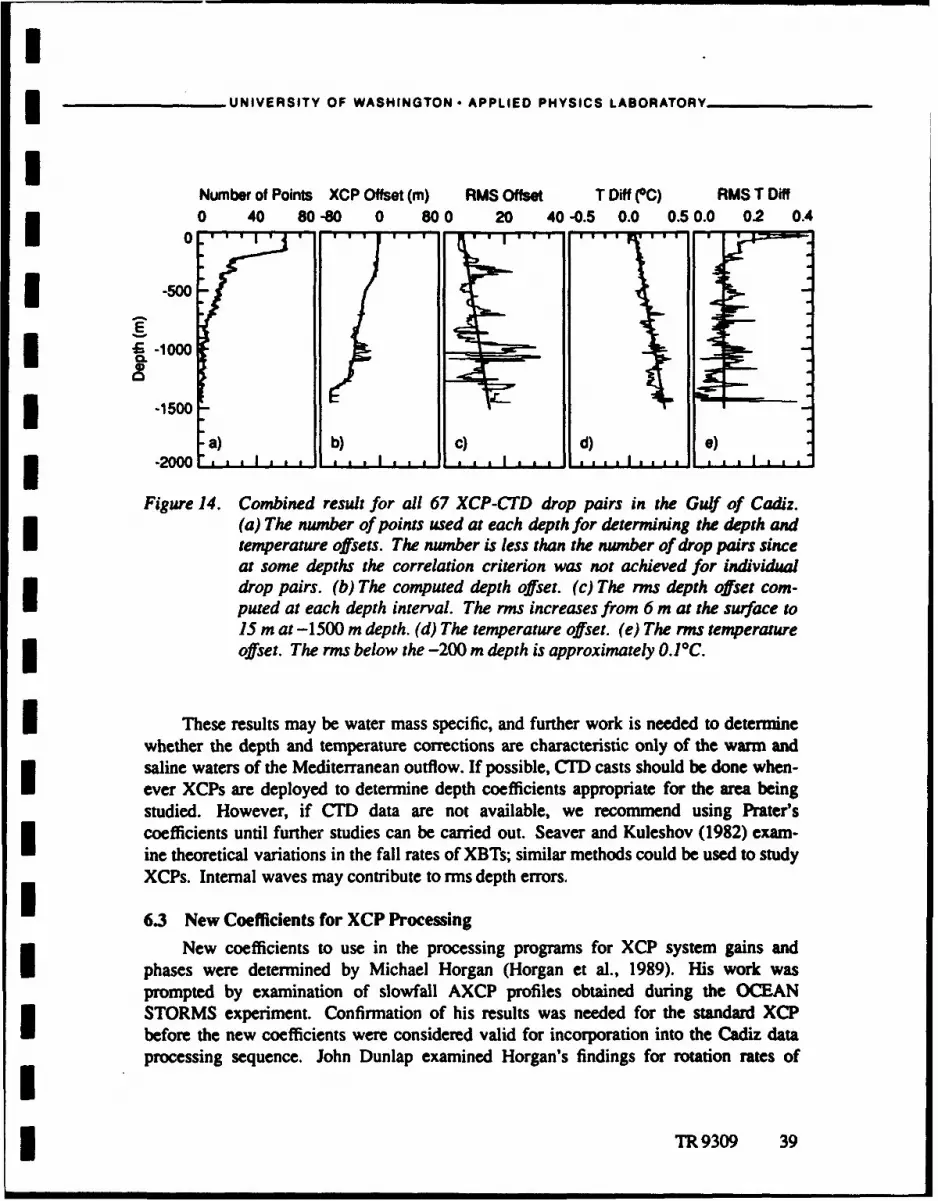
IUNIVERSITY OF WASHINGTON APPLIED PHYSICS LABORATORY
INumber of Points XCP Offset (m) RMS Offset T Diff (0C) RMS T Diff0 40 80-80 0 800 20 40-0.5 0.0 0.50.0 02 0.4
0* -500 -
ZS -1000
"a) b) c) d) e).2000M ' I I I 1 .I... Is , all . , I a l l .. L 1. ... . a A I .
Figure 14. Combined result for all 67 XCP-CTD drop pairs in the Gulf of Cadiz.(a) The number of points used at each depth for determining the depth andtemperature offsets. The number is less than the number of drop pairs sinceat some depths the correlation criterion was not achieved for individualdrop pairs. (b) The computed depth offset. (c) The rms depth offset com-puted at each depth interval. The rms increases from 6 m at the surface to15 m at -1500 m depth. (d) The temperature offset. (e) The rms temperatureoffset. The rms below the -200 m depth is approximately O.I°C.
I These results may be water mass specific, and further work is needed to determinewhether the depth and temperature corrections are characteristic only of the warm andsaline waters of the Mediterranean outflow. If possible, CTD casts should be done when-ever XCPs are deployed to determine depth coefficients appropriate for the area beingstudied. However, if CTD data are not available, we recommend using Prater'scoefficients until further studies can be carried out. Seaver and Kuleshov (1982) exam-ine theoretical variations in the fall rates of XBTs; similar methods could be used to studyXCPs. Internal waves may contribute to rms depth errors.
6.3 New Coefficients for XCP Processing
New coefficients to use in the processing programs for XCP system gains andphases were determined by Michael Horgan (Horgan et al., 1989). His work wasprompted by examination of slowfall AXCP profiles obtained during the OCEANSTORMS experiment. Confirmation of his results was needed for the standard XCPbefore the new coefficients were considered valid for incorporation into the Cadiz dataprocessing sequence. John Dunlap examined Horgan's findings for rotation rates of
TR 9309 39

1UNIVERSITY OF WASHINGTON - APPLIED PHYSICS LABORATORY
I14-18 Hz. The results of Dunlap's work are summarized by Kennelly et al. (1989b).The polynomial coefficients for gain and phase are listed in Table 4. The gains andphases are computed as a0 + a If + adJ2 . The a's at the end of the coefficient names Idenote amplitude; p's denote phase. Sanford et al. (1982) describe the meaning of eachof the coefficient names.
These new polynomial coefficients describe the measured gains and phases as a
function of rotation frequency for the entire XCP system from electrode and coil inputsto the digital output of the MK-10s. The original coefficients modeled only the analogsection of the probe from the inputs to points just prior to the V/F converters, and only thephase dependence on rotation frequency.
We conclude that the new coefficients are more accurate than the original ones for Ipredicting the MK-10 receiver output. However, the coefficients were determined foronly one XCP board set and may be different for other boards. The MK-10 phases are afunction of amplitude, and the variation of the coefficients as a function of board setshould be investigated.
Table 4. Horgan's new polynomial coefficients of gain and phase.
ao al a 2
Gefa 23866.12044581 107.99111272898 -0.905827321 1Gcca 1809.877761 -1.25653911 0.18856556
Gcoa 898.89564739 0.453188608 0.0717425016
Gefp -138.158938796 9.759010754 -0.180878978 1Gccp 29.826971133 10.265226263 -0.176531452
Gcorp 56.552652832 7.783581145 -0.112472607
Gevffa 494.66025
Gevfp '0I
Gcvja 500
Gc~fp 0
I40 TR 9309I

I__UNIVERSITY OF WASHINGTON . APPLIED PHYSICS LABORATORY
6.4 An
The copper compass coil wound coaxially around the electrode tubes is alignedsuch that its axis is nominally horizontal as the probe is falling. As the probe rotates, atime-varying potential difference is set up between the ends of the wire in the coilbecause the area of the coil facing the Earth's horizontal magnetic field (Fj,) is changingwith time. The strength of this potential difference is directly proportional to the area ofthe coil, the number of wire wraps, and the alignment of the coil axis with horizontal.3 Since the coil area and the number of wraps may change during manufacturing, wemeasure the amplitude of the potential difference, estimate F1,, and compute (wraps) xarea and call it "area." As the probe falls, it might tilt because of the vertical shear inthe ocean. This tilt causes the potential difference to change (the probe is nowmisaligned with the horizontal and is picking up some of the vertical magnetic field aswell). All the estimates of area are averaged and called A.,., and any deviation fromthis Am. indicates tilt of the probe (Sanford et al., 1982). A representative value ofA. for a particular data set should be determined prior to final processing. Previouswork shows that a value of 695 cm2 is appropriate for Mod 6 probes. Michael Horganinitially used this value in his calculations for Mod 7 OCEAN STORMS AXCPs, butlater determined an Am. of 667 cm2 for those probes. The average A.on value for allGulf of Cadiz XCPs deeper than 1000 m was 662.3 cm2 ± 8.2 cm2 . A change of 1 cm 2 inarea represents a change of 0.0027 m s'l in the v component.
6.S New C2 Value for XCPs
Michael Horgan also determined a new value for C 2 , a scale factor depending onthe sha ?e of the XCP that is used by the processing program xcppro. Using an A of695 cm and the Sippican Mod 6 depth coefficients, Horgan obtained a value ofC 2 = -0.0127. Because the Am,. and fall rate he used to compute C2 were notappropriate for the Cadiz data set, John Dunlap converted Horgan's C2 value to one suit-able for the A.. and fall-rate values determined for Mod 7 probes. Dunlap's method ofconversion is outlined by Kennelly et al. (19899b). He determined C 2 to be --0.035.
I 6.6 XCP Temperature Processing
John Dunlap developed a simple method for using probe calibrations in our XCPtemperature processing. Coefficients for a model of frequency versus thermistor resis-tance in the probe circuit were derived from the XCP calibrations values supplied by Sip-pican, Inc. Coefficients for a model of temperature versus resistance were derived fromthe Sippican thermistor specification. Dunlap's equation based on the model has beenincorporated into the new XCP processing programs and is described here.
3 The Mod 7 XCP temperature circuit frequency was modeled as
3 TR 9309 41

IUNIVERSITY OF WASHINGTON . APPLIED PHYSICS LABORATORY
F+ = (5)a C (R, + RI)
where a - 4.4, C is the value of the timing capacitor, Rt is the thermistor resistance, andR, is the value of a resistor in series with the thermistor. Sippican supplies a calibrationfor each XCP which gives two frequencies, FI and Fs2 , when two different resistors, R 1 IIand R12 , are attached to the XCP in place of the thermistor. This is done on the unpottedcircuit board before it is installed in an XCP. Resistors RtI and R, 2 are 16329 0 and4024 0, respectively, which corresponds to the Sippican thermistor specifications at 0and 30*C.
These calibration frequencies and resistances can be used to determine R. and C inEq. (5) as follows:
SFt, R 11 - Ft2 R 12 (6) 1F 2 -F, 1
and
a F, I (R, + R, 1)
Early probes used a timing capacitor with a tolerance of 10% and a potentiometer Iwhich was adjusted to give F, = 381 Hz when R, = 7855 0 (the resistance specified for150C). It was realized that this procedure did not produce the same transfer function forall probes.
Sometime after April 1984, the method was replaced with a fixed 1% resistor (R.)of 17,400 A and a parallel combination of three capacitors was used to obtain C such Ithat F, was close to 381 Hz with R, = 7855 C1 (see Sippican memorandum OM-7438,1984). This was done to make the variability from probe to probe less than 0.2*C overall,including the thermistor variability, which is approximately 0.1 *C.
The early probes had nominal component values of R, = 14,238 Q and C =0.027 pF, whereas in new probes R, = 17,400 0 and C =0.02362 pF. Note that any error Iin the model coefficient a is lumped in with C.
This circuit model can be used to process data from Mod 6 probes. In fact, the oldMod 6 method differs only in detail. Nominal calibration values for Mod 6 probes are IFt1 = 263.9 Hz and Ft2 = 475.3 Hz. The probes seldom deviate more that 0.2 Hz fromthose values, and thus individual temperature calibrations are not used.
It will probably not be necessary to use individual temperature calibrations with Unewer Mod 7 probes (neglecting the self-heating problems). They should be within0.2*C of each other.
42 TR9309

IUNIVERSITY OF WASHINGTON . APPLIED PHYSICS LABORATORY
IThe model of temperature, T, given thermistor resistance, R, is
I T- 1 2315 8cT = c In(Rj) + C2 Iln(R,) 2 + c3 -23.15. (8)
To obtain the coefficients Coc..3, we used the Sippican XBT thermistor specificationfor resistance R, versus temperature T as data for a polynomial least-squares fit to
11 y=Co+cIx+c2 x 2 +c 3 x 3 , (9)
where y 273.15 and x = ln(R,). The maximum deviation from the fit when using
data from -2 to 35.55°C was 0.01TC except at 35.000 and 35.55°C, where the pointsdeviated by more than three standard deviations. When those two points were removedfrom the fitting, the following coefficients were obtained:
co = 1.73323450654xl0- 3 (10)
c = 8.755085297563xlO- 5
C2= 1.640669605119xlO-°5
I 3 =-5.098817533782x10⁷
The standard deviation of the residuals from -2*C to 34*C is 0.004TC. This is muchbetter than the 0.2°C given in the XCP temperature specification.
Sippican Memorandum OM-7438 (1984) has coefficients for a fifth-order polyno-mial going directly from frequency to temperature for a nominal probe (Rs = 17,400 Qand C = 0.02362 gF).
T = co + (c, F,) + (c 2 F2) + (c 3 F3) + (c 4 F4) + (c5 F5). (11)
The residuals have a standard deviation of 0.010TC when using the thermistorspecification for -2 to 34TC. Examination of the residuals indicates that the fit used toobtain these coefficients included the faulty 35.00TC and 35.55TC points and that thestandard deviation would probably decrease if those two values were removed duringfitting.
Dunlap's method fit the data better than Sippican's although both fit much betterthan needed. Sippican's method can be improved by removing the 35.00( and 35.55*Cpoints. Dunlap's method offers a simpler solution for the model coefficients. Sippican'smethod offers somewhat speedier computation once the coefficients are obtained.
I
I TR 9309 43

IUNIVERSITY OF WASHINGTON . APPLIED PHYSICS LABORATORY
7. XCP PERFORMANCE NEAR THE GEOMAGNETIC EQUATOR UNear the magnetic equator (Figure 15), the XCP's performance degrades owing to
disappearance of the vertical component of the Earth's magnetic field. To understand Iwhat effects may be important near the magnetic equator, we examined the followingsimplified form of the equation for the magnetic north velocity component: n
- 4 Fh w w v
vxc=v-"V + w-w" + +j , (12)
where
V U, = velocity measured by the XCP (m s-l)v = magnetic north component of velocity (m s")
V• = conductivity-weighted vertically averaged velocity (m 51)Fh and F, = horizontal and vertical components of the Earth's magnetic
field (T)w and w = actual and assumed XCP fall rates (m s-l)H and L = vertical and horizontal length scales of the flow (m) I
N = electrode/electronic noise (V)1 = length of the electrode line (m).
Included in this equation is the desired velocity signal (v - v *), a fall rate term, aterm dependent on the characteristics of the flow, and a noise contribution. The practicalconversion of electric into velocity measurements involves approximations. Thus, the I(v H)/L term arises as a first-order correction to the zeroth-order approximation. Awayfrom the magnetic equator, this term multiplied by Fh/FZ is generally small (several cen-timeters per second) and mostly depth independent-hence it is usually neglected. Asone approaches the magnetic equator, however, F, begins to vanish. This causes termsscaled by FhIFZ to appear larger near the magnetic equator than at midlatitudes; thusdifferences between the assumed and actual fall rate and electrode/electronic noise con-tributions will be amplified near the magnetic equator. Also, the term characterizing theflow, H/L, which is neglected at midlatitudes, may become important in the vicinity ofthe magnetic equator.
From comparisons of XCP profiles with ones from the recoverable free-fall profilerTOPS (Hayes et al., 1984) near the geomagnetic equator, we determined that the XCP Uperforms well to within 1'°-2* of the magnetic equator, corresponding to FI/Fh = 0.05 inFigure 16. However, the north velocity component may degrade at latitudes greater than20 from the magnetic equator owing to terms in the north-velocity equation that are not inthe east-velocity equation. This comparison work is described in detail by Kennelly et al.(1986). The difficulties encountered with near-equatorial profiling arise from inaccurate
I44 TR9309

ILA
CL
0 I:'
0LL Ii I a
10 1.1 I 0
0D I x
0.I
0 co -
w
ov
OD cli i~j
TR 30 4

99
ýO 0 0 i IQ
39
LI
46 IR90

IUNIVERSITY OF WASHINGTON * APPLIED PHYSICS LABORATORY
Scompensation of the fall-induced sgnals for electronic noise, vessel interference, andphase angle differences.
XCPs can be used near equatorial regions, but their performance will be degraded.We would expect errors of 10 cm s-1 at 1.50 or so from the magnetic equator. If observa-tions are obtained outside the 0.05 FZ/Fh contour, data should be reliable.
9IIIIIIIIIIII
ITR 9309 47

1UNIVERSITY OF WASHINGTON * APPLIED PHYSICS LABORATORY 3
&. XCP PERFORMANCE NEAR THE GEOMAGNETIC POLE IWe have used XCPs up to a magnetic latitude of 850 (F/IFA = 10, Figure 16) and
have had no problems. We do not know from experience what magnetic latitude will betoo high for XCP operations. At very high latitudes, two effects should eventuallydegrade the signal. First, the compass coil signal will become increasingly small, as FIdecreases, until it can no longer be used. Fortunately, this is the strongest XCP signal, sovery weak F, values are required before it fails. Increasing the gain on the compasschannel could extend the latitude range if this were a problem. Second, the effect ofXCP tilt increases with increasing Fl/Fh, leading to increasing errors in velocity direc-tion because of tilt. This error is intrinsic to magnetic compasses. Within a few degreesof the magnetic pole (Figure 15), magnetic compasses will not work, because the fluctua- Itions in the magnetic field exceed its mean value. XCPs will fail there. Fortunately, thisexcludes only measurements in the Canadian Arctic Islands and on the Antarctic ice cap.The electric field signal increases at high latitude (with F.), so measuring this signal is Inot a problem.
IIIIIUIUII
48 TR9309I
I3 UNIVERSITY OF WASHINGTON . APPLIED PHYSICS LABORATORY
I9. FAILURES AND FIXES
XCPs exhibit two failure modes which can be rectified during data processing.These two modes are half coil and reversed coil. Half coil means that a probe has a valueof A,,.. that is half the usual value (approximately 667 cm2 for Mod 7 XCPs). The3 A. value is used in the XCP tilt correction. Reversed coil indicates that the probe waswired with the coil reversed. (Note: When the coil is reversed, it appears in the process-ing as if the electrodes were reversed since the reference is the coil.) It is thought thatmost of the wiring errors are coil wiring errors since those wires are easy to cross in theprobe assembly.
If these two failure modes are noted, flags can be set by editing the dropdatafile andsetting drop_.halfcoil or drop-revcoil to 1. The flags alert the program xcppro to handlethese drops as special cases. The documentation for xcppro, half coil, and reversed coilis given in Appendix 0.
During the Cadiz work, we found 4 of 184 probes (2%) with reversed coils and 2 of184 (1%) with half coils. When the software fixes were implemented, the data for theseXCPs appeared usable. However, a subsequent analysis of XCP offsets indicated thatone of the reversed-coil probes exhibited a larger offset in the v velocity component thanother XCPs launched closely to it in space and time.
IIIIIIII
I TR 9309 49

IUNIVERSITY OF WASHINGTON * APPLIED PHYSICS LABORATORY i
10. COMBINING XCP AND ADCP DATA i
The XCP measures relative velocity; that is, the horizontal velocity is known onlyto a depth invariant offset (Sanford et al., 1982). This is expressed as
vX1 P(z) = veb(z) - ý*. (13)
The offset il' (Sanford, 1971) is the conductivity-weighted vertical average of horizontal ivelocity. If the electrical conductance of the seabed is small compared with that of thewater column, and if velocity and conductivity are not correlated with depth, then PP = v-,the barotropic water velocity. If i* is known or can be estimated, then the absolute velo-city can be determined from Eq. (13).
Acoustic Doppler Current Profiler (ADCP) data, used in conjunction with ship's Iposition information (determined, e.g., from LORAN-C or GPS), provide a means ofreferencing XCPs to determine absolute velocities. The ADCP measures the velocity ofthe water at a given layer relative to the ship (v., 5(z)), while LORAN-C, GPS, or othership's navigation measurements give the velocity of the ship relative to the ground, thatis, to Earth's fixed reference frame (v,/,). The addition of these two measurements givesthe "absolute," or "true," velocity of the water relative to ground [vw,(z)]. Usingmeasurements from the XCP, the ADCP, and ship's navigation, we find
vabs(Z) = Vws(z) + Vslg = Vxcp(Z) + v*. (14)
If we let < > denote a vertical average over a range where the XCP and ADCP havedata in common, and denote a time average over the period when the XCP is falling, Ithen
< vs(Z) > = < Vws(Z)> + vs/g = < vycp(z)> + (15)
Since the XCP falls rapidly (approximately 4.5 m s-d), there is no extensive time averag-ing. Solving for i*, we find i
;* = - < VxCP(Z) > + < VWs(Z) > + vs/] • (16)
Using Eqs. (14) and (16), we obtain a vertical profile of absolute velocity, such that
Vabs(Z) = Vxcp(Z) - < Vxc,(z) > + I< vw,(z) > + V3/ . (17)
To implement this method, the ADCP and XCP velocity data should be averagedover some vertical interval satisfying the following criteria: 1
(1) The high-vertical-wavenumber internal-wave signals in the instantaneousvelocities obtained by the XCP but absent in the average ADCP velocities areaveraged out.
50 TR9309

IUNIVERSITY OF WASHINGTON * APPLIED PHYSICS LABORATORY
(2) Both the XCP and the ADCP returned good data over the interval (for theADCP data the percentage of good pings should be above 70%).
(3) The interval is deep enough to avoid mixed-layer and other near-surfaceeffects.
As an example of a suitable vertical interval, Prater (1992) averaged Gulf of CadizExpedition data over 100 to 190 m.
A method given by Joyce (1989) can be used to compute < vge(z) > by combiningthe ADCP and ship's velocities while correcting for possible errors in the ADCP align-ment and the ship's gyrocompass. The calculations are very sensitive to ship's heading.Therefore the heading must be known accurately. Poor results may be obtained duringturns, probably owing to the sluggish response of the ship's gyrocompass.
In Prater's implementation, he obtained a time series of < vats(z) > from the con-tinuous ADCP and ship's velocity data. Prater found it necessary to low-pass filter thedata using a 3-dB point of 2 hours to reduce the velocity variance due to noise in theLORAN-C measurements. He then sampled the filtered < vg(z) > time series at thetimes of XCP drops and used the resulting velocity values to modify vxcp(z). Because ofthe noise in the LORAN-C velocity estimates (rms error in velocity near 0.1 m s-l mostof the time) and the difference in the ADCP and the LORAN-C responses to changes inship speed, Prater found the data difficult to use in his analysis of a Mediterranean watereddy. The LORAN-C data also suffered from low signal-to-noise ratios as well as smallcrossing angles between stations, which contributed to the degradation of the velocityestimates. (The cruise on which Prater's measurements were obtained occurred in 1988,prior to 24-hour GPS coverage.) LORAN-C coverage also was poor because of the geo-graphic location of the cruise. However, the method does promise to be a useful way toreference XCP velocities, especial! - in light of improved ship positioning techniques.
Figure 17 illustrates the promise of Prater's method. The figure shows selectedpairs of XCP and ADCP profiles of east and north velocity from the Gulf of CadizExpedition. The dashed lines are an average of the ADCP data gathered while on sta-3 tion. The corresponding XCP data were obtained 20 minutes after the ship got underway from the CID station. Note the good agreement between features in the ADCP andXCP profiles. For plotting, the XCP data have been offset by 0.1 m s0. Because the
I ship was on station, no LORAN-C data were used in this comparison. The dotted linerepresents the difference between the ADCP and XCP profiles, the estimate of v*. Note3 that i* is relatively constant with depth.
I
3 TR 9309 51

IUNIVERSITY OF WASHINGTON APPLIED PHYSICS LABORATORY__
XCPi
ADCP (not absolute) --- -
Difference ................ u (n /s)
0 12 3
0
" I \ . I.. I /
• l : I" \ ' I
|I I.-30 I I I Ii
I . I "II
-300 " I
400
I II *I
.1oo ,*. " IA I
-400 .1•
0 12 3v (m/s)
II
Figure 17. Pairs of XCP and ADCP profiles of east (top) and north (bottom) velocityfrom the Gulf of Cadiz Expedition. The dashed line shows the average ofADCP data while on station. The corresponding XCP data were obtained
20 minutes after the ship got under way from the station.
52 TR9309

IiUNIVERSITY OF WASHINGTON . APPLIED PHYSICS LABORATORY
I 11. EFFECT OF FALL-RATE VARIATIONS ON NORTH VELOCITY
11.1 Introduction
If the fall rate, w, of the XCP is not well known, the computed north (v) velocitywill be in error. In this section, we first examine the equations governing the v com-ponent of velocity and determine the potential size of the error. Then, we present ananalysis of XCP data which illuminates the error in v. Finally, a model is proposed that3 explains the error in the XCP data in terms of variations in the XCP fall rate.
11.2 Theoretical Source of the Error
SThe equation for the geomagnetic eastward electric potential difference sensed bythe XCP is (Sanford et al., 1982)
3 -4 = Fl(v -i7)(1 + C1)- Fhlw(l + C 2), (18)
where Fh and F. are the Earth's horizontal and vertical magnetic fields, I is the electrodeseparation, C1 and C2 are XCP shape coefficients, and w is the vertical fall speed of theprobe relative to the water. Thus, the eastward electric potential measured by the XCP isdue in part to the northward motion of seawater through the Earth's vertical magneticfield, and in part to the vertical motion of the instrument through the Earth's horizontalmagnetic field. The equation for v is given by
- Fh (0+ C2 )=v- F/1(1+ C1) F, (I+C,) (19)
Let w = w0 + w'. where w0 is the empirical fall speed of the probe (see Section 6.2) andw' is any variation from the empirical value. The u velocity calculation does not dependon vertical velocity, so it is not affected.
Typical parameter values for the Cadiz data are
F, = 0.275F1, = -0.315C1 = 0.970C2 = -0.035.
3 Using these values, the expression for v becomes
V = Vrue - 0.56w'. (20)
I Thus, if w exceeds a few centimeters per second, this error in the v velocity maybecome noticeable.
I
3TR9309 53

IUNIVERSITY OF WASHINGTON - APPLIED PHYSICS LABORATORY 3
I11.3 Effect Found in Data
During analysis of XCP data from the Gulf of Cadiz Expeditioni, a "spike" wasobserved in the north (v) velocity component near 20 m on the vertical scale that did notappear in the east (u) velocity component (Figure 18a). A spike at the same verticalscale appeared in the rotation frequency (fw) of the XCP (Figure I8b). Profiles of f3show that the XCP turns 14 to 16 times a second (Figure 18c), but perturbations withvertical scales of 15 to 30 m (Figure 18d) are apparent. The rotation frequency is offsetfrom probe to probe but has the same characteristic "s" shape. The vertical scale of the
1 (a) (c) 0.8
10-2 0 4 0.
> .. .
" (90I.90
104 .- 1200 , •
104 .0
10-3 10"l 10.1 100 13 14 15 16 17 10-3 10-2 10.1 100
101 (b) .
10-0
10-4
g 1 0 iO ".. , -1200
10- L, -- 16 0
10,3 10 "2 10 ' 100 15 20 25 30 35Verlical Wavenumber (cyclm) V rticl Scale of fm Perturba•ons (m)
Figure 18. (a) Spectrum of v velocity as a function of vertical wavenumber computed Ifor eight XCPs having data at 1-m intervals from -1200 to-1600 m depth(dots). The spectra were then averaged (solid line). (b) Same as (a), but forIfrog. (c) Profiles of f,01 for the eight XCPs. (d) Vertical scale of the f,.t per-turbations. (e) Coherence of fo, and v for the eight XCPs. (f) Phase of fotand vfor the eight XCPs.
54 TR 9309 I

II UNIVERSITY OF WASHINGTON * APPLIED PHYSICS LABORATORY
perturbations is variable about 30 m above 800-rn depth, and tightly decreasingthereafter. The reason for the vertical structure of the perturbations is not known, but it
I may arise from how the wire comes off the XCP spool.
Values of fm and v are highly correlated (r = 0.9) at the vertical scale of the spike,with a phase difference of -125* (Figure 18e). Figures 18a, 18b, and 18e were madeusing data from depths of -1200 to -1600 m from eight XCPs. Repeating the spectralcalculations at different depth intervals produces the same feature, but at a different verti-cal wavenumber.
11.4 Effect Explained by Model
I A hypothesis for the source of the oscillations in frot and v is that the wire comingoff the spool induces a (somewhat) periodic upward force, causing the probe to slow andspeed its descent with the same periodicity. The fall-speed changes (the w" discussedabove), in turn, cause a change in ft which, because of the probe's moment of inertia, isphase shifted.
A model, based on work by D'Asaro (1983), was used to understand the couplingbetween w and frt better. The linear and angular momentum equations are
m'.- = g&n - CDApw 2 - FosinIf(z)] (21)
and
at - aw _ bfw, (22)
where (nominal values given in parentheses)
w = vertical velocitym = probe mass (1.9 kg, with decrease of 1.00 x 10--4 kg m'-
due to wire loss)g = gravitational acceleration (9.8 m s-1)
& = excess mass of probe in water (1.0 kg, with decrease of0.9 x 104 kg nf- due to wire loss)
p = density of water (1024 kg m-3 )CDA = drag coefficient times the probe's frontal area
F = amplitude of upward force exerted by the probe wireIfr = rotation frequency (16.26 Hz at the surface)
a = coefficient quantifying driving torque from dragon the probe's spin tabs
b = coefficient quantifying skin drag on the probe
TR9309 55

IUNIVERSITY OF WASHINGTON - APPLIED PHYSICS LABORATORY I
The coefficients CDA, a, and b were obtained from the near-surface equilibriumstate of the XCP. The forcing, F., was set at 0.12 N to match observed amplitudes of ftand v (Figures 18a and I8b and 19a and 19b). This model reproduces the fall rate of theprobe with depth (Figure 19c), the slow variation in fot with depth (Figure 19d), and thephase of fint and v (Figure 18e).
In summary, additional variance is input to the XCP v data at specificwavenumbers. The hypothesis that the v signal is caused by oscillations in the fall rate,w, is supported by a model of the XCP's dynamics. A preliminary correction to v can be
100 0. ISOIWI
10.1
S-400 90
10102
100
10-4 -1200 - 9(a) (c( (e)
1o -1 N . . -J . .1600 . .......1.0. .10.4 10-2 10"1 100 -4.4 -4.2 -4.0 10-3 10-2 10"1 100
Vertical Wavenumber (cyc/m) w (m/s) Vertical Wavem•bw (cyc/m) 3101 0 . 100
(b) (d)
i0~ -1200
10"s .1600m. . , r . n . 104'. ,.... . ....I ,,, ' T.=:..1i0- 10"2 10"' 100 ° 1 4 15 16 1 0 ~ ¶ . 0 0
14 101100p0o 10m
Vertical Wavenumber (cyclm) f,1 (Hz) Vertical Wamanmber (cyc/m)
Figure 19. (a) Model spectrum of v velocity. (b) Model spectrum of frot. (c) Model mUl(light line) and empirical (dark line) XCP fall rates. (d) Model f, o.(e) Model phase of frot and v. if) Spectrum of the corrected v velocity as am
1VI
function of vertical wavenumber computed for eight XCPs having data at1-rn intervals from -1200 to -1600 m depth (dots). The spectra were thenaveraged (solid line). 3
56 TR o30m

I UNIVERSITY OF WASHINGTON * APPLIED PHYSICS LABORATORY
made by using Eq. (19). The phase information between v (and therefore w) and f/ isknown from the data, and the magnitude of w can be estimated from the model.Figure 19f presents the v velocities from Figure 18a, corrected for the fall speed pertur-bations. Further understanding of the XCP motions is needed before more precise correc-
Itions can be made.
IIII
III
,-TR 9309 57

I
UNIVERSITY OF WASHINGTON* APPLIED PHYSICS LABORATORY
12. REFERENCES
Carlson, J. A., S. B. Hooker, M. S. Horgan, D. W. Jones, M. A. Kennelly, M. D. Prater, andT. B. Sanford, 1987: De Steiguer 1210-87 Cruise Report and Preliminary Results,APL-UW 8712, Applied Physics Laboratory, University of Washington, Seattle,WA, 45 pp.
D'Asaro, E. A., 1983: Near-surface behavior of the XCP (unpublished manuscript).
D'Asaro, E. A., T. B. Sanford, R. G. Drever, M.D. Morehead, and G. L Welsh, 1990: Air 3Expendable Current Profiling During the OCEAN STORMS Experiment,APL-UW TR 8916, Applied Physics Laboratory, University of Washington, Seat-de, WA, 66 pp. I
Hayes, S.P., H.B. Milburn, and E.F. Ford, 1984: TOPS: A free-fall velocity and CTDprofiler, J. Atmos. Oceanic Technol., 1, 220-236.
Horgan, M.S., R. G. Drever, and M.A. Kennelly, 1989: XCP Phase and Gain Tests,APL-UW 8924, Applied Physics Laboratory, University of Washington, Seattle,WA, 72 pp.
Joyce, T. M., 1989: On in situ "calibration" of shipboard ADCPs, J. Amos. OceanicTechnol., 6, 169-172.
Kennelly, M.A., P.A. McKeown and T. B. Sanford, 1986: XCP Performance near theGeomagnetic Equator, APL-UW 8607, Applied Physics Laboratory, University ofWashington, Seattle, WA, 42 pp.
Kennelly, M.A., M.D. Prater, and T.B. Sanford, 1989a: XBT and XSV Data from theGulf of Cadiz Expedition: R/V Oceanus Cruise 202, APL-UW TR 8920, Applied IPhysics Laboratory, University of Washington, Seattle, WA, 209 pp.
Kennelly, M. A., M.D. Prater, J. H. Dunlap, E. L. Kunze, and T. B. Sanford, 1989b: XCPData from the Gulf of Cadiz Expedition: RNV Oceanus Cruise 202, APL-UWTR 8925, Applied Physics Laboratory, University of Washington, Seattle, WA,206 pp.
Osse, T. J., R. G. Drever, and T. B. Sanford, 1988: The Design and Operation of aSlowfall AXCP, APL-UW 8808, Applied Physics Laboratory, University ofWashington, Seattle, WA, 46 pp.
Osse, T.J., T.B. Sanford, and M.S. Horgan, 1989: Improved measurements obtainedfrom modified expendable current profiler, Oceans '89, 5, 1598-1603, IEEE Publ INo. 89CH2780-5.
Prater, M.D., 1991: A method for depth and temperature correction of expendableprobes, J. Atmos. Oceanic Technol., 8, 888-894.
58 TR 9309 R

IUNIVERSITY OF WASHINGTON * APPLIED PHYSICS LABORATORY
Prater, M.D., 1992: Observations and Hypothesized Generation of a Meddy in the Gulfof Cadiz, APL-UW TR9210, Applied Physics Laboratory, University of Wash-ington, Seattle, WA, 143 pp.
Sanford, T. B., 1971: Motionally induced electric and magnetic fields in the sea, J. Geo-phys. Res., 76, 3476-3492.
Sanford, T. B., R. G. Drever, and J. H. Dunlap, 1978: A velocity profiler based on theprinciples of geomagnetic induction. Deep-Sea Res., 25, 183-210.
Sanford, T. B., R. G. Drever, J. H. Dunlap, and E. A. D'Asaro, 1982: Design, Operationand Performance of an Expendable Temperature and Velocity Profiler (XTVP),APL-UW 8110, Applied Physics Laboratory, University of Washington, Seattle,WA, 164 pp.
Seaver, G.A., and S. Kuleshov, 1982: Experimental and analytical error of the expend--- able bathythermograph, J. Phys. Oceanogr., 12,592-600.
Sippican, Inc., 1984: Ocean Systems Inter-Office Memorandum OM-7438 to R. Lancas-ter from M. DeConto, Subject: XCP Temperature Circuit Revision, dtd 20 April1984.
Sippican Ocean Systems, Inc., 1985: XCP Signal Processor: Operation and Mainte-I nance Manual, 488 pp.
I
TI909 5

I
-- APPENDIX A
Bibliography of XCP Publications
I
II
IIiIIII

II
Bartlett, A. C., M. A. Kennelly, E. L. Kunze, and T. B. Sanford, 1985: XCP Data from thePioneer Seamount/NOCAL Experiment, APL-UW 8509, Applied PhysicsLaboratory, University of Washington, Seattle, WA, 55 pp.
I Burns, D. A., and N. V. Lombard, 1982: Data Summary-XCP Profiles in the Vicinity ofthe Faeroe Islands during October 1980, NORDA Technical Note 142, NavalOcean Research and Development Activity, NSTL Station, MS, 185 pp.
Carlson, J. A., S. B. Hooker, M. S Horgan, D .W. Jones, M. A. Kennelly, M.D. Prater, andT. B. Sanford, 1987: De Steiguer 1210-87 Cruise Report and Preliminary Results,APL-UW TR 8712, Applied Physics Laboratory, University of Washington, Seat-tle, WA, 45 pp.
D'Asaro, E. A., 1984: Wind forced internal waves in the North Pacific and Sargasso Sea,J. Phys. Oceanogr., 14,781-794.
D'Asaro, E. A., 1988: Observations of small eddies in the Beaufort Sea, J. Geophys. Res.,93,6669-6684.
D'Asaro, E. A., and H. Perkins, 1984: A near-inertial internal wave spectrum for the Sar-gasso Sea in late summer, J. Phys. Oceanogr., 14, 489-505.
D'Asaro, E. A., T. B. Sanford, R. G. Drever, M. D. Morehead, and G. L. Welsh, 1990: AirExpendable Current Profiling during the OCEAN STORMS Experiment,APL-UW TR 8916, Applied Physics Laboratory, University of Washington, Seat-tie, WA, 66 pp.
Drever, R. G., and T. B. Sanford, 1980: An expendable temperature and velocity profiler(XTVP), Near Surface Ocean Experimental Technology Workshop Proceedings,Naval Ocean Research and Development Activity, NSTL Station, MS, 163-173.
Dunlap, J. H., R. G. Drever, and T. B. Sanford, 1981: Experience with an expendable tem-perature and velocity profiler, Oceans'81, 372-376.
Feeney, J. W., and T. B. Sanford, 1984: Velocity profiling in strong ocean currents, Proc.16th Annual Offshore Technology Conference, OTC 4835, 505-508.
Feeney, J. W., T. B. Sanford, and J. R. Haustein, 1985: Observing hurricane-driven wavesand currents, Proc. 17th Annual Offshore Technology Conference, OTC 4934,331-339.
I Glenn, S. M., G. Z. Forristall, P. Cornillon, and G. Milkowski, 1990: Observations of GulfStream Ring 83-E and their interpretation using feature models, J. Geophys. Res.,3 95, 13,043-13,063.
Gregg, M. C., E. A. D'Asaro, T. J. Shay, and N. Larson, 1986: Observations of persistentmixing and near-inertial internal waves, J. Phys. Oceanogr., 16, 856-885.
II TR 9309 Al1

II
Horgan, M.S., R. G., Drever, and M.A. Kennelly, 1989: XCP Phase and Gain Tests,APL-UW 8924, Applied Physics Laboratory, University of Washington, Seattle,WA, 72 pp.
Johnson, G. C., and T. B. Sanford, 1992: Secondary circulation in the Faroe Bank Chan- Inel Outflow, J. Phys. Oceanogr., 22, 927-933.
Jones, D. W., 1989: Velocity Profiler (XCP) Observations of a Bottom Boundary Layer inthe Strait of Juan de Fuca, APL-UW TR 8927, Applied Physics Laboratory,University of Washington, Seattle, WA, 209 pp.
Kise, R.H., W. Zenk, T.B. Sanford, and W. Hiller, 1985: Currents, fronts and eddy Ifluxes in the Canary Basin. Prog. Oceanogr., 14, 231-257.
Kennelly, M.A., P.A. McKeown, and T. B. Sanford, 1986: XCP Performance Near theGeomagnetic Equator, APL-UW 8607, Applied Physics Laboratory, University ofWashington, Seattle, WA, 42 pp.
Kennelly, M. A., M.D. Prater, J. H. Dunlap, E. L. Kunze, and T. B. Sanford, 1989: XCPData from the Gulf of Cadiz Expedition: R/V Oceanus Cruise 202, APL-UWTR 8925, Applied Physics Laboratory, University of Washington, Seattle, WA,206 pp.
Kunze, E., 1985: Near-inertial Wave Propagation in Geostrophic Shear, APL-UW 9-85,Applied Physics Laboratory, University of Washington, Seattle, WA, 90 pp.
Kunze, E., 1986: The mean and near-inertial velocity fields in a warm-core ring, J. Phys.Oceanogr., 16, 1444-1461.
Kunze, E., and T. B. Sanford, 1984: Observations of near-inertial waves in fronts, J. Phys.Oceanogr., 14,566-581. I
Kunze, E., and R. Lueck, 1986: Velocity profiles in a warm-core ring, J. Phys.Oceanogr., 16,991-995.
Kunze, E., and T. B. Sanford, 1986: Near-inertial wave interactions with mean flow andbottom topography near Caryn Seamount, J. Phys. Oceanogr., 76, 109-120.
Kunze, E., M.A. Kennelly, and T.B. Sanford, 1992: The depth dependence of shear Ifinestructure off Point Arena and near Pioneer Seamount, J. Phys. Oceanogr., 22,29-41.
Lillibridge, J. L., G. Hitchcock, T. Rossby, E. Lessard, M. Mork, and L. Golmen, 1990:Entrainment and mixing of shelf/slope waters in the near-surface Gulf Stream,J. Geophys. Res., 95, 13,065-13,087.
Osse, T.J., R.G. Drever, and T.B. Sanford, 1988: The Design and Operation of aSlowfall AXCP, APL-UW 8808, Applied Physics Laboratory, University ofWashington, Seattle, WA, 46 pp.
AA2 TR 9309

II
Osse, T. J., T. B. Sanford, and M.S. Horgan, 1989: Improved measurements obtainedfrom modified expendable current profiler, Oceans '89, 5, 1598-1603, IEEE PublNo. 89CH2780-5.
3 Paulson, C. A., and P.P. Niiler (eds), 1981: FRONTS 80: Preliminary Results from anInvestigation of the Wintertime North Pacific Subtropical Front, Reference 81-2,School of Oceanography, Oregon State University, Corvallis, OR, 108 pp.
I Prater, M.D., 1991: A method for depth and temperature correction of expendableprobes, J. Atmos. Oceanic Technol., 8, 888-894.
Prater, M.D., 1992: Observations and Hypothesized Generation of a Meddy in the Gulfof Cadiz, APL-UW TR9210, Applied Physics Laboratory, University of Wash-ington, Seattle, WA, 143 pp.
Price, J. F., M. 0. Baringer, R. G. Lueck, G. C. Johnson, I. Ambar, G. Parilla, A. Cantos,M.A. Kennelly, and T. B. Sanford, 1993: Mediterranean outflow mixing anddynamics, Science, 259, 1277-1282.
Sanford, T. B., 1980: Cruise Report and Preliminary Data Summary for USNS KaneXTVP Deployments, Technical Note 2-80, Applied Physics Laboratory, Univer-sity of Washington, Seattle, WA, 41 pp.
Sanford, T. B., 1982: Velocity profiling: Some expectations and assurances, Proc. IEEESecond Working Conj on Current Measurement, M. Dursi and W. Woodward,eds. (IEEE, New York), 101-112.
Sanford, T. B., 1982: Meteor Cruise 57: Observations and Preliminary Results, APL-UW8206, Applied Physics Laboratory, University of Washington, Seattle, WA, 31 pp.
Sanford, T. B., 1982: Meteor Cruise 57: Scientific Results, APL-UW 8213, Applied Phy-I sics Laboratory, University of Washington, Seattle, WA, 40 pp.
Sanford, T. B., 1986: Recent improvements in ocean current measurement from motionalelectric fields and currents, Proc. IEEE Third Working Conf. on Current Measure-ment, G. F Appell and W. E. Woodward, eds. (IEEE, New York), 65-76.
Sanford, T. B., J. H. Dunlap, and R. G. Drever, 1981: A Comparison of Velocity ProfilesObtained from an Expendable Temperature and Velocity Profiler (XTVP) and anAcoustically Tracked Profiler at the Atlantic Underwater Test and EvaluationCenter (AUTEC), APL-UW 8105, Applied Physics Laboratory, University ofWashington, Seattle, WA, 72 pp.
sanford, T. B., R. G. Drever, J. H. Dunlap, and E. A. D'Asaro, 1982: Design, Operationand Performance of an Expendable Temperature and Velocity Profiler (XTVP),APL-UW 8110, Applied Physics Laboratory, University of Washington, Seattle,
IWA, 164 pp.
I3 TR 9309 A3

II
Sanford, T. B., P. G. Black, J. R. Haustein, J. W. Feeney, G. Z. Forristall, and J. F. Price,1987: Ocean response to a hurricane, Part I: Observations, J. Phys. Oceanogr.,17, 2065--2083.
Smart, J. H., 1980: Direct measurements of vertical shears in the open ocean, Johns Hop-kins APL Technical Digest, 1, 284-288.
Spain, P. F., and T. B. Sanford, 1983: An Initial Determination of Seabed Electrical Con-ductances in the Florida Straits, APL-UW 8307, Applied Physics Laboratory,
University of Washington, Seattle, WA, 20 pp.
Spain P., and T. B. Sanford, 1987: Accurately monitoring the Florida Current with Imotionally induced voltages, J. Marine Res., 45, 843-870.
IIIIIIIIIUII
A4 TR 9309

I
II
i APPENDIX B
Instrument SettingsUUIIIIUIIIIUII

IIDevice Codes for HP9020 and peripherals:
Cartridge Tape Drive (HP9144) :CS80,503,0Floppy Disk Drive :CS80,7,1Internal Drive (Winchester) :CS80,7,0
The VCR play time is about 2 hours; it ends at about 5750 on the counter. The VCRshould be set to
Speed SpMPX filter Manual
Input LineSTape RemainN NOR(mal)Meter Audio LevelHiFi
Audio Select StereoAudio Record Level 10 dB (when a drop is in progress)
The Sony PCM and ac Power Adapter should be set to
I Mute OffCopy OffInput LineTracking Off
The MK-10 radio frequencies are
Channel 10 169.0 MHzChannel 12 170.5 MHzChannel14 172.0MHzChannel 16 173.5 MHz
The Gold Line, Digital RTA should be set toSCALE 3 dB/stepWEIGHT FLAT
* DECAY FAST
AVG onPEAK offPK-HD offRTA onSTORE offDISP offOPTION off
The transmitted signals that will appear on the Spectrum Analyzer are
Temperature 0.35 kHzElectric Field 1.20 kHzCompass Coil 2.40 kHzCarrier 8.00 kHz
II TR 9309 Bi1

IIII
I APPENDIX C
XCP Launch Checklist
IIIIIIIB
IIIIII

I XCP LAUNCH CHECKLIST
I DROP # PROBE S/N MOD CHANNELInitials Expiration Date
* Date Time
PREDROP TESTS: These tests should be done long before the drop, so thatI if a replacement XCP is needed there is time. DOQNQT remove the tapes and
rubber band until just before launch.
I TEST Check that the appropriate channel MK-10. is on. Turn the dial onthe Patch Panel to the proper channel and listen using the headphones. Youshould hear noise. Be careful when attaching power to the XCP's,connecting power to the wrong wire will cause the airbag to inflate. Thereare two wires without insulation on them. One wire is much longer thanthe other, this one is the squib wire and should NOT have power applied toit. Be sure squib wire does not touch case.
SQUIB WIRE FREE
I The other wire is about 1 cm long. Using the 12 V power supply, connectthe test clip (+12V) to the wire on the side of XCP and (-) to case. Turn on
Spower supply. You should hear quieting.
QUIETING
AF TEST Connect 3 pronged XCP test cable to the power supply. Becareful with the test probe, it carries 24 volts of power on it. Apply powerto the test points on XCP. Be careful of the orientation of the test probe.Listen for XCP tones. You should also see three peaks on the spectrum
I analyzer for Temperature (0.35 KHz), Electric Field (1.2 KHz) , and CompassCoil (2.40 KHz).
I XCP TONES
I PEAKS: Temp EF CC
CC TEST Wave magnet over XCP electodes. Listen for warble.
CC wiggle
Comments:IBe sure to fill out opposite side of this checklist!!!!!
TR 9309 Cl

IDROP # PROBE#__
VISUAL EXAMINATION OF AGAR Remove the 2 pieces of tape overelectrodes. Remove clear plastic that keeps the tape from touching theagar. Check the condition of the agar surrounding the electrodes and notebelow. If the probe is to be dropped immediately continue with checklist,otherwise replace clear plastic and tape over electrodes until launch time.
Agar Condition I
TO LAUNCH:
Remove 2 pieces of tape over electrodes and attach to this log sheet below. IMake sure the clear plastic that keeps the tape from touching the agar isalso removed.
TAPES_ _
II
* Remove 2 pieces of fiberglass tape at lower end of unit and tape below.
TAPES_ _
III
Remove rubber band and tape here.
RUBBER BAND_ _
* Remind bridge to maintain radio silence. I
C2 TR 9309 I

UIII
APPENDiX D
XCP Log Sheet
IIIIIIIIIIIIII

Drop # Probe S/N Channel3 Initials DateVCR Tape No. Counter Start StopI Floppy Disk No. HP9144 Tape No
Times to the nearest 5 or 10 seconds (GMT):Launch (RF on)Drop (AF on)Wire Break (AF off)Scuttle (RF off)
Latitude Longitude
Launch Position Method_ _ _ _ Method
MethodRange and bearing to mooring
Receiver used: ConfigurationI Drop Guality: Good _ Fair_ _ Bad
Depth of deepest dataFy Fz3 Simultaneous withShip speed Heading.Wind (wrt ship): Speed _ HeadingWaves: Height PeriodSea Surface Temp Method3 Method____
Water Depth
3I Comments:
TR9309 D1

III
IIi

I DROP CHECKLIST
i XCP ! XBT I xSV I I
I Drop '
Partition ready for probe type 1 I:J 2 3 I
* Check cable link to partition to find
MKIO Chf' 10 1 1 12 I 14 - ' 16I part I part I part 2 part 3
Probe Ch* 10 I 12 I 14 I 16 E IIProbe Serial
I Tapes and rubberband removed from probe Ii (see XCP Checklist)
e Check cable link to partition to find
MK 9 Top I 2 Bottom r 3Ipart 2 part 3
Probe Type (HP9020)
9 Answer questions on screen
e Load Probe
I Passed Prelaunch check (XBT only)
* Tape in VCR (count <5750) --
e VCR recording I
a Floppy in Drive j
9 HP9144 Cartridge tape running E1
* Drop probe and fill out XCP and underway logs
TR 9309 E I

I I l
I
APPENDIX F
$$ Storage Formats for XCP Data from HP-9020 Acquisition Program
IIII
IIIIII

II
F.1 Raw Data (as on HP9144 cartridge tape)
-- each record will look like2*.17 true header
n* 32* 30*17 data stream from MK101 2* 17 footer header
where n is any number and the true header is formatted
where "#,5AX,6D,22X";M$Hblen
M$ is the probe type ("7" or "7S") andHblen=32*(Nread+Nh I +Nh2), Nread=30*Nbps, Nh l =Nh2=Nbps= 17is the number of bytes following the true header.
The footer header contains the time stamp and the dropname formatted
"#,A, 12Z.DDD,AD, 13AXX";"T",TIMEDATE,"P",Part," "&Drop$
The data stream from the Mk- 10 consists of noise and 17-byte strings D$
Dinp(3)=BINIOR(NUM(D$[4; 1 ]),SHIFT(NUM(D$[5; 1I),-8))IDinp(5)=BINIOR(NUM(D$[8; 1 ),SHIFT(NUM(D$[9; 1)),-8))
Dinp(6)=BINIOR(NUM(D$[14; 1 ),SHIFT(NUM(D$[15; 1 ]),-8))Dinp(7)=BINIOR(NUM(D$[6;1]),SHIFT(NUM(D$[7;1]),-8))Dinp(8)=BINIOR(NUM(D$[12; 1]),SHIFT(NUM(D$[13; 1 ]),-8))Dinp(9)=BINIOR(NUM(D$[ 10; 1 ]),SHIFT(NUM(D$[ 13; 1]),-8))Dinp(10)=BINIOR(NUM(D$[ 16; 1 ]),SHIFT(NUM(D$[ 17; 1 ]),-8))
Dinp(4)=BINIOR(NUM(D$[2; 1]),SHIFT(NUM(D$[3; 1]),-8))
U and D$[ 1;1] is a sync byte = "G" or "B" if stream is in sync.
IIUII
I TR 9309 F1

II
F.2 Processed Data (as on floppy diskettes)
The processed data are in BDAT files with OVERLAP, BUFFERED ON, MAX-BUFFS 4, and
filename Drop$=Mf$modayhrmin&"_"&VAL$(Part)
I where Mf$="VF" for fast velocity drop and mo, day, hr and min are all 2-digit integers;e.g., VF06132043_1 represents a fast XCP drop started by partition 1 at 2043h on13 June. These files contain a list of the integers
Iz, It, lu, Iv, Ierr
I where
SIz=z*10 ! z in mIt=SGN(T)*MIN(ABS(T),32)* 1000 !T in 0CIu=SGN(u)*MIN(ABS(u),320)* 100 !u in crn/sIv=SGN(v)*MIN(ABS(v),320)*100Ierr=-SGN(Veler)*MIN(AB S(Veler),320)* 100
IIIIIIIII
ITR 9309 F2

IIII
i APPENDIX G
XCP Processing Program Overview, xcpover
IIIIIIIIIIIIII

I XCPOVER (1) UNIX Programmer's Manual XCPOVER•(1)
1 NAMExcpover - overview of XCP processing
SYNOPSISawk -f mag.in.awk prpos.out I \geomag I \awk -f mag.outawk I \hdrmerge dropdatafile
awk -f extras.awk prpos.out I \hdrmerge dropdatafile
cadiztape -p channel < kunzetapefile I \xcpsplit debug channel ouIype filenamefile rawdirectoryxcpsplit debug channel outtype filenamefile rawdirectory < dasarotapefile
I remsh apl-em -n frd9t -n -b2048 I\xcpdrtop > rawdirectory/drop
I remsh apl-em -n 9845cat -r /dev/hp9895.0/drop I \uxarc I \xcpdrtop > rawdirectory/drop
xcpftoi [-dD] indir infile filenamefile rawdirectory
xcpfloat < rawdirectory/drop I \xcpaddt xcpaddt.p dropdatafile I \xcpturn xcptun.p dropdatafile
3 xcpfloat < rawdirectory/drop I \xcpaddt xcpaddt.p dropdatafile I \xcpblf -c xcpblf.p dropdatafile Ixcppro xcppro.p dropdatafile Ixcpgrid xcpgrid.p I\xcpplot I \hpp7
DESCRIPTIONThis set of programs implements the functions of old XCP processing programs tapetogpl, xpro, and xgridusing a number of simpler programs. XCP processing in xpro included so many functions that it wasdifficult to maintain. There were many variants to do different things and no one version existed for thegeneral user. This group of programs modularizes the processing. An attempt was made to split the pro-cessing into functional groups. Hopefully modules are easier to understand and modify thus encouragingclearer processing development in the future.
SThe programs allocate main memory for the entire input file and output data so that multiple passes can bemade on the data. This allows the programs to be written simply but does require more system resources.This should not be a great problem as the XCP files are not extremely large.The data base of raw files is kept as small as possible by keeping it in 16 bit integers.DROP DATA FILEA small data base, dropdatafile, was developed for the processing parameters that are known to changefrom drop to drop. This data base is an ASCII file so that it can be easily modified by hand with an editingprogram. This is for the cases where it is not possible to obtain correct values automatically, e.g., the start
Local May 31, 1991 TR 9309 GI

3 XCPOVER (1) UNIX Programmer's Manual XCPOVER (1)
I and stop turn numbers may be hard to determine for some drops for various reasons. Various programsmodify and add to the data base for items such as the geomagnetic field, start and stop turn numbers, etc.
GEOMAGNETIC FIELD
The earth's magnetic field at each XCP drop site is obtained from 8eomag by using times and positionsfrom the log. Awk uses mag.in.awk to reformat the log file into the format required by geomag. Awk is runagain with mag.out.awk on the output of geomag to format the results correctly for inclusion in thedropdatafile data base. hdrmerge actually adds new entries or replaces previous entries in the data base.
Here is mag.in.awk used for the Cadiz data:
BEGIN jFS - "\t"print "y"I- print "/usr/local/geomag/igrf"print "9"
$7 =ffi "XCP"{drop - $8date - $1lat - $2lon = $4yr - substr(date,1,2) # year past 1900, e.g, 91 means 1991.mo = substr(date,3,2) # month number, e.g., 3 for Marchda - substr(date,5,2) # day numberlatd - substr(lat,1,2) # integer degreeslatm - substr(lat,4,5) # minutes.hundredthslath - substr(lat,10,1) # N or Slond - substr(lon,1,3) # integer degreeslonm - substr(lon,5,5) # minutes.hundredthslonh = substr(lon,11,1) # E or Wprintf "%-8s 19%02d %02d %02d %2d %05.2f %s %3d %05.2f %s\n",\
drop, yr,mo,da, latd, latm, lath, lond, lonm, lonhIHere is the version of mag.out.awk used for the Cadiz data
# mag.out.awk# modifies the "geomag" batch output for the XCP data base# this output should be piped into "hdrmerge" to modify the data base.# see "mag.in.awk" for the "geomag" input
BEGIN Iline = 0;I}line ++;
# skip first two lines of geomag outputif(line<3)
continue;
drop = $1;yr = $2;mo = $3;da - $4;
Local May 31, 1991 TR9309 G2

I XCPOVER (1) UNIX Programmer's Manual XCOVER (1)
U latd - $5;latm - $6;lath - $7;lond - $8;lonm - $9;lonh - $10;fh $11;fh *- 1.0e-5;fz - $12;fz -1.0e-5;magyar - $13;printf %# %s lat %2d %05.2f %s\n",drop,latd,latm,lath;printf " % %s_Ion %2d %05.2f %s\n",drop,lond,lonm,lonh;printf "# %s_fh %5.3f\nudropfh;printf "4 %s_fz %5.3f\n",drop,fz;if(magvar < 0)
printf "# %s3magvar %6.1f W\n",drop,-magvarelse
printf "# %s3magvar %6.lf E\n",drop,magvar
EXTRA PARAMETERS IN DROP DATA FILEHere is the version of extras.awk used for the Cadiz data. As many additional parameters as desired can beadded in any manner for later use by later processing programs. The following two parameters arerequired by xcppro only to add them to the output file header. They are not used in any xcppro computa-
U tions.
BEGIN IFS - "\t"
$7 -- "XCP" (drop - $8printf "4 %s3serialno %s\n",drop,$29printf "# %s_launchtime %s\n",drop,$1
1 XCPSPLIT
Xcpsplit is used to transfer the raw data from the HP-9020 Basic acquisition program files into separatefiles, one per drop. There is lots of extra rubbish in the raw files to be sure no data is thrown away duringacquisition.
XCPFTOI
Data files from Eric D'Asaro's "tapetogpl" program are converted to the new 16 bit format by xcpftoi.
XCPFLOATXcpflooi converts the 16 bit integer data from xcpsplit into 32 bit floating point values to make a standardGPL file. Xcpfloat can be run with the -ms option on the command line to make output suitable for input toEric D'Asaro's "xpro3" or "xpro4" processing programs.
XCPTURNI Xcpturn is used to find the turn numbers where the drop starts and ends. These are added to the
1I
Local May 31, 1991 TR9309 03

XCPOVER (1) UNIX Programmer's Manual XCPOVER (1)
dropdaafie data base for later use by xcppro and possibly other programs in the future.
PROCESSING
Xcpaddt, xcpblf and zcppro actually perform the processing previously done in xpro. Xcpgrid averages thedam onto a uniformly sampled depth grd.
DISPLAYXcpplot displays data from xcpgrid using standard scales on the HP-7550 pen plotter. This program is usedto make the books of standard plots. Gpl()) can also be used for other more refined plotting.
CHECKING START AND STOP POINTS
The following C-shell command file will plot the output of xcppro near the beginning of a drop. This isuseful to check that xcpturn found the correct points. The user may modify the dropdatfile by hand ifthese points seem incorrect.
#! /bin/csh@ ref - 'grep $drop"_turnhalf" dropdatafile I awk It print $3 I@ start - $ref - 50@ stop - $ref + 50xcpfloat < split/xcp$drop I \xcpaddt xcpaddt.p dropdatafile I \xcpblf xcpblf.p dropdatafile I \xcppro xcppro.p dropdatafile I \pick diag-0 tag-turn.$ref start-$start stop-$stop I \gpw zoom.cf
By replacing turnha/fabove with turnstop the end of the drop may be ploued.
DREVER RECEIVERHP-9845 DXGET files from the XTVP-DR (Digital Receiver or Drever Receiver) archived on 800 bpi ninetrack tape using the HP-9845 XARC4 program are transferred to the HP-9050 (apl-em) with frd9t. thenxcpdrop converts XARC4 format to xcpfloat input format:
#!/bin/shfiles-"filel file2 file3 ... "
frd9t -r -b2048 tape.idfor file in $filesdo
echo $filefrd9t -n -b2048 I \xcpdrtop > rawdirectory/$file
donefrd9t -b2048 tape.end
HP-9845 floppy disks with raw XCP data from the XTVP-DR are copied to the HP-9050 (apl-em) usingthe attached HP-9895 dual floppy disk drive with:
# !/bin/shunit-0 # 0 for the left unit; 1 for the right unit.files-'98451s /dev/hp9895.$unit I awk '(print $1)'"for file in $filesdo
echo "file-$file"
Local May 31, 1991 TR9309 G4

IXCPOVER (1) UNIX Programmer's Manual XCPOVER (1)
9845cat -r /dev/hp9895.$unit/$file I\uxarc I \
doe xcpdrtop > rawdirectory/$file
uxarc converts the raw floppy disk data to XARC4 format suitable for input to xcpdriop.I SEE ALSOawk(1). geoinag(1). bdrmerge(I), cadiziape(l), xcpspliL(1), xcpftoi(1). xcpfloar(1), xcpaddt(1), xcpwum(1).xcpblf(I). xcppro(I). xcpgrid(1). xcpploc(1). pick(l)I AUTHORJohn Dunlap, Applied Physics Laboratory, University of Washington
LoaIa 1 19 R39 G

IIII
I APPENDIX H
hdnnerge Documentation
IUIII
IIIIIIII

I HDRMERGE (1) UNIX Programm'ers Manual HDRMERGE (I)
INAME
hdrmerge - add or replace data in headers of GPL files
SYNOPSISbdrmerge filename
DESCRIPTIONHdrmerge modifies the GPL header in filename according to another GPL header from standard input. If aheader label from standard input does not exist in filename it is added to fiename. If a header label fromstandard input exists infilename its value infilename is changed to that from standard input.
If the header labels a-values and aquan exist in filename and their product is greater than zero then float-ing point binary data is assumed to follow the header in filename. This data is rewritten after the modfied
SFILES header infilename.
/usr/loca!/bin/hdrmerge
SEE ALSOxcpover(l)
DIAGNOSTICSBUGSAUTHOR
John Dunlap, Applied Physics Laboratory, University of Washington
IIIII
I
Local February 28, 1989 TR 9309 HI

IIIII APPENDIX I
xcpsplit Documentation
IIIIIII
III

XCPSPLIT( 1) UNIX Programmer's Manual XCPSPUT( 1)
INAME
xcpsplit - Split XCP HP-9020 BASIC acquisition files into separate dropsI SYNOPSISxcpsplit debug partition outtype namefile outdir < basicfile
DESCRIPTIONxcpspli separates XCP acquisition data into files, one per drop, suitable for the rest of the XCP processingprograms. The XCP acquisition runs on an HP-9020A (HP-9000 model 520) computer running the HP-BASIC operating system. A master program. MASTER.READ (two versions: D'Asaro and Kunze), andup to three partitions, PART.READ (D'Asaro) or XCP.READ (Kunze), one per MK-10 receiver, are usedin the multitasking environment.
The acquisition files were written on HP-9144 cartridge tape for Ocean Storms and Cadiz data but can alsobe written on other media. When xcpsplit is run the files have been copied to disk.
To transfer the HP-9144 tape data to the HP-UX system on the HP-9050 or HP-9020 mount the tape as aread-only file system and copy the files. The tapes cannot be mounted on the series 300 (faraday) comput-ers; they have a series 500 file system and so must be mounted on a series 500 computer. Insert the write-protected tape, then type:
/etc/mount /dev/mtc3 /mtc -r
The HP-9000 model 550 HP-UX software revision 5.21 with the patched /etc/mount command emits thefollowing erroneous warning message which should be disregarded.
/etc/mount: :Bad addresswarning: /dev/mtc3 may not be clean
Use the following command to show the file name and size on the tape.
ls -i /mtc
A single file with a default name of "DATA" should be present. It may be as large as 16 Mbytes.
To copy the data from tape to disk use:
cp /mtc/DATA basicfile
To unmount the tape when finished.
/etc/umount /dev/mtc3
Now remove the tape from the drive by pressing the unload button and waiting until the BUSY light goesOut.
It is important to NOT read the tapes more than a time or two as they will wear out with repeated accessesby the HP-UX system. This method of reading from a mounted tape in HP-UX is not easy on the stream-ing HP-9144 tape or tape drive. The drive repositions every 1 Kbytes since the operating system does nothave the ability to stream the drive in the mounted mode. (Normally, tcio is used with cartridge tapes butthat won't work in the mounted mode).
The files from Eric Kunze's version of the HP-9020 BASIC acquisition programs are piped through cadiz-tape before being processed by xcpsplit. This is to remove the XBT and XSV data which xcpsplit does notaccept. For Eric D'Asaro's version xcpsplii accepts the original BASIC file directly.
Local October 17, 1990 TR9309 I1

XCPSPLIT( 1) UNIX Programmer's Manual XCPSPLIT( 1)
If debug is greater than zero various diagnostics are printed on siderr. The higher the value the more isprinted.
Data is extracted from the tape from partition which corresponds to the partition number XCP.READ ranunder in MASTER.READ.
If owtype is short then files with integer dataare produced. This is the recommended usage in order tosave space. Xcpfloat converts these files for use by the rest of the processing programs. When outtype isfloat then a true GPL file is produced which is the same as that produced by the output of xcpflot above.Both outype short and float files have the same GPL header except for the datatype entries for eachvariable.
The namefile is a file which provides the correspondence between the original BASIC filenames and newfilenames which are the drop number. If there is no entry in namefile the original BASIC filename is usedfor output. An example of one line in the namefile for the Cadiz cruise using Eric Kunze's BASIC acquisi-tion program is:
# VF09112242_1 2466
An example for the Ocean Storms data using Eric D'Asaro's BASIC acquisition program is:
# Oct23/1036_1 2201
Output files with names found in namefile are created in the ouldir directory.
drop in the GPL header is set the same as the output file name. This drop number is used later in xcppro tolook up values in the dropdatafile.
An example for splitting partition I of tape number 6 of the Cadiz data is:
cadiztape -p 1 < SEP11.tape6 I xcpsplit 0 1 short fn.cadiz splitdir
FILES/usr/local/bin/xcpsplit/usr/tmp/xtmp.xxxxx where xxxxx is the process id of the job.
SEE ALSOxcpover(l), cadiztape(1)
DIAGNOSTICSBUGSAUTHOR
John Dunlap, Applied Physics Laboratory, University of Washington
Local October 17, 1990TR9309 12

I ~APPENDIX Jxcpftoi Documentation

XCP~Ol(1) UNIX Programmer's Manual XCPFrOI (1)
INAME
xcpftoi - convert XCP files from floating to integersSYNOPSIS
xcpftol [-dD] Wnd& lookup filenamefile outdir
DESCRIPTIONXcpfioi converts files made by tapetogpl to files that have the same format as xcpsplit output files. All thedata except the HP-9020 time stamp is converted from 4 byte floating point to 2 byte integers for morecompact disk storage. Xcpfloar with the -ms option will quickly convert these files to input acceptable tothe old xpro3 and xpro4 programs.
The -4 option of zcpftoi turns on some diagnostic output on standard error. The higher the value of D themore is printed.
The input file name is made up by concatenating indir and lookup. Lookup is also used to look up the dropname in filenamefde. The output file name is formed by concatenating outdir and the drop name.Filenamefile is a GPL header style data base with one line per drop. An example for drops 2201,2202 and2203 is shown below:
# 0ct23/1036_1 2201# 0ct23/1038_2 2202# 0ct23/1036_3 2203
This will work with the following example command line:
xcpftoi -axcp/oceanstorms/raw Oct23/1036_1 fn.os ftoi
to read the file axcpo n s/aw/0ct231l036_ and write the file ftoi/2201.
The fdenamefde for oceanstorms, fn.os, was formed by the following awk job:
P-/e/users/axcp/oceanstorms/paramrm -f awk.outfor i in 'cat list.os,do awk -f fn.os.awk < $P/$i >> awk.out
done
I where "list.os" is a file containing the drop numbers (parameter file names) and "fn.os.awk" contains:
/# flight / 4 flight-$3/'# droprealtime / I file=$3 }
/#drop / { drop-S3 )END I printf "# %s/%s %s\n",flight,file,drop}
U FILES
SEE ALSOxcpfloat(l), xcpsplit(l), xcpover(l)
DIAGNOSTICSBUGSAUTHOR
John Dunlap, Applied Physics Laboratory, University of Washington
ISLocal February 28, 1989 TR 9309 Jl

IIII
I APPENDIX K
xcpfloat Documentation
IIIIIIIIIIIIII

U XCPFLOAT( 1) UNIX Programmer's Manual XCPFILOAT( I)
NAMExcpfloat - converts xcpsplit output to GPL fortna3 SYNOPSISxcpfwoat [-sli-s]
DESCRIPTIONXcpfloa reads standard input and writes standard output. The input is asaumed to come from zcpsplit out-put and the output is a GPL file. The data base is usually kept as xcpsplit output files which are 16 bitintegers to conserve space. All the processing programs use floating point values in the files.
The -ms option converts the time variable from seconds to milliseconds in order to be computable with theold xpro3 and xpro4 programs. The -s option (default) leaves time output in seconds.
FILESI F /usr/local/bin/xcpfloat
SEE ALSOxcpover(l)
DIAGNOSTICSBUGSAUTHOR
John Dunlap, Applied Physics Laboratory, University of Washington
L o hnl Dulp ple hsc a O catobyUierst of 19a0hington K
IIIIIIIIIU3 Local October 5, 1990 TR 9309 KI

UIII
APPENDIX L
xcpturn Documentation
IIIIIIUIIIIIII

XCPTURN (1) UNIX Progmrammer's Manual XCT (IURN ()
m NAME
xupturn - determine whtm XCP drop starts and stops turnigm SYNOPSIS
xcpturn 1maafile drpdautfile [in urleg
DESCRIPTIONXcpturn fxnns hroainequency rcdofa drop to determine when it was released horn the sur-Xclunexamines the rotation frq ency rdto
face and when the drop terminated at die bottom. The turn number at half the average rotation frquencysoon after it has spun up as well as the turn number for the last turn with good data are added to thedropdatafile data base for later use by xcppro(l).
Standard input is used for the input unless the input file, infle is specified.
paramfile contains some run time parameters in GPL header format as described below.
debug is set to 0 normally. For more diagnostic output increase the value.
timeusedshould be set to twaster.
rotfsln, rotfmaxare the minimum and maximum rotation frequencies allowed in the computations.
mavg, diffmax, nokneedame used to determine the end of the drop. The drop is considered to stop at the last turn where thedifference between its rotation frequency and the average for the previous mavg turns is morethan diffmax for nokneed turns in a row.
The following is an example paramfde.
# debug 0
# timeused tmaster# rotfmin 2# rotfmax 20# mavg 20# diffmax 1# nokneed 20
An example of the two records added to the dropdatafile for drop 2208 are:
# 2208_turnhalf 740# 2208_turnatop 5947
FILES /usr/local/bin/xcptum
SEE ALSOxcpover(l)
DIAGNOSTICS -BUGS
The start of the drop depends on the downturn value in the header of the input file. This is computed inxcpaddi(l). The average from 30 to 50 turns past downturn is used to get the average rotation frequencynear the beginning of the drop. This is not good practice - the code should be put all in this program. Andthe use of magic numbers is poor.
1 The end of drop algorithm works fairly well for the drops that hit the bottom but does not find the pointwhere the wire starts to stretch just before breaking when the probe spool is exhausted. Thus there amany times 20 turns of data near the end of a deep drop where the fall rate is not known and so the north
Local March 31, 1989 TR9309 Li

I XCPTURN (1) UNIX Progmmmer's Manual XCPTURN (1)
component of velocity is not computed correctly.
The data during the period the ntation frequency is decreasing linearly is normally removed by hand byexamining a plot of the xcppro ro#,. u and v output for the 100 turns centered on the turnstop computed byUpturn. The droixLa file is then modified manually.
Slow fall probes are not handled yet.
AUTHORJohn Dunlap, Applied Physics Laboratory, University of Washington
I
IIII
Ioa ac 1 99T 39 L
L ocali Mac 31 199 lL

UIII3 APPENDIX M
xcpaddt Documentation
IIIIIIIIIIIIII
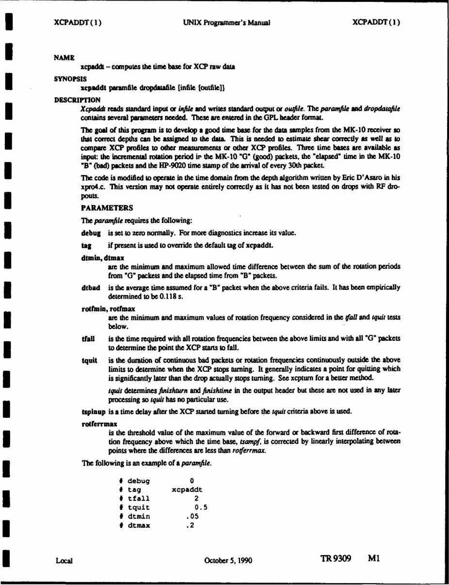
XCPADDT (1) UNIX Programmer's Manual XCPADDT (1)
NAMExcpaddt - computes the time bose for XCP raw data
SYNOPSISxcpaddt paramfile dropdatafile [infile joutfile]]
DESCRIPTIONXcpaddA reads standard input or infile and writes standard output or ouffie. The paramfde and dropdalq/iecontains several parameters needed. These are entered in the GPL header format.
The goal of this program is to develop a good time base for the data samples from the MK-1O receiver sothat correct depths can be assigned to the data. This is needed to estimate shear correctly as well as tocompare XCP profiles to other measurements or other XCP profiles. Three time bases are available asinput the incremental rotation period iv the MK-10 "G" (good) packets, the "elapsed" time in the MK-10"B" (bad) packets and the HP-9020 time stamp of the arrival of every 30th packet.
The code is modified to operate in the time domain from the depth algorithm written by Eric D'Asaro in hisxpro4.c. This version may not operate entirely correctly as it has not been tested on drops with RF dro-pouts.
PARAMETERS
The paranifile requires the following:debug is set to zero normally. For more diagnostics increase its value.tag if present is used to override the default tag of xcpaddt.
dtmin, dtmaxare the minimum and maximum allowed time difference between the sum of the rotation periodsfrom "0" packets and the elapsed time from "B" packets.
dtbad is the average time assumed for a "B" packet when the above criteria fails. It has been empiricallydetermined to be 0.118 s.
rotfmin, rotfmaxare the minimum and maximum values of rotation frequency considered in the fall and tquit testsbelow.
tfail is the time required with all rotation frequencies between the above limits and with all "G" packetsto determine the point the XCP starts to fall.
tquit is the duration of continuous bad packets or rotation frequencies continuously outside the abovelimits to determine when the XCP stops turning. It generally indicates a point for quitting whichis significantly later than the drop actually stops turning. See xcptum for a better method.
iquit determines fiishiturn and finshsime in the output header but these are not used in any laterprocessing so iquit has no particular use.
tspinup is a time delay after the XCP started turning before the tquit criteria above is used.
rotferrmaxis the threshold value of the maximum value of the forward or backward first difference of rota-tion frequency above which the time base, uampf, is corrected by linearly interpolating betweenpoints where the differences are less than roferrmax.
The following is an example of a paramfile.
# debug 0# tag xcpaddt# tfall 2# tquit 0.5# dtmin .05# dtmax .2
Local October 5, 1990 TR9309 M1

i XCPADDT (1) UNIX Progurnmer's Manual XCPADDT (1)
I# dtbad .118# rotfmin 8# rotfmax 20# rotferrmax 0.5# tspinup 3.5
The dropdtaUfde may contain a dropno_playspeed entry for this drop which is the ratio of the playbacktape speed to the record tape speed. It defaults o 1.0 if an entry cannot be found for this drop.I FILESFE usrlocal/bin/xcpaddt
SEE ALSO
xcpover(l)DIAGNOSTICSBUGSAUTHOR
John Dunlap, Applied Physics Laboratory, University of Washington
L
IIIII
jLocal October 5, 1990 TR 9309 M2

j APPENDIX N
xcpblf Documentation

XCPBLF (1) UNIX Programmer's Manual XCPBLF (1)
NAMExcpblf- XCP baseline correction and conversion to frequencies
SYNOPSISxcpblf [-c] paramfile dropdatafile [infile [outfilell
DESCRIPTIONXcpbyf corrects the in-phase and quadrature data from the XCP receiver by estimating and removing thecontributions from a slowly changing base line or average frequency of the signals.
In addition the data from the receiver is convered to frequencies.
The -c option is used to chop off the profile at turn-half and turn-stop which are obtained from thedropdatajif.The dropdwatafde is the same one used by xcppro.
The paramfile has several parameters described below in GPL header format.
debug is set to 0 normally. Higher values produce more diagnostic output.
tag if present is used to override the default tag of xcpblf.
bictype is the baseline correction type. There are presently four options, none, original, 2back, bottom.The none option applies no corrections. The original option uses the method in the XTVP report,APL-UW 8110. The 2back option solves the equations in the report assuming only a linear base-line model (El0) and only using the present and previous rotation. This option allows one to cal-culate velocities on the last turn as the XCP hits the bottom. The bottom option is like originalexcept the last point which is like 2back in order to process as close to the bottom as possible.
sl, s2, s3are the inverse of the multiplication ratios of the phase lock loops for the three channels, tempera-ture, electric field and compass coil.
rotfmin, rotfmaxare the minimum and maximum rotation frequency used to determine if the data are reasonable.Rotation frequency data is set to a bad flag value if not in the above range.
An example of paramfile contents is below.
# debug 0# tag xcpblf# bictype bottom# s3 .005# s2 .0125# s3 .025# rotfmin 1# rotfmax 20
FILES/usr/local/bin/xcpblf
SEE ALSODIAGNOSTICSBUGSAUTHOR
John Dunlap, Applied Physics Laboratory, University of Washington
Local October 8, 1990TR9309 NI

APPENDIX 0
xcppro Documentation

I XCPPROM() UNIX Prgrammer's Manuel XCPMRO (1)
INAME
xcppro - XCP processing
SYNOPSISzcppro paramfile dr•pdatafle [infile [outfilej]
DESCRIPTIONzcppro accepts the corrected in-phase and quadratw camer frequencies as well a XCP probe rolaton fe-quency. All are assumed to be the estimated probe frequencies with units of hem. The ijl or standardinput is typically produced by zcpbif, xcppro produces profiles of eatst and north velocity components andtemperature as a function of depth and pressure on standard output or outfile. The output of xcppro is suit-able for input to Gcppride
paramfile has the processing parameters and other files of parameters to use. All the parmeter files use themkhdr format similar to the GPL header for the data files. If a parameter is present in more thun oneparameter file it's value is taken from the first parameter file. The parameter file on the command line isconsidered before the rest
dropdatafie contains processing parameters specific to each drop such as the earth's magnetic field, posi-tion and start and stop points for processing. This data is maintained by other programs and zcppro readsfrom it. It is an ASCII file so any text editing pogram can be used to change values. See xcpurnW) andh urmerge(l).
One dropdatafde is maintained for each cruise or group of drops. Each parameter is prefixed by the dropname. Usually the drop name is just the sequential number of the XCP launch.
xcppro implements the part of the processing that is specific to the probe. It executes equations (23)through (30) of the XCP report, APL-UW 8110.
IThere is no filtering option in xcppro as that is typically done in xcpgrid.
PARAMFILE CONTENTS
debug is set to 0 for no debugging messages on stderr. The higher it is set the more messages weprinted.
I paramfilesspecifies a list of additional parameter files to be used to supply the parameters to xcppro.
timeusedshould be set to tmaster.
efccpO efccplare the intercept and slope as a function of rotation frequency respectively of the diffemrtial phasebetween the electric field and compass coil channels of the digital receiver used. I have not setthese to anything but zero.
mean is the area in cm^2 times the number of tunis of the compass coil. In old programs it was actuallycomputed as the average value of the area. Now it is entered as a constant. For Mod 6 probes avalue of 695 seemed to be correct. The value 667 has been determined by Michael Horgan for theOcean Storms AXCP probes. This may hold for all Mod 7 probes.
geca gcora gefaare the polynomial coefficients as a function of rotation frequency of the amplitudes of the gainsof the compass coil, correction and electric field channels before the voltage to frequency (V/F)converters in the probe. Each set of coefficients is entered on one line. The zeroth ordercoefficient is first with the others following. There may be up to 6 coefficients for up to a 5thorder polynomial.
For example if three coefficients are entered for gea, gccaO, gccal, gcca2, and the rotation fre-quency is roV then the compass coil amplitude used in the calculations is gccaO + gccal * rod +gcca2 * ro(2.
Local Sept. 30,1993 TR9309 01

I XCPPRO( l) UNIX Programmer's Manual XCPPRO( I)
Igcep gcorp WeOp
ar• polynomial coefficients used to compute the phases of the probe channel gains as a function ofrotation frequency in the same fashion as gm, gcors and gefa above.
esep is the distance in cm between electrode ports. It is also the diameter of the probe.
cl + 1.0 is the amplification factor of the electric potential sensed across the probe because the electriccurrents must go around the insulating body. The usual value used for cl for an XCP is 0.97. Itdepends on the shape of the body. For an infinite cylinder cl would be 1.0. See the EMVP report,WHOI-74-46, eqn. -il 1.
c2 + 1.0 is the factor controlling the addition of vertical fall rate to the north component of velocity. Usu-ally c2 is assumed to be -0.02 for XCP probes. See the EMVP report, WHOI-74-46, eqn. Ill- 11.
gevfa gevfpare the amplitude and phase of the gain of the voltage to frequency converters for the electric fieldchannel.
gcvfa gcvfpare the amplitude and phase of the gain of the compass coil voltage to frequency converter.
depthcalare the coefficients of the depth polynomial as a function of time: depth = depthcalO + depthcall* time + depthcal2 * time^2. Note that the depthcal values should be entered to obtain a positivedownward depth. The programs compute "z" which is positive upwards with the same absolutevalue as depth but opposite sign.
prconv are the four coefficients used to convert depth to pressure using the following formula: pr = depthI (prconvO + prconvl * depth + prconv2 * exp(depth I prconv3)) Setting the coefficients to zero
Stcalfreqinhibits the conversion.
are the two frequencies of the temperature carrier (Hz) with resistances tcalres below.
tcalres are the two resistances (ohms) of the XCP thermistor at 0 and 30 degrees C respectively.
teal are the four coefficients of the standard polynomial of logarithms of resistance to compute tem-perature from resistance. These coefficients were found by fitting the published temperature andresistance tables in the specification of the XCP thermistors: T = 273.15 + 1.0 / (tcalO +tcall*in(R) + tcal2*in(R)2 + tcal3*ln(R)y3).
tcor Specifies a linear correction as a function of depth to be added to temperature as computed above.Correction = tcorO + tcorl * depth
DROP DATA FILE CONTENTS
<drop>_halfcoilis set to 1 to indicate that the processing should use half the usual amean in the tilt correction. Ifthis parameter is not present in the dropdatafile it is assumed to be zero.
<drop>_revcoilis set to I to indicate that the probe was wired with the coil reversed. If this parameter is notpresent in the dropdatajile it is assumed to be zero. Note that when the coil is reversed it actuallyappears to the processing as if the electrodes were reversed since the reference is the coil. It isthought that most of the wiring errors are actually coil wiring errors since those wires are easier tocross in the probe assembly.
<drop>_fh <drop>.fzare the horizontal and vertical magnetic field at the drop site. The units are gauss which is100,000 nT. The vertical magnetic field is negatiwe in the northern (magnetic) hemisphere.
<drop>..turnhalfis the turn number at which the probe comes to half its nominal rotation frequency. Depth is
I Local Sept. 30, 1993 TR9309 02

HXCPPRO (1) UNIX Programmer's Manual XCPPRO (1)
computed according to time since the time at turnha f.
<drop>_turatopis the last turn number with good rotation frequency. When a drop hits the bottom this turn is thelast turn with good data. When the probe spool wire is exhausted the probe spin rate noticeablyslows for the last 10 to 20 turns. This effect is also seen in the north velocity so the fall rate isprobably changing. Presently the last 10 or 20 turns of deep drops we not processed corectly.
<drop> launchtimeis the time the probe was released from the ship or aircraft. This time detennines the position oflaunch which is assumed to be the same position of the drop. If there is significant wind thisassumption will be incorrecL
I <dro>_W•inlnois the serial number of the probe.
<drop>_magvaris the magnetic variation for use in coordinate rotation from the natural geomagnetic to geographiccoordinates. No coordinate rotation is done in the standard processing: the U and V componentsare left in the magnetic coordinate system.
I PARAMFILE EXAMPLES
The ".Asowing is an example of parameter files used in testing with the Cadiz data. Ther is nothing magicabout the file names or partioning of the data into the various files. It should be done to minimize thei number of redundant entries.
The contents of xcppro.p are:
# debug 0# paramfiles deckbox.p probe.p depthcal.p tcal.p# timeused tmaster
The contents of deckbox.p are:
# efccpO 0.
# efccpl 0.
The contents of probe.p with Michael Horgan's new coefficients are:
# amean 667# cl .97# c2 -. 02# esep 5.19# gevfa 494.66025# gevfp 0# gcvfa 500# gcvfp 0# gefa 23866.12044581 107.99111272898 -0.905827321# gcca 1809.877761 -1.25653911 0.18856556# gcora 898.89564739 0.453188608 0.0717425016# gefp -138.158938796 9.759010754 -0.180878978# gccp 29.826971133 10.265226263 -0.176531452# gcorp 56.552652832 7.783581145 -0.112472607
The contents of depthcal.p with depth calibration and Cadiz pressure conversion follow as discussed inPrater(1991).
Local Sept. 30,1993 TR 9309 03

U XCPPRO(I) UNIX Programmer's Manual XCPPRO (1)
I# depthcal 4.68 4.377 -0.00044# prconv 0.9927 -2.55e-06 0.0073 -50.0
The contents of wal.p follow. The values shown for tcr are for the Cadiz cruise as determined by Mark
# tcalfreq 285.3 449.1# tcalres 16329 4024# tcal 1.73323e-3 8.75509e-5 .64067e-5 -5.09882e-7# tcor -0.05 -1.25e-04
DROP DATA FILE EXAMPLESThe items for drop 2466 in the dopdata file are as follows. Not all of these items are used in xcppro com-putations but they are all required to be present for inclusion in the output header.
I # 2466 serialno 871058# 2466 launchtime 880911-224000# 2466_lat 36 39.40 N# 2466 _on 8 38.37 W# 2466 fh 0.268
# 2466 fz -0.330# 2466_magvar 5.9 W# 2466_turnhalf 739# 2466_turnstop 3479
I FILES
/usr/local/bin/xcppro
SEE ALSOxcpover(l)
BUGSPlease report them.
AUTHORJohn Dunlap, Applied Physics Laboatory, University of Washington
IIIII
Local Sept. 30,1993 TR 9309 04

IIII
APPENDIX P
xcpgTId Documentation
IIIIIIIIIIIIII

XCPGRID( 1) UNIX Programmer's Manual XCPGRID )
NAMExcpgrid - put XCP data on uniformly spaced depth grid
SYNOPSISxcpgrid paramfile [infile (oudile]J
DESCRIPTIONXcpgrid reads from standard input or inJile if it is present. It writes standard output or oujiffe if it is present.Input data is assumed to be from xcppro.
The paramfile has some parameters used in the processing:
debug is set to 0 normally. Increasing amounts of diagnostic output is written to standard error as debugis increased.
shearoutis a flag controlling the output of the shear variables. If I they are and if 0 they are not.
auxout is a flag controlling the output of area. rotf, cfbI and ccbl. If I they are and if 0 they are noL
zO is the initial value of the depth grid.
dz is the interval of the depth grid.
dzbin is the averaging interval for each output grid point. Usually this is set to two times dz.
Ivar is the depth variable name from xcppro. It can be set to z, depth, or pr. z is positive up whiledepth and pr (pressure) are positive down. z and depth have units of meters while pr has units ofdbar.
binmin is the fraction of a bin which must be averaged to obtain the last data point.
tmin, tmaxare the minimum and maximum temperatures allowed to be included in the output bins.
urnin, umaxare the minimum and maximum velocity components (u & v) allowed to be included in the output
h bins.
rotfinin, rotfmaxare the minimum and maximum rotation frequencies allowed for any data to be included in theoutput bins.
zfiltrotf is the recursive filtering distance for averaging the rotation frequency.
maxdevrotfis maximum deviation of rotf from the average rotation frequency. If the deviation is greater thanmaxdewvotf then no data is used from this scan.
i ~ An example of a paramfike follows:
# debug Q# shearout 1# auxoUt 1# zO 0# dz 2# dzbin 6# zvar pr# binmrn 0.75# tmax 35.0# tmin -3.0# umax 2.0# umin -2.03 # rotfmax 20.0
Local March 30, 1989 TR9309 P1

I XCPGRID( 1) UNIX Prognimmer's Manual XCPGRID(I)
I*# rotfumin 8.0# zfiltrotf 3.0
maxdevrotf 2.0
FILES /usr/local/bin/xcpgrid
SEE ALSOxcpover(l)
DIAGNOSTICSBUGSAUTFHOR3HJohn Dunlap, Applied Physics Laboratory, University of Washington
I,IIIIIII
II
Local March 30, 1989 TR 9309 P2

IIIUI APPENDiX Q
xcpplot Documentation
IIIIIIIIIIUIII

XCPPLOT( I) UNIX Programmer's Manual XCPPLOT( 1)
NAMExcpplot - standard plot for XCPs
SYNOPSISxcpplot (-dl [linilel I hpp7
DESCRIPTIONXcpplot produces a standardized color plot of zcpgrid(]) output using the HP-7550 pen plower. Thedimensions are 10 inches high and 7 inches wide. The scales are 200 meters per inch for depth and 0.2 m/sper inch for velocity. Processing parameters which are specific to the drop are labeled on the plot. Othersshould be obtained from a listing of the parameter files for each program.
The -d option is used for debugging the program. Inlie is the data file input. If infie is not present theinput is taken from standard input. The standard output of xcpplot contains HP-GL plotter commands andis normally directed to the standard input of hpp7. the pen plotter spooler.I FILES/usr/Ioca!/bin/xcpplot
SEE ALSOxcpover(1)
AUTHORJohn Dunlap, Applied Physics Laboratory, University of Washington
I Local June 7, 1989TR39 Q
IT 39 Q

ii
i APPENDIX R
- List of Selected Symbols and Acronyms
IIIHI

ADCP acoustic Doppler current profilerAF audio frequencyAPL Applied Physics LaboratoryAXCP air-launched expendable current profilerCC compass coilCID conductivity temperature depthDAT digital audio tapeEF electric fieldEM electromagneticEMVP Electro-Magnetic Velocity ProfilerFM frequency modulatedFh horizontal component of Earth's magnetic fieldFI vertical component of Earth's magnetic fieldGcca CC gain (amplifier)Gcora gain of mixing circuit (CC through EF postamplifier)SGefa EF gain (amplifier)G,,fa EF gain (V/F converter)Gcyfa CC gain (V/F converter)G,*, EF circuit phase shiftGcq, CC circuit phase shiftGcorp phase of mixing circuit (CC through EF postamplifier)
U HP Hewlett PackardNOARL Naval Oceanographic and Atmospheric Research LaboratoryNORDA Naval Ocean Research and Development ActivityNRL Naval Research LaboratoryONR Office of Naval ResearchPCM pulse code modulationSRF radio frequencySWR standing-wave ratioTOPS Total Ocean Profiling SystemV/F voltage to frequencyVCR video cassette recorderVHF very high frequencyVHS video home systemUW University of WashingtonXBT expendable bathythermographXCP expendable current profilerXSV expendable sound velocimeter
I XTVP expendable temperature and velocity profiler
I
I TR9309 Ri

Fr-m ARWO~aREPORT DOCUMENTATION PAGE I_____________
Pub•li reporting burden for this calection oa WwwomwMin is .wriemd to uvetage I hour response, including tohe lar torlevois*g "tfuwtion, searcing evhithg daet souwsces, gariu andmaistaining the data needed, and reviewing the Collection ai tn•donaion. Send ooaywrnls regarding this burden esjle at any other swet of t ollectin of •icmeonstincluding suggestionstor reducing this burden. to Washington Headquauteus Services. Directorate for Inio•rintin Operallton and Peport.. 1216 Jalteuuan Davis Highway. SAe 1204. Arliton. VA 222024 and tothe Office of information and lRegulikory Attairs, Office o Managemnent w4 Budge. Washington, DC 20603.
1. AGENCY USE ONLY (Leve bMt) 2. REPORT DATE 3i. REPORT TYPE AND DATES COVERED
August 1993 TechnicalAL TITLE AND SUBTITLE L FUNDING NUMBERS
An XCP User's Guide and Reference Manual N00014-90-J-1100N00014-84-C-01 I1N00014-87-K-0004
S. AUTHOR(S)Thomas B. Sanford, Eric A. D'Asaro, Eric L. Kunze, John H. Dunlap, Robert G. Drever,Maureen A. Kennelly, Mark D. Prater, and Michael S. Horgan
7. PERFORMING ORGANIZATION NAME(S) AND ADORESS(ES) S. PERFORMING ORGANIZATION
Applied Physics Laboratory REPORT NMER
University of Washington APL-UW TR 93091013 NE 40th StreetSeattle, WA 98105-6698
9. SPONSORING I MONITORING AGENCY NAME(S) AND ADDRESS(ES) 10. SPONSORING I MONITORING
Office of the Chief of Naval Research AGENCY REPORT NUMBER
Department of the NavyBallston Center Tower #1800 N. Quincy StreetArlington, VA 22217-5000
11. SUPPLEMENTARY NOTES
12a. DISTRIBUTION I AVAILABILITY STATEMENT 12b. DISTRIBUTION CODE
1& ABSTRACT (Maxt'mum 200 words)
This report describes expendable current profiler (XCP) instrumentation, equipment testing procedures, data acquisitionmethods, and data processing. It also provides a guide to XCP field operations.
14. SUBJECT TERMS 1I. NUMBER OF PAGESExpendable Current Profiler (XCP), XCP, AXCP, Slowfall AXCP, XCP equipment, XCP testing, 101XCP calibration, XCP field operations, XCP data acquisition, XCP data processing, motional i.. PRUICEinduction, current measurement, oceanographic instrumentation
17. SECURITY CLASSIFICATION 14. SECURITY CLASSIFICATION 119. SECURITY CLASSIFICATION 20. LIMTATION OF ABSTRACTOF REPORT OF THIS PAGE OF ABSTRACT
Unclassified Unclassified Unclassified N/A
NSN 7540-01-2W0-500 UIWdud Form 2W (Rev. 240)Petsfbed by ANS SMd. 30-102W-01


