Embed Size (px)
Citation preview
RREEVVIIEEWW OOFF EECCOONNOOMMIICC AANNDD BBUUSSIINNEESSSS SSTTUUDDIIEESS

International Editorial Board Professor Jim BELL, University of Ulster, Northern Ireland, United Kingdom Professor Jean-Pierre BERDOT, Université de Poitiers, France Professor Henri BOUQUIN, Université de Paris-Dauphine, France Professor Oana BRÂNZEI, York University, Toronto, Canada Professor Mihai CALCIU, Université de Lille, France Professor Cristian CHELARIU, York University, Canada Professor Bernard COLASSE, Université de Paris-Dauphine, France Professor Christian CORMIER, Université de Poitiers, France Professor Gerry RAMEY, Eastern Oregon University, United States of America Professor Jaroslav KITA, University of Economics Bratislava, Slovakia Professor Raymond LEBAN, Conservatoire National des Arts et Métiers, France Professor Luiz MONTANHEIRO, Sheffield Hallam University, United Kingdom Professor Louis G. POL, University of Nebraska at Omaha, United States of America Professor Bonsón Ponte, ENRIQUE, Universidad de Huelva, Spain Professor Danica PURG, President of CEEMAN, Bled School of Management, Slovenia Professor Jacques RICHARD, Université de Paris-Dauphine, France Professor Antonio García SÁNCHEZ, Universidad Politécnica de Cartagena, Spain Professor Alan SANGSTER, Aberdeen Business School, The Robert Gordon University, Scotland, United Kingdom Professor Victoria SEITZ, California State University, San Bernardino, United States of America Professor Peter WALTON, ESSEC Business School Paris, France
National Editorial Board Professor Daniel DĂIANU, Member of the Romanian Academy, President of the Romanian Society of Economics Professor Emilian DOBRESCU, Member of the Romanian Academy Professor Aurel IANCU, Member of the Romanian Academy Professor Constantin IONETE, Member of the Romanian Academy Professor Mugur ISĂRESCU, Governor of the National Bank of Romania, Member of the Romanian Academy Professor Vasile IŞAN, rector of the Alexandru Ioan Cuza University of Iaşi
Members Professor Dinu AIRINEI, Alexandru Ioan Cuza University of Iaşi Professor Ioan ANDONE, Alexandru Ioan Cuza University of Iaşi Professor Gabriela ANGHELACHE, Academy of Economic Studies, Bucharest Professor Maria BÂRSAN, Babeş-Bolyai University, Cluj-Napoca Professor Sorin BURNETE, Lucian Blaga University, Sibiu Professor Emil CAZAN, West University of Timişoara Professor Silviu CERNA, West University of Timişoara Professor Gheorghe CIOBANU, Babeş-Bolyai University, Cluj-Napoca Professor Vasile COCRIŞ, Alexandru Ioan Cuza University of Iaşi Professor Viorel CORNESCU, University of Bucharest Professor Dumitru COTLEŢ, West University of Timişoara Professor Nicoleta FARCANE, West University of Timişoara Professor Niculae FELEAGĂ, Academy of Economic Studies, Bucharest Professor Gheorghe FILIP, Alexandru Ioan Cuza University of Iaşi Professor Ion IGNAT, Alexandru Ioan Cuza University of Iaşi Professor Ion IONAŞCU, Academy of Economic Studies, Bucharest Professor Elisabeta JABA, Alexandru Ioan Cuza University of Iaşi Professor Alexandru JIVAN, West University of Timişoara Professor Mihai KORKA, Academy of Economic Studies, Bucharest Professor Dumitru MATIŞ, Babeş-Bolyai University, Cluj Napoca Professor Emil MAXIM, Alexandru Ioan Cuza University of Iaşi

Professor Dumitru MIRON, Academy of Economic Studies, Bucharest Professor Constantin MITRUŢ, Academy of Economic Studies, Bucharest Professor Tatiana MOŞTEANU, Academy of Economic Studies, Bucharest Professor Panaite NICA, Alexandru Ioan Cuza University of Iaşi Professor Ştefan NIŢCHI, Babeş-Bolyai University, Cluj Napoca Professor Dumitru OPREA, Alexandru Ioan Cuza University of Iaşi Professor Magdalena-Iordache PLATIS, University of Bucharest Professor Victor PLOAE, Ovidius University , Constanţa Professor Nicolae Tiberiu Alexandru POP, Academy of Economic Studies, Bucharest Professor Atanasiu POP, Babeş-Bolyai University, Cluj Napoca Professor Ioan POPA, Academy of Economic Studies, Bucharest Professor Constantin POPESCU, Academy of Economic Studies, Bucharest Professor Dan POPESCU, Lucian Blaga University, Sibiu Professor Gheorghe POPESCU, Babeş-Bolyai University, Cluj Napoca Professor Spiridon PRALEA, Alexandru Ioan Cuza University of Iaşi Professor Ştefan PRUTIANU, Alexandru Ioan Cuza University of Iaşi Professor Ioan ROTARIU, West University of Timişoara Professor Ion Gh. ROŞCA, Academy of Economic Studies, Bucharest Professor Constantin SASU, Alexandru Ioan Cuza University of Iaşi Professor Ion STANCU, Academy of Economic Studies, Bucharest Professor Neculai TABĂRĂ, Alexandru Ioan Cuza University of Iaşi Professor Ioan TALPOŞ, West University of Timişoara Professor Gheorghe VOINEA, Alexandru Ioan Cuza University of Iaşi Professor Vergil VOINEAGU, Academy of Economic Studies, Bucharest Professor Dumitru ZAIŢ, Alexandru Ioan Cuza University of Iaşi
Managing Editors
Editor in chief: Professor Ion POHOAŢĂ, Alexandru Ioan Cuza University of Iaşi
Assistant editor in chief: Professor Adriana ZAIŢ, Alexandru Ioan Cuza University of Iaşi Senior editor: Lecturer Olesia LUPU, Alexandru Ioan Cuza University of Iaşi Editors: Professor Marin FOTACHE, Alexandru Ioan Cuza University of Iaşi Professor Adriana PRODAN, Alexandru Ioan Cuza University of Iaşi Professor Mihaela ONOFREI, Alexandru Ioan Cuza University of Iaşi Professor Carmen PINTILESCU, Alexandru Ioan Cuza University of Iaşi Assistant Professor Costel ISTRATE, Alexandru Ioan Cuza University of Iaşi Lecturer Gabriela Gavril ANTONESEI, Alexandru Ioan Cuza University of Iaşi General editing secretary: PhD student Gabriel CUCUTEANU, Alexandru Ioan Cuza University of Iaşi
Editorial Secretary
PhD student Alin ANDRIEŞ, editing secretary PhD student Andreea IACOBUŢĂ, editing secretary PhD student Andrei MAXIM, editing secretary PhD student Ovidiu STOFOR, editing secretary PhD student Silviu TIŢĂ, editing secretary

Content
EDITORIAL .................................................................................................................................7 SCIENTIFIC RIGOUR, CREATIVITY AND DIALOGUE IN ECONOMIC SCIENCES............................ 9 Ion Pohoaţă
RESEARCH PAPER ....................................................................................................................13 REAL CONVERGENCE AND INTEGRATION......................................................................................... 15 Aurel Iancu
EVALUATION OF THE PERFORMANCE AND OF THE INTEGRATION OF THE EURO ZONE STOCK MARKET: WHICH ARE THE “RIGHT MOMENTS”? ................................................................ 29 Jean-Pierre Berdot
EUROZONE – A SENSIBLE ABSORPTION OF RISK CAPITAL? .......................................................... 43 Cicero I. Limberea
TOWARDS MEASUREMENT OF POLITICAL PRESSURE ON CENTRAL BANKS IN THE EMERGING MARKET ECONOMIES: THE CASE OF THE CENTRAL BANK OF EGYPT ................. 63 Ibrahim L. Awad
EMPIRICAL EVIDENCE ON RISK AVERSION FOR INDIVIDUAL ROMANIAN CAPITAL MARKET INVESTORS ................................................................................................................................................. 91 Cristian Păun, Radu Muşetescu, Iulian Braşoveanu, Alina Drăghici
DATA ANALYSIS WITH ORDINAL AND INTERVAL DEPENDENT VARIABLES: EXAMPLES FROM A STUDY OF REAL ESTATE SALESPEOPLE ........................................................................... 103 G. Martin Izzo, Barry E. Langford
CURRENT ISSUES....................................................................................................................117 PRO-CAPITALISM VS. ANTI-AMERICANISM IN 21ST CENTURY EUROPE .................................. 119 Sorin Burnete
HISTORY OF IDEAS.................................................................................................................127 FROM THE HUMAN CAPITAL DEFINED AS ''HOMO OECONOMICUS RATIONALIS'' TO THAT OF THE RATIONALLY BOUNDED AND OPORTUNISTIC ''HOMO CONTRACTUALIS''. AN INSTITUTIONALIST APPROACH........................................................................................................... 129 Ion Pohoaţă
BOOK REVIEW........................................................................................................................135 „EASILY DIGESTIBLE ECONOMICS”. THE DRAGON AND THE ELEPHANT................................ 137 Gabriela Gavril-Antonesei
ROCKEFELLER’S MEMOIRS .................................................................................................................. 143 Nicoleta Dabija, Gabriel Cucuteanu

CASE STUDIES........................................................................................................................ 147 ORGANIZATIONAL HEALTH ASSESSMENT: A ROMANIA FIRM CASE STUDY.......................... 149 Shaomin Huang, Gerald W. Ramey
THE TARIFF EQUIVALENT OF TARIFF-RATE QUOTAS - A CASE STUDY APPLIED TO THE IMPORT OF AN AGRICULTURAL PRODUCT IN ROMANIA ............................................................. 161 Petru Cătălin Bodea
TURKEY: GAINING MARKET SHARE IN THE U.S. READY-TO-WEAR CLOTHING MARKET ... 173 Victoria Seitz, M.B Neace, Nabil Razzouk, Esin Keyfli, Chin-Wei Tung

EDITORIAL


SCIENTIFIC RIGOUR, CREATIVITY AND DIALOGUE IN ECONOMIC SCIENCES
The foreword of the first issue of a publication usually outlines its main scientific approaches and tries to make a general description of the future methodologies employed. However, we take the liberty of somewhat drifting away from this editorial canon. Let us remember what Montesquieu wrote at the very beginning of his De l'esprit des lois (The Spirit of Laws): “Intelligent people may have laws that they make, but they may also have laws that they do not make”. We, therefore, place our message under the auspices of the words of the great French philosopher and address it to those who will find the time to read our journal.
Thus, we will not take the risk of imposing a priori strict rules and we will rather rely on the freedom of action and on the spontaneity evoked by Ludwig von Mises in his Human Action. As the famous Austrian economist said, “individuals concluded no contracts beforehand, based on which they founded human society” and yet they managed to remain in civility and freedom. That is why we believe that setting inflexible and immutable scientific behaviour and production rules might become somewhat disturbing, despite their comfortable appearance of a learned academic exercise.
We will refer to norms only to the extent to which they contribute to the promotion of fundamental rules of scientific conduct, able to enhance researchers’ individual inclinations. A proper balance between the knowledge they have acquired, their creativity and scientific rigour may endow researchers with the strength and ability required to “get the world of ideas moving”, to discover new ways and approaches in their fields, to provide comprehensive syntheses and, why not?, to shape new thinking horizons. We are convinced that creative efforts are always more successful if triggered by a self-imposed scientific rigour, which is the result of experience and even common sense rather than if they are forced upon them by “Procust's bed”, by canons and commonplaces, which in time may become frustrating for a free mind. We believe that the freedom of thinking may stimulate creative spirits and at the same time it may become a catalyzing factor, able to bring individual efforts to a valid collective result.
From another point of view, our mission, as members of the editorial team, is rather to be modest “agitators” of the spirit. We wish to provoke and maintain the dialogue between various areas of economic knowledge. How do we hope to reach such a goal without imposing unwavering rules? We start our journey from the very essence of an open economy, namely full consumer sovereignty. We shall not avoid apparently simple but extremely inconvenient questions such as: Why would a paper published in our journal be worth the time and effort to read? What are the qualities that would make it interesting and useful to readers?
The answers to these questions may undoubtedly be only partial and vague. We are perfectly aware that, as it happens in all other social sciences, the economic field has developed in time a set of scientific disciplines, which have each a well defined area of study. Therefore, any answer to our readers' questions can only be given considering a broad range of economic sciences, which, although they preserve an organic connection with the whole, provide specialized approaches. Our publication is addressed to specialists in finance, quantitative analysis, marketing, management, business informatics, as well as to theorists.

ION POHOAŢĂ
We will have to provide each and everyone of these highly demanding readers something worth reading. We hope to meet the expectations of our readers and are looking forward to a positive feed-back.
As its title proves, the Review of Economic and Business Studies will include various coss- and multi-disciplinary approaches, and is intended as a place for confrontation of ideas, for real dialogue among specialists from various economic disciplines. Without trying to be comprehensive, special consideration will be given to theoretical articles proving an in-depth understanding of the economic phenomena and research methods with a deep concern for the target audience.
From this point of view, we are positive that a major concern and research issue is the economists' preoccupation to find ways and means of increasing individual and collective wealth, on the line traced by Adam Smith, a classic in economic thought. Half a century later, the research area defined by Adam Smith, is still productive. Either empirically or theoretically, almost all researchers direct their efforts, with specific means, towards the same main goal – economic growth, by developing strategies or listing values, by studying the market or producing informational systems theories, by developing management systems or defining the role of currency or of financial instruments in the economy, or by modeling and analysing data.
Within the same framework are situated researchers concerned with the identification, definition and forecasting of economic risks, who determine continuous economic development trend-setting policies. There are cases, which may even be examples to follow, when, by taking high risks, people were successful. Even when research is given specialized names, under well-known labels in areas such as “Theory of Human Capital”, “Theory of Property Rights”, “Public Choice”, “Organizational Behaviour”, all theoretical efforts have the same economic growth-related purpose.
We are absolutely sure that it is not only the economic present and future that interest our target readers, but also its past. We start from the idea that the past is never dead. It continues to act through us and sometimes even in spite of us; it influences the present, it may be imperceptible and subtle, but is continuously active. Since the past continues into the present, and the present is reflected in the past, both forming and deforming experiences, both success and failure obviously become extremely significant. The “path dependence” analyses (leaving aside any ideological madness patterns) may interest our readers. Adam Smith, Ludwig von Mises, Friedrich Hayek, Milton Friedman, Murray Newton Rothbard, etc. continue to be highly valued landmarks, through the elegance and relevance of reasoning and through the depth of their ideas.
We are confident that the public will be interested in reading theoretical and practical
papers, following the tradition of Marshall – Pigou – Roegen, quantitative and qualitative analyses tackling the standard economic growth philosophy, arhythmomorphic or dialectic attempts at changing the neoclassical analysis approach. The purely theoretical or mainly practical papers dwelling on ways of integrating environmental economics into the overall classical economic theory may also be of great interest to our readers. If dealt with in sound, competent studies, able to bring forward strong ideas and identify goal-achieving means, the issue of sustainable economic development is still among topicalities. Any attempt at overcoming, in an institutionalized manner, the dry neoclassical explanatory geometry may continue to be attractive. Establishing a new type of transaction costs accounting, developing new theories related to company efficiency, to the role of rules in economic life, to property rights, to entrepreneurship are all issues that have preoccupied well-known Western specialists for the past thirty years. Our journal will host research on these topics, regardless of the authors’ position – be they theorists or specialists in finance, accounting, management or quantitative analysis.

Scientific Rigour, Creativity and Dialogue in Economic Sciences 11
Review of Economic and Business Studies is a publication open to all new and innovative ideas in the field of economic and business thought or having impact on it, and, in order to make them available to our readers and initiate possible debates related to them, it will also host reviews of prestigious books, which have played a major role in shaping theories. It is not our intention to impose any system or dominant ideology. Therefore, as previously mentioned we prefer dynamic research and believe that even the apparently most inflexible utterances and “verdicts” originating in famous economic thinkers may be questioned and re-analyzed.
We would also like to have beginners at our side, young researchers who have the courage (and sometimes innocence) to express their skepticism on accepted simplifying truths, to denounce routine and to ask unexpected questions, thus generating unexpected perspectives. As we all know, rationality is fundamental in an area such as economic research. However, as common sense warns us, absolute reasoning leads to (surely irrational) transgressions and to losing axiological plurality. Therefore, we believe that papers on the complexity of human existence, with an emphasis on the social dimension, papers refusing to promote a “puppet” that would justify simplified systems and theories, are more than welcome. We should not lose sight of the versatility of economic existence and of the fact that, regardless of the theoretical tools employed, we will never manage to provide a global description or make it fit into certain patterns. Consequently, we believe that economic sciences would only have to lose if they self-sufficiently rejected communication with the other human sciences or ignored ideas coming from them.
In conclusion, we hope that the Review of Economic and Business Studies will have a long editorial life, contributing to significant changes in the world of economic and business studies and that it will become, a prestigious publication through the quality of its papers. On behalf of the Managing Editors, Ion Pohoaţă, Editor-in-chief


RESEARCH PAPER

REAL CONVERGENCE AND INTEGRATION
Aurel IANCU*
Abstract. The study** is based on the critical observations that competitive market forces alone are not able to assure convergence with the developed countries. These observations are grounded on the results of the computation of the marginal rate of return to capital (which contradict the neoclassical model hypotheses), as well as on the real process of polarization of the economic activities, taking place worldwide and in accordance with the law of competition. Unlike those who trust the perfect competitive market virtues, the EU’s economic policy is realistic as it is based on the harmonization of the market forces with an economic policy based on the principle of cohesion, which supports, by means of economic levers, the less developed regions and member countries. This paper deals with the evolution of the EU cohesion funds, as well as with the results of convergence. Key words: Neoclassical model, marginal rate of return on capital, polarization,
convergence, divergence, cohesion, cohesion funds, structural funds, variation coefficient.
JEL: F02, F15, O57, P37
Economists wonder if real economy convergence can actually be achieved only in a competitive market according to the neoclassical models. In this respect, extensive studies and models have been conducted. Considering the way the determinants and trends of real convergence are approached, the studies and models may be divided into three categories: The first one views real convergence as a natural process, based exclusively on the market
forces, in accordance with which the convergence process is surer and faster as the market is larger, more functional, less distorted.
The second one denies that, in the present competitive market, there is an actual real convergence between the poor and the rich countries, but accepts the existence of the tendency of polarization or deepening of the divergences and inequalities between the centre and the periphery.
The third one considers that real convergence is necessary and possible in a competitive market, provided that economic policies are implemented to compensate for the negative effects of the inequalities or divergences, until the economic systems reach maturity or the so-called critical mass to support the self-sufficiency of the real convergence process.
Further, we make some critical comments and present some arguments in support of the alternatives that are closer to the real needs and opportunities the Romanian economy to achieve convergence with the EU real economy.
* Aurel Iancu is a Member of the Romanian Academy of Science, senior researcher within the National Institute for Economic Research, with a long experience in European and national research programmes, coordinator of PhD programmes in economic sciences. ** Part of a study within the CEEX Programme – Project No. 220/2006 “Economic Convergence and Role of Knowledge in Relation to the EU Integration”.
16 AUREL IANCU
1. CONVERGENCE THROUGH THE FUNCTIONAL COMPETITIVE MARKET FORCES The first way to perceive real convergence exclusively by the market forces is the
neoclassical growth theory. Assuming that the economic outcome (GDP per capita) is ensured by the contribution of several production factors (capital, labour, natural resources, technological progress), the neoclassical model advances the fundamental hypothesis that growth depends on the features of the rate of return on capital, which generally tends to decrease in relation to the economic growth. For a certain increase in capital, the outcome increase is less than proportional. More exactly, at the same saving (investment) rate, the marginal rate of return on capital decreases, so that poor countries, with a low amount of capital per capita, attain higher rates of return to capital than those of rich countries with a considerably higher amount of capital per capita.
According to the neoclassical model, the higher rate of return on capital achieved by the poor countries/regions as against the rich countries/regions (if the other conditions are comparable) ensure the long-term convergent economic growth. This postulate is explained by many authors (based on the Solow’s model) taking into account the assumption of equal saving rates (accumulation), population/employed population growth, capital depreciation, technological progress, etc. for all categories of countries. This is the only way that all countries, on different initial development levels, may reach the convergence or equilibrium state by economic growth rates higher in the poor countries than in the rich ones.
According to the neoclassical school, many economists consider that the competition intensification by the establishment and enlargement of the European internal market and integration would have a positive impact and offer opportunities to the countries and regions for diminishing the development and per capita income disparities in order to achieve real convergence. Only action on a larger scale of the competitive internal market forces in the EU, free of any interventionist (protectionist) policy, could guarantee the real convergence of the EU countries and regions.
The free movement of the production factors among the European countries and regions, especially through capital market integration and FDI, is an important way to achieve real convergence.
The less developed countries and regions are characterized by capital scarcity and low saving capability, due to the low income per capita. This means that those territorial entities offer opportunities for development and attract available capital from the countries rich in capital, whose companies are eager to penetrate a large safe and profitable market. After the accession, the capital inflows as investments increased. Among them, the foreign direct investments became the most important means of attracting various intangible resources, such as technology, know-how, expertise, managerial experience, etc. Foreign direct investments have clearer advantages, if compared with financial investments. But their presence in a country or region is dependent on the following requirements: a) sufficient infrastructure of high quality; b) low transaction costs (similar to those in agglomerated areas); c) abundant and cheap local resources (their low cost may compensate for the additional transaction cost, due to the scarce infrastructure); d) possibility to make horizontal investments based on scale economies, showing a significant dispersion of the production units among countries and regions, as close to the potential clients as possible.
To make the markets of the new EU countries perfectly compatible and competitive, the European Commission implements a systematic policy for the elimination of the non-competitive elements from the market by banning state aid, protectionist actions and other elements that may cause distortions of the single market and national markets.
Moreover, it is quite obvious that many economic reform measures taken by the CEE countries as well as the implementation of the Community acquis and the institutional improvement are aimed at creating a functional competitive market within every national economy and the Community market.
Real convergence and integration 17
Some economists and international financial institutions still believe that an enlarged and functional market as well as the profound economic integration require the existence of strong mechanisms that automatically lead to real convergence, without any policy in support of such convergence. The implementation of such policies means, in their opinion, many other distortions of the market.
It is quite obvious that such opinions are expressed by the supporters of the neoclassical model, as they think that only the market forces free of any intervention may set in motion efficiently the mechanisms that enable the poor countries to recover the delays by higher growth rates than those of developed countries.
Although the reasoning based on the hypothesis of decreasing rate of return and the hypothesis of perfect competition is logically correct, facts contradict such opinions. On the one hand, poor countries lack the necessary economic, scientific, technological and financial power to cope with competition, which explains, to some extent, the reverse trend, that is widening the gap (divergence) between the poor and the rich countries, and not diminishing it. On the other hand, one should not ignore the overall natural trend of clustering or polarization of the economic activities at different (national, regional or sub-regional) levels, which might become a major obstacle to convergence.
2. THE NEOCLASSICAL MODEL SHORTCOMINGS AND NEW APPROACHES The empirical research done in the last two decades to check the validity of the
neoclassical model of convergent growth has not been as relevant as expected. To clarify this crucial problem, we intend to check the veracity of the assumption concerning the existence of decreasing rate of return on capital, illustrated by the existence or non-existence of the correlation between the marginal rate of return of the physical capital (the rate of return of investment in physical capital) and the country’s development level (GDP per capita). Consequently we consider the following two indicators: (i) Rate of return of gross investment in capital (RGI) based on the ratio:
ΔGDP per capita, representing thr GDP per capita growth in 2004, as against the previous year (2003) expressed in PPP – USD
RGI = The amount of gross investment in capital per capita in 2003 (ii) Per capita Gross Domestic Product expressed in PPP-USD in 2003.
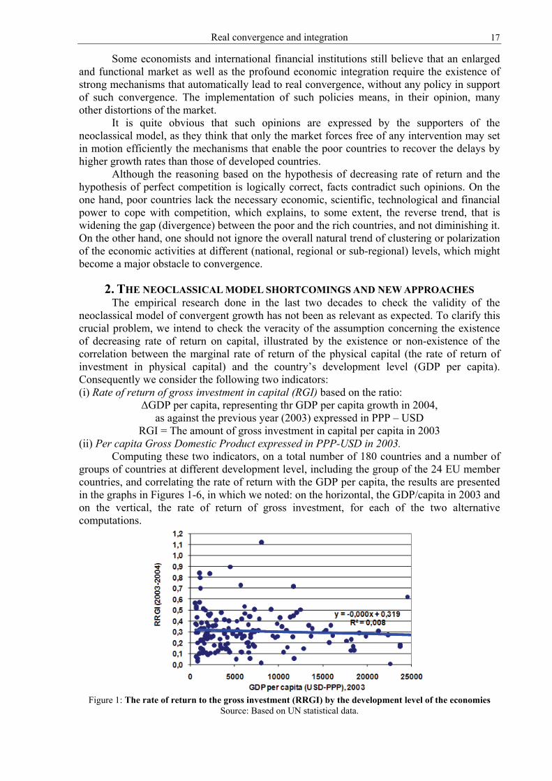
Computing these two indicators, on a total number of 180 countries and a number of groups of countries at different development level, including the group of the 24 EU member countries, and correlating the rate of return with the GDP per capita, the results are presented in the graphs in Figures 1-6, in which we noted: on the horizontal, the GDP/capita in 2003 and on the vertical, the rate of return of gross investment, for each of the two alternative computations.
Figure 1: The rate of return to the gross investment (RRGI) by the development level of the economies
Source: Based on UN statistical data.
18 AUREL IANCU
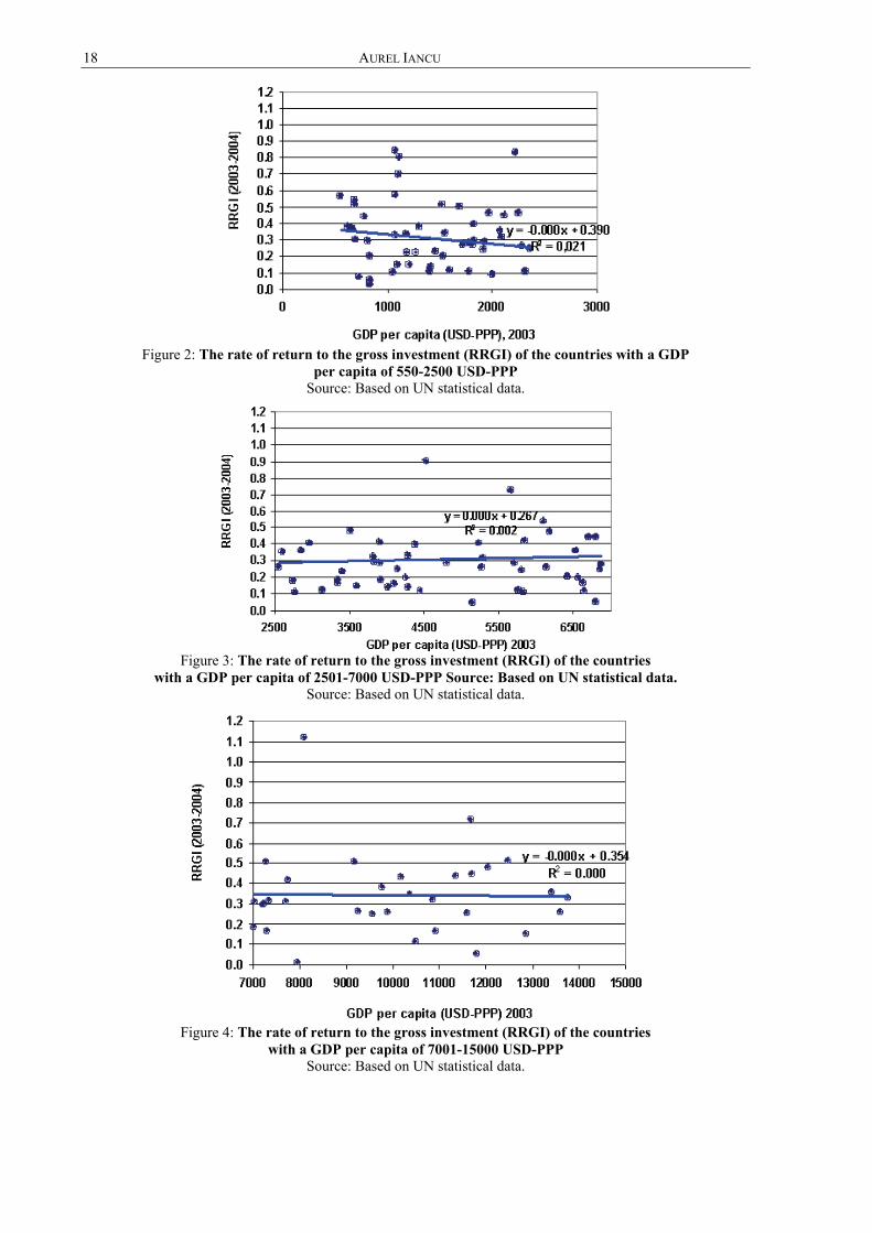
Figure 2: The rate of return to the gross investment (RRGI) of the countries with a GDP
per capita of 550-2500 USD-PPP Source: Based on UN statistical data.
Figure 3: The rate of return to the gross investment (RRGI) of the countries
with a GDP per capita of 2501-7000 USD-PPP Source: Based on UN statistical data. Source: Based on UN statistical data.
Figure 4: The rate of return to the gross investment (RRGI) of the countries
with a GDP per capita of 7001-15000 USD-PPP Source: Based on UN statistical data.
Real convergence and integration 19
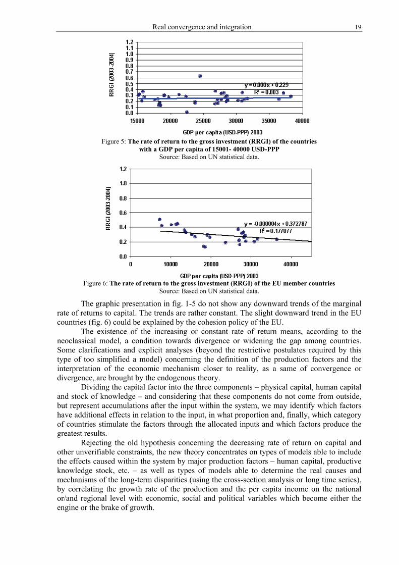
Figure 5: The rate of return to the gross investment (RRGI) of the countries
with a GDP per capita of 15001- 40000 USD-PPP Source: Based on UN statistical data.
Figure 6: The rate of return to the gross investment (RRGI) of the EU member countries
Source: Based on UN statistical data.
The graphic presentation in fig. 1-5 do not show any downward trends of the marginal rate of returns to capital. The trends are rather constant. The slight downward trend in the EU countries (fig. 6) could be explained by the cohesion policy of the EU.
The existence of the increasing or constant rate of return means, according to the neoclassical model, a condition towards divergence or widening the gap among countries. Some clarifications and explicit analyses (beyond the restrictive postulates required by this type of too simplified a model) concerning the definition of the production factors and the interpretation of the economic mechanism closer to reality, as a same of convergence or divergence, are brought by the endogenous theory.
Dividing the capital factor into the three components – physical capital, human capital and stock of knowledge – and considering that these components do not come from outside, but represent accumulations after the input within the system, we may identify which factors have additional effects in relation to the input, in what proportion and, finally, which category of countries stimulate the factors through the allocated inputs and which factors produce the greatest results.
Rejecting the old hypothesis concerning the decreasing rate of return on capital and other unverifiable constraints, the new theory concentrates on types of models able to include the effects caused within the system by major production factors – human capital, productive knowledge stock, etc. – as well as types of models able to determine the real causes and mechanisms of the long-term disparities (using the cross-section analysis or long time series), by correlating the growth rate of the production and the per capita income on the national or/and regional level with economic, social and political variables which become either the engine or the brake of growth.
20 AUREL IANCU
The new theory of convergence is based on the operational character of the effects of the intangible factors (including the economic policy factors). These effects (called “spillovers”) spill over the economy in a special way, that is, over other entities, than their direct producers. The effects exceed the input necessary for their production or their remuneration amount.
Usually, the intangible factors (knowledge, professional abilities or skills, information, innovation, know-how, etc.) are embodied in tangible production factors, and their outputs are spilled over. Spillovers may occur during the investment in physical capital (Arrow, 1962), in human capital (Lucas, 1988) or in both types of investment (Romer, 1986). According to Romer, if the spillovers are strong, the private marginal product of the physical and human capital may stay permanently above the discount rate (Romer, 1986; Thirlwall, 2001). Growth may be supported by continuous accumulation (investment), which generates positive spillovers (Grossman and Helpman, 1994), associated with the formation of the human capital (education and training or qualification) and with the Research, development and innovation (RD&I), thus preventing the diminution of the rate of return to capital or the increase in the capital-output ratio.
3. DIVERGENCE AND POLARISATION – LASTING EFFECTS OF THE COMPETITIVE MARKET FORCES
The empirical research for testing the validity of the neoclassical model has demonstrated that, in most cases, neither the hypothesis concerning the decreasing rate of return to capital, nor the real convergence between the poor and the rich countries (regions) is confirmed. It is impossible to explain the international discrepancy in the present development level only by making reference to the initial difference in factor endowment (Thirlwall, 2001). What actually counts is stimulating the development of the new factors (human capital and knowledge stock) and their increasing contribution to economic growth, detecting possible obstacles to growth in the poor countries and, finally, testing whether the mechanisms causing the inequality between the developed countries and the poor ones may last or not.
The theoretical contribution made by Perroux, Myrdal, Prebisch, etc. has changed the way of explaining real convergence and decisively influenced the direction of the economic policy for the European construction, beginning with the drafting of the Rome Treaty1. Although not always analytically rigorous, the new economic notions included in the scientific circuit, such as attraction poles, clusters, centre-periphery, flows of complementary factors, positive spillovers, etc., have broadened the horizon of the debates and the understanding of the processes taking place in the real economy, and the research area concerning the economic policy.
The above notions and the concept of circular cumulative cause of the economic processes help us explain the increasing international difference in the development level as against the similar initial conditions2. The movement of capital, the human capital and labour migration, the goods and services exchange perpetuate and even worsen international and regional development inequalities. By means of the free trade mechanisms (i.e., free of tariff and non-tariff barriers), the less developed countries, which lack the human capital and the scientific and technological capability, have to specialize in the production of mostly primary goods characterized by an inelastic or almost inelastic demand in relation to price and income.
What causes the increasing inequality between countries is the tendency of interregional and international polarization (agglomeration), especially in the context of the economic and monetary integration. As there are no barriers to the movement of goods, services and production factors, some countries and regions form strong poles of attraction and cause imbalances between countries showing important differences in the income per 1 Jacques Pelkmans, Integrare europeană. Metode şi analiza economică (Romanian translation of European. Integration. Methods and Economic Analysis), European Institute of Romania, Bucharest, 2003 2 M.G. Myrdal, Economic Theory and Underdeveloped Regions, Duckworth, London, 1956
Real convergence and integration 21
capita. The developed countries and regions endowed with factors become poles of attraction that absorb increasing amounts of high quality labour and capital from the less developed countries.
Even if during the accession process the countries make major efforts to support the economic and institutional reforms and attempts to achieve a stable development equilibrium, in real life there is a natural trend with an universal character towards the polarization of the processes, which in turn causes the broadening of the gap between the development levels of the countries and regions. Myrdal claims that the economic and social forces alike tend towards equilibrium and that the economic theory hypotheses according to which disequilibrium situations tend towards equilibrium are false (Myrdal, 1957; Thirlwall, 2001). If it were not true, then how could one explain the international differences in the standard of living? Unable to answer this question, Myrdal replaces the stable equilibrium hypothesis with what he calls the circular cumulative causation hypothesis or, briefly speaking, the cumulative causation hypothesis. This hypothesis helps us explain why the international and interregional differences in the development level may persist and increase in time.
Myrdal’s hypothesis is based on a multiplier-accelerator mechanism, which causes the income to rise at higher rates in the so-called favoured - more developed - countries and regions, which are endowed with modern infrastructure, gain scientific and technological ascendancy and enjoy physical and human capital inflows, as well as scientific and technological inflows; consequently, they become more attractive for their capital and labour than the less developed areas. The free trade in goods and services and the full freedom of movement of the production factors among countries and regions showing great differences in the development level causes increasing polarization: on the one hand, countries and regions that become richer, enjoy a significant economic growth and show attractiveness to the high-skilled production factors and, on the other hand, countries and regions characterized by stagnation and economic decline, obsolete and non-attractive infrastructure, decreasing income and taxation levels, that is, limited demand for goods and services.
Under these circumstances, there cannot be any economic convergence. The approaches and analyses initiated by Myrdal, Prebisch, Seers, etc. have led to an influent trend, based on the concept of divergence, which points out the process of polarization and the divergence between the centre and the periphery.
This trend of thought brings influence to bear upon the following levels: the practical one, reflected in the European construction projects by the adoption of some
tools of the European economic policy; the analytical one, strongly reflected in two directions:
o re-thinking the construction and interpretation of economic growth, by returning to the economic and social realities (it concerns the development of endogenous models and the econometric testing);
o new approaches to the geographic (regional) economy, taking into account real processes, such as: regional disparities, development agglomerations or poles, role of infrastructure, transaction costs.
4. COHESION – AN IMPORTANT TOOL IN SUPPORT OF THE REAL CONVERGENCE WITHIN THE EU
The chance that the poor national economies advance towards convergence within an enlarged and highly competitive single market is illusory. There are some mechanisms that rather stimulate divergence. But there are some other ones that may produce positive effects on the long-term convergence processes, although their success is rather uncertain in the absence of economic policies to support them and to prevent the negative effects. Among the most important mechanisms mentioned by Pelkmans and pointed out by us, one may find the following:
22 AUREL IANCU
the intraindustrial specialization of the less developed countries on parts of products and operations, in accordance with the comparative advantage principle, for the capitalization of the available national (local) resources at small costs;
the integration of the less developed countries into the EU makes them more attractive to foreign capital, and, first, to foreign direct investments, initially within the existing economic clusters and then extended gradually to the periphery territories, along with the infrastructure extension;
the strengthening of the competition to which the products, services, factors and companies from the less developed countries are exposed as the countries accede to the EU, which eliminates the non-competitive local activities and causes dramatic social problems, while such activities are taken over by viable competitive companies;
the integration into a large single market in accordance with the Community acquis eliminates the distortions and the obstacles to development, but does not always stimulate the development of the poor countries and regions.
The impact of the integration on economic growth, in the absence of cohesion policies, does not ensure that the poor countries will reach higher GDP per capita growth rates than the more developed countries, to enable convergence. Unlocking convergence mechanisms by cohesion policies has become one of the EU’s major objectives.
When the Rome Treaty stipulated that “the harmonious development of the economic activities” and “the continuous and balanced expansion” are the first two economic objectives, both the structural divergence and the difference in income per capita between the backward and the advanced members of the Common Market were taken into consideration. To achieve the real convergence in both cases, the Treaty was based implicitly and exclusively on the market mechanisms.
Considering the scarcity of market mechanisms for the recovery of the poor countries and regions, the EU has gradually gained tasks concerning cohesion and solidarity in order to facilitate real convergence by improving the economic performance. The adoption of the cohesion principle was mostly determined by the accession of the countries with a GDP per capita much below the EU average (Greece, Portugal and the CEE countries). The cohesion principle, applied by means of specific tools, is largely used to diminish the disparities in the GDP per capita between countries and regions by improving their performance.
The most important step taken to adopt the principles of cohesion and harmonious development was the explicit inclusion of three economic objectives concerning convergence in the Maastricht Treaty: (1) harmonious and sustainable development of the economic activities; (2) high level of convergence of the economic performance; (3) economic and social cohesion and solidarity of the member states. The objectives (concerning the real convergence of the economic performance through cohesion) were included in the Amsterdam Treaty, with some formal modifications. To apply the above-mentioned principle, two important categories of EU funds were created: structural funds and cohesion funds.
The structural funds are mostly directed to the EU regions with a GDP per capita below 75% of the EU average. The funds are provided: to support the development of the infrastructure in the backward regions; to develop human resources, mainly by training; to enable the private sector development.
The cohesion fund provides support for the EU member countries (with a GDP per capita under 90% of the EU-15 average) to meet the requirements for the European Single Market and the transition to the EMU. Until 2006, cohesion funds were granted to Greece, Ireland, Portugal and Spain. Afterwards, between 2004 and 2006 the countries which joined the EU in 2004 received the total amount of 8.495 billion euros, out of which Poland received almost half3. In 2007, Romania and Bulgaria joined the countries receiving cohesion funds. 3 In 2000-2006, until the accession to the EU, the applicant countries benefited by special lead-up programmes, such as: PHARE – assistance for the economic restructuring (lead-up to the participation in the Structural Funds); ISPA – a tool for the structural pre-accession policy (lead-up to the Cohesion Fund); SAPARD – the
Real convergence and integration 23
These funds are used to finance directly individual projects on transport infrastructure and environment, provided that they are clearly identified4.
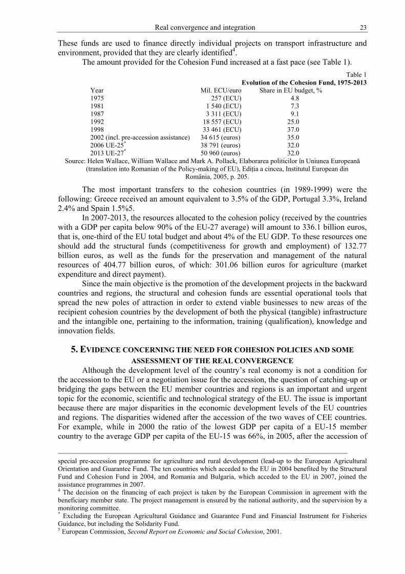
The amount provided for the Cohesion Fund increased at a fast pace (see Table 1). Table 1
Evolution of the Cohesion Fund, 1975-2013 Year Mil. ECU/euro Share in EU budget, % 1975 257 (ECU) 4.8 1981 1 540 (ECU) 7.3 1987 3 311 (ECU) 9.1 1992 18 557 (ECU) 25.0 1998 33 461 (ECU) 37.0 2002 (incl. pre-accession assistance) 34 615 (euros) 35.0 2006 UE-25* 38 791 (euros) 32.0 2013 UE-27* 50 960 (euros) 32.0
Source: Helen Wallace, William Wallace and Mark A. Pollack, Elaborarea politicilor în Uniunea Europeană (translation into Romanian of the Policy-making of EU), Ediţia a cincea, Institutul European din
România, 2005, p. 205.
The most important transfers to the cohesion countries (in 1989-1999) were the following: Greece received an amount equivalent to 3.5% of the GDP, Portugal 3.3%, Ireland 2.4% and Spain 1.5%5.
In 2007-2013, the resources allocated to the cohesion policy (received by the countries with a GDP per capita below 90% of the EU-27 average) will amount to 336.1 billion euros, that is, one-third of the EU total budget and about 4% of the EU GDP. To these resources one should add the structural funds (competitiveness for growth and employment) of 132.77 billion euros, as well as the funds for the preservation and management of the natural resources of 404.77 billion euros, of which: 301.06 billion euros for agriculture (market expenditure and direct payment).
Since the main objective is the promotion of the development projects in the backward countries and regions, the structural and cohesion funds are essential operational tools that spread the new poles of attraction in order to extend viable businesses to new areas of the recipient cohesion countries by the development of both the physical (tangible) infrastructure and the intangible one, pertaining to the information, training (qualification), knowledge and innovation fields.
5. EVIDENCE CONCERNING THE NEED FOR COHESION POLICIES AND SOME ASSESSMENT OF THE REAL CONVERGENCE
Although the development level of the country’s real economy is not a condition for the accession to the EU or a negotiation issue for the accession, the question of catching-up or bridging the gaps between the EU member countries and regions is an important and urgent topic for the economic, scientific and technological strategy of the EU. The issue is important because there are major disparities in the economic development levels of the EU countries and regions. The disparities widened after the accession of the two waves of CEE countries. For example, while in 2000 the ratio of the lowest GDP per capita of a EU-15 member country to the average GDP per capita of the EU-15 was 66%, in 2005, after the accession of
special pre-accession programme for agriculture and rural development (lead-up to the European Agricultural Orientation and Guarantee Fund. The ten countries which acceded to the EU in 2004 benefited by the Structural Fund and Cohesion Fund in 2004, and Romania and Bulgaria, which acceded to the EU in 2007, joined the assistance programmes in 2007. 4 The decision on the financing of each project is taken by the European Commission in agreement with the beneficiary member state. The project management is ensured by the national authority, and the supervision by a monitoring committee. * Excluding the European Agricultural Guidance and Guarantee Fund and Financial Instrument for Fisheries Guidance, but including the Solidarity Fund. 5 European Commission, Second Report on Economic and Social Cohesion, 2001.
24 AUREL IANCU
the ten countries, the ratio of the lowest GDP per capita to the average GDP per capita of the EU-25 reached 46.6%. After the accession of Romania and Bulgaria, the lowest GDP per capita as against the EU-25 average reached 32%.
The persistence of the disparities and underdevelopment of some EU countries and regions would mean the inconsistency with the very meaning of the European Communities and with the EU strategy, according to which the EU is supposed to become the most important economic and technological power in the world in a predictable period of time, to become the global leader in the economic, scientific, technological and living standard areas. Of course, such a strategy prevents the persistence of disparities and the existence of underdeveloped and poor regions and, also, requires the implementation of policies fully aimed at capitalizing the resources of all component countries and regions to achieve their economic and social development. That is why, the EU adopted a firm policy on economic and social cohesion, in order to achieve the real economic convergence of all member countries and regions. From this perspective, it is worth mentioning that all twelve countries of the two accession waves have become cohesion countries, since their GDP per capita has been far below the threshold of 90% of the EU average. Therefore, all these countries satisfy the basic criterion for becoming beneficiaries of the Cohesion Fund for the infrastructure and environment projects. Also, most regions of these countries are eligible for financing from the Structural Funds, since their GDP per capita is below the threshold of 75% of the EU-25 average.
The new member countries have received economic support from the EU since the pre-accession period through special lead-up programmes (PHARE, ISPA, SAPARD, etc.). In the post-accession period, the financial support offered through the new programmes is more consistent as regards the objectives and implementation mechanisms, as well as the size of the funds allocated from the EU multiannual budget (2007-2013). The question “To what extent did these policies influence the real economy convergence?” is difficult to answer by analytical impact assessments, since these policies have not yet produced effects, due to the relatively short time of application.
The clarifying elements in this matter are the overall results of the influence of all factors of convergent growth in each country, determined by means of different factors (usually, computed on long term), which show either the diminution in the inequalities between the set of analyzed economies (the evolution of the index concerning the ratio between the level indicators of the economies, dispersion, Gini index, Theil index, etc.), or the cross-section convergence (β-convergence), or, finally, the convergence of the time series, dynamic distribution, etc.6. We confine ourselves in this study to the results of the computation of two of the above indicators, which are equally simple and suggestive
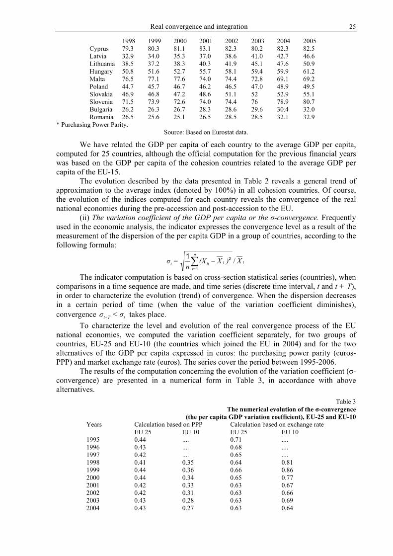
(i) The index concerning the ratio between the level indicators (GDP per capita). Relating the level of the GDP per capita of the countries to the average level of the EU for a certain period, one may find general trend of approximation of the development levels of these countries as against the EU average level in the analyzed period. Table 2 contains data on the cohesion countries pertaining to the EU-15 Group (Greece, Spain, Portugal) and the countries that joined the EU in 2004 and 2007.
Table 2 The evolution of the index concerning the ratio of the GDP per capita of
the cohesion countries and to the EU-25 average, based on PPP* (1998-2005), percentage 1998 1999 2000 2001 2002 2003 2004 2005 Greece 70.4 70.7 72.6 73.5 77.2 81.1 81.9 83.0 Spain 88.8 92.5 92.5 93.2 95.3 97.7 97.3 98.3 Portugal 78.2 80.3 80.6 79.8 79.53 72.8 72.2 70.9 Czech R. 65.3 64.9 63.7 64.9 66.5 67.7 70.04 73.07 Estonia 39.1 38.8 40.7 42.3 45.1 48.4 51.1 55.5
6 Castro, José Villaverde, “Indicators of Real Economic Convergence. A Primer”, United Nations University – Cris E–Working Papers, W-2004/2.
Real convergence and integration 25
1998 1999 2000 2001 2002 2003 2004 2005 Cyprus 79.3 80.3 81.1 83.1 82.3 80.2 82.3 82.5 Latvia 32.9 34.0 35.3 37.0 38.6 41.0 42.7 46.6 Lithuania 38.5 37.2 38.3 40.3 41.9 45.1 47.6 50.9 Hungary 50.8 51.6 52.7 55.7 58.1 59.4 59.9 61.2 Malta 76.5 77.1 77.6 74.0 74.4 72.8 69.1 69.2 Poland 44.7 45.7 46.7 46.2 46.5 47.0 48.9 49.5 Slovakia 46.9 46.8 47.2 48.6 51.1 52 52.9 55.1 Slovenia 71.5 73.9 72.6 74.0 74.4 76 78.9 80.7 Bulgaria 26.2 26.3 26.7 28.3 28.6 29.6 30.4 32.0 Romania 26.5 25.6 25.1 26.5 28.5 28.5 32.1 32.9
* Purchasing Power Parity. Source: Based on Eurostat data.
We have related the GDP per capita of each country to the average GDP per capita, computed for 25 countries, although the official computation for the previous financial years was based on the GDP per capita of the cohesion countries related to the average GDP per capita of the EU-15.
The evolution described by the data presented in Table 2 reveals a general trend of approximation to the average index (denoted by 100%) in all cohesion countries. Of course, the evolution of the indices computed for each country reveals the convergence of the real national economies during the pre-accession and post-accession to the EU.
(ii) The variation coefficient of the GDP per capita or the σ-convergence. Frequently used in the economic analysis, the indicator expresses the convergence level as a result of the measurement of the dispersion of the per capita GDP in a group of countries, according to the following formula:
t
n
=ititt X)X(X
n=σ /∑ −
1
21
The indicator computation is based on cross-section statistical series (countries), when comparisons in a time sequence are made, and time series (discrete time interval, t and t + T), in order to characterize the evolution (trend) of convergence. When the dispersion decreases in a certain period of time (when the value of the variation coefficient diminishes), convergence tTt+ σ<σ takes place.
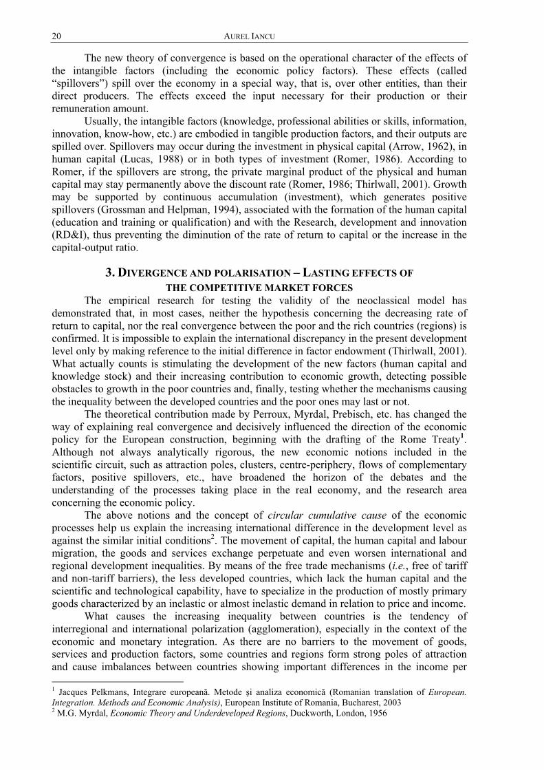
To characterize the level and evolution of the real convergence process of the EU national economies, we computed the variation coefficient separately, for two groups of countries, EU-25 and EU-10 (the countries which joined the EU in 2004) and for the two alternatives of the GDP per capita expressed in euros: the purchasing power parity (euros-PPP) and market exchange rate (euros). The series cover the period between 1995-2006.
The results of the computation concerning the evolution of the variation coefficient (σ-convergence) are presented in a numerical form in Table 3, in accordance with above alternatives.
Table 3 The numerical evolution of the σ-convergence
(the per capita GDP variation coefficient), EU-25 and EU-10 Years Calculation based on PPP Calculation based on exchange rate EU 25 EU 10 EU 25 EU 10 1995 0.44 .... 0.71 .... 1996 0.43 .... 0.68 .... 1997 0.42 .... 0.65 .... 1998 0.41 0.35 0.64 0.81 1999 0.44 0.36 0.66 0.86 2000 0.44 0.34 0.65 0.77 2001 0.42 0.33 0.63 0.67 2002 0.42 0.31 0.63 0.66 2003 0.43 0.28 0.63 0.69 2004 0.43 0.27 0.63 0.64
26 AUREL IANCU
Years Calculation based on PPP Calculation based on exchange rate EU 25 EU 10 EU 25 EU 10 2005 0.42 0.24 0.62 0.55 2006* 0.42 0.24 0.62 0.51
*Estimated data. Source: Based on Eurostat data.
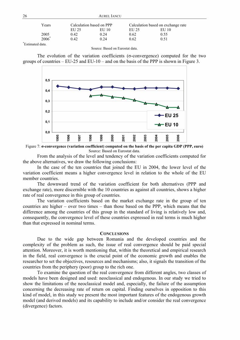
The evolution of the variation coefficients (σ-convergence) computed for the two groups of countries – EU-25 and EU-10 – and on the basis of the PPP is shown in Figure 3.
0,0
0,1
0,2
0,3
0,4
0,5
1995
1996
1997
1998
1999
2000
2001
2002
2003
2004
2005
2006
EU 25
EU 10
Figure 7: σ-convergence (variation coefficient) computed on the basis of the per capita GDP (PPP, euro)
Source: Based on Eurostat data. From the analysis of the level and tendency of the variation coefficients computed for
the above alternatives, we draw the following conclusions: In the case of the ten countries that joined the EU in 2004, the lower level of the
variation coefficient means a higher convergence level in relation to the whole of the EU member countries.
The downward trend of the variation coefficient for both alternatives (PPP and exchange rate), more discernible with the 10 countries as against all countries, shows a higher rate of real convergence in this group of countries.
The variation coefficients based on the market exchange rate in the group of ten countries are higher – over two times – than those based on the PPP, which means that the difference among the countries of this group in the standard of living is relatively low and, consequently, the convergence level of these countries expressed in real terms is much higher than that expressed in nominal terms.
CONCLUSIONS Due to the wide gap between Romania and the developed countries and the
complexity of the problem as such, the issue of real convergence should be paid special attention. Moreover, it is worth mentioning that, within the theoretical and empirical research in the field, real convergence is the crucial point of the economic growth and enables the researcher to set the objectives, resources and mechanisms; also, it signals the transition of the countries from the periphery (poor) group to the rich one.
To examine the question of the real convergence from different angles, two classes of models have been designed and used: neoclassical and endogenous. In our study we tried to show the limitations of the neoclassical model and, especially, the failure of the assumption concerning the decreasing rate of return on capital. Finding ourselves in opposition to this kind of model, in this study we present the most important features of the endogenous growth model (and derived models) and its capability to include and/or consider the real convergence (divergence) factors.
Real convergence and integration 27
The latest empirical research aimed at the validation of various convergence hypotheses proves that there is not and it cannot be an alignment of all countries with an “absolute convergence”. What the economic and social reality of the countries and regions confirm is rather the “group convergence”, viewed in its dynamics and in relation to the factors of influence acting within the system. Under the present circumstances, the factor that determines the dynamics of the developed countries is knowledge, in its multiple forms. The knowledge factor determines the higher growth rates of the developed countries, if compared to the poor ones.
As pointed out above, market mechanisms are not able to support the convergence process, especially when there is a wider gap in the development level of the countries and regions. On the contrary, the mechanism stimulates, first, the economic clustering, the formation of development poles, which rather cause wider gaps. Considering these natural processes, the European Union tries to correct the shortcomings of the free market laws by the cohesion policy, besides the sectoral policies, with favorable effects on the economic convergence of the less developed countries with the developed ones.
BIBLIOGRAPHY 1. Abramovitz M., “Catching Up, Forging Ahead, and Falling Behind”, The Journal of Economic
History, vol. 46, No. 2, “The Tasks of Economic History” (Jun. 1986), 385-406. 2. Aghion Pilippe, Eve Caroli, Cecilia Garcia-Penalosa, “Inequality and Economic Growth: The
Perspective of the New Growth Theories”, Journal of Economic Literature, vol. 37, No. 4 (Dec. 1999), 1615-1660.
3. Allen David, “Coeziunea şi fondurile structurale”, in Hellen Wallace, Willian Wallace and Mark A. Pollack (coord.) Elaborarea politicilor în Uniunea Europeană, (translation), Institutul European din România, 2005.
4. Barro Robert J., “Economic Growth in a Cross-Section of Countries”, The Quarterly Journal of Economics, vol. 106, No. 2, May 1991, 407-443.
5. Barro Robert J., Xavier Sala-i-Martin, “Convergence”, The Journal of Political Economy, vol. 100, No. 2 (April 1992), 223-251.
6. Bassanini Andrea, Stefano Scarpeta, “The Driving Forces of Economic Growth: Panel Data Evidence for the OECD Countries”, OECD Economic Studies, No. 33, 2001/II.
7. Castro Villaverde José, Indicators of Real Economic Convergence. A Primer, United Nations University, UNU-CRIS E-Working Papers, w-2004/2.
8. Dalgaard Carl-Johan, Jacob Vastrup, “On the Measurement of σ–Convergence”, Economics Letters, 70 (2001) 283-287.
9. Dăianu Dan, “Convergenţa economică. Cerinţe şi posibilităţi”, in Aurel Iancu (coordinator), Dezvoltarea economică a României. Competitivitatea şi integrarea în Uniunea Europeană, Editura Academiei Române, Bucureşti, 2003.
10. Durlauf St. N., “On the Convergence and Divergence of Growth Rates”, The Economic Journal, vol. 106, No. 437 (June 1996), 1016-1018.
11. Esteban Joan-Maria, Ray Dbraj, “On the Measurement of Polarization”, Econometrica, vol. 62, No. 4, July 1994, p. 819-851.
12. Iancu Aurel, “Problema convergenţei economice”, Oeconomica, nr. 4, 2006. 13. Idu Pompilia, “Instrumentele structurale şi convergenţa statelor în Uniunea Europeană”,
Oeconomica, nr. 3/2006. 14. Kutan Ali M., Taner M. Yigit, Convergence of Candidate Countries to the European Union, 2003. 15. Lucas Robert E. Jr., “On the Mechanics of Economic Development” (in “Economic Development
and Growth Papers”), Journal of Monetary Economics, 22/1988, 3-42. 16. Manoilescu Mihai, Forţele naţionale productive şi comerţul exterior. Teoria protecţionismului şi a
schimbului internaţional, Editura Ştiinţifică şi Enciclopedică, Bucureşti, 1986. 17. Matkowski Zbigniew, Mariusz Prochniak, Economic Convergence in the EU Accession
Countries, Warsaw School of Economics. 18. Meeusen Wim, José Villaverde (ed.), Convergence Issues in the European Union, Edward Elgar,
UK, 2002.
28 AUREL IANCU
19. Mihăescu Flavius, “Convergenţa între economiile central şi est-europene”, in Daniel Dăianu and Mugur Isărescu (coordinators), Noii economişti despre tranziţia în România, colecţia Bibliotecii Băncii Naţionale, Bucureşti, 2003.
20. Myrdal G., Economic Theory and Underdeveloped Regions, Duckworth, London, 1957. 21. Pelkmans Jacques, Integrare europeană. Metode şi analiză economică (ed. a II-a) (translation),
Institutul European din România, Bucureşti, 2003. 22. Perroux Fr., L’économie du XXe siècle, Paris, P.U.F. , 1969. 23. Perroux Fr., Pour une philosophie du nouveau développement, Paris, Aubier, Les Preses de
L’UNESCO, 1981. 24. Prebisch R., “The Periphery in the Global System of Capitalism”, C.E.P.A.L. Review, April,
1981. 25. Puga Diego, “The Rise and Fall of Regional Inequalities”, Centre for Economic Performance,
Discussion Paper, No. 314, November 1996, Revised January 1998. 26. Ranis Gustav, Stewart Frances, Ramirez Alejandro, “Economic Growth and Human
Development” (in Economic Development and Growth Papers), World Development, vol. 28, No. 6, June 2000.
27. Reiner Martin, “The Impact of the EU’s Structural and Cohesion Funds on Real Convergence in the EU”, NBP Conference, Potential Output and Barriers to Growth, Yalesie Górne, 2003.
28. Romer Paul M., “Increasing Returns and Long-Run Growth”, The Journal of Political Economy, vol. 94, No. 5 (October 1986), 1002-1039.
29. Romer Paul M., “Endogenous Technological Change”, The Journal of Political Economy, October 1990, 98,5, AB1/Inform Global.
30. Solow Robert M., “A Contribution to the Theory of Economic Growth”, The Quarterly Journal of Economics, vol. 70, No. 1 (February 1956), 65-94.
31. Thirlwall A.P., Growth and Development with Special Reference to Developing Economies (sixth ed.), 2001.
32. Wallace Helen, William Wallace and Mark A. Pollack, Elaborarea politicilor în Uniunea Europeană (translation), ediţia a cincea, Institutul European din România, 2005.
33. Zipfel Jacob, Determinants of Economic Growth, Florida State University, 2004.
EVALUATION OF THE PERFORMANCE AND OF THE INTEGRATION OF THE EURO ZONE STOCK MARKET:
WHICH ARE THE “RIGHT MOMENTS”?
Jean-Pierre BERDOT*
Abstract. This study intends to verify if, on the stock markets of the Euro zone, the integration as a process that lead to their unification is applied, even if several disparities exist among the national characteristics of the return-risk. We verify the pertinence of the consideration of third and fourth order moments in the comprehension of the arbitration mechanisms.
The first part focuses on establishing the situation of the integration of the stock markets from the Euro zone member countries on the basis of the main characteristics of the returns and the associated risk premiums. Starting with the apparent inadequacy in the traditional theory, the second part considers the usual responses to the main questions posed on the empirical plan: non-normality of the returns distributions and non-quadratic preferences of the investors. The third part solves the apparent contradiction among the risk’s characteristics and price, on one side, and the stronger and stronger correlations among the national markets and the European indexes, on the other side.
On the financial markets, the strategic variable is not the stocks’ price or the stock market indexes prices, but the growth rate of this price. This rate measures the gains in capital made by the investors and can be thought of as the return rate (except of the payment of dividends) of stocks or portfolios. This return rate calculated as ( )t t t 1 t 1R P P P− −= − (where Pt represents the assets price at the market closing moment t) presents an interest both for the statistician and the investor: 1. It influences the investors’ opportunities and strategy. 2. Its statistical attributes (empirical as well as theoretical) are more suitable for treatment
than a price series: moreover, the returns are stationary which makes the estimation and prediction easier.
Traditionally, the financial analysis concerns the arbitration among the risky financial assets on the basis of the couple return-volatility, appreciated through the first two moments of their returns distribution: mean and standard deviation. Indicators such as Sharpe’s ratio1 synthesize a priori this double dimension of the arbitration.
However, fort a long time2, the questions on the quality of the information gathered by this type of indicator have multiplied. Indeed, except of considering the normal distributions, the characteristics of the statistical series distributions can not be summarized only by their two first moments. But, the returns’ rates of the financial assets are generally non-normal. * Jean-Pierre Berdot is a Professor at the University of Poitiers, Honorary Professor of the “Alexandru Ioan Cuza” University 1 On the origin of the ratio, cf. Sharpe (1966), and on his revision, cf. Sharpe (1994). 2 We can find the first questions in Samuelson (1970) and Rubinstein (1973).
30 JEAN-PIERRE BERDOT
Consequently, it is not surprising to notice that the researches in finance are interested in the characteristics of the (centered3) moments of higher order, namely of third order (skewness) and of fourth order (kurtosis)4.
This study intends to verify the pertinence of considering third and fourth order (centered) moments in understanding the arbitration mechanisms among the directional financial assets (in connection to the benchmarks that are the market indexes). More precisely, starting from the characteristics of the national “flagship indexes” for the Euro zone, we examine the nature of the financial markets’ integration of the states that became members of the Euro zone from 1999.
The first part of the study recalls the principle of the rational investors’ choice on the financial markets and the role that the returns distribution moments may play. It sets up the description of the integration of the stock markets of the Euro zone member states on the basis of the empirical characteristics (including the first four moments) of the returns’ rates of the market indexes.
The second part explains the contribution of the traditional theories centered on the first two moments (mean and variance). It raises a contradiction, on the stock markets of the Euro zone, between the maintenance of significant differentials of the risk’s characteristics and price (traditional sign of non-integration), on one side, and the stronger and stronger correlations between national markets and European indexes, on the other side (sign of integration).
The third part starts from the apparent inadequacy of the traditional theory and gives relevant answers to the main two questions raised on the empirical plan: the non-normality of the returns’ distributions and the non-quadratic preferences of the investors. It shows that, despite the apparent disparities of all the returns characteristics associated to the national stock markets indexes of the Euro zone (means, standard deviations, Sharpe’s ratios), the integration process is at work. The apparent differentials of the price of the risk are expressing a rational evaluation of the risk associated to the moments of orders higher than 2, and especially of the major risks associated to the negativity of the skewness. The investor asks for a premium in order to compensate the high probability of extreme losses.
The main stock markets of the Euro zone are kept by their flagship indexes: Germany (DAX30 written as ALL), Austria (ATX written as AUT), Belgium (BEL20 written as BEL), Spain (IBEX35 written as ESP), France (CAC40 written as FRA), Ireland (ISEQ20 written as IRL), Italy (MIB30 written as ITA), Netherlands (AEX written as PB), and Portugal (PSI20 written as POR).
Two European indexes have been kept too: EUROSTOXX50 (flagship index written as E50) and EUROSTOXX500 (wide index of the European market written as E5000).
The estimation period starts on January 1st, 1996 and ends on December 31st, 20065 (except of the Ireland for which the data are available beginning with January 1st, 1998). The data are daily data. The returns are measured by the single daily variation of the indexes prices expressed in percentages.
The risk premium associated to these returns is expressed by the difference between the daily returns and the returns rates of the German state for 10 years.
All the data come from the DataStream database.
3 Remind that the centered moment of h order of a random variable R is )E(R))E((R=μ h
h − . The variance (the square of the standard deviation) is the centered moment of 2nd order. 4 Skewness and kurtosis are the centered moments standardized by the standard deviation σ of the variable, of the form hhμ /σ , with h = 3 for the skewness and h = 4 for the kurtosis. 5 This period was kept for the reason to analyze the dynamics of the integration for a complete stock market cycle, on the one hand, and to explain the situation of the stock markets before the adoption of the single currency, on the other hand.
Evaluation of the performance and of the integration of the Euro zone stock market… 31
I. THE FINANCIAL CHOICES IN A RISKY UNIVERSE: THE ARTICULATION BETWEEN THE RETURNS RATES MOMENTS AND THE INVESTORS’ PREFERENCES
The returns rates of stocks, portfolios, or market indexes should be considered as random variables. Indeed, it is possible to consider that the investment in Treasury bonds issued by countries such as Germany or France is safe due to the sovereign debt of such states. The investor can consider that the return rate of his placement is risk-free. It is not the same situation with the stock investments. Indeed, the future evolution of the stock prices can not be known with certainty as it is submitted to the markets hazard.
The traditional assumption is that the investors’ universe is a risky universe. In such a universe, the choice criterion is the one defined by Von Neumann and Morgenstern (1944) that is the maximization of the expected utility.
The investors’ preferences can be expressed by a utility function that depends only on the considered asset or portfolio’s return rate R, and written therefore as U(R), with U’(R)>06.
Since the return rate is random, the utility U(R) becomes a random variable. The investor’s strategy guides him to maximize his expected utility. It is not always useful to give the utility function a specific form. It is enough to develop this function by a Taylor series about the return mean E(R), supposed m. In order to simplify, we can write the centered variable of the return as: � = R – E(R) = R – m.
For reasons that will become obvious later on, the utility function will be expanded to the fourth order. When U’, U’’, U’’’, and U’’’’ represent the first, second, third and, respectively, fourth order derivatives of the utility, we have in that case:
2 3 41 1 1U(R) U(m ) U(m) U '(m) U ''(m) U '''(m) U ''''(m)2 3! 4!
= + ε = +ε + ε + ε + ε
Then, it is necessary to calculate the expected utility function. 2 3 41 1 1EU(R) E(U(m)) E( U '(m)) E( U ''(m)) E( U '''(m)) E( U ''''(m))
2 3! 4!= + ε + ε + ε + ε
Arranging7, we obtain:
2 3 41 1 1EU(R) U(m) U '(m) E( ) U ''(m) E( ) U '''(m) E( ) U ''''(m) E( )2 3! 4!
= + ε + ε + ε + ε
The expression obtained may be reinterpreted, as it is integrates the various expectations linked with the centered variable of the returns. We remember that the theoretical centered moment (about the mean) of a random variable R is defined by8. Moreover, the mean of the centered variable ε is null:
E(ε) = E((R – m)) = E(R) – m = 0. Therefore, it is possible to express the expected utility considering the theoretical
centered moments:
(1) 2 3 4
1 1 1EU(R) U(E(R)) U ''(E(R)) (R) U '''(E(R)) (R) U ''''(E(R)) (R)2 3! 4!
= + μ + μ + μ
The expression of the expected utility makes possible to infer the strategic criteria of the investors’ choice, considering their preferences revealed by the characteristics of the returns distribution function. The expected utility is the function of, on the one hand, the returns rates moments: the mean and the 2nd, 3rd and 4th order moments and, on the other
6 We refer to the general assumption according to which the marginal utility (the first derivate of the utility) is positive. The utility is always an increasing function of the return rate. 7 Remind that we consider that ε is a random centred variable, m is certain. 8 The estimators (biased) of these theoretical moments are the empirical moments (centred by the arithmetic
mean), suppose t T1 hˆ (R R)h tT t 1
=μ = −
=∑ , where Rt represents the return rate in t, T measures the number of
the observations and R is the arithmetic mean of the returns rates.
32 JEAN-PIERRE BERDOT
hand, the utility function form (especially of the 2nd, 3rd and 4th derivates), that is the investors’ preferences.
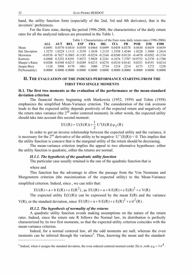
For the Euro zone, during the period 1996-2006, the characteristics of the daily return rates for all the analyzed indexes are presented in the Table 1.
Table 1: Characteristics of the Euro zone daily return rates (1996-2006) ALL AUT BEL ESP FRA IRL ITA PB POR E50 E500
Mean 0.0491 0.0570 0.0410 0.0558 0.0464 0.0499 0.0458 0.0378 0.0430 0.0439 0.0439Std. Deviation 1.5275 1.0229 1.1113 1.3339 1.3638 1.2135 1.3558 1.4344 1.0220 1.3860 1.2414Skewness -0.0536 -0.7627 0.3065 -0.1185 -0.0234 -0.2166 -0.0240 0.0124 -0.4478 -0.0202 -0.1334Kurtosis 6.0408 8.5252 8.8291 5.9472 5.9828 8.2241 6.1676 7.2707 10.0752 6.2370 6.1700Sharpe’s Ratio 0.0208 0.0388 0.0213 0.0289 0.0213 0.0276 0.0210 0.0142 0.0251 0.0191 0.0214Jarque-Bera 1124 3988 4170 1061 1080 2734 1218 2214 6173 1272 1228Pr(Normality) 0.0000 0.0000 0.0000 0.0000 0.0000 0.0000 0.0000 0.0000 0.0000 0.0000 0.0000
II. THE EVALUATION OF THE INDEXES PERFORMANCE STARTING FROM THE FIRST TWO SINGLE MOMENTS
II.1. The first two moments as the evaluation of the performance or the mean-standard deviation criterion
The financial theory beginning with Markowitz (1952, 1959) and Tobin (1958) emphasizes the simplified Mean-Variance criterion. The consideration of the risk aversion leads to that the expected utility depends positively of the expected return and negatively of the return rates variance (the 2nd order centered moment). In other words, the expected utility should take into account this second moment:
21EU(R) U(E(R)) U ''(E(R)) (R)2
= + μ
In order to get an inverse relationship between the expected utility and the variance, it is necessary for the 2nd derivative of the utility to be negative: U’’(E(R)) < 0. This implies that the utility function is concave that is the marginal utility of the return should be decreasing.
The mean-variance criterion implies the appeal to two alternative hypotheses: either the utility function is quadratic, either the returns are normal.
II.1.1. The hypothesis of the quadratic utility function The particular case usually retained is the one of the quadratic function that is b=++where b=+and=< This function has the advantage to allow the passage from the Von Neumann and
Morgenstern criterion (the maximization of the expected utility) to the Mean-Variance simplified criterion. Indeed, since b=++, we can infer that:
2EU(R) a b E(R) c E(R )= + + , as 2EU(R) a b E(R) c E(R) c V(R)= + + + The expected utility E(U(R)) can be expressed by the mean E(R) and the variance
V(R), or the standard deviation, since 2 2EU(R) a b E(R) c E(R) c (R)= + + + σ .
II.1.2. The hypothesis of normality of the returns A quadratic utility function avoids making assumptions on the nature of the return
rates. Indeed, since the return rate R follows the Normal law, its distribution is perfectly characterized by its two first moments, so that the expected utility criterion coincides with the mean-variance criterion.
Indeed, for a normal centered law, all the odd moments are null, whereas the even moments can be inferred through the variance9. Thus, knowing the mean and the standard- 9 Indeed, when σ assigns the standard deviation, the even ordered centered moment (order 2h) is μ=σ−,with 434μ = σ .
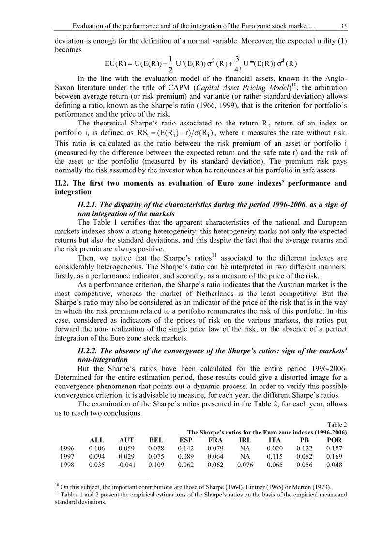
Evaluation of the performance and of the integration of the Euro zone stock market… 33
deviation is enough for the definition of a normal variable. Moreover, the expected utility (1) becomes
2 41 3EU(R) U(E(R)) U ''(E(R)) (R) U ''''(E(R)) (R)2 4!
= + σ + σ
In the line with the evaluation model of the financial assets, known in the Anglo-Saxon literature under the title of CAPM (Capital Asset Pricing Model)10, the arbitration between average return (or risk premium) and variance (or rather standard-deviation) allows defining a ratio, known as the Sharpe’s ratio (1966, 1999), that is the criterion for portfolio’s performance and the price of the risk.
The theoretical Sharpe’s ratio associated to the return Ri, return of an index or portfolio i, is defined as i i iRS (E(R ) r) (R )= − σ , where r measures the rate without risk. This ratio is calculated as the ratio between the risk premium of an asset or portfolio i (measured by the difference between the expected return and the safe rate r) and the risk of the asset or the portfolio (measured by its standard deviation). The premium risk pays normally the risk assumed by the investor when he renounces at his portfolio in safe assets.
II.2. The first two moments as evaluation of Euro zone indexes’ performance and integration
II.2.1. The disparity of the characteristics during the period 1996-2006, as a sign of non integration of the markets The Table 1 certifies that the apparent characteristics of the national and European
markets indexes show a strong heterogeneity: this heterogeneity marks not only the expected returns but also the standard deviations, and this despite the fact that the average returns and the risk premia are always positive.
Then, we notice that the Sharpe’s ratios11 associated to the different indexes are considerably heterogeneous. The Sharpe’s ratio can be interpreted in two different manners: firstly, as a performance indicator, and secondly, as a measure of the price of the risk.
As a performance criterion, the Sharpe’s ratio indicates that the Austrian market is the most competitive, whereas the market of Netherlands is the least competitive. But the Sharpe’s ratio may also be considered as an indicator of the price of the risk that is in the way in which the risk premium related to a portfolio remunerates the risk of this portfolio. In this case, considered as indicators of the prices of risk on the various markets, the ratios put forward the non- realization of the single price law of the risk, or the absence of a perfect integration of the Euro zone stock markets.
II.2.2. The absence of the convergence of the Sharpe’s ratios: sign of the markets’ non-integration But the Sharpe’s ratios have been calculated for the entire period 1996-2006.
Determined for the entire estimation period, these results could give a distorted image for a convergence phenomenon that points out a dynamic process. In order to verify this possible convergence criterion, it is advisable to measure, for each year, the different Sharpe’s ratios.
The examination of the Sharpe’s ratios presented in the Table 2, for each year, allows us to reach two conclusions.
Table 2 The Sharpe’s ratios for the Euro zone indexes (1996-2006)
ALL AUT BEL ESP FRA IRL ITA PB POR 1996 0.106 0.059 0.078 0.142 0.079 NA 0.020 0.122 0.187 1997 0.094 0.029 0.075 0.089 0.064 NA 0.115 0.082 0.169 1998 0.035 -0.041 0.109 0.062 0.062 0.076 0.065 0.056 0.048
10 On this subject, the important contributions are those of Sharpe (1964), Lintner (1965) or Merton (1973). 11 Tables 1 and 2 present the empirical estimations of the Sharpe’s ratios on the basis of the empirical means and standard deviations.
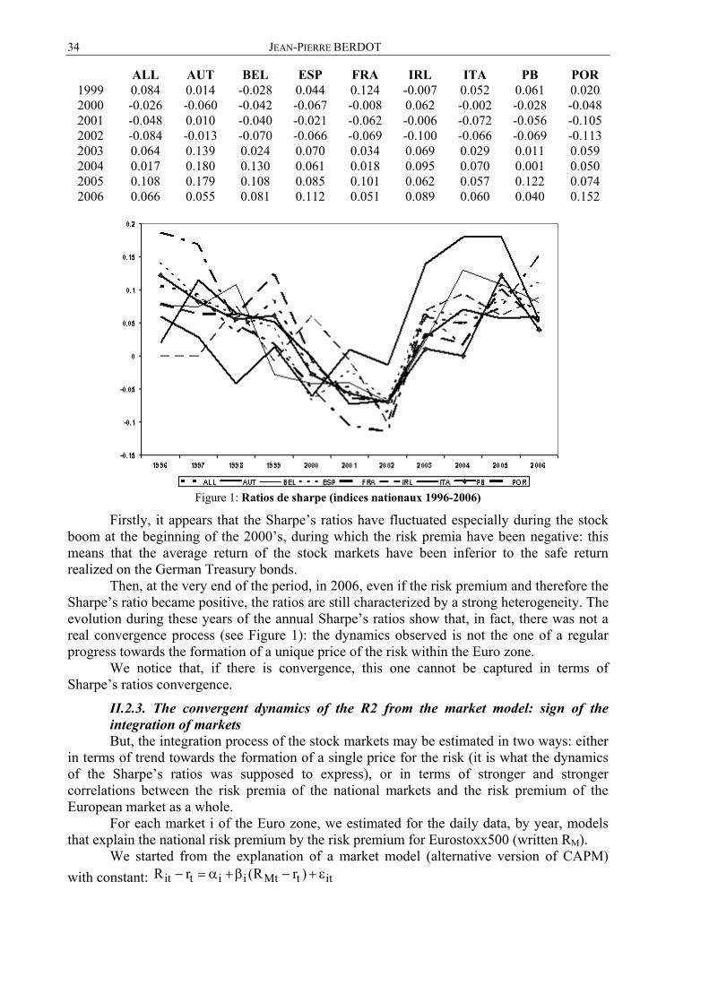
34 JEAN-PIERRE BERDOT
ALL AUT BEL ESP FRA IRL ITA PB POR 1999 0.084 0.014 -0.028 0.044 0.124 -0.007 0.052 0.061 0.020 2000 -0.026 -0.060 -0.042 -0.067 -0.008 0.062 -0.002 -0.028 -0.048 2001 -0.048 0.010 -0.040 -0.021 -0.062 -0.006 -0.072 -0.056 -0.105 2002 -0.084 -0.013 -0.070 -0.066 -0.069 -0.100 -0.066 -0.069 -0.113 2003 0.064 0.139 0.024 0.070 0.034 0.069 0.029 0.011 0.059 2004 0.017 0.180 0.130 0.061 0.018 0.095 0.070 0.001 0.050 2005 0.108 0.179 0.108 0.085 0.101 0.062 0.057 0.122 0.074 2006 0.066 0.055 0.081 0.112 0.051 0.089 0.060 0.040 0.152
Figure 1: Ratios de sharpe (indices nationaux 1996-2006)
Firstly, it appears that the Sharpe’s ratios have fluctuated especially during the stock boom at the beginning of the 2000’s, during which the risk premia have been negative: this means that the average return of the stock markets have been inferior to the safe return realized on the German Treasury bonds.
Then, at the very end of the period, in 2006, even if the risk premium and therefore the Sharpe’s ratio became positive, the ratios are still characterized by a strong heterogeneity. The evolution during these years of the annual Sharpe’s ratios show that, in fact, there was not a real convergence process (see Figure 1): the dynamics observed is not the one of a regular progress towards the formation of a unique price of the risk within the Euro zone.
We notice that, if there is convergence, this one cannot be captured in terms of Sharpe’s ratios convergence.
II.2.3. The convergent dynamics of the R2 from the market model: sign of the integration of markets But, the integration process of the stock markets may be estimated in two ways: either
in terms of trend towards the formation of a single price for the risk (it is what the dynamics of the Sharpe’s ratios was supposed to express), or in terms of stronger and stronger correlations between the risk premia of the national markets and the risk premium of the European market as a whole.
For each market i of the Euro zone, we estimated for the daily data, by year, models that explain the national risk premium by the risk premium for Eurostoxx500 (written RM).
We started from the explanation of a market model (alternative version of CAPM) with constant: it t i i Mt t itR r (R r )− = α +β − + ε
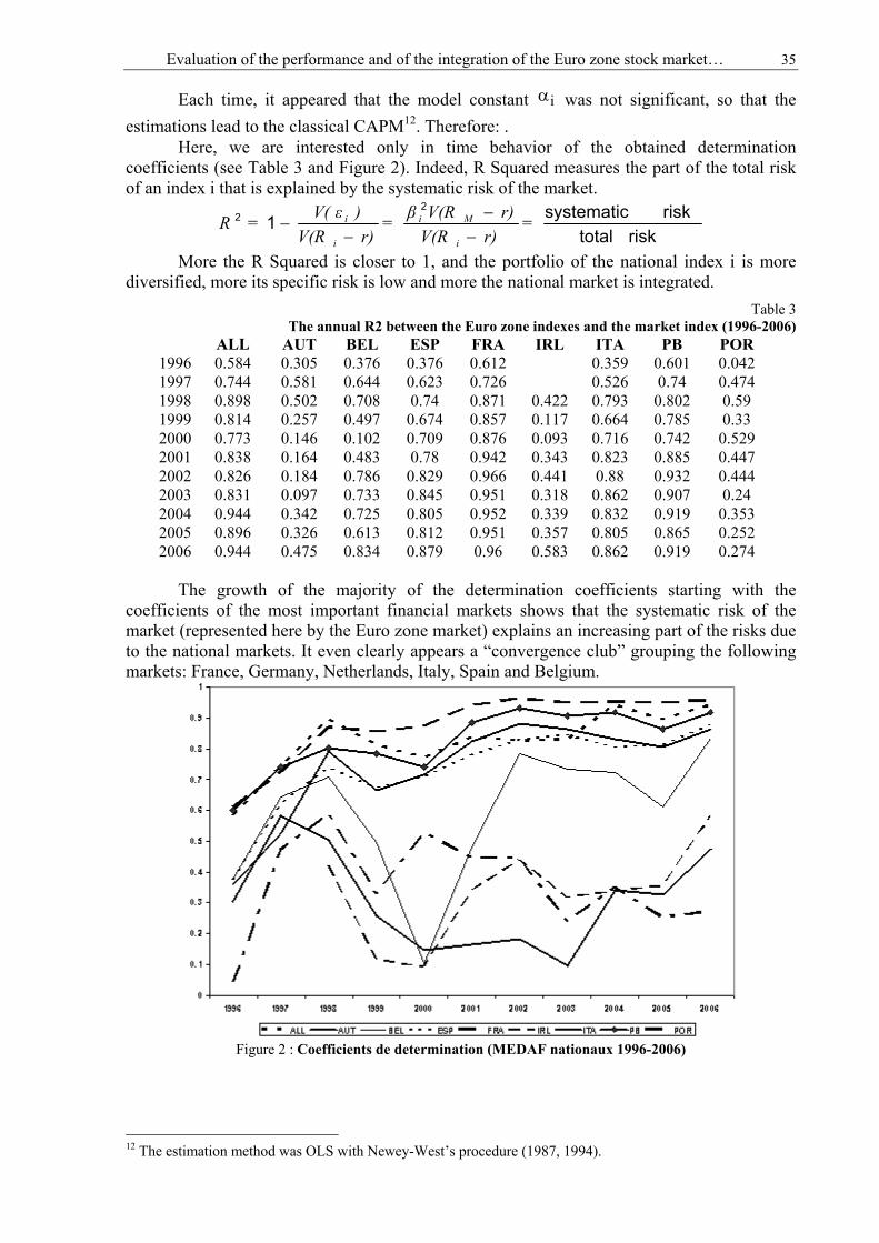
Evaluation of the performance and of the integration of the Euro zone stock market… 35
Each time, it appeared that the model constant iα was not significant, so that the estimations lead to the classical CAPM12. Therefore: −=β−+ε.
Here, we are interested only in time behavior of the obtained determination coefficients (see Table 3 and Figure 2). Indeed, R Squared measures the part of the total risk of an index i that is explained by the systematic risk of the market.
risk totalrisk systematic1
22 =
r)V(Rr)V(Rβ=
r)V(R)V( ε=R
i
Mi
i
i
−−
−−
More the R Squared is closer to 1, and the portfolio of the national index i is more diversified, more its specific risk is low and more the national market is integrated.
Table 3 The annual R2 between the Euro zone indexes and the market index (1996-2006)
ALL AUT BEL ESP FRA IRL ITA PB POR 1996 0.584 0.305 0.376 0.376 0.612 0.359 0.601 0.042 1997 0.744 0.581 0.644 0.623 0.726 0.526 0.74 0.474 1998 0.898 0.502 0.708 0.74 0.871 0.422 0.793 0.802 0.59 1999 0.814 0.257 0.497 0.674 0.857 0.117 0.664 0.785 0.33 2000 0.773 0.146 0.102 0.709 0.876 0.093 0.716 0.742 0.529 2001 0.838 0.164 0.483 0.78 0.942 0.343 0.823 0.885 0.447 2002 0.826 0.184 0.786 0.829 0.966 0.441 0.88 0.932 0.444 2003 0.831 0.097 0.733 0.845 0.951 0.318 0.862 0.907 0.24 2004 0.944 0.342 0.725 0.805 0.952 0.339 0.832 0.919 0.353 2005 0.896 0.326 0.613 0.812 0.951 0.357 0.805 0.865 0.252 2006 0.944 0.475 0.834 0.879 0.96 0.583 0.862 0.919 0.274
The growth of the majority of the determination coefficients starting with the
coefficients of the most important financial markets shows that the systematic risk of the market (represented here by the Euro zone market) explains an increasing part of the risks due to the national markets. It even clearly appears a “convergence club” grouping the following markets: France, Germany, Netherlands, Italy, Spain and Belgium.
Figure 2 : Coefficients de determination (MEDAF nationaux 1996-2006)
12 The estimation method was OLS with Newey-West’s procedure (1987, 1994).
36 JEAN-PIERRE BERDOT
These results, favorable to the integration hypothesis, are a priori in contradiction with the results previously obtained on the basis of the Sharpe’s ratios heterogeneity. But then, is it possible however to merge the integration process taking place in the Euro zone with the maintenance of the differences in the price of the risks? Or, is it possible to explain the heterogeneity of the Sharpe’s ratios starting from a hypothesis of markets’ efficiency and of investors’ rationality?
The noticed heterogeneity may come from the consideration by the investors of the risks included in the information offered by the 3rd and 4th (centered) moments.
III. THE EVALUATION OF THE INDEXES’ PERFORMANCE CONSIDERING MOMENTS OF AN ORDER HIGHER THAN 2
III.1. The deficiencies of the double criterion mean-variance When identifying risk by volatility, the classical theory assimilates Sharpe’s theory on
the price of the risk. Consequently, this theory founds the arbitration process exclusively on the consideration of the couple made of the two first moments: mean and standard deviation of the returns. As we saw, this approach is implicitly founded on two alternative hypotheses: either the returns are normal, or the utility functions of the investors adverse to risk are quadratic.
However, both of the hypotheses cannot be validated empirically.
III.1.1 The rejection of the hypothesis of normality of return rates
III.1.1.1. The 3rd and 4th ordered moments, the skewness and the kurtosis
The non-normality of the returns and the premium risk is a general phenomenon that can be easily confirmed in the case of Euro zone stock markets. For this, it is enough to calculate the 3rd and 4th order centered moments of the return rates distribution, or more precisely, to calculate the standardized centered moments.
The 3rd order centered moment allows defining the skewness coefficient that is the ratio between the centered moment µ3, and the standard deviation at power three,
3SK 3= μ σ 13. The 4th order centered moment allows defining the kurtosis coefficient that is the ratio
between the µ4 and the standard deviation at power four: 4KU 4= μ σ 14.
III.1.1.2. The skewness and the kurtosis of the return rates in the Euro zone
The estimations of the two coefficients (skewness and kurtosis) 15 are presented in Table 1. At first sight, the skewness coefficients are all negative, except for the Netherlands. In other words, the return rates are right tailed: the highly negative returns (very important losses) are frequent on the European stock markets. Above all, it appears that the return rates for all the observed stock indexes present a very important kurtosis: the return rates are highly leptokurtic.
This phenomenon is essential for understanding the investors’ behavior. Indeed, a leptokurtic variable is characterized by a distribution with fat tails. This means that the extreme values (negative or positive) of the distribution are more frequent than the “normal”. In the case of the return rates, it shows that the investor exposes himself frequently to very
13 We know that skewness is null for a symmetric variable and hence for a normal variable. It is positive for a right tailed variable and negative when the variable is left tailed. 14 For a normal law named mesokurtic, the kurtosis value is equal to 3. For a variable more flatten than the normal law (platykurtic variable), the kurtosis is inferior to 3. It is superior to 3 for a variable less flatten than the normal law (leptokurtic variable). 15 The estimations are based on the empirical estimations (biased estimation for the variance) and on the 2nd, 3rd and 4th order centred moments. On this subject, see Bickel and Doksum (1977).

Evaluation of the performance and of the integration of the Euro zone stock market… 37
important losses, even if, in compensation, he can benefit, with the same frequency, from important gains.
III.1.1.3. Tests of the return rates non-normality
The single analysis of the two coefficients is not sufficient to reject the hypothesis of normality of returns. This hypothesis must be verified in a rigorous way.
The best normality test is a global test (both of the skewness and kurtosis), the Jarque-Bera test (1980). It is based on the JB statistics that is expressed by
T T T T2 2 2 2ˆ ˆ ˆ ˆJB SK (KU 3) (SK (KU 3) )6 24 6 4
= + − = + − The variable JB under the null hypothesis of normality H0 is a Chi Square with 2
degrees of freedom: 22JB = χ . We accept the normality hypothesis if the variable JB is inferior
to the threshold value 5.99. The Table 1 for all the return rates of the Euro zone presents the JB statistics and its
probability. If this probability is higher than 5%, we accept the hypothesis of normality H0. For all cases, the probability is null, as the JB value is very high: the return rates, on
the European stock markets on the whole, are not normal.
III.1.2. The rejection of the quadratic utility function The first hypothesis (the normality of return rates) judging on the basis of the mean-
standard deviation criterion is not validated. It remains to confirm if the second hypothesis (the quadratic nature of the investors’
utility function) may be verified. The behavioral analyses traditionally lead to rejecting this second hypothesis.
Indeed, the economic agents’ behavior and, particularly, the investors’ behavior show, in a systematic way, the preference for odd moments (mean and skewness) and also an aversion for the even moments (standard deviation and kurtosis). The investors’ revealed preference is highlighted either by the behavioral experiences or by noticing the market’s irregularities.
III.1.2.1. The revealed behavior towards the moments with order higher than 2
Concerning the behavioral analysis, by way of example, we can refer to two lotteries16: in the first one, for 1 Euro, the player has one chance in a million to win 1 million Euros; in the second, the payer wins in all situations 1 Euro, but he has one chance out of a million to pay 1 million Euros.
Both of the lotteries have the same expected gain (equal to 0), the same variance (999,999) and the same kurtosis (999,998). But they are different in their skewness. In the first case, the skewness is positive (999.9985) while it is negative in the second case (-999.9985). Consequently, the players will normally show a preference towards the first lottery.
III.1.2.2. The irregularities of the market and the moments of an order higher than 2
Concerning the market’s irregularities, the investors’ aversion to a negative skewness17 may be expressed by two examples: On one side, there is an overestimation of the puts matched with an implicit high volatility
of their subjected variables: they allow limiting the excessive losses and reducing thus the negativity of the skewness of the subjected variables.
On the other side, the stocks overestimation manifests itself by abnormal high levels of the PER (price earning ratio), expressing the existence of a strong potential to increase: this overestimation remunerates the positivity of the skewness.
16 This example is drawn from Athayde & Flores (2000). 17 On this subject, see Harvey (2002).
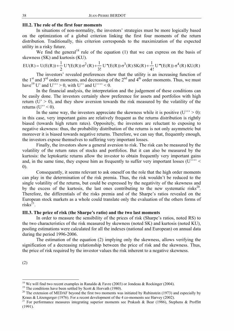
38 JEAN-PIERRE BERDOT
III.2. The role of the first four moments In situations of non-normality, the investors’ strategies must be more logically based
on the optimization of a global criterion linking the first four moments of the return distribution. Traditionally, this criterion corresponds to the maximization of the expected utility in a risky future.
We find the general18 rule of the equation (1) that we can express on the basis of skewness (SK) and kurtosis (KU).
2 3 41 1 1EU(R) U(E(R)) U ''(E(R)) (R) U '''(E(R)) (R) SK(R) U ''''(E(R)) (R) KU(R)2 3! 4!
= + σ + σ + σ The investors’ revealed preferences show that the utility is an increasing function of
the 1st and 3rd order moments, and decreasing of the 2nd and 4th order moments. Thus, we must have19 U’ and U’’’ > 0, with U’’ and U’’’’ < 0.
In the financial analysis, the interpretation and the judgement of these conditions can be easily done. The investors certainly show preference for assets and portfolios with high return (U’ > 0), and they show aversion towards the risk measured by the volatility of the returns (U’’ < 0).
In the same way, the investors appreciate the skewness while it is positive (U’’’ > 0): in this case, very important gains are relatively frequent as the returns distribution is rightly biased (towards high return rates). Oppositely, the investors are reluctant to exposing to negative skewness: thus, the probability distribution of the returns is not only asymmetric but moreover it is biased towards negative returns. Therefore, we can say that, frequently enough, the investors expose themselves to suffering very important losses.
Finally, the investors show a general aversion to risk. The risk can be measured by the volatility of the return rates of stocks and portfolios. But it can also be measured by the kurtosis: the leptokurtic returns allow the investor to obtain frequently very important gains and, in the same time, they expose him as frequently to suffer very important losses (U’’’’ < 0).
Consequently, it seems relevant to ask oneself on the role that the high order moments can play in the determination of the risk premia. Thus, the risk wouldn’t be reduced to the single volatility of the returns, but could be expressed by the negativity of the skewness and by the excess of the kurtosis, the last ones contributing to the new systematic risks20. Therefore, the differentials of the risks premia and of the Sharpe’s ratios revealed on the European stock markets as a whole could translate only the evaluation of the others forms of risks21.
III.3. The price of risk (the Sharpe’s ratio) and the two last moments In order to measure the sensibility of the prices of risk (Sharpe’s ratios, noted RS) to
the two characteristics of the risk measured by skewness (noted SK) and kurtosis (noted KU), pooling estimations were calculated for all the indexes (national and European) on annual data during the period 1996-2006.
The estimation of the equation (2) implying only the skewness, allows verifying the signification of a decreasing relationship between the price of risk and the skewness. Thus, the price of risk required by the investor values the risk inherent to a negative skewness. (2) b=++ε
18 We will find two recent examples in Ranaldo & Favre (2003) or Jondeau & Rockinger (2004). 19 The conditions have been settled by Scott & Horvath (1980). 20 The extension of MEDAF beyond the first two moments was initiated by Rubinstein (1973) and especially by Kraus & Litzengerger (1976). For a recent development of the 4 co-moments see Harvey (2002). 21 For performance measures integrating superior moments see Prakash & Bear (1986), Stephens & Proffitt (1991).
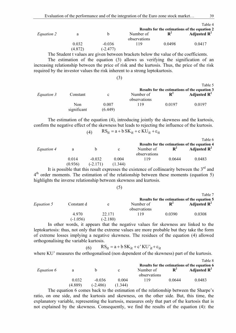
Evaluation of the performance and of the integration of the Euro zone stock market… 39
Table 4 Results for the estimations of the equation 2
Equation 2 a b Number of observations
R2 Adjusted R2
0.032 -0.036 119 0.0498 0.0417 (4.872) (-2.477)
The Student t values are given between brackets below the value of the coefficients. The estimation of the equation (3) allows us verifying the signification of an
increasing relationship between the price of risk and the kurtosis. Thus, the price of the risk required by the investor values the risk inherent to a strong leptokurtosis.
(3) =+ε Table 5
Results for the estimations of the equation 3 Equation 3 Constant c Number of
observations R2 Adjusted R2
Non 0.007 119 0.0197 0.0197 significant (6.449)
The estimation of the equation (4), introducing jointly the skewness and the kurtosis, confirm the negative effect of the skewness but leads to rejecting the influence of the kurtosis.
(4) it it it itRS a b SK c KU= + + + ε Table 6
Results for the estimations of the equation 4 Equation 4 a b c Number of
observations R2 Adjusted R2
0.014 -0.032 0.004 119 0.0644 0.0483 (0.936) (-2.171) (1.344) It is possible that this result expresses the existence of collinearity between the 3rd and
4th order moments. The estimation of the relationship between these moments (equation 5) highlights the inverse relationship between skewness and kurtosis.
(5) =++ε Table 7
Results for the estimations of the equation 5 Equation 5 Constant d e Number of
observations R2 Adjusted R2
4.970 22.171 119 0.0390 0.0308 (-1.056) (-2.180)
In other words, it appears that the negative values for skewness are linked to the leptokurtosis: thus, not only that the extreme values are more probable but they take the form of extreme losses implying a negative skewness. The residues of the equation (4) allowed orthogonalising the variable kurtosis.
(6) it it it itRS a b SK c ' KU '= + + + ε where KU’ measures the orthogonalised (non dependent of the skewness) part of the kurtosis.
Table 8 Results for the estimations of the equation 6
Equation 6 a b c Number of observations
R2 Adjusted R2
0.032 -0.036 0.004 119 0.0644 0.0483 (4.889) (-2.486) (1.344) The equation 6 comes back to the estimation of the relationship between the Sharpe’s
ratio, on one side, and the kurtosis and skewness, on the other side. But, this time, the explanatory variable, representing the kurtosis, measures only that part of the kurtosis that is not explained by the skewness. Consequently, we find the results of the equation (4): the
40 JEAN-PIERRE BERDOT
skewness is still the only explanatory variable of the Sharpe’s ratio. This suggests the extent of the content in information of the skewness: this one informs directly on the characteristics linked to the 3rd moment and indirectly on the characteristics of the 4th moment.
On the whole, these results reveal that the consideration of the (centered) moments of an order higher than 2 wouldn’t outdate the Sharpe’s ratio as a theoretical measure of the price of risk and as an empirical measure of the performance.
Indeed, the price of the risk contained by the Sharpe’s ratio incorporates the risks linked to the (centered) moments of an order higher than 2. More precisely, it means that the market values the negativity of the skewness through its determination by the price of risk.
CONCLUSIONS This study allowed us to show that, in spite of the permanence of the disparities in all
the characteristics of the returns linked to the national stock indexes within the Euro zone (means, standard deviations, Sharpe’s ratios, skewness and kurtosis), the integration process is working.
Consequently, the apparent differentials in the price of risk, as measured by the Sharpe’s ratio, express the rational evaluation of the risk linked to the moments of an order higher than 2.
Between the 3rd and 4th order (centered) moments, the skewness plays a strategic role due to the importance of its content in information on all the risks linked to these moments. Thus, the investor demands a higher return in exchange of a negative skewness. Doing so, he implicitly values the high probability of extreme losses.
This crucial role of the skewness allows for understanding the strategic importance of the studies on this subject and, more generally, of the studies on the risk of markets’ fall. But, these studies reach such conclusions that the market underestimates the risk linked to the skewness and refer to the necessity of undertaking coverage against the downside risk (for example, through buying puts). On the contrary, we show that the market values the risk, and the required returns include a premium supposed to ensure the risk coverage expressed by the skewness.
BIBLIOGRAPHY 1. Artus P., (2006), Skewness, Flash, Marchés, 2 avril. 2. Athayde (de) G. M. & R. G. Flores Jr., (2000), «Introducing Higher Moments in the CAPM:
Some Basic Ideas», in Advances in Quantitative Asset Management, Dunis (ed), Kluwer Academic Publishers, Springer.
3. Bacmann J.-F. & S. PAChE, (2004), «Optimal hedge Fund Style Allocation Under Higher Moments» in Intelligent Hedge Fund Investing, Schachter B. (ed), RiskBooks, London.
4. Bickel P.J., & K.A. doksum, (1977), Mathematical Statistics, Holden-Day, Inc. Oakland, California.
5. Harvey C. R., (2002), «Portfolio Selection with Higher Moments», NBER, Cambridge, MA. 6. Jarque C.M. & A.K. bera, (1980), «Efficient tests for Normalitiy, Homoskedasticity and Serial
Dependance of Regressions Residuals», Economic Letters, vol. 6. 7. Jondeau E. & M. Rockinger, (2004), «Optimal Portfolio Allocation Under Higher Moments»,
Working Paper, Banque de France & HEC Lausanne, January. 8. Kraus A. & R. H. Litzenberger, (1976), «Skewness Preference and the Valuation of Risky
Assets», Journal of Finance, vol. 31. 9. Lintner J., (1965), «The Valuation of Risk Assets and the Selection of Risky Investments in Stock
Portfolios and Capital Budgets», Review of Economic and Statistics, February 10. Markowitz H., (1952), “Portfolio Selection,” Journal of Finance , vol. 7, n°. 1, March. 11. Markowitz H., (1959), Portfolio Selection :Efficient Diversification of Investment, New York,
John Wiley & Sons. 12. Merton R.C., (1973), «An Intertemporal Capital Asset Pricing Model», Econometrica, vol. 41, n°
5, September.
Evaluation of the performance and of the integration of the Euro zone stock market… 41
13. Neumann von J. & O. Morgenstern (1944), Theory of Games and Economic Behaviour, Princeton, Princeton University Press.
14. Newey W. K. & K. D. West, (1987), “A Simple, Positive Semi-Definite, Heteroskedasticity and Autocorrelation Consistent Covariance Matrix”, Econometrica, vol. 55.
15. Newey W. K. & K. D. West, (1994), “Automatic Lag Selection in Covariance Matrix Estimation”, Review of Economic Studies, vol. 61.
16. Prakash A. J. & R M bear, (1986) “A Simplifying Performance Measure Recognizing Skewness”, Financial Review, vol. 21.
17. Ranaldo A. & L. Favre, (2003), “How to Price Hedge Funds : From Two- to-Four-Moment CAPM”, EDHEC-Risk, October.
18. Rubinstein M. E., (1973), “The Fundamental Theorem of Parameter-Preference Security Valuation”, Journal of Financial and Quantitative Analysis, vol. 8.
19. Samuelson P. A., (1970), “A Fundamental Approximation Theory of Portfolio Analysis in Terms of Means, Variance, and Higher Moments”, Review of Economic Studies, vol. 37.
20. Scott R. C & P. A. Horvath, (1980), “On The Direction of Preference for Moments of Higher Order Than The Variance”, Journal of Finance, 35.
21. Sharpe W., (1963), “A simplified model for portfolio analysis”, Management Science, vol. 9, n° 2, January.
22. Sharpe W., (1964), “Capital Asset Prices: A Theory of Market Equilibrium under Conditions of Risk”, Journal of Finance, vol. 19, n° 3, September.
23. Sharpe W., (1966), “Mutual Fund Performance”, Journal of Business, vol. 39. 24. Sharpe W., (1994), “The Sharpe Ratio”, Journal of Portfolio Management, vol. 20, Fall. 25. Stephens A. & D. Proffit, (1991), «Performance Measurement When Return Distributions Are
Nonsymmetric», Quarterly Journal of Business and Economics, vol. 30. 26. Tobin J., (1958), «Liquidity Preference as Behavior Towards Risk”, Review of Economic Studies,
vol. 25, n° 2, February.

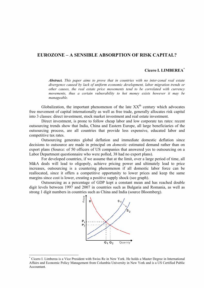
EUROZONE – A SENSIBLE ABSORPTION OF RISK CAPITAL?
Cicero I. LIMBEREA*
Abstract. This paper aims to prove that in countries with no inter-zonal real estate divergence caused by lack of uniform economic development, labor migration trends or other causes, the real estate price movements tend to be correlated with currency movements, thus a certain vulnerability to hot money exists however it may be manageable.
Globalization, the important phenomenon of the late XXth century which advocates
free movement of capital internationally as well as free trade, generally allocates risk capital into 3 classes: direct investment, stock market investment and real estate investment.
Direct investment, is prone to follow cheap labor and low corporate tax rates: recent outsourcing trends show that India, China and Eastern Europe, all large beneficiaries of the outsourcing process, are all countries that provide less expensive, educated labor and competitive tax rates.
Outsourcing generates global deflation and immediate domestic deflation since decisions to outsource are made in principal on domestic estimated demand rather than on export plans (Source: of 50 officers of US companies that answered yes to outsourcing on a Labor Department questionnaire who were polled, 38 had no export plans).
For developed countries, if we assume that at the limit, over a large period of time, all M&A deals will lead to oligopoly, achieve pricing power and ultimately lead to price increases, outsourcing is a countering phenomenon if all domestic labor force can be reallocated, since it offers a competitive opportunity to lower prices and keep the same margins since cost is lower, creating a positive supply shock (see graph).
Outsourcing as a percentage of GDP kept a constant mean and has reached double digit levels between 1997 and 2007 in countries such as Bulgaria and Romania, as well as strong 1 digit numbers in countries such as China and India (source Bloomberg).
* Cicero I. Limberea is a Vice President with Swiss Re in New York. He holds a Master Degree in International Affairs and Economic Policy Management from Columbia University in New York and is a US Certified Public Accountant.
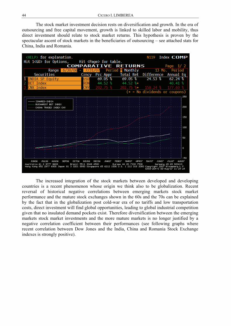
44 CICERO I. LIMBEREA
The stock market investment decision rests on diversification and growth. In the era of outsourcing and free capital movement, growth is linked to skilled labor and mobility, thus direct investment should relate to stock market returns. This hypothesis is proven by the spectacular ascent of stock markets in the beneficiaries of outsourcing – see attached stats for China, India and Romania.
The increased integration of the stock markets between developed and developing countries is a recent phenomenon whose origin we think also to be globalization. Recent reversal of historical negative correlations between emerging markets stock market performance and the mature stock exchanges shown in the 60s and the 70s can be explained by the fact that in the globalization post cold-war era of no tariffs and low transportation costs, direct investment will find global opportunities, leading to global industrial competition given that no insulated demand pockets exist. Therefore diversification between the emerging markets stock market investments and the more mature markets is no longer justified by a negative correlation coefficient between their performances (see following graphs where recent correlation between Dow Jones and the India, China and Romania Stock Exchange indexes is strongly positive).

Eurozone – a sensible absorption of risk capital? 45
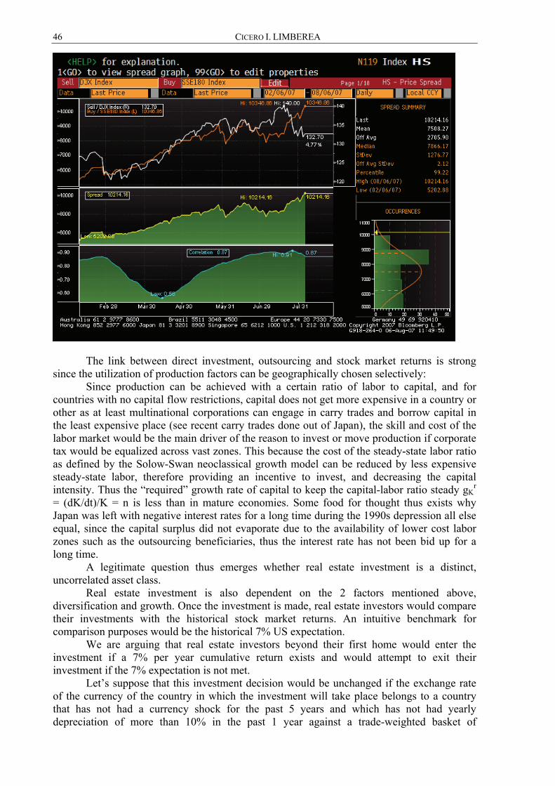
46 CICERO I. LIMBEREA
The link between direct investment, outsourcing and stock market returns is strong
since the utilization of production factors can be geographically chosen selectively: Since production can be achieved with a certain ratio of labor to capital, and for
countries with no capital flow restrictions, capital does not get more expensive in a country or other as at least multinational corporations can engage in carry trades and borrow capital in the least expensive place (see recent carry trades done out of Japan), the skill and cost of the labor market would be the main driver of the reason to invest or move production if corporate tax would be equalized across vast zones. This because the cost of the steady-state labor ratio as defined by the Solow-Swan neoclassical growth model can be reduced by less expensive steady-state labor, therefore providing an incentive to invest, and decreasing the capital intensity. Thus the “required” growth rate of capital to keep the capital-labor ratio steady gK
r = (dK/dt)/K = n is less than in mature economies. Some food for thought thus exists why Japan was left with negative interest rates for a long time during the 1990s depression all else equal, since the capital surplus did not evaporate due to the availability of lower cost labor zones such as the outsourcing beneficiaries, thus the interest rate has not been bid up for a long time.
A legitimate question thus emerges whether real estate investment is a distinct, uncorrelated asset class.
Real estate investment is also dependent on the 2 factors mentioned above, diversification and growth. Once the investment is made, real estate investors would compare their investments with the historical stock market returns. An intuitive benchmark for comparison purposes would be the historical 7% US expectation.
We are arguing that real estate investors beyond their first home would enter the investment if a 7% per year cumulative return exists and would attempt to exit their investment if the 7% expectation is not met.
Let’s suppose that this investment decision would be unchanged if the exchange rate of the currency of the country in which the investment will take place belongs to a country that has not had a currency shock for the past 5 years and which has not had yearly depreciation of more than 10% in the past 1 year against a trade-weighted basket of
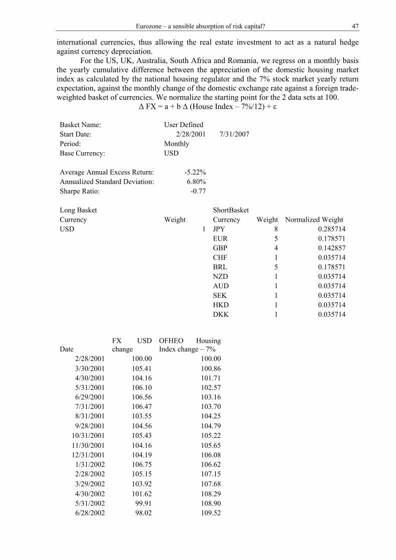
Eurozone – a sensible absorption of risk capital? 47
international currencies, thus allowing the real estate investment to act as a natural hedge against currency depreciation.
For the US, UK, Australia, South Africa and Romania, we regress on a monthly basis the yearly cumulative difference between the appreciation of the domestic housing market index as calculated by the national housing regulator and the 7% stock market yearly return expectation, against the monthly change of the domestic exchange rate against a foreign trade-weighted basket of currencies. We normalize the starting point for the 2 data sets at 100.
Δ FX = a + b Δ (House Index – 7%/12) + ε Basket Name: User Defined Start Date: 2/28/2001 7/31/2007 Period: Monthly Base Currency: USD Average Annual Excess Return: -5.22% Annualized Standard Deviation: 6.80% Sharpe Ratio: -0.77 Long Basket ShortBasket Currency Weight Currency Weight Normalized Weight USD 1 JPY 8 0.285714 EUR 5 0.178571 GBP 4 0.142857 CHF 1 0.035714 BRL 5 0.178571 NZD 1 0.035714 AUD 1 0.035714 SEK 1 0.035714 HKD 1 0.035714 DKK 1 0.035714
Date FX USD change
OFHEO Housing Index change – 7%
2/28/2001 100.00 100.00 3/30/2001 105.41 100.86 4/30/2001 104.16 101.71 5/31/2001 106.10 102.57 6/29/2001 106.56 103.16 7/31/2001 106.47 103.70 8/31/2001 103.55 104.25 9/28/2001 104.56 104.79
10/31/2001 105.43 105.22 11/30/2001 104.16 105.65 12/31/2001 104.19 106.08 1/31/2002 106.75 106.62 2/28/2002 105.15 107.15 3/29/2002 103.92 107.68 4/30/2002 101.62 108.29 5/31/2002 99.91 108.90 6/28/2002 98.02 109.52
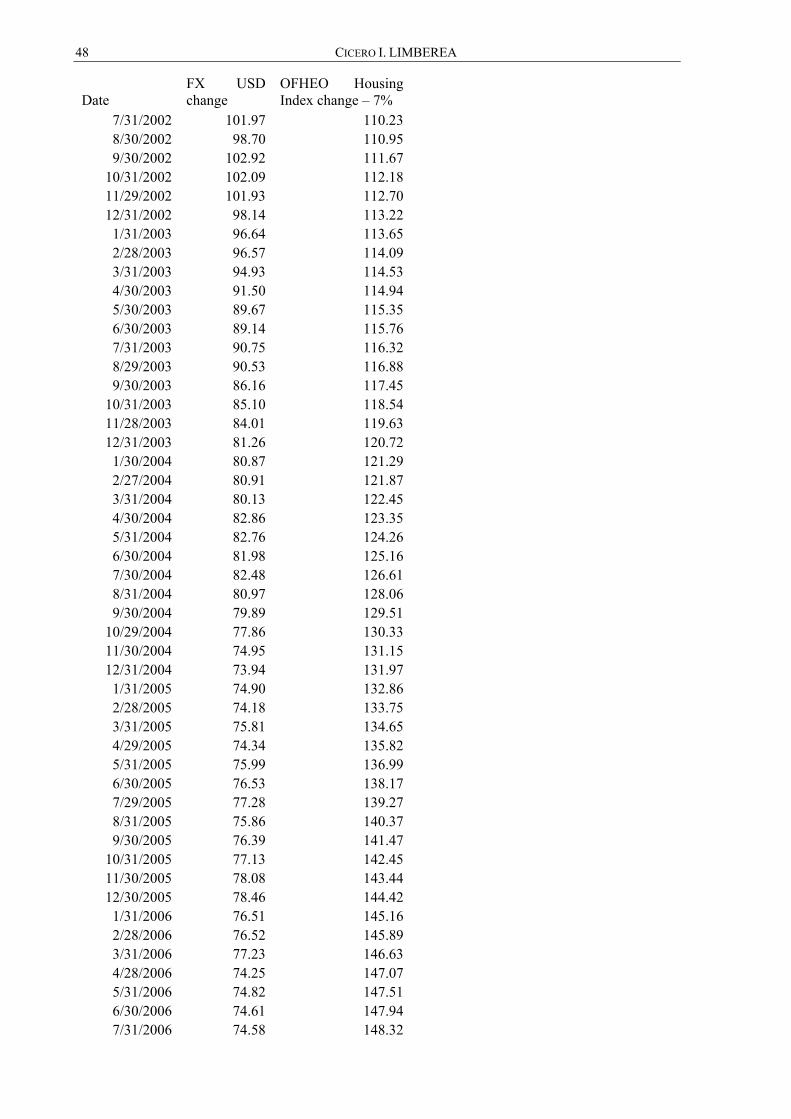
48 CICERO I. LIMBEREA
Date FX USD change
OFHEO Housing Index change – 7%
7/31/2002 101.97 110.23 8/30/2002 98.70 110.95 9/30/2002 102.92 111.67
10/31/2002 102.09 112.18 11/29/2002 101.93 112.70 12/31/2002 98.14 113.22 1/31/2003 96.64 113.65 2/28/2003 96.57 114.09 3/31/2003 94.93 114.53 4/30/2003 91.50 114.94 5/30/2003 89.67 115.35 6/30/2003 89.14 115.76 7/31/2003 90.75 116.32 8/29/2003 90.53 116.88 9/30/2003 86.16 117.45
10/31/2003 85.10 118.54 11/28/2003 84.01 119.63 12/31/2003 81.26 120.72 1/30/2004 80.87 121.29 2/27/2004 80.91 121.87 3/31/2004 80.13 122.45 4/30/2004 82.86 123.35 5/31/2004 82.76 124.26 6/30/2004 81.98 125.16 7/30/2004 82.48 126.61 8/31/2004 80.97 128.06 9/30/2004 79.89 129.51
10/29/2004 77.86 130.33 11/30/2004 74.95 131.15 12/31/2004 73.94 131.97 1/31/2005 74.90 132.86 2/28/2005 74.18 133.75 3/31/2005 75.81 134.65 4/29/2005 74.34 135.82 5/31/2005 75.99 136.99 6/30/2005 76.53 138.17 7/29/2005 77.28 139.27 8/31/2005 75.86 140.37 9/30/2005 76.39 141.47
10/31/2005 77.13 142.45 11/30/2005 78.08 143.44 12/30/2005 78.46 144.42 1/31/2006 76.51 145.16 2/28/2006 76.52 145.89 3/31/2006 77.23 146.63 4/28/2006 74.25 147.07 5/31/2006 74.82 147.51 6/30/2006 74.61 147.94 7/31/2006 74.58 148.32
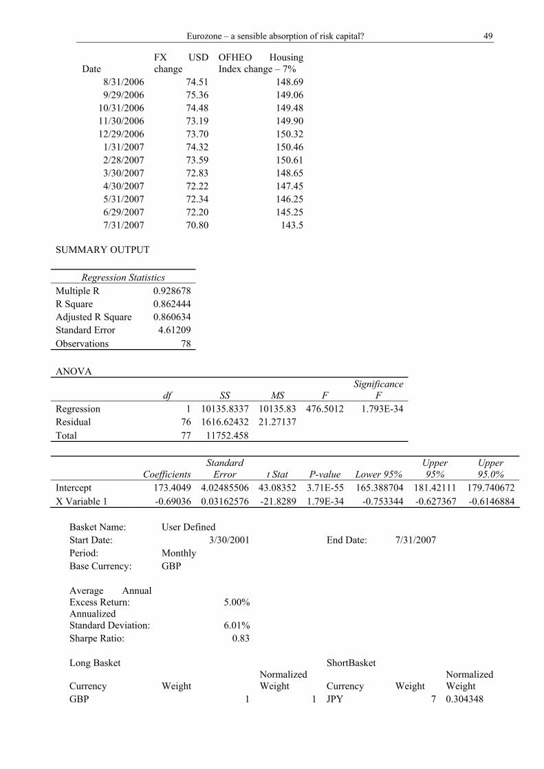
Eurozone – a sensible absorption of risk capital? 49
Date FX USD change
OFHEO Housing Index change – 7%
8/31/2006 74.51 148.69 9/29/2006 75.36 149.06
10/31/2006 74.48 149.48 11/30/2006 73.19 149.90 12/29/2006 73.70 150.32 1/31/2007 74.32 150.46 2/28/2007 73.59 150.61 3/30/2007 72.83 148.65 4/30/2007 72.22 147.45 5/31/2007 72.34 146.25 6/29/2007 72.20 145.25 7/31/2007 70.80 143.5
SUMMARY OUTPUT
Regression Statistics Multiple R 0.928678 R Square 0.862444 Adjusted R Square 0.860634 Standard Error 4.61209 Observations 78 ANOVA
df SS MS F Significance
F Regression 1 10135.8337 10135.83 476.5012 1.793E-34 Residual 76 1616.62432 21.27137 Total 77 11752.458
Coefficients Standard
Error t Stat P-value Lower 95% Upper 95%
Upper 95.0%
Intercept 173.4049 4.02485506 43.08352 3.71E-55 165.388704 181.42111 179.740672X Variable 1 -0.69036 0.03162576 -21.8289 1.79E-34 -0.753344 -0.627367 -0.6146884
Basket Name: User Defined Start Date: 3/30/2001 End Date: 7/31/2007 Period: Monthly Base Currency: GBP Average Annual Excess Return: 5.00% Annualized Standard Deviation: 6.01% Sharpe Ratio: 0.83 Long Basket ShortBasket
Currency Weight Normalized Weight Currency Weight
Normalized Weight
GBP 1 1 JPY 7 0.304348
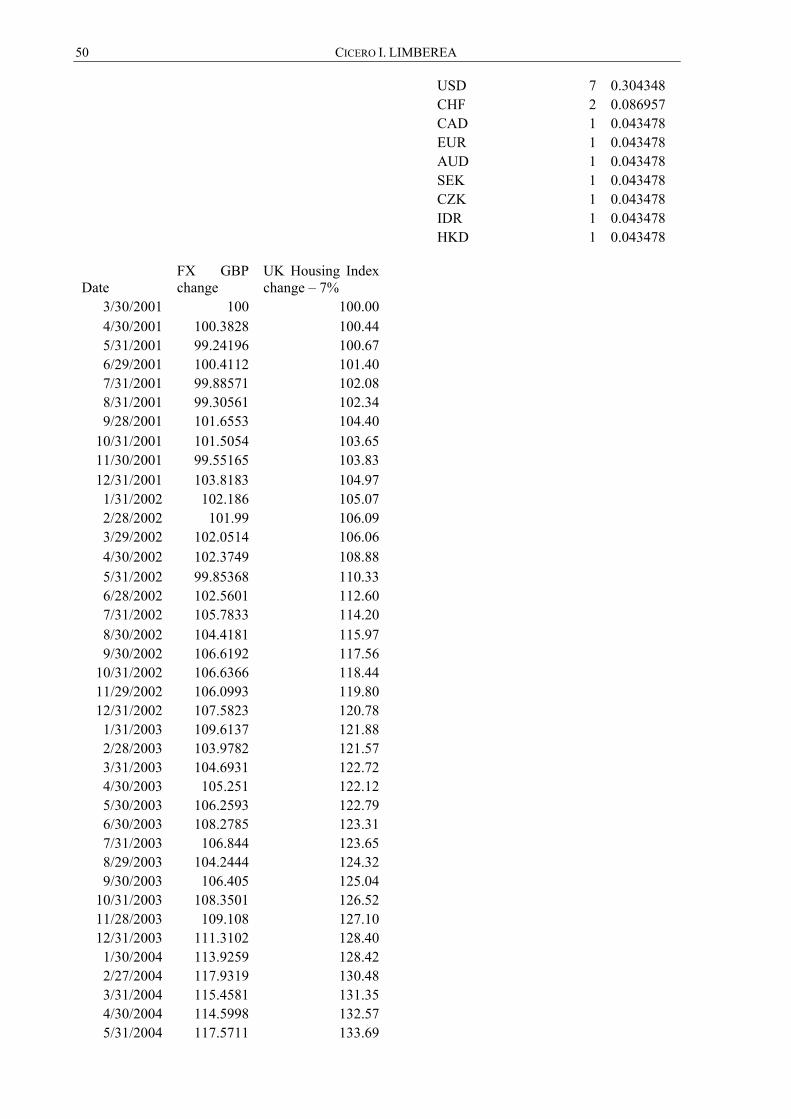
50 CICERO I. LIMBEREA
USD 7 0.304348 CHF 2 0.086957 CAD 1 0.043478 EUR 1 0.043478 AUD 1 0.043478 SEK 1 0.043478 CZK 1 0.043478 IDR 1 0.043478 HKD 1 0.043478
Date FX GBP change
UK Housing Index change – 7%
3/30/2001 100 100.004/30/2001 100.3828 100.445/31/2001 99.24196 100.676/29/2001 100.4112 101.407/31/2001 99.88571 102.088/31/2001 99.30561 102.349/28/2001 101.6553 104.40
10/31/2001 101.5054 103.6511/30/2001 99.55165 103.8312/31/2001 103.8183 104.971/31/2002 102.186 105.072/28/2002 101.99 106.093/29/2002 102.0514 106.064/30/2002 102.3749 108.885/31/2002 99.85368 110.336/28/2002 102.5601 112.607/31/2002 105.7833 114.208/30/2002 104.4181 115.979/30/2002 106.6192 117.56
10/31/2002 106.6366 118.4411/29/2002 106.0993 119.8012/31/2002 107.5823 120.781/31/2003 109.6137 121.882/28/2003 103.9782 121.573/31/2003 104.6931 122.724/30/2003 105.251 122.125/30/2003 106.2593 122.796/30/2003 108.2785 123.317/31/2003 106.844 123.658/29/2003 104.2444 124.329/30/2003 106.405 125.04
10/31/2003 108.3501 126.5211/28/2003 109.108 127.1012/31/2003 111.3102 128.401/30/2004 113.9259 128.422/27/2004 117.9319 130.483/31/2004 115.4581 131.354/30/2004 114.5998 132.575/31/2004 117.5711 133.69
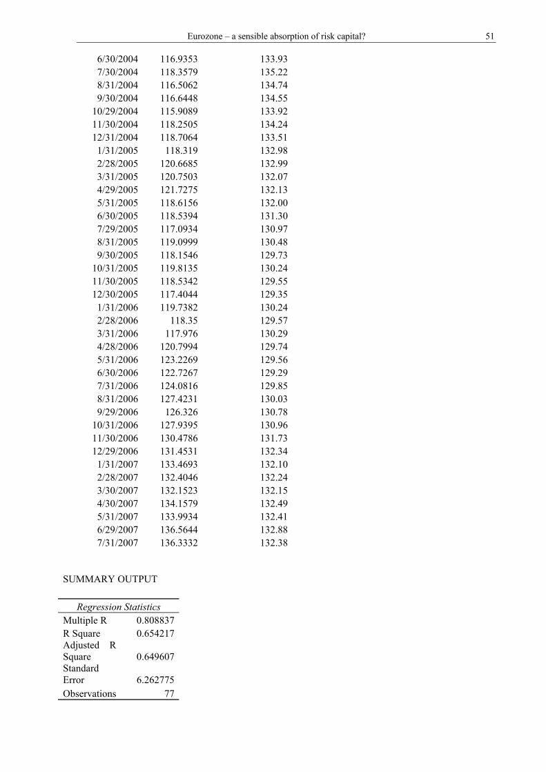
Eurozone – a sensible absorption of risk capital? 51
6/30/2004 116.9353 133.937/30/2004 118.3579 135.228/31/2004 116.5062 134.749/30/2004 116.6448 134.55
10/29/2004 115.9089 133.9211/30/2004 118.2505 134.2412/31/2004 118.7064 133.511/31/2005 118.319 132.982/28/2005 120.6685 132.993/31/2005 120.7503 132.074/29/2005 121.7275 132.135/31/2005 118.6156 132.006/30/2005 118.5394 131.307/29/2005 117.0934 130.978/31/2005 119.0999 130.489/30/2005 118.1546 129.73
10/31/2005 119.8135 130.2411/30/2005 118.5342 129.5512/30/2005 117.4044 129.351/31/2006 119.7382 130.242/28/2006 118.35 129.573/31/2006 117.976 130.294/28/2006 120.7994 129.745/31/2006 123.2269 129.566/30/2006 122.7267 129.297/31/2006 124.0816 129.858/31/2006 127.4231 130.039/29/2006 126.326 130.78
10/31/2006 127.9395 130.9611/30/2006 130.4786 131.7312/29/2006 131.4531 132.341/31/2007 133.4693 132.102/28/2007 132.4046 132.243/30/2007 132.1523 132.154/30/2007 134.1579 132.495/31/2007 133.9934 132.416/29/2007 136.5644 132.887/31/2007 136.3332 132.38
SUMMARY OUTPUT
Regression Statistics Multiple R 0.808837 R Square 0.654217 Adjusted R Square 0.649607 Standard Error 6.262775 Observations 77
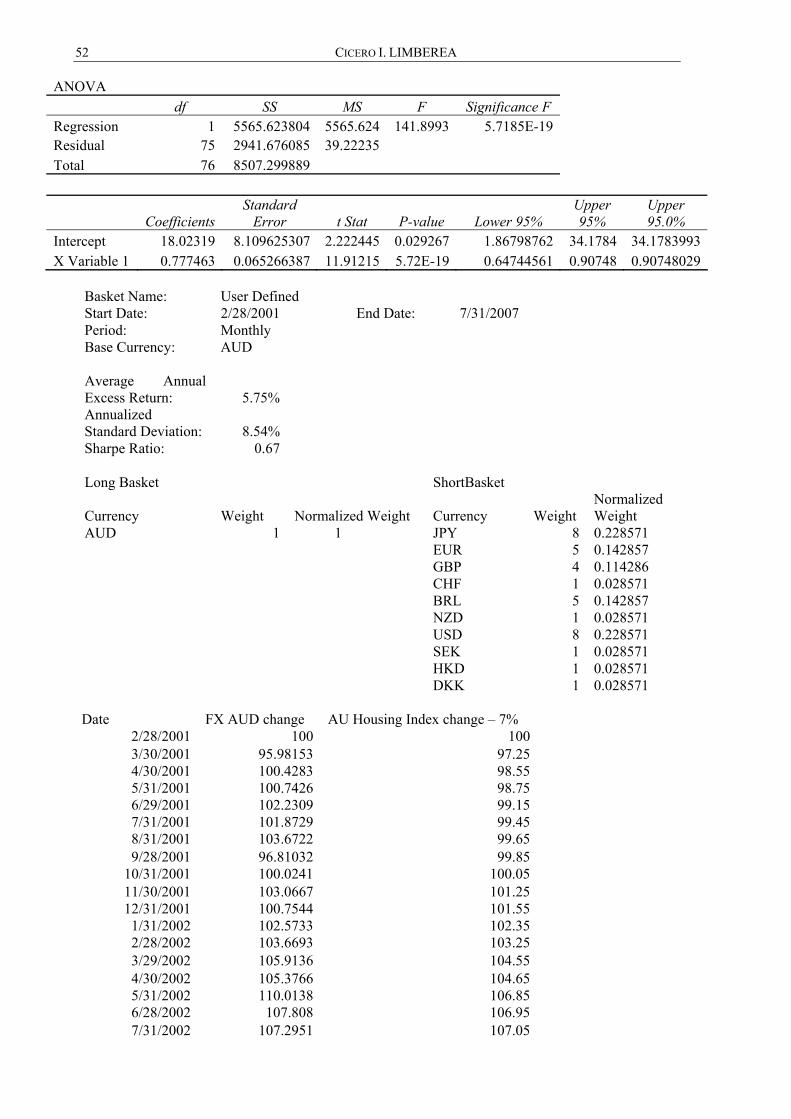
52 CICERO I. LIMBEREA
ANOVA df SS MS F Significance F
Regression 1 5565.623804 5565.624 141.8993 5.7185E-19 Residual 75 2941.676085 39.22235 Total 76 8507.299889
Coefficients Standard
Error t Stat P-value Lower 95% Upper 95%
Upper 95.0%
Intercept 18.02319 8.109625307 2.222445 0.029267 1.86798762 34.1784 34.1783993X Variable 1 0.777463 0.065266387 11.91215 5.72E-19 0.64744561 0.90748 0.90748029
Basket Name: User Defined Start Date: 2/28/2001 End Date: 7/31/2007 Period: Monthly Base Currency: AUD Average Annual Excess Return: 5.75% Annualized Standard Deviation: 8.54% Sharpe Ratio: 0.67 Long Basket ShortBasket
Currency Weight Normalized Weight Currency Weight Normalized Weight
AUD 1 1 JPY 8 0.228571 EUR 5 0.142857 GBP 4 0.114286 CHF 1 0.028571 BRL 5 0.142857 NZD 1 0.028571 USD 8 0.228571 SEK 1 0.028571 HKD 1 0.028571 DKK 1 0.028571
Date FX AUD change AU Housing Index change – 7%
2/28/2001 100 1003/30/2001 95.98153 97.254/30/2001 100.4283 98.555/31/2001 100.7426 98.756/29/2001 102.2309 99.157/31/2001 101.8729 99.458/31/2001 103.6722 99.659/28/2001 96.81032 99.85
10/31/2001 100.0241 100.0511/30/2001 103.0667 101.2512/31/2001 100.7544 101.551/31/2002 102.5733 102.352/28/2002 103.6693 103.253/29/2002 105.9136 104.554/30/2002 105.3766 104.655/31/2002 110.0138 106.856/28/2002 107.808 106.957/31/2002 107.2951 107.05
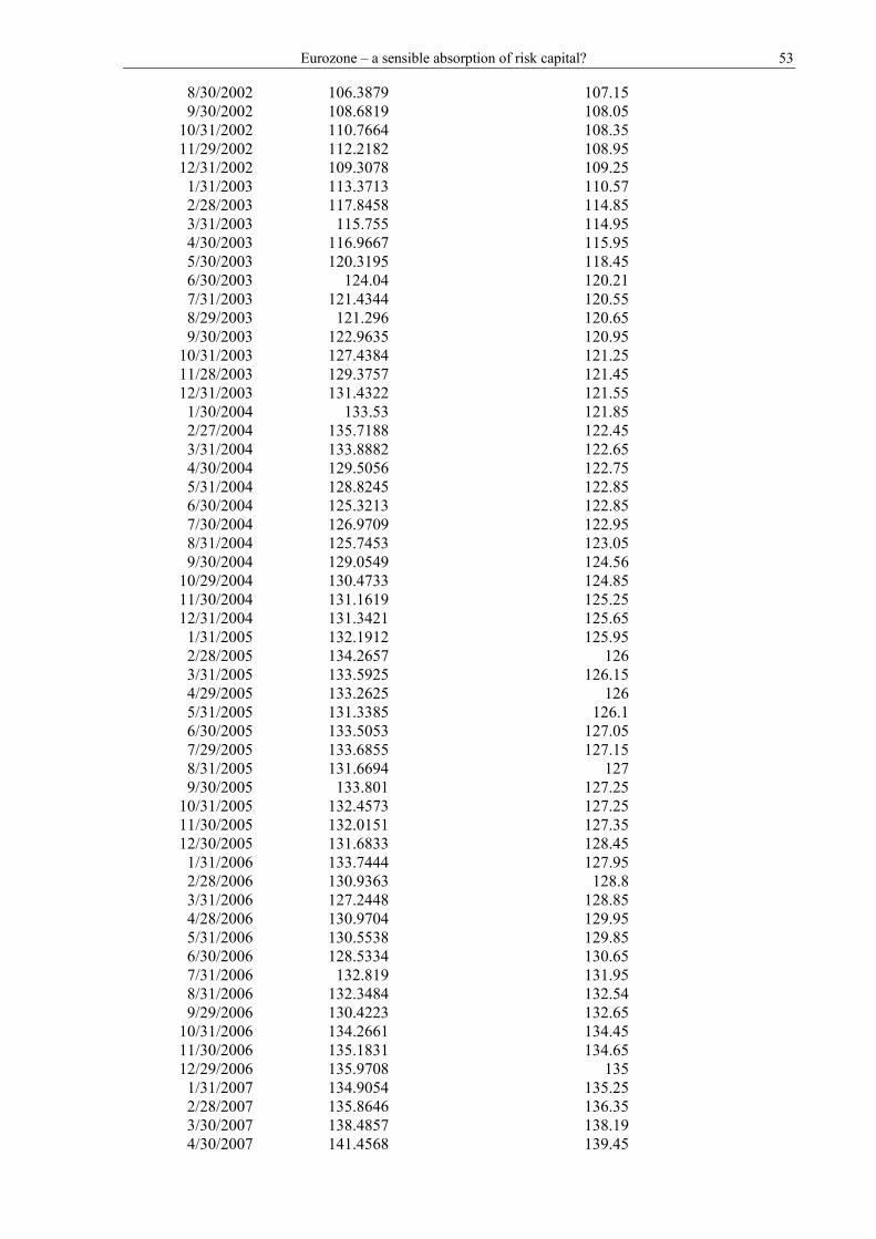
Eurozone – a sensible absorption of risk capital? 53
8/30/2002 106.3879 107.15 9/30/2002 108.6819 108.05
10/31/2002 110.7664 108.35 11/29/2002 112.2182 108.95 12/31/2002 109.3078 109.25 1/31/2003 113.3713 110.57 2/28/2003 117.8458 114.85 3/31/2003 115.755 114.95 4/30/2003 116.9667 115.95 5/30/2003 120.3195 118.45 6/30/2003 124.04 120.21 7/31/2003 121.4344 120.55 8/29/2003 121.296 120.65 9/30/2003 122.9635 120.95
10/31/2003 127.4384 121.25 11/28/2003 129.3757 121.45 12/31/2003 131.4322 121.55 1/30/2004 133.53 121.85 2/27/2004 135.7188 122.45 3/31/2004 133.8882 122.65 4/30/2004 129.5056 122.75 5/31/2004 128.8245 122.85 6/30/2004 125.3213 122.85 7/30/2004 126.9709 122.95 8/31/2004 125.7453 123.05 9/30/2004 129.0549 124.56
10/29/2004 130.4733 124.85 11/30/2004 131.1619 125.25 12/31/2004 131.3421 125.65 1/31/2005 132.1912 125.95 2/28/2005 134.2657 126 3/31/2005 133.5925 126.15 4/29/2005 133.2625 126 5/31/2005 131.3385 126.1 6/30/2005 133.5053 127.05 7/29/2005 133.6855 127.15 8/31/2005 131.6694 127 9/30/2005 133.801 127.25
10/31/2005 132.4573 127.25 11/30/2005 132.0151 127.35 12/30/2005 131.6833 128.45 1/31/2006 133.7444 127.95 2/28/2006 130.9363 128.8 3/31/2006 127.2448 128.85 4/28/2006 130.9704 129.95 5/31/2006 130.5538 129.85 6/30/2006 128.5334 130.65 7/31/2006 132.819 131.95 8/31/2006 132.3484 132.54 9/29/2006 130.4223 132.65
10/31/2006 134.2661 134.45 11/30/2006 135.1831 134.65 12/29/2006 135.9708 135 1/31/2007 134.9054 135.25 2/28/2007 135.8646 136.35 3/30/2007 138.4857 138.19 4/30/2007 141.4568 139.45
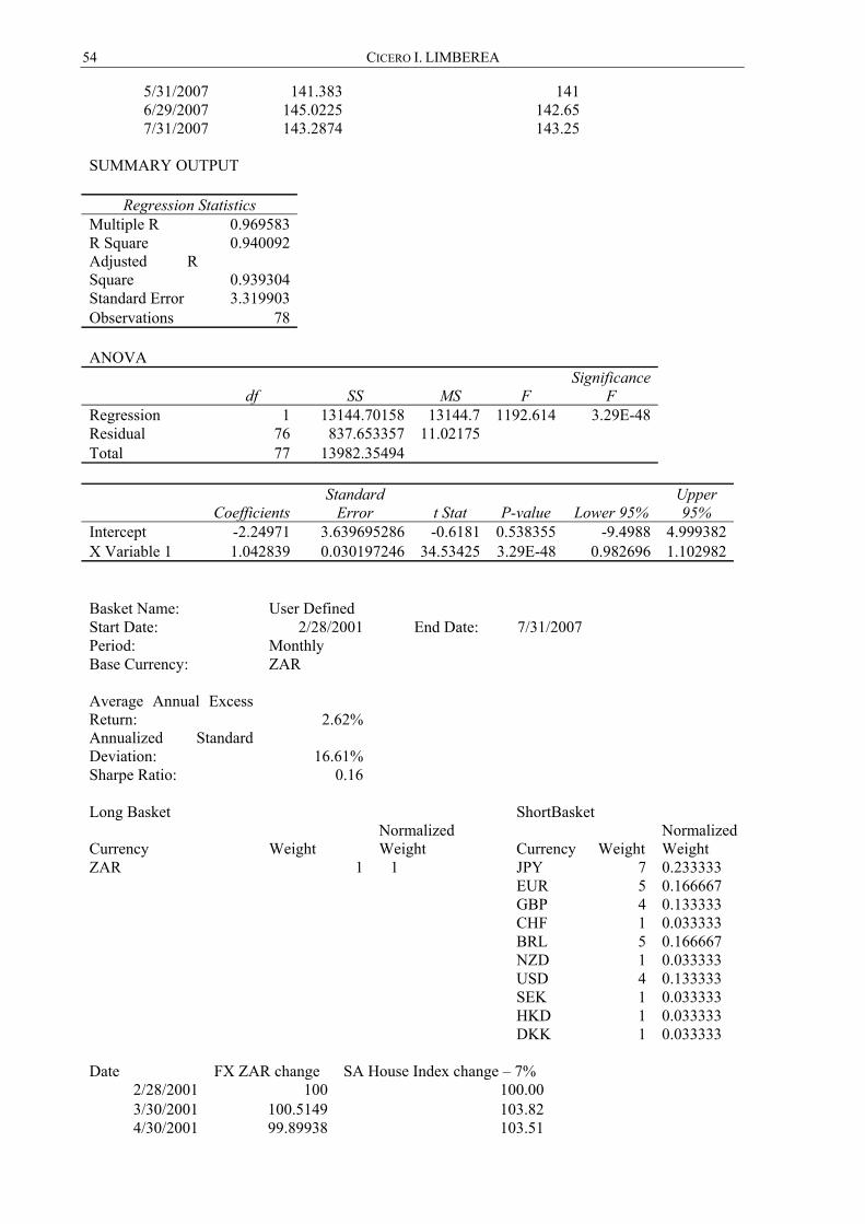
54 CICERO I. LIMBEREA
5/31/2007 141.383 1416/29/2007 145.0225 142.657/31/2007 143.2874 143.25
SUMMARY OUTPUT
Regression Statistics Multiple R 0.969583 R Square 0.940092 Adjusted R Square 0.939304 Standard Error 3.319903 Observations 78 ANOVA
df SS MS F Significance
F Regression 1 13144.70158 13144.7 1192.614 3.29E-48 Residual 76 837.653357 11.02175 Total 77 13982.35494
Coefficients Standard
Error t Stat P-value Lower 95% Upper 95%
Intercept -2.24971 3.639695286 -0.6181 0.538355 -9.4988 4.999382X Variable 1 1.042839 0.030197246 34.53425 3.29E-48 0.982696 1.102982
Basket Name: User Defined Start Date: 2/28/2001 End Date: 7/31/2007 Period: Monthly Base Currency: ZAR Average Annual Excess Return: 2.62% Annualized Standard Deviation: 16.61% Sharpe Ratio: 0.16 Long Basket ShortBasket
Currency Weight Normalized Weight Currency Weight
Normalized Weight
ZAR 1 1 JPY 7 0.233333 EUR 5 0.166667 GBP 4 0.133333 CHF 1 0.033333 BRL 5 0.166667 NZD 1 0.033333 USD 4 0.133333 SEK 1 0.033333 HKD 1 0.033333 DKK 1 0.033333
Date FX ZAR change SA House Index change – 7%
2/28/2001 100 100.003/30/2001 100.5149 103.824/30/2001 99.89938 103.51
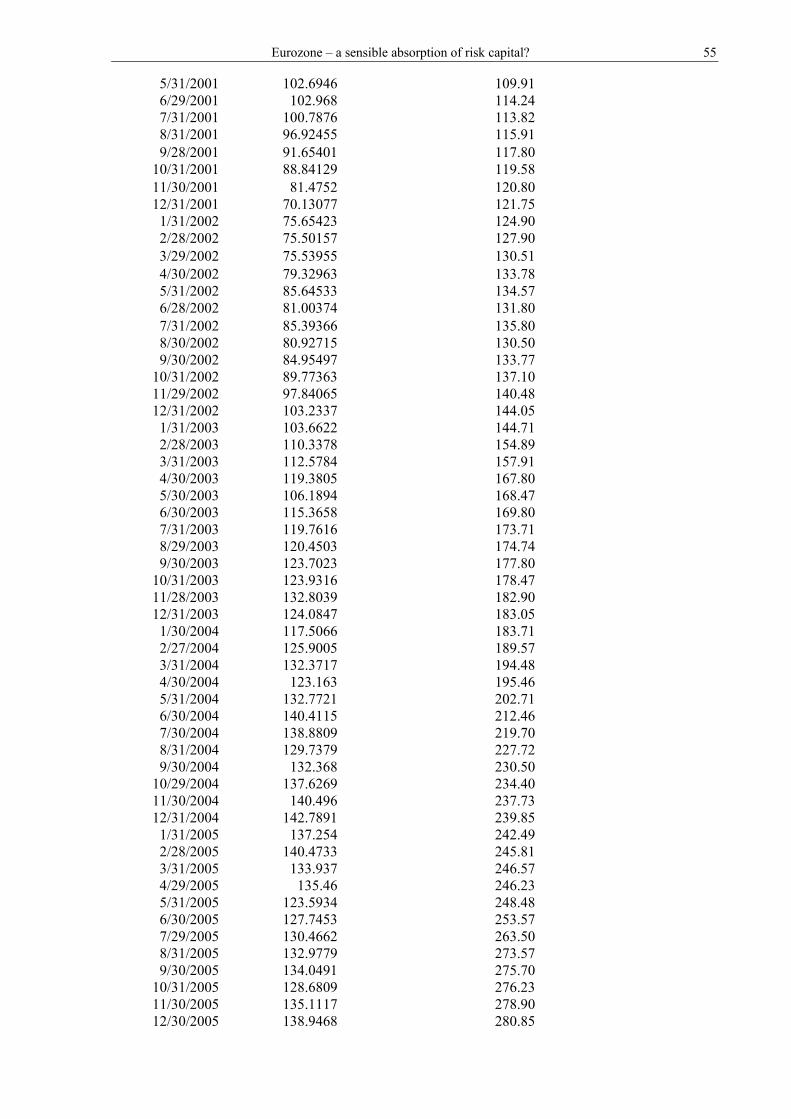
Eurozone – a sensible absorption of risk capital? 55
5/31/2001 102.6946 109.916/29/2001 102.968 114.247/31/2001 100.7876 113.828/31/2001 96.92455 115.919/28/2001 91.65401 117.80
10/31/2001 88.84129 119.5811/30/2001 81.4752 120.8012/31/2001 70.13077 121.751/31/2002 75.65423 124.902/28/2002 75.50157 127.903/29/2002 75.53955 130.514/30/2002 79.32963 133.785/31/2002 85.64533 134.576/28/2002 81.00374 131.807/31/2002 85.39366 135.808/30/2002 80.92715 130.509/30/2002 84.95497 133.77
10/31/2002 89.77363 137.1011/29/2002 97.84065 140.4812/31/2002 103.2337 144.051/31/2003 103.6622 144.712/28/2003 110.3378 154.893/31/2003 112.5784 157.914/30/2003 119.3805 167.805/30/2003 106.1894 168.476/30/2003 115.3658 169.807/31/2003 119.7616 173.718/29/2003 120.4503 174.749/30/2003 123.7023 177.80
10/31/2003 123.9316 178.4711/28/2003 132.8039 182.9012/31/2003 124.0847 183.051/30/2004 117.5066 183.712/27/2004 125.9005 189.573/31/2004 132.3717 194.484/30/2004 123.163 195.465/31/2004 132.7721 202.716/30/2004 140.4115 212.467/30/2004 138.8809 219.708/31/2004 129.7379 227.729/30/2004 132.368 230.50
10/29/2004 137.6269 234.4011/30/2004 140.496 237.7312/31/2004 142.7891 239.851/31/2005 137.254 242.492/28/2005 140.4733 245.813/31/2005 133.937 246.574/29/2005 135.46 246.235/31/2005 123.5934 248.486/30/2005 127.7453 253.577/29/2005 130.4662 263.508/31/2005 132.9779 273.579/30/2005 134.0491 275.70
10/31/2005 128.6809 276.2311/30/2005 135.1117 278.9012/30/2005 138.9468 280.85
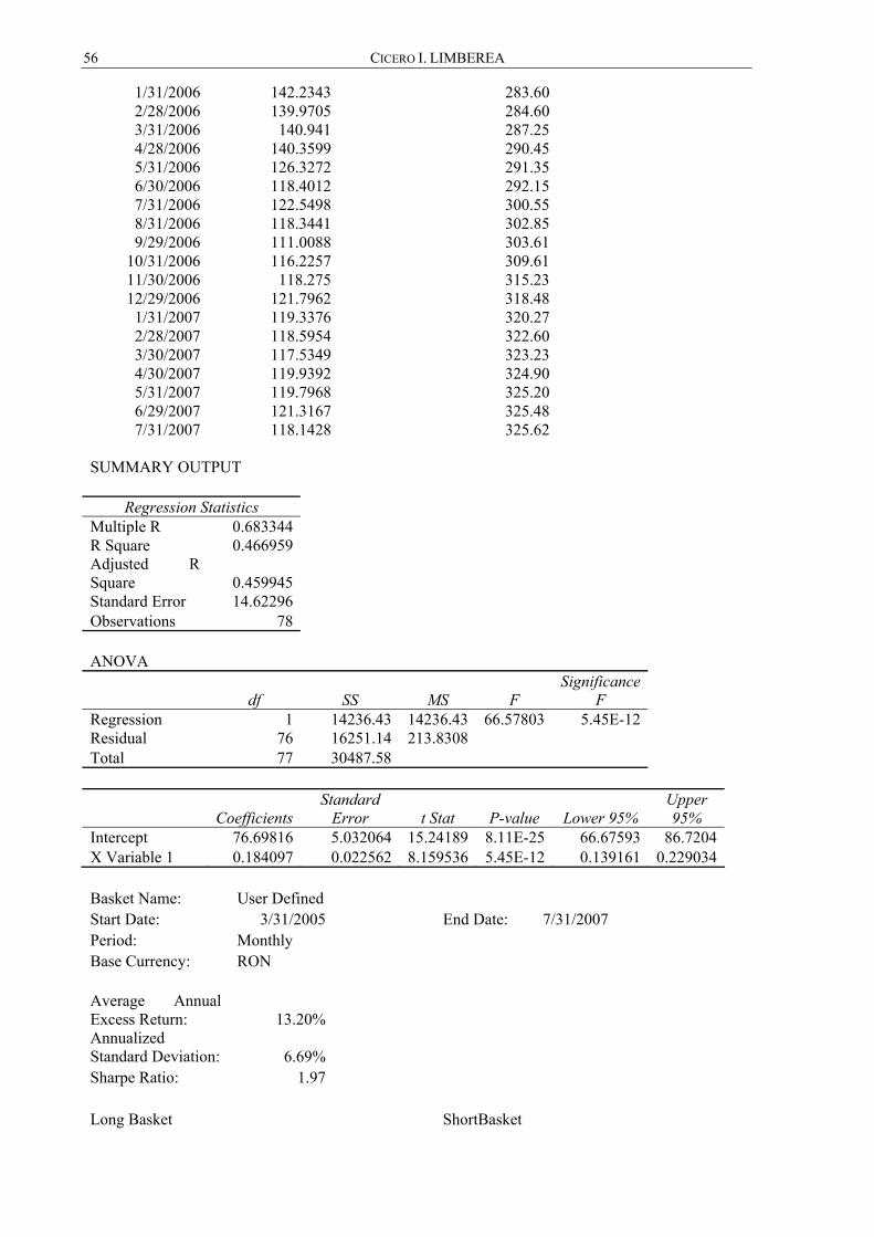
56 CICERO I. LIMBEREA
1/31/2006 142.2343 283.602/28/2006 139.9705 284.603/31/2006 140.941 287.254/28/2006 140.3599 290.455/31/2006 126.3272 291.356/30/2006 118.4012 292.157/31/2006 122.5498 300.558/31/2006 118.3441 302.859/29/2006 111.0088 303.61
10/31/2006 116.2257 309.6111/30/2006 118.275 315.2312/29/2006 121.7962 318.481/31/2007 119.3376 320.272/28/2007 118.5954 322.603/30/2007 117.5349 323.234/30/2007 119.9392 324.905/31/2007 119.7968 325.206/29/2007 121.3167 325.487/31/2007 118.1428 325.62
SUMMARY OUTPUT
Regression Statistics Multiple R 0.683344 R Square 0.466959 Adjusted R Square 0.459945 Standard Error 14.62296 Observations 78 ANOVA
df SS MS F Significance
F Regression 1 14236.43 14236.43 66.57803 5.45E-12 Residual 76 16251.14 213.8308 Total 77 30487.58
Coefficients Standard
Error t Stat P-value Lower 95% Upper 95%
Intercept 76.69816 5.032064 15.24189 8.11E-25 66.67593 86.7204 X Variable 1 0.184097 0.022562 8.159536 5.45E-12 0.139161 0.229034
Basket Name: User Defined Start Date: 3/31/2005 End Date: 7/31/2007 Period: Monthly Base Currency: RON Average Annual Excess Return: 13.20% Annualized Standard Deviation: 6.69% Sharpe Ratio: 1.97 Long Basket ShortBasket
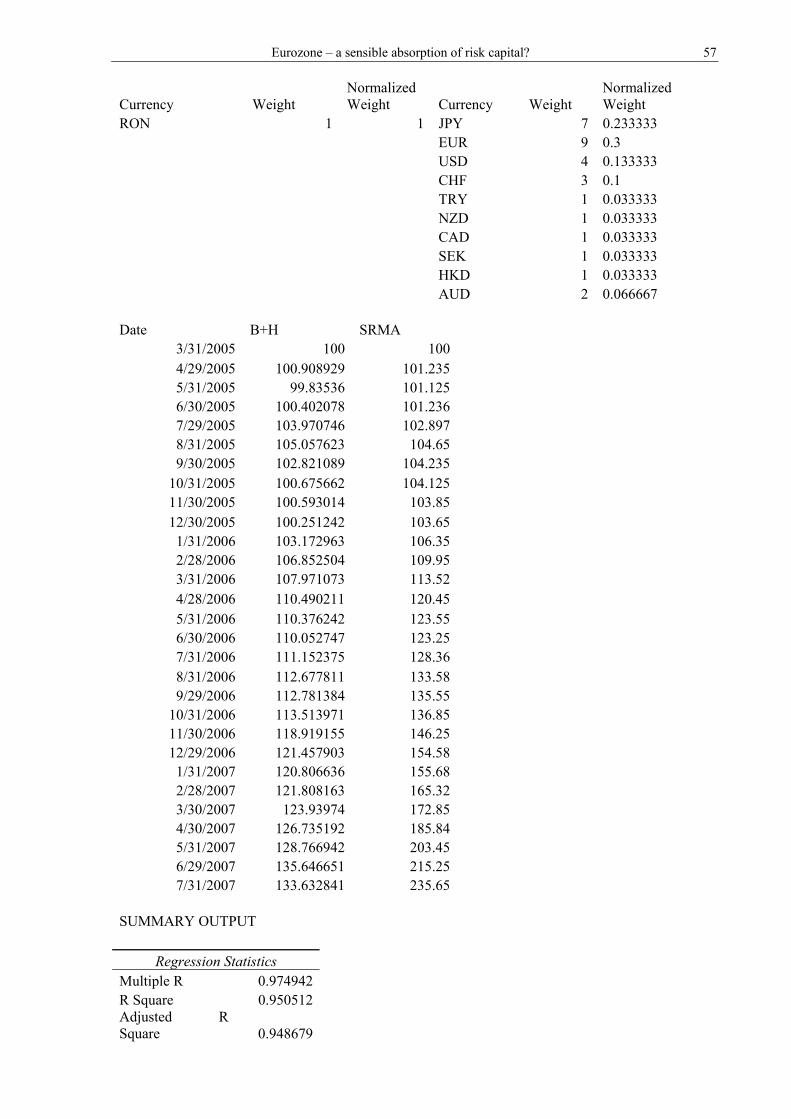
Eurozone – a sensible absorption of risk capital? 57
Currency Weight Normalized Weight Currency Weight
Normalized Weight
RON 1 1 JPY 7 0.233333 EUR 9 0.3 USD 4 0.133333 CHF 3 0.1 TRY 1 0.033333 NZD 1 0.033333 CAD 1 0.033333 SEK 1 0.033333 HKD 1 0.033333 AUD 2 0.066667
Date B+H SRMA
3/31/2005 100 1004/29/2005 100.908929 101.2355/31/2005 99.83536 101.1256/30/2005 100.402078 101.2367/29/2005 103.970746 102.8978/31/2005 105.057623 104.659/30/2005 102.821089 104.235
10/31/2005 100.675662 104.12511/30/2005 100.593014 103.8512/30/2005 100.251242 103.651/31/2006 103.172963 106.352/28/2006 106.852504 109.953/31/2006 107.971073 113.524/28/2006 110.490211 120.455/31/2006 110.376242 123.556/30/2006 110.052747 123.257/31/2006 111.152375 128.368/31/2006 112.677811 133.589/29/2006 112.781384 135.55
10/31/2006 113.513971 136.8511/30/2006 118.919155 146.2512/29/2006 121.457903 154.581/31/2007 120.806636 155.682/28/2007 121.808163 165.323/30/2007 123.93974 172.854/30/2007 126.735192 185.845/31/2007 128.766942 203.456/29/2007 135.646651 215.257/31/2007 133.632841 235.65
SUMMARY OUTPUT
Regression Statistics Multiple R 0.974942 R Square 0.950512 Adjusted R Square 0.948679
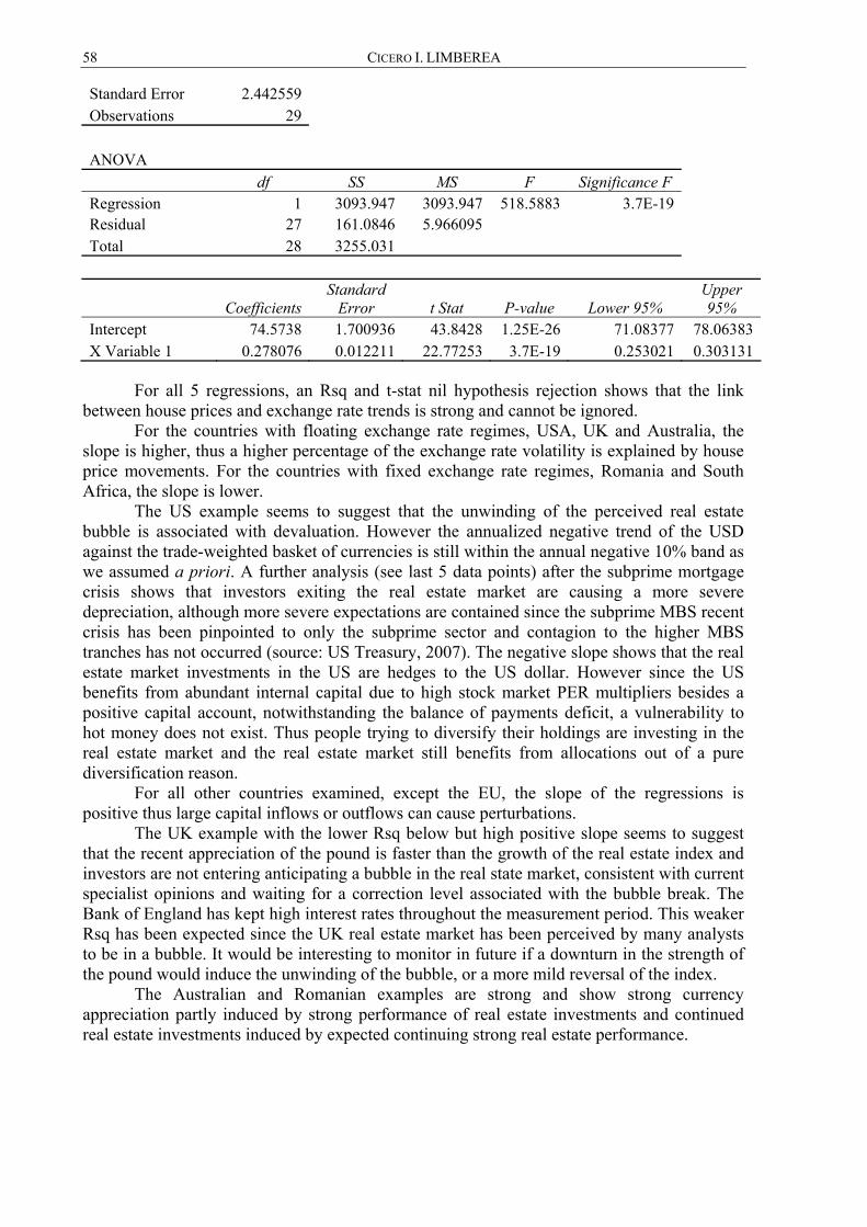
58 CICERO I. LIMBEREA
Standard Error 2.442559 Observations 29 ANOVA
df SS MS F Significance F Regression 1 3093.947 3093.947 518.5883 3.7E-19 Residual 27 161.0846 5.966095 Total 28 3255.031
Coefficients Standard
Error t Stat P-value Lower 95% Upper 95%
Intercept 74.5738 1.700936 43.8428 1.25E-26 71.08377 78.06383X Variable 1 0.278076 0.012211 22.77253 3.7E-19 0.253021 0.303131
For all 5 regressions, an Rsq and t-stat nil hypothesis rejection shows that the link
between house prices and exchange rate trends is strong and cannot be ignored. For the countries with floating exchange rate regimes, USA, UK and Australia, the
slope is higher, thus a higher percentage of the exchange rate volatility is explained by house price movements. For the countries with fixed exchange rate regimes, Romania and South Africa, the slope is lower.
The US example seems to suggest that the unwinding of the perceived real estate bubble is associated with devaluation. However the annualized negative trend of the USD against the trade-weighted basket of currencies is still within the annual negative 10% band as we assumed a priori. A further analysis (see last 5 data points) after the subprime mortgage crisis shows that investors exiting the real estate market are causing a more severe depreciation, although more severe expectations are contained since the subprime MBS recent crisis has been pinpointed to only the subprime sector and contagion to the higher MBS tranches has not occurred (source: US Treasury, 2007). The negative slope shows that the real estate market investments in the US are hedges to the US dollar. However since the US benefits from abundant internal capital due to high stock market PER multipliers besides a positive capital account, notwithstanding the balance of payments deficit, a vulnerability to hot money does not exist. Thus people trying to diversify their holdings are investing in the real estate market and the real estate market still benefits from allocations out of a pure diversification reason.
For all other countries examined, except the EU, the slope of the regressions is positive thus large capital inflows or outflows can cause perturbations.
The UK example with the lower Rsq below but high positive slope seems to suggest that the recent appreciation of the pound is faster than the growth of the real estate index and investors are not entering anticipating a bubble in the real state market, consistent with current specialist opinions and waiting for a correction level associated with the bubble break. The Bank of England has kept high interest rates throughout the measurement period. This weaker Rsq has been expected since the UK real estate market has been perceived by many analysts to be in a bubble. It would be interesting to monitor in future if a downturn in the strength of the pound would induce the unwinding of the bubble, or a more mild reversal of the index.
The Australian and Romanian examples are strong and show strong currency appreciation partly induced by strong performance of real estate investments and continued real estate investments induced by expected continuing strong real estate performance.
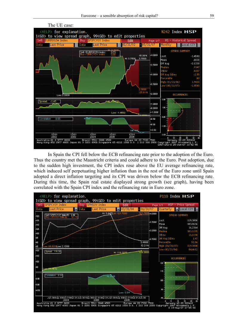
Eurozone – a sensible absorption of risk capital? 59
The UE case:
In Spain the CPI fell below the ECB refinancing rate prior to the adoption of the Euro.
Thus the country met the Maastricht criteria and could adhere to the Euro. Post adoption, due to the sudden high investment, the CPI index rose above the EU average refinancing rate, which induced self perpetuating higher inflation than in the rest of the Euro zone until Spain adopted a direct inflation targeting and its CPI was driven below the ECB refinancing rate. During this time, the Spain real estate displayed strong growth (see graph), having been correlated with the Spain CPI index and the refinancing rate in Euro zone.
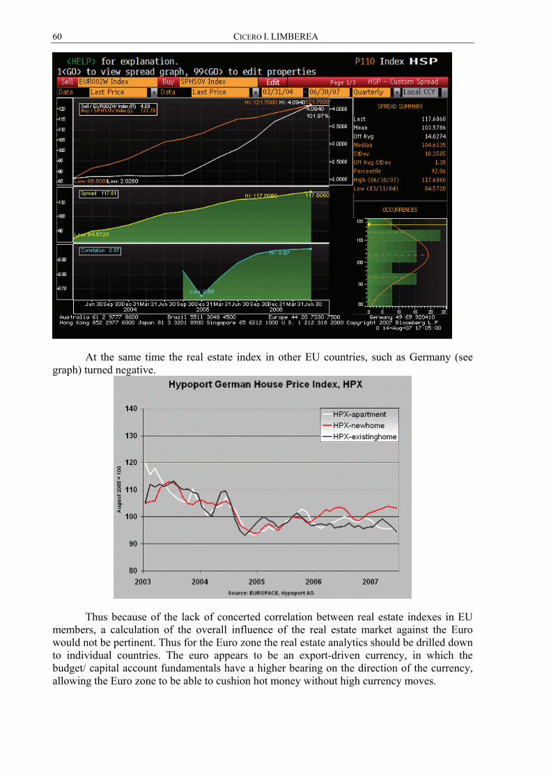
60 CICERO I. LIMBEREA
At the same time the real estate index in other EU countries, such as Germany (see graph) turned negative.
Thus because of the lack of concerted correlation between real estate indexes in EU members, a calculation of the overall influence of the real estate market against the Euro would not be pertinent. Thus for the Euro zone the real estate analytics should be drilled down to individual countries. The euro appears to be an export-driven currency, in which the budget/ capital account fundamentals have a higher bearing on the direction of the currency, allowing the Euro zone to be able to cushion hot money without high currency moves.

Eurozone – a sensible absorption of risk capital? 61
REFERENCES 1. Calvo, G., and Reinhart, C. (2002). “Fear of Floating.” Quarterly Journal of Economics, 177:
379-408. 2. Levy-Yeyati, E. and F. Sturzenegger (2004). “Classifying Exchange Rate Regimes: Deeds vs.
Words.” European Economic Review.

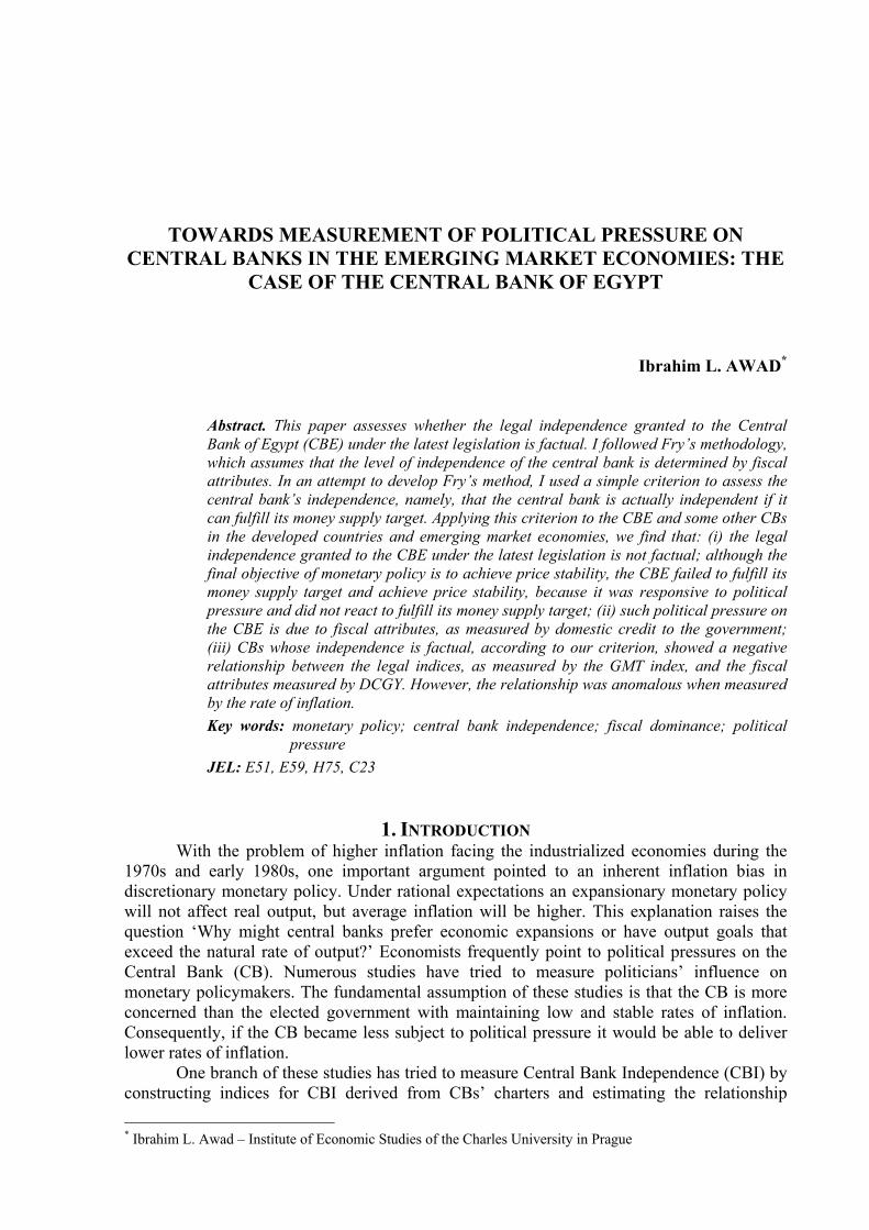
TOWARDS MEASUREMENT OF POLITICAL PRESSURE ON CENTRAL BANKS IN THE EMERGING MARKET ECONOMIES: THE
CASE OF THE CENTRAL BANK OF EGYPT
Ibrahim L. AWAD*
Abstract. This paper assesses whether the legal independence granted to the Central Bank of Egypt (CBE) under the latest legislation is factual. I followed Fry’s methodology, which assumes that the level of independence of the central bank is determined by fiscal attributes. In an attempt to develop Fry’s method, I used a simple criterion to assess the central bank’s independence, namely, that the central bank is actually independent if it can fulfill its money supply target. Applying this criterion to the CBE and some other CBs in the developed countries and emerging market economies, we find that: (i) the legal independence granted to the CBE under the latest legislation is not factual; although the final objective of monetary policy is to achieve price stability, the CBE failed to fulfill its money supply target and achieve price stability, because it was responsive to political pressure and did not react to fulfill its money supply target; (ii) such political pressure on the CBE is due to fiscal attributes, as measured by domestic credit to the government; (iii) CBs whose independence is factual, according to our criterion, showed a negative relationship between the legal indices, as measured by the GMT index, and the fiscal attributes measured by DCGY. However, the relationship was anomalous when measured by the rate of inflation. Key words: monetary policy; central bank independence; fiscal dominance; political
pressure JEL: E51, E59, H75, C23
1. INTRODUCTION With the problem of higher inflation facing the industrialized economies during the
1970s and early 1980s, one important argument pointed to an inherent inflation bias in discretionary monetary policy. Under rational expectations an expansionary monetary policy will not affect real output, but average inflation will be higher. This explanation raises the question ‘Why might central banks prefer economic expansions or have output goals that exceed the natural rate of output?’ Economists frequently point to political pressures on the Central Bank (CB). Numerous studies have tried to measure politicians’ influence on monetary policymakers. The fundamental assumption of these studies is that the CB is more concerned than the elected government with maintaining low and stable rates of inflation. Consequently, if the CB became less subject to political pressure it would be able to deliver lower rates of inflation.
One branch of these studies has tried to measure Central Bank Independence (CBI) by constructing indices for CBI derived from CBs’ charters and estimating the relationship * Ibrahim L. Awad – Institute of Economic Studies of the Charles University in Prague
64 IBRAHIM L. AWAD
between such indices and the rate of inflation. The major defect of these studies is that legal indices may not reflect the relationship between governments and CBs that exists in reality. In countries with a lower degree of democracy and where the rule of law is less strongly embedded in the political culture, as in most developing countries, there can be a wide gap between the formal legal institutional arrangements and the actual practice. Thus, for developing countries, these CBI indices may not be accurate, because legal independence does not mean actual independence.
“Actual independence is impossible to quantify” (Cukierman, 1992, p. 273). Another branch of these studies did not take Cukierman’s advice and tried to measure the actual independence of CBs using some indicators of political pressure. The central tenet of this approach is that political pressure on the CB will arise even if the CB is legally independent. A CB with any degree of independence is still part of the system of government. Consequently, politicians always try to influence the CB to adopt policies compatible with their preferences. The degree of responsiveness of the CB to such political pressure depends on the extent to which the CB is actually independent. Then, by constructing an indicator of political pressure on the CB, we can measure the degree of responsiveness of the CB to such political pressure and consequently judge whether CB independence is de facto (factual) or just de jure. The major defects of these studies are that the channels through which political pressure might work are not clear and the reaction of the CB to fiscal policy is ambiguous.
Furthermore, some studies give more attention to CBI in the developing countries, relying on the fiscal dominance hypothesis. In the developing countries the fiscal situation will constrain if not dictate the CB’s activities and therefore determine the extent of CBI. Fry (1998) tried to measure actual CB independence by estimating the reaction of the CB to the government’s demands to increase credit. In fact, domestic credit to the government is a crossing point between the CB and the government. Consequently, the reaction of the CB to such demands (pressure) represents a linkage between political pressure on the CB and the actual independence of the CB.
In this paper I followed Fry’s methodology for assessing the legal independence of CBs. I tried to develop Fry’s method using a new criterion to assess the legal independence of the Central Bank of Egypt (CBE), namely, that the CB is actually independent if it can fulfill its money supply target.
I organized this paper as follows: section 2 presents previous studies of CBI and political pressure on CBs. Section 3 assesses the previous studies. Section 4 focuses on Fry’s methodology. Section 5 focuses on our attempt to develop Fry’s method. Section 6 assesses the legal independence granted to the CBE under the latest legislation. Section 7 concludes.
2. PREVIOUS STUDIES OF CB INDEPENDENCE AND POLITICAL PRESSURE ON CBS Greater attention has been focused on the relationship between monetary policymakers
and politicians. In the literature there are two broad approaches to measuring this relationship. The first consists of studies based on legal attributes and therefore addressing the legal independence of CBs. The second involves studies based on non-legal attributes and therefore addressing political pressure on CBs. Besides these two approaches, there is another branch of studies which addresses the actual independence of CBs based on the fiscal dominance hypothesis. In this part I will briefly present each of these approaches.
2.1 Previous studies of the legal independence of CBs1 The theoretical basis of these studies depends on the notion that CBs in democratic
countries are more concerned with maintaining low and stable rates of inflation than the elected government. If a CB becomes free of political pressure it will be able to deliver stable and low rates of inflation. In the theoretical models, CBI is introduced by means of the weight placed on inflation objectives in the loss function. The CB will be more independent if such
1 For more details and other subsequent empirical studies, see Arnone et al. (2006a).
Towards Measurement of Political Pressure on Central Banks in the Emerging Market Economies… 65
weight in the loss function exceeds that of the government. The CB in this case is described as a Rogoff-conservative CB.
To measure how independent a CB is, empirical studies have constructed CBI indices based on the CB’s legal characteristics. To investigate the relationship between CBI and the inflation rate, empirical studies (Eijffinger and Keulen, 1995, p. 57) have used this equation:
Average monthly inflation (π) = α0 + α1 (CBI) + ε1 Using legal indices for CBI, many studies try to prove the theoretical assumption that
higher levels of CBI, as detected by legal indices, will lead to lower rates of inflation. These studies have also used panel data about developing and developed countries to find such a negative correlation/relationship between CBI and the rate of inflation. Finding such a relationship is important to judge whether the legal independence of the CB is factual (de facto) or just formal (de jure).
Bade and Parkin (1977) presented the first empirical study of CBI using an index based on legal attributes. The study comprises twelve industrial countries during the period 1951–1975. They measured the independence of the CB according to the following criteria: (i) the primary objective of the CB according to the law; (ii) the degree of government influence over CB policy (the government’s ability to appoint the members of the board of directors, government representation in the board of directors, and which authority controls monetary policy).
Alesina (1988, 1989) includes monetary financing rules, thus enlarging Bade and Parkin’s index of policy independence to include the following criterion: the obligation of the CB to buy short-term treasury papers, as the monetary financing obligation can seriously harm CBI with respect to monetary policy making. Alesina (1988) examines how the degree of CB autonomy affects the magnitude of political influence over the economy and monetary policy. An independent CB is able to reduce fluctuations in monetary policy brought about by the election cycle.
Grilli, Masciandaro, and Tabellini (1991) built a two-part legal index for CBI. The authors defined “political autonomy” as the ability of the CB to select the final objectives of monetary policy, and defined “economic autonomy” as the ability of the CB to select monetary policy instruments. They constructed an index from eight criteria for each part, and assigned one point for each criterion if it is satisfied2. The overall index, the total sum of the points of the two-part index, is a measurement of CBI.
Cukierman (1992) constructs three indices of CBI. The first index (LVAU-LVAW) contains 16 indicators grouped under four main headings; a heading about the chief executive officer (CEO), a heading about policy formulation (PF), a heading about the objectives of the central bank (OBJ), and a heading about the limitations on the CB for lending to the government (LL). The second index, the turnover rate of the CB’s governor (TOR), is based on the assumption that the higher is the TOR the lower is the CB’s autonomy. The third index (QVAU-QVAW) is constructed on the basis of responses given to a questionnaire exploring various aspects of the CB’s autonomy by focusing not only on the legal aspects, but also on the instruments used by the CB.
Alesina and Summers (1993) constructed another CBI index using the average of Bade and Parkin, expanded by Alesina (1988, 1989) and GMT (1991).
Describing policy independence, like GMT, as the capacity of the CB to choose the final objectives of monetary policy, Eijffinger and Schaling (1993) constructed another legal index for CBI. It comprised the formal responsibility of the CB with regard to monetary policy, the relationship between the CB and the government/parliament in the formulation of monetary policy, and the procedures for the appointment of the board of directors.
2 Grilli, Masciandaro, and Tabellini (GMT) (1991) define CB independence as autonomy in setting objectives and autonomy in setting instruments. But the most common terminology for defining CBI is due to Debelle and Fisher (1994), who defined CBI as “goal independence” and “instrument independence.”
66 IBRAHIM L. AWAD
Arnone et al. (2006b) presented an update of the GMT index based on the CB legislation as of the end of 2003. The index comprised a set of developing countries, emerging market economics, and OECD countries. The authors presented a reconstruction of the GMT index based on Cukierman (1992) for a smaller set of countries, and evaluated the changes in CB autonomy between 1992 and 2003. Their results point to a significant increase in CB autonomy particularly for developing countries. Improvements in CB autonomy had, in most cases, involved a three-stage process: an initial stage in which the political foundations for CB autonomy were laid, a stage in which operational autonomy developed, and further political autonomy in terms of policy formulation and the appointment of senior management.
Since the legal indices of CBI may not reflect the real relationship that exists in practice between the government and the CB, another methodology (see Mahadeva and Sterne, 2000) tried to avoid this limitation by asking central bankers directly, using two methods. The first method interprets responses to the general subjective question, ‘How would you define CBI?’ then uses the answers to construct an index of self-assessment of CBI. The second method involves asking central bankers, ‘How independent are your own institutions?’ The answer to this question depends on the answers to a number of objective indicators. Using probit regression, the study attempts to explain which objective indicators of CBI explain the subjective self-assessment. One of the important results of this study is that self-assessment of CBI is strongly associated with both the degree of instrument independence measured and the absence of a deficit finance obligation. Also, the results for developing countries are similar to those of the entire sample. The absence of a deficit finance obligation and instrument independence explain the self-assessment variable. Considering the study group together with developing and transitional economies, the results show that the deficit finance limits have the most important influence on the perception of CB independence.
2.2 Previous studies of political pressure on CBs The analysis of political pressure under this approach has been established on the
background of the political business cycle. Drazen (2002) argues that reconsidering the pre-electoral political monetary cycle as an explanation for political pressure on the CB is important for the following reasons: (i) there may be indirect effects of the electoral cycle on monetary policy; (ii) in countries with independent central banks, pre-electoral monetary cycles are noticeable, with money growth rates rising before elections and the inflation rate rising after elections; (iii) using policy tools other than monetary policy to influence election outcomes may have a significant effect on monetary policy. The nature of this effect depends on the interaction between the CB and politicians.
Drazen presented a theoretical model for political pressure on the CB. Since accommodating monetary policy is worth more to politicians in election years than in non-election years, the amount of pressure differs over the electoral cycle. This induces an electoral cycle in monetary policy even though the CB is independent and has no electoral motive per se. In equilibrium, the monetary authority accommodates the politicians’ desired policies in electoral years, but generally it is free of political influence in non-election years. An electoral cycle in fiscal policy may intensify the political monetary cycle, while an electoral structure that allows the government to call early elections may lessen it.
Empirical studies have tried to construct an indicator for political pressure on CBs. From the point of view of these studies, political pressure on CBs will occur even if the CB is legally independent, as politicians always try to influence the CB to adopt policies compatible with their preferences. But the degree of responsiveness of the CB to such political pressure depends on the extent to which the CB is actually independent. With a higher degree of CBI, such influence will arise only in indirect ways (since the CB, despite its independence, is still part of the system of government). So, by constructing an indicator for political pressure on the CB we can measure the degree of responsiveness of the CB to such political pressure, and consequently judge whether the independence of the CB is de facto or just de jure.
Towards Measurement of Political Pressure on Central Banks in the Emerging Market Economies… 67
Havrilesky (1993) constructed an index for political pressure on CBs. This index was based on the number of newspaper reports in which politicians revealed their preferences about a more or less restrictive monetary policy. Any article calling for a monetary easing was assigned the value +1, while any article calling for monetary tightness was assigned the value –1. The final index, as an indicator of the net political pressure, is the net summation of the negatives and positives. Havrilesky applied his study to the Federal Reserve by counting the number of reports in the Wall Street Journal of politicians arguing in favor of more or less restrictive monetary policy. He found that the Federal Reserve’s polices responded to this index.
Maier et al. (2002) applied Havrilesky’s approach to the Deutsche Bundesbank after extending the analysis to include the pressure arising from other interest groups and analyzing press reports in different newspapers. He concluded that the Bundesbank did not respond to political pressure and its policies were in line with the wishes of the banking sector.
Using the extended version of Havrilesky’s approach (1993) by Maier (2002), Gersl (2006) tried to measure and explain the political pressure on the Czech National Bank (CNB). He concluded that the CNB faced considerable political pressure toward a monetary easing in the period 1997–2005, comparable with the pressure on the Federal Reserve and slightly higher than the pressure on the Deutsche Bundesbank. However, the CNB did not succumb to such pressure. Therefore, political pressure did not have any systematic impact on the direction of monetary policy. Hence the legal independence of the CNB was proved to be factual as well.
2.3 Previous studies of the actual independence of CBs based on the fiscal dominance hypothesis
This approach gives more attention to CBs in developing countries, relying on the fiscal dominance hypothesis. In developing countries the fiscal situation will constrain, if not dictate, the CB’s activities and therefore determine the extent of the CB’s independence. To assess how independent a CB is, Fry (1998) used a simple measure based on an action that all CBs can take: reaction to increased credit demands by the government. Using the change in domestic credit as a proxy for monetary policy, he constructed a monetary policy reaction function. His hypothesis states that the extent of neutralization depends on both the size of the government deficit and the methods by which it is financed. Since governments can finance their deficit in four ways (borrowing at zero cost from the CB, borrowing from domestic commercial banks at below-market interest rates, borrowing abroad in foreign currency, and borrowing at market interest rates from the voluntary domestic private sector), the CB will be less independent if the government deficit is higher and the government uses the first two methods to finance its deficit.
Fry measured the degree of CB independence by the value of the neutralization coefficient, that is, the reaction of the CB to the government’s demand for more credit to finance the budget deficit. Since domestic credit plus net foreign assets constitute the assets backing the monetary stock, an increase in net foreign assets must be offset by a decrease in domestic credit to prevent any change in the money stock or to make the CB able to fulfill its money supply target. To examine whether CBs in developing countries are independent, Fry estimated the neutralization coefficient for a variety of developing countries. His result was that a larger deficit and greater government reliance on the domestic banking system are associated with less neutralization, and consequently less CBI.
As determined in open-economy macroeconomics, a CB-engineered increase in the real interest rate makes domestic government debt more attractive and leads to a real appreciation. However, if the increase in the real interest rate also increases the probability of default on the debt, the effect may be instead to make domestic government debt less attractive, and leads to a real depreciation. That outcome is more likely the higher the initial level of debt, the higher the proportion of foreign-currency-denominated debt, and the higher the price of risk. In such case, fiscal policy, not monetary policy, is the right instrument to
68 IBRAHIM L. AWAD
decrease inflation. Blanchard (2004) argues that this is the situation found in the Brazilian economy in 2002 and 2003.
3. ASSESSMENT OF PREVIOUS STUDIES The general conclusion found in the literature pertaining to the empirical studies of
legal CBI can be summarized as follows (Ferreira de Mendonca, 2005, and Arnone et al., 2006): (i) among industrial economies there is a strong negative correlation between de jure CBI and inflation; (ii) in developing countries there is no evident relationship between legal CBI and inflation; (iii) there is a positive correlation between the political vulnerability of the CB and the variation of inflation; (iv) countries in which the monetary authorities announced their goals for inflation presented lower rates of inflation; (v) legal CBI is not correlated with the average real growth rate; (vi) CBs with a higher degree of independence do not finance deficits.
One of the main defects of the legal indices for CBI is that the concept of independence differs across such indices, even though they deal with the same thing. In other words, there is no homogeneous concept of CBI across the legal indices. Ferreira de Mendonca (2005) examines this point using a correlation analysis for the three indices frequently used in empirical studies of CBI (Alesina and Summers, Cukierman, and GMT). Focusing on 15 industrialized countries and performing the analysis for independence indices and independence rankings, the finding was that there is no relationship between these measures of independence after the most independent countries (Germany, Switzerland, and United States) are omitted from the analysis.
Another defect of the legal indices is that they may not reflect the relationship between the government and the CB that exists in practice. In countries with a lower degree of democracy and where the rule of law is less strongly embedded in the political culture (as in most developing countries), there can be a wide gap between the formal legal institutional arrangements and the actual practice. Thus, for developing countries these CBI indices may not be accurate.
Economists have pointed out other defects in the empirical studies based on the legal indices of CBI (Walsh, 1998, pp. 379–381, and Arnone et al., 2006). (i) Average inflation and the degree of CBI might be jointly determined by the strength of the political constituencies opposed to inflation. In the absence of these constituencies, increasing CBI will not affect inflation. This means that even if the CB is independent, higher political pressure with no equivalent opposite directions may result in inflation. (ii) Another problem with the estimations of the equation given above is that it fails to correct for country-specific factors that may affect inflation and may also be correlated with the indices of CBI. Correcting for potential bias requires the inclusion of other determinants of inflation in the above equation. (iii) Most economists cast doubt on the relationship between CBI and average inflation. A complete understanding of this relationship requires a better understanding of the factors that have led to the variations in CBI across countries. The best way to understand such differences is to estimate the above equation directly for one-country rather than cross-section comparisons. However, this task is not easy. (iv) While CBI raises the issue of subjecting the CB to democratic control, the linkage between CBI and CB accountability is not clear in most of these studies.
Moreover, the political pressure approach is also criticized. Besides the other flaws of Havrilesky’s approach (see Gersl, 2006, p. 4) the major defects are as follows. (i) The channels through which political pressure might work are not clear. (ii) The reaction of the CB to fiscal policy is ambiguous. (iii) Without complete coordination between fiscal policy and monetary policy, the CB may be coerced to conduct monetary policy in favor of politicians’ interests. Such coordination between monetary and fiscal policy reflects the government’s desire, side by side with the CB, to curb inflation. This point is also not clear in this literature.
Towards Measurement of Political Pressure on Central Banks in the Emerging Market Economies… 69
Some important lessons from the previous studies are as follows. (i) Political pressure on CBs will occur with any degree of CBI. This is simply because CBs with the highest degree of independence are still within the system of government. (ii) The degree of inflation resulting from political pressure on CBs depends on whether CBI is factual or only formal. (iii) Since the degree of resulting inflation is the product of the interaction between the political pressure on the CB for a monetary easing and a higher or lower degree of responsiveness of the CB, then we can assess the degree of CBI by the ability of the CB to fulfill its money supply target in the face of political pressure. (iv) One of the crossing points between fiscal policy and monetary policy, and consequently between the government and the CB, is “domestic credit to the government.” On the one hand, this is one of the sources of political pressure on the CB. On the other hand, it constitutes an essential part of the assets backing the money supply, and so it is important for monetary policy to keep it under control.
The fiscal dominance hypothesis, discussed by Fry, represents a step in that direction. The reaction of the CB to the government’s demands to increase credit represents a linkage between political pressure on the CB and CBI. Such a reaction measures to what extent the CB is actually independent, especially in developing countries. Since CBs in the developed countries may or may not be asked to provide credit to central government, this measure (the reaction of the CB to the government’s demand for higher credit) can be developed into a comprehensive indicator of the actual independence of CBs. In the following two sections I will present Fry’s methodology in more detail and then develop it to serve my purposes.
4. FRY’S METHODOLOGY Fry began with this equation:
(1) DDCY = f(DNFAY, Xi) where DDCY represents the change in domestic credit scaled by GDP, DNFAY represents the change in net foreign assets scaled by GDP, and Xi represents the other explanatory variables other than DNFAY (the gap between domestic inflation and inflation in the industrialized economies, the gap between actual and potential output, economic growth…). Complete sterilization of net foreign assets on the supply of money implies a coefficient of DNFAY equal to –1. Since domestic credit equals domestic credit to the government (DCG) plus domestic credit to the private sector (DCP), the above equation might be written as follows:
(2) DDCPY = f( DNFAY, Xi ) – DDCGY where DDCPY is the change in domestic credit to the private sector scaled by GDP, and DDCGY is the change in domestic credit to the government scaled by GDP. The last equation represents the monetary policy reaction function that Fry used to estimate the neutralization coefficient. Complete neutralization of the government’s extra borrowing requirements implies a coefficient of –1 for DDCGY. Partial neutralization will produce a coefficient less than zero and higher than –1, and no neutralization entails a coefficient of zero. Complete neutralization represents the highest level of CBI, while zero neutralization represents, in fact, complete subordination of the CB to the government. Fry argues that,
‘a central bank that says to the government “we cannot resist your financing demands, but we shall neutralize them by squeezing the private sector and we shall tell the private sector exactly why we have to squeeze credit” is surely acting more independently than one that simply lets domestic credit rise by the full extent of any extra government borrowing from the banking system.’
Fry used a system of simultaneous equations. He treated the variable change in domestic credit to the government (DDCGY) as exogenous, and the variables the inflation gap (INFGAP) and the change in net foreign assets (DNFAY) as endogenous. He used 3SLS. The instruments are: lagged DNFAY, lagged INFGAP, and lagged money and growth rates, the rate of change in oil prices, the OECD growth rate, and the world interest rate. The estimated monetary policy reaction function was as follows:
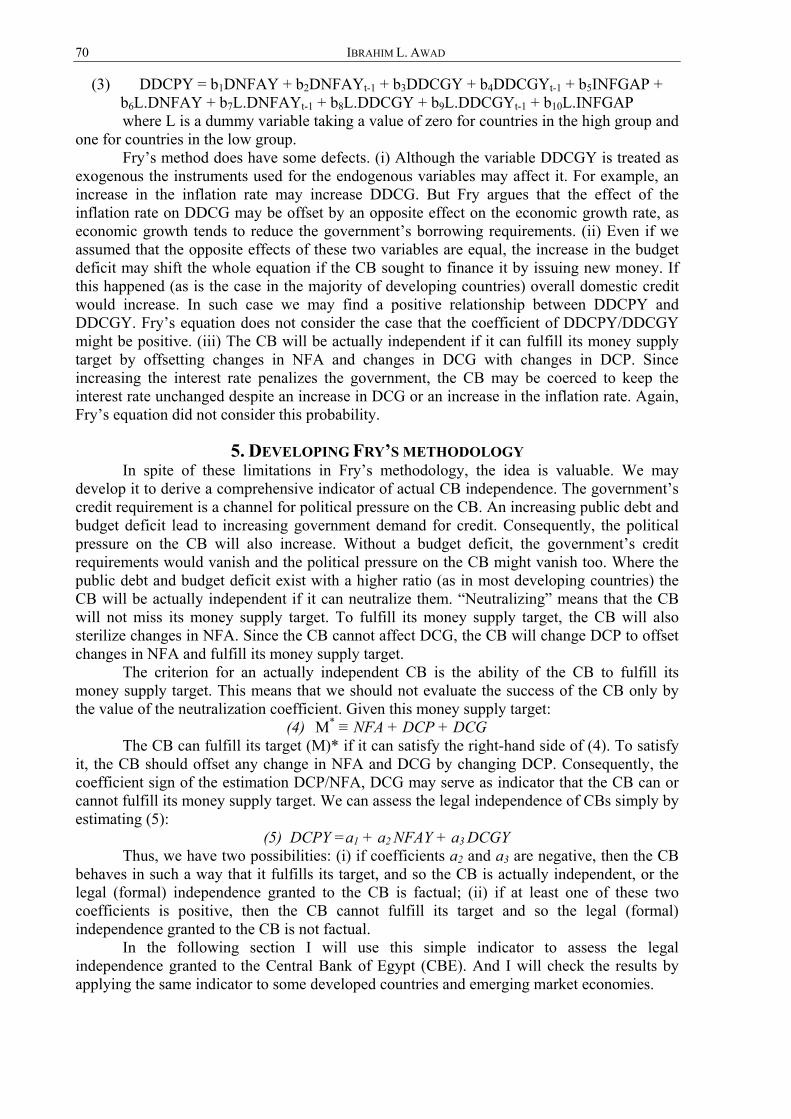
70 IBRAHIM L. AWAD
(3) DDCPY = b1DNFAY + b2DNFAYt-1 + b3DDCGY + b4DDCGYt-1 + b5INFGAP + b6L.DNFAY + b7L.DNFAYt-1 + b8L.DDCGY + b9L.DDCGYt-1 + b10L.INFGAP where L is a dummy variable taking a value of zero for countries in the high group and
one for countries in the low group. Fry’s method does have some defects. (i) Although the variable DDCGY is treated as
exogenous the instruments used for the endogenous variables may affect it. For example, an increase in the inflation rate may increase DDCG. But Fry argues that the effect of the inflation rate on DDCG may be offset by an opposite effect on the economic growth rate, as economic growth tends to reduce the government’s borrowing requirements. (ii) Even if we assumed that the opposite effects of these two variables are equal, the increase in the budget deficit may shift the whole equation if the CB sought to finance it by issuing new money. If this happened (as is the case in the majority of developing countries) overall domestic credit would increase. In such case we may find a positive relationship between DDCPY and DDCGY. Fry’s equation does not consider the case that the coefficient of DDCPY/DDCGY might be positive. (iii) The CB will be actually independent if it can fulfill its money supply target by offsetting changes in NFA and changes in DCG with changes in DCP. Since increasing the interest rate penalizes the government, the CB may be coerced to keep the interest rate unchanged despite an increase in DCG or an increase in the inflation rate. Again, Fry’s equation did not consider this probability.
5. DEVELOPING FRY’S METHODOLOGY In spite of these limitations in Fry’s methodology, the idea is valuable. We may
develop it to derive a comprehensive indicator of actual CB independence. The government’s credit requirement is a channel for political pressure on the CB. An increasing public debt and budget deficit lead to increasing government demand for credit. Consequently, the political pressure on the CB will also increase. Without a budget deficit, the government’s credit requirements would vanish and the political pressure on the CB might vanish too. Where the public debt and budget deficit exist with a higher ratio (as in most developing countries) the CB will be actually independent if it can neutralize them. “Neutralizing” means that the CB will not miss its money supply target. To fulfill its money supply target, the CB will also sterilize changes in NFA. Since the CB cannot affect DCG, the CB will change DCP to offset changes in NFA and fulfill its money supply target.
The criterion for an actually independent CB is the ability of the CB to fulfill its money supply target. This means that we should not evaluate the success of the CB only by the value of the neutralization coefficient. Given this money supply target:
(4) M* ≡ NFA + DCP + DCG The CB can fulfill its target (M)* if it can satisfy the right-hand side of (4). To satisfy
it, the CB should offset any change in NFA and DCG by changing DCP. Consequently, the coefficient sign of the estimation DCP/NFA, DCG may serve as indicator that the CB can or cannot fulfill its money supply target. We can assess the legal independence of CBs simply by estimating (5):
(5) DCPY =a1 + a2 NFAY + a3 DCGY Thus, we have two possibilities: (i) if coefficients a2 and a3 are negative, then the CB
behaves in such a way that it fulfills its target, and so the CB is actually independent, or the legal (formal) independence granted to the CB is factual; (ii) if at least one of these two coefficients is positive, then the CB cannot fulfill its target and so the legal (formal) independence granted to the CB is not factual.
In the following section I will use this simple indicator to assess the legal independence granted to the Central Bank of Egypt (CBE). And I will check the results by applying the same indicator to some developed countries and emerging market economies.
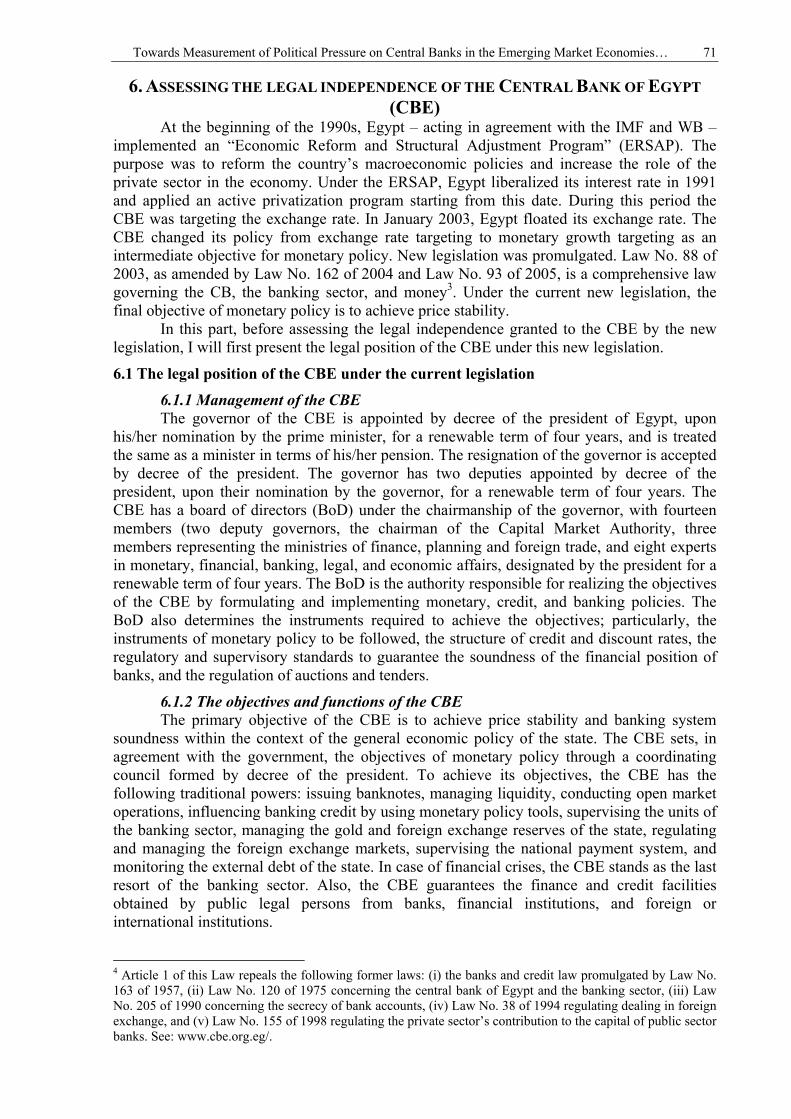
Towards Measurement of Political Pressure on Central Banks in the Emerging Market Economies… 71
6. ASSESSING THE LEGAL INDEPENDENCE OF THE CENTRAL BANK OF EGYPT (CBE)
At the beginning of the 1990s, Egypt – acting in agreement with the IMF and WB – implemented an “Economic Reform and Structural Adjustment Program” (ERSAP). The purpose was to reform the country’s macroeconomic policies and increase the role of the private sector in the economy. Under the ERSAP, Egypt liberalized its interest rate in 1991 and applied an active privatization program starting from this date. During this period the CBE was targeting the exchange rate. In January 2003, Egypt floated its exchange rate. The CBE changed its policy from exchange rate targeting to monetary growth targeting as an intermediate objective for monetary policy. New legislation was promulgated. Law No. 88 of 2003, as amended by Law No. 162 of 2004 and Law No. 93 of 2005, is a comprehensive law governing the CB, the banking sector, and money3. Under the current new legislation, the final objective of monetary policy is to achieve price stability.
In this part, before assessing the legal independence granted to the CBE by the new legislation, I will first present the legal position of the CBE under this new legislation.
6.1 The legal position of the CBE under the current legislation
6.1.1 Management of the CBE The governor of the CBE is appointed by decree of the president of Egypt, upon
his/her nomination by the prime minister, for a renewable term of four years, and is treated the same as a minister in terms of his/her pension. The resignation of the governor is accepted by decree of the president. The governor has two deputies appointed by decree of the president, upon their nomination by the governor, for a renewable term of four years. The CBE has a board of directors (BoD) under the chairmanship of the governor, with fourteen members (two deputy governors, the chairman of the Capital Market Authority, three members representing the ministries of finance, planning and foreign trade, and eight experts in monetary, financial, banking, legal, and economic affairs, designated by the president for a renewable term of four years. The BoD is the authority responsible for realizing the objectives of the CBE by formulating and implementing monetary, credit, and banking policies. The BoD also determines the instruments required to achieve the objectives; particularly, the instruments of monetary policy to be followed, the structure of credit and discount rates, the regulatory and supervisory standards to guarantee the soundness of the financial position of banks, and the regulation of auctions and tenders.
6.1.2 The objectives and functions of the CBE The primary objective of the CBE is to achieve price stability and banking system
soundness within the context of the general economic policy of the state. The CBE sets, in agreement with the government, the objectives of monetary policy through a coordinating council formed by decree of the president. To achieve its objectives, the CBE has the following traditional powers: issuing banknotes, managing liquidity, conducting open market operations, influencing banking credit by using monetary policy tools, supervising the units of the banking sector, managing the gold and foreign exchange reserves of the state, regulating and managing the foreign exchange markets, supervising the national payment system, and monitoring the external debt of the state. In case of financial crises, the CBE stands as the last resort of the banking sector. Also, the CBE guarantees the finance and credit facilities obtained by public legal persons from banks, financial institutions, and foreign or international institutions.
4 Article 1 of this Law repeals the following former laws: (i) the banks and credit law promulgated by Law No. 163 of 1957, (ii) Law No. 120 of 1975 concerning the central bank of Egypt and the banking sector, (iii) Law No. 205 of 1990 concerning the secrecy of bank accounts, (iv) Law No. 38 of 1994 regulating dealing in foreign exchange, and (v) Law No. 155 of 1998 regulating the private sector’s contribution to the capital of public sector banks. See: www.cbe.org.eg/.
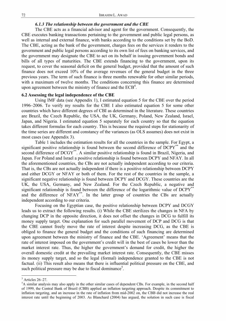
72 IBRAHIM L. AWAD
6.1.3 The relationship between the government and the CBE The CBE acts as a financial advisor and agent for the government. Consequently, the
CBE executes banking transactions pertaining to the government and public legal persons, as well as internal and external finance, with banks according to the conditions set by the BoD. The CBE, acting as the bank of the government, charges fees on the services it renders to the government and public legal persons according to its own list of fees on banking services, and the government may designate the CBE to act on its behalf in issuing government bonds and bills of all types of maturities. The CBE extends financing to the government, upon its request, to cover the seasonal deficit on the general budget, provided that the amount of such finance does not exceed 10% of the average revenues of the general budget in the three previous years. The term of such finance is three months renewable for other similar periods, with a maximum of twelve months. The conditions concerning this finance are determined upon agreement between the ministry of finance and the ECB4.
6.2 Assessing the legal independence of the CBE Using IMF data (see Appendix 1), I estimated equation 5 for the CBE over the period
1996–2006. To verify my results for the CBE I also estimated equation 5 for some other countries which have different degrees of CBI as determined in the literature. These countries are Brazil, the Czech Republic, the USA, the UK, Germany, Poland, New Zealand, Israel, Japan, and Nigeria. I estimated equation 5 separately for each country so that the equation takes different formulas for each country. This is because the required steps for stationarity of the time series are different and constancy of the variances (as OLS assumes) does not exist in most cases (see Appendix 3).
Table 1 includes the estimation results for all the countries in the sample. For Egypt, a significant positive relationship is found between the second difference of DCPY** and the second difference of DCGY**. A similar positive relationship is found in Brazil, Nigeria, and Japan. For Poland and Israel a positive relationship is found between DCPY and NFAY. In all the aforementioned countries, the CBs are not actually independent according to our criteria. That is, the CBs are not actually independent if there is a positive relationship between DCPY and either DCGY or NFAY or both of them. For the rest of the countries in the sample, a significant negative relationship is found between DCPY and DCGY. These countries are the UK, the USA, Germany, and New Zealand. For the Czech Republic, a negative and significant relationship is found between the difference of the logarithmic value of DCPY** and the difference of NFAY**. In the latter group of countries the CBs are actually independent according to our criteria.
Focusing on the Egyptian case, the positive relationship between DCPY and DCGY leads us to extract the following results. (i) While the CBE sterilizes the changes in NFA by changing DCP in the opposite direction, it does not offset the changes in DCG to fulfill its money supply target. One explanation for such parallel movement of DCP and DCG is that the CBE cannot freely move the rate of interest despite increasing DCG, as the CBE is obliged to finance the general budget and the conditions of such financing are determined upon agreement between the ministry of finance and the CBE. ‘Agreement’ means that the rate of interest imposed on the government’s credit will in the best of cases be lower than the market interest rate. Thus, the higher the government’s demand for credit, the higher the overall domestic credit at the prevailing market interest rate. Consequently, the CBE misses its money supply target, and so the legal (formal) independence granted to the CBE is not factual. (ii) This result also means that there is influential political pressure on the CBE, and such political pressure may be due to fiscal dominance5. 3 Articles 26–27. 5A similar analysis may also apply in the other similar cases of dependent CBs. For example, in the second half of 1999, the Central Bank of Brazil (CBB) applied an inflation targeting approach. Despite its commitment to inflation targeting, and an increase in the rate of inflation from mid-2002 on, the CBB did not increase the real interest rate until the beginning of 2003. As Blanchard (2004) has argued, the solution in such case is fiscal
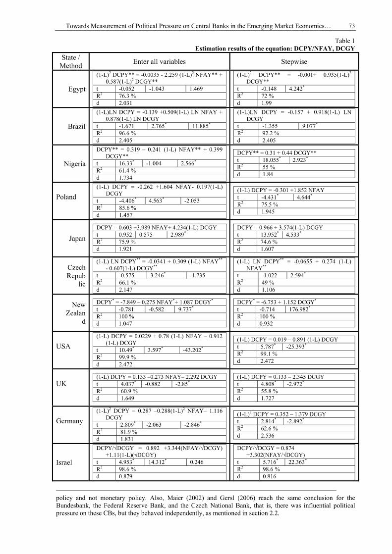
Towards Measurement of Political Pressure on Central Banks in the Emerging Market Economies… 73
Table 1 Estimation results of the equation: DCPY/NFAY, DCGY
State / Method Enter all variables Stepwise
Egypt
(1-L)2 DCPY** = -0.0035 - 2.259 (1-L)2 NFAY** + 0.587(1-L)2 DCGY**
t -0.052 -1.043 1.469 R2 76.3 % d 2.031
(1-L)2 DCPY** = -0.001+ 0.935(1-L)2 DCGY**
t -0.148 4.242* R2 72 % d 1.99
Brazil
(1-L)LN DCPY = -0.139 +0.509(1-L) LN NFAY + 0.878(1-L) LN DCGY
t -1.671 2.765* 11.885* R2 96.6 % d 2.405
(1-L)LN DCPY = -0.157 + 0.918(1-L) LN DCGY
t -1.355 9.077* R2 92.2 % d 2.405
Nigeria
DCPY** = 0.319 – 0.241 (1-L) NFAY** + 0.399 DCGY**
t 16.33* -1.004 2.566* R2 61.4 % d 1.734
DCPY** = 0.31 + 0.44 DCGY** t 18.055* 2.923* R2 55 % d 1.84
Poland
(1-L) DCPY = -0.262 +1.604 NFAY- 0.197(1-L) DCGY
t -4.406* 4.563* -2.053 R2 85.6 % d 1.457
(1-L) DCPY = -0.301 +1.852 NFAY t -4.431* 4.644* R2 75.5 % d 1.945
Japan
DCPY = 0.603 +3.989 NFAY+ 4.234(1-L) DCGY t 0.952 0.575 2.989* R2 75.9 % d 1.921
DCPY = 0.966 + 3.574(1-L) DCGY t 13.952* 4.533* R2 74.6 % d 1.607
Czech Repub
lic
(1-L) LN DCPY** = -0.0341 + 0.309 (1-L) NFAY** - 0.607(1-L) DCGY**
t -0.575 3.246* -1.735 R2 66.1 % d 2.147
(1-L) LN DCPY** = -0.0655 + 0.274 (1-L) NFAY**
t -1.022 2.594* R2 49 % d 1.106
New Zealan
d
DCPY* = -7.849 – 0.275 NFAY*+ 1.087 DCGY* t -0.781 -0.582 9.737* R2 100 % d 1.047
DCPY* = -6.753 + 1.152 DCGY* t -0.714 176.982* R2 100 % d 0.932
USA
(1-L) DCPY = 0.0229 + 0.78 (1-L) NFAY – 0.912 (1-L) DCGY
t 10.49* 3.597* -43.202* R2 99.9 % d 2.472
(1-L) DCPY = 0.019 – 0.891 (1-L) DCGY t 5.787* -25.393* R2 99.1 % d 2.472
UK
(1-L) DCPY = 0.133 –0.273 NFAY– 2.292 DCGY t 4.037* -0.882 -2.85* R2 60.9 % d 1.649
(1-L) DCPY = 0.133 – 2.345 DCGY t 4.808* -2.972* R2 55.8 % d 1.727
Germany
(1-L)2 DCPY = 0.287 –0.288(1-L)2 NFAY– 1.116 DCGY
t 2.809* -2.063 -2.846* R2 81.9 % d 1.831
(1-L)2 DCPY = 0.352 – 1.379 DCGY t 2.814* -2.892* R2 62.6 % d 2.536
Israel
DCPY/√DCGY = 0.892 +3.344(NFAY/√DCGY) +1.11(1-L)(√DCGY)
t 4.953* 14.312* 0.246 R2 98.6 % d 0.879
DCPY/√DCGY = 0.874 +3.302(NFAY/√DCGY)
t 5.716* 22.363* R2 98.6 % d 0.816
policy and not monetary policy. Also, Maier (2002) and Gersl (2006) reach the same conclusion for the Bundesbank, the Federal Reserve Bank, and the Czech National Bank, that is, there was influential political pressure on these CBs, but they behaved independently, as mentioned in section 2.2.
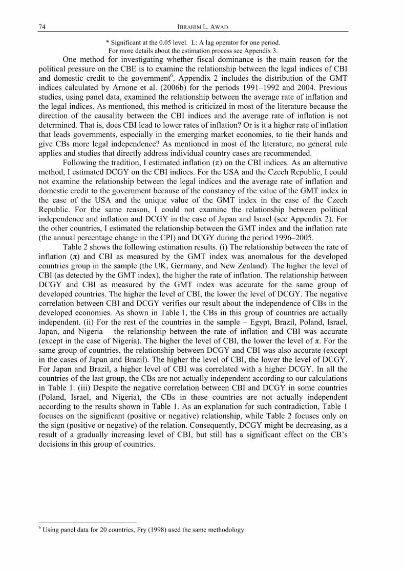
74 IBRAHIM L. AWAD
* Significant at the 0.05 level. L: A lag operator for one period. For more details about the estimation process see Appendix 3.
One method for investigating whether fiscal dominance is the main reason for the political pressure on the CBE is to examine the relationship between the legal indices of CBI and domestic credit to the government6. Appendix 2 includes the distribution of the GMT indices calculated by Arnone et al. (2006b) for the periods 1991–1992 and 2004. Previous studies, using panel data, examined the relationship between the average rate of inflation and the legal indices. As mentioned, this method is criticized in most of the literature because the direction of the causality between the CBI indices and the average rate of inflation is not determined. That is, does CBI lead to lower rates of inflation? Or is it a higher rate of inflation that leads governments, especially in the emerging market economies, to tie their hands and give CBs more legal independence? As mentioned in most of the literature, no general rule applies and studies that directly address individual country cases are recommended.
Following the tradition, I estimated inflation (π) on the CBI indices. As an alternative method, I estimated DCGY on the CBI indices. For the USA and the Czech Republic, I could not examine the relationship between the legal indices and the average rate of inflation and domestic credit to the government because of the constancy of the value of the GMT index in the case of the USA and the unique value of the GMT index in the case of the Czech Republic. For the same reason, I could not examine the relationship between political independence and inflation and DCGY in the case of Japan and Israel (see Appendix 2). For the other countries, I estimated the relationship between the GMT index and the inflation rate (the annual percentage change in the CPI) and DCGY during the period 1996–2005.
Table 2 shows the following estimation results. (i) The relationship between the rate of inflation (π) and CBI as measured by the GMT index was anomalous for the developed countries group in the sample (the UK, Germany, and New Zealand). The higher the level of CBI (as detected by the GMT index), the higher the rate of inflation. The relationship between DCGY and CBI as measured by the GMT index was accurate for the same group of developed countries. The higher the level of CBI, the lower the level of DCGY. The negative correlation between CBI and DCGY verifies our result about the independence of CBs in the developed economies. As shown in Table 1, the CBs in this group of countries are actually independent. (ii) For the rest of the countries in the sample – Egypt, Brazil, Poland, Israel, Japan, and Nigeria – the relationship between the rate of inflation and CBI was accurate (except in the case of Nigeria). The higher the level of CBI, the lower the level of π. For the same group of countries, the relationship between DCGY and CBI was also accurate (except in the cases of Japan and Brazil). The higher the level of CBI, the lower the level of DCGY. For Japan and Brazil, a higher level of CBI was correlated with a higher DCGY. In all the countries of the last group, the CBs are not actually independent according to our calculations in Table 1. (iii) Despite the negative correlation between CBI and DCGY in some countries (Poland, Israel, and Nigeria), the CBs in these countries are not actually independent according to the results shown in Table 1. As an explanation for such contradiction, Table 1 focuses on the significant (positive or negative) relationship, while Table 2 focuses only on the sign (positive or negative) of the relation. Consequently, DCGY might be decreasing, as a result of a gradually increasing level of CBI, but still has a significant effect on the CB’s decisions in this group of countries.
6 Using panel data for 20 countries, Fry (1998) used the same methodology.
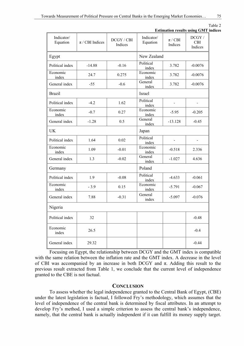
Towards Measurement of Political Pressure on Central Banks in the Emerging Market Economies… 75
Table 2 Estimation results using GMT indices
Indicator/ Equation
π / CBI Indices DCGY / CBI
Indices
Indicator/ Equation
π / CBI Indices
DCGY / CBI
Indices
Egypt New Zealand
Political index -14.88 -0.16 Political index 3.782 -0.0076
Economic index 24.7 0.275 Economic
index 3.782 -0.0076
General index -55 -0.6 General index 3.782 -0.0076
Brazil Israel
Political index -4.2 1.62 Political index - -
Economic index -0.7 0.27 Economic
index -5.95 -0.205
General index -1.28 0.5 General index -13.128 -0.45
UK Japan
Political index 1.64 0.02 Political index - -
Economic index 1.09 -0.01 Economic
index -0.518 2.336
General index 1.3 -0.02 General index -1.027 4.636
Germany Poland
Political index 1.9 -0.08 Political index -4.633 -0.061
Economic index - 3.9 0.15 Economic
index -5.791 -0.067
General index 7.88 -0.31 General index -5.097 -0.076
Nigeria
Political index 32 -0.48
Economic index 26.5 -0.4
General index 29.32 -0.44
Focusing on Egypt, the relationship between DCGY and the GMT index is compatible with the same relation between the inflation rate and the GMT index. A decrease in the level of CBI was accompanied by an increase in both DCGY and π. Adding this result to the previous result extracted from Table 1, we conclude that the current level of independence granted to the CBE is not factual.
CONCLUSION To assess whether the legal independence granted to the Central Bank of Egypt, (CBE)
under the latest legislation is factual, I followed Fry’s methodology, which assumes that the level of independence of the central bank is determined by fiscal attributes. In an attempt to develop Fry’s method, I used a simple criterion to assess the central bank’s independence, namely, that the central bank is actually independent if it can fulfill its money supply target.
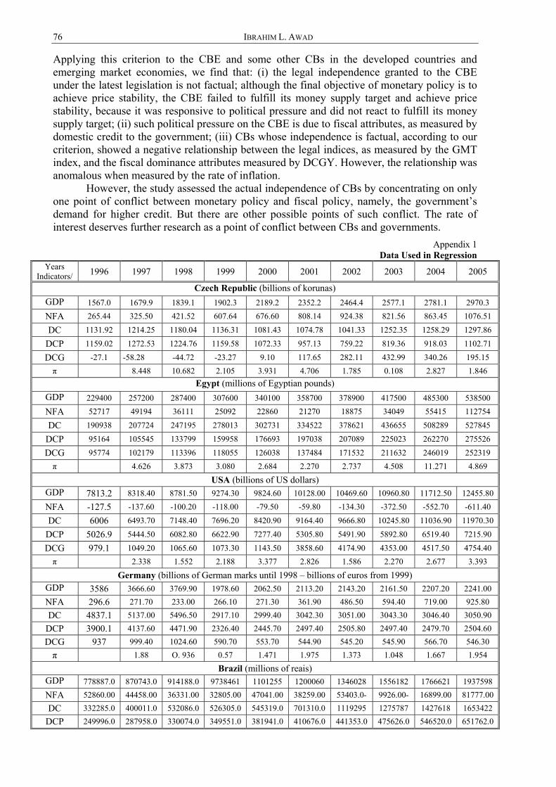
76 IBRAHIM L. AWAD
Applying this criterion to the CBE and some other CBs in the developed countries and emerging market economies, we find that: (i) the legal independence granted to the CBE under the latest legislation is not factual; although the final objective of monetary policy is to achieve price stability, the CBE failed to fulfill its money supply target and achieve price stability, because it was responsive to political pressure and did not react to fulfill its money supply target; (ii) such political pressure on the CBE is due to fiscal attributes, as measured by domestic credit to the government; (iii) CBs whose independence is factual, according to our criterion, showed a negative relationship between the legal indices, as measured by the GMT index, and the fiscal dominance attributes measured by DCGY. However, the relationship was anomalous when measured by the rate of inflation.
However, the study assessed the actual independence of CBs by concentrating on only one point of conflict between monetary policy and fiscal policy, namely, the government’s demand for higher credit. But there are other possible points of such conflict. The rate of interest deserves further research as a point of conflict between CBs and governments.
Appendix 1 Data Used in Regression
Years Indicators/ 1996 1997 1998 1999 2000 2001 2002 2003 2004 2005
Czech Republic (billions of korunas) GDP 1567.0 1679.9 1839.1 1902.3 2189.2 2352.2 2464.4 2577.1 2781.1 2970.3
NFA 265.44 325.50 421.52 607.64 676.60 808.14 924.38 821.56 863.45 1076.51
DC 1131.92 1214.25 1180.04 1136.31 1081.43 1074.78 1041.33 1252.35 1258.29 1297.86
DCP 1159.02 1272.53 1224.76 1159.58 1072.33 957.13 759.22 819.36 918.03 1102.71
DCG -27.1 -58.28 -44.72 -23.27 9.10 117.65 282.11 432.99 340.26 195.15 π 8.448 10.682 2.105 3.931 4.706 1.785 0.108 2.827 1.846
Egypt (millions of Egyptian pounds) GDP 229400 257200 287400 307600 340100 358700 378900 417500 485300 538500
NFA 52717 49194 36111 25092 22860 21270 18875 34049 55415 112754
DC 190938 207724 247195 278013 302731 334522 378621 436655 508289 527845
DCP 95164 105545 133799 159958 176693 197038 207089 225023 262270 275526
DCG 95774 102179 113396 118055 126038 137484 171532 211632 246019 252319 π 4.626 3.873 3.080 2.684 2.270 2.737 4.508 11.271 4.869
USA (billions of US dollars) GDP 7813.2 8318.40 8781.50 9274.30 9824.60 10128.00 10469.60 10960.80 11712.50 12455.80
NFA -127.5 -137.60 -100.20 -118.00 -79.50 -59.80 -134.30 -372.50 -552.70 -611.40
DC 6006 6493.70 7148.40 7696.20 8420.90 9164.40 9666.80 10245.80 11036.90 11970.30
DCP 5026.9 5444.50 6082.80 6622.90 7277.40 5305.80 5491.90 5892.80 6519.40 7215.90
DCG 979.1 1049.20 1065.60 1073.30 1143.50 3858.60 4174.90 4353.00 4517.50 4754.40 π 2.338 1.552 2.188 3.377 2.826 1.586 2.270 2.677 3.393
Germany (billions of German marks until 1998 – billions of euros from 1999) GDP 3586 3666.60 3769.90 1978.60 2062.50 2113.20 2143.20 2161.50 2207.20 2241.00 NFA 296.6 271.70 233.00 266.10 271.30 361.90 486.50 594.40 719.00 925.80 DC 4837.1 5137.00 5496.50 2917.10 2999.40 3042.30 3051.00 3043.30 3046.40 3050.90
DCP 3900.1 4137.60 4471.90 2326.40 2445.70 2497.40 2505.80 2497.40 2479.70 2504.60 DCG 937 999.40 1024.60 590.70 553.70 544.90 545.20 545.90 566.70 546.30 π 1.88 O. 936 0.57 1.471 1.975 1.373 1.048 1.667 1.954
Brazil (millions of reais) GDP 778887.0 870743.0 914188.0 9738461 1101255 1200060 1346028 1556182 1766621 1937598 NFA 52860.00 44458.00 36331.00 32805.00 47041.00 38259.00 -53403.0 -9926.00 16899.00 81777.00 DC 332285.0 400011.0 532086.0 526305.0 545319.0 701310.0 1119295 1275787 1427618 1653422
DCP 249996.0 287958.0 330074.0 349551.0 381941.0 410676.0 441353.0 475626.0 546520.0 651762.0
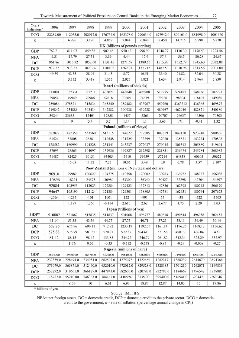
Towards Measurement of Political Pressure on Central Banks in the Emerging Market Economies… 77
Years Indicators/ 1996 1997 1998 1999 2000 2001 2002 2003 2004 2005
DCG 82289.00 112053.0 202012.0 176754.0 163378.0 290634.0 677942.0 800161.0 881098.0 1001660 π 6.926 3.196 4.859 7.044 6.840 8.450 14.715 6.598 6.870
UK (billions of pounds sterling) GDP 762.21 811.07 859.38 902.46 950.42 996.99 1048.77 1110.30 1176.53 1224.46
NFA -9.31 -17.79 27.31 3.59 4.44 -17.9 -57.6 -56.7 -80.28 -24.67
DC 961.86 1015.92 1052.60 1131.45 1271.68 1389.66 1515.93 1652.78 1845.60 2032.08
DCP 912.27 973.37 1023.66 1100.02 1262.91 1373.15 1487.53 1630.96 1813.56 2001.80
DCG 49.59 42.55 28.94 31.43 8.77 16.51 28.40 21.82 32.04 30.28
π 3.132 3.418 1.555 2.927 1.821 1.634 2.914 2.964 2.830
Israel (millions of shekels) GDP 313001 352331 387211 405021 443048 498908 517975 524187 548936 582291
NFA 29854 49949 70986 67618 70665 74639 79226 98304 118105 149080
DC 259086 278521 315834 365240 389482 433967 459760 4363312 436365 469877
DCP 219842 254886 303434 347382 390938 439228 480467 462949 482871 540180
DCG 39244 23635 12401 17858 -1457 -5261 -20707 -26637 -46506 -70303 π 9 5.4 5.2 1.14 1.1 5.63 .71 -0.41 1.32
Poland (millions of zlotys) GDP 387827 472350 553560 615115 744622 779205 807859 842120 923248 980666
NFA 61524 82808 96281 110548 131725 133899 132020 135871 143234 170808
DC 128582 160990 194228 231341 243237 272037 279045 301512 305889 319604
DCP 57095 78565 104097 137936 197827 212598 221831 236674 245284 268982
DCG 71487 82425 90131 93405 45410 59439 57214 64838 60605 50622 π 15.08 11.72 7.27 10.06 5.49 1.9 0.78 3.57 2.107
New Zealand (millions of New Zealand dollars) GDP 96910 99982 100627 104775 110558 120002 130983 139752 148927 156088
NFA -10896 -18224 -24575 -30980 -33300 -36349 -30427 -32298 -42704 -54697
DC 92084 103955 112023 122884 129423 137813 147836 162593 180242 206170
DCP 94647 105190 112124 121884 129301 138805 147781 162631 180764 207673
DCG -2564 -1235 -101 1001 122 -991 55 -38 -522 -1503 π 1.187 1.266 -0.114 2.615 2.62 2.677 1.75 2.29 3.03
Japan (trillions of yen) GDP* 510802 521862 515835 511837 501068 496777 489618 490544 496058 502457 NFA 41.94 53.33 43.36 44.77 27.73 40.71 37.23 33.11 39.49 50.14 DC 667.36 675.96 690.11 712.82 1233.19 1192.56 1161.14 1176.25 1168.12 1156.62
DCP 575.88 578.79 583.35 570.91 972.87 564.41 521.58 498.77 486.84 499 DCG 81.42 88.15 98.42 133.85 244.72 246.79 261.82 312.34 325.29 332.97 π 1.76 0.66 -0.33 -0.712 -0.758 -0.85 -0.29 -0.008 -0.27
Nigeria (millions of naira) GDP 2824000 2940000 2837000 3320000 4981000 4864000 5603000 7191000 8553000 12440000
NFA 237359.0 228494.0 234954.0 662507.0 1275072 1322480 1282217 1388239 2644679 3894366
DC 371079.0 365871.0 512490.0 632010.0 472012.0 829528.0 1328183 1701210 1262071 1169839
DCP 252292.0 310661.0 366127.0 447843.0 582606.0 820793.0 932783.0 1184669 1496542 1938885
DCG 118787.0 55210.00 146363.0 184167.0 -110594 8735.00 395400.0 516541.0 -234471 -769046
π 8.53 10 6.61 6.93 18.87 12.87 14.03 15 17.86 * billions of yen
Source: IMF, IFS NFA= net foreign assets, DC = domestic credit, DCP = domestic credit to the private sector, DCG = domestic
credit to the government, π = rate of inflation (percentage annual change in CPI)
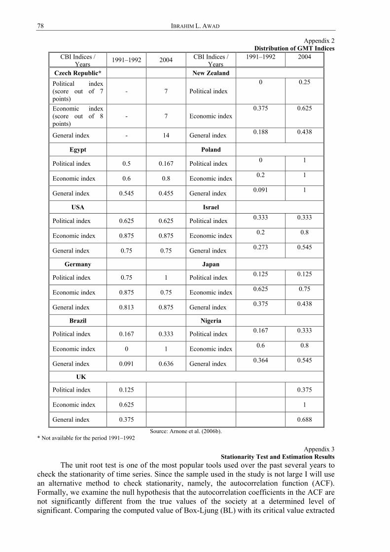
78 IBRAHIM L. AWAD
Appendix 2 Distribution of GMT Indices
CBI Indices / Years
1991–1992 2004 CBI Indices / Years
1991–1992 2004
Czech Republic* New Zealand
Political index (score out of 7 points)
- 7 Political index 0 0.25
Economic index (score out of 8 points)
- 7 Economic index 0.375 0.625
General index - 14 General index 0.188 0.438
Egypt Poland
Political index 0.5 0.167 Political index 0 1
Economic index 0.6 0.8 Economic index 0.2 1
General index 0.545 0.455 General index 0.091 1
USA Israel
Political index 0.625 0.625 Political index 0.333 0.333
Economic index 0.875 0.875 Economic index 0.2 0.8
General index 0.75 0.75 General index 0.273 0.545
Germany Japan
Political index 0.75 1 Political index 0.125 0.125
Economic index 0.875 0.75 Economic index 0.625 0.75
General index 0.813 0.875 General index 0.375 0.438
Brazil Nigeria
Political index 0.167 0.333 Political index 0.167 0.333
Economic index 0 1 Economic index 0.6 0.8
General index 0.091 0.636 General index 0.364 0.545
UK
Political index 0.125 0.375
Economic index 0.625 1
General index 0.375 0.688
Source: Arnone et al. (2006b). * Not available for the period 1991–1992
Appendix 3 Stationarity Test and Estimation Results
The unit root test is one of the most popular tools used over the past several years to check the stationarity of time series. Since the sample used in the study is not large I will use an alternative method to check stationarity, namely, the autocorrelation function (ACF). Formally, we examine the null hypothesis that the autocorrelation coefficients in the ACF are not significantly different from the true values of the society at a determined level of significant. Comparing the computed value of Box-Ljung (BL) with its critical value extracted
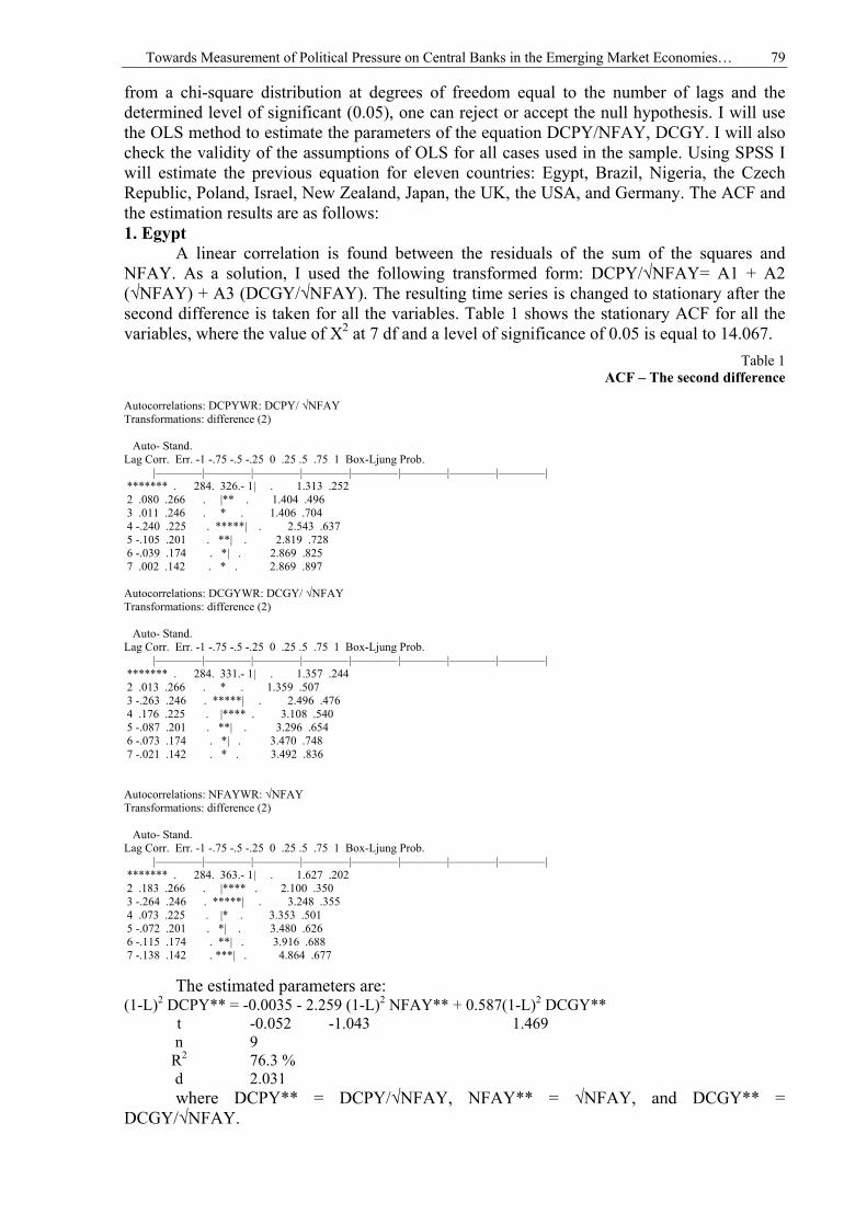
Towards Measurement of Political Pressure on Central Banks in the Emerging Market Economies… 79
from a chi-square distribution at degrees of freedom equal to the number of lags and the determined level of significant (0.05), one can reject or accept the null hypothesis. I will use the OLS method to estimate the parameters of the equation DCPY/NFAY, DCGY. I will also check the validity of the assumptions of OLS for all cases used in the sample. Using SPSS I will estimate the previous equation for eleven countries: Egypt, Brazil, Nigeria, the Czech Republic, Poland, Israel, New Zealand, Japan, the UK, the USA, and Germany. The ACF and the estimation results are as follows: 1. Egypt
A linear correlation is found between the residuals of the sum of the squares and NFAY. As a solution, I used the following transformed form: DCPY/√NFAY= A1 + A2 (√NFAY) + A3 (DCGY/√NFAY). The resulting time series is changed to stationary after the second difference is taken for all the variables. Table 1 shows the stationary ACF for all the variables, where the value of X2 at 7 df and a level of significance of 0.05 is equal to 14.067.
Table 1 ACF – The second difference
Autocorrelations: DCPYWR: DCPY/ √NFAY Transformations: difference (2) Auto- Stand. Lag Corr. Err. -1 -.75 -.5 -.25 0 .25 .5 .75 1 Box-Ljung Prob. |————|————|————|————|————|————|————|————| 1 -.326 . 284 . ******* | . 1.313 .252 2 .080 .266 . |** . 1.404 .496 3 .011 .246 . * . 1.406 .704 4 -.240 .225 . *****| . 2.543 .637 5 -.105 .201 . **| . 2.819 .728 6 -.039 .174 . *| . 2.869 .825 7 .002 .142 . * . 2.869 .897 Autocorrelations: DCGYWR: DCGY/ √NFAY Transformations: difference (2) Auto- Stand. Lag Corr. Err. -1 -.75 -.5 -.25 0 .25 .5 .75 1 Box-Ljung Prob. |————|————|————|————|————|————|————|————| 1 -.331 . 284 . ******* | . 1.357 .244 2 .013 .266 . * . 1.359 .507 3 -.263 .246 . *****| . 2.496 .476 4 .176 .225 . |**** . 3.108 .540 5 -.087 .201 . **| . 3.296 .654 6 -.073 .174 . *| . 3.470 .748 7 -.021 .142 . * . 3.492 .836 Autocorrelations: NFAYWR: √NFAY Transformations: difference (2) Auto- Stand. Lag Corr. Err. -1 -.75 -.5 -.25 0 .25 .5 .75 1 Box-Ljung Prob. |————|————|————|————|————|————|————|————| 1 -.363 . 284 . ******* | . 1.627 .202 2 .183 .266 . |**** . 2.100 .350 3 -.264 .246 . *****| . 3.248 .355 4 .073 .225 . |* . 3.353 .501 5 -.072 .201 . *| . 3.480 .626 6 -.115 .174 . **| . 3.916 .688 7 -.138 .142 . ***| . 4.864 .677
The estimated parameters are: (1-L)2 DCPY** = -0.0035 - 2.259 (1-L)2 NFAY** + 0.587(1-L)2 DCGY**
t -0.052 -1.043 1.469 n 9 R2 76.3 % d 2.031 where DCPY** = DCPY/√NFAY, NFAY** = √NFAY, and DCGY** =
DCGY/√NFAY.
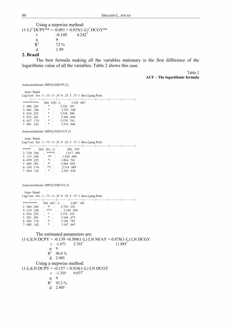
80 IBRAHIM L. AWAD
Using a stepwise method: (1-L)2 DCPY** = -0.001 + 0.935(1-L)2 DCGY**
t -0.148 4.242* n 9 R2 72 % d 1.99
2. Brazil The best formula making all the variables stationary is the first difference of the
logarithmic value of all the variables. Table 2 shows this case. Table 2
ACF – The logarithmic formula Autocorrelations: DIFF(LNDCPY,2) Auto- Stand. Lag Corr. Err. -1 -.75 -.5 -.25 0 .25 .5 .75 1 Box-Ljung Prob. |————|————|————|————|————|————|————|————| 1 -.520 . 284 **********. | . 3.352 .067 2 .006 .266 . * . 3.352 .187 3 -.001 .246 . * . 3.352 .340 4 .018 .225 . * . 3.358 .500 5 .015 .201 . * . 3.364 .644 6 -.017 .174 . * . 3.374 .761 7 .001 .142 . * . 3.374 .848 Autocorrelations: DIFF(LNNFAYY,2) Auto- Stand. Lag Corr. Err. -1 -.75 -.5 -.25 0 .25 .5 .75 1 Box-Ljung Prob. |————|————|————|————|————|————|————|————| 1 -.261 . 284 . ***** | . .842 .359 2 -.234 .266 . *****| . 1.617 .446 3 .115 .246 . |** . 1.834 .608 4 -.039 .225 . *| . 1.864 .761 5 .064 .201 . |* . 1.964 .854 6 -.103 .174 . **| . 2.314 .889 7 -.024 .142 . * . 2.343 .938 Autocorrelations: DIFF(LNDCGY,2) Auto- Stand. Lag Corr. Err. -1 -.75 -.5 -.25 0 .25 .5 .75 1 Box-Ljung Prob. |————|————|————|————|————|————|————|————| 1 -.467 . 284 ********* . | . 2.697 .101 2 .064 .266 . |* . 2.754 .252 3 -.155 .246 . ***| . 3.148 .369 4 .016 .225 . * . 3.153 .533 5 .021 .201 . * . 3.164 .675 6 .026 .174 . |* . 3.186 .785 7 -.005 .142 . * . 3.187 .867
The estimated parameters are:
(1-L)LN DCPY = -0.139 +0.509(1-L) LN NFAY + 0.878(1-L) LN DCGY t -1.671 2.765* 11.885*
n 9 R2 96.6 % d 2.405
Using a stepwise method: (1-L)LN DCPY = -0.157 + 0.918(1-L) LN DCGY
t -1.355 9.077* n 9
R2 92.2 % d 2.405

Towards Measurement of Political Pressure on Central Banks in the Emerging Market Economies… 81
3. Nigeria The residuals of the sum of the squares are found to be linearly correlated with NFAY.
As a solution, I used the following formula: DCPY/√NFAY= A1 + A2 (√NFAY) + A3 (DCGY/√NFAY) or, DCPY** = A1 + A2 NFAY** + A3 DCGY**
The resulting time series was stationary, except in the case of NFAY. Table 3 shows the stationary time series for all the variables after the first difference is taken for NFAY**, where the value of X2 at 8 df and a level of significance of 0.05 is equal to 15.5073.
The estimated parameters are as follows: DCPY** = 0.319 – 0.241 (1-L) NFAY** + 0.399 DCGY**
t 16.33* -1.004 2.566* n 9 R2 61.4 % d 1.734
Table 3 ACF – The transformed form
Autocorrelations: DCPYW: DCPY/ √NFAY Auto- Stand. Lag Corr. Err. -1 -.75 -.5 -.25 0 .25 .5 .75 1 Box-Ljung Prob. |————|————|————|————|————|————|————|————| 1 . 169 . 274 . |*** . .382 .536 2 -.617 .258 **.*********| . 6.090 .048 3 -.326 .242 . *******| . 7.912 .048 4 .142 .224 . |*** . 8.316 .081 5 .362 .204 . |*******. 11.467 .043 6 .041 .183 . |* . 11.517 .074 7 -.242 .158 .*****| . 13.867 .054 8 -.066 .129 . *| . 14.126 .079 Autocorrelations: DCGYW: DCGY/ √NFAY Auto- Stand. Lag Corr. Err. -1 -.75 -.5 -.25 0 .25 .5 .75 1 Box-Ljung Prob. |————|————|————|————|————|————|————|————| 1 . 197 . 274 . |**** . .517 .472 2 -.487 .258 **********| . 4.068 .131 3 -.161 .242 . ***| . 4.512 .211 4 .295 .224 . |****** . 6.256 .181 5 .190 .204 . |**** . 7.126 .211 6 -.164 .183 . ***| . 7.935 .243 7 -.125 .158 . ***| . 8.564 .286 8 -.101 .129 . **| . 9.182 .327 Autocorrelations: NFAYW_1: (1-L)( √NFAY) Auto- Stand. Lag Corr. Err. -1 -.75 -.5 -.25 0 .25 .5 .75 1 Box-Ljung Prob. |————|————|————|————|————|————|————|————| 1 -.018 . 284 . * . . 004 . 950
2 -.352 . 266 . ******* | . 1.756 .416 3 -.306 .246 . ******| . 3.297 .348 4 -.101 .225 . **| . 3.498 .478 5 .389 .201 . |******** 7.253 .203 6 -.063 .174 . *| . 7.384 .287 7 -.079 .142 . **| . 7.692 .361
Using a stepwise method: DCPY** = 0.31 + 0.44 DCGY**
t 18.055* 2.923* n 9 R2 55 % d 1.84
4. Czech Republic A nonlinear correlation is found between the residuals of the sum of the squares and
NFAY. As a solution, I used the following formula: DCPY/NFAY= A1 + A21/NFAY +A3 DCGY/NFAY
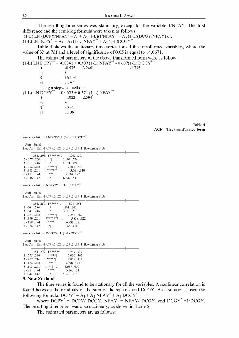
82 IBRAHIM L. AWAD
The resulting time series was stationary, except for the variable 1/NFAY. The first difference and the semi-log formula were taken as follows: (1-L) LN (DCPY/NFAY) = A1 + A2 (1-L)(1/NFAY ) + A3 (1-L)(DCGY/NFAY) or, (1-L)LN DCPY** = A1 + A2 (1-L) NFAY** + A3 (1-L)DCGY**
Table 4 shows the stationary time series for all the transformed variables, where the value of X2 at 7df and a level of significance of 0.05 is equal to 14.0671.
The estimated parameters of the above transformed form were as follow: (1-L) LN DCPY** = -0.0341 + 0.309 (1-L) NFAY** - 0.607(1-L) DCGY**
t -0.575 3.246* -1.735 n 9 R2 66.1 % d 2.147
Using a stepwise method: (1-L) LN DCPY** = -0.0655 + 0.274 (1-L) NFAY**
t -1.022 2.594* n 9 R2 49 % d 1.106
Table 4
ACF – The transformed form Autocorrelations: LNDCPY_1: (1-L) LN DCPY** Auto- Stand. Lag Corr. Err. -1 -.75 -.5 -.25 0 .25 .5 .75 1 Box-Ljung Prob. |————|————|————|————|————|————|————|————| 1 . 293 . 284 . |****** . 1.063 .303 2 -.057 .266 . *| . 1.109 .574 3 .018 .246 . * . 1.114 .774 4 -.272 .225 . *****| . 2.582 .630 5 -.353 .201 .*******| . 5.664 .340 6 -.131 .174 . ***| . 6.234 .397 7 -.016 .142 . * . 6.247 .511 Autocorrelations: NFAYW_1: (1-L) NFAY** Auto- Stand. Lag Corr. Err. -1 -.75 -.5 -.25 0 .25 .5 .75 1 Box-Ljung Prob. |————|————|————|————|————|————|————|————| 1 . 259 . 284 . |***** . .833 .361 2 .064 .266 . |* . .891 .641 3 .040 .246 . |* . .917 .821 4 -.263 .225 . *****| . 2.292 .682 5 -.379 .201 ********| . 5.838 .322 6 -.188 .174 . ****| . 6.999 .321 7 -.054 .142 . *| . 7.143 .414 Autocorrelations: DCGYW_1: (1-L) DCGY** Auto- Stand. Lag Corr. Err. -1 -.75 -.5 -.25 0 .25 .5 .75 1 Box-Ljung Prob. |————|————|————|————|————|————|————|————| 1 . 279 . 284 . |****** . .963 .327 2 -.275 .266 . *****| . 2.030 .362 3 -.227 .246 . *****| . 2.879 .411 4 -.162 .225 . ***| . 3.396 .494 5 -.103 .201 . **| . 3.657 .600 6 -.221 .174 . ****| . 5.263 .511 7 .047 .142 . |* . 5.371 .615
5. New Zealand The time series is found to be stationary for all the variables. A nonlinear correlation is
found between the residuals of the sum of the squares and DCGY. As a solution I used the following formula: DCPY* = A1 + A2 NFAY* + A3 DCGY*,
where DCPY* = DCPY/ DCGY, NFAY* = NFAY/ DCGY, and DCGY* =1/DCGY. The resulting time series was also stationary, as shown in Table 5.
The estimated parameters are as follows:
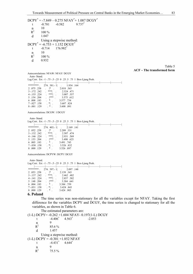
Towards Measurement of Political Pressure on Central Banks in the Emerging Market Economies… 83
DCPY* = -7.849 – 0.275 NFAY*+ 1.087 DCGY* t -0.781 -0.582 9.737* n 10 R2 100 % d 1.047
Using a stepwise method: DCPY* = -6.753 + 1.152 DCGY*
t -0.714 176.982* n 10 R2 100 % d 0.932
Table 5 ACF – The transformed form
Autocorrelations: NFAW: NFAY/ DCGY Auto- Stand. Lag Corr. Err. -1 -.75 -.5 -.25 0 .25 .5 .75 1 Box-Ljung Prob. |————|————|————|————|————|————|————|————| 1 -.381 . 274 . ******** | . 1.934 .164 2 .075 .258 . |* . 2.018 .365 3 -.172 .242 . ***| . 2.524 .471 4 -.155 .224 . ***| . 3.007 .557 5 .154 .204 . |*** . 3.575 .612 6 .008 .183 . * . 3.577 .734 7 -.027 .158 . *| . 3.607 .824 8 -.001 .129 . * . 3.608 .891 Autocorrelations: DCGW: 1/DCGY Auto- Stand. Lag Corr. Err. -1 -.75 -.5 -.25 0 .25 .5 .75 1 Box-Ljung Prob. |————|————|————|————|————|————|————|————| 1 -.403 . 274 . ******** | . 2.169 .141 2 .052 .258 . |* . 2.209 .331 3 -.132 .242 . ***| . 2.507 .474 4 -.146 .224 . ***| . 2.931 .569 5 .153 .204 . |*** . 3.490 .625 6 .005 .183 . * . 3.491 .745 7 -.030 .158 . *| . 3.526 .832 8 .000 .129 . * . 3.526 .897 Autocorrelations: DCPYW: DCPY/ DCGY Auto- Stand. Lag Corr. Err. -1 -.75 -.5 -.25 0 .25 .5 .75 1 Box-Ljung Prob. |————|————|————|————|————|————|————|————| 1 -.397 . 274 . ******** | . 2.097 .148 2 .053 .258 . |* . 2.139 .343 3 -.137 .242 . ***| . 2.462 .482 4 -.141 .224 . ***| . 2.857 .582 5 .148 .204 . |*** . 3.384 .641 6 .004 .183 . * . 3.384 .759 7 -.031 .158 . *| . 3.424 .843 8 .000 .129 . * . 3.424 .905
6. Poland The time series was non-stationary for all the variables except for NFAY. Taking the first
difference for the variables DCPY and DCGY, the time series is changed to stationary for all the variables, as shown in Table 6.
The estimated parameters are: (1-L) DCPY= -0.262 +1.604 NFAY- 0.197(1-L) DCGY
t -4.406* 4.563* -2.053 n 9 R2 85.6 % d 1.457
Using a stepwise method: (1-L) DCPY = -0.301 +1.852 NFAY
t -4.431* 4.644* n 9 R2 75.5 %
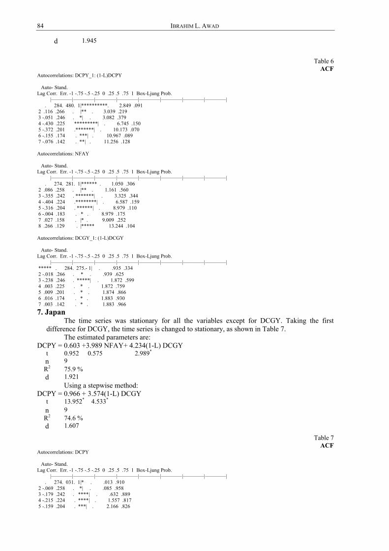
84 IBRAHIM L. AWAD
d 1.945
Table 6 ACF
Autocorrelations: DCPY_1: (1-L)DCPY Auto- Stand. Lag Corr. Err. -1 -.75 -.5 -.25 0 .25 .5 .75 1 Box-Ljung Prob. |————|————|————|————|————|————|————|————| 1 . 480 . 284 . |**********. 2.849 .091 2 .116 .266 . |** . 3.039 .219 3 -.051 .246 . *| . 3.082 .379 4 -.430 .225 *********| . 6.745 .150 5 -.372 .201 .*******| . 10.173 .070 6 -.155 .174 . ***| . 10.967 .089 7 -.076 .142 . **| . 11.256 .128 Autocorrelations: NFAY Auto- Stand. Lag Corr. Err. -1 -.75 -.5 -.25 0 .25 .5 .75 1 Box-Ljung Prob. |————|————|————|————|————|————|————|————| 1 . 281 . 274 . |****** . 1.050 .306 2 .086 .258 . |** . 1.161 .560 3 -.355 .242 . *******| . 3.325 .344 4 -.404 .224 .********| . 6.587 .159 5 -.316 .204 . ******| . 8.979 .110 6 -.004 .183 . * . 8.979 .175 7 .027 .158 . |* . 9.009 .252 8 .266 .129 . |***** 13.244 .104 Autocorrelations: DCGY_1: (1-L)DCGY Auto- Stand. Lag Corr. Err. -1 -.75 -.5 -.25 0 .25 .5 .75 1 Box-Ljung Prob. |————|————|————|————|————|————|————|————| 1 -.275 . 284 . ***** | . .935 .334 2 -.018 .266 . * . .939 .625 3 -.238 .246 . *****| . 1.872 .599 4 .003 .225 . * . 1.872 .759 5 .009 .201 . * . 1.874 .866 6 .016 .174 . * . 1.883 .930 7 .003 .142 . * . 1.883 .966 7. Japan
The time series was stationary for all the variables except for DCGY. Taking the first difference for DCGY, the time series is changed to stationary, as shown in Table 7.
The estimated parameters are: DCPY = 0.603 +3.989 NFAY+ 4.234(1-L) DCGY
t 0.952 0.575 2.989* n 9 R2 75.9 % d 1.921
Using a stepwise method: DCPY = 0.966 + 3.574(1-L) DCGY
t 13.952* 4.533* n 9 R2 74.6 % d 1.607
Table 7 ACF
Autocorrelations: DCPY Auto- Stand. Lag Corr. Err. -1 -.75 -.5 -.25 0 .25 .5 .75 1 Box-Ljung Prob. |————|————|————|————|————|————|————|————| 1 . 031 . 274 . |* . .013 .910 2 -.069 .258 . *| . .085 .958 3 -.179 .242 . ****| . .632 .889 4 -.215 .224 . ****| . 1.557 .817 5 -.159 .204 . ***| . 2.166 .826
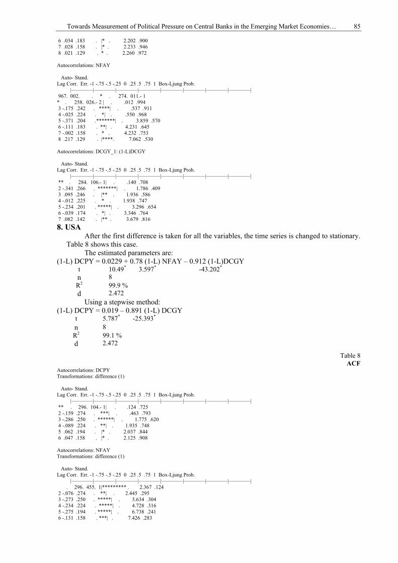
Towards Measurement of Political Pressure on Central Banks in the Emerging Market Economies… 85
6 .034 .183 . |* . 2.202 .900 7 .028 .158 . |* . 2.233 .946 8 .021 .129 . * . 2.260 .972 Autocorrelations: NFAY Auto- Stand. Lag Corr. Err. -1 -.75 -.5 -.25 0 .25 .5 .75 1 Box-Ljung Prob. |————|————|————|————|————|————|————|————| 1 -.011 . 274 . * . . 002 . 967
2 -.026 . 258 . * | . .012 .994 3 -.175 .242 . ****| . .537 .911 4 -.025 .224 . *| . .550 .968 5 -.371 .204 .*******| . 3.859 .570 6 -.111 .183 . **| . 4.231 .645 7 -.002 .158 . * . 4.232 .753 8 .217 .129 . |****. 7.062 .530 Autocorrelations: DCGY_1: (1-L)DCGY Auto- Stand. Lag Corr. Err. -1 -.75 -.5 -.25 0 .25 .5 .75 1 Box-Ljung Prob. |————|————|————|————|————|————|————|————| 1 -.106 . 284 . ** | . .140 .708 2 -.341 .266 . *******| . 1.786 .409 3 .095 .246 . |** . 1.936 .586 4 -.012 .225 . * . 1.938 .747 5 -.234 .201 . *****| . 3.296 .654 6 -.039 .174 . *| . 3.346 .764 7 .082 .142 . |** . 3.679 .816 8. USA
After the first difference is taken for all the variables, the time series is changed to stationary. Table 8 shows this case.
The estimated parameters are: (1-L) DCPY = 0.0229 + 0.78 (1-L) NFAY – 0.912 (1-L)DCGY
t 10.49* 3.597* -43.202* n 8 R2 99.9 % d 2.472
Using a stepwise method: (1-L) DCPY = 0.019 – 0.891 (1-L) DCGY
t 5.787* -25.393* n 8 R2 99.1 % d 2.472
Table 8 ACF
Autocorrelations: DCPY Transformations: difference (1) Auto- Stand. Lag Corr. Err. -1 -.75 -.5 -.25 0 .25 .5 .75 1 Box-Ljung Prob. |————|————|————|————|————|————|————|————| 1 -.104 . 296 . ** | . .124 .725 2 -.159 .274 . ***| . .463 .793 3 -.286 .250 . ******| . 1.775 .620 4 -.089 .224 . **| . 1.935 .748 5 .062 .194 . |* . 2.037 .844 6 .047 .158 . |* . 2.125 .908 Autocorrelations: NFAY Transformations: difference (1) Auto- Stand. Lag Corr. Err. -1 -.75 -.5 -.25 0 .25 .5 .75 1 Box-Ljung Prob. |————|————|————|————|————|————|————|————| 1 . 455 . 296 . |********* . 2.367 .124 2 -.076 .274 . **| . 2.445 .295 3 -.273 .250 . *****| . 3.634 .304 4 -.234 .224 . *****| . 4.728 .316 5 -.275 .194 . *****| . 6.738 .241 6 -.131 .158 . ***| . 7.426 .283

86 IBRAHIM L. AWAD
Autocorrelations: DCGY Transformations: difference (1) Auto- Stand. Lag Corr. Err. -1 -.75 -.5 -.25 0 .25 .5 .75 1 Box-Ljung Prob. |————|————|————|————|————|————|————|————| 1 -.073 . 296 . * | . .060 .806 2 -.211 .274 . ****| . .652 .722 3 -.265 .250 . *****| . 1.778 .620 4 -.084 .224 . **| . 1.919 .751 5 .064 .194 . |* . 2.028 .845 6 .047 .158 . |* . 2.117 .909 9. UK
The time series is found to be stationary for all the variables except for DCPY. Table 8 shows the stationary time series for all the variables after the first difference is taken for the variable DCPY, where the value of X2 at 8 df and a level of significance of 0.05 is equal to 15.5073. The estimated parameters are:
(1-L) DCPY = 0.133 –0.273 NFAY– 2.292 DCGY t 4.037* -0.882 -2.85* n 9 R2 60.9 % d 1.649
Using a stepwise method: (1-L) DCPY = 0.133 – 2.345 DCGY
t 4.808* -2.972* n 9 R2 55.8 % d 1.727
Table 8 ACF
Autocorrelations: DCGY Auto- Stand. Lag Corr. Err. -1 -.75 -.5 -.25 0 .25 .5 .75 1 Box-Ljung Prob. |————|————|————|————|————|————|————|————| 1 . 475 . 274 . |**********. 3.010 .083 2 .157 .258 . |*** . 3.382 .184 3 -.025 .242 . * . 3.392 .335 4 -.369 .224 . *******| . 6.116 .191 5 -.192 .204 . ****| . 7.000 .221 6 -.164 .183 . ***| . 7.805 .253 7 -.193 .158 . ****| . 9.289 .233 8 -.105 .129 . **| . 9.952 .268 Autocorrelations: NFAY Auto- Stand. Lag Corr. Err. -1 -.75 -.5 -.25 0 .25 .5 .75 1 Box-Ljung Prob. |————|————|————|————|————|————|————|————| 1 . 507 . 274 . |**********. 3.426 .064 2 .292 .258 . |****** . 4.709 .095 3 -.171 .242 . ***| . 5.211 .157 4 -.419 .224 .********| . 8.730 .068 5 -.318 .204 . ******| . 11.162 .048 6 -.324 .183 .******| . 14.303 .026 7 -.020 .158 . * . 14.319 .046 8 -.047 .129 . *| . 14.454 .071 Autocorrelations: DCPY_1: (1-L) DCPY Auto- Stand. Lag Corr. Err. -1 -.75 -.5 -.25 0 .25 .5 .75 1 Box-Ljung Prob. |————|————|————|————|————|————|————|————| 1 . 298 . 284 . |****** . 1.097 .295 2 -.257 .266 . *****| . 2.030 .362 3 -.233 .246 . *****| . 2.924 .403 4 .152 .225 . |*** . 3.384 .496 5 .203 .201 . |**** . 4.402 .493 6 -.196 .174 . ****| . 5.676 .460 7 -.300 .142 ******| . 10.133 .181
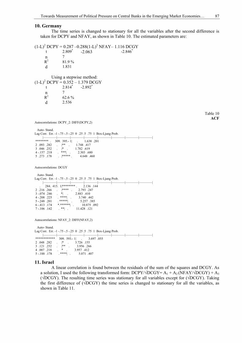
Towards Measurement of Political Pressure on Central Banks in the Emerging Market Economies… 87
10. Germany The time series is changed to stationary for all the variables after the second difference is
taken for DCPY and NFAY, as shown in Table 10. The estimated parameters are:
(1-L)2 DCPY = 0.287 –0.288(1-L)2 NFAY– 1.116 DCGY t 2.809* -2.063 -2.846* n 7 R2 81.9 % d 1.831
Using a stepwise method:
(1-L)2 DCPY = 0.352 – 1.379 DCGY t 2.814* -2.892* n 7 R2 62.6 % d 2.536
Table 10 ACF
Autocorrelations: DCPY_2: DIFF(DCPY,2) Auto- Stand. Lag Corr. Err. -1 -.75 -.5 -.25 0 .25 .5 .75 1 Box-Ljung Prob. |————|————|————|————|————|————|————|————| 1 -.395 . 309 . ******** | . 1.638 .201 2 .093 .282 . |** . 1.748 .417 3 .046 .252 . |* . 1.782 .619 4 -.157 .218 . ***| . 2.303 .680 5 .273 .178 . |***** . 4.648 .460 Autocorrelations: DCGY Auto- Stand. Lag Corr. Err. -1 -.75 -.5 -.25 0 .25 .5 .75 1 Box-Ljung Prob. |————|————|————|————|————|————|————|————| 1 . 415 . 284 . |******** . 2.136 .144 2 .216 .266 . |**** . 2.793 .247 3 -.074 .246 . *| . 2.883 .410 4 -.208 .225 . ****| . 3.740 .442 5 -.248 .201 . *****| . 5.257 .385 6 -.413 .174 *.******| . 10.875 .092 7 -.106 .142 . **| . 11.428 .121 Autocorrelations: NFAY_2: DIFF(NFAY,2) Auto- Stand. Lag Corr. Err. -1 -.75 -.5 -.25 0 .25 .5 .75 1 Box-Ljung Prob. |————|————|————|————|————|————|————|————| 1 -.593 . 309 ************ | . 3.697 .055 2 .048 .282 . |* . 3.726 .155 3 .121 .252 . |** . 3.956 .266 4 .007 .218 . * . 3.957 .412 5 -.188 .178 . ****| . 5.071 .407 11. Israel
A linear correlation is found between the residuals of the sum of the squares and DCGY. As a solution, I used the following transformed form: DCPY/√DCGY= A1 + A2 (NFAY/√DCGY) + A3 (√DCGY). The resulting time series was stationary for all variables except for (√DCGY). Taking the first difference of (√DCGY) the time series is changed to stationary for all the variables, as shown in Table 11.

88 IBRAHIM L. AWAD
Table 11 ACF
Autocorrelations: DCPYW: DCPY/√DCGY Auto- Stand. Lag Corr. Err. -1 -.75 -.5 -.25 0 .25 .5 .75 1 Box-Ljung Prob. |————|————|————|————|————|————|————|————| 1 . 262 . 274 . |***** . .915 .339 2 .103 .258 . |** . 1.075 .584 3 .056 .242 . |* . 1.128 .770 4 -.045 .224 . *| . 1.168 .883 5 -.083 .204 . **| . 1.332 .932 6 -.159 .183 . ***| . 2.090 .911 7 -.182 .158 . ****| . 3.412 .844 8 -.228 .129 *****| . 6.524 .589 Autocorrelations: NFAYW: NFAY/√DCGY Auto- Stand. Lag Corr. Err. -1 -.75 -.5 -.25 0 .25 .5 .75 1 Box-Ljung Prob. |————|————|————|————|————|————|————|————| 1 . 251 . 274 . |***** . .843 .359 2 .070 .258 . |* . .915 .633 3 -.014 .242 . * . .919 .821 4 -.067 .224 . *| . 1.007 .909 5 -.079 .204 . **| . 1.158 .949 6 -.120 .183 . **| . 1.589 .953 7 -.127 .158 . ***| . 2.230 .946 8 -.197 .129 .****| . 4.551 .804 Autocorrelations: DCGYW_1: √DCGY Auto- Stand. Lag Corr. Err. -1 -.75 -.5 -.25 0 .25 .5 .75 1 Box-Ljung Prob. |————|————|————|————|————|————|————|————| 1 -.027 . 284 . * | . .009 .925 2 .011 .266 . * . .011 .995 3 -.072 .246 . *| . .096 .992 4 -.092 .225 . **| . .264 .992 5 -.014 .201 . * . .269 .998 6 -.411 .174 *.******| . 5.837 .442 7 .007 .142 . * . 5.839 .559
The estimated parameters are: DCPY/√DCGY = 0.892 +3.344(NFAY/√DCGY) +1.11(1-L)(√DCGY)
t 4.953* 14.312* 0.246 n 9 R2 98.6 % d 0.879
Using a stepwise method: DCPY/√DCGY = 0.874 +3.302(NFAY/√DCGY)
t 5.716* 22.363* n 9 R2 98.6 % d 0.816
REFERENCES 1. Alesina, A. (1988). “Macroeconomics and Politics”, NBER Macroeconomics Annual 1988, MIT
Press, Cambridge, MA, 17–52. 2. Alesina, A. (1989). “Politics and Business Cycles in Industrial Democracies”, Economic Policy,
8, 55–98. 3. Alesina, A., and Summers, L. H. (1993). “Central Bank Independence and Macroeconomic
Performance: Some Comparative Evidence”, Journal of Money, Credit and Banking, 25, 2, 151–162.
4. Arnone, M., Laurens, B. J., and Segalotto, J. F. (2006a). “The Measurement of Central Bank Autonomy: Survey of Models, Indicators, and Empirical Evidence”, IMF Working Paper.
Towards Measurement of Political Pressure on Central Banks in the Emerging Market Economies… 89
5. Arnone, M., Laurens, B. J., and Segalotto, J. F. (2006b). “Measures of Central Bank Autonomy: Empirical Evidence for OECD, Developing, and Emerging Market Economies”, IMF Working Paper.
6. Bade, R., and Parkin, M. (1977). “Central Bank Laws and Monetary Policies: A Preliminary Investigation”, London, Ontario, Canada: University of Western Ontario.
7. Blanchard, O. (2004). “Fiscal Dominance and Inflation Targeting: Lessons from Brazil”, MIT Working Paper.
8. Blanchard, O., and Fisher, S. (1993). Lectures on Macroeconomics, MIT Press, Cambridge, MA. 9. Chotareas, G. E., and Miller, S. M. (2002). “Optimal Central Bank Contracts and Common
Agency”, Working Paper. 10. Cukierman, A. (1992). Central Bank Strategy, Credibility and Independence, MIT Press,
Cambridge, MA. 11. Debelle, G., and Fisher, S. (1994). “How Independent Should a Central Bank Be?”, Federal
Reserve Bank of Boston. 12. Drazen, A. (2002). “Laying Low During Elections: Political Pressure and Monetary Policy
Accommodation”, Tel Aviv University, University of Maryland, CEPR, and NBER. 13. Eijffinger, S., and Keulen, M. (1995). “Central Bank Independence in Another Eleven Countries”,
BNL Quarterly Review, 192. 14. Eijffinger, S., and Schaling, E. (1993). “Central Bank Independence in Twelve Industrial
Countries”, BNL Quarterly Review, 184, 64–68. 15. Ferreira de Mendonca, H. (2005). “Central Bank Independence and its Relationship to Inflation”,
CEPAL Review, 81. 16. Fry, M. J. (1998). “Assessing Central Bank Independence in Developing Countries: Do Actions
Speak Louder than Words?”, Oxford Economic Papers, 50, 512–529. 17. Gersl, A. (2006). “Political Pressure on Central Banks: The Case of the Czech National Bank”,
IES Working Paper. 18. Grilli, V., Masciandaro, D., and Tabellini, G. (GMT) (1991). “Political and Monetary Institutions
and Public Financial Policies in the Industrial Countries”, Economic Policy, 13, 341–392. 19. Havrilesky, T. (1993). The Pressures on American Monetary Policy, Kluwer Academic Publisher,
Boston. 20. Mahadeva, L., and Sterne, G. (2000). Monetary Policy Frameworks in a Global Context,
Routledge, Bank of England, London and New York. 21. Maier, P., Sturm, J. E., and de Haan, J. (2002). “Political Pressure on the Bundesbank: An
Empirical Investigation Using the Havrilesky Approach”, Journal of Macroeconomics, 24, 103–123.
22. Meyer, L. H. (2000). “The Politics of Monetary Policy: Balancing Independence and Accountability”, BIS Review, 49.
23. Walsh, C. E. (1998). Monetary Theory and Policy, MIT Press, Cambridge, MA.

EMPIRICAL EVIDENCE ON RISK AVERSION FOR INDIVIDUAL
ROMANIAN CAPITAL MARKET INVESTORS
Cristian PĂUN1
, Radu MUŞETESCU2
, Iulian BRAŞOVEANU3
, Alina DRĂGHICI4
Abstract. The evolution of stock prices is influenced by the expectations of investors
regarding the earning prospects associated to each listed company. One of the key
elements of investment decision is the positive relationship between risk and return.
Risky securities are preferred to less risky ones only if there is a higher pay-off in the
long run that could compensate the investors. The previous studies proved that
expected return direct correlated with risk and, due to the presence of risk aversion,
this relationship is assumed to be positive one. Risk premium is determined by a lot of
factors including risk aversion. The intensity of risk aversion and the evolution of it
during a specific period of time are very important for any market. This study proposed
an analysis of risk aversion that is based on a specific survey and it is very useful for
comparative analysis with other similar studies developed on the case of other emerging markets (from EU or outside EU).
.
Key words: risk aversion, individual investor, Romanian capital market
JEL: D53, G11.
The investment theory is developed based on a fundamental hypothesis of rational
agents that are interest to by securities from stock exchanges. This rationality of investors is
presumed to be concentrated on a permanently wish to maximize the individual utility (and
this could happen by trying to maximize return for the same risky securities or to
minimize risk for the same profitable securities ). In spite their rationality, investors
live with a subjective perception over risk, dealing with imperfect and incomplete
information but having also a limited capacity to understand and to evaluate risks. Most
investors proved to have a risk aversion, but we can find on the financial markets, even if
only in theory, investors that are indifferent to the risk level or that have preference for risk
when they are investing capital on financial markets (internal or external markets).
The first efforts of providing a theoretical background to the concept of risk aversion
are associated to Friedman and Savage, 1948. In their approach, the risk aversion could be
defined as using the following decisional situation: if an investor will have to choose between
two assets with similar expected returns but different risks, the risk adverse one will choose
the security with lowest level of risk. The entire modern investment theory it is based on the
idea of this utility functions associated to each individual investors (there are several utility
functions families proposed for each type of behavior. In Friedman's and Savage's opinion,
the most important factor will change in time will be “ the investor’s attitude towards risk is
the size of their wealth”. 1 PhD Lecturer, Academy of Economic Studies, Bucharest, [email protected]. 2 PhD Lecturer, Academy of Economic Studies, Bucharest, [email protected]. 3 PhD Lecturer, Academy of Economic Studies, Bucharest. 4
Assistant Professor, PhD Candidate, Academy of Economic Studies, Bucharest, [email protected].
92 CRISTIAN PĂUN, RADU MUŞETESCU, IULIAN BRAŞOVEANU, ALINA DRĂGHICI
Consequently, in practice we accept the three main investment behaviors: risk aversion,
risk neutrality and risk preference. The specialists became more and more interested to assess
the investors’ degree of risk aversion that is considered to be the initial step in the setting of
risk premium associated to each security (this risk premium is considered to be, in fact, the
price that a risk aversive investor should pay to accept in exchange a higher or a specific level
risk). The first theoretical efforts in this direction were made by John W. Pratt5
and Kenneth J.
Arrow (Aspects of the Theory of Risk-Bearing, 1965). According with their study, the risk
premium required by investors will be higher for investors with higher risk aversion. The main
factor of risk aversion, in their opinion, is the wealth of the investors (for higher risk, higher
returns being expected in this situation). The utility function shape will be relevant to catch the
relevant measure of the investors’ risk aversion degree.
The fact that investors evaluate differently the risky investment alternatives and that
the expected utility is different, is first due to psychological factors, thus the financial market
becomes the sum of unique behaviors, in which each individual investor is guided by its own
needs (primary or secondary). In these conditions, all the three investment behaviors (risk
aversion, neutrality and risk preference) may be considered rational behaviors and can be
explained only based on the different shape of the utility function associated to their
behaviors (in all three cases investors pursue, in their own way, the utility function
maximization).
According with the theory, the dimension of risk premium is positively connected to
the alternative investment risk (given by variance of returns), negatively connected with the
total amount initially invested on a specific security or on a specific risky portfolio, and
positively with the investors’ absolute risk aversion degree (measured by Arrow-Pratt
proposed index). In this case, it is clear for us that two different investors could have different
risk premiums associated to their investment choice due to their different risk aversion. It there
will be an increase with a single unit of initial wealth, the risk preference (aversion) will
determine an increase of utility, a lower risk aversion and a reduction of risk premium. The
increase with one unit of the initial wealth for the risk aversive investors calls forth a
decrease of the utility augmentation (the second grade derivative of the utility function is
strictly negative), an increase of the absolute risk aversion and implicitly an increase of the
risk premium.
The evaluation of risk premium for each investor is almost impracticable on an
important financial market (the more institutional investors the more complicated the situation
becomes). Selecting the most important financial portfolio managers in a market is
recommended in order to assess the value of the risk premium for the next period.
Currently the most applied model by analysts for determining the risk premium on a
market is the use of historic values. The simplicity of this method comes from the market
models based on the market portfolio as optimum risky portfolio. In order to measure the risk
premium in this way the mean return of the market portfolio has to be computed for the
chosen period (approximated with the market index) followed by computing the mean return
of free risk titles in a market for the chosen period (state bonds are assimilated to risk free
titles), calculating the historical risk premium as the difference between the mean return of
market portfolio and the risk free rate and extrapolation of the historical value to the next
period6 . The discounted cash flow model is used for estimating the implicit risk premium
value in the financial titles current price. Subtracting the risk premium is made in this case
from the value of the expected return on a market and the risk free rate of the market
(assimilated to the return of state bond or titles).
Currently this kind of studies was performed in very many countries (especially in the
developed ones), their conclusions being very interesting and important for understanding the
5 J.W. Pratt, Risk Aversion in the Small and in the Large, Econometrica, Vol. 32, p.122-36, 1964 6
A. Damodaran in his paper Understanding Risk, 2004, made such a complete study on the American capital
market presenting the dynamics of the risk premium in the period 1928-2001
Empirical evidence on risk aversion for individual Romanian Capital Market investors 93
investors psychology (in Asian countries, for example, the risk aversion is higher than in the
European countries, these having a higher risk aversion than the American market). By these
studies important information related to the factors influencing the investors’ risk attitude on a
local market can be obtained and also a series of interesting conclusions can be drawn
concerning the interest for financial investment, the propensity for investments/consume or
saving and the mode they can be influenced one way or the other. Measuring the risk
premium comparatively for a group of countries can provide further information regarding
their diversity and different integration degree.
Beginning with the first conclusions of the Arrow and Pratt's hypothesis regarding the influence of earnings over the investment behaviour, a series of empirical studies testing the factors that influence this complex variable were conducted. The first studies were concerned with the differences between men and women in accepting the risks of financial investments:
an empirical study was performed in 1975 by Levin, Snyder and Chapman7
on a group of 110
students using a questionnaire regarding lotteries, the results indicating that women are more
risk aversive than men; in 1997, Powell and Ansic8
questioned a small group regarding property insurance and the exchange market and again found that women are more aversive than men (this study was among the first which analyzed individual aversion towards speculative and pure risks); using information regarding the weight of the funds invested in
risky assets Jianakoplos and Bernasek9
concluded that unmarried women are more risk aversive than unmarried men (the results proved invariant with age or educational level, having children or social status of individual but still indirectly affecting investors risk
tolerance); a similar study was performed by Sunden and Surette10
who observed the direct effect of individuals’ family status on their risk aversion (married individuals are less risk aversive than the unmarried ones).
Several other studies went further in determining other demographic factors
influencing the degree of risk aversion involved in financial investments. Riley and Chow11
examined the individual investors capital allocation decision and found that the risk aversion reduces with the earnings, education and age, until the age of 65 when the aversion rises. They also discovered women’s risk aversion is higher than men's and that the coloured people
risk aversion is higher than that of white people.
Using a psychological questionnaire Zuckerman12
discovered relevant differences in
aversion related to age, sex, nationality, race, socio-economic status or family status. Using a
similar methodology, Hersch13
analyzed the individuals’ aversion towards non-financial risks
(smoking, usage of the safety belt, preventing illness, preventing dental aches) discovering
that white women with a high level of education have a higher aversion regarding these risks.
Barsky14
carried out for the first time an estimation of the minimum and maximum limits of
7
Levin Irwin P., Mary A. Snyder and Daniel P. Chapman, The Interaction of Experiential and Situational
Factors and Gender in a Simulated Risky Decision-Making Task, Journal of Psychology, 1988, 122(2),pp. 173-
181 8
Powell Melanie, and David Ansic, Gender Differences in Risk Behaviour in Financial Decision-Making: An
Experimental Analysis, Journal of Economic Psychology, 18(6), 1998, pp. 605-628 9
Jianakoplos, Nancy Ammon, and Alexandra Bernasek, Are Women More Risk Averse?, Economic Inquiry
36(4), 1998, pp. 620-630 10
Sunden, Annika E., and Brian J. Surette, Gender Differences in the Allocation of Assets in Retirement Savings
Plans, American Economic Review, Papers and Proceedings, 88(2), 1998, pp. 207-211 11
Riley, William B., Jr., and K. Victor Chow, 1992, Asset Allocation and Individual Risk Aversion, Financial
Analysts Journal, November-December, 1992, pp. 32-37 12
Zuckerman, Marvin, „Behavioral Expressions and Biosocial Bases of Sensation Seeking, Cambridge
University Press, 1994 13
Hersch, Joni, Smoking, Seat Belts, and Other Risky Consumer Decisions: Differences by Gender and Race,
Managerial and Decision Economics, 1996, 17(5), pp. 471-481 14
Barsky, Robert B., F. Thomas Juster, Miles S. Kimball, and Matthew D. Shapiro, Preference Parameters and
Behavioral Heterogeneity: An Experimental Approach in the Health and Retirement Study, Quarterly Journal of
Economics, 1997, 112(2), pp. 537-579
94 CRISTIAN PĂUN, RADU MUŞETESCU, IULIAN BRAŞOVEANU, ALINA DRĂGHICI
the investors risk aversion and defined the concept of risk tolerance as being the inverse of
risk aversion. He applied his model over returns and other demographic factors and
discovered that risk aversion varies between 0.7 and 15.8 with significant differences related
to age, sex, race, religion or nationality.
Among the most complex studies in this respect is the one performed in Holland between 1993-2000 by a team of researchers, from the University of Amsterdam leaded by
Joop Hartog15
, who questioned different socio-professional categories in order to quantify their degree of risk aversion using three local publications Brabant Survey (2800 individuals were questioned), Accountants Survey (3000 individuals, all chartered accountants, were
questioned by mail in 1996, out of which 1599 answered) and GPD Newspaper (a local
newspaper from Brabant area which included in its January 1998 Sunday issue a
questionnaire with six questions regarding the price investors would be willing to pay for a
lottery in different conditions; the questionnaire was a little more complex in this case than
the one published in the first two magazines and was concerned with other correlations – the
level of earnings, religious orientation, social status, level of education thus a series of very
interesting conclusions were drawn). Moreover it must be mentioned that the questionnaire
published in Brabant Survey the maximum accepted price was 500 guldens, in the case of
Accountants Survey the lotteries maximum accepted price was 1000 guldens while for the
questionnaire published in GPD Newspaper the lotteries maximum price was set at 200
guldens. The number of respondents and the answers’ distribution ensured the relevance of
this study, its conclusions being worthwhile.
Another study carried out in 1993 by C. Hawley and E. Fujii16
with the help of Survey
of Consumer Finances on American working persons, aged from 25 to 62, the results
indicating that the level of education, earnings and the debt degree are positively correlated
with the investors's risk tolerance and the married couples dominated by men are more risk
tolerant than the married couples dominated by women. This study showed that age is not
statistically representative for the investors risk tolerance. Hawley and Fujii study was confirmed afterwards by the studies of Warner and
Cramer (1995) and of the J. Sung and S. Hanna (1996). The last two researches used the data
obtained by „Survey of Consumer Finances” and made a distribution of risk tolerance of
different demographic groups (out of 2691 respondents more than 60% percent were willing
to take the financial market specific risks). In the case of Sung and Hanna study the risk
tolerance was almost identical up to the age of 55 and then begun to directly decrease with
age.
The race or the investor’s ethnic group is another influencing factor considered by
experts. A study conducted by Sung and Hannna17
analyzed the risk tolerance corresponding
to four ethnic groups: Caucasian, Hispanic, Black and others.
Given the substantial differences among risk tolerance capacities of these groups (the
Caucasians have the highest risk tolerance and the Blacks the lowest) we may assert that this
factor has a direct impact on the way investors accept and perceive the risk attached to
financial investments. Education also has a direct influence on risk tolerance, as several
studies prove a direct link between higher education and the acceptance of higher risk related
to investments. This might be explained by a superior understanding of risk of those with
higher education and a better capacity to predict future developments. The analysis was
conducted on four education levels: primary school, high school, college and postgraduate
studies. The results demonstrate an intense and direct impact on accepting financial risk: the
15 Joop Hartog, On a Simple Measure of Individual Risk Aversion, Timbergen Institute Discussion Paper, 2000,
pp. 8 16
Hawley, Clifford B. and E. Fujii., An empirical analysis of preferences for financial risk: further evidence on
the Friedman-Savage Model, Journal of Post Keynesian Economics, Nr. 16, vol. 2, 1993, pp. 20 – 24 17
Jaimie Sung, Sherman Hanna, Factors related to risk tolerance, Financial Counseling and Planning, Vol. 7,
1996, pag. 14
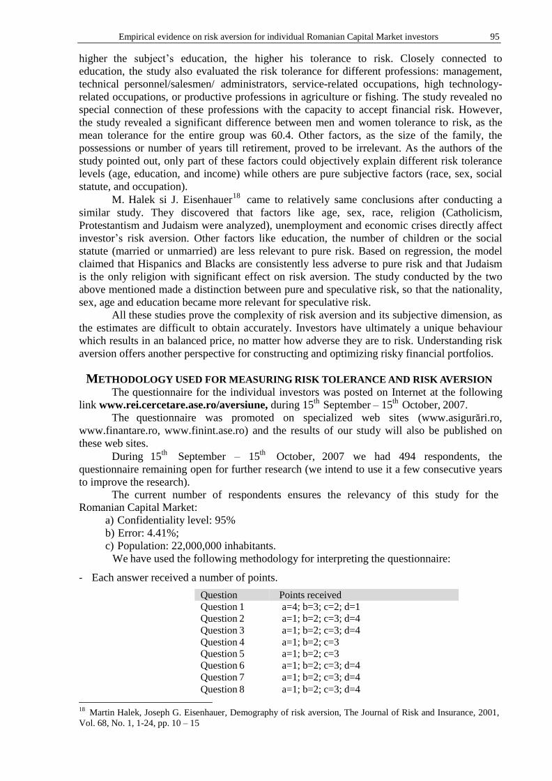
Empirical evidence on risk aversion for individual Romanian Capital Market investors 95
higher the subject’s education, the higher his tolerance to risk. Closely connected to
education, the study also evaluated the risk tolerance for different professions: management,
technical personnel/salesmen/ administrators, service-related occupations, high technology-
related occupations, or productive professions in agriculture or fishing. The study revealed no
special connection of these professions with the capacity to accept financial risk. However,
the study revealed a significant difference between men and women tolerance to risk, as the
mean tolerance for the entire group was 60.4. Other factors, as the size of the family, the
possessions or number of years till retirement, proved to be irrelevant. As the authors of the
study pointed out, only part of these factors could objectively explain different risk tolerance
levels (age, education, and income) while others are pure subjective factors (race, sex, social
statute, and occupation).
M. Halek si J. Eisenhauer18
came to relatively same conclusions after conducting a
similar study. They discovered that factors like age, sex, race, religion (Catholicism,
Protestantism and Judaism were analyzed), unemployment and economic crises directly affect
investor’s risk aversion. Other factors like education, the number of children or the social
statute (married or unmarried) are less relevant to pure risk. Based on regression, the model
claimed that Hispanics and Blacks are consistently less adverse to pure risk and that Judaism
is the only religion with significant effect on risk aversion. The study conducted by the two
above mentioned made a distinction between pure and speculative risk, so that the nationality,
sex, age and education became more relevant for speculative risk.
All these studies prove the complexity of risk aversion and its subjective dimension, as
the estimates are difficult to obtain accurately. Investors have ultimately a unique behaviour
which results in an balanced price, no matter how adverse they are to risk. Understanding risk
aversion offers another perspective for constructing and optimizing risky financial portfolios.
METHODOLOGY USED FOR MEASURING RISK TOLERANCE AND RISK AVERSION
The questionnaire for the individual investors was posted on Internet at the following
link www.rei.cercetare.ase.ro/aversiune, during 15th
September – 15th
October, 2007.
The questionnaire was promoted on specialized web sites (www.asigurări.ro,
www.finantare.ro, www.finint.ase.ro) and the results of our study will also be published on
these web sites.
During 15th
September – 15th
October, 2007 we had 494 respondents, the
questionnaire remaining open for further research (we intend to use it a few consecutive years
to improve the research).
The current number of respondents ensures the relevancy of this study for the Romanian Capital Market:
a) Confidentiality level: 95%
b) Error: 4.41%;
c) Population: 22,000,000 inhabitants.
We have used the following methodology for interpreting the questionnaire:
‐ Each answer received a number of points.
Question Points received
Question 1 a=4; b=3; c=2; d=1
Question 2 a=1; b=2; c=3; d=4
Question 3 a=1; b=2; c=3; d=4
Question 4 a=1; b=2; c=3 Question 5 a=1; b=2; c=3
Question 6 a=1; b=2; c=3; d=4
Question 7 a=1; b=2; c=3; d=4
Question 8 a=1; b=2; c=3; d=4
18 Martin Halek, Joseph G. Eisenhauer, Demography of risk aversion, The Journal of Risk and Insurance, 2001,
Vol. 68, No. 1, 1-24, pp. 10 – 15

96 CRISTIAN PĂUN, RADU MUŞETESCU, IULIAN BRAŞOVEANU, ALINA DRĂGHICI
Question Points received
Question 9 a=1; b=3
Question 10 a=1; b=3
Question 11 a=1; b=2; c=3; d=4 Question 12 a=1; b=2; c=3
Question 13 a=1; b=2; c=3; d=4
‐ Each questionnaire was evaluated and each respondent received a total number of points
reflecting he/she risk tolerance
‐ For interpreting the number of points received by each respondent we have used the
following scale:
• Number of points between 0 and 18: Low risk tolerance
• Number of points between 19 – 22: Below average risk tolerance
• Number of points between 23 – 28: Average risk tolerance
• Number of points between 29 – 32: Above average (high) risk tolerance
• Number of points between 33 – 47: Very high risk tolerance
‐ For computing the risk aversion we have used the following formula:
Aversion= 1
Tolerance
100
‐ We gave the following interpretation to this indicator
• Aversion higher than 5.6: Very high risk aversion
• Aversion between 4.5 and 5.3: High risk aversion;
• Aversion between 4.4 and 3.6: Average risk aversion;
• Aversion between 3.5 and 3.1: Low risk aversion;
• Aversion below 3.0: Very low risk aversion.
For the risk aversion factorial analysis we chose the following socio-professional
profile for individual investors: age, sex, educational level, income, occupation, social status.
For the factor age we choose five representative levels: under 30 years old, between 31–44 years old, between 45–54 years old, between 55–64 years old and over 65 years old.
Our expectations are a higher risk aversion for the extremes (persons too young or too
old) and a slight increase of the risk aversion for the respondents with ages in the middle
of the range.
Considering the educational level we have used four categories: high-school, faculty,
master, doctoral and the expectation was that the risk aversion will decrease as the
educational level increases.
For the social status factor we used five categories: unmarried, married without
children, married with children, divorced, widow. The expectation was that as the social
responsibilities increase, the risk aversion decreases, individuals being more willing to
take investment risks.
Referring to the net income, we used five income levels correlated to the medium
income: under €150, between €150-€350, between €350-€650, between €650-€850 and over
€850. We expected that the risk aversion will decrease as the income increases. For the occupational categories we used seven degrees of involvement in economic
activities: unemployed, student, employee in the budgetary sector, employee in the private
sector, entrepreneur, liberal professions and retired. The expectation was that the risk aversion
will be proportional to the risks taken in each individual’s profession.
For each socio-demographic category we computed the tolerance and average risk
aversion.
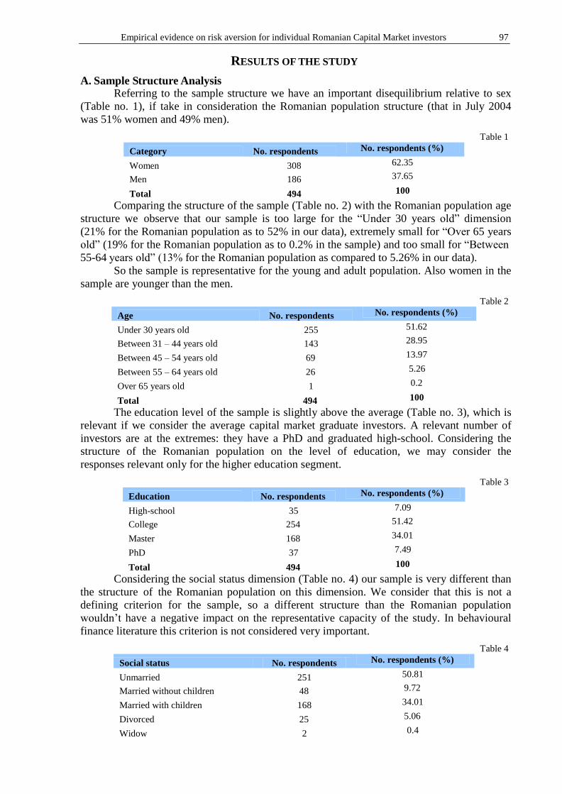
Empirical evidence on risk aversion for individual Romanian Capital Market investors 97
A. Sample Structure Analysis
RESULTS OF THE STUDY
Referring to the sample structure we have an important disequilibrium relative to sex
(Table no. 1), if take in consideration the Romanian population structure (that in July 2004
was 51% women and 49% men).
Category No. respondents No. respondents (%)
Women 308 62.35
Men 186 37.65
Total 494 100
Table 1
Comparing the structure of the sample (Table no. 2) with the Romanian population age
structure we observe that our sample is too large for the “Under 30 years old” dimension
(21% for the Romanian population as to 52% in our data), extremely small for “Over 65 years
old” (19% for the Romanian population as to 0.2% in the sample) and too small for “Between
55-64 years old” (13% for the Romanian population as compared to 5.26% in our data).
So the sample is representative for the young and adult population. Also women in the
sample are younger than the men.
Age No. respondents No. respondents (%)
Under 30 years old 255 51.62
Between 31 – 44 years old 143 28.95
Between 45 – 54 years old 69 13.97
Between 55 – 64 years old 26 5.26
Over 65 years old 1 0.2
Total 494 100
Table 2
The education level of the sample is slightly above the average (Table no. 3), which is
relevant if we consider the average capital market graduate investors. A relevant number of
investors are at the extremes: they have a PhD and graduated high-school. Considering the
structure of the Romanian population on the level of education, we may consider the
responses relevant only for the higher education segment.
Education No. respondents No. respondents (%)
High-school 35 7.09
College 254 51.42
Master 168 34.01
PhD 37 7.49
Total 494 100
Table 3
Considering the social status dimension (Table no. 4) our sample is very different than
the structure of the Romanian population on this dimension. We consider that this is not a
defining criterion for the sample, so a different structure than the Romanian population
wouldn’t have a negative impact on the representative capacity of the study. In behavioural
finance literature this criterion is not considered very important.
Social status No. respondents No. respondents (%)
Unmarried 251 50.81
Married without children 48 9.72
Married with children 168 34.01
Divorced 25 5.06
Widow 2 0.4
Table 4
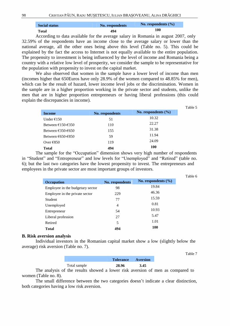
98 CRISTIAN PĂUN, RADU MUŞETESCU, IULIAN BRAŞOVEANU, ALINA DRĂGHICI
Occupation No. respondents
Employee in the budgetary sector 98
Employee in the private sector 229
Student 77
Unemployed 4
Entrepreneur 54
Liberal profession 27
Retired 5
Total 494
Social status No. respondents No. respondents (%)
Total 494 100
According to data available for the average salary in Romania in august 2007, only 32.59% of the respondents have an income close to the average salary or lower than the
national average, all the other ones being above this level (Table no. 5). This could be
explained by the fact the access to Internet is not equally available to the entire population.
The propensity to investment is being influenced by the level of income and Romania being a
country with a relative low level of prosperity, we consider the sample to be representative for
the population with propensity to invest on the capital market.
We also observed that women in the sample have a lower level of income than men
(incomes higher that 650Euros have only 28.9% of the women compared to 48.85% for men),
which can be the result of hazard, lower income level jobs or the discrimination. Women in
the sample are in a higher proportion working in the private sector and students, unlike the
men that are in higher proportion entrepreneurs or having liberal professions (this could
explain the discrepancies in income).
Income No. respondents No. respondents (%)
Under €150 51 10.32
Between €150-€350 110 22.27
Between €350-€650 155 31.38
Between €650-€850 59 11.94
Over €850 119 24.09
Total 494 100
Table 5
The sample for the “Occupation” dimension shows very high number of respondents
in “Student” and “Entrepreneur” and low levels for “Unemployed” and “Retired” (table no.
6); but the last two categories have the lowest propensity to invest. The entrepreneurs and
employees in the private sector are most important groups of investors.
B. Risk aversion analysis
No. respondents (%)
19.84
46.36
15.59
0.81
10.93
5.47
1.01
100
Table 6
Individual investors in the Romanian capital market show a low (slightly below the
average) risk aversion (Table no. 7).
Tolerance Aversion
Total sample 28.96 3.45
Table 7
The analysis of the results showed a lower risk aversion of men as compared to
women (Table no. 8).
The small difference between the two categories doesn’t indicate a clear distinction,
both categories having a low risk aversion.
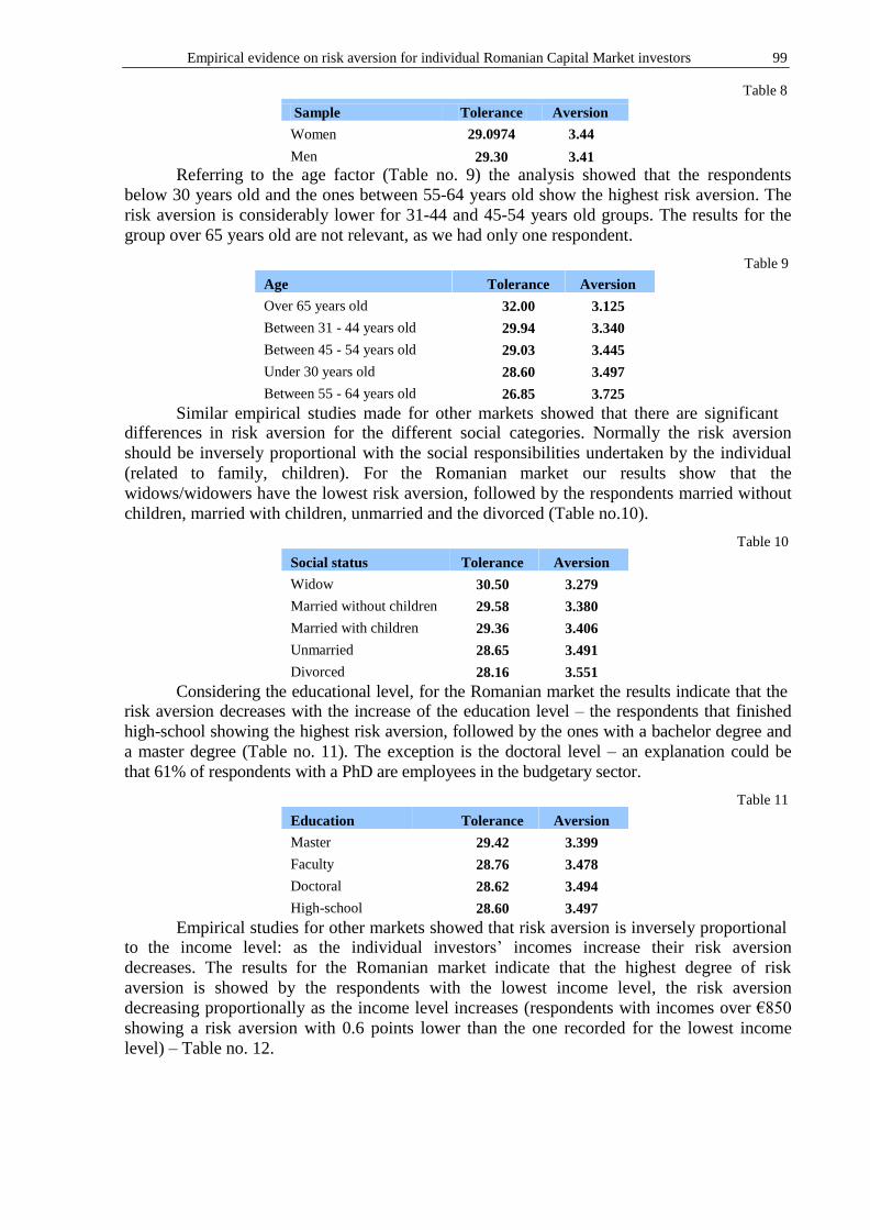
Empirical evidence on risk aversion for individual Romanian Capital Market investors 99
Sample Tolerance Aversion
Women 29.0974 3.44
Men 29.30 3.41
Table 8
Referring to the age factor (Table no. 9) the analysis showed that the respondents
below 30 years old and the ones between 55-64 years old show the highest risk aversion. The
risk aversion is considerably lower for 31-44 and 45-54 years old groups. The results for the
group over 65 years old are not relevant, as we had only one respondent.
Table 9
Age Tolerance Aversion
Over 65 years old 32.00 3.125
Between 31 - 44 years old 29.94 3.340
Between 45 - 54 years old 29.03 3.445
Under 30 years old 28.60 3.497
Between 55 - 64 years old 26.85 3.725
Similar empirical studies made for other markets showed that there are significant differences in risk aversion for the different social categories. Normally the risk aversion
should be inversely proportional with the social responsibilities undertaken by the individual
(related to family, children). For the Romanian market our results show that the
widows/widowers have the lowest risk aversion, followed by the respondents married without
children, married with children, unmarried and the divorced (Table no.10).
Table 10
Social status Tolerance Aversion
Widow 30.50 3.279
Married without children 29.58 3.380
Married with children 29.36 3.406
Unmarried 28.65 3.491
Divorced 28.16 3.551
Considering the educational level, for the Romanian market the results indicate that the risk aversion decreases with the increase of the education level – the respondents that finished
high-school showing the highest risk aversion, followed by the ones with a bachelor degree and
a master degree (Table no. 11). The exception is the doctoral level – an explanation could be
that 61% of respondents with a PhD are employees in the budgetary sector.
Table 11
Education Tolerance Aversion
Master 29.42 3.399
Faculty 28.76 3.478
Doctoral 28.62 3.494
High-school 28.60 3.497
Empirical studies for other markets showed that risk aversion is inversely proportional to the income level: as the individual investors’ incomes increase their risk aversion
decreases. The results for the Romanian market indicate that the highest degree of risk
aversion is showed by the respondents with the lowest income level, the risk aversion
decreasing proportionally as the income level increases (respondents with incomes over €850
showing a risk aversion with 0.6 points lower than the one recorded for the lowest income
level) – Table no. 12.
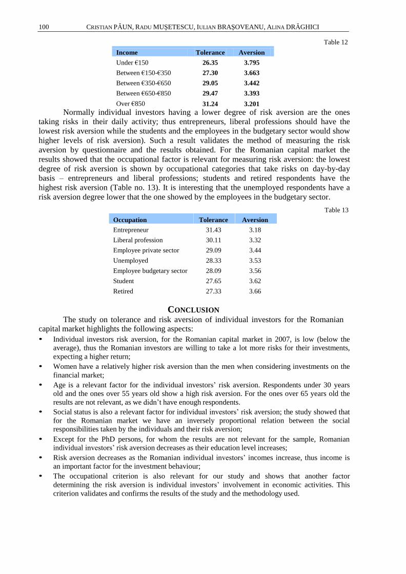
100 CRISTIAN PĂUN, RADU MUŞETESCU, IULIAN BRAŞOVEANU, ALINA DRĂGHICI
Income Tolerance Aversion
Under €150 26.35 3.795
Between €150-€350 27.30 3.663
Between €350-€650 29.05 3.442
Between €650-€850 29.47 3.393
Over €850 31.24 3.201
Table 12
Normally individual investors having a lower degree of risk aversion are the ones
taking risks in their daily activity; thus entrepreneurs, liberal professions should have the
lowest risk aversion while the students and the employees in the budgetary sector would show
higher levels of risk aversion). Such a result validates the method of measuring the risk
aversion by questionnaire and the results obtained. For the Romanian capital market the
results showed that the occupational factor is relevant for measuring risk aversion: the lowest
degree of risk aversion is shown by occupational categories that take risks on day-by-day
basis – entrepreneurs and liberal professions; students and retired respondents have the
highest risk aversion (Table no. 13). It is interesting that the unemployed respondents have a
risk aversion degree lower that the one showed by the employees in the budgetary sector.
Table 13
Occupation Tolerance Aversion
Entrepreneur 31.43 3.18
Liberal profession 30.11 3.32
Employee private sector 29.09 3.44
Unemployed 28.33 3.53
Employee budgetary sector 28.09 3.56
Student 27.65 3.62
Retired 27.33 3.66
CONCLUSION
The study on tolerance and risk aversion of individual investors for the Romanian capital market highlights the following aspects:
• Individual investors risk aversion, for the Romanian capital market in 2007, is low (below the
average), thus the Romanian investors are willing to take a lot more risks for their investments,
expecting a higher return;
• Women have a relatively higher risk aversion than the men when considering investments on the
financial market;
• Age is a relevant factor for the individual investors’ risk aversion. Respondents under 30 years
old and the ones over 55 years old show a high risk aversion. For the ones over 65 years old the
results are not relevant, as we didn’t have enough respondents.
• Social status is also a relevant factor for individual investors’ risk aversion; the study showed that
for the Romanian market we have an inversely proportional relation between the social responsibilities taken by the individuals and their risk aversion;
• Except for the PhD persons, for whom the results are not relevant for the sample, Romanian
individual investors’ risk aversion decreases as their education level increases;
• Risk aversion decreases as the Romanian individual investors’ incomes increase, thus income is
an important factor for the investment behaviour;
• The occupational criterion is also relevant for our study and shows that another factor
determining the risk aversion is individual investors’ involvement in economic activities. This
criterion validates and confirms the results of the study and the methodology used.

Empirical evidence on risk aversion for individual Romanian Capital Market investors 101
SELECTIVE REFERENCES: 1. Arrondel L., Calvo H., Oliver X. (2005), ‘Portfolio Choice and Background Risk:
Evidence from France’, Paris-Jourdan Sciences Economiques;
2. Barsky, Robert B., F. Thomas Juster, Miles S. Kimball, and Matthew D. Shapiro, (1997),
‘Preference Parameters and Behavioral Heterogeneity: An Experimental Approach in the
Health and Retirement Study’, Quarterly Journal of Economics, 112(2), pp. 537-579;
3. Bertoni, A. (2005), ‘Investors’ Self-confidence in Financial Choices: the Italian Case’,
Financial Management Association International Working Paper.
4. Hawley, Clifford B. and E. Fujii. (1993), ‘An empirical analysis of preferences for
financial risk: further evidence on the Friedman-Savage Model’, Journal of Post
Keynesian Economics, Nr. 16, vol. 2: 20 – 24;
5. Hersch, Joni, (1996), ‘Smoking, Seat Belts, and Other Risky Consumer Decisions:
Differences by Gender and Race’, Managerial and Decision Economics 17(5): pp. 471-
481;
6. J.W. Pratt (1964), ‘Risk Aversion in the Small and in the Large’, Econometrica Vol. 32:
p.122-36;
7. Jianakoplos, Nancy Ammon, and Alexandra Bernasek, (1998), ‘Are Women More Risk
Averse?’, Economic Inquiry 36(4), pp. 620-630
8. Joop Hartog (2000), ‘On a Simple Measure of Individual Risk Aversion’, Timbergen
Institute Discussion Paper: pp. 8;
9. Kapteyn, A, Teppa, F. (2002), ‘Subjective Measures of Risk Aversion and Portfolio
Choice’, CentER, Tilburg University, February 18;
10. Levin Irwin P., Mary A. Snyder and Daniel P. Chapman, (1988), ‘The Interaction of
Experiential and Situational Factors and Gender in a Simulated Risky Decision-Making
Task’, Journal of Psychology, 122(2),pp. 173-181
11. Martin Halek, Joseph G. Eisenhauer, (2001), ‘Demography of risk aversion’, The Journal
of Risk and Insurance, Vol. 68, No. 1, 1-24: 10 – 15
12. Powell Melanie, and David Ansic, (1998), ‘Gender Differences in Risk Behaviour in
Financial Decision-Making: An Experimental Analysis’, Journal of Economic
Psychology, 18(6): pp. 605-628
13. Riley, William B., Jr., and K. Victor Chow, (1992), ‘Asset Allocation and Individual Risk
Aversion’, Financial Analysts Journal, November-December, pp. 32-37;
14. Scheicher, M. (2003) ‘What drives investor risk aversion? Daily evidence from the
German equity market’, BIS Quarterly Review;
15. Sunden, Annika E., and Brian J. Surette, (1998), ‘Gender Differences in the Allocation of
Assets in Retirement Savings Plans’, American Economic Review, Papers and
Proceedings, 88(2): pp. 207-211;
16. Sung, J., Hanna, S., (1996) “Factors related to risk tolerance”, Financial Counseling and
Planning, 7, 11-20;
17. Zuckerman, Marvin, (1994), ‘Behavioral Expressions and Biosocial Bases of Sensation
Seeking’, Cambridge University Press
DATA ANALYSIS WITH ORDINAL AND INTERVAL DEPENDENT VARIABLES: EXAMPLES FROM A STUDY OF REAL ESTATE
SALESPEOPLE
G. Martin IZZO*, Barry E. LANGFORD**
Abstract. This paper re-examines the problems of estimating the parameters of an underlying linear model using survey response data in which the dependent variables are in discrete categories of ascending order (ordinal, as distinct from numerical) or, where they are observed to fall into certain groups on a continuous scale (interval), where the actual values remain unobserved. An ordered probit model is discussed as an appropriate framework for statistical analysis for ordinal dependent variables. Next, a maximum likelihood estimator (MLE) derived from grouped data regression for interval dependent variable is discussed. Using LIMDEP, a packaged statistical program, survey data from an earlier manuscript are analyzed and the findings presented. Key words: marketing research, an ordered probit model, statistical analysis, ordinal
dependent variables, maximum likelihood estimator, attitudinal survey JEL: M31, C81.
INTRODUCTION Today marketing data are collected on a wide platform of survey instruments which
generate responses in the form of ordinal, or ordered responses. In marketing, attitudinal surveys often are recorded using Likert-type scales, (Likert, 1932). A common example is the extent of agreement with a certain point of view; measured using a 5-point Likert-type scale as: strongly agree, agree, feel neutral, disagree, and strongly disagree. Other instances, types of ordered responses are often collected in response to level of educational degree, job rank, or level of position attainment. For example, in the underlying study, responses were recorded for level of licensure: broker, broker/associate, or sales associate. The measurement problem that arises is a consequence of there being no natural unit of measurement for ordered responses. A statistical technique known as the ordered probit model having been well-articulated for some time in the biometrics and social sciences literature, e.g. Aitchison and Silvey, 1957; McKelvey and Zavonia, 1975, Daykin and Moffatt, 2002, provides marketing researchers with a suitable tool for analysis.
Other survey scales used in marketing research generate responses which are categorical in nature with a known set of boundaries and a specified interval of length. This type of survey is often used to measure data on individuals’ earned income or length of time
* G. Martin Izzo – PhD, Associate Professor, Mike Cottrell School of Business, North Georgia College & State University ** Barry E. Langford – DBA, Associate Professor, Florida Gulf Coast University
104 G. MARTIN IZZO, BARRY E. LANGFORD
in occupation, reported in brackets or groups. Both of these “grouped” dependent variables were measured in the underlying study (Izzo & Langford, 2003). The measurement problem with grouped data is that of estimating an equation on the basis of data in which the dependent variable is only observed to fall within a specified interval on a continuous scale, the actual value being unobserved. Stewart (1983) addressed the measurement problem by developing a procedure known as grouped data regression, a model that provides for consistent and asymptotically efficient parameter estimation of grouped dependent variables.
The purpose of the current paper is to present analyses using the ordered probit and grouped data regression models on data from an earlier marketing study for which simple ordinary least squares regression analysis was inadequate. Re-examination of this study (Izzo & Langford, 2003) data provides discussion of analytical models which have received less attention in the marketing literature. Discussed first are the nature and research propositions of the underlying study – which measured effects of designation-granting courses offered through the National Association of Realtors® (NAR). Second, data analyses underlying that study are presented using LIMDEP , Greene, 1985, one of several statistical packages that contain routines for estimating the ordered probit and grouped data regression models, others include STATA and TSP, Hall and Cummins, 1999. Finally, this paper presents a discussion of the results of that study.
NATURE OF THE UNDERLYING STUDY The guiding research proposition in the underlying study by Izzo and Langford (2003)
was that professional education [i.e., earning a professional real estate designation] could serve as an organizational socialization technique that may serve to motivate salespeople to work smarter as well as harder. Effective sales force socialization — achievement of requisite job skills, development of appropriate behaviors, and internalization of values and norms — is likely to have a favorable impact on salespersons in terms of motivation and job satisfaction, and the organization in terms of performance (Feldman, 1976b; Walker, Churchill and Ford, 1977; Jackson, Tax and Barnes, 1994).
Professional real estate associations that sponsor the designations [e.g. Graduate Realtor Institute (GRI)] require their membership to subscribe to a higher standard of ethics and professional practice than generally would be present in most organizations. In addition, the severity of initiation requirements for membership into various professional designation groups [e.g. commercial and investment; residential specialists; office and industrial] means that members are more likely to follow the stricter professional dictates of the association (Festinger, 1957; Aronson and Mills, 1959). Further, research has shown that education is a significant predictor of cognitive moral development (CMD) (Kohlberg, 1984; Izzo, 1997). Salespeople who seek advanced real estate designations should exhibit greater cognitive moral development. These considerations give rise to the following testable hypotheses, which comprise the principal focus of this paper. H1a: Salespersons with professional designations will demonstrate greater CMD in general
situations with ethical overtones. H1b: Salespersons with professional designations will demonstrate higher levels of CMD in
industry-specific situations involving moral decision-making. Real estate salespeople pursuing professional designations do so primarily because
they have the motivation to improve their technical proficiency and selling skills2. There is additional evidence that these salespeople are able to blend the merits of both learning and performance orientations (Sujan, Weitz and Kumar, 1994). Thus, real estate salespeople with professional designations, who employ learning and performance orientations, may outperform those who rely on performance orientations exclusively. H2a : Real estate salespeople with professional designations will demonstrate superior sales earnings. 2 Although some states allow in-class professional designations or “credentialing” to fulfill continuing education licensing requirements, simpler alternatives, such as mail-order correspondence courses, are far more prevalent.
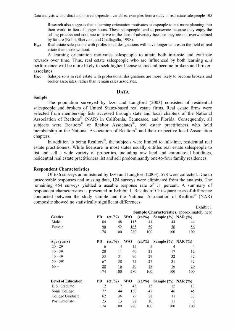
Data analysis with ordinal and interval dependent variables: examples from a study of real estate salespeople 105
Research also suggests that a learning orientation motivates salespeople to put more planning into their work, in lieu of longer hours. These salespeople tend to persevere because they enjoy the selling process and continue to strive in the face of adversity because they are not overwhelmed by failure (Kohli, Shervani, and Challagalla, 1998).
H2b: Real estate salespeople with professional designations will have longer tenures in the field of real estate than those without. A learning orientation motivates salespeople to attain both intrinsic and extrinsic
rewards over time. Thus, real estate salespeople who are influenced by both learning and performance will be more likely to seek higher license status and become brokers and broker-associates. H2C: Salespersons in real estate with professional designations are more likely to become brokers and
broker associates, rather than remain sales associates.
DATA Sample
The population surveyed by Izzo and Langford (2003) consisted of residential salespeople and brokers of United States-based real estate firms. Real estate firms were selected from membership lists accessed through state and local chapters of the National Association of Realtors® (NAR) in California, Tennessee, and Florida. Consequently, all subjects were Realtors® or Realtor Associates®, real estate practitioners who hold membership in the National Association of Realtors® and their respective local Association chapters.
In addition to being Realtors®, the subjects were limited to full-time, residential real estate practitioners. While licensure in most states usually entitles real estate salespeople to list and sell a wide variety of properties, including raw land and commercial buildings, residential real estate practitioners list and sell predominantly one-to-four family residences. Respondent Characteristics
Of 636 surveys administered by Izzo and Langford (2003), 578 were collected. Due to unscoreable responses and missing data, 124 surveys were eliminated from the analysis. The remaining 454 surveys yielded a useable response rate of 71 percent. A summary of respondent characteristics is presented in Exhibit 1. Results of Chi-square tests of difference conducted between the study sample and the National Association of Realtors® (NAR) composite showed no statistically significant differences.
Exhibit 1 Sample Characteristics, approximately here
Gender PD (ct./%) W/O (ct./%) Sample (%) NAR (%) Male 84 48 115 41 44 44 Female 90 52 165 59 56 56 174 100 280 100 100 100
Age (years) PD (ct./%) W/O (ct./%) Sample (%) NAR (%) 20 - 29 6 4 15 5 4 4 30 - 39 20 11 60 21 17 12 40 - 49 53 31 90 29 32 32 50 - 59` 67 38 75 27 31 32 60 + 28 16 50 18 16 20 174 100 280 100 100 100
Level of Education PD (ct./%) W/O (ct./%) Sample (%) NAR (%) H.S. Graduate 12 7 43 15 12 13 Some College 77 44 130 47 46 45 College Graduate 62 36 79 28 31 33 Post Graduate 23 13 28 10 11 9 174 100 280 100 100 100
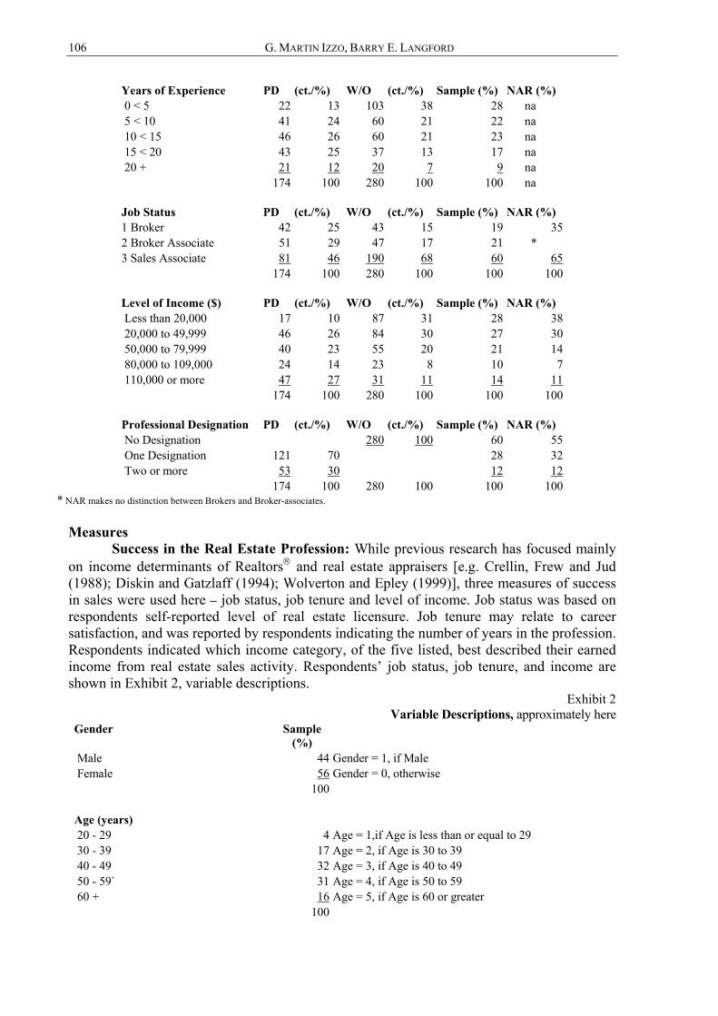
106 G. MARTIN IZZO, BARRY E. LANGFORD
Years of Experience PD (ct./%) W/O (ct./%) Sample (%) NAR (%) 0 < 5 22 13 103 38 28 na 5 < 10 41 24 60 21 22 na 10 < 15 46 26 60 21 23 na 15 < 20 43 25 37 13 17 na 20 + 21 12 20 7 9 na 174 100 280 100 100 na
Job Status PD (ct./%) W/O (ct./%) Sample (%) NAR (%) 1 Broker 42 25 43 15 19 35 2 Broker Associate 51 29 47 17 21 * 3 Sales Associate 81 46 190 68 60 65 174 100 280 100 100 100
Level of Income ($) PD (ct./%) W/O (ct./%) Sample (%) NAR (%) Less than 20,000 17 10 87 31 28 38 20,000 to 49,999 46 26 84 30 27 30 50,000 to 79,999 40 23 55 20 21 14 80,000 to 109,000 24 14 23 8 10 7 110,000 or more 47 27 31 11 14 11 174 100 280 100 100 100
Professional Designation PD (ct./%) W/O (ct./%) Sample (%) NAR (%) No Designation 280 100 60 55 One Designation 121 70 28 32 Two or more 53 30 12 12 174 100 280 100 100 100
* NAR makes no distinction between Brokers and Broker-associates. Measures
Success in the Real Estate Profession: While previous research has focused mainly on income determinants of Realtors® and real estate appraisers [e.g. Crellin, Frew and Jud (1988); Diskin and Gatzlaff (1994); Wolverton and Epley (1999)], three measures of success in sales were used here – job status, job tenure and level of income. Job status was based on respondents self-reported level of real estate licensure. Job tenure may relate to career satisfaction, and was reported by respondents indicating the number of years in the profession. Respondents indicated which income category, of the five listed, best described their earned income from real estate sales activity. Respondents’ job status, job tenure, and income are shown in Exhibit 2, variable descriptions.
Exhibit 2 Variable Descriptions, approximately here
Gender
Sample (%)
Male 44 Gender = 1, if Male Female 56 Gender = 0, otherwise 100 Age (years) 20 - 29 4 Age = 1,if Age is less than or equal to 29 30 - 39 17 Age = 2, if Age is 30 to 39 40 - 49 32 Age = 3, if Age is 40 to 49 50 - 59` 31 Age = 4, if Age is 50 to 59 60 + 16 Age = 5, if Age is 60 or greater 100
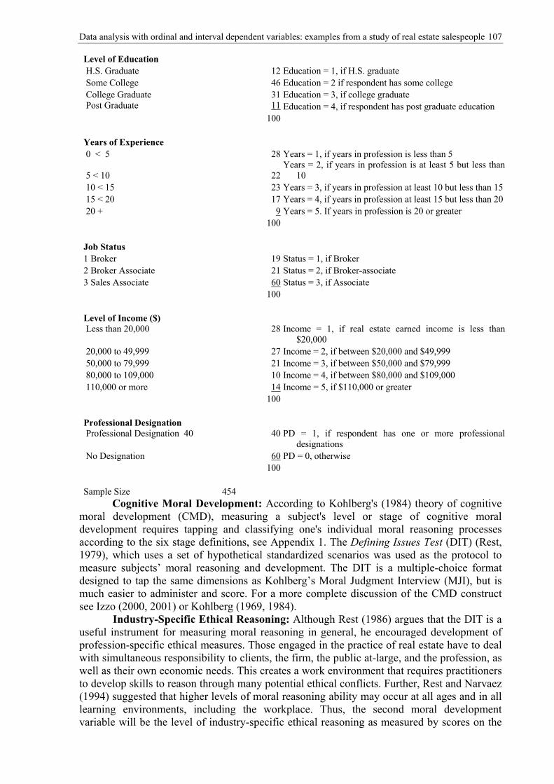
Data analysis with ordinal and interval dependent variables: examples from a study of real estate salespeople 107
Level of Education H.S. Graduate 12 Education = 1, if H.S. graduate Some College 46 Education = 2 if respondent has some college College Graduate 31 Education = 3, if college graduate Post Graduate 11 Education = 4, if respondent has post graduate education 100 Years of Experience 0 < 5 28 Years = 1, if years in profession is less than 5
5 < 10 22Years = 2, if years in profession is at least 5 but less than
10 10 < 15 23 Years = 3, if years in profession at least 10 but less than 15 15 < 20 17 Years = 4, if years in profession at least 15 but less than 20 20 + 9 Years = 5. If years in profession is 20 or greater 100 Job Status 1 Broker 19 Status = 1, if Broker 2 Broker Associate 21 Status = 2, if Broker-associate 3 Sales Associate 60 Status = 3, if Associate 100 Level of Income ($) Less than 20,000
28 Income = 1, if real estate earned income is less than
$20,000 20,000 to 49,999 27 Income = 2, if between $20,000 and $49,999 50,000 to 79,999 21 Income = 3, if between $50,000 and $79,999 80,000 to 109,000 10 Income = 4, if between $80,000 and $109,000 110,000 or more 14 Income = 5, if $110,000 or greater 100 Professional Designation Professional Designation 40 40 PD = 1, if respondent has one or more professional
designations No Designation 60 PD = 0, otherwise 100 Sample Size 454
Cognitive Moral Development: According to Kohlberg's (1984) theory of cognitive moral development (CMD), measuring a subject's level or stage of cognitive moral development requires tapping and classifying one's individual moral reasoning processes according to the six stage definitions, see Appendix 1. The Defining Issues Test (DIT) (Rest, 1979), which uses a set of hypothetical standardized scenarios was used as the protocol to measure subjects’ moral reasoning and development. The DIT is a multiple-choice format designed to tap the same dimensions as Kohlberg’s Moral Judgment Interview (MJI), but is much easier to administer and score. For a more complete discussion of the CMD construct see Izzo (2000, 2001) or Kohlberg (1969, 1984).
Industry-Specific Ethical Reasoning: Although Rest (1986) argues that the DIT is a useful instrument for measuring moral reasoning in general, he encouraged development of profession-specific ethical measures. Those engaged in the practice of real estate have to deal with simultaneous responsibility to clients, the firm, the public at-large, and the profession, as well as their own economic needs. This creates a work environment that requires practitioners to develop skills to reason through many potential ethical conflicts. Further, Rest and Narvaez (1994) suggested that higher levels of moral reasoning ability may occur at all ages and in all learning environments, including the workplace. Thus, the second moral development variable will be the level of industry-specific ethical reasoning as measured by scores on the
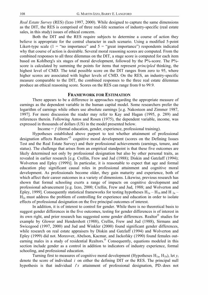
108 G. MARTIN IZZO, BARRY E. LANGFORD
Real Estate Survey (RES) (Izzo 1997, 2000). While designed to capture the same dimensions as the DIT, the RES is comprised of three real-life scenarios of industry-specific (real estate sales, in this study) issues of ethical concern.
Both the DIT and the RES require subjects to determine a course of action they believe is appropriate for the central character in each scenario. Using a modified 5-point Likert-type scale (1 = “no importance” and 5 = “great importance”) respondents indicated why that course of action is desirable. Several moral reasoning scores are computed. From the combined responses to all three dilemmas on the DIT, a stage score is computed for each item based on Kohlberg's six stages of moral development, followed by the P%-score. The P%-score is calculated by summing the points for items that represent principled thinking, the highest level of CMD. The total possible score on the DIT ranges from zero to 95, where higher scores are associated with higher levels of CMD. On the RES, an industry-specific measure comparable to the DIT, the combined responses to the three real estate dilemmas produce an ethical reasoning score. Scores on the RES can range from 0 to 99.9.
FRAMEWORK FOR ESTIMATION There appears to be a difference in approaches regarding the appropriate measure of
earnings as the dependent variable in the human capital model. Some researchers prefer the logarithm of earnings while others use absolute earnings [e.g. Nakosteen and Zimmer 1987, 1997]. For more discussion the reader may refer to Kay and Hagan (1995, p. 289) and references therein. Following Antos and Rosen (1975), the dependent variable, income, was expressed in thousands of dollars (US) in the model presented below.
Income = ƒ (formal education, gender, experience, professional training). Hypotheses established above purport to test whether attainment of professional
designation affects Realtors’® cognitive moral development (scores on the Defining Issues Test and the Real Estate Survey) and their professional achievements (earnings, tenure, and status). The challenge that arises from an empirical standpoint is that these five outcomes are likely determined not only by professional designation but also by other personal traits, as revealed in earlier research [e.g. Crellin, Frew and Jud (1988); Diskin and Gatzlaff (1994); Wolverton and Epley (1999)]. In particular, it is reasonable to expect that age and formal education play significant causal roles in professional attainment and cognitive moral development. As professionals become older, they gain maturity and experience, both of which affect their career outcomes in a variety of dimensions. Likewise, previous research has shown that formal schooling exerts a range of impacts on cognitive development and professional advancement [e.g. Izzo, 2000; Crellin, Frew and Jud, 1988; and Wolverton and Epley, 1999]. Consequently statistical frameworks for testing hypotheses H1a – H1b and H 2a – H2c must address the problem of controlling for experience and education in order to isolate effects of professional designation on the five principal outcomes of interest.
In addition, it is of interest to control for gender. While there is no theoretical basis to suggest gender differences in the five outcomes, testing for gender differences is of interest in its own right, and prior research has suggested some gender differences. Realtor® studies for example by Glower and Hendershott (1988), Crellin, Frew and Jud (1988), Sirmans and Swicegood (1997, 2000) and Jud and Winkler (2000) found significant gender differences, while research on real estate appraisers by Diskin and Gatzlaff (1994) and Wolverton and Epley (1999) did not. Moreover, Abelson, Kacmar, and Jackofsky (1990) found females out-earning males in a study of residential Realtors.® Consequently, equations modeled in this section include gender as a control in addition to indicators of industry experience, formal schooling, and professional education.
Turning first to measures of cognitive moral development (Hypotheses H1a, H1b), let yi denote the score of individual i on either the defining DIT or the RES. The principal null hypothesis is that individual si' attainment of professional designation, PD i does not
Data analysis with ordinal and interval dependent variables: examples from a study of real estate salespeople 109
enhance iy . In the context of a model that controls for time in the profession, schooling and gender, the model is expressed as a regression equation:
(1) β=i
y 1+ β 2 EXPERIENCEi
+ β 3 EDUCATIONi
+ β 4 MALE β+i 5PD ,
ie
i+
where PD i =1 if the individual possesses a professional designation, and PD i =0 otherwise.
The β ’s represent unknown parameters that measure the impact of their respective variables on iy . The random error term, ie , represents unmeasured factors that affect the dependent variable. It is assumed to possess a normal distribution across the population of real estate professionals, with a mean equal to zero and a constant variance.3
Viewed in this context, hypotheses H1a and H1b can be restated: H1a: 5β =0 in the DIT model. H1b: 5β =0 in the RES model.
Rejection of those hypotheses, based on the regression results, supports the proposition that attainment of professional designation significantly affects cognitive moral development.
The general framework, in equation (1) applies to hypotheses H2a (earnings as the dependent variable yi) and H2b (tenure in the profession as the dependent variable yi). In both cases, the critical hypothesis again focuses on the significance of β 5 the coefficient of professional designation. However, the manner in which earnings and tenure are measured in the survey instrument necessitates a different estimation procedure. In the survey, individuals placed their income (I, thousands) in one of the following categories:
I < 20; 20 � I < 50; 50 �I < 80; 80 �I < 110; and I � 110 Similarly their tenure responses (T, years), occurred as follows: T < 3; 3 � T < 6; 6 � T < 10; 10 � T < 15; 15 � T < 20; and T � 20 These responses are coded as y =1 through 5 for the earnings variable and y = 1
through 6 for the tenure variable. This gives rise to a censored data regression model (Stewart 1983), which makes use of the interval limits to estimate the parameters of the regression model. The structure of the model is identical to equation (1), but the method of maximum likelihood is used instead of least squares. The resulting estimates permit a test of the effect of professional designation on earnings after controlling for experience, education and gender, and on professional tenure, after controlling for age, education and gender.
The final hypothesis, H2c, addresses the impact of professional designation on professional status. Another statistical accommodation is necessary here, because the dependent variable is measured in discrete categories of ascending professional status: y = 0 if individual i is an associate, yI = 1 if she is a broker-associate, and yI = 2 if she is a broker. Models of this type can be estimated by means of maximum likelihood ordered probit methods. The structure of this model is again similar to equation (1), but the error term is assumed to possess a normal distribution of mean zero and variance equal to one. In this model, individual i is assumed to possess a latent propensity for professional advancement, denoted yI
*. The data do not measure yI*; instead we observe the categorical indicators defined
above:
(2) 0=iy if ,0*<
iy
1=iy if 0i
y*
� µ, and
3 If the error variance is not constant, least square estimates of the standard errors are biased. The estimation method used here uses White’s (1978) correction for heteroscedasticity to correct the standard errors. The necessary correction algorithm is available in LIMDEP 7.0 used in this study, now available in version 9.0.
110 G. MARTIN IZZO, BARRY E. LANGFORD
2=iy if .*
ui
y >
The values 0 and µ represent thresholds of the latent propensity that partition the population into associates, broker-associates, and associates, where µ is an unknown parameter. The latent index is specified in the form of a regression model:
(3) 21*
ββ +=i
y AGEi + 3β EDUCATIONi + 4β MALEi + ii ePD +5β .
Estimates of the β ’s and u are obtained by the method of maximum likelihood (Zavoina and McElvey 1975).4
To summarize, the principal hypotheses are tested by using least squares regression for H1a and H1b, maximum likelihood grouped data regression for H2a and H2b, and maximum likelihood probit regression for H2c. The following section describes the data and variable definitions that form the basis for estimation.
RESULTS The central research proposition in the Izzo and Langford (2003) study was that
professional education required to earn a professional designation is an organizational socialization tactic that is positively related to measures of success in real estate sales. Hypotheses developed above purport to test whether attainment of a professional designation affects cognitive moral development (CMD) and professional achievements, income, tenure and status. As stated above, the empirical challenge is that these outcomes are influenced not only by professional education but also personal difference factors. Consequently, statistical frameworks for testing hypotheses H1a – H2a and H2a – H2c control for experience and education in order to isolate the effects of profession designation on the five outcomes of interest. In addition, since prior research shows mixed results, and testing for gender is of interest of its own right, the models outlined above included gender as a control, along with experience and education.
Level of CMD (Hypotheses H1a and H1b) The first group of research questions asked to what extent, if any, is the effect of
professional education on the level of moral development of real estate practitioners. The analysis was limited to ordinary least squares regression comparisons of respondents' group DIT P%-scores and RES scores. Thus, no interpretation can be made about the morality or ethics of any particular group. All respondents were administered the DIT and RES. As previously discussed, the P% Score is DIT instrument's standard measure of CMD. The RES scores are shown under industry-specific moral reasoning (ISMR).
The results of estimating equations H1a and H1b using ordinary least squares regression with the entire sample of Realtors® are shown in Exhibit 3. Sample mean P%-scores were 39.16 (SD 13.5) for the group of Realtors® (n = 454). Traditional cognitive development theory [e.g. Kohlberg, ETAL] suggests that formal education and experience can contribute to advances in moral judgment. On the DIT, the coefficients for experience are negative except for YRS 16-20, while the coefficients for formal education indicate positive returns for Realtors.® However, on the RES, the coefficients for experience indicate positive returns, and the coefficients for formal education are negative except for POSTGRAD.
Exhibit 3 Regression Results, approximately here
Dependent Variable: DIT Dependent Variable: RES
4 Estimated algorithms for interval (censored) data regression and ordered probit models are available in LIMDEP 7.0, now available in version 9.0.
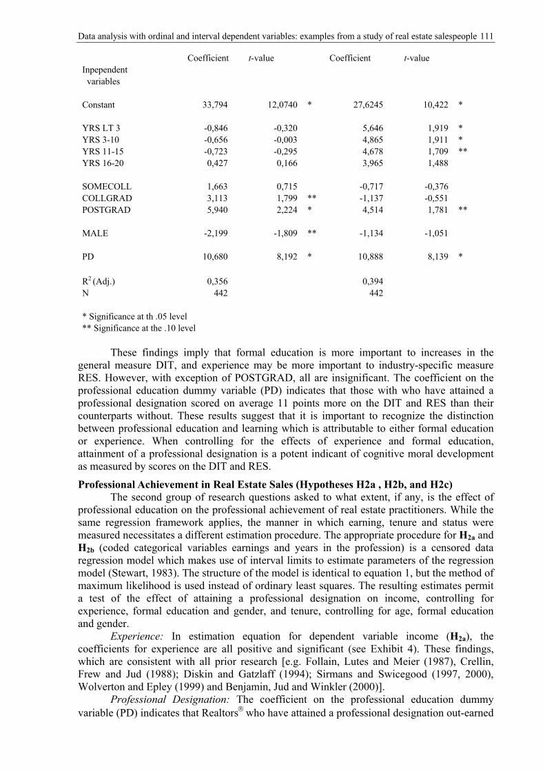
Data analysis with ordinal and interval dependent variables: examples from a study of real estate salespeople 111
Coefficient t-value Coefficient t-value Inpependent variables Constant 33,794 12,0740 * 27,6245 10,422 * YRS LT 3 -0,846 -0,320 5,646 1,919 * YRS 3-10 -0,656 -0,003 4,865 1,911 * YRS 11-15 -0,723 -0,295 4,678 1,709 ** YRS 16-20 0,427 0,166 3,965 1,488 SOMECOLL 1,663 0,715 -0,717 -0,376 COLLGRAD 3,113 1,799 ** -1,137 -0,551 POSTGRAD 5,940 2,224 * 4,514 1,781 ** MALE -2,199 -1,809 ** -1,134 -1,051 PD 10,680 8,192 * 10,888 8,139 * R2 (Adj.) 0,356 0,394 N 442 442 * Significance at th .05 level ** Significance at the .10 level
These findings imply that formal education is more important to increases in the
general measure DIT, and experience may be more important to industry-specific measure RES. However, with exception of POSTGRAD, all are insignificant. The coefficient on the professional education dummy variable (PD) indicates that those with who have attained a professional designation scored on average 11 points more on the DIT and RES than their counterparts without. These results suggest that it is important to recognize the distinction between professional education and learning which is attributable to either formal education or experience. When controlling for the effects of experience and formal education, attainment of a professional designation is a potent indicant of cognitive moral development as measured by scores on the DIT and RES.
Professional Achievement in Real Estate Sales (Hypotheses H2a , H2b, and H2c) The second group of research questions asked to what extent, if any, is the effect of
professional education on the professional achievement of real estate practitioners. While the same regression framework applies, the manner in which earning, tenure and status were measured necessitates a different estimation procedure. The appropriate procedure for H2a and H2b (coded categorical variables earnings and years in the profession) is a censored data regression model which makes use of interval limits to estimate parameters of the regression model (Stewart, 1983). The structure of the model is identical to equation 1, but the method of maximum likelihood is used instead of ordinary least squares. The resulting estimates permit a test of the effect of attaining a professional designation on income, controlling for experience, formal education and gender, and tenure, controlling for age, formal education and gender.
Experience: In estimation equation for dependent variable income (H2a), the coefficients for experience are all positive and significant (see Exhibit 4). These findings, which are consistent with all prior research [e.g. Follain, Lutes and Meier (1987), Crellin, Frew and Jud (1988); Diskin and Gatzlaff (1994); Sirmans and Swicegood (1997, 2000), Wolverton and Epley (1999) and Benjamin, Jud and Winkler (2000)].
Professional Designation: The coefficient on the professional education dummy variable (PD) indicates that Realtors® who have attained a professional designation out-earned
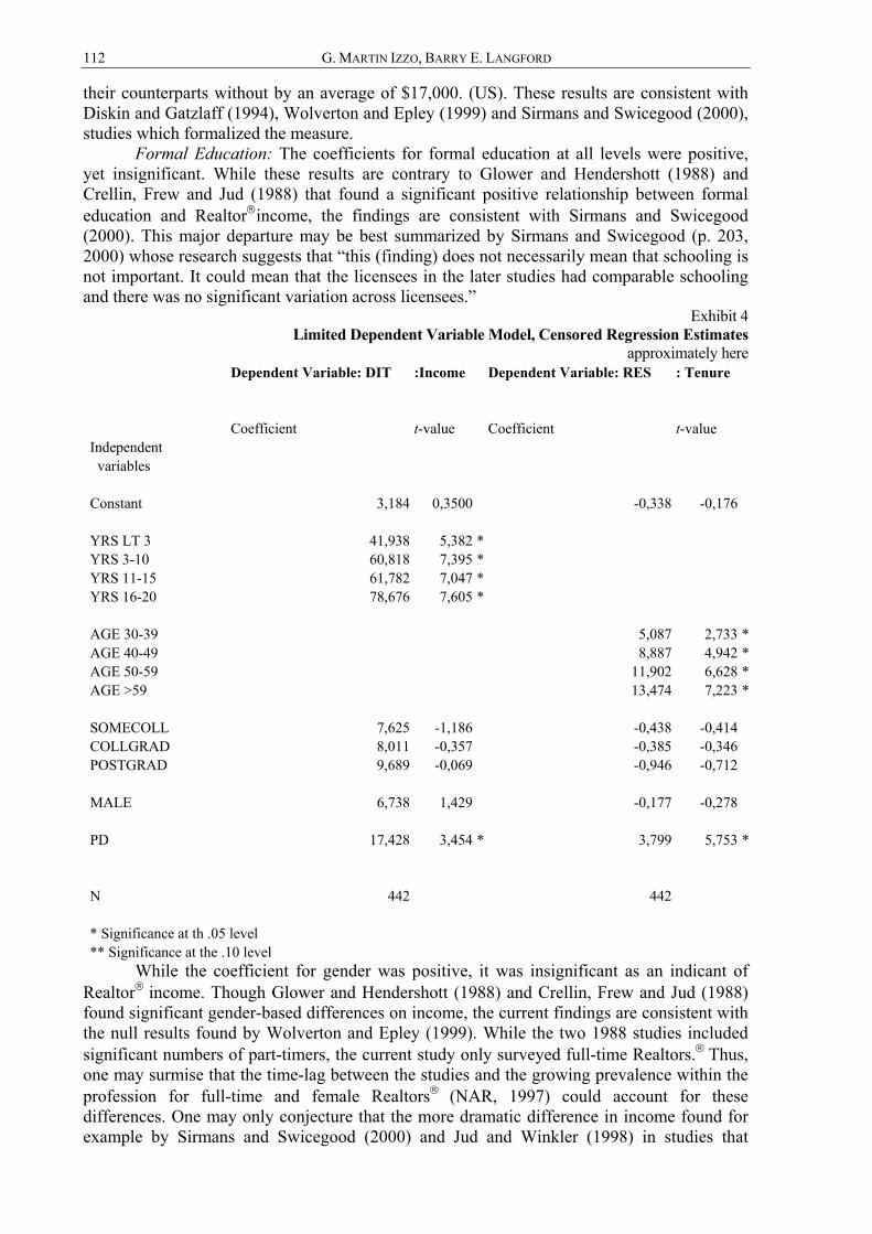
112 G. MARTIN IZZO, BARRY E. LANGFORD
their counterparts without by an average of $17,000. (US). These results are consistent with Diskin and Gatzlaff (1994), Wolverton and Epley (1999) and Sirmans and Swicegood (2000), studies which formalized the measure.
Formal Education: The coefficients for formal education at all levels were positive, yet insignificant. While these results are contrary to Glower and Hendershott (1988) and Crellin, Frew and Jud (1988) that found a significant positive relationship between formal education and Realtor®income, the findings are consistent with Sirmans and Swicegood (2000). This major departure may be best summarized by Sirmans and Swicegood (p. 203, 2000) whose research suggests that “this (finding) does not necessarily mean that schooling is not important. It could mean that the licensees in the later studies had comparable schooling and there was no significant variation across licensees.”
Exhibit 4 Limited Dependent Variable Model, Censored Regression Estimates
approximately here Dependent Variable: DIT :Income Dependent Variable: RES : Tenure Coefficient t-value Coefficient t-value Independent variables Constant 3,184 0,3500 -0,338 -0,176 YRS LT 3 41,938 5,382 * YRS 3-10 60,818 7,395 * YRS 11-15 61,782 7,047 * YRS 16-20 78,676 7,605 * AGE 30-39 5,087 2,733 *AGE 40-49 8,887 4,942 *AGE 50-59 11,902 6,628 *AGE >59 13,474 7,223 * SOMECOLL 7,625 -1,186 -0,438 -0,414 COLLGRAD 8,011 -0,357 -0,385 -0,346 POSTGRAD 9,689 -0,069 -0,946 -0,712 MALE 6,738 1,429 -0,177 -0,278 PD 17,428 3,454 * 3,799 5,753 * N 442 442 * Significance at th .05 level ** Significance at the .10 level
While the coefficient for gender was positive, it was insignificant as an indicant of Realtor® income. Though Glower and Hendershott (1988) and Crellin, Frew and Jud (1988) found significant gender-based differences on income, the current findings are consistent with the null results found by Wolverton and Epley (1999). While the two 1988 studies included significant numbers of part-timers, the current study only surveyed full-time Realtors.® Thus, one may surmise that the time-lag between the studies and the growing prevalence within the profession for full-time and female Realtors® (NAR, 1997) could account for these differences. One may only conjecture that the more dramatic difference in income found for example by Sirmans and Swicegood (2000) and Jud and Winkler (1998) in studies that
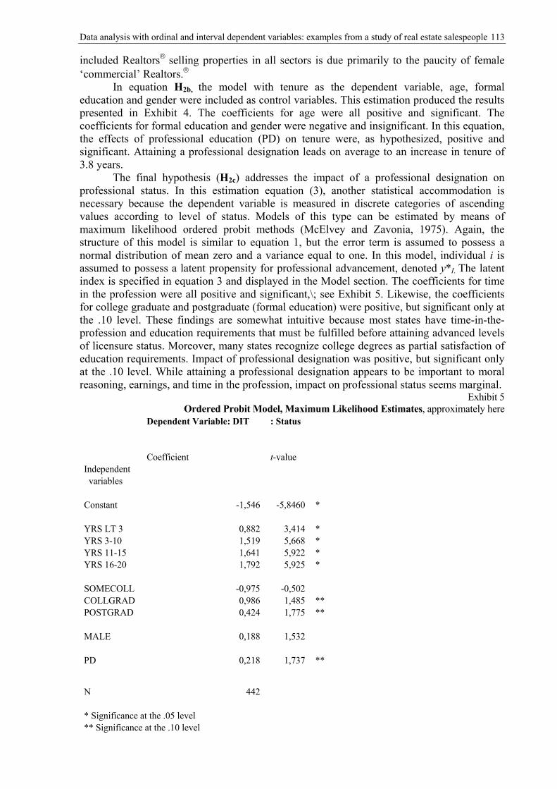
Data analysis with ordinal and interval dependent variables: examples from a study of real estate salespeople 113
included Realtors® selling properties in all sectors is due primarily to the paucity of female ‘commercial’ Realtors.®
In equation H2b, the model with tenure as the dependent variable, age, formal education and gender were included as control variables. This estimation produced the results presented in Exhibit 4. The coefficients for age were all positive and significant. The coefficients for formal education and gender were negative and insignificant. In this equation, the effects of professional education (PD) on tenure were, as hypothesized, positive and significant. Attaining a professional designation leads on average to an increase in tenure of 3.8 years.
The final hypothesis (H2c) addresses the impact of a professional designation on professional status. In this estimation equation (3), another statistical accommodation is necessary because the dependent variable is measured in discrete categories of ascending values according to level of status. Models of this type can be estimated by means of maximum likelihood ordered probit methods (McElvey and Zavonia, 1975). Again, the structure of this model is similar to equation 1, but the error term is assumed to possess a normal distribution of mean zero and a variance equal to one. In this model, individual i is assumed to possess a latent propensity for professional advancement, denoted y*I. The latent index is specified in equation 3 and displayed in the Model section. The coefficients for time in the profession were all positive and significant,\; see Exhibit 5. Likewise, the coefficients for college graduate and postgraduate (formal education) were positive, but significant only at the .10 level. These findings are somewhat intuitive because most states have time-in-the-profession and education requirements that must be fulfilled before attaining advanced levels of licensure status. Moreover, many states recognize college degrees as partial satisfaction of education requirements. Impact of professional designation was positive, but significant only at the .10 level. While attaining a professional designation appears to be important to moral reasoning, earnings, and time in the profession, impact on professional status seems marginal.
Exhibit 5 Ordered Probit Model, Maximum Likelihood Estimates, approximately here
Dependent Variable: DIT : Status Coefficient t-value Independent variables Constant -1,546 -5,8460 * YRS LT 3 0,882 3,414 * YRS 3-10 1,519 5,668 * YRS 11-15 1,641 5,922 * YRS 16-20 1,792 5,925 * SOMECOLL -0,975 -0,502 COLLGRAD 0,986 1,485 ** POSTGRAD 0,424 1,775 ** MALE 0,188 1,532 PD 0,218 1,737 ** N 442 * Significance at the .05 level ** Significance at the .10 level
114 G. MARTIN IZZO, BARRY E. LANGFORD
CONCLUSIONS This paper presented findings form an earlier study by Izzo and Langford (2003)
where several dependent variables that needed statistical accommodations were analyzed using LIMDEP 7.0, a statistical package that contains routines for estimating both the MLE for grouped data regression and the ordered probit models. The authors presented a basic discussion and analysis of the survey data which centered on research questions suggesting a positive relationship between cognitive moral development of real estate practitioners and attaining a real estate designation. As predicted in the underlying study by Izzo and Langford (2003), the effects of professional education were significant both in terms of cognitive moral development and career achievement.
The authors are members of review staff for several academic journals. This analysis emphasizes some common problems experienced during reviews of empirical manuscripts, especially those where the dependent variables are in ordinal or interval form. Manuscripts, that are otherwise well conceived papers, must often be turned away that do not control for these types of dependent variables or that attempt a ‘one size fits all’ approach to statistical analysis. While the underlying study is certainly not construed as perfect, the researchers did attempt to use the appropriate tools to go that direction. In spite of the complicated nature of the procedures used in the grouped data regression and ordered probit models, these estimations are surprisingly easy with readily available, packaged software applications such as LIMDEP.
Acknowledgements The first author gratefully wishes to acknowledge Bonnie Morris and Mary Poland of
the Stewart Library, North Georgia College and State University, for their correspondence with Internet library assistance to aid in the final preparation of this manuscript while I was overseas on a Fulbright Scholars program in Romania.
REFERENCES 1. Abelson, Michael A., K. Michele Kacmar, and Ellen F. Jackofsky (1990) Factors Influencing Real
Estate Brokerage Sales Staff Performance. Journal of Real Estate Research, 5:2, 265-75. 2. Aitchison, J. and S. Silvey (1957) The Generalisation of Probit Analysis to the Case of Multiple
Responses. Biometrika, 44, 131-44. 3. Aronson, Elliott and Judson Mills (1959) The Effect of Severity of Initiation on Liking for a
Group. Journal of Abnormal Psychology, 59, 177-181. 4. Benjamin, John D., G. Donald Jud, and G. Stacy Sirmans (2000) What Do We Know about Real
Estate Brokerage? Journal of Real Estate Research, 20 (1/2) 5-30. 5. Churchill, Gilbert A., Orville C. Walker, and Neil M. Ford (1985) The Determinants of
Salesperson Performance. Journal of Marketing Research, 22, (May), 103-18.
Data analysis with ordinal and interval dependent variables: examples from a study of real estate salespeople 115
6. Crellin, G., J.R. Frew and G. D. Jud, The Earnings of REALTORS: Some Empirical Evidence. Journal of Real Estate Research, 1988, 3:2, 69-78.
7. Daykin, Anne R. and Peter G. Moffatt (2002) Analyzing Ordered Responses: A Review of the Ordered Probit Model, Understanding Statistics, l(3), 157-66.
8. Diskin, B. A. and D. H. Gatzlaff, An Examination of the Earnings of Real Estate Appraisers. Journal of Real Estate Research, 1994, 9:4, 507-24.
9. Feldman, Daniel Charles, (1976b) A Socialization That Helps New Recruits Succeed. Personnel (Mar-Apr) 11-23.
10. Festinger, Lawrence A. (1957) A Theory of Cognitive Dissonance. Evanston, IL: Row, Peterson. 11. Follain, J. R., T. Lutes and D. A. Meier, Why Do Some Real Estate Salespeople Earn More Than
Others?, Journal of Real Estate Research, 1987, 2:1, 73-81. 12. Garvin, David A. (1993) Building a Learning Organization. Harvard Business Review (Jul-Aug),
78-91. 13. Glower, Marvin and P. H. Hendershott, (1988) The Determinants of REALTOR Income. Journal
of Real Estate Research, 3:2, 53-68. 14. Grant, E. Stephen and Alan J. Bush (1996) Salesforce Socialization Tactics: Building
Organizational Value Congruence. Journal of Personal Selling and Sales Management, 16 (Sum), 17-29.
15. Greene, William H. (1985) LIMDEP: An Econometric Modeling Program for the IBM PC, The American Statistician, 39, 210-24.
16. Hensel, Paul J. and Alan J. Dubinsky (1986) Ethical Dilemmas in Marketing: A Rationale. Journal of Business Ethics, 5, (1), 63.
17. Izzo, George (1997) Assessing the Relationship between Compulsory Ethics Education and the Cognitive Development of Real Estate Practitioners. An unpublished doctoral dissertation, University of Mississippi, Oxford.
18. Izzo, George (2000) Cognitive Moral Development and Real Estate Practitioners. Journal of Real Estate Research, 20 (1/2) 120-41.
19. Izzo, George and Barry E. Langford (2003) Realtor Designations as an Indicant of Cognitive Moral Development and Success in Real Estate Sales, Journal of Real Estate Practice and Education, Vol. 6(2), pp.191-202.
20. Jackson, Donald W., Stephen S. Tax, and, John W. Barnes (1994) Examining the Salesforce Culture: Managerial Applications and Research Propositions. Journal of Professional Selling and Sales Management. Vol. XIV, (4), 1-14.
21. Jones, Gareth R., (1986) Socialization Tactics, Self-Efficacy, and Newcomers’ Adjustments to Organizations. Academy of Management Journal, Vol. 29, No. 2, 262-79.
22. Jud, G. Donald and Daniel T. Winkler (1998) The Earnings of Real Estate Salespersons and Others in the Financial Services Industry. Journal of Real Estate Finance and Economics, 17:3, 279-91.
23. Kelley, Scott W. (1992) Organizational Socialization as Information Processing Activity. Human Organization, 42, 314-22.
24. Kohlberg, Lawrence (1969) Stage and Sequence: The Cognitive Developmental Approach to Socialization. New York: Rand McNally.
25. Kohlberg, Lawrence (1984) The Psychology of Moral Development: Essays on Moral Development. 2. San Francisco: Harper & Row.
26. Kohli, Ajay K., Tasadduq Shervani, and Goutam N. Challagalla. (1998) Learning and Performance Orientation of Salespeople: The Role of Supervisors. Journal of Marketing Research, 35 (35), 263-74.
27. Langford, Barry E. and Arnold, Danny (1990) What High Performance Salespeople Want in a Job. In Progress in Marketing Thought, Proceedings of the Southern Marketing Association, pp. 405-408.
28. Lord, Frank M. (1963) Elementary Models for Measuring Change. In C.W. Harris (Ed.) Problems in Measuring Change, Madison, WI, University of Wisconsin Press.
29. Louis, Meryl Reis (1980) Surprise and Sense Making: What Newcomers’ Experience in Entering Unfamiliar Organizational Settings. Administrative Science Quarterly, 25, (June) 226-50.
30. McKelvey, Richard D. and William Zavonia (1975) A Statistical Model for the Analysis of Ordinal Level Dependent Variables, Journal of Mathematical Sociology, 4, 103-20.
31. Porter, Lyman W., Lawlwer, Edward E., III, and Hackman, Richard J. (1975) Behavior in Organizations, New York: McGraw-Hill.
116 G. MARTIN IZZO, BARRY E. LANGFORD
32. Rest, James (1979) Development in Judging Moral Issues. Minneapolis: University of Minnesota Press.
33. Rest, James (1986) Moral Development: Advances in Research and Theory. New York: Praeger. 34. Rest, James and Darcia Narvaez (1994) Moral Development in the Professions: Psychology and
Applied Ethics. Hillsdale, N.J.: Erlbaum. 35. Schein, Edgar H. (1968) Organizational Socialization and the Profession of Management.
Industrial Management Review, 9, 1-16. 36. Sirmans, G. Stacy and Philip G. Swicegood (1997) Determinants of Real Estate Licensee Income.
Journal of Real Estate Research, 14 (1/2) 137-159. 37. Sirmans, G. Stacy and Philip G. Swicegood (2000) Determining Real Estate Licensee Income.
Journal of Real Estate Research, 20 (1/2) 189-204. 38. Stewart, Mark (1983) On Least Squares Estimation When the Dependent Variable is Grouped”.
Review of Economic Studies, (50) 19, 141-49. 39. Sujan, Harish, Barton A. Weitz, and Nirmalya Kumar (1994) Learning, Orientation, Working
Smart and Effective Selling. Journal of Marketing, 58 (Jul) 39-56. 40. Van Maanen, John (1976) Experience Organizations. In Organizational Careers: Some New
Perspectives, New York: John Wiley and Sons. 41. Van Maanen, John and Edgar H. Schein (1979) A Theory of Organizational Socialization. In
Research in Organizational Behavior, B.M. Staw (ed.) Greenwich, CT: JAI , 16-46. 42. Walker, Orville C., Jr., Gilbert A. Churchill and Neil M. Ford (1977) Motivation and Performance
in Industrial Selling: Present knowledge and needed research. Journal of Marketing Research, 14 (May) 156-68.
43. White, H. (1978) “A Heteroscedasticity Consistent Covariance Matrix and a Direct Test for Heteroscedasticity”. Econometrica (46), 817-838.
44. Wolverton, Marvin L. and Donald Epley (1999) Structural Analysis of U. S. Appraiser Income. Journal of Real Estate Research, (3)1,115-34.

Current Issues

PRO-CAPITALISM VS. ANTI-AMERICANISM IN 21ST CENTURY EUROPE
Sorin BURNETE*
Abstract. The topic of this article was inspired by a recent survey, carried out in several Western European countries, with the purpose of ascertaining the public’s expectations regarding the respective countries’ (and Europe’s) economic prospects for the first half of the 21st century. The questions were focused upon two chief issues: (1) Europe’s economic future within the context of contemporary global transformations; (2) the viability of the European economic systems. Concerning the former issue, one of the questions read: “Are you optimistic, pessimistic or neutral about the future of your country’s economy?” The French, Spaniards, Italians and even residents of the United States were rather skeptical at this point, the only optimistic being the Germans. To the question: “Do you think the European economy can compete effectively against other rising economies in Asia, such as China and India?”, distrust was even higher; over two thirds of the French interviewees gave a negative response. In the other countries, the skeptics’ share was lower but still higher than of those who answered affirmatively.1
If the above-mentioned answers could have, to a certain extent, been intuited, the questions regarding the latter issue yielded less predictable results. The subjects were asked to express a double option: between the capitalist economic system and other types of systems, on the one hand; between the European system of capitalism (admitting there is such a thing) and the American one, on the other hand. To the question: “Do you think a free-market, capitalist economy is the best economic system or not?”2, the majority of the interviewees (48 percent of the Germans, 49 percent of the Spaniards …etc.) gave affirmative answers, whereas regarding the type of capitalism they wished, most of the questioned European citizens rejected the United States’ economic system.
Why is Europe pro-capitalist? It is most likely because its prosperity owes much more to capitalism that to any other economic system. Of no less importance is the fact that all of the practical experiments of socialism have wound up in complete failure so far. In spite of that, the ideological dispute between capitalism and socialism has known a remarkable revival lately, a number of reputed scholars trying to demonstrate that both systems possess viable elements that is worth transmitting to the future.
Why is Europe anti-American? Answering this question is a bit more difficult. In the following pages, I’ll try to find some possible explanations.
“THE DEFINITION OF CAPITALISM STILL ELUSIVE”3 Capitalism, as a theoretical concept, has always been difficult to define. In the course
of the last one-and-a-half century – since it was first used by Marx until today – the term “capitalism” has never enjoyed a unanimously accepted definition. On the contrary, its use
* Sorin Burnete holds a Ph.D in International Economics, Professor at the “Lucian Blaga” University of Sibiu, Romania 1 Financial Times, Sept. 24, 2007, p.2 2 Ibid. 3 Ibid.
120 SORIN BURNETE
often triggered fierce ideological controversy. “The terms 'Capitalism' and 'Capitalistic Production' are political catchwords. They were invented by socialists, not to extend knowledge, but to carp, to criticize, to condemn. To-day, they have only to be uttered to conjure up a picture of the relentless exploitation of wage-slaves by the pitiless rich. They are scarcely ever used save to imply a disease in the body-politic.” (Mises, 1951)
The attempts to defend capitalism against its “enemies” were unsuccessful because of the extraordinary force of socialist ideas, which had seized the masses’ consciousness during the last decades of the 19th century. Thenceforth, capitalism would be defined preponderantly in opposition to socialism, obviously with the purpose to emphasize the latter’s virtues. Out of propagandistic reasons, not only the historical roots of capitalism but also its core principles and mechanisms would be systematically distorted by socialism’ advocates.
CAPITALISM “UNDER ATTACK”… The necessity to defend capitalism against the numerous attacks and detractors is a
theme that would recurrently appear in the liberal economic thought in the course of time. Actually, it would be reiterated by all Austrian School’s representatives. According to Friedrich Hayek for instance, “a lot of people would be surprised to learn that most of their beliefs about capitalism aren’t established facts but myths, fabricated for political purposes.” (Hayek, 1954) Despite their determination in defending capitalism against the tide of mystifications of all sorts, the Austrians as well as other schools of thought of liberal orientation were nevertheless unable to stave off the hard influence of leftist radicalism, much less to mitigate rampant prejudice about capitalism’s “evils”. The establishment of the soviet state, followed soon after by the ascendance of Maoism would further foster socialist ideas, igniting spirits of solidarity all over Europe, especially on the Seine’s banks. Many a progressive French intellectual would be spellbound and start exalting the stately achievements of the young communist states, largely viewed as capable of more sustained economic growth and fairer distribution of economic results relative to capitalism, the latter being presented in an ever more biased and heavily politicized fashion.
SOCIALISTS SEQUESTRATE THE FUTURE Yet with the time, such approaches became less and less persuasive. In fact,
socialism’s proponents were, from the outset, confronted with a dilemma: how to make inherent weaknesses of capitalism – which, according to Marx, will lead to its ineluctable demise – match its epoch-making achievements that no-one could deny. After all, the twentieth century civilization had been entirely built on capitalist bases. Therefore, there had to be found a new, decisive element that should render socialism’s superiority unquestionable. Since this particular thing didn’t exist, it could only be borrowed from the future; that’s were the solution lied. After all, according to socialism’s apologists, the new system did not simply emerge spontaneously; it had to be built. In brief, what they basically proposed was an eschatological solution.
This new tactic, relying on the relativity of the present and sequestration of the future was designed to release socialists from the increasing difficulty of explaining the hardships the system was being confronted with in practice. From the late 1970s on, no theoretical argument was strong enough to withstand reality: the conspicuous decline of communist societies, reflected in an ever more dented liberty, endemic poverty and widespread hopelessness. The gravity centre of ideological fight gradually moved away from the present toward the future, emphasis falling less on the past and present flaws of capitalism – from early capital accumulation to labor class pauperization to state-backed monopoly – and more on socialism’s extraordinary potential to secure humankind’s future progress.
Pro-capitalism vs. Anti-Americanism in 21st Century Europe … 121
AN INESCAPABLE DILEMMA In this new stage, the criticism of capitalism in antithesis with socialism became less
politicized, and hence more profound, focusing on the compared ability of the two systems to secure future economic progress. “The really important point in discussing the economic merits of socialism is not that of comparing the equilibrium position of a socialist and of a capitalist economy with respect to social welfare. Interesting as such comparison is for the economic theorist, it is not the real issue in the discussion of socialism. The real issue is whether the further maintenance of the capitalist system is compatible with economic progress.” (Lange, 1937)
The answer proposed by Lange to his own challenging question (quoted above) is of course, negative: capitalism as a system is, in spite of its past merits, incapable to bolster future economic development. Lange’s position relies on an older idea, exposed by Lionel Robins, according to which, in capitalism, there is striking incompatibility between the maintenance of the value of invested capital, on the one hand, and technical innovation, which leads to a decrease in costs, on the other hand. “The capitalist system seems to face an inescapable dilemma: holding back technical progress leads, through the exhaustion of profitable investment opportunities, to a state of chronic unemployment which can be remedied only by a policy of public investments on an ever-increasing scale, while a continuance of technical progress leads to the instability due to the policy of protecting the value of old investments which has been previously described.” (Lange, 1937)
OLD AND NEW MYTHS Due to a systematic propaganda by radical leftist ideologues, the popular mythology
about “rotten capitalism” and “wicked capitalists” became strongly anchored in the public consciousness and remained so until the present day, not only in Central and Eastern Europe – as one might expect – but, to a greater or lesser extent, in almost all Western European countries. Ironically enough, socialist ideas seem to have greater appeal to Western European high-schools and colleges then basic capitalist values. “A recent study of German high-school textbooks by the Institute for the German Economy in Cologne, found entrepreneurs – instead of getting credit for creating jobs – taking the blame for everything from unemployment to alcoholism to Internet fraud and cell-phone addiction.”4 “Ask any European what he learned at school about how the economy works and you’ll likely hear a similar story.”5
Since all these “truths” have been transmitted to the younger generations largely through the medium of school, it is no surprise that today, confusion among the youth is almost as high as it was in the 1960s. By then, a group of Marxist hardliners, led by Guy Debord and Jean Baudrillard inflamed young Parisians’ minds with revolutionary “ideas”, by depicting capitalism as a conventional spectacle, in which any genuine human experience will be turned into merchandise and then resold through publicity and mass media. According to Baudrillard, “the commodity has become so abstract that the economy is now nothing than a system of signs. The ‘needs’ that we express in the marketplace are not a reflection of any underlying set of real desires; they are simply a way of conceptualizing our participation in the symbolic system.” (Heath & Potter, 2005)
Although vulgar interpretations of this kind – reducing capitalism at a ‘system of signs and symbols’ – are no longer en vogue, the youth are still being told the same old story, especially in high-schools and colleges: “They taught us the market economy was a dangerous wilderness full of risk and bankruptcy…We never learned how prices affect supply and demand, only about evil managers and unjust wages.”6 Last but not least, perhaps the clearest evidence of European higher education’s obtuseness as regards teaching economics during the
4 Newsweek, August 14, 2006, p.36 5 Ibid. 6 Ibid
122 SORIN BURNETE
post-world era was provided by the very University of Vienna, where “the works of the great Austrian school of capitalist thinkers were all but ignored for more than half a century.”7
HISTORIANS LEND A HAND Judging by the above aspects, the doctrinarian confrontation between capitalism and
socialism seems endless and extremely hard to solve. However, when regarded through the eyes of historians, things will appear slightly different. Historians can have an ascendancy over economists, the latter being much too often inclined to overemphasize either mechanistic or normative aspects. Just to give an example, neo-classics – whose theoretical contribution could never be praised enough – were convinced their system was infallible. According to them, within a set of given hypotheses, a theoretical model of market economy would reach the Pareto optimal. It follows that considering other organization patterns is not necessary, since none could outperform the market system. (Nelson, 2003)
By contrast, historians’ vision is less biased and therefore, integrating and reconciliatory. “Capitalism is unconceivable without an active complicity on the part of society. Obviously it is a reality of a social and political kind and even a reality of civilization, because it is necessary that society, more or less consciously, should accept its values.” (Braudel, 1985) The famous French historian thus shifts the discussion onto a different plan. Although his position is not a direct conduit to reconciliation, it will nevertheless induce thinkers to attempt to bridge gaps and seek common points.
MARKET SOCIALISM…A SOLUTION? Market socialism thus stemmed from this particular dilemma: how to overcome the
limits of market economy, highlighted by Nelson, without forsaking the values of capitalism, referred to by Braudel? The proponents of the new paradigm believe they found the formula by which the two systems, capitalism and socialism might cohabit. The basic idea is “to combine the efficiency of markets with the egalitarian goals of socialism.” (Milonakis, 2003) If, as Nelson put it, market economy cannot deal effectively with certain fields of economic activity such as public goods, socialism can. The solution then must reside in a hybrid system – significantly coined “competitive socialism” – that should combine capitalism’s chief values (e.g. competitive resource allocation) with socialism’s (especially, public property over means of production). (Bardhan & Roemer, 1992)
Briefly, we are now “on a fresh page of history”. (Sennett, 2006) Not only have both systems managed to survive to this day but they are now closer to each other than anytime in the past. A genuine illustration of this happy “marriage” is being showcased by present-day China, whose economy has scored unprecedented growth rates lately but where liberty remains shackled. Neither did Marx’s prophecies – regarding the unavoidable death of capitalism – materialize, nor did socialism die after the collapse of totalitarian regimes in the late 1980s. But this makes figuring the society of the future even more difficult. What will it be like? It won’t be capitalist, according to some. (Drucker, 1999) It won’t be socialist either, if we were to judge by the major tendencies that are manifest in today’s world, with China as the leading example. But then…what is it going to look like?
GLOBALIZATION AND ITS CHALLENGES For the time being, we just know with pretty much certainty that Europe is, for its
majority, pro-capitalist, at least according to declarations, surveys, press articles etc. However, most of its citizens dislike the American model of capitalism, considered incompatible with Europe’s traditions and culture. How could one characterize this peculiar attitude? Does it rely on a rationale or it’s merely Americano-phobia, in fact, a pretty widespread sentiment throughout Europe? Strange as it may be, according to surveys,
7 Ibid
Pro-capitalism vs. Anti-Americanism in 21st Century Europe … 123
Europeans generally reject the American model of capitalism, which they nonetheless admit to have been the most effective in generating prosperity so far. This recognition is official, as revealed by various EU documents, e.g. the Sinclair report, published in 2003: “Over the past fifteen years the European Union (EU) has witnessed a big leap forward in its integration process... (but) the EU has underperformed in economic growth. This underperformance is all the more remarkable since it is relative not only to expectations but also to past European performance and to that of the United States…Further more, given that that the United States has achieved higher per capita growth relative to the EU through both higher levels of productivity and higher employment, this implies that the EU is actually operating inside the production possibility frontier or, in other words, is not using its resources to the full extent of their capacity.” (European Commission, 2004)
Why is the American model of capitalism so unpopular in Europe? Whatever the answer to this question, it will automatically draw the answerer into another type of dispute, at least as fierce as the historical fight between capitalism and socialism: the globalization “war”. Although written in inverted commas, the term “war” is not too hard; it expresses, literally, the manner in which the two opposing sides are interacting. What we are witnessing are not mere ideological confrontations but true guerilla warfare. “A guerilla army of anti-trade activists took control of downtown Seattle today” – read a Washington Post headline during the violent clashes that accompanied the WTO summit in December 1999. (McNally, 2002) Thus one can see the globalization war is more or less circumscribed to the free trade story, with the WTO acting the leading part. Yet this idea is dismissed by anti-globalization partisans, who claim globalization is not about free trade; rich countries which keep supporting it are no less protectionist today than they used to be three or four decades ago. According to them, the “free trade myth” is a weapon the rich world is wielding with the aim of bolstering the interests of multinationals and hurting the poor economies. However, “there is a middle ground between the extreme positions between the free-traders and the anti-globalizers. This middle ground recognizes that even if one accepts the ultimate desirability of free-trade, rushed liberalization may be harmful. Policies in the middle ground need to be found by investigating the effects of market failures on the experience of liberalization in different countries.” (Stiglitz & Charlton, 2005)
What is then the stake in the globalization war? Obviously, it’s the future of capitalism, under the auspices of which it is unfolding. It couldn’t possibly be otherwise. It is only a system of this kind – where the prevalence of private property is a guarantee for economic liberty – that could provide the required conditions for the unfettered movement of capital across national boundaries. From this standpoint, socialism could only accomplish a political globalization, probably very similar to the one the Soviets promoted during the 1960 and 1970s. Socialism could reign but over a parochial and virtually collectivized world. If today’s capitalist-type globalization is gradually eroding the power of sovereign states – assertion that nonetheless contains a trace of truth – Soviet-type interventionism led to the proliferation of totalitarian regimes and the economic ruin of the countries that fell under its influence.
AMERICANS’ BATTERED UNILATERALISM The generalized aversion against the American model of capitalism is therefore, up to
a certain degree, understandable. Many Europeans are perceiving globalization as a means to defend the US-based multinationals’ interests, thereby turning Europe into an annex of the United States’ economy. A number of unilateral actions, recently undertaken by the Americans largely contributed to the strengthening of this picture. In fact, according to American scholars, beginning with the second half on the 1980s, the US trade policy “had changed to embrace aggressive unilateralism”. (Bhagwati, 1995) The hassle around the Kyoto Protocol is a typical case in point. “The Bush administration did not merely reject the Kyoto Protocol; it declared that the United States would never sign the treaty and declined to offer
124 SORIN BURNETE
an alternative approach to global warming until many months later. And the justification that was given – that the treaty was ‘not in the United States’ economic best interests – was unlikely to appeal to a world that knows the United States is both a wealthy country and the largest producer of greenhouse gases. The administration did not just announce that it would not ratify the agreement…it took the further (and unnecessary) step of ‘removing’ the earlier US ‘signature’ from the treaty and then launched an aggressive diplomatic campaign to compel other states to reject the convention as well.” (Walt, 2005) Clearly enough, such unilateral actions (to which, one might add others such as the boycotting of China’s and Russia’s accession to the WTO, the use of the famous Super 301 to adopt economic sanctions against Japan, India and Brazil in 1989, the pressures exercised several times upon the IMF to bail out certain economies from financial crises etc.) have constantly fed widespread hostility against the American superpower, perceived as a menace rather than a stability factor.
GLOBALIZATION VIEWED AS AMERICANIZATION Since globalization is currently viewed as “the extension of capitalism throughout the
world, whereas multinational corporations are seen as the B-52s of capitalism and its global reach” (Bhagwati, 2004) and because this extension is being orchestrated by America, thereby strengthening its role as a global superpower, it isn’t difficult to understand why anti-globalization has come to be synonymous to anti-capitalism and further on, to anti-Americanism. Unfortunately, this is not a simple syllogism; it’s a reality. However, these feelings are not made manifest everywhere in the same way but have taken a variety of forms. While in the Islamic world for example, America is generally identified with the symbol of Western civilization, usually considered as being opposed to Islam, in many other Afro-Asian countries, it is being blamed for a lot of ugly practices like neocolonialism and other forms of political domination.
In Europe, anti-Americanism is more sweetened but no less biting and in most cases, unjustified. Although considered as “part of the family”, Americans are nevertheless often regarded with some kind of aristocratic superiority; actually, they are envied for their money but despised for being, allegedly, less cultivated. Moreover, throughout Europe, several types of Americano-phobia are to be encountered, the French variant being perhaps the toughest but also the most contradictory. Out of historical reasons, the French have always considered themselves morally obliged to defend the European values against the invasion of corporatist libertarianism (Korten, 1995), most of it of American origin. For nearly forty years, European anti-Americanism has swung between the “American defiance”, proclaimed during the 1960 by Jean-Jacques Servan-Schreiber and the „anti-American obsession”, admirably explained by Jean-François Revel in his well-known work, published in the early 2000s. In the mean time, the sentiments vis-à-vis the colossus across the Atlantic gradually shifted from fear to reverence and sometimes, even to hatred. Europeans’ arrogance often prompted them to hold Americans responsible for most of their incapacities and failures. (Revel, 2002)
WHY IS THE AMERICAN MODEL OF CAPITALISM UNPOPULAR? Obviously, apocalyptic visions such as Servan-Schreiber’s are no longer credible.
Since the 1980s, the amount of FDI from Europe to America equaled and even surpassed that from America to Europe. Consequently, European multinational corporations are now on a par with their US-based counterparts, in terms of global turnover and financial power. If during the first post-war decades the prevailing sentiment in Europe vis-à-vis the great potential of certain American giants like IBM, IT&T, Exxon or American Express was fear, the present criticism is focused preponderantly on macroeconomic aspects. The predilection of those who go around accusing America is the manner (considered onerous) in which the administration and the Fed understand to “manage” the global economic equilibrium. From this perspective, the huge current account deficit of the United States is often interpreted, not as a counterweight to the mercantilist-type policy of many other countries – especially China
Pro-capitalism vs. Anti-Americanism in 21st Century Europe … 125
and its smaller South-Eastern neighbors, which managed to accumulate huge amounts of reserves lately – but as a means by which the Americans are trying to get the largest slice of the globalization pie for themselves. The United States are being accused for pursuing a macroeconomic policy based on high trade imbalances and a systematic gap between spending and saving, thereby putting the global equilibrium in jeopardy. In other words, “Americans are often chided for spending too much and saving too little”.8 “The world produces increasingly more because America needs to consume more. There is no balance between America’s exports and imports. The nation that was autonomous and super-productive after the war has gradually become the hub of a system in which it is exercising more its vocation of a consumer and less the one of a producer.” (Todd, 2002)
Assertions of this kind are genuine samples of European anti-Americanism. The truth is America keeps on producing merchandise but evidently, it turns out other types of goods than it used to decades ago. Since in the early 1970s the Germans and the Japanese had already caught up with the Americans in a number of industrial branches (automobiles, chemical engineering, electronics etc.), who would have expected the latter to remain stuck in the respective fields? They naturally glided toward other domains and industries, where they held a technological advance relative to their European and Asian competitors. In reality, it isn’t the world that produces for America to consume (or “exercise its consumer vocation”) but exactly the other way around; it is America that must consume for other countries – pursuing an exacerbated mercantilism – be able to export their excess production. But this is still not the point: should China become the world’s workshop as analysts are foretelling, it is not America who will be most affected but very likely, legions of small nations like Romania and their neighbors in Eastern Europe, whose labor-intensive industries will be ruined. The Chinese tsunami already hit a great number of emerging economies as well as traditional industries in Western countries.
Briefly, the alleged consumption vocation of the Americans is not disruptive but rather supportive of global economic equilibrium. This can be inferred, among other things, from the delicate position of the dollar: it’s been depreciating against the euro, thereby hurting European exporters, but still has a high value relative to the youan, which means that US exporters are hurt in their turn. Secondly, US’s macroeconomic policy helps maintain the world equilibrium by keeping down interest rates. “America’s low saving and high consumption offsets the foreigners’ high saving and low consumption” – argues the chairman of the Fed, Ben Bernanke, a former Princeton University economist, who coined this phenomenon “the global savings glut”. 9 “Heavy saving oil producers and Asian nations had helped depress interest rates by keeping financial markets flush with cash.” 10 This situation is nevertheless expected to change in the long run, as emerging markets will be likely to save less and spend more. “The logic of the global savings glut suggests that, as the glut dissipates over the next few decades and thereby reduces the net supply of financial capital from emerging-countries, real interest rates should rise.”11
ANTI-AMERICANISM: A DISGUISE FOR ANTI-LIBERALISM If the American model is rejected, what can we say about the European model of
capitalism? What kind of a model could Europeans oppose to America’s? Unfortunately, this is hardly the case because there are several such models in practice, Europe being a big diversity “garden”. Institutional aspects that define various organizational patterns bear a deep national imprint, making any comparison with the US system difficult. “If countries possess significant institutional specificities, does it imply that each one represents a different model?” (Amable, 2004)
8 Newsweek, May 2, 2005, p.57 9 Ibid 10 International Herald Tribune, Sept. 12, 2007 11 Ibid

126 SORIN BURNETE
The answer is: maybe yes, maybe no; we couldn’t possibly know for sure. What we do know though, with pretty much certainty, is that America has so far outperformed Europe (and still ranks ahead of Europe) in a great number of domains; this mere fact – which Europeans generally admit – should strengthen (not weaken) confidence in the American model. If things are happening otherwise, there must be a psychological factor that prevents Europeans from judging objectively in this respect.
In fact, Europeans’ anti-Americanism, despite its historical roots and whatever its political motivations has always been used as a masque designed to dissimulate anti-liberalism (Revel, 2002), especially in big countries such as France, Germany, Italy etc., where popular resistance to economic and social reforms is toughest. Beyond its diversity of forms, European capitalism looks like a “hard nut to crack”; it is sclerotic and idiosyncratic. It is primarily for this reason that the American economic system is considered a threat rather than a solution.
REFERENCES 1. Amable B. (2004) – “Le modèle européen de capitalisme n'est pas en perte de vitesse”,
Problèmes économiques, 23 juin, 2004 2. Bardhan P., Roemer J.E. (1992) – „Market Socialism: A Case for Rejuvenation”, Journal of
Economic Perspectives, vol.6, nr.3 3. Bhagwati J. (1995) – “Aggressive Unilateralism: an Overview” (International Economics and
International Economic Policy, a Reader, 2nd ed., McGraw-Hill Inc. p.85) 4. Bhagwati J. (2004) – “In Defense of Globalization”, Oxford University Press, p.4 5. Braudel F. (1985) – La dynamique du capitalisme (Romanian version) , Corint, 2002, p.55 6. Drucker P. (1999) – The post-capitalist sciety (Romanian version), Polirom, 2002 7. European Commission (2004) – “An Agenda for Growing Europe” (The Sapir Report), Oxford
University Press, (www.oup.com) 8. Hayek, F. von (1954) – Capitalism and the Historians (Romanian version), Humanitas, 1998,
p.15 9. Heath J., Potter A. (2005) – The Rebel Sell, Capstone Publishing Limited, p.107 10. Korten D. (1995) – When Corporations Rule the World (Romanian version) Antet, 1995, p.181 11. Lange O. (1937) – „On the Economic Theory of Socialism: Part Two”, The Review of Economic
Studies, vol. 4, no.2 , p.128-130 12. McNally D. (2002) – Another World id Possible, Arbeiter Ring Publishing, Winnipeg, p.29 13. Milonakis D. (2003) – “New market socialism: a case for rejuvenation or inspired alchemy”
(Cambridge Journal of Economics, 27, 97-121) 14. Mises, L. Von (1951) – Socialism, an Economic and Sociological Analysis, New Haven, Yale
Univ. Press, p.122 15. Nelson R. (2003) – “On the complexities and limits of market organization”, Review of
International Political Economy („Les limites de l’économie de marché”, Sciences économiques, 10 nov. 2004)
16. Revel, J-F (2002) – L’obsession anti-américaine (Romanian version), Humanitas, 2004 17. Sennett R. (2006) – The Culture of the New Capitalism, Yale University Press, p.17-20 18. Stiglitz J., Charlton A. (2005) – Fair Trade for All. How Trade Can Promote Development,
Oxford University Press, p.115 19. Todd E. – Après l’empire. Essai sur la décomposition du système américain (Romanian version)
Albatros, 2003, p.84 20. Walt, Stephen M. (2005) – Taming American Power, the Global Response to US Primacy, W.W.
Norton & Co. Inc., p. 97

HISTORY OF IDEAS

FROM THE HUMAN CAPITAL DEFINED AS “HOMO OECONOMICUS RATIONALIS” TO THAT OF THE RATIONALLY BOUNDED AND OPORTUNISTIC “HOMO CONTRACTUALIS”. AN
INSTITUTIONALIST APPROACH
Ion POHOAŢĂ*
Abstract. The rationality (its presence or its absence) of the business, be it producer or consumer, has been a constant preoccupation of all those who dedicated their energy and talent on the sinuous road of the history of economic thinking. Without rational behaviour it was inconceivable to determine a development path. From this point of view the position of the great schools of thought is based, essentially, on two main approaches. The classics and the neoclassics had in mind the perfectly rational and well-informed individual. In reply, the institutional economy, in its old or new form (NIE), opposes to homo oeconomicus rationalis a narrow-minded and insufficiently informed homo contractualis. The consequences of this re-evaluation of the basics of the business’s potencies on the physiognomy of the theoretical approach and also on the results of practical actions are significant. Those linked to the bounded rationality hypothesis, an important operating concept in the analytical structures of NIE, may trigger debates on the theoretical basis of standard economics. Key words: bounded rationality, fulfilling, procedural rationality, opportunism,
incomplete contracts, AS IF, institution. JEL: A11, O11
1. INTRODUCTION The toughest reply NIE gave to neoclassic economics is related to the questioning of
the principle of rationality. Not the principle of rational choice but that of perfect rationality based on which there have been build the well-known models of the producer and the consumer, the main characters of the neoclassic age. Even with the “bounded” rationality only, which contradicts the Cartesian spirit of neoclassicism, NIE renders obsolete its function maximizing calculus and becoming a “special” social science, methodologically speaking. (Ménard, 2003:7)
The origins of the criticism of the (producer's or consumer's) Perfect Rationality Principle lie in the work of Th. Veblen and H. Simon.
More than a century ago, Veblen ridiculed the excessive hedonism of the neoclassic economic individual with these memorable words: “The hedonist conception on man is that of a computer operating, at the speed of light, with information on comfort and discomfort, oscillating like a homogeneous particle of the desire for happiness under the impulse of
* Ion Pohoaţă – Professor at The Alexandru Ioan Cuza University of Iaşi, coordinator of PhD programmes in
economics, Executive Director of Doctoral School in Economics
130 ION POHOAŢĂ
stimuli, carried around but still remaining intact… Self-imposed in the space of elements, it turns symmetrically around its own spiritual axis until it is caught in the parallelogram of forces where it follows the line of the resultant. When the impact force is depleted, it stops to rest, a particle of desire, self-sufficient as it used to be”. (Veblen, 1919:73-74) “The homogeneous particle” which Veblen had in mind perfectly resembles the “cubic centimeter” of homogeneous capital from J. Robinson’s Heresies, engaged in the same critical process of neoclassic “dogmatic invulnerability”. It is possible that Veblen thought of Edgeworth’s “diagram in a box” when he spoke about the “parallelogram of forces”, which includes, in a “rational” manner, pleasures and discomforts. In any case, Veblen’s words echoed. This is how H. Simon, claimed by the neoinstitutionalists as their spiritual mentor, adopts the individuals' “bounded rationality” hypothesis, accounting for the limited cognitive capacities and insufficient information. He is convinced that man is by far comparable to a programmable computer.
If this thesis, taken from H. Simon, including the sustaining arguments, turned NIE into a “special” social science, it is as true that bounded rationality had the effect of a Pandora Box. It has reignited debates on other principles, subsequent or adjacent to rationality, opened new and generous directions in research, and created a background for the disputes between the “crowned heads” of NIE. Here are some sequences of what embracing bounded rationality meant.
2. FROM MAXIMIZATION TO SATISFACTION “The introduction of bounded rationality hypothesis forces the economic researcher to
ask himself about agents’ motivation and the way they perceive and understand the environment in which they act. Indeed, agents do not always act towards maximizing their personal interest (they can, for example, to behave in an altruistic manner), and the manner they can decode their environment depends, partly, on the <<mental construction>> they have in their head” (Chabaud, Parthenay&Perez, 2004:4). This quotation, representative for the comments on North’s work, tells us, at least three things:
First: the agent’s perception of the environment cannot be a perfect one because of their limited cognitive capacity and imperfect information.
Second: this operation interferes with “the agents' motivations” which may be hedonistic or altruistic.
Third: “mental build-ups” have a major role in shaping the agent’s relation with the environment.
All of them sustain the hypothesis that the individual is not a perfectly informed robot and that he cannot set objectives that are beyond his power, he cannot hanker for optimizations or maximizations. If rationality is limited, the businesses can only ascertain a strategy that meets their prospects. This rule can be applied both for the producers and for the consumers. Louis De Alessi considers that, once the idea of “meeting the prospects” is accepted, it eliminates the familiar dichotomy between the firms' tendency to maximize their profits, on one side, and the one of families and consumers to maximize their utility, on the other (De Alessi, 1983:66). This dichotomy, we may add, is determined by the reminiscence of the Objective Theory of Value which penetrated the neoclassical structures with the help of its mentor – A. Marshall. Dichotomic or not, integrated or not in the rules of the zero-sum game imposed by the acceptance of “objectivity” of the value produced only by means of human work, individuals in the NIE environment share a common feature: “they try to maximize their objectives, which implies a detailed knowledge of the possible alternatives, high capacity to process related information as well as vast time periods available, to make choices; in reality, they settle with a <<satisfying>> (rather than <<maximizing>>) level in the pursuit of their goals and stop searching for additional alternatives when they have been reached” (Chavance, 2007:65).

From the Human Capital defined as ''Homo Oeconomicus Rationalis''… 131
3. IMPERFECT “MENTAL CONSTRUCTION”-IMPERFECT INSTITUTIONS. “PROCEDURAL RATIONALITY”
Veblen’s observation that a “mental construction” may also be “imbecile” has triggered over the years a vivid debate on the origin of inefficiency, a debate that is far from over.
Indeed, if we accept the idea that “the way in which individuals decode the environment” depends on their mental construction, which is the source for the creation of rules, then we can understand why North made such an effort to explain the persistence of inefficient institutions. Because there are, and the reality confirms it, inefficient institutions. They are the result of this chain of cause and effect: institutions = the reflex of mental construction; these mental constructions may be of higher quality or they may be “imbecile”; low-quality mental constructions = imperfect and inefficient institutions.
Faced with this scheme, one may cynically conclude that every nation has the institutions they deserve. We cannot stop here though, because neither neoinstitutionalists nor their supporters can.
Neoinstitutionalists offer three extra explanations and two solutions. The first explanation comes from biology. From this area and especially from
Darwin's theory, the theorists of economic evolution, via NIE, will find explanatory sources for what they consider to be “evolution” and “learning through imitation”. This is also the source for explaining the fact that not all individuals contribute to the same extent to the evolution of society.
The second explanation sends us to ideology (ideologies). We are particularly interested in the imperfect institutions in a country with a totalitarian ideology. In this case the institutions are “perfect” only for those in power; they assimilate these institutions and make them work for their personal interests. For all others these institutions are “imperfect”. Still, these institutions manage to survive in time. Why? Two motives are being considered:
a)It is possible that the “critical mentality” should take more time to be built; b) If the above mentioned period of time is too long, a kind of “perverted” behavior
may appear, even towards these institutions. It is possible that certain individuals, through the means of “efficient” indoctrination, start to consider “irrational” any deviation or breach, by other individuals, of rules that are “imbecile” from the beginning, but to which they got used and on which they conceive their image of the “rational”. In this case, the chance for these institutions to survive is extremely large.
The last explanation comes from North. He notices that the difficulty of rationally anticipating the future faced by the businesses is also influenced by the fact that mental constructions they use represent just a condensed history. The present is little or not at all embedded in them. “Individuals analyze the environment and solve their problems by treating the information using already existing mental schemes” (North, 1981:20). Hence, North concludes that the rationality of agents is limited also because they judge the present and anticipate the future through clichés which are linked to an already consumed experience! Is there another way? The fact that we use history to understand the present and make predictions about the future is extremely common. Not so for North, it seems.
The solution is found in a Hayekian manner, with reference to what is known as “procedural rationality”.
It starts from the premise, advocated by Hayek as well as by Misses, that the individual’s integration in the environment does not necessarily imply the understanding of the rules. They comply with and apply them not because they understand them, but for the fact that the results of their application lead to an accomplishment of their objectives. Once this is noticed, a great part of their behavior becomes a simple routine. The rational character of this rule is attained, hence, through an indirect route: through human behavior in accordance to rules determined by the satisfactory result. This is “procedural rationality”.
132 ION POHOAŢĂ
In the case of the second solution, neoinstitutionalists take into account a highly normative-charged solution. The fact is that institutions are, essentially, human creations, hence nothing stops from supporting the agents that have a low cognitive capacity with a set of institutions that make it possible to reduce uncertainty and risk.
4. LIMITED RATIONALITY – OPPORTUNISM - INCOMPLETE CONTRACTS
It has already been underlined the fact that NIE refuses complete information and perfect rationality philosophies, but not the model of rational choice. In the NIE environment individual behavior remains rational, with and within the stated limits. But the NIE environment is the real world, unlike the neoclassic one, “built” out of standardized images in order to provide the ideal picture, the Nirvana. In the NIE world everything changes. Everything is a succession of circumstances. In a world without patterns and fixed landmarks, any ex-ante –type of judgement lacks real importance. The bounded rationality of the businesses also contributes to this fact. They still have to reach their objectives, follow their personal interests. How it is possible to satisfy one’s own interests when everything is a “construction yard”? The solution proposed by NIE lies in opportunism: the business is “allowed” to “change” his behavior; in its pursuit of personal interest depending on the succession of circumstances.
Moral implications of opportunism appear to have had no influence on O. Williamson, preoccupied with setting up the trajectory of the business in a corporative governance framework. He tries, in order to “protect” himself, to relate to the philosophy of the school mentioned before writing that “this concept includes the classical and neoclassical view on personal interest (the simple <<search>>) and, eventually <<cheating>>.” (Williamson, 1979:234, our underline.-I.P.) Just as many other neoinstitutionalists, Williamson accounted for his own evolution inside some concepts. Hence, on this subject, in an interval of six years, he no longer shares the classical and neoclassical point of view and writes that “Through opportunism I understand self-interest seeking with cheating” (Williamson, 1985:47). The “subtle forms of cheating” are no longer referred to as in terms of “possibility”. While Williamson looks the other way when it comes to “lies, theft and cheating” understood as a sacrifice which has to be made in order to avoid any breach of the business’s freedom of movement, the other neoinstitutionalists seem not to feel comfortable with the dead end to which bounded rationality, via opportunism, takes this analysis. They have reasons to do so. Not for a moment have they thought that their “contractual individual” will be different from classic and neoclassic “economic individual” by being able to lie and cheat just to reach his objectives. It is difficult to find arguments to defend the image of a cheater within an economy designed to be one of “civilized” rules and institutions. The price paid to cross from the perfectly rational individual to the “real” one, imperfect and with limited rationality, seems to be too high.
Relativization of the ex-ante judgements due to bounded rationality, imperfect information and environment mobility … must, also, find itself a solution. For NIE it bears the name of “incomplete contract”. This is, obviously, an answer to the complete neoclassical contract, one filled with provisions on price, quantity, quality, terms of execution, etc. These are clearly established. The institutionalist environment of imperfections has little to do with strictness. Between the date of signing and the date of execution, “the succession of circumstances”, may change for a number of n-times the initial terms of the deal. Also, cognitive limitations prevent a one hundred percent anticipation of what is going to take place in this period. This is why neoinstitutionalists act cautiously. They have the doors open to an “incomplete contract”. Certain pledges no longer function; the parts agree to adapt the stipulations of their contract according to circumstances. And adapting means just as many renegotiations as there are changes that appear from the initial situation. When we talk about
From the Human Capital defined as ''Homo Oeconomicus Rationalis''… 133
adapting to circumstances we find ourselves on the similar field that provides “institutionalized” support for opportunism.
5. APPROXIMATING REAL BEHAVIOUR USING THE AS IF HYPOTHESIS
Just as Williamson finds in opportunism a refuge to reach a compromise between the business’s necessary freedom and his bounded rationality and power of anticipation, so does A. Alchian in using the AS IF methodological principle as an exit to saving, at least in appearance, the principle of necessary rationality. How does he do that? He transfers the problem to the market. For him, the dispute between rationality and irrationality has no meaning as long as the “battle” on the ground of rationality does not take place in the same space and at the same time when the working hypothesis is established. No, this confrontation takes place on the market. For Alchian, the market is the “selection environment”. All agents pass through its lattice. Only those corresponding to its functioning criteria are able to survive. Briefly, the market is populated by those who understand that they have no other alternative than responding to the “ungrateful” requests of minimal rationality: the cost must be lower than the income in order to leave place for profit. With regards to the actual size of the profit Alchian does not leave the line of thought of his school: not maximum profit, but accomplishment of goals. To justify the “modesty” of the business’s claims, he adds another element: the constraint imposed by risk and uncertainty. In his famous article from 1950, he builds a selection environment not only in constant movement, but also one above which there are floating the clouds of uncertainty (Alchian, 1950). And, how can one pretend, in such a framework, filled with uncertainty and unrest, maximum profit? Meeting the targets set will suffice. How does the environment – the market, solve this problem? By operating a selection and retaining only those who, even if they did not learn anything in school about the Hedonistic Principle and its marginal derivatives, act AS IF they knew everything or almost everything about this subject. In other words, the market operates by selecting “behavior models”. Those who pass through the “customs” are those who are in line with the rules of the environment. The amount of these rules stands for a condensed experience, consumed in the spirit of rationality. The businesses, also inspired by a rationalist spirit (but without being preoccupied by it) take this experience and imitate it. Rather than rewriting the history of , it is more comfortable (“rational”) to duplicate it and eventually, transmit it.
In conclusion, the rationality problem limited or not, does not derive, for Alchian, from inter-individual confrontations. Rationality is addressed to the selection environment – the market. It plays a vital and active role. By exposing themselves to its competitive environment, the businesses “find out” if their actions are more or less rational. And only those who behave according to the “AS IF” criterion and prove that that they know everything about the unwritten laws of rationality are integrated in the environment. With this spin, by sending the problem of rationality from the relations between individuals to the selection environment, Alchian thought he had saved the authentic principle.
134 ION POHOAŢĂ
BIBLIOGRAPHY: 1. Alchian, Armen (1950), “Uncertainty, Evolution and Economic Theory” Journal of Political
Economy, Vol. 58, pp. 211-221. 2. Chabaud, Didier, Parthenay, Claude, Perez, Yannick (2004), “Stability and Change în Northian
analysis: 1990–2004”, Groupe Reseaux Jean Monnet Working Paper, http://www.grjm.net/documents/Yannick-Perez/WP_CPP_2004.pdf
3. Chavance, Bernard (2007), L’économie institutionnelle, Paris: La Découverte. 4. De Alessi, L. (1983), “Property Rights, Transaction Costs and X-Efficiency: An Essay in
Economy Theory” American Economic Review, Vol.73, Nr. 1, pp. 64-81. 5. Ménard, Claude (2003), “L’approche néo- institutionnelle: des concepts, une méthode, des
resultants” Cahiers d’ economie Politique, No. 44, L’Harmattan. 6. North, Douglas (1981), Structure and Change in Economic History, New York: Norton. 7. Veblen, Thorstein (1919), “Why is Economics not an Evolutionary Science?” The Place of Science
in Modern Civilization, New York: B. W. Huebsch, pp. 56-81. 8. Williamson, Oliver (1979), “Transaction – Cost Economics: The Governance of Contractual
Relations” Journal of Law and Economics, Vol. 22, No.2, pp.233-261. 9. Williamson, Oliver (1985), The Economic Institutions of Capitalism, New York: The Free Press.

Book Review

„EASILY DIGESTIBLE ECONOMICS”. THE DRAGON AND THE ELEPHANT
Gabriela GAVRIL-ANTONESEI*
„By the time you have read it, you will know as much economics as you will probably ever need and more than the vast majority of the population.” (David Smith)
„Free lunch” and the author's portrait In an attempt to map out in words the portrait of David Smith, the Economic Editor of
„The Sunday Times”, well-known radio and TV producer in the UK, author of a couple of writings generally well-reviewed by the audience ( The Rise and Fall of Monetarism, From Boom to Bust, UK current economic policy, Free Lunch: Easily digestible economics, The Dragon and the Elephant. China, India and The New World Order), he seems to have captured the public's attention first and foremost through his thought-provoking and, at the same time, nonchalant way of approaching various complex economic topics.
Being well-familiar with the public's expectations, knowing very well his reluctant reactions to overly specialized writings, in the reading of which one needs too many dictionaries, patience and good memory; the journalist writer counts on a more straightforward, editorial style, based on quasi-narrative discourse, without neglecting the use of common questioning and amusements. His target does not exclude the educated public, but with little professional training in economics, who shows interest in the subject of inflation, the balance of payment or in other economic phenomena that influence his daily life. Perhaps the best example of how David Smith commits himself to making economy more accessible for his readers, is Free Lunch: Easily Digestible Economics, published in 2003. As he himself states, in the foreword, ingeniously entitled Appetizer, the author’s intention is to offer „an easily digestible book”. Moreover, „Unless something can be easily explained, it has no place here.”
Generously gifted with a ludic character, David Smith is often mixing rigorous research findings and empirical observations and definitions with humorous fragments, pertaining to his autobiography. He makes use of playful word combinations, even ironical citations, avoiding as much as possible getting stuck in the established jargon. He uses the colloquial style as well as the rigorous exposition of facts and data. Undoubtedly, his long journalistic experience shows out: he skillfully organizes his ideas, uses effective catch phrases, gives bold and humorous titles to lengthy analytical sequences, titles that makes us think of literary writings, entertaining productions or even cookery books, rather than of scientific textbooks.
Designed as a “free lunch” of five lectures, whose guest stars are Adam Smith, Karl Marx, John Maynard Keines, Milton Friedman, the book published in 2003, is a successful combination of rigorous data and entertainment, sweeping off the readers' concern that * Gabriela Gavril-Antonesei – Lecturer, PhD, Alexandru Ioan Cuza University of Iaşi
138 GABRIELA GAVRIL-ANTONESEI
economy would be inaccessible to ordinary man who does not claim to be an expert in this field. For example, the Cordon bleu chapter gets his “ingredients” from concepts such as monopoly, business, competition, prices, privatization, etc. In Bread and Money, there is a detailed discussion on topics such as monetary policy, inflation, the „output gap” and so on and so forth. For Desserts, important names of the American economy are called out (some known even for the mathematical insights they brought to the field), such as: Irwing Fisher, Paul Samuelson, Arthur Laffer. Arguing over coffee is an intriguing debate, without claiming to have reached some fundamental truths, on subjects such as poverty and the rich, globalization and its positive or malicious outcomes. David Smith also makes use with no hesitation of common sense expressions, comparisons that might as well make us smile, as he tries to explain abstract ideas by using concrete examples, and thus make it easier for the common reader to have an insight into intricate mechanisms and theories of economics. For example, he says at one point “economy is like when you play football” and “you cannot drive a car without oil, similarly one country cannot have inflation without money”. He genuinely debunks the taboos of scientific discourse and he does this in a nonchalant way, which may puzzle the excessively rigorous experts.
In a playful and relaxed manner, making the volume look like a full menu1, David Smith tries to satisfy his readers' appetite for economic debates, without overwhelming them with tables and „tricky diagrams” (his book contains only two equations, which is very uncommon for a contemporary economic book). Why not? He only tried to offer, aside from presenting and explaining theories and concepts, a fun, entertaining lecture. He invites us to have a good time, to “have a bite” of economic thinking; and warns us that „Economics dominates and shapes our daily lives, even when we are not aware of it. It is all encompassing.” His pedagogy, if it were for us to find one, is not concerned with producing overnight experts from his readers, but with bringing them to a certain level of insight and understanding. David Smith decides to make them have a grasp on those every-day aspects, pertaining to human development, which they would have omitted otherwise. Introducing the reader to economic topics should be, as the author believes, more than a dull presentation of raw data and materials, instead, it should be a continuous exercise of the mind, which brings along the ability to logically analyze and meaningfully understand socio-economic contexts.
The Dragon and the Elephant For a couple of years now, India and China continue to be „the hot economic story”;
there have been many papers written and debates organized on this issue. If we also include the media, with all the documentaries, tv and radio shows, and articles published, that focus on the “Two giants”, we can clearly see that the economic rise of China and India (which sent out a blast all around the world and continues to shatter it) has been a subject of great interest in economics, finance and business, even to media and the general public throughout European countries, US and Canada. Moreover, some people on the American business market, have recently talked about a certain „psychological dysfunction” creeping into the American society, as it attempts to foresee the extent to which “Chindia” (a term first introduced by Jairam Ramesh in his work Making sense of Chindia, then later on used in the title of a volume published in 2006, by Pete Engardio as editor) would change the face of global economy. This is nothing to be surprised of, as it has been the first time in the history of human kind when a country with huge population develops at such a rapid pace and to such an extent.
1 For example, as the table of contents shows it: Free lunch: Easily digestible economics (2003): Appetizer,
Starters, Main course (I), Adam – but not apple, Main course (II), Classical recipes, Cordon bleu business, Mulled Marx, Paying the bill, Keynes get cooking, Just Desserts – the Americans and, as an Addenda, for those still „hungry”, Bite-size glossary and Post-prandial reading.
„Easily digestible economics”. The Dragon and The Elephant 139
During one of his lectures, on the 24th of July 2007, on his book The Elephant and the Dragon: The Rise of India and China and what it means for all of us (W.W Northon & Company, 2007), Robyn Meredith pointed out that we need to understand what is going to happen in India and China, otherwise we may risk to be left behind. Along with the emergence of a global market place, as one Forbes journalist stressed out, the changes in India and China, spanning over the last centuries, sent out a “tsunami” which would profoundly impact the global economic tectonic plate. L. Allan Winters and Shahid Yusuf shared a similar view in Dancing with Giants: China, India and the Global Economics (World Bank Publications, 2007). Characterized by an exceeding growth in wealth, China and India may soon become, using various strategies, the main players in the global financial system: „Moreover, the growth of these giant economies will affect not only goods markets but also flows of savings, investment, and even people around the world, and will place heavy demands on the global commons, such as the oceans and the atmosphere.” According to Pete Engardio, China tends take monopoly over manual production, whilst India, an “emerging power” (M. Mohanty2), may soon become the “Center of Knowledge”. Therefore, Dancing with Giants (Winters& Yusuf), “without getting one’s toes stepped on”, seems to be, for an ever increasing number of companies, as complex as it is difficult.
David Smith's The Dragon and the Elephant. China, India and the New Order (Profile Books Ltd., 2007) ia a valuable contribution to the vast collection of works devoted to the subject of “Chindia”, and authored by various economists and journalists. The British author didn't change significantly his writing style and method for this particular book, as compared to his previous works. He admits from the very beginning, in a playful manner, that „The genesis of this book came, not in Beijing or Shanghai, or Delhi or Mumbay, or even from gazing into an economic crystal ball.”, but was instead triggered by an apparently innocent question, raised by a number of businessmen, mainly industrialists, during a discussion they had in London: „What about China and India?”. We can further state that the questions with regard to the role these superpowers have in world's economy are part of this century's “zeitgeist”. „What we will do when China and India do everything?”, „How will their markets be, and how accessible?”, “Will the Giants' influence be beneficial?”, “How much ground will US, Germany and other European countries lose before India and China?”, “What major changes will have to be made globally?”
But since the author does not actually have „an economic crystal ball”, he therefore raises significant questions, from various points of view, on this extremely vast and exciting issue, drawing on the preliminary premises for further analytical investigation, instead of trying to reach absolute answers. In the first chapter, The Return of History, he talks about the possibility that the recent economic boom of the two “Giants” may not be as surprising as it seems, instead it may actually be a second comeback of the world's state of affairs going back to 2000 years ago, when China and India represented 59% of the world's economic power. „The rise of Europe, North America and Japan – the author writes – has been, in his view, just a brief interlude in the grand historical sweep. (...) For most of the ancient and modern eras they were the twin pillars of the world economy, bastions of health and progress.” (pp. 8-9).
In order to support his theory, he finds evidence in historical data pertaining to the Chinese and Indian civilizations, from various sources, some of which have already been mentioned in economic literature. Once again, making use of common sense expressions, he says that „It takes a lifetime to understand China and perhaps longer, if that were possible, to get to grips with India”. The author admits that his point of view can in no way rival with scientific and cultural studies on China and India, neither with the current studies on this topic. Moreover, we have to mention that, unlike Robyn Meredith, Forbes's correspondent in Hong Kong, the British writer, only spent short periods of time in China and India, and therefore resumed to the “visitor's point of view”. As he could not rely on personal
2 M. Mohanty (Indian Institute of Management, Calcutta), L’Inde, une puissance émergente?, www.cerium.ca
140 GABRIELA GAVRIL-ANTONESEI
observations, David Smith tries to make a selection of the bibliographic material available, which he uses use for the historical part of this chapter, with regard to the evolution of the two countries, from the Arian migration, the first medieval Chinese dynasties, to the medieval times, Mao's “era”, Gandhi, up until now. He successfully outlines a plausible scheme that does not strike through any particularity. Far from making any bold affirmation in interpreting the data, the main relevance of the author's point of view consists of stressing the importance of historical perspective on the present economic status quo.
The transition of China and India from their initial condition of „pariah State”, and „economic backwater” to their actual status as global leading forces makes the focus of the next two chapters, Enter The Dragon and India Rising. The author is continuously bringing to our attention the interdependence created between political, social and economic aspects. He brings into discussion Deng Xiaoping's reforms after a long period of the Maoist line domination; but also, he talks about the Tiananmen massacre in 1989. He points out the constant economic growth of China, starting with 1978, which later on, during 2001-2005 ensured the country’s third position on the scale of global economic growth, and also the uncanny formula of a “socialist market economy”.
China’s opening up by expanding its market areas led to an unexpected flow of foreign capital, changed it into a real “magnetic force” for direct investments from all around the world, but this didn't completely solve all the economic and political weaknesses of China. India's development followed a similar route, from the image of violence and political instability in 1991, after Rajiv Gandhi's assassination, to its comeback on the market, in the “civilized”, economically prolific world. Although, as David Smith clearly points out, as compared with China, India had a slower start, implementing a couple of reforms merely 15 years ago, by the end of 2006, it had been showing an economic growth rate of 8%, for 3 years in a row. Perhaps that, despite the fact that some reforms proved inefficient, despite a feeble development after independence, despite the high corruption rate and social inequalities, yet unresolved, „there was a political method in the softly approach towards reform.” Was there a better strategy?
China Roars, and World Listens and India’s Networked Economy chapter ponders upon the ever increasing role the two “Giants” played in IT and telecommunications. The statistical data is indeed very impressive and seem accurately predict that by the year 2015, China will have become a technological superpower, while “the Communist Party is sitting on a powder keg of unrest that will one day explode” (p. 173). India tripled in a four-year period its “off-shoring” sector, outshined the other countries in IT, but has not yet found a solution to its social development crisis. „Is the glass half full, or half empty?”, rhetorically asks the author, coming back to an informal style, after having presented the statistical data and reports. In the chapter entitled China versus India he attempts a comparison between the two “Giants”, not only from an economic perspective, but also with regard to each country's underpinning mentalities (the continuous endeavor that the Chinese have always valued, obsessed with the idea of “growing” and trespassing the barriers of time; the Indian people's slow pace, from the European's point of view, obviously); with regard to the way each country's policy, protecting the human rights, dealing with unemployment, the banking system, the entrepreneurial spirit, urban and environment related policies.
In the last chapter, Ten Ways China and India will (and won’t) Change the World, the author comes with a well-thought Decalogue that successfully encompasses the contradictory complexity of how the two “Giants” may influence the world economy. Why won't they change the world? Because: 1. „They are the biggest thing to hit the world economy”; 2. „But they are not so big as they seem”; 3. „They will stretch the world resources”; 4. „But they won’t destroy the planet”; 5. „They will flex their diplomatic and military muscles”; 6. „But they won’t start a new Cold War”; 7. „They will provide huge market opportunities”; 8. „But they will remain relatively poor”; 9. „They will hit turbulence and trigger protectionism”; 10. „But they don’t change the rules of globalisation.... for the poor.... and for the rich...”

„Easily digestible economics”. The Dragon and The Elephant 141
Apart from the author's sense of humor, which we noticed on several other occasions
(even Lech Walensa made a humorous comment, that he is „for and even against” this idea), the journalist instinct must have guided him towards a very inspired way to end his volume. The topic stays open, fascinating and alarming at the same time, any radical position on the topic being thus ridiculed. Although the topic he chose had always attracted numerous authors, David Smith has once again successfully written another “digestible”, intelligent and informative book.

ROCKEFELLER’S MEMOIRS
David Rockefeller, Memoirs, RAO Publishing House, 2007
Nicoleta DABIJA*, Gabriel CUCUTEANU**
The famous Memoirs of the equally famous David Rockefeller, published in English in 2002 and, more recently, translated into Romanian (2007), tells the story of a prominent family who ruled over the economic and banking system in America and, therefore influenced the World's economy.
It all started with John D. Rockefeller, the author's grandfather, whose wealth soared, after founding and leading the Standard Oil company, and thus being regarded as the „richest man in America”.
Standard Oil gradually gained control over 90% of the market in oil industry, showing an increasing tendency towards monopoly. But in 1911, the trust was led to dissolution, after being thrown in litigation for a period of time.
John D. Rockefeller, despite not having pursued economic studies, understood the concept of „demand elasticity”. From his point of view, doing business was not consecutive to the market being in demand; he realized it was important to create that demand by controlling the way the products are distributed.
David Rockefeller was impressed with his grandfather's ability to stay calm and maintain his self-control despite the numerous attacks he had to face from his opponents, on one hand, and with the determination and drive he displayed in pursuing his goal, to consolidate the American oil industry.
He was a Christian who lived after the strict regulations of baptism, and his faith largely contributed to his success, along with the „art of giving” which he patronized after leaving Standard Oil, in 1897, and which became a long-living tradition of the Rockefeller family.
His philanthropic actions were not random, but fell under the rule of ten, which means that he gave one tenth of his revenue to charity. He saw charity as part of his responsibility towards the community which brought him up and educated him. But this responsibility was not just about giving, but about giving wisdom, in a well thought-out way, which is consequently an even more difficult task.
We can here name the establishment of the University of Chicago in 1980, founding the Rockefeller Institute for Medical Research in 1901, which later on became the Rockefeller University, and the Rockefeller Foundation, the first global oriented philanthropic organization, and finally the way he thoughtfully managed the funds made available for charity, in 1913.
This philanthropic tradition is carried on by the author's father, who considered the Rockefeller family as being blessed and therefore felt he had the duty to give something in return to the community. He also generously endowed the Rockefeller Fund, which soon * Nicoleta Dabija holds a PhD in Philosophy ** Gabriel Cucuteanu is a PhD Student, Alexandru Ioan Cuza University of Iaşi

144 NICOLETA DABIJA, GABRIEL CUCUTEANU
became one the top ten Fund centers, and his children had to continue his work in this direction.
David Rockefeller, the author of the family's memoirs and his grandfather's favorite, studied at Harvard and completed a PhD in Economics. His theory on business was that it had to have a purpose and bring along pleasure by attaining it, and contribute to the construction of valuable, long-lasting realities. He also thought that in business one needs the same qualities that one looks for in a true friendship relations, and these are trust, understanding and loyalty.
He made a career at the Chase National Bank, also known as “the Rockefeller Bank”, where he worked for 35 years, starting in April 1946, as soon as he came back from war. His action plan involved opening new branch offices, buying local banks and spread the Bank's activity internationally. The main reason was that, if he wanted Chase to be a leading organization it had to compete internationally for a good share of the foreign trade, even by risking to distance itself from the correspondent banks throughout the world.
He became chairman at Chase in March 1969 and promptly expressed on this occasion which were the six main directions that the bank was going to focus on under his stewardship: to lead the bank towards an international expansion; ensure a professional approach of the Human Resources; set up a more detailed organizational plan; further develop the marketing strategies; update the existing technology and take up a certain social responsibility with regard to the relation that the institution has with the community , since the quality of this relation generally bears a tremendous influence on the public image of that institution.
To meet with these objectives, David Rockefeller discloses the names of very important people he had therefore contacted; the essential tasks he had to complete, the level of success he had achieved. He seems to be puzzled by the Soviets' ignorance who did could not know the intrinsic mechanisms of a pluralist democracy and who thought that the State's officials, the president included, were playing by the rules of the Rockefeller family, imposed by virtue of their economic power. Moreover, they didn't understand the necessity to hold a completely convertible currency in order to become a leading global power; which to them seemed impossible as they were staying truthful to the Marxist dogma, as a repressive-authoritarian society.
When turning to China, once Deng Xiaoping took over leadership from the Maoist line, David Rockefeller finds a certain tolerance and openness to new ideas. Deng thought China had no choice but to mend and improve its relations with the developed countries and continue with the reform. He regarded the 21st century as the “Asian Century”, although he knew very well his country would further depend on the Occident, due to technology and capital.
In the Arabian world, it was Nasser who represented the Pen-Arab vision and the socialist ideas of the first Arabian reformers. The Saudi people were very attached to the structure and beliefs of the traditional Islamic society, and relying on their vast oil resources. They were the only ones to maintain a constant, firm alliance with the Americans, the rest of the Islam world continuously exerting pressure on the latter ones in order to win over the Palestinian territory and become independent from the USA.
Another interesting aspect that we can further consider in his work is what he mentions the relations within the family, that there is always a risk in the case of rich families, for affection to be replaced with the concern for the bank deposit, a risk that instead of enjoying purchasing anything there would be the fear of taking up undesired, high responsibilities or the doubt the one is not competent enough to take over and further prosperity within the family's tradition. But despite the turmoil caused by all these tremendous responsibilities, despite the fights between fathers and sons and among brothers, the Rockefeller family is still a brilliant example of invincible persistence due to this pervasive quality, over generations, to keep on going, despite rumors, failures and difficulties.

Rockefeller’s Memoirs 145
David Rockefeller's Memoirs, written when the author reached 88, can be extremely appealing to the uninitiated reader, passionate about reading the biography of a famous family, as they are to experts in economy or to historians focused on the 20th Century America, when the Rockefeller family played a crucial historical part.


CASE STUDIES

ORGANIZATIONAL HEALTH ASSESSMENT: A ROMANIA FIRM CASE STUDY
Shaomin HUANG*, Gerald W. RAMEY**
Abstract. Other than measuring units of output or profit to evaluate organization performance, this research develops a new assessment concept, organizational health. The survey of Work Environment Scale as the foundation data for the System-wide Interpretation of Health and Quality was used in this case study on a Romania firm. Structural measurement on organization effectiveness, leadership, and term work efficiency was conducted and further explained by three dimensional graphs with a weighted least squares method. The system-wide assessment shows multiple causalities among the endogenous variables. Key words: Organizational Assessment, Leadership, Organizational Health JEL: L21, L25, L26
1. INTRODUCTION Although the principles of economics have been not changed significantly in the last
century, people now look at the world in different ways as globalization and global warming are more obvious. In the business world, organization climate has been paid more attention since inclement market competition following globalization. Even for small firms, seeking short-term profit is not enough for long term survival and growth. Researchers also study newer patterns and the factors which can impact on organization performance, organization climate, and organization behavior.
Organization performance is often measured by effectiveness. With many intense factors as global competition, downsizing, total quality management, and decreased funding in the public sector, it is becoming more difficult to determine whether an organization is meeting performance standards. Organizations can no longer look to single variable measurement of items produced and isolated issues as valid determinants of organizational effectiveness. Reflecting on the concept of interdependence, each part of any system depends on every other part. This is very consistent with a broad based multivariate assessment of organizational effectiveness. Seashore (1993) and Denison (1996) both consider the complexity of diagnosing organizational performance and suggest that climate at least be considered as a valid measurement of organizational effectiveness. In three separate research studies directed toward organizational performance, the authors approached their issues from broad perspectives. Each study used terms such as multidimensional, employment system, and two dimensions to describe their research. However their findings did show positive linkages of single variables to increased organizational performance. The multi dimensionality of entrepreneurial orientation was the major focus of their study, however * Shaomin Huang – Lewis-Clark State College ** Gerald W. Ramey – Eastern Oregon University

150 SHAOMIN HUANG, GERALD W. RAMEY
Lumpkin and Dess (1996) also indicate that previous work has consistently linked innovation to increased performance. Ainsworth-Land (1986) also indicated that innovation is transformative. Delery and Doty (1996) showed that human resource practices and an organization’s employment system have positive significant impact on organizationally relevant performance measures. More specific to this study, they included participation/voice (involvement) as one of seven key human resource practice variables and did find it positively linked to organizational performance. Button, Mathieu, and Zajac (1996), while focusing on the complexity of goal orientation, indicate that attention to task performance is one of several positive relationships to increased organizational performance.
Organizational climate is clearly linked with leadership, but theories in this area are still in their infancy. It appears that the research on leadership is not doing all that those interested in this field would like (Bass 1981) and (Scott 2003). Zammuto (1982), Harrision (1987) and Heifitz and Laurie (2001) studied the designated and visible leaders within any system, and Burns (1978), Bass (1981), and Gleick (1987) indicate limited impact of designated leaders on selected variables within a system. According to Burns (1978), McCall and Lombardo (1978) and Gellis (2001) real leadership only happens when connections are made between the top and the bottom and throughout the system. Although there are some outstanding developments in the study of leadership theory and the delivery of leadership education, such as Lemon (1988), Bennis (1996), and Quinn and Spreitzer (2001) widely used theories and leadership training do not adequately address the results intended. In the 1990s, critics of leadership research continually pointed out deficiencies, most of which revolved around the lack of understanding and observations within the entire system. Senge (1990), Deming (1992), and Scott (1993) indicate a paradigm shift that is moving the locus of control downward in all systems. However, most leadership research has not connected multiple variables of outcome and leadership throughout the system. Edwards and Parry (1993) applied polynomial regression equations and response surface methodology to develop an interpretive framework and illustrate the relationships of difference scores of person-environment study in organizational research. Bennis (1996) discussed several factors that indirectly link autonomy to leadership. Empowerment, independence, freedom, and personal belief in the job are all part of what creates positive leadership within an organization. That takes autonomy. Handy (1996) , in his conversation on the future of work, talks freely of independence and indicates that the chaos of the future will necessitate individuals who may be selling skills to several clients or employees, or operating as independent units within an organization. His perspective seems to predict that the successful organizations will allow autonomy within the workforce. Chief executive officers recently have expressed concern over all junior managers following the excessive control models of some senior executives. Based on that assumption it is theorized that excessive control will decrease leadership within a system. Banker, Lee, Potter, and Srinivasan (1996) hypothesized and found significant that excessive monitoring led to smaller performance impacts. Oldham and Cummings (1996) found that 171 employees from two manufacturing facilities responded to leadership and produced the most creative work when supervised in a supportive manner. Also, using a concept of “conversations for accountability,” Fry (1995) suggests that leaders and supervisors in an open, non-threatening, and supportive forum will shift behavior from finger pointing into an “enabling organizational practice.” While leadership research is certainly increasing, the concept lends itself to a wide range of academic and practitioner approaches to determining what it is and how it impacts organizations.
Organization behavior is related with team work efficiency. Once again, a broader view of several dimensions is needed and the variables of clarity, peer cohesion, and work pressure are believed to have an optimal interaction to reduce destructive conflict, which increase team work efficiency. Four different articles from different types of journals were selected to show an established relationship between these variables and conflict within the organization. While not using the word clarity in their article, Heady and Smith (1996)

Organizational Health Assessment: a Romania Firm Case Study 151
certainly point to reduced noise and conflict within the organization when there is common meaning, two-way communication, and clear intent between leader stimulus and follower response. Kabanoff (1991) sets a proposition that decreased social integration and loss of cohesiveness increases potential conflict. He presents compelling discussion that the loss of social cohesiveness and the loss of sense of community constitute critical and growing problems for organizations that do not place adequate emphasis on the quality of cohesiveness. Gruenfeld, Mannix, Williams, and Neale (1996) found that direct and indirect conflict is impacted by peer cohesion in that “familiar groups may be better equipped psychologically to resolve conflicts effectively” and strangers “may lack the social ties and interpersonal knowledge” to effectively reduce destructive conflict. Reich (1996) stated “Every time a company engages in a large-scale downsizing, a chill is sent through the living rooms of millions of working families who think they could be next.” His interview is focused primarily on downsizing and the breakdown of implicit social compacts between company and employee that greatly contribute to worker anxiety. However, Reich suggests that this and other types of work pressure will cause much conflict in the organization. One impact of this type of conflict will be reduced loyalty of the work force, and it is not certain that many organizations can sustain that loss of loyalty.
2. MODEL AND DATA Human organizations, no matter if they are profit or non-profit, cannot be separated
from the basics of human behavior. These representative findings from a literature review reinforced opinions connecting each of the specific variables above to the major issues in this study; organization effectiveness, leadership, and efficiency. The measurement of three factors can represent the organization environment scale. This study also uses a broader perspective to include the connections of all the variables under study and also links specific variables to particular issues. In an institution, organization effectiveness, leadership, and team work efficiency are mostly unobserved variables. These three variables are latent variables in our theoretical model, which can be represented by some observable multi-causal endogenous variables (see Figure 1). These endogenous variables and other exogenous variables can then be used to construct a latent variable model. Since these three factors are complicate concept, they should be presented by multiple observable variables. In this study, we use three related endogenous variables in combination to measure each of these three complicated concepts. Organizational Effectiveness can be represented by task orientation, involvement, and innovation. Leadership can be represented by control, supervisor support, and autonomy. Team Work efficiency can be represented by clarity, peer cohesion, and work pressure. Together, the nine individual variables, and collectively grouped into the three major categories of Team Work Efficiency (a lateral view), Leadership (a hierarchical view) and Organizational Effectiveness (a system wide view) form the System-wide Interpretation of Health and Quality and provide a very information rich appraisal and analysis of the system’s Organizational Health.
PROPOSITION 1 (organizational effectiveness):
a) Strong attention to task orientation will lead to higher organization effectiveness. b) A more involved work force will lead to higher organization effectiveness. c) An increase in innovative practices among workers will lead to higher organization
effectiveness. d) Optimal interaction among the variables of innovation, involvement and task orientation
(collectively, not individually) within the work force will improve organization effectiveness.
Task Orientation measures the degree of emphasis on good planning, efficiency, and getting the job done. Involvement is defined as the extent to which employees are concerned about and committed to their jobs. Innovation measures the degree of emphasis on variety,

152 SHAOMIN HUANG, GERALD W. RAMEY
change, and new approaches. Increased organization effectiveness can be defined as increased organizational performance, however what measures are appropriate is more difficult to conclude. Three separate variables - task orientation, involvement, and innovation- are shown to have positive relationships with organizational performance, hence organization effectiveness.
PROPOSITION 2 (leadership):
a) An increase in appropriate supervisor support will lead to more leadership within the organization.
b) A decrease in excessive control mechanisms will create more leadership within the organization.
c) An increase in autonomy will increase leadership within the organization. d) Optimal interaction among the variables of autonomy, control, and supervisor support
(collectively, not individually) within the work force will improve leadership in the organization.
Supervisor Support is defined as the extent to which management is supportive of employees and encourages employees to be supportive of one another. Control is defined as the extent to which management user rules and pressures to keep employees under control. Autonomy is defined as the extent to which employees are encouraged to be self-sufficient and to make their own decisions. These three variables all have positively represented relationship measurement. Good leadership will improve organizational performance.
PROPOSITION 3 (team work efficiency):
a) Increased clarity in all communication will reduce destructive conflict in the organization.
b) An increase in cohesiveness among peers within the work force will decrease destructive conflict in the organization.
c) A reasonable release in work pressure will decrease destructive conflict in the organization.
d) Optimal interaction among the variables of clarity, peer cohesion, and work pressure (collectively, not individually) within the work force will reduce excessive and destructive conflict in the organization.
Clarity is defined as the extent to which employees know what to expect in their daily routine and how explicitly rules and policies are communicated. Peer Cohesion is defined as the extent to which employees are friendly and supportive of one another. Work Pressure measures the degree to which the press of working and time urgency dominate the job milieu. Team work efficiency is one of the most important elements in the modern organizations. Clarity and peer cohesion have positive relationships with team work efficiency. However, optimal level of work pressure is necessary to increase team work efficiency.
PROPOSITION 4: Assessment on organization effectiveness, leadership, and team work efficiency
showing multiple casualty effects is a valid and appropriate method of evaluating organizational health.
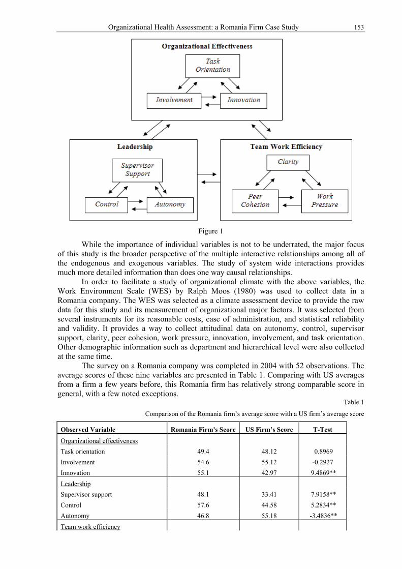
Organizational Health Assessment: a Romania Firm Case Study 153
Figure 1
While the importance of individual variables is not to be underrated, the major focus of this study is the broader perspective of the multiple interactive relationships among all of the endogenous and exogenous variables. The study of system wide interactions provides much more detailed information than does one way causal relationships.
In order to facilitate a study of organizational climate with the above variables, the Work Environment Scale (WES) by Ralph Moos (1980) was used to collect data in a Romania company. The WES was selected as a climate assessment device to provide the raw data for this study and its measurement of organizational major factors. It was selected from several instruments for its reasonable costs, ease of administration, and statistical reliability and validity. It provides a way to collect attitudinal data on autonomy, control, supervisor support, clarity, peer cohesion, work pressure, innovation, involvement, and task orientation. Other demographic information such as department and hierarchical level were also collected at the same time.
The survey on a Romania company was completed in 2004 with 52 observations. The average scores of these nine variables are presented in Table 1. Comparing with US averages from a firm a few years before, this Romania firm has relatively strong comparable score in general, with a few noted exceptions.
Table 1
Comparison of the Romania firm’s average score with a US firm’s average score
Observed Variable Romania Firm's Score US Firm’s Score T-Test
Organizational effectiveness Task orientation 49.4 48.12 0.8969 Involvement 54.6 55.12 -0.2927 Innovation 55.1 42.97 9.4869** Leadership Supervisor support 48.1 33.41 7.9158** Control 57.6 44.58 5.2834** Autonomy 46.8 55.18 -3.4836** Team work efficiency
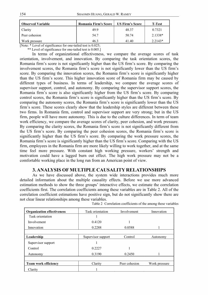
154 SHAOMIN HUANG, GERALD W. RAMEY
Observed Variable Romania Firm's Score US Firm’s Score T-Test
Clarity 49.9 48.37 0.7321 Peer cohesion 54.7 50.74 2.1338* Work pressure 46.3 41.40 2.2143*
[Note: * Level of significance for one-tailed test is 0.025; ** Level of significance for one-tailed test is 0.005.]
In terms of organizational effectiveness, we compare the average scores of task orientation, involvement, and innovation. By comparing the task orientation scores, the Romania firm’s score is not significantly higher than the US firm’s score. By comparing the involvement scores, the Romania firm’s score is not significantly lower than the US firm’s score. By comparing the innovation scores, the Romania firm’s score is significantly higher than the US firm’s score. This higher innovation score of Romania firm may be caused by different types of business. In terms of leadership, we compare the average scores of supervisor support, control, and autonomy. By comparing the supervisor support scores, the Romania firm’s score is also significantly higher from the US firm’s score. By comparing control scores, the Romania firm’s score is significantly higher than the US firm’s score. By comparing the autonomy scores, the Romania firm’s score is significantly lower than the US firm’s score. These scores clearly show that the leadership styles are different between these two firms. In Romania firm, control and supervisor support are very strong; but in the US firm, people will have more autonomy. This is due to the culture differences. In term of team work efficiency, we compare the average scores of clarity, peer cohesion, and work pressure. By comparing the clarity scores, the Romania firm’s score is not significantly different from the US firm’s score. By comparing the peer cohesion scores, the Romania firm’s score is significantly higher than the US firm’s score. By comparing the work pressure scores, the Romania firm’s score is significantly higher than the US firm’s score. Comparing with the US firm, employees in the Romania firm are more likely willing to work together, and at the same time feel more pressure. With constant high working pressure, workers’ strength and motivation could have a lagged burn out effect. The high work pressure may not be a comfortable working place in the long run from an American point of view.
3. ANALYSIS OF MULTIPLE CAUSALITY RELATIONSHIPS As we have discussed above, the system wide interactions provides much more
detailed information about the multiple causality effects. Before we use more advanced estimation methods to show the three groups’ interactive effects, we estimate the correlation coefficients first. The correlation coefficients among these variables are in Table 2. All of the correlation coefficient estimations have positive sign, but do not significantly show there are not clear linear relationships among these variables.
Table 2 Correlation coefficients of the among these variables
Organization effectiveness Task orientation Involvement Innovation Task orientation 1 Involvement 0.4120 1 Innovation 0.2288 0.0588 1 Leadership Supervisor support Control Autonomy
Supervisor support 1 Control 0.2227 1 Autonomy 0.3190 0.2450 1 Team work efficiency Clarity Peer cohesion Work pressure
Clarity 1
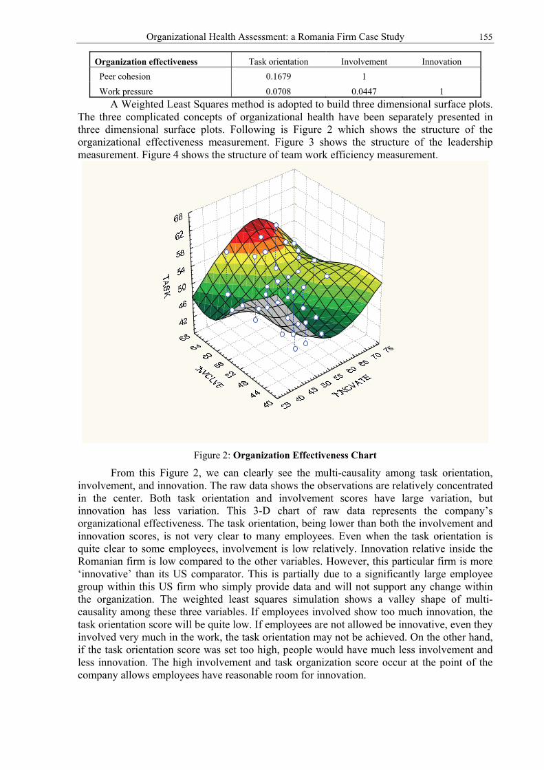
Organizational Health Assessment: a Romania Firm Case Study 155
Organization effectiveness Task orientation Involvement Innovation Peer cohesion 0.1679 1 Work pressure 0.0708 0.0447 1
A Weighted Least Squares method is adopted to build three dimensional surface plots. The three complicated concepts of organizational health have been separately presented in three dimensional surface plots. Following is Figure 2 which shows the structure of the organizational effectiveness measurement. Figure 3 shows the structure of the leadership measurement. Figure 4 shows the structure of team work efficiency measurement.
Figure 2: Organization Effectiveness Chart
From this Figure 2, we can clearly see the multi-causality among task orientation, involvement, and innovation. The raw data shows the observations are relatively concentrated in the center. Both task orientation and involvement scores have large variation, but innovation has less variation. This 3-D chart of raw data represents the company’s organizational effectiveness. The task orientation, being lower than both the involvement and innovation scores, is not very clear to many employees. Even when the task orientation is quite clear to some employees, involvement is low relatively. Innovation relative inside the Romanian firm is low compared to the other variables. However, this particular firm is more ‘innovative’ than its US comparator. This is partially due to a significantly large employee group within this US firm who simply provide data and will not support any change within the organization. The weighted least squares simulation shows a valley shape of multi-causality among these three variables. If employees involved show too much innovation, the task orientation score will be quite low. If employees are not allowed be innovative, even they involved very much in the work, the task orientation may not be achieved. On the other hand, if the task orientation score was set too high, people would have much less involvement and less innovation. The high involvement and task organization score occur at the point of the company allows employees have reasonable room for innovation.
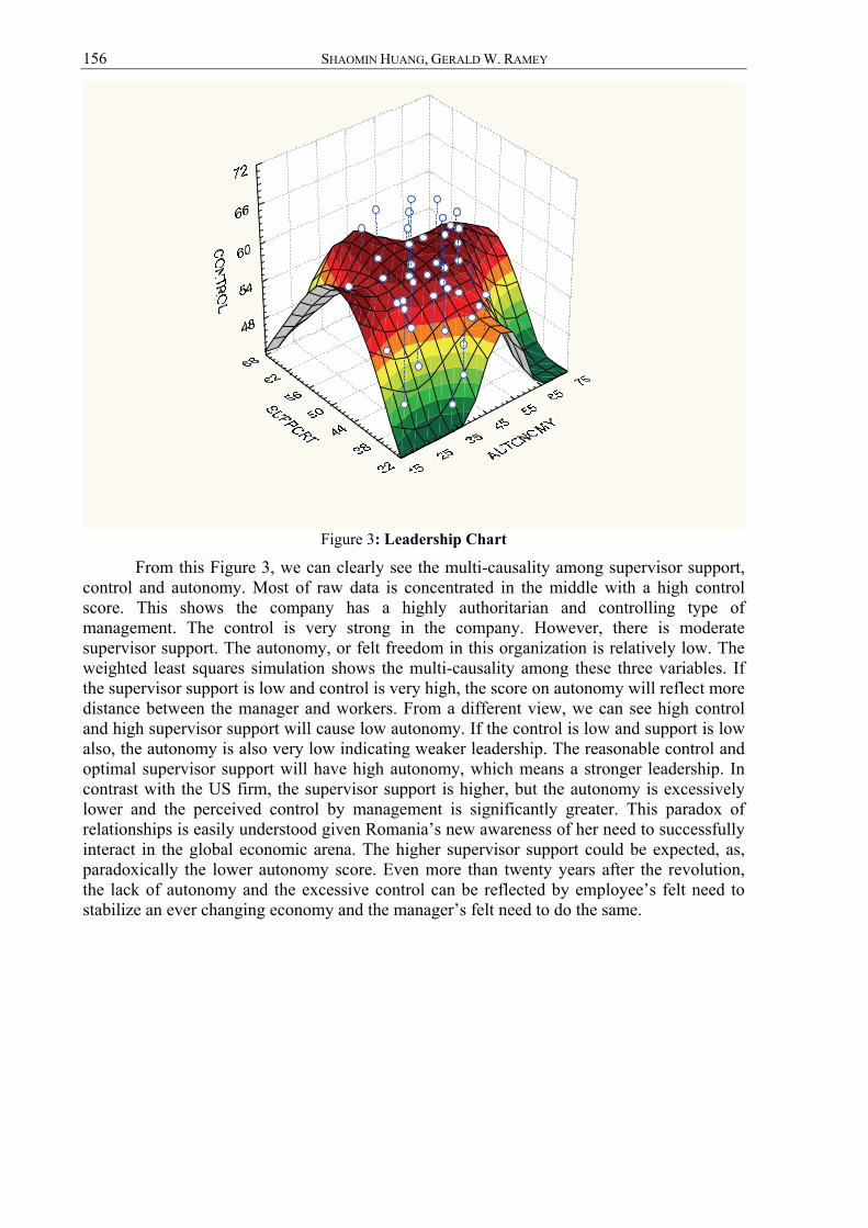
156 SHAOMIN HUANG, GERALD W. RAMEY
Figure 3: Leadership Chart
From this Figure 3, we can clearly see the multi-causality among supervisor support, control and autonomy. Most of raw data is concentrated in the middle with a high control score. This shows the company has a highly authoritarian and controlling type of management. The control is very strong in the company. However, there is moderate supervisor support. The autonomy, or felt freedom in this organization is relatively low. The weighted least squares simulation shows the multi-causality among these three variables. If the supervisor support is low and control is very high, the score on autonomy will reflect more distance between the manager and workers. From a different view, we can see high control and high supervisor support will cause low autonomy. If the control is low and support is low also, the autonomy is also very low indicating weaker leadership. The reasonable control and optimal supervisor support will have high autonomy, which means a stronger leadership. In contrast with the US firm, the supervisor support is higher, but the autonomy is excessively lower and the perceived control by management is significantly greater. This paradox of relationships is easily understood given Romania’s new awareness of her need to successfully interact in the global economic arena. The higher supervisor support could be expected, as, paradoxically the lower autonomy score. Even more than twenty years after the revolution, the lack of autonomy and the excessive control can be reflected by employee’s felt need to stabilize an ever changing economy and the manager’s felt need to do the same.

Organizational Health Assessment: a Romania Firm Case Study 157
Figure 4: Team Work Efficiency Chart
From this Figure 4, we can clearly see the multi-causality among clarity, peer cohesion, and work pressure. The raw data show most of observations as located in the central area and many of them with relatively high work pressure score. Some of them have high work pressure because of low clarity. With medium clarity and high peer cohesion, some people can get relative low work pressure. The weighted least squares simulation shows two extreme points. The combination of high clarity and low peer cohesion will reflect a high work pressure score. The combination of low clarity and high peer cohesion will come out a very low work pressure score. Other than these two extreme cases, other multi-causality among these three variables has a complicated shape. The low score on peer cohesion with low or high clarity will cause high work pressure. The high score on peer cohesion and high clarity will result low work pressure. Combining high clarity and high peer cohesion, the work pressure will be very low. Moderate clarity and moderate peer cohesion will have moderate work pressure.
4. CONCLUSION In industries, organizational performance is widely measured by output sales, seasonal
earnings, or profit margin. In academic research, organizational behavior has been widely studied but has been mainly focused on one-way causality analysis. This study uses the concept of an organization’s health to evaluate organizational performance. We look at organization effectiveness, leadership, and term work efficiency. Respect to these three unobserved structural variables, the Work Environment Scales embedded into the System-wide Interpretation of Health and Quality provide clear observable variables (task orientation, involvement, innovation, supervisor support, control, autonomy, work pressure, clarity, and peer cohesion) that have been used to conduct survey research on a Romania company. The weighted least squares method is adopted to estimate three dimensional graphs to show the multi-causality effects among these variables and evaluation of organization performance.
In this case study, a Romania company performance has been studied. We find that this firm’s organization effectiveness is good when compared to the US firm. The evaluation

158 SHAOMIN HUANG, GERALD W. RAMEY
of company’s leadership shows a relatively authoritarian and controlling style of management. The assessment on the firm’s team work efficiency is not relatively high caused by high work pressure. Since Romania is still in an economic transaction period of time, this firm’s organizational performance can be considered good. But comparing with an international standard, this firm does not have a significantly strong balance in the leadership area.
Each of the first three propositions indicate the measure of success as an optimal balance of the three micro variables. This study has shown an overall balance of variables in the organizational effectiveness category and a lack of optimal interaction in both the leadership and team work efficiency categories. The lagged impact of these observable behaviors on the organizational effectiveness category is imminent. Proposition four simply indicates that this particular process of a system-wide analysis of all of these performance indicators is an appropriate and information rich assessment process. A more detailed set of charts indicating specific relationships among the various observable variables with a number of pre-selected demographic variables is provided to the firm during exit debriefings. Given the future of Romania and the struggle, the awareness and the subsequent growth in organizational knowledge, organizational improvement in these relationships is highly likely.
BIBLIOGRAPHY 1. Ainsworth-Land, G.T. (1986). Grow or Die: The unifying principle of transformation. New York:
John Wiley & Sons. 2. Bass, B. M. (1981), Stodgill’s Handbook of Leadership: A Survey of Theory and Research. New
York: The Free Press. 3. Bennis, Warren. (1996) “On Leadership in the Midst of Downsizing,” (interviewed by Richard
Hodgetts), Organizational Dynamics, Summer 1996, 25th Anniversary Issue, pp. 15-26. 4. Burns, J.M. (1978) Leadership. New York: Harper. 5. Button, Scott B., Mathieu, John E., Zajac, Dennis M. (1996) “Goal Orientation in Organizational
Research: A Conceptual and Empirical Foundation,” Organizational Behavior and Human Decision Processes, Vol. 67, No. 1, July, pp. 26-48.
6. Delery, John E., Doty, D. Harold (1996), “Modes of Theorizing in Strategic Human Resource Management: Tests of Universalistic, Contingency, and Configurational Performance Predictions,” Academy of Management Journal, Vol. 39, No. 4, pp. 802-835.
7. Deming, W. E. (1992), Out of the Crisis. Cambridge, Mass: MIT Center for Advanced Engineering Study.
8. Denison, Daniel R. (1996), “What is the Difference between Organizational Culture and Organizational Climate? A Native’s Point of View on a Decade of Paradigm Wars” Academy of Management Review, Vol. 21, No. 3, pp. 619-654.
9. Edwards, J.R. and M.E. Parry (1993) “On the Use of Polynomial Regression Equations as An Alternative to Difference Scales in Organizational Research.” The Academy of Management Journal, Vol. 36, No.6, pp.1577-1613.
10. Fry, R. E., (1995), “Accountability in Organizational Life: Problem or Opportunity for Non Profits?” Non Profit Management and Leadership, Vol. 6, No. 2, Winter.
11. Gellis, Z. (2001). Social work perceptions of transformational and transactional leadership in health care. Social Work Research, 25.17. Retrieved August 13, 2007, from the Academic Search Premier database.
12. Gleick, J. (1987) Chaos: Making a New Science. New York: Viking. 13. Gruenfeld, D.H., E.A. Mannix, K.Y. Williams, M.A. Neale, (1996), A., “Group Composition and
Decision Making: How Member Familiarity and Information Distribution Affect Process and Performance,” Organizational Behavior and Human Decision Processes, Vol. 67, No. 1, July, pp. 1-15.
14. Handy, C. (1996), “On the Future of Work and an End to the ‘Century of the Organization’,” (interviewed by Barbara Ettorre), Organizational Dynamics, 25th Anniversary Issue, pp. 15-26.
15. Harrison, M. (1987), Diagnosing Organizations: Methods, Models and Processes. Newbury Park, California: SAGE.
Organizational Health Assessment: a Romania Firm Case Study 159
16. Heady, R. B., M. Smith, (1996), “Feedback Intensity and Leader-Follower Behavior: A Mathematical Description,” Behavioral Science: Journal of the International Society for the Systems Sciences, Vol. 41, No. 1, January, pp. 13-29.
17. Heifitz, R., & Laurie, D. (2001). The work of leadership. Harvard Business Review, 79 (11), 131-141.
18. Kabanoff, B., (1996), “Equity, Equality, Power, and Conflict,” Academy of Management Review, 1991, Vol. 16, No. 2, pp. 416-441.
19. Lemom, B. (Ed). (1988), “Management Education for the Future.” Highlights From The Meta Network.
20. Lumpkin, G.T. and G. G. Dess, (1996), “Clarifying the Entrepreneurial Orientation Construct and Linking it to Performance,” Academy of Management Review, Vol. 21, No. 1, pp. 135-172.
21. Moos, R. H. (1986), Work Environment Scale: Manual. Palo Alto, California: Consulting psychologist’s Press, Inc.
22. McCall, M. W., Jr., and M. M. Lombardo, Ed. (1978), Leadership: Where Else Can We Go? Durham, NC: Duke University.
23. Oldham, G. R., A. Cummings, (1996), “Employee Creativity: Personal and Contextual Factors at Work,” Academy of Management Journal, Vol. 39, No. 3, pp. 607-634.
24. Quinn, R., & Spreitzer, G. (2001). A company of leaders: Five disciplines for unleashing the power in your workforce. San Francisco: Jossey-Bars.
25. Reich, R. (1996) “On Insecurity, the New Social Compact, and Why it Matters if a Company Treats Employees as Costs or Assets,” Training: The Human Side of Business, August, pp. 37-41.
26. Ramey, G. W., J. H. Haehl, and S. Huang (1995), “System-Wide Assessment of Leadership and Organizational Climate.” Proceedings of The Western Decision Sciences Institute.
27. Ramey, G. W. and S. Huang (1999), “Comprehensive Analysis of Organization Behavior: Regence’s Report”, Working paper.
28. Seashore, Stanley, (1993), “Criteria of Organizational Effectiveness,” Management and Organizational Behavior Classics, 5th ed., Edited Matteson, Michael and Ivancevich, John, Irwin, Boston, Massachusetts, (reprint of July 1965 Michigan Business Review).
29. Senge, P. (1990), The Fifth Discipline. New York: Doubleday. 30. Scott, W. G. (1993), “The Management of Crisis and Tribulations.” Journal of Management
Inquiry, 2(2), pp.184-189. 31. Scott, W.R. (2003). Organizations; rational, natural and open systems. Upper Saddle River, NJ:
Prentice Hall. 32. Zammuto, R. F. (1982), Assessing Organizational Effectiveness: Systems Change, Adaptation
and Strategy. Albany, NY: State University of New York Press.

THE TARIFF EQUIVALENT OF TARIFF-RATE QUOTAS - A CASE STUDY APPLIED TO THE IMPORT OF AN AGRICULTURAL
PRODUCT IN ROMANIA
Petru Cătălin BODEA*
Abstract. The paper presents one methodology of calculating the tariff equivalent of the tariff-rate quota as a particular case of a non-tariff barrier for an agricultural product imported in Romania based on recommendations in international literature. The tariff equivalent of tariff-rate quota of imports from the EU is approximately 35%, lower than the tariff outside the quota. Nonetheless this is considerable higher when compared with the Common External Tariff (CET). Elimination of the nominal protection level as consequence of the adoption the CET is expected to stimulate imports pressure especially from price competitive import partners both from EU (such as Slovakia, Belgium, Austria, Czech Republic and Italy) and non EU countries (Serbia, Bosnia and Herzegovina, Macedonia and Croatia). A basic model forecasts that, with the lowered protection, annual imports will rise with at least 13.5 thousand tones, thus an increase of 23% compared with the average annual imports during 1990-2005. Key words: non-tariff barriers, tariff-rate quotas, tariff equivalent JEL: F13, Q17
1. INTRODUCTION Unlike the much more transparent tariffs, non-tariff barriers (subsequently called
NTB’s) are a relatively new and insufficiently explored sector of international economic relations. Although they have been traditionally used for over 7 centuries1, their importance for international trade flows has reached its peak towards the end of the 20th century.
For instance, in 2004, the number of lines in a customs list which was representative for the world average directly affected by the implementation of at least one non-tariff measure was 5620. That is a growth of over 200% compared to 1994, when the number of lines was only 1880, finding that gave support to the some economists’ claim that the reverse of the decrease in tariff protection agreed at the end of the Uruguay Round was the recrudescence of non-tariff protectionism (Fugazza, 2006:2).
The importance of non-tariff measures for the future of trade flows is especially enhanced since the lack of an agreement in this field led to the suspension of negotiations during the Doha Round. Non-tariff barriers have thus become a global apple of discord, causing disputes that involve both developing countries and especially developed countries (or blocks of countries). In this context, the preoccupations regarding the quantification of the effects produced by these non-tariff measures, especially at the level of the protected * Petru Cătălin Bodea is a PhD student in International Economic Relations at the “Alexandru Ioan Cuza” University of Iaşi 1 Some forms of non-tariff proto-protectionism are, for example, the interdictions regarding the export of non-processed wool in 1303 (France) and 1463 (England) (Favier, 2001:122).
162 PETRU CĂTĂLIN BODEA
economy (but also at the level of the trade partners) become a priority for the continuation of the multilateral negotiations in a rational, positive manner.
The preoccupations for the quantification of the non-tariff barriers have generated several methods for this purpose, among which the tariff equivalent method, frequently used both by the World Bank economists (Bora, 2002:8) and by researchers, due to its capacity of being applied to a vast range of NTB’s (Deardorff, 1997), such as quotas, variable levies, voluntary export restrictions and technical barriers2.
During the recent years, the implementation of annual tariff-rate quotas for the Romanian imports from EU countries has played an indirect role of safety valve for the introduction of competitive pressures (limited by the maximum level of the quotas) which might have helped the internal producers to adjust to the competitive pressures of the Single Market. With its accession into the European Union in 2007, Romania takes on the EU Common External Tariff, while the tariff-rate quotas are allotted in a centralized manner by the European Commission. In this context, the disappearance of the current degree of protection provided by the tariffs outside the quotas to the internal producers creates the necessity to identify and calibrate alternative instruments for alleviating the impact of the exposure to the competition pressures – especially those of the Single Market –, which must be based on the quantification of the previous nominal protection provided to the internal producers by the tariff rate quotas. The computation of the tariff equivalent for tariff rate quotas applied to an agricultural product imported in Romania is also collinear with international global concerns and recommendations3 to amplify actions necessary to calculate tariff equivalents for an extensive range of products, industries and economies which in turn shall facilitate further development of econometric model to study the international trade idiosyncrasies in response to NTB reduction.
Below, we shall give an example of the way of calculating the tariff equivalent of a specific form of non-tariff measure, i.e. the tariff-rate quota, selectively applied to the imports of potatoes in Romania after 1989, based on historical data provided by the FAOSTAT – Food and Agriculture Organization of the United Nations. We have chosen this type of non-tariff barrier4 as an example based on both the increase in the frequency of the use of tariff-rate quotas during the last decade and the greater transparency of tariff-rate quotas, compared to other non-tariff measures.
2. CALCULATING THE TARIFF EQUIVALENT OF THE NTB Some of the less used, but implicitly accepted definitions of the NTB’s states that they
are, like tariff barriers, measures that, by creating obstacles in accessing markets, prevent the functioning of the single-price law. According to this law, a market without obstacles, by 2 For example, Mitsuyo Ando in “Estimating Tariff Equivalents of Core and Non-Core Non-Tariff Measures in the APEC Member Economies” used this method to quantify – for 13 APEC countries and 21 products – the tariff equivalent of no less than 12 kinds of NTB’s, classified into 5 categories (from price measures, such as variable levies, compensatory measures, antidumping measures etc up to quantitative measures, such as tariff-rate quotas and RVE, technical, monopolistic or monitoring measures). The calculation was also facilitated by the fact that, after having obtained the price differential for the same product and having eliminated the percentage of tariff protection, Ando allotted the non-tariff protection for each product according to a distortion index of prices, specific to each NTB and calculated based on a regression developed around the frequency indicators that are specific to the 12 NTB’s. 3 “Therefore, we conclude from this survey that the most useful direction for future investigation of NTBs across industries and countries should be to aim for a comprehensive set of tariff-equivalent measures of protection (nominal, not effective) derived from the most detailed industry-specific information that can be obtained and from various different measurement techniques appropriate to the type of NTB and its method of administration” (Deardorff,1997:44) 4 From an academic point of view, the tariff-rate quotas are included in the area of non-tariff measures, although, within official taxonomies (UNCTAD, 2005:16-19), they may be classified as tariff measures. In Deardorff (Deardorff, 1997:68) and Ferrantino (Ferrantino, 2006:30), the mention is implicit, as long as the NTB evaluation measures include the quantification of tariff-rate quotas, while in Bora, they are explicitly included (Bora, 2002:37).
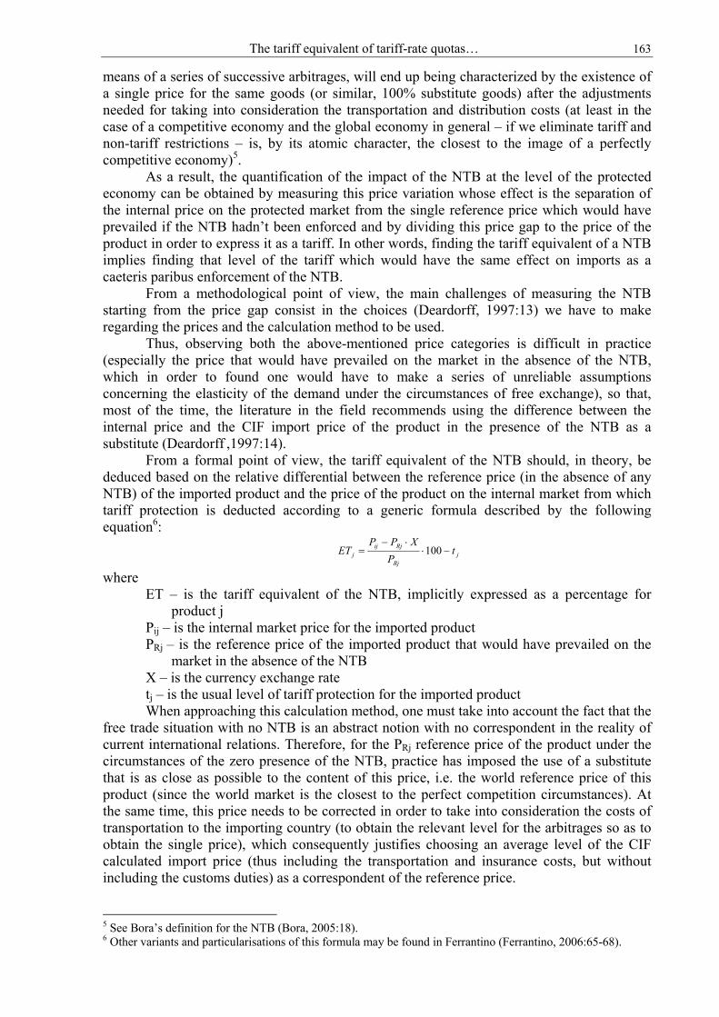
The tariff equivalent of tariff-rate quotas… 163
means of a series of successive arbitrages, will end up being characterized by the existence of a single price for the same goods (or similar, 100% substitute goods) after the adjustments needed for taking into consideration the transportation and distribution costs (at least in the case of a competitive economy and the global economy in general – if we eliminate tariff and non-tariff restrictions – is, by its atomic character, the closest to the image of a perfectly competitive economy)5.
As a result, the quantification of the impact of the NTB at the level of the protected economy can be obtained by measuring this price variation whose effect is the separation of the internal price on the protected market from the single reference price which would have prevailed if the NTB hadn’t been enforced and by dividing this price gap to the price of the product in order to express it as a tariff. In other words, finding the tariff equivalent of a NTB implies finding that level of the tariff which would have the same effect on imports as a caeteris paribus enforcement of the NTB.
From a methodological point of view, the main challenges of measuring the NTB starting from the price gap consist in the choices (Deardorff, 1997:13) we have to make regarding the prices and the calculation method to be used.
Thus, observing both the above-mentioned price categories is difficult in practice (especially the price that would have prevailed on the market in the absence of the NTB, which in order to found one would have to make a series of unreliable assumptions concerning the elasticity of the demand under the circumstances of free exchange), so that, most of the time, the literature in the field recommends using the difference between the internal price and the CIF import price of the product in the presence of the NTB as a substitute (Deardorff ,1997:14).
From a formal point of view, the tariff equivalent of the NTB should, in theory, be deduced based on the relative differential between the reference price (in the absence of any NTB) of the imported product and the price of the product on the internal market from which tariff protection is deducted according to a generic formula described by the following equation6:
jRj
Rjijj t
PXPP
ET −⋅⋅−
= 100
where ET – is the tariff equivalent of the NTB, implicitly expressed as a percentage for
product j Pij – is the internal market price for the imported product PRj – is the reference price of the imported product that would have prevailed on the
market in the absence of the NTB X – is the currency exchange rate tj – is the usual level of tariff protection for the imported product When approaching this calculation method, one must take into account the fact that the
free trade situation with no NTB is an abstract notion with no correspondent in the reality of current international relations. Therefore, for the PRj reference price of the product under the circumstances of the zero presence of the NTB, practice has imposed the use of a substitute that is as close as possible to the content of this price, i.e. the world reference price of this product (since the world market is the closest to the perfect competition circumstances). At the same time, this price needs to be corrected in order to take into consideration the costs of transportation to the importing country (to obtain the relevant level for the arbitrages so as to obtain the single price), which consequently justifies choosing an average level of the CIF calculated import price (thus including the transportation and insurance costs, but without including the customs duties) as a correspondent of the reference price.
5 See Bora’s definition for the NTB (Bora, 2005:18). 6 Other variants and particularisations of this formula may be found in Ferrantino (Ferrantino, 2006:65-68).
164 PETRU CĂTĂLIN BODEA
On the other hand, the Pij, i.e. the internal market price for the imported product, is a notion whose transparency is just as difficult to obtain with most of the usual statistics as that of the PRj, so that it is necessary to take alternatives into account. Thus, most of the time, the official statistics regarding the level of internal prices do not differentiate between imported and national products, providing a single price level for that particular product. The internal market price is thus a composite coefficient between the price of the substitute internal products (if any) and that of the imported products. Consequently, the alternatives for calculating the Pij depend on the existence of a similar internal product and on its capacity of being substituted with the imported product. Thus, if that internal product exists and is perfectly changeable with the imported one, Deardorff recommends accepting the factory production price of the internal product as a reference level for the Pij (Deardorff , 1997:65).
3. THE TARIFF-RATE QUOTAS APPLIED TO THE POTATO IMPORTS IN ROMANIA AFTER 1989
The tariff-rate quota system is a practice that became more widespread as a result of the decisions assumed by the GATT member countries within the URAA - The Uruguay Round Agreement on Agriculture (1996) to open the internal markets for the import of agricultural products. Before the end of the round, most of these products were subjected to a system of restrictive import quotas, which were later replaced by the tariff-rate quota system, the estimate being that the Uruguay Round led to the creation of over 1,300 new tariff-rate quotas (Skully, 2001:1).
From a methodological point of view, a tariff-rate quota may be assimilated to a two-level tariff, where the lower level is applied to the imports within a certain quota, whereas the higher one applies to all imports going over the quota (Ferrantino, 2006:30). A tariff-rate quota (subsequently called CT) is thus defined by 3 variables (Liapis, 2002:4): the tariff within the quota (subsequently called Tc, which is the low value of the tariff,
applied to the imports that do not go over the volume of the quota), the quota (subsequently called C, which is the quantity of imports accepted with the low
level of the tariff Tc) and the tariff outside the quota (subsequently called Ti, which is the value of the tariff applied
to the imports going over the C; it is much more prohibitive than the Tc and the Ti/ Tc ratio is often above 10).
The information concerning the level of all of these 3 dimensions characterizing a tariff-rate quota are public, as is the way of managing the quota (which needs a notification from the WTO) and, moreover, they are comparable with regard to countries and products.
Before the moment of the accession into the European Union and the adoption of the EU Common External Tariff, Romania’s import regime could be considered a liberal one (in the conservative sense of the word) due to the lack of import quotas and of the importers’ obligation to obtain an import license, as Article 1 in the Government Decision 1526/2003 mentions that “the export and import of goods from and to the customs territory of Romania is free, not being conditioned by the issuing of licenses”. The exceptions from the provisions of Article 1 were the goods subjected to measures such as the prohibitions justified by reasons of public safety, the protection of people’s health and lives, the protection of intellectual property etc, the import safeguarding measures, the export or import monitoring measures etc.
Except for the non-automatic licenses for certain sensitive products (radioactive materials, substances used for producing drugs, toxic waste etc) and for the safeguarding measures introduced for the sugar imports, predominantly from the Republic of Moldova7,
7 For example, for the year 2006, Article 1 of the Government Decision 1761/22.12.2005 stipulates: “A safeguarding measure is enforced within the Free Trade Agreement between Romania and the Republic of Moldova, signed in Bucharest, 15th February 1994, ratified by Law 94/1994, consisting of the temporary suspension of the customs duty exception for the import of refined sugar coming from the Republic of Moldova to Romania and the application of the erga omnes import customs duty stipulated in the Import Customs Tariff
The tariff equivalent of tariff-rate quotas… 165
some of the few NTBs in the field of quantitative restrictions practiced by Romania after 1989 were the tariff-rate quotas generally applied to the agricultural products coming from EU, CEFTA or South-Eastern European countries (Turkey, Albania, Macedonia, Serbia and Montenegro) and Israel.
An important part among these NTBs was played by the tariff-rate quotas enforced for the import of potatoes from the European Union. During the years when these quotas were implemented, the average maximum quantity admitted for import was that of 20,000 tons of potatoes coming from the European Union, for which the preferential customs duty was of 18.8% (while the customs duty outside the quota was somewhere between 40% and 50%, according to the period of the year when the import occurred), with an average maximum allotment quota of 0.3% / import license managed according to the “first come, first served” principle corroborated – during the recent years – with the preferential allotment of quotas to traditional importers (importers that, during the past years, applied for import quotas and actually used them entirely).
The product that the case study directly focuses on is potatoes fresh or chilled other than seeds HS 07019090908. Choosing this product as a subject for the study was based on a series of arguments especially related to its homogenous character and to the existence of the national substitute, to its dynamics, supported by the Romanian agricultural imports in the context of a decline of the internal producers’ competitiveness, and to the fact that the tariff-rate quotas applied to the import of potatoes in Romania were always entirely used; all these arguments are briefly presented below.
In order to ensure price compatibility, applying the conventional “price gap” method for finding the tariff equivalent of the tariff-rate quota requires a very good substitution between the imported product and the internal one, in other words lack of quality differential that might determine considerable variations of price and demand. Choosing potatoes as the product for applying the above-mentioned method is justified by their homogenous character (unlike that of other quota agricultural products, such as apples or chicken), as well as by the existence of a traditional production sector which, during the past 50 years, has permanently covered approximately 98% of the internal consumption (except between 1989 and 1993) and whose position is currently jeopardized by a substantial increase in imports.
At the same time, potatoes are the agricultural products whose imports had in 2006 one of the fastest rises (an almost 200% increase) compared to 2005 (after pork and tobacco)9. Moreover, the ratio of potatoes import value in the total amount of imports doubled in 2006 compared to 2005 (from 0.05% to 0.1%).
The Romanian exports, not very substantial, averaged around 6,500 tones per year during the last 10 years, with a peak of 16,000 tones in 2000. However, the historical trend is descending, as, beginning with 2004, Romanian exports witnessed a considerable loss of price competitiveness.
of Romania for 2006, for the products listed in the appendix which forms an integrant part of this decision.” The same act established a tariff-rate quota of 14,000 tons exempt from customs duties for 2006. 8 with the mention that statistics from FAOSTAT tables do not allow to identify the HS code, i.e. are based on a generic term of potatoes 9 A 7.2 million € increase compared to the same period of 2005, according to the data for April 2006, from 4.194 million to 11.357 million € (data obtained from the Ministry of Economy and Trade, the Romanian Centre for Promotion of Trade, “Sinteza privind evoluţii in comerţul exterior in perioada 01.01-30.04.2006”, http://www.dce.gov.ro/)
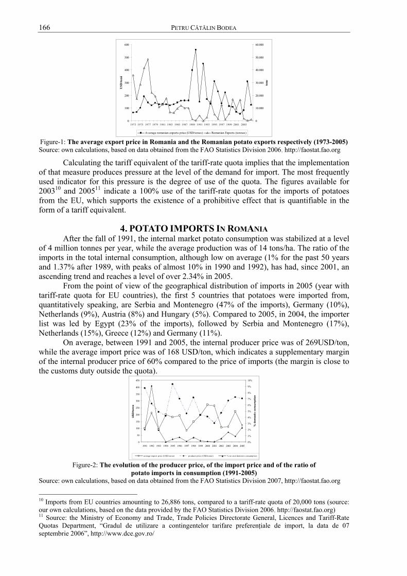
166 PETRU CĂTĂLIN BODEA
0
100
200
300
400
500
600
1973 1975 1977 1979 1981 1983 1985 1987 1989 1991 1993 1995 1997 1999 2001 2003U
SD/to
nă0
10.000
20.000
30.000
40.000
50.000
60.000
tone
Average romanian exports price (USD/tones) Romanian Exports (tonnes) Figure-1: The average export price in Romania and the Romanian potato exports respectively (1973-2005) Source: own calculations, based on data obtained from the FAO Statistics Division 2006, http://faostat.fao.org
Calculating the tariff equivalent of the tariff-rate quota implies that the implementation of that measure produces pressure at the level of the demand for import. The most frequently used indicator for this pressure is the degree of use of the quota. The figures available for 200310 and 200511 indicate a 100% use of the tariff-rate quotas for the imports of potatoes from the EU, which supports the existence of a prohibitive effect that is quantifiable in the form of a tariff equivalent.
4. POTATO IMPORTS IN ROMANIA After the fall of 1991, the internal market potato consumption was stabilized at a level
of 4 million tonnes per year, while the average production was of 14 tons/ha. The ratio of the imports in the total internal consumption, although low on average (1% for the past 50 years and 1.37% after 1989, with peaks of almost 10% in 1990 and 1992), has had, since 2001, an ascending trend and reaches a level of over 2.34% in 2005.
From the point of view of the geographical distribution of imports in 2005 (year with tariff-rate quota for EU countries), the first 5 countries that potatoes were imported from, quantitatively speaking, are Serbia and Montenegro (47% of the imports), Germany (10%), Netherlands (9%), Austria (8%) and Hungary (5%). Compared to 2005, in 2004, the importer list was led by Egypt (23% of the imports), followed by Serbia and Montenegro (17%), Netherlands (15%), Greece (12%) and Germany (11%).
On average, between 1991 and 2005, the internal producer price was of 269USD/ton, while the average import price was of 168 USD/ton, which indicates a supplementary margin of the internal producer price of 60% compared to the price of imports (the margin is close to the customs duty outside the quota).
0
50
100
150
200
250
300
350
400
450
1991 1992 1993 1994 1995 1996 1997 1998 1999 2000 2001 2002 2003 2004 2005
USD/
tonn
e
0%
1%
2%
3%
4%
5%
6%
7%
8%
9%
10%
% d
omes
tic c
onsu
mpt
ion
average import price (USD/tonne) producer price (USD/tonne) % in total domest ic consumption Figure-2: The evolution of the producer price, of the import price and of the ratio of
potato imports in consumption (1991-2005) Source: own calculations, based on data obtained from the FAO Statistics Division 2007, http://faostat.fao.org
10 Imports from EU countries amounting to 26,886 tons, compared to a tariff-rate quota of 20,000 tons (source: our own calculations, based on the data provided by the FAO Statistics Division 2006, http://faostat.fao.org) 11 Source: the Ministry of Economy and Trade, Trade Policies Directorate General, Licences and Tariff-Rate Quotas Department, “Gradul de utilizare a contingentelor tarifare preferenţiale de import, la data de 07 septembrie 2006”, http://www.dce.gov.ro/
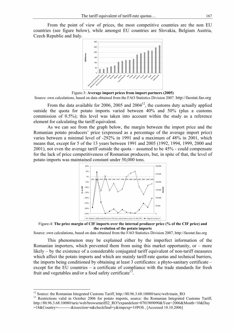
The tariff equivalent of tariff-rate quotas… 167
From the point of view of prices, the most competitive countries are the non EU countries (see figure below), while amongst EU countries are Slovakia, Belgium Austria, Czech Republic and Italy.
0
50
100
150
200
250
300
Bosnia
and H
erzego
vina
Maced
onia,
The Fmr Y
ug R
p
Serbia
and M
onten
egro
Croatia
Slovakia
Belgium
Austria
Czech
Rep
ublic
Italy
Poland
Greece
Sweden
France
Hunga
ryEgy
pt
German
y
Netherl
ands
USD
/tonn
e
Figure-3: Average import prices from import partners (2005)
Source: own calculations, based on data obtained from the FAO Statistics Division 2007, http://faostat.fao.org
From the data available for 2006, 2005 and 200412, the customs duty actually applied outside the quota for potato imports varied between 40% and 50% (plus a customs commission of 0.5%); this level was taken into account within the study as a reference element for calculating the tariff equivalent.
As we can see from the graph below, the margin between the import price and the Romanian potato producers’ price (expressed as a percentage of the average import price) varies between a minimal level of -292% in 1991 and a maximum of 48% in 2001, which means that, except for 5 of the 13 years between 1991 and 2005 (1992, 1994, 1999, 2000 and 2001), not even the average tariff outside the quota – assumed to be 45% - could compensate for the lack of price competitiveness of Romanian producers, but, in spite of that, the level of potato imports was maintained constant under 50,000 tons.
-350%
-300%
-250%
-200%
-150%
-100%
-50%
0%
50%
100%
1991 1992 1993 1994 1995 1996 1997 1998 1999 2000 2001 2002 2003 2004 2005
% in
CIF
0
50.000
100.000
150.000
200.000
250.000
300.000to
nnes
Relative differential between CIF price and producer price (% din CIF) Imports (tonnes) Figure-4: The price margin of CIF imports over the internal producer price (% of the CIF price) and
the evolution of the potato imports Source: own calculations, based on data obtained from the FAO Statistics Division 2007, http://faostat.fao.org
This phenomenon may be explained either by the imperfect information of the Romanian importers, which prevented them from using this market opportunity, or – more likely – by the existence of a considerable conjugated tariff equivalent of non-tariff measures which affect the potato imports and which are mainly tariff-rate quotas and technical barriers, the imports being conditioned by obtaining at least 3 certificates: a phyto-sanitary certificate – except for the EU countries – a certificate of compliance with the trade standards for fresh fruit and vegetables and/or a food safety certificate13.
12 Source: the Romanian Integrated Customs Tariff, http://80.96.3.68:10080/taric/web/main_RO 13 Restrictions valid in October 2006 for potato imports, source: the Romanian Integrated Customs Tariff, http://80.96.3.68:10080/taric/web/browsetariffi2_RO?expandelem=0701909090&Year=2006&Month=10&Day=18&Country=----------&issection=n&checkfinal=y&impexp=1#POS , [Accessed 18.10.2006]
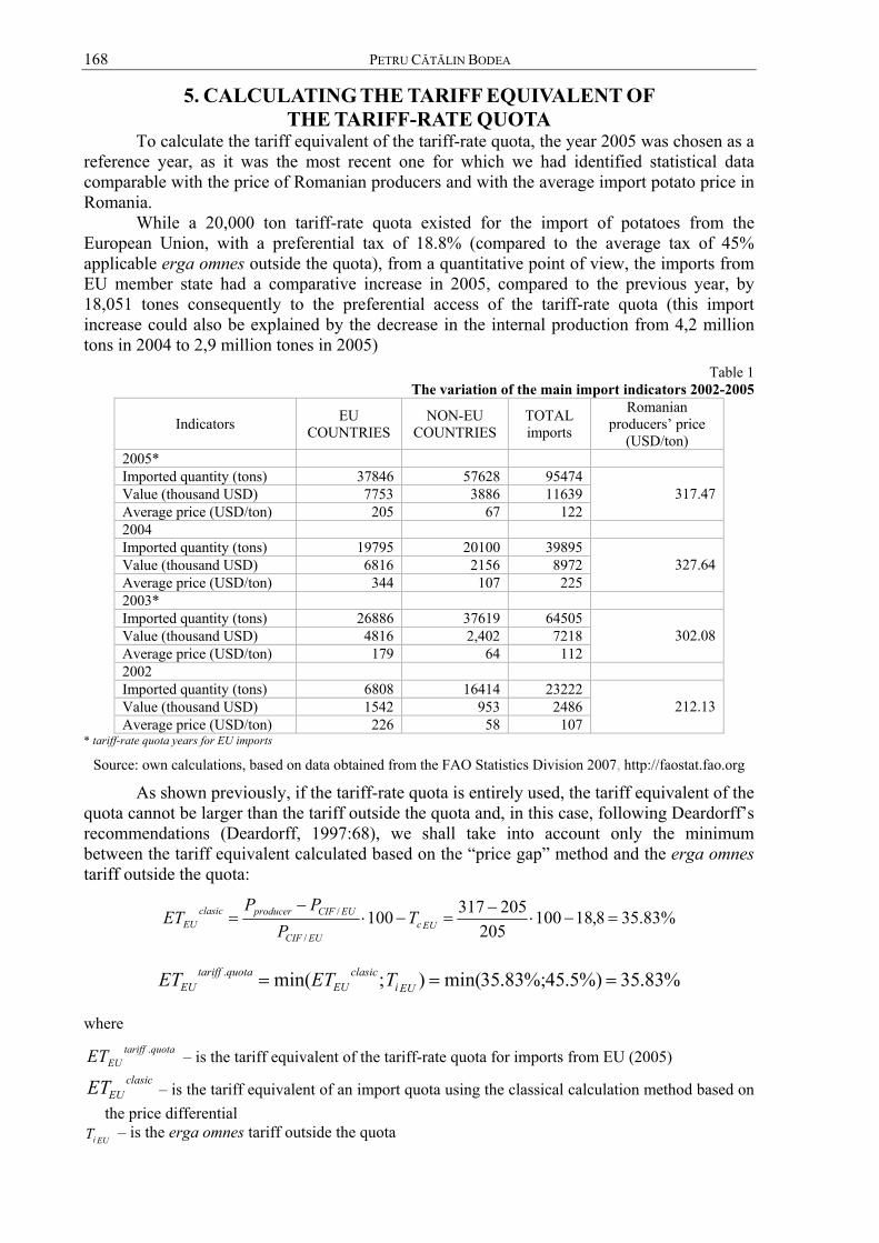
168 PETRU CĂTĂLIN BODEA
5. CALCULATING THE TARIFF EQUIVALENT OF THE TARIFF-RATE QUOTA
To calculate the tariff equivalent of the tariff-rate quota, the year 2005 was chosen as a reference year, as it was the most recent one for which we had identified statistical data comparable with the price of Romanian producers and with the average import potato price in Romania.
While a 20,000 ton tariff-rate quota existed for the import of potatoes from the European Union, with a preferential tax of 18.8% (compared to the average tax of 45% applicable erga omnes outside the quota), from a quantitative point of view, the imports from EU member state had a comparative increase in 2005, compared to the previous year, by 18,051 tones consequently to the preferential access of the tariff-rate quota (this import increase could also be explained by the decrease in the internal production from 4,2 million tons in 2004 to 2,9 million tones in 2005)
Table 1 The variation of the main import indicators 2002-2005
Indicators EU COUNTRIES
NON-EU COUNTRIES
TOTAL imports
Romanian producers’ price
(USD/ton) 2005* Imported quantity (tons) 37846 57628 95474 Value (thousand USD) 7753 3886 11639 Average price (USD/ton) 205 67 122
317.47
2004 Imported quantity (tons) 19795 20100 39895 Value (thousand USD) 6816 2156 8972 Average price (USD/ton) 344 107 225
327.64
2003* Imported quantity (tons) 26886 37619 64505 Value (thousand USD) 4816 2,402 7218 Average price (USD/ton) 179 64 112
302.08
2002 Imported quantity (tons) 6808 16414 23222 Value (thousand USD) 1542 953 2486 Average price (USD/ton) 226 58 107
212.13
* tariff-rate quota years for EU imports
Source: own calculations, based on data obtained from the FAO Statistics Division 2007, http://faostat.fao.org
As shown previously, if the tariff-rate quota is entirely used, the tariff equivalent of the quota cannot be larger than the tariff outside the quota and, in this case, following Deardorff’s recommendations (Deardorff, 1997:68), we shall take into account only the minimum between the tariff equivalent calculated based on the “price gap” method and the erga omnes tariff outside the quota:
%83.358,18100205
205317100/
/ =−⋅−
=−⋅−
= EUcEUCIF
EUCIFproducerclasicEU T
PPP
ET
%83.35%)5.45%;83.35min();min(. === EUiclasic
EUquotatariff
EU TETET
where quotatariff
EUET . – is the tariff equivalent of the tariff-rate quota for imports from EU (2005) clasic
EUET – is the tariff equivalent of an import quota using the classical calculation method based on the price differential
EUiT – is the erga omnes tariff outside the quota
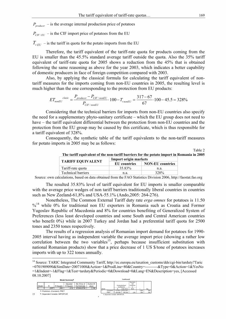
The tariff equivalent of tariff-rate quotas… 169
producerP – is the average internal production price of potatoes
EUCIFP / – is the CIF import price of potatoes from the EU
EUcT – is the tariff in quota for the potato imports from the EU
Therefore, the tariff equivalent of the tariff-rate quota for products coming from the EU is smaller than the 45.5% standard average tariff outside the quota. Also the 35% tariff equivalent of tariff-rate quota for 2005 shows a reduction from the 45% that is obtained following the same reasoning as above for the year 2003, which indicates a better capability of domestic producers in face of foreign competition compared with 2003.
Also, by applying the classical formula for calculating the tariff equivalent of non-tariff measures for the imports coming from non-EU countries in 2005, the resulting level is much higher than the one corresponding to the protection from EU products:
%3285.4510067
67317100/
/ =−⋅−
=−⋅−
= nonEUcnonEUCIF
nonEUCIFproducerclasicnonEU T
PPP
ET
Considering that the technical barriers for imports from non-EU countries also specify the need for a supplementary phyto-sanitary certificate – which the EU group does not need to have – the tariff equivalent differential between the protection from non-EU countries and the protection from the EU group may be caused by this certificate, which is thus responsible for a tariff equivalent of 328%.
Consequently, the synthetic table of the tariff equivalents to the non-tariff measures for potato imports in 2005 may be as follows:
Table 2 The tariff equivalent of the non-tariff barriers for the potato import in Romania in 2005
Import origin markets TARIFF EQUIVALENT EU countries NON-EU countries Tariff-rate quota 35.83% n.a. Technical barriers n.a. 328%
Source: own calculations, based on data obtained from the FAO Statistics Division 2006, http://faostat.fao.org
The resulted 35.83% level of tariff equivalent for EU imports is smaller comparable with the average price wedges of non tariff barriers traditionally liberal countries in countries such as New Zeeland-61,8% and USA-55.1% (Ando,2005: 264-276).
Nonetheless, The Common External Tariff duty rate erga omnes for potatoes is 11.50 %14 while 0% for traditional non EU exporters in Romania such as Croatia and Former Yugoslav Republic of Macedonia and 8% for countries benefiting of Generalized System of Preferences (less least developed countries and some South and Central American countries who benefit 0%) while in 2007 Turkey and Jordan had a preferential tariff quota for 2500 tones and 2350 tones respectively.
The results of a regression analysis of Romanian import demand for potatoes for 1990-2005 interval having as independent variable the average import price (showing a rather low correlation between the two variables15, perhaps because insufficient substitution with national Romanian products) show that a price decrease of 1 US $/tone of potatoes increases imports with up to 322 tones annually. 14 Source: TARIC Integrated Community Tariff, http://ec.europa.eu/taxation_customs/dds/cgi-bin/tarduty?Taric =0701909090&SimDate=20071008&Action=1&ProdLine=80&Country=----------&Type=0&Action=1&YesNo =1&Indent=-1&Flag=1&Test=tarduty&Periodic=0&Download=0&Lang=EN&Description=yes, [Accessed 08.10.2007]
15
Model Summaryb
,235a ,055 -,012 87244,6739 1,748Model1
R R SquareAdjustedR Square
Std. Error ofthe Estimate
Durbin-Watson
Predictors: (Constant), PRETa.
Dependent Variable: IMPORTURb. ,
Coefficientsa
112759,5 61812,931 1,824 ,090-322,056 355,344 -,235 -,906 ,380
(Constant)PRET
Model1
B Std. Error
UnstandardizedCoefficients
Beta
Standardized
Coefficients
t Sig.
Dependent Variable: IMPORTURa.
170 PETRU CĂTĂLIN BODEA
Also, based on the above mention results regarding tariff equivalent of tariff rate quotas for imports from EU countries, and as a consequence to the adoption of the Common External Tariff, the average nominal protection for Romanian producers is expected to drop in average with 35%16 after January 2007. Based on 2005 level of average import price this represents an exposure of local producers to import prices decreased with 43 US $/imported tone of potatoes which therefore might generates caeteris paribus an increase of imports of almost 14,000 tones annually (approximately 15% increase compared with the 2005 level of imports and 23% compared with the average annual imports between 1990-2005).
6. CONCLUSION The paper has presented one methodology of calculating the tariff equivalent of the
tariff-rate quota for an agricultural product imported in Romania based on recommendations in international literature. The conclusion of this study is that the protection provided to the Romanian potato producers in 2005 by the tariff-rate quota of imports from the EU is approximately 35%, smaller than the 2003 level of the same indicator and also than the 45% tariff outside the quota. Nonetheless this is considerable higher when compared with the Common External Tariff duty rate erga omnes for potatoes of 11.50 % not to mention the 0% duty for traditional non EU exporters of potatoes in Romania such as Croatia and Former Yugoslav Republic of Macedonia. Therefore the post 2007 level of protection for national producers of potatoes is expected to be considerably lowered compared with the previous price wedge ensured by the Romanian tariff quotas applied to potatoes imports from EU and erga omnes duty rate applied to imports from non-EU countries. Based on a basic import regression coefficient, the elimination of the average 35% nominal protection level as consequence of the adoption the Common External Tariff is expected to stimulate imports pressure especially from price competitive import partners both from EU (Slovakia, Belgium, Austria, Czech Republic and Italy) and non EU countries (Serbia, Bosnia and Herzegovina, Macedonia and Croatia) and rise annual imports with at least 13,5 thousand tones, thus an increase of 23% compared with the average annual imports between 1990-2005.
BIBLIOGRAPHY 1. Ando, Mitsuyo (2005), „Estimating Tariff Equivalents of Core and Non-core Non-Tariff
Measures in the APEC Member Economies”, (in Dee, Philippa and Ferrantino, Michael – Ed., Quantitative Methods For Assessing The Effects Of Non-Tarrif Measures And Trade Facilitation”), APEC Secretariat, Singapore, pp. 235-289
2. Bora, Bijit, Kuwahara, Aki and Laird, Sam (2002), “Quantification Of Non-Tariff Measures”, UNCTAD Policy Issues In International Trade And Commodities Study Series No. 18, Trade Analysis Branch, Geneva, UNCTAD http://www.unctad.org/en/docs/itcdtab19_en.pdf , [Accessed 16.09.2006]
3. Bora, Bijit (2005), „The Quatification and Impact of Non-Tariff Measures”, (in Dee, Philippa and Ferrantino, Michael – Ed., Quantitative Methods For Assessing The Effects Of Non-Tarrif Measures And Trade Facilitation”), APEC Secretariat, Singapore, pp.17-41
4. Colombatto, Enrico, (2000) “An Explanation of the Dynamics of Protectionism”, Kluwer Academic Publishers, Open Economies Review 11: 279–293, http://web.econ.unito.it/ colombatto/oer.pdf , [Accessed 05.08.2006]
5. Conway P., Janod V. and Nicoletti G. (2005), „Product Market Regulation în OECD Countries: 1998 to 2003”, OECD Economics Department Working Papers, No. 419, OECD Publishing, http://www.olis.oecd.org/olis/2005doc.nsf/43bb6130e5e86e5fc125 69fa005d004c/72b2dfdd81a241c5c1256fab008278e5/$FILE/JT00181518.PDF, [Accessed 10.06.2006]
6. Deardorff, Alan V. and Stern, Robert M. (1997)– “Measurement Of Non-Tariff Barriers”, OECD Economics Department Working Papers, No. 179, http://miranda.sourceoecd.org/
16 Tariff equivalent in case of EU imports and average tariff reduction of 45%-11,05% =33,95% in case of the rest of the countries, for simplicity we rounded to a common level of 35%
The tariff equivalent of tariff-rate quotas… 171
vl=15928046/cl=20/nw=1/rpsv/workingpapers/18151973/wp_5lgsjhvj865f.htm , [Accessed 12.09.2006]
7. Dornbusch, Rudiger and Fisher, Stanley (1997), Macroeconomia, Timişoara: Sedona 8. Favier, Jean, Aur şi mirodenii (2001), Naşterea omului de afaceri în Evul Mediu, Bucureşti:
Artemis 9. Ferrantino, Michael, (2006), „Quantifying The Trade And Economic Effects Of Non-Tariff
Measures”, OECD Trade Policy Working Paper No. 28, http://miranda.sourceoecd. org/vl=15928046/cl=20/nw=1/rpsv/workingpapers/18166873/wp_5l9z8wbgns41.htm , [Accessed 13.09.2006]
10. Fliess, Barbara and Lejarraga, Iza (2005), “Analysis Of Non-Tariff Barriers Of Concern To Developing Countries”, OECD Trade Policy Working Paper No. 16, http://miranda.sourceoecd.org/vl=15928046/cl=20/nw=1/rpsv/workingpapers/18166873/wp_5lgmv2mff48q.htm , [Accessed 17.09.2006]
11. Fliess, Barbara and Lejarraga, Izaskun (2003), “Overview Of Non-Tariff Barriers: Findings From Existing Business Surveys”, OECD Working Party of the Trade Committee, http://www.olis.oecd.org/olis/2002doc.nsf/43bb6130e5e86e5fc12569fa005d004c/da66d9940afce43fc1256ce1005404d7/$FILE/JT00140440.PDF , [Accessed 20.09.2006]
12. Fugazza, Marco and Maur, Jean-Christophe (2006) – „Non-Tariff Barriers In A Non-Tariff World”, http://www.etsg.org/ETSG2006/papers/Fugazza.PDF, [Accessed 06.10.2006]
13. Ignat, I. and Pralea S. (1994), Economie Mondială, Iaşi: Synposion 14. Liapis, Peter (2002), “Alternative Liberalisation Scenarios And Their Impacts On Quota Rents
And Tariff Revenues In Selected OECD Agricultural Markets”, OECD Directorate For Food, Agriculture And Fisheries & Trade Directorate, 2002, http://www.olis.oecd.org/olis/2002doc.nsf/43bb6130e5e86e5fc12569fa005d004c/a0daa0d0e33bcf38c1256c760045ee4a/$FILE/JT00135467.PDF, [Accessed 10.09.2006]
15. Morath, Todd and Sheldon, Ian (1999), „The Economics of Modeling Tariff-Rate Quotas”, http://trade.aers.psu.edu/pdf/trq.pdf, [Accessed 15.10.2006]
16. Movchan, Veronika and Eremenko1, Igor (2003), “Measurement Of Non-Tariff Barriers: The Case Of Ukraine”, prepared for the Fifth Annual Conference of the European Trade Study Group (ETSG) in Madrid, Kyiv, http://www.etsg.org/ETSG2003/papers/eremenko. pdf , [Accessed 7.09.2006]
17. Negrescu, Dragoş (1998), Protecţionismul Netarifar, Bucureşti: Editura Economică 18. Porter, Michael (1990), The Competitive Advantage of Nations, London: Macmillan Press Ltd 19. Pralea, Spiridon (1999), Politici Şi Reglementări În Comerţul Internaţional, Iaşi:Editura Fundaţiei
Academice “Gh. Zane” 20. Rainelli, Michel (2004), Comerţul Internaţional, Editura Arc 21. Skully, David W. (2001), “Economics of Tariff-Rate Quota Administration”, Market and Trade
Economics Division, Economic Research Service, U.S. Department of Agriculture. Technical Bulletin No. 1893, http://www.ers.usda.gov/publications/tb1893/tb1893.pdf , [Accessed 07.10.2006]
22. Södersten, Bo; Reed, Geoffrey (1994), International Economics, London: Macmillan Press Ltd. 23. Sută, Nicolae (2000), Comerţ Internaţional Şi Politici Comerciale Contemporane, Bucureşti:
Editura Eficient 24. Walkenhorst, Peter and Fliess, Barbara (2003), “Non-Tariff Measures Affecting Eu Exports:
Evidence From A Complaints-Inventory”, OECD Economics Department Working Papers No.373, http://hermia.sourceoecd.org/vl=25652335/cl=13/nw=1/rpsv/ workingpapers/18151973/wp_5lgsjhvj7wln.htm , [Accessed 06.10.2006]
25. UNCTAD (2005), Handbook of statistics, 2005, www.unctad.org/statistics/handbook , [Accessed 24.09.2006]
26. UNCTAD (2005), Methodologies, Classifications, Quantification and Development Impacts of Non-Tariff Barriers, http://www.unctad.org/Templates/Download.asp?docid= 5997 &lang=1&intItemID=1942, [Accessed 20.09.2006]
27. WTO (2006), World Trade Report 2006, http://www.wto.org/English/res_e/booksp_e/ anrep_e/world_trade_report06_e.pdf, [Accessed 18.09.2006]

TURKEY: GAINING MARKET SHARE IN THE U.S. READY-TO-WEAR CLOTHING MARKET
Victoria SEITZ1, M.B NEACE2, Nabil RAZZOUK3, Esin KEYFLI4, Chin-Wei TUNG5
Abstract. Although many believe the global textile industry is mature it is still a growing market with predictions the world textile and clothing industries are expected to grow at a three to four percent rate per year for some time to come. Moreover, it is predicted that by 2010 this industry will be a $500 billion market (Gorvett, December 6, 2006). Although China is a source for many of U.S. products, particularly apparel, the recent product recalls and the need for quality suppliers provides opportunities for Turkish goods. Hence, the overall purpose of this study was to determine the criteria needed by Turkish suppliers to gain market share in the U.S. apparel industry. Five owners of Turkish textile manufacturing firms well established in Europe and recently in the U.S. were surveyed. Results showed that entering the U.S. market as a wholesaler or distributor and gaining experience was the ‘safest’ way to start. Opening stores may be a next step but must be based on matching brand image with appropriate target markets. Population and culture are so diverse and fragmented in the U.S. most textile products can find a niche in the marketplace, subject to strategic positioning. Key words: global marketing, market share, Turkey, ready-to-wear clothing market JEL: F23, M30, M31
INTRODUCTION Jon Gorvett (International Herald Tribune, Dec 6, 2006 ), indicates that, rather than
compete with these countries, Turkey, one of the top European textile producers, is refocusing on producing quality fabric and creating niches in this global market. In particular, the focus for Turkey is penetrating the U.S. upscale textile and clothing markets.
Although many think the textile industry is mature it is a growing market with predictions to grow at a three to four percent market per year for some years to come. Moreover, it is forecasted that by 2010 this industry will be a $500 billion market (Gorvett, December 6, 2006)
Despite down cycles at times, the U.S. is an attractive market with one of the largest and most technologically powerful world economies, the largest GDP of $43.5 trillion, along with a very large consumer population of 301 million in 2007. These add up to a purchasing power of $12.98 trillion. Followed by the European Union, the U.S. is also the world’s largest importer with a trade import deficit of $1.855 trillion in 2006 (World Fact Book, 2007). And, probably, the most powerful influence the USA yields is its dominance over world’s business transactions and its involvement in foreign affairs. 1 Victoria Seitz – Professor, PhD, California State University, San Bernardino 2 M.B Neace – Professor, PhD, Mercer University 3 Nabil Razzouk – Professor, PhD, California State University, San Bernardino 4 Esin Keyfli – MBA, California State University, San Bernardino 5 Chin-Wei Tung, PhD, Department of Industrial Management, Lunghwa University of Science and Technology, Taiwan

174 VICTORIA SEITZ, M.B NEACE, NABIL RAZZOUK, ESIN KEYFLI, CHIN-WEI TUNG
The apparel industry is the most successfully, globally sourced product (Byonungho 2004). For example, most brands have their headquarters in the United States with manufacturing facilities in other counties, such as Liz Claiborne with 240 factories in 31 countries. Clothing brands may be headquartered, such as Yes St. Laurent in Paris and Gianni Versace in Italy, while their many fabrics come from a wide variety of countries and are manufactured in still other countries for their ready-to-wear lines. Although international designer textile brands may do everything in their home country, U.S. brands, both national and private (i.e., Kenmore and Craftsman for Sears; Arizona and Stafford for J.C. Penney; Victoria Secret and Gap for the Limited), are faced with growing demands, and hence source globally for the best that the dollar can buy as they expand. Although this is a paper regarding textile and manufacturer sectors, recent, scandals in other sectors such as tainted shrimp, toys with lead paint and dog food tainted with contaminated whey, all from China demonstrate that global sourcing is not only prevalent in most industry sectors throughout the world, it also carries risks for brand owners. Given the above, problems of global sourcing is finding and nurturing dependable suppliers that will provide the quality standards, reliable delivery and flexible delivery schedules at a value price for U.S. retailers, manufacturers and textile suppliers. (Su, Gargeya, and Richter, 2005).
Although China is a source for many of U.S. products, particularly apparel, recent scandals and the need for quality suppliers provide opportunities for Turkish goods, especially textiles, one of their world class industries. Hence, the overall purpose of our study was to determine criteria needed by Turkish suppliers to gain additional market share in the U.S. apparel industry. Specifically, the objectives were as follows: 1. Analysis of the US ready-to-wear industry: size, scope and trends. 2. Determine proven success factors for Turkish companies who want to enter and/or
increase their share of the U.S. apparel and textile market. 3. Provide an analysis of strengths and weaknesses of the Turkish ready-to-wear industry in
comparison to its major competitors.
RELEVANT LITERATURE Shelton and Wachter (2005), noted that, “As a result of the Multi-Fiber Agreement
(MFA) 1974, Agreement on Textiles and Clothing (ATC) 1994, NAFTA 1994, and the transitional programs of the WTO of 1995, global sourcing had re-directed the course of U.S. textiles and apparel trade markets to lower cost offshore locations at the expense of U.S. jobs. By January 1, 2005, quota elimination in the textile and apparel trade in the U.S. resulted in job opportunities in low wage countries and jobs lost in developed countries (Shelton, Wachter, (2005). Additionally, Shelton and Wachter (2005) underscored that outsourcing entails more efficient use of capital, technology, labor, and other inputs of business that are considered “none-core”. Given the higher cost of labor in the U.S. and other developed nations, Oh and Suh (2003) noted that the textile and apparel industry in these countries experienced plant closings, layoffs, and even bankruptcies, resulting from intense, worldwide lower cost competition. Similarly, competitive pressures from outside the U.S. forced many companies to outsource to remain competitive (Su, Gargeya, Richter, 2005). U.S. foreign policy makers have been working with countries that border it, Canada and Mexico (NAFTA), also with Central American-Dominican Free Trade Act, and subsequently toward a North and South American Union to be more competitive with the European Union and other trade groups such as those in the Pacific Rim.
Approximately 570,000 jobs have been lost in the textile and apparel industries in the U.S. from 1973-2005 (Department of Labor-BLS 2005), yet the sector continues to employ 547,800 individuals (American Manufacturing Trade Action Coalition Press Release, June 2, 2007). Borneman (2006) noted that U.S. talk of free trade and tariff free trade has made it difficult for implementing the Central American-Dominican Republic Free Trade Agreement
Turkey: Gaining Market Share in the U.S. Ready-to-Wear Clothing Market 175
and NAFTA due to uncompetitive labor costs and lack of safe distribution channels crossing the borders into the U.S.
In this ever-expanding world of globalization, most companies are trying to identify their strengths and weaknesses relative to other players regarding production, efficiency, cost structure, resources, experience and quality, to thrive. By focusing on their strengths and outsourcing their uncompetitive processes, companies can improve performance and redirect their growth positively. However, U.S. industrial policies have thrived on promoting economies of scale while many other countries implemented policies that protected and improved their national economies and industries that were negatively impacted by low cost labor markets. Though these new country agreements were considered barriers for U.S. businesses, some saw them as opportunities for importing to the U.S. As the world continues to move toward a quota-free trading system in textiles and apparel, companies that can compete are continually to improving the quality of their fabric goods for world markets.
The U.S. Ready-to-Wear Clothing Industry Because of its modest growth rate, the U.S. market is very competitive and price
pressures are always intense. The clothing market in the U.S. was $127.1 billion in 2003 and grew 3.7 percent from the year before and is forecasted to reach $147.5 billion in 2008, representing a market growth rate of 3.1 percent per year between 2003 and 2008 (U.S. Clothing Retailing 2004, Snapshots International Inc.). Further, family clothing stores, representing 49.3 percent of the retail textile market, by value, constituted the largest segment in 2003. By value was the GAP was the largest textile retailer, with a 12.5 percent market share, followed by The Limited with a seven percent market share (U.S. Clothing Retailing 2004, Snapshots International Inc.).
The US imported $80.071 billion in apparel from China followed by Mexico with an eight percent share (WTO, 2006). Although Turkey is the fourth largest exporter in the world and the largest exporter to the European Union in 2005; it ranked 24th in apparel exports to the U.S. (World Trade Report 2006, WTO). Since the elimination of quotas U.S. retail buyers increased their sourcing from Pacific Rim nations, particularly from China now up to 43 percent, while decreasing sourcing from developing economies in East Asia and Turkey to 17 percent.
However, according to Davidson (2006) a big thorn in China-US trade relations was that China keeps the yuan artificially low in value making it a prime market for global sourcing and leading to further increases in the US trading deficit, particularly with China. Talks are currently on-going concerning a level playing field in exports for both countries, primarily through a Chinese adjustment of its yuan with its global trading partners.
Turkey Ready-to-Wear Clothing Industry Turkey’s ready-to-wear clothing industry is one of the major industries of its economy
and international trade. According to Sevim and Emek (2006) clothing and textiles had annual sales of $30 billion and a 26 percent share of total export volume in 2005. Turkey is the fourth largest clothing supplier in the world and second largest supplier to the European Union. Under the World Trade Organization Agreement on Textiles and Clothing (WTO, 2006) – this sector continues to maintain and enhance its competitiveness despite the abolition of quotas (Sevim and Emek, Turkish Clothing Industry Report, Export Promotion Center of Turkey, 2006). Germany, the UK and the U.S. are the most important markets for Turkish exports, with export shares of 27%, 18%, and 8% respectively. However, compared to 2004 data, exports to the U.S. have declined 21 percent. Hence, understanding the causal factors has potential for reversing this decline and growing apparel and textile exports to the U.S.
176 VICTORIA SEITZ, M.B NEACE, NABIL RAZZOUK, ESIN KEYFLI, CHIN-WEI TUNG
METHODOLOGY Sample
To determine what strategies would help Turkish firms gain market share in the US, five Turkish companies with brand equity in European markets for approximately ten years were surveyed. These companies have been active players in the U.S. market in recent years and a major reason for their selection. Target companies in this study were contacted via telephone or e-mail, and asked to participate in the study based on their past performance in the U.S. market.
In addition to survey data the companies’ product lines, distribution channels, advertising, promotion and public relations strategies were examined. Finally, American and Turkish governmental trade organizations were sought out for their insights on Turkey gaining textile and apparel market share in the U.S.
Instrument Upon their acceptance, a questionnaire consisting of thirty questions was distributed
via e-mail. Respondents were given the option of corresponding by e-mail or telephone, as well as, to omit any questions considered inappropriate or proprietary. Many of the questions required just a yes/no response or were otherwise open-ended. Some of the questions included the following: 1. How do you evaluate your performance in the US market? What are your future goals? 2. Are the products manufactured in the US? 3. Which distribution channels have you used? (wholesalers, retail stores, e-stores,
telemarketing) 4. Why and how did you decide to enter the US? Were there any major factors that enabled
your decision to establish business in the US? 5. Were there any governmental factors to help foster your exports to the US? 6. Are your products in their Turkish design, or are they customized according to US market
needs (ex: rapper jeans, XXL sizes etc?) 7. If you have an established brand, how is its awareness? Do you have plans to improve
your brand equity? What other strategies do you plan to improve it? 8. What are the key success factors and value propositions of your company? 9. How do you segment the US market? Which segments you target? 10. Do you utilize or cooperate with any research company to find out unmet customer needs
or expectations? 11. What assets and competencies should a business have to build brand image and maintain
sustainable success in the US? 12. Who are your competitors in the US market? 13. What are their major strengths or weaknesses? 14. Are there any US derived import tariffs or regulations that limit your exports and/or sales
activities? 15. What do you consider the future threats and opportunities in the US and for your
business? 16. Are there any major strategic uncertainties? ( Ex: export policy , dollar’s strength etc) 17. How would you plan to respond to a possible demand change or a completely new
product line necessity etc? 18. When you compare to Turkish market what are the major differences between US and
Turkey (ex: Costs, customer motivation, advertising , promotion and sales activities, etc) 19. What percent of the sales income is used for advertising, promotion and PR activities? 20. Which media channels are used for advertising ( print media, mail postings, e-mail
postings, newspapers, magazines, radio, TV , internet, events , sponsorships, promotions etc.)
Turkey: Gaining Market Share in the U.S. Ready-to-Wear Clothing Market 177
RESULTS All respondents had opened their own chain stores in Europe (approximately 15 to 20
years ago) and were still expanding. All respondents had been doing business in the U.S. a minimum of ten years and began as suppliers for U.S. brand names. All respondents agreed that their main competitive advantages were: (1) reasonable prices; (2) quality products; and (3) the trust they provided in the market after being trained and gaining experience from the major brands (Duan and Neace 2006).
All respondents, now seasoned to the U.S. market’s peculiarities – subsequently opened retail stores in major cities of the U.S. (New York, Washington, Las Vegas, Los Angeles, San Francisco, Chicago, and Miami) about five years ago. Another common characteristic among respondents was that all produced innovative designs by professional designers using high quality fabrics and were capable of responding to large orders with a quick response time. Further, all respondents owned their manufacturing units that enabled them to respond quickly to changes in demand and to make profitability adjustments. Respondents stated that continued expansion in the U.S. market share, they would open stores in new market locations and increase awareness of their brands by participating in a variety of international fairs and trade shows.
Turkish clothing brands offered by respondents included a broad variety of lifestyle products in clothing fashions and accessories. Their specialty clothing stores offered extensive collections of business and semi-casual menswear and women’s wear, extended denim collections, shirts, t-shirts, sweatshirts, and sweaters. Accessories comprised a broad range of products such as footwear, eyewear, jewelry, and leather goods. Jean manufacturers and specialty clothing producers employed well-known designers from Italy, France, Spain and Turkey. Many of these designers incorporated high quality Turkish fabrics in their product lines.
Sample Turkish firms employed middle to high and high-end pricing strategies due to their product quality and variety. Since they owned their manufacturing units, they had considerable leverage in adjusting prices to market supply/demand fluctuations. Throughout their stores they utilized the single price standard retail pricing policy; thus, all consumers paid the same preset price for any given item.
Respondents that also functioned as suppliers to wholesalers and distributors indicated that despite lower per unit profits than those similar items sold in their own stores, they still preferred working with them due to the increased sales volume and the parallel economies of scale. This strategy worked as a hedge against risks when opening their own stores.
Respondents that were jean manufacturers have moiré standardized products, and hence utilized on-line sales through their web sites (e.g., www.littlebigjeans.com, www.mavi.com/shop). Although some sample firms did not provide us consumer on-line sales, they all provided English language websites aimed at the U.S. markets, where virtual fashion shows of their seasonal collections were important strategic merchandising strategies. These web sites offered brand profiles for potential consumers plus wholesaling opportunities for private brand retailers (www.sarar.com.tr, www.damat.com.tr, www.viraclub.com). Moreover, respondents indicated all had showrooms in key markets for potential buyers.
Retail and intermediary advertising and promotion strategies were used by all respondents. Specifically, their advertising, sales promotions, and publicity budgets were continually adjusted depending on supply demand conditions. However, compared to competitors their advertising budgets were relatively a small percentage of their overall U.S. sales. They preferred to localize retail advertising for their stores depending on competitive market conditions where the stores were located. Due to their product lines, they preferred to advertise in regional editions where available of fashion, lifestyle, sports and entertainment publications such as Vogue, Women’s Wear Daily, and People. Ads usually consisted of celebrities and/or models wearing the companies’ brands in settings designed to involve
178 VICTORIA SEITZ, M.B NEACE, NABIL RAZZOUK, ESIN KEYFLI, CHIN-WEI TUNG
viewers emotionally through enhanced depictions. Billboards, local radio stations and on-line advertising were also used in some unique markets but to a lesser extent.
Sales promotions were another medium that enabled Turkish firms to selectively improve their sales. Promotions were employed on national holidays such as Easter, Thanksgiving, Memorial Day, and Christmas; along with seasonal events such as in-store fashion shows, various types of gatherings, DJ and/or live music, ethnic and community events. Also noted was the use of sales coupons offered through their stores, via mail, and in e-mail and web sites that could be downloaded. Essentially all of our sample firms employed very similar merchandising strategies, varying only with specialty fashion products.
CONCLUSIONS AND IMPLICATIONS According to clothing industry analyses, macroeconomic conditions such as interest
rates, currency parities, and stability of market indicators all play important roles in global marketing. On the other hand, knowledge of local socio-economic factors such as fashion trends, consumer preferences, social trends and cultural habits are most important to new start-up retailers and can often allow for success in selected market niches. Also product and service quality, quick and timely response to consumer needs, as well as fluctuating demands of large macro economies are all necessary issues for surviving in a highly competitive markets, such s the U.S. retail industry. Since all of our Turkish manufacturing firms have overseas locations, it is very important for them to forecast potential problem scenarios and be prepared for them. Efficient inventory management is essential by responding to changing situations in a timely manner to the point of moving excessive inventory in some to locations to other stores where demand remains strong. There are several software programs available for managing this crucial area of merchandising management (e.g., Cisco, IBM, SAP). This includes timed strategies for price reductions of seasonal merchandise and/or contracts with discount merchandisers such as Marshalls and T.J. Max to clear ‘old’ inventory.
Key factors affecting revenue growth and profitability of clothing companies doing business in the U.S. included controlled growth, knowledge of market segments and their dynamics - continually matching products and revising product selection to satisfy dynamic (and often fickle) consumers. Moreover, store location, atmosphere, visual merchandising, product selection and consumer service quality, pricing, carefully selected and designed advertising/promotional campaigns, and appropriate distribution channels are essential to communicate brand image. Poor choices of alternate distribution channels harm brand image. High-end, high priced brands should be matched with ‘high-end’ distribution outlets.
Findings showed that entering the U.S. market as a wholesaler or distributor first and gaining experience was the safest way to start. Opening stores may be the next desired step but must be based on matching the brand image with the appropriate target market. Because the make-up of U.S. population and culture are so diverse and fragmented most textile products can find niches in the marketplace, subject to strategic positioning. As Turkish textile producers and clothing manufacturers, with their European successes should consider maintaining those strategies with aspirations of becoming a global brands in the U.S. marketplace. Turkish manufacturers should utilize a differentiation strategy when moving to the next step with their own stores to enhance continued success. Continually tailoring product lines to accommodate current fashion trends is crucial, but not at the expense of established brand images.
Many consumers with discretionary income purchase online or in catalogs. Given this, a well-designed, user friendly, secure on-line store, as well as catalogs have a proven history of building sales volume and should selectively be employed by our Turkish firms. Regarding product availability, same, or next day delivery services are indispensable to consumers who are time poor and in their peak earning years. To reach these consumers advertising/promotion budgets should include not only media advertising but also publicity
Turkey: Gaining Market Share in the U.S. Ready-to-Wear Clothing Market 179
via sponsored events held at their stores/showrooms. On-line stores are inevitable in today’s ever-increasing electronic environment.
Additionally, census data show that median incomes of ‘married’ and cohabitating couples - were 60 percent of the population with median household incomes of almost twice that of single households. This suggests carrying family-oriented product lines, creating regional member clubs and supporting family events - cocktails, dinners, concerts - that would attract this segment and encourage customer loyalty. Moreover, the U.S. demographic picture suggests the proportional rise of the Hispanic market segment warrants catering to their needs via hiring Spanish speaking salespeople; developing a product line that meets the unique fashion desires of this market subset and targeting communications to Latino media.
Another interesting demographic trend in the U.S. (and Western Europe) is the overweight/obesity issue. Turkish manufacturers should address this opportunity by adjusting their lines of clothing that addresses the needs of this ‘large’ market segment. Two-thirds of Americans are overweight and it is a multimillion dollar market. In fact, a study of plus-size clothing retail sales for women and girls, and big and tall clothing for men and boys, totaled $76 billion in retail sales in 2006 and is anticipated to be a $100 billion market by 2012 (Mindbranch Inc.’s Research, June 2007). Turkish manufacturers that want to enter the U.S. market need to carry a variety of big (XXL) sizes in their product line, to include this segment if it meets with the desired image of the brand. Or possibly create brands that target this market segment.
The U.S. is a dynamic, diverse growing market for textiles and clothing as the above reports. It is also very competitive. Turkish textile and clothing manufacturers can be successful in expanding their U.S. market share but only if they maintain and nurture strong supply chain relationships, stay abreast and incorporate when appropriate new technologies, and, of course, be ever diligent in their monitoring of consumer trends in clothing and fashion.
REFERENCES 1. American Manufacturing Trade Action Coalition, “USA – Post NAFTA Job Loss in Textiles &
Apparel Exceeds 1mn”, June 2, 2007, American Manufacturing Trade Action Coalition press release. www.fibre2fashion.com/news/association-news/amtac/ newesdetails.aspx?news_id=35976&page+1
2. Annual Retail Trade Survey (2005). U.S Census Bureau. Retrieved May 8, 2007 www.retailindustry.about.com/gi/dynamic/offsite.htm?zi=1/XJ&sdn=retailindustry&zu=http%3A%2F%2Fwww.census.gov%2Fsvsd%2Fwww%2Fartstbl.html
3. Borneman, Jim (2006), “Regional Support in a Global Fight,” Textile World. Atlanta, Vol. 156, No.3, 26-33.www.libproxy.lib.csusb.edu/login?url=http://proquest.umi. com.libproxy.lib.csusb.edu/pweb?did=1059153111&sid=10&Fmt=4&clientId=17861&RQT=309&VName=PQD
4. Brandyberry, Gregg (2006). “How to Survive in a Global Economy,” Purchasing; Metals Edition, Vol. 135, No.16, 53-53.www.libproxy.lib.csusb.edu/login?url=http://search. ebscohost.com/login.aspx?direct=true&db=&AN=23032064&site=bsi-live Department of Labor (2005). Employment Trends in the Textile And Apparel Industries,1973-2005. Bureau of Labor Statistics (Chart 4. Employment Declines in the Textile and Apparel Industries – Actual, 1973-1994, and Projected, 1994-2005.
5. Byoungho Jin (2004). “Apparel Industry in East Asian Newly Industrialized Countries: Competitive Advantage, Challenge and Implications,” Journal of Fashion Marketing and Management, Vol. 8, No. 2. www.emeraldinsight.com.libproxy.lib.csusb.edu/Insight/ viewContentItem.do?contentType=Article&contentId=858580
6. Central Intelligence Agency (2005). World Fact Book, 2007, Vol. 9, No. 3, 318 – 329. www.emeraldinsight.com/Insight/viewContentItem.do?contentType=Article&contentId=15 13023
7. CITA Press Release (2005), “U.S. Imposes Temporary Quotas on Clothing Imports from China”, USINFO.STATE.GOV, May 13, 2005. www.usinfo.state.gov/eap/Archive/2005/ May/17.328852.html
180 VICTORIA SEITZ, M.B NEACE, NABIL RAZZOUK, ESIN KEYFLI, CHIN-WEI TUNG
8. Davidson, Adam (2006). “How China's Currency Policy Affects You,” NPR, April 20, 2006. www.npr.org/templates/story/story.php?storyId=5353313
9. Duan, Zhirong, M. B. Neace (2006). “Social Capital and Strategic Choices of Exporting Entrepreneurs in China: A Social Exchange Perspective in an Inter-Cultural Environment,” in International Business Trends: Contemporary Readings, Eds. Sam Fullerton and David Moore, 201-212
10. Gorvett, Jon (2006). “Turkish Textiles Putting Quality First,” International Herald Tribune. Paris, Dec 6, 2006. www.iht.com/articles/2006/12/05/reports/rtext.php
11. Harris, Ken, Megan Margraff (2007). “A New Dimension In Retail Analysis,” Brandweek., Vol. 48, No. 20, 19-21
12. Hopkins, Brent (2007). “Latino Buying Power More Influential,” Knight Ridder Tribune Business News, Washington, D.C., Apr 13, 1.www.usitc.gov/tradeshifts/2006/ tradeshifts_textiles.htm
13. Hyunjoo Oh, Moon W. Suh (2003). “What is Happening to the US Textile Industry? Reflections on NAFTA and US Corporate Strategies” Journal of Fashion Marketing and Management,Vol. 2, 119–137.
14. Mindbranch Research (2007). “Plus-Size and Big and Tall Clothing in the U.S.,” Packaged Facts, www.mindbranch.com/plus-size-R567-621/
15. National Trade Data, Trade Stats Express Data, May 25, 2007. www.tse.export.gov/ 16. Pan, Ester (2005). “The U.S-China Relationship: Policy Goals,” Council on Foreign Relations
(November 11). www.cfr.org/publication/9205/uschina_relationship.html 17. PR Newswire (2004). “Meridian Releases Results of 2003 National Shopping Behavior
Study.”www.hispanicbusiness.com/news/newsbyid.asp?id=14260 18. Rob Portman and Bo Xilai (2005). “STR Portman Announces US-China Broad Textile
Agreement.” Office of the United States Trade Representative - Press Release. www.ustr.gov/Document_Library/Press_Releases/2005/November/USTR_Portman_ Announces_US-China_Broad_Textile_Agreement.html
19. Su, J., V. B. Gargeya, S. J. Richter (2005). “Global Sourcing Shifts in the U.S. Textile and Apparel Industry: A Cluster Analysis,” Journal of the Textile Institute, Vol. 96, No. 4, 261. www.atypon-link.com/WHP/dol/abs/10.1533/joti.2003.0044?cookieSet=1& journalCode =joti Umit, Sevim, Emek.Alparslan (2006). “Turkish Clothing Industry Report 2006,” Export Promotion Center of Turkey, 2006
20. Shelton, Ruth K, Kathy Wachter (2005). “Effects of Global Sourcing on Textiles and Apparel,” Journal of Fashion Marketing and Management, Vol. 9, No.3, 318-329.
21. U.S. International Trade Commission. SHIFTS IN U.S. MERCHANDISE TRADE 2005. Retrieved June 5, 2007.
22. U.S. Census Bureau Statistics (2007). 2005 American Community Survey. Retrieved May 26, 2007. www.factfinder.census.gov
23. U.S. Census Bureau Statistics (2007). Older Americans, Update 2006. Retrieved May 22, 2007. www.agingstats.gov/agingstatsdotnet/Main_Site/Data/2006_Documents/slides/ OA_2006.ppt
24. U.S. Census Bureau (2004). U.S. Interim Projections by Age, Sex, Race, and Hispanic Origin. www.census.gov/ipc/www/usinterimproj/
25. U.S. Newwire (2007). “AARP-The Magazine Surpasses the Big 3.” Washington: May 23, 2007. 26. US Clothing Retailing. (2004). Snapshots International Ltd. Publication, October 2004, REPORT
DOI. www.dx.doi.org/10.1337/us310054 27. World Trade Organization (2006). INTERNATIONAL TRADE STATISTICS 2006, Trade by
Sector.Retrieved June 8, 2007, www.wto.org/english/res_e/statis_e/ its2006_e/section4_e/iv82.xls
28. World Trade Organization (2006). World Trade Report 2006. www.wto.org/ english/res_e/booksp_e/anrep_e/world_trade_report06_e.pdf


