8-Node solid-shell elements selective mass scaling for explicit dynamic analysis of layered thin-walled structures

Computational Mechanics DOI 10.1007/s00466-015-1188-4

8-Node solid-shell elements selective mass scalingfor explicit dynamic analysis of layered thin-walledstructures

F. Confalonieri · A. Ghisi · U. Perego

Received: January 7, 2015 / Accepted: July 25, 2015

Abstract To overcome the issue of spurious maximum eigenfrequencies leadingto small steps in explicit time integration, a recently proposed selective mass scal-ing technique, specifically conceived for 8-node hexahedral solid-shell elements, isreconsidered for application to layered shells, where several solid-shell elementsare used through the thickness of thin-walled structures.

In this case, the resulting scaled mass matrix is not perfectly diagonal. However,the introduced coupling is shown to be limited to the nodes belonging to thesame fiber through the thickness, so that the additional computational burden isalmost negligible and by far compensated by the larger size of the critical timestep. The proposed numerical tests show that the adopted mass scaling leads toa critical time step size which is determined by the element in-plane dimensionsonly, independent of the layers number, with negligible accuracy loss, both in smalland large displacement problems.

Keywords Explicit time integration · selective mass scaling · solid-shell elements ·layered thin-walled structures

1 Introduction

Solid-shell elements (see, e.g., Hauptmann and Schweizerhof (1998), Tan and Vu-Quoc (2005), Abed-Meraim and Combescure (2009), Schwarze and Reese (2011),Abed-Meraim et al (2013), Naceur et al (2013)), characterized by displacementdegrees of freedom (dofs) only, allow for the implementation of complex, fullythree-dimensional constitutive laws. Their use is thus particularly suitable for theanalysis of fracture and delamination problems in thin walled structures. How-ever, the element small thickness with respect to the in-plane dimensions makes

Federica Confalonieri, Aldo Ghisi, Umberto PeregoPolitecnico di Milano, Department of Civil and Environmental EngineeringPiazza Leonardo da Vinci 32, Milano, ItalyE-mail: [email protected]: [email protected]: [email protected]

2 F. Confalonieri et al.

the simulation computationally expensive, when a conditionally stable explicit in-tegration scheme is adopted, as it is often done in highly nonlinear problems. Inthe case of a central difference time integration scheme, the critical time step isdetermined by the highest eigenfrequency ωmax of the assembled mesh:

∆t ≤ 2

ωmax. (1)

It can be shown that a conservative bound for the structure critical eigenfrequencycan be obtained by considering the maximum eigenfrequency ωemax of an individualelement of the mesh, i.e.:

ωmax ≤ maxe{ωemax}. (2)

Furthermore, the Courant-Friedrichs-Lewy (CFL) condition states that the criticaltime step coincides with the so called traversal time, i.e. the time required by adilatational stress wave to run across the shortest element dimension. In the caseof solid-shell elements, the CFL condition may lead to extremely low values ofthe critical time step, since the thickness dimension is, by definition, sensiblysmaller than the in-plane ones, thus determining the characteristic length of theelement. As a consequence, the computational cost of an explicit simulation cangrow significantly when the structure is discretized with solid-shell elements.

Dynamic problems can be generally categorized as either wave propagation orstructural dynamics problems. In the first case, the load has a short duration (typ-ically of the order of microseconds) when compared to the to the lowest structuraleigenperiods, as in the case of impact or blast loading conditions. The structuralresponse is characterized by short-term transient effects, with stress waves propa-gating through the structure, and is rich in high frequencies, usually of the orderof kilo-Hertz (kHz) or higher. On the other hand, structural dynamics problemsare characterized by long dynamic load duration (usually in a time frame frommilliseconds to seconds), with a frequency content typically of the order of fewhundred Hertz.

According to (Zukas (2004), chapt. 1), there is not clear demarcation betweenthese two areas. He lists a number of indicators to characterize structural dynamicproblems. Among these, one of the most important is that structural dynamicproblems involve global deformations, primarily caused by the lowest structuraleigenmodes. Another usual way to classify dynamic problems is on the basis ofthe strain rate magnitude. According to Zukas (2004), typical strain rates forstructural dynamic problems are in the range of 10−2 ÷ 102 per second. Accordigto Meyers (1994), strain rates up to 100 per second can be classified as “quasi-static”, whereas strain rates in the range 101 − 103 can be classified as “dynamic-low” and fall in the category of structural dynamic problems.

In structural dynamic problems, where the main contribution to the over-all dynamical behaviour derives from the lowest eigenfrequencies, related to therigid body motions of individual elements, a selective mass scaling technique, i.e.a scaling limited to a certain portion of the dofs without affecting the dynam-ical response, can be introduced to increase the critical time step, in order toreduce the computational burden of the simulation. The basic idea is to modifythe solid-shell element mass matrix, artificially scaling down the highest structuraleigenfrequencies, without significantly altering the lowest ones. A mass scaling rig-orously satisfying this requirement can be obtained by summing to the mass matrix

Solid-shell selective mass scaling for layered thin-walled structures 3

the stiffness matrix multiplied by a scaling parameter (Macek and Aubert (1995),Olovsson et al (2005)). This solution does not alter the lowest eigenfrequencies, butit is computationally burdensome, since the diagonal structure of the mass matrixis lost. Moreover, when the problem is highly non linear, for example in the pres-ence of large deformations, the stiffness matrix can change significantly during theanalysis. As an alternative to the stiffness matrix, Olovsson et al (2005) proposedto use a fixed added mass matrix, with a kernel including the translational rigidbody modes of an individual element. Other techniques for selective mass scalinghave been developed in recent years, such as: bipenalty methods limiting bothstiffness and mass matrices in Hetherington et al (2012), micro-inertia or inertiapenalty formulations both of which can be actually seen, along with the classicalmass scaling, in a unified framework, as shown in Askes et al (2011). Tkachukand Bischoff (2013b) proposed a variational framework for a rigorous approachto the selective mass scaling problem, formulating a penalized mixed Hamilton’sprinciple, based on displacement, velocity and momentum as independent fields inthe functional. Other possibilities for the choice of the scaled mass matrix are alsoexplored in Tkachuk and Bischoff (2013a), where optimality criteria are studiedsuch as eigenmode preservation, conditioning and sparsity of the mass matrix.

Most of the cited methods, however, produce non-diagonal scaled mass matriceswhich require to be inverted at each time step for the computation of the nodalaccelerations. A possible solution to this problem has been proposed in Tkachukand Bischoff (2015), where a method for a direct variational construction of asparse inverse matrix has been formulated, together with a new selective massscaling to be applied directly to the inverse mass matrix. A different approachhas been considered in Olovsson et al (2004) and Cocchetti et al (2013), wherethe relative motion in the thickness direction of thin-walled structures has beenpenalized by the addition of artificial inertia. The method proposed in Cocchettiet al (2013), specifically conceived for parallelepiped solid-shell elements, has beenextended to distorted solid-shell elements in Cocchetti et al (2015), together witha strategy for the computation of the optimal scaling factor and of the criticaltime step size.

In the present work, the selective mass scaling procedure proposed in Coc-chetti et al (2015) for single-layer 8-node solid-shell elements is generalized to thecase of multi-layer shells. The goal is to penalize the relative motion between theshell upper and lower surfaces, so that the critical time step is determined onlyby the minimum in-plane size of the elements, as with standard four-nodes shellelement meshes, independent of the number of layers or solid-shell elements usedfor through-the-thickness discretization.

The paper is structured as follows. In section 2, the selective mass scaling pro-cedure for single-layer shells is briefly described, while the extension to multi-layershell structures is presented in section 3. The critical issue of the determination ofthe optimal mass scaling factor and of the computation of the critical time stepsize is briefly recalled in section 4, before discussing the numerical examples show-ing the advantages of the proposed method in section 5. We draw our conclusionsin section 6.


Fig. 1 Eight-node solid-shell element

2 Selective mass scaling of single layer shells

The geometry of the reference 8-node solid-shell element is shown in Fig. 1. Itconsists of a solid 8-node brick element with a dimension, the thickness, that issignificantly smaller than the other two, so that it is always possible to identifythe element upper and lower surfaces in an unambiguous way. Let x = x(ξ, η, ζ)be the isoparametric mapping defining the coordinates x of a point of the elementin terms of the coordinates ξ, η, ζ of a point of its 2× 2× 2 parent cube and let Xbe the column matrix gathering its nodal coordinates:

X24×1

=

X1−412×1

X5−812×1

, (3)

where X1−4 and X5−8 contain the coordinates of nodes belonging to the elementlower and upper surfaces, respectively. Following Cocchetti et al (2013, 2015), theelement geometry and kinematics are expressed in terms of variables related tomiddle surface nodes, as in classical shell elements, and to the element cornerfibers, i.e. to the segments connecting corresponding pairs of nodes belonging tothe lower and upper surfaces (Fig. 1). The coordinates of the nodes belonging tothe middle surface, which will be hereafter referred to as “corner nodes”, in greyin Fig. 1, can be defined as:

Xm

12×1=

X5−8 + X1−4

2. (4)

The term “corner fiber coordinates” will be used to denote the semi-length ∆X ofcorner fibers:

∆X12×1

=X5−8 −X1−4

2. (5)

The transformed coordinates Xm and ∆X are gathered in the column matrixX:

X24×1

=

[Xm

∆X,

]. (6)

A linear transformation can be defined to map the original nodal coordinates Xinto the transformed ones X:

X24×1

= Q24×24

X24×1

, (7)


with:

Q =

[I12 −I12I12 I12

], Q−1 =

1

2QT , (8)

where I12 is the 12×12 identity matrix.Adopting the same notation introduced for the nodal coordinates, the kine-

matic solution can be expressed either in terms of the classical nodal dofs or interms of corner nodes (i.e. nodes belonging to the middle surface) and corner fibersquantities.

Let us consider the element nodal accelerations (the notation extends straight-forwardly also to velocities and displacements). As in (3) and (6), the elementnodal accelerations vectors ae and ae, can be defined as:

ae =

[a1−4

a5−8

], ae =

[am

∆a

], (9)

where:

ame =a5−8 + a1−4

2, ∆ae =

a5−8 − a1−4

2(10)

and

ae = Qae. (11)

The balance momentum equation of an undamped element can be written byusing the principle of virtual work as:

δaTeMeae = δaTe fe, (12)

δae being the virtual accelerations at the nodes of element e, Me the elementmass matrix and fe = fexte − f inte the difference between the vectors of externaland internal equivalent nodal forces. A lumped mass matrix is here considered:

Me24×24

=

mlow

12×120

0 mup

12×12

, (13)

being mlow and mup the diagonal matrices collecting the mass coefficients of thenodes belonging to the lower and upper surfaces, respectively.

Using in (12) the linear transformation (11), the system motion can be ex-pressed in terms of corner nodal and corner fibers dofs as follows:

δaTe Meae = δaTe fe, (14)

with

Me24×24

= QTMeQ =

[(mup + mlow

) (mup −mlow

)(mup −mlow

) (mup + mlow

)]e

, (15)

fe = QT fe =

[f1−4 + f5−8

−f1−4 + f5−8

]e

. (16)

As discussed in Cocchetti et al (2015), the off-diagonal terms of Me are zero forparallelepiped elements and are small compared to the diagonal ones for acceptably


distorted elements, so that they can be safely set to zero. In the following, thelumped transformed mass matrix Melump will be considered:

Melump =

[(mup + mlow

)0

0(mup + mlow

)]e

. (17)

In structural dynamics problems, the structural response is mainly determinedby individual elements translational rigid body modes, which are governed bycorner nodes dofs. From this consideration, it follows that the element maximumfrequency can be reduced by increasing only the mass coefficients related to thecorner fibers dofs, which concern relative displacements and rotations betweenthe upper and lower surfaces and are therefore related to higher eigenmodes andeigenfrequencies. In this way, the lowest eigenfrequencies are left mainly unaffectedand the structural response is well reproduced. To this purpose, let the scaledtransformed mass matrix Mα

elump be defined as:

Mαelump =

[(mup + mlow

)0

0 αe(mup + mlow

)]e

, (18)

where αe is the element mass scaling parameter, so that equation (14) becomes:

δaTe Mαelump ae = δaTe fe. (19)

The selective mass scaling in (18) leaves the inertia associated to the elementtranslational rigid body modes unaltered, while the inertia associated to rotationalrigid body modes is increased. The effect of this spurious increase has been dis-cussed in Cocchetti et al (2015) and it has been shown to be negligible in mostcases. However, one must be aware that this type of mass scaling could not besuitable for problems where the rotational rigid body component of the motion isprevailing.

When a single-layer problem is addressed, the selective mass scaling techniqueproposed in Cocchetti et al (2013, 2015) has been shown to preserve the diagonalstructure not only of a single element mass matrix, but also of the assembledstructure, when its motion is described as in (19) in terms of transformed dofs.This implies that transformed element mass contributions in (18), coming fromadjacent elements sharing the same global dofs, have to be assembled. This isstraightforward for single layer shells, since their inertia and force terms can beeasily summed up, as they depend only on the dofs pertaining to the consideredcorner fiber.

3 Selective mass scaling of multiple layers shells

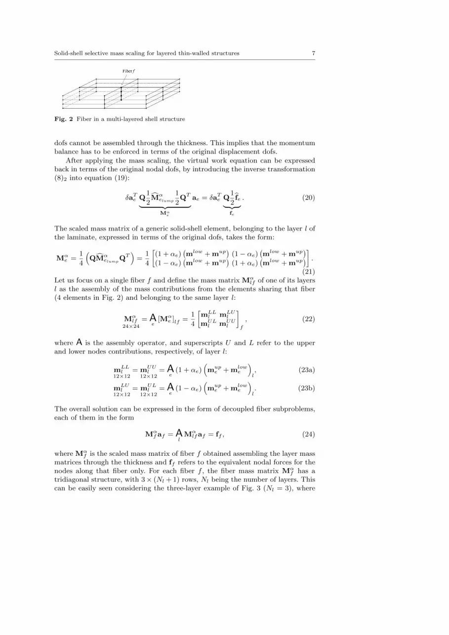
When a layered structure is considered, several solid-shell elements, one for eachlayer is assumed hereafter, are used for the discretization through the thickness(Fig. 2). In this case, the term “fiber” defines the multi-layer segment connectingall the nodes through the shell thickness at the same in-plane position. As shown inFig. 2, a multi-layer fiber is then formed by a set of corner fibers belonging to theelements stacked up along the thickness. Unlike in the case of a single layer shell,the procedure described in Section 2 cannot be directly applied, since corner fiber


Fig. 2 Fiber in a multi-layered shell structure

dofs cannot be assembled through the thickness. This implies that the momentumbalance has to be enforced in terms of the original displacement dofs.

After applying the mass scaling, the virtual work equation can be expressedback in terms of the original nodal dofs, by introducing the inverse transformation(8)2 into equation (19):

δaTe Q1

2Mαelump

1

2QT︸︷︷︸

Mαe

ae = δaTe Q1

2fe︸︷︷︸

fe

. (20)

The scaled mass matrix of a generic solid-shell element, belonging to the layer l ofthe laminate, expressed in terms of the original dofs, takes the form:

Mαe =

1

4

(QMα

elumpQT)

=1

4

[(1 + αe)

(mlow + mup

)(1− αe)

(mlow + mup

)(1− αe)

(mlow + mup

)(1 + αe)

(mlow + mup

)] .(21)

Let us focus on a single fiber f and define the mass matrix Mαlf of one of its layers

l as the assembly of the mass contributions from the elements sharing that fiber(4 elements in Fig. 2) and belonging to the same layer l :

Mαlf

24×24

= Ae

[Mαe ]lf =

1

4

[mLLl mLU

l

mULl mUU

l

]f

, (22)

where A is the assembly operator, and superscripts U and L refer to the upperand lower nodes contributions, respectively, of layer l:

mLLl

12×12= mUU

l12×12

= Ae

(1 + αe)(mupe + mlow

e

)l, (23a)

mLUl

12×12= mUL

l12×12

= Ae

(1− αe)(mupe + mlow

e

)l. (23b)

The overall solution can be expressed in the form of decoupled fiber subproblems,each of them in the form

Mαf af = A

lMαlfaf = ff , (24)

where Mαf is the scaled mass matrix of fiber f obtained assembling the layer mass

matrices through the thickness and ff refers to the equivalent nodal forces for thenodes along that fiber only. For each fiber f , the fiber mass matrix Mα

f has atridiagonal structure, with 3× (Nl + 1) rows, Nl being the number of layers. Thiscan be easily seen considering the three-layer example of Fig. 3 (Nl = 3), where


Fig. 3 Example of three-layered fiber

the mass matrix Mαf related to the fiber f crossing the layers i, j, and k is given

by:

Mαf

12Nl×12Nl

=

mLLi mLU

i 0 0

mULi mUU

i + mLLj mLU

j 0

0 mULj mUU

j + mLLk mLU

k

0 0 mULk mUU

k

. (25)

The overall solving system can be obtained by assembling over all the fibers,namely:

Mαa = AfMfaf = A

fff = f , (26)

where the global mass matrix Mα is a block diagonal matrix, each block consistingof a tridiagonal matrix of the type in (25), corresponding to the dofs of a single fiberf. In view of the mild tridiagonal coupling, the computation of the accelerations atfiber nodes can be carried out very effectively, e.g. by an explicit LU decompositionof the fiber mass matrix, involving a number of dofs proportional to the layernumber, which is usually small. The small burden, additional with respect to thecase of a fully diagonal mass matrix, is by far compensated by the larger stabletime step which can be used in the computation.

4 Optimal mass scaling factor and maximum eigenfrequencycomputation

The definition of the optimal value of the selective mass scaling factor α is theresult of a trade-off between two conflicting objectives. On one side, large values ofα lead to an increasing reduction of the element maximum eigenfrequency, allowingfor the use of larger stable time steps. On the other side, an accurate reproductionof the structural dynamical properties requires to consider values of α as small aspossible. For a deformed solid-shell element, a typical reduction of the maximumeigenfrequency with the mass scaling factor is shown in Fig. 4 (Cocchetti et al(2015)). While for small values of α there is a rapid gain in terms of time step size,for large values of α there is almost no gain at the cost of a growing loss of accuracyin the structural response, due to the modified mass. It is therefore essential todefine a criterion for the definition of the optimal element scaling factor.

In unstructured meshes, the elements are all different and α has to be computedindividually for each element in a pre-processing step. After defining the elementoptimal scaling factor, one has to compute the time step size to be used for sta-ble integration with the central difference scheme. In large deformation problems,the element size and shape can change considerably during the analysis, possibly


Fig. 4 Decrease of max eigenfrequency ωmax for increasing scaling factor α.

requiring a repeated run-time computation of the critical time step. A computa-tionally effective technique for the estimation of the critical time step is thereforealso necessary.

Since it can be shown that the maximum element eigenfrequency is associatedto the thickness vibration mode, in Cocchetti et al (2015) an equivalence has beenestablished between selective and geometric scaling, where geometric scaling meansartificially increasing the element thickness while the in-plane dimensions are keptconstant. Interpreting the Jacobian J = ∂x/∂ξ of the isogeometric mapping asthe deformation gradient of the deformation process transforming the parent cubic2 × 2 × 2 element into the current distorted shape, c = J−TJ−1 is the Cauchydeformation tensor and

c =3∑i=1

γ2i ti ⊗ ti (27)

represents its spectral decomposition, where γ21 ≤ γ22 ≤ γ23 are the principalstretches and t3 represents the direction of maximum shortening in the currentconfiguration, i.e. the thickness direction of the distorted element.

The procedure proposed in Cocchetti et al (2015) consists of defining

αopt =

(γ3γ2

)2

, (28)

so that after the scaling the thickness becomes of a size comparable to the elementin-plane dimensions. Alternatively, if L1, L2, h0 define the approximate elementin-plane and thickness dimensions as the distances between centroids of elementfaces, i.e.

L1 = ‖x(1, 0, 0)− x(−1, 0, 0)‖, L2 = ‖x(0, 1, 0)− x(0,−1, 0)‖,h0 = ‖x(0, 0, 1)− x(0, 0,−1)‖,

(29)


a quick and inexpensive estimate of αopt can be achieved by setting

αopt =L2min

h20, Lmin = min{L1, L2}. (30)

For parallelepiped elements, the criteria in (28) and (30) are equivalent.In the present context of laminated shells, where several solid-shell elements

are stacked one on top of the other, the layers have in general different thicknessesand a different value of αopt has to be computed for each layer, according to either(28) or (30). As it will be shown in the numerical examples, the selective massscaling will allow to use the same time step, only dictated by the element in-planedimensions, no matter what is the number of layers used to discretize the shellthickness.

Once α has been chosen for each element in the mesh, the size of the stabletime step has to be approximated rigorously from below, to avoid an unstabletime integration. The stable time step is determined according to (1) and (2),where ωemax is estimated for each element according to the procedure proposedin Cocchetti et al (2015) for arbitrarily distorted solid-shell elements with scaledmasses, which is based on the procedure proposed by Flanagan and Belytschko(1984) for constant strain hexahedra (for simplicity of notation the element indexe is hereafter discarded). An upper bound ω2

G of ωmax is first computed makinguse of Gershgorin’s theorem as:

ω2max ≤ ω2

G =2µ

ρ0

ν

1− 2νI1/α

1 + maxi

3∑j=1

∣∣[c1/α

0 ]ij∣∣ . (31)

In (31), µ is the elastic shear modulus, ν is Poisson’s ratio, ρ is the mass density,c1/α

0 is the Cauchy deformation tensor of the scaled element, defined as:

c1/α

0 =(J

√α

0

)−T (J

√α

0

)−1, J

√α

0 = J0I√α

3 , I√α

3 =

1 0 00 1 00 0√α

, (32)

where J0 is the Jacobian of the element isoparametric mapping evaluated at theelement centroid. I1/α

1 in (31) is the first invariant of c1/α

0 .A sharper rigorous bound ω2

N−R on ωemax can be obtained for each elementperforming one Newton-Raphson iteration for the search of the maximum rootof the characteristic equation f

(ω2;α

)= 0 of the element eigenvalue problem,

starting from the tentative solution ω2 = ω2G:

ω2N−R = ω2

G −f(ω2G;αopt

)f ′ (ω2

G;αopt), (33)

where

f(ω2;α

)=(ω2)3− 1− ν

1− 2ν

2µ

ρ0I1/α

1

(ω2)2

+1

1− 2ν

(2µ

ρ0

)2

I1/α

2 ω2 − 1 + ν

1− 2ν

(2µ

ρ0

)3

I1/α

3 = 0

f ′(ω2;α

)=df

dω2

(34)


Fig. 5 Rotational patch test: geometry.

and I1/α

2 , I1/α

3 are the second and third invariants, respectively, of c1/α

0 .

As discussed in Cocchetti et al (2015) on the basis of an extensive numerical in-vestigation, ω2

N−R approximates ωmax from above with an average approximationof about 1% and a peak error of about 3%.

5 Numerical results

Seven numerical examples are here proposed to check the accuracy of the massscaling procedure and the computational gain. The Q1ST solid-shell element, de-veloped in Schwarze and Reese (2011), is used in all cases and the scaling parameteris computed using either the simplified approach in (30) or the procedure in (28).

5.1 Rotational patch test

As highlighted in Section 2, the proposed selective mass scaling technique affectsrigid body rotations. The rotational patch test presented in Cocchetti et al (2015)is here considered to numerically asses the effect of selective mass scaling on therotational inertia in the presence of layered shells. The parallelepiped patch, shownin Fig. 5, has a square in-plane shape of size L = 2 m and thickness H = 0.1 m. A

uniform angular velocity ω =π

4

rad

saround the x axis is imposed to the boundary

nodes. Furthermore, in order to reproduce the rigid body rotation conditions, cen-tripetal body forces of the same magnitude of the theoretical centrifugal inertiaforces, but with opposite sign, are applied to the elements of the patch. The intro-duction of the selectively scaled mass matrix causes a deviation from the situationof perfectly rigid body motion. In Cocchetti et al (2015), it has been proposed


Table 1 Rotational patch test: comparison between scaled and unscaled time step sizes.

Number of layers Layer thickness γ α ∆tα ∆t0

(m) (µs) (µs)

1 0.100 20 100 126.49 17.212 0.050 40 400 126.49 8.624 0.025 80 1600 126.49 4.31

to evaluate the error ε due to the modified rotational inertia in terms of kineticenergy:

ε =Kα −K0

K0, (35)

where Kα and K0 are the kinetic energies of the scaled and of the original system,respectively. The energy error for the patch has been shown to be well approxi-mated by the following expression, correlating the error to the mass scaling factor,to the element geometry and to the distance RG between the patch centroid andthe rotation axis:

ε = (α− 1)1

4γ2(RGL

)2 , (36)

being γ =L

hthe ratio between the patch width and the element thickness. This

expression shows that the error decreases with the square of the ratio RG/L,which measures the importance of the translational component of the motion withrespect to the rotational one.

The analysis has been performed considering increasing values of the distanceRG, namely RG = [2, 4, 6, 8, 10, 20]. Moreover, the simulations have been run con-sidering a plate discretization with 1, 2 and 4 homogeneous layers of equal thick-ness. Four square elements are used for the in-plane discretization. Table 1 givesthe values of the mass scaling factor α, equal for all elements in the mesh, of theratio γ in these three cases and of the stable time steps ∆tα and ∆t0 computedwith scaled and unscaled masses, respectively. The computational gain can beeasily evaluated by comparing the time steps.

Figure 6 shows the trend of the energy error (35) for increasing values of theratio between the radius RG and the in-plane patch size L. The numerical resultsare consistent with the analytical estimate in (36): the numerical error decreasesalmost quadratically at increasing distance RG. It can also be observed that thenumerical solutions obtained for the three cases are, as expected, almost perfectlyoverlapped, despite the different number of layers and the fact that the same timestep has been used in all cases.

5.2 Small displacements cantilever beam

In this second example the cantilever beam depicted in Fig. 7 is considered toshow the capability of the proposed selective mass scaling procedure to reproducethe dynamical behavior of a linear elastic thin structure in small displacements,over a time interval spanning several fundamental periods of the beam. The beam


Fig. 6 Rotational patch test: comparison between numerical and analytical error.

Fig. 7 Small displacements cantilever beam: geometry, boundary and loading conditions.

has a length L = 6000 mm and a rectangular cross section width W = 200 mmand depth H = 100 mm. A material with Young’s modulus E = 2 × 105 MPa,Poisson’s ratio ν = 0.3 and density ρ = 7500 kg/m3 has been chosen. The analysishas been performed considering an increasing number of homogeneous layers ofequal thickness, namely 1,2,4,6,8,10. In all cases, the cantilever is clamped at oneside and a concentrated step load F = 500 N, which remains constant in time, isapplied at the free tip, equally distributed among the tip nodes. A small load hasbeen chosen, so that small displacements can be assumed, with tip displacementover beam length ratio of the order of 10−3 in the static case.

Two different discretizations, displayed in Fig. 8, have been considered, denotedin the following as mesh A and mesh B, respectively: the first mesh is made ofsix regular parallelepiped elements, while six distorted elements have been usedfor the second one. For mesh A, the application of equations (28) and (30) for thecomputation of α gives the same result:

α = N2lW 2

H2= 4N2

l (37)


Fig. 8 Small displacements cantilever beam: top view of adopted meshes. a) Mesh A, regularelements. b) Mesh B, distorted elements.

Table 2 Small displacements cantilever beam: mass scaling factors for mesh A.

Number of layers Layer thickness α(mm)

1 100.00 4.002 50.00 16.004 25.00 64.006 16.67 144.008 12.50 256.0010 10.00 400.00

Table 3 Small displacements cantilever beam: mass scaling factors for mesh B computedaccording to (28).

Element number 1 layer 2 layers 4 layers 6 layers

1 3.98 15.93 63.73 143.392 4.00 15.98 63.94 143.863 3.89 15.55 62.20 139.964 3.98 15.92 63.70 143.335 3.96 15.83 63.32 142.496 3.99 15.98 63.91 143.79

Table 4 Small displacements cantilever beam: mass scaling factors for mesh B computedaccording to (30).

Element 1 layer 2 layers 4 layers 6 layers 8 layersnumber

1 4.31 17.23 68.93 151.37 275.712 4.12 16.46 65.85 148.10 262.403 5.70 22.81 91.25 205.23 364.994 4.35 17.39 69.57 156.47 278.285 4.99 19.96 79.84 179.57 319.366 4.25 16.98 67.92 152.76 271.68

and the scaling factor increases with the square of the layers number Nl. Theobtained values are shown in Table 2. For mesh B, since we intentionally gave tothe elements different distortions, a different scaling factor is obtained for eachelement. The values obtained with equation (28) and (30) are shown in Tables 3and 4. Also in this case, the scaling factor increases with the square of Nl andsimilar values are obtained with the two methods.


Table 5 Small displacements cantilever beam: updated mass scaling factors for mesh B com-puted according to (28).

Element number 1 layer 2 layers 4 layers 6 layers 8 layers 10 layers

1 3.78 15.12 60.46 136.04 241.85 377.882 3.74 14.96 59.84 134.63 239.34 373.973 3.89 15.55 62.20 139.96 248.81 388.774 3.78 15.10 60.40 135.90 241.59 377.495 3.78 15.13 60.53 136.20 242.14 378.346 3.73 14.93 59.70 134.33 238.80 373.13

Table 6 Small displacements cantilever beam: number of layers and critical time step beforemass scaling.

Number of layers Layer thickness ∆t0 (µs) ∆t0 (µs)(mm) mesh A mesh B

1 100.00 16.21 16.172 50.00 8.29 8.294 25.00 4.17 4.176 16.67 2.78 2.788 12.50 2.09 2.0810 10.00 1.67 1.67

Table 7 Small displacements cantilever beam: critical time step after mass scaling.

∆tα (µs) ∆tα (µs) ∆tα (µs)mesh A mesh B - α eq. (28) mesh B - α eq. (30)

27.83 27.65 28.00

Since the elements are different, according to (2) the critical time step to beused for time integration is determined by the element exhibiting the highesteigenfrequency ωmax = max{ωemax}. A possible intervention, aimed at minimizingthe alteration of the structural dynamical properties, consists of reducing all thescale factors in Tables 3 and 4, with the exception of the one of the element withthe maximum eigenfrequency ωmax, in such a way that all scaled elements possessthe same highest eigenfrequency. This can be easily done by setting ω2 = ω2

max in(34)1 and then solving for α for each element. This additional computation has tobe carried out only once, in a pre-processing step, and therefore is not expensive.

The recomputed values of α in Table 3 are shown in Table 5. For the dis-torted mesh B, the critical element is the number 3 and its scaling factor remainsunchanged. With the exception of element 3, all scaling factors are smaller thanthose in Table 3. The differences between values in the two tables are not large,since the elements have similar sizes. Much larger differences can be expected instrongly unstructured meshes.

Table 6 shows the stable time steps∆t0 for the unscaled mass matrix, computedfor the two meshes for increasing number of layers: it can be noted that the timestep size decreases linearly with the layers number. The time step sizes obtainedafter application of mass scaling, using the values of α in Tables 3 and 4 are shownin Table 7. For both meshes, the obtained value of ∆tα, determined by the in-plane


Fig. 9 Small displacements cantilever beam: time history of tip displacement.

element size, is independent of the number of layers. Therefore, only one value isshown in the table. In the 10 layers case, the computational gain, quantified asthe ratio between the adopted time step and ∆t0, is of about 16.7 times for meshB and slightly higher for mesh A.

The time evolution of the vertical tip displacement is displayed in Fig. 9: itcan be seen that the curves, obtained with a different number of layers, are almostperfectly overlapped, even when multiple time periods are considered. A zoom onthe first time period for the 10-layer case is shown in Fig. 10 to get a refined viewon the differences between the numerical solutions. Note that the analytical staticsolution for the tip displacement is equal to 10.8 mm.

5.3 Cantilever beam: large displacements case

The large displacements dynamical response of the impulsively loaded cantileverbeam shown in Fig. 11 is analyzed. The beam length is equal to 100 mm, whileits cross section is 20 mm wide and 2 mm deep. A linear elastic material has beenconsidered with E = 1768 MPa, ν = 0.3 and ρ = 3000 kg/m3. A uniform transversetip load per unit surface p, linearly increasing with time from 0 to 0.5 · 10−3 MPaat t = 5 ms, is applied and distributed over the tip nodes. The analysis is run for5 ms, after which very large tip displacements are achieved. An increasing numberof homogeneous layers of equal thickness has been considered, namely 1,2,4,8,16.Table 8 provides the values of the mass scaling factor, computed according to eq.28, and of the stable time step. As in the previous example, it can be noted thatthe critical time step is not affected by the reduction in the element thickness,but it is determined only by the in-plane size. The comparison between the timehistories of vertical tip displacements obtained in the different cases is displayedin Fig. 12.

Displaced configurations for varying number of layers, at the final time instantt = 5 ms, are shown in Fig. 13. Despite the high values of α = 1600 used in the 16layers case and the notably large rotations of some elements, there are no visibledifferences in the displaced configurations in the four cases shown in Fig. 13.


Fig. 10 Small displacements cantilever beam. Tip vertical displacement: zoom on the firsttime period.

Fig. 11 Large displacements cantilever beam: geometry, boundary and loading conditions.

Table 8 Large displacements cantilever beam: mass scaling factor and critical time step size.

Number of layers Layer thickness α (eq. 28) ∆tα ∆t0

(mm) (µs) (µs)

1 2.00 6.25 4.119 2.1712 1.00 25.00 4.119 1.1144 0.50 100.00 4.119 0.5608 0.25 400.00 4.119 0.28116 0.125 1600.00 4.119 0.140

5.4 Pinched cylinder

A cylindrical shell, clamped at one end, is loaded at the other end by a pair ofconcentrated forces applied at two diametrically opposite points, as shown in Fig.14. This benchmark problem has been proposed in Ibrahimbegovic et al (2001).Because of symmetry, only one half of the specimen is considered. The lengthof the cylinder is L = 3.048 m, while its radius is equal to R = 1.016 m. The


Fig. 12 Large displacements cantilever beam: time history of vertical tip displacement.

Fig. 13 Large displacements cantilever beam: deformed shapes at t = 5 ms.

thickness is equal to t = 0.03 m. The material has been considered linear elasticwith Young’s modulus E = 2.0685 · 107 N/m2, Poisson’s ratio ν = 0.3 and densityρ = 1000 kg/m3. The concentrated load increases linearly with time from 0 N to900 N in 0.9 s.

The simulation has been performed considering three different numbers Nl ofhomogeneous layers of uniform thickness, namely 2, 4 and 6. 1920 x Nl solid-shellelements have been used in the discretization. Table 9 provides the values of thetime step and of the maximum mass scaling factor determined in the three cases onthe basis of the simplified procedure in (30). Thanks to the mass scaling, the sametime step is obtained in all cases. The same analysis has also been run with thecommercial code Abaqus using the same number of classical S4R shell elements, to


Fig. 14 Pinched cylinder: geometry, mesh, boundary and loading conditions.

Table 9 Pinched cylinder: stable time step and mass scaling factor

Number of layers ∆tα α eq. (30)(ms)

2 0.1504 26.814 0.1504 107.606 0.1504 242.63

test the numerical results obtained with the implemented code. The time historiesof the displacement along z of the loading point are displayed in Fig. 15. It canbe noted that the four curves are almost perfectly overlapped up to the end ofthe analysis. In Fig. 16 the contour plots of the displacement along z obtained inthe three cases are compared to the result of the Abaqus simulation. A very goodagreement can be observed also in this case.

5.5 Peeling test

A double cantilever beam subjected to peeling-like loading conditions is sim-ulated in this example with the aim to assess the modifications of the through-the-thickness stresses due to the mass scaling application. Figure 17 shows theanalyzed geometry overlapped to the final deformed shape. The left end of thebeam is clamped, while a vertical displacement, linearly increasing in time from0 to 5 mm in 0.1 s, is prescribed on the right end of the specimen, at the tip ofthe free arm. By exploiting symmetry, only the upper half of the beam of totalthickness of 10 mm (i.e. the peeling arm thickness is equal to 5 mm) is analyzed.The beam is 24 mm wide and has a total length of 200 mm with a peeling armof 100 mm. The peeling arm has been discretized by means of five layers of equalthickness. The beam is made of steel with Young’s modulus E = 210000 MPa,Poisson’s ratio ν = 0.2 and mass density ρ = 7800 kg/m3. Since the mesh is struc-tured and all the layers have the same thickness, a unique value of mass scaling


Fig. 15 Pinched cylinder: displacement along z of the loaded point.

Fig. 16 Pinched cylinder: contour plots of displacement along z.

parameter has been computed, α = 59.17. The critical time steps, evaluated ap-plying the mass scaling procedure or not, are equal to ∆t0 = 1.8264 · 10−6 s and∆tα = 1.6201 · 10−5 s, respectively.

The distribution of the stress component σx along the beam thickness, beingdirection x aligned with the beam axis, has been evaluated at the centroids of thefive elements B-C-D-E-F placed at the right of the beam mid-length, i.e. the firstelements of the peeling arm (see Fig. 17), at five subsequent time instants (Fig.18). The two stress distributions appear to be almost identical throughout thethickness.

Figure 19 shows the time evolution of the σz stress component, being z thethickness direction, evaluated at the centroid of element A, placed at the left of thebeam mid-length at the bottom of the cross section (Fig. 17), with and withoutselective mass scaling. In both cases, the representative stress points have beenplotted at about every 10−3 s, and oscillate with comparable amplitude around the


Fig. 17 Peeling test: geometry, boundary conditions, discretization and final deformed shape.

same straight line defining the stress growth due to the linearly growing intensityof the applied load.

5.6 Sandwich beam with soft core

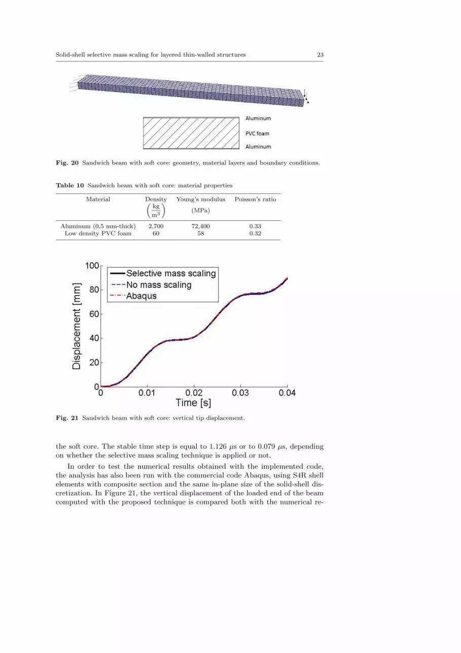
While structures with uniform material through the thickness were consideredin the previous examples, in this case the bending response of a cantilever sandwichbeam with soft core is addressed. The beam length is equal to 600 mm, whileits rectangular cross section is 60 mm wide and 20 mm deep. As shown in Fig.20, one side of the beam is completely clamped, while a surface load, linearlyincreasing with time from 0 to 0.05 MPa in 0.04 s, is applied at the opposite one.As in Sokolinsky et al (2003), the sandwich beam is composed of two externalaluminum thin face sheets and of a soft core of low-density PVC foam. Bothaluminum layers are 0.5 mm thick, while the thickness of the soft core is equalto 19 mm. The mechanical properties of the two materials are listed in Table 10.Each aluminum layer has been discretized by only one solid-shell element through-the-thickness, while five solid-shell elements of equal thickness are stacked up tomodel the soft core. The adopted mesh, characterized by 2520 solid-shell elements,has been obtained considering an in-plane size of the elements equal to 10 mm.Although the mesh is structured, two different values of the mass scaling parameterhave to be defined, since different materials and element thicknesses are present:in particular, the mass matrices of the elements belonging to the aluminum layersare scaled by α = 400, while α = 6.93 is adopted for the elements belonging to


Fig. 18 Peeling test: longitudinal stress component σx at the elements B-C-D-E-F (see Fig.17) of the free arm.

Fig. 19 Peeling test: vertical stress component σz at element A (see Fig. 17) of the clampedregion.


Fig. 20 Sandwich beam with soft core: geometry, material layers and boundary conditions.

Table 10 Sandwich beam with soft core: material properties

Material Density Young’s modulus Poisson’s ratio(kg

m3

)(MPa)

Aluminum (0.5 mm-thick) 2,700 72,400 0.33Low density PVC foam 60 58 0.32

Fig. 21 Sandwich beam with soft core: vertical tip displacement.

the soft core. The stable time step is equal to 1.126 µs or to 0.079 µs, dependingon whether the selective mass scaling technique is applied or not.

In order to test the numerical results obtained with the implemented code,the analysis has also been run with the commercial code Abaqus, using S4R shellelements with composite section and the same in-plane size of the solid-shell dis-cretization. In Figure 21, the vertical displacement of the loaded end of the beamcomputed with the proposed technique is compared both with the numerical re-


Fig. 22 Sandwich plate with hard core: a) geometry and boundary conditions, b) materiallayers.

sult obtained without applying the selective mass scaling procedure and with thoseobtained using the commercial code.

5.7 Sandwich plate with hard core

A 10 mm x 10 mm square sandwich plate with hard core, fully clamped at oneedge, is subject to a transverse distributed load, applied at the opposite one andlinearly increasing with time from 0 to 0.0025 MPa in 0.5 ms (Fig. 22a). The plateis composed of two external layers of low density polyethylene (LDPE) with thick-nesses equal to 30 µm (upper layer) and 21 µm (lower layer), and of an internallayer of aluminum of thickness 9 µm, as shown in Fig. 22b. The overall thickness ofthe cross section is equal to 60 µm. The material properties are listed in Table 5.4and are taken from Frangi et al (2010). Because of the small thicknesses involvedin the model, the through-the-thickness discretization has been obtained using onesolid-shell element per layer. The in-plane size of the element is equal to 0.5 mm:the resulting mesh of 1200 elements is shown in Fig. 22 together with the boundaryconditions of the problem. Three different values of the mass scaling parametershave been computed: the mass matrices of the elements belonging to the three lay-ers (bottom up) are scaled by α equal to 277.78, 3086.42, and 566.89, respectively.The stable time steps, computed by applying or not the selective mass scaling, areequal to 9.487 · 10−8 s and 2.327 · 10−9 s, respectively. The elements belonging tothe aluminum layer turn out to be the critical ones in determining the maximumeigenfrequency ωmax. The mass scaling parameters of the other elements are notre-computed after the estimation of ωmax in order to consider a more severe teston the accuracy of the numerical results. The loaded edge deflection is plotted inFig. 23. The maximum displacement reached at the end of the analysis is about


Table 11 Sandwich plate with hard core: material properties

Material Density Young’s modulus Poisson’s ratio(kg

m3

)(MPa)

Aluminum (9 µm-thick) 2,700 30,000 0.30Low density polyethylene (LDPE) 1,000 500 0.40

Fig. 23 Sandwich plate with hard core: maximum vertical displacement.

one hundred times greater than the plate thickness.

6 Conclusions

A selective mass scaling procedure for layered thin-walled structures, discretizedwith one or more solid-shell elements per layer, has been presented and its perfor-mance has been assessed by means of several numerical examples. The method is anatural extension to multi-layer structures of what has been proposed in Cocchettiet al (2013); Pagani et al (2014); Cocchetti et al (2015) for homogeneous, one-layer shells. The scaling procedure can be applied to distorted 8-node solid-shellelements, with nodal displacements dofs. The proposed scaling reduces the highesteigenfrequencies, while the lower ones, associated to the rigid body translations,remain almost unaffected. As a result, when the dynamical behavior is governedby the lowest frequencies, the structural response is well reproduced. The inertiaassociated to rotational rigid body motions is increased by the mass scaling. Thisimplies a modification of the resulting kinetic energy that, however, is shown to be


negligible when the translational component of the motion of individual elementsis dominant.

The mass matrix resulting from the application of the selective mass scaling isblock diagonal, where each block corresponds to the degrees of freedom of a singlethrough-the-thickness fiber, and it is characterized by a tridiagonal structure. Itsdimensions are directly related to the number of layers, typically small. Therefore,the solution of the small linear system providing the accelerations of the nodesbelonging to the same fiber is inexpensive and the small additional burden is byfar compensated by the largest stable time step.

A critical role is played by the choice of the mass scaling factor. The crite-rion proposed in Cocchetti et al (2015) has been used together with the strategyproposed there for the computation of the critical time step size. The considerednumerical tests have shown that, using this criterion, it is possible to performexplicit dynamics simulations with an increasing number of solid-shell elementsthrough the shell thickness, using the same stable time step, independent of thenumber of layers and determined by the in-plane element size, with negligibleaccuracy loss.

Acknowledgements The financial support by Tetra Pak Packaging Solutions is kindly ac-knowledged.

References

Abed-Meraim F, Combescure A (2009) An improved assumed strain solid-shellelement formulation with physical stabilization for geometric non-linear appli-cations and elastic-plastic stability analysis. International Journal for NumericalMethods in Engineering 80(13):1640–1686

Abed-Meraim F, T VD, Combescure A (2013) New quadratic solid-shell elementsand their evaluation on linear benchmark problems. Computing 95(5):373–394

Askes H, Nguyen DCD, Tyas A (2011) Increasing the critical time step: micro-inertia, inertia penalties and mass scaling. Computational Mechanics 47(6):657–667

Cocchetti G, Pagani M, Perego U (2013) Selective mass scaling and critical time-step estimate for explicit dynamics analyses with solid-shell elements. Comput-ers & Structures 127:39–52

Cocchetti G, Pagani M, Perego U (2015) Selective mass scaling for distortedsolid-shell elements in explicit dynamics: optimal scaling factor and stable timestep estimate. International Journal for Numerical Methods in Engineering101(9):700–731

Flanagan D, Belytschko T (1984) Eigenvalues and stable time steps for the uniformstrain hexaedron and quadilateral. Journal of Applied Mechanics 51(1):35–40

Frangi A, Pagani M, Perego U, Borsari R (2010) Directional cohesive elements forthe simulation of blade cutting of thin shells. Computer Modeling in Engineeringand Sciences (CMES) 57(3):205

Hauptmann R, Schweizerhof K (1998) A systematic development of ’solid-shell’element formulations for linear and non-linear analyses employing only displace-ment degrees of freedom. International Journal for Numerical Methods in Engi-neering 42(1):49–69


Hetherington J, Rodriguez-Ferran A, Askes H (2012) A new bipenalty formula-tion for ensuring time step stability in time domain computational dynamics.International Journal for Numerical Methods in Engineering 90:269–286

Ibrahimbegovic A, Brank B, Courtois P (2001) Stress resultant geometrically exactform of classical shell model and vector-like parametrization of constrained finiterotations. International Journal for Numerical Methods in Engineering 52:1235–1252

Macek RW, Aubert BH (1995) A mass penalty technique to control the criticaltime increment in explicit dynamic finite element analyses. Earthquake Engi-neering and Structural Dynamics 24(10):1315–1331

Meyers MA (1994) Dynamic behavior of materials. Wiley, New YorkNaceur H, Shiri S, Coutellier D, Batoz JL (2013) On the modeling and design of

composite multilayered structures using solid-shell finite element model. FiniteElements in Analysis and Design 70-71:1–14

Olovsson L, Unosson M, Simonsson K (2004) Selective mass scaling for thin walledstructures modeled with tri-linear solid elements. Computational Mechanics34(2):134–136

Olovsson L, Simonsson K, Unosson M (2005) Selective mass scaling for explicitfinite element analyses. International Journal for Numerical Methods in Engi-neering 63(10):1436–1445

Pagani M, Reese S, Perego U (2014) Computationally efficient explicit nonlinearanalyses using reduced integration-based solid-shell finite elements. ComputerMethods in Applied Mechanics and Engineering 268:141–159

Schwarze M, Reese S (2011) A reduced integration solid-shell finite element basedon the EAS and the ANS concept: large deformation problems. InternationalJournal for Numerical Methods in Engineering 85(3):289–329

Sokolinsky VS, Shen H, Vaikhanski L, Nutt SR (2003) Experimental and analyticalstudy of nonlinear bending response of sandwich beams. Composite Structures60:219–229

Tan X, Vu-Quoc L (2005) Efficient and accurate multilayer solid-shell element:non-linear materials at finite strain. International Journal 63(15):2124–2170

Tkachuk A, Bischoff M (2013a) Local and global strategies for optimal selectivemass scaling. Computational Mechanics 53(6):1197–1207

Tkachuk A, Bischoff M (2013b) Variational methods for selective mass scaling.Computational Mechanics 52(3):563–570

Tkachuk A, Bischoff M (2015) Direct and sparse construction of consistent inversemass matrices: general variational formulation and application to selective massscaling. International Journal for Numerical Methods in Engineering 101(6):435–469

Zukas JA (2004) Introduction to hydrocodes. Elsevier, Amsterdam

Documents

8-Node solid-shell elements selective mass scaling for explicit dynamic analysis of layered thin-walled structures