Embed Size (px)
Citation preview
Chapter 2 Dynamic Pricing Models Abstract In this chapter, some pricing models are presented that are character-ized by the following assumptions: (i) the number of potential customers is not limited, and as a consequence, the size of the population is not a parameter of the model, (ii) only one type of item is concerned, (iii) a monopoly situation is con-sidered, and (iv) customers buy items as soon as the price is less than or equal to the price they are prepared to pay (myopic customers). A deterministic model with time-dated items is presented and illustrated first. To build this model, the rela-tionship between the price per item and demand has to be established. Then, the stochastic version of the same model is analyzed. A Poisson process generates customers’ arrivals. Finally, a stochastic model with salvage value where the price is a function of inventory level is considered. Detailed algorithms, numerical ex-amples and figures are provided for each model. These models provide practical insights into pricing mechanisms.
2.1 Introduction
Any dynamic pricing model requires establishing how demand responds to changes in price. This chapter is dedicated to mathematical models of monopoly systems. The reader will notice that strong assumptions are made to obtain tracta-ble models. Indeed, such mathematical models can hardly represent real-life situa-tions, but they do illustrate the relationship between price and customers’ purchas-ing behavior.
In this chapter we consider the case of time-dated items, i.e., items that must be sold before a given point in time, say T. Furthermore, there is no supply option be-fore time T. This situation is common in the food industry, the toy business (when toys must be sold before Christmas, for instance), marketing products (products associated with special events like movies, football matches, etc.), fashion apparel

42 2 Dynamic Pricing Models
(because the selling period ends when a season finishes), airplane tickets (which are obsolete when the plane takes off), to quote just a few.
The goal is to find a strategy (dynamic pricing, also called yield management or revenue management) that leads to the maximum expected revenue by time T, assuming that the process starts at time 0. This strategy consists in selecting a set of adequate prices for the items that vary according to the number of unsold items and, in some cases, to the time. At a given point in time, we assume that the price of an item is a non-increasing function of the inventory level. For a given inven-tory level, prices are going down over time.
Indeed, a huge number of models exist, depending of the situation at hand and the assumptions made to reach a working model. For instance, selling airplane tickets requires a pricing strategy that leads to very cheap tickets as takeoff nears, while selling fashion apparel is less constrained since a second market exists, i.e., it is still possible to sell these items at discount after the deadline.
For the models presented in this chapter, we assume that:
• The number of potential customers is infinite. As a consequence, the size of the population does not belong to the set of parameters of the models.
• A single type of item is concerned and its sales are not affected by other types of items.
• We are in a monopoly situation, which means that there is no competition with other companies selling the same type of item. Note that, due to price discrimi-nation, a company can be monopolistic in one segment of the population while other companies sell the same type of item with slight differences to other seg-ments. This requires a sophisticated fencing strategy that prevents customers from moving to a cheaper segment.
• Customers are myopic, which means that they buy as soon as the price is less than the one they are prepared to pay. Strategic customers who optimize their purchasing behavior in response to the pricing strategy of the company are not considered in this chapter; game theory is used when strategic customers are concerned.
To summarize, this chapter provides an insight into mathematical pricing mod-els. Note also that few convenient models exist without the assumptions presented above, that is to say a monopoly situation, an infinite number of potential custom-ers who are myopic and no supply option. The reader will also observe that nega-tive exponential functions are often used to make the model manageable and few persuasive arguments are proposed to justify this choice: this is why we consider that most of these models are more useful to understand dynamic pricing than to treat real-life situations.
2.2 Time-dated Items: a Deterministic Model 43
2.2 Time-dated Items: a Deterministic Model
2.2.1 Problem Setting
In this model, we know the initial inventory 0s : it is the maximal quantity that can be sold by time T. We assume that demands appear at times T,,2,1 L , and tx represents the demand at time t. The demands are real and positive. The price of one item at time t is denoted by tp , and this price is a function of the demand and the time: ( )txpp tt ,= .
We assume that there exists a one-to-one relationship between demand and price at any time { }Tt L,2,1∈ . Thus, ),( tpxx tt = is the relation that pro-vides the demand when the price is fixed.
We also assume that:
• ),( tpx is continuously differentiable with regard to p. • ),( tpx is lower and upper bounded and tends to zero as p tends to its maxi-
mal value.
Finally, the problem can be expressed as follows:
Maximize ∑=
T
ttt xp
1
(2.1)
subject to:
01
sxT
tt ≤∑
=
(2.2)
0≥tx for { }Tt L,2,1∈ (2.3)
),( min tpxx tt ≤ for { }Tt L,2,1∈ (2.4)
where mintp is the minimal value of tp .
Criterion 2.1 means that the objective is to maximize the total revenue. Con-straint 2.2 guarantees that the total demand at horizon T does not exceed the initial inventory. Constraints 2.3 are introduced to make sure that demands are never less than zero. Finally, Constraints 2.4 provide the upper bound of the demand at any time.

44 2 Dynamic Pricing Models
2.2.2 Solving the Problem: Overall Approach
To solve this problem, we use the Kuhn and Tucker approach based on Lagrange multipliers. Since tp is a function of tx , then tt xp is the function of tx . Taking into account the constraints of the problem, the Lagrangian is:
)),((
)(),(),,,,,,,,,(
min
11
10
1111
tpxxlx
sxxtxpllxxL
tt
T
tt
T
ttt
T
ttt
T
ttTTT
−−+
−−=
∑∑
∑∑
==
==
μ
λμμλ LLL
(2.5)
The goal is to solve the T equations:
0=∂∂
txL for { }Tt L,2,1∈ (2.6)
Together with the 2T +1 complementary slackness conditions:
0)( 01
=−∑=
sxT
ttλ (2.7)
⎭⎬⎫
=−
=
0)),((
0min tpxxl
x
ttt
ttμ for { }Tt L,2,1∈ (2.8)
Thus, we have 3T +1 equations for the 3T +1 unknowns that are:
,,,,,,, 11 TTxx μμλ LL Tll ,,1 L
A solution to the system of Equations 2.6–2.8 is admissible if ,0≥λ ,0≥tμ 0≥tl and if Inequalities 2.2–2.4 hold.
Note that, due to Relations 2.7 and 2.8:
0=λ and/or 01
sxT
tt =∑
=
0=tμ and/or 0=tx for { }Tt L,2,1∈
0=tl and/or ),( min tpxx tt = for { }Tt L,2,1∈

2.2 Time-dated Items: a Deterministic Model 45
2.2.3 Solving the Problem: Example for a Given Price Function
We consider the case:
tDDxBAtxp tt +
−= )(),(
where A, B and D are positive constants. As a consequence:
)(1),(D
tDpAB
tpx tt+
−=
As we can see:
• The price is a decreasing function of t.
• The demand must remain less than BA , otherwise the cost would become nega-
tive.
The problem to be solved is (see (2.1)–(2.4)):
Maximize tD
DxxBA t
T
tt +
−∑=
)(1
subject to:
01
sxT
tt ≤∑
=
⎪⎭
⎪⎬⎫
≤
≥
BAx
x
t
t 0 for { }Tt ,,2,1 L∈
The last constraints guarantee that prices remain greater than or equal to zero. In this case, the Lagrangian is:
)(
)()(),,,,,,,,,(
11
10
2
1111
BAxlx
sxtD
DxBxAllxxL
T
tttt
T
tt
T
ttt
T
ttTTT
−−+
−−+
−=
∑∑
∑∑
==
==
μ
λμμλ LLL

46 2 Dynamic Pricing Models
According to Relations 2.6–2.8, the system of equations to solve is:
0)2( =−+−+
− ttt ltD
DxBA μλ for { }Tt ,,2,1 L∈ (2.9)
0)( 01
=−∑=
sxT
ttλ (2.10)
0=tt xμ for { }Tt ,,2,1 L∈ (2.11)
0)/( =− BAxl tt for { }Tt ,,2,1 L∈ (2.12)
Whatever { }Tt ,,2,1 L∈ , tx is either equal to 0, or to BA / , or belongs to )/,0( BA (which represents the interval without its limits). This third option is
justified as follows. If neither of the first two options holds, then 0== tt lμ and Relation 2.9 be-
comes:
0)2( =−+
− λtD
DxBA t
Let us first assume that BAxt /= . In this case, 0=tμ and Equality 2.9 be-comes:
tltDDAA +=+
− λ)2(
The first member of this equality is negative, while the second member is greater than or equal to 0 since both λ and lt must be less than or equal to 0 for the solution to be admissible. As a conclusion, tx cannot be equal to BA / , and therefore, see (2.12), lt = 0 whatever t.
Let us now assume that 0=tx . In this case, and keeping in mind that lt = 0, Equality 2.9 becomes:
0=+−+ ttD
DA μλ or 0>++
= ttDDA μλ
Thus, according to (2.10), 01
sxT
tt =∑
=

2.2 Time-dated Items: a Deterministic Model 47
Finally, assume that )/,0( BAxt ∈ . In this case, 0== tt lμ and
tDDxBA t +
−= )2(λ .
As a consequence, ( ]BAxt /2/,0∈ and )(21
DtDA
Bxt
+−= λ .
We have to consider two cases:
1. If BAxt /2/= then, according to Equations 2.9 and 2.10:
0=λ and 01
sxT
tt ≤∑
=
(2.13)
2. If )/2/,0( BAxt ∈ , then, according to Equations 2.9 and 2.10:
0>λ and 01
sxT
tt =∑
=
(2.14)
Let be { }{ }0,,,2,1 >∈= txTttY L and NY the number of elements of Y. From (2.13) and (2.14) it appears that:
• If 0/2/ sBAT ≤× , then BAxt /2/= for { }Tt ,,2,1 L∈ is an admissible so-lution.
• If 0/2/ sBANY ≥× , then 01
sxT
tt =∑
=
. Since )(21
DtDA
Bxt
+−= λ when
0>tx , equality 01
sxT
tt =∑
=
becomes 0)(21 s
DtDA
BYt
=⎭⎬⎫
⎩⎨⎧ +
−∑∈
λ and
∑∈
+−
=
YtY
Y
tDNsDBADN 02
λ . Finally:
)2(21 0
DtD
tDNsDBADNA
Bx
YtY
Yt
++−
−=∑∈
for Yt∈ (2.15)
We derive an algorithm from the above results.

48 2 Dynamic Pricing Models
Algorithm 2.1.
1. If 0/2/ sBAT ≤× , then BAxt /2/= for { }Tt L,2,1∈ , compute the criterion
tDDxxBAC t
T
tt +
−=∑=
)(1
* and set tt xx =* for { }Tt L,2,1∈ , otherwise set 0* =C .
2. If 0/2/ sBAT ≥× , then for all sequences [ ]TyyyY ,,, 21 L= , where 1or0=ty : 2.1. Set 0=tx if 0=ty or compute xt using (2.15) if 1=ty . 2.2. If )/2/or0( BAxx tt >< for at least one { }Tt ,,2,1 L∈ , then go to the next sequence
Y. Otherwise, compute tD
DxxBAC tyt
tt
+−= ∑
=
)(1
.
2.3. If *CC > : 2.3.1. Set CC =* . 2.3.2. Set tt xx =* for { }Tt L,2,1∈ .
3. The solution of the problem is { } Tttx ,,2,1*
L= and *C contains the optimal value.
This algorithm consists of computing the value of the criterion for each of the
feasible solutions and keeping the solution with the greater value of the criterion. Indeed, this approach can be applied only to problems of reasonable size since the number of feasible solutions is upper bounded by T2 .
Numerical Illustrations
We present 3 examples. Demands and prices are rounded and T = 10. They are listed in the increasing order of time.
Example 1
A = 200, B = 10 and D = 10 Initial inventory level: 150 Demands: 10, 10, 10, 10, 10, 10, 10, 10, 10, 10 Prices (per item): 90.91, 83.33, 76.92, 71.43, 66.67, 62.5, 58.82, 55.56, 52.63, 50 Total demand: 100 Revenue: 6687.71
Example 2
A = 500, B = 5 and D = 10 Initial inventory level: 150 Demands: 25.56, 23.33, 21.11, 18.89, 16.67, 14.44, 12.22, 10.0, 7.78, 0 Prices (per item): 338.38, 319.44, 303.42, 289.68, 277.78, 267.36, 258.17, 250.0, 242.69, 0 Total demand: 150

2.3 Dynamic Pricing for Time-dated Products: a Stochastic Model 49
Revenue: 44 013.1
Example 3
A = 500, B = 10 and D = 2 Initial inventory level: 200 Demands: 22.67, 22.56, 22.44, 22.33, 22.22, 22.11, 22.0, 21.89, 21.78, 0 Prices (per item): 260.32, 249.49, 239.61, 230.56, 222.22, 214.53, 207.41, 200.79, 194.64, 0 Total demand: 200 Revenue: 44 933.7
2.2.4 Remarks
Three remarks can be made concerning this model:
• The main difficulty consists in establishing the deterministic relationship be-tween the demand and the price per item. In fact, establishing such a relation-ship is a nightmare. Several approaches are usually used to reach this objective. One of them is to carry out a survey among a large population, asking custom-ers the price they are prepared to pay for one item. Let n be the size of the population and sp the number of customers who are prepared to pay p or more for one item, then sp / n is the proportion of customers who will buy at cost p. Then, evaluating at k the number of customers who demonstrate some interest in the item, we can consider that the demand is nsk p /× when the price is p. Another approach is to design a “virtual shop” on the Internet and to play with potential customers to extract the same information as before. This is particu-larly efficient for products sold via the Internet. Ebay and other auction sites can often provide this initial function for price and demand surveying.
• In the model developed in this section, demands and prices are continuous. The problem becomes much more complicated if demands are discrete. Linear in-terpolation is usually enough to provide a near-optimal solution.
• In this model, we also assumed that the value of one item equals zero after time T. We express this situation by saying that there is no salvage value.
2.3 Dynamic Pricing for Time-dated Products: a Stochastic Model
In this model, we assume that there is no salvage value, i.e., that the value of an item equals zero at time T.
50 2 Dynamic Pricing Models
We are in the case of imperfect competition, which means that the vendor has the monopoly of the items. The monopoly could be the consequence of a specific-ity of the items that requires a very special know-how, a technological special fea-ture, a novelty or the existence of item differentiation that results in a very large spectrum of similar items.
In the case of imperfect competition, customers respond to the price. Furthermore, this model is risk-neutral, which means that the objective is only
to maximize the expected revenue at time T, without taking into account the risk of poor performance. This kind of model applies when the number of problem in-stances is large enough to annihilate risk, which is a consequence of the “large number” statistical rule.
These hypotheses are the same as those introduced in the previous model. The differences will appear in the next subsection.
This approach is presented in detail in (Gallego and Van Ryzin, 1994).
2.3.1 Problem Considered
To make the explanation simple, consider that possible customers appear at ran-dom. Each customer buys an item, or not, depending on the price and the maxi-mum amount of money they are prepared to pay for it.
We assume that a Poisson process generates the arrival of the customers.1 Let δ be an “infinitely small” increment of time t. The probability that a cus-
tomer appears during the period [ ), δ+tt is δλ , and at most one customer can appear during this period. In this model, we assume that λ is constant. In particu-lar, λ depends neither on time nor on the number of unsold items. In other words, the arrival process of customers is steady.
After arriving in the system, a customer may buy an item. As mentioned be-fore, this decision depends on the price of the item and the amount of money they are prepared to pay for it. We denote by ( )pf the density of probability reflect-ing the fact that a customer is prepared to pay p for one unit of product. The fol-lowing characteristics hold:
1 In this study, a Poisson process of parameter λ generates the arrival of one potential customer dur-ing an “infinitely small” period δ with the probability δλ and does not generate any customer with the probability δλ−1 . In this process, the probability of the arrival of more than one potential cus-tomer is ( )δo , which is practically equivalent to zero. Another way to express the Poisson process is to say that the probability that k potential customers arrive during a period [ ]t,0 is:
( ) ( )!
expkt
tPk
kλ
λ−= .

2.3 Dynamic Pricing for Time-dated Products: a Stochastic Model 51
• The density ( )pf is a decreasing function of p, which means that the more expensive the product, the smaller the probability that a customer is prepared to pay this amount of money.
• If the price of an item is p, then any customer who is prepared to pay p1 ≥ p will buy it. Thus, the probability of buying an item when the price is p is:
( ) ( ) ( ) ( )pFuufuufpPp
upu
−=−== ∫∫=
+∞
=
1d1d0
where )( pF is the distribution function of the price. This probability tends to 0 when p tends to infinity and to 1 when p tends to 0. A set of n items are available at time 0. We define the value ( )tkv , , [ ]nk ,0∈ and [ ]Tt ,0∈ , as the maximum ex-
pected revenue we can obtain by time T from k items available at time t. We as-sume that ( )tkv , is continuously differentiable with regard to t. Thus, ( )0,nv is the solution to the problem.
Indeed, ( ) 0,0 =tv , [ ]Tt ,0∈∀ and ( ) 0, =Tkv , [ ]nk ,0∈∀ . In other words, if the inventory is empty at time t, we cannot expect any further revenue. Also, if the inventory is not empty at time T, it is no longer possible to sell the items that are in inventory.
Assume that k is the number of items available at time t. Three cases should be considered when the system evolves from time t to time δ+t :
• No customer appears during the period [ ), δ+tt . The probability of this non-event is δλ−1 and the value associated with the state ( )δ+tk, at time δ+t is ( )δ+tkv , .
• A customer appears during the period [ ), δ+tt (probability δλ ), but does not buy anything (probability ( )pF ). Finally, the probability associated with this case is ( )pFδλ and the value associated with the system is still ( )δ+tkv , at time δ+t .
• A customer appears during the period [ ), δ+tt (probability δλ ) and buys one item (probability ( )pF−1 ). The probability associated with this case is
( )[ ]pF−1δλ and the value associated with the system at time δ+t is ( ) cptkv −++− δ,1 . In this expression, p is the price of one item and c is the
marginal cost when selling one item (cost to invoice, packaging, transportation, for instance). The cost c depends neither on the inventory level nor on the time. It is assumed to be less than p.
Figure 2.1 represents the evolution of the number of items during the elemen-tary period [ ), δ+tt if k items are available at time t.

52 2 Dynamic Pricing Models
t t+δ
Inventory level
Time
v (k,t) v (k,t+δ)
v (k–1,t+δ) k–1
k ( )[ ]pF−−= 11Pr δλ
( )[ ]pF−= 1Pr δλ p–c
Figure 2.1 Evolution of the number of items
Let p* be the optimal cost of one item at time t when the inventory level is k, and ( )tkv , the maximum expected revenue for the state ),( tk of the system. At time δ+t the maximum expected revenue becomes either ( )δ+tkv , with the probability ( )[ ]*11 pF−− δλ or ),1( δ+− tkv with the probability
( )[ ]*1 pF−δλ , but, in the later case, some revenue has been taken by the re-tailer when the item was sold and this amount is p*–c. In terms of flow, we can consider that the flow p*–c of money exited the system during the elementary pe-riod [ ), δ+tt . Thus, writing the balance of the maximum expected revenues, we obtain:
( ) ( )[ ][ ] ( )( )[ ] ( )[ ]cptkvpF
tkvpFtkv−++−−+
+−−=*,1*1
,*11,δδλδδλ
As a consequence:
( ) ( ) ( ) ( ) ( )( )[ ] ( )[ ] ⎭
⎬⎫
⎩⎨⎧
−++−−++++−
=≥ cptkvpF
tkvpFtkvtkv
p δδλδδλδδλ
,11,,1
Max,0
This equality can be rewritten as:
( ) ( ) ( )[ ] ( )( )[ ] ( )[ ]⎭⎬
⎫
⎩⎨⎧
−++−−++−−+
=≥ cptkvpF
tkvpFtkvtkv
p δδλδδλδ
,11,1,
Max,0
This equality leads to:
( ) ( ) ( )[ ] ( )( )[ ] ( )[ ] ⎭⎬
⎫
⎩⎨⎧
−++−−++−−
=−+
−≥ cptkvpF
tkvpFtkvtkvp δ
δλ
δδ
,11,1
Max,,0
2.3 Dynamic Pricing for Time-dated Products: a Stochastic Model 53
If δ tends to 0, the previous equality becomes:
( ) =tkv t ,'
( )[ ] ( ) ( )[ ] ( )[ ]{ }cptkvpFtkvpFp
−+−−−−−≥
,11,1Min0
λ (2.16)
The solution of the problem (i.e., maximizing the revenue) consists of finding, for each pair ( )tk, , the price *p that minimizes the second member of Equal-ity 2.16, and then solving the differential equation (2.16). Thus, two values will be associated to the pair ( )tk, :
• The price ( )tkp ,* that should be assigned to a unit of product at time t if the inventory level is k.
• The maximum expected revenue on period ],[ Tt if the inventory level is k at time t.
Unfortunately, it is impossible to find an analytic solution for a general func-tion ( )pF . From this point onwards, we assume that:
( ) ppF α−−= e1 (2.17)
where 0>α .
2.3.2 Solution to the Problem
According to Relation 2.17, Equation 2.16 becomes:
( ) ( ) ( )( ){ }cptkvtkvtkv p
pt +−−−−= −
≥,1,eMin,
0
' αλ (2.18)
Since 0e >− pα , the minimum value of the second member of (2.18) is ob-tained for the value ( )tkp ,* of p that makes its derivative with regard to p equal to 0. Thus, ( )tkp ,* is the solution of:
( ) ( )[ ] 01,1,e =−−+−+−− cptkvtkvp ααααα

54 2 Dynamic Pricing Models
Finally:
( ) ( ) ( )α1,1,,* ++−−= ctkvtkvtkp (2.19)
By replacing p by ( )tkp ,* in Equation 2.18 we obtain:
( ) ( ) ( )[ ]αα
αλ /1,1,' e, ++−−−−= ctkvtkv
t tkv (2.20)
Equation 2.20 holds for k > 1. As we can see, the derivative of v with respect to t is negative. This means that
the maximum expected revenue decreases when the time increases, whatever the inventory level. In other words, the closer the deadline, the smaller the maximum expected revenue for any given inventory level.
For k = 0, the differential equation is useless since we know that:
( ) [ ]Tttv ,00,0 ∈∀=
For k = 1, the differential equation (2.20) is rewritten as:
( ) ( )[ ]αα
αλ /1,1' e,1 ++−−= ctv
t tv
The solution to this differential equation is:
( )( ) ( )
⎪⎭
⎪⎬⎫
⎪⎩
⎪⎨⎧ −
= ∑=
+−k
j
jcjj
jtTtkv
0
1
!eln1,
αλα
(2.21)
Let set:
( )( ) ( )∑
=
+− −=
k
j
jcjj
jtTtkA
0
1
!e,
αλ
With this definition, Relation 2.21 can be rewritten as:
( )[ ]tkAtkv ,ln1),(α
=
and Relation 2.19 becomes:

2.3 Dynamic Pricing for Time-dated Products: a Stochastic Model 55
( ) ( )( ) αα
1,1
,ln1,* ++⎥⎦
⎤⎢⎣
⎡−
= ctkA
tkAtkp
or:
( ) ( )( ) ⎥
⎦
⎤⎢⎣
⎡−
=+
tkAtkAtkp
c
,1,eln1,*
1 α
α (2.22)
Finally, for any pair ( )tk, , we can compute ( )tkA , and ( )tkA ,1− , and thus we can compute the optimal price associated to this pair by applying Relation 2.22. Note that, when we refer to the state of the system, we refer to the pair ( )tk, .
In this model, the system change over time according to a frozen control char-acterized by parameters α that provides the probability for a customer to buy an item, and λ that defines the probability for a customer to appear in the system during an elementary period. Thus, the behavior of customers, as well as their de-cision-making process, is frozen as soon as λ and α are selected. As a conse-quence, this model is not very useful in practice, but it is a good example of help-ing the reader to understand the objective of dynamic pricing that consists in adjusting dynamically the price of the items to the state of the system.
Example
We illustrate the above presentation using an example defined by the following parameters:
• 8.0=α . Remember that the greater α , the faster the probability of buying a product decreases with the cost.
• 5.1=λ . Remember that the greater λ , the greater the probability that a cus-tomer enters the system.
• The initial level of the inventory is 10. • T=20.
The probability of reaching the inventory level k at time t is represented in Fig-ure 2.2. At time 0, the inventory level is equal to 10 with probability 1. When time increases, the set of possible inventory levels with significant probabilities in-creases and the mean value of the inventory level decreases.
Figure 2.3 represents the optimal price of a product according to the time and the inventory level. For a given inventory level, price decreases with time. Simi-larly, at a given time, the price increases when the inventory level decreases.

56 2 Dynamic Pricing Models
15
9
13
17 0 2 4 6 8 100
0.1
0.2
0.3
0.4
0.5
0.6
0.7
0.8
0.9
1
Probability
Time
Inventory level
Figure 2.2 Probability versus time and inventory level
1
3
5
7
9
0
4
8 12
16
1.5
2
2.5
3
3.5
4
4.5
Price
Inventory levelTime
Figure 2.3 Optimal price versus time and inventory level
2.3.3 Probability for the Number of Items at a Given Point in Time
Let n be the number of items available at time 0. We denote by ( )tkr , the prob-ability that k items are still available at time t.

2.3 Dynamic Pricing for Time-dated Products: a Stochastic Model 57
Indeed, ( ) 10, =nr since the initial state ( )0,n is given and ( ) 00, =kr whatever the number k of items, { }1...,,1,0 −∈ nk .
Result 1
The probability to have k unsold items at time t is:
( )( ) ( )( ) ( )0,!
,]e[,1
nAkntkAttkr
knc
−=
−+− αλ (2.23)
Proof Let td be an elementary increment of t. To have k items at time tt d+ we should be in one of the following cases:
• The number of items at time t was k + 1 (this case holds only if k < n), a cus-tomer appeared on the time interval [ )ttt d, + (probability tdλ ) and this cus-
tomer bought an item ( probability ( )tkp ,1*e +−α ). • The number of items at time t was k and either no customer appeared on the
time interval [ )ttt d, + (probability td1 λ− ) or one customer appeared but
he/she didn’t buy anything (probability ( )( )tkpt ,*e1d αλ −− ).
As a consequence, we obtain the following relation:
( ) ( ) ( ) ( ) ( ) ]ed1[,ed,1d, ,*,1* tkptkp ttkrttkrttkr αα λλ −+− −++=+ (2.24)
when k < n, and
( ) ( ) ( ) ]ed1[,d, ,* tnpttnrttnr αλ −−=+ (2.25)
Let us first consider Relation 2.25. It leads to:
( ) ( ) ( )tnpt tnrtnr ,*' e,, αλ −−=
Using Relation 2.22, we obtain:
( ) ( ) WtnAtnr += ,ln,ln , where W is constant.
Since ( ) 10, =nr , the previous relation leads to:
( )0,ln nAW −=

58 2 Dynamic Pricing Models
Finally:
( )( )0,
,),(nA
tnAtnr = (2.26)
Thus, Relation 2.23 holds for k = n. From Relation 2.24 and using (2.22), we derive:
( ) =tkr t ,'
( )( ) ( )( ) ( )
( ) ( )( )tkA
tkAtkrtkA
tkAtkrcc
,,1e,
,1,e,1
11 −−
++
+−+− αα
λλ (2.27)
If we write Equation 2.27 for k = n–1, we can use Equation 2.26 to obtain a dif-ferential equation in ( )tnr ,1− . Solving this equation leads to:
( )( ) ( )
( )0,,1e,1
1
nAtnAttnr
c −=−
+− αλ
In turn, this result used with Relation 2.27 leads to a differential equation in ( )tnr ,2− . As soon as the general form of the solution is recognized, a recursion
is applied to verify the result. Q.E.D. Result 2 concerns the expected number of items sold at the end of period t.
Result 2 The expected number of items sold by time t is
( ) ( )0,/0,1e )1( nAnAtE ct −= +− αλ
Proof Taking into account Result 1:
( ) ( ) ( )( ) ( )
( ) ( )∑∑=
−+−
= −−=−=
n
k
kncn
kt nAkn
tkAtkntkrknE0
1
0 0,!,]e[,
αλ
This relation can be rewritten as:
( )( ) ( )
( ) ( )∑−
=
−−+−+−
−−=
1
0
111
0,!1,]e[e
n
k
kncc
t nAkntkAttE
αα λλ

2.3 Dynamic Pricing for Time-dated Products: a Stochastic Model 59
( ) ( )( )
( ) ( )( ) ( )∑
−
=
−−+−+−
−−−−
=1
0
111
0,1!1,]e[
0,0,1e n
k
kncc
t nAkntkAt
nAnAtE
αα λλ
The sum in the second member of the equality is equal to 1 since the elements of this sum are the probability ( )tkr , assuming that the initial number of items is n–1.
This completes the proof. Q.E.D.
Example
As we can see in Figure 2.4:
• The number of items sold by time T is an increasing function of λ when α is fixed; in other words, the lower the average probability that a customer arrives in the system, the lower the number of items sold at time T.
• The number of products sold by time T is a decreasing function of α when λ is fixed; in other words, the higher the average price of a product, the lower the number of items sold by time T.
0.2
0.6
1
1.4
1.8
0.2 0.
6
1 1.4 1.
8
0123456789
Number of products sold
Alpha Lambda
Figure 2.4 Number of products sold by time T with regards to λ (lambda) and α (alpha)
2.3.4 Remarks
In the model presented in this section, it is assumed that the buying activity pro-ceeds in two steps: first, a buyer enters the system with a given probability that

60 2 Dynamic Pricing Models
depends on parameter α and, second, he/she decides to buy an item or not, de-pending on the maximum amount of money he/she is prepared to pay for it, and this buying probability depends upon a parameter denoted by λ . Furthermore, the value of one item is equal to zero at time T, the horizon of the problem; in other words, there is no salvage value.
The biggest drawback with this model is related to its following characteristics:
1. We have to compute the maximum value of ( )[ ] ( ) ( )[ ]cptkvtkvpF +−−−− ,1,1 with respect to p. Let p* be the
value of p that leads to this maximum value. The problem is that, if we want to solve the differential equation (2.18) analytically, we must be able to express p* as a function of v.
2. We then have to be able to solve the differential equation in which p* is re-placed by its function of v.
These two conditions make the computation of an analytical solution usually impossible, mainly if the problem at hand is a real-life problem, especially if the probability density is not exponential.
2.4 Stochastic Dynamic Pricing for Items with Salvage Values
The difference from the previous model lies not only in the existence of salvage values, but also in the fact that there exists a one-to-one relationship between the demand intensity, denoted by λ , and the price for one item, denoted by p. Thus, the two-stage buying process that was the basis of the previous model vanishes.
We assume that the demand follows a Poisson process of parameter λ . We also assume that only a finite number of prices can be chosen by the retailer and that each price is associated with one demand intensity.
Some additional assumptions will be made. They will be presented in detail in the next section.
2.4.1 Problem Studied
The period available to sell the items is ],0[ T and the number of items available at time 0 is n. We denote by { }∞= ppppP N ,...,,, 21 the set of prices that can be chosen by the retailer and by { }∞=Λ λλλλ ,,...,, 21 N the corresponding demand intensities.
Establishing the relationship between the elements of P and the elements of Λ is not an easy task. We assume that this task has been performed at this point of the process.

2.4 Stochastic Dynamic Pricing for Items with Salvage Values 61
The available prices are arranged in their decreasing order, i.e., ∞>>>> pppp N...21 , and thus ∞<<<< λλλλ N...21 since the greater the
price, the lower the demand intensity: the price is a decreasing function of the de-mand intensity.
As mentioned before, salvage values are included in the model, which means that it is still possible to sell the unsold items in a secondary market after time T. We denote by ( )Trw , the salvage value of r items unsold at the deadline T. In other words, ( )Trw , is the selling price in the second market of the r unsold items at time T. The salvage value ( )Trw , is assumed to be non-decreasing and concave in r. This means that:
1. The salvage value of the remaining items increases with the number of items, which is realistic.
2. The average price of one item is a non-increasing function of the number of items. It may also happen that the price per unit does not depend upon the number of remaining items: it is the borderline case. Note that this second hy-pothesis is quite common.
We denote by ),( trp the price of one item at time t if the inventory level is r. We also assume that:
( ) ( )TnpTwTnwn
,),1(,1≤≤
where ( )Tnp , is the price of one item when the inventory level is still full just before the end of the selling period.
Indeed, according to the hypotheses made before, ( ) ( )tkpTnp ,, ≤ for { }nk ...,,2,1∈ and ),0[ Tt∈ . In other words, selling one item for its salvage
value is always worse than selling it before time T, whatever the inventory level. We first consider the case when the price of one item depends on the inventory
level only.
2.4.2 Price as a Function of Inventory Levels: General Case
2.4.2.1 Model
In practice, it is rare to assign a different price for each inventory level, except if the items under consideration are very expensive (cars, for instance). This case will be considered in Section 2.4.3. For the time being, we assume that the same

62 2 Dynamic Pricing Models
price applies when the inventory level lies between two given limits. In the fol-lowing, ki is the rank of the i-th item sold.
We would like to recall the following convention: writing ( ]bax ,∈ means that a does not belong to the interval (i.e., x cannot take the value a) while b does (i.e., x can take the value b). Also, to simplify the notations, we introduce
∑=
=i
jji nN
1
for si ...,,2,1= , where s is the number of levels, N0 = 0, and jn is
the number of items sold at price jp . If n is the inventory level at time 0, we assume that:
• Price 1p applies to the k1-th item sold when ),[ 101 NNk ∈ . • Price 2p applies to the k2-th item sold when ),[ 212 NNk ∈ . … • Price ip applies to the ki-th item sold when ),[ 1 iii NNk −∈ . … • Price sp applies to the ks-th item sold when ),[ 1 sss NNk −∈ .
Indeed,
s
s
jj Nnn ==∑
=1
At this point of the discussion, the goal does not consist in finding the values of parameters ni that optimize the mean value of the revenue. We just want to pro-pose a tool that provides the mean value of the revenue when the values of the pa-rameters are given.
Let { }iii NNk ...,,11 +∈ − and let [ ]( )rbaki ,,Pr be the probability that ki items are sold during period [ ]ba, if the inventory level is r at time a. The for-mulation of the probability has been slightly modified to precisely match the ini-tial value of the inventory, which will be useful in the remainder of the section to avoid confusion. When the initial inventory is n, this information is ignored and we use the previous notation.
In Figure 2.5, we provide the structure that underlies the computation of ).],0[,(Pr Tki
We first write that the probability that ik items are sold during period ],0[ T is the integral on ],0[ T with regard to t1 of the product of the two following fac-tors (Bayer’s theorem):
• The probability that 11 Nn = items are sold in period ],0( 1t , the last item being sold at time t1. This probability is:

2.4 Stochastic Dynamic Pricing for Items with Salvage Values 63
n2
ni-1
ni
ns
n1 N1 N2
Ni-2 Ni-1
Ni
Ns-1 Ns
ki
1λ
2λ
1−iλ
iλ
sλ
ki MMM
MMM
Figure 2.5 Structure used to compute the probability to sell ki items in [ 0, T ]
( )( ) 1111
1
111 d)(exp
!1
1
ttn
t n
λλλ−
−
−
• The probability that 1Nki − items are sold during period ],( 1 Tt , knowing that the inventory level at time t1 is 1Nn − . This probability is:
{ }111 ],(,Pr NnTtNki −−
Finally, )],0[,(Pr Tki is expressed as:
[ ]( ) ( )( ) ( ) ( ) 1111111
0 1
111 d],(,Prexp
!1,0,Pr
1
1
tNnTtNktn
tTk i
T
t
n
i −−−−
= ∫=
−
λλλ
We now compute { }111 ],(,Pr NnTtNki −− as the integral on the interval ],( 1 Tt with respect to t2 of the product of the following two factors:
1. The probability that n2 items are sold on period ],( 21 tt , the last item being sold at time t2. This probability is:
( )( ) 22122
2
1122 d])([exp
!1][ 2
tttn
tt n
λλλ−−
−− −
2. The probability that 2Nki − items are sold during period ],( 2 Tt , knowing that the inventory level at time t2 is 2Nn − . This probability is:
64 2 Dynamic Pricing Models
( )222 ],(,Pr NnTtNki −−
Thus,
( )( ) ( )[ ] ( ) 22222122
2
1122
111
d],(,Prexp!1][
)],(,(Pr
12
2
tNnTtNkttn
tt
NnTtNk
i
T
tt
n
i
−−−−−−
=
−−
∫=
−
λλλ
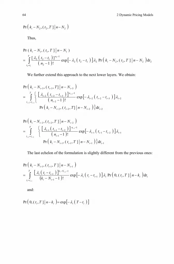
We further extend this approach to the next lower layers. We obtain:
( )( )[ ]( ) ( )[ ]
( ) } 2222
23222
1322
333
d],(,Pr
exp!1
],(,Pr
32
2
−−−−
−−−−= −
−−−−
−−−
−−
−−⎩⎨⎧
−−
=
−−
∫−−
−
iiiii
iiii
T
tt i
niii
iiii
tNnTtNk
ttn
tt
NnTtNk
ii
i
λλλ
( )( )[ ]( ) ( )[ ]
( ) } 1111
12111
1211
222
d],(,Pr
exp!1
],(,Pr
21
1
−−−−
−−−−= −
−−−−
−−−
−−
−−⎩⎨⎧
−−
=
−−
∫−−
−
iiiii
iiii
T
tt i
niii
iiii
tNnTtNk
ttn
tt
NnTtNk
ii
i
λλλ
The last echelon of the formulation is slightly different from the previous ones:
( )( )[ ]( ) ( )[ ] ( ) iiiiiii
T
tt ii
Nkiii
iiii
tknTtttNktt
NnTtNk
ii
ii
d],(,0Prexp!1
],(,Pr
11
11
111
1
1
−−−−−
−=
−−
−= −
−−−
−−−
∫−
−
λλλ
and:
( ) ( )[ ]iiii tTknTt −−=− λexp],(,0Pr

2.4 Stochastic Dynamic Pricing for Items with Salvage Values 65
This sequence of equalities can be rewritten as a unique relation:
[ ]( ) ( ) ( )
( )( )( )
( )[ ]( ) ( )[ ] 111
1
0
1
1
11
11
1
1
1
1
dddexpexp
!11
!)1(1,0,Pr
}
{1 12 1
1
1
ttttTtt
tttt
NknTk
iiii
i
jjjj
T
t
T
tt
T
tt
i
j
Nkii
njj
ii
i
j j
i
j
Nknji
ii
iij
ii
i
j
L
L
−=
−
= = =
−
=
−−−
−−
−
=
−
=
−
−−−−
−−
−−⎟⎟⎠
⎞⎜⎜⎝
⎛
−=
∏
∫ ∫ ∫ ∏
∏∏
−
−
−
λλ
λλ
(2.28)
This relation holds for ki = 1, 2, …, n–1. The probability that any item is sold by horizon T is:
)(exp)],0[,0(Pr 1 TT λ−=
Furthermore, the probability that all the items are sold at time T is:
[ ]( ) [ ]( )∑−
=
−=1
0
,0,Pr1,0,Prn
k
TkTn
Assuming that the probabilities are known, the mean value of the revenue is:
( ) [ ]( ) ( ) ( )[ ]{ }∑=
−+=n
k
TknwkpkTkTnv0
,,0,Pr, (2.29)
where ( ) ipkp = if { }ii NNk ...,,11 +∈ − .
2.4.2.2 Computation of the Mean Value of the Revenue
An analytical expression of the integrals of the second member in Relation 2.28 is possible only for very small values of parameters i and ni since the complexity of the solution increases exponentially. This is why a numerical approach is neces-sary.
We chose the Monte-Carlo approach. In order to simplify the notations, we de-note by kq the probability [ ]( )Tk ,0,Pr and by ip the cost of one item if the inventory level k belongs to { }ii NN ...,,11 +− . Others notations are those intro-duced in the previous subsection.

66 2 Dynamic Pricing Models
Algorithm 2.2.
1. Compute )(exp 10 Tq λ−= . 2. For 1 to1 −= nk do:
2.1. Compute i such that ii NkN ≤<−1 . 2.2. If 1>i set jj nK = for 1...,,1 −= ij .
2.3. 1−−= ii NkK .
2.4. u = 1. 2.5. For ij ...,,1= do jK
juu λ= .
At this point, u contains the term ∏−
=
− −⎟⎠⎞⎜
⎝⎛
1
1
1
i
j
Nknj
ii
i
j λλ of Formulae (2.28).
The Monte-Carlo method starts below. 2.6. Set qk = 0. 2.7. For Mc = 1 to M do: M is the number of iterations (around 10 000). 2.7.1. Set t0 = 0. 2.7.2. For ij ...,,1= generate tj at random on ],[ 1 Tt j− .
2.7.3. Set w = 1, s = 0, z = 1. 2.7.4. For ij ...,,1= do:
2.7.4.1. Compute ( )
!)1(
11
−
−=
−−
j
Kjj
Ktt
vj
.
2.7.4.2. Compute ( )1−−= jtTvv . 2.7.4.3. Compute vww = . 2.7.4.4. If ( )ij < , then compute ( ) ][exp 1−−−= jjj ttzz λ .
2.7.4.5. If ( )[ ij = and ( ) ]iNk < do: 2.7.4.5.1. Compute ][exp 1−= jj tzz λ .
2.7.4.5.2. If ( )1Mc = , then compute ][exp Tuu jλ−= .
2.7.4.6. If ( )[ ij = and ( ) ]iNk = do: 2.7.4.6.1. Compute ( ) ][exp 11 jjjjj tttzz +− +−−= λλ .
2.7.4.6.2. If ( )1Mc = , then compute ][exp 1 Tuu j+−= λ . 2.7.5. End of loop j . 2.7.6. Compute zww = . 2.7.7. Compute Mwqq kk /+= .
2.8. End of loop Mc. 2.9. Compute uqq kk = .
3. End of loop k.
Computation of qn.
4. Set 0=u .

2.4 Stochastic Dynamic Pricing for Items with Salvage Values 67
5. For 1...,,0 −= nk do kquu += . 6. Compute uqn −=1 .
Computation of the mean value of the revenue denoted by Ct.
7. Set Ct = 0. 8. For nk to0= do:
8.1. Set 0cc = . 8.2. Compute i such that ii NkN ≤<−1 . 8.3. If 1>i do jj np+= cccc for 1...,,1 −= ij .
8.4. Compute ( ) ii pNk 1cccc −−+= . 8.5. Compute ( )[ ]Tknwqk ,ccCtCt −++= .
9. End of loop k.
2.4.2.3 Improvement of the Solution
We denote by sini ,,2,1, L= the initial sizes of the layers, from the upper to the lower one, and by iλ (respectively, ip ) the corresponding demand intensities (re-spectively, prices). Remember that sλλλ <<< L21 and sppp >>> L21 .
Since a numerical approach has been used to evaluate the probabilities of the states of the system at time T and the mean value of the revenue knowing the lay-ers, we can also use a numerical approach to reach the layers that maximize the mean value of the revenue. We chose a simulated annealing algorithm to improve a given solution. This method is an iterative approach and some layers may be-come empty (and thus disappear) during the process. This requires some addi-tional notations.
We denote by r0 the number of layers, by 0in the size of the i-th layer and by
0iλ (respectively, 0
ip ) the corresponding demand intensities (respectively, prices)
for 0,,2,1 ri L= at the beginning of an iteration of the simulated annealing algo-
rithm or the initial stage. Indeed, sr ≤0 . At the beginning of the first iteration, sr =0 , iiii nn λλ == 00 , and ii pp =0 for si ,,2,1 L= .
We denote by r1 the number of layers at the end of the first iteration, by 1in the
size of the i-th layer, and by 1iλ (respectively, 1
ip ) the corresponding demand in-
tensities (respectively, prices) for 1,,2,1 ri L= . Indeed, sr ≤1 . Furthermore, the corresponding mean value of the revenue is .Copt1

68 2 Dynamic Pricing Models
1λ 2λ 3λ 4λ 5λ 6λ 7λ 8λ 9λ
*1λ *
2λ *3λ *
4λ
r1=4
0 0 0 0 0 1 2 3 4 TT
r0= s= 9 Figure 2.6 Links between the second and the initial iteration
We introduce a vector TT to link the initial demand intensities (and thus the initial price), with the current demand intensities and prices. This linkage is illus-trated in Figure 2.6.
Algorithm 2.3 describes the simulated annealing mechanism that we apply to our problem. Note: Algorithm 2.3 contains Algorithm 2.2.
Algorithm 2.3.
1. Introduce ins λ,, , ip for si ,,2,1 L= and the salvage costs ),( Tkw for .,,2,1 nk L=
2. Generate at random in for si ,,2,1 L= such that nns
ii =∑
=1, the value generated being inte-
ger and positive. The first two steps of the algorithm provide the initial data. 3. Introduce KK.
KK is the number of iterations that will be made. For instance, we may assign the value 2000 or 3000 to this variable.
4. Set ,0 sr = iiiiii nnpp === 000 and,λλ for si ,,2,1 L= .
This set of values represents the initial solution that is called S0. 5. Compute the mean value of the revenue corresponding to solution S0. We denote this value
Copt0. This is obtained by applying Algorithm 2.2. 6. We set 0* SS ≡ and 0Copt*Copt = .
For each iteration, S* contains the best solution and Copt* the greatest mean value of the revenue obtained since the beginning of the algorithm.
The simulated annealing process starts at this point. 7. For kkt = 1 to KK do:
7.1. For i = 1 to s set TTi = 0. 7.2. Set i = 1 and j = 1. 7.3. While )( 0ri ≤
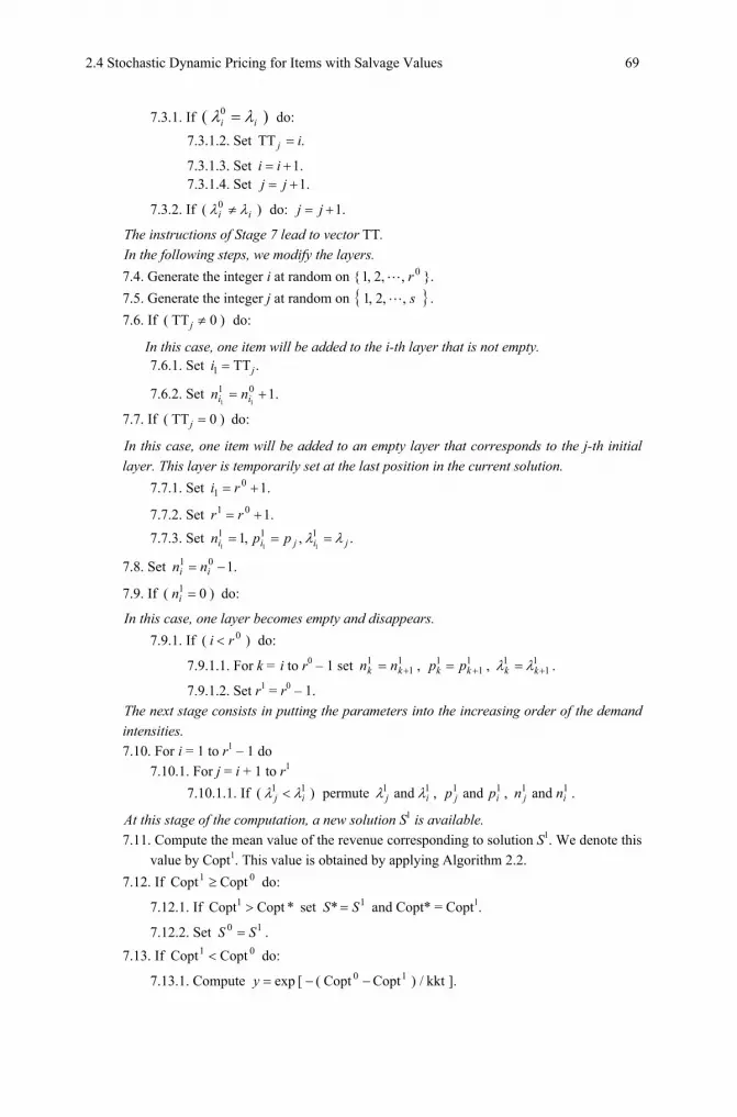
2.4 Stochastic Dynamic Pricing for Items with Salvage Values 69
7.3.1. If )( 0ii λλ = do:
7.3.1.2. Set .TT ij =
7.3.1.3. Set .1+= ii 7.3.1.4. Set .1+= jj
7.3.2. If )( 0ii λλ ≠ do: .1+= jj
The instructions of Stage 7 lead to vector TT. In the following steps, we modify the layers.
7.4. Generate the integer i at random on { 0,,2,1 rL }. 7.5. Generate the integer j at random on }{ s,,2,1 L . 7.6. If )0TT( ≠j do:
In this case, one item will be added to the i-th layer that is not empty. 7.6.1. Set .TT1 ji =
7.6.2. Set .10111+= ii nn
7.7. If )0TT( =j do:
In this case, one item will be added to an empty layer that corresponds to the j-th initial layer. This layer is temporarily set at the last position in the current solution.
7.7.1. Set .101 += ri
7.7.2. Set .101 += rr 7.7.3. Set .,,1 111
111 jijii ppn λλ ===
7.8. Set .101 −= ii nn
7.9. If )0( 1 =in do:
In this case, one layer becomes empty and disappears. 7.9.1. If )( 0ri < do:
7.9.1.1. For k = i to r0 – 1 set 11
1+= kk nn , 1
11
+= kk pp , 11
1+= kk λλ .
7.9.1.2. Set r1 = r0 – 1. The next stage consists in putting the parameters into the increasing order of the demand intensities.
7.10. For i = 1 to r1 – 1 do 7.10.1. For j = i + 1 to r1 7.10.1.1. If )( 11
ij λλ < permute 11 and ij λλ , 11 and ij pp , 11 and ij nn .
At this stage of the computation, a new solution S1 is available. 7.11. Compute the mean value of the revenue corresponding to solution S1. We denote this
value by Copt1. This value is obtained by applying Algorithm 2.2. 7.12. If 01 CoptCopt ≥ do:
7.12.1. If *CoptCopt1 > set 1* SS = and Copt* = Copt1.
7.12.2. Set 10 SS = . 7.13. If 01 CoptCopt < do:
7.13.1. Compute ].kkt/)CoptCopt([exp 10 −−=y

70 2 Dynamic Pricing Models
7.13.2. Generate x at random on ]1,0[ (probability density 1).
7.13.3. If )( yx ≤ set 10 SS = .
2.4.2.4 Numerical Example
In the case presented hereafter, the number of items to sold before time T is 25 (n = 25). A one-to-one relationship has been established between five prices and five demand intensities. These data are presented in Table 2.1.
Table 2.1 Price versus demand intensity
Price 20 14 10 7 5
Demand intensity 0.2 0.4 0.6 0.8 1
The salvage value is linear: each item can be sold on the second market for 2 monetary units. The computation starts with five layers numbered from the upper to the lower layer. Each of them is initially made with 5 consecutive inventory levels. The number of iterations made in the simulated annealing process is 5000.
Remark: A large number of choices (see Appendix A) are available when ap-plying simulated annealing for defining, in particular:
• the number of iterations; • the evolution of the “temperature” that affects the selection of the next state; • the “neighborhood” of a solution.
In Table 2.2, we give some intermediate results provided by the simulated an-nealing algorithm. The last one is the near-optimal solution.
Table 2.2 Some intermediate steps of the simulated annealing process
Iteration number
Solution Mean value of the revenue (rounded)
1
Layer size Price
Demand intensity
5 20 0.2
5 14 0.4
5 10 0.6
5 7
0.8
5 5 1
174
16
Layer size Price
Demand intensity
2 20 0.2
4 14 0.4
6 10 0.6
7 7
0.8
6 6 1
184
993
Layer size Price
Demand intensity
0 20 0.2
11 14 0.4
1 10 0.6
10 7
0.8
3 6 1
199
1243
Layer size Price
Demand intensity
0 20 0.2
13 14 0.4
1 10 0.6
10 7
0.8
1 6 1
202
3642
Layer size Price
Demand intensity
0 20 0.2
1 14 0.4
15 10 0.6
1 7
0.8
8 6 1
205
4006
Layer size Price
Demand intensity
0 20 0.2
1 14 0.4
17 10 0.6
7 7
0.8
0 6 1
211

2.4 Stochastic Dynamic Pricing for Items with Salvage Values 71
0
0.02
0.04
0.06
0.08
0.1
0.12
0.14
0 2 4 6 8 10 12 14 16 18 20 22 24
Inventory level
Prob
abili
ty
Figure 2.7 Probabilities at time T for the last structure of layers
Figure 2.7 provides the probabilities of the different inventory levels at time T for the last structure of layers.
2.4.2.5 How to Use the Approach?
The previous approach is used on a periodic basis. This strategy corresponds to the usual behavior of vendors: they choose a pricing policy on a given period (one or two weeks for instance) and they reconsider the pricing policy for the next period according to the inventory level at the end of the previous period, and so on. In other words, they work on a rolling-horizon basis.
2.4.3 Price as a Function of Inventory Levels: a Special Case
We assume that the demand intensity, and thus the price, is different from one in-ventory level to the next. This kind of situation happens when the items are expen-sive (cars, for instance). In this particular case, it is possible to express analytically the probability that k items are sold at the end of period T.
We denote by iλ the demand intensity when the inventory level is i and the price of the next item is pi. The initial inventory level is n. Indeed
121 ... λλλλ <<<< −nn and, as mentioned earlier, 121 ... pppp nn >>>> − .

72 2 Dynamic Pricing Models
As in the previous section, [ ]( )21,,Pr ttk refers to the probability that k items are sold in period [ ]21, tt .
Since at each inventory level the demand is generated by a Poisson process:
• [ ]( ) ( )TT nλ−= exp,0,0Pr
• [ ]( ) ttTtT n
T
tnn d])([exp)(exp,0,1Pr 1
0
−−−= −=∫ λλλ
)(exp)(exp 111
TT nnn
nn
nn
n−
−−
−−
−−−
−= λλλ
λλλλ
λ
• [ ] [ ] [ ] tTttTT
tn d,,0(Pr),0,1(Pr),0,2(Pr
01∫
=−= λ
⎭⎬⎫
−−−
+
−−−
+⎩⎨⎧
−−−
=
−−−−
−
−−−−
−=
−−−
−
−−−
−
−−−
=−−
−
−
=−
−
−
∫
∫
)()()(exp
)()()(exp
)()()(exp
d])([exp)(exp
d])([exp)(exp
122
2
211
1
211
021
1
1
02
1
1
nnnn
n
nnnn
n
nnnn
nnn
T
tnn
nn
nn
T
tnn
nn
nn
T
TT
ttTt
ttTt
λλλλλ
λλλλλ
λλλλλλλ
λλλλ
λλ
λλλλλλ
At this level of the computation, it appears that the formula could be:
( )∑∏
∏=
≠=
−−
−−
=−
⎪⎪⎪
⎩
⎪⎪⎪
⎨
⎧
⎪⎪⎪
⎭
⎪⎪⎪
⎬
⎫
−
−−=
k
ik
ijj
jnin
ink
iin
k TTk0
0
1
0 )(
)(exp)1()],0[,(Prλλ
λλ
for k = 1,…, n–1 (2.30)
To complete the proof, we will show that if (2.30) holds for k, then it also holds for k +1. If we express )],0[,1(Pr Tk + according to )],0[,(Pr tk (Bayes’ theorem), we obtain:

2.4 Stochastic Dynamic Pricing for Items with Salvage Values 73
( tTttkTkT
tkn d)],[,0(Pr)],0[,Pr)],0[,1(Pr
0∫=
−=+ λ
( ) ttTtT
tknkn
k
ik
ijj
jnin
ink
iin
k d])([exp)(
)(exp)1(0
10
0
1
0∫ ∑
∏∏
=−−−
=
≠=
−−
−−
=−
⎥⎥⎥⎥⎥⎥⎥
⎦
⎤
−−
⎢⎢⎢⎢⎢⎢
⎣
⎡
⎪⎪⎪
⎩
⎪⎪⎪
⎨
⎧
⎪⎪⎪
⎭
⎪⎪⎪
⎬
⎫
−
−−= λλ
λλ
λλ
Developing this expression, we reach the following equality:
( )
( ) ∑∏
∏
∑∏
∏
=+
≠=
−−
−−=
−+
=+
≠=
−−
−
=−
+
⎪⎪⎪
⎩
⎪⎪⎪
⎨
⎧
⎪⎪⎪
⎭
⎪⎪⎪
⎬
⎫
−−−−
⎪⎪⎪
⎩
⎪⎪⎪
⎨
⎧
⎪⎪⎪
⎭
⎪⎪⎪
⎬
⎫
−
−−=+
k
ik
ijj
jnin
kn
k
iin
k
k
ik
ijj
jnin
ink
iin
k
T
TTk
01
0
10
1
01
0
0
1
)(
1)(exp)1(
)(
)(exp)1()],0[,1(Pr
λλλλ
λλ
λλ
(2.31)
Expanding the left side of the following equality, we obtain:
∑∏
+
=+
≠=
−−
⎪⎪⎪
⎩
⎪⎪⎪
⎨
⎧
=
⎪⎪⎪
⎭
⎪⎪⎪
⎬
⎫
−
1
01
0
0)(
1k
ik
ijj
jnin λλ
This equality can be rewritten as:

74 2 Dynamic Pricing Models
∏∑
∏+
+≠=
−−−=
+
≠=
−− −=
⎪⎪⎪
⎩
⎪⎪⎪
⎨
⎧
⎪⎪⎪
⎭
⎪⎪⎪
⎬
⎫
−− 1
10
10
1
0
)(
1
)(
1k
kjj
jnkn
k
ik
ijj
jnin λλλλ
Thus, Equation 2.31 becomes:
( )
( )∏
∏
∑∏
∏
+
+≠=
−−−
−−=
−+
=+
≠=
−−
−
=−
+
−−−+
⎪⎪⎪
⎩
⎪⎪⎪
⎨
⎧
⎪⎪⎪
⎭
⎪⎪⎪
⎬
⎫
−
−−=+
1
10
1
10
1
01
0
0
1
)(
1)(exp)1(
)(
)(exp)1()],0[,1(Pr
k
kjj
jnkn
kn
k
iin
k
k
ik
ijj
jnin
ink
iin
k
T
TTk
λλλλ
λλ
λλ
( )∑∏
∏+
=+
≠=
−−
−
=−
+
⎪⎪⎪
⎩
⎪⎪⎪
⎨
⎧
⎪⎪⎪
⎭
⎪⎪⎪
⎬
⎫
−
−−=
1
01
0
0
1
)(
)(exp)1(k
ik
ijj
jnin
ink
iin
k T
λλ
λλ
This completes the computation. Result 3 is derived from the above development. In this result, according to the usual mathematical convention, we assume that if no factor remains in a product,
then the product equals 1. For instance, 1=∏=
m
niia if m < n.
Result 3 The probability that k items are sold in period [ 0, T ] is given by (2.30) for
{ }1,...,1 −∈ nk . Furthermore, [ ]( ) [ ]( )∑−
=
−=1
0
,0,Pr1,0,Prn
k
TkTn . Then
the mean value of the revenue can be obtained applying (2.29), Section 2.4.2.1.

Further Reading 75
2.5 Concluding Remarks
The goal of this chapter was to provide an insight into the domain of pricing mod-els. We limited ourselves to time-dated items with no supply option in a monopo-listic environment with myopic customers. Although these assumptions drastically simplify the problem, many additional restrictive assumptions are required to ob-tain a mathematical model that is easy to analyze.
Nevertheless, the numerical development of the stochastic dynamic pricing model with salvage values is an interesting tool when integrated in a rolling-horizon approach since it allows prices to be adjusted periodically according to the inventory level and time, as required in the case of sales. Unfortunately, the one-to-one relationship between price and demand intensity remains under the respon-sibility of the user, and is not a risk-free task.
In our opinion, the pricing models are simply tools to help better understand what dynamic pricing is rather than something to solve real-life problems.
Reference
Gallego G, Van Ryzin G (1994) Optimal dynamic pricing of inventories with stochastic demand over finite horizons. Manag. Sci. 40:999–1020
Further Reading
Belobaba PP (1989) Application of a probabilistic decision model to airline seat inventory con-trol. Oper. Res. 37:183–197
Bitran GR, Mondschein SV (1995) An application of yield management to the hotel industry considering multiple day stays. Oper. Res. 43:427–443
Bitran GR, Gilbert SM (1996) Managing hotel reservations with uncertain arrivals. Oper. Res. 44:35–49
Caroll WJ, Grimes RC (1995) Evolutionary change in product management: Experiences in the car rental industry. Interfaces 25:84–104
Chen F, Federgruen A, Zheng YS (2001) Near-optimal pricing and replenishment strategies for a retail/distribution system. Oper. Res. 49(6):839–853
Chen F, Federgruen A, Zheng YS (2001) Coordination mechanisms for a distribution system with one supplier and multiple retailers. Manag. Sci. 47:693–708
Federgruen A, Heching A (1997) Combined pricing and inventory control under uncertainty. Oper. Res. 47:454–475
Federgruen A, Zipkin P (1986) An inventory model with limited production capacity and uncer-tain demands. Math. Oper. Res. 11:193–215
Feng Y, Gallego G (1995) Optimal starting times for end-of-season sales and optimal stopping times for promotional fares. Manag. Sci. 41:1371–1391
Gallego G, Van Ryzin G (1997) A multi-product dynamic pricing problem and its application to network yield management. Oper. Res. 45:24–41

76 2 Dynamic Pricing Models
Gaimon C (1988) Simultaneous and dynamic price, production, inventory and capacity deci-sions. Eur. J. Oper. Res. 35:426–441
Garcia-Diaz A, Kuyumcu A (1997) A Cutting-Plane Procedure for Maximizing Revenues in Yield Management. Comput. Ind. Eng. 33:51–54
Gerchak Y, Parlar M, Yee TKM (1985) Optimal rationing policies and production quantities for products with several demand classes. Can. J. Adm. Sci. 2:161–176
Kimes SE (1989) Yield management: A tool for capacity constrained service firms. J. Oper. Manag. 8:348–363
Levin Y, McGill J, Nediak M (2007) Price guarantees in dynamic pricing and revenue manage-ment. Oper. Res. 55(1):75–97
McGill J, Van Ryzin G (1999) Revenue management: Research overview and prospects. Transp. Sci. 33(2):233–256
Petruzzi NC, Dada M (2002) Dynamic pricing and inventory control with learning. Nav. Res. Log. Quart. 49:304–325
Raju CVL, Narahari Y, Ravikumar K (2006) Learning dynamic prices in electronic retail mar-kets with customer segmentation. Ann. Oper. Res. 143(1):59–75
Talluri KT, Van Ryzin GJ (2004) The Theory and Practice of Revenue Management. Kluwer Academic Publishers, Norwell, MA
Van Mieghem J, Dada M (1999) Price versus production postponement: Capacity and competi-tion. Manag. Sci. 45(12):1631–1649
Vulcano G, Van Ryzin G, Maglaras C (2002) Optimal dynamic auctions for revenue manage-ment. Manag. Sci. 48(11):1388–1407
Zhao W, Zheng Y-S (2000) Optimal dynamic pricing for perishable assets with nonhomogene-ous demand. Manag. Sci. 46(3):375–388

http://www.springer.com/978-1-84996-016-8


