A Bayesian Approach to the Assessment of West Greenland Halibut: Rationale and Critique

NOT TO BE CITED WITHOUT PRIOR

REFERENCE TO THE AUTHOR(S)

Northwest Atlantic Fisheries Organization

Serial No. Nxxx NAFO SCR Doc. 14/xx

SCIENTIFIC COUNCIL MEETING – JUNE 2014

A Bayesian Approach to the Assessment of West Greenland Halibut:

Rationale and Critique.

By

Aldo P. Solari

Greenland Institute of Natural Resources (GINR)

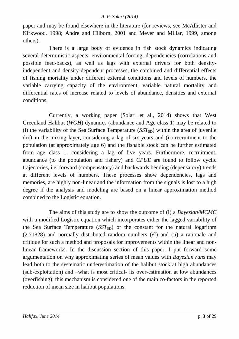
E-mail: <[email protected]>

ABSTRACT.

A Bayesian/MCMC approach with the modified Logistic equation

incorporating a term which integrates either the constant for the natural logarithm

(2.71828) and normally distributed random numbers (ev) or the variability of the Sea

Surface Temperature (SSTSD, lagged 6 years) with auto-correlated residuals is

implemented. The SST was sampled from the area of West Greenland Halibut (WGH)

juvenile (age class 1) drift in the mixing layer (which is proposed as a system-wide

co-driver).

The evaluation of both sub-exploitation and overfishing shifts in relation

to the cut lines for BMSY: 0.3 (unrealistic), zero or the mean from the standardized

series (highly precautionary) or (local) linear equilibrium values (relatively useful)

and the stock appears to be over-exploited (even assuming the linear fit) during 2012-

11 and close to equilibrium values during years 2006-2009.

It is suggested that the Bayesian framework may be useful, provided that

the population model that underlies the simulations has the sufficient degree of

resolution to describe the complex dynamics which may drive both recruitment and

abundance in WGH.

While the incorporation of the environmental forcing results in a

forecasted biomass series that approximates non-linear approaches developed by the

author, estimates and reference points are considered rough proxies (of proxies) and

the method does neither show the resolution nor the capacity to explain the (highly

non-linear) mechanics behind the data. The correlation between both of the simulated

outcomes is significant (p<0.05). The Bayesian/Logistic approach is unable to

A Bayesian Approach to the Assessment of West Greenland Halibut: Rationale and Critique.

NAFO Scientific Council Meeting p. 2 of 29

discriminate between results from either random or auto-correlated residuals with a

clear memory effect in the series (common in such dynamical systems). The (between

years) variability is “crunched down” by the method which approximates series of

means with no dispersion (linear methods may be inappropriate to address the

variability in the signal).

This implies several shortcomings which may be critical to achieve both

short and medium term management plans as well as sustainability and conservation:

it may lead to assessment errors as the stock may be both underestimated at high

abundances (leads to sub-exploitation) and -what is most important- overestimated at

relatively low numbers (leads to systematic overfishing when the stock is as most

vulnerable): this mechanism is regarded as a co-factor contributing to the reduction of

mean size in halibut populations as the effects of overfishing may have the highest

impact as the stock is overestimated in the relatively lower abundances.

The critique herein is expressed on basis of the grounds of population

processes seen as non-linear dynamical systems, resulting from the interaction

between both abiotic and biotic factors, showing strong dependencies to external

forcing, lags and cycles or pseudo-cycles.

Several concepts such as constant and dynamic reference points,

differential intrinsic rate of increase, variable carrying capacity, environmental

forcing and differential effects of fishing mortality, among others, are discussed in

order to propose improvements for the assessment and modeling of the WGH

dynamics.

Key words: Bayesian, logistic equation, West Greenland Halibut, variability, modeling, assessment,

sub-exploitation, overfishing, sustainability, conservation.

INTRODUCTION.

Currently, linear approaches -such as the Bayesian Markov Chain Monte

Carlo (Bayesian/MCMC, also called herein "Bayesian runs" and "Bayesian-Logistic"

approach) methods in combination with the Logistic equation (or some derivative)

are being used for fisheries assessment. Some of the fundamental assumptions of this

probabilistic framework are that (a) population processes (such as recruitment and the

temporal evolution of biomass) are the result of random processes, (b) neither

environmental forcing (correlations with external variables) nor memories (longer

than a year) or lags are taken into account and –among other factors- (c) residuals are

expected to be random. Also, Bayesian runs are carried out on abundance, catches

and Catch Per Unit Effort (CPUE) series in which no variability in the data is

analyzed: the signals (which are to be approximated) consist of mean values which

may give some rough indications of trends. Nevertheless, the lack of the main part of

the information in the signal (which lies in the variability of the data) is omitted.

Further details on the background for Bayesian runs are beyond the scope of this

A. P. Solari (2014)

Halifax, June 2014 p. 3 of 29

paper and may be found elsewhere in the literature (for reviews, see McAllister and

Kirkwood. 1998; Andre and Hilborn, 2001 and Meyer and Millar, 1999, among

others).

There is a large body of evidence in fish stock dynamics indicating

several deterministic aspects: environmental forcing, dependencies (correlations and

possible feed-backs), as well as lags with external drivers for both density-

independent and density-dependent processes, the combined and differential effects

of fishing mortality under different external conditions and levels of numbers, the

variable carrying capacity of the environment, variable natural mortality and

differential rates of increase related to levels of abundance, densities and external

conditions.

Currently, a working paper (Solari et al., 2014) shows that West

Greenland Halibut (WGH) dynamics (abundance and Age class 1) may be related to

(i) the variability of the Sea Surface Temperature (SSTSD) within the area of juvenile

drift in the mixing layer, considering a lag of six years and (ii) recruitment to the

population (at approximately age 6) and the fishable stock can be further estimated

from age class 1, considering a lag of five years. Furthermore, recruitment,

abundance (to the population and fishery) and CPUE are found to follow cyclic

trajectories, i.e. forward (compensatory) and backwards bending (depensatory) trends

at different levels of numbers. These processes show dependencies, lags and

memories, are highly non-linear and the information from the signals is lost to a high

degree if the analysis and modeling are based on a linear approximation method

combined to the Logistic equation.

The aims of this study are to show the outcome of (i) a Bayesian/MCMC

with a modified Logistic equation which incorporates either the lagged variability of

the Sea Surface Temperature (SSTSD) or the constant for the natural logarithm

(2.71828) and normally distributed random numbers (ev) and (ii) a rationale and

critique for such a method and proposals for improvements within the linear and non-

linear frameworks. In the discussion section of this paper, I put forward some

argumentation on why approximating series of mean values with Bayesian runs may

lead both to the systematic underestimation of the halibut stock at high abundances

(sub-exploitation) and –what is most critical- its over-estimation at low abundances

(overfishing): this mechanism is considered one of the main co-factors in the reported

reduction of mean size in halibut populations.



DATA, BAYESIAN RUNS AND RESULTS.

Data on abundance and total catches (in 103 Tn

3) on West Greenland

(NAFO areas 0 and 1) after Jørgensen (2012) and GINR (2013) were used in this

study (Fig. 1). Until the end of the development of the environmental forcing study

referred in this study, no raw data was made available. We used both WinBUGS and

R scripts to run the analysis and simulations.

For the Bayesian simulations, we used two models, namely:

Model 1.

(Eq. 1)

Model 2.

(Eq. 2)

where B is biomass, H is the harvest (or catches), r is the intrinsic rate of increase and

K is the carrying capacity, being and SSTSD (in Eq. 1) the standard deviations or

variability in the environmental series, considering a six years lag (which is the

assumed time to recruitment to the population in WGH), e (in Eq. 2) the constant

(2.71828, the base of the natural logarithm) and v a (normally distributed) random

number (sampled for each iteration).

Unless otherwise stated, all the variables were log transformed (Log) and

standardized (Z) both to meet the conditions for statistical normality and to facilitate

visual comparison. The main results are presented in this section and complementary

information on the simulations (Model 2) is given in Appendix I.

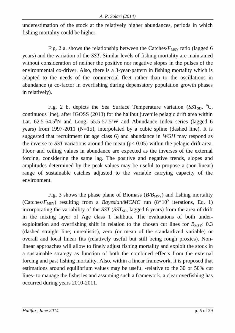
Fig. 1 shows the biomass (after Jørgensen, 2012) and catch (103

Tn3, after

Jørgensen and Treble, 2014) series. Catches are close to the linear equilibrium values.

Mean (survey) values are used to recommend catch levels and the within area/year

variability in the data (the signal) is omitted. From a non-linear viewpoint, this

implies both that (a) the oscillations and variability of the data around mean values

(the signal of highest value) are poorly understood and the stock appears to be both

overestimated and overfished at the lower abundances and (b) there is an

A. P. Solari (2014)


underestimation of the stock at the relatively higher abundances, periods in which

fishing mortality could be higher.

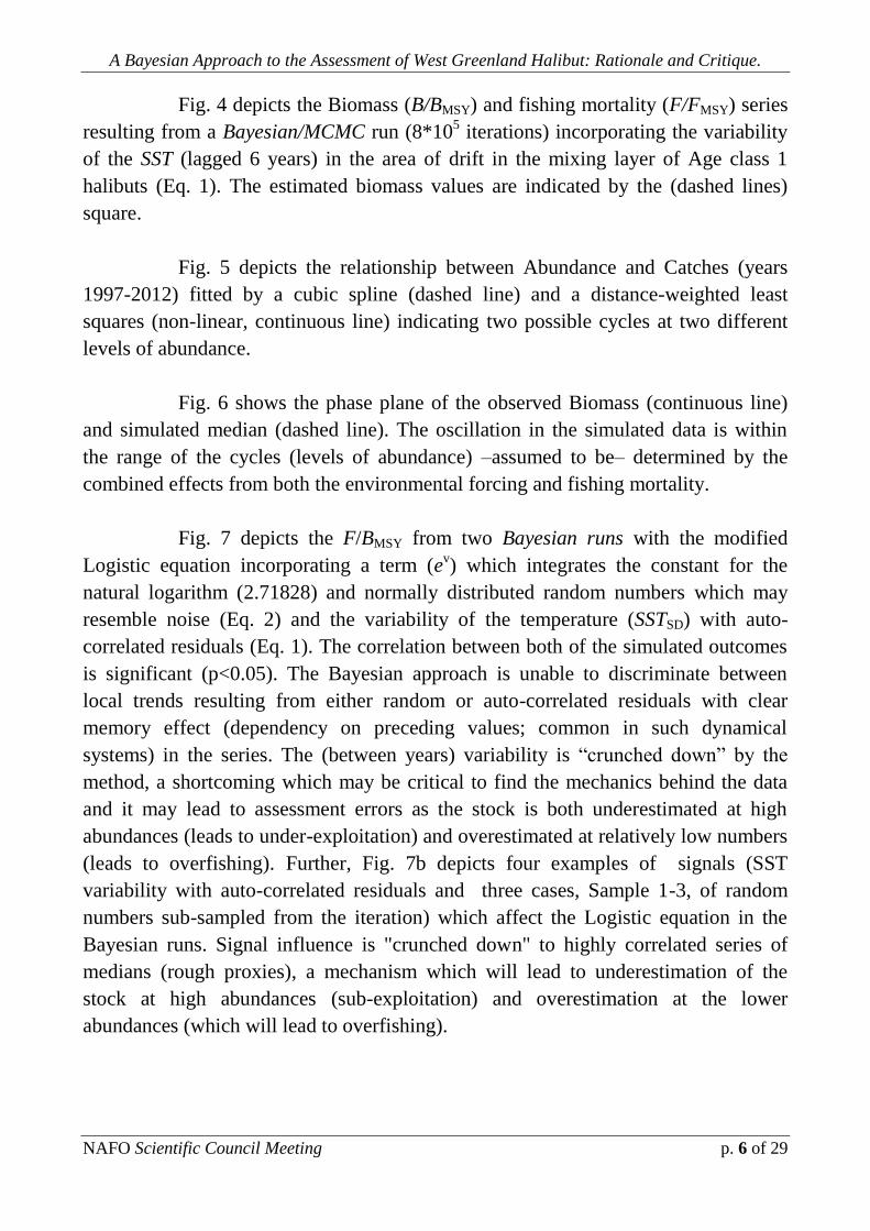
Fig. 2 a. shows the relationship between the Catches/FMSY ratio (lagged 6

years) and the variation of the SST. Similar levels of fishing mortality are maintained

without consideration of neither the positive nor negative slopes in the pulses of the

environmental co-driver. Also, there is a 3-year-pattern in fishing mortality which is

adapted to the needs of the commercial fleet rather than to the oscillations in

abundance (a co-factor in overfishing during depensatory population growth phases

in relatively).

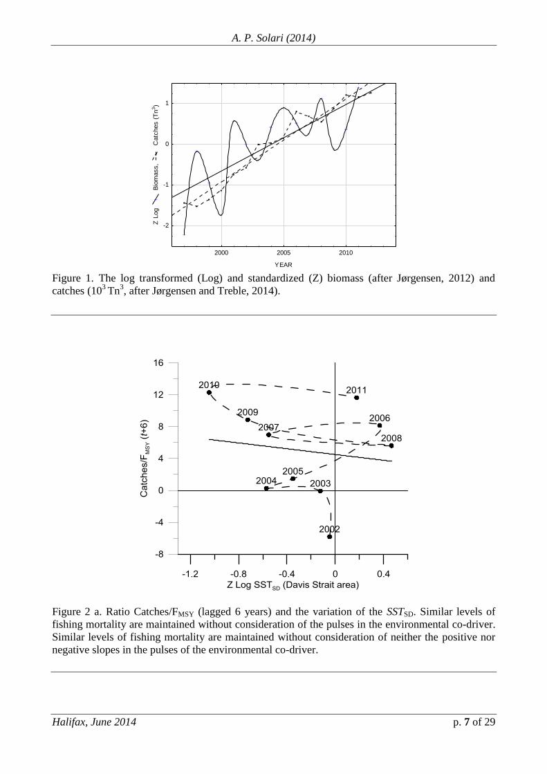
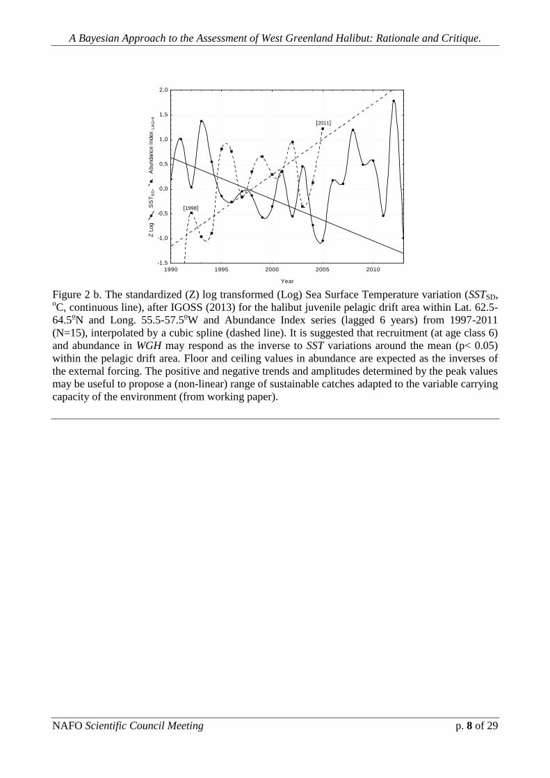
Fig. 2 b. depicts the Sea Surface Temperature variation (SSTSD, oC,

continuous line), after IGOSS (2013) for the halibut juvenile pelagic drift area within

Lat. 62.5-64.5oN and Long. 55.5-57.5

oW and Abundance Index series (lagged 6

years) from 1997-2011 (N=15), interpolated by a cubic spline (dashed line). It is

suggested that recruitment (at age class 6) and abundance in WGH may respond as

the inverse to SST variations around the mean (p< 0.05) within the pelagic drift area.

Floor and ceiling values in abundance are expected as the inverses of the external

forcing, considering the same lag. The positive and negative trends, slopes and

amplitudes determined by the peak values may be useful to propose a (non-linear)

range of sustainable catches adjusted to the variable carrying capacity of the

environment.

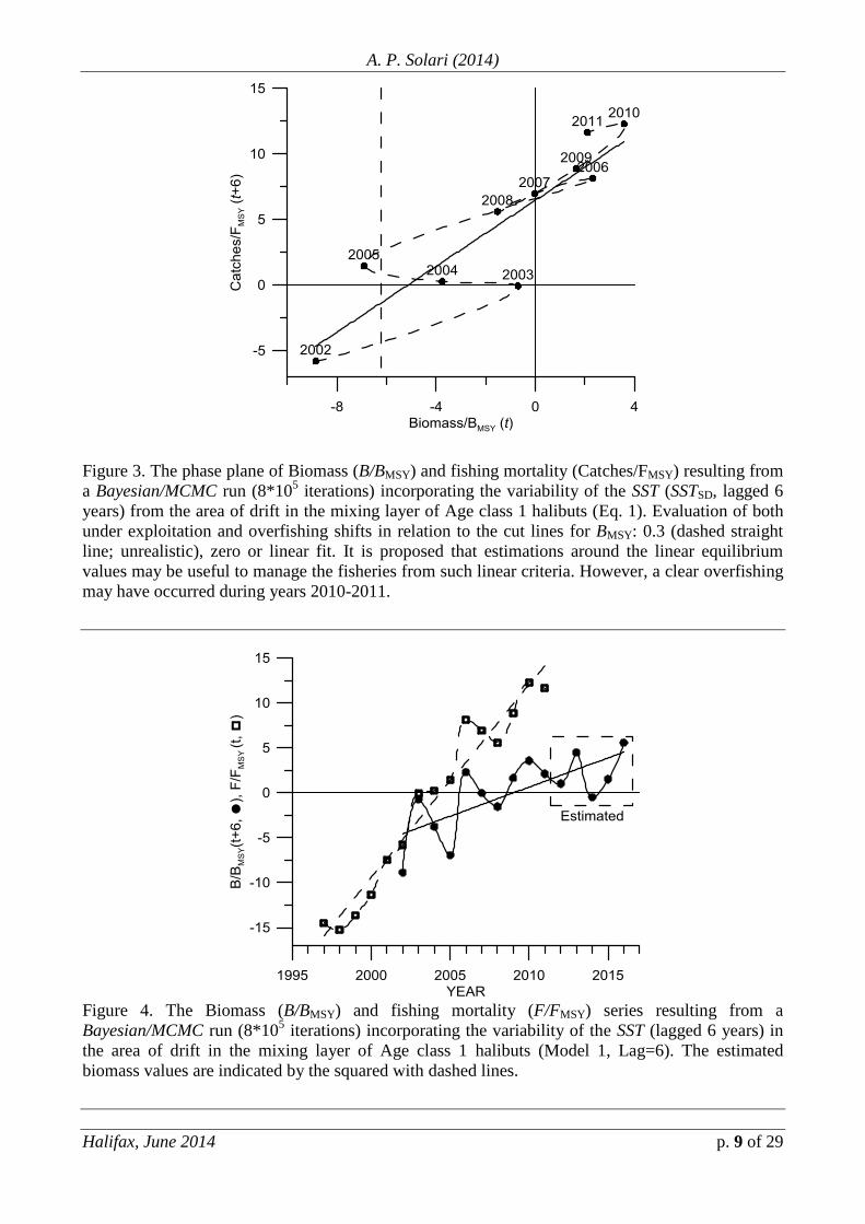
Fig. 3 shows the phase plane of Biomass (B/BMSY) and fishing mortality

(Catches/FMSY) resulting from a Bayesian/MCMC run (8*105 iterations, Eq. 1)

incorporating the variability of the SST (SSTSD, lagged 6 years) from the area of drift

in the mixing layer of Age class 1 halibuts. The evaluations of both under-

exploitation and overfishing shift in relation to the chosen cut lines for BMSY: 0.3

(dashed straight line; unrealistic), zero (or mean of the standardized variable) or

overall and local linear fits (relatively useful but still being rough proxies). Non-

linear approaches will allow to finely adjust fishing mortality and exploit the stock in

a sustainable strategy as function of both the combined effects from the external

forcing and past fishing mortality. Also, within a linear framework, it is proposed that

estimations around equilibrium values may be useful -relative to the 30 or 50% cut

lines- to manage the fisheries and assuming such a framework, a clear overfishing has

occurred during years 2010-2011.



Fig. 4 depicts the Biomass (B/BMSY) and fishing mortality (F/FMSY) series

resulting from a Bayesian/MCMC run (8*105 iterations) incorporating the variability

of the SST (lagged 6 years) in the area of drift in the mixing layer of Age class 1

halibuts (Eq. 1). The estimated biomass values are indicated by the (dashed lines)

square.

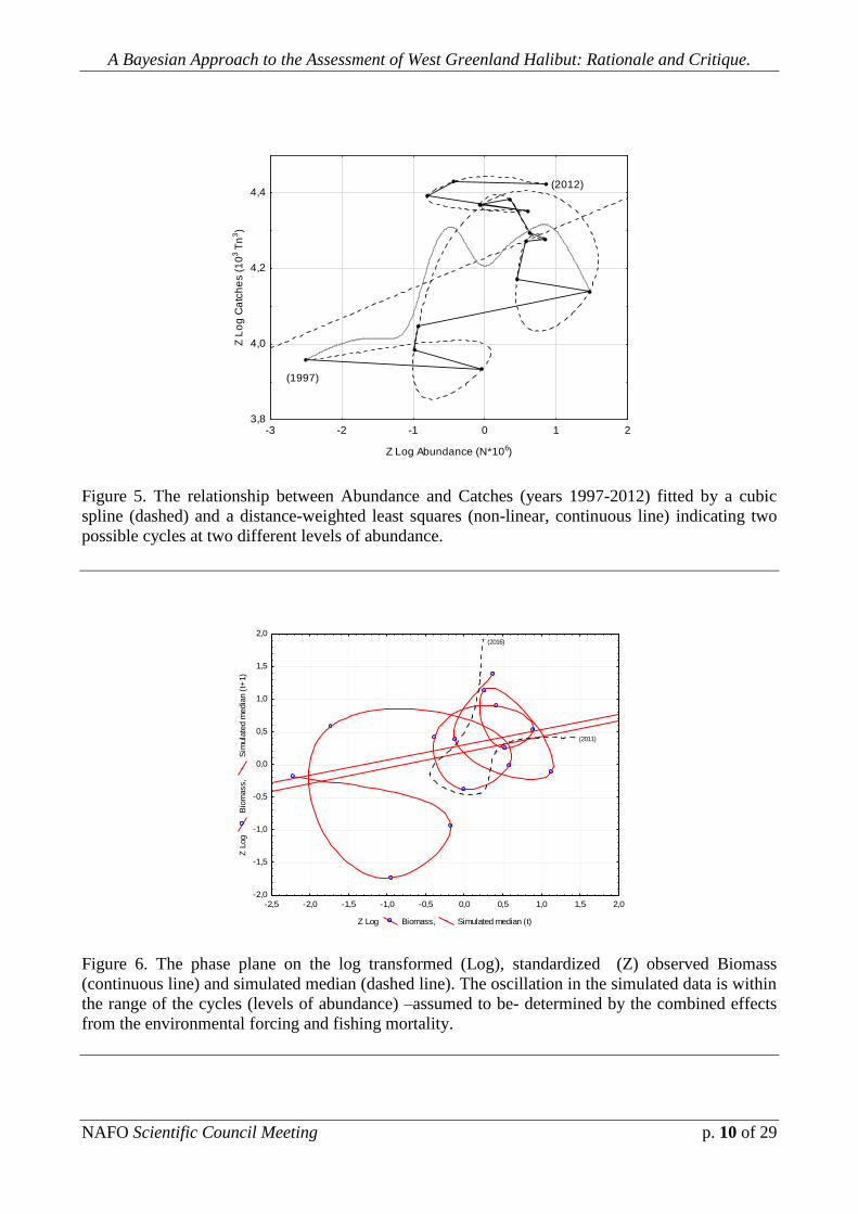
Fig. 5 depicts the relationship between Abundance and Catches (years

1997-2012) fitted by a cubic spline (dashed line) and a distance-weighted least

squares (non-linear, continuous line) indicating two possible cycles at two different

levels of abundance.

Fig. 6 shows the phase plane of the observed Biomass (continuous line)

and simulated median (dashed line). The oscillation in the simulated data is within

the range of the cycles (levels of abundance) –assumed to be– determined by the

combined effects from both the environmental forcing and fishing mortality.

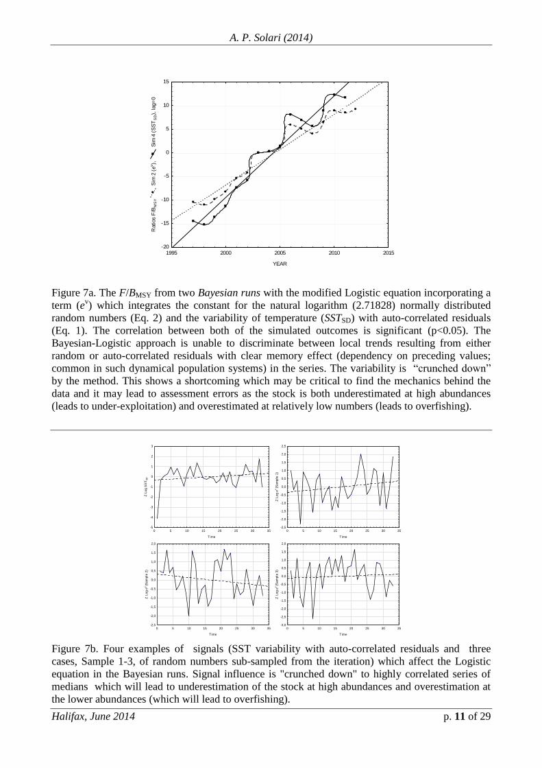
Fig. 7 depicts the F/BMSY from two Bayesian runs with the modified

Logistic equation incorporating a term (ev) which integrates the constant for the

natural logarithm (2.71828) and normally distributed random numbers which may

resemble noise (Eq. 2) and the variability of the temperature (SSTSD) with auto-

correlated residuals (Eq. 1). The correlation between both of the simulated outcomes

is significant (p<0.05). The Bayesian approach is unable to discriminate between

local trends resulting from either random or auto-correlated residuals with clear

memory effect (dependency on preceding values; common in such dynamical

systems) in the series. The (between years) variability is “crunched down” by the

method, a shortcoming which may be critical to find the mechanics behind the data

and it may lead to assessment errors as the stock is both underestimated at high

abundances (leads to under-exploitation) and overestimated at relatively low numbers

(leads to overfishing). Further, Fig. 7b depicts four examples of signals (SST

variability with auto-correlated residuals and three cases, Sample 1-3, of random

numbers sub-sampled from the iteration) which affect the Logistic equation in the

Bayesian runs. Signal influence is "crunched down" to highly correlated series of

medians (rough proxies), a mechanism which will lead to underestimation of the

stock at high abundances (sub-exploitation) and overestimation at the lower

abundances (which will lead to overfishing).

A. P. Solari (2014)


2000 2005 2010

YEAR

-2

-1

0

1

Z L

og

Bio

mass,

Catc

hes (

Tn

3)

Figure 1. The log transformed (Log) and standardized (Z) biomass (after Jørgensen, 2012) and

catches (103

Tn3, after Jørgensen and Treble, 2014).

Figure 2 a. Ratio Catches/FMSY (lagged 6 years) and the variation of the SSTSD. Similar levels of

fishing mortality are maintained without consideration of the pulses in the environmental co-driver.

Similar levels of fishing mortality are maintained without consideration of neither the positive nor

negative slopes in the pulses of the environmental co-driver.



Figure 2 b. The standardized (Z) log transformed (Log) Sea Surface Temperature variation (SSTSD, oC, continuous line), after IGOSS (2013) for the halibut juvenile pelagic drift area within Lat. 62.5-

64.5oN and Long. 55.5-57.5

oW and Abundance Index series (lagged 6 years) from 1997-2011

(N=15), interpolated by a cubic spline (dashed line). It is suggested that recruitment (at age class 6)

and abundance in WGH may respond as the inverse to SST variations around the mean (p< 0.05)

within the pelagic drift area. Floor and ceiling values in abundance are expected as the inverses of

the external forcing. The positive and negative trends and amplitudes determined by the peak values

may be useful to propose a (non-linear) range of sustainable catches adapted to the variable carrying

capacity of the environment (from working paper).

1990 1995 2000 2005 2010

Year

-1,5

-1,0

-0,5

0,0

0,5

1,0

1,5

2,0

Z L

og

SS

TS

D,

Abundance I

ndex L

AG

=6

[2011]

[1998]

A. P. Solari (2014)


Figure 3. The phase plane of Biomass (B/BMSY) and fishing mortality (Catches/FMSY) resulting from

a Bayesian/MCMC run (8*105 iterations) incorporating the variability of the SST (SSTSD, lagged 6

years) from the area of drift in the mixing layer of Age class 1 halibuts (Eq. 1). Evaluation of both

under exploitation and overfishing shifts in relation to the cut lines for BMSY: 0.3 (dashed straight

line; unrealistic), zero or linear fit. It is proposed that estimations around the linear equilibrium

values may be useful to manage the fisheries from such linear criteria. However, a clear overfishing

may have occurred during years 2010-2011.

Figure 4. The Biomass (B/BMSY) and fishing mortality (F/FMSY) series resulting from a

Bayesian/MCMC run (8*105 iterations) incorporating the variability of the SST (lagged 6 years) in

the area of drift in the mixing layer of Age class 1 halibuts (Model 1, Lag=6). The estimated

biomass values are indicated by the squared with dashed lines.



Figure 5. The relationship between Abundance and Catches (years 1997-2012) fitted by a cubic

spline (dashed) and a distance-weighted least squares (non-linear, continuous line) indicating two

possible cycles at two different levels of abundance.

-2,5 -2,0 -1,5 -1,0 -0,5 0,0 0,5 1,0 1,5 2,0

Z Log Biomass, Simulated median (t)

-2,0

-1,5

-1,0

-0,5

0,0

0,5

1,0

1,5

2,0

Z L

og

Bio

mass,

Sim

ula

ted m

edia

n (

t+1)

(2016)

(2011)

Figure 6. The phase plane on the log transformed (Log), standardized (Z) observed Biomass

(continuous line) and simulated median (dashed line). The oscillation in the simulated data is within

the range of the cycles (levels of abundance) –assumed to be- determined by the combined effects

from the environmental forcing and fishing mortality.

-3 -2 -1 0 1 2

Z Log Abundance (N*106)

3,8

4,0

4,2

4,4

Z L

og

Ca

tch

es (

10

3 T

n3)

(1997)

(2012)

A. P. Solari (2014)


1995 2000 2005 2010 2015

YEAR

-20

-15

-10

-5

0

5

10

15

Ratios F

/BM

SY

Sim

2 (

ev),

S

im 4

(S

ST

SD),

lag=

0

Figure 7a. The F/BMSY from two Bayesian runs with the modified Logistic equation incorporating a

term (ev) which integrates the constant for the natural logarithm (2.71828) normally distributed

random numbers (Eq. 2) and the variability of temperature (SSTSD) with auto-correlated residuals

(Eq. 1). The correlation between both of the simulated outcomes is significant (p<0.05). The

Bayesian-Logistic approach is unable to discriminate between local trends resulting from either

random or auto-correlated residuals with clear memory effect (dependency on preceding values;

common in such dynamical population systems) in the series. The variability is “crunched down”

by the method. This shows a shortcoming which may be critical to find the mechanics behind the

data and it may lead to assessment errors as the stock is both underestimated at high abundances

(leads to under-exploitation) and overestimated at relatively low numbers (leads to overfishing).

Figure 7b. Four examples of signals (SST variability with auto-correlated residuals and three

cases, Sample 1-3, of random numbers sub-sampled from the iteration) which affect the Logistic

equation in the Bayesian runs. Signal influence is "crunched down" to highly correlated series of

medians which will lead to underestimation of the stock at high abundances and overestimation at

the lower abundances (which will lead to overfishing).

0 5 10 15 20 25 30 35

Time

-5

-4

-3

-2

-1

0

1

2

3

Z L

og S

ST

SD

0 5 10 15 20 25 30 35

Time

-2,5

-2,0

-1,5

-1,0

-0,5

0,0

0,5

1,0

1,5

2,0

2,5

Z L

og e

v (S

am

ple

1)

0 5 10 15 20 25 30 35

Time

-2,5

-2,0

-1,5

-1,0

-0,5

0,0

0,5

1,0

1,5

2,0

Z L

og e

v (S

am

ple

2)

0 5 10 15 20 25 30 35

Time

-3,0

-2,5

-2,0

-1,5

-1,0

-0,5

0,0

0,5

1,0

1,5

2,0

Z L

og e

v (S

am

ple

3)



DISCUSSION.

Rationale and critique.

WGH is a key species for food safety, the livelihood of the fishermen

communities and the economy of Greenland, as well. As researchers, our mission is

to improve and deliver a scientifically based assessment and the frameworks and

tools to achieve the sustainable exploitation and conservation of the stocks.

This critique is expressed on basis of both (i) the grounds of population

processes seen as non-linear dynamical systems, resulting from the interaction

between both abiotic and biotic factors combined to the variable carrying capacity of

the environment and differential effects of fishing mortality. Such systems show

strong dependencies to the external forcing, lags and periodicities which are driven

both by density-dependence and the environment; (ii) the aim to improve both the

assessment and modeling on WGH in order to optimize the exploitation of the stock,

attaining sustainability and conservation.

The pioneers in fishery science, at the end of the 18th century (the so

called “observational oceanographers”) and the first papers published at the

International Council for the Exploration of the Seas (ICES), during the beginning of

the 1900’s, related both recruitment and abundance in marine fish, birds and

mammals to cycles in the environment (Petersen, 1896; Hjort, 1914; Hjort, 1926;

Iselin, 1938; Russell, 1939; Iselin, 1940; Rollefsen, 1948). The historical perspective

on the environmental forcing as a co-driver and the original descriptions by the

oceanographers from a century ago are key factors for the understanding of the

mechanics behind the data. Furthermore, there is an increasing body of evidence

showing both that recruitment (to the population, area and fishery) and the temporal

evolution of abundance may be the result of deterministic, density-dependent and

density-independent population processes which are both affected by the combined

effects from the environmental forcing and levels of exploitation at several discrete

levels of abundance. The volume of scientific literature on populations as dynamical

systems and the multi-oscillatory nature of the environmental forcing is voluminous

and I have chosen to refer to a few of our own studies such as Solari et al. 1997,

2003, 2008, 2010; Bas et al., 1999; Solari, 2008, 2010, 2011, 2012; Ganzedo et al.,

2009 and those by Sharp et al., 1983, 2003).

A. P. Solari (2014)


Assessment based on series of mean values.

Currently, the WGH assessment is carried out on series of mean values (a

basic descriptive statistic resulting in highly rough proxies) from the surveys: the

variability in the data, maxima, minima, outliers, signal-to-noise-ratio (which may be

density-dependent), missing values (which may show the absence of a species due to

impacts of different nature) and environmental forcing (a knowledge which will

allow us to finely adjust fishing mortality and propose short and medium term

sustainable strategies), among other factors, are omitted from the analysis. The (non-

linear) signal is stripped-down to a level (yearly mean values) which hardly can

reflect the main information on the (density-dependent and density-independent)

population processes. Also, it can be misleading, as the variability in the external

forcing (which is the case for WGH offshore) may show significantly different trends

from the series of means and local trends in maxima and minima may (do) differ.

Variability in the population series may depend both on the density dependent

processes and differential responses to a set of external combined effects (such as

from environmental pulses combined to the levels of fishing mortality, during the

positive and negative growth phases of a cycle or period of some frequency). Also,

we may be dealing with population processes consisting of multi-oscillatory/multi-

frequency signals, that is, population responses to external pulses of different

frequencies. Furthermore, linear approximations to the series of means will solely

replicate the aforementioned shortcomings as the main (non-linear) signal on the

population process (which reflects critical dynamical features) is taken out.

Moreover, working (solely) on series of means may have highly negative

consequences on the assessment and management of the WGH stocks: (i) It sets the

grounds for the underestimation of the stock at high abundances (which leads to a

sub-exploitation) and the overestimation of population numbers at the lower

abundances (which leads to overfishing). (ii) It implies that recommended TAC's will

be below (for the higher abundances, i.e. abundances above equilibrium values) and

above the sustainable ranges of exploitation (for the lower abundances, i.e.

abundances below equilibrium values), adjusted to the variable carrying capacity of

the environment, hence fishing less than possible during years with relatively higher

recruitment to the population/area and fishery (compensatory phases) whereas a

significantly higher fishing mortality will occur during the negative growth

(depensatory) phases. (iii) Sustainable strategies and conservation require the analysis

and modeling of the non-linear signals whereas series of means and approximations

through different (linear) methods -as currently applied- imply that such critical aims



become impossible to achieve. Fig. 8 and 9 show an schematic overview on these

mechanisms.

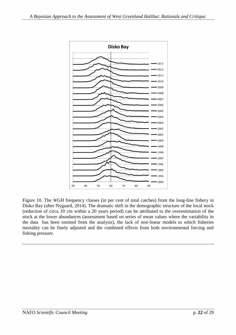
Fig. 10 depicts the WGH frequency classes (in per cent of total catches)

from the long-line fishery in Disko Bay (after Nygaard, 2014). . The dramatic shift in

the demographic structure of the local stock (reduction of circa 10 cm within a 20

years period) can be attributed to the overestimation of the population at the lower

abundances (assessment based on series of mean values where the variability in the

data has been omitted from the analysis), the lack of non-linear models to which

fisheries mortality can be finely adjusted and the combined effects from both

environmental forcing and differential effects of the fishing mortality. Juvenile

mortality (as a by-catch) from the shrimp fishery (which still remains to be

addressed) may even contribute to demographic changes in the structure of the local

stock. Although a source of error may be attributed to the tendency of the long-line to

catch smaller individuals, the size of the samples comply above any requirements for

statistical conditions and the shift reflected by the data is gradual and clear.

A successful assessment on WGH oriented both to sustainability and

conservation should be based on the scientific method, proposal and testing for null

hypothesis and carry out a full analysis of the data matrix using the wealth of linear

and non-linear methods in order to uncover the highest possible knowledge on the

population processes and environmental forcing in question.

The Bayesian-Logistic framework.

The (Gibbs sampler and) Bayesian framework may be useful, provided

that the population model that underlies the simulations has the sufficient degree of

resolution to describe the complex dynamics we address: estimates and reference

points derived from the Bayesian/MCMC-Logistic approach result in rough estimates

(i.e. "proxies-of-proxies") and the method does neither incorporate key factors nor

shows the capacity to explain the mechanics behind the data or allows to propose a

short or medium term exploitation strategy for conservation as the signal is crunched

and causes for population processes remain unknown.

In general, the Logistic equation (or any derivative) is used to fit the

outcome of the simulations while it may solely explain between 0.2-0.3 of the

(between years) mean (or median) values in the series: no temporal evolution is

considered for which trends in maxima and minima, strong correlations, memories,

A. P. Solari (2014)


auto-correlated residuals and lags (common in such dynamical systems) remain

ignored.

The resolution of the Bayesian-Logistic method becomes further critical

as it is the aggregated data (mean values with a highly reduced signal) which is

presented in the stock assessment reports. No variability analysis (on ceilings, floors,

local slopes, outliers and missing values, among other features) is considered and the

"crunching" of the signal incapacitates the assessment to finely adjust fishing

mortality to the relatively high and -most importantly- the lower abundances.

Further, it is omitted that means and variability may show different trends

(which is the case for the relationships in WGH abundance and the environmental

forcing). Means (or medians) should be linked to the local (positive and negative

growth) trends and the within- and between- year/s variability in the data: this may

reflect in a higher degree the spatio-temporal evolution of the process and associated

relationships, as well. The variability in the data is the part of the signals which

reflect the features of highest weight in such population processes for which it should

be incorporated into both the analysis and modeling of the WGH dynamics.

The issue of priors is critical, as well. Criteria for selecting priors are

subjective: different authors chose parameters without any scientific evidence - in a

"best-guess" pattern. Priors are often chosen on an arbitrary basis which may not be

related to the signal reflecting the population process. This is an artifact of the

probabilistic approach as variables which may be strongly correlated to the

population process and be a relatively safe ground for the estimations are still

ignored. Priors should be chosen both for maxima and minima in relation to the effect

of key (system-wide) environmental factors and differential effects of fishing

mortality.

If we assume that a probabilistic, linear approach combined to the

Logistic equation can be used to describe a population system, then we should be able

to find a convergence of results as compared to non-linear approaches. If we aim to

use linear methods to analyze and model WGH dynamics, it may be mandatory to

approximate the (non-linear) signals, as far as possible, in order to carry out a

realistic fisheries assessment: this will enable us both to determine higher fishing

mortality during periods of relatively higher abundances and adjust the fishing

regimes to the lower abundances without any overestimation of the stock during

periods of either low abundances or negative growth.



There are several further aspects which could be addressed to test for

alternative models to describe the dynamics of WGH. A key question is how to

describe –in a relatively simple and effective way- such complex systems without

incurring in models with too many parameters or a multi-dimensionality which would

be difficult to understand.

A linear (Bayesian/MCMC) approximation to a series of means

(abundance from surveys, commercial catches and CPUE) becomes -in the

assessment- a "three proxy set", one approximating the other (i.e. "a proxy (linear

estimation) of a proxy (mean abundance series) of a proxy (signal in the raw data)".

The maximum resolution in such an approach will go no further than a series of mean

or median values. The signal in the series of observations is taken out and both

reference points and estimations are rough or poor. Furthermore, it will make nearly

impossible to propose short (3-4) and medium (5-10 years) term sustainable fishing

strategies as the method considers a single year of memory whereas we know that the

environmental forcing (system-wide variables) show longer dependencies or memory

effects (i.e. strong correlations and dependencies on preceding values).

An advice based upon such "proxies-of-proxies" results contributes

further to the underestimation of the stock at high abundances (i.e. sub-exploitation)

and the overestimation of stock numbers at the lower abundances (which leads to

overfishing). "Higher" and "lower" in this context are determined by values above

and below (linear or non-linear) equilibria (i.e. as the stock is at a standstill, it neither

grows positively or negatively). This may be one of the co-factors which explains the

reduction in mean body length in halibut (and other) populations: the stock is

overestimated for the lower population abundances and the overfishing which occurs

acts as a selective force shifting the demographic structure towards the smaller sizes.

Moreover, the Bayesian/MCMC-Logistic approach will lead both to rough

(or poor) reference points as it eliminates the non-linear signals (expected to be of

different frequencies) from the data. which implies that it will make nearly

impossible to propose short (3-4) and medium (5-10 years) term sustainable fishing

strategies as the method, as well, considers a single year of memory (whereas we

know that external forcing system-wide variables show longer dependencies on

preceding values). Graphical representations of the described mechanism are depicted

in Figs. 8 and 9. It is the variability in the data that will allow us to adjust fishing

mortality to appropriate levels as the carrying capacity of the environment may vary.

A. P. Solari (2014)


A key question is whether the underestimation of the stock at high

abundances (which leads to under exploitation, a higher fishing mortality is possible)

may compensate for the overfishing which may occur as the stock is overestimated in

the lower abundances: the answer can be negative as we have detected a shift or bias

towards the smaller individuals during the last ten years. This has been reported at the

NAFO meeting, 2014) for other stocks which are exploited using linear frameworks,

as well.

The Logistic equation (and derivatives, such as the Schaefer production

model): this approach –contrary to the scientific evidence in a wealth of publications

where year class strength and abundance are related to environmental pulses-

assumes that (i) r and K are constant and residuals are random and (ii) the population

trajectory between zero and K/2 will be compensatory, independently of fishing

mortality regime and density dependence (no Allé Effect or minimum viable

population under which numbers and oscillations will tend either to a stand-still or

zero). Further, neither lags nor memory effects or dependencies are assumed. The

Logistic model has neither the sufficient degree of resolution nor the flexibility to

describe such complex population systems and will explain less than (approximately)

25% of the variability in the data

Uncertainty may be an overused argument (due to the probabilistic nature

of the approach) to "tag" estimations on a population process (recruitment, temporal

evolution of abundance) which is assumed to be stochastic: there is still a serious

doubt on whether uncertainty can be attributed either to randomness or it is a

parameter or a variable. However, there is evidence of both an environmental forcing

(a co-factor determining year class strength and recruitment to the population and

fishery) and auto-correlated residuals, common in (deterministic) population

processes. We may -more realistically- assume that population signals may contain

certain degrees of noise (or signal-to-noise ratio) which -in turn- may change as

function of (i) age (series for juveniles appear to be more noisy than for other

frequency classes), (ii) density dependence (relatively higher abundance cycles may

show more outliers and a higher degree of noise) and (iii) density-independence

(differential effects of the environmental forcing upon frequency classes and areas).

The analysis of the signal-to-noise ratio (critical to finely estimate uncertainty

determination of the fishable biomass and for short and medium term fisheries

management plans) requires signal analysis to determine the level of possible white

noise in the signal for different abundance cycles, frequency classes and

environmental conditions.



Auto-correlated residuals are common in dynamical systems as

population processes may respond to trends in environmental forcing and memory

(arising from the interaction of the population with the environment) is a key feature

determining such dependencies on preceding values.

Reference points (r, K and K/2, MSY, BMSY, FMSY) are key concepts and

may have important consequences to fish stock analysis (estimation of recruitment

and abundance), as well as management and conservation issues (recommended

fishing mortality ranges, TAC's, exploitation strategies, avoidance of recruitment

overfishing, among other critical factors). These are based on the Bayesian/MCMC

method linked to the Schaefer (1954) “Production –or Maximum Sustainable Yield"

model which is a modification of the Logistic equation. While the constants (mainly r

and K) may have a mathematical sense for the chosen model, the resulting description

of temporal evolution of the population system is a highly rough proxy. A critical

discussion on the reference points is suggested in order to improve both the

assessment and modeling on the WGH and other exploited species, as well:

Intrinsic rate of increase (r). Within the logistic framework, it is both

assumed that this parameter is constant and (what is critical) that a population will

compensate no matter the exploitation regime and pulses from the environment. In

this study, it is proposed that this parameter is not a constant but changes values

within and between different cycles of abundance as a function of density-

dependence: r is expected to change in both the compensatory and depensatory

phases (at the zero and maximum slopes) of population growth and at inflection

points (which are 6, 3 for a compensatory phase and 3 for a depensatory).

Furthermore, there should be instantaneous values of r, as well, due to the ever

changing environment and forward and backwards bending nature of the CPUE.

However, the complexity of this issue should be reduced to a degree which we may

handle both from the conceptual, computational and pragmatic viewpoints. For WGH

modeling, we may come to consider, at least, two values of r in each trajectory or

cycle, at different levels of numbers: one for the positive growth of the population

and another for the depensatory or negative growth phase.

Carrying capacity (K). It is assumed that K is the maximum number of

individuals in a population that can be sustained by the environment, indefinitely.

The value of K, in classical fisheries assessments is drawn as a constant value over

the years for which data exists. For instance, there may be over 50 years long series

for which a constant value is determined around the minima and it is inferred that

A. P. Solari (2014)


such "ceiling" is the K of the stock over the NAFO area/s. A single, constant value of

K is misleading and has not the resolution to describe the ceiling or number of

individuals that -for a certain area with particular environmental conditions- can be

sustained. There is a large and increasing body of scientific evidence (since the end of

the 1800´s) to the contrary and it is proposed that all population processes (such as

growth, reproduction, recruitment, migration, availability of food items and other

limiting resources in an ever changing environment) should be translated to a variable

carrying capacity (Kt or Ki) which operates in each population cycle. This is one of

the critical aspects of highest weight in modeling population dynamics and one of the

key concepts to approach sustainability and conservation.

Maximum Sustainable Yield (MSY). This is another concept that should

be discussed (and modified) as it -classically- is proposed as a constant or the

maximum yield that can be harvested from a population, "indefinitely". Further, the

MSY is considered a midpoint (or K/2) towards K (which is, again, a constant). This

concept becomes critical as K/2 is overestimated for lower abundances (or negative

growth/depensatory phases in the cycles) which will lead to overfishing during poor

environmental conditions.

Natural mortality (M). This parameter -assumed to be constant in

approaches linked to the Logistic equation- is associated to processes (predation,

disease, cannibalism, competition among others) which are density-dependent and -

hence- M should be addressed as variable. Also, there are genetic factors associated

to M which may change as the structure of the population becomes biased (through

fishing mortality) towards the smaller sizes (such as the case in WGH) in which

higher population turn-over speeds may be expected. Furthermore, it is expected that

this parameter may change as function of the variable carrying capacity of the

environment.

Priors and non-dynamic reference points may be artifacts of the

probabilistic framework linked to the Logistic model and -as I see it- they will

ultimately be translated to assessments which will contribute to change the

demographic structure of the population, overfishing and recruitment-overfishing. On

the contrary, dynamic or differential reference points are needed for attaining

sustainable exploitation strategies: these should be adjusted both to the positive and

negative local growth trends and variable carrying capacity of the environment.



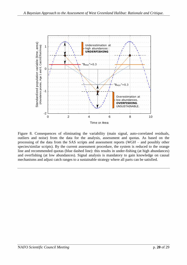
Figure 8. Consequences of eliminating the variability (main signal, auto-correlated residuals,

outliers and noise) from the data for the analysis, assessment and quotas. As based on the

processing of the data from the SAS scripts and assessment reports (WGH – and possibly other

species/similar scripts). By the current assessment procedure, the system is reduced to the orange

line and recommended quotas (blue dashed line): this results in under-fishing (at high abundances)

and overfishing (at low abundances). Signal analysis is mandatory to gain knowledge on causal

mechanisms and adjust catch ranges to a sustainable strategy where all parts can be satisfied.

0 2 4 6 8 10

Time or Area

-2

-1

0

1

Sta

nd

ard

ize

d p

op

ula

tio

n v

ari

ab

le (

tim

e, a

rea

)(A

bundance p

roxie

s,

Age 1

and 6

, C

atc

h/E

ffort

/Are

a)

Overestimation at

low abundances.

OVERFISHING.

UNSUSTAINABLE.

Underestimation at

high abundances:

UNDERFISHING

”BMSY”=0.3

”BMSY”=0.3

A. P. Solari (2014)


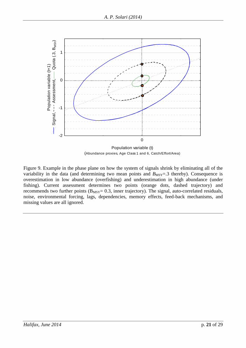
Figure 9. Example in the phase plane on how the system of signals shrink by eliminating all of the

variability in the data (and determining two mean points and BMSY=.3 thereby). Consequence is

overestimation in low abundance (overfishing) and underestimation in high abundance (under

fishing). Current assessment determines two points (orange dots, dashed trajectory) and

recommends two further points (BMSY= 0.3, inner trajectory). The signal, auto-correlated residuals,

noise, environmental forcing, lags, dependencies, memory effects, feed-back mechanisms, and

missing values are all ignored.

0

Population variable (t)

(Abundance proxies, Age Class 1 and 6, Catch/Effort/Area)

-2

-1

0

1P

op

ula

tio

n v

ari

ab

le (

t+1

)

Sig

na

l, A

sse

ssm

en

t, Q

uo

ta (

.3, B

MS

Y)



Figure 10. The WGH frequency classes (in per cent of total catches) from the long-line fishery in

Disko Bay (after Nygaard, 2014). The dramatic shift in the demographic structure of the local stock

(reduction of circa 10 cm within a 20 years period) can be attributed to the overestimation of the

stock at the lower abundances (assessment based on series of mean values where the variability in

the data has been omitted from the analysis), the lack of non-linear models to which fisheries

mortality can be finely adjusted and the combined effects from both environmental forcing and

fishing pressure.

A. P. Solari (2014)


Approaching sustainability and conservation.

At the Greenland Institute of Natural Resources (GINR), the combined

shrimp-halibut surveys meet high international standards (infrastructure, manpower,

know-how and sampling methods). A solid field work is a key factor for developing

better assessment tools and the base for attaining both sustainability and

conservation. However, it should be combined to a data analysis and modeling which

take into account the signals which may reflect the environmental forcing and

population processes under different fishing mortality levels.

Quantifying the contribution of compensatory and depensatory mechanisms,

the environmental forcing and differential effects of fishing mortality in determining

year class strength and population abundance are essential factors for assessing the

spatio-temporal evolution of the stock and possible responses to exploitation

strategies, variations in the carrying capacity of the environment and -eventually-

climate change.

However, much remains to be known on the life history and dynamics of

WGH. We deal with complex systems with interlinked features, lags, dependencies

and delayed responses both to the combined effects from external pulses and fishing

mortality during both compensation and depensation. Also, there may be possible

feed-back mechanisms mediated through the positive and negative density-

dependencies.

Although signal analysis and non-linear approaches can be more appropriate

to model such systems, an effective linear approach should seek and describe further

scientific evidences on both density-dependent and density-independent population

processes, beyond the oversimplification derived from the assumption of populations

processes being the result of random walks. Some of these aspects –to be

incorporated into the modeling on WGH dynamics- are as follows, namely:

(i) System approaches using General Additive Models (GAM’s) with both

linear and non-linear functions (to describe variability, maxima and minima); (ii)

System-wide environmental variables which may be proxies of the variable carrying

capacity of the environment, K(t) or K(i).

(iii) Fishing mortality adjusted to K(t) and different, discrete levels of

abundance (i.e. "orbits of stability"), differential values for the (dynamic) reference

points, depending on whether abundance is under compensation or depensation.

(iv) Other factors such as: signal-to-noise ratio, outliers, zeroes, null and

missing values, environmental forcing, optimal environmental values determining

year class strength and abundance, spatial distribution, maxima and minima related to

the conditions they arise, within year temporal and spatial variability, differential



effects of fishing mortality, short-to-medium term management plans, environmental

impact of trawling, by-catches of juvenile halibuts in the shrimp fishery, abundance

of shrimp and polar cod, ice production, linkage of off-shore and in-shore systems,

drift of age class 1, gonad development, among other factors.

(v) Otolith readings (through the Laser Ablation/Spectrometry method) to

(through isotope determination) to estimate the timing for recruitment, age,

migrations, foraging, speed of growth, a proxy of K(t), density dependence, memory

effects, among other factors (on-going project).

(vi) Also, we aim to propose spatial exclusion areas (with null fishing

mortality) in order to conserve the stock from recruitment overfishing and distribute

fishing effort to correct -if possible- the demographic shift toward the smaller sizes

detected under recent years.-

A. P. Solari (2014)


References.

Andre, E. and R. Hilborn (2001). Bayesian Stock Assessment Methods in Fisheries - User's Manual.

FAO, 2001.

Bas, C, A. P. Solari and J. M. Martín (1999). Considerations over a new recruitment model for

exploited fish populations. Royal Academy of Sciences, Barcelona. Vol. LVIII, Num. 5:157-183.

Ganzedo, U., E. Zorita, A. P. Solari, G. Chust, A. Santana del Pino and J. J. Castro (2009). What drove

tuna captures between the XVI (1525) and XVII (1756) centuries in Southern Europe ? ICES J. of Mar. Sc. 66.

Hjort, J. 1914. Fluctuations in the great fisheries of northern Europe, viewed in the light of biologic

research. Rapports et Proces-Verbaux des Re´unions du Conseil Permanent International pour l’Exploration de la Mer,

1. 227 pp.

Hjort, J. 1926. Fluctuations in the year classes of important food fishes. Journal du Conseil Permanent

International pour l’Exploration de la Mer, 1: 5–38.

Iselin, C. O’C. 1938. Theory concerning the causes and results of the long-period variations in the

strength of the Gulf Stream. http:// dlaweb.whoi.edu/archives.html.

Iselin, C. O’C. 1940. Preliminary report on long-period variations in the transport of the Gulf Stream

system. Papers in Physical Oceanography and Meteorology published by Massachusetts Institute of Technology (MIT)

and Woods Hole Oceanographic Institution (WHOI). Contribution 261 from the WHOI, Woods Hole, MA, July 1940.

Jørgensen O. and M. Treble (2014). Assessment of the Greenland Halibut Stock Component in NAFO

subarea 0 + Division 1A Offshore + Divisions 1B-1F. NAFO SCR Doc. 14/027. Serial No. N6322. Scientific Council

Meeting, June 2014.

McAllister M. and G. P. Kirkwood (1998). Bayesian stock assessment: a review and example

application using the logistic model. ICES Journal of Marine Science, 55: 1031–1060.

Meyer R. and R. B. Millar (1999). BUGS in Bayesian stock assessments. Can. J. Fish. Aquat. Sci. 56:

1078–1086.

Petersen, C. 1896. The yearly immigration of young place into Limfjorden from the German sea.

Report of the Danish Biological Station, 6. 48 pp.

Rollefsen, G. 1948. Climatic changes in the Arctic in relation to plants and animals. Rapports et

Proces-Verbaux des Reunions du Conseil Permanent International pour l’Exploration de la Mer, 125: 31–35.

Russell, E. S. 1939. An elementary treatment of the overfishing problem. Rapports et Proces-Verbaux

des Reunions du Conseil Permanent International pour l’Exploration de la Mer, 110: 7–14.

Sharp, G. D. 2003. Future climate change and regional fisheries: a collaborative analysis. FAO

Fisheries Technical Paper, 452. 75 pp.

Sharp, G. D., Csirke, J., and Garcia, S. 1983. Modelling fisheries: what was the question? In

Proceedings of the Expert Consultation to Examine Changes in Abundance and Species Composition of Neritic Fish

Resources, San Jose, Costa Rica, 18–29 April 1983, pp. 1177–1224. Ed. by G. D. Sharp, and J. Csirke. FAO Fisheries

Report, 291(3).

Solari, A. P., Castro, J. J., and Bas, C. 2003. On skipjack tuna dynamics: similarity at several scales.

In Handbook of Scaling Methods in Aquatic Ecology. 1. Measurement, Analysis, Simulation, pp. 183–200. Ed. by L.

Seuront, and P. G. Strutton. CRC Press, Boca Raton, FL. 600 pp.

Solari, A. P., Martın Gonzalez, J. M., and Bas, C. 1997. Stock and recruitment in Baltic cod (Gadus

morhua): a new, non-linear approach. ICES Journal of Marine Science, 54: 427–443.



Solari, A. P., J. J. Castro and C. Bas (2003). On skipjack tuna dynamics: similarity at several scales.

In "Scales in Aquatic Ecology. Measurement, analyses and simulation". Edited by Laurent Seuront (CNRS, France) and

Peter G. Strutton (Monterey Bay Aquarium Research Institute, USA). CRC Press.

Solari, A. P. (2008). New non-linear model for the study and exploitation of fishery resources. Mem.

PhD Thesis. University of Las Palmas.

Solari, A. P., E. Balguerías, C. Bas, E. Beibou, J. J. Castro, A. Faraj, D. Jouffre and M. Taleb (2008).

Final Project Report: WP/3 Environmental Models “Multi-oscillatory System Approach”. Improve Scientific and

Technical Advices for Fisheries Management (ISTAM).

Solari, A. P., Mª T. G. Santamaría, Mª F. Borges, A. M. P. Santos, H. Mendes, E. Balguerías, J. A.

Díaz Cordero, J. J. Castro and C. Bas (4)

(2010). On the dynamics of Sardina pilchardus: orbits of stability and

environmental forcing. ICES J. of Mar. Sc. 67.

Solari, A. P., Mª T. G. Santamaría, Mª F. Borges, M. Santos, H. Mendes, E. Balguerías, J. J. Castro and

C. Bas (2008). On the dynamics of Sardina pilchardus: orbits of stability and environmental forcing. Report from the

EUROCEANS Integrated Project.

Solari, A. P. (2010). Report on the mission for a workshop on General Linear (GLM’s) and Additive

(GAM’s) Models and Mixed Approaches (MA’s) for the Estimation of Abundance and Management in Artisanal

Fisheries in the Islamic Republic of Mauritania. Project GCP/MAU/032/SPA. Food and Agriculture Organization

(FAO), United Nations.

Solari, A. P. (2011). Report on the mission for the Estimation of Abundance and Management

Recommendations for the Artisanal Fisheries in the Islamic Republic of Mauritania. Project GCP/MAU/032/SPA.

Food and Agriculture Organization (FAO), United Nations.

Solari, A. P. (2012). Report on the mission for a seminar on the Dynamics, Spatial Exclusion Model

and Geometric Approach for the study and management of the Octopus stocks in the upwelling areas of the Islamic

Republic of Mauritania. Project GCP/MAU/032/SPA. Food and Agriculture Organization (FAO), United Nations.

Solari, A. P. (2012). Report on the mission Sustainable Strategies for the Study and Exploitation of

Octopus Stocks in the Islamic Republic of Mauritania: Geometric Approach and Sustainable Total Allowed Catches

(S-TAC’s). Project GCP/MAU/032/SPA. Food and Agriculture Organization (FAO), United Nations.

Solari, A. P., J. M. Martin-Gonzalez and C. Bas (1997). Stock and recruitment in Baltic cod (Gadus

morhua): a new, non-linear approach. ICES J. of Mar. Sc. 54:427-443.

A. P. Solari (2014)


Appendix I.

Commented WinBUGS runs.

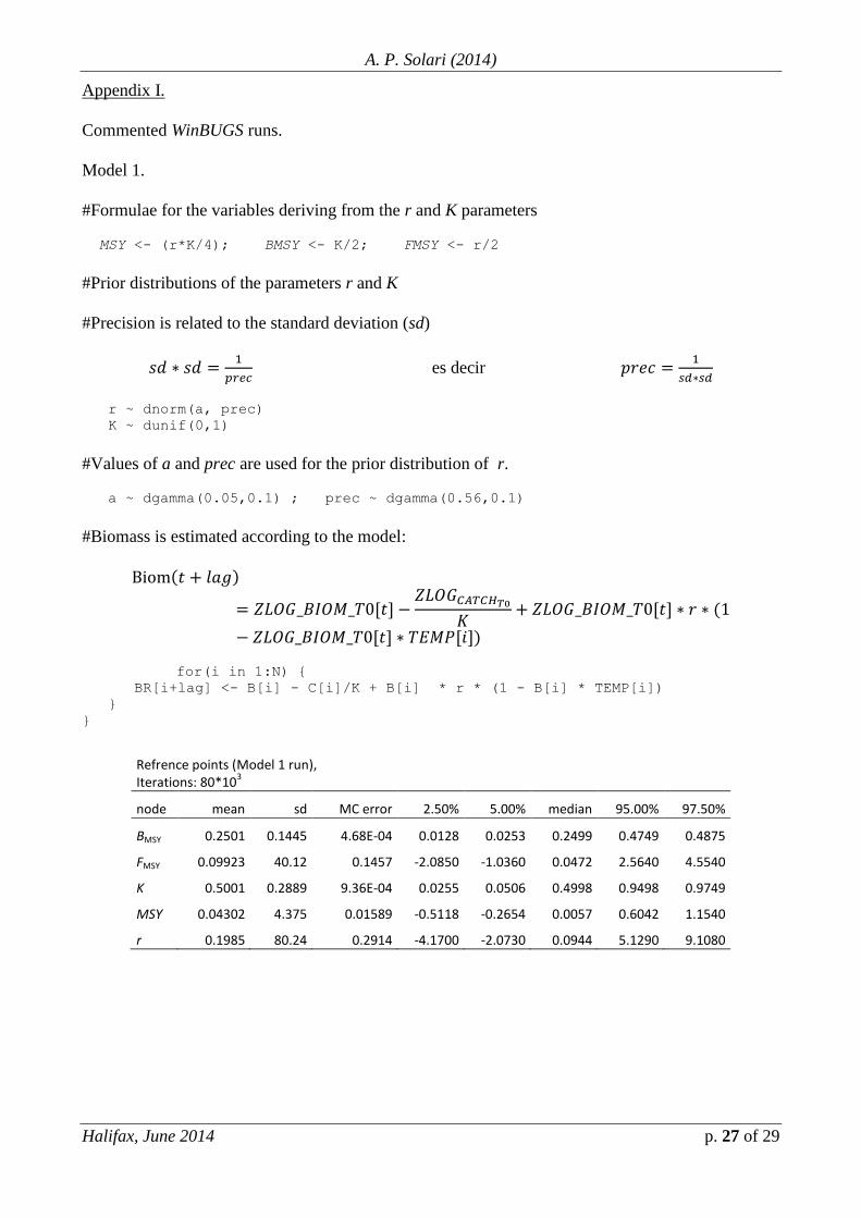
Model 1.

#Formulae for the variables deriving from the r and K parameters

MSY <- (r*K/4); BMSY <- K/2; FMSY <- r/2

#Prior distributions of the parameters r and K

#Precision is related to the standard deviation (sd)

es decir

r ~ dnorm(a, prec)

K ~ dunif(0,1)

#Values of a and prec are used for the prior distribution of r.

a ~ dgamma(0.05,0.1) ; prec ~ dgamma(0.56,0.1)

#Biomass is estimated according to the model:

for(i in 1:N) {

BR[i+lag] <- B[i] - C[i]/K + B[i] * r * (1 - B[i] * TEMP[i])

}

}

Refrence points (Model 1 run), Iterations: 80*10

3

node mean sd MC error 2.50% 5.00% median 95.00% 97.50%

BMSY 0.2501 0.1445 4.68E-04 0.0128 0.0253 0.2499 0.4749 0.4875

FMSY 0.09923 40.12 0.1457 -2.0850 -1.0360 0.0472 2.5640 4.5540

K 0.5001 0.2889 9.36E-04 0.0255 0.0506 0.4998 0.9498 0.9749

MSY 0.04302 4.375 0.01589 -0.5118 -0.2654 0.0057 0.6042 1.1540

r 0.1985 80.24 0.2914 -4.1700 -2.0730 0.0944 5.1290 9.1080



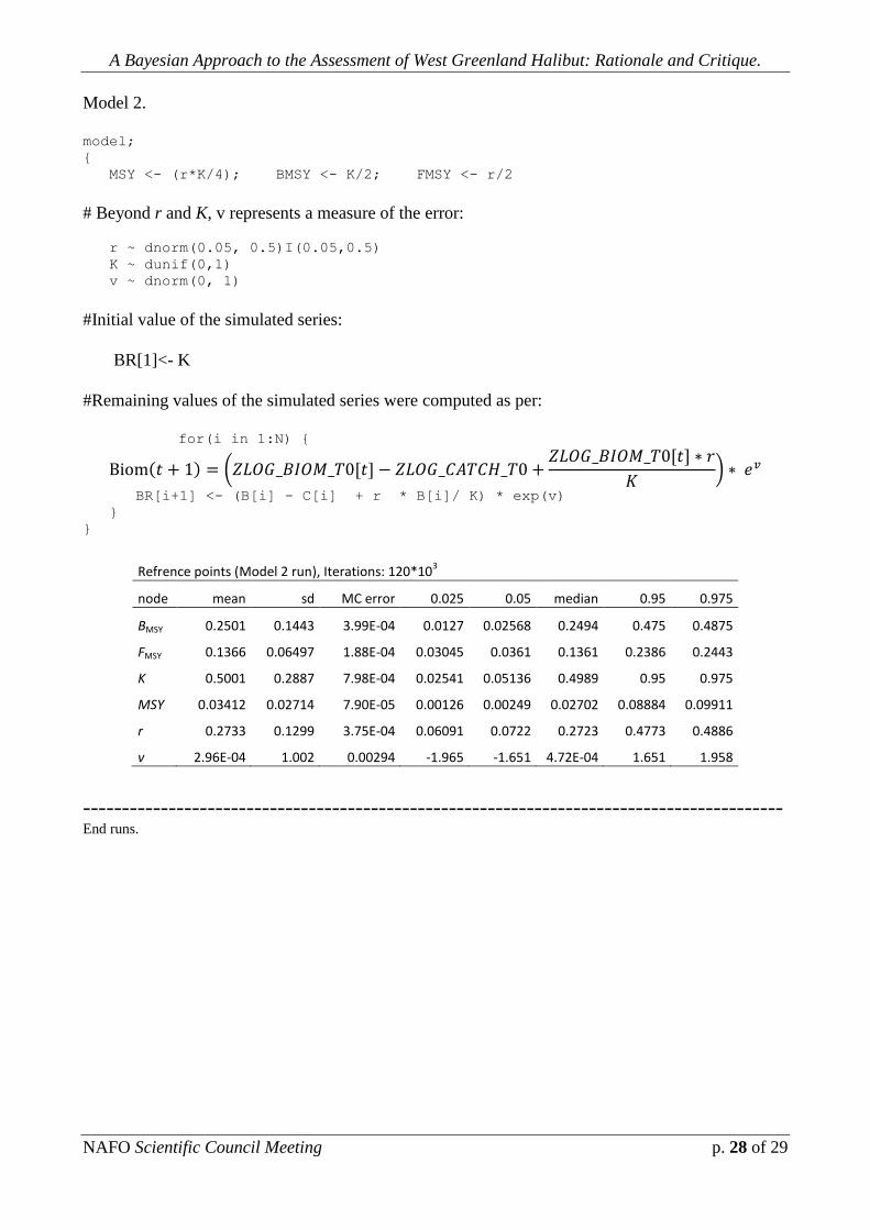
Model 2.

model;

{

MSY <- (r*K/4); BMSY <- K/2; FMSY <- r/2

# Beyond r and K, v represents a measure of the error:

r ~ dnorm(0.05, 0.5)I(0.05,0.5)

K ~ dunif(0,1)

v ~ dnorm(0, 1)

#Initial value of the simulated series:

BR[1]<- K

#Remaining values of the simulated series were computed as per:

for(i in 1:N) {

BR[i+1] <- (B[i] - C[i] + r * B[i]/ K) * exp(v)

}

}

Refrence points (Model 2 run), Iterations: 120*103

node mean sd MC error 0.025 0.05 median 0.95 0.975

BMSY 0.2501 0.1443 3.99E-04 0.0127 0.02568 0.2494 0.475 0.4875

FMSY 0.1366 0.06497 1.88E-04 0.03045 0.0361 0.1361 0.2386 0.2443

K 0.5001 0.2887 7.98E-04 0.02541 0.05136 0.4989 0.95 0.975

MSY 0.03412 0.02714 7.90E-05 0.00126 0.00249 0.02702 0.08884 0.09911

r 0.2733 0.1299 3.75E-04 0.06091 0.0722 0.2723 0.4773 0.4886

v 2.96E-04 1.002 0.00294 -1.965 -1.651 4.72E-04 1.651 1.958

------------------------------------------------------------------------------------------ End runs.

A. P. Solari (2014)


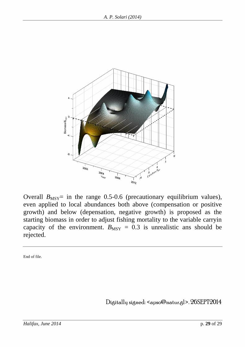
Overall BMSY= in the range 0.5-0.6 (precautionary equilibrium values),

even applied to local abundances both above (compensation or positive

growth) and below (depensation, negative growth) is proposed as the

starting biomass in order to adjust fishing mortality to the variable carryin

capacity of the environment. BMSY = 0.3 is unrealistic ans should be

rejected.

End of file.

Digitally signed: <[email protected]>. 26SEPT2014

Documents

A Bayesian Approach to the Assessment of West Greenland Halibut: Rationale and Critique