Embed Size (px)
Citation preview
INTERNATIONAL JOURNAL FOR NUMERICAL METHODS I N ENGINEERING, VOL. 26,2403-2438 ( 1 988)
A BEAM FINITE ELEMENT NON-LINEAR THEORY WITH FINITE ROTATIONS
A. CARDONA* AND M. GERADIN'
L.T.A.S., Dynamique des Constructions Mkcaniques, Uniuersitk de LiPge, Rue Ernest Solvay, 21. 8-4000 Liige, Belgium
SUMMARY
1. INTRODUCTION
The problem of modelling three-dimensional highly flexible frame structures has recently gained increased interest because of new space industry needs: in fact, there exist plans for installing large deployable structures in outer space to serve as antennae, radio telescopes, solar panels, etc. These kinds of structures necessarily have low mass and very high flexibility, so that large displacements behaviour ought to be considered. Other applications of three-dimensional frame structures include modelling of multibody systems and offshore structures. All these applications can be focussed from the point of view of a general mechanism problem.
A first approach to introduce flexibility effects in mechanisms analysis is to adopt a hypothesis of small displacements and rotations in an element-attached or body-attached frame. Under such conditions, linear finite elements can be easily extended to handle problems in a non-linear range.' - This hypothesis, however, is not very well suited to model highly flexible members. Other approximations involve the definition of a set of generalized deformation parameters at the element level6, ' or the formulation of three-dimensional degenerated beam elements.' Another formulation consists in deriving directly the beam equations from a three-dimensional non-linear theory, with a full account of finite rotations, and afterwards introducing the appropriate beam kinematical assumption^.^ - l 3
The latter approach is followed in this paper. In consequence, we are first concerned with the accurate representation of finite rotations of any magnitude in the three-dimensional space. Different techniques to parametrize rotations are proposed in the literature. Traditionally, geometrically derived measures such as Euler angles were used in rigid body dynamics. Techniques more appropriate to computations in a finite element analysis context include Euler parameter^,^, 1 4 , ' Rodrigues parameters (also called semi-tangential rotations or rotational pseudovector),'6 the conformal rotation vector4~" and the rotational vector.' ' 3 12916 Reference 18 gives a review on the different parametrizations and relations derived from them.
In this work we have chosen the rotational vector to parametrize rotations: it has a simple geometric meaning, it does not introduce any singularity in representing rotations of any magnitude and, at the same time, the set of parameters is minimal.
* Becario Externo y Miembro de la Carrera del lnvestigador del Consejo Nacional de Investigaciones Cientificas y Tecnicas de la Republica Argentina
Professor, Universite de Liege, Belgium
0029%5981/88/112403-36$18.00 0 1988 by John Wiley & Sons, Ltd.
Received 29 September 1987 Revised 1 March 1988
2404 A. CARDONA AND M. GERADIN
The three-dimensional rotations representation problem can be treated from a differential geometry point of view. ' ' 9 Proper orthogonal transformations constitute a non-conmutative (Lie) group referred to as the special orthogonal group SO(3) and every system of parametrization is a projection from SO(3) onto a specific tangent vector space to SO(3).
Rotation increments can be expressed as vectors in the tangent space to SO(3) at the actual rotation. Concerning the rotational degrees of freedom, the resulting formulation is a sort of Eulerian approach. It allows, on one hand, a relatively simple derivation of fully linearized static and dynamic operators but, on the other hand, these operators are non-symmetric in a general case (however, symmetry is shown to be recovered at equilibrium in statics, provided appropriate conditions of load conservation are respected"). Rotation updating requires a special procedure, and time integrators should be adapted to a special handling of the rotation parameters."
These inconveniences are avoided when rotations are expressed as vectors in any parametriz- ation system, in which case rotational degrees of freedom are treated from a total Lagrangian point of view. Accordingly, full symmetry of operators is obtained in this case for the conservative loading case. The elements developed can be directly integrated into a standard finite element code, without resorting to any special procedure of updating at the solver level, either in the statics or in the dynamics case. Unfortunately, this procedure does not allow an easy manipulation of rotations exceeding n, as shown in Section 6.
The alternative we have followed is to employ an updated Lagrangian formulation: rotations are described as increments with respect to a previous configuration. Full symmetry of operators is then recovered, and the time integrator is quite naturally extended to treat the rotational degrees of freedom.
The paper outline is as follows. Section 2 describes the way we manipulate rotations; expressions related to incremental rotations, angular velocities and accelerations are developed. In Section 3 these tools are employed to formulate the rigid body dynamics problem. In Sections 4 and 5, a non-linear theory of beams with full account of finite rotations is resumed. The development follows closely the presentation in Reference 11; however, the finite element formulation proposed in Section 6 differs in the way rotations are discretized, allowing one to obtain symmetrical matrices. Section 7 finally describes the time integration scheme.
The element was implemented in the MECANO mechanism analysis package which possess some rigid joints modelling capabilities.' Examples of application to static and dynamic structural and mechanisms problems are given. In particular, an example illustrating the analysis of a module of a three-dimensional deployable frame is presented.
2. FINITE ROTATIONS DESCRIPTION
2.1. Parametrizati,on of rotations
The rotation operator R is defined as a linear operator such that
R: B3+B3
RTR =RRT= 1; det R = 1
It belongs to the so-called Lie group of proper orthogonal linear transformations SO(3).
speaking, we may write Owing to the orthonormality requirement, R has only three free parameters. Generally
A BEAM F.E. NON-LINEAR THEORY 2405
where u l , u2, u3 are three independent parameters retained to described the rotation. Various choices exist, according to the adopted technique of representation; i.e. Euler angles, quaternion or Euler parameters, the conformal rotation vector, the rotational vector and the rotational pseudovector.
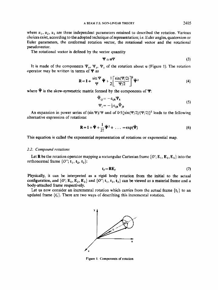
The rotational vector is defined by the vector quantity
YGUY (3) It is made of the components Y,, Y,,, Y z of the rotation about u (Figure 1). The rotation
operator may be written in terms of Y as
sinY - 1 sin(Y’/2) Y + z ~ [ YJ2 ] *2
R = l + - Y
where is the skew-symmetric matrix formed by the components of \y: - y..= -&.. y
y.= - - ‘ E . y I J IJk k -
I 2 i jk j k
(4)
( 5 )
An expansion in power series of (sin Y)/Y and of 0.5 [~in(Y’/2)’/(YY/2)]~ leads to the following alternative expression of rotations:
R=I+*+’P+ 2! . . . =exp(*) (6)
This equation is called the exponential representation of rotations or exponential map.
2.2. Compound rotations
orthonormal frame (0“; t,, tz, t3}: Let R be the rotation operator mapping a rectangular Cartesian frame (0’; E l , E,, E3} into the
t, = RE, (7) Physically, it can be interpreted as a rigid body rotation from the initial to the actual configuration, and (0’; El , E,, E3} and (0”; t,, t,, t3} can be viewed as a material frame and a body-attached frame respectively.
Let us now consider an incremental rotation which carries from the actual frame (t,} to an updated frame {ti}. There are two ways of describing this incremental rotation.
Figure 1. Components of rotation
2406 A. CARDONA A N D M. G E R A D I N
(i) Via a left translation (spatial rotation) In this case the total rotation from the initial frame is given by the left-application of an
incremental rotation operator R(l, to the actual rotation R:
R’ = R,,,R
ti = R(,,t, = R,,,RE,
The incremental rotation can be seen as a rotation applied to the actual frame { t , ) ; (ii) Via a right translation (material rotation)
Now the total rotation from the initial basis is given by the right-application of an incremental rotation operator R(r, to the actual rotation R:
R’ = RR(,,
ti = RR(,,E, (9)
The incremental rotation can be seen as a rotation applied to the material frame {E,}. Let 8 and 0 be the rotational vectors corresponding to the spatial rotation R(,, and to the
material rotation R,,,, respectively:
Using equations (8 and 9), it can be easily seen that the spatial and the material vectors are mutually related by
0 = R O (1 1) The rotational pseudovector $ (Rodrigues parameters), is an alternative form of parametrizing
rotations which has the advantage of providing a simple formula to calculate the parameters of the composed rotation. We will define it through its relation with the rotational vector:
where Il\lrll =(I).$):.
terms of the rotational pseudovectors of the composing rotations as follows: The rotational pseudovector corresponding to the total rotation can be directly computed in
Note that, if R =exp(q), then + = RY = Y. The symbols are changed to show the formula equally applies to cases where one composes two increments, for which R # exp(9).
The rotational pseudovector has the inconvenience of presenting a singularity in the represen- tation of R when 1 1 + 1 1 =n, and has thus to be used with caution. We retain here equations (13), which will be employed to derive properties related to the composition of rotations.
We remark that equivalent formulae of composition exist for other techniques of parametriz- ation; all of them can be seen as specific forms derived from the quaternion (Euler parameters) product.
A BEAM F.E. NON-LINEAR THEORY 2407
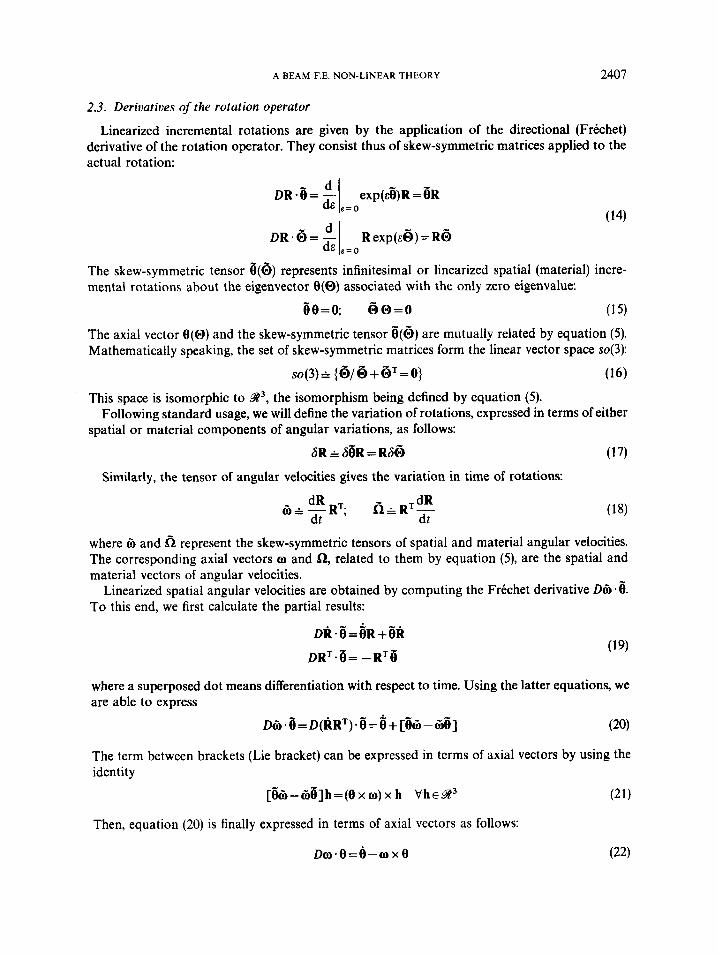
2.3. Derivatives of the rotation operator
Linearized incremental rotations are given by the application of the directional (Frechet) derivative of the rotation operator. They consist thus of skew-symmetric matrices applied to the actual rotation:
DR 8 = - exp(&)R = 6R - :61e=o
The skew-symmetric tensor 6(6) represents infinitesimal or linearized spatial (material) incre- mental rotations about the eigenvector e ( 0 ) associated with the only zero eigenvalue:
fje=o; 6o=o (15)
The axial vector O ( 0 ) and the skew-symmetric tensor 6(6) are mutually related by equation (5). Mathematically speaking, the set of skew-symmetric matrices form the linear vector space so(3):
SO@) & {6/ 6 + 6' = o} (16) This space is isomorphic to W3, the isomorphism being defined by equation (5).
spatial or material components of angular variations, as follows: Following standard usage, we will define the variation of rotations, expressed in terms of either
6R 66R = R 6 6 (17)
Similarly, the tensor of angular velocities gives the variation in time of rotations:
where 6 and fi represent the skew-symmetric tensors of spatial and material angular velocities. The corresponding axial vectors o and a, related to them by equation (5), are the spatial and material vectors of angular velocities.
Linearized spatial angular velocities are obtained by computing the Frkchet derivative Dc3 * 6. To this end, we first calculate the partial results:
where a superposed dot means differentiation with respect to time. Using the latter equations, we are able to express
DQ - 6 = D(RRT) * 6 = 6 + [6& - 661 (20)
The term between brackets (Lie bracket) can be expressed in terms of axial vectors by using the identity
[6c3-c36]h=(exo)x h Vh€@ (21)
Then, equation (20) is finally expressed in terms of axial vectors as follows:
D o . e = e - o x e (22)
2408 A. CARDONA AND M. GERADIN
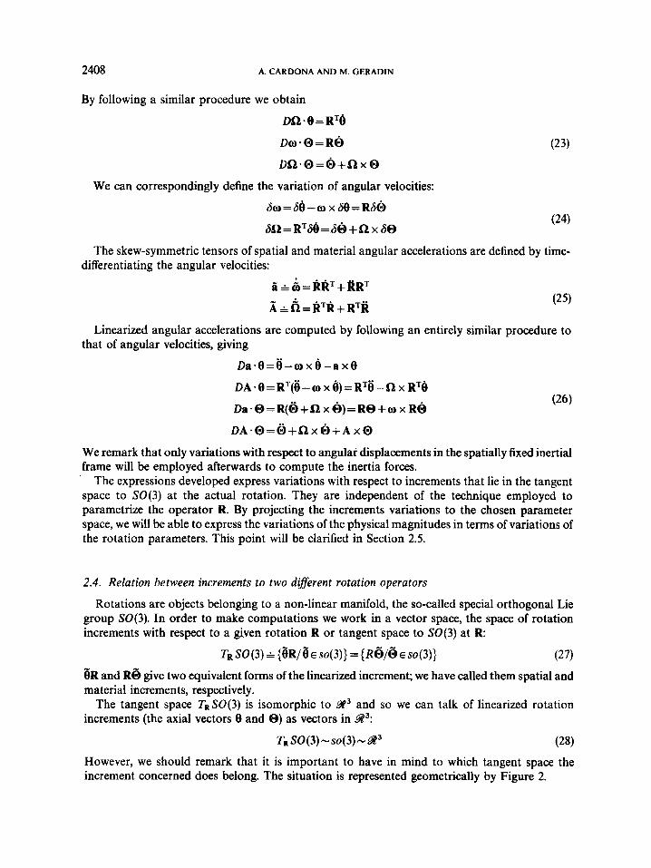
By following a similar procedure we obtain
Dn * 8 = R'6
D O . @ = RO D n * O = O + n x 0
We can correspondingly define the variation of angular velocities:
60=66-0 x Se=RSO
6R = R T 6 8 = 6 8 +a x 6 0
The skew-symmetric tensors of spatial and material angular accelerations are defined by time- differentiating the angular velocities:
ii &=@a'+ #RT I - (25) A = ~ = R T R + R T R
Linearized angular accelerations are computed by following an entirely similar procedure to that of angular velocities, giving
Da.f3=0-m x e - a x e
DA-O=RT(8-OX6)=RT~-QXRT6 (26)
D a . O = R ( & + n x & ) = R O + o x R 6
D A . o = ~ + ~ x O + A x o We remark that only variations with respect to angular displacements in the spatially fixed inertial frame will be employed afterwards to compute the inertia forces.
The expressions developed express variations with respect to increments that lie in the tangent space to SO(3) at the actual rotation. They are independent of the technique employed to parametrize the operator R. By projecting the increments variations to the chosen parameter space, we will be able to express the variations of the physical magnitudes in terms of variations of the rotation parameters. This point will be clarified in Section 2.5.
2.4. Relation between increments to two different rotation operators
Rotations are objects belonging to a non-linear manifold, the so-called special orthogonal Lie group SO(3). In order to make computations we work in a vector space, the space of rotation increments with respect to a given rotation R or tangent space to SO(3) at R
T R S O ( ~ ) = { 8 R / 8 ~ s o ( 3 ) } = { R ~ / ~ ) E s o ( ~ ) } (27) 8R and R 6 give two equivalent forms of the linearized increment; we have called them spatial and material increments, respectively.
The tangent space TESO(3) is isomorphic to 9' and so we can talk of linearized rotation increments (the axial vectors 8 and 0) as vectors in W3:
TR S0(3 ) -~0(3 ) - 9E3 (28) However, we should remark that it is important to have in mind to which tangent space the increment concerned does belong. The situation is represented geometrically by Figure 2.
A BEAM F.E. NON-LINEAR THEORY 2409
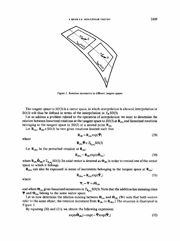
Figure 2. Rotation increments in different tangent spaces
The tangent space to SO(3) is a vector space, in which interpolation is allowed; interpolation in SO(3) will thus be defined in terms of the interpolation in TRSO(3).
Let us address a problem related to the operation of interpolation: we want to determine the relation between linearized rotations at the tangent space to SO(3) at R(A) and linearized rotations belonging to the tangent space to SO(3) at a second point R(B).
Let Ro,, R(B) E SO(3) be two given rotations located such that
where
Let R(B)& be the perturbed rotation at R(B):
R(B)&= R,,~xP(E%)) (30)
where R(B)@(B) E TR(. SO(3). Its axial vector is denoted as space to which it belongs.
in order to remind one of the vector
R(B)E can also be expressed in terms of increments belonging to the tangent space at R(A):
where
and where gives linearized increments in TR(*)S0(3). Note that the addition has meaning since Y and @(A) belong to the same vector space.
(We note that both vectors refer to the same object, the rotation increment from R(B) to R(B),.) The situation is illustrated in Figure 3.
Let us now determine the relation existing between @(A) and
By equating (30) and (31), we obtain the following expression:
exp(e6{,,) =exp(- q)exp(*J (32)
2410 A. CARDONA AND M. GERADIN
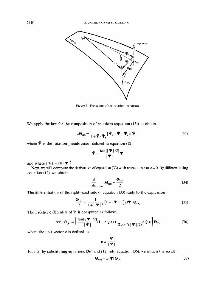
Figure 3. Projection of the rotation increment
We apply the law for the composition of rotations (equation (13)) to obtain ~
[Y&-Y-Y& x Y] 1 &a(,) = (33)
where ? is the rotation pseudovector defined in equation (12):
and where 1 1 Y' I / = (I. Y)+.
equation (1 2), we obtain Next, we will compute the derivative of equation (33) with respect to E at E = 0. By differentiating
The differentiation of the right-hand side of equation (33) leads to the expression
The FrCchet differential of is computed as follows:
where the unit vector e is defined as
YJ
/ I / I eA-
Finally, by substituting equations (36) and (12) into equation (35), we obtain the result
@(B) = T ( W @ ( A ) (37)
A BEAM F E. NON-LINEAR THEORY 241 1
with the linear transformation T(Y) defined by
It is clearly seen that when Y-+O*T(Y)+l, as expected. Next, let us inverse equation (38). First, we express from equation (32):
e x P ( t ) = exP(%exP(4,)) (39)
We apply again the law for the composition of rotations (equation (12)) to obtain
Let us compute next the derivative of the latter equation with respect to E at E=O. The differentiation of the right-hand side gives:
(RHS) = (1 +Y 0 + [ 9 x 1)- 2
The FrCchet differential D\Y - @(A) is given by equation (36), which takes the form
DQ @(A) = U ( ~ ) @ ( A ) (42)
In order to explicit @(A), we will invert U(Y); this can be made by noting that
where
Then, by replacing into equation (40) and afer some algebraic steps we arrive at the final result:
@(A) =T- '('f')@,B) (44)
with the linear transformation T-'(Y) given by
The last equation could also be obtained directly by inversing (38), after noting that - ( u l + B e O e + y q ) - ' = u l 1 + p , e O e + y , Y
where
-Y Y 2 II 1 1 ' + a2
Y1=
One observes again in equation (45) that when Y+O-T-'(Y)-+I.
2412 A. CARDONA AND M. GERADIN
The Frkchet derivative of T will be needed for multiple purposes; its expression can be directly evaluated from equation (38), giving
Computation in the limit, when II Y II -0, gives
2.5. Choice of a system of parametrization: TlSO(3)
The system of parametrization that we adopt to represent rotations is, as pointed out in Section 2.1, the rotational vector (it will be noted in what follows with a Y). From the discussion in Section 2.2, it is not difficult to see that these vectors constitute, in fact, the vector space T l S O ( 3 ) or, which is the same, the tangent space to SO(3) at the identity. Interpolation operations, which are essential to build a finite element approximation and/or to formulate a numerical time integration scheme, will be done in this vector space.
Equation (37) gives rise to three useful relations that will be repeatedly employed afterwards:
6 0 = T(Y)6I
n = T(Y)Y (49)
K =T(Y)Y'
Here 6 0 is the material angular variation, is the material angular velocity, and K is the material curvature vector; 6 I is the variation of the rotational vector, \L represents its time derivative, and Y' the derivative with respect to the length parameter of the beam. We clearly appreciate in these expressions the duality already evidenced in Figure 3: 60, a, K represent objects in the tangent space to SO(3) at R, while 6 I , Y, Y' give the same objects as seen from the rotation parameter space.
Angular accelerations can be computed by time differentiating equation (49b):
A =T* +TY where
and where the Frechet derivative of T is given in equation (47). We see that when I+O==-A-q. The elements of the vector space T R S 0 ( 3 ) allow one to represent rotations of any magnitude.
However, by inspecting equation (38), we notice that T(Y) becomes singular when 11 Y 11 +2kx, k = 1, 2, . . . , that is to say, the parametrization presents a certain number of differentiability holes. This inconvenience can be surmounted by restricting the rotational vector to values in the range
II II x (51)
This range is enough to represent any rotation, as can be easily seen from equation (4).
A BEAM F.E. NON-LINEAR THEORY 2413
Whenever any rotation violates condition (5 I), the rotational vector is corrected according to
I* = (1 - &)I
It can be readily verified that \y* satisfies the two following conditions:
R(Y*) = R(Y) (exp(q*) = exp(q))
7 T ~ l l Y l l < 2 ~ ~ l l v * l l ~ 7 t
When employing a total Lagrangian formulation (see Section 6(ii)), we will need to compute corrected values for the time derivatives of the rotational vector, which can be obtained by differentiating (52):
3. RIGID BODY DYNAMICS WITH FINITE ROTATIONS
We will first summarize the equations of motion for a rigid body, in order to gain some insight into the dynamics problem and then treat the deformable bodies dynamics problem.
Let (O;e,, e2, e3} and (0'; E l , E,, E3} be fixed spatial and material Cartesian frames, respectively, and let (x,, x2, x,) and (XI, X,, X,) be their corresponding co-ordinate systems. Moreover, let the material frame be defined such that its origin coincides with the centre of mass and its axes are oriented along the body principal axes of inertia at the initial configuration.
The actual configuration of the body Q(t) may be completely specified through the centre of mass position x,(t) and through the body rotation R(t) from the initial configuration:
Let (0"; t,; t,; t3} be a body fixed Cartesian frame with origin at the centre of mass and basis vectors defined by
t,(t) G R(t)E, (55)
x(t)=xo(t)+ R(t)X (56)
The spatial position x ( t ) of an arbitrary point P at any time instant t can be given by
where X are the material co-ordinates of the point P. The kinetic energy of the body is then computed as
S * S p d V
= ;( I B x o - So p dV+ (57)
2414 A. CARDONA AND M. GERADIN
where B is the domain occupied by the body. The body’s mass and tensor of inertia are computed by
m= JBpdY
ll= XT%p d V = ((X. X)1 -X X)p dV 1.- J B
The material frame was oriented along the principal axes of inertia, so that the latter expression can be further simplified giving ll = Diag(1, , I,, Z3).
By replacing the expression for material angular velocities (1 8) into (57), the kinetic energy of the body is written as
T=+(mx, . x, +n-lln) (59)
We remark that this equation is written in terms of a constant tensor of inertia. If spatial angular velocities were used, the rotation dependent tensor of inertia I = R l l R T should have been employed (it depends on rotations, excluding particular cases of isotropic or partially isotropic inertia).
Inertia forces can be derived by replacing the expression of angular velocity variations (24) into the kinetic energy equation and afterwards applying Hamilton’s principle. They can be expressed either in spatial or material components. We develop next the expressions for the spatial components of inertia forces:
Owing to the arbitrariness of variations 6xo and 68 and of the time limits t , and t,, the inertia forces of the rigid body can be finally computed as follows:
Material component of inertia forces give their expression in an inertial frame oriented according to the direction of material axes at the time instant considered:,
We remark that the denominations ‘spatial’ and ‘material’ are employed only to indicate the way in which rotations are handled, with the intention of comparing formulations with both kind of components. Linear magnitudes are always given in spatial components because they are clearly better expressed in this way.
Equilibrium of the rigid body is reached when inertia forces equal externally applied forces:
Here, g,,, and G,,, denote the vectors of spatial and material components of externally applied loads and torques. For the moment, we will assume that external loads are conservative.
A BEAM F.E. NON-LINEAR THEORY 241 5
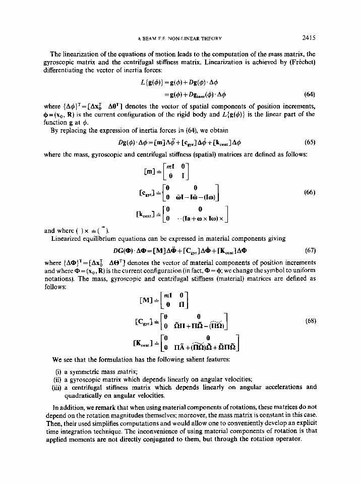
The linearization of the equations of motion leads to the computation of the mass matrix, the gyroscopic matrix and the centrifugal stiffness matrix. Linearization is achieved by (Frechet) differentiating the vector of inertia forces:
L ( g ( 4 ) I = g ( 4 ) + W 4 ) . A 4
= g ( 4 ) + @ i n e r ( + ) . A 4 (64) where (A4}'= [Ax: AO'] denotes the vector of spatial components of position increments, t$=(x,,, R) is the current configuration of the rigid body and L{g(+)} is the linear part of the function g at 4.
By replacing the expression of inertia forces in (64), we obtain
D g ( 4 ) . A 4 = Cml A$+ CC,,,l A 4 + Ck,,"l1~4 (65)
where the mass, gyroscopic and centrifugal stiffness (spatial) matrices are defined as follows:
ml 0 M=[ I]
0 - ( I a + o x 10) x
and where( ) x A( -). Linearized equilibrium equations can be expressed in material components giving
DG(@). A@ = [MI A 6 + [C,,,] A& + [K,,,,]A@ (67)
where {A@}'= [Ax: AOT] denotes the vector of material components of position increments and where @ = (xo, R) is the current configuration (in fact, @ = 4; we change the symbol to uniform notations). The mass, gyroscopic and centrifugal stiffness (material) matrices are defined as follows:
We see that the formulation has the following salient features:
(i) a symmetric mass matrix; (ii) a gyroscopic matrix which depends linearly on angular velocities; (iii) a centrifugal stiffness matrix which depends linearly on angular accelerations and
In addition, we remark that when using material components of rotations, these matrices do not depend on the rotation magnitudes themselves; moreover, the mass matrix is constant in this case. Then, their used simplifies computations and would allow one to conveniently develop an explicit time integration technique. The inconvenience of using material components of rotation is that applied moments are not directly conjugated to them, but through the rotation operator.
quadratically on angular velocities.
2416 A. CARDONA AND M. GERADIN
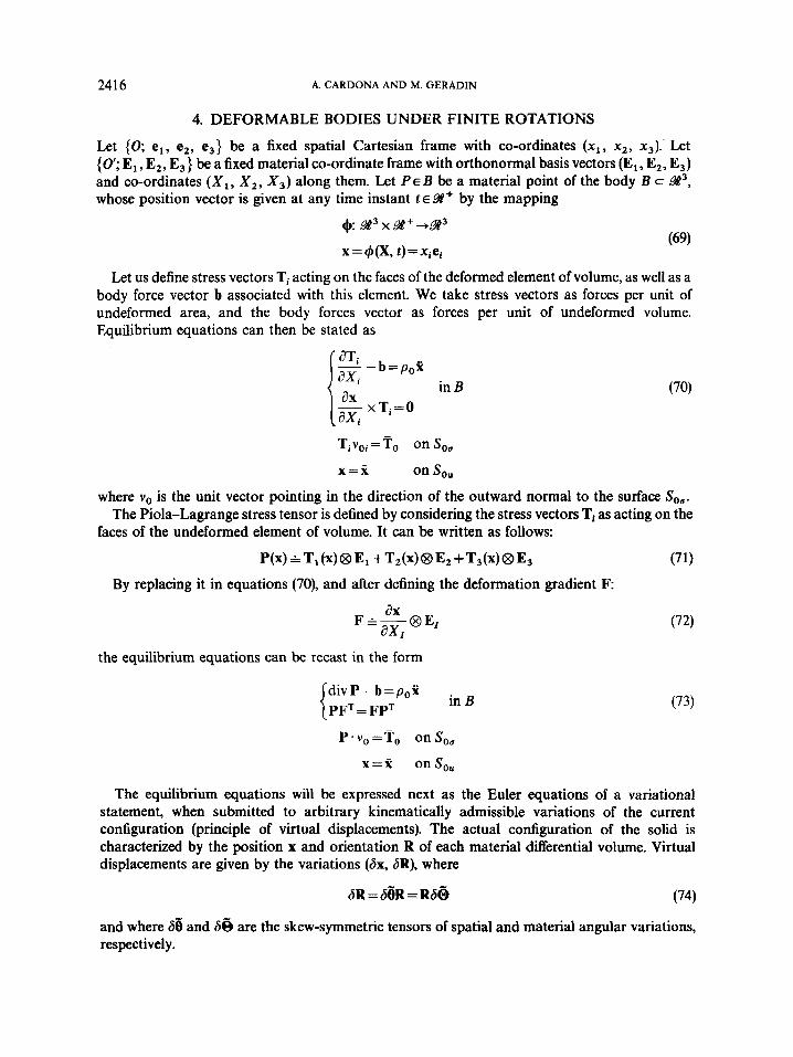
4. DEFORMABLE BODIES UNDER FINITE ROTATIONS
Let (0; el, e,, e3} be a fixed spatial Cartesian frame with co-ordinates (xl, x,, xg). Let (0; El, E,, E3} be a fixed material co-ordinate frame with orthonormal basis vectors (El, E,, E3) and co-ordinates (XI, X,, X,) along them. Let P E B be a material point of the body B c W3, whose position vector is given at any time instant ~ E W + by the mapping
$: w3 x w+ - 9 3
x=4(X, t )=xiei
Let us define stress vectors Ti acting on the faces of the deformed element of volume, as well as a body force vector b associated with this element. We take stress vectors as forces per unit of undeformed area, and the body forces vector as forces per unit of undeformed volume. Equilibrium equations can then be stated as
- - b = p o x
in B
- Ti voi =To on So,
x=jZ on SO"
where vo is the unit vector pointing in the direction of the outward normal to the surface Son. The Piola-Lagrange stress tensor is defined by considering the stress vectors Ti as acting on the
faces of the undeformed element of volume. It can be written as follows:
P(x) * Ti 6) 63 El + Tz (x) @ E, + T3 (x) @ E, (71)
By replacing it in equations (70), and after defining the deformation gradient F
the equilibrium equations can be recast in the form
div P - b = pox PFT = FPT in B
P.vo=To onso,
x=X onS,,
(73)
The equilibrium equations will be expressed next as the Euler equations of a variational statement, when submitted to arbitrary kinematically admissible variations of the current configuration (principle of virtual displacements). The actual configuration of the solid is characterized by the position x and orientation R of each material differential volume. Virtual displacements are given by the variations (ax, dR), where
(74) 6~ = 6 8 ~ = R&
and where 68 and 6 6 are the skew-symmetric tensors of spatial and material angular variations, respectively.
A BEAM F.E. NON-LINEAR THEORY 241 7
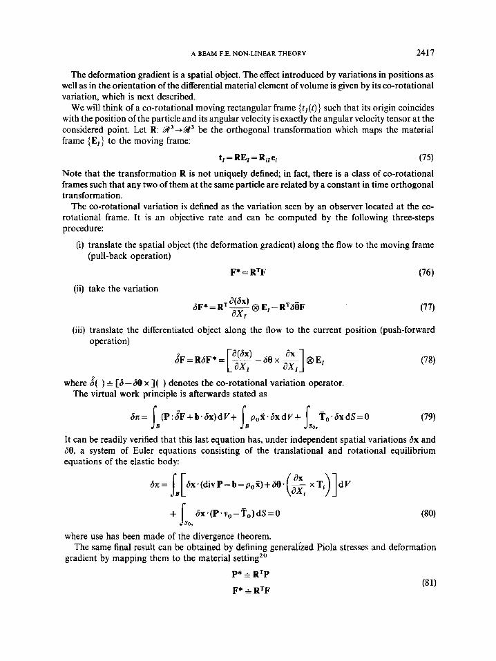
The deformation gradient is a spatial object. The effect introduced by variations in positions as well as in the orientation of the differential material element of volume is given by its co-rotational variation, which is next described.
We will think of a co-rotational moving rectangular frame { t r ( t ) } such that its origin coincides with the position of the particle and its angular velocity is exactly the angular velocity tensor at the considered point. Let R: B3+W3 be the Orthogonal transformation which maps the material frame {El} to the moving frame:
t, = RE, = R,,e, (75) Note that the transformation R is not uniquely defined; in fact, there is a class of co-rotational frames such that any two of them at the same particle are related by a constant in time orthogonal transformation.
The co-rotational variation is defined as the variation seen by an observer located at the co- rotational frame. It is an objective rate and can be computed by the following three-steps procedure:
(9
(ii)
(iii)
translate the spatial object (the deformation gradient) along the flow to the moving frame (pull-back operation)
F* = RTF (76)
(77)
translate the differentiated object along the flow to the current position (push-forward operation)
where ;( ) G [S -68 x ]( ) denotes the co-rotational variation operator. The virtual work principle is afterwards stated as
6~ = (P : $F + b* 6x) d V + p o x . 6x d V + To. 6x dS = 0 (79) i. 5. 6,. It can be readily verified that this last equation has, under independent spatial variations 6x and 68, a system of Euler equations consisting of the translational and rotational equilibrium equations of the elastic body:
6n= ~B[6x.(divP-b-p,x)+68* ( a i - xTi >] dV
+ 6,. 6x.(P.vo-To)dS=0
where use has been made of the divergence theorem.
gradient by mapping them to the material setting” The same final result can be obtained by defining generalized Piola stresses and deformation
P* A RTP
F* A RTF
2418 A. CARDONA AND M. GERADIN
Equation (79) then results by computing 6F* and replacing into the work equation:
P* : 6F* dY= lB P : & d Y
Note that P* and F* are not uniquely determined; in fact there exist infinite choices for them according to the definition of the co-rotational frame.
When treating the rigid body we suggested that material components of rotations be employed in order to simplify the dynamic equations. Accordingly to, the rotational terms in (80) can be recast in the form
The orthogonality of R implies then the verification (in a weak sense) of the rotational equilibrium equations.
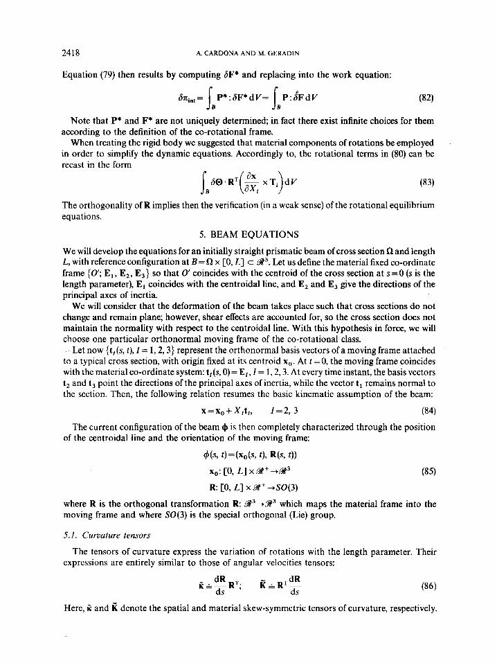
5. BEAM EQUATIONS
We will develop the equations for an initially straight prismatic beam of cross section Q and length L, with reference configuration at B = R x [O, L] c B3. Let us define the material fixed co-ordinate frame (0'; El, E,, E3} so that 0' coincides with the centroid of the cross section at s=O (s is the length parameter), El coincides with the centroidal line, and E, and E, give the directions of the principal axes of inertia.
We will consider that the deformation of the beam takes place such that cross sections do not change and remain plane; however, shear effects are accounted for, so the cross section does not maintain the normality with respect to the centroidal line. With this hypothesis in force, we will choose one particular orthonormal moving frame of the co-rotational class.
Let now { t,(s, t ) , I = 1 ,2 ,3 ) represent the orthonormal basis vectors of a moving frame attached to a typical cross section, with origin fixed at its centroid xo. At t = 0, the moving frame coincides with the material co-ordinate system: t,(s, 0) = E,, I = 1,2,3. At every time instant, the basis vectors t, and t, point the directions of the principal axes of inertia, while the vector t l remains normal to the section. Then, the following relation resumes the basic kinematic assumption of the beam:
x=xo+X,t,, 1 = 2 , 3 (84)
The current configuration of the beam 4 is then completely characterized through the position of the centroidal line and the orientation of the moving frame:
where R is the orthogonal transformation R g3+a3 which maps the material frame into the moving frame and where SO(3) is the special orthogonal (Lie) group.
5.1. Curvature tensors
The tensors of curvature express the variation of rotations with the length parameter. Their expressions are entirely similar to those of angular velocities tensors:
Here, ii and denote the spatial and material skew-symmetric tensors of curvature, respectively.
A BEAM F.E. NON-LINEAR THEORY 2419
The axial vectors of curvature K and K are related to them by equations (5).
at a perturbed configuration is given by We will next compute expressions for linearized curvatures. First, the material curvature tensor
d - d ds ds
&=R:-RR,=K+RTexp(-&))(exp(t6))R
Linearized material curvatures are then obtained by computing the FrCchet derivative:
The linearized material curvatures (axial) vector results:
It can be easily shown by the same procedure that the linearized spatial curvature vector is given
Variations of curvatures are then expressed as follows:
6K= d(se' - + se x K ds
5.2. Kinetic energy of the beam
We will define the kinetic energy density function of the beam as follows:
By taking into account the kinematic assumption, equation (84), and by following a similar development as for the rigid body, we rewrite ~(s) in the manner
t ( S ) = (p(s)X, * x, +a. n(s)n) (93)
where p(s) is the mass density per unit of undeformed length, x, is the velocity vector at the centroid, n is the material angular velocity vector of the cross section and II is the constant in time cross section tensor of inertia, defined by
c
ll= z'zp, dS = Diag(I,, I , , I , ) J O
(94)
and where I , , I , , I, are the principal mass moments of inertia of the cross section ( I , = I , + 13). The linear and angular inertia forces at s are derived through the application of the Hamilton
principle, leading to
-6t(s)= 6x,. pa, + 68. (la + o x lo)
= ~x,.~P,+~@-(IIA+RxI'I~) (95)
where I is the configuration dependent spatial mass moment of inertia (I & RIIRT).
2420 A. CARDONA AND M. GERADIN
We remark the complete analogy that exists between the dynamics treatment of the rigid body and that of the beam, clearly motivated by the hypothesis of undeformability of the cross section.
5.3. Internal work of the beam
beam can be written as By replacing the basic kinematic assumption in equation (72), the deformation gradient of the
F = - + K x ( x - x ~ ) @El+tz@Ez+t3@EE3 (96) (",: ) where K is the spatial curvature of the beam.
The deformation gradient expression is further simplified by noting that R = t, @ E,, thus giving
The latter equation clearly expresses the decomposition of the deformation gradient into one term corresponding to the deformation normal to the cross section plus a second term giving the rotation of the moving frame. Owing to the effect of shear strain, t, does not coincide with the tangent vector (dX,/ds).
We will now compute the co-rotational variation of the deformation gradient. First, the pull- back operation gives
We take variations, and by using equation (91) and afterwards performing the push-forward operation, we obtain
We can see that, under the undeformable plane sections hypothesis, the only stress vector that works is the vector oriented normally to the beam section.
We define the centroidal line strain y as follows:
Y(S, t ) = ( ( F ( x o , t)-R)E1= - -t1 (2 ) Then, the co-rotational variation of the deformation gradient can be written as
s"F = (&+ s " ~ x (x - xo)) @El (101) where & and $K are the co-rotational variations of the centroidal line strain and spatial curvature, respectively.
The virtual internal work of the beam results:
where the resultant contact force n and the resultant moment m over the cross section R are
A BEAM F.E. NON-LINEAR THEORY 242 1
defined as
n(s,t)= = 1 T, dS n
The resultant force n and moment m and conjugate strains y and K are spatial objects. Their material counterparts are defined by mapping them to the material setting via the orthogonal transformation R:
N & RTn
M =RTm
Then, the virtual internal work can be rewritten in terms of material components as follows: r
We note that the final equation could also be derived directly from the three-dimensional theory through the definition of generalized Piola stresses on the material frame and subsequent imposition of the kinematic assumption (84).
5.4. External work
By replacing the beam kinematic assumption in the expression of external work, we obtain
6neXt = lB b . 6xo d V + 6, To . axo dS
+ j B X x b-68dV+ jsonX x To.68dS
We define the distributed load and moment per unit of undeformed length as follows:
n(s, t ) = In b dS + To dx
m(s, t ) = X x b d S + X x T o d x I I. Then, the external work of the beam results:
2422 A. CARDONA AND M. GERADIN
where M = RTm is the applied external moment expressed in material components. We remark that this moment is measured in a spatially fixed set of axes, but its components are expressed in the co-rotational basis.
5.5. Motion equations of the beam
By equating the internal virtual work of the beam (equation (102)) to the virtual work of the external and inertia forces (equations (108) and (95)), we state following form of the principle of virtual displacements:
SZ= 1 (n-&++-&)ds- ((ii-pxo).Sx0
+ (m -1a - o x 10). SO) ds IO.LI
( 109)
[ O . Ll s The Euler equations conjugate to the variations of the position of the centroidal line and of
orientation of the cross section allow us to re-express the beam spatial equations of motion:
>> ds
where use has been made of the divergence theorem.
and rotational terms are expressed in the material setting: Instead of using the weak form (109), we will use the following equivalent form in which efforts
In doing so, we will simplify the inertial terms as shown for the rigid body. After regrouping terms, the weak form of the beam motion equation is rewritten as follows:
with the generalized displacements variation S@, deformations E, efforts Q, external forces F,,, and inertia forces Finer defined by
A BEAM F.E. NON-LINEAR THEORY 2423
By using equations (91) and (104) we compute the strain variations 6r and SK:
We next define the strain operator B(@):
such that 6~ =Baa. Then, the weak form (1 12) can be rewritten as follows:
G(6@, @) = (B6@. c + 6 0 . (Finer - Fexl)) ds s [O,LI
5.6. Constitutive model
efforts are linearly related to the strain measures: In what follows, we will assume a hyperelastic material behaviour, in which the beam material
[:]=c[:] with the material elasticity tensor defined by
C 4 Diag(EA, G A , , G A , , GJ, EI,, EI,) (1 18)
Here, EA is the axial stiffness, GA, and GA, define the shear stiffness along the cross section principal directions, GJ is the torsional stiffness and E l , and EZ, are the principal bending stiffness.
5.7. Linearization of the weak form
@(s, t ) = ( x , ( s , t), R(s, t ) ) . By definition, we have Let us denote by L[C(S@, @)I the linear part of the functional (1 16) at the current configuration
L[G(6@, @)]=G(6@, @)+DG(6@, @ ) ] * A @ (1 19)
where A@ Away from the equilibrium, the term G ( ) supplies the residual force at the given configuration.
We will consider G as the sum of three terms: the contribution of internal forces Gint, that of the inertia forces Gin,, and that of the external forces Gext:
(Axo, A m ) designates the incremental (material) generalized displacements.
G(S@, @)= Gint(d@, @) + Giner(fi@Y @)- Gext(h@) ( 120)
Conservative loads are assumed, so that G,,, does not depend on the current configuration.
stiffness, the gyroscopic and the mass operators, which will be evaluated next. The Frechet differential DG(6@, a). A@ gives rise to the tangent stiffness, the centrifugal
2424 A. CARDONA AND M. GERADIN
( i ) Tangent stiffness operator. The tangent stiffness operator results from the linearization of the first term in equation (120). It is decomposed as usual into the sum of two operators: the material tangent stiffness derived from the linearization of the generalized stresses ci and the geometrical tangent stiffness, which results from the linearization of the strain operator B.
The linearization of stresses leads to the expression
Dci . A@ = CB(@)A@ (121) Then, the material tangent stiffness operator is expressed in the form
D,Gin,(6@, @).A@ = (BG@)*C(BA@)ds s r0.u
The linearization of the strain operator B is next accomplished:
- A 0 x (RTGxb) - [ A 0 x (RTxb)] x 6 0 + (RTAxb) x 6 0 ( A o l + K x A@) x 6 0 D [B(@)S@]. A@ =
where ( )’ =d/ds. By using the latter equation we obtain the expression of the geometrical tangent stiffness operator:
- N . ( A Q R ~ ~ x ~ ) + N . (- A Q R ~ X ~ + R ~ A X ~ ) x 60 to. Ll
( 124)
s D, Gint(6@, @) . A@ =
+M.(AO’+K x A@) x 60)ds
Then, after some rearrangements we rewrite this equation in the form
#-
where
0 0 -RN D(@)=[ 0
0 1 ] mRT $I
A I [(RTx6) @ N - ((RTxb). N)1+ K @ M -(K * M) 11
( i i ) Linearization of inertiaforces. The linearization of the inertia forces is treated similarly to the rigid body case. The inertial part of the functional is written
Giner(6@, @) = 6@. Finer ds s I0,LI
A BEAM F.E. NON-LINEAR THEORY 2425
Then, the Frkchet differential gives the tangent inertia operator which will be split into three terms:
DGiner(a@, @). A@ = (DmGiner(a@, @) + DgGiner(a@* @)
+ D c Giner(a@* @I) * A@ (1271 These terms corresponds to the mass, gyroscopic and centrifugal stiffness respectively, and are computed as follows:
DmGine,(G@, @)-A@= 1 a@-[ P1 0 ]A&ds 10. Ll o n
A&& 0 DgGiner(G@, @) * A@ =
D , Gine,(6@, @) * A@ =
6. FINITE ELEMENT FORMULATION
We will next consider the finite element formulation of the variational equations of the beam. The developed element is based on a linear interpolation of both the displacements and the rotation parameters. The components of the rotational vector in TlSO(3) were chosen as generalized parameters to represent rotations at the nodes of the discretization. A uniformly reduced integration rule is employed to avoid the locking phenomenon.
We will discuss three forms of expressing the discretized operators:
(i) a first one, in which incremental rotations are given in TRS0(3); (ii) a second one, in which the same terms are directly given in T1S0(3); (iii) a third and last one, in which the incremental rotations are given in Tar,, S 0 ( 3 ) , where Rrcf
is the rotation operator at a previously converged configuration.
From the point of view of the rotational degrees of freedom treatment, these formulations can be seen as Eulerian, total Lagrangian and updated Lagrangian, respectively. In the last formulation, rotations are expressed as increments with respect to a previously computed one. The discretized operators obtained by applying the first technique are a direct translation of the operators developed in Section 5; the equations are relatively simple but the formulation has the disadvantage of providing unsymmetrical matrices. When using the second formulation, the equations are a little more involved and a full linearization of the rotational inertial terms is difficult to obtain, but it has the clear advantage of giving symmetrical matrices for the conservative problem. In the latter case, the matrices are entirely similar to those computed in (ii), but it easily handles situations with arbitrarily large rotations, exceeding the bound 11 Y 11 > n.
We will first describe briefly methods (i) and (ii). For these cases, interpolated displacements and rotations are given by
where xoI, Y, are the nodal values of position and rotation parameters, N,(s) is the linear interpolation function corresponding to node I and summation is extended to the two nodes of the element. The rotational vectors Y , "1 belong to TlSO(3).
2426 A. CARDONA AND M. GERADIN
Displacements variations are given as usual by 6xo =N,6xo,; angle variations are computed by applying (49a), giving
6 0 ( ~ ) = T(Y) 6" = NIT(NIY 1 ) 6 8 , ( 130)
6 0 ( s ) = N j T ( ~ ) T - ' ( ~ , ) 6 0 , x N , 6 0 , (131)
for the formulation (ii), and
when using the formulation (i). The latter equation could also be interpreted as a linear interpolation of the rotation variations; however, this procedure is not formally correct because 6 0 , and 602 belong to different vector spaces.
The material curvatures vector, which is needed to calculate the elemental internal forces and stiffness, is approximated by projecting the interpolated length derivative of the rotational vector Y' to the tangent space TuS0(3):
K=T(Y)Y'=T(Y)N;'I', (132)
(i) Formulation in TuSO(3)
equation (1 15); it is expressed as The strain4isplacements matrix B: is the discrete counterpart of the strains operator B(@),
N;RT N,(RTx6) 0 N;l+N,R -1
and is such that it verifies
(133)
where the implied summation is extended to both nodes of the element. The residual vector G is given by the sum
where the internal, inertial and external forces vectors Ginr, Giner and G,,, are computed through the integrals
Gint, = B:T(s)a(s)ds s [O,LI
Giner, = I NT(s)Finer(s)ds
Gext, = 1 NT(s)Fext(s)ds
[O.LI
[O. Ll
where N,=Nj1,.6.
geometrical tangent stiffness matrices: The tangent stiffness matrix is computed by adding the contributions of the material and
where the blocks corresponding to nodes I and J of these matrices are obtained by computing the
A BEAM F.E. NON-LINEAR THEORY 2421
integrals
The matrix Y: is computed as follows:
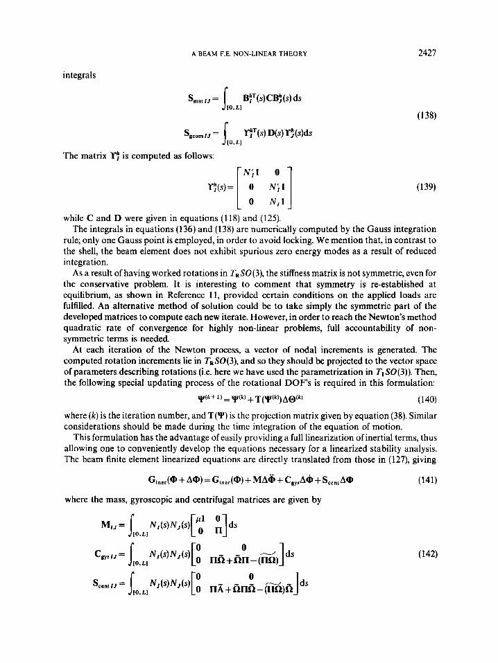
while C and D were given in equations (118) and (125). The integrals in equations (136) and (138) are numerically computed by the Gauss integration
rule; only one Gauss point is employed, in order to avoid locking. We mention that, in contrast to the shell, the beam element does not exhibit spurious zero energy modes as a result of reduced integration.
As a result of having worked rotations in TRS0(3), the stiffness matrix is not symmetric, even for the conservative problem. It is interesting to comment that symmetry is re-established at equilibrium, as shown in Reference 11, provided certain conditions on the applied loads are fulfilled. An alternative method of solution could be to take simply the symmetric part of the developed matrices to compute each new iterate. However, in order to reach the Newton's method quadratic rate of convergence for highly non-linear problems, full accountability of non- symmetric terms is needed.
At each iteration of the Newton process, a vector of nodal increments is generated. The computed rotation increments lie in TRS0(3), and so they should be projected to the vector space of parameters describing rotations (i.e. here we have used the parametrization in TlSO(3)). Then, the following special updating process of the rotational DOF's is required in this formulation:
+T(I(k))AO(k) ( 140) \ y ( k + 1 ) = \yW
where (k) is the iteration number, and T(Y) is the projection matrix given by equation (38). Similar considerations should be made during the time integration of the equation of motion.
This formulation has the advantage of easily providing a full linearization of inertial terms, thus allowing one to conveniently develop the equations necessary for a linearized stability analysis. The beam finite element linearized equations are directly translated from those in (127), giving
(141) Giner(@ + A@) = Ciner(@) + M A 6 + CgyrAO + SCen,A@
where the mass, gyroscopic and centrifugal matrices are given by
2428 A. CARDONA AND M. GERADIN
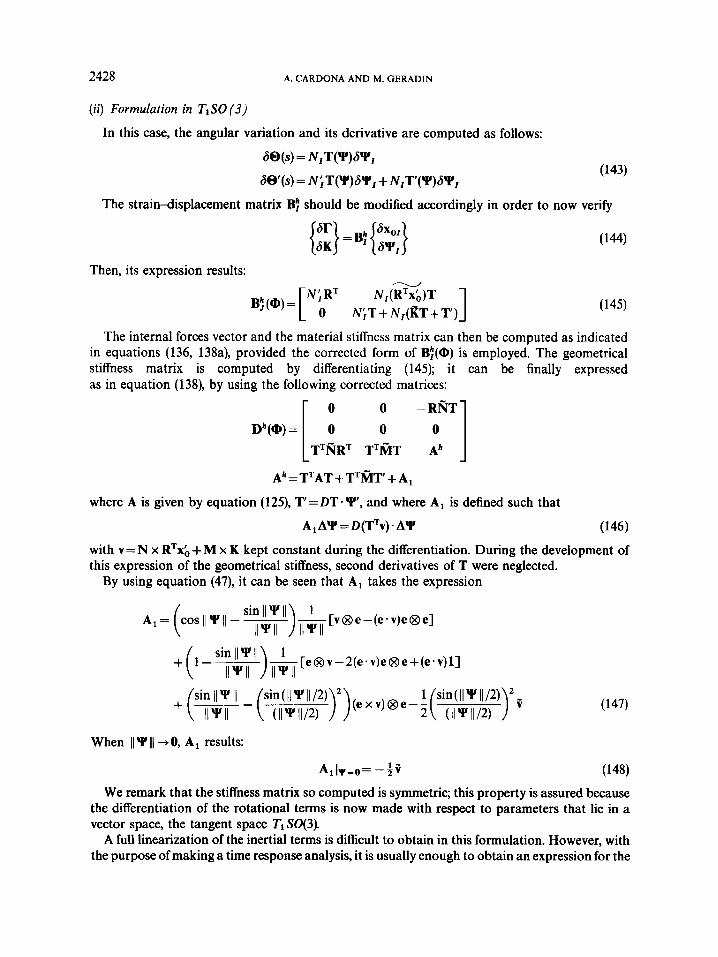
(ii) Formulation in TISO (3)
In this case, the angular variation and its derivative are computed as follows:
~O(S) = N,T(Y)GY,
S@'(S) = N;T(Y)GY',+N,T'(Y)61, (143)
The straindisplacement matrix B! should be modified accordingly in order to now verify
Then, its expression results:
N,(RTxb)T o N;T + N,(KT + T) B'j(@)= YiRT (145)
The internal forces vector and the material stiffness matrix can then be computed as indicated in equations (136, 138a), provided the corrected form of B!(@) is employed. The geometrical stiffness matrix is computed by differentiating (145); it can be finally expressed as in equation (138), by using the following corrected matrices:
o -RRT
O I
D"(@)= 0 0 " T ~ R R ~ T~ICXT
A" = T ~ A T + T ~ ~ W +A,
where A is given by equation (125), T=DT-Y', and where A, is defined such that
A1AY =D(TT~)-AY (146) with v = N x RTxb + M x K kept constant during the differentiation. During the development of this expression of the geometrical stiffness, second derivatives of T were neglected.
By using equation (47), it can be seen that A, takes the expression
[e 6 v - 2(e . v)e 8 e + (e . v ) l ]
When IIY 1) -0, A, results:
(148) 1 - A, Iy=o= - Z V
We remark that the stiffness matrix so computed is symmetric; this property is assured because the differentiation of the rotational terms is now made with respect to parameters that lie in a vector space, the tangent space TlSO(3).
A full linearization of the inertial terms is difficult to obtain in this formulation. However, with the purpose of making a time response analysis, it is usually enough to obtain an expression for the
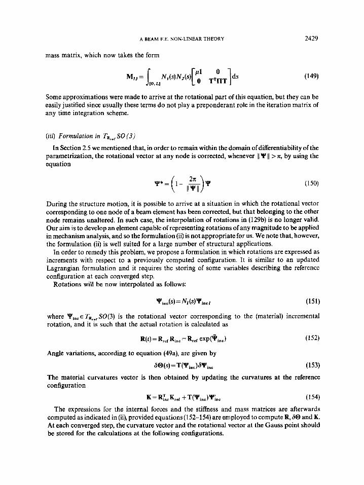
A BEAM F.E. NON-LINEAR THEORY 2429
mass matrix, which now takes the form
Some approximations were made to arrive at the rotational part of this equation, but they can be easily justified since usually these terms do not play a preponderant role in the iteration matrix of any time integration scheme.
(iii) Formulation in T R r s T SO (3)
In Section 2.5 we mentioned that, in order to remain within the domain of differentiability of the parametrization, the rotational vector at any node is corrected, whenever 11 Y 11 > n, by using the equation
During the structure motion, it is possible to arrive at a situation in which the rotational vector corresponding to one node of a beam element has been corrected, but that belonging to the other node remains unaltered. In such case, the interpolation of rotations in (129b) is no longer valid. Our aim is to develop an element capable of representing rotations of any magnitude to be applied in mechanism analysis, and so the formulation (ii) is not appropriate for us. We note that, however, the formulation (ii) is well suited for a large number of structural applications.
In order to remedy this problem, we propose a formulation in which rotations are expressed as increments with respect to a previously computed configuration. It is similar to an updated Lagrangian formulation and it requires the storing of some variables describing the reference configuration at each converged step.
Rotations will be now interpolated as follows:
vinc(S)= NAs)yincl (151)
where Yinc E TR,,, SO(3) is the rotational vector corresponding to the (material) incremental rotation, and it is such that the actual rotation is calculated as
~ ( t ) = ~ , , r Rinc=Rret exp(*inc) (152)
a@(s) =TP’inc)aVinc (153)
Angle variations, according to equation (49a), are given by
The material curvatures vector is then obtained by updating the curvatures at the reference configuration
The expressions for the internal forces and the stiffness and mass matrices are afterwards computed as indicated in (ii), provided equations (152-154) are employed to compute R, 6 0 and K. At each converged step, the curvature vector and the rotational vector at the Gauss point should be stored for the calculations at the following configurations.
2430 A. C A R D O N A A N D M. GERADIN
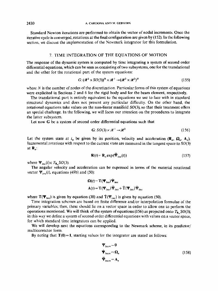
Standard Newton iterations are performed to obtain the vector of nodal increments. Once the iterative cycle is converged, rotations at the final configuration are given by (1 52). In the following section, we discuss the implementation of the Newmark integrator for this formulation.
7. TIME INTEGRATlON OF THE EQUATIONS OF MOTION
The response of the dynamic system is computed by time integrating a system of second order differential equations, which can be seen as consisting of two subsystems, one for the translational and the other for the rotational part of the system equations:
G: (a3 x S 0 ( 3 ) ) N x B+ +(B3 x 93)N (155)
where N is the number of nodes of the discretization. Particular forms of this system of equations were explicited in Sections 2 and 6 for the rigid body and for the beam element, respectively.
The translational part is entirely equivalent to the equations we use to face with in standard structural dynamics and does not present any particular difficulty. On the other hand, the rotational equations take values on the non-linear manifold S 0 ( 3 ) , so that their treatment offers an special challenge. In the following, we will focus our attention on the procedures to integrate the latter subsystem.
Let now G be a system of second order differential equations such that
G: SO(3) x .9?+ +a3 (156)
Let the system state at t, be given by its position, velocity and acceleration (R,, a,,, A,,). Incremental rotations with respect to the current state are measured in the tangent space to SO(3) at R,,:
~ ( t ) =Rnexp@inc(t)) (1 57)
where Y i n C ( t ) ~ T'"SO(3).
vector Yinc(t), equations (49b) and (50): The angular velocity and acceleration can be expressed in terms of the material rotational
Wt)=T(vinc)*inc
~ ( t ) =TWinc)*inc + * P i n c ) * i n c
where T(VinC) is given by equation (38) and T(Yinc) is given by equation (50). Time integration schemes are based on finite difference and/or interpolation formulae of the
primary variables; then, these should lie on a vector space in order to allow one to perform the operations mentioned. We will think of the system of equations (156) as projected onto TR,S0(3); in this way we define a system of second order differential equations with values on a vector space, for which standard time integrators can be applied.
We will develop next the equations corresponding to the Newmark scheme, in its predictor/ multicorrector form.
By noting that T(0) = 1, starting values for the integrator are stated as follows:
A BEAM F.E. NON-LINEAR THEORY 243 I
Then, the predictor and corrector equations are written as usual:
where h = ( t , + l -t,) is the time step and j and y are the parameters of the Newmark scheme. Corrected values for R, + 1, a, + A, + are computed by using equations (1 57), (49b) and (50).
Iterations are pursued until the system reaches an equilibrium state, which is characterized by the vanishing of the virtual work:
6\Yinc. Giki 1 = 0 (161)
where 6\Yinc lies in the tangent space to SO(3) at R,. In practice, equation (161) is considered to be satisfied whenever the inequality 11 Gikl 11 < E is satisfied, where 11 Gikl 11 is any suitable norm of the residual vector Gikl and E is a prespecified tolerance.
is determined by requiring that the linearized equilibrium equations at the current state vanish:
The iteration increment
6\Yinc . L Gik; 1 = 6\YinC.(Gik1 + SLY,, Aye)) = 0 ( 1 62)
where the dynamical pseudo-stiffness matrix is defined as follows:
Particular expressions for the mass and stiffness matrices of the rigid body and of the beam element were derived in Sections 2 and 6.
We note that the widely known properties of second order accuracy and unconditional stability held by the Newmark scheme (for appropriate values of the constants j and y ) are naturally extended to the integration in SO(3). In fact we should speak of a linearized stability property, which provides necessary (but not sufficient) conditions for stability in non-linear systems. We refer to Reference 21 for a detailed discussion on the subject.
8. NUMERICAL EXAMPLES
8.1. Spinning t o p 2 2
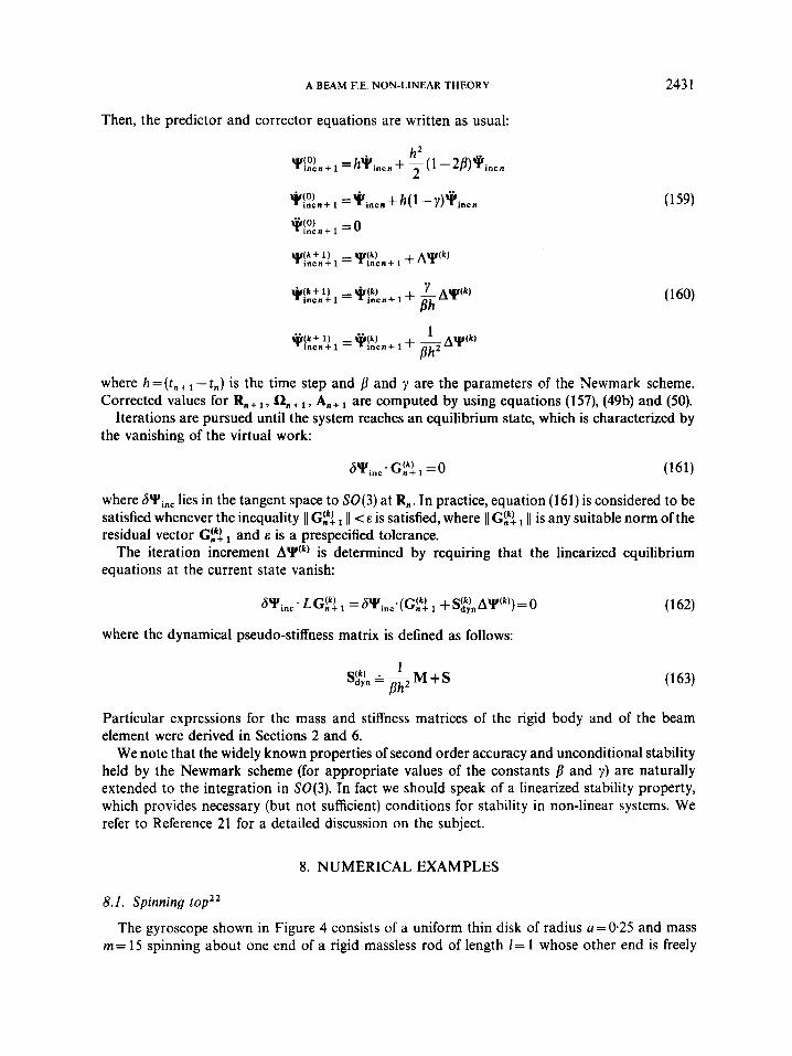
The gyroscope shown in Figure 4 consists of a uniform thin disk of radius a=0.25 and mass m = 15 spinning about one end of a rigid massless rod of length I = 1 whose other end is freely
2432 A. CARDONA AND M. GERADIN
Figure 4. Spinning top in a gravity field g
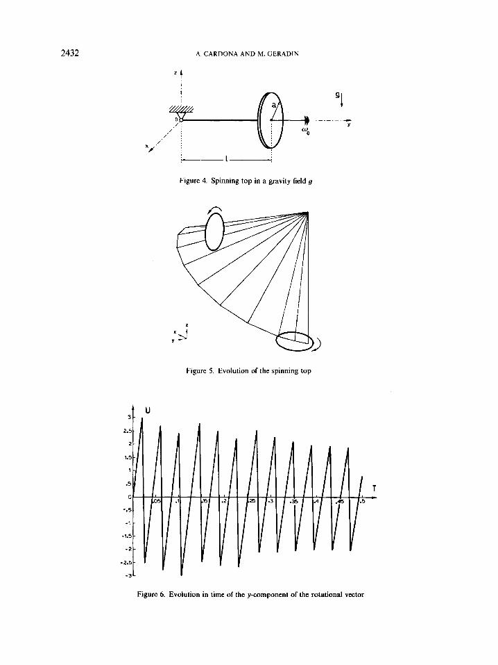
Figure 5. Evolution of the spinning top
+ u
Figure 6. Evolution in time of the y-component of the rotational vector
A BEAM F.E. NON-LINEAR THEORY 243 3
articulated at a fixed point 0. The gravity constant is g=9.81 and the initial conditions are
a, =O
n 2 = w 0 , w0=150 ( 164) 2a2
3-a2+41w0 a --
For these conditions the rod moves through the bottom position at z = - 1. Figure 5 illustrates the simulation results obtained by time integrating the equations of motion with 100 steps of 0.05. Figure 6 displays the evolution in time of the y-component of the rotational vector. We note the discontinuity in time introduced at 11 \Y 11 = K to remain within the zone of differentiability of T. The angular (material) velocity in a direction normally oriented to the principal axis of the body is plotted in Figure 7. A small amount of numerical damping was introduced to avoid the oscillations induced by the presence of constraints, by fixing the Newmark’s integrator parameters b= 0.25( 1 + a)’ and y = 0-5 + a, with a = 0.05. The mean number of iterations per time step was 3.
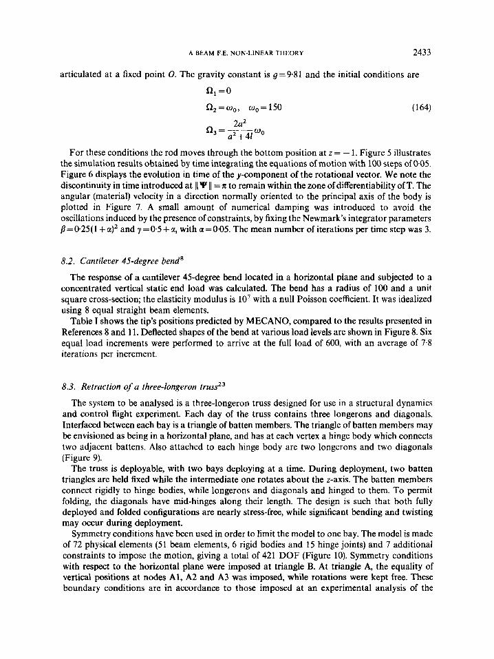
8.2. Cantilever 45-degree bend’
The response of a cantilever 45-degree bend located in a horizontal plane and subjected to a concentrated vertical static end load was calculated. The bend has a radius of 100 and a unit square cross-section; the elasticity modulus is lo7 with a null Poisson coefficient. It was idealized using 8 equal straight beam elements.
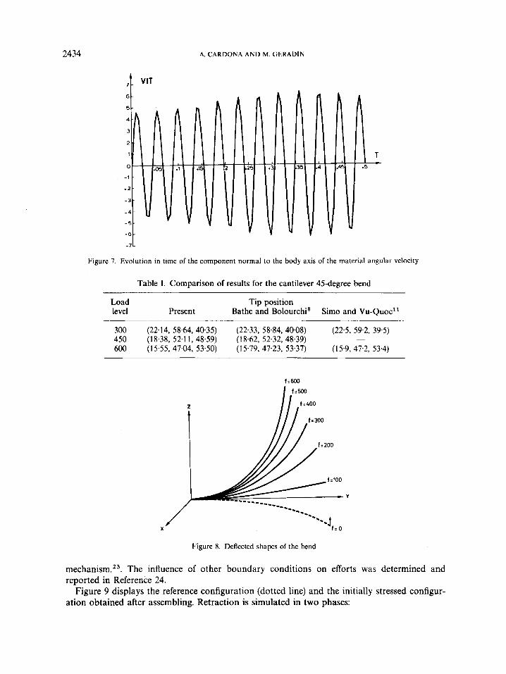
Table I shows the tip’s positions predicted by MECANO, compared to the results presented in References 8 and 1 1. Deflected shapes of the bend at various load levels are shown in Figure 8. Six equal load increments were performed to arrive at the full load of 600, with an average of 7.8 iterations per increment.
8.3. Retraction of a three-longeron trussz3
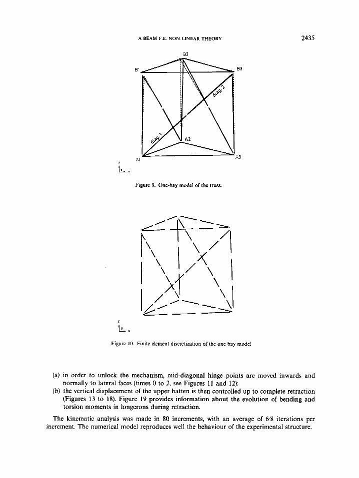
The system to be analysed is a three-longeron truss designed for use in a structural dynamics and control Aight experiment. Each day of the truss contains three longerons and diagonals. Interfaced between each bay is a triangle of batten members. The triangle of batten members may be envisioned as being in a horizontal plane, and has at each vertex a hinge body which connects two adjacent battens. Also attached to each hinge body are two longerons and two diagonals (Figure 9).
The truss is deployable, with two bays deploying at a time. During deployment, two batten triangles are held fixed while the intermediate one rotates about the z-axis. The batten members connect rigidly to hinge bodies, while longerons and diagonals and hinged to them. To permit folding, the diagonals have mid-hinges along their length. The design is such that both fully deployed and folded configurations are nearly stress-free, while significant bending and twisting may occur during deployment.
Symmetry conditions have been used in order to limit the model to one bay. The model is made of 72 physical elements (51 beam elements, 6 rigid bodies and 15 hinge joints) and 7 additional constraints to impose the motion, giving a total of 421 DOF (Figure 10). Symmetry conditions with respect to the horizontal plane were imposed at triangle B. At triangle A, the equality of vertical positions at nodes Al , A2 and A3 was imposed, while rotations were kept free. These boundary conditions are in accordance to those imposed at an experimental analysis of the
2434 A. CARDONA AND M . GERADIN
-7L
Figure 7. Evolution in time of the component normal to the body axis of the material angular velocity
Table 1. Comparison of results for the cantilever 45-degree bend
Load Tip position level Present Bathe and Bolourchi' Simo and Vu-Quoc"
300 (22.14, 58.64, 40.35) (22.33, 58.84, 40.08) (22.5, 59.2, 39.5) 450 (18.38, 52.11, 48.59) (18.62, 52.32, 48.39) ~
600 ( 1 5.55, 47.04, 53.50) ( 1 5.79, 47.23, 53.37) ( 1 5.9, 47.2, 53.4)
f = GOO I f.500
Figure 8. Deflected shapes of the bend
mechani~rn.~~. The influence of other boundary conditions on efforts was determined and reported in Reference 24.
Figure 9 displays the reference configuration (dotted line) and the initially stressed configur- ation obtained after assembling. Retraction is simulated in two phases:
A BEAM F.E. NON-LINEAR THEORY 2435
02
2
L x Figure 9. One-bay model of the truss.
2
k" Figure 10. Finite element discretization of the one bay model
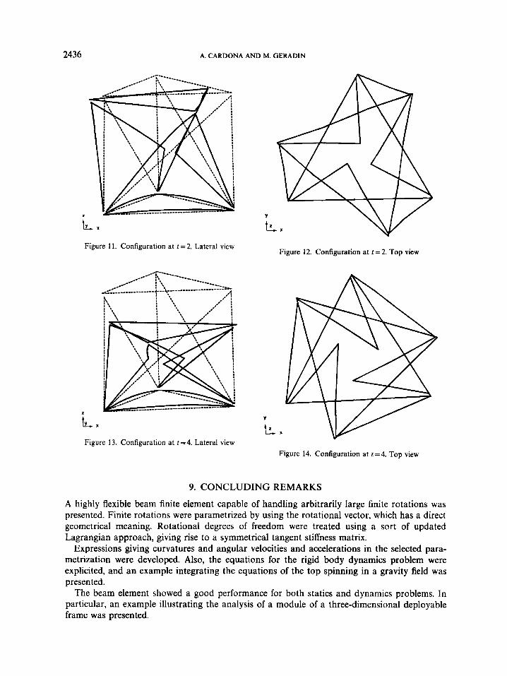
(a) in order to unlock the mechanism, mid-diagonal hinge points are moved inwards and normally to lateral faces (times 0 to 2, see Figures 11 and 12):
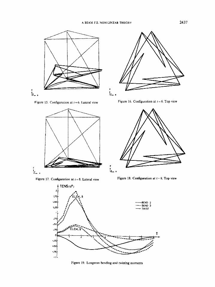
(b) the vertical displacement of the upper batten is then controlled up to complete retraction (Figures 13 to 18). Figure 19 provides information about the evolution of bending and torsion moments in longerons during retraction.
The kinematic analysis was made in 80 increments, with an average of 6.8 iterations per increment. The numerical model reproduces well the behaviour of the experimental structure.
2436 A. CARDONA AND M. GERADIN
L X
Figure 1 1 . Configuration at t = 2. Lateral view
2
L X
Figure 13. Configuration at t=4 . Lateral view
Figure 12. Configuration at t = 2 . Top view
Y
k X
Figure 14. Configuration at t=4. Top view
9. CONCLUDING REMARKS
A highly flexible beam finite element capable of handling arbitrarily large finite rotations was presented. Finite rotations were parametrized by using the rotational vector, which has a direct geometrical meaning. Rotational degrees of freedom were treated using a sort of updated Lagrangian approach, giving rise to a symmetrical tangent stiffness matrix.
Expressions giving curvatures and angular velocities and accelerations in the selected para- metrization were developed. Also, the equations for the rigid body dynamics problem were explicited, and an example integrating the equations of the top spinning in a gravity field was presented.
The beam element showed a good performance for both statics and dynamics problems. In particular, an example illustrating the analysis of a module of a three-dimensional deployable frame was presented.
A BEAM F.E. NON-LINEAR THEORY
k. t.
2437
Figure 15. Configuration at r =6. Lateral view
z
L x Figure 17. Configuration at r = 8. Lateral view
4 TENS(io5)
Figure 16. Configuration at t = 6. Top view
t. Figure 18. Configuration at t = 8. Top view
2 -
I - :75 -
- 1 L
Figure 19. Longeron bending and twisting moments
--...BEND 2 -____ BEND 3 - TWIST
2438 A. CARDONA AND M GERADIN
REFERENCES
1. M. Geradin, G. Robert and C. Bernardin, ‘Dynamic modelling of manipulators with flexible members’, in A. Danthine
2. J. Song and E. J. Haug, ‘Dynamic analysis of planar flexible mechanisms’, Comp. Methods Appl. Mech. Eng., 24,
3. M. Geradin, G. Robert and P. Buchet, ‘Kinematic and dynamic analysis of mechanisms: a finite element approach based on Euler parameters’, in P. Bergan et al. (eds.), Finite Element Methods for Nonlinear Problems, Springer-Verlag, Berlin, 1986.
4. M. Geradin and A. Cardona, ‘Kinematics and dynamics of rigid and flexible mechanisms using finite elements and quaternion algebra’, Comp. Mech., to appear.
5. 0. P. Agrawal and A. A. Shabana, ‘Application of deformable-body mean axis to flexible multibody system dynamics’, Comp. Methods Appl. Mech. Eng., 56, 217-245 (1986).
6. J. F. Besseling,.‘Non-linear theory for elastic beams and rods and its finite element representation’, Comp. Methods Appl. Mech. Eng., 31, 205-220 (1982).
7. K. Van Der Werff and J. B. Jonker, ‘Dynamics of flexible mechanisms’, in E. J. Haug (ed.), Computer Aided Analysis and Optimization of Mechanical System Dynamics, Springer-Verlag, Berlin, 1984.
8. K. J. Bathe and S . Bolourchi, ‘Large displacement analysis of three-dimensional beam structures’, Int. j . numer. methods eng., 14, 961-986 (1979).
9. K. Kondoh, K. Tanaka and S. N. Atluri, ‘An explicit expression for the tangent-stiffness of a finitely deformed 3-D beam and its use in the analysis of space frames’, Comp. Struct., 24, 253-271 (1986).
10. J. C. Simo, ‘A finite strain beam formulation. The three-dimensional dynamic problem. Part I’, Comp. Methods App l . Mech. Eng., 49, 55-70 (1985).
11. J. C. Simo and L. Vu-Quoc, ‘A three-dimensional finite strain rod model. Part 11: compurational aspects’, Comp. Methods Appl. Mech. Eny., 58, 79-116 (1986).
12. L. Vu-Quoc, ‘Dynamics of flexible structures performing large overall motions: a geometrically-nonlinear approach, Mem. UCB/ERL M86/36, University of California, Berkeley, CA, 1986.
13. K. C. Park, ‘Flexible beam dynamics: part I--formulation’, Center for Space Structures and Control, University of Colorado, Boulder, 1986.
14. R. A. Wehage, ‘Quaternions and Euler parameters. A briefexposition’, in E. J. Haug (ed.), Computer Aided Analysis urul Optimization of Mechanical System Dynamics, Springer-Verlag. Berlin, 1984.
15. P. E. Nikravesh, R. A. Wehage and 0. K. Kwon, ‘Euler parameters in computational kinematics and dynamics. Part 1’. J . Mech. Trans. Auto. Design, 107, 358-365 (1985).
16. J. Argyris, ‘An excursion into large finite rotations’, Comp. Methods Appl. Mech. Eng., 32, 85-155 (1982). 17. V. Milenkovic, ‘Coordinates suitable for angular motion synthesis in robots’, Proc. ROBOT 6 Conference, 1982. 18. K. W. Spring, ‘Euler parameters and the use of quaternion algebra in the manipulation of finite rotations: a review’,
19. A. Cardona and M. Geradin, ‘SAMCEF module d‘analyse de mecanismes MECANO (manuel d‘utilisation)’, LTAS
20. E. Reissner, ‘Some aspects of the variational principles problem in elasticity’, Comp. Mech., 1, 3-9 (1986). 21. T. J. R. Hughes, ‘Analysis of transient algorithms with particular reference to stability problems’, in T. Belytschko and
T. J. R. Hughes, (eds.), Computational Methodsfor Transient Analysis, North-Holland, Amsterdam, 1983. 22. J. B. Jonker, ‘Dynamic of spatial mechanisms with flexible links’, Report No. 804, Department of Mechanical
Engineering, Delft University of Technology, 1984. 23. J. Housner, Private communication, 1986. 24. M. Geradin and A. Cardona,’Analysis of the retraction of a deployable three longeron truss’, LTAS report, University
and M . Geradin (eds.), Advanced Software in Robotics, North-Holland, Amsterdam, 1984.
359-381 (1980).
Mechanism Machine Theory, 21, 365-373 (1986).
report, University of Liege, Belgium, 1987.
of Liege, 1987.


