A Case Study of Climate Change Impacts on Navigation on the Mackenzie River

Canadian Water Resources Journal Vol. 31(1): 57–68 (2006) © 2006 Canadian Water Resources AssociationRevue canadienne des ressources hydriques

Rudy Y.-J. Sung1, Donald H. Burn1 and Eric D. Soulis1

1 Department of Civil Engineering, University of Waterloo, Waterloo, ON N2L 3G1

Submitted June 2005; accepted January 2006. Written comments on this paper will be accepted until June 2006.

A Case Study of Climate Change Impacts on

Navigation on the Mackenzie River

Rudy Y.-J. Sung, Donald H. Burn and Eric D. Soulis

Abstract: The impacts of climate change on the Mackenzie River are examined through a case study that considers navigational requirements for barge transportation. Climate change scenarios are used to estimate projected changes in streamflow, and potential changes in water levels, through the use of a hydrological model and a hydraulic model. The climate change scenarios suggest an earlier spring freshet and increased fall flow while some scenarios suggest lower flows in the summer period. From a navigational perspective, the climate change scenarios are generally favourable, indicating an extended navigation season, in comparison to the base conditions.

Résumé : Les incidences du changement climatique sur le fleuve Mackenzie sont examinées à l’aide d’une étude de cas qui se penche sur les besoins de navigation pour le transport par barge. Les scénarios de changement climatique servent à estimer les changements projetés dans l’écoulement fluvial et les éventuels changements des niveaux d’eau, à l’aide d’un modèle hydrologique et d’un modèle hydraulique. Les scénarios de changement climatique laissent entrevoir une crue nivale de printemps plus précoce ainsi qu’un débit d’automne accru, tandis que certains scénarios semblent indiquer des débits plus bas au cours de l’été. Du point de vue de la navigation, les scénarios de changement climatique sont en général favorables, ce qui laisse entrevoir une saison de navigation prolongée, en comparaison des conditions de base.

Introduction

One of the most significant impacts of climate change on humankind is the potential effect on water resources, on which humans depend for drinking water, agricultural irrigation, waste removal and transportation. With an ever-increasing population, and increasing demand for water, climate change could exacerbate the already-stressed water resources

in many parts of the world (IPCC, 2001). It is thus important to study future climate change scenarios to assess their potential impacts on water resources so that appropriate adaptation and mitigation strategies may be developed.

The goal of this research is to apply a modelling methodology to evaluate the impacts of climate change on water resources. The methodology is demonstrated through a case study on the Mackenzie River, using

58 Canadian Water Resources Journal/Revue canadienne des ressources hydriques

© 2006 Canadian Water Resources Association

hydrological and hydraulic models in combination with the outputs from several General Circulation Models (GCMs). The selected water resource application in the case study is navigation on the Mackenzie River.

Climate changes affect the precipitation and temperature, which in turn can affect the amount of water in streams, rivers and lakes. The depth of water determines the carrying capacity for river transportation, which is generally the most efficient transportation mode for moving bulk cargo (Sanderson, 1987). Low water levels can expose river bottom features and create eddies and cross currents that are hazardous for river navigation. Changes in the timing of flow events can affect navigation. This can be particularly noticeable in areas with a short navigation season, such as northern Canada (e.g., earlier ice melt leading to a longer navigational season).

Methodology

Data from climate models were used to drive a hydrological and hydraulic model from which estimates of water levels, at select locations, were obtained. Both a base condition and projected future climate conditions were used and the difference in the results was used to quantify the potential climate change impacts. The projected climate inputs for the hydrological model were created by applying generated precipitation and temperature changes to a base climatic condition.

Climate Modelling

Climate scenarios are used to estimate the impact of future climate change. The climate scenarios are based on climate emission scenarios standardized by the Intergovernmental Panel on Climate Change (IPCC). The IPCC developed a set of emission scenarios described in the IPCC Special Report on Emission Scenarios (SRES) (Nakicenovic et al., 2000). The scenarios are based on four different narrative storylines spanning a range of demographic, economic and technological driving forces of future greenhouse gas and sulphur emissions. In each of these four storylines, no single scenario is treated as more or less likely than the others belonging to the same group. There are 40 scenarios in total, each representing a specific quantification to one of the four storylines.

To reduce the number of scenarios, the IPCC teams identified six “marker” scenarios to facilitate climate change studies. This research focussed on the A2 and B2 scenarios. The A2 scenario family projects a high population growth (i.e., a population of 15 billion by 2100) with a significant decline in fertility for most regions. The B2 scenario family is based on the long-term UN Medium 1998 population projection of 10.4 billion by 2100.

GCMs model the global climate by using equations that govern the behaviour and the interactions between the atmosphere, the hydrosphere, the cryosphere, the lithosphere and the biosphere. GCMs differ in their capabilities and outputs due to differences in conceptualization and parameterization of atmospheric processes and surface-atmosphere exchange processes (Leavesley et al., 1992). Since GCMs produce different future temperature and precipitation change projections, it is important to consider the output from several GCMs to establish a range of potential outcomes based on the best available science. Three GCMs were selected for this study: CGCM2, HADCM3 and CSIRO-Mk2b. CGCM2 was selected for its Canadian, cold climate modelling origin and the others were selected to establish a range of outputs that covers the high, medium and low values, in terms of projected future temperature and precipitation change.

The Canadian Global Coupled Model 2 (CGCM2), with a spatial resolution of 3.75o longitude by 3.75o latitude, is an improved version of the earlier CGCM1. Of special note are changes made to the ocean mixing parameterization (Gent and McWilliams, 1990) as well as modifications to the ocean spinup and flux adjustment procedures. A description of CGCM2, and a comparison to CGCM1, can be found in Flato and Boer (2001).

HadCM3 is a coupled atmosphere-ocean general circulation model developed at the Hadley Centre, a part of the United Kingdom Met Office (Gordon et al., 2000; Pope et al., 2000). The higher ocean resolution of HadCM3 gives it the advantage of not needing flux adjustment (additional “artificial” heat and freshwater fluxes at the ocean surface) to produce a good simulation, unlike its earlier versions or many other GCMs. The HadCM3 atmospheric component consists of 19 levels, with a horizontal resolution of 2.5° latitude by 3.75° longitude. The HadCM3 oceanic component has 20 levels with a

Sung, Burn and Soulis 59


horizontal resolution of 1.25° by 1.25°, believed to be detailed enough to represent important details in oceanic current structures.

The Commonwealth Scientific and Industrial Research Organization (CSIRO) global climate model incorporates all the major components of the climate system. The model represents the global atmosphere with a resolution of approximately 3.2° latitude by 5.6° longitude, along with 18 levels of vertical resolution through the lowest 20 km of the atmosphere. Once initialized with a realistic climate state, the only inputs needed are the solar radiation, the concentrations of greenhouse gases, and the concentration of sulfate aerosols (Watterson et al., 1997).

The GCM-generated future climate scenarios were obtained from the Canadian Climate Impact Scenarios (CCIS) project based in Victoria, British Columbia. The CCIS project contains many SRES climate scenarios in the form of projections of temperature and precipitation change. The scenarios are divided into four time periods consisting of the baseline, 2020s, 2050s and the 2080s scenarios, representing the periods 1961-1990, 2010-2039, 2040-2069 and 2070-2099, respectively. Only the 2080s scenario was used herein to illustrate the potential climate impact.

The scenarios represent temperature change in absolute terms with respect to a base condition and precipitation in relative (i.e., percentage change) terms with respect to a base precipitation. These predicted changes in temperature and precipitation are applied to the base condition to create the future climate condition. The SRES climate scenarios are obtained at their original GCM spatial resolution. As suggested by Miller and Russell (1992), the spatial scale of GCMs is too coarse for typical hydrological applications. However, it is possible to use GCM output for applications that cover a reasonable number of GCM grid cells (Arora and Boer, 2001). Therefore, no downscaling was performed in this work as the study area (i.e., Mackenzie River Basin) satisfies this condition.

Streamflow Modelling

Catchment runoff and streamflow routing models were driven by modelled precipitation and temperature to generate runoff and streamflow. A hydrological model was used to generate runoff into the rivers and

streams in the study area. However, the hydrological model’s routing mechanism was only used for the river tributaries. The routing of the main stem of the river was conducted using a hydraulic model that can accurately route flows for a large river system using purely physically-based formulations.

Streamflow modelling in this work was performed using the WATFLOOD model, which is a physically-based distributed hydrological model developed at the University of Waterloo. WATFLOOD is used for flow forecasting and stream modelling through an integrated set of computer programs that can model watersheds with response times ranging from one hour to several weeks. Processes incorporated in the model include interception, infiltration, evaporation, snow accumulation and ablation, interflow, recharge, baseflow, and overland and channel routing (Kouwen, 2000).

The base climate data in WATFLOOD were temperature and precipitation fields generated by the Canadian Meteorological Centre (CMC) Global Environmental Multi-scale Model (GEM) and its predecessors. GEM is an integrated forecasting and data assimilation system designed for operational weather forecasting. The period of data available for this work in the WATFLOOD format was from 1994 to 2000. The database consisted of gridded 4-hour temperature and precipitation taken from successive 12-hour forecasts. The GEM dataset contains the best gridded estimates of conditions in the watershed and was used to represent base conditions. This has the advantage of providing a uniform starting point when comparing future climate projections but has the disadvantage of having to assume that the base conditions for the various GCMs and the GEM are not substantially different.

WATFLOOD’s hydrological modelling emphasizes the physical characteristics of a watershed and uses conceptual physical laws to predict the response of a basin to precipitation. The hydrological modelling uses the Grouped Response Unit (GRU) method to model large watersheds. The GRU is based on the concept that similarly vegetated areas will respond in similar ways to precipitation (Kouwen et al., 1993). Therefore, WATFLOOD uses geo-referenced satellite data and forms pixels of data with specific land cover types in a watershed. The GRU technique is designed to maximize the computational efficiency in large watershed modelling and is especially suited to the study area for this work.



The surface runoff from the different land cover classes is added to the base flow to form the total inflow to the river system. These flows are then added to the channel passing through the grid. The outflow and other contributing flow are then routed as inflows for the grids downstream. The routing mechanism consists of three different routing methods (Kouwen, 2000). In this work, the external method was chosen by specifying the reach numbers where the contributions to these reaches are printed to a file. This method was used since WATFLOOD is only used to route the tributaries leading into the Mackenzie River. Therefore, the reaches that WATFLOOD is responsible for end at the confluence of the Mackenzie River and its tributaries. The flow routing of the Mackenzie River, starting from Fort Simpson, was handled by the hydraulic routing mechanisms in the River1D Model, which is a more complex flood routing model than the storage routing technique that is used in WATFLOOD.

River1D (Hicks and Steffler, 1992) is based on the characteristic dissipative Galerkin (CDG) finite element scheme and is a hybrid numerical model based on two formulations of the one-dimensional unsteady open channel flow equations (St. Venant equations). The hybrid model is capable of both flood routing and flood level forecasting. When routing the reaches between gauging stations, the model uses the cdg1-D finite element model (Hicks and Steffler, 1992), which is based on a fully conservative, rectangular channel equation formulation (Hicks, 1996). When forecasting the flood level at locations such as a populated area, the model uses the cdg1-Dn finite element scheme, which incorporates natural channel characteristics, based on an extended version of the St. Venant equations. A geometry file and a boundary file form the basis for inputs into River 1D. The geometry file is a finite element representation of the river in terms of nodes, representing either a distance downstream or a confluence of the Mackenzie River and its many tributaries. The boundary file contains a series of WATFLOOD-generated hydrographs at all of the known tributary inflow locations into the Mackenzie River.

Water Level Modelling

Water levels can ideally be determined by inputting streamflows to a hydraulic model (e.g., River1D, HEC-RAS), given detailed cross-section information. Unfortunately, detailed cross-sections were not available for the locations in this case study. Therefore, a water level relationship was needed to establish the water levels at a target location from the water levels at a source location. A target location is a location that lacks the means to relate streamflows to water levels (i.e., through stage-discharge rating curves), thus requiring a water level relationship with a source location for which a stage discharge rating curve exists. Water levels at the target and the source location can be related through a general gauge-to-gauge relationship, which can be obtained from Canadian Hydrographic Service hydrographic charts. A second method is to directly establish a water level relationship by using gauged water levels at the target and the source location. This latter method is more accurate than the general gauge relationships, but requires gauged water levels at both the source and the target locations. Generally, the second method cannot be applied due to the lack of gauged water level data at the study locations and therefore the gauge-to-gauge relationship was used herein.

Case Study

Description of Site

The study area is the Mackenzie River Basin. The basin has a population of approximately 300,000 people, with the majority of the population living in the south and a small but significant native population living in the north. The Mackenzie River is the largest Canadian river flowing into the Arctic Ocean. The river and its major tributaries, the Athabasca, Liard and Peace Rivers, represent one of the largest river systems in the world, with a drainage area of 1,800,000 km2 encompassing parts of the Yukon and Northwest Territories, British Columbia, Alberta and Saskatchewan.

The mainstem of the Mackenzie River, with the majority of flows coming from Great Slave Lake (GSL), has a mean annual flow of 9,000 m3/s, a maximum daily flow of 35,000 m3/s and a minimum daily flow



of 1,680 m3/s. The Mackenzie River has traditionally played a crucial role in providing transportation of people and supplies to northern communities and industries. Many people depend on the annual shipment of supplies and equipment in the spring by barges on the river, which are pushed by shallow-draft tugboats. Even though there are transportation alternatives by land and air, the Mackenzie River continues to be the mainstay for moving northern communities’ commodities and supplies, as river transportation is the most economical alternative.

The river transportation system extends from Hay River on GSL to Tuktoyaktuk on the Arctic coast (see Figure 1). Due to its high latitude, the Mackenzie River has a short navigational season and therefore water levels during this period are critical as they directly

affect the quantity of supplies that the communities can receive. Spring break-up of the Mackenzie River Basin commences in early May at the mouth of the Liard River system and proceeds north from Fort Simpson. In late May, GSL begins to lose its ice cover, though ice jams at the entrance to the Mackenzie River may further delay the navigation starting date. Under normal conditions, barging operation can begin at Hay River around June 1, but when strong east winds prevail, ice pileup in the river mouth can delay the start until June 10. Even though the average potential shipping season is estimated to be 137 days, ice jams at the outlet of GSL, weather conditions and low late season water levels usually result in a shorter actual shipping season.

Figure 1. Location map showing the Mackenzie River and the navigational area modelled.



Barge companies generally prepare loading in early May, start loading in mid May, and start barging in early June. Timing of the shipment is important, since water levels are generally higher at the start of the operating season, allowing greater drafting depth, and thus heavier barge loading. There are many locations on the Mackenzie River that are historically prone to navigational hazards. These hazards include shallow water, narrow channel, sharp curvatures or strong cross-currents. For example, due to the depth condition at some locations, the water depth is seldom deep enough for the barges to pass through with their full capacity, even during high water periods.

As an example, the navigation conditions at Ramparts Rapids (see Figure 1) are presented. These straight and entrenched rapids are confined by a series of limestone ledges that are submerged at high water stages. However, at low water conditions, usually towards the end of the navigation season, a distinct drop in water level and an increase in water velocity (up to 12 km/h) can occur within a length of approximately 460 meters. In September 1981, low water conditions caused the suspension of barging activity for two days. There have been times when the barges had to be winched through the rapids, which is economically unacceptable for barging operations.

Modelling Process

Seven years of GEM data (precipitation and temperature) were available as input for WATFLOOD. Two years, 1997 and 1998, were selected to represent a high and a low flow year, respectively. Based on 56 years of monthly streamflow records from the Water Survey of Canada (WSC) Fort Simpson gauging station on the Mackenzie River, monthly flows for 1997 are above the 90th percentile for the entire year. Monthly flows for 1998 are below the 50th percentile, with the flow in the critical late summer and early fall period below the 15th percentile.

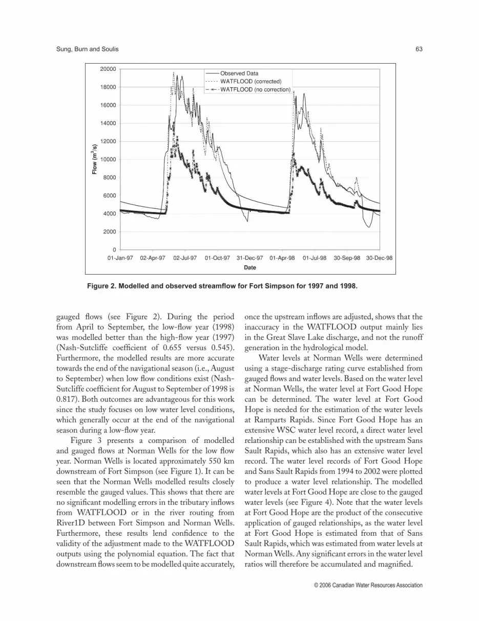
Under the base climate condition, WATFLOOD-generated streamflows at Fort Simpson are lower than the observed streamflows for both the high-flow (1997) and low-flow (1998) years. The flow patterns between the modelled and observed streamflows, other than their magnitude, are quite similar (see Figure 2). The modelled flows contain an offset from the observed streamflows. Since previous results indicated that WATFLOOD-

generated tributary inflows are generally quite accurate (including the largest tributary, the Liard River), the source of error was suspected to be at Great Slave Lake, located upstream of the Mackenzie River. GSL is very poorly modelled due to its size and complex outlet. As a result, stage-discharge rating curves of good quality are unavailable, severely hindering the ability to model the Mackenzie River flow.

The modelled flow from the lake was adjusted (corrected) using a relationship between the modelled and gauged flow during the navigational season (i.e., when no ice conditions are expected). The relationship between the modelled and gauged flow during the navigation season was examined at Fort Simpson, the most upstream location on the Mackenzie River with reliable gauge data. The Liard River joins the Mackenzie River at this location, which is also the most upstream node modelled in WATFLOOD as the Liard River is the first significant tributary on the Mackenzie River. Since previous results show that the Liard River modelled inflow is quite accurate, and since there are no significant tributaries between the GSL outlet and Fort Simpson, it is reasonable to assume that any discrepancies between modelled and gauged flows at Fort Simpson come mainly from GSL outflow.

The WATFLOOD modelled flows and WSC gauged flows at Fort Simpson during the navigational season were plotted to determine the nature of the relationship. A second order polynomial was found to provide an adequate fit to the data and the resulting relationship was used to adjust the modelled flow values. Figure 2 shows the streamflow at Fort Simpson for the uncorrected WATFLOOD results, the corrected WATFLOOD results and the observed values. The improvement in the corrected flows is apparent from the figure and is further demonstrated in the improvement in the Nash-Sutcliffe coefficient (Nash and Sutcliffe, 1970), which is 0.666 for the corrected WATFLOOD results and 0.220 for the uncorrected WATFLOOD results. Note that the modelling was not focussed on the ice covered period and hence the results are not as good during this period as they are during the navigation season.

Results

After the adjustments, the Mackenzie River modelled flows at Fort Simpson adequately match the historical



gauged flows (see Figure 2). During the period from April to September, the low-flow year (1998) was modelled better than the high-flow year (1997) (Nash-Sutcliffe coefficient of 0.655 versus 0.545). Furthermore, the modelled results are more accurate towards the end of the navigational season (i.e., August to September) when low flow conditions exist (Nash-Sutcliffe coefficient for August to September of 1998 is 0.817). Both outcomes are advantageous for this work since the study focuses on low water level conditions, which generally occur at the end of the navigational season during a low-flow year.

Figure 3 presents a comparison of modelled and gauged flows at Norman Wells for the low flow year. Norman Wells is located approximately 550 km downstream of Fort Simpson (see Figure 1). It can be seen that the Norman Wells modelled results closely resemble the gauged values. This shows that there are no significant modelling errors in the tributary inflows from WATFLOOD or in the river routing from River1D between Fort Simpson and Norman Wells. Furthermore, these results lend confidence to the validity of the adjustment made to the WATFLOOD outputs using the polynomial equation. The fact that downstream flows seem to be modelled quite accurately,

once the upstream inflows are adjusted, shows that the inaccuracy in the WATFLOOD output mainly lies in the Great Slave Lake discharge, and not the runoff generation in the hydrological model.

Water levels at Norman Wells were determined using a stage-discharge rating curve established from gauged flows and water levels. Based on the water level at Norman Wells, the water level at Fort Good Hope can be determined. The water level at Fort Good Hope is needed for the estimation of the water levels at Ramparts Rapids. Since Fort Good Hope has an extensive WSC water level record, a direct water level relationship can be established with the upstream Sans Sault Rapids, which also has an extensive water level record. The water level records of Fort Good Hope and Sans Sault Rapids from 1994 to 2002 were plotted to produce a water level relationship. The modelled water levels at Fort Good Hope are close to the gauged water levels (see Figure 4). Note that the water levels at Fort Good Hope are the product of the consecutive application of gauged relationships, as the water level at Fort Good Hope is estimated from that of Sans Sault Rapids, which was estimated from water levels at Norman Wells. Any significant errors in the water level ratios will therefore be accumulated and magnified.

Figure 2. Modelled and observed streamflow for Fort Simpson for 1997 and 1998.



Figure 3. Modelled and gauged streamflow at Norman Wells for the low flow year.

Figure 4. Modelled and gauged water levels at Fort Good Hope for the low flow year.



Streamflow projections were obtained using the IPCC SRES scenarios generated by the three GCMs discussed earlier. The projections were generated from the base climate data from 1997 and 1998. Gridded change fields from each model were applied to the gridded GEM precipitation and temperature data to obtain the projected climate change scenarios. From this point on, the projections using the 1997 base year will be referred to as the high-flow condition while the projections using the 1998 base year will be referred to as the low-flow condition. Due to the focus on navigation, and thus the concern for low streamflow conditions, greater attention will be paid to the low-flow condition.

A consistent pattern for the three GCMs is that around the beginning of September the modelled flow rises above that of the base condition, as shown in Figure 5. For the rest of the navigational season, however, the projected flows fluctuate depending on the climate scenario and GCM. It was found that the projected flows can differ significantly under the same climate forcing condition and the same base year, based on the different GCMs used. CGCM2 has the lowest flow projection of the three GCMs and its A21 and B21 scenario flows are generally below that of the

base condition until after September. For CSIRO-Mk2b, there is a short duration in the beginning of the navigation season when the flows are less than that of CGCM2 and the base condition. After the middle of July, however, CSIRO-Mk2b’s flows exceed that of CGCM2 and the base condition projections. Finally, the HadCM3 model yielded the highest total flow projections that are consistently above that of CGCM2 and the base condition during the navigational season. During the beginning of the navigational season ( June to mid-July), the HadCM3 flows are substantially higher than those of CSIRO-Mk2b. After this period, however, the flows of HadCM3 are higher than those of CSIRO-Mk2b only during the low-flow condition projection. Most of the modelled flows have an earlier spring freshet than that of the base condition (Figure 5). Therefore, it appears that under the IPCC scenarios studied herein there is a shift to earlier spring freshets, which usually means lower flows in the beginning of the navigational season. A trend of earlier spring freshet dates has also been identified in the observational record for some of the major tributaries of the Mackenzie River (Burn et al., 2004).

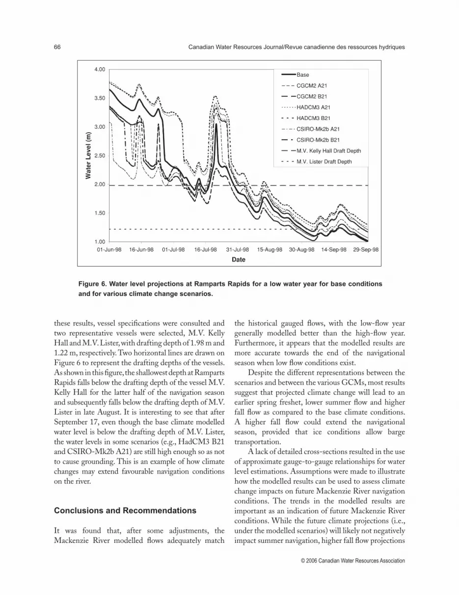
The low-flow condition water level projections are shown in Figure 6. To incorporate drafting depth into

Figure 5. Streamflow projections for Fort Simpson for a low water year for base conditions and

for various climate change scenarios.



these results, vessel specifications were consulted and two representative vessels were selected, M.V. Kelly Hall and M.V. Lister, with drafting depth of 1.98 m and 1.22 m, respectively. Two horizontal lines are drawn on Figure 6 to represent the drafting depths of the vessels. As shown in this figure, the shallowest depth at Ramparts Rapids falls below the drafting depth of the vessel M.V. Kelly Hall for the latter half of the navigation season and subsequently falls below the drafting depth of M.V. Lister in late August. It is interesting to see that after September 17, even though the base climate modelled water level is below the drafting depth of M.V. Lister, the water levels in some scenarios (e.g., HadCM3 B21 and CSIRO-Mk2b A21) are still high enough so as not to cause grounding. This is an example of how climate changes may extend favourable navigation conditions on the river.

Conclusions and Recommendations

It was found that, after some adjustments, the Mackenzie River modelled flows adequately match

Figure 6. Water level projections at Ramparts Rapids for a low water year for base conditions

and for various climate change scenarios.

the historical gauged flows, with the low-flow year generally modelled better than the high-flow year. Furthermore, it appears that the modelled results are more accurate towards the end of the navigational season when low flow conditions exist.

Despite the different representations between the scenarios and between the various GCMs, most results suggest that projected climate change will lead to an earlier spring freshet, lower summer flow and higher fall flow as compared to the base climate conditions. A higher fall flow could extend the navigational season, provided that ice conditions allow barge transportation.

A lack of detailed cross-sections resulted in the use of approximate gauge-to-gauge relationships for water level estimations. Assumptions were made to illustrate how the modelled results can be used to assess climate change impacts on future Mackenzie River navigation conditions. The trends in the modelled results are important as an indication of future Mackenzie River conditions. While the future climate projections (i.e., under the modelled scenarios) will likely not negatively impact summer navigation, higher fall flow projections



could mean a possible extension of the navigational season in the future. This is particularly important for navigation at locations where low water depth is a common concern.

Throughout the modelling process, methodologies were developed in response to a lack of physical data on the Mackenzie River. It is recommended that a good stage-discharge relationship be developed for the outlet of Great Slave Lake to improve the hydrological modelling. Detailed cross-sections should be surveyed at selected study locations so modelled flows can be accurately transformed into water levels. Future modelling should incorporate finer spatial and temporal resolution for the climate scenarios. Modelling with more SRES scenarios (e.g., A1, A1F and B1) and ensemble results are also recommended. Furthermore, a wider range of GCMs should be incorporated into future studies and climate projections should be expanded to other time periods (e.g., 2020 and 2050).

Acknowledgements

The research described in this paper was supported by grants from the Mackenzie GEWEX Study (MAGS) and the Natural Sciences and Engineering Research Council of Canada (NSERC). These contributions are gratefully acknowledged. Dr. Faye Hicks graciously provided access to, and training with, the River1D model. Mr. Frank Seglenieks provided advice and assistance with the WATFLOOD modelling. The paper has benefited from constructive comments from two anonymous reviewers. The second author wishes to thank Dr. Al Pietroniro for assuming editorial duties for this paper.

References

Arora, V.K. and G.J. Boer. 2001. “Effects of Simulated Climate Change on the Hydrology of Major River Basins.” Journal of Geophysical Research-Atmospheres, 106(D4): 3335-3348.

Burn, D.H., O.I. Abdul Aziz and A. Pietroniro. 2004. “A Comparison of Trends in Hydrological Variables for Two Watersheds in the Mackenzie River Basin.” Canadian Water Resources Journal, 29(4): 283-298.

Flato, G.M. and G.J. Boer. 2001. “Warming Asymmetry in Climate Change Simulations.” Geophysical Research Letters, 28: 195-198.

Gent, P.R. and J.C. McWilliams. 1990. “Isopycnal Mixing in Ocean Circulation Models.” Journal of Physical Oceanography, 20: 150-155.

Gordon, C., C. Cooper, C.A. Senior, H. Banks, J.M. Gregory, T.C. Johns, J.F.B. Mitchell and R.A. Wood. 2000. “The Simulation of SST, Sea Ice Extents and Ocean Heat Transport in a Version of the Hadley Centre Coupled Model without Flux Adjustments.” Climate Dynamics, 16: 147-168.

Hicks, F.E. and P.M. Steffler. 1992. “A Characteristic-Dissipative-Galerkin Scheme for Open Channel Flow.” Journal of Hydraulic Engineering, 118(2): 337-352.

Hicks, F.E. 1996. “Hydraulic Flood Routing with Minimal Channel Data: Peace River, Canada.” Canadian Journal of Civil Engineering, 23(2): 524-535.

IPCC. 2001. Climate Change 2001: Contribution of Working Group I to the Third Assessment Report of the Intergovernmental Panel on Climate Change. Cambridge University Press. Cambridge, UK.

Kouwen, N., E.D. Soulis, A. Pietroniro, J. Donald and R.A. Harrington. 1993. “Grouped Response Units for Distributed Hydrologic Modelling.” Journal of Water Resources Planning and Management, 119(3): 289-305.

Kouwen, N. 2000. WATFLOOD/SPL9: Hydrological Model and Flood Forecasting System. Department of Civil Engineering, University of Waterloo, Waterloo, ON.

Leavesley, G.H., M.D. Branson and L.E. Hay. 1992. “Using Coupled Atmospheric and Hydrologic Models to Investigate the Effects of Climate Change in Mountainous Regions.” In Managing Water Resources During Global Change, Proceedings, AWRA 28th Annual Conference and Symposium: 691-700, American Water Resources Association. Bethesda, MD.



Miller, J.R. and G.L. Russell. 1992. “The Impact of Global Warming on River Runoff.” Journal of Geophysical Research-Atmospheres, 97(D3): 2757-2764.

Nakicenovic, N., J. Alcamo, G. Davis, B. de Vries, J. Fenhann, S. Gaffin, K. Gregory, A. Grübler, T.Y. Jung, T. Kram, E.L. La Rovere, L. Michaelis, S. Mori, T. Morita, W. Pepper, H. Pitcher, L. Price, K. Raihi, A. Roehrl, H.H. Rogner, A. Sankovski, M. Schlesinger, P. Shukla, S. Smith, R. Swart, S. van Rooijen, N. Victor and Z. Dadi. 2000. Emissions Scenarios. A Special Report of Working Group III of the Intergovernmental Panel on Climate Change. Cambridge University Press. Cambridge, UK.

Nash, J.E. and J. Sutcliffe. 1970. “River Flow Forecasting Through Conceptual Models.” Journal of Hydrology, 10: 282-290.

Pope, V.D., M.L. Gallani, P.R. Rowntree and R.A. Stratton. 2000. “The Impact of New Physical Parameterizations in the Hadley Centre Climate Model - HadCM3.” Climate Dynamics, 16: 123-146.

Sanderson, M. 1987. Implications of Climatic Change for Navigation and Power Generation in the Great Lakes: Summary of Great Lakes Institute Reports. Climate Change Digest, Canadian Climate Centre. Downsview, ON.

Watterson, I.G., S.P. O’Farrell and M.R. Dix. 1997. “Energy Transport in Climates Simulated by a GCM which Includes Dynamic Sea-Ice.” Journal of Geophysical Research-Atmospheres, 102(D10): 11027–11037.

Documents

A Case Study of Climate Change Impacts on Navigation on the Mackenzie River