A Coarse-Grained Model for Force-Induced Protein Deformation and Kinetics

A Coarse-Grained Model for Force-Induced Protein Deformationand Kinetics

Helene Karcher,* Seung E. Lee,* Mohammad R. Kaazempur-Mofrad,y and Roger D. Kamm**Department of Mechanical Engineering and Division of Biological Engineering, Massachusetts Institute of Technology, Cambridge,Massachusetts 02139; and yDepartment of Bioengineering, University of California, Berkeley, California 94720

ABSTRACT Force-induced changes in protein conformation are thought to be responsible for certain cellular responses tomechanical force. Changes in conformation subsequently initiate a biochemical response by alterations in, for example, bindingaffinity to another protein or enzymatic activity. Here, a model of protein extension under external forcing is created inspired byKramers’ theory for reaction rate kinetics in liquids. The protein is assumed to have two distinct conformational states: a relaxedstate, C1, preferred in the absence of external force, and an extended state, C2, favored under force application. In the contextof mechanotransduction, the extended state is a conformation from which the protein can initiate signaling. Appearance andpersistence of C2 are assumed to lead to transduction of the mechanical signal into a chemical one. The protein energylandscape is represented by two harmonic wells of stiffness k1 and k2, whose minima correspond to conformations C1 and C2.First passage time tf from C1 to C2 is determined from the Fokker-Plank equation employing several different approaches foundin the literature. These various approaches exhibit significant differences in behavior as force increases. Although the level ofapplied force and the energy difference between states largely determine equilibrium, the dominant influence on tf is the heightof the transition state. Distortions in the energy landscape due to force can also have a significant influence, however, exhibitinga weaker force dependence than exponential as previously reported, approaching a nearly constant value at a level of force thatdepends on the ratio k1/k2. Two model systems are used to demonstrate the utility of this approach: a short a-helix undergoinga transition between two well-defined states and a simple molecular motor.

INTRODUCTION

Cells sense mechanical stimuli and respond by varying their

biological behavior accordingly. Although the mechanisms

for sensation and transduction of mechanical forces into

biological signals are still largely unknown, the hypothesis

of mechanotransduction through force-induced changes in

molecular conformation has been gaining broad support

(1–3). Alternatively, either membrane-associated or intra-

cellular proteins might change conformation under force,

undergoing a transition to a state with enhanced binding affinity

or altered enzymatic activity, thereby initiating a signaling

cascade. In particular, force transmission from the extracel-

lular matrix to the cell interior occurs through a chain of pro-

teins, e.g., the fibronectin/integrin bond, integrin-associated

proteins on the intracellular side (paxillin, talin, vinculin,

etc.), and proteins linking the focal adhesion complex to the

cytoskeleton (4), any of which would be a candidate for con-

formational change and force transduction into a biochem-

ical signal.

Here we present a generic coarse-grained model linking

force to protein conformational change, analyzed in terms of

the mechanical properties of the protein states. Assuming

that binding is a force-independent event and occurs pref-

erentially in one conformation (relaxed or extended), our

model links force applied to a protein to its propensity to

initiate a signal. We consider a simplifying case of a protein

having just two conformational states: C1, dominating with-

out force application, and C2, an extended state favored by

force. Our analysis is based on the simplest possible energy

landscape corresponding to this situation: two harmonic wells

whose minima represent the two states (see Fig. 1), con-

nected via a one-dimensional trajectory. Even though most

proteins are likely to sample several intermediary conforma-

tions (local minima between the wells) while traversing a

complex reaction trajectory (5), our model accounts only for

the highest energy peak, or the last one encountered before

the reactive state is attained. Both the equilibrium distribution

of states as well as the kinetics of reaction are considered.

Few studies of force-induced alterations between two pro-

tein conformations leading to signaling have been reported,

and these largely focus on mechanosensitive ion channels.

For example, force is thought to induce the change in con-

ductance seen in hair cells (e.g., Gillespie and Walker (6) and

Howard and Hudspeth (7)) and in the MscL stretch-activated

ion channel (e.g., Wiggins and Phillips (8)). The need for

kinetic or transition rate analysis stems from two observa-

tions: i), mechanical stimulation of cells or proteins in vivo,

in experiments and in simulations spans a wide range of time

scales from picoseconds (molecular dynamics simulations)

to hours (cell remodeling); hence regimes likely exist for

which kinetics dominates over thermodynamic equilibrium,

and ii), some proteins are likely to function out of

equilibrium (e.g., molecular motors cannot function at equi-

librium (cf. Fisher and Kolomeisky (9)).

Submitted October 20, 2004, and accepted for publication December 28,2005.

Address reprint requests to Prof. Roger D. Kamm, 500 Technology Square,

Rm. NE47-315, Massachusetts Institute of Technology, Cambridge, MA

02139. Tel.: 617-253-5330; Fax: 617-258-5239; E-mail: [email protected].

� 2006 by the Biophysical Society

0006-3495/06/04/2686/12 $2.00 doi: 10.1529/biophysj.104.054841

2686 Biophysical Journal Volume 90 April 2006 2686–2697

Here we adopt a widely used microscopic approach based on

the Smoluchowski equation to deduce mean first-passage

times. Four different approaches (described and labeled i–iv in

Methods) are used to derive kinetic information on diffusion-

controlled reactions (10) and their predictions compared. This

general approach has been successfully applied to nonforced

reactions (e.g., Kramers (11) and Schulten and co-workers

(12,13)) in the case of a two-state, double-well landscape), as

well as forced reactions of bond rupture by escape from a single

energy well (14–16). Another method to account for force

dependence of kinetic constants is to apply Bell’s phenome-

nological exponential dependence on force for the rate of bond

dissociation (17). This approach has been extended to time-

dependent applied forces to find statistics on the rupture forces

in atomic force microscopy (AFM) experiments (15).

Several methods have been proposed to extract kinetic

information from single-molecule pulling experiments leading

to unbinding from a substrate or unfolding. AFM results have

been analyzed in the context of mean first passage-times (16)

on one-dimensional energy landscapes to investigate rupture of

the avidin-biotin bond. Whereas unbinding was then modeled

as escape from a single energy well, here we introduce a two-

well landscape to model the transition between two stable,

native conformational states of a single molecule. Izrailev et al.

(16) distinguish several regimes depending on the level of force

applied to the biotin molecule, and found that the conditions

relevant to AFM experiments correspond to what they termed

the ‘‘activated regime’’. This regime corresponds to the limit of

large energy barriers (large Ptr; as defined in Methods) in the

kinetic studies of conformational changes presented here.

Hummer and Szabo (15) present another method to extract rate

kinetics from pulling experiments, also based on escape from a

single energy well.

Most kinetic models for protein deformation or unbinding

consider only the energy barrier between states, whereas we

propose a model that takes into account the shape of the

landscape along the entire reaction path. Molecular dynamics

offers ways to link conformational changes of specific pro-

teins under forces applied at specified protein locations. How-

ever, such simulations require knowledge of the full atomic

structure specific to the particular protein, and typically are

confined, due tocomputational constraints, to forces large com-

pared to those experienced in vivo. Our approach is comple-

mentary in that it only considers a single degree of freedom or

trajectory and a single transition between states. All intra-

protein force interactions are therefore represented by the two

parabolic wells to produce a simplified model for the purpose

of the examining both equilibrium states and kinetics.

METHODS

General approach

Protein deformation typically occurs in a viscous-dominated regime (18),

where motion along the reaction coordinate exhibits randomness and ap-

pears Brownian. To account for both these fluctuations and the landscape

shape (not merely the transition peak energy), we use an approach based on

statistical mechanics theory similar to Kramers (11) in the presence of an

external force. Movement of the protein extremity is described using the

Smoluchowski equation (see, e.g., Hanggi et al. (19), a force balance on a

microcanonical ensemble of particles). Similar methods have been success-

fully applied to a single parabolic well to describe bond rupture rates under

force (14–16). Several methods are used and compared to determine mean

first-passage times along the energy landscape, which, in some instances,

can then be used to deduce kinetic rate constants for forced conformational

changes as a function of the protein mechanical characteristics.

The energy landscape for protein extension

Consider a protein having two conformational states: C1, preferentially pop-

ulated when no force is applied, and C2, an extended state, and acted upon by

a contact force (see Fig. 1). A simple energy landscape E(x) describing this

situation consists of two parabolic wells:

EðxÞ ¼ 1

2k1x

2 � Fx for x, xtr

EðxÞ ¼ 1

2k2ðx � x2Þ2

1E2 � Fx for x$ xtr

; (1)

with k1 and k2 stiffness values of the first and second well, respectively, xtr

the position of the transition state, x2 the position of the extended state C2

when no force is applied, E2 the zero-force free-energy difference between

C1 and C2, and F the force applied to the protein.

A single reaction coordinate, x, is chosen, corresponding to the direction

of protein deformation and force application. Energy minima (describing C1

and C2 states, respectively) are located initially at x ¼ 0 and x ¼ x2: The two

parabolas intersect at a transition state x ¼ xtr: With increasing force, the

transition state remains at the same reaction coordinate xtr; but the minima

shift to x ¼ xmin1 ¼ F=k1 and x ¼ xmin2 ¼ x21F=k2:

Parameter constraints

Although the parameters are free to vary, the simple landscape geometry

adopted imposes several constraints on the range of values:

1. To ensure that C1 is the preferred state at zero force, it is required that

E2 be .0.

2. The minimum of the first well (when distorted by force) should not pass

the transition point; i.e., F=k1 , xtr; leading to the constraint PF , 2Ptr;

with PF ¼ Fxtr=kT; Ptr ¼ 1=2k; x2tr=kT ; and k the Boltzmann constant.

3. Similarly, the transition point should not pass the minimum of the

second well; i.e., xtr , x21F=k2; leading to the constraint PE,Ptr;

with PE ¼ E2=kT :

Influence of force on equilibriumA potentially measurable quantity is the equilibrium constant for protein

extension, i.e., the ratio of conformational probabilities K ¼ p2=p1; where

p1 and p2 are the probabilities corresponding to the relaxed (C1) or extended

(C2) states, respectively. The equilibrium constant K depends only on the

difference in energy DEðFÞ ¼ Eðx ¼ xmin2Þ � Eðx ¼ xmin1Þ between ex-

tended and relaxed states and not on the details of the landscape, as described

by Boltzmann’s law (20): K ¼ exp½�DEðFÞ=ðkTÞ�:Force consequently leads to a reduction in the thermodynamic cost in

passing from state C1 to C2, and the ratio of conformational probabilities is

therefore (21)

K ¼ expFx2

kT1

F2

2kT

1

k2

� 1

k1

� �� E2

kT

� �: (2)

Force-Induced Protein Deformation and Kinetics 2687

Biophysical Journal 90(8) 2686–2697

First-passage time calculation

Mean first-passage time tf associated with the transition from C1 to C2 is

calculated as the main kinetic information on protein extension. The quantity

tf has been extensively used as a measure of reaction times (11,12,14,21),

and in this study represents the average time necessary for the protein

extremity to diffuse from its equilibrium state C1 (minimum of the first well)

to the elongated state C2 (minimum of the second well) (Fig. 1). Similarly,

the reverse mean first-passage time tr for the protein to change conformation

from C2 to C1 is calculated as a kinetic constant characteristic of the protein

conformational in the reverse direction (Fig. 1).

The mean first-passage time tf can be evaluated in different ways

depending on assumptions chosen to solve the Fokker-Plank equation

governing the protein conformational change (see Appendix). Previous

methods (11,12,14,21) begin by integrating the Fokker-Plank equation

between a reaction coordinate x and the reaction coordinate of the final state

(i.e., xmin2 ¼ x21F=k2 in our case), and make the assumption that the

probability of the final state remains close to zero. This latter assumption,

i.e., C2 is not yet populated, is relevant for our model of mechanotransduc-

tion where signaling would be initiated as soon as the extended state

becomes populated.

Kramers (11) and Evans and Ritchie (11,14) assume a stationary

current across the energy barrier and that the barrier itself is much larger

than the thermal energy; consequently, they only need to consider the

landscape shape near the initial state and in the vicinity of the barrier. They

then deduce the forward kinetic rate as being ;1=tf : As an alternative to

this last step, Schulten and co-workers (12,13) and Howard (21) integrate

the Fokker-Plank equation a second time using one of the following two

assumptions: i), at all times, the molecular conformation resides between

the starting and the final reaction coordinate (21), i.e.,R xmin2

xmin1pðxÞdx ¼ 1;

with pðxÞ the probability of finding the protein in conformation x; or ii), the

flux of probability approaches zero as x/6N (Eq. 2.1 in Schulten et al.

(12)). Howard’s assumption is less realistic for our case where the protein

also samples conformations x, xmin1: In our case, we follow Schulten and

co-workers’ approach (zero flux at infinity), as it seems most realistic and

appropriate for conformational change and compare predictions obtained

from all methods.

We calculated the normalized passage time Tf ¼ ðtfD=x2trÞ for each

method (Kramers (11) and Evans and Ritchie (14), Schulten and co-workers

(12,13), or Howard (21) applied to our two-well landscape (Eq. 16, see

Appendix). For example Schulten and co-workers’ method gives

Tf ¼tfD

x2

tr

¼Z amin2

amin1

expðEðuÞÞZ u

�N

expð�EðvÞÞdv� �

du; (3)

where the normalized reaction coordinate is u ¼ x=xtr; the integral bound-

aries are amin1 ¼ xmin1=xtr; amin2 ¼ xmin2=xtr; and the normalized energy

landscape

E ¼ E

kT¼ Ptru

2 �PFu for u , 1

¼ Ptr=Pkðu� x2=xtrÞ21PE �PFu for u$ 1

:

(4)

Therefore, Tf depends upon only four parameters:

PF ¼Fxtr

kT; Ptr ¼

1

2k1x

2

tr

kT; Pk ¼

k1

k2

; and PE ¼E2

kT: (5)

The expression for TfðPF;Ptr;Pk;PEÞ is not algebraically tractable, and

was evaluated numerically using Maple 9 (Maplesoft, Waterloo, Ontario,

Canada) for a range of values PF;Ptr;Pk;PE:

Similarly, the normalized reverse passage time Tr ¼ trD=x2tr is

Tr ¼trD

x2

tr

¼Z amin2

amin1

expð�EðuÞÞZ 1N

u

expðEðvÞÞdv� �

du: (6)

Finally, calculating a passage time starting from the single coordinate xmin1

fails to account for the distribution of initial states within the first energy

well. To do so, we modified the expression of the extension time:

tf ¼Z xtr

2xmin1�xtr

pBoltzmannðzÞtfðzÞdz; (7)

with pBoltzmannðzÞ ¼ ð1=ZÞexp �EðzÞ� �

; Z ¼R xtr

2xmin1�xtrexp �EðzÞ

� �dz; and

tf ðzÞ ¼ the first passage time from z to xmin2; obtained replacing amin1 by

z=xtr in Eq. 3. Equation 7 was evaluated numerically using discrete Riemann

integrals with both 15 and 20 terms.

To summarize, we calculated the extension time for a double-well energy

landscape using four different methods (see Table 1):

i. Double integration of the Fokker-Plank equation with the conditionR xmin2

xmin1pðxÞdx ¼ 1 (drawn from Howard (21)).

ii. Double integration of the Fokker-Plank equation with the flux of

probability going to zero at x/6N (based on Howard (12) and

Schulten and co-workers (13)).

iii. Simple integration with assumptions on the landscape shape (based on

Kramer (11) and Evans and Ritchie (14).

iv. Average of passage times obtained with method ii, weighted to take into

account the Boltzmann distribution of initial conformations within the

first well (see Eq. 7). Whereas method iv is perhaps the most rigorous, it

is also the most computationally intensive. As discussed below, based

on a comparison of the four approaches, we chose to use method ii for

the bulk of the results presented here.

Smoothed landscape

The double-well energy landscape we consider has a cusp at the transition

state x ¼ xtr: This could artificially influence our results since the landscape

along the entire reaction path is used to calculate extension times and, as we

show below, the transition state is a primary determinant of tf. To study the

effect of this cusp on our results, the energy landscape was smoothed using

Thiele’s continued fraction interpolation (22) by fitting points on the

landscape to a rational fraction using Maple 9 (Maplesoft). The 18 or 22

points used for fitting were equally spaced in each well, but avoided the cusp

at 60.05 xtr: We then compared the smoothed landscape with the one

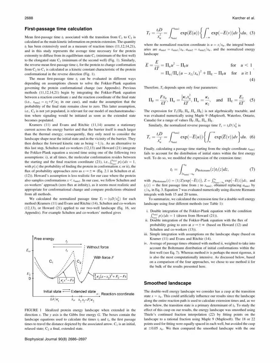
FIGURE 1 Idealized protein energy landscape when extended in the

direction x. The y axis is the Gibbs free energy G. The boxes contain the

landscape equations used to calculate the times tf and tr, the first passage

times to travel the distance depicted by the associated arrow. C1 is an initial,

relaxed state; C2 a final, extended state.

2688 Karcher et al.


containing the cusp by slightly modifying Ptr so that both landscapes had

precisely the same energy barrier (Fig. 2).

Extension times tf calculated using the smoothed potential differed from

those of the cusp potential in proportion to the quality of the fit (see inset in

Fig. 2). In addition, the agreement was better when the barrier height was

large (small dimensionless force PF), i.e., when the cusp is the dominant

feature of the landscape. We also verified that the agreement between the

extension times for the smooth and cusp potentials improved with the quality

of the fit. Therefore, we concluded that the cusp in our landscape per se did

not have a significant impact on the extension time results, and only present

results using the simple cusp potential.

Characteristic time for protein extension

Consider a constant force F applied to the protein at time t ¼ 0 (with a

loading rate �kf, kr). The first-order kinetic equation describing the con-

version from initial state to extended state is

dp1

dt¼ �kfp1 1 krp2; (8)

with p1 and p2 the probability of conformations C1 and C2, respectively, and

kf and kr the forward and reverse rate constants for the protein to change

conformation from C1 to C2. In some instances (see Discussion), kf and kr

can be approximated as the inverse of the mean first-passage time associated

with the transition, i.e.,

kf � 1=tf and kr � 1=tr: (9)

Behind such an evaluation for kf and kr is a partitioning of all microstates into

two classes, e.g., by designating all the states by either shorter than or more

extended than the transition state. Consequently, kf � 1=tf and kr � 1=tr(Eq. 9) is only valid when tf and tr are similar to the passage times just to the

barrier x ¼ xtr:

Solving Eq. 8 using the initial condition p1ðt ¼ 01Þ ¼ 1; the time course

of the probability of both conformations is

p1 ¼1

11K½1 � exp½�ðkf 1 krÞt��

p2 ¼1

11K½K1 exp½�ðkf 1 krÞt��: (10)

Therefore, the characteristic time to obtain the new equilibrium is

1= kf1krð Þ; directly calculable from the passage times tf and tr when the

approximations of Eq. 9 are valid.

Steered molecular dynamics simulations on asimplified protein model

For the purpose of comparison to our coarse-grained simulations, we

constructed a simple a-helix (a 15 mer of polyalanine) and analyzed it using

steered molecular dynamics (SMD) (23). One advantage of an a-helix is that

the helical axis uniquely defines a unidirectional reaction coordinate, along

which the external force is applied. An extensive free-energy calculation

using constant velocity SMD and Jarzynski’s equality has recently been

reported by Park et al. (24) on a very similar deca-alanine a-helix. Here

however, rather than attempting to evaluate the potential of mean force, we

applied a constant force and used distance constraints on the 15 mer of

polyalanine to compare our SMD results with those from the coarse-grained

model. The number of alanine residues in the polypeptide and the distance

constraints selection has been selected so as to yield a stable and simple

model that exhibits two distinct conformations. Many parameters extracted

from the constant force SMD of this specifically designed model can be

better related to our coarse-grained model, as seen in the Results section.

The polyalanine a-helix was constructed by creating a linear polyalanine

sequence and specifying all the f-dihedral angles to �57� and all the

c-dihedral angles to �47�, which is characteristic dihedral angles for an

a-helix. The N- and C-termini were capped with an amino group and a

carboxylate group, respectively, with ionic states representative of the

physiological pH level. The CHARMM (26) script for creating an a-helix is

available online (25). The commercially available molecular dynamics

software CHARMM (26) was used to carry out the SMD simulations with

the ACE2 implicit water module (27) and SHAKE constraints (28) for

efficiency. Energy of the a-helix structure was minimized in 15,000 steps,

TABLE 1 Equations used to obtain the dimensionless

extension time to go from conformation C1 to conformation C2

Method

Equation used to evaluate the

dimensionless extension time ðtfD=x2trÞ References

i

Z amin2

amin1

exp �EðuÞð ÞZ amin2

u

exp EðvÞð Þdv� �

du (21)

ii

Z amin2

amin1

exp EðuÞð ÞZ u

�N

exp �EðvÞð Þdv� �

du (12,13)

iii

Z amin2

amin1

exp EðuÞð Þdu ffiffiffiffiffiffi

Ptr

p

rexp � P

2

F

2Ptr

� �(11,14)

iv

Z 1

2amin1�1

pBoltzmannðwÞTfðwÞdw with

pBoltzmannðwÞ ¼ exp �EðwÞð ÞZ 1

2amin1�1

exp �EðuÞð Þdu and

Tf ðwÞ ¼Z amin2

w

exp EðuÞð ÞZ u

�N

exp �EðvÞð Þdv� �

du

(12,13)

Results from these different methods are compared in Results and in Fig. 6.

FIGURE 2 Example of energy landscape smoothing when

Pk ¼ 1; PE ¼ 4; and PF ¼ 0: Smooth landscape (solid line) is obtained

by the Thiele interpolation of 22 points (s) on a landscape with an energy

barrier Ptr ¼ 10: It is then compared with the cusp landscape having the

same energy barrier (dashed line). (Inset) Extension times obtained with the

two landscape types (smooth or with cusp) as a function of force. Parameters

are the same except for PF; which is allowed to vary.



heated to 300 K in 40 ps, and the system was equilibrated for 120 ps using a

time step of 2 fs. After equilibration, the helix was repositioned placing the

N-terminus at the origin and the C-terminus along the x axis. Holding the

helix fixed by a harmonic constraint at the N-terminus, the C-terminus was

pulled with constant force along the x axis. After a sequence of simulations

in which several polypeptides arrangements were tried, we chose an

a-helical system with 11 potential H-bonds, with six forced to remain intact

under force and the other five allowed to form or break due to the combined

effects of electrostatic attraction and van der Waals repulsion. The criterion

for this choice was that the system exhibits two distinct states, with no

apparent intermediate states. We imposed nuclear Overhauser effect con-

straints to the six H-bonding pairs, out of 11 possible, starting from the

N-terminus carbonyl group, by specifying a limit distance of 4.25 A between

ith carbonyl carbon and (i 1 4)th amide nitrogen with a force constant of

10.0 kcal/mol A2. This model leaves five H-bonding pairs near the

C-terminus to simultaneously either all break or all form to yield two distinct

conformations (C1 and C2). The polyalanine a-helix was constructed by

creating a linear polyalanine sequence and specifying all the f-dihedral

angles to �57� and all the c-dihedral angles to �47�, which is the char-

acteristic dihedral angle for an a-helix. The N- and C-termini were capped

with an amino group and a carboxylate group, respectively, with ionic states

representative of the physiological pH level. The CHARMM (29) script for

creating an a-helix is available online (25). Simulations were performed for

100 ns per simulation at forces of 30 pN, 65 pN, 70 pN, 75 pN, 80 pN, 85

pN, and 100 pN.

Thermal fluctuations caused the forced end to exhibit relatively large

displacements perpendicular to the direction of force application (see Fig. 3;

left end is fixed and right end fluctuates). To compare with our single-

dimensional coarse-grained model, we therefore present results in terms of

the time-averaged component of force acting along the axis of the a-helix.

Parameters were extracted from SMD simulations for comparison with

our coarse-grained model. End-to-end distances, defined as the distance

between the two termini (Fig. 3), were recorded every 4 ps and used to

generate histograms (Fig. 4 B) to identify the most frequently sampled

configurations.

Forward mean first-passage time from the coiled to extended conforma-

tion (tf ) was determined, assuming ergodicity, as the average time the mole-

cule resides in state C1 before undergoing a transition to C2, whereas reverse

mean passage time (tr) was determined as the time residing in the extended

conformation (C2) before returning to the coiled conformation (C1) (Fig. 4

A). We introduced these SMD-determined parameters into our coarse-

grained model, and compared the forward and reverse mean passage times

obtained by both methods (SMD and coarse-grained model).

RESULTS

Selected parameter ranges

To represent a protein with two distinct conformational

states, we chose Ptr � 1 (baseline value of 10, with varia-

tions between 5 and 25). To assure that, in the unforced con-

dition, C1 was the preferred state, we further specified that

expðE2=kTÞ ¼ expPE.1; hence PE.0:PE ¼ 4 was se-

lected as our baseline value, with variations considered be-

tween 0 and 10. No restrictions were imposed on the relative

values of well stiffness k ¼ k1=k2; so we chose a baseline

value of Pk ¼ 1 with variations in the range 0.2–5.

Forces ;100 pN have been shown to rupture molecular

bonds (30), and conformational changes are likely to involve

lower forces of at most a few tens of piconewtons (for com-

parison, myosin motors produce 3–4 pN force (cf. (30,31)).

Typical distances between protein conformational states

x2 ; 0.1–10 nm—yielding 0, xtr #x2 ; 0:1�10nm—

and kT ; 4 pN.nm at body temperature led us to vary PF

from 0 to 20 (corresponding, for example, to F¼40 pN and

xtr¼2 nm).

Equilibrium states

The probability of each conformational state at equilibrium is

described by Eq. 2, as obtained previously by Howard (21).

The second term in the argument of the exponential suggests

nonmonotonic behavior in the special case of k1,k2 and

large F2: cases in which K increases, then decreases as

applied force is increased (consistent with the hypothesis put

forward by Howard (21)). However, the parameter con-

straints (see Methods) preclude this from happening. One

could argue that constraint 2 (the transition point should not

cross over the reaction coordinate of the extended state, see

the ‘‘Parameter constraints’’ paragraph in Methods) is only

necessary for our kinetic study, and could be relaxed in this

thermodynamic approach. Even so, we found that this cor-

responds to cases where the force is so large that the first well

minimum is at a more extended coordinate than the second

well minimum, clearly an unrealistic situation.

Another important consequence of Eq. 2 is that for typical

values of the parameters, conversion of the protein from 10%

to 90% in the extended state C2, occurs over a very narrow

range of only a few PF (see Fig. 5). Large values of Pk; i.e.,

a relaxed state C1 stiffer than C2, make this transition even

sharper (see Fig. 5).

Comparison of extension time predictions

Of the four approximate methods described above, method

iv is the most accurate but also the most computationally

demanding. Extension times obtained with this method dif-

fered by no more than 5% (for PF , 20) from those obtained

with method ii, which does not include the last averaging of

method iv (see Eq. 7 and Fig. 6). Therefore we concluded

FIGURE 3 Two distinct conformations, C1 (top) and C2 (bottom), of the

simplified protein model used in SMD example. Left end of the helix is held

fixed, whereas the right end is pulled with a constant force in the direction

shown by the arrow. Six hydrogen-bonding pairs near the fixed end are

constrained not to break.

2690 Karcher et al.


that we could use method ii as an accurate estimate for the

extension time.

Somewhat surprisingly, method i matched closely with

that of method ii up to PF;10 (see Fig. 6), despite what

might at first appear to be a rather simplistic and restrictive

assumption in the former—that the probability of confor-

mations between the two energy minima equals 1 at all

times, i.e.R xmin2

xmin1pðxÞdx ¼ 1:

Finally, as expected, results from method iii, similar to

Evans and Ritchie (14) and Kramers (11), agree with results

from the other methods for low force, but the departure for

PF $ 2 was quite dramatic (see Fig. 6). This suggests that the

assumption that the energy barrier is much greater that the

thermal energy used by these authors and in method iii

breaks down, for ðPtr �PFÞ$ 8 or, for the parameters used

in Fig. 6, PF # 2: We drew the same conclusion from

FIGURE 4 (A) Time trace of the end-to-end distance

of the helix at F¼ 78.2 pN (corrected from F¼80 pN).

A forward passage time and a reverse passage time are

shown. Mean passage times are obtained by averaging

throughout the simulation. (B) Histograms showing

single and double peaks at various force magnitudes.

Linear shift on the peaks are evident with varying

forces.



comparison of results from methods i and ii with the

analytical solution provided by Kramers (11) in the specific

case of a potential with a cusp and a high-energy barrier, i.e.,

Ptr

ffiffiffiffiffiffiffiffiffiffiffiffiffiffiffiffiffiffiffiffiffiffiffiffiffiffiffiffiðPtr �PFÞ=p

p3 expð�Ptr1PFÞ in our notation. All

results presented from this point onward were obtained using

method ii.

Variations of forward and reverse firstpassage times

Force significantly enhances transition from the initial to

extended state for all cases in the chosen range of parameter

values (10#Ptr # 25; 0:2#Pk # 5; 0#PE # 10). In all

cases, a larger force applied to the protein induced a shorter

extension time tf (Figs. 7–9). For example, at the baseline

values Ptr ¼ 10; PE ¼ 4; and Pk ¼ 1; tf decreases from

;1.54 103 xtr2 /D at PF ¼ 0 to ;0.29 xtr

2 /D at PF ¼ 15;enabling the protein to change conformation ;5500 times

faster when forced. Note that the C1 to C2 transition time

under force is then at least 3.5 times shorter than the pure

diffusion time xtr2 /D, corresponding to C1 to C2 conversion

for a protein with zero stiffness (i.e., a flat energy landscape).

At low forces (PF , 5–10, depending on the other dimen-

sionless parameters), the decrease in tf is exponential (con-

sistent with the law proposed for bond dissociation by Bell

(17)), but the transition is less rapid at larger forces (Figs. 7–9).

At constant Ptr ¼ 10; PE ¼ 4; tf decreases with Pk

(Fig. 7) approaching a plateau of tf ; 0.5 xtr2/D for Pk $ 5

(data not shown). At these given values for Ptr and PE; the

transition cannot occur in a time ,500 xtr2/D without force

(data not shown). Lowering the transition energy Ptr has the

expected effect of hastening transition to the extended state

(Fig. 8). However, the exponential dependence of tf on force

breaks down at lower forces for small transition energies Ptr

(Fig. 8). Varying PE; the dimensionless zero-force energy

difference between C1 and C2 does not significantly influence

the variations of the extension time with force (Fig. 9). In

general terms, whereas equilibrium is largely determined by

PE and PF; extension times are relatively insensitive to PE;and depend primarily on Ptr and PF: The effects of Pk are

generally small, except for higher values of PF:Variations in the reverse mean first-passage time tr as com-

puted from Eq. 6 generally vary as K 3 tf , so that the model

is self-consistent (K � tf=tr) as well as being in agreement

with equilibrium thermodynamics.

As a limiting case, the first-passage time to diffuse up the

first well (from C1 to the transition state) was calculated with

our method i and compared with the analytical formula

FIGURE 5 Equilibrium ratio of probabilities K ¼ p2=p1 of finding the

protein in extended/initial state as a function of force applied PF: The

parameters are Pk ¼ 1 (dotted lines) or 5 (solid lines), PE ¼ 0 (¤), 2 (:),

or 4 (n), and Ptr ¼ 10: Negative forces PF , 0 oppose protein extension.

FIGURE 6 Dimensionless protein extension time tfD=x2tr versus dimen-

sionless force applied PF: The other dimensionless parameters are held

constant: Pk ¼ 1; Ptr ¼ 10; and PE ¼ 4: Kramers’ analytical formula for

the dimensionless time in the specific case of a potential with a cusp at the

energy barrier (inverse of the dimensionless kinetic rate of Kramers (11) is

expressed in our notation as Ptr

ffiffiffiffiffiffiffiffiffiffiffiffiffiffiffiffiffiffiffiffiffiffiffiffiffiffiffiffiPtr �PFð Þ=p

p3 exp �Ptr 1PFð Þ

� ��1.

Its validity is restricted to low PF: Method i is based on Howard (21),

method ii on Schulten et al. (12), method iii on Kramers (11) and Evans and

Ritchie (14), and method iv is a finer estimate of the extension time based on

method ii (see text for details). Method iii is also only valid for low PF;

therefore results for large forces (beyond the range of validity) are

represented by a thinner, dotted line.

FIGURE 7 Dimensionless extension time tfD=x2tr versus dimensionless

force applied PF: The other dimensionless parameters are held constant:

Ptr ¼ 10; PE ¼ 4; and Pk ¼ ½; 1, or 2. (Insets) Normalized energy

landscape used to calculate the extension time (same parameters).

2692 Karcher et al.


available for F ¼ 0 (11,21) and Ptr � 1: Reasonable agree-

ment (maximum difference of nearly 10%) was observed in

the chosen parameter range (see first paragraph of Results).

Characteristic time for conformational change

The characteristic (relaxation) time to reach equilibrium

probabilities of extended and initial conformational states

upon application of a stepwise force is 1=ðkf1krÞ (see Eq. 10).

Application of a small force (PF,;3) tends to increase the

relaxation time to reach equilibrium and obtain a large prob-

ability of extended state (data not shown), i.e., the forward

constant is not increasing fast enough to exceed the drop of the

reverse constant under small forces. Large forces, in contrast,

favor the extended state at equilibrium while increasing the

kinetic of conversion to the extended state (data not shown).

Typical values for these times are 1=ðkf1krÞ; 1=kf;70 ns

(for our baseline values withPF ¼ 10; xtr ¼ 2 nm andD; 67

mm2/s (21)). The time to ramp the force from zero to its constant

value must therefore be much greater than 70 ns for our

analysis to be valid. Even though the characteristic relaxation

time 1=ðkf1krÞmay decrease with force, the probability of the

extended state at any point in time p2(t) (see Eq. 10) always

increases with force (data not shown), as the final equilibrium

probability p2(t ¼ N) is increased by force.

Comparison of coarse-grained model toSMD simulation

The end-to-end distance (l) was extracted at each time frame

(4 ps per frame) from all of the SMD simulations (e.g., F ¼78.2 pN shown in Fig. 4 A). Plotting the histogram of l, the

molecule is seen to sample two predominant conformations

(end-to-end distances with the most occurrences on Fig. 4, Aand B). Assuming ergodicity, these conformations corre-

spond to energy minima of our idealized energy landscape:

xmin1 ¼ F=k1 and xmin2 ¼ x21F=k2: Plotting the end-to-end

distance with the most occurrences (xmin1 and xmin2) as a

function of force (data not shown) yields the zero-force end-

to-end distance of C1 and C2 (l1 ¼ 2:1185 nm and l2 ¼2:9307 nm; respectively; hence the reaction coordinate

x2 ¼ l2 � l1 ¼ 0:8122 nm). The locations of xmin1 and xmin2

determined from the peaks of the histograms follow a linear

trend with applied force xmin1 ¼ F=k1 and xmin2 ¼ x21F=k2:The slope ratio of xmin1 and xmin2 from the same plot gives

Pk � 0:44: Thermal fluctuations are greater at small forces

(C1) than at large forces (C2) (see Fig. 4 A), hence k2.k1;roughly by a factor of 2. At F ¼ 74 pN, the SMD simulations

show that the molecule spends an equal amount of time in

states C1 and C2. This, as well as the geometric constraints

described in Methods, lead to the parameter values PE �13:2; Ptr � 20; and a transition state xtr ¼ 0:6 nm (0, xtr

, x2). Finally, it follows that PF � 0:143FðpNÞ; k1 �1070 pN=nm; and k2 � 2183 pN=nm.

The passage time tf decreased with applied force, and trincreased with applied force both with lower and upper limits

of zero and infinity, respectively (see Fig. 10). Hence, the

coarse-grained model and SMD simulations yielded similar

trends, though extension times exhibited a stronger depen-

dence on force with the coarse-grained model. Since the ex-

tension times are dependent upon the shape of the energy

landscape, one explanation for the difference in extension

rates could be that the actual shape of the wells is different

from the assumed parabolic wells.

DISCUSSION

A generic model is developed for protein extension em-

ploying the physics of diffusion under force inspired by



Pk ¼ 1; PE ¼ 4; and Ptr ¼ 10; 15, or 20. (Insets) Normalized energy land-

scape used to calculate the extension time (same parameters).



Pk ¼ 1; Ptr ¼ 10; and PE ¼ 0; 4, or 8. (Insets) Normalized energy land-

scape used to calculate the extension time (same parameters).



Kramers’ theory. The protein is assumed to have two distinct

conformational states: a relaxed state, C1, preferred in the

absence of external force, and an extended state, C2, pop-

ulated under force application. Our model takes into account

the mechanical features of the protein, as influenced by the

weak interactions within a single protein. Its main purpose is

to mechanically characterize the behavior of a protein’s force-

induced deformations and kinetics using a coarse-grained,

approximate method. For now, we focus on the simplest

system, and present an approach that incorporates a two-

potential well energy landscape. Equilibrium results show

that transitions to an activated state can occur over a narrow

range of applied force. Extension times initially follow the

anticipated exponential dependence on force, but the behav-

ior deviates as the energy landscape becomes increasingly

distorted. When cast in dimensionless form, all these results

can be expressed in terms of four dimensionless parameters.

Extension times are predominantly influenced by conditions

at the transition state, although the stiffness of the potential

well can become significant under higher applied forces.

Simulations of complete unfolding of a protein (e.g., titin

in Rief et al. (32), fibronectin domain in Gao et al. (33)), or

unbinding from a substrate (e.g., avidin-biotin in Izrailev

et al. (16)) have typically used large forces (on the order of

nanonewtons) to be computationally feasible with (SMD,

and hence fall within a drift motion regime (16). As this

probes a different regime from the thermally activated one

used in our coarse-grained model (16,34), we performed new

simulations with smaller, steady forces (30–90 pN), inducing

small deformations (,1 nm, compared to ;28 nm for un-

folding of a single titin domain (32)) and slow kinetics (time-

scales on the order of nanoseconds rather than picoseconds).

These slower transitions with smaller displacements are

perhaps of more interest in the context of mechanotransduc-

tion. Using parameter values taken from equilibrium condi-

tions, reasonable agreement was obtained for the variation in

time constants with applied force (Fig. 10). Values of tf and

tr extracted from SMD do not vary as rapidly with force as

those computed with the coarse-grained model. A reason for

this discrepancy could be that more energy dimensions are

sampled in SMD than in our one-dimensional coarse-grained

model, or that these differences reflect the more complicated

shape of the true energy landscape.

Equilibrium analysis

Thermodynamic analysis shows that conversion of the

protein from 10% to 90% in the extended state usually

occurs over a very narrow force change of a few kT=x2tr; i.e., a

few piconewtons for states separated by distances x2 ; xtr on

the order of nanometers. This can be viewed in the context of

forced-induced conformational changes in intracellular pro-

teins, leading to changes in binding affinities or enzymatic

activities, as has been proposed as a mechanism for mechano-

transduction (30). The methodology presented here might

therefore be useful in the creation of coarse-grained models

of mechanosensing. Typical forces needed to rupture bonds

are on the order of tens to hundreds of piconewtons, e.g., 20

pN for fibronectin-integrin (35), up to 170 pN for biotin-

avidin (36). Our study shows that with reasonable parameter

values, nanometer-scale conformational changes require only

a few tens of piconewton force (see Fig. 5).

Variations of forward and reverse passage times

Increasing force has the anticipated effect of enhancing the

transition from initial to extended state for all cases con-

sidered. However, the decrease in reaction time tf with

increased force is relatively minor under certain conditions,

in particular when the second well stiffness is small (large

Pk) making the extended state very compliant and sensitive

to distortion by force. This behavior can be explained by the

large distortion of the softer extended state under applied

force. At large Pk; a softer extended state experiences a

relatively large distortion (Dx ¼ F/k2) under applied force,

whereas the initial state C1 only displaces by Dx¼ F/k1. This

lengthens the path to travel down the second well, so that the

time to travel from the energy barrier down to C2 becomes

significant compared to the time it takes to travel up the first

well from C1 to the energy barrier. Incidentally, this in-

validates the concept of reaction (or extension) rate (e.g.,

used in Eqs. 8 and 10), which neglects relaxation in the

second well as a prerequisite (11). Only in cases where the

time to travel down the second well is negligible (low

forces applied), does 1=tf represent the extension rate kf : A

protein’s propensity to rapidly transform from one confor-

mational state to another state under force is hence directly

FIGURE 10 Protein extension times from coarse-grained model as a

function of applied force along the helix axis direction. (Dotted line) SMD

results from pulling on 15 mer of polyalanine forming an a-helix. Extension

times are extracted as explained in Methods and in Fig. 5. (Solid line)

Results from coarse-grained model with Pk ¼ 0:44; PE � 13:2; and

Ptr ¼ 20 (see text for parameter extraction). Both the coarse-grained model

and SMD simulations exhibit similar trends for the first-passage times

transforming the initial into the extended state (tf ) or the reverse (tr).

2694 Karcher et al.


dependent on the relative stiffnesses of these conformations,

characterized by the dimensionless parameter, Pk:

Comparison with other models

Evans and Ritchie (14) first described bond rupture adding

external force to the Fokker-Plank equation and using a sin-

gle harmonic well appropriate for bond dissociation. Here,

we have added a second harmonic well with its own char-

acteristics and location to model a second extended confor-

mational state to link the applied force to conformational

changes. Our predictions for the force-dependence of protein

extension time can be compared with existing models for the

force-dependent bond rupture rate, as both phenomena

include a force-aided escape from an energy well over an

energy barrier. Bell’s analysis (17) states that the rate of bond

rupture is proportional to expðaPFÞ; with a a scaling factor

close to unity. Evans and Ritchie’s experimentally validated

model for bond rupture under force predicts a dependence on

force for the rupture rate � ðf =fBÞexpðf =fBÞ; where f and fBcorrespond to PF and 111=ð4PtrÞ in our notation, respec-

tively (14). This corresponds to a slightly stronger depen-

dence on force than the Bell model with the dissociation

rate increasing more rapidly with force when PF � #5: Our

results for the inverse of the time of C1 to C2 extension

exhibit a weaker dependence on force than either Evans and

Ritchie (14) or Bell (17) (see, e.g., Figs. 7–9), especially

visible at higher forces where we find a plateau, whereas

none was predicted for bond dissociation (14,17). We

believe that the weaker dependence at high force arises from

the distortion of the extended conformation, which lengthens

the time to reach C2 (see Results). Note that the inverse of the

extension time approaches Evans and Ritchie’s dissociation

rate at large forces, as it should, when Pk becomes small

(very stiff extended state), so that movement down the

second well is rapid.

Ritort and others (37) describe molecular conformational

changes under force using dissipated work, and offer a means

of deducing equilibrium landscape characteristics from mul-

tiple pulling experiments on the molecule in cases when the

energy barrier is small. Landscape obtained in such a manner

could be combined with our studies to examine the effect on

kinetics of different landscapes. We find, like Fischer and

Kolomeisky (9), that even with a simple two-state model, the

velocity versus load plots exhibit different shapes depending

on the values chosen for the parameters.

Application of the theory to a simpleprocessive motor

Our protein deformation model can be used to reproduce

some of the features of a processive molecular motor being

forced in the direction opposing its movement. A well-studied

example is the movement of kinesin along a microtubule.

According to recent experiments (38), the power stroke in

the kinesin reaction cycle should be well aligned with the

microtubule axis. We therefore consider the power stroke to

be a single longitudinal load-dependent conformational change

of x2 ¼ 8.2 nm (kinesin step size) along the microtubule axis,

which can be slowed by reverse force application, and that

the forward progression time tfðFÞ can be determined by our

analysis. Attributing a global characteristic time tG to all

other (longitudinal load-independent) rate-limiting confor-

mational changes in the kinesin reaction cycle, the rate of the

kinesin cycle can be written ðtfðFÞ1tGÞ�1: Kinesin velocity

vðFÞ along the microtubule is then computed as the step size

divided by the kinesin cycle time

vðFÞ ¼ x2

tfðFÞ1 tG; (11)

where tf Fð Þ is a function of D, xtr, Ptr; Pk; and PE: Based on

experimental results (38,39), we selected D, Ptr; and PE so

that i), vðF ¼ 0Þ � 650 nm=s; ii), vðF ¼ �6 pNÞ � 0 (stall-

ing force), and iii), the position of the energy maximum is at

xtr ¼ 2:7 nm of the initial, prestroke kinesin state. Pk was

arbitrarily set to unity as it had little effect on vðFÞ: Adjusting

the characteristic time tG; we were able to capture the trend of

kinesin velocity variations with force (see Fig. 11).

As expected, the load-independent conformational changes

(characterized by tG) are responsible for the velocity plateau at

positive forces (see Fig. 11). This would imply that the force-

dependent ‘‘power stroke’’ is not rate-limiting for these force

values, as has been suggested by others (e.g., Block et al.

(38)).

Note that a diffusivity of D ¼ 3:8 106 nm2=s was found to

best satisfy the constraints mentioned above. This value is

FIGURE 11 Model prediction for kinesin velocity (solid curve) as a

function of force for a single longitudinal force-dependent conformational

change in the kinesin cycle (see text for expression and calculation of the

velocity). Solid circles correspond to optical force clamp measurements

from Block and others ((38), Fig.4 A) under saturating ATP conditions

(1.6 mM ATP).



;20 times smaller than the diffusivity of a free-floating 100

kDa globular protein domain (15). This is consistent with the

360 kDa kinesin being attached to the microtubule during the

whole reaction cycle, and hence restrained in its diffusion.

Application to mechanotransduction

Interest in the fundamental mechanisms of mechanotrans-

duction has led to an increased focus on force-induced con-

formational change, producing subsequent alterations in

binding affinity or enzymatic activity. Progress has been

slow, however, since numerous proteins are involved in the

transmission of force into and throughout the cell, and only a

small fraction of these are sufficiently well characterized to

permit detailed analysis, either by molecular dynamics sim-

ulation or experimentally. Alternative, more approximate

methods are therefore needed if progress is to be made in the

near term. Here, a simple, coarse-grained model of protein

conformational change is presented, capable of simulating

some of the basic characteristics of protein kinetics and

conformational change. Numerous simplifications are made,

representing the true energy landscape by a single degree of

freedom in the direction of forcing, and assuming harmonic

potential wells with just two well-defined minima. Despite

its simplicity, however, the current model can serve as a

useful starting point for more detailed models. Since the

solutions are obtained numerically, other, nonharmonic po-

tential wells with multiple minima could be simulated, and

deformations could be allowed in two or even three dimen-

sions, if information were available to support such exten-

sions. Similarly, simulation of multiple proteins, such as

those comprising a focal adhesion, becomes computationally

feasible.

APPENDIX: GENERAL PRINCIPLE OF PASSAGETIME CALCULATION

To determine t0, mean first-passage time over a distance x0, consider an

ensemble of identical particles in a one-dimensional box bounded by a

reflecting wall at x¼ 0 and an absorbing wall at x¼ x0. As soon as a particle

hits the absorbing wall it is placed back at x ¼ 0 so that the total number of

particles is conserved. The first-passage time is given at steady state by

t0 ¼ 1=jðx0Þ ¼ 1=j0; (12)

where jðxÞ the normalized flux of particles at position x in the 1x direction,

constant and equal to j0 throughout the box due to conservation of particles.

If each particle is subjected to both diffusion and a ‘‘drift’’ due to an external

force F(x), the flux is

jðxÞ ¼ �D@p

@xðxÞ1FðxÞ

gpðxÞ; (13)

where pðx; tÞ is the probability of a particle to be at position x, D the

diffusivity of the particle, g the drag coefficient, and F(x) the external force

applied on the particle in the x direction.

Finally taking the derivative of Eq. 13, one obtains the Fokker-Plank

equation at steady state:

�D@

2p

@x2 ðxÞ1@

@x

FðxÞg

pðxÞ� �

¼ 0: (14)

Finding the passage time t0 requires solving Eq. 14 for pðx; tÞ with two

boundary conditions, one of them being

pðx ¼ x0Þ ¼ 0 ðabsorbing wallÞ: (15)

In the simplest method, we present (method i, based on Howard (21)) an

integral condition:R x0

0pðxÞdx ¼ ð1=2Þ is specified. Consequently F(x), the

external force acting on the particle (or protein domain), is a combination of

a harmonic spring force (exerted by the rest of the molecule on the pulled

domain), and a constant external force F, corresponding to a total energy

EðxÞ described in Eq. 1. Considering diffusion between two arbitrary points

x ¼ 0 to x ¼ x0 and using these boundaries to integrate Eq. 14, we obtain the

following passage time (method i):

t0 ¼1

j0¼ 1

2D

Z x0

0

exp �EðxÞkT

� � Z x0

x

expEðyÞkT

� �dy

� �dx:

(16)

Details on evaluation of passage times using methods ii–iv are provided in

Table 1.

Support for this work from the National Institutes of Health

(P01HL064858) is gratefully acknowledged.

REFERENCES

1. Chen, C. S., J. Tan, and J. Tien. 2004. Mechanotransduction at cell-matrix and cell-cell contacts. Annu. Rev. Biomed. Eng. 6:275–302.

2. Janmey, P. A., and D. A. Weitz. 2004. Dealing with mechanics:mechanisms of force transduction in cells. Trends Biochem. Sci. 29:364–370.

3. Zhu, C., G. Bao, and N. Wang. 2000. Cell mechanics: mechanicalresponse, cell adhesion, and molecular deformation. Annu. Rev.Biomed. Eng. 2:189–226.

4. Geiger, B., and A. Bershadsky. 2002. Exploring the neighborhoodadhesion-coupled cell mechanosensors. Cell. 110:139–142.

5. Elber, R., and M. Karplus. 1987. Multiple conformational states ofproteins: a molecular dynamics analysis of myoglobin. Science. 235:318–321.

6. Gillespie, P. G., and R. G. Walker. 2001. Molecular basis ofmechanosensory transduction. Nature. 413:194–202.

7. Howard, J., and A. J. Hudspeth. 1988. Compliance of the hair bundleassociated with gating of mechanoelectrical transduction channels inthe bullfrog’s saccular hair cell. Neuron. 1:189–199.

8. Wiggins, P., and R. Phillips. 2004. Analytic models for mechano-transduction: gating a mechanosensitive channel. Proc. Natl. Acad. Sci.USA. 101:4071–4076.

9. Fisher, M. E., and A. B. Kolomeisky. 1999. The force exerted by amolecular motor. Proc. Natl. Acad. Sci. USA. 96:6597–6602.

10. Zwanzig, R. 2001. Nonequilibrium Statistical Mechanics. OxfordUniversity Press, New York.

11. Kramers, H. 1940. Brownian motion in a field of force and thediffusion model of chemical reactions. Physica (Utrecht). 7:284–304.

12. Schulten, K., Z. Schulten, and A. Szabo. 1981. Dynamics of reac-tions involving diffusive barrier crossing. J. Chem. Phys. 74:4426–4432.

13. Szabo, A., K. Schulten, and Z. Schulten. 1980. First passage timeapproach to diffusion controlled reactions. J. Chem. Phys. 72:4350–4357.

14. Evans, E., and K. Ritchie. 1997. Dynamic strength of molecularadhesion bonds. Biophys. J. 72:1541–1555.

2696 Karcher et al.


15. Hummer, G., and A. Szabo. 2003. Kinetics from nonequilibrium

single-molecule pulling experiments. Biophys. J. 85:5–15.

16. Izrailev, S., S. Stepaniants, M. Balsera, Y. Oono, and K. Schulten.

1997. Molecular dynamics study of unbinding of the avidin-biotin

complex. Biophys. J. 72:1568–1581.

17. Bell, G. I. 1978. Models for the specific adhesion of cells to cells.

Science. 200:618–627.

18. Frauenfelder, H., and P. G. Wolynes. 1985. Rate theories and puzzles

of hemeprotein kinetics. Science. 229:337–345.

19. Hanggi, P., P. Talkner, and M. Borkovec. 1990. Reaction-rate theory:

fifty years after Kramers. Rev. Mod. Phys. 62:251–342.

20. Reif, F. 1965. Fundamentals of Statistical and Thermal Physics.

McGraw-Hill, New York.

21. Howard, J. 2001. Mechanics of Motor Proteins and the Cytoskeleton.

M. Sunderland, editor. Sinauer Associates, Sunderland, MA.

22. M. Abramowitz and I. Stegun. 1965. Handbook of Mathematical

Functions. Dover Publications, New York.

23. Lu, H., and K. Schulten. 1999. Steered molecular dynamics simulations

of force-induced protein domain unfolding. Proteins. 35:453–463.

24. Park, S., F. Khalili-Araghi, E. Tajkhorshid, and K. Schulten. 2003.

Free energy calculation from steered molecular dynamics simulations

using Jarzynski’s equality. J. Chem. Phys. 119:3559–3566.

25. CHARMM Principles. 1997. http://www.sinica.edu.tw/;scimath/msi/

insight2K/. Molecular Simulations, San Diego, CA.

26. Brooks, B. R., R. E. Bruccoleri, B. D. Olafson, D. J. States, S.

Swaminathan, and M. Karplus. 1983. CHARMM—a program for

macromolecular energy, minimization, and dynamics calculations.

J. Comput. Chem. 4:187–217.

27. Calimet, N., M. Schaefer, and T. Simonson. 2001. Protein molecular

dynamics with the generalized Born/ACE solvent model. Proteins.45:144–158.

28. Krautler, V., W. F. Van Gunsteren, and P. H. Hunenberger. 2001. A

fast SHAKE: algorithm to solve distance constraint equations for small

molecules in molecular dynamics simulations. J. Comput. Chem.22:501–508.

29. Brooks, B., R. Bruccoleri, B. Olafson, D. States, S. Swaminathan, andM. Karplus. 1983. CHARMM: a program for macromolecular energy,minimization, and dynamics calculations. J. Comput. Chem. 4:187–217.

30. Huang, H., R. D. Kamm, and R. T. Lee. 2004. Cell mechanics andmechanotransduction: pathways, probes, and physiology. Am. J.Physiol. Cell Physiol. 287:C1–11.

31. Finer, J. T., R. M. Simmons, and J. A. Spudich. 1994. Single myosinmolecule mechanics: piconewton forces and nanometre steps. Nature.368:113–119.

32. Rief, M., M. Gautel, F. Oesterhelt, J. M. Fernandez, and H. E. Gaub.1997. Reversible unfolding of individual titin immunoglobulindomains by AFM. Science. 276:1109–1112.

33. Gao, M., D. Craig, V. Vogel, and K. Schulten. 2002. Identifyingunfolding intermediates of FN-III10 by steered molecular dynamics.J. Mol. Biol. 323:939–950.

34. Grubmuller, H., B. Heymann, and P. Tavan. 1996. Ligand binding:molecular mechanics calculation of the streptavidin-biotin ruptureforce. Science. 271:997–999.

35. Thoumine, O., P. Kocian, A. Kottelat, and J.-J. Meister. 2000. Short-term binding of fibroblasts to fibronectin: optical tweezers experimentsand probabilistic analysis. Eur. Biophys. J. 29:398–408.

36. Merkel, R., P. Nassoy, A. Leung, K. Ritchie, and E. Evans. 1999.Energy landscapes of receptor-ligand bonds explored with dynamicforce spectroscopy. Nature. 397:50–53.

37. Ritort, F., C. Bustamante, and I. Tinoco Jr. 2002. A two-state kineticmodel for the unfolding of single molecules by mechanical force. Proc.Natl. Acad. Sci. USA. 99:13544–13548.

38. Block, S. M., C. L. Asbury, J. W. Shaevitz, and M. J. Lang. 2003.Probing the kinesin reaction cycle with a 2D optical force clamp. Proc.Natl. Acad. Sci. USA. 100:2351–2356.

39. Visscher, K., M. J. Schnitzer, and S. M. Block. 1999. Single kinesinmolecules studied with a molecular force clamp. Nature. 400:184–189.



Documents

A Coarse-Grained Model for Force-Induced Protein Deformation and Kinetics