IEICE TRANS. INF. & SYST., VOL.E89–D, NO.1 JANUARY 2006139

PAPER Special Section on New Technologies and their Applications of the Internet III

A Comparative Analysis on the Signaling Load of Mobile IPv6 andHierarchical Mobile IPv6: Analytical Approach∗

Ki-Sik KONG†a), Student Member, MoonBae SONG†, Nonmember, KwangJin PARK†, Student Member,and Chong-Sun HWANG†, Nonmember

SUMMARY This paper presents a novel analytical approach to eval-uate the signaling load of Mobile IPv6 (MIPv6) and Hierarchical MobileIPv6 (HMIPv6). Previous analytical approaches for IP mobility manage-ment have not provided a complete and general framework for the perfor-mance analysis; no consideration of either periodic binding refresh cost orextra packet tunneling cost from the viewpoint of IP mobility management,and no in-depth investigation with respect to various system parameters.In this paper, according to the proposed analytical approach, we derive thelocation update costs (i.e., the sum of binding update costs and binding re-fresh costs), packet tunneling costs, inside-domain signaling costs, outside-domain signaling costs, and total signaling costs, which are generated by amobile node (MN) during its average domain residence time in case MIPv6or HMIPv6 is deployed under the same network architecture, respectively.Moreover, based on these derived costs, we evaluate the impacts of varioussystem parameters on the signaling costs generated by an MN in MIPv6and HMIPv6. The aim of this paper is not to determine which protocolperforms better, but evaluate the performance that can be expected for eachprotocol under the various conditions, broaden our deep understanding ofthe various parameters that may influence the performance, and provideinsight for the deployment of the two protocols.key words: Mobile IP, Mobile IPv6, Hierarchical Mobile IPv6, mobilitymanagement

1. Introduction

The exponential growth in wireless communication andportable devices have prompted research into mobility sup-port in networking protocols. Based on the next generationInternet protocol, IPv6, Mobile IPv6 (MIPv6) [1] has beendeveloped by the IETF with some new functionalities. Al-though MIPv6 solves some problems such as triangle rout-ing, security, and limited IP address space addressed in Mo-bile IPv4 (MIPv4) [2], [3], it still has a problem neverthe-less. That is, MIPv6 handles local mobility of a mobile node(MN) in the same way as it handles global mobility. As aresult, an MN sends the binding update (BU) message to itshome agent (HA) and correspondent node (CN) each time itchanges its point-of-attachment regardless of locality.

In order to overcome these drawbacks, HierarchicalMobile IPv6 (HMIPv6) [4], [5] has been proposed to reducethe signaling load in the backbone networks and to improvehandoff performance by reducing handoff latency. HMIPv6

Manuscript received March 11, 2005.Manuscript revised June 20, 2005.†The authors are with the Department of Computer Science

and Engineering, Korea University, Seoul, Korea.∗This research was supported by University IT Research Cen-

ter Project.a) E-mail: kskong@disys.korea.ac.kr

DOI: 10.1093/ietisy/e89–d.1.139

introduces a new entity, the mobility anchor point (MAP),which works as a proxy for the HA in a foreign network.In other words, HMIPv6 makes the MN’s mobility withinMAP domain transparent to the HA and the CNs.

Generally, the performance of IP mobility protocolsmay vary widely depending on the change of the MNs’ mo-bility and traffic related characteristics [6]. Therefore, it isessential to analyze and evaluate the IP mobility protocolsunder the various conditions, and more in-depth study onthese protocols should be considered as the first step to de-sign more efficient IP mobility management scheme.

The aim of this paper is not to determine which pro-tocol performs better, but evaluate the performance that canbe expected for each protocol under the various conditions,broaden our understanding of the various parameters thatinfluence the performance, and help the network design anddeployment decision.

The remainder of this paper is organized as follows.In Sect. 2, we briefly describe the related work, and men-tion the contributions of this paper. In Sect. 3, we analyzethe signaling load problem associated with IP mobility man-agement. In Sect. 4, we describe the mobility and networkmodels for the performance analysis. In Sect. 5, the vari-ous signaling cost functions in MIPv6 and HMIPv6 are an-alytically derived. Section 6 investigates the impacts of thevarious system parameters on the signaling costs. Finally,conclusions and future work are given in Sect. 7.

2. Related Work

There have been a lot of work on the performance analy-sis of IP mobility protocols. Most of them, however, havemainly conducted performance evaluation by simulation.Recently, several analytical approaches for IP mobility pro-tocols have been proposed. In terms of the performanceanalysis of HMIPv6, there is some difference between thework in [5] and our work. While the work in [5] made agood contribution toward introducing a new IP mobility pro-tocol, they mainly focused on evaluating the signaling band-width according to the BU emission frequency without con-sidering the packet tunneling cost. As already introducedand studied in location management for PCS networks [7],in order to evaluate the efficiency of IP mobility manage-ment protocol, the tradeoff relationship between the locationupdate cost and the packet tunneling cost has to be taken intoconsideration in terms of the total signaling cost [8]. In [9],

Copyright c© 2006 The Institute of Electronics, Information and Communication Engineers

140IEICE TRANS. INF. & SYST., VOL.E89–D, NO.1 JANUARY 2006

the authors proposed an analytic model for the performanceanalysis of HMIPv6 in IP-based cellular networks, which isbased on the random walk mobility model. Though theiranalysis is well-defined, however, they do not take both theperiodic binding update and the effect of binding lifetimeinto consideration.

Although the recent analytical approaches made a goodcontribution toward understanding the performance of IPmobility protocols, they have some drawbacks or lack ofanalysis as follows:

• Lack of comprehensive and comparative analysis withrespect to various system parameters in MIPv6 andHMIPv6 in terms of signaling load†.• No consideration of either binding refresh (BR) cost

(i,e., the impacts of the binding lifetime) or packet tun-neling (or delivery) cost, which may have significantimpact on the performance of IP mobility protocols.

The contribution of this paper is as follows:

• Based on a novel analytical approach, we provide anew framework to compare the performance betweenMIPv6 and HMIPv6 in terms of signaling load. We an-alytically derive the various signaling costs, which aregenerated by an MN during its average domain resi-dence time in case MIPv6 or HMIPv6 is deployed un-der the same network architecture, respectively. In ad-dition, we investigate the impacts of various mobilityand traffic related parameters on the signaling costs ofMIPv6 and HMIPv6. From the practical point of view,these evaluation can provide a quantitative view on theperformance of the IP mobility protocols.• From the viewpoint of IP mobility management, the

previous analyses did not consider either the periodicBR or the extra packet tunneling, which may have sig-nificant impacts on the performance of IP mobility pro-tocols. On the contrary, we conduct more in-depth andcomplete performance analysis between MIPv6 andHMIPv6 by considering both the periodic BR and theextra packet tunneling.

3. Signaling Load Problem Statement

Recent studies present that the reduction of the signalingload associated with IP mobility management is one of thesignificant challenges to IP mobility support protocols [10],[11]. A lot of alternative strategies have been proposed re-cently to reduce the signaling load in IP-based wireless net-works [8], [11]–[15].

Based on the survey of the state-of-the-art literature, weidentify the problems and scenarios that may be caused bythe increase of the signaling load generated by the binding-related messages and the packet tunneling in the networks.

• Reduced scalability. As the number of the MNs in-creases in the networks, the number of the binding-related messages such as BU and BR messages in-creases proportionally, and the generated signaling

load can become quite overwhelming. Therefore, theincrease of the signaling load in the networks maycause the scalability problem in terms of the overallnetwork resources [4], [5], [8], [11]. When MIPv6 orHMIPv6 is deployed to a large-scale wireless mobilenetwork such as CDMA 2000 network††, the efforts to-ward reducing the signaling load in the entire networksare expected to be more emphasized because a hugenumber of the MNs will be serviced in the networks.• Processing overhead at the mobility agents. Mobil-

ity agents such as the HA and the MAP have two maintasks: processing binding-related messages and packetencapsulation/decapsulation. Thus, the increase in thenumber of the BU/BR messages and the packet tunnel-ing may cause the processing overhead at the mobilityagents. These processing costs also may cause consid-erable delay [17]–[19].• Fragmentation overhead. Packet tunneling causes

additional bandwidth consumption. This may resultin the packet size exceeding the maximum transferunit (MTU), and thus may cause fragmentation over-head. Fragmentation also may degrade TCP perfor-mance [19], [20].

4. Description of Mobility and Network Models

In this section, we describe user mobility and network mod-els to evaluate the performance of MIPv6 and HMIPv6.

4.1 Mobility Model

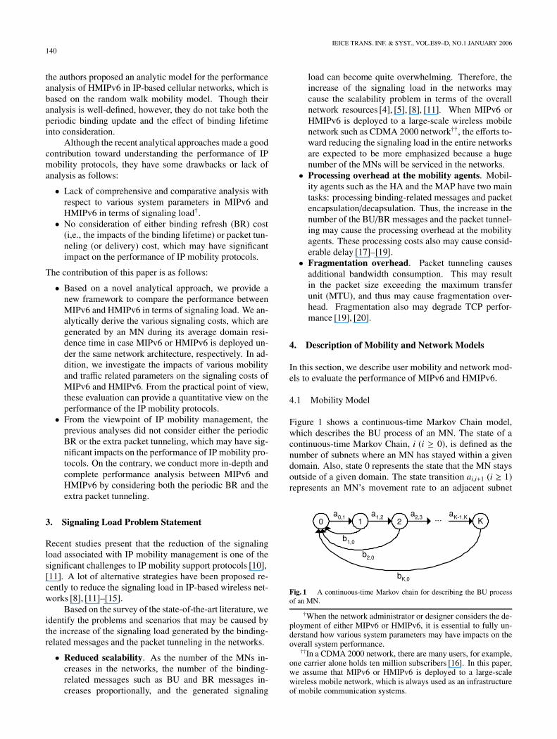
Figure 1 shows a continuous-time Markov Chain model,which describes the BU process of an MN. The state of acontinuous-time Markov Chain, i (i ≥ 0), is defined as thenumber of subnets where an MN has stayed within a givendomain. Also, state 0 represents the state that the MN staysoutside of a given domain. The state transition ai,i+1 (i ≥ 1)represents an MN’s movement rate to an adjacent subnet

Fig. 1 A continuous-time Markov chain for describing the BU processof an MN.

†When the network administrator or designer considers the de-ployment of either MIPv6 or HMIPv6, it is essential to fully un-derstand how various system parameters may have impacts on theoverall system performance.††In a CDMA 2000 network, there are many users, for example,

one carrier alone holds ten million subscribers [16]. In this paper,we assume that MIPv6 or HMIPv6 is deployed to a large-scalewireless mobile network, which is always used as an infrastructureof mobile communication systems.

KONG et al.: A COMPARATIVE ANALYSIS ON THE SIGNALING LOAD OF MOBILE IPV6 AND HIERARCHICAL MOBILE IPV6141

within a given domain, and the state transition a0,1 repre-sents an MN’s movement rate to a subnet within a givendomain from another domain. On the other hand, bi,0 (i ≥ 1)represents an MN’s movement rate to another domain froma given domain. In addition, for the analysis of the signalingcosts generated by an MN during its average domain resi-dence time, we assume that an MN moves out of a givendomain within the maximum of finite K movements†.

On the other hand, in order to obtain an MN’s move-ment rates, we assume a fluid flow mobility model [21]. Themodel assumes the followings:

• The MNs are moving at an average speed of v, andtheir movement direction is uniformly distributed over[0, 2π].• All the subnets are of the same circular shape and size,

and form together a contiguous area.• A domain†† is composed of N equally subnets.

The parameters used for the analysis of an MN’s movementrates are summarized as follows:

• γ : the movement rate for an MN out of a subnet• λ : the movement rate for an MN out of a subnet within

a given domain• µ : the movement rate for an MN out of a domain

From [21], the movement rate γ for an MN out of a subnetcan be derived as

γ =2v√πS

(1)

where S is the subnet area. Since we assume that a domainis composed of N equally subnets, therefore, the movementrate µ for an MN out of a domain is

µ =2v√πNS

(2)

Note that an MN that moves out of a domain will also moveout of a subnet. So, the movement rate λ for an MN out ofa subnet within a given domain is obtained from Eq. (1) and(2):

λ = γ − µ =(1 − 1√

N

)γ (3)

Therefore, in Fig. 1, we get ai,i+1 (i ≥ 1) = λ and a0,1 =

bi,0 = µ, respectively.On the other hand, we assume that πi is the equilibrium

probability of state i. Thus, we can obtain the followingequations from a continuous-time Markov Chain given inFig. 1.

µπ0 = µK∑

i=1

πi (4)

µπi−1 = (λ + µ)πi, i = 1 (5)

λπi = (λ + µ)πi+1, 2 ≤ i ≤ K − 1 (6)

λπi−1 = µπi, i = K (7)

On the other hand, by the law of the total probability, thesum of the probabilities of all states is 1. Thus,

π0 + π1 + π2 + · · · + πK =

K∑i=0

πi = 1 (8)

By substituting Eq. (8) into Eq. (4), we can obtain the equi-librium probability of state 0, π0. Thus,

π0 =12

(9)

Finally, using Eq. (5),(6),(7) and (9), πi can be derived as

πi =

12

if i = 0

12

(µ

λ + µ

) (λ

λ + µ

)i−1

if 1 ≤ i ≤ K − 1

12

(λ

λ + µ

)i−1

if i = K

(10)

4.2 Network Model

Similar to [22], we consider a simplistic two-layer hierarchi-cal network model given in Fig. 2. The first layer has a meshtopology, which consists of M nodes. Each first layer nodeis a root of a N-ary tree with depth of 1. For the analysis,we assume the followings:

• Each domain is composed of all the second layer nodesunder the same first layer node. In addition, the HAand the access routers (ARs) are all second layer nodes(we define the domain size (N) as the number of all thesecond layer nodes under the same first layer node).

Fig. 2 Network model.

†For the analysis of signaling load in Sect. 5, we consider thesignaling costs generated by an MN on average from when it entersa given domain to when it moves out of the given domain. How-ever, in a certain special case, the MN may not move out of thegiven domain after it enters the given domain. Therefore, we limitthe maximum allowable number of the subnet movements within agiven domain to the finite number of K.††A domain can be Internet service provider (ISP) networks, a

campus networks or company networks, etc. The description ofdomain in this literature is addressed in Sect. 4.2.

142IEICE TRANS. INF. & SYST., VOL.E89–D, NO.1 JANUARY 2006

• For the performance analysis of the two protocols un-der the same network architecture, if HMIPv6 is con-sidered, the functionality of the MAP is assumed to beplaced on the first layer node. Otherwise, the first layernode is just the border router of a given domain.• The CN, the MN, and the HA are located in the differ-

ent domains.• The link hops between the first layer nodes is a, and the

link hops between the first and second layer nodes inthe same domain is b, respectively. In addition, the linkhop between the CN and the CN’s default AR is zero.For simplicity, we do not consider the transmission costover the wireless link.• Let the ratio of the network scale (r) be 0.1 < r = b

a <1, and b = 3 are assumed.

In this model, by adjusting the ratio of the network scale inthe network model shown in Fig. 2, we can investigate theimpact of the distance among the CN, the HA and the MN.In other words, the large value of r means that the MN islocated close to the HA or the CN, and the small value of rmeans that the MN is located far away from the HA or theCN.

5. Analytical Modeling of Signaling Load in MIPv6and HMIPv6

Based on the user mobility and network models given inthe previous section, we analytically derive the location up-date costs (i.e., the sum of the binding update costs andthe binding refresh costs), packet tunneling costs, inside-domain signaling costs, outside-domain signaling costs, andtotal signaling costs, generated by an MN during its aver-age domain residence time in MIPv6 and HMIPv6 (For bothinside-domain signaling costs and outside-domain signalingcosts, refer to Appendix.).

In this paper, for the analysis, we differentiate thebinding-related messages as follows:

• Binding Update (BU) Message, which is generated byan MN’s subnet crossings.• Binding Refresh (BR) Message, which is periodically

generated whenever the binding lifetime is close to ex-piration.• Binding Acknowledgement (BAck) Message, which is

an acknowledgement message for the BU or the BRmessage.

For the analysis, several parameters and assumptions givenin the Sect. 4 are used.

5.1 Analysis of Signaling Load in HMIPv6

According to our mobility model given in Sect. 4, the aver-age binding update cost in HMIPv6 (UHmip) can be derivedas

UHmip = π0 × (Um+Uh+εUc)+(Φ(K) − 1)×Um (11)

where Um, Uh and Uc are the binding update costs to registerwith the MAP, the HA and the CN, in MIPv6 and HMIPv6,respectively. Also, ε is the average number of the CNs whenan MN moves into/out of a given domain. By applying theBU operation to the network model given in Sect. 4, Um,Uh and Uc can be expressed as 2S bub, 2S bu(a + 2b), andS bu(a + 2b), respectively. Here, S bu represents the signal-ing bandwidth consumption generated by a BU/BR/BAckmessage. Note that the HA and the MAP must return BAckmessage to the MN [1], [4]. In addition, for simplicity, weassume that the binding related messages are only sent alonein a separate packet without being piggybacked, and do notconsider the BAck message from the CN.

In addition, Φ(K) means the average number of thesubnets that an MN stays within a given domain, which isderived from the continuous-time Markov Chain given inFig. 1, and can be expressed as follows:

Φ(K) = π1 + 2π2 + 3π3 + · · · + KπK =

K∑i=1

iπi (12)

On the other hand, for the calculation of the signaling costsgenerated by sending the BR message to the CNs or receiv-ing the BAck message from the CNs during an MN’s aver-age domain residence time, we roughly define the ratio ofan MN’s average binding time for the CNs to its averagedomain residence time, δ as the followings:

δ =

∑ni=1 Ci

n

∆(13)

where ∆ means an MN’s average domain residence time,and Ci represents the binding time for the i-th CN, whichhas been recorded in an MN’s binding update list during itsaverage domain residence time. Also, n means the numberof all the CNs recorded in the MN’s binding update list dur-ing its average domain residence time.

Let the binding lifetimes for the MAP, the HA, and theCN in HMIPv6 be Tm, Th and Tc, respectively. Also, let theMN’s subnet residence time be tsub. Then, the average rateof sending the BR message to the MAP in HMIPv6 whilean MN stays in a subnet is � tsub

Tm�. Similarly, the average

rates of sending the BR message to the HA and the CN inHMIPv6 during an MN’s average domain residence time be-come � tsubΦ(K)

Th� and δ×� tsubΦ(K)

Tc�, respectively. Consequently,

the average binding refresh cost in HMIPv6 (RHmip) can bederived as follows:

RHmip = UmΦ(K) ×⌊tsub

Tm

⌋+ Uh ×

⌊tsubΦ(K)

Th

⌋

+δUc ×⌊tsubΦ(K)

Tc

⌋(14)

Therefore, the average location update cost in HMIPv6(LHmip) generated by the binding related messages is

LHmip = UHmip + RHmip (15)

On the other hand, let the probability that a single packet

KONG et al.: A COMPARATIVE ANALYSIS ON THE SIGNALING LOAD OF MOBILE IPV6 AND HIERARCHICAL MOBILE IPV6143

is routed directly to the MN without being intercepted bythe HA be q. Then, the average packet tunneling cost inHMIPv6 (THmip) can be derived as follows:

THmip = ptsub ×Φ(K) × {qDdir + (1 − q)Dindir} (16)

where p is the average packet arrival rate to an MN persubnet. Also, Ddir and Dindir are the packet tunneling costgenerated by a direct single packet delivery (not interceptedby the HA) and the packet tunneling cost generated by de-livering a single packet routed indirectly through the HA,in HMIPv6, respectively. According to our network modeland assumptions, Ddir and Dindir can be expressed as S ptband S pt(a + 2b), respectively. Here, S pt represents the addi-tional signaling bandwidth consumption generated by tun-neling per packet.

Finally, the total signaling cost (CHmip) in HMIPv6 canbe expressed as follows:

CHmip = LHmip + THmip (17)

5.2 Analysis of Signaling Load in MIPv6

Similar to Eq. (11), the average binding update cost inMIPv6 (UMip) can be derived as follows.

UMip = π0 × (Uh + εUc) + (Φ(K) − 1) × (Uh + εUc)

= {π0 + (Φ(K) − 1)} × (Uh + εUc) (18)

Let the binding lifetimes for the HA and the CN in MIPv6 beT̄h and T̄c, respectively. Then, the average binding refreshcost in MIPv6 (RMip) can be derived as follows:

RMip = Φ(K) ×(Uh ×

⌊tsub

T̄h

⌋+ δUc ×

⌊tsub

T̄c

⌋)(19)

Therefore, the average location update cost in MIPv6 (LMip)generated by the binding related messages is

LMip = UMip + RMip (20)

On the other hand, the average packet tunneling cost inMIPv6 (TMip) can be derived as follows:

TMip = ptsub × Φ(K) × {qD̄dir + (1 − q)D̄indir} (21)

where D̄dir and D̄indir are the packet tunneling cost gener-ated by a direct single packet delivery and the packet tun-neling cost generated by delivering a single packet routedindirectly through the HA, in MIPv6, respectively. Accord-ing to our network model and assumptions, D̄dir and D̄indir

can be expressed as 0 and S pt(a + 2b), respectively.Finally, the total signaling cost (CMip) in MIPv6 can be

expressed as follows:

CMip = LMip + TMip. (22)

6. Numerical Results

This section evaluates the performance of MIPv6 andHMIPv6 based on the analysis given in the previous sec-tion.For the analysis, we first study the impacts of the fol-

lowing various parameters on the signaling costs generatedby an MN during its average domain residence time in eachprotocol:

• Impact of the average moving speed of an MN, v• Impact of the binding lifetime, T• Impact of the ratio of the network scale, r• Impact of the average packet arrival rate, p• Impact of the probability that a single packet is routed

directly to the MN without being intercepted by theHA, q• Impact of the domain size, N

In terms of the operation type for IP mobility management,the total signaling cost can be expressed as the sum of thebinding update, binding refresh and packet tunneling costs.On the other hand, the total signaling cost can be also ex-pressed as the sum of the inside-domain and the outside-domain signaling costs. Therefore, in Sect. 6.3 and 6.4, wedecompose and investigate the total signaling costs to com-pare such costs of the two protocols as follows:

• Comparison of the binding update, binding refresh andpacket tunneling costs• Comparison of the inside-domain signaling costs and

the outside-domain signaling costs

Finally, we evaluate the conditions where the performancegain between the two protocols is larger or smaller in termsof the total signaling cost. These evaluation can providea quantitative view and insight on the comparative perfor-mance analysis between the two protocols. Similar to theanalysis technique adopted in [11], the performance met-ric used is the accumulative signaling bandwidth consump-tion in bytes, which is generated by both the BU/BR/BAckmessages and the packet tunneling, during an MN’s aver-age domain residence time in MIPv6 and HMIPv6 (i.e.,signaling bandwidth in bytes × number o f the link hops

an MN′ s average domain residence time ).The default parameter values for the analysis are given

in Table 1. For the analysis, from Eq. (1) and (2), tsub is

derived as√πS

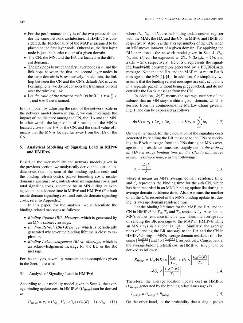
2v . On the other hand, from Eq. (12), Φ(K)is plotted as a function of K in Fig. 3. From this figure,

Fig. 3 Φ(K) as a function of K.

144IEICE TRANS. INF. & SYST., VOL.E89–D, NO.1 JANUARY 2006

Table 1 Default parameter value.

Parameter Description Value

N Domain size 25

S Subnet area 10 Km2

T Binding lifetime 0.3 hrv An average speed of an MN 20 Km/hrp An average packet arrival rate to an MN per subnet 100 pkts/hrq Prob.[A single packet is routed directly to the MN, not via the HA] 0.7

r Ratio of the network scale 0.2

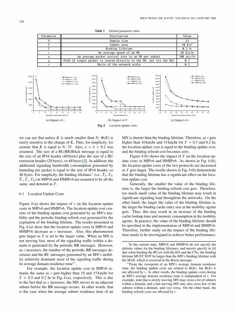
(a) Impact of v (b) Impact of T (c) Impact of r

Fig. 4 Location update costs.

we can see that unless K is much smaller than N, Φ(K) israrely sensitive to the change of K. Thus, for simplicity, weassume that K is equal to N, 25. Also, ε = δ = 0.1 wasassumed. The size of a BU/BR/BAck message is equal tothe size of an IPv6 header (40 bytes) plus the size of a BUextension header (28 bytes), so 68 bytes [5]. In addition, theadditional signaling bandwidth consumption generated bytunneling per packet is equal to the size of IPv6 header, so40 bytes. For simplicity, the binding lifetimes† (i.e., T̄h, Th,T̄c, Tc, Tm) in MIPv6 and HMIPv6 are assumed to be all thesame, and denoted as T .

6.1 Location Update Costs

Figure 4 (a) shows the impact of v on the location updatecosts in MIPv6 and HMIPv6. The location update cost con-sists of the binding update cost generated by an MN’s mo-bility and the periodic binding refresh cost generated by theexpiration of the binding lifetime. The results presented inFig. 4 (a) show that the location update costs in MIPv6 andHMIPv6 decrease as v increases. Also, this phenomenongets larger as T is set to the larger value. When an MN isnot moving fast, most of the signaling traffic within a do-main is generated by the periodic BR messages. However,as v increases, the number of the periodic BR messages de-creases and the BU messages generated by an MN’s mobil-ity relatively dominate most of the signaling traffic duringits average domain residence time††.

For example, the location update cost in MIPv6 re-mains the same as v gets higher than 10 and 15 km/hr forT = 0.5 and 0.2 hr in Fig. 4 (a), respectively. This is dueto the fact that as v increases, the MN moves to an adjacentsubnet before the BR message occurs. In other words, thatis the case when the average subnet residence time of an

MN is shorter than the binding lifetime. Therefore, as v getshigher than 10 km/hr and 15 km/hr for T = 0.5 and 0.2 hr,the location update cost is equal to the binding update cost,and the binding refresh cost becomes zero.

Figure 4 (b) shows the impact of T on the location up-date costs in MIPv6 and HMIPv6. As shown in Fig. 4 (b),the location update costs of the two protocols are decreasedas T gets larger. The results shown in Fig. 4 (b) demonstratethat the binding lifetime has a significant effect on the loca-tion update cost.

Generally, the smaller the value of the binding life-time is, the larger the binding refresh cost gets. Therefore,too much small value of the binding lifetime may result insignificant signaling load throughout the networks. On theother hand, the larger the value of the binding lifetime is,the larger the binding cache entry size at the mobility agentsgets. Thus, this may result in an increase of the bindingcache lookup time and memory consumption at the mobilityagents. In practice, the value of the binding lifetime shouldbe specified in the implementation of MIPv6 and HMIPv6.Therefore, further study on the impact of the binding life-time needs to be investigated to achieve better performance.

†In the current state, MIPv6 and HMIPv6 do not specify thedefinite values for the binding lifetimes, and merely specify in [4]that when binding the RCoA with the HA and the CNs, the bindinglifetime MUST NOT be larger than the MN’s binding lifetime withthe MAP, which is received in the BAck message.††From the viewpoint of an MN’s average domain residence

time, the binding update costs are related to Φ(K), but Φ(K) isnot affected by v. In other words, the binding update costs duringan MN’s average domain residence time is independent of v. Forexample, note that a slowly moving MN may cross a lot of subnetswithin a domain, and a fast moving MN may also cross few of thesubnets within a domain, and vice versa. On the other hand, thebinding refresh costs are affected by v.

KONG et al.: A COMPARATIVE ANALYSIS ON THE SIGNALING LOAD OF MOBILE IPV6 AND HIERARCHICAL MOBILE IPV6145

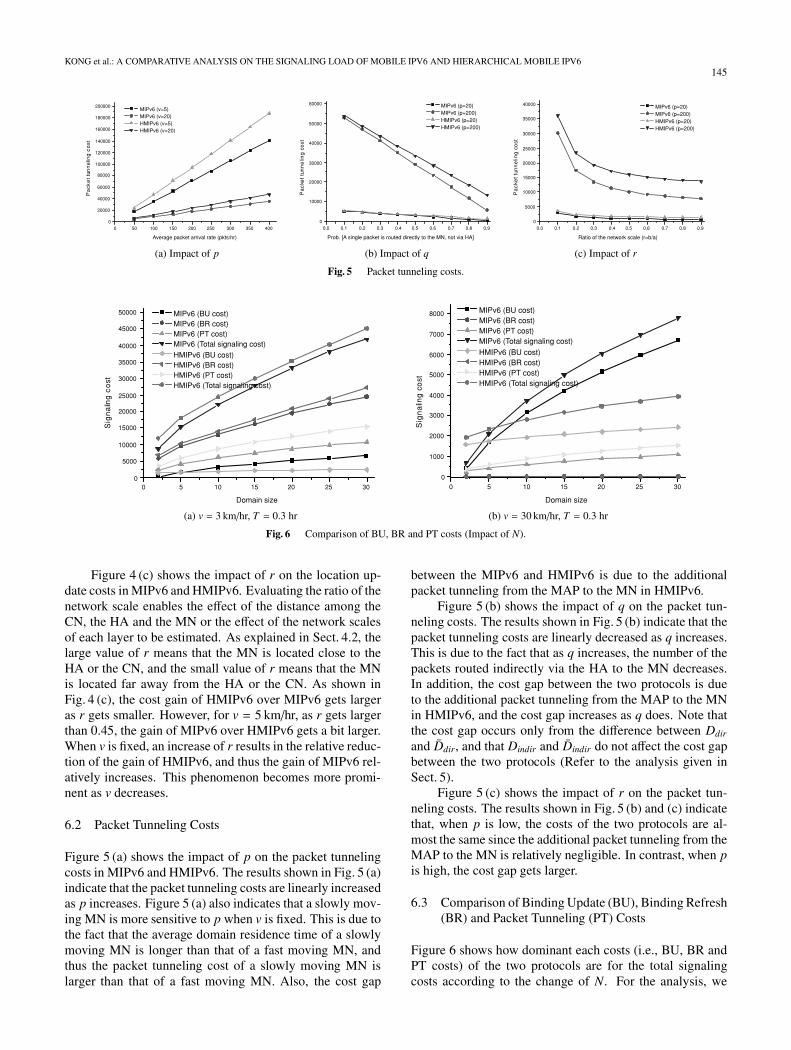
(a) Impact of p (b) Impact of q (c) Impact of r

Fig. 5 Packet tunneling costs.

(a) v = 3 km/hr, T = 0.3 hr (b) v = 30 km/hr, T = 0.3 hr

Fig. 6 Comparison of BU, BR and PT costs (Impact of N).

Figure 4 (c) shows the impact of r on the location up-date costs in MIPv6 and HMIPv6. Evaluating the ratio of thenetwork scale enables the effect of the distance among theCN, the HA and the MN or the effect of the network scalesof each layer to be estimated. As explained in Sect. 4.2, thelarge value of r means that the MN is located close to theHA or the CN, and the small value of r means that the MNis located far away from the HA or the CN. As shown inFig. 4 (c), the cost gain of HMIPv6 over MIPv6 gets largeras r gets smaller. However, for v = 5 km/hr, as r gets largerthan 0.45, the gain of MIPv6 over HMIPv6 gets a bit larger.When v is fixed, an increase of r results in the relative reduc-tion of the gain of HMIPv6, and thus the gain of MIPv6 rel-atively increases. This phenomenon becomes more promi-nent as v decreases.

6.2 Packet Tunneling Costs

Figure 5 (a) shows the impact of p on the packet tunnelingcosts in MIPv6 and HMIPv6. The results shown in Fig. 5 (a)indicate that the packet tunneling costs are linearly increasedas p increases. Figure 5 (a) also indicates that a slowly mov-ing MN is more sensitive to p when v is fixed. This is due tothe fact that the average domain residence time of a slowlymoving MN is longer than that of a fast moving MN, andthus the packet tunneling cost of a slowly moving MN islarger than that of a fast moving MN. Also, the cost gap

between the MIPv6 and HMIPv6 is due to the additionalpacket tunneling from the MAP to the MN in HMIPv6.

Figure 5 (b) shows the impact of q on the packet tun-neling costs. The results shown in Fig. 5 (b) indicate that thepacket tunneling costs are linearly decreased as q increases.This is due to the fact that as q increases, the number of thepackets routed indirectly via the HA to the MN decreases.In addition, the cost gap between the two protocols is dueto the additional packet tunneling from the MAP to the MNin HMIPv6, and the cost gap increases as q does. Note thatthe cost gap occurs only from the difference between Ddir

and D̄dir, and that Dindir and D̄indir do not affect the cost gapbetween the two protocols (Refer to the analysis given inSect. 5).

Figure 5 (c) shows the impact of r on the packet tun-neling costs. The results shown in Fig. 5 (b) and (c) indicatethat, when p is low, the costs of the two protocols are al-most the same since the additional packet tunneling from theMAP to the MN is relatively negligible. In contrast, when pis high, the cost gap gets larger.

6.3 Comparison of Binding Update (BU), Binding Refresh(BR) and Packet Tunneling (PT) Costs

Figure 6 shows how dominant each costs (i.e., BU, BR andPT costs) of the two protocols are for the total signalingcosts according to the change of N. For the analysis, we

146IEICE TRANS. INF. & SYST., VOL.E89–D, NO.1 JANUARY 2006

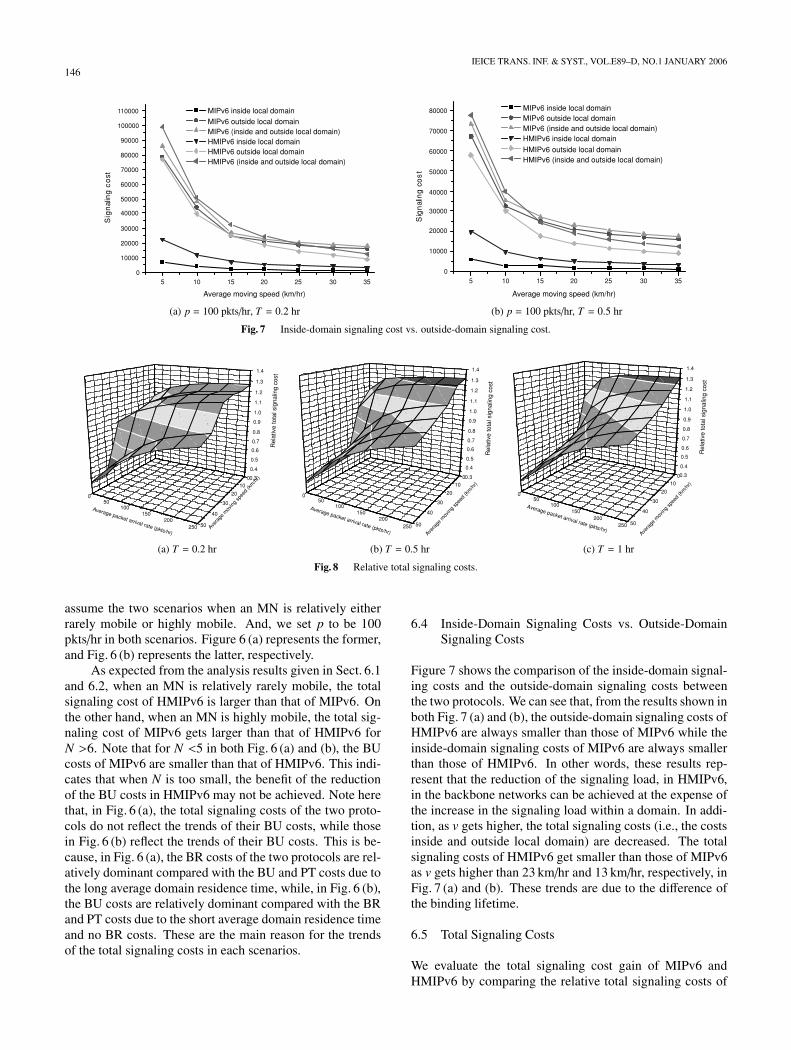
(a) p = 100 pkts/hr, T = 0.2 hr (b) p = 100 pkts/hr, T = 0.5 hr

Fig. 7 Inside-domain signaling cost vs. outside-domain signaling cost.

(a) T = 0.2 hr (b) T = 0.5 hr (c) T = 1 hr

Fig. 8 Relative total signaling costs.

assume the two scenarios when an MN is relatively eitherrarely mobile or highly mobile. And, we set p to be 100pkts/hr in both scenarios. Figure 6 (a) represents the former,and Fig. 6 (b) represents the latter, respectively.

As expected from the analysis results given in Sect. 6.1and 6.2, when an MN is relatively rarely mobile, the totalsignaling cost of HMIPv6 is larger than that of MIPv6. Onthe other hand, when an MN is highly mobile, the total sig-naling cost of MIPv6 gets larger than that of HMIPv6 forN >6. Note that for N <5 in both Fig. 6 (a) and (b), the BUcosts of MIPv6 are smaller than that of HMIPv6. This indi-cates that when N is too small, the benefit of the reductionof the BU costs in HMIPv6 may not be achieved. Note herethat, in Fig. 6 (a), the total signaling costs of the two proto-cols do not reflect the trends of their BU costs, while thosein Fig. 6 (b) reflect the trends of their BU costs. This is be-cause, in Fig. 6 (a), the BR costs of the two protocols are rel-atively dominant compared with the BU and PT costs due tothe long average domain residence time, while, in Fig. 6 (b),the BU costs are relatively dominant compared with the BRand PT costs due to the short average domain residence timeand no BR costs. These are the main reason for the trendsof the total signaling costs in each scenarios.

6.4 Inside-Domain Signaling Costs vs. Outside-DomainSignaling Costs

Figure 7 shows the comparison of the inside-domain signal-ing costs and the outside-domain signaling costs betweenthe two protocols. We can see that, from the results shown inboth Fig. 7 (a) and (b), the outside-domain signaling costs ofHMIPv6 are always smaller than those of MIPv6 while theinside-domain signaling costs of MIPv6 are always smallerthan those of HMIPv6. In other words, these results rep-resent that the reduction of the signaling load, in HMIPv6,in the backbone networks can be achieved at the expense ofthe increase in the signaling load within a domain. In addi-tion, as v gets higher, the total signaling costs (i.e., the costsinside and outside local domain) are decreased. The totalsignaling costs of HMIPv6 get smaller than those of MIPv6as v gets higher than 23 km/hr and 13 km/hr, respectively, inFig. 7 (a) and (b). These trends are due to the difference ofthe binding lifetime.

6.5 Total Signaling Costs

We evaluate the total signaling cost gain of MIPv6 andHMIPv6 by comparing the relative total signaling costs of

KONG et al.: A COMPARATIVE ANALYSIS ON THE SIGNALING LOAD OF MOBILE IPV6 AND HIERARCHICAL MOBILE IPV6147

these two protocols during an MN’s average domain resi-dence time. This evaluation is investigated to show the vari-ation of the relative total signaling costs between MIPv6 andHMIPv6 according to the change of v, p and T . For the anal-ysis, we define the relative total signaling cost as the ratio ofthe total signaling cost of HMIPv6 to that of MIPv6. There-fore, a relative total signaling cost of 1 means that the totalsignaling costs in each protocol are exactly the same.

The results shown in Fig. 8 indicate the following sev-eral facts. As v increases, the signaling cost gain of HMIPv6over MIPv6 gets larger, and this trends go into the reverseas v decreases. In addition, under the same value of v, thecost gain of HMIPv6 over MIPv6 gets larger as p decreasesor as T is set to the larger value. HMIPv6 aims to reducethe number of the BU messages in the backbone network byusing the MAP. However, this does not imply any change tothe periodic BR messages that an MN has to send to the HAand the CN, and the MN should rather send it to the MAPadditionally. In addition, since the MAP acts as a local HAin HMIPv6, it receives all packets on behalf of the MNsit is serving and should tunnel the received packets to theMNs. In other words, from the viewpoint of the signalingbandwidth consumption, the signaling bandwidth consump-tion inside a domain in HMIPv6 is generally larger than thatin MIPv6 because of the additional periodic BR messagesto the MAP and the packet tunneling from the MAP to theMN.

In addition, this phenomenon becomes more prominentas an MN stays for a considerable time within a domain orspecific subnets (i.e., when v is very small) or as incomingpacket arrival rate gets high. This is due to the fact thatthe binding refresh cost and packet tunneling cost are pro-portional to a domain (or subnet) residence time and packetarrival rate, respectively. These are the reason why the gainof MIPv6 over HMIPv6 gets larger as v and T decrease orp increases. On the other hand, the cost gain of HMIPv6over MIPv6 gets larger as v increases, and this phenomenonbecomes more prominent as p decreases or T is set to thelarger value. The results shown in Fig. 8 verify these facts.

7. Conclusions and Future Work

In this paper, we developed a novel analytical approachfor the comparative performance analysis of signaling loadin MIPv6 and HMIPv6. The analytical results provided adeep understanding of the overall performance of MIPv6and HMIPv6, and demonstrated that as the average speedof an MN gets higher and the binding lifetime is set to thelarger value, or as its average packet arrival rate gets lower,the total signaling cost generated by an MN during its av-erage domain residence time in HMIPv6 will get relativelysmaller than that in MIPv6, and that under the reverse con-ditions, the total signaling cost in MIPv6 will get relativelysmaller than that in HMIPv6. In addition, the observationsfrom our analysis results provided a motivation to our an-other work for HMIPv6, and this can be seen in [14].

Our future research subjects include validating our nu-

merical results using simulation experiments. Then, we in-tend to extend our analytical model to more general frame-work in order to study other IPv6 protocols such as fast han-dovers for MIPv6 and fast handovers for HMIPv6.

References

[1] D. Johnson and C. Perkins, “Mobility support in IPv6,” RFC 3775,June 2004.

[2] C. Perkins, “IP mobility support for IPv4,” RFC 3344, Aug. 2002.[3] C. Perkins, “Mobile IP,” IEEE Commun. Mag., vol.35, no.5, pp.84–

99, May 1997.[4] H. Soliman, C. Castelluccia, K. Malki, L. Bellier, “Hierarchical

Mobile IPv6 mobility management (HMIPv6),” draft-ietf-mipshop-hmipv6-04.txt, Dec. 2004.

[5] C. Castelluccia, “HMIPv6: A hierarchical mobile IPv6 proposal,”ACM Mobile Computing and Communications Review, vol.4, no.1,pp.48–59, Jan. 2000.

[6] A. Campbell, J. Gomez, S. Kim, C. Wan, Z. Turanyi, and A. Valko,“Comparison of IP micromobility protocols,” IEEE Pers. Commun.,vol.9, pp.72–82, Feb. 2002.

[7] I.F. Akyildiz, J. McNair, J. Ho, H. Uzunalioglu, and W. Wang,“Mobility management in next-generation wireless systems,” Proc.IEEE, vol.87, no.8, pp.1347–1384, Aug. 1999.

[8] J. Xie and I.F. Akyildiz, “A novel distributed dynamic location man-agement scheme for minimizing signaling costs in Mobile IP,” IEEETrans. Mobilecom., vol.1, no.3, pp.163–175, July-Sept. 2002.

[9] S. Pack and Y. Choi, “Performance analysis of hierarchical MobileIPv6 in IP-based cellular networks,” Proc. PIMRC 2003, pp.2818–2822, Sept. 2003.

[10] I.F. Akyildiz, J. Xie, and S. Mohanty, “A survey of mobility manage-ment in next-generation all-IP-based wireless systems,” IEEE Wire-less Commun., vol.11, no.4, pp.16–28, Aug. 2004.

[11] X. Zhang, G. Castellanos, and A.T. Campbell, “P-MIP: Pag-ing extensions for Mobile IP,” Mobile Networks and Applications(MONET), vol.7, no.2, pp.127–141, March 2002.

[12] W. Ma and Y. Fang, “Dynamic hierarchical mobility managementstrategy for Mobile IP networks,” IEEE J. Sel. Areas Commun.,vol.22, no.4, pp.664–676, May 2004.

[13] Y. Bejerano and I.Cidon, “An anchor chain scheme for IP mobilitymanagement,” Wirel. Netw., vol.9, no.5, pp.409–420, 2003.

[14] K. Kong, S. Roh, and C. Hwang, “History-based auxiliary mobilitymanagement strategy for hierarchical Mobile IPv6 networks,” IEICETrans. Fundamentals, vol.E88-A, no.7, pp.1845–1858, July 2005.

[15] Y. Lee and I.F. Akyildiz, “A new scheme for reducing link andsignaling costs in Mobile IP,” IEEE Trans. Comput., vol.51, no.6,pp.706–711, June 2003.

[16] T. Kubo, H. Yokota, A. Idoue, and T. Hasegawa, “Fast data trans-fer method in Mobile IP based backbone networks,” IEICE Trans.Commun., vol.E87-B, no.3, pp.516–522, March 2004.

[17] K. Kawano, K. Kinoshita, and K. Murakami, “A mobility-basedterminal management in IPv6 networks,” IEICE Trans. Commun.,vol.E85-B, no.10, pp.2090–2099, Oct. 2002.

[18] S. Pack, B. Lee, and Y. Choi, “Proactive load control scheme at mo-bility anchor point in hierarchical Mobile IPv6 networks,” IEICETrans. Inf. & Syst., vol.E87-D, no.12, pp.2578–2585, Dec. 2004.

[19] R. Wakikawa, S. Koshiba, T. Ernst, J. Charbon, K. Uehara, and J.Murai, “Enhanced mobile network protocol for its robustness andpolicy based routing,” IEICE Trans. Commun., vol.E87-B, no.3,pp.445–452, March 2004.

[20] A.D. Pramil, S. Antoine, and A.H. Aghvami, “TCP performance en-hancement over Mobile IPv6: Innovative fragmentation avoidanceand adaptive routing techniques,” IEE Proc., Commun., vol.151,no.4, pp.337–346, Aug. 2004.

[21] F. Baumann and I. Niemegeers, “An evaluation of location manage-ment procedures,” Proc. UPC’94, pp.359–364, Sept. 1994.

148IEICE TRANS. INF. & SYST., VOL.E89–D, NO.1 JANUARY 2006

[22] T. Ihara, H. Ohnishi, and Y. Takagi, “Mobile IP route optimizationmethod for a carrier-scale IP network,” Proc. ICECCS 2000, pp.11–14, Sept. 2000.

Appendix: Inside-Domain Signaling Costs vs. Outside-Domain Signaling Costs

In the Appendix, we derive the inside-domain signalingcosts and outside-domain signaling costs, in MIPv6 andHMIPv6, respectively. By applying each operation to thenetwork model given in Sect. 4, these costs can be easily de-rived. These costs can be used for comparing the signalingload between the inside and the outside domain. In Sect. 6,the Fig. 7 was plotted based on the following equations.

UHmip = π0 × (Um + Uh + εUc) + (Φ(K) − 1) × Um

= UinnerHmip + Uouter

Hmip (A· 1)

UinnerHmip = S bu × {π0 × (4b+εb)+2b×(Φ(K) − 1)} (A· 2)

UouterHmip = S bu × π0 × {2(a + b) + ε(a + b)} (A· 3)

where UinnerHmip and Uouter

Hmip represent the inside-domain bindingupdate cost and the outside-domain binding update cost, inHMIPv6, during an MN’s average domain residence time,respectively.

RHmip = UmΦ(K) ×⌊tsub

Tm

⌋+ Uh ×

⌊tsubΦ(K)

Th

⌋

+ δUc ×⌊tsubΦ(K)

Tc

⌋

= RinnerHmip + Router

Hmip (A· 4)

RinnerHmip = S bu ×

{Φ(K) × 2b ×

⌊tsub

Tm

⌋

+2b ×⌊tsubΦ(K)

Th

⌋+ δb ×

⌊tsubΦ(K)

Tc

⌋}(A· 5)

RouterHmip = S bu ×

{2(a + b) ×

⌊tsubΦ(K)

Th

⌋

+δ(a + b) ×⌊tsubΦ(K)

Tc

⌋}(A· 6)

where RinnerHmip and Router

Hmip represent the inside-domain bindingrefresh cost and the outside-domain binding refresh cost, inHMIPv6, during an MN’s average domain residence time,respectively.

THmip = ptsub ×Φ(K) × {qDdir + (1 − q)Dindir}= T inner

Hmip + T outerHmip (A· 7)

T innerHmip = S pt × ptsub ×Φ(K) × b (A· 8)

T outerHmip = S pt × ptsub ×Φ(K) × (1 − q)(a + b) (A· 9)

where T innerHmip and T outer

Hmip represent the inside-domain packettunneling cost and the outside-domain packet tunneling cost,in HMIPv6, during an MN’s average domain residence time,respectively.

CinnerHmip = Uinner

Hmip + RinnerHmip + T inner

Hmip (A· 10)

CouterHmip = Uouter

Hmip + RouterHmip + T outer

Hmip (A· 11)

where CinnerHmip and Couter

Hmip represent the inside-domain signal-ing cost and the outside-domain signaling cost, in HMIPv6,during an MN’s average domain residence time, respec-tively.

Finally, the total signaling cost in HMIPv6, CtotalHmip can

be expressed as

CtotalHmip = Cinner

Hmip +CouterHmip (A· 12)

Now, we derive the various signaling costs inside andoutside domain, in MIPv6, in the following.

UMip = {π0 + (Φ(K) − 1)} × (Uh + εUc)

= UinnerMip + Uouter

Mip (A· 13)

UinnerMip = S bu × {π0 + (Φ(K) − 1)} × (2b + εb) (A· 14)

UouterMip = S bu×{π0+(Φ(K)−1)}×{2(a + b) + ε(a + b)}

(A· 15)

where UinnerMip and Uouter

Mip represent the inside-domain bind-ing update cost and the outside-domain binding update cost,in MIPv6, during an MN’s average domain residence time,respectively.

RMip = Φ(K) ×(Uh ×

⌊tsub

T̄h

⌋+ δUc ×

⌊tsub

T̄c

⌋)

= RinnerMip + Router

Mip (A· 16)

RinnerMip = S bu × Φ(K) ×

(2b ×

⌊tsub

T̄h

⌋+ δb ×

⌊tsub

T̄c

⌋)

(A· 17)

RouterMip = S bu × Φ(K) ×

{2(a + b) ×

⌊tsub

T̄h

⌋

+ δ(a + b) ×⌊tsub

T̄c

⌋}(A· 18)

where RinnerMip and Router

Mip represent the inside-domain bindingrefresh cost and the outside-domain binding refresh cost, inMIPv6, during an MN’s average domain residence time, re-spectively.

TMip = ptsub ×Φ(K) × {qD̄dir + (1 − q)D̄indir}= T inner

Mip + T outerMip (A· 19)

T innerMip = S pt × ptsub × Φ(K) × b(1 − q) (A· 20)

T outerMip = S pt × ptsub × Φ(K) × (1 − q)(a + b) (A· 21)

where T innerMip and T outer

Mip represent the inside-domain packettunneling cost and the outside-domain packet tunneling cost,in MIPv6, during an MN’s average domain residence time,respectively.

CinnerMip = Uinner

Mip + RinnerMip + T inner

Mip (A· 22)

CouterMip = Uouter

Mip + RouterMip + T outer

Mip (A· 23)

where CinnerMip and Couter

Mip represent the inside-domain signal-ing cost and the outside-domain signaling cost, in MIPv6,

KONG et al.: A COMPARATIVE ANALYSIS ON THE SIGNALING LOAD OF MOBILE IPV6 AND HIERARCHICAL MOBILE IPV6149

during an MN’s average domain residence time, respec-tively.

Finally, the total signaling cost in MIPv6, CtotalMip can be

expressed as

CtotalMip = Cinner

Mip + CouterMip (A· 24)

Ki-Sik Kong received his B.S. and M.S.degrees in Computer Science and Engineeringfrom Korea University, Seoul, Korea in 1999and 2001, respectively. Currently, he is workingtoward a Ph.D. degree in Computer Science andEngineering at Korea University. Since 2001, hehas been a researcher in the Research Instituteof Computer Information and Communicationat Korea University. His research interests in-clude wireless mobile networking protocols andcomputer communications. Specifically, he is

researching IP mobility/QoS support in next-generation wireless mobilenetworks, Mobile IP, network mobility (NEMO) and performance evalua-tion.

MoonBae Song received his B.S. degreein computer science from Kunsan National Uni-versity in 1996, and his M.S. degree in com-puter science from Soongsil University in 1998.He received his Ph.D. in computer science fromKorea University in 2005. Currently, he is aresearch assistant professor in the Research In-stitute of Computer Information and Communi-cation at Korea University. His research inter-ests include moving object databases, location-aware services, context-awareness, and data

management for mobile computing.

KwangJin Park received his B.S. and M.S.degree in Computer Science from Korea Uni-versity, Korea in 2000 and 2002, respectively.He is currently a Ph.D. candidate in ComputerScience and Engineering and a researcher in theResearch Institute of Computer Information andCommunication at Korea University. His re-search interests include location-dependent in-formation systems, mobile databases, and mo-bile computing systems.

Chong-Sun Hwang received his M.S.degree in Mathematics from Korea University,Seoul, Korea in 1970, and Ph.D. degree in stat-ics and Computer Science from University ofGeorgia in 1978. From 1978 to 1980, he wasan Associate Professor at South Carolina LanderState University. He is currently a Full Profes-sor in the Department of Computer Science andEngineering at Korea University, Seoul, Korea.Since 1995, he has been a Dean in the GraduateSchool of Computer Science and Technology at

Korea University. His research interests include distributed systems, dis-tributed algorithms, and mobile computing systems.