A description of competing fusion systems

www.elsevier.com/locate/inffus

Information Fusion 7 (2006) 346–360

A description of competing fusion systems q

Steven N. Thorsen, Mark E. Oxley *

Department of Mathematics and Statistics, Graduate School of Engineering and Management, Air Force Institute of Technology,

2950 Hobson Way, Wright-Patterson Air Force Base, OH 45433-7765, USA

Received 11 January 2005; received in revised form 14 October 2005; accepted 17 October 2005Available online 6 December 2005

Abstract

A mathematical description of fusion is presented using category theory. A category of fusion rules is developed. The category def-inition is derived for a model of a classification system beginning with an event set and leading to the final labeling of the event. Func-tionals on receiver operating characteristic (ROC) curves are developed to form a partial ordering of families of classification systems.The arguments of these functionals point to specific ROCs and, under various choices of input data, correspond to the Bayes optimalthreshold (BOT) and the Neyman–Pearson threshold of the families of classification systems. The functionals are extended for use overROC curves and ROC manifolds where the number of classes of interest in the fusion system exceeds two and the parameters used aremulti-dimensional. Choosing a particular functional, therefore, provides the qualitative requirements to define a fusor and choose thebest competing classification system.� 2005 Elsevier B.V. All rights reserved.

Keywords: Fusion; Optimization; Fusor; Category theory; Information fusion; Bayes optimal; Calculus of variations; Functional

1. Introduction

Information fusion is a rapidly advancing science.Researchers are daily adding to the known repertoire offusion techniques (that is, fusion rules). An organizationthat is building a fusion system to detect or identify objectswill want to get the best possible result for the moneyexpended. It is this goal which motivates the need to con-struct a way to compete various fusion rules for acquisitionpurposes. There are many different methods and strategiesinvolved with developing classification systems. Some relyon likelihood ratios, some on randomized techniques,and still others on a myriad of schemes. To add to this,

1566-2535/$ - see front matter � 2005 Elsevier B.V. All rights reserved.

doi:10.1016/j.inffus.2005.10.003

q A short version of this study was presented at the Seventh Interna-tional Conference on Information Fusion (Fusion 2004) in Stockholm,Sweden [1]. The views expressed in this article are those of the authors anddo not reflect the official policy or position of the United States Air Force,Department of Defense, or the US Government.

* Corresponding author. Tel.: +1 937 2553636x4515; fax: +1 937 6564413.

E-mail addresses: [email protected] (S.N. Thorsen), [email protected] (M.E. Oxley).

there exists the fusion of all these technologies which createeven more classification systems. Since the receiver operat-ing characteristics (ROCs) can be developed for such sys-tems under test conditions, we propose a functionaldefined on ROC curves as a method of quantifying the per-formance of a classification system. A ROC curve is a set ofROCs which define a continuous, non-decreasing (ordepending upon the axes chosen, non-increasing) functionin ROC space (the concept of ROC curves is developedin Section 3).

This functional then allows for the development of acogent definition of what is fusion (i.e., the differencebetween fusion rules, which do not have a reliance uponany qualitative difference between the �new� fused resultand the �old� non-fused result) and what we term fusors(a subcategory of fusion rules, see Section 2), which do relyupon the qualitative differences. In other words, how doesone know the new fused result is ‘‘better’’ than what previ-ously existed? (see Wald [2]). While the development ofsome classification systems require knowledge of class con-ditional probability density functions, others do not. Atesting organization would not reveal the exact test

mailto:[email protected]



S.N. Thorsen, M.E. Oxley / Information Fusion 7 (2006) 346–360 347

scenario to those proposing different classification systemsa priori. Therefore, even those systems relying upon classconditional density knowledge a priori can, at best, esti-mate the test scenario (and by extension can only estimatethe operational conditions the system will be used in later!).

The functional we propose allows a researcher (or tester)who is competing classification systems to evaluate theirperformance. Each system generates a ROC, or a ROCcurve in the case of a family of classification systems, basedon the test scenario. The desired scenario of the test orga-nization may be examined with a perturbation in theassumptions (without actually retesting), and functionalaverages compared as well, so performance can be com-pared over a range of assumed cost functions and priorprobabilities. The result is a sound mathematical approachto comparing classification systems. The functional is scal-able to a finite number of classes (the classical detectionproblem being two classes), with the development ofROC manifolds of dimension m P 3 (making a ROC(m � 1)-manifold, see Section 5.1). The functional willoperate on discrete ROC points in the m-dimensionalROC space as well as over a continuum of ROCs. Ulti-mately, under certain assumptions and constraints, we willbe able to compete classification systems, fusion rules,fusors (fusion rules with a constraint), and fusion systemsin order to choose the best from among finitely manycompetitors.

The relationships between ROCs, ROC curves, and per-formance has been studied for some time, and some prop-erties are well-known. The foundations for two-class labelsets can be reviewed in [3–10]. The method of discoveryof these properties are different from our own. Previously,the conditional class density functions were assumed to beknown, and differential calculus was applied to demon-strate certain properties. For example, for likelihood-basedclassifiers, the fact that the slope of a ROC curve at a pointis the likelihood ratio which produces this point, was dis-covered in this manner [3]. Using cost functions in relationto ROC curves to analyze best performance seems to haverecently (2001) been recognized by Provost and Foster [11],based on work previously published by [4,10,12]. The mainassumption in most of the cited work, with regard to ROCcurve properties, is that the distribution functions of theconditional class densities are known and differentiablewith respect to the likelihood ratio (as a parameter). Wetake the approach that, as a beginning for the theory, theROC curve is continuous and differentiable, and we applyvariational calculus to a functional which has the effect ofidentifying the point on the curve which minimizes BayesCost. Under any particular assumption, such a point existsfor every family of classification systems. This is not to saythe classification system is Bayes Optimal with respect toall possible classification schemes, but rather it is Bayesoptimal with respect to the classification systems withinthe family producing the ROC curve. The solution to theoptimization of the functional allows us to extend thisproperty to n-class classification systems, so that we can

define and measure performance of ROC manifolds (andthe families of classification systems producing them).

We believe this functional (which is really a family offunctionals) eliminates the need to discuss classificationsystem performance in terms of area under the curve(AUC), which is so prevalently used in the medical commu-nity, or volume under the ROC surface (VUS) [13,14], sincethese performance �metrics� do nothing to describe a classi-fication system�s value under a specific cost–prior assump-tion. Any family of classification systems will be set to oneparticular threshold (at any one time), and so its perfor-mance will be measured at only one point on the ROCcurve. The question is ‘‘What threshold will the userchoose?’’ We submit that this performance can be calcu-lated very quickly under the test conditions desired (usingROC manifolds) by applying vector space methods to theinformation revealed by the calculus of variationsapproach.

Additionally, the novelty of this approach also relies onthe fact that no class conditional densities are assumed (bythe tester), so that the parameters of the functional can bechosen to reflect the desired operational assumptions ofinterest to the tester. For example, the tester could establishthat Neyman–Pearson criteria will form the data of thefunctional, or that he wants to minimize Bayes cost. Thetester may wish to examine performance under a range ofhypotheses. Once the data are established, the functionalwill induce a partial ordering on the set of competingsystems.

We have found category theory useful for the descrip-tion of fusion and fusion systems [1,15–17]. We are notalone in this, since there has already been some ground-work published [18,19] applying category theory to the sci-ence of information fusion. Category theory has also beenused to prove certain properties of learning and memoryusing neural nets [20–23]. Category theory is a branch ofmathematics useful for demonstrating mathematical rela-tionships and properties of mathematical constructs, suchas groups, rings, modules, etc., as well as properties whichare universal among like constructs. It is a very useful toolto describe the relationships involved in the systems of clas-sification families. We are using the language of categorytheory in order to discover universal properties amongfusors and to provide mathematical rigor to the definitions.It has been our goal to engage the data fusion communityto think in terms of generalities when studying fusion pro-cesses in order to abstract the processes and perhaps gainsome knowledge and insight to properties that may goundetected otherwise. We have drawn upon the work ofvarious authors in category theory literature [24–27] topresent the definitions, which can be found in AppendixA, of this paper.

2. Modelling fusion within the event to label model

Let X be a set of states (or outcomes) for a universal (orsure) event, and T � R be a bounded interval of time.

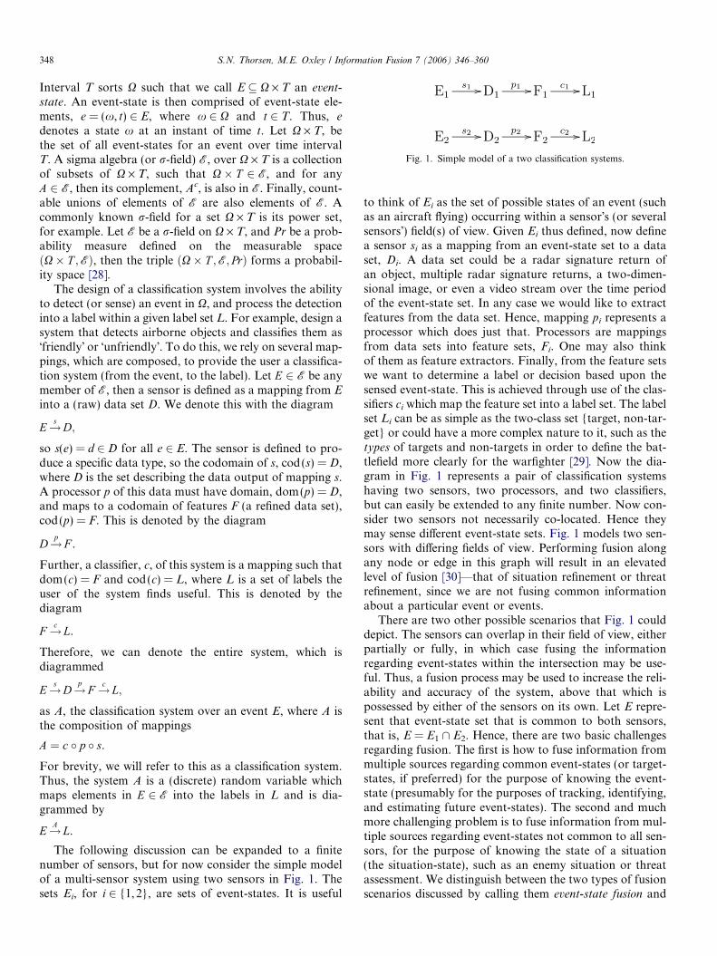
Fig. 1. Simple model of a two classification systems.

348 S.N. Thorsen, M.E. Oxley / Information Fusion 7 (2006) 346–360

Interval T sorts X such that we call E � X · T an event-

state. An event-state is then comprised of event-state ele-ments, e = (x, t) 2 E, where x 2 X and t 2 T. Thus, e

denotes a state x at an instant of time t. Let X · T, bethe set of all event-states for an event over time intervalT. A sigma algebra (or r-field) E, over X · T is a collectionof subsets of X · T, such that X� T 2 E, and for anyA 2 E, then its complement, Ac, is also in E. Finally, count-able unions of elements of E are also elements of E. Acommonly known r-field for a set X · T is its power set,for example. Let E be a r-field on X · T, and Pr be a prob-ability measure defined on the measurable spaceðX� T ;EÞ, then the triple ðX� T ;E; PrÞ forms a probabil-ity space [28].

The design of a classification system involves the abilityto detect (or sense) an event in X, and process the detectioninto a label within a given label set L. For example, design asystem that detects airborne objects and classifies them as�friendly� or �unfriendly�. To do this, we rely on several map-pings, which are composed, to provide the user a classifica-tion system (from the event, to the label). Let E 2 E be anymember of E, then a sensor is defined as a mapping from Einto a (raw) data set D. We denote this with the diagram

E!s D;

so s(e) = d 2 D for all e 2 E. The sensor is defined to pro-duce a specific data type, so the codomain of s, cod(s) = D,where D is the set describing the data output of mapping s.A processor p of this data must have domain, dom(p) = D,and maps to a codomain of features F (a refined data set),cod(p) = F. This is denoted by the diagram

D!p F .

Further, a classifier, c, of this system is a mapping such thatdom(c) = F and cod(c) = L, where L is a set of labels theuser of the system finds useful. This is denoted by thediagram

F !c L.

Therefore, we can denote the entire system, which isdiagrammed

E!s D!p F !c L;

as A, the classification system over an event E, where A isthe composition of mappings

A ¼ c � p � s.

For brevity, we will refer to this as a classification system.Thus, the system A is a (discrete) random variable whichmaps elements in E 2 E into the labels in L and is dia-grammed by

E!A L.

The following discussion can be expanded to a finitenumber of sensors, but for now consider the simple modelof a multi-sensor system using two sensors in Fig. 1. Thesets Ei, for i 2 {1,2}, are sets of event-states. It is useful

to think of Ei as the set of possible states of an event (suchas an aircraft flying) occurring within a sensor�s (or severalsensors�) field(s) of view. Given Ei thus defined, now definea sensor si as a mapping from an event-state set to a dataset, Di. A data set could be a radar signature return ofan object, multiple radar signature returns, a two-dimen-sional image, or even a video stream over the time periodof the event-state set. In any case we would like to extractfeatures from the data set. Hence, mapping pi represents aprocessor which does just that. Processors are mappingsfrom data sets into feature sets, Fi. One may also thinkof them as feature extractors. Finally, from the feature setswe want to determine a label or decision based upon thesensed event-state. This is achieved through use of the clas-sifiers ci which map the feature set into a label set. The labelset Li can be as simple as the two-class set {target, non-tar-get} or could have a more complex nature to it, such as thetypes of targets and non-targets in order to define the bat-tlefield more clearly for the warfighter [29]. Now the dia-gram in Fig. 1 represents a pair of classification systemshaving two sensors, two processors, and two classifiers,but can easily be extended to any finite number. Now con-sider two sensors not necessarily co-located. Hence theymay sense different event-state sets. Fig. 1 models two sen-sors with differing fields of view. Performing fusion alongany node or edge in this graph will result in an elevatedlevel of fusion [30]—that of situation refinement or threatrefinement, since we are not fusing common informationabout a particular event or events.

There are two other possible scenarios that Fig. 1 coulddepict. The sensors can overlap in their field of view, eitherpartially or fully, in which case fusing the informationregarding event-states within the intersection may be use-ful. Thus, a fusion process may be used to increase the reli-ability and accuracy of the system, above that which ispossessed by either of the sensors on its own. Let E repre-sent that event-state set that is common to both sensors,that is, E = E1 \ E2. Hence, there are two basic challengesregarding fusion. The first is how to fuse information frommultiple sources regarding common event-states (or target-states, if preferred) for the purpose of knowing the event-state (presumably for the purposes of tracking, identifying,and estimating future event-states). The second and muchmore challenging problem is to fuse information from mul-tiple sources regarding event-states not common to all sen-sors, for the purpose of knowing the state of a situation(the situation-state), such as an enemy situation or threatassessment. We distinguish between the two types of fusionscenarios discussed by calling them event-state fusion and

Fig. 2. Two classification systems with overlapping field of view.

Fig. 3. Fusion rule applied to data sets.

Fig. 4. Fusion rule applied within a dual sensor process.


situation-state fusion, respectively. Therefore, Fig. 2 repre-sents the Event-State-to-Label model of two classificationsystems. The only restriction necessary for the usefulnessof this model is that a common field of view be used. Con-sequently, D1 and D2 can actually be the same data setunder the model, while s1 and s2 could be different sensors.

At this point we begin to consider categories generatedby these data sets. Let D ¼ ðD; IdD; IdD; �Þ be the discretecategory generated by data set D. We use these categoriesto define fusion rules of classification systems.

Definition 1 (Fusion rule of n classification systems). Sup-pose we have n classification systems to be fused. For eachi = 1, . . .,n, let Oi be a category of data generated (ifnecessary) from the ith source of data (this could be rawdata, features, or labels). Then the product

pðnÞ ¼Yn

i¼1

Oi

is a product category. For a category of data, O0, the expo-nential, O

pðnÞ0 , is a category of fusion rules, each rule of

which maps the products of data objects Ob(p(n)) to a dataobject in ObðO0Þ, and maps data arrows in Ar(p(n)) to ar-rows in ArðO0Þ. These fusion rules are functors, whichmake up the objects of the category. The arrows of the cat-egory are natural transformations between them.

If the Oi are categories generated from sensor sources(i.e., outputs), then we call OpðnÞ

0 a category of data-fusionrules and use the symbols D

pðnÞ0 . If they are generated by

processor sources, then call OpðnÞ0 a category of feature-

fusion rules and use the symbols FpðnÞ0 . Finally, if they have

classifiers as sources, then call them label-fusion rules (or,alternatively, decision-fusion rules) and use the symbolsL

pðnÞ0 . If we let O be the category which has as objects

the n + 1 data categories, Oi for i = 0,1, . . .,n, and witharrows the functors between them, and include the prod-ucts within this category, then we see that, in particular,the fusion rules are a category of functors (with arrowsthe natural transformations that may exist between thefusion rules).

A fusion rule could be a Boolean rule, a filter, an estima-tor, or an algorithm. There is no restriction on the output,with regard to being a ‘‘better’’ output than a systemdesigned without a fusion rule, since that requires a newdefinition. We now desire to show how defining a fusor(see Definition 5) as a fusion rule with a constraint changes

the classification system model into an event-state fusionmodel. Continuing to consider the two classification fami-lies in Fig. 2, a fusion rule can be applied to either the datasets or the feature sets. Given a fusion rule R for the twodata sets as in Fig. 3, our model becomes that of Fig. 4.Notice we use a different arrow to denote a fusion rule.A new data set, processor, feature set, and classifier maybecome necessary as a result of the fusion rule having a dif-ferent codomain than the previous systems. The label setmay change also, but for now, consider a two-class labelset, that of

L ¼ L1 ¼ L2 ¼ fTarget; Non-targetg.In a within-fusion scenario (see [31]), the data sets are

identical, D1 = D2 = D3. This is easily seen in the casewhere two sensors are the same type (that is, they collectthe same measurements, but from possibly different loca-tions relative to the overlapping field of view). In the casewhere the data sets are truly different, a composite dataset which is different from the first two (possibly even theproduct of the first two) is created as the codomain ofthe fusion rule.

At this point we may consider, in what way is the systemin Fig. 4 superior to the original systems shown in Fig. 2with L = L1 = L2? One way of comparing performance insuch systems is to compare the systems� receiver operatingcharacteristics (ROC) curves.

3. Developing a ROC curve

Setting aside the fusion of classification systems for amoment, we focus on a generic classification of an event-state itself. Let ðE;E; PrÞ be a probability space. Let thelabel set L = {T,N}, where T = target and N = non-target.Let E = ET [ EN, where ET \ EN = ;, so that fET;ENg is apartition of E into the two classes. Let c be a classifier suchthat

E!c L

is a classification system. Recall that the mapping c inducesa ‘‘natural’’ mapping, which we denote c\, the pre-image ofc (\ is the natural symbol in music, a becuadro in Spanish,

Fig. 6. A typical ROC curve.


and we use it to distinguish from the inverse symbol �1. It ispossible that the inverse exists, but not guaranteed). Hence,if L is the power set of L, then

c\ : L! E.

Thus, we can calculate the probability of true positive,

P tp ¼Prðc\ðT Þ \ ETÞ

PrðETÞ¼ 1� Prðc\ðNÞ \ ETÞ

PrðETÞð1Þ

which is estimated by the true positive rate (TPR), and theprobability of false positive,

P fp ¼Prðc\ðT Þ \ ENÞ

PrðENÞð2Þ

which is estimated by the false positive rate (FPR), or falsealarm rate. The ordered pair (Pfp,Ptp) 2 [0, 1] · [0, 1] is theROC for the system. Now it is desirable for a classificationsystem to have a parameter associated with the classifier,such that changing the parameter (which is possibly mul-ti-dimensional) changes the ROC. In such a case, a param-eter set H would be chosen such that the family ofclassification systems, C ¼ fchjh 2 Hg, maps the event setinto the label set, and such that the curvef ¼ fðP fpðchÞ; P tpðchÞÞ : h 2 Hg is the projection of the tra-jectory s ¼ fðh; P fpðchÞ; P tpðchÞÞ : h 2 Hg into the Pfp–Ptp

plane. In this case, we have that

P tpðchÞ ¼Prðc\hðT Þ \ ETÞ

PrðETÞ; ð3Þ

and

P fpðchÞ ¼Prðc\hðT Þ \ ENÞ

PrðENÞ. ð4Þ

We call such a parameter set an admissible parameter set ifthe image of Pfp(ch) is onto [0,1]. Note the parameter neednot necessarily be associated with the classifier of the sys-tem, but could be associated instead with the sensor(s),processor(s), or any combination of the three. Consider,for example, the three classification systems in Fig. 5. Eachsystem will generate a ROC curve when H is an admissibleparameter set. What is key is that the final parameter setmust produce a corresponding ROC curve as a continuouscurve from (0,0) through (1,1) in the Pfp � Ptp plane as theexample in Fig. 6 shows. The parameter h is the thresholdof the ROC. We can, at this point, advocate that the ROC

Fig. 5. Three classification systems with admissible parameters eachproduce a ROC curve.

curve be designated by the classification system that gener-ates it, and not just the classifier. Therefore, the systems inFig. 5 will be designated as in Fig. 7, a shorthand methodfor describing the composition of sensor(s), processor(s),and classifier(s), that is, A1,h = c � p � sh, A2,h = c � ph � s,and A3,h = ch � p � s.

Assume that ðE;E; PrÞ is a probability space, andE = ET [ EN, with ET \ EN = ;, so that fET;ENg � E isa partition of E into the two classes of events. LetA ¼ fAhjh 2 Hg, where E!Ah L. Is there a threshold,h* 2 H, such that Ah� performs best in the family of classi-fication systems, A? It is well-known and accepted that thethreshold for which the probability of a misclassification(or Bayes error) is minimized is considered best anddenoted the Bayes optimal threshold (BOT). That is, doesthere exist h* 2 H which minimizes the quantity

PrðA\hðETÞ \ ENÞ [ ðA\

hðENÞ \ ETÞ

¼ PrðA\hðETÞ \ ENÞ þ PrðA\

hðENÞ \ ETÞ¼ P fpðAhÞPrðENÞ þ ð1� P tpðAhÞÞPrðETÞ; ð5Þ

where Pr(ET) and Pr(EN) are the prior probabilities of thetarget class and non-target class, respectively? If yes, thenh* is the BOT for the family of classification systems A.

Fig. 7. Three classification systems.


An obvious question at this point is, given two familiesof classification systems, A ¼ fAhjh 2 Hg andB ¼ fB/j/ 2 Ug, which family is best? This is not an easyquestion to answer, as demonstrated in [32]. It is temptingto use some measure of the BOT, but notice that the BOTis dependent upon the selection of prior probabilities. Thepriors are generally not known, so selection of a better clas-sification system based on ROC curves may not be possi-ble, since ROC curves for different families can overlap.Rather, we should ask the question, given an operatingassumption of our prior probabilities, such as PrðETÞ ¼ 1

4,

can we choose among competing families of classificationsystems one that is superior to the others? One way toanswer the question is derived in an unexpected way.

4. A variational calculus solution to determining the Bayes

optimal threshold of a family of classification systems

Suppose the ROC curves are smooth (differentiable)over the entire range, i.e., we consider the set X ¼ff : ½0; 1� ! Rj f is differentiable at each x 2 ð0; 1Þ and itsderivative f 0 is continuous at each x 2 ð0; 1Þg. This is con-sistent with Alsing�s proof [32] in that, given enough data allROC curve estimates converge to the ROC curve. Given adiagram describing the family of classification systemsA ¼ fAh : h 2 Hg, with H an admissible parameter set(assumed to be one-dimensional), and ðE;E; PrÞ a probabil-ity space of features, there is a set sA ¼ fðh; P fpðAhÞ;P tpðAhÞÞ : h 2 Hg which is called the ROC trajectory forthe classification system family A. The projection of theROC trajectory onto the (Pfp,Ptp)-plane is the setfA ¼ fðP fpðAhÞ; P tpðAhÞÞ : h 2 Hg which is the ROC curveof the classification system family A. Hence, for h 2 [0, 1]such that h = Pfp(Ah) for some h 2 H, we have that

½P fp�\ðfhgÞ ¼ fAhg () h;

that is, the pre-image of h under Pfp( Æ ) is the classificationsystem Ah, which we assume has a one-to-one and ontocorrespondence to h. Therefore, the BOT of the family ofclassification systems A, denoted by h*, corresponds tosome h� ¼ P fpðAh� Þ 2 ½0; 1�, which may not be unique, un-less the function Pfp( Æ ) is one-to-one. So, there is at leastone such h*, now what can we learn about it? Considerthe problem stated as follows:

Let a,b P 0. Among all smooth curves which originateon the point (0,1) and terminate on the ROC curve f,find the curve, defined by the function Y, which mini-mizes the functionalZ
J ½Y � ¼
h

0

½aþ bj _Y ðxÞj�dx. ð6Þ

The value of h 2 [0, 1] depends on the function Y whichsatisfies the constraints

Y ð0Þ ¼ 1;

Y ðhÞ ¼ f ðhÞ.ð7Þ

Observe that h = Pfp(Ah), f(h) = Ptp(Ah) for some h 2 H,and b = 1 � a with a = Pr(N), the prior probability of anon-target.

The functional J identifies the curve with the smallestarclength (measured with respect to the weighted 1-norm)from the point (0, 1) to the ROC curve. The constraintsof Eq. (7) imply that the curve must begin at (0,1) and ter-minate on the ROC curve. Any differentiable function Y

that minimizes J, subject to the constraints (7), necessarilymust be a solution to Euler�s equation [33]

o

oyGðx; Y ðxÞ; _Y ðxÞÞ � d

dxo

ozGðx; Y ðxÞ; _Y ðxÞÞ ¼ 0

for all x 2 ð0; hÞ. ð8Þ

From Eq. (6) we define G(x,y,z) = a + bjzj, so that ooy G ¼ 0

and ooz G ¼ bsgn ðzÞ. Hence, we have that Y solves the Euler

equation

� d

dtsgn ð _Y ðxÞÞ ¼ 0 for all x 2 ð0; hÞ. ð9Þ

Integrating this equation yields sgnð _Y ðxÞÞ is constant for allx 2 [0, h]. Since Y(x) 6 1 for all x 2 (0,h), and Y(0) = 1,from constraints (7), then sgn ð _Y ðxÞÞ must be 0 or �1.Now, if sgnð _Y ðxÞÞ ¼ 0 for all x, then 1 = Y(0) =Y(h) = Y(1) due to the smoothness of the ROC curve.Substituting this solution into the functional J in Eq. (6)yields

J ½Y � ¼ ah ¼ PrðNÞP fpðAhÞ ð10Þwith Pfp(Ah) = 1. Thus, J[Y] = Pr(N) and the weighted(1-norm) arclength of curve Y is therefore Pr(N). On theother hand, if sgn ð _Y ðxÞÞ ¼ �1 for all x 2 (0,h), thenj _Y ðxÞj ¼ � _Y ðxÞ and substituting this into J directly in Eq.(6) yields

J ½Y � ¼Z h

0

½a� b _Y ðxÞ�dx ð11Þ

¼ ahþ bsgn ð _Y ðhÞÞY ðhÞ � bsgn ð _Y ð0ÞÞY ð0Þ¼ ah� b½Y ðhÞ � Y ð0Þ�¼ ahþ ½1� Y ðhÞ�b¼ P fpðAhÞPrðNÞ þ ð1� P tpðAhÞÞPrðT Þ. ð12Þ

Notice that Eq. (12) is identical to the unminimized Eq. (5).Therefore, h = h* which minimizes Eq. (12) corresponds tothe BOT, h*, of the classification system family A. Thetransversality condition [33] of this problem is

aþ bj _Y ðxÞjjx¼h� þ bðf 0ðxÞ � _Y ðxÞÞsgn ð _Y ðxÞÞjx¼h� ¼ 0; ð13Þso that

f 0ðh�Þ ¼ ab

ð14Þ

which is

f 0ðh�Þ ¼ PrðNÞPrðT Þ . ð15Þ


This is a global minimum, since, it is clear the J is a convexfunctional. So the transversality condition tells us that theBOT of the family of classification systems corresponds toa point on the ROC curve which has a derivative equal tothe ratio of prior probabilities, PrðNÞ

PrðT Þ. Therefore, if one pre-sumes a ratio of prior probabilities equal to 1, then thepoint on the curve corresponding to the BOT will have atangent to the ROC curve with slope 1. We could substitutea = CfpP(N) and b = CfnP(T) where Cfp and Cfn are thecosts of making each error, or we could specify a cost–priorratio

CfpPðNÞCfnPðT Þ, if we wish to consider costs in addition to the

prior probabilities. This gives us an idea of what wouldmake a good functional for determining which families ofclassification systems are more desirable than others. Animmediate approach would be to choose a preferred priorratio and construct a linear variety through the optimalROC point (0, 1). Then take the 2-norm of the vector whichminimizes the distance from the ROC curve to the linearvariety. However, it is still possible that many ROC curvescould be constructed so that the BOT for each one has thesame distance to the linear variety. This would set up anequivalence class of families of classification system, so thatthis distance induces a partial order of these families. Thisis similar to the problem faced when using area under thecurve (AUC) of a ROC curve as a functional. In both casesthe underlying posterior conditional probabilities are un-known and there are just too many possible combinationsof posterior distributions that can produce ROC curveswith the same AUC (or equal BOT functional values).The point, however, is that under a functional based onthe BOT, we would have a ‘‘leveled playing field’’ sincewe are debating which ROC (and therefore the classifica-tion system it represents) is better based on the same priorprobabilities. Families of classification systems with equalAUC are considered equal over the entire range of possiblepriors and therefore, AUC is of less value. Furthermore,the AUC functional does not relate its values to the un-known priors at all. Rather, it is related to the value ofthe class conditional probabilities associated with a familyof classification systems over all possible false positive val-ues. It is therefore essentially useless as a functional in try-ing to discover an appropriate operating threshold for aclassification system.

5. ROC manifolds

5.1. Constructing the three-dimensional ROC manifold

So far we have considered the fusion of only those clas-sification systems which produce a two-class output. Whatif there were a choice of three classes with the correspond-ing label set L ¼ f‘1; ‘2; ‘3g?

Let ðE;E; PrÞ be the probability space over which we willapply a classification system. Let H = H1 · H2 be anadmissible parameter set for a family of classification sys-tems. We will use the generalized approach and build aROC manifold from the family of classification systems

E!AH L, where L ¼ f‘1; ‘2; ‘3g is a three-class label set. LetfE1E2;E3g be a partition of E, so that Ei corresponds toclass ‘i. We say Pijj(Ah) is the conditional probability ofthe classification system Ah labeling an elementary evente 2 E as class i when event Ej has occurred, that is

P ijjðAhÞ ¼PrðA\

hð‘iÞ \ EjÞPrðEjÞ

;

where Pr(Ej) is the prior probability of class ‘j.Consider now the Bayes error of the classification sys-

tem. First, we define the Bayes error function as

BEðAhÞ¼ Pr½ðA\hð‘1Þ\E3Þ[ðA\

hð‘2Þ\E3Þ[ðA\hð‘1Þ\E2Þ

[ðA\hð‘3Þ\E2Þ[ðA\

hð‘2Þ\E1Þ[ðA\hð‘3Þ\E1Þ�

¼ PrðA\hð‘1Þ\E3ÞþPrðA\

hð‘2Þ\E3ÞþPrðA\

hð‘1Þ\E2ÞþPrðA\hð‘3Þ\E2Þ

þPrðA\hð‘2Þ\E1ÞþPrðA\

hð‘3Þ\E1Þ

¼ 1�P 3j3ðA\hð‘3ÞÞ

h iPrðE3Þþ 1�P 2j2ðA\

hð‘3ÞÞh i

PrðE2Þ

þ 1�P 1j1ðAhð‘3ÞÞ� �

PrðE1Þ. ð16Þ

We wish to minimize the Bayes error function over theadmissible set of parameters. If h* 2 H minimizes BE(Ah),then h* is called the BOT for the family of classificationsystems {Ahjh 2 H}. If the errors within class have thesame cost (as is the case with this construction) then wecan have three error axes, 1 � P3j3(Ah), 1 � P2j2(Ah), and1 � P1j1(Ah). Assume the first parameter h1 correspondsto axis 1 � P1j1(Ah), and the second parameter h2 corre-sponds to the axis 1 � P2j2(Ah). If error costs are not equal,then we need 32 � 3 = 6 axes for our ROC space and fivefree parameters to create a ROC 5-manifold. This leadsus to extend the calculus of variations approach identifyingthe corresponding BOT for a given set of priorprobabilities.

5.2. Extending the calculus of variations approach

to ROC manifolds

For n classes, we specify m = n2 � n dimensions assum-ing differing costs for each error. Each axis then is a type offalse positive for a given class, so that the optimal ROCpoint is the origin, (0,0, . . ., 0). The method used in thissection follows and extends that of [34]. Let xm =f(x1,x2, . . .,xm � 1) be the equation of the ROC manifoldresiding in m-dimensional space. Define the function

Wðx1; x2; . . . ; xmÞ ¼: f ðx1; x2; . . . ; xm�1Þ � xm;

then M ¼ fðx1; . . . ; xmÞjWðx1; . . . ; xmÞ ¼ 0g is the ROCmanifold. We assume all first-order partial derivatives existand are continuous for W. For each t 2 [0, 1] letR(t) = (X1(t), . . .,Xm(t)) be the position vector which pointsto a point on a smooth trajectory, beginning at the initialpoint (0, . . ., 0) and terminating on the manifold M. Thus,R(0) = (0, . . ., 0) and there is some tf 2 (0, 1] such thatRðtfÞ 2M, with tf dependent upon the particular R.


Choose weights ai > 0 for i = 1, . . .,m such thatPm

i¼1ai 6 1,and let k Æk1 denote the weighted 1-norm defined on a vec-tor v = (v1, . . .,vm) by

kvk1 ¼Xm

i¼1

aijvij. ð17Þ

Define the functional J1

J 1½R� ¼Z tf

0

k _RðtÞk1 dt. ð18Þ

For ease of notation, define

Gðt; x; yÞ ¼ kyk1.

Hence, we write Eq. (18) as

J 1½R� ¼Z tf

0

Gdt; ð19Þ

and suppress the integrand variables as is customary in thecalculus of variables. We wish to minimize J1, and seek tofind the optimal function R* with initial and terminalpoints as discussed subject to the constraints. The mathe-matics describing this process are shown in Appendix B.Once the Euler equations with transversality conditionsare solved, we have the result that

rWðR�ðt�f ÞÞ ¼�1

amða1; . . . ; amÞ ¼ n ð20Þ

is the normal to the ROC manifold M at the terminal pointof R�ðt�f Þ on the smooth trajectory minimizing J1. Theweights, ai, are the product of a prior probability of a par-ticular class and a cost of the particular error.

6. A functional for comparing classifier families

Having shown using calculus of variations that the opti-mal points of the ROC manifold can be found correspond-ing to a simple normal vector, based on the initial data ofprior probabilities and costs, we turn to developing a func-tional, which will calculate a value in R corresponding tothe optimal value of the cost. The functional requires inputof prior probabilities, costs, and constraints. The ROCmanifold point which yields a minimum norm is the pointon the ROC manifold which is optimal under the assumeddata. Thus, families of classification systems can be com-pared using this functional, and the best classification sys-tem (and perhaps the best operating parameter) can bechosen. When the best classification system is chosen fromcompeting families of classification systems which usefusion rules, these rules are in essence competed againsteach other and against the original systems without fusion.This enables a definition of fusors which is given in Section7. Recall that the main point of this paper is to generalize amethod to compete families of classification systems withthe specific intent to define and compete fusion rules. Thefunctional we propose will do this, however, other func-tionals can be developed as well. Ultimately, once the func-tional, along with its associated data is chosen, one has a

way of defining fusion (and what we call fusors) for thegiven problem.

Let n 2 N be the number of classes of interest, andm = n2 � n. We construct the functional over the spaceX ¼ Cð½0; 1�m�1

;RÞ [ C1ðð0; 1Þm�1;RÞ, recognizing that we

are competing ROC curves, which are by definition a sub-set of X. The functional

F 2 : X ! R;

where n = 2 is the number of classes, is denoted F2( Æ ; c1,c2,a,b)for the ROC curves corresponding to a two-class family ofclassification systems, where c1 = C2j1Pr(‘1) is the cost ofthe error of declaring class E2 when the class is truthfullyE1 times the prior probability of class E1, c2 = C1j2Pr(‘2)is the cost of the error of declaring class E1 when the classis truthfully E2 times the prior probability of class E2, whilea = P1j2 and b = P1j1 are the acceptable limits of false po-sitive and true positive rates. Without loss of generality,we assume c1 to be the dependent constraint. The quadru-ple (c1,c2,a,b) comprises the data of the functional F2.

Definition 2 (ROC curve functional). Let (c1,c2,a,b) begiven data. Let

y0 ¼0

1

� �; C ¼

c1

c2

� �;

and

V C ¼ fvjv ¼ kC 8k 2 Rg.

Then VC + y0 is a linear variety through the supremumROC point, (0, 1), over all possible ROC curves, underthe data. Let f 2 X and let f be non-decreasing. Let Rðf Þbe the range of f, and let

T ¼ ð½0; a� � ½b; 1�Þ \Rðf Þ.

Let zC ¼ minv2V Cy2T

jjvþ y0 � yjj2. Then define

F 2ð; c1; c2; a; bÞ : X ! R

by

F 2ðf ; c1; c2; a; bÞ ¼ffiffiffi2p� zC 8f 2 X . ð21Þ

It should be clear that the constantffiffiffi2p

is the largest theo-retical distance from all linear varieties to a curve in ROCspace.

So far, it is shown that Fn is minimal at the Bayes opti-mal point of the ROC curve under no constraints restrict-ing the values possible for it to take on in ROC space (i.e.,a = 1 and b = 0 in the two-class case, and a = (1, . . ., 1) inthe n-class case). We can now relate this functional to theNeyman–Pearson (N–P) criteria. Recall that the N–P crite-ria is also known as the most powerful test of size a0, whena0 is the a priori assigned maximum false positive rate [5].Given a family of classification systems A ¼ fAH : h 2 Hg,the N–P criteria could be written as

maxh2H

P 1j1ðAhÞ subject to P 1j2ðAhÞ 6 a0.

Fig. 8. Geometry of calculating the ROC functional, F2 for a point (withvector q) on ROC curve fC.


Theorem 3 (ROC functional-Neyman–Pearson equiva-lence). Let c1 be the dependent constraint, and

P2i¼1ci 6 1.

The ROC functional F2( Æ ; c1,c2,a,b) under data (1,0,a0,0)

yields the same point on a ROC curve as the Neyman–

Pearson criteria with a 6 a0.

Proof. Suppose (c1,c2,a,b) = (1,0,a0,0). Then C = (1,0)and

V C ¼ vjv ¼k

0

� �8k 2 R

� �;

and let

y0 ¼0

1

� �.

Thus, VC + y0 is the appropriate linear variety. Let

T ¼ ð½0; a0� � ½0; 1�Þ \Rðf Þ;where f is a ROC curve and consider bN 2 f([0,a0]) as theoptimal point in the image of f under the N–P criteria.Then zN = 1 � bN is the distance to VC + y0. Now,

F 2ðf Þ ¼ffiffiffi2p� zC;

where

zC ¼ minv2V Cy2T

kvþ y0 � yk2.

Thus, we have that bN P b, "b = f(a) "a 6 a0. Hence,1 � bN 6 1 � b, "b = f(a), "a 6 a0. Then for

yN ¼aN

bN

� �;

we have that

½ð1� bNÞ2�1=2 ¼

aN

1

� ��

aN

bN

� �

¼aN

1

� �� yN

6 aN

1

� ��

a

b

� �

"b = f(a), "a 6 a0. Thus, letting y ¼ ab

� �we have that

mina6a0

a

1

� ��yN

6 min

a6a0y2½0;a0��f ð½0;a0�Þ

a

1

� ��y

ð22Þ

¼ mina6a0

y2½0;a0��f ð½0;a0�Þ

a

0

� �þ

0

1

� ��y

ð23Þ

¼ minv2V C

y2½0;a0��f ð½0;a0�Þ

kvþy0�yk. ð24Þ

On the other hand,

minv2V C

y2½0;a0��f ð½0;a0�Þ

kvþ y0 � yk 6 minv2V C

kvþ y0 � yNk ð25Þ

6aN

1

� �� yN

ð26Þ

¼0

1� bN

� � ð27Þ

¼ 1� bN. ð28Þ

Therefore, we have that

zC ¼ minv2V C

y2½0;a0��f ð½0;a0�Þ

kvþ y0 � yk ¼ 1� bN.

But zC = 1 � bR, so that bR = bN. So, we have that theROC functional, under data (1,0,a0,0), acting on a ROCcurve corresponds to the power of the most powerful testof size a0. h

The calculation and scalability of the functional isstraightforward. Suppose we have n classes. In the two-class case, one axis may be chosen as P1j1, but in the n-classcase, each axis is an error axis. This is absolutely necessaryin the case where costs of errors differ within a class. If weapply this methodology to the two-class case, the two axeswould be P1j2 and P2j1 with the ROC curve starting atpoint (0, 1) and terminating at point (1,0). A ROC at theorigin would represent the perfect classification systemunder this scheme. For the n-class case, we havem = n2 � n error axes. Without loss of generality, wechoose the conditional class probability of class n givenn � 1 to be the dependent variable, so that cm is the cost–prior product associated with pnjn � 1. Let m = k2 � k. Letd = (c1, . . .,cm,a1, . . .,am) be the data, and let eachr = 1,2, . . .,m be associated with one of the m pairs, (i, j),where for each i = 1,2, . . .,k with i 5 j, we have aj = 1,2, . . .,k. Let am be associated with pkjk�1. Then letq = (q1, . . .,qm), so that

Q ¼ qjqr ¼ pijj; r ¼ 1; . . . ;m; pijj 6 ar; r 6¼ m;n

i; j ¼ 1; . . . ; k; i 6¼ jo

be the set of points comprising the ROC curve within theconstraints. Then we have that y0 = (0,0, . . ., 0) and

Fig. 9. ROC curves of two competing classification systems.


n ¼ �1cmðc1; . . . ; cmÞ, so that if we are given the ROC curve

represented by Q, denoted by fQ, we have that

F nðfQ; dÞ ¼ffiffiffi2p�min

q2Q

hq� y;�nik � nk

� �

¼ffiffiffi2p�min

q2Q

hq;�nik � nk

� �ð29Þ

if Q is not empty, and

F nðfQ; dÞ ¼ 0;

otherwise. Fig. 8 shows the geometry of the ROC func-tional calculation where the number of classes is n = 2,and the given data is (c,a). In this case, m = 22 � 2 = 2.

7. Fusors

We are now in a position to define a way in which wecan compete fusion rules. Suppose we have a system suchas that in Fig. 2. Each branch has a ROC curve that canbe associated with the family of classification systems,and we now have a viable means of competing eachbranch. If we can only choose among the two classificationsystems, choose the one whose associated ROC functionalis greater. Therefore, we can also compete these two classi-fication systems with a new system that fuses the two datasets (or the feature sets for that matter) by fixing a thirdfamily of classification systems, which is based on thefusion rule, and finding the ROC functional of the event-to-label system corresponding to the fused data (features).If the fused system�s ROC functional is greater than eitherof the original two, then the fusion rule is a fusor. Repeat-ing this process on a finite number of fusion rules, we dis-cover a finite collection of fusors with associated ROCfunctional values. The fusor that is the best choice is thefusor corresponding to the largest ROC functional value.

Do you want to change your a priori probabilities? Sim-ply adjust c in the ROC functional�s data and recalculatethe ROC functional for each corresponding ROC andchoose the largest value. The corresponding fusor is thenthe best fusor to select under your criteria. Therefore, givena finite collection of fusion rules, we have for fixed ROCfunctional data a partial ordering of fusors.

Definition 4 (Similar families of classification systems).Two families of classification systems A and B are calledsimilar if and only if they operate on the same r-field andtheir output is the same label set, where each set element isdefined the same way for each classification system.

Definition 5 (Fusor). Let I � N be a finite subset of thenatural numbers, with sup I ¼ n. Given fAigi2I a finite col-lection of similar families of classification systems, let OpðnÞ

0

be the category of fusion rules associated with the productof n data sets. Assume a functional, q, on the associatedROC curves of the classification systems, both originaland fused. Then given that fAi is the ROC curve of the

ith family of classification systems, and fR the ROC curveof the classification family, AR, associated with fusion ruleR 2 ObðOpðnÞ

0 Þ, we say that

Ai Aj () qðfAiÞP qðfAjÞ; ð30Þ

so that if AR Ai for all i 2 I, then R is called a fusor.

There is then a category of fusors, which is a subcate-gory of O

pðnÞ0 , and whose arrows are such that given R;S

objects of this subcategory, then there exists an arrow,R!q S, if and only if, AR AS.

By way of example, suppose we start with the system

with L an n-class label set. Let Ah = ah � p1 � s1 andB/ = b/ � p2 � s2, and consider a functional Fn on theROC curves fA and fB where A and B are defined as fam-ilies of the respective classification systems shown (Fn beingcreated under the assumptions and data of the researcher�schoice). Then, given fusion rules S, such as that in Fig. 10,and T and a second fusion branch

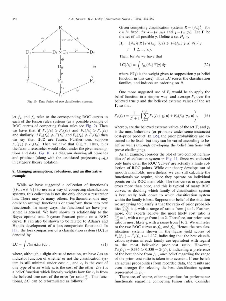
Fig. 10. Data fusion of two classification systems.


let fS and fT refer to the corresponding ROC curves toeach of the fusion rule�s systems (as a possible example ofROC curves of competing fusion rules see Fig. 9). Thenwe have that if F nðfSÞP F nðfAÞ and F nðfSÞP F nðfBÞand similarly, if F nðfTÞP F ðfAÞ and F nðfTÞP F nðfBÞ thenwe say that S;T are fusors. Furthermore, supposeF nðfSÞP F nðfTÞ. Then we have that S T. Thus, S isthe fusor a researcher would select under the given assump-tions and data. Fig. 10 is a diagram showing all branchesand products (along with the associated projectors q1,q2)in category theory notation.

8. Changing assumptions, robustness, and an illustrative

example

While we have suggested a collection of functionalsðfF n : n 2 NgÞ to use as a way of competing classificationsystems, this collection is not the only choice a researcherhas. There may be many others. Furthermore, one maydesire to average functionals or transform them into newfunctionals. In many ways, the functional we have pre-sented is general. We have shown its relationship to theBayes optimal and Neyman–Pearson points on a ROCcurve. It can also be shown to be related to Adam�s andHand�s development of a loss comparison functional. In[35], the loss comparison of a classification system (LC) isdenoted by

LC ¼Z

Iðc1ÞLðc1Þdc1; ð31Þ

where, although a slight abuse of notation, we have I as anindicator function of whether or not the classification sys-tem is still minimal under cost c1, and c1 is the cost ofone type of error while c0 is the cost of the other. L(c1) isa belief function which linearly weights how far c1 is fromthe believed true cost of the error (or ratio c0

c1). This func-

tional, LC, can be reformulated as follows:

Given competing classification systems R ¼ fAigki¼1 for

k 2 N fixed, fix a = (a1,a2) and c = (c1,c2). Let C bethe set of all possible c. Define a set Hc by

Hc ¼ Aj 2 R j F 2ðfAj ; c; aÞP F 2ðfAi ; c; aÞ 8i 6¼ j;

i ¼ 1; 2; . . . ; kg.

Then, for Ai we have that

LCðAiÞ ¼Z

CIHcðAiÞW ðcÞdc; ð32Þ

where W(c) is the weight given to supposition c (a belieffunction in this case). Thus LC scores the classificationfamilies, and induces an ordering on R.

One more suggested use of Fn would be to apply thebelief function in a simpler way, and average Fn over thebelieved true c and the believed extreme values of the setC, so that

SnðfAÞ ¼1

2n þ 1

X2n

i¼1

F nðfA; ci; aÞ þ F nðfA; c0; aÞ !

; ð33Þ

where ci are the believed extreme values of the set C, and c0

is the most believable (or probable under some instances)cost–prior product. In [35], the prior probabilities are as-sumed to be fixed, but they can be varied according to be-lief as well (although developing the belief functions willprove challenging).

As an example, consider the plot of two competing fam-ilies of classification system in Fig. 11. Since we collectedonly finite data, the ROC �curves� are actually a finite col-lection of ROC points. While our theory develops out ofsmooth manifolds, nevertheless, we can still calculate thefunctionals we require, since they operate on individualpoints on the ROC manifolds. The two curves in questioncross more than once, and this is typical of many ROCcurves, so deciding which family of classification systemis best really boils down to which classification systemwithin the family is best. Suppose our belief of the situationwe are trying to classify is that the ratio of prior probabil-ities PrðE1Þ

PrðE2Þis 1

2, with a range of ratios from 1

3to 1. Further-

more, our experts believe the most likely cost ratio isC2j1C1j2¼ 1, with a range from 1

2to 2. Therefore, our prior–cost

ratio is most likely 12, with a range from 1

6to 2. We will refer

to the two ROC curves as fC1and fC2

. Hence, the two clas-sification systems shown in the figure yield scores ofF 2ðfC1

Þ ¼ F 2ðfC2Þ ¼ 1:137, indicating that the best classifi-

cation systems in each family are equivalent with regardto the most believable prior–cost ratio. However,S2ðfC1

Þ ¼ 0:336 P 0:330 ¼ S2ðfC2Þ, indicating a preference

of the best choice from fC1, once belief regarding the range

of the prior–cost ratio is taken into account. If our beliefsare actual probabilities from recorded data, the results areeven stronger for selecting the best classification systemrepresented in fC1

.There are, of course, other suggestions for performance

functionals regarding competing fusion rules. Consider

Fig. 11. ROC curves of two competing classifier systems.


fusion rules as algorithms, divorcing them from the entireclassification system. Mahler [36] recommends using math-ematical information MoEs (measures of effectiveness)with respect to comparing performance of fusion algo-rithms (fusion rules). In particular, he refers to level 1fusion MoEs as being traditionally �localized� in their com-petence. His preferred approach is to use an information�metric�, the Kullback–Leibler discrimination functional,

KðfG; f Þ ¼Z

XfGðxÞlog2

fGðxÞf ðxÞ

� �dx;

where fG is a probability distribution of perfect or nearperfect ground truth, f is a probability distribution associ-ated with the fused output of the algorithm and X is theset of all possible measurements of the observation. Thisworks fine, if such distributions are at hand. One draw-back is that it measures the expected value of uncertaintyand therefore its relationship to costs and prior probabil-ities is obscure (as was the case with the Neyman–Pearsoncriteria). The previous functionals we have forwarded forconsideration operate on families of classification systems(in particular, ROC manifolds), not just systems which en-joy well-developed and tested probability distributionfunctions.

9. Conclusion

A fusion researcher should have a viable method ofcompeting fusion rules. This is required to correctly definefusion, and to demonstrate improvements over existingmethods. Every fusion system can generate a correspond-ing ROC curve, and under a mild assumption of smooth-

ness of the ROC curve, a Bayes optimal threshold (BOT)can be found for each family of classification systems.Given additional assumptions on the a priori probabilitiesof the classes of interest, along with given thresholds for theconditional probabilities of errors, a functional can be gen-erated over the ROC manifolds. Every such functional willgenerate a partial ordering on families of classification sys-tems, categories of fusion rules, and ultimately categoriesof fusors, which can then be used to select the best fusorfrom among a finite collection of fusors. We demonstrateone such functional, the ROC functional, which is scalableto ROC manifolds in dimensions higher than 2, as well asto families of classification systems which do not generateROC curves at all. The ROC functional, when populatedwith the appropriate data choices, will yield a value corre-sponding the Bayes optimal threshold with respect to theclassification system family being examined. The Ney-man–Pearson threshold of a classification system is shownto correspond to the output of the ROC functional withone such data choice (so that it corresponds with the Bayesoptimal threshold under one set of assumptions). Ulti-mately, a researcher could choose a cost–prior ratio whichseems most reasonable, then perturbate it, calculate themean ROC functional value, and choose the classificationsystem with the greatest average ROC functional value.This value would be a relative comparison of how robustthat classification system is to changes compared withother classification systems (e.g., it would answer the ques-tion of how much change is endured before another classi-fication system is optimal?). The relationship of the ROCfunctional to other functionals, including the loss compar-ison functional, is demonstrated. Finally, there are otherfunctionals to choose from, one which we mentioned, theKullback–Leibler discrimination functional, may be unre-lated to the ROC functional, yet may be suitable in partic-ular circumstances where prior probabilities and costs arenot fathomable, but probability distributions for fusionsystem algorithms and ground truth are available.

Appendix A

This appendix contains definitions for the understandingof category theory. We have drawn upon the work of var-ious authors in category theory literature [24–27] to presentthe definitions.

Definition 6 (Category). A category C is denoted as a 4-tuple, ðObðCÞ;ArðCÞ; IdðCÞ; �Þ, and consists of thefollowing:

(A1) A collection of objects denoted ObðCÞ.(A2) A collection of arrows denoted ArðCÞ.(A3) Two mappings, called domain (dom) and codomain

(cod), which assign to an arrow f 2 ArðCÞ a domainand codomain from the objects of ObðCÞ. Thus, forarrow f, given by O1!

fO2, dom(f) = O1 and cod(f) =

O2.


(A4) A mapping assigning each object O 2 ObðCÞ anunique arrow 1O 2 IdðCÞ called the identity arrow,such that

O!1O O;

and such that for any existing element, x, of O, wehave that

x 7!1O x.

(A5) A mapping, �, called composition, ArðCÞ� ArðCÞ!�

ArðCÞ. Thus, given f ; g 2 ArðCÞ with cod(f) =dom(g) there exists an unique h 2 ArðCÞ such thath = g � f.

Axioms A3–A5 lead to the associative and identity rules:

• Associative rule. Given appropriately defined arrows f, g,and h 2 ArðCÞ we have that

ðf � gÞ � h ¼ f � ðg � hÞ.• Identity rule. Given arrows A!f B and B!g A, then there

exists identity arrow 1A such that 1A � g = g andf � 1A = f.

Definition 7 (Subcategory). A subcategory B of A is acategory whose objects are some of the objects of A andwhose arrows are some of the arrows of A, such that foreach arrow f in B, dom(f) and cod(f) are in ObðBÞ, alongwith each composition of arrows, and an identity arrow foreach element of ObðBÞ.

Definition 8 (Discrete category). A discrete category is acategory whose only arrows are identity arrows.

A category of interest is the category Set, which has asits objects sets, that is Ob(Set) is a collection of sets, andits arrows, Ar(Set), the collection of all total functionsdefined on these sets, with its composition being the typicalcomposition of functions. Clearly this construct has iden-tity arrows and the associative rule applies, so it is indeeda category. The subcategories of interest to us are first, sub-categories of particular types of data sets, denoted D,whose objects are similar types of data and whose arrowsconsist of only the identity arrows, and second, subcatego-ries of particular types of feature sets, denoted F, whoseobjects are similar types of features, and whose arrowsare only the identity arrows. The objects and arrows ofthese categories shall correspond to a particular sensor sys-tem, so they will represent all of the possible data (or fea-tures) that can be generated by the sensor or processor.For example, the data generated by a particular sensor sys-tem may be represented in an N · N real-valued matrix. Inthis case, D ¼ ðRN�N ; idD; idD; �Þ represents a discrete cate-gory, whose objects are N · N matrices over the field of realnumbers, and whose arrows are only identity arrows, withcomposition, �, being the usual composition of functions.

A further categorical concept which will be useful is afunctor.

Definition 9 (Functor). A functor F between two catego-ries A and B is a pair of maps ðFOb;FArÞ

ObðAÞ !FOb

ObðBÞ;

ArðAÞ!FAr

ArðBÞ;

such that F maps ObðAÞ to ObðBÞ and ArðAÞ to ArðBÞwhile preserving the associative property of the composi-tion map and preserving identity maps.

Thus, given categories A;B and functor F : A! B, ifA 2 ObðAÞ and f ; g; h; 1A 2 ArðAÞ such that f � g = h isdefined, then there exists B 2 ObðBÞ andf 0; g0; h0; 1B 2 ArðBÞ such that

(i) FObðAÞ ¼ B.(ii) FArðf Þ ¼ f 0, FArðgÞ ¼ g0.

(iii) h0 ¼ FArðhÞ ¼ FArðf � gÞ ¼ FArðf Þ � FArðgÞ ¼ f 0 � g0.(iv) FArð1AÞ ¼ 1FObðAÞ ¼ 1B.

Definition 10 (Natural transformation). Given categoriesA and B and functors F and G with A!

FB and

A!G B, then a natural transformation is a family of arrowsm ¼ fmA j A 2 ObðAÞg such that for each f 2 ArðAÞ,A!f A0, A0 2 ObðAÞ, the square

commutes. We then say the arrows mA are the componentsof m : F! G, and call m the natural transformation of F toG.

Definition 11 (Functor category AB). Given categories Aand B, the notation AB represents the category of all func-tors F such that B!F A. This category has all such func-tors as objects and the natural transformations betweenthem as arrows.

Definition 12 (Product category). Let fCigni¼1 represent a

finite collection of small categories (i.e., those which canbe described using sets). Then

Yn

i¼1

Ci ¼ C1 � C2 � � Cn

is the corresponding product category.

Appendix B

Here we prove the extension of the calculus of variationsapproach to ROC manifolds. From Eq. (19) we generate


the first variation of J1. Let b > 0 be fixed, and leta 2 [�b,b] be a family of real parameters. Let

fRðt; aÞ ¼ ðX 1ðt; aÞ; . . . ;X mðt; aÞÞja 2 ½�b; b�g ð34Þbe a family of one-parameter trajectories which containsthe optimal curve defined by the function R*. Furthermore,we assume R(t, 0) = R*(t). Let Rðtf ; aÞ 2M for alla 2 [�b,b]. By the implicit function theorem there existsa function Tf(a) such that RðT fðaÞ; aÞ 2M for all a. Thus,Rðt�f ; 0Þ ¼ R�ðt�f Þ so that T fð0Þ ¼ t�f . Since R* minimizes J1,then a necessary optimality condition is that the first vari-ation of

J 1½Rð; aÞ� ¼Z T f ðaÞ

0

Gdt ð35Þ

is zero at a = 0 (see [33]), that is,

d

daJ ½Rð; aÞ�ja¼0 ¼ 0. ð36Þ

We use the operator notation

d ¼ d

daja¼0

for brevity. Applying Leibniz�s rule to J1[R( Æ ,a)] in Eq.(35) we get the derivative to be

dJ ½R�� ¼ G�jt¼t�fdT f þ

Z t�f

0

ðrxG� dRþryG� d _RÞdt;

ð37Þwhere G* is a suppressed notation for Gðt;R�ðtÞ; _R

�ðtÞÞ.Now integrating by parts yields

dJ ½R�� ¼ G�jt¼t�fdT f þ ½ryG� dR�t

�f

0

þZ t�

f

0

ðrxG� dR� d

dtryG� dRÞdt. ð38Þ

At a = 0 the necessary optimality condition implies

dJ ½R�� ¼ G�jt¼t�fdT f þ ½ryG� dR�t¼t�

f

þZ t�

f

0

rxG� dR� d

dtryG� dR

� �dt ¼ 0. ð39Þ

Since this must be true over all admissible variations(dR,dTf), we have the Euler equations

rxG� � d

dtryG� ¼ 0 ð40Þ

for all t 2 ½0; t�f � and a transversality condition

G�jt¼t�fdT f þ ½ryG� dR�t¼t�

f¼ 0. ð41Þ

Since G is independent of x then $xG* = 0. Using this insolving the Euler Eq. (40), yields

d

dtryG� ¼ 0; ð42Þ

hence, for i = 1, . . ., m

d

dtsgn ½ _X �i ðtÞ� ¼ 0 for all t 2 ð0; tfÞ. ð43Þ

Thus, integrating for each i = 1, . . .,m, we have

sgn ½ _X �i ðtÞ� ¼ Ki. ð44ÞHence, sgn ð _X

�i ðtÞÞ ¼ Ki for some constant Ki 2 R. For

i = 1, . . .,m, we have that DX �i ðtÞP 0 and Dt > 0 for all t,so that Ki = 0 or 1. We make the assumption thatX �i ðtfÞ 6¼ 0 for some i, since to say otherwise would indicatewe have the perfect classification system. Thus, we havethat Ki = 1 for at least one i. Hence, we have that{1,2, . . ., m} = N1 [ N0 is a partition such that

sgn ð _X�i ðtÞÞ ¼ 1

for all i 2 N1, and

sgn ð _X�i ðtÞÞ ¼ 0

for all i 2 N0. Since, R(Tf(a),a) terminates on M forall a, then W(R(Tf(a),a)) = 0 for all a. Let R�ðt�f Þ ¼ðx�1; . . . ; x�mÞ 2M. Hence,

X mðT fðaÞ; aÞ ¼ f ðX 1ðT fðaÞ; aÞ; . . . ;X m�1ðT fðaÞ; aÞÞ ð45Þ

for all a. Taking the variation of each side of Eq. (45), wehave

_X�mðt�f ÞdT f þ dX mðt�f Þ ¼

Xm�1

i¼1

of ðx�1; . . . ; x�m�1Þoxi

½dT f þ dX iðt�f Þ�.

ð46Þ

Expanding Eq. (46) and defining Hi(t) = dXi(t), we have

_X mðt�f ÞdT f þ Hmðt�f Þ ¼Xm�1

i¼1

of ðx�1; . . . ; x�m�1Þoxi

_X iðt�f ÞdT f

þXm�1

i¼1

of ðx�1; . . . ; x�m�1Þoxi

H iðt�f Þ. ð47Þ

Rearranging terms, rewriting in vector notation, and let-ting f � ¼ f ðx�1; . . . ; x�m�1Þ we have

of �

ox1

; . . . ;of �

oxm�1

;�1

� � H 1ðt�f Þ; . . . ;H m�1ðt�f Þ;H mðt�f Þ� �

þ of �

ox1

; . . . ;of �

oxm�1

;�1

� � _R�ðt�f ÞdT f ¼ 0 ð48Þ

which can be rewritten as

rW� Hðt�f Þ þ rW� _R�ðt�f ÞdT f ¼ 0. ð49Þ

From Eq. (41) we write

ryG�jt�fHðt�f Þ þ G�jt�

fdT f ¼ 0. ð50Þ

Since both Eqs. (49) and (50) must be true over all varia-tions and all possible one-parameter families, we have

rW�jt�f¼ kryG�jt�

fð51Þ

for some k 2 R. Hence, for i = 1, . . .,m we have

oWoxi

t¼t�

f

¼ kaisgn ð _X�i ðt�f ÞÞ. ð52Þ


In the case of i = m we have that

�1 ¼ oW�

ox3

jt¼t�f¼ ka3. ð53Þ

Thus, we have that k ¼ �1am

. Hence, for i = 1, . . .,m we havethat

oW�

oxi

t¼t�

f

¼ �ai

am. ð54Þ

This is a global minimum since we are optimizing a convexfunctional [34]. This solution agrees with the limited ap-proach, based on observation, made by Haspert [37].

References

[1] S. Thorsen, M. Oxley, Comparing fusors within a category of fusors,in: Proceedings of the Seventh International Conference of Informa-tion Fusion, ISIF, Stockholm, Sweden, 2004, pp. 435–441.

[2] L. Wald, Some terms of reference in data fusion, IEEE Transactionson Geoscience and Remote Sensing 37 (3) (1999) 1190–1193.

[3] D.M. Green, J.A. Swets, Signal Detection Theory and Psychophysics,John Wiley and Sons, New York, 1966.

[4] J.A. Hanley, B.J. McNeil, The meaning and use of the area under areceiver operating characteristic (ROC) curve, Radiology 143 (1982)29–36.

[5] L.L. Scharf, Statistical Signal Processing, Addison-Wesley, MA,1991.

[6] F.J. Provost, T. Fawcett, Robust classification systems for impreciseenvironments, in: AAAI/IAAI, 1998, pp. 706–713. Available from:<http://citeseer.ist.psu.edu/provost98robust.html>.

[7] L.C. Ludeman, Random Processes Filtering, Estimation, and Detec-tion, John Wiley and Sons, New Jersey, 2003.

[8] R.O. Duda, P.E. Hart, D.G. Stork, Pattern Classification, second ed.,John Wiley and Sons, New York, 2001.

[9] H.L. Van Trees, Detection, Estimation, and Modulation Theory,John Wiley and Sons, New York, 2001.

[10] C.E. Metz, Basic principles of ROC analysis, Seminars in NuclearMedicine 8 (4) (1978) 283–298.

[11] F.J. Provost, T. Fawcett, Robust classification for imprecise envi-ronments, Machine Learning 42 (3) (2001) 203–231. Available from:<http://citeseer.ist.psu.edu/provost01robust.html>.

[12] J.A. Swets, Measuring the accuracy of diagnostic systems, Science 240(1988) 1285–1293.

[13] C. Ferri, J. Hernandez-Orallo, M.A. Salido, Volume under the ROCsurface for multi-class problems, Exact computation and evaluationof approximations, 2003. Available from: <http://citeseer.ist.psu.edu/ferri03volume.html>.

[14] D. Mossman, Three-way ROCs, Medical Decision Making 19 (1)(1999) 78–89.

[15] S.N. Thorsen, M.E. Oxley, Describing data fusion using categorytheory, in: Proceedings of the Sixth International Conference onInformation Fusion, ISIF, Cairns Australia, 2003, pp. 1202–1206.

[16] S.N. Thorsen, M.E. Oxley, Multisensor fusion description usingcategory theory, in: IEEE Aerospace Conference. Proceedings, 2004,pp. 2016–2021.

[17] M.E. Oxley, S.N. Thorsen, Fusion and integration: What�s thedifference? in: P. Svensson, J. Schubert (Eds.), Proceedings of theSeventh International Conference on Information Fusion, Interna-

tional Society of Information Fusion, CA, 2004, pp. 429–434. Availablefrom: <http://www.fusion2004.foi.se/papers/IF04-0429.pdf>.

[18] S.A. DeLoach, M.M. Kokar, Category theory approach to fusion ofwavelet-based features, in: Proceedings of the Second InternationalConference on Fusion (Fusion 1999), vol. I, 1999, pp. 117–124.

[19] M.M. Kokar, J.A. Tomasik, J. Weyman, Data vs. decision fusion inthe category theory framework, in: Proceedings of the FourthInternational Conference on Fusion (Fusion 2001), vol. I, 2001.

[20] M. Healy, T. Caudell, Y. Xiao, From categorical semantics to neuralnetwork design, in: IEEE Transactions on Neural Networks,Proceedings of International Joint Conference on Neural Networks(IJCNN �03), 2003, pp. 1981–1986.

[21] M. Healy, Category theory applied to neural modeling and graphicalrepresentations, in: IEEE Transactions on Neural Networks, INNS-ENNS Proceedings of International Joint Conference on NeuralNetworks (IJCNN �00), vol. 3, 2000, pp. 35–40. Available from:<http://citeseer.ist.psu.edu/healy00category.html>.

[22] M. Healy, T. Caudell, A categorical semantic analysis of artarchitectures, in: IEEE Transactions on Neural Networks, Proceed-ings of International Joint Conference on Neural Networks (IJCNN�01), vol. 1, 2001, pp. 38–43.

[23] M. Healy, Colimits in memory: Category theory and neural systems,in: IEEE Transactions on Neural Networks, Proceedings of Interna-tional Joint Conference on Neural Networks (IJCNN �01), vol. 1,1999, pp. 492–496.

[24] S. MacLane, Categories for the Working Mathematician, second ed.,Springer, New York, 1978.

[25] C. McClarty, Elementary Categories, Elementary Toposes, OxfordUniversity Press, New York, 1992.

[26] J. Adamek, H. Herrlich, G. Strecker, Abstract and ConcreteCategories, John Wiley and Sons, New York, 1990.

[27] F.W. Lawvere, S.H. Schanuel, Conceptual Mathematics, A FirstIntroduction to Categories, Cambridge University Press, CambridgeUK, 1991.

[28] P. Billingsley, Probability and Measure, third ed., John Wiley andSons, New York, 1995.

[29] L. Xu, A. Krzyak, Y.C. Suen, Methods of combining multipleclassifiers and their applications to handwriting recognition, in: IEEETransactions on Systems, Man, and Cybernetics, vol. XXII, 1992, pp.418–435.

[30] D.L. Hall, J. Llinas, Handbook of Multisensor Data Fusion, CRCPress, Florida, 2001.

[31] C. Schubert, M.E. Oxley, K.W. Bauer, A comparison of ROC curvesfor label-fused within and across classifier systems, in: Proceedings ofthe Ninth International Conference on Information Fusion, Interna-tional Society of Information Fusion, 2005.

[32] S.G. Alsing, The evaluation of competing classifiers, Ph.D. disserta-tion, Air Force Institute of Technology, Wright-Patterson AFB OH,March 2000.

[33] I.M. Gelfand, S.V. Fomin, Calculus of Variations, Dover, New York,2000.

[34] D.G. Luenberger, Optimization by Vector Space MethodsWileyProfessional Paperback Series, John Wiley and Sons, New York,1969.

[35] N. Adams, D. Hand, Improving the practice of classifier performanceassessment, Neural Computation XII (2000) 305–311.

[36] R.P. Mahler, An Introduction to Multisource–Multitarget Statisticsand its Applications, Lockheed Martin, MN, 2000.

[37] J.K. Haspert, Optimum ID sensor fusion for multiple target types,Technical Report IDA Document D-2451, Institute for DefenseAnalyses, March 2000.

http://citeseer.ist.psu.edu/provost98robust.html

http://citeseer.ist.psu.edu/provost01robust.html

http://citeseer.ist.psu.edu/ferri03volume.html

http://citeseer.ist.psu.edu/ferri03volume.html

http://www.fusion2004.foi.se/papers/IF04-0429.pdf

http://citeseer.ist.psu.edu/healy00category.html

Documents

A description of competing fusion systems