A filtered backprojection algorithm with ray-by-ray noise weightingGengsheng L. Zeng and Alex Zamyatin Citation: Medical Physics 40, 031113 (2013); doi: 10.1118/1.4790696 View online: http://dx.doi.org/10.1118/1.4790696 View Table of Contents: http://scitation.aip.org/content/aapm/journal/medphys/40/3?ver=pdfcov Published by the American Association of Physicists in Medicine Articles you may be interested in Assessment of the dose reduction potential of a model-based iterative reconstruction algorithm using a task-based performance metrology Med. Phys. 42, 314 (2015); 10.1118/1.4903899 Characterization of adaptive statistical iterative reconstruction algorithm for dose reduction in CT: A pediatriconcology perspective Med. Phys. 39, 5520 (2012); 10.1118/1.4745563 A filtered backprojection MAP algorithm with nonuniform sampling and noise modeling Med. Phys. 39, 2170 (2012); 10.1118/1.3697736 Noise-resolution tradeoffs in x-ray CT imaging: A comparison of penalized alternating minimization and filteredbackprojection algorithms Med. Phys. 38, 1444 (2011); 10.1118/1.3549757 Matched view weighting in tilted-plane-based reconstruction algorithms to suppress helical artifacts and optimizenoise characteristics Med. Phys. 30, 2912 (2003); 10.1118/1.1619231

A filtered backprojection algorithm with ray-by-ray noise weightingGengsheng L. Zenga)

Utah Center for Advanced Imaging Research (UCAIR), Department of Radiology, University of Utah,Salt Lake City, Utah 84108

Alex Zamyatinb)

Toshiba Medical Research Institute USA, Inc., 706 North Deerpath Drive, Vernon Hills, Illinois 60061

(Received 1 August 2012; revised 15 January 2013; accepted for publication 23 January 2013;published 28 February 2013)

Purpose: This paper derives a ray-by-ray weighted filtered backprojection (rFBP) algorithm, basedon our recently developed view-by-view weighted, filtered backprojection (vFBP) algorithm.Methods: The rFBP algorithm directly extends the vFBP algorithm by letting the noise weightingvary from channel to channel within each view. The projection data can be weighted in inverse pro-portion to their noise variances. Also, an edge-preserving bilateral filter is suggested to perform postfiltering to further reduce the noise. The proposed algorithm has been implemented for the circular-orbit cone-beam geometry based on Feldkamp’s algorithm.Results: Image reconstructions with computer simulations and clinical cadaver data are presented toillustrate the effectiveness and feasibility of the proposed algorithm. The new FBP-type algorithm isable to significantly reduce or remove the noise texture, which the conventional FBP is unable to do.The computation time of the proposed rFBP algorithm is approximately the same as the conventionalFBP algorithm.Conclusions: A ray-based noise-weighting scheme is introduced to the FBP algorithm. Thisnew FBP-type algorithm significantly reduces or removes the streaking artifacts in low-dose CT.© 2013 American Association of Physicists in Medicine. [http://dx.doi.org/10.1118/1.4790696]

Key words: image reconstruction, analytical reconstruction algorithm, tomography, noise modeling,CT, edge-preserving filtering

I. INTRODUCTION

The filtered backprojection (FBP) algorithm has been in usefor several decades.1–5 It is the work horse in x-ray CT andnuclear medicine image reconstruction. A drawback of theFBP algorithm is that it produces very noisy images whenthe data are noisy. By contrast, the iterative algorithms areable to incorporate the projection noise model and produceless noisy images than the FBP algorithm.6–10 As a trend, theFBP algorithm is gradually getting replaced by iterative algo-rithms. However, iterative algorithms have long computationtimes. In order to shorten the computation times, effort hasbeen made to transform a regular iterative algorithm into aniterative FBP algorithm.11

Recently we developed a noniterative FBP algorithm thatcan model the projection noise on a view-by-view basis, inwhich an average or a maximum noise variance is used forall projection rays in each view.12 It was an initial attemptto use the FBP algorithm to model data noise. In the view-by-view weighted FBP (vFBP) algorithm, a single weightingfactor, w(view), is assigned to all projection rays in a view.This noise-weighting scheme is not as accurate as ray-by-raynoise weighting, which is now proposed in the current paper.

The regularization term in our previous vFBP algorithmwas quadratic. We realize that a quadric regularization termis unable to perform edge-preserving smoothing. The cur-rent paper therefore uses an edge-preserving bilateral fil-ter as a post filter to further reduce the noise. The ray-wise weighting FBP (rFBP) algorithm will be developed in

Sec. II. A specially designed bilateral filter is also presented inSec. II. Computer simulations and an application to low-doseclinical cone-beam CT image reconstruction are presented inSec. III. Discussion and conclusions are given in Sec. IV.

II. METHODS

II.A. Ray-by-ray noise weighted FBP algorithm

Statistical weighting in iterative reconstruction algorithmsis a well-established practice.13–15 Because the iterative algo-rithms use long computations times, in CT imaging, noisecontrol is normally achieved using either prefiltering orpostfiltering.16–20 In prefiltering methods, a lowpass filter ora nonlinear filter can be used, where the filtering strengthor bandwidth for each measurement is determined by themodel.16, 19 We have previously introduced a view-by-viewweighting FBP algorithm (referred to as the vFBP algorithm)by minimizing a weighted least-square objective function.12

The vFBP algorithm is almost the same as the conventionalFBP algorithm, except that the ramp filter |ω| is replaced by

Hk,α,β,w(ω) =1 − (

1 − αw|ω| − αβR

)k

1 + β Rw|ω| |ω|,

with ω �= 0,

and Hk,α,β,w(0) = 0, (1)

where ω is the frequency variable in the projection space, kcorresponds to the iteration number in an iterative algorithm,

031113-1 Med. Phys. 40 (3), March 2013 © 2013 Am. Assoc. Phys. Med. 031113-10094-2405/2013/40(3)/031113/7/$30.00

031113-2 G. L. Zeng and A. A. Zamyatin: FBP algorithm with ray-wise noise weighting 031113-2

α corresponds to the step-size in an iterative algorithm, β isthe contributing factor of the regularization term in the ob-jective function, w is the weighting function varying with theview angle [i.e., w = w(view)], and R is the filter functionin the regularization term. In this paper, the minimum normregularization is assumed and R is a constant 1 in (1). Thegeneralized ramp-filter (1) is used for projection data filter-ing, and the filtered data are backprojected to obtain the finalimage. No modification is required for the backprojector, forthe vFBP or for the new rFBP algorithm.

Next, we will extend the view-by-view noise weightingto ray-by-ray noise weighting in an ad hoc manner. Forthe ray-based noise weighting, w is a function of the ray:w = w(ray). A popular approach to assigning the weightingfactor is to let w(ray) be proportional to the reciprocal of thenoise variance of the ray measurement. At each view angle,we quantize the ray-based weighting function into N + 1 val-ues: w0, w1, . . . , wN , which in turn give N + 1 different filtersas defined in (1). They are

Hk,α,β,wn(ω) =

1 − (1 − αwn

|ω| − αβ)k

1 + β|ω|wn

|ω|,

with

ω �= 0, and Hk,α,β,wn(0) = 0, (2)

for n = 0, 1, 2, . . . , N. Using these N + 1 filters, N + 1 sets offiltered projections are obtained. Before backprojection, oneof these N + 1 projections is selected for each ray according toits proper weighting function, which will be further explainedwhen implementation issues are discussed later in this paper.Only one backprojection is performed using the selected fil-tered projections.

II.B. Edge-preserving bilateral filter

One drawback of the rFBP algorithm is that its Bayesian(regularization) prior must be quadratic and it is unable toincorporate edge-preserving filtering during image recon-struction. The objective function and the Bayesian prior arenot shown in this paper; the interested reader should referto Ref. 12 for its setup. Our strategy is to apply a nonlinear,edge-preserving, bilateral filter to the result of the rFBPreconstruction.

Bilateral filters are a class of nonlinear filters that are spec-ified by both domain (Fdomain) and range (Frange) functions.21

A general form of the input/output relationship of a bilateralfilter is

xoutput

k =

∑j∈�(k)

xinput

j Fdomain(k, j )Frange

(x

input

k − xinput

j

)∑

j∈�(k)Fdomain(k, j )Frange

(x

input

k − xinput

j

) ,

(3)

where xinput

j represents the jth pixel of the input (unfiltered)

image, xoutput

j represents the jth pixel of the output (filtered)image, �(k) is a neighborhood around pixel k, Fdomain is a“domain” function, and Frange is a “range” function. In many

applications, Fdomain and Frange are chosen to be Gaussianfunctions.

Bilateral filters can be specially designed according to theapplication. The edge-preserving bilateral filter in this paperis described as follows.

� Specify a small neighborhood �(k) centered at pixel k,for example, an r x r region in a two-dimensional (2D)image. At each image pixel k, filtering is performed onlyin this region.

� Specify a threshold value Th. This value Th representsthe smallest edge jump or smallest detectable contrast.Image variation smaller than this value Th is considerednoise.

� At each image pixel k, the filtered image value xk is theaverage value of all pixels in the set {xj: j ∈ �(k) and|xk − xj| < Th}.

Using the notation in (3), our design is as follows:

�(k) = an r × r region, centered at pixel k, (4)

Fdomain(k, j ) = 1 if j ∈ �(k),

and

Fdomain(k, j ) = 0 if j /∈ �(k), (5)

Frange(xk − xj ) = 1 if |xk − xj | < T h,

and

Frange(xk − xj ) = 0 if |xk − xj | ≥ T h. (6)

Our strategy is to use the average value to replace the orig-inal image value. Not every image pixel is allowed to partic-ipate in the “average” operation. To be qualified, a pixel xj

must satisfy two conditions: it must be in the close neighbor-hood of the pixel of interest xk, and its value xj is close enoughto the value of xk. One could use a larger neighborhood �(k)or use a smaller neighborhood �(k) but apply the smaller filtermultiple times.

A drawback of this bilateral filter is that if the noise influ-ence is larger than the smallest contrast Th, the noise influencecannot be filtered out. Any edge whose contrast is smallerthan Th will be smoothed out.

II.C. Implementation of the new rFBP algorithm

Let the inverse Fourier transform of Hk,α,β,w (ω) behk,α,β,w (t), which is the spatial-domain kernel of the 1D mod-ified ramp filter. In the rFBP algorithm, w is a function of theprojection ray, therefore, w = w(t, θ ). Let p(t, θ ) be the pro-jection at view θ and location t on the detector, and q(t, θ ) bethe filtered projection. Then q(t, θ ) is defined by the followingintegral:

q(t, θ ) =∫ ∞

−∞p(τ, θ )hk,α,β,w(t,θ ) (t − τ ) dτ, (7)

which is not a convolution, because the kernel hk,α,β,w(t,θ ) (τ )depends on t. The final image is obtained by backprojectingq(t, θ ) into the image domain, and the backprojector is the

Medical Physics, Vol. 40, No. 3, March 2013

031113-3 G. L. Zeng and A. A. Zamyatin: FBP algorithm with ray-wise noise weighting 031113-3

same as that in a conventional FBP algorithm. Therefore, theonly thing new in implementing the rFBP algorithm is to cal-culate q(t, θ ), which will be discussed in detail as follows.

One way to calculate q(t, θ ) is to use (7) to filter the projec-tions in the spatial domain. However, we currently do not havean analytical expression for the integration kernel hk,α,β,w (t).Our strategy is to implement (7) in the Fourier domain andto quantize the weighting function w(t, θ ) into 11 values ofexp(− 0.1 · n · pmax), where pmax is the maximum projectionvalue, and n = 0, 1, 2, . . . ,10. The efficient fast Fourier trans-form (FFT) is used. The implementation steps of calculatingq(t, θ ) are given below.

Before the projections data are ready to process, form11 Fourier domain filter transfer functions Hk,α,β,wn

(ω) asdefined in (2) with wn = exp(−0.1 · n · pmax), n = 0, 1, 2,. . . ,10, respectively. Note that in implementation, ω is a dis-crete frequency index and takes the integer values of 0, 1, 2,. . . and so on.

Step 1: At each view angle θ , find the 1D Fouriertransform of p(t, θ ) with respect to t, obtainingP(ω, θ ).

Step 2: Form 11 versions of Qn(ω, θ ) = P(ω, θ )Hk,α,β,wn

(ω) with n = 0, 1, . . . , 10.Step 3: Take the 1D inverse Fourier transform of Qn(ω, θ )

with respect to ω, obtaining qn(t,θ ) with n = 0,1, . . . , 10.

Step 4: Construct q(t,θ ) by letting q(t,θ ) = qn(t,θ ) if p(t,θ ) ≈ 0.1 · n · pmax.

II.D. Low-dose cadaver CT study

To illustrate the feasibility of the proposed rFBP algorithm,a cadaver torso was scanned using an x-ray CT scanner witha low-dose setting. The images were then reconstructed by aconventional FBP (the Feldkamp) algorithm23 as well as theproposed rFBP algorithm. Data were collected with a diag-nostic scanner (Aquilion ONETM, Toshiba America MedicalSystems, Tustin, CA, USA; raw data courtesy of Leiden Uni-versity Medical Center).

The imaging geometry was cone-beam, the x-ray sourcetrajectory was a circle of radius 600 mm. The detector had320 rows, the row-height was 0.5 mm, each row had 896 chan-nels, and the fan angle was 49.2◦. A low-dose noisy scan wascarried out. The tube voltage was 120 kV and current was60 mA. There were 1200 views uniformly sampled over 360◦.

The Feldkamp algorithm is an FBP algorithm. The datawere first weighted with a cosine function, and then a 1Dramp filter was applied to each row of the cone-beam projec-tions. Finally a cone-beam backprojection was used to gen-erate a 3D image volume. In our implementation, the 1Dramp filter was replaced by the newly developed ramp fil-ter (2). The parameter β was selected as 2.6 × 10−5, itera-tion index k was chosen as infinity, and the step-size α wasnot needed. The noise weighting function was defined byw(t, θ ) = exp(−p(t, θ )), in which we assumed that the trans-mission measurement was approximately Poisson distributed

and the line-integral p(t,θ ) was the logarithm of the transmis-sion measurement.

The image volume was reconstructed in a 512 × 512 × 3203D array, and one axial slice is used for display in this paper.The bilateral post filtering was performed slice by slice, usinga 9 × 9 neighborhood and the threshold of 70 HU.

II.E. Computer simulation

The image array was 800 × 800, the pixel size was0.575 mm × 0.575 mm, the number of views was 900 over360◦, the number of detection channels was 896, and the fo-cal length was 600 mm. The x-ray source flux had 106 counts.

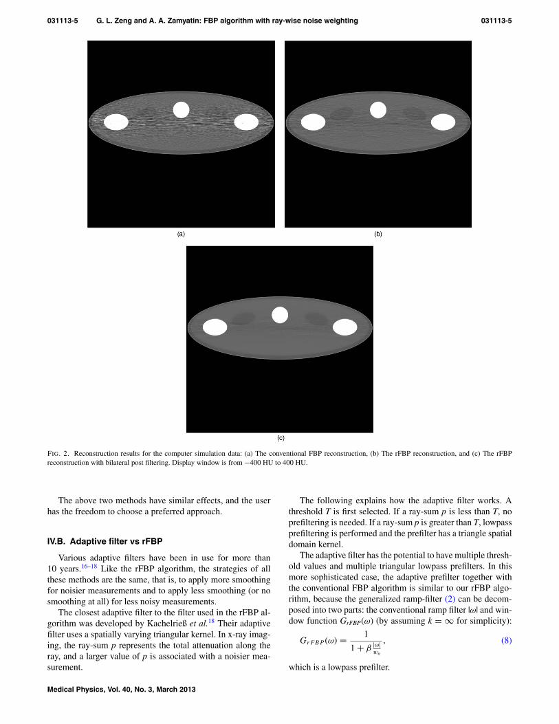
The images were reconstructed by both the conventionalFBP algorithm and the proposed rFBP algorithm. In the rFBPreconstruction, the parameter k was chosen as 1 000 000 andthe parameter α was 0.5. The noise weighting was chosen asw = e−0.3p, where p was the converted line-integral measure-ment for a ray. Noise weighting w is a double-edged sword.It can suppress some noise that is caused by anisotropic noisecontribution from different projections; it can also cause someshadow artifacts if the noise weighting function w fluctu-ates too much. Since the standard noise weighting functionw = e−p introduces some severe shadow artifacts, we re-placed it by w = e−0.3p that has less dynamic change thanw = e−p.

A bilateral post filter with r = 9 and Th = 50 HU was usedto further reduce the noise.

III. RESULTS

III.A. The cadaver data

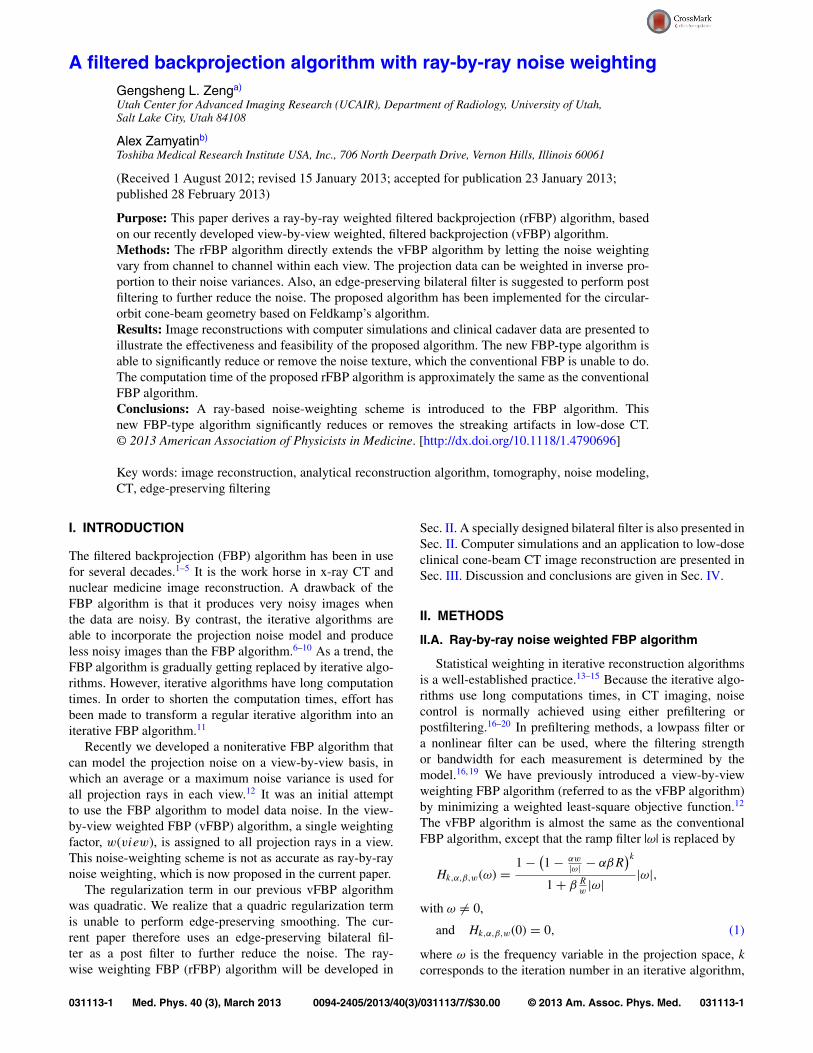
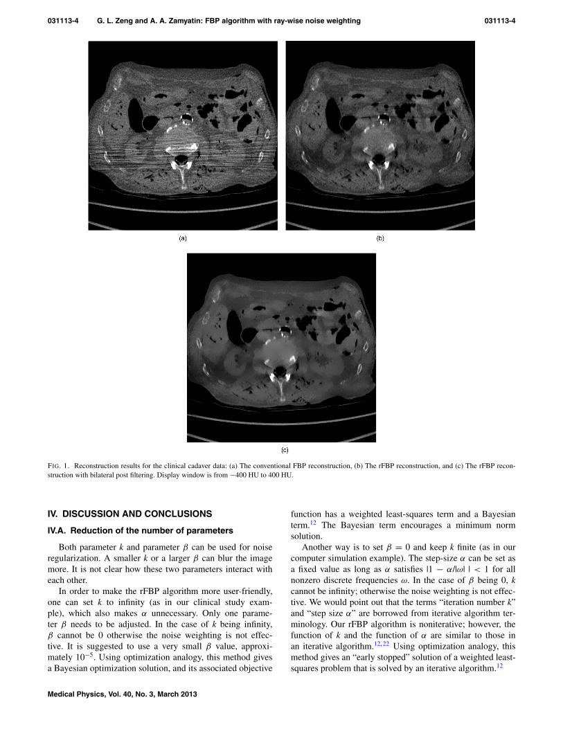
Figure 1(a) shows the conventional FBP Feldkamp’s re-construction of a transverse slice in the abdominal region ofthe cadaver. This study used low dose. The cadaver arms wereoutside the display field of view; the arms further attenuatedthe x-rays, creating streak artifacts in the middle of the imagefrom left-to-right across the torso. Figure 1(b) shows the rFBPreconstruction, with β = 2.6 × 10−5, k = ∞, and w = e−p.The ray-based noise weighting in the rFBP algorithm effec-tively removes the streaking artifacts that appear in Fig. 1(a).

Figure 1(c) shows the result of the bilateral post filtering,using the rFBP result as the input. The image in Fig. 1(c) isless noisy than Fig. 1(b) while it maintains the main edgesin Fig. 1(b) un-smoothed. The images are displayed from−400 HU to 400 HU.

III.B. Computer simulation data

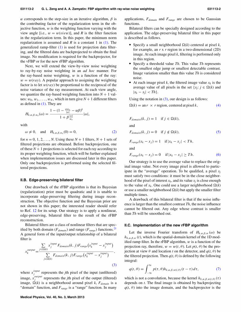
Figure 2 shows a real-size phantom study, which comparesthe conventional FBP reconstruction (see Fig. 2(a)) with theproposed rFBP reconstruction (see Fig. 2(b)), using β = 0, k= 1 000 000, α = 0.5, and w = e−0.3p. It is observed thatstreaking artifacts that appeared in the FBP reconstructionhave been reduced in the rFBP reconstruction. The bilateralpost filtering result is shown in Fig. 2(c); the input image forthe bilateral filter is the result of the rFBP reconstruction. Theimages are displayed from −400 HU to 400 HU.

Medical Physics, Vol. 40, No. 3, March 2013

031113-4 G. L. Zeng and A. A. Zamyatin: FBP algorithm with ray-wise noise weighting 031113-4

FIG. 1. Reconstruction results for the clinical cadaver data: (a) The conventional FBP reconstruction, (b) The rFBP reconstruction, and (c) The rFBP recon-struction with bilateral post filtering. Display window is from −400 HU to 400 HU.

IV. DISCUSSION AND CONCLUSIONS

IV.A. Reduction of the number of parameters

Both parameter k and parameter β can be used for noiseregularization. A smaller k or a larger β can blur the imagemore. It is not clear how these two parameters interact witheach other.

In order to make the rFBP algorithm more user-friendly,one can set k to infinity (as in our clinical study exam-ple), which also makes α unnecessary. Only one parame-ter β needs to be adjusted. In the case of k being infinity,β cannot be 0 otherwise the noise weighting is not effec-tive. It is suggested to use a very small β value, approxi-mately 10−5. Using optimization analogy, this method givesa Bayesian optimization solution, and its associated objective

function has a weighted least-squares term and a Bayesianterm.12 The Bayesian term encourages a minimum normsolution.

Another way is to set β = 0 and keep k finite (as in ourcomputer simulation example). The step-size α can be set asa fixed value as long as α satisfies |1 − α/|ω| | < 1 for allnonzero discrete frequencies ω. In the case of β being 0, kcannot be infinity; otherwise the noise weighting is not effec-tive. We would point out that the terms “iteration number k”and “step size α” are borrowed from iterative algorithm ter-minology. Our rFBP algorithm is noniterative; however, thefunction of k and the function of α are similar to those inan iterative algorithm.12, 22 Using optimization analogy, thismethod gives an “early stopped” solution of a weighted least-squares problem that is solved by an iterative algorithm.12

Medical Physics, Vol. 40, No. 3, March 2013

031113-5 G. L. Zeng and A. A. Zamyatin: FBP algorithm with ray-wise noise weighting 031113-5

FIG. 2. Reconstruction results for the computer simulation data: (a) The conventional FBP reconstruction, (b) The rFBP reconstruction, and (c) The rFBPreconstruction with bilateral post filtering. Display window is from −400 HU to 400 HU.

The above two methods have similar effects, and the userhas the freedom to choose a preferred approach.

IV.B. Adaptive filter vs rFBP

Various adaptive filters have been in use for more than10 years.16–18 Like the rFBP algorithm, the strategies of allthese methods are the same, that is, to apply more smoothingfor noisier measurements and to apply less smoothing (or nosmoothing at all) for less noisy measurements.

The closest adaptive filter to the filter used in the rFBP al-gorithm was developed by Kachelrieß et al.18 Their adaptivefilter uses a spatially varying triangular kernel. In x-ray imag-ing, the ray-sum p represents the total attenuation along theray, and a larger value of p is associated with a noisier mea-surement.

The following explains how the adaptive filter works. Athreshold T is first selected. If a ray-sum p is less than T, noprefiltering is needed. If a ray-sum p is greater than T, lowpassprefiltering is performed and the prefilter has a triangle spatialdomain kernel.

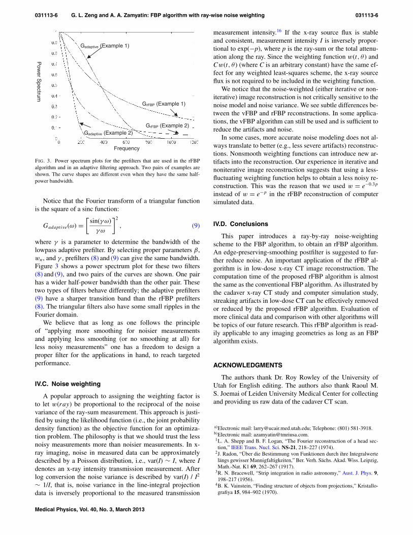
The adaptive filter has the potential to have multiple thresh-old values and multiple triangular lowpass prefilters. In thismore sophisticated case, the adaptive prefilter together withthe conventional FBP algorithm is similar to our rFBP algo-rithm, because the generalized ramp-filter (2) can be decom-posed into two parts: the conventional ramp filter |ω| and win-dow function GrFBP(ω) (by assuming k = ∞ for simplicity):

GrFBP (ω) = 1

1 + β|ω|wn

, (8)

which is a lowpass prefilter.

Medical Physics, Vol. 40, No. 3, March 2013

031113-6 G. L. Zeng and A. A. Zamyatin: FBP algorithm with ray-wise noise weighting 031113-6

GrFBP (Example 1)

GrFBP (Example 2) Gadaptive (Example 2)

Gadaptive (Example 1)

Frequency

Pow

er Spectrum

FIG. 3. Power spectrum plots for the prefilters that are used in the rFBPalgorithm and in an adaptive filtering approach. Two pairs of examples areshown. The curve shapes are different even when they have the same half-power bandwidth.

Notice that the Fourier transform of a triangular functionis the square of a sinc function:

Gadaptive(ω) =[

sin(γω)

γω

]2

, (9)

where γ is a parameter to determine the bandwidth of thelowpass adaptive prefilter. By selecting proper parameters β,wn, and γ , prefilters (8) and (9) can give the same bandwidth.Figure 3 shows a power spectrum plot for these two filters(8) and (9), and two pairs of the curves are shown. One pairhas a wider half-power bandwidth than the other pair. Thesetwo types of filters behave differently; the adaptive prefilters(9) have a sharper transition band than the rFBP prefilters(8). The triangular filters also have some small ripples in theFourier domain.

We believe that as long as one follows the principleof “applying more smoothing for noisier measurementsand applying less smoothing (or no smoothing at all) forless noisy measurements” one has a freedom to design aproper filter for the applications in hand, to reach targetedperformance.

IV.C. Noise weighting

A popular approach to assigning the weighting factor isto let w(ray) be proportional to the reciprocal of the noisevariance of the ray-sum measurement. This approach is justi-fied by using the likelihood function (i.e., the joint probabilitydensity function) as the objective function for an optimiza-tion problem. The philosophy is that we should trust the lessnoisy measurements more than noisier measurements. In x-ray imaging, noise in measured data can be approximatelydescribed by a Poisson distribution, i.e., var(I) ∼ I, where Idenotes an x-ray intensity transmission measurement. Afterlog conversion the noise variance is described by var(I) / I2

∼ 1/I, that is, noise variance in the line-integral projectiondata is inversely proportional to the measured transmission

measurement intensity.16 If the x-ray source flux is stableand consistent, measurement intensity I is inversely propor-tional to exp(−p), where p is the ray-sum or the total attenu-ation along the ray. Since the weighting function w(t, θ ) andCw(t, θ ) (where C is an arbitrary constant) have the same ef-fect for any weighted least-squares scheme, the x-ray sourceflux is not required to be included in the weighting function.

We notice that the noise-weighted (either iterative or non-iterative) image reconstruction is not critically sensitive to thenoise model and noise variance. We see subtle differences be-tween the vFBP and rFBP reconstructions. In some applica-tions, the vFBP algorithm can still be used and is sufficient toreduce the artifacts and noise.

In some cases, more accurate noise modeling does not al-ways translate to better (e.g., less severe artifacts) reconstruc-tions. Nonsmooth weighting functions can introduce new ar-tifacts into the reconstruction. Our experience in iterative andnoniterative image reconstruction suggests that using a less-fluctuating weighting function helps to obtain a less noisy re-construction. This was the reason that we used w = e−0.3p

instead of w = e−p in the rFBP reconstruction of computersimulated data.

IV.D. Conclusions

This paper introduces a ray-by-ray noise-weightingscheme to the FBP algorithm, to obtain an rFBP algorithm.An edge-preserving-smoothing postfilter is suggested to fur-ther reduce noise. An important application of the rFBP al-gorithm is in low-dose x-ray CT image reconstruction. Thecomputation time of the proposed rFBP algorithm is almostthe same as the conventional FBP algorithm. As illustrated bythe cadaver x-ray CT study and computer simulation study,streaking artifacts in low-dose CT can be effectively removedor reduced by the proposed rFBP algorithm. Evaluation ofmore clinical data and comparison with other algorithms willbe topics of our future research. This rFBP algorithm is read-ily applicable to any imaging geometries as long as an FBPalgorithm exists.

ACKNOWLEDGMENTS

The authors thank Dr. Roy Rowley of the University ofUtah for English editing. The authors also thank Raoul M.S. Joemai of Leiden University Medical Center for collectingand providing us raw data of the cadaver CT scan.

a)Electronic mail: larry@ucair.med.utah.edu; Telephone: (801) 581-3918.b)Electronic mail: azamyatin@tmriusa.com.1L. A. Shepp and B. F. Logan, “The Fourier reconstruction of a head sec-tion,” IEEE Trans. Nucl. Sci. NS-21, 218–227 (1974).

2J. Radon, “Über die Bestimmung von Funktionen durch ihre Integralwertelängs gewisser Mannigfaltigkeiten,” Ber. Verh. Sächs. Akad. Wiss. Leipzig,Math.-Nat. K1 69, 262–267 (1917).

3R. N. Bracewell, “Strip integration in radio astronomy,” Aust. J. Phys. 9,198–217 (1956).

4B. K. Vainstein, “Finding structure of objects from projections,” Kristallo-grafiya 15, 984–902 (1970).

Medical Physics, Vol. 40, No. 3, March 2013

031113-7 G. L. Zeng and A. A. Zamyatin: FBP algorithm with ray-wise noise weighting 031113-7

5G. L. Zeng, Medical Image Reconstruction, A Conceptual Tutorial(Springer, Beijing, 2010).

6S. German and D. E. McClure, “Statistical methods for tomographic imagereconstruction,” Bull. Internat. Statist. Inst. LII-4, 5–21 (1987).

7A. Dempster, N. Laird, and D. Rubin, “Maximum likelihood from incom-plete data via the EM algorithm,” J. R. Stat. Soc. Ser. B (Methodol) 39B,1–38 (1977).

8L. A. Shepp and Y. Vardi, “Maximum likelihood reconstruction for emis-sion tomography,” IEEE Trans. Med. Imaging 1, 113–122 (1982).

9H. M. Hudson and R. S. Larkin, “Accelerated image reconstruction usingordered subsets of projection data,” IEEE Trans. Med. Imaging 13, 601–609 (1994).

10K. Langer and R. Carson, “EM reconstruction algorithms for emission andtransmission tomography,” J. Comput. Assist. Tomogr. 8, 302–316 (1984).

11A. H. Delaney and Y. Bresler, “A fast and accurate Fourier algorithm foriterative parallel-beam tomography,” IEEE Trans. Image Process. 5, 740–753 (1996).

12G. L. Zeng, “A filtered backprojection MAP algorithm with non-uniformsampling and noise modeling,” Med. Phys. 39, 2170–2178 (2012).

13D. Shi, Y. Zou, and A. A. Zamyatin, “Weighted simultaneous algebraic re-construction technique,” in Proceedings of the 11th International Meetingon Fully Three-Dimensional Image Reconstruction Meeting in Radiologyand Nuclear Medicine, Potsdam, Germany (2011), pp. 160–162.

14J. Thibault, K. Sauer, C. Bouman, and J. Hsieh, “A three-dimensional sta-tistical approach to improved image quality for multislice helical CT,”Med. Phys. 34, 4526–4544 (2007).

15T. Kohler, R. Proksa, and T. Nielsen, “SNR-weighted ART applied totransmission tomography,” IEEE Nuclear Science Symposium and Medi-

cal Imaging Conference Record (IEEE, Portland, Oregon, 2003), pp. 2739–2742.

16J. Hsieh, “Adaptive streak artifact reduction in computed tomography re-sulting from excessive x-ray photon noise,” Med. Phys. 25, 2139–2147(1998).

17M. Kachelrieß, “Branchless vectorized median filtering,” IEEE MedicalImaging Conference Record, Workshop on High Performance MedicalImaging (IEEE, Orlando, Florida, 2009), Vol. HP3-5, pp. 4099–4105.

18M. Kachelrieß, O. Watzke, and W. A. Kalender, “Generalized multi-dimensional adaptive filtering for conventional and spiral single-slice,multi-slice, and cone-beam CT,” Med. Phys. 28, 475–490 (2001).

19A. A. Zamyatin, Z. Yang, and N. Akino, “Streak artifacts and noise reduc-tion in low dose computed tomography,” IEEE Nuclear Science Symposiumand Medical Imaging Conference Record (IEEE, Valencia, Spain, 2011),pp. 4150–4151.

20Z. Yang, M. D. Silver, and Y. Noshi, “Adaptive weighted aniso-tropic diffu-sion for computed tomography denoising,” Proceedings of the 11th Inter-national Meeting on Fully Three-Dimensional Image Reconstruction Meet-ing in Radiology and Nuclear Medicine (IEEE, Potsdam, Germany, 2011),pp. 210–213.

21C. Tomasi and R. Manduchi, “Bilateral Filtering for Gray and Color Im-ages,” in Proceedings of the 1998 IEEE International Conference on Com-puter Vision (IEEE, Bombay, India, 1998).

22G. L. Zeng, “A filtered backprojection algorithm with characteris-tics of the iterative Landweber algorithm,” Med. Phys. 39, 603–607(2012).

23L. A. Feldkamp, L. C. Davis, and J. W. Kress, “Practical cone beam algo-rithm,” J. Opt. Soc. Am. A 1, 612–619 (1984).

Medical Physics, Vol. 40, No. 3, March 2013