A FLUX-CORRECTED FINITE ELEMENT METHOD FOR CHEMOTAXISPROBLEMS ∗

ROBERT STREHL, ANDRIY SOKOLOV, DMITRI KUZMIN AND STEFAN TUREK†

Abstract. An implicit flux-corrected transport (FCT) algorithm is developed for a class of chemotaxis models.The coefficients of the Galerkin finite element discretization are adjusted in such a way as to guarantee mass con-servation and keep the cell density nonnegative. The numerical behaviour of the proposed high-resolution scheme istested on the blow-up problem for a minimal chemotaxis model withsingularities. It is also shown that the resultsfor anEscherichia colichemotaxis model are in good agreement with experimental data reported in the literature.

Key words chemotaxis models, pattern formation, flux limiters, finite elements

1. Introduction. Chemotaxis, an oriented movement towards or away from regions ofhigher concentrations of certain chemicals, plays a vitally important role in the evolution ofmany living organisms. The chemotactical response gives numerous creatures, ranging frombacteria and protozoa to tissue cells, a chance to find more favourable locations in their envi-ronments. This feature improves their ability to search forfood, detect the location of matesor escape danger. Chemotaxis is encountered in many medicaland biological applications,including bacteria/cells aggregation and pattern formation processes, tumour growth, etc.

The first mathematical description of chemotactical processes was given by Keller andSegel [14, 15], who modeled the aggregation of the slime mold amoebaDictyostelium dis-coideum. Their work was followed by the development of sophisticated models for variouschemotaxis problems [2, 5, 13, 20, 27]. The numerical treatment of chemotaxis equations hasalso been addressed by many authors [7, 9, 10, 16, 23, 28]. However, some implementationaspects still call for further research. In particular, it is difficult to design a robust, accurate,and efficient numerical algorithm that does not produce negative densities or concentrations[7]. In the present paper, positivity constraints for the Galerkin finite element discretizationare enforced using a generalized flux-corrected transport (FCT) algorithm [4, 17, 19, 29].

A representative class of chemotaxis models based on advection-reaction-diffusion equa-tions is considered in what follows. Following the notationof [13], the nonlinear PDE sys-tems to be solved in a two-dimensional domainΩ ⊂ R

2 are written in the unified form

ut = ∇ · (D(u)∇u − A(u)B(c)C(∇c)) + f(u),(1.1)

ct = d∆c − s(u) c + g(u)u in Ω,(1.2)

whereu(x, t) denotes the cell density andc(x, t) is the chemoattractant concentration. Thefunctional dependence of the involved coefficients onu andc defines a particular model. Avariety of complex chemotactical processes can be modelledin this way [2, 5, 16, 20, 27].

The above transport equations foru andc are endowed with the initial conditions

(1.3) u|t=0 = u0, c|t=0 = c0 in Ω,

and homogeneous Neumann boundary conditions are prescribed on the boundaryΓ of Ω

(1.4) n · (D(u)∇u − A(u)B(c)C(∇c)) = n · ∇c = 0 on Γ.

One of the numerical problems to be dealt with is due to the rapid growth of solutionsto system (1.1)–(1.2) in a small neighbourhood of certain points or curves. In particular,

∗This research was supported by the German Research Foundation through the grant KU 1530/3.†Institute of Applied Mathematics, LS III, TU Dortmund, Vogelpothsweg 87, D-44227 Dortmund, Germany

(robert.strehl@math.uni-dortmund.de, asokolow@math.uni-dortmund.de,kuzmin@math.uni-dortmund.de, ture@featflow.de).

1

2 R. STREHL, A. SOKOLOV, D. KUZMIN AND S. TUREK

the blow-up phenomenon, or a singular spiky behaviour of exact solutions, may give riseto nonphysical oscillations if the employed numerical scheme is not guaranteed to satisfythe discrete maximum principle (DMP). The available numerical techniques include variouspositivity-preserving finite volume and finite element schemes [7, 11, 25], operator-splitting,fractional step algorithms [23, 28], interior penalty discontinuous Galerkin methods [9, 10],and cell-overcrowding prevention models [6, 8, 22]. The flux-corrected transport paradigmto be described in Section2 represents a promising new approach to the blow-up problem.

Another interesting application of the proposed methodology is the numerical prediction ofbacteria pattern formations. The nonlinear dependence ofB(c) on the chemoattractant con-centrationc can produce travelling waves [3, 24]. Attracting and repulsing substances behavein different ways. As shown by the numerical study of Aida et al. [1, 2] and confirmed exper-imentally, the pattern for small values of the parameterχ = B(c) resembles a honeycomb,stripe or perforated stripe, while a chaotic spot pattern isobserved for large values ofχ. InSection3, the proposed FEM-FCT algorithm is applied to 2D pattern formation problems.The results to be presented are in good agreement with the available experimental data.

2. Flux-corrected transport. A segregated approach to the numerical solution of thenonlinear model problem (1.1)–(1.2) is adopted. In each time step, the transport equation forthe chemoattractant concentrationc(x, t) is solved prior to that for the cell densityu(x, t).Both equations are written in weak form and discretized in space using (conforming) bilinearfinite elements. The discretization in time is performed by the implicit Euler method; Crank-Nicolson and fractional step schemes will be considered in aforthcoming paper. The systemof linearized algebraic equations consists of two decoupled subproblems for the unknownsun+1 andcn+1 at timetn+1:

[M(1) + ∆tL(Dn) − ∆tK(cn)]un+1 = M(1)un,(2.1)

[M(1) + ∆tL(d) − ∆tM(sn)] cn+1 = M(1)cn + ∆tM(gn)un,(2.2)

whereM(·) denotes the (consistent) mass matrix,L(·) is a discrete diffusion operator, andK(c) is a discrete transport operator due to the chemotactical flux A(u)B(c)C(∇c). Theentries ofM(·), L(·) andK(c) are defined in (2.3)–(2.5). In (2.1)–(2.2) the settingDn =D(un), sn = s(un) andgn = g(un) is used.

Given a set of piecewise-polynomial basis functionsϕi, the standard Galerkin dis-cretization yields the following formulae for the coefficients of the matricesM , L, andK

mij(ψ) =

∫

Ω

ϕiϕjψ dx, ψ ∈ 1, s(u), g(u),(2.3)

lij(ψ) =

∫

Ω

∇ϕi · ∇ϕjψ dx, ψ ∈ D(u), d,(2.4)

kij(c) =

∫

Ω

∇ϕi · A(ϕj)B(c)C(∇c) dx.(2.5)

In the last formula, the discontinuous concentration gradient∇c can be replaced by a super-convergent approximation constructed using (slope-limited) reconstruction techniques [18].

As shown by Kuzminet al. [18, 19, 17], positivity constraints can be readily enforced atthe discrete level using a conservative manipulation of thematricesM andK. The formeris approximated by its diagonal counterpartML constructed using row-sum mass lumping

(2.6) ML := diagmi, mi =∑

j

mij(1).

A flux-corrected finite element method for chemotaxis problems 3

Next, all negative off-diagonal entries ofK are eliminated by adding an artificial diffusionoperatorD. For conservation reasons, this matrix must be symmetric with zero row andcolumn sums. For any pair of neighbouring nodesi andj, the entrydij is defined as [18, 19]

(2.7) dij = max−kij , 0,−kji = dji, ∀j 6= i.

The result is a positivity-preserving discretization of low order. By construction, the differ-encef between the residual of this scheme and that of the underlying Galerkin approximationadmits a conservative decomposition into a sum of skew-symmetric antidiffusive fluxes

(2.8) fi =∑

j 6=i

fij , fji = −fij , ∀j 6= i.

To achieve high resolution while keeping the scheme positivity-preserving, each flux is mul-tiplied by a solution-dependent correction factorαij ∈ [0, 1] and inserted into the right-handside of the nonoscillatory low-order scheme. The original Galerkin discretization correspondsto the settingαij := 1. It may be used in regions where the numerical solution is smooth andwell-resolved. The settingαij := 0 is appropriate in the neighborhood of steep fronts.

In essence, the off-diagonal entries of the sparse matricesM andK are replaced by

m∗ij := αijmij , k∗

ij := kij + (1 − αij)dij ,

while the diagonal coefficients of the flux-corrected Galerkin operators are given by

m∗ii := mi −

∑

j 6=i

αijmij , k∗ii := kii −

∑

j 6=i

(1 − αij)dij .

In implicit FEM-FCT schemes [17, 18, 19], the optimal values ofαij are determined usingZalesak’s algorithm [29]. The limiting process begins with cancelling all fluxes that arediffusive in nature and tend to flatten the solution profiles.The required modification is:

fij := 0 if fij(uj − ui) > 0,

whereu is a positivity-preserving solution of low order [17, 18, 19]. The remaining fluxesare truly antidiffusive, and the computation ofαij involves the following algorithmic steps:

1. Compute the sums of positive/negative antidiffusive fluxes into nodei

P+i =

∑

j 6=i

max0, fij, P−i =

∑

j 6=i

min0, fij.

2. Compute the distance to a local extremum of the auxiliary solutionu

Q+i = max0,max

j 6=i(uj − ui), Q−

i = min0,minj 6=i

(uj − ui).

3. Compute the nodal correction factors for the net increment to nodei

R+i = min

1,mi Q+

i

∆tP+i

, R−i = min

1,mi Q−

i

∆tP−i

.

4. Check the sign of the antidiffusive flux and apply the correction factor

αij =

minR+i , R−

j , if fij > 0,

minR−i , R+

j , otherwise.

For practical implementation details, we refer to the original publications by Kuzminet al.[17, 18, 19]. In the context of chemotaxis problems, the above limitingstrategy ensures thatthe cell densityu(x, t) and concentrationc(x, t) remain nonnegative. However, the resultantalgebraic systems are nonlinear and must be solved iteratively. As a remedy, the antidiffusivefluxesfij for an implicit FCT algorithm can be linearized about a low-order predictor [17].

4 R. STREHL, A. SOKOLOV, D. KUZMIN AND S. TUREK

3. Numerical results. In this section, the developed FEM-FCT algorithm is appliedtochemotaxis models that call for the use of positivity-preserving discretization techniques.

(a) t = 10−5 (b) t = 4 · 10−5

(c) t = 6 · 10−5 (d) t = 1.2 · 10−4

FIG. 3.1.Blow-up in the center, standard Galerkin scheme,h =1

128, ∆t = 10−6.

3.1. Blow-up in the center of the domain.The minimal Keller-Segel chemotaxis model

ut = ∆u −∇ · (u∇c),(3.1)

ct = ∆c − c + u(3.2)

can be written in the form (1.1)–(1.2). The corresponding parameter settings are as follows:

A(u) = u, B(c) = 1, C(∇c) = ∇c, D(u) = 1,

d = 1, s(u) = 1, g(u) = 1, f(u) = 0.

The following bell-shaped initial conditions [7] are prescribed inΩ = (0, 1)2 at t = 0

(3.3)u0(x, y) = 1000 e−100((x−0.5)2+(y−0.5)2),

c0(x, y) = 500 e−50((x−0.5)2+(y−0.5)2).

The radially symmetric solution to the initial boundary value problem (3.1)–(3.3) has a peakin the center of the domainΩ, where the blow-up ofu andc occurs in finite time [12, 26].

The numerical solutions to the blow-up problem are computedon a uniform grid of bi-linear finite elements. The mesh size and time step are given by h = 1/128 and∆t = 10−6,respectively. Snapshots of the results obtained with the standard Galerkin discretization ofsystem (3.1)–(3.2) are displayed in Fig.3.1. The two diagrams in Fig.3.2 show the distri-bution of the cell densityu along the horizontal liney = 0.5 at two time instants. Note that

A flux-corrected finite element method for chemotaxis problems 5

u becomes negative at a certain intermediate time. The nonphysical negative values growrapidly as time evolves, which leads to an abnormal termination of the simulation run.

(a) t = 6 · 10−5 (b) t = 1.2 · 10−4

FIG. 3.2.Blow-up in the center, Galerkin solution aty = 0.5, h =1

128, ∆t = 10−6.

Next, we apply the FCT correction to the discretized form of the minimal chemotaxis sys-tem (3.1)–(3.2) and perform simulations with the same parameter settings as before. Thenumerical solutions presented in Figs3.3and3.4are seen to be positive and nonoscillatory.

(a) t = 10−5 (b) t = 4 · 10−5

(c) t = 6 · 10−5 (d) t = 1.2 · 10−4

FIG. 3.3.Blow-up in the center, FEM-FCT scheme,h =1

128, ∆t = 10−6.

6 R. STREHL, A. SOKOLOV, D. KUZMIN AND S. TUREK

(a) t = 6 · 10−5 (b) t = 1.2 · 10−4

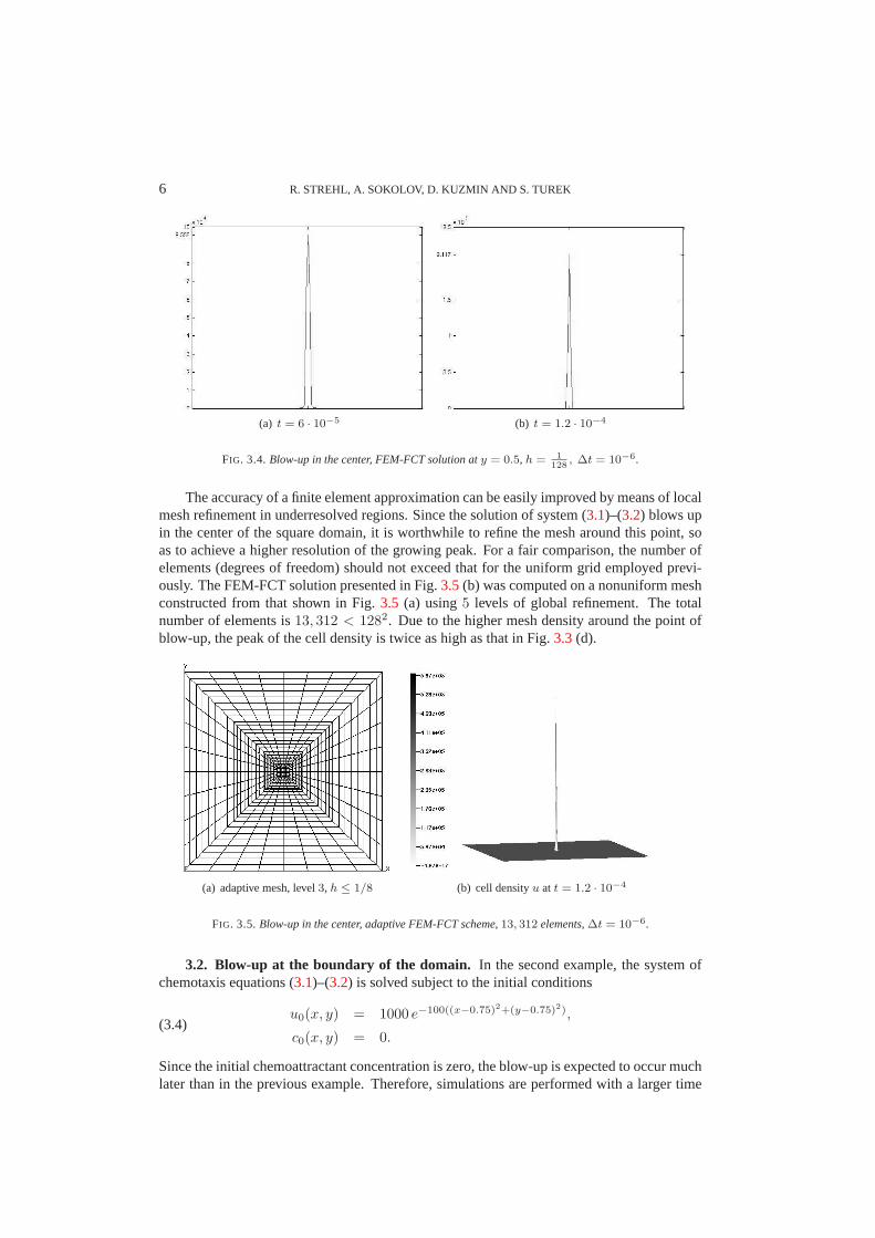
FIG. 3.4.Blow-up in the center, FEM-FCT solution aty = 0.5, h =1

128, ∆t = 10−6.

The accuracy of a finite element approximation can be easily improved by means of localmesh refinement in underresolved regions. Since the solution of system (3.1)–(3.2) blows upin the center of the square domain, it is worthwhile to refine the mesh around this point, soas to achieve a higher resolution of the growing peak. For a fair comparison, the number ofelements (degrees of freedom) should not exceed that for theuniform grid employed previ-ously. The FEM-FCT solution presented in Fig.3.5(b) was computed on a nonuniform meshconstructed from that shown in Fig.3.5 (a) using5 levels of global refinement. The totalnumber of elements is13, 312 < 1282. Due to the higher mesh density around the point ofblow-up, the peak of the cell density is twice as high as that in Fig.3.3(d).

(a) adaptive mesh, level3, h ≤ 1/8 (b) cell densityu at t = 1.2 · 10−4

FIG. 3.5.Blow-up in the center, adaptive FEM-FCT scheme,13, 312 elements,∆t = 10−6.

3.2. Blow-up at the boundary of the domain. In the second example, the system ofchemotaxis equations (3.1)–(3.2) is solved subject to the initial conditions

(3.4)u0(x, y) = 1000 e−100((x−0.75)2+(y−0.75)2),

c0(x, y) = 0.

Since the initial chemoattractant concentration is zero, the blow-up is expected to occur muchlater than in the previous example. Therefore, simulationsare performed with a larger time

A flux-corrected finite element method for chemotaxis problems 7

step∆t = 10−3. As time evolves, the solution of system (3.1)–(3.2) assumes a spiky formand moves towards the upper right corner of the domain. The results obtained with the stan-dard Galerkin discretization are displayed in Fig.3.6. Again, the cell density becomes neg-ative, and nonphysical oscillations are observed in the corner. These problems can be curedusing algebraic flux correction of FCT type, as demonstratedby the solutions in Fig.3.7.

(a) t = 0.01 (b) t = 0.05

(c) t = 0.07 (d) t = 0.1

FIG. 3.6.Blow-up in the corner, Galerkin scheme,h =1

128, ∆t = 10−3.

The point of blow-up may depend on the geometry on the computational domain, as wellas on the imposed boundary conditions [11]. For example, letΩ be a circle of radius0.5centered at the point(0.5, 0.5). A typical coarse mesh is depicted in Fig.3.8(a). The purposeof the numerical experiment to be performed is to find out if the blow-up point tends to anyparticular location. The peak of the initial profileu0 is placed at the point(0.6, 0.6)

(3.5)u0(x, y) = 1000 e−100((x−0.6)2+(y−0.6)2),

c0(x, y) = 0.

All other settings are the same as in the case of the square domain. The FEM-FCT results inFig.3.8(b,c,d) were obtained with9216 bilinear elements. The distribution of the cell densitymoves in the radial direction and blows up at the boundary of the circle in finite time.

8 R. STREHL, A. SOKOLOV, D. KUZMIN AND S. TUREK

(a) t = 0.01 (b) t = 0.05

(c) t = 0.07 (d) t = 0.1

FIG. 3.7.Blow-up in the corner, FEM-FCT scheme,h =1

128, ∆t = 10−3.

(a) coarse mesh (b) t = 0.085

(c) t = 0.14 (d) t = 0.2

FIG. 3.8.Blow-up at a circular boundary, FEM-FCT scheme,∆t = 10−3.

A flux-corrected finite element method for chemotaxis problems 9

3.3. Pattern formation. In the last example, we consider a more complicated and real-istic chemotaxis model. It describes the complex space-time patterns formed by motile cellsof Escherichia coli. There are several different approaches to modeling the distribution ofthese bacteria. One of them leads to the following system of differential equations [5]

ut = D1∆u − α∇ ·

(

u

(1 + c)2∇c

)

,(3.6)

ct = D2∆c + βw u2

σ + u2.(3.7)

For theoretical analysis, numerical algorithms, and simulation results we refer to [7, 16, 27].In another model, proposed by Mimura and Tsujikawa [21], only diffusion, chemotaxis,

and growth of bacteria are taken into account. The corresponding PDE system reads

ut = D1∆u − χ∇ · (u∇c) + u2(1 − u),(3.8)

ct = ∆c − βc + u.(3.9)

For a detailed presentation of this approach see, e.g., [1, 2]. Obviously, both of the abovesystems are of the form (1.1)–(1.2) and can be solved using the FEM-FCT algorithm.

Consider the Mimura-Tsujikawa model (3.8)–(3.9) with D1 = 0.0625, χ = 8.5, andβ = 32. These parameter settings are taken from [1, 2]. The initial conditions are given by

u0(x, y) = 1 + σ(x, y),

c0(x, y) = 1/32,

whereσ(x, y) is a small perturbation defined as

σ(x, y) =

random, if ‖x − (8, 8)T ‖ ≤ 1.5,

0, otherwise.

Numerical simulations are performed in the square domainΩ = (0, 16)2. A uniformmesh of conforming bilinear finite elements withh = 1/8 is employed, that means16384elements. The time step is taken to be∆t = 0.1. The solutions are very sensitive to thechoice of parameters, especiallyχ, σ, etc. Figure4.1 illustrates the temporal evolution ofthe cell distribution obtained with the implicit FEM-FCT algorithm. The presented resultsare in good agreement with those reported in [1, 2]. The same formation patterns have beenobserved experimentally [5].

4. Conclusion. An implicit flux-corrected transport algorithm was developed for theunified form (1.1)–(1.2) of chemotaxis models. Positivity constraints were enforced using anonlinear blend of high- and low-order approximations. Thelimiting strategy is fully mul-tidimensional and applicable to (multi-)linear finite element discretizations on unstructuredmeshes. A preliminary numerical study of the implicit FEM-FCT scheme was performed forthe minimal Keller-Segel model. The flux-corrected Galerkin approximation was shown to besufficiently accurate and positivity-preserving, even in the case of solutions with sharp peaksthat blow-up in the center or at the boundary of the domain. Anexample that illustrates thebenefits of local mesh refinement was included. Last but not least, realistic simulation resultswere obtained for a representative model of chemotactical pattern formation. The proposed

10 R. STREHL, A. SOKOLOV, D. KUZMIN AND S. TUREK

methodology is suitable for a 3D implementation and seems tobe a promising approach to thenumerical treatment of real-life chemotaxis problems in medicine and biology. Next step willbe to apply flux-corrected transport algorithms for stronger coupling of (1.1)–(1.2), thoroughstudy of time-stepping and precise quantative comparison with existing numerical results,see, e.g., [7, 9, 10, 25].

(a) t = 0.01 (b) t = 0.05

(c) t = 0.07 (d) t = 0.1

FIG. 4.1.Pattern formation simulated with the FEM-FCT algorithm,∆t = 0.1, h =1

8.

REFERENCES

[1] M. A IDA , T. TSUJIKAWA, M. EFENDIEV, A. YAGI AND M. M IMURA , Lower estimate of the attractor di-mension for a chemotaxis growth system, Journal of the London Mathematical Society, ISSN 0024-6107,74(2):453–474, 2006.

[2] M. A IDA AND A. YAGI, Target pattern solutions for chemotaxis-growth system, Scientiae Mathematicae Japon-icae,59(3):577–590, 2004.

[3] A. B ONAMI , D. HILHORST, E. LOGAK AND M. M IMURA , Singular limit of chemotaxis-growth model, Adv.Differential Equations,6:1173–1218, 2001.

[4] J. P. BORIS AND D. L. BOOK, Flux-corrected transport. I. SHASTA, A fluid transport algorithm that works, J.Comput. Phys.,11:38–69, 1973.

[5] E. O. BUDRENE AND H. C. BERG, Dynamics of formation of symmetrical patterns by chemotactic bacteria,Nature,376(6535):49–53, 1995.

A flux-corrected finite element method for chemotaxis problems 11

[6] M. BURGER, M. DI FRANCESCO ANDY. DOLAK -STRUSS, The Keller-Segel model for chemotaxis with pre-vention of overcrowding: Linear vs. nonlinear diffusion, SIAM J. Math. Anal.,38:1288–1315, 2006.

[7] A. CHERTOCK AND A. K URGANOV, A second-order positivity preserving central-upwind scheme for chemo-taxis and haptotaxis models, Numer. Math.,111:169–205, 2008.

[8] Y. D OLAK AND C. SCHMEISER, The Keller-Segel model with logistic sensitivity functionand small diffusivity,SIAM J. Appl. Math.,66:595–615, 2005.

[9] Y. EPSHTEYN, Discontinuous Galerkin methods for the chemotaxis and haptotaxis models, J. Comput. Appl.Math.,224(1):168–181, 2009.

[10] Y. EPSHTEYN ANDA. K URGANOV, New interior penalty discontinuous Galerkin methods for the Keller-Segelchemotaxis model, SIAM J. Numer. Anal.,47(1):386–408, 2008.

[11] F. FILBET, A finite volume scheme for the Patlak-Keller-Segel chemotaxis model, Numer. Math.,104(4):457–488, 2006.

[12] M. A. HERRERO ANDJ. J. L. VELAZQUEZ, A blow-up mechanism for a chemotaxis model, Ann. Sc. Norm.Super.,24:633–683, 1997.

[13] T. HILLEN AND K. J. PAINTER, A user’s guide to PDE models for chemotaxis, J. Math. Biol.,58(1):183–217,2009.

[14] E. F. KELLER AND E. F. SEGEL, Initiation of slime mold aggregation viewed as an instability, J. Theor. Biol.,26:399–415, 1970.

[15] E. F. KELLER AND E. F. SEGEL, Model for chemotaxis, J. Theor. Biol.,30:225–234, 1971.[16] B. S. KIRK AND G. F. CAREY, A parallel, adaptive finite element scheme for modeling chemotactic biological

systems, Commun. Numer. Meth. Engrg., 2009, in press (doi:10.1002/cnm.1173).[17] D. KUZMIN , Explicit and implicit FEM-TVD algorithms with flux linearization, J. Comput. Phys.,228:2517–

2534, 2009.[18] D. KUZMIN AND M. M OLLER, Algebraic flux correction I. Scalar conservation laws, in: D. KUZMIN ,

R. LOHNER, S. TUREK (Eds.), Flux-Corrected Transport: Principles, Algorithms, and Applications,Springer, Berlin, 2005, pp. 155–206.

[19] D. KUZMIN AND S. TUREK, Flux correction tools for finite elements, J. Comput. Phys.,175:525–558, 2002.[20] I. R. LAPIDUS AND R. SCHILLER, Model for the chemotactic response of a bacterial population, Biophys J.,

16(7):779–789, 1976.[21] M. M IMURA AND T. TSUJIKAWA, Aggregating pattern dynamics in a chemotaxis model including growth,

Physica A,230:499–543, 1996.[22] A. B. POTAPOV, T. HILLEN , Metastability in chemotaxis models, J. Dyn. Diff. Eq.,17:293–330, 2005.[23] D. L. ROPP AND J. N. SHADID , Stability of operator splitting methods for systems with indefinite operators:

Advection-diffusion-reaction systems, J. Comput. Phys., 2009, in press (doi:10.1016/j.jcp.2009.02.001).[24] H. R. SCHWETLICK, Travelling fronts for multidimensional nonlinear transport equations, Analyse non

lineaire,17(4):523–550, 2000.[25] N. SAITO, Conservative upwind finite-element method for a simplified Keller-Segel system modelling chemo-

taxis, IMA J. Numer. Anal.,27:332–365, 2007.[26] T. SUZUKI , Free energy and self-interacting particles, Boston: Birkhauser[27] R. TYSON, S. R. LUBKIN AND J. D. MURRAY, A minimal mechanism for bacteria pattern formation, Proc.

Biol. Sci.,266(1416):299–304, 1999.[28] R. TYSON, L. G. STERN AND R. J. LEVEQUE, Fractional step methods applied to a chemotaxis model, J.

Math. Biol.,41:455–475, 1996.[29] S. T. ZALESAK, Fully multidimensional flux-corrected transport algorithms for fluids, J. Comput. Phys.,

31:335–362, 1979.