A Hybrid Controller based on the Egocentric PerceptualPrinciple

Zinovi Rabinovich∗, Nicholas R. Jennings

Electronics and Computer Science, University of Southampton, Southampton, SO17 1BJ, UK

Abstract

In this paper we extend the control methodology based on Extended Markov Track-ing (EMT) by providing the control algorithm with capabilities to calibrate andeven partially reconstruct the environment’s model. This enables us to resolve theproblem of performance deterioration due to model incoherence, a problem facedin all model-based control methods. The new algorithm,Ensemble Actions EMT(EA-EMT), utilises the initial environment model as a library of state transitionfunctions and applies a variation of prediction with experts to assemble and cali-brate a revised model. By so doing, this is the first hybrid control algorithm thatenables on-line adaptation within the egocentric control framework which dictatesthe control of an agent’s perceptions, rather than an agent’s environment state. Inour experiments, we performed a range of tests with increasing model incoher-ence induced by three types of exogenous environment perturbations:catastrophic– the environment becomes completely inconsistent with the model,deviating –some aspect of the environment behaviour diverges compared to that specified inthe model, andperiodic – the environment alternates between several possible di-vergences. The results show that EA-EMT resolved model incoherence and signif-icantly outperformed its EMT predecessor by up to 95%.

Keywords: hybrid control, perceptual control, dynamics based control,Kullback-Leibler divergence

1. Introduction1

Egocentric perceptual control (EPC) formulates a control problem in terms of an2

agent’s perceptions, i.e. its internal interpretation of sensory input, ratherthan the3

actual environment state [1]. As a direct outcome of this representation, any task4

∗Corresponding authorEmail addresses: zr@ecs.soton.ac.uk (Zinovi Rabinovich),

nrj@ecs.soton.ac.uk (Nicholas R. Jennings)

Preprint submitted to Robotics and Autonomous Systems April 11, 2010

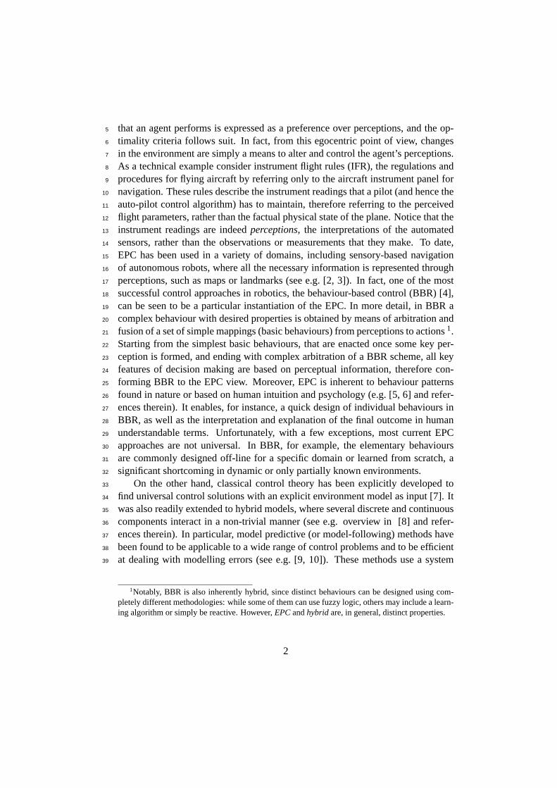
that an agent performs is expressed as a preference over perceptions, and the op-5

timality criteria follows suit. In fact, from this egocentric point of view, changes6

in the environment are simply a means to alter and control the agent’s perceptions.7

As a technical example consider instrument flight rules (IFR), the regulations and8

procedures for flying aircraft by referring only to the aircraft instrument panel for9

navigation. These rules describe the instrument readings that a pilot (andhence the10

auto-pilot control algorithm) has to maintain, therefore referring to the perceived11

flight parameters, rather than the factual physical state of the plane. Notice that the12

instrument readings are indeedperceptions, the interpretations of the automated13

sensors, rather than the observations or measurements that they make. Todate,14

EPC has been used in a variety of domains, including sensory-based navigation15

of autonomous robots, where all the necessary information is represented through16

perceptions, such as maps or landmarks (see e.g. [2, 3]). In fact, oneof the most17

successful control approaches in robotics, the behaviour-based control (BBR) [4],18

can be seen to be a particular instantiation of the EPC. In more detail, in BBR a19

complex behaviour with desired properties is obtained by means of arbitrationand20

fusion of a set of simple mappings (basic behaviours) from perceptions to actions1.21

Starting from the simplest basic behaviours, that are enacted once some key per-22

ception is formed, and ending with complex arbitration of a BBR scheme, all key23

features of decision making are based on perceptual information, therefore con-24

forming BBR to the EPC view. Moreover, EPC is inherent to behaviour patterns25

found in nature or based on human intuition and psychology (e.g. [5, 6] and refer-26

ences therein). It enables, for instance, a quick design of individual behaviours in27

BBR, as well as the interpretation and explanation of the final outcome in human28

understandable terms. Unfortunately, with a few exceptions, most current EPC29

approaches are not universal. In BBR, for example, the elementary behaviours30

are commonly designed off-line for a specific domain or learned from scratch, a31

significant shortcoming in dynamic or only partially known environments.32

On the other hand, classical control theory has been explicitly developedto33

find universal control solutions with an explicit environment model as input[7]. It34

was also readily extended to hybrid models, where several discrete and continuous35

components interact in a non-trivial manner (see e.g. overview in [8] andrefer-36

ences therein). In particular, model predictive (or model-following) methods have37

been found to be applicable to a wide range of control problems and to be efficient38

at dealing with modelling errors (see e.g. [9, 10]). These methods use a system39

1Notably, BBR is also inherently hybrid, since distinct behaviours can be designed using com-pletely different methodologies: while some of them can use fuzzy logic, others may include a learn-ing algorithm or simply be reactive. However,EPC andhybrid are, in general, distinct properties.

2

model to generate predictions on the system development, and compute a control40

signal to optimise this predicted behaviour. Furthermore, the methodology read-41

ily accepts various learning techniques, both to calculate the control signaland to42

adaptively calibrate the model in dynamic or partially known environments. How-43

ever, the detail of the model calibration may vary according to the imposed system44

structure and dynamics assumptions. For instance, in reinforcement learning ar-45

chitectures, such as Dyna [11], model corrections are local to the current environ-46

ment state. Dyna’s principles are also echoed by the modern Bayesian techniques47

where a POMDP model is recovered while finding the reward maximising policy48

(e.g. [12, 13]). However, the success of these works has been conditioned on the49

domain being well factored or on the presence of an oracle to query for the true50

system state. Furthermore, these approaches can not address the problem of an51

environment that drifts through a continuous range of models due to their rigid as-52

sumptions on system structure. To address this issue, much stronger, hybrid control53

methods have been constructed, usually based on the model predictive (or model-54

following) principle (see e.g. [14–16]). Some methods even provide theoretical55

guarantees [14], however at the price of requiring additional modifications to work56

with discrete space domains or losing this capability entirely.57

Given these complementary strengths, the fusion of EPC with model-based58

control can potentially lead to an extremely powerful framework. It would combine59

the egocentric autonomous representation, i.e. dynamic system without external60

control input, of a task and the capability to incorporate high level environment61

knowledge in the form of a system model. Unfortunately, various as they are,62

classic control theory approaches have an important underlying assumption: the63

subject of the optimality criteria are the state and the dynamics of the environment.64

Be that the expected accumulated cost of the state variation (e.g. the classic work of65

Stengel [7]), be that the proximity to an ideal distribution over system trajectories66

(e.g. [17]) or be that the cost of system stability (e.g. [18]), the optimality criteria67

always comes back to consider the underlying system state transitions as theutility68

source, even if the environment model contains observed quantities only (e.g. [19]).69

By so doing, this assumption explicitly contradicts the EPC point of view, which70

hinders the aforementioned fusion of the two control principles.71

In fact, the only control algorithm that possesses a complete fusion of boththe72

model-based control principles and the EPC view is the Extended Markov Track-73

ing (EMT) algorithm [20] and its descendants (e.g. [21, 22]). However, as our74

experiments have revealed, the standard EMT can not cope well with modelin-75

coherences. To this end, in this paper we propose an extended EMT algorithm76

that has all the aforementioned capabilities: it is an egocentric perceptual control77

algorithm, it is a universal model-based controller, it is adaptive to environment78

changes by means of an on-line model calibration, it is a hybrid controller capable79

3

of operating in mixed discrete-continuous domains or domains with a hierarchical80

abstraction of actions. In more detail, for each action available to the agent, we de-81

ploy an experts ensemble [23] to learn a good estimate of an action’s effects. Such82

ensembles are known to provide highly flexible and dynamic estimates, which in83

our case corresponds to fast estimation and calibration of a system model. Notice84

that this estimate is with respect to the predictive capabilities of the action effects85

on the agent’s perceptions. Now, the expert ensemble is composed of a finite set86

of potential effects an action may have, mined from an initial environment model,87

which are dynamically merged together into a single estimate of an action’s effect.88

The new control algorithm, the Ensemble Action EMT (EA-EMT) then uses the89

collection of these estimates to form a complete environment model and proceeds90

to follow the normal EMT flow of action selection.91

To demonstrate the adaptive efficacy of the EA-EMT algorithm we have de-92

vised a set of experiments with various incoherences of the initial system model.93

In a discrete state environment we have investigated the effects of exogenous per-94

turbations of three types:catastrophic – the environment becomes completely in-95

consistent with the model,deviating – some aspect of the environment behaviour96

diverges compared to that specified in the model, andperiodic – the environment97

alternates between several possible divergences. The results show that EA-EMT re-98

solved model incoherence and outperformed its EMT predecessor by upto 95%. To99

clearly demonstrate the hybrid nature and capabilities of the EA-EMT algorithm,100

we have devised an additional experiment with a continuous state environment,101

where a task had to be achieved by switching between several pre-specified sub-102

controllers. In this continuous state environment we have also compared theeffects103

a deviating inconsistency has on EMT-based approaches (both the standard EMT104

and the EA-EM) and the classical model-following approach. In our experiments,105

EMT has outperformed the model-following controller under model incoherence,106

and both have been outstripped by EA-EMT by at least 40% in error rate.107

To summarise, the contributions of this paper are as follows. First, we intro-108

duce a new hybrid control method that is equally applicable in environments with109

discrete, continuous or mixed environment state. This enables the algorithm to110

serve both as a universal low level mechanism of action selection, and asa high111

level switching mechanism between separate tuned controllers in a hybrid archi-112

tecture. In particular, the algorithm is resistant to switching noise, the capability113

well beyond even the most modern switching methods (e.g. [14]). Second,our ap-114

proach provides, for first time, an adaptive controller version of the model-based115

EPC paradigm, enabling in observable terms. Third, EA-EMT is the first algorithm116

that, without sacrificing its generality with respect to its environment’s continuity,117

is capable of composing a good control signal even if the underlying environment118

dynamics are non-stationary, and change over time.119

4

The rest of the paper is organised as follows. In Section 2 we detail the opera-120

tion of the standard EMT Control algorithm. Section 3 follows with the description121

of our new EA-EMT algorithm, detailing how it reconstructs and calibrates theen-122

vironment model through the use of expert ensembles. Experimental support for123

the effectiveness of our approach in handling various model incoherences is given124

in Sections 4, while the experiments of Section 5 are designed to expose the hybrid125

nature of our algorithm. To underline the algorithm’s capability to work in envi-126

ronments with changing behavioural trends, our experiments take a special focus127

on the on-line property of the EA-EMT model calibration. Section 6 summarises128

the results and gives future directions of this research.129

2. EMT Control130

EPC controllers are constructed around some perceptual concept, andnecessarily131

include a subsystem that creates and maintains these perceptions by accumulating132

and interpreting the observed data. In the case of an EMT Controller the percep-133

tion is that of the autonomic system dynamics, where the system state appears134

to stochastically develop over time without external influence. The convenience135

of this choice is made apparent by the following observation. Assume that some136

control has been plugged into the environment. The resulting overall system is137

autonomic, and describes the behaviour of the control-augmented environment in138

all possible states. Furthermore, although we may not know what specific control139

law will bring it about, we frequently can describe the autonomic dynamics thatwe140

would consider to be ideal or optimal. For example, in IFR, the behaviour of in-141

strument gauge is described without specifying what actions the pilot has totake to142

achieve this behaviour. This approach is adopted by the EMT controllers,the con-143

trol task is described by a perception of an idealised autonomic system dynamics,144

and the algorithm has to sequence actions to achieve the perception of this ideal.145

To do so, however, the controller requires a subsystem that creates and maintains146

the necessary perception, and in this paper the subsystem is the ExtendedMarkov147

Tracking (EMT) algorithm, that also lends its name to the entire control scheme.148

Formally, the EMT algorithm produces and maintains an estimate of a stochas-149

tic state transition function that models the autonomic system behaviour. It does150

so by performing a conservative update, specifically it minimises the Kullback-151

Leibler divergence between the new and the old estimate, with the limitation that152

the new estimate has to match the most recently observed system transition. In153

more detail, assume that two probability distributions over the system state,pt and154

pt+1, are given that describe two consecutive states of knowledge about the system,155

andτEMTt is the old estimate of the system dynamics. Then the EMT update, abbre-156

viated byτEMTt+1 = H

[

pt → pt+1, τEMTt

]

, is the solution of the optimisation problem157

5

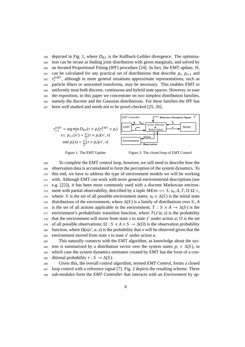
depicted in Fig. 1, whereDKL is the Kullback-Leibler divergence. The optimisa-158

tion can be recast as finding joint distribution with given marginals, and solved by159

an Iterated Proportional Fitting (IPF) procedure [24]. In fact, the EMTupdate,H,160

can be calculated for any practical set of distributions that describept, pt+1 and161

τEMTt , although in more general situations approximate representations, such as162

particle filters or unscented transforms, may be necessary. This enablesEMT to163

uniformly treat both discrete, continuous and hybrid state spaces. However, to ease164

the exposition, in this paper we concentrate on two simplest distribution families,165

namely the discrete and the Gaussian distributions. For these families the IPF has166

been well studied and needs not to be proof-checked [25, 26].167

τEMTt+1 = arg min

τDKL(τ × pt‖τ

EMTt × pt)

s.t. pt+1(x′) =∑

x(τ × pt)(x′, x)

andpt(x) =∑

x′(τ × pt)(x′, x)

Figure 1: The EMT Update

Pt

Pt+1

τEMT

Ta

Environment

τ*

Belief UpdateEMT

Action Selection& Modela

Action

Observation

EMT Controller Reference (Dynamics) Signal

Figure 2: The closed loop of EMT Control

To complete the EMT control loop, however, we still need to describe how the168

observation data is accumulated to form the perception of the system dynamics. To169

this end, we have to address the type of environment models we will be working170

with. Although EMT can work with more general environmental descriptions (see171

e.g. [22]), it has been more commonly used with a discrete Markovian environ-172

ment with partial observability, described by a tupleMEnv =< S , s0, A,T,O,Ω >,173

where:S is the set of all possible environment states;s0 ∈ ∆(S ) is the initial state174

distributions of the environment, where∆(S ) is a family of distributions overS ; A175

is the set of all actions applicable in the environment;T : S × A → ∆(S ) is the176

environment’s probabilistic transition function, whereT (s′|a, s) is the probability177

that the environment will move from states to states′ under actiona; O is the set178

of all possible observations;Ω : S × A × S → ∆(O) is the observation probability179

function, whereΩ(o|s′, a, s) is the probability thato will be observed given that the180

environment moved from states to states′ under actiona.181

This naturally connects with the EMT algorithm, as knowledge about the sys-182

tem is summarised by a distribution vector over the system statespt ∈ ∆(S ), in183

which case the system dynamics estimator created by EMT has the form of a con-184

ditional probabilityτ : S → ∆(S ).185

Given this, the overall control algorithm, termedEMT Control, forms a closed186

loop control with a reference signal [7]. Fig. 2 depicts the resulting scheme. Three187

sub-modules form theEMT Controller that interacts with anEnvironment by ap-188

6

plying actions in and receiving observations from it: theModel, theEMT estimator,189

and the decision making module ofAction Selection and Belief Update. TheModel190

module is queried for the effectsTa of an actiona on the real system state. These191

effects are used both in predicting future perceptions, and in filtering the observed192

data to maintain system state beliefs. TheEMT module is used to estimate the per-193

ceived dynamicsτEMT that explain the change in beliefs about the system frompt194

at timet to pt+1 at timet + 1. The central, decision making module, interconnects195

the Model and the EMT estimator, and implements the EMT Control algorithm,196

the detail of which we describe below. Finally, the reference signal,τ∗, encodes197

the task to be performed and formally takes the form of the conditional probability198

τ∗ : S → ∆(S ).199

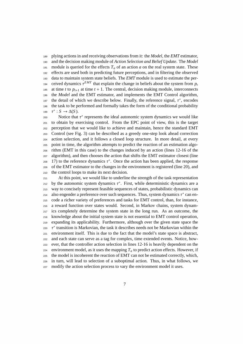
Notice thatτ∗ represents the ideal autonomic system dynamics we would like200

to obtain by exercising control. From the EPC point of view, this is the target201

perception that we would like to achieve and maintain, hence the standard EMT202

Control (see Fig. 3) can be described as a greedy one-step look ahead correction203

action selection, and it follows a closed loop structure. In more detail, at every204

point in time, the algorithm attempts to predict the reaction of an estimation algo-205

rithm (EMT in this case) to the changes induced by an action (lines 12-16 of the206

algorithm), and then chooses the action that shifts the EMT estimator closest (line207

17) to the reference dynamicsτ∗. Once the action has been applied, the response208

of the EMT estimator to the changes in the environment is registered (line 20), and209

the control loops to make its next decision.210

At this point, we would like to underline the strength of the task representation211

by the autonomic system dynamicsτ∗. First, while deterministic dynamics are a212

way to concisely represent feasible sequences of states, probabilistic dynamics can213

also engender a preference over such sequences. Thus, system dynamicsτ∗ can en-214

code a richer variety of preferences and tasks for EMT control, than,for instance,215

a reward function over states would. Second, in Markov chains, systemdynam-216

ics completely determine the system state in the long run. As an outcome, the217

knowledge about the initial system state is not essential to EMT control operation,218

expanding its applicability. Furthermore, although over the given state space the219

τ∗ transition is Markovian, the task it describes needs not be Markovian withinthe220

environment itself. This is due to the fact that the model’s state space is abstract,221

and each state can serve as a tag for complex, time extended events. Notice,how-222

ever, that the controller action selection in lines 12-16 is heavily dependenton the223

environment model, as it uses the mappingTa to predict action effects. However, if224

the model is incoherent the reaction of EMT can not be estimated correctly, which,225

in turn, will lead to selection of a suboptimal action. Thus, in what follows, we226

modify the action selection process to vary the environment model it uses.227

7

Require:Set the system state estimator:p0(s) = s0 ∈ ∆(S )Set the system dynamics estimator:τEMT

0 (s|s) = prior(s|s)Set time tot = 0.

11: loop12: for all a ∈ A do13: Set Ta = Ta use transition model T directly14: Set pa

t+1 = Ta ∗ pt

15: SetDa = H[

pt → pat+1, τ

EMTt

]

16: SetV(a) = 〈DKL (Da‖τ∗)〉pt

17: Selecta∗ = arg mina

V(a)

18: Apply a∗, receive observationo ∈ O19: Computept+1 due to the Bayesian update:pt+1(s) ∝ Ω(o|s, a)

∑

s′ T (s|a, s′)pt(s′)20: ComputeτEMT

t+1 = H[

pt → pt+1, τEMTt

]

21–25: no model update26: Sett := t + 1

Figure 3: The standard EMT control algorithm. Note: EA-EMT will modify lines 13,21-25.

3. Ensemble Action EMT228

Although the standard EMT Control is attractive in its combination of the ego-229

centric control perspective and the task description by the perceived system dy-230

namics, our experiments (see Section 4) have revealed that its performance de-231

teriorates significantly if the environment model is incoherent. However, webe-232

lieve (and will subsequently demonstrate) that, by providing the algorithm with233

an additional method to correct model incoherences, it is possible to rectify the234

deterioration. Now, there are many incoherences a Markovian model,MEnv =<235

S , s0, A,T,O,Ω >, may have. Specifically, while the choice of the state, action236

and observation spaces, as well as the observability function, may be dictated by237

subjective considerations (e.g. to make it more readable for the human domain238

designers), the transition functionT is always dictated by the environment. Thus,239

in this work we choose to concentrate on the quality of the transition functionT .240

This function maps actions into stochastic matrices, so that for each actiona ∈ A241

the matrixTa = T (·|·, a) models the effects of that action on the system state.242

The difference between the matrixTa and the true effects of the actiona ∈ A is243

the incoherence type we have resolved in the EA-EMT algorithm (Fig. 4). Thus,244

while the standard EMT Control views the transition mapping,a 7→ Ta, to be con-245

stant, the EA-EMT algorithm modifies its transition mapping over time, reducing246

the mapping’s incoherence. However, before we go into the details of howit was247

implemented, we need to explain the principles of the approach taken by EA-EMT.248

EA-EMT assumes that, although the mappingT : A → ∆(S )S is incoherent,249

the set of matricesTA = Ta = T (·|·, a)a∈A represents feasible effects that the250

actions may have. The algorithm then attempts to assemble a better mapping,251

8

T : A → ∆(S )S , based on the setTA. More specifically, for each actiona ∈ A252

the transition matrixTa is a weighted linear combination of matrices in the set253

TA, that is Ta =∑

b∈A Tb ∗ wa(b). Intuitively, the weightwa(b) represents the254

similarity between the matrixTb ∈ TA and the effects that the actiona ∈ A has on255

on the environment state. As the interaction between the EA-EMT algorithm and256

the environment progresses, the weightswa(·) are updated, modifying the mapping257

T : A→ ∆(S )S to reduce its incoherence with the environment.258

The intuition behind this approach stems fromPolytopic Linear Models (PLM)259

with continuous state, where a complex non-linear system is represented asa com-260

bination of a finite set of simpler linear sub-systems [15]. Similarly, in our for-261

malism, an actiona ∈ A may be more than a primitive operation. Rather, it may262

represent a subsystem with a complex underlying controller, which forces the sys-263

tem to follow dynamics described byTa. In fact, by enriching the setTA, one can264

guarantee that environment incoherences of interest will be well captured. As an265

utterly extreme example consider a dynamic system with a discrete state space.266

By settingTA to be the set of permutation matrices, we essentially allowTa to be267

any matrix from the polytope of stochastic matrices, and endow EA-EMT with the268

capability to capture any environment disturbance, be it a randomly reoccurring269

one or be it a disturbance localised to a particular system state. Although the re-270

lationship between the composition ofTA and its expressiveness needs not be this271

extreme, and in practice only small sizedTA is required, its exact properties are272

non-trivial. In fact, it forms a separate branch of research, where the works by An-273

gelis [15] and Cesa-Bianchi [23] are only few representatives of a vast literature,274

that falls out of scope of this paper. Nevertheless, we can safely assume thatTA275

forms a sufficiently large polytope that includes all relevant system dynamics.276

Now, the update of the weightswa(·) is based on the approach of predictions277

with expert ensembles [23]. The intuition behind this approach is that, when mak-278

ing a prediction or a decision, a readily available set of feasible alternatives (the279

expert ensemble) can be merged together to form a prediction which is potentially280

better than any of the alternatives standing alone. The dynamic properties of this281

merger are such, that it can be readily applied even if the best prediction (or the282

best decision) is not stationary, but rather changes over time. This made the choice283

of expert ensembles particularly attractive to maintain a system model in varying,284

unstable environments. Specifically, in our algorithm theexpert ensemble is the set285

TA, where each expert attempts to predict the effects an action would have onthe286

environment state. From this point of view, the weightwa(b) expresses how much287

the expertTb ∈ TA is trusted to capture the effects of the actiona ∈ A correctly.288

Once EA-EMT has applied an action,a∗, it measures the discrepancy between the289

effecta∗ had and the effect predicted by expertTb. The lower the discrepancy, the290

higher will be the weightwa∗(b) when the next control decision is made.291

9

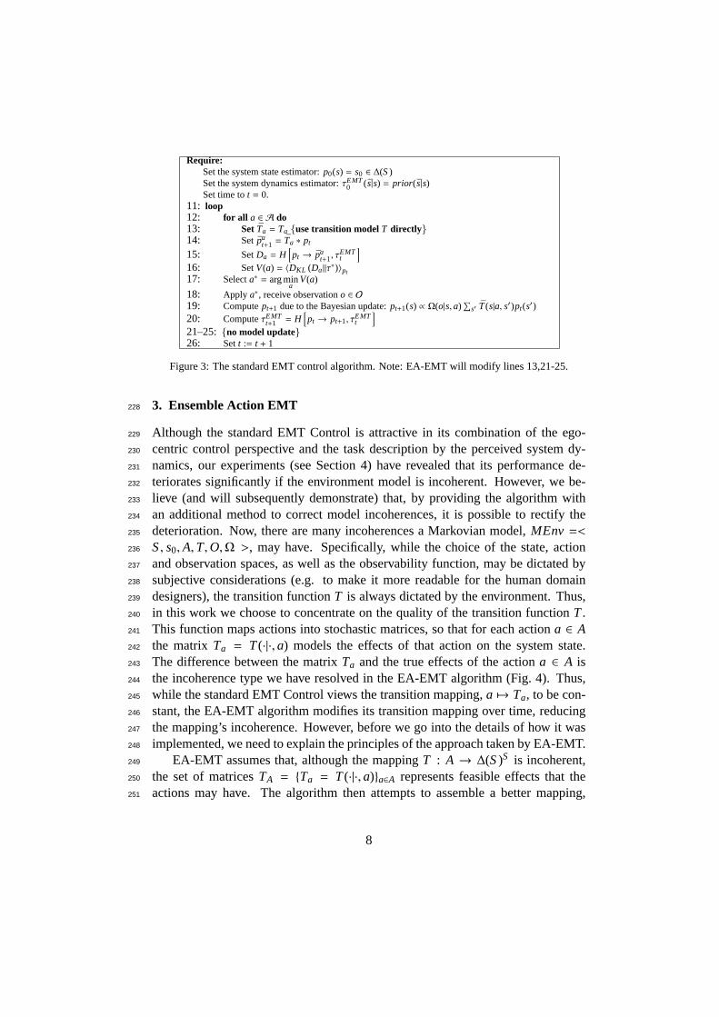
Given the above principles, we have modified the standard controller algo-292

rithm. Specifically, line 13, previously directly substituted into the calculations the293

transition function from the provided model. Whereas now it uses a weightedcom-294

bination of the matrices inTA, which is continually tuned by the expert ensemble295

to improve its representation of an action’s effects. The rest of the computations296

proceed as before until the EMT estimate,τEMTt+1 , of the action outcome is com-297

puted in line 20: the algorithm predicts the effects of each action on the EMT298

estimate, chooses the action that would bringτEMTt+1 closest to the reference signal299

τ∗, applies the action and receives an observation. At that point, the algorithm has300

to measure the performance of each expert, and update the weights. Now,recall301

that the algorithm operates in terms of subjective beliefs, the relevant effects of302

the action are thus those expressed in the EMT estimateτEMTt+1 . This means that303

the performance of each expert can be expressed by the distance between the es-304

timateτEMTt+1 and the estimate that would have been obtained based on the expert305

prediction. This distance is computed in lines 22-24, and the weight of the expert is306

updated accordingly. Specifically, the old weight of the expert is multiplied byβd,307

whereβ ∈ (0,1) is the parameter of the update andd is the distance above. Once308

all weights are updated, they are normalised to sum to 1, so thatTa at the next step309

will be a stochastic matrix. Notice that all these operations take time polynomial in310

the model parameters, such as the size of state, action and observation spaces. This311

makes EA-EMT a computationally efficient and scalable algorithm, an attractive312

property systems where environment models tend to be large.313

Require:. . .Set action weight vectors:wa(a′) ∝ δa(a′) + ǫSet time tot = 0.

11: loop. . . . . . . . . . . . . . .

13: SetTa =∑

a′ Ta′ ∗ wa(a′). . . . . . . . . . . . . . .

21: for all a ∈ A do22: Set pa

t+1 = Ta ∗ pt

23: SetDa = H[

pt → pat+1, τ

EMTt

]

24: SetV(a) =⟨

DKL

(

Da‖τEMTt+1

)⟩

pt

25: Setwa∗ (a) ∝ wa∗ (a)βV(a)

26: Sett := t + 1

Figure 4: The EA-EMT control algorithm: only changes to the standard EMT control are shown.

4. Experimental Evaluation: Discrete State Space314

To test the effectiveness of the EA-EMT algorithm, we have devised a setof com-315

parative tests with the standard EMT Controller. The latter is a natural baseline,316

10

as it is the only other universal control algorithm capable of complete fusion of317

the EPC and the model-based paradigms. In discrete state systems this is also the318

only baseline, as no other control algorithm can reproduce the action selection se-319

quence of EMT. Fortunately, in the environments with a continuous state space,320

which we tend to in Section 5, the sequence of actions selected by EMT can beat321

least partially reproduced by model-following control algorithms, and we imme-322

diately use it to provide an additional baseline comparison. In all cases, wehave323

preferred a simulated system so that the true effects of our control algorithm will324

not be confused with the properties of an embodied physical system.325

Now, to support comparability with previous work on EMT variations, all tests326

were based on modifications of the Drunk Man (D-Man) domain: a controlled327

random walk over a linear graph (see Fig. 5 for the principle structure) with ac-328

tions weakly modulating the probability (only a small discrete set of probabilities329

in the range (ǫ,1 − ǫ) with ǫ ≫ 0 is attainable) of the left and the right steps.330

The domain is also partially observable, namely, instead of its true position on the331

graph, an agent receives as an observation a random position within thetwo step332

neighbourhood of agent’s location. In turn, a task within the domain is represented333

by a conditional probabilityτ∗(s′|s), the reference signal for the controller, spec-334

ifying what sort of motion through the state space has to be induced. Duringan335

experiment run, the control algorithm was provided with a Markovian environment336

model,MEnv =< S , s0, A,T,O,Ω >, incoherent with the true behaviour of the do-337

main. The incoherences were created by introducing exogenous perturbations to338

the behaviour of the D-Man domain. In particular, three perturbations, making the339

model of the standard D-Man domain increasingly incoherent with the actualenvi-340

ronment behaviour, were used:Deviating, where an additional deterministic step341

(to the right) was done;Periodic, where the direction of an additional deterministic342

step changed over time; andCatastrophic, where a random permutation of actions343

was selectedσ : A → A, so that when the controller applied actiona ∈ A, the344

environment responded instead toσ(a). Three baselines where obtained in various

s*0 1 2

(1−p)

.......... n(1−a)p

ap

Figure 5: Principle structure of the Drunk Man domain.

345

combinations: standard EMT Control algorithm operating in a perturbed environ-346

ment, standard EMT Control operating within an unperturbed environment, and347

standard EMT Control operating in a perturbed environment with its model cor-348

rectly encoding the environment perturbation. At least two baselines are present349

in each experimental setting to provide comparative performance bounds and the350

11

99.5% confidence envelope is depicted in all plots. In all our experiments the ref-351

erence dynamics for the controller is given byτ∗(s′|s) ∝ δs∗(s′) + ǫ, whereǫ > 0352

is small. In other words, the target prescribes that the environment shouldalmost353

surely move to the ideal states∗ from any other state. In our experiments the state354

space wasS = 0, ...,12, and the ideal states∗ = 6. Notice that, due to the prob-355

abilistic nature of the domain, any reasonable2 control scheme set to accomplish356

the task would result in a bell shaped empirical distribution of the system state.357

Success of the control scheme can then be readily appreciated visually bythe dif-358

ference of the expected value and the ideal system state, as well as the standard359

deviation of the empirical state distribution. The empirical distribution was taken360

over a 200 decision stepsliding window, to obtain statistically significant distri-361

bution shape. In turn, the overall length of experimental runs was then chosen362

to be sufficiently large to enable analysis of stable trends of the empirical 200-363

step distribution. In particular, for thecatastrophic and thedeviating perturbations364

each experiment run was 1000 steps. The necessity to obtain statistical signifi-365

cance while preventing the algorithm from completely stabilising, has also led to366

the choice of the 500 step period for theperiodic perturbation experiments, accom-367

panied by the 5000 step total length of each experiment run. Although alternative368

experimental setups were also run, varying both the sliding window size and the369

experiment length, their results were similar, we, therefore, omit them due to space370

limitations. Nevertheless, the aforementioned sequence of choices is reflected in371

the way our experimental results are presented:deviating, catastrophic and then372

periodic perturbations. Furthermore, to present an overall evaluation of a control373

scheme’s performance, rather than a comparison of multiple parameters, wealso374

measured the distance between the empirical distribution andδs∗ usingl1 norm.375

To further the intuition of this domain, consider once more the IFR example376

where the pilot has to maintain flight level within the air corridor prescribed bythe377

ground control. If we discretise the space of possible flight levels we will obtain a378

linear graph depicted in Fig. 5. The transitions between the states are controlled,379

but are also subject to random changes in the air density or wind gusts. Ideally, the380

auto-pilot will need to actively return the airplane to the ideal, centre flight level.381

4.1. Deviating Perturbation382

In this experiment we introduce a deviating perturbation. That is, beyond the usual383

probabilistic step, the environment has also deterministically shifted in one direc-384

tion along the linear graph. For example (referring to Fig. 5) if the system reached385

2Unreasonable, for instance, would be choosing a constant action to equalise the left and theright step probabilities, as this would result in an almost uniform distribution,utterly defeating thecontroller purpose.

12

−2 0 2 4 6 8 10 12 14−0.05

0

0.05

0.1

0.15

0.2

0.25

0.3

State

Em

piric

al fr

eque

ncy

EA−EMTEMT ControlEMT Control+ model

(a) Persistent shift

0 2 4 6 8 10 12

0.05

0.1

0.15

0.2

0.25

0.3

State

Em

piric

al fr

eque

ncy

EA−EMT

EMT Control

EMT Control+nonperturbed

(b) Random permutation

Figure 6: EA-EMT performance under (a) deviating and (b) catastrophic perturbations

statek ∈ 0, ..., n − 1, the additional step will shift it to statek + 1. In this con-386

text, Fig. 6(a) shows the empirical distribution of system states under three control387

strategies: the EA-EMT controller and the standard EMT Controller equipped with388

the standard D-Man model (thus excluding the shift modelling), and the standard389

EMT Controller equipped with the environment model that explicitly captures the390

additional shift. The figure shows the complete empirical distribution of the EA-391

EMT obtained during the first 200 control choices made in this experiment, and392

marks a definitive improvement in performance. This can be seen from the fact393

that the standard EMT Control fails to enforce the reference dynamicsτ∗, with394

the system spending the majority of its time away from the ideal state,s∗ = 6,395

while EA-EMT manages to force the state distribution to concentrate closer tos∗.396

In fact, the distance betweenδs∗ and the EA-EMT distribution induced in the first397

200 steps is 40% less than the comparable distance for the EMT controller. This,398

however, does not fully reflect the adaptability of EA-EMT. To this end, Fig. 7(a)399

shows how the mean of the empirical distributions of the 200 step windows behave.400

The distributions induced by EMT Control do not change over time, resultingin401

straight horizontal lines depicting the constancy of the mean. On the other hand,402

the data shows that EA-EMT quickly adapts, the algorithm induces the empirical403

state distribution with the mean approaching the ideal states∗ = 6. In this respect,404

EA-EMT even slightly surpasses the performance of the standard EMT algorithm405

with the correct environment model. This is due to the adaptive portion of EA-406

EMT contributing to the tie breaking when considering similar actions – this tie407

breaking is rigid in EMT Control. Similar pictures occur with respect to the vari-408

ance of the empirical distributions. This means that EA-EMT overcomes the model409

13

incoherence and increasingly concentrates the state empirical distribution around410

the ideal state, which is exactly what the reference dynamics,τ∗, requires.

0 100 200 300 400 500 600 700 8006

6.5

7

7.5

8

8.5

Window start

Em

piric

al fr

eque

ncy

mea

n

EA−EMTEMT ControlEMT Control+ model

(a) Persistent Shift

0 100 200 300 400 500 600 700 80010

−2

10−1

100

101

Window start

l 1 dis

tanc

e be

twee

n em

piric

al fr

eque

ncie

s

EA−EMTEMT ControlConfidence Envelope

(b) Random Permutation

0 1000 2000 3000 4000 50003

4

5

6

7

8

9

Window start

Em

piric

al fr

eque

ncy

mea

n

EA−EMTEMT ControlEMT Control+nonperturbedConfidence Envelope

(c) Switching Shift

Figure 7: EA-EMT adaptation to various perturbations. Notice the log-scaleof theY axis in (b).

411

4.2. Catastrophic Perturbation412

The action space of the D-Man domain has a simple intuitive interpretation – the413

action sets how quickly the system state will shift left or right. The deviating per-414

turbation did not exceed this interpretation, it simply meant that the system will415

naturally move in one direction faster than the other. In a way it also meant that416

the perturbation induced a very mild model incoherence – principally the modelre-417

mained correct. However, EA-EMT can adapt to much more severe model incoher-418

ences. In fact, in the next set of experiments the environment model is completely419

incorrect. For each run in this experiment set a random permutationσ : A → A420

14

was selected. Then, when actiona ∈ A was applied, the environment reacted as if421

the action wasσ(a).422

In more depth, Fig. 6(b) shows the empirical distributions obtained in the first423

200 steps of decision making. Permuting the action breaks any connection between424

what EMT Control expects the action to do and what actually occurs in the environ-425

ment, essentially the actions are scrambled and the EMT Control chooses a random426

action. This results in the algorithm’s failure – the empirical state distribution is427

equivalent to that of applying no control at all, with higher probability of terminal428

states due to the failure of the respective left and right steps. In contrast, EA-EMT429

easily adapts and performs increasingly well, as can be seen in Fig. 7(b).Follow-430

ing the development of the empirical distribution within a 200 step sliding window,431

the figure shows thel1 distance from the distribution formed by the standard EMT432

algorithm in the non-perturbed environment. This data demonstrates that EA-EMT433

exponentially quickly discovers the true effects of actions and approaches the per-434

formance of the EMT control in a non-perturbed environment. Even though the435

empirical distribution of the first 200 steps includes the first decisions made based436

on the scrambled model, it already recovers 70% of the performance lost due to the437

model incoherence and, through further adaptation, it reaches 95% recovery.438

4.3. Periodic Perturbation439

Finally, it is important to ensure that the algorithm can perform well in a dynami-440

cally changing environment. For example, a robot’s body is subject to environmen-441

tal effects, and its response to control will change accordingly. Some environment442

parameters, like the daily temperature variation on Lunar surface, may be extreme443

and persistently reoccurring. To test EA-EMT in such environments, we consider444

yet another perturbation: an additional deterministic step is made, and the direction445

of the step switches between left and right with constant period (500 control steps446

in our experiments). The shape of the distributions formed by the controllersare447

equivalent to those in the persistent shift experiment (see Fig. 6(a)), and we omit448

the respective graph. On the other hand, the development of the empiricaldistri-449

bution over time is quite different. In particular, Fig. 7(c) shows the behaviour of450

the mean value for empirical distributions calculated within a 200 step sliding win-451

dow. While the standard algorithm literally switches from one value to another,452

depending on the direction of the shift, the performance of EA-EMT always shows453

recovery after a direction switch occurs. Notice also, that the magnitude ofthe454

mean variation at the switch point becomes significantly (25%) less for EA-EMT455

than the standard EMT. This suggests that, beyond its ability to recover fromir-456

relevant adaptations, the adaptive controller version learns to reduce the control457

inertia. In other words the algorithm reduces the impact of the sudden change in458

the environment behaviour, stabilising the overall performance.459

15

5. Experimental Evaluation: Continuous State Space460

To complete the demonstration of our algorithm, we apply EA-EMT to a continu-461

ous state environment, where a task is achieved by switching between pre-specified462

sub-controllers. This combination of the discrete switching and the continuous463

switching components, clearly show EA-EMT to be a hybrid controller. Notably,464

neither the structure nor the principle of application change with the transition from465

a discrete to a continuous state space. The transition is achieved simply by replac-466

ing the finite dimensional vector, that has represented state probability distribution467

in the discrete case, by a Gaussian distribution to represent the state distribution468

of the continuous domain. Similarly, stochastic transition matrix is replaced by a469

conditional Gaussian distribution to capture system dynamics. Furthermore,the470

amount of underlying calculations grows only polynomially with the dimension of471

the state and the observation spaces. It is this computational scalability, and the fact472

that no modification is required nor made to the reasoning of the action selection473

procedure, which remains fully and completely intact whatever the environment474

dimensionality is, that grant EA-EMT almost universal applicability. It allowsour475

algorithm to be deployed both as a direct low level controller, and as a partof a476

complex hierarchical hybrid controller with multiple levels of abstraction.

Figure 8: Hovercraft scheme.

477

The specific domain we chose is that of a hovercraft with three thrusters de-478

picted in Fig. 8. Solid arrows show thruster directions, while the hollow arrow479

denotes a potential mistake in that thruster’s model. From the perspective ofour480

IFR example, such modelling mistake would correspond to a sudden change inthe481

plane’s responses, for instance due to a collision with a bird or a mechanical mal-482

function. The system generically develops in discrete time using the equation:483

xk+1

xk+1

yk+1

yk+1

=

1 h 0 00 1 0 00 0 1 h0 0 0 1

xk

xk

yk

yk

+

h2

2 0h 00 h2

20 h

[v1, v2, v3]

u1

u2

u3

484

In the equation,vi denotes the directional force distribution of a thruster,ui485

16

its basic level of activity, andh denotes the time span during which the thrust486

was applied. To further underline the use of EA-EMT as a switching mecha-487

nism of a hybrid controller, we restrictui in our experiments to a finite discrete488

set. Specifically, we used 5 activation levels between 0.2 and 1.0 in equal inter-489

vals, and only one thruster could have a non-zero activation at any time, so that490

total of 15 distinct joint activations were possible. This naturally simulates the491

situation that occurs in hybrid systems, where an action corresponds to theap-492

plication of a distinct sub-system controller, rather than a choice of a continuous493

value control signal. Two configurations of thrusters were used. Configuration A,494

[v1, v2, v3] =[

1 0 −10 1 −1

]

, that corresponds to the solid arrows in Fig. 8; and config-495

uration B, [v1, v2, v3] =[

1 0 −1−0.3 1 −1

]

, that corresponds to a structural failure of a496

thruster depicted by the hollow arrow. In all experiments, while the controlleral-497

gorithm was given either the environment model with thruster Configuration Aor498

B, the actual motion of the hover craft was always simulated using Configuration499

A. This discrepancy allowed us to test the performance of our algorithm under a500

deviating modelling incoherence.501

Now, to provide a quantitative performance measure, we have set several con-502

trol algorithms with the task to simulate a gradual spiralling descent towards zero503

from rest at coordinates [1,1], which we have described by an autonomic linear504

system with the equation given below. Recalling once more our IFR scenario, such505

system would correspond, for example, to the necessary relative properties of the506

altitude and speed of the airplane, as well as their development in time, during a507

landing procedure. As before,h denotes the time span of a single step, whileλ de-508

notes the decay of the spiral andθ the rotation angle of a single step of the system.509

xk+1

xk+1

yk+1

yk+1

=

λ cos(θ) 0 −λ sin(θ) 02h (λ cos(θ) − 1) −1 − 2

hλ sin(θ) 0λ sin(θ) 0 λ cos(θ) 02hλ sin(θ) 0 2

h (λ cos(θ) − 1) −1

xk

xk

yk

yk

510

511

In more detail, the algorithms we have considered were EMT, EA-EMT and512

a discrete Model Follower Controller (MFC). The latter algorithm has been se-513

lected for its robustness and ubiquity of its principle (see e.g. [7, 14, 16]), making514

it suitable to produce a baseline comparison. The MFC algorithm operated in the515

usual manner, specifically, given the current hover coordinates, thealgorithm se-516

lected thrust to minimise the discrepancy between the outcome predicted by the517

task’s equation and the equation of the hovercraft’s model. We have tunedEMT518

initialisation and task representation parameters so that, for the ConfigurationA519

thrusters model, its decisions coincide with MFC. We conjecture, in fact, that EMT520

is formally a more general approach than MFC, in that EMT can always be tuned521

to reproduce MFC’s behaviour. The resulting hovercraft trajectory isdepicted in522

17

−1.5 −1 −0.5 0 0.5 1 1.5−1.5

−1

−0.5

0

0.5

1

1.5

Position X−axis

Pos

ition

Y−

axis

Ideal ReferenceEMT with correct model

(a) EMT (and MFC) with Configuration A (correct)model

−1.5 −1 −0.5 0 0.5 1 1.5 2−1.5

−1

−0.5

0

0.5

1

1.5

Position X−axis

Pos

ition

Y−

axis

Ideal ReferenceEMT + bad model

(b) EMT with Configuration B (wrong) model

−1.5 −1 −0.5 0 0.5 1 1.5−1.5

−1

−0.5

0

0.5

1

Position X−axis

Pos

ition

Y−

axis

Ideal ReferenceEA−EMT + bad model

(c) EA-EMT with Configuration B model

0 50 100 150 200 250 3000

5

10

15

20

25

30

35

40

45

Time step

Cum

mul

ativ

e de

viat

ion

in d

esce

nt

EMT with correct modelEMT + bad modelMFC + bad modelEA−EMT + bad model

(d) Cumulative error of controllers

Figure 9: Hovercraft trajectories under various controllers algorithmsand controller models and theircumulative error. In all cases physical simulation adopts thruster Configuration A.

Fig. 9(a). The dotted line represents the ideal trajectory that could have been ob-523

tained if the thrustsui where continuous, rather than discretised. The Fig. 9(a)524

also demonstrates that the task we posed can be indeed solved by an application525

of the standard EMT controller or MFC, forming a performance baseline where526

the environment develops exactly as the controller’s model describes it. Inturn527

Fig 9(b) and Fig 9(c) depict the performance of the EMT and EA-EMT algorithms528

provided with Configuration B (wrong) thruster model. Due to the aforementioned529

EMT tuning, even under Configuration B the trajectories of EMT and MFC are530

extremely similar, and we omit the latter due to space limitations.531

However, Fig.s 9(a), 9(b), 9(c) can only provide an intuition as to how various532

algorithms cope with the task. To clearly distinguish and evaluate the control algo-533

18

rithms’ performance we have calculated the cumulative error of these trajectories.534

That is, for each experiment run at each time step we have computed the difference535

between the system state that results from the discrete level of thrust chosen by536

a control algorithm and the system state that resulted from the application of the537

analytically computed continuous thrust. Fig. 9(d) depicts the accumulation of that538

discrepancy over time. Initially slightly worse, due to slack expert ensemble initial-539

isation, over time EA-EMT significantly outperforms both EMT and MFC. Perhaps540

to further underline the strength of the EMT-based approach in general,notice that,541

under model incoherence, even the standard EMT outperforms MFC, and aggre-542

gates trajectory error at a lower rate. Notice that due to thrust discretisation zero543

error is unachievable, as is witnessed by the error accumulation of EMT (and MFC544

since they coincide in this case) with the correct Configuration A thrusters model.545

Furthermore, we have calculated the accumulated thrust utilised by all algorithmic546

solutions when faced with the bad Configuration B model. The results are given in547

Table 1. The data confirms that EA-EMT recovers significant portion of losses due548

to model incoherence. Furthermore, to complete our investigation, we have also549

measured the amount of energy consumed by the control algorithms in terms of550

the applied thrust vector norm (see the third column of Table 1). Although atfirst551

sight it may look that EA-EMT has conserved some energy by a faster moveto a552

lower spiral loop, in fact, and unlike a passive descent under a gravitational pull,553

maintaining a tighter trajectory at the same speed necessitates ever higher energy554

levels to counter the centrifugal force. We are, therefore, inclined to conclude that555

the energy conservation is an algorithmic property of EA-EMT.556

Algorithm/Thruster Configuration Total Energy Total Trajectory DiscrepancyEMT(MFC)/Configuration A 132.6 21.067285

MFC/Configuration B 150.8 43.036976EMT/Configuration B 140.4 40.56558

EA-EMT/Configuration B 117.6 35.400698

Table 1: Total trajectory discrepancy and energy consumption over 300 steps

6. Conclusions and Future Work557

In this paper we present the Ensemble Action EMT algorithm – a control solution558

that has three important properties: it is anegocentric perceptual controller; it is559

a universal model-based controller; it is an on-line model calibrating controller;560

and it is ahybrid controller capable of operating in mixed discrete-continuous or561

hierarchical action abstraction domains. As an EPC solution, EA-EMT describes562

the control task and the optimality criteria in terms of the agent’s interpretation563

19

of sensory input, thus enabling an autonomous agent to formulate internal control564

tasks, rather than just following an external command. Being a universalmodel-565

based solution, EA-EMT is capable of utilising a given environment model, but is566

not bound to one model or one environment in particular. Finally, on-line model567

calibration enables EA-EMT application to changing or simply poorly modelled568

environments.569

EA-EMT is unlike other adaptive control algorithms based on expert ensem-570

bles, where experts directly produce actions or plans to be fused (e.g. [16, 27,571

28]) 3. Rather, EA-EMT operates in two distinct modules: the expert-based model572

estimation and a control algorithm that utilises that model. This enables greater573

design flexibility, and generalisation, particularly with respect to the model type574

that experts produce. For instance, in robotic soccer – a domain well known to575

attract hybrid control solutions – environment models are frequently found at the576

edge of logic and probability-based approaches, especially in opponentplan recog-577

nition [29–31]. Nevertheless, because of the employed probabilistic notions, these578

models can still be successfully weighted and fused, albeit necessitating aninfer-579

ence process to do so [29–31]. Furthermore, they still can be evaluatedand com-580

pared via the Kullback-Leibler divergence. As a result, EA-EMT can beexpanded581

to operate even in such a highly complex and dynamic environment as robotic582

soccer. In fact, the on-line adaptability of the EA-EMT and its computational effi-583

ciency will be particularly useful.584

Finally, we also would like to investigate the possibility of altering the weight585

adaptation to includeforgetting (inherent tendency of weights to equalise over586

time) andupdate extrapolation (simultaneous weight modification of actions with587

similar effects). In particular, forgetting and update extrapolation can serve well588

in combination with learning approaches. Specifically, we would like to consider589

the situation where a library of behaviour primitives (or experts) is dynamically590

composed (see e.g. MOSAIC [16]). In this case, the appearance of new control591

sub-systems can be handled better, if the expert mixture can be initialised, rather592

than learned over time, by means ofupdate extrapolation. Similarly, older sub-593

systems can be phased out more effectively ifforgetting is applied.594

[1] W. T. Powers, Behavior: The control of perception, Aldine de Gruyter, 1973.595

[2] S. Thrun, Bayesian landmark learning for mobile robot localization, Machine596

Learning 33 (1) (1998) 41–76.597

3Notably, these methods, particularly Haruno et al. [16], naturally assume control signal metric,which we do not, therefore allowing for more abstract action spaces

20

[3] A. Lazanas, J. claude Latombe, Landmark-based robot navigation, in: Algo-598

rithmica, 1992, pp. 816–822.599

[4] R. C. Arkin, Behavior-Based Robotics, MIT Press, 1998.600

[5] M. M. Taylor, Editorial: Perceptual control theory and its application,Inter-601

national Journal of Human-Computer Studies 50 (6) (1999) 433–444.602

[6] W. T. Bourbon, Perceptual control theory, in: H. L. Roitblat, J.-A.Meyer603

(Eds.), Comparative approaches to cognitive science, MIT Press, 1995.604

[7] R. F. Stengel, Optimal Control and Estimation, Dover Publications, 1994.605

[8] Z. Sun, S. S. Ge, Analysis and synsthesis of switched linear controlsystems,606

Automatica 41 (2005) 181–195.607

[9] M. Morari, J. Lee, Model predictive control: Past, present and future, Com-608

puters and Chemical Engineering 23 (9) (1999) 667–682.609

[10] J. Morningred, B. Paden, D. Seborg, D. Mellichamp, An adaptivenonlinear610

predictive controller, Chem. Eng. Sci 47 (4) (1992) 755–765.611

[11] R. S. Sutton, Integrated architectures for learning, planning, andreact-612

ing based on approximating dynamic programming, in: Proceedings of the613

ICML, 1990, pp. 216–224.614

[12] P. Poupart, N. Vlassis, Model-based bayesian reinforcement learning in par-615

tially observable domains, in: Proceedings of the ISAIM, 2008.616

[13] R. Jaulmes, J. Pineau, D. Precup, A formal framework for robotlearning and617

control under model uncertainty, in: IEEE ICRA, 2007.618

[14] L. Giovanini, A. W. Ordys, M. J. Grimble, Adaptive predictive control us-619

ing multiple models, switching and tuning, International Journal of Control,620

Automation, and Systems 4 (6) (2006) 669–681.621

[15] G. Angelis, System analysis, modelling and control with polytopic linear622

models, Ph.D. thesis, University of Eindhoven (2001).623

[16] M. Haruno, D. M. Wolpert, M. Kawato, MOSAIC model for sensorimotor624

learning and control, Neural Computation 13 (2001) 2201–2220.625

[17] M. Karny, T. V. Guy, Fully probabilistic control design, Systems andControl626

Letters 55 (4) (2006) 259–265.627

21

[18] A. Robertsson, On observer-based control of non-linear systems, Ph.D. thesis,628

Department of Automatic Control, Lund Institute of Technology (1999).629

[19] M. R. James, S. Singh, M. L. Littman, Planning with predictive state repre-630

sentations, in: Proceedings of the ICMLA, 2004, pp. 304–311.631

[20] Z. Rabinovich, J. S. Rosenschein, Extended Markov Tracking with an appli-632

cation to control, in: The 1st MOO Workshop, 2004, pp. 95–100.633

[21] Z. Rabinovich, J. S. Rosenschein, Multiagent coordination by Extended634

Markov Tracking, in: The 4th AAMAS, 2005, pp. 431–438.635

[22] A. Adam, Z. Rabinovich, J. S. Rosenschein, Dynamics based control with636

PSRs, in: 7th AAMAS, 2008, pp. 387–394.637

[23] N. Cesa-Bianchi, G. Lugosi, Prediction, learning, and games, Cambridge638

University Press, 2006.639

[24] S. Kullback, Probability densities with given marginals, The Annals of Math-640

ematical Statistics 39 (4) (1968) 1236–1243.641

[25] E. Cramer, Conditional iterative proportional fitting for Gaussian distribu-642

tions, Journal of Multivarate Analysis 65 (2) (1998) 261–276.643

[26] S.-C. Fang, J. R. Rajasekera, H. S. J. Tsao, Entropy Optimization and Math-644

ematical Programming, Kluwer Academic Publishers, 1997.645

[27] E. Even-Dar, S. M. Kakade, Y. Mansour, Experts in a Markov decision pro-646

cess, in: NIPS, 2004.647

[28] B. Argall, B. Browning, M. Veloso, Learning to select state machinesusing648

expert advice on an autonomous robot, in: ICRA, 2007.649

[29] H. Bui, A general model for online probabilistic plan recognition, in: 18th650

IJCAI, 2003, pp. 1309–1315.651

[30] P. Riley, M. Veloso, Recognizing probabilistic opponent movement models,652

in: The 5th RoboCup Competitions and Conferences, 2002.653

[31] D. V. Pynadath, M. P. Wellman, Probabilistic state-dependent grammars for654

plan recognition, in: 16th UAI, 2000, pp. 507–514.655

22