Embed Size (px)
Citation preview

MATHEMATICS OF COMPUTATIONVolume 74, Number 251, Pages 1067–1095S 0025-5718(04)01718-1Article electronically published on October 5, 2004
A LOCALLY CONSERVATIVE LDG METHODFOR THE INCOMPRESSIBLE NAVIER-STOKES EQUATIONS
BERNARDO COCKBURN, GUIDO KANSCHAT, AND DOMINIK SCHOTZAU
Abstract. In this paper a new local discontinuous Galerkin method for theincompressible stationary Navier-Stokes equations is proposed and analyzed.Four important features render this method unique: its stability, its local con-servativity, its high-order accuracy, and the exact satisfaction of the incom-pressibility constraint. Although the method uses completely discontinuousapproximations, a globally divergence-free approximate velocity in H(div;Ω)is obtained by simple, element-by-element post-processing. Optimal error esti-mates are proven and an iterative procedure used to compute the approximatesolution is shown to converge. This procedure is nothing but a discrete versionof the classical fixed point iteration used to obtain existence and uniqueness ofsolutions to the incompressible Navier-Stokes equations by solving a sequenceof Oseen problems. Numerical results are shown which verify the theoreticalrates of convergence. They also confirm the independence of the number offixed point iterations with respect to the discretization parameters. Finally,they show that the method works well for a wide range of Reynolds numbers.
1. Introduction
In this paper we propose and analyze a local discontinuous Galerkin (LDG)method for the stationary incompressible Navier-Stokes equations
−ν∆u + ∇ · (u⊗ u) + ∇p = f in Ω,
∇ · u = 0 in Ω,(1.1)u = 0 on Γ = ∂Ω.
Here ν is the kinematic viscosity, u the velocity, p the pressure, and f the externalbody force. For the sake of simplicity, we take Ω to be a polygonal domain of R
2.This paper is the fourth in a series ([9], [8], and [7]) devoted to the study of the
LDG method as applied to incompressible fluid flow problems. In [9], we considered
Received by the editor June 10, 2003 and, in revised form, March 12, 2004.2000 Mathematics Subject Classification. Primary 65N30.Key words and phrases. Finite element methods, discontinuous Galerkin methods, incompress-
ible Navier-Stokes equations.The first author was supported in part by the National Science Foundation (Grant DMS-
0107609) and by the University of Minnesota Supercomputing Institute.This work was carried out in part while the authors were at the Mathematisches Forschungsin-
stitut Oberwolfach for the meeting on Discontinuous Galerkin Methods in April 21–27, 2002 andwhile the second and third authors visited the School of Mathematics, University of Minnesota,in September 2002.
c©2004 American Mathematical Society
1067
License or copyright restrictions may apply to redistribution; see http://www.ams.org/journal-terms-of-use

1068 BERNARDO COCKBURN, GUIDO KANSCHAT, AND DOMINIK SCHOTZAU
the Stokes equations
−ν∆u + ∇p = f in Ω,
∇ · u = 0 in Ω,(1.2)u = 0 on Γ,
and focused on the problem of how to deal with the incompressibility condition.Later, in [8], we considered the Oseen equations
−ν∆u + (w · ∇)u + ∇p = f in Ω,
∇ · u = 0 in Ω,(1.3)u = 0 on Γ,
where the convective velocity w was taken to be a smooth function, and focusedon the problem of how to incorporate the linear convective term. The resultingmethod was shown to be optimally convergent and robust for a wide range ofReynolds numbers. A succinct review of this work can be found in [7].
In this paper, we continue our study of LDG methods for incompressible flowsand consider their application to the Navier-Stokes equations (1.1). Our mainconcern is to devise LDG methods that are locally conservative and can be provento be stable. The local conservativity, a property highly valued by practitioners ofcomputational fluid dynamics, is a discrete version of the identity
(1.4)∫
∂K
(−ν ∇u · nK + (u · nK)u + pnK) ds =∫
K
f dx,
where K is an arbitrary subdomain of Ω with outward normal unit vector nK .This property can be easily enforced by LDG methods as soon as the equations arewritten in divergence form. However, to devise an LDG method that can be provento be stable (that is, that satisfies a discrete version of the stability estimate forthe continuous case,
(1.5) ‖u‖1 ≤ CP ‖f‖0
ν,
where the constant CP is the Poincare constant) is extremely difficult.The reason for this is that, in order to obtain the stability estimate (1.5), the
incompressibility condition must be used. It is well known that, for many numericalmethods for the Stokes and the Oseen equations, a weakly enforced incompressibil-ity is enough to guarantee stability. However, this is not so for the Navier-Stokesequations because of the presence of nonlinear convection. Moreover, the now stan-dard solution to this problem, [21], [22], which is based on a suitable modificationof the nonlinearity of the Navier-Stokes equations, cannot be used. This happensbecause such a modification does not have divergence form and hence prevents LDGmethods from being locally conservative.
The main contribution of this paper is to show how to overcome this difficulty.In fact, we show that this can be done in two ways. The first one focuses on theconvective nonlinearity and is based on a new modification in divergence form ofthe nonlinearity; it will be explored elsewhere in detail. The second one, which con-stitutes the main subject of this paper, focuses on the incompressibility constraintand is based on discretizing the Oseen equations (1.3) where the convective velocityw is taken to be a projection of the approximate velocity uh,
(1.6) w = Puh,
License or copyright restrictions may apply to redistribution; see http://www.ams.org/journal-terms-of-use

A LOCALLY CONSERVATIVE LDG METHOD 1069
into the space of globally divergence-free functions. This projection is a slightmodification of well-known projections Πh with the property
Ph∇· = ∇ · Πh,
where Ph is an L2-projection; see [5]. Its implementation is very efficient as it canbe computed in an element-by-element fashion.
Thus, given the convective velocity w = Puh, the resulting scheme is nothingbut the LDG method [8] already studied for the Oseen equations (1.3). Sincethat method is stable, high-order accurate and locally conservative, so is the LDGmethod under consideration. Moreover, the approximation to the velocity givenby w has continuous normal components across elements and is globally divergencefree in H(div; Ω) = v ∈ L2(Ω)2 : ∇·v ∈ L2(Ω). To the knowledge of the authors,no other numerical scheme for the incompressible Navier-Stokes equations has allthese properties.
Of course, the convective velocity w depends on the discrete velocity field uh
through (1.6) and, hence, we need to use an iterative method to compute it. To doso, we note that if S(uh) is the LDG approximate velocity of the Oseen problemwith convective velocity w = Puh, then the approximate velocity uh of the LDGmethod under consideration is a fixed point of S. If S is proven to be a contraction,to compute the approximate solution uh, we can use the fixed point iteration
u+1h := S(u
h).
This is nothing but a discrete version of the argument used to prove the existenceand uniqueness of the exact solution of (1.1). It ensures the existence and unique-ness of the exact solution (u, p) ∈ H1
0 (Ω)2 × L2(Ω)/R of (1.1) under a smallnesscondition of the type
(1.7)CΩCP ‖f‖0
ν2< 1,
where CΩ > 0 only depends on Ω; see [17, Theorem 10.1.1] and the referencestherein. We mimic this argument to show that the approximate solution of theLDG method exists and is unique under a similar condition.
Let us point out that exact incompressibility can be achieved trivially if the LDGmethod has a velocity space that is div-conforming, i.e., it is included in H(div; Ω).In this particular case, weak incompressibility implies exact incompressibility, pro-vided that the discrete spaces are matched correctly. As will be discussed below,this approach can be viewed as a particular LDG method for which the opera-tor P is chosen to be the identity. Consequently, all the results of this paper holdtrue verbatim for methods that are based on div-conforming velocity spaces. Fur-thermore, we note that, although we have used the LDG method to discretize theterms associated with the viscosity effects, any other DG discretization whose pri-mal form is both coercive and continuous could have been used to that effect; seethe discussions in [2] and [19].
The organization of the paper is as follows. In Section 2 we discuss the ideas thatmotivate the devising of the LDG method we propose in this paper. In Section 3we present the LDG discretization in detail and verify its local conservativity. InSection 4 we state and discuss the main results, namely, the stability of the method,the convergence of the fixed point iteration, and the a priori error estimates, and inSection 5 we present their proofs. In Section 6 we present numerical experimentsverifying the theoretical results. We end in Section 7 with some concluding remarks.
License or copyright restrictions may apply to redistribution; see http://www.ams.org/journal-terms-of-use

1070 BERNARDO COCKBURN, GUIDO KANSCHAT, AND DOMINIK SCHOTZAU
2. Devising the LDG method
In this section we discuss the ideas that led us to the devising of an LDG methodthat is both stable and locally conservative. To keep the discussion as simple andclear as possible, we do not work with the numerical method. Instead, we workdirectly with the equations (1.1) and infer, from their structure, the properties ofthe corresponding LDG method.
2.1. A locally conservative LDG method. Since the incompressible Navier-Stokes equations (1.1) are written in divergence form, a locally conservative LDGmethod can be easily constructed. However, it is very difficult to prove its stability.Let us illustrate this difficulty by using the equations for the exact solution.
If we multiply the first equation of (1.1) by u, integrate by parts and use theboundary conditions, we get
ν
∫Ω
∇u : ∇u dx +12
∫Ω
|u |2 ∇ · u dx −∫
Ω
p∇ · u dx =∫
Ω
f · u dx.
We see that we must use the incompressibility condition to obtain the equation
ν
∫Ω
∇u : ∇u dx =∫
Ω
f · u dx,
from which the stability estimate (1.5) immediately follows.In general, since exact incompressibility is very difficult to achieve after dis-
cretization, it is usually only enforced weakly. This weak incompressibility isenough, in a wide variety of cases, to guarantee that the discrete version of theterm ∫
Ω
p∇ · u dx
is exactly zero, as for most mixed methods for the Stokes and Navier-Stokes equa-tions, or nonnegative, as for the LDG methods considered for the Stokes [9] andOseen [8] problems. Unfortunately, this is not true for the discrete version of theterm
12
∫Ω
|u |2 ∇ · u dx,
because the square of the modulus of the approximate velocity does not necessarilybelong to the space of the approximate pressure.
2.2. The classical modification of the nonlinearity. A solution to this impassecan be obtained by using a now classical technique proposed back in the 1960s; see[21] and [22]. From our perspective, it consists in modifying the nonlinearity of theequations as follows:
−ν∆u + ∇ · (u ⊗ u) − 12(∇ · u)u + ∇p = f in Ω,
∇ · u = 0 in Ω,
u = 0 on Γ.
To see that this solves the problem, multiply the first equation by u, integrate byparts, and use the boundary conditions to get
ν
∫Ω
∇u : ∇u dx −∫
Ω
p∇ · u dx =∫
Ω
f · u dx.
License or copyright restrictions may apply to redistribution; see http://www.ams.org/journal-terms-of-use

A LOCALLY CONSERVATIVE LDG METHOD 1071
As a consequence, stability can follow from weak incompressibility. This is thecase for most mixed methods for the Navier-Stokes equations. It is also the case forthe first discontinuous Galerkin method for the incompressible Navier-Stokes equa-tions [13], a method which uses locally divergence-free polynomial approximationsof the velocity, and for the more recent discontinuous Galerkin method developedin [10].
The only problem with this approach is that local conservativity cannot beachieved because the first equation is not written in divergence form.
2.3. A new modification of the nonlinearity. To overcome this difficulty, it isenough to take another glance at the first equation in this section to realize thatinstead of working with the kinematic pressure p, we should work with the newvariable
P = p − 12|u |2.
If we incorporate this unorthodox pressure into the Navier-Stokes equations, we get
−ν∆u + ∇ · (u⊗ u) +12∇|u |2 + ∇P = f in Ω,
∇ · u = 0 in Ω,
u = 0 on Γ.
We now see that, since the above modification is in divergence form, locally con-servative LDG methods can easily be constructed. Moreover, since we have
ν
∫Ω
∇u : ∇u dx −∫
Ω
P ∇ · u dx =∫
Ω
f · u dx,
we also see that the stability of the LDG method can follow from weak incompress-ibility. The LDG method obtained with this approach can indeed be proven to havethose properties; it is going to be studied thoroughly in a forthcoming paper.
2.4. Enforcing exact incompressibility. As we have seen, suitable modifica-tions of the nonlinearity can be introduced which allow us to obtain stability byusing only weakly incompressible approximations to the velocity. The approach weconsider in this paper does not rely on a modification of that type. Instead, it isbased on enforcing exact incompressibility in the space
H(div; Ω) := v ∈ L2(Ω)2 : ∇ · v ∈ L2(Ω).The idea that allows this to happen is based on two observations. The first is thatwe can rewrite the Navier-Stokes equations as the Oseen problem
−ν∆u + (w · ∇)u + ∇p = f in Ω,
∇ · u = 0 in Ω,
u = 0 on Γ,
where, of course, w = u. If we multiply the first equation by u, integrate by parts,and use the boundary conditions, we get
ν
∫Ω
∇u : ∇u dx − 12
∫Ω
|u |2 ∇ · w dx −∫
Ω
p∇ · u dx =∫
Ω
f · u dx.
This suggests that we consider an LDG method with two different (but stronglyrelated) approximations to the velocity: one approximation for u and another for w.The stability for the LDG method would then be achieved if the approximation to u
License or copyright restrictions may apply to redistribution; see http://www.ams.org/journal-terms-of-use

1072 BERNARDO COCKBURN, GUIDO KANSCHAT, AND DOMINIK SCHOTZAU
is weakly incompressible and if the approximation to w is exactly incompressible.Further, local conservativity can be readily achieved for such an LDG method.Indeed, the fact that the equations are not written in conservative form can becompensated for by the fact that the approximation to w is globally divergencefree.
The second observation is that, if the approximation to u given by an LDGmethod uh is weakly incompressible, it is possible to compute, in an element-by-element fashion, another approximation, w = P(uh), which is exactly incompress-ible. As we shall see, the post-processing operator P is a slight modification of thewell-known Brezzi-Douglas-Marini (BDM) interpolation operator; see [4].
We note that the post-processing procedure can be omitted in the particular casewhere the velocity space is div-conforming. Indeed, in this case the fact that theapproximation to the velocity is weakly incompressible does imply that it is exactlyincompressible, provided the pressure space is chosen suitably. Hence, we can takew = uh.
We are now ready to describe the LDG method in detail.
3. The LDG method
In this section, we introduce a locally conservative LDG discretization for theNavier-Stokes equations (1.1).
3.1. Meshes and trace operators. We begin by introducing some notation. Wedenote by Th a regular and shape-regular triangulation of mesh-size h of the do-main Ω into triangles K. We further denote by EI
h the set of all interior edgesof Th and by EB
h the set of all boundary edges. We set Eh = EIh ∪ EB
h .Next we introduce notation associated with traces. Let K+ and K− be two
adjacent elements of Th. Let x be an arbitrary point of the interior edge e =∂K+ ∩ ∂K− ∈ EI
h . Let ϕ be a piecewise smooth scalar-, vector-, or matrix-valuedfunction and let us denote by ϕ± the traces of ϕ on e taken from within the interiorof K±. Then, we define the mean value · at x ∈ e as
ϕ :=12(ϕ+ + ϕ−).
Further, for a generic multiplication operator , we define the jump [[·]] at x ∈ e as
[[ϕ n]] := ϕ+ nK+ + ϕ− nK− .
Here, nK denotes an outward unit normal vector on the boundary ∂K of element K.On boundary edges, we set accordingly ϕ := ϕ, and [[ϕ n]] := ϕ n, with ndenoting the outward unit normal vector on Γ.
3.2. The LDG method for the Oseen equations. We now recall the LDGmethod for the Oseen equations (1.3). We assume that the convective velocityfield w is in the space
J(Th) = v ∈ L2(Ω)2 : ∇ · v ≡ 0 and v|K ∈ H1(K)2, K ∈ Th.
License or copyright restrictions may apply to redistribution; see http://www.ams.org/journal-terms-of-use

A LOCALLY CONSERVATIVE LDG METHOD 1073
We begin by introducing the auxiliary variable σ = ν∇u and rewriting the Oseenequations as
σ = ν∇u in Ω,
−∇ · σ + (w · ∇)u + ∇p = f in Ω,(3.1)∇ · u = 0 in Ω,
u = 0 on Γ.
Next, we introduce the space Σh × Vh × Qh where
Σh = v ∈ L2(Ω)2×2 : τ |K ∈ Pk(K)2×2, K ∈ Th ,Vh = v ∈ L2(Ω)2 : v|K ∈ Pk(K)2, K ∈ Th ,Qh = q ∈ L2(Ω) : q|K ∈ Pk−1(K), K ∈ Th,
∫Ω q dx = 0 ,
for an approximation order k ≥ 1. Here Pk(K) denotes the space of polynomials oftotal degree at most k on K. For simplicity we consider here only so-called mixed-order elements where the approximation degree in the pressure is of one order lowerthan the one in the velocity.
Finally, we define the approximate solution (σh,u, ph) ∈ Σh × Vh × Qh byrequesting that for each K ∈ Th,∫
K
σh : τ dx = −ν
∫K
uh · ∇ · τ dx + ν
∫∂K
uσh · τ · nK ds,(3.2) ∫
K
[σh : ∇v − ph ∇ · v
]dx −
∫∂K
[σh : (v ⊗ nK) − ph v · nK
]ds(3.3)
−∫
K
uh · ∇ · (v ⊗ w) dx +∫
∂K
w · nK uwh · v ds =
∫K
f · v dx,
−∫
K
uh · ∇q dx +∫
∂K
uph · nKq ds = 0,(3.4)
for all test functions (τ ,v, q) ∈ Σh × Vh × Qh. Each of the above equations isenforced locally, that is, element by element, due to the appearance of the so-callednumerical fluxes uσ
h, σh, ph, uwh , and up
h.Thanks to this structure of the LDG method we immediately get that∫
∂K
(−σh · nK + (w · nK) uwh + ph nK) ds −
∫K
uh ∇ ·w dx =∫
K
f dx,
and since w is globally divergence free, we obtain a discrete version of the propertyof local conservativity (1.4), namely,∫
∂K
(−σh · nK + (w · nK) uwh + ph nK) ds =
∫K
f dx.
In other words, the LDG method is locally conservative.To ensure that the method is also stable (and high-order accurate), the numerical
fluxes, which are nothing but discrete approximations to the traces on the boundaryof the elements, must be defined carefully. As we shall prove, the numerical fluxesthat define the LDG method for the Oseen equations [8] do ensure stability. Forthe sake of clarity we consider the fluxes in their simplest form.
License or copyright restrictions may apply to redistribution; see http://www.ams.org/journal-terms-of-use

1074 BERNARDO COCKBURN, GUIDO KANSCHAT, AND DOMINIK SCHOTZAU
The convective numerical flux. For the convective flux uwh in (3.3), we take the
standard upwind flux introduced in [15, 18]. For an element K ∈ Th, we set
uwh (x) =
limε↓0 uh (x − εw(x)) , x ∈ ∂K \ Γ−,
0, x ∈ ∂K ∩ Γ−,(3.5)
where Γ− is the inflow part of Γ given by
Γ− = x ∈ Γ : w(x) · n(x) < 0 .
The diffusive numerical fluxes. If a face e lies inside the domain Ω, we take
(3.6) σh = σh − κ[[uh ⊗ n]], uσh = uh,
and, if e lies on the boundary, we take
(3.7) σh = σh − κuh ⊗ n, uσh = 0.
As will be shown later, the role of the parameter κ is to ensure the stability of themethod; see also [6].
The numerical fluxes related to the incompressibility constraint. The numericalfluxes associated with the incompressibility constraint, up
h and ph, are defined byusing an analogous recipe. If the face e lies on the interior of Ω, we take
(3.8) uph = uh, ph = ph.
On the boundary, we set
(3.9) uph = 0, ph = ph.
This completes the definition of the LDG method for the Oseen problem in (3.1).
Remark 3.1. Notice that one can take the div-conforming velocity space
(3.10) Vh = v ∈ Vh : ∇ · v ∈ L2(Ω),while keeping the other spaces and definitions above unchanged.
3.3. The post-processing operator. To complete the definition of the LDGmethod for the Navier-Stokes equations (1.1), it only remains to introduce what werefer to as the post-processing operator P and to set w = Puh in the approximation(3.2)–(3.4).
For a piecewise smooth velocity field u, we define the operator P by
Pu|K = PK
(u|K , up
), K ∈ Th,
where up is the numerical flux (3.8)–(3.9) related to the incompressibility constraint.For each element, the local operator PK is given via the moments∫
e
PKu · nK ϕds =∫
e
up · nK ϕds ∀ϕ ∈ Pk(e), for any edge e ⊂ ∂K,∫K
PKu · ∇ϕdx =∫
K
u · ∇ϕdx ∀ϕ ∈ Pk−1(K),∫K
PKu · Ψ dx =∫
K
u ·Ψ dx ∀Ψ ∈ Ψk(K),
whereΨk(K) = Ψ ∈ L2(K)2 : DF t
KΨ FK ∈ Ψk(K).
License or copyright restrictions may apply to redistribution; see http://www.ams.org/journal-terms-of-use

A LOCALLY CONSERVATIVE LDG METHOD 1075
Here, FK : K → K denotes the elemental mapping and DFK its Jacobian. On thereference triangle K = (x1, x2) : x1 > 0, x1 + x2 < 1, the space Ψk(K) is definedby
Ψk(K) = Ψ ∈ Pk(K)2 : ∇ ·Ψ = 0 in K, Ψ · nK
= 0 on ∂K.The post-processing operator P is well defined and can be computed in an
element-by-element fashion. Moreover, if uh ∈ Vh satisfies the equations (3.4),that is, if it is weakly incompressible, then w = Puh is exactly incompressible.These results are gathered in the next result and are given in terms of the Piolatransformation, which maps any vector field v on the reference triangle K into
PK v = det(DFK)−1 DFK v F−1K , K ∈ Th,
and of the BDM projection on K, PBDM
K; see [4].
Proposition 3.2. We have the following results.
(1) Pu is well defined and Pu is in the space Vh = v ∈ Vh : ∇ · v ∈ L2(Ω).(2) If u ∈ H1
0 (Ω)2 and K ∈ Th, then PKu = PK PBDM
KP−1
K u.(3) If u ∈ Vh satisfies (3.4), then ∇ · Pu = 0 in Ω and Pu ∈ J(Th).
Proof. The proof of the first assertion is straightforward, and that of the secondeasily follows from the definitions of the projections and from the fact that if u ∈H1
0 (Ω)2, then up = u.To prove the third assertion, we first observe that ∇ · Pu ∈ Qh. This is due to
the fact that ∇ · Pu|K ∈ Pk−1(K) for all K ∈ Th and∫Ω
∇ · Pu dx =∫
Γ
Pu · n ds =∫
Γ
up · n ds = 0,
in view of the definitions of P and up in (3.9).Now, let u ∈ Vh satisfy (3.4). For q ∈ Qh, we obtain∫
Ω
∇ · Pu q dx =∑
K∈Th
(−
∫K
Pu · ∇q dx +∫
∂K
Pu · nKq ds
)=
∑K∈Th
(−
∫K
u · ∇q dx +∫
∂K
up · nKq ds
)= 0.
Here, we have used integration by parts, the properties of P and (3.4). Thus, wehave ∇ · Pu ≡ 0 in Ω. It follows that Pu ∈ J(Th).
Remark 3.3. For the LDG method using the div-conforming space Vh in (3.10), itcan be readily seen that a field u ∈ Vh satisfying (3.4) already is exactly incom-pressible and belongs to J(Th). Hence, for this particular LDG method, we cantake P as the identity.
3.4. The mixed setting of the LDG method. Next we recast the LDG methodunder consideration in a classical mixed setting, not only to facilitate its analysisbut to be able to state our main results in a more precise way. Thus, we eliminatethe auxiliary variable σh and show that the approximation (uh, ph) ∈ Vh × Qh
License or copyright restrictions may apply to redistribution; see http://www.ams.org/journal-terms-of-use

1076 BERNARDO COCKBURN, GUIDO KANSCHAT, AND DOMINIK SCHOTZAU
given by the LDG method satisfies
Ah(uh,v) + Oh(w;uh,v) + Bh(v, ph) =∫
Ω
f · v dx,(3.11)
−Bh(uh, q) = 0,(3.12)
for all (v, q) ∈ Vh × Qh where
(3.13) w = Puh.
Here the forms Ah, Oh, and Bh are associated to the discretization of the Laplacian,the convective term, and the incompressibility constraint, respectively. We proceedin several steps.
Step 1: Solving for σh in terms of uh. To be able to eliminate the auxiliary vari-able σh, we introduce the lifting operator L : Vh → Σh by∫
Ω
L(v) : τ dx =∑e∈Eh
∫e
[[v ⊗ n]] : τ ds ∀τ ∈ Σh.
It is now easy to see that the equation defining σh in terms of uh, equation (3.2),can be rewritten as
(3.14) σh = ν[∇huh − L(uh)
],
with ∇h denoting the elementwise gradient. Note that, σh can be computed from uh
in an element-by-element fashion. Using this identity, it is possible to eliminate σh
from the equations, as we show next.
Step 2: Eliminating σh. To eliminate σh from equation (3.3), we make use of asecond lifting operator M : Vh → Qh given by∫
Ω
M(v) q dx =∑e∈Eh
∫e
q[[v · n]] ds ∀q ∈ Qh.
If we insert the expression of σh into equation (3.3) and use the definitions of thenumerical fluxes and the lifting operators, we readily get (see [2], [8], and [19])
Ah(uh,v) + Oh(w;uh,v) + Bh(v, ph) =∫
Ω
f · v dx,
where
Ah(u,v) :=∫
Ω
ν[∇hu− L(u)
]:[∇hv − L(v)
]dx
+∑e∈Eh
∫e
κ [[u ⊗ n]] : [[v ⊗ n]] ds,
Oh(w;u,v) := −∑
K∈Th
∫K
u · ∇ · (v ⊗ w) dx +∑K
∫∂K\Γ−
w · nK uw · v ds,
Bh(v, q) := −∫
Ω
q∇h · v dx +∫
Ω
qM(v) dx.
This completes the elimination of the auxiliary variable σh from the equationsdefining the LDG method. Note that exactly the same form Bh is also used in themixed DG approaches of [11], [23], [19], [10].
License or copyright restrictions may apply to redistribution; see http://www.ams.org/journal-terms-of-use

A LOCALLY CONSERVATIVE LDG METHOD 1077
Step 3: Rewriting the incompressibility constraint. Finally, it is a simple exerciseto see that equation (3.4) can be rewritten as
−Bh(uh, q) = 0 ∀q ∈ Qh.
This shows that the LDG method in (3.2)–(3.4) can be cast in the form given in(3.11)–(3.12).
4. The main results
In this section, we state and discuss the main results of this paper.
4.1. Preliminaries. We consider LDG methods with a very specific stabilizationfunction κ. To define it, we introduce on the edges the local mesh-size function hby h|e := he for all e ∈ Eh, with he denoting the length of the edge e. We then set
(4.1) κ := νκ0h−1,
with κ0 > 0 independent of the mesh-size and the viscosity ν.The results will be stated in terms of norms we introduce next. We consider the
space
(4.2) V(h) := H10 (Ω)2 + Vh,
endowed with the norm
‖v‖21,h :=
∑K∈Th
‖∇v‖20,K +
∑e∈Eh
∫e
κ0h−1 |[[v ⊗ n]]|2 ds.
For this norm, we have the Poincare inequality
(4.3) ‖v‖0 ≤ Cp‖v‖1,h ∀v ∈ V(h),
for a constant Cp > 0 independent of the mesh-size; see, e.g., [1, 3]. Finally, thespace Qh is equipped with the L2-norm ‖ · ‖0.
4.2. Stability properties of the bilinear forms. Here we collect crucial stabilityproperties of the forms that are used to define the LDG method. Our main resultswill be stated in terms of the corresponding stability constants.
Continuity. First we study the continuity of the forms involved in the LDG method.We observe that the lifting operators L and M can be extended to operators L :V(h) → Σh and M : V(h) → Qh, respectively, using the same definitions. It isthen well known (from, e.g., [16, Section 3] and [19, Lemma 7.2]) that
‖L(v)‖20 ≤ C2
lift
∑e∈Eh
∫e
κ0h−1|[[v ⊗ n]]|2 ds, v ∈ V(h),(4.4)
‖M(v)‖20 ≤ C2
lift
∑e∈Eh
∫e
κ0h−1|[[v ⊗ n]]|2 ds, v ∈ V(h),(4.5)
for a constant Clift only depending on κ0, the shape-regularity of the mesh, and thepolynomial degree k. As a consequence, the forms Ah and Bh are well defined andcontinuous on V(h) × V(h) and V(h) × L2(Ω).
License or copyright restrictions may apply to redistribution; see http://www.ams.org/journal-terms-of-use
1078 BERNARDO COCKBURN, GUIDO KANSCHAT, AND DOMINIK SCHOTZAU
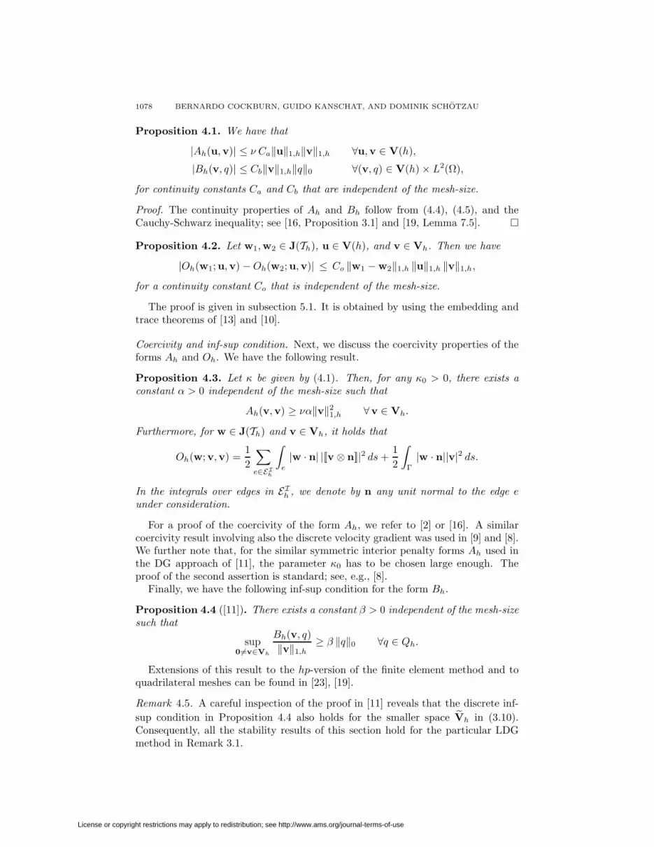
Proposition 4.1. We have that
|Ah(u,v)| ≤ ν Ca‖u‖1,h‖v‖1,h ∀u,v ∈ V(h),
|Bh(v, q)| ≤ Cb‖v‖1,h‖q‖0 ∀(v, q) ∈ V(h) × L2(Ω),
for continuity constants Ca and Cb that are independent of the mesh-size.
Proof. The continuity properties of Ah and Bh follow from (4.4), (4.5), and theCauchy-Schwarz inequality; see [16, Proposition 3.1] and [19, Lemma 7.5].
Proposition 4.2. Let w1,w2 ∈ J(Th), u ∈ V(h), and v ∈ Vh. Then we have
|Oh(w1;u,v) − Oh(w2;u,v)| ≤ Co ‖w1 − w2‖1,h ‖u‖1,h ‖v‖1,h,
for a continuity constant Co that is independent of the mesh-size.
The proof is given in subsection 5.1. It is obtained by using the embedding andtrace theorems of [13] and [10].
Coercivity and inf-sup condition. Next, we discuss the coercivity properties of theforms Ah and Oh. We have the following result.
Proposition 4.3. Let κ be given by (4.1). Then, for any κ0 > 0, there exists aconstant α > 0 independent of the mesh-size such that
Ah(v,v) ≥ να‖v‖21,h ∀v ∈ Vh.
Furthermore, for w ∈ J(Th) and v ∈ Vh, it holds that
Oh(w;v,v) =12
∑e∈EI
h
∫e
|w · n| |[[v ⊗ n]]|2 ds +12
∫Γ
|w · n||v|2 ds.
In the integrals over edges in EIh , we denote by n any unit normal to the edge e
under consideration.
For a proof of the coercivity of the form Ah, we refer to [2] or [16]. A similarcoercivity result involving also the discrete velocity gradient was used in [9] and [8].We further note that, for the similar symmetric interior penalty forms Ah used inthe DG approach of [11], the parameter κ0 has to be chosen large enough. Theproof of the second assertion is standard; see, e.g., [8].
Finally, we have the following inf-sup condition for the form Bh.
Proposition 4.4 ([11]). There exists a constant β > 0 independent of the mesh-sizesuch that
sup0 =v∈Vh
Bh(v, q)‖v‖1,h
≥ β ‖q‖0 ∀q ∈ Qh.
Extensions of this result to the hp-version of the finite element method and toquadrilateral meshes can be found in [23], [19].
Remark 4.5. A careful inspection of the proof in [11] reveals that the discrete inf-sup condition in Proposition 4.4 also holds for the smaller space Vh in (3.10).Consequently, all the stability results of this section hold for the particular LDGmethod in Remark 3.1.
License or copyright restrictions may apply to redistribution; see http://www.ams.org/journal-terms-of-use

A LOCALLY CONSERVATIVE LDG METHOD 1079
Stability of the post-processing operator. The next result states that the operator P
is a bounded linear operator from Vh to Vh with respect to the norm ‖ · ‖1,h. It isone of the main technical results needed to analyze the locally conservative LDGmethod (3.11)–(3.13).
Proposition 4.6. Let v ∈ Vh. Then we have
‖Pv ‖1,h ≤ Cstab‖v ‖1,h,
with a stability constant Cstab > 0 that is independent of the mesh-size.
The proof of this proposition is given in subsection 5.2 below. We remark that,for the LDG method in Remark 3.1, we have Cstab = 1 since P is chosen as theidentity.
We are now ready to state our main results.
4.3. The results. Our first result states that, under a smallness condition simi-lar to the one for the exact solution (1.7), the LDG method (3.11)–(3.13) definesa unique discrete approximation. Moreover, it actually gives an efficient way tocompute it.
Theorem 4.7 (Existence and uniqueness of discrete solutions). Assume that
(4.6) µ :=Co Cstab Cp‖f‖0
ν2 α2< 1.
Then the LDG method (3.11)–(3.13) defines a unique solution (uh, ph) ∈ Vh ×Qh.It satisfies the bounds
‖uh‖1,h ≤ Cp‖f‖0
ν α,(4.7)
‖ph‖0 ≤ β−1
(Ca + 2α
α
)Cp ‖f‖0,(4.8)
as well as
(4.9)∑e∈EI
h
∫e
|Puh · n| |[[uh ⊗ n]]|2 ds +∫
Γ
|Puh · n||uh|2 ds ≤C2
p‖f‖20
ν α.
Moreover, if (u+1h , p+1
h ) is the approximate solution given by the LDG methodin (3.11)–(3.12) for the Oseen equations with w = Pu
h, ≥ 0, then
‖uh − u+1h ‖1,h ≤ 2
(Cp‖f‖0
να
)µ
(1 − µ),
‖ph − p+1h ‖0 ≤ 2 β−1
(Ca + 2α
α
)Cp‖f‖0
µ
(1 − µ),
for any initial guess (u0h, p0
h) ∈ Vh × Qh.
This result, whose proof is given in subsection 5.3, states that the LDG methodin (3.11)–(3.13) is well defined and that we can compute its approximate solutionby solving a sequence of Oseen problems. Since the parameter µ is independentof the mesh-size, the convergence of that sequence is always exponential and socomputationally efficient.
Note that if we set(4.10)
α = min1, α, Cpoinc = maxCP , Cp, CO = maxCΩ, CoCstab,
License or copyright restrictions may apply to redistribution; see http://www.ams.org/journal-terms-of-use

1080 BERNARDO COCKBURN, GUIDO KANSCHAT, AND DOMINIK SCHOTZAU
then both the smallness assumptions in (1.7) and (4.6) are satisfied if we have that
COCpoinc‖f‖0
ν2 α2
< 1.
Hence, both the Navier-Stokes equations and their LDG approximations areuniquely solvable. Under a smallness condition that is slightly more restrictive,we obtain the following estimates.
Theorem 4.8 (Error estimates). Assume that
(4.11)COCpoinc‖f‖0
ν2 α2
≤ 12,
and that the exact solution (u, p) of the Navier-Stokes equations (1.1) satisfies
(4.12) u ∈ Hs+1(Ω)2, p ∈ Hs(Ω), s ≥ 1.
Then
‖u− uh‖1,h ≤Cu Capp
[‖u‖s+1 + ν−1 ‖p‖s
]hmink,s,
‖u− Puh‖1,h≤Cw Capp
[‖u‖s+1 + ν−1 ‖p‖s
]hmink,s,
‖p − ph‖0 ≤Cp Capp
[ν ‖u‖s+1 + ‖p‖s
]hmink,s,
‖σ − σh‖0 ≤Cσ Capp
[ν ‖u‖s+1 + ‖p‖s
]hmink,s,
where Capp only depends on the regularity of the mesh and the polynomial degree k,and
Cu = max(β + Cb
β
)(2 Ca + 3 α
α
),1 + Cstab
Cstab,2 Cb
α,
2α
,(4.13)
Cw = (1 + Cstab) + Cstab Cu,(4.14)
Cp = max(Ca + α
β
)Cu,
α (1 + Cstab)2β Cstab
,β + Cb
β,1β
,(4.15)
Cσ = (1 + Clift)Cu.(4.16)
This result, whose proof is given in subsection 5.4, states that the LDG methodunder consideration converges with optimal order. Note also that, since the functionw = Puh is exactly divergence free, it provides an optimally convergent globallysolenoidal approximation to the velocity!
Let us briefly discuss some extensions of these results.• First, we point out that all the results of this section are valid verbatim for the
LDG method in Remark 3.1 where Vh is replaced by the div-conforming space Vh
in (3.10) and P is chosen to be the identity.• Although here we only considered the case of triangular meshes, the results of
this paper can be straightforwardly extended to simplicial meshes in three dimen-sions. Furthermore, the LDG approach we propose here can be easily extended toQk − Qk − Pk−1 elements on quadrilateral or hexahedral affine meshes by using apost-processing operator P that is given by a slight modification of the BDM pro-jection on quadrilaterals or hexahedra; see [5]. The results in this section then holdtrue for this LDG method as well. This fact is actually verified in our numericalexperiments for which we have used square meshes and Q1 − Q1 − P0 elements.However, the extension of our results to Qk −Qk −Qk−1 elements on quadrilateralmeshes is not straightforward. Although, by using a post-processing operator P
License or copyright restrictions may apply to redistribution; see http://www.ams.org/journal-terms-of-use

A LOCALLY CONSERVATIVE LDG METHOD 1081
that is a slight modification of the standard Raviart-Thomas projection, it is easyto define a solenoidal velocity field w that belongs to the anisotropic polynomialspace Qk−1,k×Qk,k−1. The approximation properties in this space give rise to onlysuboptimal convergence rates. If, on the other hand, the polynomial degree of thepost-processed velocity is increased, the field w cannot be shown to be solenoidal,as ∇ · Vh ⊂ Qh.
• Finally, let us remark that here we have used the LDG approach to discretizethe viscous terms. However, our results remain valid for any other DG discretizationof these terms whose primal bilinear form Ah is both coercive and continuous, suchas, e.g., the interior penalty form. For detail, we refer the reader to the discussionsin [2] and [19].
5. Proofs
In this section, we provide the proofs of our main results.
5.1. Proof of Proposition 4.2. We begin by proving Proposition 4.2. To dothis, note that, if we insert the definition of the upwinding numerical flux into theform Oh, we have
Oh(w;u,v) = −∑
K∈Th
∫K
u · ∇ · (v ⊗ w) dx
+∑
K∈Th
∫∂K
[w · nKu − 1
2|w · nK |(uext − u)
]· v ds.
Here, uext denotes the exterior trace of u taken over the edge under considerationand set to zero on the boundary. If we perform now a simple integration by parts,we get
Oh(w;u,v) =∑
K∈Th
∫K
∇u : (v ⊗ w) dx
+∑
K∈Th
∫∂K
[12w · nK(uext − u) − 1
2|w · nK |(uext − u)
]· v ds.
This implies that
Oh(w1;u,v) − Oh(w2;u,v) = T1 + T2,
where
T1 =∑
K∈Th
∫K
∇u :(v ⊗ (w1 − w2)
)dx,
T2 =∑
K∈Th
∫∂K
12(w1 − w2) · nK(uext − u) · v ds
−∑
K∈Th
∫∂K
12
(|w1 · nK | − |w2 · nK |
)(uext − u) · v ds.
To bound the term T1, we recall the following embedding result proved in [13,Proposition 4.5] for smooth and convex domains and in [10, Lemma 6.2] for generalpolygons:
‖v‖L4(Ω) ≤ C‖v‖1,h, v ∈ w ∈ L2(Ω)2 : w|K ∈ H1(K)2, K ∈ Th,
License or copyright restrictions may apply to redistribution; see http://www.ams.org/journal-terms-of-use

1082 BERNARDO COCKBURN, GUIDO KANSCHAT, AND DOMINIK SCHOTZAU
with a constant independent of the mesh-size. (We point out that the broken H1-norm used in [13] is slightly different than the one we use here. However, a carefulinspection of the proof of Proposition 4.5 therein shows that, in fact the result holdsfor our definition of ‖ · ‖1,h.) It is then clear that we can use Holder’s inequality toobtain
|T1| ≤ ‖w1 − w2‖L4(Ω)‖u‖1,h‖v‖L4(Ω) ≤ C‖w1 − w2‖1,h‖u‖1,h‖v‖1,h.
It remains to estimate the term T2. Using the Lipschitz continuity of the functionx → |x|, we get
|T2| ≤∑
K∈Th
∫∂K
|w1 · nK − w2 · nK | |[[u⊗ n]]| |v| ds,
and, proceeding as in the proof of [13, Proposition 4.5], we obtain
|T2| ≤ C‖w1 − w2‖1,h‖u‖1,h‖v‖1,h,
with a constant independent of the mesh-size. This completes the proof of Propo-sition 4.2.
5.2. Proof of Proposition 4.6. We prove Proposition 4.6 by first establishinglocal stability bounds over patches of elements and then by summing up these localresults.
Let v ∈ Vh be fixed. We proceed in several steps.Step 1: Local bounds in the interior. Let e = ∂K1 ∩ ∂K2 be an interior edge
shared by two elements K1 and K2. We wish to establish a local stability boundover the patch formed by K1 and K2. Namely, by defining the local seminorm
|v|2e = ‖∇v‖20,K1
+ ‖∇v‖20,K2
+∫
e
h−1|[[v ⊗ n]]|2 ds,
we claim that
(5.1) |Pv|2e ≤ C[|v|2e+
∫∂K1
h−1|(v−vp)·nK1 |2 ds+∫
∂K2
h−1|(v−vp)·nK2 |2 ds],
with a constant C independent of the mesh-size.To prove (5.1), it is enough to consider the case where K1 and K2 form a reference
patch of unit size. The general case then follows from a scaling argument and theshape-regularity assumption on the mesh, by mapping K1 ∪ K2 onto the referencepatch using elementwise Piola transforms.
By the triangle inequality, we have
(5.2) |Pv|e ≤ |v − Pv|e + |v|e.
It remains to bound |v− Pv|e. To do so, we note that, for any element K ∈ Th,the restriction (v−Pv)|K belongs to Pk(K)2 and is uniquely defined by the moments∫
e
(v − Pv) · nK ϕds =∫
e
(v − vp) · nK ϕds ∀ϕ ∈ Pk(e), e ⊂ ∂K,∫K
(v − Pv) · ∇ϕdx = 0 ∀ϕ ∈ Pk−1(K),∫K
(v − Pv) ·Ψ dx = 0 ∀Ψ ∈ Ψk(K).
License or copyright restrictions may apply to redistribution; see http://www.ams.org/journal-terms-of-use
A LOCALLY CONSERVATIVE LDG METHOD 1083
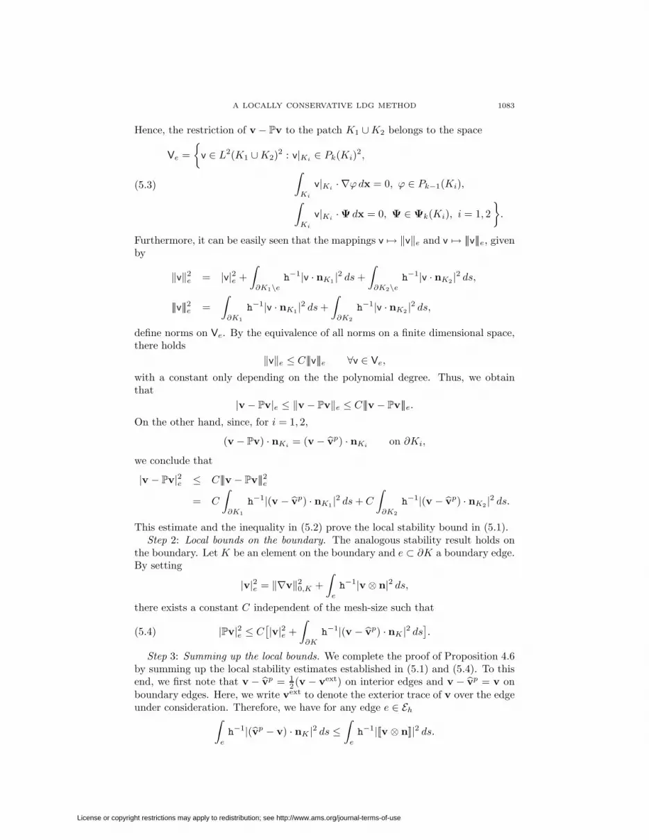
Hence, the restriction of v − Pv to the patch K1 ∪ K2 belongs to the space
Ve =
v ∈ L2(K1 ∪ K2)2 : v|Ki ∈ Pk(Ki)2,∫Ki
v|Ki · ∇ϕdx = 0, ϕ ∈ Pk−1(Ki),∫Ki
v|Ki ·Ψ dx = 0, Ψ ∈ Ψk(Ki), i = 1, 2
.
(5.3)
Furthermore, it can be easily seen that the mappings v → ‖v‖e and v → |||v|||e, givenby
‖v‖2e = |v|2e +
∫∂K1\e
h−1|v · nK1 |2 ds +∫
∂K2\e
h−1|v · nK2 |2 ds,
|||v|||2e =∫
∂K1
h−1|v · nK1 |2 ds +∫
∂K2
h−1|v · nK2 |2 ds,
define norms on Ve. By the equivalence of all norms on a finite dimensional space,there holds
‖v‖e ≤ C|||v|||e ∀v ∈ Ve,
with a constant only depending on the the polynomial degree. Thus, we obtainthat
|v − Pv|e ≤ ‖v − Pv‖e ≤ C|||v − Pv|||e.On the other hand, since, for i = 1, 2,
(v − Pv) · nKi = (v − vp) · nKi on ∂Ki,
we conclude that
|v − Pv|2e ≤ C|||v − Pv|||2e= C
∫∂K1
h−1|(v − vp) · nK1 |2 ds + C
∫∂K2
h−1|(v − vp) · nK2 |2 ds.
This estimate and the inequality in (5.2) prove the local stability bound in (5.1).Step 2: Local bounds on the boundary. The analogous stability result holds on
the boundary. Let K be an element on the boundary and e ⊂ ∂K a boundary edge.By setting
|v|2e = ‖∇v‖20,K +
∫e
h−1|v ⊗ n|2 ds,
there exists a constant C independent of the mesh-size such that
(5.4) |Pv|2e ≤ C[|v|2e +
∫∂K
h−1|(v − vp) · nK |2 ds].
Step 3: Summing up the local bounds. We complete the proof of Proposition 4.6by summing up the local stability estimates established in (5.1) and (5.4). To thisend, we first note that v − vp = 1
2 (v − vext) on interior edges and v − vp = v onboundary edges. Here, we write vext to denote the exterior trace of v over the edgeunder consideration. Therefore, we have for any edge e ∈ Eh∫
e
h−1|(vp − v) · nK |2 ds ≤∫
e
h−1|[[v ⊗ n]]|2 ds.
License or copyright restrictions may apply to redistribution; see http://www.ams.org/journal-terms-of-use

1084 BERNARDO COCKBURN, GUIDO KANSCHAT, AND DOMINIK SCHOTZAU
Using the local bounds in (5.1) and (5.4) and the above estimate for v − vp, weobtain
‖Pv‖21,h ≤ C
∑e∈Eh
|Pv|2e
≤ C∑e∈Eh
|v|2e + C∑
K∈Th
∫∂K
h−1|(v − vp) · nK |2 ds
≤ C∑e∈Eh
|v|2e + C∑e∈Eh
∫e
h−1|[[v ⊗ n]]|2 ds
≤ C‖v‖21,h,
with constants C independent of the mesh-size. This completes the proof of Propo-sition 4.6.
5.3. Proof of Theorem 4.7. To prove Theorem 4.7, we proceed as follows. First,we eliminate the pressure from the problem by restricting ourselves to the weaklydivergence-free subspace of Vh,
(5.5) Zh = v ∈ Vh : Bh(v, q) = 0 ∀q ∈ Qh .
The approximate velocity is thus characterized as the only function uh ∈ Zh suchthat
(5.6) Ah(uh,v) + Oh(Puh;uh,v) =∫
Ω
f · v dx ∀v ∈ Zh.
Then, we construct a contractive mapping S defined on a ball of Zh whose onlyfixed point is precisely the above velocity. The properties for the correspondingpressure ph then follow from its characterization
Bh(v, ph) =∫
Ω
f · v dx − Ah(uh,v) − Oh(Puh;uh,v) ∀v ∈ Vh/Zh,
and from the inf-sup condition for the incompressibility form Bh.We proceed in several steps.Step 1: The operator S. We begin by introducing the operator S. For u ∈ Zh,
u = S(u) denotes the solution of the following problem. Find u ∈ Zh such that
Ah(u,v) + Oh(Pu;u,v) =∫
Ω
f · v dx ∀v ∈ Zh.
Note that since u ∈ Zh we have, by Proposition 3.2, that Pu ∈ Jh(Th). As aconsequence, this problem is uniquely solvable.
Furthermore, by the coercivity of the form Ah and Oh in Proposition 4.3,
να‖u‖21,h ≤ Ah(u,u) + Oh(Pu;u,u)
=∫
Ω
f · u dx
≤ ‖f‖0‖u‖0.
By the Poincare inequality in (4.3), we obtain
να‖u‖21,h ≤ Cp‖f‖0‖u‖1,h.
License or copyright restrictions may apply to redistribution; see http://www.ams.org/journal-terms-of-use
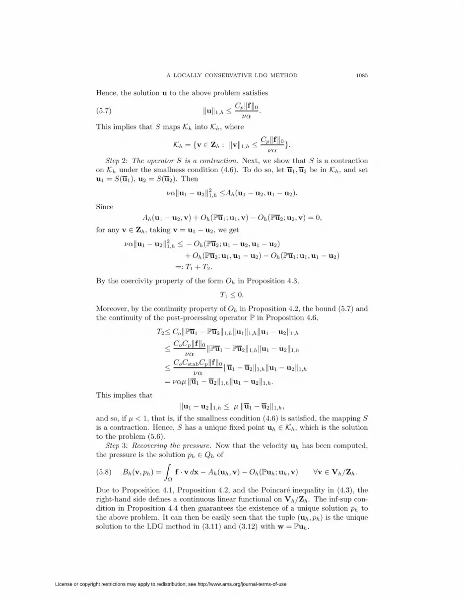
A LOCALLY CONSERVATIVE LDG METHOD 1085
Hence, the solution u to the above problem satisfies
(5.7) ‖u‖1,h ≤ Cp‖f‖0
να.
This implies that S maps Kh into Kh, where
Kh = v ∈ Zh : ‖v‖1,h ≤ Cp‖f‖0
να.
Step 2: The operator S is a contraction. Next, we show that S is a contractionon Kh under the smallness condition (4.6). To do so, let u1,u2 be in Kh, and setu1 = S(u1), u2 = S(u2). Then
να‖u1 − u2‖21,h ≤Ah(u1 − u2,u1 − u2).
SinceAh(u1 − u2,v) + Oh(Pu1;u1,v) − Oh(Pu2;u2,v) = 0,
for any v ∈ Zh, taking v = u1 − u2, we get
να‖u1 − u2‖21,h ≤ − Oh(Pu2;u1 − u2,u1 − u2)
+ Oh(Pu2;u1,u1 − u2) − Oh(Pu1;u1,u1 − u2)=: T1 + T2.
By the coercivity property of the form Oh in Proposition 4.3,
T1 ≤ 0.
Moreover, by the continuity property of Oh in Proposition 4.2, the bound (5.7) andthe continuity of the post-processing operator P in Proposition 4.6,
T2≤ Co‖Pu1 − Pu2‖1,h‖u1‖1,h‖u1 − u2‖1,h
≤ CoCp‖f‖0
να‖Pu1 − Pu2‖1,h‖u1 − u2‖1,h
≤ CoCstabCp‖f‖0
να‖u1 − u2‖1,h‖u1 − u2‖1,h
= ναµ ‖u1 − u2‖1,h‖u1 − u2‖1,h.
This implies that‖u1 − u2‖1,h ≤ µ ‖u1 − u2‖1,h,
and so, if µ < 1, that is, if the smallness condition (4.6) is satisfied, the mapping Sis a contraction. Hence, S has a unique fixed point uh ∈ Kh, which is the solutionto the problem (5.6).
Step 3: Recovering the pressure. Now that the velocity uh has been computed,the pressure is the solution ph ∈ Qh of
(5.8) Bh(v, ph) =∫
Ω
f · v dx − Ah(uh,v) − Oh(Puh;uh,v) ∀v ∈ Vh/Zh.
Due to Proposition 4.1, Proposition 4.2, and the Poincare inequality in (4.3), theright-hand side defines a continuous linear functional on Vh/Zh. The inf-sup con-dition in Proposition 4.4 then guarantees the existence of a unique solution ph tothe above problem. It can then be easily seen that the tuple (uh, ph) is the uniquesolution to the LDG method in (3.11) and (3.12) with w = Puh.
License or copyright restrictions may apply to redistribution; see http://www.ams.org/journal-terms-of-use

1086 BERNARDO COCKBURN, GUIDO KANSCHAT, AND DOMINIK SCHOTZAU
Step 4: The stability bounds. Next, let us show the stability bounds for (uh, ph)in Theorem 4.7. The bound for ‖uh‖1,h in (4.7) follows in a straightforward waysince uh ∈ Kh. To obtain the bound for the upwind term in (4.9), note that
να‖uh‖21,h + Oh(Puh;uh,uh) ≤ Cp‖f‖0‖uh‖2
1,h ≤ 12
C2p‖f‖2
0
να+
12να‖uh‖2
1,h.
Similarly to the previous arguments, here we have used the coercivity of Ah, equa-tion (5.6) with test function v = uh, and the Poincare inequality (4.3). Bringingthe term 1
2να‖uh‖21,h to the left-hand side and observing the coercivity of Oh give
the stability bound in (4.9).Moreover, using the inf-sup condition in Proposition 4.4, the Poincare inequality
in (4.3), the continuity properties in Proposition 4.1 and Proposition 4.2, and thestability of P in Proposition 4.6, we have from (5.8)
β‖ph‖0 ≤ sup0 =v∈Vh
Bh(v, ph)‖v‖1,h
≤ Cp‖f‖0 + ν Ca‖uh‖1,h + CoCstab‖uh‖21,h.
Taking into account the stability bound for uh and assumption (4.6) gives
‖ph‖0 ≤ β−1
(Cp‖f‖0 +
CaCp‖f‖0
α+
CoCstabCp‖f‖0
ν2α2Cp‖f‖0
)≤ β−1Cp‖f‖0
(2 +
Ca
α
).
This gives the desired bound (4.8) for ph.Step 5: The convergence estimates. It remains to prove the error estimates for
the sequence (uh, p
h)≥0. Let us begin with that of the velocity. From Step 3, wehave that u+1
h = S(uh). As a consequence, since S is a contraction with Lipschitz
constant µ, we immediately get
‖uh − u+1h ‖1,h ≤
(µ
(1 − µ)
)‖u2
h − u1h‖1,h.
The result now follows from the fact that, by the stability bound (5.7),
‖umh ‖1,h ≤ Cp‖f‖0
να,
for m ≥ 1.To obtain the estimate for the pressure, we proceed as follows. First, we note
that, from Step 4, we have
Bh(v, p+1h ) =
∫Ω
f · v dx − Ah(u+1h ,v) − Oh(Pu
h;u+1h ,v) ∀v ∈ Vh.
This implies that
Bh(v, ph − p+1h ) = −Ah(uh − u+1
h ,v) − Oh(Puh;uh,v) + Oh(Puh;uh,v)
−Oh(Puh;uh,v) + Oh(Pu
h;u+1h ,v)
= −Ah(uh − u+1h ,v) − Oh(Puh;uh,v) + Oh(Pu
h;uh,v)
Oh(Puh;u+1
h − uh,v).
We insert this expression in the inf-sup condition for Bh, use the stability propertiesof Ah, Oh, and P, take into account the bounds for ‖uh‖1,h, ‖u
h‖1,h, and the
License or copyright restrictions may apply to redistribution; see http://www.ams.org/journal-terms-of-use

A LOCALLY CONSERVATIVE LDG METHOD 1087
contraction property of S to obtain
‖ph − p+1h ‖0 ≤ β−1
(νCaµ +
CoCstabCp‖f‖0
να(1 + µ)
)‖uh − u
h‖1,h
≤ β−1µ (νCa + 2να) ‖uh − uh‖1,h.
The desired bound for ‖ph − p+1h ‖0 then follows from the bound for ‖uh − u
h‖1,h.This completes the proof of Theorem 4.7.
5.4. Proof of Theorem 4.8. Here, we derive the error estimates in Theorem 4.8.To do that, we modify the approach used in [8] to get error estimates for theLDG method for the Oseen problem in two ways. First, we use the nonconformingapproach introduced in [16] and later used in [19], and consider the expression
Rh(u, p) := sup0 =v∈Vh
|Rh(u, p;v)|‖v‖1,h
,
where
Rh(u, p;v) := Ah(u,v) + Oh(u;u,v) + Bh(v, p) −∫
Ω
f · v dx, v ∈ Vh.
The second modification is, of course, due to the presence of the convective non-linearity.
Proof. We proceed in several steps.Step 1: The abstract estimate for ‖u−u‖1,h. Let us begin with the estimate for
the error ‖u− u‖1,h. We claim that we have
‖u− uh‖1,h ≤ Cu
[inf
v∈Vh
‖u− v‖1,h + infv∈Vh
‖u− v‖1,h(5.9)
+ infq∈Qh
1ν‖p − q‖0 +
1νRh(u, p)
],
where Cu is given by (4.13).To prove this result, we proceed as in the error analysis of standard mixed
methods (see, e.g., [5]) and consider first an element v ∈ Zh where Zh is the kernelin (5.5). We then have the trivial inequality
(5.10) ‖u− uh‖1,h ≤ ‖u− v‖1,h + ‖v − uh‖1,h.
Next, we obtain an estimate of v − uh. By the coercivity property of the form Ah
in Proposition 4.3, we have
(5.11) ν α ‖v − uh‖21,h ≤ ν α ‖v − uh‖2
1,h ≤ Ah(v − uh,v − uh),
and since
Ah(u − uh, v) + Oh(u;u, v) − Oh(Puh;uh, v) + Bh(v, p − ph) = Rh(u, p; v)
for any v ∈ Vh, for v = v − uh, we get that
Ah(v − uh,v − uh) = Ah(v − u,v − uh)
− Oh(u;u,v − uh) + Oh(Puh;uh,v − uh)
− Bh(v − uh, p − ph)
+ Rh(u, p;v − uh)=: T1 + T2 + T3 + T4.
License or copyright restrictions may apply to redistribution; see http://www.ams.org/journal-terms-of-use

1088 BERNARDO COCKBURN, GUIDO KANSCHAT, AND DOMINIK SCHOTZAU
Hence,α ν ‖v − uh‖2
1,h ≤ T1 + T2 + T3 + T4.
The terms T1, T3, and T4 can be easily estimated as follows. First, by thecontinuity of the form Ah,
T1 ≤ ν Ca‖u− v‖1,h‖v − uh‖1,h.
Then, by the definition of Rh and Rh,
T4 ≤ Rh(u, p) ‖v − uh‖1,h.
Finally, since v − uh ∈ Zh, we have
Bh(v − uh, p − ph) = Bh(v − uh, p) = Bh(v − uh, p − q),
for any q ∈ Qh. From Proposition 4.1, it follows that
T3 ≤ Cb‖v − uh‖1,h‖p − q‖0 ∀ q ∈ Qh.
It remains to estimate the term T2. To do that, consider the identity
T2 = − Oh(Pv;u,v − uh) + Oh(Puh;u,v − uh)
− Oh(Puh;v − uh,v − uh)
+ Oh(Pv;u,v − uh) − Oh(u;u,v − uh)
+ Oh(Puh;v − u,v − uh)=: T21 + T22 + T23 + T24.
Note that due to Propositions 4.2 and 4.6, the stability bound for u in (1.5), andthe definitions of the parameters in (4.10), we have
T21 ≤ Co Cstab‖u‖1‖v − uh‖21,h
≤ Co Cstab CP ‖f‖0
ν‖v − uh‖2
1,h
≤ CO Cpoinc‖f‖0
να‖v − uh‖2
1,h
≤ 12να ‖v − uh‖2
1,h,
by the smallness condition (4.11).Next, by the coercivity property of Oh in Proposition 4.3,
T22 ≤ 0,
and, by Propositions 4.2 and 4.6, and the bound for uh in Theorem 4.7,
T24≤CoCstabCp‖f‖0
να‖u− v‖1,h‖v − uh‖1,h
≤ COCpoinc‖f‖0
να‖u− v‖1,h‖v − uh‖1,h
≤12να ‖u− v‖1,h‖v − uh‖1,h,
by the smallness condition (4.11).
License or copyright restrictions may apply to redistribution; see http://www.ams.org/journal-terms-of-use

A LOCALLY CONSERVATIVE LDG METHOD 1089
Finally, by the Lipschitz property of the form Oh in Proposition 4.2, we have
T23≤Co‖u− Pv‖1,h‖u‖1‖v − uh‖1,h
≤CoCP ‖f‖0
ν‖u− Pv‖1,h‖v − uh‖1,h
≤ να
2 Cstab‖u− Pv‖1,h‖v − uh‖1,h,
by the bound for u in (1.5) and the smallness condition (4.11). Now, take anarbitrary function v in Vh. Since P reproduces functions in Vh, we have Pv = v,and so
‖u− Pv‖1,h ≤ ‖u− v‖1,h + ‖Pv − Pv‖1,h
≤ ‖u− v‖1,h + Cstab‖v − v‖1,h
≤ (1 + Cstab)‖u − v‖1,h + Cstab‖u− v‖1,h,
by Proposition 4.6. This implies that
T23≤να
2
((1 + Cstab
Cstab
)‖u− v‖1,h + ‖u− v‖1,h
)‖v − uh‖1,h.
Thus, gathering all the estimates above and inserting them in the right-handside of inequality (5.11), and bringing T21 to the left-hand side, we obtain
‖v − uh‖1,h ≤ 2(
Ca + α
α
)‖u− v‖1,h +
(1 + Cstab
Cstab
)‖u− v‖1,h
+(
2 Cb
να
)‖p − q‖0 +
(2
να
)Rh(u, p).
Inserting this estimate in the right-hand side of inequality (5.10), we get
‖u− uh‖1,h ≤(
2Ca + 3α
α
)‖u− v‖1,h +
(1 + Cstab
Cstab
)‖u− v‖1,h
+(
2 Cb
να
)‖p− q‖0 +
(2
να
)Rh(u, p),
(5.12)
for any v ∈ Zh, v ∈ Vh, and q ∈ Qh.It remains to replace v ∈ Zh by an arbitrary function in v ∈ Vh. To this end,
fix v ∈ Vh and consider the problem: Find r ∈ Vh such that
Bh(r, q) = Bh(u − v, q) ∀q ∈ Qh.
The inf-sup condition in Proposition 4.4 guarantees that such a solution r exists.Furthermore, it can be easily seen that we have
‖r‖1,h ≤ β−1Cb‖u− v‖1,h,
in view of the inf-sup condition for Bh and the continuity of the form Bh. Byconstruction and since Bh(u, q) = 0 for any q ∈ Qh, we further have that r+v ∈ Zh.Inserting r+v in (5.12), employing the triangle inequality, and taking into accountthe above bound for r yield the abstract error estimate (5.9) for the velocity.
Step 2: The abstract estimate for ‖u−Puh‖1,h. As a consequence of the approx-imation result (5.9), we obtain the estimate of the error between u and its globallysolenoidal approximation Puh
(5.13) ‖u− Puh‖1,h ≤ (1 + Cstab) infv∈Vh
‖u− v‖1,h + Cstab‖u− uh‖1,h.
License or copyright restrictions may apply to redistribution; see http://www.ams.org/journal-terms-of-use

1090 BERNARDO COCKBURN, GUIDO KANSCHAT, AND DOMINIK SCHOTZAU
To see this, note that
‖u− Puh‖1,h ≤ ‖u− v‖1,h + ‖v − Puh‖1,h
≤ ‖u− v‖1,h + Cstab‖v − uh‖1,h
≤ (1 + Cstab)‖u − v‖1,h + Cstab‖u− uh‖1,h,
where v is any element of Vh. Here we have used the stability bound in Propo-sition 4.6 and the fact that P reproduces polynomials in Vh. This shows theinequality (5.13).
Step 3: The abstract estimate for the pressure. Now, let us obtain the estimatefor the pressure. We claim that the error in the pressure satisfies
‖p − ph‖0 ≤ Cp
[inf
v∈Vh
ν ‖u− v‖1,h + infv∈Vh
ν ‖u− v‖1,h(5.14)
+ infq∈Qh
‖p − q‖0 + Rh(u, p)],
where Cp is given by (4.15).To see this, we proceed in a way similar to the one used to deal with the velocity.
Thus, we begin by noting that for q ∈ Qh
‖p− ph‖0 ≤ ‖q − ph‖0 + ‖p− q‖0
≤ β−1 supv∈Vh
Bh(v, q − ph)‖v‖1,h
+ ‖p − q‖0
≤ β−1 supv∈Vh
Bh(v, p − ph)‖v‖1,h
+ β−1 supv∈Vh
Bh(v, q − p)‖v‖1,h
+ ‖p − q‖0,
where we have used the inf-sup condition in Proposition 4.4. Therefore,
(5.15) ‖p− ph‖0 ≤ β−1 supv∈Vh
Bh(v, p − ph)‖v‖1,h
+ (1 + β−1Cb) ‖p − q‖0,
by the continuity of the form Bh.To bound the first term on the right-hand side of (5.15), we note that
Bh(v, p − ph) = −Ah(u − uh,v) − Oh(u;u,v) + Oh(Puh;uh,v) + Rh(u, p;v),
for any v ∈ Vh, and proceed as in the previous step to obtain
Bh(v, p − ph) = Ah(u− uh,v) + Oh(Puh;uh − u,v)
+ Oh(Puh;u,v) − Oh(u;u,v) + Rh(u, p;v)
≤[
(ν Ca +12ν α) ‖u− uh‖1,h
+ν α
2 Cstab‖u− Puh‖1,h + Rh(u, p)
]‖v‖1,h,
and since
‖u− Puh‖1,h ≤ (1 + Cstab)‖u − v‖1,h + Cstab‖u− uh‖1,h,
from Step 2, we get
Bh(v, p − ph) ≤(Ca + α) ν ‖u− uh‖1,h
+α
2
(1 + Cstab
Cstab
)ν ‖u− v‖1,h + Rh(u, p).
License or copyright restrictions may apply to redistribution; see http://www.ams.org/journal-terms-of-use

A LOCALLY CONSERVATIVE LDG METHOD 1091
Inserting this inequality in (5.15) and using the bound (5.9) for ‖u − uh‖1,h fromStep 1, we immediately obtain the abstract estimate (5.14) for the pressure.
Step 4: The abstract estimate for the velocity gradient. To derive the errorestimate for σ − σh, we note that from (3.14) we have
σ − σh = ν[∇u −∇huh + L(uh)
].
Hence,
‖σ − σh‖0 ≤ ν‖u− uh‖1,h + ν‖L(uh)‖0.
Using the stability bound (4.4) for the lifting operator L yields
‖L(uh)‖20 ≤ C2
lift
∑e∈Eh
∫e
κ0h−1|[[uh ⊗ n]]|2 ds ≤ C2
lift‖u− uh‖21,h.
The last inequality follows as the jumps of the exact solution vanish. This showsthat
(5.16) ‖σ − σh‖0 ≤ ν (1 + Clift) ‖u− uh‖1,h.
Step 5: Approximation estimates. Under the regularity assumption (4.12), thestandard approximation property
infv∈Vh
ν ‖u− v‖1,h + infq∈Qh
‖p − q‖0 ≤ Capphmink,s[ν ‖u‖s+1 + ‖p‖s
]holds. Moreover, from the results in [5] (see also [11, Section 3]) we have
infv∈Vh
‖u− v‖1,h ≤ Capphmink,s‖u‖s+1.
Finally, we have that
Rh(u, p) ≤ Capphmink,s[ν ‖u‖s+1 + ‖p‖s
],
with a constant Capp independent of the mesh-size.To see the estimate of the residual, we proceed as follows. For v ∈ Vh, it is easy
to see that Rh(u, p;v) is given by
Rh(u, p;v) =∑e∈Eh
∫e
ν∇u−P h(ν∇u) : [[v⊗n]] ds−∑e∈Eh
∫e
p−Php[[v ·n]] ds,
with P h : L2(Ω)2×2 → Σh and Ph : L2(Ω)/R → Qh denoting the L2-projectionsonto Σh and Qh, respectively. The desired estimate then follows by proceeding asthe proof of [19, Proposition 8.1] and using standard approximation results for Ph
and Ph.Step 6: Conclusion. It is now a simple matter to see that the error estimates of
Theorem 4.8 follow by inserting the approximation estimates obtained in the pre-vious step into the abstract bounds for the velocity (5.9), for its globally solenoidalpost-processing (5.13), the pressure (5.14), and the velocity gradient (5.16). Thiscompletes the proof of Theorem 4.8.
License or copyright restrictions may apply to redistribution; see http://www.ams.org/journal-terms-of-use

1092 BERNARDO COCKBURN, GUIDO KANSCHAT, AND DOMINIK SCHOTZAU
6. Numerical results
In this section, we present numerical experiments that show that the theoreticalrates of convergence are sharp. We also display the behavior of the iterative methodas a function of the Reynolds number.
As a reference solution in our tests, we take the analytical solution (u, p) of theincompressible Navier-Stokes equations that was obtained by Kovasznay in [14].For a given viscosity ν, this solution is given by
u1(x, y) = 1 − eλx cos(2πy),
u2(x, y) =λ
2πeλx sin(2πy),
p(x, y) = −12e2λx + p,
where
λ =−8π2
ν−1 +√
ν−2 + 64π2.
It solves (1.1) with a suitably chosen right-hand side f . Here, the constant p is suchthat
∫Ω
p dx = 0. Further we use the values of the exact solution u = (u1, u2) toprescribe inhomogeneous Dirichlet boundary data g for the velocity on the wholeboundary of the computational domain, which we take to be Ω = (− 1
2 , 32 ) × (0, 2).
Note that in this case, the numerical fluxes (on edges e lying on the boundary)must be modified as
uwh (x) =
limε↓0 uh (x − εw(x)) , x ∈ e \ Γ−,
g(x), x ∈ e ∩ Γ−,
σh = σh − κ(uh − g) ⊗ n, uσh = g,
uph = g, ph = ph.
We consider square meshes that are generated by refining the single grid cell(− 1
2 , 32 ) × (0, 2) uniformly. Therefore, a mesh on “level” L consists of 2L by 2L
cells. All computations are performed with bilinear shape functions for σh and uh
and piecewise constants for ph, according to the remarks in subsection 4.3. Thestabilization function κ is chosen as in (4.1) with κ0 = 4. Our analysis then pre-dicts first-order convergence for uh in the norm ‖.‖1,h and for the pressure in theL2-norm.
In Table 1 we show the errors and convergence rates in p, u and σ obtainedfor ν = 0.1. The errors in p and σ are measured in the L2-norm while u − uh
and u − Puh are evaluated in the norm ‖.‖1,h. We observe the predicted first-order convergence for all the error components, in full agreement with the resultsof Theorem 4.8. Note that we have scaled the L2-error in σ by ν−1 so that thiserror can be directly compared to the H1-errors in u−uh and u−Puh. These threeerrors are all of the same magnitude, with a slight advantage for the post-processedsolution.
In Table 2 we show the seminorm of the errors u − uh and u − Puh whichmeasures their jumps. Note that it superconverges with order 3/2. This meansthat the relative contribution of this seminorm to the ‖ · ‖1,h-norm diminishes as hdecreases. An analysis of this phenomenon remains to be carried out.
License or copyright restrictions may apply to redistribution; see http://www.ams.org/journal-terms-of-use

A LOCALLY CONSERVATIVE LDG METHOD 1093
Table 1. Errors and orders of convergence for ν = 0.1.
L ‖p − ph‖0 ‖u− uh‖1,h ‖u− Puh‖1,h ν−1‖σ − σh‖0
3 2.2e+0 — 1.2e+1 — 8.1e+0 — 7.0e-0 —4 1.0e+0 1.12 5.4e+0 1.11 3.2e+0 1.33 3.4e-0 1.055 4.8e-1 1.10 2.4e+0 1.16 1.4e+0 1.18 1.6e-0 1.076 2.3e-1 1.04 1.1e+0 1.18 6.8e-1 1.06 7.8e-1 1.047 1.2e-1 1.01 4.7e-1 1.17 3.4e-1 1.02 3.9e-1 1.028 5.8e-2 1.00 2.2e-1 1.13 1.7e-1 1.01 1.9e-1 1.02
Table 2. Errors and orders of convergence for ν = 0.1 in theseminorm |v|h :=
∑e∈Eh
∫e
κ0h−1 |[[v ⊗ n]]|2 ds1/2.
L |u− uh |h |u − Puh |h3 9.1e+0 — 4.8e+0 —4 4.2e+0 1.11 1.5e+0 1.725 1.8e+0 1.23 4.7e-1 1.646 7.2e-1 1.32 1.6e-1 1.547 2.8e-1 1.39 5.6e-2 1.528 1.0e-1 1.44 2.0e-2 1.51
In Table 3 we show the L2-errors in the velocities and their corresponding con-vergence orders. In the first column we observe that the velocities converge withsecond-order accuracy. In the second column, we notice that by post-processing theerror is reduced by a factor of roughly 3/2. Therefore, the post-processed solution
Table 3. L2-errors and orders of convergence in the velocity andL∞-norm of the divergence of the post-processed solution Puh forν = 0.1.
L ‖u− uh‖0 ‖u− Puh‖0 ‖∇ · Puh‖∞3 6.4e-1 — 4.9e-1 — 1.4e-124 1.6e-1 2.03 1.1e-1 2.22 1.4e-125 3.3e-2 2.22 2.0e-2 2.37 3.2e-126 7.1e-3 2.24 4.2e-3 2.27 1.5e-117 1.6e-3 2.19 9.8e-4 2.12 1.8e-128 3.5e-4 2.13 2.4e-4 2.04 2.9e-11
Table 4. Number of iterations for convergence of the nonlinear iteration.
L ν = 1 ν = 0.1 ν = 0.013 14 33 8654 10 21 1065 8 16 546 6 12 297 5 10 188 6 10 13
License or copyright restrictions may apply to redistribution; see http://www.ams.org/journal-terms-of-use

1094 BERNARDO COCKBURN, GUIDO KANSCHAT, AND DOMINIK SCHOTZAU
should be used as the best approximation obtained by our scheme. Furthermore,we show the L∞-norms of the divergence of Puh (evaluated at the points of a 4-by-4Gauss formula on each cell). These are of the order of the residual of the nonlineariteration, confirming that the post-processed solution is indeed divergence free.
The convergence of the nonlinear iteration under consideration is illustrated inTable 4. The number of steps required to reduce the start residual by a factor of107 is displayed. The initial guess for the iterations is the vector u0
h = 0.The linear system in each step is solved by a preconditioned GMRES method up
to a relative accuracy of 10−4, using the preconditioners described in [12]. There-fore, the error of the linear iterations is small enough to be neglected. Table 4shows that the number of iteration steps is not only bounded independently of themesh-size, but in fact decreasing. This is in perfect agreement with our theoreticalresults in Theorem 4.7. If we decrease the viscosity, the increase of the numberof iteration steps for convergence is quite moderate on fine grids. Of course, thisonly holds as long as there is convergence. With ν = 10−3, the nonlinear iterationdoes not converge anymore, probably because the stationary solution is not stablein this case.
7. Concluding remarks
In this paper, we described and analyzed a new LDG method for the approxima-tion of the two-dimensional incompressible Navier-Stokes equations on triangularmeshes. The approximation is based on discontinuous Pk − Pk − Pk−1 elementsfor the approximation of the velocity, the velocity gradient, and the pressure, re-spectively, and on a post-processing procedure. Alternatively, the approximationof the velocity field can be based on div-conforming BDM elements for which thisprocedure can be omitted. These are the only DG methods that are locally conser-vative and stable for the incompressible Navier-Stokes equations. They are also theonly methods that provide a systematic and simple way to obtain an approximatevelocity that is exactly divergence free for polynomials of degree greater than orequal to 1; see [20].
As discussed in subsection 4.3, the results of this paper can be extended in astraightforward way to simplicial meshes in three dimensions and to Qk−Qk−Pk−1
elements on quadrilateral or hexahedral affine meshes. Future work will be devotedto extending the methods to the case in which the numerical flux up
h depends also onthe pressure. This happens, for example, when all the unknowns are approximatedwith the same polynomial space; see [9], [8]. Indeed, in this case, the operator P
depends not only on the velocity but also on the pressure. As a consequence, theanalysis of the convergence of the fixed point iteration is much more delicate. Itwill be carried out in a forthcoming paper.
References
[1] D. N. Arnold, An interior penalty finite element method with discontinuous elements, SIAMJ. Numer. Anal. 19 (1982), 742–760. MR0664882 (83f:65173)
[2] D. N. Arnold, F. Brezzi, B. Cockburn, and L. D. Marini, Unified analysis of discontinu-
ous Galerkin methods for elliptic problems, SIAM J. Numer. Anal. 39 (2002), 1749–1779.MR1885715 (2002k:65183)
[3] S. Brenner, Poincare-Friedrichs inequalities for piecewise H1 functions, SIAM J. Numer.Anal. 41 (2003), 306–324. MR1974504 (2004d:65140)
License or copyright restrictions may apply to redistribution; see http://www.ams.org/journal-terms-of-use

A LOCALLY CONSERVATIVE LDG METHOD 1095
[4] F. Brezzi, J. Douglas, Jr., and L. D. Marini, Two families of mixed finite elements for secondorder elliptic problems, Numer. Math. 47 (1985), 217–235. MR0799685 (87g:65133)
[5] F. Brezzi and M. Fortin, Mixed and hybrid finite element methods, Springer Verlag, 1991.MR1115205 (92d:65187)
[6] P. Castillo, B. Cockburn, I. Perugia, and D. Schotzau, An a priori error analysis of thelocal discontinuous Galerkin method for elliptic problems, SIAM J. Numer. Anal. 38 (2000),1676–1706. MR1813251 (2002k:65175)
[7] B. Cockburn, G. Kanschat, and D. Schotzau, The local discontinuous Galerkin methods forlinear incompressible flow: A review, Computers and Fluids (Special Issue: Residual basedmethods and discontinuous Galerkin schemes), to appear.
[8] , Local discontinuous Galerkin methods for the Oseen equations, Math. Comp. 73(2004), 569–593. MR2031395
[9] B. Cockburn, G. Kanschat, D. Schotzau, and C. Schwab, Local discontinuous Galerkin meth-ods for the Stokes system, SIAM J. Numer. Anal. 40 (2002), 319–343. MR2003g:65141
[10] V. Girault, B. Riviere, and M. F. Wheeler, A discontinuous Galerkin method with non-overlapping domain decomposition for the Stokes and Navier-Stokes problems, Math. Comp.,74 (2005), 53–84.
[11] P. Hansbo and M.G. Larson, Discontinuous finite element methods for incompressible andnearly incompressible elasticity by use of Nitsche’s method, Comput. Methods Appl. Mech.
Engrg., 191 (2002), 1895–1908. MR1886000 (2003j:74057)[12] G. Kanschat, Block preconditioners for LDG discretizations of linear incompressible flow
problems, J. Sci. Comput., 25 (2003), 815–831.[13] O. A. Karakashian and W.N. Jureidini, A nonconforming finite element method for the
stationary Navier-Stokes equations, SIAM J. Numer. Anal., 35 (1998), 93–120. MR99d:65320[14] L. I. G. Kovasznay, Laminar flow behind a two-dimensional grid, Proc. Camb. Philos. Soc.
44 (1948), 58–62. MR0024282 (9:476d)[15] P. Lesaint and P. A. Raviart, On a finite element method for solving the neutron trans-
port equation, Mathematical Aspects of Finite Elements in Partial Differential Equations(C. de Boor, ed.), Academic Press, 1974, pp. 89–145. MR0658142 (58:31918)
[16] I. Perugia and D. Schotzau, An hp-analysis of the local discontinuous Galerkin method fordiffusion problems, J. Sci. Comput. (Special Issue: Proceedings of the Fifth InternationalConference on Spectral and High Order Methods (ICOSAHOM-01), Uppsala, Sweden) 17(2002), 561–571. MR1910752
[17] A. Quarteroni and A. Valli, Numerical approximation of partial differential equations,Springer, New York, 1994. MR1299729 (95i:65005)
[18] W.H. Reed and T.R. Hill, Triangular mesh methods for the neutron transport equation, Tech.Report LA-UR-73-479, Los Alamos Scientific Laboratory, 1973.
[19] D. Schotzau, C. Schwab, and A. Toselli, hp-DGFEM for incompressible flows, SIAM J.Numer. Anal. 40 (2003), 2171–2194. MR1974180
[20] L. R. Scott and M. Vogelius, Norm estimates for a maximal right inverse of the divergenceoperator in spaces of piecewise polynomials, RAIRO Model. Math. Anal. Numer. 19 (1985),111–143. MR0813691 (87i:65190)
[21] R. Temam, Sur l’approximation des solutions des equations de Navier-Stokes, C. R. Acad.Sci. Paris Ser. A 216 (1966), 219–221. MR0211059 (35:1941)
[22] , Une methode d’approximation de la solutions des equations de Navier-Stokes, Bull.Soc. Math. France 98 (1968), 115–152. MR0237972 (38:6249)
[23] A. Toselli, hp-discontinuous Galerkin approximations for the Stokes problem, Math. ModelsMethods Appl. Sci. 12 (2002), 1565–1616. MR1938957 (2003m:65211)
School of Mathematics, University of Minnesota, Vincent Hall, Minneapolis, Min-
nesota 55455
E-mail address: [email protected]
Institut fur Angewandte Mathematik, Universitat Heidelberg, Im Neuenheimer
Feld 293/294, 69120 Heidelberg, Germany
E-mail address: [email protected]
Mathematics Department, University of British Columbia, 1984 Mathematics Road,
Vancouver, British Columbia V6T 1Z2, Canada
E-mail address: [email protected]
License or copyright restrictions may apply to redistribution; see http://www.ams.org/journal-terms-of-use


