Hierarchical models for service-oriented systems

Roberto Bruni1, Fabio Gadducci1, Andrea Corradini1,Alberto Lluch Lafuente2, and Ugo Montanari1

1 Department of Computer Science, University of Pisa, Italy2 IMT Institute for Advance Studies Lucca, Italy

Abstract. We present our approach to the denotation and representationof hierarchical graphs: a suitable algebra of hierarchical graphs and twodomains of interpretations. Each domain of interpretation focuses ona particular perspective of the graph hierarchy: the top view (nestedboxes) is based on a notion of embedded graphs while the side view (treehierarchy) is based on gs-graphs. Our algebra can be understood as ahigh-level language for describing such graphical models, which are wellsuited for defining graphical representations of service-oriented systemswhere nesting (e.g. sessions, transactions, locations) and linking (e.g.shared channels, resources, names) are key aspects.

1 Introduction

As witnessed by a vast literature, graphs offer a convenient ground for thespecification and analysis of software systems. As an example, the use of graphsas a suitable domain for the visualisation of a system specified by algebraic meansis pursued in various proposals, based on traditional Graph Transformation [15],Bigraphical Reactive Systems [16], and Synchronised Hyperedge Replacement [13].

Despite their expressiveness and flexibility, the use of these formalisms to builda graphical representation for an existing specification language involves two ma-jor challenges. First, encoding system configurations (states), guaranteeing thatstructural equivalence is preserved: i.e. equivalent (e.g. structurally congruent)configurations are mapped into equivalent (e.g. isomorphic) graphs. Second, en-coding system dynamics (e.g. behaviour, reconfigurations, model transformations,refactorings), guaranteeing that the original semantics is respected.

Preserving structural equivalence has several advantages. It offers an intuitivenormal form representation for systems, and it allows us to reuse results andtechniques from graph theory for solving specific problems. In particular, thesoundness of the encoding is necessary to use graph transformation approaches [10]to model dynamic aspects since (sub)graph isomorphism is at the base of therule matching mechanism.

The encoding of configurations given with an algebraic syntax (e.g. as inprocess calculi) is facilitated by their structure (i.e. processes are terms) since itcan be defined inductively. In absence of an algebraic presentation for the languageunder consideration, ad-hoc algebraic syntax must be developed if one wants tobenefit from structural induction in proofs, transformations or definitions. Still,

most graph models are not equipped with algebraic syntax and those that existrequire advanced skills to deal with sophisticated models involving set-theoreticdefinitions of graphs with interfaces (e.g. [15]) or complex type systems (e.g. [7]),hampering definitions and proofs. Moreover, one encounters a severe drawback:namely, the syntax of graph formalisms are often very different from the sourcelanguage and not provided with suitable primitives to deal with features thatcommonly arise in algebraic specifications, like names (e.g. references, channels),name restrictions (e.g. hiding, nonce generation) or hierarchical aspects (e.g.ambients, scopes) in the case of process calculi. Identifying the right structure isfundamental to provide scalable techniques.

Our goal is to define a simple flexible syntax for hierarchical models and todevelop a technique that simplifies the definition of graphical representationsof languages. We think that nesting and linking must be treated as first-classconcepts, conveniently represented with a suitable syntax that allows one toexpress and exploit them. Nesting and linking are two key structural aspects thatarise repeatedly in computer systems: consider e.g. the structure of file systems,composite diagrams, networks, membranes, sessions, transactions, locations,structured state machines or XML files. In particular, nesting plays a fundamentalrole for abstracting the complexity of a system by offering different levels ofdetail. Various graphical models of nesting and sharing structures already existbut (as we claim in [3–5]) none of them offer a simple, intuitive syntax.

Here, the gap between the different levels of abstraction at which algebraicspecifications and graphical models reside is filled by a simple algebra that enjoysprimitives for dealing with names, restriction, parallel composition and, mostimportantly, nesting and that is equipped with a (sound and complete) set ofaxioms equating two terms whenever they represent isomorphic graphs. Besidesfacilitating the visual specification of configurations, the algebraic structurefacilitates definitions, transformations and proofs by induction.

Structure of this chapter. § 2 introduces the algebra of hierarchical graphs. § 3presents our two models of hierarchical graphs. § 4 shows the expressiveness andflexibility of our design algebra in modelling heterogeneous notations, rangingfrom workflow languages to sophisticated process calculi.

2 The syntax of hierarchical graphs

We introduce our algebra of hierarchical graphs that we call designs. The algebraicpresentation of designs is mostly inspired by the graph algebra of [9].

Definition 1 (design). A design is a term of sort D generated by the grammar

D ::= Lx[G] G ::= 0 | x | l〈x〉 | G | G | (νx)G | D〈x〉

where l and L are drawn from vocabularies E and D of edge and design labels,respectively, x is taken from a global set N of nodes and x ∈ N ∗ is a list of nodes.

2

As a matter of notation, we let bxc denote the set of elements of a list x and,conversely, dXe the vector of elements of an ordered set X. We overload | · | todenote both the length of a list and the cardinality of a set.

Terms generated by G and D are meant to represent (possibly hierarchical)graphs and “edge-encapsulated” hierarchical graphs, respectively. The syntaxhas the following informal meaning: 0 represents the empty graph, x is a discretegraph containing node x only, l〈x〉 is a graph formed by an l-labelled (hyper)edgeattached to nodes x (the i-th tentacle to the i-th node in x, sometimes denotedby x[i]), G | H is the graph resulting from the parallel composition of graphsG and H (their disjoint union up to shared nodes), (νx)G is the graph G aftermaking node x not visible from the outside (borrowing nominal calculus jargonwe say that the node x is restricted), and D〈x〉 is a graph formed by attachingdesign D to nodes x (the i-th node in the interface of D to the i-th node in x).

A term Lx[G] is a design labelled by L, with body graph G whose nodes x areexposed in the interface. To clarify the exact role of the interface of a design, wecan use a programming metaphor: a design Lx[G] is like a procedure declarationwhere x is the list of formal parameters. Then, term Lx[G]〈y〉 represents theapplication of the procedure to the list of actual parameters y; of course, in thiscase the lengths of x and y must be equal (more precisely, the applicability of adesign to a list of nodes must satisfy other requirements to be detailed later inthe definition of well-formedness). In the following, we shall often write L[G]〈y〉as a shorthand for Ly[G]〈y〉.

Restriction (νx)G acts as a binder for x in G and similarly Lx[G] binds x inG. As usual, restrictions and interfaces lead to the notion of free nodes.

Definition 2 (free nodes). The free nodes of a design or a graph are denotedby the function fn(·), defined as follows

fn(0) = ∅ fn(x) = xfn(l(x)) = bxc fn(G | H) = fn(G) ∪ fn(H)

fn((νx)G) = fn(G) \ {x} fn(D〈x〉) = fn(D) ∪ bxcfn(Lx[G]) = fn(G) \ bxc

Example 1. Let a, b ∈ E , A ∈ D, u, v, w, x, y ∈ N . We write and depict in Fig. 1some terms of our algebra, where for helping intuition an informal, appealingvisual notation is preferred to the formal underlying graphs that will be describedin [4]. Nodes are represented by circles, edges by small rounded boxes, and designsby large shaded boxes with a top bar. The first tentacle of an edge is representedby a plain arrow with no head, while the second one is denoted by a normal arrow.In the particular examples only free nodes are annotated with their identities,while restricted nodes are anonymous (no label). Note how the tentacles of a-and b-labelled boxes attached to x and y do actually cross the interface and arehence denoted by small black boxes in border of the A-labelled designs. Thisdoes not happen for tentacles attached to w since it is shared node.

In practice, it is very frequent that one is interested in disciplining the useof edge and design labels so to be attached only to a specific number of nodes

3

Fig. 1. Some terms of the graph algebra and their informal visual notation

(possibly of specific sorts) or to contain graphs of a specific shape. To this aim itis typically the case that: 1) nodes are sorted, in which case their labels take theform x : s for x ∈ X the name and s ∈ S the sort of the node; 2) each label l ∈ E(resp. L ∈ D) has a fixed rank denoted ar(l) ∈ S∗ (resp. ar(L) ∈ S∗); 3) designscan be partitioned according to their top-level labels (i.e. the set of design labelsD can be seen as the set of sorts, with a membership predicate D : L that holdswhenever D = Lx[G] for some x and G).

We say that a design (or a graph) is well-typed if for each occurrence of atyped operator Lx[G] we have that the (vectors of) types of x and L coincide, andsimilarly for typed operators D〈x〉 and l(x). From now on, we restrict our attentionto well-formed designs: all the axioms are going to preserve well-formedness andall the derived operators used for the encodings are well-formed.

Definition 3 (well-formedness). A well-typed design or graph is well-formedif:

1. for each occurrence of design Lx[G] we have bxc ⊆ fn(G);2. for each occurrence of graph Lx[G]〈y〉, the substitution x/y is a function.

Intuitively, the restriction on the mapping x/y allows x to account for matchingof nodes in the interface: distinct nodes in y must correspond to distinct nodesin x (as the list x can contain repetitions).

In order to have a notion of “structurally equivalent” designs, the algebraincludes the structural graph axioms of [9] such as associativity and commutativityfor | with identity 0 (axioms DA1–DA3 in Definition 4) and name extrusion (DA4–DA6). In addition, it includes axioms to α-rename bound nodes (DA7–DA8), anaxiom for making immaterial the addition of a node to a graph where that samenode is already free (DA9) and another one ensuring that global names are notlocalised within hierarchical edges (DA10).

4

Definition 4 (design axioms). The structural congruence ≡D over well-formeddesigns and graphs is the least congruence satisfying

G | H ≡ H | G (DA1) G | (νx)H ≡ (νx)(G | H) if x 6∈ fn(G) (DA6)G | (H | I) ≡ (G | H) | I (DA2) Lx[G] ≡ Ly[G{y/x}] if byc ∩ fn(G) = ∅ (DA7)

G | 0 ≡ G (DA3) (νx)G ≡ (νy)G{y/x} if y 6∈ fn(G) (DA8)(νx)(νy)G ≡ (νy)(νx)G (DA4) x | G ≡ G if x ∈ fn(G) (DA9)

(νx)0 ≡ 0 (DA5) Lx[z | G]〈y〉 ≡ z | Lx[G]〈y〉 if z 6∈ bxc (DA10)

where in axiom (DA7) the substitution is required to be a function (to avoid nodecoalescing) and to respect the typing (to preserve well-formedness).

It is immediate to observe that structural congruence respects free nodes, i.e.G ≡D H implies fn(G) = fn(H) for any G, H. Moreover, being ≡D a congruence,we remark, e.g. that Lx[G] ≡D Lx[H] whenever G ≡D H.

One important aspect of our algebra is allowing the derivation of standardrepresentatives for the equivalence classes induced by ≡D.

Definition 5 (Normalized form). A term G is in normalised form if it is 0or it has the shape (for some n + m + p + q ≥ 1 and suitable nodes xj, zk andedges lh〈vh〉, Li

yi[Gi]〈wi〉):

(νx1) . . . (νxm)( z1 | . . . | zn | l1〈v1〉 | . . . | lp〈vp〉 | L1y1

[G1]〈w1〉 | . . . | Lqyq

[Gq]〈wq〉 )

where all terms Gi are in normalised form, all nodes xj are pairwise distinct, allnodes zk are pairwise distinct and letting X = {x1, . . . , xm} and Z = {z1, . . . , zn}we have X ⊆ Z, fn(G) = Z \X and fn(Li

yi[Gi]〈wi〉) = Z for all i = 1...q .

Proposition 1. Any term G admits a ≡D-equivalent term norm(G) in nor-malised form.

Roughly, in norm(G) the top-level restrictions are grouped to the left, andall the global names zk are made explicit and propagated inside each singlecomponent Li

yi[Gi]〈wi〉. Up to α-renaming and to nodes and edges permutation,

the normalised form is actually proved to be unique.

3 The models of hierarchical graphs

In this section we present our two models of hierarchical graphs.

3.1 Top-view model

In [4] we have defined a new, suitable notion of hierarchical graphs with interface:roughly they extend ordinary hyper-graphs with the possibility to embed (recur-sively) a hierarchical graph within each edge, thus inducing a layered structure ofnodes and edges. Notably, the nodes defined in one layer are also visible below inthe hierarchy (but not above). The main result of [4] is to show that the encoding

5

of design terms in hierarchical graphs is surjective and that the axiomatisationof the design algebra is sound and complete w.r.t. the encoding. Moreover, in thepresence of flattening- or extrusion-axioms (see § 4.1) the encoding can be slightlymodified so to extend the validity of main results. The drawing of hierarchicalgraphs as defined in [4] is along the informal drawing seen in Fig. 1: to someextent they illustrate a top view of the system.

We first present the set of plain graphs and graph layers, upon which we buildour novel notion of hierarchical graphs. In the following, N and A = AE ] ADdenote the universe of nodes and edges, respectively, for A indexed over thevocabularies E and D.

Definition 6 (graph layer). The set L of graph layers is the set of tuplesG = 〈NG, EG, tG, FG〉 where EG ⊆ A is a (finite) set of edges, NG ⊆ N a (finite)set of nodes, tG : EG → N∗

G a tentacle function, and FG ⊆ NG a set of free nodes.The set P of plain graphs contains those graph layers G such that EG ⊆ AE .

Thus, we just equipped the standard notion of hypergraph with a chosen set offree nodes, intuitively denoting those nodes that are available to the environment,mimicking free names of our algebra. Next, we build the set of hierarchical graphs.

Definition 7 (hierarchical graph). The set H of hierarchical graphs is thesmallest set3 containing all the tuples G = 〈NG, EG, tG, iG, xG, rG, FG〉 where

1. 〈EG, NG, tG, FG〉 is a graph layer,2. iG : EG ∩AD → H is an embedding function (we say iG(e) is the inner graph

of e ∈ EG ∩ AD),3. xG : EG ∩ AD → N ∗ is an exposure function (xG(e) tells which nodes of

iG(e) are exposed and in which order), such that for all e ∈ EG ∩ AD

(a) bxG(e)c ⊆ NiG(e) \FiG(e), i.e. free nodes of inner graphs are not exposed;(b) |xG(e)| = |tG(e)|, i.e. exposure and tentacle functions have the same

arity;4

(c) ∀n, m ∈ N if xG(e)[n] = xG(e)[m] then tG(e)[n] = tG(e)[m], i.e. it is notpossible to expose a node twice without attaching it to the same externalnode.

4. rG : EG ∩AD → (NG ↪→ N ) is a renaming function (rG(e) tells how nodesNG are named in iG(e)), such that for all e ∈ EG ∩AD rG(e)(NG) = FiG(e),i.e. the nodes of the graph are (after renaming) the free nodes of inner layers.

Thus, a hierarchical graph G is either a plain graph, or it is equipped witha function associating to each edge in EG ∩ AD another graph. The tuple〈NG, EG, tG, iG〉 recalls the layered model of hierarchical graphs of [11], with iG

3 Taking the least set we exclude cyclic dependencies from containment, like a graphbeing embedded in one of its edges.

4 We shall not put any emphasis on the typing of the graph, but clearly if the setof nodes is many sorted an additional requirement should force the exposure andtentacle functions to agree on the node types.

6

Fig. 2. A hierarchical graph (left) and its simplified representation (right)

being the function that embeds a graph (of a lower layer) inside an edge. Nodesharing is introduced by the graph component FG and the renaming function rG,inspired by the graphs with (cospan-based) interfaces of [15]. In practice, we shalloften assume that rG(e) (when defined) is the ordinary inclusion: the generalcase is useful for embedding (and reuse) graphs without renaming their nodes.

Example 2. Consider the last term of Example 1 and its informal graphicalrepresentation on Fig. 1 (right). Its actual interpretation as a hierarchical graphappears in Fig. 2 (left) decorated with the most relevant annotations (the tentacle,exposition and renaming functions for the two hierarchical edges). As witnessedby Fig. 2 (right), we can introduce convenient shorthands, such as dotted linesfor mapping parameters, node-sharing represented by unique nodes and tentaclescrossing the hierarchy levels, dropping the order of tentacles in favour of graphicaldecorations (missing or different heads and tails) to get a simplified notation thatstill retains all the relevant information. Note that such a simplified representationis very close to the informal notation shown in Fig. 1.

The above example should highlight that the algebra is providing a simplesyntax that hides the complexities of our hierarchical model. The syntax canthen be used in definitions, proofs and transformations in a much more friendlyway than would be the case when working directly with the actual graphs.

We now present the interpretation of terms as graphs. In the definition belowwe assume that subscripts refer to the corresponding encoded graph. For instance,JGK = 〈NG, EG, tG, iG, xG, rG, FG〉.

7

Definition 8 (graph interpretation). The encoding J·K, mapping well-formedterms into graphs, is the function inductively defined as

JxK = 〈{x}, ∅,⊥,⊥,⊥,⊥, {x}〉 Jl〈x〉K = 〈bxc, {e′},⊥,⊥,⊥,⊥, bxc〉JG | HK = JGK⊕ JHK J0K = 〈∅, ∅,⊥,⊥,⊥,⊥, ∅〉J(νx)GK = 〈NG, EG, tG, iG, xG, rG, FG \ x〉

JLx[G]〈y〉K = 〈NG, {e}, e 7→ y, e 7→ JGK⊕ JbycK, e 7→ x, e 7→ idN , (FG \ bxc) ∪ byc〉

where e′ ∈ AE and e ∈ AD, ⊥ denotes the empty function, and G ⊕ H is agraph composition operation that build the disjoint union of G and H up to theircommon free nodes (see [4] for the full definition).

The encoding into (plain) graphs of the empty design, isolated nodes andsingle edges is trivial. Node restriction consists of removing the restricted nodefrom the set of free nodes. The encoding of the parallel composition is as expected:a disjoint union of the corresponding hierarchical graphs up to common freenodes, plus a possible saturation of the sub-graphs with the nodes now appearingin the top graph layer. A hierarchical edge (last two rows) is basically a graphwith a single edge (which is mapped to the corresponding body graph) and acopy of the free nodes of the body graph (properly mapped to the correspondingcopies in the body), while adding the names byc among the free ones.

The main result in [4] shows that the encoding is sound and complete, meaningthat equivalent terms are mapped to isomorphic graph (and vice versa).

Theorem 1 (cf. [4]). Let G1, G2 be well-formed terms generated by the designalgebra. Then, G1 ≡d G2 if and only if JG1K is isomorphic to JG2K.

Moreover, the encoding is surjective.

Proposition 2 (cf. [4]). Let G be a graph. Then, there exists a well-formedterm G generated by the design algebra such that G is isomorphic to JGK.

3.2 Side-view model

The graphs-within-edges model corresponds, to some extent, to the top-viewof the system. Another possibility is to take a side-view of the system, wherecontainment is traced by dependencies between items in different layers (analogousto the representation of inheritance via arrows in UML class diagrams).

In [3] we have followed the side-view approach to interpret (a slight variationof) the algebra in § 2 over a class of graphs already available in the literature,called gs-graphs [14]. Roughly, gs-graphs are an extension of term-graphs [1]tailored to many-sorted hypersignatures. Moreover, in the formalisation of themodel we have exploited the algebraic structure of gs-graph in terms of theso-called gs-monoidal theories [8]. Here we extend [3] to the design algebra ofDef. 1 that allows for a more general form of interface.

While we refer the interested reader to [3] for most technical details, themain idea is to take a signature ΣD,E whose sorts correspond to node sorts andwhose operators correspond to the labels of edges. One additional sort • is also

8

(op)f ∈ Σu,v

f : u → v(id)

u ∈ S∗

idu : u → u(bang)

u ∈ S∗

!u : u → ε(dup)

u ∈ S∗

∇u : u → uu

(sym)u, v ∈ S∗

ρu,v : uv → vu(seq)

t : u → v t′ : v → w

t; t′ : u → w(par)

t : u → v t′ : u′ → v′

t⊗ t′ : uu′ → vv′

Fig. 3. Inference rules of gs-monoidal theories

introduced to represent “locations” within the hierarchy. Formally, for nodessorted over S and edges labelled over D ∪ E , we let S• = S ∪ {•}, assuming that• 6∈ S, and let ΣD,E denote the signature over S• defined as follows:

ΣD,E = {l : •, ar(l) → ε | l ∈ E}∪{L : •, ar(L) → •, ar(L) | L ∈ D}∪{νs : • → s | s ∈ S}

Thus, each hierarchical edge L ∈ D defines an operator L ∈ ΣD,E that takesas arguments a location and the list of actual parameters and returns a locationand the list of formal parameters (i.e., it provides the inner graph with thelocation where to reside and with a local environment). Of course, the type andnumber of parameters corresponds to the rank of L. Plain edges l provide noresult (their co-arity is ε, the empty list)

By analogy with the well-known construction that given an ordinary signatureallows to define its initial model as the free cartesian category of terms over thatsignature, starting from ΣD,E we can generate the so-called free gs-monoidaltheory GS(ΣD,E), that accounts for all the gs-graphs that can be defined overthe signature ΣD,E : differently from cartesian categories, gs-monoidal categoriesaccount for the sharing of sub- terms/graphs and for the presence of hidden sub-terms/graphs.

The expressions of interest are generated by the rules depicted in Fig. 3: theyare obtained from some basic (families of) terms by closing them with respectto sequential (seq) and parallel (par) composition. By rule (op), the basic termsinclude one generator for each operator of the signature: these can be consideredas the elementary bricks of our expressions, and conceptually correspond tothe hyperedges of the term graphs. All other basic terms define the wires thatcan be used to build our graphs: the identities (id), the dischargers (bang), theduplicators (dup) and the symmetries (sym).

Note that expressions t are “typed” over pairs of lists of sorts and that theirtypes determine the admissibility of sequential composition. For t : u → v, withrespect to our intuitive view of systems, the source u expresses the top-interface oft, that must be matched when embedding the expression in a larger context; thetarget v expresses the inner-interface, that constrains the admissible sub-graphsthat can be placed below t; sequential composition represents the placing of onesystem (e.g. t′ : v → w) below another (e.g. t; t′).

Definition 9 (gs-monoidal theory). Given a hypersignature Σ over a set ofsorts S, the associated gs-monoidal theory GS(Σ) is the category whose objects

9

are the elements of S∗, and whose arrows are equivalence classes of gs-monoidalterms, i.e., terms generated by the inference rules in Fig. 3 subject to the followingconditions

– identities and sequential composition satisfy the axioms of categories:[identity] idu ; t = t = t ; idv for all t : u → v;[associativity] t1 ; (t2 ; t3) = (t1 ; t2) ; t3 whenever any side is defined,

– ⊗ is a monoidal functor with unit idε, i.e. it satisfies:[functoriality] iduv = idu ⊗ idv, and(t1 ⊗ t2) ; (t′1 ⊗ t′2) = (t1 ; t′1)⊗ (t2 ; t′2) whenever both sides are defined,[monoid] t⊗ idε = t = idε ⊗ t t1 ⊗ (t2 ⊗ t3) = (t1 ⊗ t2)⊗ t3

– ρ is a natural transformation, i.e. it satisfies:[naturality] (t⊗t′) ; ρv,v′ = ρu,u′ ; (t′⊗t) for all t : u → v and t′ : u′ → v′

and furthermore it satisfies:[symmetry] (idu ⊗ ρv,w) ; (ρu,w ⊗ idv) = ρu⊗v,w ρu,v ; ρv,u = idu⊗v

ρε,u = ρu,ε = idu

– ∇ and ! satisfy the following axioms:[unit] !ε = ∇ε = idε

[duplication] ∇u ; (idu ⊗∇u) = ∇u ; (∇u ⊗ idu) ∇u ; (idu⊗!u) = idu

∇u ; ρu,u = ∇u

[monoidality] ∇uv ; (idu ⊗ ρv,u ⊗ idv) = ∇u ⊗∇v !uv =!u⊗!v

We call a wiring any arrow of GS(Σ) which is obtained from the rules of Fig. 3without using rule (op). Notice that the definition of wiring is well-given, becauseany operator symbol introduced by rule (op) is preserved by all the axioms of thetheory. Notably, the wirings of GS(Σ) from u to v are in bijective correspondencewith the set of functions {k : |v| → |u| | u[k(i)] = v[i] for all 1 ≤ i ≤ |v|}, wherefor an ordinal n ∈ N, we write n for the set {1, . . . , n}.

The key consequence is that when drawing gs-graphs, we can abstract awayfrom the way and order in which tentacles cross each other, because the axiomsof gs-monoidal theories establish the equivalence of all drawings representing thesame (set of) connections.

Then, each term G is translated to a gs-graph having • followed by (alinearisation of) the sorts of free nodes fn(G) as source interface and the emptylist of sorts ε as target interface. To fix the set-to-list correspondence betweenfn(G) and the source interface, we exploit the concept of an assignment.

Definition 10 (Assignment). An assignment is a function σ ∈⋃

n∈N{f : n →X × S | f is injective}. An assignment σ : n → X × S for a given n ∈ N isuniquely determined by a list of nodes without repetitions (because it is injective),namely σ(1), σ(2), . . . , σ(n): we shall often represent it this way and write x:s ∈ σas a shorthand for x : s belonging to img(σ), the image of σ.

In the following, by τ(σ) we denote τ(σ(1), σ(2), . . . , σ(n)), i.e., the sequenceof sorts of the nodes in img(σ). Furthermore, for a given list of nodes y ∈ (X×S)∗

and an assignment σ such that |y| ⊆ img(σ), we let kσy : |y| → |σ| be the function

such that kσy (i) = σ−1(y|i) for all 0 < i ≤ |y|.

10

Definition 11 (GS-graph encoding). Given an assignment σ = x1:s1, . . . , xn:sn and a term G with fn(G) ⊆ img(σ) such that all its bound variables carrydifferent names5 (also different from the names in σ), we define the gs-graphJGKσ : •, τ(σ) → ε by structural induction as follows (assuming that ⊗ hasconventional precedence over ;):

– J0Kσ = Jx : sKσ =!•,τ(σ) : •, τ(σ) → ε

– Jl〈y〉Kσ = id• ⊗ wir(kσy ) ; l : •, τ(σ) → ε, where the expression wir(kσ

y ) :τ(σ) → ar(l) is the wiring uniquely determined by kσ

y : |ar(b)| → |σ|.

– JLx[G]〈y〉Kσ = id•⊗∇τ(σ) ; (id•⊗wir(kσy ) ; L)⊗ idτ(σ) ; JGKx,σ : •, τ(σ) → ε,

where w.l.o.g. we assume bxc ∩ bσc = ∅ and the expression wir(kσy ) : τ(σ) →

ar(L) is the wiring uniquely determined by kσy : |ar(b)| → |σ|.

– JG|HKσ = ∇•,τ(σ) ; JGKσ ⊗ JHKσ : •, τ(σ) → ε

– J(ν x : s)GKσ = JGKσ : •, τ(σ) → ε if x : s 6∈ fn(G)

– J(ν x : s)GKσ = (∇• ; id• ⊗ νs) ⊗ idτ(σ) ; JGKx:s,σ : •, τ(σ) → ε otherwise,where w.l.o.g. we assume x : s 6∈ bσc.

Note that although J0Kσ and Jx : sKσ are defined in the same way, the first isdefined for any σ, while the second one is defined only if x : s ∈ σ.

Theorem 2 (cf. [3]). Let G and H be two terms such that G ≡D H iff for anyassignment σ we have JGKσ = JHKσ.

Contrary to the encoding in § 3.1 the encoding applies to a restricted classof terms and is not surjective: The crucial fact is that the scoping discipline ofrestriction restricts the visibility of a localised nodes x : s in such a way that itcannot be used from edges outside the one where (ν x : s) appears, but such anode scoping discipline has no counterpart in gs-graphs. This fact suggests thatour algebra can serve to characterise exactly those term graphs with well-scopedreferences to nodes.

We conclude by sketching in Fig. 4 the gs-graphs corresponding to the twohierarchical graphs in Fig. 1: A[(νw)(a〈x,w〉 | a〈w, y〉)]〈x, y〉 on the left, and(νw)(Au,v[G]〈x, y〉 | Au,v[G]〈y, x〉 ) on the right (for G = a〈u, w〉 | a〈w, v〉).The drawing is decorated with: an external dashed line enclosing the gs-graphand emphasising its interface, the names of free nodes available, some dottedlines suggesting the correspondence between actual and formal parameters ofA-labelled edges. Such a decoration is not part of the formal definition and hasthe only purpose to ease the intuitive correspondence with Fig. 1.

5 This also means that in any occurrence of Lx[G] the list x has no repetitions.

11

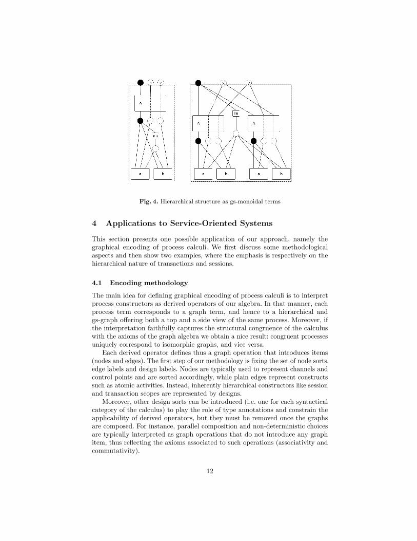
Fig. 4. Hierarchical structure as gs-monoidal terms

4 Applications to Service-Oriented Systems

This section presents one possible application of our approach, namely thegraphical encoding of process calculi. We first discuss some methodologicalaspects and then show two examples, where the emphasis is respectively on thehierarchical nature of transactions and sessions.

4.1 Encoding methodology

The main idea for defining graphical encoding of process calculi is to interpretprocess constructors as derived operators of our algebra. In that manner, eachprocess term corresponds to a graph term, and hence to a hierarchical andgs-graph offering both a top and a side view of the same process. Moreover, ifthe interpretation faithfully captures the structural congruence of the calculuswith the axioms of the graph algebra we obtain a nice result: congruent processesuniquely correspond to isomorphic graphs, and vice versa.

Each derived operator defines thus a graph operation that introduces items(nodes and edges). The first step of our methodology is fixing the set of node sorts,edge labels and design labels. Nodes are typically used to represent channels andcontrol points and are sorted accordingly, while plain edges represent constructssuch as atomic activities. Instead, inherently hierarchical constructors like sessionand transaction scopes are represented by designs.

Moreover, other design sorts can be introduced (i.e. one for each syntacticalcategory of the calculus) to play the role of type annotations and constrain theapplicability of derived operators, but they must be removed once the graphsare composed. For instance, parallel composition and non-deterministic choicesare typically interpreted as graph operations that do not introduce any graphitem, thus reflecting the axioms associated to such operations (associativity andcommutativity).

12

The removal of such annotations is done by introducing flattening axioms,which implicitly remove (by performing some kind of hyper-edge replacement [12])those edges satisfying a specific membership predicate (i.e. being typed with theannotation sorts).

Definition 12 (flattening axiom). The flattening axiom flatL for a designlabel L is Lx[G]〈y〉 ≡ G{y/x}.

It is evident that when flatL is considered, then L-labelled edges are immaterial.Flattening is fundamental in order to characterise classes of graphs by meansof derived operators. Indeed, flattening is used in all encondings, where somedesign labels are used just for the sake of composing various classes of processesand not really to build scopes. So nesting has two roles: as a means to enclose agraph and as a sort of typed interface to enable disciplined graph compositions.The presence of flattening axioms makes the first role immaterial.

Another kind of axioms that are sometimes useful to be included in thestructural congruence are extrusion axioms.

Definition 13 (extrusion axiom). The extrusion axiom extrL for a designlabel L is Lx[(νz)G〈y〉] ≡ (νz)Lx[G]〈y〉, where z 6∈ bxc ∪ byc.

Extrusion axioms are needed to handle those calculi in which name restrictionis not localised inside a scope or it is allowed to cross the boundaries of somescopes, as it may happen for some process calculi. Indeed, we shall see in § 4.3how extrusion axioms are used to capture extrusion for some scope constructs.

Note that the addition of axiom flatL also implies the validity of axiom extrL,hence in the following we assume that for each label L exactly one of the followingcases applies: either only the extrusion or only the flattening axiom for L ispresent; or none of flatL and extrL is present. Of course the presence of suchaxioms for a chosen set of labels is often fundamental for the soundness of theencoding.

4.2 Transaction Workflows

We consider in this section the nested sagas with programmable compensationsof [6], a calculus for long running transactions that aims at providing a corelanguage for composing activities into sagas (atomic transactions) or processes(non-atomic compensable activities). Formally, the syntax of sagas is as follows.

Definition 14 (sagas syntax). Let Λ be a set of atomic activities ranged overby a. The sets S of sagas and P of compensable processes are all the termsgenerated by S and P in the grammar below, respectively.

S ::= a | {P} P ::= S%S | P ;P | P | P

For the sake of simplicity, with respect to the original presentation we ne-glect the introduction of nil processes and non-compensable activities. A saga

13

Fig. 5. Type graph for sagas

is an atomic activity or an arbitrarily complex transaction built out from acompensable processes. A basic process A%B is built by declaring a saga A asan ordinary flow and equipping it with another saga B as its compensation flow.The calculus provides also primitives for composing processes in sequence andparallel (split&join).

Definition 15 (sagas structural congruence). The structural congruencefor sagas is the relation ≡S⊆ P ×P, closed under sagas construction, inductivelygenerated by the following set of axioms (for any P,Q,R ∈ P):

P ; (Q;R) ≡ (P ;Q);R (sA1)P | Q ≡ Q | P (sA2)

P | (Q | R) ≡ (P | Q) | R (sA3)

Encoding sagas. We now define the graphical encoding of sagas. As explained,the first step is to interpret syntactical categories of the calculus as suitabledesign labels and constructors as derived operators over our graph algebra. Inthis case we decide to introduce design labels N for Nested sagas, S for Sagas,P for compensable Pairs and T (Transactions) for compensable processes. Notethat N can be read as a subsort of S, while P as a subsort of T . Figure 5illustrates the shapes of the nodes and boxes we shall exploit. We have chosen anarity of four tentacles for pairs and transactions to denote the following controlpoints: entry of the ordinary flow (incoming filled arrow), exit of the ordinaryflow (outgoing filled arrow), entry of the compensation flow (incoming emptyarrow) and exit of the compensation flow (outgoing empty arrow). Activities andsagas are represented by edges with only two tentacles (for the ordinary flow).Note that we have actually a family of activity edges, one for each activity in Λ.Since S and T are just used for composition, we let the flattening axioms flatSand flatT hold (whence the dotted borders in Fig. 5).

The encoding is formally defined as follows (cf. Fig. 6).

Definition 16 (sagas encoding). The interpretation of the sagas operatorsover the design algebra is given by

a def= Sp,q[a〈p, q〉]{Q} def= Np,q[(νt)Q〈p, q, t, q〉]

A % B def= Pp,q,r,s[A〈p, q〉 | B〈r, s〉]Q ; R def= Tp,q,r,s[(νu, v)(Q〈p, u, v, s〉 | R〈u, q, r, v〉)]

Q | R def= Tp,q,r,s[Q〈p, q, r, s〉 | R〈p, q, r, s〉]

14

Fig. 6. Graphical interpretation for sagas.

Note again that some primitives of the calculus are considered as materialin the encoding, i.e. represented by graph items like edges. This is the case ofactivities as shown in Fig. 5 and also of compensable pairs and nested sagas.Instead, sequencing and parallel composition (see Fig. 6) are immaterial andtheir associated axioms are captured by the flattening axioms.

The proposed encoding is sound and complete, i.e. equivalent processes andsagas are mapped into isomorphic graphs as shown in [4].

Proposition 3 (cf. [4]). For any Q,R ∈ P we have Q ≡S R iff Q ≡D R.

Example 3. Consider the following example, inspired from [6] of the saga

{acceptOrder%refuseOrder ; ( updateCredit%refundOrder |prepareOrder%updateStock) |{addPoints%skip}%{substractPoints%skip} ) }

The saga is used for modelling a scenario for dealing with purchase orders.The initial activity (acceptOrder) handles requests from clients. The next threeprocesses are executed in parallel. The first one (updateCredit) charges the amountof the order to the balance of the client. The second one (prepareOrder) handlesthe packaging of the order and updates the stock. The third one deals with pointreward activities: it is formed by a nested saga to update the reward balanceof a user (part of a program for accumulating points with purchases). All theactivities have a corresponding compensation to undo the actions performedby the successful completion of the activities. Note that activity addPoints hasa vacuous compensation (skip) to avoid aborting the purchase when the pointaccumulation activity aborts due to the absence of a reward account (idem foractivity substractPoints). The corresponding hierarchical graph is in Fig. 7.

15

Fig. 7. Graphical encoding of a saga

4.3 Service Sessions

This section sketches the graphical representation of CaSPiS [2], a session-centredcalculus developed within Sensoria. We have chosen this calculus since itrepresents a non-trivial example of the interplay between nesting and linkingintroduced by nested sessions, pipelines and communication. We briefly overviewCaSPiS and we refer the interested readers to [2] for an exhaustive description.We remark that we focus here on the close-free fragment of the calculus and wepresent a slightly simplified syntax. Both decisions are for the sake of a convenientand clean presentation and constitute no limitation.

Definition 17 (CaSPiS syntax). Let Z be a set of session names, S a set ofservice names and V a set of value names. The set P of processes consists of allthe terms generated by P in the grammar below

P ::= 0 | r . P | P > Q | (νw)P | P | P | A.PA ::= s | s | (?x) | 〈u〉 | 〈u〉↑

where s ∈ S, r ∈ Z, u ∈ V, w ∈ V ∪ Z and x is a value variable.

Service definitions and invocations are written like input and output prefixesin CCS. Thus s.P defines a service s that can be invoked by s.Q. Synchronisationof s.P and s.Q leads to the creation of a new session, identified by a fresh namer that can be viewed as a private, synchronous channel binding caller and callee.Since client and service may be far apart, a session naturally comes with two

16

sides, written r.P , and r.Q, with r bound somewhere above them by (νr). Rulesgoverning creation and scoping of sessions are based on those of the restrictionoperator in the π-calculus. Note that nested invocations to services yield separatesessions and thus hierarchies of nested sessions.

When two partner sides r . P and r . Q are deployed, intra-session communi-cation is done via input and output actions 〈u〉 and (?x): values produced by Pcan be consumed by Q, and vice versa.

Values can be returned outside a session to the enclosing environment usingthe return operator 〈 · 〉↑. Return values can be consumed by other sessions sides,or used locally to invoke other services, to start new activities. Local consumptionis achieved using the pipeline operator P > Q . Here, a new instance of processQ is activated each time P emits a value that Q can consume. Notably, the newinstance of Q runs within the same session as P > Q, not in a fresh one.

Summarising, each CaSPiS process can be thought of as running in anenvironment providing it different means of communication: one channel for“standard” input, one channel for “standard” output and one channel for returningvalues one level up.

Example 4. Consider the process (νa)(νb)(a.(P1|b.P2)|a.P3|b.P4). It representsa typical situation where two sessions a and b have been created (e.g. upon twoservice invocations). Agent a. (P1|b .P2) participates to sessions a and b (assumeP1 is the protocol for a and P2 the one for b), with the b side nested in a. Thecounter-party protocols for a and b are P3 and P4, respectively, and they runseparately. Notably, values returned one level up by P2 can be consumed by P3.

Definition 18 (CaSPiS structural congruence). The structural congruencefor CaSPiS processes is the relation ≡C⊆ P×P, closed under process construction,inductively generated by the following set of axioms

P | (Q | R) ≡ (P | Q) | R) (CA1) P | (νn)Q ≡ (νn)(P | Q) if n 6∈ fn(P ) (CA6)P | Q ≡ Q | P (CA2) ((νn)Q) > P ≡ (νn)(Q > P ) if n 6∈ fn(P ) (CA7)P | 0 ≡ P (CA3) A.(νn)P ≡ (νn)A.P if n 6∈ A (CA8)

(νn)(νm)P ≡ (νm)(νn)P (CA4) r . (νn)P ≡ (νn)r . P if n 6= r (CA9)(νn)0 ≡ 0 (CA5) (νn)P ≡ (νm)P{m/n} if m 6∈ fn(P ) (CA10)

(?x).P ≡ (?y).P{y/x} if y 6∈ fn(P ) (CA11)

Encoding CaSPiS. We first define the alphabets of edge labels and nodes. Theset D of design labels is composed by P , S, D, I, F and T which respectivelystand for Parallel processes, Sessions, service Definitions, service Invocations andpipes (From and To). The set E of edge labels contains def (service definition),inv (service invocation), in (input), out (output) and ret (return). The node sortsconsidered are ◦ (channels), • (control points), ∗ (service names, i.e. S) and �(values, i.e. V). We assume that for each session name r there is a correspondingchannel node.

The graphical representation of each design and edge label and their respectiveranks can be found in Fig. 8. For instance, designs of type P are all of the formPp,t,o,i[G] where p is the control point representing the process start of execution,t is the returning channel, o is the output channel and i is the input channel. Vice

17

Fig. 8. Type graph for CaSPiS.

versa, designs of type D and I only expose the starting point of execution: theyare not strictly necessary for the encoding, but can be very useful for visualisationpurposes (they enclose the interaction protocols between callers and callees).We let the flattening axiom flatP hold, together with extrusion axioms extrS,extrD, extrI, extrF. Hence, edges of type P are immaterial (they can be consideredas type annotations) and edges of type T define the only rigid hierarchy w.r.t.containment and name scoping. Other explicit hierarchies for edge containmentare given by session nesting (S), service definition (D), service invocation (I) andpipelining (F ). As usual, flattening processes allows for getting rid of the axiomsfor parallel composition (see [15]). The presence of extrusion axioms is motivatedby the structural congruence axioms of CaSPiS, namely CA7 motivates extrF,CA8 motivates both extrD and extrI, and CA9 motivates extrS. Note that we usedashed border for designs for which the extrusion axiom hold, while designs tobe flattened are depicted with dotted borders.

Definition 19 (CaSPiS encoding). The interpretation of CaSPiS operatorsover the design algebra is given by

s.Q def= Pp,t,o,i[ t|o|i|D[ (νq, t′, o′, i′)(def〈p, s, q〉|Q〈q, t′, o′, i′〉) ]〈p〉 ]s.Q def= Pp,t,o,i[ t|o|i| I[ (νq, t′, o′, i′)(inv〈p, s, q〉|Q〈q, t′, o′, i′〉) ]〈p〉 ]

r . Q def= Pp,t,o,i[ t|i|S[Q〈p, o, r, r〉 ]〈p, o〉 ]Q > R def= Pp,t,o,i[ o | (νm)(F[Q〈p, t,m, i〉 ]〈p, t,m, i〉 |

T[ (νq, t′, o′)R〈q, t′, o′,m〉 ]〈m〉 ) ]Q|R def= Pp,t,o,i[Q〈p, t, o, i〉|R〈p, t, o, i〉 ]

(νw)Q def= Pp,t,o,i[(νw)Q〈p, t, o, i〉]0 def= Pp,t,o,i[ p|t|o|i ]

〈u〉.Q def= Pp,t,o,i[ (νq)(out〈p, q, u, o〉 |Q〈q, t, o, i〉) ]〈u〉↑.Q def= Pp,t,o,i[ (νq)(ret〈p, q, u, t〉 |Q〈q, t, o, i〉) ](?x).Q def= Pp,t,o,i[ (νq, x)(in〈p, q, x, i〉 |Q〈q, t, o, i〉) ]

Proposition 4 (cf. [4]). For any Q,R ∈ P we have Q ≡C R iff Q ≡D R.

18

Fig. 9. Example of session nesting.

Instead of providing the visualisation of the encoding and a detailed explana-tion (for which we refer to [5]) we prefer to concentrate on the representation ofsession nesting with the typical session situation presented before. Figure 9 depictsthe graphical representation of our example, where the graph has been furthersimplified (e.g. fusing nodes, removing isolated nodes and irrelevant tentacles)to focus on the main issues and make immediate the correspondence with theprocess term. The figure evidences the hierarchy introduced by session nestingand how it is crossed by intra-session communication. It is also worth to notethat the graph highlights the fact that the return channel of a nested session ispipelined into the output channel of the enclosing session. More precisely, thereturn channel of the immediate session where P2 lives (i.e. b) is connected tothe output channel of the session containing it, i.e. the session channel a.

5 Conclusion

This chapter collects results from [3–5]. We presented our specification formalismbased on a convenient algebra of hierarchical graphs: its features make it well-suited for the specification of systems with inherently hierarchical aspects and inparticular, process calculi with notions of scope and containment (like ambients,membranes, sessions and transactions). Some advantages of our approach are dueto the graph algebra, whose syntax resembles standard algebraic specificationsand, in particular, it is close to the syntax found in nominal calculi. The key pointis to exploit the algebraic structure of both designs and graphs when provingproperties of an encoding, facilitating proofs by structural induction.

References

1. H. Barendregt, M. van Eekelen, J. Glauert, J. Kennaway, M. Plasmeijer, andM. Sleep. Term graph reduction. In Proceedings of the 1st International Conference

19

on Parallel Architectures and Languages Europe (PARLE’87), volume 259 of LectureNotes in Computer Science, pages 141–158. Springer Verlag, 1987.

2. M. Boreale, R. Bruni, R. De Nicola, and M. Loreti. Sessions and pipelines forstructured service programming. In G. Barthe and F. S. de Boer, editors, Proceedingsof the 10th IFIP International Conference on Formal Methods for Open Object-basedDistributed Systems (FMOODS’08), volume 5051 of Lecture Notes in ComputerScience, pages 19–38. Springer Verlag, 2008.

3. R. Bruni, A. Corradini, F. Gadducci, A. Lluch Lafuente, and U. Montanari. Ongs-monoidal theories for graphs with nesting. Submitted.

4. R. Bruni, F. Gadducci, and A. Lluch Lafuente. An algebra of hierarchical graphsand its application to structural encoding. Submitted.

5. R. Bruni, F. Gadducci, and A. Lluch Lafuente. A graph syntax for processes andservices. In S. Jianwen and C. Laneve, editors, Proceedings of the 6th InternationalWorkshop on Web Services and Formal Methods (WS-FM’09), Lecture Notes inComputer Science. Springer Verlag, 2009. To Appear.

6. R. Bruni, H. C. Melgratti, and U. Montanari. Theoretical foundations for com-pensations in flow composition languages. In J. Palsberg and M. Abadi, editors,Proceedings of the 32nd International Symposium on Principles of ProgrammingLanguages (POPL’05), pages 209–220. ACM, 2005.

7. M. Bundgaard and V. Sassone. Typed polyadic pi-calculus in bigraphs. In A. Bossiand M. J. Maher, editors, Proceedings of the 8th International Symposium onPrinciples and Practice of Declarative Programming (PPDP’06), pages 1–12. ACM,2006.

8. A. Corradini and F. Gadducci. An algebraic presentation of term graphs, viags-monoidal categories. Applied Categorical Structures, 7:299–331, 1999.

9. A. Corradini, U. Montanari, and F. Rossi. An abstract machine for concurrentmodular systems: CHARM. Theoretical Computer Science, 122(1-2):165–200, 1994.

10. A. Corradini, U. Montanari, F. Rossi, H. Ehrig, R. Heckel, and M. Lowe. AlgebraicApproaches to Graph Transformation - Part I: Basic Concepts and Double PushoutApproach. In G. Rozenberg, editor, Handbook of Graph Grammars and Computingby Graph Transformation, pages 163–246. World Scientific, 1997.

11. F. Drewes, B. Hoffmann, and D. Plump. Hierarchical graph transformation. Journalon Computer and System Sciences, 64(2):249–283, 2002.

12. F. Drewes, H.-J. Kreowski, and A. Habel. Hyperedge replacement, graph grammars.In G. Rozenberg, editor, Handbook of Graph Grammars and Computing by GraphTransformations, Volume 1: Foundations, pages 95–162. World Scientific, 1997.

13. G. L. Ferrari, D. Hirsch, I. Lanese, U. Montanari, and E. Tuosto. Synchronisedhyperedge replacement as a model for service oriented computing. In F. S. de Boer,M. M. Bonsangue, S. Graf, and W. P. de Roever, editors, Proceedings of the4th International Symposium on Formal Methods for Components and Objects(FMCO’05), volume 4111 of LNCS, pages 22–43. Springer, 2006.

14. G. L. Ferrari and U. Montanari. Tile formats for located and mobile systems.Information and Computation, 156(1-2):173–235, 2000.

15. F. Gadducci. Term graph rewriting for the pi-calculus. In A. Ohori, editor,Proceedings of the 1st Asian Symposium on Programming Languages and Systems(APLAS’03), volume 2895 of Lecture Notes in Computer Science, pages 37–54.Springer Verlag, 2003.

16. R. Milner. Pure bigraphs: Structure and dynamics. Information and Computation,204(1):60–122, 2006.

20