doi.org/10.26434/chemrxiv.7679798.v1

A Machine Learning Based Intramolecular Potential for a FlexibleOrganic MoleculeDaniel Cole, Letif Mones, Gábor Csányi

Submitted date: 06/02/2019 • Posted date: 06/02/2019Licence: CC BY 4.0Citation information: Cole, Daniel; Mones, Letif; Csányi, Gábor (2019): A Machine Learning BasedIntramolecular Potential for a Flexible Organic Molecule. ChemRxiv. Preprint.

One limitation of the accuracy of computational predictions of protein-ligand binding free energies is the fixedfunctional form of the intramolecular component of the molecular mechanics force fields. Here, we employ thekernel regression machine learning technique to construct an analytical potential, using the GaussianApproximation Potential software and framework, that reproduces the quantum mechanical potential energysurface of a small, flexible, drug-like molecule, 3-(benzyloxy)pyridin-2-amine. Challenges linked to the highdimensionality of the configurational space of the molecule are overcome by developing an iterative trainingprotocol and employing a representation that separates short and long range interactions. The analyticalmodel is connected to the MCPRO simulation software, which allows us to perform Monte Carlo simulations ofthe small molecule bound to two proteins, p38 MAP kinase and leukotriene A4 hydrolase, as well as in water.We demonstrate corrections to absolute protein-ligand binding free energies obtained with our machinelearning based intramolecular model of up to 2 kcal/mol.

File list (2)

download fileview on ChemRxivmanuscript_GAP.pdf (1.17 MiB)

download fileview on ChemRxivsupp_info.pdf (283.02 KiB)

A machine learning based intramolecular

potential for a flexible organic molecule

Daniel J. Cole,∗,† Letif Mones,‡ and Gabor Csanyi‡

†School of Natural and Environmental Sciences, Newcastle University, Newcastle upon

Tyne NE1 7RU, United Kingdom

‡Engineering Laboratory, University of Cambridge, Trumpington Street, Cambridge CB2

1PZ, United Kingdom

E-mail: daniel.cole@ncl.ac.uk

1

Abstract

One limitation of the accuracy of computational predictions of protein–ligand bind-

ing free energies is the fixed functional form of the intramolecular component of the

molecular mechanics force fields. Here, we employ the kernel regression machine learn-

ing technique to construct an analytical potential, using the Gaussian Approximation

Potential software and framework, that reproduces the quantum mechanical potential

energy surface of a small, flexible, drug-like molecule, 3-(benzyloxy)pyridin-2-amine.

Challenges linked to the high dimensionality of the configurational space of the molecule

are overcome by developing an iterative training protocol and employing a representa-

tion that separates short and long range interactions. The analytical model is connected

to the MCPRO simulation software, which allows us to perform Monte Carlo simula-

tions of the small molecule bound to two proteins, p38 MAP kinase and leukotriene A4

hydrolase, as well as in water. We demonstrate corrections to absolute protein–ligand

binding free energies obtained with our machine learning based intramolecular model

of up to 2 kcal mol−1.

2

1 Introduction

Figure 1: (a) 3-(benzyloxy)pyridin-2-amine (3BPA). (b) Bound to p38 MAP kinase (PDB:1W7H).1 (c) Bound to leukotriene A4 hydrolase (PDB: 3FTY).2

The interplay of the intramolecular, or internal, energy of a molecule and the non-bonded

energetics that determine its interactions with its environment play a crucial role in simu-

lations of protein folding,3 crystal structure prediction,4 protein–ligand binding,5 and many

more. In particular, oral drugs are typically flexible, containing on average 5.4 rotatable

bonds,6 and are therefore capable of populating many free energy minima both in solution

and also when bound to their target. Computational analysis has revealed that the majority

of ligands bind in a conformation within 0.5 kcal mol−1 of a local energy minimum.7 To be

successful, docking or any other method used in computer-aided structure-based drug design

must be able to accurately predict both the bioactive conformation of the molecule and the

free energy change that accompanies its binding from solution.

The potential energy surfaces of organic molecules for practical applications are typically

modelled using transferable molecular mechanics force fields such as AMBER,8 CHARMM,9

GROMOS10 or OPLS.11 When combined with molecular dynamics (MD) or Monte Carlo

(MC) sampling, these force fields may be used to predict, for example, liquid properties

of small molecules,12,13 structural propensities of peptides,14,15 and protein–ligand binding

free energies,16,17 all with reasonable accuracy. The intramolecular component of the force

field is typically modelled by harmonic bond and angle potentials to represent two- and

three-body terms, respectively, an anharmonic torsional term to model dihedral rotations,

and Coulomb and Lennard-Jones terms to account for interactions between atoms separated

3

by three or more bonds.8,18,19 Details vary between these transferable force fields, but the

fixed functional form is common to all. Thus, no matter how carefully the force field is

parametrized, accuracy will ultimately be limited by the choice of this functional form.

For the description of intramolecular energetics quantum mechanics (QM) is seemingly

preferable and is frequently used in computational enzymology applications.20 However, the

computational cost associated with QM simulations is high, particularly for free energy

predictions which require extensive (alchemical and/or conformational) sampling.21 In order

to make a calculation tractable the level of QM theory (basis set and exchange-correlation

functional, for example) is often compromised, which again raises questions over the final

accuracy.22

Alternatively, one can construct direct fits to the high dimensional QM potential energy

surface of the molecule. There is a wide range of methods available for fitting bond, angle

and dihedral parameters of the MM force field to QM energies, gradients and Hessian ma-

trices,23–27 and these often include extended functional forms such as cross-terms to account

for coupling between internal coordinates.28 However, for larger, more flexible molecules,

longer-range atomic interactions beyond the 1-4 interaction are also crucial in determining

molecular conformation. For these molecules, a consistent, accurate approach to approx-

imating the QM potential energy surface is key. Rather than relying on human intuition

to decide on the most appropriate functional form this MM force field should take, it is

preferable to harness the recent advances of machine learning inspired techniques. There

are several neural network and kernel based techniques recently developed for material sys-

tems that can predict quantum energies and forces with remarkable accuracy.29–34 Since

these potentials need to be trained on only a few thousand (well dispersed) configurations,

the underlying quantum mechanical data can be of high accuracy while maintaining afford-

able computational expense. These techniques have been successfully used to reproduce the

atomisation energies of small organic molecules35–38 and the QM potential energy surfaces of

selected intermediate-sized organic molecules.39,40 However, the chosen molecules only had

4

very limited internal degrees of freedom, which significantly simplifies the problem.

In this work, we investigate the use of machine learning in developing accurate repre-

sentations of the potential energy surface of a flexible, “drug-like” molecule for use in e.g.

structure-based lead optimization efforts. We employ the Gaussian Approximation Potential

(GAP)41 framework that is based on a sparse Gaussian process regression technique, which

is formally equivalent to kernel ridge regression.42,43 GAP uses both QM energy and gradient

information and although it was originally developed for material systems, it has been used

successfully to describe molecular properties.35,36 Here we use it to create a potential energy

surface for 3-(benzyloxy)pyridin-2-amine (3BPA, Figure 1). Although still somewhat smaller

than typical drug-like molecules (molecular weight of 200, three rotatable bonds, and three

hydrogen bond donors/acceptors), it represents a challenging test case for machine learning

due to its internal flexibility. The high effective dimensionality of the configurational mani-

fold of the molecule requires a relatively large amount of training data extensively sampled

from the potential energy surface. To address these challenges, we developed an iterative pro-

tocol to gradually improve the reconstructed potential, and applied sparsification techniques

to cope with the relatively large amount of training data. Despite its small size, 3PBA has

been identified in two separate fragment screens as an efficient ligand of p38 MAP kinase1

and leukotriene A4 hydrolase.2 In the former study, although its binding affinity was found

to be greater than 1 mM in an enzyme bioassay, 3BPA has a clearly defined binding mode to

the hinge region of the ATP binding site of the kinase (Figure 1(b)).1 While in the latter, the

same compound binds near the bottom of the substrate binding cleft of leukotriene A4 hy-

drolase with sub-mM affinity (Figure 1(c)).2 To investigate the binding of 3BPA in these two

environments, we have interfaced GAP with the MCPRO software.18 MCPRO is a tool for

structure-based lead optimization through the use of free energy perturbation (FEP) theory

combined with Monte Carlo sampling of protein–ligand binding modes. It has been used for

the successful computationally guided design of inhibitors of targets including HIV-1 reverse

transcriptase44 and macrophage migration inhibitory factor,45 and has recently been applied

5

to the fragment-based design of inhibitors of the Aurora A kinase – TPX2 protein-protein

interaction.46 As we will show, our interface between GAP and MCPRO allows us to perform

Monte Carlo simulations of 3BPA in a range of environments, and to compute corrections

to the binding free energy that is computed using molecular mechanics force fields.

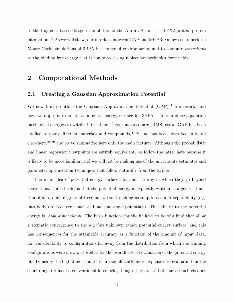
2 Computational Methods

2.1 Creating a Gaussian Approximation Potential

We now briefly outline the Gaussian Approximation Potential (GAP)41 framework, and

how we apply it to create a potential energy surface for 3BPA that reproduces quantum

mechanical energies to within 1.0 kcal mol−1 root mean square (RMS) error. GAP has been

applied to many different materials and compounds,47–57 and has been described in detail

elsewhere,58,59 and so we summarize here only the main features. Although the probabilistic

and linear regression viewpoints are entirely equivalent, we follow the latter here because it

is likely to be more familiar, and we will not be making use of the uncertainty estimates and

parameter optimization techniques that follow naturally from the former.

The main idea of potential energy surface fits, and the way in which they go beyond

conventional force fields, is that the potential energy is explicitly written as a generic func-

tion of all atomic degrees of freedom, without making assumptions about separability (e.g.

into body ordered terms such as bond and angle potentials). Thus the fit to the potential

energy is high dimensional. The basis functions for the fit have to be of a kind that allow

systematic convergence to the a priori unknown target potential energy surface, and this

has consequences for the attainable accuracy as a function of the amount of input data,

for transferability to configurations far away from the distribution from which the training

configurations were drawn, as well as for the overall cost of evaluation of the potential energy

fit. Typically the high dimensional fits are significantly more expensive to evaluate than the

short range terms of a conventional force field, though they are still of course much cheaper

6

than a QM calculation, or the evaluation of the electrostatic potential of a large system that

includes a protein and explicit solvent molecules.

Let us denote conformations of a molecule by letters A,B, etc. irrespective of how they

are represented numerically. The target function, which in our case is the QM potential

energy, is written as a linear combination of basis functions:

E(A) =∑B∈M

xBK(A,B), (1)

where K is a positive definite similarity function between two conformations, often called a

kernel function, which customarily takes the value 1 for identical conformations and smaller

values for pairs of conformations that are less similar to one another, and x are the unknown

coefficients. The sum ranges over a set M of representative conformations. For finite M , the

basis is not complete, but by choosing the set appropriately (typically by drawing conforma-

tions from the same or a related distribution corresponding to where we expect to evaluate

the function) the basis set is made relevant, and by enlarging the representative set, the

approximation error can be decreased. This manner in which the basis set is adapted to the

data is the principal way by which the problem of high dimensionality is circumvented. The

success of this type of fitting then depends entirely on the regularity properties (colloquially,

smoothness) of the target function.

The approximation can be significantly improved by choosing a numerical representation

of conformations and a kernel function that respect basic physical symmetries of the potential

energy of a molecule. These are translation, global rotation, and permutation symmetries.

The first two apply to any physical system, and we factor them out of the representation

by transforming the set of Cartesian coordinates into the vector of all interatomic distances,

R = {||ri − rj||}i<j. Note how the dimensionality of this representation scales with the

square of the number of atoms, n, but this is of little consequence, since all our samples

will lie on the 3n dimensional manifold. Alternatively, one could work with the well known

7

internal coordinates of the z-matrix, and this choice would not increase the dimensionality.

However, the potential energy function is clearly a much less regular function of the internal

coordinates, because changing some angles would correspond to much more drastic changes

in Cartesian coordinates than others.

The complete permutation symmetry group of 3BPA has only 8 elements, and so we

simply sum the kernel function over the action of the group over one of its arguments,

resulting in a permutationally invariant kernel,

K(A,B) =∑π∈G

K(A, π(B)), (2)

where G is the permutation group of the molecule and π is one of its elements. This tech-

nique is applicable to any representation of the molecular conformation and any base kernel

K, and results in a permutationally invariant potential energy. In the present work, we

use a Gaussian base kernel (often called a “squared exponential” kernel to distinguish this

choice from Gaussian probability distributions) which, in terms of the interatomic distance

representations, is given by:

K(A,B) = δ2 exp

[−1

2

D∑i=1

(RAi −RBi )2

θ2i

], (3)

where RAi is the ith element of the vector of interatomic distances of conformation A, RBi is

the corresponding element for conformation B, D is the number of elements in the represen-

tation vector, δ is an energy scale parameter and the θi are length scale parameters (one for

each dimension of the representation vector).

The coefficients in the ansatz (1) are determined by regularized least squares regression

using energies and forces computed using quantum chemistry techniques on a diverse set of

conformations (see below for further details). Given N conformations with n atoms in each,

we have N(3n + 1) pieces of data, leading to the same number of linear equations when

(1) is substituted either directly (for the energy) or by taking its derivative with respect to

8

atomic positions (to obtain the forces). Let us collect the M unknown coefficients in (1)

into a vector x, concatenate all the available data (energies e and forces f) into the vector

y = [e f ], and let L be the linear operator connecting this data vector with the energies

of the input configurations, so that y = Le. Note that L consists of two blocks, the upper

block is just the identity, and the lower block is the negative differential operator. With this,

the regularized least squares problem is linear and can be written as:

minx‖LKNMx− y‖2Λ + ‖x‖2K, (4)

where KNM is the N × M kernel (or design) matrix, with elements given by the kernel

function between the M representative configurations and all the N training configurations,

and Λ is a diagonal matrix, whose elements are a set of parameters that control the relative

weight of energy and force data and also the trade-off between accuracy and regularity of

the fit. The solution to this linear problem is given by:

x∗ = [KMM + (LKNM)TΛLKNM ]−1(LKNM)TΛy, (5)

where KMM refers to the M × M square matrix given by the kernel values between the

representative configurations.

We note that the method of Chmiela et al. for generating potential energy surfaces of

small organic molecules60 uses the same kernel ridge regression technique with the following

differences: (i) they include only gradient observables (i.e. forces) while GAP reconstructs

the surface using both potential energies and forces, (ii) they use the same number of basis

functions as there are data, which corresponds to M = 3Nn above, (iii) their basis functions

for the potential energy are derivatives of a base kernel (such as a Gaussian) with respect to

atomic positions, rather than the base kernel itself, (iv) they use the inverse of interatomic

distances as the arguments of the kernel. We have found no significant advantage to any of

these variations, and note that (ii) would result in a larger linear problem, thus significantly

9

increasing the computational cost. We typically find that M � 3Nn is sufficient.

Beyond the basic framework outlined above, we used one additional twist, inspired by

the form of empirical organic force fields. There, the energy is typically separated into a

larger bonded terms (i.e. terms involving up to 1–4 bonded interactions) and smaller non-

bonded interactions (the electrostatic and Lennard-Jones interactions computed for all other

atom pairs). We adapted this strategy for the multi-dimensional kernel fit by describing the

total energy as the sum of two separate terms, both having the same form as (1), with the

only difference between them being that for the first, only interatomic distances spanning

bond positions 1–4 are included in the configuration vector R, whereas for the second, all

interatomic distances are included. The fit for both terms is carried out together with an

extra weight factor of 0.1 included for the second term (using the δ parameter), corresponding

to the smaller (non-bonded) energy it is describing.

2.2 Generating Training Data

The goal of the GAP training procedure was to recreate the QM potential energy surface

of 3BPA at the MP2/6-311G(2d,p) level of theory. This choice represents a compromise

between accuracy and computational expense; one energy and force evaluation requires ap-

proximately 1 cpuhr, which makes it feasible to generate thousands of data points. However,

accurate characterization of the multidimensional potential energy surface requires extensive

sampling, which is not practical with an expensive QM method, so we used the following

protocol.

First, we performed several independent molecular dynamics (MD) simulations in the

gas phase using MP2 but with a smaller, cheaper basis set (6-31G). The simulations were

carried out at temperatures of 300, 600 and 1200 K for 30 ps per trajectory using a Langevin

thermostat with a collision frequency of 5 ps−1. The computational cost was approximately

1000 cpu hours for each trajectory. Altogether we collected 3000 independent configurations

of 3BPA at 300 K, 1000 configurations at 600 K, and 1000 configurations at 1200 K. The

10

energies and forces were then recomputed at the MP2/6-311G(2d,p) level of theory for each

of these 5000 configurations.

The original training set included 3000 configurations (1000 configurations at each of

the three temperatures), while for the test we used 2000 configurations collected from the

MD simulation performed at 300 K. The representative configurations for equation (1) were

generated as follows. We picked 250 configurations from the original small basis set MD run,

and for each of these, we displaced each of the atoms, in turn, by 0.5 A along each Cartesian

direction. This results in M = 27× 3× 250 = 20250 configurations and corresponding basis

functions. Note that we do not need QM energies or forces for these configurations, since

they do not enter the fit, just serve to generate basis functions. We found that this procedure

worked significantly better than just picking all representative configurations randomly from

the MD trajectory itself.

The diagonal elements in Λ were set to be 106, and the length scale parameter θi was

chosen to be 20 times the range of the data distribution in each dimension of the configuration

vector R. The RMS errors of the fitted potential on the 2000 test configurations were

0.57 kcal mol−1 for the energy and 0.95 kcal mol−1 A−1 for the forces.

We then ran simulations with the fitted potential both in water solution and bound to

leukotriene A4 hydrolase (see Section 2.3). These latter simulations revealed a number of

samples with very high energy when evaluated with the QM method. Therefore, 300 such

configurations were added to the training set, and the potential refitted. Such iterative

fitting has been used before,47,50,53 and is expected to be an important technique for creating

transferable machine learning potentials. The new GAP model had a similar RMS error on

the test sets (0.65 kcal mol−1 and 0.95 kcal mol−1 A−1 for energies and forces, respectively)

and was stable in subsequent simulations (Section 3). In what follows, we refer to the two

versions of our machine learned intramolecular potentials as GAP-v1 and GAP-v2.

11

Figure 2: Free energy cycle used to compute the GAP correction to the MM binding freeenergy. Simulations are performed of the ligand (L) in water and bound to the receptor (R).

2.3 Interfacing GAP and MCPRO

GAP is implemented in a modified version of MCPRO (version 2.3) to allow Monte Carlo

sampling of 3BPA in water or bound to a protein. The total potential energy (EMM) of a

receptor–ligand complex is broken down as follows:

EMM = EL + ER + ERL (6)

where EL represents the intramolecular energy of the ligand, ER the potential energy of

the receptor, including water molecules, and ERL the interaction energy between ligand and

receptor. Similar to a hybrid QM/MM simulation set-up, we treat the various energetic

components using different levels of theory. The protein environment is described using

the OPLS-AA/M force field,14 and water molecules using the TIP4P model. Receptor–

ligand interactions are described using standard OPLS/CM1A Coulombic and Lennard-Jones

interactions.18,61 The intramolecular potental energy of the ligand is written in the general

12

form:

EL = (1− λ)EGAP + λEMM (7)

which allows us to perform standard MM simulations using the OPLS/CM1A force field

(λ = 1), GAP simulations in which the ligand energetics are determined as in Section 2.1

(λ = 0), or any intermediate state determined by the coupling parameter λ. The latter

feature allows us to employ free energy perturbation (FEP) theory to smoothly alter the

ligand intramolecular energy between the GAP and OPLS/CM1A force fields, and thus to

compute the free energy difference between the two states. Figure 2 shows the proposed

free energy cycle used to correct the MM binding free energy. Conventional FEP studies

compute the (absolute or relative) free energy required to extract the ligand from solution

into the protein binding site (∆GMM). The corrected binding free energy is given by:

∆GGAP = ∆GMM + ∆GA −∆GB (8)

where ∆GA and ∆GB are the free energy differences between the GAP (λ = 0) and MM (λ =

1) models computed in water and protein environments respectively. The implementation

of GAP is fully compatible with the replica exchange with solute tempering method,17,62,63

which allows us to perform enhanced sampling of the ligand degrees of freedom, and with

the JAWS algorithm, which aids hydration of the binding site in the bound simulations.64

Full details of the set-up and parameters used in the MC/FEP calculations are provided in

the Supporting Information.

3 Results

We begin by examining in more detail the training data used in the construction of the

GAP. As shown in Figure 1, 3BPA has three flexible dihedral angles connecting the two

saturated six-membered rings. As such, the relatively large accessible conformational space

13

Figure 3: Distribution of the dihedral angles sampled in (a) training set 1, (b) training set2, and (c) during MC simulations.

14

poses a challenge for machine learning techniques. Figure 3(a) shows the 2D distribution

of the dihedral angles φ1 and φ2 sampled during the QM dynamics used to train GAP-

v1 (3000 configurations). The use of high temperatures allows a thorough sampling of

conformational space in this case. The white circles show the positions of the corresponding

dihedral angles in the two crystal structures studied here.1,2 The compound bound to p38

MAP kinase adopts a conformation that is well sampled by our training data (φ1 = 334◦,

φ2 = 204◦). Interestingly, on the other hand, the pose in the leukotriene A4 hydrolase crystal

structure is in a seemingly disallowed region of conformational space (φ1 = 168◦, φ2 = 116◦).

Closer inspection reveals that, in this conformation, the –NH2 group on the aminopyridine

is in unphysical close contact with the –CH2– linker (Figure 1(c) and Figure S2). This is,

therefore, likely an artefact of the crystal structure refinement. By visual inspection, we were

able to orient 3BPA within the leukotriene A4 hydrolase binding site with a conformation

that is more consistent with the QM dynamics (φ1 ∼ 270◦, φ2 ∼ 270◦). We therefore used

this bound conformation as the starting point for our MC simulations.

Table 1: RMS errors (kcal mol−1) in the total energies of configurations taken from MCsimulations in three different environments relative to QM. a excluding one outlying config-uration. b Configurations were sampled from the GAP-v2 trajectories, and the MM and QMenergies were shifted to align the mean energies.

Water p38 MAP kinase Leukotriene A4 hydrolaseGAP-v1 0.83 0.60 19.04GAP-v2 1.42 (0.93a) 0.95 1.13

OPLS/CM1Ab 11.87 (4.85a) 3.36 3.45

As described in Section 2.3, we ran MC simulations of 3BPA in three different environ-

ments, using GAP-v1 to describe its intramolecular energetics, and the OPLS/CM1A force

field to describe its interactions with the proteins and water. In order to test the ability of

the GAP to reproduce the QM potential energy surface, 300 configurations of 3BPA were

saved from each trajectory, and its energetics recomputed at the MP2/6-311G(2d,p) level

of theory in vacuum. Table 1 shows the RMS error in the GAP for 3BPA in water, and

bound to the two proteins. The errors are less than 1 kcal mol−1 in water and bound to

15

p38 MAP kinase, which is consistent with the reported accuracy of the GAP on the test set

described in Section 2.2. However, despite the reorientation of 3BPA in the binding pocket

of leukotriene A4 hydrolase, the RMS errors in the GAP are extremely high (19 kcal mol−1).

This result is consistent with a lack of training data in the region of conformational space

close to φ1 = 270◦, φ2 = 270◦ (Figure 3(a)). Therefore, 300 configurations were extracted

from MC simulations of 3BPA bound to leukotriene A4 hydrolase and were added to the

original training set to produce the dihedral angle distribution shown in Figure 3(b).

Figure 4: Correlation between GAP (left) and OPLS (right) and QM energies of 3BPAsampled from MC simulations. Not all OPLS MM data are displayed for clarity. The meanenergy of each distribution has been shifted to zero.

MC simulations of the second iteration of the GAP (GAP-v2) were run in the three envi-

ronments and the errors are summarized in Table 1. Now, the errors are close to 1 kcal mol−1

in all three environments. Figure 4 further reveals a very good correlation between GAP

and QM intramolecular energies, although there is one significant outlier whose phenyl and

pyridine rings approach too close (Figure 4, inset). Removal of this configuration from the

ensemble of 3BPA in water reduces the error in the GAP still further from 1.42 kcal mol−1

to 0.93 kcal mol−1. Further iterative training of the GAP would prevent sampling of this

configuration during the MC simulations. Figure 3(c) shows the distribution of dihedral an-

gles sampled during these three MC simulations, and reveals that all areas of conformational

space are well-represented by the training data. Furthermore, the structures sampled are in

16

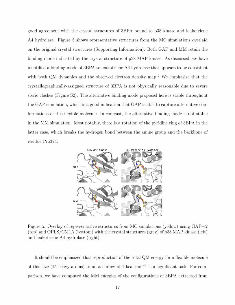
good agreement with the crystal structures of 3BPA bound to p38 kinase and leukotriene

A4 hydrolase. Figure 5 shows representative structures from the MC simulations overlaid

on the original crystal structures (Supporting Information). Both GAP and MM retain the

binding mode indicated by the crystal structure of p38 MAP kinase. As discussed, we have

identified a binding mode of 3BPA to leukotriene A4 hydrolase that appears to be consistent

with both QM dynamics and the observed electron density map.2 We emphasize that the

crystallographically-assigned structure of 3BPA is not physically reasonable due to severe

steric clashes (Figure S2). The alternative binding mode proposed here is stable throughout

the GAP simulation, which is a good indication that GAP is able to capture alternative con-

formations of this flexible molecule. In contrast, the alternative binding mode is not stable

in the MM simulation. Most notably, there is a rotation of the pyridine ring of 3BPA in the

latter case, which breaks the hydrogen bond between the amine group and the backbone of

residue Pro374.

Figure 5: Overlay of representative structures from MC simulations (yellow) using GAP-v2(top) and OPLS/CM1A (bottom) with the crystal structures (grey) of p38 MAP kinase (left)and leukotriene A4 hydrolase (right).

It should be emphasized that reproduction of the total QM energy for a flexible molecule

of this size (15 heavy atoms) to an accuracy of 1 kcal mol−1 is a significant task. For com-

parison, we have computed the MM energies of the configurations of 3BPA extracted from

17

the GAP-v2 MC simulations in the three different environments. Table 1 and Figure 3

summarize the accuracy of OPLS/CM1A, which is expected to be typical of standard small

molecule force fields, in comparison with QM data. As expected, the MM force field is

significantly less accurate than the machine learning potential. These improvements in in-

tramolecular energetics are expected to carry over into improved thermodynamic quantities,

such as binding free energies.

Table 2: GAP corrections (kcal mol−1) to the MM binding free energy of 3BPA to twoproteins.

p38 MAP kinase Leukotriene A4 hydrolaseGAP-v1 +1.3 –GAP-v2 +1.0 +2.0

As discussed in Section 2.3, our implementation of GAP in the MCPRO software allows us

to estimate corrections to protein–ligand binding free energies using free energy perturbation

theory. In particular, the intramolecular energetics of the ligand were smoothly altered from

GAP to OPLS/CM1A and the free energy cycle shown in Figure 2 was employed to compute

the correction to the binding free energy, ∆GA − ∆GB (eq 8). Note that we have not

computed the absolute binding free energies here. Focussing first on the binding of 3BPA to

p38 MAP kinase, both GAP-v1 and GAP-v2 give a correction to the MM binding free energy

of close to 1 kcal mol−1. That is, we expect the standard MM force field to over-estimate

binding, in this case, due to inaccuracies in the treatment of intramolecular energetics of

the ligand in water and in the protein binding site. It is reassuring that the two versions of

GAP agree on the magnitude of the correction; one would not expect the addition of extra

training configurations to substantially affect the energetics of the molecule in either water

or the p38 kinase binding site. The correction to the binding of 3BPA to leukotriene A4

hydrolase is larger, which is consistent with the inability of the MM force field to produce a

binding mode that is consistent with the experimental electron density map (Figure 5).

18

4 Discussion and Conclusions

In this paper, we have reported the first construction, training and application of the Gaus-

sian approximation potential to an organic molecule with significant conformational flexibil-

ity. The potential is a full dimensional fit of the molecular potential energy surface, with

squared-exponential basis functions corresponding to conformations from a Monte Carlo run.

The potential can be systematically improved by adding more training data (energies and

gradients) and more basis functions. Iterative training was used, whereby further conforma-

tions are collected from an MD run with a previous version of the potential.

The GAP was trained using just 3300 (MP2/6-311G(2d,p)) QM calculations in total. In

comparison, computation of the thermodynamic quantities reported in this paper required

around 108 evaluations of the ligand intramolecular energetics, which would have been in-

feasible using even a very inaccurate QM/MM approach. The second version of the GAP is

able to reproduce QM energies to a high accuracy of close to 1 kcal mol−1 following training

on a gas phase QM MD data set, supplemented by configurations of the ligand taken from

the binding site of leukotriene A4 hydrolase. We envisage iterative fitting approaches such

as this being a key feature of future machine learning potentials to fill any gaps in the train-

ing data, especially if corrections can be automated and made on-the-fly. It is encouraging

that substantial improvements could be made to version 2 of the GAP with only 300 extra

training configurations and minimal changes to its behavior in the water and p38 kinase

environments.

We have chosen to demonstrate the application of the GAP to the computation of cor-

rections to the MM binding free energy of 3BPA to two proteins. The GAP is used to

describe the intramolecular energetics of the ligand only. It should be emphasized that there

are still inaccuracies in protein dynamics and protein–ligand interactions due to the use of

standard MM force fields for these components of the total energy. However, a wide range

of parallel work is being devoted to improving these components.14,25,65 By making use of

free energy perturbation theory, we estimate the corrections to MM binding free energies to

19

be close to 1 and 2 kcal mol−1 for p38 kinase and leukotriene A4 hydrolase, respectively. For

comparison, a recent study of 138 experimentally-verified FEP predictions of relative free

energies of binding found that the accuracy of the computed results is close to 1 kcal mol−1.

The computation of absolute binding free energies is expected to be less accurate than rel-

ative free energies, nevertheless it appears that substantial accuracy gains are achievable

by improving the description of intramolecular energetics. Of course, in computer-aided

drug design one is typically interested in the relative binding free energies of a congeneric

series of ligands, and similar free energy cycles could be employed also in these applications.

Meanwhile, the potential uses of machine learning for construction of potentials for flexible

organic molecules include applications such as computational enzymology, and construction

of ground and excited state potential energy surfaces for photochemistry applications.

Acknowledgement

The authors are grateful to Graeme Robb (AstraZeneca) for helpful discussion. This research

made use of the Rocket High Performance Computing service at Newcastle University.

Supporting Information Available

Computational methods, convergence of free energies, and analysis of crystallographic struc-

ture of 3BPA in complex with leukotriene A4 hydrolase. This material is available free of

charge via the Internet at http://pubs.acs.org/.

References

(1) Hartshorn, M. J.; Murray, C. W.; Cleasby, A.; Frederickson, M.; Tickle, I. J.; Jhoti, H.

J. Med. Chem. 2005, 48, 403–413.

(2) Davies, D. R.; Mamat, B.; Magnusson, O. T.; Christensen, J.; Haraldsson, M. H.;

20

Mishra, R.; Pease, B.; Hansen, E.; Singh, J.; Zembower, D.; Kim, H.; Kiselyov, A. S.;

Burgin, A. B.; Gurney, M. E.; Stewart, L. J. J. Med. Chem. 2009, 52, 4694–4715.

(3) Lindorff-Larsen, K.; Piana, S.; Dror, R. O.; Shaw, D. E. Science 2011, 334, 517–520.

(4) Reilly, A. M.; Cooper, R. I.; Adjiman, C. S.; Bhattacharya, S.; Boese, A. D.; Bran-

denburg, J. G.; Bygrave, P. J.; Bylsma, R.; Campbell, J. E.; Car, R.; Case, D. H.;

Chadha, R.; Cole, J. C.; Cosburn, K.; Cuppen, H. M.; Curtis, F.; Day, G. M.; DiSta-

sio Jr, R. A.; Dzyabchenko, A.; van Eijck, B. P.; Elking, D. M.; van den Ende, J. A.;

Facelli, J. C.; Ferraro, M. B.; Fusti-Molnar, L.; Gatsiou, C.-A.; Gee, T. S.; de Gelder, R.;

Ghiringhelli, L. M.; Goto, H.; Grimme, S.; Guo, R.; Hofmann, D. W. M.; Hoja, J.; Hyl-

ton, R. K.; Iuzzolino, L.; Jankiewicz, W.; de Jong, D. T.; Kendrick, J.; de Klerk, N.

J. J.; Ko, H.-Y.; Kuleshova, L. N.; Li, X.; Lohani, S.; Leusen, F. J. J.; Lund, A. M.;

Lv, J.; Ma, Y.; Marom, N.; Masunov, A. E.; McCabe, P.; McMahon, D. P.; Meekes, H.;

Metz, M. P.; Misquitta, A. J.; Mohamed, S.; Monserrat, B.; Needs, R. J.; Neu-

mann, M. A.; Nyman, J.; Obata, S.; Oberhofer, H.; Oganov, A. R.; Orendt, A. M.;

Pagola, G. I.; Pantelides, C. C.; Pickard, C. J.; Podeszwa, R.; Price, L. S.; Price, S. L.;

Pulido, A.; Read, M. G.; Reuter, K.; Schneider, E.; Schober, C.; Shields, G. P.;

Singh, P.; Sugden, I. J.; Szalewicz, K.; Taylor, C. R.; Tkatchenko, A.; Tucker-

man, M. E.; Vacarro, F.; Vasileiadis, M.; Vazquez-Mayagoitia, A.; Vogt, L.; Wang, Y.;

Watson, R. E.; de Wijs, G. A.; Yang, J.; Zhu, Q.; Groom, C. R. Acta Crystallographica

Section B 2016, 72, 439–459.

(5) Mobley, D. L.; Gilson, M. K. Annu. Rev. Biophys. 2017, 46, 531–558.

(6) Vieth, M.; Siegel, M. G.; Higgs, R. E.; Watson, I. A.; Robertson, D. H.; Savin, K. A.;

Durst, G. L.; Hipskind, P. A. J. Med. Chem. 2004, 47, 224–232.

(7) Butler, K. T.; Luque, F. J.; Barril, X. J. Comp. Chem. 2009, 30, 601–610.

(8) Cornell, W. D.; Ciepiak, P.; Bayly, C. I.; Gould, I. R.; Merz, K. M.; Ferguson, D. M.;

21

Spellmeyer, D. C.; Fox, T.; Caldwell, J. W.; Kollman, P. A. J. Am. Chem. Soc. 1995,

117, 5179–5197.

(9) Brooks, B. R.; Brooks, C. L.; Mackerell, A. D.; Nilsson, L.; Petrella, R. J.; Roux, B.;

Won, Y.; Archontis, G.; Bartels, C.; Boresch, S.; Caflisch, A.; Caves, L.; Cui, Q.;

Dinner, A. R.; Feig, M.; Fischer, S.; Gao, J.; Hodoscek, M.; Im, W.; Kuczera, K.;

Lazaridis, T.; Ma, J.; Ovchinnikov, V.; Paci, E.; Pastor, R. W.; Post, C. B.; Pu, J. Z.;

Schaefer, M.; Tidor, B.; Venable, R. M.; Woodcock, H. L.; Wu, X.; Yang, W.;

York, D. M.; Karplus, M. J. Comput. Chem. 2009, 30, 1545–1614.

(10) Horta, B. A. C.; Fuchs, P. F. J.; van Gunsteren, W. F.; Hunenberger, P. H. J. Chem.

Theory Comput. 2011, 7, 1016–1031.

(11) Jorgensen, W. L.; Tirado-Rives, J. J. Am. Chem. Soc. 1988, 110, 1657–1666.

(12) Shivakumar, D.; Harder, E.; Damm, W.; Friesner, R. A.; Sherman, W. J. Chem. Theory

Comput. 2012, 8, 2553–2558.

(13) Dodda, L. S.; Vilseck, J. Z.; Cutrona, K. J.; Jorgensen, W. L. J. Chem. Theory Comput.

2015, 11, 4273–4282.

(14) Robertson, M. J.; Tirado-Rives, J.; Jorgensen, W. L. J. Chem. Theory Comput. 2015,

11, 3499–3509.

(15) Huang, J.; Rauscher, S.; Nawrocki, G.; Ran, T.; Feig, M.; de Groot, B. L.;

Grubmuller, H.; Mackerell Jr, A. D. Nature Methods 2017, 14, 71–73.

(16) Wang, L.; Wu, Y.; Deng, Y.; Kim, B.; Pierce, L.; Krilov, G.; Lupyan, D.; Robinson, S.;

Dahlgren, M.; Greenwood, J.; Romero, D. L.; Masse, C.; Knight, J. L.; Steinbrecher, T.;

Beuming, T.; Damm, W.; Harder, E.; Sherman, W.; Brewer, M.; Wester, R.; Mur-

cko, M.; Frye, L.; Farid, R.; Lin, T.; Mobley, D. L.; Jorgensen, W. L.; Berne, B. J.;

Friesner, R. A.; Abel, R. J. Am. Chem. Soc. 2015, 137, 2695–2703.

22

(17) Cole, D. J.; Tirado-Rives, J.; Jorgensen, W. L. Biochim. Biophys. Acta, Gen. Subj.

2015, 1850, 966–971.

(18) Jorgensen, W. L.; Tirado-Rives, J. J. Comput. Chem. 2005, 26, 1689–1700.

(19) Mackerell Jr, A. D. J. Comput. Chem. 2004, 25, 1584–1604.

(20) Lonsdale, R.; Ranaghan, K. E.; Mulholland, A. J. Chem. Commun. 2010, 46, 2354–

2372.

(21) Fattebert, J.-L.; Lau, E.; Bennion, B. J.; Huang, P.; Lightstone, F. C. J. Chem. Theory

Comput. 2015, 11, 5688–5695.

(22) Cole, D. J.; Hine, N. D. M. J. Phys.: Condens. Matter 2016, 28, 393001.

(23) Grimme, S. J. Chem. Theory Comput. 2014, 10, 4497–4514.

(24) Barone, V.; Cacelli, I.; De Mitri, N.; Licari, D.; Monti, S.; Prampolini, G. Phys. Chem.

Chem. Phys. 2013, 15, 3736–3751.

(25) Allen, A. E. A.; Payne, M. C.; Cole, D. J. J. Chem. Theory Comput. 2018, 14, 274–281.

(26) Wang, L.-P.; McKiernan, K. A.; Gomes, J.; Beauchamp, K. A.; Head-Gordon, T.;

Rice, J. E.; Swope, W. C.; Martınez, T. J.; Pande, V. S. J. Phys. Chem. B. 2017, 121,

4023–4039.

(27) Hagler, A. T. J. Chem. Theory Comput. 2015, 11, 5555–5572.

(28) Cerezo, J.; Prampolini, G.; Cacelli, I. Theor. Chem. Acc. 2018, 137, 80.

(29) Behler, J.; Parrinello, M. Phys. Rev. Lett. 2007, 98, 146401.

(30) Bartok, A. P.; Payne, M. C.; Kondor, R.; Csanyi, G. Phys. Rev. Lett. 2010, 104, 136403.

(31) Bartok, A. P.; Gillan, M. J.; Manby, F. R.; Csanyi, G. Phys. Rev. B 2013, 88, 054104.

23

(32) Behler, J. Int. J. Quantum Chem. 2015, 115, 1032–1050.

(33) Nguyen, T. T.; Szekely, E.; Imbalzano, G.; Behler, J.; Csanyi, G.; Ceriotti, M.;

Gotz, A. W.; Paesani, F. J. Chem. Phys. 2018, 148, 241725.

(34) Bartok, A. P.; Kermode, J.; Bernstein, N.; Csanyi, G. Phys. Rev. X 2018, 8, 041048.

(35) Bartok, A. P.; De, S.; Poelking, C.; Bernstein, N.; Kermode, J. R.; Csanyi, G.; Ceri-

otti, M. Science Advances 2017, 3, e1701816.

(36) Willatt, M. J.; Musil, F.; Ceriotti, M. Phys. Chem. Chem. Phys. 2018, 20, 29661–29668.

(37) Faber, F. A.; Christensen, A. S.; Huang, B.; von Lilienfeld, O. A. J. Chem. Phys. 2018,

148, 241717.

(38) Schutt, K. T.; Sauceda, H. E.; Kindermans, P. J.; Tkatchenko, A.; Muller, K. R. J.

Chem. Phys. 2018, 148, 241722.

(39) Smith, J. S.; Isayev, O.; Roitberg, A. E. Chem. Sci. 2017, 8, 3192–3203.

(40) Chmiela, S.; Sauceda, H. E.; Muller, K.-R.; Tkatchenko, A. Nat. Comms. 2018, 9,

3887.

(41) Bartok, A. P.; Payne, M. C.; Kondor, R.; Csanyi, G. Phys. Rev. Lett. 2010, 104, 136403.

(42) Rasmussen, C. E.; Williams, C. K. I. Gaussian Processes for Machine Learning (Adap-

tive Computation and Machine Learning series); MIT Press, Cambridge MA, 2005.

(43) MacKay, D. J. Information Theory, Inference and Learning Algorithms ; Cambridge

University Press, Cambridge, UK, 2003.

(44) Bollini, M.; Domaoal, R. A.; Thakur, V. V.; Gallardo-Macias, R.; Spasov, K. A.; An-

derson, K. S.; Jorgensen, W. L. J. Med. Chem. 2011, 54, 8582–8591.

24

(45) Dziedzic, P.; Cisneros, J. A.; Robertson, M. J.; Hare, A. A.; Danford, N. E.; Baxter, R.

H. G.; Jorgensen, W. L. J. Am. Chem. Soc. 2015, 137, 2996–3003.

(46) Cole, D. J.; Janecek, M.; Stokes, J. E.; Rossmann, M.; Faver, J. C.; McKenzie, G. J.;

Venkitaraman, A. R.; Hyvonen, M.; Spring, D. R.; Huggins, D. J.; Jorgensen, W. L.

Chem. Commun. 2017, 53, 9372–9375.

(47) Deringer, V. L.; Csanyi, G. Phys. Rev. B 2017, 95, 094203.

(48) Mocanu, F. C.; Konstantinou, K.; Lee, T. H.; Bernstein, N.; Deringer, V. L.; Csanyi, G.;

Elliott, S. R. J. Phys. Chem. B 2018, 122, 8998–9006.

(49) Maresca, F.; Dragoni, D.; Csanyi, G.; Marzari, N.; Curtin, W. A. npj Comput. Mater.

2018, 69 .

(50) Deringer, V. L.; Proserpio, D. M.; Csanyi, G.; Pickard, C. J. Faraday Discuss. 2018,

211, 45–59.

(51) Deringer, V. L.; Bernstein, N.; Bartok, A. P.; Cliffe, M. J.; Kerber, R. N.; Mar-

bella, L. E.; Grey, C. P.; Elliott, S. R.; Csanyi, G. J. Phys. Chem. Lett. 2018, 9,

2879–2885.

(52) Mavracic, J.; Mocanu, F. C.; Deringer, V. L.; Csanyi, G.; Elliott, S. R. J. Phys. Chem.

Lett. 2018, 9, 2985–2990.

(53) Deringer, V. L.; Pickard, C. J.; Csanyi, G. Phys. Rev. Lett. 2018, 120, 156001.

(54) Fujikake, S.; Deringer, V. L.; Lee, T. H.; Krynski, M.; Elliott, S. R.; Csanyi, G. J.

Chem. Phys. 2018, 148, 241714.

(55) Rowe, P.; Csanyi, G.; Alfe, D.; Michaelides, A. Phys. Rev. B 2018, 97, 054303.

(56) Caro, M. A.; Deringer, V. L.; Koskinen, J.; Laurila, T.; Csanyi, G. Phys. Rev. Lett.

2018, 120, 166101.

25

(57) Dragoni, D.; Daff, T. D.; Csanyi, G.; Marzari, N. Phys. Rev. Materials 2018, 2, 013808.

(58) Bartok, A. P.; Csnyi, G. International Journal of Quantum Chemistry 2015, 115,

1051–1057.

(59) Ceriotti, M.; Willatt, M. J.; Csanyi, G. Handbook of Materials Modeling ; 2018.

(60) Chmiela, S.; Tkatchenko, A.; Sauceda, H. E.; Poltavsky, I.; Schutt, K. T.; Muller, K.-R.

Science Advances 2017, 3 .

(61) Udier-Blagovic, M.; Morales De Tirado, P.; Pearlman, S. A.; Jorgensen, W. L. J. Com-

put. Chem. 2004, 25, 1322–1332.

(62) Wang, L.; Berne, B. J.; Friesner, R. A. Proc. Natl. Acad. Sci. U.S.A. 2012, 109, 1937–

1942.

(63) Cole, D. J.; Tirado-Rives, J.; Jorgensen, W. L. J. Chem. Theory Comput. 2014, 10,

565–571.

(64) Michel, J.; Tirado-Rives, J.; Jorgensen, W. L. J. Phys. Chem. B 2009, 113, 13337–

13346.

(65) Cole, D. J.; Vilseck, J. Z.; Tirado-Rives, J.; Payne, M. C.; Jorgensen, W. L. J. Chem.

Theory Comput. 2016, 12, 2312–2323.

26

Graphical TOC Entry

27

download fileview on ChemRxivmanuscript_GAP.pdf (1.17 MiB)

Supporting Information for:

A machine learning based intramolecular

potential for a flexible organic molecule

Daniel J. Cole,∗,† Letif Mones,‡ and Gabor Csanyi‡

†School of Natural and Environmental Sciences, Newcastle University, Newcastle upon

Tyne NE1 7RU, United Kingdom

‡Engineering Laboratory, University of Cambridge, Trumpington Street, Cambridge CB2

1PZ, United Kingdom

E-mail: daniel.cole@ncl.ac.uk

1

S1 Computational Methods

The initial protein-ligand coordinates were constructed from the 1W7H1 and 3FTY2 PDB

files. For p38 kinase, the 213 residues closest to the ligand were retained. For leukotriene

A4 hydrolase, 309 protein residues were retained, and the configuration of the ligand was

adjusted by inspection with reference to the QM data as explained in the main text. Monte

Carlo simulations were performed using the MCPRO software package.3 In both cases, all

protein residues within 12.5 A of the ligand were free to move, and backbone motions were

controlled using the concerted rotation algorithm.4 The protein-ligand complexes were sol-

vated in 25 A water caps and the JAWS algorithm5 was run to determine initial water

molecule distributions around the ligand. For the simulations of 3BPA in water, the molecule

was solvated in a 25 A water cap.

Free energy perturbation (FEP) calculations employed 11 λ windows of simple overlap

sampling6 to perturb from the GAP to the OPLS/CM1A potentials as described in the

main text. At each λ window, four replicas of the system were run in parallel with replica

exchange with solute tempering (REST) enhanced sampling applied to the ligand.7–9 Both

bound and unbound Monte Carlo (MC) simulations comprised 10 million (M) configurations

of equilibration, and 30 M configurations of averaging. Figure S1 shows the convergence

of the relative binding free energy correction with respect to the number of MC steps. In

the REST approach, high temperature replicas of the system facilitate crossing of any high

energy barriers to sampling, and replica exchange ensures correct Boltzmann sampling in the

room temperature replica. REST temperature scaling factors were chosen to be exponentially

distributed (25, 86, 160, 250 oC), and exchange attempts were made every 10 000 MC steps.

Representative snapshots from the Monte Carlo simulations were generated using the

Bio3D software package.10 A principal component analysis (PCA) was performed on the

ensemble of computed structures, and a cluster analysis was performed in the space of the

first two PCs, separating the frames into two clusters. The average structure of each group

was computed, and a representative snapshot was selected that is closest (smallest RMSD)

2

to the average structure. Figure 5 in the main text displays the representative snapshot from

cluster 1 of each simulation overlaid on the relevant experimental crystal structure.

3

-0.5

0

0.5

1

1.5

2

2.5

3

0 5 10 15 20 25 30∆

GA -

∆G

B /

kca

l/m

ol

MC configurations / M

p38 MAP kinaseLeukotriene A4 hydrolase

Figure S1: Convergence of the correction to the binding free energy (eq 5 of main text) withrespect to the number of Monte Carlo configurations sampled during FEP.

Figure S2: Stick and space-filling representations of the small molecule, 3BPA, extractedfrom its complex with leukotriene A4 hydrolase (PDB: 3FTY). An unphysical clash betweenthe aminopyridine and –CH2– linker is evident.

4

References

(1) Hartshorn, M. J.; Murray, C. W.; Cleasby, A.; Frederickson, M.; Tickle, I. J.; Jhoti, H.

J. Med. Chem. 2005, 48, 403–413.

(2) Davies, D. R.; Mamat, B.; Magnusson, O. T.; Christensen, J.; Haraldsson, M. H.;

Mishra, R.; Pease, B.; Hansen, E.; Singh, J.; Zembower, D.; Kim, H.; Kiselyov, A. S.;

Burgin, A. B.; Gurney, M. E.; Stewart, L. J. J. Med. Chem. 2009, 52, 4694–4715.

(3) Jorgensen, W. L.; Tirado-Rives, J. J. Comput. Chem. 2005, 26, 1689–1700.

(4) Ulmschneider, J. P.; Jorgensen, W. L. J. Chem. Phys. 2003, 118, 4261–4271.

(5) Michel, J.; Tirado-Rives, J.; Jorgensen, W. L. J. Phys. Chem. B 2009, 113, 13337–

13346.

(6) Jorgensen, W. L.; Thomas, L. L. J. Chem. Theory Comput. 2008, 4, 869–876.

(7) Wang, L.; Berne, B. J.; Friesner, R. A. Proc. Natl. Acad. Sci. U.S.A. 2012, 109, 1937–

1942.

(8) Cole, D. J.; Tirado-Rives, J.; Jorgensen, W. L. J. Chem. Theory Comput. 2014, 10,

565–571.

(9) Cole, D. J.; Janecek, M.; Stokes, J. E.; Rossmann, M.; Faver, J. C.; McKenzie, G. J.;

Venkitaraman, A. R.; Hyvonen, M.; Spring, D. R.; Huggins, D. J.; Jorgensen, W. L.

Chem. Commun. 2017, 53, 9372–9375.

(10) Grant, B. J.; Rodrigues, A. P. C.; ElSawy, K. M.; McCammon, J. A.; Caves, L. S. D.

Bioinformatics 2006, 22, 2695–2696.

5

download fileview on ChemRxivsupp_info.pdf (283.02 KiB)