A MAD view of Trumpler 14

Astronomy & Astrophysics manuscript no. 13688 c© ESO 2010March 12, 2010

A MAD view of Trumpler 14?

H. Sana1,2, Y. Momany1,3, M. Gieles1, G. Carraro1, Y. Beletsky1, V. D. Ivanov1, G. De Silva4, G. James4

1 European Southern Observatory, Alonso de Cordova 3107, Vitacura, Santiago 19, Chilee-mail: [email protected]

2 Sterrenkundig Instituut ’Anton Pannekoek’, Universiteit van Amsterdam, Science Park 904, 1098 XH Amsterdam, The Netherlands

3 INAF, Osservatorio Astronomico di Padova, Vicolo dell’Osservatorio 5, I-35122 Padova, Italy

4 European Southern Observatory, Karl-Schwarzschild-Str. 2, D-85748 Garching bei Munchen, Germany

Received September 15, 1996; accepted March 16, 1997

ABSTRACT

We present adaptive optics (AO) near-infrared observations of the core of the Tr 14 cluster in the Carina region obtained with theESO multi-conjugate AO demonstrator, MAD. Our campaign yields AO-corrected observations with an image quality of about 0.2′′across the 2′ field of view, which is the widest AO mosaic ever obtained. We detected almost 2000 sources spanning a dynamic rangeof 10 mag. The pre-main sequence (PMS) locus in the colour-magnitude diagram is well reproduced by Palla & Stahler isochroneswith an age of 3 to 5 × 105 yr, confirming the very young age of the cluster. We derive a very high (deprojected) central densityn0 ∼ 4.5(±0.5) × 104 pc−3 and estimate the total mass of the cluster to be about ∼ 4.3+3.3

−1.5 × 103 M�, although contamination ofthe field of view might have a significant impact on the derived mass. We show that the pairing process is largely dominated bychance alignment so that physical pairs are difficult to disentangle from spurious ones based on our single epoch observation. Yet, weidentify 150 likely bound pairs, 30% of these with a separation smaller than 0.5′′ (∼1300AU). We further show that at the 2σ levelmassive stars have more companions than lower-mass stars and that those companions are respectively brighter on average, thus moremassive. Finally, we find some hints of mass segregation for stars heavier than about 10 M�. If confirmed, the observed degree ofmass segregation could be explained by dynamical evolution, despite the young age of the cluster.

Key words. Instrumentation: adaptive optics – Stars: early-type – Stars: pre-main sequence – binaries: visual – open clusters andassociations: individual: Tr 14

1. Introduction

Massive stars do not form in isolation. They are born and, formost of them, are living in OB associations and young clusters(Maız-Apellaniz et al., 2004). Indeed, most of the field casesare runaway objects that can be traced back to their natal clus-ter/association (de Wit et al., 2005). Even the best cases of fieldmassive stars are now questioned in favour of an ejection sce-nario (Gvaramadze & Bomans, 2008).

One of the most striking and important properties of high-mass stars is their high degree of multiplicity. Yet accurate ob-servational constraints of the multiplicity properties and of theunderlying parameter distributions are still lacking. These quan-tities are however critical as they trace the final products of high-mass star formation and early dynamical evolution. In nearbyopen clusters, the minimal spectroscopic binary (SB) fractionis in the range of 40% to 60% (Sana et al., 2008, 2009, 2010),which is similar to the 57% SB fraction observed for the galacticO-star population as a whole (Mason et al., 2009).

While spectroscopy is suitable to detect the short- andintermediate-period binaries (P < 10 yr), adaptive optics (AO)observations can tackle the problem from the other side of the

? Based on observations obtained with the MCAO Demonstrator(MAD) at the VLT Melipal Nasmyth focus (ESO public data re-lease). Tables 3 and 5 are only available in electronic form at theCDS via anonymous ftp to cdsarc.u-strasbg.fr (130.79.128.5) or viahttp://cdsweb.u-strasbg.fr/cgi-bin/qcat?J/A+A/

separation range (see e.g. discussion in Sana & Le Bouquin,2009). As an example, Turner et al. (2008) obtained a minimalfraction of massive stars with companions of 37% within an an-gular separation of 0.2 to 6′′. However, their survey is limited toobjects with declination δ > −42◦. It is thus missing some of themost interesting star formation regions of the Galaxy, like theCarina nebula region.

In this context, we undertook a multi-band NIR AOcampaign on the main Carina region clusters with the Multi-Conjugate Adaptive Optics (MCAO) Demonstrator (MAD,Marchetti et al., 2007). Beside deep NIR photometry of theindividual clusters, our survey was designed to provide us withhigh-resolution imaging of the close environment of a sampleof 60 O/WR massive stars in the Carina region. Unfortunately,the bad weather at the end of the second MAD demonstrationrun in January 2008 prevented the completion of the project.Valuable H and KS photometry of the sole Tr 14 cluster couldbe obtained. The 2′ field of view (fov) still provides us withhigh-quality information of the surrounding of ∼30 early-typestars with masses above 10 M�. It also constitutes the mostextended AO mosaic ever acquired.

Located inside Carina at a distance of 1.5-3.0 kpc, Tr 14 isan ideal target to search for multiplicity around massive stars be-cause it contains more than 10 O-type stars and several hundredsof B-type stars (Vazquez et al., 1996). Large differences in thedistance to Trumpler 14 arise from adopting different extinction

arX

iv:1

003.

2208

v1 [

astr

o-ph

.SR

] 1

0 M

ar 2

010

http://cdsweb.u-strasbg.fr/cgi-bin/qcat?J/A+A/

2 H. Sana et al.: A MAD view of Trumpler 14

Table 1. Field centering (F.C.) for on-object (Tr 14) and on-skyobservations and coordinates of the natural guide stars (NGSs).

RA DEC V magTr 14 F.C. 10:43:55.00 −59:33:03.0 . . .Sky F.C. 10:43:06.53 −59:37:46.1 . . .

NGS1 10:43:59.92 −59:32:25.4 9.3NGS2 10:43:57.69 −59:33:39.2 11.2NGS3 10:43:48.82 −59:33:24.8 10.7

Table 2. Log of the MAD observations of Tr 14.

DP RA DEC DIT NDIT NIMA Tot.

Trumpler 14 observations

#1 10:43:56.0 −59:32:46 2s 30 2×14 28 min#2 10:43:56.5 −59:33:29 2s 15 2×8 8 min#3 10:43:53.5 −59:33:28 2s 15 2×8 8 min#4 10:43:53.5 −59:32:41 2s 15 2×8 8 min

Sky field observations (MCAO in open loop)

#1 10:43:07.5 −59:37:29 2s 30 8 8 min#2 10:43:08.0 −59:38:12 2s 15 8 4 min#3 10:43:05.0 −59:38:11 2s 15 8 4 min#4 10:43:05.0 −59:37:24 2s 15 8 4 min

Fig. 1. 2MASS K band image of Tr 14. The cross and thelarge circle indicate the centre and the size of the 2′ MADfield of view. The four 57′′×57′′ boxes show the position of theCAMCAO camera in the adopted 4-point dither pattern, whilethe selected NGSs are identified by the smaller circles.

laws and evolutionary tracks (Carraro et al., 2004). Differencesin distance can partially account for diverse estimates of massand structural parameters. Its mass was first estimated to be2000 M� (Vazquez et al., 1996). However, the photometry usedby these authors barely reached the turn-on point of the pre-mainsequence (PMS), while they extrapolated the mass assuming aSalpeter initial mass function (IMF). More recently, Ascensoet al. (2007) used much deeper IR photometry, which revealedthe very rich PMS population and provided a more robust massestimate of 9000 M�. Vazquez et al. (1996) reported a core ra-dius of 4.2 pc, while Ascenso et al. (2007) revised it to 1.14 pc,

x

x

x

x

x

x

Fig. 2. Averaged FWHM and Strehl ratio maps as computed overthe MAD field of view (yellow circle). The three red crossesshow the locations of the NGSs. North is to the top and East tothe right.

and detected for the first time a core-halo structure, which is typ-ical of these young clusters (e.g., Baume et al., 2004). Tr 14 isindeed very young, not yet relaxed and has been forming stars inthe last 4 Myr (Vazquez et al., 1996).

The layout of the paper is as follows. Sections 2 and 3 de-scribe the observations, data reduction and photometric analy-sis. Section 4 presents the NIR properties of Tr 14 and discussesthe cluster structure. Section 5 analyses the pairing properties inTr 14. Section 6 describes an artificial star experiment designedto quantify the detection biases in the vicinity of the bright stars.It also presents two simple models that generalise the results of

H. Sana et al.: A MAD view of Trumpler 14 3

Fig. 3. False colour image of the 2′ fov of the MAD observations (blue is H band; red, KS band). North is to the top and East to theleft.

the artificial star experiment. As such, it provides support to theresults of this paper. Finally, Sect. 7 investigates the cluster masssegregation status. and Sect. 8 summarizes our results.

2. Observations and data reduction

The MAD instrument is an adaptive optics facility aiming atcorrecting for the atmospheric turbulence over a wide field-of-view, and as such constitutes a pathfinder experiment for MCAOtechniques. Briefly, MAD relies on three natural guide stars(NGSs) to improve the image quality (IQ) over a 2′-diameterfov. Optimal correction is reached within the triangle formed bythe three NGSs although some decent correction is still attainedoutside, mostly depending on the observing conditions and onthe coherence time of the atmospheric turbulence.

The CAMCAO IR camera images a 57′′×57′′ region in theMAD fov and is mounted on a scanning table, so that the full 2′-diameter fov can be covered with a 4- or 5-point dither pattern.The detector used is an Hawaii 2k×2k, yielding an effective pixelsize on sky of 0.028′′.

Because of the constraints imposed by the geometry and themagnitudes of the NGSs as well as by the brightness limit of thedetector (typically KS > 8), the Carina clusters turned out to be

ideal targets for our purposes. Combined with the large collect-ing area of an 8-m class telescope, MAD was offering a uniqueopportunity to collect the missing high-spatial resolution obser-vations to characterize a statistically significant set of massivestars.

On the night of January 10, 2008 during the second ScienceDemonstration (SD) run, the MAD team acquired H and KSband observations of Tr 14. Because of the mentioned con-straints on the choice of the NGSs, the MAD pointing was offsetfrom the cluster centre by about 0.4′ to the W-SW and a 4-pointdither pattern was used to cover the (almost) full 2′ diameterfov (Fig. 1). We obtained 28 images for a total exposure timeof 28 min on the central field of the cluster (DP#1) and eight30sec images in the three remaining DPs. The size of the jitterbox was 10′′. We further followed a standard object-sky-objectstrategy. The jitter and dither pattern for the on- and off-targetobservations were identical, although the sky observations wereobtained without AO correction. The sky field, located about 5′SW from the cluster centre, is one of the few IR-source depletedregions of the neighbourhood. The journal of the on- and off-target observations is summarized in Table 2. For each ditherposition (Col. 1), Cols. 2 and 3 list the coordinates of the four-point dither pattern. The detector integration time (DIT) and the


Fig. 4. Close-up view of the KS band image around selected mas-sive stars. The image size is 200×200 pixels, corresponding toapproximately 5.5×5.5′′ on the sky.

number of repetitions at each jitter position (NDIT) are given inCols. 4 and 5. Finally, Cols. 6 and 7 respectively indicate thenumber of images and the total integration time spent on eachdither position.

The data were reduced with the iraf package. All science andsky frames were dark-subtracted and flatfielded with the calibra-tions obtained by the SD-team in January 2008. A master-skywas created for each dither position (DP) by taking the medianof the corresponding sky images. The few visible sources in thesky images were manually masked out before computing the me-dian sky. This master-sky was subtracted from the individual sci-ence images. While the point spread function (PSF) photometry(see Sect. 3) was performed on the individual images, we alsocombined the images into a 2′ diameter mosaic that was usedto estimate the overall IQ of the campaign. We note the pres-ence of electronic ghosts offset by n × 128 pix from a brightsource (with n = ±1,±2,±3, ...) along the detector reading di-rection. We thus systematically masked out the correspondingsub-regions. Thanks to the jittering and to the fact that two con-tiguous CAMCAO quadrants do not have the same read-out ori-entation, most of the masked zones were recovered when com-bining the different frames.

Ambient conditions during our observations were as fol-lows. The R band seeing was varying between 0.9′′ and 1.8′′,corresponding to a KS band seeing between 0.7′′ and 1.5′′. Thecoherence time was in the range of 2 to 3 ms. Even though theambient conditions were clearly below average for the Paranalsite, the MCAO still provided a decent improvement with anfull-width half maximum (FWHM) of the PSF of 0.2′′ overmost of the 2′ fov. The corresponding Strehl ratio was estimatedin the range of 5-10% (Fig. 2). Figure 3 displays a false colourmontage of our data on Tr 14, while Fig. 4 presents a close-upview on a 5×5′′ region, with the aim to emphasize the shape and

Fig. 5. Comparison of the H (upper panel) and KS band (lowerpanel) photometry obtained in this paper (MAD) with that ofAscenso et al. (2007, SOFI). The squares indicate the stars usedto compute the zero point difference.

Fig. 6. H and KS band 1-σ error bars on the PSF photometryplotted versus the star magnitude.

smoothness of the PSF, even on the co-added images.

3. PSF photometry

Stellar photometry was obtained with the PSF fitting techniqueusing the well-tested daophot/allstar/allframe (Stetson, 1987,1994) packages. The advantage of using allframe is that it em-ploys PSF photometry on the individual images, thereby it ac-counts better for the varying near infrared sky and seeing con-ditions. The latter have indeed a significant impact on the qual-ity of the AO correction and thus of the actual IQ of the data.The PSF of each individual image was generated with a PENNYfunction that had a quadratic dependence on position in theframe, using a selected list of well isolated stars.


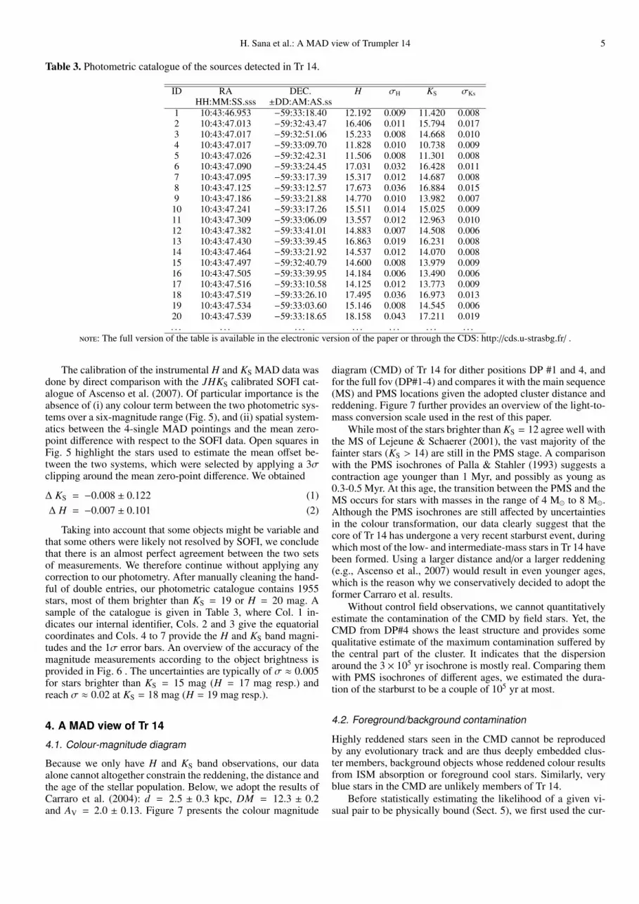
Table 3. Photometric catalogue of the sources detected in Tr 14.

ID RA DEC. H σH KS σKsHH:MM:SS.sss ±DD:AM:AS.ss

1 10:43:46.953 −59:33:18.40 12.192 0.009 11.420 0.0082 10:43:47.013 −59:32:43.47 16.406 0.011 15.794 0.0173 10:43:47.017 −59:32:51.06 15.233 0.008 14.668 0.0104 10:43:47.017 −59:33:09.70 11.828 0.010 10.738 0.0095 10:43:47.026 −59:32:42.31 11.506 0.008 11.301 0.0086 10:43:47.090 −59:33:24.45 17.031 0.032 16.428 0.0117 10:43:47.095 −59:33:17.39 15.317 0.012 14.687 0.0088 10:43:47.125 −59:33:12.57 17.673 0.036 16.884 0.0159 10:43:47.186 −59:33:21.88 14.770 0.010 13.982 0.007

10 10:43:47.241 −59:33:17.26 15.511 0.014 15.025 0.00911 10:43:47.309 −59:33:06.09 13.557 0.012 12.963 0.01012 10:43:47.382 −59:33:41.01 14.883 0.007 14.508 0.00613 10:43:47.430 −59:33:39.45 16.863 0.019 16.231 0.00814 10:43:47.464 −59:33:21.92 14.537 0.012 14.070 0.00815 10:43:47.497 −59:32:40.79 14.600 0.008 13.979 0.00916 10:43:47.505 −59:33:39.95 14.184 0.006 13.490 0.00617 10:43:47.516 −59:33:10.58 14.125 0.012 13.773 0.00918 10:43:47.519 −59:33:26.10 17.495 0.036 16.973 0.01319 10:43:47.534 −59:33:03.60 15.146 0.008 14.545 0.00620 10:43:47.539 −59:33:18.65 18.158 0.043 17.211 0.019. . . . . . . . . . . . . . . . . . . . .

note: The full version of the table is available in the electronic version of the paper or through the CDS: http://cds.u-strasbg.fr/ .

The calibration of the instrumental H and KS MAD data wasdone by direct comparison with the JHKS calibrated SOFI cat-alogue of Ascenso et al. (2007). Of particular importance is theabsence of (i) any colour term between the two photometric sys-tems over a six-magnitude range (Fig. 5), and (ii) spatial system-atics between the 4-single MAD pointings and the mean zero-point difference with respect to the SOFI data. Open squares inFig. 5 highlight the stars used to estimate the mean offset be-tween the two systems, which were selected by applying a 3σclipping around the mean zero-point difference. We obtained

∆ KS = −0.008 ± 0.122 (1)∆ H = −0.007 ± 0.101 (2)

Taking into account that some objects might be variable andthat some others were likely not resolved by SOFI, we concludethat there is an almost perfect agreement between the two setsof measurements. We therefore continue without applying anycorrection to our photometry. After manually cleaning the hand-ful of double entries, our photometric catalogue contains 1955stars, most of them brighter than KS = 19 or H = 20 mag. Asample of the catalogue is given in Table 3, where Col. 1 in-dicates our internal identifier, Cols. 2 and 3 give the equatorialcoordinates and Cols. 4 to 7 provide the H and KS band magni-tudes and the 1σ error bars. An overview of the accuracy of themagnitude measurements according to the object brightness isprovided in Fig. 6 . The uncertainties are typically of σ ≈ 0.005for stars brighter than KS = 15 mag (H = 17 mag resp.) andreach σ ≈ 0.02 at KS = 18 mag (H = 19 mag resp.).

4. A MAD view of Tr 14

4.1. Colour-magnitude diagram

Because we only have H and KS band observations, our dataalone cannot altogether constrain the reddening, the distance andthe age of the stellar population. Below, we adopt the results ofCarraro et al. (2004): d = 2.5 ± 0.3 kpc, DM = 12.3 ± 0.2and AV = 2.0 ± 0.13. Figure 7 presents the colour magnitude

diagram (CMD) of Tr 14 for dither positions DP #1 and 4, andfor the full fov (DP#1-4) and compares it with the main sequence(MS) and PMS locations given the adopted cluster distance andreddening. Figure 7 further provides an overview of the light-to-mass conversion scale used in the rest of this paper.

While most of the stars brighter than KS = 12 agree well withthe MS of Lejeune & Schaerer (2001), the vast majority of thefainter stars (KS > 14) are still in the PMS stage. A comparisonwith the PMS isochrones of Palla & Stahler (1993) suggests acontraction age younger than 1 Myr, and possibly as young as0.3-0.5 Myr. At this age, the transition between the PMS and theMS occurs for stars with masses in the range of 4 M� to 8 M�.Although the PMS isochrones are still affected by uncertaintiesin the colour transformation, our data clearly suggest that thecore of Tr 14 has undergone a very recent starburst event, duringwhich most of the low- and intermediate-mass stars in Tr 14 havebeen formed. Using a larger distance and/or a larger reddening(e.g., Ascenso et al., 2007) would result in even younger ages,which is the reason why we conservatively decided to adopt theformer Carraro et al. results.

Without control field observations, we cannot quantitativelyestimate the contamination of the CMD by field stars. Yet, theCMD from DP#4 shows the least structure and provides somequalitative estimate of the maximum contamination suffered bythe central part of the cluster. It indicates that the dispersionaround the 3 × 105 yr isochrone is mostly real. Comparing themwith PMS isochrones of different ages, we estimated the dura-tion of the starburst to be a couple of 105 yr at most.

4.2. Foreground/background contamination

Highly reddened stars seen in the CMD cannot be reproducedby any evolutionary track and are thus deeply embedded clus-ter members, background objects whose reddened colour resultsfrom ISM absorption or foreground cool stars. Similarly, veryblue stars in the CMD are unlikely members of Tr 14.

Before statistically estimating the likelihood of a given vi-sual pair to be physically bound (Sect. 5), we first used the cur-

http://cds.u-strasbg.fr/


-1 0 1 220

15

10

5

H-Ks

DP#1

-1 0 1 2

H-Ks

DP#4

-1 0 1 2

H-Ks

DP#1-4

Fig. 7. Left: Tr 14 CMD for DP #1. Middle: CMD for DP #4. Right: complete Tr 14 CMD (DP#1 to 4). The dashed lines show theMS from Lejeune & Schaerer (2001) and from Palla & Stahler (1993) for stars with masses M > 6 M� and M ≤ 6 M� respectively.Diamonds and left-hand labels indicate the MS masses. The plain lines show the log(age/yr) = 5.5 PMS isochrone from Palla &Stahler for PMS stars with masses between 0.1 and 6.0 M�. Squares and right-hand labels indicate the corresponding PMS masses.DM = 12.3 and AV = 2.0 were adopted as discussed in Sect. 4.1.

Fig. 8. Tr 14 CMD. The plain lines delimit the adopted locus ofcluster members (see text) while the stars show the objects notconsidered in Sect. 5.

rent results to clean our catalogue from improbable cluster mem-bers. For bright stars (KS > 12 mag), we required the H − KScolour to be within 0.2 mag from the expected locus of MS starswith M > 6 M�. For stars fainter than KS = 12 mag, we adoptedthe following relations as the left and right H − KS limits in theCMD (Fig. 8):

(H − KS)left = 0.043(KS − 12), (3)(H − KS)right = 0.3 − 2.0/(KS − 20). (4)

Both relations are obtained as an approximate to the ±2σ inter-val around the typical H − KS colour of an 0.3 Myr PMS starfor a given KS magnitude. Applying those criteria, we excluded12 bright and 233 faint stars. This represents about 12.5% ofour total sample. Below, we also focus on stars brighter thanKS = 18 mag. This excludes an additional 198 stars (≈10%

Fig. 9. Distribution of the reddest and bluest stars in Tr14. Thedot and the open circles show the location of the faint (12 < KS <18 mag) and bright (KS > 12 mag) stars respectively. Asterisksand crosses identify the bluest and reddest faint stars, while thefilled circles trace the reddest bright stars. For the latter, the sym-bol size is proportional to the KS magnitude. The dashed circleshows a 1′ diameter region centered on HD93129A. North is atthe top and East to the left.

of our sample), resulting in a list of 1495 likely members withKS < 18 mag.

Figure 9 displays the spatial distribution of the rejected blueand red stars. The faint reddest stars agree well with a random


Fig. 10. Tr 14 surface number density distributions for the fullcluster population (circles) and for the PMS (triangles) and MS(diamonds) populations. Upper and lower panels show the den-sity profiles obtained, respectively, before and after applying thecolour criteria of Fig. 8. In both cases only stars with magnitudeKS < 18 mag have been considered. Different lines show thebest-fit EFF87 profiles described in Table 4.

spread in the field. The faint bluest ones are mostly located inthe North and East edges and suggest larger color uncertaintiesin that zone. The surface density of the brighter red stars how-ever shows a clear enhancement that correlates with the centralpart of the cluster. This suggests that the corresponding starsare rather highly reddened objects associated with Tr 14. Weacknowledge that we might thus have rejected some membersof Tr 14. Preserving the homogeneity of the reddening proper-ties of the bright star sample is however more important and weargue that the resulting few extra rejections will not affect thestatistical companionship properties discussed in Sect. 5.

4.3. Cluster structure

Adopting the cluster centre as defined by Ascenso et al. (2007),we computed the radial profile of the star surface density(Fig. 10). Ascenso et al. (2007) proposed a core-halo structurewith a respective approximate radius of 1′ and 5′. Although ourdata set covers a limited area, there is no indication of a transitionbetween the two regimes. We can thus consider that our fov isstrictly dominated by the core of the cluster. The cluster param-eters derived below thus only apply to the core of the core-halostructure.

To better quantify the surface density variations, we fittedElson et al. (1987, hereafter EFF87) profiles, better suited foryoung open clusters than King profiles, to all three populations.Following EFF87, we adopt the notation

Σ(r) = Σ0(1 + r2/a2)−γ/2, (5)

where Σ0 is the surface number density at the centre. With thebest-fit parameters (Table 4) we also computed the radius, rc,where the surface number density drops to half its centre value1

and the (deprojected) central number density, n0, following Eqs.22 and 13b of EFF87, respectively. The central density obtained,n0 = 4.5+0.5

−0.5 × 104 pc−3, is very high.Integrating the surface number density profile to infinity and

assuming an average stellar mass of 0.64 M� as suitable for aKroupa (2001) IMF, our results indicate an asymptotic mass of∼ 4.3+3.3

−1.5×103 M�, with 30% of the mass within the inner parsecof the profile. This value should be taken as an upper limit to themass in the cluster core because of the possible contaminationof the fov by field stars. Our mass estimate is somewhat lowerthan the value of 9 × 103 M� obtained by Ascenso et al. (2007)based on mass-function considerations. Yet the value of Ascensoet al. falls within the upper limit of our uncertainties after cor-recting for the different assumption on the distances. Part of thedifference in the mass determination might also be caused by ourprofile only probing the core region of the core-halo structure,which likely has a steeper profile than the halo.

As a first attempt to search for differences between the low-and high-mass star properties, we also computed the densityprofiles of two sub-populations in Tr 14: the MS stars (KS <12 mag) and the PMS stars (12 < KS < 18 mag). From Fig. 10(upper panel), the PMS stars occupy a larger core but displaya steeper decrease than the MS population. Because the pop-ulation of the cluster is dominated by low mass stars, there islittle difference between the number density profile of the PMSstars and that of the whole cluster. The more massive MS stars(KS < 12 mag) however seem to be slightly more concentratedtowards the cluster centre (see also discussion in Sect. 7). Asmentioned earlier, the PMS profile seems to display a steeperslope, but Table 4 reveals that this difference is not very signifi-cant (only at the 1.8σ level).

As a second step, we also re-computed the density profilesafter applying the colour and magnitude criteria defined in theprevious section (Sect. 4.2), thus focussing on the most proba-ble members. The cluster core radius is found to be larger andthe profiles display a significantly steeper decrease with radius(Fig. 10, lower panel). The central surface density is also reducedby a factor 2.6 and the deprojected central number density by afactor 4.7 (Table 4). Following these adjustments, the asymptoticmass of the core is reduced to 1.4+0.4

−0.3 × 103 M�. Because of the

1 This value is often referred to as the core radius. Because Tr 14 dis-played a core-halo structure, rc should be understood as the core radiusof the core itself.


Table 4. Best-fit EFF87 parameters for different populations in Tr 14.

Population KS range Σ0 [pc−2] a [pc] γ rc [pc] n0 [pc−3]

Without colour selection

MS 6–12 1077 ± 567 0.05 ± 0.03 1.66 ± 0.27 0.06+0.03−0.03 9871+10497

−6376

PMS 12–18 10330 ± 770 0.13 ± 0.01 2.17 ± 0.08 0.11+0.01−0.01 40715+5019

−4520

All 6–18 11116 ± 817 0.13 ± 0.01 2.18 ± 0.08 0.11+0.01−0.01 44665+5390

−4864

With colour selection

MS 6–12 3097 ± 14013 0.01 ± 0.03 1.25 ± 0.39 0.01+0.05−0.05 . . .

PMS 12–18 3977 ± 289 0.32 ± 0.04 3.26 ± 0.19 0.23+0.03−0.03 8348+1258

−1070

All 6–18 4321 ± 316 0.30 ± 0.03 3.10 ± 0.17 0.22+0.03−0.03 9491+1394

−1199

note: The uncertainties on Σ0, a and γ are the 1σ error bars. The uncertainties rc and n0 were computed using Monte Carlo simulations assuminga Gaussian distribution of the errors on Σ0, a and γ. The quoted values give the 0.68 confidence interval.

Fig. 11. Cumulative distribution of the distance to the closestneighbour (dmin). The horizontal dotted line shows the size ofour sample.

sharper slope of the profile, one now finds 75% of the total massin the inner parsec. Interestingly, the more massive stars showno core-structure, and their density profile is well representedby a simple power-law. This is somewhat comparable to whatCampbell et al. (2010) found for the massive stars in R136.

5. Companion analysis

5.1. General properties

With about 1500 likely members in a 2′-diameter fov, the meansurface density is 477 src/arcmin2, or 0.133 src/arcsec2. Theclosest pair detected in our PSF photometry is separated by0.24′′ and half the sources have a neighbour at no more than1.25′′ (Fig 11). Figure 12 illustrates empirically the maximumreachable flux contrast between two close sources as a func-tion of their separation. The magnitude difference2 ∆KS roughlyscales as the cubic root of the separation:

∆KS = 6(d − 0.24)1/3. (6)2 Below, the brightest star of a pair is adopted as the primary. We

adopt the convention ∆KS = KS,sec − KsS,prim ≥ 0, where KS,prim andKS,sec are the primary and secondary magnitudes respectively.

Fig. 12. Magnitude difference ∆KS of detected visual pairs as afunction of the distance d. The plain line is defined by Eq. 6.

Flux contrasts of ∆KS = 1/3/5/8 are reached at separations d =0.25/0.5/1.0/2.0′′ respectively.

5.2. Chance alignment

Because of the high source surface density, the number of pairsquickly increases with separation. To quantify the chance thatan observed pair results from spurious alignment, we followedthe approach of Duchene et al. (2001). We define Pbound asthe complementary probability to the one that a given pair(KS,prim,KS,sec), with a separation d, occurs by chance:

Pbound = exp

− KS,sec∑KS=KS,prim

WKS

πR2

, (7)

where R is the field radius, taken as 60′′. WKS is the actual surfacearea of a star of magnitude KS and is given by

WKS = π(d2 − d2

min

(KS − KS,prim

)), (8)

where dmin is the minimal separation at which a star of magni-tude KS can be detected in the neighbourhood of a star of mag-nitude KS,prim. It is estimated by inverting Eq. 6 thus

dmin(∆KS) = (|∆KS|/6)3 + 0.24. (9)


Fig. 13. Probability that a pair is physically bound Pbound plottedvs. the binary separation d. The plain curve delimits the locuswere no pairs are found and corresponds to Pbound = exp(−(d −0.24)2/2).

Fig. 14. Same as Fig. 12 where the population of likely boundsystems has been over-plotted with red (Pbound > 0.90) or bluesquares (Pbound > 0.99). Plain red and blue lines identified thetypical locus of the two populations.

As expected, Fig. 13 shows that the likelihood of findingphysically bound pairs, Pbound, decreases steeply with separa-tion. Typically, only pairs with a brightness ratio close to unityor with a separation of less than 0.5′′ cannot be explained byprojection effects (Fig. 14). This implies that wider or larger fluxcontrast systems, if existing, cannot be individually disentan-gled from the pairs arising by chance alignment along the lineof sight.

Table 5 lists the 150 pairs separated by 5′′ or less and withPbound ≥ 0.99. The first column indicates the primary and sec-ondary IDs from Table 3. Columns. 2-3 and Cols. 4-5 list theH and KS magnitudes of the primary and secondary compo-nents, respectively. The separation of the pair is given in Col. 6.The two closest pairs detected have a separation of 0.24′′ and0.25′′ (only 600 AU at the Tr 14 distance) and ∆KS ≈0.6-0.7mag (Fig. 15). The closest probable companion to a massive staris a KS = 13.2 mag star at 0.4′′ from the B1 V star Tr14-19(pair ID #1530-1536 in Table 5). Of the 31 stars brighter than

Fig. 15. Close-up view in the KS band image of the four closestpairs of Table 5. The displayed regions are 6′′×6′′ and the sep-arations are all in the range of 0.24′′-0.30′′. Their identifiers asgiven in Table 3 are overlaid on the images.

Table 5. List of likely bound visual pairs (Pbound ≥ 0.99).

IDprim-IDsec Hprim KS,prim Hsec KS,sec d (′′)656- 664 17.490 16.655 18.313 17.359 0.24306- 299 15.088 14.798 15.997 15.380 0.25

1446-1451 14.097 13.323 13.803 13.560 0.28902- 896 17.697 17.044 18.709 17.784 0.29

1024-1025 14.842 14.455 15.941 15.349 0.291091-1092 16.165 15.342 15.979 15.459 0.29156- 157 17.303 16.715 17.665 17.084 0.30

1581-1579 15.277 14.653 15.407 15.030 0.311488-1491 14.205 13.941 16.044 15.530 0.321445-1453 16.320 16.014 17.395 16.981 0.321398-1389 14.326 13.931 15.461 14.942 0.331152-1149 14.867 14.498 16.254 15.229 0.341351-1343 12.899 12.542 15.742 14.876 0.34828- 825 17.984 17.458 19.244 18.233 0.34

1780-1779 16.527 16.052 16.829 16.322 0.341320-1318 15.386 15.024 16.267 15.660 0.34945- 955 15.533 15.122 16.289 15.724 0.35

1163-1155 16.471 15.241 16.277 15.674 0.351101-1104 12.828 12.320 15.311 14.589 0.361202-1200 15.949 15.449 16.106 15.506 0.36

. . . . . . . . . . . . . . . . . .note: The full version of the table is available in the electronic version

of the paper or through the CDS: http://cds.u-strasbg.fr/ .

KS = 11 mag, only six have high probability companions in therange of 0.4′′ to 2.5′′, i.e. 19%. Because of the observationalbiases discussed and of the filtering criteria applied, the statisti-cal distribution of the selected pairs is not representative of theunderlying distribution and will not be discussed further.

http://cds.u-strasbg.fr/


Fig. 16. Left: Average number of companions per star for a givenmaximum companion magnitude. Right: Cumulative distribu-tion functions (CDF) of the companion brightness. The centralstars are taken in four ranges as indicated in the upper left-handlegend. Only pairs with separations in the range of 0.5′′-2.5′′have been considered.

5.3. Companion frequency

To search for variations in the companionship properties of dif-ferent sub-populations, we first computed the average number ofcompanions per star, considering various magnitude ranges bothfor the central star and for the companions (Fig. 16, left panel).We applied the same colour and magnitude selections defined inSect. 4.2. We further adopted an exclusion radius of 5′′ betweeneach central star so that each companion is only assigned to oneprimary, preserving the independence of the different samples.In this particular case and to allow direct comparison betweenthe different samples, we did not require that KS,prim < KS,sec.For the central stars, we consider four ranges of magnitudes:

- the massive stars : 6 < KS,prim < 11, corresponding to M >10 M� MS stars);

- the intermediate-mass stars : 11 < KS,prim < 13, correspond-ing to 10 > M > 4 M� stars;

- the solar-mass PMS stars : 13 < KS,prim < 14, correspondingto 2.5 > M > 0.5 M� PMS stars;

- the low-mass PMS stars : 15 < KS,prim < 16, correspondingto 0.2 > M > 0.1 M� PMS stars;

where the isochrones of Fig. 7 have been adopted as guidelinesfor the mass conversion. The companion magnitude was chosenin the range of 9.5 < KS,sec < 18. Finally, we restrained ourcomparison to the 0.5′′-2.5′′ separation regime. As we will showbelow (Sect. 6.1), the observational biases have a very limitedimpact on our results in that range.

Under those assumptions, we found that massive MS starshave on average 3.8 ± 0.5 companions, while solar-mass PMSstars have 3.0 ± 0.2 companions. The number of companionsof intermediate-mass stars and of low-mass PMS stars are notsignificantly different from one another. Most of the differenceis however found for KS,sec < 17: 3.5 ± 0.4 companions for MSstars against 2.5 ± 0.2 for lower mass stars. The difference is

Fig. 17. Average number of companions per star as a functionof the companion brightness. The central stars are taken in fourranges as indicated in the upper left-hand legend. A moving av-erage with a 2 mag bin has been used and the considered separa-tion range is 0.5′′-2.5′′. The various envelopes give the 1σ errorbars.

thus significant at the 2.5σ. This corresponds to a rejection ofthe null hypothesis that massive and lower-mass stars have thesame number of companions with a significance level better than0.01. Because this is seen against the observational biases (seeSect. 6.2.2), this result is likely to be even more significant.

5.4. Magnitude distribution

We computed the distributions of the companion magnitudesfor the various stellar populations considered above using a 2-mag wide moving average along the companion magnitude axis(Fig. 17). Most of the differences between the distribution func-tions of the massive stars and of the lower-mass stars result fromthe range KS,sec < 14. The more massive stars display thus abouttwice as many solar-mass companions as the lower mass stars.The situation is reverse for fainter, low-mass PMS companions,where the lower-mass stars tend to have more companions. Thelatter effect can however result from the difficulty to detect ex-tremely faint stars in the wings of the brightest stars. To allow forquantitative statistical testing, we also built the cumulative dis-tribution functions (CDF) of the companion brightness (Fig. 16,right panel). Using a two-sided Kolmogorov-Smirnov (KS) test,one can reject at the 2σ level the null hypothesis that the high-mass and the solar-mass stars share the same companion CDF.

5.5. Companion spatial distribution

To investigate the spatial distribution of the companions, we builtthe growth curves of the number of companions as a functionof the separation. For the curves to be more robust against lownumber statistics, we concentrated on the total growth curve ofa given stellar population rather than on the growth curve of in-


Fig. 18. Upper panel: growth curve for the companions of mas-sive stars. The plain line indicates the expected distribution fora uniform distribution of the companions in the field of view.Lower panel: same as upper panel for the companions of solar-mass stars.

dividual targets. We further limited the companions to massesabove 0.1 M�, which roughly corresponds to a magnitude limitof KS = 16 mag and, as in the previous paragraph, we restrainedour comparison to the 0.5-2.5′′ separation regime.

Figure 18 compares the companion growth curves aroundhigh-mass and around solar-mass stars with the theoretical dis-tribution expected from random association with an underlyinguniform distribution across the field. On the one hand, massivestars seem to have their companions statistically further awaythan expected from a uniform repartition. On the other hand, thegrowth curve of solar-mass PMS stars follows the expected trendfrom random association. Yet in both cases a KS test does notallow us to reject the null hypothesis that both realisations arecompatible with the uniform distribution in the considered sepa-ration range. Similarly, a two-sided KS test does not allow us toclaim that both growth curves are different from one another.

5.6. Summary

To summarize the results of this section, the closest pair of de-tected stars in our data is separated by 0.24′′ (∼600 AU), in goodagreement with the IQ of Sect. 2. Equation 6 gives an empirical

Fig. 19. Cumulative distribution functions (CDFs) of the dis-tance from each artificial star to (i) the closest artificial star (plaincurve), (ii) the closest source in field (dashed line), (iii) the clos-est bright star with KS < 11 (dashed-dotted line).

estimate of the maximum contrast achieved as a function of theseparation Sect. 5.1. The pairing properties are well describedby chance alignment except for the closest pairs (d < 0.5 ′′)and for the pairs with similar magnitude components (Fig. 14),yet we identified 150 likely bound pairs (Sect. 5.2). Massivestars further tend to have more companions than lower-massstars (Sect. 5.3). Those companions are brighter on average, thusmore massive (Sect. 5.4). The spatial distribution of the compan-ions of massive stars is however not significantly different fromthose of PMS star companions (Sect. 5.5). The significance ofthose results is better than 2σ but no better than 3σ, and remainsthus limited. The situation is however reminiscent of the case ofNGC 6611 where Duchene et al. (2001) found that massive starsare more likely to have bound companions compared to solar-mass stars. For Tr 14, the fov is definitely more crowded andprobably more heavily contaminated, which seriously compli-cates both the companionship analysis and the interpretation ofthe results.

6. Observational biases

This section first describes an artificial star experiment designedto quantify the detection biases in the vicinity of the bright stars.It also presents two simple models that generalise the results ofthe artificial star experiment and provide an estimate of the im-pact of various observational biases on the results of this paper.

6.1. Artificial star experiment

Most of the difference in the companion properties of massiveand lower-mass stars are found for companions in the range13 < KS,sec < 14. In this section, we describe and analyse theresults of an artificial star experiment that aims at better un-derstanding the limitation of our data in that range, justifyingsome of the choices made in the previous section. The PSF ofthe brightest sources indeed show strong and extended wings,which decrease the detection likelihood in the neighbourhood ofa bright star. As a by-product, the results of this experiment alsoprovide an independent estimate of the photometric errors andof the completeness of our catalogue for the tested parameterrange, but this is not our main purpose.


Fig. 20. Lower panel: Comparison between the input and outputmagnitudes for the artificial star experiment as a function of theseparation the to closest bright star in the fov (KS < 11). Thesquares and diamonds respectively give ∆mag = KS,out − KS,inand Hout − Hin. Upper panel: same as lower panel for the colourof the artificial stars : ∆(H − K) = (H − KS)out − (H − KS)in.

Fig. 21. Artificial star recovery fraction as a function of the dis-tance d to a bright neighbour (KS < 11). The plain line showsa linear interpolation between the detection and non-detectionregime and is given by frecov = (d − 0.35)/0.2, for d in the range0.35–0.55′′.

The artificial star experiment follows a procedure similar tothat presented in Momany et al. (2002, 2008). In particular, starswith known H and KS magnitudes were simulated into the in-dividual H and KS images using the PSF of each image andtaking into account the quadratic dependence of the PSF withthe position in each frame. The entire reduction procedure wasthen repeated and the artificial stars were reduced as describedin Sect. 2.

To the first order, stars brighter than KS = 11 in Tr 14 havemasses of 10 M� or more (see e.g. Fig. 7). As in Sect. 5, weadopted this limit for our massive star sample. We thus selected14 bright stars with 9 ≤ KS ≤ 11. Around each of them wesimulated 50 companions with 13 ≤ KS,in ≤ 14 and Hin −KS,in =0.35, spread in a 5′′ radius. The colour of the artificial stars were

Fig. 22. Detection probability as a function of the stellar magni-tude resulting from the effect of the crowding in the Tr 14 fov.

chosen to reproduce the colour of typical PMS stars in Tr 14,which are the dominant type of sources in that magnitude range.

Seven hundred artificial stars were thus simulated in the Hand KS images. To optimise the computation time of this com-plicated procedure, all the artificial stars were added simultane-ously. While this led to some heavier crowding than in the orig-inal field, this will be taken into account in the analysis. Thisfurther allows us to study the detection biases using artificiallycontrolled pairs.

6.1.1. Separation distribution

Figure 19 shows the cumulative distribution of the separationsof the artificial stars with respect to one another, with respectto the closest source in the field and with respect to the closestbright source in the field. It shows that we are able to investigatevarious ranges of separation, from the crowding of the artificialstars among themselves to the effect of field density. We firstfocus on the closest detections. The main results of the artificialstar experiment in this respect are :

- The closest recovered pair of artificial stars is separated bydsep = 0.2′′, in good agreement with the IQ derived earlier,

- The recovery fraction of artificial pairs for which both com-ponents are further away than 0.6′′ from any source in theimage is better than 0.99 for dsep > 0.24′′,

- Excluding all pairs of artificial stars with dsep < 0.3′′, theclosest separation between a recovered artificial stars and astar at least as bright is 0.23′′,

- Similarly, the closest separation between a recovered artifi-cial star and a massive star (KS < 11) is 0.38′′, in perfectagreement with what we found in our data (Sect. 5.2),

- All in all, there is a good agreement between the resultsof the artificial star experiment and the maximum reachablecontrast as a function of the separation described empiricallyby Eq. 6.

As a first result, the artificial star experiment allows us to vali-date up to ∆KS = 5 mag at least the empirical contrast vs. sepa-ration function introduced earlier. This result will be used belowto build a first-order analytical model of the observational biasesaffecting our data.


6.1.2. Recovery fraction

To estimate the recovery fraction of solar-mass PMS stars in thewings of the brighter massive stars, we first excluded all the closeartificial pairs from our analysis. We also exclude all the artificialstars that fall closer than 0.3′′ from any source fainter than KS =11 in our data. With this we eliminate the uncertainties due to (i)crowding among the artificial stars and (ii) confusion betweenthe artificial stars and the numerous field sources in our data.Almost 500 artificial stars are left, providing a decent coverageof the parameter space.

Figure 21 shows the recovery fraction as a function of theseparation to the closest bright star. As mentioned earlier, thefirst detection occurs for a separation of 0.38′′. For dsep > 0.53′′,all the artificial stars are recovered. Between 0.38′′ and 0.53′′,the recovery fraction is approximately 0.4 and remains constantover the interval.

6.1.3. Photometric uncertainties

The comparison between the artificial star input (KS,in) and re-covered (KS,out) magnitudes provides us with a more realistic es-timate of the photometric errors (Fig. 20). It reveals that the ac-curacy of both the retrieved magnitudes and of the colour term issignificantly affected within ≈ 1′′ from a bright star, the faintercompanion being up to 0.1 mag too red. It also reveals a slightsystematic shift in the retrieved colour and magnitudes, even atlarger distance. Rejecting the few significantly deviant points re-sulting from the crowding, we obtained for the artificial starsmore distant than 1.5′′ from the closest bright star

Hout − Hin = 0.008 ± 0.020 (10)KS,out − KS,in = 0.008 ± 0.026 (11)

(H − KS)out − (H − KS)in = −0.021 ± 0.019, (12)

Those are slightly larger deviations that the formal errors of thePSF photometry (Fig. 6). The systematic increase of the H −KScolour when getting closer to the bright companion could resultfrom a slightly better IQ obtained in the KS band compared tothe H band, and thus a better subtraction of the bright star wingsfor a given separation.

6.2. Analytical models

6.2.1. Impact of crowding

Given the very steep transition in the detection probability oncethe separation to a brighter source increases, and because theartificial star experiment generally agrees with the empirical de-tection limit given by Eq. 9, one can develop a very simple modelto estimate the impact of the crowding in the field. It relies on thefollowing hypotheses :

- A brighter star is always detected if falling on top of or veryclose to a fainter one,

- Non-detection is the consequence of shadowing by brighterstars in the fov,

- The spatial distribution of the stars in the field is random.

The detection probability of a source of a given magnitude K0S

can then be written as

Pdetect.(K0S) = 1 −

ΣKS≤K0S

(πd2(∆KS)

)Afov

, (13)

Fig. 23. Detection probability model for pairs with separation inthe range of 0.5′′-2.5′′ and for various brightness ranges of thecentral star.

where d(∆KS) is given by Eq. 9 and where Afov is the area of theconsidered fov. In Eq. 13, the sum is performed over all sourcesbrighter than K0

S. Figure 22 shows the resulting detection proba-bility. According to this model, completeness level of 0.99, 0.95and 0.90 are reached for stars brighter than KS = 14, 16 and17 respectively. While our model is certainly too crude to ade-quately describe the faint end, it still shows that the crowdinghas a very limited impact in Tr 14. In particular, this indicatesthat the star counts used to fit the Tr 14 profile and to estimatethe cluster core mass are unlikely to be significantly biased.

6.2.2. Companion detection threshold

In Sect. 5.3 to 5.5, we focused our analysis to the 0.5-2.5′′ sepa-rations. In this section, we develop again a simple model to betterquantify the impact of the observational biases in that range. Asabove, we use Eq. 9 to define the region where a star outshinesclose fainter neighbours given the magnitude contrast of the pair.In particular, the detection probability of a neighbour of magni-tude KS,sec in the vicinity of a KS,prim central star can be mod-elled as the ratio between the area where one of the componentsdoes not outshine the other and the total area considered. For anannulus region Rmin–Rmax around the central star, the detectionprobability can thus be written as

Pdetect. =

1.0, if d < R′′min;

1.0 − d2(∆KS)−R2min

R2max−R2

minif Rmin ≤ d < R′′max;

0.0, if d ≥ Rmax.

(14)

Figure 23 compares the detection probability in the 0.5-2.5′′ sep-aration range for the various central star-brightness ranges usedearlier. For the bright primary interval, the curve displayed re-sults from the average of Pdetect. computed individually for allthe bright primaries considered to build Figs. 16 and 17. Thecentral magnitude of the primary intervals has been used for theother three categories.

Our results show that the detection of the companions tointermediate-mass stars (11 < KS < 13) and to solar-mass PMSstars (13 < KS < 14) stars is mostly unaffected. As expected, thelower mass PMS (15 < KS,prim < 16) are less likely to be foundclose to a bright stars. However, taking into account the numberof bright stars in the field, one can prove this to be completelynegligible. The largest biases are affecting the companions of


Fig. 24. Evolution of ΛMSR with the adopted magnitude limitKS,min for the massive star sample. The circles and triangles in-dicate the results obtained with and without the colour and mag-nitude selection criteria of Fig. 8. The upper and lower N valuesgive the number of stars considered in each step and for bothsamples. The dotted line indicates ΛMSR = 1, i.e., no mass seg-regation.

bright stars. Pdetect. is passing below 0.9 at KS = 14 and below0.5 at KS ≈ 17. One can further show that up to one companionper star is likely lost at KS,sec < 16 in Fig. 16.

7. Mass segregation

As introduced in Sect. 4.3, the more massive MS stars seem moreconcentrated towards the cluster centre than the lower mass PMSstars. The best-fit EFF87 profiles (Table 4) confirm that this dif-ference is indeed significant at the 4σ level. This could be in-terpreted as a hint for mass segregation, although Ascenso et al.(2009) warned against hasty conclusions because numerous ob-servational biases are actually favouring the detection of masssegregation, even in non-segregated clusters.

Allison et al. (2009) recently introduced an alternativemethod to investigate mass segregation, which is insensitive tobiases like the exact location of the cluster centre, and less sen-sitive (although quantification is still lacking) to the incomplete-ness effects. Their method compared the minimum spanning tree(MST), the shortest open path connecting all points of a sample,of the massive stars to the equivalent path of low mass stars (seeAllison et al. for a full description of the algorithm). The masssegregation ratio (ΛMSR), i.e. the ratio between the average ran-dom path length and that of the massive stars, allows them toquantify the deviation between the massive star sample and thereference sample. Following their approach, Fig. 24 displays theevolution of ΛMSR with the adopted magnitude limit (KS,min) forthe massive star sample. The reference distribution consists ofstars with 14 < KS < 16 and was drawn 500 times from our cat-alogue, with each sample containing the same number of stars asfound in the bright sample. The dispersion obtained gives us theerror bars on ΛMSR as displayed in Fig. 24. In the above proce-dure, we deliberately remained far from the limiting magnitude

of our catalogue to minimize the completion biases. The methodis in principle still affected by crowding and by the shadowingin the vicinity of bright stars. We showed in Sect. 6.1.2 howeverthat the former effect had a very limited impact down to KS < 16at least. The effect of the shadowing in the vicinity of bright starsis more difficult to estimate, although one can expect that the ab-solute number of 14 < KS < 16 stars lost is proportionally verysmall compared to the number of stars in that interval. This re-sults from the low number of bright stars and from the limitedradius at which they can outshine a fainter neighbour.

We computed the MST first with and without the colour se-lection defined in Sect. 4.2 (Fig. 24). Focussing on the mostprobable members (thus applying the colour selection), wefound some indication of mass segregation down to KS,min ≈

10.5 mag at the 1.5σ level. As expected, the degree of mass seg-regation is increasing with the average brightness of a sample,thus with the mean stellar mass. The largest mass segregationratio is obtained for the few brightest, most massive stars afterapplying the membership selection. Yet the 1.5σ confidence ofthis result remains at the limit of the detection.

Because the sensitivity of the MST to the completeness of asample is not fully understood (Allison et al., 2009), we cannotdraw firm conclusions. We note however that two independentmethods, profile fitting and MST analysis, both point towardsmass segregation, as can be expected for the most massive starsin such a cluster.

Obviously our observations only allow us to investigate thecurrent mass segregation status of the cluster and we cannot dis-tinguish whether this segregation, if confirmed, is primordial oris the product of early dynamical evolution. Given the expectedcluster mass and size and its stellar contents as obtained inSect. 4.3 after colour selection, we estimated the typical dynami-cal friction time-scale tdf of 10 M� and 20 M� stars (correspond-ing to resp. KS ≈ 11 mag and 9.5 mag in our data). FollowingSpitzer & Hart (1971) and Portegies Zwart & McMillan (2002), we obtained tdf ≈ 7.2 × 105 yr and 3.6 × 105 yr respectively.Considering the estimated age of the cluster, 3-5×105 yr, the dy-namical friction time-scales agree with the results of Fig. 24,where mass segregation begins to appear somewhere between10 M�and 20 M�. As a consequence, if mass segregation is con-firmed, it does not need to be primordial but can probably beexplained by dynamical evolution.

8. Summary and conclusions

Using the ESO MCAO demonstrator MAD, we have acquireddeep H and KS photometry of a 2′ region around the central partof Tr 14. The average IQ of our campaign is about 0.2′′ and thedynamic range is about 10 mag. The image presented in Fig. 1is by far the largest AO-corrected mosaic ever acquired.

Using PSF photometry, we investigated the sensitivity offaint companions detected in the vicinity of bright sources. Wederived several empirical relations that can be used as input forinstrumental simulations, to estimate the performance of AOtechniques versus seeing-limited techniques or, as done later inthis paper, to build first-order analytical models of the impact ofsome observational biases. In particular, the contrast vs. sepa-ration limit has been validated over a 5 magnitude range by anartificial star experiment.

Despite a probably significant contamination by field stars,the Tr 14 CMD shows a very clear PMS population. Its locationin the CMD can be reproduced by PMS isochrones with con-traction ages of 3 to 5 × 105 yr. Interestingly, Tr 14 cannot besignificantly further away than the distance obtained by Carraro


et al. (2004) i.e., 2.5 kpc, as this would result in an even ear-lier contraction age. We derive the surface density profile of thecluster core and of different subpopulations. For stars brighterthan KS = 18 mag, the surface density profiles are well re-produced by EFF87 profiles over our full fov, and we providequantitative constraints on the spatial extent of the cluster andon its stellar contents. Adopting the core-halo description sug-gested by Ascenso et al. (2007), we report that the transition be-tween the core and the halo is not covered by our data, implyingthat the core is strictly dominating the density profile in a radiusof 0.9 pc at least. Using colour criteria to select the most likelycluster members, the density profiles of the more massive MSstars are best described by a power-law (or, equivalently, by anEFF87 profile with a very small core radius).

We also investigated the companionship properties in Tr 14.We showed that the number of companions and the pair asso-ciation process is on average well reproduced by chance align-ment from a uniform population randomly distributed across thefield. Only stars with a brightness ratio close to unity or with aseparation of less less than 0.5′′ cannot be explained by spuri-ous alignment and are thus true binary candidates. This does notimply that large light-ratio and/or wider pairs do not exist, butrather that they cannot be individually disentangled with statisti-cal arguments. Still, 19% of our massive star sample have a highprobability physical companion.

Focusing on the 0.5′′-2.5′′ separation range, where the obser-vational biases are unable to invalidate our results, we comparedthe companion distributions of massive stars with those of lowermass stars. In Tr 14, the high-mass stars (M > 10 M�) tend tohave more solar-mass companions than lower-mass comparisonsamples. Those companions are brighter on average, thus moremassive. Finally, no difference could be found in the spatial dis-tribution of the companions of low and high-mass stars.

Lastly, we employed the MST technique of Allison et al.(2009) to investigate possible mass segregation in Tr 14. Againwe found marginally significant results (at the 1.5σ level), sug-gesting some degree of mass segregation for the more massivestars of the cluster (M > 10 M�) . Although the sensitivity of themethod to incompleteness is still not fully quantified, we notethat early dynamical evolution can reproduce the observed hintsof mass segregation in Tr 14, despite the cluster’s young age.

Acknowledgements. The authors are greatly indebted to Paola Amico and to theMAD SD team for their excellent support during the preparation and executionof the observations. We also express our thanks to the referee for his help, whichclarified the manuscript, and to Dr. Joana Ascenso for useful discussions.

ReferencesAllison, R. J., Goodwin, S. P., Parker, R. J., et al. 2009, MNRAS, 395, 1449Ascenso, J., Alves, J., & Lago, M. T. V. T. 2009, A&A, 495, 147Ascenso, J., Alves, J., Vicente, S., & Lago, M. T. V. T. 2007, A&A, 476, 199Baume, G., Vazquez, R. A., & Carraro, G. 2004, MNRAS, 355, 475Campbell, M. A., Evans, C. J., Mackey, A. D., et al. 2010, MNRAS, in press

(arXiv:1002.0288)Carraro, G., Romaniello, M., Ventura, P., & Patat, F. 2004, A&A, 418, 525de Wit, W. J., Testi, L., Palla, F., & Zinnecker, H. 2005, A&A, 437, 247Duchene, G., Simon, T., Eisloffel, J., & Bouvier, J. 2001, A&A, 379, 147Elson, R. A. W., Fall, S. M., & Freeman, K. C. 1987, ApJ, 323, 54Gvaramadze, V. V. & Bomans, D. J. 2008, A&A, 490, 1071Kroupa, P. 2001, MNRAS, 322, 231Lejeune, T. & Schaerer, D. 2001, A&A, 366, 538Maız-Apellaniz, J., Walborn, N. R., Galue, H. A., & Wei, L. H. 2004, ApJS, 151,

103Marchetti, E., Brast, R., Delabre, B., et al. 2007, The Messenger, 129, 8Mason, B. D., Hartkopf, W. I., Gies, D. R., Henry, T. J., & Helsel, J. W. 2009,

AJ, 137, 3358Momany, Y., Held, E. V., Saviane, I., & Rizzi, L. 2002, A&A, 384, 393

Momany, Y., Ortolani, S., Bonatto, C., Bica, E., & Barbuy, B. 2008, MNRAS,391, 1650

Palla, F. & Stahler, S. W. 1993, ApJ, 418, 414Portegies Zwart, S. F. & McMillan, S. L. W. 2002, ApJ, 576, 899Sana, H. & Le Bouquin, J.-B. 2009, in The interferometric view of hot stars, ed.

T. Rivinius & M. Cure, Rev. Mex. Conf. Ser., in press (arXiv:0906.5003)Sana, H., Gosset, E., Naze, Y., Rauw, G., & Linder, N. 2008, MNRAS, 386, 447Sana, H., Gosset, E., & Evans, C. J. 2009, MNRAS, 400, 1479Sana, H., James, G., & Gosset, E. 2010, MNRAS, submittedSpitzer, L. J. & Hart, M. H. 1971, ApJ, 164, 399Stetson, P. B. 1987, PASP, 99, 191Stetson, P. B. 1994, PASP, 106, 250Turner, N. H., ten Brummelaar, T. A., Roberts, L. C., et al. 2008, AJ, 136, 554Vazquez, R. A., Baume, G., Feinstein, A., & Prado, P. 1996, A&AS, 116, 75

http://arxiv.org/abs/1002.0288

http://arxiv.org/abs/0906.5003

Documents

A MAD view of Trumpler 14