A microfabricated dielectrophoretic trapping array for cell-basedbiological assays

by

Joel Voldman

B.S., University of Massachusetts at Amherst, 1995S.M. Massachusetts Institute of Technology, 1997

Department of Electrical Engineering and Computer Science in partialfulfillment of the requirements for the degree of

Doctor of Philosophy

at the

MASSACHUSETTS INSTITUTE OF TECHNOLOGYJune 2001

© 2001 Massachusetts Institute of TechnologyAll rights reserved

8ARKER

JUL 1 12001

Signature of Author................

Certified by...........

.... .. ................................Deparint of E ct angineerqng and Computer Science

May 20, 2001

........ . . . ........ . ..... 1....

Martin A. SchmidtProfessor of Electrical Engineering

Thesis Supervisor

Certified by............. ......................I Martha L. Gray

Edward Hood Taplin Professor of Medical & Ejectrical EngineeringThesis Supervisor

Certified by.............. '..........................

Mehmet TonerAssociate Professor of Bioengineering

Hrvard Medical SchoolTo_6sfIfprvisor

2

Accepted by.....................Arthur C. Smith

Chairman, Department Committee on Graduate Students

Submitted to the

A microfabricated dielectrophoretic trapping array for cell-based biological assays

by

Joel Voldman

Submitted to the Department of Electrical Engineering and Computer Science on May 20, 2001in partial fulfillment of the requirements for the degree of Doctor of Philosophy in Electrical

Engineering and Computer Science

ABSTRACT

This thesis presents the development of a small planar array of microfabricated traps for holdingsingle cells and performing assays on them. The traps use the phenomenon ofdielectrophoresis-the force on polarizable bodies in a non-uniform electric field-to makepotential energy wells. These potential energy wells are electrically switchable, arrayable, andamenable to batch fabrication. The trapping arrays have potential use as a cytometer formonitoring the dynamics of populations of single cells and then sorting those cells based uponthose dynamics.

To design such traps, I have developed a modeling environment that can absolutelypredict the ability of DEP-based traps to hold particles against liquid flows, which are thedominant destabilizing force in these systems. I have used the common easy-to-fabricate planarquadrupole trap to verify the accuracy of these modeling tools, and in the process determinedwhy planar quadrupole traps behave as they do.

I next used the modeling tools to design an improved quadrupole trap-the extrudedquadrupole-that has the potential to hold particles lOx-100x stronger. The extruded quadrupoletrap consists of a set of microfabricated gold posts arranged in a trapezoidal fashion, to ease traploading, and includes metal substrate shunts to improve performance. The fabrication processfor small arrays of these traps uses electroplating of gold into an SU-8 mold to achieve therequired geometries.

The final section of the thesis details experiments using small arrays of these extrudedquadrupole traps. Experiments were performed with beads to verify the strong nature of the trapand then with cells to demonstrate qualitative operation of the arrays and the ability to performdynamic fluorescent assays on multiple single cells followed by sorting. The technology is nowwell poised to enable the development of biological assays that are currently unavailable.

Thesis Supervisor: Martin A. SchmidtTitle: Professor of Electrical Engineering and Computer Science

Thesis Supervisor: Martha L. GrayTitle: Edward Hood Taplin Professor of Medical & Electrical Engineering

Thesis Supervisor: Mehmet TonerTitle: Associate Professor of Bioengineering, Harvard Medical School

3

Acknowledgements

Many people have helped make my time at MIT an enjoyable one. I want to first thankMarty for allowing me to join the group 6 years ago, when all I knew about MEMS was that theywere cool. It was certainly a risk, but one that I think has paid off well. Marty not only let mejoin the group, he also allowed me to indulge my interest in BioMEMS, which I thought was thecoolest part of MEMS. Our plundering through that field, resulted in this thesis, and it's been afun journey. All through it, Marty had genuine concern for my well-being and what was best forme. He never micromanaged, allowing me to make my own mistakes.

Early on we decided to collaborate with Martha, and she quickly became not just acollaborator but also a bona-fide 2 advisor. Her perspective from the bio end of things ensuredthat the project would not just be cool, but actually useful. In addition, her outlook on theprocess and perspective on academia did much to shape my views.

At the start of my Ph.D., we all wanted to work with Mehmet, since he was such a nice,fun guy with neat ideas. I have really appreciated his many ideas and enthusiasm about science.He has also proved exceptionally gifted as a career counselor, both in the advice he dispensesand his candor in dispensing it. Plus, he reads stuff really quickly.

I'd like to also thank some other professors at MIT with whom I have had contact. I'veappreciated SDS' ability to quickly divine the good from the crap, and also the career advice hehas given me. I've enjoyed my numerous chats with Tayo and his enthusiasm as we were bothgoing through MIT's growth process.

The staff at the MTL helped me get this stuff done. Central to this is Vicky, who isresponsible for running the place but still has the courage to say and do what's right even if it'srisky; JoeD, for his warmth; Kurt, for having no boundaries on how he can help; Debb, for herattitude and for treating me like I deserve; and Pat and Anne, for their help in navigating theintricacies of MIT beaurocracy.

As much as my advisors, the group of students and postdocs that I have been surroundedwith have really helped bring me through these six years. Certainly, at least half of what Ilearned has been from these folks. It's a resource that cannot be overstated. Central to it all hasbeen the past and present Schmidt group, whose members helped me both intellectually andemotionally. A few people deserve special mention-LP, my first mentor, a stellar example, andknower of all things; Shipreck, for his advice, his superb scientific wit, his opinions oneverything, and his stories; Dr. Folch, for his arguments with Shipreck, his hatred of cheese, andhis take on biomems; Dr. J, for her accent, tea breaks, and ability to listen to my whining; jowu,for more tea breaks and Japanese mania; Christine, who has intellectually blossomed in the past3 years, and agreed to take over as lab czar; fujimori, for yet even more tea breaks, good advice,and ruminations; boss, for all the office conversations and general heehaw good times; and ofcourse Samara, my partner in hell for these six years, who not only is extremely sharp, but hasgood manners.

Finally, I'd like to thank my friends and family, for their support, and Jenny, foreverything.

4

Contents

Chapter 1 : Introduction ................................................................................................. 131.1 Bio-m icrosystem s................................................................................................. 131.2 The D A C ............................................................................................................... 14

1.2.1 O verview ........................................................................................................ 141.2.2 A pplications ................................................................................................. 15

1.3 M icron-sized particle m anipulation ..................................................................... 181.4 D ielectrophoresis................................................................................................. 19

1.4.1 Physics: dipole approxim ation ..................................................................... 191.4.2 Physics: M ultipolar theory ............................................................................ 231.4.3 M icroscale DEP: separation system s ............................................................ 241.4.4 M icroscale DEP: traps................................................................................. 251.4.5 O ther m icroscale electrom echanics............................................................... 26

1.5 Electric fields and cells ........................................................................................ 271.5.1 Current-induced heating ............................................................................... 271.5.2 D irect electric-field interactions.................................................................... 27

1.6 Scope of the thesis............................................................................................... 30Chapter 2 : M odeling environm ent ............................................................................... 31

2.1 M otivation ............................................................................................................... 312.2 O verview ................................................................................................................. 31

2.2.1 M odel Param eters........................................................................................ 332.2.2 Electric field calculation............................................................................... 332.2.3 D EP force calculation.................................................................................... 352.2.4 O ther forces ................................................................................................... 362.2.5 H olding point determ ination ........................................................................ 382.2.6 H olding force sim ulation............................................................................. 422.2.7 Effect of particle density and fluid flow on isosurfaces................................43

2.3 D iscussion ............................................................................................................... 462.3.1 M odeling environm ent ................................................................................. 462.3.2 Param eter-space exploration ........................................................................ 472.3.3 Lim itations ................................................................................................... 47

2.4 Conclusion............................................................................................................... 48Chapter 3 : H olding forces of the planar quadrupole .................................................... 49

3.1 Experim ental vehicle- the planar quadrupole .................................................... 493.2 Experimental methods-fab, packaging, test setup, methodology ..................... 49

3.2.1 Stock Solutions............................................................................................. 493.2.2 B eads .......................................................................................................... 493.2.3 Electrode Traps ............................................................................................ 503.2.4 Packaging ...................................................................................................... 503.2.5 Cham ber height m easurem ent ...................................................................... 513.2.6 Electrical Excitation ...................................................................................... 513.2.7 Fluidics ............................................................................................................. 513.2.8 O ptics ............................................................................................................... 513.2.9 Release flowrate m easurem ents ................................................................... 513.2.10 M odeling ................................................................................................... 51

5

3.3 Results ..................................................................................................................... 523.3.1 Single-bead holding...................................................................................... 523.3.2 Release flowrate as the voltage is varied-the holding characteristic .......... 533.3.3 H olding characteristic as the particle diam eter is varied............................... 563.3.4 H olding characteristic changes with frequency............................................. 57

3.4 D iscussion ............................................................................................................... 5811 A 11 r%1,rl r_~-3.-. I D r i ur e m easurem ents ................................................................................. 583.4.2 Shear flow approxim ation to Poiseuille flow ............................................... 603.4.3 A greem ent between predictions and experim ents......................................... 603.4.4 Forces responsible for anomalous frequency effects ................................... 61

3.5 Conclusion...............................................................................................................62Chapter 4 :Extruded trap design.................................................................................... 63

4.1 M aterials and M ethods........................................................................................ 634.1.1 M odeling ........................................................................................................ 63

4.2 The extruded trap - introduction........................................................................... 634.2.1 Electrode num ber.......................................................................................... 644.2.2 Electrode shape/arrangem ent ........................................................................ 66

4.3 The extruded trap- optim ization ........................................................................ 664.3.1 Electrode height............................................................................................. 674.3.2 Electrode arrangem ent/diam eter................................................................... 674.3.3 Trap switching............................................................................................... 684.3.4 W iring...............................................................................................................69

4.4 System -level design............................................................................................. 724.4.1 Fill tim e........................................................................................................ 734.4.2 Shear on cells.............................................................................................. 734.4.3 Transm em brane potential............................................................................. 74

4.5 Final design ............................................................................................................. 764.6 Conclusion...............................................................................................................79

Chapter 5 : Array fabrication, packaging & test setup ...................................................... 815.1 Fabrication...............................................................................................................81

5.1.1 Substrate interconnect ................................................................................. 815.1.2 SU -8 m old deposition.................................................................................... 825.1.3 Electroplating the electrodes ........................................................................ 855.1.4 SU -8 m old rem oval ...................................................................................... 865.1.5 Titanium adhesion-layer rem oval.....................................................................885.1.6 Form ing the SU -8 channel .......................................................................... 895.1.7 Final fabrication .......................................................................................... 90

5.2 Packaging ................................................................................................................ 905.2.1 A ssem bling the package................................................................................ 91

5.3 Test setup.................................................................................................................935.4 Conclusion...............................................................................................................94

Chapter 6 : Trap validation............................................................................................. 956.1 M aterials and M ethods ........................................................................................ 95

6.1.1 M aterials...........................................................................................................956.1.2 Test m ethodology......................................................................................... 956.1.3 M odeling ...................................................................................................... 95

6

6.2 As-fabricated geom etries...................................................................................... 956.2.1 Trap geom etry .............................................................................................. 966.2.2 Cham ber geom etry ........................................................................................ 98

6.3 Results ..................................................................................................................... 986.3.1 Trap switching............................................................................................... 986.3.2 Holding characteristics with beads............................................................... 986.3.3 Holding characteristics with cells .................................................................. 101

6.4 D iscussion ............................................................................................................. 1016.4.1 M odel and trap validation .............................................................................. 1016.4.2 Deviation between m odel and experim ent ..................................................... 1026.4.3 Com parison to existing traps..........................................................................1046.4.4 Holding forces ................................................................................................ 1066.4.5 Outlook for future trap design........................................................................107

6.5 Conclusion............................................................................................................. 108Chapter 7 : Cell-based operation..................................................................................... 109

7.1 M aterials and M ethods .......................................................................................... 1097.1.1 Cell culture ..................................................................................................... 1097.1.2 Assay buffer ................................................................................................... 1097.1.3 Cell assay preparation .................................................................................... 1097.1.4 Calcein labeling.............................................................................................. 1097.1.5 Electrode Traps .............................................................................................. 1107.1.6 Cham ber purging and cleaning ...................................................................... 1107.1.7 Optics ............................................................................................................. 1107.1.8 Im age analysis ................................................................................................ 1107.1.9 Release flowrate m easurem ents ..................................................................... 1117.1.10 M odeling ...................................................................................................... 111

7.2 Results ................................................................................................................... 1117.2.1 Qualitative operation ...................................................................................... 1117.2.2 Quantitative operation .................................................................................... 115

7.3 D iscussion ............................................................................................................. 1267.3.1 Single-cell m anipulation ................................................................................ 1267.3.2 Lag tim e to stim ulus entry.............................................................................. 1277.3.3 D ynam ic assays .............................................................................................. 128

7.4 Conclusions ........................................................................................................... 129Chapter 8 : Conclusions .................................................................................................. 131

8.1 Thesis contributions .............................................................................................. 1318.2 Outlook, challenges and future work .................................................................... 132

Appendix A : Derivation of the DEP force on a homogenous sphere ............................ 137Appendix B : Fabrication Process flow...........................................................................141References ....................................................................................................................... 143

7

List of Figures

FIGURE 1-1: SYSTEM DIAGRAM OF THE pDAC.......................................................................... 15FIGURE 1-2: D IELECTROPHORESIS................................................................................................ 20FIGURE 1-3: CM FACTOR FOR THREE SITUATIONS..........................................................................22PQTC'T TD TT 1 A:. XT TtD -in A rTT'f C"TnTT TmTR~ mi-cIJLulXjL) x_ ii. lNLL I 1X%1-rrJ _UN UIJ L) %UJ U a...................................................Z

FIGURE 1-5: ELECTRICAL MODEL OF THE CELL .......................................................................... 28

FIGURE 2-1: OVERVIEW OF MODELING ENVIRONMENT, SHOWING THE MAJOR STEPS .................. 32FIGURE 2-2: SCHEMATIC OF SIMULATED PLANAR QUADRUPOLE GEOMETRY ............................... 33FIGURE 2-3: PLOTS OF THE ELECTRIC FIELD INTENSITY FOR THE QUADRUPOLE GEOMETRY ........... 34FIGURE 2-4: PLOTS OF THE DEP FORCE (UP TO N=2) IN THE X-Y PLANE DERIVED FROM THE

ELECTRIC FIELD PICTURED IN FIGURE 2-3 .......................................................................... 37FIGURE 2-5: ZERO-FORCE ISOSURFACES...................................................................................... 39FIGURE 2-6: BOUNDING BOX ALGORITHM IN TWO DIMENSIONS.................................................. 40

FIGURE 2-7: SCHEMATIC OF POINT-IN-POLYGON TESTS............................................................... 41

FIGURE 2-8: FLOWCHART FOR HOLDING FORCE PROGRAM. ............................................................ 43

FIGURE 2-9: FLOWCHART FOR RELAXATION PROGRAM .............................................................. 43

FIGURE 2-10: THE EFFECT OF PARTICLE DENSITY ON THE HOLDING POINTS ............................... 44FIGURE 2-11: EFFECT OF FLOW ON THE HOLDING POINTS............................................................... 45FIGURE 3-1: (A) PHOTOGRAPH OF THE COMPLETED QUADRUPOLE ELECTRODES. (B) SCHEMATIC OF

PACKAGING ASSEMBLY. (C) SCHEMATIC OF FLUIDIC SUBSYSTEM ...................................... 50FIGURE 3-2: (A) SCHEMATIC OF FLOW CHAMBER. (B) RELEASE FLOWRATE AND HOLDING FORCE

M EA SU REM E N TS ..................................................................................................................... 52FIGURE 3-3: SCHEMATIC SHOWING HOW THE NUMBER OF PARTICLES PER TRAP VARIES WITH

A PPLIED FLO W ........................................................................................................................ 53FIGURE 3-4: EXPERIMENTAL (0) AND SIMULATED (-) HOLDING CHARACTERISTICS FOR BEADS IN

THE PLANAR QUADRUPOLE TRAP OF FIGURE 3-1A AS THE BEAD DIAMETER WAS VARIED ....... 54FIGURE 3-5: EXPLANATION OF HOLDING CHARACTERISTICS AS VOLTAGE IS VARIED .................. 55FIGURE 3-6: COMPARISON OF EXTRACTED EXPERIMENTAL (0) AND SIMULATED (-) PEAK

VOLTAGE (A), PEAK RELEASE FLOWRATE (B), AND BASELINE RELEASE FLOWRATE (C). ........ 56FIGURE 3-7: CALCULATED CM FACTOR (DIPOLE TERM) FOR A POLYSTYRENE BEAD IN SALT

SO L U T IO N . .............................................................................................................................. 5 7FIGURE 3-8: EXPERIMENTAL (0) AND SIMULATED (-) HOLDING CHARACTERISTICS FOR 10.00 gM

BEADS FOR THREE DIFFERENT FREQUENCIES AT SOLUTION CONDUCTIVITIES OF 0.01 S/M (A-C)

AND 0.75 M S/M (D -F ) ....................................................................................................... 59FIGURE 4-1: DEP HOLDING IN ONE DIMENSION........................................................................... 64FIGURE 4-2: DEP HOLDING IN TWO DIMENSIONS ........................................................................... 65FIGURE 4-3: EVOLUTION OF THE EXTRUDED TRAP ..................................................................... 66FIGURE 4-4: COMPARISON OF X-DIRECTED BARRIERS FOR TWO TRAP GEOMETRIES .................... 67FIGURE 4-5: RESULTS OF TRAP OPTIMIZATION SIMULATIONS ...................................................... 69FIGURE 4-6: TRAP SWITCHING VIA ONE ELECTRODE.................................................................... 70FIGURE 4-7: HOLDING CHARACTERISTIC OF THE SINGLE-WIRE TRAP...........................................71

FIGURE 4-8: RESULTS FROM VARIOUS WIRING SCHEMES ................................................................ 71

FIGURE 4-9: IN-PLANE HOLDING OF SELECTED WIRING SCHEME .................................................. 72

8

FIGURE 4-10: (A) TRANSMEMBRANE POTENTIAL OF HL-60 CELLS. (B) THE DIPOLE TERM OF THE

CM FACTOR FOR THE SAME CELLS ......................................................................................... 74

FIGURE 4-11: SYSTEM-LEVEL DESIGN OF CHAMBER HEIGHT ....................................................... 76

FIGURE 4-12: SCHEMATIC OF A 1X8 ARRAY OF TRAPS, SHOWING THE INTERCONNECTS AND POSTS.

....................................................................... 77FIGURE 4-13: HOLDING CHARACTERISTIC FOR FINAL TRAP........................................................77

FIGURE 4-14: COMPARISON OF THE HOLDING CHARACTERISTICS OF THE FINALIZED TRAP DESIGN

WITH THE PLANAR QUADRUPOLE OF CHAPTER 3 FOR 10.0-pM BEADS ................................. 78FIGURE 5-1: FABRICATION PROCESS FLOW FOR THE EXTRUDED TRAPS. ..................................... 81FIGURE 5-2: TOP-DOWN VIEW OF THE SUBSTRATE INTERCONNECT FOLLOWING AU ETCHING ........ 82FIGURE 5-3: DEKTAK MEASUREMENTS OF THE EDGE BEAD FROM SU-8 COATING WITHOUT (A) AND

W ITH (B) A FINAL HIGH-SPEED SPIN.................................................................................... 83FIGURE 5-4: DEKTAK MEASUREMENTS OF THE SU-8 EDGE BEAD FOLLOWING PGMEA TREATMENT

O F TH E ED G E ........................................................................................................................... 84FIGURE 5-5: IMAGE OF A 1X8 ARRAY AFTER SU-8 DEVELOPMENT AND ASHING. ........................ 85FIGURE 5-6: SCHEMATIC OF THE ELECTROPLATING SETUP. ........................................................ 85

FIGURE 5-7: ELECTROPLATING & SU-8 STRIPPING PROCESS...................................................... 87

FIGURE 5-8: ELECTRODES AFTER TITANIUM REMOVAL ............................................................... 88FIGURE 5-9: FINAL FABRICATION STEPS ...................................................................................... 89FIGURE 5-10: FINAL SEMS OF THE COMPLETED CHIPS. .............................................................. 90FIGURE 5-11: PACKAGING OF THE EXTRUDED ARRAY ................................................................. 91FIGURE 5-12: ASSEMBLING THE PACKAGING............................................................................... 91FIGURE 5-13: THE ALUMINUM FLUIDIC CARRIER AND PRINTED CIRCUIT BOARD.......................... 92

FIGURE 5-14: ELECTRICAL DRIVING CIRCUIT. ............................................................................. 93FIGURE 5-15: PHOTOGRAPHS OF THE TEST SETUP....................................................................... 93FIGURE 6-1: (A) SEM OF A COMPLETED TRAP OVERLAID WITH THE MASK DRAWING. (B) SEM OF A

FA L L E N PO ST .......................................................................................................................... 96FIGURE 6-2: TOP-DOWN SEM S OF TWO POSTS ............................................................................ 97FIGURE 6-3: MOVIE FRAMES SHOWING ELECTRICAL CONTROL OF THE TRAPS ............................. 98FIGURE 6-4: SUPERIMPOSED DATA FOR HOLDING CHARACTERISTICS .......................................... 99FIGURE 6-5: MODEL PREDICTIONS OF THE HOLDING CHARACTERISTICS....................................... 100FIGURE 6-6: EXTRACTED HOLDING FORCES OF THE EXTRUDED QUADRUPOLE TRAPS ................... 101FIGURE 6-7: SIMULATED HOLDING CHARACTERISTICS FOR HL-60 CELLS IN THE FINALIZED TRAPS

............................................................................................................................................. 1 0 2FIGURE 6-8: PREDICTED PARTICLE LOCATIONS AT RELEASE USING THE INTERPOLATED RESULTS 103FIGURE 6-9: COMPARISON BETWEEN THE SIMULATED HOLDING CHARACTERISTICS OF BEADS IN

TRAPS WITH 3.5-gM (-) AND 4.0-gM (---) ELECTRODE TAPERS........................................... 104FIGURE 6-10: DEPICTION OF DRAG FORCE ON PARTICLES IN THE CHAMBER ................................. 106FIGURE 6-11: HOLDING FORCES IN EXTRUDED TRAPS .................................................................. 107FIGURE 7-1: LOADING A 1X8 ARRAY OF TRAPS WITH CALCEIN-LABELED HL-60 CELLS............... 112FIGURE 7-2: SINGLE-CELL DISCRIMINATION................................................................................. 113

FIGURE 7-3: INDEPENDENT TRAP CONTROL .................................................................................. 114

FIGURE 7-4: RESULTS OF CELL-HOLDING EXPERIMENTS AT VARIOUS FREQUENCIES .................... 115

FIGURE 7-5: CM FACTOR FOR 9.3-pM HL-60 CELLS WHEN THE MEMBRANE CAPACITANCE IS 1.6gF/CM2 (-) AND 4.0 gF/CM2 (i).......................116

9

FIGURE 7-6: CM FACTOR HL-60 CELLS WITH THE APPROXIMATIONS FOR THE VARIOUS FREQUENCY

DEPENDENCIES INDICATED ................................................................................................... 117FIGURE 7-7: EFFECTS OF CHANGES IN THE MEMBRANE CAPACITANCE ON THE PREDICTED HOLDING

CHARACTERISTICS OF 9.3-RM HL-60 CELLS ......................................................................... 117FIGURE 7-8: CELL HOLDING DATA OVERLAID WITH A PATCH (LIGHT GRAY) DENOTING THE EXTENTS

OF THE PREDICTED PARAMETERS .......................................................................................... 118FIGURE 7-9: 10 pWM CALCEIN LOADING OF HL-60 CELLS ............................................................. 119FIGURE 7-10: CALCEIN LOADING AT 10 M ................................................................................. 121FIGURE 7-11: EFFECT OF CHANGING THE CAMERA SENSITIVITY ON THE EXTRACTED PARAMETERS

............................................................................................................................................. 1 2 2FIGURE 7-12: CALCEIN LOADING AT 1 M ................................................................................... 123

FIGURE 7-13: CALCEIN LEAKAGE AT 100 gG/ML ......................................................................... 125FIGURE A-i: FORCE ON A UNIFORM SPHERE IN A NON-UNIFORM ELECTRIC FIELD ........................ 137FIGURE A-2: FORCE ON AN X-ORIENTED DIPOLE IN AN X-DIRECTED NON-UNIFORM ELECTRIC FIELD.

............................................................................................................................................. 1 3 9

10

List of Tables

TABLE 4-1: M ATRIX FOR TRAP OPTIMIZATION ............................................................................ 68TABLE 4-2: SYSTEM-LEVEL SPECIFICATIONS OF THE pDAC. .................................................... 73TABLE 4-3: FINAL SYSTEM-LEVEL DESIGN PARAMETERS .......................................................... 78TABLE 6-1: COMPARISON BETWEEN AS-DESIGNED AND AS-FABRICATED GEOMETRIES .................. 96TABLE 6-2: COMPARISON OF HOLDING AGAINST FLOW BETWEEN THE OPPOSED OCTOPOLE AND THE

EXTRUDED QUADRUPOLE TRAP FOR BEADS........................................................................... 105

11

List of Symbols

Description

1/m Plane-determination coefficientsmm2 Cross-sectional area

F/cm 2 C,] membranepAcitnce

- Clausius-Mossotti factorDistance between entrance and

ptm exit electrodescm2/s DiffusivityC/m2 Electric displacement fieldV/m Electric field

Electric field in i-, m-, n-thV/rn directionsV/M Constant electric fieldV/rn Cell membrane electric field

V/m Electric field components

Hz FrequencyN Dielectrophoretic force

N n-th order DEP force

N Hydrodynamic drag force

An, B, Cn, DnAC,

CM

d

DD

E, E

Ei, Em, E,

EOEt

EX,,,y, E

FFdep, Fdep

F "n)

Fdrag

F*drag

Fgrav

F(n)

F, Fy, F,

gGmn

h

ho

Ix,iyI z

K

li12L

n

nnmax

p, p

P, P1, P2, P3

Pe

QQrfr, r

Non-dimensional drag with walleffectsGravitational forcen-th order DEP force in i-thdirectionForce componentsGravitational force constantCell membrane conductanceChamber heightNominal chamber height

m Unit vectors

cm 2/s Dispersion coefficientmm Chamber lengthmm Dispersion length

Lm Entrance electrode separationprn Exit electrode separationmm Tubing length

- DEP force order;- Number of data points taken;- # of electrodes/dimension

M Vector normal- Maximum DEP force order

C-m Dipole moment

- Points in polygon

p1/minptl/min

m

Peclet numberVolume flowrateRelease flowrateSpatial coordinate

Symbol Units

rR

Re

tf

U

UcUdep

V

VO

Vmw

x, y, zXi, Xm, Xn

Description

M Post diametermtrn Particle radius

- 1eynJLs numbers Chamber fill time

mm/s

mm/sNV

M3mm3

Vmm

m

d/Vmin-a v 2

A

Ecyto

-CM;,

(D

17ppPm

PcyoPined

ae

17- t

Linear flowrate

Centerline fluid velocityDEP potential energyVoltage

Tubing void volume

Transmembrane voltageChamber width

Spatial coordinates

Fitting parameter

Membrane thickness;nm Determinant of A,B,C,D1/rn coefficients

F/m Permittivity

F/m

F/m

F/m

F/mF/mrad

V

Pa-sg/cm

3

g/cm 3

Q-mS-MS/m

Cytoplasmic permittivity

Particle permittivity

Effective particle permittivity

Medium permittivityMembrane permittivityAximuthal angle

Electrical potential

Fluid viscosityParticle densityMedium density

Cytoplasmic resistivityMedium resistivityConductivity

S/M Cytoplasmic conductivity

O-m S/M Medium conductivity

17 S/m Particle conductivity

O-s S/M Membrane conductivitysec; Time constant;

TPa Shear stressZMw sec Maxwell-Wagner time constant

c0 rad/sec Radian frequency

Symbol Units

N

N

N

S/cm 2

tmpm

12

Chapter 1: Introduction

This thesis describes the development of arrays of microfabricated electric-field traps forholding single bioparticles-beads and cells. The traps use dielectrophoretic forces to holdparticles in a non-contact fashion and can be individually toggled to release selected particlesubpopulations.

In this chapter I will begin with an overview of microsystem technology as applied tobioscience. This will lead to an introduction to the overall project goal-a cytometer for probingthe dynamic behavior of many single cells. The cytometer consists in large part of a planar arrayof traps, and so I will then discuss the physics behind these traps and how they fit into their field.I will conclude the chapter with an overview of the effects of electric fields on cells and anoutline of the rest of the thesis.

1.1 Bio-microsystemsMicrosystems have great potential to affect bioscience. The first applications arose in the

1970s, beginning with the development of cortical implants at the University of Michigan [1]and the commercialization of intravenous blood-pressure sensors [2]. One way to examinewhere bioscience and microsystems intersect is to look at the properties of microsystems thatsuite them for application to bioscience [3]. When applied in the right instances to exploit theseproperties, microsystems can significantly enhance existing devices or even enable entirely newones.

The most obvious property of microsystems is their intrinsically small size. For clinicalapplications, this can allow the development of point-of-care devices for use "at the bedside"rather than at a central facility, reducing the time is takes to get results [4]. The small size ofmicrosystems also means that small volumes of samples and reagents are necessary. Thisdecreases costs, reduces waste, and increases the number of assays that can be performed withexpensive chemical libraries [5].

Another useful property of microsystems is their high surface-area-to-volume ratio,which enhances processes that are dominated by surfaces-such as heat transfer. This allowsmicrofabricated chambers for polymerase chain reactions to ramp temperatures very quickly [6].Integration with electronic components such as circuits can buffer and amplify low-levelelectrical signals, such as those recorded from neurons [7], making them easier to detect.Parallelization of microsystems allows for high throughput, which is crucial for suchtechnologies as DNA sequencing [8]. The geometrical control inherent in microfabricationtechnology allows one to make structures that can constrain diffusion of components [9] orcontrol cell-cell interactions [10]. Finally, batch processing, common in the semiconductorindustry, has the potential to reduce the costs and increase the homogeneity of microsystems,allowing them to be disposable. This property is important for clinical applications becausethere is no need to resterilize devices and also for analytical assays to eliminate issues of samplecarryover. In addition, batch fabrication is important for lithographically defined DNA chips,where it enables the creation of highly dense arrays of nucleic acids [11].

A different way to look at the intersection of microsystems and bioscience is byexamining where in bioscience the applications have been. Examining the literature reveals thatthe most interest to date has been in molecular biology and biochemistry. There are several

13

reasons for this. First, and most importantly, the Human Genome Project has resulted in greatneed for high-throughput technologies for sequencing DNA and analyzing the RNA transcriptsin cells. This led to the development of capillary electrophoresis [12]-and its subsequentminiaturization [13]-and DNA chips [11]. In addition, molecular biology and biochemistry, asopposed to cell biology, do not entail working with living cells, which adds a layer ofcomplexity.

Working at the cellular level is an area that has lagged behind in comparison to theresearch at the molecular level and microfluidics applications. While examples exist of excellentrecent research in this field, the integration of living cells into microsystems (or microdevices) isstill in its infancy. With this knowledge in mind, our research group has been interested indeveloping tools to manipulate multiple single cells.

1.2 The pDAC

1.2.1 OverviewThe motivation behind developing arrays of single-particle traps is a system for

monitoring the dynamics of biological cells and sorting them based on those dynamics. Thissystem, called the "pDAC" (microfabrication-based dynamic array cytometer), combines thestrengths of two established biological instruments-the microscope and flow cytometer-toyield a device capable of performing biological assays that are currently unavailable.Microscopy enables researchers to study the dynamic response of cells in a field of view to astimulus. A common example is monitoring the concentration of intracellular Ca with afluorescent dye as a cell-membrane receptor-mediated pathway is provoked [14]. While one canmeasure fast dynamics (<seconds) with sub-cellular resolution, it is difficult to measure thedynamics of many cells using microscopy. This is due to the limited field of view of microscopeobjectives coupled with the fact that cell location is not known and so must be determined viasoftware. In addition, removing the cells after analysis is tedious. Flow cytometry can performsimilar analyses on large numbers of cells, but only tracks each cell at one time point. Dynamicanalyses can be performed by exposing a cell population to a stimulus and looking at the cellsone at a time over time, but this assumes a homogeneous population, and sorting based uponthose dynamics is still a challenge.

The area of analysis missing from both flow cytometry and microscopy is the ability tolook at many cells, each individually, over time, and sort them using dynamic response as a sortvariable. This is the goal of the pDAC.

As shown in Figure 1-1, the system will consist of four parts: 1) a microfabricated chip(cell-array chip) that will capture and hold many cells (e.g., 10,000) in an array; 2) a fluidicsystem to introduce the cells and stimuli to the chip, and to collect released cells with fractioncollectors; 3) an optical system to fluorescently interrogate the cell array and record an ensembleof single-cell data; and 4) a control system to selectively release those cells that display a givenbehavior or signal pattern.

Although both the optical system and the cell-array chip present significant engineeringchallenges, this thesis concerns the implementation of the cell-array chip, which will capture,hold, and selectively release the cells. This chip contains a two-dimensional planar array ofsingle-cell traps, each of which must be individually addressable to have the ability to turn onand off. Traps in general are potential energy wells, and I use electrical potential energy via thephenomenon of dielectrophoresis to construct these wells.

14

OptialSystem

R55R54

R53

Cellreservoir

Stimulus

R55C45

C46

C47

ime

ControlSystem

Fract

Waste5

Fraction Fraction1 3

Figure 1-1: System diagram of the pLDAC.

1.2.2 ApplicationsThe gDAC will be useful for luminescence-based single-cell assays that measure the

dynamics of many cells individually and sort those cells into arbitrary sub-populations basedupon those dynamics (or any other response). The basic premise underlying its development isthat information is encoded into the dynamics of cellular behavior-not just the steady-statevalues-and that tools designed to investigate those dynamics can probe that information. It is

possible to imagine applications that utilize part of the gDAC's capabilities-e.g., observingdifferential dynamics but not sorting, or sorting based upon single time-point responses. Themost powerful assays, of course, will be those that combine all these capabilities.

Applications can be roughly divided into basic cell-biological studies to elucidate cell

behavior and applied technological uses, such as for drug discovery. Both of these applicationswill likely involve single-cell-based reporter gene assays, in which the gene product of interest is

monitored, or "reported", by a visble protein that is either fused to the protein of interest or underthe same regulatory control [15]. Examples of reporter proteins include GFP [16], luciferase

[17], and f-lactamase [18]. One can investigate many different cellular pathways in this way,

especially for drug discovery applications [19, 20]. A challenge for the gDAC is that while

many reporter proteins exist, fewer are amenable to single-cell use, either because of sensitivity

requirements or difficulty in assaying with intact cells [21].For basic cell biology, the pDAC can be used to investigate how differences in genotypes

affect the dynamics of phenotypic response, especially as applied to cellular signaling

pathways.One example is the aforementioned Ca2' response assay [14]. In such an assay, one

might discover that a statistically significant subpopulation of cells had a lag in the calciumresponse to an upstream agonist. By sorting out this subpopulation and sequencing the DNA

15

ion

encoding for the proteins in that pathway, one could investigate the gene mutations that may beresponsible for the dynamical changes. Then one could go back and introduce those mutationsinto new populations to begin to determine what is happening in the cell. The key part, though,is the assay to probe this information, which is enabled by the tDAC.

One might envision performing such an assay with a system like the Laser ScanningCytometer (LSC), which uses a scanned laser to record fluorescence data from cells on a slide,forming a planar cytometer [22]. Cells, distributed randomly on the slide, are located viasoftware from a minimum fluorescence intensity value. The LSC has been used for manyapplications, including cancer research [23], apoptosis [24], and cytogenetics [25]. Twoproblems present themselves, however. First, one cannot sort with the LSC, as the cells areattached to the substrate and there is no way to selectively remove subpopulations. Thus, itwould be difficult to select the interesting subpopulation for further analysis. Second, the scantime limits dynamic analyses (<100 cells/second [26]). The pDAC, because all the cells areprecisely registered to the substrate, has the potential for a simpler and thereby much fasteroptical subsystem.

Another alternative for dynamic assays is to use a flow cytometer. Flow cytometerscurrently (and for the foreseeable future) have the highest throughput for any single cell-basedsorting device. Researchers have investigated the use of flow cytometers for dynamic assays.One system, described by Dunne in 1992, describes modifications to a conventional flowcytometer that allows sorting based upon dynamic responses for general applications [27]. Hissystem modifies a conventional flow cytometer, adding a reference bead solution to preciselycalibrate the stimulus time (t=0) and a delay line so that he can precisely vary the transit time tothe detector, thus removing the time uncertainties involved in stimulating cells with conventionalflow cytometric setups. He performed proof-of-concept assays, such as stimulating a responsivesublcone of rat pheochromocytoma PC12 with bradykinin and measuring the calcium responsedynamics. This system, though, and all other flow-based systems can only view cells at one timepoint, and so the sort is based upon the premise that the population is homogeneous, which is theexact opposite premise envisioned for the calcium-response assay. Thus, flow cytometry is notappropriate for this assay.

Other interesting problems in basic cellular signaling could be investigated with thegDAC. For instance, there is much current interest in constructing and analyzing geneticregulatory networks [28-30]. In endogenous regulatory networks, there is interest in determiningthe origin of heterogeneity across cell populations. For instance, researchers have investigateddifferent models to explain the whether the distribution in T-cell division rates acrosspopulations following stimulation with the cytokine IL-2 is due to stochastic mechanisms in ahomogeneous population or due to heterogeneity in either genotype or expression levels of cell-cycle regulating proteins [31]. For cell-cycle induction by IL-2, at least, the differences are dueto differential expression of the IL-2 receptor, rather than stochastic differences. The gDACcould be used with the appropriate reporter to investigate such pathways because of its ability tosee acquire dynamic data on statistically significant cell populations with single-cell resolution.For instance, one could look for subpopulations that displayed significantly different kinetics inresponse to IL-2 and then determine whether those differences were due to varying genotypesthat could be reconciled with the model.

The RDAC could also be used as a convenient platform to investigate exogenousregulatory networks, such as the recently introduced genetic toggle switch [30]. In thesesystems, researchers introduce complete regulatory networks that exhibit some predicted

16

dynamic behavior, in this case bistability. Assays could be performed with the gDAC to bothtest the predicted responses and to sort cells into subpopulations depending on their responses forfurther study. As the complexity of these regulatory networks increases, the uses for a platformcapable of dynamic assay followed by selection will increase.

Other assays could be used to investigate how differential time responses of cells affectdownstream fates, such as differentiation. For instance, it is known that treatment of the PC12cell line with nerve growth factor (NGF) leads to differentiation while treatment with epidermalgrowth factor (EGF) leads to cell proliferation, even though the two growth factors excite thesame intracellular signaling pathway [32]. The difference in response to the two growth factorsis thought to lie in the dynamics of activation of an intermediate signaling protein-extracellularsignal-regulated kinase (ERK). Specifically, NGF leads to sustained (-hrs) activation of ERK,while EGF leads to transient activation (<1 hr). Thus, the information determining the fate of thecell is encoded in the dynamic response of ERK. Using the gDAC, one could fluorescentlymonitor intracellular ERK levels and therefore have an assay for this signaling system.Researchers could then, for example, investigate how mutations in the upstream signalingproteins affect the dynamics of ERK activation, thus gaining insight into exactly how a dynamicsignal is encoded and translated by the cell.

This assay also bridges into possible drug discovery applications. For instance, acompany might be interested in finding a small molecule that will affect the fates of cells. Asimplistic example would be to search for ligands that would send cells into their differentiatedstates, such as to develop tissues for tissue engineering applications. By monitoring anintermediate messenger (such as an ERK-p-lactamase fusion) whose dynamics determineswhether a cell will differentiate or not, one could test for drugs that induced differentiationwithout waiting for the cell to actually differentiate.

Other assays with both drug discovery and basic cell biology applications includemapping the kinetics of a signaling pathway, thus gaining insight into how to perturb it to exerttherapeutic influences. IL-2 has shown promise in treating AIDS and as an adjuvant in cancertherapy [33]. However, the systemic doses needed to exert therapeutic affects can cause toxicity.Mapping the kinetics of IL-2 and its receptor has led to specific insight into that pathway as wellas generic insight into how to design drugs that exert maximum therapeutic effect by optimizingtheir binding properties to receptors [33]. Another example is determining drug resistance intumor cells by examining uptake and efflux rates of anti-cancer agents [34]. This assay can beperformed with flow cytometry, but using the gDAC eliminates the homogeneous populationassumption. This makes it possible to search for cell subpopulations within a tumor that are drugresistant and would not be affected by the anti-cancer agent. Both of these examples involvemapping of kinetic parameters involving dynamic assays. The pDAC provides an alternativeplatform for performing such experiments and additionally for selecting mutants that displayinteresting dynamic behaviors.

Another generic assay is the use of 1-lactamase as a reporter for drug discoveryapplications, because it can be easily detected in single cells. This reporter system has alreadybeen used to monitor gene induction dynamics in single living cells and perform clonal selection[18]. It has also been used for genome-wide gene trapping, whereby promoterless -lactamase israndomly inserted into the genome to find genes that are activated by specific signalingpathways, their case T-cell activation [35]. One could use the same system with the pDAC toinvestigate the dynamics of different pathways, identifying promoters and genes that displaydifferential dynamic responses.

17

In related work, several companies are interested in high-throughput cell-based assays fordrug discovery, such as could be performed by the gDAC. Biolog (www.biolog.com) makes aset of Phenotype MicroArraysTM that can probe several hundred metabolic phenotypes of E. coli.However, these are not single-cell assays and cannot be sorted, and so do not replace the pDAC.Another company, Cellomics, is developing assay technology for both single- and multi-cellularassays. The idea here is to monitor the intracellular behavior of multiple single cells patternedon a substrate-as opposed to a bulk parameter on an aliquot of cells-to extract "high contentinformation" from cellular assays [36, 37]. While they can monitor dynamics, and are movingtowards a microfabricated format, they cannot sort cells with their method nor have theyestablished methods for use with non-adherent cells in their approach.

Finally, one could approach the pDAC simply as a microfabricated cell sorter. It couldconceivably compete with the throughput of other microfabricated cell sorters, which tend to beextremely slow (-cells/sec), although it is doubtful that it could compete with conventional flow-activated cell sorters, which have very high throughputs (~104 cells/sec). Thus, the value-addedby the gDAC will most likely be the combination of cell sorting with dynamic assays [38-40].

In summary, the gDAC has many potential uses for basic and applied cell biology, mostlikely for assays that probe the dynamics of signaling pathways in single cells and then sort thosecells into subpopulations based upon those dynamics.

1.3 Micron-sized particle manipulationOne might envision several methods to position cells in a planar array, such as is needed

for the gDAC. Among the forces most suitable for positioning micron-sized particles areacoustic, optical, physical, and electrical forces. Ultrasonic fields use acoustical energy to eithertrap particles at field nulls [41, 42] or to actually levitate small volumes of liquids in air with oneor a few cells inside [43]. Ultrasonic particle manipulation, however, suffers from problems ofarrayability and sufficient localization to trap single particles and is thus unsuitable for ourapplication.

Optical tweezers use optical gradient forces to trap particles at the focal point of stronglyfocused laser beams [44, 45]. Optical tweezers can be used to manipulate single particles inthree-dimensions and allow concurrent imaging, but they do not scale well-manipulation of twoparticles requires two beams, and so on. Recent work has tried to overcome this limitation byeither scanning the beam [46] or manipulating its phase in the Fourier plane [47, 48]. The workis still preliminary, in that it is unclear whether truly real-time manipulations and trap toggling ispossible and whether the laser power scales favorably with the number of traps. In addition,such systems are limited in the area they can occupy because they require the use of highnumerical aperture (and thus high magnification) objectives, which do not cover a large area; thepossibility of a 1cm x 1cm array of optical traps is doubtful.

Nonetheless, researchers have attempted to use optical tweezers to develop an automatedplanar cytometer [49]. The idea here was to use imaging algorithms to determine cell locationson a coverslip in a field of view and then use optical tweezers to automatically move cells ofinterested to specified locations. The system, however, to my knowledge was never developedbeyond the proof-of-concept stage. Other researchers have used optical tweezers with low-NAobjectives, to attain only radial confinement and thus propel cells along the beam axis [50].Using this apparatus they were able to pattern -100's of cells into arbitrary geometries.However, the current throughput is very low (-2.5 cells/min) and there is no way to remove cellsfollowing assay.

18

Another particle-manipulation technology is simply to use physical forces to containparticles. This can take the form of arrays of microfabricated wells into which particles can bedeposited and shielded from destabilizing fluid flows, thus effecting trapping [51, 52]. Thesemethods cannot effect sorting, however, as they use passive holding. Active releasemechanisms, such as by using microbubbles, could be implemented, but the research is stillpreliminary [51]. Alternatively, researchers have used electrically responsive polymers to grab100-gm-sized beads and move them around [53]. The applicability of this work to cells isdoubtful at best, because 1) it is unclear if the technology can be used to hold cells, which aregenerally smaller (e.g., <20-gm), and 2) the method is user-intensive and unlikely to be scalable.In addition, all physical trapping techniques may cause contact-induced cellular responses thatmay interfere with assay results [54].

Electrical forces are well suited for manipulating cells and for the gDAC in general.Electric fields can be used to manipulate cells either by a Coulomb force on a particle's charge ora dielectrophoretic (DEP) force on a particle's dipole. To create stable traps, however, only thedielectrophoretic forces can be used, as it is impossible to stably trap charges in anelectroquasistatic field. DEP-based particle traps have many advantages over theaforementioned forces for manipulating micron-sized particles. First, they are amenable tomicrofabrication, meaning that they have the potential to be arrayed and thus scale well. Second,they can trap particles of various sizes-sub-micron to tens of microns in diameter-dependingon the trap geometry. In addition, since they are active traps, they can be turned off, releasingparticles and effecting sorting. Finally, because they are electrical, they can be individuallyaddressed, as needed for the gDAC. Because of these advantages, I have chosen to use DEP-based particle traps in this thesis.

1.4 DielectrophoresisHaving chosen dielectrophoresis (DEP) as the trapping force, in this section I will

describe the physics behind this phenomenon and give an overview of the field.

1.4.1 Physics: dipole approximationDielectrophoresis refers to the action of a body in a non-uniform electric field when the

body and the surrounding medium have different polarizabilities. DEP is easiest illustrated withreference to Figure 1-2. On the left side of Figure 1-2, a charged body and a neutral body (withdifferent permittivity than the medium) are placed in a uniform electric field. The charged bodyfeels a force, but the neutral body, while experiencing a dipole moment, does not feel a net force.This is because each half of the induced dipole feels opposite and equal forces, which cancel.On the right side of Figure 1-2, this same body is placed in a non-uniform electric field. Now thetwo halves of the induced dipole experience a different force magnitude and thus a net force isproduced. This is the dielectrophoretic force.

19

Uniform Field Nonuniform Field

L-v Electr de

Charged Neu ral Fbody body Net

- Induced No + Ikkor e

Net Charge NetForce -.- -

Ej 7dy

Electrode +V| Electric field lines Electrode

Figure 1-2: Dielectrophoresis. The left panel shows the behavior of particles in uniform electric fields, while theright panel shows the net force experienced in a non-uniform electric field.

Depending on the relative polarizabilities of the particle and the medium, the body willfeel a force that propels it toward field maxima (termed positive DEP) or field minima (negativeDEP). If one sets up a situation with negative DEP (n-DEP) then one can make stable trappingstructures to trap particles [55]. In addition, the direction of the force is independent of thepolarity of the applied voltage; switching the polarity of the voltage does not change thedirection of the force-it is still towards the field maximum. Thus DEP works equally well withboth DC and AC fields.

DEP should be contrasted with electrophoresis, where one manipulates charged particlesin a dissipative medium with electric fields [56], as there are several important differences. First,DEP does not require the particle to be charged in order to manipulate it; the particle must onlydiffer electrically from the medium that it is in. Second, DEP works with AC fields, whereas nonet electrophoretic movement occurs in such a field. Thus, with DEP one can avoid problemssuch as electrode polarization effects [57] and electrolysis at electrodes. Even more importantly,the use of AC fields reduces membrane charging of biological cells. While explained fully in§1.5.2, membrane charging is due to the potential developed across cell membranes in electricfields. This potential, which can impact cell physiology, can be diminished by the application ofhigh-frequency fields. Third, electrophoretic systems cannot create stable traps, as opposed to

DEP-one needs electromagnetic fields to trap charges. Finally, DEP forces increase with the

square of the electric field (described below), whereas electrophoretic forces increase linearlywith the electric field.

This is not to say that electrophoresis is without applicability. It is excellent for

transporting charged particles across large distances, which is difficult with DEP. Second, manymolecules are charged and are thus movable with this technique. Third, when coupled with

electroosmosis, electrophoresis makes a powerful separation system. However, for trappingparticles in place, DEP is the method of choice.

The force in Figure 1-2, where an induced dipole is affected by a non-uniform electric

field, is given by ([58] & Appendix A)

Fdep = 27tmR 3 Re[_CM (9)- Vg 2(r)] (1-1)

20

where Em is the permittivity of the medium surrounding the particle, R is the radius of theparticle, o is the radian frequency of the applied field, r refers to the spatial coordinate, and E isthe complex applied electric field.

The Clausius-Mossotti factor (CM)-CM factor-gives the frequency (w) dependence ofthe force, and its sign determines whether the particle experiences positive or negative DEP. TheClausius-Mossotti factor comes from solving Laplace's equation and matching the boundaryconditions for the electric field at the surface of the particle (Appendix A). For a homogeneousspherical particle in an electric field, the CM factor is given by

E - eCm = , (1-2)

where EM and _ are the complex permittivities of the medium and the particle, respectively,

and are each given by e = E + a /(jo), where e is the permittivity of the medium or particle, ais

the conductivity of the medium or particle, and j is Vi.Other CM factors can be derived for spherical shells (to approximate white blood cells)

and oblate spheroids (to approximate red blood cells) [58]. When working with shells, onesolves for boundary conditions at all the interfaces, generating a CM factor with the same form

as (1-2) but with an effective permittivity f,, in place of e, , where e, contains the multi-layer

information. For cells with a membrane (but no cell wall), this effective permittivity can bederived as [58]

E =C,- RE , (1-3)PC R+e

where the membrane is described as a shell with a complex surface capacitance C,=C,,+Gm/j0.Cm and Gm are the surface capacitance and conductance, respectively, given by C.=Cs/A andGm=or/A, where A is the membane thickness and the e and a are the permittivity andconductivity of the membrane.

There are several important elements to Eqn. (1-1). First, the frequency dependence ofthe force resides solely in the CM factor, while the spatial dependence resides in the electric fieldterm. Thus, investigations into the spatial and frequency dependencies of the DEP force onlyneed to examine those terms. Second, the specific properties of the particle only emerge throughthe CM factor, so determining the force on different types of particles only involves recalculatingthe CM factor (and the R3 factor, of course). Third, the force increases with R3 and so is stronglydependent on the particle size.

Much insight into the frequency dependence of the force can be gained by examining theCM factor for a homogeneous sphere. First, the CM factor can only vary between +1 (E >E,e.g., the particle is much more polarizable than the medium) and -0.5 (EF<<E, e.g., the particle ismuch less polarizable than the medium). Thus n-DEP can only be half as strong as p-DEP.Second, by taking the appropriate limits, one finds that at low frequency the CM factor (Eqn.(1-2)) reduces to

CM= m u (1-4)whil ah + 2f-

while at high frequency it is

21

6 -8eCM - m (1-5)

W-- E, + 2,Thus, similar to many electroquasistatic systems, the CM factor will be dominated by relativepermittivities at high frequency and conductivities at low frequencies; the induced dipole variesbetween a free charge dipole and a polarization dipole. The relaxation time separating the tworegimes is

e +±28

Z"MW = m (1-6)p + 20-m

and is denoted TMW to indicate that the physical origin is Maxwell-Wagner interfacialpolarization [59].

This Maxwell-Wagner interfacial polarization causes the frequency variations in the CMfactor. It is due to the competition between the charging processes in the particle and medium,resulting in charge buildup at the particle/medium interface. If the particle and medium are bothnon-conducting, then there is no charge buildup and the CM factor will be constant with nofrequency dependence (Figure 1-3A). Adding conductivity to the system results in a frequencydispersion in the CM factor due to the differing rates of interfacial polarization at the spheresurface (Figure 1-3B). A spherical shell electrically approximates a membrane-bound cell.Since it has two interfaces, there are two dispersions in its CM factor, as shown in Figure 1-3C.In general, all three situations depicted in Figure 1-3 can result in p-DEP or n-DEP at variousfrequencies depending on the sign of the CM factor.

Combining the -0.5 limit of the CM factor with the results of Eqn's (1-4) & (1-5), onesees that maximizing n-DEP requires a particle that is much less conductive or polarizable than

0.5-0

U

(0)

(A)- 0 .5 1 , , ,,,,,, , ,-- ,7, , , ,,, , ,,

103 104 105 10 10 108

frequency (Hz)

Figure 1-3: CM factor for three situations. (A) a non-conducting uniform sphere with Ep=2.4 in non-conducting

water (Em=80). The water is much more polarizable than the sphere, and thus the CM factor is -- 0.5. (B) The same

sphere, but with a conductivity o-,=0.01 S/m in non-conducting water. Now there is one dispersion-at lowfrequencies the bead is much more conducting than the water & hence there is p-DEP, while at high frequencies the

2situation is as in (A). (C) A spherical shell (approximating a cell), with (Ey,,=75, Cml= jF/cm , .Y,,=0.5 S/m, Gm=5mS/cm2) in a 0.1 S/m salt solution, calculated using results from [58]. Now there are two interfaces and thus twodispersions. Depending on the frequency, the shell can experience n-DEP or p-DEP.

22

its medium at some frequency. Latex beads in salt water easily meet this requirement as they areelectrically insulating and have lower permittivities than the high (water~80) permittivity ofwater. Cells are more complicated because they are multi-walled structures, but are essentiallybags of salt water. The membrane insulates the cell at low frequencies, but at medium and highfrequencies the cell properties are dominated by either the cytoplasmic conductivity orpermittivity, respectively. Since these are both high and similar to salt water, it is difficult to getn-DEP and large CM factors in this frequency range. However, one needs to work in thisfrequency range to minimize membrane charging. Thus, to get trapping of cells in this frequencyrange one needs to work in medium that is more conductive than the cytoplasm (-0.5 S/m), suchas saline (o-I S/m). This leads to need for microscaling of DEP traps, as I will explain below.

1.4.2 Physics: Multipolar theoryAlthough the DEP force can be obtained using Eqn. (1-1), the force calculated using that

expression assumes that only a dipole is induced in the particle. In fact, arbitrary multipoles canbe induced in the particle, depending on the spatial variation of the field that it is immersed in.Specifically, the dipole approximation will become invalid when the field non-uniformitiesbecome great enough to induce significant higher-order multipoles in the particle. This caneasily happen in microfabricated electrode arrays, where the size of the particle can becomeequal to characteristic field dimensions. In addition, in some electrode geometries there existsfield nulls. Since the induced dipole is proportional to the electric field, the dipoleapproximation to the DEP force is zero there. Thus at least the quadrupole moment must betaken into account to correctly model these forces.

Multipole DEP theory has recently been developed, by two groups of researchers, toaddress the limitations of the dipole theory. One group has used an effective moment approachto calculate all the induced moments and the forces on them [60-63]. The other group has takena more rigorous approach using Maxwell's stress tensor [64]. Fortunately, both sets of results areidentical, meaning that it is now possible to calculate the DEP forces on lossy particles inarbitrarily polarized non-uniform electric fields. A compact tensor representation of the finalresult in a form similar to Eqn. (A-11) is

F ") p n)[]n(V)" E (1-7)dep

where n refers to the force order (n=1 is the dipole, n=2 is the quadropole, etc.), jn) is the

multipolar induced-moment tensor, and [-]" and (V)" represent n dot products and gradient

operations. Thus one sees that the n-th force order is given by the interaction of the n-th-ordermultipolar moment with the n-th gradient of the electric field. For n=1 the result reverts to theforce on a dipole (Eqn. (A- 11)).

A more explicit version of this expression for the time-averaged force in the i-th direction(for sinusoidal excitation) is

23

( F(')=) - 27mR3ReLCM(1)E, ' E'A

(F(2)) 2R'RFCM (2) a E a2 2 (1-8)

3 [ a3xm nxnax']

for the dipole (n=1) and quadrupole (n=2) force orders [61]. The Einstein summationconvention has been applied in Eqn. (1-8). I will use this formulation in later chapters tocalculate the DEP forces given the electric fields. The multipolar CM factor for a uniform lossydielectric sphere is given by

CM (n) = -(1-9)

nE, + (n +1)g,

It has the same form as the dipolar CM factor (Eqn. (1-2)) but has smaller limits. Thequadrupolar CM factor (n=2), for example, can only vary between +1/2 and -1/3.

1.4.3 Microscale DEP: separation systemsDEP has been increasingly coupled with microfabrication for a variety of reasons. First,

the surface-area-to-volume ratio of the system increases as the electrodes are scaled down,enhancing the ability of the system to remove heat generated by ohmic conduction in the media.This enables the use of DEP with cells at high frequencies. As explained above, such use entailsoperation in highly conductive saline (-1 S/m), which leads to high power densities (G-E2 ~ 109W/m 3). Were it not for the high surface-area-to-volume ratio, the temperatures created in thesesystems would prohibit their use with live cells.

Second, reducing the size of structures reduces the applied voltage and slew rates neededto obtain certain electric fields/gradients, thus allowing the use of less expensive drivingelectronics. Third, microfabrication allows the creation of almost any two-dimensional extrudedgeometry, which is useful for electrode design. Fourth, microscale electrodes produce forces in arange well suited for cell manipulation. General reviews of microscale DEP are found in [65-67].

One main thrust of published microscale DEP research has been to make devices that canseparate cells into subpopulations based upon differences in their electrical properties(manifested thru the CM factor). The separations are achieved using two different methods. Thefirst method finds operating conditions where one subpopulation experiences p-DEP and theother n-DEP. In such a situation, the p-DEP subpopulation will be attracted to the electrodeswhereas the n-DEP subpopulation will be pushed away. Since particles under p-DEP canexperience a stronger DEP force, one can then impose a fluid flow to remove only the n-DEPsubpopulation, effecting a separation. The other major class of separations is based upondiffering DEP force magnitudes, due to either differences in particle radius or some electricalproperty. In this case, the force magnitudes are of the same sign, but of differing strength,allowing separation.

Using the first method, researchers have separated many types of cells, including HeLacells from blood cells [68], human breast cancer cells from blood cells [69], yeast based uponviability [70-72], CD34' stem cells from bone marrow and peripheral blood cells [70, 73], andbacteria from blood cells [71, 74]. One group has been using DEP to separate very smallparticles such as viruses and sub-micron beads [75-78].

24

The other separation method has not seen as extensive use. It has been coupled withfield-force fractionation to separate different sized beads and HL-60 cells from peripheral bloodmononuclear cells [79-82] and to perform differential analysis of leukocyte subpopulations [83].Here, the differing electrical properties result in different levitation heights, which exposes thesub-populations to dissimilar hydrodynamic drag forces, effecting separation. Size-basedseparation using a chaotic ratchet effect with dielectrophoresis has also been demonstrated [84].

Using a different approach, Fielder et al., have created a dielectrophoretic cell sorter thatoperates by switching DEP forces to propel incoming cells into one of two output channels [85].

1.4.4 Microscale DEP: trapsThe other main thrust of DEP research has been to make particle traps. Almost any

electrode arrangement, operated in a suitable fashion, can make a rudimentary particle trap.Much of the early work used non-microfabricated electrodes to levitate air bubbles and cells ineither a n-DEP situation [55, 86] or feedback-controlled p-DEP [87, 88], with the primary focusbeing the validation of the dipole theory (Eqn. (1-1)). One can also trap particles at electrodesurfaces using p-DEP [89], although it is difficult to subsequently remove them (i.e., turn the trapoff) and they are subjected to extremely high electric fields there; this technique is thus seldomused with cells, although it has been used to trap DNA [90] and proteins [91].

Probably the first major reports of microscale n-DEP traps appeared in 1992 & 1993 bythe group at the Institute for Biology at Humboldt University in Germany [92, 93]. Theymotivated the use of the opposed octopole (Figure 1-4A) to make a strong DEP trap and haveused it almost exclusively since then. Other electrode geometries, such as interdigitatedelectrodes or castellated electrodes ([75], Figure 1-4B) can make rudimentary traps, althoughthese are usually used for particle separation rather than particle trapping.

Other research has investigated the particle-size limits of DEP traps. As the particle sizedecreases, the DEP force decreases as R3 (Eqn. (1-1)) while Brownian motion increases with theinverse of the radius [94]. Thus, there should exist a minimum particle size that can be trappedin a given field. Much work has focused on determining these limits [95-97], with theconfounding issue being that other trapping forces, most notably electrohydrodynamic flows[77], make it difficult to determine the actual trapping mechanism. Current results indicate thattrapping of sub-100-nm particles is possible solely with n-DEP forces [78].

(B)

(A)

Figure 1-4: n-DEP trapping structures. (A) A diagram and photograph of a three-dimensional opposed octopole

(from [98]). The octopole consists of two planar quadrupoles on substrates placed apart (and often slightly rotated)

from each other. (B) An SEM of a castellated electrode structure (from [75]).

25

Quantifying the forces in DEP traps is a necessary prerequisite to designing strongerones. Besides the early quantification work mentioned above [55, 86-88], other researchers havealso explored DEP forces in a quantitative manner. While the frequency dependence included inthe Clausius-Mossotti factor has long been verified, analyses of the magnitude of the DEP forcesin various geometries is a less mature field. The group at Humboldt university have performedsemi-quantitative analyses of the DEP force contours on their structures [92, 93]. Theseresearchers, using the same structures, have also measured particle height to infer DEP forcetrends, although no quantitative agreement was shown. Bahaj and Bailey measured levitationheights of divinyl benzene particles in macroscale ring-disc geometries to attempt to match theDEP forces to theory [99]. Results only marginally agreed with predictions, probably due to theapproximations in the calculations of the electric field and the lack of knowledge of the beadproperties. X.-B. Wang et al., used spiral electrodes and measured radial velocity and levitationheight of breast cancer cells as they varied frequency, particle radius, and medium conductivity[100]. They then matched the data to DEP theory, using fitting parameters to account forunknown material properties, and obtained good agreement. This same set of researchersperformed similar analyses using erythroleukemia cells in interdigitated electrode geometries,again obtaining good fits of the data to the theory [101]. One issue with both of these studies isthat use of fitting parameters may make it easier to force data to agree with theory. While theabove-mentioned work does begin to provide a quantitative basis for DEP forces, a system thatcan quantitatively predict how well DEP traps of arbitrary geometry can hold cells is lacking.Such a system would be particularly valuable as a design tool.

1.4.5 Other microscale electromechanicsStill other examples use dielectrophoretic forces in manners different than described

above. For example, Washizu has used p-DEP to move isolated water droplets on a hydrophobicsurface [102]. Desai et al. used traveling-wave DEP forces to move solid micron-sized particlesin air above a surface, the stated application being to concentrate airborne particles [103].

Several other techniques closely related to DEP can induce microscale manipulations.Besides generating forces on an induced dipole, one can generate torques on the dipole byplacing it in a rotating electric field. This technique is called electrorotation [104]. Measuringthe particle rotation rate as the field frequency changes can be used to determine the electricalproperties of micron-sized particles.

Pearl chains are strings of particles that can be produced when the induced dipolesgenerated by electric fields interact [58]. At certain frequency ranges the induced dipoles fromneighboring particles will attract each other, forming long chains of particles resembling pearlnecklaces.

In addition, induced dipoles can cause electrodeformation of the cells, either contractileor tensile, depending upon the sign of the CM factor [105, 106]. If the forces are large enough,they can be used to cause cell fission and budding of membrane vesicles [107].

Electrohydrodynamic forces are another microscale electromechanical technique that canbe used to induce particle motion, this time by dragging induced dipoles or charges through afluid, entraining the fluid and thus causing pumping. Pump can be made by varying the phase ona series of interdigitated electrodes to induce either particle or fluid transport [94, 108].

Finally, a number of electrical techniques specifically for use with cells deserve mention.Electropermeabilization (also known as electroporation or electroinjection) uses large (kV/cm)

26

electric-field pulses (gs-ms) to reversibly permeabilize cell membranes, allowing the transport ofreagents into and out of the cell [105, 106, 109]. Application of the pulses, usually by parallel-plate electrodes, causes reversible short-term (-sec) permeabilization of the membrane when thetransmembrane potential reaches -1V. Electrofusion uses similar electric field pulses, but cancause two cells to fuse when they are brought into contact [106, 110]. Electrofusion is oftencoupled with DEP and pearl chain formation to align and bring the cell populations into contact.

1.5 Electric fields and cellsSince dielectrophoresis involves manipulating cells in strong electric fields, one needs to

know how these electric fields might affect cell physiology. Ideally, one would like to determinethe conditions under which the electric fields will not affect the cells. Of course, cells arecomplex systems and thus extra caution needs to be exercised for any device that uses electricfields to manipulate cells in order to prevent or minimize any potential influences of the electricfields on the cells. The physiological impact of fields on the cells can be split into the effectsdue to current flow, which causes heating, and direct interactions of the fields with the cell. I'llconsider each of these in turn.

1.5.1 Current-induced heatingElectric fields in a conductive medium will cause power dissipation in the form of Joule

heating. The induced temperature changes can have many effects on cell physiology. Asmentioned in § 1.4.3, microscale DEP is advantageous in that it minimizes temperature rises dueto dissipated power. However, because cells can be very sensitive to temperature changes, it isnot assured that any temperature rises will be inconsequential. In this thesis I have notspecifically examined the temperature distributions caused by DEP traps. Performing aquantitative analysis would involve solving for the temperature distribution caused by theelectric field-induced Joule heating, taking into account the perturbation of the fields by the cells.

Temperature is a potent affecter of cell physiology [111-114]. Very high temperatures(>4 0C above physiological) are known to lead to rapid cell death, and research has focused ondetermining how to use such knowledge to selectively kill cancer cells [115]. Less-extremetemperature excursions also have physiological effects, possibly due to the exponentialtemperature dependence of kinetic processes in the cell [116]. One well-studied response is theinduction of the heat-shock proteins [113, 117]. These proteins are molecular chaperones, one oftheir roles being to prevent other proteins from denaturing when under environmental stresses.

While it is still unclear as to the minimum temperature excursion needed to induceresponses in the cell, one must try to minimize any such excursions. A common rule of thumb isto keep variations to <1 'C, which is the approximate daily variation in body temperature [116].Alternatively, one could determine by experiments that imposed temperature loads do not affectthe particular pathway being investigated.

1.5.2 Direct electric-field interactionsElectric fields can also directly affect the cells. A simple electrical model of the cell

describes it as a membrane-covered sphere consisting of the cytoplasm and the cell membrane(Figure 1-5) [59, 118-121]. The cytoplasm is modeled as a uniform medium with somepermittivity and conductivity, while the membrane is described as a shell with the surfaceelectrical properties defined in Eqn. (1-3).

27

Extracellular Gm

medium E

Cell membran VtM

R-Cm -GM

Cytoplasm Ec1 *

Figure 1-5: Electrical model of the cell. The model consists of three capacitor-resistor pairs in series representingthe cytoplasm, cell membrane, and extracellular medium. The transmembrane voltage is equivalent to the voltageacross the middle capacitor.

By determining where the fields exist in the cell as the frequency is varied, one candetermine likely pathways by which the fields could impact physiology. In the model shown inFigure 1-5, the imposed fields can exist across the cell membrane or the cytoplasm. Thequalitative electrical behavior of the cell can be explained with reference to this model. Theconductance of the cell membrane is usually much smaller than that of the medium andcytoplasm, while the RC-pairs of the medium and cytoplasm usually have similar values. At lowfrequencies (<MIHz) the circuit looks like a resistive divider and because the membraneresistance is large the voltage is primarily dropped across it. This voltage is distinct from theendogenous transmembrane potential that exists in the cell. Rather, it represents the voltagederived from the externally applied field. The total potential difference across the cell would begiven by the sum of the imposed and endogenous potentials.

At higher frequencies the impedance of the membrane capacitor comes into play and thevoltage across the membrane starts to decrease. Finally, at very high frequencies (100's MIHz)the model looks like a capacitive divider and the membrane voltage saturates.

Quantitatively, the imposed transmembrane voltage can be derived as [59]

1.5EIRVm=I (1-10)

VI+ (car)2

where o is the radian frequency of the applied field and ris the time constant given by

RCm p,, +I/ 2pmed ) (-11+ RG (pO +1/ 2Pmed

where pcyto and Pmed are the cytoplasmic and medium resistivities (Q-m). At low frequencies IVm|is constant at 1.5|EIR but decreases above the characteristic frequency (1/). This model doesnot take into account the high-frequency saturation of the voltage.

At the frequencies used in DEP-10's kHz to 10's MHz-the most probably route ofinteraction between the electric fields and the cell is at the membrane [122]. There are several

28

reasons for this. First, electric fields already exist at the cell membrane, leading totransmembrane voltages in the 10's of millivolts (V,,, in Figure 1-5). Changes in these voltagescould affect voltage-sensitive proteins, such as voltage-gated ion channels [123]. Second, theelectric field across the membrane is greatly amplified over that in solution. From Eqn. (1-10)one gets that at low frequencies

|Vm= =.5ER 1.5|E|RV1+ (0)c (1-12)

Etm~ VI A =Vm (1 .EJ|E,,\ =|' = (L.5 %)|E

and thus the transmembrane field (Etrn) is multiplied by a factor of 1.5R/A (-1000), which canlead to quite large membrane fields. This does not preclude effects due to cytoplasmic electricfields. However, these effects have not been as intensily studied, perhaps because 1) those fieldswill induce current flow and thus heating, which is not a direct interaction, 2) the fields are notlocalized to an area (e.g., the membrane) that is likely to have field-dependent proteins, and 3)unlike the membrane fields, the cytoplasmic fields are not amplified.

Several studies have investigated possible direct links between electric fields and cells.At low frequencies, much investigation has focused on 60-Hz electromagnetic fields and theirpossible effects, although the studies thus far are inconclusive [124]. DC fields have also beeninvestigated, and have been shown to affect cell growth [125] as well as reorganization ofmembrane components [126]. At high frequencies, research has focused on the biologicaleffects of microwave radiation, again inconclusively [127].

In the frequency ranges involved in DEP, there has been much less research. Tsong hasprovided evidence that some membrane-bound ATPases respond to fields in the kHz-MHzrange, providing at least one avenue for interaction [122]. Electroporation and electrofusion areother obvious, although more violent, electric field-membrane coupling mechanisms [106].

Still other research has been concerned specifically with the effects of DEP on cells, andhas investigated several different indicators of cell physiology to try to elucidate any effects.One of the first studies was by the Fuhr et al., who investigated viability, anchorage time,motility, cell growth rates, and lag times after subjecting L929 and 3T3 fibroblast cells in HBSSto short and long (up to 3 days) exposure to 30-60 kV/m fields at 10-40 MHz near planarquadrupoles [131]. They estimated that the transmembrane load was <20 mV. The fields had nodiscernable effect.

Another study investigated changes in cell growth rate, glucose uptake, lactate andmonoclonal antibody production in CHO & HFN 7.1 cells on top of interdigitated electrodesexcited at 10 MHz with ~ 105 V/m in DMEM (for the HFN 7.1 cells) or serum-free medium (forthe CHO cells) [128]. Under these conditions they observed no differences in the measuredproperties between the cells and control populations.

Archer et al. subjected fibroblast-like BHK 21 C13 cells to p-DEP forces produced byplanar electrodes arranged in a sawtooth configuration [129]. They used low-conductivity (10mS/m) isoosmotic solutions and applied fields of ~105 V/m at 5 MHz. They monitored cellmorphology, cell doubling time, oxidative respiration (mitochondrial stress assay), alterations inexpression of the immediate-early protein fos, and non-specific gene transcription directly after a15 minute exposure and after a 30-min time delay. They observed 20-30% upregulation of fosexpression and a upregulation of a few unknown genes (determined via mRNA analysis).Measured steady-state temperatures near the cells were <1 'C above normal, and their calculated

29

transmembrane voltage under their conditions was <100 pV, which should be easily tolerable.The mechanism-thermal or electrical-of the increased gene expression was left unclear. It ispossible that artifacts from p-DEP attraction of the cells to the electrodes led to observedchanges. Either way, this study certainly demonstrates the possibility that DEP forces couldaffect cell physiology.

Glasser and Fuhr attempted to differentiate between heating and electric-field effects onL929 mouse fibroblast cells in RPMI to the fields from planar quadrupoles [130]. They imposed-40kV/m fields of between 100 kHZ and 15 MHz for 3 days and observed monolayers of cellsnear the electrodes with a video microscopy setup, similar to their previous study [131]. Theyindirectly determined that fields of -40 kV/m caused an -2 'C temperature increase in the cells,but did not affect cell-division rates. They found that as they increased field frequency (from500 kHZ to 15 MHz) the maximum tolerable field strength (before cell-division rates werealtered) increased. This is consistent with a decrease in the transmembrane load with increasingfrequency.

Wang et al. studied DS 19 murine erythroleukemia cells exposed to fields (~105 V/m) of 1kHz-10 MHz in low-conductivity solutions for up to 40-min [132]. They found no effects due tofields above 10 kHz. They determined that hydrogen peroxide produced by reactions at theelectrode interfaces for 1 kHz fields caused changes in cell growth lag phase, and that removal ofthe peroxide restored normal cell growth.

In summary, studies specifically interested in the effects of kHz-MHz electroquasistaticfields on cells thus far demonstrate that choosing conditions under which the transmembraneloads and cell heating are small-e.g., >MHz frequencies, and fields in -10's kV/m range-canobviate any gross effects. Subtler effects, such as upregulation of certain genetic pathways oractivation of membrane-bound components could still occur, and thus DEP, as with any otherassay technique, must be used with care.

1.6 Scope of the thesisThe primary concern of this thesis is the development of methods to design DEP traps

and implementation of these methods in a proof-of-concept small array as a demonstration of thepDAC. I have not concerned myself with the other substantial problems involved in developingthe cytometer-imaging the cytometer, scaling up the number of traps, or designing the controlsystems to operate the traps. These are whole theses unto themselves.

In Chapter 2 I will describe the modeling tools that I developed to enable the quantitativedesign of DEP traps, such as for the ptDAC, as well as the reasoning behind their development.In Chapter 3 I'll present experiments that I performed on a specific trap design-the planarquadrupole-to validate the modeling tools and investigate how that trap works. Once this isdone, in Chapter 4 I will demonstrate one use of these modeling tools-for designing trap arraysthat can meet the requirements of the cytometer. Chapter 5 describes how I fabricated andpackaged these improved trap arrays as well as the setup used for testing them. In Chapter 6 I'lldescribe experiments with beads designed to validate the extruded trap performance, while inChapter 7 I'll describe exploratory assays with cells meant to show proof-of-concept operation ofthe cytometer. I will finish in Chapter 8 with remarks on the significance of the thesis as well asdirections for future work.

30

Chapter 2: Modeling environment

Now that I have presented an overview of the pDAC project and DEP-based traps, I willdescribe in this chapter the modeling tools that I developed to allow for quantitative trap design.Most of the description in this and the next chapter will be directed toward planar quadrupoletraps as this was the vehicle with which I initially validated the modeling. I will first motivatethe need for modeling and then describe the modeling program and some results in detail.

Throughout the chapter there will be references to Matlab commands and the m-files thatcomprise the modeling environment. They will be displayed in this font.

2.1 MotivationMuch DEP-based-trap design to date has been of a qualitative nature, for a variety of

reasons. One reason is that many current microscale DEP traps are meant to capture manyparticles at once. The electrostatic interactions between the many particles in such a trap make itvery difficult to quantitatively analyze-although Schnelle et al. [93] performed pioneering workon the validation of the shape of the force fields in these systems. Additionally, traps for largeparticles (such as cells) are "easy" to make-many electrode configurations and experimentalconditions will generate some sort of trapping, and thus detailed analysis may not be necessary.The maturation of microscale DEP-based systems, however, has led to the need for microscaleDEP-based systems that effect quantitative functions, such as precise single-cell holding andmanipulation. For these applications-such as the pDAC-one needs to quantitativelyunderstand and design DEP-based traps.

In order to understand and predict the interaction of forces on particles in thesemicrosystems, I have developed this modeling environment to quantitatively predict the behaviorof single particles in DEP-based systems, with particular emphasis on predicting the "strength"of DEP-based cell traps at steady state. Strength is defined as the ability of a trap to hold asingle particle against a fluid flow. It is the destabilizing flow that will be encountered in ourcytometer, and is likely to be the destabilizing force in many cell-based microsystems.

Furthermore, the modeling environment allows for the investigation of multipolar DEPforces (Eqn. (1-7)). Most previous analyses incorporate only the dipole approximation to theDEP force [71, 89], which, while dominating the responses of many systems, does notadequately describe the physical situation at electric-field nulls or where the particle sizebecomes significant compared to electric field non-uniformities. An important exception is workby Washizu and Jones [133], who used the quadrupolar force order to explain particle size-dependent levitation in quadropole traps. To extend this work, I have implemented in themodeling environment an iterative algorithm to compute the multipolar DEP forces, trivializingthe ability to compute these higher-order force terms, which can now accurately describe theDEP forces in arbitrary electrode geometries.

2.2 OverviewAn overview of the modeling environment is given in Figure 2-1. It has been written

using the Matlab computing environment (R13, The Mathworks, Inc., Natick, MA) to takeadvantage of the diverse numerical and visualization algorithms available within. The modeling

31

has undergone approximately five major algorithmic revisions since its inception. Only the finalstate is detailed here. I originally also wrote code to analyze 2D geometries, but have notcontinued developing it to the sophistication of the 3D program described herein. The 2Dprogram is simpler and faster to run, however, and could be resurrected if needed.

The modeling environment, though general, has been written expressly to analyze theproblem encountered in microscale DEP traps-that of single particles held in such traps againstfluid flows, as illustrated in Figure 2-2. In this chapter I will describe its application to planarquadrupole traps. I will show the actual use of this modeling environment for a priori trapdesign in Chapter 4.

The model takes electric-field data and other experimental parameters and computes thetotal force on the particle everywhere in space. From this, zero-force isosurfaces are constructed,one for each force component, to determine where the forces in each direction are zero. (Anisosurface is the three-dimensional equivalent of a contour line.) The modeling environmentthen looks for intersections of these three zero-force isosurfaces, which correspond to locationswhere the total force on the particle is zero and thus where the particle can be held. These pointsare called holding points and by varying the applied flowrate for a given experimental condition,the modeling environment can determine when the holding points cease to exist and therefore thestrength of the DEP particle trap.

Obtain 3-D electricfield data

multorder Calculate CalculateDEP force at gravitational hydrodynamic

all pornt force force

Compute total force onparticle

Find zero-forceisosurfaces

Find points where the totalforce is zero & stable

Doany

such pointsexist?

YES x NO

The particle will be The particle will betrapped under released under

these conditions these conditions

Figure 2-1: Overview of modeling environment, showing the major steps. From user-provided electric field dataand other experimental parameters, the forces on the particle (DEP, HD drag, and gravitation) are computed in allspace and the zero-force isosurfaces are determined. Following this, points of zero net force are searched for. Ifthey exist, they can represent holding points for particles in traps.

32

2.2.1 Model ParametersUnless specified otherwise, all simulations performed in this chapter had the following

parameters. The voltage was 1 V, the particles were beads with a density of 1.062 gm/cm 3, the

solution relative permittivity was 80 (water), the solution conductivity was 0.01 S/m, the bead

relative permittivity was 2.5, the bead conductivity was 0.2 mS/m, the bead radius was 5 gm, the

flow chamber height was 0.73 mm and its width was 7 mm. These parameters approximate the

situation used in the validation experiments of Chapter 3.

2.2.2 Electric field calculationMany methods exist to calculate electric fields in electroquasistatic systems. Some of the

commonly used electrode geometries have analytical solutions, such as the point quadrupole and

octopole, the cone-plate geometry [87], and the polynomial electrodes [134]. Other commonly

used geometries, such as the interdigitated electrodes, have been solved using commercial field

solvers [75]. Still other approaches have involved developing efficient algorithms to calculate

the electric fields in two and three dimensions [71, 89, 135-137]. Due to the diversity of

methods available to obtain the electric fields in these systems, I have developed the modeling

tools to "assume" that the fields are known, and therefore allow the user to calculate the electric

fields any way they wish.The modeling environment computes all quantities on a regularly spaced grid, and so

requires that electric field data be given in a regularly spaced grid in all space. The field data can

be obtained from any source that can generate such data. Since the DEP force calculations

involves taking multiple derivatives of the field variables (Eqn. (1-8)), care must be taken to

obtain fine-enough simulation results in order to minimize errors.I have successfully used field data from both the commercial FEM solver Maxwell 3D

(Ansoft, Pittsburgh, PA) and the commercial BEM solver Coulomb3D (Integrated Engineering

Software, Winnipeg, Canada). For the planar quadrupole electrode structure shown in Figure 2-2

(discussed in this and the next chapter) I used results from Maxwell 3D. Using this simulator,

one can export field solutions into an ASCII file and use subroutines to massage the data into a

matrix form that the program can handle (dload3). I simulate only the upper-half of the trap,

using symmetry boundary conditions at the glass substrate. Field data from the central portion of

g\ 2

x electrode tip. X \ -50 ptmparabolic

flow profile bead

Figure 2-2: Schematic of simulated planar quadrupole geometry. Shown is central portion of the planar quadrupole,

which is driven with 180-degree out-of-phase alternating voltages on adjacent electrodes. The gap between opposite

electrodes is 24 tm, while the radius of curvature of the electrode tip is 4 tm. The electrodes increase in width

away from the electrode tip to reduce resistive losses, with a final width of 500 pim. A bead, trapped at the electrode

gaps, will experience the DEP forces, HD drag forces from the parabolic flow profile, a gravitational force due to its

weight, and, if it is on the substrate surface, an upward force due to the substrate.

33

the quadrupole is written to a grid, using a grid spacing of 0.5-2 [tm, and smoothed using aGaussian low-pass filter. Simulations are run using a 1V potential difference between electrodesand field results for other voltage differences are obtained by linearly scaling the electric field todifferent voltages, using the linearity of the electric field with voltage.

In Figure 2-3 I plot the electric field intensity at various heights above the substrate. Onesees the circular contours of the familiar quadrupole field near the origin and its perturbationnear the electrodes, which lessens as the height above the substrate is increased.

0 1000030

(A) z=020

10

0

-10

-20

-30

30 -20(B) z=10 ptm

20

10

20000 30000

0 20

0

-10

-20

-3030

20

10

0

-10

-20

-30

-20

(C) z= 20 jim

0 20

-20 0x (pm)

20

Figure 2-3: Plots of the electric field intensity for the quadrupole geometry shown in Figure 2-2 at various heightsabove the substrate for 1 V applied to the electrodes. The heights are 0 (A), 10 ptm (B), and 20 pim (C).

34

E

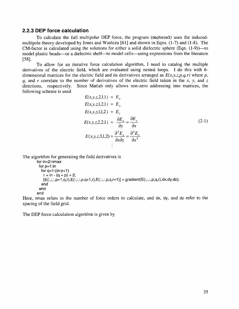
2.2.3 DEP force calculationTo calculate the full multipolar DEP force, the program (depforce3) uses the induced-

multipole theory developed by Jones and Washizu [61] and shown in Eqns. (1-7) and (1-8). TheCM-factor is calculated using the solutions for either a solid dielectric sphere (Eqn. (1-9))-tomodel plastic beads-or a dielectric shell-to model cells-using expressions from the literature[58].

To allow for an iterative force calculation algorithm, I need to catalog the multiplederivatives of the electric field, which are evaluated using nested loops. I do this with 6-dimensional matrices for the electric field and its derivatives arranged as E(xy,z,p,q,r) where p,q, and r correlate to the number of derivatives of the electric field taken in the x, y, and zdirections, respectively. Since Matlab only allows non-zero addressing into matrices, thefollowing scheme is used

E(x,y,z,2,1,1) = ExE(x,y,z,1,2,1) = E,E(x,y,z,1,1,2) = EZ

_ E _ E~E(x,y,z,2,2,1) - x - ax (2-1)

ay ax

a 2 E a2EE(x,y,z,3,1,2) -- -

The algorithm for generating the field derivatives isfor in=2:nmax

for p=1:infor q=1:(in-p+1)

r = in - (q + p) + 2;[E(:,:,:,p+1,q,r),E(:,:,:,p,q+1,r),E(:,:,:,p,q,r+1)] = gradient(E(:,:,:,p,q,r),dx,dy,dz);

endend

endHere, nmax refers to the number of force orders to calculate, and dx, dy, and dz refer to thespacing of the field grid.

The DEP force calculation algorithm is given by

35

F ") = 2 (El R 2nl C (n)K( (n -1)!(2n -1)!! Re M

(F G ), F), (F (i ) = 0

for i =1 to n

for p =0 to n

for q =0 to (i-p) (2-2)r = i-(p+q)

(F()) = (F,(')) + F i)E(x, y, z, p + 1, q + 1, r + 1)E(x, y, z, p + 2, q + 1, r + 1)

(F)) = (F25i)) + Fof )E(x, y, z, p + 1, q + 1, r + 1)E(x, y, z, p + 1, q + 2, r + 1)

=F3C )=(F 3(')) + F G)E(x, y, z, p +1, q + 1, r + 1)E(x, y, z, p + 1, q + 1, r + 2)

end; end; endwhere F0 ") is a constant calculated once. For the systems described in this thesis, the electricfields are real and so I do not need to worry about complex values except for the CM factor. Theresulting forces are stored in five-dimensional arrays.

This iterative DEP force calculation is one of the strengths of the modeling environmentbecause it makes it simple to compute multipolar DEP forces in all space. From the electric fielddata in Figure 2-3 I can easily obtain the vector force field plots of Figure 2-4, which show thein-plane components of the calculated DEP forces on a polystyrene bead, up to n=2, at the sameheights as Figure 2-3. One can see that a particle will be brought to and trapped at the z-axis(with no fluid flow) as long as it is brought within a certain distance (-20 gm for Figure 2-4B)of the origin.

2.2.4 Other forcesThe modeling includes three other forces-the gravitational force, the hydrodynamic

(HD) drag force on the particle, and a rigid substrate bottom boundary. The magnitude of thegravitational force is given by

4Fgrav =-TR3(p, p-p,)g (2-3)

3where pn and p, refer to the densities of the medium and the particle, respectively, and g is thegravitational acceleration constant. Cells and beads are denser than the medium and thus have anet downward force.

The HD drag force imposed on a stationary particle by a moving fluid is governed by thecreeping flow approximation because of the small dimensions and low flow rates involved inthese microsystems. For these simulations I have used a self-consistently solved analyticalformulation for the drag force on a stationary sphere in shear flow [138] or plane Poiseuille flow[139]. Other solved flow profiles could be implemented. Although parabolic Poiseiulle flow(from parallel-plate flow chambers) is often used with DEP traps, the shear flow approximationis justified when the levitation height and particle radius are much less than the height of thechamber. The HD drag force has the general form of the Stokes drag on a sphere

Frag = 6rt7R -(4 Uc /h)- F,.g -z (2-4)

36

where q is the viscosity of the fluid, U, is the fluid velocity at the channel midline, h is thechannel height, Fdg is a non-dimensional factor incorporating the wall effects, and z is the

height of the center of the sphere. I also calculate flow-induced lift forces on the particle,although I do not incorporate them into the force balance because they are much smaller thanother forces in this system. It would be trivial to incorporate them for other system designs.

The final "force" is the implementation of a rigid bottom boundary defined by thesubstrate. This lets me simulate particles sitting on the substrate surface. To do this Iautomatically adjust the z-directed total force on the particle so that it is zero (or positive) when

30

20

10

0

-10

-20

-30

30

20

10

0

-10

-20

''.\Z

- - --'.

-20 0 20

(B)z=10pm

- ~ --

- - --- ---- - - - -

-30- -20 0 20

20

10

0

-10

-20

-30-

(C) z=2O im l. .

- -

- - f /i- -

''tIi i;'' /- - -e* -~ I I-I.I- If t i s

-- - - - -- - 0 20I ~ - -

x-- - - -- -"~ ( I\\pm) - --

Figure 2-4: Plots of the DEP force (up to n=2) in the x-y plane derived from the electric field pictured in Figure 2-3at heights of 0 (A), 10 ptm (B), and 20 ptm (C). The z-directed DEP forces are not shown here (for clarity). Notethat the arrow length in each plot is scaled independently.

37

I

the particle is sitting on the substrate.

2.2.5 Holding point determinationAt this point, I have calculated the total force experienced by the particle in all of space

for a given electrode geometry and a given set of conditions (Figure 2-1). Now I must determinewhether the particle can indeed be held by the trap in this circumstance. To do this, the programmust find points in space (called holding points) where the particle experiences zero net force.These are the only points where one can expect to find a particle (at steady state). If I thenincrease the destabilizing fluid forces and determine when the holding points cease to exist, I cancompute the strength of the trap.

The algorithm proceeds as follows. For each of the three total-force components (F, Fy,F,) the program finds the surface where that force component is zero-the zero-force isosurface.Once it has the three isosurfaces, it must find where they intersect to find points where the netforce is zero-holding points. I implement this by checking for three-way intersections amongthe polygons comprising the surfaces. Since the majority of the polygons comprising eachsurface will be too far away from each other to possibly intersect, the program first does a quickcheck to exclude such pairings. This reduces the number of computationally intensiveoperations. The program performs this quick check by first looking for possible intersectionsbetween polygons comprising the isosurfaces of two force components. Then it takes thepolygons of those two isosurfaces that might be intersecting and checks them against the thirdisosurface. This produces a set of polygons that represent areas where the three surfaces mightbe intersecting. It then perform computations on this set of polygons to determine whether anythree-way intersection points actually exist and whether they are stable holding points.

Finding zero-force isosurfaces (asspol)

The isosurfaces are easily computed in Matlab using the isosurface command. Thisreturns a set of triangles (known as patches) that comprise the surface. To keep the number oftriangles reasonable, I first limit the volume within which the isosurfaces are computed with thereducevolume command. This requires knowing where the surfaces are likely to intersect, i.e.,where the region of interest is. This is not usually a problem-one simply runs coarsesimulations covering the full volume and then refines. The second tactic that I use to limit thenumber of triangles is to limit the number of faces in the surface with the reducepatch command.This commands reforms the isosurface with fewer patches while trying to minimize any errors. Iusually use 700 patches (triangles) per isosurface.

Examples of the three isosurfaces for the planar quadrupole are shown in Figure 2-5. TheF,=O (Figure 2-5A) and Fy=0 (Figure 2-5B) isosurfaces are predominately composed of planes atx=0 and y=O, respectively. In fact, due to the symmetry of this electrode configuration, the twoisosurfaces are the same, just rotated 90-degrees with respect to each other. This makes sense inthe context of Figure 2-4 where one sees that the x-directed DEP force is zero at the x=0 plane,and that the y-directed DEP force is zero at the y=O plane. The symmetry in the Fx=0 and Fy=0isosurfaces will disappear when an x-directed flow is imposed. The other parts of the isosurfacesin these plots represent other regions where those force components are zero. However,subsequent analysis, such as by examining Figure 2-4, shows that these correspond to unstableforce minima; particles at those points would not be stably held. Figure 2-5C shows the Fz=Oisosurface, which is cone-shaped. In Figure 2-5D one sees a closeup of the three isosurfacessuperimposed, showing the putative holding point located at (x,y,z) = (0,0,12 pm).

38

(A) F,=O

50

5Y (gm) 0

0

E

N

N

(D) F=O

0 -------20

y (1m) 0 0-20 -20 x (pim)

Figure 2-5: Zero-force isosurfaces. Shown are the three isosurfaces corresponding to the F,=O (A), Fy=O (B), and

F,=O (C) isosurfaces calculated from the electric fields in Figure 2-3, when no flow is applied. Panel D shows a

close-up of the intersection of the three isosurfaces, illustrating the existence of a holding point at (xy,z)=(0,0,l2

pm).

Finding possible two-way intersections (asspol)

Now that the three isosurfaces have been computed, I need to check them against each

other to find the intersection point. As stated above, this is first done by performing a quickcheck for possible intersections and then checking those possible intersection points. The firststage of the quick check is to check two surfaces against each other (checkpol2). Since the vastmajority of the patches making up the two sets of isosurfaces won't intersect, I first do a grosstest to winnow down the list of possibly intersecting patches (checkpol, minmax). This test, calleda bounding box test, is well known in computer graphics and is illustrated in two dimensions inFigure 2-6. Basically, if two patches' bounding boxes do not intersect, then the two patchescannot intersect.

To optimize the algorithm for Matlab, I tried to remove for loops and replace them with

vectorized operations. In addition, keeping all variable sizes small enough to fit into memory(without writing to disk) keeps the algorithm fast. My approach was to create large matrices-called minmax matrices-representing all possible two-way combinations from a pair ofsurfaces. Thus, is one surface had n triangles and the other had m triangles then each matrix (one

for each surface) would have m -n rows. Each row contains the extreme coordinates of each

39

(C) F =0

40

N

50 0

y (m) -50 -50 x (gm)

50

(B) F=O

50

50

50

y (m) 00

-50 -50 X (pm)

x (pm)II-50 -50

Polygon

Bounding Box

Figure 2-6: Bounding box algorithm in two dimensions. If the bounding boxes of the two patches do not intersect,then the patches cannot intersect. Extension to three dimensions only involves checking one more dimension. In

the program, the two polygons are actually both triangles.

triangle-e.g., the maximum x-coordinate of the triangle, the minimum x-coordinate of the

triangle, etc. Since these matrices could get very large, the program can chop up the surfaces to

make smaller comparisons if necessary. These minmax matrices are set up in such a way as

adding two corresponding rows together and checking the sign of the result performs the

bounding box comparison. The final step is to look through the list of comparisons to find ones

that meet the test, and export those as a new matrix ready for the set of three-way comparisons.

Finding possible three-way intersections (asspol)

At this point I have a matrix where each row is a pair of possibly intersecting patches.

The first patch of each pair is compared against the third isosurface using the bounding-box

algorithms to find possible three-way intersections. The result is a matrix where each row

contains the coordinates of triangles that might intersect.

Finding intersection points (f indint)

The final step is to check if these possible intersections actually intersect. Using the

bounding-box algorithms to minimize the number of intersections that actually need to be

checked greatly reduces execution time since this final step is computationally intensive.

Essentially, the algorithm finds the intersection point of the three triangles and determines

whether the intersection point actually lies within all three triangles. Only points that lie within

all three triangles represent zero-force points.The intersection point of three planes is given by [140]

planel: Alx+Bly+Clz+D1 =0

plane 2: A 2 x+B 2 y+C 2z+D 2 =0

plane 3: A 3x+B 3 y+ C 3 z+D 3 =0

1 Di B C1 1 A, D, C,

x=-- D2 B 2 C 2 ,y=-- A2 D2 C 2 (2-5)A A 2

D3 B3 C3 A3 D3 C 3

1= Al B Di A, B, C,

z-- A2 B2 D2 A=A2 B2 C 2

A3 B3 D3 A3 B3 C3

A will be zero if the three planes intersect in a straight line or not at all.

For each polygon, the code takes the three vertices and computes the A, B, C, and D

coefficients for the plane formed by those vertices. The conversion between the A, B, C, and D

coefficients and the coordinates is given by

40

EMeL

y1 zi 1 z, x, 1 x1 y 1 1 x1 y1 zIA= y 2 z2 1,B= z 2 X2 1,C= x 2 Y 2 lD=-x 2 Y 2 z2 (2-6)

Y3 Z3 1 Z3 X3 1 X 3 Y 3 1 X3 Y3 Z 3

where x,, y, and zn refer to the coordinates of each vertex. This generates three planes (one foreach polygon).

The program then computes A and checks to see if it is zero. If it is not zero, it calculatesthe intersection point. The task now is to find the subset of intersection points that lie within allthree polygons; only these represent intersections between the zero-force isosurfaces. Checkingwhether a point is in a polygon is another classic computational geometry problem. Theparticular algorithm I use was obtained from [141] (pnpoly2). As shown in Figure 2-7, thealgorithm goes around the polygon and checks to see if the point is always on the same side ofeach line segment. For convex polygons, this will be true if the point is inside the polygon.Practically, this is done by computing the cross product between the line segment of the polygonand the vector formed by the point and one of the line segment's vertices. If this cross productalways has the same sign, then the point is inside the polygon.

Unfortunately, the point-in-polygon test will not necessarily judge points on the verticesor sides of the polygon to be inside the polygon. Therefore, if a point is deemed to not be in thepolygon, the program tests to see if the point is "near" the polygon. The near distance is set to10 gim. The code determines the perpendicular distance from the point to each line segment,makes sure that this perpendicular intersection point is "within" the line segment, and then usesthe perpendicular distance to see if the point is "close" to the line segment. If it is, then the pointis deemed inside the polygon.

The point-in-polygon routine only works in two dimensions. To account for this, I wrotea set of operations to rotate each polygon and point onto the xy-plane to remove the 3dimension (rotatept). This is done by picking the three vertices and computing the surfacenormal and tangent. Each point is then transformed according to the following

(p3 - p2) x (p3-- pl)(p3 - p2) x (p3 - p1)

p3 -plP p3-pl (2-7)

yp =nxxp

p'= rxp yp nIp]

where p1, p2, and p3 are the three points in the polygon, p are all the points in the polygon, and

polygon points

Figure 2-7: Schematic of point-in-polygon tests. The point inside the polygon is always to the right of the vectors,whereas the point outside the polygon is sometimes to the left and sometimes to the right.

41

p'are the rotated points.The code finally returns a set of points describing the intersection of the three isosurfaces.

Due to the way in which the bounding-box comparisons were made earlier, the intersection-finding routine often generates multiple identical points. Another m-file (expts) takes thesepoints and returns only unique points.

The last important thing to check is whether the zero-force points represent stable forceminima (minpts). To check this, I have implemented an algorithm that determines whetherF -dr <0 for each direction away from a putative holding point [142]. This essentially checkswhether the particle needs to perform work on the system in order to move away from the zero-force point, in which case the point is stable. Other more heuristic methods, such as volumeexclusion, are also used.

2.2.6 Holding force simulationAn overall program (hforce3) is wrapped around the above code to determine the end

variable-usually the flowrate needed to release the particle, which I call the release flowrate.The program varies the flowrate in the model to find the threshold where no holding points exist.That threshold flowrate is the release flowrate and is found using a simple relaxation algorithm.The holding force can then be easily extracted from the release flowrate.

A schematic of the algorithm is shown in Figure 2-8. The code involves two loops, oneinside the other, letting me cycle through two sets of initial conditions-for instance, sweepingthe bead diameter while also varying the applied voltage. The program only increments to thenext set of conditions when the current set has converged. For each set of conditions, it goesthrough a loop, guessing at the release flowrate until it finds it. The first time through the loop,the program calculates all the field variables, while it only calculates the variables that changewith flowrate during subsequent iterations. Also during subsequent iterations, the program onlylooks for three-way possibly intersecting polygons-it reuses the two-way polygons from thenon-changing force directions (Fy and F,). Both of these strategies greatly diminish theexecution time. After all field variables are calculated and possibly intersecting polygons found,the program finds the holding points, if any exist. Then the program takes this information andfeeds it to the relaxation algorithm, which decides if this is indeed the release flowrate. If it isthen the program records interesting values and increments to the next set of conditions. If not,the relaxation algorithm generates a new guess to try the next time.

The relaxation program (relax) implements a simple bisection algorithm with somemodifications. The program asks a series of questions to determine the particular situation that itis in and then takes appropriate action (Figure 2-9). First, it tests to see if it has found the releaseflowrate by looking at the current and previous guesses and seeing if they are close enough toeach other (within some tolerance). If it has converged, then all is well and it tells that to theholding force program. If it hasn't, then it must decide whether it has overshot or undershot therelease flowrate. This is done by looking to see if there are any holding points. If there are, thenit means that the flowrate is not high enough. If there aren't any, then it means that it hasovershot the flowrate. Once it knows if it is too high or too low, it must determine a new suitableguess. It does this by first looking to see if there is a "good" previous guess. If so, then it meansthat the actual answer lies somewhere between the current guess and the previous guess. Itsimply bisects the two for the next guess. If it has never found a good guess, then it means that ithasn't approached the critical region yet, and so must keep hunting. If it is too high, it dividesthe previous guess by a factor, usually between 1.3 and 2. If it is too low, then it multiplies by

42

the same factor. If it is too high, it also must check to make sure that it is at a reasonable value.If it falls below some absolute minimum, then it means that for this particular situation, noholding force exists. In this case, the program just moves to the next set of conditions. Thismost often happens at the voltage extremes, depending on the geometry.

2.2.7 Effect of particle density and fluid flow on isosurfacesTo illustrate the use of the modeling environment for understanding physical phenomena

in these microsystems, I address two trends-changes in particle density and the addition of fluidflow (HD drag forces). Figure 2-10 shows the effect of particle density (and thus weight) on theF,=O isosurface (which is the only one affected). As the particle density is increased from 1.020g/cm 3 (Figure 2-10A) to 1.250 g/cm 3 (Figure 2-10C), the particle weight would increase, andfrom Eqn. (2-3), one would expect the particle to be levitated at lower heights. Observing Figure2-10, one sees that this is indeed the case. Two important features are apparent. First, the wholeisosurface decreases in height, corresponding to lower levitation heights, as expected. Second, atsome critical particle density, the cone of the isosurface will reach z=5 gm (and flatten),whereupon the particle (with R=5 tm) will no longer be levitated (Figure 2-10C). This shows

Cycle through conditions

- Initialize guess vector

Firsttime through 4

loop?

YES N O

Recalculate onlyCalcult components that

all variables vary with flowrate

Find holding points

Go through relaxation algorithm

Use newHave we releasefound the NO flowrate

release flowrate? guess fromrelaxationalgorithm

YES

Record release flowrate,locations, etc.

Move to next set of conditions

Figure 2-8: Flowchart for holding forceprogram.

Given: current value of release flowrateprevious value of release flowrateupper limit of release flowratelower limit of releease flowrate

Are

cu n I currentThen we have Sand previous

converged values closeenoughto

each

NO

Arethere

any holdingpoints?

N YES

Bisect the Bisect thecurrent Is Is current

guess and YEs there there YES guess andthe lower 4- a lower an upper - the upperbound to bound? bound? bound tofind the find the

new guess NO new guess

NODecrease Is

the N thecurrent NO new value Inras h

guess belo the current guessand try absolute and try again

YESNo release flowrateexss

Figure 2-9: Flowchart for relaxation program.

43

the effect of the bottom boundary "force" that I have implemented.One also sees that a sharp edge is produced where the Fz=O isosurface cone flattens into a

plane in Figure 2-10C. This will cause difficulties in the holding point extraction, as discussedbelow.

The effect of fluid flow is important to understanding how these traps work, as fluid flowis the destabilizing force that encountered in most DEP-based traps. When fluid flow in the x-direction is imposed, only the Fx=0 isosurface is affected. In Figure 2-11 I show the effect offluid flow by examining the intersection of the Fx=O and Fz=O isosurfaces as the flowrate isincreased. In Figure 2-1 IA, I show the isosurfaces under conditions of no flow. This is similarto the situation depicted in Figure 2-5D, except that now the Fy=O isosurface is not shownbecause it will be consist of an x-z plane at y=O that will be unaffected by changes in an x-directed HD drag force. One sees that the Fx=O isosurface "bends" over as the flow is increased(Figure 2-1 1B-C), because the HD drag force increases with height (see Eqn. (2-4)), causing theregion where Fx=O to move to x>O. However, for moderate flows (Figure 2-11B), the two

density = 1.020 gm/cm3

40,- --

Ei 20 ---N

50

y ( Lm) -50 -50 0 50x ( tm)

density 1.062 gm/cm3

40 -- ---- - -

(B)

NI

50510 1-

y (jim) -50 -40 -20 0 20 40x (m)

density = 1.250 gm/cm3

40 , --- --- -- - - - -

N

0 . - -50 -

0y (jim) -50 -40 -20 0 20 40

x (jm)

Figure 2-10: The effect of particle density on the holding points. Shown are the results of three simulations wherethe particle density is varied from 1.020 gm/cm 3 (A) to 1.062 gm/cm3 (B) to 1.250 gm/cm 3 (C). Only the F,=Oisosurface is shown.

44

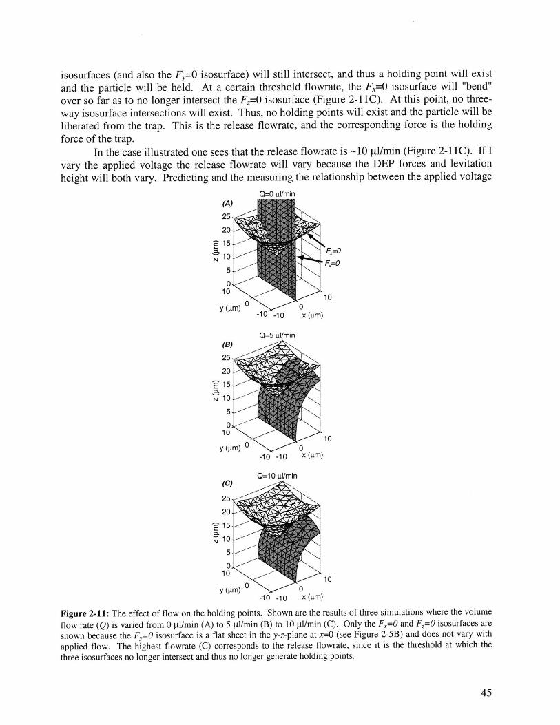
isosurfaces (and also the Fy=O isosurface) will still intersect, and thus a holding point will existand the particle will be held. At a certain threshold flowrate, the F,=0 isosurface will "bend"over so far as to no longer intersect the Fz=O isosurface (Figure 2-1 1C). At this point, no three-way isosurface intersections will exist. Thus, no holding points will exist and the particle will beliberated from the trap. This is the release flowrate, and the corresponding force is the holdingforce of the trap.

In the case illustrated one sees that the release flowrate is -10 gl/min (Figure 2-1 1C). If Ivary the applied voltage the release flowrate will vary because the DEP forces and levitationheight will both vary. Predicting and the measuring the relationship between the applied voltage

Q=0 gf/min

N

F=0

100

x (Um)

N

100

x (gm)

Q=10 i/min

N

Figure 2-11: The effect of flow on the holding points. Shown are the results of three simulations where the volume

flow rate (Q) is varied from 0 p/min (A) to 5 p1/min (B) to 10 p1/min (C). Only the F,=O and F,=O isosurfaces are

shown because the Fy=O isosurface is a flat sheet in the y-z-plane at x=0 (see Figure 2-5B) and does not vary with

applied flow. The highest flowrate (C) corresponds to the release flowrate, since it is the threshold at which the

three isosurfaces no longer intersect and thus no longer generate holding points.

45

0=5 gl/mir(B)

25,

20-

15

10,

5,

010

y (gm) 0-10 -10

and the release flowrate forms a good method to validate the model, which is what I have done inChapter 3.

2.3 Discussion

2.3.1 Modeling environmentThe various manipulations performed, starting with the electric field and experimental

parameters, show the utility of the type of integration that I have chosen for these simulationsand the suitability of the modeling environment for the design of microscale DEP-based traps.With this design tool, I can now quickly evaluate different designs using a combination ofinteractive and automatic means.

The interactivity comes from the combination of Matlab's numerical and visualizationcapabilities with the modeling environment, and lets me simultaneously investigate the variousfields and forces on particles. One can, for instance, jump quickly from the zero-forceisosurfaces (Figure 2-5) to the force plots (Figure 2-4) to determine whether zero-force pointsrepresent holding points by examining the directions of the force arrows around the zero-forcepoints.

In addition to these interactive possibilities, the automatic computation of the releaseflowrate allows one to run comparative analyses of different traps rather easily. In largemeasure, this is enabled by the iterative DEP force calculation, which trivializes the ability tocompute multipolar DEP forces in all space. This is needed for either highly symmetric, small,or complicated trap geometries. Highly symmetric traps, such as the quadrupole described here,have symmetries that necessitate higher-order moments to properly explain levitation, even inthe limit of large traps, as was recognized in 1993 [133]. This is illustrated in the cone-shapedFz=O isosurface of Figure 2-5C. The isosurface minimum at the origin corresponds to the fieldnull, where the dipole term in the DEP force goes to zero and the quadropolar force orderdominates. Computing only the dipole force order would give an Fz=O isosurface that instead ofbeing cone-shaped would look like a cylinder near the origin and never intersect the z-axis; suchan isosurface would not predict levitation.

While highly symmetric traps always need multipolar force calculations, the modelingenvironment enables the designer to design arbitrary traps-unencumbered by the need to keepthe particle much smaller than the field non-uniformities. Analytical approaches, such asundertaken by Washizu and Jones [133], while effective for the simple quadropole geometry andproviding analytical representations of the various parameter dependencies, would be difficult toextend to these situations. Arbitrary trap design has two benefits. One is for single-cell traps.As traps are scaled down to the size necessary to trap single cells, the cells invariably become asignificant fraction of any characteristic dimension, and thus quadrupolar and higher-ordermoments may come into play. The other is for non-analytical electrode geometries, which canshape the electric field or introduce steric effects for more effective trapping. Both of theseapproaches could be implemented with extruded quadrupole traps. Non-analytical effects areeven seen in the planar quadrupole structures, which, although well approximated near the originby four point charges, deviate significantly from the point-charge quadrupole away from theorigin, especially near the plane of the substrate (Figure 2-3A).

In addition to arbitrary trap design, there is a direct extension from the beads modeledhere to more complex and biologically relevant cell-based systems. The extension to cellsinvolves manipulation of the CM factor, and the appropriate forms of the CM factor for various

46

types of cells, such as mammalian cells and protoplasts, have been determined assuming variouselectrical models [58, 120] and are generally accepted in the community. The accuracy of themodels is determined by the extent to which the various parameters describing them (such asmembrane capacitance, etc.) are known and homogeneous among a cell population.

2.3.2 Parameter-space explorationA primary use of the modeling environment is to explore the effects of experimental

parameters on the interplay of forces. The forces considered in the model all vary differentlywith such experimental parameters as voltage, frequency, particle radius, etc, which can make itdifficult to predict how parametric variations will affect holding. The model allows one to makethese predictions easily and quantitatively. One way to visualize the interplay of forces isthrough the zero-force isosurfaces, which provide a convenient bridge between the vector forcefields and the holding points. This can either be used to confirm ones' intuition, as whenpredicting that "heavier" particles will be "harder" to levitate (Figure 2-10), or can provideinsight into situations that are more difficult to grasp initially-such as the interaction betweenDEP and HD drag forces (Figure 2-11).

This interaction is actually the primary concern in developing DEP-based cell traps thatcan hold cells against flow. One can expect that for a given situation, a particle will be held inthe trap until some threshold destabilizing flowrate (the release flowrate) is applied, whereuponthe particle will be released. Figure 2-11 shows this development, where the F,=O isosurface"bends" over until holding points cease to exist. Since the system aim of the gDAC is to developtraps where the flow needed to "bend" the isosurface is "large" as determined by some externalspecification, this amounts to increasing the "stiffness" of the isosurface.

Since this isosurface represents the interplay between HD drag and DEP forces, I canalter either force to effect greater holding. Realizing that the HD drag forces increase away fromsurfaces (Eqn. (2-4)), one sees that keeping the particle close to the substrate will increase theholding. Manipulating the shape of the electric fields to remove the decay in DEP force awayfrom the substrate can also increase holding. This can be done by using an octopole cage [93,143] or by introducing extruded electrodes that remove the z-directed DEP variation. This is infact what I will proceed to do in Chapter 4 when designing the extruded traps. Thus the insightsobtained via the modeling environment will guide future microscale DEP design.

2.3.3 LimitationsWhile the modeling environment provides for the types of analyses required by the

ptDAC, others may encounter limitations. First, the implementation of rigid surfaces, such asmight be found in hybrid DEP-mechanical traps, is difficult to do. This requires moresophisticated particle-boundary intersection algorithms than the simple one implemented for thesubstrate surface. Second, algorithms have not been optimized for memory usage, and thusanalyses using large (or very fine) grids can quickly command >100 Mb of memory. If this islarger than the available physical memory, the time needed to swap in and out of the hard diskwill dramatically slow the analysis.

Another limitation concerns the use of discrete grids and polygons. This discretizationintroduces numerical "noise" into the isosurface intersection algorithms. The "noise" makes thelocation algorithms very sensitive where two non-smooth isosurfaces are intersecting. The mostpronounced case of this is when the particle is on the substrate, because the F,=0 isosurface has a

47

sharp corner near the origin in this case (Figure 2-10C). This effect is seen in the holdingcharacteristics of both systems later in this thesis.

An additional limitation is the inability to perform analyses of non-linearly-polarizedDEP excitations (such as for electrorotation and traveling-wave DEP studies), although this wasnot the intent of the modeling environment and could be implemented since the relevantmultipolar theories have been worked out [60]. Also, dynamic analyses cannot be performed,although the force matrices allow the determination of force streamlines (and hence particletrajectories in certain situations). Finally, electrohydrodynamic forces, which can be substantialin some experimental situations [144], are not incorporated. This would require the calculationof the temperature and charge distribution in the fluid, which is not a simple addition to the code.EHD forces will become important in the analysis of the planar quadrupole in the next chapter.

2.4 ConclusionIn this chapter I have presented an integrated modeling environment for the development

of DEP-based single-particle traps. The modeling environment can take user-supplied electricfield data and other experimental parameters and determine the efficacy of DEP-based cell traps.I have shown that the modeling environment gives insight into the interplay between forces inDEP-based microsystems, such as those describing the balance between DEP and HD dragforces. In addition, the use of an iterative DEP force calculation makes it easy to compute theDEP forces to arbitrary order, allowing for exact analyses of arbitrarily complex electrodegeometries. Experimental validation of the modeling environment is presented in the nextchapter. With these modeling tools it is now possible to perform a priori quantitative designs ofvarious DEP traps for high-performance applications, which is what I will do in Chapter 4.

48

Chapter 3: Holding forces of the planar quadrupole

Much information can be learned by experimentally determining the holding forces ofplanar quadrupole traps. First, the results can be used to validate the modeling environment anddetermine the parameter space within which its predictions are valid. Second, the results can beused to gain insight into the functioning of the planar quadrupole and DEP-based single-particletraps in general, as well as to determine whether the planar quadrupole can meet therequirements of the pDAC. In this chapter I will describe experiments with planar quadrupoletraps, varying the trapped particle size, the applied voltage, the applied frequency, and thesolution conductivity, to determine this information.

3.1 Experimental vehicle-the planar quadrupoleI have decided to use the planar quadrupole shown in Figure 2-2 as the experimental

vehicle for the following reasons. First, the planar quadrupole is perhaps the most commonlyused DEP trap, and there thus exists a rich set of comparisons to make. Second, correctmodeling of the planar quadrupole demands that one use at least the 2"d-order multipole(quadrupole), thus providing the ability to demonstrate the ease to which these multipoles can becalculated. Third, the planar quadrupole is easy to fabricate for experimental verification of themodel.

Instead of using living cells as the test particle, I have used beads for the verificationstudies. The reason for this is that during the verification stage it is important to minimizevariations in the test parameters so that the true accuracy of the models can be rigorouslydetermined. This is possible by using latex beads, which have precise and accurately determinedphysical and electrical properties.

3.2 Experimental methods-fab, packaging, test setup, methodologyIn this section I will describe in detail the materials and methods used in the verificationexperiments.

3.2.1 Stock SolutionsSolutions of two different conductivities-0.01 S/m and 0.75 mS/m-were made by taking DIwater with 0.05% Triton X-100 (Sigma, St. Loius, MO) added and adding appropriate amountsof Hank's Balanced Salt Solution (HBSS, GibcoBRL, Grand Island, NY), also with 0.05% TritonX-100, until the nominal conductivity was reached, as indicated by a Orion Model 125conductivity meter (Beverly, MA). Solutions were filtered through a 0.45-micron filter (MicronSeparations, Inc., Westborough, MA) and their conductivity measured before each use.

3.2.2 BeadsPolystyrene beads (incorporating 2% divinyl benzene), with density 1.062 g/cm 3, in threediameters-7.58 pm (0.08 pm std. dev.), 10.00 pm (0.09 pm std. dev.), and 13.20 pm (0.89 pmstd. dev.)-packaged as 10 % solids in water were purchased from Bangs Laboratories (Fishers,IN). 15 p.L of each bead solution was washed twice in 1.5 mL of the appropriate conductivity

49

stock solution and finally resuspended in 1.5 mL of stock solution. All bead solutions wererefrigerated and used within two months.

3.2.3 Electrode TrapsThin-film quadrupole electrodes were fabricated using conventional microfabrication processes.Standard (25 mm x 75 mm) microscope slides were cleaned for 10 minutes in a Piranha solution(3:1 H2 SO 4 :H 20 2 ) and blow dried. Photolithography was then performed using the image-reversal photoresist Hoechst AZ-5214 (Somerville, NJ)-which gives re-entrant resist profiles-to define the electrode patterns. 200 A of chrome and 5000 A of gold were then evaporated ontothe slides followed by resist dissolution and metal liftoff in acetone. Finally, the slides werecleaned in methanol and isopropanol and blow-dried. An image of the completed electrodes isshown in Figure 3-lA, along with relevant dimensions.

3.2.4 PackagingThe packaging scheme is shown in Figure 3-1B. Fluid inlet and outlet holes were drilled

in the glass slides with 0.75-mm diamond drill bits (C.R. Laurence, Los Angeles, CA).Poly(dimethylsiloxane) gaskets, cast in machined molds from monomer (Sylgard 184, DowCorning, Midland, MI), above and below the slide functioned as the spacer material and bottomsealing gasket, respectively. The top of the chamber consisted of a glass slide that had been cutto a width of 16 mm and clamped down using an aluminum block. With this setup, the flowchamber sustained >200 gImin flows without leaking.(A) d(B)

..eiecirode

Deaa(C)Stock solution syringe 1 To flow chamber

Syringe pump Beadsolutionsyringe

Stock vWaassolution -Injectionsyringe 2 Waste valve Waste

spring-contact probe 0 aluminum

0 block

0

glass cover

contact spacer

padsslide withelectrodes

gasket

outlet flow pathinlet flow path

plexiglass flow chamber

Figure 3-1: (A) Photograph of the completed quadrupole electrodes, showing a single 10.00 ptm bead captured intrap; (B) Schematic of packaging assembly, showing the stack of layers comprising the flow chamber along the withthe electrical connections via spring-contact probes; (C) Schematic of fluidic subsystem.

50

gass s e

3.2.5 Chamber height measurementThe chamber height of the fully assembled unfilled package was measured at various points withan optical interferometer coupled to a z-axis linear gage (543 Series, Mitutoyo/MTI Corp.,Aurora, IL) on a Nikon microscope (UM-2, Nikon Inc., Melville, NY). Corrections were madefor the indices of refraction of the different materials. The measured chamber height was 0.73 +0.01 mm.

3.2.6 Electrical ExcitationSine wave excitation up to 20 MHz and 10 Vpp (into 50 Q) was generated by an HP 3314Asignal generator (Hewlett-Packard, Palo Alto, CA). This signal was split and sent into 4 high-speed amplifiers (LM7171, Analog Devices, Norwood, MA)-2 non-inverting and 2 inverting-that amplified the signal 2x. The amplifiers delivered 1800 phase-shifted signals with negligiblegain and phase error up to 10 MHz. The output from the amplifiers was sent via coaxial spring-contact probes (Interconnect Devices, Inc., Kansas City, KS) to the contact pads at the edge ofthe glass slide (Figure 3-1B).

3.2.7 FluidicsFluidic connection to the package was made via HPLC connectors and tubing (Figure 3-1C).The fluidic test subsystem consisted of a 4-way valve (V-101D, Upchurch Scientific, OakHarbor, WA) that allowed the interchange of syringes without introducing bubbles. The beadsolution was injected into the flow using an injection valve (V-450, Upchurch Scientific, OakHarbor, WA). Flow was initiated by a syringe pump (KD-101, KD Scientific, Boston, MA)using a 5 mL Hamilton luer-lock syringe (1005TLL, Reno, Nevada).

3.2.8 OpticsThe beads were viewed using a Microzoom microscope (Wentworth Labs, Brookfield, CT) withlong-working distance objectives on a semiconductor probe station. Images could be capturedusing a Panasonic WV-D5000 video camera (Secaucus, NJ) and a Sony VCR.

3.2.9 Release flowrate measurementsOnce beads were captured in the quadrupole trap, flow was initiated. In the parallel-plate flowchamber, beads experienced a transverse hydrodynamic force that tended to dislodge them fromequilibrium at the center of the trap and thus acted as a destabilizing force (Figure 3-2). If thebead was held in the trap at the end of two minutes, the bead was considered captured. This timewas chosen empirically by observing that beads >90% of beads held for two minutes would beheld indefinitely (tested up to -5-10 minutes). The flowrate was adjusted to find the minimumflowrate (within 1 jtL/min) at which the bead was released within two minutes. This is termedthe "release flowrate". The flowrate was adjusted above and below the release flowrate to ensurethat the true release flowrate was determined. In practice, a given bead could be used repeatedlyby stopping the flow immediately after it was released, in order to pull the bead back into thetrap.

3.2.10 ModelingThe modeling was performed with the specifications described in §2.2.1, using FEM dataobtained from Maxwell 3D (Ansoft, Pittsburgh, PA). For the current work I simulated the upper-

51

(A) not to scale

lectrode

parallel plateflow chamb

particle xparabolic electrode

flow profile

applied(B) HD force particle

electrode

Figure 3-2: (A) Schematic of flow chamber, showing a bead in the trap experiencing a parabolic HD drag force; (B)Release flowrate and holding force measurements. The flowrate (force) is increased until the bead is liberated fromthe trap. The parabolic flow profile is approximately linear at when the particle is close to the substrate.

half of the trap in Figure 3-1A, using symmetry boundary conditions at the glass substrate. Field

data from the central portion of the quadrupole was written to a grid, using a grid spacing of 0.5-

2 pim, and smoothed using a three-dimensional Gaussian low-pass filter with the followingparameters: three-grid-point convolution kernel (in each direction) with a standard deviation of

1.3 grid points. The filtering was used in lieu of long simulation times to reduce high-spatialfrequency noise. The modeling performed in this chapter used an older version of the simulation

program that represented the isosurfaces not only with triangles but also with 4-, 5-, and 6-sidedpolygons. All computations on these isosurfaces are as described in Chapter 2. This

representation was later abandoned in favor of the simplicity of using only 3-sided polygons.

3.3 Results

3.3.1 Single-bead holdingFigure 3-lA shows a trap holding a single 10.00-gm bead. This shows that the traps do work, atleast rudimentarily. Interestingly, even with these un-optimized traps, I have demonstratedsingle-bead capture: when two beads are captured in a trap, the second bead will be held withless force than the first, meaning that I can apply a flowrate that will selectively remove the

second bead while still holding the first. Thus, I can get single-particle trapping, which is a

necessary requirement for the gDAC. In practice this discriminating flowrate is determined

empirically because the modeling tools are unable to accommodate the interactions of two

particles in a trap. Schematically, the number of particles held in a trap varies with the imposed

flowrate as in Figure 3-3. One way to think about it is that the size of the potential-energy well

that comprises the trap decreases as the flowrate is increased. Thus, there will exist a range of

flowrates such that the size of the well is larger than one but less than two particles. In this flow

regime, only one particle can be held per trap. Empirically, this occurs at approximately 90% of

the release flowrate for a given set of experimental parameters.

52

a I

3 release0- flowrate

2-

flowrateFigure 3-3: Schematic showing how the number of particles per trap varies with applied flow. Close to but below

the release flowrate only one particle can "fit" in the trap.

3.3.2 Release flowrate as the voltage is varied-the holding characteristicBy varying the voltage and measuring the release flowrate, I can generate what I call the

holding characteristic of the trap for a particular set of experimental conditions. By comparing

the shape and absolute values of the measured holding characteristic with the predictions based

upon the modeling environment, I can evaluate the accuracy and completeness of the modeling

environment.The typical shape of the holding characteristic for these traps is shown in Figure 3-4A for

7.58-+m beads in 0.01 S/m solutions at a frequency of 1 MIHz. The characteristic behavior in

these traps is that the release flowrate increases from zero until a maximum release flowrate (the

peak release flowrate) is achieved (at the peak voltage), after which it decreases quickly and then

reaches a plateau (the baseline release flowrate). To validate the model, I have compared the

match between these three parameters, as they define the shape of the holding characteristic.

To get a sense of the scatter in the experimental results, I repeatedly took data for the

10.00-gm beads using more than -10 different beads over three months. Individual release

flowrates were measured between one and nine times, with each measurement being double-

checked. I have included this scatter and the flowrate discretization error in Figure 3-4B. The

other data shown in the rest of the chapter can be assumed to possess similar scatter over this

time frame. I then used these results as an internal control when acquiring the rest of the data

presented in this paper. I did this by taking data from equivalent conditions during subsequent

runs to establish experimental precision. When this was inconvenient (as with different solution

conductivities) I used the prior knowledge that the curves should not greatly shift to check

against the previous data. In addition, equivalent data points were taken before and after each

experimental run to estimate any short-term drift (usually <5%). I did observe a long-term

downward drift (towards lower release flowrate) in the release characteristic of -16% (which

therefore accounts for the majority of the scatter). Several factors could account for this trend,

such as changes in the chamber geometry, experimental solutions, or room temperature.

Turning back to Figure 3-4A, I also show the predicted holding characteristics calculated

including either only the dipole (n=1, '....') or dipole and quadrupole (-) DEP force terms. One

sees that the computing only the dipole term gives a monotonically increasing holding

characteristic (....) because the z-directed force from the dipole term is unable to induce levitation

near the field null, where the particle is located. As described below, this levitation is the key to

53

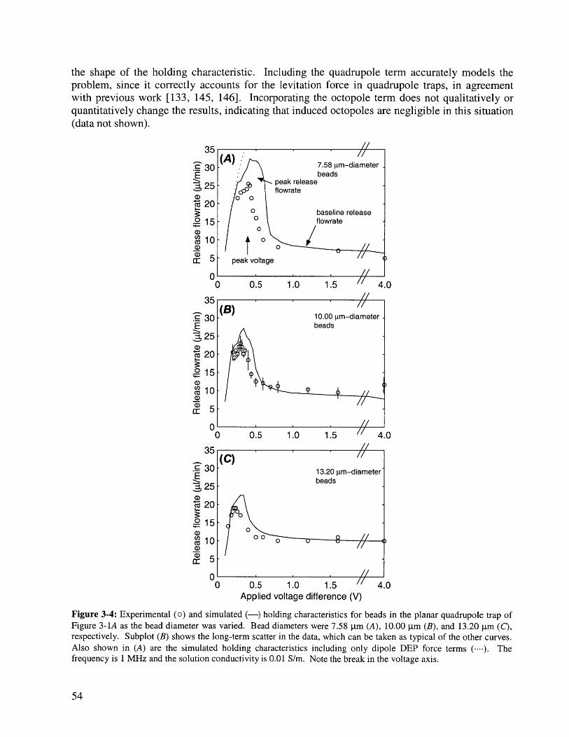
the shape of the holding characteristic. Including the quadrupole term accurately models theproblem, since it correctly accounts for the levitation force in quadrupole traps, in agreementwith previous work [133, 145, 146]. Incorporating the octopole term does not qualitatively orquantitatively change the results, indicating that induced octopoles are negligible in this situation(data not shown).

0 0.5 1.0 1.5

[(A):7.58 pm-diameterbeads

peak releaseco flowrate

-o 0

o baseline releaseo flowrate

0 /0 //

- peak voltage

10.00 jm-diameter.beads

4.0

) 0.5 1.0 1.5 4.0i //

0 0.5 1.0 1.5Applied voltage difference (V)

4.0

Figure 3-4: Experimental (o) and simulated (-) holding characteristics for beads in the planar quadrupole trap ofFigure 3-1A as the bead diameter was varied. Bead diameters were 7.58 pm (A), 10.00 pm (B), and 13.20 gm (C),respectively. Subplot (B) shows the long-term scatter in the data, which can be taken as typical of the other curves.Also shown in (A) are the simulated holding characteristics including only dipole DEP force terms (..--). Thefrequency is 1 MHz and the solution conductivity is 0.01 S/m. Note the break in the voltage axis.

54

35

. 30E

25

c20

015CDn 10

a)C 5

0

35

30

25

20

15

10

5

0

35

30

25

20

15

lo0

5

0

E

(2

U)

.,

0

CDC,,

a)CEIr

(C) I13.20 pm-diameterbeads

- 00 -

-

The match between the experiment and the 2 d-order simulations is significant, especially

considering that there are no adjustable parameters. All parameters needed in the model have

come from either measurements, company data, or literature values. The simulations predict a

higher release flowrate (27%) at the peak voltage, a higher peak voltage (5%), and a higher

baseline release flowrate (8%).The trend in release flowrate as the voltage is varied (Figure 3-4A) is initially non-

intuitive, but becomes apparent when one recognizes that the DEP force influences the height of

the particle. This is shown in Figure 3-5, where I plot the predicted release flowrate along with

the predicted holding force and the predicted height of the particle at release for a 7.58-gm bead

in the quadrupole trap.When no voltage is applied, there is no confining force, and neglecting any stiction

effects between the bead and the surface of the glass slide-which have been measured at less

than 1-2 gi/min-the release flowrate should be zero. As the voltage is increased, the DEPforces will create a confining well (Figure 3-5A). In this pre-levitation regime, the z-directed

component of this force, which serves to levitate the bead, will initially not be large enough to

overcome the gravitational force and thus the bead will remain on the slide surface. The force

pushing the bead from the trap-the fluid flow-varies linearly with height of the bead and

volume flow rate (Eqn. (2-4)). Thus, if the bead height does not change but the confining forces

increase, the release flowrate will also increase.At some threshold voltage, the z-directed DEP force will exactly balance the gravitational

force and the bead will start to be levitated (Figure 3-5B). This voltage corresponds to the peak

voltage and peak flowrate. Any increase past this voltage and the bead will be levitated upwards

and then experience larger HD drag forces (Eqn. (2-4)). As can be seen from Figure 3-5, the

height of the particle (---) increases quickly with voltage once it is levitated, and particle will

0.8 - 40(A) (B) (C)

21j 0.6 release flowrate 30

height at release '' .)

.CL CZ~

O 2 -' holding force 10 .

0 00 1 2 3 4

Applied voltage difference (V)

(A) pre-levitationdrag bead

forces DEP forces

gravitational forcesubstrate

(B) rapid ascent

(C) saturation

Figure 3-5: Explanation of holding characteristics as voltage is varied, showing the simulated release flowrate (-),

the holding force (---), and the height of the particle when it is released (---). (A) Pre-levitation. At very low

voltages, the gravitation force cannot overcome the z-directed DEP force, and the bead is not levitated; (B) Rapid

ascent. At a certain voltage the bead will just become levitated and the holding characteristics will peak; (C)

Saturation. At high voltages, the increase in holding force is balanced by the increased particle levitation height,

resulting in a flat release flowrate profile.

55

Mle=__ - --- - __Iit _ __ MMII__

experience a rapid ascent. Therefore, the increased exposure to the HD drag forces with littleincrease in the DEP force causes the release flowrate characteristic to decrease. This can becontrasted with simulations involving only the dipole DEP-force term (Figure 3-4A, '....') wherethe release flowrate never decreases because the particle never becomes levitated.

Observing the particle height versus voltage curve (Figure 3-5, --- ), one sees that after aninitial rapid ascent, the slope of the curve decreases and saturates because the z-directed DEPforces decrease rapidly as the bead is levitated away from the electrodes. This is in accord withthe measured height versus voltage characteristics of other researchers [92]. At this point, theholding force increases with voltage (Figure 3-5,'-.-.') are matched by the increases in the HDdrag forces due to the increased particle height (Figure 3-5,'---'). They thus balance each otherand give a saturated flat release-flowrate characteristic (Figure 3-5C,'-').

3.3.3 Holding characteristic as the particle diameter is variedSince the DEP forces vary as R3 (dipole) and R5 (quadrupole), the gravitational force varies withR 3, and the HD drag forces vary with R, I can use differing particle sizes to evaluate the accuracyof the modeling environment to see if it predicts the correct particle size effects. This will helpdetermine whether the model accounts for these forces adequately and whether other forces aresignificant. I have performed experiments with three different bead sizes to explore this trend.The results are shown in Figure 3-4, along with the predicted results (simulated including up tothe n=2 DEP force term). Although all three bead diameters show the same characteristicpeaking-declining-plateau response, the values of the peak release flowrate, peak voltage, andbaseline release flowrates all differ as the bead diameter changes.

These differences are shown Figure 3-6, where the three parameters that define theholding characteristic have been extracted from the simulation and experimental results. Inmaking this comparison I extracted parameters from only one data set consisting of three runs at

0 .5 (A)

ca c75 0.25- ID

caU)

01

-40 (B)

CU-

01

15 (C

U1) =-

10. --

CD

M 58 10 12 14

Bead diameter (tm)

Figure 3-6: Comparison of extracted experimental (o) and simulated (-) peak voltage (A), peak release flowrate(B), and baseline release flowrate (C) from one data set. The frequency is 1 MHz and the solution conductivity is0.01 S/m.

56

different bead diameters to eliminate the long-term drift seen in Figure 3-4B (and thus I only usea subset of the data displayed in Figure 3-4B). The scatter was estimated from the uncertainty inthe peak height (n=7 data points for 10.00-ptm beads, n=2 for other diameters) and position (n=5for 10.00-gm beads, n=2 for others) during these runs and from the release flowrates collected atvoltages greater than 0.8 V for the baseline (n>6 for each diameter). In all cases, the scatter was<17% and usually was <5%.

As the bead diameter is increased, the baseline release flowrate (Figure 3-6C) increaseswhile both the peak voltage (Figure 3-6A) and peak release flowrate (Figure 3-6B) decrease. Theagreement between simulations and experiment is good, with the dependencies capturedquantitatively-the maximum differences are 30% for the peak voltage, 27% for the peakflowrate, and 9% for the baseline release flowrate.

The trends (Figure 3-6) can be explained in accordance with DEP theory. As the beaddiameter is increased, the voltage necessary to initially levitate the bead (which corresponds tothe peak voltage) will decrease because the levitation forces increase with bead diameter. Thesesmaller voltages cause the bead to experience smaller DEP confining forces before beinglevitated. This leads to the decrease in peak release flowrate with bead diameter. Finally, theincreasing baseline release flowrate with diameter is due to the fact that while the HD drag forcesincrease only linearly with diameter, the DEP confining forces increase as R3 and R .

3.3.4 Holding characteristic changes with frequencyWhile the first two trends (voltage and bead diameter) evaluate the spatial aspects of our model,the frequency trends are a test of the CM factor of the DEP force, which is the only frequency-dependent component that I have included. The CM factor (Eqn. (1-2)) for 10.00-pm diameterbeads is shown in Figure 3-7. Although only the dipole term of the CM factor is shown, thequadrupole and higher terms display similar behavior, although at slightly different dispersionfrequencies and smaller ranges (e.g., the quadrupole term can only vary between -1/3 and +1/2).To generate Figure 3-7, the conductivity of the beads was estimated by using very-low-conductivity stock solutions and measuring the n-DEP to p-DEP transition frequencies, when thebeads would switch from being repelled to being attracted to the electrodes, respectively. Fittingthese to the zeros of the CM factor gave a conductivity estimate of 2e-4 S/m, which is in accordwith literature values for unmodified polystyrene beads of this size [147].

As the frequency is decreased, the CM factor goes from being permittivity dominated toconductivity dominated (Eqns. (1-4) & (1-5)). For the high-conductivity solution (0.01 S/m), nodispersion is apparent because the CM factor is dominated by the properties of the stock solution.

0Sa2=2e-4 S/m

-0.1 - =80

E2=2.5-0.2-

2 -.. 3 -=7.5e-4 S/m0

-0.4

-0.5'10 10 10 10 10 10

frequency (Hz)

Figure 3-7: Calculated CM factor (dipole term) for a polystyrene bead in salt solution.

57

For the low-conductivity solution (0.75 mS/m), the CM factor decreases in magnitude as thefrequency is decreased. Since the CM factor directly multiplies the DEP force equation (Eqn.(1-1)), changes in the CM factor will cause corresponding changes in the DEP force at a givenvoltage. Thus, I expect little frequency dependence of the forces at 0.01 S/m and somedependence at 0.75 mS/m. In essence, the CM factor changes are equivalent to scaling along thevoltage axis, and should thus only shift the holding characteristic along that dimension.

Two frequency sweeps were performed, at both high (0.01 S/m) and low (0.75 mS/m)solution conductivities. Both of the 1 MHz holding characteristics (Figure 3-8A,D) agree wellwith predictions, although the peak flowrates and peak voltages are smaller than predicted.While these predictions can be partly explained by the sensitivity of the simulations around thepeak flowrate, they could also be due to temperature changes in the measurement room-causingthe chamber height and experimental properties to change-or experimental observations ofneglected forces. The 100 kHz holding characteristics (Figure 3-8B,E) for both solutions alsohave the predicted shape, although the low conductivity characteristic (Figure 3-8E) deviatesmore from predictions than the 0.01 S/m characteristic (Figure 3-8B). The 10 kHz holdingcharacteristics (Figure 3-8CF) for both solution conductivities exhibit very different shapes thatcannot be explained by our modeling environment.

The only frequency dependence included in the model is through the CM factor. The 10kHz curves, which show completely different holding characteristics, can clearly not beexplained through manipulation of the CM factor. The 100 kHz curve at the low conductivitysolution has the same characteristic shape, but is shifted towards lower voltages and releaseflowrates. As explained before, the release flowrate shift cannot be caused by changes in the CMfactor. For the voltage shift to be caused by changes in the CM factor, the CM factor would haveto decrease (become more negative) at low frequencies. Not only would this require anextremely small (and physically dubious) bead conductivity (-le-6 S/m), but because the CMfactor is already near its theoretical minimum, the increase in the magnitude of the CM factorwould be much too small to account for the experimental observations (data not shown).

The shifts in the 100 kHz (and also possibly the 1 MHz) holding characteristics can bemore readily explained by the existence of an upward destabilizing force on the bead. The 10kHz characteristics are consistent with the existence of an extra confining force on the bead.Thus, I conclude that the cause of the discrepancies is due to other forces that are not accountedfor in the model, as discussed below.

3.4 Discussion

3.4.1 DEP force measurementsThe development of the multipolar DEP theory coupled with the decreasing cost of

computing power and the increasing sophistication of microscale DEP researchers has led toseveral recent attempts to construct quantitative DEP microdevices that are amenable tomodeling. Recent work [143, 148] has even started to concentrate on the interaction betweenDEP and HD forces, in their case determining the flow needed to break through a DEP barrier,similar to our case. The difference between their situation and the one presented here is that theparticles in that work are located at the centerline of Poiseuille flow, and thus the drag force iswell-defined by the Stokes drag on a sphere. This allows them to derive analyticalrepresentations for the force balance. As particles approach surfaces, this analytical formulationbecomes hopelessly complicated, necessitating a numerical approach as taken here.

58

The experimental approach-the determination of release flowrate-has manyadvantages over direct measurements of the DEP force. First, the efficacy of particle traps inmany applications will be the ability of the trap to hold a particle against fluid flow. Thus, thismeasurement, even if not correlated to theory, would still be valuable. The comparison withtheory, however, is ultimately more useful, since the validation of the modeling environmentallows for future trap design with confidence that the fundamental physics in a specific operating

a=0.01 S/M 7=0.75 mS/m

) 0.5 1.0 1.5 4.I I

) 0.5 1.0 1.5 4.0

//

0 0.5 1.0 1.5 4.0Applied voltage difference (V)

50

40

30

20

10

'U

0 0

50

40

30

20

10

01C

50

40

30

20

10

00

0.5 1.0 1.5//

//- - 1

(E) frequency = 100 kHz

00

00 00- / ...

frequency = 10 kHz

- ~//...

' ' '00 0 0 0 0

0.5 1.0 1.5Applied voltage difference (V)

4.0

4.0

4.0

0.5 1.0 1.5'I

//

Figure 3-8: Experimental (o) and simulated (-) holding characteristics for 10.00 gm beads for three differentfrequencies at solution conductivities of 0.01 S/m (A-C) and 0.75 mS/m (D-F). Results are shown for frequencies of1 MHz (A,D), 100 kHZ (B,E), and 10 kHz (CF). The 10 kHz holding characteristic at 0.01 S/m (C) increasesquickly with voltage and so is truncated in the plot. Note the break in the voltage axis.

59

'

(A) I 1Lfrequency = 1 MHz

0

00 0 0

- I

(D) 7

frequency = 1 MHz

00

0 --0- -I

C

0aOCO,a)

C

a)

0

CO)a)

a,

C

0

CZ

CE

50

40

30

20

10

0

50

40

30

20

10

0

50

40

30

20

10

0

(B) frequency = 100 kHz

0 0

0 0

- /

(C) / frequency = 10 kHz

00

0

0

- //

' ' '

'

I

o

-I

T

regime of interest are being accounted for.There are several implications of these results for such future trap design. First, larger

voltages are not necessarily better; optimal holding occurs in our structures at -0.3V. The besttrapping occurs when particles are "deep" in a potential energy well. For these planarquadrupole traps, this occurs when the particles are on the substrate or just barely levitated.Second, planar quadrupoles are quite weak traps (holding at <20 gl/min), and so exploringalternate geometries may lead to much higher holding forces. While operating at lowfrequencies is one route to higher holding (Figure 3-8CF), this regime most likely involvesforces other than those accounted for in the model, complicating such designs. If these forcescould be understood and harnessed, however, they might themselves provide routes to higherholding.

The agreement with predictions also allows one to extract DEP forces, which themselvesare useful for testing the DEP theory itself or determining the electrical properties of particles.Other researchers testing the theory have used particle levitation [88, 145], flow-induced particledisplacement in DEP traps [143, 149], and particle velocity measurements in DEP force fields[150]. The release flowrate method described represents a new addition to this list. The closecoupling with our numerical modeling environment removes limits that other methods may havewith respect to electrode geometries or experimental conditions.

Finally, examining Figure 3-5, one sees that the forces are in the sub-pN range. Thisgives an indication to the sensitivity of the measurement methodology. This is comparable to theforce sensitivities of optical tweezers [151, 152], which is the most closely related biophysicalmeasurement. The agreement in shape and actual value of the predicted and measured holdingcharacteristics gives strong validation that the model correctly accounts for the DEP, HD drag,and gravitational forces in our system.

3.4.2 Shear flow approximation to Poiseuille flowI have used shear-flow drag forces instead of Poiseuille flow (which actually exists

within the parallel-plate flow chamber) to compare predictions to experiments. At the beadheights encountered in these experiments, the deviation between the shear and parabolic flowprofiles is less than 2%, and thus both models should be expected to give the same drag forceand thus holding characteristic. I checked this assumption by comparing predictions usinganalytically solved drag forces for each flow profile [138, 139]. The two drag force formulationsgave release flowrates that differed by 10%, which was found to be due to a 10% difference indrag forces predicted by the two theories near the substrate. The reason for the differences is notentirely clear, but I have chosen to use the shear flow model for the following reasons: 1) itinvolves interpolating within a l-D parameter space, versus 2-D for the Poiseuille flow; 2) theregions of operation are well within its parameter space, whereas I am at the asymptotes of thePoiseuille flow model; and 3) it predicts release flowrates that agree better with experiments.Regardless of the flow profile chosen, the predictions are only affected by 10%.

3.4.3 Agreement between predictions and experimentsThe agreement between predictions and experiments in Figure 3-4 and Figure 3-6 is

remarkable, especially since no fitting parameters were used. This leads to the conclusion thatthe model accurately accounts for the DEP, gravitational, and HD drag forces. One possiblecause of the existing discrepancies that one can rule out would be errors associated with physicaland experimental parameters such as bead radius, chamber width, etc. Using the modeling

60

environment to perform sensitivity analyses shows that reasonable errors in these quantitieswould not result in the observed deviations between prediction and experiment.

Other causes of error include the sensitivity of the release flowrate determination aroundthe peak height due to noise in the numerics, brownian motion of the particle into lower force-confining regions [78], and electrohydrodynamic (EHD) flows, as discussed below. In addition,although the symmetry of the ideal quadrupole electrode structure precludes any substrate-liquidmaterial interface or charge relaxation effects from affecting the electric fields, the actualphysical situation could have asymmetries that cause these effects to appear. A final source oferror is that heat generation will cause inhomogeneities in the electrical properties of the system,which could alter the electric fields.

To remove this final source of error and to include the interfacial effects properly in non-symmetrical electrode geometries, the electric field would need to be calculated self-consistentlyincluding frequency and temperature effects, as others have done [148]. Here one sees thebenefit of the arbitrary choice of field solver, as it allows easily implementation of such achange.

3.4.4 Forces responsible for anomalous frequency effectsThe experimental results agree with predictions at high frequencies, but as the frequency

is lowered, anomalies surface that cannot be explained by manipulating the model. The sourceof the discrepancies most consistent with observations is forces unaccounted for in the model,which I conclude are induced by EHD flows. I have ruled out flow-induced lift forces and linearpolarization effects; calculated flow induced-lift forces for this experimental situation are muchtoo small (~ 1017 N) [153], and linear polarization effects, which would reducing the electric fieldin the medium [57], would affect predictions much as the CM factor does and thus only shift thecurves toward higher voltages.

EHD flows, induced by the interaction between either thermally generated or double-layer charge with electric fields in fluids [154-156], can impart either confining or destabilizingforces. The type of force is dictated by the origin of the charge (thermal of double-layer) and theapplied frequency relative to the relaxation frequency of the medium (which has the form oFe)[144, 154].

Several lines of evidence are consistent with EHD flows being the cause of the releaseflowrate deviations. First, flows not predicted by DEP theory alone (and attributed to EHDphenomena) have been observed repeatedly by DEP researchers working on microscaleelectrodes [77, 94, 97, 144, 154, 157-160]. Second, small debris (-tm) inadvertently introducedinto the chamber will flow in circulatory patterns (reminiscent of other reported EHD flowpatterns) around the electrodes at various voltages and frequencies. Third, the observedincreases (Figure 3-8CF) and decreases in the holding forces (Figure 3-8E) with frequency areconsistent with frequency-dependent changes in the magnitude and direction of the EHD flows(for systems such as the planar quadrupole that possess both thermally induced and double-layercharge). Future work could incorporate these effects into the modeling environment.

Thus, based on both the experimental observations and a plausible rational for frequency-related deviations between model and experiment, I conclude that the modeling environmentaccounts for DEP, HD drag, and gravitational forces, and thus is valid under conditions whereother forces are negligible. Avoiding possible EHD effects necessitates design at relatively highfrequencies or for relatively large particles. For the cell-based single-particle DEP traps, such aswould be used in the tDAC, this regime provides a great deal of latitude in design since one

61

would normally like to operate at high frequencies to minimize induced transmembranepotentials (§1.5.2).

3.5 ConclusionIn this chapter I have used a microfabricated planar quadrupole as an experimental

vehicle for evaluating modeling tools that can quantitatively predict DEP-based trapperformance. I have been able to compare the predicted and experimental results and foundthem to be quite close, with no adjusted parameters. In addition, I have determined HD and DEPforces at the sub-pN level. Anomalous frequency-dependent behaviors were observed, mostlikely caused by electrohydrodynamic flows, and do not affect the validity of the modelingenvironment, but rather provide bounds on the design space where the environment is valid. Thecombination of modeling and experiments gives insight into the nature of DEP traps and can actas a guide in the design of stronger single-particle traps for various biological applications. Thedesign of such stronger traps is the focus of the next chapter.

62

Chapter 4: Extruded trap design

Now that I have demonstrated the validity of the modeling environment for modeling therelevant forces (DEP, gravity, HD drag) in these microsystems, the next step is to design a trapthat can meet the system requirements of the pDAC, where the strength of the trap is paramount.The design will start by motivating the use of a quadrupole trap, but this time using extrudedelectrodes, as opposed to the planar electrodes described earlier. I will continue the design bydetermining the exact geometry of the trap-post diameters, spacings, etc.-and how toelectrically connect the trap to the outside world while maintaining holding. After choosing thetrap dimensions, I will conclude with a system-level design to determine the chamber geometryand operating conditions necessary to meet the requirements of the pDAC.

4.1 Materials and Methods

4.1.1 ModelingAll modeling performed in this chapter used the modeling environment described in Chapter 2.Drag forces were computed using a parabolic (as opposed to shear) flow profile, to betterrepresent the physical situation. Unless noted otherwise, the simulations were performed onbeads with f=20 MHz, R=10 gm, p,=1.0 6 2 g/cm3 , e,=2.5, ",=i0-4 S/i, Um=1 S/M (toapproximate physiological saline), w=5 mm, h=150 gim, and simulating the dipole andquadrupole force orders (nmax=2). All extruded traps had 50-gm-tall posts unless notedotherwise. Although the final traps will use cells, beads are appropriate for the relative designemployed throughout much of the chapter.

4.2 The extruded trap - introductionThe major reason for the weakness of the planar trap is that the electric field (and hence

the confining force) decays away from the substrate. One approach for making a stronger trap,therefore, is to eliminate this decay. Another problem with the planar trap is that increases involtage cause the particle to levitate higher, exposing it to stronger drag forces. Designing a trapwhere the height does not increase with voltage will increase its strength.

An extruded three-dimensional trap solves both of these problems and is amenable tomicrofabrication. First, extending the electrodes in the z-direction can eliminate the field decayaway from the substrate. Second, extruded traps add an element of axial symmetry to the field,which to a first approximation (away from the electrode top & bottom) eliminates z-directedDEP forces. Given that bioparticles will have weight, the absence of any z-directed DEP forcemeans that the particle will always be found on the substrate. Since the drag force is smallestnear the substrate, the particle is effectively "shielded" from the drag forces. As I will show,deviations from perfect axial symmetry will affect this, but the conclusions remain-theextruded trap may be an avenue towards meeting the gDAC system requirements.

63

4.2.1 Electrode numberThe next major issue to deal with is the electrode structure. Several questions arise. How

many electrodes are necessary? How should they be shaped? How should they be arranged? Iwill answer these in turn.

Minimizing the number of discrete electrodes to hold a single cell directly minimizes thenumber of interconnections and is therefore desirable. The question that presents itself iswhether strong three-dimensional confinement can be achieved with two electrodes. Severallines of argument lead to the conclusion that it is difficult, if not improbable. The approach is tostart from one-dimension and determine how many electrodes are necessary for one-dimensionalholding. I can then extrapolate to three-dimensions, making the necessary corrections.

In order to get DEP confinement, one needs a non-zero electric field (to induce thedipole) and a variation in that field (to get a non-zero VlE12). Figure 4-1 shows the electric fieldand JE 2 factor for one and two point electrodes in one dimension. The |E 2 factor is proportionalto the potential energy of the DEP force UDEP,

Fde,= 27eR 3 -Re[CM -V|E 2 ] = -VUDEP (4-1)

UDEP = -27rm R 3 -Re[CM -E12]and so plotting JE 2 gives the profile of the potential energy. One sees that Figure 4-1B exhibits awell in the DEP potential energy around x=O, while the single-electrode case (Figure 4-1A) doesnot, and thus only the two-electrode configuration results in confinement.

Now imagine the two point electrodes on a two-dimensional plane (Figure 4-2). Theholding in the x-direction, along the x-axis, will be similar to the above. Since the field and its

0.5 0.5(A) (B)

0.4 - 0.4-

0.3- 0.3

0.2- 0.2-Cnn

0.1 0.1

0 -- 0 ......

-0.2 -0.2

-0.3 -0.3

-0.4 -0.4

-0.5 -0.5 '-10 -5 0 5 10 -10 -5 0 5 10

x (arb. units) x (arb. units)Figure 4-1: DEP holding in one dimension. (A) Plots of the electric field E (-) and |E 2 (---) inarbitrary units due to one point electrode at x=5 in one dimension. (B) Same as (A), but for twopoint electrodes (x=-5,+5) in one dimension. With two electrodes, a potential energy wellappears (---) around x=O and thus would provide one-dimensional holding.

64

0.05

0.04-

0.03

-0.02--

0.01

0>-44

2 2

-. 0-2 -2

y -4 -4X

Figure 4-2: DEP holding in two dimensions. A surface plot of JE2 near two point electrodes. Two electrodes give

an effective potential well in the x-direction only. There is negligible confinement in the y-direction.

slope go to infinity in the vicinity of the electrodes, the x-directed holding will also go to infinity.In a real device, this means that the x-directed holding will be large with this configuration. The

y-directed holding, on the other hand, will be much smaller because there are no electrodes on

the y-axis to cause an infinite force. Thus, the cage will be orders of magnitude large in x than in

y, and one can regard the two electrodes as possessing one dimension of holding. (In actuality,there is a small y-directed confining force on the y-axis at x=O, but this will be negligiblecompared to the x-directed confining force).

From the above discussion, one learns that two electrodes are necessary for one-

dimensional confinement, while more are needed for two-dimensional confinement.Extrapolating, I can see that to get strong holding in n-dimensions requires 2n electrodes,arranged two per direction. This is consistent with the planar quadrupole, which with 4electrodes holds in two dimensions; it does not by itself hold in the z-direction-the weight ofthe particle counterbalances the destabilizing z-directed DEP force.

One could imagine a trap involving three electrodes arrange triangularly to give two-dimensional confinement. However, it is not trivial in this case to determine the proper voltagesto apply to the electrodes-more than two discrete potentials are needed. This is not to say thatthree electrodes arranged in some fashion cannot meet these requirements. However, it is a

difficulty that can be easily circumvented by going to a 2n electrode configuration.For the ptDAC, I am primarily concerned with strong trapping in two dimensions, and

thus four electrodes will be sufficient. Trapping in the z-direction can be handled by the weightof the particle, as with the planar quadrupole.

A few caveats must be mentioned as per the above discussion. First, the above

discussion concerns highly symmetric charge distributions on each axis. For actual extruded

65

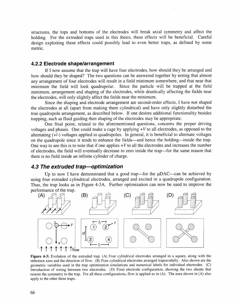
structures, the tops and bottoms of the electrodes will break axial symmetry and affect theholding. For the extruded traps used in this thesis, these effects will be beneficial. Carefuldesign exploiting these effects could possibly lead to even better traps, as defined by somemetric.

4.2.2 Electrode shape/arrangementIf I now assume that the trap will have four electrodes, how should they be arranged and

how should they be shaped? The two questions can be answered together by noting that almostany arrangement of four electrodes will result in a field minimum somewhere, and that near thatminimum the field will look quadrupolar. Since the particle will be trapped at the fieldminimum, arrangement and shaping of the electrodes, while drastically affecting the fields nearthe electrodes, will only slightly affect the fields near the minimum.

Since the shaping and electrode arrangement are second-order effects, I have not shapedthe electrodes at all (apart from making them cylindrical) and have only slightly disturbed thetrue quadrupole arrangement, as described below. If one desires additional functionality besidestrapping, such as fluid guiding then shaping of the electrodes may be appropriate.

One final point, related to the aforementioned questions, concerns the proper drivingvoltages and phases. One could make a cage by applying +V to all electrodes, as opposed to thealternating (+/-) voltages applied to quadrupoles. In general, it is beneficial to alternate voltageson the quadrupole since it tends to enhance the fields-and hence the holding-inside the trap.One way to see this is to note that if one applies +V to all the electrodes and increases the numberof electrodes, the field will eventually decrease to zero inside the trap-for the same reason thatthere is no field inside an infinite cylinder of charge.

4.3 The extruded trap-optimizationUp to now I have demonstrated that a good trap-for the gDAC-can be achieved by

using four extruded cylindrical electrodes, arranged and excited in a quadrupole configuration.Thus, the trap looks as in Figure 4-3A. Further optimization can now be used to improve theperformance of the trap.

(A) (B) (C) (D)

O0. 0x d

oI I® 0Vthhtttlow I

Figure 4-3: Evolution of the extruded trap. (A) Four cylindrical electrodes arranged in a square, along with thereference axes and the direction of flow. (B) Four cylindrical electrodes arranged trapezoidally. Also shown are thegeometric variables used in the trap optimization simulations and numerical labels for individual electrodes. (C)Introduction of wiring between two electrodes. (D) Final electrode configuration, showing the two shunts thatrestore the symmetry to the trap. For all these configurations, flow is applied as in (A). The axes shown in (A) alsoapply to the other three traps.

66

4.3.1 Electrode heightFor perfectly cylindrical electrodes, the electrodes need to be at least as high as the

diameter of a cell and additionally encounter a good fraction of the cells in the flow. The

constraint is that high-aspect-ratio posts will be fragile and difficult to fabricate. Later on in this

chapter I will perform a system-level design of the chamber, the result being that the chamber

will be 150 pm high. I have thus chosen an electrode height of 50 gm, which is >4x as high as

the cell radius, and 1/3 of the chamber height. Thus, this height should allow traps to encounter

at least 1/3 of the cells in the flow (more if the cells are allowed to settle) and be much taller than

the cell size, so that a cell can fit within the trap.

4.3.2 Electrode arrangement/diameterThe next characteristic to pin down is the electrode arrangement. I want to have a low

barrier for entry into the trap, but a high barrier to exit. This will make it easy to load the traps

but still result in strong traps. The entry barrier field is in large measure determined by

electrodes 3 & 4, while electrodes 1 & 2 largely determine the exit barrier (see Figure 4-3B).

Thus, by increasing the separation of electrodes 3 & 4 with respect to the separation between 1 &

2, the trap should be easier to load and still remain strong.Indeed, this is the case. Figure 4-4 shows a plot of the lE term (proportional to the DEP

potential energy) along the y-axis for two differently asymmetric trap geometries under the same

experimental conditions. The change in the entrance-electrode spacing from 50 gm to 70 pm

G

/D 00 5 -w

I 0 x

4. exitbarrier

3- .entrance8 barrier

50pma)

x- a) 11=70pgm

-

.............................

0''

-10 0 10 20 30 40 50 60x (jm)

Figure 4-4: Comparison of x-directed barriers for two trap geometries. The first geometry (-) is only slightly

asymmetrical, with an entrance-electrode separation (l) of 50-gm and an exit-electrode separation (12) of 40-gm.

The second geometry (---) has the same exit-electrode separation but a 70-gm entrance-electrode geometry. Plotted

is the E12 factor along the y-axis at a height of 16 gim. The height of the rightmost peak (at x=40 gm), corresponding

to entrance barrier, is lowered more than the second peak upon changing to more asymmetric trap geometry. The

axes are as defined in the inset.

67

barely affects the exit barrier height (at x=0) but lowers the entrance barrier height -5x, makingthe trap much easier to load.

For a final optimization of the trap geometry-electrode diameter, absolute spacings,etc.-I performed a series of simulations within a matrix of variations (Table 4-1), varying eachparameter while holding the others constant, to determine the final geometry. The simulationsare all for beads in these traps, and so the absolute release flowrates predicted will not be thesame as when using cells. In fact, the traps can be expected to be weaker with cells because oftheir smaller CM factor. However, since I am only interested here in the relative performance ofthe different trap designs, simulations with beads are appropriate. In the system-level designsection later on, I will perform simulations with cells to converge to an absolute design.

The results are shown in Figure 4-5, where I plot the calculated release flowrate andimposed electric field at 3V. This choice of parameters is because the release flowrate is anindicator of performance whereas the imposed electric field is a variable that must be minimized,as I will discuss below in the system-level design section. Knowing that all traps havemonotonic holding characteristics with the same basic shape, only one simulation point isnecessary to compare them.

In agreement with the result in Figure 4-4, the variation of l has a negligible effect onperformance (Figure 4-5B), as does the variation of the trap length d (Figure 4-5D). Changes inthe post radius r and the exit-barrier separation 12 dramatically affect both the holding and theelectric field in fairly linear manners. This makes sense by noting that the inner distancebetween the posts is 12-2r and that this is the primary variable that will affect the imposed electricfield (at a given voltage) near the exit and thus the trap strength. Choosing an electrode radius of10 gm for fabrication ease, I have chosen an overall exit-post spacing (12) of 40 gm to giveclearance for the cells, a trap length d=40 gm, and an entrance-electrode spacing of l1=60 gm.The final electrode arrangement is shown in Figure 4-3B and in the figure in Table 4-1.

4.3.3 Trap switchingThe pDAC requires the ability to individually control trap sites. To minimize external

connections, it would be advantageous if only one electrode needed to be switched to "turn off" awhole trap. One way to accomplish this is to switch the polarity of one electrode in thequadrupole, thus eliminating the symmetric arrangement of potentials. The result of doing this isshown in Figure 4-6. Here I plot the vector force fields in the xy-plane at the height of 16 ptmwhen the quadrupole is stimulated with alternating polarities (Figure 4-6A), and when the

/,.-40 ptm

Initial geometry d-40 mr10 m

/,=60 gmVariable Range of variation

r 5 pm, 10 m, 15 lm11 50 m, 60 m, 70 tm12 30 tm, 40 pm, 50 md 30 Jim, 40 ptm, 50 jim

Table 4-1: Matrix for trap optimization. Shown is a top-down view of the initial trap geometry. Below that are thevariables that were varied, one at a time, to trace out the design space. Bold numbers indicate the starting trapgeometry on which the variations were made.

68

000

10 1r (tm)

140

100E CD

80 2-T 0

60 a)U)

40

20

45 50

1000

800-

600-

400-

200

50

55 60. (tm)

55 60d (pm)

Figure 4-5: Results of trap optimization simulations. Plotted are the release flowrate (-, left y-axis) electric fieldexperienced by the particle at release (---, right y-axis) for various trap geometries defined in (Table 4-1) underidentical experimental conditions. Shown are variations in (A) electrode radius r, (B) entrance-electrode spacing 11,(C) exit-electrode spacing 12, and (D) trap length d.

polarity of electrode #2 is reversed (Figure 4-6B). The change in polarity of one electrode isenough to disrupt the potential energy well and eject the particle. Thus, in the final trap designthis electrode is wired to be switchable in this way. The imposition of flow during release wouldchange the trajectory of the ejected particle. Although it is unclear in this analysis what exactlythat trajectory will be, the particle will be ejected in either situation, which is the goal.

4.3.4 WiringFor ease of fabrication, I have chosen to limit metalization to one layer with no dielectric

insulation between the metal and the fluid. The following discussion of how to compensate forthis becomes moot if multilayer metalizations and/or insulators can be used.

The optimal way to wire an array of traps within a small area and keep the lead count lowis to tie one pair of electrodes to the same potential by connecting them through the middle of the

69

0

CaC)

(B)800

600

400

200

015

1000

(C) -

(A)

140

120

100E

80

60

40

20

65 70

(D)

a)

-,

aOCD

800

600

400

200

r) I

30 35 402 (pm)

14J IUJ -U

120 '5 800-

100- EE (D

80 600-

60

40 0200

202

20A

140

120

100,E

80I-

60

40

20

6 065 70

_____.-- ___-17 7 ----I

5 50--

100 . 100(A) .... (B)

50 50 ............... . . . .. . . . .. .. . . .

... .. . .. .

-100 -10-

...... ........

0 ...... 1........ . . . .. ..

. . . . . . . .. ..... 0

~......./, f..........

0 - .........

-~...................

-50 - :::. -50 -

..........

-100, 1 -1001

0 50 100 0 50 100

x (Gm) x (Gm)

Figure 4-6: Trap switching via one electrode. (A) A vector plot of the DEP force in the xy-plane at a height of 16pim when the trap is excited conventionally (as shown in the figure). Within the trap, all arrows point to the center,indicating that a particle will be trapped in this circumstance. (B) Plot of the same situation when the polarity of thetop-left electrode is changed from + V to -V. There is no longer a trapping region in this configuration. The blackline shows the trajectory of a particle at the trapping point in (A) upon initiation of the excitation pattern in (B). Theparticle is ejected from the trap. This particular trap had 100-pim-tall posts with d=50 pim, l=40 jim, and 12=80 jim.

trap, as shown in Figure 4-3C. Simulating the holding characteristic of this trap, I show inFigure 4-7 that the trap is much weaker than the ideal trap with no wiring (Figure 4-3B). Thisfigure also reinforces the monotonic nature of the holding characteristic for the extruded trapregardless of the specific trap geometry. The reason that the interconnected trap is much weakerthan the "ideal" trap is that the interconnect disrupts the symmetry of the trap, reducing itsquadrupolar nature and thus its strength. One approach towards restoring the strength of the trapgiven the need for the interconnect would be to restore its symmetry.

I empirically designed and simulated a number of possible wiring schemes to try torestore the trap strength. To efficiently compare the wiring schemes, I simulated their behaviorat one voltage under identical experimental conditions (R=10 gm bead, f=20 MHz, w=5 mm,

-,=1 S/m). The designs and simulated release flowrates are shown in Figure 4-8. Althoughseveral wiring schemes (#4-#6) perform equally well in restoring the trap strength, wiringscheme #4 delivers the most restoration of the holding while minimizing the encountered electricfield. As described below in the system-level design, minimizing the electric field encounteredby the particle is essential for optimal performance. I have thus chosen wiring scheme #4 forthese traps, shown in Figure 4-3D.

70

1 2 3voltage (V)

4 5 6

Figure 4-7: Holding characteristic of the single-wire trap. Plotted is the release flowrate versus voltage for thetrapezoidal trap with (---) and without (-) a substrate interconnect between electrodes #1 & #4. The introductionof the substrate interconnect drastically reduces the holding in the trap and thus its performance.

(A) 0 00l

0

a)

a)

200

150

100

50

080

(C)

2 3 4 5wiring scheme

6 7 8 9

Figure 4-8: Results from various wiring schemes. (A) Shown are various empirically designed wiring schemes.The two left-most schemes are, from left to right, no internal wiring and a single interconnect. The rest of theschemes are designed restore the performance of the trap. (B) The release flowrate at 2V due to the wiring schemesin (A). The left-most result, from a trap with no interconnect, possesses the highest release flowrate and is the idealtrap. (C) The electric field encountered in the various traps in (A) at 2V. The schemes that improve the symmetryof the trap tend to restore most of the holding. Wiring scheme #4 is most effective at restoring holding whileminimizing the encountered electric field.

71

1800

1600

1400

1200

1000

800

600

-)

0

aZ

- no interconnectone wire

-

400

200

00

(B)

so

6 0E

40

20

00 1

I

Q_ ' 00 OU

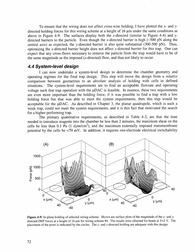
To ensure that the wiring does not affect cross-wise holding, I have plotted the x- and y-directed holding forces for this wiring scheme at a height of 16 pm under the same conditions asabove in Figure 4-9. The surfaces display both the x-directed (similar to Figure 4-4) and y-directed barriers to the particle. Even though the x-directed barrier is high (-500 pN along thecentral axis) as expected, the y-directed barrier is also quite substantial (300-500 pN). Thus,optimizing the x-directed barrier height does not affect y-directed barrier for this trap. One canexpect that any cross-flows necessary to remove the particle from the trap would have to be ofthe same magnitude as the imposed (x-directed) flow, and thus not likely to occur.

4.4 System-level designI can now undertake a system-level design to determine the chamber geometry and

operating regimes for the final trap design. This step will move the design from a relativecomparison between geometries to an absolute analysis of holding with cells in definedsituations. The system-level requirements are to find an acceptable flowrate and operatingvoltage such that trap operation with the gDAC is feasible. In essence, these two requirementsare even more important than the holding force; if it was possible to find a trap with a lowholding force but that was able to meet the system requirements, then this trap would beacceptable for the gDAC. As described in Chapter 3, the planar quadrupole, which is such aweak trap, could not meet the system requirements, and it is this fact that motivated the searchfor a higher-performing trap.

The primary quantitative requirements, as described in Table 4-2, are that the timeneeded to introduce reagents into the chamber be less than 2 minutes, the maximum shear on thecells be less than 0.1 Pa (1 dyne/cm2), and the maximum externally imposed transmembranepotential by the cells be <70 mV. In addition, it requires one-electrode electrical switchability

(A) (B)

ThNI N

I >1

0 0X -4M) 0 X (-m)

4 -4 0. g)4 40

40

0y (AiM)

Figure 4-9: In-plane holding of selected wiring scheme. Shown are surface plots of the magnitude of the x- and y-directed DEP forces at a height of 16 pm for wiring scheme #4. The results were obtained for beads at V=2 V. Theplacement of the posts is indicated by the circles. The x- and y-directed holding are adequate with this design.

72

1500.

Z 1000,

5 500.

0.

Parameter TargetFill time 120 s

Maximum shear stress 0.1 PaMaximum transmembrane potential 70 mV

Electrical switchability One electrodeArrayability Yes

Table 4-2: System-level specifications of the pDAC.

and a trap geometry that is easily arrayable. Most of these parameters are more stronglydependent on chamber height than width because the flow approximates plane Poiseuille flow-the width simply sets the volume flowrate.

4.4.1 Fill timeIn order to operate the gDAC in a timely manner, it must not take too long to introduce

reagents into the chamber. For the gDAC, I have chosen 120 s as an appropriate fill time. Thisfill time will be dependent on the void volume of the system and the maximum flowrate that thetrap can withstand. Thus, I can trade off void volume for flowrate if the fill time is fixed (as itis). For a rectangular chamber, the volume flowrate (Q) needed is

Q = (wlh +VO) / tf (4-2)

Where w, 1, and h are the chamber width, length, and height, respectively, Vo is the void volumeof the tubing, and tj is the fill time. The chamber will be approximately 8x2x0.15 mm or 2.4 gd,and thus its volume will be dwarfed by any tubing void volume. In this case, Eqn. (4-2) can beapproximated as

Q ~= V0 / tf (4-3 )and to 1st order the chamber dimensions do not affect the fill time. A reasonable void volume toexpect is 20 pl, which corresponds to about 10 cm of standard 0.020"-diameter HPLC tubing.This gives a target flowrate of 10 gl/min that the trap must withstand.

In many respects these parameters-fill time, chamber volume, and void volume-areextrinsic to the performance of the trap itself. One can always redesign the experimental setupand protocol to vary these parameters.

4.4.2 Shear on cellsStationary cells in the traps will experience shear forces from the flow. The maximum

shear experienced by the cells must be less than that which will cause any physiologicaldisturbance. Arterial shear stress is about 1.5-2.0 Pa (15-20 dyne/cm 2) [161], and so I want tokeep shear stress levels well below that value, or about 0.1 Pa (1 dyne/cm2). To get an estimateof the shear, two extreme cases can be considered-1) the cell against the substrate, and 2) thecell in the center of flow.

Against, the substrate, the cell will feel approximately the wall shear resulting from planePoiseuille flow, which is

=4Ucl/h= j2(jQ1= 6Q (4-4)h 2A wh 27

where Pis the shear stress, U, is the centerline flow velocity, A is the cross-sectional area and t

is the viscosity of the water.

73

At the centerline of the chamber, the cell will experience shear due to the Stokes' flowaround it, which at its maximum is given by

3Vc 3 3q 9Q2R 2R 2A 4whR

Thus I see that the centerline shear will be -h/3R larger than the wall shear. It is bettertherefore to keep the cell near the wall, rather than in the flow. For our situation, where the cellis about 1/5 of the distance between the substrate and the centerline, the first (and smaller)expression for the shear is appropriate. In this case the shear is strongly dependent on thechamber height (1/h 2) if the flowrate (Q) is independent of chamber height (Eqn. (4-3)). Asdescribed below, the final design will result in an imposed shear of 0.03 Pa, which is within thegoals.

4.4.3 Transmembrane potentialAs discussed in §1.5.2, the imposed electric field can directly affect cell physiology by

perturbing the cell's endogenous transmembrane potential. To minimize such effects one mustlimit imposed transmembrane potential, in this case to <70 mV (Table 4-2). This feeds back intothe design because I can calculate the imposed transmembrane load for a nominal electric field ata given frequency. Since that load will scale linearly with the electric field (Eqn. (1-10)), thiswill directly limit the maximum electric field that the cell can be exposed to, which is aparameter that can be extracted from the models. In Figure 4-10A I have plotted the computed

C,C

E >100E '

VCO

0

0

S-0.2

-0.30

-0.4

n r.

(A)

-(B)

104 106 108

Frequency (Hz)

Figure 4-10: (A) Transmembrane potential of HL-60 cells. Plotted is the transmembrane potential imposed on HL-60 cells for an incident field of 1 V/m as the field frequency is varied. The transmembrane potential decreaseslogarithmically above a critical frequency and saturates at a yet higher frequency. (B) The dipole term of the CMfactor for the same cells. The CM factor is saturated at -0.5 for low frequencies and experiences two dispersions asthe frequency increases.

74

transmembrane load imposed on HL-60 cells using Eqn. (1-10) but including the high-frequencydielectric saturation effect. I have used parameters for HL-60 cells described by the Gascoynegroup [81] with radius R=6.25 pim, membrane capacitance and conductance C=1.6 gF/cm 2 &GM=0.22 S/cm 2, membrane thickness A=1 nm, and cytoplasmic permittivity and conductivity ofecyt,= 7 5 F/m & o-yto= 0 .7 5 S/m. The solution conductivity (of HBSS) was measured as 1.0 S/m.The figure shows that frequencies above 1 MHz are necessary and that operation at 20 MHz (atthe limit of our signal generator) is preferable. At this latter frequency, the transmembranevoltage is 0.4 jV for a 1 V/m field, and thus a 70 mV maximum transmembrane potential leadsto a maximum electric field in the vicinity of the cell of -1.8x10 5 V/m.

In Figure 4-10B I show the dipole term of the CM factor for the same cell, which, inanalogy to Eqn. (1-2), is given by

E - ECM= -e - (4-6)

£ +2e,-p -M

where Ep refers to effective complex permittivity of the cell (Eqn. (1-3)) and f. is the complexpermittivity of the medium. The transmembrane voltage and CM factor experience dispersionsat the same frequency, which isn't surprising since they both represent time-constants ofcharging on either side of the membrane. The CM factor does not go to zero after the dispersion,however. This is because while the transmembrane voltage is across the membrane RC pair, theCM factor is due to the voltage across the network compared to the voltage across the medium inthe absence of the cell; in effect, the CM factor represents the disturbance in the field due to thecell [119]. This disturbance exists whether the voltage is dropped across the membrane or thecytoplasm.

To get an estimate of how the electric field (and thus transmembrane potential) scaleswith the chamber height, I can use the fact (see Figure 4-7) that the release flowratecharacteristic for the extruded traps has approximately the form

Q, = aV 2 (4-7)

where Qf is the release flowrate and a is some fitting parameter. In essence, the release flowrateis dependent on the square of the voltage. This makes sense if one considers that the dipole termof the DEP force also goes as V. I can introduce chamber height as a parameter, using thelinearity of flow with chamber height, by

Qf = aV 2 h (4-8)

where ho is some nominal chamber height. Thus, if a given Qf is needed to meet the systemparameters then the voltage needed will scale as

V = Q ho (4-9)ah

which goes as 1/Ih. Thus, increasing the chamber height should decrease the voltage needed,and thus the electric field experienced by the cells.

From the calculated holding characteristics for HL-60 cells, I can determine the chamberheight and width that meet the system parameters along with an operating voltage and flowrate.The design is iterative, in that I simulate the characteristics for some chamber geometry and thenuse those results to optimize the chamber geometry. The program can easily record the electricfield experienced by the cell at the point of release. Then, using the chamber height as aparameter, I can calculate the flowrate needed from Eqn. (4-2), the voltage that is therefore

75

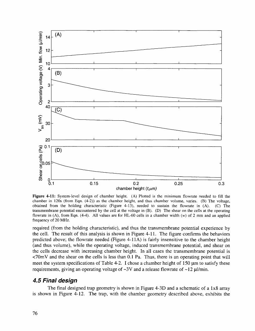
14 -(A

012-

10

0

>34C

L0 -2

40

E30

E

20(

CO,

,0.050

0.1 0.15 0.2 0.25 0.3chamber height (tpm)

Figure 4-11: System-level design of chamber height. (A) Plotted is the minimum flowrate needed to fill thechamber in 120s (from Eqn. (4-2)) as the chamber height, and thus chamber volume, varies. (B) The voltage,obtained from the holding characteristic (Figure 4-13), needed to sustain the flowrate in (A). (C) Thetransmembrane potential encountered by the cell at the voltage in (B). (D) The shear on the cells at the operatingflowrate in (A), from Eqn. (4-4). All values are for HL-60 cells in a chamber width (w) of 2 mm and an appliedfrequency of 20 MHz.

required (from the holding characteristic), and thus the transmembrane potential experience bythe cell. The result of this analysis is shown in Figure 4-11. The figure confirms the behaviorspredicted above; the flowrate needed (Figure 4-11A) is fairly insensitive to the chamber height(and thus volume), while the operating voltage, induced transmembrane potential, and shear onthe cells decrease with increasing chamber height. In all cases the transmembrane potential is<70mV and the shear on the cells is less than 0.1 Pa. Thus, there is an operating point that willmeet the system specifications of Table 4-2. I chose a chamber height of 150 iim to satisfy theserequirements, giving an operating voltage of -3V and a release flowrate of -12 gl/min.

4.5 Final designThe final designed trap geometry is shown in Figure 4-3D and a schematic of a 1x8 array

is shown in Figure 4-12. The trap, with the chamber geometry described above, exhibits the

76

Figure 4-12: Schematic of a 1x8 array of traps, showing the interconnects and posts.

holding characteristic shown in Figure 4-13 for 10.0-gm beads and HL-60 cells. Thecharacteristic is indeed monotonic and approximately quadratic with voltage (again confirmingthe validity of Eqn. (4-7)). The actual release flowrates are much smaller than those shownduring the relative design employed in the previous part of the chapter, even for the beads. The

primary reason for this is that those simulations used 20-gm beads, while these use 10-gm beads,which gives an -8x difference between the two (due to the R3 factor).

The differences in holding between the beads and cells shown in Figure 4-13 is almostentirely directly due to the differences in the CM factors (--0.1 for the cells, -- 0.5 for the beads)while the rest is due to differences in the particle sizes.

50

--- 10.0- gm beads40 ----- HL60 cells

cD30-

0-20-a)C,)CZ

S 0) - . - - -~ -2 10-

0 ~~ ~---'-'0.5 1 1.5 2 2.5 3

Voltage (V)

Figure 4-13: Holding characteristic for final trap (Figure 4-3D) in the finalized trap geometry, for 10.0-pim beads

(-) and HL-60 (---) cells at 20MHz. The holding characteristics are monotonic and are roughly proportional to V2.

77

The extracted system-level parameters for the final design are shown in Table 4-3. Asshown, the trap and chamber geometry meets all the system parameters for the gDAC.

I can compare the behavior of the final trap design with that of the planar quadrupoledescribed in 0. For this comparison I have "placed" both traps in the same flow chamber (width,height), so that a fair comparison can be obtained. In Figure 4-14 I show the results of thiscomparison. Both the predicted release flowrates and holding forces of the extruded traps aremuch larger than for the planar quadrupole. In addition, the monotonic behavior of the extruded

Parameter Target Value Final ValueTime to load chamber 120 s 120 s

Shear on cells <0.1 Pa 0.03 PaTransmembrane load <70 mV -30 mV

Electrical switchability Y YArrayability Y Y

Operating voltage (V) 3 VOperating frequency (1) 20 MHz

Release flowrate 12 pl/minChamber height (h) 150 pmChamber width (w) 2 mm

I,=40 pm

0 0 r=10 tm

Trap dimensions d=40 tm

/=60 gm

electrode height = 50 pim

Table 4-3: Final system-level design parameters. Shownparameters in the design. Below that are displayed the trapobtain those values.

''1

.10

01 0

a10CU,

10 L0 1 2

Voltage (V)

are the target and final values for the five systemdimensions and operating characteristics necessary to

102

0.

0

.01

100

3 0 1 2Voltage (V)

3

Figure 4-14: Comparison of the holding characteristics of the finalized trap design with the planar quadrupole of 0for 10.0-pum beads, both simulated with the finalized chamber geometry. (A) Plotted is the release flowrate versusvoltage for the extruded (-) and planar quadrupoles (---). (B) Plotted is the extracted holding force versus voltagefor the extruded (-) and planar quadrupoles (---). The extruded trap is at least an order of magnitude stronger thanthe planar trap.

78

.planarextruded

trap allows the user to "turn up the voltage" if more holding is desired.

4.6 ConclusionIn this chapter I have undertaken the design of an improved DEP-based single-particle

trap with characteristics that can meet the system requirements of the iDAC. Through extensiveuse of the modeling tools developed in Chapter 2, I have designed a trap that is an extrudedquadrupole with an asymmetric trapezoidal geometry. It can be easily arrayed and is electricallyswitchable. The trap also incorporates substrate shunts to improve holding when only one layerof metal is used with no dielectric. Through the evaluation of the design in terms of the systemparameters for tDAC operation, I have determined operating characteristics and chambergeometries that will result in successful operation.

79

80

Chapter 5: Array fabrication, packaging & test setup

In this chapter I will describe the fabrication process for making the extruded trap arrays

as well as the packaging and setup needed to test them. Various type of arrays were fabricated-

1x4, 2x4 & 1x8-examples of which are shown throughout the chapter. The fabrication process

is mostly concerned with obtaining a set of extruded posts by electroplating gold into an SU-8

mold. Other process steps form substrate interconnects and a fluidic chamber around the

electrode arrays. The latter part of the chapter describes the packaging scheme needed to obtain

electrical, optical, and fluidic connection to the chips, and finally the test setup used in the final

two chapters of this thesis.

5.1 FabricationThe fabrication process for making the extruded traps essentially involves fabricating

extruded posts via electroplating into a mold and then encapsulating the array within a

photoresist channel. The fabrication process flow for the making the extruded arrays is shown in

Figure 5-1.

5.1.1 Substrate interconnectThe first step in the process flow is to pattern the interconnect layer that resides on the

substrate. I have chosen to use gold for the interconnect layer due to its biocompatibility [162]

and because of the availability of differential etchants between it, titanium, and glass, the need

for which is explained below.The process starts with 100-mm-diameter 1-mm thick pyrex wafers. The thickness was

chosen simply because of material availability. I cleaned the wafers with a 10-min Piranha clean

and then used an e-beam evaporator to deposit 1700 A of titanium and 5000 A of gold (Figure

5-1A).I chose to use titanium under the gold for several reasons. First, it serves as an adhesion

layer between the glass and the gold. Second, the titanium can be etched with dilute HF, which

has high selectively to gold and glass. Finally, and most importantly, the SU-8 molding material

that I will use later adheres fairly well to the titanium. I determined this last property by

performing a series of experiments testing the adhesion of SU-8 to various metals (Cr, Ti, Ni, Pt)

(A) (B) (C) (D) (E) (F)

-, --r II -..............glass Ti SU-8

Figure 5-1: Fabrication process flow for the extruded traps.

81

and found that titanium performs best.Following deposition, I performed standard contact lithography and pattern etching of the

gold to define the substrate interconnect (Figure 5-1B). I used a potassium iodide-based etchant(Gold Etchant Type-TFA, Transene, Danvers, MA), which displays high selectivity to titaniumand glass, to etch the gold. The availability of this selective etchant enables the use of thisgold/titanium/glass tri-layer system, as described above. The etchant severely undercutsphotoresist (although much less than aqua regia), so the as-drawn mask features were biased toaccount for this. The nominal undercut for perfect isotropy would be 5000 A, but the actualundercuts were closer to 2 gm. Thus I used 8-gm linewidths on the mask to achieve 4-gmfeatures. In practice, however, the undercut was a bit more, and final features varied fromentirely undercut (Figure 5-2A) to -3-4-gm linewidths (Figure 5-2B). Different etchantformulations (manufactured by Transene) could be used in the future to reduce this undercut.

The best way to obtain well-defined metal lines is by lift-off, so the question arises as towhy I chose not to use that process. The reason is that it is impossible with lift-off to obtain a Ti-Au metal bilayer and have patterns on only one of the layers. The unpatterned Ti layer is neededfor the electroplating process (described below). Thus, pattern etching of the gold is the bestalternative.

5.1.2 SU-8 mold depositionThe extruded electrodes are fashioned from posts electroplated into SU-8 (Figure 5-1C &

Figure 5-1D). SU-8 is a epoxy-based negative photoresist developed by IBM in the 1980's [163,164]. It is useful because it can be patterned with conventional contact lithography into high-aspect-ratio microstructures. The photoresist can be spun with single coats into layers rangingfrom a few microns to 100's of microns thick (depending on the formulation), and is extremelyconformal. In addition, the developed photoresist is quite robust and can be fashioned intostructural layers. Essentially, the photoresist enables one to do LIGA with conventionalequipment.

SU-8 has been used as a mold for electroplating by several researchers [163-165]. Thechallenges lie in (1) getting it to adhere to the substrate, (2) patterning sufficiently high-aspect-ratio structures, and (3) removing the SU-8 following electrodeposition.

Figure 5-2: Top-down view of the substrate interconnect following Au etching. Shown is an example of excessiveundercut (A) and an acceptable specimen (B).

82

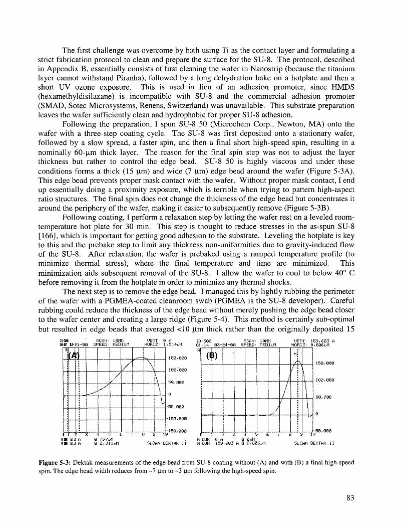
The first challenge was overcome by both using Ti as the contact layer and formulating astrict fabrication protocol to clean and prepare the surface for the SU-8. The protocol, describedin Appendix B, essentially consists of first cleaning the wafer in Nanostrip (because the titaniumlayer cannot withstand Piranha), followed by a long dehydration bake on a hotplate and then ashort UV ozone exposure. This is used in lieu of an adhesion promoter, since HMDS(hexamethyldisilazane) is incompatible with SU-8 and the commercial adhesion promoter(SMAD, Sotec Microsystems, Renens, Switzerland) was unavailable. This substrate preparationleaves the wafer sufficiently clean and hydrophobic for proper SU-8 adhesion.

Following the preparation, I spun SU-8 50 (Microchem Corp., Newton, MA) onto thewafer with a three-step coating cycle. The SU-8 was first deposited onto a stationary wafer,followed by a slow spread, a faster spin, and then a final short high-speed spin, resulting in anominally 60- tm thick layer. The reason for the final spin step was not to adjust the layerthickness but rather to control the edge bead. SU-8 50 is highly viscous and under theseconditions forms a thick (15 ptm) and wide (7 tm) edge bead around the wafer (Figure 5-3A).This edge bead prevents proper mask contact with the wafer. Without proper mask contact, I endup essentially doing a proximity exposure, which is terrible when trying to pattern high-aspectratio structures. The final spin does not change the thickness of the edge bead but concentrates itaround the periphery of the wafer, making it easier to subsequently remove (Figure 5-3B).

Following coating, I perform a relaxation step by letting the wafer rest on a leveled room-temperature hot plate for 30 min. This step is thought to reduce stresses in the as-spun SU-8[166], which is important for getting good adhesion to the substrate. Leveling the hotplate is keyto this and the prebake step to limit any thickness non-uniformities due to gravity-induced flowof the SU-8. After relaxation, the wafer is prebaked using a ramped temperature profile (tominimize thermal stress), where the final temperature and time are minimized. Thisminimization aids subsequent removal of the SU-8. I allow the wafer to cool to below 400 Cbefore removing it from the hotplate in order to minimize any thermal shocks.

The next step is to remove the edge bead. I managed this by lightly rubbing the perimeterof the wafer with a PGMEA-coated cleanroom swab (PGMEA is the SU-8 developer). Carefulrubbing could reduce the thickness of the edge bead without merely pushing the edge bead closerto the wafer center and creating a large ridge (Figure 5-4). This method is certainly sub-optimalbut resulted in edge beads that averaged <10 pm thick rather than the originally deposited 15

TO CAN: 16611 OERT;L 0 AD 100 SCAN: 10111 (IEFT; 159, 603 Li04;8? 1- i SPEED; MEDIUM HOHIZ; 1Eit4DM Li 14 03-24-00 SPEED; MEDIUM HDFI21 Eb60EA'

R:150. 066

100.. 0012

1512. 12121

(p) M:

- - -- - - - -

1150 12012

100.000

1521.121212

12

-SE. 02101 2 2 4 1 6 7 8 9 10 0 1 2 31 4 5i 6 E., 9 10

R CM: 813 fi '9 ?97um R CUJR t 0 i A 8 12OI-5E: 813 A 12 _31 Lull SLOAN DEKTAK II M CUR: 159,603 A 12,606uM SLOAN DEKTAK II

Figure 5-3: Dektak measurements of the edge bead from SU-8 coating without (A) and with (B) a final high-speedspin. The edge bead width reduces from -7 pm to -3 pm following the high-speed spin.

83

10:250 SCAN: 1'MM00:21 04-0-00i SPEED. MEDTIUMR

UERT:,398)A1

.0 3000

-10.000

-250 00

-3MO.O33

R CUR: 0 A I? 0.PP1 CUB; 58,36 A R 398.A SLOAN QEKTAK II

Figure 5-4: Dektak measurements of the SU-8 edge bead following PGMEA treatment of the edge. The edge beadhas decreased to -6 pm in this example. A spike appears where the edge of the swab has created an SU-8 ridge.

pim. One cannot simply perform a wafer-perimeter photo exposure step to remove the edge beadbecause the SU-8 is not a positive resist. Perhaps a more optimal technique would be to prebakethe SU-8 with a cylindrical Teflon weight on the wafer that had a hole in it to permit SU-8solvent fumes to escape. Such a jig would not adhere to the SU-8 and might significantly reducethe edge bead. Of course, the best method would probably be to use a coater with an integratededge-bead removal system.

Following prebake, I performed contact lithography to define the holes in the SU-8 forthe electrodes. The key to performing this lithography step is to obtain good contact between themask and the SU-8 by minimizing any airgap. To do this, it's important to both remove the edgebead and use the vacuum contact mode on the aligner. Despite the thickness of the SU-8 one cansee thru it well enough to achieve a few microns of alignment tolerance, which is sufficient forthis application.

I chose the minimum exposure that would harden the photoresist without overexposinginto the electrode holes-usually 40 seconds. When high-aspect-ratio features are desired,optimizing (and usually minimizing) the exposure is crucial. After exposure comes a rampedpostbake on a hotplate, again minimizing the bake time to aid in future SU-8 removal.

The final step is to develop the SU-8 in PGMEA. This developer will remove theunexposed regions of the photoresist. Five minutes was sufficient to open up the electrode holes,followed by cycles of coating the wafer with PGMEA and spin-drying it to try to remove residuefrom the bottoms of the holes. Removal could be seen by a clearing of the bottoms of the holes aviewed under a microscope, although the thickness and small diameter of the holes made itdifficult to see into them easily.

I eventually learned that simply rinsing the SU-8 in PGMEA is insufficient for removingall organic debris at the bottom of the holes and thus allowing electroplating initiation to occur.The solution to this was to introduce an oxygen ashing step after the development step andimmediately before the electroplating. Ashing was performed in a barrel asher for 20-40minutes, where the endpoint was that the bottoms of the holes across the wafer would appearclear under the microscope. This step drastically improved the yield of post initiation.Overashing will reduce the adhesion of the SU-8 to the substrate and cause underplating, sominimizing the ashing time is important.

84

9r.

After this step, the wafer looked as in Figure 5-6. The cracks in the SU-8 are due toshrinkage in the developer and are confined to the surface, thus not affecting the SU-8'ssuitability as a mold. These cracks result from stress can affect adhesion to the substrate andcause subsequent underplating, depending on the pattern and total stress involved. This was nota problem for the circular patterns, but has been a problem for rectangular regions, especiallynear corners.

5.1.3 Electroplating the electrodesThe next step is to electroplate the posts into the SU-8 mold (Figure 5-1D). As for the

interconnects, I wanted to use gold for the electrode posts because of its biocompatibility. Iperformed the electroplating in a cyanide-based gold plating solution (Orotemp 24, Technic Inc.,Anaheim, CA). Literature reports, however, suggest that non-cyanide gold plating solutions mayactually function better in the presence of photoresists [167].

The electroplating setup is shown in Figure 5-5. It consists of a closed-loop hotplate-stirrer to heat and stir the plating solution, a power supply to apply current, and a jig to hold thewafer and anode in the solution. I used an insulated dip-style thermocouple to measure thesolution temperature without affecting the electrochemistry. The power supply was a pulse-plating supply (Dynatronix, Amery, WI) capable of forward and reverse pulse plating. I used a

Figure 5-6: Image of a 1x8 array after SU-8 development and ashing.

pulse-platingpower supply

single-wafer carrierwafer

thermocouple

goldanode

hotplate stirrer

Figure 5-5: Schematic of the electroplating setup.

85

j tand

lid

.............................

1-mil-thick 100x100 mm gold sheet as the anode and held the wafer (cathode) in the solutionwith a single-wafer carrier clipped at one end to complete the electrical circuit.

Electroplating works by forcing a constant current through the circuit composed of thepower supply, anode, cathode, and plating bath. The faradaic current at the electrode/electrolyteinterfaces oxidizes and reduces the species at the anode and cathode surfaces, resulting insolubilization of the gold foil (anode) and deposition of metal at the cathode [168]. Because ofthe availability of the pulse-plating supply, I used 1 ms forward-going pulses with a 10% dutycycle. The pulsing helps to refresh the concentration of electroactive species at the interface andthus increase the efficiency of the plating and reduce the time. With this setup, the manufacturerquoted plating rates of 0.1-0.3 gm/min with 1-3 mA/cm 2 of current and this is what I obtained inpractice. The current density needed to obtain these rates was difficult to measure because thesmall plated area introduced large errors, and so these parameters were determined via trial anderror.

The need for the continuous titanium layer becomes apparent now. I used it to form acontinuous electrode connecting all plated posts to the clip. I could not simply use the patternedgold layer for this connection as the patterns are not all connected together. In addition, thecontinuous nature of the titanium layer gives a low resistance to the layer, which minimizesvoltage drops and enhances plating uniformity.

As noted above, I found it necessary to ash the wafers before electroplating. I originallytried electroplating without ashing, and found that the plating was difficult to initiate and that theyield was low. After trying several things (addition of surfactant, overnight developing of theSU-8) I realized that there was an organic layer at the bottom of the electrode holes that wasextremely difficult to remove by developing alone. Upon introduction of the ash step,electroplating initiated readily.

One other potential problem with electroplating into a photoresist mold is underplating ofthe photoresist pattern due to delamination of the photoresist from the substrate. This can beinduced by thermal expansion mismatch between the photoresist and substrate, inherent stressesin the photoresist, and chemical attack of the photoresist by the plating solution. This was not aproblem for these circular structures, although other geometries may be more susceptible.

In practice I electroplated for a few hours and then measured the thickness with amicroscope-coupled z-axis interferometry system to determine the deposition rate. Then I wouldobtain an approximate endpoint time and check the thickness every few minutes as the timeapproached to obtain the desired electrode height of 50-gm. In addition, I would rotate the waferevery few hours to even out deposition-rate differences due to temperature and current-densitygradients. With these techniques I was able to obtain post heights that varied ~10% across thewafer. Figure 5-7A shows an array structure after electroplating.

5.1.4 SU-8 mold removalAfter forming the extruded electrodes, I need to remove the SU-8 mold (Figure 5-1E).

The resistance of SU-8 to chemical attack becomes a problem now because there is as of yet nostandard procedure to remove the films. Various approaches have been tried, from high-temperature ashing [169] to NMP-based resist strippers [170]. Piranha solutions will remove theSU-8 but will also remove most metals, including the Ti adhesion layer that I used here. I havedeveloped a three-step technique involving a wet stripper, an oxygen ash, and a wet chemicalclean that seems to work fairly well.

86

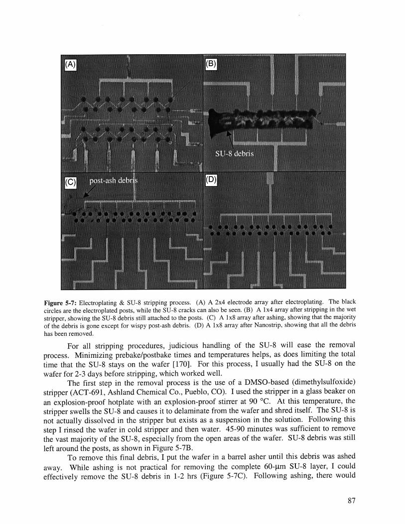
Figure 5-7: Electroplating & SU-8 stripping process. (A) A 2x4 electrode array after electroplating. The black

circles are the electroplated posts, while the SU-8 cracks can also be seen. (B) A 1x4 array after stripping in the wet

stripper, showing the SU-8 debris still attached to the posts. (C) A 1x8 array after ashing, showing that the majority

of the debris is gone except for wispy post-ash debris. (D) A 1x8 array after Nanostrip, showing that all the debris

has been removed.

For all stripping procedures, judicious handling of the SU-8 will ease the removal

process. Minimizing prebake/postbake times and temperatures helps, as does limiting the total

time that the SU-8 stays on the wafer [170]. For this process, I usually had the SU-8 on the

wafer for 2-3 days before stripping, which worked well.The first step in the removal process is the use of a DMSO-based (dimethylsulfoxide)

stripper (ACT-691, Ashland Chemical Co., Pueblo, CO). I used the stripper in a glass beaker on

an explosion-proof hotplate with an explosion-proof stirrer at 90 'C. At this temperature, the

stripper swells the SU-8 and causes it to delaminate from the wafer and shred itself. The SU-8 is

not actually dissolved in the stripper but exists as a suspension in the solution. Following this

step I rinsed the wafer in cold stripper and then water. 45-90 minutes was sufficient to remove

the vast majority of the SU-8, especially from the open areas of the wafer. SU-8 debris was still

left around the posts, as shown in Figure 5-7B.To remove this final debris, I put the wafer in a barrel asher until this debris was ashed

away. While ashing is not practical for removing the complete 60-gm SU-8 layer, I could

effectively remove the SU-8 debris in 1-2 hrs (Figure 5-7C). Following ashing, there would

87

often be wispy debris in and around the posts (but off the substrate). A quick 5-min Nanostriptreatment removed these, most likely by simply dragging them away during rinsing. The finalelectrode structure is shown in Figure 5-7D.

5.1.5 Titanium adhesion-layer removalThe next step is to remove the Ti layer that had served to provide electrical contact for

the electroplating (Figure 5-1F). If left in place, it would electrically short the posts together,preventing operation of the traps. Removal was straightforward with a dilute HF:H 20 etch,which did not attack the gold and at these timescales and concentrations did negligible damage tothe glass wafer. I endpointed the etch by looking to see when the wafer became transparent,indicating the loss of the titanium layer. Careful endpointing was necessary to preventundercutting and lift-off of the gold lines. After Ti layer removal, the electrode structure lookedas in Figure 5-8A. An underside view (Figure 5-8C) shows how the gold layer is undercut. Thisreinforces the need to start with gold lines that are as wide as possible and to endpoint the etchaccurately. Failure to do this can result in lift-off of the gold lines if the titanium layer is entirelyetched away. This two-step undercut (first gold, then titanium) was a major source of yield loss.

I found that a very thin film of unknown origin would be left over following the strippingprocess (Figure 5-8). The film could be distinguished under optical microscopy because of its

Figure 5-8: Electrodes after titanium removal. (A) Top-down optical micrograph of a 1x4 array (B) SEM closeupof a gold line, showing the attached residue film. This film can also be seen in (A) and (C). (C) Underside view ofthe posts, showing the titanium undercut during etching.

88

thin-film interference effects. Fluoroscope examination revealed that the film was not

fluorescent, and thus probably not an organic residue such as photoresist. Dektak and SEM

measurements showed it to be much thinner than 1 pm. Careful SEM analysis indicated that the

film was actually attached to the underside of the gold, but not to the substrate (Figure 5-8B),suggesting that the film was present on top of the titanium, and only became apparent following

Ti removal. This further suggests that the film is the result of some reaction between the Ti and

the SU-8, induced by either light, temperature, or the SU-8 stripper. As the film was non-

conductive (tested with a probe station), I did not investigate its properties further, although it is

probably a Ti/organic compound.

5.1.6 Forming the SU-8 channelI decided to form the channel out of SU-8 (Figure 5-9A). I did not use PDMS

(polydimethylsolixane), which has the advantage of being removable & reusable because the

validation experiments require accurate knowledge of the channel height, which may be difficult

to control given the compliance of the PDMS under pressure. In addition, for fluorescence

microscopy I reasoned that using a standard coverslip as the look-thru medium may result in less

distortion than looking through PDMS.The SU-8 channel formation is a straightforward SU-8 lithography step. I varied the spin

cycle to obtain a thicker film and varied the exposure, bake, and develop times, but otherwise the

process was the same as described above. There were no apparent problems with the SU-8

causing the posts to deform during application and the film thickness near the electrodes was not

affected by their presence.In Figure 5-10 I show SEMs of a completed 1x8 array device. One sees that the yield is

excellent within the array, and was approximately 30% across the wafer (with yield defined as

percentage of devices with all traps intact). The major yield-loss mechanisms were loss of posts

during the wet etching of the substrate interconnects or during handling after SU-8 mold

(A) (B) (C)

Figure 5-9: Final fabrication steps. (A) Forming the SU-8 channel. (B) Dicing and drilling the fluidic access holes.

(C) Capping the channel with a coverslip.

89

Figure 5-10: Final SEMs of the completed chips. (A) a 1x8 array in an SU-8 channel. (B) a close-up of the array.(C) A closeup of a single trap.

removal. The final electrodes have a tapered geometry and slightly domed tops (Figure 5-10C).

5.1.7 Final fabricationThe final steps, after channel formation, were to dice the wafers (Figure 5-9B), drill

fluidic access holes (Figure 5-9B), and cap the channel (Figure 5-9C). I'll describe the first twosteps in this section; capping the channel is done during packaging. The dicing was performedwith a conventional diesaw. I protected the posts during dicing by backfilling the channels withAZ4620 photoresist. After dicing, I soaked the chips in acetone to remove the photoresist.

Access holes were drilled into the glass with a 0.75-mm diamond-tipped drill bit (C. R.Laurence, Los Angeles, CA) registered to gold marks formed on the slide during the firstlithography step. The drilling of the holes usually resulted in a slightly tapered hole that waswider at the bottom of the chip, which actually eased in aligning the chip during packaging.

5.2 PackagingThe packaging requirements for the small array are three-fold. Electrically, I need to

bring 20-MIHz signals of a few volts to the electrode tips. Optically, I need to be able to performfluorescence microcopy of cells held in the traps. From a fluidics standpoint, I need to introducecell-containing liquids onto the chip at around 1 psi.

The packaging solution that meets these needs is shown in Figure 5-11. The electricalconnections start from the electrodes, go under the SU-8 channel out to the chip periphery, andare finally wire-bonded to a ceramic package that fits on a ZIF-socket and is connected to aprinted-circuit board. The optical solution is to use a coverslip to attain a high-fidelity opticaltransfer system that would be compatible with coverslip-corrected objectives. The package islow-profile, in that there are no protrusions above the plane of the coverslip, which makes it easyto mount the package under a conventional microscope. In addition, since the cells are at most-300 prm away for the objective, low-working-distance objectives with high numerical aperturescan be used. The fluidic connections are made with an aluminum block that has a protrusionwhich rises up through the middle of the ZIF socket and carries fluidic channel to the chip.Locking the ceramic carrier into the ZIF socket with o-rings in-between ensures a leak-proofseal.

90

(A) chip (B)tape

carrier

ZIF socket

o-rin boar~d

standoffsv-",

tubingaluminum block

flow path

Figure 5-11: Packaging of the extruded array. (A) Schematic and (B) photograph of the packaging assembly. An

aluminum block serves as the substrate. It has cutouts to carry the flow within tubing . The flow path continues

through o-rings and mates with the bottom of the ceramic carrier, thru double-sided tape, and into the channel on the

chip.

5.2.1 Assembling the packageThe packaging assembly starts with the diced chips (Figure 5-12A). The first step is to

drill the fluidic access holes, as described above. Concurrently, I take a 64-pin ceramic carrier

package with a 0.4"xO.4" die area (Spectrum Semiconductor Materials, Inc., San Jose, CA) and

drill holes in it (with the diamond drill bit) that will line up with the holes in the chip and the

holes in the aluminum package (Figure 5-12B). To mount the chip onto the ceramic carrier and

make fluid-tight seals, I use double-sided tape with openings cut in it for each of the holes.

At this point I gold wirebond the connections from the chip to the ceramic carrier.

Wirebonding will ensure that I can reliable transfer the signals necessary for operation to the

electrodes.Following wirebonding, I attach the coverslip top to the channel. The top is a coverslip

Figure 5-12: Assembling the packaging. (A) Naked chip and ceramic carrier, (B) with holes, (C) mounted together

with double-sided tape & the coverslip.

91

that has been scribed and cleaved to the approximate size of the outer channel dimensions. Imechanically clamp the coverslip on top of the channel and then apply five-minute epoxy to theassembly to create a fluidic seal (Figure 5-9C). One drawback to this assembly method is thatthe distance between the coverslip and the channel will vary depending on how much epoxyflows into the gap, which means that a secondary measurement of the channel height isnecessary. More importantly, it means that the coverslip and substrate may not be perfectlyparallel, which will introduce optical aberrations.

At this point the ceramic carrier is ready to mate with the rest of the package. Thisconsists of an aluminum block that has been shaped to have a protrusion (Figure 5-11 & Figure5-13). The bottom of the block has cutouts that carry 0.020" (I.D.) PEEK tubing (UpchurchScientific, Oak Harbor, WA). The tubing has been permanently bent with a heat gun and gluedonto the aluminum block with Ducco cement. The tubing serves as a low-void-volume fluidiccarrier from the edge of the block almost to the chip itself. The fluidic path briefly goes throughthe aluminum and then emerges on the top of the protrusion at a groove for a size #001 o-ring(Parker Hannifin Co., Lexington, KY).

A printed circuit board, which contains a simple circuit to drive the electrodes and a ZIFsocket (3M, St. Paul, MN) for the ceramic carrier to sit in, is mated to the aluminum block sothat the protrusion goes through an opening machined out of the ZIF socket. Clamping the chipinto the ZIF-socket automatically aligns and seals the fluidic connections and makes theelectrical connections to the circuit board, completing the package. This makes it relatively easyto interchange ceramic carriers, and hence chips, during testing.

The driving circuit is shown in Figure 5-14. The signal from the signal generator goes toa quad buffer (MAX496, Maxim Integrated Products, Sunnyvale, CA). Two of the electrodes oneach trap are wired to ground, while one is permanently wired to the output of the buffer. Theother is wired to the output of the buffer but through a SPDT switch, which allows switching ofthe electrode to ground, thereby controlling the trap. The four outputs of the quad buffer areequally shared between the permanently wired and controlled electrodes. While this circuit isnot electrically ideal, in that the SPDT switches are not designed to switch these types of signals,it works adequately for my purposes, and can send 20-MHz 5 Vpp signals with good fidelity tothe electrodes. Occasional ringing of the circuit occurs, but this is accompanied by an increase inthe supply current to the buffer and can be easily detected with the current monitor integratedinto the power supply. Switching the SPDT switches back and forth removes the ringing.

Figure 5-13: The aluminum fluidic carrier and printed circuit board.

92

signalgenerator

quad buffer

1 7 . . . . . . . .... ..

GND

GND

Figure 5-14: Electrical driving circuit.

5.3 Test setupThe test setup is identical to the one used in Chapter 3 except that it resides on a Zeiss

Universal upright fluorescence microscope (Figure 5-15). The microscope is equipped with afluorescent slider permitting four filter combinations. The microscope has been modified toallow the use of both reflected brightfield and epi-fluorescence by re-directing the brightfieldlightpath from the transmitted to the reflected mode. This requires the use of a half-silveredmirror in one slot of the filter slider. The microscope uses a halogen lamp for its brightfieldsource and a 150W Xenon lamp for its fluorescent source. It is equipped with both amonochrome video CCD camera (TM-7CN, Pulnix America, Inc., Sunnyvale, CA) and a cooledcolor-CCD imager (SPOT-RT Color, Diagnostic Instruments, Sterling Heights, MI).Unfortunately, I was unable to install an automatic shutter system because of the physical

microscope

fluorescentfilter slider -

fluidics

package

Figure 5-15: Photographs of the test setup.

93

SPDT

constraints of the microscope, and so performed all shuttering manually.

5.4 ConclusionIn this chapter I have described the fabrication process flow, packaging, and test setup

needed to fabricate, package, and test the extruded trap arrays. The process flow useselectroplating into an SU-8 mold to define the posts that are necessary for the new trap design.This process had to overcome the challenges of using and removing SU-8, which can be bothdifficult to apply and to remove. In addition, the process used wet etching of the gold substrateinterconnects and the use of an SU-8 chamber to ease the process complexity. The packagingdesign allows for easy assembly and interchangeability of individual chips, while meeting thestringent requirements for electrical input, optical access, and fluidic connection.

94

Chapter 6: Trap validation

The first objective upon completion of the array was to validate that the improved DEP traps doindeed exhibit stronger holding. To do this, I followed a similar testing protocol as for the planarquadrupole traps-measuring the release flowrate of beads under different conditions-andcompared the results to the model predictions, now using the as-fabricated rather than idealgeometries. As described below, the results do validate the predictions of superior trap strength.

6.1 Materials and Methods

6.1.1 MaterialsAll beads and solutions were prepared as in Chapter 2. I used the same three bead sizes asbefore-7.58 gm, 10.00 gm, and 13.20 pm-although with fresh 0.01 S/m HBSS solutionscontaining 0.5% (v/v) Triton X-100.

6.1.2 Test methodologyThe methodology was similar to what I used for the planar quadrupole traps: trap a bead at agiven voltage and measure the minimum flowrate needed to dislodge the bead from the trap. Islightly modified the testing procedure for use with the extruded traps. First, I considered a one-minute hold time as constituting holding to speed up the data-taking procedure. Initial testsshowed that the vast majority of beads held for one minute were indefinitely held. Second,instead of varying the applied flow to find the "true" release flowrate for a given voltage, Iincreased or decreased the flow monotonically and measured all release flowrates that I found. Ibelieve that this more closely approximates the true errors in the measurements and made theerror analysis much easier. Third, I obtained data from any of the three working traps in the 1x4array that I used, dictated by which trap(s) happened to be holding beads then. This gives abetter estimate of the variations within an array. Finally, I performed three runs on different days(over 2 weeks) to get a sense of the drift.

6.1.3 ModelingSimulations were performed using the modeling environment described in Chapter 2.Simulations encompassed both as-designed (no taper, and with as-drawn geometries) and as-fabricated geometries (described below). Bead simulations used the experimental parameters forthe holding experiments - p,=1.062 g/cm 3, q-,=0.01 S/m, o,=2x10 4 S/M, ep=2.5, f=1 MHz or 20MHz, w=2 mm. The chamber height (h), as described below, was 159.5 gm. Dipole andquadrupole force orders were simulated. Cell simulations used the same parameters, except thatu-=1 S/m. The nominal values for HL-60 cells were from [81], with C,,=1.6 pF/cm 2, GM=0.22S/cm 2, A=1 nm, eyt,=75 F/m & OcYt=0.75 S/m.

6.2 As-fabricated geometriesIn order to be able to compare experiments to predictions, I must know what the device

dimensions as fabricated really are. I performed measurements on the device and package to

95

extract parameters that would affect the modeling, so that I could perform simulations with theas-fabricated devices to accurately predict the trap strength.

6.2.1 Trap geometryFigure 6-1 shows SEMs of fabricated traps. While these traps are not the specific traps

used in the experiments, they are from the same wafer and so constitute a representative sample.In Figure 6-lA I show comparisons to the as-drawn geometries. The interconnect lines aresignificantly narrower (3.7 gm wide instead of 8 pm) than drawn, due to the gold-etch undercut,and slightly narrower than the anticipated width of 4 pm. The values that I used for the wiringgeometry in the revised simulations are shown in the figure and Table 6-1.

The negative tone of the SU-8 confers a conical shape to the posts, and modeling thistaper is necessary to accurately predict trap strength. This is because the taper breaks the axialsymmetry of the trap, creating a divergence in the field in the z-direction and thus a positive z-directed DEP force. As can be seen in Figure 6-1B, the taper is actually a compound taper, with

(A) (B)

Figure 6-1: (A) SEM of a completed trap overlaid with the mask drawing. The post tops appear larger than thedrawn geometries because this particular array was electroplated too long and mushroomed at the top of the posts.The numbers refer to lengths (in microns) of the various segments of the interconnect geometry that weresubsequently used in the electric-field modeling. (B) SEM of a fallen post, showing the taper angle along the lengthof the post. The taper varies between 2.00 and 3.10.

Dimension As-designed As-fabricated ModeledElectrode height 50 jim 47-50 gm 50 pm

Electrode diameter 20 jim 18-20 gm at top with a 18-20 pm at top with a20 - 30 taper 3.5 & 4.0 pm taper

Substrate interconnect width 8 pim drawn, 4 gm designed 3.7 gm 3.7 pmChamber width (w) 2 mm 1.983 ± 0.003 mm 2 mmChamber height (h) 150 pim 157-162 pim 159.5 pm

Table 6-1: Comparison between as-designed and as-fabricated geometries for the traps used in this chapter.

96

an upper-section taper of 3.10, a lower-section taper of 2.00, and an overall averaged taper of 2.40

using values from this SEM figure. For a 50-pm high post, the overall taper of 2.40 leads to a

4.2-jim difference in the diameter of the post between the top and bottom. Using a microscope-

mounted x-y micrometer stage I measured the taper of this post to be 4jm with approximately 1

jim of error, which is consistent with the SEM angle measurement.Another measurement that I performed was to use SEMs of top-down views of the posts

to get proportions of the diameters at the post top and bottom. From Figure 6-2, the tops of the

posts are 81% (Figure 6-2, left) and 84% (Figure 6-2, right) of the diameters of the bottoms. The

error in this measurement is due to the difficulty in assigning a diameter to the non-circular

profiles of the posts. However, using 18 jim as the diameter at the top of a 50-pm-high post

gives an overall taper of between 3.4 (84%) and 4.2 (81%) jm, which is consistent with the

measurements from Figure 6-1B.As I shall show below, the taper dramatically affects the predicted results. Assembling

the above measurements, I can state that the taper angle varies between 20 and 30 and is probably

multi-valued along the length of the post.I measured the height and diameter of the posts from the traps used in the validation

experiments. Heights ranged from 47-50 jm (<x>=48.1 ± 2.2 jm, n=12), measured with a

microscope-mounted z-axis micrometer, although the domed tops of the posts (Figure 5-10C)

make it difficult to precisely define the height. I measured the diameters at the top of the posts

with a microscope-mounted x-y micrometer stage. The values ranged from 18-20 pm (<x>=18.8

± 0.8 jm, n=5), with the primarily errors coming from the resolution of the micrometer stage (1

pm), the deviations from perfect circularity of the posts, and the domed character of the post

tops. I believe the absolute error to be about 1-2 pm.Assembling all this data, I modeled the traps to have the interconnect geometries as

described in Figure 6-1A, posts with 50 jm height, a taper of 3.5 jim (2.00) or 4.0 pm (2.30), and

Figure 6-2: Top-down SEMs of two posts (different sample than Figure 6-1), with the top and bottom diameters

circled. The major and minor axes of the ellipses, in arbitrary units, are given by the two numbers for each ellipse.

Approximate circle diameters can be obtained by averaging the values. The figure shows that the top dimensions

are smaller than the bottom dimensions. Averaging the dimensions to get an average diameter for each circle, the

left subfigure has an 81% ratio of top-to-bottom diameter while the right subfigure has an 84% ratio.

97

post diameters (at the top) of between 18 pm and 20 gm (Table 6-1).

6.2.2 Chamber geometryThe chamber width of the tested device was measured with a microscope-mounted x-y

micrometer stage to be 1.98 mm (<x>=1.983 ± 0.003 mm, n=3), and modeled as 2 mm. Thechamber height of the tested device was measured with a microscope-mounted z-axis micrometerto be 157-162 gm (<x>=159.6 ± 2.4 pm, n=9), and modeled as 159.5 jm. The chamber heightappeared to change over the course of the experiments as evidenced by the change in theappearance of the glue between the coverslip and the SU-8 chamber; by the end of theexperiments, water was seeping much farther into the space where the glue was than at thebeginning (but not leaking out of the chamber). This drift will affect the holding in an inverselylinear manner.

6.3 Results

6.3.1 Trap switchingI performed experiments to validate the single-electrode switching described in §4.3.3

and Figure 4-6. In Figure 6-3 I show three images of beads held in traps showing that I can turnone trap off independently of the other. Under flow, the released bead flows away when onlyone electrode is toggled between +V and ground.

6.3.2 Holding characteristics with beadsI performed experiments as described above to obtain the holding characteristics of these

traps. The results are shown in Figure 6-4. The error bars represent experimental errors of onestandard deviation. All release flowrate measurements were taken 3-8 times and on average 4.3times. The data demonstrates that the holding in these traps is size selective with larger beadsexhibiting stronger holding, as one would predict given the R3 dependence of the DEP force(dipole term). The stated error includes systematic deviations between individual traps-onetrap was consistently weaker than the other two.

In Figure 6-5 I show comparisons between the experimental results and the modeling

Fluid Flow

Figure 6-3: Movie frames showing electrical control of the traps. (A) Flow (3 pl/min) is applied from left to right,with two 10.0-pm beads held in each of two traps. (B & C) The bottom trap is turned off by switching its bottom-right electrode, causing the bead to flow away while the bead in the top trap is held. Traps were energized at 1.5 Vand 1 MHz.

98

50

-40--13.2-A beads

a) 031 0.0--pm beads

20-CU

1D -D 7.6-Am beads~10o

00 1 2 3 4

Voltage (V)

Figure 6-4: Superimposed data for holding characteristics. Shown are the results of release flowrate measurementswith 7.6-pm (o), 10.0-pm (x), and 13.2-pim (V) beads in the extruded trap. Measurements were performed at 1MHz.

using a 3.5-pm taper. The smaller model prediction in each subplot corresponds to a postdiameter of 18-21.5 gim, while the larger model prediction corresponds to a post diameter of 19-22.5 pim. As stated before, this is within the limit of my measurements of the post diameter. Themodel predictions for the 18-21.5-gm post diameter for the 7.6-gm beads (Figure 6-5A) hassome numerical noise in it, similar to the effects seen in the planar quadrupole holdingcharacteristics in Chapter 3. There is no physical significance to this noise.

The first feature to notice is that for all bead sizes the experimental data is bounded bythe predictions. Furthermore these are absolute predictions, as for the planar quadrupole. Thus,the model is further validated. Second, the traps are working as predicted, which is a validationof the design methodology.

It is possible to obtain a best fit, within the experimentally measured post diameters, byfinding the linearly interpolated post diameter that would minimize the error between theexperiments and models. While there is not any absolute knowledge gained by this maneuver, itdoes allow for easier visual representation and manipulation of the data. Ideally the fit would beindependent of which set of data was used to generate it. In other words, fitting to the 7.6-gmbead characteristic should give the same fitted post diameter as a fit to the 13.2-gm beadcharacteristic. Unfortunately, the modeling is not perfect and this is not the case.

Lacking this, one might fit the data using the 7.6-gm beads and extrapolate the results forthe larger beads. The rational here is that the smallest bead is least likely to be disturbed by 2 "d-order effects, such as fluid flow, that are not accounted for in our model and therefore thoseresults are likely to be most accurate. Unfortunately, Figure 6-5A shows that the simulations for

the two post diameters are not well spread out and so the resultant fit will likely not be precise.

99

40

C 30

S200

CD,

10

a0

40

60

a)_40

0

CO,cz 20(D

02

Voltage (V)

60

50

40

3,0020I U

(A)

0 1 2 3Voltage (V)

(C) 1

- ~/ -

80

E

0

CDC,,Caa)

60

40

20

03

(B)/

1 2g

0 12

Voltage (V)

(D)

0 1 2Voltage (V)

Figure 6-5: Model predictions of the holding characteristics. The data is shown as discrete points while thesimulation results are shown for 18-21.5-jim (-) and 19-22.5-pim (---) posts. The data and predictions are shownfor (A) 7.6-jm (o), (B) 10.0-jm (x), and (C) 13.2-jm (V) bead diameters. (D) Plotted is a best-fit interpolation(18.7-22.2-ptm diameter posts) of the predictions to the data in (B) and then the use of that fit parameter to predictthe holding characteristics for the other bead sizes.

Using the 10-gm bead characteristics for the fit is a good compromise between minimizing the2"d-order effects while maximizing the fitting resolution.

Figure 6-5D shows the results of linearly interpolating the results for the 10.0-gm beadsand then extrapolating the extracted post diameter to the other two bead sizes. The post diametercorresponding to this fit is 18.7 gim, which is very close to the measured average post diameter asdescribed above (see §6.2.1). This results in a maximum error between the fit and the dataaverages of 1.1 gl/min (4% of full scale (FS)) for the 7.6-gm beads, 1.2 gl/min (3% of FS) forthe 10.0-gm beads, and 2.2 gl/min (5% of FS) for the 13.2-gm beads. Incorporating themeasurement errors, only 7 of 28 simulated values fall outside the lc measurement errors, with amaximum miss of 0.7 gl/min. Using a 2y measurement error (corresponding to a 87%confidence level), all predictions fall within the experiments. Two data points whose measuredexperimental precision was 0 gl/min will never match predictions without incorporatingsystematic experimental errors, which I have not done.

With confidence in the model I can extract the holding forces from the simulations, asshown in Figure 6-6. The results show the greatly increased strength of the new trap, as

100

0

0 1

3

)

3

.

-

compared to the planar trap (see also Figure 4-14). For instance, a 10.0-pLm bead is held with 65pN of force at 2V, as opposed to the 0.5-1 pN of the planar quadrupole. The trap is indeed 10-100x stronger, as predicted in §4.5.

6.3.3 Holding characteristics with cellsTo see if the traps are meeting the system requirements for the gDAC, I ran simulations

with HL-60 cells using the validated as-fabricated geometries. I used parameters for HL-60 cellsgiven in §4.4.3 with an applied frequency was 20 MHz.

In Figure 6-7 I show the holding characteristics and holding forces for the HL-60 cells inthis system. These differ from the ideal characteristics given in Figure 4-13 because of thedifference between designed and as-fabricated geometries. As can be seen, however, thedifference is slight and thus the operating conditions determined in §4.5 are still valid.

6.4 Discussion

6.4.1 Model and trap validationThe results described above demonstrate the utility of the modeling environment for

designing DEP-based traps for bioscience applications. I have been able to a priori design a trapgeometry that could meet the system applications of the gDAC without performing any trial-and-error experiments. In addition, the geometry used for the extruded traps is much morecomplicated than the planar quadrupole, involving an asymmetric electrode placement, exposedwiring within the trap, and the tapered three-dimensional profile of the posts. Despite all of thesechallenges, the model has been successful in predicting the performance of these traps.

300(A) - 13.2-pim (B)

- -- 10.0-ptm 2

250- 7.6-i m 10- 10.0-pim, planar

Z 200 - -0CL0,D

40 150 - ; $100..9 10

5~10 - ~ 10 0

50

0.5 1 1.5 2 2.5 3 0.5 1 1.5 2 2.5 3Voltage (V) Voltage (V)

Figure 6-6: Extracted holding forces of the extruded quadrupole traps, using the same fit as for the holdingcharacteristics (Figure 6-5D). Plotted are holding forces for 13.2-jim (-), 10.0-jim (---), and 7.6-jim (....) beadsusing (A) linear and (B) logarithmic scales. Also shown (-) for comparison are the results from Figure 4-14 for10.0-jim beads in the planar quadrupole. In (A) the results for the planar quadrupole (-) are so small that they lieon the x-axis.

101

15 60(A) ___--as-fabricated (B)

---- as-designed 5-

10- z40-

0 30

C5- OC20-

10

0 00.5 1 1.5 2 2.5 3 0.5 1 1.5 2 2.5 3

Voltage (V) Voltage (V)

Figure 6-7: Simulated holding characteristics for HL-60 cells in the finalized traps, interpolated using the same fitas for the beads and compared to the designed holding characteristics of Figure 4-13. (A) Release flowrate versusvoltage for the as-designed (---) and as-fabricated (-) traps. (B) Extracted holding forces versus voltage for thedesigned (---) and as-fabricated (-) traps.

The results also demonstrate an internal consistency to the design process-the modelingand the trap are both validated by these measurements. This validation, coupled with the resultsfrom the planar quadrupole, strongly suggest that such modeling could be useful in the future.

Looking at the dipole form of the DEP force (Eqn. (1-1)), one would expect the trappingto follow an R3 law. Figure 6-4 shows that the ratio is actually less than that. In fact, the holdinggoes approximately as Rx with x=1.4-1.5. A possible explanation for this can be seen in Figure6-8, where I have plotted that predicted locations of the particles at release. Although thepredicted characteristics contain significant numerical noise at V=1V and 3V (due to thediscretization of the problem space), they do suggest that the particle positions differ for thedifferent bead sizes. If this is true then since all three particles settle into the different releasepoints, the drags and DEP forces experienced will differ, and can account for the observed non-cubed-law behavior. In fact, the discrepancy reinforces the utility of the model in accounting forthe complex behaviors in these traps.

6.4.2 Deviation between model and experimentAlthough the model certainly has succeeded in predicting the holding characteristics for

beads in the extruded quadrupole traps, I can speculate as the origins of the remaining deviationsbetween experiment and model. This is useful in trying to ascertain the appropriate space withinwhich the model has predictive power, which is necessary for future designs. One must reiteratehowever that the agreement, as depicted in Figure 6-5, is within the experimental error and thusthe model predicts the experimental results extremely well. This is much better than could beexpected in a real-world situation involving cells, whose variable size and electrical propertiescould swamp any 2 "-order effects neglected in the model. For the purposes of real-worldoperation one must pick an operating regime (flow, voltage, frequency) such that there is acomfortable margin in the holding characteristics for all encountered particle variations. Such a

102

15 -

(A)14 -_-_---_-_-_-

E13 -

12

11-1 (B

-1.2

L -1.4

-1.6

-1.818 - - -

(C)

E - - --

N 16 '77

15I0.5 1 1.5 2 2.5 3 3.5

Voltage (V)

Figure 6-8: Predicted particle locations at release using the interpolated results. Plotted are the simulated x-

locations (A), y-locations (B), and z-locations (C) of the 13.2-jtm (-), 10.0-pm (---), and 7.6-gm (---) beads rightbelow the release flowrate. The coordinates are as defined in Figure 4-3A.

design falls outside the scope of this thesis, but the path towards its implementation is clear andthe necessary design tools are now in place.

Several effects have been neglected in the model. Besides those described in Chapter 3(EHD, HD lift forces), several are specific to the extruded geometries. First and foremost, themodeled flow field (Poiseuille) is clearly different from the actual flow pattern, which will befully three-dimensional in the vicinity of the electrodes. The deviation is insignificant forpredictions using the extruded quadrupole, but other geometries that might disturb the flowfurther would benefit from full CFD modeling. Such modeling could also be used to design theelectrode structure to physically control the flow in addition to controlling the electric fields.This would add another "knob" in the design and could lead to higher performance.

Second, care must be taken to ensure that the simulated geometries match what isactually being fabricated. In my case, the deviations in the as-fabricated geometry from thedesigns significantly affect the predictions. First, the compound taper has not been modeled, noris the actual taper exactly as modeled. In Figure 6-9 I show the comparisons of simulationsusing 3.5-jtm and 4.0-pm tapers. The different taper angle influences the characteristics for thelarger bead sizes dramatically, even though the posts are only 1 gm closer together at thesubstrate. The 4.0-gm taper reduces the separation between the holding characteristics for the

103

60

50-

40 -13.2-pm

30-0

a)CO)

A20-

10 -o

7.6-tm

0.5 1 1.5 2 2.5 3 3.5Voltage (V)

Figure 6-9: Comparison between the simulated holding characteristics of beads in traps with 3.5-gm (-) and 4.0-pm (---) electrode tapers. All posts have an 18-pm top diameter and are 50-pm tall. Results from the 3.5-gmtapered traps exhibit a higher slope at large voltages and bead diameters than the 4.0-gm tapered traps. The 3.5-gmtapered traps better represent the data (see Figure 6-5).

10.0-gm and 13.2-gm beads. The 3.5-gm taper, used in the fits in Figure 6-5, gives a betterrepresentation of the data. This is consistent with the fact that the beads are to be found near thelower half of the posts (Figure 6-8) where the taper is closer to 2.0' (corresponding to 3.5-gm),as shown in Figure 6-2. Generating trap designs that are robust to such variations is aninteresting future use of the modeling, and a readily conceivable one.

The previous discussion emphasizes that the sensitivity of the predictions with respect tothe post geometry could easily result in the deviations. Another geometrical deviation is thatsome of the posts may not be exactly perpendicular to the substrate. This could be caused duringfabrication-a common mechanism for yield loss was non-perpendicular posts. Although thetested devices did not display overt non-perpendicularity, it is still possible to be off a fewdegrees and remain visually undetectable. A final geometrical discrepancy is that the posts arenot perfectly spherical, as demonstrated in Figure 6-2.

6.4.3 Comparison to existing trapsAlthough I have established that this trap holds better than the planar quadrupole

described in Chapter 3, it is necessary to compare it to other DEP and non-DEP traps to fairlyevaluate it. As described in Chapter 1, the DEP community can be split into researchers who useDEP for separations and those who use it for trapping. As early as 1993, the group at HumboldtUniversity in Berlin described how a three-dimensional electrode configuration in the form anoctopole (Figure 1-4) was necessary to "close" the trap and obtain a cage and, presumably, highholding [93]. This group has since exclusively explored this configuration and has recentlystarted performing quantitative trapping experiments. My search through the literature hasrevealed no other researchers interested in using DEP traps to hold particles against flows.

104

I I I I I

Among the five reports from the Fuhr group that mention some quantitative measure oftrap strength [85, 98, 143, 148, 149], I have chosen to compare the extruded trap to their mostrecent report [98]. The reason for this is that it contains the most complete description of theexperimental parameters, enabling a fair comparison. This report describes the strength of theoctopole for holding particles against flow under various electrical excitation schemes. Thecomparison is summarized in Table 6-2.

The first issue in making a comparison resides in whether to compare the trapperformance at equivalent voltages or equivalent electric-field strengths. The former can beviewed as an extrinsic comparison and the latter as an intrinsic one, because the forcesfundamentally depend on electric fields, not voltages. Unfortunately, it is difficult to compareelectric fields because the non-uniform (i.e. non-spatially constant) nature of the fields in DEPmakes it impossible to obtain a single value for their strength. I have thus chosen to compare thetrap strengths at equivalent voltages. Because the characteristic electrode separation is similarfor both traps, however, the electric fields will be similar and thus the comparison can be viewedas both extrinsinc and intrinsic.

In addition, since both traps will increase in strength monotonically with voltage, thereare no system-level constraints on the maximum voltage applied; the upper limit will be thedetermined by the generation of EHD flows due to heating effects. Thus, both traps can becompared at equivalent voltages.

From the dipole approximation to the DEP force (Eqn. (1-1)), one sees that an accuratecomparison requires normalization for different particle radii, CM factors, media permittivitiesand electric field strengths. The last factor is accounted for by comparing at the same voltage,and the media permittivities are the same because both traps are used in water. Table 6-2 showsthat the real parts of the calculated CM factors are nearly identical. This is because at thesefrequencies the CM factor is dominated by the media conductivity, which is much higher thanthe particle conductivity. Use in physiological saline would not change the CM factors, and thusthe comparison would still hold.

The particle radii are different, so I have normalized their results by the cube of the ratio,using the R3 dependence of the DEP force. I can perform this normalization for the octopole trapbecause the particle location will not be dependent on its size-it will always be held at themidstream. For the extruded quadrupole the particle locations change with radius, and thus thestrict R3dependence does not hold.

The results show that the extruded trap is significantly stronger than the opposedoctopole-the holding forces are -5x larger for similar fields. Although their trap is much easierto fabricate, it is much more difficult to package (because one needs to align the opposedquadrupoles and then make electrical connections to an upside-down substrate). In addition, theheight of their chamber is locked to the characteristic dimension of their trap-the separation

Eectrode Partide Linear Vdum-eEectrode spacing cianreter flowate flowrate Holcng force Norrlized

configuration (JM) (pm) CMfactor (rms) (Vrrin) (p) holdcingoctopole 40 14.9 -0.47 0.2 0.13 28 20extrded

quadrnpoe 40 13.2 -0.48 1.3 15 95 95

Table 6-2: Comparison of holding against flow between the opposed octopole and the extruded quadrupole trap forbeads. The normalized holding for the octopole was obtained from scaling by the cube of the particle radii. Thevolume flowrate for the octopole results was obtained from the given linear flowrate and the chamber dimensions.The extruded quadrupole exhibits higher holding against volume & linear flowrates and higher holding forces.

105

between the opposed quadrupoles. The extruded quadrupole relaxes this constraint, addinganother variable into the design process. Thus, the work involved in the complex design of theextruded quadrupole is rewarded.

The other comparison to make is to optical tweezers, which may have significant usageoverlap. Optical tweezers are advantageous when one needs long-range three-axis control ofsingle particles or when electric access is difficult to achieve. However, if one only needs tolocalize a particle, wants to trap many particles, or does not have easy optical access, then DEPbecomes the trapping method of choice. In terms of strength, optical tweezers usually haveholding strengths of a 1-100 piconewtons [151, 152], which are similar to those attainable withthe extruded trap.

6.4.4 Holding forcesThe extracted holding forces (Figure 6-6) are more than those experienced in

conventional traps, and -5x larger than in the opposed octopole. Although these results werepredicted, they still may appear startling. A few simple calculations to show self-consistencydemonstrate that these results are indeed reasonable.

First, since the drag force in the trap is less than the drag force at the centerline of thechamber, the holding force of a particle in the trap must be less than the drag force on the sameparticle along the centerline. This is because the parabolic flow profile necessitates that theparticle in the trap is exposed to a flow velocity that is smaller than the centerline velocity

(Figure 6-10). In Figure 6-11 I plot, along with the calculated holding forces of 13.2-gm beads

in the extruded traps (as in Figure 6-6), the Stokes' drag on 13.2-pm beads in the centerline ofthe chamber at the release flowrate. The relevant expression is

Fragcenterlne = 67nrhRU, = 6;ri7R *Qrf (6-1)

The plot shows that the centerline drag force is indeed always larger than the holding force. Afurther refinement can be taken by simply correcting the centerline drag to the fluid velocity atthe height of the particle

velocity profiledrag force

chamber centerline

7]._particle

- .electrode

Figure 6-10: Depiction of drag force on particles in the chamber. Shown is the parabolic flow velocity profile (in

gray) and the drag force profile (in thick black). The drag force follows the velocity profile except near the edges,

where particle-wall interactions alter the profile (indicated by dotted black line). The drag on a particle in the trap is

smaller than at the centerline because it is near the edge of the parabolic flow profile.

106

140

120- holding force --- centerline drag

100- cell-ht drag

0 6040-60-

00.5 1 1.5 2 2.5 3

Voltage (V)

Figure 6-11: Holding forces in extruded traps. Plotted is the computed holding force on 13.2-pm beads in the

extruded traps as the voltage is varied (-), along with the drag force at the centerline of the flow (---) and at theparticle height found using eqn (6-2) (--). The computed holding force is always smaller than the centerline drag,as expected, and remarkably close to the results obtained using the flowrate-corrected Stokes' drag (Eqn. (6-2)).

Z 2~

Fdrgta 67ziiRU(z) = Fdg,,rj, Iz-j (6-2)

where z refers to the height of the particle above the substrate. The expression in the brackets isthe parabolic velocity profile found in the parallel-plate chamber. The results of this are alsoshown in Figure 6-11, demonstrating that this simple expression approximates the observedholding forces very well. Thus, the holding forces are in-line with what would be expected atthose flows, increasing our confidence in the strength of these traps.

Such good agreement with such a simple model might inspire the question as to why Iuse a complicated model (described in Chapter 2) for the drag forces. The reason for the goodagreement with this simple model is that for the extruded traps the particles are held relatively faraway from the wall, and so the 2nd-order flow disturbances due to particle-wall interactions areminimized. Since it is not possible to know where the particle will be when designing a newtrap, the more complete flow model is necessary. This is seen in the design for the planarquadrupole, where the particle is found on the substrate for low voltages.

6.4.5 Outlook for future trap designGiven the knowledge obtained about trap design, I can give qualitative speculations as to

how to make future traps even stronger. I want to stress, however, that strength isn't everything.Other system parameters, given that the strength is adequate, may become "bottlenecks."Nevertheless, several things are apparent.

First, one reason for the high trap strength is that the low height of the particle above thesubstrate shields it from the drag force. An easy way to increase the strength even further is tolower that height. Figure 6-8 shows that the particles average about -16 im above the surfaceand thus could be lowered. Several ways exist to accomplish this. First, the upward DEP force

107

is due to the slope of the posts and the wiring in the center of the trap. Removing the effect ofthe wiring by passivating it and tailoring the slope of the posts (perhaps even making themreentrant) could tailor the height of the particle, even pushing it against the substrate, therebymaximally shielding it from the flow.

From a fabrication/packaging standpoint, making robust traps is crucial. The current trapgeometry is very stable during operation-not a single post has been damaged after packaging.However, gold is soft, and the posts can easily get bent during fabrication steps, especially wetsteps. This can be alleviated by either 1) using a different geometry without posts, 2) increasingthe diameter of the posts, 3) encapsulating the posts in SU-8 till after diesaw, or 4) using a hardermetal.

Finally, the strong sensitivity of the predicted trap performance on the taper anglesuggests that this specific trap geometry is not robust towards processing variations. Designing atrap where taper angle does not affect the position of the particle or the electric field strength,such as a trap that forces the particle to the substrate, should be much more stable in this regard.

6.5 ConclusionIn this chapter I have described initial tests with the extruded traps demonstrating that

they indeed operate as designed. Similar to the experiments performed in Chapter 3, I have usedbeads as surrogate cells to quantitatively determine the holding forces in these traps. Thepredicted holding characteristics, once adjusted for the actual geometries of the fabricateddevice, are very close to the observations. This demonstrates that the modeling environment canbe used for predictive design of traps much different that those it was validated with, and that itthus is a truly useful tool. In addition, these results introduce the extruded quadrupole trap intothe literature, which, although more difficult to fabricate over planar traps, has numerousadvantages.

108

Chapter 7: Cell-based operation

Up to this point, I have designed and fabricated an array of extruded quadrupole traps thathave been shown to hold beads stronger than the planar quadrupole traps. In this chapter, I willdemonstrate the use of these traps with cells, showing the proof-of-concept operation of thepDAC. The capabilities that constitute proof-of-concept operation are: holding with cells,single-cell discrimination, independent trap control, and dynamic fluorescent assays.

7.1 Materials and Methods

7.1.1 Cell cultureHL-60 cells were obtained from ATCC (Manassas, VA). They were cultured in T25 or T75flasks in RPMI-1640 (BioWhittaker, Walkersville, MID) with 5% (v/v) fetal bovine serum (JRHBiosciences, Lenexa, KS), 2 mM L-glutamine (Sigma, St. Louis, MO), 100 I1U/ml penicillin, and100 gg/ml streptomycin (Sigma Cell Culture, St. Louis, MO) in a 95% 02/5% CO 2 atmosphereat 37 'C. Cultures were maintained between 105 and 106 cells/ml. They were subculturedapproximately every 7 days by gently pippetting the media up and down to break up clumps andadding cell suspension to fresh media to obtain a cell density of 105 cells/ml (determined byTrypan Blue dye exclusion with a hemacytometer).

7.1.2 Assay bufferThe assay buffer was made by adding 10 mg/ml of bovine serum albumin (BSA,

Boehringer Manheim, Indianapolis, IN) to Hank's Buffered Salt Solution (HBSS, GibcoBRL,Grand Island, NY). The detergent solution was made by adding 100 gg/ml of sodium dodecylsulfate (SDS, GibcoBRL, Grand Island, NY) to the assay buffer.

7.1.3 Cell assay preparationAliquots of cells were obtained from the flasks. They were centrifuged for 5-8 min at

125 x g and the supernatant discarded. Fresh assay buffer was added and this Procedure wasrepeated 2x, with the final volume adjusted to obtain a cell concentration of -4x10 cells/ml.

7.1.4 Calcein labelingFor calcein labeling or leakage experiments, calcein-AM (Molecular Probes, Eugene,

OR) was added to the assay buffer to obtain a concentration of 10 jiM. Equal volumes of thiscalcein solution were added to the cells suspended in the assay buffer, to obtain a final calceinconcentration of 5 pM, and incubated at room temperature for 30-45 minutes. Followingincubation, the cells were washed in the assay buffer 2x to remove extracellular calcein from thesolution.

Aliquots of the calcein-labeled cell suspensions were added to the chamber via theinjection valve (Figure 3-1C). To perform calcein leakage experiments, the detergent solutionwas subsequently introduced into the chamber via the four-way valve (Figure 3-iC) after thecells had been trapped.

109

Calcein-loading experiments were performed by injecting unlabeled cells into thechamber, capturing them in the traps, and then using the four-way valve to inject 1 gM or 10 gMcalcein in the assay buffer.

7.1.5 Electrode TrapsThe extruded quadrupoles were prepared as described in 0. For the holding experiments, I usedthe same trap array that was used in 0, while other devices were used for the rest of theexperiments presented in this chapter. The packaging and test setup are also as described in 0.

7.1.6 Chamber purging and cleaningBefore commencing any cell injections, the chamber was flushed with the assay buffer for -20min, usually at 50 gl/min. After experiments were complete, the chamber was cleaned with -1ml of HBSS/BSA solution, then -1 ml of HBSS/Triton X-100 solution, then -1 ml of DI H20,and finally dried with N2.

7.1.7 OpticsThe devices were observed under a Zeiss Universal upright microscope, modified for use withboth epi-fluorescence and reflected brightfield illumination. A filter set for calcein, comprised ofa 485-nm bandpass excitation filter, a 505-nm dichroic filter, and a 530-nm longpass emissionfilter was obtained from Omega Optical (Brattleboro, VT) and thinned to 3-mm thickness to fitinto the microscope's filter slots. Images were recorded with a video camera (TM-7CN, PulnixAmerica, Inc., Sunnyvale, CA) or a cooled-color CCD (Spot-RT Color, Diagnostic Instruments,Sterling Heights, MI) and stored on a Pentium-class computer. Time-lapse images weremanually shuttered because of the difficulty of attaching an automatic shutter to the microscope.Movies were captured with a Pinnacle Systems DC10plus analog capture board (Mountain View,CA) connected to the video camera.

7.1.8 Image analysisVarious still-image analysis operations were performed using either Scion Image (ScionCorporation, Frederick, MI), Adobe Photoshop (Adobe Corporation, San Jose, CA), or theMatlab Image Processing Toolbox (The Mathworks, Natick, MA). Movies were edited usingeither the DC10plus software or Adobe Premiere (Adobe Corporation, San Jose, CA). Celldiameters for the holding experiments were obtained by converting measured pixel distances toactual lengths via calibrations obtained at different magnifications with a ruled microscope slide.

Fluorescence intensities for the dynamic assays were determined via Matlab. Algorithmsfound the pixel area comprising each cell in a series of time-lapse images by thresholding theimages. From the pixel values, the mean and maximum intensity values could be recorded.Other values, such as cell area (in pixels), could easily be determined from the thresholdedimage. A swath of nominally dark pixels was used to determine the background intensity level,which was subtracted from the measurements. Changes in the exposure time or gain of thecamera were compensated for by linearly scaling the measured pixel values.

Multicolor images were created by adding the grayscale fluorescence images to the greenchannel of color brightfield images in either Photoshop or Matlab.

110

7.1.9 Release flowrate measurementsThe release flowrate measurements were performed identically to those in Chapter 3. Briefly,after trapping a cell, an image was taken so that its diameter could be subsequently determined.Flow was initiated, and if the cell stayed in the trap for 60 sec, the cell was considered captured.The flowrate was increased in 1 pl/min steps until the cell was ejected, and this flowrate wastermed the release flowrate.

7.1.10 ModelingAll modeling to compare to the measured holding characteristics used the as-fabricatedgeometries, as described in Chapter 6. Although the cell membrane capacitance varied in thesimulations (described below), the nominal values for HL-60 cells were from [81], with C=1.6pF/cm 2, G.=0.22 S/cm 2, A=1 nm, eyt,=75 F/m & cyT=0.75 S/m.

7.2 Results

7.2.1 Qualitative operationArray loading

Array operation with cells was fairly straightforward. After warming up the electronicequipment and purging the chamber with -1 ml of the assay buffer run at 50 gl/min, I wouldinject a -50-55 pl plug of cells. After the cell-containing aliquot had started to enter thechamber, I would turn off the flow for -1-2 min to allow the cells to settle to the chamberbottom. At this point I would restart the flow, but at a flowrate that was less than the releaseflowrate for a given voltage & frequency. Cells near the surface of chip would flow by the arrayand be trapped, while cells far above the substrate would simply flow over the traps. The use ofBSA in the assay buffer was advantageous here in that it prevented cells from adhering to thesubstrate after they had settled.

A typical example of array loading is shown in Figure 7-1, which shows the loading of a1x8 array with calcein-labeled HL-60 cells. The first image (Figure 7-1A) was taken 5 sec afterthe application of flow, but before any cells were loaded into the array. One cell (solid arrow) isnearing trap #6, while two other cells (dotted arrows) approach trap #3. In Figure 7-1B, the firstcell has been trapped, and by Figure 7-1D, 9.5 sec after the start of the flow, the two cellsdenoted by the dotted arrows have been loaded into trap #3. Figure 7-1F and Figure 7-iG showa similar situation with two cells being loaded into trap #5. Figure 7-ID and Figure 7-1E show acell (solid arrow) that is being repelled from the post and is driven crosswise against the flowinto trap #4. 23 seconds after the start of flow, six of the eight traps have been loaded with cells.Since one trap (#2) does not work, this means that six of seven functional traps have been loadedin 23 seconds.

This loading sequence, which is typical, demonstrates a few common themes in operatingthese traps. First, in the loading phase, when the applied flow is much less than the releaseflowrate for the given operating conditions, it is likely that more than one cell will be loaded intoa given trap. Second, the actual loading time will vary with cell concentration and flowrate-introducing a high concentration of cells will load the trap very quickly, but will also make itmuch more probable that >1 cell will be trapped in a given site. Obtaining one cell-per-trap,after loading, is the topic of the next section. Third, the trapezoidal structure of the posts aids the

ill

t=5 s

Hi

t=12 s 5 S t=16 s t=23 s

Figure 7-1: Loading a 1x8 array of traps with calcein-labeled HL-60 cells. Shown are fluorescence images

extracted from video with the post locations superimposed and denoted by gray circles. The cell intensities were

scaled and gamma-shifted to make them easier to visualize. The flowrate was 10 gl/min from left to right while the

electrodes were energized at 3V and 20 MHz. The time stamp of the frames (after the initiation of flow) is given in

the bottom left of each frame.

loading process-both physically by the obstruction of the posts and also electrically due to thelower loading barrier (Figure 4-4).Single-cell discrimination

One of the requirements of the gDAC is that the traps must be able to be set to hold onlyone cell per site. In Figure 7-1, I show that after loading it is possible that some traps will holdmore than one cell. Single-cell discrimination can be performed after loading by applying a

flowrate that is close to but less than the release flowrate for a given set of conditions. Startingwith a loaded trap, I can effect single-cell discrimination by now applying a higher flowrate than

during loading. As shown in Figure 7-2, this causes the cells to revolve around each other. Themaximum separation between the cells increases as the flowrate increases, until one of the cells

is released. This is seen happening in Figure 7-2D at a flowrate of 12 gl/min, 30 seconds afterthe 2nd cell was caught.

While the operating conditions needed to obtain discrimination are obtained empirically,they still follow the pattern shown in Figure 3-3. One additional complication of using cells isthat the operating window for obtaining single-cell discrimination is smaller than with beads, for

112

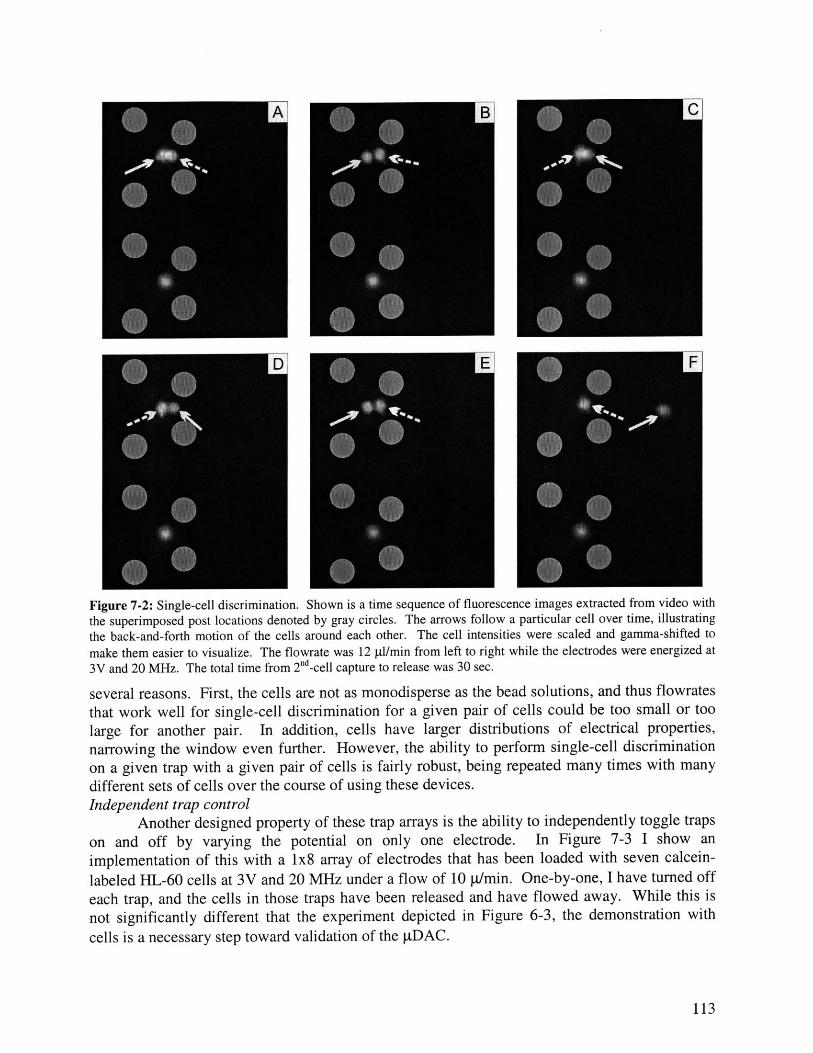
Figure 7-2: Single-cell discrimination. Shown is a time sequence of fluorescence images extracted from video with

the superimposed post locations denoted by gray circles. The arrows follow a particular cell over time, illustrating

the back-and-forth motion of the cells around each other. The cell intensities were scaled and gamma-shifted to

make them easier to visualize. The flowrate was 12 pl/min from left to right while the electrodes were energized at

3V and 20 MHz. The total time from 2 d-cell capture to release was 30 sec.

several reasons. First, the cells are not as monodisperse as the bead solutions, and thus flowrates

that work well for single-cell discrimination for a given pair of cells could be too small or too

large for another pair. In addition, cells have larger distributions of electrical properties,

narrowing the window even further. However, the ability to perform single-cell discrimination

on a given trap with a given pair of cells is fairly robust, being repeated many times with many

different sets of cells over the course of using these devices.Independent trap control

Another designed property of these trap arrays is the ability to independently toggle traps

on and off by varying the potential on only one electrode. In Figure 7-3 I show an

implementation of this with a 1x8 array of electrodes that has been loaded with seven calcein-

labeled HL-60 cells at 3V and 20 MiHz under a flow of 10 p/min. One-by-one, I have turned off

each trap, and the cells in those traps have been released and have flowed away. While this is

not significantly different that the experiment depicted in Figure 6-3, the demonstration with

cells is a necessary step toward validation of the pDAC.

113

Figure 7-3: Independent trap control. Shown are a series of composite brightfield and fluorescence images

illustrating selective and independent trap control. Seven calcein-labeled HL-60 cells, trapped in a 1x8 array, are

individually released in a defined yet arbitrary manner in Panels 1 to 8. The arrows indicate the cell locations, while

the black box indicates the trap that was just turned off. Electrodes were energized with 3V at 20 MHz and flow

was from left-to-right at 10 p1/min.

114

7.2.2 Quantitative operationHolding with cells

Following qualitative validation of the operation of the small array with cells, the firstquantitative experiments sought to determine if Figure 6-7 gives a correct representation of theholding characteristics of cells. Given the validation experiments performed with beads inChapter 6, the idea here was not to validate the modeling but rather to determine if the electricalmodel of the cell that I used was reasonable. The reason for this is that the difference betweenbeads and cells will only manifest itself in the CM factor (and, if they are different sizes, in theR3 factor). Thus, if the bead experiments compare well with the model predictions, which theydo, then any deviations with cells can be isolated to an incorrect model for the CM factor.

I performed holding experiments with ten different unlabeled cells in one of the traps ofthe same device used in Chapter 6. I varied the frequency between 1 MHz, 10 MHZ, and 20MHz, and chose three voltage points IV, 2V, and 3V. Each cell was used for between one andfour data points, depending on whether I could retrieve it after it was released, for a total of 14data points. I obtained the diameters of each of the cells from images taken with the CCDcamera. The average cell diameter was 11.4 gm, with a range of between 9.3 and 14.4. This isfairly close to the cell diameter of 12.5 gm that I used in the model predictions.

In Figure 7-4 I show the results of the holding experiments at various frequenciessuperimposed on top of the holding predictions at one frequency-20 MHz (from Figure 6-7).Even though the predictions were made using a single cell size and a single frequency, they canbe useful in orienting the comparison. Two features are apparent in the comparison. First, thepredicted results at 20 MHz are fairly close to the actual data at all frequencies, indicating thatthe model for the CM factor is not too far off. Second, there is no significant frequency trendamongst the data taken in Figure 7-4. However, the CM factor that I used for these cells, andshown in Figure 7-5, has a large difference between the lowest frequency of 1 MHz (CM=-0.32)and the two higher frequencies-10 MHz (CM=-0.10) and 20 MHz (CM=-0.09). This differencewould cause the predicted holding characteristics at 1 MIHz to be much larger than all the datashown in Figure 7-4. The fact that the data match the f=20 MHz predictions well suggests thatthe predicted CM factor at that frequency is accurate, and that the dispersion at ~1 MHz (Figure7-5) needs to be shifted to lower frequency to increase the size of the plateau between 10 and 50

20 I

1 MHz

15 [ 10 MHz

20 MHzE

10

05

a1)

0

0.5 1 1oltage (V2 2.5 3

Figure 7-4: Results of cell-holding experiments at various frequencies superimposed on the predicted holding

characteristics for 12.5-jm diameter HL-60 cells at 20 MHz (from Figure 6-7, using Cm=1.6 pF/cm 2). Plotted is datafor cells taken at 1 MHz (o), 10 MHz (o), and 20 MHz (0).

115

0

- C =1.6 pF/cm 2

-0.1 m2-1 , C =4 PF/cm 2 -

-0.2

0.3

-0.4 -

-0.510 104 10 10 10 10a 10

frequency (Hz)

Figure 7-5: CM factor for 9.3-pim HL-60 cells when the membrane capacitance is 1.6 pF/cm2 (-) and 4.0 gF/cm 2

(-). The calculated CM factor for C,,=1.6 pF/cm2 is similar to that of Figure 4-10B. Also indicated on the plot arevertical lines representing the three frequencies where experimental holding data were taken.

MHz.To determine which parameters in the model for the CM factor influence this plateau, one

can take the appropriate limits of the CM factor expression of Eqn. (1-3). One simplifyingassumption is that in most cases (including here) the membrane conductance (G,,) can beneglected. With this assumption, the approximations for the frequency dependencies of the CMfactor for cells in highly conductive media are shown in Figure 7-6. A quick check of theapproximate dependencies shows them to be plausible. For instance, at low frequencies, thesituation is conductivity dominated (Eqn. (1-4)), with the cell conductivity being represented byits surface conductance and cell radius. At high frequencies, the situation is permittivitydominated (Eqn. (1-5)), with the permittivity of the cytoplasm representing the cell. The CMfactor at MHz frequencies, in the region of interest, is also conductivity dominated but this timewith the cell represented by its cytoplasmic conductivity.

Examining the 1 MHz dispersion, one sees that its frequency is controlled by themembrane capacitance (Cm), since the medium conductivity (a-,) is fixed and the cell radius (R)is known. Thus, to decrease the dispersion frequency, one must increase the membranecapacitance. Increasing this value from 1.6 pF/cm 2 , used in the predictions of Figure 6-7, to 4.0pF/cm2, does indeed move the dispersion to lower frequency without disturbing the plateaulevels (Figure 7-5). In addition, modeling the CM factor for the smallest measured cell sizegives a worst-case scenario, since the dispersion frequency will be highest for the smallest cells(Figure 7-6). With this membrane capacitance, there is still a difference in the CM factors at 1MHz and 20 MHz, but it is much smaller-CM=-0.16 at 1 MHz and CM=-0.09 at 10 MHz and20 MHz. Increasing the membrane capacitance further would reduce this difference even more.However, increasing the value too much would lead to overoptimization past the limits of themeasurements and possibly to a non-physical membrane capacitance.

Is C,,=4.0 pF/cm 2 itself a reasonable result? Huang et al.'s measurements found amembrane capacitance for HL-60 cells of 1.6 ± 0.95 F/cm2 [81], and which is lower than thethat being considered here. The chosen value of C, is still plausible, however, because 1) it is in

116

0

-0.1

-.0.2

-0.3

-0.4

-0.5

,Gn-G,,,R +G,,R +

10 3

, , ,

0 4 1 5 06 10 7

frequency (Hz)10 8 10 9

Figure 7-6: CM factor HL-60 cells with the approximations for the various frequency dependencies indicated. The

solid arrows indicate approximations to the CM factor in various frequency regimes, while the dotted arrows

indicate the approximate dispersion frequencies separating those regimes.

the pF/cm2 range typical of cells, 2) different cell populations cultured under different conditions

can be expected to yield diversity in their electrical properties, and 3) Huang et al.'s values were

determined for cells in low-conductivity media, and the membrane electrical properties may be

dependent on the suspension medium. Thus, the value of 4.0 pF/cm2 is plausible. More

extensive experiments could refine these values, leading possibly to an alternate hypothesis, but

is beyond the scope of this thesis.In Figure 7-7 I plot the effects of this change in the membrane capacitance on the

predicted holding characteristics. Here I have only simulated the characteristics at V=1V, 2V,

(A) -O--1 MHz--- 10 MHz

20 MHz

C =1.6 pF/cm2

m .

(B) -.- 1 MHz--- 10 MHz

20 MHz

C =4 RF/cm2

)

2.5 3

Figure 7-7: Effects of changes in the membrane capacitance on the predicted holding characteristics of 9.3-pm HL-

60 cells when their membrane capacitance (Cm) is (A) 1.6 pF/cm2 or (B) 4.0 FF/cm2. Plotted are the predicted

holding characteristics at 1 MHz (-o), 10 MHz (--o--), and 20 MHz (--0--), for cells in traps with 19-22.5-pm

diameter posts. The results at 10 MHz and 20 MHz are indistinguishable and thus overlap. Increasing the

membrane capacitance lessens the difference between the holding characteristics at different frequencies.

117

20

EE

0

15

10

5

01.5 2 2.5 3 1 1.5 2

Voltage (V) Voltage (V)

SaW + 2cr

2ne+2s

aa

2am 2

1

3V, and so the results are not as smooth as for finer simulations performed elsewhere in thisthesis. The results clearly indicate that increasing the membrane capacitance decreases thedifferences between the holding characteristics at higher frequencies (10 MiHz and 20 MHz)versus those at 1 MHz, which is what was predicted. Specifically, the maximum difference inholding characteristics versus frequency goes from 13 gl/min for C"=1.6 gF/cm 2 to 4 p1/min for

2 2C,=4.0 pF/cm2. The results for C,=4.0 gF/cm still have some frequency dependence, but themagnitude is small enough to be within the experimental uncertainties.

Figure 7-8 shows the final results of superimposing the experimental cell holding data ontop of the extents of simulations encompassing the parameter space. For there results Iperformed simulations across the measured cell diameters (9.3 Rm to 14.4 gm), theexperimentally applied frequencies (1 MHz to 20 MHz), as well as the two post profiles that Idetermined in Chapter 6 spanned the as-fabricated geometries. The minimum and maximumlimits of all these simulations were extracted and comprised the predicted space.

All the cell-holding results fall within the predicted space, lending credence to the chosenform of the CM factor. Further optimization could be employed to reduce the size of the designspace, but would not be appropriate here given that there is not much data and thus not muchstatistical significance. The goal of these experiments was to verify that the cell holdingcharacteristics were not radically different than predicted, and this has been accomplished.Calcein loading

One of the most interesting properties of the pDAC is the ability to monitor thefluorescent dynamics of multiple individual cells. To demonstrate this, I used a simple calcein-loading assay, whereby the non-fluorescent precursor calcein-AM is passively loaded into cellsthrough the cell membrane. Once inside a viable cell, the calcein-AM will be cleaved bycytoplasmic esterases to form a non-cell-membrane permeant fluorophore, thus turning live cellsgreen.

I performed this assay by introducing unlabeled HL-60 cells into the chamber andtrapping them in the array. After they were trapped, I introduced calcein-AM in the assay buffer

20 -

0 1 MHz

D 10MHz

~ 15 - 20 MHz

E

10 -0

1 1.5 2 2.5 3Voltage (V)

Figure 7-8: Cell holding data overlaid with a patch (light gray) denoting the extents of the predicted parameters.

The predictions spanned the measured cell sizes of 9.3-14.4 pm, frequencies of 1 MHz-20 MHz, and post top

diameters of 18.5-19 ptm. All the data lies within the predicted space.

118

into the chamber, at a concentration of 10 tM and a flowrate of 10 gi/min, and monitored thecells' fluorescence over time.

Figure 7-9 shows four time-sequence images of the loading of five traps from one run.Image analysis at the end of the experiment, upon releasing the cells, indicated that traps #2 and

#3 contained two cells at the end of the experiment. Other image analysis, using a high-magnification objective, suggested that trap #5 contained two cells at the beginning but not at theend of the experiment (it is unclear when the 2nd cell was released from that trap). It appears thattraps #1 and #4 contained only one cell for the entire experiment. The images clearly indicatethat the cells are getting brighter over time. The last panel, Figure 7-9D, shows that cells in twoof the traps (#2 & #3) have disappeared because I toggled their traps to release them. Thus, thisfigure shows the observation of fluorescence information over time on a minimum of two

individual cells-and possibly up to five, depending on when the 2nd cells entered/exited the

traps-followed by sorting.One can also extract quantitative fluorescence information from these images. The

choice of which fluorescent parameter to follow-mean fluorescence, maximum fluorescence, orsome other parameter-would presumably be dictated by the particular assay being performed;for these assays I simply monitored the mean and maximum intensities of the cells.

A B C D

18

3

4

t=19 Mi t=25 mi t=35 mi t=42 mi

Figure 7-9: 10 tM calcein loading of HL-60 cells. Shown is a time sequence of fluorescence images with the

superimposed post locations denoted by gray circles. The timepoints of the images are shown in the lower left

corners. The experimental parameters were V=3V, fr20 MHz, flowrate=1O p11/mm. The image pixel values werelinearly adjusted to maximize the intensity of (C), with the same transform subsequently applied to panels AB, & D.

119

Figure 7-10 shows the results of extracting this information from the sequence of images.In these plots I show the mean (Figure 7-10A) and maximum (Figure 7-10B) intensities in eachof the traps over time, as well as the normalized mean intensity (Figure 7-10C) and the cell area(Figure 7-10D). The mean intensities of each of the curves have been shifted relative to eachother to ease comparison. The normalized mean intensities (Figure 7-10C) were determined foreach site by normalizing the mean intensities to the minimum and maximum encounteredintensities during the experimental time course.

One can see that the mean fluorescence intensities of the cells in the five traps increasesover time, following similar kinetics, with a 50% rise time of -20 minutes (Figure 7-10C). Themean intensities of the cells increase approximately 800 units over the background. Although itappears as though the cells' fluorescence saturates near the end of the experiment, this could alsobe due to the saturation of the camera at that exposure setting-the maximum intensities of someof the cells flatten out at that time period. Since I did not run the experiments longer it isimpossible to determine if the cellular fluorescence saturated or not. In practice, I found thatcells loaded with calcein in tubes for up to -50 minutes displayed only marginally higherfluorescence intensities, suggesting that the cellular fluorescence is indeed saturating.

Also apparent in the figure are discontinuities in the fluorescence intensities, e.g., Figure7-10C at 23 minutes. This is due to the fact that several times during the experiment (at t=13, 17,& 23 minutes) I had to reduce the camera sensitivity to avoid saturation. Although the pixelvalues can be linearly scaled to account for this, the information extracted from the images doesnot follow these simple rules. The reason for this is depicted in Figure 7-11. The difficulty isthat the background noise level does not change 2x when the gain is changed 2x, and since thecell will have some intensity distribution due to the different optical path lengths across itsdiameter, the cutoff of this distribution will not scale perfectly, leading to the discontinuities inthe extracted data, most notably in the extracted cell areas (Figure 7-10D).

The extracted cell area for trap #5 shows a very large spike at 13 minutes. The reason forthis is that the setup was not properly shielded from the light at this timepoint, leading to a muchlarger background level and thus a significantly deviation in the cell intensity. Since the cell(s)was fairly dim at this timepoint, however, it did not affect the extracted intensities. In addition,there is a general dip in the intensity values for all the cells at t=37 minutes. The cause of this isunclear, although the fact that it occurred in all the cells suggests that it was an experimentalartifact, perhaps due to a short-term decrease in lamp intensity.

These last few issues are experimental artifacts that could easily be corrected. The resultof the experiment, however, remains undiminished. There has been a marked increase influorescence due to the introduction of a "stimulus", in this case calcein, followed by sortingafter the experiment was complete.

120

3000

C,,

C1 200

-: 800

2G 100C

C1000

C

400

0T, 1C

X500

.6 0.8

0.6

C

0.48Ca

C0.4

N0.2

E

o 0250

2 cells/trap

1 c ell/trap

(C)

(D) insufficient light shielding200

150

100

50

A0 5 10 15 20

Time (min)25 30 35 40

Figure 7-10: Calcein loading at 10 pM. Plotted is the time course of fluorescence of cells in the five traps shown in

Figure 7-9 due to injection of 10 pM calcein solution. Shown are the (A) mean intensity over the cell area, (B)

maximum intensity, (C) normalized mean intensity, and (D) cell area. The mean intensities in (A) are each offset

400 intensity units for clearer display. The error bars denote the standard deviations of the mean intensities across

the cell area. The normalized mean intensity (C) was determined by normalizing the mean intensity values (A) to

the minimum and maximum values over the time course. A threshold value of 35 was used to extract these results.

Flow was initiated at t=0 minutes. The values are all adjusted for a camera exposure time of 3 sec and a gain of 4.

121

75-a)

b*-MO-IE- , - - - . -- - - - .- 7.

start flow calcein enters chamber decreased camera gain release #2, #3

I-- actual cell size

apparent cell size,G=2C

G=2 apparent cell size,G=1

G=1

background

distance

Figure 7-11: Effect of changing the camera sensitivity on the extracted parameters. Depicted are the recordedfluorescence pixel values over the cell area when the camera gain is changed from G=1 to G=2. Since the intensitiesincrease but the background level does not, the apparent cell size changes.

Although the fluorescence intensities of the cells in Figure 7-10 increase over thethreshold 11 minutes after the start of flow, examination of the actual images shows that theirfluorescence is visible 8 minutes after the initiation of flow. Their intensity at this timepoint islower than the threshold used in the data extractions, which is why that point is not included inFigure 7-10. The lag time between start of the flow and the initiation of fluorescence isappropriate given that the measured volume between the 4-way valve and the chamber is -94 pl,and the flow rate was 10 gl/min. This gives a mean time of entry of the calcein of approximately9.5 minutes. Due to the parabolic flow profile, however, the calcein will disperse as it is beingconvected, and should arrive somewhat earlier than 9.5 minutes, which is consistent with theseobservations.

Decreasing the void volume would decrease this lag. Actually, the gDAC designspecified a 20 gl void volume to meet the system requirements. The reason for the much largervoid volume in the actual device is simply a constraint of the current experimental setup.Optimization of this setup could easily reduce the void volume to the appropriate value.

In Figure 7-12 I show the results of a similar experiment, except that this time the calceinconcentration was 1 gM. In this experiment I have trapped cells in four traps-2 cells in each oftraps #1 and #4 and 1 cell/trap in trap #2 and #3-under the same conditions as before. Twofeatures distinguish these results. First, the mean intensity values are much lower than with the10 gM-calcein injection (200 units, versus 800 units for the 10 gM injection), which is consistentwith a lower intracellular concentration due to the higher extracellular concentration. Second,the loading kinetics are slower, since the time to achieve 50% of the maximum fluorescence is-35 min for the 1-gM injection (Figure 7-12C) and -20 min for the 10-gM injection (Figure7-10C).

Again there is a discontinuity in the measurements at t=37 minutes due a reduction in thecamera gain.

122

star600

CO

Z 300

200

(t 100

0600

2 500

-d 400

CO,:300

4-0200C:

100

01

C2. 0.8

a 0.6C

0

aN

10.2

0Z 0150

5' 100a

CZ

< 50

05 10 15 20

Time (mi25 30 35 40

Figure 7-12: Calcein loading at 1 pM. Plotted is the time course of fluorescence of four cells due to injection of 1pM calcein solution. Shown are the (A) mean intensity over the cell area, (B) maximum intensity, (C) normalized

mean intensity, and (D) cell area. The mean intensities in (A) are each offset 100 intensity units for clearer display.

The error bars denote the standard deviations of the mean intensities across the cell area. The normalized mean

intensity (C) was determined by normalizing the mean intensity values (A) to the minimum and maximum values

over the time course. A threshold value of 20 was used to extract these results. Flow was initiated at t=0 minutes.

The values are all adjusted for a camera exposure time of 3 sec and a gain of 4.

123

(A ) I I I I I--2--3

cells/tran +l~~s

(B)

(C)

(D)

0 45

macaw=

reduce camera gainflow

Fluorescence intensity calibrationsIn order to compare the fluorescence intensities between the two experiments (and even

over the course of one experiment), I need to demonstrate that the optical setup does not driftover the course of an experiment and over different days. The factors that could change are thecamera gain and exposure-time settings and the Xenon lamp intensity. The fluorescenceintensity should be linear with camera gain and exposure time, and so changes between these twofactors can be correlated by simply ratioing the pixel values. This is what was done over thecourse of the two experiments, and worked well apart from difficulties with the backgroundlevels.

The Xenon lamp intensity is more likely to be a source of error. If the lamp intensityvaries then the measured calcein intensities need to be corrected for this in order to makecomparisons between runs and even during runs. Since I do not have the ability monitor theXenon lamp intensity with the current setup, I performed a surrogate experiment to examine theshort- and long-term variations in the lamp intensity. Using a set of fluorescein-labeledmicrospheres, I took identical images of the same field of data over several days under identicalexposures. Performing data analysis (similar to that done on the dynamic assays) on severalbeads in the fields, the variations in the mean intensity values over a period of seconds were 1-2%, while over 2 hours it was -18% and between two different days was -35%.

Thus, since both reported experiments were performed over the course of a few hours,variations in the optical setup are unlikely to account for the differences in the measuredintensities. This correlates with my visual inspections, which indicated that the 10-gM injectionbecame much brighter and had faster kinetics than the 1-gM injection. Therefore, I concludethat the experimental results represent real differences in calcein loading due to the changes inthe calcein concentration.Calcein leakage

The inverse experiment to calcein loading is calcein leakage. In this experiment, I takeHL-60 cells that have been preloaded with calcein and permeabilize their membranes with adetergent solution. Increasing the permeability of the membrane allows the calcein to leak out,decreasing the cellular fluorescence intensity.

Figure 7-13 shows the results of an experiment demonstrating calcein leakage. Theholding parameters-V=3V,f=20 MHz, and a flow of 10 gl/min-are the same as for the calceinloading experiments. The three cells' areas and mean fluorescence intensities are fairly constantover the course of the experiment until the cells disappear, which occurs between 19 and 25minutes after the start of flow. Specifically, the cells' mean fluorescence declines 50% for cell#1, 5% for cell #2, and 14% for cell #3 from the initial intensity values. None of the valuesreach the background intensity value before the cell is lost.

One reason for this is that as the permeability of the membrane increases due to SDSincorporation, it becomes more difficult for the cell to keep its cytoplasmic electricalconductivity different than that of the extracellular medium. As these two compartmentsequilibrate, the CM factor will decrease (Figure 7-6) and the cell will be released. A secondreason for the rather shallow decline is that I observed that individual cells experienced a sharpfluorescence loss over a period of seconds directly before release. Images were taken every twominutes, however, which is too slow to capture these dynamics.

124

start flow400

300

200

100(

0300

)

)

)

SDS enters chamber

25(

20

15C

10

5

0.

0.

C

0.

0.E

0

C

$25

15

100 5 10 15

Time (min)20 25 30

Figure 7-13: Calcein leakage at 100 ptg/ml. Plotted is the time course of fluorescence of three cells due to injectionof SDS solution. Shown are the (A) mean intensity over the cell area, (B) maximum intensity, (C) normalized meanintensity, and (D) cell area. The mean intensities in (A) are each offset 100 intensity units for clearer display. Theerror bars denote the standard deviations of the mean intensities across the cell area. The normalized mean intensity(C) was determined by normalizing the mean intensity values (A) to the minimum and maximum values over thetime course. A threshold value of 15 was used to determine the cell areas. Flow was started at t=0 minutes. Theimages were obtained at a camera exposure time of 1 sec and a gain of 1.

125

A-

C

-Q)

(A)

~ G2

- --- 3

cell #2 trappedT

.- - -- --

(B)..... New cell

-. &~- --- captured

- Originalcell lost I

(C)

6A

... .G.............. ..............

[- ~2nd cell) -D transiently trapped

00....... ....... ------- ------ ..... -----

-A

As with the calcein loading, the leakage experiments contain a few experimental artifacts.The area and normalized fluorescence of cell #1 have peaks at 6 and 9 minutes. Directobservation of the images suggests that this is due to 2 cells being transiently trapped duringthose timepoints. Cell #2 only became trapped after the first image was taken, which is why itdoes not appear for the t=0 timepoint. Cell #3 appears to be lost after 19 minutes, but thenreappears at 23 minutes. This is no doubt due to a second cell that was trapped in this site afterthe first was lost.

Instead of calcein leakage, the decline in cell intensity could be due to field-induced celldeath, random cell death, or just stochastic loss of a cell from a trap. This is unlikely, however,for several reasons. First, a control experiment under the same conditions but without SDS didnot result in a significant decrease in calcein intensity nor loss of cells from traps over a period of34 minutes (data not shown). Second, I have held both labeled and unlabeled cells in traps for>90 minutes without cell loss. Third, repeating this experiment resulted in a similar behavior onanother set of cells, with loss of fluorescence occurring stochastically -15-21 minutes after theonset of flow (data not shown).

These results represent a second validation of the ability to monitor dynamic fluorescenceinformation on multiple single cells. They demonstrate that it is possible to perform a variety ofassays with these trap arrays, with both increasing and decreasing fluorescent responses. Theyalso expose the challenges in having a robust optical setup.

7.3 Discussion

7.3.1 Single-cell manipulationThe results presented in this chapter demonstrate that these traps are well suited for

manipulating multiple single cells. The main results are three-fold. First, it is straightforward toload the array with cells-it does not take special, tedious procedures to accomplish this. This isprimarily a result of the strong as-designed holding strength and the trapezoidal orientation of thetraps, which "focus" cells into the traps. Second, the ability to turn traps on-and-off by togglingone electrode has again been validated, a feature that would probably have not been anticipatedwithout the results of the modeling. Third, the measured holding characteristics for these trapsare close to what was predicted, with the predicted window encompassing the measurements.Thus, the a priori design has been extended to the desired endpoint; I needed a trap that operatedwith cells in a certain fashion, and with the modeling tools was able to design a trap that metthose requirements.

The trap operation at 10 pl/min with 3V applied at 20 MHz for the majority of the resultsshown in this chapter was not random-it lies directly within the calculated operating window ofFigure 7-8. It is also the operating condition that was determined in Chapter 4 at the conclusionof the trap design to be the one that would meet the system requirements of the gDAC. Thus,again the modeling environment has shown that it can absolutely predict trap performance in avariety of experimental situations.

Single-cell discrimination is not a designed feature of these traps-nowhere in themodeling can I determine the operating conditions necessary for this. However, this step iscrucial to successful operation of the trap array, and optimizing this variable will be necessary inthe next generation of traps. It is plausible to imagine that many trap geometries will operate insuch a fashion that conditions will exist where only cell could be held. However, determining

126

how to manipulate the geometries such that this operating window is large and resistant tochanges in cell size and electrical properties will be crucial for robust operation of large arrays.

An alternative approach would be to keep the single-cell operating window fixed and usethe loading step of the array to select for large cells and favorable electrical properties. Forexample, by setting the flowrate during loading to be relatively high, say 13 gl/min with a 3Vand 20 MHz excitation, I would only allow the largest of cells to be trapped in the array, and thusachieve a relatively monodisperse trapped population. This would be useful if one were toperform subsequent electroporation of trapped cells, since the optimal electroporation conditionschange with cell size. However, for other biological assays, performing this selection at thebeginning of the assay might select out cells that display interesting phenotypes.

The task of ensuring that only one cell was in a given well was difficult to perform for thedynamic assays reported in this chapter. For the calcein loading assays, releasing the cells at theend of the experiment allowed me to determine how many cells were in a given site, and byobserving cells revolving around each other under flow I was sometimes able to determine thenumber of cells/site before or during an experiment. Unfortunately, this is not a practicalprocedure as the number of sites is scaled up. The extracted fluorescence data also does not givea clear indication of which traps contain >1 cell. The maximum intensities and cell areas of the1-gM calcein loading experiment (Figure 7-12) show that traps #1 and #4, which contained twocells, were clearly higher than the other two traps. However, the 10-gM calcein loadingexperiment (Figure 7-10) contains no such clear correlation between the extracted informationand traps that contained two cells (#2, #3, and #5). Correct loading and monitoring of the single-cell traps will be a necessary step for the next generation of traps.

Understanding the behavior of the cells revolving around each other, observed in Figure7-2, will be crucial to designing single-particle traps. Although I am not able to provide adefinitive explanation for the phenomenon at this point, I can speculate as to its origin. Whentwo similar polarizable particles are placed close to each other in an electric field, their induceddipoles will attract each other. Thus, the revolving could be due to attraction between theseinduced dipoles or due to movement of the dipoles within the potential energy well of the trap.The latter seems more probable, as the attraction between the induced dipoles decreases withseparation, and thus would probably not cause such revolving to occur. As the particles pass byeach other, however, the dipolar attractive forces would affect the dynamics of the process. Aproposed mechanism for the revolving is that the variation in drag force with height introduces anon-zero curl into the system-the higher particle being pushed more strongly. This will send itto the back of the trap, where it feels a stronger restoring pushing it back to the center.

7.3.2 Lag time to stimulus entryA major challenge with using pressure-driven flow is that the parabolic flow profile

causes the solute to disperse faster than due to diffusion alone. The phenomenon is known asTaylor dispersion [171], and the end result for the movement of solute in a circular tube-likethe HPLC tubing used here, is that the diffusion coefficient for calcein can be replaced by adispersion coefficient, still obeying the diffusion equation, but given by

K = D( 1+ Pe 192) (7-1)

where K is the dispersion coefficient, D is the diffusivity of the solute, and Pe is the Pecletnumber, which is a non-dimensional quantity that represents the interplay between convectionand diffusion, and for a circular tube is given by

127

Pe = 2UR (7-2)D

where U is the mean flow velocity and R is the tube radius. Thus, as the Peclet numberincreases, convective effects dominate diffusive effects.

Calcein's diffusivity in water is 3.3x10-6 cm 2 /s [172]. A volume flow rate (Q) of 10gl/min through the 0.015"-diameter HPLC tubing gives U=1.5 mm/s, which leads to Pe~1700-a convection-dominated regime. In this regime, the dispersion coefficient can be approximatedby

K =UR (7-3)48D

For the experiments performed in this chapter, where I am flowing through a definedlength of tubing (L), I can determine how the dispersion length (the length over which theconcentration will be smeared out) will be affected by the chosen flowrate. The dispersion

length (ld), as for diffusion, is approximately 1d =-1R7, where t is the elapsed time. The time

can be determined from the measured void volume (94 gl) and the volume flowrate Q. InsertingK into this expression and using the relationship between the volume flowrate and the averageflow velocity U, one obtains that

1 = D (7-4)

and thus the dispersion length increases with the square root of the tube length and the flowrate.Inserting the appropriate values leads to a dispersion length of 5.3 cm. In other words, thebeginning of the plug will the -5.3 cm downstream than would be expected from the averageflowrate alone. This means that the calcein will arrive in the chamber -35 seconds beforeexpected, or after 8.8 minutes, rather than the 9.4 minutes that is expected.

This arrival time is approximate, since it represents the characteristic dispersion lengthbut lower calcein concentrations will be present in the chamber at earlier times. Thus, the onsetof dynamic events should be -<8 minutes, which is indeed what is observed in the experiments.

7.3.3 Dynamic assaysThe calcein loading and leakage assays are perhaps the culmination of this thesis.

Starting from the desire to do these assays, I first determined why planar quadrupole traps couldnot be used and then designed traps that could be used for such assays. In this chapter I havefinally used these traps for such assays, closing the loop.

The significance of these results is large. I have made a small array of traps that can 1)observe fluorescence information on 2) multiple individual cells 3) over time, and 4) sort basedupon that information. This is the idea behind the gDAC, and its feasibility has now beendemonstrated.

The dynamic assays demonstrate that introducing various "stimuli" into the system causemeasurably different changes in the both the values as well as the dynamics of the responses, andthus that sorting based upon dynamic response is a viable option; the extension to biologicallyrelevant assays does not involve any new fundamental developments.

These dynamic assays also illustrate some of the challenges involved in designing thenext set of traps and the assays to use with them. First, it can be difficult to determine absolutelywhether a cell in a given image is the same as the one in an image taken at a later timepoint. This

128

is exacerbated by the challenge of obtaining and maintaining only one cell/site. Because ofphotobleaching effects, it is not practical to monitor the cells continuously over the course of anexperiment. Other ways must be found to secure this information. Two are apparent-electricalmonitoring of the electrode impedance, which may be able to detect the presence of a cell, anddevelopment of an electrical "fence" to prevent cells from approaching the array once it isloaded. The impedance technique would have the added advantage of being able to detect whentwo cells are in a trap, which is difficult to do now purely from fluorescence images. A thirdoption would be the development of a trap whose electrical characteristics could be tuned suchthat one set of conditions would make it easy to load (much like the current trapezoidal trap),while another set of conditions would make it very difficult to load. The modeling environmentcan aid in the design of these improvements.

Another issue is that the cells rotate under the imposition of flow. This means thatsubcellular localization of the fluorescence would be extremely difficult. While it is conceivablethat one could differentiate between membrane-bound and nuclear fluorescence, investigatingtrafficking within the cell is very difficult at this stage. In addition, even observing fluorescencefrom the total cell is affected by the rotation. Since most cells are not perfectly spherical, therotation induces a time-varying change in the fluorescence intensities and measured celldiameter, which could lead to misleading data.

Another interesting challenge in using these traps is in performing the data analysis.Much like DNA microarrays, collecting the data is only half the battle. Making sense of a largenumber of spots, especially to extract meaningful dynamic information, is nontrivial. Thechallenge is to determine whether deviations result from "real" population inhomogeneities orwhether they are experimental artifacts or uninteresting biological noise. Thus, posing thecorrect question and including the proper controls will be crucial for the proper use of sucharrays. In-depth investigation of each cell at each time point, while manageable at the proof-of-concept stage, will not scale well. Again, however, working at the microscale helps deliverssolutions to these problems. For instance, one could use parallel-flowing low-Reynolds numberflows to perform multiple simultaneous experiments on a side-by-side cell population, thusincluding the proper controls.

7.4 ConclusionsIn this chapter I have demonstrated the use of the small trap arrays with cells. I have

demonstrated general operation of the arrays-loading, single-cell discrimination, independenttrap toggling, cell holding -and dynamic fluorescent assays using calcein loading and leakageas two model systems. The results demonstrate proof-of-concept operation of the gDAC andthat the modeling tools developed earlier can indeed be used for real-world trap design basedupon a set of system parameters.

129

130

Chapter 8: Conclusions

In this chapter I will conclude with a discussion of the major contributions of this thesis. I willthen give my outlook on the future, the challenges that need to be addressed, and in turn possibleavenues of future work to address those challenges.

8.1 Thesis contributionsThe contributions of this thesis span several disciplines. The "big picture"

accomplishment is the development and implementation of the pDAC concept-a planar arrayof single-cell traps coupled with sorting based upon dynamic assays. The results in Chapter 7,demonstrating dynamic calcein assays on a lx8 array of DEP-based traps, are the synthesis ofthis contribution. Its proof-of-concept operation opens the door to a whole set of previouslyunavailable assays-namely, those based upon dynamic information content.

In the field of dielectrophoresis, this thesis greatly extends the state of sophistication ofDEP-based traps. I have developed modeling tools that for the first time allow for a prioridesign of DEP-based particle traps based upon a set of system parameters-in this case,operation under a certain flowrate while minimizing the shear stress and electric fields to whichthe cells are exposed.

The modeling tools also introduce a number of contributions. The first is that themodeling gives general insight into the interplay between the gravitational, DEP, and HD dragforces operating on particles in these traps at the microscale. Second is the incorporation of analgorithm that allows for the computation of arbitrary DEP force orders, removing limitations ofthe trap geometries that can be simulated. Third is the open nature of the modeling environment,in that it can use as inputs HD forces and electric fields computed using specialized tools.Finally, the use of a force formulation (rather than potential functions) makes it straightforwardto add in any other forces, such as EHD flows.

The experiments with the planar quadrupole introduced a new quantitative measurementfor examining DEP-based single-particle traps-namely, the release flowrate. Not only is this arobust measurable parameter, but it will also often be the parameter of interest in microfluidicsystems. In addition, the experiments, when coupled with the model, illustrate the deficiencies inthe planar quadrupole for strong holding against flow.

The end result of the use of the modeling tools has been the development of the extrudedtrap and the demonstration of its stronger holding. The extruded trap has many novelcharacteristics-it is a batch-fabricatable, extruded-electrode trap design incorporating atrapezoidal structure and substrate shunts to improve holding. In addition, the trap is electricallyswitchable and easily arrayable. It represents a vast increase in the sophistication of DEP-basedsingle-particle traps.

Although the fabrication process did not require any groundbreaking advances, theexperience gained in learning to use SU-8 as a removable mold for electroplating will be usefulfor other researchers. In addition, the packaging scheme employed for the extruded traps solvesmany problems encountered in these systems-that of interfacing electrical, optical, and fluidicinputs to a microfabricated device with a package that is easy-to-use and robust.

131

Demonstrating that the trap is as strong as predicted, within the limits of themeasurements, presents a second validation of the modeling tools and the proof that themodeling can be used to actually design real traps that meet system parameters on the first try.

Finally, showing proof-of-concept operation with cells validates that DEP-based particletraps such as these can be useful to bioscience, and that really the end of this thesis presents thebeginning of a rich vein of research that can be both intellectually and practically rewarding.

8.2 Outlook, challenges and future workThe culmination of this thesis represents the genesis of a new field of inquiry-electric

field-mediated cellular assay systems. The system application described throughout this thesis-the pDAC-has been realized in proof-of-concept form. In addition, the idea of cell sortingbased upon dynamic response, even if implemented in a form widely divergent of the pDAC, isextremely powerful.

Nonetheless, several significant challenges exist in bringing the gDAC from the 1x8array depicted in Chapter 7 to a truly useful device. These can be divided into issues related tomanufacturing a useable device, operating it, and finally how to verify it to obtain biologicallyrelevant information. I conclude with thoughts on likely applications of the gDAC.

puDAC manufacturingImprovements need to be made in manufacturability. The design was not optimized with

respect to expected variations in the manufacturing process. The holding characteristics havebeen shown to be fairly sensitive to trap diameters and electrode taper angles, and since it isdifficult to control these parameters, the design is thus not tolerant to manufacturing variations.In addition, the released posts were fairly fragile during processing and packaging (although notduring operation). These issues could be overcome by either using a different trap geometry orchanging the post dimensions to make them more stable.

In addition, for large-scale trapping (e.g., >20), it may be necessary to use a simplerfabrication process and thus a radically different trap geometry. Robust operation withbiological materials is extremely challenging even on blank substrates, and thus a simple designwill be crucial. The results in Chapter 3 conclusively show that the planar quadrupole isinadequate, but perhaps a simpler trap than the extruded quadrupole exists. For instance, onecould position the planar quadrupole over a well in the substrate such that field was pushing theparticle into the well but that turning off the field would eject the particle.

/IDAC operationOne must also solve challenges related to operating a large-scale array. First, one must

improve the system to obtain robust single-cell holding. As described in Chapter 7, while it ispossible to get single-cell discrimination in any given trap, obtaining such discrimination acrossan array of traps, given biological variability, is extremely difficult. Fortunately, there areseveral possible ways to overcome this. The most direct route is by implementing close-loopcontrol of the trap loading and operating conditions. One could imagine time-multiplexing theapplied voltage with an impedance-sensing circuit that would be able to determine when aparticle had entered the trap. After sensing the cell's entry, the electrical excitation could bechanged to prevent other cells from entering the trap. Such a trap could be designed using themodeling tools so that one excitation would facilitate loading while another would prevent it.Optical techniques, using either a generic fluorescence marker (e.g., viability) or even brightfielddetection, could serve the same purpose and possibly add specificity to the trapping. Likely

132

issues are to make sure that only one cell is captured-not a doublet-and that debris in thesolution isn't mistakenly captured.

Another way towards robust single-particle loading is to design a trap and operatingconditions such that single-particle trapping is highly favored over multi-particle trapping. Sucha step would require the implementation of modeling to determine the single-particle operatingregime for a given trap, etc. This modeling may be complicated because of the need to simulatedynamic events-whether an incoming particle can be captured, rather than whether a capturedparticle can be held-with deformable particles. With this model extension in place, however,one could then optimize for single-particle operation. Using steric effects and fluid-structureguiding, it might be possible to design a trap where the capture of one particle served to "close"the trap to others. Since this technique would have simpler electronics (no control system), it isadvantageous to close-loop control.

After the ability to load traps with only one particle has been demonstrated, the nextchallenge is to load an array of traps, keep all the cells there over time without exchanging cellswith the incoming flow, and then release cells so that they can be collected. The challenge inloading a two-dimensional array of traps is in loading the downstream rows, because they wouldbe shielded from incoming cells by the upstream rows. Close-loop control would allow one toload the back row first and then move forward. Alternately, one could have the traps arrangedtwo-dimensionally but have the flow meander through the traps and then load them serially.This would also need close-loop control. Other approaches, significantly different thanpresented here, may also solve this problem. The ultimate goal would be a trap geometry thatwould "pull" a cell out of the flow when unloaded but then be transparent to other cells whenloaded.

Ensuring that the cells at one timepoint are the same as at the next timepoint is fairlystraightforward. The most significant cause of this uncertainty with the current design is thatthere is no way to "turn off' the incoming flow of cells without turning off the flow. DEPprovides an elegant solution here, because it can move particles without affecting flows. Thus,one could have a main DEP barrier at the chamber inlet, and once the traps were loaded thiswould divert all incoming cells to waste without affecting the reagent flow.

The final operational challenge is to collect released cell populations. The issue here ishow to actually transfer the cell or cells released from the array to an external container (e.g.,384-well plate) without losing the cell(s) or exchanging it with another. The first issue is to getthe cells into the flow stream without affecting the cells in other traps. This could be done byeither having a dedicated sort channel or ejecting the cells in the z-direction so that they wereabove the traps (for the extruded quadrupole). Then the cells must be directed to an outlet andcaptured. Here one could use DEP barriers to direct released cells to a chamber where a DEPmulti-particle trap would concentrate the cells and then release the cell plug into the outlet.Nonetheless, ensuring that single micron-sized cells in flow correctly traverse a >mm-length pathis extremely challenging.

Directly related to collecting released cells is obtaining individual trap addressing withpassive electronics. Two layers of metal will almost certainly be needed due to the wiringcomplexity, but to minimize external connections one would still like row-column trapaddressing. The direct way to implement this requires active electronics at each trap site, whichwould prohibitively increase the fabrication complexity. Alternatively, one may either use alimited number (-100) of directly addressed traps or implement a passive row-column

133

addressing scheme. It's unclear how the latter would work, but I am not convinced that it isimpossible.

Other challenges exist. Imaging the arrays will become nontrivial as the number of trapsincreases. The optimal solution will capitalize on the fact that one knows the cell locations in thegDAC to simplify the optics and thus permit high-throughput optical monitoring. One canimagine perhaps an array of microlenses to direct light from each trap to its own individual CCDpixel. Such research has much synergy with that involved in imaging microarrays, and thuswould have wide-ranging significance. While I have not examined these issues in depth,conversations with optical engineers have indicated that the problems are tractable.

uDAC verificationSeveral issues need to be addressed to be able to extract biologically useful information

from assays performed with the pDAC. First, investigating the heating in these microsystemswill be crucial because the biological community will require proof that the temperatureexcursions are small. Even though I can assume that the small scale limits induced temperaturegradients, the results in Chapter 3 strongly suggest that heating can be a major factor in thesesystems and presents one upper limit to the voltages that one can apply at the microscale.Fortunately, it should not be too difficult to take the electric field data and flow information andport that to modeling to calculate temperature distributions. Such investigations would alsoinclude an experimental component to measure the actual temperature distributions.

In addition, more research needs to be undertaken to determine the effects of the traps oncells, either directly thru the electric fields or indirectly due to heating effects. Given theavailability of microarray technology, one should be able to determine which pathways are beingaffected in cells exposed to given situations. With careful experimental design to obtaingeneralizable data, it would then be possible to set operating windows for different assays toprotect against field-induced artifacts. This could also feed back into the trap design and arrayimplementation itself, creating a gDAC scheme that is tolerant to such effects.

Using the gDAC for biological assays would also benefit from allowing use withadherent cells and or extending it to allow intracellular imaging. The two challenges are similar,in that performing intracellular imaging requires that one stabilize the cell against flow-inducedrotation, as would be achieved by using adhered cells. The challenge then is to remove the cell.This might done by first trapping the nonadhered cells in the traps, lowering them to thesubstrate so they can attach, performing the assay, and then introducing trypsin into the chamberto cause them to detach and be trapped in suspension again. While attached, the cells areamenable to intracellular imaging, although such imaging would slow the throughput of theoptics. One might also be able to use polymers whose hydrophobicity is electricallyprogrammable, allowing the attachment/detachment process to occur without enzymes. Thequestion of how to intracellularly image nonadhered cells is more challenging, and would requiresomehow pinning the cell down to prevent rotation. It's unclear how to do this easily.

pDAC applicationsFinally, investigations into biologically relevant dynamic assays to be performed with the

gDAC are warranted. One simple yet nontrivial experiment that provides new biologicalinformation-differentiating between two alternate mechanisms in a pathway, for example-would provide an ideal vehicle with which to get biologists' attention.

Examining the proposed assays discussed in §1.2.2 in light of the course of the thesis, Ican speculate as to where the pDAC might actually be useful for answering real biological

134

problems. I believe that one of the most powerful applications will be in using luminescentassays to tease out the quantitative operation of the cell, resulting in information suitable forincorporation into predictive cellular models. Biological modeling-to understand howdecisions are made in the cell and then to affect those decisions to attain useful behaviors-is inneed of assay technologies that can be used to probe model predictions. Results are needed onpopulations of single cells to get both the mean and the distribution. Predictions can come in theform of time-responses of behavior due to a stimulus, and thus dynamic information is important.Where the piDAC has its most power, however, is by allowing the researcher to sort those cellsthat are not responding as desired and investigate their genome to determine how DNA variationaffects phenotype.

Another field of inquiry that I find particularly exciting is how dynamic signals conveyinformation in the cell. The idea that the time-course of a signal, rather than its steady-statevalues, is the signal is extremely interesting. This research is more difficult, however, thananalyzing cellular models because the questions here are not well defined. This is becausealthough there are examples of signaling thru dynamic information content (e.g., EGF), assaytechnologies to investigate such behavior are not readily available, and thus this field isimmature. It is likely, however, that other such pathways exist. The gDAC, because it can sortbased upon dynamics, is well suited for probing these problems.

Other useful modes of inquiry might take advantage of different features of the gDAC ormay be used in conjunction with the previously described assays. For instance, one can performconcurrent differential experiments by introducing different liquid streams. This would allowparallel assays if the streams contained different reagents. Or it is possible to use the gDAC as avehicle for applying pN forces to an array of suspended objects. One could also use theelectrical nature of the forces to probe for electrical changes in the cell due to changes inphysiology. While not discounting these ideas, they are not as inherently interesting to me.

DEP technologyDEP technology has other uses for biology. Given the demonstration that I can design

high-strength traps, it may be possible to design DEP structures to impose strong forces on cellsand thus move them around quickly. Such a system could be used as a cell sorter and possiblyapproach the high sorting rates that other microfabricated devices have been unable to achieve.Alternatively, single DEP traps, not encumbered by the requirements of scalability, switchability,etc., could be designed to be extremely strong, allowing the probing of forces in the 100's of pNrange that are currently unattainable by optical tweezers.

Although many challenges exist, none are fundamentally insurmountable, and thus DEPtechnology and the gDAC in particular have great potential to impact bioscience.

135

136

Appendix A: Derivation of the DEP force on ahomogenous sphere

In this appendix I will derive Eqn. (1-1) & (1-2) using the classical electroquasistatic

arguments found in [58, 173]. The situation is as depicted in Figure A-1. The problem involves

placing a non-conducting sphere with permittivity E, into a non-conducting medium with

permittivity Em and applying a slightly non-uniform field. If the field is only slightly non-

uniform, I can assume that the induced dipole is that which would be found in a uniform field

and that the DEP force is the force on that induced dipole. Extension to lossy particles/media

and sinusoidally time-varying fields simply involves introducing phasor notation and replacing

the static permittivities with their complex (frequency dependent) counterparts.The first step is to find the magnitude of the dipole induced in a sphere in a uniform field

(Figure A-1B). The potential due to a uniform field E = E~iz in spherical coordinates is given

by(D = -Eorcos# (A-1)

where r and # are defined in Figure A-1B. The problem now involves solving Laplace's

equation V2 i) =0 for the potential everywhere due to the sphere. There are two regions, and I

can try the following solution formsAr cos#b r < R

D{ Ercos#+B 2 cos r > R (A-2)r

Where A and B are constants to be determined. Inside the sphere, the field is uniform, but

outside the sphere the field is a superposition of the original uniform field and a dipole field.

This formulation already meets the boundary condition at large r, which is that the field should

reduce to the imposed uniform field. The boundary conditions at the surface of the sphere are

that the potential and the normal component of the D field should be continuous.

XIep P

(A) (B) (C)

Figure A-1: (A) A uniform sphere with permittivity Ep is placed in a slightly nonuniform field in a medium with Em.

The problem is decomposed into finding the dipole moment of a sphere in a uniform field (B) and then finding the

force on a dipole in a non-uniform field (C).

137

Mathematically, this means that

|r=R r=R+

AR cos 0 = -EOR cos + BR 2 cosf# (A-3)

AR 3 = -E 0 R 3 + Band

Dn - r=R- =Dnr=R+

6pEr (r = R~) = EmEr(r = R+)

P ar r=R- a r=R, (A-4)

eAcos = -EOEM cos0 - 2Be 3 COS

6,AR3 =-E 0 EMR 3 - 2B,From (A-3) & (A-4) I can solve for A and B and thus the potential everywhere. The

second term in the potential for r>R (Eqn. (A-1)) has the form of the potential due to a dipole,with B relating to its strength. Since this is what I am interested in, I need only solve for B andput it in a form from which I can extract its dipole moment. Solving for B I get

6 -6B=EOR3 P -M (A-5)

EP+ 2EmOne sees the origin of the Clausius-Mossotti factor coming about by solving the boundaryconditions.

The potential due to a dipole in a medium with permittivity Em is

D= P4 remr 2 cos (A-6)

Equating this with the potential due to the induced dipole gives the strength of the induced dipoleas

6 -6E=B= ER 3 E

4m EP + 26m (A-7)

6 -6ep = 47rE, ER 3 p M

EP E+ 2Em

Now the problem reduces to finding the force on a dipole p in a non-uniform field (FigureA-1C). This is easiest illustrated in one-dimension, as shown in Figure A-2, and thengeneralized to three. Two point charges placed along the x-axis a distance d apart are subjectedto an electric field E = E(x)i . The Coulomb force on the dipole is

Fx = qE(xo +d)-qE(xo) (A-8)If the field is only slightly non-uniform, I can represent the field at xo+d by a two-term Taylorexpansion

dEE(xo + d) = E(xo) + d (A-9)

dx ,Plugging this into Eqn. (A-8), one gets that the force on the dipole is

138

dEF=q E(xo)+d -qE(xo)

dx O

F qd-E (A-10)dx

dEdx

where I have substituted in the dipole moment for a dipole oriented along the x-axis is px=qd.

Thus Eqn. (A-10) shows that a point dipole will only have a force in a non-uniform field, and

that this force is proportional to the field gradient and the magnitude of the dipole.

Eqn. (A-10) is for a one-dimensional dipole & field. To generalize to three dimensions,

the dipole and the field become vectors and a vector Taylor series is needed for the derivation.

The result isFdep = p VE (A-11)

where one can perform the gradient operation on E first, generating a tensor, or dot p into V,

generating a scalar that acts on E.Now that I have the form of the force on a dipole in a non-uniform field (Eqn. (A- 11))

and the induced dipole in a uniform field (Eqn. (A-7)), I can combine the results to find the DEP

force. The force isFe, = p -VE

Fdep =41rEM R 3 E- E E -VE (A-12)E, + 2Em

In an electroquasistatic field, the factor E -VE can be simplified to 2 VIE12, giving the force

Fde, = 271CmR 3 p'M VE12EP + 2cm (A-13)

Fdep = 2tEmR3CM- VIE12

Generalizing to sinusoidally varying fields and lossy particles & media, one gets the form of

Fdep = 27EmR 3 Re[CM(6w) -VIE 2(r)] (A-14)

where now the CM factor has an explicit frequency dependence and the real parts of the field &

CM factor must be taken to get the force. This equation is identical to Eqn. (1-1).

-.-q +sq -. E,(X)

xx+d

Figure A-2: Force on an x-oriented dipole in an x-directed non-uniform electric field.

139

140

Appendix B: Fabrication Process flow

starting material: 1-mm thick 100-mm Pyrex wafersall processing in TRL or diesaw room

Description MachineDeposit Ti/Au layer

wafer adeposit Ti/Au

Define Au interconnect layerHMDS HMDScoat wafer coaterprebake prebakeovenexpose photoresist KS2develop photoresist photo-wet-rpostbake postbakeoven

Etch Auetch Austrip photoresist

Define electrodeclean waferdehydrateuv ozoneclean & level hotplate

acid-hoodacid-hood

holes in SU-8acid-hoodhotplate

uv ozone& clean spacer waf

Parameters

cid-hood Piranha: 3:1 H2 SO 4 :H 2 0 2 , time = 10 min

ebeam pump down to 1 e-6 torrdeposit 1700 A Ti: ramp 1-4 A/s for first 1200 A, 5 A/s fornext 500 Adeposit 5000 A Au: ramp 1-5 A/s for first 1000 A, 5 A/sfor next 4000 A

standard photoresist, standard recipe90 deg. C, time=30 mintime=40 secOCG934 3:2, -4 min120 deg. C, time=30 min

1 L of KI-based etchant (rate=28 A/s), time=-21 0 secNanostrip, time=10 min

Nanostrip, time=12 min200 C, time=60 mintime=25 miner

14 coat wafer

15 relax

16 prebake

17 edgebead removal18 edgebead removal

bakerepeat edgebead removal

19 expose SU-8

20 post-exposure bake

21 develop SU-8

pispinner pour SU-8 50 onto stationary wafer until there is -2"circle500rpm 15s, 1.1 krpm 1Os, 6krpm 5s

hotplate 1 hr at room temp, turn wafer 90 deg. every 15 minutes

hotplate ramp from room temp to 105 deg. C, total time=25 min,let cool to <40 deg. C

pispinner rub edge of wafer w/ q-tip dipped in PGMEAhotplate ramp from room temp to 50 deg. C, total time=20 min, let

cool to <40 deg. Cas necessary

EV1 multiple exposure: 5sec on/5sec wait, repeat 5xvacuum + hard contact

hotplate clean back of wafer and spacer wafer w/ PGMEA toensure good thermal contactramp from room temp to 105 deg. C, total time=1 3 min,let cool to <40 deg. C

pispinner PGMEA, 5min w/ occasional agitation, dry, repeatspray w/ SU-8 & spin dry on spinner 3x

141

clean

Step

12

345678

910

111213

asher time=20 min + 4 min right before electroplatingElectroplate posts

23 electroplate KOHhood -1.4L of Orotemp 24 plating bath, 65 deg. C w/ stirring

forward-pulse mode = 0.1 ms on, 0.9 ms offcurrent = 30 mA (-3 mA/cm 2), voltage -0.44V

24 strip SU-8

2526

ash SU-8clean wafer

Strip SU-8

Etch Ti laye27 etch Ti layer

28293031

Form SU-8 channelnanostrip acid-hooddehydrate hotplateuv ozone uv ozonecoat wafer pispinner

total time -3 hrs w/ occasional dep rate checks

photo-wet-r ACT691, 90 deg. C, stirred & heated w/ explosion-proofequipmenttime=90 min, although only 60 min was neededrinse with DI & N2 bubbler, blowdry

asher time=120 min, although only 60 min was neededacid-hood Nanostrip, time=5min

acid-hood 100:1 H20:HFendpoint w/ wafer clearing, time=- 110 sec

time=10 min200 C, time=90 min (only 60 min needed)time = 45 min (only 25 min needed)pour su-8 50 onto stationary wafer until there is -2" circle

32 relax33 prebake

34 expose SU-8

35 post-exposure bake

36 develop SU-8

Dice wafer37 protect wafer

dice waferrelease devices

500 rpm 15sec, 0.95 krpm 30sechotplate time=30 min at room temperaturehotplate ramp from room temp to 105 deg. C, total time=98 min,

let cool to <40 deg. CEV1 multiple exposure: 5sec on/5sec wait, repeat 12x

soft contacthotplate clean back of wafer and spacer wafer w/ PGMEA to

ensure good thermal contactramp from room temp to 105 deg. C, total time=23 min,let cool to <40 deg. C

pispinner PGMEA, 5min w/ occasional agitation, dry, repeatspray w/ SU-8 & spin dry on spinner 3x

coaterhotplatediesaw

group lab

dab AZ4620 into chambers to protect posts90 deg. C, time -45 minuse 6-pass settingacetone

3839

142

22 ash descum

References

[1] K. D. Wise, J. B. Angell, and A. Starr, "An integrated-circuit approach to extracellularmicroelectrodes," IEEE Transactions on Biomedical Engineering, vol. 17, pp. 238-47,1970.

[2] H. K. Wen, J. Hynecek, and S. F. Boettcher, "Development of a miniature pressuretransducer for biomedical applications," IEEE Transactions on Electron Devices, vol.ED-26, pp. 1896-905, 1979.

[3] J. Voldman, M. L. Gray, and M. A. Schmidt, "Microfabrication in Biology andMedicine," Annu. Rev. Biomed. Engr., vol. 1, pp. 401-425, 1999.

[4] E. Jacobs, E. Vadasdi, L. Sarkozi, and N. Colman, "Analytical Evaluation of I-StatPortable Clinical Analyzer and Use by Nonlaboratory Health-Care Professionals,"Clinical Chemistry, vol. 39, pp. 1069-1074, 1993.

[5] D. Vetter, "Miniaturization for drug discovery applications," Drug Discovery Today, vol.3, pp. 404-408, 1998.

[6] C. H. Mastrangelo, M. A. Bums, and D. T. Burke, "Microfabricated devices for geneticdiagnostics," Proceedings of the IEEE, vol. 86, pp. 1769-1787, 1998.

[7] K. D. Wise, "Micromachined interfaces to the cellular world," Sensors and Materials,vol. 10, pp. 385-395, 1998.

[8] Y. N. Shi, P. C. Simpson, J. R. Scherer, D. Wexler, C. Skibola, M. T. Smith, and R. A.Mathies, "Radial capillary array electrophoresis microplate and scanner for high-performance nucleic acid analysis," Analytical Chemistry, vol. 71, pp. 5354-5361, 1999.

[9] C. D. T. Bratten, P. H. Cobbold, and J. M. Cooper, "Single-cell measurements of purinerelease using a micromachined electroanalytical sensor," Analytical Chemistry, vol. 70,pp. 1164-1170, 1998.

[10] S. N. Bhatia, M. L. Yarmush, and M. Toner, "Controlling cell interactions bymicropatterning in co-cultures: Hepatocytes and 3T3 fibroblasts," Journal of BiomedicalMaterials Research, vol. 34, pp. 189-199, 1997.

[11] S. P. A. Fodor, J. L. Read, M. C. Pirrung, L. Stryer, A. T. Lu, and D. Solas, "Light-directed, spatially addressable parallel chemical synthesis," Science, vol. 251, pp. 767-773, 1991.

[12] A. Guttman, A. S. Cohen, D. N. Heiger, and B. L. Karger, "Analytical andMicropreparative Ultrahigh Resolution of Oligonucleotides by Polyacrylamide-Gel High-Performance Capillary Electrophoresis," Analytical Chemistry, vol. 62, pp. 137-141,1990.

[13] D. J. Harrison, A. Manz, Z. H. Fan, H. Ludi, and H. M. Widmer, "CapillaryElectrophoresis and Sample Injection Systems Integrated on a Planar Glass Chip,"Analytical Chemistry, vol. 64, pp. 1926-1932, 1992.

[14] J. R. Sotelo and J. C. Benech, Eds., Calcium and cellular metabolism: transport andregulation. New York: Plenum Press, 1997.

[15] J. C. Lewis, A. Feltus, C. M. Ensor, S. Ramanathan, and S. Daunert, "Applications ofreporter genes," Analytical Chemistry, vol. 70, pp. 579A-585A, 1998.

[16] R. Y. Tsien, "The green fluorescent protein," Annual Review of Biochemistry, vol. 67, pp.509-544, 1998.

143

[17] L. J. Kricka, "Chemiluminescent and bioluminescent techniques," Clinical Chemistry,vol. 37, pp. 1472-1481, 1991.

[18] G. Zlokarnik, P. A. Negulescu, T. E. Knapp, L. Mere, N. Burres, L. X. Feng, M.Whitney, K. Roemer, and R. Y. Tsien, "Quantitation of transcription and clonal selectionof single living cells with beta-lactamase as reporter," Science, vol. 279, pp. 84-88, 1998.

[19] J. E. Gonzalez and P. A. Negulescu, "Intracellular detection assays for high-throughputscreening," Current Opinion in Biotechnology, vol. 9, pp. 624-631, 1998.

[20] A. Joyeux, P. Balaguer, P. Germain, A. M. Boussioux, M. Pons, and J. C. Nicolas,"Engineered cell lines as a tool for monitoring biological activity of hormone analogs,"Analytical Biochemistry, vol. 249, pp. 119-130, 1997.

[21] G. A. Rutter, H. J. Kennedy, C. D. Wood, M. R. H. White, and J. M. Tavare, "Real-timeimaging of gene expression in single living cells," Chemistry & Biology, vol. 5, pp.R285-R290, 1998.

[22] L. A. Kamentsky and L. D. Kamentsky, "Microscope-based multiparameter laserscanning cytometer yielding data comparable to flow-cytometry data," Cytometry, vol.12, pp. 381-387, 1991.

[23] K. Sasaki, A. Kurose, Y. Miura, T. Sato, and E. Ikeda, "DNA ploidy analysis by laserscanning cytometry (LSC) in colorectal cancers and comparison with flow cytometry,"Cytometry, vol. 23, pp. 106-109, 1996.

[24] E. Bedner, X. Li, W. Gorczyca, M. R. Melamed, and Z. Darzynkiewicz, "Analysis ofapoptosis by laser scanning cytometry," Cytometry, vol. 35, pp. 181-195, 1999.

[25] L. A. Kamentsky, L. D. Kamentsky, J. A. Fletcher, A. Kurose, and K. Sasaki, "Methodsfor automatic multiparameter analysis of fluorescence in situ hybridized specimens with alaser scanning cytometer," Cytometry, vol. 27, pp. 117-125, 1997.

[26] Z. Darzynkiewicz, E. Bedner, X. Li, W. Gorczyca, and M. R. Melamed, "Laser-scanningcytometry: A new instrumentation with many applications," Experimental Cell Research,vol. 249, pp. 1-12, 1999.

[27] J. F. Dunne, "Time window analysis and sorting," Cytometry, vol. 12, pp. 597-601, 1991.[28] H. H. McAdams and A. Arkin, "Stochastic mechanisms in gene expression," Proceedings

of the National Academy of Sciences of the United States of America, vol. 94, pp. 814-819, 1997.

[29] H. H. McAdams and A. Arkin, "Gene regulation: Towards a circuit engineeringdiscipline," Current Biology, vol. 10, pp. R318-R320, 2000.

[30] T. S. Gardner, C. R. Cantor, and J. J. Collins, "Construction of a genetic toggle switch inEscherichia coli," Nature, vol. 403, pp. 339-342, 2000.

[31] K. A. Smith, "Cell growth signal transduction is quantal," Receptor Activation byAntigens, Cytokines, Hormones, and Growth Factors, vol. 766, pp. 263-271, 1995.

[32] C. J. Marshall, "Specificity of Receptor Tyrosine Kinase Signaling - Transient VersusSustained Extracellular Signal-Regulated Kinase Activation," Cell, vol. 80, pp. 179-185,1995.

[33] E. M. Fallon and D. A. Lauffenburger, "Computational model for effects ofligand/receptor binding properties on interleukin-2 trafficking dynamics and T cellproliferation response," Biotechnology Progress, vol. 16, pp. 905-916, 2000.

[34] M. Ramanathan, "Flow cytometry applications in pharmacodynamics and drug delivery,"Pharmaceutical Research, vol. 14, pp. 1106-1114, 1997.

144

[35] M. Whitney, E. Rockenstein, G. Cantin, T. Knapp, G. Zlokarnik, P. Sanders, K. Durick,F. F. Craig, and P. A. Negulescu, "A genome-wide functional assay of signal transductionin living mammalian cells," Nature Biotechnology, vol. 16, pp. 1329-1333, 1998.

[36] K. A. Giuliano, R. L. DeBiasio, R. T. Dunlay, A. Gough, J. M. Volosky, J. Zock, G. N.Pavlakis, and D. L. Taylor, "High-content screening: A new approach to easing keybottlenecks in the drug discovery process," Journal of Biomolecular Screening, vol. 2,pp. 249-259, 1997.

[37] R. Kapur, K. A. Giuliano, M. Campana, T. Adams, K. Olson, D. Jung, M. Mrksich, C.Vasudevan, and D. L. Taylor, "Streamlining the drug discovery process by integratingminiaturization, high throughput screening, high content screening, and automation onthe CellChip system," Biomedical Microdevices, vol. 2, pp. 99-109, 1999.

[38] D. Sobek, S. D. Senturia, and M. L. Gray, "Microfabricated fused silica flow chambersfor flow cytometry," In Solid-State Sensor and Actuator Work., Hilton Head Island, SC,USA, 1994, pp. 260-3.

[39] E. Altendorf, D. Zebert, M. Holl, and P. Yager, "Differential blood cell counts obtainedusing a microchannel based flow cytometer," In Proc. Int. Solid State Sensors andActuators Conf (Transducers '97), Chicago, IL, USA, 1997, pp. 531-4.

[40] A. Y. Fu, C. Spence, A. Scherer, F. H. Arnold, and S. R. Quake, "A microfabricatedfluorescence-activated cell sorter," Nature Biotechnology, vol. 17, pp. 1109-1111, 1999.

[41] R. M. Moroney, R. M. White, and R. T. Howe, "Ultrasonically induced microtransport,"In IEEE Micro Electro Mechanical Systems, Nara, Japan, 1991, pp. 277-82.

[42] J. Wu, "Acoustical tweezers," Journal of the Acoustical Society of America, vol. 89, pp.2140-3, 1991.

[43] S. Nilsson, S. Santesson, E. Degerman, T. Johansson, T. Laurell, J. Nilsson, and J.Johansson, "Airborne chemistry for biological micro analysis," In Micro Total AnalysisSystems 2000, Enschede, Netherlands, 2000, pp. 19-24.

[44] A. Ashkin, K. Schutze, J. M. Dziedzic, U. Euteneuer, and M. Schliwa, "Force Generationof Organelle Transport Measured In vivo By an Infrared-Laser Trap," Nature, vol. 348,pp. 346-348, 1990.

[45] A. Ashkin, "Optical trapping and manipulation of neutral particles using lasers," ProcNatl Acad Sci U S A, vol. 94, pp. 4853-60, 1997.

[46] C. Mio, T. Gong, A. Terray, and D. W. M. Marr, "Design of a scanning laser optical trapfor multiparticle manipulation," Review of Scientific Instruments, vol. 71, pp. 2196-2200,2000.

[47] J. Liesener, M. Reicherter, T. Haist, and H. J. Tiziani, "Multi-functional optical tweezersusing computer-generated holograms," Optics Communications, vol. 185, pp. 77-82,2000.

[48] E. R. Dufresne and D. G. Grier, "Optical tweezer arrays and optical substrates createdwith diffractive optics," Review of Scientific Instruments, vol. 69, pp. 1974-1977, 1998.

[49] T. N. Buican, "Automated Cell-Separation Techniques Based on Optical Trapping," ACSSymposium Series, vol. 464, pp. 59-72, 1991.

[50] D. J. Odde and M. J. Renn, "Laser-guided direct writing of living cells," Biotechnologyand Bioengineering, vol. 67, pp. 312-318, 2000.

[51] R. A. Braff, "Microbubble cell actuator," diss, Cambridge: MIT, 1999.

145

[52] K. Sato, Y. Kawamura, S. Tanaka, K. Uchida, and H. Kohida, "Individual and massoperation of biological cells using micromechanical silicon devices," Sensors &Actuators A-Physical, vol. A21-A23, pp. 948-53, 1990.

[53] E. W. H. Jager, 0. Inganas, and I. Lundstrom, "Microrobots for micrometer-size objectsin aqueous media: Potential tools for single-cell manipulation," Science, vol. 288, pp.2335-2338, 2000.

[54] T. D. Brown, "Techniques for mechanical stimulation of cells in vitro: a review," Journalof Biomechanics, vol. 33, pp. 3-14, 2000.

[55] T. B. Jones and G. W. Bliss, "Bubble dielectrophoresis," Journal of Applied Physics, vol.48, pp. 1412-17, 1977.

[56] A. J. Grodzinsky and M. L. Yarmush, "Electrokinetic Separations," in Bioprocessing,vol. 3, Biotechnology : a multi-volume comprehensive treatise, G. Stephanopoulus, Ed.,2nd ed. Weinheim [Germany] ; New York: VCH, 1991, pp. 680-93.

[57] H. P. Schwan, "Linear and nonlinear electrode polarization and biological materials,"Annals of Biomedical Engineering, vol. 20, pp. 269-88, 1992.

[58] T. B. Jones, Electromechanics of particles. Cambridge: Cambridge University Press,1995.

[59] H. P. Schwan, "Dielectrophoresis and rotation of cells," in Electroporation andelectrofusion in cell biology, E. Neumann, A. E. Sowers, and C. A. Jordan, Eds. NewYork: Plenum Press, 1989, pp. 3-21.

[60] M. Washizu and T. B. Jones, "Generalized multipolar dielectrophoretic force andelectrorotational torque calculation," Journal of Electrostatics, vol. 38, pp. 199-211,1996.

[61] T. B. Jones and M. Washizu, "Multipolar dielectrophoretic and electrorotation theory,"Journal of Electrostatics, vol. 37, pp. 121-34, 1996.

[62] T. B. Jones and M. Washizu, "Equilibria and dynamics of DEP-levitated particles:multipolar theory," Journal of Electrostatics, vol. 33, pp. 199-212, 1994.

[63] M. Washizu and T. B. Jones, "Multipolar dielectrophoretic force calculation," Journal ofElectrostatics, vol. 33, pp. 187-98, 1994.

[64] X. Wang, X.-B. Wang, and P. R. C. Gascoyne, "General expressions for dielectrophoreticforce and electrorotational torque derived using the Maxwell stress tensor method,"Journal of Electrostatics, vol. 39, pp. 277-95, 1997.

[65] G. Fuhr and S. G. Shirley, "Biological application of microstructures," in MicrosystemTechnology in Chemistry and Life Science, vol. 194, Topics in Current Chemistry. Berlin:Springer-Verlag Berlin, 1998, pp. 83-116.

[66] R. Pethig, "Application of A.C. electrical fields to the manipulation and characterisation,"in Automation in Biotechnology: a collection of contributions based on lecturespresented at the Fourth Toyota Conference, Aichi, Japan, 21-24 October 1990, I. Karube,Ed. Aichi, Japan: Elsevier Science Publishers B. V., 1990, pp. 159-185.

[67] R. Pethig, "Dielectrophoresis: Using inhomogeneous AC electrical fields to separate andmanipulate cells," Critical Reviews in Biotechnology, vol. 16, pp. 331-348, 1996.

[68] J. Cheng, E. L. Sheldon, L. Wu, M. J. Heller, and J. P. O'Connell, "Isolation of culturedcervical carcinoma cells mixed with peripheral blood cells on a bioelectronic chip,"Analytical Chemistry, vol. 70, pp. 2321-2326, 1998.

146

[69] P. R. C. Gascoyne, X.-B. Wang, Y. Huang, and F. F. Becker, "Dielectrophoreticseparation of cancer cells from blood," IEEE Transactions on Industry Applications, vol.33, pp. 670-8, 1997.

[70] G. H. Markx, M. S. Talary, and R. Pethig, "Separation of viable and non-viable yeastusing dielectrophoresis," Journal of Biotechnology, vol. 32, pp. 29-37, 1994.

[71] X. B. Wang, Y. Huang, J. P. H. Burt, G. H. Markx, and R. B. U. K. Pethig, "Selectivedielectrophoretic confinement of bioparticles in potential energy wells," Journal ofPhysics D (Applied Physics), vol. 26, pp. 1278-85, 1993.

[72] M. S. Talary, J. P. H. Burt, J. A. Tame, and R. Pethig, "Electromanipulation andseparation of cells using travelling electric fields," Journal of Physics D (AppliedPhysics), vol. 29, pp. 2198-203, 1996.

[73] M. S. Talary, K. I. Mills, T. Hoy, A. K. Burnett, and R. Pethig, "Dielectrophoreticseparation and enrichment of CD34+ cell subpopulation from bone marrow andperipheral blood stem cells," Medical & Biological Engineering & Computing, vol. 33,pp. 235-7, 1995.

[74] J. Cheng, E. L. Sheldon, L. Wu, A. Uribe, L. 0. Gerrue, J. Carrino, M. J. Heller, and J. P.O'Connell, "Preparation and hybridization analysis of DNA/RNA from E-coli onmicrofabricated bioelectronic chips," Nature Biotechnology, vol. 16, pp. 541-546, 1998.

[75] N. G. Green and H. Morgan, "Dielectrophoretic separation of nano-particles," Journal ofPhysics D-Applied Physics, vol. 30, pp. L41-L44, 1997.

[76] N. G. Green and H. Morgan, "Dielectrophoretic investigations of sub-micrometre latexspheres," Journal of Physics D-Applied Physics, vol. 30, pp. 2626-2633, 1997.

[77] N. G. Green and H. Morgan, "Separation of submicrometre particles using a combinationof dielectrophoretic and electrohydrodynamic forces," Journal of Physics D-AppliedPhysics, vol. 31, pp. L25-L30, 1998.

[78] M. P. Hughes and H. Morgan, "Dielectrophoretic trapping of single sub-micrometre scalebioparticles," Journal of Physics D-Applied Physics, vol. 31, pp. 2205-2210, 1998.

[79] G. H. Markx, R. Pethig, and J. Rousselet, "The dielectrophoretic levitation of latex beads,with reference to field-flow fractionation," Journal of Physics D (Applied Physics), vol.30, pp. 2470-7, 1997.

[80] X.-B. Wang, J. Vykoukal, F. F. Becker, and P. R. C. Gascoyne, "Separation ofpolystyrene microbeads using dielectrophoretic/gravitational field-flow-fractionation,"Biophysical Journal, vol. 74, pp. 2689-701, 1998.

[81] Y. Huang, X.-B. Wang, F. F. Becker, and P. R. C. Gascoyne, "Introducingdielectrophoresis as a new force field for field-flow fractionation," Biophysical Journal,vol. 73, pp. 1118-29, 1997.

[82] P. R. C. Gascoyne, X. B. Wang, and J. Vykoukal, "A microfluidic device combiningdielectrophoresis and field flow fractionation for partical and cell discrimination," InSolid-State Sensor and Actuator Workshop, Hilton Head Island, South Carolina, 1998,pp. 37-38.

[83] J. Yang, Y. Huang, and P. R. C. Gascoyne, "Differential Analysis of Human Leukocytesby Dielectrophoretic Field-Flow-Fractionation," Biophysical journal, vol. 78, pp. 2680,2000.

[84] L. Gorre-Talini, J. P. Spatz, and P. Silberzan, "Dielectrophoretic ratchets," Chaos, vol. 8,pp. 650-6, 1998.

147

[85] S. Fiedler, S. G. Shirley, T. Schnelle, and G. Fuhr, "Dielectrophoretic sorting of particlesand cells in a microsystem," Analytical Chemistry, vol. 70, pp. 1909-1915, 1998.

[86] T. B. Jones and G. A. C. C. 0. U. S. A. Kallio, "Dielectrophoretic levitation of spheresand shells," Journal of Electrostatics, vol. 6, pp. 207-24, 1979.

[87] T. B. Jones and J. P. Kraybill, "Active feedback-controlled dielectrophoretic levitation,"Journal of Applied Physics, vol. 60, pp. 1247-52, 1986.

[88] K. V. I. S. Kaler and T. B. Jones, "Dielectrophoretic spectra of single cells determined byfeedback-controlled levitation," Biophysical Journal, vol. 57, pp. 173-82, 1990.

[89] J. Suehiro and R. Pethig, "The dielectrophoretic movement and positioning of abiological cell using a three-dimensional grid electrode system," Journal of Physics D-Applied Physics, vol. 31, pp. 3298-3305, 1998.

[90] T. Yamamoto, 0. Kurosawa, H. Kabata, N. Shimamoto, and M. Washizu, "Molecularsurgery of DNA based on electrostatic micromanipulation," IEEE Transactions onIndustry Applications, vol. 36, pp. 1010-17, 2000.

[91] M. Washizu, S. Suzuki, 0. Kurosawa, T. Nishizaka, and T. Shinohara, "Moleculardielectrophoresis of biopolymers," IEEE Transactions on Industry Applications, vol. 30,pp. 835-43, 1994.

[92] G. Fuhr, W. M. Arnold, R. Hagedorn, T. Muller, W. Benecke, B. Wagner, and U.Zimmermann, "Levitation, holding, and rotation of cells within traps made by high-frequency fields," Biochimica Et Biophysica Acta, vol. 1108, pp. 215-223, 1992.

[93] T. Schnelle, R. Hagedorn, G. Fuhr, S. Fiedler, and T. Muller, "3-Dimensional electric-field traps for manipulation of cells - calculation and experimental verification,"Biochimica Et Biophysica Acta, vol. 1157, pp. 127-140, 1993.

[94] N. G. Green, A. Ramos, and H. Morgan, "AC electrokinetics: a survey of sub-micrometreparticle dynamics," Journal of Physics D-Applied Physics, vol. 33, pp. 632-641, 2000.

[95] N. G. Green and H. Morgan, "Dielectrophoresis of submicrometer latex spheres. 1.Experimental results," Journal of Physical Chemistry B, vol. 103, pp. 41-50, 1999.

[96] N. G. Green, H. Morgan, and J. J. Milner, "Manipulation and trapping of sub-micronbioparticles using dielectrophoresis," Journal of Biochemical and Biophysical Methods,vol. 35, pp. 89-102, 1997.

[97] T. Muller, A. Gerardino, T. Schnelle, S. G. Shirley, F. Bordoni, G. De Gasperis, R.Leoni, and G. Fuhr, "Trapping of micrometre and sub-micrometre particles by high-frequency electric fields and hydrodynamic forces," Journal of Physics D (AppliedPhysics), vol. 29, pp. 340-9, 1996.

[98] T. Schnelle, T. Muller, and G. Fuhr, "Trapping in AC octode field cages," Journal ofElectrostatics, vol. 50, pp. 17-29, 2000.

[99] A. S. Bahaj and A. G. Bailey, "Dielectrophoresis of small particles," In IndustryApplication Society IEEE-IAS Annual Meeting, Cleveland, OH, USA, 1979, pp. 154-7.

[100] X.-B. Wang, Y. Huang, X. Wang, F. F. Becker, and P. R. C. Gascoyne,"Dielectrophoretic manipulation of cells with spiral electrodes," Biophysical Journal, vol.72, pp. 1887-99, 1997.

[101] X.-B. Wang, Y. Huang, P. R. C. Gascoyne, and F. F. Becker, "Dielectrophoreticmanipulation of particles," IEEE Transactions on Industry Applications, vol. 33, pp. 660-9, 1997.

[102] M. Washizu, "Electrostatic actuation of liquid droplets for micro-reactor applications," InIEEE Industry Applications Conference, New York, NY, 1997, pp. 1867-73.

148

[103] A. Desai, S. W. Lee, and Y. C. Tai, "A MEMS electrostatic particle transportationsystem," Sensors & Actuators A-Physical, vol. A73, pp. 37-44, 1999.

[104] G. Fuhr and R. Hagedorn, "Cell electrorotation," in Electrical manipulation of cells, P. T.Lynch and M. R. Davey, Eds. New York: Chapman & Hall, 1996, pp., pp. 37-70.

[105] U. Zimmermann, U. Friedrich, H. Mussauer, P. Gessner, K. Hamel, and V. Sukhoruhov,"Electromanipulation of mammalian cells: Fundamentals and application," IEEETransactions on Plasma Science, vol. 28, pp. 72-82, 2000.

[106] U. Zimmermann, "Electrical Breakdown, Electropermeabilization and Electrofusion,"Reviews of Physiology Biochemistry and Pharmacology, vol. 105, pp. 175-256, 1986.

[107] P. Marszalek and T. Y. Tsong, "Cell Fission and Formation of Mini Cell-Bodies by High-Frequency Alternating Electric-Field," Biophysical Journal, vol. 68, pp. 1218-1221,1995.

[108] G. Fuhr, T. Schnelle, and B. Wagner, "Travelling wave-driven microfabricatedelectrohydrodynamic pumps for liquids," Journal of Micromechanics andMicroengineering, vol. 4, pp. 217-226, 1994.

[109] J. C. Weaver, "Electroporation of cells and tissues," IEEE Transactions on PlasmaScience, vol. 28, pp. 24-33, 2000.

[110] I. G. Abidor and A. E. Sowers, "Kinetics and Mechanism of Cell-MembraneElectrofusion," Biophysical Journal, vol. 61, pp. 1557-1569, 1992.

[111] S. Lindquist, "The heat-shock response," Annu Rev Biochem, vol. 55, pp. 1151-91, 1986.[112] E. A. Craig, "The heat shock response," CRC Crit Rev Biochem, vol. 18, pp. 239-80,

1985.[113] R. H. Burdon, "Heat-Shock and the Heat-Shock Proteins," Biochemical Journal, vol. 240,

pp. 313-324, 1986.[114] J. R. Subjeck and T. T. Shyy, "Stress Protein Systems of Mammalian-Cells," American

Journal of Physiology, vol. 250, pp. C1-C17, 1986.[115] M. Urano and E. B. Douple, Thermal effects on cells and tissues. Utrecht, The

Netherlands: VSP, 1988.[116] J. C. Weaver, T. E. Vaughan, and G. T. Martin, "Biological Effects Due to Weak Electric

and Magnetic Fields: The Temperature Variation Threshold," Biophys. J., vol. 76, pp.3026-3030, 1999.

[117] S. W. Carper, J. J. Duffy, and E. W. Gerner, "Heat-Shock Proteins in Thermotoleranceand Other Cellular Processes," Cancer Research, vol. 47, pp. 5249-5255, 1987.

[118] J. Gimsa and D. Wachner, "A polarization model overcoming the geometric restrictionsof the laplace solution for spheroidal cells: Obtaining new equations for field-inducedforces and transmembrane potential," Biophysical Journal, vol. 77, pp. 1316-1326, 1999.

[119] J. Gimsa and D. Wachner, "A Unified Resistor-Capacitor Model for Impedance,Dielectrophoresis, Electrorotation, and Induced Transmembrane Potential," Biophys. J.,vol. 75, pp. 1107-1116, 1998.

[120] A. Irimajiri, T. Hanai, and A. Inouye, "A dielectric theory of "multi-stratified shell"model with its application to a lymphoma cell," Journal of Theoretical Biology, vol. 78,pp. 251-69, 1979.

[121] C. Grosse and H. P. T. A. Schwan, "Cellular membrane potentials induced by alternatingfields," Biophysical Journal, vol. 63, pp. 1632-42, 1992.

149

[122] T. Y. Tsong, "Molecular recognition and processing of periodic signals in cells study ofactivation of membrane ATPases by alternating electric fields," Biochimica et BiophysicaActa, vol. 1113, pp. 53-70, 1992.

[123] W. A. Catterall, "Structure and Function of Voltage-Gated Ion Channels," Annual Reviewof Biochemistry, vol. 64, pp. 493-531, 1995.

[124] A. Lacy-Hulbert, J. C. Metcalfe, and R. Hesketh, "Biological responses toelectromagnetic fields?," FASEB Journal, vol. 12, pp. 395-420, 1998.

[125] L. F. Jaffe and M. M. Poo, "Neurites grow faster towards the cathode than the anode in asteady field," J Exp Zool, vol. 209, pp. 115-28, 1979.

[126] T. A. Ryan, J. Myers, D. Holowka, B. Baird, and W. W. Webb, "Molecular crowding onthe cell surface," Science, vol. 239, pp. 61-4, 1988.

[127] C. Polk and E. Postow, Handbook of biological effects of electromagnetic fields, 2nd ed.Boca Raton, FL: CRC Press, 1996.

[128] A. Docoslis, N. Kalogerakis, and L. A. Behie, "Dielectrophoretic forces can be safelyused to retain viable cells in perfusion cultures of animal cells," Cytotechnology, vol. 30,pp. 133, 1999.

[129] S. Archer, T. T. Li, A. T. Evans, S. T. Britland, and H. Morgan, "Cell reactions todielectrophoretic manipulation," Biochemical and Biophysical ResearchCommunications, vol. 257, pp. 687-698, 1999.

[130] H. Glasser and G. Fuhr, "Cultivation of cells under strong ac-electric field -differentiation between heating and trans-membrane potential effects,"Bioelectrochemistry and Bioenergetics, vol. 47, pp. 301-310, 1998.

[131] G. Fuhr, H. Glasser, T. Muller, and T. Schnelle, "Cell manipulation and cultivation underAC electric-field influence in highly conductive culture media," Biochimica EtBiophysica Acta-General Subjects, vol. 1201, pp. 353-360, 1994.

[132] X. J. Wang, J. Yang, and P. R. C. Gascoyne, "Role of peroxide in AC electrical fieldexposure effects on Friend murine erythroleukemia cells during dielectrophoreticmanipulations," Biochimica Et Biophysica Acta-General Subjects, vol. 1426, pp. 53-68,1999.

[133] M. Washizu, T. B. Jones, and K. V. I. S. Kaler, "Higher-order dielectrophoretic effects:levitation at a field null," Biochimica et Biophysica Acta, vol. 1158, pp. 40-46, 1993.

[134] Y. Huang and R. Pethig, "Electrode design for negative dielectrophoresis," MeasurementScience & Technology, vol. 2, pp. 1142-6, 1991.

[135] G. Bartsch, M. Baumann, and R. Grebe, "Numerical calculation of electric fieldssurrounding biological cells in three dimensions," Bioelectrochemistry & Bioenergetics,vol. 42, pp. 221-226, 1997.

[136] R. Holzel, "Electric field calculation for electrorotation electrodes," Journal of Physics D(Applied Physics), vol. 26, pp. 2112-16, 1993.

[137] M. P. Hughes, X. B. Wang, F. F. Becker, P. R. C. Gascoyne, and R. B. U. K. Pethig,"Computer-aided analyses of electric fields used in electrorotation studies," Journal ofPhysics D (Applied Physics), vol. 27, pp. 1564-70, 1994.

[138] A. J. Goldman, R. G. Cox, and H. Brenner, "Slow viscous motion of a sphere parallel to aplane wall - II Couette flow," Chemical Engineering Science, vol. 22, pp. 653-60, 1967.

[139] P. Ganatos, R. Pfeffer, and S. Weinbaum, "A strong interaction theory for the creepingmotion of a sphere between plane parallel boundaries. Part 2. Parallel motion," Journal ofFluid Mechanics, vol. 99, pp. 755-783, 1980.

150

[140] G. A. Korn and T. M. Kom, Mathematical handbook for scientists and engineers;definitions, theorems, and formulas for reference and review, 2nd ed. New York:McGraw-Hill, 1968.

[141] P. Bourke, "Determining whether or not a point lies on the interior of a polygon,", vol.1998, 1987.

[142] A. Blake, Handbook of mechanics, materials, and structures. New York: Wiley, 1985.[143] T. Muller, G. Gradl, S. Howitz, S. Shirley, T. Schnelle, and G. Fuhr, "A 3-D

microelectrode system for handling and caging single cells and particles," Biosensors &Bioelectronics, vol. 14, pp. 247-256, 1999.

[144] A. Ramos, H. Morgan, N. G. Green, and A. Castellanos, "The role ofelectrohydrodynamic forces in the dielectrophoretic manipulation and separation ofparticles," Journal of Electrostatics, vol. 47, pp. 71-81, 1999.

[145] L. F. Hartley, K. Kaler, and R. Paul, "Quadrupole levitation of microscopic dielectricparticles," Journal of Electrostatics, vol. 46, pp. 233-246, 1999.

[146] T. Schnelle, T. Muller, and G. Fuhr, "The influence of higher moments on particlebehaviour in dielectrophoretic field cages," Journal of Electrostatics, vol. 46, pp. 13,1999.

[147] W. M. Arnold, H. P. Schwan, and U. Zimmermann, "Surface conductance and otherproperties of latex particles measured by electrorotation," Journal of Physical Chemistry,vol. 91, pp. 5093- 8, 1987.

[148] T. Schnelle, T. Muller, G. Gradl, S. G. Shirley, and G. Fuhr, "Paired microelectrodesystem: dielectrophoretic particle sorting and force calibration," Journal of Electrostatics,vol. 47, pp. 121-132, 1999.

[149] G. Fuhr, T. Schnelle, T. Muller, H. Hitzler, S. Monajembashi, and K. 0. Greulich, "Forcemeasurements of optical tweezers in electro-optical cages," Applied Physics A-MaterialsScience & Processing, vol. 67, pp. 385-390, 1998.

[150] J. M. Cruz and F. J. Garcia-Diego, "Dielectrophoretic force measurements in yeast cellsby the Stokes method," In IEEE Industry Applications Conference, New Orleans, LA,USA, 1997, pp. 2012-18.

[151] W. H. Wright, G. J. Sonek, and M. W. Berns, "Parametric Study of the Forces OnMicrospheres Held By Optical Tweezers," Applied Optics, vol. 33, pp. 1735-1748, 1994.

[152] K. Svoboda and S. M. Block, "Biological Applications of Optical Forces," AnnualReview of Biophysics and Biomolecular Structure, vol. 23, pp. 247-285, 1994.

[153] G. P. Krishnan and D. T. Leighton, "Inertial lift on a moving sphere in contact with aplane wall in a shear-flow," Physics of Fluids, vol. 7, pp. 2538-2545, 1995.

[154] A. Ramos, H. Morgan, N. G. Green, and A. Castellanos, "Ac electrokinetics: a review offorces in microelectrode structures," Journal of Physics D-Applied Physics, vol. 31, pp.2338-2353, 1998.

[155] J. R. Melcher and G. I. Taylor, "Electrohydrodynamics: a review of the role of interfacialshear stresses," Annual review offluid mechanics, vol. 1, pp. 111-46, 1969.

[156] J. R. Melcher, Continuum electromechanics. Cambridge, Mass.: MIT Press, 1981.[157] G. Fuhr, R. Hagedorn, T. Muller, W. Benecke, and B. Wagner, "Microfabricated

electrohydrodynamic (EHD) pumps for liquids of higher conductivity," Journal ofMicroelectromechanical Systems, vol. 1, pp. 141-6, 1992.

[158] M. P. Hughes, "AC electrokinetics: applications for nanotechnology," Nanotechnology,vol. 11,pp. 124-132, 2000.

151

[159] N. G. Green, A. Ramos, A. Gonzalez, A. Castellanos, and H. Morgan, "Electric fieldinduced fluid flow on microelectrodes: the effect of illumination," Journal of Physics D-Applied Physics, vol. 33, pp. L13-L17, 2000.

[160] N. G. Green, A. Ramos, A. Gonzalez, H. Morgan, and A. Castellanos, "Fluid flowinduced by nonuniform ac electric fields in electrolytes on microelectrodes. I.Experimental measurements," Physical Review E, vol. 61, pp. 4011-4018, 2000.

[161] H.-J. Hsieh, N.-Q. Li, and J. A. Frangos, "Shear stress-induced gene expression in humanendothelial cells," in Tissue engineering: current perspectives, E. Bell, Ed. Boston:Birkhauser, 1993, pp. 155-66.

[162] J. C. Wataha, C. T. Hanks, and R. G. Craig, "The In vitro Effects of Metal-Cations onEukaryotic Cell- Metabolism," Journal of Biomedical Materials Research, vol. 25, pp.1133-1149, 1991.

[163] H. Lorenz, M. Despont, N. Fahrni, J. Brugger, P. Vettiger, and P. Renaud, "High-aspect-ratio, ultrathick, negative-tone near-UV photoresist and its applications for MEMS,"Sensors & Actuators A-Physical, vol. A64, pp. 33-9, 1998.

[164] K. Y. Lee, N. LaBianca, S. A. Rishton, S. Zolgharnain, J. D. Gelorme, J. Shaw, and T. H.P. Chang, "Micromachining applications of a high resolution ultrathick photoresist,"Journal of Vacuum Science & Technology B, vol. 13, pp. 3012-3016, 1995.

[165] C. Harris, Y. Desta, K. W. Kelly, and G. Calderon, "Inexpensive, quickly predicable X-ray mask for LIGA," Microsystem Technologies, vol. 5, pp. 189-93, 1999.

[166] C. Hyun-Kee and K. Yong-Kweon, "UV-LIGA process for high aspect ratio structureusing stress barrier and C-shaped etch hole," Sensors & Actuators A-Physical, vol. A84,pp. 342-50, 2000.

[167] W. D. Bonivert, J. M. Hruby, J. T. Hachman, C. K. Malek, K. H. Jackson, R. A. Brennen,M. H. Hecht, and D. Wiberg, "Electroplating for LIGA processing," In Proceedings ofthe Fourth International Symposium on Magnetic Materials, Processes, and Devices.Applications to Storage and Microelectromechanical Systems (MEMS), 1996, pp. 397-403.

[168] M. J. Madou, Fundamentals of microfabrication. Boca Raton: CRC, 1997.[169] T. Kawabata and K. Maenaka, "The micromachined accelerometer fabrication using thick

resist," In Technical digest of the 16th Sensor Symposium, Japan, 1998, pp. 199-202.[170] D. Mcintosh, Ashland ACT Corp., 2000.[171] W. M. Deen, Analysis of transport phenomena. New York: Oxford University Press,

1998.[172] N. Yoshida, M. Tamura, and M. Kinjo, "Fluorescence correlation spectroscopy: A new

tool for probing the microenvironment of the internal space of organelles," SingleMolecules, vol. 1, pp. 279-83, 2000.

[173] H. A. Haus and J. R. Melcher, Electromagnetic fields and energy. Englewood Cliffs,N.J.: Prentice Hall, 1989.

152