A Network Topology Design Game: How to Choose Communication Links in an Adversarial Environment?

Title Suppressed Due to Excessive Length 5

1

2 3 4

5 1 2 3 4 5 6 7 8

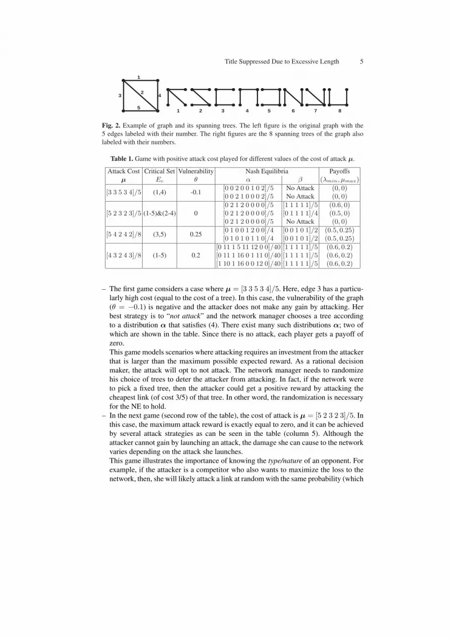
Fig. 2. Example of graph and its spanning trees. The left figure is the original graph with the5 edges labeled with their number. The right figures are the 8 spanning trees of the graph alsolabeled with their numbers.

Table 1. Game with positive attack cost played for different values of the cost of attack µ.

Attack Cost Critical Set Vulnerability Nash Equilibria Payoffsµ Ec θ α β (λmin, µmax)

[3 3 5 3 4]/5 (1,4) -0.1[0 0 2 0 0 1 0 2]/5 No Attack (0, 0)[0 0 2 1 0 0 0 2]/5 No Attack (0, 0)

[5 2 3 2 3]/5 (1-5)&(2-4) 0[0 2 1 2 0 0 0 0]/5 [1 1 1 1 1]/5 (0.6, 0)[0 2 1 2 0 0 0 0]/5 [0 1 1 1 1]/4 (0.5, 0)[0 2 1 2 0 0 0 0]/5 No Attack (0, 0)

[5 4 2 4 2]/8 (3,5) 0.25[0 1 0 0 1 2 0 0]/4 [0 0 1 0 1]/2 (0.5, 0.25)[0 1 0 1 0 1 1 0]/4 [0 0 1 0 1]/2 (0.5, 0.25)

[4 3 2 4 3]/8 (1-5) 0.2[0 11 1 5 11 12 0 0]/40 [1 1 1 1 1]/5 (0.6, 0.2)[0 11 1 16 0 1 11 0]/40 [1 1 1 1 1]/5 (0.6, 0.2)[1 10 1 16 0 0 12 0]/40 [1 1 1 1 1]/5 (0.6, 0.2)

– The first game considers a case where µ = [3 3 5 3 4]/5. Here, edge 3 has a particu-larly high cost (equal to the cost of a tree). In this case, the vulnerability of the graph(θ = −0.1) is negative and the attacker does not make any gain by attacking. Herbest strategy is to “not attack” and the network manager chooses a tree accordingto a distribution α that satisfies (4). There exist many such distributions α; two ofwhich are shown in the table. Since there is no attack, each player gets a payoff ofzero.This game models scenarios where attacking requires an investment from the attackerthat is larger than the maximum possible expected reward. As a rational decisionmaker, the attack will opt to not attack. The network manager needs to randomizehis choice of trees to deter the attacker from attacking. In fact, if the network wereto pick a fixed tree, then the attacker could get a positive reward by attacking thecheapest link (of cost 3/5) of that tree. In other word, the randomization is necessaryfor the NE to hold.

– In the next game (second row of the table), the cost of attack is µ = [5 2 3 2 3]/5. Inthis case, the maximum attack reward is exactly equal to zero, and it can be achievedby several attack strategies as can be seen in the table (column 5). Although theattacker cannot gain by launching an attack, the damage she can cause to the networkvaries depending on the attack she launches.This game illustrates the importance of knowing the type/nature of an opponent. Forexample, if the attacker is a competitor who also wants to maximize the loss to thenetwork, then, she will likely attack a link at random with the same probability (which

6 Assane Gueye, Jean C. Walrand, and Venkat Anantharam

gives a loss of 0.6). However, if the attacker is just interested in her own payoff, thenshe will probably not launch an attack.

– From these two examples and the first part of the theorem, one can infer that if thenetwork manager is able to influence the attack costs µ, for example making thelinks harder to attack by investing on security (physical protection, Firewalls, Intru-sion Prevention Systems (IPS) to avoid Denial of Service (DoS), etc...), then he candeter the attacker from attacking. This can be done by investing on the links to thepoint that M(E) ≤ µ(E) for all subsets of edges E ⊆ E . One can compute theoptimal investment by solving an optimal reinforcement like problem. The networkreinforcement problem of [4] is related to minimizing the price of increasing the costof attack of individual edges in order to achieve a target vulnerability (here 0) for thegraph. For details see [4]. If the cost of attack can be estimated by some means, thiscan be a very good candidate for preventive security.

– The last two games are examples where the maximum attack reward is strictly posi-tive. In the first one, the attacker only targets the links that are less costly which turnout to be the minimum cutset of the graph (seen by the attacker). In the second ex-ample, the minimum cut seen by the attacker corresponds to links 3 and 5. However,the attack’s reward is maximized by targeting all the links with the same probabilityas it is shown in the table.

– If all links of the graph have the same cost µ(e) = µ, then the vulnerability of asubset E (defined in equation 3) becomes θ(E) = M(E)−µ(E)

|E| = M(E)|E| − µ, and

a critical subset is one that maximizes the ratio M(E)|E| . This definition of criticality

corresponds to the one given in [8] where the cost of attack was assumed to be zero.Theorem 1 implies that if the cost of attack µ is larger than M(E)

|E| for all E, theattacker will not attack. In fact, the net gain of attacking will be negative. If, in theother hand µ > maxE⊆E

(M(E)|E|

), then the second part of Theorem 1 corresponds

to the critical subset attack theorem in [8] with γE = 1 for some critical subset E.The attacker can take any convex combination of uniform attack on the links in acritical subset, and the manager will choose trees according to (6).

– If γEc = 1 for a some critical subset Ec, we have that the corresponding attack is totarget uniformly links in Ec. The defense strategy should verify

∑T3e αT −µ(e) ≤

M(Ec)|Ec| for all e ∈ E , and equality holds for each e ∈ Ec. Also, by the Nash equilibria

conditions it must be that for any spanning tree T

∑

e∈T

β(e) =∑

e∈T

1e∈Ec

|Ec| =|Ec ∩ T ||Ec| ≥ M(Ec)

|Ec| . (8)

The minimum value in the equation above is achieved at each T for which αT > 0.Since the defender’s payoff is equal to M(Ec)

|Ec| , we have thatM(Ec) = minT (|E ∩ T |) =|Ec ∩ T | for each T for which αT > 0. In other words, the defender will select onlyspanning trees that cross the critical subset in the minimum number of links. Further-more, the net reward (

∑T3e αT − µ(e)) is the same at each link e of the critical

subset Ec. This quantity is equal to θ, the vulnerability of the subset Ec. For anyother link, this quantity should be less than θ.


– We have seen in [8] that if the cost of attack is zero, the attacker targets edges on agiven critical subset with the same probability. The theorem of this paper tells thatthis still holds even with positive cost of attack. The attack operates by taking convexcombination of uniform strategies on critical subsets.This uniformity of attack on critical subsets comes from the geometry of the blockerPb

A of the spanning tree polyhedron PA induced by the defender’s payoff matrix A(which is the spanning tree incidence matrix – see appendix B). The attack is nolonger uniform if the payoff matrix changes. To see this, assume for example that thedefender incurs a certain operation cost ηT by choosing spanning tree T . In this casehis payoff matrix is given as AT,e = 1e∈T + ηT . We consider the simplest none-trivial topology of two nodes connected by two parallel edges e1 and e2. With thistopology, edge e1 corresponds to tree T1. Similarly for link e2 and tree T2. We furthersimplify by assuming that the attack cost µ = 0.Letting (α, 1 − α) and (β, 1 − β) respectively be the defender’s and the attacker’sstrategy, the expected attack loss for the defender can be written as L(α, β) = α(2β+η1−η2−1)+1−β +η2. The attacker’s expected reward is R(α, β) = β(2α−1)+1 − α. By analyzing these payoff functions, we see that the NE is given as follow.If η1 ≥ 1 + η2, then α = 0 and β = 0. If η2 ≥ 1 + η1, then α = 1 and β = 1. If0 < |η1 − η2| < 1, then α = 1/2 and β = η2−η1+1

2 . Hence, the attacker’s mixedstrategy equilibrium is not in general uniform. We get the uniform distribution onlyif η1 = η2.This shows the importance of the geometry of the problem (namely the polyhedroninduced by the payoff matrix and its blocker) for the determination of the NE struc-ture. The authors have found that [7] for the quasi-zero-sum game defined in section2 with arbitrary nonnegative payoff matrix A, and attack cost µ ≥ 0, the attacker’sNE strategies are obtained by normalizing critical vertices of the blocker polyhedronPb

A. In the case of the spanning tree game, the blocker is such that the normalizedvertices correspond to uniform distributions. For a general payoff matrix, normalizedvertices can give arbitrary distribution.

– The Nash equilibria characterization provided in this paper (and which the authorshave studied in a more general setting [7], [6]) can be considered as an application ofthe result in [1] to the particular case of quasi zero-sum game. Although Avis et al.were not interested in characterizing Nash equilibria (which would be very laboriousfor an arbitrary two-player matrix game) and did not explicitly consider the notion ofblockers, all the ingredients we have used in our NE characterization can be derivedfrom their results. Our use of the combinatorial notion of blocker was the key toour success in characterizing the mixed strategy Nash equilibria of the game. Toour knowledge, such notion was not used before in the context of computing Nashequilibria.

6 Proof of the Critical Subset Attack Theorem

In this section we provide a proof of the Nash equilibrium theorem presented in section4. In the first part of the proof, we argue that the strategies given in the theorem forθ ≤ 0 and θ ≥ 0 are best responses to each other. The second part shows the existence


of a distribution α that satisfies (4) if θ ≤ 0 and (6) if θ ≥ 0. The last part of theproof shows that when µ = 0, all Nash equilibria have the form given in part (2) of thetheorem. The proof requires the notion blocking pair of polyhedra that we define in theappendix section B.

6.1 Best Responses

First, notice that if the attacker chooses to not attack, then any α will result to theminimum loss of zero for the defender (in particular the one given in the theorem).Also, if α is such that α(e)− µ(e) ≤ 0, ∀ e ∈ E , one can easily see from (2) that notattacking is a dominant strategy for the attacker. Thus, if θ ≤ 0, the strategies given inthe theorem are best responses to each other.

Next, we show that if θ ≥ 0 the strategies given in (5) and (6) are best response toeach other. We start by showing that:

Lemma 1. If θ ≥ 0, then not attacking is a dominated strategy for the attacker. Thedomination is strict if θ > 0.

The Lemma implies that if θ ≥ 0 the attacker can always at least do as well as than notattacking (and better strictly better if θ > 0).Proof sketch: The proof follows from the fact that if θ ≥ 0, then, the attacker canalways get a nonnegative attack reward by uniformly targeting the edges of a criticalsubset E. Indeed, there always exists at least one critical subset. The reward of such at-tack is lower bounded by M(E)−µ(E)

|E| , which is greater than zero under the assumptionthat θ ≥ 0. The bound is strict if θ > 0.

Now, suppose that the defender plays a strategy α that satisfies (6). Then, any dis-tribution β of the form β(e) =

∑E∈C γE

1e∈E

|E| for some distribution γ = (γE , E ∈ C),achieves a reward of θ. This is the maximum possible reward that the attacker can get.To see this, observe that for any β,

R(α, β) =∑

e∈Eβ(e) (α(e)− µ(e)) ≤

∑

e∈Eβ(e)θ = θ. (9)

The upper bound of θ is achieved by any β = ( 1e∈E

|E| , e ∈ E) uniform on a critical subset

E ∈ C. In fact, replacing such β in (2) and reordering the terms, we get

R(α, β) =∑

T∈TαT

(∑

e∈E

1e∈E

|E| 1e∈T −∑

e∈E

1e∈E

|E| µ(e)

)(10)

=∑

T∈TαT

(|E ∩ T ||E| −

∑

e∈E

1e∈E

|E| µ(e)

)(11)

≥∑

T∈TαT

M(E)|E| − µ(E)

|E| =M(E)|E| − µ(E)

|E| = θ, (12)

where in the last step we use the fact that E is critical.As a consequence, any distribution of the form ( 1e∈E

|E| , e ∈ E) for E ∈ C critical is abest response and any convex combination of those distributions is also a best response.


Now assume that β is given as in (5) for some distribution (γE , E ∈ C). Then, thedistribution (αT , T ∈ T ) in (6) achieves a loss of r(γ) =

∑E∈C γE

M(E)|E| . This is the

minimum possible loss. To see this, use this expression for β to rewrite the expectedloss (1) (for any α) as

L(α, β) =∑

T∈TαT

(∑

E∈CγE

(∑

e∈E

1e∈E

|E| 1e∈T

))(13)

≥∑

T∈TαT

(∑

E∈CγEM(E)|E|

)(14)

=∑

T∈TαT r(γ) = r(γ). (15)

To get the first equation (13) from (1), we have reversed the order of the summationsover E and over C.The lower bound r(γ) can be achieved by choosing α such that

∑T∈T αT 1e∈T =

θ + µ(e) for each e ∈ E such that β(e) > 0 (the existence of such α is shown in thesecond part of the theorem). This can be seen by using

∑T∈T αT 1e∈T = θ+µ(e) and

β(e) =∑

E∈C γE1e∈E

|E| in (1) to get

L(α,β) =∑

e∈Eβ(e)

(∑

T∈TαT 1e∈T

)=

∑

e∈Eβ(e) (θ + µ(e)) (16)

= θ +∑

e∈E

(∑

E∈CγE

1e∈E

|E| µ(e)

)(17)

= θ +∑

E∈CγE

(∑

e∈E

1e∈E

|E| µ(e)

)(18)

= θ +∑

E∈CγE

(µ(E)|E|

)(19)

= θ +∑

E∈CγE

(M(E)|E| − θ

)(20)

=∑

E∈CγEM(E)|E| = r(γ) (21)

This implies that the distribution (αT , T ∈ T ) in (6) is a best response to β given in(5).

6.2 Existence of the Equilibrium Distribution α

In the previous section we have shown that the strategies given in the theorem are bestresponses to each other. The distribution in (5) exists by definition. However, a priori,one does not know if there exists a probability distribution that satisfies (4) if θ ≤ 0.


Similarly, if θ ≥ 0, one needs to show the existence of a distribution that verifies theconditions in (6). Using the results discussed in appendix B, we show the existence ofsuch distributions. More concretely, we will show that:

– if θ ≤ 0, there exists α verifying, α ≥ 0, 1′T α = 1, and A′α ≤ µ,– if θ ≥ 0, there exists α verifying, α ≥ 0, 1′T α = 1, and A′α ≤ θ1E + µ, with

equality in the constraints for each e such that β(e) > 0.

Recall ‘A’ is the tree-link incidence matrix AT,e = 1e∈T . Also, the spanning tree poly-hedron PA is characterized by (see appendix B, [8], and [3])

PA = {x ∈ Rm+ | x(E(P )) ≥ |P |−1, for all feasible partitions P = {V1, V2, . . . , V|P |}}.

(22)P is said to be a feasible partition of the nodes V of G if each Vi induces a connectedsubgraph G(Vi) of G. We let E(P ) denote the set of edges going from one member ofthe partition to another, and GE(P ) be the graph obtained by removing from G the edgesgoing across P . The number of connected components of GE(P ) is denoted Q(GE(P ))and is equal the size of the partition P . We have also shown in [8] that M(E) =Q(GE)− 1 for all E ⊆ E .

Now, we claim that,

Lemma 2. – If θ ≤ 0, then µ ∈ PA.– If θ ≥ 0, then (θ1E + µ) ∈ PA.

Using the first part of this lemma, and Lemma 3 of Appendix B, we conclude that ifθ ≤ 0, the value of the following LP is greater than 1.

Maximize 1′T x, subject to A′x ≤ µ, and x ≥ 0. (23)

Using this, we can construct a distribution α satisfying (4) by normalizing any solutionof this LP.

Similarly, if θ ≥ 0, we can construct a distribution α that satisfies A′α ≤ θ1E + µ.This gives an α for which we still need to show that equality holds whenever β(e) > 0,where β is a distribution of the form (5). For that, we make the following additionalclaims.

Theorem 2. Let x∗ be the solution of the following LP:

Maximize 1′T x

subject to A′x ≤ b, x ≥ 0. (24)

where b = θ1E + µ. Then,a) 1′T x∗ ≤ 1;b) A′x∗(e) = b(e), ∀ e ∈ E for which β(e) > 0, where β is given in (5).

Notice that, from Lemma 2 we have that the value of the linear program is greater than1. This, combined with part a) of the theorem, imply that the value of the LP is exactly 1.Part b) of the theorem gives the equality conditions that we needed. As a consequence,x∗ satisfies (6) and implies the existence of the NE distribution α when θ ≥ 0.


6.2.1 Proof of Lemma 2

– By definition of θ, we have θ ≤ 0 ⇔ µ(E) ≥ M(E) for all E ⊆ E . [8, Lemma 1]gives M(E) = Q(GE)− 1, where Q(GE) is the number of connected componentsof the graph G when all edges in E are removed. Thus, θ ≤ 0 ⇔ µ(E) ≥ Q(GE)−1for all E ⊆ E .Now, let P be a feasible partition of the nodes V of G. Using the above observations,we can conclude that

θ ≤ 0 ⇔ µ (E(P )) ≥ Q(GE(P ))− 1 = |P | − 1 (25)

Since the partition P is feasible, µ (E(P )) ≥ |P | − 1 implies that µ ∈ PA, whichends the proof of the first part of the lemma.

– To prove that the vector b = θ1E + µ ≥ 0 belongs to the polyhedron PA wheneverθ ≥ 0, we argue that

b (E(P )) ≥ |P | − 1, for all feasible partitions P . (26)

Recall, from the above that for all feasible partitions P

M(E(P )) = |P | − 1. (27)

Now, assume that b does not verify (26)– i.e b (E(P )) < |P | − 1, for some feasiblepartition P . Then one must have,

|P | − 1 >∑

e∈E(P )

be = θ (E(P ))∑

e∈E(P )

1 +∑

e∈E(P )

µ(e) (28)

= θ (E(P )) |E(P )|+ µ (E(P )) (29)= M (E(P ))− µ (E(P )) + µ (E(P )) = M (E(P )) (30)

which contradicts (27). Thus, b (E(P )) ≥ |P | − 1 for all feasible P , or equivalentlyb ∈ PA.

6.2.2 Proof of Theorem 2

a) To prove that 1′T x∗ ≤ 1, we first observe that


β′A′x =∑

T∈TxT

(∑

e∈Eβ(e)1e∈T

)(31)

=∑

T∈TxT

(∑

e∈E

(∑

E∈CγE

1e∈E

|E|

)1e∈T

)(32)

=∑

T∈TxT

(∑

E∈CγE

(∑

e∈E

1e∈E

|E| 1e∈T

))(33)

=∑

T∈TxT

(∑

E∈CγE

( |E ∩ T ||E|

))(34)

≥∑

T∈TxT

(∑

E∈CγEM(E)|E|

)(35)

=∑

T∈TxT r(γ) (36)

= r(γ)1′T x (37)

On the other hand, from the constraints A′x ≤ b = θ1E + µ and using the samearguments as in (16)-(21), we have that

β′Λ′x ≤ β′ (θ1E + µ) = θ + β′µ = r(γ). (38)

Combining (37) and (38), it follows that,

r(γ)1′T x ≤ β′Λ′x ≤ r(γ). (39)

Thus 1′T x ≤ 1 for all feasible x, i.e. the value of the program is at most 1.b) Notice from the above and from the conclusion of Lemma 2 that for θ ≥ 0 the

value of the LP defined in Theorem 2 is exactly equal to 1. Thus,

β′A′x∗ = r(γ)1T x∗ = r(γ). (40)

Also, A′x∗ ≤ θ1E + µ by the constraints of the primal LP above.Now, assume that A′x∗(e) < θ + µ(e) for some e ∈ E with β(e) > 0. Then,

β′A′x∗ =∑

e∈Eβ(e)A′x∗(e) (41)

<∑

e∈Eβ(e)(θ + µ(e)) (42)

= θ +∑

e∈Eβ(e)µ(e) (43)

= r(γ), (44)

where the last equality is obtained by using the same arguments as in (16)-(21). Thiscontradicts observation (40). As a consequence, A′x∗(e) = θ + µ(e) for all e ∈ E withβ(e) > 0.This ends the proof of the theorem and establishes the existence of an α satisfying (6)for any β defined as in (5).


6.3 Enumerating all Nash Equilibria

In this section, we consider the zero-sum game where µ = 0 and show that all Nashequilibria of the game have the form given in Theorem 1 equations (5) and (6).

In this case, since there is no cost of attack, θ > 0. We claim that for any strategypair (αT , T ∈ T ) and (β(e), e ∈ E) that are in Nash equilibrium, it must be the casethat (β(e), e ∈ E) is given by

β(e) =∑

E∈CγE

1e∈E

|E| , (45)

for some probability distribution (γE , E ∈ C) on the set of critical subsets.As a consequence of this, we will conclude that α must be in the form given in the Nashequilibrium theorem.

Because of space limitations, we describe the main points of the proof in appendixA and for the full proof, we refer the interested reader to [6] and [7].

7 Conclusion and future work

This paper studies a generalization of the topology design game defined in [8], where anetwork manager is choosing a spanning tree of a graph as communication infrastruc-ture, and an attacker is trying to disrupt the communication tree by attacking one linkof the graph. Assuming that the attacker incurs a positive cost by attacking any givenlink of the network, we revisit the notions of vulnerability and criticality of a subset oflinks.

We have determined the values of the attack costs for which a rational attacker willopt to not launch an attack. When the attacker decides to attack, we have shown thatthere always exists a NE under which she attacks randomly, with the same probability,links in a given critical subset. The randomization can also be done across critical sub-sets. The network manager chooses only spanning trees that cross the critical set in theminimum number of edges, and such that the sum of the probabilities of all trees goingthrough any link in the critical set minus the cost of attacking that link, is the same.

For the game of zero costs of attack studied in [8], we have characterized the setof all Nash equilibria. The NE strategies are such that the attacker will always targetlinks in critical subsets and attacks all links in the same critical subset with the sameprobability.

We have shown, by a simple example, that the uniformity of the attack on eachcritical subset is a consequence of the geometry of the problem. Mainly, the vertices ofthe blocker of the spanning tree polyhedron are such that if normalized, they results touniform distribution. This is not always the case. For instance, if the defender incursdifferent cost of choosing different spanning trees, the attack strategies are no longeruniform on critical subsets.

The proof concepts presented in this paper have been generalized to identify Nashequilibria for a class of quasi zero-sum games. For details of the general study, we referthe interested readers to [7] and [6].


Acknowledgments

The authors would like to thank members of the Berkeley MURI and Netecon groupsfor their valuable input. Our special thanks go to Prof. Dorit Hochbaum for suggestinga set of very related papers. The work of the authors was supported by the ARO MURIgrant W911NF-08-1-0233 and by the NSF grants CNS-0627161 and its continuation,CNS-0910702.

References

1. David Avis, Gabriel Rosenberg, Rahul Savani, and Bernhard von Stengel. Enumeration ofNash Equilibria for Two-Player Games. Economic Theory, 42:9–37, 2010.

2. Stephen Boyd and Lieven Vandenberghe. Convex Optimization. Cambridge University Press,March 2004.

3. S Chopra. On the Spanning Tree Polyhedron. Operations Research Letters, 8(1):25 – 29,1989.

4. William H. Cunningham. Optimal Attack and Reinforcement of a Network. J. ACM,32(3):549–561, 1985.

5. D R Fulkerson. Blocking and Anti-Blocking Pairs of Polyhedra. Math. Programming,(1):168–194, 1971.

6. Assane Gueye. A Game Theoretical Approach to Communication Security. PhD dissertation,University of California, Berkeley, Electrical Engineering and Computer Sciences, March2011.

7. Assane Gueye, Jean C. Walrand, and Venkat Anantharam. Bloking Games. Technical report,University of California, Berkeley, December 2010. http://www.eecs.berkeley.edu/~agueye/index.html.

8. Assane Gueye, Jean C. Walrand, and Venkat Anantharam. Design of Network Topology in anAdversarial Environment. In GameSec 2010, Conference on Decision and Game Theory forSecurity, pages 1–20. Springer-Verlag Berlin Heidelberg 2010, November 2010.

9. Laurence A. Wolsey and George L. Nemhauser. Integer and Combinatorial Optimization.Wiley-Interscience, 1 edition, November 1999.

A Proof sketch of the NE enumeration claim

Theorem 1, tells that if the attack costs µ = 0, then all Nash equilibrium pairs (α, β)of the game have the form given in (6) for α and in (5) for β. To show this, we claimthat for any strategy pair (αT , T ∈ T ) and (β(e), e ∈ E) that are in Nash equilibrium,it must be the case that β is given by

β(e) =∑

E∈CγE

1e∈E

|E| , (46)

for some probability distribution (γE , E ∈ C) on the set of critical subsets.We prove this claim by scaling any mixed strategy β (seen as a vector in R

|E|+ ) with

a proper constant such that it belongs to the blocker of the spanning tree polyhedron.The proof is based on the following ideas.


– Since the spanning tree polyhedron PA and its blocker PbA are given in terms of

feasible partitions, we establish a correspondence between feasible partitions andcritical subsets of the graphs. Basically, we show that every critical subset is the setof edges going across the elements of some feasible partition. We define the notionof critical partitions ΠC (corresponding to critical subsets) and show the followingequivalent claim:

β(e) =∑

P∈ΠC

γP

1e∈E(P )

|E(P )| , (47)

where γ is now viewed as a distribution on the critical partitions.– Because the game is zero-sum, we know that all NE (α,β) have payoff θ > 0 which

is given as:

θ =∑

T∈TαT

(∑

e∈Eβ(e)1e∈T

)> 0. (48)

We argue that∑

e∈E β(e)1e∈T > 0 for all T , and can be scaled by a constant κ sothat

∑e∈E κβ(e)1e∈T ≥ 1. This means that the vector κβ belongs to the blocker

of the spanning tree polyhedron (see Theorem 3 of the appendix). Recall that [8] thevertices of this blocker are vectors of the form (1e∈E(P )

|P |−1 , e ∈ E), for some feasiblepartitions P .We argue that by making the proper choice of κ the vector κβ can be written as

κβ(e) =∑

P∈ΠC

γP

1e∈E(P )

|P | − 1, (49)

and show that the proper κ must be in the form κ = |P |−1|E(P )| for some critical partition

P ∈ ΠC . But all critical partitions (subsets) have the same ratio |P |−1|E(P )| . By dividing

the equation by κ we get

β(e) =∑

P∈ΠC

γP

1e∈E(P )

|E(P )| . (50)

Using the correspondence between critical partitions and critical subsets, we get theclaim in (46).

B Blocking Pair of Matrices

The discussion in this appendix section is mostly based on [9, pp. 99-101].Let A be a r×m nonnegative matrix. The polyhedron PA associated with A is definedas the vector sum of the convex hull of its rows (a1, . . . , ar) and the nonnegative orthant:

PA = conv.hull (a1, . . . ,ar) + Rm+ . (51)

A row ai of A is said to be inessential if it dominates a convex combination of otherrows of A. If all the rows of A are essential, we say that A is proper. In this discussion


we will assume that A is proper. For example, if A is the tree-link incidence matrix ofthe spanning trees of a graph, then A is a proper matrix and PA defines the spanningpolyhedron of the graph.Next we define the blocker of the polyhedron PA.

Definition 2. The blocker PbA of PA is defined as:

PbA =

{x ∈ Rm

+ : x · y ≥ 1, ∀ y ∈ PA

}(52)

We are interested in characterizing the polyhedron PA and its blocker PbA. This is given

by the following theorem by Fulkerson [5]. It is based on the fact that there is a one-to-one correspondence between the rows of A and the extreme points of PA.

Theorem 3. Let the r-by-m matrix A be proper with rows a1, . . . ,ar, and let the poly-hedron PA be defined as in (51). Let b1, . . . ,bs be the extreme points of Pb

A, and let Bbe the matrix having those points as rows. Then,

i. The blocker PbA of PA is given by Pb

A ={x ∈ Rm

+ : Ax ≥ 1}

.ii. B is proper, and the polyhedronPA can be described asPA =

{x ∈ Rm

+ : Bx ≥ 1}

.

iii. The blocker of the blocker PbA verifies

(PbA

)b = PA.

A and B are said to form a blocking pair of matrices.

Blocking pairs of matrices play an important role in the combinatorial problem ofmaximum packing (see Fulkerson[5]). In this paper, we use the theory of blocking pairto provide an easy argument for the existence of a probability distribution that satisfiesa certain number of constraints.Consider the following linear program:

Maximize 1′x

subject to A′x ≤ w, and x ≥ 0, (53)

where the constraint A′ is a nonnegative matrix.We are interested to knowing whether the value of the program is greater than 1 or not.The following lemma gives an answer to that question.

Lemma 3. The value of the LP in (53) is greater than 1 if and only if w belongs to thepolyhedron PA defined by A.

Proof. The proof of the lemma is as follow.First notice that strong duality holds for this LP. In fact, Slater’s condition [2] is satisfiedfor any nonnegative w. The dual of the LP is given as:

Minimize w′y

subject to Ay ≥ 1, and y ≥ 0. (54)

The constraints of the dual program (54) define the blockerPbA =

{y ∈ Rm

+ : Ay ≥ 1}

of the polyhedron PA.Now, if w belongs to PA, then for all y ∈ Pb

A, we have that w′y ≥ 1.Conversely, if w′y ≥ 1 for all y ∈ Pb

A, then w must be in the blocker of PbA which is

PA.

Documents

A Network Topology Design Game: How to Choose Communication Links in an Adversarial Environment?