A neural tree model for classification of computing grid resources using PSO tasks scheduling

A NEURAL TREE MODEL FOR

CLASSIFICATION OF COMPUTING GRID

RESOURCES USING PSO TASKS

SCHEDULING

Jarmila Skrinarova∗, Ladislav Huraj†, Vladimır Siladi‡

Abstract: This paper proposes a model of neural tree architecture with probabilis-tic neurons. These trees are used for classification of a large amount of computergrid resources to classes. The first tree is used for classification of hardware partof dataset. The second tree classifies patterns of software identifiers. Trees areimplemented to successfully separate inputs into nine classes of resources. We pro-pose Particle Swarm Optimization model for tasks scheduling in computer grid.We compared time of creation of schedule and time of makespan in six series ofexperiments without and with using neural trees. In experiments with using neuraltree we gained the subset of suitable computational resources. The aim is effectivemapping of a large batch of tasks into particular resources. On the base of expe-riments we can say that improvements have been made even for middle and smallbatch of tasks.

Key words: Neural tree, PSO optimization, tasks scheduling

Received: February 19, 2013Revised and accepted: April 17, 2013

1. Introduction

Computational grids can be used for solving problems that require processing oflarge quantity of operations or data. Grid computing allows sharing of distributedcomputing and data resources such as processing, network bandwidth and stor-age capacity to create a cohesive resource environment for executing distributedapplications [1].

∗Jarmila SkrinarovaFaculty of Natural Sciences Matej Bel University, [email protected]

†Ladislav HurajFaculty of Natural Sciences Ss. Cyril and Methodius University, [email protected]

‡Vladimır SiladiFaculty of Natural Sciences Matej Bel University, [email protected]

c⃝ICS AS CR 2013 223

Neural Network World 3/13, 223-241

Job scheduling in its different forms is computationally hard. It has been shownthat the problem of finding optimal scheduling in heterogeneous systems is, in gene-ral, NP-hard [6, 8]. An application can generate several jobs which, in turn, can becomposed of subtasks and the Grid system is responsible for sending each subtaskto a resource to be solved. Grid systems contain schedulers that automatically andefficiently find the most appropriate machines to execute an assembly of tasks.

Task represents a computational unit which runs on a grid node. Typically itis a program and possibly associated data. A task is considered as an indivisibleschedulable unit.

Job is a computational activity made up of several tasks that could require dif-ferent processing capabilities and could have different resource requirements (CPU,number of nodes, memory, software libraries, etc.) and constraints, usually ex-pressed within the job description. In the simplest case, a job could have just onetask.

Grid scheduler is created by software components, which are responsible for amapping of tasks to grid resources under multiple criteria and grid environmentconfigurations. The computational grid, hierarchical by nature, is usually modeledas a multi-level system, which allows efficient management of geographically dis-tributed resources and tasks scheduling under various criteria, including securityand resource reliability requirements [31, 32]. The model is often a hybrid of cen-tralized and decentralized modules. In the centralized module, there is a centralauthority. It is some metascheduler or meta-broker and it has knowledge of thesystem by monitoring the resources and interacts with local job dispatchers in or-der to define optimal schedules. In the decentralized module, the local schedulersinteract with each other to manage the task pool. This kind of scheduler has theknowledge about the resource clusters, but they cannot monitor the whole system[38, 39, 17]. The hierarchical model addresses scalability and fault-tolerance issues.A meta-broker model is an example of the hierarchical two level grid system. Inthis model, grid users submit their tasks or applications to the meta-broker whichuses also the information supplied by the resource owners to match the users tasksto appropriate resources [18].

This paper is organized as follows. Section 2 shortly reports on related works.Section 3 introduce Computational model for Grid scheduling and optimizationcriteria. Neural networks focused on multilayer perceptron (MLP) and radial basisactivation function (RBF) with competitive learning rule are briefly outlined inSection 4. Neural tree is described in Section 5. There is a model of particle swarmoptimization (PSO) algorithm for discrete variables introduced in Section 6. Datadescription and simulation tools are proposed in Section 7. Section 8 is focused onsimulations and experimental results.

2. Related Works

Several stochastic and heuristic optimization methods have been proposed for jobscheduling in computational grids. Monte Carlo methods, Simulated Annealing,Tabu Search, Genetic Algorithms [33, 34], among others, attempt to avoid the pre-mature convergence to the local minima. An implementation of Simulated Anne-aling for grid scheduling was proposed in [25, 26]. Recently some parallel genetic

224

Skrinarova J. et al. : A neural tree model for classification of computing grid. . .

algorithms frameworks have been used for designing the effective grid schedulers.Lim et al. [19] propose Grid-Enabled Hierarchical Parallel Genetic Algorithm (GE-HPGA). Another method of improving the scheduling quality is the hybridizationof the heuristics with Local Search methods for the problem [20]. Particle SwarmOptimization algorithms have been implemented for grid scheduling [35, 36, 37].A hybrid version of genetic algorithms and Tabu searching is proposed by Xhafa etal. [21]. Other approaches to the problem include the use of Fuzzy Particle SwarmOptimization [22], Artificial Neural Networks [23] and economic-based approaches[24].

3. Computational Model for Grid Scheduling andOptimization Criteria

In this part computation model for Grid scheduling is presented. The computa-tional capacity of the node depends on its:

• Number of CPUs

• Amount of memory

• Basic storage space

• Other specifications

The node has its own processing speed, which can be expressed in the number ofCycles Per Unit Time (CPUT) [3].

A job is considered as a single set of multiple atomic operations (tasks). Thetask is allocated to execute on one single node without pre-emption. The task hasinput and output data and processing requirements in order to complete its task.The task has a processing length expressed in the number of cycles.

A schedule is the mapping of the tasks to specific time intervals of the gridnodes.

A scheduling problem is specified by:

• A set of machines

• A set of jobs

• Optimality criteria

• Environmental specifications

• Other constraints

One of the most popular optimization criteria is the minimization of the makespan.Makespan is an indicator of the general productivity of the grid system. Smallvalues of makespan mean that the scheduler is providing good and efficient planningof tasks to resources. Makespan indicates the time when the last task finishes.Flowtime is the sum of finalization times of all the tasks.

225


Let Jj (j{1, 2, . . . , n}) be independent user jobs on Gi (i{1, 2, . . . ,m}) heteroge-neous grid nodes with an objective of minimizing the completion time and utilizingthe nodes effectively.

Number of CPUT expresses speed of every node. The length of each job isspecified by the number of cycles. Each job Jj has its processing requirement thatcan be expressed in number of cycles. A node Gi has its calculating speed and it isexpressed in cycles/second. Any job Jj has to be processed in the one of grid nodesGi until completion. Since all the nodes at each stage are identical and preemptionsare not allowed, to define a schedule it suffices to specify the completion time forall tasks comprising each job [1, 3].

To formulate our objective, we define:

• completion time Ci,j(i{1, 2, . . . ,m}, j{1, 2, . . . , n}) that the grid node Gi fi-nishes the job Jj , represents the time that the grid node Gi finishes all thejobs scheduled for itself,

• makespan can be expressed as the Cmax = max {C1, C2, . . . , Cn} and it isthe maximum completion time of all jobs Jj ,

• mean flowtime is∑n

j=1 Cj and it is the sum of completion times of all n jobs.

An optimal schedule will be the one that optimizes the flowtime and makespan.In our contribution we will minimize Cmax. It guaranties that no job takes too

long. For minimization we choose PSO algorithm.

4. MLP and RBF Neural Networks

Multiple Layer Perceptron (MLP) network [2] is a feed-forward structure composedof an input layer of neurons, one or more hidden layers and an output layer. Neu-rons in the nearest layers can be interconnected by weighted connections. Given isan input vector, the output vector is computed by a forward pass which computesthe activity levels of each layer in turn using the already computed activity levelsin the earlier layers.

A non-linear activation function is one in which the output of a unit is a non-decreasing and differentiable function of the network total output.

netk =∑j

wkjaj . (1)

In relation (1) aj is an output from j-th neuron and weights wkj are weightingsignals between neuron k and neuron j in lower level.

The output from the k-th neuron is ak = f(netk) and f is an activation function.An error of the p-th pattern is given as:

Ep =1

2

∑k

(tpk − apk)2. (2)

The system first uses the input vector to produce its own output vector andthen compares this with the desired output. If there is no difference, no learning

226


takes place. Otherwise, the weights are changed to reduce the difference in thedirection from the output layer to the input layer. This way of learning is callederror back-propagation algorithm. There are several modifications of the learningalgorithms. The known modifications are the gradient descent algorithm, gradientdescent with momentum, conjugate gradients algorithms (e.g. Powell-Beale) orLevenberg-Marquardt algorithms.

Radial-basis-function RBF network is a feed-forward structure composed ofan input layer, a hidden layer with RBF neurons and a linear output layer [15].Adjustable weights among the neurons are only between hidden and output layer.The inputs are directly connected to the neurons in the hidden layer via unityweights. A neuron I in RBF network in the first (hidden) layer [16] has the followingtransfer function:

z(x) = r(∥x− p∥)/σi. (3)

The element z(x) is i-th output of the neuron in the hidden layer. The argumentx is the input vector x = [x1, x2, . . . xq]

T , r(.) is a radial basis function and pi, σi

are the center and the width for the i-th RBF neuron. Output yi of the i-th linearneuron in the output layer assuming the number of RBF neurons n is

yi =n∑

j=1

wijz(x). (4)

Equation (4) represents linear operation.Typical radial-basis-function is Gaussian function, in this case the transfer fun-

ction is

zi(x) = e∥x−pi∥2

σ2 . (5)

Elements pi, σi are the center and the standard deviation in relation (5). Parameterσi is also called the spread parameter.

Probabilistic neural network is a special kind of RBF network. In the probabilis-tic neural networks the linear layer is replaced by a competitive layer. Competitivelearning rule consists of three basic elements:

• A set of neurons that are all the same except for some randomly distributedsynaptic weights, and which, therefore, respond differently to a given set ofinput patterns.

• A limit imposed on the “strength” of each neuron.

• A mechanism that permits the neurons to compete for the right to respondto a given subset of inputs, such that only one output neuron, or only oneneuron per group, is active at the time. The neuron that wins the competitionis called winner-takes-all.

According to the standard competitive learning rule, the change wij can be definedby [15]:

∆wij =

{η(xi − wji), if neuron j wins the competition0, if neuron j loses the competition

(6)

where η is learning rate parameter.

227


5. Neural Tree

A neural tree is a decision tree with a simple perceptron for each intermediate ornon-terminal node [16]. Two main phases can be distinguished:

• Training

• Classification

The training phaseThe role of this phase is to construct the neural tree. The tree is generated recur-sively by partitioning a training set consisting of feature vectors and their corre-sponding class labels. There are two kinds of nodes in the tree (intermediate nodesand leaf nodes). The procedure of constructing the tree involves three steps:

• Computing internal nodes

• Determining leaf nodes

• Labeling leaf nodes

An intermediate node classifies the input patterns into different classes. Theleaf node gives input patterns into a single class which is used as the label for theleaf node. The neural tree arranges recursively partition of the training set suchthat each generated path ends with a leaf node. The training algorithm, alongwith the computation of the tree structure, calculates the connection’s weights foreach node. Each connection’s weight is adjusted by minimizing a cost function asmean square error or another error function. These weights are used during theclassification phase to classify unseen patterns.

The neural tree training algorithm consists of particular steps:

• First node (root) is created.

• The patterns of the training set are presented to the root node. The nodeis trained to divide the training set into subsets. The process stops afterreaching some condition, for example mean square error of net.

• When a subset is homogeneous, a leaf node is associated and labeled as thecorresponding class (Fig. 1).

• When some of subsets is not homogeneous, a new node is added to the neuraltree at the next level. We can continue by second step. The training processis progressing and all subsets gradually become homogenous (Fig. 2).

• Training process is finished when all nodes become the leaf nodes (Fig. 3).

The classification phaseIn the phase of classification, unknown patterns are presented to the root node.The class is obtained by going through the tree from root to the leaf nodes. Theactivation values f are computed for each node, on the base of each connection’sweight. The activation values of the current node determine the next node toconsider until a leaf node is reached. In every node the winner takes-all rule (6) isapplied.

228


Fig. 1 Partition of the training set by the root node.

Fig. 2 Partition by the internal node.

Fig. 3 Final neural tree.

229


6. The Model of Particle Swarm OptimizerAlgorithm for Discrete Variables

The PSO algorithm was invented by Kennedy, Eberhart and Shi [4]. It is apopulation-based algorithm with fewer parameters to implement. The PSO al-gorithm was first applied to the optimization problems with continuous variables.Recently, it has been used to solve optimization problems with discrete variables[5, 7]. The optimization problem with discrete variables is a combination optimiza-tion problem which obtains its best solution from all possible variable combina-tions. The scalar S includes all permissive discrete variables arranged in ascendingsequence. Each element of the scalar S is given a sequence number to representthe value of the discrete variable correspondingly. It can be expressed as followsSd = {X1, X2, . . . Xj , . . . Xp} , 1 ≤ j ≤ p.

A mapping function h(j) is selected to index the sequence numbers of the ele-ments in set S and represents the value Xj of the discrete variables correspondinglyh(i) = Xj .

Thus, the sequence numbers of the elements will substitute the discrete valuesin the scalar S. This method is used to search for an optimum solution, and makesthe variables to be searched for in a continuous space.

The PSO algorithm includes a number of particles. The particles are initial-ized randomly in the search space. The position of the i-th particle in the spacecan be described by a vector xj , xi =

(x1i , x2i , . . . , xdi , . . . , xDi

), 1 ≤ d ≤ D,

i = 1, . . . , n, where D is the dimension of the particle, and n is the number of di-mensions. The scalar xdi = {1, 2, . . . , j, . . . , p} corresponds to the discrete variableset {X1, X2, . . . , Xj , . . . , Xp} by the mapped function h(j). Therefore, the particleflies through the continuous space, but only stays at the integer space. In otherwords, all the components of the vector xi are integer numbers. The positions ofthe particles are updated based on each particle’s personal best position as well asthe best position found by the swarm in all iterations. The objective function isevaluated for each particle, and the fitness value is used to determine which posi-tion in the search space is the best of the others. The swarm is updated by therelations (7) and (8)

V k+1i = ωV

(k)i + c1r1

(P

(k)i − x

(k)i

)+ c2r2

(P (k)g − x

(k)i

). (7)

x(k+1)i = INT

(x(k )i + V

(k+1)i

), (8)

where 1 ≤ I ≤ n, represent the current position and the velocity of each particle

at the k-th iteration, respectively, P(k)i and P

(k)g the best global position among

all the particles in the swarm (called gbest), r1 and r2 are two uniform randomsequences generated from (0, 1), and ω the inertia weight used to discount theprevious velocity of the particle persevered [8, 9, 10].

7. Data Description and Simulation Tools

In this paper, we use the data based on the parameters of the real grid systemNordugrid. See http://www.nordugrid.org/monitor/loadmon.php. There are

230


about 70 computing resources with a different number of CPUs (from 2 to 9856).Grid equipment involves a wide range of hardware. Available are multiprocessorsSMP with shared memory based on architecture MIPS and multicomputer clustersusing 32-bit and 64-bit processors. Internal connections among nodes are realizedusing special networks Myrinet (2.5Gb/s) and Infiniband (20Gb/s) for some se-lected nodes, and Gigabit Ethernet (1Gb/s) otherwise. Clusters use mostly 1Gb/sEthernet or Infiniband for their internal communication. They can have differentcapacity of data storages, operating systems, compilers and application software.We can widely classify resources into 3 categories on the base of numbers of CPUs:

• S – small (1 – 100 CPUs)

• M – middle (100 – 1000 CPUs)

• L – large (1000 – 10000 CPUs)

User tasks include more required parameters of resources. For that reason thefinal characteristic of computing resources can be classified by different kinds ofparameters:

• Numbers of CPUs are from the range 1 – 10000 and we classify it (1 – 3)

• Capacity of data storage is from 1 – 40000 and it corresponds to (1 – 3)

• Bandwidth between CPUs and data storages is classified (1 – 3)

• Type of operating system (1 – 5)

• Type of compiler (0 – 4)

• Type software for applications (0 – 9)

Every computing resource is denoted by a unique number and 6 previous parame-ters (three from the hardware and three from the software point of view). Everypattern is characterized by vector of 7 parameters. This is the way of coding eachcomputing element.

On the other hand, we need to code a task and its characteristics. Theseattributes are considered the most important for our analysis:

• Length – length of the calculation in millions instructions or another unitwhich can relatively measure task size (1 – 100000).

• Input file size – size of the input file, before the task execution starts (1 – 3)

• Output file size – size of the output file, after the task execution ends (1 – 3)

• Type of operating system (1 – 5)

• Type of compiler (0 – 4)

• Type software for applications (0 – 9)

231


We have designed a model of scheduling system which consists of two basic parts.The first part is created by the neural tree. The goal of the neural tree is to matchthe users’ tasks to an appropriate class of resources. We modeled this resourcebroker as a neural tree created in Matlab software tools.

The second part of our scheduling system is modeled using GridSim toolkit –grid simulation tool for modelling resources and scheduling applications for paralleland distributed systems. The aim of this part is to design a model that finds optimalschedule (or schedule very close to optimal) for running tasks on group of resources.As an optimization criterion we use makespan Cmax. For minimization makespanwe choose and implement PSO algorithm.

The GridSim toolkit allows modeling and simulation of entities in parallel anddistributed computing systems-users, applications, resources, and schedulers fordesign and evaluation of scheduling algorithms. This level of scheduling systemuses algorithms for mapping jobs to resources to optimize system or user objectivesdepending on their goals. GridSim toolkit is written in Java and is available on-line[11].

One computing task is represented by a Gridlet class which contains severalattributes defining character of the task (length, input file size and output filesize).

We assume that we know task complexity, and we can express it in the sameunits as computer efficiency.

Grid resources are presented by a GridResource class which describes characte-ristics of the resource. It also contains ResourceCharacteristic object which containsa list of all computers in the cluster, number of their processors and their efficiency.The GridSim works only with the part of resources that was chosen by neural tree.To be able to compare the efficiency of all CPUs, we chose to use a simple measureunit which presents the number of floating point operations per second. Evalu-ation of every processor used is based on data taken from website of Geekbenchbenchmark [12]. We created web application tool on the base of GridSim for cre-ating models of grid scheduling algorithm and evaluating these models in processof simulation. There are implemented PSO algorithms, too [33, 34, 35, 36, 37].

8. Simulations and Experimental Results

We have designed a neural tree on the base of probabilistic neural network andknown structure of data. Structure of data is described in the previous part of thispaper.

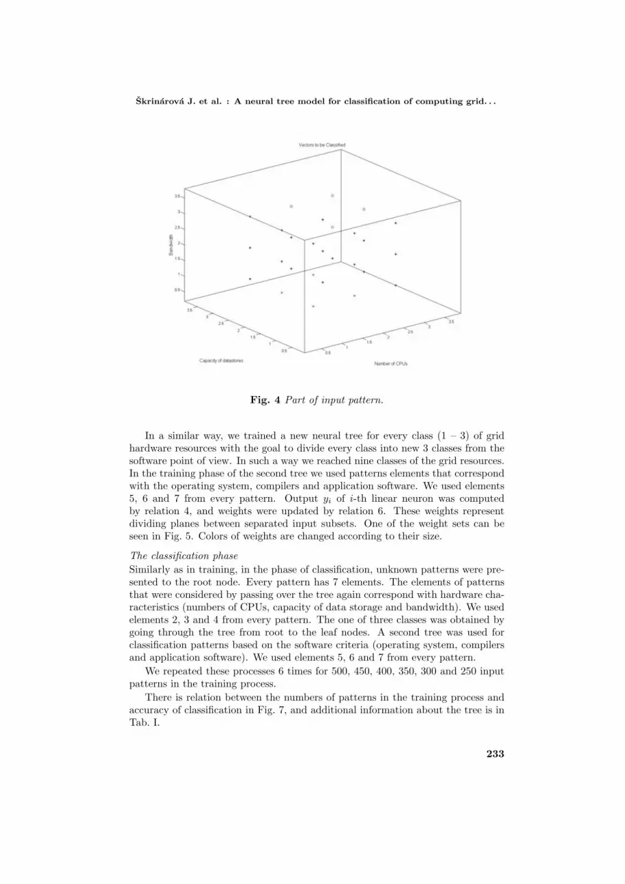
The training process of neural treePatterns were prepared from the data sets. Every pattern has 7 elements. Thetraining set was presented to the root node and subsequently its parts to othercreated nodes. The tree was trained to divide the training set into three subsets thatinclude some portion of numbers of CPUs, capacity of data storage and bandwidth.We used elements 2, 3 and 4 from every pattern (Fig. 4). These categories representgrid performance from the hardware point of view. We measured sum square error(Fig. 6) and mean square error of net as the stop criterion. After that we gainedcorresponding class 1, 2 or 3 of grid resources.

232


Fig. 4 Part of input pattern.

In a similar way, we trained a new neural tree for every class (1 – 3) of gridhardware resources with the goal to divide every class into new 3 classes from thesoftware point of view. In such a way we reached nine classes of the grid resources.In the training phase of the second tree we used patterns elements that correspondwith the operating system, compilers and application software. We used elements5, 6 and 7 from every pattern. Output yi of i-th linear neuron was computedby relation 4, and weights were updated by relation 6. These weights representdividing planes between separated input subsets. One of the weight sets can beseen in Fig. 5. Colors of weights are changed according to their size.

The classification phase

Similarly as in training, in the phase of classification, unknown patterns were pre-sented to the root node. Every pattern has 7 elements. The elements of patternsthat were considered by passing over the tree again correspond with hardware cha-racteristics (numbers of CPUs, capacity of data storage and bandwidth). We usedelements 2, 3 and 4 from every pattern. The one of three classes was obtained bygoing through the tree from root to the leaf nodes. A second tree was used forclassification patterns based on the software criteria (operating system, compilersand application software). We used elements 5, 6 and 7 from every pattern.

We repeated these processes 6 times for 500, 450, 400, 350, 300 and 250 inputpatterns in the training process.

There is relation between the numbers of patterns in the training process andaccuracy of classification in Fig. 7, and additional information about the tree is inTab. I.

233


Fig. 5 Evolution of weight in the process of training.

Fig. 6 Performance of sum square error in the process of training tree.

234


Fig. 7 Relation between numbers of patterns in the training process and accuracyof classification.

Number of Percentage average Depth of Totalpatterns accuracy of classification tree nodes

500 95.25 8 143450 93.76 8 135400 87.51 7 124350 85.27 7 108300 75.73 5 92250 62.14 4 35

Tab. I Measured data after classification phase of the first neural tree.

After using neural trees, we have separated grid resources into nine classes.The patterns that correspond with the nine classes have been implemented tothe GridSim toolkit in GridResource class which describes characteristics of theresource and contains ResourceCharacteristic.

We executed a total of 6 series of experiments with different tasks (see Tab. II).The first and second series of tasks were aimed at scheduling a very large numberof tasks. The first simulation input has 1001 – 5000 tasks with a large size oftheir length. The second batch consists of small tasks. Series 3 and 4 use 101 –1000 tasks and series 5 and 6 are designed for 1 – 100 tasks. We assume a smalldiversity of length of tasks, which means that all task lengths can be distributed into

235


an input interval. All tasks were generated randomly providing only minimum andmaximum values of length, and file size. Other hardware or software parameters oftasks are associated to every series. On the base of all the values and parameterstasks are mapped only on the one class of grid resources we have gained from theneural trees.

Number of Size of Type of Type ofSeries tasks task input files output files

size sizeSeries 1 1001 – 5000 10 001 – 100 000 1 – 3 1 – 3Series 2 1001 – 5000 1 – 10 000 1 – 3 1 – 3Series 3 101 – 1000 10 001 – 100 000 1 – 3 1 – 3Series 4 101 – 1000 1 – 10 000 1 – 3 1 – 3Series 5 1 – 100 10 001 – 100 000 1 – 3 1 – 3Series 6 1 – 100 1 – 10 000 1 – 3 1 – 3

Tab. II Main characteristics of tasks series.

First, we applied the PSO scheduling algorithm 10 times in all series (see Tab. II)of experiments without using neural tree classification. All schedules were success-fully created. Subsequently, we used PSO scheduling algorithm again 10 times inall series of experiments while using neural tree classification of grid resources. Allschedules were successfully created again.

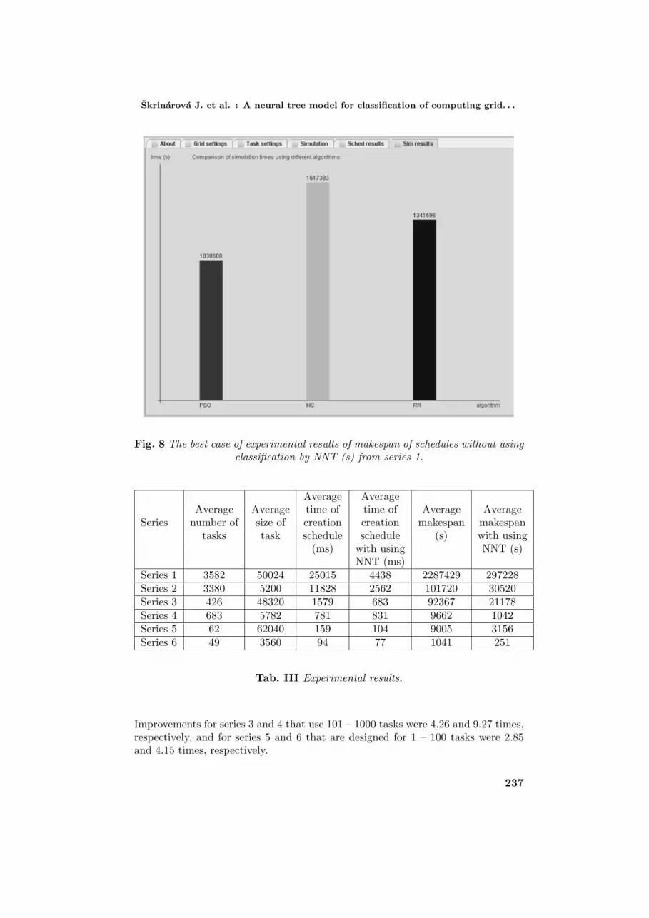
Experimental results of average time of creating schedule (ms) and averagetime of makespan of schedules (s) with and without neural network tree are in thetable (see Tab. III). There is a comparison of three algorithms (PSO, Hill climbingand Round Robin) in Figs. 8 and 9. There are values of schedules makespan (s)in these figures. For this paper we take into account only simulation time of PSOoptimization of scheduling. The best experimental case of schedule creating withoutusing neural tree for series 1 is in the figure (see Fig. 8). The worst experimentalcase of schedule creating when using neural tree for series 1 is in figure (see Fig. 9).

We have used three different variants of this algorithm that differ in algorithmparameters. PSO-1 variant uses 10 particles and 300 iterations for series 5 and6. Variant PSO-2 uses 20 particles and 300 iterations for series 3 and 4. VariantPSO-3 uses 30 particles and 500 iterations for series 1 and 2.

There is a comparison of average time of schedule creation without and withneural tree in figure (see Fig. 10). We can see comparison of time of makespan ofschedules without and with using neural tree in the figure (see Fig. 11). There arevertical axes in logarithmic scale to base 10 in the figures (see Fig. 10 and Fig. 11).We have assumed improvement in scheduling in systems with large portions of tasksfor high performance computing. This assumption was confirmed. The experimentsshow that there are also improvements in cases of middle and relatively smallportions of tasks (up to 100).

The average improvement of the makespan criterion for schedules by usingNNT with a large number of tasks, large task length (series 1) was 7.7 times, andimprovement for a large number of relatively small tasks (series 2) was 3.33 times.

236


Fig. 8 The best case of experimental results of makespan of schedules without usingclassification by NNT (s) from series 1.

Average AverageAverage Average time of time of Average Average

Series number of size of creation creation makespan makespantasks task schedule schedule (s) with using

(ms) with using NNT (s)NNT (ms)

Series 1 3582 50024 25015 4438 2287429 297228Series 2 3380 5200 11828 2562 101720 30520Series 3 426 48320 1579 683 92367 21178Series 4 683 5782 781 831 9662 1042Series 5 62 62040 159 104 9005 3156Series 6 49 3560 94 77 1041 251

Tab. III Experimental results.

Improvements for series 3 and 4 that use 101 – 1000 tasks were 4.26 and 9.27 times,respectively, and for series 5 and 6 that are designed for 1 – 100 tasks were 2.85and 4.15 times, respectively.

237


Fig. 9 The worst case of experimental results of makespan of schedules with usingclassification by NNT (s) from series 1.

Fig. 10 Comparison of average time of schedule creation without and with NNT.

238


Fig. 11 Comparison of time of makespan of schedules without and with NNT.

9. Conclusion

Job scheduling is computationally hard. It has been shown that the problem offinding optimal scheduling in heterogeneous systems is in general NP-hard.

This paper proposes a model of neural tree architecture with probabilistic neu-rons. These trees are used for classification of a large amount of computer grid re-sources to classes. The first tree is used for classification hardware part of dataset.The second tree classifies patterns of software identifiers. The trees are imple-mented to successfully separate inputs into nine classes of resources. We proposedParticle Swarm Optimization algorithm for tasks scheduling in computer grid. Wecompared time of creation of schedule and time of makespan for each of six series ofexperiments without and with NNT. In the experiments using NNT we gained thesubset of suitable computational resources. The aim was effective mapping of largetasks into particular resources. On the base of our experiments we can say thatimprovements have been made even for middle and small batch of tasks. Averageimprovement for each used structure batch of tasks is 5.28 when using NNT forclassification of resources against the experiments without neural tree.

In future works we plan to apply wave probabilities [27, 28], Heisenberg’s un-certainty limit [29] or information circuits [30] in our neural net models to speedup classification or to eliminate indefinites.

Acknowledgement

This work is partially supported by the High Performance Computing Centre ofMatej Bel University in Banska Bystrica, Slovakia (HPCC UMB).

239


References

[1] Xhafa F., Abraham A.: Computational models and heuristic methods for Grid schedulingproblems. Future Generation Computer Systems, 26, 2010, pp. 608–621.

[2] Rummelhardt D. E., Hinton G. E., Williams R. J.: Learning Representations by Back-propagation error. Parallel Distributed Processing: Explorations in the Microstructure ofCognition, MA: MIT Press, 1, 1986, pp. 318–362.

[3] Liu H., Abraham A., Hassainen A.: Scheduling jobs on computational grids using a fuzzyparticle swarm optimization algorithm. Future Generation Computer Systems, 2009.

[4] Kennedy J., Eberhart R. C., Shi Y.: Swarm intelligence, Morgan Kaufman, San Francisco.

[5] Li L. J., Huang Z. B., Liu F.: A heuristic particle swarm optimizer (HPSO) for optimizationof pin connected structures. Computing Structure, 85, 2007, pp. 340–349.

[6] Skrinarova J., Melichercık M.: Measuring concurrency of parallel algorithms. 1st Interna-tional Conference on Information Technology Gdansk: IEEE computer society, IEEE CatalogNumber: CFP0825E-PRT, 2008, pp. 289–292, ISBN 978-1-4244-2244-9.

[7] Parsopoulos K. E., Vrahatis M. N.: Recent approaches to global optimization problemsthrough particle swarm optimization. Natural Computing, 12, 2002, pp. 235–306.

[8] Shi Y., Eberhart R. C.: A modified particle swarm optimizer. Proceedings of IEEE congresson evolutionary computation, 1997, pp. 303–308.

[9] Li L. J., Huang Zy B., Liu F.: A heuristic particle swarm optimization method for trussstructures with discrete variables. Computers & Structures, 87, 2004, pp. 435–443.

[10] He S., Wu Q. H., Wen J. Y.: A particle swarm optimizer with passive congregation. Biosys-tems, 2004, 78, pp, 135–47.

[11] Buyya R., Murshed M. M.: GridSim: a toolkit for the modelling and simulation of distributedresource management and scheduling for Grid computing. Concurrency and Computation:Practice and Experience, 2002, pp. 1175–1220.

[12] Geekbench, Geekbench result browser 2011 http://browse.geekbench.ca/, 2010.[Online; ac-cessed 19–March–2012].

[13] Skrinarova J., Krnac M.: E-learning course for scheduling of computer grid, InternationalConference Interactive Collaborative Learning ICL 2011. Wien : International Associaton ofOnline Engineering, IEEE Computer Society, 2011, pp. 352–356, ISBN 978-1-4577-1746-8.

[14] Luger G. F.: Artificial Intelligence: Structures and Strategies for Complex Problem Solving,Addison-Wesley Longman Publishing Co., Inc., Boston, MA, 2001.

[15] Haykin S.: Neural Networks, a comprehensive foundation. Prentice Hall, 1994.

[16] Micheloni Ch., Rani A., Kumar S., Foresti G. L.: A balanced neural tree for pattern classi-fication. Neural Networks, 2012, 27, pp. 81–90.

[17] Martincova P., Grondzak K.: Effective distributed query processing on the grid. In: 2ndInternational Workshop on Grid Computing for Complex Problems – GCCP 2006. November2006 IISAS Bratislava, Slovakia, pp. 129–135, ISBN 978-80-969202-6-6.

[18] Ko lodziej J., Xhafa F: Enhancing the genetic-based scheduling in computational grids by astructured hierarchical population. In: Future Generation Computer Systems, 27, 8, October2011, pp. 1035–1046.

[19] Lim D., Ong Y.-S., Jin Y.: Efficient hierarchical parallel genetic algorithms using grid com-puting, Future Generation Computer Systems, 23, 4, 2007, pp. 658–670.

[20] Ritchie G., Levine J.: A fast effective local search for scheduling independent jobs in het-erogeneous computing environments. Tech. Rep., Centre for Intelligent Systems and theirApplications, University of Edinburgh, 2003.

[21] Xhafa F., Gonzalez J. A., Dahal K. P., Abraham A.: A GA(TS) hybrid algorithm forscheduling in computational grids. HAIS, 2009, pp. 285–292.

[22] Liu H., Abraham A., Hassanien A. E.: Scheduling jobs on computational grids using a fuzzyparticle swarm optimization algorithm. Future Generation Computer Systems, 26, 8, 2010,pp.1336–1343.

240


[23] Kalantari M., Akbari M. K.: A parallel solution for scheduling of real time applications ongrid environments. Future Generation Computer Systems, 25, 7, 2009, pp. 704–716.

[24] Buyya R.: Economic-based distributed resource management and scheduling for grid com-puting, Ph.D. Thesis, Monash University, Australia, 2002.

[25] Schaefer R., Ko lodziej J.: Genetic search reinforced by the population hierarchy, Foundationsof Genetic Algorithms VII, Morgan, 2003, pp. 369–385.

[26] Yarkhan A., Dongarra J.: Experiments with scheduling using simulated annealing in a gridenvironment. In: Proc. of the 3rd International Workshop on Grid Computing, 2002, pp.232–242.

[27] Svıtek M.: Wave probabilities and quantum entanglement. Neural Network World, 18, 5,2008, pp. 401–406, ISSN 1210-0552.

[28] Svıtek M.: Wave Probabilistic Models. Neural Network World. 17, 5, 2007, pp. 469–481,ISSN 1210–0552.

[29] Svıtek M.: Investigation to Heisenberg’s uncertainty limit. Neural Network World, 8, 6, 2008,pp. 489–498, ISSN 1210–0552.

[30] Svıtek M., Votruba Z., Moos P.: Towards Information Circuits, Neural Network World, 20,2, 2010, pp. 241–247, ISSN 1210–0552.

[31] Huraj L., Reiser H.: VO Intersection Trust in Ad hoc Grid Environments. In: Fifth Interna-tional Conference on Networking and Services (ICNS 2009), Valencia, Spain, IEEE ComputerSociety, April 2009, pp. 456–461.

[32] Huraj L., Siladi V., Skrinarova J.: Towards a VO Intersection Trust model for Ad hoc Gridenvironment: Design and simulation results. IAENG International Journal of ComputerScience 2013, ISSN: 1819–9224.

[33] Skrinarova J., Krnac M.: Particle Swarm Optimization Model for Grid Scheduling. SecondInternational Conference on Computer Modelling and Simulation, CSSIM 2011. Brno, CzechRepublic, September 5-7, 2011. Brno: Brno University of Technology, pp. 146–153, ISBN978-80-214-4320-4.

[34] Skrinarova J., Krnac M.: Particle Swarm Optimization for Grid Scheduling. Informatics2011: Eleventh International Conference on Informatics, Roznava, November, 2011 Kosice:Faculty of Electrical Engineering and Informatics of the Technical University, 2011, pp. 153-158, ISBN 978-80-89284-94-8.

[35] Skrinarova J., Zelinka F.: The grid scheduling. GCCP 2010 6th International Workshop onGrid Computing for Complex Problems, Bratislava, November, 2010. Bratislava: II SAS, pp.100–107, ISBN 978-80-970145-3-7.

[36] Skrinarova J.: TSP Models for cluster computing on the base of genetic algorithm. 5thInternational Workshop on Grid Computing for Complex Problems. GCCP 2009. October,2009. Bratislava: II SAS, pp. 110–117, ISBN 978-80-970145-1-3.

[37] Skrinarova J., Zelinka F.: TSP Model of genetic algorithm on the base of Cluster computing.Informatics 2009 Tenth International Conference on Informatics, Herlany, November, 2009.Kosice: Technical University of Kosice, 2009, pp. 326–331, ISBN 978-80-8086-126-1.

[38] Martincova P.: Performance of simulated Grid scheduling algorithms. Journal of Information,Control and Management Systems, 5, 2/1, 2007, pp. 261–270, ISSN 1336-1716.

[39] Martincova P.: Global scheduling on the grid. InfoTech-2008 Proceedings of the InternationalConference on Information Technologies. September 2008, Varna St. Constantine and Elenaresort, Bulgaria. Sofia: Technical University, 2008, pp. 75–82, ISBN 978-954-9518-56-6.

241

242

Documents

A neural tree model for classification of computing grid resources using PSO tasks scheduling