Running head: BAYESIAN MODEL SELECTION

A Non-Technical Introduction to the Evaluation of Informative Hypotheses using Bayesian

Model Selection

Rens van de Schoot, Joris Mulder,

Herbert Hoijtink

Department of Methodology and Statistics

Utrecht University, The Netherlands

Marcel A. G. Van Aken, Judit S. Dubas, Bram Orobio de Castro

Department of Developmental Psychology

Utrecht University, The Netherlands

Wim Meeus

Research Centre Adolescent Development

Utrecht University, The Netherlands

Jan-Willem Romeijn

Department of Philosophy

Groningen University, The Netherlands

Abstract

In practice, it is often the case that a researcher has expectations about their research questions

that can be formulated in terms of informative hypotheses. For example, the mean of group 1 is

larger than the mean of group 2 and group 3, but smaller than group 4. Bayesian model selection

(BMS) can be used to evaluate such informative hypotheses using Bayes factors as selection

criteria. By now, a wide variety of models specified with (in)equality constraints can be analyzed

using BMS. Although BMS has been described in previous articles, these papers are rather

technical and published solely in statistical journals. The main objective of this article is to

provide an easy to read introduction to BMS. Moreover, we provide a two-step procedure how to

interpret the results of BMS. This is illustrated using an example from psychology.

Keywords: Bayesian model selection, inequality constraints, informative hypothesis, Bayes

factors.

A Non-Technical Introduction to the Evaluation of Informative Hypotheses with Bayesian Model

Selection

Null hypothesis testing has been the dominant research tool in the social and behavioural

sciences over the latter half of the past century. A valuable alternative for testing the null

hypothesis is evaluating informative hypotheses using Bayesian Model Selection (BMS)

(Hoijtink, Klugkist, & Boelen, 2008). We call a hypothesis informative if it contains information

about the relationship between model parameters. More specifically, model parameters such as

mean scores or regression coefficients can be constrained to being greater or smaller than either a

fixed value or other statistical parameters. An example of an informative hypothesis is that the

mean of a variable of group 1, is larger than the mean of group 2, which in turn is smaller than

group 3. Evaluation of informative hypotheses using BMS is emerging in the psychological

literature (Boelen & Hoijtink, 2008; Laudy, et al., 2005; Meeus, Van de Schoot, Keijsers,

Schwartz, & Branje, 2009; Van de Schoot, Hoijtink, & Doosje, 2009; Van de Schoot, & Wong,

2008; Van Well, Kolk, & Klugkist, 2008).

Previous articles about the methodology mainly deal with the technical aspects (for an

overview see: Hoijtink et al., 2008). The purpose of this article is therefore to (i) present an easy

to read introduction to BMS for applied researchers, and (ii) to provide guidelines how to

interpret the results of BMS. This is necessary because, unlike classical hypothesis testing, BMS

does not use p-values, but Bayes factors. These are calculated for each informative under

evaluation and provide the amount of support from the data for each hypothesis. The

methodology is illustrated using a study from developmental psychology.

Example

Van Aken and Dubas (2004) investigated differences between three personality types in

adolescence: resilient (R), over-controlled (O), and under-controlled adolescents (U). The main

question was whether psychosocial functioning (externalizing (E), internalizing (I) and social

problem (S) behavior) is the result of the interplay between personality and support from family.

Just like in the original article, personality type was assessed by big-five personality

markers (Gerris, Houtmans et al., 1998). Furthermore, the problem behaviour list (PBL; De

Bruyn, Vermulst, & Scholte, 2003) was used to obtain parent reports on children’s behavioural

problems, measured on a 5-point scale. Finally, the relational support inventory (RSI; Scholte,

Van Lieshout, & Van Aken, 2001) was used to measure the support that children receive from

their parents to obtain high versus low family support.

Based on personality type (R, O, U), high or low family support (H, L), 3 x 2 = 6 groups

of adolescents were constructed assessed on three dependent variables (E, I, S), see Table 1. Let

µ denote the mean score on the dependent variable, for example µRHE is the mean score for

Resilient adolescents with High family support on the dependent variable Externalizing behavior.

Below, three expectations are presented concerning the ordering of these 6 groups. Such

expectations are what we call informative hypotheses.

The first two expectations (HA and HB) are based on several studies showing that the three

personality types have a distinct pattern of psychosocial and relational functioning (see, for

example, Van Aken, Van Lieshout, Scholte, & Haselager, 2002). The first expectation (HA)

states that under-controllers are expected to have the most externalizing problems and over-

controllers are expected to have the most internalizing problems. Over-controllers (O) and under-

controllers (U) are believed to score higher on social problems compared to resilient adolescents

(R). Moreover, no constraints are specified with respect to high/low family support. The

informative hypothesis HA can be formulated as

(µRHE, µRLE, µOHE, µOLE) < (µUHE, µULE)

HA : (µRHI, µRLI, µUHI, µULI) < (µOHI, µOLI) (1)

(µRHS, µRLS) < (µOHS, µOLS, µUHS, µULS).

The second expectation (HB) states, additionally to HA, that resilient adolescents best

function in all psychosocial domains in comparison to the other two types of adolescents. Hence,

the informative hypothesis HB contains two additional constraints in comparison to HA,

(µRHE, µRLE) < (µOHE, µOLE) < (µUHE, µULE)

HB : (µRHI, µRLI) < (µUHI, µULI) < (µOHI, µOLI) (2)

(µRHS, µRLS) < (µOHS, µOLS, µUHS, µULS).

Previous research also indicates that it is the combination of personality type and the

quality of social relationships that determines the risk level for experiencing more problem

behavior (Van Aken et al., 2002). Therefore, additional constraints are constructed for the third

expectation (HC). Over- and under-controllers with high perceived support from parents are

expected to function better in psychosocial domains than those with low perceived support. For

the resilient group, the level of support from parents is not related to problem behavior. The

additional constraints for informative hypothesis HC are

(µRHE = µRLE) , (µOHE < µOLE) , (µUHE < µULE)

HC : (µRHI = µRLI) , (µUHI < µULI) , (µOHI < µOLI) (3)

(µRHS = µRLS) , (µOHS < µOLS) , (µUHS < µULS).

Now that the research expectations are carefully formulated, the goal is to determine

which of hypothesis HA or HB receives most support from the data. The best of these two

hypotheses is then combined with the constraints of HC to investigate whether these additional

constraints are supported by the data.

The Method of Bayesian Model Selection

The method of BMS provides an answer to the research question which informative

hypothesis receives most support from the data. This is described step by step in this section.

Simple Example

To explain BMS, consider the following simple example. Suppose the research question

is whether over- (O) and under-controlled (U) adolescents differ on externalizing behavioral

problems. Furthermore, suppose the first hypothesis (HA) postulates that there is no restriction

between the means on externalizing behaviour, that is, any combination of means is admissible.

This model is also known as the unconstrained hypothesis. The second hypothesis (HB)

postulates that the externalizing behavioral problems of both groups are equal. This model is also

known as an equality constrained hypothesis. The third hypothesis (HC) postulates that over-

controlled adolescents score lower on externalizing problem behavior than under-controlled

adolescents. This model is also known as an inequality constrained hypothesis. Formally, the

three hypotheses in this simple example are

HA: µO , µU;

HB: µO = µU; (7)

HC: µO < µU.

To evaluate the set of hypotheses in (7) with BMS, three components are needed that will

be explained successively: (1) admissible parameter space, which represents the expectations of

the researcher; (2) the likelihood of data, which represents the information in the data set with

respect to µO and µU ; and (3) the marginal likelihood, which represents the support from the data

for each hypothesis, combining model fit and model size. This latter component can be converted

in Bayes a factor, which is the model selection criterion used in our methodology and combines

the above components.

Admissible Parameter Space

The first component is the admissible parameter space, which is based on the (in)equality

constraints in the informative hypothesis. Let the squares in Figure 1 represent the complete

parameter space. For HA, every combination of µO and µU is permitted, and therefore, the

admissible parameter space of HA is equal to the total parameter space (Figure 1). For HB, µO and

µU must be equal, which implies that only that part of the parameter space is admissible in which

µO is equal to µU. This is represented by the diagonal in Figure 1. For HC, only combinations of

µO and µU are permitted in which µO is smaller than µU, which results in the lower triangle in

Figure 1. Thus, the admissible parameter space is the total of all possible combinations of the two

means for µO and µU that satisfy the restrictions of each of the hypotheses (HA, HB, HC) before

observing the data. In sum, with respect to admissible parameter space, the hypotheses can be

ordered from a small parameter space to a large parameter space: HB, HC, HA.

The actual specification of prior distributions in this situation is far from easy and is not

considered the topic of this paper. The interested reader is referred to Mulder, Hoijtink, and

Klugkist (2009) for a detailed description of a default specification of the prior used in the

software.

Likelihood of the Data

The second component is the likelihood of the data, which is the representation of the

information about the means in the data set. In Figure 2 the likelihood function is plotted as a

function of µO and µU. The higher this surface, the more likely is the corresponding combination

of µO and µU in the population. In this example the (hypothetical) sample means are 3.6 for µO

and 4.1 for µU. So, given the data, the combination µO = 3.6 and µU = 4.1 is the most plausible, or

the most likely combination of values for the population means. As can be seen in Figure 2, the

likelihood function achieves its maximum for this combination. Other combinations of means are

less likely, for example for the combination µO = 1.5 and µU = 2.1 the likelihood function is much

lower.

Marginal Likelihood

The third component is the marginal likelihood (M, in Table 2), which is a measure for

the degree of support for each hypothesis provided by the data. The marginal likelihood is

approximately equal to the average height of the likelihood function within the admissible

parameter space.

Figure 1 presents the admissible parameter space for each hypothesis. Figure 2 displays

the likelihood of the data. Both pieces of information are combined in Figure 3. The likelihood

function in Figure 2 is presented as a contour-plot in Figure 3. The circles are iso-density

contours of the likelihood function. The maximum likelihood is located in the centre of the

smallest ellipse. Remember that when moving away from this centre, the likelihood of the

combination of population means of µO and µU becomes smaller.

Because the admissible parameter space for HA is equal to the complete parameter space,

the marginal likelihood of HA can be computed as the average height of the likelihood in the

complete parameter space, see Table 2. This value is only meaningful in comparison to the

marginal likelihood values of the other hypotheses under investigation. For HB the average height

of the likelihood function is computed on the diagonal in Figure 3. For HC, the average height of

the likelihood function is computed in the lower triangle in Figure 3. The results are presented in

the first column in Table 2. As can be seen in this table, HC has the highest value, followed by HA

and HB, respectively.

When taking a closer look at Figure 3, we can inspect two things: model fit and model

size. Consider HC and note that the size admissible parameter space is in between hypothesis HA

and HC. Also note that the maximum of the likelihood function in located within the admissible

parameter space of HC and HA, but not in HB. Moreover, the likelihood function in the upper

triangle of the total parameter space, which is incorporated in HA but not in HC, is low.

Consequently, the average height of the likelihood of HC is larger than the average height of HA.

Hence, the marginal likelihood of HC is larger than the marginal likelihood of HA. For HB the

maximum of the likelihood is not within the admissible parameter space HB. For this reason, the

marginal likelihoods of HA and HC are larger than the marginal likelihood of HB. Hence, the

marginal likelihood rewards a hypothesis with the correct (in)equalities in the informative

hypothesis, and therefore, it combines model fit and model size of a hypothesis.

Software

Software is available for: analysis of (co)variance models (Klugkist, Laudy, & Hoijtink,

2005; Kuiper, & Hoijtink, 2009), latent class analyzes (Laudy, Boom, & Hoijtink, 2005;

Hoijtink, 1998, 2001), order restricted contingency tables (Laudy & Hoijtink, 2007), and

multivariate linear models (Mulder, Hoijtink, & Klugkist, 2009). For more information see the

edited book by Hoijtink, and colleagues (2008) or www.fss.uu.nl/ms/informativehypothesis.

The Results of Bayesian Model Selection

In the previous section we computed the marginal likelihood values, which can be used to

compare a set of hypotheses. In this section, we show how the outcomes of the marginal

likelihood can be used to calculate relative amount of support for a certain hypothesis compared

to the other hypotheses. This can be done using Bayes Factors (BFs).

Bayes Factors

Bayes Factors are defined as the ratio of two marginal likelihoods (Ms). The outcome represents

the amount of evidence in favour of one hypothesis compared to another hypothesis. The BF for

HC compared to HA can be obtained from the marginal likelihoods of both hypotheses:

2 e 2.83

e 5.71

M

MBF

67-

-67

A

CCA ≈==

This Bayes factor, BFCA, implies that after observing the data, HC receives two times more

support from the data than HA. For BFCB the result implies that HC receives

31 e 1.81

e 5.71

M

MBF

68-

-67

A

BBA ≈==

as much support from the data than HB.

Interpretation of the Results

When evaluating a set of hypotheses using Bayes factors, we advice the following two-

step procedure.

Step 1

In the first step, the BF of each informative hypothesis is calculated against the

unconstrained hypothesis. If the BF of a certain informative hypothesis versus the unconstrained

hypothesis is larger than 1, it can be concluded that there is support from the data in favour of the

informative hypothesis. If the BF of a certain informative hypothesis versus the unconstrained

hypothesis is smaller than 1, it can be concluded that there no support from data for the

informative hypothesis. The reason for calculating Bayes factors, is to inspect the overall model

fit of the hypotheses under investigation. The informative hypotheses can be divided in a set of

“supported” hypotheses and a set of “unsupported” hypotheses. If all informative hypotheses are

considered “unsupported”, the unconstrained hypothesis receives most evidence, and new

informative hypothesis specification is called for. Unless a researcher is interested in which

hypothesis out of a set of “unsupported” hypotheses is least unsupported.

In our simple example, HA is the unconstrained hypothesis. The Bayes factor, BFCA, for

HC compared to HA is 2 (see Table 2), indicating that HC receives support from the data. The

BFBA for HB compared to HA is .06 implying that HB receives less support from the data than the

unconstrained hypothesis HA. Hence, the informative hypothesis HB can be considered as

“unsupported” while the informative hypothesis HC can be considered as “supported”.

Step 2

In the second step, we compare all the informative hypotheses under investigation with

each other. From these results, it can be concluded whether the data (strongly) supports a single

informative hypothesis or several informative hypotheses. For our simple example, the two

informative hypotheses are HB and HC. These hypotheses are now directly compared with each

other by calculating the Bayes factor BFCB. The methodology allows for doing so, if we use the

BFs against the unconstrained hypothesis, in our example, BFCA and BFBA. The BFCB can now be

calculated by

.31.06

2

BF

BFBF

BA

CACB ≈==

This result suggests strong evidence in favour of hypothesis HC in comparison to hypothesis HB.

So, if we were to choose between the informative hypotheses under investigation, hypothesis HC

receives most support from the data. From this analysis it can be concluded that over-controlled

adolescents score lower on externalizing problem behavior than under-controlled adolescents.

Example Reconsidered

In this section we show how the informative hypotheses of the example of Van Aken and

Dubas (2004) can be evaluated by first examining the descriptive statistics and applying classical

MANOVA, and second, by applying BMS. Table 3 presents the observed means for all groups.

We follow the two-step procedure described before to interpret the results.

Step 1. The first step involves comparing all informative hypotheses HA, HB, and HC to

the unconstraint hypothesis, which we shall denote by HU. The results, which are displayed in the

second column of Table 4 (BF*), show that all informative hypotheses have a BF larger than 1

versus HU. For example, the BF between HA and HU is 30.28, indicating that HA receives 30.28

times more support than HU. From these BFs, it can be concluded that each of the hypotheses HA,

HB, and HC receives support from the data.

Step 2. The second step involves comparing informative hypotheses with each other using BFs.

We first want to compare HA with HB to decide whether additionally to the constraints of HA,

resilient adolescents function best in all psychosocial domains. The BF of HB against HA is given

by BFBA = BFBU/BFAU = 64.20/30.28 = 2.12. This result implies that the support for HB is about

2 times as strong in comparison to HA. From this analysis it can be concluded that additional to

the constraints of HA, there is also evidence that resilient adolescents score lower on

externalizing behavior than over-controlled adolescents and resilient adolescents score lower on

internalizing behavior than under-controlled adolescents as was assumed by expectation HB.

Secondly, we are interested whether the additional constraints of HC in (3) in comparison

to the constraints of HB are supported by the data. Consequently, the additional constraints of HC

are combined with the constraints of HB, leading to the informative hypothesis HC, i.e.,

(µRHE = µRLE) < (µOHE < µOLE) < (µUHE < µULE)

HC: (µRHI = µRLI) < (µUHI,< µULI) < (µOHI < µOLI) (4)

(µRHS = µRLS) < (µOHS < µOLS) , (µUHS < µULS).

For this reason, we calculated the BFs of HC versus HA and HB (see the fourth column in

Table 4). The BFs show that there is much support in favour of HC against HA and HB. For

example, the BF for HC against HB is 21.79, stating that there is approximately 21 times as much

support for HC compared to HB. From this analysis it can be concluded that the additional

constraints of HC are a meaningful addition to the constraints of HB.

In conclusion, the results of BMS provide strong support for the idea that it is the

combination of personality type and the quality of social relationships that puts adolescents at

risk for experiencing more problem behavior.

Conclusion

In practice it is often the case that a researcher has expectations in terms of (in)equality

constraints between means or regression coefficients. We refer to such expectation as informative

hypotheses, because these include information about the ordering of the parameters. In this

paper, we have shown that Bayes factors (BFs) which is a Bayesian model selection criteria,

provide useful tools when determining whether such expectations are supported by the data.

These selection criteria quantify the amount of support an informative hypothesis receives from

the data. BFs combine the information available in the data into just one single result for each

informative hypothesis taking all constraints simultaneously into account. Furthermore, we

proposed an easy to use two-step procedure to interpret the outcomes of these model selection

criteria. In the end, the results of BMS provide a direct answer to the research question at hand.

References

Boelen, P. A., & Hoijtink, H. (2008). Famous psychological data sets and hypotheses. In H.

Hoijtink, I. Klugkist, & P. A. Boelen (Eds.). Bayesian evaluation of informative

hypothesis (chap. 1). New York: Springer.

De Bruyn, E. E. J., Vermulst, A. A., & Scholte, R. H. J. (2003). The Nijmegen problem

behaviour list: Construction and psychometric characteristics (manuscript submitted for

publication).

Gerris, J. R. M., Houtmans, M. J. M., Kwaaitaal-Roosen, E. M. G., Schipper, J. C., Vermulst, A.

A., & Janssens, J. M. A. M. (1998). Parents, adolescents, and young adults in Dutch

families: A longitudinal study. Nijmegen, The Netherlands: Institute of Family Studies,

University of Nijmegen.

Hoijtink, H. (1998). Constrained latent class analysis using the Gibbs sampler and posterior

predictive p-values: Applications to educational testing. Statistica Sinica, 8, 691-712.

Hoijtink, H. (2001). Confirmatory latent class analysis: Model selection using Bayes factors and

(pseudo) likelihood ratio statistics. Multivariate Behavioral Research, 36, 563-588.

Hoijtink, H., Klugkist, I., & Boelen, P. A. (Eds.). (2008). Bayesian evaluation of informative

hypotheses. New-York: Springer.

Klugkist, I., Laudy, O., & Hoijtink, H. (2005). Inequality constrained analysis of variance: A

Bayesian approach. Psychological Methods, 10, 477-493.

Kuiper, R. M., & Hoijtink, H. (2009). Comparisons of means using confirmatory and exploratory

approaches. Manuscript submitted for publication.

Laudy, O., Boom, J., & Hoijtink, H. (2005). Bayesian computational methods for inequality

constrained latent class analysis. In A. Van der Ark & M. A. C. K. Sijtsma (Eds.). New

development in categorical data analysis for the social and behavioural sciences (p. 63-

82). Erlbaum: Londen.

Laudy, O., & Hoijtink, H. (2007). Bayesian methods for the analysis of inequality constrained

contingency tables. Statistical Methods in Medical Research, 16, 123-138.

Meeus, W., R. Van de Schoot, L. Keijsers, S. J. Schwartz, and S. Branje. (2009). On the

Progression and Stability of Adolescent Identity Formation. A Five-Wave Longitudinal

Study in Early-to-middle and Middle-to-late Adolescence. Conditional accepted in Child

Development.

Mulder, J., Hoijtink, H., & Klugkist, I. (2009). Equality and Inequality Constrained Multivariate

Linear Models: Objective Model Selection Using Constrained Posterior Priors. Submitted

for publication.

Scholte, R. H. J., Van Lieshout, C. F. M., & Van Aken, M. A. G. (2001). Relational support in

adolescence: Factors, types, and adjustment. Journal of Research in Adolescence, 11, 71-

94.

Van de Schoot, R., Hoijtink, H., & Doosje, S (2009). Rechtstreeks verwachtingen evalueren of

de nul hypothese toetsen? [Directly evaluating expectations or testing the null hypothesis.

Null hypothesis testing versus Bayesian Model Selection]. De Psyshcoloog, 4, 196 – 203.

Van de Schoot, R., & Wong, T. (2008). Do delinquent young adults have a high or a low level of

self-concept: applying Bayesian model selection and informative hypotheses? Manuscript

submitted for publication.

Van Aken, M. A. G., & Dubas, J. D. (2004). Personality type, social relationships, and problem

behaviour in adolescence. European Journal of Developmental Psychology, 1, 331-348.

Van Aken, M. A. G., Van Lieshout, C. F. M., Scholte, R. H. J., & Haselager, G. J. T. (2002).

Personality types in childhood and adolescence: Main effects and person relationship

transactions. In L. Pulkkinen & A. Caspi (Eds.), Pathways to successful development:

Personality over the life course. Cambridge: Cambridge University Press.

Van Well, S., Kolk, A. M., & Klugkist, I. (2008). The relationship between sex, gender role

identification, and the gender relevance of a stressor on physiological and subjective

stress responses: Sex and gender (mis)match effects. Behavior Modification, 32, 427-449.

Table 1.

Groups of Adolescents Based on Personality Type, Problem Behavior and Support.

Problem behavior

Externalizing Internalizing Social

Resilient High family support µRHE µRHI µRHS

Low family support µRLE µRLI µRLS

Over High family support µOHE µOHI µOHS

Low family support µOLE µOLI µOLS

Under High family support µUHE µUHI µUHS

Low family support µULE µULI µULS

Table 2.

Results of BMS for the Simple Example.

Expectation M BF

HA 2.83 e-67

1

HB 1.81 e-68

0.06

HC 5.71 e-67

1.99

note M = Marginal Likelihood; BF = Bayes Factor.

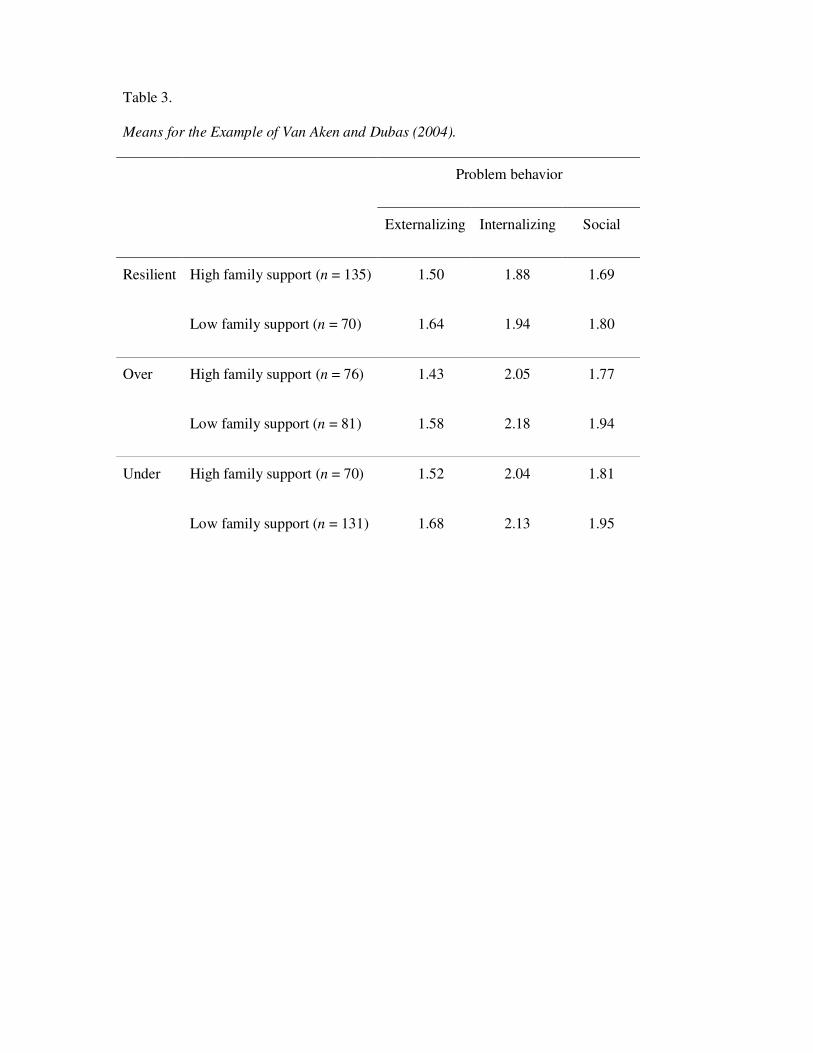
Table 3.

Means for the Example of Van Aken and Dubas (2004).

Problem behavior

Externalizing Internalizing Social

Resilient High family support (n = 135) 1.50 1.88 1.69

Low family support (n = 70) 1.64 1.94 1.80

Over High family support (n = 76) 1.43 2.05 1.77

Low family support (n = 81) 1.58 2.18 1.94

Under High family support (n = 70) 1.52 2.04 1.81

Low family support (n = 131) 1.68 2.13 1.95

Table 4.

Results of BMS for the Example of Van Aken and Dubas (2004).

Expectation BF* BF** BF***

HA 30.28 1 46.20

HB 64.20 2.12 21.79

HC 1399.00 - 1

* BF compared to the unconstrained hypothesis HU

** BF between HA and HB

*** BF of an informative hypothesis versus hypothesis HC

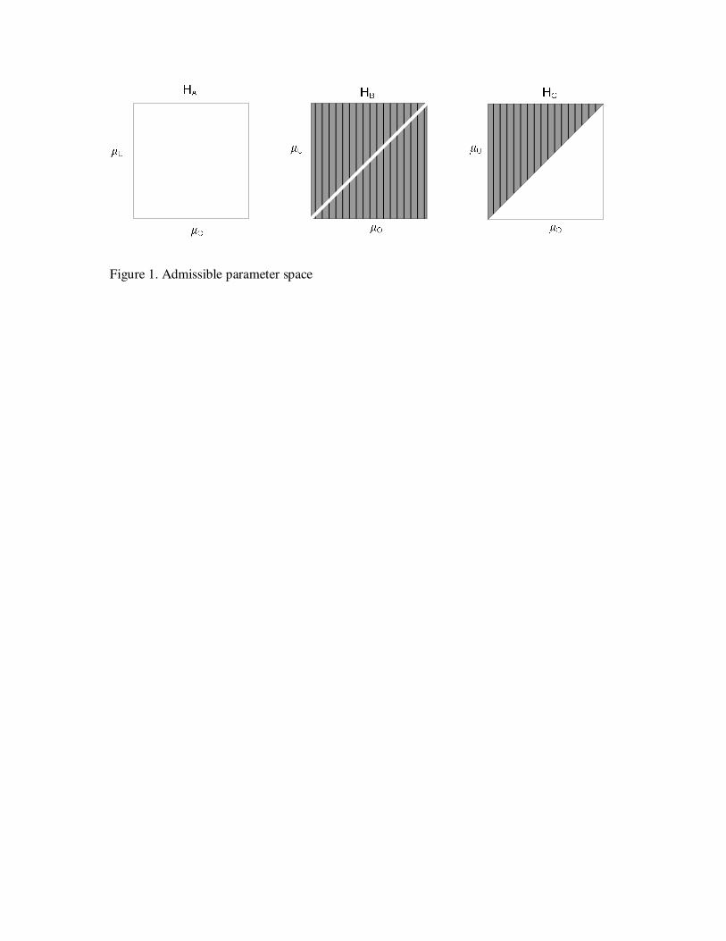
Figure 1. Admissible parameter space

Figure 2. Likelihood of the data

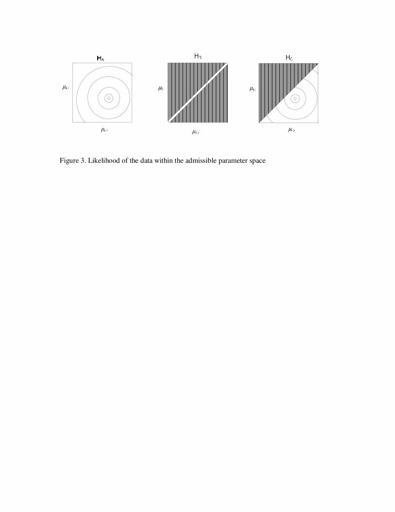
Figure 3. Likelihood of the data within the admissible parameter space