A one-dimensional reaction/di�usion systemwith a fast reactionThomas I. SeidmanDepartment of Mathematics and StatisticsUniversity of Maryland Baltimore CountyBaltimore, MD 21228e-mail: hseidman@math.umbc.eduiLeonid V. KalachevDepartment of Mathematical SciencesUniversity of MontanaMissoula, MT 59802e-mail: hleonid@selway.umt.eduiABSTRACT: We consider a system of second order ordinary di�erential equa-tions describing steady state for a 3{component chemical system (with di�usion)in the case when one of the reactions is fast. We discuss the existence of solutionsand the existence, uniqueness, and characterization of a limit as the rate of thefast reaction approaches in�nity.KeyWords: reaction/di�usion system, boundary value problem, steady state,fast reaction, asymptotics.

1

1. IntroductionFrom the viewpoint of chemical engineering, our objective is to understandthe di�usion controlled rate for a surface reaction 2A + B ! D in terms of acoupled pair of rapid irreversible binary reactions1A+B �! C; A + C �! D (1.1)involving an intermediate complex C. Mathematically, this will lead us to consider21The system (1.1) in a `�lm' (cf., [5]) was also treated as a model problem in [2], thereinvolving much di�erent considerations. For a perspective of one general setting in whichproblems of this sort arise, see [3] for a discussion of some of the modeling issues arising in thecontext of bubble reactors. We are here indebted to J. Romanainen, of Kemira Chemicals, forraising the question discussed in this paper.2The variables u; v; w of (1.2) represent normalized concentrations of A;B;C, respectively;we have omitted consideration of the reaction product D as well as of any other species whosereactions, if coupled at all with (1.1), are negligible within the membrane. The quadraticterms �uv and �uw are then the usual kinetics for reactions in dilute solution. The variable xrepresents position transverse to the membrane thickness; we are assuming that this situationis e�ectively constant in directions paralllel to the surface. We have chosen units to scale themembrane thickness to 1 and the di�usion coe�cients by a to get aj = O(1). Note that thismeans that the original reaction rates have been multiplied by h2=a; as they appear here, wehave � = O(1) and �� 1 (with �!1 later). [It would also have been be possible, using thestructure of the equation, to normalize the concentrations so as to have � = 1 as well, but wehave chosen not to do this.] The boundary conditions (1.3) correspond to the situation we willbe describing.2

the system of ordinary di�erential equationsa1u00 � �uv � �uw = 0a2v00 � �uv = 0a3w00 + �uv � �uw = 0 on (0; 1) (1.2)with the boundary conditionsu = � > 0; v0 = 0; w0 = 0 at x = 0;u0 = 0; v = � > 0; w0 = 0 at x = 1 (1.3)and the paper will be concerned primarily with the limiting behavior as �!1(with �; �; and � �xed) for solutions of (1.2)-(1.3). In particular, our objectivewill be the determination of q := R �uv for large � (!1), which corresponds tothe rate of production of C and of consumption of B | and also to the rate ofproduction of D, since the assumed boundary conditions for w ensure that thesecond reaction in (1.1) must go to completion.This analysis is interesting in its own right | both for the application and asleading to some interesting analysis | but may also serve as a model problem, inthat the techniques developed here may also be of use for similar situations. Tothis end, part of our analysis is presented in greater generality than is actuallyneeded for (1.2) and Remark 4 in Section 5 provides some brief further indicationof the scope of these ideas.Following the framework of Chapters 13{15 of [1], which we recommend as areference for the determination of di�usion controlled reaction rates and applica-tions, we �rst sketch the heuristic analysis of (1.1) when both �; � are e�ectivelyin�nite. Our point will be that this must be modi�ed | the objective of ouranalysis from the viewpoint of the application | when the second reaction in(1.1) is less rapid than is appropriate for that argument.3

For our purposes, one postulates steady state in a thin di�usive layer3 (suchas a membrane) of thickness h with the concentration of A maintained at A� onone side (x = 0) and, similarly, B = B� on the other (x = h). For both reactionsin (1.1) taken to be `instantaneous', we then have a reaction plane (x = x�h)within the di�usive layer with pure di�usion of B (i.e., with no reaction in theabsence of A) for x�h < x < h and pure di�usion of A for 0 < x < x�h soone has straight-line concentration pro�les. To obtain the overall stoichiometry2A + B ! D, the second reaction in (1.1) must go to completion so we mustassume that it takes place at the same reaction plane.4 The relevant slopes are�A�=x�h, B�=(1 � x�)h and the ux balance for this stoichiometry then givesa1A�=x� = 2a2B�=(1 � x�) where a1; a2 are the di�usion coe�cients for A;B,respectively. As the ux of B necessarily equals the production of D, the surfacereaction produces D at the rate_D =: q = (a1=2h)A� + (a2=h)B� (1.5)per unit area. Note that the situation is `di�usion controlled' as, even with3Di�usion is, e.g., on the order of 10�5cm2=sec | which is slow for a `normal' length scalebut fast enough (on the scale of a layer thickness h which may be about 10�3cm) that approachto steady state would be rapid compared to the `normal' time scale; in particular, one wouldexpect quasi-steady state `tracking' of comparatively slower parameter variations.4Otherwise we would get (1 + �)A+B ! �D + (1� �)C (1.4)where � here represents the fraction of the C produced which does become involved in thesecond reaction so (1 � �) is the remaining fraction which does not become so involved |presumably `escaping' by transport across x = h. This problem is not our present concern, butwe will comment on it in Section 5, Remark 4.4

this approximating assumption of in�nitely fast reaction speeds �; � in (1.1), thee�ective composite reaction rate is �nite, depending on the di�usion coe�cientsa1; a2 (normalized by the thickness h).We actually wish to consider (1.1) in a setting with the reaction rate � = O(1)(on the di�usive time scale) but still with the �rst reaction very much faster:�� 1. Thus, we take �!1 and anticipate a well-de�ned reaction plane withinthe membrane for the �rst reaction while noting that the second will now bedistributed over the region 0 < x < x�h where the component A is available.This means, of course, that in this region one will not have the straight linepro�le which made possible the simple analysis above.We do continue to want the second reaction to go to completion, as above,and so assume that the membrane is such as to give `no ux conditions' for thecomplex C on each side, so C cannot leave the membrane once produced. Thisis a somewhat di�cult situation to work with, since the Dirichlet conditions foru; v imply `potentially in�nite' sources of the reagents A;B which produce it.Thus, a steady state can only be possible if the net production of C would be0, i.e., if the production of C in the �rst reaction would always be balanced byits consumption in the second, slower reaction. It is not at all clear a prioriwhether such a balance should occur, but the consumption of C from the secondreaction might be expected to `grow' (from a time-dependent viewpoint) as theconcentration of C would build up and so one might hope that `eventually' itwould become high enough to give this balance | provided enough A remainedto maintain the slower reaction at this level.Section 2 will be devoted to obtaining suitable estimates and showing thatone does, in fact, have steady state solutions for �nite � > 0; the �rst part5

of Section 3 obtains an estimate giving enough compactness to ensure, at leastfor subsequences, some convergence as � ! 1. These arguments of Sections 2and 3 already depend somewhat delicately on the interaction of reactions andboundary conditions in our model problem but have a `PDE avor' and arepresented from that point of view, although with �nal emphasis on the speci�callyone-dimensional case consistent with our original motivation.As in the earlier heuristic argument, it is intuitively clear that A;B e�ectivelycannot coexist for very large � | if they were together they would `immediately'react to form C | so, in the limit �!1 we must have uv � 0 (i.e., A;B mustoccupy distinct geometric regions). Section 3 is concerned with a mathemati-cal demonstration of the corresponding characterization of `limit solutions', forthe subsequences noted above, with a return to the speci�cally one-dimensionalsetting for the more detailed convergence analysis.The chemical engineers' principal concern here would be with the determi-nation, as the parameters �; � (and �) vary, of the rate of production of D or,equivalently, the rate at which an external supply of B is being consumed by uxinto the membrane. [As already noted, this is q := R �uv.] For this determinationto be well-de�ned, it is necessary to show that the characterization of the limitsolution implies uniqueness, which is demonstrated in Section 4. This also com-pletes the convergence argument as � ! 1 by eliminating the need to extractsubsequences.The uniqueness argument seems rather specialized to the ODE context and tothe particular system at hand. Indeed, there seems no reason on physical groundsto expect uniqueness generally for problems of this sort. Although we do not, atpresent, know any actual example of such behavior, one might anticipate `track-6

ing' (in quasi-steady state), for slowly varying data in the boundary conditions,with the physical selection from among multiple steady states depending hys-teretically on the history of that variation.Finally, we note that the present paper is to be viewed as the initiation of amore complete program of investigation. In particular, we note that: (1) whilewe are exclusively concerned here with the steady state problem we anticipaterelated results for the time-dependent evolution and (2) the present results maybe viewed as providing the leading term of a singular perturbation expansion inpowers of "1=3 (cf. Remarks 1,2 in Section 5 and [4]) for the small parameter" := 1=�.2. Existence of a steady state solutionWhile our principal interest is with the one-dimensional problem (1.2)-(1.3),the considerations of this section and the next extend to a higher-dimensionalsetting so the results will be presented in that more general context, especially asthis exposition seems likely to provide a deeper understanding of the underlyingargument. In this section we present the argument for existence of (at least one)solution of the steady state problem. As already noted in the Introduction, themajor di�culty will be to bound the production rate of C (i.e., to bound thegeneration term R �uv) and then to bound the total amount of C at steady state(i.e., R w).We will now be considering a bounded region � IRm (physically, m =1; 2; 3, but mathematically we may have any m � 1) and the steady state reac-

7

tion/di�usion system takes the form8>>>>>><>>>>>>: a1 4 u� �uv � �uw = 0a2 4 v � �uv = 0a3 4w + �uv � �uw = 0 on u = � on �A with u� = 0 on @ n �Av = � on �B with v� = 0 on @ n �Bw� = 0 on @:(2.1)

Here �A;�B are separated portions of the boundary @ and �; � are (traces5 on�A;�B, repectively, of) functions such that�; � 2 H1() with 0 � � � ��; 0 � � � ��and Z�A � =: � > 0 (2.2)for positive constants ��; ��; �. For the region , we assume su�cient regularityfor the usual trace theorems; we will later state some further mild conditions(automatic for the one-dimensional case) which will be used in obtaining relevantestimates.We will prove existence by an argument using the Schauder Fixpoint Theorem.With M > 0 to be determined later, we setS = SM := f(u; v; w) : 0 � u � ��; 0 � v � ��; 0 � w; Rw � Mg� L2()� L2()� L1() (2.3)and then de�ne on S a map M : (u; v; w) 7! (u; v; rw) with u; v; w; r given bythe steps:5We need, e.g., 0 � � � �� only on �A but note that the global assumption involves no furtherloss of generality: else, just replace � pointwise on by minf��; �+g with �+ := maxf�; 0g.8

1. Solve for u the linear problema14 u� �uv � �uw = 0 withu = � on �A and u� = 0 on @ n �A (2.4)2. Using u from (2.4), solve for v the linear problema24 v � �uv = 0 withv = � on �B and v� = 0 on @ n �B (2.5)3. Using u; v from (2.4), (2.5), solve for w the linear problema3 4w + �uv � �uw = 0 with w� = 0 on @ (2.6)4. Set r := M=kwk1 if kwk1 � M and r := 1 if kwk1 � M .There is no question about the solvability of (2.4) when v; w � 0. MaximumPrinciple arguments then give u � 0 and u � ��; we brie y sketch the argumentfor the latter. [Take z := (u� ��)+ := maxf0; u� ��g � 0 as test function in theweak form of (2.4) | noting that z = 0 on �A so the boundary term vanishesafter application of the Divergence Theorem, that rz � ru = jrzj2, and thatuz � 0 | to get a1 Z jrzj2 = � Z[�v + �w]uz � 0whence z is a constant, necessarily 0 as z = 0 on �A. To show u � 0 onecorrespondingly takes z := u� := minf0; ug � 0.] Given u � 0, similar argumentsgive 0 � v � �� from (2.5). At this point we have an estimate0 � Z �uv =: q � �q (2.7)with �q = ��� ��jj for the moment, although we shall later be at pains to obtainan estimate for �q independent of �. 9

Since 0 � u 6� 0 as � > 0, the Neumann problem (2.6) is solvable for w: oneconsequence of the estimates we will shortly obtain is that one has a Fredholmoperator of index 0 for which 0 cannot be an eigenvalue, i.e., there cannot be anontrivial solution of the equation with � = 0. Since Q := �uv � 0, anotherMaximum Principle argument (now taking z := w� := minf0; wg � 0) showsthat w � 0. [We may note here that the positivity u; v; w � 0 is certainlynecessary for a physical interpretation of these as concentrations.] The de�nitionof r now ensures that M =MM maps SM to itself for any choice of M > 0. Wewill obtain estimates showing that M may be chosen (large enough) to ensurethat r = 1 at a �xpoint of M so one has a solution of (2.1). First, however, toensure the existence of a �xpoint by the Schauder Theorem we must commenton the continuity and compactness of M. Taking z = (u� �) as test function inthe weak form of (2.4), one getsa1kruk2 = a1 R ru � r� + R [�v + �w]u�� R [�v + �w]u2� a1krukkr�k+ �� [R �uv + ���M ]kruk2 � kr�k2 + 2��[��� ��jj+ ���M ]=a1 (2.8)and, similarly, krvk2 � kr�k2+2���q=a2 | giving H1() bounds (whence L2()compactness) for those components. Given this compactness and the uniquenessfor the equations, one easily gets continuity of the maps: v; w 7! u and then;u 7! v.Most of our e�ort must be devoted, as indicated in the Introduction, to esti-mating w. To this end, we �rst note from (2.6) thatZ[�uv � �uw] = a3 Z4w = 0 so Z �uw = Z �uv =: q (2.9)as w� = 0 on @. Next, we write w = �w +! where R �w= 0 and ! is a constant10

(so !jj = R w = kwk1). Now (2.6) gives �a34 �w= [�uv � �uw] with �w�= 0whence, using (2.7), k �w kW � Kk�uv � �uwk1 � 2K�q (2.10)for some suitable space W depending on the dimension m and the geometryof . For our present purposes, we only need compactness of the embedding6W ,! L1() with the consequent L1 estimatek �w k1 � �K �q: (2.11)Now suppose we were to have a lower bound on the amount of A in the system:Z u � �1 > 0: (2.12)Observing that R uw = R u �w +! R u, we get from (2.11) that�!�1 � �! Z u = Z �uw � � Z u �w� �q + ���k �w k1 � �1+ �K� �q; (2.13)with compactness since ! is one-dimensional. As before, this will give continuityas well as compactness for the map: u; v 7! w | once we can verify (2.12) | sothe Schauder Theorem will apply to ensure existence of a �xpoint of M. Notethat we have bounded kwk1 = jj! independently of the choice of M , so one canchoose M > �1+ �K� �q=��1 and be certain of obtaining r = 1 in step 4 at the�xpoint so this gives the desired solution of (2.1).It seems plausible that our next argument, verifying (2.12), could be modi�edto apply to more general geometries, but we avoid considerable complication by6This is a very mild restriction on | for a smooth boundary one would expect a `shifttheorem' giving W = W 2;1(). Certainly we have this for the one-dimensional setting withW =W 2;1(0; 1) � C0;1[0; 1]. 11

presenting this only for the case of a region which is cylindrical near �A | i.e.,such that we may coordinatize position in near �A by (x; y) with y 2 Y � IRm�1for 0 < x < � so the relevant portion � � has the form � = (0; �)� Y with�A = f0g � Y. We setU(x) := a1 ZY u(x; y) dy for 0 � x � �:Note that 0 < �U 0(0) = �a1 RY ux dy���x=0 = a1 R�A u� = a1 R@ u�= R a1 4 u = R �uv + R �uw;� 2�q: (2.14)Further, for 0 < x < � and y 2 @Y we have (x; y) 2 @ n �A with coincidence ofthe normals to @ and to @Y whence RY4yu = R@Y u� = 0 for 0 < x < � soU 00 = ZY a1 4 u = ZY [�uv + �uw] � 0whence U 0(x) � U 0(0) � �2�q on (0; �). Since (2.2) gives U(0) = a1� > 0, wethen have U(x) � maxf0; a1�� 2�qxg which givesZ u � 1a1 Z �0 U(x) dx � min(��2 ; a1�24�q ) =: �1: (2.15)This completes the proof of our existence result.3. Estimates; Convergence as �!1In this section we consider the convergence (for subsequences) of solutions of(1.2)-(1.3) as � ! 1. The section naturally divides into two parts: showing12

that all solutions we consider will lie in a �xed compact set, independent of�, assuring the existence of convergent subsequences with � = �k ! 1 andthen characterizing the limit functions [�u; �v; �w]. The �rst part essentially consistsof bounding q := R �uv (which is just the production rate of C) and, as in theprevious section, it is reasonable to do this in the PDE context for (2.1), obtaininga �-independent estimate for �q in (2.7). For the second part, we will �rst commentbrie y on the PDE context but will then return to the one-dimensional settingof (1.2)-(1.3) for detailed treatment. In that context we will obtain convergenceon [0; x�], where x� 2 (0; 1) is a new unknown variable, to a solution ofa1�u00 = ��u �w = a3 �w00; �v � 0 on (0; x�);�u = � > 0; �a1�u0 = 2q; �w0 = 0 at x = 0;�u = 0; �a1�u0 = a3 �w0 = q at x = x� (3.1)with convergence on [x�; 1] to�u � 0; �v = �x� x�1� x� ; �w = const = �w(x�) =: w�: (3.2)For the �rst part, in reconsidering (2.7), it is convenient to introduce a function# on such that7 0 � # � 1; 4# = 0 on # = 8<: 0 on �A1 on �B #� 2 L1(@) (3.3)7To have 0 � # � 1 on just requires interpolation between 0 and 1 on the remainder of@. It may be a mild restriction on that this can be done so as to have #� 2 L1(@). Wenote that one could omit the equation 4# = 0, asking instead only that 4# 2 L1() witha minor modi�cation of (3.5). In the one-dimensional case we could take #(x) = x, giving�q = 4[a1� + a2�] in (3.5) | although we note that (3.11) gives half that and further note(3.16). 13

Note that the boundary conditions in (3.3) and (2.1) give(1� #)u� � 0 � #v� on @: (3.4)Now, with #� 2 (0; 1), set < := fx 2 : # � #�g, > := fx 2 : # � #�g. On< one has (1� #�) � (1� #) and �uv � a1 4 u so one obtains(1� #�) Z< �uv � Z<(1� #)a1 4 u � Z(1� #)a1 4 u == �a1 Z@ u#� � a1�� Z@ j#�j :Similarly, one has #� � # on > and �uv = a2 4 v so#� Z> �uv � Z> #a2 4 v � Z #a2 4 v == �a2 Z@ v#� � a2 �� Z@ j#� j :Adding these estimates and minimizing over the choice of #� gives �q: one obtainsthe desired form of (2.7),q := Z �uv � �pa1 �� +qa2 ���2 Z@ j#� j =: �q: (3.5)From (2.8), taken at the �xpoint of M, and the similar estimate for v, onehas kuk(1) � �kr�k2 + 2���qa1 + jj��2�1=2kvk(1) � "kr�k2 + 2���qa2 + jj��2#1=2 (3.6)(where k � k(1) denotes the usual H1()-norm) so these are now bounded inde-pendently of �; �. Similarly, we have (2.11) bounding8 k �w kW independently of8We also note that the bound for v 2 H1() immediately bounds Q = 4v 2 H�1()| in terms of �q, of course, but without assuming an embedding L1() ,! H�1() which isunavailable for the higher dimensional case. This, in turn, would easily bound �w in H1()without using (2.10). 14

�; �. Using (2.12) | whether or not obtained as (2.15), in a somewhat specialgeometry | one has (2.13) bounding ! independently of � and of � � ��.Thus, for solutions (u; v; w) of (2.1) one has(u; v; w) bounded in H1()�H1()� [W + IR]; uniformly as �!1: (3.7)By compactness it follows that, for any sequence � = �k !1, there is a subse-quence for which one has convergence in, e.g., L2()� L2()� L1()(u; v; w) ! (�u; �v; �w)and one can also ask that u; v each converge weakly in H1() and pointwise aeon with some similar convergence for w, depending on the nature of W.Fixing any such subsequence and its limit, we now turn to the second part ofthe section: characterization of the limit functions (�u; �v; �w).The �rst observation is that all the uniform estimates we have obtained alsoapply in the limit | so 0 � �u � ��, etc. The product uv converges pointwise to�u�v and is uniformly dominated by the (integrable) constant ���� so uv ! �u�v inL1() by Lebesgue's Dominated Convergence Theorem. Since kuvk1 � �q=�! 0,one then must have �u�v � 0 (ae on ) as expected. Next, we observe thatju � �uj �w is dominated by �� �w and converges pointwise to 0 so u �w ! �u �w inL1(); we have kuw � u �wk1 � ��kw � �wk1 ! 0 so uw � u �w ! 0 in L1().Thus, �uw ! ��u �w in L1(). Since 4 is continuous from H1() to H�1(),hence also continuous between weak topologies, Q = 4v * 4�v =: �Q 2 H�1().[Somewhat independently, we note that L1() embeds (isometrically) in the dualspace [C(�)]� (= fmeasures on �g) and that Q := �uv is uniformly boundedin L1() so we have weak-� convergence there: Q �* �Q and �Q is a measure on�. We know that k �Qkm � �q.] Since each Q is positive (�; u; v � 0), one has15

immediately that �Q is a positive measure. We similarly note that 4u * 4�u inH�1() so ��u�v 2 L1() \H�1().Since the boundary conditions are independent of �, we see that the limit func-tions satisfy these as well (in some suitable sense; classical for the one-dimensionalcase) and so satisfy the limit system8>>>>>><>>>>>>: a1 4 �u� �Q� ��u �w = 0a2 4 �v � �Q = 0a3 4 �w + �Q� ��u �w = 0 on �u = � on �A with �u� = 0 on @ n �A�v = � on �B with �v� = 0 on @ n �B�w� = 0 on @:(3.8)

Either again taking limits or directly from (3.8), we haveZ�A �u� = 2q = 2 Z�B �v� with q := h �Q; 1i = lim�!1 Z �uv = Z ��u �w: (3.9)It is reasonable to conjecture that the distribution �Q is supported on aninterface (of codimension 1) partitioning into the subregions on which one has�u > 0, �v > 0, respectively, where it just gives the jump in the gradient across this`reaction surface'. We do not pursue this characterization for the general PDEsetting (although, note Remark 3 in Section 5), but now restrict our attention to(1.2)-(1.3) for more detailed treatment.In the one-dimensional case we have H1(0; 1) ,! C0;(1=2)�[0; 1] and W =W 2;1(0; 1) ,! C0;1[0; 1] so the convergence we have been discussing in the argu-ment for (3.8) implies uniform convergence on [0; 1]; we have a pointwise uniformupper bound for w and so for �w. A key observation in the one-dimensional settingis that the positivity of u00; v00 means that u0; v0 are monotone increasing so, with16

the boundary conditions u0(1) = 0 = v0(0), one has0 � a2v0(x) � a2v0(1) = q = q(�); 0 � �a1u0(x) � �a1u0(0) = 2q (3.10)| a2v0(x) = R x0 a2v00 = R x0 �uv � R 10 �uv =: q, etc. This also gives1� xa2 Z x0 �uv = (1� x)v0(x) � Z 1x v0 = � � v(x) � �;xa1 Z 1x �uv � �xu0(x) � � Z x0 u0 = �� u(x) � �;adding gives q � [a2�=(1�x)+a1�=x] and minimizing over x gives the alternativebound q � �pa1� +qa2��2 = �q � 2(a1� + a2�) (3.11)in this setting.We have L2-weak convergence for these derivatives9 so also 0 � �v0 � q,0 � ��u0 � 2q in the limit. This also implies that u; �u are decreasing and v; �vincreasing on [0; 1]. Since we have �u�v � 0, it follows that v(0) ! �v(0) = 0 < �as �u(0) = u(0) = � > 0 and, similarly, u(1)! �u(1) = 0. Thus, for each � (largeenough to ensure v(0) < � and u(1) < �) there is some � = �(�) 2 (0; 1) suchthat u(x) � v(x) on [0; �); u(x) � v(x) on (�; 1]:We have u(x) � � � 2qx so we also have �u(x) � � � 2qx > 0 for 0 � x < �=2q;similarly, v(x) � ��q(1�x) > 0 for 0 � (1�x) < �=q. Thus, � 2 [�=2�q; 1��=�q].Again extracting a subsequence if necessary, we have convergence � ! x� for somex� 2 [�=2�q; 1� �=�q]; in the limit one has10�u � 0; �v � 0 on [0; x�]; �v � 0; �u � 0 on [x�; 1]: (3.12)9Actually, one has uniform convergence on compact subsets of [0; 1]nfx�g with �u; �v; �w smoothexcept at x�.10As u; v; �u; �v are continuous, this is not merely `ae'.17

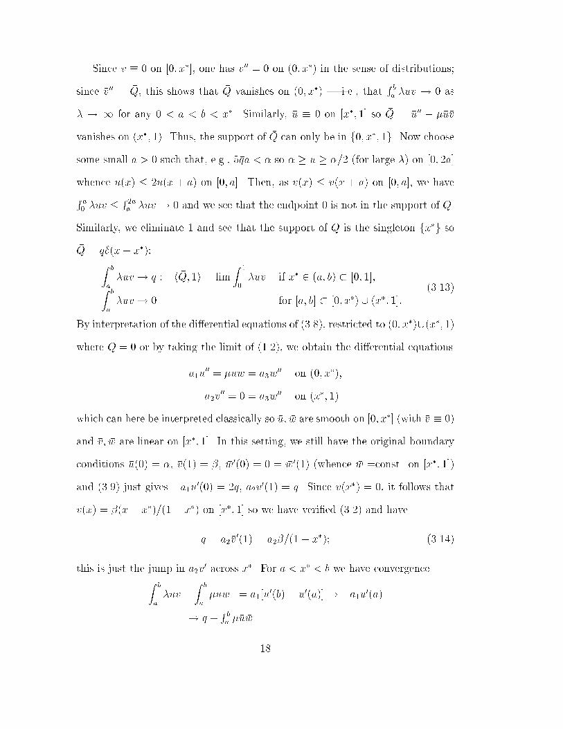
Since �v � 0 on [0; x�], one has �v00 = 0 on (0; x�) in the sense of distributions;since �v00 = �Q, this shows that �Q vanishes on (0; x�) | i.e., that R ba �uv ! 0 as� ! 1 for any 0 < a < b < x�. Similarly, �u � 0 on [x�; 1] so �Q = �u00 � ��u�vvanishes on (x�; 1). Thus, the support of �Q can only be in f0; x�; 1g. Now choosesome small a > 0 such that, e.g., 5�qa < � so � � u � �=2 (for large �) on [0; 2a]whence u(x) � 2u(x + a) on [0; a]. Then, as v(x) � v(x + a) on [0; a], we haveR a0 �uv � R 2aa �uv ! 0 and we see that the endpoint 0 is not in the support of �Q.Similarly, we eliminate 1 and see that the support of �Q is the singleton fx�g so�Q = q�(x� x�):Z ba �uv ! q := h �Q; 1i = lim Z 10 �uv if x� 2 (a; b) � [0; 1];Z ba �uv ! 0 for [a; b] � [0; x�) [ (x�; 1]: (3.13)By interpretation of the di�erential equations of (3.8), restricted to (0; x�)[(x�; 1)where �Q = 0 or by taking the limit of (1.2), we obtain the di�erential equationsa1�u00 = ��u �w = a3 �w00 on (0; x�);a2�v00 = 0 = a3 �w00 on (x�; 1)which can here be interpreted classically so �u; �w are smooth on [0; x�] (with �v � 0)and �v; �w are linear on [x�; 1]. In this setting, we still have the original boundaryconditions �u(0) = �, �v(1) = �, �w0(0) = 0 = �w0(1) (whence �w =const. on [x�; 1])and (3.9) just gives �a1�u0(0) = 2q, a2�v0(1) = q. Since �v(x�) = 0, it follows that�v(x) = �(x� x�)=(1� x�) on [x�; 1] so we have veri�ed (3.2) and haveq = a2�v0(1) = a2�=(1� x�); (3.14)this is just the jump in a2�v0 across x�. For a < x� < b we have convergenceZ ba �uv + Z ba �uw = a1[u0(b)� u0(a)]! �a1�u0(a)! q + R ba ��u �w 18

and letting a! x��, b! x�+ (so R ba ��u �w! 0) gives �a1�u0(x��) = q; similarly,we obtain a3 �w0(x��) = q, completing the veri�cation of (3.1).Note that (3.1) and the monotone decrease of �u0 give 2q � �a1�u0 � q on(0; x�) so, integrating, we have x�(2q=a1) � � � 0 � x�(q=a1). Combining thiswith (3.14) from (3.1) gives a1�a1� + 2a2� � x� � a1�a1� + a2� : (3.15)An immediate consequence of (3.15), using (3.14) again, is thata2� + 12a1� � q � a2� + a1� (3.16)| with the minimal value corresponding (with our normalization) to (1.5), wherewe also had � ! 1, and the maximal value corresponding to a similar compu-tation of the rate of consumption of B from the reaction A+B �! C alone, i.e.,�!1 with � = 0. Of course, the maximal value in (3.16) also provides a newbound �q in the limit.4. Uniqueness of the limit solutionIn this section we show uniqueness of the solution of the limit problem (3.1)[(3.2).Recalling that �v = 0 in [0; x�], we consider the problem (3.1); note that x� is hereunknown, except for (3.15), with q and �w(x�) =: �w� also unknown, except for(3.16).Subtracting the �rst di�erential equation of (3.1) from the other and integrat-ing twice with the additional conditions at x�, we obtain a3 �w = a1�u + a3 �w� �2q(x� � x) whencea1�u00 = ��u[a1�u+ a3 �w� � 2q(x� � x)]=a3 for 0 < x < x�:19

At this point we eliminate the unknowns x� and q by a substitution: if we sets := � �qa1a3 �1=3(x� � x); y := "a21a3�q2 #1=3u; ! := " a23�q2a1 #1=3 �w�; (4.1)then, with a bit of manipulation, the equation and initial conditions for the newvariable y = y(s) = y(s; !) take the form:yss = y(y + ! � 2s)y(0) = 0; ys(0) = 1; (4.2)with ! an unknown parameter. As �a1�u0(0) = 2q, we also haveys(s0) = 2 (4.3)where s = s0 corresponds to x = 0 so (4.1) gives s0 = (�q=a1a3)1=3x�. We mayreformulate this, using (3.14) to eliminate q, as an equation for x� in terms of s0: (x�)3 + x� � 1 = 0 := a2a1a3 ��s30 ! : (4.4)We note also that, since �u; �w > 0 on (0; x�), we must havey > 0; y + ! � 2s > 0 for 0 < s < s0: (4.5)Since the de�nition (4.3) of s0 gives ys < 2 on (0; s0) and so y(s)� 2s < 0, it isonly the strict positivity of ! which makes it at all possible to have y+!�2s > 0;on the other hand, that condition certainly ensures that y > 0.The key idea of our argument is to introduce a function: ! 7! U(!) as follows:Given !, solve the initial value problem (4.2), for s > 0 until ys attainsthe value 2, de�ning s0 = s0(!) by (4.3) and then setting = (!) := a2a1a3 ��s30(!) ; � = �(!) := y(s0(!); !); (4.6)20

|with s0; ; � unde�ned if (4.5) fails. (Note that (4.5) gives yss > 0 soone has uniqueness for the determination of s0 > 0 with > 0; � > 0also unique.) Now solve for x� = x�(!) as the unique positive root ofthe cubic (4.4), noting that this gives 0 < x� < 1 since > 0, and sodetermines q = q(!) := a2��=(1� x�) > 0. Finally, setU = U(!) := h� q2(!)=a21a3i1=3 �(!): (4.7)While this construction of U(!) is independent of our derivation from (3.1), etc.,it certainly is motivated by that, and we note from (4.1) (and the derivation)that when !; : : : do correspond to a solution of (3.1), then U(!) is just �u(0).The desired uniqueness is then an immediate consequence of the fact, whoseproof we defer momentarily, that U is a strictly decreasing function of ! | moreprecisely, that we will show the following.Lemma: There is some !0 > 0 such that U(�) is unde�ned for ! � !0 andis de�ned for ! > !0 with a vertical asymptote at !0. Where de�ned, U(�) is astrictly decreasing positive function of ! with U ! 0 as ! !1.We keep �; � > 0 �xed for our analysis, but do remark that the de�nitions of!0; y; s0; � are entirely independent of �; � and that, for �xed ! > !0, obviouslyincreases with the product �� so x�; q; U decrease as �; � increase.Since U(!) should correspond to u(0) for a solution of (3.1), we must haveU(!) = �: (4.8)From our present viewpoint, noting the lemma, we may use (4.8) to determine !uniquely | with existence of a solution ensured by our previous analysis | and21

so, as in the construction of U , to determine y; x�; q; w�. This then gives [�u; �v; �w]on [0; x�] satisfying (3.1) and the boundary conditions and then (3.2) also gives[�u; �v; �w] on [x�; 1]. Thus, the uniqueness of ! implies uniqueness of the triple[�u; �v; �w], which completes the uniqueness proof for the solution of the limit system(3.1){(3.2). Note that this uniqueness of the limit ensures that [u; v; w]! [�u; �v; �w]as following (3.7), but now without considering any extraction of sequences orsubsequences.Proof of the Lemma: From (4.8) and our work in the preceding sectionswhich showed existence of solutions to (3.1){(3.2) for each � > 0, we see thatU(!) is necessarily de�ned for some values of ! and that the range of U(�) is(0;1). We have already noted that (4.5) cannot hold if ! � 0 and a continuityargument then shows that U(!) must be unde�ned for ! < !0 for some !0 > 0.Fix any !1 for which U(!1) is de�ned and set s1 := s0(!1) > 0 so (4.5) holdson (0; s1]. A standard Maximum Principle argument shows that for ! > !1 wewill have a strict increase in y; ys; yss at each �xed s 2 (0; s1] so (4.5) holds on(0; s1] for any ! > !1. Thus, if U(!1) is de�ned, then U(!) is de�ned for any! > !1 and we may �x !0 > 0 so that U(!) is unde�ned for any ! < !0 and isde�ned for any ! > !0; we will later show that U(!0) is itself unde�ned.Now set z = z(s) := ys(s). Since yss > 0 by (4.5), z(�) is strictly increasing in sso we can invert to get s = �(z) = �(z; !). By the Maximum Principle argumentabove, we have z(s; !) strictly increasing in ! for each �xed s > 0 so, inversely,�(z; !) must be strictly decreasing in ! for each �xed z > 1. In particular, notingthat s0(!) = �(2; !), we see that s0(�) is a strictly decreasing function of ! wherede�ned. It immediately follows that is a strictly increasing function of !.Further, implicit di�erentiation of (4.4) gives dx�=d = �(x�)3=[3 (x�)2 + 1] < 022

so we have x�(!) a strictly decreasing function of ! and, immediately, q = q(!) :=�a2�=(1� x�) is also a strictly decreasing function of !.Next we wish to show that � = y(s0) is a decreasing function of ! so, with theabove, (4.7) would give strict decrease for U(�). [We know that y is increasing inboth s and ! but, since s0 is decreasing in !, decrease of y(s0) is not yet clear.]We now de�ne Y (z; !) := [y(�(z; !); !)]2| i.e., Y (z) = y2(s), suppressing the dependence on !|and conversely y = pY .By the chain rule,2yz = 2yys = dYds = dYdz dzds = dYdz yss = dYdz y(y + ! � 2s);whence dYdz = 2zpY + ! � 2�(z; !) ; Y (1) = 0: (4.9)[Note that (4.5) ensures positivity of the denominator.] Since @[! � 2�]=@! > 0,the right hand side in (4.9) is decreasing in !, so | again by a Maximum Principleargument | Y is (strictly) decreasing as a function of ! for each �xed z 2 (1; 2].In particular, �(!) = qY (2; !) decreases as ! increases.At this point we note that U cannot be de�ned (�nite) at !0 | if it were,then we would have U(!) � U(!0) < 1 wherever de�ned, which would con-tradict our observation that the range of U(�) is all of (0;1). We have thusshown that ! 7! U must have a vertical asymptote at ! = !0+ and must thendecay monotonically to 0 as ! !1. This completes the proof of the lemma.It is interesting to consider the dependence of w� = w(1) = [�a1=a23]1=3q2=3!23

on �. From the Lemma and (4.8) we see that ! !1 as �! 0 and ! ! !0 > 0as � ! 1. We then note that when � ! 1 the estimates (3.16) give q ! 1and we have w� !1. On the other hand, for �! 0 one has q ! a2� and againw� ! 1; this does not contradict our estimate (2.13) for w since � ! 0 alsogives �1 ! 0. Compare Remark 2 in the next section.5. Further remarksRemark 1. We have shown the uniform convergence as � ! 1 of so-lutions [u; v; w] of (1.2), (1.3) to the unique solution [�u; �v; �w] of the limit system(3.1)[(3.2) and it is then natural to inquire as to the rate of convergence. Moregenerally, one might seek more detailed knowledge of the nature of this conver-gence in terms of a suitable asymptotic expansion, using methods of singularperturbation theory since one obtains11"u00 = uv + "uw;"v00 = uv;"w00 = �uv + "uw (5.1)on dividing by � and introducing the small parameter " := 1=�! 0+.Following the approaches of [6], this program can be carried through to getsuch an expansion in powers of "1=3 with a `stretched variable' � := (x�x�)="1=3 inthe internal interface layer within which the fast reaction A+B �! C is strongly11For expository simplicity, we restrict attention here to the case a1 = a2 = a3 = a with thescaling that a = 1 and � = 1.24

active. We note here the principal result to be obtained:u(x) = u(x; ") = �u(x) + "1=3z(�) +O �"2=3� ;v(x) = v(x; ") = �v(x) + "1=3z(�) +O �"2=3� ;w(x) = w(x; ") = �w(x)� "1=3z(�) +O �"2=3� ; (5.2)with an estimate jz(�)j � q2=32Ai0(0)Ai �q1=3j�j�where Ai(�) is the Airy function and q is the limit value obtained (for the partic-ular �; �) in Section 4.In developing this, we have the advantage of our work of the previous sectionshere, giving the leading terms [�u; �v; �w] and so permitting some simpli�cation ofthe general techniques of [6] for this application. We do note that the generaljusti�catory results of [6] (cf., in particular, the discussion on pp. 41{82 there)do not apply to the present context without some technical modi�cation. All ofthis more detailed treatment will be deferred to another paper [4], focussing onthe singular perturbation analysis of (5.1).Remark 2. It is interesting to note that setting � = 0+ in (3.1){(3.2)| i.e., considering lim�!0 lim�!1 | gives u � 0, v = �x (and w unde�ned:w � 1), whereas if we set � = 0 immediately in (1.3) then we again get u � 0,but now with v � � and w � [arbitrary constant � 0]. We may then ask whathappens if � ! 0, � ! 1 in a coordinated way. For the particular relationp�� � constant=: ~�, numerical computation shows, and analysis con�rms, thatone then gets an expansion in powers of p" (with " := 1=�! 0, as above). Thissingular perturbation analysis also will be deferred to [4].Remark 3. To indicate what might be done to continue the characteri-25

zation of solutions of (3.8), we introduce z := a1u�a2v. This satis�es 4z = �uw,avoiding the term Q := �uv for which the limit is necessarily singular. Letting�!1, we have z ! �z with 4�z = (� �w=a1)�z+�z = a1� on �A; �z = �a2� on �B;�z� = 0 on @ n [�A [ �B] (5.3)where we have noted that �u�v � 0 with �u � 0; �v � 0 so a1�u = �z+(:= maxf0; �zg)and, similarly, a2�v = ��z�. Since the coe�cient (� �w=a1) is not actually given,12this does not determine �z (and so �u; �v), but it can be useful in extracting infor-mation.For example: assume �A connected with � strictly positive there. If therewould then be a (maximal) subregion � � not connected to �A on whichu > 0, then we would have �z+ = �z there and �z = 0 on @� by the assumedmaximality. A Maximum Principle argument would immediately give �z � 0on �, contradicting its de�nition. With a similar argument for �v to show therecannot be enclosed pockets of B, one has a partition13 of into simply connectedregions A and B, corresponding to (0; x�) and (x�; 1) for the one-dimensional12We could also introduce the function y := a3w+2a2v�a1u and note that this is harmonic.One could then replace (5.3) by the system4�y � 0; 4�z = (�=a1a3) [�y�z+ + �z+�z]except for the di�culty that we do not have boundary conditions for y; �y in any easily availableform.13Once one might obtain greater regularity for �u; �v, a strong Maximum Principle argumentwould show that there cannot be any intermediate subregion with �u; �v; �z � 0 so the interfaceis a single surface �. One would then wish to investigate the regularity of this interface, aproblem of a sort which has been considered in a variety of comparable contexts, and of the26

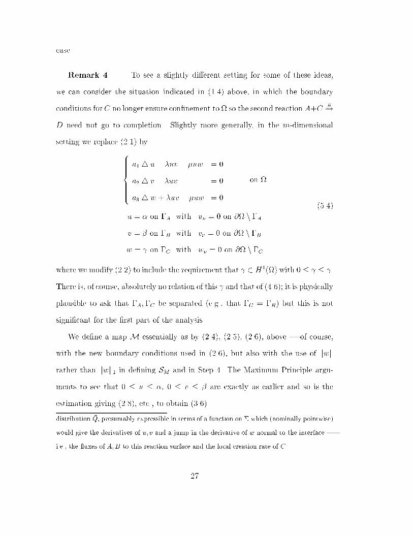
case.Remark 4. To see a slightly di�erent setting for some of these ideas,we can consider the situation indicated in (1.4) above, in which the boundaryconditions forC no longer ensure con�nement to so the second reaction A+C �!D need not go to completion. Slightly more generally, in the m-dimensionalsetting we replace (2.1) by8>>>>>><>>>>>>: a1 4 u� �uv � �uw = 0a2 4 v � �uv = 0a3 4w + �uv � �uw = 0 on u = � on �A with u� = 0 on @ n �Av = � on �B with v� = 0 on @ n �Bw = on �C with w� = 0 on @ n �C(5.4)

where we modify (2.2) to include the requirement that 2 H1() with 0 � � � .There is, of course, absolutely no relation of this and that of (4.6); it is physicallyplausible to ask that �A;�C be separated (e.g., that �C = �B) but this is notsigni�cant for the �rst part of the analysis.We de�ne a map M essentially as by (2.4), (2.5), (2.6), above | of course,with the new boundary conditions used in (2.6), but also with the use of kwkrather than kwk1 in de�ning SM and in Step 4. The Maximum Principle argu-ments to see that 0 � u � ��, 0 � v � �� are exactly as earlier and so is theestimation giving (2.8), etc., to obtain (3.6).distribution �Q, presumably expressible in terms of a function on � which (nominally pointwise)would give the derivatives of �u; �v and a jump in the derivative of �w normal to the interface |i.e., the uxes of A;B to this reaction surface and the local creation rate of C.27

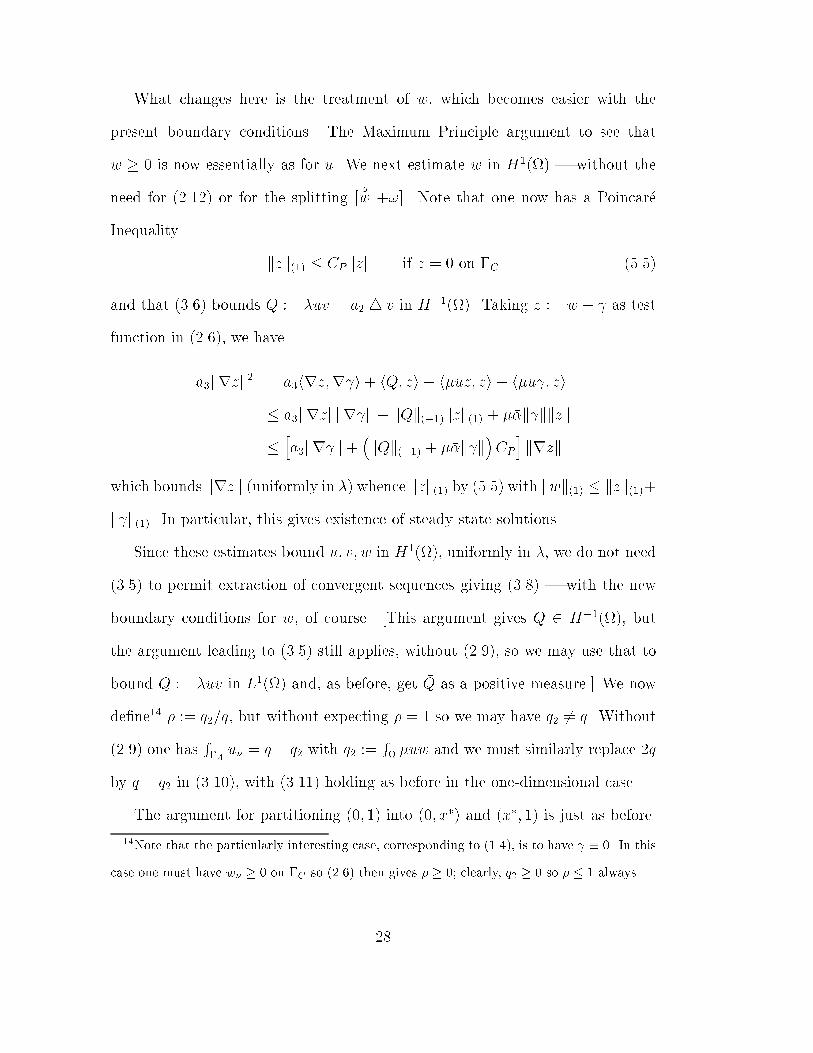
What changes here is the treatment of w, which becomes easier with thepresent boundary conditions. The Maximum Principle argument to see thatw � 0 is now essentially as for u. We next estimate w in H1() | without theneed for (2.12) or for the splitting [ �w +!]. Note that one now has a Poincar�eInequality kzk(1) � CPkzk if z = 0 on �C (5.5)and that (3.6) bounds Q := �uv = a2 4 v in H�1(). Taking z := w � as testfunction in (2.6), we havea3krzk2 = a3hrz;r i+ hQ; zi � h�uz; zi � h�u ; zi� a3krzkkr k+ kQk(�1)kzk(1) + ���k kkzk� ha3kr k+ �kQk(�1) + ���k k�CP i krzkwhich bounds krzk (uniformly in �) whence kzk(1) by (5.5) with kwk(1) � kzk(1)+k k(1). In particular, this gives existence of steady state solutions.Since these estimates bound u; v; w in H1(), uniformly in �, we do not need(3.5) to permit extraction of convergent sequences giving (3.8) | with the newboundary conditions for w, of course. [This argument gives �Q 2 H�1(), butthe argument leading to (3.5) still applies, without (2.9), so we may use that tobound Q := �uv in L1() and, as before, get �Q as a positive measure.] We nowde�ne14 � := q2=q, but without expecting � = 1 so we may have q2 6= q. Without(2.9) one has R�A u� = q+ q2 with q2 := R �uw and we must similarly replace 2qby q + q2 in (3.10), with (3.11) holding as before in the one-dimensional case.The argument for partitioning (0; 1) into (0; x�) and (x�; 1) is just as before.14Note that the particularly interesting case, corresponding to (1.4), is to have � 0. In thiscase one must have w� � 0 on �C so (2.6) then gives � � 0; clearly, q2 � 0 so � � 1 always.28

Again we have straight line pro�les on [x�; 1] where �u � 0:�v = �x� x�1� x� ; �w = w� + [ � w�]x� x�1� x� ; (5.6)with w� := �w(x�) and again we havea1�u00 = ��u �w = a3 �w00 for 0 < x < x�but with new boundary conditions: the jump across x� in �u0; �v0; � �w0 is again q,giving �a1�u0(x��) = q = a2�=(1� x�), but nowa1�u���x��0 = a3 �w���x��0 = q2 = �q:Thus we have�a1�u0(0) = q+q2 = (1+�)q and �w = w�+[a1�u� (1 + �)q(x� x�)] =a3on [0; x�]. Substitutions much like (4.1) now giveyss = y(y + ! � (1 + �)s)y(0) = 0; ys(0) = 1; and ys(s0) = 1 + �; (5.7)corresponding to (4.2), (4.3). Note that we now have two unknown parametersto determine | ! and now also �.Temporarily �xing �, we use essentially the same construction of U(!) =U(!; �) as earlier and the identical argument shows that U is a decreasing functionof ! so (4.8) determines !, etc. | now, of course, as functions of �. Returningto (5.6), we now have w� + (�a2=a3)� = � (�a2=a3) (5.8)since �a3 �w0 = (1� �)q and a2�v0 = q at x = 1. Using w� = w�(�) as determinedfrom (4.8), etc., we may consider (5.8) as an equation for the determination ofthe parameter � (and so of the solution). Although relevant information as to29

�-dependence can be obtained by arguments parallel to those used in the proofof the Lemma of Section 4, we do not pursue this; it is not yet clear whether[w�(�) + (�a2=a3)�] would always be a strictly monotone function of �, whichwould ensure a unique determination.Acknowledgments. This work was partially supported by the Univer-sity of Montana Grants Program. The �rst author owes thanks to D. Hilhorst(Univ. Paris-Sud) for several stimulating conversations at the initiation of thisinvestigation.References[1] E.L. Cussler, Di�usion; Mass Transfer in Fluid Systems, Cambridge Univ.Press, Cambridge, 1984.[2] H. Haario and T.I. Seidman, Reaction and Di�usion at a Gas/Liquid Inter-face, II, SIAM J. Math. Anal. 25 (1994), pp. 1069{1084.[3] H. Haario and T.I. Seidman, The modeling of bubble reactors, to appear.[4] L.V. Kalachev and T.I. Seidman, Singular perturbation analysis of a di�u-sion/reaction system with a fast reaction, to appear.[5] W. Nernst, Theorie der Reaktionsgeschwindigkeit in heterogenen Systemer,Z. Phys. Chem. 47 (1904), pp. 52{55.[6] A.B. Vasil'eva, V.F. Butuzov and L.V. Kalachev, The Boundary FunctionMethod for Singular Perturbation Problems, Philadelphia, SIAM, 1995.30