Embed Size (px)
Citation preview
A PORTRAIT OF THE NUCLEUS OF COMET67P/CHURYUMOV-GERASIMENKO
PHILIPPE L. LAMY1,∗, IMRE TOTH1,7, BJORN J. R. DAVIDSSON2,OLIVIER GROUSSIN3, PEDRO GUTIERREZ4, LAURENT JORDA1,
MIKKO KAASALAINEN5 and STEPHEN C. LOWRY6
1Laboratoire d’Astrophysique de Marseille, BP 8, 13376, Marseille Cedex 12, France2Uppsala Observatory, Uppsala, Sweden
3Department of Astronomy, University of Maryland, College Park, MD, USA4Instituto de Astrofısica de Andalucıa-CSIC, Granada, Spain
5Department of Mathematics and Statistics, University of Helsinki, Helsinki, Finland6Department of Physics and Astronomy, Queen’s University, Belfast, United Kingdom
7Konkoly Observatory, Budapest, Hungary(∗Author for correspondence: E-mail: [email protected])
(Received 29 May 2006; Accepted in final form: 17 November 2006)
Abstract. In 2003, comet 67P/Churyumov–Gerasimenko was selected as the new target of the Rosettamission as the most suitable alternative to the original target, comet 46P/Wirtanen, on the basis oforbital considerations even though very little was known about the physical properties of its nucleus.In a matter of a few years and based on highly focused observational campaigns as well as thoroughtheoretical investigations, a detailed portrait of this nucleus has been established that will serve asa baseline for planning the Rosetta operations and observations. In this review article, we present anovel method to determine the size and shape of a cometary nucleus: several visible light curves wereinverted to produce a size–scale free three–dimensional shape, the size scaling being imposed by athermal light curve. The procedure converges to two solutions which are only marginally different.The nucleus of comet 67P/Churyumov–Gerasimenko emerges as an irregular body with an effectiveradius (that of the sphere having the same volume) = 1.72 km and moderate axial ratios a/b = 1.26 anda/c = 1.5 to 1.6. The overall dimensions measured along the principal axis for the two solutions are4.49–4.75 km, 3.54–3.77 km and 2.94–2.92 km. The nucleus is found to be in principal axis rotationwith a period = 12.4–12.7 h. Merging all observational constraints allow us to specify two regions forthe direction of the rotational axis of the nucleus: RA = 220◦+50◦
−30◦ and Dec = −70◦ ± 10◦ (retrograde
rotation) or RA = 40◦+50◦−30◦ and Dec = +70◦ ± 10◦ (prograde), the better convergence of the various
determinations presently favoring the first solution. The phase function, although constrained by onlytwo data points, exhibits a strong opposition effect rather similar to that of comet 9P/Tempel 1. Thedefinition of the disk–integrated albedo of an irregular body having a strong opposition effect raisesproblems, and the various alternatives led to a R-band geometric albedo in the range 0.045–0.060,consistent with our present knowledge of cometary nuclei. The active fraction is low, not exceeding∼7% at perihelion, and is probably limited to one or two active regions subjected to a strong seasonaleffect, a picture coherent with the asymmetric behaviour of the coma. Our slightly downward revisionof the size of the nucleus of comet 67P/Churyumov-Gerasimenko resulting from the present analysis(with the correlative increase of the albedo compared to the originally assumed value of 0.04), andour best estimate of the bulk density of 370 kg m−3, lead to a mass of ∼8 × 10¹² kg which shouldease the landing of Philae and insure the overall success of the Rosetta mission.
Space Science Reviews (2007) 128: 23–66DOI: 10.1007/s11214-007-9146-x C© Springer 2007
24 P. L. LAMY ET AL.
Keywords: solar system, comet, cometary nucleus, 67P/Churyumov-Gerasimenko, Rosetta spacemission
1. Introduction
Comet 67P/Churyumov-Gerasimenko (hereafter 67P/C-G) is not a newcomer inthe landscape of cometary targets for space missions. In 1985, it appeared in thelist of ten selected comets accessible by space probes prepared by Yeomans (1985).This interest did not stem from the fact that it was particularly attractive from thepoint of view of cometary science, nor from some a-priori knowledge (it appearedto be a typical Jupiter-family comet), but from a favorable orbital geometry for arendezvous. Again, in the early 1990’s, comet 67P/C-G was kept among severalpotential target candidates of in-situ flyby and/or rendezvous space missions, andit received some attention from ground-based observers (Osip et al., 1992).
However when it was selected as the new target of the Rosetta mission in 2003following the cancellation of the launch to the original target, comet 46P/Wirtanen,very little was known about the physical properties of its nucleus, and a vigorouseffort of characterization was therefore required to best prepare the mission. Ratherthan a massive, world-wide observing campaign which could lead to ambiguousresults – see the example of comet 9P/Tempel 1, the target of the Deep Impactmission (Meech et al., 2005; Belton et al., 2005) – the present authors, as well asa few others whose results are quoted and incorporated into this article, opted forhighly targeted observational campaigns with the most appropriate telescopes, aswell as thorough theoretical investigations. From these investigations, performedover just a few years, a detailed portrait of the nucleus of comet 67P/C-G emerges,which probably makes it the best described cometary nucleus, with the naturalexception of those which have been visited by spaceprobes.
The purpose of this present article is to review these works and establish a refer-ence model of the nucleus of 67P/C-G that will serve as a baseline for planning theRosetta operations and observations. We restrict ourselves to the physical quantitieswhich can be safely deduced from observations or well-founded models, avoidingaspects that remain rather speculative such as surface morphology, composition,material strength, internal structure. For these questions, the interested reader isrefered to our standard current knowledge as for instance summarized in the recentComets II book.
2. Discovery, Orbit and Orbital Evolution
2.1. SERENDIPITOUS DISCOVERY OF COMET 1969h
In September 1969, Klim Ivanovich Churyumov and Svetlana Ivanovna Gera-simenko of the Kiev Shevchenko National University, went to the Alma-Ata
THE NUCLEUS OF COMET 67P/CHURYUMOV-GERASIMENKO 25
Astrophysical Institute to conduct a survey of short-period and new comets. Thegroup at Kiev University had established itself as a stronghold of cometary obser-vations and studies, and has published more than 1000 scientific papers devoted tocomets in different journals, books and proceedings during the period 1939–2000(Churyumov, 2002). At the Alma-Ata observatory, Gerasimenko used the 50-cmf/2.4 Maksutov telescope of the Astrophysical Institute of the Academy of Sciencesin the Kazakh SSR. On the night of 11/12 September, she observed several comets,including comet 32P/Comas-Sola (1969 VIII = 1968g). Unfortunately, the platewith comet Comas-Sola was defective and at first, she wanted to throw this plateaway. However, on the faded background, not far from the center, there was anobject which she assumed to be Comas-Sola. So, the plate was saved for furtherexamination.
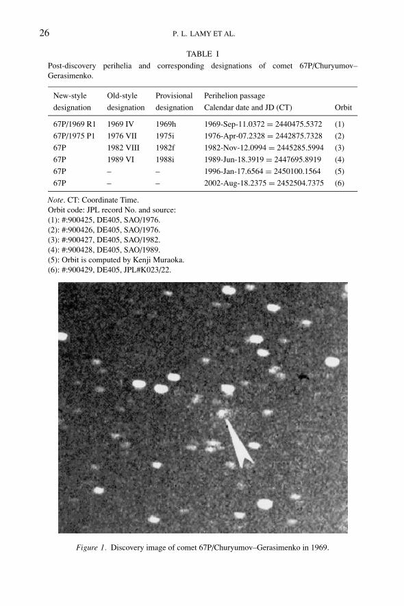
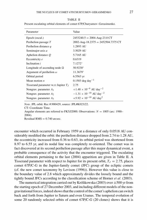
After returning to their home institute in Kiev in October 1969, Churyumovand Gerasimenko started to inspect all photographic plates. They did find comet32P/Comas Sola on the plate obtained by Gerasimenko on September 11.92 UT at itsexpected position. However, at a distance of about 1.8◦, they noticed another objectwhich eventually turned out to be a new comet. It had an apparent photographicmagnitude of 13, a central condensation diameter of about 0.3 arcmin and a fainttail about 1 arcmin in length at position angle 280◦ (angle measured from celestialequatorial North through East in the sky plane). Altogether, five positions could bemeasured for this object on the Alma-Ata plates from September 9.91 to 21.93 UT(see Figure 1 for an example). On 23 October 1969, the report of this discoverywas sent from Kiev Observatory, the Soviet center for cometary astronomy, to theCentral Bureau for Astronomical Telegrams (CBAT) of the IAU (SAO, Cambridge,Massachusetts), and its director B. Marsden then alerted the cometary community.C. Scovil photographed the new comet on October 31 with the 22-inch Maksutovtelescope at Stamford, Connecticut, as a 14th-magnitude coma. In addition, J. Bortlesucceeded in finding it on an early plate taken by C. Scovil on September 14 that hadbeen exposed for comet Comas Sola. It was later photographed on November 5 by E.Roemer with the new 90-inch reflector of Steward Observatory in Arizona (Roemer,1970, see also Sky and Telescope (1969)). The orbit calculated by B. Marsdenindicated that the new comet was of the short-period type. It received the provisionaldesignation 1969h, and was later named after Churyumov and Gerasimenko, so thespoiled plate brought them good luck.
All new- and old-style nomenclature designations of comet 67P/C-G are sum-marized in Table I as well as the post-discovery dates of perihelion. The discoveryof 11.92 September 1969 UT thus took place very close to the perihelion passageof 11.0372 September at 1.284 AU from the Sun.
2.2. ORBITAL EVOLUTION
The orbital evolution of comet 67P/C-G is chaotic due to repeated close encounterswith Jupiter (Carusi et al., 1985; Belyaev et al., 1986; Krolikowska, 2003). The
26 P. L. LAMY ET AL.
TABLE I
Post-discovery perihelia and corresponding designations of comet 67P/Churyumov–Gerasimenko.
New-style Old-style Provisional Perihelion passage
designation designation designation Calendar date and JD (CT) Orbit
67P/1969 R1 1969 IV 1969h 1969-Sep-11.0372 = 2440475.5372 (1)
67P/1975 P1 1976 VII 1975i 1976-Apr-07.2328 = 2442875.7328 (2)
67P 1982 VIII 1982f 1982-Nov-12.0994 = 2445285.5994 (3)
67P 1989 VI 1988i 1989-Jun-18.3919 = 2447695.8919 (4)
67P – – 1996-Jan-17.6564 = 2450100.1564 (5)
67P – – 2002-Aug-18.2375 = 2452504.7375 (6)
Note. CT: Coordinate Time.Orbit code: JPL record No. and source:(1): #:900425, DE405, SAO/1976.(2): #:900426, DE405, SAO/1976.(3): #:900427, DE405, SAO/1982.(4): #:900428, DE405, SAO/1989.(5): Orbit is computed by Kenji Muraoka.(6): #:900429, DE405, JPL#K023/22.
Figure 1. Discovery image of comet 67P/Churyumov–Gerasimenko in 1969.
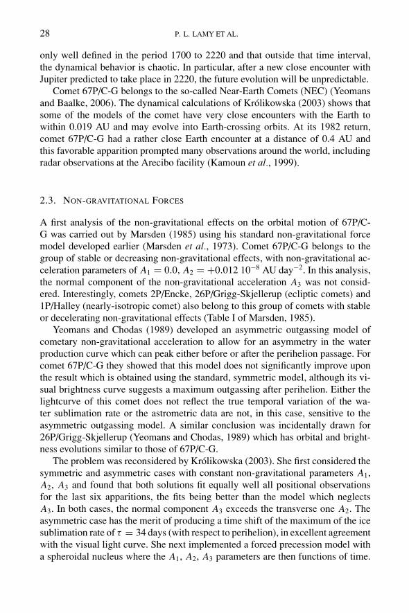
THE NUCLEUS OF COMET 67P/CHURYUMOV-GERASIMENKO 27
TABLE II
Present osculating orbital elements of comet 67P/Churyumov–Gerasimenko.
Parameter Value
Epoch (oscul.) 2453240.5 = 2004-Aug-23.0 CT
Perihelion passage T 2002-Aug-18.2375 = 2452504.7375 CT
Perihelion distance q 1.2893 AU
Semimajor-axis a 3.5029 AU
Aphelion distance Q 5.7165 AU
Eccentricity e 0.6319
Inclination i 7.1272◦
Longitude of ascending node � 50.9230◦
Argument of perihelion ω 11.3679◦
Orbital period 6.5563 yr
Mean motion n 0.1503 deg day−1
Tisserand parameter w.r.t Jupiter TJ 2.75
Nongrav. parameter A1 +1.48 × 10⁻⁹ AU day−2
Nongrav. parameter A2 −1.31 × 10⁻¹⁰ AU day−2
Nongrav. parameter A3 +5.92 × 10⁻¹⁰ AU day2
Note. JPL orbit: Rec #:900429, source: JPL#K023/22.CT: Coordinate Time.Angular elements are referred to FK5/J2000. Observations: N = 1005 (arc: 1988–2004).Residual RMS = 0.740 arcsec.
encounter which occurred in February 1959 at a distance of only 0.0518 AU con-siderably modified the orbit: the perihelion distance dropped from 2.74 to 1.28 AU,the eccentricity increased from 0.36 to 0.63, its orbital period was shortened from8.97 to 6.55 yr, and its nodal line was completely re-oriented. The comet was infact discovered at its second perihelion passage after this major dynamical event, aprobable consequence of the activity that the encounter triggered. The osculatingorbital elements pertaining to the last (2004) apparition are given in Table II. ATisserand parameter with respect to Jupiter for its present orbit, TJ = 2.75, placescomet 67P/C-G in the Jupiter-family comet (JFC) group of the ecliptic comets(cf. the new comet taxonomy by Levison (1996)). However this value is close tothe boundary value of 2.8 which approximately divides the loosely bound and thetightly bound JFCs according to the classification scheme of Horner et al. (2003).
The numerical integration carried out by Krolikowska (2003) over ±500 yr fromthe starting epoch of 27 December 2003, and including different models of the non-gravitational forces, indeed shows that the control of the comet’s aphelion can switchback and forth from Jupiter to Saturn and even Uranus. The temporal evolution ofsome 20 randomly selected orbits of comet 67P/C-G (20 clones) shows that it is
28 P. L. LAMY ET AL.
only well defined in the period 1700 to 2220 and that outside that time interval,the dynamical behavior is chaotic. In particular, after a new close encounter withJupiter predicted to take place in 2220, the future evolution will be unpredictable.
Comet 67P/C-G belongs to the so-called Near-Earth Comets (NEC) (Yeomansand Baalke, 2006). The dynamical calculations of Krolikowska (2003) shows thatsome of the models of the comet have very close encounters with the Earth towithin 0.019 AU and may evolve into Earth-crossing orbits. At its 1982 return,comet 67P/C-G had a rather close Earth encounter at a distance of 0.4 AU andthis favorable apparition prompted many observations around the world, includingradar observations at the Arecibo facility (Kamoun et al., 1999).
2.3. NON-GRAVITATIONAL FORCES
A first analysis of the non-gravitational effects on the orbital motion of 67P/C-G was carried out by Marsden (1985) using his standard non-gravitational forcemodel developed earlier (Marsden et al., 1973). Comet 67P/C-G belongs to thegroup of stable or decreasing non-gravitational effects, with non-gravitational ac-celeration parameters of A1 = 0.0, A2 = +0.012 10−8 AU day−2. In this analysis,the normal component of the non-gravitational acceleration A3 was not consid-ered. Interestingly, comets 2P/Encke, 26P/Grigg-Skjellerup (ecliptic comets) and1P/Halley (nearly-isotropic comet) also belong to this group of comets with stableor decelerating non-gravitational effects (Table I of Marsden, 1985).
Yeomans and Chodas (1989) developed an asymmetric outgassing model ofcometary non-gravitational acceleration to allow for an asymmetry in the waterproduction curve which can peak either before or after the perihelion passage. Forcomet 67P/C-G they showed that this model does not significantly improve uponthe result which is obtained using the standard, symmetric model, although its vi-sual brightness curve suggests a maximum outgassing after perihelion. Either thelightcurve of this comet does not reflect the true temporal variation of the wa-ter sublimation rate or the astrometric data are not, in this case, sensitive to theasymmetric outgassing model. A similar conclusion was incidentally drawn for26P/Grigg-Skjellerup (Yeomans and Chodas, 1989) which has orbital and bright-ness evolutions similar to those of 67P/C-G.
The problem was reconsidered by Krolikowska (2003). She first considered thesymmetric and asymmetric cases with constant non-gravitational parameters A1,A2, A3 and found that both solutions fit equally well all positional observationsfor the last six apparitions, the fits being better than the model which neglectsA3. In both cases, the normal component A3 exceeds the transverse one A2. Theasymmetric case has the merit of producing a time shift of the maximum of the icesublimation rate of τ = 34 days (with respect to perihelion), in excellent agreementwith the visual light curve. She next implemented a forced precession model witha spheroidal nucleus where the A1, A2, A3 parameters are then functions of time.
THE NUCLEUS OF COMET 67P/CHURYUMOV-GERASIMENKO 29
She found that the orbital reconfiguration which occurred in 1959 significantlyincreased the non-gravitational force but that thereafter, its temporal variation israther regular. The forced precession model of 67P/C-G which satisfies τ = 34 dayshas implications on the shape and rotational state of the nucleus, which will bediscussed in Section 4.
3. Summary of Observations of the Nucleus
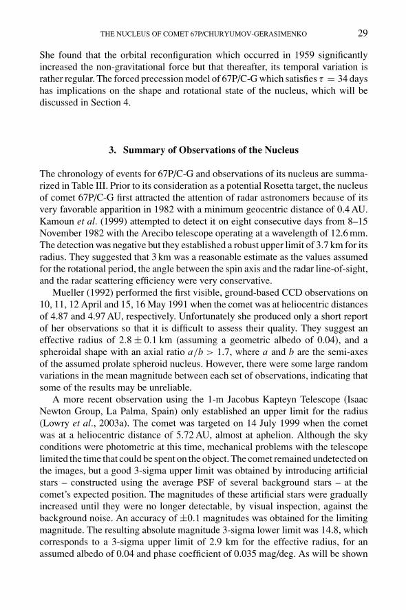
The chronology of events for 67P/C-G and observations of its nucleus are summa-rized in Table III. Prior to its consideration as a potential Rosetta target, the nucleusof comet 67P/C-G first attracted the attention of radar astronomers because of itsvery favorable apparition in 1982 with a minimum geocentric distance of 0.4 AU.Kamoun et al. (1999) attempted to detect it on eight consecutive days from 8–15November 1982 with the Arecibo telescope operating at a wavelength of 12.6 mm.The detection was negative but they established a robust upper limit of 3.7 km for itsradius. They suggested that 3 km was a reasonable estimate as the values assumedfor the rotational period, the angle between the spin axis and the radar line-of-sight,and the radar scattering efficiency were very conservative.
Mueller (1992) performed the first visible, ground-based CCD observations on10, 11, 12 April and 15, 16 May 1991 when the comet was at heliocentric distancesof 4.87 and 4.97 AU, respectively. Unfortunately she produced only a short reportof her observations so that it is difficult to assess their quality. They suggest aneffective radius of 2.8 ± 0.1 km (assuming a geometric albedo of 0.04), and aspheroidal shape with an axial ratio a/b > 1.7, where a and b are the semi-axesof the assumed prolate spheroid nucleus. However, there were some large randomvariations in the mean magnitude between each set of observations, indicating thatsome of the results may be unreliable.
A more recent observation using the 1-m Jacobus Kapteyn Telescope (IsaacNewton Group, La Palma, Spain) only established an upper limit for the radius(Lowry et al., 2003a). The comet was targeted on 14 July 1999 when the cometwas at a heliocentric distance of 5.72 AU, almost at aphelion. Although the skyconditions were photometric at this time, mechanical problems with the telescopelimited the time that could be spent on the object. The comet remained undetected onthe images, but a good 3-sigma upper limit was obtained by introducing artificialstars – constructed using the average PSF of several background stars – at thecomet’s expected position. The magnitudes of these artificial stars were graduallyincreased until they were no longer detectable, by visual inspection, against thebackground noise. An accuracy of ±0.1 magnitudes was obtained for the limitingmagnitude. The resulting absolute magnitude 3-sigma lower limit was 14.8, whichcorresponds to a 3-sigma upper limit of 2.9 km for the effective radius, for anassumed albedo of 0.04 and phase coefficient of 0.035 mag/deg. As will be shown
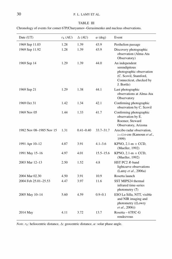
30 P. L. LAMY ET AL.
TABLE III
Chronology of events for comet 67P/Churyumov–Gerasimenko and nucleus observations.
Date (UT) rh (AU) � (AU) α (deg) Event
1969 Sep 11.03 1.28 1.39 43.9 Perihelion passage
1969 Sep 11.92 1.28 1.39 43.9 Discovery photographicobservation (Alma-AtaObservatory)
1969 Sep 14 1.29 1.39 44.0 An independentserendipitousphotographic observation(C. Scovil, Stamford,Connecticut, checked byJ. Bortle)
1969 Sep 21 1.29 1.38 44.1 Last photographicobservations at Alma-AtaObservatory
1969 Oct 31 1.42 1.34 42.1 Confirming photographicobservation by C. Scovil
1969 Nov 05 1.44 1.33 41.7 Confirming photographicobservation by E.Roemer, StewardObservatory, Arizona
1982 Nov 08–1985 Nov 15 1.31 0.41–0.40 33.7–31.7 Arecibo radar observation,λ=12.6-cm (Kamoun et al.,1999)
1991 Apr 10–12 4.87 3.91 4.1–3.6 KPNO, 2.1-m + CCD,(Mueller, 1992)
1991 May 15–16 4.97 4.01 15.5–15.6 KPNO, 2.1-m + CCD,(Mueller, 1992)
2003 Mar 12–13 2.50 1.52 4.8 HST PC2 R-bandlightcurve observations(Lamy et al., 2006a)
2004 Mar 02.30 4.50 3.91 10.9 Rosetta launch
2004 Feb 25.01–25.53 4.47 3.97 11.6 SST MIPS24 thermalinfrared time-seriesphotometry (?)
2005 May 10–14 5.60 4.59 0.9–0.1 ESO La Silla, NTT, visibleand NIR imaging andphotometry ((Lowryet al., 2006))
2014 May 4.11 3.72 13.7 Rosetta – 67P/C-Grendezvous
Note. rh : heliocentric distance, �: geocentric distance, α: solar phase angle.
THE NUCLEUS OF COMET 67P/CHURYUMOV-GERASIMENKO 31
in the discussion below, if Lowry et al. (2003a) had taken just a few more exposures,then the nucleus would certainly have been detected.
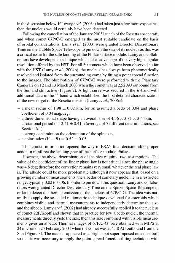
Following the cancellation of the January 2003 launch of the Rosetta spacecraft,and when comet 67P/C-G emerged as the most suitable candidate on the basisof orbital considerations, Lamy et al. (2003) were granted Director DiscretionaryTime on the Hubble Space Telescope to pin down the size of its nucleus as this wasa critical issue for the safe landing of the Philae surface module. Lamy and collab-orators have developed a technique which takes advantage of the very high angularresolution offered by the HST. For all 30 comets which have been observed so farwith the HST (Lamy et al., 2004b), the nucleus has always been photometricallyresolved and isolated from the surrounding coma by fitting a point spread functionto the images. The observations of 67P/C-G were performed with the PlanetaryCamera 2 on 12 and 13 March 2003 when the comet was at 2.52 AU outbound fromthe Sun and still active (Figure 2). A light curve was secured in the R-band withadditional data in the V -band which established the first detailed characterizationof the new target of the Rosetta mission (Lamy et al., 2006a):
– a mean radius of 1.98 ± 0.02 km, for an assumed albedo of 0.04 and phasecoefficient of 0.04 mag/deg;
– a three-dimensional shape having an overall size of 4.56 × 3.81 × 3.44 km;– a rotational period of 12.41 ± 0.41 h (average of 7 different determinations, see
Section 6.1);– a strong constraint on the orientation of the spin axis;– a color index (V − R) = 0.52 ± 0.05.
This crucial information opened the way to ESA’s final decision after properaction to reinforce the landing gear of the surface module Philae.
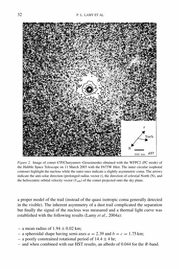
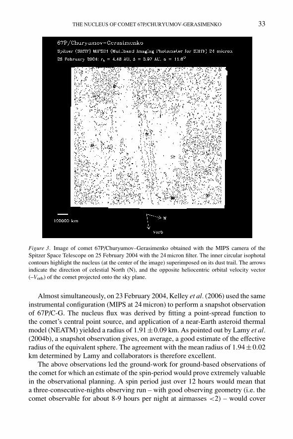
However, the above determination of the size required two assumptions. Thevalue of the coefficient of the linear phase law is not critical since the phase anglewas 4.8 deg; therefore the correction remains very small whatever the real phase lawis. The albedo could be more problematic although it now appears that, based on agrowing number of measurements, the albedos of cometary nuclei lie in a restrictedrange, typically 0.02 to 0.06. In order to pin down this question, Lamy and collabo-rators were granted Director Discretionary Time on the Spitzer Space Telescope inorder to detect the thermal emission of the nucleus of 67P/C-G. The idea was nat-urally to apply the so-called radiometric technique developed for asteroids whichcombines visible and thermal measurements to independently determine the sizeand the albedo. Lamy et al. (2002) had already successfully applied it to the nucleusof comet 22P/Kopff and shown that in practice for low albedo nuclei, the thermalmeasurements directly yield the size; then this size combined with visible measure-ments gives an albedo. Thermal images of 67P/C-G were obtained with MIPS at24 micron on 25 February 2004 when the comet was at 4.48 AU outbound from theSun (Figure 3). The nucleus appeared as a bright spot superimposed on a dust trailso that it was necessary to apply the point-spread function fitting technique with
32 P. L. LAMY ET AL.
Figure 2. Image of comet 67P/Churyumov–Gerasimenko obtained with the WFPC2 (PC mode) ofthe Hubble Space Telescope on 11 March 2003 with the F675W filter. The inner circular isophotalcontours highlight the nucleus while the outer ones indicate a slightly asymmetric coma. The arrowsindicate the anti-solar direction (prolonged radius vector r), the direction of celestial North (N), andthe heliocentric orbital velocity vector (Vorb) of the comet projected onto the sky plane.
a proper model of the trail (instead of the quasi isotropic coma generally detectedin the visible). The inherent asymmetry of a dust trail complicated the separationbut finally the signal of the nucleus was measured and a thermal light curve wasestablished with the following results (Lamy et al., 2004a):
– a mean radius of 1.94 ± 0.02 km;– a spheroidal shape having semi-axes a = 2.39 and b = c = 1.75 km;– a poorly constrained rotational period of 14.4 ± 4 hr;– and when combined with our HST results, an albedo of 0.044 for the R-band.
THE NUCLEUS OF COMET 67P/CHURYUMOV-GERASIMENKO 33
Figure 3. Image of comet 67P/Churyumov–Gerasimenko obtained with the MIPS camera of theSpitzer Space Telescope on 25 February 2004 with the 24 micron filter. The inner circular isophotalcontours highlight the nucleus (at the center of the image) superimposed on its dust trail. The arrowsindicate the direction of celestial North (N), and the opposite heliocentric orbital velocity vector(–Vorb) of the comet projected onto the sky plane.
Almost simultaneously, on 23 February 2004, Kelley et al. (2006) used the sameinstrumental configuration (MIPS at 24 micron) to perform a snapshot observationof 67P/C-G. The nucleus flux was derived by fitting a point-spread function tothe comet’s central point source, and application of a near-Earth asteroid thermalmodel (NEATM) yielded a radius of 1.91±0.09 km. As pointed out by Lamy et al.(2004b), a snapshot observation gives, on average, a good estimate of the effectiveradius of the equivalent sphere. The agreement with the mean radius of 1.94±0.02km determined by Lamy and collaborators is therefore excellent.
The above observations led the ground-work for ground-based observations ofthe comet for which an estimate of the spin-period would prove extremely valuablein the observational planning. A spin period just over 12 hours would mean thata three-consecutive-nights observing run – with good observing geometry (i.e. thecomet observable for about 8-9 hours per night at airmasses <2) – would cover
34 P. L. LAMY ET AL.
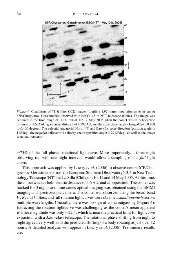
Figure 4. Coaddition of 71 R-filter CCD images (totalling 1.97 hours integration time) of comet67P/Churyumov–Gerasimenko observed with ESO’s 3.5-m NTT telescope (Chile). The image wasacquired in the time range of UT 01:01–09:07 12 May 2005 when the comet was at heliocentricdistance of 5.602 AU, geocentric distance of 4.592 AU, and the solar phase angle changed from 0.468to 0.400 degrees. The celestial equatorial North (N) and East (E), solar direction (position angle is115 deg), the negative heliocentric velocity vector (position angle is 291.5 deg), as well as the imagescale are indicated.
∼75% of the full phased rotational lightcurve. More importantly, a three nightobserving run with one-night intervals would allow a sampling of the full lightcurve.
This approach was applied by Lowry et al. (2006) to observe comet 67P/Chu-ryumov-Gerasimenko from the European Southern Observatory’s 3.5-m New Tech-nology Telescope (NTT) at La Silla (Chile) on 10, 12 and 14 May 2005. At this time,the comet was at a heliocentric distance of 5.6 AU, and at opposition. The comet wastracked for 3 nights and time-series optical imaging was obtained using the EMMIimaging and spectroscopic camera. The comet was observed using the broad-bandV , R, and I filters, and full rotation lightcurves were obtained simultaneously acrossmultiple wavelengths. Crucially, there was no sign of coma outgassing (Figure 4).Extracting the rotation lightcurve was challenging as the comet’s mean apparentR-filter magnitude was only ∼22.4, which is near the practical limit for lightcurveextraction with a 3.5m-class telescope. The rotational phase-shifting from night tonight agreed very well with the predicted shifting of a body rotating at just over 12hours. A detailed analysis will appear in Lowry et al. (2006). Preliminary resultsare:
THE NUCLEUS OF COMET 67P/CHURYUMOV-GERASIMENKO 35
– a rotational period of 12.72 ± 0.05 hr;– a mean R absolute magnitude of 15.34 ± 0.03, slightly brighter than expected
from the HST photometry of Lamy et al. (2006a);– a mean effective radius of 2.26 ± 0.03 km assuming an albedo of 0.04 and a
phase coefficient of 0.04 mag/deg;– an axial ratio of ≥1.42 ± 0.05, suggesting a spheroidal body having semi-axes
a = 2.94 and b = c = 2.07 km;– a color index (V − R) = 0.41 ± 0.04.
It should immediately be emphasized that the comet was observed from the NTTat a very small phase angles (≤0.83◦), where an opposition effect is expected, thusinvalidating the use of a simple linear law for the phase function. This question willbe addressed in Section 7.1.
4. Nucleus Properties Obtained from Non-gravitational Force Modeling
The idea of extracting information about cometary nuclei by utilizing non-gravitational forces dates back to the classical articles of Whipple (1950, 1951)in the framework of his concept of an icy conglomerate. It was later elaboratedupon in the so-called forced precession model by Whipple and Sekanina (1979),subsequently refined by Sekanina in a series of papers.
In that model, it is assumed that the nucleus is shaped as a spheroid, charac-terized by an equatorial radius Requ and a center–to–pole distance Rpol. A forcevector is acting on the model nucleus due to outgassing, thereby introducing non-gravitational orbit changes, and a torque which modifies the rotational state of thenucleus. The direction of the force vector is normally taken as the inward surfacenormal at the sub-solar point, shifted by an angle ηlag in the direction of nucleusrotation along the sub-solar latitude, to mimic the effect of a thermal lag. Themodulus of the force vector is determined by some function of time (e.g., basedon the light curve, or an analytical approximation relating the water productionrate with heliocentric distance), scaled by a constant jet factor fjet (responsible forthe non-gravitational acceleration) and a constant torque factor ftor (responsiblefor the nucleus precession rate). By requiring that empirical astrometry is repro-duced as well as possible, six parameters can be estimated: Rpol/Requ, ηlag, fjet,ftor ∝ Prot/Requ (where Prot is the rotational period), and two time–dependent an-gles describing the orientation of the spin axis. It is noted that solutions yieldingRpol/Requ < 1 correspond to an oblate nucleus rotating around its shortest principalaxis, while solutions Rpol/Requ > 1 correspond to a prolate nucleus rotating aroundits largest principal axis.
Non-gravitational orbit modifications have also been used in order to estimatemasses and bulk densities in cometary nuclei (see Rickman, 1986 for the pioneeringwork, and Skorov and Rickman, 1999).
36 P. L. LAMY ET AL.
As already introduced in Section 2.3, Krolikowska (2003) developed a forcedprecession model for comet 67P/C-G. Her asymmetric case with τ = 34 daysyielded a prolate spheroidal body rotating around its largest principal axis, hav-ing an axial ratio Rpol/Requ = 1.16, and a torque factor such that Prot/Requ =4.6 ± 1.4 hr/km. The orientation of the rotational axis in 2003 is defined by RA≈ 17◦ and Dec ≈ 5◦, and she also presented its temporal evolution. However, itmust be pointed out that rotation around the largest principal axis is highly un-likely for a real body. Furthermore, the suggested pole orientation is not consistentwith other existing estimates (Section 6.2), and the resulting small aspect angle atthe time of the HST observations in 2003 is hardly compatible with the observedlightcurve amplitude.
More elaborate modeling was carried out by Davidsson and Gutierrez (2005).They calculated the water production rate and the non-gravitational force vector asfunctions of time, for 13 million model comet nuclei with different sizes, prolateellipsoidal shapes, spin axis orientations, surface activity patterns, and thermophys-ical properties. Probable nucleus parameters for comet 67P/C-G were obtained bystudying the properties of a sub-set of model nuclei, which simultaneously repro-duced a number of empirical data: the nucleus rotational light curve, the temporalvariation of the water production rate, and non-gravitational changes (per appari-tion) of the orbital period, longitude of perihelion and longitude of the ascendingnode.
According to Davidsson and Gutierrez (2005), it is highly probable that comet67P/C-G has a nucleus semi-major axis of ∼2.5 km, a semi-minor axis of ∼1.8 km(yielding an axis ratio 1.4), and a bulk density in the range 100–370 kg m−3. Thenucleus angular momentum vector is confined to two well defined regions in the(obliquity I , argument ) plane1, corresponding to the same axis, but differentsenses of rotation. The first region is defined by = 60◦ ±15◦ and I = 120◦ ±30◦
while the second region is defined by = 240◦ ± 15◦ and I = 60◦ ± 30◦.However, these solutions are only valid when assuming that the models are
reasonably accurate, and when applying the nominal empirical values for the waterproduction rate and non-gravitational change of the orbital period per apparition inthe analysis. For example, if calculated water production rates within a rather thickenvelope around the measured data are considered, it may no longer be possible toconstrain the size, shape, and spin axis orientation of the nucleus, although modelingby Davidsson and Gutierrez (2005) shows that an upper limit on the nucleus bulkdensity confidently can be placed at 600 kg m−3 (see also Section 6).
5. The Size and Shape of the Nucleus
The light curves derived from the HST and NTT observations share the samefeature of being highly asymmetric. Such a feature is not uncommon among co-
1See for instance Sekanina (1981) for a definition of these angles.
THE NUCLEUS OF COMET 67P/CHURYUMOV-GERASIMENKO 37
metary nuclei and is in fact present in the light curves of the nucleus of 2P/Encke(Fernandez, 2005; Lowry et al., 2003b) and of comet 9P/Tempel 1 (Lamy et al.,2006b). It implies that we were seeing the varying cross section of a rotating bodyhaving a complex shape, and the difference in amplitude between the HST and NTTlight curves also implies that the nucleus was observed at different aspect angles.In principle, large-scale surface inhomogeneities could also be advocated but arenot supported by the presently available images that the in situ space missions havereturned from four different cometary nuclei.
The deviation of the light curves from the simple solution of a prolate spheroidis so pronounced that it is certainly worthwhile investigating the implications forthe shape of the nucleus of 67P/C-G. We therefore apply the inversion proceduredeveloped by Kaasalainen et al. (2001), and already applied to the HST light curvealone (Lamy et al., 2006a), to the whole set of HST+NTT light curves. Two op-tions are available for performing the inversion, convex and non-convex modelings.There is a fundamental difference between the stability and reliability of these twoapproaches, and between the parameter spaces the two employ. The convex model-ing is performed in the parameter space describing the Gaussian image of a shape,and this image is then transformed into shape information in radius space. Dueto so-called Minkowski stability, convex inversion is quite stable against the in-correctness of the scattering model (including slight albedo variegation) or othersystematic or random errors. Nonconvex inversion is performed in the radius spacedirectly, which makes the whole process much more vulnerable and ambiguous:it is sensitive to (systematic) errors and the insufficiency of the scattering model.However, in the case of a limited data set as presently the case for 67P/C-G, thissecond approach, with an additional inertia tensor regularization to force the rota-tional state to remain close to principal axis rotation so as to rule out unphysicalpole solutions, is more efficient. Further details can be found in the articles ofKaasalainen and Lamberg (2006) and references therein, and of Kaasalainen andDurech (2007).
The inversion requires a scattering law (combined with a phase function), and weconsidered that the nucleus of 67P/C-G is extensively covered by an ice–free dustmantle in agreement with a fractional active area of a few percents (see Section 9.3).To be consistent with our earlier work (Lamy et al., 2006a), the scattering law wasobtained using the Hapke formalism with the parameters of asteroid 253 Mathilde(Clark et al., 1999). This choice has in fact no impact on the result: as shown byKaasalainen et al. (2001), the chosen model does not make much difference forlight curve inversion.
We present in Figure 5 two unconnected solutions (denoted A and B) yieldedby the simultaneous inversion of our whole set of HST+NTT light curves that areonly typical samples of the possible models. Nevertheless, it is interesting to notethat the number of other solutions is already limited with this data set, and that theirglobal shape characteristics are roughly similar to those of the solutions presentedhere. These two solutions produce the best fits to the observation curves under the
38 P. L. LAMY ET AL.
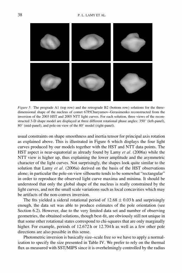
Figure 5. The prograde A1 (top row) and the retrograde B2 (bottom row) solutions for the three-dimensional shape of the nucleus of comet 67P/Churyumov–Gerasimenko reconstructed from theinversion of the 2003 HST and 2005 NTT light curves. For each solution, three views of the recon-structed 3-D shape model are displayed at three different rotational phase angles: 350◦ (left-panel),80◦ (mid-panel), and pole-on view of the 80◦ model (right-panel).
usual constraints on shape smoothness and inertia tensor for principal axis rotationas explained above. This is illustrated in Figure 6 which displays the four lightcurves produced by our models together with the HST and NTT data points. TheHST aspect is near-equatorial as already found by Lamy et al. (2006a) while theNTT view is higher up, thus explaining the lower amplitude and the asymmetriccharacter of the light curves. Not surprisingly, the shapes look quite similar to thesolution that Lamy et al. (2006a) derived on the basis of the HST observationsalone; in particular the pole-on view silhouette tends to be somewhat “rectangular”in order to reproduce the observed light curve maxima and minima. It should beunderstood that only the global shape of the nucleus is really constrained by thelight curves, and not the small scale variations such as local concavities which maybe artifacts of the non-convex inversion.
The fits yielded a sideral rotational period of 12.68 ± 0.03 h and surprisinglyenough, the data set was able to produce estimates of the pole orientation (seeSection 6.2). However, due to the very limited data set and number of observinggeometries, the obtained solutions, though best-fit, are obviously still not unique inthat some other rotational states correspond to chi-squares that are only marginallyhigher. For example, periods of 12.672 h or 12.704 h as well as a few other poledirections are also possible in this sense.
Photometric inversion is basically size–scale free so we have to apply a normal-ization to specify the size presented in Table IV. We prefer to rely on the thermalflux as measured with SST/MIPS since it is overhelmingly controlled by the radius
THE NUCLEUS OF COMET 67P/CHURYUMOV-GERASIMENKO 39
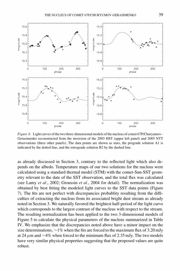
Figure 6. Light curves of the two three-dimensional models of the nucleus of comet 67P/Churyumov–Gerasimenko reconstructed from the inversion of the 2003 HST (upper left panel) and 2005 NTTobservations (three other panels). The data points are shown as stars, the prograde solution A1 isindicated by the dotted line, and the retrograde solution B2 by the dashed line.
as already discussed in Section 3, contrary to the reflected light which also de-pends on the albedo. Temperature maps of our two solutions for the nucleus werecalculated using a standard thermal model (STM) with the comet-Sun-SST geom-etry relevant to the date of the SST observation, and the total flux was calculated(see Lamy et al., 2002; Groussin et al., 2004 for detail). The normalization wasobtained by best fitting the modeled light curves to the SST data points (Figure7). The fits are not perfect with discrepancies probablity resulting from the diffi-culties of extracting the nucleus from its associated bright dust stream as alreadynoted in Section 3. We naturally favored the brightest half-period of the light curvewhich corresponds to the largest contrast of the nucleus with respect to the stream.The resulting normalization has been applied to the two 3-dimensional models ofFigure 5 to calculate the physical parameters of the nucleus summarized in TableIV. We emphasize that the discrepancies noted above have a minor impact on thesize determinations, ∼1% when the fits are forced to the maximum flux of 3.20 mJyat 24 μm and ∼4% when forced to the minimum flux of 2.35 mJy. The two modelshave very similar physical properties suggesting that the proposed values are quiterobust.
40 P. L. LAMY ET AL.
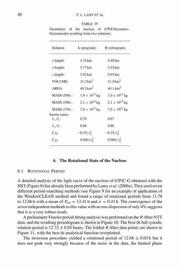
TABLE IV
Parameters of the nucleus of 67P/Churyumov–Gerasimenko resulting from two solutions.
Solution A (prograde) B (retrograde)
x length: 4.74 km 4.49 km
y length: 3.77 km 3.53 km
z length: 2.92 km 2.93 km
VOLUME: 21.2 km3 21.3 km3
AREA: 40.2 km2 40.1 km2
MASS (500) : 1.0 × 10¹³ kg 1.0 × 10¹³ kg
MASS (100) : 2.1 × 10¹² kg 2.1 × 10¹² kg
MASS (370) : 7.8 × 10¹² kg 7.9 × 10¹² kg
Inertia ratios:Ix/Iz : 0.70 0.67
Iy/Iz : 0.86 0.86
C20: −0.33/r20 −0.35/r2
0
C22: 0.060/r20 0.060/r2
0
6. The Rotational State of the Nucleus
6.1. ROTATIONAL PERIOD
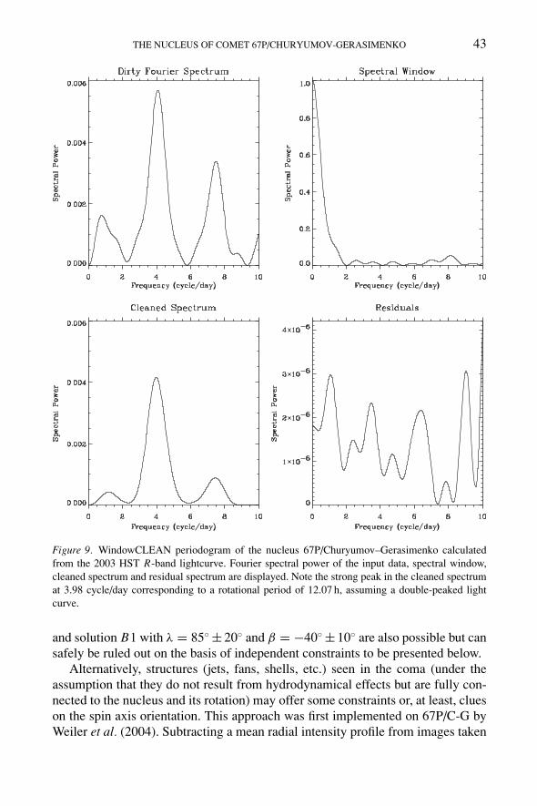
A detailed analysis of the light curve of the nucleus of 67P/C-G obtained with theHST (Figure 8) has already been performed by Lamy et al. (2006a). They used sevendifferent period-searching methods (see Figure 9 for an example of application ofthe WindowCLEAN method and found a range of rotational periods from 11.78to 12.86 h with a mean of Prot = 12.41 h and σ = 0.41 h. The convergence of theseven independent methods to this value with an rms dispersion of only 4% suggeststhat it is a very robust result.
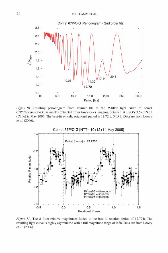
A preliminary Fourier period-fitting analysis was performed on the R-filter NTTdata, and the resulting periodogram is shown in Figure 10. The best-fit full synodicrotation period is 12.72 ± 0.05 hours. The folded R-filter data points are shown inFigure 11, with the best-fit analytical function overplotted.
The inversion procedure yielded a rotational period of 12.68 ± 0.03 h but itdoes not peak very strongly because of the noise in the data, the limited phase
THE NUCLEUS OF COMET 67P/CHURYUMOV-GERASIMENKO 41
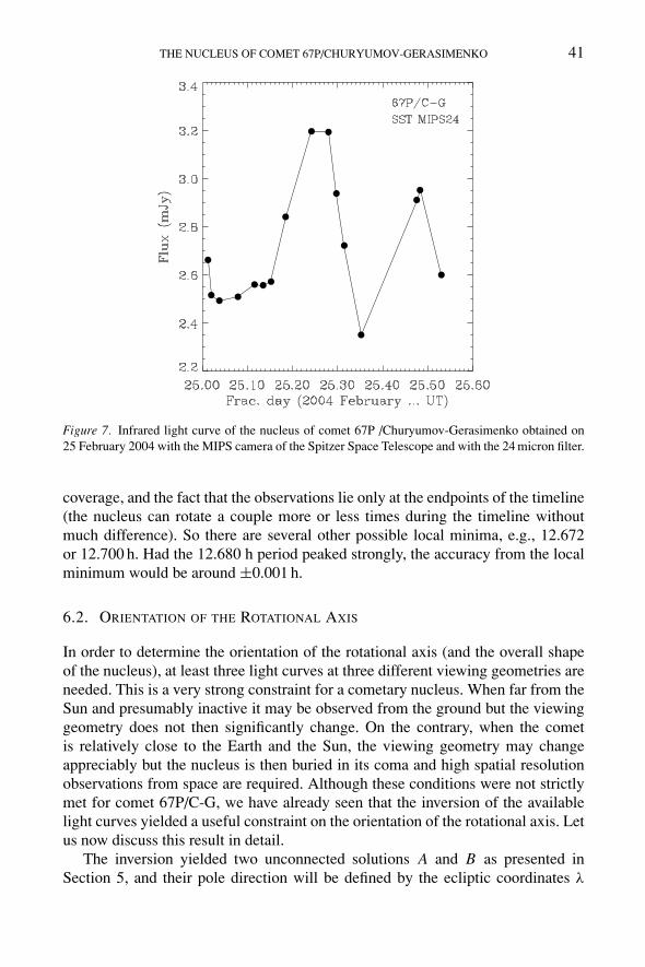
Figure 7. Infrared light curve of the nucleus of comet 67P /Churyumov-Gerasimenko obtained on25 February 2004 with the MIPS camera of the Spitzer Space Telescope and with the 24 micron filter.
coverage, and the fact that the observations lie only at the endpoints of the timeline(the nucleus can rotate a couple more or less times during the timeline withoutmuch difference). So there are several other possible local minima, e.g., 12.672or 12.700 h. Had the 12.680 h period peaked strongly, the accuracy from the localminimum would be around ±0.001 h.
6.2. ORIENTATION OF THE ROTATIONAL AXIS
In order to determine the orientation of the rotational axis (and the overall shapeof the nucleus), at least three light curves at three different viewing geometries areneeded. This is a very strong constraint for a cometary nucleus. When far from theSun and presumably inactive it may be observed from the ground but the viewinggeometry does not then significantly change. On the contrary, when the cometis relatively close to the Earth and the Sun, the viewing geometry may changeappreciably but the nucleus is then buried in its coma and high spatial resolutionobservations from space are required. Although these conditions were not strictlymet for comet 67P/C-G, we have already seen that the inversion of the availablelight curves yielded a useful constraint on the orientation of the rotational axis. Letus now discuss this result in detail.
The inversion yielded two unconnected solutions A and B as presented inSection 5, and their pole direction will be defined by the ecliptic coordinates λ
42 P. L. LAMY ET AL.
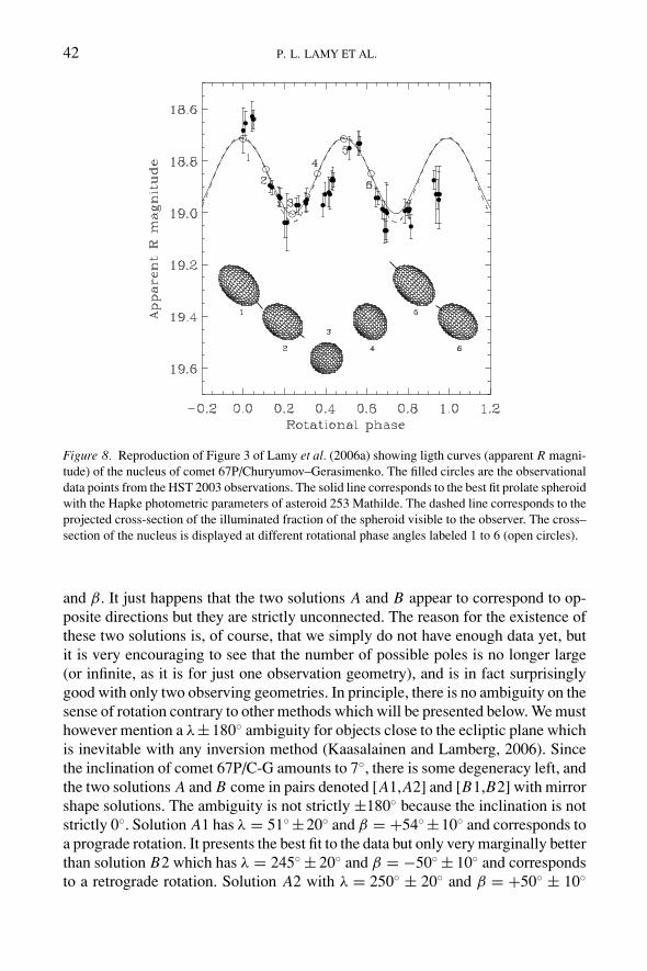
Figure 8. Reproduction of Figure 3 of Lamy et al. (2006a) showing ligth curves (apparent R magni-tude) of the nucleus of comet 67P/Churyumov–Gerasimenko. The filled circles are the observationaldata points from the HST 2003 observations. The solid line corresponds to the best fit prolate spheroidwith the Hapke photometric parameters of asteroid 253 Mathilde. The dashed line corresponds to theprojected cross-section of the illuminated fraction of the spheroid visible to the observer. The cross–section of the nucleus is displayed at different rotational phase angles labeled 1 to 6 (open circles).
and β. It just happens that the two solutions A and B appear to correspond to op-posite directions but they are strictly unconnected. The reason for the existence ofthese two solutions is, of course, that we simply do not have enough data yet, butit is very encouraging to see that the number of possible poles is no longer large(or infinite, as it is for just one observation geometry), and is in fact surprisinglygood with only two observing geometries. In principle, there is no ambiguity on thesense of rotation contrary to other methods which will be presented below. We musthowever mention a λ±180◦ ambiguity for objects close to the ecliptic plane whichis inevitable with any inversion method (Kaasalainen and Lamberg, 2006). Sincethe inclination of comet 67P/C-G amounts to 7◦, there is some degeneracy left, andthe two solutions A and B come in pairs denoted [A1,A2] and [B1,B2] with mirrorshape solutions. The ambiguity is not strictly ±180◦ because the inclination is notstrictly 0◦. Solution A1 has λ = 51◦ ±20◦ and β = +54◦ ±10◦ and corresponds toa prograde rotation. It presents the best fit to the data but only very marginally betterthan solution B2 which has λ = 245◦ ± 20◦ and β = −50◦ ± 10◦ and correspondsto a retrograde rotation. Solution A2 with λ = 250◦ ± 20◦ and β = +50◦ ± 10◦
THE NUCLEUS OF COMET 67P/CHURYUMOV-GERASIMENKO 43
Figure 9. WindowCLEAN periodogram of the nucleus 67P/Churyumov–Gerasimenko calculatedfrom the 2003 HST R-band lightcurve. Fourier spectral power of the input data, spectral window,cleaned spectrum and residual spectrum are displayed. Note the strong peak in the cleaned spectrumat 3.98 cycle/day corresponding to a rotational period of 12.07 h, assuming a double-peaked lightcurve.
and solution B1 with λ = 85◦ ± 20◦ and β = −40◦ ± 10◦ are also possible but cansafely be ruled out on the basis of independent constraints to be presented below.
Alternatively, structures (jets, fans, shells, etc.) seen in the coma (under theassumption that they do not result from hydrodynamical effects but are fully con-nected to the nucleus and its rotation) may offer some constraints or, at least, clueson the spin axis orientation. This approach was first implemented on 67P/C-G byWeiler et al. (2004). Subtracting a mean radial intensity profile from images taken
44 P. L. LAMY ET AL.
1.0
1.2
1.4
1.6
1.8
2.0
2.2
2.4
2.6
0.0 5.0 10.0 15.0 20.0 25.0 30.0
χ2/N
fre
e
Period [hrs]
Comet 67P/C-G [Periodogram - 2nd order fits]
12.72
14.3017.14
10.08
20.41
Figure 10. Resulting periodogram from Fourier fits to the R-filter light curve of comet67P/Churyumov–Gerasimenko extracted from time-series imaging obtained at ESO’s 3.5-m NTT(Chile) in May 2005. The best-fit synodic rotational period is 12.72 ± 0.05 h. Data are from Lowryet al. (2006).
Comet 67P/C-G [NTT - 10+12+14 May 2005]
-0.5 0.0 0.5 1.0 1.5
Rotational Phase
0.4
0.2
0.0
-0.2
-0.4
Rela
tive
R m
agnitude
Period [hours] = 12.7200
10may05 = diamonds12may05 = squares14may05 = triangles
Figure 11. The R-filter relative magnitudes folded to the best-fit rotation period of 12.72 h. Theresulting light curve is highly asymmetric with a full magnitude range of 0.38. Data are from Lowryet al. (2006).
THE NUCLEUS OF COMET 67P/CHURYUMOV-GERASIMENKO 45
in March 2003, they identified two radial structures (apart from the tail) in the comawhich they interpreted as the edges of a cone originating from a single active areaon the rotating nucleus. Under this assumption, they estimated from the positionangles of these structures, that the inclination of the projected rotational axis tothe orbital plane would be approximately 40◦. Schleicher (2006) applied the samemethod on images taken in January 1996 and detected a strong sunward radialfeature in the coma of 67P/C-G. Considering several alternatives to explain thepresence of such a structure, he proposed a plausible explanation (compatible withother constraints derived from a detailed photometric analysis) similar to that ofWeiler et al. (2004), that is the edge of a cone swept out by the rotation of a jet froma single active region. Using a Monte Carlo simulation of this jet and imposing theconstraint given by Weiler et al. (2004) on the inclination, he found that the bestpossible solution for the rotational axis is either RA ≈ 57◦ and Dec ≈ +65◦ orthe opposite direction RA ≈ 223◦ and Dec ≈ −65◦, since the sense of rotation isunconstrained.
As discussed in Section 4, the forced precession models allow one to deriveconstraints on the orientation of the rotational axis from the outgassing–inducedvariations of the cometary orbit.
Krolikowska (2003)’s solution for an oblate body rotating around its shortestprincipal axis, had an orientation in 2003 defined by RA ≈ 17◦ and Dec ≈ +5◦
in order to satisfy the astrometric observations of the last 6 orbits of 67P/C-G.According to our present understanding of the rotation of minor bodies of thesolar system, this configuration appears extremely unlikely, and furthermore incontradiction with all other lines of evidence.
Chesley (2004) also tried to fit astrometric observations of 67P/C-G but usinga different approach. He modeled the nongravitational accelerations as outgassingfrom body-fixed jets that thrust according to the insolation level. This study resultedin several possible pole orientations yielding a reasonable fit to the orbit. Consider-ing the constraint given by Weiler et al. (2004), he estimated that the pole orientationof 67P/C-G is within 10◦ of RA = 90◦ and Dec = +75◦, with no constraint on thesense of rotation (i.e. the opposite direction is equally possible).
More recently, Davidsson and Gutierrez (2005), using an elaborate thermophys-ical model found that all observational constraints were simultaneously satisfiedwhen the rotational axis is confined to two well defined regions in the [obliquity,argument] plane (see Sekanina, 1981 for a definition of these angles). The firstregion is defined by an argument of 60◦ ± 15◦ and an obliquity of 120◦ ± 30◦. Thesecond region is characterized by an argument of 240◦ ± 15◦ and an obliquity of60◦ ± 30◦.
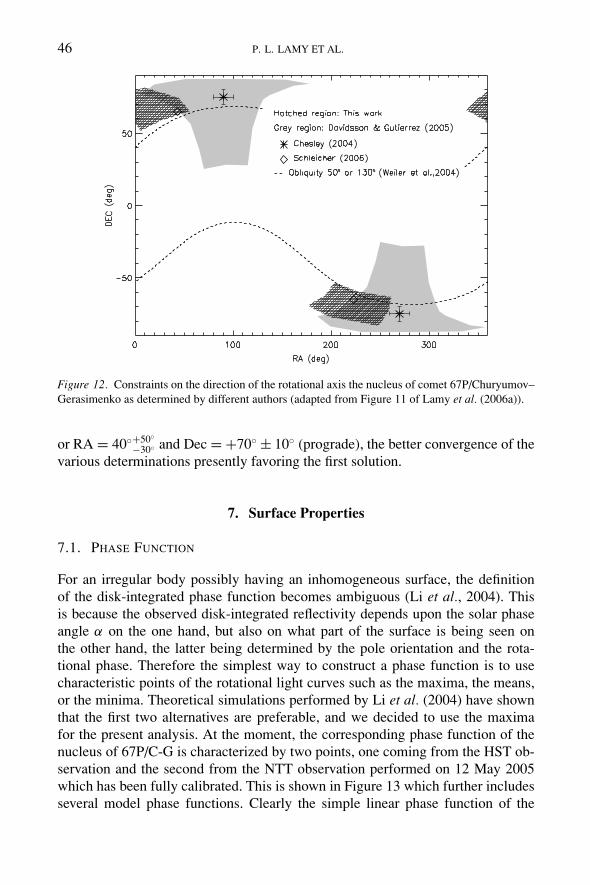
Figure 12 presents all the above constraints and solutions in the [RA, Dec] plane.It can be seen that they concentrate in two very well defined regions correspond-ing to opposite directions and implying an intermediate obliquity. Based on thesepresent evidences, the direction of the rotational axis of the nucleus of the cometis defined by either RA = 220◦+50◦
−30◦ and Dec = −70◦ ± 10◦ (retrograde rotation)
46 P. L. LAMY ET AL.
Figure 12. Constraints on the direction of the rotational axis the nucleus of comet 67P/Churyumov–Gerasimenko as determined by different authors (adapted from Figure 11 of Lamy et al. (2006a)).
or RA = 40◦+50◦−30◦ and Dec = +70◦ ± 10◦ (prograde), the better convergence of the
various determinations presently favoring the first solution.
7. Surface Properties
7.1. PHASE FUNCTION
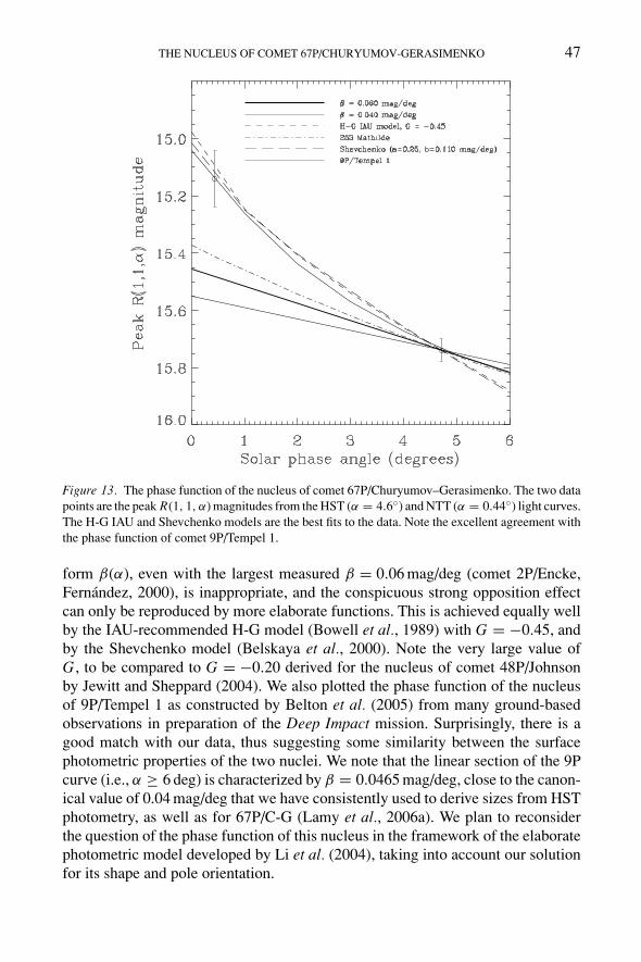
For an irregular body possibly having an inhomogeneous surface, the definitionof the disk-integrated phase function becomes ambiguous (Li et al., 2004). Thisis because the observed disk-integrated reflectivity depends upon the solar phaseangle α on the one hand, but also on what part of the surface is being seen onthe other hand, the latter being determined by the pole orientation and the rota-tional phase. Therefore the simplest way to construct a phase function is to usecharacteristic points of the rotational light curves such as the maxima, the means,or the minima. Theoretical simulations performed by Li et al. (2004) have shownthat the first two alternatives are preferable, and we decided to use the maximafor the present analysis. At the moment, the corresponding phase function of thenucleus of 67P/C-G is characterized by two points, one coming from the HST ob-servation and the second from the NTT observation performed on 12 May 2005which has been fully calibrated. This is shown in Figure 13 which further includesseveral model phase functions. Clearly the simple linear phase function of the
THE NUCLEUS OF COMET 67P/CHURYUMOV-GERASIMENKO 47
Figure 13. The phase function of the nucleus of comet 67P/Churyumov–Gerasimenko. The two datapoints are the peak R(1, 1, α) magnitudes from the HST (α = 4.6◦) and NTT (α = 0.44◦) light curves.The H-G IAU and Shevchenko models are the best fits to the data. Note the excellent agreement withthe phase function of comet 9P/Tempel 1.
form β(α), even with the largest measured β = 0.06 mag/deg (comet 2P/Encke,Fernandez, 2000), is inappropriate, and the conspicuous strong opposition effectcan only be reproduced by more elaborate functions. This is achieved equally wellby the IAU-recommended H-G model (Bowell et al., 1989) with G = −0.45, andby the Shevchenko model (Belskaya et al., 2000). Note the very large value ofG, to be compared to G = −0.20 derived for the nucleus of comet 48P/Johnsonby Jewitt and Sheppard (2004). We also plotted the phase function of the nucleusof 9P/Tempel 1 as constructed by Belton et al. (2005) from many ground-basedobservations in preparation of the Deep Impact mission. Surprisingly, there is agood match with our data, thus suggesting some similarity between the surfacephotometric properties of the two nuclei. We note that the linear section of the 9Pcurve (i.e., α ≥ 6 deg) is characterized by β = 0.0465 mag/deg, close to the canon-ical value of 0.04 mag/deg that we have consistently used to derive sizes from HSTphotometry, as well as for 67P/C-G (Lamy et al., 2006a). We plan to reconsiderthe question of the phase function of this nucleus in the framework of the elaboratephotometric model developed by Li et al. (2004), taking into account our solutionfor its shape and pole orientation.
48 P. L. LAMY ET AL.
7.2. GEOMETRIC ALBEDO
As with the phase function, the definition of the disk-integrated albedo of an ir-regular body raises problems (see discussion in Lamy et al., 2004b). The simplestapproach to obtain an estimate is to rely on the standard formula relating magni-tudes to cross-sections (Russell, 1916; Jewitt, 1991). In the present application, themaximum and minimum geometric cross-sections were calculated from our two3-D models of the nucleus at the time of the HST observations, and associated to theextreme apparent magnitudes then measured. The above formula also involves thephase function but it is important to realize here that the relevant correction shouldexclude the opposition effect. This is because the disk–integrated reflectance isrelative to that produced by a perfect diffusing disk which does not exhibit suchan effect. Otherwise the opposition surge would translate into an artificial increaseof the albedo. Conventional wisdom calls for relying on magnitudes obtained atphase angles beyond about 5◦ and using a simple linear law for the phase func-tion β(α) = βα. In our case, we do not have the proper data to estimate the phasecoefficient β, and we considered two solutions:
– the canonical value β = 0.04 mag/deg which we have consistently used in thepast,
– the value β = 0.0465 mag/deg suggested by the linear part of the phase functionof comet 9P as discussed in the above section.
The eight determinations of pR (R-band) resulting from these two values, the twocomet models and the extreme cross–sections/magnitudes, lie in the range 0.050to 0.059, well within the accepted range of the albedos of cometary nuclei (Lamyet al., 2004b; Fernandez et al., 2001). We note that the HST magnitudes obtainedat a phase angle α = 4.8◦ could already be biased by the opposition effect, andthat a correction of 0.1 mag would decrease the above range to 0.045–0.054. Theseranges basically reflect the uncertainties coming from both the measurements andfrom the method.
7.3. COLOR OF THE NUCLEUS
Lamy et al. (2006a) measured almost simultaneously the R and V magnitudes ofthe nucleus of comet 67P/C-G during six HST orbits (out of a total of eleven). Theyfound (V − R) color indices of the nucleus ranging from 0.47±0.08 to 0.59±0.11.This variation is only marginally statistically significant given the error bars, so theyadopted the average value of (V − R) = 0.52 ± 0.05. Partial reduction of the NTTobservations led to (V − R) = 0.41 ± 0.04. Time-series VRI colors will later beavailable when the full data set is analyzed, and it will be interesting to see whetherthey reveal rotational color variations that would suggest a variation of the coloracross the surface of the nucleus, as detected, for example, on comet 2P/Encke(Lowry et al., 2003b). Another possible explanation would invoke a dependence of
THE NUCLEUS OF COMET 67P/CHURYUMOV-GERASIMENKO 49
the color on the phase angle. Whatever the outcome, the present two determinationsare compatible at the 2-sigma level, and are very close to the mean value of 0.49 ±0.03 obtained for the nuclei of 34 ecliptic comets (Lamy and Toth, 2007). So asfar as color is concerned, the nucleus of comet 67P/C-G has a quite standard redcolor (with respect to the Sun). The corresponding normalized reflectivities andreflectivity gradients of the nucleus of 67P/C-G were calculated from the abovecolor indices, minus that of the Sun, and normalized to a value of 1 at 550 nm, theeffective wavelength of the V band. The HST color index leads to S(λ = 650 nm) =1.17 ± 0.05 and S′(550, 650 nm) = 17% per kA , while the NTT determinationleads to S(λ = 650 nm) = 1.06 ± 0.09 and S′(550, 650 nm) = 5.7% per kA .
8. Internal Properties
8.1. DENSITY AND MASS OF THE NUCLEUS
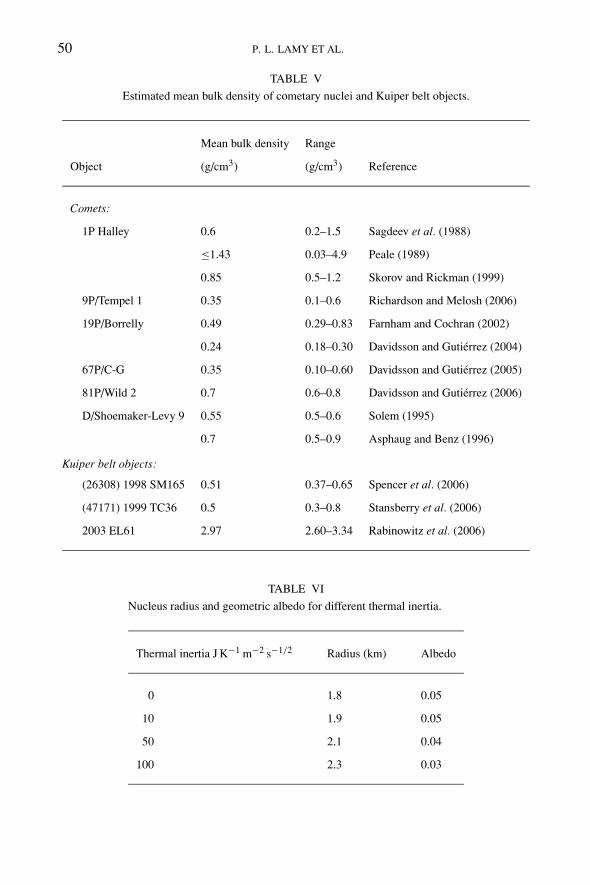
Table V summarizes several estimates or determinations of the density of come-tary nuclei as well as related objects. We note the convergence to rather low val-ues, typically 500 kg m−3, even for a large Kuiper belt object. For the nucleusof comet 67P/C-G, and based on their detailed model, Davidsson and Gutierrez(2005) concluded that this value is however an upper limit and favored a range of100–370 kg m−3.
We have therefore used the three values 100, 370 and 500 kg m−3 to estimatethe mass of the nucleus (Table IV). The two models yield identical results in therange 2.1×10¹²–1.1×10¹³ kg.
8.2. THERMAL INERTIA
The thermal inertia of comet 67P/C-G is obviously unknown. In the previous sec-tion, we used a standard thermal model to derive the size of the nucleus with theinherent assumption of a null thermal inertia. Even if this assumption is not realistic,it is justified according to our previous works (e.g., Groussin et al., 2004) and therecent results of the Deep Impact mission on comet 9P/Tempel 1 (A’Hearn et al.,2005). The thermal inertia of the nucleus of 9P/Tempel 1 is most probably less than50 J K−1 m−2 s−1/2 (Groussin et al., 2006), and we anticipate the same range forthat of comet 67P/C-G.
In order to estimate the error on the radius and on the geometric albedo due to theuncertainty on the thermal inertia, we repeated the calculations presented in Sec-tion with thermal inertias of 10, 50 and 100 J K−1 m−2 s−1/2, and present the resultsin Table VI. The higher the thermal inertia, the larger the radius and the lower thegeometric albedo, as expected. A maximum thermal inertia of 50 J K−1 m−2 s−1/2
50 P. L. LAMY ET AL.
TABLE V
Estimated mean bulk density of cometary nuclei and Kuiper belt objects.
Mean bulk density Range
Object (g/cm3) (g/cm3) Reference
Comets:
1P Halley 0.6 0.2–1.5 Sagdeev et al. (1988)
≤1.43 0.03–4.9 Peale (1989)
0.85 0.5–1.2 Skorov and Rickman (1999)
9P/Tempel 1 0.35 0.1–0.6 Richardson and Melosh (2006)
19P/Borrelly 0.49 0.29–0.83 Farnham and Cochran (2002)
0.24 0.18–0.30 Davidsson and Gutierrez (2004)
67P/C-G 0.35 0.10–0.60 Davidsson and Gutierrez (2005)
81P/Wild 2 0.7 0.6–0.8 Davidsson and Gutierrez (2006)
D/Shoemaker-Levy 9 0.55 0.5–0.6 Solem (1995)
0.7 0.5–0.9 Asphaug and Benz (1996)
Kuiper belt objects:
(26308) 1998 SM165 0.51 0.37–0.65 Spencer et al. (2006)
(47171) 1999 TC36 0.5 0.3–0.8 Stansberry et al. (2006)
2003 EL61 2.97 2.60–3.34 Rabinowitz et al. (2006)
TABLE VI
Nucleus radius and geometric albedo for different thermal inertia.
Thermal inertia J K−1 m−2 s−1/2 Radius (km) Albedo
0 1.8 0.05
10 1.9 0.05
50 2.1 0.04
100 2.3 0.03
THE NUCLEUS OF COMET 67P/CHURYUMOV-GERASIMENKO 51
would increase the size by 17%, and decrease the albedo by 25% relative to ournominal model with a null thermal inertia.
8.3. MOMENTS OF INERTIA
From a rotational dynamics perspective, the shape of our model nucleus can beassimilated to that of a prolate body, for which we calculated the ratios of themoments of inertia in a body-fixed, triaxial coordinate system whose origin is atthe center of mass of the body and whose axes (x,y,z) correspond to the principalaxes of smallest, intermediate, and largest moments of inertia, respectively: Ix/Iz ,and Iy/Iz . The results presented in Table IV are essentially identical for the twomodels.
8.4. GRAVITY FIELD
We performed a first order analysis of the gravity field of our model nucleus,along the lines described by Scheeres et al. (1998) for asteroid 4179 Toutatis. Themost important terms of the harmonic expansion of the gravity field correspondto the coefficients of second degree and order C20 and C22. Assuming that thebody is rotating in the minimum energy state of its angular momentum, i.e., aboutthe principal axis of the largest moment of inertia (z-axis), and assuming that thebody is homogeneous with a uniform density, we found the dimensionless valuesreported in Table IV. Note that ro is an arbitrary normalization radius which maybe suppressed as it has no real dynamical significance, in which case the C20 andC22 coefficients then have dimensions of km2.
9. Activity of the Nucleus
9.1. GAS PRODUCTION RATES
Production rate measurements of five species are available for 67P/C-G: OH (usedfor calculating the production rate of H2O), CN, C2, C3, and NH. All these specieswere detected during both the 1982 and 1996 apparitions. For the 2002 apparition,only a single CN measurement is available.
Production rates of CN, C2, and C3 obtained from spectra measured during theMcDonald observatory faint comet survey have been reported by Cochran et al.(1992). The same CN rates were also published by Storrs et al. (1992). Anothermajor data set originates from groundbased narrowband photometry performedat Lowell observatory, with OH and CN production rates reported by Osip et al.(1992). This data set has recently been re–calibrated by Schleicher (2006), whoalso report additional production rates of C2, C3, and NH. Hanner et al. (1985),
52 P. L. LAMY ET AL.
0 100 200 300
1027
1028
H2O
Q [
mo
lec s
]
Hanner et al. (1985)Cochran et al. (1992)Crovisier et al. (2002)Makinen (2004)Schulz et al. (2004)Weiler et al. (2004)Schleicher (2006)Numerical fit
0 100 200 300
1024
1025
CN
0 100 200 300
1024
1025
C2
0 100 200 30010
23
1024
C3
Q [
mo
lec s
]
0 100 200 30010
24
1025
1026
NH
Time from perihelion [days]
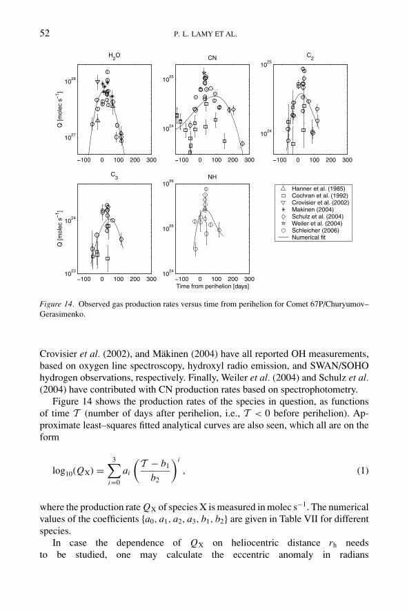
Figure 14. Observed gas production rates versus time from perihelion for Comet 67P/Churyumov–Gerasimenko.
Crovisier et al. (2002), and Makinen (2004) have all reported OH measurements,based on oxygen line spectroscopy, hydroxyl radio emission, and SWAN/SOHOhydrogen observations, respectively. Finally, Weiler et al. (2004) and Schulz et al.(2004) have contributed with CN production rates based on spectrophotometry.
Figure 14 shows the production rates of the species in question, as functionsof time T (number of days after perihelion, i.e., T < 0 before perihelion). Ap-proximate least–squares fitted analytical curves are also seen, which all are on theform
log10(QX) =3∑
i=0
ai
(T − b1
b2
)i
, (1)
where the production rate QX of species X is measured in molec s−1. The numericalvalues of the coefficients {a0, a1, a2, a3, b1, b2} are given in Table VII for differentspecies.
In case the dependence of QX on heliocentric distance rh needsto be studied, one may calculate the eccentric anomaly in radians
THE NUCLEUS OF COMET 67P/CHURYUMOV-GERASIMENKO 53
TABLE VII
Coefficients for gas production rate analytical fits with Equation (1).
Validity range
Species b1 b2 a0 a1 a2 a3 (days)
H2O 32.847 46.992 27.8037 −0.18439 −0.20696 0.026326 −80 to 150
CN 20.2479 92.3756 24.5429 0.27882 −0.11770 −0.056959 −150 to 300
C2 20.0644 51.5860 24.5819 −0.0081104 −0.20111 0.04352 −70 to 130
C3 15.5643 44.0559 23.9686 0.18638 −0.12665 −0.0075334 −70 to 130
NH 28.2459 36.4303 25.4235 0.018054 −0.17020 0.033281 −40 to 140
Note. Coefficients to be used with Equation (1) in order to obtain approximate analytical expressionsfor the gas production rates. Note that the numerical fits have a limited validity range, as specifiedin the last column.
as
E(rh) = cos−1
(1
e
{1 − rh
a
})≈ cos−1 (1.583 − 0.452rh) , (2)
where a and e are the semi–major axis and eccentricity, respectively, and then applyKepler’s equation,
T (rh) = 365.25a3/2
2π(E(rh) − e sin E(rh))
≈ 381.4E(rh) − 241 sin E(rh). (3)
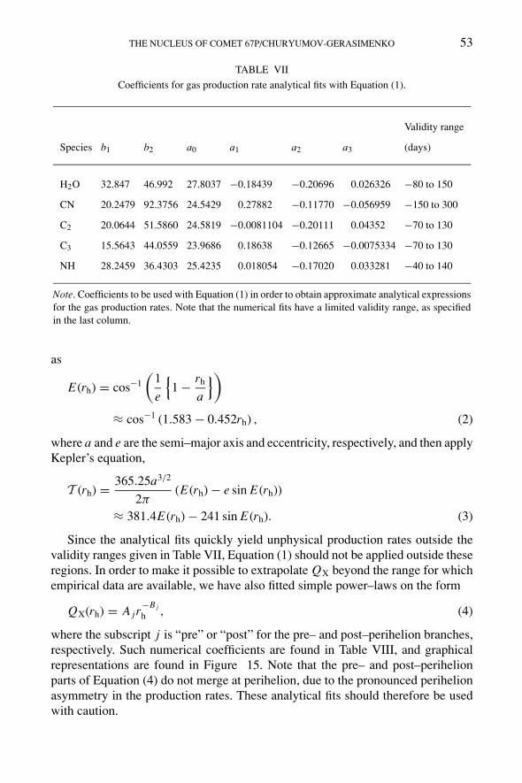
Since the analytical fits quickly yield unphysical production rates outside thevalidity ranges given in Table VII, Equation (1) should not be applied outside theseregions. In order to make it possible to extrapolate QX beyond the range for whichempirical data are available, we have also fitted simple power–laws on the form
QX(rh) = A jr−B j
h , (4)
where the subscript j is “pre” or “post” for the pre– and post–perihelion branches,respectively. Such numerical coefficients are found in Table VIII, and graphicalrepresentations are found in Figure 15. Note that the pre– and post–perihelionparts of Equation (4) do not merge at perihelion, due to the pronounced perihelionasymmetry in the production rates. These analytical fits should therefore be usedwith caution.
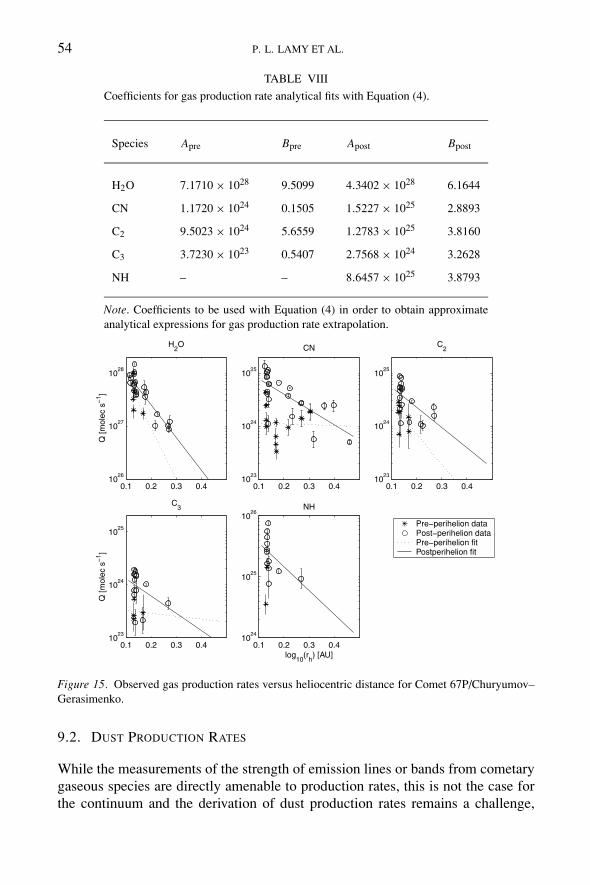
54 P. L. LAMY ET AL.
TABLE VIII
Coefficients for gas production rate analytical fits with Equation (4).
Species Apre Bpre Apost Bpost
H2O 7.1710 × 1028 9.5099 4.3402 × 1028 6.1644
CN 1.1720 × 1024 0.1505 1.5227 × 1025 2.8893
C2 9.5023 × 1024 5.6559 1.2783 × 1025 3.8160
C3 3.7230 × 10²³ 0.5407 2.7568 × 1024 3.2628
NH – – 8.6457 × 1025 3.8793
Note. Coefficients to be used with Equation (4) in order to obtain approximateanalytical expressions for gas production rate extrapolation.
0.1 0.2 0.3 0.410
26
1027
1028
H2O
Q [
mo
lec s
]
Postperihelion fit
0.1 0.2 0.3 0.410
23
1024
1025
CN
0.1 0.2 0.3 0.410
23
1024
1025
C2
0.1 0.2 0.3 0.410
23
1024
1025
C3
Q [
mo
lec s
]
0.1 0.2 0.3 0.410
24
1025
1026
NH
log10
(rh) [AU]
Figure 15. Observed gas production rates versus heliocentric distance for Comet 67P/Churyumov–Gerasimenko.
9.2. DUST PRODUCTION RATES
While the measurements of the strength of emission lines or bands from cometarygaseous species are directly amenable to production rates, this is not the case forthe continuum and the derivation of dust production rates remains a challenge,
THE NUCLEUS OF COMET 67P/CHURYUMOV-GERASIMENKO 55
requiring a model for the dust expansion as well as numerous assumptions. In orderto circumvent this problem, A’Hearn et al. (1984) introduced the quantity A fρ asa way of simply quantifying the dust activity. A fρ is easily calculated from thephotometry of the dust coma (the integral of the observed flux in a given circu-lar aperture), and has therefore enjoyed considerable popularity among cometaryobservers, to the point of being a proxy for the dust production rate itself. Un-fortunately, and as testified by the works which attempted to correctly handle theproblem (e.g., Newburn and Spinrad (1985), Singh et al. (1992)), this is far frombeing the case. Apart from making sense only when the comet sports a steady–state,circularly symmetric coma insuring that A fρ is independant of the aperture radius,it depends upon the phase angle and the wavelength, two limitations which areoften overlooked when comparing various determinations at different heliocentricdistances. This has particularly affected comet 67P/C-G as the late ““outburst”’reported by Kidger (2003) has convincingly been shown by Schleicher (2006) toresult from a phase angle effect (an opposition effect by the way). Another biaswhich may affect A fρ as a proxy to actual, on-going dust production, is the pres-ence of an old population of slow–moving large dust particles forming a dust trail,conspicuously detected in the infrared by the IRAS and Spitzer space telescopes(Sykes and Walker, 1992; Kelley et al., 2006).
Several authors (Weiler et al., 2004; Fulle et al., 2004; Moreno et al., 2004; Lamyet al., 2006a) calculated the dust production rate of comet 67P/C-G implementingdifferent models. This question is thoroughfully discussed in this issue by Agarwalet al. (this issue) in their modeling of the dust environment of comet 67P/C-G.
9.3. ACTIVE AREAS AND ACTIVITY PATTERN
The ensemble of data on the water production rate spanning a large range of he-liocentric distances reveals a strong pre- to post-perihelion asymmetry, with peakproductivity occurring ∼1 month after perihelion passage, as well as large rotationalvariability. Adopting a rotationally averaged peak value QH2O = 1 × 1028 mol s−1
at rh ∼ 1.36 AU, we followed the standard (but oversimplified) practice, and cal-culated the fraction of active surface area on the nucleus on the basis of a simplewater sublimation model that assumes a permanently illuminated isotropic source(Cowan and A’Hearn, 1979). An active area of 2.8 km2 is thus required to yield theabove water production rate. For our two model nuclei with a total surface area of40 km2, this corresponds to a maximum active fraction of 7%, implying that thebulk of the surface of the nucleus of 67P/C-G is inactive. Schleicher (2006) arguesthat the above simple model overestimates the active area as it is probably closeto sub-solar latitudes thus resulting in more efficient sublimation, and suggests aneven lower peak value. Modeling performed by Davidsson and Gutierrez (2005)indicates that a fraction of active surface area (stationary size) of 4% is capable ofreproducing the empirical QH2O data equally well as Equation (1).
56 P. L. LAMY ET AL.
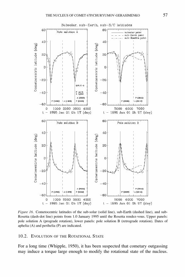
The activity pattern of the nucleus of comet 67P/C-G has been thoroughly dis-cussed by Schleicher (2006) on the basis of the photometric behaviour of its gasand dust coma characterized by a large pre- to post-perihelion asymmetry and rota-tional variability, and the presence of a sunward radial feature. The most plausiblescenario, also advocated for other comets, relies on one or more isolated sourceregions located at mid-latitude and turning on and off as the nucleus rotates (shortterm variability) combined with a seasonal change in solar latitude (asymmetryabout perihelion). That such a change prevails for our two pole solutions is clearlydemonstrated in Figure 16 where we display the cometocentric latitude of the sub-solar point. An additional piece of information comes from models of the dusttail by Fulle et al. (2004) and Moreno et al. (2004) which agree on a much largerpopulation of mm and cm sized grains than most short-period comets, with a peakproduction taking place several months prior to perihelion followed by a markeddrop-off thereafter, at a time when the gas production reaches its maximum. Themost plausible scenario to explain this behaviour has been proposed by Schleicher(2006). It requires:
– a source region in one hemisphere dominated by large grains which is in “sum-mer” while the comet approaches the Sun, and which is no longer illuminatedshortly after perihelion;
– a much larger source region (or regions) in the other hemisphere coming undersolar illumination shortly after perihelion (seasonal effect) and producing copiousamounts of gas and small-sized grains but depleted in large-sized grains.
We note that a similar scenario has already been proposed for comet 2P/Enckeby Lamy et al. (2003a) to precisely explain very distinct pre- and post-perihelionphotometric behaviours.
10. Evolution of the Nucleus
10.1. SURFACE EROSION OF THE NUCLEUS
Integration of the numerically fitted QH2O(T ) functions in the−450 ≤ T ≤ 450 dayinterval (i.e., the rh ≤ 4 AU segment of the orbit) yields a total water production of2.2 × 109 kg. Assuming a surface area of 40 km2, and that 4% of the surface is onthe average actively contributing to the water production, means that each m2 ofactive area must contribute ∼1000 kg of ice per apparition.
Assuming a 0.7 : 0.3 mixture of ice and dust by volume in compacted cometarymaterial (which, for reasonable values of solid densities of these materials, yield adust–to–ice mass ratio of about 0.8, see Hage and Greenberg, 1990), and a porosityof 70% in the surface material, means that there is approximately 200 kg of ice ina cubic meter of porous ice/dust material. As a consequence, the active areas of67P/C-G typically erode at a rate of approximately 5 m per apparition.
THE NUCLEUS OF COMET 67P/CHURYUMOV-GERASIMENKO 57
Figure 16. Cometocentric latitudes of the sub-solar (solid line), sub-Earth (dashed line), and sub-Rosetta (dash-dot line) points from 1.0 January 1995 until the Rosetta rendez-vous. Upper panels:pole solution A (prograde rotation), lower panels: pole solution B (retrograde rotation). Dates ofaphelia (A) and perihelia (P) are indicated.
10.2. EVOLUTION OF THE ROTATIONAL STATE
For a long time (Whipple, 1950), it has been suspected that cometary outgassingmay induce a torque large enough to modify the rotational state of the nucleus.
58 P. L. LAMY ET AL.
The evidence that comet 1P/Halley and other comets are likely rotating in complexmode, along with plausible detections of spin period changes in some comets (e.g.Mueller and Ferrin, 1996; Gutierrez et al., 2003a) triggered studies on the effect ofthe outgassing–induced torque on cometary spin states (e.g., Peale and Lissauer,1989; Samarasinha et al., 1996; Neishtadt, 2002; Gutierrez et al., 2003b). Thesestudies confirm that the momentum transferred to the nucleus by the sublimating icecan certainly modify the angular momentum even in comparatively small periodsof time. The timescale τ for a sublimation–induced change of the spin period Prot
or the angular momentum L of a cometary nucleus can be estimated by using therelationship (Samarasinha et al., 1986)
τ ≈ 8π2αρr5n
3ηd rnmvProt(5)
where α is a ratio between the actual moment of inertia and the moment of inertia ofa spherical body with the same mean radius as the nucleus rn , drn is a characteristicmoment arm, η is a global momentum transfer coefficient, m is the mass loss ratedue to sublimation, and v is the gas velocity.
The previous expression can be used to estimate, in a first approximation, thetimescale of the evolution of the rotational parameters of 67P/C-G. For typicalvalues of these parameters (see Jorda and Gutierrez, 2002), a water production atperihelion of 1 × 1028 molec s−1 (see Section 9.1), and a mean radius of � 2 km,the timescale for a change of the spin period and/or angular momentum direction ofa 67P/C-G–like comet is approximately 4 years, i.e. a fraction of its orbital period.This comparatively short timescale suggests that it is likely that comet 67P/C-G undergoes significant changes in its angular momentum after every perihelionpassage, just due to the momentum transferred by the outgassing.
In support of the Rosetta mission, and in order to estimate the amplitude of thepossible rotational changes, Gutierrez et al. (2005) extensively studied the rotationalevolution of a 67P/C-G–like comet under the sublimation–induced torque. Takingall the available observational constraints into account (e.g. water production rate atperihelion, size, spin period, etc.), these authors performed numerical simulationsfor a large set of initial conditions, including several body-shapes, various initialangular momenta (including the possibility of being rotating in complex mode),different activity patterns, etc. Figures 17 and 18 illustrate possible changes both inthe spin period and in the angular momentum direction of 67P/C-G during 2.5 orbits.As a general result, typical spin period changes that 67P/C-G may undergo when itis near perihelion are of about 0.001–0.05 hr day−1, depending on nucleus shape,activity pattern, etc. This means that the spin period of 67P/C-G may significantlyevolve from now until 2014 (when Rosetta will encounter the comet). During thistime interval, the spin period may indeed change by hours in the worst case. Overthe time span of the Rosetta observations, the spin period may change by 0.5 hr.Concerning variations of the angular momentum orientation, Gutierrez et al. (2005)
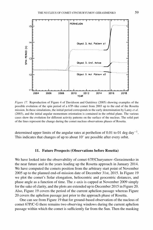
THE NUCLEUS OF COMET 67P/CHURYUMOV-GERASIMENKO 59
Figure 17. Reproduction of Figure 4 of Davidsson and Gutierrez (2005) showing examples of thepossible evolution of the spin period of a 67P–like comet from 2003 up to the end of the Rosettamission. In these simulations, the initial period corresponds to the early determination by Lamy et al.(2003), and the initial angular momentum orientation is contained in the orbital plane. The variouscases show the evolution for different activity patterns on the surface of the nucleus. The solid partof the lines represent the change during the comet nucleus observations phases of Rosetta.
determined upper limits of the angular rates at perihelion of 0.01 to 01 deg day−1.This indicates that changes of up to about 10◦ are possible after every orbit.
11. Future Prospects (Observations before Rosetta)
We have looked into the observability of comet 67P/Churyumov–Gerasimenko inthe near future and in the years leading up the Rosetta approach in January 2014.We have computed the comets position from the arbitrary start point of November2005 up to the planned end-of-mission date of December 31st, 2015. In Figure 19we plot the comet’s Solar elongation, heliocentric and geocentric distances, andphase angle as a function of time. The x-axis is capped at November 2009 simplyfor the sake of clarity, and the plots are extended up to December 2015 in Figure 20.Also, Figure 19 covers the period of the current aphelion passage whereas Figure20 covers the aphelion passage just prior to the approach phase of Rosetta.
One can see from Figure 19 that for ground-based observation of the nucleus ofcomet 67P/C-G there remains two observing windows during the current aphelionpassage within which the comet is sufficiently far from the Sun. Then the masking
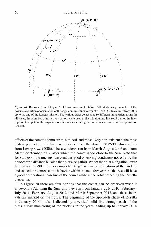
60 P. L. LAMY ET AL.
Figure 18. Reproduction of Figure 5 of Davidsson and Gutierrez (2005) showing examples of thepossible evolution of orientation of the angular momentum vector of a 67P/C-G–like comet from 2003up to the end of the Rosetta mission. The various cases correspond to different initial orientations. Inall cases, the same body and activity pattern were used in the calculations. The solid part of the linesrepresent the path of the angular momentum vector during the comet nucleus observations phases ofRosetta.
effects of the comet’s coma are minimized, and most likely non-existent at the mostdistant points from the Sun, as indicated from the above ESO/NTT observationsfrom Lowry et al. (2006). These windows run from March-August 2006 and fromMarch-September 2007, after which the comet is too close to the Sun. Note thatfor studies of the nucleus, we consider good observing conditions not only by theheliocentric distance but also the solar elongation. We set the solar elongation lowerlimit at about ∼90◦. It is very important to get as much observations of the nucleusand indeed the comets coma behavior within the next few years so that we will havea good observational baseline of the comet while in the orbit preceding the Rosettaencounter.
In Figure 20 there are four periods that the comet can be observed when itis beyond 3 AU from the Sun, and they run from January–July 2010, February–July 2011, February–August 2012, and March-September 2013, and these inter-vals are marked on the figure. The beginning of the approach phase of Rosettain January 2014 is also indicated by a vertical solid line through each of theplots. Close monitoring of the nucleus in the years leading up to January 2014
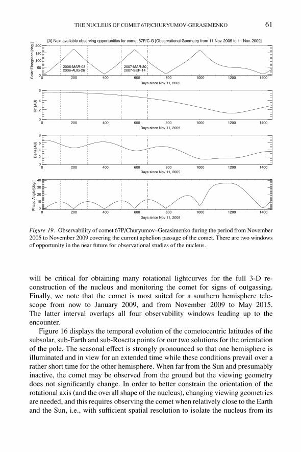
THE NUCLEUS OF COMET 67P/CHURYUMOV-GERASIMENKO 61
[A] Next available observing opportunities for comet 67P/C-G [Observational Geometry from 11 Nov. 2005 to 11 Nov. 2009]
0 200 400 600 800 1000 1200 1400
Days since Nov 11, 2005
0
50
100
150
200
So
lar
Elo
ng
atio
n [
de
g.]
2006-MAR-082006-AUG-26
2007-MAR-302007-SEP-14
0 200 400 600 800 1000 1200 1400
Days since Nov 11, 2005
0
2
4
6
Rh
[A
U]
0 200 400 600 800 1000 1200 1400
Days since Nov 11, 2005
0
2
4
6
8
De
lta
[A
U]
0 200 400 600 800 1000 1200 1400
Days since Nov 11, 2005
0
10
20
30
40
Ph
ase
An
gle
[d
eg
.]
Figure 19. Observability of comet 67P/Churyumov–Gerasimenko during the period from November2005 to November 2009 covering the current aphelion passage of the comet. There are two windowsof opportunity in the near future for observational studies of the nucleus.
will be critical for obtaining many rotational lightcurves for the full 3-D re-construction of the nucleus and monitoring the comet for signs of outgassing.Finally, we note that the comet is most suited for a southern hemisphere tele-scope from now to January 2009, and from November 2009 to May 2015.The latter interval overlaps all four observability windows leading up to theencounter.
Figure 16 displays the temporal evolution of the cometocentric latitudes of thesubsolar, sub-Earth and sub-Rosetta points for our two solutions for the orientationof the pole. The seasonal effect is strongly pronounced so that one hemisphere isilluminated and in view for an extended time while these conditions prevail over arather short time for the other hemisphere. When far from the Sun and presumablyinactive, the comet may be observed from the ground but the viewing geometrydoes not significantly change. In order to better constrain the orientation of therotational axis (and the overall shape of the nucleus), changing viewing geometriesare needed, and this requires observing the comet when relatively close to the Earthand the Sun, i.e., with sufficient spatial resolution to isolate the nucleus from its
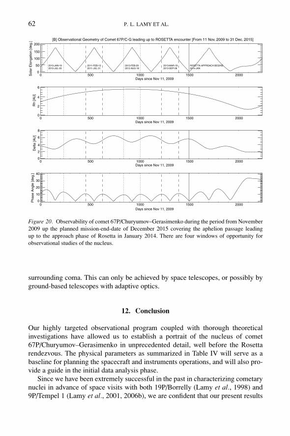
62 P. L. LAMY ET AL.
[B] Observational Geometry of Comet 67P/C-G leading up to ROSETTA encounter [From 11 Nov. 2009 to 31 Dec. 2015]
0 500 1000 1500 2000Days since Nov 11, 2009
0
50
100
150
200
So
lar
Elo
ng
atio
n [
de
g.]
2010-JAN-192010-JUL-03
2011-FEB-132011-JUL-31
2012-FEB-292012-AUG-18
2013-MAR-192013-SEP-06
ROSETTA APPROACH BEGINS2014-JAN
0 500 1000 1500 2000Days since Nov 11, 2009
0
2
4
6
Rh
[A
U]
0 500 1000 1500 2000Days since Nov 11, 2009
0
2
4
6
8
De
lta
[A
U]
0 500 1000 1500 2000
Days since Nov 11, 2009
0
10
20
30
40
Ph
ase
An
gle
[d
eg
.]
Figure 20. Observability of comet 67P/Churyumov–Gerasimenko during the period from November2009 up the planned mission-end-date of December 2015 covering the aphelion passage leadingup to the approach phase of Rosetta in January 2014. There are four windows of opportunity forobservational studies of the nucleus.
surrounding coma. This can only be achieved by space telescopes, or possibly byground-based telescopes with adaptive optics.
12. Conclusion
Our highly targeted observational program coupled with thorough theoreticalinvestigations have allowed us to establish a portrait of the nucleus of comet67P/Churyumov–Gerasimenko in unprecedented detail, well before the Rosettarendezvous. The physical parameters as summarized in Table IV will serve as abaseline for planning the spacecraft and instruments operations, and will also pro-vide a guide in the initial data analysis phase.
Since we have been extremely successful in the past in characterizing cometarynuclei in advance of space visits with both 19P/Borrelly (Lamy et al., 1998) and9P/Tempel 1 (Lamy et al., 2001, 2006b), we are confident that our present results
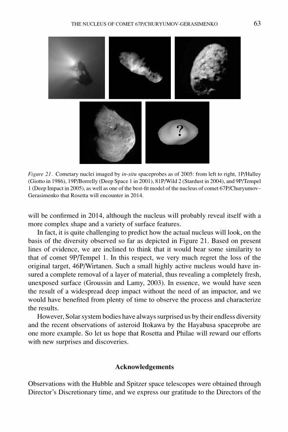
THE NUCLEUS OF COMET 67P/CHURYUMOV-GERASIMENKO 63
Figure 21. Cometary nuclei imaged by in-situ spaceprobes as of 2005: from left to right, 1P/Halley(Giotto in 1986), 19P/Borrelly (Deep Space 1 in 2001), 81P/Wild 2 (Stardust in 2004), and 9P/Tempel1 (Deep Impact in 2005), as well as one of the best-fit model of the nucleus of comet 67P/Churyumov–Gerasimenko that Rosetta will encounter in 2014.
will be confirmed in 2014, although the nucleus will probably reveal itself with amore complex shape and a variety of surface features.
In fact, it is quite challenging to predict how the actual nucleus will look, on thebasis of the diversity observed so far as depicted in Figure 21. Based on presentlines of evidence, we are inclined to think that it would bear some similarity tothat of comet 9P/Tempel 1. In this respect, we very much regret the loss of theoriginal target, 46P/Wirtanen. Such a small highly active nucleus would have in-sured a complete removal of a layer of material, thus revealing a completely fresh,unexposed surface (Groussin and Lamy, 2003). In essence, we would have seenthe result of a widespread deep impact without the need of an impactor, and wewould have benefited from plenty of time to observe the process and characterizethe results.
However, Solar system bodies have always surprised us by their endless diversityand the recent observations of asteroid Itokawa by the Hayabusa spaceprobe areone more example. So let us hope that Rosetta and Philae will reward our effortswith new surprises and discoveries.
Acknowledgements
Observations with the Hubble and Spitzer space telescopes were obtained throughDirector’s Discretionary time, and we express our gratitude to the Directors of the
64 P. L. LAMY ET AL.
respective institutes. On-going studies of comet 67P/Churyumov-Gerasimenko atLaboratoire d’Astrophysique de Marseille are financially supported by CNES (Cen-tre National d’Etudes Spatiales) in the framework of the Rosetta/OSIRIS project.The work by S. C. Lowry was performed in part at Queen’s University, Belfast. Weacknowledge JPL’s Horizons online ephemeris generator for providing the comet’sfuture observability.
References
Agarwal, J., Muller, M., and Grun, E.: Space Sci. Rev., this issue, doi: 10.1007/s11214-006-9139-1.A’Hearn, M. F., Schleicher, D. G., Millis, R. L., Feldman, P. D., and Thompson, D. T.: 1984, Astron.
J. 89, 579.A’Hearn, M. F., Belton, M. J. S., Delamere, W. A., and 30 colleagues: 2005, Science 310, 258.Asphaug, E., and Benz, W.: 1996, Icarus 121, 225.Belskaya, I. N., and Shevchenko, V. G.: 2000, Icarus 147, 94.Belton, M. J. S., Meech, K. J., A’Hearn, M. F., Groussin, O., McFadden, L., Lisse, C., et al.: 2005,
Space Sci. Rev. 117, 137.Belyaev, N. A, Kresak, L., and Pittich, E. M.: 1986, Catalogue of Short-Period Comets, Slovak
Academy of Sciences, Astronomical Institute, Bratislava.Bowell, E., Hapke, B., Domingue, D., Lumme, K., Peltoniemi, H., and Harris, A. W.: 1989, in R. P.
Binzel, T. Gehrels, and M. S. Matthews (eds.), Asteroids, university of arizona press, Tucson, p.524.
Carusi, A., Perozzi, E., Valsecchi, G. B., and Kresak, L.: 1985, Long-Term Evolution of Short-PeriodComets, Adam Hilger, Bristol.
Chesley, S.R.: 2004, Bull. Amer. Astron. Soc. 36, 1118.Churyumov, K. I.: 2002, Highlights of Astron. 12, 365.Churyumov, K. I.: 2003, Comet 67P/Churyumov–Gerasimenko to be targeted. In The Magellanic
Times, IAU Daily Newspaper, XXVth IAU General Assembly, 13–26 July 2003, Sydney, Australia,Day Eight, p. 4.
Clark, B. E., Veverka, J., Helfenstein, P. Thomas, P. C., Bell, J. F., Harch, A.: 1999, Icarus 140, 53.Cochran, A. L., Barker, E. S., Ramseyer, T. F., and Storrs, A. D.: 1992, Icarus 98, 151.Cowan, J. J., and A’Hearn, M. F.: 1979, Moon Planets 21, 155.Crovisier, J., Colom, P., Gerard, E, Bockelee–Morvan, D., and Bourgois, G.: 2002, Astron. Astrophys.
393, 1053.Davidsson, B. J. R., and Gutierrez, P. J.: 2004, Icarus 168, 392.Davidsson, B. J. R., and Gutierrez, P. J.: 2005, Icarus 176, 453.Davidsson, B. J. R., and Gutierrez, P. J.: 2006, Icarus 180, 224.Farnham, T. L., and Cochran, A. L.: 2002, Icarus 160, 398.Fernandez, Y. R., Lisse, C. M., Kaufl, U. H., Peschke, S. B., Weaver, H. A., A’Hearn, M. F., et al.:
2000, Icarus 147, 145.Fernandez, Y. R., Jewitt, D. C., and Sheppard, S. S.: 2001, Astrophys. J. 553, L197.Fernandez, Y. R., Lowry, S. C., Weissman, P. R., Mueller, B. E. A., Samarasinha, N. H., Belton, M.
J. S., et al.: 2005, Icarus 175, 194.Fulle, M., Barbieri, C., Cremonese, G., Rauer, H. Weiler, M., Milani, G., and Luhustri, R.: 2004,
Astron. Astrophys. 422, 357.Groussin, O., and Lamy, P. L.: 2003, Astron. Astrophys. 412, 879.Groussin, O., Lamy, P., Jorda, L., and Toth, I.: 2004, Astron. Astrophys. 419, 375.
THE NUCLEUS OF COMET 67P/CHURYUMOV-GERASIMENKO 65
Groussin, O., A’Hearn, M. F., Li, J.-Y., Thomas, P. C., Sunshine, J. M., Lisse, C. M., et al.: 2006,LPSC 37, Abstr. No. 1297.
Gutierrez, P. J., de Leon, J., Jorda, L., Licandro, J., Lara, L. M., and Lamy, P.: 2003a, Astron. Astrophys.407, L37.
Gutierrez, P. J., Jorda, L., Ortiz, J. L., and Rodrigo, R.: 2003b, Astron. Astrophys. 406, 1123.Gutierrez, P. J., Jorda, L., Samarasinha, N. H., and Lamy, P.: 2005, Planet. Space Sci. 53, 1135.Hage, J. I., and Greenberg, J. M.: 1990, Astrophys. J. 361, 260.Hanner, M. S., Tedesco, E., Tokunaga, A. T., Veeder, G. J., Lester, D. F., Witteborn, F. C., et al.: 1985,
Icarus 64, 11.Horner, J., Evans, N. W., Bailey, M. E., and Asher, D. J.: 2003, Mon. Not. R. Astr. Soc. 343, 1057.Jewitt, D.: 1991, in R.L. Newburn, Jr., M. Neugebauer, J. Rahe (eds.), Comets in the Post-Halley Era,
Vol. 1, p. 19.Jewitt, D. C., and Sheppard, S. S.: 2004, Astron. J. 127, 1784.Jorda, L., and Gutierrez, P. J.: 2002, Earth Moon and Planets 89, 135.Kaasalainen, M., Torppe, J., and Muinonen, K.: 2001, Icarus 153, 37.Kaasalainen, M., Pravec, P., Krugly, Yu., and 19 colleagues: 2004, Icarus 167, 178.Kaasalainen, M., and Lamberg, L.: 2006, Inverse Probl. 22, 749.Kaasalainen, M., and Durech, J.: 2007, in A. Milani, G. Valsecchi and D. Vokrouhlicky (eds.), Near
Earth Objects, Our Celestial Neighbors: Opportunity and Risk. Proceedings IAU SymposiumNo. 236, in press.
Kamoun, P., Campbell, D., Pettengill, G., and Shapiro, I.: 1999, Planet. Space Sci. 47, 23.Kelley, M. S., Reach, W. T., and Lien, D. J.: 2006, Icarus, submitted.Kidger, M. R.: 2003, Astron. Astrophys. 408, 767.Krolikowska, M.: 2003, Acta Astronomica 53, 195.Lamy, P. L., Toth, I., and Weaver, H. A.: 1998, Astron. Astrophys. 337, 945.Lamy, P. L., Toth, I., A’Hearn, M. F., Weaver, H. A., and Weissman, P. R.: 2001, Icarus 154, 337.Lamy, P. L., Toth, I., Jorda, L., Groussin, O., A’Hearn, M. F., and Weaver, H. A.: 2002, Icarus 156,
442.Lamy, P., Bisecker, D. A., and Groussin, O.: 2003, Icarus 163, 142.Lamy P., Toth, I., Weaver, H., Jorda, L., and Kaasalainen, M.: 2003, Bull. Amer. Astr. Soc. 35, 970.Lamy, P. L., Jorda, L., Toth, I., Weaver, H. A., Cruikshank, D., and Fernandez, Y.: 2004, In 35th
COSPAR Scientific Assembly, 18–25 July 2004, Paris, France, p. 1824.Lamy, P. L., Toth, I., Fernandez, Y. R., and Weaver, H. A.: 2004, in M. C. Festou, H. U. Keller, and
H. A. Weaver (eds.), Comets II, University of Arizona Press, Tucson, p. 223.Lamy, P. L., Toth, I., Weaver, H. A., Jorda, L., and Kaasalainen, M.: 2006a, Astron. Astrophys. 458,
669.Lamy, P. L., Toth, I., A’Hearn, M. F., Weaver, H. A., and Jorda, L.: 2006b, Icarus., in press.Lamy, P. L., and Toth, I.: 2007, Icarus, submitted.Levison, H. F.: 1996, ASP Conf. Ser. 107, 173.Li, J., A’Hearn, M. F., and McFadden, L. A.: 2004, Icarus 172, 415.Lowry S., Fitzsimmons, A., and Collander-Brown, S.: 2003, Astron. Astrophys. 397, 329.Lowry, S. C., Weissman, P. R., Sykes, M. V., and Reach, W. T.: 2003, LPSC 34, Abstr. 2056.Lowry, S. C., Fitzsimmons, A., Lamy, P., Toth, I., and Jorda, L.: 2006, Personal communication.Makinen, J. T. T.: 2004, in L. Colangeli, E. M. Epifani, and P. Palumbo (eds.), The New Rosetta
Targets, Kluwer Academic Publishers, p. 61.Marsden, B. G., Sekanina, Z., and Yeomans, D. K.: 1973, Astron. J. 78, 211.Marsden, B. G.: 1985, Dynamics of Comets: Their Origin and Evolution, Dordrecht, The Netherlands,
D. Reidel Publishing Co., p. 343.Meech, K. J. Ageorges, N. A’Hearn, M. F., and 206 colleagues: 2005, Science 310, 265.
66 P. L. LAMY ET AL.
Moreno, F., Lara, L. M., Munoz, O., Lopez-Moreno, J. J., and Molina, A.: 2004, Astrophys. J. 613,1263.
Mueller, B. E. A.: 1992, in A. W. Harris and E. Bowell (eds.), Asteroids, Comets Meteors 1991, Lunarand Planetary Institute, Houston, 1991, p. 425.
Mueller, B. E. A., and Ferrin, I.: 1996, Icarus 123, 463.Neishtadt, A. I., Scheeres, D. J., Sidorenko, V. V., and Vasiliev, A. A.: 2002, Icarus 157, 205.Newburn, R. L., and Spinrad, H.: 1985, Astron, J. 90, 2591.Osip, D. J., Schleicher, D. G., and Millis, R. L.: 1992, Icarus 98, 115.Peale, S. J.: 1989, Icarus 82, 36.Peale, S. J., and Lissauer, J. J.: 1989, Icarus 79, 396.Rabinowitz, D. L., Barkume, K., Brown, M. E., and Roe, H.: 2006, Astrophys. J. 639, 1238.Richardson, J. E., and Melosh, H. J.: 2006, LPSC 37, Abstr. 1836.Rickman, H.: 1986, in ESA Workship on the Comet Nucleus Sample Return Mission, 15–17 July 1986,
Canterbury, England, p. 195.Roemer, E.: 1970, Publ. Astr. Soc. Pacific 82, 151.Russell, H. N.: 1916, Astrophys. J. 43, 173.Sagdeev, R. Z., Elyasberg, P. E., and Moroz, V. I.: 1988, Nature 331, 240.Samarasinha, N. H., A’Hearn, M. F., Hoban, S., and Klingesmith, D. A.: 1986, in B. Battrick, E. J.
Rolfe, and R. Reinhard (eds.), 20th ESLAB Symp. on the Exploration of Halley’s Comet, ESA-SP250 Vol. I, p. 487.
Samarasinha, N. H., Mueller, B. E. A., and Belton, M. J. S.: 1996, Planet. Space Sci. 44, 275.Scheeres, D. J., Ostro, S. J., Hudson, R. S., Dejong, E. M., and Suzuki, S.: 1998, Icarus 132, 53.Schleicher, D. G.: 2006, Icarus 181, 442.Schulz, R., Stuwe, J. A., and Boehnhardt, H.: 2004, Astron. Astrophys. 422, L19.Sekanina, Z.: 1981, Annu. Rev. Earth Planet. Sci. 9, 113.Singh, P. D., de Almeida, A. A., and Huebner, W. F.: 1992, Astron. J. 104, 848.Skorov, Y. V., and Rickman, H.: 1999, Planet. Space Sci. 47, 935.Sky and Telescope 38, 6, 381.Solem, J. C.: 1995, Astron, Astrophys. 302, 596.Spencer, J. R., Stansberry, J. A., Grundy, W. M., and Noll, K. S.: 2006, Bull. Amer. Astr. Soc. 38,
Abstr. [34.01].Stansberry, J. A., Grundy, W. M., Margot, J. L., Cruikshank, D. P., Emery, J. P., Rieke, G. H., et al.:
2006, Astrophys. J. 643, 556.Storrs, A. D., Cochran, A. L., and Barker, E. S.: 1992, Icarus 98, 163.Sykes, M. V., and Walker, R. G.: 1992, Icarus 95, 180.Weiler, M., Rauer, H., and Helbert, J.: 2004, Astron. Astrophys. 414, 749.Whipple, F.: 1950, Astrophys. J. 111, 375.Whipple, F.: 1951, Astrophys. J. 113, 464.Whipple, F. L., and Sekanina, Z.: 1979, Astron. J. 84, 1894.Yeomans, D. K.: 1985, Dynamics of Comets: Their Origin and Evolution, Dordrecht, The Netherlands,
D. Reidel Publishing Co., p. 415.Yeomans, D. K., and Chodas, P. W.: 1989, Astron. J. 98, 1083.Yeomans, D. K., and Baalke, R. C.: 2006, Near-Earth Comet (NEC) orbital Elements:
http://neo.jpl.nasa.gov/cgi-bin/neoelem?type=NEC.


