Embed Size (px)
Citation preview
A posteriori analysis of penalized and mixed formulations
of Koiter’s shell model
Saloua Aouadi1, Adel Blouza2 and Linda El Alaoui3
Abstract
In the present paper, we are interested in finite element approximations of a Koiter model for linearlyelastic shells with little regularity. To perform conforming method, we present a penalized and amixed formulations of the model allowing to approximate and to enforce weakly mechanical con-straints, respectively. We establish existence and uniqueness of the solution to the both formulations.Moreover, a posteriori analysis is led yielding an upper bound and a lower bound of the error. Finally,numerical results are presented to illustrate the efficiency of the a posteriori estimators. We therefore,propose a mesh adaptivity strategy relying on these indicators.
Resume
Nous presentons des versions penalisee et mixte du modele de Koiter pour des coques lineairementelastiques de surface moyenne peu reguliere. Nous en proposons une approximation par elementsfinis. L’analyse a posteriori du probleme mene a la construction d’indicateurs d’erreurs qui satisfontdes estimations optimales. Nous donnons quelques tests numeriques afin de valider et d’illustrerl’efficacite des estimateurs a postriori sur lesquels est basee notre strategie d’adaptation de maillage.
1 Introduction
Our purpose in this work is to approximate the solution of Koiter’s shell equations in Cartesian coordinatesthat is appropriate for linearly elastic shells which present curvature discontinuities. Our intent is to usefinite elements of class C0 and implement the approximation scheme as simply as possible using thegeneral purpose, free software, finite element package FreeFem++ (http://www.freefem.org).
The formulation of Koiter’s model used here was introduced in Blouza and Le Dret [6]. This for-mulation is based on the idea of using a local basis-free formulation where the unknowns are describedin Cartesian coordinates instead of covariant or contravariant components as is usually done in shelltheory, see for example [4]. This formulation is able to accommodate shells with a W 2,∞-midsurface,thus allowing for curvature discontinuities, as opposed to C3 in the classical formalism. Even though itwas proven to be well-posed and to be the natural limit of the classical formulation when a sequence ofregular midsurfaces converges to a W 2,∞-midsurface in [7].
There are different finite element approximations of two-dimensional shell models. Concerning con-forming methods, we mention the Argyris triangle provides a P5 Hermite interpolation of class C1 withhigh order convergence in O(h4) (h is the meshsize) when the solution is smooth enough. This elementwas used for example in [3] to study the linear Koiter’s model for a C3-shell in the classical covariantformulation. This method was applied to approximate geometrically exact shell models in [11]. TheArgyris element was also used in [14] for the numerical analysis of Koiter’s model for shells with littleregularity in the Cartesian formulation proposed in [6].
Still in the context of shells with little regularity, a non conforming DKT element was used in [13] toapproximate Koiter’s model similar to the one introduced in [6].
1Faculte des Sciences de Tunis, Campus Universitaire 1060 Tunis, Tunisie, email: [email protected] de mathematiques Raphael Salem, Universite de Rouen, 76821 Mont-St-Aignan Cedex, France, email:
[email protected] Paris 13, CNRS, UMR 7539 LAGA 99, avenue Jean-Baptiste Clement F-93 430 Villetaneuse France email:
1

This article is organized as follows. We first briefly recall the geometry of the midsurface and Koiter’sshell formulation given in [6]. This formulation involves the displacement vector, a vector unknown thatbelongs to H1 and such that its directional partial second derivatives are in L2.
Therefore, in section 3, we introduce a version of Koiter’s model where the unknowns are the displace-ment and the rotation of the normal to the midsurface. These unknowns are related by a tangency anda neglected transverse shears meaning conditions. We, then, give a penalized Koiter’s model intendedto approximate the above mentioned constraints. We prove the existence and uniqueness of the solutionof the penalized model and establish its convergence to the solution of the original Koiter’s problemwhen the penalization parameter goes to 0. Furthermore, we discretize the problem by P2–conformingfinite element and comment the numerical analysis aspects, which are rather standard. We also lead aposteriori analysis yielding upper and lower bounds of the error.
In section 4, we present a mixed formulation of Koiter’s model in which the tangency condition andthe neglected transverse shears shell behaviour are enforced by two Lagrange multipliers. We prove thatthe inf-sup condition is satisfied and then that the mixed formulation is well-posed and solves the originalKoiter’s problem. We introduce a P2 × P1 × P1 × P1 conforming finite element discretization for whichwe establish a discrete inf–sup condition. We end this section by a posteriori analysis.
Finally, in section 5 we present numerical results illustrating the efficiency of our methods and weshow how the a posteriori estimators can be used to refine adaptively the mesh to the computed solution.
2 Notation
Greek indices and exponents take their values in the set {1, 2} and Latin indices and exponents taketheir values in the set {1, 2, 3}. Unless otherwise specified, the summation convention for indices andexponents is assumed.
Let (e1, e2, e3) be the canonical orthonormal basis of the Euclidean space R3. We note u·v the innerproduct of R3, |u| =
√u·v the associated Euclidean norm and u ∧ v the vector product of u and v.
Let ω be a domain of R2. We consider a shell whose midsurface is given by S = ϕ(ω) where ϕ ∈W 2,∞(ω; R3) is one-to-one mapping such that the two vectors
aα = ∂αϕ,
are linearly independent at each point x ∈ ω. Let
a3 =a1 ∧ a2
|a1 ∧ a2|,
be the unit normal vector on the midsurface at point ϕ(x). The vectors ai define the local covariantbasis at point ϕ(x). The contravariant basis ai is defined by the relations ai·aj = δji where δji is theKronecker symbol. In particular a3(x) = a3(x). Note that all these vectors are of class W 1,∞. We leta(x) = |a1(x) ∧ a2(x)|2 so that
√a(x) is the area element of the midsurface in the chart ϕ.
The first and second fundamental forms of the surface are given in covariant components by aαβ =aα·aβ , and bαβ = a3·∂βaα. Let u ∈ H1(ω; R3) such that ∂αβu·a3 ∈ L2(ω), be a midsurface displacement,H1-regular mappings from ω into R3, given in covariant and Cartesian components by
u(x) = ui(x)ai(x) = uci (x)ei, where ui = u·ai and uci = u·ei.
Let aαβρσ ∈ L∞(ω) be the elasticity tensor, which we assume to satisfy the usal symmetries and to beuniformly strictly positive. In the case of homogeneous, isotropic material with Lame moduli µ > 0 andλ ≥ 0, we have
aαβρσ = 2µ(aαβaρσ + aασaβσ) +4λµλ+ 2µ
aαβaρσ,
where aαβ = aα·aβ are the contravariant components of the first fundamental form. In this context, thecovariant components of the change of metric tensor read
γαβ(u) =12
(∂αu·aβ + ∂βu·aα), (1)
2

and the covariant components of the change of curvature tensor read
Υαβ(u) = (∂αβu− Γραβ∂ρu)·a3, (2)
see [6]. Note that all these quantities make sense for shells with little regularity, and are easily expressedwith the Cartesian coordinates of the unknowns and geometrical data.
We assume that the boundary ∂ω of the chart domain is divided into two parts: γ0 of strictly positive1-dimensional measure on which the shell is clamped and a complementary part γ1 on which the shell issubjected to applied tractions and moments.
Let us consider the function space, introduced in [6], which is appropriate in the context of shells withlittle regularity
V ={v ∈ H1(ω; R3); ∂αv·a3 ∈ H1(ω), v = ∂αv·a3 = 0 on γ0
}. (3)
This space is endowed with the natural Hilbert norm
‖v‖V =(‖v‖2H1(ω;R3) + ‖(∂αv·a3)aα‖2H1(ω;R3)
) 12 . (4)
Let us now recall the usual formulation of Koiter’s problem. Find u ∈ V such that
a(u; v) = L(v), ∀v ∈ V, (5)
where
a(u; v) =
∫ω
eaαβρσ[γαβ(u)γρσ(v) +
e2
12Υαβ(u)Υρσ(v)
]√a dx (6)
andL(v) =
∫ω
f ·v√a dx+
∫γ1
(M ·ψ(v) +N ·v) ldτ, (7)
where ψ(v) is the infinitesimal rotation vector given by
ψ(v) = εαβ(∂βv·a3)aα +12εαβ(∂αv·aβ)a3,
N = N iai and M = Mαaα ∧ a3 = εβαMαaβ are the applied traction density and the applied moment
density respectively. Here, ε11 = ε11 = ε22 = ε22 = 0, ε12 = −ε21 = 1/√a and ε12 = −ε21 =
√a. Finally,
l =√aαβτατβ is the length element on ∂ω, where (τ1, τ2) is the covariant coordinates of the unit vector
tangent to ∂ω.
Theorem 2.1 Let f ∈ L2(ω; R3) be a given resultant force density, M ∈ L2(γ1; R3) such that M ·a3 = 0almost every where on γ1, N ∈ L2(γ1; R3) and e > 0 the thickness of the shell. Then there exists a uniquesolution to the problem (5).
Proof. See [6]. �
Note that for v, s ∈ V,Υαβ(v) can be rewritten as
Υαβ(v, s) =12
(∂αv·∂βa3 + ∂βv·∂αa3 + ∂αs·aβ + ∂βs·aα), (8)
where s = −∂αv·a3aα. Thus, on introducing the Hilbert space W defined by
W ={
(v, s) ∈ [H1(ω; R3)]2; s+ (∂αv·a3)aα = 0; v = s = 0 on γ0
}, (9)
problem (5) becomes the following: Find U = (u, r) ∈W such that
a(U ;V ) = L(V ), ∀V = (v, s) ∈W, (10)
where
a(U ;V ) =
∫ω
eaαβρσ[γαβ(u)γρσ(v) +
e2
12Υαβ(u, r)Υρσ(v, s)
]√a dx, (11)
3

andL(V ) =
∫ω
f ·v√a dx+
∫γ1
(M ·s+N ·v) ldτ. (12)
Now, the unknowns are the displacement u and the rotation r of the normal to the midsurface a3. Letus note that the expression (8) has been introduced, initially in [13] for considering the DKT approachto Koiter’s model, and used in [1] for describing more general shells, namely when ϕ belongs to W 1,∞
and such that a3 ∈W 1,∞.As the solution (u, r) is in H1, C0-Lagrange P1 elements should be sufficient. However, we immediately
encounter a problem since the functional constraint r = −∂αu·a3aα in ω clearly cannot be implemented
in a conforming way for a general shell. We thus introduce a penalized Koiter problem in which theunknowns are the displacement u and the rotation r, elements of the space H1(ω; R3) without anyfunctional constraint.
Let us introduce the relaxed function space
X ={
(v, s) ∈ [H1(ω; R3)]2; v = s = 0 on γ0
}, (13)
and equip it with the norm
‖(v, s)‖X =(‖v‖2H1(ω;R3) + ‖s‖2H1(ω;R3)
) 12 . (14)
Here and in the sequel we make use of the following notational device: arguments in a bilinear formare separated by a semicolon, whereas members of a couple are separated by a comma. This will helpkeep track of who does what, since our bilinear forms often apply to couples.
3 A penalized version of Koiter’s model
In this section we propose a penalized formulation of (10), we establish its well–posedeness and presentits finite element discretization. We also derive a posteriori error indicators leading to an upper and alower bound of the finite element discretization error.
Let p ∈ R such that 0 < p ≤ 1. The penalized formulation we consider is the following. FindUp = (up, rp) ∈ X such that
a(Up;V ) +1pb(Up;V ) = L(V ), ∀V = (v, s) ∈ X, (15)
whereb(Up;V ) =
∫ω
q(Up)·q(V ) dx, (16)
withq(V ) = s+ ∂αv·a3a
α. (17)
Theorem 3.1 Let f ∈ L2(ω; R3) be a given resultant force density, M ∈ L2(γ1; R3) such that M ·a3 = 0almost every where on γ1, N ∈ L2(γ1; R3) and e > 0 the thickness of the shell. Then there exists a uniquesolution to (15).
Let us first recall the following version of the infinitesimal rigid displacement lemma, which is an essentialtool for the proof of the theorem. We refer to [6] for more details about this lemma.
Lemma 3.2 Let (u, r) ∈ [H1(ω; R3)]2 and assume that ϕ ∈W 2,∞(ω; R3).
i) If γαβ(u) = 0, then there exists ψ ∈ L2(ω; R3) such that ∂αu = ψ ∧ aα.
ii) If r = −∂αu·a3aα and Υαβ(u, r) = 0, then ψ is a constant vector in R3 and there exists c ∈ R3 such
that
4

u(x) = c+ ψ ∧ ϕ(x),
andr(x) = −(εαβψ·aβ(x))aα,
where ε11 = ε22 = 0 and ε12 = −ε21 = |a1 ∧ a2|.
This lemma allows to define the following norm:
|||(v, s)||| ={∑α,β
(‖γαβ(v)‖2L2(ω) + ‖Υαβ(v, s)‖2L2(ω)) + ‖(s+ ∂βv·a3aβ)‖2L2(ω,R3)
} 12. (18)
Now we are in position to prove the ellipticity of the penalized bilinear form.
Lemma 3.3 The bilinear form a+ 1pb in (15) is X-elliptic, uniformly with respect to p.
Proof. The proof follows lines similar to those given in [6]. We nonetheless include it for the reader’sconvenience. As p ≤ 1 and due to the positive definiteness of the elasticity tensor, there exists a constantC > 0 such that for all V = (v, s) ∈ X
a(V ;V ) +1pb(V ;V ) ≥ C|||V |||2. (19)
Thus it suffices to prove that |||·||| is a norm equivalent to the norm ‖·‖X. We use the standard contradictionargument. Let us assume that there exists a sequence (vn, sn) ∈ X such that ‖(vn, sn)‖X = 1 but|||(vn, sn)||| → 0 when n→ 0. There exists a subsequence, still denoted (vn, sn), and (v, s) ∈ X such that
(vn, sn) ⇀ (v, s), γαβ(vn) ⇀ γαβ(v),Υαβ(vn, sn) ⇀ Υαβ(v, s),sn + ∂αvn·a3a
α ⇀ s+ ∂αv·a3aα,
weakly in their respective spaces. By Rellich’s theorem, we have
(vn, sn) −→ (v, s) strongly in [L2(ω; R3)]2.
Moreover, as |||(vn, sn)||| → 0 it holds that
γαβ(vn)→ 0,Υαβ(vn, sn)→ 0, and sn + ∂αvn·a3aα → 0 strongly in L2(ω). (20)
Therefore, we getγαβ(v) = Υαβ(v, s) = s+ ∂αv·a3a
α = 0.
By the infinitesimal rigid displacement lemma 3.2 and the boundary conditions, we first conclude thatv = ψ = 0. The second part of lemma 3.2 shows that s = 0.
Let us now introduce the two-dimensional vector (wn)α = vn·aα. We have wn → 0 in L2(ω; R2)strongly. Let us define 2eαβ(w) = ∂αwβ + ∂βwα. It is easy to see that
eαβ(wn) = γαβ(vn) +12vn·(∂βaα + ∂αaβ) −→ 0 strongly in L2(ω).
Then, by (20) and the two-dimensional Korn inequality, we deduce that
wn −→ 0 strongly in H1(ω; R2).
Next we note that∂ρvn·aα = ∂ρ((wn)α)− vn·∂ρaα −→ 0 strongly in L2(ω).
Moreover, as sn → 0 strongly in L2(ω; R3) we already know by (20) that
∂ρvn·a3 −→ 0 strongly in L2(ω).
5

We deduce by (3) and (3) that
∂ρvn = (∂ρvn·ak)ak −→ 0 strongly in L2(ω; R3).
Hence, it follows that vn → 0 strongly in H1(ω; R3).Next, let (w′n)α = sn·aα. Clearly, w′n → 0 strongly in L2(ω,R2). On the other hand, since
2eαβ(w′n) = 2Υαβ(vn, sn)− (∂αvn·∂βa3 + ∂βvn·∂αa3) + sn·(∂αaβ + ∂βaα),
we see by (20) thateαβ(w′n) −→ 0 strongly in L2(ω).
Thus, again by the two-dimensional Korn inequality, we conclude that
w′n −→ 0 strongly in H1(ω; R2).
Moreover, the Poincare inequality and (20) imply that
sn·a3 −→ 0 strongly in H1(ω).
Consequently, since sn = (sn·ai)ai, it follows that sn → 0 strongly in H1(ω; R3).Combining now the convergence of vn and sn, we see that ‖(vn, sn)‖X → 0, which contradicts the
hypothesis and proves the lemma. �
Proof. (of Theorem 3.1) The proof follows from the Lax-Milgram Lemma. �
It is now fairly classical that the penalization provides an approximation of the constrained problem.In addition, due to the specific structure of the problem, we have explicit error estimates.
Theorem 3.4 Let U = (u, r) and Up = (up, rp) be the unique solutions of problems (5) and (15) respec-tively. Then, there exists a constant C > 0 such that
‖rp + ∂αup·a3aα‖L2(ω;R3) ≤ C
√p, (21)
and‖Up − U‖X −→ 0 when p→ 0. (22)
Proof. Since p ≤ 1, we have
C|||Up|||2 ≤ a(Up;Up) +1pb(Up;Up) = L(Up),
showing that Up is bounded in X uniformly with respect to p. Then,
‖rp + ∂αup·a3aα‖2L2(ω) = b(Up;Up) = p
(L(Up)− a(Up;Up)
),
and by applying the Cauchy-Schwarz inequality we deduce estimate (21).We notice that since U belongs to the kernel of b, we have b(Up;Up) = b(Up−U ;Up) = b(Up−U ;Up−U).
Let us denote by Up = (up, rp) a subsequence that converges to (w, z) weakly in X. Thanks to (21) wehave z = ∂αw·a3a
α. Thus, passing to the limit in (15), we deduce that (w, z) = (u, r) by the uniquenessof the solution of problem (5). Hence, the whole sequence converges weakly in X.Now, using the uniform ellipticity established in Lemma 3.3, we get
C‖Up − U‖2X ≤ a(Up − U ;Up − U) +1pb(Up;Up)
= a(Up;Up − U)− a(U ;Up − U) +1pb(Up;Up)
= L(Up − U)− 1pb(Up;Up − U)− a(U ;Up − U) +
1pb(Up;Up)
= L(Up − U)− a(U ;Up − U) −→ 0 when p→ 0,
by the weak convergence established above. �
6

3.1 A finite element formulation
Let us first introduce some notation. Let (Th)h be a shape-regular family of triangulations of ω. For atriangle K ∈ Th, let hK be its diameter and set h = maxK∈Th hK . We denote by Sh the set of verticesin Th. For any subdomain ∆ of ω and for k ≥ 0 we define by Pk(∆) the space of polynomials on ∆ withdegree ≤ k. In what follows, C denotes a constant independent of h and p.The discrete space of admissible displacements and rotations is given by
Xh = {(v, s) ∈ [C0(ω; R3)]2, (v, s)|K ∈ [P2(K,R3)]2, v = s = 0 on γ0} ⊂ X. (23)
Thus the discrete problem reads: Find Up,h = (up,h, rp,h) ∈ Xh such that
a(Up,h;Vh) +1pb(Up,h;Vh) = L(Vh), ∀Vh = (vh, sh) ∈ Xh. (24)
Theorem 3.5 Let f ∈ L2(ω; R3) be a given resultant force density, M ∈ L2(γ1; R3) such that M ·a3 = 0almost every where on γ1, N ∈ L2(γ1; R3) and e > 0 the thickness of the shell. There exists h0 > 0such that for all h ≤ h0 and for any data (f,N,M) there exists a unique solution to (24). Moreover, thissolution satisfies
‖Up,h‖X ≤ Cp ‖L‖, (Cp depends on p).
There exists a sequence hp → 0 such that
‖(u, r)− (up,hp , rp,hp)‖X −→ 0 when p→ 0. (25)
Assume that the solution Up belongs to [H2(ω,R3)]2 for all 0 < p ≤ 1, then there exists a constant Cpsuch that
‖Up,h − Up‖X ≤ Cph‖Up‖[H2(ω,R3)]2 . (26)
Proof. For each p, we have up,h → up when h → 0 by virtue of the classical properties of Galerkinmethod and by a converging diagonal sequence we get (25).
Remark 3.1 i) Since we are mostly interested in shells with little regularity, otherwise classical for-mulations would apply, it is presumably not useful to look for higher order elements in the hope ofimproving the rate of convergence. Indeed, even without taking into account the penalization term,in the case of such a shell, the underlying system of PDEs has nonsmooth coefficients. It is thereforeunclear whether elliptic regularity can be applied to yield an H2 regularity. Note however that, ifthe midsurface chart is smooth and we want to use our formulation nonetheless for simplicity ascompared to the classical approach, then elliptic regularity will apply.
ii) Let us finally mention that numerical results underline a lack of stability of P2 × P1 finite elementdiscretization. Note that in this work we do not concern ourselves with locking. We refer to [2] fora locking-free mixed formulation of Naghdi’s model, valid for a class of shell midsurfaces.
3.2 A posteriori error estimates
We first introduce additional notation an recall some well-known results.
Notation and preliminaries results
Let E1h denote the set of edges of elements of Th that are contained in γ1. For an element K of Th, let EK
be the set of edges belonging to K which are not contained in γ0 and E1K be the set of elements of EK
which are contained in γ1 and let ωK the set of elements of Th sharing an edge with K. For an edge ein EK , let he be its length. For an edge e we choose a unit normal vector νe = (ν1, ν2), with the furtherassumption that, when e belongs to E1
K , ν is outward to ω. For a piecewise continuous function ψ on Th,[ψ]e denotes the jump of ψ across e. For a boundary edge, e, we identify [ψ]e with ψ. The arbitrarinessin the sign of [ψ]e is irrelevant in the analysis below. We recall from [16] the existence of a Clement type
7
operator Ch, mapping from H1(ω) into H1(ω). Let us introduce the stress resultant and the stress couplegiven by their contravariant components, respectively by
nαβ(u) = εaαβρσγαβ(u), mαβ(U) =ε3
12aαβρσΥαβ(u, r). (27)
Thus, the bilinear form in (15) can be rewritten as
a(U, V ) +1pb(U, V ) =
∫ω
[nρσ(u)γρσ(v) +mρσ(u, r)Υρσ(v, s)]√a dx+
1p
∫ω
q(U)·q(V ) dx. (28)
We also observe that
Υρσ(v, s) = θρσ(v) + γρσ(s), with θρσ(v) =12
(∂ρv·∂σa3 + ∂σv·∂ρa3). (29)
Thanks to the symmetry properties of tensors defined in (27), we check that the problem (16) is equivalentto the following system of partial differential equations
−∂ρ(nρσ(up)aσ
√a+mρσ(Up)∂σa3
√a+ 1
pq(Up)·aρa3
)= f√a in ω,
−∂ρ(mρσ(U)aσ
√a)
+ 1pq(Up) = 0 in ω,
up = rp = 0 on γ0,
νρ
(nρσ(up)aσ
√a+mρσ(Up)∂σa3
√a+ 1
pq(Up)·aρa3)
)= Nl on γ1,
νρ
(mρσ(Up)∂σa3
√a)
= Ml on γ1.
From now, we denote fh, Mh and Nh the L2–projection onto the space of piecewise constant functionsof the data f,M and N respectively. Similarly, we introduce approximation of the coefficients namelyaαβh , aαβρσh , (
√a)h and `h the L2–projection onto the space of piecewise Pk functions of aαβ , aαβρσ,
√a
and l respectively. Similarly, we consider approximations ahk and akh of the vectors ak and ak and dhα of∂αa3 in the space Pk. We also denote by γhαβ(·) and Υh
αβ(·) the coefficients of the tensors introduced in(1)–(8) where all coefficients are replaced by their approximations. For instance, γhαβ(·) is given by
γhαβ(u) =12
(∂αu·ahβ + ∂βu·ahα).
This leads to the definition of an approximate linear form
Lh(V ) =∫ω
fh·v (√a)h dx+
∫γ1
(Nh·v +Mh·s) lh dτ,
and of approximate bilinear forms
ah(U, V ) =∫ω
eaαβρσh
[γhαβ(u)γhρσ(v) +
e2
12Υhαβ(U)Υh
ρσ(V )](√a)h dx,
bh(U, V ) =∫ω
qh(U)·qh(V ) dx, with qh(V ) = s+ ∂αv·ah3ahα.
Those approximations lead to define the local approximation error indicator on the data. For all K inTh,
ε(d)K =hK ‖f − fh‖L2(K,R3) +
∑e∈E1K
h12e (‖N −Nh‖L2(e,R3) + ‖M −Mh‖L2(e,R3)), (30)
and the global approximation error indicator on the coefficients
ε(c)h =‖
√a− (
√a)h‖L∞(ω) + h
12 ‖l − lh‖L∞(γ1) + sup
1≤α,β,ρ,σ≤2‖aαβρσ − aαβρσh ‖L∞(ω)
+ sup1≤k≤3
‖ak − ahk‖L∞(ω,R3) + sup1≤α≤2
‖∂αa3 − dhα‖L∞(ω,R3).
8

We now introduce the error indicators.For all K in Th, the error indicators η(1)
p,K and η(2)p,K are defined by
η(1)p,K = hK ‖fh(
√a)h + ∂ρQ
ρh(Up,h
)‖L2(K,R3) +
∑e∈EK\E1K
h12e ‖[νρQ
ρh(Up,h)
]e‖L2(e,R3)
+∑e∈E1K
h12e ‖Nh lh −Qρh(Up,h)‖L2(e,R3),
η(2)p,K = hK ‖∂ρ
(mρσh (Up,h)ahσ(
√a)h)
+1pqh(Up,h)‖L2(K,R3) +
∑e∈EK\E1K
h12e ‖[νρm
ρσh (Up,h)ahσ(
√a)h
]e‖L2(e,R3)
+∑e∈E1K
h12e ‖Mh lh − νρmρσ
h (Up,h)ahσ(√a)h‖L2(e,R3),
whereQρh(Up,h) =
((nρσh (up,h)ahσ +mρσ
h (Up,h)dhσ)(√a)h +
1pqh(Up,h)·aρha
h3
).
Theorem 3.6 (Global upper bound) Let f ∈ L2(ω; R3) be a given resultant force density, M ∈L2(γ1; R3) such that M ·a3 = 0 almost every where on γ1, N ∈ L2(γ1; R3) and e > 0 the thicknessof the shell. Then, the following a posteriori error estimate holds between the solution Up of problem (15)and the solution Up,h of problem (24).
‖U − Up,h‖X ≤ c(( ∑K∈Th
([η(1)p,K ]2 + [η(2)
p,K ]2 + [ε(d)K ]2)) 1
2 + ε(c)h
). (31)
Proof. Since a+ 1pb is X-elliptic, it holds for V = U −Up,h = (v, s) and Vh = (Chv, Chs) = (vh, sh) that
C‖U − Up,h‖2X ≤(L − Lh)(V − Vh)− (a− ah)(Up,h, V − Vh)− 1p
(b− bh)(rp,h, s− sh)
+ Lh(V − Vh)− ah(Up,h, V − Vh)− 1pbh(rp,h, s− sh). (32)
The first three terms in the right hand side of the above inequality can be bounded as in [19], namely
|(L − Lh)(V − Vh)− (a− ah)(Up,h, V − Vh)− 1p
(b− bh)(rp,h, s− sh)|
≤C(( ∑
K∈Th
[ε(d)K ]2) 1
2 + ε(c)h
)‖V ‖X.
Setting V −Vh = (v−vh, 0) with vh = Chv in (24) and integrating by parts the two last terms in the righthand side of the inequality (32), using the Cauchy-Schwarz inequality and the properties of Ch yield that
Lh(V − Vh)− ah(Up,h, V − Vh)− 1pbh(Up,h, V − Vh)
=∑K∈Th
∫K
fh(√a)h(v − vh)− ∂ρ
(nρσh (up,h)ahσ(
√a)h +mρσ
h (Up,h)∂σah3 (√a)h +
1pqh(Up,h)·aρha
h3
)(v − vh)dx
+∑K∈Th
∫∂K
nρσh (up,h)ahσ(√a)h +mρσ
h (Up,h)∂σah3 (√a)h +
1pqh(Up,h)·aρha
h3
)(v − vh)µKdx
≤
( ∑K∈Th
[η(1)p,K ]2
) 12
‖V ‖X.
9

Similarly, on setting V − Vh = (0, s− sh) with sh = Chs it holds that
Lh(V − Vh)− ah(Up,h, V − Vh)− 1pbh(Up,h, V − Vh)
=∑K∈Th
∫K
∂ρ(mρσh (Up,h)ahσ(
√a)h)
+1pqh(Up,h)
)(s− sh)dx+
∑K∈Th
∫∂K
mρσh (Up,h)ahσ(
√a)h(s− sh)dx
≤
( ∑K∈Th
[η(2)p,K ]2
) 12
‖V ‖X.
Combining the above inequalities and (32) leads to the result (31). �
We end this section by the lower bound of the error indicators. We refer to ([15], §1.2) for the proof.
Theorem 3.7 (Local lower bounds) Let f ∈ L2(ω; R3) be a given resultant force density, M ∈L2(γ1; R3) such that M ·a3 = 0 almost every where on γ1, N ∈ L2(γ1; R3) and e > 0 the thicknessof the shell. Then, the following bounds hold.
η(i)p,K ≤ c
(‖U − Up,h‖X(ωK) +
( ∑κ⊂ωK
[ε(d)κ ]2) 1
2 + ε(c)h
), i = 1, 2. (33)
Remark 3.2 If we assume f in L1(ω,R3), then the term ε(c)h can be decomposed on each element leading
to a local lower bound of the error.
4 A mixed formulation
In the previous section we have approximated the constraint r + ∂αu·a3aα = 0 when the penalization
parameter goes to zero. In this section, our purpose is to enforce that constraint by the way of aLagrange multiplier. To this end we introduce the bilinear form
∫ωλ·(s + ∂αv·a3a
α) dx with (v, s) ∈ Xand λ ∈ L2(ω,R3). Unfortunately, this bilinear form does not satisfy an inf-sup condition. Indeed, fora given λ in L2(ω,R3) such that its normal component λ·a3 does not belong to H1(ω), it does not existV = (v, s) ∈ X such that s + (∂αv·a3)aα = λ. We thus split the constraint into a tangency and normalconstraints that are r·a3 = 0 and r·aα + ∂αu·a3 = 0, respectively.The mixed formulation we consider, here, consists in finding (U, λ, λ) = ((u, r), λ, (λ1, λ2)) ∈ X×H1
γ0(ω)×[L2(ω)]2 (where λα = λ·aα) such that
a(U ;V ) + b1(s·a3; λ) + b2(V ;λ) = L(V ), ∀V = (v, s) ∈ X,b1((r·a3); µ) = 0, ∀µ ∈ H1
γ0(ω),
b2(U ;µ) = 0, ∀µ ∈ [L2(ω)]2,
(34)
whereb1(µ; ν) =
∫ω
∂αµ∂αν dx, and b2(V ;λ) =∫ω
λα(s·aα + ∂αv·a3) dx. (35)
We recall that the unknown U = (u, r) denotes the displacement u and the rotational r of the normal tothe midsurface. The unknowns λ and λ denote the Lagrange multipliers that enforce, respectively, theconstraints r·a3 = 0 and r·aα + ∂αu·a3 = 0.
Theorem 4.1 Let f ∈ L2(ω; R3) be a given resultant force density, M ∈ L2(γ1; R3) such that M ·a3 = 0almost every where on γ1, N ∈ L2(γ1; R3) and e > 0 the thickness of the shell. Then, there exists aunique solution to (34). Moreover, U is the solution of Koiter’s problem (5).
Proof. As the bilinear form a is elliptic on X we only need to establish the inf-sup condition of b1 + b2,[10]. This is the object of the lemma below.
10

Lemma 4.2 There exists a constant β > 0 such that
inf(λ,λ)∈H1
γ0(ω)×[L2(ω)]2
supV=(v,s)∈X
b1(s·a3; λ) + b2(V ;λ)‖V ‖X + ‖λ‖H1
γ0(ω) + ‖λ‖[L2(ω)]2
≥ β. (36)
Proof. Let (λ, λ) be in H1γ0(ω) × [L2(ω)]2. There exist v ∈ H1
γ0(ω,R3) such that ∂αv = λαa3 ands ∈ H1
γ0(ω; R3) such that s = λa3. It holds, on setting V = (v, s) that
supV=(v,s)∈X
b1(s·a3; λ) + b2(V ;λ)‖V ‖X
≥ b1(s·a3; λ) + b2(V ;λ)‖V ‖X
=
∫ω|∂αλ|2 dx+
∫ωλα(λa3·aα + λα) dx‖V ‖X
≥ C‖λ‖2H1
γ0(ω) + ‖λ‖2[L2(ω)]2(
‖λ‖2[L2(ω)]2 + ‖λ‖2H1γ0
(ω)
) 12≥ C
(‖λ‖2[L2(ω)]2 + ‖λ‖2H1
γ0(ω)
) 12,
where we have used the fact that a3 is an unit vector, that a3·aα = 0 and the Poincare inequality. Hence,we conclude (see [10]) to the existence and uniqueness of a solution to the mixed formulation (34).
Let us now check that U is the solution to the usual Koiter problem (5). Taking µ = r·a3 andµα = µ·aα = r·aα + ∂αu·a3 in the second and third equations of (34), yields that U ∈ V. Then, takingV ∈ V vanishes all terms involving b1 and b2 in the first equation of (34). Whence the result. �
4.1 A mixed finite element discretization
We introduce the finite element spaces.
Xh = {(vh, sh) ∈ [C0(ω,R3)]2 ;∀K ∈ Th, (vh, sh)|K ∈ P2(K,R3)× P1(K,R3), vh = sh = 0 on γ0},
Mh = {µh ∈ C0(ω) ;∀K ∈ Th, µh|K ∈ P1(K), µh = 0 on γ0},
andYh = {µh = (µαh) ∈ C0(ω)2,∀K ∈ Th, µαh|K ∈ P1(K)}.
Then a mixed finite element discretization of (34) consists in finding (Uh, λh, λh) ∈ Xh ×Mh × Yh suchthat for all (Vh, µh, µh) ∈ Xh ×Mh × Yh, a(Uh;Vh) + b1(sh·a3; λh) + b2(Vh;λh) = L(Vh), ∀Vh = (vh, sh) ∈ Xh,
b1(rh·a3; µh) = 0 ∀µh ∈Mh,b2(Uh;µh) = 0, ∀µh ∈ Yh.
(37)
Theorem 4.3 Let f ∈ L2(ω; R3) be a given resultant force density, M ∈ L2(γ1; R3) such that M ·a3 = 0almost every where on γ1, N ∈ L2(γ1; R3) and e > 0 the thickness of the shell. Then, there exists aunique solution to (37). Moreover, the solution satisfies
‖Uh‖X + ‖λh‖H1γ0
(ω) + ‖λh‖[L2(ω)]2 ≤ c‖L‖, (38)
and‖U − Uh‖X + ‖λ− λh‖H1
γ0(ω) + ‖λ− λh‖[L2(ω)]2 → 0 when h→ 0.
Proof. The existence and uniqueness of a solution to (37) is based on the discrete inf–sup conditiongiven in Lemma 4.6 below. This compatibility condition requires the following geometrical result.
Lemma 4.4 Let ϕ be a W 2,∞ chart. There exists a constant C > 0 such that for all x, y in ω,
|a3(x)·(a3(x)− a3(y))| ≤ C‖x− y‖2. (39)
11

The proof follows the same lines as the one given in [1, Lemma 3.5].We now turn to the discrete inf-sup conditions. Let Πh denote either the vector-valued Lagrange
interpolation operator from C00 (ω; R3) into Xh or the scalar-valued Lagrange interpolation operator from
C00 (ω) into Mh, depending on the context, and ψhj the shape function associated with the vertex sj ∈ Sh.
Lemma 4.5 For all µαh ∈ Yh, we set Rh(µαh) = Πh(µαha3). Then, there exists a constant C > 0 suchthat ∫
ω
(Rh(µαh)·a3)µαh dx ≥ C‖µαh‖2[L2(ω)]2 . (40)
Proof. Note that while µαh is scalar piecewise P1, µαha3 is vector-valued and Rh(µαh) is vector-valuedpiecewise P1. Let us set δh = Rh(µαh)·a3 − µαh then∫
ω
(Rh(µαh)·a3)µαh dx =∑α
‖µαh‖2L2(ω) +∑α
∫ω
(δh·a3)µαh dx
≤∑α
‖µαh‖L2(ω) +∑α
‖µαh‖[L2(w)]2‖δh‖L2(ω).
On recalling that, for x ∈ ω, µαh(x) =∑sj∈Sh µαh(sj)ψhj (x) and using the Lagrange interpolation
operator, we getRh(µαh)·a3(x) =
∑sj∈Sh
µαh(sj)[a3(sj)·a3(x)]ψhj (x),
andδh(x) =
∑sj∈Sh
µαh(sj)[(a3(sj)− a3(x))·a3(x)]ψhj (x).
Since a3(x) is a unit vector it holds that
‖δh‖L∞(ω)≤ 3‖µαh‖L∞(ω) maxj
maxKj
[C
h|(a3(sj)− a3(x))|
],
where Kj stand for all the triangles sharing the vertex sj . Lemma 4.4 yields that
‖δh‖L∞(ω)≤ 3‖µαh‖L∞(ω)C
h|sj − x|2≤ Ch|µαh|L∞(ω),
where C does not depend on h nor on µαh. Finally, we appeal to the classical discrete Sobolev estimate(see [9]) and deduce that
‖δh‖L∞(ω)≤C‖δh‖L∞(ω)≤ Ch‖µαh‖L∞(ω),≤ 12‖µαh‖L2(ω).
We are now in a position to prove the crucial uniform discrete inf-sup condition.
Lemma 4.6 There exists β∗ > 0 independent of h such that
inf(λh,λh)∈Mh×Yh
supVh∈Xh
b1(sh·a3, λh) + b2(Vh;λh)‖Vh‖X + ‖λh‖M + ‖λh‖[L2(ω)]2
≥ β∗. (41)
Proof. Let (λh, λh) ∈Mh × Yh. There exists
vh ∈ {vh ∈ C0(ω; R3), vh|K ∈ P2(K), vh = 0 on γ0},
such that ∂αvh = Rh(λαh) and sh ∈ Yh such that sh = λha3. On setting Vh = (vh, sh), we get
supVh=(vh,sh)∈Xh
b1(sh·a3; λh) + b2(Vh;λh)‖Vh‖X
≥ b1(sh·a3; λh) + b2(Vh;λh)‖Vh‖X
≥ C∫ω|λh|2 dx+
∫ωλα(λha3·aα +Rh(λαh)·a3) dx(
‖λαh‖2[L2(ω)]2 + ‖λh‖2M) 1
2
≥ C(‖λh‖2M + ‖λh‖2[L2(ω)]2
) 12,
where we have used the fact that a3 is a unit vector, a3·aα = 0 and Lemma 4.5. �
12

Remark 4.1 The proofs of the existence-uniqueness and the convergence remain valid if rh, λh and λhare sought in P2 as well.
4.2 A posteriori error estimates
In this section we derive residual a posteriori error estimators yielding upper and lower bounds of the error.As in the penalized case we introduce bilinear forms b1h and b2h approximating b1 and b2 respectively.
Let us introduce the discretization error indicators
η(1)K = hK ‖fh(
√a)h + ∂ρQ
ρ(Uh)‖L2(K;R3) +∑
e∈EK\E1K
h12e ‖[νρQ
ρ(Uh)]e‖L2(e;R3)
+∑e∈E1K
h12e ‖Nh lh − νρQρ(Uh)‖L2(e;R3),
η(2)K = hK ‖∂ρ
(mρσh (Uh)ahσ(
√a)h)− λρaρ + ∂ρ(∂ρλhah3 )− ∂ρλhdhρ‖L2(K;R3)
+∑
e∈EK\E1K
h12e ‖[νρ(mρσh (Uh)ahσ(
√a)h + ∂ρλha
h3
)]e‖L2(e;R3)
+∑e∈E1K
h12e ‖Mh lh − νρ(mρσ
h (Uh)ahσ(√a)h − ∂ρλhah3 )‖L2(e;R3),
η(3)K = hK ‖∂ρ
(∂ρrh·ah3 + rh·dhρ)‖L2(K;R3)
+∑
e∈EK\E1K
h12e ‖[(∂ν(rh·ah3 )
]e‖L2(e;R3)
+∑e∈E1K
h12e ‖∂ν(rh·ah3 )‖L2(e;R3),
η(4)K = hK
∑ρ
‖rh·ahρ + ∂ρuh·ah3‖L2(K;R3).
withQρ(Uh) =
(nρσh (uh)ahσ +mρσ
h (Uh)dhσ)
(√a)h + λhρa
h3 .
Theorem 4.7 (Global upper bound) Let f ∈ L2(ω; R3) be a given resultant force density, M ∈L2(γ1; R3) such that M ·a3 = 0 almost every where on γ1, N ∈ L2(γ1; R3) and e > 0 the thickness of theshell. Then, the following a posteriori error estimate holds between the solution (U, λ, λ) of problem (34)and the solution (Uh, λh, λh) of problem (37).
‖U−Uh‖X+‖λ−λh‖H1γ0
(ω)+‖λ−λh‖[L2(ω)]2 ≤ C(( ∑K∈Th
([η(1)K ]2+[η(2)
K ]2+[η(3)K ]2+[η(4)
K ]2+[ε(d)K ]2)) 1
2 +ε(c)h).
(42)
Proof. The coercivity of a and the inf-sup condition (36) yield that,
‖U − Uh‖X + ‖λ− λh‖H1γ0
(ω) + ‖λ− λh‖[L2(ω)]2
≤ supV,‖V ‖X=1
{a(U − Uh;V ) + b1(V ; λ− λh) + b2(V ;λ− λh)}. (43)
Moreover, we have the residual equations
a(U − Uh;V ) + b1(V ; λ− λh) + b2(V ;λ− λh)
= (L − Lh)(V − Vh)− (a− ah)(Uh;V − Vh)− (b1 − b1h)(V − Vh; λh)− (b2 − b2h)(V − Vh;λh)
+ Lh(V − Vh) + ah(Uh;V − Vh) + b1h(V − Vh; λh) + b2h(V − Vh;λh) ∀V ∈ X,∀Vh ∈ Xh,b1((r − rh)·a3, µ) = (b1 − bh)(rh·a3, µ− µh) + bh(rh·a3, µ− µh), ∀µ ∈ H1
γ0(ω) ,∀µh ∈Mh,
b2(U − Uh, µ) = (b2 − b2h)(Uh, µ− µh) + b2h(Uh, µ− µh), ∀µ ∈ [L2(ω)]2 ,∀µh ∈ Yh.
13

Owing to (38), the usual techniques on the approximation of the coefficients lead to
|(L − Lh)(V − Vh) + (a− ah)(Uh;V − Vh) + (b1 − b1h)(V − Vh; λh) + (b2 − b2h)(V − Vh;λh)|
≤ C
(∑K
[ηdK ]2) 1
2
+ ε(c)h .
On choosing V = (v, 0) with v ∈ H1γ0(ω), on setting w = v − Chv, integrating by parts elementwise and
using classical techniques of residual estimates it holds that
ah(U − Uh;V ) + b1h(V ; λ− λh) + b2h(V ;λ− λh) =∫ω
fh·w (√a)h dx+
∫γ1
Nh·w lh dτ
+∑K∈Th
(∫K
∂ρ((nρσh (uh)ahσ +mρσ
h (Uh)dhσ)(√a)h + λhρa
h3
)·w dx
−∫∂K
νρ((nρσh (uh)ahσ +mρσ
h (Uh)dhσ)(√a)h + λhρa
h3 )·w dτ
).
The Cauchy-Schwarz inequality and the interpolation properties of the Clement operator [16], yield
ah(U − Uh;V ) + b1h(V ; λ− λh) + b2h(V ;λ− λh) ≤ C
( ∑K∈Th
[η(1)K ]2
) 12
‖v‖H1(ω).
In the same way on choosing V = (0, s) with s ∈ H1(ω; R3), we get
ah(U − Uh;V ) + b1h(V ; λ− λh) + b2h(V ;λ− λh) ≤ C
( ∑K∈Th
[η(2)K ]2
) 12
‖s‖H1(ω;R3).
Furthermore, we can easily prove for µ ∈ H1γ0(ω) and µh ∈Mh that
b1h((r − rh)·a3, µ− µh) ≤ C
( ∑K∈Th
[η(3)K ]2
) 12
‖µ‖H1(ω),
and for µ ∈ [L2(ω)]2 and µh ∈ Yh
b2h(U − Uh, µ− µh) ≤ C
( ∑K∈Th
[η(4)K ]2
) 12
‖µ‖[L2(ω)]2 .
Then, combining (43) and the above inequalities leads to the global upper bound (42).
Theorem 4.8 (Local lower bound) Let f ∈ L2(ω; R3) be a given resultant force density, M ∈L2(γ1; R3) such that M ·a3 = 0 almost every where on γ1, N ∈ L2(γ1; R3) and e > 0 the thicknessof the shell. Then, the following local bounds hold for all indicators η(i)
K , i = 1, · · · , 4.
η(i)K ≤ c
(‖U−Uh‖X(ωK) +‖λ− λh‖H1(ωK) +‖λ−λh‖L2(ωK) +
( ∑κ⊂ωK
[ε(d)κ ]2) 1
2 +ε(c)h
), i = 1, · · · , 4. (44)
Remark 4.2 1) The error indicators are in agreement with the strong formulation of Koiter’s problem
−∂ρ(nρσ(u)aσ
√a+mρσ(U)∂σa3
√a+ λρa3
)= f√a in ω,
−∂ρ(mρσ(U)aσ
√a)
+ λαaα − ∂ρρλa3 + ∂ρλ∂ρa3 = 0 in ω,
r·a3 = 0 in ω,r·aρ + ∂ρu·a3 = 0 in ω,
u = r = 0 on γ0,
λ = 0 on γ0,
νρ
(nρσ(u)aσ
√a+mρσ(U)∂σa3
√a+ λρa3
)= Nl on γ1,
νρ
(mρσ(U)∂σa3
√a+ λρa3
)= Ml on γ1.
14
2) The Lagrange multiplier λ has a force mechanical meaning that prevents pinching. Indeed, it cor-responds to a change in length of the deformed normal fiber in the three-dimensional Kirchhoff–Lovedisplacement constructed from u and r. The unknown λ is the Lagrange multiplier that enforces theconstraint r·aα + ∂αv·a3 = 0 has a force mechanical meaning that prevents transverse shears throughthe shell thickness. Note that when nonzero, r·aα + ∂αv·a3 it corresponds to a change in direction of thedeformed normal fiber in the three-dimensional shell.
5 Numerics
In this section, we implement the discretization of both penalized and mixed approaches, compare themon a literature benchmark, and apply them to genuinely W 2,∞ shells.
5.1 Implementation details
Both model formulations only require the knowledge of aα, a3, and ∂αa3. All other quantities, eithergeometrical like the elasticity tensor or kinematical like the strain tensors, can be expressed by meansof dot products involving these quantities. Our code automatically constructs the bilinear forms, withminimal user input. This works well if an analytic description of the midsurface is available.
Three-dimensional visualization of the undeformed and deformed shells uses Medit,4 a free meshvisualization software available at http://www.ann.jussieu.fr/˜frey /logiciels/medit.html.In respect of remark 4.1 the solution of the mixed method is computed in the P 2 finite elements space.All the tests were run on 2.2 GHz Apple PowerBook G4 laptops and 2GHz single-processor Apple XserveG5.
5.2 The hyperbolic paraboloid shell
This test is a literature benchmark for shell elements. We use this example, in which the midsurface ofthe shell is represented by a chart of class C∞, mainly to validate our code. It does not constitute arelevant test for the W 2,∞ case.
The reference domain of the midsurface is given by
ω ={
(x, y) ∈ R2, |x|+ |y| <√
2b},
and the chart is defined by
ϕ(x, y) =(x, y,
c
2b2(x2 − y2)
)T,
where b = 50 cm and c = 10 cm.The shell is clamped on ∂ω and subjected to a uniform pressure q = 0.01 kp/cm2. The mechanical
data areE = 2.85 104 kp/cm2, ν = 0.4,
and the thickness of the shell is e = 0.8 cm.The reference value for this test is the normal displacement at the center A of the shell. Its value
computed by various methods is of −0.024 cm; see [3].Due to the symmetries of the problem, we use the computational domain
ω′ ={
(x, y) ∈ R2, 0 < x, 0 < y, x+ y <√
2b},
and enforce the symmetry conditions
u2 = 0, r2 = 0 on y = 0, and u1 = 0, r1 = 0 on x = 0.
These conditions are obtained by expressing the continuity of the three-dimensional Kirchhoff-Love dis-placement U = u(x)+x3r(x) along these edges. The isovalues of the three components of the displacement
15

Figure 1: Isovalues of the cartesian displacement components: u1 (left), u2 (middle) and u3 (right).
are given in Figure 1. In tables 1 and 2 the value of normal displacement at A, the range of values ofthe constraints and the tangency of the rotation vector are reported for the penalized and mixed formu-lation respectively. Those values are given in respect of the number of degree of freedom. Note that thecomputations are performed on the same three meshes for both method. The penalization parameter in(15) is chosen equal to E
2(1+ν) .
Degrees of freedom 3278 4650 6286
(uph·ah3 )(A) −0.024451 −0.0243683 −0.0243279
Range of values for qh(Uph)·ah1 −1.72998−05 2.02244−05 −7.6038−06 1.30361−05 −7.03193−06 1.23384−05
Range of values for qh(Uph)·ah2 −1.33745−05 2.76814−05 −8.95655−06 1.39093−05 −6.9764−06 1.02938−05
Range of values for rph·ah3 −4.27147−06 3.14767−06 −2.16897−06 2.56384−06 −2.01314−06 1.974−06
Table 1: Penalized formulation: approximation of the displacement and constraints.
Degrees of freedom 4785 7380 10675
(uh·a3)(A) −0.0244202 −0.0243383 −0.024313
Range of values for qh(Uh)·ah1 −1.60475−4 0.000145428 −1.03554−4 1.04717−4 −5.9302−05 7.01685−05
Range of values for qh(Uh)·ah2 −8.9348−05 7.81964−05 −9.23568−05 8.22762−05 −5.39086−05 8.08893−05
Range of values for rh·ah3 −1.24356−05 3.56998−05 −1.0454−05 1.94113−05 −1.16357−05 1.64499−05
Table 2: Mixed formulation: approximation of the displacement and constraints.
It is clear that both methods achieve excellent tangency of the rotation vector as the approximationof r·a3 is close to 0. Similar performance in terms of the constraints are obtained. One can observethat the approximations of q(U)·aα are close to 0 as well. This means that the functional constraintr = −∂αu·a3a
α is numerically satisfied. The numerical results obtained for the reference value are alsovery satisfactory as they are close to −0.024, the value given in the literature.
5.3 A hat W 2,∞-shell
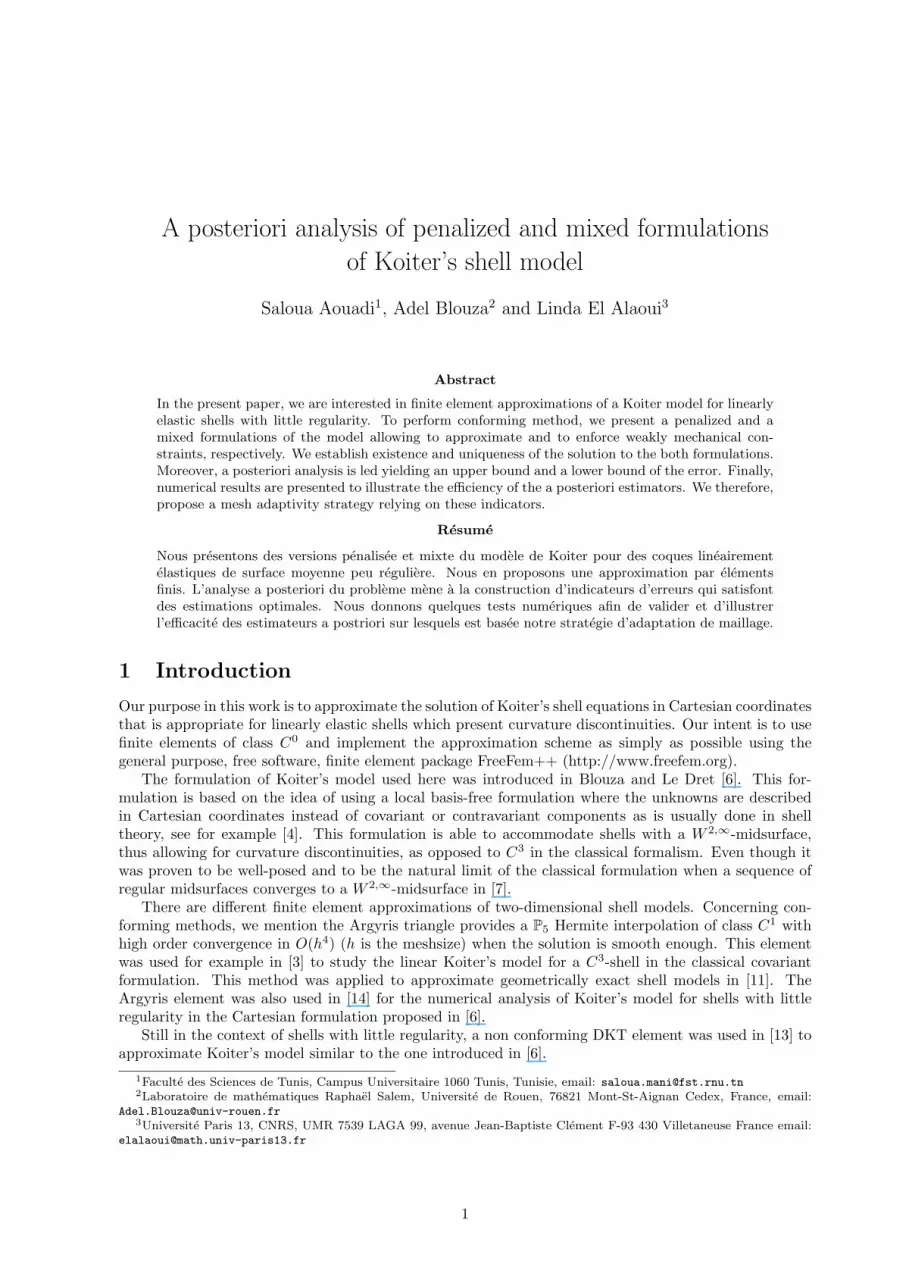
A three circle hat made is a classical structure with W 2,∞ midsurfce regularity, see Figure 2 where ADEBrepresents a three-centered arch. Clearly these connected arcs present two curvature discontinuities (atpoints D and E) and the same will be true for arches based on it.
We present numerical results for a long, tunnel-like shell based on a slightly extended hat arc.The mechanical data are given by E = 3.0 106 kp/cm2, ν = 0.3 and the thickness of the shell e equals
0.5 cm. Clamping is assumed on both rectilinear sides of the shell.The natural chart for this shell is of class W 2,∞. It is obtained by parametrizing the hat by arclength.
The computational domain is a rectangle ]−17.32, 17.32[×]−30, 30[. (We do not compute the shell on apart of the domain by using the symmetries but on the whole domain for a better visualization.)
4This software was designed and developed at the Laboratoire Jacques-Louis Lions of the University Pierre et MarieCurie.
16
Figure 2: ADEB is a hat or three-centered arch.
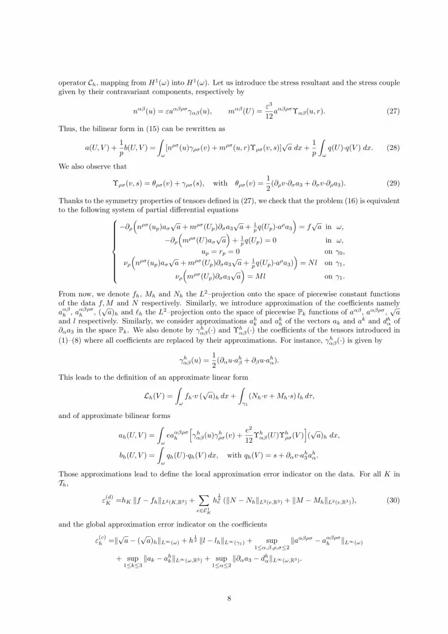
The vertical displacement of the center of the shell is u3(0, 0) = −0.004 cm. In Figure 3 isovalues ofthe cartesian displacement components are plotted for both methods. These are the results in the case ofboundary conditions are enforced on the whole boundary ∂ω. Note that the mesh ignores the curvaturediscontinuity namely we do not refine the mesh around the curvature discontinuities.
Figure 3: Isovalues of the cartesian displacement components: u1 (left), u2 (middle) and u3 (right) whithboundary condition on the circular part. Penalized (top) and mixed (bottom) model.
Figure 4 shows the isovalues of u·a3 calculated with the penalized and the mixed method. We canobserve that u·a3 is sensitive to the curvature discontinuities.
Mesh adaptation
Now we use the error indicators derived in the previous sections, to refine the mesh in respect of thecomputed solution. The adaptation algorithm is the following, see [19].
1. A mesh is generated such that(∑
K∈Th(ηdK)2)1/2 + η
(c)h is smaller than a given tolerance.
2. The usual mesh refinement or coarsening algorithm based on an equidistribution of the discretizationerror indicators is used.
17
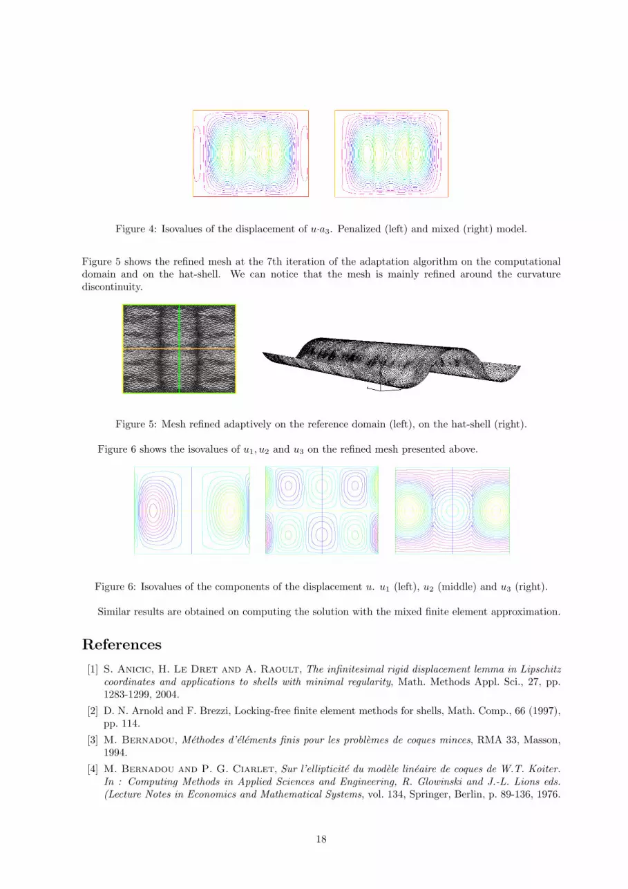
Figure 4: Isovalues of the displacement of u·a3. Penalized (left) and mixed (right) model.
Figure 5 shows the refined mesh at the 7th iteration of the adaptation algorithm on the computationaldomain and on the hat-shell. We can notice that the mesh is mainly refined around the curvaturediscontinuity.
Figure 5: Mesh refined adaptively on the reference domain (left), on the hat-shell (right).
Figure 6 shows the isovalues of u1, u2 and u3 on the refined mesh presented above.IsoValue-0.00203251-0.00181856-0.00160461-0.00139066-0.00117671-0.000962766-0.000748818-0.00053487-0.000320922-0.0001069740.0001069740.0003209220.000534870.0007488180.0009627660.001176710.001390660.001604610.001818560.00203251
u1 IsoValue-0.0015095-0.0013506-0.00119171-0.00103281-0.000873919-0.000715025-0.000556131-0.000397236-0.000238342-7.94472e-057.94472e-050.0002383420.0003972360.0005561310.0007150250.0008739190.001032810.001191710.00135060.0015095
u2IsoValue-0.0104306-0.00989565-0.00936075-0.00882585-0.00829095-0.00775605-0.00722115-0.00668625-0.00615135-0.00561645-0.00508155-0.00454665-0.00401175-0.00347685-0.00294195-0.00240705-0.00187215-0.00133725-0.00080235-0.00026745
dcv
Figure 6: Isovalues of the components of the displacement u. u1 (left), u2 (middle) and u3 (right).
Similar results are obtained on computing the solution with the mixed finite element approximation.
References
[1] S. Anicic, H. Le Dret and A. Raoult, The infinitesimal rigid displacement lemma in Lipschitzcoordinates and applications to shells with minimal regularity, Math. Methods Appl. Sci., 27, pp.1283-1299, 2004.
[2] D. N. Arnold and F. Brezzi, Locking-free finite element methods for shells, Math. Comp., 66 (1997),pp. 114.
[3] M. Bernadou, Methodes d’elements finis pour les problemes de coques minces, RMA 33, Masson,1994.
[4] M. Bernadou and P. G. Ciarlet, Sur l’ellipticite du modele lineaire de coques de W.T. Koiter.In : Computing Methods in Applied Sciences and Engineering, R. Glowinski and J.-L. Lions eds.(Lecture Notes in Economics and Mathematical Systems, vol. 134, Springer, Berlin, p. 89-136, 1976.
18

[5] A. Blouza, F. Hecht and H. Le Dret, Two finite element approximation of Naghdi’s shell modelin cartesian coordinates, SIAM J. Numer. Anal., Vol 44, 2, pp. 636-654, 2006.
[6] A. Blouza and H. Le Dret, Existence and uniqueness for the linear Koiter model for shells withlittle regularity, Quarterly of Applied Mathematics, Vol LVII, N2, p. 317-337, 1999.
[7] A. Blouza and H. Le Dret, An up-to-the boundary version of Friedrichs’s Lemma And applica-tions to the linear Koiter shell model, SIAM J. Math. Anal. Vol. 33, No. 4, pp. 877-895, 2001.
[8] A. Blouza and H. Le Dret, Nagdhi’s shell model: Existence, uniqueness and continuous depen-dence on the midsurface, Journal of Elasticity 64, 199-216, 2001.
[9] J. H. Bramble, J. E. Pasciak, and A. H. Schatz, The construction of preconditioners forelliptic problems by substructuring, I, Math. Comp., 47 (1986), pp. 103–134.
[10] V. Girault P.-A. Raviart, Finite element methods for Navier-Stokes equations, Theory andalgorithms, Springer Series in Computational Mathematics, 5. Springer-Verlag, Berlin, 1986.
[11] M. Carrive, P. Le Tallec and J. Mouro, Approximation par elements finis d’un modele decoque geometriquement exacte, Revue Europeene des elements finis, 4, pp. 633-662, 1995.
[12] P. G. Ciarlet, The Finite Element Method for Elliptic Problems. Series ”Studies in Mathematicsand its Applications”, North-Holland, Amsterdam, 1978.
[13] P. Le Tallec and S. Mani, Analyse numerique d’un modele de coque de Koiter discretise en basecartesienne par elements finis DKT, M2AN, Vol. 32, N 4, p.p. 433-450, 1998.
[14] N. Kerdid and P. Mato Eiroa, Conforming finite element approximation for shells with littleregularity, Comput. Methods Appli. Mech. Engrg., 188, pp. 95-107, 2000.
[15] R. Verfurth, A Review of a Posteriori Error Estimation and Adaptive Mesh-Refinement Tech-niques, Teubner Verlag and J. Wiley, Stuttgart, ISBN 3-519-02605-8, 127 pp. 1996.
[16] P. Clement, Approximation by finite element functions using local regularization, RAIRO, Anal.Numer., 9, pp. 77-84, 1975.
[17] C. Bernardi and A. Blouza, Spectral discretization of a Naghdi model , SIAM J. Numer. Anal.,Vol. 45, 2007, no 6, pp. 2653-2670.
[18] C. Bernardi, C. Canuto and Y. Maday, Generalized inf-sup condition for Chebyshev spectralapproximation of the Stokes problem , SIAM J. Numer. Anal. 25 (1988), no. 6, 1237–1271.
[19] C. Bernardi, A. Blouza, F. Hecht and H. Le Dret, A posteriori analysis of finite elementdiscretizations of a Naghdi shell model, soumis, 2009.
19


