Embed Size (px)
Citation preview
STATISTICS IN MEDICINEStatist. Med. (in press)Published online in Wiley InterScience(www.interscience.wiley.com) DOI: 10.1002/sim.2941
A probabilistic algorithm for robust interference suppressionin bioelectromagnetic sensor data
Srikantan S. Nagarajan1,∗,†, Hagai T. Attias2, Kenneth E. Hild II1 andKensuke Sekihara3
1Department of Radiology, University of California at San Francisco, 513 Parnassus Avenue 5362,San Francisco, CA 94122, U.S.A.
2Golden Metallic Inc., San Francisco, CA 94147, U.S.A.3Department of Electronic Systems and Engineering, Tokyo Metropolitan Institute of Technology,
191-0065, Japan
SUMMARY
Magnetoencephalography (MEG) and electroencephalography (EEG) sensor measurements are often con-taminated by several interferences such as background activity from outside the regions of interest, bybiological and non-biological artifacts, and by sensor noise. Here, we introduce a probabilistic graphicalmodel and inference algorithm based on variational-Bayes expectation-maximization for estimation ofactivity of interest through interference suppression. The algorithm exploits the fact that electromagneticrecording data can often be partitioned into baseline periods, when only interferences are present, andactive time periods, when activity of interest is present in addition to interferences. This algorithm isfound to be robust and efficient and significantly superior to many other existing approaches on real andsimulated data. Copyright q 2007 John Wiley & Sons, Ltd.
KEY WORDS: magnetoencephalography; electroencephalography; graphical models
1. INTRODUCTION
Bioelectromagnetic data are obtained by measuring electric and magnetic fields, which arise inbiological tissues using a sensor array. This paper is focused on electromagnetic fields arisingfrom the brain, but the techniques presented here apply to other biological systems, such as theheart. For brain tissues, electroencephalography (EEG) data are obtained by measuring electricfields using an electrode array placed on the scalp, and magnetoencephalography (MEG) data
∗Correspondence to: Srikantan S. Nagarajan, Department of Radiology, University of California at San Francisco,513 Parnassus Avenue 5362, San Francisco, CA 94143-0628, U.S.A.
†E-mail: [email protected], [email protected]
Contract/grant sponsor: NIH; contract/grant numbers: R01DC004855, R01DC006435
Received 19 April 2007Copyright q 2007 John Wiley & Sons, Ltd. Accepted 23 April 2007
S. S. NAGARAJAN ET AL.
are obtained by measuring magnetic fields using a SQUID array surrounding the head. Amongexisting techniques for non-invasive mapping of brain functions, both MEG and EEG have thehighest temporal resolution. Both are used by basic neuroscientists in studies of brain functions.They are also used by clinicians, most commonly in patients suffering from brain tumors andepilepsy. In brain tumor patients, MEG is used to map the cognitive function of the tumor areaand of neighboring areas, in order to guide neurosurgical planning, navigation, and tumor re-section. Similarly, in epilepsy patients, MEG and EEG are often used to map where epilepticactivity originates and to map the cognitive function of brain regions surrounding epileptogeniczones.
However, current techniques for functional brain mapping using MEG and EEG suffer fromimportant shortcomings. The data captured by the sensor array arise not only from signal frombrain sources located in areas of interest, but also from other sources, termed interference sources.These include sources in other brain areas, such as spontaneous brain activity, biological sourcesoutside the brain, such as eye blinks, and non-biological sources, such as power lines. Signals frominterference sources overlap with those from the brain sources of interest, making it difficult toaccurately reconstruct the activity of desired brain areas. The task of removing interference signalsfrom the sensor data is termed interference suppression.
This paper focuses on the stimulus-evoked experimental paradigm, which is extremely popularin EEG and MEG studies. In this paradigm, a stimulus is presented to the subject at a series ofequally spaced time points. Each presentation produces activity in a set of brain sources, whichgenerates an electromagnetic field captured by the sensor array. Those data constitute the stimulus-evoked response, and analyzing them can help to gain some insight into the mechanism used bythe brain to process the stimulus and similar sensory inputs. Perhaps the most important use ofstimulus evoked responses is to identify the brain locations of the sources evoked by the stimulus.Unfortunately, the presence of interference often results in very inaccurate estimates of thoselocations.
Many approaches to the problem of interference suppression in stimulus-evoked responses havebeen taken, with varying degrees of success. One common method is using a large number ofstimulus presentations (100–200), also termed trials, and averaging the response across trials.The underlying assumption there is that interference signals in different trials are statisticallyindependent, whereas evoked signals are not. Hence, averaging over sufficiently many trials wouldminimize interference and reveal the clean-evoked response. However, the required large numberof trials results in several drawbacks. Since subjects can typically tolerate only 1–2 h of recordingsin the sensor array, the number of stimulus conditions that can be obtained within an experimentis limited. Furthermore, although the evoked response may vary a little across a small number oftrials, it could be non-stationary over a large number of trials. In such cases, averaging would yieldan inaccurate estimate of the evoked response. Moreover, many rapid brain processes that occurwithin the course of single trials or a small number of trials cannot be examined by averagingacross many trials.
Data-driven approaches such as principal component analysis (PCA), Wiener filtering, matchedfiltering, and more recently, independent component analysis (ICA), have also been used forinterference suppression [1–3]. Some disadvantages of such approaches include the need to makesubjective choices when running them, such as setting the threshold in PCA and selecting relevantcomponents in ICA. An important drawback of most of those methods is their inability to exploitthe pre-/post-stimulus partition of the data (see below). In the experiments section, we demonstratethat the new technique presented here significantly outperforms those methods.
Copyright q 2007 John Wiley & Sons, Ltd. Statist. Med. (in press)DOI: 10.1002/sim
A PROBABILISTIC ALGORITHM FOR ROBUST INTERFERENCE SUPPRESSION
This paper presents a new technique for interference suppression in stimulus-evoked EEG/MEGdata. Our approach to this problem is formulated in the framework of probabilistic graphical modelswith hidden variables, which has been developed considerably during the last decade in the fieldsof machine learning and statistics. In this approach, we describe the observed sensor data interms of three types of unobserved signals, arising from evoked sources, interference sources,and sensor noise. Those signals are described in our model by hidden variables with their ownprobability distribution and depend on the sources via an appropriate probability distribution,derived from the physics of the problem. The model exploits the fact that the data are partitionedinto two periods: pre-stimulus period, where the data include just the response of interference andsensor noise sources, and post-stimulus period, where the data also include the response of evokedsources. Combining those distributions, we obtain a probabilistic model for the sensor data. Wepresent a variational Bayesian expectation-maximization (VB-EM) algorithm that infers the modelparameters from data. VB-EM is an extension of standard EM that has two major advantages: (1)it automatically infers the optimal number of interference and evoked sources required to explainthe sensor data and (2) it computes a full posterior distribution over model parameters, rather thana point estimate, which effectively prevents overfitting.
The paper is organized as follows. The probabilistic graphical model, termed partitioned factoranalysis (PFA), is defined in mathematical terms in the next section. Section 3 presents the VB-EMalgorithm for inferring this model from data. Section 4 provides an estimator for the clean-evokedresponse, i.e. the contribution of the evoked sources alone to the sensor data, using the model toremove the contribution of the interference sources. This section also presents an automaticallyregularized estimator of the correlation matrix of the clean-evoked response. Section 5 demonstrates,using real and simulated data, that the algorithm provides interference-robust estimates of the timecourse of the stimulus-evoked response. Section 6 concludes with a discussion of our results andof extensions to PFA.
2. PFA PROBABILISTIC GRAPHICAL MODEL
This section presents the PFA probabilistic graphical model, which is the focus of this paper.The PFA model describes observed EEG/MEG sensor data in terms of three types of underlying,unobserved signals: (1) signals arising from stimulus-evoked sources; (2) signals arising frominterference sources; and (3) sensor noise signals. The model is inferred from data by an algorithmpresented in the next section. Following inference, the model is used to separate the evoked sourcesignals from those of the interference sources and from sensor noise, thus providing a clean versionof the evoked response. In addition, it produces a regularized correlation matrix of the clean-evokedresponse, which facilitates localization.
Let yin denote the signal recorded by sensor i = 1 : My at time n = 1 : N . We assume that thesesignals arise from Mx evoked factors and Mu interference factors that are combined linearly. Letx jn denote the signal of evoked factor j = 1 : Mx , and let u jn denote the signal of interferencefactor j = 1 : Mu , both at time n. We use the term factor rather than source for a reason explainedbelow. Let Ai j denote the evoked mixing matrix, and let Bi j denote the interference mixing matrix.Those matrices contain the coefficients of the linear combination of the factors that produces thedata. They are analogous to the factor loading matrix in the factor analysis model. Let vin denote
Copyright q 2007 John Wiley & Sons, Ltd. Statist. Med. (in press)DOI: 10.1002/sim
S. S. NAGARAJAN ET AL.
the noise signal on sensor i . Mathematically
yin =Mx∑j=1
Ai j x jn +Mu∑j=1
Bi j u jn + vin (1)
We use an evoked stimulus paradigm, where a stimulus is presented at a specific time, termedthe stimulus onset time. The stimulus onset time is defined as n = N0+1. The period preceding theonset n = 1 : N0 is termed pre-stimulus period, and the period following the onset n = N0 + 1 : Nis termed post-stimulus period. We assume that the evoked factors are active only post-stimulusand satisfy x jn = 0 before its onset. Hence, using vector notations
yn ={Bun + vn, n = 1 : N0
Axn + Bun + vn, n = N0 + 1 : N (2)
To turn (2) into a probabilistic model, each signal must be modelled by a probability distribution.Here, each evoked factor is modelled by a Gaussian distribution‡ with zero mean and unit precision
p(x jn) =N(x jn | 0, 1) (3)
We model the factors as mutually statistically independent, hence
p(xn) =Mx∏j=1
p(x jn) =N(xn | 0, I ) (4)
For interference signals, we also employ a Gaussian model. Each interference factor is modelledby a zero-mean Gaussian distribution with unit precision, p(u jn) =N(u jn | 0, 1). PFA describesthe factors as independent:
p(un) =Mu∏j=1
p(u jn) =N(un | 0, I ) (5)
The sensor noise is modelled by a zero-mean Gaussian distribution with a diagonal precisionmatrix �,
p(vn) =N(vn | 0, �) (6)
From (2) we obtain p(yn | xn, un) = p(vn), where we substitute vn = yn − Axn − Bun with xn = 0for n = 1 : N0. Hence, we obtain the distribution of the sensor signals conditioned on the evokedand interference factors,
p(yn | xn, un, A, B) ={N(yn | Bun, �), n = 1 : N0
N(yn | Axn + Bun, �), n = N0 + 1 : N (7)
‡A Gaussian distribution over a random vector z with mean � and precision matrix � is defined by
N(x |�,�)=∣∣∣∣ �2�
∣∣∣∣1/2 exp[− 12 (x−�)T�(x−�)]
The precision matrix is defined as the inverse of the covariance matrix.
Copyright q 2007 John Wiley & Sons, Ltd. Statist. Med. (in press)DOI: 10.1002/sim
A PROBABILISTIC ALGORITHM FOR ROBUST INTERFERENCE SUPPRESSION
PFA also makes an i.i.d. assumption, meaning the signals at different time points are independent.Hence,
p(y | x, u, A, B) =N∏
n=1p(yn | xn, un, A, B)
p(x) =N∏
n=N0+1p(xn)
p(u) =N∏
n=1p(un)
(8)
where y, x, u denote collectively the signals yn, xn, un at all time points. The i.i.d. assumption ismade for simplicity, and implies that the algorithm presented below can exploit the spatial statisticsof the data but not their temporal statistics.
To complete the definition of PFA, we must specify prior distributions over the model parameters.For the noise precision matrix �, we choose a flat prior, p(�) = const. For the mixing matricesA, B, we use a conjugate prior. A prior distribution is termed conjugate w.r.t. a model when itsfunctional form is identical to that of the posterior distribution (see the discussion below equation(A15)). We choose a prior where all matrix elements are independent zero-mean Gaussians
p(A) =∏i jN(Ai j | 0, �i� j )
p(B) =∏i jN(Bi j | 0, �i� j )
(9)
and the precision of the i j th matrix element is proportional to the noise precision �i on sensor i .It is the � dependence which makes this prior conjugate. (It can be shown that in the limit of zerosensor noise � →∞; the impact of the prior on the posterior mean of A, B would vanish in theabsence of this dependence, which would be undesirable.) The proportionality constants � j and� j constitute the parameters of the prior, a.k.a. hyperparameters. Equations (8), (9) together withequations (4), (5), (7) fully define the PFA model.
3. INFERRING THE PFA MODEL FROM DATA: A VB-EM ALGORITHM
This section presents an algorithm that infers the PFA model from data. PFA is a probabilisticmodel with hidden variables, since the evoked and interference factors are not directly observable.We use an extended version of the expectation maximization (EM) algorithm to infer the modelfrom data. This version is termed VB-EM.
Standard EM computes the most likely parameter value given the observed data, a.k.a. themaximum a posteriori (MAP) estimate. In contrast, VB-EM considers all possible parameter values,and computes the probability of each value conditioned on the observed data. VB-EM thereforetreats hidden variables and parameters on equal footing by computing posterior distributions forboth quantities. One may, however, choose to compute a posterior only over one set of modelparameters, while computing just a MAP estimate for the other set.
VB-EM is an iterative algorithm, where each iteration consists of an E-step and an M-step. TheE-step computes the sufficient statistics (SS) of the hidden variables, and the M-step computes
Copyright q 2007 John Wiley & Sons, Ltd. Statist. Med. (in press)DOI: 10.1002/sim
S. S. NAGARAJAN ET AL.
the SS of the parameters. (SS of an unobserved variable are quantities that define its posteriordistribution.) The algorithm is iterated to convergence, which is guaranteed.
The VB-EM algorithm has several advantages compared with standard EM. It is more robust tooverfitting, which can be a significant problem when working with high-dimensional but relativelyshort time series, as we do in this paper. It produces automatically regularized estimators, suchas for the evoked response correlation matrix, whereas standard EM produces under-conditionedones. In addition, the variance of the posterior distribution it computes (essentially the estimator’svariance or squared error) provides a measure of the range of parameter values compatible withthe data.
We now describe the VB-EM algorithm for the PFA model. A full derivation is provided inAppendix A.
3.1. E-step
The E-step of VB-EM computes the SS for the hidden variables conditioned on the data. For thepre-stimulus period n = 1 : N0, the hidden variables are the interference factors un . Compute theirposterior mean un and covariance � by
un = �BT�yn
� = (BT�B + I + My�BB)−1(10)
where B are �BB are computed in the M-step by equations (15)–(17). B is the posterior meanof the interference mixing matrix, and �BB is related to its posterior covariance (specifically, theposterior covariance of the i th row of B is �BB/�i ; see Appendix A).
For the post-stimulus period n = N0 + 1 : N , the hidden variables include the evoked andinterference factors xn, un . To simplify the notation, we combine the evoked and interferencefactors into a single vector, and their mixing matrices into a single matrix. Let L ′ = Mx + Mube the combined number of evoked and interference factors. Let A′ denote the My × L ′ matrixcontaining A and B, and let x ′
n denote the L ′ × 1 vector containing xn and un
x ′n =
(xn
un
), A′ = (A B) (11)
The SS are computed as follows. At time n, compute the posterior means xn and un of theevoked and interference factors, and their posterior covariance �, by
x ′n = � A′T�yn
� = ( A′T� A′ + I + My�)−1(12)
Here, as in (11), we have combined the posterior means of the factors into a single vector x ′n , and
the posterior means of the mixing matrices into a single matrix A′,
x ′n =
(xn
un
), A′ = ( A B) (13)
where A, B, � are computed in the M-step by equations (15)–(17). As explained in Appendix A,�/�i is the posterior covariance of row i of A′.
Copyright q 2007 John Wiley & Sons, Ltd. Statist. Med. (in press)DOI: 10.1002/sim
A PROBABILISTIC ALGORITHM FOR ROBUST INTERFERENCE SUPPRESSION
The covariances �xx and �uu of the evoked and interference factors, and their cross-covariance�xu , are obtained by appropriately dividing � into quadrants
�=(
�xx �xu
�Txu �uu
)(14)
where �xx is the top left Mx × Mx block of �, �xu is the top right Mx × Mu block, and �uu isthe bottom right Mu × Mu block. These covariances are used in the M-step.
3.2. M-step
The M-step of VB-EM computes the SS for the model parameters conditioned on the data. Wedivide the parameters into two sets. The first set includes the mixing matrices A, B, for whichwe compute full posterior distributions. The second set includes the noise precision � and thehyperparameters matrices �, �, for which we compute MAP estimates.
Compute the posterior means of the mixing matrices by
A = Ryx�
B = Ryu�(15)
where
�=(Rxx + � Rxu
RTxu Ruu + �
)−1
(16)
The quantities Ryx , Ryu, Rxx , Rxu, Ruu are posterior correlations between the factors and the dataand among the factors themselves, and are computed below. �, � are diagonal matrices with thehyperparameters � j , � j on the diagonal.
The covariances �AA and �BB corresponding to the evoked and interference mixing matrix(see Appendix A), and �AB corresponding to their cross-covariance, are obtained by appropriatelydividing � into quadrants
� =(
�AA �AB
�TAB �BB
)(17)
where �AA is the top left L × L block of �, �AB is the top right L × M block, and �BB is thebottom right M × M block.
Next, use those covariances to update the hyperparameter matrices �, � by
�−1 = diag
(1
MyAT� A + �AA
)
�−1 = diag
(1
MyBT�B + �BB
) (18)
and to update the noise precision matrix � by
�−1 = 1
Ndiag(Ryy − ART
yx − B RTyu) (19)
Copyright q 2007 John Wiley & Sons, Ltd. Statist. Med. (in press)DOI: 10.1002/sim
S. S. NAGARAJAN ET AL.
3.2.1. Posterior means and correlations of the factors. Here we compute the posterior correlations,used above, between the factors and the data and among the factors themselves. Let xn =〈xn〉 andun =〈un〉 denote the posterior mean of the evoked and interference factors. During the pre-stimulusperiod n = 1 : N0, xn = 0 and un is given by (10). During the post-stimulus period n = N0 +1 : N ,they are given by (12), (13).
Let Ryx =∑n〈ynxTn 〉 and Ryu =∑n〈ynuTn 〉 denote the data-evoked and data-interference pos-terior correlations. Then
Ryx =N∑
n=N0+1yn x
Tn
Ryu =N∑
n=1ynu
Tn
(20)
Let Rxx =∑n〈xnxTn 〉, Rxu =∑n〈xnuTn 〉, and Ruu = ∑n〈unuTn 〉 denote the evoked–evoked,
evoked–interference, and interference–interference posterior correlations. Then
Rxx =N∑
n=N0+1(xn x
Tn + �xx )
Rxu =N∑
n=N0+1(xnu
Tn + �xu)
Ruu =N0∑n=1
(unuTn + �) +
N∑n=N0+1
(unuTn + �uu)
(21)
using the factors covariances (14).Finally, let Ryy denote the data–data correlation
Ryy =N∑
n=1yn y
Tn (22)
4. ESTIMATING CLEAN-EVOKED RESPONSE AND ITS CORRELATION MATRIX
In this section, we present two sets of estimators computed by the PFA model after inferring itfrom data. The first estimator computes the clean-evoked response. The second estimator computesa well-conditioned correlation matrix for the signals obtained by the first estimator.
Let zin denote the combined contribution from all evoked factors to sensor signal i . Then
zin =Mx∑j=1
Ai j x jn (23)
Let zin denote the estimators of zin . This means that zin =〈zin〉, where the average is w.r.t. theposterior over A, x . Computing this estimate amounts to obtaining a clean version of the combinedcontribution of the evoked factors, removing contributions from interference factors and sensor
Copyright q 2007 John Wiley & Sons, Ltd. Statist. Med. (in press)DOI: 10.1002/sim
A PROBABILISTIC ALGORITHM FOR ROBUST INTERFERENCE SUPPRESSION
noise. We obtain
zin =Mx∑j=1
Ai j x jn (24)
Next, consider the correlation matrix of the evoked response, which is a required input for local-ization algorithms such as beamforming. Let C denote the correlation of the combined contributionfrom all evoked factors. Then
C =N∑
n=N0+1znz
Tn (25)
Let C denote the estimator of C . This means, as above, that C = 〈C〉. We obtain
C = ARxx AT + �−1 Tr(Rxx�AA) (26)
We point out an important fact about the estimated correlation matrix C . It is always wellconditioned, due to the diagonal �AA term. Hence, the VB-EM approach automatically producesregularized correlation matrix. Note that the correlation matrix obtained directly from the signalestimates,
∑n zn z
Tn , is under-conditioned.
5. MODEL-ORDER SELECTION, INITIALIZATION AND COMPLEXITY
One advantage of the algorithm presented here is that it offers a principled method of model-order selection. Model-order selection in PFA algorithm refers to the choice of Mx and Mu .The MAP estimates of the hyperparameters of the mixing matrices can be used to estimate thenumber of factors by thresholding. Alternatively, we can compute the maximum of the posteriorover model structure q(Mx , Mu |y), which is equivalent to maximizing the marginal log likelihoodlog p(y|Mx , Mu). The marginal log likelihood obtained by integrating over all hidden variablesis also referred to as the evidence. The evidence penalizes complexity and corresponds to theBayesian information criterion (BIC) and the minimum description length (MDL) for infinite data[4]. It can be shown that the evidence is lower bounded by a free energy objective function F, asdefined in equations (A5) and (A6). Therefore, after computing F for different model orders Mxand Mu , we can choose
Mx , Mu = argmaxMx ,Mu
F(Mx , Mu)
Although, the proposed algorithm is fairly robust to initialization, the specific initializations ofthe parameters that we use in the Results section are as follows. We initialize the mixing matrixB to the dominant eigen-vectors of the data obtained in the pre-stimulus period. The evokedfactor mixing matrix A is initialized as the dominant eigen-vectors of the post-stimulus data afterpre-whitening with the pre-stimulus data covariance. � is initialized to be uniform across sensorsand equal to the inverse of the least-significant eigenvalue of the pre-stimulus data. � and � areinitially assumed to be identity matrices.
For each iteration of the algorithm, the computational complexity of estimation of the PFAgraphical model is O(N ∗ (Mx + Mu) ∗ My). So, PFA is linear in the number of time samples,sensors and factors.
Copyright q 2007 John Wiley & Sons, Ltd. Statist. Med. (in press)DOI: 10.1002/sim
S. S. NAGARAJAN ET AL.
6. RESULTS
6.1. Simulations
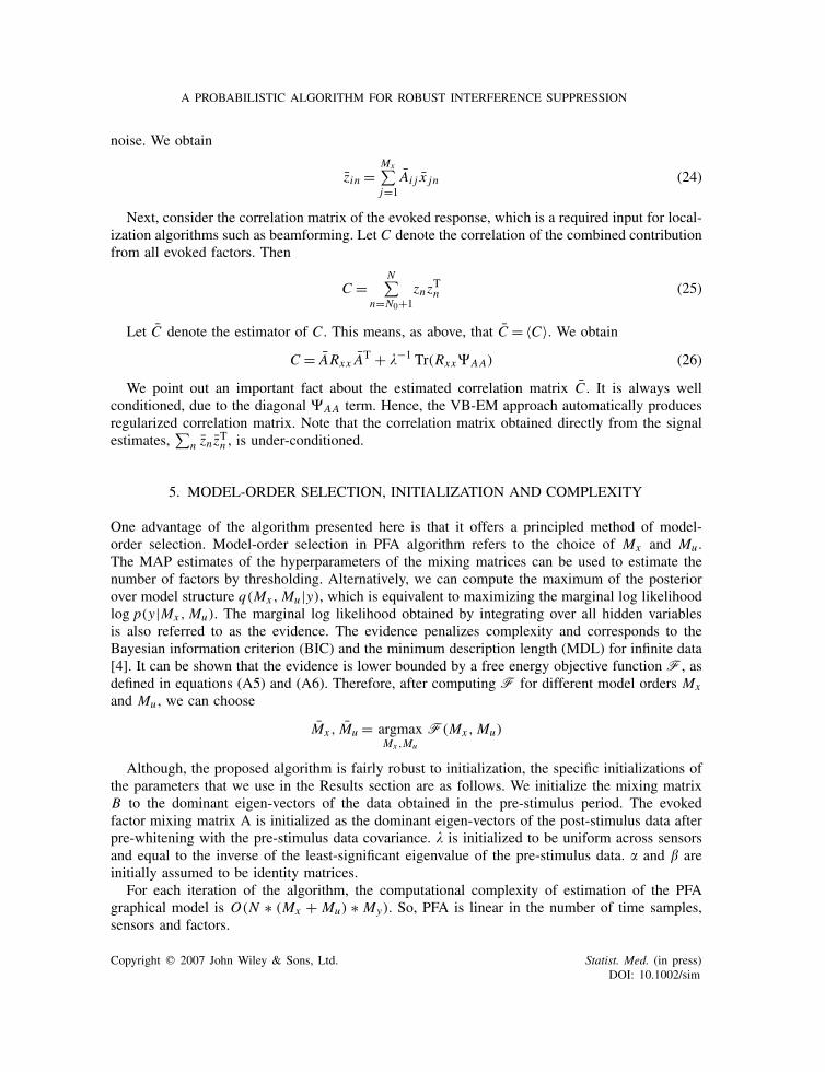
Figure 1 shows an example of performance for the proposed interference suppression algorithmon simulated data. The top row shows simulated noisy MEG data created assuming three brainsources and 25 interference sources and 275 sensors. The middle row shows the true signal thatis present in the post-stimulus period within the noisy MEG data. The bottom row shows theestimated signal extracted by PFA. When the true signal y∗ is known, denoising performance canbe quantified using the output signal-to-noise/interference ratio (SNIR)
SNIR= 1
My
My∑m=1
10 log10
∑Nn=N0
y∗2m,n∑N
n=N0(y∗
m,n − ym,n)2(dB)
For the example shown, the input SNIR is −13 dB and the output SNIR is −2 dB.In more extensive simulations, we compare interference suppression performance for the pro-
posed probabilistic algorithm with five other standard methods used in practice—PCA [5], WienerFiltering [2], ICA using TDSEP [6] and/or FastICA [7]), and trial averaging. TDSEP and FastICAwere chosen as the representative ICA methods based on their low computational complexity.Furthermore, when there are more than about 50 sensors, as is typically for high-resolution EEG,MEG, or magnetocardiography (MCG) systems, TDSEP and FastICA do not require additionaldimensionality reduction. We report the better results between these two ICA algorithms. Withthe exception of the trial mean, all the above interference suppression methods are spatial filteringmethods that apply a linear transformation that is applied to the observed data to obtain an estimateof the underlying signal.
The proposed algorithm, and the comparison methods mentioned above, could be applied eitherto concatenated single-trial data or to trial-averaged data. For interference suppression performance,
Figure 1. Example of performance of the proposed algorithm.
Copyright q 2007 John Wiley & Sons, Ltd. Statist. Med. (in press)DOI: 10.1002/sim
A PROBABILISTIC ALGORITHM FOR ROBUST INTERFERENCE SUPPRESSION
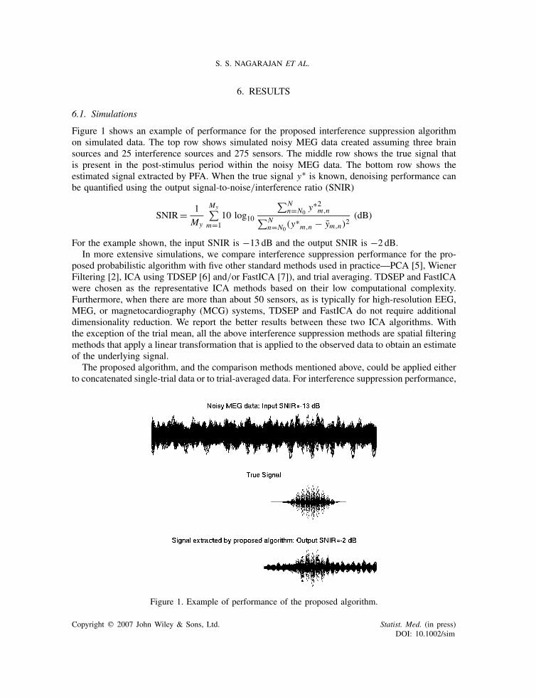
Figure 2. Output SNIR as a function of the input SIR for 10 trials and input SNR= 0 dB.
we first apply each method to the trial-averaged data so that we can directly compare it with thetrial mean. In some cases (as noted), we also apply the interference suppression on single-trialdata and then compute the trial average.
For the simulation results below, there are 1000 data points per trial (the first 63% of which corre-sponds to the inactive period), My = 132 sensors, Mx = 2 factors, Ms = 2 sources, and Mu = 1000interference signals. Results shown represent the mean over 10 Monte Carlo repetitions and theerror bars are used to indicate one standard error of the mean. The input signal-to-interference ratio(SIR) is the ratio of the power of the factors to the power of the interferences (measured in sensorspace). Likewise, the input signal-to-noise ratios (SNR) is the ratio of the power of the factors tothe power of the additive noise. The number of factors, Mx , must be specified for all denoisingmethods except the trial mean. The proposed method must also be supplied with a known numberof interference signals, Mu . To simplify the comparisons, it is assumed that the number of factorsis the true number and the number of interference signals Mu = 50.
Figure 2 shows the interference suppression performance as a function of the input SIR. OnlyThe input SNR is held constant at 0 dB and the number of trials is 10. All of the methods performbetter than the trial mean. PFA performs the best across all input SIR. The performances of bothPCA and Wiener approach that of PFA as the input SIR increases.
Figure 3 shows the interference suppression performance as a function of the number of trials.The input SIR and input SNR are held constant at −5 and 0 dB, respectively. In this figure thetrial mean outperforms TDSEP and PFA outperforms the other four methods.
6.2. Model-order selection
We demonstrate robustness to model-order selection using the PFA criterion with simulated data.Figures 4 and 5 show the results of using the PFA criterion, the evidence under the variationalapproximation, as a function of model order. For these two figures there are M∗
x = 2 sources,M∗
u = 10 interferences, 1000 data per trial, and 10 trials of data. Figure 4 plots the PFA criterion
Copyright q 2007 John Wiley & Sons, Ltd. Statist. Med. (in press)DOI: 10.1002/sim
S. S. NAGARAJAN ET AL.
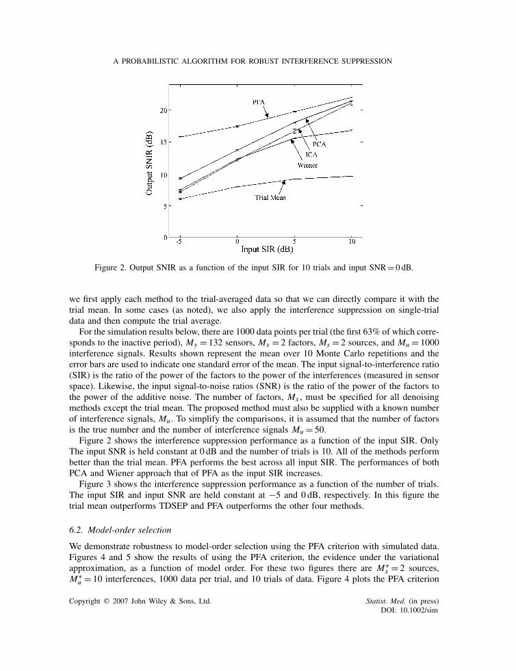
Figure 3. Output SNIR as a function of the number of trials for input SIR=−5 dB and input SNR= 0 dB.
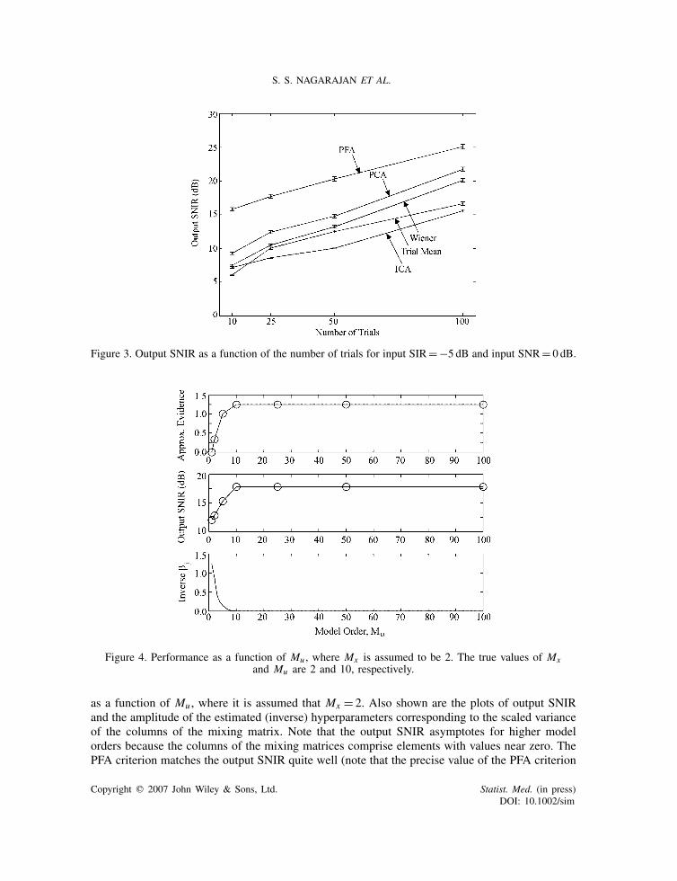
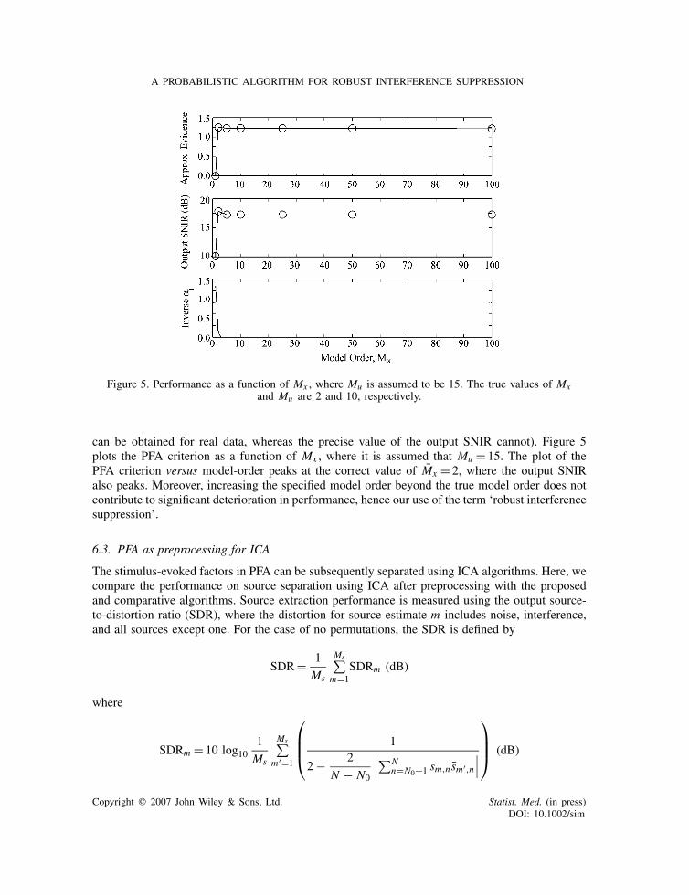
Figure 4. Performance as a function of Mu , where Mx is assumed to be 2. The true values of Mxand Mu are 2 and 10, respectively.
as a function of Mu , where it is assumed that Mx = 2. Also shown are the plots of output SNIRand the amplitude of the estimated (inverse) hyperparameters corresponding to the scaled varianceof the columns of the mixing matrix. Note that the output SNIR asymptotes for higher modelorders because the columns of the mixing matrices comprise elements with values near zero. ThePFA criterion matches the output SNIR quite well (note that the precise value of the PFA criterion
Copyright q 2007 John Wiley & Sons, Ltd. Statist. Med. (in press)DOI: 10.1002/sim
A PROBABILISTIC ALGORITHM FOR ROBUST INTERFERENCE SUPPRESSION
Figure 5. Performance as a function of Mx , where Mu is assumed to be 15. The true values of Mxand Mu are 2 and 10, respectively.
can be obtained for real data, whereas the precise value of the output SNIR cannot). Figure 5plots the PFA criterion as a function of Mx , where it is assumed that Mu = 15. The plot of thePFA criterion versus model-order peaks at the correct value of Mx = 2, where the output SNIRalso peaks. Moreover, increasing the specified model order beyond the true model order does notcontribute to significant deterioration in performance, hence our use of the term ‘robust interferencesuppression’.
6.3. PFA as preprocessing for ICA
The stimulus-evoked factors in PFA can be subsequently separated using ICA algorithms. Here, wecompare the performance on source separation using ICA after preprocessing with the proposedand comparative algorithms. Source extraction performance is measured using the output source-to-distortion ratio (SDR), where the distortion for source estimate m includes noise, interference,and all sources except one. For the case of no permutations, the SDR is defined by
SDR= 1
Ms
Ms∑m=1
SDRm (dB)
where
SDRm = 10 log101
Ms
Ms∑m′=1
⎛⎜⎜⎝ 1
2 − 2
N − N0
∣∣∣∑Nn=N0+1 sm,nsm′,n
∣∣∣
⎞⎟⎟⎠ (dB)
Copyright q 2007 John Wiley & Sons, Ltd. Statist. Med. (in press)DOI: 10.1002/sim
S. S. NAGARAJAN ET AL.
sn =W−1xn is the true source vector at time n, and both sm,n and sm,n are normalized to have unitvariance. The definition above is easily extended to account for any possible permutation. Thismetric reflects the performance of both the interference suppression/dimension reduction algorithmand the ICA algorithm. The interference suppression method accounts for all differences in SDRperformance below, since, for each experiment, the same ICA algorithm is used. In general, wefound that TDSEP performed better than FastICA for denoising and FastICA performed betterthan TDSEP for source extraction. For TDSEP and FastICA, the source subspace is automaticallydetermined by selecting the components that have the largest ratio of active power to inactivepower. The first component is given by
m1 = argmaxm
∑Nn=N0
s2m,n∑N0−1n=1 s2m,n
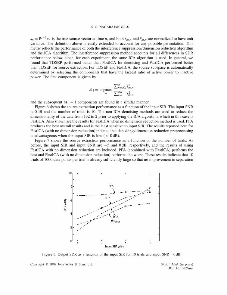
and the subsequent Mx − 1 components are found in a similar manner.Figure 6 shows the source extraction performance as a function of the input SIR. The input SNR
is 0 dB and the number of trials is 10. The non-ICA denoising methods are used to reduce thedimensionality of the data from 132 to 2 prior to applying the ICA algorithm, which in this case isFastICA. Also shown are the results for FastICA when no dimension reduction method is used. PFAproduces the best overall results and is the least sensitive to input SIR. The results reported here forFastICA (with no dimension reduction) indicate that denoising/dimension reduction preprocessingis advantageous when the input SIR is low (<10 dB).
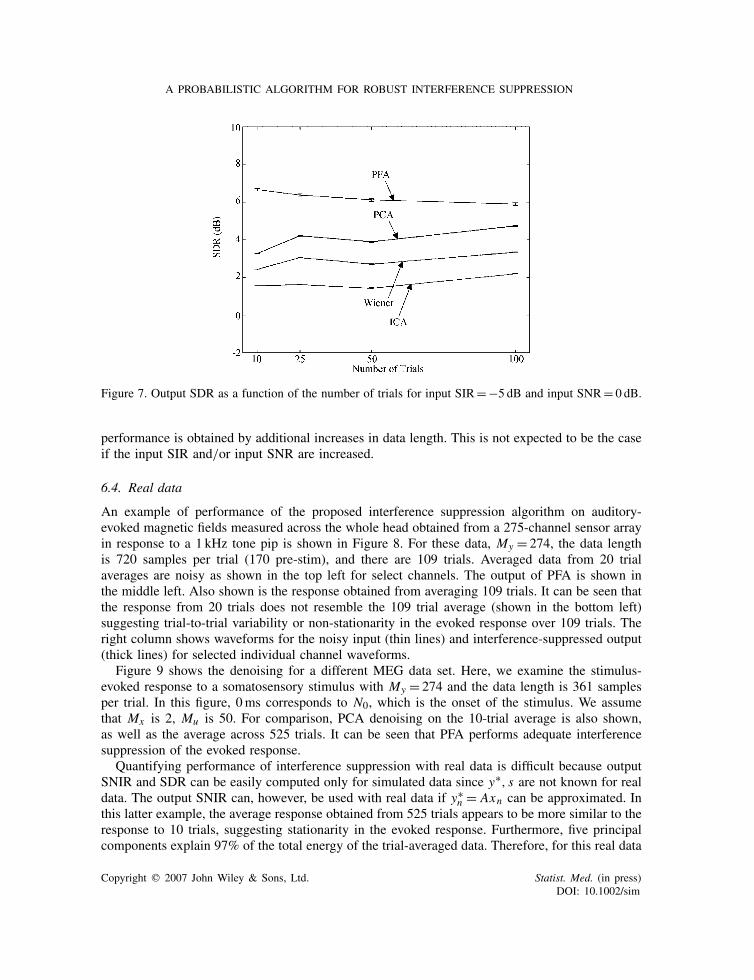
Figure 7 shows the source extraction performance as a function of the number of trials. Asbefore, the input SIR and input SNR are −5 and 0 dB, respectively, and the results of usingFastICA with no dimension reduction are included. PFA (combined with FastICA) performs thebest and FastICA (with no dimension reduction) performs the worst. These results indicate that 10trials of 1000 data points per trial is already sufficiently large so that no improvement in separation
Figure 6. Output SDR as a function of the input SIR for 10 trials and input SNR= 0 dB.
Copyright q 2007 John Wiley & Sons, Ltd. Statist. Med. (in press)DOI: 10.1002/sim
A PROBABILISTIC ALGORITHM FOR ROBUST INTERFERENCE SUPPRESSION
Figure 7. Output SDR as a function of the number of trials for input SIR=−5 dB and input SNR= 0 dB.
performance is obtained by additional increases in data length. This is not expected to be the caseif the input SIR and/or input SNR are increased.
6.4. Real data
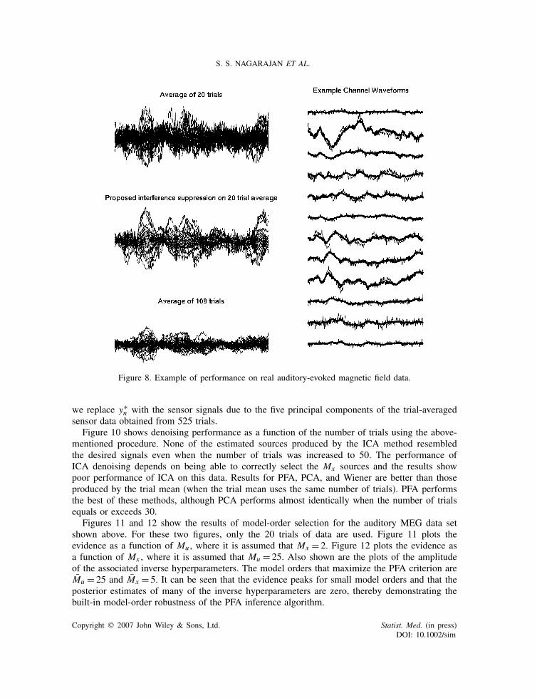
An example of performance of the proposed interference suppression algorithm on auditory-evoked magnetic fields measured across the whole head obtained from a 275-channel sensor arrayin response to a 1 kHz tone pip is shown in Figure 8. For these data, My = 274, the data lengthis 720 samples per trial (170 pre-stim), and there are 109 trials. Averaged data from 20 trialaverages are noisy as shown in the top left for select channels. The output of PFA is shown inthe middle left. Also shown is the response obtained from averaging 109 trials. It can be seen thatthe response from 20 trials does not resemble the 109 trial average (shown in the bottom left)suggesting trial-to-trial variability or non-stationarity in the evoked response over 109 trials. Theright column shows waveforms for the noisy input (thin lines) and interference-suppressed output(thick lines) for selected individual channel waveforms.
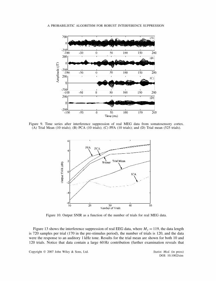
Figure 9 shows the denoising for a different MEG data set. Here, we examine the stimulus-evoked response to a somatosensory stimulus with My = 274 and the data length is 361 samplesper trial. In this figure, 0ms corresponds to N0, which is the onset of the stimulus. We assumethat Mx is 2, Mu is 50. For comparison, PCA denoising on the 10-trial average is also shown,as well as the average across 525 trials. It can be seen that PFA performs adequate interferencesuppression of the evoked response.
Quantifying performance of interference suppression with real data is difficult because outputSNIR and SDR can be easily computed only for simulated data since y∗, s are not known for realdata. The output SNIR can, however, be used with real data if y∗
n = Axn can be approximated. Inthis latter example, the average response obtained from 525 trials appears to be more similar to theresponse to 10 trials, suggesting stationarity in the evoked response. Furthermore, five principalcomponents explain 97% of the total energy of the trial-averaged data. Therefore, for this real data
Copyright q 2007 John Wiley & Sons, Ltd. Statist. Med. (in press)DOI: 10.1002/sim
S. S. NAGARAJAN ET AL.
Figure 8. Example of performance on real auditory-evoked magnetic field data.
we replace y∗n with the sensor signals due to the five principal components of the trial-averaged
sensor data obtained from 525 trials.Figure 10 shows denoising performance as a function of the number of trials using the above-
mentioned procedure. None of the estimated sources produced by the ICA method resembledthe desired signals even when the number of trials was increased to 50. The performance ofICA denoising depends on being able to correctly select the Mx sources and the results showpoor performance of ICA on this data. Results for PFA, PCA, and Wiener are better than thoseproduced by the trial mean (when the trial mean uses the same number of trials). PFA performsthe best of these methods, although PCA performs almost identically when the number of trialsequals or exceeds 30.
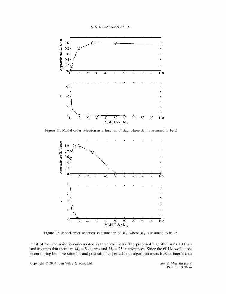
Figures 11 and 12 show the results of model-order selection for the auditory MEG data setshown above. For these two figures, only the 20 trials of data are used. Figure 11 plots theevidence as a function of Mu , where it is assumed that Mx = 2. Figure 12 plots the evidence asa function of Mx , where it is assumed that Mu = 25. Also shown are the plots of the amplitudeof the associated inverse hyperparameters. The model orders that maximize the PFA criterion areMu = 25 and Mx = 5. It can be seen that the evidence peaks for small model orders and that theposterior estimates of many of the inverse hyperparameters are zero, thereby demonstrating thebuilt-in model-order robustness of the PFA inference algorithm.
Copyright q 2007 John Wiley & Sons, Ltd. Statist. Med. (in press)DOI: 10.1002/sim
A PROBABILISTIC ALGORITHM FOR ROBUST INTERFERENCE SUPPRESSION
Figure 9. Time series after interference suppression of real MEG data from somatosensory cortex.(A) Trial Mean (10 trials); (B) PCA (10 trials); (C) PFA (10 trials); and (D) Trial mean (525 trials).
Figure 10. Output SNIR as a function of the number of trials for real MEG data.
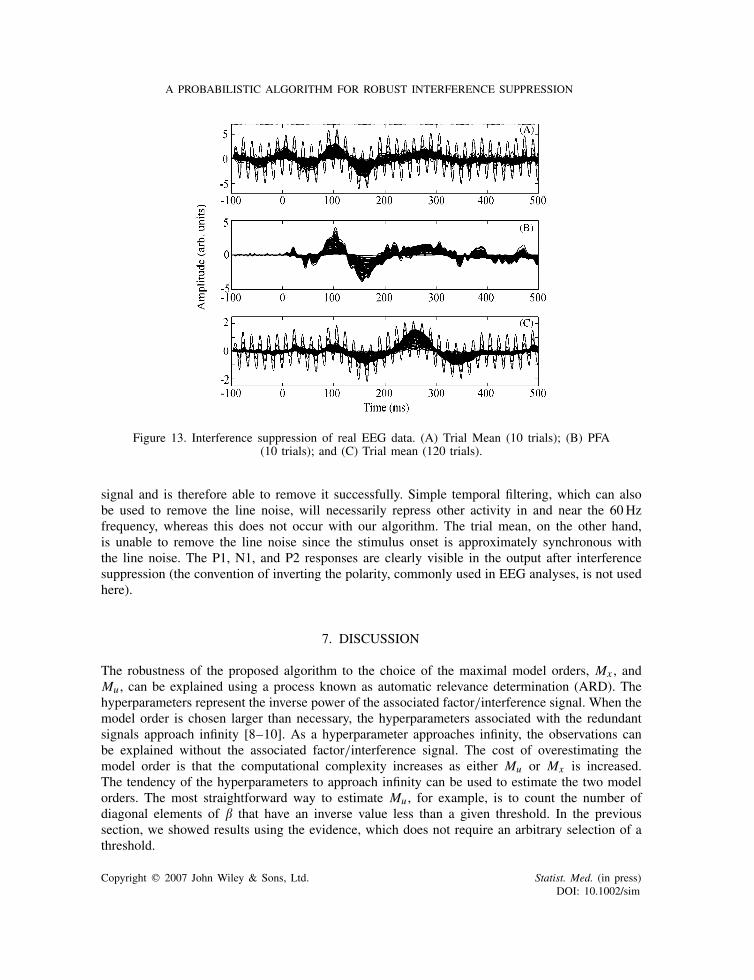
Figure 13 shows the interference suppression of real EEG data, where My = 119, the data lengthis 720 samples per trial (170 in the pre-stimulus period), the number of trials is 120, and the datawere the response to an auditory 1 kHz tone. Results for the trial mean are shown for both 10 and120 trials. Notice that data contain a large 60Hz contribution (further examination reveals that
Copyright q 2007 John Wiley & Sons, Ltd. Statist. Med. (in press)DOI: 10.1002/sim
S. S. NAGARAJAN ET AL.
Figure 11. Model-order selection as a function of Mu , where Mx is assumed to be 2.
Figure 12. Model-order selection as a function of Mx , where Mu is assumed to be 25.
most of the line noise is concentrated in three channels). The proposed algorithm uses 10 trialsand assumes that there are Mx = 5 sources and Mu = 25 interferences. Since the 60Hz oscillationsoccur during both pre-stimulus and post-stimulus periods, our algorithm treats it as an interference
Copyright q 2007 John Wiley & Sons, Ltd. Statist. Med. (in press)DOI: 10.1002/sim
A PROBABILISTIC ALGORITHM FOR ROBUST INTERFERENCE SUPPRESSION
Figure 13. Interference suppression of real EEG data. (A) Trial Mean (10 trials); (B) PFA(10 trials); and (C) Trial mean (120 trials).
signal and is therefore able to remove it successfully. Simple temporal filtering, which can alsobe used to remove the line noise, will necessarily repress other activity in and near the 60Hzfrequency, whereas this does not occur with our algorithm. The trial mean, on the other hand,is unable to remove the line noise since the stimulus onset is approximately synchronous withthe line noise. The P1, N1, and P2 responses are clearly visible in the output after interferencesuppression (the convention of inverting the polarity, commonly used in EEG analyses, is not usedhere).
7. DISCUSSION
The robustness of the proposed algorithm to the choice of the maximal model orders, Mx , andMu , can be explained using a process known as automatic relevance determination (ARD). Thehyperparameters represent the inverse power of the associated factor/interference signal. When themodel order is chosen larger than necessary, the hyperparameters associated with the redundantsignals approach infinity [8–10]. As a hyperparameter approaches infinity, the observations canbe explained without the associated factor/interference signal. The cost of overestimating themodel order is that the computational complexity increases as either Mu or Mx is increased.The tendency of the hyperparameters to approach infinity can be used to estimate the two modelorders. The most straightforward way to estimate Mu , for example, is to count the number ofdiagonal elements of � that have an inverse value less than a given threshold. In the previoussection, we showed results using the evidence, which does not require an arbitrary selection of athreshold.
Copyright q 2007 John Wiley & Sons, Ltd. Statist. Med. (in press)DOI: 10.1002/sim
S. S. NAGARAJAN ET AL.
The proposed algorithm, as given above, has a potential problem of identifiability between theestimation of A and B, especially if the amount of data in the pre-stimulus period is small and bothA and B are primarily estimated from the post-stimulus period (data may have equal likelihood toarise from a source factor and from an interference factor). To avoid this problem, we perform atwo-step procedure for PFA. In the first step, we estimate the interference factor mixing matrix andthe sensor noise precision from data in the pre-stimulus period. In this case, the update equationfor � uses only the pre-stimulus data and is
�−1 = 1
Ndiag(Ryy − B Ryu
T) (27)
The update rules for B and � are the same as listed in equation (20), with a modified �BB = (Ruu+�)−1. Subsequently, for post-stimulus data, we freeze the above parameters and estimate A usinga modified update rule,
A= (Ryx − BRyx )�AA (28)
where �AA = (Rxx + �)−1. All other update rules are identical to those listed above.Furthermore, the proposed model currently assumes that the interferences are statistically sta-
tionary between the pre- and post-stimulus periods. However, we can relax this assumption andmodel non-stationary changes in the power of interference if there are no changes in the loca-tion of the interferences. We assume that, in the post-stimulus period, the probability distributionof the interference factors is p(un) =∏Mu
m=1 p(um,n) =N(un|0, �), where � is a diagonal pre-cision matrix that is equal to the inverse of the power fluctuations of the interference in thepost-stimulus period. In this case, we can learn � from the post-stimulus period using the updaterule �−1 = diag((1/N )Ruu), where Ruu is calculated only for the post-stimulus period.
The algorithm currently assumes that the prior distributions for evoked and interference factorsare i.i.d. and invariant to the time-index permutation. However, this does not appear to impactperformance because in all the simulations presented in the paper both the background sources wereassumed to be sinusoidal (with bimodal distributions) or damped sinusoids (with super-Gaussiandistributions), rather than Gaussians as assumed in the model. Moreover, since the performanceof the algorithm is also good on real bioelectromagnetic data, where the interference factors areindeed oscillatory, the algorithm has some degree of robustness with respect to assumptions aboutthe prior distribution of interference and evoked factors. Since estimation is data dependent, ifthe data suggest that factors have temporal continuity, then the estimated factors will have somesmoothness. Nevertheless, an algorithm that is able to exploit temporal correlation in factors couldpotentially be more powerful. We are currently pursuing such an extension, using several differentmodels that incorporate temporal statistics of the evoked and interference factors, whose parametersare inferred from data. Algorithms derived from such models perform interference suppressionusing not just spatial but also spatio-temporal filtering. On a separate note, since bioelectromagneticdata are often non-Gaussian, we are currently extending the model to incorporate non-Gaussianfactor models.
APPENDIX A: THE VB-EM ALGORITHM
This section outlines the derivation of the VB-EM algorithm that infers the PFA model fromdata.
Copyright q 2007 John Wiley & Sons, Ltd. Statist. Med. (in press)DOI: 10.1002/sim
A PROBABILISTIC ALGORITHM FOR ROBUST INTERFERENCE SUPPRESSION
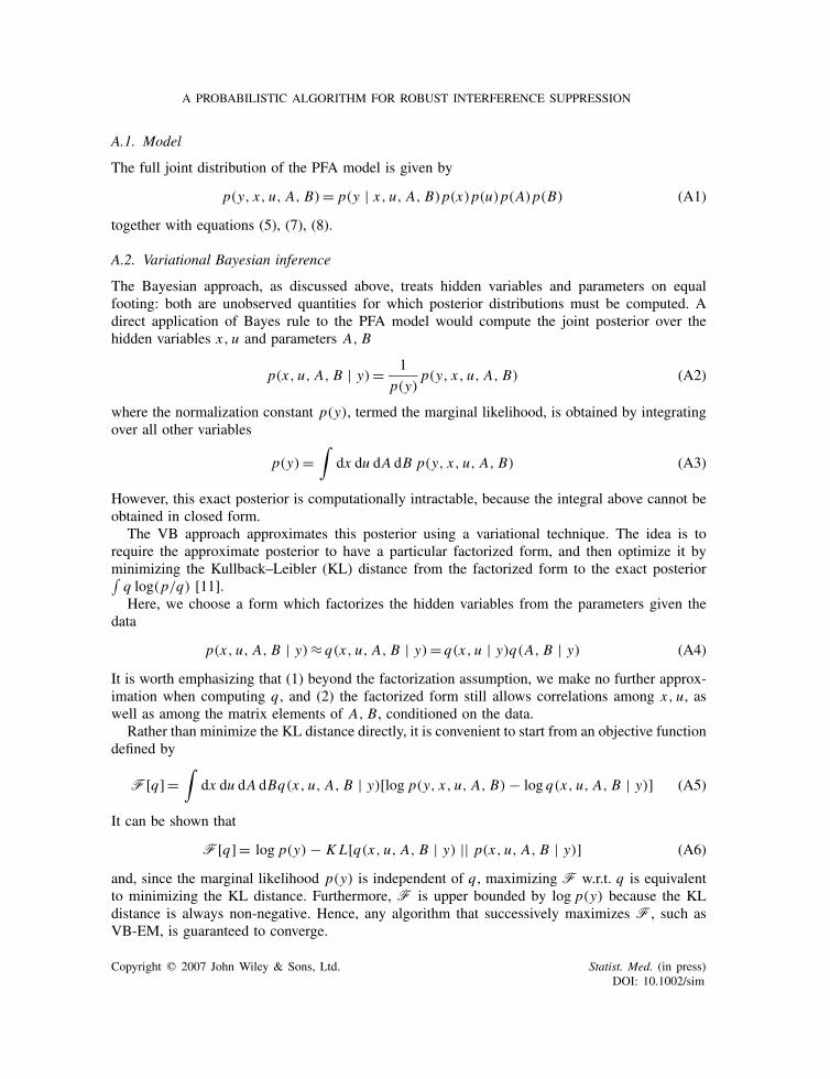
A.1. Model
The full joint distribution of the PFA model is given by
p(y, x, u, A, B) = p(y | x, u, A, B)p(x)p(u)p(A)p(B) (A1)
together with equations (5), (7), (8).
A.2. Variational Bayesian inference
The Bayesian approach, as discussed above, treats hidden variables and parameters on equalfooting: both are unobserved quantities for which posterior distributions must be computed. Adirect application of Bayes rule to the PFA model would compute the joint posterior over thehidden variables x, u and parameters A, B
p(x, u, A, B | y)= 1
p(y)p(y, x, u, A, B) (A2)
where the normalization constant p(y), termed the marginal likelihood, is obtained by integratingover all other variables
p(y) =∫
dx du dA dB p(y, x, u, A, B) (A3)
However, this exact posterior is computationally intractable, because the integral above cannot beobtained in closed form.
The VB approach approximates this posterior using a variational technique. The idea is torequire the approximate posterior to have a particular factorized form, and then optimize it byminimizing the Kullback–Leibler (KL) distance from the factorized form to the exact posterior∫q log(p/q) [11].Here, we choose a form which factorizes the hidden variables from the parameters given the
data
p(x, u, A, B | y)≈ q(x, u, A, B | y) = q(x, u | y)q(A, B | y) (A4)
It is worth emphasizing that (1) beyond the factorization assumption, we make no further approx-imation when computing q , and (2) the factorized form still allows correlations among x, u, aswell as among the matrix elements of A, B, conditioned on the data.
Rather than minimize the KL distance directly, it is convenient to start from an objective functiondefined by
F[q]=∫
dx du dA dBq(x, u, A, B | y)[log p(y, x, u, A, B) − log q(x, u, A, B | y)] (A5)
It can be shown that
F[q]= log p(y) − K L[q(x, u, A, B | y) || p(x, u, A, B | y)] (A6)
and, since the marginal likelihood p(y) is independent of q , maximizing F w.r.t. q is equivalentto minimizing the KL distance. Furthermore, F is upper bounded by log p(y) because the KLdistance is always non-negative. Hence, any algorithm that successively maximizes F, such asVB-EM, is guaranteed to converge.
Copyright q 2007 John Wiley & Sons, Ltd. Statist. Med. (in press)DOI: 10.1002/sim
S. S. NAGARAJAN ET AL.
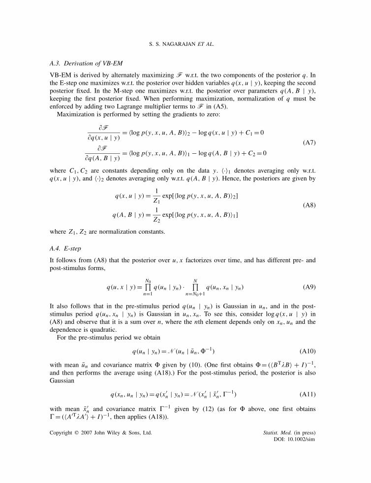
A.3. Derivation of VB-EM
VB-EM is derived by alternately maximizing F w.r.t. the two components of the posterior q . Inthe E-step one maximizes w.r.t. the posterior over hidden variables q(x, u | y), keeping the secondposterior fixed. In the M-step one maximizes w.r.t. the posterior over parameters q(A, B | y),keeping the first posterior fixed. When performing maximization, normalization of q must beenforced by adding two Lagrange multiplier terms to F in (A5).
Maximization is performed by setting the gradients to zero:
�F�q(x, u | y) = 〈log p(y, x, u, A, B)〉2 − log q(x, u | y) + C1 = 0
�F�q(A, B | y) = 〈log p(y, x, u, A, B)〉1 − log q(A, B | y) + C2 = 0
(A7)
where C1,C2 are constants depending only on the data y. 〈·〉1 denotes averaging only w.r.t.q(x, u | y), and 〈·〉2 denotes averaging only w.r.t. q(A, B | y). Hence, the posteriors are given by
q(x, u | y) = 1
Z1exp[〈log p(y, x, u, A, B)〉2]
q(A, B | y) = 1
Z2exp[〈log p(y, x, u, A, B)〉1]
(A8)
where Z1, Z2 are normalization constants.
A.4. E-step
It follows from (A8) that the posterior over u, x factorizes over time, and has different pre- andpost-stimulus forms,
q(u, x | y)=N0∏n=1
q(un | yn) ·N∏
n=N0+1q(un, xn | yn) (A9)
It also follows that in the pre-stimulus period q(un | yn) is Gaussian in un , and in the post-stimulus period q(un, xn | yn) is Gaussian in un, xn . To see this, consider log q(x, u | y) in(A8) and observe that it is a sum over n, where the nth element depends only on xn, un and thedependence is quadratic.
For the pre-stimulus period we obtain
q(un | yn) =N(un | un, �−1) (A10)
with mean un and covariance matrix � given by (10). (One first obtains �= (〈BT�B〉 + I )−1,and then performs the average using (A18).) For the post-stimulus period, the posterior is alsoGaussian
q(xn, un | yn) = q(x ′n | yn) =N(x ′
n | x ′n, �
−1) (A11)
with mean x ′n and covariance matrix �−1 given by (12) (as for � above, one first obtains
� = (〈A′T�A′〉 + I )−1, then applies (A18)).
Copyright q 2007 John Wiley & Sons, Ltd. Statist. Med. (in press)DOI: 10.1002/sim
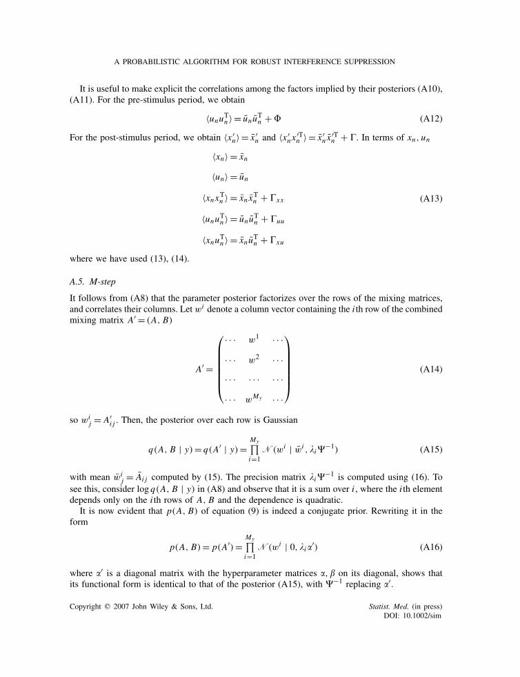
A PROBABILISTIC ALGORITHM FOR ROBUST INTERFERENCE SUPPRESSION
It is useful to make explicit the correlations among the factors implied by their posteriors (A10),(A11). For the pre-stimulus period, we obtain
〈unuTn 〉= unuTn + � (A12)
For the post-stimulus period, we obtain 〈x ′n〉 = x ′
n and 〈x ′nx
′Tn 〉 = x ′
n x′Tn + �. In terms of xn, un
〈xn〉 = xn
〈un〉 = un
〈xnxTn 〉 = xn xTn + �xx
〈unuTn 〉 = unuTn + �uu
〈xnuTn 〉 = xnuTn + �xu
(A13)
where we have used (13), (14).
A.5. M-step
It follows from (A8) that the parameter posterior factorizes over the rows of the mixing matrices,and correlates their columns. Let wi denote a column vector containing the i th row of the combinedmixing matrix A′ = (A, B)
A′ =
⎛⎜⎜⎜⎜⎜⎜⎝
· · · w1 · · ·· · · w2 · · ·· · · · · · · · ·· · · wMy · · ·
⎞⎟⎟⎟⎟⎟⎟⎠
(A14)
so wij = A′
i j . Then, the posterior over each row is Gaussian
q(A, B | y)= q(A′ | y) =My∏i=1
N(wi | wi , �i�−1) (A15)
with mean wij = Ai j computed by (15). The precision matrix �i�−1 is computed using (16). To
see this, consider log q(A, B | y) in (A8) and observe that it is a sum over i , where the i th elementdepends only on the i th rows of A, B and the dependence is quadratic.
It is now evident that p(A, B) of equation (9) is indeed a conjugate prior. Rewriting it in theform
p(A, B) = p(A′) =My∏i=1
N(wi | 0, �i�′) (A16)
where �′ is a diagonal matrix with the hyperparameter matrices �, � on its diagonal, shows thatits functional form is identical to that of the posterior (A15), with �−1 replacing �′.
Copyright q 2007 John Wiley & Sons, Ltd. Statist. Med. (in press)DOI: 10.1002/sim
S. S. NAGARAJAN ET AL.
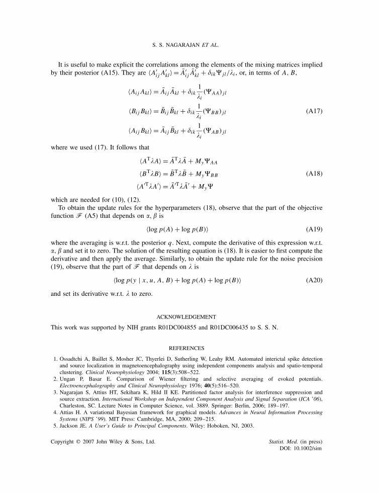
It is useful to make explicit the correlations among the elements of the mixing matrices impliedby their posterior (A15). They are 〈A′
i j A′kl〉 = A′
i j A′kl + �ik� jl/�i , or, in terms of A, B,
〈Ai j Akl〉 = Ai j Akl + �ik1
�i(�AA) jl
〈Bi j Bkl〉 = Bi j Bkl + �ik1
�i(�BB) jl
〈Ai j Bkl〉 = Ai j Bkl + �ik1
�i(�AB) jl
(A17)
where we used (17). It follows that
〈AT�A〉 = AT� A + My�AA
〈BT�B〉 = BT�B + My�BB
〈A′T�A′〉 = A′T� A′ + My�
(A18)
which are needed for (10), (12).To obtain the update rules for the hyperparameters (18), observe that the part of the objective
function F (A5) that depends on �, � is
〈log p(A) + log p(B)〉 (A19)
where the averaging is w.r.t. the posterior q . Next, compute the derivative of this expression w.r.t.�, � and set it to zero. The solution of the resulting equation is (18). It is easier to first compute thederivative and then apply the average. Similarly, to obtain the update rule for the noise precision(19), observe that the part of F that depends on � is
〈log p(y | x, u, A, B) + log p(A) + log p(B)〉 (A20)
and set its derivative w.r.t. � to zero.
ACKNOWLEDGEMENT
This work was supported by NIH grants R01DC004855 and R01DC006435 to S. S. N.
REFERENCES
1. Ossadtchi A, Baillet S, Mosher JC, Thyerlei D, Sutherling W, Leahy RM. Automated interictal spike detectionand source localization in magnetoencephalography using independent components analysis and spatio-temporalclustering. Clinical Neurophysiology 2004; 115(3):508–522.
2. Ungan P, Basar E. Comparison of Wiener filtering and selective averaging of evoked potentials.Electroencephalography and Clinical Neurophysiology 1976; 40(5):516–520.
3. Nagarajan S, Attius HT, Sekihara K, Hild II KE. Partitioned factor analysis for interference suppression andsource extraction. International Workshop on Independent Component Analysis and Signal Separation (ICA ’06),Charleston, SC. Lecture Notes in Computer Science, vol. 3889. Springer: Berlin, 2006; 189–197.
4. Attias H. A variational Bayesian framework for graphical models. Advances in Neural Information ProcessingSystems (NIPS ’99). MIT Press: Cambridge, MA, 2000; 209–215.
5. Jackson JE. A User’s Guide to Principal Components. Wiley: Hoboken, NJ, 2003.
Copyright q 2007 John Wiley & Sons, Ltd. Statist. Med. (in press)DOI: 10.1002/sim

A PROBABILISTIC ALGORITHM FOR ROBUST INTERFERENCE SUPPRESSION
6. Ziehe A, Muller KR. TDSEP—an efficient algorithm for blind separation using time structure. InternationalConference on Artificial Neural Networks (ICANN ’98), Skovde, Sweden, September 1998; 675–680.
7. Hyvarinen A. Fast and robust fixed-point algorithms for independent component analysis. IEEE Transactions onNeural Networks 1999; 10(3):626–634.
8. MacKay DJC. Bayesian non-linear modeling for the energy prediction competition. ASHRAE Transactions 1994;100(2):1053–1062.
9. Sahani M, Linden J. Evidence optimization techniques for estimating stimulus–response functions. Advancesin Neural Information Processing Systems (NIPS ’02), vol. 15. MIT Press: Cambridge, MA, December 2002;301–308.
10. MacKay DJC. Bayesian interpolation. Neural Computation 1992; 4(3):415–447.11. Cover TM, Thomas JA. Elements of Information Theory. Wiley: New York, 1991.
Copyright q 2007 John Wiley & Sons, Ltd. Statist. Med. (in press)DOI: 10.1002/sim


